1

Richard LoulouGERAD and McGill University, Montreal QC.HALOA / KANLOMaryse LabrietGERAD, Montreal QC.CIEMAT, Madrid, Spain

The TIMES Integrated AssessmentModel (TIAM): some details on modeland database

TIAM Day, Ottawa March 14, 2007

2

PLAN

1. The TIAM Equilibrium

2. TIAM sectors: some details

1. Demands

2. Technologies

3. Trade

4. Emissions, abatement options

3. The TIAM Climate Module

4. VEDA3 Interface

TIM

ES In

tegr

ated

Asse

ssm

entM

odel

3

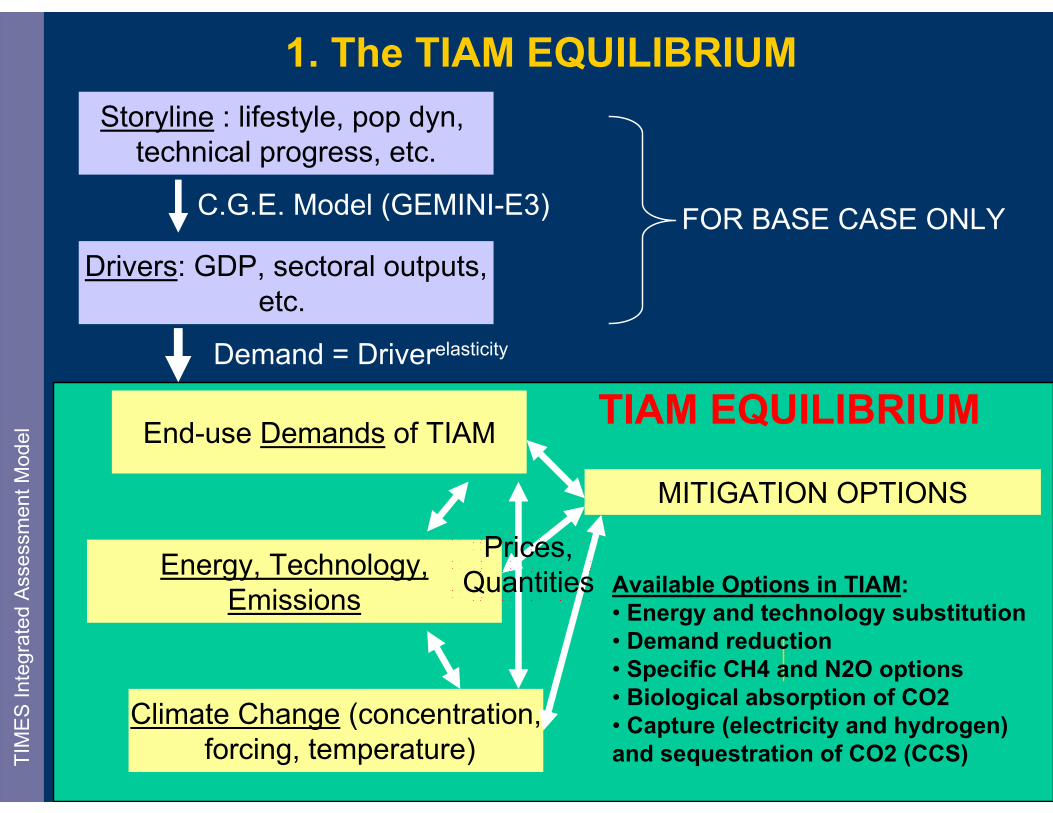
1. The TIAM EQUILIBRIUMTI

MES

Inte

grat

edAs

sess

men

tMod

el

Storyline : lifestyle, pop dyn, technical progress, etc.

Drivers: GDP, sectoral outputs,etc.

End-use Demands of TIAM

Demand = Driverelasticity

C.G.E. Model (GEMINI-E3)

Energy, Technology,Emissions

Climate Change (concentration,forcing, temperature)

Available Options in TIAM:• Energy and technology substitution• Demand reduction• Specific CH4 and N2O options• Biological absorption of CO2• Capture (electricity and hydrogen) and sequestration of CO2 (CCS)

FOR BASE CASE ONLY

MITIGATION OPTIONS

TIAM EQUILIBRIUM

Prices,Quantities

4

The TIAM Equilibrium

For each new run, TIAM simultaneouslyrecalculates– Energy produced, consumed, – Energy prices– Technology adoption, abandonment– Emissions – Emission prices– Climate variables– Demands for energy services

These quantities and prices are in equilibrium– Over all sectors, periods in the horizon, regions– The equilibrium maximizes total surplus (suppliers +

consumers surpluses) via Linear Programming

TIM

ES In

tegr

ated

Asse

ssm

entM

odel

5

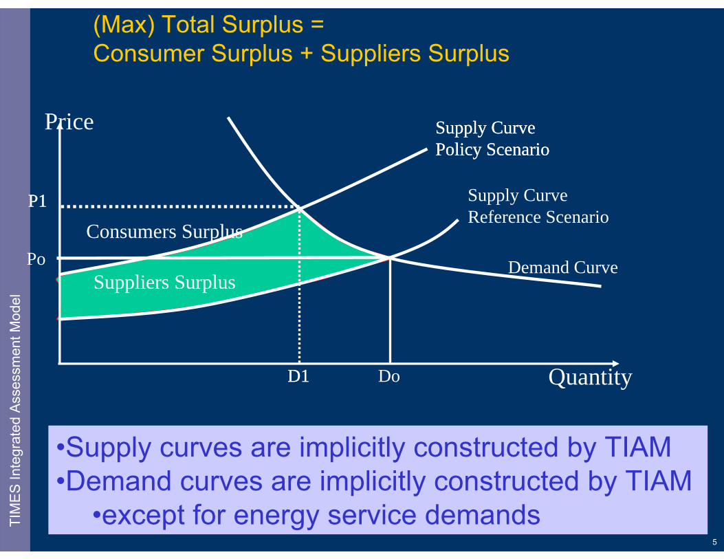
(Max) Total Surplus = Consumer Surplus + Suppliers Surplus

TIM

ES In

tegr

ated

Asse

ssm

entM

odel

Suppliers SurplusDemand Curve

Supply CurveReference Scenario

Quantity

Price

Do

Po

Supply CurvePolicy Scenario

D1

P1

Consumers Surplus

Supply CurvePolicy Scenario

D1

P1

•Supply curves are implicitly constructed by TIAM•Demand curves are implicitly constructed by TIAM

•except for energy service demands

6

15 regions + OPEC/Non-OPECTI

MES

Inte

grat

edAs

sess

men

tMod

el

Africa*Australia-New ZealandCanadaCentral and South America*China

Middle-East*Other Developing Asia*South KoreaUnited StatesWestern Europe

* OPEC and Non-OPEC countries are separated in primary and secondary sectors ⇒ oil production strategies and oil price control by OPEC countries

Eastern EuropeFormer Soviet Union IndiaJapanMexico

7

List of countries in multi-country regionsTI

MES

Inte

grat

edAs

sess

men

tMod

el

8

Reference Energy System

Carbon capture

Carbon sequestration

CO2 Terrestrialsequestration

Landfills Manure Bio burning, rice, enteric ferm WastewaterNon-energy

sectors (CH4)

CH4 options

CH4 options CH4 options

N2O options

Fossil Fuel Reserves

(oil, coal, gas)

BiomassPotential

RenewablePotential

WIN SOLGEO TDLHYD

SecondaryTransformation

OPEC/NON-OPEC regrouping

OIL***GAS***COA***

Electricity Fuels

ELC***Electricity

Cogeneration

Heat

BIO***

Nuclear NUC

End Use Fuels

TransportTech.

AgricultureTech.

CommercialTech.

ResidentialTech.

IndustrialServiceCompo-

sition

I***

I** (6) A** (1) C** (8) R** (11) T** (16)

AGR*** COM*** RES*** TRA***IND***

UpstreamFuels

HET

Auto ProductionINDELC

CogenerationINDELCIS**

Hydrogen production and distribution

SYNHYD

OI****GA****CO****

BIO***

ELC

BIO***

ELC

HET

ELC

TradeTrade

Extraction

IndustrialTech.

ClimateModule

Atm.Conc∆Forcing∆Temp

Used for

reporting&

settingtargets

42 Demands

9

A. Demand projectionsTI

MES

Inte

grat

edAs

sess

men

tMod

el

Storyline : populationdynamics, technical progress, etc.

Drivers: GDP, sectoral outputs,

End-use demands of TIAM

DEM = K*(Driver)elasticity

GEM-E3

Elasticities:- “some” saturation in the long term ⇒ lower elasticities- convergence between developing and industrialized countries

GDP: moderate annual growth (2.1%)GDP(2100) = 8*GDP(2000)POP: from 6 to 9 billions (2000-2100)

10

TIM

ES In

tegr

ated

Asse

ssm

entM

odel

End-use demands (1/2)Code Unit

Transportation segments (15)Autos TRT Billion vehicle-km/yearBuses TRB Billion vehicle-km/yearLight trucks TRL Billion vehicle-km/yearCommercial trucks TRC Billion vehicle-km/yearMedium trucks TRM Billion vehicle-km/yearHeavy trucks TRH Billion vehicle-km/yearTwo wheelers TRW Billion vehicle-km/yearThree wheelers TRE Billion vehicle-km/yearInternational aviation TAI PJ/yearDomestic aviation TAD PJ/yearFreight rail transportation TTF PJ/yearPassengers rail transportation TTP PJ/yearInternal navigation TWD PJ/yearInternational navigation (bunkers) TWI PJ/yearNon-energy uses in transport NEU PJ/yearResidential segments* (11)Space heating RH1, RH2, RH3, RH4 PJ/yearSpace cooling RC1, RC2, RC3, RC4 PJ/yearHot water heating RWH PJ/yearLighting RL1, RL2, RL3, RL4 PJ/yearCooking RK1, RK2, RK3, RK4 PJ/yearRefrigerators and freezers RRF PJ/yearCloth washers RCW PJ/yearCloth dryers RCD PJ/yearDish washers RDW PJ/yearMiscellaneous electric energy REA PJ/yearOther energy uses ROT PJ/year

11

TIM

ES In

tegr

ated

Asse

ssm

entM

odel

End-use demands (2/2)Commercial segments* (8)Space heating CH1, CH2. CH3, CH4 PJ/yearSpace cooling CC1, CC2. CC3. CC4 PJ/yearHot water heating CHW PJ/yearLighting CLA PJ/yearCooking CCK PJ/yearRefrigerators and freezers CRF PJ/yearElectric equipments COE PJ/yearOther energy uses COT PJ/yearAgriculture segment (1)Agriculture AGRIndustrial segments** (6)Iron and steel IIS Millions tonnesNon ferrous metals INF Millions tonnesChemicals ICH PJPulp and paper ILP Millions tonnesNon metal minerals INM PJOther industries IOI PJOther segment (1)Other non specified energy consumption ONO PJ/year

12

Drivers used to build energy service demands in TIAM (1/2): DEM = K*DRIVERelasticity

TIM

ES In

tegr

ated

Asse

ssm

entM

odel

DEMANDTransportationAutomobile travelBus travel2 & 3 wheelersRail passenger travelDomestic aviation travelInternational Aviation travelTrucksFret railDomestic Navigation Bunkers

All regions after 2050 + OECD regions Non-OECD before 2050 before 2050

Space heating HOU HOUSpace Cooling HOU GDPPWater Heating POP POPLighting GDPP GDPPCooking POP POPRefrigeration and Freezing HOU GDPPWashers HOU GDPPDryers HOU GDPPDish washers HOU GDPPOther appliances GDPP GDPPOther HOU GDPP

Residential

GDPGDPGDPGDP

POPPOPGDPGDP

DRIVERAll regionsGDP/capita

POP

13

TIM

ES In

tegr

ated

Asse

ssm

entM

odel

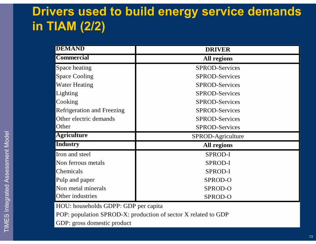
DEMANDCommercialSpace heatingSpace CoolingWater Heating LightingCookingRefrigeration and FreezingOther electric demandsOther AgricultureIndustry

Iron and steelNon ferrous metalsChemicalsPulp and paper Non metal mineralsOther industries

GDP: gross domestic product

DRIVER

SPROD-OSPROD-O

HOU: households GDPP: GDP per capita POP: population SPROD-X: production of sector X related to GDP

SPROD-ISPROD-I SPROD-I SPROD-O

SPROD-ServicesSPROD-Services

SPROD-AgricultureAll regions

SPROD-ServicesSPROD-ServicesSPROD-ServicesSPROD-Services

All regionsSPROD-ServicesSPROD-Services

Drivers used to build energy service demands in TIAM (2/2)

14

TIM

ES In

tegr

ated

Asse

ssm

entM

odel

Demand handling in VEDA3

15

B. End-Use sectors

Automobile travelBus travel2 & 3 wheelersRail passenger travelDomestic aviation travelInternational Aviation travelTrucksFret railDomestic Navigation Bunkers

Steam boilerProcess heatMachine driveElectro-Chemical ProcessFeedstocksOthers

Transport

Commercial

Residential

Agriculture

Industry

Iron and steelNon ferrous metalsChemicalsPulp and paper Non metal mineralsOther industries

Generic demand

Technologies Demands for energy services

Space heatingSpace CoolingWater Heating LightingCookingRefrigeration and FreezingWashers (only RES)Dryers (only RES)Dish washers (only RES)Other appliances (only RES)Other electric demands (only COM)Other

TIM

ES In

tegr

ated

Asse

ssm

entM

odel

Fuels

Fuels

Fuels

Fuels

Fuels

16

C. Calibration to initial yearTI

MES

Inte

grat

edAs

sess

men

tMod

el

Calibration consists in matching detailed energybalances in initial period (Base year =2000) Data sources:

Energy Statistics and Balances of OECD and Non-OECD countries given by the International Energy AgencyAdjusted by regional or national statistics if necessary and available

International and region specific statistics (installed capacities and resource potentials) from many sources (IEA-ETP, USDOE, USEPA, USGS, EGRID, NRCAN, WEC, etc.)

17

D. Primary and secondary energy sectors

Fossil resources and extractionDifferent types of reserves (characteristics of the resource, cumulative potential, cost)Eg. Oil: 21 (conventional, oil sands, located, enhanced recovery, new

discovery…)Gas: 9 (conventional, unconventional, not connected)Coal: 4 (brown coal, hard coal, located, new discovery)

►Reviewed and revised by IER (Stuttgart) in 2006

TIM

ES In

tegr

ated

Asse

ssm

entM

odel

Oil refining

Flexiblerefinery

Refined petroleum products: variable share of RPPs in the total output

Emissions due to energy consumption and the process itself

Crude oil

Energy consumption

18

D. Primary and secondary energy (cont’d)Renewable and nuclearGeothermal: Shallow, deep and very deepHydro: Dam and run-of-river

WEC technical potential Wind: Four plant-and-location combinations (different costs and AF)

Equivalent to 10% of the theoretical potential provided by IPCC-TAR ~ WEC assuming 4% of the land area

SolarNuclear: Basecase = min of 64 EJ/yr, max of 95 EJ/yr in 2100Biomass: Includes industrial wastes, municipal wastes, solid biomass,

biogas from landfills, liquids from biomass (IEA categories)World potential = 238 EJ in 2100Practical and technical constraints (distance of a biomass production site from demand centres, land-use conflicts)

Main sources of dataIEA-ETP, World Energy Council, IPCC-TAR, US Geological Survey, …

TIM

ES In

tegr

ated

Asse

ssm

entM

odel

19

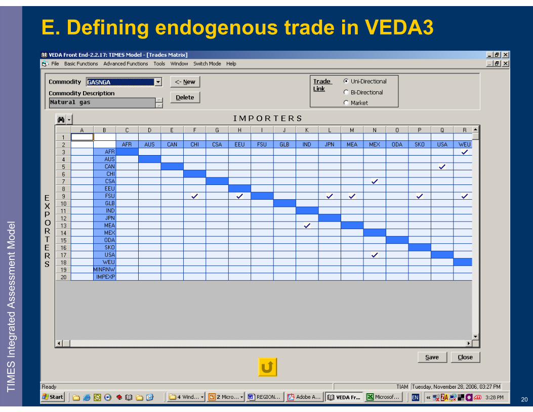
E. Energy and emission trade

Endogenous trade of coal, crude oil, gas, liquefied gas (revised by IER)⇒ price and amount of traded energy are endogenous⇒ the impact of environmental policies on trade is simulated

Endogenous trade of CO2 (or GHG) permits

The user can choose which gases/energy commodity and which regions are included in trade (eg. only CO2, all GHGs, only some countries)

TIM

ES In

tegr

ated

Asse

ssm

entM

odel

All CO2***CO2 TOTCO2

All GHGs***CO2***CH4***N2O

GHG

NonCO2***CH4***N2O

NONCO2

Based on the GWP of greenhouse gases

20

E. Defining endogenous trade in VEDA3TI

MES

Inte

grat

edAs

sess

men

tMod

el

21

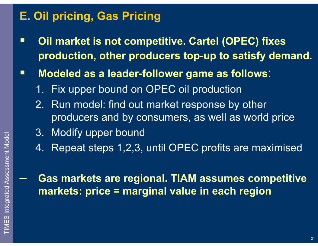
E. Oil pricing, Gas Pricing

Oil market is not competitive. Cartel (OPEC) fixes production, other producers top-up to satisfy demand.Modeled as a leader-follower game as follows:1. Fix upper bound on OPEC oil production2. Run model: find out market response by other

producers and by consumers, as well as world price3. Modify upper bound4. Repeat steps 1,2,3, until OPEC profits are maximised

– Gas markets are regional. TIAM assumes competitivemarkets: price = marginal value in each region

TIM

ES In

tegr

ated

Asse

ssm

entM

odel

22

F. Electricity sector (cogen and autoprod not shown)TI

MES

Inte

grat

edAs

sess

men

tMod

el

16 existing power plants

51 new power plants

10 power plants with CO2 capture

Regional templates

SubResNewTech

SubResSequestration

The price of electricity generated by power plants with CO2 capture ~ 50% higher than the electricity price generated by power plants without capture.

RemarksLimited share of coal plants in the total electricity produced by fossil fuel powerplants (local air quality requirements)

Examples of resultsCCGT bridges the transition to more advanced fossil and zero-carbon plants Primary consumption of coal may increase in the long term when associated with CCS and with the removal of the coal power plants limit (assuming new coal power plants are “clean” plants)

23

G. Hydrogen sectorTI

MES

Inte

grat

edAs

sess

men

tMod

el

5 hydrogen plantsw/o CO2 capture

3 hydrogen plantswith CO2 capture

Distributiontechnologies

Mix (15%) with gas for IND

Mix (15%) with gas for RES

Mix (15%) with gas for COM

H2 vehicles(38)

Gas for IND

Gasfor RES

Gasfor COM

H2 fromNGA, Methanol, Electrolysis

24

H. CO2 capture and sequestration

Capture

Power plants Hydrogen plantsIndustry not incl. (iron and steel,cement, ammonia)

Geological, ocean & advanced storage

CUM=4157 GtCFrom 4 to 12$/tC

Depleted oil/gas fieldsCoal bedsSaline aquifers (cheapest)Deep ocean+ Mineralization (expensive)

Terrestrial sinksCUM= 98 GtC

From 5 to 800$/tC

Forestry, soils

CO2

TransportationFrom 3 to 55$/tC

RemarkSources of data: IEA-ETP, EMF-22 (EPA), literature, IPCC,

TIM

ES In

tegr

ated

Asse

ssm

entM

odel

25

I. CH4 emissions and abatement options (energy and non-energy – EMF21&22)

TIM

ES In

tegr

ated

Asse

ssm

entM

odel

(regional variations)

% modeled CH4 emissions in 2000

Abatement technologies

TIAM EMF TIAM Non-energy emissions Manure 4% 5 4 Landfill 13% 11 11 Wastewater 10% 0 0 Biomass burning, Enteric Fermentation, Rice 46% 0 0 Energy emissions Primary oil 2% 4 4 Coal mining 7% 8 8 Gas production, transmission and distribution 13% 35 14 Biofuel combustion 4% - Many Fuel combustion (stationary and mobile) 1% - Many Total 100 % 63 41

CH4 abatement optionsSome EMF options were not modeled due to very high cost or very small potential (eg. some I&M options related to gas pipelines)Combustion (energy sectors): many options available in TIAM (energy substitution or penetration of more efficient technologies)

26

I. CH4 and N2O (energy and non-energy – EMF22)TI

MES

Inte

grat

edAs

sess

men

tMod

el

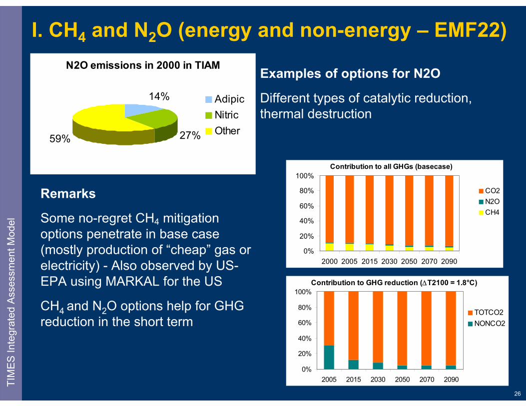
Remarks

Some no-regret CH4 mitigation options penetrate in base case (mostly production of “cheap” gas or electricity) - Also observed by US-EPA using MARKAL for the US

CH4 and N2O options help for GHG reduction in the short term

N2O emissions in 2000 in TIAM

14%

27%59%

AdipicNitricOther

Contribution to GHG reduction (∆T2100 = 1.8°C)

0%

20%

40%

60%

80%

100%

2005 2015 2030 2050 2070 2090

TOTCO2NONCO2

Examples of options for N2O

Different types of catalytic reduction, thermal destruction

Contribution to all GHGs (basecase)

0%

20%

40%

60%

80%

100%

2000 2005 2015 2030 2050 2070 2090

CO2N2OCH4

27

I. CH4 abatement options (1/2)TI

MES

Inte

grat

edAs

sess

men

tMod

el

ACH4MAN01 Farm Scale Digesters-A (cool climate)ACH4MAN02 Farm Scale Digesters-A (warm climate)ACH4MAN03 Farm Scale Digesters-B (cool climate)ACH4MAN04 Farm Scale Digesters-B (warm climate)Not modeled Centralized Digesters (cool climate)

RCH4WLF01 Anaerobic digestion 1 (AD1)RCH4WLF02 Anaerobic digestion 2 (AD2)RCH4WLF03 Composting (C1)RCH4WLF04 Mechanical Biological TreatmentRCH4WLF05 Heat ProductionRCH4WLF06 Increased OxidationRCH4WLF07 Direct Gas Use (profitable at base price)RCH4WLF08 Electricity GenerationRCH4WLF09 Direct Gas Use (profitable above base price) RCH4WLF10 FlaringRCH4WLF11 Composting (C2)

UNCH4OIL01 Flaring instead of Venting (Offshore)UNCH4OIL02 Flaring instead of Venting (Onshore)UNCH4OIL03 Associated Gas (vented) Mix with Other OptionsUNCH4OIL04 Associated Gas (flared) Mix with Other Options

+ Same options for OPEC

UNCH4COA01 Degasification and Pipeline InjectionUNCH4COA02 Enhanced Degasification, Gas Enrichment, and Pipeline InjectionUNCH4COA03 Catalytic Oxidation (US)UNCH4COA04 FlaringUNCH4COA05 Degasification and Power Production – AUNCH4COA06 Degasification and Power Production – B UNCH4COA07 Degasification and Power Production – C UNCH4COA08 Catalytic Oxidation (EU)

+ Same options for OPEC

Manure

Landfill

Primary oil

Coal mining

28

I. CH4 abatement options (2/2)TI

MES

Inte

grat

edAs

sess

men

tMod

el

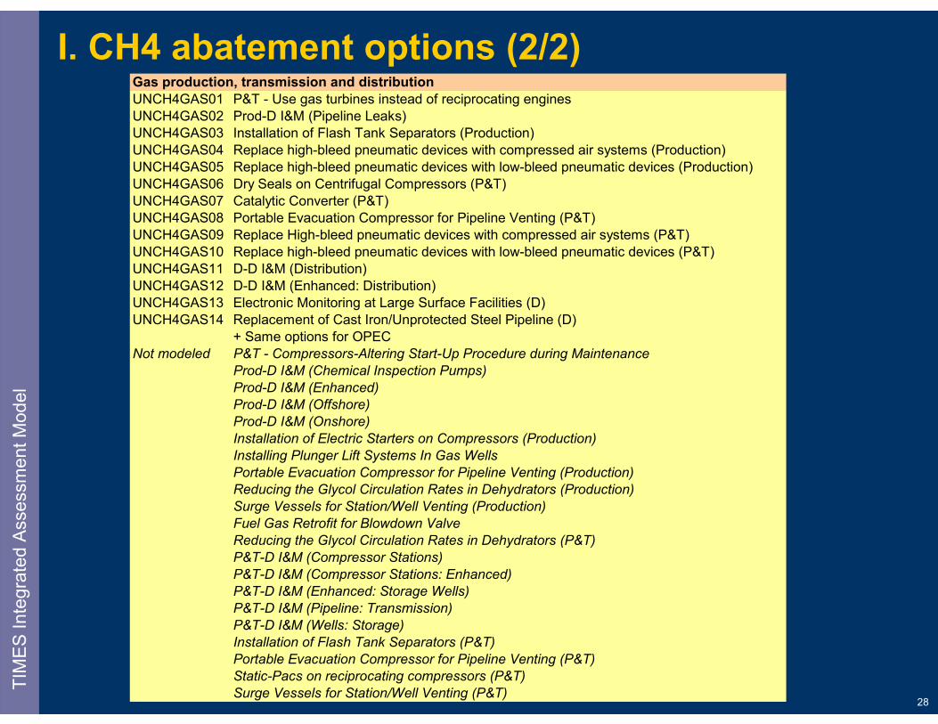
UNCH4GAS01 P&T - Use gas turbines instead of reciprocating enginesUNCH4GAS02 Prod-D I&M (Pipeline Leaks)UNCH4GAS03 Installation of Flash Tank Separators (Production)UNCH4GAS04 Replace high-bleed pneumatic devices with compressed air systems (Production)UNCH4GAS05 Replace high-bleed pneumatic devices with low-bleed pneumatic devices (Production)UNCH4GAS06 Dry Seals on Centrifugal Compressors (P&T)UNCH4GAS07 Catalytic Converter (P&T)UNCH4GAS08 Portable Evacuation Compressor for Pipeline Venting (P&T)UNCH4GAS09 Replace High-bleed pneumatic devices with compressed air systems (P&T)UNCH4GAS10 Replace high-bleed pneumatic devices with low-bleed pneumatic devices (P&T)UNCH4GAS11 D-D I&M (Distribution)UNCH4GAS12 D-D I&M (Enhanced: Distribution)UNCH4GAS13 Electronic Monitoring at Large Surface Facilities (D)UNCH4GAS14 Replacement of Cast Iron/Unprotected Steel Pipeline (D)

+ Same options for OPECNot modeled P&T - Compressors-Altering Start-Up Procedure during Maintenance

Prod-D I&M (Chemical Inspection Pumps)Prod-D I&M (Enhanced)Prod-D I&M (Offshore)Prod-D I&M (Onshore)Installation of Electric Starters on Compressors (Production)Installing Plunger Lift Systems In Gas WellsPortable Evacuation Compressor for Pipeline Venting (Production)Reducing the Glycol Circulation Rates in Dehydrators (Production)Surge Vessels for Station/Well Venting (Production)Fuel Gas Retrofit for Blowdown ValveReducing the Glycol Circulation Rates in Dehydrators (P&T)P&T-D I&M (Compressor Stations)P&T-D I&M (Compressor Stations: Enhanced)P&T-D I&M (Enhanced: Storage Wells)P&T-D I&M (Pipeline: Transmission)P&T-D I&M (Wells: Storage)Installation of Flash Tank Separators (P&T)Portable Evacuation Compressor for Pipeline Venting (P&T)Static-Pacs on reciprocating compressors (P&T)Surge Vessels for Station/Well Venting (P&T)

Gas production, transmission and distribution

29

I. N2O abatement optionsTI

MES

Inte

grat

edAs

sess

men

tMod

el

Adipic AcidICH4ADI01 Thermal DestructionNitric AcidICH4NIT01 Grand Paroisse - High Temperature Catalytic Reduction MethodICH4NIT02 BASF - High Temperature Catalytic Reduction MethodICH4NIT03 Norsk Hydro - High Temperature Catalytic Reduction MethodICH4NIT04 HITK – High Temperature Catalytic Reduction MethodICH4NIT05 Krupp Uhde - Low Temperature Catalytic Reduction MethodICH4NIT06 ECN - Low temperature selective catalytic reduction with propane additionICH4NIT07 Non-Selective Catalytic Reduction (NSCR)

30

II. CLIMATE MODULE

31

Climate moduleTI

MES

Inte

grat

edAs

sess

men

tMod

el

ENERGYSYSTEM

NONENERGY

SECTORS

GHG EMI

CO2eq

CONC.ATM

RADIATIVEFORCING

∆TSURFACECO2

CH4

N2O

Etc.

CONC.OCEAN UP

CONC.OCEAN LO

∆TDEEP

Residual Exo forcingCH4 & N2O

as CO2eq

Tropospheric O3,HFC, black carbon

32

Concentrations of GHG (in CO2-equivalent) (3 layer model)

1. CO2atm(t) = Emi(t) + CO2atm(t-1)*(1-fatm,up) + CO2up(t-1)*fup,atm

2. CO2up(t) = CO2up(t-1)*(1-fup,atm -fup,lo) + CO2lo(t-1)* flo,up + CO2atm(t-)*fatm,up

3. CO2lo(t) = CO2lo(t-1)*(1-flo,up) + CO2up(t-1)* fup,lo

Atmospheric forcing

4. ∆F(t) = γ/ln2 * ln [ CO2atm(t)/CO2atm (pre-ind) ] + O(t)

Temperatures (2 layers)

5. ∆Tup(t) = ∆Tup(t-1) + σ1*{∆F(t) – 3.7/Cs *∆Tup(t-1) - σ2 [∆Tup(t-1) - ∆Tlo (t-1)] } 6. ∆Tlo(t) = ∆Tup(t-1)* σ3 + ∆Tlo (t-1)* g22

Climate equations(as adapted from Nordhaus and Boyer, 1999)

Lag parameterClimate sensitivity

TIM

ES In

tegr

ated

Asse

ssm

entM

odel

33

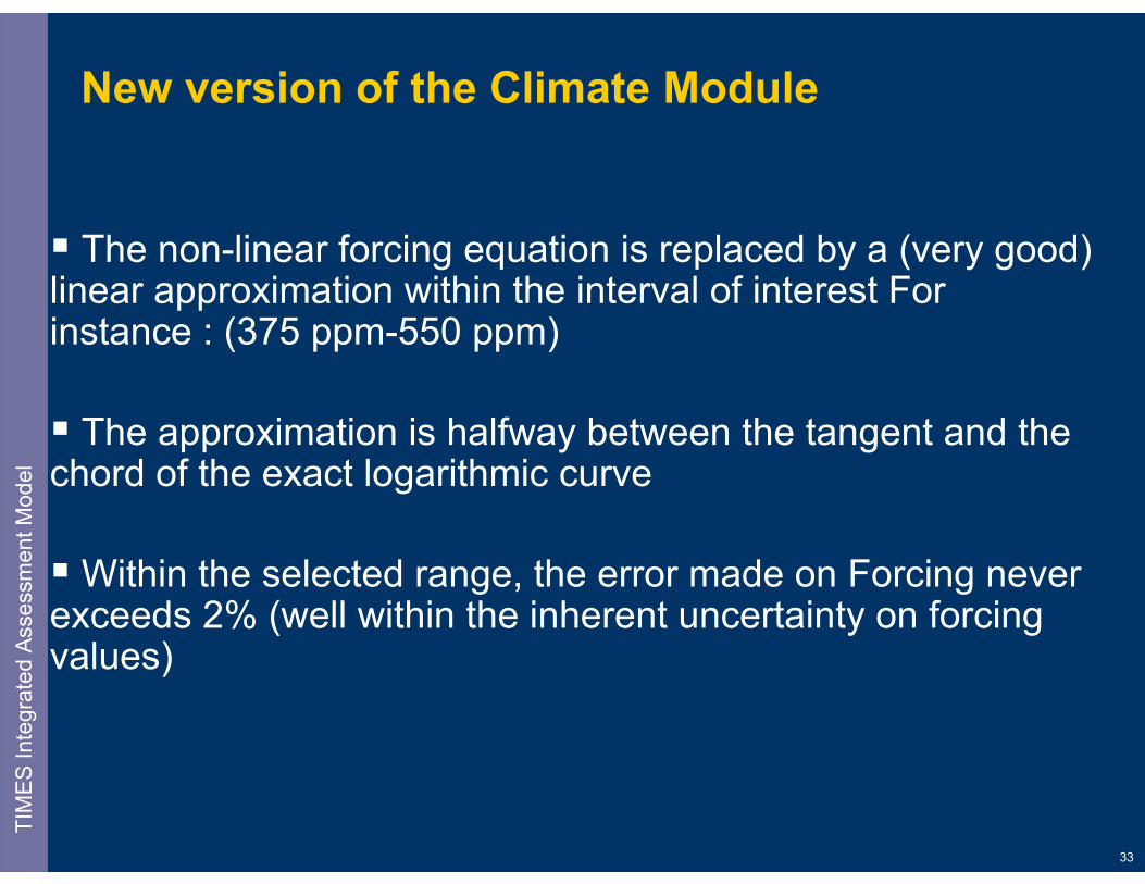
New version of the Climate Module

The non-linear forcing equation is replaced by a (very good) linear approximation within the interval of interest For instance : (375 ppm-550 ppm)

The approximation is halfway between the tangent and the chord of the exact logarithmic curve

Within the selected range, the error made on Forcing never exceeds 2% (well within the inherent uncertainty on forcing values)

TIM

ES In

tegr

ated

Asse

ssm

entM

odel

34

Linearized forcing equation

Relative error less than 2% in range (375 ppm; 550 ppm)

Approximate vs exact forcing

-5-4-3-2-1012

0 0.5 1 1.5 2 2.5 3Radiative forcing

Linear approximation

M/Mo

Range

TIM

ES In

tegr

ated

Asse

ssm

entM

odel