the shapley value, the core, and the shapley - shubik ...fukito/shapley_1a.pdfthe shapley value, the...

The Shapley Value, The Core, and The Shapley

- Shubik Power Index: A SimulationToshitaka Fukiharu

School of Social Informatics

Aoyama Gakuin University

March, 2013

Introduction

The concept of Shapley values was first introduced into the game theory by Shapley [1953] in the framework of transferable payoffs,

playing an important role in the game theory. According to a standard textbook on game theory it is interpreted as in what follows. “Suppose

that all the players are arranged in some order, all orders being equally likely. Then player i’s Shapley value is the expected marginal

contribution over all orders of player i to the set of players who precede him” (Osborne and Rubinstein [1994, p.291]). This concept has been

applied to the parties’ power in the political election, as Shapley-Shubik Power Index (Shapley and Shubik [1954]). The Shapley-Shubik

Index has been applied to actual election systems (Leech [2002] and Suzuki [1994]).

The aim of this paper is, first, to provide the Mathematica programs to compute Shapley values and Shapley-Shubik Power Index. Utilizing

them the relation between the core and Shapley values, and the paradox of Shapley-Shubik Power Index are examined.

In Section I the relation between core and Shapley values is examined. It is known that the Shapley values may not belong to the core.

Utilizing simulation approach, we compute the probability of “the Shapley values belong to the core”. In Section II, the paradox of Shapley-

Shubik Power Index is examined. It is often observed that even if a political party loses in an actual election, its Shapley-Shubik Power Index

rises, and vice versa. Utilizing simulation approach, this paradox is examined theoretically.

Before proceeding, we refer to the Mathematica function to create all the possible cases for the permutation of selecting k elements from

{1,2, ..., n}.

In[1]:= b@n_, 2D := Select@Partition@Flatten@Table@8i, j<, 8i, 1, n<, 8j, 1, n<DD, 2D,

Length@Union@ðDD � 2 &D;

b$aug@x_, n_, k_D :=

Select@Partition@Flatten@Table@8x@@iDD, j<, 8i, 1, Length@xD<, 8j, 1, n<DD,

Dimensions@xD@@2DD + 1D, Length@Union@ðDD � k &D;

b@n_, k_D := b$aug@b@n, k - 1D, n, kD

In[3]:= b@3, 2D

Out[3]= 881, 2<, 81, 3<, 82, 1<, 82, 3<, 83, 1<, 83, 2<<

I: The Shapley Values and The Core

In this section, we define the Shapley values and examine the relation between the Shapley values and the core.

I-1: The Shapley Values

We examine an n - player game, in which transferable payoffs are stipulated for each coalition. Let the set of players be N={1,2, ...,n}, and

arbitrary coalition be S={i1, ..., is}. Payoff for S is stipulated by v[S]. Following Suzuki [1994, Chapter 9], as an example we assume there are

3 players and v[S] is given by the following.

In[4]:= Clear@vD

In[5]:= v@8<D = 0; v@81<D = 10; v@82<D = 20; v@83<D = 30; v@81, 2<D = 60; v@81, 3<D = 70;

v@82, 3<D = 80;

v@81, 2, 3<D = 120;

There are 6 cases of order through which 3 players arrive at the site of coalition.

In[6]:= data1 = b@3, 3D

Out[6]= 881, 2, 3<, 81, 3, 2<, 82, 1, 3<, 82, 3, 1<, 83, 1, 2<, 83, 2, 1<<

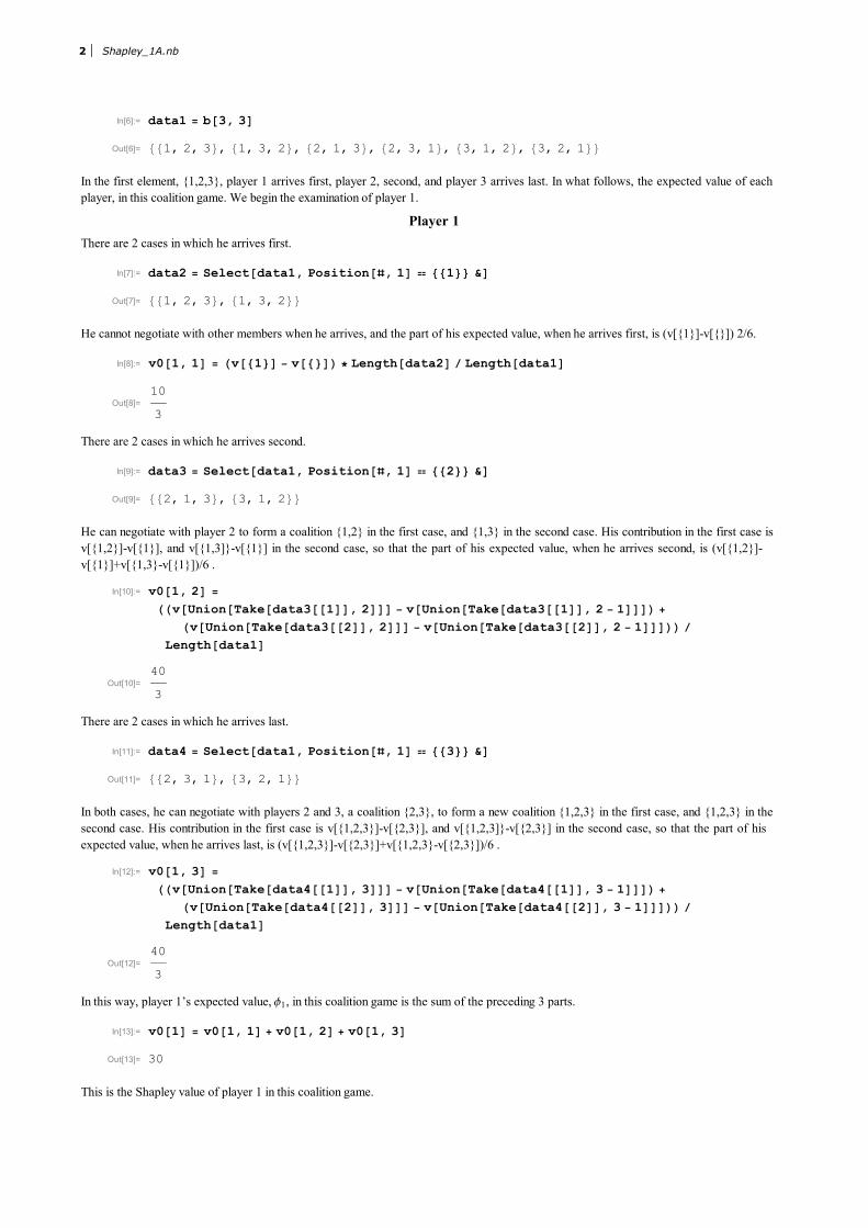
In the first element, {1,2,3}, player 1 arrives first, player 2, second, and player 3 arrives last. In what follows, the expected value of each

player, in this coalition game. We begin the examination of player 1.

Player 1

There are 2 cases in which he arrives first.

In[7]:= data2 = Select@data1, Position@ð, 1D � 881<< &D

Out[7]= 881, 2, 3<, 81, 3, 2<<

He cannot negotiate with other members when he arrives, and the part of his expected value, when he arrives first, is (v[{1}]-v[{}]) 2/6.

In[8]:= v0@1, 1D = Hv@81<D - v@8<DL * Length@data2D � Length@data1D

Out[8]=

10

3

There are 2 cases in which he arrives second.


Out[9]= 882, 1, 3<, 83, 1, 2<<

He can negotiate with player 2 to form a coalition {1,2} in the first case, and {1,3} in the second case. His contribution in the first case is

v[{1,2}]-v[{1}], and v[{1,3]}-v[{1}] in the second case, so that the part of his expected value, when he arrives second, is (v[{1,2}]-

v[{1}]+v[{1,3}-v[{1}])/6 .

In[10]:= v0@1, 2D =

HHv@Union@Take@data3@@1DD, 2DDD - v@Union@Take@data3@@1DD, 2 - 1DDDL +

Hv@Union@Take@data3@@2DD, 2DDD - v@Union@Take@data3@@2DD, 2 - 1DDDLL �Length@data1D

Out[10]=

40

3

There are 2 cases in which he arrives last.


Out[11]= 882, 3, 1<, 83, 2, 1<<

In both cases, he can negotiate with players 2 and 3, a coalition {2,3}, to form a new coalition {1,2,3} in the first case, and {1,2,3} in the

second case. His contribution in the first case is v[{1,2,3}]-v[{2,3}], and v[{1,2,3]}-v[{2,3}] in the second case, so that the part of his

expected value, when he arrives last, is (v[{1,2,3}]-v[{2,3}]+v[{1,2,3}-v[{2,3}])/6 .

In[12]:= v0@1, 3D =


Hv@Union@Take@data4@@2DD, 3DDD - v@Union@Take@data4@@2DD, 3 - 1DDDLL �Length@data1D

Out[12]=

40

3

In this way, player 1’s expected value, Φ1, in this coalition game is the sum of the preceding 3 parts.

In[13]:= v0@1D = v0@1, 1D + v0@1, 2D + v0@1, 3D

Out[13]= 30

This is the Shapley value of player 1 in this coalition game.

2 Shapley_1A.nb

Player 2

In exactly the same way, player 2’s expected value, Φ2, in this coalition game is computed as in what follows.

In[14]:= data2 = Select@data1, Position@ð, 2D � 881<< &D;

v0@2, 1D = Hv@82<D - v@8<DL * Length@data2D � Length@data1D;

data3 = Select@data1, Position@ð, 2D � 882<< &D;

v0@2, 2D =


Hv@Union@Take@data3@@2DD, 2DDD - v@Union@Take@data3@@2DD, 2 - 1DDDLL �Length@data1D; data4 = Select@data1, Position@ð, 2D � 883<< &D;

v0@2, 3D =


Hv@Union@Take@data4@@2DD, 3DDD - v@Union@Take@data4@@2DD, 3 - 1DDDLL �Length@data1D; v0@2D = v0@2, 1D + v0@2, 2D + v0@2, 3D

Out[14]= 40


Player 3

In exactly the same way, player 3’s expected value, Φ3, in this coalition game is computed as in what follows.

In[15]:= data2 = Select@data1, Position@ð, 3D � 881<< &D;

v0@3, 1D = Hv@83<D - v@8<DL * Length@data2D � Length@data1D;

data3 = Select@data1, Position@ð, 3D � 882<< &D;

v0@3, 2D =


Hv@Union@Take@data3@@2DD, 2DDD - v@Union@Take@data3@@2DD, 2 - 1DDDLL �Length@data1D; data4 = Select@data1, Position@ð, 3D � 883<< &D;

v0@3, 3D =


Hv@Union@Take@data4@@2DD, 3DDD - v@Union@Take@data4@@2DD, 3 - 1DDDLL �Length@data1D; v0@3D = v0@3, 1D + v0@3, 2D + v0@3, 3D

Out[15]= 50


In general, the Shapley values for the coalition game, {Φ1, Φ2, ..., Φn} is defined by the following.

Φi =ÚSÌN ΓHSL@v@SD - v@S - 8i<D (i=1, ..., n} (1)

where Γ[S]=(s–1)!/(n–s)!/n! for s: the number of elements in S. This definition can be formalized as a functin p[i,n], given the payoff

specification.

In[16]:= Clear @vD

In[17]:= Hdata0@n_D := Subsets@Table@i, 8i, 1, n<DDL;

HdataA@k_, n_D := Select@data0@nD, Length@Intersection@ð, 8k<DD � 1 &DL;

HdataAA@k_, i_, n_D := Select@dataA@k, nD, Length@ðD � i &DL;

Hp@k_, n_D :=

Sum@HHi - 1L! * HHn - iL!L � Hn!LL *

Sum@v@dataAA@k, i, nD@@jDDD - v@Complement@dataAA@k, i, nD@@jDD, 8k<DD,

8j, 1, Length@dataAA@k, i, nDD<D, 8i, 1, n<DL

As an application, we can easily compute the Shapley values for the coalition games of cost sharing of a dam between 5 members in Japan

(Suzuki [1994, Chapter 15, p.349]).

Shapley_1A.nb 3

In[18]:= v@8<D = 0; v@81<D = 0; v@82<D = 0; v@83<D = 0; v@84<D = 0; v@85<D = 0;

v@81, 2<D = 0; v@81, 3<D = 49.7; v@81, 4<D = 47.1; v@81, 5<D = 55.8;

v@82, 3<D = 3.3; v@82, 4<D = 201.3; v@82, 5<D = 237.6; v@83, 4<D = 130.8;

v@83, 5<D = 131.2; v@84, 5<D = 288.4; v@81, 2, 3<D = 49.7; v@81, 2, 4<D = 229.5;

v@81, 2, 5<D = 259.6; v@81, 3, 4<D = 239.3; v@81, 3, 5<D = 278.0;

v@81, 4, 5<D = 428.2; v@82, 3, 4<D = 289.1; v@82, 3, 5<D = 288.8;

v@82, 4, 5<D = 428.2; v@83, 4, 5<D = 432.8; v@81, 2, 3, 4<D = 371.9;

v@81, 2, 3, 5<D = 435.7; v@81, 2, 4, 5<D = 556.5; v@81, 3, 4, 5<D = 562.5;

v@82, 3, 4, 5<D = 562.8;

v@81, 2, 3, 4, 5<D = 679.2;

In[19]:= 8p@1, 5D, p@2, 5D, p@3, 5D, p@4, 5D, p@5, 5D<

Out[19]= 871.685, 100.943, 94.5767, 193.277, 218.718<

I-2: Applications

Returning to Suzuki [1994, Chapter 10], we confirm that the function provides exactly the same result as in Suzuki [1994, Chapter 10,

Example 7, p.241].

In[20]:= Clear@vD

In[21]:= v@8<D = 0; v@81<D = 0; v@82<D = 0; v@83<D = 0; v@84<D = 0; v@85<D = 0;

v@81, 2<D = 0; v@81, 3<D = 150; v@81, 4<D = 70; v@82, 3<D = 100; v@82, 4<D = 50;

v@83, 4<D = 0; v@81, 2, 3<D = 150; v@81, 2, 4<D = 70; v@81, 3, 4<D = 150;

v@82, 3, 4<D = 100;

v@81, 2, 3, 4<D = 200;

In[22]:= 8p@1, 4D, p@2, 4D, p@3, 4D, p@4, 4D<

Out[22]= :185

3

,

100

3

,

230

3

,

85

3

>

In order to examine the relation between the Shapley values and core, we consider Example 3 (Suzuki[ 1994, Chapter 9, p .199]}. This

example is also an example in Osborne and Rubinstein [1994, Example 294.3, p .294].

I-2-1 Glove Game 1

Suppose that player 1 has a right-hand part of a pair of gloves, while player 2 and player 3 have each left-hand part. The pair is needed for

the glove to play a proper role, and the coalition game can be constructed as in what follows.

In[23]:= v@8<D = 0; v@81<D = 0; v@82<D = 0; v@83<D = 0; v@81, 2<D = 6; v@81, 3<D = 6;

v@82, 3<D = 0;

v@81, 2, 3<D = 6;

In[24]:= 8p@1, 3D, p@2, 3D, p@3, 3D<

Out[24]= 84, 1, 1<

Now suppose that there are 10 players, and player 1 has a right-hand part of a glove, while all the other players have each left-hand part of

the glove. The pair is needed for the glove to play a proper role as above, and the coalition game can be constructed as in what follows,

where S contains {1} and the number of elements is at least 2, the payoff is 6, while it is zero otherwise.

In[25]:= Clear@vD

The payoffs for coalitions can be constructed as in what follows.

In[26]:= Map@v, Subsets@81, 2, 3, 4, 5, 6, 7, 8, 9, 10<DD;

In[27]:= v@a_D := If@Length@Intersection@81<, aDD � 1 && Length@aD ³ 2, 6, 0D

Utilizing these payoffs and the Shapley value function, we can compute the Shapley values for the i - player games (i = 2, 10).

4 Shapley_1A.nb

In[28]:= 8v@81, 2<D, v@82, 4<D<

Out[28]= 86, 0<

In[29]:= Table@Table@p@i, jD, 8i, 1, j<D, 8j, 2, 10<D

Out[29]= :83, 3<, 84, 1, 1<, :9

2

,

1

2

,

1

2

,

1

2

>, :24

5

,

3

10

,

3

10

,

3

10

,

3

10

>,

:5,

1

5

,

1

5

,

1

5

,

1

5

,

1

5

>, :36

7

,

1

7

,

1

7

,

1

7

,

1

7

,

1

7

,

1

7

>,

:21

4

,

3

28

,

3

28

,

3

28

,

3

28

,

3

28

,

3

28

,

3

28

>, :16

3

,

1

12

,

1

12

,

1

12

,

1

12

,

1

12

,

1

12

,

1

12

,

1

12

>,

:27

5

,

1

15

,

1

15

,

1

15

,

1

15

,

1

15

,

1

15

,

1

15

,

1

15

,

1

15

>>

In[30]:= N@%D

Out[30]= 883., 3.<, 84., 1., 1.<, 84.5, 0.5, 0.5, 0.5<,

84.8, 0.3, 0.3, 0.3, 0.3<, 85., 0.2, 0.2, 0.2, 0.2, 0.2<,

85.14286, 0.142857, 0.142857, 0.142857, 0.142857, 0.142857, 0.142857<,

85.25, 0.107143, 0.107143, 0.107143, 0.107143, 0.107143, 0.107143, 0.107143<,

85.33333, 0.0833333, 0.0833333, 0.0833333, 0.0833333, 0.0833333,

0.0833333, 0.0833333, 0.0833333<, 85.4, 0.0666667, 0.0666667, 0.0666667,

0.0666667, 0.0666667, 0.0666667, 0.0666667, 0.0666667, 0.0666667<<

We may conclude that Shapley value of player 1 converges to 6, while those of other players converge to 0 each.

I-2-2 Glove Game 2

In this subsection the core for a coalition game is defined. Core is the distribution of resources, which cannot be blocked by arbitrary

coalition. It is difficult to analyze core in the non-transferable payoff (utility) case (Arrow and Hahn [1973, Chapter 8]). The analysis of core

in the context of transferable payoffs, however, is somewhat easier. The core is defined, under the condition of weak cohesiveness, the

following set of distributions of payoffs among the players

C(v)={x= 8xi<i=1n : ÚiÎS xi ³v(S) "SÌN} (2)

It is said that v satisfies superadditivity if

v(SÜT)³v(S)+v(T) for arbitrary disjoint coalitions S and T. (3)

It is said that v satisfies cohesivity if

v(N)³Úi=1K vHSiL for arbitrary partion 8Si<i=1

K of N. (4)

The cohesivity is a special case of superadditivity (Osborne and Rubinstein [1994, p.258]). It is said that v satisfies weak-cohesiveness

(Suzuki [1994, p.182]) if

v(N)³ v(S) +ÚiÎN-S vHiL for arbitrary coalition SÌN. (5)

From (2) it is clear that the core is defined by the system of linear inequalities. It is not guaranteed that the core is non-empty.

For 3 player hand glove game, we examine if the core exists. Payoffs are defined by the following.

In[31]:= v@8<D = 0; v@81<D = 0; v@82<D = 0; v@83<D = 0; v@81, 2<D = 6; v@81, 3<D = 6;

v@82, 3<D = 0;

v@81, 2, 3<D = 6;

We define the candidates for the core as the following set, T. T consists of x= 8xi<i=13 , where x1+x2+x3=6, and xi=n/10 for integer 0£n£60.

Shapley_1A.nb 5

In[32]:= t1 = Table@i � 10, 8i, 0, 60<D;

t2 =

Partition@Flatten@Table@8t1@@iDD, t1@@jDD, t1@@kDD<, 8i, 1, 61<, 8j, 1, 61<, 8k, 1, 61<DD, 3D;

t3 = Select@t2, ð@@1DD + ð@@2DD + ð@@3DD � 6 &D;

In[33]:= Take@t3, -10D

Out[33]= ::57

10

, 0,

3

10

>, :57

10

,

1

10

,

1

5

>, :57

10

,

1

5

,

1

10

>, :57

10

,

3

10

, 0>, :29

5

, 0,

1

5

>,

:29

5

,

1

10

,

1

10

>, :29

5

,

1

5

, 0>, :59

10

, 0,

1

10

>, :59

10

,

1

10

, 0>, 86, 0, 0<>

There is a unique element in C(v): {6,0,0}. This result corresponds with Osborne and Rubinstein [1994, p.294, Example 294.3].

In[34]:= Select@t3,

ð@@1DD ³ v@81<D && ð@@2DD ³ v@82<D && ð@@3DD ³ v@83<D && ð@@1DD + ð@@2DD ³ v@81, 2<D &&

ð@@1DD + ð@@3DD ³ v@81, 3<D && ð@@2DD + ð@@3DD ³ v@82, 3<D &&

ð@@1DD + ð@@2DD + ð@@3DD ³ v@81, 2, 3<D &D

Out[34]= 886, 0, 0<<

As shown in 1.2.1, the set of Shapley values for this game is {4,1,1}. Thus, the Shapley value does not necessarily belong to the core, even if

the core exists. It was shown, however, that the Shapley value may well converge to {6, 0, 0, ....} as the number of the players with left-hand

part of the glove increases. In what follows, in order to examine the core for 4-player game, we define the candidates for the core as the

following set, T. T consists of x= 8xi<i=14 , where x1+x2+x3+x4=6, and xi=n/10 for integer 0£n£60.

In[35]:= t1 = Table@i � 10, 8i, 0, 60<D;

t2 =

Partition@Flatten@Table@8t1@@iDD, t1@@jDD, t1@@kDD, t1@@lDD<, 8i, 1, 61<, 8j, 1, 61<,

8k, 1, 61<, 8l, 1, 61<DD, 4D;

t3 = Select@t2, ð@@1DD + ð@@2DD + ð@@3DD + ð@@4DD � 6 &D;

In[36]:= Take@t3, 10D

Out[36]= :80, 0, 0, 6<, :0, 0,

1

10

,

59

10

>, :0, 0,

1

5

,

29

5

>, :0, 0,

3

10

,

57

10

>, :0, 0,

2

5

,

28

5

>,

:0, 0,

1

2

,

11

2

>, :0, 0,

3

5

,

27

5

>, :0, 0,

7

10

,

53

10

>, :0, 0,

4

5

,

26

5

>, :0, 0,

9

10

,

51

10

>>

There is a unique element in C(v): {6,0,0,0}.

In[37]:= Select@t3,

ð@@1DD ³ v@81<D && ð@@2DD ³ v@82<D && ð@@3DD ³ v@83<D && ð@@4DD ³ v@84<D &&




ð@@1DD + ð@@2DD + ð@@3DD ³ v@81, 2, 3<D && ð@@1DD + ð@@2DD + ð@@4DD ³ v@81, 2, 4<D &&


ð@@1DD + ð@@2DD + ð@@3DD + ð@@4DD ³ v@81, 2, 3, 4<D &D

Out[37]= 886, 0, 0, 0<<

It is expected that the set of Shapley values converges to {6, 0, 0, ....} as the number of the players with left-hand part of the gloves increases.

I-2-3 Modified Glove Game 1

Now, suppose that the player 2 has a left-hand part and a binder of the right-hand and left-hand parts of the gloves, and the value of a pair of

gloves with binder is 7. The Shapley value of this coalition game is {9/2,3/2,1}.

6 Shapley_1A.nb

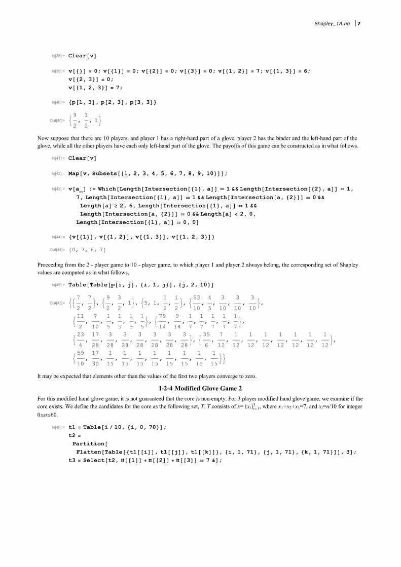
In[38]:= Clear@vD

In[39]:= v@8<D = 0; v@81<D = 0; v@82<D = 0; v@83<D = 0; v@81, 2<D = 7; v@81, 3<D = 6;

v@82, 3<D = 0;

v@81, 2, 3<D = 7;

In[40]:= 8p@1, 3D, p@2, 3D, p@3, 3D<

Out[40]= :9

2

,

3

2

, 1>

Now suppose that there are 10 players, and player 1 has a right-hand part of a glove, player 2 has the binder and the left-hand part of the

glove, while all the other players have each only left-hand part of the glove. The payoffs of this game can be constructed as in what follows.

In[41]:= Clear@vD

In[42]:= Map@v, Subsets@81, 2, 3, 4, 5, 6, 7, 8, 9, 10<DD;

In[43]:= v@a_D := Which@Length@Intersection@81<, aDD � 1 && Length@Intersection@82<, aDD � 1,

7, Length@Intersection@81<, aDD � 1 && Length@Intersection@a, 82<DD � 0 &&

Length@aD ³ 2, 6, Length@Intersection@81<, aDD � 1 &&

Length@Intersection@a, 82<DD � 0 && Length@aD < 2, 0,

Length@Intersection@81<, aDD � 0, 0D

In[44]:= 8v@81<D, v@81, 2<D, v@81, 3<D, v@81, 2, 3<D<

Out[44]= 80, 7, 6, 7<

Proceeding from the 2 - player game to 10 - player game, to which player 1 and player 2 always belong, the corresponding set of Shapley

values are computed as in what follows.

In[45]:= Table@Table@p@i, jD, 8i, 1, j<D, 8j, 2, 10<D

Out[45]= ::7

2

,

7

2

>, :9

2

,

3

2

, 1>, :5, 1,

1

2

,

1

2

>, :53

10

,

4

5

,

3

10

,

3

10

,

3

10

>,

:11

2

,

7

10

,

1

5

,

1

5

,

1

5

,

1

5

>, :79

14

,

9

14

,

1

7

,

1

7

,

1

7

,

1

7

,

1

7

>,

:23

4

,

17

28

,

3

28

,

3

28

,

3

28

,

3

28

,

3

28

,

3

28

>, :35

6

,

7

12

,

1

12

,

1

12

,

1

12

,

1

12

,

1

12

,

1

12

,

1

12

>,

:59

10

,

17

30

,

1

15

,

1

15

,

1

15

,

1

15

,

1

15

,

1

15

,

1

15

,

1

15

>>

It may be expected that elements other than the values of the first two players converge to zero.

I-2-4 Modified Glove Game 2

For this modified hand glove game, it is not guaranteed that the core is non-empty. For 3 player modified hand glove game, we examine if the

core exists. We define the candidates for the core as the following set, T. T consists of x= 8xi<i=13 , where x1+x2+x3=7, and xi=n/10 for integer

0£n£60.

In[46]:= t1 = Table@i � 10, 8i, 0, 70<D;

t2 =

Partition@Flatten@Table@8t1@@iDD, t1@@jDD, t1@@kDD<, 8i, 1, 71<, 8j, 1, 71<, 8k, 1, 71<DD, 3D;

t3 = Select@t2, ð@@1DD + ð@@2DD + ð@@3DD � 7 &D;

Shapley_1A.nb 7

In[47]:= Take@t3, 10D

Out[47]= :80, 0, 7<, :0,

1

10

,

69

10

>, :0,

1

5

,

34

5

>, :0,

3

10

,

67

10

>, :0,

2

5

,

33

5

>,

:0,

1

2

,

13

2

>, :0,

3

5

,

32

5

>, :0,

7

10

,

63

10

>, :0,

4

5

,

31

5

>, :0,

9

10

,

61

10

>>

In this modified game, C(v) may well consist of the line segment between {6,1,0} and {7,0,0}. The set of Shapley values does not belong to

C(v).

In[48]:= Select@t3,

ð@@1DD ³ v@81<D && ð@@2DD ³ v@82<D && ð@@3DD ³ v@83<D && ð@@1DD + ð@@2DD ³ v@81, 2<D &&


ð@@1DD + ð@@2DD + ð@@3DD ³ v@81, 2, 3<D &D

Out[48]= :86, 1, 0<, :61

10

,

9

10

, 0>, :31

5

,

4

5

, 0>, :63

10

,

7

10

, 0>, :32

5

,

3

5

, 0>,

:13

2

,

1

2

, 0>, :33

5

,

2

5

, 0>, :67

10

,

3

10

, 0>, :34

5

,

1

5

, 0>, :69

10

,

1

10

, 0>, 87, 0, 0<>

In what follows, in order to examine the core for 4-player game, we define the candidates for the core as the following set, T. T consists of

x= 8xi<i=14 , where x1+x2+x3+x4=7, and xi=n/10 for integer 0£n£70.

In[49]:= t1 = Table@i � 10, 8i, 0, 70<D;

t2 =

Partition@Flatten@Table@8t1@@iDD, t1@@jDD, t1@@kDD, t1@@lDD<, 8i, 1, 71<, 8j, 1, 71<,

8k, 1, 71<, 8l, 1, 71<DD, 4D;

t3 = Select@t2, ð@@1DD + ð@@2DD + ð@@3DD + ð@@4DD � 7 &D;

In[50]:= Take@t3, 10D

Out[50]= :80, 0, 0, 7<, :0, 0,

1

10

,

69

10

>, :0, 0,

1

5

,

34

5

>, :0, 0,

3

10

,

67

10

>, :0, 0,

2

5

,

33

5

>,

:0, 0,

1

2

,

13

2

>, :0, 0,

3

5

,

32

5

>, :0, 0,

7

10

,

63

10

>, :0, 0,

4

5

,

31

5

>, :0, 0,

9

10

,

61

10

>>

In[51]:= Select@t3,







ð@@1DD + ð@@2DD + ð@@3DD + ð@@4DD ³ v@81, 2, 3, 4<D &D

Out[51]= :86, 1, 0, 0<, :61

10

,

9

10

, 0, 0>, :31

5

,

4

5

, 0, 0>,

:63

10

,

7

10

, 0, 0>, :32

5

,

3

5

, 0, 0>, :13

2

,

1

2

, 0, 0>, :33

5

,

2

5

, 0, 0>,

:67

10

,

3

10

, 0, 0>, :34

5

,

1

5

, 0, 0>, :69

10

,

1

10

, 0, 0>, 87, 0, 0, 0<>

In this modified game, C(v) may well consist of the line segment between {6,1,0,0} and {7,0,0,0}. The set of Shapley values does not belong

to C(v). In what follows, in order to examine the core for 5-player game, we define the candidates for the core as the following set, T. T

consists of x= 8xi<i=15 , where x1+x2+x3+x4+x5=7, and xi=n/10 for integer 0£n£70.

In[52]:= t4 = Select@t2, ð@@1DD + ð@@2DD + ð@@3DD + ð@@4DD £ 7 &D;

8 Shapley_1A.nb

In[53]:= t5 = Table@8t4@@iDD, 7 - Apply@Plus, t4@@iDDD<, 8i, 1, Length@t4D<D;

In[54]:= t6 = Table@Partition@Flatten@t5@@iDDD, 5D@@1DD, 8i, 1, Length@t5D<D;

In[55]:= Take@t6, 10D

Out[55]= :80, 0, 0, 0, 7<, :0, 0, 0,

1

10

,

69

10

>, :0, 0, 0,

1

5

,

34

5

>,

:0, 0, 0,

3

10

,

67

10

>, :0, 0, 0,

2

5

,

33

5

>, :0, 0, 0,

1

2

,

13

2

>, :0, 0, 0,

3

5

,

32

5

>,

:0, 0, 0,

7

10

,

63

10

>, :0, 0, 0,

4

5

,

31

5

>, :0, 0, 0,

9

10

,

61

10

>>

In[56]:= Select@t6,


ð@@5DD ³ v@85<D && ð@@1DD + ð@@2DD ³ v@81, 2<D && ð@@1DD + ð@@3DD ³ v@81, 3<D &&










ð@@1DD + ð@@2DD + ð@@3DD + ð@@4DD ³ v@81, 2, 3, 4<D &&

ð@@1DD + ð@@2DD + ð@@3DD + ð@@5DD ³ v@81, 2, 3, 5<D &&

ð@@1DD + ð@@2DD + ð@@4DD + ð@@5DD ³ v@81, 2, 4, 5<D &&

ð@@1DD + ð@@3DD + ð@@4DD + ð@@5DD ³ v@81, 3, 4, 5<D &&

ð@@2DD + ð@@3DD + ð@@4DD + ð@@5DD ³ v@82, 3, 4, 5<D &&

ð@@1DD + ð@@2DD + ð@@3DD + ð@@4DD + ð@@5DD ³ v@81, 2, 3, 4, 5<D &D

Out[56]= :86, 1, 0, 0, 0<, :61

10

,

9

10

, 0, 0, 0>, :31

5

,

4

5

, 0, 0, 0>,

:63

10

,

7

10

, 0, 0, 0>, :32

5

,

3

5

, 0, 0, 0>, :13

2

,

1

2

, 0, 0, 0>, :33

5

,

2

5

, 0, 0, 0>,

:67

10

,

3

10

, 0, 0, 0>, :34

5

,

1

5

, 0, 0, 0>, :69

10

,

1

10

, 0, 0, 0>, 87, 0, 0, 0, 0<>

In this modified game, C(v) may well consist of the line segment between {6,1,0,0,0} and {7,0,0,0,0}. The set of Shapley values does not

belong to C(v). As the number of players increases, however, it may well be expected that the limit of the Shapley values belongs to the limit

set of the core. If we regard player 1 Intel with the technology of processor, player 2 the Japanese manufacturers with the excellent technol-

ogy of memory chips, with all others those of standard technology of memory chips, the example of this subsections may well explain the

tragedy of the Japanese semiconductor industry.

I-3: Probability of “the Core Includes the Shapley Value”: 3 Player Game

For the transferable payoffs, the general necessary and sufficient conditions for the existence of non-empty core is known, as the game is

balanced (Osborne and Rubinstein [1994, Proposition 262.1]). When the number of players is 3 and the game is super-additive, we have a

neat theorem with the necessary and sufficient conditions for the existence of non-empty core (Suzuki [1994, p.229, Theorem 8). It is the

following simple inequality:

2v[{1,2,3}]³v[{1,2}]+v[{1,3}]+v[{2,3}] (6)

In this subsection we examine the probability of “the Shapley values belong to the core” in this 3-player game, utilizing simulation approach.

By the following program, we can construct {v(S)} arbitrarily selected with super-additivity where v(S) is an integer satisfying 0£v(S)£1000

and (6) is satisfied.

Shapley_1A.nb 9

In[57]:= Clear@vD

In[58]:= f2@x_D :=

If@x@@2DD + x@@3DD £ x@@5DD && x@@2DD + x@@4DD £ x@@6DD && x@@3DD + x@@4DD £ x@@7DD &&

x@@4DD + x@@5DD £ x@@8DD && x@@3DD + x@@6DD £ x@@8DD && x@@2DD + x@@7DD £ x@@8DD &&

x@@2DD + x@@3DD + x@@4DD < x@@8DD &&

H2 v@81, 2, 3<D ³ Hv@81, 2<D + v@81, 3<D + v@82, 3<DLL, x,

8v@8<D = 0, v@81<D = Random@Integer, 80, 1000<D,

v@82<D = Random@Integer, 80, 1000<D, v@83<D = Random@Integer, 80, 1000<D,

v@81, 2<D = Random@Integer, 80, 1000<D, v@81, 3<D = Random@Integer, 80, 1000<D,

v@82, 3<D = Random@Integer, 80, 1000<D,

v@81, 2, 3<D = Random@Integer, 80, 1000<D<D

In[59]:= FixedPoint@f2, 8v@8<D = 0, v@81<D = Random@Integer, 80, 1000<D,



v@82, 3<D = Random@Integer, 80, 1000<D, v@81, 2, 3<D = Random@Integer, 80, 1000<D<D

Out[59]= 80, 88, 95, 89, 369, 454, 403, 644<

In the following simulation, selecting 1000 tuples of such {v(S)} arbitrarily, we can count the number of the cases with the property of “the

Shapley values belong to the core”.

In[60]:= Timing@Count@

Table@FixedPoint@f2, 8v@8<D = 0, v@81<D = Random@Integer, 80, 1000<D,



v@82, 3<D = Random@Integer, 80, 1000<D,

v@81, 2, 3<D = Random@Integer, 80, 1000<D<D;

Length@Select@8p@1, 3D - v@81<D, p@2, 3D - v@82<D, p@3, 3D - v@83<D,

p@1, 3D + p@2, 3D - v@81, 2<D, p@1, 3D + p@3, 3D - v@81, 3<D,

p@2, 3D + p@3, 3D - v@82, 3<D<, ð ³ 0 &DD, 81000<D, 6DD

Out[60]= 823.914953, 649<

Approximately, 2/3 is the probability of “the Shapley values belong to the core”.

II The Shapley-Shubik Power Index and the Voting Paradox

The approach through Shapley values has been applied to the voting game as the Shapley-Shubik Power Index (Shapley and Shubik [1954]),

and paradoxes have been pointed out. In this section these paradoxes are examined.

II - 1: The Shapley-Shubik Power Index

Following Example 6 in Suzuki [1994, p .210], the Shapely - Shubik Power Index is defined. Suppose that there are 5 political parties and

Party 1 has 6 representatives in a parliament, Party 2, 4, Party 3, 2, Party 4, 2, and Party 5 has 1. Since there are 15 votes in this parliament, 8

votes are required to enact a legislation through simple majority rule. By the following Mathematica program, 16 types of coalitions are

possible to enact proposed laws.

10 Shapley_1A.nb

In[61]:= d1 = 86, 4, 2, 2, 1<;

d2 =

Select@Partition@Flatten@Table@8d1@@i1DD + d1@@i2DD, 8i1, i2<<, 8i1, 1, Length@d1D<,

8i2, 1, Length@d1D<DD, 3D, ð@@2DD =!= ð@@3DD &D;

d3 =

Select@Partition@Flatten@Table@8d1@@i1DD + d1@@i2DD + d1@@i3DD, 8i1, i2, i3<<,

8i1, 1, Length@d1D<, 8i2, 1, Length@d1D<, 8i3, 1, Length@d1D<DD, 4D,

Length@Union@8ð@@2DD, ð@@3DD, ð@@4DD<DD � 3 &D;

d4 =

Select@Partition@

Flatten@Table@8d1@@i1DD + d1@@i2DD + d1@@i3DD + d1@@i4DD, 8i1, i2, i3, i4<<,

8i1, 1, Length@d1D<, 8i2, 1, Length@d1D<, 8i3, 1, Length@d1D<,

8i4, 1, Length@d1D<DD, 5D,

Length@Union@8ð@@2DD, ð@@3DD, ð@@4DD, ð@@5DD<DD � 4 &D;

d5 = Join@d2, d3, d4, 88Apply@Plus, d1D, 1, 2, 3, 4, 5<<D;

d6 = Select@d5, ð@@1DD ³ 8 &D;

d7 = Union@Table@Union@Delete@d6@@iDD, 1DD, 8i, 1, Length@d6D<DD

Out[61]= 881, 2<, 81, 3<, 81, 4<, 81, 2, 3<, 81, 2, 4<, 81, 2, 5<,

81, 3, 4<, 81, 3, 5<, 81, 4, 5<, 82, 3, 4<, 81, 2, 3, 4<, 81, 2, 3, 5<,

81, 2, 4, 5<, 81, 3, 4, 5<, 82, 3, 4, 5<, 81, 2, 3, 4, 5<<

There are 120 cases of order through which 5 players arrive at the site of coalition. 10 cases are shown as in what follows.

In[62]:= d7 = b@5, 5D; Take@d7, 10D

Out[62]= 881, 2, 3, 4, 5<, 81, 2, 3, 5, 4<, 81, 2, 4, 3, 5<, 81, 2, 4, 5, 3<, 81, 2, 5, 3, 4<,

81, 2, 5, 4, 3<, 81, 3, 2, 4, 5<, 81, 3, 2, 5, 4<, 81, 3, 4, 2, 5<, 81, 3, 4, 5, 2<<

In the first element, Party 1 and Party 2 has collective vote of 10, so that Party 2 is the “pivot” in the coalition {1, 2}. In the last (10th)

element, Party 1 and Party 3 has collective vote of 8, so that Party 3 is the “pivot” in the coalition {1,3}. The following program finds the

pivots for 120 possible cases.

In[63]:= d10 = Table@d8@kD = Table@Take@d7@@kDD, iD, 8i, 2, 5<D;

d9@kD =

Table@8d8@kD@@iDD, Sum@d1@@d8@kD@@iDD@@jDDDD, 8j, 1, Length@d8@kD@@iDDD<D<,

8i, 1, Length@d8@kDD<D; Last@First@Select@d9@kD, ð@@2DD ³ 8 &DD@@1DDD,

8k, 1, Length@d7D<D

Out[63]= 82, 2, 2, 2, 2, 2, 3, 3, 3, 3, 3, 3, 4, 4, 4, 4, 4, 4, 2, 2, 3, 3, 4, 4, 1, 1, 1, 1, 1, 1, 1,

1, 4, 4, 1, 4, 1, 1, 3, 3, 1, 3, 1, 1, 1, 4, 1, 3, 1, 1, 1, 1, 1, 1, 1, 1, 4, 4, 1, 4, 1,

1, 2, 2, 1, 2, 1, 1, 1, 4, 1, 2, 1, 1, 1, 1, 1, 1, 1, 1, 3, 3, 1, 3, 1, 1, 2, 2, 1, 2, 1,

1, 1, 3, 1, 2, 2, 2, 3, 3, 4, 4, 1, 1, 1, 4, 1, 3, 1, 1, 1, 4, 1, 2, 1, 1, 1, 3, 1, 2<

The Shapley-Shubik Power Index is defined by the set of each party’s probability of becoming the “pivot”. It is computed as in what follows.

In[64]:= Table@Count@d10, iD � Length@d7D, 8i, 1, 5<D

Out[64]= :1

2

,

1

6

,

1

6

,

1

6

, 0>

In general, it is known that the Shapley-Shubik power index can be computed by the following formula (Suzuki [1994, p.214]).

Φi =(1/n!)ÚSÎWi Hs - 1L ! Hn–sL ! (i=1, ..., n} (7)

where {W1, ..., Wk} is the set of coalitions, and s is the number of elements of that coalition. Given the set of votes of political parties and the

number the votes to enact a legislation, the following function, SSI, computes the coalition sets and the set of Shapley-Shubik power indices,

when the number of the political parties is at most 10.

Shapley_1A.nb 11

In general, it is known that the Shapley-Shubik power index can be computed by the following formula (Suzuki [1994, p.214]).

Φi =(1/n!)ÚSÎWi Hs - 1L ! Hn–sL ! (i=1, ..., n} (7)

where {W1, ..., Wk} is the set of coalitions, and s is the number of elements of that coalition. Given the set of votes of political parties and the

number the votes to enact a legislation, the following function, SSI, computes the coalition sets and the set of Shapley-Shubik power indices,

when the number of the political parties is at most 10.

In[65]:= SSI@elected_, m0_D := Module@8k1, k2A, k2, k3A, k3, k4, k5, k6, k7, n0, w<,

k1 = elected; n0 = Length@k1D; k2A@n_D := If@n £ n0, b@n0, nD, 8<D;

k2A@n_D := If@n £ n0, b@n0, nD, 8<D; Table@k2@nD = k2A@nD, 8n, 2, n0<D;

k3A@n_D :=

Partition@Flatten@Table@8Apply@Plus, k1@@k2@nD@@iDDDDD, k2@nD@@iDD<,

8i, 1, Length@k2@nDD<DD, n + 1D;

Table@k3@nD = If@n £ n0, k3A@nD, 8<D, 8n, 2, 10<D;

k4 = Join@k3@2D, k3@3D, k3@4D, k3@5D, k3@6D, k3@7D, k3@8D, k3@9D, k3@10DD;

k5 = Select@k4, ð@@1DD ³ m0 &D;

k6 = Union@Table@Union@Delete@k5@@iDD, 1DD, 8i, 1, Length@k5D<DD;

w@j_D :=

Select@k6,

HLength@Intersection@8j<, ðDDL ³ 1 &&

HLength@Intersection@8Complement@ð, 8j<D<, k6DDL � 0 &D;

k7@n_D := H1 � n0!L Sum@HLength@w@nD@@iDDD - 1L! * Hn0 - Length@w@nD@@iDDDL!,

8i, 1, Length@w@nDD<D; Table@k7@nD, 8n, 1, n0<DD

It is ascertained that the function computes the set of Shapley-Shubik power indices for the above example.

In[66]:= SSI@d1, 8D

Out[66]= :1

2

,

1

6

,

1

6

,

1

6

, 0>

II - 2. Paradox of Shapley-Shubik Power Index: Kanagawa Prefecture

It has been argued that there are paradoxes for the Shapley-Shubik power index. In order to explain this paradox, we refer to the actual

election results in Kanagawa Prefecture, Japan (Suzuki [1994, Example 9, pp.215-6]). The set of the numbers of elected candidates of 7

political parties, in the 1987 selection, is {41, 28, 14, 16, 13, 2, 1} where the second element is that of Socialist Party. The simple majority

rule requires the political parties to collect 58 votes to enact a legislation. Utilizing the SSI function, we obtain exactly the same set of

Shapley-Shubik power indices as in Suzuki [1994].

In[67]:= SSI@841, 28, 14, 16, 13, 2, 1<, 58D

Out[67]= :11

30

,

7

30

,

1

10

,

1

6

,

1

15

,

1

30

,

1

30

>

In[68]:= N@%D

Out[68]= 80.366667, 0.233333, 0.1, 0.166667, 0.0666667, 0.0333333, 0.0333333<

In the 1991 election, the set of the numbers of elected candidates of 8 political parties is {48, 30,13,12,9,1,1,1}where the second element is

that of Socialist Party. As above, the simple majority rule requires the political parties to collect 58 votes to enact a legislation. Utilizing the

SSI function, we obtain exactly the same set of Shapley-Shubik power indices as in Suzuki [1994].

In[69]:= SSI@848, 30, 13, 12, 9, 1, 1, 1<, 58D

Out[69]= :79

140

,

47

420

,

47

420

,

47

420

,

9

140

,

1

84

,

1

84

,

1

84

>

In[70]:= N@%D

Out[70]= 80.564286, 0.111905, 0.111905, 0.111905, 0.0642857, 0.0119048, 0.0119048, 0.0119048<

Suzuki [1994, p.216] interprets that there is a paradox of the Shapley-Shubik power index in this election result, since it fell in spite of the

increased number of elected candidates of Socialist Party. As he admits (Suzuki [1994, p.217]), however, this phenomenon might be a case

which should not be called a paradox, since too many changes took place for other parties. In what follows, utilizing SSI function, we

conducts simulations, which examine what would happen if only one elected seat decreases from a political party and the seat is added to

other party. In what follows, first, a 7-element tuple is selected randomly, with each element smaller than 58, and the sum smaller than 116,

creating 8-element tuple with the 8th element the difference between 116 and the sum of the first 7 elements. For this tuple, we compute the

difference between the SSI for this tuple and the one for this tuple+{-1, 1, 0, 0, 0, 0, 0, 0}. We repeat this simulation 1000 times.

12 Shapley_1A.nb

Suzuki [1994, p.216] interprets that there is a paradox of the Shapley-Shubik power index in this election result, since it fell in spite of the

increased number of elected candidates of Socialist Party. As he admits (Suzuki [1994, p.217]), however, this phenomenon might be a case

which should not be called a paradox, since too many changes took place for other parties. In what follows, utilizing SSI function, we

conducts simulations, which examine what would happen if only one elected seat decreases from a political party and the seat is added to

other party. In what follows, first, a 7-element tuple is selected randomly, with each element smaller than 58, and the sum smaller than 116,

creating 8-element tuple with the 8th element the difference between 116 and the sum of the first 7 elements. For this tuple, we compute the

difference between the SSI for this tuple and the one for this tuple+{-1, 1, 0, 0, 0, 0, 0, 0}. We repeat this simulation 1000 times.

In[71]:= f@x_, n_, y_D := If@Apply@Plus, xD < y, x, Table@Random@Integer, 81, y � 2<D, 8n<DD

In[72]:= f0@x_D := f@x, 7, 116D

In[73]:= Timing@b1 = Table@Clear@a1, a2, a3D;

a1 = FixedPoint@f0, 8Random@Integer, 81, 58<D, Random@Integer, 81, 58<D,

Random@Integer, 81, 58<D, Random@Integer, 81, 58<D,


Random@Integer, 81, 58<D<D; a2 = Flatten@8a1, 116 - Apply@Plus, a1D<D;

8a2, HSSI@a2, 58D - SSI@a2 + 8-1, 1, 0, 0, 0, 0, 0, 0<, 58DL<, 81000<D;D

Out[73]= 819 993.228561, Null<

The first element in the following indicates the number of cases in which the difference is positive, the second the one with equality, and the

third the one with negativity.

In[74]:= 8Length@Select@b1, ð@@2, 1DD > 0 &DD, Length@Select@b1, ð@@2, 1DD == 0 &DD,

Length@Select@b1, ð@@2, 1DD < 0 &DD<

Out[74]= 8852, 148, 0<

Note that there is no cases, in which the difference is negative. Thus, we may conclude that one party’s increased one seat in an election

implies the non-decrease of SSI.

II - 3. Paradox of Shapley-Shubik Power Index: Kyoto Prefecture

In this subsection, we refer to the actual election results in Kyoto Prefecture, Japan (Suzuki [1994, Example 9, p.215]). The set of the

numbers of elected seats of 6 political parties, in the 1978 selection, is {19, 15, 11, 8, 6, 4} where the first element is that of Liberal Demo-

crat Party. The simple majority rule requires the political parties to collect 32 votes to enact a legislation. Utilizing the SSI function, we obtain

exactly the same set of Shapley-Shubik power indices as in Suzuki [1994].

In[75]:= SSI@819, 15, 11, 8, 6, 4<, 32D

Out[75]= :1

3

,

4

15

,

1

6

,

1

10

,

1

10

,

1

30

>

In[76]:= N@%D

Out[76]= 80.333333, 0.266667, 0.166667, 0.1, 0.1, 0.0333333<

In the 1982 election, the set of the numbers of elected seats of 6 political parties is {18, 16, 8, 8, 6, 7} where the second element is that of

Liberal Democrat Party. As above, the simple majority rule requires the political parties to collect 32 votes to enact a legislation. Utilizing the

SSI function, we obtain exactly the same set of Shapley-Shubik power indices as in Suzuki [1994].

In[77]:= SSI@818, 16, 8, 8, 6, 7<, 32D

Out[77]= :11

30

,

7

30

,

2

15

,

2

15

,

1

15

,

1

15

>

In[78]:= N@%D

Out[78]= 80.366667, 0.233333, 0.133333, 0.133333, 0.0666667, 0.0666667<

Suzuki [1994, p.215] also interprets that there is a paradox of the Shapley-Shubik power index in this election result, since it rose for LDP in

spite of the decreased number of elected seats of LDP. In what follows, utilizing SSI function, we conducts simulations, which examine what

would happen if only one elected seat decreases from a political party and the seat is added to other party. In what follows, first, a 5-element

tuple is selected randomly, with each element smaller than 31, and the sum smaller than 63, creating 6-element tuple with the 6th element the

difference between 63 and the sum of the first 5 elements. For this tuple, we compute the difference between the SSI for this tuple and the

one for this tuple+{-1, 1, 0, 0, 0, 0}. We repeat this process 10 times.

In[79]:= Clear@f0D; f0@x_D := f@x, 5, 63D

Shapley_1A.nb 13

In[80]:= Timing@b1 = Table@Clear@a1, a2D;

a1 = FixedPoint@f0, 8Random@Integer, 81, 31<D, Random@Integer, 81, 31<D,


Random@Integer, 81, 31<D<D; a2 = Flatten@8a1, 63 - Apply@Plus, a1D<D;

8a2, SSI@a2, 32D<, 81000<D;D

Out[80]= 8132.725651, Null<

The first element in the following indicates the number of cases in which the difference is positive, the second, the one with equality, and the

third, the one with negativity.

In[81]:= 8Length@Select@b1, ð@@2, 1DD > 0 &DD, Length@Select@b1, ð@@2, 1DD == 0 &DD,

Length@Select@b1, ð@@2, 1DD < 0 &DD<

Out[81]= 8912, 88, 0<

Note that there is no cases, in which the difference is negative. Thus, as in the previous subsection, we may conclude that one party’s

increased one seat in an election implies the non-decrease of SSI.

Conclusions

Main aim of this paper is to construct Mathematica functions to compute the Shapley values and the Shapley-Shubik power index. It was

shown that it is easy to construct them. In Section I, ascertaining that the Shapley-value function quickly solves the exercises in Osborne and

Rubinstein [1994] and Suzuki [1994], it was first applied to the relation between the Shapley value and the core. It is well known that the set

of Shapley values might not belong to the core. Utilizing the glove game in Suzuki [1994] we showed that as the number of left-hand glove

holders increases to infinity, the set of Shapley values may well converge to the core. Next, modifying this glove game, we examined the

tragedy of Japanese semi-conductor industry. Supposing that the right-hand glove holder is INTEL, the manufacturer of CPU, and the left-

hand glove and binder holder is the Japanese semiconductor industry, the manufacturer of excellent memory chips, and the left-hand glove

holders without binder are Taiwan, Korea, and others. It was shown, first, that as the number of the left-hand glove holders without binder

increases to infinity, the Shapley value of INTEL rises to more than the value of the pair of gloves, while that of Japan is converging to less

than the value of binder. Next, it was shown that the set of Shapley values tends to converge to a point in the core, as the number of the left-

hand holders without binder increases to infinity. Finally, in this section, for the 3-player coalition game, the probability of “the set of Shapley

values belongs to the core” is approximately 2/3, by simulation.

In Section II, the function to compute the Shapley-Shubik power index was constructed easily. After solving exercises in Suzuki [1994], we

applied it to the paradox of the Shapley-Shubik power index. Utilizing actual election results, Suzuki [1994] explained that paradoxes took

place in that the losing (winning) political parties have higher (lower) Shapley-Shubik power index. In this section, by simulation, it was

shown that if the change of election is that of one-seat loss, then the Shapley-Shubik power index of the losing party is never higher.

References

Arrow, K. J., and F. H. Hahn [1971], General Competitive Analysis, Holden-Day Inc. San Francisco.

Leech, D. [2002], “Designing the Voting System for the Council of the European Union,” Public Choice 113, 437-464.

Osborne, M. J. and A. Rubinstein [1994], A Course in Game Theory, MIT Press.

Shapley, L. S. [1953], “A Value for N-Person Games”, in Kuhn, H. W. and Tucker, A. W. Contributions to the Theory of Games I, Prince-

ton: Princeton University

Press, 307-317.

Shapley, L. S. and M. Shubik [1954], “A Method for Evaluating the Distribution of Power in a Committee System”, American Political

Science Review 48, 787-792.

Suzuki, M. [1994], The New Game Theory (in Japanese), Keiso-Shobo.

14 Shapley_1A.nb

the shapley value, the core, and the shapley - shubik ...fukito/shapley_1a.pdfthe shapley value, the...

Documents