the role of spatio-temporal effects in anaerobic digestion of solid waste

Nonlinear Analysis 63 (2005) e1497–e1505www.elsevier.com/locate/na

The role of spatio-temporal effects in anaerobicdigestion of solid waste

Hermann J. EberlDepartment of Mathematics and Statistics, University of Guelph, Guelph, Ont., Canada N1G 2W1

Abstract

Using methods of mathematical modelling and computer simulation, we study the effect that spatialdistribution of material has on the process duration of anaerobic digestion of solid waste. The need fora spatio-temporal model is demonstrated by analysis of the solutions of an ODE model in dependenceof model parameters and initial data. The spatio-temporal model is obtained by inclusion of masstransfer processes. This leads to a semi-linear diffusion–reaction system, the transient behavior ofwhich we study numerically. Our focus is on the temporal spreading of so-called methanogenic pocketsin bounded domains. These are regions, in which the qualitative behavior of the model solution isdifferent than in their neighborhood.� 2005 Elsevier Ltd. All rights reserved.

PACS: −02.30.Jr; 02.60.Cb; 87.23.Cc; 89.20.Kk

Keywords: Mathematical model; Diffusion–reaction; Anaerobic digestion

1. Introduction

Anaerobic digestion of solid waste is a rather slow process. In laboratory reactors andlandfill sites it can take many days or even several years, which makes experimental stud-ies very difficult. Moreover, these experiments can be extremely costly because of spacerequirements. Therefore, mathematical modelling and computer simulation seem attractivealternatives. Most models used by engineers today are formulated as ordinary differentialequations (e.g. [1]) and, thus, cannot describe spatial effects. Due to the large number of sub-processes that are often considered and due to the huge number of model parameters, these

E-mail address: [email protected] (H.J. Eberl).

0362-546X/$ - see front matter � 2005 Elsevier Ltd. All rights reserved.doi:10.1016/j.na.2005.01.045

http://www.elsevier.com/locate/na

mailto:[email protected]

e1498 H.J. Eberl / Nonlinear Analysis 63 (2005) e1497–e1505

models typically can be studied only by numerical simulations, which makes it difficult toobtain a complete picture about the model behavior. Our goal is to demonstrate the impor-tance of taking spatio-temporal effects into account. We do this by first studying a lumpedmodel and classifying its solutions. It turns out that they, indeed, can be very different inthe initial transient phase, depending on the initial data. The model is formulated for thedependent variables waste density w, volatile fatty acids (VFA) s, methanogenic biomassb, and methane concentration p. Two basic processes are taken into account: (i) during hy-drolysis, the waste w is degraded and VFA s are produced, while (ii) during methanogenesismethanogenic biomass b is produced and VFA s are reduced, see [5]. Furthermore, we takedecay of methanogenic biomass due to cell death into account. Both process rates (i) and(ii) depend on s, in particular high values of s are inhibitory. As in many models in micro-biology and microbiology based engineering applications, the kinetic terms describing theinteraction of dependent variables are only known qualitatively and the specific reactionterms are often chosen in a somewhat ad hoc manner, leading to the problem of uncertainmodel parameters. We take this into account in our study and replace the explicit form ofreaction terms by functions about which we only know that they are (piecewise) monotone.

To overcome the limitations stemming from the lumped model approach, spatial masstransfer effects will be included in the model in the second part of our study. This approachwas suggested in [7], where also some one-dimensional numerical simulations have beencarried out. It leads to a three-dimensional semi-linear system of partial differential equa-tions which we study numerically in order to measure the effect of initially heterogeneousdistribution of material on process duration. Our particular attention is turned to the spread-ing of methanogenic pockets. These are regions in which the local behavior of the solutionsis different than in their neighborhood, especially production of methanogenic biomass isincreased.

2. Mathematical models

2.1. A spatially uniform model

We consider the lumped model for hydrolysis and methanogensis

w = −k1wF(s),

s = k2wF(s) − k3G(s)b,

b = (k4G(s) − k5)b,

p = k6G(s)b (1)

with initial data

w(0) = w0 > 0, s(0) = s0 > 0, b(0) = b0 > 0, p(0) = p0 �0.

The rate function F(s) describes the dependence of hydrolysis on the concentration of VFA.It is a continuous, smooth, decreasing function such that F(0) = 1, F(s) > 0 for s > 0, andlims→∞ F(s) = 0, F ∈ C[R+

0 ]. G(s) describes the dependence of methanogenesis on s.It is a continuous, smooth, positive, “single bump” function with G(0) = 0, G(s) > 0 for

H.J. Eberl / Nonlinear Analysis 63 (2005) e1497–e1505 e1499

s > 0, limS→∞ G(s)=0, G ∈ C[R+0 ]. It has a maximum S such that G′(s) > 0 for all s < S

and G′(s) < 0 for all s > S. Both functions F and G and the model parameters are relatedby the following formal conditions:

(H1) the function H1(s) := G(s)/F (s) is monotonously increasing;(H2) the function H2(s) := k1F(s) + k4G(s) − k5 has exactly one root S;(H3) k4G(S) > k5.

Note that these restrictions are not severe for practical applications. With the given qual-itative behavior of F and G as well as (H1), the conditions (H2) and (H3) are essentiallyconditions on the parameters k1,4,5. For example, (H1)–(H3) are fulfilled by the functionsand parameters used by Eberl [2] and Vavilin et al. [7] and by many other phenomenologicalprototype functions. Imposing these non-critical conditions, however, simplifies the anal-ysis of the model. From the single-bump property of G(s) and (H3) it is clear that thereare exactly two values S1 and S2 such that k4G(s) − k5 = 0 (without loss of generality weuse S1 < S2). With (H2) it follows S > S2. It is straightforward to show by standard invari-ance criteria that the solutions of (1) are non-negative if the initial data are non-negative.Furthermore, from (1) we obtain by integration over t,

k2

k1w + s + k3

k6p = const, (2)

where the constant depends only on initial data and model parameters. Since w, s, b, p arenon-negative, this shows that w, s, p are bounded. That also b is bounded follows from theboundedness of p, which is an upper estimate of k6b/k4 (if the initial data for p are such thatp(0)�k6b0/k4). With the boundedness of s and the positivity of F it follows that w → 0as t → ∞. In a similar manner as (2) we obtain

k2

k1w + s + k3

k4b + k3k5

k4

∫b dt = const. (3)

Since the w, s, b are bounded and positive, it follows that∫

b dt must be bounded as well,and hence, b → 0 as t → ∞.

p does not appear in any of the equations for w, s, b. Therefore the fourth equation canbe decoupled and we are left with a three-dimensional problem. It is easy to verify that thissystem has the set of steady states M = {(0, s, 0); s�0}. Since w, b → 0 as t → ∞, weconclude that all solutions eventually approach the set M. Standard arguments show that(0, s, 0) is unstable for S1 < s < S2, i.e. in the s-range where the growth rate of b is positive.The transient behavior of a particular model solution depends on the parameters and verymuch on the initial data. While it is easy to show (by the signs of the right-hand sides)that w is always decreasing and p is increasing, the situation is more complicated for s andb. A classification of types of solutions of (1), however, can be obtained by monotonicityarguments. The key observations for this purpose are formulated as two Lemmas:

Lemma 1. The component s of the solution of (1) does not have a local minimum smallerthan S.


Proof. Let s be a local minimum attained at t0 > 0.Then s(t0)=k2w(t0)F (s)−k3G(s)b(t0)=0 and

s(t0) = − k1k2w(t0)F2(s) − k3G(s)(k4G(s) − k5)b(t0)

= k2w(t0)F (s)(−k1F(s) − (k4G(s) − k5)) = −k2w(t0)F (s)H2(s)

with s(t0)�0 and (H2) it follows s� S. �

Lemma 2. The component b(t) of the solution of (1) is strictly decreasing for all t > 0 ifand only if either s(t) < S1 for all t > 0 or s(t) > S2 for all t > 0.

Proof. This follows from the equation for b with continuity arguments. �

From the equation for b in (1), it follows that a local extreme value b of b at t0 > 0 impliesthat either s(t0)=S1 or s(t0)=S2. Taking the sign of b(t0)=k4G

′(s(t0))bs(t0) into account(using G′(S1) > 0 and G′(S2) < 0 according to the definition of G and (H3)), shows thatb = b(t0) of b can be characterized to be one of

Type I: Maximum with s(t0) = S1, s leaving (S1, S2),Type II: Minimum with s(t0) = S1, s entering (S1, S2),Type III: Maximum with s(t0) = S2, s leaving (S1, S2),Type IV: Minimum with s(t0) = S2, s entering (S1, S2).With Lemmas 1 and 2 and continuity arguments it is concluded that only the following

sequences of local extreme values of b are possible after which b decreases strictly to 0: I(solution of type 1), III (type 2), III–IV–I (type 3), IV–I (type 4), II–I (type 5), II–III (type6), II–III–IV–I (type 7). Solutions according to Lemma 2 are referred to as solutions of type0. By the sequence of extreme values of b also the qualitative behavior of s is determined(monotonicity and passing through S1,2). It is important to note that the particular type ofthe solution of (1) depends not only on model parameters but also on the inital data. A moredetailed description together with some a priori criteria that allow classification of solutionscan be found in [3].

This brief analysis shows that for a given set of model parameters ki and coefficientfunctions F(s), G(s), various types of solution are possible. In laboratory reactors andlandfill sites, the initial distribution of material typically is not uniform. Hence, a lumpedmodel like (1) or the more expanded but the same concept following Anaerobic DigestionModel No 1 [1] cannot be expected to give an accurate description of the process and itsduration. In particular we will focus on so-called methanogenic pockets. These are regionsin which an increased methanogenic activity takes place, i.e. in which the production of Pis much higher than in their neighborhood.

2.2. Spatio-temporal effects

In [7] it was demonstrated that spatial effects like methanogenic pockets are triggered bymass transfer mechanisms. Including convection and diffusion in (1) leads to the semi-linear


system of partial differential equations

Wt = DW�W − �1u∇W − k1WF(S), (4)

St = DS�S − u∇S + k2WF(S) − k3G(S)B, (5)

Bt = DB�B − �2u∇B + k4G(S)B − k5B, (6)

Pt = DP �P − u∇P + k6G(S)B, (7)

where DS?DB≫DW ≈ 0 (DW > 0 very small), DP > 0, ki > 0, k1 > k2, k3 > k6 > k4,�i �0. The convective velocity u refers to leachate flow, e.g. re-circulation in a reactor.For the initial data we assume the functions W0, S0, B0, P0 ∈ L2(�) to be non-negativeand bounded. The positive invariance of the positive cone can be established for (4)–(7)with standard arguments, e.g. [6]. However, it can be shown with [4] that no boundedpositive invariant interval exists. For the remainder of our study we neglect leachate flowand consider purely diffusive mass transfer with homogeneous Neumann conditions, i.e.

u ≡ 0, x ∈ �, �nW = �nS = �nB = �nP = 0, x ∈ ��. (8)

Using arguments similar to (2) and (3) we show with (8) that the total amount of material,∫W dx

∫S dx,

∫B dx,

∫P dx is bounded for all t. Moreover, (1) can be used in the usual

way to construct upper and lower bounds for W, S, B (depending on W0, S0, B0). Thisimplies the pointwise boundedness of the solution. In particular, if all of W and S is decayedin the course of the process (W, S → 0 as t → ∞), the amount of methane obtained as anenergy resource is given a priori by

limt→∞

∫�(P − P0) dx = k6

k3

∫�

(k2

k1W0 + S0

)dx. (9)

Note, that decoupling the equation for P from the other equations leaves us with a system ofthree equations (4)–(6). Since it is not easy to obtain useful quantitative estimates to studythe effect of spatially heterogeneous initial data on process duration and transient behavior,we shall resort to numerical simulations for this purpose.

3. Computer simulations

Simulations are carried out for a rectangular domain � ⊂ R3. We assume that diffusionof W vanishes, i.e. that DW = 0. In accordance with [2], the inhibitory effect of large S onthe reaction rates are modelled by

F(S) = 1

1 +(

Sk7

)3 , G(S) = S

S + k9· 1

1 +(

Sk8

)3 . (10)

The parameters are summarized in Tables 1 and 2. The computational scheme developed formodel (4) and its performance is described in [2]. The key idea upon which the scheme isbased is that each equation of (4)–(7) is of different type, e.g. if S is fixed, then B is described


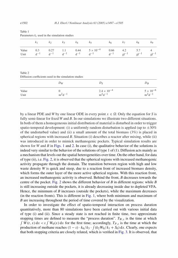
Table 1Parameters ki used in the simulation studies

k1 k2 k3 k4 k5 k6 k7 k8 k9

Value 0.3 0.27 1.1 0.44 5 × 10−4 0.66 4.2 5.7 4Unit d−1 d−1 d−1 d−1 d−1 d−1 gl−1 gl−1 gl−1

Table 2Diffusion coefficients used in the simulation studies

DW DS DB

Value 0 2.4 × 10−4 5 × 10−6

Unit m2d−1 m2d−1 m2d−1

by a linear PDE and W by one linear ODE in every point x ∈ �. Only the equation for S isfully semi-linear for fixed W and B. In our simulations we illustrate two different situations.In both of them a homogeneous initial distribution of material is disturbed in order to triggerspatio-temporal development: (i) a uniformly random disturbation is applied (up to ±30%of the undisturbed value) and (ii) a small amount of the total biomass (3%) is placed inspherical regions with increased B. Situation (i) describes a reactor after mixing, while (ii)was introduced in order to mimick methanogenic pockets. Typical simulation results areshown for W and B in Figs. 1 and 2. In case (i), the qualitative behavior of the solutions isindeed very similar to the behavior of the solutions of type 1 of (1). Diffusion acts mainly asa mechanism that levels out the spatial heterogeneities over time. On the other hand, for dataof type (ii), i.e. Fig. 2, it is observed that the spherical regions with increased methanogenicactivity propagate through the domain. The transition between region with high and lowwaste density W is quick and steep, due to a reaction front of increased biomass density,which forms the outer layer of the more active spherical regions. With this reaction front,an increased methanogenic activity is observed. Behind the front, B decreases towards thecentre of the pocket. Fig. 2 shows the different behavior of B in different regions: while Bis still increasing outside the pockets, it is already decreasing inside due to depleted VFA.Hence, the minimum of B increases (outside the pockets), while the maximum decreases(in the reaction fronts). This is different in Fig. 1, where both minimum and maximum ofB are increasing throughout the period of time covered by the visualization.

In order to investigate the effect of spatio-temporal interaction on process durationquantitatively, more than 80 simulations have been carried out with various initial dataof type (i) and (ii). Since a steady state is not reached in finite time, two approximatestopping times are defined to measure the “process duration”. TW,� is the time at which∫

W(t, x) dx < �∫

W0(x) dx for the first time; accordingly, TP,� is the time at which theproduction of methane reaches (1 − �) · k6/k3 · ∫ (k2W0/k1 + S0) dx. Clearly, one expectsthat both stopping criteria are closely related, which is verified in Fig. 3. It is observed, that


0.700.70 0.900.90 1.101.10 1.301.30 0.220.22 0.290.29 0.370.37 0.440.44 0.100.10 0.190.19 0.280.28 0.360.36

0.000.00 0.110.11 0.220.22 0.320.32 0.000.00 0.100.10 0.200.20 0.290.29 0.000.00 0.070.07 0.140.14 0.220.22

1.021.02 0.160.16 1.311.31 1.451.45 1.211.21 1.331.33 1.461.46 1.581.58 1.391.39 1.511.51 1.631.63 1.761.76

1.631.63 1.781.78 1.931.93 2.092.09 2.172.17 2.492.49 2.822.82 3.143.14 8.658.65 9.259.25 9.849.84 10.4310.43

Fig. 1. Model simulation of (4)–(6) for data of type (i). Shown are W/w0 (top two rows) att=1, 491, 541, 561, 571, 581 d where W > 0.01w0 and B/b0 (lower two rows) at t=91, 191, 291, 391, 491, 591 d.Note that the color bar is newly adjusted for every picture, containing information about the minimum and maxi-mum values of the reported variable.


0.00 0.33 0.67 1.00 0.00 0.27 0.54 0.81 0.00 0.22 0.44 0.66

0.00 0.18 0.37 0.55 0.00 0.15 0.30 0.45 0.00 0.12 0.24 0.36

1.18 7.12 13.07 19.01 1.33 6.24 11.16 16.07 1.40 5.42 9.44 13.46

0.94 4.72 8.51 12.29 0.62 4.03 7.43 10.84 0.41 2.94 5.48 8.02

Fig. 2. Model simulation of (4)–(6) for data of type (ii). Shown are W/w0 (top two rows) att=1, 91, 191, 291, 391, 491 d where W > 0.01w0 and B/b0 (lower two rows) at t=91, 191, 391, 491, 591, 691 d.The domain is cut in half for better visibility. Note that the color bar is newly adjusted for every picture, containinginformation about the minimum and maximum values of the reported variable.

the maximum process duration measured is twice as large as the minimum duration. Thisobservation is independent of the choice of �. Since the stopping time for various data fromgroup (i) are very similar, the large fluctuations are entirely due to data from group (ii). Inparticular, different data sets of (ii) can lead to an accelerated or decelerated process.


eps=0.01 eps=0.05700

650

600

550

500

450

400

350350 400 450 500 550 600 650 700

Tp

[d]

Tw [d]

650

600

550

500

450

400

350

300350300 400 450 500 550 600

Tp

[d]

Tw [d]

Fig. 3. Stopping times Ts and Tp for the simulations carried out. Reported are the evaluations for � = 0.01 and� = 0.05.

4. Conclusion

The qualitative behavior of the lumped model (1) implies that spatially distributed modelsare necessary to correctly describe process duration of anaerobic digestion of solid waste.The simulation of a PDE extension of the model based on [7] showed that spatio-temporaleffects can in fact be responsible for fluctuation of the process duration over a range of 100%,even if only around 3% of the material is initially placed in small pockets with increasedmethanogenic biomass. This is due to the spreading of regions of increased methanogenicactivity that propagate under formation of transient chemical reaction fronts.

Acknowledgements

Supported in parts by NSERC Canada (Discovery Grant, 261336-03) and Volkswagen-Stiftung (Young Academics In Interdisc. Env. Res., II/78039).

References

[1] D.J. Batstone, J. Keller, I. Angelidaki, S.V. Kalyuzhnyi, S.G. Pavlostathis, A. Rozzi, W.T.M. Sanders, H.Siegrist, V.A. Vavilin, The IWA anaerobic digestion model No. 1 (ADM1), Water Sci. Technol. 45 (10) (2002)65–73.

[2] H.J. Eberl, Simulation of chemical reaction fronts in anaerobic digestion of solid waste, Lecture Notes Comput.Sci. 2667 (2003) 503–512.

[3] H.J. Eberl, A spatio-temporal simulation study of seeding induced mass transfer limitations in anaerobicdigestion of solid waste and their effect on process duration, submitted.

[4] M.A. Efendiev, H.J. Eberl, R. Lasser, Necessary and sufficient conditions for positive invariance inconvection–diffusion–reaction systems, submitted.

[5] H.C. Flemming, M. Faulstich, Was geschieht bei der biologischen Abfallbehandlung? (What happens duringbiological treatment of solid waste?), in: Faulstich et al. (Eds.), Praxis der BiologischenAbfallbehandlung—18.Mülltechnisches Seminar, Berichte aus Wassergüte- und Abfallwirtschaft, vol. 121, 1995, pp. 5–48.

[6] J. Smoller, Shock Waves and Reaction–Diffusion Equations, Springer, Berlin, 1983.[7] V.A. Vavilin, M.Y. Shchelkanov, S.V. Rytov, Effect of mass transfer on concentration wave propagation during

anaerobic digestion of solid waste, Water Res. 36 (2002) 2405–2409.

the role of spatio-temporal effects in anaerobic digestion of solid waste

Documents