The Restricted 3-Body Problem: A Mission toL4

Rebecca Mitchell and Mary Hammack

Last updated July 27, 2011

Abstract

The investigation sought to find a cost efficient route for a space-craft to travel using Lagrangian Equilibrium points in the sun-earthsystem. By expressing the restricted three body problem as a systemof ordinary differential equations and linearization we understand thebehavior of points geometrically. Using these methods and a programwhich approximates solutions in systems of differential equations, wewere able to find an orbit which uses the unstable nature of L1 toshoot off towards L4.

Contents

1 Introduction 2

2 Ordinary Differential Equations 32.1 Existence and Uniqueness . . . . . . . . . . . . . . . . 32.2 Phase Plane Portraits . . . . . . . . . . . . . . . . . . 4

2.2.1 Example . . . . . . . . . . . . . . . . . . . . . . 42.3 Equilibrium Points . . . . . . . . . . . . . . . . . . . . 5

2.3.1 Example . . . . . . . . . . . . . . . . . . . . . . 52.4 Linearization . . . . . . . . . . . . . . . . . . . . . . . 5

2.4.1 Example . . . . . . . . . . . . . . . . . . . . . . 62.5 Stability . . . . . . . . . . . . . . . . . . . . . . . . . . 72.6 Integrals . . . . . . . . . . . . . . . . . . . . . . . . . . 7

2.6.1 Example . . . . . . . . . . . . . . . . . . . . . . 7

3 Orbits of Celestial Bodies 83.1 Newton’s Law of Universal Gravitation . . . . . . . . . 8

3.1.1 The 2-body Problem . . . . . . . . . . . . . . . 8

1

3.1.2 The n-Body Problem . . . . . . . . . . . . . . . 93.2 The Restricted 3-body Problem . . . . . . . . . . . . . 9

3.2.1 Kepler’s Theorem . . . . . . . . . . . . . . . . 93.2.2 Rotated Coordinate System . . . . . . . . . . . 93.2.3 Lagrangian Equilibrium Points . . . . . . . . . 113.2.4 Jacobi Integral . . . . . . . . . . . . . . . . . . 12

4 ODE45 124.1 Example . . . . . . . . . . . . . . . . . . . . . . . . . . 13

5 Analysis of Linearization at Lagrange Points 145.1 Linearization at Lagrange Points . . . . . . . . . . . . 145.2 Eigenvalues and Stability . . . . . . . . . . . . . . . . 165.3 Change of Basis . . . . . . . . . . . . . . . . . . . . . . 185.4 Examples . . . . . . . . . . . . . . . . . . . . . . . . . 18

5.4.1 Plots at the Linearization of L4 . . . . . . . . . 185.4.2 Plots at the Linearization of L1 . . . . . . . . . 20

6 A Path from Earth’s Orbit to L4 216.0.3 Using L1 as a Slingshot to Get to L4 . . . . . . 21

7 Conclusion 23

1 Introduction

This summer, July 21, 2011, marked the end of NASA’s space shuttlemissions. Part of NASA’s plan for the future includes sending moreunmanned spacecraft to study the Moon, Mars, and the outer plan-ets. As part of this next stage, NASA is investigating ways to savefuel [?]. One way NASA could do this is by using the gravitationalfield of the earth and the sun, and ultimately other planets, to pullthe spacecraft where they want it to go. The goal of our project wasto find a fuel-saving path, using the chaotic nature of the system, bywhich a spacecraft could travel from an Earth orbit to L4, a point inspace that forms an equilateral triangle with Earth and the Sun.

This problem is interesting for several reasons. Firstly, L4 is an in-teresting point to travel to because it is an equilibrium point of theordinary differential equations that govern the motion of a spacecraftnear the sun and the earth. Also, some small objects have collectedat this point and could be interesting to study. Secondly, using chaosis interesting because it could cut down on the amount of fuel neededsince we are letting gravity do most of the work instead of relying

2

heavily on the spacecraft’s propulsion system, which burns fuel. Thisis very important because getting fuel into space for spacecrafts is veryexpensive, about $10,000 per pound of fuel [?]. Lastly, this problem isinteresting because in the last 20 years NASA has tried to incorporatesome of these same ideas in planning space missions. The Japanesesatellite Hiten, after completing its original mission, was sent on a fol-low on mission to pass through the L4 of the Earth and Moon system.Hiten was also the first to exploit the low energy chaotic orbits likethe one we considered [?]. These types of paths could easily becomemore and more important in the near future as NASA plans to sendspacecraft to the Moon, Mars, and the outer planets in the next sev-eral years.

The result of our project is a trajectory for a spacecraft that starts inEarth orbit, uses its propulsion system to give it a small push, sling-shots off an unstable equilibrium point in the system, and goes towardL4, where it must use a small amount of energy to slow it down sothat it can orbit at L4.

We used matlab ode45 to find approximate solutions to our system ofordinary differential equatinos. We also looked at Jacobian Integralsto analyze the energy and the linearization of the system to analyzestability and instability.

2 Ordinary Differential Equations

Before we discuss the 3-body Problem and the Restricted 3-body Prob-lem it is necessary to recall some facts about ordinary differentialequations (ODEs).

2.1 Existence and Uniqueness

First, let us recall one of the most fundamental theorems of differentialequations, The existence and uniqueness theorem.

Theorem 1. Given any initial condition (t0, x0) for the equationx = g(t, x), there exists a unique solution with x(t0) = x0.Given initial conditions (t0, x0, x0) for the equation x = g(t, x, x),there exists a unique solution with x(t0) = x0 and x(t0) = x0.

Similarly, for systems we have the following theorem.

Theorem 2. ~x = ~f(t, ~x) has a unique solution with ~x(t0) = ~x0.~x = ~f(t, ~x, ~x) has a unique solution with ~x.(t0) = ~x0 and ~x(t0) = ~x0

3

Figure 1: Note that the phase plane portrait graphs the position, θ, withrespect to the velocity, v.

2.2 Phase Plane Portraits

Now we will discuss a few terms and ideas that will be helpful when welater discuss the Restricted 3-body Problem. Note that ~f : Rn → Rncan be thought of as a vector field on Rn and the solutions of the ODEare parallel to the vector field.

Definition 3. A phase plane portrait is a sketch of the images ofsome solutions. The time dependence cannot be seen from the phaseplane.

2.2.1 Example

Consider a simple pendulum described by the second order differentialequation θ+ sin(θ) = 0. This equation can be written as the followingsystem of two first order differential equations.{

θ = vv = − sin(θ)

For this system, the vector field ~f : R2 → R2 is

~f

([θv

])=

[v

− sin(θ)

].

Figure 1 is an example of a phase plane portrait for the simple pen-dulum problem. The solutions shown are the solutions for initial con-ditions θ ∈ [−π, π] with v = 0.

4

2.3 Equilibrium Points

Definition 4. We say that ~x0 ∈ Rn is an equilibrium point if

~f( ~x0) = 0

Lemma 5. If ~x0 is an equilibrium point, then ~x(t) = ~x0 is a solution

Proof. ~x0 is a constant so ~x(t) = 0. ~x0 is an equilibrium point, so~f(~x(t)) = ~f(~x0) = 0. Thus ~x(t) = ~f(~x(t)).

2.3.1 Example

Recall the simple pendulum from the previous section.

~f

([θv

])=

[v

− sin(θ)

]We can solve for the equilibrium points with θ ∈ [−π, π] and we find(θ0, v0) ∈ {(−π, 0), (0, 0), (π, 0)}. The initial condition (0, 0) corre-sponds to the instance when the pendulum is hanging straight down.The initial conditions (−π, 0), (π, 0) correspond to the instances whenthe pendulum is standing straight up and whether θ is considered pos-itive or negative. If the pendulum starts at either of these positionswith zero velocity and no forces acting on it besides gravity then itwill stay at the starting position.

2.4 Linearization

The linearization of an ODE is used to see the qualitative behaviorof an ODE in a very small neighborhood around a point. This is anideal tool for analyzing what happens around equilibrium points.

Definition 6. The linearization of ~x = ~f(~x) at the equilibrium point~x0 is the linear ODE ~y = D~f(~x0) · ~y.

Explicitly, this means y : R→ Rn is a function,

~f =

f1f2...fn

is a vector field and

D~f(~x0) · ~y =

∂f1(~x0)∂y1

∂f1(~x0)∂y2

. . . ∂f1(~x0)∂yn

∂f2(~x0)∂y1...

∂fn(~x0)∂y1

. . . ∂fn(~x0∂yn

y1y2...yn

5

(a) (0,0) (b) (±π, π)

Figure 2: The phase plane portraits of the linearization of the simple pen-dulum at its equilibrium points.

2.4.1 Example

Now we will find the linearization of the equilibrium points for thependulum example. Recall we have the system.[

θv

]=

[v

− sin(θ)

]= ~f(θ, v) =

[f1(θ, v)f2(θ, v)

]Using the equation ~y = D~f( ~x0) · ~y we find that

D~f(θ, v) =

[0 1

− cos(θ) 0

]so f(0, 0) =

[0 1−1 0

].

This means that

~y =

[y1y2

]=

[y2−y1

].

If we draw the phase plane portrait of the linearized system we wouldget something like Figure 2(b) near (0,0). Now consider the other twoequilibrium points (π, 0) and (−π, 0). Since our linearization matrixonly depends on − cos(θ) and we know that cos(θ) is an even function,the linearization matrix for both points will be equal. So we have

~f(±π, 0) =

[0 11 0

].

This means that

~y =

[y1y2

]=

[y2y1

].

If you draw the phase plane portrait of the linearized system you willget something like Figure 2(b) near (±π, π).

6

2.5 Stability

As you probably noticed the linearization of the equilibrium pointsindicates drastically different behavior at θ = 0 point compared to thebehavior at the θ = ±π points. This different behavior is a key pointwhen talking the about stability of equilibrium points.

Definition 7. A solution ~x(t) is stable if ∀ε > 0 ∃δ > 0 such that if~y(t) is a solution with |~x(0)− ~y(0)| < δ then |~x(t)− ~y(t)| < ε ∀t ≥ 0.Otherwise the solution is unstable.

A quick look at the phase plane portraits of the linearization of theequilibrium points of the pendulum illustrates this very well. Noticethat in the linearization of the θ = 0 point near by solutions are ellipsesand therefore stay near the equilibrium point for all time.

If you look at the phase plane portraits of linearization of the other twopoints, θ = ±π you see that if the initial condition is just a little a awayfrom the equilibrium point that it follows one of the hyperbolic pathswhich get farther away from the equilibrium point as time goes on.These hyperbolic paths translate into real life in how if the pendulumis just a little short of completely vertical it will fall back down thenswing back and forth unless stopped by an external force. On the otherhand, if the initial condition has the pendulum perfectly vertical buthas even the smallest velocity of positive or negative value, then itwill swing around and around without changing direction. Thus theθ = ±π equilibrium points are unstable points.

2.6 Integrals

Definition 8. A function H : Rn → R is an integral if ddtH(~x(t)) = 0

for all solutions ~t.

2.6.1 Example

We will now find the integral for the simple pendulum. Recall we havethe differential equation

θ + sin θ = 0.

Now we multiply the whole equation by θ so we have

θθ + θ sin(θ) = 0.

Which is equivalent to the following equation.

d

dt(1

2θ2 − cos(θ)) = 0

7

Recall θ = v, thus we have the integral

H(θ, v) =1

2v2 − cos(θ).

3 Orbits of Celestial Bodies

3.1 Newton’s Law of Universal Gravitation

3.1.1 The 2-body Problem

Given 2 Bodies, one at ~x1 with mass m1 and the other at ~x2 withmass m2, then the force exerted by m2 on m1 is

~F1 =Gm1m2(~x2 − ~x1)|~x2 − ~x1|3

And the force exerted on m2 by m1 is

~F2 =Gm1m2(~x1 − ~x2)|~x1 − ~x2|3

where G is the gravitational constant. Using Newton’s second law,F = ma, we can rewrite these equations as a system of 2nd orderdifferential equations: ~x1 = Gm2(~x2−~x1)

|~x2−~x1|3

~x2 = Gm1(~x1−~x2)|~x1−~x2|3

The fact that angular momentum is conserved allows us to rotate thecoordinate system so that m1 and m2 only move on a plane and theirpositions can be described by real numbers x1 and x2 rather thanvectors. By setting the center of mass at the origin and assuming thaty represents the distance between the bodies such that y = x1 − x2and M = Gm1 + G2, we can express the problem as the differentialequation

y = −My2

Then we are able to find an implicit solution for ~y:

1√2c1

[√y

(y +

M

c1

)− M

c1ln

(√y +

√y +

M

c1

)]= −t+ c2

where c1 and c2 are constants.

8

3.1.2 The n-Body Problem

Similarly, if there are three masses m1, m2, and m3 with positions ~x1,~x2, and ~x3 respectively, we derive the system:

~x1 = Gm2(~x2−~x1)|~x2−~x1|3

+ Gm3(~x3−~x1)|~x3−~x1|3

~x2 = Gm1(~x1−~x2)|~x1−~x2|3

+ Gm3(~x3−~x2)|~x3−~x2|3

~x3 = Gm1(~x1−~x3)|~x1−~x2|3

+ Gm2(~x2−~x3)|~x2−~x3|3

Given n masses m1,m2, . . . ,mn, the motion of the ith body is de-scribed by

~xi =∑n

i 6=jGmj( ~xj−~xi)| ~xj−~xi|3

There is no known solution for n ≥ 3.

3.2 The Restricted 3-body Problem

3.2.1 Kepler’s Theorem

Kepler’s theorem applies to the 2-body problem. Recall that ~y(t) =~x1(t)− ~x2(t).

Theorem 9. Assume that ~y(t) =

[y1y2

]. If E = 1

2 |~y|2 − M

|~y| < 0 and

G3 = y1y2 − y2y1 6= 0 then ~y traces out an ellipse with eccentricityb = (1 + 2EG2

3)12 , semimajor axis of length a = − 1

2E , and a focus atthe origin. ~y(t) sweeps out area at a constant speed and the period of

the orbit is 2πa32 .

Remark 10. If the orbit is a circle, then ~y(t) rotates at a constantspeed.

3.2.2 Rotated Coordinate System

The 3-body problem can be simplified by assuming that m3 is muchsmaller than m1 and m2, so that the force it exerts on the other twomasses is negligible. For example, if m1 is the sun and m2 is theearth, m3 could be a satellite. The paths of m1 and m2 can be foundby solving the 2-body problem and the motion of m3 is described bythe equation:

~x3 =Gm1(~x1 − ~x3)|~x1 − ~x3|3

+Gm2(~x2 − ~x3)|~x2 − ~x3|3

(1)

If we assume that ~x1 and ~x2 have circular orbits, by Kepler’s Theorem,we can assume that they rotate at a constant speed. We can therefore

9

create a coordinate system that rotates at the same speed so that ~x1and ~x2 always remain on the line y = 0 in the xy-plane. To do this,we first express the positions of m1 and m2 in polar coordinates:

~x1(t) =

[−r1 cos

(2πtτ

)−r1 sin

(2πtτ

) ]

~x2(t) =

[ m1m2r2 cos

(2πtτ

)m1m2r2 sin

(2πtτ

) ]where r1 and r2 are the distances of m1 and m2 from the origin re-spectively and τ is the period of rotation. First we set the center ofmass as the origin so that r2 = m1

m2r1. We will simply rename r = r1.

We rotate the coordinates by −2πtτ using the matrix R to ensure that

m1 and m2 always remain on the line y = 0:

R(t) =

[cos(2πtτ

)sin(2πtτ

)− sin

(2πtτ

)cos(2πtτ

) ]

~xr1 = R~x1 =

[−r0

]

~xr2 = R~x2 =

[ m1m2r

0

]We then use R to find an equation for ~xr3:

~xr3 = R~x3~xr3 = R~x3 + R~x3~xr3 = R~x3 + 2R~x3 + R~x3

=(4π2

τ2− Gm1

r13− Gm2

r23

)~xr3 + 4π

τ

[0 1−1 0

]~x3 + Gm1

r13~xr1 + Gm2

r23~xr2

where r13 is the distance between m1 and m3 and r23 is the distancebetween m2 and m3 Using this equation, we will create a system offirst order differential equations with the values x, y, u, v, such thatx and y are the components of ~x3 and u and v are their respectivevelocities. We also substitute the components of ~x1 and ~x2.

x = uy = v

u = 4π2

τ2x+ (−r − x)Gm1

r313+(m1m2r − x

)Gm2

r323+ 4π

τ v

v = 4π2

τ2y − yGm1

r313− yGm2

r323− 4π

τ u

10

We can further simplify the system by changing our units of time,

mass, and distance so that G = 1, m1 +m2 = 1 and r(

1 + m1m2

)= 1.

Since m2 = 1 −m1, we will rename m1 to simply be µ. This makesthe system becomes:

x = uy = v

u = x+ (µ− 1− x) µr313

+ (µ− x)1−µr323

+ 2v

v = y − y µr313− y 1−µ

r323− 2u

where r13 =√

(1− µ+ x)2 + y2) and r23 =√

(−µ+ x)2 + y2. Notethat r = 1− µ.

3.2.3 Lagrangian Equilibrium Points

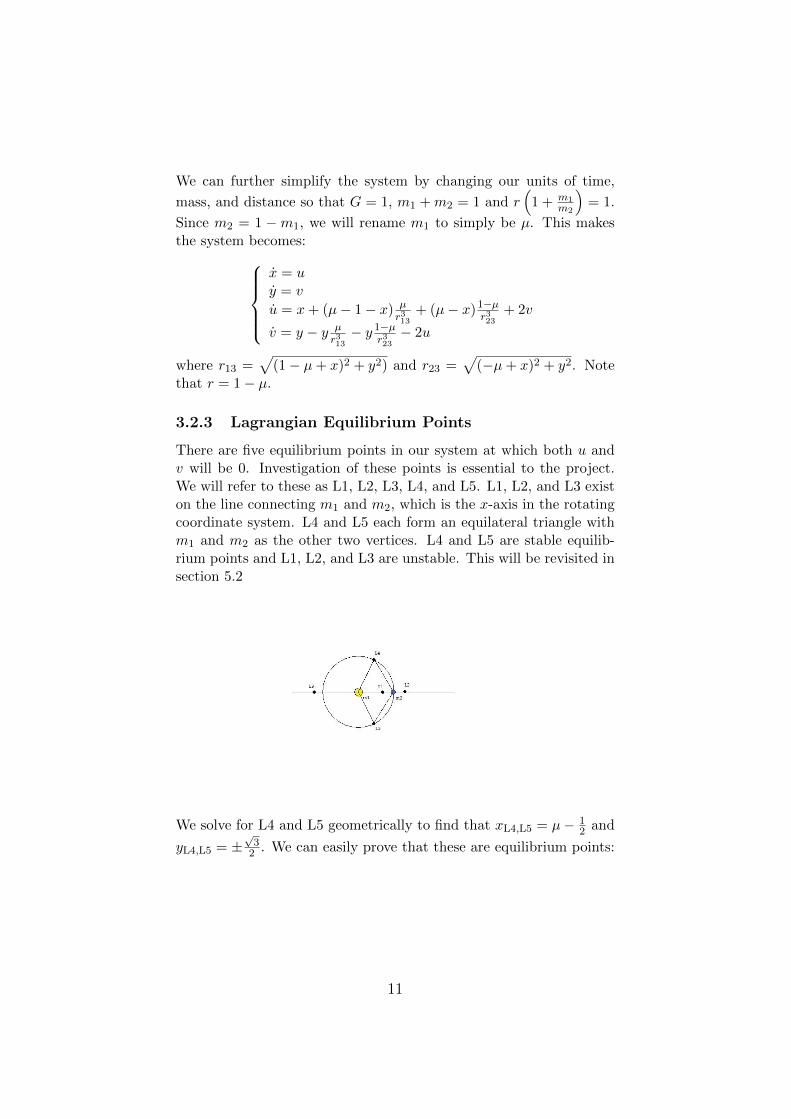
There are five equilibrium points in our system at which both u andv will be 0. Investigation of these points is essential to the project.We will refer to these as L1, L2, L3, L4, and L5. L1, L2, and L3 existon the line connecting m1 and m2, which is the x-axis in the rotatingcoordinate system. L4 and L5 each form an equilateral triangle withm1 and m2 as the other two vertices. L4 and L5 are stable equilib-rium points and L1, L2, and L3 are unstable. This will be revisited insection 5.2

We solve for L4 and L5 geometrically to find that xL4,L5 = µ− 12 and

yL4,L5 = ±√32 . We can easily prove that these are equilibrium points:

11

Proof. Since u,v=0 and r13 = r23 = 1

u = µ− 1

2+

[µ− 1−

(µ− 1

2

)]µ+

[µ−

(µ− 1

2

)](1− µ) + 2(0)

= µ− 1

2− 1

2µ− 1

2µ+

1

2= 0

v = ±√

3

2∓√

3

2µ∓√

3

2(1− µ)− 2(0)

= ±√

3

2∓√

3

2µ∓√

3

2±√

3

2µ

= 0

To find L1, L2, and L3, we must solve the three equations:

0 = xL1 + (µ− 1− xL1)µ

(r + xL1)3+ (µ− xL1)

1− µ(1− r − xL1)3

0 = xL2 + (µ− 1− xL2)µ

(r + xL2)3+ (µ− xL2)

1− µ(−1 + r + xL2)3

0 = xL3 + (µ− 1− xL3)µ

(−r − xL3)3+ (µ− xL3)

1− µ(1− r − xL3)3

3.2.4 Jacobi Integral

The Jacobi Integral is a function that produces the total energy perunit mass of the system, as it is the only known conserved quantity ofthe 3-body problem:

E =1

2(u2 + v2)− 1

2(x2 + y2)−

(µ√

(1− µ+ x)2 + y2+

1− µ√(µ+ x)2 + y2

)

The first term represents the kinetic energy, as it is only dependenton u and v and the second two terms represent the potential energyas they are dependent on x, y, and µ.

4 ODE45

In finding the numerical approximations of the solutions to the differ-ential equations for both the pendulum problem and the restricted 3-body problem, we used the matlab function ode45. This ode45 solver

12

is based on an explicit Runge-Kutta (4,5) formula, the Dormand-Prince pair. It is a one-step solver in computing y(tn), it needsonly the solution at the immediately preceding time point, y(tn-1).This function takes three arguments. The first of these is the functionname of a function containing the system of first order differentialequations ode45 will solve. The second is the vector containing theinitial time and the final time over which ode45 will integrate the sys-tem. The last argument is a vector of initial conditions. ode45 returnsa column vector with the time at each instance for which the numericalapproximation is calculated and a matrix where each column containsthe approximated values of the solution of the ODE at the particulartime for a variable in your system of ODEs. In the programs we usedto numerically approximate solutions for the restricted 3-body prob-lem we needed more precision. To achieve this, we used the odeset

function which created a structure options that allowed us to adjustthe relative error tolerance and the absolute error tolerance. The rel-ative error tolerance is relative to the whole matrix of solutions andthe absolute tolerance determines the threshold of acceptable error foreach individual component of the solution matrix. The default rela-tive error tolerance, 1e-3, corresponds to about 0.1% accuracy. Thedefault absolute error tolerance is 1e-6. In the program we used tofind approximations for the restricted 3-body problem, solveL1.m weused AbsTol =1e-10 and RelTol = 1e-7 [?].

4.1 Example

The following is an example of the code we used to solve the systemof differential equations of the pendulum. First we have the m-filewe called system_ex(t,x) which defines the system of differentialequations [

θv

]=

[v

− sin(θ)

].

If we compare this system to the following code, we see that θ=xprime(1,1),v=xprime(2,1), v=x(1), and θ=x(2). Note that while the functiontakes a time t it is not used in the system because the system doesnot depend on time. The function system_ex takes a time argumentonly because the ode45 function requires it.

function [xprime] = system_ex(t,x)

xprime(1,1)=-sin(x(2));

xprime(2,1)=x(1);

end

13

This is the m-file we called pendulums.m that uses ode45 to solvethe system and plots the solutions for the initial conditions with θ =[−5, 5] with a step of .2 and zero velocity.

hold on

for i=-5:.2:5

[t,y] = ode45(’system_ex’,[0,11],[i 0]);

x1=y(:,1);

x2=y(:,2);

plot(x2,x1);

plot(-x2,x1);

end

hold off

Figure 3: Pendulum

Figure 3 is the figure plotted by this file in matlab.

5 Analysis of Linearization at Lagrange

Points

5.1 Linearization at Lagrange Points

Another way to analyze the behavior of solutions near the equilibriumpoints is by studying the linearization of the system. Recall that thelinearization of ~x = D~f(~x0~y. Where

~f =

f1f2f3f4

and

14

f1(x, y, u, v) = u

f2(x, y, u, v) = v

f3(x, y, u, v) = x+ (µ− 1− x)µ

r313+ (µ− x)

1− µr323

+ 2v

f4(x, y, u, v) = y − y µr313− y1− µ

r323− 2u

The entries of the linearization matrix will the be the partial deriva-tives of f1, f2, f3, and f4 in respect to x, y, u, and v:

∂f1∂x

∂f1∂y

∂f1∂u

∂f1∂v

∂f2∂x

∂f2∂y

∂f2∂u

∂f2∂v

∂f3∂x

∂f3∂y

∂f3∂u

∂f3∂v

∂f4∂x

∂f4∂y

∂f4∂u

∂f4∂v

To find the linearization at L4, we substitute the initial conditions,

x = µ− 12 , y =

√32 , u = 0, and v = 0 to find the matrix:

L4 =

0 0 1 00 0 0 134

6√3µ−3

√3

4 0 26√3µ−3

√3

494 −2 0

By substituting x = µ−1

2 and y = − sqrt32 , we get a similar linearization

for L5:

L5 =

0 0 1 00 0 0 134

−6√3µ+3

√3

4 0 2−6√3µ+3

√3

494 −2 0

To obtain the matrices for L1, L2, and L3 we would also substitutethe coordinates of each Lagrangian point, but because they are rootsof high degree polynomials, we are unable to solve for these pointsexactly, so we set µ to be the mass of the sun (.999996996) where1−µ is the mass of the earth and found numerical solutions. We werethen able to find the linearizations:

L1 =

0 0 1.0000 00 0 0 1.0000

9.1289 0 0 2.00000 −3.0644 −2.0000 0

15

L2 =

0 0 1.0000 00 0 0 1.0000

2.9410 0 0 2.00000 0.0295 −2.0000 0

L3 =

0 0 1.0000 00 0 0 1.0000

3.0000 0 0 2.00000 −0.0000 −2.000 0

To find a given vector ~v(t) in respect to a linearization, let’s say L4,we compute eL4t~v.

5.2 Eigenvalues and Stability

We can analyze the stability of the Lagrangian points by computingthe eigenvalues and eigenvectors. However creating phase plane por-traits is difficult because the system exists in R4, so we will only be ableto produce plots in terms of two or three of the variables. To computethe eigenvalues of L4, we must solve for λ when det(L4 − λI) = 0:

det(L4 − λI) = λ4 + λ2 +27µ(1− µ)

4= 0

Solving det(L5 − λI) = 0 gives the same equation. The solutions tothis equation are

λ1 =

√−√

27µ2 − 27µ+ 1− 1

2

λ2 = −

√−√

27µ2 − 27µ+ 1− 1

2

λ3 =

√√27µ2 − 27µ+ 1− 1

2

λ4 = −

√√27µ2 − 27µ+ 1− 1

2

Since, by construction, 0 < µ < 1, the eigenvalues are all strictly imag-inary. Therefore, points nearby will orbit the equilibrium point. Thisis what we expect, since L4 and L5 are stable. When µ = .999996996as it is with the sun and the earth, the eigenvalues become

16

λ1 = 0.99999i

λ2 = −0.999989i

λ3 = 0.00450i

λ4 = −0.00450i

To find the eigenvectors we solve (L4 − λnI)~vn = ~0 for n = 1, 2, 3, 4.Staying in the sun/earth system, the eigenvectors are

~v1 =

0.57009

0.22787 + 0.35082i−0.00000 + 0.57009i−0.35082 + 0.22787i

, ~v2 =

0.57009

0.22787− 0.35082i−0.00000− 0.57009i−0.35082− 0.22787i

,

~v3 =

0.86601

0.49999 + 0.00347i−0.00000 + 0.00390i−0.00002 + 0.00225i

, ~v4 =

0.86601

0.49999− 0.00347i−0.00000− 0.00390i−0.00002− 0.00225i

We use the same process to compute the eigenvalues and eigenvectorsof L1:

λ1 = −2.53400

λ2 = 2.53400

λ3 = 2.08727i

λ4 = −2.08727i

~v1 =

0.323770.17298−0.82043−0.43834

, ~v2 =

−0.323770.17298−0.820430.43834

,

~v3 =

−0.12777 + 0.00000i0.00000− 0.41274i0.00000− 0.26668i

0.86151

, v4 =

−0.12777− 0.00000i0.00000 + 0.41274i0.00000 + 0.26668i

0.86151

L1 has two imaginary eigenvalues, so it will orbit around the equilib-rium point, but because it also has a positive real eigenvalue, pointswill spiral outward. Therefore, L1 is not stable.

17

5.3 Change of Basis

Unfortunately plotting the linearizations is not possible because wecannot graph in 4-space. However, we can examine the projectiononto various planes and spaces. We must change to a basis consistingof eigenvectors to best understand what is happening. Given fourlinearly independent vectors, ~b1, ~b2, ~b3, and ~b4, we create the matrix

B =[~b1 ~b2 ~b3 ~b4

]To find a vector ~v in respect to the new basis, we compute B−1~v. Recallthat L4 has four complex eigenvectors, where ~v2 is the conjugate of~v1 and ~v4 is the conjugate of ~v3. Let us make the basis to be the realand imaginary parts of ~v1 and ~v3 so that we have

B =[<(~v1) =(~v1) <(~v3) =(~v3)

]=

0.57009 0 0.86601 00.22787 0.35082 0.49999 0.00347−0.00000 0.57009 −0.00000 0.00390−0.35082 0.22787 −0.00002 0.00225

Instead of simply computing eL4t~v to find ~v(t) in respect to the lin-earization at L4, we must find B−1eL4t~v. In contrast, L1 has two realeigenvectors, ~v1 and ~v2, and two complex vectors of which ~v4 is theconjugate of ~v3. We will make our basis to be the two real vectors andthe real and imaginary parts of ~v3:

B =[~v1 ~v2 <(~v3) =(~v3)

]=

0.32377 −.032377 −0.12777 0.000000.17298 0.17298 0.00000 −0.41274−0.82043 −0.82043 0.00000 −0.26668−0.43834 0.43834 0.86151 0

As with L1, vectors can be found in respect to B by computing eL1t~v.We are now able to plot the projection of a given linearization ontoeither a plane or space in respect to two or three of the basis vectors.

5.4 Examples

5.4.1 Plots at the Linearization of L4

This is a plot of

0.00010.0001

00

in respect to the xy-plane over 0 < t <

1000. We expect the orbits to wind around the surface of a torus butthat is hard to see in these coordinates.

18

This is the plot of

0.00010.0001

00

in respect to the plane formed by ~v1 and

~v2 over 0 < t < 1000. The orbit forms a circle, as we expect, becauseit is the projection on to the plane of two complex eigenvectors. Itrepresents winding around a torus in one direction.

This is a plot of

0.00010.0001

00

in respect to the space formed by ~v1, ~v2,

and ~v3 over 0 < t < 1000.

19

5.4.2 Plots at the Linearization of L1

This is a plot of

0.00010.0001

00

in respect to the hyperbolic plane formed

by the real eigenvectors, v1 and v2.

This is a plot of

.10

−.3601655041499258; 0

in respect to real vector

v1 and the real and imaginary part of v3. Note that the point orbitsL1 at first and then shoots off towards infinityThis is a plot of the same as above, but in respect to the plane formedby ~v1 and ~v2.

This is a plot of 〈0.0001, 0.0001, 0, 0〉 in respect to the space formed by~v1, ~v3, and ~v4 over 0 < t < 10. Notice that the point initially orbitsL1, but then shoots of towards infinity.

20

6 A Path from Earth’s Orbit to L4

Using ODE45 and the linearizations of the equilibrium points, we caneasily analyze the orbits of various initial conditions in the hopes offinding paths between equilibrium points that minimize fuel usage.The Jacobi Integral will allow us to determine the change of energyrequired to make the desired journey.

6.0.3 Using L1 as a Slingshot to Get to L4

Let’s assume that we wished for a spacecraft beginning in earth’sorbit to go very close to L1 and then shoot off towards L4 where itwill be captured and orbit or stay at the equilibrium point. Usingthe Jacobi Integral, we compute the energy at the initial conditions tobe -1.500306675688968. By setting initial conditions that match thisenergy, we obtain trajectories that get in the vicinity of L4:

21

However, all of these orbits remain a certain distance away fromL4, so we must adjust the energy of the initial conditions until we finda path that intersects L4. Doing so, we find that the initial conditionx=1.001040859733099, y=4.006220125610000e-004, u=-0.035468773164696,and v=0.064881573444297, which does exactly that:

Another change in velocity is required to slow the spacecraft tocome to rest at L4. By looking at the projection onto the hyperbolicplane formed by the real eigenvectors of the linearization at L1, wesee how the unstable nature of this equilibrium point slingshots thespacecraft towards L4.

Using the Jacobi integral, we find that the change of energy perunit mass required to kick the spacecraft out of Earth’s orbit andthen stop it at L4 is 2.803724847259878e-004. We can compare thiswith a trajectory that does not use the instability of L1 to get toL4. A point starting with the initial conditions x=1.001040859733099,y=4.006220125610000e-004, u=-0.030187384585606-1.074214289913, andv=.48 produces the orbit:

22

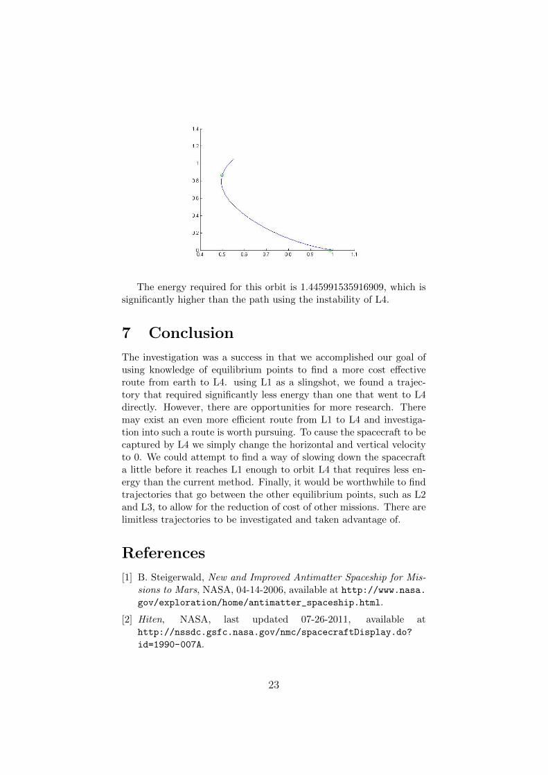
The energy required for this orbit is 1.445991535916909, which issignificantly higher than the path using the instability of L4.

7 Conclusion

The investigation was a success in that we accomplished our goal ofusing knowledge of equilibrium points to find a more cost effectiveroute from earth to L4. using L1 as a slingshot, we found a trajec-tory that required significantly less energy than one that went to L4directly. However, there are opportunities for more research. Theremay exist an even more efficient route from L1 to L4 and investiga-tion into such a route is worth pursuing. To cause the spacecraft to becaptured by L4 we simply change the horizontal and vertical velocityto 0. We could attempt to find a way of slowing down the spacecrafta little before it reaches L1 enough to orbit L4 that requires less en-ergy than the current method. Finally, it would be worthwhile to findtrajectories that go between the other equilibrium points, such as L2and L3, to allow for the reduction of cost of other missions. There arelimitless trajectories to be investigated and taken advantage of.

References

[1] B. Steigerwald, New and Improved Antimatter Spaceship for Mis-sions to Mars, NASA, 04-14-2006, available at http://www.nasa.gov/exploration/home/antimatter_spaceship.html.

[2] Hiten, NASA, last updated 07-26-2011, available athttp://nssdc.gsfc.nasa.gov/nmc/spacecraftDisplay.do?

id=1990-007A.

23

[3] ode23, ode45, ode113, ode15s, ode23s, ode23t, ode23tb, Math-Works, last updated 07-26-2011 , available at http://www.

mathworks.com/help/techdoc/ref/ode23.html.

[4] What’s Next for NASA?, NASA, 07-01-2011, available at http:

//www.nasa.gov/about/whats_next.html.

24