the quantitative relationship between visibility and … · · 2014-05-12the quantitative...

The quantitative relationship between visibility and mass concentration of PM2.5 in Beijing

J.-L. Wang1, Y.-H. Zhang2, M. Shao2 & X.-L. Liu3 1Institute of Urban Meteorology, CMA, Beijing, China 2State Joint Key Laboratory of Environmental Simulation and Pollution Control, College of Environmental Sciences, Peking University, Beijing, China 3Beijing Meteorological Information and Network Center, Beijing, China

Abstract

The pollution of PM2.5 is a serious environmental problem in Beijing. The annual average concentration of PM2.5 in 2001 from seasonal monitor results was more than six times that of the US national ambient air quality standards proposed by US EPA. The major contributors to mass of PM2.5 were organics, crustal elements and sulfate. The chemical composition of PM2.5 varied largely with season, but was similar at different monitor stations in the same season. The fine particles (PM2.5) cause atmospheric visibility deterioration through light extinction. The mass concentrations of PM2.5 were anti-correlated to the visibility, the best fits between atmospheric visibility and the mass concentrations of PM2.5 varied throughout the year: following a power law in spring, exponential in summer, logarithmic in autumn, and power or exponential in winter. As in each season the meteorological parameters such as air temperature and relative humidity change from day to day, the reason for the above correlations between PM2.5 and visibility obtained at different seasons probably come from the differences in chemical compositions of PM2.5. Keywords: PM2.5, atmospheric urban aerosol, air pollution, meteorological factor, visibility.

1 Introduction

Aerosol is of great concern in current atmospheric chemistry researches (Wang [9]). The research on physical and chemical properties of aerosol is important for

© 2006 WIT PressWIT Transactions on Ecology and the Environment, Vol 86, www.witpress.com, ISSN 1743-3541 (on-line)

Air Pollution XIV 595

doi:10.2495/AIR06059

understanding their environmental impacts. Fine particles (PM2.5) are air pollutants with complex chemical composition that include harmful componants. They not only result in atmospheric visibility deterioration through light extinction, but also are very harmful to human health as they produce deposits deep in human lungs and are very difficult to ventilate out (Prospero [6]; An et al. [1]). This has aroused public’s attention (Zhang et al., 2003). The research on atmospheric fine particles is of increasing interest in China, and numerous experiments have been conducted for fine particle measurements (Mao et al. [5]; Song et al., 2003). The recent monitoring results indicate (Wang et al., 2000) that the ambient levels of PM2.5 show an increasing trend in Beijing. The fine particle pollution has become one of the most important issues in the air pollution (Cheng et al., 2002). One concern about ambient fine particles is the impact of high levels of PM2.5 on atmospheric visibility (Song et al., 2003), the anti-correlation was found in cities between the concentrations of ambient PM2.5 and atmospheric visibility. Liu [3] reviewed the roles of mass concentrations of particles as well as the chemical species in the optical properties of particles and found that the statistical relationship between mass concentration of PM2.5 and visibility varied with meteorological parameters like relative humidity, and also varied with size distribution and chemical compositions of PM2.5. Actually, both light scattering and light absorption capacity of particles relates to their chemical components (Liu and Shao [4]). To avoid the complexity of mechanisms for the impact of PM2.5 on visibility, it would be helpful to obtain the statistical relationship between mass concentration of PM2.5 and visibility in a city, which would provide a quick response of level of PM2.5 pollution solely from visibility measurements. This work will investigate the quantitative relationship between mass concentrations of PM2.5 and visibility under various meteorological conditions for a whole year of measurement, and provide data for further detailed studies to understand the mechanisms of optical properties of PM2.5.

2 Experiment

Institute of Urban Meteorology, CMA, in cooperation with Peking University, performed a monitoring of PM2.5 and atmospheric visibility in 2001 at four seasons: spring (March), summer (June), autumn (September), and winter (December). The experiment was designed to investigate physical and chemical properties of fine particle, and to explore the statistical relationship between fine particles and atmospheric visibility. Beijing had less precipitation and higher air temperature in the year 2001. As to the seasons, compared to the long-term average, Beijing had more snow in winter, less precipitation and higher temperature, stronger wind and dust in spring; less precipitation and obvious higher temperature in summer; and higher temperature in autumn. Six Anderson RAAS-400 samplers with four PM2.5 channels were used to collect PM2.5 particles. They were installed in six different stations to perform


596 Air Pollution XIV

simultaneous sampling: Atmosphere Exploration Base of China Meteorological Administration (AEBCMA), Peking University (PKU), DongSi (DS), Capital Airport (CA), Yongledian (YLD), Mingling (ML). The sampling flow rate of four sampling channels is 16.7L/min. The sampler used three kind filters: 2 Teflon filters with 2µm aperture, a nylon filter with 1µm aperture, and a quartz filter with 1µm aperture. The site of AEBCMA was located in the southeast of Beijing, with lower hypsography (height above sea level) and more foggy days. The visibility was obviously lower. The PKU site was located in the northwest of Beijing, and the apparatus was installed on the top of a six-floor experiment building, about 20 m above ground. The DS site was located in the center of Beijing City, a commercial and traffic condensed area and the apparatus was installed on the top of a three-floor building, about 10 m above ground. The CA observation site was located in the northeast of Beijing, and the apparatus was installed on the top of the two-floor building of town near the airport, about 7 m above ground. The YLD site was located in the plain area far southeast of Beijing City, and the apparatus was installed on the top of the three-floor building of development area, about 10 m above ground. The ML was located in the north mountain area of Beijing, and the apparatus was installed on the top of first-floor building, about 4 m above ground. The sampling was done in days in selected four months, each sample was collected for 24h. If dust storm was encountered, more samples were then taken. An Anderson CAMMS PM2.5 sampler was installed on the ground of AEBCMA, which measured the real time mass concentrations of PM2.5 (Wang et al., 2004). And for the filters, trace elements, ionic species and OC, EC of PM2.5 were analyzed by ICP, x-ray fluorescence and thermo-optical method. The DPVS (Digital Photo Visibility System) is installed on the top of bungalow of AEBCMA’ observation site, about 3m above ground, monitoring the real time atmospheric visibility. Other relevant meteorological data were available from routine observation at AEBCMA, including diurnal horary wind speed; relative humidity at four times a day (02h, 08h, 12h, 20h); precipitation data at 2 durations a day (20-08h, 08-20h) (Wang et al., 2004).

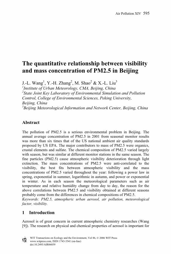
3 The spatial-temporal distributing of PM2.5 in Beijing 3.1 The distribution of fine particles in four seasons in Beijing Figure 1 shows the seasonal and annual average mass concentrations of PM2.5 obtained from film sample data at the six monitor stations in the Beijing area in 2001. As shown from the figure, PM2.5 mass concentrations were the highest in summer, up to 115.40 µg/m3, lowest in autumn, only 64.05 µg/m3, 95.33 µg/m3

in spring and 99.49µg/m3 in winter. If the average we obtained at above four seasons was used as annual average, the annual average level of PM2.5 was 93.57 µg/m3. As China has not yet established a national ambient air quality standard for PM2.5, the US standard proposed by US EPA (Environmental Protection Agency) in 1997, that is, daily average 65µg/m3 and annual average 15µg/m3, was adopted for our data assessment. From our measurement, PM2.5 concentrations in Beijing City were more than 6 times as the US air quality standards of PM2.5, showing it was already a very serious problem.



020406080

100120140

Spring Summer Autumn Winter Year

PM2.

5(µg

m-3) PM2.5

Figure 1: Seasonal and annual average mass concentrations of PM2.5 in

Beijing in 2001.

020406080

100120140

PKU DS CAYLD ML

AEBCMA

Averag

e

PM2.

5(µ g

m-3

) PM2.5

Figure 2: Annual average mass concentrations of PM2.5 at 6 sites in Beijing in 2001.

3.2 The spatial distribution of fine particles

The annual average mass concentrations of PM2.5 at six stations were also obtained in the Beijing area in 2001, as shown in Figure 2. The highest annual average PM2.5 level was obtained at AEBCMA, reaching about 130µg/m3. The main reasons were the low diffusion of air mass together with strong emissions of particles. The AEBCMA site has low topography, even below apparent horizon, and there was generally no strong wind. Meanwhile, combustion sources and traffic emissions were relatively condensed in vicinity area, and in 2001, numbers of high buildings were constructed in the surrounding region of our monitoring site. All these factors made the mass concentrations of PM2.5 the highest in our measurements.

4 Quantitative relationship between PM2.5 mass concentrations and visibility

Using real time sample data of seasonal atmospheric visibility and mass concentrations of PM2.5, combining simultaneous routine meteorological data in



observatory, the relationship between atmospheric visibility and mass concentrations of PM2.5 has been analyzed statistically.

y = 9E+09x-2.0899

CC = 0.801(13 samples)Wind speed = 1level

0

100

200

300

400

500

0 2000 4000 6000 8000 10000 12000

Visibility(m)

PM2.

5(µ g

/m3 )

y = 42309x-0.7791


0

20

40

60

80

100

0 10000 20000 30000 40000 50000Visibility(m)

PM

2.5(

µg/m3 )

y = 2E+09x-1.9906


0

40

80

120

160

0 5000 10000 15000 20000Visibility(m)

PM

2.5(

µg/m3 )

y = 2E+08x-1.6988

CC = 0.513(14 samples)Wind speed = 4level)

0

40

80

120

160

0 5000 10000 15000 20000Visibility(m)

PM2.

5(µg

/m3 )

Figure 3: Discrete chart between visibility and PM2.5 concentrations under

different wind speed levels at AEBCMA in the spring of 2001.

4.1 Spring time

Beijing city in spring is dry and windy, and it is favorable for the out-spreading of pollutants. In the spring 2001, Beijing had less precipitation, higher temperature, stronger wind and 17 dusty days, which is more than normal.



Statistical data indicates that the correlation between visibility and mass concentrations of PM2.5 is not good in days with a strong wind but is good in breezy days (wind speed less than level 4, that is 7.0m s-1), and with decreasing wind speed the correlation improves. The correlation between visibility and PM2.5 concentrations is statistically analyzed according to different wind speed level, and takes the form of a power law. Figure 3 shows a discrete chart of PM2.5 mass concentrations and visibility in breezy days, where CC gives the correlation coefficient. The correlation between the both on different wind speed level was shown in table 1.

Table 1: Correlation between visibility and PM2.5’s concentrations on different wind speed levels at AEBCMA in the spring of 2001.

Wind speed (level)

1 level (1.5m s-

1) 2 level (3.0 m s-1)

3 level (5.5 m s-

1) 4 level (7.0m s-

1) Sample number 13 16 44 14 Correlation Power Power Power Power Equation y = 9E+09x-

2.0899 y = 42309x-

0.7791 y = 2E+09x-1.9906 y = 2E+08x-1.6988

Correlation coefficient (%)

0.801 0.717 0.456 0.513

4.2 Summer time

Higher temperatures and more smog was recorded in the summer of 2001 in Beijing, smog days were up to 22 days in June, taking up about 73% of this month. The relative humidity was higher and visibility is low. The main weather characteristic at AEBCMA in June in 2001 was shown in table 2.

Table 2: Main weather characteristic in June in 2001.

Smog days (d) Average Humidity (%)

Average Visibility (m) Average Temperature (ºC)

22 63 4716.2 24.7

4.2.1 The classification of samples In summer, relative humidity and precipitation are the main factors affecting the mass concentrations of fine particles. So the correlation between visibility and PM2.5’s mass concentrations is analyzed according to the two factors. Figure 4 shows discrete chart of total samples of visibility and PM2.5’s mass concentrations data in June in 2001, figure 5 shows discrete chart of the both under the condition of precipitation or no-precipitation days, and their correlation is shown in table 3.

4.2.2 Sample analysis under no precipitation Under no precipitation, the correlation between visibility and PM2.5’s mass concentrations is also different with different humidity. When relative humidity is less than 70%, both are exponential, and the correlation modulus is very good,



while when relative humidity is more than 70%, both are logarithmic, and the correlation coefficient is not good. The correlation between visibility and PM2.5’s mass concentrations in no precipitation days is showed in table 4, figure 6 is discrete chart.

Total samples

y = 143.26e-0.0003x

CC = 0.691(349 samples)

0306090

120150

0 5000 10000 15000Visibility(m)

PM2.

5(?g

/m3 )

Figure 4: Total samples of visibility and PM2.5’s mass concentrations data

discrete chart in June in 2001.

y = 117.48e-0.0003x

CC = 0.693(163 samples)Precipitation samples

0

30

60

90

120

150

0 5000 10000 15000Visibility(m)

PM2.

5(?g

/m3 )

y = 143.78e-0.0003x

CC = 0.669(186 samples)No precipitation samples

0306090

120150

0 5000 10000 15000Visibility(m)

PM

2.5(

?g/m3 )

Figure 5: Discrete chart of visibility and PM2.5’s mass concentrations data

under the condition of precipitation or no-precipitation in June in 2001.

4.2.3 Sample analysis with precipitation In precipitation days, when relative humidity is less than 90%, the correlation between visibility and PM2.5’s mass concentrations is exponential, and the correlation coefficient is better. When relative humidity is more than 90%, it follows a power law and the correlation coefficient is good. Table 5 shows the



correlation between visibility and PM2.5 mass concentrations: the discrete chart for when relative humidity is more than 90% is shown in figure 7.

Table 3: The relationship between visibility and PM2.5’s mass concentrations under the condition of precipitation or no-precipitation in June in 2001.

Total samples No precipitation samples

Precipitation samples

Sample number 349 186 163 Average humidity 63.68 55.25 75.07 Correlation Exponential Exponential Exponential Equation y = 143.26e-0.0003x y = 143.78e-0.0003x y = 117.48e-0.0003x Correlation coefficient (%)

0.691 0.669 0.693

Table 4: The correlation between visibility and PM2.5’s mass concentrations in no precipitation days in June in 2001.

y = 194.56e-0.0004x

CC = 0.852(123 samples）RH < 70%

0

30

60

90

120

0 2000 4000 6000 8000 10000 12000 14000Visibility(m)

PM2.

5(?g

/m3 )

y = -19.476Ln(x) + 200.5CC = 0.325(63 samples)

RH >= 70%

0

30

60

90

0 2000 4000 6000 8000 10000Visibility(m)

PM2.

5(?g

/m3 )

Figure 6: Visibility and PM2.5’s mass concentrations discrete chart in no

precipitation days in the summer of 2001.

No precipitation total sample

Relative humidity <70%

Relative humidity >=70%

Sample number 186 123 63 Correlation Exponential Exponential Logarithm Equation y = 143.78e-0.0003x y = 194.56e-0.0004x y = -19.476Ln(x) +

200.5 Correlation coefficient (%)

0.669 0.852 0.325



4.3 Autumn time

In the fall of 2001, the average relative humidity at AEBCMA is 62.4%, 10% lower than average for the year. Analyzing the correlation between visibility and PM2.5’s mass concentrations in autumn, it was found that the correlation depends not only on relative humidity but also on wind direction. A discrete chart of the correlation between the mass concentrations of PM2.5 and visibility during autumn in 2001 is shown in figure 8, including the cases in total samples except thick fog days, no fog days and foggy days in different wind directions in the autumn of 2001. Their correlation was shown from table 6 to table 9. In autumn, the correlation between the mass concentration of PM2.5 and visibility is good except in thick fog days, the correlation coefficient is greater than 0.8 and both are logarithmic. In gentle fog and southern wind or south deflection wind days, the mass is higher and the visibility is lower. In thicker fog days, the correlation between them is not good.

y = 6E+08x-2.0658

CC = 0.913(13 samples)RH >= 90%

0

30

60

90

0 2000 4000 6000 8000 10000Visibility(m)

PM2.

5(?g

/m3 )

Figure 7: Visibility and PM2.5’s mass concentrations discrete chart in

precipitation days in the summer of 2001.

Table 5: The correlation between visibility and PM2.5’s mass concentrations in precipitation days in June 2001.

Precipitation total sample

Relative humidity < 90%

Relative humidity >=90%

Sample number 163 150 13 Correlation Exponential Exponential Power Equation y = 117.48e-0.0003x y = 120.67e-0.0003x y = 6E+08x-2.0658 Correlation coefficient (%)

0.693 0.689 0.913

4.4 Winter time

In Beijing’s winter, coal burning made the primary emission of fine particles increase; car emissions are a low layer pollution source and atmospheric inverse temperature made them slow to diffuse. Atmospheric radiation inverse



temperature was formed earlier but reduced later in the day, and this was the important reason why fine particles could accumulate to higher concentrations in winter. In addition, cold air from the north of Beijing brought dry air with strong wind to Beijing city, atmospheric radiation inverse temperature was easily broken off, pollutant was in favor of diffusion, therefore the PM2.5 pollution level in winter varies greatly. Further statistical analysis indicated that the correlation between visibility and PM2.5’s mass concentrations was not only correlated with wind direction, but also to wind speed and relative humidity.

4.4.1 Total sample In December 2001, the total sample was 81: a discrete chart of visibility and PM2.5’s mass concentrations is shown in figure 9. The correlation between of them was shown in table 10, both are exponential.

4.4.2 Different wind direction and wind speed level The correlation between visibility and PM2.5’s mass concentrations was discussed according to different wind direction and wind speed levels. A discrete chart of visibility and PM2.5’s mass concentrations at AEBCMA under different wind direction in winter of Beijing in 2001 is shown in figure 10. With a north wind, the correlation followed a power law; when it was deflection south wind, the correlation was exponential. When the wind speed varied the correlation followed a power law, when the wind speed level was less than 3 the correlation was bad. On the other hand, when the wind speed level was more than 3 the correlation was good. The correlation between visibility and PM2.5’s mass concentrations in different wind speed level is shown in table 11.

4.4.3 Different humidity level The correlation between visibility and PM2.5’s mass concentrations was analyzed in different relative humidity levels. Analysis results indicated that correlation between the both variables was exponential. When the relative humidity was less than 30% or more than 70% correlation coefficient of the variables is high, while when the relative humidity was more than 30% and less than 70% the correlation coefficient is small, which showed that the correlation was good when it was dry and heavy humidity. The correlation between visibility and PM2.5’s mass concentrations in different humidity levels is shown in table 12, in which relative humidity was abbreviated as RH. To sum up, we plotted all the data points together in fig.11. It can be seen from fig.11 that the correlation between PM2.5 concentrations and visibility may vary due to changing meteorological conditions. The fittings can be generally placed into 2 groups: one was for the data points obtained in winter and spring, another one for summer and fall. We guess this was possibly due to the chemical compositions of PM2.5 were to some extent similar in spring and winter, and also similar for the time from summer to autumn. This assumption needs to be checked by future analysis of seasonal patterns of chemical structure in PM2.5.



y = -18.724Ln(x) + 199.36CC = 0.914(57 samples)

Total samples except thick fog days

0

20

40

60

80

0 10000 20000 30000 40000

Visibility(m)

PM2.

5(?g

/m3 )

y = -16.293Ln(x) + 178.57CC = 0.855(32 samples)

Samples in gentle fog days

0

20

40

60

80

0 5000 10000 15000 20000 25000

Visibility(m)

PM2.

5(?g

/m3 )

y = -10.051Ln(x) + 119.4CC = 0.807(19 samples)Samples of south wind or

deflection south wind days

0

20

40

60

80

0 5000 10000 15000 20000 25000Visibility(m)

PM2.

5(?g

/m3 )

y = -25.428Ln(x) + 264.09 CC = 0.909(20 samples) Samples in no fog days

0

10

20

30

40

0 10000 20000 30000 40000Visibility(m)

PM2.

5(?g

/m3 )

Figure 8: Discrete chart of visibility and PM2.5’s mass concentrations in no

fog days and foggy days in autumn of 2001.



Table 6: Sample (except thick fog days) correlation between visibility and PM2.5’s mass concentrations in September of 2001.

Total samples (except thick fog days) Sample number 57 Correlation Logarithm Equation y = -18.724Ln(x) + 199.36 Correlation coefficient (%) 0.914

Table 7: Correlation between visibility and PM2.5’s mass concentrations in gentle fog days in September of 2001.

4.4.4 Gentle fog

Sample number 32 Correlation Logarithm Equation y = -16.293Ln(x) + 178.57 Correlation coefficient (%) 0.855

Table 8: Correlation between visibility and PM2.5’s mass concentrations in gentle fog (south wind, deflection south wind) days in September of 2001.

Gentle fog (south wind, deflection south wind)

Sample number 19

Correlation Logarithm Equation y = -10.051Ln(x) + 119.4 Correlation coefficient (%) 0.807

Table 9: Correlation between visibility and PM2.5’s mass concentrations in no fog days in September of 2001.

4.4.5 No fog

Sample number 20 Correlation Logarithm Equation y = -25.428Ln(x) + 264.09 Correlation coefficient (%) 0.909

y = 945.26e-0.0002x

CC = 0.577(81 samples)Total samples

0100200300400500600

0 5000 10000 15000Visibility(m)

PM2.5(ug/m3 )

Figure 9: Total samples discrete chart of visibility and PM2.5’s mass

concentrations in winter in 2001.



Table 10: The correlation between visibility and PM2.5’s mass concentrations of total samples in December of 2001.

Total samples

Sample number 81 Correlation Exponential Equation y = 945.26e-0.0002x

Correlation coefficient (%) 0.577

y = 705e-0.0002x

CC = 0.523(25 samplesSouth wind)

0

100

200

300

400

0 5000 10000 15000Visibility(m)

PM2.5(ug/m3 )

y = 2182.4e-0.0003x

CC = 0.692(40 samples)North wind

0

200

400

600

800

0 5000 10000 15000Visibility(m)

PM2.5(ug/m3 )

Figure 10: Discrete chart of visibility and PM2.5’s mass concentrations at AEBCMA under different wind directions in Beijing in the winter of 2001.

Table 11: The correlation between visibility and PM2.5’s mass concentrations in different wind speed levels in December of 2001.

Wind speed level 1 level 2 level 3 level Sample number 26 44 9 Correlation power Power power equation y = 2E+06x-1.0354 y = 1E+07x-1.2675 y = 1E+10x-2.0951

Correlation coefficient (%)

0.411 0.303 0.764



Table 12: The correlation between visibility and PM2.5’s mass concentrations in different RH levels in December of 2001.

H RH=<30% 30%< RH =<70% RH>70% Sample number 48 23 8 correlation exponential Exponential exponential equation y = 2267.1e-0.0003x y = 793.34e-0.0002x y = 2047.5e-0.0004x Correlation coefficient (%)

0.645 0.535 0.812

Figure 11: The relationship between mass concentrations of PM2.5 and visibility in Beijing in 2001.

5 Conclusions

The pollution of PM2.5 was very serious in Beijing and much greater than the US national standard proposed by US EPA. The correlation between visibility and mass concentrations of PM2.5 followed a power law in spring. The correlation between them was not good in strong wind, but on the condition of wind speed level less than 4 the correlation between them was good. The lower the wind speed, the higher the correlation coefficient. This was likely due to the variation of the portion of crustal elements in PM2.5. The harder wind blows in spring time, the more unstable of the percentages of crustal elements in mass of PM2.5. In summer, the main factors affecting visibility and mass concentrations of PM2.5 were relative humidity and precipitation; the analyzed result showed that the correlation between visibility and mass concentrations of PM2.5 was exponential, whether precipitation or not. In the no precipitation days of summer, when relative humidity is less than 70%, the correlation between them is very good, and when relative humidity is more than 70% the correlation is not good.

y = 5E+11x-2.5004

R2 = 0.4831

y = 212590x-1.0578

R2 = 0.3524

0

100

200

300

400

500

600

0 5000 10000 15000 20000 25000 30000 35000 40000 45000

Visibility (m)

PM2.

5(µg

/m3 )

spring

summer

autumn

winter



The level of relative humidity will possibly change the concentrations of water soluble ions in PM2.5, and hence influence the correlation between PM2.5 and visibility. In the fall, the correlation between visibility and mass concentrations of PM2.5 has a close relationship under various meteorological conditions. The correlation between them was very good except in thick foggy days, where the correlation coefficient was always greater than 0.8. The correlation was linear in mild fog and a northern wind or northwest wind, mass concentrations of PM2.5 were lower and visibility was higher. In other cases, the correlation between visibility and PM2.5 was logarithmic. Mass concentrations of PM2.5 were higher and visibility was lower in mild fog with a southern or deflection south wind. Very similar to the situation in the fall, the correlation between visibility and mass concentrations of PM2.5 in winter were also good under variable relative humidity and wind. Statistical results showed the correlation between visibility and mass concentrations of PM2.5 were essentially exponential under different wind direction, while following a power under varying wind levels. However, it is likely that mass concentrations of PM2.5 varied due to emissions and the weather system. The chemical compositions were relatively stable in fall and winter. The chemical composition was suspected to affect the role of PM2.5 in atmospheric visibility; the actual reason causing the different correlation between mass concentrations of PM2.5 and atmospheric visibility is not fully understood so far. It is expected that the exploration of the relationships between the weather conditions and PM2.5 levels may provide the necessary scientific basis for the establishment of NAAQS of PM2.5 in China.

Acknowledgements

We thank C.S. Kiang for his help in developing experimental methods. This research was supported by the Beijing Municipal Natural Science Foundation (Project Number: 8012009).

References

[1] An J L, Zhang R J, Han Z W, 2000. Seasonal Changes of Total Suspended Particles in the Air of 15 Big Cities in Northern Parts of China, Climatic and Environmental Research, 5: 25-29.

[2] Cheng X J, Huang M Y, An J L, 2002. Scale Analysis of Atmospheric Transport Equation of Air Pollutants (SOX), Acta Meteorologica Sinica, 60: 468-476.

[3] Liu X M, 2002. The study on the relationship between atmospheric visibility and particles. Master thesis of Peking University.

[4] Liu X M, Shao M, 2004. The analysis of sources of ambient light extinction coefficient in summer time of Beijing city, Acta Scientiae Circumstantiae, 24(2): 185-189.



[5] Mao J T, Zhang J H, Wang, M H, 2002. Summary Comment On Research of Atmospheric Aerosl in China, Acta Meteorologica Sinica, 60(5): 625-634.

[6] Prospero J M, 1999. Long-range transport of mineral dust in the global atmosphere: Impact of African dust on the environment of the southeastern United States, Proc Natl Acad Sci USA, 96: 3396-3403.

[7] Song Y, Tang X Y, Zhang Y H, 2003. The Study of the Status and Degradation of Visibility in Beijing, Research of Environmental Sciences, 6: 10-12.

[8] Song Y, Tang X Y, Fang C, et al., 2003. Relationship between the visibility degradation and particle pollution in Beijing, Acta Scientiae Circumstantiae, 23(4):468-471

[9] Wang A P, 1998. The new tendency in study of aerosol. Environmental Chemistry, 18: 10-15.

[10] Wang J L, Zhang Y H, Shao M et al., 2004. The chemical composition and quantitative relationship between meteorological condition and fine particles in Beijing. Journal of Environmental Sciences 16, 860-864.

[11] Wang J L, Xie Z, Zhang Y H et al., 2004. The Research on The Mass Concentration Characteristics of Fine Particles in Beijing, Acta Meteorologica Sinica, 62: 104-110.

[12] Wang W, Tang D G, Liu H J, 2000. Research on Current Pollution Status and Pollution Characteristics of PM2.5 in China, Research of Environmental Sciences, 13: 1-5.

[13] Zhang R J, Xu Y F, Han Z W, 2003. Inorganic chemical composition and source signature of PM2.5 in Beijing during ACE-Asia period, Chinese Science Bulletin, 48: 730-733.



the quantitative relationship between visibility and … · · 2014-05-12the quantitative...

Documents