the permanent and inductive magnetic moments of ganymede · perimposed an induced magnetic dipole...
TRANSCRIPT

Icarus 157, 507–522 (2002)doi:10.1006/icar.2002.6834
The Permanent and Inductive Magnetic Moments of Ganymede
M. G. Kivelson
Institute of Geophysics and Planetary Physics, and Department of Earth and Space Sciences, University of California,Los Angeles, Los Angeles, California 90095-1567
E-mail: [email protected]
and
K. K. Khurana and M. Volwerk1
Institute of Geophysics and Planetary Physics, University of California, Los Angeles, Los Angeles, California 90095-1567
Received December 14, 2000; revised November 5, 2001
Data acquired by the Galileo magnetometer on five passes byGanymede have been used to characterize Ganymede’s internalmagnetic moments. Three of the five passes were useful for determi-nation of the internal moments through quadrupole order. Modelsrepresenting the internal field as the sum of dipole and quadrupoleterms or as the sum of a permanent dipole field upon which is su-perimposed an induced magnetic dipole driven by the time varyingcomponent of the externally imposed magnetic field of Jupiter’smagnetosphere give equally satisfactory fits to the data. The per-manent dipole moment has an equatorial field magnitude 719 nT.It is tilted by 176◦ from the spin axis with the pole in the southernhemisphere rotated by 24◦ from the Jupiter-facing meridian planetoward the trailing hemisphere. The data are consistent with aninductive response of a good electrical conductor of radius approx-imately 1 Ganymede radius. Although the data do not enable us toestablish the presence of an inductive response beyond doubt, wefavor the inductive response model because it gives a good fit tothe data using only four parameters to describe the internal sourcesof fields, whereas the equally good dipole plus quadrupole fit re-quires eight parameters. An inductive response is consistent with aburied conducting shell, probably liquid water with dissolved elec-trolytes, somewhere in the first few hundred km below Ganymede’ssurface. The depth at which the ocean is buried beneath the surfaceis somewhat uncertain, but our favored model suggests a depth ofthe order of 150 km. As both temperature and pressure increasewith depth and the melting temperature of pure ice decreases toa minimum at ∼170 km depth, it seems possible that near thislocation, a layer of water would be sandwiched between layersof ice. c© 2002 Elsevier Science (USA)
Key Words: Ganymede, interiors; magnetic fields; Jupiter, mag-netosphere.
1 Present address: Institut fur Weltraumforschung, Oesterr. Akad. derWissenschaften, Schmiedlstr. 6, 8042 GRAZ, Austria.
INTRODUCTION
50
Ganymede, Jupiter’s third Galilean satellite, has an internalmagnetic dipole (Kivelson et al. 1996, 1997) strong enough tocreate its own mini-magnetosphere inside of Jupiter’s larger one(Gurnett et al. 1996, Kivelson et al. 1996). Magnetopause cross-ings were identified in the Galileo magnetometer data (Kivelsonet al. 1992) acquired during flybys of Ganymede (Kivelson et al.1997). Williams et al. (1997a) used data from the energetic par-ticle detector (EPD) (Williams et al. 1992) to confirm that en-ergetic electrons are trapped on closed field lines (connectedto Ganymede at both ends) within Ganymede’s magnetosphere.This important feature of the near-Ganymede environment isconsistent with analysis of field line resonances found in themagnetometer data by Volwerk et al. (1999).
The magnetometer data acquired near closest approach toGanymede on the G1 (June 27, 1996) and G2 (September 6,1996) flybys were well modeled as the field of a centered inter-nal dipole with equatorial surface field strength approximately750 nT tilted by ∼170◦ with respect to Ganymede’s rotationalaxis (Kivelson et al. 1997).
With data now available from several additional passes (seeTable I, which lists all Ganymede passes including one in late2000, and Fig. 1, which shows the trajectories of the differentpasses), it is appropriate to revisit the modeling of the inter-nal field. We present here several new results. First, based onan improved analysis of the data from selected passes, we placetighter constraints on the dipole moment and discuss limits on thequadrupole contributions. The quadrupole moment can be takenas evidence for the depth at which the dynamo driving the fieldis located (Lowes 1974, Elphic and Russell 1978, Connerney1993), although the argument is not without its critics. We alsoconsider the possibilities of remanent ferromagnetism (Craryand Bagenal 1998) or magnetoconvection (Sarson et al. 1997) asthe field generation mechanism. Second, we address the question
7
0019-1035/02 $35.00c© 2002 Elsevier Science (USA)
All rights reserved.

508 KIVELSON, KHURANA, AND VOLWERK
TABLE IInformation Regarding Galileo’s Encounters with Ganymede
Planetocentrica Locationb Background fieldc
Pass Date C/A UT LT Alt. (km) Lat. (◦) Long. (◦) rel. to ps BbgX Bbg
Y BbgZ
G1 06/27/96 0629:07 11.27 838 30 247 above 6 −79 −79G2 09/06/96 1859:34 10.78 264 79 236 above 17 −73 −85G7 04/05/97 0709:58 19.74 3105 56 270 below −3 84 −76G8 05/07/97 1556:09 8.11 1606 28 85 center −11 11 −77G28 05/20/00 1010:10 0.78 900 −13 89 below −7 78 −76G29 12/28/00 0858 23.9 2320 62 269 above −9 −83 −79
a Planetocentric location is provided with East longitude measured from the prime meridian plane centered on the Jupiter-facing side.b This column describes Ganymede’s location relative to the center of Jupiter’s magnetospheric plasma sheet at the time of the pass.c These columns are estimates of the components of the background field at the location of Ganymede at the time of the pass. They are obtained by fitting a
polynomial to the field measured before and after the perturbations associated withCartesian coordinate system that we refer to as GphiO.
of whether the dipole moment changes in time or remains un-changed from one pass to the next. We consider the latter pos-sibility because Ganymede could, in principle, respond induc-tively to time variations of the external magnetic field presentat its location in the jovian magnetosphere. Temporal variationsarise because Jupiter’s tilted dipole moment changes its orienta-tion as the planet rotates. Ganymede’s internal structure appearsto include a metallic core, a rocky mantle, and an icy outerlayer, a model inferred from measurements of the gravitationalmoments (Anderson et al. 1996) and magnetic data (Schubertet al. 1996, McKinnon 1997). An inductive response could bepresent if the icy layer contains electrically conducting paths as,for example, in regions of partial or complete melt of sufficientthickness.
The icy moons Europa and Callisto respond inductively tothe variations of magnetic field present at their orbits but neitherpossesses a substantial permanent magnetic moment (Khuranaet al. 1998, Kivelson et al. 1999). The measured magnetic pertur-bations observed on different passes by these bodies have beeninterpreted as evidence for subsurface oceans or analogous con-ducting layers (Kivelson et al. 2000). At Ganymede, however,extracting evidence of an inductive response in the presence ofa large permanent magnetic moment requires a particularly re-fined assessment of the changes in the magnetic moment frompass to pass. For a perfectly conducting sphere, induced sur-face currents produce magnetic perturbations that cancel thenormal component of a varying external field on the surface.The time-varying field at Ganymede is directed nearly alongthe Jupiter–Ganymede vector and has an amplitude of ∼100 nT(Table I). An induced internal dipole with 100 nT polar field(50 nT equatorial) antiparallel to the time-varying field along theJupiter–Ganymede vector satisfies the required boundary con-dition at the surface. Thus, the induced dipole moment will beat most ∼50/700 or 6% of the permanent magnetic moment. Asan induced magnetic moment is approximately perpendicular tothe spin axis, induction can change the magnitude of the mag-
netic moment by no more than 0.2% and change its tilt by only±3.6◦.the Ganymede encounter appear in the data and are given in a Ganymede-centered
Characterizing the internal fields of the moons of Jupiter witha high degree of accuracy is complicated by the fact that onlya small portion of data from a flyby is acquired at altitudeslow enough for the signature of internal sources to dominateother sources of magnetic field (see Table I). In addition, fieldperturbations arising from strong currents that develop within theplasma of Jupiter’s magnetosphere in the region of interactionwith the moons are important near closest approach and mustbe separately established.
In this paper, we first discuss our approach to fitting the datafrom the multiple passes of the Galileo mission. We then de-scribe how we looked for an inductive response. We end bysummarizing the implications of our findings for Ganymede’sinternal structure.
GANYMEDE’S INTERNAL SOURCES FITTED WITHDIPOLE MOMENTS EVALUATED PASS BY PASS
The original estimates of Ganymede’s dipole moment(Kivelson et al. 1996, 1997) were based on data from the first twopasses by Ganymede. With data now available from six passesby Ganymede, with one additional pass providing crucial data,we are able to refine the multipole moment analysis.
Three useful Ganymede-centered coordinate systems are il-lustrated in Fig. 2. For characterizing the internal field, it is con-ventional to use right-handed spherical coordinates (referred toas Gsph) that rotate with Ganymede. Longitude is measuredfrom the Jupiter-facing meridian; colatitude is measured fromthe rotation axis. A related Cartesian coordinate system (ξ, η, ζ )has ξ toward Jupiter and ζ along the rotation axis. For character-izing the external plasma and field, it is convenient to use coor-dinates that relate to the direction of flow of the jovian plasma.In this Cartesian coordinate system (referred to as GphiO), Xis along the flow direction, Y is along the Ganymede–Jupitervector, and Z is along the spin axis. These coordinates are anal-ogous to the earth-centered GSE coordinates that relate to the
direction of flow of the solar wind onto Earth’s environment.These definitions imply that X = −η, Y = ξ , and Z = ζ .
509
the planet. Totion changes i
MAGNETIC MOMENT OF GANYMEDE
d
FIG. 1. Plots of Galileo’s passes by GanymeThe G1 and G2 flybys occurred when Ganymede was locatedwell above the magnetospheric current sheet (see Table I) in aregion where Jupiter’s magnetospheric field points away from
determine whether the internal moment orienta-n phase with the externally imposed field, data
e. The coordinate system is defined in the text.
from passes at different locations relative to the current sheetmust be analyzed. The G8 flyby occurred when Ganymede wasnear the center of the current sheet and the G7 and G28 flybys
occurred when Ganymede was well below the magnetosphericcurrent sheet and the magnetospheric magnetic field pointed
N
510 KIVELSON, KHURAFIG. 2. Schematic of the coordinate systems used in the analysis. Theorigin of the axes is at the center of Ganymede.
radially inward toward Jupiter. G29, the last flyby of the mission,occurred at a magnetospheric location similar to that previouslyexamined on passes G1 and G2. The complete set of passesenables us to examine Ganymede in the presence of varying ex-ternal field orientations. However, some of the passes are notoptimal for analysis of internal sources. We will return later inthe paper to a discussion of criteria used to determine data usefulfor our purposes.
The measured magnetic fields contain both the backgroundmagnetic field (Bbg(t)) of Jupiter, which varies very little overthe scale of Ganymede’s radius, and the magnetic signaturesassociated with Ganymede, which vary markedly on the samespatial scale. In evaluating sources of magnetic field internal toGanymede, we look for changes supplementary to the changes inthe jovian field that would have been measured along Galileo’strajectory had Ganymede been absent. Khurana’s (1997) modelof the magnetospheric magnetic field provides a rough estimateof the background field, but we improve our estimates post-flybyby fitting a polynomial to the components of the magnetic fieldmeasured before and after the entry into the near vicinity ofGanymede.
We have assessed the quality of our fit to the background fieldby using data from orbits that do not come close to Ganymedebut cut through its orbit at System III longitudes similar to thoseused for this study of the internal field. We fit a polynomialto data taken before and after an interval of one hour near thecrossing of the Ganymede orbit. We find that the polynomialrepresents the magnetic field measured within the excised in-terval with a standard deviation of less than 2 nT. Furthermorethe background field changes little over the intervals fitted (nearGanymede’s orbit, the components change by <3 nT over dis-tances ∼1 RG = 2634 km) and the variation is roughly linear.Errors in the representation of the background field will very
slightly affect external moments in the fits but internal momentswill be negligibly affected. The difference between the data andA, AND VOLWERK
the fitted background field is dominated by the magnetic fieldfrom sources within Ganymede and by the effects of magne-topause currents and other currents arising from the interactionof magnetospheric plasma with Ganymede.
Figures showing the measured magnetic field componentsand the field magnitude near closest approach for the first fourpasses by Ganymede can be found elsewhere (Kivelson et al.1998). Here we plot data from the G28 flyby in order to illus-trate the type of magnetic field measurements that are used in theanalysis. Figure 3 shows the three components of the magneticfield and its magnitude from measurements at 0.3 s resolutionand the fit to the slowly varying background field for 30 minaround closest approach for the G28 pass of May 20, 2000. Aschematic view of the field is shown in Fig. 4 to help put themeasurements in context. In Figure 4, the field lines are cal-culated for a vacuum superposition model of the backgroundfield of Jupiter (approximated as locally uniform in an orien-tation appropriate for the G28 pass with components given inTable I) and the internal magnetic moment of Ganymede pro-jected into the Ganymede-centered plane perpendicular to theflow direction. The G28 trajectory has been projected into thesame plane and marked with time tags. As in previously pub-lished schematics of the magnetic field (Kivelson et al. 1998),three types of field lines can be identified. Those that close onGanymede at both ends are referred to as closed field lines.Those with one end on Ganymede are referred to as open fieldlines, and those with both ends at Jupiter are referred to asjovian field lines. A separatrix between field lines with at leastone end on Ganymede and the jovian field lines can be clearlyidentified. Although in our simplified model no current flowson this separatrix boundary, it resembles in other respects themagnetopause. The times of magnetopause crossings should beclose to the times of the crossings of the separatrix (Kivelsonet al. 1997, Williams et al. 1997a, 1997b). However, the crosssection of the separatrix in the x-y plane is roughly circularand the trajectory lies on a chord, not a diameter, of this circle.Thus, Galileo is expected to encounter the separatrix later on itsinbound crossing and earlier on its outbound crossing than thetimes for separatrix crossings in Fig. 4. The times for the cross-ings are: inbound crossings at ∼1004:30 UT in Fig. 3 comparedwith ∼0959 UT in Fig. 4 and outbound crossings at ∼1019 UTin Fig. 3 compared with ∼1026 UT in Fig. 4, consistent withexpectations.
The separatrix corresponds to the approximate position ofthe magnetopause but gives no insight into the currents thatflow on it. However, field rotations evident in the data arisebecause of boundary currents, so their influence can be read-ily estimated from the actual data. Magnetopause currents aresheet-like and produce perturbations that vary slowly with dis-tance normal to the boundary. This effect can be seen in Fig. 3where an abrupt field rotation at 1004 UT decreases the By com-ponent by 124 nT with a smaller change in the Bz component andwhat appears to be a return to background in the Bx component.
(In a minimum variance coordinate system, the change in themaximum variance direction across the boundary is 174 nT.)
MAGNETIC MOMENT OF GANYMEDE 511
FIG. 3. Magnetometer data for G28 (three components and the field magnitude in nT) vs. UT. The rotations on a time scale of a few minutes near 1005 anda
1019 UT (see shading) represent crossings of the current layer of Ganymede’s mFor the next 2 min, the By and Bx components change veryslowly because perturbations arising from magnetopause cur-rents dominate those arising from sources internal to Ganymede.Subsequently, the field changes rather rapidly as Galileo movescloser to the moon. Analogous signatures are familiar for in-bound passes through the dayside of the terrestrial magneto-sphere where the field jumps to roughly double the dipole fieldmagnitude near the magnetopause and changes little over severalRE until it approaches the dipole field value near 6 RE. Inward ofthis distance, the field magnitude follows the dipole field modelrather well. (Figure 1.12 in Russell (1995) shows that a simi-lar pattern is observed on passes through the terrestrial daysidemagnetosphere.)
In order to focus on the portion of the pass that yields informa-tion useful for characterizing internal field sources, we fit onlythat part of the flyby data in which the deviation from back-
ground of the field component with the largest change acrossthe magnetopause is at least double its jump in magnetic fieldgnetopause.
strength at the magnetopause. This approach eliminates portionsof the data in which fluctuations arising from the proximity ofmagnetopause currents may contribute extraneous signals whileretaining a major portion of the signal dominated by sourcesinternal to Ganymede. The relevant time intervals are given inTable II. Extending or reducing the intervals by 30 s at each endproduces less than ∼10% changes of fit parameters. We fit thedata separately for each pass with a model containing a centereddipole moment at Ganymede and a uniform magnetic field (UFX,UFY, UFZ). We report the magnitude of the magnetic dipole mo-ment (in nT) in terms of the magnitude of the magnetic field itproduces at Ganymede’s surface (i.e., at the radial distance 1 RG)at the dipole equator. (If M is the equatorial surface field magni-tude, the magnitude of the dipole moment in standard SI units ofAmp-m2 is 4π M(nT)RG(km)3/µo = 1.83 × 10¹⁷ M(nT).) Theuniform field components approximate the perturbations pro-
duced by magnetopause currents, which are taken as constantfor each separate pass and assumed to vary little over the selected
512 KIVELSON, KHURAN
FIG. 4. Vacuum superposition of an internal dipole field and a uniformfield with orientation appropriate to that present during the G28 pass. The cutis in the y-z plane of the GphiO coordinate system and Galileo’s trajectory hasbeen projected into this plane. Following the nomenclature explained in thetext, jovian field lines are dashed, closed field lines are solid, open field lines aredotted, and the separatrix is a heavy solid curve.
intervals. The parameters of the internal dipole obtained fromthe different flybys vary considerably with the fits to passes G8
and G7 as the outliers, a matter that we explain in the next The values of the uniform field contributions are expected to section.TABLE IIFits to the Data Near Closest Approach Represented Separately for Each Pass as an Internal Dipole Plus a Constant Magnetic Field
g01
dg1
1 h11
Starta Finish Bmaxb Altc (MZ ) (MY ) (−MX ) UFXe UFY UFZ rms f
pass UT UT nT km nT nT nT nT nT nT nTG1 06:24:56 06:35:58 481 838 −673 85 53 −63 26 12 8.9G2 18:57:38 19:05:27 1167 264 −728 66 −11 −62 21 15 4.1G7g 07:07:53 07:17:52 219 3105 −781 33 −42 −38 −13 5 1.4G8 15:53:42 15:57:51 224 1606 −549 39 −89 −36 −4 126 12.7G28 10:08:05 10:12:19 348 900 −698 16 25 34 −13 85 15.7
a The second and third columns are the start and end times used for the fit.b Bmax is the maximum magnetic field strength measured in the interval specified in columns 2 and 3.c The altitude at closest approach.d g0
1 , g11 , h1
1 are the internal moment coefficients of first order in the Gsph coordinate system; Cartesian moments are given in the GphiO coordinate system. Bothcoordinate systems are defined in the text.
e UFX, UFY, and UFZ are the uniform magnetic field components of the fit in GphiO. They relate to the external coefficients of fit by UFX = H11 , UFY = −G1
1,UFZ = −G0
1.f The rms error is calculated for the difference between data and model in the fitting interval.
vary from pass to pass, but the multipole moments are assumed
g Arguments in the text explain that the information in the G7 and G8 passes doein Tables III–V.
A, AND VOLWERK
GANYMEDE’S INTERNAL SOURCES FITTED WITH FIXEDDIPOLE AND QUADRUPOLE MOMENTS
The dipole components in Table II are inconsistent from onepass to another. As the passes occur at different planetocentriclatitudes and longitudes, the scattered values may reflect con-tributions of higher order internal multipole moments. Fits ofthe limited data available to dipole plus quadrupole momentsrequire that the information content of the passes be adequate todistinguish the variations related to different multipole momentsalong the trajectory. In order to avoid fitting data to passes withinsufficient information content, we next assess the sensitivity ofthe measurements along each of the trajectories to contributionsof low-order multipole moments by assuming that the ampli-tudes of all dipole and quadrupole coefficients are identical atthe surface. Assigning a nominal surface amplitude of 50 nT toeach of the first eight multipoles (g0
1, g11, h1
1, g02, g1
2, g22, h1
2, h22)
as defined in Walker and Russell (1995), we plot (Fig. 5) the per-turbations that would be present along the five trajectories. Moststriking is the small amplitude of distinctive variations along theG7, G8, and G29 trajectories, all of which have closest approachaltitudes of 1600 km or more, compared with the signatures onthe other, lower altitude, trajectories. For the low-altitude passes(G1, G2, and G28), the signatures of some of the components areclearly evident, with amplitudes of at least 20 nT. Therefore, weidentify the latter three passes as relevant to the determination ofthe internal dipole plus quadrupole coefficients. In addition, eachpass includes contributions from magnetopause currents that weapproximate as uniform fields (which appear in the multipole fitas the first-order external coefficients: G0
1, G11, H 1
1 ).
s not constrain the dipole moment, so these passes are omitted from the averages
MAGNETIC MOMENT OF GANYMEDE 513
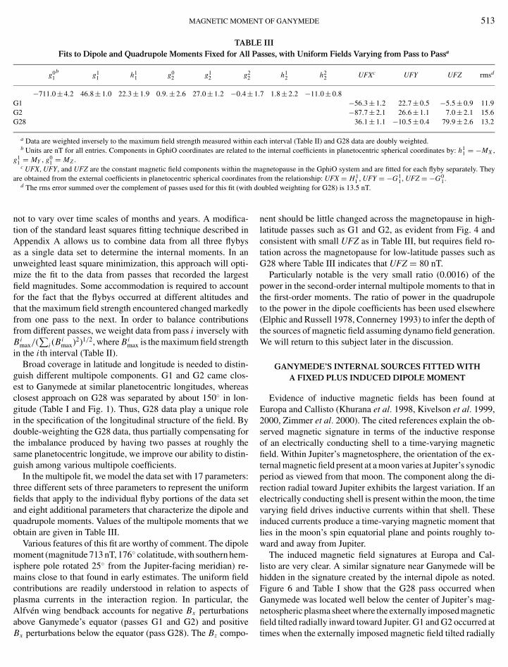
TABLE IIIFits to Dipole and Quadrupole Moments Fixed for All Passes, with Uniform Fields Varying from Pass to Passa
g01
bg1
1 h11 g0
2 g12 g2
2 h12 h2
2 UFXc UFY UFZ rmsd
−711.0 ± 4.2 46.8 ± 1.0 22.3 ± 1.9 0.9. ± 2.6 27.0 ± 1.2 −0.4 ± 1.7 1.8 ± 2.2 −11.0 ± 0.8G1 −56.3 ± 1.2 22.7 ± 0.5 −5.5 ± 0.9 11.9G2 −87.7 ± 2.1 26.6 ± 1.1 7.0 ± 2.1 15.6G28 36.1 ± 1.1 −10.5 ± 0.4 79.9 ± 2.6 13.2
a Data are weighted inversely to the maximum field strength measured within each interval (Table II) and G28 data are doubly weighted.b Units are nT for all entries. Components in GphiO coordinates are related to the internal coefficients in planetocentric spherical coordinates by: h1
1 = −MX ,g1
1 = MY , g01 = MZ .
c UFX, UFY, and UFZ are the constant magnetic field components within the magnetopause in the GphiO system and are fitted for each flyby separately. They
are obtained from the external coefficients in planetocentric spherical coordinates from the relationship: UFX = H11 , UFY = −G11, UFZ = −G0
1.d d
The rms error summed over the complement of passes used for this fit (withnot to vary over time scales of months and years. A modifica-tion of the standard least squares fitting technique described inAppendix A allows us to combine data from all three flybysas a single data set to determine the internal moments. In anunweighted least square minimization, this approach will opti-mize the fit to the data from passes that recorded the largestfield magnitudes. Some accommodation is required to accountfor the fact that the flybys occurred at different altitudes andthat the maximum field strength encountered changed markedlyfrom one pass to the next. In order to balance contributionsfrom different passes, we weight data from pass i inversely withBi
max/(∑
i (Bimax)2)1/2, where Bi
max is the maximum field strengthin the i th interval (Table II).
Broad coverage in latitude and longitude is needed to distin-guish different multipole components. G1 and G2 came clos-est to Ganymede at similar planetocentric longitudes, whereasclosest approach on G28 was separated by about 150◦ in lon-gitude (Table I and Fig. 1). Thus, G28 data play a unique rolein the specification of the longitudinal structure of the field. Bydouble-weighting the G28 data, thus partially compensating forthe imbalance produced by having two passes at roughly thesame planetocentric longitude, we improve our ability to distin-guish among various multipole coefficients.
In the multipole fit, we model the data set with 17 parameters:three different sets of three parameters to represent the uniformfields that apply to the individual flyby portions of the data setand eight additional parameters that characterize the dipole andquadrupole moments. Values of the multipole moments that weobtain are given in Table III.
Various features of this fit are worthy of comment. The dipolemoment (magnitude 713 nT, 176◦ colatitude, with southern hem-isphere pole rotated 25◦ from the Jupiter-facing meridian) re-mains close to that found in early estimates. The uniform fieldcontributions are readily understood in relation to aspects ofplasma currents in the interaction region. In particular, theAlfven wing bendback accounts for negative Bx perturbations
above Ganymede’s equator (passes G1 and G2) and positiveBx perturbations below the equator (pass G28). The Bz compo-oubled weighting for G28) is 13.5 nT.
nent should be little changed across the magnetopause in high-latitude passes such as G1 and G2, as evident from Fig. 4 andconsistent with small UFZ as in Table III, but requires field ro-tation across the magnetopause for low-latitude passes such asG28 where Table III indicates that UFZ = 80 nT.
Particularly notable is the very small ratio (0.0016) of thepower in the second-order internal multipole moments to that inthe first-order moments. The ratio of power in the quadrupoleto the power in the dipole coefficients has been used elsewhere(Elphic and Russell 1978, Connerney 1993) to infer the depth ofthe sources of magnetic field assuming dynamo field generation.We will return to this subject later in the discussion.
GANYMEDE’S INTERNAL SOURCES FITTED WITHA FIXED PLUS INDUCED DIPOLE MOMENT
Evidence of inductive magnetic fields has been found atEuropa and Callisto (Khurana et al. 1998, Kivelson et al. 1999,2000, Zimmer et al. 2000). The cited references explain the ob-served magnetic signature in terms of the inductive responseof an electrically conducting shell to a time-varying magneticfield. Within Jupiter’s magnetosphere, the orientation of the ex-ternal magnetic field present at a moon varies at Jupiter’s synodicperiod as viewed from that moon. The component along the di-rection radial toward Jupiter exhibits the largest variation. If anelectrically conducting shell is present within the moon, the timevarying field drives inductive currents within that shell. Theseinduced currents produce a time-varying magnetic moment thatlies in the moon’s spin equatorial plane and points roughly to-ward and away from Jupiter.
The induced magnetic field signatures at Europa and Cal-listo are very clear. A similar signature near Ganymede will behidden in the signature created by the internal dipole as noted.Figure 6 and Table I show that the G28 pass occurred whenGanymede was located well below the center of Jupiter’s mag-netospheric plasma sheet where the externally imposed magnetic
field tilted radially inward toward Jupiter. G1 and G2 occurred attimes when the externally imposed magnetic field tilted radially
514 KIVELSON, KHURANA, AND VOLWERK
FIG. 5. Traces of the contributions of the dipole and quadrupolar moments along the portions of the passes used for fitting internal moments assuming thats
the surface amplitudes of all coefficients at the surface are 50 nT. G1 is blue, G2 ioutward from Jupiter. Thus, the three flybys used to obtain low-order multipole coefficients are also valuable in determining
whether an inductive response is present. The external field forG1 and G2 was directed radially outward, whereas the externalred, G7 is green, G8 is cyan, G28 is black, and G29 is gray.
field for G28 was directed radially inward. Were there an inducedmagnetic moment, it would be antiparallel to the radial (relative
to Jupiter) component of the external field and its orientation forG28 would differ from that for G1 and G2.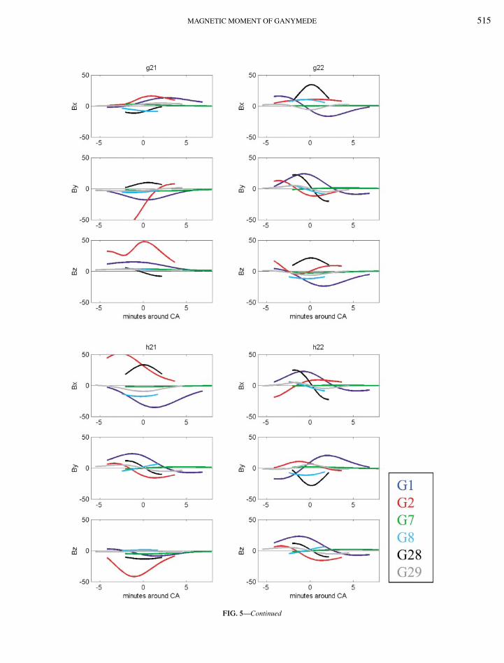
MAGNETIC MOMENT OF GANYMEDE 515
FIG. 5—Continued

N
516 KIVELSON, KHURAFIG. 6. The variation of modeled field components transverse toGanymede’s spin axis over a Jupiter rotation period in Ganymede’s frame(Khurana 1997). The values anticipated at the times of the Ganymede passes areindicated.
We use a two-step approach to test the possibility that thevariations among the fits to the three critical passes given inTable II arise through inductive responses. First, we assume thatthe dipole moment does not vary. We use the approach outlined inthe appendix but this time to find a single best-fit dipole momentplus different uniform fields for each orbit. Weighting by theinverse of the maximum field measured in each interval anddoubling the weight of the G28 interval as before, we follow theprocedure previously summarized but this time determine only12 fit parameters. Results for this fit are given in Table IV, whichshows changes of 2% in MZ , 17% in MX and 13% in MY relativeto the values of Table III. The total rms error (see Appendix Cfor definition) increases from 13.5 nT to 15.1 nT. As anticipated,
the three dipole parameters fit the data less accurately than do imum field in the interval and double weighting the G28 pass. three dipole and five quadrupole parameters.TABLE IVFits to a Dipole Moment Fixed for All Passes, with Uniform Fields Varying from Pass to Pass
g01
ag1
1 h11 UFXb UFY UFZ rmsc
−727.3 ± 1.6 52.8 ± 0.7 18.4 ± 1.1G1 −56.4 ± 0.6 20.4 ± 0.4 −10.1 ± 0.6 14.5G2 −76.5 ± 1.4 16.9 ± 1.1 25.2 ± 1.6 11.0G28 39.6 ± 0.6 −0.9 ± 0.4 73.4 ± 0.8 18.5
a Data are weighted inversely to the maximum field strength measured within intervals (Table II) used for individual passes and G28 is doubly weighted.b Units are nT for all entries. h1
1 = −MX , g11 = MY , g0
1 = MZ .c UFX, UFY, and UFZ are the constant magnetic field components created by the magnetopause currents, fitted for each flyby separately. UFX = H1
1 , UFY =
Table V gives the results of this analysis.
−G11, UFZ = −G0
1.d The rms error summed over the complement of passes used for this fit (with d
A, AND VOLWERK
We next modify our approach by assuming that the internalsources include both a time-varying moment arising from in-duction and a constant dipole moment. As described above, atime-varying uniform magnetic field imposed on a perfectly con-ducting sphere induces a magnetic dipole with equatorial surfacemagnitude half that of the driving field, oriented antiparallel tothe instantaneous driving field. Imperfect electrical conductiv-ity decreases the magnitude of the induced dipole moment andintroduces a phase lag. Zimmer et al. (2000) have applied thetheory of conducting spherical shells to the problem of the induc-tive responses of Europa and Callisto. They show that a shell ofCallisto’s radius (which is close to Ganymede’s) responds witha phase lag corresponding to less than 10◦ of Jupiter rotationif the shell thickness is more than ∼10 km, provided its con-ductivity is greater than or equal to that of terrestrial seawater.Such a phase shift is too small to be detected, particularly forencounters that occur well off the center of the magnetosphericcurrent sheet in a region where the field changes slowly withtime. Consequently, we carry out our analysis ignoring correc-tions for phase lag and characterize the inductive response interms of the amplitude of the induced field. We introduce a pa-rameter, the response efficiency α, that equals the ratio of themagnitude of the induced dipole moment at Ganymede’s surfaceto that of a perfectly conducting sphere of 1 RG. As the dominanttime variability of the background field is in the direction radialfrom Jupiter (the Y -direction in GphiO coordinates), we assumethat MX and MZ are fixed for all passes and that MY (t) respondsto the driving field, Bbg
Y (t), as MY (t) = MYo − αBbgY (t). Here
MY o is the Y -component of the constant dipole moment and theinductive contribution is opposed to the driving field, which wetake to have the values provided in Table I. Values of α < 1 canarise from a combination of imperfect electrical conductivity, asmall shell thickness, and/or a shell radius <1 RG.
With the introduction of the response efficiency, at least fourfixed internal parameters must be specified, the three compo-nents of the permanent magnetic moment (where MYo is g1
1 ofthe dipole fit) and α. Again, we use the approach described inAppendix A, weighting all passes with the inverse of the max-
oubled weighting for G28) is 15.1 nT.
MAGNETIC MOMENT OF GANYMEDE 517
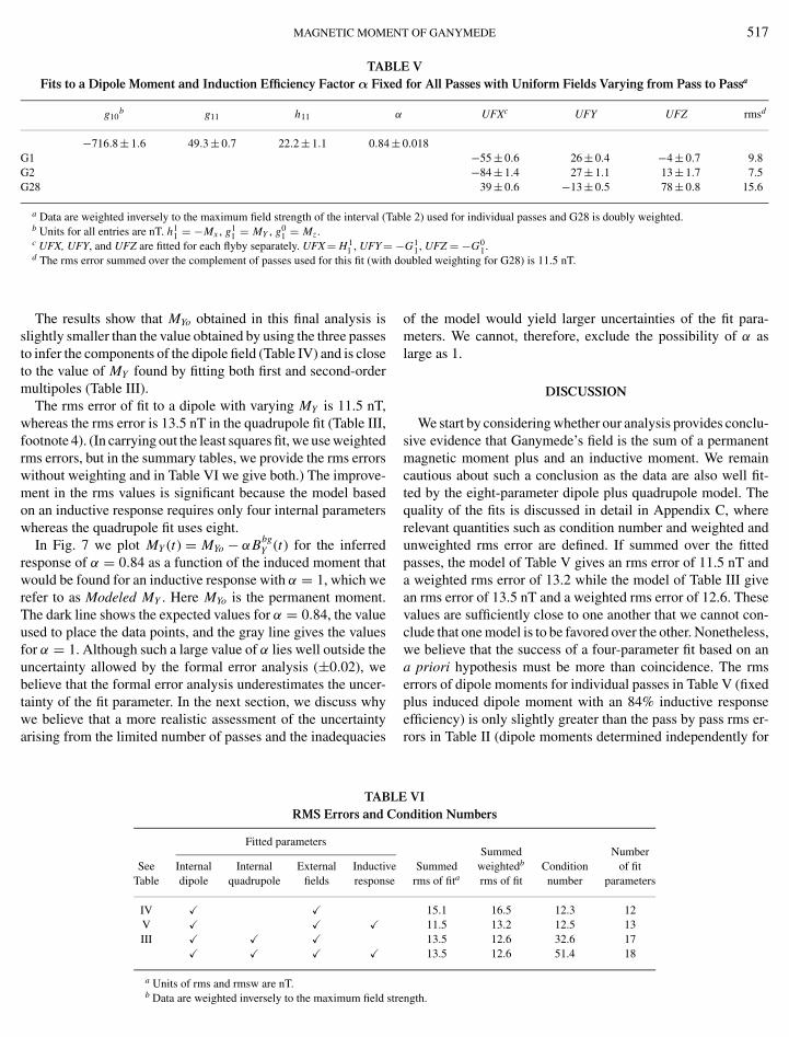
TABLE VFits to a Dipole Moment and Induction Efficiency Factor α Fixed for All Passes with Uniform Fields Varying from Pass to Passa
g10b g11 h11 α UFXc UFY UFZ rmsd
−716.8 ± 1.6 49.3 ± 0.7 22.2 ± 1.1 0.84 ± 0.018G1 −55 ± 0.6 26 ± 0.4 −4 ± 0.7 9.8G2 −84 ± 1.4 27 ± 1.1 13 ± 1.7 7.5G28 39 ± 0.6 −13 ± 0.5 78 ± 0.8 15.6
a Data are weighted inversely to the maximum field strength of the interval (Table 2) used for individual passes and G28 is doubly weighted.b Units for all entries are nT. h1
1 = −Mx , g11 = MY , g0
1 = Mz .
c UFX, UFY, and UFZ are fitted for each flyby separately. UFX = H11 , UFY = −G11, UFZ = −G0
1.d The rms error summed over the complement of passes used for this fit (with doubled weighting for G28) is 11.5 nT.
The results show that MYo obtained in this final analysis isslightly smaller than the value obtained by using the three passesto infer the components of the dipole field (Table IV) and is closeto the value of MY found by fitting both first and second-ordermultipoles (Table III).
The rms error of fit to a dipole with varying MY is 11.5 nT,whereas the rms error is 13.5 nT in the quadrupole fit (Table III,footnote 4). (In carrying out the least squares fit, we use weightedrms errors, but in the summary tables, we provide the rms errorswithout weighting and in Table VI we give both.) The improve-ment in the rms values is significant because the model basedon an inductive response requires only four internal parameterswhereas the quadrupole fit uses eight.
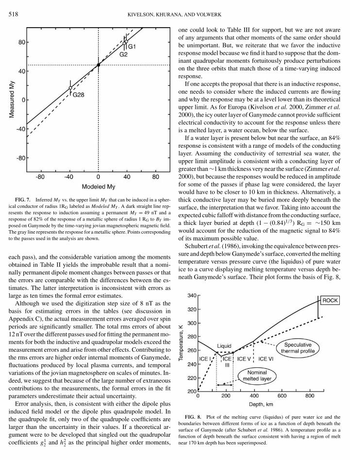
In Fig. 7 we plot MY (t) = MYo − αBbgY (t) for the inferred
response of α = 0.84 as a function of the induced moment thatwould be found for an inductive response with α = 1, which werefer to as Modeled MY . Here MYo is the permanent moment.The dark line shows the expected values for α = 0.84, the valueused to place the data points, and the gray line gives the valuesfor α = 1. Although such a large value of α lies well outside theuncertainty allowed by the formal error analysis (±0.02), webelieve that the formal error analysis underestimates the uncer-tainty of the fit parameter. In the next section, we discuss why
we believe that a more realistic assessment of the uncertaintyarising from the limited number of passes and the inadequaciesefficiency) is only slightly greater than the pass by pass rms er-rors in Table II (dipole moments determined independently for
TABLE VIRMS Errors and Condition Numbers
Fitted parametersSummed Number
See Internal Internal External Inductive Summed weightedb Condition of fitTable dipole quadrupole fields response rms of fita rms of fit number parameters
IV � � 15.1 16.5 12.3 12V � � � 11.5 13.2 12.5 13III � � � 13.5 12.6 32.6 17
� � � � 13.5 12.6 51.4 18
a
Units of rms and rmsw are nT.b Data are weighted inversely to the maximum field strof the model would yield larger uncertainties of the fit para-meters. We cannot, therefore, exclude the possibility of α aslarge as 1.
DISCUSSION
We start by considering whether our analysis provides conclu-sive evidence that Ganymede’s field is the sum of a permanentmagnetic moment plus and an inductive moment. We remaincautious about such a conclusion as the data are also well fit-ted by the eight-parameter dipole plus quadrupole model. Thequality of the fits is discussed in detail in Appendix C, whererelevant quantities such as condition number and weighted andunweighted rms error are defined. If summed over the fittedpasses, the model of Table V gives an rms error of 11.5 nT anda weighted rms error of 13.2 while the model of Table III givean rms error of 13.5 nT and a weighted rms error of 12.6. Thesevalues are sufficiently close to one another that we cannot con-clude that one model is to be favored over the other. Nonetheless,we believe that the success of a four-parameter fit based on ana priori hypothesis must be more than coincidence. The rmserrors of dipole moments for individual passes in Table V (fixedplus induced dipole moment with an 84% inductive response
ength.
N
518 KIVELSON, KHURAFIG. 7. Inferred MY vs. the upper limit MY that can be induced in a spher-ical conductor of radius 1RG labeled as Modeled MY . A dark straight line rep-resents the response to induction assuming a permanent MY = 49 nT and aresponse of 82% of the response of a metallic sphere of radius 1 RG to BY im-posed on Ganymede by the time-varying jovian magnetospheric magnetic field.The gray line represents the response for a metallic sphere. Points correspondingto the passes used in the analysis are shown.
each pass), and the considerable variation among the momentsobtained in Table II yields the improbable result that a nomi-nally permanent dipole moment changes between passes or thatthe errors are comparable with the differences between the es-timates. The latter interpretation is inconsistent with errors aslarge as ten times the formal error estimates.
Although we used the digitization step size of 8 nT as thebasis for estimating errors in the tables (see discussion inAppendix C), the actual measurement errors averaged over spinperiods are significantly smaller. The total rms errors of about12 nT over the different passes used for fitting the permanent mo-ments for both the inductive and quadrupolar models exceed themeasurement errors and arise from other effects. Contributing tothe rms errors are higher order internal moments of Ganymede,fluctuations produced by local plasma currents, and temporalvariations of the jovian magnetosphere on scales of minutes. In-deed, we suggest that because of the large number of extraneouscontributions to the measurements, the formal errors in the fitparameters underestimate their actual uncertainty.
Error analysis, then, is consistent with either the dipole plusinduced field model or the dipole plus quadrupole model. Inthe quadrupole fit, only two of the quadrupole coefficients arelarger than the uncertainty in their values. If a theoretical ar-
gument were to be developed that singled out the quadrupolarcoefficients g12 and h22 as the principal higher order moments,
A, AND VOLWERK
one could look to Table III for support, but we are not awareof any arguments that other moments of the same order shouldbe unimportant. But, we reiterate that we favor the inductiveresponse model because we find it hard to suppose that the dom-inant quadrupolar moments fortuitously produce perturbationson the three orbits that match those of a time-varying inducedresponse.
If one accepts the proposal that there is an inductive response,one needs to consider where the induced currents are flowingand why the response may be at a level lower than its theoreticalupper limit. As for Europa (Kivelson et al. 2000, Zimmer et al.2000), the icy outer layer of Ganymede cannot provide sufficientelectrical conductivity to account for the response unless thereis a melted layer, a water ocean, below the surface.
If a water layer is present below but near the surface, an 84%response is consistent with a range of models of the conductinglayer. Assuming the conductivity of terrestrial sea water, theupper limit amplitude is consistent with a conducting layer ofgreater than∼1 km thickness very near the surface (Zimmer et al.2000), but because the responses would be reduced in amplitudefor some of the passes if phase lag were considered, the layerwould have to be closer to 10 km in thickness. Alternatively, athick conductive layer may be buried more deeply beneath thesurface, the interpretation that we favor. Taking into account theexpected cubic falloff with distance from the conducting surface,a thick layer buried at depth (1 − (0.84)1/3) RG = ∼150 kmwould account for the reduction of the magnetic signal to 84%of its maximum possible value.
Schubert et al. (1986), invoking the equivalence between pres-sure and depth below Ganymede’s surface, converted the meltingtemperature versus pressure curve (the liquidus) of pure waterice to a curve displaying melting temperature versus depth be-neath Ganymede’s surface. Their plot forms the basis of Fig. 8,
FIG. 8. Plot of the melting curve (liquidus) of pure water ice and theboundaries between different forms of ice as a function of depth beneath thesurface of Ganymede (after Schubert et al. 1986). A temperature profile as a
function of depth beneath the surface consistent with having a region of meltnear 170 km depth has been superimposed.
N
thick outer icy shell (Anderson et al. 1996). Melting within the
MAGNETIC MOME
which shows that in the interior of Ganymede the minimumtemperature at which water ice melts occurs at a depth of 170 km.(The minimum melting temperature would decrease if salt weredissolved in the water.) We have added a possible temperatureprofile to the plot of the liquidus. If the temperature rises rapidlyin the first 100–150 km beneath the surface and increases moreslowly (adiabatically) at greater depth, a layer of melt wouldbe found sandwiched between layers of ice surrounding the∼170 km depth. Thus, the most probable value of the responsefactor α suggests a depth for the buried ocean that is reasona-ble on physical grounds. Additional work is underway to relatethe observations to properties of a possible subsurface ocean.
Finally, we return to the implications of the small values ob-tained for the quadrupole coefficients (Table III). (Note that thequadrupole moments are smaller if one also allows for inductiveresponses, but the values obtained for a fixed dipole moment willsuffice to make the arguments.) One possible interpretation ofthe small amplitude of the higher order multipoles is that the re-gion in which the permanent internal field is generated is deeplyburied. This concept, proposed by Lowes (1974), has been ap-plied by Elphic and Russell (1978) to a determination of the“apparent source depths” of the fields of Mercury and Jupiterand by Connerney (1993) to Earth and the outer planets. Theapproach identifies a depth at which the power in multipoles oforder n
Un = (n + 1)
(RG
r
)2n+4 n∑m=0
[(gm
n
)2 + (hm
n
)2](1)
is comparable for all orders, based on the idea that the momentsarise from turbulent motions in the source region. Although theratio of first two orders of multipole moments can be no morethan suggestive, we note that the ratio of power is
(U2
U1
)= 3
2
(RG
r
)2 ∑2m=0
[(gm
2
)2 + (hm
2
)2]∑1
m=0
[(gm
1
)2 + (hm
1
)2] , (2)
which yields 0.0016 from Table III, down by almost two or-ders of magnitude relative to the analogous ratios for Earthor Jupiter (Elphic and Russell 1978, Connerney 1993). Withras defined as the radius of the source sphere, i.e., the distancefrom Ganymede’s center to the “apparent source depth” at whichU2/U1 = 1,
ras
RG=
(3
2
∑2m=0
[(gm
2
)2 + (hm
2
)2]∑1
m=0
[(gm
1
)2 + (hm
1
)2])1/2
(3)
For the values in Table III, ras = 0.049 RG = 130 km. This es-timate of the apparent source radius is hard to reconcile withestimates of the size of the metallic core whose radius is be-lieved to fall between 0.25 RG = 658 km and 0.5 RG = 1317 km(Anderson et al. 1996). It should be noted, however, that Elphic
and Russell (1978) find that the quadrupole power at Earth isT OF GANYMEDE 519
lower by almost an order of magnitude than the trend providedby the dipole moment and the n > 2 multipole moments, so theestimate of the source depth from U1 and U2 alone may be mis-leading. It does seem reasonable to conclude, however, that ifGanymede’s field is generated by dynamo action, the source liesfar below the surface.
The small ratio of the quadrupole to dipole power does notnecessarily require a deeply buried dynamo because dynamomodels admit a great variety of solutions. Magnetoconvection,for example, provides an interesting alternative to the dynamomechanism for generating the fields of satellites (e.g., Sarsonet al. 1997). Magnetoconvection produces a planetary field byamplification of an externally imposed magnetic field such as theaverage Bbg at Ganymede. Fluid motions amplify the imposedfield much as in a dynamo, but the internal field decays if theexternal field vanishes. A possible consequence of this modelcould be that the symmetry of a uniform external field imposes adominantly dipolar symmetry on the internal field and thereforeproduces an internal response with weak higher order multi-poles. Yet another proposed source of the permanent magneticmoment is remanent ferromagnetism (Crary and Bagenal 1998)which would also imply dipolar symmetry for the field. Thus,our conclusion that the quadrupolar terms are very small may beregarded as providing encouragement for further investigationof magnetoconvection or remanent magnetization as the mecha-nism for generating Ganymede’s permanent magnetic field.
CONCLUSIONS
Magnetometer data from all five passes by Ganymede havebeen used to refine our evaluation of the moon’s permanentdipole moment. The fits of Tables III and V are consistentwith a magnetic moment characterized by an equatorial sur-face field magnitude M = 719 ± 2 nT tilted by 176◦ ± 1◦ fromthe spin axis with the pole in the southern hemisphere rotatedby 24◦ ± 1◦ from the Jupiter-facing meridian plane toward thetrailing hemisphere. In SI units, the dipole moment is = 1.32 ×10²⁰ Amp-m2. The magnitude is very slightly smaller than ini-tially suggested (Kivelson et al. 1996) and the orientation iscloser to antiparallel to the spin axis.
Magnetometer data from Galileo’s multiple flybys ofGanymede provide significant, but not unambiguous, evidencethat the moon, like its neighboring satellites Europa and Callisto,responds inductively to Jupiter’s time-varying magnetic field.The response is roughly 84% of the response expected for ametallic sphere of the same radius but there may be considerableuncertainty in this estimate. The outer layer of Ganymede is pre-dominantly formed of water ice, which is not a good conductorof electricity. The most likely source of electrical conductivitywithin a water ice environment is a liquid water layer bearingelectrolytes such as salts and acids. Our data indicate that thelocus of the current carrying layer is buried within the 800 km
ice shell occurs most readily near 170 km beneath the surface

520 KIVELSON, KHURAN
where increasing pressure reduces the melting temperature to itslowest value. If we assume conductivity comparable to or higherthan that of terrestrial sea water, our analysis is consistent with adepth for the conducting layer close to this location. The oceanwould lie between two layers of ice. Ganymede’s large size rela-tive to its two ice covered neighbors Europa and Callisto and theevidence previously found that the nearby moons are respondinginductively lends credibility to the evidence that Ganymede isresponding inductively to the temporal variations of the jovianmagnetic field.
Although we cannot rule out other interpretations of the datadiscussed above, we view the inductive response interpretationas highly probable. Regrettably, as illustrated in Fig. 5, datafrom G29, the final Ganymede encounter of the Galileo mission,did not add meaningfully to the information already availablefor the analysis of Ganymede’s internal magnetic properties.However, planning for more Jupiter orbiting spacecraft missionscontinues, and it should be recognized that future opportunitiesto take magnetometer data in Ganymede’s environment can bedesigned to acquire data necessary to distinguish between thesignature of fixed internal quadrupole moments and the signatureof an induced dipole moment.
APPENDIX A: LEAST SQUARES FITS
We use a weighted least squares fit to determine a single set of multipolecomponents for multiple passes and different constant field components foreach individual flyby. The input data are values of the magnetic field b alongeach of a set of trajectories. These measurements are related to the matrix of themodel field coefficients x by a matrix A, a function of Galileo’s location relativeto Ganymede that varies from one pass to another. With the error defined ase = (Ax − b), a least squares fit requires us to minimize the square sum ofE = eT e/2 (where the superscript T indicates the transpose) with respect to theunknown parameters of the model. This requires dE/dx = 0. The parameters ofthe model are then the solutions of
d
dx1
2(Ax − b)T (Ax − b) = 1
2AT (Ax − b) + 1
2(Ax − b)T A
= AT (Ax − b) = 0, (A1)
which by matrix inversion gives
x = (AT A)−1AT b. (A2)
As the passes vary considerably in altitude and in maximum field strength, fitsto the full data set are biased toward fitting the lowest altitude passes (see Table I).In order to optimize the fit over the full data set, we weight the contributions ofdifferent passes inversely by Bi
max/(∑
i (Bimax)2)1/2, where Bi
max is the maximumfield strength in the i th interval. In our application, the contribution of G28is treated as if there had been two identical G28 passes, so i = 1, . . . 4. In aweighted least squares fit one redefines E as E = eT W2e/2, where W is adiagonal weighting matrix. The equivalent to (A2) is then
x = (WAT WA)−1WAT Wb. (A3)
In this paper the measurements b consist of the three components of themagnetic field in the GphiO coordinate system. If we fit only dipole coefficients
of the internal field, the matrix A for each data point is a 3 × 12 matrix, built upin the following form: [3A, UF(G1), UF(G2), UF(G7), UF(G28)], where 3AA, AND VOLWERK
is a 3 × 3 submatrix that relates the dipole field along the orbit to the Cartesiancomponents of the dipole moment:
R =√
X2 + Y 2 + Z2
3 A11 = (3X2 − R2)/R5, 3 A12 = 3XY/R5, 3 A13 = 3X Z/R5,(A4)
3 A21 = 3XY/R5, 3 A22 = (3Y 2 − R2)/R5, 3 A23 = 3Y Z/R5,
3 A31 = 3X Z/R5, 3 A32 = 3Y Z/R5, 3 A33 = (3Z2 − R2)/R5.
The next three 3 × 3 submatrices are I if the data being fitted correspond tothe specified orbit, or 0 if not.
For each data point this matrix is calculated and added as new rows, which,for n data points leads to a new matrix A of dimension 3n × 16. The abovecalculation of the least squares fit is then performed as specified by Eq. (A2).The extension to fits of higher order multipoles produces larger matrices, butthere is no conceptual change in the approach.
For the final fit, a parameter of a different type (α) is fitted in addition to thedipole coefficients but the process remains as described above.
APPENDIX B: SINGULAR VALUE DECOMPOSITION
We have used the generalized inverse theory to reconfirm the least squaresanalysis and to determine the uniqueness and the robustness of the fits. Thetheory of generalized inversion was discussed in detail by Lanczos (1961) andhighlighted by Jackson (1972) in the context of geophysical data inversion.Applications of the technique to invert geophysical magnetic data have beenmade by Pedersen (1975) and Connerney (1981).
The linear set of equations that we must invert can be written in the matrixform as
Y = AX, (B1)
where Y is a column matrix of the N magnetic field observations, A is the N ×M matrix, which relates observations to the model parameters X (the variousinternal and external spherical harmonic terms and the response). (In terms of theindex n used in Appendix A, N = 3n.) As N > M in our case, the linear systemis overdetermined and a least squares inversion provides the best estimates ofthe model parameters.
The idea behind the generalized inverse technique is to decompose the Amatrix into the form
A = U�VT , (B2)
where U, �, and V satisfy the following eigenvalue problems:
AAT U = �2U (B3)
AT AV = �2V. (B4)
The � matrix is a diagonal M × M matrix with the M eigenvalues arrangedalong the diagonal of the matrix in order of decreasing magnitude. U is anN × M matrix with the M eigenvectors of Eq. (3) arranged in N columns; V isan M × M matrix with the M eigenvectors of Eq. (4) arranged in M columns.The least squares inverse of matrix A is
H = V�UT . (B5)
APPENDIX C: ESTIMATING THE VALIDITY OF THE FITS:CONDITION NUMBER AND RMS DEVIATIONS
An examination of the U, �, and V matrices gives insight into the inversionprocess. For example, the ratio of the largest to the lowest eigenvalue (called

N
MAGNETIC MOMEthe condition number of the matrix A) provides a measure of the invertibility ofmatrix A. If the condition number is large, the solution is poorly constrained bythe data and the poorly determined model parameters have large errors associatedwith them. There is no rigorous selection criterion for how large the conditionnumber can become and still imply a good fit. Indeed, the number is expected toincrease with the number of parameters being determined, yet this does not meanthat the solutions are poor. In applications to internal fields of planets, valuesas large as 60 are regarded as adequately small. The solutions of Tables III–Vhave condition numbers smaller than 32.6 and are tabulated in Table VI. It can beseen that for least square fits in which quadrupole terms are omitted (the first tworows of the table), the condition numbers are quite small (<13). The conditionnumber increases to a value of 32.6 when dipole, quadrupole, and externalfield parameters are optimized. When the induction response is simultaneouslyoptimized, the condition number almost doubles, increasing to a value of 51.4.This large increase reflects the fact that the available data cannot distinguish theh1
2 quadrupole contributions from the induction response. The V matrix for thisfit reveals that these two parameters require large contributions from the threeeigenvectors corresponding to the three smallest eigenvalues.
Estimates of the errors of the fit parameters can be obtained from the matrix V.The standard error associated with a parameter j (assuming that the observationsare statistically independent) is given by
S j = σB
√√√√P≤M∑i=1
Vi, j2
λi2 , (C1)
where σB is the standard uncertainty associated with the measurements (assumedconstant in this work). The uncertainties of the fit parameters given in Table III–Vwere calculated from Eq. (B6) for P = M and σB = 8 nT. This value of thestandard uncertainty corresponds to the digitization of the magnetometer inits highest field range (Kivelson et al. 1992) and overestimates the error ofmeasurement. Uncertainties in position relative to Ganymede are less than 1 km,implying that the uncertainty in range �R/R = 4 × 10⁻⁴ is allowed for withinthe value of 8nT that we used for σB .
It is useful to confirm that the model provides a good representation of thedata by calculating the root mean square deviation of the fit to the measuredquantities. In Table VI we tabulate the rms deviations both for weighted andunweighted cases, where weighting is relevant to the approach used to reduce thedisproportionately large contribution of the lowest altitude flyby. The definitionof the summed weighted rms of fit (rmsw) is
rmsw =
[(w2
1
∑j,G1 [�B j (G1)]2 + w2
2
∑j,G2 [�B j (G2)]2
+ 2w228
∑j [�B j,G28(G28)]2
)/N
]1/2
1/4(w1 + w2 + 2w28)1/2, (C2)
where the weight of the i th pass by Ganymede (Gi) is wi = [Bmax(Gi)]−1
and Bmax(Gi) is tabulated in Table II. Here �B j,Gi represents the deviationsof the NGi individual data points on pass Gi from the fit for that pass. N =NG1 + NG2 + 2NG28 is the total number of data points in the data set. Thesummed rms of fit is defined by
rms = rmsw with wi = 1 for all i. (C3)
Lanczos (1961) has shown that a more robust inverse (called the generalizedinverse) is obtained by retaining only the P largest eigenvalues of the V matrixand their eigenvectors in Eq. (B5). However, in some cases, the eigenvectorcorresponding to the smallest eigenvalues contributes significantly to the fit andit may not be appropriate to drop it. For the Ganymede fits, we found thatwhen we dropped the smallest eigenvalue from the 18-parameter solution (fittedparameters listed in the last row of Table VI), the new solution was almostidentical to the 17-parameter solution of the third row. The summed rms error of
fit changed from 13.5 to 13.4. The insignificant change confirms the previouslynoted fact that the inductive response merely reproduces contributions that couldT OF GANYMEDE 521
equally be attributed to h12. In other cases, when the smallest eigenvalues was
dropped, the rms error increased by almost a factor of 2. For example, the rmserror of fit to the case of Table III increased from 13.5 nT to 28.7 nT when theeigenvector with the smallest eigenvalue was dropped, indicating that it was notappropriate to use the generalized inverse solution.
ACKNOWLEDGMENTS
The authors acknowledge helpful discussions of this topic with ChristopheZimmer and Paul O’Brien. Didier Sornette provided useful insight into datafitting philosophy. We are grateful to Z. J. Yu who directed our attention to someprograms useful in applying singular value decomposition to our data. Thisresearch was supported by the National Aeronautics and Space Administrationthrough Jet Propulsion Laboratory under Contract JPL 958694 and by NASAunder NAG 5-7959. This paper was originally published as a UCLA IGPPpublication, #5562.
REFERENCES
Anderson, J. D., E. L. Lau, W. L. Shogren, G. Schubert, and W. B. Moore 1996.Gravitational constraints on the internal structure of Ganymede. Nature 384,541–543.
Connerney, J. E. P. 1981. The magnetic field of Jupiter: A generalized inverseapproach. J. Geophys. Res. 86, 7679–7693.
Connerney J. E. P. 1993. Magnetic fields of the outer planets. J. Geophys. Res.98, 18,659–18,679.
Crary F. J., and F. Bagenal 1998. Remanent ferromagnetism and the interiorstructure of Ganymede. J. Geophys. Res. 103, 25,757–25,774.
Elphic, R. C., and C. T. Russell 1978. On the apparent source depth of planetarymagnetic fields. Geophys. Res. Lett. 5, 211–214.
Gurnett, D. A., W. S. Kurth, A. Roux, S. J. Bolton, and C. F. Kennel 1996.Evidence for a magnetosphere at Ganymede from plasma-wave observationsby the Galileo spacecraft. Nature 384, 535–537.
Jackson, D. D. 1972. Interpretation of inaccurate, insufficient and inconsistentdata. Geophys. J. R. Astron. Soc. 28, 97–109.
Khurana, K. K. 1997. Euler potential models of Jupiter’s magnetospheric field.J. Geophys. Res. 102, 11,295–11,306.
Khurana, K. K., M. G. Kivelson, D. J. Stevenson, G. Schubert, C. T. Russell,R. J. Walker, S. Joy, and C. Polanskey 1998. Induced magnetic fields asevidence for subsurface oceans in Europa and Callisto. Nature 395, 777–780.
Kivelson, M. G., K. K. Khurana, J. D. Means, C. T. Russell, and R. C. Snare 1992.The Galileo magnetic field investigation. Space Science Rev. 60, 357–383.
Kivelson, M. G., K. K. Khurana, C. T. Russell, R. J. Walker, J. Warnecke,F. V. Coroniti, C. Polanskey, D. J. Southwood, and G. Schubert 1996.Discovery of Ganymede’s magnetic field by the Galileo spacecraft. Nature384, 537–541.
Kivelson, M. G., K. K. Khurana, F. V. Coroniti, S. Joy, C. T. Russell, R. J.Walker, J. Warnecke, L. Bennett and C. Polanskey 1997. The magnetic fieldand magnetosphere of Ganymede. Geophys. Res. Lett. 24, 2155.
Kivelson, M. G., J. Warnecke, L. Bennett, S. Joy, K. K. Khurana, J. A. Linker,C. T. Russell, R. J. Walker, and C. Polanskey 1998. Ganymede’s magneto-sphere: Magnetometer overview. J. Geophys. Res. 103, 19,963–19,972.
Kivelson, M. G., K. K. Khurana, D. J. Stevenson, L. Bennett, S. Joy, C. T. Russell,R. J. Walker, C. Zimmer, and C. Polanskey 1999. Europa and Callisto: Inducedor intrinsic fields in a periodically varying plasma environment. J. Geophys.Res. 104, 4609–4626.
Kivelson, M. G., K. K. Khurana, C. T. Russell, M. Volwerk, R. J. Walker, andC. Zimmer 2000. Galileo magnetometer measurements: A stronger case fora subsurface ocean at Europa. Science 289, 1340–1343.
Lanczos, C. 1961. Linear Differential Operations, Van Nostrand, Princeton, NJ.

N
522 KIVELSON, KHURALowes, F. J. 1974. Spatial power spectrum of the main geomagnetic field.Geophys. J. R. 36, 717.
McKinnon, W. B. 1997. Galileo at Jupiter—Meetings with remarkable moons.Nature 390, 23.
Pedersen, L. B. 1977. Interpretation of potential field data: A generalized inverseapproach. Geophys. Prospect. 25, 199.
Russell, C. T. 1995. A brief history of solar-terrestrial physics. In Introductionto Space Physics (M. G. Kivelson and C. T. Russell, Eds.), Cambridge Univ.Press, New York.
Sarson G. R., C. A. Jones, K. Zhang, G. Schubert 1997. Magnetoconvectiondynamos and the magnetic fields of Io and Ganymede. Science 276, 1106.
Schubert, G., T. Spohn, and R. Reynolds 1986. Thermal histories, composi-tions and internal structures of the moons of the Solar System. In Satellites(J. A. Burns and M. S. Matthews, Eds.), pp. 224–292, University of ArizonaPress, Tucson, Arizona.
Schubert, G., K. Zhang, M. G. Kivelson, and J. D. Anderson 1996. The magneticfield and internal structure of Ganymede. Nature 384, 544–545.
A, AND VOLWERK
Volwerk, M., M. G. Kivelson, K. K. Khurana, and R. L. McPherron 1999.Probing Ganymede’s magnetosphere with field line resonances. J. Geophys.Res. 104, 14,729–14,738.
Walker, R. J., and C. T. Russell 1995. Solar-wind interactions with magnetizedplanets. In Introduction to Space Physics (M. G. Kivelson, and C. T. Russell,Eds.), Cambridge Univ. Press, New York.
Williams, D. J., R. W. McEntire, S. Jaskulek, and B. Wilken 1992. The GalileoEnergetic Particles Detector. Space Science Rev. 60, 385–412.
Williams, D. J., B. Mauk, and R. W. McEntire 1997a. Trapped electrons inGanymede’s magnetic field. Geophys. Res. Lett. 24, 2953.
Williams, D. J., B. H. Mauk, R. W. McEntire, E. C. Roelof, T. P. Armstrong,B. Wilken, J. G. Roederer, S. M. Krimigis, T. A. Fritz, L. J. Lanzerotti, andN. Murphy 1997b. Energetic particle signatures at Ganymede: Implicationsfor Ganymede’s magnetic field. Geophys. Res. Lett. 24, 2163.
Zimmer, C., K. K. Khurana, and M. G. Kivelson 2000. Subsurface oceans on
Europa and Callisto: Constraints from Galileo magnetometer observations.Icarus 147, 329–347.