The Neymann-Pearson Lemma Suppose that the data x1, … , xn has joint density function

f(x1, … , xn ;)

where is either 1 or 2.Let

g(x1, … , xn) = f(x1, … , xn ;1) and

h(x1, … , xn) = f(x1, … , xn ;2)

We want to test

H0: = 1 (g is the correct distribution) against

HA: = 2 (h is the correct distribution)

The Neymann-Pearson Lemma states that the Uniformly Most Powerful (UMP) test of size is to reject H0 if:

2 1

1 1

, ,

, ,n

n

L h x xk

L g x x

and accept H0 if:

2 1

1 1

, ,

, ,n

n

L h x xk

L g x x

where k is chosen so that the test is of size .

0

0.01

0.02

0.03

0.04

0.05

0 20 40 60 80 100

Neyman Pearson Lemma

g(x)

h(x)

x

0

0.01

0.02

0.03

0.04

0.05

0 20 40 60 80 100

Neyman Pearson Lemma

g(x)

h(x)

x

0

0.01

0.02

0.03

0.04

0.05

0 20 40 60 80 100

Neyman Pearson Lemma

g(x)

h(x)

x

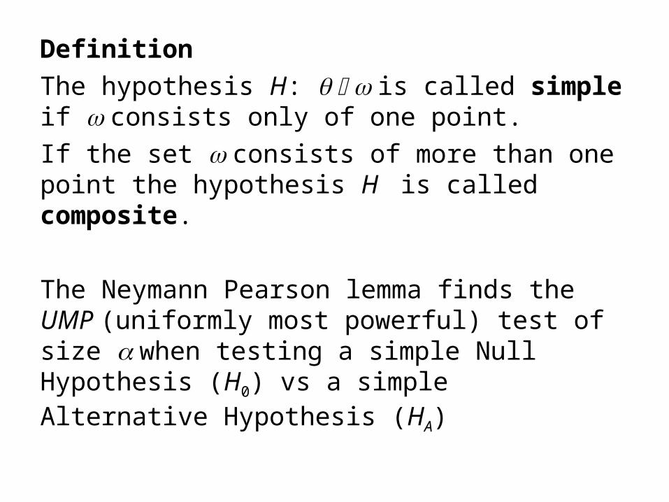
Definition

The hypothesis H: is called simple if consists only of one point.

If the set consists of more than one point the hypothesis H is called composite.

The Neymann Pearson lemma finds the UMP (uniformly most powerful) test of size when testing a simple Null Hypothesis (H0) vs a simple Alternative Hypothesis (HA)

A technique for finding the UMP (uniformly most powerful) test of size for testing a simple Null Hypothesis (H0) vs a composite Alternative Hypothesis (HA).1. Pick an arbitrary value of the parameter, 1, when the

Alternative Hypothesis (HA) is true. (convert HA into a simple hypothesis

2. Use the Neymann Pearson lemma to find UMP (uniformly most powerful) test of size for testing a simple Null Hypothesis (H0) vs a simple Alternative Hypothesis

3. If this test does not depend on the choice of 1 then the test found is the uniformly most powerful test of size for testing a simple Null Hypothesis (H0) vs a composite Alternative Hypothesis (HA).

(1) .AH

(1) .AH

Likelihood Ratio Tests

A general technique for developing tests using the Likelihood functionThis technique works for composite Null hypotheses (H0) and composite Alternative hypotheses (HA)

Likelihood Ratio Tests

Suppose that the data x1, … , xn has joint density function

f(x1, … , xn ; 1, … , p)

where (1, … , p) are unknown parameters assumed to lie in (a subset of p-dimensional space).

Let denote a subset of .

We want to test

H0: (1, … , p) against

HA: (1, … , p)

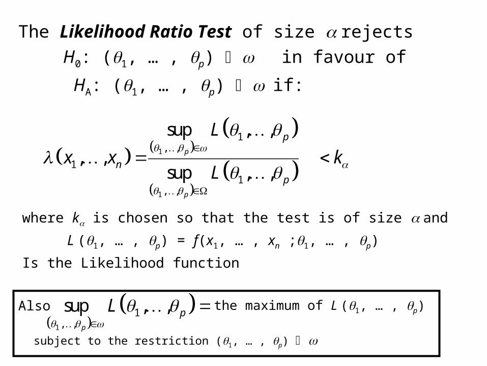
The Likelihood Ratio Test of size rejects

H0: (1, … , p) in favour of

HA: (1, … , p) if:

1

1

1, ,

1

1, ,

sup , ,

, , sup , ,

p

p

p

n

p

L

x x kL

where k is chosen so that the test is of size and

L (1, … , p) = f(x1, … , xn ;1, … , p)

Is the Likelihood function

1

1, ,

sup , ,p

pL

the maximum of L (1, … , p)

subject to the restriction (1, … , p)

Also

Example Suppose that x1, … , xn is a sample from the Normal distribution with mean (unknown) and variance 2 (unknown).

Then x1, … , xn have joint density function

f(x1, … , xn ; ) 21

221

/ 2

1

2

n

ii

x

n ne

Suppose that we want to test

H0: = 0

against HA: ≠0

L( ) = f(x1, … , xn ; )

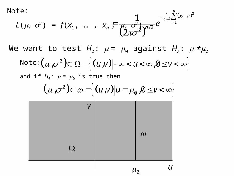
Note:

We want to test H0: = 0 against HA: ≠0

21

221

/ 22

1

2

n

ii

x

n e

L(2) = f(x1, … , xn ; 2)

2, , ,0u v u v

20, , ,0u v u v

Note:

and if H0: = 0 is true then

u

v

0

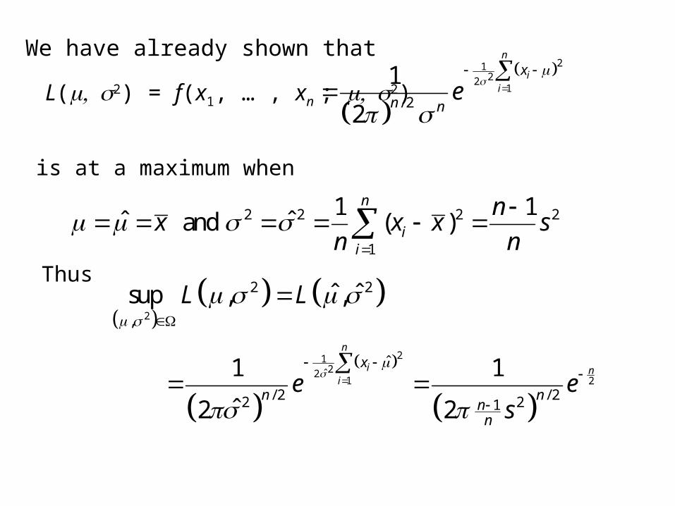
We have already shown that

is at a maximum when

21

221

/ 2

1

2

n

ii

x

n ne

L(2) = f(x1, … , xn ; 2)

2 2 2 2

1

1 1ˆ ˆ and ( )

n

ii

nx x x s

n n

2

2 2

,

ˆ ˆsup , ,L L

Thus

212ˆ2

1 2

ˆ

/ 2 / 22 21

1 1

ˆ2 2

n

i ni

x

n nnn

e es

Now consider maximizing

when

2122

1

/ 22

1

2

n

ii

x

n e

L(2) = f(x1, … , xn ; 2)

20, , ,0u v u v

This is equivalent to choosing v to maximize

2102

1

/ 2

1

2

n

ivi

x

nL v ev

or 21

021

ln ln 2 ln2 2

n

ivi

n nl v L v v x

Hence

if

or

22102

1

10

2

n

ii

nl v v x

v

2

021

1 1

2 2

n

ii

nx

v v

220

1

1ˆ̂n

ii

v xn

Thus

Is maximized subject to

2122

1

/ 22

1

2

n

ii

x

n e

L(2) = f(x1, … , xn ; 2)

20, , ,0u v u v

when 2 2 2

0 01

1ˆ ˆˆ ˆ and ( )n

ii

xn

2

2 2

,

ˆ ˆˆ ˆsup , ,L L

2

12ˆ̂2

1 2

ˆ̂

/ 2 / 22 2

1 1

ˆ ˆˆ ˆ2 2

n

i ni

x

n ne e

thus

The Likelihood Ratio Test of size rejects

H0: = 0 in favour of

HA: ≠ 0 if:

2

2

22

,

1 2 2

,

sup , ˆ ˆˆ ˆ,, , =

ˆ ˆsup , ,n

LL

x x kL L

2

2

/ 2/ 22 2

2

/ 2

1

ˆ̂2 ˆ1 ˆ̂

ˆ2

n

n

nn

n

e

ke

i.e. if

or 22/

2

ˆˆ̂

nk

Now 2 2 2

1

1 1ˆ ( )

n

ii

nx x s

n n

and

2 2 20 0

1 1

1 1ˆ̂ ( ) ( )n n

i ii i

x x x xn n

2 2

01

1( ) ( )

n

ii

x x n xn

2 2 2 20 0

1 11 ( ) ( )

nn s n x s x

n n

thus

22/

2

ˆˆ̂

nk

and

22

22 2

0

1ˆˆ 1ˆ ( )

ns

nn

s xn

20

2

1

( )1

1

xnn s

/ 22

02

1if

( )1

1

nkxn

n s

2

02 / 2

( ) 1or 1

1 n

xn

n s k

2

02 / 2

( ) 11 1

n

n xn

s k

0/ 2

( ) 11 1

n

n xn

s k

The Likelihood Ratio Test of size rejects

H0: = 0 in favour of

HA: ≠ 0 if:

or

0/ 2

( ) 11 1

n

n xn K

s k

0 0( ) ( ) or

n x n xK K

s s

where k (or K) are chosen so that the test is of size .

The value that achieves this is 1/ 2

nK t

Conclusion: The Likelihood Ratio Test of size for testing

H0: = 0 against

HA: ≠ 0

is the Students t-test

Example Suppose that x1, … , xn is a sample from the Uniform distribution from 0 to (unknown)

Then x1, … , xn have joint density function

f(x1, … , xn ;) 1

10 , ,

0 otherwise

nnx x

Suppose that we want to test

H0: = 0

against HA: ≠0

Note: L() = f(x1, … , xn ;) 1

max

0 max

in i

ii

x

x

We have already shown that

is at a maximum when

L() = f(x1, … , xn ;)

ˆ max ii

x

1ˆsup maxmax

n

ii

ii

L L L xx

Thus

1max

0 max

in i

ii

x

x

Also it can be shown that

is maximized subject to = {0} when

L() = f(x1, … , xn ;)

0

ˆ̂

000

0

1maxˆ̂

sup

0 max

n

ii

ii

xL L L

x

Thus

1max

0 max

in i

ii

x

x

Hence

0

ˆ̂sup

ˆsup max ii

LL L

L L L x

00

0

maxmax

0 max

n

ii

ii

ii

xx

x

We will reject H0 if < k

00

max when max

n

ii

ii

xk x

Hence will reject H0 if:

0 max ii

x

or if

1

0

maxn

ii

xk

i. e.

1

0max ni

ix k K or

Summarizing: We reject H0 if:

0 max ii

x

or if 0max ii

x

Where K (equivalently k) is chosen so that

1

0max ni

ix k K

Again to find K we need to determine the sampling distribution of :

and

max ii

P x K when H0 is true

max ii

x when H0 is true

max ii

U x

then max ii

G u P U u P x u

The sampling distribution of:

We wantmax i

iP x K

when H0 is true

max ii

x

Let

1 , ,n n

n n

u uP x u x u

0

n

n

u

when H0 is true

0

n

n

K

thus

0

nK

or0

nK

Final Summary: We reject H0 if:

0 max ii

x

or if 0max ii

x 0max ni

ix and

Example: Suppose we have a sample of n = 30 from the Uniform distribution

0 10 max ii

x or if

0max 10ii

x 300max 10 .05 9.05n

ii

x and

3.4 7.5 8.1 6.0 6.6 0.8 3.4 3.0 0.6 7.18.1 3.3 4.1 7.6 0.7 7.7 8.9 1.5 1.2 5.39.5 2.1 6.0 7.4 6.6 8.3 3.1 7.8 9.6 1.1

max 9.6ii

x

We want to test H0: = 10 (0) against H0: ≠ 10

We are going to reject H0: = 10 if:

But max 9.05ii

x hence we accept H0: = 10.

Comparing Populations

Proportions and means

Sums, Differences, Combinations of R.V.’s

A linear combination of random variables, X, Y, . . . is a combination of the form:

L = aX + bY + …

where a, b, etc. are numbers – positive or negative.

Most common:Sum = X + Y Difference = X – Y

Means of Linear Combinations

The mean of L is:

L= a X+ b Y+ …

Most common:

X+Y = X + Y

X – Y = X - Y

If L = aX + bY + …

Variances of Linear CombinationsIf X, Y, . . . are independent random variables and

L = aX + bY + … then

Most common:

22222YXL ba

222YXYX

222YXYX

If X, Y, . . . are independent normal random variables, then L = aX + bY + … is normally distributed.

In particular:

X + Y is normal with

X – Y is normal with

Combining Independent Normal Random Variables

22 deviation standard

mean

YX

YX

22 deviation standard

mean

YX

YX

Comparing proportions

Situation• We have two populations (1 and 2)• Let p1 denote the probability (proportion) of

“success” in population 1.• Let p2 denote the probability (proportion) of

“success” in population 2.• Objective is to compare the two population

proportions

We want to test either:

21210 : vs: .1 ppHppH A

21210 : vs: .2 ppHppH A

21210 : vs: .3 ppHppH A

or

or

is an estimate of pi (i = 1,2)

i

iipip n

ppp

ii

1 and ˆˆ

ˆ ipRecall:

has approximately a normal distribution with

ˆ ip

Where: A sample of n1 is selected from population 1 resulting in x1 successes

A sample of n2 is selected from population 2 resulting in x2 successes

2

22

1

11

ˆ and

ˆ

n

xp

n

xp

is an estimate of p1 – p2

21ˆˆ - 21

pppp

21 ˆ- ˆ pp

We want to estimate and test p1 – p2

has approximately a normal distribution with

21 ˆ- ˆ pp

2

22

1

112ˆ

2ˆˆˆ

11 and

2121 n

pp

n

pppppp

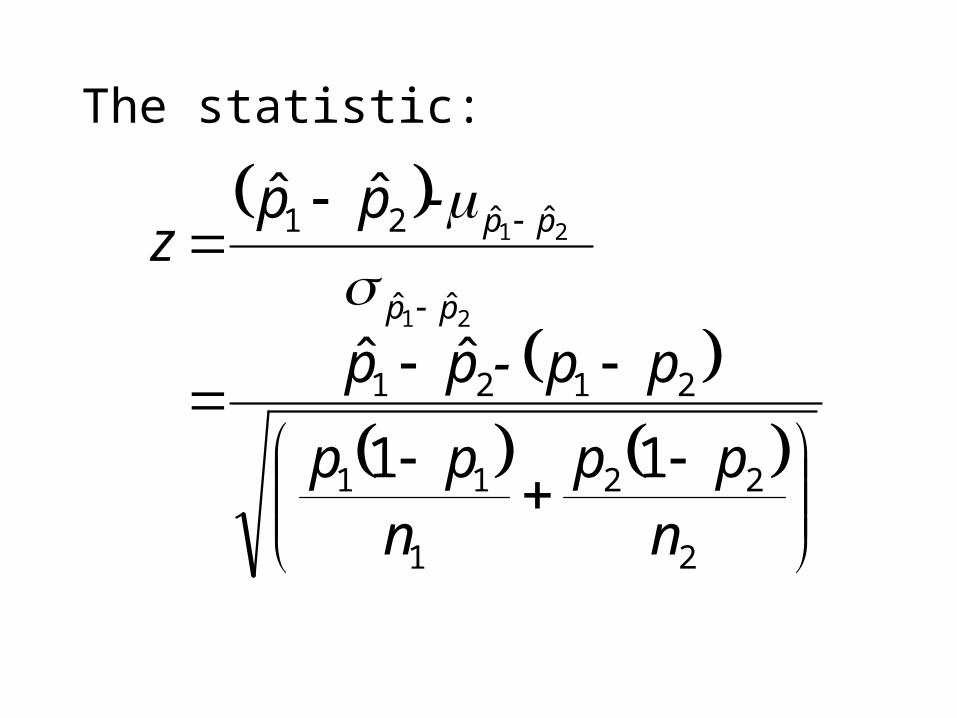
The statistic:

ˆˆ

21

21

ˆˆ

ˆˆ21

pp

pp-ppz

11

ˆˆ

2

22

1

11

2121

npp

npp

pp-pp

If : 210 ppH

say and 0 2121 ppppp then

is true

Hence

111

ˆˆ

ˆˆ

21

21

ˆˆ

21

21

nnpp

ppppz

pp

11ˆ1ˆ

ˆˆ

21

21

nnpp

pp

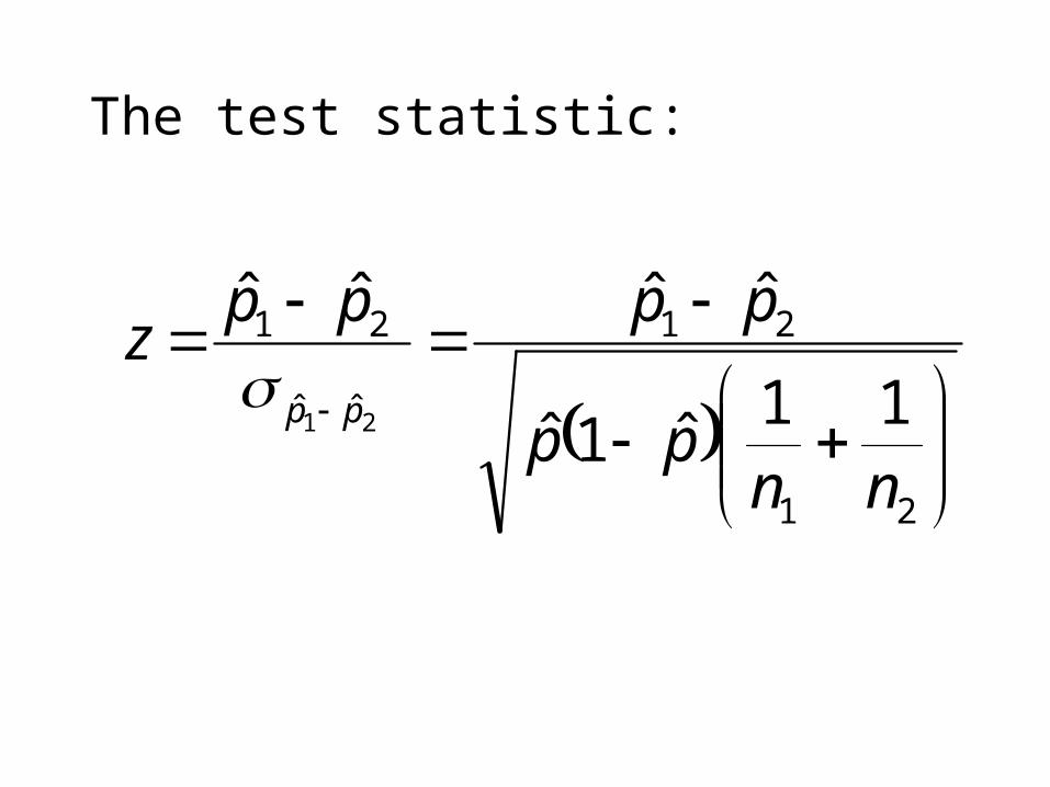
The test statistic:

11ˆ1ˆ

ˆˆ

ˆˆ

21

21

ˆˆ

21

21

nnpp

ppppz

pp

Where: A sample of n1 is selected from population 1 resulting in x1 successes

A sample of n2 is selected from population 2 resulting in x2 successes

2

22

1

11

ˆ and

ˆ

n

xp

n

xp

21

21 ˆ

nn

xxp

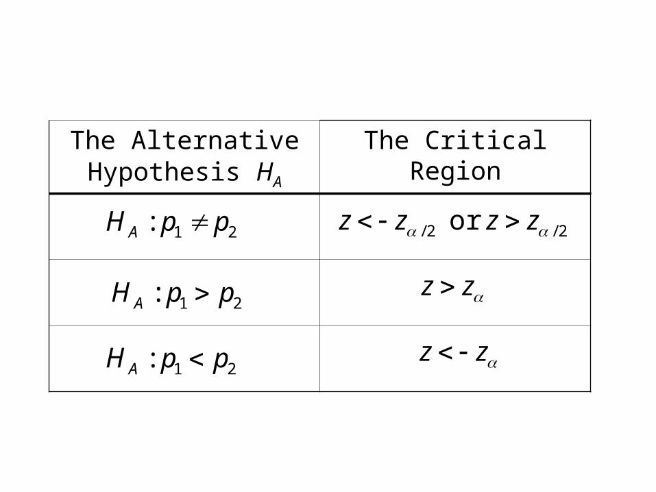
The Alternative Hypothesis HA

The Critical Region

21: ppH A

21: ppH A

21: ppH A

2/2/ or zzzz

zz

zz

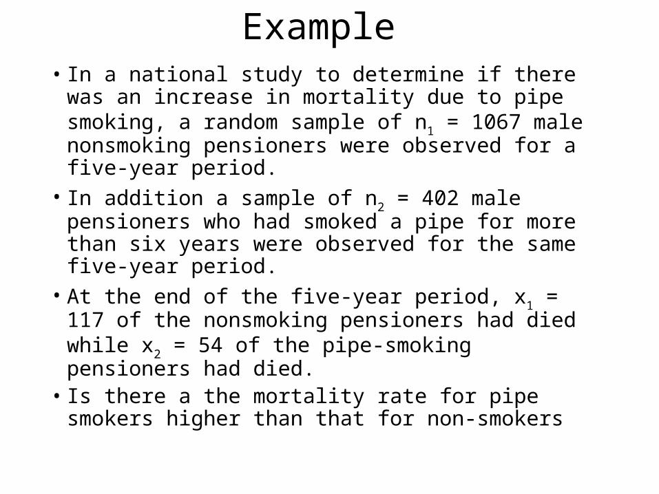
Example• In a national study to determine if there was an

increase in mortality due to pipe smoking, a random sample of n1 = 1067 male nonsmoking pensioners were observed for a five-year period.

• In addition a sample of n2 = 402 male pensioners who had smoked a pipe for more than six years were observed for the same five-year period.

• At the end of the five-year period, x1 = 117 of the nonsmoking pensioners had died while x2 = 54 of the pipe-smoking pensioners had died.

• Is there a the mortality rate for pipe smokers higher than that for non-smokers

We want to test:

21210 : vs: ppHppH A

The test statistic:

11ˆ1ˆ

ˆˆ

ˆˆ

21

21

ˆˆ

21

21

nnpp

ppppz

pp

Note:

1097.01067

117

ˆ

1

11

n

xp

1343.0402

54 ˆ

2

22

n

xp

4021067

54117 ˆ

21

21

nn

xxp

1164.01469

171

The test statistic:

11ˆ1ˆ

ˆˆ

21

21

nnpp

ppz

4021

10671

1164.011164.0

1343.1097.0

315.1

We reject H0 if:

645.1 05.0 zzz

Not true hence we accept H0.

Conclusion: There is not a significant ( = 0.05) increase in the mortality rate due to pipe-smoking

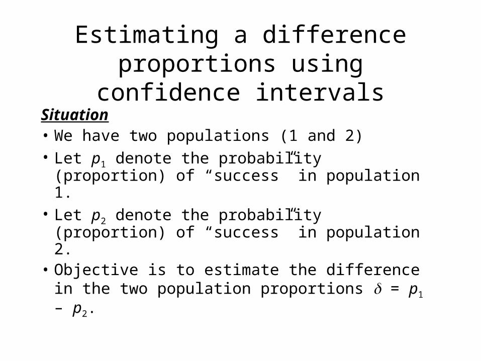
Estimating a difference proportions using confidence intervals

Situation• We have two populations (1 and 2)• Let p1 denote the probability (proportion) of

“success” in population 1.• Let p2 denote the probability (proportion) of

“success” in population 2.• Objective is to estimate the difference in the

two population proportions = p1 – p2.

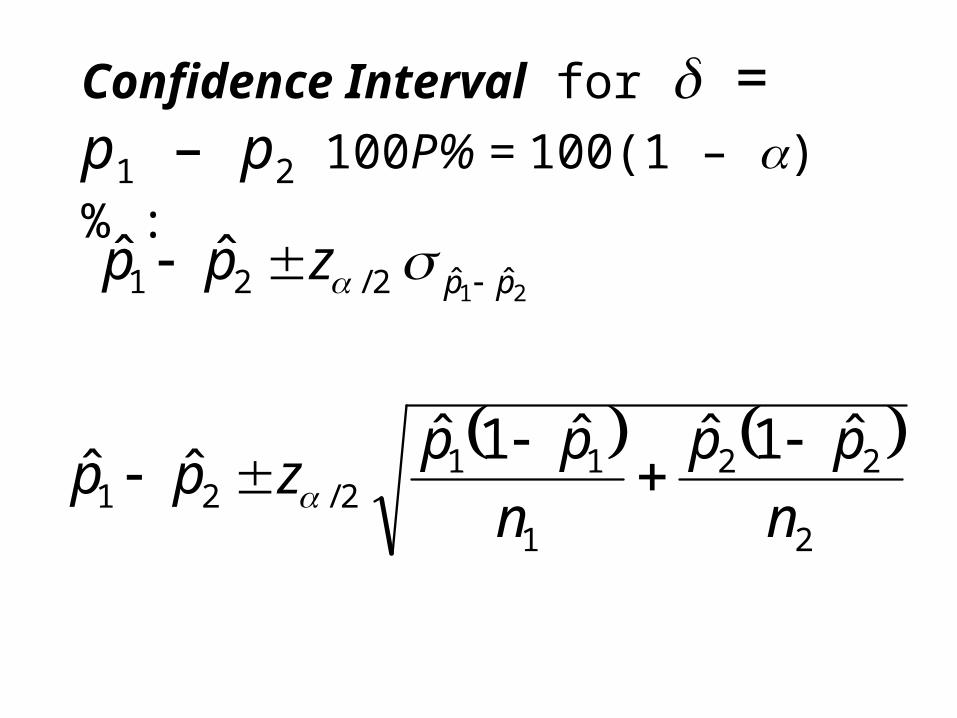
Confidence Interval for = p1 – p2

100P% = 100(1 – ) % :

ˆˆ21 ˆˆ2/21 ppzpp

2

22

1

112/21

ˆ1ˆˆ1ˆ ˆˆ

n

pp

n

ppzpp

Example• Estimating the increase in the mortality rate

for pipe smokers higher over that for non-smokers = p2 – p1

2

22

1

112/12

ˆ1ˆˆ1ˆ ˆˆ

n

pp

n

ppzpp

402

1343.011343.0

1067

1097.011097.0 960.11097.01343.0

0382.00247.0

0629.0 to0136.0%29.6 to%36.1