the measurement of tax elasticity in india · on net income and profits), (3) import tax (...
TRANSCRIPT

Munich Personal RePEc Archive
The Measurement of Tax Elasticity in
India: A Time Series Approach
Acharya, Hem
Faculty of Management Studies, University of Delhi
January 2011
Online at https://mpra.ub.uni-muenchen.de/47090/
MPRA Paper No. 47090, posted 20 May 2013 21:14 UTC

The Measurement of Tax Elasticity in India:
A Time Series Approach
"It was only for the good of his subjects that he collected taxes from them, just as the Sun draws
moisture from the Earth to give it back a thousand fold" –
--Kalidas in Raghuvansh eulogizing KING DALIP.
Hem Acharya
Faculty of Management Studies, University of Delhi
Abstract
Revenue generation is an important goal of tax reform. The built-in responsiveness of
revenues to changes in income, tax elasticity, provides very critical information for tax policy
formulation. This paper utilises a time series approach to empirically estimate tax elasticities
for India for the period 1991-2010. Tax elasticities are computed for income, turnover, excise,
import and total taxes for the post-reform period. The elasticity coefficients reveal a low
responsiveness of taxes to income growth and the value being less than unity in most of the
cases.

1. Introduction
It is essential to estimate built-in tax elasticity or tax elasticity which measures percentage
increase in tax revenue due to the changes in the base caused by a one percent rise in GDP.
However, estimation suffers from a specification bias due to the lack of an observable
quantitative variable capable of reflecting all changes in an individual (or overall) tax system in
public finance.
As the primary purpose of tax policy adjustment in developing countries is to increase the
revenue, the study of tax elasticity and various parameters affecting tax collection becomes
important. An elastic tax system is desirable especially to developing countries. It is also
important for revenue forecasting purposes, for analyzing the automatic stabilizing property of
tax system and examining the progressivity of tax system.
Tax elasticity is defined as
TE = %∆Revenue ÷ %∆Base. ------------------------------- (1)
Revenue is calculated as it would have been if there were no changes in the tax laws, including
the tax rates or bases. Thus the tax elasticity is a hypothetical construct. It tries to reconstruct
what would have happened if there had been no changes in the tax rules - i.e. what tax revenue
would have been if last year’s laws continued to apply this year. The increases are measured in
real terms i.e., after adjusting for inflation for an unbiased analysis and result.
There are varieties of taxes, such as import tax, export tax, excise tax, sales/value
added/turnover tax, and corporate income tax and so on; throughout this study, the term
"individual tax” will be used to refer to each of these taxes. Each tax has its own tax system--a
set of laws and regulations governing the process of estimation, assessment and collection of its
corresponding tax revenue--which will be called the "individual tax system". The term
"discretionary tax measures (DTMs)" will be used to describe changes in these systems which
include changes in statutory tax rates, tax bases, tax allowances and credits, and of tax
administrative efficiency.
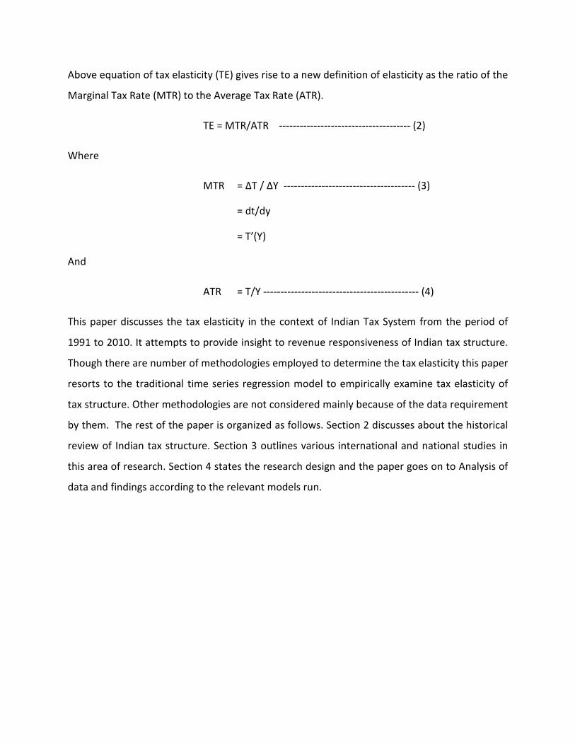
Above equation of tax elasticity (TE) gives rise to a new definition of elasticity as the ratio of the
Marginal Tax Rate (MTR) to the Average Tax Rate (ATR).
TE = MTR/ATR -------------------------------------- (2)
Where
MTR = ∆T / ∆Y -------------------------------------- (3)
= dt/dy
= T’(Y)
And
ATR = T/Y --------------------------------------------- (4)
This paper discusses the tax elasticity in the context of Indian Tax System from the period of
1991 to 2010. It attempts to provide insight to revenue responsiveness of Indian tax structure.
Though there are number of methodologies employed to determine the tax elasticity this paper
resorts to the traditional time series regression model to empirically examine tax elasticity of
tax structure. Other methodologies are not considered mainly because of the data requirement
by them. The rest of the paper is organized as follows. Section 2 discusses about the historical
review of Indian tax structure. Section 3 outlines various international and national studies in
this area of research. Section 4 states the research design and the paper goes on to Analysis of
data and findings according to the relevant models run.

2. Historical Background
There are two types of taxes viz., 1) Direct taxes ( eg. Income tax, Wealth tax ) and 2) Indirect
taxes ( eg. Custom duty, Excise duty etc.). Direct taxes are the taxes which are not shifted i.e.,
the incidence of of which falls on persons who pay them to the Government. Similarly Indirect
taxes are the taxes in which the burden of paying Tax is shifted through a change in price.
Direct taxes come under progressive taxation. It creates better civic consciousness. It also
serves the purpose of transference of income from rich to poor.
Indirect taxes are difficult to evade. It is generally included in the price. Indirect taxes on drinks,
narcotics and tobacco serve a social purpose by discouraging their consumption.
Indian tax system is characterized by : a) High dependence on indirect taxes b) low average
effective tax rates and tax productivity c) High marginal effective tax rates and large tax-
induced Distortions on investment and financing decisions.
Income tax in India was introduced in 1860 , discontinued in 1873 and reintroduced in 1886.
More than 130 countries worldwide have introduced VAT, India being one of the last few to
introduce it. VAT was introduced in 1999 and was implemented in April,2005 in some states.
Tax revenues form about 20% of the total national income of India (2005-2006). Amongst the
third world countries India is one of the high taxes countries.
Among the working 40% working population only 2.5% are liable to pay income tax in India. So
we can say that Indian tax structure relies on a very narrow population base. Agricultural
income is wholly exempt from the income tax despite the fact that a new class of rich farmers
have emerged in country who can easily pay taxes. Service sector which accounts for more than
50% of GDP contributes just 7.8% towards tax revenue and 0.8% towards GDP. The cost of
collection of tax has increased from Rs. 543 crores in 1990-91 to more than Rs. 3663 crores in
2006-2007
3. Literature Review
a. International Context
While researching about tax elasticity in his paper “An Econometric Method for Estimating the
Tax Elasticity and the Impact on Revenues of Discretionary Tax Measures” , Jaber Ehdaie
classifies all the individual taxes to major five categories (1) corporate income tax, (2) other
direct taxes (individual income tax, social security, payroll tax, tax on property and other taxes
on net income and profits), (3) import tax ( tariff/customs duties and other charges), (4) tax on
exports, and (5) tax on domestic consumption (general sales, turnover or value added taxes,
selective excises on goods and services, taxes on use of goods or property and permission to
perform activities, stamp tax and other domestic indirect taxes).
There is not a single economic channel through which changes in the individual tax systems
affect individual tax bases. Because of this this paper uses private consumption, imports,
exports, value added in non-agriculture sector and GDP respectively as proxy variables for
potential tax bases of domestic consumption tax, import tax, export tax, corporate income tax
and other direct taxes.
The major part of this analysis lies in demonstrating that the elasticity of reported income is not
a primitive parameter and it identifies strength of its dependence on a particular administrative
instrument of the tax base. It turns out that the elasticity of taxable income varies
systematically with the tax base and that this effect is quantitatively important. (Wojciech
Kopczuk 2003)
Wojciech Kopczuk (2003) argues that there are two major aspects of the tax system that are
responsible for determining the broadness of the tax base. First, deductions and adjustments
explicitly exclude parts of income from taxation. As they vary, the tax base of the taxpayer
varies. Second, tax bases of itemizers and non-itemizers are different. Importantly, the effects
of such changes vary also cross-sectionally. Changes in the standard deduction affect the
itemization status (and therefore the tax base) only of those individuals whose gain from
itemization are small enough. The elimination of charitable deduction for non-itemizers affects

the tax base of people making charitable contributions but not of the others. Changes in the
medical deduction affect the tax base of itemizers who have high enough medical expenses.
These effects can interact suggesting that the tax base effects are not simple functions of
income (and, therefore, aiding in the identification of the effect).
The elasticity of income determines only the cost of taxation, while any complete analysis of
policy requires understanding benefits as well. There may be trade-offs involved in the choice
of tax base to the extent that deductions from the tax base are socially beneficial on, for
example, redistributive grounds. Also, a broader tax base may feature different administrative
costs (Yitzhaki, 1979; Wilson, 1989).
The inverse relationship between tax rates and revenue is mentioned by Adam Smith in The
Wealth of Nations (1776) –
High taxes, sometimes by diminishing the consumption of the taxed
commodities, and sometimes by encouraging smuggling, frequently afford a smaller
revenue to government than what might be drawn from more moderate taxes. (Book V,
Chapter II)
After the introduction of the Laffer curve in 1974, the quality of debate deteriorates
significantly. Jude Wanniski (1978) chronicles every fiscal catastrophe from the fall of the
Roman Empire to the Great Depression and attributes each of them to some tax hike occurring
within a few years in either direction. At various points in his analysis Wanniski suggests (a) that
the mere existence of a prohibitive range implies taxes should be reduced, (b) that the peak of
the curve is at a 25 percent tax rate, and (c) that the peak of the curve "is the point at which the
electorate desires to be taxed".-' The welfare maximizing government would operate
somewhere on the normal range with the size of its budget determined by standard cost—
benefit analysis.
For the opposition, Kiefer (1978) asserts that there is no tax rate for the overall economy which
can be measured on the horizontal axis, and that "the Laffer Curve represents a gross
simplification of a major portion of macro-economics into a single curved line." These
arguments are not compelling, either, in view of the large number of economic models which
oversimplify in order to comprehend and convey economic phenomena. Kiefer also begrudges
the supply-side concentration, reminding us that income and substitution effects tend to be
offsetting. "By concentrating primarily on incentive and supply-side effects, the Laffer Curve
largely ignores the actual mechanism by which fiscal policy exerts its biggest and most
immediate impact - demand side effects." One gets the feeling that these antagonists are
talking past
Tax Stability: The revenue from different taxes varies from year to year. Taxes whose revenue
is relatively stable, or whose revenue is negatively correlated with the revenue from other
taxes, are likely to be particularly helpful in giving stability to the overall stream of revenue.
Revenue stability is desirable, at least from the government’s perspective, in that it makes it
easier to put together plausible spending and borrowing plans for the year ahead. A simple
measure of the stability of tax revenue is the coefficient of variation (CV), which is defined as
the standard deviation of tax revenue (as a fraction of GDP usually) divided by its mean; i.e.
Coefficient of Variation = Standard Deviation ÷ Mean.
b. National Context
In estimating the built-in elasticity of a tax either the time series data on tax revenues need to
be adjusted to eliminate the effects of discretionary tax measures, or a suitable estimation
methodology has to be adopted. The most appropriate method would clearly depend upon the
availability, nature and reliability of information on tax revenues, discretionary changes in the
tax structure and tax bases. Over the years, at least four approaches have been used :
(1) Proportional adjustment;
(2) Constant rate structure;
(3) Divisia index; and
(4) Econometric methods.
In the Indian case, estimates of tax yields arising out of discretionary changes in tax
rates and coverages are routinely available in the budget documents. Therefore, the
application of the proportional adjustment method is perfectly feasible for estimating tax
elasticities in India. There have been several such attempts, but the weight of general opinion
is that these estimates are not particularly accurate, primarily because of the questionable
reliability of the budget estimates of the effects of the discretionary changes. This judgment is
based primarily on comparisons between the predicted and the actual tax collections for in-
sample forecasts. (Pronab Sen)
The result of this dissatisfaction with the methodology has been that the use of
elasticity estimates in forecasting tax collections has all but ceased in India, and recourse is
increasingly being taken to the use of buoyancy estimates for most analytical purposes. Pronab
Sen argues that this is unfortunate, since the use of buoyancies in making forecasts or
projections implicitly assumes that there is a well-defined trend in the discretionary changes
that have been made in the past, and that this trend will continue in the future as well.

4. Research and Design:
Objectives:
To determine Tax Elasticity for India from period 1990-91 to 2009-2010
Variable Selection:
For the purpose the variables used for the study purpose are:
LTDT: Natural Log Total Direct Tax
LTIDT: Natural Log Total Indirect Tax
LGT: Natural Log Gross Tax
LGDPF: Natural Log GDP at current prices factor cost
LGDPM: Natural Log GDP at current prices market price
The data pertaining to Direct, Indirect and Gross tax is only taken as there is no discretionary
tax changes data available for the various constituents of the Indirect tax such as Customs,
Excise and Service tax for India. This has put limitation of a more meaningful study.
The tax revenue and corresponding tax base will be taken as shown below:
Tax Revenue Proxy Base
Direct Tax GDP current at factor cost
Indirect Tax GDP current at factor cost
Gross Tax GDP current at market price
Sample Selection:
The data pertaining to taxes and the GDP has been taken from the RBI database:
http://dbie.rbi.org.in/InfoViewApp/listing/main.do?appKind=InfoView&service=%2FInfoViewAp
p%2Fcommon%2FappService.do
The data pertaining to the discretionary changes in tax and the resultant revenue loss/gain has
been taken from the Budget speeches from 1991-92 to 2009-2010:

http://indiabudget.nic.in/
Time Period:
The time period selected for the study is between1991-92 and 2009-2010. The reason for the
same is that there has been structural break in 1990-91 in Indian scenario due to various LPG
policies adopted by India and opening up of its economy. From the tax base perspective there
has been phenomenon changes starting this period and thus only this part is relevant for the
study. Using data prior to 1990-91 with later data will result in spurious results and thus
incorrect model.
5. Methodology:
We will first convert our tax revenue series to the adjusted form, adjusting for the discretionary
changes in the tax over the years. Our base year will be 1991-92 and thereon we will adjust our
tax revenue as shown below:
Where,
AT n-1 = the Adjusted Tax
T n-1=actual Tax revenue
D n = Revenue effect of discretionary changes
For the reference year we will have:
Now the time series based regression model will be used to perform the study. Tax buoyancies
have been calculated to measure the effect of the discretionary changes in the various taxes.
The estimation of the tax elasticity will be done through the regression analysis based on the
partitioning approach where the tax elasticity will be divided into tax to base and base to
income elasticity. The equations can be represented as shown below:
Tax to Base:

Where:
T = Adjusted Tax revenue
X = Tax Base
Base to Income Elasticity:
Where:
B = Tax Base
Y = GDP at current market price
Now the coefficients calculated in above regression equations (b and c) can be used to give an
overall estimate of the elasticity by using equation:
Overall elasticity = b*c
Limitations:
1) The data is for overall categories of direct tax and indirect tax only and should have been for
the subgroups for better matching with the tax bases. At present it has lead to the
generalization and thus the results will be very general in nature.
2) The data pertaining to 1991 and hence forth has been taken and so the number of
observations are very less but the more data collection is restricted by the availability of
coherent data in Indian perspective.
6. Analysis and Findings:
Stationarity Test: Using ADF Method
H0: The variable has a unit root

Variable ADF(c,t,p) t-Statistics Prob.
LTDT ADF(0,0,0) 7.871282 1.0000
LTIDT ADF(0,0,0) 4.296678 0.9999
LGT ADF(0,0,0) 6.584881 1.0000
LGDPF ADF(0,0,0) 2.530098 0.9947
LGDPM ADF(0,0,0) 2.324860 0.9922
ΔLTDT ADF(1,0,0) -3.783960 0.0123*
ΔLTIDT ADF(1,0,0) -1.681008 0.0869**
ΔLGT ADF(1,0,0) -2.947668 0.0606**
ΔLGDPF ADF(1,0,0) -2.809527 0.0790**
ΔLGDPM ADF(1,0,0) -2.797117 0.0795**
*Significant at 5% level
**Significant at 10% level
All series found to be stationery at first level of difference only.
Structural Break Tests:
We need not perform the Perron structural breakpoint test due to various reasons:
1) From the visual inspection the various taxes doesn’t show any significant deviation
2) It is well known that the major structural break happens in 1990-91 for India and our
data is after this time period only
3) The data set is too small to have any meaningful analysis of the structural break as
significant observations are required prior as well as after the break pint for the analysis
Tax to Base Elasticity:
Direct Tax:
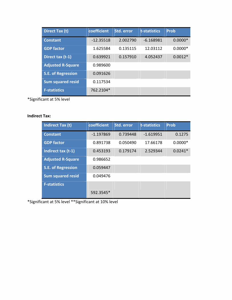
Direct Tax (t) coefficient Std. error t-statistics Prob
Constant -12.35518 2.002790 -6.168981 0.0000*
GDP factor 1.625584 0.135115 12.03112 0.0000*
Direct tax (t-1) 0.639921 0.157910 4.052437 0.0012*
Adjusted R-Square 0.989600
S.E. of Regression 0.091626
Sum squared resid 0.117534
F-statistics 762.2104*
*Significant at 5% level
Indirect Tax:
Indirect Tax (t) coefficient Std. error t-statistics Prob
Constant -1.197869 0.739448 -1.619951 0.1275
GDP factor 0.891738 0.050490 17.66178 0.0000*
Indirect tax (t-1) 0.453193 0.179174 2.529344 0.0241*
Adjusted R-Square 0.986652
S.E. of Regression 0.059447
Sum squared resid 0.049476
F-statistics
592.3545*
*Significant at 5% level **Significant at 10% level

Gross Tax:
Gross Tax (t) Coefficient Std. error t-statistics Prob
Constant -5.355947 1.267525 -4.225516 0.0007*
GDP market 1.203048 0.084496 14.23786 0.0000*
Gross tax (t-1) 0.639060 0.132908 4.808301 0.0002*
Adjusted R-Square 0.991898
S.E. of Regression 0.063000
Sum squared resid 0.059535
F-statistics
1041.608*
*Significant at 5% level **Significant at 10% level
Base to Income elasticity:
Now in order to estimate base to income elasticity, we have a problem of existence of
simultaneity bias in the equations. The GDP at factor cost and GDP at market price were all
thought to be endogenous and so a 2-Stage Least square (2SLS) approach has to be adopted.
Now for LGDPF we have:
LGDPF = α + β LGDPM + €
But the LGDPM constitutes an endogenous variable in all the base to income and so need to be
purged of the constituting stochastic content in the first stage of the 2SLS procedure.
FIRST STAGE:
LGDPMt = α + β LGDPMt-1 + γ LG + €
Where:
LGDPMt : Log GDP at market price
LGDPMt-1 : Delayed Log GDP at market price

LG: Log of Government spending
Here Government spending (LG) and lagged value of LGDPM are two exogenous variables that
have been used to estimate the fitted values in the first stage of the 2SLS. Now we will proceed
to second stage where we will be using the fitted value (Y) in the equations to find the base to
elasticity.
SECOND STAGE:
LGDPFt = α + β Yt + €
Where:
LGDPFt : Log GDP at factor cost
Yt : Fitted value of Log GDP at market price
The results are as shown below:
Dependent Variable: GDP_FACTOR
Method: Two-Stage Least Squares
Date: 12/11/10 Time: 12:58
Sample (adjusted): 1993 2009
Included observations: 17 after adjustments
Instrument specification: C GDP_MARKET GOVT_SPENDING
GDP_MARKET(-1)
Variable Coefficie
nt
Std. Error t-Statistic Prob.
C -
0.16878
0.030211 -
5.586858
0.0001

4
GDP_MARKET 1.00559
0
0.002076 484.2787 0.0000
R-squared 0.99993
6
Mean dependent
var
14.45042
Adjusted R-
squared
0.99993
2
S.D. dependent var 0.591270
S.E. of regression 0.00488
4
Sum squared resid 0.000358
F-statistic 234525.
8
Durbin-Watson stat 1.492414
Prob(F-statistic) 0.00000
0
Second-Stage SSR 0.000358
J-statistic 5.99299
3
Instrument rank 4
Prob(J-statistic) 0.04996
2
Dependent Variable: GDP_MARKET
Method: Two-Stage Least Squares
Date: 12/11/10 Time: 13:03
Sample (adjusted): 1993 2009
Included observations: 17 after adjustments
Instrument specification: C GDP_MARKET GOVT_SPENDING
GDP_MARKET(-1)
Variable Coefficie
nt
Std. Error t-Statistic Prob.

C -2.39E-
12
6.19E-13 -
3.864063
0.0015
GDP_MARKET 1.00000
0
4.26E-14 2.35E+13 0.0000
R-squared 1.00000
0
Mean dependent
var
14.53794
Adjusted R-
squared
1.00000
0
S.D. dependent var 0.587965
S.E. of regression 1.00E-13 Sum squared resid 1.50E-25
F-statistic 5.52E+2
6
Durbin-Watson stat 0.045565
Prob(F-statistic) 0.00000
0
Second-Stage SSR 1.36E-12
J-statistic 0.00012
0
Instrument rank 4
Prob(J-statistic) 0.99994
0
Hence the elasticity can be summarized as below:
Tax Elasticity
Tax Coefficient SE
Direct Tax 1.625584 0.135115
Indirect Tax 0.891738 0.050490
Gross Tax 1.203048 0.084496
Tax Buoyancy
Tax Coefficient SE

Direct Tax 1.005590 0.002076
Indirect Tax 1.005590 0.002076
Gross Tax 1.000000 4.26E-14
Overall elasticity
Tax Elasticity
Direct Tax 1.634671
Indirect Tax 0.896722
Gross Tax 1.203048
As can be seen from the results:
Tax Elasticity of Direct tax is high at 1.62 compared to other taxes and thus showing that
changes in taxes has been higher than the changes in tax base and thus showing that more and
more people from the tax base are paying more taxes. This is a healthy sign and can lead to
lowering of effective tax rate with time. This can also be result of increasing effective tax rate
for individuals and the corporate and thus showing the increasing tax burden. In former case
the trend is favorable and in the later it is not. For indirect tax the elasticity is less than 1 and
thus the chnge in tax revenue collection is not keeping up with the changes in the tax base. This
shows that government has been lenient or conservative with the tax collection in indirect tax
area. For overall gross tax collection the elasticity is again high at 1.2 and shows that govt has
been able to get more tax revenue collection with relatively less changing tax base. It might be
advantageous in short term in terms of revenues but in long run it can burden tax payers
leading to more and more black money and non-disclosures.
In terms of tax buoyancy, both direct tax and indirect tax shows nearly 1 as elasticity as
expected. There is no deviation from the expected results.
The overall elasticity remains same as tax elasticity as there is not much different from 1 for tax
buoyancy.
7. Summary and Recommendations:
The overall outlook looks good for India as the elasticity calculated are high and more than 1
and thus shows that the tax revenue collections responds better to the changes in tax base and
income. The collection always is more than change in the tax base and so either through higher
effective tax rates or better compliance, the tax collections exceeds changes in the tax base.

APPENDIX
Data available:
Years Total
Direct
Tax
Servic
e Tax
Excise
Tax
Custom
s
Indirect
tax
Gross
Tax
GDP at
factor
cost
currect
prices
Private
consum
ption at
market
price
Private
Consumpt
ion
Governme
nt
Consumpt
ion
Imports of
goods and
service
GDP at
current
market
price
1991-92 15207 NA 28110 22257 52059 67266 594168 451815 435723 74814 47850.8 654729
1992-93 18132 NA 30831 23776 56434 74566 681517 506915 490823 84720 63374.5 752591
1993-94 20298 NA 31697 22193 55392 75690 792150 581447 562932 98279 73101.0 865805
1994-95 26966 407
37347 26789 65328 92294 925239 669124 651951 109346 89970.7 1015764
1995-96 33563 862
40187 35757 77661 111224 1083289 769542 751734 129572 122678.1 1191813
1996-97 38891 1059
45008 42851 89871 128762 1260710 905672 886559 146933 138919.7 1378617
1997-98 48260 1586 47962 40193 90960 139220 1401934 981262 965339 173780 154176.3 1527158
1998-99 46600 1957 53246 48668 97197 143797 1616082 1130216 1121595 215232 178331.9 1751199
1999-2000 57959 2128 61902 48420 113794 171753 1786526 1257541 1253643 252744 215236.5 1952036
2000-01 68305 2613 68526 47542 120298 188603 1925017 1345583 1339274 265088 230872.8 2102314
2001-02 69198 3302 72555 40268 117862 187060 2097726 1470302 1467195 281786 245199.7 2278952
2002-03 83088 4122 82310 44852 133178 216266 2261415 1552618 1551365 290978 297205.9 2454561
2003-04 105089 7891 90774 48629 149259 254348 2538170 1703546 1699486 310297 359107.7 2754620
2004-05 132771 14200 99125 57611 172187 304958 2877701 1848110 1840406 338052 501064.5 3149407
2005-06 165216 23055 111226 65067 199433 364649 3282385 2064296 2055387 375562 660408.9 3586743
2006-07 230181 37597 117612 86327 241331 471512 3779384 2319826 2307822 421546 840506.3 4129173
2007-08 312213 51301 123425 104119 279134 591347 4320892 2605859 2596084 479099 1012311.7 4723400
2008-09 333818 60941 109343 99850 269680 603498 4933183 NA 2913386 616447 1374435.6 5321753
2009-10 379559 58484 104659 84244 247357 626916 NA NA NA NA
1356468.7 5856569
Years Changes
in Direct
Tax
Changes
Service
Tax
Changes
Excise
Tax
Changes
Customs
Tax
Changes in
Indirect
Tax
Changes
in Gross
Tax
Adjusted
Direct Tax
Adjusted
Indirect Tax
Adjusted
Gross Tax
1991-92 2136 NA 1440 -744 696 3528 15916 52250 68513
1992-93 795 NA 2210 -2023 187 1169 17844 51161 64211
1993-94 -300 NA -2249 -3273 -5522 -11344 18580 53574 70347
1994-95 -2430 NA 106 -2282 -2176 -6782 26277 64122 89286
1995-96 -900 NA -311 -1179 -1490 -3880 34323 79208 115163
1996-97 912 NA 760 950 1710 4332 41198 87554 126649
1997-98 2651 NA 0 -2625 -2625 -2599 47342 99199 155773
1998-99 -950 220 5009 3304 8533 16116 49012 102742 151657
1999-2000 3100 NA NA NA 6234 9334 62988 115509 180104
2000-01 5080 NA 3252 -1428 1824 8728 63623 122867 188227
2001-02 -5500 NA 4677 -2128 2549 -402 74745 121890 200981
2002-03 6000 NA 6700 -2200 4500 15000 80848 136183 216553

2003-04 -2955 NA NA NA 3294 339 106638 149259 256000
2004-05 2000 NA NA NA 0 2000 137685 172187 309994
2005-06 6000 NA NA NA 0 6000 168109 201100 369325
2006-07 4000 NA NA NA 2000 6000 232414 241331 473940
2007-08 3000 NA NA NA 0 3000 312213 273205 585640
2008-09 0 NA NA NA -5900 -5900 333818 271878 605429
2009-10 0 NA NA NA 2000 2000 379559 247357 626916
Stationarity Tests Results:
Null Hypothesis: DIRECT_TAX has a unit root
Exogenous: None
Lag Length: 0 (Automatic - based on SIC, maxlag=0)
t-Statistic Prob.*
Augmented Dickey-Fuller test statistic 7.871282 1.0000
Test critical values: 1% level -2.699769
5% level -1.961409
10% level -1.606610
*MacKinnon (1996) one-sided p-values.
Warning: Probabilities and critical values calculated for 20 observations
and may not be accurate for a sample size of 18
Augmented Dickey-Fuller Test Equation
Dependent Variable: D(DIRECT_TAX)
Method: Least Squares
Date: 12/10/10 Time: 23:28
Sample (adjusted): 1993 2010
Included observations: 18 after adjustments
Variable Coefficient Std. Error t-Statistic Prob.
DIRECT_TAX(-1) 0.016037 0.002037 7.871282 0.0000
R-squared -0.006753 Mean dependent var 0.178736
Adjusted R-squared -0.006753 S.D. dependent var 0.095927
S.E. of regression 0.096251 Akaike info criterion -1.789766
Sum squared resid 0.157492 Schwarz criterion -1.740301
Log likelihood 17.10790 Hannan-Quinn criter. -1.782946
Durbin-Watson stat 1.975558
Null Hypothesis: D(DIRECT_TAX) has a unit root
Exogenous: Constant
Lag Length: 0 (Automatic - based on SIC, maxlag=0)
t-Statistic Prob.*
Augmented Dickey-Fuller test statistic -3.783960 0.0123

Test critical values: 1% level -3.886751
5% level -3.052169
10% level -2.666593
*MacKinnon (1996) one-sided p-values.
Warning: Probabilities and critical values calculated for 20 observations
and may not be accurate for a sample size of 17
Augmented Dickey-Fuller Test Equation
Dependent Variable: D(DIRECT_TAX,2)
Method: Least Squares
Date: 12/10/10 Time: 23:30
Sample (adjusted): 1994 2010
Included observations: 17 after adjustments
Variable Coefficient Std. Error t-Statistic Prob.
D(DIRECT_TAX(-1)) -0.985366 0.260406 -3.783960 0.0018
C 0.176243 0.053404 3.300172 0.0049
R-squared 0.488375 Mean dependent var -0.002795
Adjusted R-squared 0.454267 S.D. dependent var 0.138221
S.E. of regression 0.102109 Akaike info criterion -1.615419
Sum squared resid 0.156394 Schwarz criterion -1.517394
Log likelihood 15.73106 Hannan-Quinn criter. -1.605675
F-statistic 14.31835 Durbin-Watson stat 1.956256
Prob(F-statistic) 0.001801
Null Hypothesis: INDIRECT_TAX has a unit root
Exogenous: None
Lag Length: 0 (Automatic - based on SIC, maxlag=0)
t-Statistic Prob.*
Augmented Dickey-Fuller test statistic 4.296678 0.9999
Test critical values: 1% level -2.699769
5% level -1.961409
10% level -1.606610
*MacKinnon (1996) one-sided p-values.
Warning: Probabilities and critical values calculated for 20 observations
and may not be accurate for a sample size of 18
Augmented Dickey-Fuller Test Equation
Dependent Variable: D(INDIRECT_TAX)
Method: Least Squares
Date: 12/10/10 Time: 23:33
Sample (adjusted): 1993 2010
Included observations: 18 after adjustments
Variable Coefficient Std. Error t-Statistic Prob.
INDIRECT_TAX(-1) 0.007351 0.001711 4.296678 0.0005
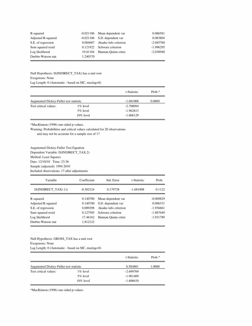
R-squared -0.021186 Mean dependent var 0.086581
Adjusted R-squared -0.021186 S.D. dependent var 0.083804
S.E. of regression 0.084687 Akaike info criterion -2.045760
Sum squared resid 0.121922 Schwarz criterion -1.996295
Log likelihood 19.41184 Hannan-Quinn criter. -2.038940
Durbin-Watson stat 1.240370
Null Hypothesis: D(INDIRECT_TAX) has a unit root
Exogenous: None
Lag Length: 0 (Automatic - based on SIC, maxlag=0)
t-Statistic Prob.*
Augmented Dickey-Fuller test statistic -1.681008 0.0869
Test critical values: 1% level -2.708094
5% level -1.962813
10% level -1.606129
*MacKinnon (1996) one-sided p-values.
Warning: Probabilities and critical values calculated for 20 observations
and may not be accurate for a sample size of 17
Augmented Dickey-Fuller Test Equation
Dependent Variable: D(INDIRECT_TAX,2)
Method: Least Squares
Date: 12/10/10 Time: 23:36
Sample (adjusted): 1994 2010
Included observations: 17 after adjustments
Variable Coefficient Std. Error t-Statistic Prob.
D(INDIRECT_TAX(-1)) -0.302124 0.179728 -1.681008 0.1122
R-squared 0.140700 Mean dependent var -0.009829
Adjusted R-squared 0.140700 S.D. dependent var 0.096331
S.E. of regression 0.089298 Akaike info criterion -1.936661
Sum squared resid 0.127585 Schwarz criterion -1.887649
Log likelihood 17.46162 Hannan-Quinn criter. -1.931789
Durbin-Watson stat 1.812122
Null Hypothesis: GROSS_TAX has a unit root
Exogenous: None
Lag Length: 0 (Automatic - based on SIC, maxlag=0)
t-Statistic Prob.*
Augmented Dickey-Fuller test statistic 6.584881 1.0000
Test critical values: 1% level -2.699769
5% level -1.961409
10% level -1.606610
*MacKinnon (1996) one-sided p-values.
Warning: Probabilities and critical values calculated for 20 observations
and may not be accurate for a sample size of 18
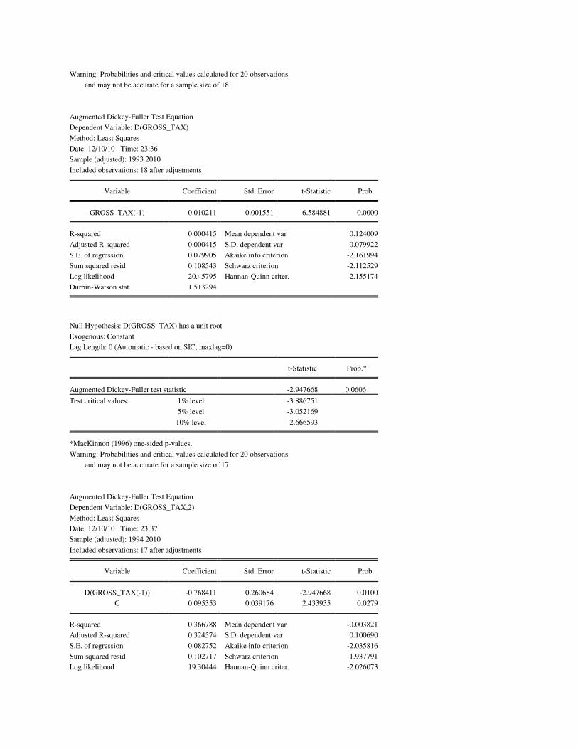
Augmented Dickey-Fuller Test Equation
Dependent Variable: D(GROSS_TAX)
Method: Least Squares
Date: 12/10/10 Time: 23:36
Sample (adjusted): 1993 2010
Included observations: 18 after adjustments
Variable Coefficient Std. Error t-Statistic Prob.
GROSS_TAX(-1) 0.010211 0.001551 6.584881 0.0000
R-squared 0.000415 Mean dependent var 0.124009
Adjusted R-squared 0.000415 S.D. dependent var 0.079922
S.E. of regression 0.079905 Akaike info criterion -2.161994
Sum squared resid 0.108543 Schwarz criterion -2.112529
Log likelihood 20.45795 Hannan-Quinn criter. -2.155174
Durbin-Watson stat 1.513294
Null Hypothesis: D(GROSS_TAX) has a unit root
Exogenous: Constant
Lag Length: 0 (Automatic - based on SIC, maxlag=0)
t-Statistic Prob.*
Augmented Dickey-Fuller test statistic -2.947668 0.0606
Test critical values: 1% level -3.886751
5% level -3.052169
10% level -2.666593
*MacKinnon (1996) one-sided p-values.
Warning: Probabilities and critical values calculated for 20 observations
and may not be accurate for a sample size of 17
Augmented Dickey-Fuller Test Equation
Dependent Variable: D(GROSS_TAX,2)
Method: Least Squares
Date: 12/10/10 Time: 23:37
Sample (adjusted): 1994 2010
Included observations: 17 after adjustments
Variable Coefficient Std. Error t-Statistic Prob.
D(GROSS_TAX(-1)) -0.768411 0.260684 -2.947668 0.0100
C 0.095353 0.039176 2.433935 0.0279
R-squared 0.366788 Mean dependent var -0.003821
Adjusted R-squared 0.324574 S.D. dependent var 0.100690
S.E. of regression 0.082752 Akaike info criterion -2.035816
Sum squared resid 0.102717 Schwarz criterion -1.937791
Log likelihood 19.30444 Hannan-Quinn criter. -2.026073

F-statistic 8.688748 Durbin-Watson stat 1.748350
Prob(F-statistic) 0.009981
Null Hypothesis: GDP_FACTOR has a unit root
Exogenous: None
Lag Length: 1 (Automatic - based on SIC, maxlag=1)
t-Statistic Prob.*
Augmented Dickey-Fuller test statistic 2.530098 0.9947
Test critical values: 1% level -2.717511
5% level -1.964418
10% level -1.605603
*MacKinnon (1996) one-sided p-values.
Warning: Probabilities and critical values calculated for 20 observations
and may not be accurate for a sample size of 16
Augmented Dickey-Fuller Test Equation
Dependent Variable: D(GDP_FACTOR)
Method: Least Squares
Date: 12/11/10 Time: 00:02
Sample (adjusted): 1994 2009
Included observations: 16 after adjustments
Variable Coefficient Std. Error t-Statistic Prob.
GDP_FACTOR(-1) 0.003548 0.001402 2.530098 0.0240
D(GDP_FACTOR(-1)) 0.567181 0.152700 3.714351 0.0023
R-squared 0.432668 Mean dependent var 0.123714
Adjusted R-squared 0.392145 S.D. dependent var 0.027873
S.E. of regression 0.021731 Akaike info criterion -4.703680
Sum squared resid 0.006611 Schwarz criterion -4.607107
Log likelihood 39.62944 Hannan-Quinn criter. -4.698735
Durbin-Watson stat 2.147327
Null Hypothesis: D(GDP_FACTOR) has a unit root
Exogenous: Constant
Lag Length: 0 (Automatic - based on SIC, maxlag=1)
t-Statistic Prob.*
Augmented Dickey-Fuller test statistic -2.809527 0.0790
Test critical values: 1% level -3.920350
5% level -3.065585
10% level -2.673459
*MacKinnon (1996) one-sided p-values.
Warning: Probabilities and critical values calculated for 20 observations
and may not be accurate for a sample size of 16

Augmented Dickey-Fuller Test Equation
Dependent Variable: D(GDP_FACTOR,2)
Method: Least Squares
Date: 12/11/10 Time: 00:03
Sample (adjusted): 1994 2009
Included observations: 16 after adjustments
Variable Coefficient Std. Error t-Statistic Prob.
D(GDP_FACTOR(-1)) -0.462975 0.164788 -2.809527 0.0139
C 0.054938 0.021794 2.520842 0.0245
R-squared 0.360539 Mean dependent var -0.004354
Adjusted R-squared 0.314863 S.D. dependent var 0.026284
S.E. of regression 0.021756 Akaike info criterion -4.701386
Sum squared resid 0.006627 Schwarz criterion -4.604812
Log likelihood 39.61109 Hannan-Quinn criter. -4.696441
F-statistic 7.893444 Durbin-Watson stat 2.063007
Prob(F-statistic) 0.013917
Null Hypothesis: GDP_MARKET has a unit root
Exogenous: None
Lag Length: 1 (Automatic - based on SIC, maxlag=1)
t-Statistic Prob.*
Augmented Dickey-Fuller test statistic 2.324860 0.9922
Test critical values: 1% level -2.708094
5% level -1.962813
10% level -1.606129
*MacKinnon (1996) one-sided p-values.
Warning: Probabilities and critical values calculated for 20 observations
and may not be accurate for a sample size of 17
Augmented Dickey-Fuller Test Equation
Dependent Variable: D(GDP_MARKET)
Method: Least Squares
Date: 12/11/10 Time: 00:06
Sample (adjusted): 1994 2010
Included observations: 17 after adjustments
Variable Coefficient Std. Error t-Statistic Prob.
GDP_MARKET(-1) 0.003384 0.001456 2.324860 0.0345
D(GDP_MARKET(-1)) 0.562801 0.162024 3.473566 0.0034
R-squared 0.360723 Mean dependent var 0.120694
Adjusted R-squared 0.318105 S.D. dependent var 0.027654
S.E. of regression 0.022836 Akaike info criterion -4.610812
Sum squared resid 0.007822 Schwarz criterion -4.512787
Log likelihood 41.19190 Hannan-Quinn criter. -4.601068
Durbin-Watson stat 1.813243

Null Hypothesis: D(GDP_MARKET) has a unit root
Exogenous: Constant
Lag Length: 0 (Automatic - based on SIC, maxlag=1)
t-Statistic Prob.*
Augmented Dickey-Fuller test statistic -2.797117 0.0795
Test critical values: 1% level -3.886751
5% level -3.052169
10% level -2.666593
*MacKinnon (1996) one-sided p-values.
Warning: Probabilities and critical values calculated for 20 observations
and may not be accurate for a sample size of 17
Augmented Dickey-Fuller Test Equation
Dependent Variable: D(GDP_MARKET,2)
Method: Least Squares
Date: 12/11/10 Time: 00:06
Sample (adjusted): 1994 2010
Included observations: 17 after adjustments
Variable Coefficient Std. Error t-Statistic Prob.
D(GDP_MARKET(-1)) -0.481019 0.171970 -2.797117 0.0135
C 0.054895 0.022477 2.442246 0.0275
R-squared 0.342793 Mean dependent var -0.006091
Adjusted R-squared 0.298979 S.D. dependent var 0.026908
S.E. of regression 0.022529 Akaike info criterion -4.637867
Sum squared resid 0.007614 Schwarz criterion -4.539842
Log likelihood 41.42187 Hannan-Quinn criter. -4.628123
F-statistic 7.823866 Durbin-Watson stat 1.767187
Prob(F-statistic) 0.013538
Regression results:
Dependent Variable: DIRECT_TAX
Method: Least Squares
Date: 12/11/10 Time: 02:38
Sample (adjusted): 1993 2009
Included observations: 17 after adjustments
Convergence achieved after 6 iterations
Variable Coefficient Std. Error t-Statistic Prob.
C -12.35518 2.002790 -6.168981 0.0000
GDP_FACTOR 1.625584 0.135115 12.03112 0.0000
AR(1) 0.639921 0.157910 4.052437 0.0012
R-squared 0.990900 Mean dependent var 11.18303
Adjusted R-squared 0.989600 S.D. dependent var 0.898453
S.E. of regression 0.091626 Akaike info criterion -1.783423

Sum squared resid 0.117534 Schwarz criterion -1.636385
Log likelihood 18.15909 Hannan-Quinn criter. -1.768807
F-statistic 762.2104 Durbin-Watson stat 2.283138
Prob(F-statistic) 0.000000
Inverted AR Roots .64
Dependent Variable: INDIRECT_TAX
Method: Least Squares
Date: 12/11/10 Time: 12:13
Sample (adjusted): 1993 2009
Included observations: 17 after adjustments
Convergence achieved after 6 iterations
Variable Coefficient Std. Error t-Statistic Prob.
C -1.197869 0.739448 -1.619951 0.1275
GDP_FACTOR 0.891738 0.050490 17.66178 0.0000
AR(1) 0.453193 0.179174 2.529344 0.0241
R-squared 0.988321 Mean dependent var 11.70277
Adjusted R-squared 0.986652 S.D. dependent var 0.514553
S.E. of regression 0.059447 Akaike info criterion -2.648664
Sum squared resid 0.049476 Schwarz criterion -2.501626
Log likelihood 25.51364 Hannan-Quinn criter. -2.634048
F-statistic 592.3545 Durbin-Watson stat 1.807187
Prob(F-statistic) 0.000000
Inverted AR Roots .45
Dependent Variable: GROSS_TAX
Method: Least Squares
Date: 12/11/10 Time: 02:53
Sample (adjusted): 1993 2010
Included observations: 18 after adjustments
Convergence achieved after 6 iterations
Variable Coefficient Std. Error t-Statistic Prob.
C -5.355947 1.267525 -4.225516 0.0007
GDP_MARKET 1.203048 0.084496 14.23786 0.0000
AR(1) 0.639060 0.132908 4.808301 0.0002
R-squared 0.992851 Mean dependent var 12.25057
Adjusted R-squared 0.991898 S.D. dependent var 0.699908
S.E. of regression 0.063000 Akaike info criterion -2.540353
Sum squared resid 0.059535 Schwarz criterion -2.391958
Log likelihood 25.86318 Hannan-Quinn criter. -2.519892
F-statistic 1041.608 Durbin-Watson stat 1.763938
Prob(F-statistic) 0.000000
Inverted AR Roots .64


References:
1. Don Fullerton, ON THE POSSIBILITY ON AN INVERSE RELATIONSHIP BETWEEN TAX RATES
AND GOVERNMENT REVENUES (Apr 1980) NBER Working Paper No. 467
2. Jaber Ehdaie, An Econometric Method for Estimating the Tax Elasticity and the Impact
on Revenues of Discretionary Tax Measures (Applied to Malawi and Mauritius) ( Feb
1990, World Bank )
3. John Creedy & Norman Gemmell ,
The Elasticity of Taxable Income and the Tax Revenue Elasticity ( Oct 2010),
Research Paper Number 1110
4. Jonathan Haughton, ESTIMATING TAX BUOYANCY, ELASTICITY AND STABILITY (Apr 1998)
5. Pronab Sen, A NOTE ON ESTIMATING TAX ELASTICITIES , Planning Commission India.
6. Rajaraman, Indira, Goyal, Rajan and Khundrakpam, Jeevan Kumar, Tax Buoyancy
Estimates for Indian States (October 2005). Available at SSRN:
http://ssrn.com/abstract=826345
7. Wojciech Kopczuk, TAX BASES, TAX RATES AND THE ELASTICITY OF REPORTED INCOME (
Oct 2003 )Working Paper 10044 http://www.nber.org/papers/w10044
8. http://www.icai.org/resource_file/16791tsibf.pdf (Accessed on 10 Dec 2010 )
9. http://dbie.rbi.org.in/InfoViewApp/listing/main.do?appKind=InfoView&service=%2FInf
oViewApp%2Fcommon%2FappService.do
10. http://indiabudget.nic.in/