The Low Beta Model

Successful Portfolios LLC

October 2013

Brad Norbom, CFA

Portfolio Manager

Successful Portfolios LLC

Brad@successsfulportfolios.com

1

Introduction

Higher risk stocks have a greater expected return than lower risk stocks if investors

rationally demand a proportional return for risk. Put another way, the risky long shot should pay

off more than the safer favorite. However, there is evidence that behavioral biases lead many

investors to over-weight risky stocks and under-weight safer stocks. We present evidence that a

portfolio of low risk stocks may generate higher returns than a portfolio of higher risk stocks.

Quantifying a Stock’s Risk with Beta

One can think of a stock generally having two types of risks, unsystematic risk and

systematic risk. Unsystematic risk is company specific. For example, company specific risk

might be financial statement fraud or a company’s products falling out of favor. This

unsystematic risk can be reduced through diversification. Systematic risk, or market risk,

describes the market’s influence on a particular stock. A bear market tends to drag stocks down

and vice versa for a bull market.

A stock’s beta (β) is a measure of its sensitivity to the returns on the overall stock market.

It is a measure of systematic risk that cannot be avoided by diversification.1 An asset with a beta

of .5, on average, would have half the magnitude of price fluctuations compared to the stock

market. A beta greater than 1 means the asset is riskier than the stock market.

The Low Volatility Anomaly

Andrea Frazzini and Lasse Pedersen (2011), in their research paper “Betting against

Beta,” conclude that it does not pay to take risks associated high beta stocks. Their findings are

at odds with the principle that investors, overall, demand proportionately high returns for holding

a portfolio of high risks stocks. Frazzini and Pedersen contend that because many investment

managers have investment policies that prohibit leverage, they attempt to boost their returns by

overweighting riskier assets. Because investors bid up the prices of riskier stocks, the expected

returns from them are too low. Academics refer to this as “Low Volatility Anomaly”.

1 Please see the Glossary for a complete description of Beta and other terms that we bounce around in our paper.

2

Our Testing Confirms the Low Beta Anomaly

Frazzini and Pedersen constructed 10 portfolios comprised of U.S. Equities sorted by

their betas. Portfolio 1, the Betting against Beta (BAB) portfolio, consisted of equal weights of

10% of stocks that had the lowest historical beta, the bottom decile. Portfolio 10, the Betting on

Beta (BOB) portfolio held the top decile beta stocks in equal weights. In an 86-year investment

simulation with monthly rebalancing to equal weights, the BAB portfolio scored higher risk

adjusted returns.

Using the Portfolio 123 back tester, we replicated the Frazzini and Pedersen’s findings.

Portfolios of lower beta stocks outperformed portfolios of higher beta stocks. We tested 12

years’ of data (February 1, 2001 through September 26, 2013) on S&P 500 Index constituent

stocks.2 We chose the S&P 500 because the index is widely followed and the stocks within the

index are highly liquid. Portfolio123 utilizes a point-in-time database for the S&P 500. Point-

in-time means the database has the historically correct index constituents for any point in time.

First, we created two portfolios: a Betting against Beta (BAB) Portfolio of the 50 lowest

beta stocks and a Betting on Beta (BOB) Portfolio of the 50 highest beta stocks. The portfolios

were rebalanced every 28 days. We included .2% for slippage and commissions on each trade.

In Figure 1 and Table 1, we see that the BAB Portfolio of low beta stocks outperformed

the S&P 500 ETF (SPY), which in turn outperformed the BOB Portfolio of high beta stocks.

Figure 1 – Back-test Total Returns: 02/01/2001 - 09/26/2013

2 While Portfolio 123 has security data going back as far as 1999, we felt that the large number of N/A’s returned

prior to February 2001 in our Analyst Surprise and Analyst Next Fiscal Year Estimate nodes was too great to

accurately simulate the model’s performance.

-100%

-50%

0%

50%

100%

150%

200%

250%

2001 2002 2003 2004 2005 2006 2007 2008 2009 2010 2011 2012 2013

BAB

BOB

SP 500 ETF

3

We also ran the same test excluding stocks in the S&P 500 Utilities Sector (BAB ex-

Utilities) shown in Figure 2 and Table 1. We expected that by throwing out utility stocks, our

hypothetical return would diminish.

Figure 2 – Back-test Total Returns: 02/01/2001 - 09/26/2013

Table 1 – Back-test Risk & Return Measures: 02/01/2001 - 09/26/2013

Annualized

Return

Max

Drawdown

Sharpe

Ratio

Sortino

Ratio

Standard

Deviation R

2 Beta Alpha

BAB Portfolio 8.77% -37.79% .30 .38 16.84% .65 .54 4.93%

BAB ex-Util. 9.97% -36.16% .37 .49 16.65% .69 .55 6.08%

BOB Portfolio -3.19% -86.71% -.13 -.17 54.91% .72 1.85 -6.46%

S&P 500 ETF 3.61% -55.19% -.01 -.01 25.16% - - -

To our surprise, the BAB ex-Utilities Portfolio outperformed. There are a couple of

implications. First, we gained confidence in the robustness of the BAB model because we

removed a potential hindsight bias. We knew that the utility sector had outperformed the broader

market over the 12-year test period. Second, a common criticism to the BAB model is that it is

industry dependent, “going long stodgy (but perhaps ultimately profitable) industries and by an

assumption that the returns are driven by value effects (Asness, Frazzini, & Pedersen, 2013).”

We wondered what would happen if we removed utilities and staples, the sectors

containing the stodgiest and most value tilted industries, from our universe. See Table 2.

-100%

-50%

0%

50%

100%

150%

200%

250%

2001 2002 2003 2004 2005 2006 2007 2008 2009 2010 2011 2012 2013

BAB

BOB

SP 500 ETF

BAB ex Util

4

Table 2 – Back-test Risk & Return Measures: 02/01/2001 - 09/26/2013

Annualized

Return

Max

Drawdown

Sharpe

Ratio

Sortino

Ratio

Standard

Deviation R

2 Beta Alpha

BAB Portfolio 8.77% -37.79% .30 .38 16.84% .65 .54 4.93%

BAB ex-Util. 9.97% -36.16% .37 .49 16.65% .69 .55 6.08%

BAB ex-Util. &

ex-Staples

10.75% -44.50% .36 .46 19.67% .69 .65 6.85%

BOB Portfolio -3.19% -86.71% -.13 -.17 54.91% .72 1.85 -6.46%

S&P 500 ETF 3.61% -55.19% -.01 -.01 25.16% - - -

After eliminating two of the least volatile sectors in the S&P 500 universe, the BAB ex-

Utilities and Staples portfolio (BAB ex-Util. & ex-Staples, Table 2, above) consisted of the

lowest beta stocks of the most cyclical and growth tilted industries and still produced superior

absolute and risk adjusted returns compared to the S&P 500 ETF.

Might the Low Volatility Anomaly Persist in the Future?

From all the published research that we have read, the evidence of the Low Volatility

Anomaly’s historical existence is robust. The question of whether the anomaly will continue in

the future depends on the forces of arbitrage. That is to say, will enough participants bet against

beta in the future to arbitrage away the strategy’s excess returns? Baker, Bradley, and Wurgler

(2010) argue that the Low Volatility Anomaly will persist because of behavioral biases and

benchmarking.

Behavioral Biases

Human brains are hardwired with certain predispositions, or biases. On a grand scale,

investor behavioral biases push stock prices far above and below intrinsic values. Baker et al

credit Preference for Lotteries, Overconfidence, and Representativeness as the investor biases at

work in the Low Volatility Anomaly.

5

Table 3 - Examples of Behavioral Biases

Behavioral Bias Example

Preference for Lotteries Rationally, people should not play games with a negative expected return. I am going to

play the lottery anyway, because… you never know.

Overconfidence Investors and analysts tend to be overconfident in the precision of their forecasts. I am

90% confident that XYZ.Q will earn $9.314 per share next year.

Representativeness Believing a high beta stock is representative of a good investment. My brother-in-law’s

cousin bought a stock just like this one and he made a killing.

The Tourist and the Reluctant Shark

Behaviorally biased investment decisions initially generate excess returns for institutional

investment managers savvy enough to identify and exploit them. However, as more savvy

investors press their advantage, they devour excess returns to a point of non-existence. At least

that is how things should work. The Low Volatility Anomaly may be more persistent. This is

analogous to a shark unwilling to pick off the portly tourist bobbing just off the beach.

An institutional investment manager is most often evaluated by his or her Information

Ratio (IR), or the average excess returns to a benchmark divided by the standard deviation of

these excess returns (tracking error). By focusing on excess returns while minimalizing the

tracking error, i.e., keeping the portfolio’s beta close to 1, institutional investment managers are

disincentivized from overweighting low beta stocks (Baker et al, 2010). Furthermore, because of

leverage constraints, many institutional managers cannot lever up low beta portfolios to achieve

risk parity with their benchmark (Frazzini et al, 2011).

Exploiting the Low Volatility Anomaly: The Low Beta Model

We created the Low Beta (LB) Model to exploit the Low Volatility Anomaly. The LB

Model selects boring stocks. We purposely avoid stocks that exhibit lottery like return payoffs,

enthusiastic analyst profit projections, and the antithesis of what many investors think makes for

a good stock investment. In the LB Model simulation, presented later, we will see if our model

for selecting boring stocks has the potential for producing exciting returns.

6

How Boring Can We Get? - The LB Model Opportunity Set

The LB Model opportunity set includes approximately 250 stocks with betas less than the

median beta for the S&P 500. We calculate up to a 750-day daily return beta, with a minimum

of 500 days of data. Stocks with less than 500 days of return data are not eligible for the LB

Model portfolio.

“Yawn” - The LB Model’s 3-Factor Ranking System

The LB Model ranks the 250 or so stocks in its opportunity set based on a three equally

weighted factors. Subject to sector weight and data availability constraints, the LB Model starts

by purchasing the 30 highest ranked stocks. We detail these constraints further on. For the LB

Model’s first factor rank, and in the spirit of the BAB strategy, lower beta stocks receive a higher

rank score.

The second factor rank uses inputs related to analyst expectations. It has two equally

weighted nodes. The first node looks at the absolute percentage surprise from the stock’s

previous earnings announcement. Any earnings surprise, good or bad, counts against the stock’s

rank score. The second node looks at the next fiscal year analyst expectations. There must be

five or more analyst estimates available. Relatively large disagreement among analysts on a

company’s next fiscal year results reduces the stock’s ranking. We assume that large earnings

surprises and analyst disagreements are indicative of higher future betas.

For the third factor rank, the LB Model utilizes the 300-day and 150-day momentum

formula that we first developed in creating the Select Directional ETF Model (SDM). For more

information, download the SDM whitepaper and actual performance from our website,

www.successfulportfolios.com. Broadly stated, stocks demonstrating recent persistent relative

price strength receive a higher rank in the LB Model.

The LB Model Diversification Requirements and Trading Rules

To help neutralize the industry and value effects and not hold too high a concentration of

any one sector, we added sector-weighting constraints as the first buy rule (Table 4). The second

buy rule requires a stock to have at least 5 analyst estimates for the next fiscal year.

7

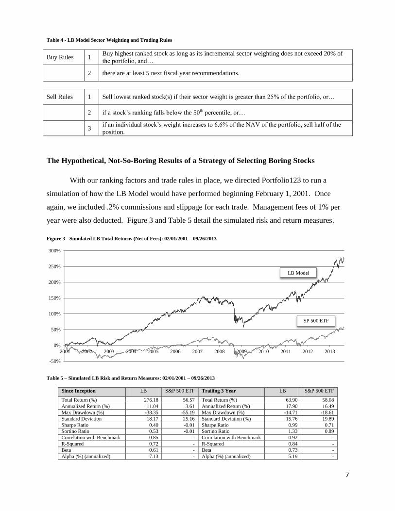
Table 4 - LB Model Sector Weighting and Trading Rules

Buy Rules 1 Buy highest ranked stock as long as its incremental sector weighting does not exceed 20% of

the portfolio, and…

2 there are at least 5 next fiscal year recommendations.

Sell Rules 1 Sell lowest ranked stock(s) if their sector weight is greater than 25% of the portfolio, or…

2 if a stock’s ranking falls below the 50th

percentile, or…

3 if an individual stock’s weight increases to 6.6% of the NAV of the portfolio, sell half of the

position.

The Hypothetical, Not-So-Boring Results of a Strategy of Selecting Boring Stocks

With our ranking factors and trade rules in place, we directed Portfolio123 to run a

simulation of how the LB Model would have performed beginning February 1, 2001. Once

again, we included .2% commissions and slippage for each trade. Management fees of 1% per

year were also deducted. Figure 3 and Table 5 detail the simulated risk and return measures.

Figure 3 - Simulated LB Total Returns (Net of Fees): 02/01/2001 – 09/26/2013

Table 5 – Simulated LB Risk and Return Measures: 02/01/2001 – 09/26/2013

Since Inception LB S&P 500 ETF Trailing 3 Year LB S&P 500 ETF

Total Return (%) 276.18 56.57 Total Return (%) 63.90 58.08

Annualized Return (%) 11.04 3.61 Annualized Return (%) 17.90 16.49

Max Drawdown (%) -38.35 -55.19 Max Drawdown (%) -14.71 -18.61

Standard Deviation 18.17 25.16 Standard Deviation (%) 15.76 19.89

Sharpe Ratio 0.40 -0.01 Sharpe Ratio 0.99 0.71

Sortino Ratio 0.53 -0.01 Sortino Ratio 1.33 0.89

Correlation with Benchmark 0.85 - Correlation with Benchmark 0.92 -

R-Squared 0.72 - R-Squared 0.84 -

Beta 0.61 - Beta 0.73 -

Alpha (%) (annualized) 7.13 - Alpha (%) (annualized) 5.19 -

-50%

0%

50%

100%

150%

200%

250%

300%

2001 2002 2003 2004 2005 2006 2007 2008 2009 2010 2011 2012 2013

LB Model

SP 500 ETF

8

The simulated LB Model returned a not-so-boring 276.2% vs. 56.5% on the S&P 500

ETF. The average holding period of a stock during the simulation was 511 days. That would

qualify for lower long-term capital gains tax rates. Annualized turnover was a reasonable and

tax-efficient 53.6%. Realized winning trades were 56.9% (128/225) of total trades. Overall

winning trades (including unrealized gains) were 60.4% (154/255). Remember that past or

simulated returns are not necessarily indicative of future results.

We ran regression analyses3 based on the Capital Asset Pricing Model (CAPM) and the

Fama-French Model (Appendix 1).4 The LB Model’s alpha (outperformance) was statistically

significant relative to returns on the CRSP NYSE/AMEX/NASDAQ Value-Weighted Market

Index with a P- value of .0019.

Running additional simulations for different market regimes provides an idea of how the

LB Model might perform in future bull and bear markets. In Table 6, we can see the LB Model

outperformed the S&P 500 ETF in absolute return and risk adjusted return in 3 out of 4 periods.5

Table 6 - Simulated LB Model Performance in Bear and Bull Markets

Bear Markets LB S&P 500 ETF LB S&P 500 ETF

Inception Date 02/01/2001 10/12/2007

End Date 10/04/2002 03/06/2009

Total Return (%) 8.33 -40.02 -40.55 -54.61

Annualized Return (%) 4.91 -26.37 -31.04 -43.14

Max Drawdown (%) -22.62 -39.99 -41.45 -54.31

Standard Deviation 18.38 28.91 32.35 46.16

Sharpe Ratio 0.0 -1.08 -1.07 -1.01

Sortino Ratio 0.0 -1.71 -1.51 -1.42

Correlation with Benchmark .62 - .94 -

R-Squared .39 - .88 -

Beta .40 - .66 -

Alpha (%) (annualized) 11.90 - -3.72 -

Bull Markets LB S&P 500 ETF LB S&P 500 ETF

Inception Date 10/04/2002 03/06/2009

End Date 10/12/2007 09/26/2013

Total Return (%) 112.39 111.45 123.82 172.00

Annualized Return (%) 16.18 16.08 19.33 24.55

Max Drawdown (%) -9.13 -14.18 -14.55 -18.61

Standard Deviation 13.34 16.38 15.96 22.25

Sharpe Ratio .88 .71 1.04 .98

Sortino Ratio 1.28 1.04 1.45 1.33

Correlation with Benchmark .81 - .90 -

R-Squared .65 - .80 -

Beta .66 - .64 -

Alpha (%) (annualized) 3.93 - 2.56 -

3 We thank Wesley Gray, PH.D. for the very informative Excel tutorial on calculating and analyzing Fama-French

Alpha found at http://turnkeyanalyst.com/2012/01/12/alphacalculation/. 4 Kenneth French provides a trove of highly useful return data at

http://mba.tuck.dartmouth.edu/pages/faculty/ken.french/index.html 5 We present a portion of the first bear market in our period simulation because of a lack of analyst projection and

surprises data prior to 02/2001. Nonetheless, the S&P 500 ETF still declined 40% during this abbreviated period.

9

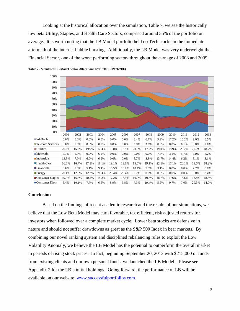
Looking at the historical allocation over the simulation, Table 7, we see the historically

low beta Utility, Staples, and Health Care Sectors, comprised around 55% of the portfolio on

average. It is worth noting that the LB Model portfolio held no Tech stocks in the immediate

aftermath of the internet bubble bursting. Additionally, the LB Model was very underweight the

Financial Sector, one of the worst performing sectors throughout the carnage of 2008 and 2009.

Table 7 - Simulated LB Model Sector Allocation: 02/01/2001 - 09/26/2013

Conclusion

Based on the findings of recent academic research and the results of our simulations, we

believe that the Low Beta Model may earn favorable, tax efficient, risk adjusted returns for

investors when followed over a complete market cycle. Lower beta stocks are defensive in

nature and should not suffer drawdowns as great as the S&P 500 Index in bear markets. By

combining our novel ranking system and disciplined rebalancing rules to exploit the Low

Volatility Anomaly, we believe the LB Model has the potential to outperform the overall market

in periods of rising stock prices. In fact, beginning September 20, 2013 with $215,000 of funds

from existing clients and our own personal funds, we launched the LB Model . Please see

Appendix 2 for the LB’s initial holdings. Going forward, the performance of LB will be

available on our website, www.successfulportfolios.com.

2001 2002 2003 2004 2005 2006 2007 2008 2009 2010 2011 2012 2013

InfoTech 0.0% 0.0% 0.0% 0.0% 0.0% 0.0% 3.4% 6.7% 9.9% 17.2% 16.2% 9.6% 8.5%

Telecom Services 0.0% 0.0% 0.0% 0.0% 0.0% 0.0% 5.9% 3.6% 0.0% 0.0% 6.1% 0.0% 7.6%

Utilities 20.0% 16.2% 19.9% 17.3% 15.0% 16.9% 20.3% 17.7% 19.0% 18.9% 20.2% 20.0% 18.7%

Materials 6.7% 9.9% 9.9% 6.2% 0.0% 0.0% 0.0% 0.0% 7.6% 3.1% 5.7% 6.0% 8.2%

Industrials 13.3% 7.9% 6.9% 6.2% 0.0% 0.0% 5.7% 8.8% 13.7% 14.4% 6.2% 3.1% 3.1%

Health Care 16.6% 16.7% 17.8% 18.1% 19.1% 19.1% 15.6% 19.1% 22.1% 17.1% 20.1% 19.6% 18.2%

Financials 0.0% 9.8% 5.1% 9.1% 16.5% 19.0% 18.1% 5.0% 3.1% 0.0% 0.0% 2.7% 0.0%

Energy 20.1% 12.5% 12.2% 21.3% 23.4% 20.4% 3.7% 0.0% 0.0% 0.0% 0.0% 0.0% 3.4%

Consumer Staples 19.9% 16.6% 20.5% 15.2% 17.2% 18.9% 19.9% 19.8% 18.7% 19.6% 18.6% 18.8% 18.5%

Consumer Discr 3.4% 10.1% 7.7% 6.6% 8.9% 5.8% 7.3% 19.4% 5.9% 9.7% 7.0% 20.3% 14.0%

0%

10%

20%

30%

40%

50%

60%

70%

80%

90%

100%

10

References

Asness, C., Frazzini, A., & Pedersen, L. (2013, May 10). Low-Risk Investing Without Industry Bets.

Retrieved from Social Science Research Network: http://ssrn.com/abstract=2259244

Baker, M., Bradley, B., & Wurgler, J. (2010, March). Benchmarks as Limits to Arbitrage: Understanding

the Low Volatility Anomaly. Retrieved from Social Science Research Network.

Frazzini, A., & Pedersen, L. (2011, October). Betting against Beta. Retrieved from Social Science

Research Network: http://papers.ssrn.com/sol3/papers.cfm?abstract_id=2049939

11

Appendix 1 CAPM and Fama-French Model Regressions

Capital Asset Pricing Model

Regression Statistics

Multiple R 0.85257704

R Square 0.726887609

Adjusted R Square 0.726801698

Standard Error 0.49710962

Observations 3181

ANOVA

df SS MS F Significance F

Regression 1 2090.839641 2090.839641 8460.896637 0

Residual 3179 785.5880415 0.247117975

Total 3180 2876.427682

Coefficients Standard Error t Stat P-value Lower 95% Upper 95% Lower 95.0% Upper 95.0%

Alpha 0.027314566 0.008814944 3.098666025 0.001960931 0.010031014 0.044598118 0.010031014 0.044598118

Mkt-RF 0.6170988 0.006708826 91.98313235 0 0.603944735 0.630252865 0.603944735 0.630252865

Fama French 3 Factor Model

Regression Statistics

Multiple R 0.854058637

R Square 0.729416155

Adjusted R Square 0.729160646

Standard Error 0.494958805

Observations 3181

ANOVA

df SS MS F Significance F

Regression 3 2098.11282 699.3709401 2854.759153 0

Residual 3177 778.3148622 0.244984218

Total 3180 2876.427682

Coefficients Standard Error t Stat P-value Lower 95% Upper 95% Lower 95.0% Upper 95.0%

Alpha 0.02729337 0.008784222 3.10709021 0.001906077 0.01007005 0.044516691 0.01007005 0.044516691

Beta w/ Mkt-RF 0.61536682 0.006810771 90.35200734 0 0.602012867 0.628720773 0.602012867 0.628720773

Beta w/ SMB -0.05630611 0.015393557 -3.65777105 0.000258547 -0.086488424 -0.02612379 -0.086488424 -0.026123791

Beta w/ HML 0.058026798 0.015177721 3.823156199 0.000134282 0.028267674 0.087785921 0.028267674 0.087785921

12

Appendix 2 –The LB Model Portfolio - Inception: 09/20/2013

Consumer

Discretionary

20%

Consumer Staples

20%

Energy

3%

Financials

7%

Health Care

20%

Industrials

14%

Utilities

13%

Information

Technology

3%

Ticker Name Stock Sector Industry Group

% Fwd Div

Yld Equity Style Box

TWC Time Warner Cable Inc Communication Services Communication Services 2.19 Large Growth

HAS Hasbro, Inc. Consumer Cyclical Travel & Leisure 3.2 Mid-Cap Value

NKE Nike, Inc. Class B Consumer Cyclical Manufacturing - Apparel & Furniture 1.11 Large Growth

ORLY O'Reilly Automotive Inc Consumer Cyclical Autos 0 Mid-Cap Growth

TJX TJX Companies Consumer Cyclical Retail - Apparel & Specialty 0.99 Large Growth

CAG ConAgra Foods, Inc. Consumer Defensive Consumer Packaged Goods 3.16 Mid-Cap Value

CL Colgate-Palmolive Company Consumer Defensive Consumer Packaged Goods 2.14 Large Growth

GIS General Mills, Inc. Consumer Defensive Consumer Packaged Goods 3.04 Large Core

HSY The Hershey Company Consumer Defensive Consumer Packaged Goods 2 Large Growth

KR Kroger Co Consumer Defensive Retail - Defensive 1.54 Large Core

MDLZ Mondelez International Inc Consumer Defensive Consumer Packaged Goods 1.69 Large Core

SE Spectra Energy Corp Energy Oil & Gas - Midstream 3.45 Large Value

AON Aon plc Financial Services Brokers & Exchanges 0.92 Large Growth

MMC Marsh & McLennan Companies, Inc. Financial Services Brokers & Exchanges 2.18 Large Growth

ABC AmerisourceBergen Corp Healthcare Medical Distribution 1.32 Mid-Cap Core

AMGN Amgen Inc Healthcare Biotechnology 1.63 Large Core

BMY Bristol-Myers Squibb Company Healthcare Drug Manufacturers 2.86 Large Core

GILD Gilead Sciences Inc Healthcare Biotechnology 0 Large Growth

JNJ Johnson & Johnson Healthcare Drug Manufacturers 2.87 Large Value

MDT Medtronic, Inc. Healthcare Medical Devices 1.94 Large Core

COL Rockwell Collins, Inc. Industrials Aerospace & Defense 1.67 Mid-Cap Value

LLL L-3 Communications Holdings Inc Industrials Aerospace & Defense 2.29 Mid-Cap Value

NLSN Nielsen Holdings NV Industrials Business Services 2.09 Mid-Cap Growth

WM Waste Management Inc Industrials Waste Management 3.37 Large Value

FIS Fidelity National Information Services, Inc. Technology Application Software 1.85 Mid-Cap Core

TRIP TripAdvisor Inc Technology Online Media 0 Mid-Cap Growth

AEP American Electric Power Co Inc Utilities Utilities - Regulated 4.3 Large Value

CMS CMS Energy Corp Utilities Utilities - Regulated 3.68 Mid-Cap Value

NI NiSource Inc Utilities Utilities - Regulated 3.11 Mid-Cap Value

XEL Xcel Energy Inc Utilities Utilities - Regulated 3.85 Mid-Cap Value

2.15

13

Portfolio 123’s Glossary

https://www.portfolio123.com/doc/doc_risk_glossary.jsp

Alpha vs. Benchmark Index

Alpha is another statistic in Modern Portfolio Theory (MPT) generated from a linear regression of the fund's returns

less the risk free rate against the market's returns less the risk free rate. It measures the difference between the fund's

actual returns and its expected performance given its level of risk (as measured by beta).

Alpha is frequently used to measure manager or strategy performance. A positive alpha figure indicates the fund has

performed better than its beta would predict. In contrast, a negative alpha indicates a fund has underperformed given

the expectations established by the fund's beta. Some investors see the alpha as a measurement of the value added or

subtracted by a fund's manager/strategy.

However, there are limitations to alpha statistic's ability to accurately depict a manager's added or subtracted value.

In some cases, a negative alpha can result from the expenses that are present in the fund figures but are not present

in the figures of the comparison index. Alpha is dependent on the accuracy of beta: If the investor accepts beta as a

conclusive definition of risk, a positive alpha would be a conclusive indicator of good fund performance. Of course,

the value of beta is dependent on another statistic, known as R-squared.

For Alpha, the calculation is listed below.

Alpha = (Fund Return - Treasury) - ((Beta x (Benchmark - Treasury))

Benchmark = Total Return of Benchmark Index

Treasury = Return on 13-week Treasury Bill

Annualized Benchmark Return

This is the annualized return on the benchmark index (e.g. Standard and Poor's 500).

Annualized Return

This is the annualized total return on an asset. A total return can be annualized in the expression:

Annual ret. = (Tot. Ret. + 1)^(365.25 ⁄ days) - 1

Annualized Turnover

The rate of trading activity in a fund's portfolio of investments, equal to the lesser of purchases or sales, for a year,

divided by average total assets.

Beta vs. Benchmark Index

Beta is another statistic in Modern Portfolio Theory (MPT) generated from a linear regression of the fund's returns

less the risk free rate against the market's returns less the risk free rate. It measures the fund's sensitivity to market

movements. For example, a fund that has a beta of 1.10 means that for every return in the S&P 500 (or the chosen

benchmark), the fund's returns, on average, will be 1.10 * the benchmark return. So if the S&P returns 10%, the fund

will return 11%. The reverse is true if the benchmark declines. If the benchmark returns -10%, the fund will return -

11%. Conversely, a beta of 0.85 indicates that the fund has performed 15% worse than the index in up markets and

15% better in down markets. Therefore, by definition, the beta of the benchmark is 1.

A low beta does not mean that the fund has a low level of volatility, though; rather, a low beta means only that the

fund's market-related risk is low. A specialty fund that invests primarily in gold, for example, will often have a low

beta (and a low R-squared), relative to the S&P 500 index, as its performance is tied more closely to the price of

gold and gold-mining stocks than to the overall stock market. Thus, though the specialty fund might fluctuate wildly

because of rapid changes in gold prices, its beta relative to the S&P may remain low.

14

Correlation

The correlation coefficient is a measure of the strength of the linear relationship between two random variables,

where the value 0 indicates independent variables, and 1 completely correlated variables. So, intuitively, this can be

used to determine how the returns on a fund and returns on a benchmark are correlated. By convention, correlation is

denoted by the greek letter ρ, and the coefficient used here is found by dividing the covariance of the two variables

by the product of their standard deviations.

Maximum Drawdown

Maximum Drawdown can be loosely defined as the largest drop from a peak to a bottom in a certain time period.

R-Squared vs. Benchmark Index

The R-Squared statistic is computationally the square of the correlation statistic (so, ρ2). Conceptually, it represents

the percentage of the fund's returns that are explained by the returns of the benchmark. An R-squared of 1 means

that the fund's returns are completely explained by the returns of the index. Conversely, a low R-squared indicates

that very few of the fund's returns are explained by the returns of benchmark index. For example, An R-Squared of

50% means that 50% of the fund's returns can be explained by the benchmark's returns. Therefore, R-squared can be

used to judge the significance of the fund's beta or alpha statistics. Generally, a higher R-squared will indicate a

more useful beta figure. If the R-squared is lower, then the beta is less relevant to the fund's performance.

Sharpe Ratio

The Sharpe ratio is a risk-adjusted measure developed by Nobel Laureate William Sharpe. It measures the return per

unit of risk. In other words, it measures how efficiently the fund is performing relative to its level of risk - the higher

the Sharpe ratio, the higher the return given its risk. The Sharpe Ratio is calculated as the ratio of return of the fund

above the risk-free return to annualized standard deviation. Risk-free return is the average monthly return of the 10Y

Note over the appropriate period.

Sharpe Ratio = ( Annualized Return - Risk Free Return ) ⁄ Annualized Std. Dev.

Sortino Ratio

This ratio is computationally very similar to the Sharpe Ratio, but divides from the excess return of the portfolio by

the standard deviation of the negative returns. The Sortino Ratio therefore uses downside standard deviation as the

proxy for risk for investors, instead of using standard deviation of all the fund's returns, as this number includes

upside standard deviation. This in effect removes the negative penalty that the Sharpe Ratio imposes on positive

returns.

To help you intuitively use this ratio, imagine a hypothetical portfolio, Portfolio A, which never experiences

negative returns. However, Portfolio A has incredible standard deviation in its positive returns: one day it returns

0.1% and another 1000%. The standard deviation of Portfolio A will therefore be very large. When measured by

Sharpe Ratio, Portfolio A will have a low ratio, because it is symmetric in its treatment of upside and downside

deviation. However, the Sortino Ratio of Portfolio A will be infinite! This is the case because there is zero standard

deviation in negative returns. The Sortino Ratio only considers downside standard deviation as important.

Similarly, imagine Portfolio B, where there are only negative returns. In this case, the Sharpe Ratio and the Sortino

Ratio will be exactly the same.

Therefore, the higher the Sortino Ratio, the better the risk adjusted (as measured by downside standard deviation)

returns are for your portfolio.

Standard Deviation (Volatility)

This statistical measurement of dispersion about an average depicts how widely a model or simulation returns are

varied over a certain period of time. When a fund has a high standard deviation, the predicted range of performance

is wide, implying greater volatility.

15

Investors can use the standard deviation of historical performance to try to predict the range of returns that are most

likely in the future. Since a model's returns are assumed to follow a normal distribution, then approximately 68% of

the time the returns will fall within one standard deviation of the mean, and 95% of the time within two standard

deviations. For example, for a fund with a mean annual return of 10% and a standard deviation of 2%, you would

expect the return to be between 8% and 12% about 68%of the time, and between 6% and 14% about 95% of the

time.

At Portfolio123, the standard deviation is computed using the three year trailing weekly returns, and since inception.

The results are then annualized.

Total Return

The total return on a fund is expressed as a percentage. That is, it is calculated as a simple return in the formula:

Tot. Ret. = ( Ending capital ⁄ Starting Capital ) - 1.

At Portfolio123, we calculate the total return on the fund since it's inception, and for the trailing day, week, four

weeks, thirteen weeks, twenty-six weeks, year and three years.

Year to Date

This is the total return on an asset since the beginning of the financial year.

Notes on Portfolio123's calculations

We only calculate risk statistics for portfolios and simulations with over 6 month's worth of data. On the "Risk" page

we display the Modern Portfolio Theory and Volatility measurements for that portfolio or simulation, for two time

periods:

1. from inception to end date

2. for a three year period beginning three years before the end date, given that the inception date for the fund

is more than three years before the end date.