the itk software guide book 2: design and functionality
TRANSCRIPT

The ITK Software Guide
Book 2: Design and Functionality
Fourth Edition
Updated for ITK version 4.9
Hans J. Johnson, Matthew M. McCormick, Luis Ibanez,
and the Insight Software Consortium
January 29, 2016
http://itk.org
Email: [email protected]


The purpose of computing is Insight, not numbers.
Richard Hamming


ABSTRACT
The Insight Toolkit (ITK) is an open-source software toolkit for performing registration and segmen-
tation. Segmentation is the process of identifying and classifying data found in a digitally sampled
representation. Typically the sampled representation is an image acquired from such medical instru-
mentation as CT or MRI scanners. Registration is the task of aligning or developing correspondences
between data. For example, in the medical environment, a CT scan may be aligned with a MRI scan
in order to combine the information contained in both.
ITK is a cross-platform software. It uses a build environment known as CMake to manage platform-
specific project generation and compilation process in a platform-independent way. ITK is imple-
mented in C++. ITK’s implementation style employs generic programming, which involves the
use of templates to generate, at compile-time, code that can be applied generically to any class or
data-type that supports the operations used by the template. The use of C++ templating means that
the code is highly efficient and many issues are discovered at compile-time, rather than at run-time
during program execution. It also means that many of ITK’s algorithms can be applied to arbitrary
spatial dimensions and pixel types.
An automated wrapping system integrated with ITK generates an interface between C++ and a high-
level programming language Python. This enables rapid prototyping and faster exploration of ideas
by shortening the edit-compile-execute cycle. In addition to automated wrapping, the SimpleITK
project provides a streamlined interface to ITK that is available for C++, Python, Java, CSharp, R,
Tcl and Ruby.
Developers from around the world can use, debug, maintain, and extend the software because ITK
is an open-source project. ITK uses a model of software development known as Extreme Program-
ming. Extreme Programming collapses the usual software development methodology into a simulta-
neous iterative process of design-implement-test-release. The key features of Extreme Programming
are communication and testing. Communication among the members of the ITK community is what
helps manage the rapid evolution of the software. Testing is what keeps the software stable. An
extensive testing process supported by the system known as CDash measures the quality of ITK
code on a daily basis. The ITK Testing Dashboard is updated continuously, reflecting the quality of

the code at any moment.
The most recent version of this document is available online at
http://itk.org/ItkSoftwareGuide.pdf. This book is a guide to developing software
with ITK; it is the second of two companion books. This book covers detailed design and
functionality for reading and writing images, filtering, registration, segmentation, and performing
statistical analysis. The first book covers building and installation, general architecture and design,
as well as the process of contributing in the ITK community.

CONTRIBUTORS
The Insight Toolkit (ITK) has been created by the efforts of many talented individuals and presti-
gious organizations. It is also due in great part to the vision of the program established by Dr. Terry
Yoo and Dr. Michael Ackerman at the National Library of Medicine.
This book lists a few of these contributors in the following paragraphs. Not all developers of ITK
are credited here, so please visit the Web pages at http://itk.org/ITK/project/parti.html for the names
of additional contributors, as well as checking the GIT source logs for code contributions.
The following is a brief description of the contributors to this software guide and their contributions.
Luis Ibanez is principal author of this text. He assisted in the design and layout of the text, im-
plemented the bulk of the LATEX and CMake build process, and was responsible for the bulk of the
content. He also developed most of the example code found in the Insight/Examples directory.
Will Schroeder helped design and establish the organization of this text and the Insight/Examples
directory. He is principal content editor, and has authored several chapters.
Lydia Ng authored the description for the registration framework and its components, the section
on the multiresolution framework, and the section on deformable registration methods. She also
edited the section on the resampling image filter and the sections on various level set segmentation
algorithms.
Joshua Cates authored the iterators chapter and the text and examples describing watershed seg-
mentation. He also co-authored the level-set segmentation material.
Jisung Kim authored the chapter on the statistics framework.
Julien Jomier contributed the chapter on spatial objects and examples on model-based registration
using spatial objects.
Karthik Krishnan reconfigured the process for automatically generating images from all the exam-
ples. Added a large number of new examples and updated the Filtering and Segmentation chapters

vi
for the second edition.
Stephen Aylward contributed material describing spatial objects and their application.
Tessa Sundaram contributed the section on deformable registration using the finite element method.
YinPeng Jin contributed the examples on hybrid segmentation methods.
Celina Imielinska authored the section describing the principles of hybrid segmentation methods.
Mark Foskey contributed the examples on the AutomaticTopologyMeshSource class.
Mathieu Malaterre contributed the entire section on the description and use of DICOM readers and
writers based on the GDCM library. He also contributed an example on the use of the VTKImageIO
class.
Gavin Baker contributed the section on how to write composite filters. Also known as minipipeline
filters.
Since the software guide is generated in part from the ITK source code itself, many ITK developers
have been involved in updating and extending the ITK documentation. These include David Doria,
Bradley Lowekamp, Mark Foskey, Gaetan Lehmann, Andreas Schuh, Tom Vercauteren, Cory
Quammen, Daniel Blezek, Paul Hughett, Matthew McCormick, Josh Cates, Arnaud Gelas,
Jim Miller, Brad King, Gabe Hart, Hans Johnson.
Hans Johnson, Kent Williams, Constantine Zakkaroff, Xiaoxiao Liu, Ali Ghayoor, and
Matthew McCormick updated the documentation for the initial ITK Version 4 release.
Luis Ibanez and Sebastien Barre designed the original Book 1 cover. Matthew McCormick and
Brad King updated the code to produce the Book 1 cover for ITK 4 and VTK 6. Xiaoxiao Liu, Bill
Lorensen, Luis Ibanez,and Matthew McCormick created the 3D printed anatomical objects that
were photographed by Sebastien Barre for the Book 2 cover. Steve Jordan designed the layout of
the covers.
Lisa Avila, Hans Johnson, Matthew McCormick, Sandy McKenzie, Christopher Mullins,
Katie Osterdahl, and Michka Popoff prepared the book for the 4.7 print release.

CONTENTS
1 Reading and Writing Images 1
1.1 Basic Example . . . . . . . . . . . . . . . . . . . . . . . . . . . . . . . . . . . . . . . . . . 1
1.2 Pluggable Factories . . . . . . . . . . . . . . . . . . . . . . . . . . . . . . . . . . . . . . . . 5
1.3 Using ImageIO Classes Explicitly . . . . . . . . . . . . . . . . . . . . . . . . . . . . . . . . 5
1.4 Reading and Writing RGB Images . . . . . . . . . . . . . . . . . . . . . . . . . . . . . . . . 7
1.5 Reading, Casting and Writing Images . . . . . . . . . . . . . . . . . . . . . . . . . . . . . . 8
1.6 Extracting Regions . . . . . . . . . . . . . . . . . . . . . . . . . . . . . . . . . . . . . . . . 10
1.7 Extracting Slices . . . . . . . . . . . . . . . . . . . . . . . . . . . . . . . . . . . . . . . . . 12
1.8 Reading and Writing Vector Images . . . . . . . . . . . . . . . . . . . . . . . . . . . . . . . 14
1.8.1 The Minimal Example . . . . . . . . . . . . . . . . . . . . . . . . . . . . . . . . . 14
1.8.2 Producing and Writing Covariant Images . . . . . . . . . . . . . . . . . . . . . . . 16
1.8.3 Reading Covariant Images . . . . . . . . . . . . . . . . . . . . . . . . . . . . . . . 18
1.9 Reading and Writing Complex Images . . . . . . . . . . . . . . . . . . . . . . . . . . . . . 20
1.10 Extracting Components from Vector Images . . . . . . . . . . . . . . . . . . . . . . . . . . 21
1.11 Reading and Writing Image Series . . . . . . . . . . . . . . . . . . . . . . . . . . . . . . . . 23
1.11.1 Reading Image Series . . . . . . . . . . . . . . . . . . . . . . . . . . . . . . . . . . 24
1.11.2 Writing Image Series . . . . . . . . . . . . . . . . . . . . . . . . . . . . . . . . . . 25
1.11.3 Reading and Writing Series of RGB Images . . . . . . . . . . . . . . . . . . . . . . 27
1.12 Reading and Writing DICOM Images . . . . . . . . . . . . . . . . . . . . . . . . . . . . . . 30
1.12.1 Foreword . . . . . . . . . . . . . . . . . . . . . . . . . . . . . . . . . . . . . . . . 30

viii CONTENTS
1.12.2 Reading and Writing a 2D Image . . . . . . . . . . . . . . . . . . . . . . . . . . . . 31
1.12.3 Reading a 2D DICOM Series and Writing a Volume . . . . . . . . . . . . . . . . . . 34
1.12.4 Reading a 2D DICOM Series and Writing a 2D DICOM Series . . . . . . . . . . . . 38
1.12.5 Printing DICOM Tags From One Slice . . . . . . . . . . . . . . . . . . . . . . . . . 41
1.12.6 Printing DICOM Tags From a Series . . . . . . . . . . . . . . . . . . . . . . . . . . 44
1.12.7 Changing a DICOM Header . . . . . . . . . . . . . . . . . . . . . . . . . . . . . . 47
2 Filtering 51
2.1 Thresholding . . . . . . . . . . . . . . . . . . . . . . . . . . . . . . . . . . . . . . . . . . . 51
2.1.1 Binary Thresholding . . . . . . . . . . . . . . . . . . . . . . . . . . . . . . . . . . 51
2.1.2 General Thresholding . . . . . . . . . . . . . . . . . . . . . . . . . . . . . . . . . . 54
2.2 Edge Detection . . . . . . . . . . . . . . . . . . . . . . . . . . . . . . . . . . . . . . . . . . 57
2.2.1 Canny Edge Detection . . . . . . . . . . . . . . . . . . . . . . . . . . . . . . . . . 57
2.3 Casting and Intensity Mapping . . . . . . . . . . . . . . . . . . . . . . . . . . . . . . . . . . 58
2.3.1 Linear Mappings . . . . . . . . . . . . . . . . . . . . . . . . . . . . . . . . . . . . 59
2.3.2 Non Linear Mappings . . . . . . . . . . . . . . . . . . . . . . . . . . . . . . . . . . 61
2.4 Gradients . . . . . . . . . . . . . . . . . . . . . . . . . . . . . . . . . . . . . . . . . . . . . 64
2.4.1 Gradient Magnitude . . . . . . . . . . . . . . . . . . . . . . . . . . . . . . . . . . . 64
2.4.2 Gradient Magnitude With Smoothing . . . . . . . . . . . . . . . . . . . . . . . . . 66
2.4.3 Derivative Without Smoothing . . . . . . . . . . . . . . . . . . . . . . . . . . . . . 68
2.5 Second Order Derivatives . . . . . . . . . . . . . . . . . . . . . . . . . . . . . . . . . . . . 69
2.5.1 Second Order Recursive Gaussian . . . . . . . . . . . . . . . . . . . . . . . . . . . 69
2.5.2 Laplacian Filters . . . . . . . . . . . . . . . . . . . . . . . . . . . . . . . . . . . . 74
Laplacian Filter Recursive Gaussian . . . . . . . . . . . . . . . . . . . . . . . . . . . 74
2.6 Neighborhood Filters . . . . . . . . . . . . . . . . . . . . . . . . . . . . . . . . . . . . . . . 79
2.6.1 Mean Filter . . . . . . . . . . . . . . . . . . . . . . . . . . . . . . . . . . . . . . . 79
2.6.2 Median Filter . . . . . . . . . . . . . . . . . . . . . . . . . . . . . . . . . . . . . . 81
2.6.3 Mathematical Morphology . . . . . . . . . . . . . . . . . . . . . . . . . . . . . . . 82
Binary Filters . . . . . . . . . . . . . . . . . . . . . . . . . . . . . . . . . . . . . . . 83
Grayscale Filters . . . . . . . . . . . . . . . . . . . . . . . . . . . . . . . . . . . . . 86
2.6.4 Voting Filters . . . . . . . . . . . . . . . . . . . . . . . . . . . . . . . . . . . . . . 88
Binary Median Filter . . . . . . . . . . . . . . . . . . . . . . . . . . . . . . . . . . . 88

CONTENTS ix
Hole Filling Filter . . . . . . . . . . . . . . . . . . . . . . . . . . . . . . . . . . . . 90
Iterative Hole Filling Filter . . . . . . . . . . . . . . . . . . . . . . . . . . . . . . . . 94
2.7 Smoothing Filters . . . . . . . . . . . . . . . . . . . . . . . . . . . . . . . . . . . . . . . . 95
2.7.1 Blurring . . . . . . . . . . . . . . . . . . . . . . . . . . . . . . . . . . . . . . . . . 97
Discrete Gaussian . . . . . . . . . . . . . . . . . . . . . . . . . . . . . . . . . . . . . 97
Binomial Blurring . . . . . . . . . . . . . . . . . . . . . . . . . . . . . . . . . . . . 99
Recursive Gaussian IIR . . . . . . . . . . . . . . . . . . . . . . . . . . . . . . . . . . 100
2.7.2 Local Blurring . . . . . . . . . . . . . . . . . . . . . . . . . . . . . . . . . . . . . 103
Gaussian Blur Image Function . . . . . . . . . . . . . . . . . . . . . . . . . . . . . . 104
2.7.3 Edge Preserving Smoothing . . . . . . . . . . . . . . . . . . . . . . . . . . . . . . 104
Introduction to Anisotropic Diffusion . . . . . . . . . . . . . . . . . . . . . . . . . . 104
Gradient Anisotropic Diffusion . . . . . . . . . . . . . . . . . . . . . . . . . . . . . 105
Curvature Anisotropic Diffusion . . . . . . . . . . . . . . . . . . . . . . . . . . . . . 107
Curvature Flow . . . . . . . . . . . . . . . . . . . . . . . . . . . . . . . . . . . . . . 110
MinMaxCurvature Flow . . . . . . . . . . . . . . . . . . . . . . . . . . . . . . . . . 112
Bilateral Filter . . . . . . . . . . . . . . . . . . . . . . . . . . . . . . . . . . . . . . 115
2.7.4 Edge Preserving Smoothing in Vector Images . . . . . . . . . . . . . . . . . . . . . 117
Vector Gradient Anisotropic Diffusion . . . . . . . . . . . . . . . . . . . . . . . . . . 118
Vector Curvature Anisotropic Diffusion . . . . . . . . . . . . . . . . . . . . . . . . . 119
2.7.5 Edge Preserving Smoothing in Color Images . . . . . . . . . . . . . . . . . . . . . 122
Gradient Anisotropic Diffusion . . . . . . . . . . . . . . . . . . . . . . . . . . . . . 122
Curvature Anisotropic Diffusion . . . . . . . . . . . . . . . . . . . . . . . . . . . . . 123
2.8 Distance Map . . . . . . . . . . . . . . . . . . . . . . . . . . . . . . . . . . . . . . . . . . . 125
2.9 Geometric Transformations . . . . . . . . . . . . . . . . . . . . . . . . . . . . . . . . . . . 130
2.9.1 Filters You Should be Afraid to Use . . . . . . . . . . . . . . . . . . . . . . . . . . 130
2.9.2 Change Information Image Filter . . . . . . . . . . . . . . . . . . . . . . . . . . . . 130
2.9.3 Flip Image Filter . . . . . . . . . . . . . . . . . . . . . . . . . . . . . . . . . . . . 130
2.9.4 Resample Image Filter . . . . . . . . . . . . . . . . . . . . . . . . . . . . . . . . . 131
Introduction . . . . . . . . . . . . . . . . . . . . . . . . . . . . . . . . . . . . . . . . 131
Importance of Spacing and Origin . . . . . . . . . . . . . . . . . . . . . . . . . . . . 137
A Complete Example . . . . . . . . . . . . . . . . . . . . . . . . . . . . . . . . . . . 143

x CONTENTS
Rotating an Image . . . . . . . . . . . . . . . . . . . . . . . . . . . . . . . . . . . . 147
Rotating and Scaling an Image . . . . . . . . . . . . . . . . . . . . . . . . . . . . . . 149
Resampling using a deformation field . . . . . . . . . . . . . . . . . . . . . . . . . . 151
Subsampling and image in the same space . . . . . . . . . . . . . . . . . . . . . . . . 152
Resampling an Anisotropic image to make it Isotropic . . . . . . . . . . . . . . . . . 155
2.10 Frequency Domain . . . . . . . . . . . . . . . . . . . . . . . . . . . . . . . . . . . . . . . . 160
2.10.1 Computing a Fast Fourier Transform (FFT) . . . . . . . . . . . . . . . . . . . . . . 160
2.10.2 Filtering on the Frequency Domain . . . . . . . . . . . . . . . . . . . . . . . . . . . 163
2.11 Extracting Surfaces . . . . . . . . . . . . . . . . . . . . . . . . . . . . . . . . . . . . . . . . 166
2.11.1 Surface extraction . . . . . . . . . . . . . . . . . . . . . . . . . . . . . . . . . . . . 166
3 Registration 169
3.1 Registration Framework . . . . . . . . . . . . . . . . . . . . . . . . . . . . . . . . . . . . . 169
3.2 ”Hello World” Registration . . . . . . . . . . . . . . . . . . . . . . . . . . . . . . . . . . . 171
3.3 Features of the Registration Framework . . . . . . . . . . . . . . . . . . . . . . . . . . . . . 181
3.4 Monitoring Registration . . . . . . . . . . . . . . . . . . . . . . . . . . . . . . . . . . . . . 184
3.5 Multi-Modality Registration . . . . . . . . . . . . . . . . . . . . . . . . . . . . . . . . . . . 189
3.5.1 Mattes Mutual Information . . . . . . . . . . . . . . . . . . . . . . . . . . . . . . . 189
3.6 Centered Transforms . . . . . . . . . . . . . . . . . . . . . . . . . . . . . . . . . . . . . . 196
3.6.1 Rigid Registration in 2D . . . . . . . . . . . . . . . . . . . . . . . . . . . . . . . . 196
3.6.2 Initializing with Image Moments . . . . . . . . . . . . . . . . . . . . . . . . . . . . 203
3.6.3 Similarity Transform in 2D . . . . . . . . . . . . . . . . . . . . . . . . . . . . . . . 210
3.6.4 Rigid Transform in 3D . . . . . . . . . . . . . . . . . . . . . . . . . . . . . . . . . 214
3.6.5 Centered Affine Transform . . . . . . . . . . . . . . . . . . . . . . . . . . . . . . . 219
3.7 Multi-Resolution Registration . . . . . . . . . . . . . . . . . . . . . . . . . . . . . . . . . . 222
3.7.1 Fundamentals . . . . . . . . . . . . . . . . . . . . . . . . . . . . . . . . . . . . . . 224
3.8 Multi-Stage Registration . . . . . . . . . . . . . . . . . . . . . . . . . . . . . . . . . . . . . 230
3.8.1 Fundamentals . . . . . . . . . . . . . . . . . . . . . . . . . . . . . . . . . . . . . . 231
3.8.2 Cascaded Multistage Registration . . . . . . . . . . . . . . . . . . . . . . . . . . . 239
3.9 Transforms . . . . . . . . . . . . . . . . . . . . . . . . . . . . . . . . . . . . . . . . . . . . 244
3.9.1 Geometrical Representation . . . . . . . . . . . . . . . . . . . . . . . . . . . . . . 244
3.9.2 Transform General Properties . . . . . . . . . . . . . . . . . . . . . . . . . . . . . 247

CONTENTS xi
3.9.3 Identity Transform . . . . . . . . . . . . . . . . . . . . . . . . . . . . . . . . . . . 248
3.9.4 Translation Transform . . . . . . . . . . . . . . . . . . . . . . . . . . . . . . . . . 248
3.9.5 Scale Transform . . . . . . . . . . . . . . . . . . . . . . . . . . . . . . . . . . . . . 249
3.9.6 Scale Logarithmic Transform . . . . . . . . . . . . . . . . . . . . . . . . . . . . . . 251
3.9.7 Euler2DTransform . . . . . . . . . . . . . . . . . . . . . . . . . . . . . . . . . . . 251
3.9.8 CenteredRigid2DTransform . . . . . . . . . . . . . . . . . . . . . . . . . . . . . . 252
3.9.9 Similarity2DTransform . . . . . . . . . . . . . . . . . . . . . . . . . . . . . . . . . 254
3.9.10 QuaternionRigidTransform . . . . . . . . . . . . . . . . . . . . . . . . . . . . . . . 255
3.9.11 VersorTransform . . . . . . . . . . . . . . . . . . . . . . . . . . . . . . . . . . . . 256
3.9.12 VersorRigid3DTransform . . . . . . . . . . . . . . . . . . . . . . . . . . . . . . . . 256
3.9.13 Euler3DTransform . . . . . . . . . . . . . . . . . . . . . . . . . . . . . . . . . . . 257
3.9.14 Similarity3DTransform . . . . . . . . . . . . . . . . . . . . . . . . . . . . . . . . . 258
3.9.15 Rigid3DPerspectiveTransform . . . . . . . . . . . . . . . . . . . . . . . . . . . . . 259
3.9.16 AffineTransform . . . . . . . . . . . . . . . . . . . . . . . . . . . . . . . . . . . . 259
3.9.17 BSplineDeformableTransform . . . . . . . . . . . . . . . . . . . . . . . . . . . . . 261
3.9.18 KernelTransforms . . . . . . . . . . . . . . . . . . . . . . . . . . . . . . . . . . . . 262
3.10 Interpolators . . . . . . . . . . . . . . . . . . . . . . . . . . . . . . . . . . . . . . . . . . . 264
3.10.1 Nearest Neighbor Interpolation . . . . . . . . . . . . . . . . . . . . . . . . . . . . . 265
3.10.2 Linear Interpolation . . . . . . . . . . . . . . . . . . . . . . . . . . . . . . . . . . . 265
3.10.3 B-Spline Interpolation . . . . . . . . . . . . . . . . . . . . . . . . . . . . . . . . . 265
3.10.4 Windowed Sinc Interpolation . . . . . . . . . . . . . . . . . . . . . . . . . . . . . . 266
3.11 Metrics . . . . . . . . . . . . . . . . . . . . . . . . . . . . . . . . . . . . . . . . . . . . . . 269
3.11.1 Mean Squares Metric . . . . . . . . . . . . . . . . . . . . . . . . . . . . . . . . . . 271
Exploring a Metric . . . . . . . . . . . . . . . . . . . . . . . . . . . . . . . . . . . . 271
3.11.2 Normalized Correlation Metric . . . . . . . . . . . . . . . . . . . . . . . . . . . . . 274
3.11.3 Mutual Information Metric . . . . . . . . . . . . . . . . . . . . . . . . . . . . . . . 274
Parzen Windowing . . . . . . . . . . . . . . . . . . . . . . . . . . . . . . . . . . . . 275
Mattes et al. Implementation . . . . . . . . . . . . . . . . . . . . . . . . . . . . . . . 276
3.11.4 Normalized Mutual Information Metric . . . . . . . . . . . . . . . . . . . . . . . . 276
3.11.5 Demons metric . . . . . . . . . . . . . . . . . . . . . . . . . . . . . . . . . . . . . 276
3.11.6 ANTS neighborhood correlation metric . . . . . . . . . . . . . . . . . . . . . . . . 277

xii CONTENTS
3.12 Optimizers . . . . . . . . . . . . . . . . . . . . . . . . . . . . . . . . . . . . . . . . . . . . 278
3.12.1 Registration using the One plus One Evolutionary Optimizer . . . . . . . . . . . . . 280
3.12.2 Registration using masks constructed with Spatial objects . . . . . . . . . . . . . . . 282
3.12.3 Rigid registrations incorporating prior knowledge . . . . . . . . . . . . . . . . . . . 284
3.13 Deformable Registration . . . . . . . . . . . . . . . . . . . . . . . . . . . . . . . . . . . . . 287
3.13.1 FEM-Based Image Registration . . . . . . . . . . . . . . . . . . . . . . . . . . . . 287
3.13.2 BSplines Image Registration . . . . . . . . . . . . . . . . . . . . . . . . . . . . . . 291
3.13.3 Level Set Motion for Deformable Registration . . . . . . . . . . . . . . . . . . . . . 294
3.13.4 BSplines Multi-Grid Image Registration . . . . . . . . . . . . . . . . . . . . . . . . 297
3.13.5 BSplines Multi-Grid Image Registration in 3D . . . . . . . . . . . . . . . . . . . . . 300
3.13.6 Image Warping with Kernel Splines . . . . . . . . . . . . . . . . . . . . . . . . . . 302
3.13.7 Image Warping with BSplines . . . . . . . . . . . . . . . . . . . . . . . . . . . . . 303
3.14 Demons Deformable Registration . . . . . . . . . . . . . . . . . . . . . . . . . . . . . . . . 307
3.14.1 Asymmetrical Demons Deformable Registration . . . . . . . . . . . . . . . . . . . . 308
3.14.2 Symmetrical Demons Deformable Registration . . . . . . . . . . . . . . . . . . . . 311
3.15 Visualizing Deformation fields . . . . . . . . . . . . . . . . . . . . . . . . . . . . . . . . . . 315
3.15.1 Visualizing 2D deformation fields . . . . . . . . . . . . . . . . . . . . . . . . . . . 315
3.15.2 Visualizing 3D deformation fields . . . . . . . . . . . . . . . . . . . . . . . . . . . 316
3.16 Model Based Registration . . . . . . . . . . . . . . . . . . . . . . . . . . . . . . . . . . . . 321
3.17 Point Set Registration . . . . . . . . . . . . . . . . . . . . . . . . . . . . . . . . . . . . . . 331
3.17.1 Point Set Registration in 2D . . . . . . . . . . . . . . . . . . . . . . . . . . . . . . 331
3.17.2 Point Set Registration in 3D . . . . . . . . . . . . . . . . . . . . . . . . . . . . . . 335
3.17.3 Point Set to Distance Map Metric . . . . . . . . . . . . . . . . . . . . . . . . . . . 337
3.18 Registration Troubleshooting . . . . . . . . . . . . . . . . . . . . . . . . . . . . . . . . . . 339
3.18.1 Too many samples outside moving image buffer . . . . . . . . . . . . . . . . . . . . 339
3.18.2 General heuristics for parameter fine-tunning . . . . . . . . . . . . . . . . . . . . . 339
4 Segmentation 343
4.1 Region Growing . . . . . . . . . . . . . . . . . . . . . . . . . . . . . . . . . . . . . . . . . 343
4.1.1 Connected Threshold . . . . . . . . . . . . . . . . . . . . . . . . . . . . . . . . . . 344
4.1.2 Otsu Segmentation . . . . . . . . . . . . . . . . . . . . . . . . . . . . . . . . . . . 347
4.1.3 Neighborhood Connected . . . . . . . . . . . . . . . . . . . . . . . . . . . . . . . . 351

CONTENTS xiii
4.1.4 Confidence Connected . . . . . . . . . . . . . . . . . . . . . . . . . . . . . . . . . 354
Application of the Confidence Connected filter on the Brain Web Data . . . . . . . . . 357
4.1.5 Isolated Connected . . . . . . . . . . . . . . . . . . . . . . . . . . . . . . . . . . . 359
4.1.6 Confidence Connected in Vector Images . . . . . . . . . . . . . . . . . . . . . . . . 361
4.2 Segmentation Based on Watersheds . . . . . . . . . . . . . . . . . . . . . . . . . . . . . . . 364
4.2.1 Overview . . . . . . . . . . . . . . . . . . . . . . . . . . . . . . . . . . . . . . . . 364
4.2.2 Using the ITK Watershed Filter . . . . . . . . . . . . . . . . . . . . . . . . . . . . . 366
4.3 Level Set Segmentation . . . . . . . . . . . . . . . . . . . . . . . . . . . . . . . . . . . . . 370
4.3.1 Fast Marching Segmentation . . . . . . . . . . . . . . . . . . . . . . . . . . . . . . 372
4.3.2 Shape Detection Segmentation . . . . . . . . . . . . . . . . . . . . . . . . . . . . . 379
4.3.3 Geodesic Active Contours Segmentation . . . . . . . . . . . . . . . . . . . . . . . . 387
4.3.4 Threshold Level Set Segmentation . . . . . . . . . . . . . . . . . . . . . . . . . . . 390
4.3.5 Canny-Edge Level Set Segmentation . . . . . . . . . . . . . . . . . . . . . . . . . . 395
4.3.6 Laplacian Level Set Segmentation . . . . . . . . . . . . . . . . . . . . . . . . . . . 399
4.3.7 Geodesic Active Contours Segmentation With Shape Guidance . . . . . . . . . . . . 402
4.4 Feature Extraction . . . . . . . . . . . . . . . . . . . . . . . . . . . . . . . . . . . . . . . . 413
4.4.1 Hough Transform . . . . . . . . . . . . . . . . . . . . . . . . . . . . . . . . . . . . 413
Line Extraction . . . . . . . . . . . . . . . . . . . . . . . . . . . . . . . . . . . . . . 413
Circle Extraction . . . . . . . . . . . . . . . . . . . . . . . . . . . . . . . . . . . . . 417
5 Statistics 421
5.1 Data Containers . . . . . . . . . . . . . . . . . . . . . . . . . . . . . . . . . . . . . . . . . 421
5.1.1 Sample Interface . . . . . . . . . . . . . . . . . . . . . . . . . . . . . . . . . . . . 422
5.1.2 Sample Adaptors . . . . . . . . . . . . . . . . . . . . . . . . . . . . . . . . . . . . 424
ImageToListSampleAdaptor . . . . . . . . . . . . . . . . . . . . . . . . . . . . . . . 424
PointSetToListSampleAdaptor . . . . . . . . . . . . . . . . . . . . . . . . . . . . . . 426
5.1.3 Histogram . . . . . . . . . . . . . . . . . . . . . . . . . . . . . . . . . . . . . . . . 429
5.1.4 Subsample . . . . . . . . . . . . . . . . . . . . . . . . . . . . . . . . . . . . . . . . 432
5.1.5 MembershipSample . . . . . . . . . . . . . . . . . . . . . . . . . . . . . . . . . . . 435
5.1.6 MembershipSampleGenerator . . . . . . . . . . . . . . . . . . . . . . . . . . . . . 438
5.1.7 K-d Tree . . . . . . . . . . . . . . . . . . . . . . . . . . . . . . . . . . . . . . . . . 440
5.2 Algorithms and Functions . . . . . . . . . . . . . . . . . . . . . . . . . . . . . . . . . . . . 445

xiv CONTENTS
5.2.1 Sample Statistics . . . . . . . . . . . . . . . . . . . . . . . . . . . . . . . . . . . . 446
Mean and Covariance . . . . . . . . . . . . . . . . . . . . . . . . . . . . . . . . . . . 446
Weighted Mean and Covariance . . . . . . . . . . . . . . . . . . . . . . . . . . . . . 448
5.2.2 Sample Generation . . . . . . . . . . . . . . . . . . . . . . . . . . . . . . . . . . . 451
SampleToHistogramFilter . . . . . . . . . . . . . . . . . . . . . . . . . . . . . . . . 451
NeighborhoodSampler . . . . . . . . . . . . . . . . . . . . . . . . . . . . . . . . . . 453
5.2.3 Sample Sorting . . . . . . . . . . . . . . . . . . . . . . . . . . . . . . . . . . . . . 455
5.2.4 Probability Density Functions . . . . . . . . . . . . . . . . . . . . . . . . . . . . . 457
Gaussian Distribution . . . . . . . . . . . . . . . . . . . . . . . . . . . . . . . . . . . 458
5.2.5 Distance Metric . . . . . . . . . . . . . . . . . . . . . . . . . . . . . . . . . . . . . 459
Euclidean Distance . . . . . . . . . . . . . . . . . . . . . . . . . . . . . . . . . . . . 459
5.2.6 Decision Rules . . . . . . . . . . . . . . . . . . . . . . . . . . . . . . . . . . . . . 460
Maximum Decision Rule . . . . . . . . . . . . . . . . . . . . . . . . . . . . . . . . . 461
Minimum Decision Rule . . . . . . . . . . . . . . . . . . . . . . . . . . . . . . . . . 461
Maximum Ratio Decision Rule . . . . . . . . . . . . . . . . . . . . . . . . . . . . . 462
5.2.7 Random Variable Generation . . . . . . . . . . . . . . . . . . . . . . . . . . . . . . 463
Normal (Gaussian) Distribution . . . . . . . . . . . . . . . . . . . . . . . . . . . . . 463
5.3 Statistics applied to Images . . . . . . . . . . . . . . . . . . . . . . . . . . . . . . . . . . . 464
5.3.1 Image Histograms . . . . . . . . . . . . . . . . . . . . . . . . . . . . . . . . . . . . 464
Scalar Image Histogram with Adaptor . . . . . . . . . . . . . . . . . . . . . . . . . . 464
Scalar Image Histogram with Generator . . . . . . . . . . . . . . . . . . . . . . . . . 466
Color Image Histogram with Generator . . . . . . . . . . . . . . . . . . . . . . . . . 468
Color Image Histogram Writing . . . . . . . . . . . . . . . . . . . . . . . . . . . . . 472
5.3.2 Image Information Theory . . . . . . . . . . . . . . . . . . . . . . . . . . . . . . . 475
Computing Image Entropy . . . . . . . . . . . . . . . . . . . . . . . . . . . . . . . . 475
Computing Images Mutual Information . . . . . . . . . . . . . . . . . . . . . . . . . 479
5.4 Classification . . . . . . . . . . . . . . . . . . . . . . . . . . . . . . . . . . . . . . . . . . . 484
5.4.1 k-d Tree Based k-Means Clustering . . . . . . . . . . . . . . . . . . . . . . . . . . 485
5.4.2 K-Means Classification . . . . . . . . . . . . . . . . . . . . . . . . . . . . . . . . . 491
5.4.3 Bayesian Plug-In Classifier . . . . . . . . . . . . . . . . . . . . . . . . . . . . . . . 494
5.4.4 Expectation Maximization Mixture Model Estimation . . . . . . . . . . . . . . . . . 500

CONTENTS xv
5.4.5 Classification using Markov Random Field . . . . . . . . . . . . . . . . . . . . . . 504


LIST OF FIGURES
1.1 Collaboration diagram of the ImageIO classes . . . . . . . . . . . . . . . . . . . . . . . . . . 3
1.2 Use cases of ImageIO factories . . . . . . . . . . . . . . . . . . . . . . . . . . . . . . . . . . 4
1.3 Class diagram of ImageIO factories . . . . . . . . . . . . . . . . . . . . . . . . . . . . . . . 4
2.1 BinaryThresholdImageFilter transfer function . . . . . . . . . . . . . . . . . . . . . . . . . . 52
2.2 BinaryThresholdImageFilter output . . . . . . . . . . . . . . . . . . . . . . . . . . . . . . . 53
2.3 ThresholdImageFilter using the threshold-below mode. . . . . . . . . . . . . . . . . . . . . . 54
2.4 ThresholdImageFilter using the threshold-above mode . . . . . . . . . . . . . . . . . . . . . 54
2.5 ThresholdImageFilter using the threshold-outside mode . . . . . . . . . . . . . . . . . . . . . 55
2.6 Sigmoid Parameters . . . . . . . . . . . . . . . . . . . . . . . . . . . . . . . . . . . . . . . . 62
2.7 Effect of the Sigmoid filter. . . . . . . . . . . . . . . . . . . . . . . . . . . . . . . . . . . . . 63
2.8 GradientMagnitudeImageFilter output . . . . . . . . . . . . . . . . . . . . . . . . . . . . . . 66
2.9 GradientMagnitudeRecursiveGaussianImageFilter output . . . . . . . . . . . . . . . . . . . . 68
2.10 Effect of the Derivative filter. . . . . . . . . . . . . . . . . . . . . . . . . . . . . . . . . . . . 70
2.11 Output of the LaplacianRecursiveGaussianImageFilter. . . . . . . . . . . . . . . . . . . . . . 77
2.12 Effect of the MedianImageFilter . . . . . . . . . . . . . . . . . . . . . . . . . . . . . . . . . 81
2.13 Effect of the Median filter. . . . . . . . . . . . . . . . . . . . . . . . . . . . . . . . . . . . . 83
2.14 Effect of erosion and dilation in a binary image. . . . . . . . . . . . . . . . . . . . . . . . . . 85
2.15 Effect of erosion and dilation in a grayscale image. . . . . . . . . . . . . . . . . . . . . . . . 88
2.16 Effect of the BinaryMedian filter. . . . . . . . . . . . . . . . . . . . . . . . . . . . . . . . . . 90

xviii List of Figures
2.17 Effect of many iterations on the BinaryMedian filter. . . . . . . . . . . . . . . . . . . . . . . 91
2.18 Effect of the VotingBinaryHoleFilling filter. . . . . . . . . . . . . . . . . . . . . . . . . . . . 93
2.19 Effect of the VotingBinaryIterativeHoleFilling filter. . . . . . . . . . . . . . . . . . . . . . . . 96
2.20 DiscreteGaussianImageFilter Gaussian diagram. . . . . . . . . . . . . . . . . . . . . . . . . . 97
2.21 DiscreteGaussianImageFilter output . . . . . . . . . . . . . . . . . . . . . . . . . . . . . . . 99
2.22 BinomialBlurImageFilter output. . . . . . . . . . . . . . . . . . . . . . . . . . . . . . . . . . 100
2.23 Output of the SmoothingRecursiveGaussianImageFilter. . . . . . . . . . . . . . . . . . . . . 103
2.24 GradientAnisotropicDiffusionImageFilter output . . . . . . . . . . . . . . . . . . . . . . . . 107
2.25 CurvatureAnisotropicDiffusionImageFilter output . . . . . . . . . . . . . . . . . . . . . . . . 109
2.26 CurvatureFlowImageFilter output . . . . . . . . . . . . . . . . . . . . . . . . . . . . . . . . 112
2.27 MinMaxCurvatureFlow computation . . . . . . . . . . . . . . . . . . . . . . . . . . . . . . . 113
2.28 MinMaxCurvatureFlowImageFilter output . . . . . . . . . . . . . . . . . . . . . . . . . . . . 115
2.29 BilateralImageFilter output . . . . . . . . . . . . . . . . . . . . . . . . . . . . . . . . . . . . 118
2.30 VectorGradientAnisotropicDiffusionImageFilter output . . . . . . . . . . . . . . . . . . . . . 120
2.31 VectorCurvatureAnisotropicDiffusionImageFilter output . . . . . . . . . . . . . . . . . . . . 121
2.32 VectorGradientAnisotropicDiffusionImageFilter on RGB . . . . . . . . . . . . . . . . . . . . 124
2.33 VectorCurvatureAnisotropicDiffusionImageFilter output on RGB . . . . . . . . . . . . . . . . 126
2.34 Various Anisotropic Diffusion compared . . . . . . . . . . . . . . . . . . . . . . . . . . . . . 126
2.35 DanielssonDistanceMapImageFilter output . . . . . . . . . . . . . . . . . . . . . . . . . . . 128
2.36 SignedDanielssonDistanceMapImageFilter output . . . . . . . . . . . . . . . . . . . . . . . . 130
2.37 Effect of the FlipImageFilter . . . . . . . . . . . . . . . . . . . . . . . . . . . . . . . . . . . 132
2.38 Effect of the Resample filter . . . . . . . . . . . . . . . . . . . . . . . . . . . . . . . . . . . 134
2.39 Analysis of resampling in common coordinate system . . . . . . . . . . . . . . . . . . . . . . 135
2.40 ResampleImageFilter with a translation by (−30,−50) . . . . . . . . . . . . . . . . . . . . . 136
2.41 ResampleImageFilter. Analysis of a translation by (−30,−50) . . . . . . . . . . . . . . . . . 136
2.42 ResampleImageFilter highlighting image borders . . . . . . . . . . . . . . . . . . . . . . . . 137
2.43 ResampleImageFilter selecting the origin of the output image . . . . . . . . . . . . . . . . . . 139
2.44 ResampleImageFilter origin in the output image . . . . . . . . . . . . . . . . . . . . . . . . . 140
2.45 ResampleImageFilter selecting the origin of the input image . . . . . . . . . . . . . . . . . . 140
2.46 ResampleImageFilter use of naive viewers . . . . . . . . . . . . . . . . . . . . . . . . . . . . 141
2.47 ResampleImageFilter and output image spacing . . . . . . . . . . . . . . . . . . . . . . . . . 142

List of Figures xix
2.48 ResampleImageFilter naive viewers . . . . . . . . . . . . . . . . . . . . . . . . . . . . . . . 143
2.49 ResampleImageFilter with non-unit spacing . . . . . . . . . . . . . . . . . . . . . . . . . . . 144
2.50 Effect of a rotation on the resampling filter. . . . . . . . . . . . . . . . . . . . . . . . . . . . 145
2.51 Input and output image placed in a common reference system . . . . . . . . . . . . . . . . . . 145
2.52 Effect of the Resample filter rotating an image . . . . . . . . . . . . . . . . . . . . . . . . . . 149
2.53 Effect of the Resample filter rotating and scaling an image . . . . . . . . . . . . . . . . . . . 151
3.1 Image Registration Concept . . . . . . . . . . . . . . . . . . . . . . . . . . . . . . . . . . . 169
3.2 A Typical Registration Framework Components . . . . . . . . . . . . . . . . . . . . . . . . . 170
3.3 Registration Framework Components . . . . . . . . . . . . . . . . . . . . . . . . . . . . . . 170
3.4 Fixed and Moving images in registration framework . . . . . . . . . . . . . . . . . . . . . . . 177
3.5 HelloWorld registration output images . . . . . . . . . . . . . . . . . . . . . . . . . . . . . . 178
3.6 Pipeline structure of the registration example . . . . . . . . . . . . . . . . . . . . . . . . . . 179
3.7 Trace of translations and metrics during registration . . . . . . . . . . . . . . . . . . . . . . . 181
3.8 Registration Coordinate Systems . . . . . . . . . . . . . . . . . . . . . . . . . . . . . . . . . 182
3.9 Command/Observer and the Registration Framework . . . . . . . . . . . . . . . . . . . . . . 187
3.10 Multi-Modality Registration Inputs . . . . . . . . . . . . . . . . . . . . . . . . . . . . . . . . 192
3.11 MattesMutualInformationImageToImageMetricv4 output images . . . . . . . . . . . . . . . . 193
3.12 MattesMutualInformationImageToImageMetricv4 output plots . . . . . . . . . . . . . . . . . 194
3.13 MattesMutualInformationImageToImageMetricv4 number of bins . . . . . . . . . . . . . . . 195
3.14 Rigid2D Registration input images . . . . . . . . . . . . . . . . . . . . . . . . . . . . . . . . 201
3.15 Rigid2D Registration output images . . . . . . . . . . . . . . . . . . . . . . . . . . . . . . . 201
3.16 Rigid2D Registration output plots . . . . . . . . . . . . . . . . . . . . . . . . . . . . . . . . 202
3.17 Rigid2D Registration input images . . . . . . . . . . . . . . . . . . . . . . . . . . . . . . . . 203
3.18 Rigid2D Registration output images . . . . . . . . . . . . . . . . . . . . . . . . . . . . . . . 204
3.19 Rigid2D Registration output plots . . . . . . . . . . . . . . . . . . . . . . . . . . . . . . . . 204
3.20 Effect of changing the center of rotation . . . . . . . . . . . . . . . . . . . . . . . . . . . . . 208
3.21 CenteredTransformInitializer input images . . . . . . . . . . . . . . . . . . . . . . . . . . . . 209
3.22 CenteredTransformInitializer output images . . . . . . . . . . . . . . . . . . . . . . . . . . . 209
3.23 CenteredTransformInitializer output plots . . . . . . . . . . . . . . . . . . . . . . . . . . . . 210
3.24 Fixed and Moving image registered with CenteredSimilarity2DTransform . . . . . . . . . . . 213
3.25 Output of the CenteredSimilarity2DTransform registration . . . . . . . . . . . . . . . . . . . 213

xx List of Figures
3.26 CenteredSimilarity2DTransform registration plots . . . . . . . . . . . . . . . . . . . . . . . . 214
3.27 CenteredTransformInitializer input images . . . . . . . . . . . . . . . . . . . . . . . . . . . . 218
3.28 CenteredTransformInitializer output images . . . . . . . . . . . . . . . . . . . . . . . . . . . 218
3.29 CenteredTransformInitializer output plots . . . . . . . . . . . . . . . . . . . . . . . . . . . . 219
3.30 AffineTransform registration . . . . . . . . . . . . . . . . . . . . . . . . . . . . . . . . . . . 223
3.31 AffineTransform output images . . . . . . . . . . . . . . . . . . . . . . . . . . . . . . . . . . 223
3.32 AffineTransform output plots . . . . . . . . . . . . . . . . . . . . . . . . . . . . . . . . . . . 224
3.33 Conceptual representation of Multi-Resolution registration . . . . . . . . . . . . . . . . . . . 225
3.34 Multi-Resolution registration input images . . . . . . . . . . . . . . . . . . . . . . . . . . . . 229
3.35 Multi-Resolution registration output images . . . . . . . . . . . . . . . . . . . . . . . . . . . 230
3.36 AffineTransform registration . . . . . . . . . . . . . . . . . . . . . . . . . . . . . . . . . . . 238
3.37 Multistage registration input images . . . . . . . . . . . . . . . . . . . . . . . . . . . . . . . 239
3.38 Multistage registration input images . . . . . . . . . . . . . . . . . . . . . . . . . . . . . . . 243
3.39 Geometrical representation objects in ITK . . . . . . . . . . . . . . . . . . . . . . . . . . . . 244
3.40 Mapping moving image to fixed image in Registration . . . . . . . . . . . . . . . . . . . . . 264
3.41 Need for interpolation in Registration . . . . . . . . . . . . . . . . . . . . . . . . . . . . . . 264
3.42 BSpline Interpolation Concepts . . . . . . . . . . . . . . . . . . . . . . . . . . . . . . . . . . 266
3.43 Parzen Windowing in Mutual Information . . . . . . . . . . . . . . . . . . . . . . . . . . . . 269
3.44 Mean Squares Metric Plots . . . . . . . . . . . . . . . . . . . . . . . . . . . . . . . . . . . . 273
3.45 Class diagram of the Optimizers hierarchy in ITKv4 . . . . . . . . . . . . . . . . . . . . . . . 279
3.46 FEM-based deformable registration results . . . . . . . . . . . . . . . . . . . . . . . . . . . . 287
3.47 Demon’s deformable registration output . . . . . . . . . . . . . . . . . . . . . . . . . . . . . 297
3.48 Demon’s deformable registration output . . . . . . . . . . . . . . . . . . . . . . . . . . . . . 311
3.49 Demon’s deformable registration output . . . . . . . . . . . . . . . . . . . . . . . . . . . . . 315
3.50 Deformation field magnitudes . . . . . . . . . . . . . . . . . . . . . . . . . . . . . . . . . . 316
3.51 Calculator . . . . . . . . . . . . . . . . . . . . . . . . . . . . . . . . . . . . . . . . . . . . . 317
3.52 Visualized Def field . . . . . . . . . . . . . . . . . . . . . . . . . . . . . . . . . . . . . . . . 317
3.53 Visualized Def field4 . . . . . . . . . . . . . . . . . . . . . . . . . . . . . . . . . . . . . . . 318
3.54 Deformation field output . . . . . . . . . . . . . . . . . . . . . . . . . . . . . . . . . . . . . 320
3.55 Difference image . . . . . . . . . . . . . . . . . . . . . . . . . . . . . . . . . . . . . . . . . 320
3.56 Model to Image Registration Framework Components . . . . . . . . . . . . . . . . . . . . . . 321

List of Figures xxi
3.57 Model to Image Registration Framework Concept . . . . . . . . . . . . . . . . . . . . . . . . 322
3.58 SpatialObject to Image Registration results . . . . . . . . . . . . . . . . . . . . . . . . . . . 332
4.1 ConnectedThreshold segmentation results . . . . . . . . . . . . . . . . . . . . . . . . . . . . 346
4.2 OtsuThresholdImageFilter output . . . . . . . . . . . . . . . . . . . . . . . . . . . . . . . . . 349
4.3 NeighborhoodConnected segmentation results . . . . . . . . . . . . . . . . . . . . . . . . . 353
4.4 ConfidenceConnected segmentation results . . . . . . . . . . . . . . . . . . . . . . . . . . . 357
4.5 Whitematter Confidence Connected segmentation. . . . . . . . . . . . . . . . . . . . . . . . . 358
4.6 Axial, sagittal, and coronal slice of Confidence Connected segmentation. . . . . . . . . . . . . 358
4.7 IsolatedConnected segmentation results . . . . . . . . . . . . . . . . . . . . . . . . . . . . . 361
4.8 VectorConfidenceConnected segmentation results . . . . . . . . . . . . . . . . . . . . . . . . 363
4.9 Watershed Catchment Basins . . . . . . . . . . . . . . . . . . . . . . . . . . . . . . . . . . . 365
4.10 Watersheds Hierarchy of Regions . . . . . . . . . . . . . . . . . . . . . . . . . . . . . . . . . 365
4.11 Watersheds filter composition . . . . . . . . . . . . . . . . . . . . . . . . . . . . . . . . . . . 366
4.12 Watershed segmentation output . . . . . . . . . . . . . . . . . . . . . . . . . . . . . . . . . . 369
4.13 Zero Set Concept . . . . . . . . . . . . . . . . . . . . . . . . . . . . . . . . . . . . . . . . . 370
4.14 Grid position of the embedded level-set surface. . . . . . . . . . . . . . . . . . . . . . . . . . 371
4.15 FastMarchingImageFilter collaboration diagram . . . . . . . . . . . . . . . . . . . . . . . . . 372
4.16 FastMarchingImageFilter intermediate output . . . . . . . . . . . . . . . . . . . . . . . . . . 378
4.17 FastMarchingImageFilter segmentations . . . . . . . . . . . . . . . . . . . . . . . . . . . . . 379
4.18 ShapeDetectionLevelSetImageFilter collaboration diagram . . . . . . . . . . . . . . . . . . . 380
4.19 ShapeDetectionLevelSetImageFilter intermediate output . . . . . . . . . . . . . . . . . . . . 386
4.20 ShapeDetectionLevelSetImageFilter segmentations . . . . . . . . . . . . . . . . . . . . . . . 387
4.21 GeodesicActiveContourLevelSetImageFilter collaboration diagram . . . . . . . . . . . . . . . 388
4.22 GeodesicActiveContourLevelSetImageFilter intermediate output . . . . . . . . . . . . . . . . 391
4.23 GeodesicActiveContourImageFilter segmentations . . . . . . . . . . . . . . . . . . . . . . . 392
4.24 ThresholdSegmentationLevelSetImageFilter collaboration diagram . . . . . . . . . . . . . . . 393
4.25 Propagation term for threshold-based level set segmentation . . . . . . . . . . . . . . . . . . 393
4.26 ThresholdSegmentationLevelSet segmentations . . . . . . . . . . . . . . . . . . . . . . . . . 395
4.27 CannySegmentationLevelSetImageFilter collaboration diagram . . . . . . . . . . . . . . . . . 397
4.28 Segmentation results of CannyLevelSetImageFilter . . . . . . . . . . . . . . . . . . . . . . . 399
4.29 LaplacianSegmentationLevelSetImageFilter collaboration diagram . . . . . . . . . . . . . . . 400

xxii List of Figures
4.30 Segmentation results of LaplacianLevelSetImageFilter . . . . . . . . . . . . . . . . . . . . . 402
4.31 GeodesicActiveContourShapePriorLevelSetImageFilter collaboration diagram . . . . . . . . . 404
4.32 GeodesicActiveContourShapePriorImageFilter input image and initial model . . . . . . . . . 412
4.33 Corpus callosum PCA modes . . . . . . . . . . . . . . . . . . . . . . . . . . . . . . . . . . . 412
4.34 GeodesicActiveContourShapePriorImageFilter segmentations . . . . . . . . . . . . . . . . . . 413
5.1 Sample class inheritance tree . . . . . . . . . . . . . . . . . . . . . . . . . . . . . . . . . . . 421
5.2 Histogram . . . . . . . . . . . . . . . . . . . . . . . . . . . . . . . . . . . . . . . . . . . . . 430
5.3 Simple conceptual classifier . . . . . . . . . . . . . . . . . . . . . . . . . . . . . . . . . . . 484
5.4 Statistical classification framework . . . . . . . . . . . . . . . . . . . . . . . . . . . . . . . . 485
5.5 Two normal distributions plot . . . . . . . . . . . . . . . . . . . . . . . . . . . . . . . . . . . 487
5.6 Output of the KMeans classifier . . . . . . . . . . . . . . . . . . . . . . . . . . . . . . . . . 494
5.7 Bayesian plug-in classifier for two Gaussian classes . . . . . . . . . . . . . . . . . . . . . . . 495
5.8 Output of the ScalarImageMarkovRandomField . . . . . . . . . . . . . . . . . . . . . . . . . 509

LIST OF TABLES
3.1 Geometrical Elementary Objects . . . . . . . . . . . . . . . . . . . . . . . . . . . . . . . . . 245
3.2 Identity Transform Characteristics . . . . . . . . . . . . . . . . . . . . . . . . . . . . . . . . 248
3.3 Translation Transform Characteristics . . . . . . . . . . . . . . . . . . . . . . . . . . . . . . 249
3.4 Scale Transform Characteristics . . . . . . . . . . . . . . . . . . . . . . . . . . . . . . . . . 250
3.5 Scale Logarithmic Transform Characteristics . . . . . . . . . . . . . . . . . . . . . . . . . . 251
3.6 Euler2D Transform Characteristics . . . . . . . . . . . . . . . . . . . . . . . . . . . . . . . . 252
3.7 CenteredRigid2D Transform Characteristics . . . . . . . . . . . . . . . . . . . . . . . . . . . 253
3.8 Similarity2D Transform Characteristics . . . . . . . . . . . . . . . . . . . . . . . . . . . . . 254
3.9 QuaternionRigid Transform Characteristics . . . . . . . . . . . . . . . . . . . . . . . . . . . 255
3.10 Versor Transform Characteristics . . . . . . . . . . . . . . . . . . . . . . . . . . . . . . . . . 256
3.11 Versor Rigid3D Transform Characteristics . . . . . . . . . . . . . . . . . . . . . . . . . . . . 257
3.12 Euler3D Transform Characteristics . . . . . . . . . . . . . . . . . . . . . . . . . . . . . . . . 258
3.13 Similarity3D Transform Characteristics . . . . . . . . . . . . . . . . . . . . . . . . . . . . . 259
3.14 Rigid3DPerspective Transform Characteristics . . . . . . . . . . . . . . . . . . . . . . . . . . 260
3.15 Affine Transform Characteristics . . . . . . . . . . . . . . . . . . . . . . . . . . . . . . . . . 260
3.16 BSpline Deformable Transform Characteristics . . . . . . . . . . . . . . . . . . . . . . . . . 262
3.17 LBFGS Optimizer trace . . . . . . . . . . . . . . . . . . . . . . . . . . . . . . . . . . . . . . 319
4.1 ConnectedThreshold example parameters . . . . . . . . . . . . . . . . . . . . . . . . . . . . 346
4.2 IsolatedConnectedImageFilter example parameters . . . . . . . . . . . . . . . . . . . . . . . 360

xxiv List of Tables
4.3 FastMarching segmentation example parameters . . . . . . . . . . . . . . . . . . . . . . . . . 379
4.4 ShapeDetection example parameters . . . . . . . . . . . . . . . . . . . . . . . . . . . . . . . 387
4.5 GeodesicActiveContour segmentation example parameters . . . . . . . . . . . . . . . . . . . 390
4.6 ThresholdSegmentationLevelSet segmentation parameters . . . . . . . . . . . . . . . . . . . 396

CHAPTER
ONE
READING AND WRITING IMAGES
This chapter describes the toolkit architecture supporting reading and writing of images to files. ITK
does not enforce any particular file format, instead, it provides a structure supporting a variety of
formats that can be easily extended by the user as new formats become available.
We begin the chapter with some simple examples of file I/O.
1.1 Basic Example
The source code for this section can be found in the file
ImageReadWrite.cxx.
The classes responsible for reading and writing images are located at the beginning and end of the
data processing pipeline. These classes are known as data sources (readers) and data sinks (writers).
Generally speaking they are referred to as filters, although readers have no pipeline input and writers
have no pipeline output.
The reading of images is managed by the class itk::ImageFileReader while writing is performed
by the class itk::ImageFileWriter. These two classes are independent of any particular file
format. The actual low level task of reading and writing specific file formats is done behind the
scenes by a family of classes of type itk::ImageIO.
The first step for performing reading and writing is to include the following headers.
#include "itkImageFileReader.h"
#include "itkImageFileWriter.h"
Then, as usual, a decision must be made about the type of pixel used to represent the image processed
by the pipeline. Note that when reading and writing images, the pixel type of the image is not
necessarily the same as the pixel type stored in the file. Your choice of the pixel type (and hence
template parameter) should be driven mainly by two considerations:

2 Chapter 1. Reading and Writing Images
• It should be possible to cast the pixel type in the file to the pixel type you select. This casting
will be performed using the standard C-language rules, so you will have to make sure that the
conversion does not result in information being lost.
• The pixel type in memory should be appropriate to the type of processing you intend to apply
on the images.
A typical selection for medical images is illustrated in the following lines.
typedef short PixelType;
const unsigned int Dimension = 2;
typedef itk::Image< PixelType, Dimension > ImageType;
Note that the dimension of the image in memory should match that of the image in the file. There
are a couple of special cases in which this condition may be relaxed, but in general it is better to
ensure that both dimensions match.
We can now instantiate the types of the reader and writer. These two classes are parameterized over
the image type.
typedef itk::ImageFileReader< ImageType > ReaderType;
typedef itk::ImageFileWriter< ImageType > WriterType;
Then, we create one object of each type using the New() method and assign the result to a
itk::SmartPointer.
ReaderType::Pointer reader = ReaderType::New();
WriterType::Pointer writer = WriterType::New();
The name of the file to be read or written is passed to the SetFileName() method.
reader->SetFileName( inputFilename );
writer->SetFileName( outputFilename );
We can now connect these readers and writers to filters to create a pipeline. For example, we can
create a short pipeline by passing the output of the reader directly to the input of the writer.
writer->SetInput( reader->GetOutput() );
At first glance this may look like a quite useless program, but it is actually implementing a powerful
file format conversion tool! The execution of the pipeline is triggered by the invocation of the
Update() methods in one of the final objects. In this case, the final data pipeline object is the writer.
It is a wise practice of defensive programming to insert any Update() call inside a try/catch block
in case exceptions are thrown during the execution of the pipeline.

1.1. Basic Example 3
1
PNGImageIO DicomImageIOMetaImageIO
CanReadFile():boolCanWriteFile():bool
ImageIO
VTKImageIO
RawImageIO
GiplImageIO VOLImageIO
ImageFileWriterImageFileReader
1
1 1
Figure 1.1: Collaboration diagram of the ImageIO classes.
try
{
writer->Update();
}
catch( itk::ExceptionObject & err )
{
std::cerr << "ExceptionObject caught !" << std::endl;
std::cerr << err << std::endl;
return EXIT_FAILURE;
}
Note that exceptions should only be caught by pieces of code that know what to do with them. In
a typical application this catch block should probably reside in the GUI code. The action on the
catch block could inform the user about the failure of the IO operation.
The IO architecture of the toolkit makes it possible to avoid explicit specification of the file format
used to read or write images.1 The object factory mechanism enables the ImageFileReader and
ImageFileWriter to determine (at run-time) which file format it is working with. Typically, file
formats are chosen based on the filename extension, but the architecture supports arbitrarily complex
processes to determine whether a file can be read or written. Alternatively, the user can specify the
data file format by explicit instantiation and assignment of the appropriate itk::ImageIO subclass.
For historical reasons and as a convenience to the user, the itk::ImageFileWriter also has a
Write() method that is aliased to the Update() method. You can in principle use either of them
but Update() is recommended since Write() may be deprecated in the future.
To better understand the IO architecture, please refer to Figures 1.1, 1.2, and 1.3.
The following section describes the internals of the IO architecture provided in the toolkit.
1In this example no file format is specified; this program can be used as a general file conversion utility.

4 Chapter 1. Reading and Writing Images
filename
Register
CanWrite ?
CanRead ?
MetaImageIOFactory
PNGImageIOFactory
ImageIOFactory
Pluggable Factories Pluggable Factories
ImageFileReader
ImageFileWriter
CreateImageIOfor Reading
CreateImageIOfor Writing
filename
filename
filename
Figure 1.2: Use cases of ImageIO factories.
1
Ge4xImageIOFactory
PNGImageIOFactory
JPEGImageIOFactory
VTKImageIOFactory
NrrdImageIOFactory
MetaImageIOFactory
DicomImageIOFactory
GDCMImageIOFactory
VOLImageIOFactory
BMPImageIOFactory
MetaImageIOFactory
TIFFImageIOFactory SiemensVisionIOFactory
StimulateImageIOFactory
GiplImageIOFactory
RawImageIOFactory
AnalyzeImageIOFactory
RegisterFactory(factory:ObjectFactoryBase)
ObjectFactoryBase
CreateImageIO(string)RegisterBuiltInFactories()
ImageIOFactory
*
Figure 1.3: Class diagram of the ImageIO factories.

1.2. Pluggable Factories 5
1.2 Pluggable Factories
The principle behind the input/output mechanism used in ITK is known as pluggable-factories
[21]. This concept is illustrated in the UML diagram in Figure 1.1. From the user’s point of
view the objects responsible for reading and writing files are the itk::ImageFileReader and
itk::ImageFileWriter classes. These two classes, however, are not aware of the details involved
in reading or writing particular file formats like PNG or DICOM. What they do is dispatch the user’s
requests to a set of specific classes that are aware of the details of image file formats. These classes
are the itk::ImageIO classes. The ITK delegation mechanism enables users to extend the number
of supported file formats by just adding new classes to the ImageIO hierarchy.
Each instance of ImageFileReader and ImageFileWriter has a pointer to an ImageIO object. If this
pointer is empty, it will be impossible to read or write an image and the image file reader/writer
must determine which ImageIO class to use to perform IO operations. This is done basically by
passing the filename to a centralized class, the itk::ImageIOFactory and asking it to identify any
subclass of ImageIO capable of reading or writing the user-specified file. This is illustrated by the
use cases on the right side of Figure 1.2. The ImageIOFactory acts here as a dispatcher that helps
locate the actual IO factory classes corresponding to each file format.
Each class derived from ImageIO must provide an associated factory class capable of producing an
instance of the ImageIO class. For example, for PNG files, there is a itk::PNGImageIO object
that knows how to read this image files and there is a itk::PNGImageIOFactory class capable
of constructing a PNGImageIO object and returning a pointer to it. Each time a new file format is
added (i.e., a new ImageIO subclass is created), a factory must be implemented as a derived class of
the ObjectFactoryBase class as illustrated in Figure 1.3.
For example, in order to read PNG files, a PNGImageIOFactory is created and registered with the
central ImageIOFactory singleton2 class as illustrated in the left side of Figure 1.2. When the Im-
ageFileReader asks the ImageIOFactory for an ImageIO capable of reading the file identified with
filename the ImageIOFactory will iterate over the list of registered factories and will ask each one of
them if they know how to read the file. The factory that responds affirmatively will be used to create
the specific ImageIO instance that will be returned to the ImageFileReader and used to perform the
read operations.
In most cases the mechanism is transparent to the user who only interacts with the ImageFileReader
and ImageFileWriter. It is possible, however, to explicitly select the type of ImageIO object to use.
This is illustrated by the following example.
1.3 Using ImageIO Classes Explicitly
The source code for this section can be found in the file
ImageReadExportVTK.cxx.
2Singleton means that there is only one instance of this class in a particular application

6 Chapter 1. Reading and Writing Images
In cases where the user knows what file format to use and wants to indicate this explicitly, a specific
itk::ImageIO class can be instantiated and assigned to the image file reader or writer. This cir-
cumvents the itk::ImageIOFactory mechanism which tries to find the appropriate ImageIO class
for performing the IO operations. Explicit selection of the ImageIO also allows the user to invoke
specialized features of a particular class which may not be available from the general API provided
by ImageIO.
The following example illustrates explicit instantiation of an IO class (in this case a VTK file format),
setting its parameters and then connecting it to the itk::ImageFileWriter .
The example begins by including the appropriate headers.
#include "itkImageFileReader.h"
#include "itkImageFileWriter.h"
#include "itkVTKImageIO.h"
Then, as usual, we select the pixel types and the image dimension. Remember, if the file format
represents pixels with a particular type, C-style casting will be performed to convert the data.
typedef unsigned short PixelType;
const unsigned int Dimension = 2;
typedef itk::Image< PixelType, Dimension > ImageType;
We can now instantiate the reader and writer. These two classes are parameterized over the image
type. We instantiate the itk::VTKImageIO class as well. Note that the ImageIO objects are not
templated.
typedef itk::ImageFileReader< ImageType > ReaderType;
typedef itk::ImageFileWriter< ImageType > WriterType;
typedef itk::VTKImageIO ImageIOType;
Then, we create one object of each type using the New() method and assigning the result to a
itk::SmartPointer.
ReaderType::Pointer reader = ReaderType::New();
WriterType::Pointer writer = WriterType::New();
ImageIOType::Pointer vtkIO = ImageIOType::New();
The name of the file to be read or written is passed with the SetFileName() method.
reader->SetFileName( inputFilename );
writer->SetFileName( outputFilename );
We can now connect these readers and writers to filters in a pipeline. For example, we can create a
short pipeline by passing the output of the reader directly to the input of the writer.
writer->SetInput( reader->GetOutput() );
Explicitly declaring the specific VTKImageIO allow users to invoke methods specific to a particular
IO class. For example, the following line specifies to the writer to use ASCII format when writing

1.4. Reading and Writing RGB Images 7
the pixel data.
vtkIO->SetFileTypeToASCII();
The VTKImageIO object is then connected to the ImageFileWriter. This will short-circuit the action
of the ImageIOFactory mechanism. The ImageFileWriter will not attempt to look for other ImageIO
objects capable of performing the writing tasks. It will simply invoke the one provided by the user.
writer->SetImageIO( vtkIO );
Finally we invoke Update() on the ImageFileWriter and place this call inside a try/catch block in
case any errors occur during the writing process.
try
{
writer->Update();
}
catch( itk::ExceptionObject & err )
{
std::cerr << "ExceptionObject caught !" << std::endl;
std::cerr << err << std::endl;
return EXIT_FAILURE;
}
Although this example only illustrates how to use an explicit ImageIO class with the Image-
FileWriter, the same can be done with the ImageFileReader. The typical case in which this is
done is when reading raw image files with the itk::RawImageIO object. The drawback of this
approach is that the parameters of the image have to be explicitly written in the code. The direct use
of raw files is strongly discouraged in medical imaging. It is always better to create a header for
a raw file by using any of the file formats that combine a text header file and a raw binary file, like
itk::MetaImageIO, itk::GiplImageIO and itk::VTKImageIO.
1.4 Reading and Writing RGB Images
The source code for this section can be found in the file
RGBImageReadWrite.cxx.
RGB images are commonly used for representing data acquired from cryogenic sections, optical
microscopy and endoscopy. This example illustrates how to read and write RGB color images to
and from a file. This requires the following headers as shown.
#include "itkRGBPixel.h"
#include "itkImage.h"
#include "itkImageFileReader.h"
#include "itkImageFileWriter.h"

8 Chapter 1. Reading and Writing Images
The itk::RGBPixel class is templated over the type used to represent each one of the red, green
and blue components. A typical instantiation of the RGB image class might be as follows.
typedef itk::RGBPixel< unsigned char > PixelType;
typedef itk::Image< PixelType, 2 > ImageType;
The image type is used as a template parameter to instantiate the reader and writer.
typedef itk::ImageFileReader< ImageType > ReaderType;
typedef itk::ImageFileWriter< ImageType > WriterType;
ReaderType::Pointer reader = ReaderType::New();
WriterType::Pointer writer = WriterType::New();
The filenames of the input and output files must be provided to the reader and writer respectively.
reader->SetFileName( inputFilename );
writer->SetFileName( outputFilename );
Finally, execution of the pipeline can be triggered by invoking the Update() method in the writer.
writer->Update();
You may have noticed that apart from the declaration of the PixelType there is nothing in this code
specific to RGB images. All the actions required to support color images are implemented internally
in the itk::ImageIO objects.
1.5 Reading, Casting and Writing Images
The source code for this section can be found in the file
ImageReadCastWrite.cxx.
Given that ITK is based on the Generic Programming paradigm, most of the types are defined at
compilation time. It is sometimes important to anticipate conversion between different types of
images. The following example illustrates the common case of reading an image of one pixel type
and writing it as a different pixel type. This process not only involves casting but also rescaling the
image intensity since the dynamic range of the input and output pixel types can be quite different.
The itk::RescaleIntensityImageFilter is used here to linearly rescale the image values.
The first step in this example is to include the appropriate headers.
#include "itkImageFileReader.h"
#include "itkImageFileWriter.h"
#include "itkRescaleIntensityImageFilter.h"
Then, as usual, a decision should be made about the pixel type that should be used to represent the
images. Note that when reading an image, this pixel type is not necessarily the pixel type of the

1.5. Reading, Casting and Writing Images 9
image stored in the file. Instead, it is the type that will be used to store the image as soon as it is read
into memory.
typedef float InputPixelType;
typedef unsigned char OutputPixelType;
const unsigned int Dimension = 2;
typedef itk::Image< InputPixelType, Dimension > InputImageType;
typedef itk::Image< OutputPixelType, Dimension > OutputImageType;
Note that the dimension of the image in memory should match the one of the image in the file. There
are a couple of special cases in which this condition may be relaxed, but in general it is better to
ensure that both dimensions match.
We can now instantiate the types of the reader and writer. These two classes are parameterized over
the image type.
typedef itk::ImageFileReader< InputImageType > ReaderType;
typedef itk::ImageFileWriter< OutputImageType > WriterType;
Below we instantiate the RescaleIntensityImageFilter class that will linearly scale the image inten-
sities.
typedef itk::RescaleIntensityImageFilter<
InputImageType,
OutputImageType > FilterType;
A filter object is constructed and the minimum and maximum values of the output are selected using
the SetOutputMinimum() and SetOutputMaximum() methods.
FilterType::Pointer filter = FilterType::New();
filter->SetOutputMinimum( 0 );
filter->SetOutputMaximum( 255 );
Then, we create the reader and writer and connect the pipeline.
ReaderType::Pointer reader = ReaderType::New();
WriterType::Pointer writer = WriterType::New();
filter->SetInput( reader->GetOutput() );
writer->SetInput( filter->GetOutput() );
The name of the files to be read and written are passed with the SetFileName() method.
reader->SetFileName( inputFilename );
writer->SetFileName( outputFilename );
Finally we trigger the execution of the pipeline with the Update() method on the writer. The output
image will then be the scaled and cast version of the input image.

10 Chapter 1. Reading and Writing Images
try
{
writer->Update();
}
catch( itk::ExceptionObject & err )
{
std::cerr << "ExceptionObject caught !" << std::endl;
std::cerr << err << std::endl;
return EXIT_FAILURE;
}
1.6 Extracting Regions
The source code for this section can be found in the file
ImageReadRegionOfInterestWrite.cxx.
This example should arguably be placed in the previous filtering chapter. However its usefulness for
typical IO operations makes it interesting to mention here. The purpose of this example is to read an
image, extract a subregion and write this subregion to a file. This is a common task when we want
to apply a computationally intensive method to the region of interest of an image.
As usual with ITK IO, we begin by including the appropriate header files.
#include "itkImageFileReader.h"
#include "itkImageFileWriter.h"
The itk::RegionOfInterestImageFilter is the filter used to extract a region from an image. Its
header is included below.
#include "itkRegionOfInterestImageFilter.h"
Image types are defined below.
typedef signed short InputPixelType;
typedef signed short OutputPixelType;
const unsigned int Dimension = 2;
typedef itk::Image< InputPixelType, Dimension > InputImageType;
typedef itk::Image< OutputPixelType, Dimension > OutputImageType;
The types for the itk::ImageFileReader and itk::ImageFileWriter are instantiated using the
image types.
typedef itk::ImageFileReader< InputImageType > ReaderType;
typedef itk::ImageFileWriter< OutputImageType > WriterType;
The RegionOfInterestImageFilter type is instantiated using the input and output image types. A
filter object is created with the New() method and assigned to a itk::SmartPointer.

1.6. Extracting Regions 11
typedef itk::RegionOfInterestImageFilter< InputImageType,
OutputImageType > FilterType;
FilterType::Pointer filter = FilterType::New();
The RegionOfInterestImageFilter requires a region to be defined by the user. The region is specified
by an itk::Index indicating the pixel where the region starts and an itk::Size indicating how
many pixels the region has along each dimension. In this example, the specification of the region is
taken from the command line arguments (this example assumes that a 2D image is being processed).
OutputImageType::IndexType start;
start[0] = atoi( argv[3] );
start[1] = atoi( argv[4] );
OutputImageType::SizeType size;
size[0] = atoi( argv[5] );
size[1] = atoi( argv[6] );
An itk::ImageRegion object is created and initialized with start and size obtained from the com-
mand line.
OutputImageType::RegionType desiredRegion;
desiredRegion.SetSize( size );
desiredRegion.SetIndex( start );
Then the region is passed to the filter using the SetRegionOfInterest() method.
filter->SetRegionOfInterest( desiredRegion );
Below, we create the reader and writer using the New() method and assign the result to a
itk::SmartPointer.
ReaderType::Pointer reader = ReaderType::New();
WriterType::Pointer writer = WriterType::New();
The name of the file to be read or written is passed with the SetFileName() method.
reader->SetFileName( inputFilename );
writer->SetFileName( outputFilename );
Below we connect the reader, filter and writer to form the data processing pipeline.
filter->SetInput( reader->GetOutput() );
writer->SetInput( filter->GetOutput() );
Finally we execute the pipeline by invoking Update() on the writer. The call is placed in a
try/catch block in case exceptions are thrown.

12 Chapter 1. Reading and Writing Images
try
{
writer->Update();
}
catch( itk::ExceptionObject & err )
{
std::cerr << "ExceptionObject caught !" << std::endl;
std::cerr << err << std::endl;
return EXIT_FAILURE;
}
1.7 Extracting Slices
The source code for this section can be found in the file
ImageReadExtractWrite.cxx.
This example illustrates the common task of extracting a 2D slice from a 3D volume. This is typi-
cally used for display purposes and for expediting user feedback in interactive programs. Here we
simply read a 3D volume, extract one of its slices and save it as a 2D image. Note that caution
should be used when working with 2D slices from a 3D dataset, since for most image processing
operations, the application of a filter on an extracted slice is not equivalent to first applying the filter
in the volume and then extracting the slice.
In this example we start by including the appropriate header files.
#include "itkImageFileReader.h"
#include "itkImageFileWriter.h"
The filter used to extract a region from an image is the itk::ExtractImageFilter. Its header is
included below. This filter is capable of extracting (N −1)-dimensional images from N-dimensional
ones.
#include "itkExtractImageFilter.h"
Image types are defined below. Note that the input image type is 3D and the output image type is
2D.
typedef signed short InputPixelType;
typedef signed short OutputPixelType;
typedef itk::Image< InputPixelType, 3 > InputImageType;
typedef itk::Image< OutputPixelType, 2 > OutputImageType;
The types for the itk::ImageFileReader and itk::ImageFileWriter are instantiated using the
image types.
typedef itk::ImageFileReader< InputImageType > ReaderType;
typedef itk::ImageFileWriter< OutputImageType > WriterType;

1.7. Extracting Slices 13
Below, we create the reader and writer using the New() method and assign the result to a
itk::SmartPointer.
ReaderType::Pointer reader = ReaderType::New();
WriterType::Pointer writer = WriterType::New();
The name of the file to be read or written is passed with the SetFileName() method.
reader->SetFileName( inputFilename );
writer->SetFileName( outputFilename );
The ExtractImageFilter type is instantiated using the input and output image types. A filter object is
created with the New() method and assigned to a itk::SmartPointer.
typedef itk::ExtractImageFilter< InputImageType,
OutputImageType > FilterType;
FilterType::Pointer filter = FilterType::New();
filter->InPlaceOn();
filter->SetDirectionCollapseToSubmatrix();
The ExtractImageFilter requires a region to be defined by the user. The region is specified by an
itk::Index indicating the pixel where the region starts and an itk::Size indicating how many
pixels the region has along each dimension. In order to extract a 2D image from a 3D data set, it is
enough to set the size of the region to 0 in one dimension. This will indicate to ExtractImageFilter
that a dimensional reduction has been specified. Here we take the region from the largest possible
region of the input image. Note that UpdateOutputInformation() is being called first on the
reader. This method updates the metadata in the output image without actually reading in the bulk-
data.
reader->UpdateOutputInformation();
InputImageType::RegionType inputRegion =
reader->GetOutput()->GetLargestPossibleRegion();
We take the size from the region and collapse the size in the Z component by setting its value to 0.
This will indicate to the ExtractImageFilter that the output image should have a dimension less than
the input image.
InputImageType::SizeType size = inputRegion.GetSize();
size[2] = 0;
Note that in this case we are extracting a Z slice, and for that reason, the dimension to be collapsed
is the one with index 2. You may keep in mind the association of index components {X = 0,Y =1,Z = 2}. If we were interested in extracting a slice perpendicular to the Y axis we would have set
size[1]=0;.
Then, we take the index from the region and set its Z value to the slice number we want to extract.
In this example we obtain the slice number from the command line arguments.

14 Chapter 1. Reading and Writing Images
InputImageType::IndexType start = inputRegion.GetIndex();
const unsigned int sliceNumber = atoi( argv[3] );
start[2] = sliceNumber;
Finally, an itk::ImageRegion object is created and initialized with the start and size we just
prepared using the slice information.
InputImageType::RegionType desiredRegion;
desiredRegion.SetSize( size );
desiredRegion.SetIndex( start );
Then the region is passed to the filter using the SetExtractionRegion() method.
filter->SetExtractionRegion( desiredRegion );
Below we connect the reader, filter and writer to form the data processing pipeline.
filter->SetInput( reader->GetOutput() );
writer->SetInput( filter->GetOutput() );
Finally we execute the pipeline by invoking Update() on the writer. The call is placed in a
try/catch block in case exceptions are thrown.
try
{
writer->Update();
}
catch( itk::ExceptionObject & err )
{
std::cerr << "ExceptionObject caught !" << std::endl;
std::cerr << err << std::endl;
return EXIT_FAILURE;
}
1.8 Reading and Writing Vector Images
Images whose pixel type is a Vector, a CovariantVector, an Array, or a Complex are quite common
in image processing. It is convenient then to describe rapidly how those images can be saved into
files and how they can be read from those files later on.
1.8.1 The Minimal Example
The source code for this section can be found in the file
VectorImageReadWrite.cxx.
This example illustrates how to read and write an image of pixel type itk::Vector.

1.8. Reading and Writing Vector Images 15
We should include the header files for the Image, the ImageFileReader and the ImageFileWriter.
#include "itkImage.h"
#include "itkImageFileReader.h"
#include "itkImageFileWriter.h"
Then we define the specific type of vector to be used as pixel type.
const unsigned int VectorDimension = 3;
typedef itk::Vector< float, VectorDimension > PixelType;
We define the image dimension, and along with the pixel type we use it for fully instantiating the
image type.
const unsigned int ImageDimension = 2;
typedef itk::Image< PixelType, ImageDimension > ImageType;
Having the image type at hand, we can instantiate the reader and writer types, and use them for
creating one object of each type.
typedef itk::ImageFileReader< ImageType > ReaderType;
typedef itk::ImageFileWriter< ImageType > WriterType;
ReaderType::Pointer reader = ReaderType::New();
WriterType::Pointer writer = WriterType::New();
A filename must be provided to both the reader and the writer. In this particular case we take those
filenames from the command line arguments.
reader->SetFileName( argv[1] );
writer->SetFileName( argv[2] );
This being a minimal example, we create a short pipeline where we simply connect the output of the
reader to the input of the writer.
writer->SetInput( reader->GetOutput() );
The execution of this short pipeline is triggered by invoking the writer’s Update() method. This
invocation must be placed inside a try/catch block since its execution may result in exceptions
being thrown.

16 Chapter 1. Reading and Writing Images
try
{
writer->Update();
}
catch( itk::ExceptionObject & err )
{
std::cerr << "ExceptionObject caught !" << std::endl;
std::cerr << err << std::endl;
return EXIT_FAILURE;
}
Of course, you could envision the addition of filters in between the reader and the writer. Those
filters could perform operations on the vector image.
1.8.2 Producing and Writing Covariant Images
The source code for this section can be found in the file
CovariantVectorImageWrite.cxx.
This example illustrates how to write an image whose pixel type is CovariantVector. For prac-
tical purposes all the content in this example is applicable to images of pixel type itk::Vector,
itk::Point and itk::FixedArray. These pixel types are similar in that they are all arrays of
fixed size in which the components have the same representational type.
In order to make this example a bit more interesting we setup a pipeline to read an im-
age, compute its gradient and write the gradient to a file. Gradients are represented with
itk::CovariantVectors as opposed to Vectors. In this way, gradients are transformed correctly
under itk::AffineTransforms or in general, any transform having anisotropic scaling.
Let’s start by including the relevant header files.
#include "itkImageFileReader.h"
#include "itkImageFileWriter.h"
We use the itk::GradientRecursiveGaussianImageFilter in order to compute the image gra-
dient. The output of this filter is an image whose pixels are CovariantVectors.
#include "itkGradientRecursiveGaussianImageFilter.h"
We read an image of signed short pixels and compute the gradient to produce an image of Co-
variantVectors where each component is of type float.

1.8. Reading and Writing Vector Images 17
typedef signed short InputPixelType;
typedef float ComponentType;
const unsigned int Dimension = 2;
typedef itk::CovariantVector< ComponentType,
Dimension > OutputPixelType;
typedef itk::Image< InputPixelType, Dimension > InputImageType;
typedef itk::Image< OutputPixelType, Dimension > OutputImageType;
The itk::ImageFileReader and itk::ImageFileWriter are instantiated using the image types.
typedef itk::ImageFileReader< InputImageType > ReaderType;
typedef itk::ImageFileWriter< OutputImageType > WriterType;
The GradientRecursiveGaussianImageFilter class is instantiated using the input and output image
types. A filter object is created with the New() method and assigned to a itk::SmartPointer.
typedef itk::GradientRecursiveGaussianImageFilter<
InputImageType,
OutputImageType > FilterType;
FilterType::Pointer filter = FilterType::New();
We select a value for the σ parameter of the GradientRecursiveGaussianImageFilter. Note that σ for
this filter is specified in millimeters.
filter->SetSigma( 1.5 ); // Sigma in millimeters
Below, we create the reader and writer using the New() method and assign the result to a
itk::SmartPointer.
ReaderType::Pointer reader = ReaderType::New();
WriterType::Pointer writer = WriterType::New();
The name of the file to be read or written is passed to the SetFileName() method.
reader->SetFileName( inputFilename );
writer->SetFileName( outputFilename );
Below we connect the reader, filter and writer to form the data processing pipeline.
filter->SetInput( reader->GetOutput() );
writer->SetInput( filter->GetOutput() );
Finally we execute the pipeline by invoking Update() on the writer. The call is placed in a
try/catch block in case exceptions are thrown.

18 Chapter 1. Reading and Writing Images
try
{
writer->Update();
}
catch( itk::ExceptionObject & err )
{
std::cerr << "ExceptionObject caught !" << std::endl;
std::cerr << err << std::endl;
return EXIT_FAILURE;
}
1.8.3 Reading Covariant Images
Let’s now take the image that we just created and read it into another program.
The source code for this section can be found in the file
CovariantVectorImageRead.cxx.
This example illustrates how to read an image whose pixel type is CovariantVector. For practi-
cal purposes this example is applicable to images of pixel type itk::Vector, itk::Point and
itk::FixedArray. These pixel types are similar in that they are all arrays of fixed size in which
the components have the same representation type.
In this example we are reading a gradient image from a file (written in the previous example) and
computing its magnitude using the itk::VectorMagnitudeImageFilter . Note that this filter is
different from the itk::GradientMagnitudeImageFilter which actually takes a scalar image as
input and computes the magnitude of its gradient. The VectorMagnitudeImageFilter class takes an
image of vector pixel type as input and computes pixel-wise the magnitude of each vector.
Let’s start by including the relevant header files.
#include "itkImageFileReader.h"
#include "itkImageFileWriter.h"
#include "itkVectorMagnitudeImageFilter.h"
#include "itkRescaleIntensityImageFilter.h"
We read an image of itk::CovariantVector pixels and compute pixel magnitude to pro-
duce an image where each pixel is of type unsigned short. The components of the Covari-
antVector are selected to be float here. Notice that a renormalization is required in order to
map the dynamic range of the magnitude values into the range of the output pixel type. The
itk::RescaleIntensityImageFilter is used to achieve this.

1.8. Reading and Writing Vector Images 19
typedef float ComponentType;
const unsigned int Dimension = 2;
typedef itk::CovariantVector< ComponentType,
Dimension > InputPixelType;
typedef float MagnitudePixelType;
typedef unsigned short OutputPixelType;
typedef itk::Image< InputPixelType, Dimension > InputImageType;
typedef itk::Image< MagnitudePixelType, Dimension > MagnitudeImageType;
typedef itk::Image< OutputPixelType, Dimension > OutputImageType;
The itk::ImageFileReader and itk::ImageFileWriter are instantiated using the image types.
typedef itk::ImageFileReader< InputImageType > ReaderType;
typedef itk::ImageFileWriter< OutputImageType > WriterType;
The VectorMagnitudeImageFilter is instantiated using the input and output image types. A filter
object is created with the New() method and assigned to a itk::SmartPointer.
typedef itk::VectorMagnitudeImageFilter<
InputImageType,
MagnitudeImageType > FilterType;
FilterType::Pointer filter = FilterType::New();
The RescaleIntensityImageFilter class is instantiated next.
typedef itk::RescaleIntensityImageFilter<
MagnitudeImageType,
OutputImageType > RescaleFilterType;
RescaleFilterType::Pointer rescaler = RescaleFilterType::New();
In the following the minimum and maximum values for the output image are specified. Note the use
of the itk::NumericTraits class which allows us to define a number of type-related constants in
a generic way. The use of traits is a fundamental characteristic of generic programming [5, 1].
rescaler->SetOutputMinimum( itk::NumericTraits< OutputPixelType >::min() );
rescaler->SetOutputMaximum( itk::NumericTraits< OutputPixelType >::max() );
Below, we create the reader and writer using the New() method and assign the result to a
itk::SmartPointer.
ReaderType::Pointer reader = ReaderType::New();
WriterType::Pointer writer = WriterType::New();
The name of the file to be read or written is passed with the SetFileName() method.
reader->SetFileName( inputFilename );
writer->SetFileName( outputFilename );

20 Chapter 1. Reading and Writing Images
Below we connect the reader, filter and writer to form the data processing pipeline.
filter->SetInput( reader->GetOutput() );
rescaler->SetInput( filter->GetOutput() );
writer->SetInput( rescaler->GetOutput() );
Finally we execute the pipeline by invoking Update() on the writer. The call is placed in a
try/catch block in case exceptions are thrown.
try
{
writer->Update();
}
catch( itk::ExceptionObject & err )
{
std::cerr << "ExceptionObject caught !" << std::endl;
std::cerr << err << std::endl;
return EXIT_FAILURE;
}
1.9 Reading and Writing Complex Images
The source code for this section can be found in the file
ComplexImageReadWrite.cxx.
This example illustrates how to read and write an image of pixel type std::complex. The complex
type is defined as an integral part of the C++ language. The characteristics of the type are specified
in the C++ standard document in Chapter 26 ”Numerics Library”, page 565, in particular in section
26.2 [4].
We start by including the headers of the complex class, the image, and the reader and writer classes.
#include <complex>
#include "itkImage.h"
#include "itkImageFileReader.h"
#include "itkImageFileWriter.h"
The image dimension and pixel type must be declared. In this case we use the std::complex<> as
the pixel type. Using the dimension and pixel type we proceed to instantiate the image type.
const unsigned int Dimension = 2;
typedef std::complex< float > PixelType;
typedef itk::Image< PixelType, Dimension > ImageType;
The image file reader and writer types are instantiated using the image type. We can then create
objects for both of them.

1.10. Extracting Components from Vector Images 21
typedef itk::ImageFileReader< ImageType > ReaderType;
typedef itk::ImageFileWriter< ImageType > WriterType;
ReaderType::Pointer reader = ReaderType::New();
WriterType::Pointer writer = WriterType::New();
File names should be provided for both the reader and the writer. In this particular example we take
those file names from the command line arguments.
reader->SetFileName( argv[1] );
writer->SetFileName( argv[2] );
Here we simply connect the output of the reader as input to the writer. This simple program could
be used for converting complex images from one file format to another.
writer->SetInput( reader->GetOutput() );
The execution of this short pipeline is triggered by invoking the Update() method of the writer.
This invocation must be placed inside a try/catch block since its execution may result in exceptions
being thrown.
try
{
writer->Update();
}
catch( itk::ExceptionObject & err )
{
std::cerr << "ExceptionObject caught !" << std::endl;
std::cerr << err << std::endl;
return EXIT_FAILURE;
}
For a more interesting use of this code, you may want to add a filter in between the reader and the
writer and perform any complex image to complex image operation. A practical application of this
code is presented in section 2.10 in the context of Fourier analysis.
1.10 Extracting Components from Vector Images
The source code for this section can be found in the file
CovariantVectorImageExtractComponent.cxx.
This example illustrates how to read an image whose pixel type is CovariantVector, extract one
of its components to form a scalar image and finally save this image into a file.
The itk::VectorIndexSelectionCastImageFilter is used to extract a scalar from the vector
image. It is also possible to cast the component type when using this filter. It is the user’s responsi-
bility to make sure that the cast will not result in any information loss.

22 Chapter 1. Reading and Writing Images
Let’s start by including the relevant header files.
#include "itkImageFileReader.h"
#include "itkImageFileWriter.h"
#include "itkVectorIndexSelectionCastImageFilter.h"
#include "itkRescaleIntensityImageFilter.h"
We read an image of itk::CovariantVector pixels and extract one of its components to generate
a scalar image of a consistent pixel type. Then, we rescale the intensities of this scalar image and
write it as an image of unsigned short pixels.
typedef float ComponentType;
const unsigned int Dimension = 2;
typedef itk::CovariantVector< ComponentType,
Dimension > InputPixelType;
typedef unsigned short OutputPixelType;
typedef itk::Image< InputPixelType, Dimension > InputImageType;
typedef itk::Image< ComponentType, Dimension > ComponentImageType;
typedef itk::Image< OutputPixelType, Dimension > OutputImageType;
The itk::ImageFileReader and itk::ImageFileWriter are instantiated using the image types.
typedef itk::ImageFileReader< InputImageType > ReaderType;
typedef itk::ImageFileWriter< OutputImageType > WriterType;
The VectorIndexSelectionCastImageFilter is instantiated using the input and output image types. A
filter object is created with the New() method and assigned to a itk::SmartPointer.
typedef itk::VectorIndexSelectionCastImageFilter<
InputImageType,
ComponentImageType > FilterType;
FilterType::Pointer componentExtractor = FilterType::New();
The VectorIndexSelectionCastImageFilter class requires us to specify which of the vector compo-
nents is to be extracted from the vector image. This is done with the SetIndex() method. In this
example we obtain this value from the command line arguments.
componentExtractor->SetIndex( indexOfComponentToExtract );
The itk::RescaleIntensityImageFilter filter is instantiated here.
typedef itk::RescaleIntensityImageFilter<
ComponentImageType,
OutputImageType > RescaleFilterType;
RescaleFilterType::Pointer rescaler = RescaleFilterType::New();

1.11. Reading and Writing Image Series 23
The minimum and maximum values for the output image are specified in the following. Note the
use of the itk::NumericTraits class which allows us to define a number of type-related constants
in a generic way. The use of traits is a fundamental characteristic of generic programming [5, 1].
rescaler->SetOutputMinimum( itk::NumericTraits< OutputPixelType >::min() );
rescaler->SetOutputMaximum( itk::NumericTraits< OutputPixelType >::max() );
Below, we create the reader and writer using the New() method and assign the result to a
itk::SmartPointer.
ReaderType::Pointer reader = ReaderType::New();
WriterType::Pointer writer = WriterType::New();
The name of the file to be read or written is passed to the SetFileName() method.
reader->SetFileName( inputFilename );
writer->SetFileName( outputFilename );
Below we connect the reader, filter and writer to form the data processing pipeline.
componentExtractor->SetInput( reader->GetOutput() );
rescaler->SetInput( componentExtractor->GetOutput() );
writer->SetInput( rescaler->GetOutput() );
Finally we execute the pipeline by invoking Update() on the writer. The call is placed in a
try/catch block in case exceptions are thrown.
try
{
writer->Update();
}
catch( itk::ExceptionObject & err )
{
std::cerr << "ExceptionObject caught !" << std::endl;
std::cerr << err << std::endl;
return EXIT_FAILURE;
}
1.11 Reading and Writing Image Series
It is still quite common to store 3D medical images in sets of files each one containing a single slice
of a volume dataset. Those 2D files can be read as individual 2D images, or can be grouped together
in order to reconstruct a 3D dataset. The same practice can be extended to higher dimensions, for
example, for managing 4D datasets by using sets of files each one containing a 3D image. This
practice is common in the domain of cardiac imaging, perfusion, functional MRI and PET. This
section illustrates the functionalities available in ITK for dealing with reading and writing series of
images.

24 Chapter 1. Reading and Writing Images
1.11.1 Reading Image Series
The source code for this section can be found in the file
ImageSeriesReadWrite.cxx.
This example illustrates how to read a series of 2D slices from independent files in order to compose
a volume. The class itk::ImageSeriesReader is used for this purpose. This class works in
combination with a generator of filenames that will provide a list of files to be read. In this particular
example we use the itk::NumericSeriesFileNames class as a filename generator. This generator
uses a printf style of string format with a “%d” field that will be successively replaced by a number
specified by the user. Here we will use a format like “file%03d.png” for reading PNG files named
file001.png, file002.png, file003.png... and so on.
This requires the following headers as shown.
#include "itkImage.h"
#include "itkImageSeriesReader.h"
#include "itkImageFileWriter.h"
#include "itkNumericSeriesFileNames.h"
#include "itkPNGImageIO.h"
We start by defining the PixelType and ImageType.
typedef unsigned char PixelType;
const unsigned int Dimension = 3;
typedef itk::Image< PixelType, Dimension > ImageType;
The image type is used as a template parameter to instantiate the reader and writer.
typedef itk::ImageSeriesReader< ImageType > ReaderType;
typedef itk::ImageFileWriter< ImageType > WriterType;
ReaderType::Pointer reader = ReaderType::New();
WriterType::Pointer writer = WriterType::New();
Then, we declare the filename generator type and create one instance of it.
typedef itk::NumericSeriesFileNames NameGeneratorType;
NameGeneratorType::Pointer nameGenerator = NameGeneratorType::New();
The filename generator requires us to provide a pattern of text for the filenames, and numbers for
the initial value, last value and increment to be used for generating the names of the files.
nameGenerator->SetSeriesFormat( "vwe%03d.png" );
nameGenerator->SetStartIndex( first );
nameGenerator->SetEndIndex( last );
nameGenerator->SetIncrementIndex( 1 );

1.11. Reading and Writing Image Series 25
The ImageIO object that actually performs the read process is now connected to the ImageSeries-
Reader. This is the safest way of making sure that we use an ImageIO object that is appropriate for
the type of files that we want to read.
reader->SetImageIO( itk::PNGImageIO::New() );
The filenames of the input files must be provided to the reader, while the writer is instructed to write
the same volume dataset in a single file.
reader->SetFileNames( nameGenerator->GetFileNames() );
writer->SetFileName( outputFilename );
We connect the output of the reader to the input of the writer.
writer->SetInput( reader->GetOutput() );
Finally, execution of the pipeline can be triggered by invoking the Update() method in the writer.
This call must be placed in a try/catch block since exceptions be potentially be thrown in the
process of reading or writing the images.
try
{
writer->Update();
}
catch( itk::ExceptionObject & err )
{
std::cerr << "ExceptionObject caught !" << std::endl;
std::cerr << err << std::endl;
return EXIT_FAILURE;
}
1.11.2 Writing Image Series
The source code for this section can be found in the file
ImageReadImageSeriesWrite.cxx.
This example illustrates how to save an image using the itk::ImageSeriesWriter. This class
enables the saving of a 3D volume as a set of files containing one 2D slice per file.
The type of the input image is declared here and it is used for declaring the type of the reader. This
will be a conventional 3D image reader.
typedef itk::Image< unsigned char, 3 > ImageType;
typedef itk::ImageFileReader< ImageType > ReaderType;
The reader object is constructed using the New() operator and assigning the result to a
SmartPointer. The filename of the 3D volume to be read is taken from the command line ar-

26 Chapter 1. Reading and Writing Images
guments and passed to the reader using the SetFileName() method.
ReaderType::Pointer reader = ReaderType::New();
reader->SetFileName( argv[1] );
The type of the series writer must be instantiated taking into account that the input file is a 3D
volume and the output files are 2D images. Additionally, the output of the reader is connected as
input to the writer.
typedef itk::Image< unsigned char, 2 > Image2DType;
typedef itk::ImageSeriesWriter< ImageType, Image2DType > WriterType;
WriterType::Pointer writer = WriterType::New();
writer->SetInput( reader->GetOutput() );
The writer requires a list of filenames to be generated. This list can be produced with the help of the
itk::NumericSeriesFileNames class.
typedef itk::NumericSeriesFileNames NameGeneratorType;
NameGeneratorType::Pointer nameGenerator = NameGeneratorType::New();
The NumericSeriesFileNames class requires an input string in order to have a template for gener-
ating the filenames of all the output slices. Here we compose this string using a prefix taken from
the command line arguments and adding the extension for PNG files.
std::string format = argv[2];
format += "%03d.";
format += argv[3]; // filename extension
nameGenerator->SetSeriesFormat( format.c_str() );
The input string is going to be used for generating filenames by setting the values of the first and last
slice. This can be done by collecting information from the input image. Note that before attempting
to take any image information from the reader, its execution must be triggered with the invocation
of the Update() method, and since this invocation can potentially throw exceptions, it must be put
inside a try/catch block.
try
{
reader->Update();
}
catch( itk::ExceptionObject & excp )
{
std::cerr << "Exception thrown while reading the image" << std::endl;
std::cerr << excp << std::endl;
}
Now that the image has been read we can query its largest possible region and recover information

1.11. Reading and Writing Image Series 27
about the number of pixels along every dimension.
ImageType::ConstPointer inputImage = reader->GetOutput();
ImageType::RegionType region = inputImage->GetLargestPossibleRegion();
ImageType::IndexType start = region.GetIndex();
ImageType::SizeType size = region.GetSize();
With this information we can find the number that will identify the first and last slices of the 3D data
set. These numerical values are then passed to the filename generator object that will compose the
names of the files where the slices are going to be stored.
const unsigned int firstSlice = start[2];
const unsigned int lastSlice = start[2] + size[2] - 1;
nameGenerator->SetStartIndex( firstSlice );
nameGenerator->SetEndIndex( lastSlice );
nameGenerator->SetIncrementIndex( 1 );
The list of filenames is taken from the names generator and it is passed to the series writer.
writer->SetFileNames( nameGenerator->GetFileNames() );
Finally we trigger the execution of the pipeline with the Update() method on the writer. At this
point the slices of the image will be saved in individual files containing a single slice per file. The
filenames used for these slices are those produced by the filename generator.
try
{
writer->Update();
}
catch( itk::ExceptionObject & excp )
{
std::cerr << "Exception thrown while reading the image" << std::endl;
std::cerr << excp << std::endl;
}
Note that by saving data into isolated slices we are losing information that may be significant for
medical applications, such as the interslice spacing in millimeters.
1.11.3 Reading and Writing Series of RGB Images
The source code for this section can be found in the file
RGBImageSeriesReadWrite.cxx.
RGB images are commonly used for representing data acquired from cryogenic sections, optical
microscopy and endoscopy. This example illustrates how to read RGB color images from a set of
files containing individual 2D slices in order to compose a 3D color dataset. Then we will save it
into a single 3D file, and finally save it again as a set of 2D slices with other names.

28 Chapter 1. Reading and Writing Images
This requires the following headers as shown.
#include "itkRGBPixel.h"
#include "itkImage.h"
#include "itkImageSeriesReader.h"
#include "itkImageSeriesWriter.h"
#include "itkNumericSeriesFileNames.h"
#include "itkPNGImageIO.h"
The itk::RGBPixel class is templated over the type used to represent each one of the Red, Green
and Blue components. A typical instantiation of the RGB image class might be as follows.
typedef itk::RGBPixel< unsigned char > PixelType;
const unsigned int Dimension = 3;
typedef itk::Image< PixelType, Dimension > ImageType;
The image type is used as a template parameter to instantiate the series reader and the volumetric
writer.
typedef itk::ImageSeriesReader< ImageType > SeriesReaderType;
typedef itk::ImageFileWriter< ImageType > WriterType;
SeriesReaderType::Pointer seriesReader = SeriesReaderType::New();
WriterType::Pointer writer = WriterType::New();
We use a NumericSeriesFileNames class in order to generate the filenames of the slices to be read.
Later on in this example we will reuse this object in order to generate the filenames of the slices to
be written.
typedef itk::NumericSeriesFileNames NameGeneratorType;
NameGeneratorType::Pointer nameGenerator = NameGeneratorType::New();
nameGenerator->SetStartIndex( first );
nameGenerator->SetEndIndex( last );
nameGenerator->SetIncrementIndex( 1 );
nameGenerator->SetSeriesFormat( "vwe%03d.png" );
The ImageIO object that actually performs the read process is now connected to the ImageSeries-
Reader.
seriesReader->SetImageIO( itk::PNGImageIO::New() );
The filenames of the input slices are taken from the names generator and passed to the series reader.
seriesReader->SetFileNames( nameGenerator->GetFileNames() );
The name of the volumetric output image is passed to the image writer, and we connect the output
of the series reader to the input of the volumetric writer.

1.11. Reading and Writing Image Series 29
writer->SetFileName( outputFilename );
writer->SetInput( seriesReader->GetOutput() );
Finally, execution of the pipeline can be triggered by invoking the Update() method in the volu-
metric writer. This, of course, is done from inside a try/catch block.
try
{
writer->Update();
}
catch( itk::ExceptionObject & excp )
{
std::cerr << "Error reading the series " << std::endl;
std::cerr << excp << std::endl;
}
We now proceed to save the same volumetric dataset as a set of slices. This is done only to illustrate
the process for saving a volume as a series of 2D individual datasets. The type of the series writer
must be instantiated taking into account that the input file is a 3D volume and the output files are 2D
images. Additionally, the output of the series reader is connected as input to the series writer.
typedef itk::Image< PixelType, 2 > Image2DType;
typedef itk::ImageSeriesWriter< ImageType, Image2DType > SeriesWriterType;
SeriesWriterType::Pointer seriesWriter = SeriesWriterType::New();
seriesWriter->SetInput( seriesReader->GetOutput() );
We now reuse the filename generator in order to produce the list of filenames for the output series.
In this case we just need to modify the format of the filename generator. Then, we pass the list of
output filenames to the series writer.
nameGenerator->SetSeriesFormat( "output%03d.png" );
seriesWriter->SetFileNames( nameGenerator->GetFileNames() );
Finally we trigger the execution of the series writer from inside a try/catch block.
try
{
seriesWriter->Update();
}
catch( itk::ExceptionObject & excp )
{
std::cerr << "Error reading the series " << std::endl;
std::cerr << excp << std::endl;
}
You may have noticed that apart from the declaration of the PixelType there is nothing in this code
that is specific to RGB images. All the actions required to support color images are implemented

30 Chapter 1. Reading and Writing Images
internally in the itk::ImageIO objects.
1.12 Reading and Writing DICOM Images
1.12.1 Foreword
With the introduction of computed tomography (CT) followed by other digital diagnostic imaging
modalities such as MRI in the 1970’s, and the increasing use of computers in clinical applications,
the American College of Radiology (ACR)3 and the National Electrical Manufacturers Association
(NEMA)4 recognized the need for a standard method for transferring images as well as associated
information between devices manufactured from various vendors.
ACR and NEMA formed a joint committee to develop a standard for Digital Imaging and Commu-
nications in Medicine (DICOM). This standard was developed in liaison with other Standardization
Organizations such as CEN TC251, JIRA including IEEE, HL7 and ANSI USA as reviewers.
DICOM is a comprehensive set of standards for handling, storing and transmitting information in
medical imaging. The DICOM standard was developed based on the previous NEMA specification.
The standard specifies a file format definition as well as a network communication protocol. DICOM
was developed to enable integration of scanners, servers, workstations and network hardware from
multiple vendors into an image archiving and communication system.
DICOM files consist of a header and a body of image data. The header contains standardized as well
as free-form fields. The set of standardized fields is called the public DICOM dictionary, an instance
of this dictionary is available in ITK in the file Insight/Utilities/gdcm/Dict/dicomV3.dic.
The list of free-form fields is also called the shadow dictionary.
A single DICOM file can contain multiples frames, allowing storage of volumes or animations.
Image data can be compressed using a large variety of standards, including JPEG (both lossy and
lossless), LZW (Lempel Ziv Welch), and RLE (Run-length encoding).
The DICOM Standard is an evolving standard and it is maintained in accordance with the Proce-
dures of the DICOM Standards Committee. Proposals for enhancements are forthcoming from the
DICOM Committee member organizations based on input from users of the Standard. These pro-
posals are considered for inclusion in future editions of the Standard. A requirement in updating the
Standard is to maintain effective compatibility with previous editions.
For a more detailed description of the DICOM standard see [44].
The following sections illustrate how to use the functionalities that ITK provides for reading and
writing DICOM files. This is extremely important in the domain of medical imaging since most
of the images that are acquired in a clinical setting are stored and transported using the DICOM
standard.
3http://www.acr.org4http://www.nema.org

1.12. Reading and Writing DICOM Images 31
DICOM functionalities in ITK are provided by the GDCM library. This open source library was de-
veloped by the CREATIS Team 5 at INSA-Lyon [7]. Although originally this library was distributed
under a LGPL License6, the CREATIS Team was lucid enough to understand the limitations of that
license and agreed to adopt the more open BSD-like License7. This change in their licensing made
possible to distribute GDCM along with ITK.
GDCM is now maintained by Mathieu Malaterre and the GDCM community. The version distributed
with ITK gets updated with major releases of the GDCM library.
1.12.2 Reading and Writing a 2D Image
The source code for this section can be found in the file
DicomImageReadWrite.cxx.
This example illustrates how to read a single DICOM slice and write it back as another DICOM
slice. In the process an intensity rescaling is also applied.
In order to read and write the slice we use the itk::GDCMImageIO class which encapsulates a
connection to the underlying GDCM library. In this way we gain access from ITK to the DICOM
functionalities offered by GDCM. The GDCMImageIO object is connected as the ImageIO object
to be used by the itk::ImageFileWriter.
We should first include the following header files.
#include "itkImageFileReader.h"
#include "itkImageFileWriter.h"
#include "itkRescaleIntensityImageFilter.h"
#include "itkGDCMImageIO.h"
Then we declare the pixel type and image dimension, and use them for instantiating the image type
to be read.
typedef signed short InputPixelType;
const unsigned int InputDimension = 2;
typedef itk::Image< InputPixelType, InputDimension > InputImageType;
With the image type we can instantiate the type of the reader, create one, and set the filename of the
image to be read.
typedef itk::ImageFileReader< InputImageType > ReaderType;
ReaderType::Pointer reader = ReaderType::New();
reader->SetFileName( argv[1] );
GDCMImageIO is an ImageIO class for reading and writing DICOM v3 and ACR/NEMA images.
5http://www.creatis.insa-lyon.fr6http://www.gnu.org/copyleft/lesser.html7http://www.opensource.org/licenses/bsd-license.php

32 Chapter 1. Reading and Writing Images
The GDCMImageIO object is constructed here and connected to the ImageFileReader.
typedef itk::GDCMImageIO ImageIOType;
ImageIOType::Pointer gdcmImageIO = ImageIOType::New();
reader->SetImageIO( gdcmImageIO );
At this point we can trigger the reading process by invoking the Update() method. Since this
reading process may eventually throw an exception, we place the invocation inside a try/catch
block.
try
{
reader->Update();
}
catch (itk::ExceptionObject & e)
{
std::cerr << "exception in file reader " << std::endl;
std::cerr << e << std::endl;
return EXIT_FAILURE;
}
We now have the image in memory and can get access to it using the GetOutput() method of the
reader. In the remainder of this current example, we focus on showing how to save this image again
in DICOM format in a new file.
First, we must instantiate an ImageFileWriter type. Then, we construct one, set the filename to be
used for writing, and connect the input image to be written. Since in this example we write the
image in different ways, and in each case use a different writer, we enumerated the variable names
of the writer objects as well as their types.
typedef itk::ImageFileWriter< InputImageType > Writer1Type;
Writer1Type::Pointer writer1 = Writer1Type::New();
writer1->SetFileName( argv[2] );
writer1->SetInput( reader->GetOutput() );
We need to explicitly set the proper image IO (GDCMImageIO) to the writer filter since the input
DICOM dictionary is being passed along the writing process. The dictionary contains all necessary
information that a valid DICOM file should contain, like Patient Name, Patient ID, Institution Name,
etc.
writer1->SetImageIO( gdcmImageIO );
The writing process is triggered by invoking the Update() method. Since this execution may result
in exceptions being thrown we place the Update() call inside a try/catch block.

1.12. Reading and Writing DICOM Images 33
try
{
writer1->Update();
}
catch (itk::ExceptionObject & e)
{
std::cerr << "exception in file writer " << std::endl;
std::cerr << e << std::endl;
return EXIT_FAILURE;
}
We will now rescale the image using the RescaleIntensityImageFilter. For this purpose we use a
better suited pixel type: unsigned char instead of signed short. The minimum and maximum
values of the output image are explicitly defined in the rescaling filter.
typedef unsigned char WritePixelType;
typedef itk::Image< WritePixelType, 2 > WriteImageType;
typedef itk::RescaleIntensityImageFilter<
InputImageType, WriteImageType > RescaleFilterType;
RescaleFilterType::Pointer rescaler = RescaleFilterType::New();
rescaler->SetOutputMinimum( 0 );
rescaler->SetOutputMaximum( 255 );
We create a second writer object that will save the rescaled image into a new file, which is not in
DICOM format. This is done only for the sake of verifying the image against the one that will be
saved in DICOM format later in this example.
typedef itk::ImageFileWriter< WriteImageType > Writer2Type;
Writer2Type::Pointer writer2 = Writer2Type::New();
writer2->SetFileName( argv[3] );
rescaler->SetInput( reader->GetOutput() );
writer2->SetInput( rescaler->GetOutput() );
The writer can be executed by invoking the Update() method from inside a try/catch block.
We proceed now to save the same rescaled image into a file in DICOM format. For this purpose we
just need to set up a itk::ImageFileWriter and pass to it the rescaled image as input.
typedef itk::ImageFileWriter< WriteImageType > Writer3Type;
Writer3Type::Pointer writer3 = Writer3Type::New();
writer3->SetFileName( argv[4] );
writer3->SetInput( rescaler->GetOutput() );
We now need to explicitly set the proper image IO (GDCMImageIO), but also we must tell the

34 Chapter 1. Reading and Writing Images
ImageFileWriter to not use the MetaDataDictionary from the input but from the GDCMImageIO
since this is the one that contains the DICOM specific information
The GDCMImageIO object will automatically detect the pixel type, in this case unsigned char
and it will update the DICOM header information accordingly.
writer3->UseInputMetaDataDictionaryOff ();
writer3->SetImageIO( gdcmImageIO );
Finally we trigger the execution of the DICOM writer by invoking the Update() method from inside
a try/catch block.
try
{
writer3->Update();
}
catch (itk::ExceptionObject & e)
{
std::cerr << "Exception in file writer " << std::endl;
std::cerr << e << std::endl;
return EXIT_FAILURE;
}
1.12.3 Reading a 2D DICOM Series and Writing a Volume
The source code for this section can be found in the file
DicomSeriesReadImageWrite2.cxx.
Probably the most common representation of datasets in clinical applications is the one that uses
sets of DICOM slices in order to compose 3-dimensional images. This is the case for CT, MRI and
PET scanners. It is very common therefore for image analysts to have to process volumetric images
stored in a set of DICOM files belonging to a common DICOM series.
The following example illustrates how to use ITK functionalities in order to read a DICOM series
into a volume and then save this volume in another file format.
The example begins by including the appropriate headers. In particular we will need the
itk::GDCMImageIO object in order to have access to the capabilities of the GDCM library for read-
ing DICOM files, and the itk::GDCMSeriesFileNames object for generating the lists of filenames
identifying the slices of a common volumetric dataset.
#include "itkImage.h"
#include "itkGDCMImageIO.h"
#include "itkGDCMSeriesFileNames.h"
#include "itkImageSeriesReader.h"
#include "itkImageFileWriter.h"
We define the pixel type and dimension of the image to be read. In this particular case, the dimen-
sionality of the image is 3, and we assume a signed short pixel type that is commonly used for

1.12. Reading and Writing DICOM Images 35
X-Rays CT scanners.
The image orientation information contained in the direction cosines of the DICOM header are read
in and passed correctly down the image processing pipeline.
typedef signed short PixelType;
const unsigned int Dimension = 3;
typedef itk::Image< PixelType, Dimension > ImageType;
We use the image type for instantiating the type of the series reader and for constructing one object
of its type.
typedef itk::ImageSeriesReader< ImageType > ReaderType;
ReaderType::Pointer reader = ReaderType::New();
A GDCMImageIO object is created and connected to the reader. This object is the one that is aware
of the internal intricacies of the DICOM format.
typedef itk::GDCMImageIO ImageIOType;
ImageIOType::Pointer dicomIO = ImageIOType::New();
reader->SetImageIO( dicomIO );
Now we face one of the main challenges of the process of reading a DICOM series: to identify
from a given directory the set of filenames that belong together to the same volumetric image.
Fortunately for us, GDCM offers functionalities for solving this problem and we just need to in-
voke those functionalities through an ITK class that encapsulates a communication with GDCM
classes. This ITK object is the GDCMSeriesFileNames. Conveniently, we only need to pass to
this class the name of the directory where the DICOM slices are stored. This is done with the
SetDirectory() method. The GDCMSeriesFileNames object will explore the directory and will
generate a sequence of filenames for DICOM files for one study/series. In this example, we also call
the SetUseSeriesDetails(true) function that tells the GDCMSeriesFileNames object to use ad-
ditional DICOM information to distinguish unique volumes within the directory. This is useful, for
example, if a DICOM device assigns the same SeriesID to a scout scan and its 3D volume; by using
additional DICOM information the scout scan will not be included as part of the 3D volume. Note
that SetUseSeriesDetails(true) must be called prior to calling SetDirectory(). By default
SetUseSeriesDetails(true) will use the following DICOM tags to sub-refine a set of files into
multiple series:
0020 0011 Series Number
0018 0024 Sequence Name
0018 0050 Slice Thickness
0028 0010 Rows
0028 0011 Columns

36 Chapter 1. Reading and Writing Images
If this is not enough for your specific case you can always add some more restrictions using the
AddSeriesRestriction() method. In this example we will use the DICOM Tag: 0008 0021 DA
1 Series Date, to sub-refine each series. The format for passing the argument is a string containing
first the group then the element of the DICOM tag, separated by a pipe (|) sign.
typedef itk::GDCMSeriesFileNames NamesGeneratorType;
NamesGeneratorType::Pointer nameGenerator = NamesGeneratorType::New();
nameGenerator->SetUseSeriesDetails( true );
nameGenerator->AddSeriesRestriction("0008|0021" );
nameGenerator->SetDirectory( argv[1] );
The GDCMSeriesFileNames object first identifies the list of DICOM series present in the given
directory. We receive that list in a reference to a container of strings and then we can do things like
print out all the series identifiers that the generator had found. Since the process of finding the series
identifiers can potentially throw exceptions, it is wise to put this code inside a try/catch block.
typedef std::vector< std::string > SeriesIdContainer;
const SeriesIdContainer & seriesUID = nameGenerator->GetSeriesUIDs();
SeriesIdContainer::const_iterator seriesItr = seriesUID.begin();
SeriesIdContainer::const_iterator seriesEnd = seriesUID.end();
while( seriesItr != seriesEnd )
{
std::cout << seriesItr->c_str() << std::endl;
++seriesItr;
}
Given that it is common to find multiple DICOM series in the same directory, we must tell the
GDCM classes what specific series we want to read. In this example we do this by checking first if
the user has provided a series identifier in the command line arguments. If no series identifier has
been passed, then we simply use the first series found during the exploration of the directory.
std::string seriesIdentifier;
if( argc > 3 ) // If no optional series identifier
{
seriesIdentifier = argv[3];
}
else
{
seriesIdentifier = seriesUID.begin()->c_str();
}
We pass the series identifier to the name generator and ask for all the filenames associated to that
series. This list is returned in a container of strings by the GetFileNames() method.

1.12. Reading and Writing DICOM Images 37
typedef std::vector< std::string > FileNamesContainer;
FileNamesContainer fileNames;
fileNames = nameGenerator->GetFileNames( seriesIdentifier );
The list of filenames can now be passed to the itk::ImageSeriesReader using the
SetFileNames() method.
reader->SetFileNames( fileNames );
Finally we can trigger the reading process by invoking the Update() method in the reader. This call
as usual is placed inside a try/catch block.
try
{
reader->Update();
}
catch (itk::ExceptionObject &ex)
{
std::cout << ex << std::endl;
return EXIT_FAILURE;
}
At this point, we have a volumetric image in memory that we can access by invoking the
GetOutput() method of the reader.
We proceed now to save the volumetric image in another file, as specified by the user in the com-
mand line arguments of this program. Thanks to the ImageIO factory mechanism, only the filename
extension is needed to identify the file format in this case.
typedef itk::ImageFileWriter< ImageType > WriterType;
WriterType::Pointer writer = WriterType::New();
writer->SetFileName( argv[2] );
writer->SetInput( reader->GetOutput() );
The process of writing the image is initiated by invoking the Update() method of the writer.
writer->Update();
Note that in addition to writing the volumetric image to a file we could have used it as the input
for any 3D processing pipeline. Keep in mind that DICOM is simply a file format and a network
protocol. Once the image data has been loaded into memory, it behaves as any other volumetric
dataset that you could have loaded from any other file format.

38 Chapter 1. Reading and Writing Images
1.12.4 Reading a 2D DICOM Series and Writing a 2D DICOM Series
The source code for this section can be found in the file
DicomSeriesReadSeriesWrite.cxx.
This example illustrates how to read a DICOM series into a volume and then save this volume into
another DICOM series using the exact same header information. It makes use of the GDCM library.
The main purpose of this example is to show how to properly propagate the DICOM specific infor-
mation along the pipeline to be able to correctly write back the image using the information from
the input DICOM files.
Please note that writing DICOM files is quite a delicate operation since we are dealing with a sig-
nificant amount of patient specific data. It is your responsibility to verify that the DICOM headers
generated from this code are not introducing risks in the diagnosis or treatment of patients. It is as
well your responsibility to make sure that the privacy of the patient is respected when you process
data sets that contain personal information. Privacy issues are regulated in the United States by the
HIPAA norms8. You would probably find similar legislation in every country.
When saving datasets in DICOM format it must be made clear whether these datasets have been
processed in any way, and if so, you should inform the recipients of the data about the purpose and
potential consequences of the processing. This is fundamental if the datasets are intended to be used
for diagnosis, treatment or follow-up of patients. For example, the simple reduction of a dataset from
a 16-bits/pixel to a 8-bits/pixel representation may make it impossible to detect certain pathologies
and as a result will expose the patient to the risk of remaining untreated for a long period of time
while her/his pathology progresses.
You are strongly encouraged to get familiar with the report on medical errors “To Err is Human”,
produced by the U.S. Institute of Medicine [32]. Raising awareness about the high frequency of
medical errors is a first step in reducing their occurrence.
After all these warnings, let us now go back to the code and get familiar with the use of ITK and
GDCM for writing DICOM Series. The first step that we must take is to include the header files of
the relevant classes. We include the GDCMImageIO class, the GDCM filenames generator, as well
as the series reader and writer.
#include "itkGDCMImageIO.h"
#include "itkGDCMSeriesFileNames.h"
#include "itkImageSeriesReader.h"
#include "itkImageSeriesWriter.h"
As a second step, we define the image type to be used in this example. This is done by explicitly
selecting a pixel type and a dimension. Using the image type we can define the type of the series
reader.
8The Health Insurance Portability and Accountability Act of 1996. http://www.cms.hhs.gov/hipaa/

1.12. Reading and Writing DICOM Images 39
typedef signed short PixelType;
const unsigned int Dimension = 3;
typedef itk::Image< PixelType, Dimension > ImageType;
typedef itk::ImageSeriesReader< ImageType > ReaderType;
We also declare types for the itk::GDCMImageIO object that will actually read and write the DI-
COM images, and the itk::GDCMSeriesFileNames object that will generate and order all the
filenames for the slices composing the volume dataset. Once we have the types, we proceed to
create instances of both objects.
typedef itk::GDCMImageIO ImageIOType;
typedef itk::GDCMSeriesFileNames NamesGeneratorType;
ImageIOType::Pointer gdcmIO = ImageIOType::New();
NamesGeneratorType::Pointer namesGenerator = NamesGeneratorType::New();
Just as the previous example, we get the DICOM filenames from the directory. Note however, that in
this case we use the SetInputDirectory() method instead of the SetDirectory(). This is done
because in the present case we will use the filenames generator for producing both the filenames for
reading and the filenames for writing. Then, we invoke the GetInputFileNames() method in order
to get the list of filenames to read.
namesGenerator->SetInputDirectory( argv[1] );
const ReaderType::FileNamesContainer & filenames =
namesGenerator->GetInputFileNames();
We construct one instance of the series reader object. Set the DICOM image IO object to be used
with it, and set the list of filenames to read.
ReaderType::Pointer reader = ReaderType::New();
reader->SetImageIO( gdcmIO );
reader->SetFileNames( filenames );
We can trigger the reading process by calling the Update() method on the series reader. It is wise
to put this invocation inside a try/catch block since the process may eventually throw exceptions.
reader->Update();
At this point we have the volumetric data loaded in memory and we can access it by invoking the
GetOutput() method in the reader.
Now we can prepare the process for writing the dataset. First, we take the name of the output
directory from the command line arguments.
const char * outputDirectory = argv[2];

40 Chapter 1. Reading and Writing Images
Second, we make sure the output directory exists, using the cross-platform tools:
itksys::SystemTools. In this case we choose to create the directory if it does not exist yet.
itksys::SystemTools::MakeDirectory( outputDirectory );
We explicitly instantiate the image type to be used for writing, and use the image type for instanti-
ating the type of the series writer.
typedef signed short OutputPixelType;
const unsigned int OutputDimension = 2;
typedef itk::Image< OutputPixelType, OutputDimension > Image2DType;
typedef itk::ImageSeriesWriter<
ImageType, Image2DType > SeriesWriterType;
We construct a series writer and connect to its input the output from the reader. Then we pass the
GDCM image IO object in order to be able to write the images in DICOM format.
SeriesWriterType::Pointer seriesWriter = SeriesWriterType::New();
seriesWriter->SetInput( reader->GetOutput() );
seriesWriter->SetImageIO( gdcmIO );
It is time now to setup the GDCMSeriesFileNames to generate new filenames using another output
directory. Then simply pass those newly generated files to the series writer.
namesGenerator->SetOutputDirectory( outputDirectory );
seriesWriter->SetFileNames( namesGenerator->GetOutputFileNames() );
The following line of code is extremely important for this process to work correctly. The line is
taking the MetaDataDictionary from the input reader and passing it to the output writer. This step is
important because the MetaDataDictionary contains all the entries of the input DICOM header.
seriesWriter->SetMetaDataDictionaryArray(
reader->GetMetaDataDictionaryArray() );
Finally we trigger the writing process by invoking the Update() method in the series writer. We
place this call inside a try/catch block, in case any exception is thrown during the writing process.
try
{
seriesWriter->Update();
}
catch( itk::ExceptionObject & excp )
{
std::cerr << "Exception thrown while writing the series " << std::endl;
std::cerr << excp << std::endl;
return EXIT_FAILURE;
}

1.12. Reading and Writing DICOM Images 41
Please keep in mind that you should avoid generating DICOM files which have the appearance of
being produced by a scanner. It should be clear from the directory or filenames that these data were
the result of the execution of some sort of algorithm. This will prevent your dataset from being used
as scanner data by accident.
1.12.5 Printing DICOM Tags From One Slice
The source code for this section can be found in the file
DicomImageReadPrintTags.cxx.
It is often valuable to be able to query the entries from the header of a DICOM file. This can be
used for consistency checking, or simply for verifying that we have the correct dataset in our hands.
This example illustrates how to read a DICOM file and then print out most of the DICOM header
information. The binary fields of the DICOM header are skipped.
The headers of the main classes involved in this example are specified below. They include the
image file reader, the GDCMImageIO object, the MetaDataDictionary and its entry element, the
MetaDataObject.
#include "itkImageFileReader.h"
#include "itkGDCMImageIO.h"
#include "itkMetaDataObject.h"
We instantiate the type to be used for storing the image once it is read into memory.
typedef signed short PixelType;
const unsigned int Dimension = 2;
typedef itk::Image< PixelType, Dimension > ImageType;
Using the image type as a template parameter we instantiate the type of the image file reader and
construct one instance of it.
typedef itk::ImageFileReader< ImageType > ReaderType;
ReaderType::Pointer reader = ReaderType::New();
The GDCM image IO type is declared and used for constructing one image IO object.
typedef itk::GDCMImageIO ImageIOType;
ImageIOType::Pointer dicomIO = ImageIOType::New();
We pass to the reader the filename of the image to be read and connect the ImageIO object to it too.
reader->SetFileName( argv[1] );
reader->SetImageIO( dicomIO );

42 Chapter 1. Reading and Writing Images
The reading process is triggered with a call to the Update() method. This call should be placed
inside a try/catch block because its execution may result in exceptions being thrown.
reader->Update();
Now that the image has been read, we obtain the MetaDataDictionary from the ImageIO object
using the GetMetaDataDictionary() method.
typedef itk::MetaDataDictionary DictionaryType;
const DictionaryType & dictionary = dicomIO->GetMetaDataDictionary();
Since we are interested only in the DICOM tags that can be expressed in strings, we declare a
MetaDataObject suitable for managing strings.
typedef itk::MetaDataObject< std::string > MetaDataStringType;
We instantiate the iterators that will make possible to walk through all the entries of the MetaData-
Dictionary.
DictionaryType::ConstIterator itr = dictionary.Begin();
DictionaryType::ConstIterator end = dictionary.End();
For each one of the entries in the dictionary, we check first if its element can be converted to a string,
a dynamic cast is used for this purpose.
while( itr != end )
{
itk::MetaDataObjectBase::Pointer entry = itr->second;
MetaDataStringType::Pointer entryvalue =
dynamic_cast<MetaDataStringType *>( entry.GetPointer() );
For those entries that can be converted, we take their DICOM tag and pass it to the
GetLabelFromTag() method of the GDCMImageIO class. This method checks the DICOM dictio-
nary and returns the string label associated with the tag that we are providing in the tagkey variable.
If the label is found, it is returned in labelId variable. The method itself returns false if the tagkey
is not found in the dictionary. For example ”0010|0010” in tagkey becomes ”Patient’s Name” in
labelId.
if( entryvalue )
{
std::string tagkey = itr->first;
std::string labelId;
bool found = itk::GDCMImageIO::GetLabelFromTag( tagkey, labelId );
The actual value of the dictionary entry is obtained as a string with the
GetMetaDataObjectValue() method.

1.12. Reading and Writing DICOM Images 43
std::string tagvalue = entryvalue->GetMetaDataObjectValue();
At this point we can print out an entry by concatenating the DICOM Name or label, the numeric tag
and its actual value.
if( found )
{
std::cout << "(" << tagkey << ") " << labelId;
std::cout << " = " << tagvalue.c_str() << std::endl;
}
Finally we just close the loop that will walk through all the Dictionary entries.
++itr;
}
It is also possible to read a specific tag. In that case the string of the entry can be used for querying
the MetaDataDictionary.
std::string entryId = "0010|0010";
DictionaryType::ConstIterator tagItr = dictionary.Find( entryId );
If the entry is actually found in the Dictionary, then we can attempt to convert it to a string entry by
using a dynamic cast.
if( tagItr != end )
{
MetaDataStringType::ConstPointer entryvalue =
dynamic_cast<const MetaDataStringType *>(
tagItr->second.GetPointer() );
If the dynamic cast succeeds, then we can print out the values of the label, the tag and the actual
value.
if( entryvalue )
{
std::string tagvalue = entryvalue->GetMetaDataObjectValue();
std::cout << "Patient’s Name (" << entryId << ") ";
std::cout << " is: " << tagvalue.c_str() << std::endl;
}
Another way to read a specific tag is to use the encapsulation above MetaDataDictionary. Note that
this is stricly equivalent to the above code.

44 Chapter 1. Reading and Writing Images
std::string tagkey = "0008|1050";
std::string labelId;
if( itk::GDCMImageIO::GetLabelFromTag( tagkey, labelId ) )
{
std::string value;
std::cout << labelId << " (" << tagkey << "): ";
if( dicomIO->GetValueFromTag(tagkey, value) )
{
std::cout << value;
}
else
{
std::cout << "(No Value Found in File)";
}
std::cout << std::endl;
}
else
{
std::cerr << "Trying to access inexistant DICOM tag." << std::endl;
}
For a full description of the DICOM dictionary please look at the file.
Insight/Utilities/gdcm/Dicts/dicomV3.dic
The following piece of code will print out the proper pixel type / component for instantiating an
itk::ImageFileReader that can properly import the printed DICOM file.
itk::ImageIOBase::IOPixelType pixelType
= reader->GetImageIO()->GetPixelType();
itk::ImageIOBase::IOComponentType componentType
= reader->GetImageIO()->GetComponentType();
std::cout << "PixelType: " << reader->GetImageIO()
->GetPixelTypeAsString(pixelType) << std::endl;
std::cout << "Component Type: " << reader->GetImageIO()
->GetComponentTypeAsString(componentType) << std::endl;
1.12.6 Printing DICOM Tags From a Series
The source code for this section can be found in the file
DicomSeriesReadPrintTags.cxx.
This example illustrates how to read a DICOM series into a volume and then print most of the
DICOM header information. The binary fields are skipped.
The header files for the series reader and the GDCM classes for image IO and name generation
should be included first.
#include "itkImageSeriesReader.h"
#include "itkGDCMImageIO.h"
#include "itkGDCMSeriesFileNames.h"

1.12. Reading and Writing DICOM Images 45
Next, we instantiate the type to be used for storing the image once it is read into memory.
typedef signed short PixelType;
const unsigned int Dimension = 3;
typedef itk::Image< PixelType, Dimension > ImageType;
We use the image type for instantiating the series reader type and then we construct one object of
this class.
typedef itk::ImageSeriesReader< ImageType > ReaderType;
ReaderType::Pointer reader = ReaderType::New();
A GDCMImageIO object is created and assigned to the reader.
typedef itk::GDCMImageIO ImageIOType;
ImageIOType::Pointer dicomIO = ImageIOType::New();
reader->SetImageIO( dicomIO );
A GDCMSeriesFileNames is declared in order to generate the names of DICOM slices. We specify
the directory with the SetInputDirectory() method and, in this case, take the directory name
from the command line arguments. You could have obtained the directory name from a file dialog
in a GUI.
typedef itk::GDCMSeriesFileNames NamesGeneratorType;
NamesGeneratorType::Pointer nameGenerator = NamesGeneratorType::New();
nameGenerator->SetInputDirectory( argv[1] );
The list of files to read is obtained from the name generator by invoking the GetInputFileNames()
method and receiving the results in a container of strings. The list of filenames is passed to the
reader using the SetFileNames() method.
typedef std::vector<std::string> FileNamesContainer;
FileNamesContainer fileNames = nameGenerator->GetInputFileNames();
reader->SetFileNames( fileNames );
We trigger the reader by invoking the Update() method. This invocation should normally be done
inside a try/catch block given that it may eventually throw exceptions.
reader->Update();
ITK internally queries GDCM and obtains all the DICOM tags from the file headers. The tag
values are stored in the itk::MetaDataDictionary which is a general-purpose container for
{key,value} pairs. The Metadata dictionary can be recovered from any ImageIO class by invok-

46 Chapter 1. Reading and Writing Images
ing the GetMetaDataDictionary() method.
typedef itk::MetaDataDictionary DictionaryType;
const DictionaryType & dictionary = dicomIO->GetMetaDataDictionary();
In this example, we are only interested in the DICOM tags that can be represented as strings. There-
fore, we declare a itk::MetaDataObject of string type in order to receive those particular values.
typedef itk::MetaDataObject< std::string > MetaDataStringType;
The metadata dictionary is organized as a container with its corresponding iterators. We can there-
fore visit all its entries by first getting access to its Begin() and End() methods.
DictionaryType::ConstIterator itr = dictionary.Begin();
DictionaryType::ConstIterator end = dictionary.End();
We are now ready for walking through the list of DICOM tags. For this purpose we use the itera-
tors that we just declared. At every entry we attempt to convert it into a string entry by using the
dynamic cast based on RTTI information9. The dictionary is organized like a std::map struc-
ture, so we should use the first and second members of every entry in order to get access to the
{key,value} pairs.
while( itr != end )
{
itk::MetaDataObjectBase::Pointer entry = itr->second;
MetaDataStringType::Pointer entryvalue =
dynamic_cast<MetaDataStringType *>( entry.GetPointer() );
if( entryvalue )
{
std::string tagkey = itr->first;
std::string tagvalue = entryvalue->GetMetaDataObjectValue();
std::cout << tagkey << " = " << tagvalue << std::endl;
}
++itr;
}
It is also possible to query for specific entries instead of reading all of them as we did above. In this
case, the user must provide the tag identifier using the standard DICOM encoding. The identifier is
stored in a string and used as key in the dictionary.
9Run Time Type Information

1.12. Reading and Writing DICOM Images 47
std::string entryId = "0010|0010";
DictionaryType::ConstIterator tagItr = dictionary.Find( entryId );
if( tagItr == end )
{
std::cerr << "Tag " << entryId;
std::cerr << " not found in the DICOM header" << std::endl;
return EXIT_FAILURE;
}
Since the entry may or may not be of string type we must again use a dynamic cast in order to
attempt to convert it to a string dictionary entry. If the conversion is successful, we can then print
out its content.
MetaDataStringType::ConstPointer entryvalue =
dynamic_cast<const MetaDataStringType *>( tagItr->second.GetPointer() );
if( entryvalue )
{
std::string tagvalue = entryvalue->GetMetaDataObjectValue();
std::cout << "Patient’s Name (" << entryId << ") ";
std::cout << " is: " << tagvalue << std::endl;
}
else
{
std::cerr << "Entry was not of string type" << std::endl;
return EXIT_FAILURE;
}
This type of functionality will probably be more useful when provided through a graphical user
interface. For a full description of the DICOM dictionary please look at the following file.
Insight/Utilities/gdcm/Dicts/dicomV3.dic
1.12.7 Changing a DICOM Header
The source code for this section can be found in the file
DicomImageReadChangeHeaderWrite.cxx.
This example illustrates how to read a single DICOM slice and write it back with some changed
header information as another DICOM slice. Header Key/Value pairs can be specified on the com-
mand line. The keys are defined in the file
Insight/Utilities/gdcm/Dicts/dicomV3.dic.
Please note that modifying the content of a DICOM header is a very risky operation. The header
contains fundamental information about the patient and therefore its consistency must be protected
from any data corruption. Before attempting to modify the DICOM headers of your files, you
must make sure that you have a very good reason for doing so, and that you can ensure that this

48 Chapter 1. Reading and Writing Images
information change will not result in a lower quality of health care being delivered to the patient.
We must start by including the relevant header files. Here we include the image reader, image writer,
the image, the metadata dictionary and its entries, the metadata objects and the GDCMImageIO. The
metadata dictionary is the data container that stores all the entries from the DICOM header once the
DICOM image file is read into an ITK image.
#include "itkImageFileReader.h"
#include "itkImageFileWriter.h"
#include "itkImage.h"
#include "itkMetaDataObject.h"
#include "itkGDCMImageIO.h"
We declare the image type by selecting a particular pixel type and image dimension.
typedef signed short InputPixelType;
const unsigned int Dimension = 2;
typedef itk::Image< InputPixelType, Dimension > InputImageType;
We instantiate the reader type by using the image type as template parameter. An instance of the
reader is created and the file name to be read is taken from the command line arguments.
typedef itk::ImageFileReader< InputImageType > ReaderType;
ReaderType::Pointer reader = ReaderType::New();
reader->SetFileName( argv[1] );
The GDCMImageIO object is created in order to provide the services for reading and writing DI-
COM files. The newly created image IO class is connected to the reader.
typedef itk::GDCMImageIO ImageIOType;
ImageIOType::Pointer gdcmImageIO = ImageIOType::New();
reader->SetImageIO( gdcmImageIO );
The reading of the image is triggered by invoking Update() in the reader.
reader->Update();
We take the metadata dictionary from the image that the reader had loaded in memory.
InputImageType::Pointer inputImage = reader->GetOutput();
typedef itk::MetaDataDictionary DictionaryType;
DictionaryType & dictionary = inputImage->GetMetaDataDictionary();
Now we access the entries in the metadata dictionary, and for particular key values we assign a
new content to the entry. This is done here by taking {key,value} pairs from the command line
arguments. The relevant method is EncapsulateMetaData that takes the dictionary and for a given
key provided by entryId, replaces the current value with the content of the value variable. This is
repeated for every potential pair present in the command line arguments.

1.12. Reading and Writing DICOM Images 49
for (int i = 3; i < argc; i+=2)
{
std::string entryId( argv[i] );
std::string value( argv[i+1] );
itk::EncapsulateMetaData<std::string>( dictionary, entryId, value );
}
Now that the dictionary has been updated, we proceed to save the image. This output image will
have the modified data associated with its DICOM header.
Using the image type, we instantiate a writer type and construct a writer. A short pipeline between
the reader and the writer is connected. The filename to write is taken from the command line
arguments. The image IO object is connected to the writer.
typedef itk::ImageFileWriter< InputImageType > Writer1Type;
Writer1Type::Pointer writer1 = Writer1Type::New();
writer1->SetInput( reader->GetOutput() );
writer1->SetFileName( argv[2] );
writer1->SetImageIO( gdcmImageIO );
Execution of the writer is triggered by invoking the Update() method.
writer1->Update();
Remember again, that modifying the header entries of a DICOM file involves very serious risks for
patients and therefore must be done with extreme caution.


CHAPTER
TWO
FILTERING
This chapter introduces the most commonly used filters found in the toolkit. Most of these filters are
intended to process images. They will accept one or more images as input and will produce one or
more images as output. ITK is based on a data pipeline architecture in which the output of one filter
is passed as input to another filter. (See the Data Processing Pipeline section in Book 1 for more
information.)
2.1 Thresholding
The thresholding operation is used to change or identify pixel values based on specifying one or more
values (called the threshold value). The following sections describe how to perform thresholding
operations using ITK.
2.1.1 Binary Thresholding
The source code for this section can be found in the file
BinaryThresholdImageFilter.cxx.
This example illustrates the use of the binary threshold image filter. This filter is used to trans-
form an image into a binary image by changing the pixel values according to the rule illustrated in
Figure 2.1. The user defines two thresholds—Upper and Lower—and two intensity values—Inside
and Outside. For each pixel in the input image, the value of the pixel is compared with the lower
and upper thresholds. If the pixel value is inside the range defined by [Lower,Upper] the output
pixel is assigned the InsideValue. Otherwise the output pixels are assigned to the OutsideValue.
Thresholding is commonly applied as the last operation of a segmentation pipeline.
The first step required to use the itk::BinaryThresholdImageFilter is to include its header file.
#include "itkBinaryThresholdImageFilter.h"
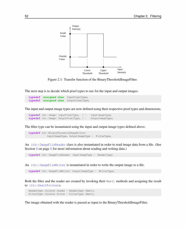
52 Chapter 2. Filtering
ThresholdUpper
Threshold
OutputIntensity
InputIntensity
OutsideValue
InsideValue
Lower
Figure 2.1: Transfer function of the BinaryThresholdImageFilter.
The next step is to decide which pixel types to use for the input and output images.
typedef unsigned char InputPixelType;
typedef unsigned char OutputPixelType;
The input and output image types are now defined using their respective pixel types and dimensions.
typedef itk::Image< InputPixelType, 2 > InputImageType;
typedef itk::Image< OutputPixelType, 2 > OutputImageType;
The filter type can be instantiated using the input and output image types defined above.
typedef itk::BinaryThresholdImageFilter<
InputImageType, OutputImageType > FilterType;
An itk::ImageFileReader class is also instantiated in order to read image data from a file. (See
Section 1 on page 1 for more information about reading and writing data.)
typedef itk::ImageFileReader< InputImageType > ReaderType;
An itk::ImageFileWriter is instantiated in order to write the output image to a file.
typedef itk::ImageFileWriter< OutputImageType > WriterType;
Both the filter and the reader are created by invoking their New() methods and assigning the result
to itk::SmartPointers.
ReaderType::Pointer reader = ReaderType::New();
FilterType::Pointer filter = FilterType::New();
The image obtained with the reader is passed as input to the BinaryThresholdImageFilter.

2.1. Thresholding 53
Figure 2.2: Effect of the BinaryThresholdImageFilter on a slice from a MRI proton density image of the brain.
filter->SetInput( reader->GetOutput() );
The method SetOutsideValue() defines the intensity value to be assigned to those pixels
whose intensities are outside the range defined by the lower and upper thresholds. The method
SetInsideValue() defines the intensity value to be assigned to pixels with intensities falling in-
side the threshold range.
filter->SetOutsideValue( outsideValue );
filter->SetInsideValue( insideValue );
The methods SetLowerThreshold() and SetUpperThreshold() define the range of the input
image intensities that will be transformed into the InsideValue. Note that the lower and upper
thresholds are values of the type of the input image pixels, while the inside and outside values are of
the type of the output image pixels.
filter->SetLowerThreshold( lowerThreshold );
filter->SetUpperThreshold( upperThreshold );
The execution of the filter is triggered by invoking the Update() method. If the filter’s output
has been passed as input to subsequent filters, the Update() call on any downstream filters in the
pipeline will indirectly trigger the update of this filter.
filter->Update();

54 Chapter 2. Filtering
Value
OutputIntensity
InputIntensity
ThresholdBelow
UnchangedIntensities
Outside
Figure 2.3: ThresholdImageFilter using the threshold-below mode.
Intensity
InputIntensity
UnchangedIntensities
ThresholdAbove
OutsideValue
Output
Figure 2.4: ThresholdImageFilter using the threshold-above mode.
Figure 2.2 illustrates the effect of this filter on a MRI proton density image of the brain. This
figure shows the limitations of the filter for performing segmentation by itself. These limitations are
particularly noticeable in noisy images and in images lacking spatial uniformity as is the case with
MRI due to field bias.
The following classes provide similar functionality:
• itk::ThresholdImageFilter
2.1.2 General Thresholding
The source code for this section can be found in the file
ThresholdImageFilter.cxx.

2.1. Thresholding 55
Value
OutputIntensity
LowerThreshold
UnchangedIntensities
UpperThreshold
InputIntensity
Outside
Figure 2.5: ThresholdImageFilter using the threshold-outside mode.
This example illustrates the use of the itk::ThresholdImageFilter. This filter can be used to
transform the intensity levels of an image in three different ways.
• First, the user can define a single threshold. Any pixels with values below this threshold will
be replaced by a user defined value, called here the OutsideValue. Pixels with values above
the threshold remain unchanged. This type of thresholding is illustrated in Figure 2.3.
• Second, the user can define a particular threshold such that all the pixels with values above
the threshold will be replaced by the OutsideValue. Pixels with values below the threshold
remain unchanged. This is illustrated in Figure 2.4.
• Third, the user can provide two thresholds. All the pixels with intensity values inside the
range defined by the two thresholds will remain unchanged. Pixels with values outside this
range will be assigned to the OutsideValue. This is illustrated in Figure 2.5.
The following methods choose among the three operating modes of the filter.
• ThresholdBelow()
• ThresholdAbove()
• ThresholdOutside()
The first step required to use this filter is to include its header file.
#include "itkThresholdImageFilter.h"
Then we must decide what pixel type to use for the image. This filter is templated over a single
image type because the algorithm only modifies pixel values outside the specified range, passing the
rest through unchanged.

56 Chapter 2. Filtering
typedef unsigned char PixelType;
The image is defined using the pixel type and the dimension.
typedef itk::Image< PixelType, 2 > ImageType;
The filter can be instantiated using the image type defined above.
typedef itk::ThresholdImageFilter< ImageType > FilterType;
An itk::ImageFileReader class is also instantiated in order to read image data from a file.
typedef itk::ImageFileReader< ImageType > ReaderType;
An itk::ImageFileWriter is instantiated in order to write the output image to a file.
typedef itk::ImageFileWriter< ImageType > WriterType;
Both the filter and the reader are created by invoking their New() methods and assigning the result
to SmartPointers.
ReaderType::Pointer reader = ReaderType::New();
FilterType::Pointer filter = FilterType::New();
The image obtained with the reader is passed as input to the itk::ThresholdImageFilter.
filter->SetInput( reader->GetOutput() );
The method SetOutsideValue() defines the intensity value to be assigned to those pixels whose
intensities are outside the range defined by the lower and upper thresholds.
filter->SetOutsideValue( 0 );
The method ThresholdBelow() defines the intensity value below which pixels of the input image
will be changed to the OutsideValue.
filter->ThresholdBelow( 180 );
The filter is executed by invoking the Update() method. If the filter is part of a larger image
processing pipeline, calling Update() on a downstream filter will also trigger update of this filter.
filter->Update();
The output of this example is shown in Figure 2.3. The second operating mode of the filter is now

2.2. Edge Detection 57
enabled by calling the method ThresholdAbove().
filter->ThresholdAbove( 180 );
filter->Update();
Updating the filter with this new setting produces the output shown in Figure 2.4. The third operating
mode of the filter is enabled by calling ThresholdOutside().
filter->ThresholdOutside( 170,190 );
filter->Update();
The output of this third, “band-pass” thresholding mode is shown in Figure 2.5.
The examples in this section also illustrate the limitations of the thresholding filter for performing
segmentation by itself. These limitations are particularly noticeable in noisy images and in images
lacking spatial uniformity, as is the case with MRI due to field bias.
The following classes provide similar functionality:
• itk::BinaryThresholdImageFilter
2.2 Edge Detection
2.2.1 Canny Edge Detection
The source code for this section can be found in the file
CannyEdgeDetectionImageFilter.cxx.
This example introduces the use of the itk::CannyEdgeDetectionImageFilter . Canny edge
detection is widely used for edge detection since it is the optimal solution satisfying the constraints
of good sensitivity, localization and noise robustness. To achieve this end, Canny edge detection is
implemented internally as a multi-stage algorithm, which involves Gaussian smoothing to remove
noise, calculation of gradient magnitudes to localize edge features, non-maximum suppression to
remove suprious features, and finally thresholding to yield a binary image. Though the specifics of
this internal pipeline are largely abstracted from the user of the class, it is nonetheless beneficial to
have a general understanding of these components so that parameters can be appropriately adjusted.
The first step required for using this filter is to include its header file.
#include "itkCannyEdgeDetectionImageFilter.h"
In this example, images are read and written with unsigned char pixel type. However, Canny edge
detection requires floating point pixel types in order to avoid numerical errors. For this reason, a
separate internal image type with pixel type double is defined for edge detection.

58 Chapter 2. Filtering
const unsigned int Dimension = 2;
typedef unsigned char CharPixelType; // IO
typedef double RealPixelType; // Operations
typedef itk::Image< CharPixelType, Dimension > CharImageType;
typedef itk::Image< RealPixelType, Dimension > RealImageType;
The CharImageType image is cast to and from RealImageType using itk::CastImageFilter
and RescaleIntensityImageFilter, respectively; both the input and output of
CannyEdgeDetectionImageFilter are RealImageType.
typedef itk::CastImageFilter< CharImageType, RealImageType >
CastToRealFilterType;
typedef itk::CannyEdgeDetectionImageFilter< RealImageType, RealImageType >
CannyFilterType;
typedef itk::RescaleIntensityImageFilter< RealImageType, CharImageType >
RescaleFilterType;
In this example, three parameters of the Canny edge detection filter may be set via the
SetVariance(), SetUpperThreshold(), and SetLowerThreshold() methods. Based on the pre-
vious discussion of the steps in the internal pipeline, we understand that variance adjusts the
amount of Gaussian smoothing and upperThreshold and lowerThreshold control which edges
are selected in the final step.
cannyFilter->SetVariance( variance );
cannyFilter->SetUpperThreshold( upperThreshold );
cannyFilter->SetLowerThreshold( lowerThreshold );
Finally, Update() is called on writer to trigger excecution of the pipeline. As usual, the call is
wrapped in a try/catch block.
try
{
writer->Update();
}
catch( itk::ExceptionObject & err )
{
std::cout << "ExceptionObject caught !" << std::endl;
std::cout << err << std::endl;
return EXIT_FAILURE;
}
2.3 Casting and Intensity Mapping
The filters discussed in this section perform pixel-wise intensity mappings. Casting is used to convert
one pixel type to another, while intensity mappings also take into account the different intensity
ranges of the pixel types.

2.3. Casting and Intensity Mapping 59
2.3.1 Linear Mappings
The source code for this section can be found in the file
CastingImageFilters.cxx.
Due to the use of Generic Programming in the toolkit, most types are resolved at compile-time. Few
decisions regarding type conversion are left to run-time. It is up to the user to anticipate the pixel
type-conversions required in the data pipeline. In medical imaging applications it is usually not
desirable to use a general pixel type since this may result in the loss of valuable information.
This section introduces the mechanisms for explicit casting of images that flow through the
pipeline. The following four filters are treated in this section: itk::CastImageFilter,
itk::RescaleIntensityImageFilter, itk::ShiftScaleImageFilter and
itk::NormalizeImageFilter . These filters are not directly related to each other except
that they all modify pixel values. They are presented together here for the purpose of comparing
their individual features.
The CastImageFilter is a very simple filter that acts pixel-wise on an input image, casting every pixel
to the type of the output image. Note that this filter does not perform any arithmetic operation on the
intensities. Applying CastImageFilter is equivalent to performing a C-Style cast on every pixel.
outputPixel = static cast<OutputPixelType>( inputPixel )
The RescaleIntensityImageFilter linearly scales the pixel values in such a way that the minimum and
maximum values of the input are mapped to minimum and maximum values provided by the user.
This is a typical process for forcing the dynamic range of the image to fit within a particular scale
and is common for image display. The linear transformation applied by this filter can be expressed
as
out putPixel = (inputPixel− inpMin)× (outMax− outMin)
(inpMax− inpMin)+ outMin
.
The ShiftScaleImageFilter also applies a linear transformation to the intensities of the input image,
but the transformation is specified by the user in the form of a multiplying factor and a value to be
added. This can be expressed as
out putPixel = (inputPixel+ Shi f t)× Scale
.
The parameters of the linear transformation applied by the NormalizeImageFilter are computed
internally such that the statistical distribution of gray levels in the output image have zero mean and
a variance of one. This intensity correction is particularly useful in registration applications as a
preprocessing step to the evaluation of mutual information metrics. The linear transformation of
NormalizeImageFilter is given as

60 Chapter 2. Filtering
out putPixel =(inputPixel−mean)√
variance.
As usual, the first step required to use these filters is to include their header files.
#include "itkCastImageFilter.h"
#include "itkRescaleIntensityImageFilter.h"
#include "itkNormalizeImageFilter.h"
Let’s define pixel types for the input and output images.
typedef unsigned char InputPixelType;
typedef float OutputPixelType;
Then, the input and output image types are defined.
typedef itk::Image< InputPixelType, 3 > InputImageType;
typedef itk::Image< OutputPixelType, 3 > OutputImageType;
The filters are instantiated using the defined image types.
typedef itk::CastImageFilter<
InputImageType, OutputImageType > CastFilterType;
typedef itk::RescaleIntensityImageFilter<
InputImageType, OutputImageType > RescaleFilterType;
typedef itk::ShiftScaleImageFilter<
InputImageType, OutputImageType > ShiftScaleFilterType;
typedef itk::NormalizeImageFilter<
InputImageType, OutputImageType > NormalizeFilterType;
Object filters are created by invoking the New() method and assigning the result to
itk::SmartPointers.
CastFilterType::Pointer castFilter = CastFilterType::New();
RescaleFilterType::Pointer rescaleFilter = RescaleFilterType::New();
ShiftScaleFilterType::Pointer shiftFilter = ShiftScaleFilterType::New();
NormalizeFilterType::Pointer normalizeFilter = NormalizeFilterType::New();
The output of a reader filter (whose creation is not shown here) is now connected as input to the
various casting filters.
castFilter->SetInput( reader->GetOutput() );
shiftFilter->SetInput( reader->GetOutput() );
rescaleFilter->SetInput( reader->GetOutput() );
normalizeFilter->SetInput( reader->GetOutput() );
Next we proceed to setup the parameters required by each filter. The CastImageFilter and the Nor-

2.3. Casting and Intensity Mapping 61
malizeImageFilter do not require any parameters. The RescaleIntensityImageFilter, on the other
hand, requires the user to provide the desired minimum and maximum pixel values of the output
image. This is done by using the SetOutputMinimum() and SetOutputMaximum() methods as
illustrated below.
rescaleFilter->SetOutputMinimum( 10 );
rescaleFilter->SetOutputMaximum( 250 );
The ShiftScaleImageFilter requires a multiplication factor (scale) and a post-scaling additive value
(shift). The methods SetScale() and SetShift() are used, respectively, to set these values.
shiftFilter->SetScale( 1.2 );
shiftFilter->SetShift( 25 );
Finally, the filters are executed by invoking the Update() method.
castFilter->Update();
shiftFilter->Update();
rescaleFilter->Update();
normalizeFilter->Update();
2.3.2 Non Linear Mappings
The following filter can be seen as a variant of the casting filters. Its main difference is the use of a
smooth and continuous transition function of non-linear form.
The source code for this section can be found in the file
SigmoidImageFilter.cxx.
The itk::SigmoidImageFilter is commonly used as an intensity transform. It maps a specific
range of intensity values into a new intensity range by making a very smooth and continuous tran-
sition in the borders of the range. Sigmoids are widely used as a mechanism for focusing attention
on a particular set of values and progressively attenuating the values outside that range. In order to
extend the flexibility of the Sigmoid filter, its implementation in ITK includes four parameters that
can be tuned to select its input and output intensity ranges. The following equation represents the
Sigmoid intensity transformation, applied pixel-wise.
I′ = (Max−Min) · 1(
1+ e−(
I−βα
)) +Min (2.1)
In the equation above, I is the intensity of the input pixel, I′ the intensity of the output pixel,
Min,Max are the minimum and maximum values of the output image, α defines the width of the
input intensity range, and β defines the intensity around which the range is centered. Figure 2.6
illustrates the significance of each parameter.

62 Chapter 2. Filtering
OutputMaximum
OutputMinimum
Alpha=−1
0.6
0.8
1
−10 −5 0 5 10
0.2
0
Alpha=0.25
Alpha=0.5
Alpha=4
Alpha=2
Alpha=10.4
Beta = −4
Beta = 0
Beta = 2Beta = 4
Beta = −2
0
−10 −5 0 5 10
0.8
0.6
0.4
0.2
1
Figure 2.6: Effects of the various parameters in the SigmoidImageFilter. The alpha parameter defines the width
of the intensity window. The beta parameter defines the center of the intensity window.
This filter will work on images of any dimension and will take advantage of multiple processors
when available.
The header file corresponding to this filter should be included first.
#include "itkSigmoidImageFilter.h"
Then pixel and image types for the filter input and output must be defined.
typedef unsigned char InputPixelType;
typedef unsigned char OutputPixelType;
typedef itk::Image< InputPixelType, 2 > InputImageType;
typedef itk::Image< OutputPixelType, 2 > OutputImageType;
Using the image types, we instantiate the filter type and create the filter object.
typedef itk::SigmoidImageFilter<
InputImageType, OutputImageType > SigmoidFilterType;
SigmoidFilterType::Pointer sigmoidFilter = SigmoidFilterType::New();
The minimum and maximum values desired in the output are defined using the methods
SetOutputMinimum() and SetOutputMaximum().
sigmoidFilter->SetOutputMinimum( outputMinimum );
sigmoidFilter->SetOutputMaximum( outputMaximum );
The coefficients α and β are set with the methods SetAlpha() and SetBeta(). Note that α is
proportional to the width of the input intensity window. As rule of thumb, we may say that the
window is the interval [−3α,3α]. The boundaries of the intensity window are not sharp. The αcurve approaches its extrema smoothly, as shown in Figure 2.6. You may want to think about this
in the same terms as when taking a range in a population of measures by defining an interval of
[−3σ,+3σ] around the population mean.

2.3. Casting and Intensity Mapping 63
Figure 2.7: Effect of the Sigmoid filter on a slice from a MRI proton density brain image.
sigmoidFilter->SetAlpha( alpha );
sigmoidFilter->SetBeta( beta );
The input to the SigmoidImageFilter can be taken from any other filter, such as an image file reader,
for example. The output can be passed down the pipeline to other filters, like an image file writer.
An Update() call on any downstream filter will trigger the execution of the Sigmoid filter.
sigmoidFilter->SetInput( reader->GetOutput() );
writer->SetInput( sigmoidFilter->GetOutput() );
writer->Update();
Figure 2.7 illustrates the effect of this filter on a slice of MRI brain image using the following
parameters.
• Minimum = 10
• Maximum = 240
• α = 10
• β = 170
As can be seen from the figure, the intensities of the white matter were expanded in their dynamic
range, while intensity values lower than β−3α and higher than β+3α became progressively mapped

64 Chapter 2. Filtering
to the minimum and maximum output values. This is the way in which a Sigmoid can be used for
performing smooth intensity windowing.
Note that both α and β can be positive and negative. A negative α will have the effect of negating
the image. This is illustrated on the left side of Figure 2.6. An application of the Sigmoid filter as
preprocessing for segmentation is presented in Section 4.3.1.
Sigmoid curves are common in the natural world. They represent the plot of sensitivity to a stimulus.
They are also the integral curve of the Gaussian and, therefore, appear naturally as the response to
signals whose distribution is Gaussian.
2.4 Gradients
Computation of gradients is a fairly common operation in image processing. The term “gradient”
may refer in some contexts to the gradient vectors and in others to the magnitude of the gradient vec-
tors. ITK filters attempt to reduce this ambiguity by including the magnitude term when appropriate.
ITK provides filters for computing both the image of gradient vectors and the image of magnitudes.
2.4.1 Gradient Magnitude
The source code for this section can be found in the file
GradientMagnitudeImageFilter.cxx.
The magnitude of the image gradient is extensively used in image analysis, mainly to help
in the determination of object contours and the separation of homogeneous regions. The
itk::GradientMagnitudeImageFilter computes the magnitude of the image gradient at each
pixel location using a simple finite differences approach. For example, in the case of 2D the compu-
tation is equivalent to convolving the image with masks of type
-1 0 1
1
0
-1
then adding the sum of their squares and computing the square root of the sum.
This filter will work on images of any dimension thanks to the internal use of
itk::NeighborhoodIterator and itk::NeighborhoodOperator.
The first step required to use this filter is to include its header file.
#include "itkGradientMagnitudeImageFilter.h"

2.4. Gradients 65
Types should be chosen for the pixels of the input and output images.
typedef float InputPixelType;
typedef float OutputPixelType;
The input and output image types can be defined using the pixel types.
typedef itk::Image< InputPixelType, 2 > InputImageType;
typedef itk::Image< OutputPixelType, 2 > OutputImageType;
The type of the gradient magnitude filter is defined by the input image and the output image types.
typedef itk::GradientMagnitudeImageFilter<
InputImageType, OutputImageType > FilterType;
A filter object is created by invoking the New() method and assigning the result to a
itk::SmartPointer.
FilterType::Pointer filter = FilterType::New();
The input image can be obtained from the output of another filter. Here, the source is an image
reader.
filter->SetInput( reader->GetOutput() );
Finally, the filter is executed by invoking the Update() method.
filter->Update();
If the output of this filter has been connected to other filters in a pipeline, updating any of the
downstream filters will also trigger an update of this filter. For example, the gradient magnitude
filter may be connected to an image writer.
rescaler->SetInput( filter->GetOutput() );
writer->SetInput( rescaler->GetOutput() );
writer->Update();
Figure 2.8 illustrates the effect of the gradient magnitude filter on a MRI proton density image of
the brain. The figure shows the sensitivity of this filter to noisy data.
Attention should be paid to the image type chosen to represent the output image since the dynamic
range of the gradient magnitude image is usually smaller than the dynamic range of the input image.
As always, there are exceptions to this rule, for example, synthetic images that contain high contrast
objects.
This filter does not apply any smoothing to the image before computing the gradients. The results
can therefore be very sensitive to noise and may not be the best choice for scale-space analysis.

66 Chapter 2. Filtering
Figure 2.8: Effect of the GradientMagnitudeImageFilter on a slice from a MRI proton density image of the brain.
2.4.2 Gradient Magnitude With Smoothing
The source code for this section can be found in the file
GradientMagnitudeRecursiveGaussianImageFilter.cxx.
Differentiation is an ill-defined operation over digital data. In practice it is convenient to define a
scale in which the differentiation should be performed. This is usually done by preprocessing the
data with a smoothing filter. It has been shown that a Gaussian kernel is the most convenient choice
for performing such smoothing. By choosing a particular value for the standard deviation (σ) of the
Gaussian, an associated scale is selected that ignores high frequency content, commonly considered
image noise.
The itk::GradientMagnitudeRecursiveGaussianImageFilter computes the magnitude of the
image gradient at each pixel location. The computational process is equivalent to first smoothing the
image by convolving it with a Gaussian kernel and then applying a differential operator. The user
selects the value of σ.
Internally this is done by applying an IIR 1 filter that approximates a convolution with the derivative
of the Gaussian kernel. Traditional convolution will produce a more accurate result, but the IIR
approach is much faster, especially using large σs [16, 17].
GradientMagnitudeRecursiveGaussianImageFilter will work on images of any dimension by taking
advantage of the natural separability of the Gaussian kernel and its derivatives.
1Infinite Impulse Response

2.4. Gradients 67
The first step required to use this filter is to include its header file.
#include "itkGradientMagnitudeRecursiveGaussianImageFilter.h"
Types should be instantiated based on the pixels of the input and output images.
typedef float InputPixelType;
typedef float OutputPixelType;
With them, the input and output image types can be instantiated.
typedef itk::Image< InputPixelType, 2 > InputImageType;
typedef itk::Image< OutputPixelType, 2 > OutputImageType;
The filter type is now instantiated using both the input image and the output image types.
typedef itk::GradientMagnitudeRecursiveGaussianImageFilter<
InputImageType, OutputImageType > FilterType;
A filter object is created by invoking the New() method and assigning the result to a
itk::SmartPointer.
FilterType::Pointer filter = FilterType::New();
The input image can be obtained from the output of another filter. Here, an image reader is used as
source.
filter->SetInput( reader->GetOutput() );
The standard deviation of the Gaussian smoothing kernel is now set.
filter->SetSigma( sigma );
Finally the filter is executed by invoking the Update() method.
filter->Update();
If connected to other filters in a pipeline, this filter will automatically update when any downstream
filters are updated. For example, we may connect this gradient magnitude filter to an image file
writer and then update the writer.
rescaler->SetInput( filter->GetOutput() );
writer->SetInput( rescaler->GetOutput() );
writer->Update();
Figure 2.9 illustrates the effect of this filter on a MRI proton density image of the brain using σvalues of 3 (left) and 5 (right). The figure shows how the sensitivity to noise can be regulated by

68 Chapter 2. Filtering
Figure 2.9: Effect of the GradientMagnitudeRecursiveGaussianImageFilter on a slice from a MRI proton density
image of the brain.
selecting an appropriate σ. This type of scale-tunable filter is suitable for performing scale-space
analysis.
Attention should be paid to the image type chosen to represent the output image since the dynamic
range of the gradient magnitude image is usually smaller than the dynamic range of the input image.
2.4.3 Derivative Without Smoothing
The source code for this section can be found in the file
DerivativeImageFilter.cxx.
The itk::DerivativeImageFilter is used for computing the partial derivative of an image, the
derivative of an image along a particular axial direction.
The header file corresponding to this filter should be included first.
#include "itkDerivativeImageFilter.h"
Next, the pixel types for the input and output images must be defined and, with them, the image
types can be instantiated. Note that it is important to select a signed type for the image, since the
values of the derivatives will be positive as well as negative.

2.5. Second Order Derivatives 69
typedef float InputPixelType;
typedef float OutputPixelType;
const unsigned int Dimension = 2;
typedef itk::Image< InputPixelType, Dimension > InputImageType;
typedef itk::Image< OutputPixelType, Dimension > OutputImageType;
Using the image types, it is now possible to define the filter type and create the filter object.
typedef itk::DerivativeImageFilter<
InputImageType, OutputImageType > FilterType;
FilterType::Pointer filter = FilterType::New();
The order of the derivative is selected with the SetOrder() method. The direction along which the
derivative will be computed is selected with the SetDirection() method.
filter->SetOrder( atoi( argv[4] ) );
filter->SetDirection( atoi( argv[5] ) );
The input to the filter can be taken from any other filter, for example a reader. The output can be
passed down the pipeline to other filters, for example, a writer. An Update() call on any downstream
filter will trigger the execution of the derivative filter.
filter->SetInput( reader->GetOutput() );
writer->SetInput( filter->GetOutput() );
writer->Update();
Figure 2.10 illustrates the effect of the DerivativeImageFilter on a slice of MRI brain image. The
derivative is taken along the x direction. The sensitivity to noise in the image is evident from this
result.
2.5 Second Order Derivatives
2.5.1 Second Order Recursive Gaussian
The source code for this section can be found in the file
SecondDerivativeRecursiveGaussianImageFilter.cxx.
This example illustrates how to compute second derivatives of a 3D image using the
itk::RecursiveGaussianImageFilter.
It’s good to be able to compute the raw derivative without any smoothing, but this can be problem-
atic in a medical imaging scenario, when images will often have a certain amount of noise. It’s
almost always more desirable to include a smoothing step first, where an image is convolved with
a Gaussian kernel in whichever directions the user desires a derivative. The nature of the Gaussian

70 Chapter 2. Filtering
Figure 2.10: Effect of the Derivative filter on a slice from a MRI proton density brain image.
kernel makes it easy to combine these two steps into one, using an infinite impulse response (IIR)
filter. In this example, all the second derivatives are computed independently in the same way, as
if they were intended to be used for building the Hessian matrix of the image (a square matrix of
second-order derivatives of an image, which is useful in many image processing techniques).
First, we will include the relevant header files: the itkRecursiveGaussianImageFilter, the image
reader, writer, and duplicator.
#include "itkRecursiveGaussianImageFilter.h"
#include "itkImageFileReader.h"
#include "itkImageFileWriter.h"
#include "itkImageDuplicator.h"
#include <string>
Next, we declare our pixel type and output pixel type to be floats, and our image dimension to be 3.
typedef float PixelType;
typedef float OutputPixelType;
const unsigned int Dimension = 3;
Using these definitions, define the image types, reader and writer types, and duplicator types, which
are templated over the pixel types and dimension. Then, instantiate the reader, writer, and duplicator
with the New() method.

2.5. Second Order Derivatives 71
typedef itk::Image< PixelType, Dimension > ImageType;
typedef itk::Image< OutputPixelType, Dimension > OutputImageType;
typedef itk::ImageFileReader< ImageType > ReaderType;
typedef itk::ImageFileWriter< OutputImageType > WriterType;
typedef itk::ImageDuplicator< OutputImageType > DuplicatorType;
typedef itk::RecursiveGaussianImageFilter<
ImageType,
ImageType > FilterType;
ReaderType::Pointer reader = ReaderType::New();
WriterType::Pointer writer = WriterType::New();
DuplicatorType::Pointer duplicator = DuplicatorType::New();
Here we create three new filters. For each derivative we take, we will want to smooth in that
direction first. So after the filters are created, each is given a dimension, and set to (in this
example) the same sigma. Note that here, σ represents the standard deviation, whereas the
itk::DiscreteGaussianImageFilter exposes the SetVariance method.
FilterType::Pointer ga = FilterType::New();
FilterType::Pointer gb = FilterType::New();
FilterType::Pointer gc = FilterType::New();
ga->SetDirection( 0 );
gb->SetDirection( 1 );
gc->SetDirection( 2 );
if( argc > 3 )
{
const float sigma = atof( argv[3] );
ga->SetSigma( sigma );
gb->SetSigma( sigma );
gc->SetSigma( sigma );
}
First we will compute the second derivative of the z-direction. In order to do this, we smooth in the
x- and y- directions, and finally smooth and compute the derivative in the z-direction. Taking the
zero-order derivative is equivalent to simply smoothing in that direction. This result is commonly
notated Izz.

72 Chapter 2. Filtering
ga->SetZeroOrder();
gb->SetZeroOrder();
gc->SetSecondOrder();
ImageType::Pointer inputImage = reader->GetOutput();
ga->SetInput( inputImage );
gb->SetInput( ga->GetOutput() );
gc->SetInput( gb->GetOutput() );
duplicator->SetInputImage( gc->GetOutput() );
gc->Update();
duplicator->Update();
ImageType::Pointer Izz = duplicator->GetModifiableOutput();
Recall that gc is the filter responsible for taking the second derivative. We can now take advantage
of the pipeline architecture and, without much hassle, switch the direction of gc and gb, so that gc
now takes the derivatives in the y-direction. Now we only need to call Update() on gc to re-run
the entire pipeline from ga to gc, obtaining the second-order derivative in the y-direction, which is
commonly notated Iyy.
gc->SetDirection( 1 ); // gc now works along Y
gb->SetDirection( 2 ); // gb now works along Z
gc->Update();
duplicator->Update();
ImageType::Pointer Iyy = duplicator->GetModifiableOutput();
Now we switch the directions of gc with that of ga in order to take the derivatives in the x-direction.
This will give us Ixx.
gc->SetDirection( 0 ); // gc now works along X
ga->SetDirection( 1 ); // ga now works along Y
gc->Update();
duplicator->Update();
ImageType::Pointer Ixx = duplicator->GetModifiableOutput();
Now we can reset the directions to their original values, and compute first derivatives in different
directions. Since we set both gb and gc to compute first derivatives, and ga to zero-order (which is
only smoothing) we will obtain Iyz.

2.5. Second Order Derivatives 73
ga->SetDirection( 0 );
gb->SetDirection( 1 );
gc->SetDirection( 2 );
ga->SetZeroOrder();
gb->SetFirstOrder();
gc->SetFirstOrder();
gc->Update();
duplicator->Update();
ImageType::Pointer Iyz = duplicator->GetModifiableOutput();
Here is how you may easily obtain Ixz.
ga->SetDirection( 1 );
gb->SetDirection( 0 );
gc->SetDirection( 2 );
ga->SetZeroOrder();
gb->SetFirstOrder();
gc->SetFirstOrder();
gc->Update();
duplicator->Update();
ImageType::Pointer Ixz = duplicator->GetModifiableOutput();
For the sake of completeness, here is how you may compute Ixz and Ixy.
writer->SetInput( Ixz );
outputFileName = outputPrefix + "-Ixz.mhd";
writer->SetFileName( outputFileName.c_str() );
writer->Update();
ga->SetDirection( 2 );
gb->SetDirection( 0 );
gc->SetDirection( 1 );
ga->SetZeroOrder();
gb->SetFirstOrder();
gc->SetFirstOrder();
gc->Update();
duplicator->Update();
ImageType::Pointer Ixy = duplicator->GetModifiableOutput();
writer->SetInput( Ixy );
outputFileName = outputPrefix + "-Ixy.mhd";
writer->SetFileName( outputFileName.c_str() );
writer->Update();

74 Chapter 2. Filtering
2.5.2 Laplacian Filters
Laplacian Filter Recursive Gaussian
The source code for this section can be found in the file
LaplacianRecursiveGaussianImageFilter1.cxx.
This example illustrates how to use the itk::RecursiveGaussianImageFilter for computing
the Laplacian of a 2D image.
The first step required to use this filter is to include its header file.
#include "itkRecursiveGaussianImageFilter.h"
Types should be selected on the desired input and output pixel types.
typedef float InputPixelType;
typedef float OutputPixelType;
The input and output image types are instantiated using the pixel types.
typedef itk::Image< InputPixelType, 2 > InputImageType;
typedef itk::Image< OutputPixelType, 2 > OutputImageType;
The filter type is now instantiated using both the input image and the output image types.
typedef itk::RecursiveGaussianImageFilter<
InputImageType, OutputImageType > FilterType;
This filter applies the approximation of the convolution along a single dimension. It is therefore
necessary to concatenate several of these filters to produce smoothing in all directions. In this
example, we create a pair of filters since we are processing a 2D image. The filters are created by
invoking the New() method and assigning the result to a itk::SmartPointer.
We need two filters for computing the X component of the Laplacian and two other filters for com-
puting the Y component.
FilterType::Pointer filterX1 = FilterType::New();
FilterType::Pointer filterY1 = FilterType::New();
FilterType::Pointer filterX2 = FilterType::New();
FilterType::Pointer filterY2 = FilterType::New();
Since each one of the newly created filters has the potential to perform filtering along any dimension,
we have to restrict each one to a particular direction. This is done with the SetDirection() method.

2.5. Second Order Derivatives 75
filterX1->SetDirection( 0 ); // 0 --> X direction
filterY1->SetDirection( 1 ); // 1 --> Y direction
filterX2->SetDirection( 0 ); // 0 --> X direction
filterY2->SetDirection( 1 ); // 1 --> Y direction
The itk::RecursiveGaussianImageFilter can approximate the convolution with the Gaussian
or with its first and second derivatives. We select one of these options by using the SetOrder()
method. Note that the argument is an enum whose values can be ZeroOrder, FirstOrder and
SecondOrder. For example, to compute the x partial derivative we should select FirstOrder for
x and ZeroOrder for y. Here we want only to smooth in x and y, so we select ZeroOrder in both
directions.
filterX1->SetOrder( FilterType::ZeroOrder );
filterY1->SetOrder( FilterType::SecondOrder );
filterX2->SetOrder( FilterType::SecondOrder );
filterY2->SetOrder( FilterType::ZeroOrder );
There are two typical ways of normalizing Gaussians depending on their application. For scale-
space analysis it is desirable to use a normalization that will preserve the maximum value of the
input. This normalization is represented by the following equation.
1
σ√
2π(2.2)
In applications that use the Gaussian as a solution of the diffusion equation it is desirable to use a
normalization that preserves the integral of the signal. This last approach can be seen as a conserva-
tion of mass principle. This is represented by the following equation.
1
σ2√
2π(2.3)
The itk::RecursiveGaussianImageFilter has a boolean flag that allows users to select between
these two normalization options. Selection is done with the method SetNormalizeAcrossScale().
Enable this flag when analyzing an image across scale-space. In the current example, this setting
has no impact because we are actually renormalizing the output to the dynamic range of the reader,
so we simply disable the flag.
const bool normalizeAcrossScale = false;
filterX1->SetNormalizeAcrossScale( normalizeAcrossScale );
filterY1->SetNormalizeAcrossScale( normalizeAcrossScale );
filterX2->SetNormalizeAcrossScale( normalizeAcrossScale );
filterY2->SetNormalizeAcrossScale( normalizeAcrossScale );
The input image can be obtained from the output of another filter. Here, an image reader is used as
the source. The image is passed to the x filter and then to the y filter. The reason for keeping these
two filters separate is that it is usual in scale-space applications to compute not only the smoothing

76 Chapter 2. Filtering
but also combinations of derivatives at different orders and smoothing. Some factorization is pos-
sible when separate filters are used to generate the intermediate results. Here this capability is less
interesting, though, since we only want to smooth the image in all directions.
filterX1->SetInput( reader->GetOutput() );
filterY1->SetInput( filterX1->GetOutput() );
filterY2->SetInput( reader->GetOutput() );
filterX2->SetInput( filterY2->GetOutput() );
It is now time to select the σ of the Gaussian used to smooth the data. Note that σ must be passed to
both filters and that sigma is considered to be in millimeters. That is, at the moment of applying the
smoothing process, the filter will take into account the spacing values defined in the image.
filterX1->SetSigma( sigma );
filterY1->SetSigma( sigma );
filterX2->SetSigma( sigma );
filterY2->SetSigma( sigma );
Finally the two components of the Laplacian should be added together. The itk::AddImageFilter
is used for this purpose.
typedef itk::AddImageFilter<
OutputImageType,
OutputImageType,
OutputImageType > AddFilterType;
AddFilterType::Pointer addFilter = AddFilterType::New();
addFilter->SetInput1( filterY1->GetOutput() );
addFilter->SetInput2( filterX2->GetOutput() );
The filters are triggered by invoking Update() on the Add filter at the end of the pipeline.
try
{
addFilter->Update();
}
catch( itk::ExceptionObject & err )
{
std::cout << "ExceptionObject caught !" << std::endl;
std::cout << err << std::endl;
return EXIT_FAILURE;
}
The resulting image could be saved to a file using the itk::ImageFileWriter class.

2.5. Second Order Derivatives 77
Figure 2.11: Effect of the LaplacianRecursiveGaussianImageFilter on a slice from a MRI proton density image
of the brain.
typedef float WritePixelType;
typedef itk::Image< WritePixelType, 2 > WriteImageType;
typedef itk::ImageFileWriter< WriteImageType > WriterType;
WriterType::Pointer writer = WriterType::New();
writer->SetInput( addFilter->GetOutput() );
writer->SetFileName( argv[2] );
writer->Update();
The source code for this section can be found in the file
LaplacianRecursiveGaussianImageFilter2.cxx.
The previous example showed how to use the itk::RecursiveGaussianImageFilter
for computing the equivalent of a Laplacian of an image after smoothing with a Gaus-
sian. The elements used in this previous example have been packaged together in the
itk::LaplacianRecursiveGaussianImageFilter in order to simplify its usage. This current
example shows how to use this convenience filter for achieving the same results as the previous
example.
The first step required to use this filter is to include its header file.

78 Chapter 2. Filtering
#include "itkLaplacianRecursiveGaussianImageFilter.h"
Types should be selected on the desired input and output pixel types.
typedef float InputPixelType;
typedef float OutputPixelType;
The input and output image types are instantiated using the pixel types.
typedef itk::Image< InputPixelType, 2 > InputImageType;
typedef itk::Image< OutputPixelType, 2 > OutputImageType;
The filter type is now instantiated using both the input image and the output image types.
typedef itk::LaplacianRecursiveGaussianImageFilter<
InputImageType, OutputImageType > FilterType;
This filter packages all the components illustrated in the previous example. The filter is created by
invoking the New() method and assigning the result to a itk::SmartPointer.
FilterType::Pointer laplacian = FilterType::New();
The option for normalizing across scale space can also be selected in this filter.
laplacian->SetNormalizeAcrossScale( false );
The input image can be obtained from the output of another filter. Here, an image reader is used as
the source.
laplacian->SetInput( reader->GetOutput() );
It is now time to select the σ of the Gaussian used to smooth the data. Note that σ must be passed to
both filters and that sigma is considered to be in millimeters. That is, at the moment of applying the
smoothing process, the filter will take into account the spacing values defined in the image.
laplacian->SetSigma( sigma );
Finally the pipeline is executed by invoking the Update() method.

2.6. Neighborhood Filters 79
try
{
laplacian->Update();
}
catch( itk::ExceptionObject & err )
{
std::cout << "ExceptionObject caught !" << std::endl;
std::cout << err << std::endl;
return EXIT_FAILURE;
}
2.6 Neighborhood Filters
The concept of locality is frequently encountered in image processing in the form of filters that
compute every output pixel using information from a small region in the neighborhood of the input
pixel. The classical form of these filters are the 3× 3 filters in 2D images. Convolution masks
based on these neighborhoods can perform diverse tasks ranging from noise reduction, to differential
operations, to mathematical morphology.
The Insight toolkit implements an elegant approach to neighborhood-based image filtering. The
input image is processed using a special iterator called the itk::NeighborhoodIterator . This
iterator is capable of moving over all the pixels in an image and, for each position, it can address
the pixels in a local neighborhood. Operators are defined that apply an algorithmic operation in
the neighborhood of the input pixel to produce a value for the output pixel. The following section
describes some of the more commonly used filters that take advantage of this construction. (See the
Iterators chapter in Book 1 for more information.)
2.6.1 Mean Filter
The source code for this section can be found in the file
MeanImageFilter.cxx.
The itk::MeanImageFilter is commonly used for noise reduction. The filter computes the value
of each output pixel by finding the statistical mean of the neighborhood of the corresponding input
pixel. The following figure illustrates the local effect of the MeanImageFilter in a 2D case. The
statistical mean of the neighborhood on the left is passed as the output value associated with the
pixel at the center of the neighborhood.
25 30 32
27 25 29
28 26 50
✲ 30.22 ✲ 30

80 Chapter 2. Filtering
Note that this algorithm is sensitive to the presence of outliers in the neighbor-
hood. This filter will work on images of any dimension thanks to the internal use of
itk::SmartNeighborhoodIterator and itk::NeighborhoodOperator . The size of the neigh-
borhood over which the mean is computed can be set by the user.
The header file corresponding to this filter should be included first.
#include "itkMeanImageFilter.h"
Then the pixel types for input and output image must be defined and, with them, the image types
can be instantiated.
typedef unsigned char InputPixelType;
typedef unsigned char OutputPixelType;
typedef itk::Image< InputPixelType, 2 > InputImageType;
typedef itk::Image< OutputPixelType, 2 > OutputImageType;
Using the image types it is now possible to instantiate the filter type and create the filter object.
typedef itk::MeanImageFilter<
InputImageType, OutputImageType > FilterType;
FilterType::Pointer filter = FilterType::New();
The size of the neighborhood is defined along every dimension by passing a SizeType object with
the corresponding values. The value on each dimension is used as the semi-size of a rectangular
box. For example, in 2D a size of 1,2 will result in a 3× 5 neighborhood.
InputImageType::SizeType indexRadius;
indexRadius[0] = 1; // radius along x
indexRadius[1] = 1; // radius along y
filter->SetRadius( indexRadius );
The input to the filter can be taken from any other filter, for example a reader. The output can be
passed down the pipeline to other filters, for example, a writer. An update call on any downstream
filter will trigger the execution of the mean filter.
filter->SetInput( reader->GetOutput() );
writer->SetInput( filter->GetOutput() );
writer->Update();
Figure 2.12 illustrates the effect of this filter on a slice of MRI brain image using neighborhood radii
of 1,1 which corresponds to a 3× 3 classical neighborhood. It can be seen from this picture that
edges are rapidly degraded by the diffusion of intensity values among neighbors.

2.6. Neighborhood Filters 81
Figure 2.12: Effect of the MeanImageFilter on a slice from a MRI proton density brain image.
2.6.2 Median Filter
The source code for this section can be found in the file
MedianImageFilter.cxx.
The itk::MedianImageFilter is commonly used as a robust approach for noise reduction. This
filter is particularly efficient against salt-and-pepper noise. In other words, it is robust to the presence
of gray-level outliers. MedianImageFilter computes the value of each output pixel as the statistical
median of the neighborhood of values around the corresponding input pixel. The following figure
illustrates the local effect of this filter in a 2D case. The statistical median of the neighborhood on
the left is passed as the output value associated with the pixel at the center of the neighborhood.
25 30 32
27 25 29
28 26 50
✲ 28
This filter will work on images of any dimension thanks to the internal use of
itk::NeighborhoodIterator and itk::NeighborhoodOperator . The size of the neighborhood
over which the median is computed can be set by the user.
The header file corresponding to this filter should be included first.
#include "itkMedianImageFilter.h"

82 Chapter 2. Filtering
Then the pixel and image types of the input and output must be defined.
typedef unsigned char InputPixelType;
typedef unsigned char OutputPixelType;
typedef itk::Image< InputPixelType, 2 > InputImageType;
typedef itk::Image< OutputPixelType, 2 > OutputImageType;
Using the image types, it is now possible to define the filter type and create the filter object.
typedef itk::MedianImageFilter<
InputImageType, OutputImageType > FilterType;
FilterType::Pointer filter = FilterType::New();
The size of the neighborhood is defined along every dimension by passing a SizeType object with
the corresponding values. The value on each dimension is used as the semi-size of a rectangular
box. For example, in 2D a size of 1,2 will result in a 3× 5 neighborhood.
InputImageType::SizeType indexRadius;
indexRadius[0] = 1; // radius along x
indexRadius[1] = 1; // radius along y
filter->SetRadius( indexRadius );
The input to the filter can be taken from any other filter, for example a reader. The output can be
passed down the pipeline to other filters, for example, a writer. An update call on any downstream
filter will trigger the execution of the median filter.
filter->SetInput( reader->GetOutput() );
writer->SetInput( filter->GetOutput() );
writer->Update();
Figure 2.13 illustrates the effect of the MedianImageFilter filter on a slice of MRI brain image using
a neighborhood radius of 1,1, which corresponds to a 3× 3 classical neighborhood. The filtered
image demonstrates the moderate tendency of the median filter to preserve edges.
2.6.3 Mathematical Morphology
Mathematical morphology has proved to be a powerful resource for image processing and anal-
ysis [56]. ITK implements mathematical morphology filters using NeighborhoodIterators and
itk::NeighborhoodOperators. The toolkit contains two types of image morphology algorithms:
filters that operate on binary images and filters that operate on grayscale images.

2.6. Neighborhood Filters 83
Figure 2.13: Effect of the MedianImageFilter on a slice from a MRI proton density brain image.
Binary Filters
The source code for this section can be found in the file
MathematicalMorphologyBinaryFilters.cxx.
The following section illustrates the use of filters that perform basic mathematical
morphology operations on binary images. The itk::BinaryErodeImageFilter and
itk::BinaryDilateImageFilter are described here. The filter names clearly specify the type
of image on which they operate. The header files required to construct a simple example of the use
of the mathematical morphology filters are included below.
#include "itkBinaryErodeImageFilter.h"
#include "itkBinaryDilateImageFilter.h"
#include "itkBinaryBallStructuringElement.h"
The following code defines the input and output pixel types and their associated image types.
const unsigned int Dimension = 2;
typedef unsigned char InputPixelType;
typedef unsigned char OutputPixelType;
typedef itk::Image< InputPixelType, Dimension > InputImageType;
typedef itk::Image< OutputPixelType, Dimension > OutputImageType;
Mathematical morphology operations are implemented by applying an operator over the neighbor-

84 Chapter 2. Filtering
hood of each input pixel. The combination of the rule and the neighborhood is known as structuring
element. Although some rules have become de facto standards for image processing, there is a good
deal of freedom as to what kind of algorithmic rule should be applied to the neighborhood. The
implementation in ITK follows the typical rule of minimum for erosion and maximum for dilation.
The structuring element is implemented as a NeighborhoodOperator. In particular, the default struc-
turing element is the itk::BinaryBallStructuringElement class. This class is instantiated
using the pixel type and dimension of the input image.
typedef itk::BinaryBallStructuringElement<
InputPixelType,
Dimension > StructuringElementType;
The structuring element type is then used along with the input and output image types for instanti-
ating the type of the filters.
typedef itk::BinaryErodeImageFilter<
InputImageType,
OutputImageType,
StructuringElementType > ErodeFilterType;
typedef itk::BinaryDilateImageFilter<
InputImageType,
OutputImageType,
StructuringElementType > DilateFilterType;
The filters can now be created by invoking the New() method and assigning the result to
itk::SmartPointers.
ErodeFilterType::Pointer binaryErode = ErodeFilterType::New();
DilateFilterType::Pointer binaryDilate = DilateFilterType::New();
The structuring element is not a reference counted class. Thus it is created as a C++ stack object
instead of using New() and SmartPointers. The radius of the neighborhood associated with the struc-
turing element is defined with the SetRadius() method and the CreateStructuringElement()
method is invoked in order to initialize the operator. The resulting structuring element is passed to
the mathematical morphology filter through the SetKernel() method, as illustrated below.
StructuringElementType structuringElement;
structuringElement.SetRadius( 1 ); // 3x3 structuring element
structuringElement.CreateStructuringElement();
binaryErode->SetKernel( structuringElement );
binaryDilate->SetKernel( structuringElement );
A binary image is provided as input to the filters. This image might be, for example, the output of a
binary threshold image filter.

2.6. Neighborhood Filters 85
Figure 2.14: Effect of erosion and dilation in a binary image.
thresholder->SetInput( reader->GetOutput() );
InputPixelType background = 0;
InputPixelType foreground = 255;
thresholder->SetOutsideValue( background );
thresholder->SetInsideValue( foreground );
thresholder->SetLowerThreshold( lowerThreshold );
thresholder->SetUpperThreshold( upperThreshold );
binaryErode->SetInput( thresholder->GetOutput() );
binaryDilate->SetInput( thresholder->GetOutput() );
The values that correspond to “objects” in the binary image are specified with the methods
SetErodeValue() and SetDilateValue(). The value passed to these methods will be consid-
ered the value over which the dilation and erosion rules will apply.
binaryErode->SetErodeValue( foreground );
binaryDilate->SetDilateValue( foreground );
The filter is executed by invoking its Update() method, or by updating any downstream filter, such
as an image writer.
writerDilation->SetInput( binaryDilate->GetOutput() );
writerDilation->Update();
Figure 2.14 illustrates the effect of the erosion and dilation filters on a binary image from a MRI
brain slice. The figure shows how these operations can be used to remove spurious details from
segmented images.

86 Chapter 2. Filtering
Grayscale Filters
The source code for this section can be found in the file
MathematicalMorphologyGrayscaleFilters.cxx.
The following section illustrates the use of filters for performing basic mathematical mor-
phology operations on grayscale images. The itk::GrayscaleErodeImageFilter and
itk::GrayscaleDilateImageFilter are covered in this example. The filter names clearly spec-
ify the type of image on which they operate. The header files required for a simple example of the
use of grayscale mathematical morphology filters are presented below.
#include "itkGrayscaleErodeImageFilter.h"
#include "itkGrayscaleDilateImageFilter.h"
#include "itkBinaryBallStructuringElement.h"
The following code defines the input and output pixel types and their associated image types.
const unsigned int Dimension = 2;
typedef unsigned char InputPixelType;
typedef unsigned char OutputPixelType;
typedef itk::Image< InputPixelType, Dimension > InputImageType;
typedef itk::Image< OutputPixelType, Dimension > OutputImageType;
Mathematical morphology operations are based on the application of an operator over a neighbor-
hood of each input pixel. The combination of the rule and the neighborhood is known as structuring
element. Although some rules have become the de facto standard in image processing there is a
good deal of freedom as to what kind of algorithmic rule should be applied on the neighborhood.
The implementation in ITK follows the typical rule of minimum for erosion and maximum for dila-
tion.
The structuring element is implemented as a itk::NeighborhoodOperator. In particular, the
default structuring element is the itk::BinaryBallStructuringElement class. This class is
instantiated using the pixel type and dimension of the input image.
typedef itk::BinaryBallStructuringElement<
InputPixelType,
Dimension > StructuringElementType;
The structuring element type is then used along with the input and output image types for instanti-
ating the type of the filters.

2.6. Neighborhood Filters 87
typedef itk::GrayscaleErodeImageFilter<
InputImageType,
OutputImageType,
StructuringElementType > ErodeFilterType;
typedef itk::GrayscaleDilateImageFilter<
InputImageType,
OutputImageType,
StructuringElementType > DilateFilterType;
The filters can now be created by invoking the New() method and assigning the result to SmartPoint-
ers.
ErodeFilterType::Pointer grayscaleErode = ErodeFilterType::New();
DilateFilterType::Pointer grayscaleDilate = DilateFilterType::New();
The structuring element is not a reference counted class. Thus it is created as a C++ stack object
instead of using New() and SmartPointers. The radius of the neighborhood associated with the struc-
turing element is defined with the SetRadius() method and the CreateStructuringElement()
method is invoked in order to initialize the operator. The resulting structuring element is passed to
the mathematical morphology filter through the SetKernel() method, as illustrated below.
StructuringElementType structuringElement;
structuringElement.SetRadius( 1 ); // 3x3 structuring element
structuringElement.CreateStructuringElement();
grayscaleErode->SetKernel( structuringElement );
grayscaleDilate->SetKernel( structuringElement );
A grayscale image is provided as input to the filters. This image might be, for example, the output
of a reader.
grayscaleErode->SetInput( reader->GetOutput() );
grayscaleDilate->SetInput( reader->GetOutput() );
The filter is executed by invoking its Update() method, or by updating any downstream filter, such
as an image writer.
writerDilation->SetInput( grayscaleDilate->GetOutput() );
writerDilation->Update();
Figure 2.15 illustrates the effect of the erosion and dilation filters on a binary image from a MRI
brain slice. The figure shows how these operations can be used to remove spurious details from
segmented images.

88 Chapter 2. Filtering
Figure 2.15: Effect of erosion and dilation in a grayscale image.
2.6.4 Voting Filters
Voting filters are quite a generic family of filters. In fact, both the Dilate and Erode filters from
Mathematical Morphology are very particular cases of the broader family of voting filters. In a vot-
ing filter, the outcome of a pixel is decided by counting the number of pixels in its neighborhood and
applying a rule to the result of that counting. For example, the typical implementation of erosion in
terms of a voting filter will be to label a foreground pixel as background if the number of background
neighbors is greater than or equal to 1. In this context, you could imagine variations of erosion in
which the count could be changed to require at least 3 foreground pixels in its neighborhood.
Binary Median Filter
One case of a voting filter is the BinaryMedianImageFilter. This filter is equivalent to applying a
Median filter over a binary image. Having a binary image as input makes it possible to optimize the
execution of the filter since there is no real need for sorting the pixels according to their frequency
in the neighborhood.
The source code for this section can be found in the file
BinaryMedianImageFilter.cxx.
The itk::BinaryMedianImageFilter is commonly used as a robust approach for noise reduction.
BinaryMedianImageFilter computes the value of each output pixel as the statistical median of the
neighborhood of values around the corresponding input pixel. When the input images are binary,
the implementation can be optimized by simply counting the number of pixels ON/OFF around the
current pixel.
This filter will work on images of any dimension thanks to the internal use of
itk::NeighborhoodIterator and itk::NeighborhoodOperator . The size of the neighborhood

2.6. Neighborhood Filters 89
over which the median is computed can be set by the user.
The header file corresponding to this filter should be included first.
#include "itkBinaryMedianImageFilter.h"
Then the pixel and image types of the input and output must be defined.
typedef unsigned char InputPixelType;
typedef unsigned char OutputPixelType;
typedef itk::Image< InputPixelType, 2 > InputImageType;
typedef itk::Image< OutputPixelType, 2 > OutputImageType;
Using the image types, it is now possible to define the filter type and create the filter object.
typedef itk::BinaryMedianImageFilter<
InputImageType, OutputImageType > FilterType;
FilterType::Pointer filter = FilterType::New();
The size of the neighborhood is defined along every dimension by passing a SizeType object with
the corresponding values. The value on each dimension is used as the semi-size of a rectangular
box. For example, in 2D a size of 1,2 will result in a 3× 5 neighborhood.
InputImageType::SizeType indexRadius;
indexRadius[0] = radiusX; // radius along x
indexRadius[1] = radiusY; // radius along y
filter->SetRadius( indexRadius );
The input to the filter can be taken from any other filter, for example a reader. The output can be
passed down the pipeline to other filters, for example, a writer. An update call on any downstream
filter will trigger the execution of the median filter.
filter->SetInput( reader->GetOutput() );
writer->SetInput( filter->GetOutput() );
writer->Update();
Figure 2.16 illustrates the effect of the BinaryMedianImageFilter filter on a slice of MRI brain image
using a neighborhood radius of 2,2, which corresponds to a 5× 5 classical neighborhood. The
filtered image demonstrates the capability of this filter for reducing noise both in the background
and foreground of the image, as well as smoothing the contours of the regions.
The typical effect of median filtration on a noisy digital image is a dramatic reduction in impulse
noise spikes. The filter also tends to preserve brightness differences across signal steps, resulting in
reduced blurring of regional boundaries. The filter also tends to preserve the positions of boundaries
in an image.
Figure 2.17 below shows the effect of running the median filter with a 3x3 classical window size

90 Chapter 2. Filtering
Figure 2.16: Effect of the BinaryMedianImageFilter on a slice from a MRI proton density brain image that has
been thresholded in order to produce a binary image.
1, 10 and 50 times. There is a tradeoff in noise reduction and the sharpness of the image when the
window size is increased.
Hole Filling Filter
Another variation of voting filters is the Hole Filling filter. This filter converts background pixels into
foreground only when the number of foreground pixels is a majority of the neighbors. By selecting
the size of the majority, this filter can be tuned to fill in holes of different sizes. To be more precise,
the effect of the filter is actually related to the curvature of the edge in which the pixel is located.
The source code for this section can be found in the file
VotingBinaryHoleFillingImageFilter.cxx.
The itk::VotingBinaryHoleFillingImageFilter applies a voting operation in order to fill in
cavities. This can be used for smoothing contours and for filling holes in binary images.
The header file corresponding to this filter should be included first.
#include "itkVotingBinaryHoleFillingImageFilter.h"
Then the pixel and image types of the input and output must be defined.

2.6. Neighborhood Filters 91
Figure 2.17: Effect of 1, 10 and 50 iterations of the BinaryMedianImageFilter using a 3x3 window.

92 Chapter 2. Filtering
typedef unsigned char InputPixelType;
typedef unsigned char OutputPixelType;
typedef itk::Image< InputPixelType, 2 > InputImageType;
typedef itk::Image< OutputPixelType, 2 > OutputImageType;
Using the image types, it is now possible to define the filter type and create the filter object.
typedef itk::VotingBinaryHoleFillingImageFilter<
InputImageType, OutputImageType > FilterType;
FilterType::Pointer filter = FilterType::New();
The size of the neighborhood is defined along every dimension by passing a SizeType object with
the corresponding values. The value on each dimension is used as the semi-size of a rectangular
box. For example, in 2D a size of 1,2 will result in a 3× 5 neighborhood.
InputImageType::SizeType indexRadius;
indexRadius[0] = radiusX; // radius along x
indexRadius[1] = radiusY; // radius along y
filter->SetRadius( indexRadius );
Since the filter is expecting a binary image as input, we must specify the levels that are going to
be considered background and foreground. This is done with the SetForegroundValue() and
SetBackgroundValue() methods.
filter->SetBackgroundValue( 0 );
filter->SetForegroundValue( 255 );
We must also specify the majority threshold that is going to be used as the decision criterion for
converting a background pixel into a foreground pixel. The rule of conversion is that a background
pixel will be converted into a foreground pixel if the number of foreground neighbors surpass the
number of background neighbors by the majority value. For example, in a 2D image, with neigh-
borhood of radius 1, the neighborhood will have size 3× 3. If we set the majority value to 2, then
we are requiring that the number of foreground neighbors should be at least (3x3 -1 )/2 + majority.
This is done with the SetMajorityThreshold() method.
filter->SetMajorityThreshold( 2 );
The input to the filter can be taken from any other filter, for example a reader. The output can be
passed down the pipeline to other filters, for example, a writer. An update call on any downstream
filter will trigger the execution of the median filter.
filter->SetInput( reader->GetOutput() );
writer->SetInput( filter->GetOutput() );
writer->Update();

2.6. Neighborhood Filters 93
Figure 2.18: Effect of the VotingBinaryHoleFillingImageFilter on a slice from a MRI proton density brain image
that has been thresholded in order to produce a binary image. The output images have used radius 1,2 and 3
respectively.

94 Chapter 2. Filtering
Figure 2.18 illustrates the effect of the VotingBinaryHoleFillingImageFilter filter on a thresholded
slice of MRI brain image using neighborhood radii of 1,1, 2,2 and 3,3 that correspond respectively
to neighborhoods of size 3× 3, 5× 5, 7× 7. The filtered image demonstrates the capability of this
filter for reducing noise both in the background and foreground of the image, as well as smoothing
the contours of the regions.
Iterative Hole Filling Filter
The Hole Filling filter can be used in an iterative way, by applying it repeatedly until no pixel
changes. In this context, the filter can be seen as a binary variation of a Level Set filter.
The source code for this section can be found in the file
VotingBinaryIterativeHoleFillingImageFilter.cxx.
The itk::VotingBinaryIterativeHoleFillingImageFilter applies a voting operation in or-
der to fill in cavities. This can be used for smoothing contours and for filling holes in binary images.
This filter runs a itk::VotingBinaryHoleFillingImageFilter internally until no pixels change
or the maximum number of iterations has been reached.
The header file corresponding to this filter should be included first.
#include "itkVotingBinaryIterativeHoleFillingImageFilter.h"
Then the pixel and image types must be defined. Note that this filter requires the input and output
images to be of the same type, therefore a single image type is required for the template instantiation.
typedef unsigned char PixelType;
typedef itk::Image< PixelType, 2 > ImageType;
Using the image types, it is now possible to define the filter type and create the filter object.
typedef itk::VotingBinaryIterativeHoleFillingImageFilter<
ImageType > FilterType;
FilterType::Pointer filter = FilterType::New();
The size of the neighborhood is defined along every dimension by passing a SizeType object with
the corresponding values. The value on each dimension is used as the semi-size of a rectangular
box. For example, in 2D a size of 1,2 will result in a 3× 5 neighborhood.
ImageType::SizeType indexRadius;
indexRadius[0] = radiusX; // radius along x
indexRadius[1] = radiusY; // radius along y
filter->SetRadius( indexRadius );

2.7. Smoothing Filters 95
Since the filter is expecting a binary image as input, we must specify the levels that are going to
be considered background and foreground. This is done with the SetForegroundValue() and
SetBackgroundValue() methods.
filter->SetBackgroundValue( 0 );
filter->SetForegroundValue( 255 );
We must also specify the majority threshold that is going to be used as the decision criterion for
converting a background pixel into a foreground pixel. The rule of conversion is that a background
pixel will be converted into a foreground pixel if the number of foreground neighbors surpass the
number of background neighbors by the majority value. For example, in a 2D image, with neigh-
borhood of radius 1, the neighborhood will have size 3× 3. If we set the majority value to 2, then
we are requiring that the number of foreground neighbors should be at least (3x3 -1 )/2 + majority.
This is done with the SetMajorityThreshold() method.
filter->SetMajorityThreshold( 2 );
Finally we specify the maximum number of iterations for which this filter should run. The number
of iterations will determine the maximum size of holes and cavities that this filter will be able to fill.
The more iterations you run, the larger the cavities that will be filled in.
filter->SetMaximumNumberOfIterations( numberOfIterations );
The input to the filter can be taken from any other filter, for example a reader. The output can be
passed down the pipeline to other filters, for example, a writer. An update call on any downstream
filter will trigger the execution of the median filter.
filter->SetInput( reader->GetOutput() );
writer->SetInput( filter->GetOutput() );
writer->Update();
Figure 2.19 illustrates the effect of the VotingBinaryIterativeHoleFillingImageFilter filter on a
thresholded slice of MRI brain image using neighborhood radii of 1,1, 2,2 and 3,3 that corre-
spond respectively to neighborhoods of size 3×3, 5×5, 7×7. The filtered image demonstrates the
capability of this filter for reducing noise both in the background and foreground of the image, as
well as smoothing the contours of the regions.
2.7 Smoothing Filters
Real image data has a level of uncertainty which is manifested in the variability of measures assigned
to pixels. This uncertainty is usually interpreted as noise and considered an undesirable component
of the image data. This section describes several methods that can be applied to reduce noise on
images.

96 Chapter 2. Filtering
Figure 2.19: Effect of the VotingBinaryIterativeHoleFillingImageFilter on a slice from a MRI proton density brain
image that has been thresholded in order to produce a binary image. The output images have used radius 1,2
and 3 respectively.

2.7. Smoothing Filters 97
2.7.1 Blurring
Blurring is the traditional approach for removing noise from images. It is usually implemented in
the form of a convolution with a kernel. The effect of blurring on the image spectrum is to attenuate
high spatial frequencies. Different kernels attenuate frequencies in different ways. One of the most
commonly used kernels is the Gaussian. Two implementations of Gaussian smoothing are available
in the toolkit. The first one is based on a traditional convolution while the other is based on the
application of IIR filters that approximate the convolution with a Gaussian [16, 17].
Discrete Gaussian
The source code for this section can be found in the file
DiscreteGaussianImageFilter.cxx.
The itk::DiscreteGaussianImageFilter com-
KernelWidth
Error
0
0.2
0.3
0.4
0.5
0.6
0.7
0.8
0.9
1
−2 −1.5 −1 −0.5 0 0.5 1 1.5 2
0.1
Figure 2.20: Discretized Gaussian.
putes the convolution of the input image with a Gaus-
sian kernel. This is done in ND by taking advantage
of the separability of the Gaussian kernel. A one-
dimensional Gaussian function is discretized on a con-
volution kernel. The size of the kernel is extended
until there are enough discrete points in the Gaussian
to ensure that a user-provided maximum error is not
exceeded. Since the size of the kernel is unknown a
priori, it is necessary to impose a limit to its growth.
The user can thus provide a value to be the maximum
admissible size of the kernel. Discretization error is
defined as the difference between the area under the
discrete Gaussian curve (which has finite support) and the area under the continuous Gaussian.
Gaussian kernels in ITK are constructed according to the theory of Tony Lindeberg [35] so that
smoothing and derivative operations commute before and after discretization. In other words, finite
difference derivatives on an image I that has been smoothed by convolution with the Gaussian are
equivalent to finite differences computed on I by convolving with a derivative of the Gaussian.
The first step required to use this filter is to include its header file. As with other examples, the
includes here are truncated to those specific for this example.
#include "itkDiscreteGaussianImageFilter.h"
Types should be chosen for the pixels of the input and output images. Image types can be instantiated
using the pixel type and dimension.

98 Chapter 2. Filtering
typedef float InputPixelType;
typedef float OutputPixelType;
typedef itk::Image< InputPixelType, 2 > InputImageType;
typedef itk::Image< OutputPixelType, 2 > OutputImageType;
The discrete Gaussian filter type is instantiated using the input and output image types. A corre-
sponding filter object is created.
typedef itk::DiscreteGaussianImageFilter<
InputImageType, OutputImageType > FilterType;
FilterType::Pointer filter = FilterType::New();
The input image can be obtained from the output of another filter. Here, an image reader is used as
its input.
filter->SetInput( reader->GetOutput() );
The filter requires the user to provide a value for the variance associated with the Gaussian kernel.
The method SetVariance() is used for this purpose. The discrete Gaussian is constructed as a
convolution kernel. The maximum kernel size can be set by the user. Note that the combination of
variance and kernel-size values may result in a truncated Gaussian kernel.
filter->SetVariance( gaussianVariance );
filter->SetMaximumKernelWidth( maxKernelWidth );
Finally, the filter is executed by invoking the Update() method.
filter->Update();
If the output of this filter has been connected to other filters down the pipeline, updating any of the
downstream filters will trigger the execution of this one. For example, a writer could be used after
the filter.
rescaler->SetInput( filter->GetOutput() );
writer->SetInput( rescaler->GetOutput() );
writer->Update();
Figure 2.21 illustrates the effect of this filter on a MRI proton density image of the brain.
Note that large Gaussian variances will produce large convolution kernels and correspondingly
longer computation times. Unless a high degree of accuracy is required, it may be more desirable to
use the approximating itk::RecursiveGaussianImageFilter with large variances.

2.7. Smoothing Filters 99
Figure 2.21: Effect of the DiscreteGaussianImageFilter on a slice from a MRI proton density image of the brain.
Binomial Blurring
The source code for this section can be found in the file
BinomialBlurImageFilter.cxx.
The itk::BinomialBlurImageFilter computes a nearest neighbor average along each dimen-
sion. The process is repeated a number of times, as specified by the user. In principle, after a large
number of iterations the result will approach the convolution with a Gaussian.
The first step required to use this filter is to include its header file.
#include "itkBinomialBlurImageFilter.h"
Types should be chosen for the pixels of the input and output images. Image types can be instantiated
using the pixel type and dimension.
typedef float InputPixelType;
typedef float OutputPixelType;
typedef itk::Image< InputPixelType, 2 > InputImageType;
typedef itk::Image< OutputPixelType, 2 > OutputImageType;
The filter type is now instantiated using both the input image and the output image types. Then a
filter object is created.

100 Chapter 2. Filtering
Figure 2.22: Effect of the BinomialBlurImageFilter on a slice from a MRI proton density image of the brain.
typedef itk::BinomialBlurImageFilter<
InputImageType, OutputImageType > FilterType;
FilterType::Pointer filter = FilterType::New();
The input image can be obtained from the output of another filter. Here, an image reader is used
as the source. The number of repetitions is set with the SetRepetitions() method. Computation
time will increase linearly with the number of repetitions selected. Finally, the filter can be executed
by calling the Update() method.
filter->SetInput( reader->GetOutput() );
filter->SetRepetitions( repetitions );
filter->Update();
Figure 2.22 illustrates the effect of this filter on a MRI proton density image of the brain.
Note that the standard deviation σ of the equivalent Gaussian is fixed. In the spatial spectrum, the
effect of every iteration of this filter is like a multiplication with a sinus cardinal function.
Recursive Gaussian IIR
The source code for this section can be found in the file
SmoothingRecursiveGaussianImageFilter.cxx.
The classical method of smoothing an image by convolution with a Gaussian kernel has the draw-

2.7. Smoothing Filters 101
back that it is slow when the standard deviation σ of the Gaussian is large. This is due to the larger
size of the kernel, which results in a higher number of computations per pixel.
The itk::RecursiveGaussianImageFilter implements an approximation of convolution with
the Gaussian and its derivatives by using IIR2 filters. In practice this filter requires a constant number
of operations for approximating the convolution, regardless of the σ value [16, 17].
The first step required to use this filter is to include its header file.
#include "itkRecursiveGaussianImageFilter.h"
Types should be selected on the desired input and output pixel types.
typedef float InputPixelType;
typedef float OutputPixelType;
The input and output image types are instantiated using the pixel types.
typedef itk::Image< InputPixelType, 2 > InputImageType;
typedef itk::Image< OutputPixelType, 2 > OutputImageType;
The filter type is now instantiated using both the input image and the output image types.
typedef itk::RecursiveGaussianImageFilter<
InputImageType, OutputImageType > FilterType;
This filter applies the approximation of the convolution along a single dimension. It is therefore
necessary to concatenate several of these filters to produce smoothing in all directions. In this
example, we create a pair of filters since we are processing a 2D image. The filters are created by
invoking the New() method and assigning the result to a itk::SmartPointer.
FilterType::Pointer filterX = FilterType::New();
FilterType::Pointer filterY = FilterType::New();
Since each one of the newly created filters has the potential to perform filtering along any dimension,
we have to restrict each one to a particular direction. This is done with the SetDirection() method.
filterX->SetDirection( 0 ); // 0 --> X direction
filterY->SetDirection( 1 ); // 1 --> Y direction
The itk::RecursiveGaussianImageFilter can approximate the convolution with the Gaussian
or with its first and second derivatives. We select one of these options by using the SetOrder()
method. Note that the argument is an enum whose values can be ZeroOrder, FirstOrder and
SecondOrder. For example, to compute the x partial derivative we should select FirstOrder for
x and ZeroOrder for y. Here we want only to smooth in x and y, so we select ZeroOrder in both
directions.
2Infinite Impulse Response

102 Chapter 2. Filtering
filterX->SetOrder( FilterType::ZeroOrder );
filterY->SetOrder( FilterType::ZeroOrder );
There are two typical ways of normalizing Gaussians depending on their application. For scale-
space analysis it is desirable to use a normalization that will preserve the maximum value of the
input. This normalization is represented by the following equation.
1
σ√
2π(2.4)
In applications that use the Gaussian as a solution of the diffusion equation it is desirable to use a
normalization that preserve the integral of the signal. This last approach can be seen as a conserva-
tion of mass principle. This is represented by the following equation.
1
σ2√
2π(2.5)
The itk::RecursiveGaussianImageFilter has a boolean flag that allows users to select between
these two normalization options. Selection is done with the method SetNormalizeAcrossScale().
Enable this flag to analyzing an image across scale-space. In the current example, this setting has
no impact because we are actually renormalizing the output to the dynamic range of the reader, so
we simply disable the flag.
filterX->SetNormalizeAcrossScale( false );
filterY->SetNormalizeAcrossScale( false );
The input image can be obtained from the output of another filter. Here, an image reader is used as
the source. The image is passed to the x filter and then to the y filter. The reason for keeping these
two filters separate is that it is usual in scale-space applications to compute not only the smoothing
but also combinations of derivatives at different orders and smoothing. Some factorization is pos-
sible when separate filters are used to generate the intermediate results. Here this capability is less
interesting, though, since we only want to smooth the image in all directions.
filterX->SetInput( reader->GetOutput() );
filterY->SetInput( filterX->GetOutput() );
It is now time to select the σ of the Gaussian used to smooth the data. Note that σ must be passed to
both filters and that sigma is considered to be in millimeters. That is, at the moment of applying the
smoothing process, the filter will take into account the spacing values defined in the image.
filterX->SetSigma( sigma );
filterY->SetSigma( sigma );
Finally the pipeline is executed by invoking the Update() method.
filterY->Update();

2.7. Smoothing Filters 103
Figure 2.23: Effect of the SmoothingRecursiveGaussianImageFilter on a slice from a MRI proton density image
of the brain.
Figure 2.23 illustrates the effect of this filter on a MRI proton density image of the brain using σvalues of 3 (left) and 5 (right). The figure shows how the attenuation of noise can be regulated by se-
lecting the appropriate standard deviation. This type of scale-tunable filter is suitable for performing
scale-space analysis.
The RecursiveGaussianFilters can also be applied on multi-component images. For instance, the
above filter could have applied with RGBPixel as the pixel type. Each component is then indepen-
dently filtered. However the RescaleIntensityImageFilter will not work on RGBPixels since it does
not mathematically make sense to rescale the output of multi-component images.
2.7.2 Local Blurring
In some cases it is desirable to compute smoothing in restricted regions of the image, or to do it
using different parameters that are computed locally. The following sections describe options for
applying local smoothing in images.

104 Chapter 2. Filtering
Gaussian Blur Image Function
The source code for this section can be found in the file
GaussianBlurImageFunction.cxx.
2.7.3 Edge Preserving Smoothing
Introduction to Anisotropic Diffusion
The drawback of image denoising (smoothing) is that it tends to blur away the sharp boundaries in
the image that help to distinguish between the larger-scale anatomical structures that one is trying
to characterize (which also limits the size of the smoothing kernels in most applications). Even in
cases where smoothing does not obliterate boundaries, it tends to distort the fine structure of the
image and thereby changes subtle aspects of the anatomical shapes in question.
Perona and Malik [46] introduced an alternative to linear-filtering that they called anisotropic diffu-
sion. Anisotropic diffusion is closely related to the earlier work of Grossberg [23], who used similar
nonlinear diffusion processes to model human vision. The motivation for anisotropic diffusion (also
called nonuniform or variable conductance diffusion) is that a Gaussian smoothed image is a single
time slice of the solution to the heat equation, that has the original image as its initial conditions.
Thus, the solution to∂g(x,y, t)
∂t= ∇ ·∇g(x,y, t), (2.6)
where g(x,y,0) = f (x,y) is the input image, is g(x,y, t) = G(√
2t)⊗ f (x,y), where G(σ) is a Gaus-
sian with standard deviation σ.
Anisotropic diffusion includes a variable conductance term that, in turn, depends on the differential
structure of the image. Thus, the variable conductance can be formulated to limit the smoothing at
“edges” in images, as measured by high gradient magnitude, for example.
gt = ∇ · c(|∇g|)∇g, (2.7)
where, for notational convenience, we leave off the independent parameters of g and use the sub-
scripts with respect to those parameters to indicate partial derivatives. The function c(|∇g|) is a
fuzzy cutoff that reduces the conductance at areas of large |∇g|, and can be any one of a number of
functions. The literature has shown
c(|∇g|) = e− |∇g|2
2k2 (2.8)
to be quite effective. Notice that conductance term introduces a free parameter k, the conductance
parameter, that controls the sensitivity of the process to edge contrast. Thus, anisotropic diffu-
sion entails two free parameters: the conductance parameter, k, and the time parameter, t, that is
analogous to σ, the effective width of the filter when using Gaussian kernels.
Equation 2.7 is a nonlinear partial differential equation that can be solved on a discrete grid using
finite forward differences. Thus, the smoothed image is obtained only by an iterative process, not a

2.7. Smoothing Filters 105
convolution or non-stationary, linear filter. Typically, the number of iterations required for practical
results are small, and large 2D images can be processed in several tens of seconds using carefully
written code running on modern, general purpose, single-processor computers. The technique ap-
plies readily and effectively to 3D images, but requires more processing time.
In the early 1990’s several research groups [22, 68] demonstrated the effectiveness of anisotropic
diffusion on medical images. In a series of papers on the subject [72, 70, 71, 68, 69, 66], Whitaker
described a detailed analytical and empirical analysis, introduced a smoothing term in the conduc-
tance that made the process more robust, invented a numerical scheme that virtually eliminated
directional artifacts in the original algorithm, and generalized anisotropic diffusion to vector-valued
images, an image processing technique that can be used on vector-valued medical data (such as the
color cryosection data of the Visible Human Project).
For a vector-valued input ~F : U 7→ ℜm the process takes the form
~Ft = ∇ · c(D~F)~F , (2.9)
where D~F is a dissimilarity measure of ~F , a generalization of the gradient magnitude to vector-
valued images, that can incorporate linear and nonlinear coordinate transformations on the range of~F . In this way, the smoothing of the multiple images associated with vector-valued data is coupled
through the conductance term, that fuses the information in the different images. Thus vector-
valued, nonlinear diffusion can combine low-level image features (e.g. edges) across all “channels”
of a vector-valued image in order to preserve or enhance those features in all of image “channels”.
Vector-valued anisotropic diffusion is useful for denoising data from devices that produce multiple
values such as MRI or color photography. When performing nonlinear diffusion on a color image,
the color channels are diffused separately, but linked through the conductance term. Vector-valued
diffusion is also useful for processing registered data from different devices or for denoising higher-
order geometric or statistical features from scalar-valued images [66, 73].
The output of anisotropic diffusion is an image or set of images that demonstrates reduced noise and
texture but preserves, and can also enhance, edges. Such images are useful for a variety of processes
including statistical classification, visualization, and geometric feature extraction. Previous work
has shown [69] that anisotropic diffusion, over a wide range of conductance parameters, offers
quantifiable advantages over linear filtering for edge detection in medical images.
Since the effectiveness of nonlinear diffusion was first demonstrated, numerous variations of this ap-
proach have surfaced in the literature [61]. These include alternatives for constructing dissimilarity
measures [54], directional (i.e., tensor-valued) conductance terms [65, 3] and level set interpretations
[67].
Gradient Anisotropic Diffusion
The source code for this section can be found in the file
GradientAnisotropicDiffusionImageFilter.cxx.

106 Chapter 2. Filtering
The itk::GradientAnisotropicDiffusionImageFilter implements an N-dimensional version
of the classic Perona-Malik anisotropic diffusion equation for scalar-valued images [46].
The conductance term for this implementation is chosen as a function of the gradient magnitude of
the image at each point, reducing the strength of diffusion at edge pixels.
C(x) = e−(‖∇U(x)‖
K )2(2.10)
The numerical implementation of this equation is similar to that described in the Perona-Malik paper
[46], but uses a more robust technique for gradient magnitude estimation and has been generalized
to N-dimensions.
The first step required to use this filter is to include its header file.
#include "itkGradientAnisotropicDiffusionImageFilter.h"
Types should be selected based on the pixel types required for the input and output images. The
image types are defined using the pixel type and the dimension.
typedef float InputPixelType;
typedef float OutputPixelType;
typedef itk::Image< InputPixelType, 2 > InputImageType;
typedef itk::Image< OutputPixelType, 2 > OutputImageType;
The filter type is now instantiated using both the input image and the output image types. The filter
object is created by the New() method.
typedef itk::GradientAnisotropicDiffusionImageFilter<
InputImageType, OutputImageType > FilterType;
FilterType::Pointer filter = FilterType::New();
The input image can be obtained from the output of another filter. Here, an image reader is used as
source.
filter->SetInput( reader->GetOutput() );
This filter requires three parameters: the number of iterations to be performed, the time
step and the conductance parameter used in the computation of the level set evolution.
These parameters are set using the methods SetNumberOfIterations(), SetTimeStep() and
SetConductanceParameter() respectively. The filter can be executed by invoking Update().
filter->SetNumberOfIterations( numberOfIterations );
filter->SetTimeStep( timeStep );
filter->SetConductanceParameter( conductance );
filter->Update();

2.7. Smoothing Filters 107
Figure 2.24: Effect of the GradientAnisotropicDiffusionImageFilter on a slice from a MRI Proton Density image
of the brain.
Typical values for the time step are 0.25 in 2D images and 0.125 in 3D images. The number of
iterations is typically set to 5; more iterations result in further smoothing and will increase the
computing time linearly.
Figure 2.24 illustrates the effect of this filter on a MRI proton density image of the brain. In this
example the filter was run with a time step of 0.25, and 5 iterations. The figure shows how homoge-
neous regions are smoothed and edges are preserved.
The following classes provide similar functionality:
• itk::BilateralImageFilter
• itk::CurvatureAnisotropicDiffusionImageFilter
• itk::CurvatureFlowImageFilter
Curvature Anisotropic Diffusion
The source code for this section can be found in the file
CurvatureAnisotropicDiffusionImageFilter.cxx.
The itk::CurvatureAnisotropicDiffusionImageFilter performs anisotropic diffusion on an
image using a modified curvature diffusion equation (MCDE).

108 Chapter 2. Filtering
MCDE does not exhibit the edge enhancing properties of classic anisotropic diffusion, which can un-
der certain conditions undergo a “negative” diffusion, which enhances the contrast of edges. Equa-
tions of the form of MCDE always undergo positive diffusion, with the conductance term only
varying the strength of that diffusion.
Qualitatively, MCDE compares well with other non-linear diffusion techniques. It is less sensitive to
contrast than classic Perona-Malik style diffusion, and preserves finer detailed structures in images.
There is a potential speed trade-off for using this function in place of itkGradientNDAnisotrop-
icDiffusionFunction. Each iteration of the solution takes roughly twice as long. Fewer iterations,
however, may be required to reach an acceptable solution.
The MCDE equation is given as:
ft =| ∇ f | ∇ · c(| ∇ f |) ∇ f
| ∇ f | (2.11)
where the conductance modified curvature term is
∇ · ∇ f
| ∇ f | (2.12)
The first step required for using this filter is to include its header file.
#include "itkCurvatureAnisotropicDiffusionImageFilter.h"
Types should be selected based on the pixel types required for the input and output images. The
image types are defined using the pixel type and the dimension.
typedef float InputPixelType;
typedef float OutputPixelType;
typedef itk::Image< InputPixelType, 2 > InputImageType;
typedef itk::Image< OutputPixelType, 2 > OutputImageType;
The filter type is now instantiated using both the input image and the output image types. The filter
object is created by the New() method.
typedef itk::CurvatureAnisotropicDiffusionImageFilter<
InputImageType, OutputImageType > FilterType;
FilterType::Pointer filter = FilterType::New();
The input image can be obtained from the output of another filter. Here, an image reader is used as
source.
filter->SetInput( reader->GetOutput() );

2.7. Smoothing Filters 109
Figure 2.25: Effect of the CurvatureAnisotropicDiffusionImageFilter on a slice from a MRI Proton Density image
of the brain.
This filter requires three parameters: the number of iterations to be performed, the time step used in
the computation of the level set evolution and the value of conductance. These parameters are set
using the methods SetNumberOfIterations(), SetTimeStep() and SetConductance() respec-
tively. The filter can be executed by invoking Update().
filter->SetNumberOfIterations( numberOfIterations );
filter->SetTimeStep( timeStep );
filter->SetConductanceParameter( conductance );
if (useImageSpacing)
{
filter->UseImageSpacingOn();
}
filter->Update();
Typical values for the time step are 0.125 in 2D images and 0.0625 in 3D images. The number of
iterations can be usually around 5, more iterations will result in further smoothing and will increase
the computing time linearly. The conductance parameter is usually around 3.0.
Figure 2.25 illustrates the effect of this filter on a MRI proton density image of the brain. In this
example the filter was run with a time step of 0.125, 5 iterations and a conductance value of 3.0.
The figure shows how homogeneous regions are smoothed and edges are preserved.
The following classes provide similar functionality:
• itk::BilateralImageFilter

110 Chapter 2. Filtering
• itk::CurvatureFlowImageFilter
• itk::GradientAnisotropicDiffusionImageFilter
Curvature Flow
The source code for this section can be found in the file
CurvatureFlowImageFilter.cxx.
The itk::CurvatureFlowImageFilter performs edge-preserving smoothing in a similar fashion
to the classical anisotropic diffusion. The filter uses a level set formulation where the iso-intensity
contours in an image are viewed as level sets, where pixels of a particular intensity form one level
set. The level set function is then evolved under the control of a diffusion equation where the speed
is proportional to the curvature of the contour:
It = κ|∇I| (2.13)
where κ is the curvature.
Areas of high curvature will diffuse faster than areas of low curvature. Hence, small jagged noise
artifacts will disappear quickly, while large scale interfaces will be slow to evolve, thereby preserv-
ing sharp boundaries between objects. However, it should be noted that although the evolution at
the boundary is slow, some diffusion will still occur. Thus, continual application of this curvature
flow scheme will eventually result in the removal of information as each contour shrinks to a point
and disappears.
The first step required to use this filter is to include its header file.
#include "itkCurvatureFlowImageFilter.h"
Types should be selected based on the pixel types required for the input and output images.
typedef float InputPixelType;
typedef float OutputPixelType;
With them, the input and output image types can be instantiated.
typedef itk::Image< InputPixelType, 2 > InputImageType;
typedef itk::Image< OutputPixelType, 2 > OutputImageType;
The CurvatureFlow filter type is now instantiated using both the input image and the output image
types.
typedef itk::CurvatureFlowImageFilter<
InputImageType, OutputImageType > FilterType;

2.7. Smoothing Filters 111
A filter object is created by invoking the New() method and assigning the result to a
itk::SmartPointer.
FilterType::Pointer filter = FilterType::New();
The input image can be obtained from the output of another filter. Here, an image reader is used as
source.
filter->SetInput( reader->GetOutput() );
The CurvatureFlow filter requires two parameters: the number of iterations to be performed and the
time step used in the computation of the level set evolution. These two parameters are set using
the methods SetNumberOfIterations() and SetTimeStep() respectively. Then the filter can be
executed by invoking Update().
filter->SetNumberOfIterations( numberOfIterations );
filter->SetTimeStep( timeStep );
filter->Update();
Typical values for the time step are 0.125 in 2D images and 0.0625 in 3D images. The number
of iterations can be usually around 10, more iterations will result in further smoothing and will
increase the computing time linearly. Edge-preserving behavior is not guaranteed by this filter.
Some degradation will occur on the edges and will increase as the number of iterations is increased.
If the output of this filter has been connected to other filters down the pipeline, updating any of the
downstream filters will trigger the execution of this one. For example, a writer filter could be used
after the curvature flow filter.
rescaler->SetInput( filter->GetOutput() );
writer->SetInput( rescaler->GetOutput() );
writer->Update();
Figure 2.26 illustrates the effect of this filter on a MRI proton density image of the brain. In this
example the filter was run with a time step of 0.25 and 10 iterations. The figure shows how homo-
geneous regions are smoothed and edges are preserved.
The following classes provide similar functionality:
• itk::GradientAnisotropicDiffusionImageFilter
• itk::CurvatureAnisotropicDiffusionImageFilter
• itk::BilateralImageFilter

112 Chapter 2. Filtering
Figure 2.26: Effect of the CurvatureFlowImageFilter on a slice from a MRI proton density image of the brain.
MinMaxCurvature Flow
The source code for this section can be found in the file
MinMaxCurvatureFlowImageFilter.cxx.
The MinMax curvature flow filter applies a variant of the curvature flow algorithm where diffusion
is turned on or off depending of the scale of the noise that one wants to remove. The evolution speed
is switched between min(κ,0) and max(κ,0) such that:
It = F |∇I| (2.14)
where F is defined as
F =
{
max(κ,0) : Average < T hreshold
min(κ,0) : Average ≥ T hreshold(2.15)
The Average is the average intensity computed over a neighborhood of a user-specified radius of
the pixel. The choice of the radius governs the scale of the noise to be removed. The T hreshold is
calculated as the average of pixel intensities along the direction perpendicular to the gradient at the
extrema of the local neighborhood.
A speed of F = max(κ,0) will cause small dark regions in a predominantly light region to shrink.
Conversely, a speed of F = min(κ,0), will cause light regions in a predominantly dark region to

2.7. Smoothing Filters 113
Gradient
Iso−curves
Figure 2.27: Elements involved in the computation of min-max curvature flow.
shrink. Comparison between the neighborhood average and the threshold is used to select the the
right speed function to use. This switching prevents the unwanted diffusion of the simple curvature
flow method.
Figure 2.27 shows the main elements involved in the computation. The set of square pixels represent
the neighborhood over which the average intensity is being computed. The gray pixels are those ly-
ing close to the direction perpendicular to the gradient. The pixels which intersect the neighborhood
bounds are used to compute the threshold value in the equation above. The integer radius of the
neighborhood is selected by the user.
The first step required to use the itk::MinMaxCurvatureFlowImageFilter is to include its header
file.
#include "itkMinMaxCurvatureFlowImageFilter.h"
Types should be selected based on the pixel types required for the input and output images. The
input and output image types are instantiated.
typedef float InputPixelType;
typedef float OutputPixelType;
typedef itk::Image< InputPixelType, 2 > InputImageType;
typedef itk::Image< OutputPixelType, 2 > OutputImageType;
The itk::MinMaxCurvatureFlowImageFilter type is now instantiated using both the input im-
age and the output image types. The filter is then created using the New() method.

114 Chapter 2. Filtering
typedef itk::MinMaxCurvatureFlowImageFilter<
InputImageType, OutputImageType > FilterType;
FilterType::Pointer filter = FilterType::New();
The input image can be obtained from the output of another filter. Here, an image reader is used as
source.
filter->SetInput( reader->GetOutput() );
The itk::MinMaxCurvatureFlowImageFilter requires the two normal parameters of the Curva-
tureFlow image, the number of iterations to be performed and the time step used in the computation
of the level set evolution. In addition, the radius of the neighborhood is also required. This last
parameter is passed using the SetStencilRadius() method. Note that the radius is provided as
an integer number since it is referring to a number of pixels from the center to the border of the
neighborhood. Then the filter can be executed by invoking Update().
filter->SetTimeStep( timeStep );
filter->SetNumberOfIterations( numberOfIterations );
filter->SetStencilRadius( radius );
filter->Update();
Typical values for the time step are 0.125 in 2D images and 0.0625 in 3D images. The number of
iterations can be usually around 10, more iterations will result in further smoothing and will increase
the computing time linearly. The radius of the stencil can be typically 1. The edge-preserving
characteristic is not perfect on this filter. Some degradation will occur on the edges and will increase
as the number of iterations is increased.
If the output of this filter has been connected to other filters down the pipeline, updating any of the
downstream filters will trigger the execution of this one. For example, a writer filter can be used
after the curvature flow filter.
rescaler->SetInput( filter->GetOutput() );
writer->SetInput( rescaler->GetOutput() );
writer->Update();
Figure 2.28 illustrates the effect of this filter on a MRI proton density image of the brain. In this
example the filter was run with a time step of 0.125, 10 iterations and a radius of 1. The figure shows
how homogeneous regions are smoothed and edges are preserved. Notice also, that the result in the
figure has sharper edges than the same example using simple curvature flow in Figure 2.26.
The following classes provide similar functionality:
• itk::CurvatureFlowImageFilter

2.7. Smoothing Filters 115
Figure 2.28: Effect of the MinMaxCurvatureFlowImageFilter on a slice from a MRI proton density image of the
brain.
Bilateral Filter
The source code for this section can be found in the file
BilateralImageFilter.cxx.
The itk::BilateralImageFilter performs smoothing by using both domain and range neigh-
borhoods. Pixels that are close to a pixel in the image domain and similar to a pixel in the image
range are used to calculate the filtered value. Two Gaussian kernels (one in the image domain and
one in the image range) are used to smooth the image. The result is an image that is smoothed in
homogeneous regions yet has edges preserved. The result is similar to anisotropic diffusion but the
implementation is non-iterative. Another benefit to bilateral filtering is that any distance metric can
be used for kernel smoothing the image range. Bilateral filtering is capable of reducing the noise in
an image by an order of magnitude while maintaining edges. The bilateral operator used here was
described by Tomasi and Manduchi (Bilateral Filtering for Gray and Color Images. IEEE ICCV.
1998.)
The filtering operation can be described by the following equation
h(x) = k(x)−1∫
ωf (w)c(x,w)s( f (x), f (w))dw (2.16)
where x holds the coordinates of a ND point, f (x) is the input image and h(x) is the output image.
The convolution kernels c() and s() are associated with the spatial and intensity domain respec-

116 Chapter 2. Filtering
tively. The ND integral is computed over ω which is a neighborhood of the pixel located at x. The
normalization factor k(x) is computed as
k(x) =
∫ω
c(x,w)s( f (x), f (w))dw (2.17)
The default implementation of this filter uses Gaussian kernels for both c() and s(). The c kernel
can be described as
c(x,w) = e(||x−w||2
σ2c
)(2.18)
where σc is provided by the user and defines how close pixel neighbors should be in order to be
considered for the computation of the output value. The s kernel is given by
s( f (x), f (w)) = e(( f (x)− f (w)2
σ2s
)(2.19)
where σs is provided by the user and defines how close the neighbor’s intensity be in order to be
considered for the computation of the output value.
The first step required to use this filter is to include its header file.
#include "itkBilateralImageFilter.h"
The image types are instantiated using pixel type and dimension.
typedef unsigned char InputPixelType;
typedef unsigned char OutputPixelType;
typedef itk::Image< InputPixelType, 2 > InputImageType;
typedef itk::Image< OutputPixelType, 2 > OutputImageType;
The bilateral filter type is now instantiated using both the input image and the output image types
and the filter object is created.
typedef itk::BilateralImageFilter<
InputImageType, OutputImageType > FilterType;
FilterType::Pointer filter = FilterType::New();
The input image can be obtained from the output of another filter. Here, an image reader is used as
a source.
filter->SetInput( reader->GetOutput() );
The Bilateral filter requires two parameters. First, we must specify the standard deviation σ to be
used for the Gaussian kernel on image intensities. Second, the set of σs to be used along each

2.7. Smoothing Filters 117
dimension in the space domain. This second parameter is supplied as an array of float or double
values. The array dimension matches the image dimension. This mechanism makes it possible to
enforce more coherence along some directions. For example, more smoothing can be done along
the X direction than along the Y direction.
In the following code example, the σ values are taken from the command line. Note the use of
ImageType::ImageDimension to get access to the image dimension at compile time.
const unsigned int Dimension = InputImageType::ImageDimension;
double domainSigmas[ Dimension ];
for(unsigned int i=0; i<Dimension; i++)
{
domainSigmas[i] = atof( argv[3] );
}
const double rangeSigma = atof( argv[4] );
The filter parameters are set with the methods SetRangeSigma() and SetDomainSigma().
filter->SetDomainSigma( domainSigmas );
filter->SetRangeSigma( rangeSigma );
The output of the filter is connected here to a intensity rescaler filter and then to a writer. Invoking
Update() on the writer triggers the execution of both filters.
rescaler->SetInput( filter->GetOutput() );
writer->SetInput( rescaler->GetOutput() );
writer->Update();
Figure 2.29 illustrates the effect of this filter on a MRI proton density image of the brain. In this
example the filter was run with a range σ of 5.0 and a domain σ of 6.0. The figure shows how
homogeneous regions are smoothed and edges are preserved.
The following classes provide similar functionality:
• itk::GradientAnisotropicDiffusionImageFilter
• itk::CurvatureAnisotropicDiffusionImageFilter
• itk::CurvatureFlowImageFilter
2.7.4 Edge Preserving Smoothing in Vector Images
Anisotropic diffusion can also be applied to images whose pixels are vectors. In this case the dif-
fusion is computed independently for each vector component. The following classes implement
versions of anisotropic diffusion on vector images.

118 Chapter 2. Filtering
Figure 2.29: Effect of the BilateralImageFilter on a slice from a MRI proton density image of the brain.
Vector Gradient Anisotropic Diffusion
The source code for this section can be found in the file
VectorGradientAnisotropicDiffusionImageFilter.cxx.
The itk::VectorGradientAnisotropicDiffusionImageFilter implements an N-dimensional
version of the classic Perona-Malik anisotropic diffusion equation for vector-valued images. Typi-
cally in vector-valued diffusion, vector components are diffused independently of one another using
a conductance term that is linked across the components. The diffusion equation was illustrated in
2.7.3.
This filter is designed to process images of itk::Vector type. The code relies on various typedefs
and overloaded operators defined in itk::Vector. It is perfectly reasonable, however, to apply
this filter to images of other, user-defined types as long as the appropriate typedefs and operator
overloads are in place. As a general rule, follow the example of itk::Vector in defining your data
types.
The first step required to use this filter is to include its header file.
#include "itkVectorGradientAnisotropicDiffusionImageFilter.h"
Types should be selected based on required pixel type for the input and output images. The image
types are defined using the pixel type and the dimension.

2.7. Smoothing Filters 119
typedef float InputPixelType;
typedef itk::CovariantVector< float, 2 > VectorPixelType;
typedef itk::Image< InputPixelType, 2 > InputImageType;
typedef itk::Image< VectorPixelType, 2 > VectorImageType;
The filter type is now instantiated using both the input image and the output image types. The filter
object is created by the New() method.
typedef itk::VectorGradientAnisotropicDiffusionImageFilter<
VectorImageType, VectorImageType > FilterType;
FilterType::Pointer filter = FilterType::New();
The input image can be obtained from the output of another filter. Here, an image reader is used as
source and its data is passed through a gradient filter in order to generate an image of vectors.
gradient->SetInput( reader->GetOutput() );
filter->SetInput( gradient->GetOutput() );
This filter requires two parameters: the number of iterations to be performed and the time step
used in the computation of the level set evolution. These parameters are set using the methods
SetNumberOfIterations() and SetTimeStep() respectively. The filter can be executed by in-
voking Update().
filter->SetNumberOfIterations( numberOfIterations );
filter->SetTimeStep( timeStep );
filter->SetConductanceParameter(1.0);
filter->Update();
Typical values for the time step are 0.125 in 2D images and 0.0625 in 3D images. The number of
iterations can be usually around 5, however more iterations will result in further smoothing and will
linearly increase the computing time.
Figure 2.30 illustrates the effect of this filter on a MRI proton density image of the brain. The images
show the X component of the gradient before (left) and after (right) the application of the filter. In
this example the filter was run with a time step of 0.25, and 5 iterations.
Vector Curvature Anisotropic Diffusion
The source code for this section can be found in the file
VectorCurvatureAnisotropicDiffusionImageFilter.cxx.
The itk::VectorCurvatureAnisotropicDiffusionImageFilter performs anisotropic diffu-
sion on a vector image using a modified curvature diffusion equation (MCDE). The MCDE is the
same described in 2.7.3.
Typically in vector-valued diffusion, vector components are diffused independently of one another
using a conductance term that is linked across the components.
This filter is designed to process images of itk::Vector type. The code relies on various typedefs

120 Chapter 2. Filtering
Figure 2.30: Effect of the VectorGradientAnisotropicDiffusionImageFilter on the X component of the gradient
from a MRI proton density brain image.
and overloaded operators defined in itk::Vector. It is perfectly reasonable, however, to apply
this filter to images of other, user-defined types as long as the appropriate typedefs and operator
overloads are in place. As a general rule, follow the example of the itk::Vector class in defining
your data types.
The first step required to use this filter is to include its header file.
#include "itkVectorCurvatureAnisotropicDiffusionImageFilter.h"
Types should be selected based on required pixel type for the input and output images. The image
types are defined using the pixel type and the dimension.
typedef float InputPixelType;
typedef itk::CovariantVector< float, 2 > VectorPixelType;
typedef itk::Image< InputPixelType, 2 > InputImageType;
typedef itk::Image< VectorPixelType, 2 > VectorImageType;
The filter type is now instantiated using both the input image and the output image types. The filter
object is created by the New() method.
typedef itk::VectorCurvatureAnisotropicDiffusionImageFilter<
VectorImageType, VectorImageType > FilterType;
FilterType::Pointer filter = FilterType::New();

2.7. Smoothing Filters 121
Figure 2.31: Effect of the VectorCurvatureAnisotropicDiffusionImageFilter on the X component of the gradient
from a MRIproton density brain image.
The input image can be obtained from the output of another filter. Here, an image reader is used as
source and its data is passed through a gradient filter in order to generate an image of vectors.
gradient->SetInput( reader->GetOutput() );
filter->SetInput( gradient->GetOutput() );
This filter requires two parameters: the number of iterations to be performed and the time step
used in the computation of the level set evolution. These parameters are set using the methods
SetNumberOfIterations() and SetTimeStep() respectively. The filter can be executed by in-
voking Update().
filter->SetNumberOfIterations( numberOfIterations );
filter->SetTimeStep( timeStep );
filter->SetConductanceParameter(1.0);
filter->Update();
Typical values for the time step are 0.125 in 2D images and 0.0625 in 3D images. The number of
iterations can be usually around 5, however more iterations will result in further smoothing and will
increase the computing time linearly.
Figure 2.31 illustrates the effect of this filter on a MRI proton density image of the brain. The images
show the X component of the gradient before (left) and after (right) the application of the filter. In
this example the filter was run with a time step of 0.25, and 5 iterations.

122 Chapter 2. Filtering
2.7.5 Edge Preserving Smoothing in Color Images
Gradient Anisotropic Diffusion
The source code for this section can be found in the file
RGBGradientAnisotropicDiffusionImageFilter.cxx.
The vector anisotropic diffusion approach applies to color images equally well. As in the vector
case, each RGB component is diffused independently. The following example illustrates the use of
the Vector curvature anisotropic diffusion filter on an image with itk::RGBPixel type.
The first step required to use this filter is to include its header file.
#include "itkVectorGradientAnisotropicDiffusionImageFilter.h"
Also the headers for Image and RGBPixel type are required.
#include "itkRGBPixel.h"
#include "itkImage.h"
It is desirable to perform the computation on the RGB image using float representation. However
for input and output purposes unsigned char RGB components are commonly used. It is nec-
essary to cast the type of color components along the pipeline before writing them to a file. The
itk::VectorCastImageFilter is used to achieve this goal.
#include "itkImageFileReader.h"
#include "itkImageFileWriter.h"
#include "itkVectorCastImageFilter.h"
The image type is defined using the pixel type and the dimension.
typedef itk::RGBPixel< float > InputPixelType;
typedef itk::Image< InputPixelType, 2 > InputImageType;
The filter type is now instantiated and a filter object is created by the New() method.
typedef itk::VectorGradientAnisotropicDiffusionImageFilter<
InputImageType, InputImageType > FilterType;
FilterType::Pointer filter = FilterType::New();
The input image can be obtained from the output of another filter. Here, an image reader is used as
source.
typedef itk::ImageFileReader< InputImageType > ReaderType;
ReaderType::Pointer reader = ReaderType::New();
reader->SetFileName( argv[1] );
filter->SetInput( reader->GetOutput() );
This filter requires two parameters: the number of iterations to be performed and the time step

2.7. Smoothing Filters 123
used in the computation of the level set evolution. These parameters are set using the methods
SetNumberOfIterations() and SetTimeStep() respectively. The filter can be executed by in-
voking Update().
filter->SetNumberOfIterations( numberOfIterations );
filter->SetTimeStep( timeStep );
filter->SetConductanceParameter(1.0);
filter->Update();
The filter output is now cast to unsigned char RGB components by using the
itk::VectorCastImageFilter.
typedef itk::RGBPixel< unsigned char > WritePixelType;
typedef itk::Image< WritePixelType, 2 > WriteImageType;
typedef itk::VectorCastImageFilter<
InputImageType, WriteImageType > CasterType;
CasterType::Pointer caster = CasterType::New();
Finally, the writer type can be instantiated. One writer is created and connected to the output of the
cast filter.
typedef itk::ImageFileWriter< WriteImageType > WriterType;
WriterType::Pointer writer = WriterType::New();
caster->SetInput( filter->GetOutput() );
writer->SetInput( caster->GetOutput() );
writer->SetFileName( argv[2] );
writer->Update();
Figure 2.32 illustrates the effect of this filter on a RGB image from a cryogenic section of the Visible
Woman data set. In this example the filter was run with a time step of 0.125, and 20 iterations. The
input image has 570× 670 pixels and the processing took 4 minutes on a Pentium 4 2GHz.
Curvature Anisotropic Diffusion
The source code for this section can be found in the file
RGBCurvatureAnisotropicDiffusionImageFilter.cxx.
The vector anisotropic diffusion approach can be applied equally well to color images. As in the
vector case, each RGB component is diffused independently. The following example illustrates
the use of the itk::VectorCurvatureAnisotropicDiffusionImageFilter on an image with
itk::RGBPixel type.
The first step required to use this filter is to include its header file.
#include "itkVectorCurvatureAnisotropicDiffusionImageFilter.h"
Also the headers for Image and RGBPixel type are required.

124 Chapter 2. Filtering
Figure 2.32: Effect of the VectorGradientAnisotropicDiffusionImageFilter on a RGB image from a cryogenic
section of the Visible Woman data set.
#include "itkRGBPixel.h"
#include "itkImage.h"
It is desirable to perform the computation on the RGB image using float representation. How-
ever for input and output purposes unsigned char RGB components are commonly used. It is
necessary to cast the type of color components in the pipeline before writing them to a file. The
itk::VectorCastImageFilter is used to achieve this goal.
#include "itkImageFileReader.h"
#include "itkImageFileWriter.h"
#include "itkVectorCastImageFilter.h"
The image type is defined using the pixel type and the dimension.
typedef itk::RGBPixel< float > InputPixelType;
typedef itk::Image< InputPixelType, 2 > InputImageType;
The filter type is now instantiated and a filter object is created by the New() method.
typedef itk::VectorCurvatureAnisotropicDiffusionImageFilter<
InputImageType, InputImageType > FilterType;
FilterType::Pointer filter = FilterType::New();
The input image can be obtained from the output of another filter. Here, an image reader is used as
a source.

2.8. Distance Map 125
typedef itk::ImageFileReader< InputImageType > ReaderType;
ReaderType::Pointer reader = ReaderType::New();
reader->SetFileName( argv[1] );
filter->SetInput( reader->GetOutput() );
This filter requires two parameters: the number of iterations to be performed and the time step
used in the computation of the level set evolution. These parameters are set using the methods
SetNumberOfIterations() and SetTimeStep() respectively. The filter can be executed by in-
voking Update().
filter->SetNumberOfIterations( numberOfIterations );
filter->SetTimeStep( timeStep );
filter->SetConductanceParameter(1.0);
filter->Update();
The filter output is now cast to unsigned char RGB components by using the
itk::VectorCastImageFilter.
typedef itk::RGBPixel< unsigned char > WritePixelType;
typedef itk::Image< WritePixelType, 2 > WriteImageType;
typedef itk::VectorCastImageFilter<
InputImageType, WriteImageType > CasterType;
CasterType::Pointer caster = CasterType::New();
Finally, the writer type can be instantiated. One writer is created and connected to the output of the
cast filter.
typedef itk::ImageFileWriter< WriteImageType > WriterType;
WriterType::Pointer writer = WriterType::New();
caster->SetInput( filter->GetOutput() );
writer->SetInput( caster->GetOutput() );
writer->SetFileName( argv[2] );
writer->Update();
Figure 2.33 illustrates the effect of this filter on a RGB image from a cryogenic section of the Visible
Woman data set. In this example the filter was run with a time step of 0.125, and 20 iterations. The
input image has 570× 670 pixels and the processing took 4 minutes on a Pentium 4 at 2GHz.
Figure 2.34 compares the effect of the gradient and curvature anisotropic diffusion filters on a small
region of the same cryogenic slice used in Figure 2.33. The region used in this figure is only 127×162 pixels and took 14 seconds to compute on the same platform.
2.8 Distance Map
The source code for this section can be found in the file
DanielssonDistanceMapImageFilter.cxx.
This example illustrates the use of the itk::DanielssonDistanceMapImageFilter . This filter

126 Chapter 2. Filtering
Figure 2.33: Effect of the VectorCurvatureAnisotropicDiffusionImageFilter on a RGB image from a cryogenic
section of the Visible Woman data set.
Figure 2.34: Comparison between the gradient (center) and curvature (right) Anisotropic Diffusion filters. Orig-
inal image at left.

2.8. Distance Map 127
generates a distance map from the input image using the algorithm developed by Danielsson [13].
As secondary outputs, a Voronoi partition of the input elements is produced, as well as a vector
image with the components of the distance vector to the closest point. The input to the map is
assumed to be a set of points on the input image. The label of each group of pixels is assigned by
the itk::ConnectedComponentImageFilter .
The first step required to use this filter is to include its header file.
#include "itkDanielssonDistanceMapImageFilter.h"
Then we must decide what pixel types to use for the input and output images. Since the output will
contain distances measured in pixels, the pixel type should be able to represent at least the width
of the image, or said in N-dimensional terms, the maximum extension along all the dimensions.
The input, output (distance map), and voronoi partition image types are now defined using their
respective pixel type and dimension.
typedef unsigned char InputPixelType;
typedef unsigned short OutputPixelType;
typedef unsigned char VoronoiPixelType;
typedef itk::Image< InputPixelType, 2 > InputImageType;
typedef itk::Image< OutputPixelType, 2 > OutputImageType;
typedef itk::Image< VoronoiPixelType, 2 > VoronoiImageType;
The filter type can be instantiated using the input and output image types defined above. A filter
object is created with the New() method.
typedef itk::DanielssonDistanceMapImageFilter<
InputImageType, OutputImageType, VoronoiImageType > FilterType;
FilterType::Pointer filter = FilterType::New();
The input to the filter is taken from a reader and its output is passed to a
itk::RescaleIntensityImageFilter and then to a writer. The scaler and writer are both
templated over the image type, so we instantiate a separate pipeline for the voronoi partition map
starting at the scaler.
labeler->SetInput(reader->GetOutput() );
filter->SetInput( labeler->GetOutput() );
scaler->SetInput( filter->GetOutput() );
writer->SetInput( scaler->GetOutput() );
The Voronoi map is obtained with the GetVoronoiMap() method. In the lines below we connect
this output to the intensity rescaler.
voronoiScaler->SetInput( filter->GetVoronoiMap() );
voronoiWriter->SetInput( voronoiScaler->GetOutput() );
Figure 2.35 illustrates the effect of this filter on a binary image with a set of points. The input image
is shown at the left, and the distance map at the center and the Voronoi partition at the right. This
filter computes distance maps in N-dimensions and is therefore capable of producing N-dimensional

128 Chapter 2. Filtering
Figure 2.35: DanielssonDistanceMapImageFilter output. Set of pixels, distance map and Voronoi partition.
Voronoi partitions.
The distance filter also produces an image of itk::Offset pixels representing the vectorial distance
to the closest object in the scene. The type of this output image is defined by the VectorImageType
trait of the filter type.
typedef FilterType::VectorImageType OffsetImageType;
We can use this type for instantiating an itk::ImageFileWriter type and creating an object of
this class in the following lines.
typedef itk::ImageFileWriter< OffsetImageType > WriterOffsetType;
WriterOffsetType::Pointer offsetWriter = WriterOffsetType::New();
The output of the distance filter can be connected as input to the writer.
offsetWriter->SetInput( filter->GetVectorDistanceMap() );
Execution of the writer is triggered by the invocation of the Update() method. Since this method
can potentially throw exceptions it must be placed in a try/catch block.
try
{
offsetWriter->Update();
}
catch( itk::ExceptionObject & exp )
{
std::cerr << "Exception caught !" << std::endl;
std::cerr << exp << std::endl;
}
Note that only the itk::MetaImageIO class supports reading and writing images of pixel type
itk::Offset.

2.8. Distance Map 129
The source code for this section can be found in the file
SignedDanielssonDistanceMapImageFilter.cxx.
This example illustrates the use of the itk::SignedDanielssonDistanceMapImageFilter. This
filter generates a distance map by running Danielsson distance map twice, once on the input image
and once on the flipped image.
The first step required to use this filter is to include its header file.
#include "itkSignedDanielssonDistanceMapImageFilter.h"
Then we must decide what pixel types to use for the input and output images. Since the output will
contain distances measured in pixels, the pixel type should be able to represent at least the width of
the image, or said in N-dimensional terms, the maximum extension along all the dimensions. The
input and output image types are now defined using their respective pixel type and dimension.
typedef unsigned char InputPixelType;
typedef float OutputPixelType;
typedef unsigned short VoronoiPixelType;
const unsigned int Dimension = 2;
typedef itk::Image< InputPixelType, Dimension > InputImageType;
typedef itk::Image< OutputPixelType, Dimension > OutputImageType;
typedef itk::Image< VoronoiPixelType, Dimension > VoronoiImageType;
The only change with respect to the previous example is to replace the DanielssonDistanceMapIm-
ageFilter with the SignedDanielssonDistanceMapImageFilter.
typedef itk::SignedDanielssonDistanceMapImageFilter<
InputImageType,
OutputImageType,
VoronoiImageType > FilterType;
FilterType::Pointer filter = FilterType::New();
The distances inside the circle are defined to be negative, while the distances outside the circle are
positive. To change the convention, use the InsideIsPositive(bool) function.
Figure 2.36 illustrates the effect of this filter. The input image and the distance map are shown.

130 Chapter 2. Filtering
Figure 2.36: SignedDanielssonDistanceMapImageFilter applied on a binary circle image. The intensity has
been rescaled for purposes of display.
2.9 Geometric Transformations
2.9.1 Filters You Should be Afraid to Use
2.9.2 Change Information Image Filter
This one is the scariest and most dangerous filter in the entire toolkit. You should not use this filter
unless you are entirely certain that you know what you are doing. In fact if you decide to use this
filter, you should write your code, then go for a long walk, get more coffee and ask yourself if you
really needed to use this filter. If the answer is yes, then you should discuss this issue with someone
you trust and get his/her opinion in writing. In general, if you need to use this filter, it means that
you have a poor image provider that is putting your career at risk along with the life of any potential
patient whose images you may end up processing.
2.9.3 Flip Image Filter
The source code for this section can be found in the file
FlipImageFilter.cxx.
The itk::FlipImageFilter is used for flipping the image content in any of the coordinate axes.
This filter must be used with EXTREME caution. You probably don’t want to appear in the news-
papers as responsible for a surgery mistake in which a doctor extirpates the left kidney when he
should have extracted the right one3 . If that prospect doesn’t scare you, maybe it is time for you to
reconsider your career in medical image processing. Flipping effects which seem innocuous at first
view may still have dangerous consequences. For example, flipping the cranio-caudal axis of a CT
scan forces an observer to flip the left-right axis in order to make sense of the image.
3Wrong side surgery accounts for 2% of the reported medical errors in the United States. Trivial... but equally dangerous.

2.9. Geometric Transformations 131
The header file corresponding to this filter should be included first.
#include "itkFlipImageFilter.h"
Then the pixel types for input and output image must be defined and, with them, the image types
can be instantiated.
typedef unsigned char PixelType;
typedef itk::Image< PixelType, 2 > ImageType;
Using the image types it is now possible to instantiate the filter type and create the filter object.
typedef itk::FlipImageFilter< ImageType > FilterType;
FilterType::Pointer filter = FilterType::New();
The axes to flip are specified in the form of an Array. In this case we take them from the command
line arguments.
typedef FilterType::FlipAxesArrayType FlipAxesArrayType;
FlipAxesArrayType flipArray;
flipArray[0] = atoi( argv[3] );
flipArray[1] = atoi( argv[4] );
filter->SetFlipAxes( flipArray );
The input to the filter can be taken from any other filter, for example a reader. The output can
be passed down the pipeline to other filters, for example, a writer. Invoking Update() on any
downstream filter will trigger the execution of the FlipImage filter.
filter->SetInput( reader->GetOutput() );
writer->SetInput( filter->GetOutput() );
writer->Update();
Figure 2.37 illustrates the effect of this filter on a slice of an MRI brain image using a flip array [0,1]which means that the Y axis was flipped while the X axis was conserved.
2.9.4 Resample Image Filter
Introduction
The source code for this section can be found in the file
ResampleImageFilter.cxx.
Resampling an image is a very important task in image analysis. It is especially important in the
frame of image registration. The itk::ResampleImageFilter implements image resampling

132 Chapter 2. Filtering
Figure 2.37: Effect of the FlipImageFilter on a slice from a MRI proton density brain image.
through the use of itk::Transforms. The inputs expected by this filter are an image, a trans-
form and an interpolator. The space coordinates of the image are mapped through the transform in
order to generate a new image. The extent and spacing of the resulting image are selected by the
user. Resampling is performed in space coordinates, not pixel/grid coordinates. It is quite important
to ensure that image spacing is properly set on the images involved. The interpolator is required
since the mapping from one space to the other will often require evaluation of the intensity of the
image at non-grid positions.
The header file corresponding to this filter should be included first.
#include "itkResampleImageFilter.h"
The header files corresponding to the transform and interpolator must also be included.
#include "itkAffineTransform.h"
#include "itkNearestNeighborInterpolateImageFunction.h"
The dimension and pixel types for input and output image must be defined and with them the image
types can be instantiated.
const unsigned int Dimension = 2;
typedef unsigned char InputPixelType;
typedef unsigned char OutputPixelType;
typedef itk::Image< InputPixelType, Dimension > InputImageType;
typedef itk::Image< OutputPixelType, Dimension > OutputImageType;

2.9. Geometric Transformations 133
Using the image and transform types it is now possible to instantiate the filter type and create the
filter object.
typedef itk::ResampleImageFilter<InputImageType,OutputImageType> FilterType;
FilterType::Pointer filter = FilterType::New();
The transform type is typically defined using the image dimension and the type used for representing
space coordinates.
typedef itk::AffineTransform< double, Dimension > TransformType;
An instance of the transform object is instantiated and passed to the resample filter. By default, the
parameters of the transform are set to represent the identity transform.
TransformType::Pointer transform = TransformType::New();
filter->SetTransform( transform );
The interpolator type is defined using the full image type and the type used for representing space
coordinates.
typedef itk::NearestNeighborInterpolateImageFunction<
InputImageType, double > InterpolatorType;
An instance of the interpolator object is instantiated and passed to the resample filter.
InterpolatorType::Pointer interpolator = InterpolatorType::New();
filter->SetInterpolator( interpolator );
Given that some pixels of the output image may end up being mapped outside the extent of the
input image it is necessary to decide what values to assign to them. This is done by invoking the
SetDefaultPixelValue() method.
filter->SetDefaultPixelValue( 0 );
The sampling grid of the output space is specified with the spacing along each dimension and the
origin.
// pixel spacing in millimeters along X and Y
const double spacing[ Dimension ] = { 1.0, 1.0 };
filter->SetOutputSpacing( spacing );
// Physical space coordinate of origin for X and Y
const double origin[ Dimension ] = { 0.0, 0.0 };
filter->SetOutputOrigin( origin );
InputImageType::DirectionType direction;
direction.SetIdentity();
filter->SetOutputDirection( direction );

134 Chapter 2. Filtering
Figure 2.38: Effect of the resample filter.
The extent of the sampling grid on the output image is defined by a SizeType and is set using the
SetSize() method.
InputImageType::SizeType size;
size[0] = 300; // number of pixels along X
size[1] = 300; // number of pixels along Y
filter->SetSize( size );
The input to the filter can be taken from any other filter, for example a reader. The output can be
passed down the pipeline to other filters, for example a writer. An update call on any downstream
filter will trigger the execution of the resampling filter.
filter->SetInput( reader->GetOutput() );
writer->SetInput( filter->GetOutput() );
writer->Update();
Figure 2.38 illustrates the effect of this filter on a slice of MRI brain image using an affine transform
containing an identity transform. Note that any analysis of the behavior of this filter must be done
on the space coordinate system in millimeters, not with respect to the sampling grid in pixels. The
figure shows the resulting image in the lower left quarter of the extent. This may seem odd if
analyzed in terms of the image grid but is quite clear when seen with respect to space coordinates.
Figure 2.38 is particularly misleading because the images are rescaled to fit nicely on the text of this
book. Figure 2.39 clarifies the situation. It shows the two same images placed on an equally-scaled

2.9. Geometric Transformations 135
0 10050 150 200
0
50
100
150
200
250
300
IdentityTransform
0 10050 150 200 250 300
0
50
100
150
200
250
300
Input Image Resampled Image
300 x 300 pixels
181 x 217 pixels
Figure 2.39: Analysis of the resample image done in a common coordinate system.
coordinate system. It becomes clear here that an identity transform is being used to map the image
data, and that simply, we have requested to resample additional empty space around the image. The
input image is 181×217 pixels in size and we have requested an output of 300×300 pixels. In this
case, the input and output images both have spacing of 1mm× 1mm and origin of (0.0,0.0).
Let’s now set values on the transform. Note that the supplied transform represents the mapping of
points from the output space to the input space. The following code sets up a translation.
TransformType::OutputVectorType translation;
translation[0] = -30; // X translation in millimeters
translation[1] = -50; // Y translation in millimeters
transform->Translate( translation );
The output image resulting from the translation can be seen in Figure 2.40. Again, it is better to
interpret the result in a common coordinate system as illustrated in Figure 2.41.
Probably the most important thing to keep in mind when resampling images is that the transform is
used to map points from the output image space into the input image space. In this case, Figure
2.41 shows that the translation is applied to every point of the output image and the resulting position
is used to read the intensity from the input image. In this way, the gray level of the point P in the
output image is taken from the point T (P) in the input image. Where T is the transformation.
In the specific case of the Figure 2.41, the value of point (105,188) in the output image is taken
from the point (75,138) of the input image because the transformation applied was a translation of
(−30,−50).
It is sometimes useful to intentionally set the default output value to a distinct gray value in order

136 Chapter 2. Filtering
Figure 2.40: ResampleImageFilter with a translation by (−30,−50).
0 10050 150 200
0
50
100
150
200
250
300
0 10050 150 200 250 300
0
50
100
150
200
250
300
TranslationTransform
Input Image Resampled Image
300 x 300 pixels
181 x 217 pixels
(105,188)
(75,138)
T={−30,−50}
Figure 2.41: ResampleImageFilter. Analysis of a translation by (−30,−50).

2.9. Geometric Transformations 137
0 10050 150 200
0
50
100
150
200
250
300
0 10050 150 200 250 300
0
50
100
150
200
250
300
TranslationTransform
Input Image Resampled Image
300 x 300 pixels
181 x 217 pixelsT={−30,−50}
(0,0)
(30,50)
Figure 2.42: ResampleImageFilter highlighting image borders with SetDefaultPixelValue().
to highlight the mapping of the image borders. For example, the following code sets the default
external value of 100. The result is shown in the right side of Figure 2.42.
filter->SetDefaultPixelValue( 100 );
With this change we can better appreciate the effect of the previous translation transform on the
image resampling. Figure 2.42 illustrates how the point (30,50) of the output image gets its gray
value from the point (0,0) of the input image.
Importance of Spacing and Origin
The source code for this section can be found in the file
ResampleImageFilter2.cxx.
During the computation of the resampled image all the pixels in the output region are visited. This
visit is performed using ImageIterators which walk in the integer grid-space of the image. For
each pixel, we need to convert grid position to space coordinates using the image spacing and origin.
For example, the pixel of index I = (20,50) in an image of origin O = (19.0,29.0) and pixel spacing
S = (1.3,1.5) corresponds to the spatial position
P[i] = I[i]× S[i]+O[i] (2.20)

138 Chapter 2. Filtering
which in this case leads to P = (20× 1.3+ 19.0,50×1.5+ 29.0) and finally P = (45.0,104.0)
The space coordinates of P are mapped using the transform T supplied to the
itk::ResampleImageFilter in order to map the point P to the input image space point
Q = T (P).
The whole process is illustrated in Figure 2.43. In order to correctly interpret the process of the
ResampleImageFilter you should be aware of the origin and spacing settings of both the input and
output images.
In order to facilitate the interpretation of the transform we set the default pixel value to a value
distinct from the image background.
filter->SetDefaultPixelValue( 50 );
Let’s set up a uniform spacing for the output image.
// pixel spacing in millimeters along X & Y
const double spacing[ Dimension ] = { 1.0, 1.0 };
filter->SetOutputSpacing( spacing );
We will preserve the orientation of the input image by using the following call.
filter->SetOutputDirection( reader->GetOutput()->GetDirection() );
Additionally, we will specify a non-zero origin. Note that the values provided here will be those of
the space coordinates for the pixel of index (0,0).
// space coordinate of origin
const double origin[ Dimension ] = { 30.0, 40.0 };
filter->SetOutputOrigin( origin );
We set the transform to identity in order to better appreciate the effect of the origin selection.
transform->SetIdentity();
filter->SetTransform( transform );
The output resulting from these filter settings is analyzed in Figure 2.43.
In the figure, the output image point with index I = (0,0) has space coordinates P = (30,40). The
identity transform maps this point to Q = (30,40) in the input image space. Because the input image
in this case happens to have spacing (1.0,1.0) and origin (0.0,0.0), the physical point Q = (30,40)maps to the pixel with index I = (30,40).
The code for a different selection of origin and image size is illustrated below. The resulting output
is presented in Figure 2.44.
size[0] = 150; // number of pixels along X
size[1] = 200; // number of pixels along Y
filter->SetSize( size );

2.9. Geometric Transformations 139
0 10050 150 200
0
50
100
150
200
250
300
0 10050 150 200 250 300
0
50
100
150
200
250
300
IdentityTransform
Resampled ImageInput Image
DefaultPixelValue
Origin=(30,40)Index=(0,0)Index=(0,0)
Origin=(0,0)
Size=181x217 Spacing=(1.0,1.0)
Size=300x300 Spacing=(1.0,1.0)
Figure 2.43: ResampleImageFilter selecting the origin of the output image.
// space coordinate of origin
const double origin[ Dimension ] = { 60.0, 30.0 };
filter->SetOutputOrigin( origin );
The output image point with index I = (0,0) now has space coordinates P = (60,30). The identity
transform maps this point to Q = (60,30) in the input image space. Because the input image in this
case happens to have spacing (1.0,1.0) and origin (0.0,0.0), the physical point Q = (60,30) maps
to the pixel with index I = (60,30).
Let’s now analyze the effect of a non-zero origin in the input image. Keeping the output image
settings of the previous example, we modify only the origin values on the file header of the input
image. The new origin assigned to the input image is O = (50,70). An identity transform is still
used as input for the ResampleImageFilter. The result of executing the filter with these parameters
is presented in Figure 2.45.
The pixel with index I = (56,120) on the output image has coordinates P = (116,150) in physical
space. The identity transform maps P to the point Q = (116,150) on the input image space. The
coordinates of Q are associated with the pixel of index I = (66,80) on the input image.
Now consider the effect of the output spacing on the process of image resampling. In order to
simplify the analysis, let’s set the origin back to zero in both the input and output images.

140 Chapter 2. Filtering
DefaultPixelValue
0 10050 150 200
0
50
100
150
200
250
300
0 10050 150 200 250 300
0
50
100
150
200
250
300
IdentityTransform
Origin=(60,30)Index=(0,0)
Size=150x200
Size=181x217
Spacing=(1.0,1.0)
Spacing=(1.0,1.0)
Resampled ImageInput Image
Origin=(0,0)Index=(0,0)
Figure 2.44: ResampleImageFilter origin in the output image.
Size=150x200
0 10050 150 200
0
50
100
150
200
250
300
0 10050 150 200 250 300
0
50
100
150
200
250
300
IdentityTransform
Index=(0,0)Origin=(50,70)
Index=(0,0)
Origin=(60,30)
DefaultPixelValue
I=(56,120)I=(66,80)
Spacing=(1.0,1.0)
Size=181x217
Resampled ImageInput Image
Spacing=(1.0,1.0)
Figure 2.45: Effect of selecting the origin of the input image with ResampleImageFilter.

2.9. Geometric Transformations 141
Figure 2.46: Resampling with different spacing seen by a naive viewer (center) and a correct viewer (right),
input image (left).
// space coordinate of origin
const double origin[ Dimension ] = { 0.0, 0.0 };
filter->SetOutputOrigin( origin );
We then specify a non-unit spacing for the output image.
// pixel spacing in millimeters
const double spacing[ Dimension ] = { 2.0, 3.0 };
filter->SetOutputSpacing( spacing );
Additionally, we reduce the output image extent, since the new pixels are now covering a larger area
of 2.0mm× 3.0mm.
size[0] = 80; // number of pixels along X
size[1] = 50; // number of pixels along Y
filter->SetSize( size );
With these new parameters the physical extent of the output image is 160 millimeters by 150 mil-
limeters.
Before attempting to analyze the effect of the resampling image filter it is important to make sure
that the image viewer used to display the input and output images takes the spacing into account
and appropriately scales the images on the screen. Please note that images in formats like PNG are
not capable of representing origin and spacing. The toolkit assumes trivial default values for them.
Figure 2.46 (center) illustrates the effect of using a naive viewer that does not take pixel spacing into
account. A correct display is presented at the right in the same figure4.
The filter output is analyzed in a common coordinate system with the input from Figure 2.47. In this
figure, pixel I =(33,27) of the output image is located at coordinates P=(66.0,81.0) of the physical
4A viewer is provided with ITK under the name of MetaImageViewer. This viewer takes into account pixel spacing.

142 Chapter 2. Filtering
P=(66.0,81.0)
0 10050 150 200
0
50
100
150
200
250
300
0 10050 150 200 250 300
0
50
100
150
200
250
300
IdentityTransform
Physical extent=(160.0,150.0)
I=(66,81)Q=(66.0,81.0)
I=(33,27)
Resampled ImageInput Image
Spacing=(1.0,1.0)
Size=181x217
Spacing=(2.0,3.0)
Size=80x50
Physical extent=(181.0,217.0)
Figure 2.47: Effect of selecting the spacing on the output image.
space. The identity transform maps this point to Q = (66.0,81.0) in the input image physical space.
The point Q is then associated to the pixel of index I = (66,81) on the input image, because this
image has zero origin and unit spacing.
The input image spacing is also an important factor in the process of resampling an image. The
following example illustrates the effect of non-unit pixel spacing on the input image. An input
image similar to the those used in Figures 2.43 to 2.47 has been resampled to have pixel spacing
of 2mm× 3mm. The input image is presented in Figure 2.48 as viewed with a naive image viewer
(left) and with a correct image viewer (right).
The following code is used to transform this non-unit spacing input image into another non-unit
spacing image located at a non-zero origin. The comparison between input and output in a common
reference system is presented in figure 2.49.
Here we start by selecting the origin of the output image.
// space coordinate of origin
const double origin[ Dimension ] = { 25.0, 35.0 };
filter->SetOutputOrigin( origin );
We then select the number of pixels along each dimension.
size[0] = 40; // number of pixels along X
size[1] = 45; // number of pixels along Y
filter->SetSize( size );
Finally, we set the output pixel spacing.

2.9. Geometric Transformations 143
Figure 2.48: Input image with 2×3mm spacing as seen with a naive viewer (left) and a correct viewer (right).
const double spacing[ Dimension ] = { 4.0, 4.5 };
filter->SetOutputSpacing( spacing );
Figure 2.49 shows the analysis of the filter output under these conditions. First, notice that the origin
of the output image corresponds to the settings O = (25.0,35.0) millimeters, spacing (4.0,4.5)millimeters and size (40,45) pixels. With these parameters the pixel of index I = (10,10) in the
output image is associated with the spatial point of coordinates P = (10× 4.0+ 25.0,10× 4.5+35.0)) = (65.0,80.0). This point is mapped by the transform—identity in this particular case—to
the point Q = (65.0,80.0) in the input image space. The point Q is then associated with the pixel
of index I = ((65.0− 0.0)/2.0− (80.0− 0.0)/3.0) = (32.5,26.6). Note that the index does not
fall on a grid position. For this reason the value to be assigned to the output pixel is computed by
interpolating values on the input image around the non-integer index I = (32.5,26.6).
Note also that the discretization of the image is more visible on the output presented on the right
side of Figure 2.49 due to the choice of a low resolution—just 40× 45 pixels.
A Complete Example
The source code for this section can be found in the file
ResampleImageFilter3.cxx.
Previous examples have described the basic principles behind the itk::ResampleImageFilter.
Now it’s time to have some fun with it.

144 Chapter 2. Filtering
Origin=(25.0,35.0)
0 10050 150 200
0
50
100
150
200
250
300
0 10050 150 200 250 300
0
50
100
150
200
250
300
IdentityTransform
Size=40x45
Spacing=(4.0,4.5)
Physical extent=(160.0,202.5)
Size=90x72
Spacing=(2.0,3.0)
Physical extent=(180.0,216.0)
Input Image
I=(10,10)
P=(65.0,80.0)
Q=(65.0,80.0)I=(32.5,26.6)
Resampled Image
Figure 2.49: Effect of non-unit spacing on the input and output images.
Figure 2.51 illustrates the general case of the resampling process. The origin and spacing of the
output image has been selected to be different from those of the input image. The circles represent
the center of pixels. They are inscribed in a rectangle representing the coverage of this pixel. The
spacing specifies the distance between pixel centers along every dimension.
The transform applied is a rotation of 30 degrees. It is important to note here that the transform
supplied to the itk::ResampleImageFilter is a clockwise rotation. This transform rotates the
coordinate system of the output image 30 degrees clockwise. When the two images are relocated in
a common coordinate system—as in Figure 2.51—the result is that the frame of the output image
appears rotated 30 degrees clockwise. If the output image is seen with its coordinate system verti-
cally aligned—as in Figure 2.50—the image content appears rotated 30 degrees counter-clockwise.
Before continuing to read this section, you may want to meditate a bit on this fact while enjoying a
cup of (Colombian) coffee.
The following code implements the conditions illustrated in Figure 2.51 with two differences: the
output spacing is 40 times smaller and there are 40 times more pixels in both dimensions. Without
these changes, few details will be recognizable in the images. Note that the spacing and origin of
the input image should be prepared in advance by using other means since this filter cannot alter the
actual content of the input image in any way.
In order to facilitate the interpretation of the transform we set the default pixel value to value be
distinct from the image background.
filter->SetDefaultPixelValue( 100 );

2.9. Geometric Transformations 145
Figure 2.50: Effect of a rotation on the resampling filter. Input image at left, output image at right.
0 10050 150 200
0
50
100
150
200
250
300
0 10050 150 200 250 300
0
50
100
150
200
250
300
30.0
20.0
Size=5x4
Spacing=( 40.0, 30.0 )
Physical extent=( 200.0, 120.0 )
Size=7x6
Spacing=( 20.0, 30.0 )
Physical extent=( 140.0, 180.0 )
Rotation 30Transform
Resampled ImageInput Image
Origin=(60.0,70.0) Origin=(50.0,130.0)
30.0
40.0
Figure 2.51: Input and output image placed in a common reference system.

146 Chapter 2. Filtering
The spacing is selected here to be 40 times smaller than the one illustrated in Figure 2.51.
double spacing[ Dimension ];
spacing[0] = 40.0 / 40.0; // pixel spacing in millimeters along X
spacing[1] = 30.0 / 40.0; // pixel spacing in millimeters along Y
filter->SetOutputSpacing( spacing );
We will preserve the orientation of the input image by using the following call.
filter->SetOutputDirection( reader->GetOutput()->GetDirection() );
Let us now set up the origin of the output image. Note that the values provided here will be those of
the space coordinates for the output image pixel of index (0,0).
double origin[ Dimension ];
origin[0] = 50.0; // X space coordinate of origin
origin[1] = 130.0; // Y space coordinate of origin
filter->SetOutputOrigin( origin );
The output image size is defined to be 40 times the one illustrated on the Figure 2.51.
InputImageType::SizeType size;
size[0] = 5 * 40; // number of pixels along X
size[1] = 4 * 40; // number of pixels along Y
filter->SetSize( size );
Rotations are performed around the origin of physical coordinates—not the image origin nor the
image center. Hence, the process of positioning the output image frame as it is shown in Figure 2.51
requires three steps. First, the image origin must be moved to the origin of the coordinate system.
This is done by applying a translation equal to the negative values of the image origin.
TransformType::OutputVectorType translation1;
translation1[0] = -origin[0];
translation1[1] = -origin[1];
transform->Translate( translation1 );
In a second step, a rotation of 30 degrees is performed. In the itk::AffineTransform, angles are
specified in radians. Also, a second boolean argument is used to specify if the current modification
of the transform should be pre-composed or post-composed with the current transform content. In
this case the argument is set to false to indicate that the rotation should be applied after the current
transform content.
const double degreesToRadians = std::atan(1.0) / 45.0;
transform->Rotate2D( -30.0 * degreesToRadians, false );
The third and final step implies translating the image origin back to its previous location. This is be
done by applying a translation equal to the origin values.

2.9. Geometric Transformations 147
TransformType::OutputVectorType translation2;
translation2[0] = origin[0];
translation2[1] = origin[1];
transform->Translate( translation2, false );
filter->SetTransform( transform );
Figure 2.50 presents the actual input and output images of this example as shown by a correct viewer
which takes spacing into account. Note the clockwise versus counter-clockwise effect discussed
previously between the representation in Figure 2.51 and Figure 2.50.
As a final exercise, let’s track the mapping of an individual pixel. Keep in mind that the trans-
formation is initiated by walking through the pixels of the output image. This is the only way to
ensure that the image will be generated without holes or redundant values. When you think about
transformation it is always useful to analyze things from the output image towards the input image.
Let’s take the pixel with index I = (1,2) from the output image. The physical coordinates of
this point in the output image reference system are P = (1 × 40.0 + 50.0,2 × 30.0 + 130.0) =(90.0,190.0) millimeters.
This point P is now mapped through the itk::AffineTransform into the input image space.
The operation subtracts the origin, applies a 30 degrees rotation and adds the origin back. Let’s
follow those steps. Subtracting the origin from P leads to P1 = (40.0,60.0), the rotation maps P1 to
P2 = (40.0× cos(30.0)+ 60.0× sin(30.0),40.0× sin(30.0)− 60.0× cos(30.0)) = (64.64,31.96).Finally this point is translated back by the amount of the image origin. This moves P2 to P3 =(114.64,161.96).
The point P3 is now in the coordinate system of the input image. The pixel of the input image
associated with this physical position is computed using the origin and spacing of the input image.
I = ((114.64− 60.0)/20.0,(161− 70.0)/30.0) which results in I = (2.7,3.0). Note that this is a
non-grid position since the values are non-integers. This means that the gray value to be assigned to
the output image pixel I = (1,2) must be computed by interpolation of the input image values.
In this particular code the interpolator used is simply a
itk::NearestNeighborInterpolateImageFunction which will assign the value of the closest
pixel. This ends up being the pixel of index I = (3,3) and can be seen from Figure 2.51.
Rotating an Image
The source code for this section can be found in the file
ResampleImageFilter4.cxx.
The following example illustrates how to rotate an image around its center. In this particular case an
itk::AffineTransform is used to map the input space into the output space.
The header of the affine transform is included below.
#include "itkAffineTransform.h"

148 Chapter 2. Filtering
The transform type is instantiated using the coordinate representation type and the space di-
mension. Then a transform object is constructed with the New() method and passed to a
itk::SmartPointer.
typedef itk::AffineTransform< double, Dimension > TransformType;
TransformType::Pointer transform = TransformType::New();
The parameters of the output image are taken from the input image.
reader->Update();
const InputImageType * inputImage = reader->GetOutput();
const InputImageType::SpacingType & spacing = inputImage->GetSpacing();
const InputImageType::PointType & origin = inputImage->GetOrigin();
InputImageType::SizeType size =
inputImage->GetLargestPossibleRegion().GetSize();
filter->SetOutputOrigin( origin );
filter->SetOutputSpacing( spacing );
filter->SetOutputDirection( inputImage->GetDirection() );
filter->SetSize( size );
Rotations are performed around the origin of physical coordinates—not the image origin nor the
image center. Hence, the process of positioning the output image frame as it is shown in Figure 2.52
requires three steps. First, the image origin must be moved to the origin of the coordinate system.
This is done by applying a translation equal to the negative values of the image origin.
TransformType::OutputVectorType translation1;
const double imageCenterX = origin[0] + spacing[0] * size[0] / 2.0;
const double imageCenterY = origin[1] + spacing[1] * size[1] / 2.0;
translation1[0] = -imageCenterX;
translation1[1] = -imageCenterY;
transform->Translate( translation1 );
In a second step, the rotation is specified using the method Rotate2D().
const double degreesToRadians = std::atan(1.0) / 45.0;
const double angle = angleInDegrees * degreesToRadians;
transform->Rotate2D( -angle, false );
The third and final step requires translating the image origin back to its previous location. This is be
done by applying a translation equal to the origin values.
TransformType::OutputVectorType translation2;
translation2[0] = imageCenterX;
translation2[1] = imageCenterY;
transform->Translate( translation2, false );
filter->SetTransform( transform );

2.9. Geometric Transformations 149
Figure 2.52: Effect of the resample filter rotating an image.
The output of the resampling filter is connected to a writer and the execution of the pipeline is
triggered by a writer update.
try
{
writer->Update();
}
catch( itk::ExceptionObject & excep )
{
std::cerr << "Exception caught !" << std::endl;
std::cerr << excep << std::endl;
}
Rotating and Scaling an Image
The source code for this section can be found in the file
ResampleImageFilter5.cxx.
This example illustrates the use of the itk::Similarity2DTransform. A similarity transform
involves rotation, translation and scaling. Since the parameterization of rotations is difficult to get
in a generic ND case, a particular implementation is available for 2D.
The header file of the transform is included below.
#include "itkSimilarity2DTransform.h"
150 Chapter 2. Filtering
The transform type is instantiated using the coordinate representation type as the single template
parameter.
typedef itk::Similarity2DTransform< double > TransformType;
A transform object is constructed by calling New() and passing the result to a itk::SmartPointer.
TransformType::Pointer transform = TransformType::New();
The parameters of the output image are taken from the input image.
The Similarity2DTransform allows the user to select the center of rotation. This center is used for
both rotation and scaling operations.
TransformType::InputPointType rotationCenter;
rotationCenter[0] = origin[0] + spacing[0] * size[0] / 2.0;
rotationCenter[1] = origin[1] + spacing[1] * size[1] / 2.0;
transform->SetCenter( rotationCenter );
The rotation is specified with the method SetAngle().
const double degreesToRadians = std::atan(1.0) / 45.0;
const double angle = angleInDegrees * degreesToRadians;
transform->SetAngle( angle );
The scale change is defined using the method SetScale().
transform->SetScale( scale );
A translation to be applied after the rotation and scaling can be specified with the method
SetTranslation().
TransformType::OutputVectorType translation;
translation[0] = 13.0;
translation[1] = 17.0;
transform->SetTranslation( translation );
filter->SetTransform( transform );
Note that the order in which rotation, scaling and translation are defined is irrelevant in this trans-
form. This is not the case in the Affine transform which is very generic and allows different combi-
nations for initialization. In the Similarity2DTransform class the rotation and scaling will always be
applied before the translation.
Figure 2.53 shows the effect of this rotation, translation and scaling on a slice of a brain MRI. The
scale applied for producing this figure was 1.2 and the rotation angle was 10◦.

2.9. Geometric Transformations 151
Figure 2.53: Effect of the resample filter rotating and scaling an image.
Resampling using a deformation field
The source code for this section can be found in the file
WarpImageFilter1.cxx.
This example illustrates how to use the WarpImageFilter and a deformation field for resampling an
image. This is typically done as the last step of a deformable registration algorithm.
#include "itkWarpImageFilter.h"
The deformation field is represented as an image of vector pixel types. The dimension of the vectors
is the same as the dimension of the input image. Each vector in the deformation field represents the
distance between a geometric point in the input space and a point in the output space such that:
pin = pout + distance (2.21)
typedef float VectorComponentType;
typedef itk::Vector< VectorComponentType, Dimension > VectorPixelType;
typedef itk::Image< VectorPixelType, Dimension > DisplacementFieldType;
typedef unsigned char PixelType;
typedef itk::Image< PixelType, Dimension > ImageType;
The field is read from a file, through a reader instantiated over the vector pixel types.
typedef itk::ImageFileReader< DisplacementFieldType > FieldReaderType;

152 Chapter 2. Filtering
FieldReaderType::Pointer fieldReader = FieldReaderType::New();
fieldReader->SetFileName( argv[2] );
fieldReader->Update();
DisplacementFieldType::ConstPointer deformationField =
fieldReader->GetOutput();
The itk::WarpImageFilter is templated over the input image type, output image type and the
deformation field type.
typedef itk::WarpImageFilter< ImageType,
ImageType,
DisplacementFieldType > FilterType;
FilterType::Pointer filter = FilterType::New();
Typically the mapped position does not correspond to an integer pixel position in the input image.
Interpolation via an image function is used to compute values at non-integer positions. This is done
via the SetInterpolator() method.
typedef itk::LinearInterpolateImageFunction<
ImageType, double > InterpolatorType;
InterpolatorType::Pointer interpolator = InterpolatorType::New();
filter->SetInterpolator( interpolator );
The output image spacing and origin may be set via SetOutputSpacing(), SetOutputOrigin(). This is
taken from the deformation field.
filter->SetOutputSpacing( deformationField->GetSpacing() );
filter->SetOutputOrigin( deformationField->GetOrigin() );
filter->SetOutputDirection( deformationField->GetDirection() );
filter->SetDisplacementField( deformationField );
Subsampling and image in the same space
The source code for this section can be found in the file
SubsampleVolume.cxx.
This example illustrates how to perform subsampling of a volume using ITK classes. In order
to avoid aliasing artifacts, the volume must be processed by a low-pass filter before resampling.
Here we use the itk::RecursiveGaussianImageFilter as a low-pass filter. The image is then
resampled by using three different factors, one per dimension of the image.
The most important headers to include here are those corresponding to the resampling image filter,
the transform, the interpolator and the smoothing filter.

2.9. Geometric Transformations 153
#include "itkResampleImageFilter.h"
#include "itkIdentityTransform.h"
#include "itkRecursiveGaussianImageFilter.h"
We explicitly instantiate the pixel type and dimension of the input image, and the images that will
be used internally for computing the resampling.
const unsigned int Dimension = 3;
typedef unsigned char InputPixelType;
typedef float InternalPixelType;
typedef unsigned char OutputPixelType;
typedef itk::Image< InputPixelType, Dimension > InputImageType;
typedef itk::Image< InternalPixelType, Dimension > InternalImageType;
typedef itk::Image< OutputPixelType, Dimension > OutputImageType;
In this particular case we take the factors for resampling directly from the command line arguments.
const double factorX = atof( argv[3] );
const double factorY = atof( argv[4] );
const double factorZ = atof( argv[5] );
A casting filter is instantiated in order to convert the pixel type of the input image into the pixel type
desired for computing the resampling.
typedef itk::CastImageFilter< InputImageType,
InternalImageType > CastFilterType;
CastFilterType::Pointer caster = CastFilterType::New();
caster->SetInput( inputImage );
The smoothing filter of choice is the RecursiveGaussianImageFilter. We create three of them
in order to have the freedom of performing smoothing with different sigma values along each di-
mension.
typedef itk::RecursiveGaussianImageFilter<
InternalImageType,
InternalImageType > GaussianFilterType;
GaussianFilterType::Pointer smootherX = GaussianFilterType::New();
GaussianFilterType::Pointer smootherY = GaussianFilterType::New();
GaussianFilterType::Pointer smootherZ = GaussianFilterType::New();
The smoothing filters are connected in a cascade in the pipeline.
smootherX->SetInput( caster->GetOutput() );
smootherY->SetInput( smootherX->GetOutput() );
smootherZ->SetInput( smootherY->GetOutput() );
The sigma values to use in the smoothing filters are computed based on the pixel spacing of the input

154 Chapter 2. Filtering
image and the factors provided as arguments.
const InputImageType::SpacingType& inputSpacing = inputImage->GetSpacing();
const double sigmaX = inputSpacing[0] * factorX;
const double sigmaY = inputSpacing[1] * factorY;
const double sigmaZ = inputSpacing[2] * factorZ;
smootherX->SetSigma( sigmaX );
smootherY->SetSigma( sigmaY );
smootherZ->SetSigma( sigmaZ );
We instruct each one of the smoothing filters to act along a particular direction of the image, and set
them to use normalization across scale space in order to account for the reduction of intensity that
accompanies the diffusion process associated with the Gaussian smoothing.
smootherX->SetDirection( 0 );
smootherY->SetDirection( 1 );
smootherZ->SetDirection( 2 );
smootherX->SetNormalizeAcrossScale( false );
smootherY->SetNormalizeAcrossScale( false );
smootherZ->SetNormalizeAcrossScale( false );
The type of the resampling filter is instantiated using the internal image type and the output image
type.
typedef itk::ResampleImageFilter<
InternalImageType, OutputImageType > ResampleFilterType;
ResampleFilterType::Pointer resampler = ResampleFilterType::New();
Since the resampling is performed in the same physical extent of the input image, we select the
IdentityTransform as the one to be used by the resampling filter.
typedef itk::IdentityTransform< double, Dimension > TransformType;
TransformType::Pointer transform = TransformType::New();
transform->SetIdentity();
resampler->SetTransform( transform );
The Linear interpolator is selected because it provides a good run-time performance.
For applications that require better precision you may want to replace this interpo-
lator with the itk::BSplineInterpolateImageFunction interpolator or with the
itk::WindowedSincInterpolateImageFunction interpolator.
typedef itk::LinearInterpolateImageFunction<
InternalImageType, double > InterpolatorType;
InterpolatorType::Pointer interpolator = InterpolatorType::New();
resampler->SetInterpolator( interpolator );
The spacing to be used in the grid of the resampled image is computed using the input image spacing

2.9. Geometric Transformations 155
and the factors provided in the command line arguments.
OutputImageType::SpacingType spacing;
spacing[0] = inputSpacing[0] * factorX;
spacing[1] = inputSpacing[1] * factorY;
spacing[2] = inputSpacing[2] * factorZ;
resampler->SetOutputSpacing( spacing );
The origin and direction of the input image are both preserved and passed to the output image.
resampler->SetOutputOrigin( inputImage->GetOrigin() );
resampler->SetOutputDirection( inputImage->GetDirection() );
The number of pixels to use along each direction on the grid of the resampled image is computed
using the number of pixels in the input image and the sampling factors.
InputImageType::SizeType inputSize =
inputImage->GetLargestPossibleRegion().GetSize();
typedef InputImageType::SizeType::SizeValueType SizeValueType;
InputImageType::SizeType size;
size[0] = static_cast< SizeValueType >( inputSize[0] / factorX );
size[1] = static_cast< SizeValueType >( inputSize[1] / factorY );
size[2] = static_cast< SizeValueType >( inputSize[2] / factorZ );
resampler->SetSize( size );
Finally, the input to the resampler is taken from the output of the smoothing filter.
resampler->SetInput( smootherZ->GetOutput() );
At this point we can trigger the execution of the resampling by calling the Update() method, or we
can choose to pass the output of the resampling filter to another section of pipeline, for example, an
image writer.
Resampling an Anisotropic image to make it Isotropic
The source code for this section can be found in the file
ResampleVolumesToBeIsotropic.cxx.
It is unfortunate that it is still very common to find medical image datasets that have been acquired
with large inter-slice spacings that result in voxels with anisotropic shapes. In many cases these
voxels have ratios of [1 : 5] or even [1 : 10] between the resolution in the plane (x,y) and the res-
olution along the z axis. These datasets are close to useless for the purpose of computer-assisted
image analysis. The abundance of datasets acquired with anisotropic voxel sizes bespeaks a dearth

156 Chapter 2. Filtering
of understanding of the third dimension and its importance for medical image analysis in clinical
settings and radiology reading rooms. Datasets acquired with large anisotropies bring with them the
regressive message: “I do not think 3D is informative”. They stubbornly insist: “all that you need
to know, can be known by looking at individual slices, one by one”. However, the fallacy of this
statement is made evident by simply viewing the slices when reconstructed in any of the orthog-
onal planes. The rectangular pixel shape is ugly and distorted, and cripples any signal processing
algorithm not designed specifically for this type of image.
Image analysts have a long educational battle to fight in the radiological setting in order to bring the
message that 3D datasets acquired with anisotropies larger than [1 : 2] are simply dismissive of the
most fundamental concept of digital signal processing: The Shannon Sampling Theorem [58, 59].
Facing the inertia of many clinical imaging departments and their blithe insistence that these images
are “good enough” for image processing, some image analysts have stoically tried to deal with these
poor datasets. These image analysts usually proceed to subsample the high in-plane resolution and
to super-sample the inter-slice resolution with the purpose of faking the type of dataset that they
should have received in the first place: an isotropic dataset. This example is an illustration of how
such an operation can be performed using the filters available in the Insight Toolkit.
Note that this example is not presented here as a solution to the problem of anisotropic datasets. On
the contrary, this is simply a dangerous palliative which will only perpetuate the errant convictions
of image acquisition departments. The real solution to the problem of the anisotropic dataset is to
educate radiologists regarding the principles of image processing. If you really care about the tech-
nical decency of the medical image processing field, and you really care about providing your best
effort to the patients who will receive health care directly or indirectly affected by your processed
images, then it is your duty to reject anisotropic datasets and to patiently explain to your radiol-
ogist why anisotropic data are problematic for processing, and require crude workarounds which
handicap your ability to draw accurate conclusions from the data and preclude his or her ability to
provide quality care. Any barbarity such as a [1 : 5] anisotropy ratio should be considered as a mere
collection of slices, and not an authentic 3D dataset.
Please, before employing the techniques covered in this section, do kindly invite your fellow radi-
ologist to see the dataset in an orthogonal slice. Magnify that image in a viewer without any linear
interpolation until you see the daunting reality of the rectangular pixels. Let her/him know how ab-
surd it is to process digital data which have been sampled at ratios of [1 : 5] or [1 : 10]. Then, inform
them that your only option is to throw away all that high in-plane resolution and to make up data
between the slices in order to compensate for the low resolution. Only then will you be justified in
using the following code.
Let’s now move into the code. It is appropriate for you to experience guilt5, because your use
the code below is the evidence that we have lost one more battle on the quest for real 3D dataset
processing.
This example performs subsampling on the in-plane resolution and performs super-sampling along
5A feeling of regret or remorse for having committed some improper act; a recognition of one’s own responsibility for
doing something wrong.

2.9. Geometric Transformations 157
the inter-slices resolution. The subsampling process requires that we preprocess the data with a
smoothing filter in order to avoid the occurrence of aliasing effects due to overlap of the spectrum
in the frequency domain [58, 59]. The smoothing is performed here using the RecursiveGaussian
filter, because it provides a convenient run-time performance.
The first thing that you will need to do in order to resample this ugly anisotropic dataset is to include
the header files for the itk::ResampleImageFilter, and the Gaussian smoothing filter.
#include "itkResampleImageFilter.h"
#include "itkRecursiveGaussianImageFilter.h"
The resampling filter will need a Transform in order to map point coordinates and will need an
interpolator in order to compute intensity values for the new resampled image. In this particular case
we use the itk::IdentityTransform because the image is going to be resampled by preserving
the physical extent of the sampled region. The Linear interpolator is used as a common trade-off6.
#include "itkIdentityTransform.h"
Note that, as part of the preprocessing of the image, in this example we are also rescaling the
range of intensities. This operation has already been described as Intensity Windowing. In a real
clinical application, this step requires careful consideration of the range of intensities that contain
information about the anatomical structures that are of interest for the current clinical application. It
practice you may want to remove this step of intensity rescaling.
#include "itkIntensityWindowingImageFilter.h"
We make explicit now our choices for the pixel type and dimension of the input image to be pro-
cessed, as well as the pixel type that we intend to use for the internal computation during the smooth-
ing and resampling.
const unsigned int Dimension = 3;
typedef unsigned short InputPixelType;
typedef float InternalPixelType;
typedef itk::Image< InputPixelType, Dimension > InputImageType;
typedef itk::Image< InternalPixelType, Dimension > InternalImageType;
We instantiate the smoothing filter that will be used on the preprocessing for subsampling the in-
plane resolution of the dataset.
typedef itk::RecursiveGaussianImageFilter<
InternalImageType,
InternalImageType > GaussianFilterType;
6Although arguably we should use one type of interpolator for the in-plane subsampling process and another one for
the inter-slice supersampling. But again, one should wonder why we apply any technical sophistication here, when we are
covering up for an improper acquisition of medical data, trying to make it look as if it was correctly acquired.

158 Chapter 2. Filtering
We create two instances of the smoothing filter: one will smooth along the X direction while the
other will smooth along the Y direction. They are connected in a cascade in the pipeline, while
taking their input from the intensity windowing filter. Note that you may want to skip the intensity
windowing scale and simply take the input directly from the reader.
GaussianFilterType::Pointer smootherX = GaussianFilterType::New();
GaussianFilterType::Pointer smootherY = GaussianFilterType::New();
smootherX->SetInput( intensityWindowing->GetOutput() );
smootherY->SetInput( smootherX->GetOutput() );
We must now provide the settings for the resampling itself. This is done by searching for a value
of isotropic resolution that will provide a trade-off between the evil of subsampling and the evil
of supersampling. We advance here the conjecture that the geometrical mean between the in-plane
and the inter-slice resolutions should be a convenient isotropic resolution to use. This conjecture
is supported on nothing other than intuition and common sense. You can rightfully argue that this
choice deserves a more technical consideration, but then, if you are so concerned about the technical
integrity of the image sampling process, you should not be using this code, and should discuss these
issues with the radiologist who acquired this ugly anisotropic dataset.
We take the image from the input and then request its array of pixel spacing values.
InputImageType::ConstPointer inputImage = reader->GetOutput();
const InputImageType::SpacingType& inputSpacing = inputImage->GetSpacing();
and apply our ad-hoc conjecture that the correct anisotropic resolution to use is the geometrical mean
of the in-plane and inter-slice resolutions. Then set this spacing as the Sigma value to be used for
the Gaussian smoothing at the preprocessing stage.
const double isoSpacing = std::sqrt( inputSpacing[2] * inputSpacing[0] );
smootherX->SetSigma( isoSpacing );
smootherY->SetSigma( isoSpacing );
We instruct the smoothing filters to act along the X and Y direction respectively.
smootherX->SetDirection( 0 );
smootherY->SetDirection( 1 );
Now that we have taken care of the smoothing in-plane, we proceed to instantiate the resampling
filter that will reconstruct an isotropic image. We start by declaring the pixel type to be used as the
output of this filter, then instantiate the image type and the type for the resampling filter. Finally we
construct an instantiation of the filter.

2.9. Geometric Transformations 159
typedef unsigned char OutputPixelType;
typedef itk::Image< OutputPixelType, Dimension > OutputImageType;
typedef itk::ResampleImageFilter<
InternalImageType, OutputImageType > ResampleFilterType;
ResampleFilterType::Pointer resampler = ResampleFilterType::New();
The resampling filter requires that we provide a Transform, which in this particular case can simply
be an identity transform.
typedef itk::IdentityTransform< double, Dimension > TransformType;
TransformType::Pointer transform = TransformType::New();
transform->SetIdentity();
resampler->SetTransform( transform );
The filter also requires an interpolator to be passed to it. In this case we chose to use a linear
interpolator.
typedef itk::LinearInterpolateImageFunction<
InternalImageType, double > InterpolatorType;
InterpolatorType::Pointer interpolator = InterpolatorType::New();
resampler->SetInterpolator( interpolator );
The pixel spacing of the resampled dataset is loaded in a SpacingType and passed to the resampling
filter.
OutputImageType::SpacingType spacing;
spacing[0] = isoSpacing;
spacing[1] = isoSpacing;
spacing[2] = isoSpacing;
resampler->SetOutputSpacing( spacing );
The origin and orientation of the output image is maintained, since we decided to resample the image
in the same physical extent of the input anisotropic image.
resampler->SetOutputOrigin( inputImage->GetOrigin() );
resampler->SetOutputDirection( inputImage->GetDirection() );
The number of pixels to use along each dimension in the grid of the resampled image is computed
using the ratio between the pixel spacings of the input image and those of the output image. Note that
the computation of the number of pixels along the Z direction is slightly different with the purpose
of making sure that we don’t attempt to compute pixels that are outside of the original anisotropic
dataset.

160 Chapter 2. Filtering
InputImageType::SizeType inputSize =
inputImage->GetLargestPossibleRegion().GetSize();
typedef InputImageType::SizeType::SizeValueType SizeValueType;
const double dx = inputSize[0] * inputSpacing[0] / isoSpacing;
const double dy = inputSize[1] * inputSpacing[1] / isoSpacing;
const double dz = (inputSize[2] - 1 ) * inputSpacing[2] / isoSpacing;
Finally the values are stored in a SizeType and passed to the resampling filter. Note that this
process requires a casting since the computations are performed in double, while the elements of
the SizeType are integers.
InputImageType::SizeType size;
size[0] = static_cast<SizeValueType>( dx );
size[1] = static_cast<SizeValueType>( dy );
size[2] = static_cast<SizeValueType>( dz );
resampler->SetSize( size );
Our last action is to take the input for the resampling image filter from the output of the cascade of
smoothing filters, and then to trigger the execution of the pipeline by invoking the Update() method
on the resampling filter.
resampler->SetInput( smootherY->GetOutput() );
resampler->Update();
At this point we should take a moment in silence to reflect on the circumstances that have led us to
accept this cover-up for the improper acquisition of medical data.
2.10 Frequency Domain
2.10.1 Computing a Fast Fourier Transform (FFT)
The source code for this section can be found in the file
FFTImageFilter.cxx.
In this section we assume that you are familiar with Spectral Analysis, in particular with the concepts
of the Fourier Transform and the numerical implementation of the Fast Fourier transform. If you are
not familiar with these concepts you may want to consult first any of the many available introductory
books to spectral analysis [8, 9].
This example illustrates how to use the Fast Fourier Transform filter (FFT) for processing an
image in the spectral domain. Given that FFT computation can be CPU intensive, there are
multiple hardware specific implementations of FFT. It is convenient in many cases to dele-

2.10. Frequency Domain 161
gate the actual computation of the transform to local available libraries. Particular examples
of those libraries are fftw7 and the VXL implementation of FFT. For this reason ITK pro-
vides a base abstract class that factorizes the interface to multiple specific implementations of
FFT. This base class is the itk::ForwardFFTImageFilter, and two of its derived classes are
itk::VnlForwardFFTImageFilter and itk::FFTWRealToComplexConjugateImageFilter.
A typical application that uses FFT will need to include the following header files.
#include "itkImage.h"
#include "itkVnlForwardFFTImageFilter.h"
#include "itkComplexToRealImageFilter.h"
#include "itkComplexToImaginaryImageFilter.h"
The first decision to make is related to the pixel type and dimension of the images on which we want
to compute the Fourier transform.
typedef float PixelType;
const unsigned int Dimension = 2;
typedef itk::Image< PixelType, Dimension > ImageType;
We use the same image type in order to instantiate the FFT filter, in this case the
itk::VnlForwardFFTImageFilter. Once the filter type is instantiated, we can use it for creat-
ing one object by invoking the New() method and assigning the result to a SmartPointer.
typedef itk::VnlForwardFFTImageFilter< ImageType > FFTFilterType;
FFTFilterType::Pointer fftFilter = FFTFilterType::New();
The input to this filter can be taken from a reader, for example.
typedef itk::ImageFileReader< ImageType > ReaderType;
ReaderType::Pointer reader = ReaderType::New();
reader->SetFileName( argv[1] );
fftFilter->SetInput( reader->GetOutput() );
The execution of the filter can be triggered by invoking the Update() method. Since this invocation
can eventually throw an exception, the call must be placed inside a try/catch block.
try
{
fftFilter->Update();
}
catch( itk::ExceptionObject & excp )
{
std::cerr << "Error: " << std::endl;
std::cerr << excp << std::endl;
return EXIT_FAILURE;
}
7http://www.fftw.org

162 Chapter 2. Filtering
In general the output of the FFT filter will be a complex image. We can proceed to save this image
in a file for further analysis. This can be done by simply instantiating an itk::ImageFileWriter
using the trait of the output image from the FFT filter. We construct one instance of the writer and
pass the output of the FFT filter as the input of the writer.
typedef FFTFilterType::OutputImageType ComplexImageType;
typedef itk::ImageFileWriter< ComplexImageType > ComplexWriterType;
ComplexWriterType::Pointer complexWriter = ComplexWriterType::New();
complexWriter->SetFileName( argv[4] );
complexWriter->SetInput( fftFilter->GetOutput() );
Finally we invoke the Update() method placed inside a try/catch block.
try
{
complexWriter->Update();
}
catch( itk::ExceptionObject & excp )
{
std::cerr << "Error: " << std::endl;
std::cerr << excp << std::endl;
return EXIT_FAILURE;
}
In addition to saving the complex image into a file, we could also extract its real and imaginary
parts for further analysis. This can be done with the itk::ComplexToRealImageFilter and the
itk::ComplexToImaginaryImageFilter .
We instantiate first the ImageFilter that will help us to extract the real part from the complex image.
The ComplexToRealImageFilter takes as its first template parameter the type of the complex
image and as its second template parameter it takes the type of the output image pixel. We create
one instance of this filter and connect as its input the output of the FFT filter.
typedef itk::ComplexToRealImageFilter<
ComplexImageType, ImageType > RealFilterType;
RealFilterType::Pointer realFilter = RealFilterType::New();
realFilter->SetInput( fftFilter->GetOutput() );
Since the range of intensities in the Fourier domain can be quite concentrated, it is con-
venient to rescale the image in order to visualize it. For this purpose we instantiate a
itk::RescaleIntensityImageFilter that will rescale the intensities of the real image into a
range suitable for writing in a file. We also set the minimum and maximum values of the output to
the range of the pixel type used for writing.

2.10. Frequency Domain 163
typedef itk::RescaleIntensityImageFilter<
ImageType,
WriteImageType > RescaleFilterType;
RescaleFilterType::Pointer intensityRescaler = RescaleFilterType::New();
intensityRescaler->SetInput( realFilter->GetOutput() );
intensityRescaler->SetOutputMinimum( 0 );
intensityRescaler->SetOutputMaximum( 255 );
We can now instantiate the ImageFilter that will help us to extract the imaginary part from the
complex image. The filter that we use here is the itk::ComplexToImaginaryImageFilter. It
takes as first template parameter the type of the complex image and as second template parameter it
takes the type of the output image pixel. An instance of the filter is created, and its input is connected
to the output of the FFT filter.
typedef FFTFilterType::OutputImageType ComplexImageType;
typedef itk::ComplexToImaginaryImageFilter<
ComplexImageType, ImageType > ImaginaryFilterType;
ImaginaryFilterType::Pointer imaginaryFilter = ImaginaryFilterType::New();
imaginaryFilter->SetInput( fftFilter->GetOutput() );
The Imaginary image can then be rescaled and saved into a file, just as we did with the Real part.
For the sake of illustrating the use of a itk::ImageFileReader on Complex images, here we
instantiate a reader that will load the Complex image that we just saved. Note that nothing special
is required in this case. The instantiation is done just the same as for any other type of image, which
once again illustrates the power of Generic Programming.
typedef itk::ImageFileReader< ComplexImageType > ComplexReaderType;
ComplexReaderType::Pointer complexReader = ComplexReaderType::New();
complexReader->SetFileName( argv[4] );
complexReader->Update();
2.10.2 Filtering on the Frequency Domain
The source code for this section can be found in the file
FFTImageFilterFourierDomainFiltering.cxx.
One of the most common image processing operations performed in the Fourier Domain is the
masking of the spectrum in order to eliminate a range of spatial frequencies from the input image.
This operation is typically performed by taking the input image, computing its Fourier transform
using a FFT filter, masking the resulting image in the Fourier domain with a mask, and finally

164 Chapter 2. Filtering
taking the result of the masking and computing its inverse Fourier transform.
This typical process is illustrated in the example below.
We start by including the headers of the FFT filters and the Mask image filter. Note that we use two
different types of FFT filters here. The first one expects as input an image of real pixel type (real
in the sense of complex numbers) and produces as output a complex image. The second FFT filter
expects as in put a complex image and produces a real image as output.
#include "itkVnlForwardFFTImageFilter.h"
#include "itkVnlInverseFFTImageFilter.h"
#include "itkMaskImageFilter.h"
The first decision to make is related to the pixel type and dimension of the images on which we want
to compute the Fourier transform.
typedef float InputPixelType;
const unsigned int Dimension = 2;
typedef itk::Image< InputPixelType, Dimension > InputImageType;
Then we select the pixel type to use for the mask image and instantiate the image type of the mask.
typedef unsigned char MaskPixelType;
typedef itk::Image< MaskPixelType, Dimension > MaskImageType;
Both the input image and the mask image can be read from files or could be obtained as the output
of a preprocessing pipeline. We omit here the details of reading the image since the process is quite
standard.
Now the itk::VnlForwardFFTImageFilter can be instantiated. Like most ITK filters, the FFT
filter is instantiated using the full image type. By not setting the output image type, we decide to use
the default one provided by the filter. Using this type we construct one instance of the filter.
typedef itk::VnlForwardFFTImageFilter< InputImageType > FFTFilterType;
FFTFilterType::Pointer fftFilter = FFTFilterType::New();
fftFilter->SetInput( inputReader->GetOutput() );
Since our purpose is to perform filtering in the frequency domain by altering the weights of the
image spectrum, we need a filter that will mask the Fourier transform of the input image with a
binary image. Note that the type of the spectral image is taken here from the traits of the FFT filter.
typedef FFTFilterType::OutputImageType SpectralImageType;
typedef itk::MaskImageFilter< SpectralImageType,
MaskImageType,
SpectralImageType > MaskFilterType;
MaskFilterType::Pointer maskFilter = MaskFilterType::New();

2.10. Frequency Domain 165
We connect the inputs to the mask filter by taking the outputs from the first FFT filter and from the
reader of the Mask image.
maskFilter->SetInput1( fftFilter->GetOutput() );
maskFilter->SetInput2( maskReader->GetOutput() );
For the purpose of verifying the aspect of the spectrum after being filtered with the mask, we can
write out the output of the Mask filter to a file.
typedef itk::ImageFileWriter< SpectralImageType > SpectralWriterType;
SpectralWriterType::Pointer spectralWriter = SpectralWriterType::New();
spectralWriter->SetFileName("filteredSpectrum.mhd");
spectralWriter->SetInput( maskFilter->GetOutput() );
spectralWriter->Update();
The output of the mask filter will contain the filtered spectrum of the input image. We must then
apply an inverse Fourier transform on it in order to obtain the filtered version of the input image.
For that purpose we create another instance of the FFT filter.
typedef itk::VnlInverseFFTImageFilter<
SpectralImageType > IFFTFilterType;
IFFTFilterType::Pointer fftInverseFilter = IFFTFilterType::New();
fftInverseFilter->SetInput( maskFilter->GetOutput() );
The execution of the pipeline can be triggered by invoking the Update() method in this last filter.
Since this invocation can eventually throw an exception, the call must be placed inside a try/catch
block.
try
{
fftInverseFilter->Update();
}
catch( itk::ExceptionObject & excp )
{
std::cerr << "Error: " << std::endl;
std::cerr << excp << std::endl;
return EXIT_FAILURE;
}
The result of the filtering can now be saved into an image file, or be passed to a subsequent process-
ing pipeline. Here we simply write it out to an image file.
typedef itk::ImageFileWriter< InputImageType > WriterType;
WriterType::Pointer writer = WriterType::New();
writer->SetFileName( argv[3] );
writer->SetInput( fftInverseFilter->GetOutput() );
Note that this example is just a minimal illustration of the multiple types of processing that are

166 Chapter 2. Filtering
possible in the Fourier domain.
2.11 Extracting Surfaces
2.11.1 Surface extraction
The source code for this section can be found in the file
SurfaceExtraction.cxx.
Surface extraction has attracted continuous interest since the early days of image analysis, especially
in the context of medical applications. Although it is commonly associated with image segmenta-
tion, surface extraction is not in itself a segmentation technique, instead it is a transformation that
changes the way a segmentation is represented. In its most common form, isosurface extraction is
the equivalent of image thresholding followed by surface extraction.
Probably the most widely known method of surface extraction is the Marching Cubes algorithm [37].
Although it has been followed by a number of variants [55], Marching Cubes has become an icon in
medical image processing. The following example illustrates how to perform surface extraction in
ITK using an algorithm similar to Marching Cubes 8.
The representation of unstructured data in ITK is done with the itk::Mesh. This class enables us
to represent N-Dimensional grids of varied topology. It is natural for the filter that extracts surfaces
from an image to produce a mesh as its output.
We initiate our example by including the header files of the surface extraction filter, the image and
the mesh.
#include "itkBinaryMask3DMeshSource.h"
#include "itkImage.h"
We define then the pixel type and dimension of the image from which we are going to extract the
surface.
const unsigned int Dimension = 3;
typedef unsigned char PixelType;
typedef itk::Image< PixelType, Dimension > ImageType;
With the same image type we instantiate the type of an ImageFileReader and construct one with the
purpose of reading in the input image.
typedef itk::ImageFileReader< ImageType > ReaderType;
ReaderType::Pointer reader = ReaderType::New();
reader->SetFileName( argv[1] );
The type of the itk::Mesh is instantiated by specifying the type to be associated with the pixel
8Note that the Marching Cubes algorithm is covered by a patent that expired on June 5th 2005.

2.11. Extracting Surfaces 167
value of the Mesh nodes. This particular pixel type happens to be irrelevant for the purpose of
extracting the surface.
typedef itk::Mesh<double> MeshType;
Having declared the Image and Mesh types we can now instantiate the surface extraction filter, and
construct one by invoking its New() method.
typedef itk::BinaryMask3DMeshSource< ImageType, MeshType > MeshSourceType;
MeshSourceType::Pointer meshSource = MeshSourceType::New();
In this example, the pixel value associated with the object to be extracted is read from the command
line arguments and it is passed to the filter by using the SetObjectValue() method. Note that this
is different from the traditional isovalue used in the Marching Cubes algorithm. In the case of the
BinaryMask3DMeshSource filter, the object values define the membership of pixels to the object
from which the surface will be extracted. In other words, the surface will be surrounding all pixels
with value equal to the ObjectValue parameter.
const PixelType objectValue = static_cast<PixelType>( atof( argv[2] ) );
meshSource->SetObjectValue( objectValue );
The input to the surface extraction filter is taken from the output of the image reader.
meshSource->SetInput( reader->GetOutput() );
Finally we trigger the execution of the pipeline by invoking the Update() method. Given that the
pipeline may throw an exception this call must be place inside a try/catch block.
try
{
meshSource->Update();
}
catch( itk::ExceptionObject & exp )
{
std::cerr << "Exception thrown during Update() " << std::endl;
std::cerr << exp << std::endl;
return EXIT_FAILURE;
}
We print out the number of nodes and cells in order to inspect the output mesh.
std::cout << "Nodes = " << meshSource->GetNumberOfNodes() << std::endl;
std::cout << "Cells = " << meshSource->GetNumberOfCells() << std::endl;
This resulting Mesh could be used as input for a deformable model segmentation algorithm, or it
could be converted to a format suitable for visualization in an interactive application.


CHAPTER
THREE
REGISTRATION
This chapter introduces ITK’s capabili-
Tp q
Figure 3.1: Image registration is the task of finding a spa-
tial transform mapping one image into another.
ties for performing image registration.
Image registration is the process of
determining the spatial transform that
maps points from one image to homol-
ogous points on a object in the second
image. This concept is schematically
represented in Figure 3.1. In ITK, regis-
tration is performed within a framework
of pluggable components that can easily
be interchanged. This flexibility means that a combinatorial variety of registration methods can be
created, allowing users to pick and choose the right tools for their specific application.
3.1 Registration Framework
Let’s begin with a simplified typical registration framework where its components and their inter-
connections are shown in Figure 3.2. The basic input data to the registration process are two images:
one is defined as the fixed image f (X) and the other as the moving image m(X), where X represents
a position in N-dimensional space. Registration is treated as an optimization problem with the goal
of finding the spatial mapping that will bring the moving image into alignment with the fixed image.
The transform component T (X) represents the spatial mapping of points from the fixed image space
to points in the moving image space. The interpolator is used to evaluate moving image intensities
at non-grid positions. The metric component S( f ,m◦T ) provides a measure of how well the fixed
image is matched by the transformed moving image. This measure forms a quantitative criterion to
be optimized by the optimizer over the search space defined by the parameters of the transform.
ITKv4 registration framework provides more flexibility to the above traditional registration concept.
In this new framework, the registration computations can happen on a physical grid completely
different than the fixed image domain having different sampling density. This “sampling domain” is

170 Chapter 3. Registration
parameters
Optimizer
Transform
Interpolator
Metric
Moving Image
Fixed Imagefitness value
points
pixels
pixels
pixels
Transform
Figure 3.2: The basic components of a typical registration framework are two input images, a transform, a
metric, an interpolator and an optimizer.
Figure 3.3: The basic components of the ITKv4 registration framework.
considered as a new component in the registration framework known as virtual image that can be
an arbitrary set of physical points, not necessarily a uniform grid of points.
Various ITKv4 registration components are illustrated in Figure 3.3. Boxes with dashed borders
show data objects, while those with solid borders show process objects.
The matching Metric class is a key component that controls most parts of the registration process
since it handles fixed, moving and virtual images as well as fixed and moving transforms and inter-
polators.
Fixed and moving transforms and interpolators are used by the metric to evaluate the intensity values
of the fixed and moving images at each physical point of the virtual space. Those intensity values
are then used by the metric cost function to evaluate the fitness value and derivatives, which are
passed to the optimizer that asks the moving transform to update its parameters based on the outputs
of the cost function. Since the moving transform is shared between metric and optimizer, the above

3.2. ”Hello World” Registration 171
process will be repeated till the convergence criteria are met.
Later in section 3.3 you will get a better understanding of the behind-the-scenes processes of ITKv4
registration framework. First, we begin with some simple registration examples.
3.2 ”Hello World” Registration
The source code for this section can be found in the file
ImageRegistration1.cxx.
This example illustrates the use of the image registration framework in Insight. It should be read as
a “Hello World” for ITK registration. Instead of means to an end, this example should be read as a
basic introduction to the elements typically involved when solving a problem of image registration.
A registration method requires the following set of components: two input images, a transform, a
metric and an optimizer. Some of these components are parameterized by the image type for which
the registration is intended. The following header files provide declarations of common types used
for these components.
#include "itkImageRegistrationMethodv4.h"
#include "itkTranslationTransform.h"
#include "itkMeanSquaresImageToImageMetricv4.h"
#include "itkRegularStepGradientDescentOptimizerv4.h"
The type of each registration component should be instantiated first. We start by selecting the image
dimension and the types to be used for representing image pixels.
const unsigned int Dimension = 2;
typedef float PixelType;
The types of the input images are instantiated by the following lines.
typedef itk::Image< PixelType, Dimension > FixedImageType;
typedef itk::Image< PixelType, Dimension > MovingImageType;
The transform that will map the fixed image space into the moving image space is defined below.
typedef itk::TranslationTransform< double, Dimension > TransformType;
An optimizer is required to explore the parameter space of the transform in search of optimal values
of the metric.
typedef itk::RegularStepGradientDescentOptimizerv4<double> OptimizerType;
The metric will compare how well the two images match each other. Metric types are usually
templated over the image types as seen in the following type declaration.

172 Chapter 3. Registration
typedef itk::MeanSquaresImageToImageMetricv4<
FixedImageType,
MovingImageType > MetricType;
The registration method type is instantiated using the types of the fixed and moving images as well
as the output transform type. This class is responsible for interconnecting all the components that
we have described so far.
typedef itk::ImageRegistrationMethodv4<
FixedImageType,
MovingImageType,
TransformType > RegistrationType;
Each one of the registration components is created using its New() method and is assigned to its
respective itk::SmartPointer.
MetricType::Pointer metric = MetricType::New();
OptimizerType::Pointer optimizer = OptimizerType::New();
RegistrationType::Pointer registration = RegistrationType::New();
Each component is now connected to the instance of the registration method.
registration->SetMetric( metric );
registration->SetOptimizer( optimizer );
In this example the transform object does not need to be created and passed to the registration
method like above since the registration filter will instantiate an internal transform object using the
transform type that is passed to it as a template parameter.
Metric needs an interpolator to evaluate the intensities of the fixed and moving images at non-grid
positions. The types of fixed and moving interpolators are declared here.
typedef itk::LinearInterpolateImageFunction<
FixedImageType,
double > FixedLinearInterpolatorType;
typedef itk::LinearInterpolateImageFunction<
MovingImageType,
double > MovingLinearInterpolatorType;
Then, fixed and moving interpolators are created and passed to the metric. Since linear interpolators
are used as default, we could skip the following step in this example.
FixedLinearInterpolatorType::Pointer fixedInterpolator =
FixedLinearInterpolatorType::New();
MovingLinearInterpolatorType::Pointer movingInterpolator =
MovingLinearInterpolatorType::New();
metric->SetFixedInterpolator( fixedInterpolator );
metric->SetMovingInterpolator( movingInterpolator );
In this example, the fixed and moving images are read from files. This requires the

3.2. ”Hello World” Registration 173
itk::ImageRegistrationMethodv4 to acquire its inputs from the output of the readers.
registration->SetFixedImage( fixedImageReader->GetOutput() );
registration->SetMovingImage( movingImageReader->GetOutput() );
Now the registration process should be initialized. ITKv4 registration framework provides initial
transforms for both fixed and moving images. These transforms can be used to setup an initial
known correction of the misalignment between the virtual domain and fixed/moving image spaces.
In this particular case, a translation transform is being used for initialization of the moving image
space. The array of parameters for the initial moving transform is simply composed of the translation
values along each dimension. Setting the values of the parameters to zero initializes the transform to
an Identity transform. Note that the array constructor requires the number of elements to be passed
as an argument.
TransformType::Pointer movingInitialTransform = TransformType::New();
TransformType::ParametersType initialParameters(
movingInitialTransform->GetNumberOfParameters() );
initialParameters[0] = 0.0; // Initial offset in mm along X
initialParameters[1] = 0.0; // Initial offset in mm along Y
movingInitialTransform->SetParameters( initialParameters );
registration->SetMovingInitialTransform( movingInitialTransform );
In the registration filter this moving initial transform will be added to a composite transform that
already includes an instantiation of the output optimizable transform; then, the resultant composite
transform will be used by the optimizer to evaluate the metric values at each iteration.
Despite this, the fixed initial transform does not contribute to the optimization process. It is only
used to access the fixed image from the virtual image space where the metric evaluation happens.
Virtual images are a new concept added to the ITKv4 registration framework, which potentially lets
us to do the registration process in a physical domain totally different from the fixed and moving
image domains. In fact, the region over which metric evaluation is performed is called virtual image
domain. This domain defines the resolution at which the evaluation is performed, as well as the
physical coordinate system.
The virtual reference domain is taken from the “virtual image” buffered region, and the input images
should be accessed from this reference space using the fixed and moving initial transforms.
The legacy intuitive registration framework can be considered as a special case where the virtual
domain is the same as the fixed image domain. As this case practically happens in most of the real
life applications, the virtual image is set to be the same as the fixed image by default. However,
the user can define the virtual domain differently than the fixed image domain by calling either
SetVirtualDomain or SetVirtualDomainFromImage.
In this example, like the most examples of this chapter, the virtual image is considered the same as
the fixed image. Since the registration process happens in the fixed image physical domain, the fixed

174 Chapter 3. Registration
initial transform maintains its default value of identity and does not need to be set.
However, a “Hello World!” example should show all the basics, so all the registration components
are explicity set here.
In the next section of this chapter, you will get a better understanding from behind the scenes of the
registration process when the initial fixed transform is not identity.
TransformType::Pointer identityTransform = TransformType::New();
identityTransform->SetIdentity();
registration->SetFixedInitialTransform( identityTransform );
Note that the above process shows only one way of initializing the registration configura-
tion. Another option is to initialize the output optimizable transform directly. In this ap-
proach, a transform object is created, initialized, and then passed to the registration method via
SetInitialTransform(). This approach is shown in section 3.6.1.
At this point the registration method is ready for execution. The optimizer is the component that
drives the execution of the registration. However, the ImageRegistrationMethodv4 class orchestrates
the ensemble to make sure that everything is in place before control is passed to the optimizer.
It is usually desirable to fine tune the parameters of the optimizer. Each optimizer has particular
parameters that must be interpreted in the context of the optimization strategy it implements. The
optimizer used in this example is a variant of gradient descent that attempts to prevent it from taking
steps that are too large. At each iteration, this optimizer will take a step along the direction of
the itk::ImageToImageMetricv4 derivative. Each time the direction of the derivative abruptly
changes, the optimizer assumes that a local extrema has been passed and reacts by reducing the step
length by a relaxation factor. The reducing factor should have a value between 0 and 1. This factor
is set to 0.5 by default, and it can be changed to a different value via SetRelaxationFactor().
Also, the default value for the initial step length is 1, and this value can be changed manually with
the method SetLearningRate().
In addition to manual settings, the initial step size can also be estimated automatically, either at
each iteration or only at the first iteration, by assigning a ScalesEstimator (as will be seen in later
examples).
After several reductions of the step length, the optimizer may be moving in a very restricted area of
the transform parameter space. By the method SetMinimumStepLength(), the user can define how
small the step length should be to consider convergence to have been reached. This is equivalent to
defining the precision with which the final transform should be known. User can also set some other
stop criteria manually like maximum number of iterations.
In other gradient descent-based optimizers of the ITKv4 frame-
work, such as itk::GradientDescentLineSearchOptimizerv4 and
itk::ConjugateGradientLineSearchOptimizerv4 , the convergence criteria are set via
SetMinimumConvergenceValue() which is computed based on the results of the last few itera-
tions. The number of iterations involved in computations are defined by the convergence window

3.2. ”Hello World” Registration 175
size via SetConvergenceWindowSize() which is shown in later examples of this chapter.
Also note that unlike the previous versions, ITKv4 optimizers do not have a “maximize/minimize”
option to modify the effect of the metric derivatives. Each assigned metric is assumed to return a
parameter derivative result that ”improves” the optimization.
optimizer->SetLearningRate( 4 );
optimizer->SetMinimumStepLength( 0.001 );
optimizer->SetRelaxationFactor( 0.5 );
In case the optimizer never succeeds reaching the desired precision tolerance, it is prudent to estab-
lish a limit on the number of iterations to be performed. This maximum number is defined with the
method SetNumberOfIterations().
optimizer->SetNumberOfIterations( 200 );
ITKv4 facilitates a multi-level registration framework whereby each stage is different in the resolu-
tion of its virtual space and the smoothness of the fixed and moving images. These criteria need to
be defined before registration starts. Otherwise, the default values will be used. In this example, we
run a simple registration in one level with no space shrinking or smoothing on the input data.
const unsigned int numberOfLevels = 1;
RegistrationType::ShrinkFactorsArrayType shrinkFactorsPerLevel;
shrinkFactorsPerLevel.SetSize( 1 );
shrinkFactorsPerLevel[0] = 1;
RegistrationType::SmoothingSigmasArrayType smoothingSigmasPerLevel;
smoothingSigmasPerLevel.SetSize( 1 );
smoothingSigmasPerLevel[0] = 0;
registration->SetNumberOfLevels ( numberOfLevels );
registration->SetSmoothingSigmasPerLevel( smoothingSigmasPerLevel );
registration->SetShrinkFactorsPerLevel( shrinkFactorsPerLevel );
The registration process is triggered by an invocation of the Update() method. If something goes
wrong during the initialization or execution of the registration an exception will be thrown. We
should therefore place the Update() method inside a try/catch block as illustrated in the following
lines.

176 Chapter 3. Registration
try
{
registration->Update();
std::cout << "Optimizer stop condition: "
<< registration->GetOptimizer()->GetStopConditionDescription()
<< std::endl;
}
catch( itk::ExceptionObject & err )
{
std::cerr << "ExceptionObject caught !" << std::endl;
std::cerr << err << std::endl;
return EXIT_FAILURE;
}
In a real life application, you may attempt to recover from the error by taking more effective actions
in the catch block. Here we are simply printing out a message and then terminating the execution of
the program.
The result of the registration process is obtained using the GetTransform() method that returns a
constant pointer to the output transform.
TransformType::ConstPointer transform = registration->GetTransform();
In the case of the itk::TranslationTransform, there is a straightforward interpretation of the
parameters. Each element of the array corresponds to a translation along one spatial dimension.
TransformType::ParametersType finalParameters = transform->GetParameters();
const double TranslationAlongX = finalParameters[0];
const double TranslationAlongY = finalParameters[1];
The optimizer can be queried for the actual number of iterations performed to reach convergence.
The GetCurrentIteration() method returns this value. A large number of iterations may be an
indication that the learning rate has been set too small, which is undesirable since it results in long
computational times.
const unsigned int numberOfIterations = optimizer->GetCurrentIteration();
The value of the image metric corresponding to the last set of parameters can be obtained with the
GetValue() method of the optimizer.
const double bestValue = optimizer->GetValue();
Let’s execute this example over two of the images provided in Examples/Data:
• BrainProtonDensitySliceBorder20.png
• BrainProtonDensitySliceShifted13x17y.png
The second image is the result of intentionally translating the first image by (13,17) millimeters.

3.2. ”Hello World” Registration 177
Figure 3.4: Fixed and Moving image provided as input to the registration method.
Both images have unit-spacing and are shown in Figure 3.4. The registration takes 20 iterations and
the resulting transform parameters are:
Translation X = 13.0012
Translation Y = 16.9999
As expected, these values match quite well the misalignment that we intentionally introduced in the
moving image.
It is common, as the last step of a registration task, to use the resulting transform to map the moving
image into the fixed image space.
Before the mapping process, notice that we have not used the direct initialization of the output
transform in this example, so the parameters of the moving initial transform are not reflected in the
output parameters of the registration filter. Hence, a composite transform is needed to concatenate
both initial and output transforms together.
typedef itk::CompositeTransform<
double,
Dimension > CompositeTransformType;
CompositeTransformType::Pointer outputCompositeTransform =
CompositeTransformType::New();
outputCompositeTransform->AddTransform( movingInitialTransform );
outputCompositeTransform->AddTransform(
registration->GetModifiableTransform() );

178 Chapter 3. Registration
Figure 3.5: Mapped moving image and its difference with the fixed image before and after registration
Now the mapping process is easily done with the itk::ResampleImageFilter. Please refer to
Section 2.9.4 for details on the use of this filter. First, a ResampleImageFilter type is instantiated
using the image types. It is convenient to use the fixed image type as the output type since it is likely
that the transformed moving image will be compared with the fixed image.
typedef itk::ResampleImageFilter<
MovingImageType,
FixedImageType > ResampleFilterType;
A resampling filter is created and the moving image is connected as its input.
ResampleFilterType::Pointer resampler = ResampleFilterType::New();
resampler->SetInput( movingImageReader->GetOutput() );
The created output composite transform is also passed as input to the resampling filter.
resampler->SetTransform( outputCompositeTransform );
As described in Section 2.9.4, the ResampleImageFilter requires additional parameters to be spec-
ified, in particular, the spacing, origin and size of the output image. The default pixel value is also
set to a distinct gray level in order to highlight the regions that are mapped outside of the moving
image.
FixedImageType::Pointer fixedImage = fixedImageReader->GetOutput();
resampler->SetSize( fixedImage->GetLargestPossibleRegion().GetSize() );
resampler->SetOutputOrigin( fixedImage->GetOrigin() );
resampler->SetOutputSpacing( fixedImage->GetSpacing() );
resampler->SetOutputDirection( fixedImage->GetDirection() );
resampler->SetDefaultPixelValue( 100 );
The output of the filter is passed to a writer that will store the image in a file. An

3.2. ”Hello World” Registration 179
ParametersOptimizer
Transform
Interpolator
MetricFixed Image
Reader
Reader
Moving Image
FilterResample
Transform
SubtractFilter Writer
SubtractFilter WriterFilter
Resample
Registration Method
Figure 3.6: Pipeline structure of the registration example.
itk::CastImageFilter is used to convert the pixel type of the resampled image to the final type
used by the writer. The cast and writer filters are instantiated below.
typedef unsigned char OutputPixelType;
typedef itk::Image< OutputPixelType, Dimension > OutputImageType;
typedef itk::CastImageFilter<
FixedImageType,
OutputImageType > CastFilterType;
typedef itk::ImageFileWriter< OutputImageType > WriterType;
The filters are created by invoking their New() method.
WriterType::Pointer writer = WriterType::New();
CastFilterType::Pointer caster = CastFilterType::New();
The filters are connected together and the Update() method of the writer is invoked in order to
trigger the execution of the pipeline.
caster->SetInput( resampler->GetOutput() );
writer->SetInput( caster->GetOutput() );
writer->Update();
The fixed image and the transformed moving image can easily be compared using the
itk::SubtractImageFilter. This pixel-wise filter computes the difference between homologous
pixels of its two input images.
typedef itk::SubtractImageFilter<
FixedImageType,
FixedImageType,
FixedImageType > DifferenceFilterType;
DifferenceFilterType::Pointer difference = DifferenceFilterType::New();
difference->SetInput1( fixedImageReader->GetOutput() );
difference->SetInput2( resampler->GetOutput() );

180 Chapter 3. Registration
Note that the use of subtraction as a method for comparing the images is appropriate here because
we chose to represent the images using a pixel type float. A different filter would have been used
if the pixel type of the images were any of the unsigned integer types.
Since the differences between the two images may correspond to very low values of intensity, we
rescale those intensities with a itk::RescaleIntensityImageFilter in order to make them more
visible. This rescaling will also make it possible to visualize the negative values even if we save the
difference image in a file format that only supports unsigned pixel values1. We also reduce the
DefaultPixelValue to “1” in order to prevent that value from absorbing the dynamic range of the
differences between the two images.
typedef itk::RescaleIntensityImageFilter<
FixedImageType,
OutputImageType > RescalerType;
RescalerType::Pointer intensityRescaler = RescalerType::New();
intensityRescaler->SetInput( difference->GetOutput() );
intensityRescaler->SetOutputMinimum( 0 );
intensityRescaler->SetOutputMaximum( 255 );
resampler->SetDefaultPixelValue( 1 );
Its output can be passed to another writer.
WriterType::Pointer writer2 = WriterType::New();
writer2->SetInput( intensityRescaler->GetOutput() );
For the purpose of comparison, the difference between the fixed image and the moving image before
registration can also be computed by simply setting the transform to an identity transform. Note
that the resampling is still necessary because the moving image does not necessarily have the same
spacing, origin and number of pixels as the fixed image. Therefore a pixel-by-pixel operation cannot
in general be performed. The resampling process with an identity transform will ensure that we have
a representation of the moving image in the grid of the fixed image.
resampler->SetTransform( identityTransform );
The complete pipeline structure of the current example is presented in Figure 3.6. The components
of the registration method are depicted as well. Figure 3.5 (left) shows the result of resampling the
moving image in order to map it onto the fixed image space. The top and right borders of the image
appear in the gray level selected with the SetDefaultPixelValue() in the ResampleImageFilter.
The center image shows the difference between the fixed image and the original moving image
(i.e. the difference before the registration is performed). The right image shows the difference
between the fixed image and the transformed moving image (i.e. after the registration has been
performed). Both difference images have been rescaled in intensity in order to highlight those pixels
where differences exist. Note that the final registration is still off by a fraction of a pixel, which
1This is the case of PNG, BMP, JPEG and TIFF among other common file formats.

3.3. Features of the Registration Framework 181
2
4
6
8
10
12
14
16
18
20
2 4 6 8 10 12 14
Y T
rans
latio
ns (
mm
)
X Translations (mm)
0
500
1000
1500
2000
2500
3000
3500
4000
4500
0 5 10 15 20
Mea
n S
quar
es M
etric
Iteration No.
Figure 3.7: The sequence of translations and metric values at each iteration of the optimizer.
causes bands around edges of anatomical structures to appear in the difference image. A perfect
registration would have produced a null difference image.
It is always useful to keep in mind that registration is essentially an optimization problem. Figure
3.7 helps to reinforce this notion by showing the trace of translations and values of the image metric
at each iteration of the optimizer. It can be seen from the top figure that the step length is reduced
progressively as the optimizer gets closer to the metric extrema. The bottom plot clearly shows how
the metric value decreases as the optimization advances. The log plot helps to highlight the normal
oscillations of the optimizer around the extrema value.
In this section, we used a very simple example to introduce the basic components of a registra-
tion process in ITKv4. However, studying this example alone is not enough to start using the
itk::ImageRegistrationMethodv4. In order to choose the best registration practice for a spe-
cific application, knowledge of other registration method instantiations and their capabilities are
required. For example, direct initialization of the output optimizable transform is shown in sec-
tion 3.6.1. This method can simplify the registration process in many cases. Also, multi-resolution
and multistage registration approaches are illustrated in sections 3.7 and 3.8. These examples illus-
trate the flexibility in the usage of ITKv4 registration method framework that can help to provide
faster and more reliable registration processes.
3.3 Features of the Registration Framework
This section presents internals of the registration process in ITKv4. Understanding what actually
happens is necessary to have a correct interpretation of the results of a registration filter. It also
helps to understand the most common difficulties that users encounter when they start using the

182 Chapter 3. Registration
Figure 3.8: Different coordinate systems involved in the image registration process. Note that the transform
being optimized is the one mapping from the physical space of the virtual image into the physical space of the
moving image.
ITKv4 registration framework:
• Registration is done in physical coordinates
• The direction of the transform maps from the space of the virtual image to that of the moving
image
These two topics tend to create confusion because they are implemented in different ways in other
systems, and community members tend to have different expectations regarding how registration
should work in ITKv4. The situation is further complicated by the way most people describe image
operations, as if they were manually performed on a continuous picture on a piece of paper.
These concepts are discussed in this section through a general example shown in Figure 3.8.
Recall that ITKv4 does the registration in “physical” space where fixed, moving and virtual images
are placed. Also, note that the term of virtual image is deceptive here since it does not refer to

3.3. Features of the Registration Framework 183
any actual image. In fact, the virtual image defines the origin, direction and the spacing of a space
lattice that holds the output resampled image of the registration process. The virtual pixel lattice is
illustrated in green at the top left side of Figure 3.8.
As shown in this figure, generally there are two transforms involved in the registration process even
though only one of them is being optimized. Tvm maps points from physical virtual space onto the
physical space of the moving image, and in the same way Tv f finds homologous points between
physical virtual space and the physical space of the fixed image. Note that only Tvm is optimized
during the registration process. Tv f cannot be optimized. The fixed transform usually is an identity
transform since the virtual image lattice is commonly defined as the fixed image lattice.
When the registration starts, the algorithm goes through each grid point of the virtual lattice in a
raster sweep. At each point the fixed and moving transforms find coordinates of the homologous
points in the fixed and moving image physical spaces, and interpolators are used to find the pixel
intensities if mapped points are in non-grid positions. These intensity values are passed to a cost
function to find the current metric value.
Note the direction of the mapping transforms here. For example, if you consider the Tvm transform,
confusion often occurs since the transform shifts a virtual lattice point on the positive X direction.
The visual effect of this mapping, once the moving image is resampled, is equivalent to manually
shifting the moving image along the negative X direction. In the same way, when the Tvm transform
applies a clock-wise rotation to the virtual space points, the visual effect of this mapping, once the
moving image has been resampled, is equivalent to manually rotating the moving image counter-
clock-wise. The same relationships also occur with the Tv f transform between the virtual space and
the fixed image space.
This mapping direction is chosen because the moving image is resampled on the grid of the virtual
image. In the resampling process, an algorithm iterates through every pixel of the output image and
computes the intensity assigned to this pixel by mapping to its location in the moving image.
Instead, if we were to use the transform mapping coordinates from the moving image physical space
into the virtual image physical space, then the resampling process would not guarantee that every
pixel in the grid of the virtual image would receive one and only one value. In other words, the
resampling would result in an image with holes and redundant or overlapping pixel values.
As seen in the previous examples, and as corroborated in the remaining examples in this chapter,
the transform computed by the registration framework can be used directly in the resampling filter
in order to map the moving image onto the discrete grid of the virtual image.
There are exceptional cases in which the transform desired is actually the inverse transform of the
one computed by the ITK registration framework. Only those cases may require invoking the
GetInverse() method that most transforms offer. Before attempting this, read the examples on
resampling illustrated in section 2.9 in order to familiarize yourself with the correct interpretation of
the transforms.
Now we come back to the situation illustrated in Figure 3.8. This figure shows the flexibility of
the ITKv4 registration framework. We can register two images with different scales, sizes and
resolutions. Also, we can create the output warped image with any desired size and resolution.

184 Chapter 3. Registration
Nevertheless, note that the spatial transform computed during the registration process does not need
to be concerned about a different number of pixels and different pixel sizes between fixed, moving
and output images because the conversion from index space to the physical space implicitly takes
care of the required scaling factor between the involved images.
One important consequence of this fact is that having the correct image origin, image pixel size, and
image direction is fundamental for the success of the registration process in ITK, since we need this
information to compute the exact location of each pixel lattice in the physical space; we must make
sure that the correct values for the origin, spacing, and direction of all fixed, moving and virtual
images are provided.
In this example, the spatial transform computed will physically map the brain from the moving
image onto the virtual space and minimize its difference with the resampled brain from the fixed
image into the virtual space. Fortunately in practice there is no need to resample the fixed image
since the virtual image physical domain is often assumed to be the same as physical domain of the
fixed image.
3.4 Monitoring Registration
The source code for this section can be found in the file
ImageRegistration3.cxx.
Given the numerous parameters involved in tuning a registration method for a particular applica-
tion, it is not uncommon for a registration process to run for several minutes and still produce a
useless result. To avoid this situation it is quite helpful to track the evolution of the registration as
it progresses. The following section illustrates the mechanisms provided in ITK for monitoring the
activity of the ImageRegistrationMethodv4 class.
Insight implements the Observer/Command design pattern [21]. The classes involved in this imple-
mentation are the itk::Object, itk::Command and itk::EventObject classes. The Object is
the base class of most ITK objects. This class maintains a linked list of pointers to event observers.
The role of observers is played by the Command class. Observers register themselves with an Ob-
ject, declaring that they are interested in receiving notification when a particular event happens. A
set of events is represented by the hierarchy of the Event class. Typical events are Start, End,
Progress and Iteration.
Registration is controlled by an itk::Optimizer, which generally executes an iterative process.
Most Optimizer classes invoke an itk::IterationEvent at the end of each iteration. When an
event is invoked by an object, this object goes through its list of registered observers (Commands)
and checks whether any one of them has expressed interest in the current event type. Whenever such
an observer is found, its corresponding Execute() method is invoked. In this context, Execute()
methods should be considered callbacks. As such, some of the common sense rules of callbacks
should be respected. For example, Execute() methods should not perform heavy computational
tasks. They are expected to execute rapidly, for example, printing out a message or updating a value

3.4. Monitoring Registration 185
in a GUI.
The following code illustrates a simple way of creating a Observer/Command to monitor a registra-
tion process. This new class derives from the Command class and provides a specific implementation
of the Execute() method. First, the header file of the Command class must be included.
#include "itkCommand.h"
Our custom command class is called CommandIterationUpdate. It derives from the Command
class and declares for convenience the types Self and Superclass. This facilitates the use of
standard macros later in the class implementation.
class CommandIterationUpdate : public itk::Command
{
public:
typedef CommandIterationUpdate Self;
typedef itk::Command Superclass;
The following typedef declares the type of the SmartPointer capable of holding a reference to this
object.
typedef itk::SmartPointer<Self> Pointer;
The itkNewMacro takes care of defining all the necessary code for the New() method. Those
with curious minds are invited to see the details of the macro in the file itkMacro.h in the
Insight/Code/Common directory.
itkNewMacro( Self );
In order to ensure that the New() method is used to instantiate the class (and not the C++ new
operator), the constructor is declared protected.
protected:
CommandIterationUpdate() {};
Since this Command object will be observing the optimizer, the following typedefs are useful for
converting pointers when the Execute() method is invoked. Note the use of const on the dec-
laration of OptimizerPointer. This is relevant since, in this case, the observer is not intending
to modify the optimizer in any way. A const interface ensures that all operations invoked on the
optimizer are read-only.
typedef itk::RegularStepGradientDescentOptimizerv4<double> OptimizerType;
typedef const OptimizerType * OptimizerPointer;
ITK enforces const-correctness. There is hence a distinction between the Execute() method that
can be invoked from a const object and the one that can be invoked from a non-const object. In
this particular example the non-const version simply invoke the const version. In a more elaborate

186 Chapter 3. Registration
situation the implementation of both Execute() methods could be quite different. For example,
you could imagine a non-const interaction in which the observer decides to stop the optimizer
in response to a divergent behavior. A similar case could happen when a user is controlling the
registration process from a GUI.
void Execute(itk::Object *caller,
const itk::EventObject & event) ITK_OVERRIDE
{
Execute( (const itk::Object *)caller, event);
}
Finally we get to the heart of the observer, the Execute() method. Two arguments are passed to this
method. The first argument is the pointer to the object that invoked the event. The second argument
is the event that was invoked.
void Execute(const itk::Object * object,
const itk::EventObject & event) ITK_OVERRIDE
{
Note that the first argument is a pointer to an Object even though the actual object invoking the event
is probably a subclass of Object. In our case we know that the actual object is an optimizer. Thus
we can perform a dynamic cast to the real type of the object.
OptimizerPointer optimizer =
static_cast< OptimizerPointer >( object );
The next step is to verify that the event invoked is actually the one in which we are interested. This is
checked using the RTTI2 support. The CheckEvent() method allows us to compare the actual type
of two events. In this case we compare the type of the received event with an IterationEvent. The
comparison will return true if event is of type IterationEvent or derives from IterationEvent.
If we find that the event is not of the expected type then the Execute() method of this command
observer should return without any further action.
if( ! itk::IterationEvent().CheckEvent( &event ) )
{
return;
}
If the event matches the type we are looking for, we are ready to query data from the optimizer.
Here, for example, we get the current number of iterations, the current value of the cost function and
the current position on the parameter space. All of these values are printed to the standard output.
You could imagine more elaborate actions like updating a GUI or refreshing a visualization pipeline.
std::cout << optimizer->GetCurrentIteration() << " = ";
std::cout << optimizer->GetValue() << " : ";
std::cout << optimizer->GetCurrentPosition() << std::endl;
This concludes our implementation of a minimal Command class capable of observing our registra-
2RTTI stands for: Run-Time Type Information

3.4. Monitoring Registration 187
Figure 3.9: Interaction between the Command/Observer and the Registration Method.
tion method. We can now move on to configuring the registration process.
Once all the registration components are in place we can create one instance of our observer. This
is done with the standard New() method and assigned to a SmartPointer.
CommandIterationUpdate::Pointer observer = CommandIterationUpdate::New();
The newly created command is registered as observer on the optimizer, using the AddObserver()
method. Note that the event type is provided as the first argument to this method. In order for the
RTTI mechanism to work correctly, a newly created event of the desired type must be passed as
the first argument. The second argument is simply the smart pointer to the observer. Figure 3.9
illustrates the interaction between the Command/Observer class and the registration method.
optimizer->AddObserver( itk::IterationEvent(), observer );
At this point, we are ready to execute the registration. The typical call to Update() will do it. Note
again the use of the try/catch block around the Update() method in case an exception is thrown.
try
{
registration->Update();
std::cout << "Optimizer stop condition: "
<< registration->GetOptimizer()->GetStopConditionDescription()
<< std::endl;
}
catch( itk::ExceptionObject & err )
{
std::cout << "ExceptionObject caught !" << std::endl;
std::cout << err << std::endl;
return EXIT_FAILURE;
}

188 Chapter 3. Registration
The registration process is applied to the following images in Examples/Data:
• BrainProtonDensitySliceBorder20.png
• BrainProtonDensitySliceShifted13x17y.png
It produces the following output.
0 = 4499.45 : [2.9286959512455857, 2.7244705953923805]
1 = 3860.84 : [6.135143776902402, 5.115849348610004]
2 = 3508.02 : [8.822660051952475, 8.078492808653918]
3 = 3117.31 : [10.968558473732326, 11.454158663474674]
4 = 2125.43 : [13.105290365964755, 14.835634202454191]
5 = 911.308 : [12.75173580401588, 18.819978461140323]
6 = 741.417 : [13.139053510563274, 16.857840597942413]
7 = 16.8918 : [12.356787624301035, 17.480785285045815]
8 = 233.714 : [12.79212443526829, 17.234854683011704]
9 = 39.8027 : [13.167510875734614, 16.904574468172815]
10 = 16.5731 : [12.938831371165355, 17.005597654570586]
11 = 1.68763 : [13.063495692092735, 16.996443033457986]
12 = 1.79437 : [13.001061362657559, 16.999307384689935]
13 = 0.000762481 : [12.945418587211314, 17.0277701944711]
14 = 1.74802 : [12.974454390534774, 17.01621663980765]
15 = 0.430253 : [13.002439510423766, 17.002309966416835]
16 = 0.00531816 : [12.989877586882951, 16.99301810428082]
17 = 0.0721346 : [12.996759235073881, 16.996716492365685]
18 = 0.00996773 : [13.00288423694971, 17.00156618393022]
19 = 0.00516378 : [12.99928608126834, 17.000045636412015]
20 = 0.000228075 : [13.00123653240422, 16.999943471681494]
You can verify from the code in the Execute() method that the first column is the iteration num-
ber, the second column is the metric value and the third and fourth columns are the parameters of
the transform, which is a 2D translation transform in this case. By tracking these values as the
registration progresses, you will be able to determine whether the optimizer is advancing in the
right direction and whether the step-length is reasonable or not. That will allow you to interrupt
the registration process and fine-tune parameters without having to wait until the optimizer stops by
itself.

3.5. Multi-Modality Registration 189
3.5 Multi-Modality Registration
Some of the most challenging cases of image registration arise when images of different modalities
are involved. In such cases, metrics based on direct comparison of gray levels are not applicable.
It has been extensively shown that metrics based on the evaluation of mutual information are well
suited for overcoming the difficulties of multi-modality registration.
The concept of Mutual Information is derived from Information Theory and its application to image
registration has been proposed in different forms by different groups [12, 38, 64]; a more detailed
review can be found in [24, 47]. The Insight Toolkit currently provides two different implementa-
tions of Mutual Information metrics (see section 3.11 for details). The following example illustrates
the practical use of one of these metrics.
3.5.1 Mattes Mutual Information
The source code for this section can be found in the file
ImageRegistration4.cxx.
In this example, we will solve a simple multi-modality problem using an implementation of mutual
information. This implementation was published by Mattes et. al [41].
First, we include the header files of the components used in this example.
#include "itkImageRegistrationMethodv4.h"
#include "itkTranslationTransform.h"
#include "itkMattesMutualInformationImageToImageMetricv4.h"
#include "itkRegularStepGradientDescentOptimizerv4.h"
In this example the image types and all registration components, except the metric, are declared as
in Section 3.2. The Mattes mutual information metric type is instantiated using the image types.
typedef itk::MattesMutualInformationImageToImageMetricv4<
FixedImageType,
MovingImageType > MetricType;
The metric is created using the New() method and then connected to the registration object.
MetricType::Pointer metric = MetricType::New();
registration->SetMetric( metric );
The metric requires the user to specify the number of bins used to compute the entropy. In a typical
application, 50 histogram bins are sufficient. Note however, that the number of bins may have
dramatic effects on the optimizer’s behavior.
unsigned int numberOfBins = 24;
metric->SetNumberOfHistogramBins( numberOfBins );

190 Chapter 3. Registration
To calculate the image gradients, an image gradient calculator based on ImageFunction is
used instead of image gradient filters. Image gradient methods are defined in the superclass
ImageToImageMetricv4.
metric->SetUseMovingImageGradientFilter( false );
metric->SetUseFixedImageGradientFilter( false );
Notice that in the ITKv4 registration framework, optimizers always try to minimize the cost function,
and the metrics always return a parameter and derivative result that improves the optimization, so
this metric computes the negative mutual information. The optimization parameters are tuned for
this example, so they are not exactly the same as the parameters used in Section 3.2.
optimizer->SetLearningRate( 8.00 );
optimizer->SetMinimumStepLength( 0.001 );
optimizer->SetNumberOfIterations( 200 );
optimizer->ReturnBestParametersAndValueOn();
Note that large values of the learning rate will make the optimizer unstable. Small values, on the
other hand, may result in the optimizer needing too many iterations in order to walk to the extrema of
the cost function. The easy way of fine tuning this parameter is to start with small values, probably
in the range of {1.0,5.0}. Once the other registration parameters have been tuned for producing
convergence, you may want to revisit the learning rate and start increasing its value until you observe
that the optimization becomes unstable. The ideal value for this parameter is the one that results in
a minimum number of iterations while still keeping a stable path on the parametric space of the
optimization. Keep in mind that this parameter is a multiplicative factor applied on the gradient of
the metric. Therefore, its effect on the optimizer step length is proportional to the metric values
themselves. Metrics with large values will require you to use smaller values for the learning rate in
order to maintain a similar optimizer behavior.
Whenever the regular step gradient descent optimizer encounters change in the direction of move-
ment in the parametric space, it reduces the size of the step length. The rate at which the step length
is reduced is controlled by a relaxation factor. The default value of the factor is 0.5. This value,
however may prove to be inadequate for noisy metrics since they tend to induce erratic movements
on the optimizers and therefore result in many directional changes. In those conditions, the opti-
mizer will rapidly shrink the step length while it is still too far from the location of the extrema in
the cost function. In this example we set the relaxation factor to a number higher than the default in
order to prevent the premature shrinkage of the step length.
optimizer->SetRelaxationFactor( 0.8 );
Instead of using the whole virtual domain (usually fixed image domain) for the registra-
tion, we can use a spatial sampled point set by supplying an arbitrary point list over which
to evaluate the metric. The point list is expected to be in the fixed image domain, and
the points are transformed into the virtual domain internally as needed. The user can de-
fine the point set via SetFixedSampledPointSet(), and the point set is used by calling
SetUsedFixedSampledPointSet().

3.5. Multi-Modality Registration 191
Also, instead of dealing with the metric directly, the user may define the sampling percentage and
sampling strategy for the registration framework at each level. In this case, the registration filter
manages the sampling operation over the fixed image space based on the input strategy (REGULAR,
RANDOM) and passes the sampled point set to the metric internally.
RegistrationType::MetricSamplingStrategyType samplingStrategy =
RegistrationType::RANDOM;
The number of spatial samples to be used depends on the content of the image. If the images are
smooth and do not contain many details, the number of spatial samples can usually be as low as
1% of the total number of pixels in the fixed image. On the other hand, if the images are detailed,
it may be necessary to use a much higher proportion, such as 20% to 50%. Increasing the number
of samples improves the smoothness of the metric, and therefore helps when this metric is used in
conjunction with optimizers that rely of the continuity of the metric values. The trade-off, of course,
is that a larger number of samples results in longer computation times per every evaluation of the
metric.
One mechanism for bringing the metric to its limit is to disable the sampling and use all the pixels
present in the FixedImageRegion. This can be done with the SetUseFixedSampledPointSet(
false ) method. You may want to try this option only while you are fine tuning all other parameters
of your registration. We don’t use this method in this current example though.
It has been demonstrated empirically that the number of samples is not a critical parameter for the
registration process. When you start fine tuning your own registration process, you should start
using high values of number of samples, for example in the range of 20% to 50% of the number of
pixels in the fixed image. Once you have succeeded to register your images you can then reduce the
number of samples progressively until you find a good compromise on the time it takes to compute
one evaluation of the metric. Note that it is not useful to have very fast evaluations of the metric
if the noise in their values results in more iterations being required by the optimizer to converge.
You must then study the behavior of the metric values as the iterations progress, just as illustrated in
section 3.4.
double samplingPercentage = 0.20;
In ITKv4, a single virtual domain or spatial sample point set is used for the all iterations of the
registration process. The use of a single sample set results in a smooth cost function that can improve
the functionality of the optimizer.
registration->SetMetricSamplingStrategy( samplingStrategy );
registration->SetMetricSamplingPercentage( samplingPercentage );
Let’s execute this example over two of the images provided in Examples/Data:
• BrainT1SliceBorder20.png
• BrainProtonDensitySliceShifted13x17y.png

192 Chapter 3. Registration
Figure 3.10: A T1 MRI (fixed image) and a proton density MRI (moving image) are provided as input to the
registration method.
The second image is the result of intentionally translating the image BrainProtonDensitySlice-
Border20.png by (13,17) millimeters. Both images have unit-spacing and are shown in Figure
3.10. The registration process converges after 46 iterations and produces the following results:
Translation X = 13.0204
Translation Y = 17.0006
These values are a very close match to the true misalignment introduced in the moving image.
The result of resampling the moving image is presented on the left of Figure 3.11. The center and
right parts of the figure present a checkerboard composite of the fixed and moving images before
and after registration respectively.
Figure 3.12 (upper-left) shows the sequence of translations followed by the optimizer as it searched
the parameter space. The upper-right figure presents a closer look at the convergence basin for the
last iterations of the optimizer. The bottom of the same figure shows the sequence of metric values
computed as the optimizer searched the parameter space.
You must note however that there are a number of non-trivial issues involved in the fine tuning of
parameters for the optimization. For example, the number of bins used in the estimation of Mutual
Information has a dramatic effect on the performance of the optimizer. In order to illustrate this
effect, the same example has been executed using a range of different values for the number of
bins, from 10 to 30. If you repeat this experiment, you will notice that depending on the number

3.5. Multi-Modality Registration 193
Figure 3.11: The mapped moving image (left) and the composition of fixed and moving images before (center)
and after (right) registration with Mattes mutual information.
of bins used, the optimizer’s path may get trapped early on in local minima. Figure 3.13 shows the
multiple paths that the optimizer took in the parametric space of the transform as a result of different
selections on the number of bins used by the Mattes Mutual Information metric. Note that many of
the paths die in local minima instead of reaching the extrema value on the upper right corner.
Effects such as the one illustrated here highlight how useless is to compare different algorithms based
on a non-exhaustive search of their parameter setting. It is quite difficult to be able to claim that a
particular selection of parameters represent the best combination for running a particular algorithm.
Therefore, when comparing the performance of two or more different algorithms, we are faced with
the challenge of proving that none of the algorithms involved in the comparison are being run with
a sub-optimal set of parameters.
The plots in Figures 3.12 and 3.13 were generated using Gnuplot3. The scripts used for this purpose
are available in the ITKSoftwareGuide Git repository under the directory
ITKSoftwareGuide/SoftwareGuide/Art.
Data for the plots were taken directly from the output that the Command/Observer in this example
prints out to the console. The output was processed with the UNIX editor sed4 in order to remove
commas and brackets that were confusing for Gnuplot’s parser. Both the shell script for running sed
and for running Gnuplot are available in the directory indicated above. You may find useful to run
them in order to verify the results presented here, and to eventually modify them for profiling your
own registrations.
Open Science is not just an abstract concept. Open Science is something to be practiced every day
with the simple gesture of sharing information with your peers, and by providing all the tools that
they need for replicating the results that you are reporting. In Open Science, the only bad results are
3http://www.gnuplot.info/4http://www.gnu.org/software/sed/sed.html

194 Chapter 3. Registration
4
6
8
10
12
14
16
18
6 7 8 9 10 11 12 13 14 15 16 17
Y T
rans
latio
ns (
mm
)
X Translations (mm)
16.6
16.8
17
17.2
17.4
12.6 12.8 13 13.2 13.4
Y T
rans
latio
ns (
mm
)
X Translations (mm)
-1
-0.9
-0.8
-0.7
-0.6
-0.5
-0.4
-0.3
0 5 10 15 20 25 30 35 40 45 50
Mutual
Inform
ation M
attes
Iteration No.
Figure 3.12: Sequence of translations and metric values at each iteration of the optimizer.

3.5. Multi-Modality Registration 195
0
2
4
6
8
10
12
14
16
18
20
-2 0 2 4 6 8 10 12 14 16
Y T
ransl
atio
ns
(mm
)
X Translations (mm)
Figure 3.13: Sensitivity of the optimization path to the number of Bins used for estimating the value of Mutual
Information with Mattes et al. approach.

196 Chapter 3. Registration
those that can not be replicated5. Science is dead when people blindly trust authorities 6 instead of
verifying their statements by performing their own experiments [48, 49].
3.6 Centered Transforms
The ITK image coordinate origin is typically located in one of the image corners (see the Defining
Origin and Spacing section of Book 1 for details). This results in counter-intuitive transform be-
havior when rotations and scaling are involved. Users tend to assume that rotations and scaling are
performed around a fixed point at the center of the image. In order to compensate for this difference
in natural interpretation, the concept of centered transforms have been introduced into the toolkit.
The following sections describe the main characteristics of such transforms.
The introduction of the centered transforms in the Insight Toolkit reflects the dynamic nature of a
software library when it evolves in harmony with the requests of the community that it serves. This
dynamism has, as everything else in real life, some advantages and some disadvantages. The main
advantage is that when a need is identified by the users, it gets implemented in a matter of days
or weeks. This capability for rapidly responding to the needs of a community is one of the major
strengths of Open Source software. It has the additional safety that if the rest of the community
does not wish to adopt a particular change, an isolated user can always implement that change in her
local copy of the toolkit, since all the source code of ITK is available in a Apache 2.0 license7 that
does not restrict modification nor distribution of the code, and that does not impose the assimilation
demands of viral licenses such as GPL8.
The main disadvantage of dynamism, is of course, the fact that there is continuous change and a
need for perpetual adaptation. The evolution of software occurs at different scales, some changes
happen to evolve in localized regions of the code, while from time to time accommodations of a
larger scale are needed. The need for continuous changes is addressed in Extreme Programming
with the methodology of Refactoring. At any given point, the structure of the code may not project
the organized and neatly distributed architecture that may have resulted from a monolithic and static
design. There are, after all, good reasons why living beings can not have straight angles. What you
are about to witness in this section is a clear example of the diversity of species that flourishes when
evolution is in action [14].
3.6.1 Rigid Registration in 2D
The source code for this section can be found in the file
ImageRegistration5.cxx.
5http://science.creativecommons.org/6For example: Reviewers of Scientific Journals.7http://www.opensource.org/licenses/Apache-2.08http://www.gnu.org/copyleft/gpl.html

3.6. Centered Transforms 197
This example illustrates the use of the itk::CenteredRigid2DTransform for performing rigid
registration in 2D. The example code is for the most part identical to that presented in Sec-
tion 3.2. The main difference is the use of the CenteredRigid2DTransform here instead of the
itk::TranslationTransform .
In addition to the headers included in previous examples, the following header must also be included.
#include "itkCenteredRigid2DTransform.h"
The transform type is instantiated using the code below. The only template parameter for this class
is the representation type of the space coordinates.
typedef itk::CenteredRigid2DTransform< double > TransformType;
In the Hello World! example, we used Fixed/Moving initial transforms to initialize the registration
configuration. That approach was good to get an intuition of the registration method, specifically
when we aim to run a multistage registration process, from which the output of each stage can be
used to initialize the next registration stage.
To get a better underestanding of the registration process in such situations, consider an example of 3
stages registration process that is started using an initial moving transform (Γmi). Multiple stages are
handled by linking multiple instantiations of the itk::ImageRegistrationMethodv4 class. Inside
the registration filter of the first stage, the initial moving transform is added to an internal composite
transform along with an updatable identity transform (Γu). Although the whole composite transform
is used for metric evaluation, only the Γu is set to be updated by the optimizer at each iteration. The
Γu will be considered as the output transform of the current stage when the optimization process is
converged. This implies that the output of this stage does not include the initialization parameters,
so we need to concatenate the output and the initialization transform into a composite transform to
be considered as the final transform of the first registration stage.
T1(x) = Γmi(Γstage1(x))
Consider that, as explained in section 3.3, the above transform is a mapping from the vitual domain
(i.e. fixed image space, when no fixed initial transform) to the moving image space.
Then, the result transform of the first stage will be used as the initial moving transform for the second
stage of the registration process, and this approach goes on until the last stage of the registration
process.
At the end of the registration process, the Γmi and the outputs of each stage can be concatenated into
a final composite transform that is considered to be the final output of the whole registration process.
I′m(x) = Im(Γmi(Γstage1(Γstage2
(Γstage3(x)))))
The above approach is especially useful if individual stages are characterized by different types of
transforms, e.g. when we run a rigid registration process that is proceeded by an affine registration
which is completed by a BSpline registration at the end.

198 Chapter 3. Registration
In addition to the above method, there is also a direct initialization method in which the initial
transform will be optimized directly. In this way the initial transform will be modified during the
registration process, so it can be used as the final transform when the registration process is com-
pleted. This direct approach is conceptually close to what was happening in ITKv3 registration.
Using this method is very simple and efficient when we have only one level of registration, which is
the case in this example. Also, a good application of this initialization method in a multi-stage sce-
nario is when two consequent stages have the same transform types, or at least the initial parameters
can easily be inferred from the result of the previous stage, such as when a translation transform is
followed by a rigid transform.
The direct initialization approach is shown by the current example in which we try to initialize the
parameters of the optimizable transform (Γu) directly.
For this purpose, first, the initial transform object is constructed below. This transform will be
initialized, and its initial parameters will be used when the registration process starts.
TransformType::Pointer initialTransform = TransformType::New();
In this example, the input images are taken from readers. The code below updates the readers in
order to ensure that the image parameters (size, origin and spacing) are valid when used to initialize
the transform. We intend to use the center of the fixed image as the rotation center and then use the
vector between the fixed image center and the moving image center as the initial translation to be
applied after the rotation.
fixedImageReader->Update();
movingImageReader->Update();
The center of rotation is computed using the origin, size and spacing of the fixed image.
FixedImageType::Pointer fixedImage = fixedImageReader->GetOutput();
const SpacingType fixedSpacing = fixedImage->GetSpacing();
const OriginType fixedOrigin = fixedImage->GetOrigin();
const RegionType fixedRegion = fixedImage->GetLargestPossibleRegion();
const SizeType fixedSize = fixedRegion.GetSize();
TransformType::InputPointType centerFixed;
centerFixed[0] = fixedOrigin[0] + fixedSpacing[0] * fixedSize[0] / 2.0;
centerFixed[1] = fixedOrigin[1] + fixedSpacing[1] * fixedSize[1] / 2.0;
The center of the moving image is computed in a similar way.

3.6. Centered Transforms 199
MovingImageType::Pointer movingImage = movingImageReader->GetOutput();
const SpacingType movingSpacing = movingImage->GetSpacing();
const OriginType movingOrigin = movingImage->GetOrigin();
const RegionType movingRegion = movingImage->GetLargestPossibleRegion();
const SizeType movingSize = movingRegion.GetSize();
TransformType::InputPointType centerMoving;
centerMoving[0] = movingOrigin[0] + movingSpacing[0] * movingSize[0] / 2.0;
centerMoving[1] = movingOrigin[1] + movingSpacing[1] * movingSize[1] / 2.0;
Then, we initialize the transform by passing the center of the fixed image as the rotation center
with the SetCenter() method. Also, the translation is set as the vector relating the center of
the moving image to the center of the fixed image. This last vector is passed with the method
SetTranslation().
initialTransform->SetCenter( centerFixed );
initialTransform->SetTranslation( centerMoving - centerFixed );
Let’s finally initialize the rotation with a zero angle.
initialTransform->SetAngle( 0.0 );
Now the current parameters of the initial transform will be set to a registration method, so they can
be assigned to the Γu directly. Note that you should not confuse the following function with the
SetMoving(Fixed)InitialTransform() methods that were used in Hello World! example.
registration->SetInitialTransform( initialTransform );
Keep in mind that the scale of units in rotation and translation is quite different. For example, here
we know that the first element of the parameters array corresponds to the angle that is measured in
radians, while the other parameters correspond to the translations and the center point coordinates
that are measured in millimeters, so a naive application of gradient descent optimizer will not pro-
duce a smooth change of parameters, because a similar change of δ to each parameter will produce
a different magnitude of impact on the transform. As the result, we need “parameter scales” to
customize the learning rate for each parameter. We can take advantage of the scaling functionality
provided by the optimizers.
In this example we use small factors in the scales associated with translations and the coordinates
of the rotation center. However, for the transforms with larger parameters sets, it is not intuitive for
a user to set the scales. Fortunately, a framework for automated estimation of parameter scales is
provided by ITKv4 that will be discussed later in the example of section 3.8.

200 Chapter 3. Registration
typedef OptimizerType::ScalesType OptimizerScalesType;
OptimizerScalesType optimizerScales(
initialTransform->GetNumberOfParameters() );
const double translationScale = 1.0 / 1000.0;
optimizerScales[0] = 1.0;
optimizerScales[1] = translationScale;
optimizerScales[2] = translationScale;
optimizerScales[3] = translationScale;
optimizerScales[4] = translationScale;
optimizer->SetScales( optimizerScales );
Next we set the normal parameters of the optimization method. In this case we are using an
itk::RegularStepGradientDescentOptimizerv4. Below, we define the optimization param-
eters like the relaxation factor, learning rate (initial step length), minimal step length and number of
iterations. These last two act as stopping criteria for the optimization.
double initialStepLength = 0.1;
optimizer->SetRelaxationFactor( 0.6 );
optimizer->SetLearningRate( initialStepLength );
optimizer->SetMinimumStepLength( 0.001 );
optimizer->SetNumberOfIterations( 200 );
Let’s execute this example over two of the images provided in Examples/Data:
• BrainProtonDensitySliceBorder20.png
• BrainProtonDensitySliceRotated10.png
The second image is the result of intentionally rotating the first image by 10 degrees around the
geometrical center of the image. Both images have unit-spacing and are shown in Figure 3.14. The
registration takes 20 iterations and produces the results:
[0.17762, 110.489, 128.487, 0.00925022, 0.00140223]
These results are interpreted as
• Angle = 0.17762 radians
• Center = (110.489,128.487) millimeters
• Translation = (0.00925022,0.00140223)millimeters
As expected, these values match the misalignment intentionally introduced into the moving image
quite well, since 10 degrees is about 0.174532 radians.

3.6. Centered Transforms 201
Figure 3.14: Fixed and moving images are provided as input to the registration method using the Centered-
Rigid2D transform.
Figure 3.15: Resampled moving image (left). Differences between the fixed and moving images, before (cen-
ter) and after (right) registration using the CenteredRigid2D transform.

202 Chapter 3. Registration
0
500
1000
1500
2000
2500
0 2 4 6 8 10 12 14 16 18
Squa
re D
iffe
renc
es M
etri
c
Iteration No.
0.02
0.04
0.06
0.08
0.1
0.12
0.14
0.16
0.18
0 2 4 6 8 10 12 14 16 18
Rot
atio
n A
ngle
(ra
dian
s)
Iteration No.
-0.07
-0.06
-0.05
-0.04
-0.03
-0.02
-0.01
0
0.01
0.02
-0.05 0 0.05 0.1 0.15 0.2
Y T
rans
latio
ns (
mm
)
X Translations (mm)
Figure 3.16: Metric values, rotation angle and translations during registration with the CenteredRigid2D trans-
form.
Figure 3.15 shows from left to right the resampled moving image after registration, the difference
between the fixed and moving images before registration, and the difference between the fixed and
resampled moving image after registration. It can be seen from the last difference image that the
rotational component has been solved but that a small centering misalignment persists.
Figure 3.16 shows plots of the main output parameters produced from the registration process. This
includes the metric values at every iteration, the angle values at every iteration, and the translation
components of the transform as the registration progresses.
Let’s now consider the case in which rotations and translations are present in the initial registration,
as in the following pair of images:
• BrainProtonDensitySliceBorder20.png
• BrainProtonDensitySliceR10X13Y17.png
The second image is the result of intentionally rotating the first image by 10 degrees and then trans-
lating it 13mm in X and 17mm in Y . Both images have unit-spacing and are shown in Figure 3.17.
In order to accelerate convergence it is convenient to use a larger step length as shown here.
optimizer->SetMaximumStepLength( 1.3 );
The registration now takes 35 iterations and produces the following results:
[0.174552, 110.041, 128.917, 12.9339, 15.9149]
These parameters are interpreted as
• Angle = 0.17452 radians

3.6. Centered Transforms 203
Figure 3.17: Fixed and moving images provided as input to the registration method using the CenteredRigid2D
transform.
• Center = (110.041,128.917) millimeters
• Translation = (12.9339,15.9149) millimeters
These values approximately match the initial misalignment intentionally introduced into the moving
image, since 10 degrees is about 0.174532 radians. The horizontal translation is well resolved while
the vertical translation ends up being off by about one millimeter.
Figure 3.18 shows the output of the registration. The rightmost image of this figure shows the
difference between the fixed image and the resampled moving image after registration.
Figure 3.19 shows plots of the main output registration parameters when the rotation and translations
are combined. These results include the metric values at every iteration, the angle values at every
iteration, and the translation components of the registration as the registration converges. It can be
seen from the smoothness of these plots that a larger step length could have been supported easily
by the optimizer. You may want to modify this value in order to get a better idea of how to tune the
parameters.
3.6.2 Initializing with Image Moments
The source code for this section can be found in the file
ImageRegistration6.cxx.

204 Chapter 3. Registration
Figure 3.18: Resampled moving image (left). Differences between the fixed and moving images, before (cen-
ter) and after (right) registration with the CenteredRigid2D transform.
0
500
1000
1500
2000
2500
3000
3500
4000
4500
0 5 10 15 20 25 30 35
Squa
re D
iffe
renc
es M
etri
c
Iteration No.
0
0.05
0.1
0.15
0.2
0.25
0.3
0.35
0.4
0.45
0.5
0 5 10 15 20 25 30 35
Rot
atio
n A
ngle
(ra
dian
s)
Iteration No.
0
2
4
6
8
10
12
14
16
18
0 2 4 6 8 10 12 14
Y T
rans
latio
ns (
mm
)
X Translations (mm)
Figure 3.19: Metric values, rotation angle and translations during the registration using the CenteredRigid2D
transform on an image with rotation and translation mis-registration.

3.6. Centered Transforms 205
This example illustrates the use of the itk::CenteredRigid2DTransform for performing regis-
tration. The example code is for the most part identical to the one presented in Section 3.6.1. Even
though this current example is done in 2D, the class itk::CenteredTransformInitializer is
quite generic and could be used in other dimensions. The objective of the initializer class is to
simplify the computation of the center of rotation and the translation required to initialize certain
transforms such as the CenteredRigid2DTransform. The initializer accepts two images and a trans-
form as inputs. The images are considered to be the fixed and moving images of the registration
problem, while the transform is the one used to register the images.
The CenteredRigid2DTransform supports two modes of operation. In the first mode, the centers
of the images are computed as space coordinates using the image origin, size and spacing. The
center of the fixed image is assigned as the rotational center of the transform while the vector going
from the fixed image center to the moving image center is passed as the initial translation of the
transform. In the second mode, the image centers are not computed geometrically but by using
the moments of the intensity gray levels. The center of mass of each image is computed using the
helper class itk::ImageMomentsCalculator. The center of mass of the fixed image is passed as
the rotational center of the transform while the vector going from the fixed image center of mass to
the moving image center of mass is passed as the initial translation of the transform. This second
mode of operation is quite convenient when the anatomical structures of interest are not centered
in the image. In such cases the alignment of the centers of mass provides a better rough initial
registration than the simple use of the geometrical centers. The validity of the initial registration
should be questioned when the two images are acquired in different imaging modalities. In those
cases, the center of mass of intensities in one modality does not necessarily match the center of mass
of intensities in the other imaging modality.
The following are the most relevant headers in this example.
#include "itkCenteredRigid2DTransform.h"
#include "itkCenteredTransformInitializer.h"
The transform type is instantiated using the code below. The only template parameter of this class
is the representation type of the space coordinates.
typedef itk::CenteredRigid2DTransform< double > TransformType;
Like the previous section, a direct initialization method is used here. The transform object is con-
structed below. This transform will be initialized, and its initial parameters will be considered as the
parameters to be used when the registration process begins.
TransformType::Pointer transform = TransformType::New();
The input images are taken from readers. It is not necessary to explicitly call Update() on the
readers since the CenteredTransformInitializer class will do it as part of its initialization. The fol-
lowing code instantiates the initializer. This class is templated over the fixed and moving images
type as well as the transform type. An initializer is then constructed by calling the New() method

206 Chapter 3. Registration
and assigning the result to a itk::SmartPointer.
typedef itk::CenteredTransformInitializer<
TransformType,
FixedImageType,
MovingImageType > TransformInitializerType;
TransformInitializerType::Pointer initializer =
TransformInitializerType::New();
The initializer is now connected to the transform and to the fixed and moving images.
initializer->SetTransform( transform );
initializer->SetFixedImage( fixedImageReader->GetOutput() );
initializer->SetMovingImage( movingImageReader->GetOutput() );
The use of the geometrical centers is selected by calling GeometryOn() while the use of center of
mass is selected by calling MomentsOn(). Below we select the center of mass mode.
initializer->MomentsOn();
Finally, the computation of the center and translation is triggered by the InitializeTransform()
method. The resulting values will be passed directly to the transform.
initializer->InitializeTransform();
The remaining parameters of the transform are initialized as before.
transform->SetAngle( 0.0 );
Now the initialized transform object will be set to the registration method, and the starting point of
the registration is defined by its initial parameters.
If the InPlaceOn() method is called, this initialized transform will be the output transform object
or “grafted” to the output. Otherwise, this “InitialTransform” will be deep-copied or “cloned” to the
output.
registration->SetInitialTransform( transform );
registration->InPlaceOn();
Since the registration filter has InPlace set, the transform object is grafted to the output and is
updated by the registration method.
Let’s execute this example over some of the images provided in Examples/Data, for example:
• BrainProtonDensitySliceBorder20.png
• BrainProtonDensitySliceR10X13Y17.png

3.6. Centered Transforms 207
The second image is the result of intentionally rotating the first image by 10 degrees and shifting
it 13mm in X and 17mm in Y . Both images have unit-spacing and are shown in Figure 3.14. The
registration takes 22 iterations and produces:
[0.17429, 111.172, 131.563, 12.4582, 16.0724]
These parameters are interpreted as
• Angle = 0.17429 radians
• Center = (111.172,131.563) millimeters
• Translation = (12.4582,16.0724) millimeters
Note that the reported translation is not the translation of (13,17) that might be expected. The reason
is that the five parameters of the CenteredRigid2DTransform are redundant. The actual movement in
space is described by only 3 parameters. This means that there are infinite combinations of rotation
center and translations that will represent the same actual movement in space. It is more illustrative
in this case to take a look at the actual rotation matrix and offset resulting from the five parameters.
TransformType::MatrixType matrix = transform->GetMatrix();
TransformType::OffsetType offset = transform->GetOffset();
std::cout << "Matrix = " << std::endl << matrix << std::endl;
std::cout << "Offset = " << std::endl << offset << std::endl;
Which produces the following output.
Matrix =
0.98485 -0.173409
0.173409 0.98485
Offset =
[36.9567, -1.21272]
This output illustrates how counter-intuitive the mix of center of rotation and translations can be.
Figure 3.20 will clarify this situation. The figure shows the original image on the left. A rotation of
10◦ around the center of the image is shown in the middle. The same rotation performed around the
origin of coordinates is shown on the right. It can be seen here that changing the center of rotation
introduces additional translations.
Let’s analyze what happens to the center of the image that we just registered. Under the point of view
of rotating 10◦ around the center and then applying a translation of (13mm,17mm). The image has
a size of (221×257) pixels and unit spacing. Hence its center has coordinates (110.5,128.5). Since
the rotation is done around this point, the center behaves as the fixed point of the transformation and

208 Chapter 3. Registration
Original Image
10
20
30
40
50
60
0
0 10 20 30 40 50 0 10 20 30 40 50
10
20
30
40
50
60
0
0 10 20 30 40 50
10
20
30
40
50
60
0
1010
Rotation around image center Rotation around origin
Figure 3.20: Effect of changing the center of rotation.
remains unchanged. Then with the (13mm,17mm) translation it is mapped to (123.5,145.5) which
becomes its final position.
The matrix and offset that we obtained at the end of the registration indicate that this should be
equivalent to a rotation of 10◦ around the origin, followed by a translation of (36.95,−1.21). Let’s
compute this in detail. First the rotation of the image center by 10◦ around the origin will move
the point to (86.52,147.97). Now, applying a translation of (36.95,−1.21) maps this point to
(123.47,146.76), which is close to the result of our previous computation.
It is unlikely that we could have chosen these translations as the initial guess, since we tend to think
about images in a coordinate system whose origin is in the center of the image.
You may be wondering why the actual movement is represented by three parameters when we take
the trouble of using five. In particular, why use a 5-dimensional optimizer space instead of a 3-
dimensional one? The answer is that by using five parameters we have a much simpler way of
initializing the transform with the rotation matrix and offset. Using the minimum three parameters
it is not obvious how to determine what the initial rotation and translations should be.
Figure 3.22 shows the output of the registration. The image on the right of this figure shows the
differences between the fixed image and the resampled moving image after registration.
Figure 3.23 plots the output parameters of the registration process. It includes the metric values at
every iteration, the angle values at every iteration, and the values of the translation components as
the registration progresses. Note that this is the complementary translation as used in the transform,
not the actual total translation that is used in the transform offset. We could modify the observer to
print the total offset instead of printing the array of parameters. Let’s call that an exercise for the
reader!
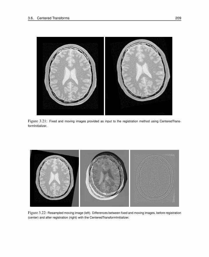
3.6. Centered Transforms 209
Figure 3.21: Fixed and moving images provided as input to the registration method using CenteredTrans-
formInitializer.
Figure 3.22: Resampled moving image (left). Differences between fixed and moving images, before registration
(center) and after registration (right) with the CenteredTransformInitializer.

210 Chapter 3. Registration
0
200
400
600
800
1000
1200
1400
1600
0 5 10 15 20 25
Squa
re D
iffe
renc
es M
etri
c
Iteration No.
0
0.02
0.04
0.06
0.08
0.1
0.12
0.14
0.16
0.18
0 5 10 15 20 25
Rot
atio
n A
ngle
(ra
dian
s)
Iteration No.
15.8
15.85
15.9
15.95
16
16.05
16.1
12.3 12.35 12.4 12.45 12.5 12.55 12.6 12.65 12.7 12.75 12.8 12.85
Y T
rans
latio
ns (
mm
)
X Translations (mm)
Figure 3.23: Plots of the Metric, rotation angle, center of rotation and translations during the registration using
CenteredTransformInitializer.
3.6.3 Similarity Transform in 2D
The source code for this section can be found in the file
ImageRegistration7.cxx.
This example illustrates the use of the itk::CenteredSimilarity2DTransform class for per-
forming registration in 2D. The example code is for the most part identical to the code presented
in Section 3.6.2. The main difference is the use of itk::CenteredSimilarity2DTransform here
rather than the itk::CenteredRigid2DTransform class.
A similarity transform can be seen as a composition of rotations, translations and uniform (isotropic)scaling. It preserves angles and maps lines into lines. This transform is implemented in the toolkit
as deriving from a rigid 2D transform and with a scale parameter added.
When using this transform, attention should be paid to the fact that scaling and translations are not
independent. In the same way that rotations can locally be seen as translations, scaling also results
in local displacements. Scaling is performed in general with respect to the origin of coordinates.
However, we already saw how ambiguous that could be in the case of rotations. For this reason,
this transform also allows users to setup a specific center. This center is used both for rotation and
scaling.
In addition to the headers included in previous examples, here the following header must be included.
#include "itkCenteredSimilarity2DTransform.h"
The Transform class is instantiated using the code below. The only template parameter of this class
is the representation type of the space coordinates.
typedef itk::CenteredSimilarity2DTransform< double > TransformType;

3.6. Centered Transforms 211
As before, the transform object is constructed and initialized before it is passed to the registration
filter.
TransformType::Pointer transform = TransformType::New();
In this example, we again use the helper class itk::CenteredTransformInitializer to compute
a reasonable value for the initial center of rotation and the translation.
typedef itk::CenteredTransformInitializer<
TransformType,
FixedImageType,
MovingImageType > TransformInitializerType;
TransformInitializerType::Pointer initializer
= TransformInitializerType::New();
initializer->SetTransform( transform );
initializer->SetFixedImage( fixedImageReader->GetOutput() );
initializer->SetMovingImage( movingImageReader->GetOutput() );
initializer->MomentsOn();
initializer->InitializeTransform();
The remaining parameters of the transform are initialized below.
transform->SetScale( initialScale );
transform->SetAngle( initialAngle );
Now the initialized transform object will be set to the registration method, and its initial parameters
are used to initialize the registration process.
Also, by calling the InPlaceOn() method, this initialized transform will be the output transform
object or “grafted” to the output of the registration process.
registration->SetInitialTransform( transform );
registration->InPlaceOn();
Keeping in mind that the scale of units in scaling, rotation and translation are quite different, we take
advantage of the scaling functionality provided by the optimizers. We know that the first element of
the parameters array corresponds to the scale factor, the second corresponds to the angle, third and
fourth are the center of rotation and fifth and sixth are the remaining translation. We use henceforth
small factors in the scales associated with translations and the rotation center.

212 Chapter 3. Registration
typedef OptimizerType::ScalesType OptimizerScalesType;
OptimizerScalesType optimizerScales( transform->GetNumberOfParameters() );
const double translationScale = 1.0 / 100.0;
optimizerScales[0] = 10.0;
optimizerScales[1] = 1.0;
optimizerScales[2] = translationScale;
optimizerScales[3] = translationScale;
optimizerScales[4] = translationScale;
optimizerScales[5] = translationScale;
optimizer->SetScales( optimizerScales );
We also set the ordinary parameters of the optimization method. In this case we are using a
itk::RegularStepGradientDescentOptimizerv4. Below we define the optimization parame-
ters, i.e. initial learning rate (step length), minimal step length and number of iterations. The last
two act as stopping criteria for the optimization.
optimizer->SetLearningRate( steplength );
optimizer->SetMinimumStepLength( 0.0001 );
optimizer->SetNumberOfIterations( 500 );
Let’s execute this example over some of the images provided in Examples/Data, for example:
• BrainProtonDensitySliceBorder20.png
• BrainProtonDensitySliceR10X13Y17S12.png
The second image is the result of intentionally rotating the first image by 10 degrees, scaling by
1/1.2 and then translating by (−13,−17). Both images have unit-spacing and are shown in Figure
3.24. The registration takes 60 iterations and produces:
[0.833193, -0.174514, 111.025, 131.92, -12.7267, -12.757]
That are interpreted as
• Scale factor = 0.833193
• Angle = −0.174514 radians
• Center = (111.025,131.92) millimeters
• Translation = (−12.7267,−12.757)millimeters
These values approximate the misalignment intentionally introduced into the moving image. Since
10 degrees is about 0.174532 radians.

3.6. Centered Transforms 213
Figure 3.24: Fixed and Moving image provided as input to the registration method using the Similarity2D
transform.
Figure 3.25: Resampled moving image (left). Differences between fixed and moving images, before (center)
and after (right) registration with the Similarity2D transform.

214 Chapter 3. Registration
0
2000
4000
6000
8000
10000
12000
14000
16000
0 10 20 30 40 50 60
Squa
re D
iffe
renc
es M
etri
c
Iteration No.
-0.55
-0.5
-0.45
-0.4
-0.35
-0.3
-0.25
-0.2
-0.15
-0.1
0 10 20 30 40 50 60
Rot
atio
n A
ngle
(ra
dian
s)
Iteration No.
0.5
0.6
0.7
0.8
0.9
1
1.1
1.2
0 10 20 30 40 50 60
Scal
e Fa
ctor
Iteration No.
-14
-13.8
-13.6
-13.4
-13.2
-13
-12.8
-12.6
-13.1 -13 -12.9 -12.8 -12.7 -12.6 -12.5 -12.4 -12.3 -12.2 -12.1
Y T
rans
latio
ns (
mm
)
X Translations (mm)
Figure 3.26: Plots of the Metric, rotation angle, scale factor, and translations during the registration using
Similarity2D transform.
Figure 3.25 shows the output of the registration. The right image shows the squared magnitude of
pixel differences between the fixed image and the resampled moving image.
Figure 3.26 shows the plots of the main output parameters of the registration process. The metric
values at every iteration are shown on the left. The rotation angle and scale factor values are shown
in the two center plots while the translation components of the registration are presented in the plot
on the right.
3.6.4 Rigid Transform in 3D
The source code for this section can be found in the file
ImageRegistration8.cxx.
This example illustrates the use of the itk::VersorRigid3DTransform class for performing reg-
istration of two 3D images. The class itk::CenteredTransformInitializer is used to initialize
the center and translation of the transform. The case of rigid registration of 3D images is probably
one of the most common uses of image registration.
The following are the most relevant headers of this example.
#include "itkVersorRigid3DTransform.h"
#include "itkCenteredTransformInitializer.h"
The parameter space of the VersorRigid3DTransform is not a vector space, because addition is
not a closed operation in the space of versor components. Hence, we need to use Versor composi-
tion operation to update the first three components of the parameter array (rotation parameters), and
Vector addition for updating the last three components of the parameters array (translation parame-
ters) [25, 28].
In the previous version of ITK, a special optimizer, itk::VersorRigid3DTransformOptimizer

3.6. Centered Transforms 215
was needed for registration to deal with versor computations. Fortunately in ITKv4, the
itk::RegularStepGradientDescentOptimizerv4 can be used for both vector and versor trans-
form optimizations because, in the new registration framework, the task of updating parameters
is delegated to the moving transform itself. The UpdateTransformParameters method is imple-
mented in the itk::Transform class as a virtual function, and all the derived transform classes
can have their own implementations of this function. Due to this fact, the updating function is re-
implemented for versor transforms so it can handle versor composition of the rotation parameters.
#include "itkRegularStepGradientDescentOptimizerv4.h"
The Transform class is instantiated using the code below. The only template parameter to this class
is the representation type of the space coordinates.
typedef itk::VersorRigid3DTransform< double > TransformType;
The initial transform object is constructed below. This transform will be initialized, and its initial
parameters will be used when the registration process starts.
TransformType::Pointer initialTransform = TransformType::New();
The input images are taken from readers. It is not necessary here to explicitly call Update() on the
readers since the itk::CenteredTransformInitializer will do it as part of its computations.
The following code instantiates the type of the initializer. This class is templated over the fixed and
moving image types as well as the transform type. An initializer is then constructed by calling the
New() method and assigning the result to a smart pointer.
typedef itk::CenteredTransformInitializer<
TransformType,
FixedImageType,
MovingImageType > TransformInitializerType;
TransformInitializerType::Pointer initializer =
TransformInitializerType::New();
The initializer is now connected to the transform and to the fixed and moving images.
initializer->SetTransform( initialTransform );
initializer->SetFixedImage( fixedImageReader->GetOutput() );
initializer->SetMovingImage( movingImageReader->GetOutput() );
The use of the geometrical centers is selected by calling GeometryOn() while the use of center of
mass is selected by calling MomentsOn(). Below we select the center of mass mode.
initializer->MomentsOn();
Finally, the computation of the center and translation is triggered by the InitializeTransform()
method. The resulting values will be passed directly to the transform.

216 Chapter 3. Registration
initializer->InitializeTransform();
The rotation part of the transform is initialized using a itk::Versor which is simply a unit quater-
nion. The VersorType can be obtained from the transform traits. The versor itself defines the type
of the vector used to indicate the rotation axis. This trait can be extracted as VectorType. The
following lines create a versor object and initialize its parameters by passing a rotation axis and an
angle.
typedef TransformType::VersorType VersorType;
typedef VersorType::VectorType VectorType;
VersorType rotation;
VectorType axis;
axis[0] = 0.0;
axis[1] = 0.0;
axis[2] = 1.0;
const double angle = 0;
rotation.Set( axis, angle );
initialTransform->SetRotation( rotation );
Now the current initialized transform will be set to the registration method, so its initial parameters
can be used to initialize the registration process.
registration->SetInitialTransform( initialTransform );
Let’s execute this example over some of the images available in the following website
http://public.kitware.com/pub/itk/Data/BrainWeb.
Note that the images in this website are compressed in .tgz files. You should download these files
and decompress them in your local system. After decompressing and extracting the files you could
take a pair of volumes, for example the pair:
• brainweb1e1a10f20.mha
• brainweb1e1a10f20Rot10Tx15.mha
The second image is the result of intentionally rotating the first image by 10 degrees around the
origin and shifting it 15mm in X .
Also, instead of doing the above steps manually, you can turn on the following flag in your build
environment:
ITK USE BRAINWEB DATA
Then, the above data will be loaded to your local ITK build directory.
The registration takes 21 iterations and produces:
[7.2295e-05, -7.20626e-05, -0.0872168, 2.64765, -17.4626, -0.00147153]

3.6. Centered Transforms 217
That are interpreted as
• Versor = (7.2295e− 05,−7.20626e−05,−0.0872168)
• Translation = (2.64765,−17.4626,−0.00147153)millimeters
This Versor is equivalent to a rotation of 9.98 degrees around the Z axis.
Note that the reported translation is not the translation of (15.0,0.0,0.0) that we may be naively ex-
pecting. The reason is that the VersorRigid3DTransform is applying the rotation around the cen-
ter found by the CenteredTransformInitializer and then adding the translation vector shown
above.
It is more illustrative in this case to take a look at the actual rotation matrix and offset resulting from
the 6 parameters.
TransformType::MatrixType matrix = finalTransform->GetMatrix();
TransformType::OffsetType offset = finalTransform->GetOffset();
std::cout << "Matrix = " << std::endl << matrix << std::endl;
std::cout << "Offset = " << std::endl << offset << std::endl;
The output of this print statements is
Matrix =
0.984786 0.173769 -0.000156187
-0.173769 0.984786 -0.000131469
0.000130965 0.000156609 1
Offset =
[-15, 0.0189186, -0.0305439]
From the rotation matrix it is possible to deduce that the rotation is happening in the X,Y plane and
that the angle is on the order of arcsin(0.173769) which is very close to 10 degrees, as we expected.
Figure 3.28 shows the output of the registration. The center image in this figure shows the differences
between the fixed image and the resampled moving image before the registration. The image on the
right side presents the difference between the fixed image and the resampled moving image after
the registration has been performed. Note that these images are individual slices extracted from the
actual volumes. For details, look at the source code of this example, where the ExtractImageFilter
is used to extract a slice from the the center of each one of the volumes. One of the main purposes
of this example is to illustrate that the toolkit can perform registration on images of any dimension.
The only limitations are, as usual, the amount of memory available for the images and the amount
of computation time that it will take to complete the optimization process.
Figure 3.29 shows the plots of the main output parameters of the registration process. The Z com-
ponent of the versor is plotted as an indication of how the rotation progresses. The X,Y translation
components of the registration are plotted at every iteration too.

218 Chapter 3. Registration
Figure 3.27: Fixed and moving image provided as input to the registration method using CenteredTransformIni-
tializer.
Figure 3.28: Resampled moving image (left). Differences between fixed and moving images, before (center)
and after (right) registration with the CenteredTransformInitializer.

3.6. Centered Transforms 219
0
500
1000
1500
2000
2500
0 5 10 15 20
Squa
re D
iffe
renc
es M
etri
c
Iteration No.
-0.09
-0.08
-0.07
-0.06
-0.05
-0.04
-0.03
-0.02
-0.01
0 5 10 15 20
Z V
erso
r C
ompo
nent
Iteration No.
-17.6
-17.4
-17.2
-17
-16.8
-16.6
-16.4
-16.2
-16
-15.8
2.3 2.35 2.4 2.45 2.5 2.55 2.6 2.65 2.7
Y T
rans
latio
ns (
mm
)
X Translations (mm)
Figure 3.29: Plots of the metric, rotation angle, center of rotation and translations during the registration using
CenteredTransformInitializer.
Shell and Gnuplot scripts for generating the diagrams in Figure 3.29 are available in the
ITKSoftwareGuide Git repository under the directory
ITKSoftwareGuide/SoftwareGuide/Art.
You are strongly encouraged to run the example code, since only in this way can you gain first-hand
experience with the behavior of the registration process. Once again, this is a simple reflection of
the philosophy that we put forward in this book:
If you can not replicate it, then it does not exist!
We have seen enough published papers with pretty pictures, presenting results that in practice are
impossible to replicate. That is vanity, not science.
3.6.5 Centered Affine Transform
The source code for this section can be found in the file
ImageRegistration9.cxx.
This example illustrates the use of the itk::AffineTransform for performing registration in 2D.
The example code is, for the most part, identical to that in 3.6.2. The main difference is the use of
the AffineTransform here instead of the itk::CenteredRigid2DTransform. We will focus on the
most relevant changes in the current code and skip the basic elements already explained in previous
examples.
Let’s start by including the header file of the AffineTransform.
#include "itkAffineTransform.h"
We then define the types of the images to be registered.

220 Chapter 3. Registration
const unsigned int Dimension = 2;
typedef float PixelType;
typedef itk::Image< PixelType, Dimension > FixedImageType;
typedef itk::Image< PixelType, Dimension > MovingImageType;
The transform type is instantiated using the code below. The template parameters of this class are
the representation type of the space coordinates and the space dimension.
typedef itk::AffineTransform< double, Dimension > TransformType;
The transform object is constructed below and is initialized before the registration process starts.
TransformType::Pointer transform = TransformType::New();
In this example, we again use the itk::CenteredTransformInitializer helper class in order to
compute reasonable values for the initial center of rotation and the translations. The initializer is set
to use the center of mass of each image as the initial correspondence correction.
typedef itk::CenteredTransformInitializer<
TransformType,
FixedImageType,
MovingImageType > TransformInitializerType;
TransformInitializerType::Pointer initializer
= TransformInitializerType::New();
initializer->SetTransform( transform );
initializer->SetFixedImage( fixedImageReader->GetOutput() );
initializer->SetMovingImage( movingImageReader->GetOutput() );
initializer->MomentsOn();
initializer->InitializeTransform();
Now we pass the transform object to the registration filter, and it will be grafted to the output trans-
form of the registration filter by updating its parameters during the the registration process.
registration->SetInitialTransform( transform );
registration->InPlaceOn();
Keeping in mind that the scale of units in scaling, rotation and translation are quite different, we
take advantage of the scaling functionality provided by the optimizers. We know that the first N ×N
elements of the parameters array correspond to the rotation matrix factor, and the last N are the
components of the translation to be applied after multiplication with the matrix is performed.

3.6. Centered Transforms 221
typedef OptimizerType::ScalesType OptimizerScalesType;
OptimizerScalesType optimizerScales( transform->GetNumberOfParameters() );
optimizerScales[0] = 1.0;
optimizerScales[1] = 1.0;
optimizerScales[2] = 1.0;
optimizerScales[3] = 1.0;
optimizerScales[4] = translationScale;
optimizerScales[5] = translationScale;
optimizer->SetScales( optimizerScales );
We also set the usual parameters of the optimization method. In this case we are using an
itk::RegularStepGradientDescentOptimizerv4 as before. Below, we define the optimization
parameters like learning rate (initial step length), minimum step length and number of iterations.
These last two act as stopping criteria for the optimization.
optimizer->SetLearningRate( steplength );
optimizer->SetMinimumStepLength( 0.0001 );
optimizer->SetNumberOfIterations( maxNumberOfIterations );
Finally we trigger the execution of the registration method by calling the Update() method. The
call is placed in a try/catch block in the case any exceptions are thrown.
try
{
registration->Update();
std::cout << "Optimizer stop condition: "
<< registration->GetOptimizer()->GetStopConditionDescription()
<< std::endl;
}
catch( itk::ExceptionObject & err )
{
std::cerr << "ExceptionObject caught !" << std::endl;
std::cerr << err << std::endl;
return EXIT_FAILURE;
}
Once the optimization converges, we recover the parameters from the registration method. We can
also recover the final value of the metric with the GetValue() method and the final number of
iterations with the GetCurrentIteration() method.
const TransformType::ParametersType finalParameters =
registration->GetOutput()->Get()->GetParameters();
const double finalRotationCenterX = transform->GetCenter()[0];
const double finalRotationCenterY = transform->GetCenter()[1];
const double finalTranslationX = finalParameters[4];
const double finalTranslationY = finalParameters[5];
const unsigned int numberOfIterations = optimizer->GetCurrentIteration();
const double bestValue = optimizer->GetValue();

222 Chapter 3. Registration
Let’s execute this example over two of the images provided in Examples/Data:
• BrainProtonDensitySliceBorder20.png
• BrainProtonDensitySliceR10X13Y17.png
The second image is the result of intentionally rotating the first image by 10 degrees and then trans-
lating by (−13,−17). Both images have unit-spacing and are shown in Figure 3.30. We execute
the code using the following parameters: step length=1.0, translation scale= 0.0001 and maximum
number of iterations = 300. With these images and parameters the registration takes 92 iterations
and produces
90 44.0851 [0.9849, -0.1729, 0.1725, 0.9848, 12.4541, 16.0759] AffineAngle: 9.9494
These results are interpreted as
• Iterations = 92
• Final Metric = 44.0386
• Center = (111.204,131.591) millimeters
• Translation = (12.4542,16.076) millimeters
• Affine scales = (1.00014, .999732)
The second component of the matrix values is usually associated with sinθ. We obtain the rota-
tion through SVD of the affine matrix. The value is 9.9494 degrees, which is approximately the
intentional misalignment of 10.0 degrees.
Figure 3.31 shows the output of the registration. The right most image of this figure shows the
squared magnitude difference between the fixed image and the resampled moving image.
Figure 3.32 shows the plots of the main output parameters of the registration process. The metric
values at every iteration are shown on the left plot. The angle values are shown on the middle plot,
while the translation components of the registration are presented on the right plot. Note that the
final total offset of the transform is to be computed as a combination of the shift due to rotation plus
the explicit translation set on the transform.
3.7 Multi-Resolution Registration
Performing image registration using a multi-resolution approach is widely used to improve speed,
accuracy and robustness. The basic idea is that registration is first performed at a coarse scale where

3.7. Multi-Resolution Registration 223
Figure 3.30: Fixed and moving images provided as input to the registration method using the AffineTransform.
Figure 3.31: The resampled moving image (left), and the difference between the fixed and moving images
before (center) and after (right) registration with the AffineTransform transform.

224 Chapter 3. Registration
0
500
1000
1500
2000
2500
3000
3500
4000
4500
5000
0 10 20 30 40 50 60 70 80 90
Squa
re D
iffe
renc
es M
etri
c
Iteration No.
1
2
3
4
5
6
7
8
9
10
0 10 20 30 40 50 60 70 80 90
Ang
le (
degr
ees)
Iteration No.
15
15.2
15.4
15.6
15.8
16
16.2
16.4
12 12.5 13 13.5 14 14.5 15
Y T
rans
latio
ns (
mm
)
X Translations (mm)
Figure 3.32: Metric values, rotation angle and translations during the registration using the AffineTransform
transform.
the images have fewer pixels. The spatial mapping determined at the coarse level is then used
to initialize registration at the next finer scale. This process is repeated until it reaches the finest
possible scale. This coarse-to-fine strategy greatly improves the registration success rate and also
increases robustness by eliminating local optima at coarser scales. Robustness can be improved even
more by smoothing the images at coarse scales.
In all previous examples we ran the registration process at a single resolution. However, the ITKv4
registration framework is structured to provide a multi-resolution registration method. For this pur-
pose we only need to define the number of levels as well as the resolution and smoothness of the
input images at each level. The registration filter smoothes and subsamples the images according to
user-defined ShrinkFactor and SmoothingSigma vectors.
We now present the multi-resolution capabilities of the framework by way of an example.
3.7.1 Fundamentals
The source code for this section can be found in the file
MultiResImageRegistration1.cxx.
This example illustrates the use of the itk::ImageRegistrationMethodv4 to solve a simple
multi-modality registration problem by a multi-resolution approach. Since ITKv4 registration
method is designed based on a multi-resolution structure, a separate set of classes are no longer
required to run the registration process of this example.
This a great advantage over the previous versions of ITK, as in ITKv3 we had to use a different filter (
itk::MultiResolutionImageRegistrationMethod) to run a multi-resolution process. Also, we
had to use image pyramids filters ( itk::MultiResolutionPyramidImageFilter) for creating the
sequence of downsampled images. Hence, you can see how ITKv4 framework is more user-friendly
in more complex situations.

3.7. Multi-Resolution Registration 225
Transform
Registration Level 0
Registration Level 2
Registration Level 1
Registration Level 3
Registration Level 4
Transform
Fixed ImagePyramidMoving Image
Pyramid
Transform
Transform
Transform
Figure 3.33: Conceptual representation of the multi-resolution registration process.
To begin the example, we include the headers of the registration components we will use.
#include "itkImageRegistrationMethodv4.h"
#include "itkTranslationTransform.h"
#include "itkMattesMutualInformationImageToImageMetricv4.h"
#include "itkRegularStepGradientDescentOptimizerv4.h"
The ImageRegistrationMethodv4 solves a registration problem in a coarse-to-fine manner as illus-
trated in Figure 3.33. The registration is first performed at the coarsest level using the images at the
first level of the fixed and moving image pyramids. The transform parameters determined by the
registration are then used to initialize the registration at the next finer level using images from the
second level of the pyramids. This process is repeated as we work up to the finest level of image
resolution.
In a typical registration scenario, a user will tweak component settings or even swap out components
between multi-resolution levels. For example, when optimizing at a coarse resolution, it may be
possible to take more aggressive step sizes and have a more relaxed convergence criterion.
Tweaking the components between resolution levels can be done using ITK’s implementation of
the Command/Observer design pattern. Before beginning registration at each resolution level,
where ImageRegistrationMethodv4 invokes a MultiResolutionIterationEvent(). The regis-
tration components can be changed by implementing a itk::Command which responds to the event.
A brief description of the interaction between events and commands was previously presented in
Section 3.4.
We will illustrate this mechanism by changing the parameters of the optimizer between each resolu-
tion level by way of a simple interface command. First, we include the header file of the Command
class.

226 Chapter 3. Registration
#include "itkCommand.h"
Our new interface command class is called RegistrationInterfaceCommand. It derives from
Command and is templated over the multi-resolution registration type.
template <typename TRegistration>
class RegistrationInterfaceCommand : public itk::Command
{
We then define Self, Superclass, Pointer, New() and a constructor in a similar fashion to the
CommandIterationUpdate class in Section 3.4.
public:
typedef RegistrationInterfaceCommand Self;
typedef itk::Command Superclass;
typedef itk::SmartPointer<Self> Pointer;
itkNewMacro( Self );
protected:
RegistrationInterfaceCommand() {};
For convenience, we declare types useful for converting pointers in the Execute() method.
public:
typedef TRegistration RegistrationType;
typedef RegistrationType * RegistrationPointer;
typedef itk::RegularStepGradientDescentOptimizerv4<double> OptimizerType;
typedef OptimizerType * OptimizerPointer;
Two arguments are passed to the Execute() method: the first is the pointer to the object which
invoked the event and the second is the event that was invoked.
void Execute( itk::Object * object,
const itk::EventObject & event) ITK_OVERRIDE
{
First we verify that the event invoked is of the right type,
itk::MultiResolutionIterationEvent(). If not, we return without any further action.
if( !(itk::MultiResolutionIterationEvent().CheckEvent( &event ) ) )
{
return;
}
We then convert the input object pointer to a RegistrationPointer. Note that no error checking is done
here to verify the dynamic cast was successful since we know the actual object is a registration
method. Then we ask for the optimizer object from the registration method.
RegistrationPointer registration =
static_cast<RegistrationPointer>( object );
OptimizerPointer optimizer = static_cast< OptimizerPointer >(
registration->GetModifiableOptimizer() );

3.7. Multi-Resolution Registration 227
If this is the first resolution level we set the learning rate (representing the first step size) and the
minimum step length (representing the convergence criterion) to large values. At each subsequent
resolution level, we will reduce the minimum step length by a factor of 5 in order to allow the
optimizer to focus on progressively smaller regions. The learning rate is set up to the current step
length. In this way, when the optimizer is reinitialized at the beginning of the registration process
for the next level, the step length will simply start with the last value used for the previous level.
This will guarantee the continuity of the path taken by the optimizer through the parameter space.
if ( registration->GetCurrentLevel() == 0 )
{
optimizer->SetLearningRate( 16.00 );
optimizer->SetMinimumStepLength( 2.5 );
}
else
{
optimizer->SetLearningRate( optimizer->GetCurrentStepLength() );
optimizer->SetMinimumStepLength(
optimizer->GetMinimumStepLength() * 0.2 );
}
Another version of the Execute() method accepting a const input object is also required since this
method is defined as pure virtual in the base class. This version simply returns without taking any
action.
void Execute(const itk::Object * , const itk::EventObject & ) ITK_OVERRIDE
{
return;
}
};
The fixed and moving image types are defined as in previous examples. The downsampled images
for different resolution levels are created internally by the registration method based on the values
provided for ShrinkFactor and SmoothingSigma vectors.
The types for the registration components are then derived using the fixed and moving image type,
as in previous examples.
To set the optimizer parameters, note that LearningRate and MinimumStepLength are set in the
obsever at the begining of each resolution level. The other optimizer parameters are set as follows.
optimizer->SetNumberOfIterations( 200 );
optimizer->SetRelaxationFactor( 0.5 );
We set the number of multi-resolution levels to three and set the corresponding shrink factor and
smoothing sigma values for each resolution level. Using smoothing in the subsampled images in
low-resolution levels can avoid large fluctuations in the metric function, which prevents the opti-
mizer from becoming trapped in local minima. In this simple example we have no smoothing, and
we have used small shrinkings for the first two resolution levels.

228 Chapter 3. Registration
const unsigned int numberOfLevels = 3;
RegistrationType::ShrinkFactorsArrayType shrinkFactorsPerLevel;
shrinkFactorsPerLevel.SetSize( 3 );
shrinkFactorsPerLevel[0] = 3;
shrinkFactorsPerLevel[1] = 2;
shrinkFactorsPerLevel[2] = 1;
RegistrationType::SmoothingSigmasArrayType smoothingSigmasPerLevel;
smoothingSigmasPerLevel.SetSize( 3 );
smoothingSigmasPerLevel[0] = 0;
smoothingSigmasPerLevel[1] = 0;
smoothingSigmasPerLevel[2] = 0;
registration->SetNumberOfLevels ( numberOfLevels );
registration->SetShrinkFactorsPerLevel( shrinkFactorsPerLevel );
registration->SetSmoothingSigmasPerLevel( smoothingSigmasPerLevel );
Once all the registration components are in place we can create an instance of our interface command
and connect it to the registration object using the AddObserver() method.
typedef RegistrationInterfaceCommand<RegistrationType> CommandType;
CommandType::Pointer command = CommandType::New();
registration->AddObserver( itk::MultiResolutionIterationEvent(), command );
Then we trigger the registration process by calling Update().
Let’s execute this example using the following images
• BrainT1SliceBorder20.png
• BrainProtonDensitySliceShifted13x17y.png
The output produced by the execution of the method is
0 -0.316956 [11.4200, 11.2063]
1 -0.562048 [18.2938, 25.6545]
2 -0.407696 [11.3643, 21.6569]
3 -0.5702 [13.7244, 18.4274]
4 -0.803252 [11.1634, 15.3547]
0 -0.697586 [12.8778, 16.3846]
1 -0.901984 [13.1794, 18.3617]
2 -0.827423 [13.0545, 17.3695]
3 -0.92754 [12.8528, 16.3901]
4 -0.902671 [12.9426, 16.8819]
5 -0.941212 [13.1402, 17.3413]

3.7. Multi-Resolution Registration 229
Figure 3.34: Mapped moving image (left) and composition of fixed and moving images before (center) and
after (right) registration.
0 -0.922239 [13.0364, 17.1138]
1 -0.930203 [12.9463, 16.8806]
2 -0.930959 [13.0191, 16.9822]
Result =
Translation X = 13.0192
Translation Y = 16.9823
Iterations = 4
Metric value = -0.929237
These values are a close match to the true misalignment of (13,17) introduced in the moving image.
The result of resampling the moving image is presented in the left image of Figure 3.34. The center
and right images of the figure depict a checkerboard composite of the fixed and moving images
before and after registration.
Figure 3.35 (left) shows the sequence of translations followed by the optimizer as it searched the
parameter space. The right side of the same figure shows the sequence of metric values computed
as the optimizer searched the parameter space. From the trace, we can see that with the more
aggressive optimization parameters we get quite close to the optimal value within 5 iterations with
the remaining iterations just doing fine adjustments. It is interesting to compare these results with
those of the single resolution example in Section 3.5.1, where 46 iterations were required as more
conservative optimization parameters had to be used.

230 Chapter 3. Registration
10
12
14
16
18
20
22
24
26
11 12 13 14 15 16 17 18 19
Y T
rans
latio
ns (
mm
)
X Translations (mm)
-1
-0.9
-0.8
-0.7
-0.6
-0.5
-0.4
-0.3
0 2 4 6 8 10 12 14
Met
ric
Iteration No.
Figure 3.35: Sequence of translations and metric values at each iteration of the optimizer.
3.8 Multi-Stage Registration
In section 3.7 you noticed how to tweak component settings between multi-resolution levels and saw
how it can benefit the registration process. That is, the matching metric gets close to the optimal
value before final parameter adjustments in full resolution. This approach saves large amounts of
time in most practical cases, since fewer iterations are required at the full resolution level. This is
helpful in cases like a deformable registration process on a large dataset, e.g. a high-resolution 3D
image.
Another possible scheme is to apply a simple rigid transform for the initial coarse registration, then
upgrade to an affine transform at the finer level. Finally, proceed to a deformable transform at the
last level when we are close enough to the optimal value.
Fortunately, itk::ImageRegistrationMethodv4 allows for multistage registration whereby each
stage is characterized by possibly different transforms and different image metrics. As in the above
situation, you may want to perform a linear registration followed by a deformable registration with
both stages performed across multiple resolutions.
Multiple stages are handled by linking multiple instantiations of this class. An optional composite
transform can be used as a container to concatenate the output transforms of multiple stages.
We now present the multistage capabilities of the framework by way of an example.

3.8. Multi-Stage Registration 231
3.8.1 Fundamentals
The source code for this section can be found in the file
MultiStageImageRegistration1.cxx.
This example illustrates the use of more complex components of the registration framework. In
particular, it introduces a multistage, multi-resolution approach to run a multi-modal registration
process using two linear itk::TranslationTransform and itk::AffineTransform . Also, it
shows the use of Scale Estimators for fine-tuning the scale parameters of the optimizer when an
Affine transform is used. The itk::RegistrationParameterScalesFromPhysicalShift filter
is used for automatic estimation of the parameters scales.
To begin the example, we include the headers of the registration components we will use.
#include "itkImageRegistrationMethodv4.h"
#include "itkMattesMutualInformationImageToImageMetricv4.h"
#include "itkRegularStepGradientDescentOptimizerv4.h"
#include "itkConjugateGradientLineSearchOptimizerv4.h"
#include "itkTranslationTransform.h"
#include "itkAffineTransform.h"
#include "itkCompositeTransform.h"
In a multistage scenario, each stage needs an individual instantiation of the
itk::ImageRegistrationMethodv4, so each stage can possibly have a different transform,
a different optimizer, and a different image metric and can be performed in multiple levels. The
configuration of the registration method at each stage closely follows the procedure in the previous
section.
In early stages we can use simpler transforms and more aggressive optimization parameters to take
big steps toward the optimal value. Then, at the final stage we can have a more complex transform
to do fine adjustments of the final parameters.
A possible scheme is to use a simple translation transform for initial coarse registration levels and
upgrade to an affine transform at the finer level. Since we have two different types of transforms, we
can use a multistage registration approach as shown in the current example.
First we need to configure the registration components of the initial stage. The instantiation of the
transform type requires only the dimension of the space and the type used for representing space
coordinates.
typedef itk::TranslationTransform< double, Dimension > TTransformType;
The types of other registration components are defined here.
itk::RegularStepGradientDescentOptimizerv4 is used as the optimizer of the first stage.
Also, we use itk::MattesMutualInformationImageToImageMetricv4 as the metric since it
is fitted for a multi-modal registration.

232 Chapter 3. Registration
typedef itk::RegularStepGradientDescentOptimizerv4< double > TOptimizerType;
typedef itk::MattesMutualInformationImageToImageMetricv4<
FixedImageType,
MovingImageType > MetricType;
typedef itk::ImageRegistrationMethodv4<
FixedImageType,
MovingImageType,
TTransformType > TRegistrationType;
Then, all the components are instantiated using their New() method and connected to the registration
object as in previous examples.
The output transform of the registration process will be constructed internally in the registration filter
since the related TransformType is already passed to the registration method as a template parameter.
However, we should provide an initial moving transform for the registration method if needed.
TTransformType::Pointer movingInitTx = TTransformType::New();
After setting the initial parameters, the initial transform can be passed to the registration filter by
SetMovingInitialTransform() method.
transRegistration->SetMovingInitialTransform( movingInitTx );
We can use a itk::CompositeTransform to stack all the output transforms resulted from multiple
stages. This composite transform should also hold the moving initial transform (if it exists) because
as explained in section 3.6.1, the output of each registration stage does not include the input initial
transform to that stage.
typedef itk::CompositeTransform< double,
Dimension > CompositeTransformType;
CompositeTransformType::Pointer compositeTransform =
CompositeTransformType::New();
compositeTransform->AddTransform( movingInitTx );
In the case of this simple example, the first stage is run only in one level of registration at a coarse
resolution.
const unsigned int numberOfLevels1 = 1;
TRegistrationType::ShrinkFactorsArrayType shrinkFactorsPerLevel1;
shrinkFactorsPerLevel1.SetSize( numberOfLevels1 );
shrinkFactorsPerLevel1[0] = 3;
TRegistrationType::SmoothingSigmasArrayType smoothingSigmasPerLevel1;
smoothingSigmasPerLevel1.SetSize( numberOfLevels1 );
smoothingSigmasPerLevel1[0] = 2;
transRegistration->SetNumberOfLevels ( numberOfLevels1 );
transRegistration->SetShrinkFactorsPerLevel( shrinkFactorsPerLevel1 );
transRegistration->SetSmoothingSigmasPerLevel( smoothingSigmasPerLevel1 );

3.8. Multi-Stage Registration 233
Also, for this initial stage we can use a more agressive parameter set for the optimizer by taking a
big step size and relaxing stop criteria.
transOptimizer->SetLearningRate( 16 );
transOptimizer->SetMinimumStepLength( 1.5 );
Once all the registration components are in place, we trigger the registration process by calling
Update() and add the result output transform to the final composite transform, so this composite
transform can be used to initialize the next registration stage.
try
{
transRegistration->Update();
std::cout << "Optimizer stop condition: "
<< transRegistration->GetOptimizer()->GetStopConditionDescription()
<< std::endl;
}
catch( itk::ExceptionObject & err )
{
std::cout << "ExceptionObject caught !" << std::endl;
std::cout << err << std::endl;
return EXIT_FAILURE;
}
compositeTransform->AddTransform(
transRegistration->GetModifiableTransform() );
Now we can upgrade to an Affine transform as the second stage of registration process. The Affine-
Transform is a linear transformation that maps lines into lines. It can be used to represent transla-
tions, rotations, anisotropic scaling, shearing or any combination of them. Details about the affine
transform can be seen in Section 3.9.16. The instantiation of the transform type requires only the
dimension of the space and the type used for representing space coordinates.
typedef itk::AffineTransform< double, Dimension > ATransformType;
We also use a different optimizer in configuration of the second stage while the metric is kept the
same as before.
typedef itk::ConjugateGradientLineSearchOptimizerv4Template<
double > AOptimizerType;
typedef itk::ImageRegistrationMethodv4<
FixedImageType,
MovingImageType,
ATransformType > ARegistrationType;
Again all the components are instantiated using their New() method and connected to the registration
object like in previous stages.
The current stage can be initialized using the initial transform of the registration and the result
transform of the previous stage, so that both are concatenated into the composite transform.

234 Chapter 3. Registration
affineRegistration->SetMovingInitialTransform( compositeTransform );
In Section 3.6.2 we showed the importance of center of rotation in the registration process. In Affine
transforms, the center of rotation is defined by the fixed parameters set, which are set by default to
[0, 0]. However, consider a situation where the origin of the virtual space, in which the registration
is run, is far away from the zero origin. In such cases, leaving the center of rotation as the default
value can make the optimization process unstable. Therefore, we are always interested to set the
center of rotation to the center of virtual space which is usually the fixed image space.
Note that either center of gravity or geometrical center can be used as the center of rotation. In this
example center of rotation is set to the geometrical center of the fixed image. We could also use
itk::ImageMomentsCalculator filter to compute the center of mass.
Based on the above discussion, the user must set the fixed parameters of the registration transform
outside of the registraton method, so first we instantiate an object of the output transform type.
ATransformType::Pointer affineTx = ATransformType::New();
Then, we compute the physical center of the fixed image and set that as the center of the output
Affine transform.
typedef FixedImageType::SpacingType SpacingType;
typedef FixedImageType::PointType OriginType;
typedef FixedImageType::RegionType RegionType;
typedef FixedImageType::SizeType SizeType;
FixedImageType::Pointer fixedImage = fixedImageReader->GetOutput();
const SpacingType fixedSpacing = fixedImage->GetSpacing();
const OriginType fixedOrigin = fixedImage->GetOrigin();
const RegionType fixedRegion = fixedImage->GetLargestPossibleRegion();
const SizeType fixedSize = fixedRegion.GetSize();
ATransformType::InputPointType centerFixed;
centerFixed[0] =
fixedOrigin[0] + fixedSpacing[0] * fixedSize[0] / 2.0;
centerFixed[1] =
fixedOrigin[1] + fixedSpacing[1] * fixedSize[1] / 2.0;
const unsigned int numberOfFixedParameters =
affineTx->GetFixedParameters().Size();
ATransformType::ParametersType fixedParameters( numberOfFixedParameters );
for (unsigned int i = 0; i < numberOfFixedParameters; ++i)
{
fixedParameters[i] = centerFixed[i];
}
affineTx->SetFixedParameters( fixedParameters );
Then, the initialized output transform should be connected to the registration object by using
SetInitialTransform() method.

3.8. Multi-Stage Registration 235
It is important to distinguish between the SetInitialTransform() and
SetMovingInitialTransform() that was used to initialize the registration stage based on
the results of the previous stages. You can assume that the first one is used for direct manipulation
of the optimizable transform in current registration process.
affineRegistration->SetInitialTransform( affineTx );
The set of optimizable parameters in the Affine transform have different dynamic ranges. Typi-
cally the parameters associated with the matrix have values around [−1 : 1], although they are not
restricted to this interval. Parameters associated with translations, on the other hand, tend to have
much higher values, typically on the order of 10.0 to 100.0. This difference in dynamic range neg-
atively affects the performance of gradient descent optimizers. ITK provides some mechanisms
to compensate for such differences in values among the parameters when they are passed to the
optimizer.
The first mechanism consists of providing an array of scale factors to the optimizer. These factors
re-normalize the gradient components before they are used to compute the step of the optimizer
at the current iteration. These scales are estimated by the user intuitively as shown in previous
examples of this chapter. In our particular case, a common choice for the scale parameters is to set
all those associated with the matrix coefficients to 1.0, that is, the first N ×N factors. Then, we set
the remaining scale factors to a small value.
Here the affine transform is represented by the matrix M and the vector T. The transformation of a
point P into P′ is expressed as
[
P′x
P′y
]
=
[
M11 M12
M21 M22
]
·[
Px
Py
]
+
[
Tx
Ty
]
(3.1)
Based on the above discussion, we need much smaller scales for translation parameters of vector
T (Tx, Ty) compared to the parameters of matrix M (M11, M12, M21, M22). However, it is not easy
to have an intuitive estimation of all parameter scales when we have to deal with a large paramter
space.
Fortunately, ITKv4 provides a framework for automated parameter scaling.
itk::RegistrationParameterScalesEstimator vastly reduces the difficulty of tuning pa-
rameters for different transform/metric combinations. Parameter scales are estimated by analyzing
the result of a small parameter update on the change in the magnitude of physical space deformation
induced by the transformation.
The impact from a unit change of a parameter may be defined in multiple ways, such
as the maximum shift of voxels in index or physical space, or the average norm of
transform Jacobian. Filters itk::RegistrationParameterScalesFromPhysicalShift and
itk::RegistrationParameterScalesFromIndexShift use the first definition to estimate the
scales, while the itk::RegistrationParameterScalesFromJacobian filter estimates scales
based on the later definition. In all methods, the goal is to rescale the transform parameters such that
a unit change of each scaled parameter will have the same impact on deformation.

236 Chapter 3. Registration
In this example the first filter is chosen to estimate the parameter scales. The scales estimator will
then be passed to optimizer.
typedef itk::RegistrationParameterScalesFromPhysicalShift<
MetricType> ScalesEstimatorType;
ScalesEstimatorType::Pointer scalesEstimator =
ScalesEstimatorType::New();
scalesEstimator->SetMetric( affineMetric );
scalesEstimator->SetTransformForward( true );
affineOptimizer->SetScalesEstimator( scalesEstimator );
The step length has to be proportional to the expected values of the parameters in the search space.
Since the expected values of the matrix coefficients are around 1.0, the initial step of the optimization
should be a small number compared to 1.0. As a guideline, it is useful to think of the matrix
coefficients as combinations of cos(θ) and sin(θ). This leads to use values close to the expected
rotation measured in radians. For example, a rotation of 1.0 degree is about 0.017 radians.
However, we need not worry about the above considerations. Thanks to the ScalesEstimator, the
initial step size can also be estimated automatically, either at each iteration or only at the first iter-
ation. In this example we choose to estimate learning rate once at the begining of the registration
process.
affineOptimizer->SetDoEstimateLearningRateOnce( true );
affineOptimizer->SetDoEstimateLearningRateAtEachIteration( false );
At the second stage, we run two levels of registration, where the second level is run in full resolution
in which we do the final adjustments of the output parameters.
const unsigned int numberOfLevels2 = 2;
ARegistrationType::ShrinkFactorsArrayType shrinkFactorsPerLevel2;
shrinkFactorsPerLevel2.SetSize( numberOfLevels2 );
shrinkFactorsPerLevel2[0] = 2;
shrinkFactorsPerLevel2[1] = 1;
ARegistrationType::SmoothingSigmasArrayType smoothingSigmasPerLevel2;
smoothingSigmasPerLevel2.SetSize( numberOfLevels2 );
smoothingSigmasPerLevel2[0] = 1;
smoothingSigmasPerLevel2[1] = 0;
affineRegistration->SetNumberOfLevels ( numberOfLevels2 );
affineRegistration->SetShrinkFactorsPerLevel( shrinkFactorsPerLevel2 );
affineRegistration->SetSmoothingSigmasPerLevel( smoothingSigmasPerLevel2 );
Finally we trigger the registration process by calling Update() and add the output transform of
the last stage to the composite transform. This composite transform will be considered as the final
transform of this multistage registration process and will be used by the resampler to resample the
moving image in to the virtual domain space (fixed image space if there is no fixed initial transform).

3.8. Multi-Stage Registration 237
try
{
affineRegistration->Update();
std::cout << "Optimizer stop condition: "
<< affineRegistration->GetOptimizer()->GetStopConditionDescription()
<< std::endl;
}
catch( itk::ExceptionObject & err )
{
std::cout << "ExceptionObject caught !" << std::endl;
std::cout << err << std::endl;
return EXIT_FAILURE;
}
compositeTransform->AddTransform(
affineRegistration->GetModifiableTransform() );
Let’s execute this example using the following multi-modality images:
• BrainT1SliceBorder20.png
• BrainProtonDensitySliceR10X13Y17.png
The second image is the result of intentionally rotating the first image by 10 degrees and then trans-
lating by (−13,−17). Both images have unit-spacing and are shown in Figure 3.36.
The registration converges after 5 iterations in the translation stage. Also, in the second stage, the
registration converges after 46 iterations in the first level, and 6 iterations in the second level. The
final results when printed as an array of parameters are:
Initial parameters of the registration process:
[3, 5]
Translation parameters after first registration stage:
[9.0346, 10.8303]
Affine parameters after second registration stage:
[0.9864, -0.1733, 0.1738, 0.9863, 0.9693, 0.1482]
As it can be seen, the translation parameters after the first stage compensate most of the offset be-
tween the fixed and moving images. When the images are close to each other, the affine registration
is run for the rotation and the final match. By reordering the Affine array of parameters as coeffi-
cients of matrix M and vector T they can now be seen as
M =
[
0.9864 −0.1733
0.1738 0.9863
]
and T =
[
0.9693
0.1482
]
(3.2)

238 Chapter 3. Registration
Figure 3.36: Fixed and moving images provided as input to the registration method using the AffineTransform.
In this form, it is easier to interpret the effect of the transform. The matrix M is responsible for
scaling, rotation and shearing while T is responsible for translations.
The second component of the matrix values is usually associated with sinθ. We obtain the rotation
through SVD of the affine matrix. The value is 9.975 degrees, which is approximately the intentional
misalignment of 10.0 degrees.
Also, let’s compute the total translation values resulting from initial transform, translation transform,
and the Affine transform together.
In X direction:
3+ 9.0346+ 0.9693= 13.0036 (3.3)
In Y direction:
5+ 10.8303+0.1482= 15.9785 (3.4)
It can be seen that the translation values closely match the true misalignment introduced in the
moving image.
It is important to note that once the images are registered at a sub-pixel level, any further improve-
ment of the registration relies heavily on the quality of the interpolator. It may then be reasonable to
use a coarse and fast interpolator in the lower resolution levels and switch to a high-quality but slow
interpolator in the final resolution level. However, in this example we used a linear interpolator for
all stages and different registration levels since it is so fast.
The result of resampling the moving image is presented in the left image of Figure 3.37. The center

3.8. Multi-Stage Registration 239
Figure 3.37: Mapped moving image (left) and composition of fixed and moving images before (center) and
after (right) registration.
and right images of the figure depict a checkerboard composite of the fixed and moving images
before and after registration.
3.8.2 Cascaded Multistage Registration
The source code for this section can be found in the file
MultiStageImageRegistration2.cxx.
This examples shows how different stages can be cascaded together directly in a multistage registra-
tion process. The example code is, for the most part, identical to the previous multistage example.
The main difference is that no initial transform is used, and the output of the first stage is directly
linked to the second stage, and the whole registration process is triggered only once by calling
Update() after the last stage stage.
We will focus on the most relevent changes in current code and skip all the similar parts already
explained in the previous example.
Let’s start by defining different types of the first stage.
typedef itk::TranslationTransform< double, Dimension > TTransformType;
typedef itk::RegularStepGradientDescentOptimizerv4<double> TOptimizerType;
typedef itk::MattesMutualInformationImageToImageMetricv4<
FixedImageType,
MovingImageType > MetricType;
typedef itk::ImageRegistrationMethodv4<
FixedImageType,
MovingImageType > TRegistrationType;
Type definitions are the same as previous example with an important subtle change: the transform

240 Chapter 3. Registration
type is not passed to the registration method as a template parameter anymore. In this case, the
registration filter will consider the transform base class itk::Transform as the type of its output
transform.
Instead of passing the transform type, we create an explicit instantiation of the transform ob-
ject outside of the registration filter, and connect that to the registration object using the
SetInitialTransform() method. Also, by calling InPlaceOn() method, this transform object
will be the output transform of the registration filter or will be grafted to the output.
TTransformType::Pointer translationTx = TTransformType::New();
transRegistration->SetInitialTransform( translationTx );
transRegistration->InPlaceOn();
Also, there is no initial transform defined for this example.
As in the previous example, the first stage is run using only one level of registration at a coarse
resolution level. However, notice that we do not need to update the translation registration filter at
this step since the output of this stage will be directly connected to the initial input of the next stage.
Due to ITK’s pipeline structure, when we call the Update() at the last stage, the first stage will be
updated as well.
Now we upgrade to an Affine transform as the second stage of registration process, and as before,
we initially define and instantiate different components of the current registration stage. We have
used a new optimizer but the same metric in new configurations.
typedef itk::AffineTransform< double, Dimension > ATransformType;
typedef itk::ConjugateGradientLineSearchOptimizerv4Template<
double > AOptimizerType;
typedef itk::ImageRegistrationMethodv4<
FixedImageType,
MovingImageType > ARegistrationType;
Again notice that TransformType is not passed to the type definition of the registration filter. It is
important because when the registration filter considers transform base class itk::Transform as
the type of its output transform, it prevents the type mismatch when the two stages are cascaded to
each other.
Then, all components are instantiated using their New() method and connected to the registration
object among the transform type. Despite the previous example, here we use the fixed image’s center
of mass to initialize the fixed parameters of the Affine transform. itk::ImageMomentsCalculator
filter is used for this purpose.

3.8. Multi-Stage Registration 241
typedef itk::ImageMomentsCalculator<
FixedImageType > FixedImageCalculatorType;
FixedImageCalculatorType::Pointer fixedCalculator =
FixedImageCalculatorType::New();
fixedCalculator->SetImage( fixedImage );
fixedCalculator->Compute();
FixedImageCalculatorType::VectorType fixedCenter =
fixedCalculator->GetCenterOfGravity();
Then, we initialize the fixed parameters (center of rotation) in the Affine transform and connect that
to the registration object.
ATransformType::Pointer affineTx = ATransformType::New();
const unsigned int numberOfFixedParameters =
affineTx->GetFixedParameters().Size();
ATransformType::ParametersType fixedParameters( numberOfFixedParameters );
for (unsigned int i = 0; i < numberOfFixedParameters; ++i)
{
fixedParameters[i] = fixedCenter[i];
}
affineTx->SetFixedParameters( fixedParameters );
affineRegistration->SetInitialTransform( affineTx );
affineRegistration->InPlaceOn();
Now, the output of the first stage is wrapped through a itk::DataObjectDecorator
and is passed to the input of the second stage as the moving initial transform via
SetMovingInitialTransformInput() method. Note that this API has an “Input” word attached
to the name of another initialization method SetMovingInitialTransform() that already has been
used in previous example. This extension means that the following API expects a data object deco-
rator type.
affineRegistration->SetMovingInitialTransformInput(
transRegistration->GetTransformOutput() );
Second stage runs two levels of registration, where the second level is run in full resolution.
Once all the registration components are in place, finally we trigger the whole registration process,
including two cascaded registration stages, by calling Update() on the registration filter of the last
stage, which causes both stages be updated.

242 Chapter 3. Registration
try
{
affineRegistration->Update();
std::cout << "Optimizer stop condition: "
<< affineRegistration->
GetOptimizer()->GetStopConditionDescription()
<< std::endl;
}
catch( itk::ExceptionObject & err )
{
std::cout << "ExceptionObject caught !" << std::endl;
std::cout << err << std::endl;
return EXIT_FAILURE;
}
Finally, a composite transform is used to concatenate the results of all stages together, which will
be considered as the final output of this multistage process and will be passed to the resampler to
resample the moving image into the virtual domain space (fixed image space if there is no fixed
initial transform).
typedef itk::CompositeTransform< double,
Dimension > CompositeTransformType;
CompositeTransformType::Pointer compositeTransform =
CompositeTransformType::New();
compositeTransform->AddTransform( translationTx );
compositeTransform->AddTransform( affineTx );
Let’s execute this example using the same multi-modality images as before. The registration con-
verges after 6 iterations in the first stage, also in 45 and 11 iterations corresponding to the first level
and second level of the Affine stage. The final results when printed as an array of parameters are:
Translation parameters after first registration stage:
[11.600, 15.1814]
Affine parameters after second registration stage:
[0.9860, -0.1742, 0.1751, 0.9862, 0.9219, 0.8023]
Let’s reorder the Affine array of parameters again as coefficients of matrix M and vector T. They
can now be seen as
M =
[
0.9860 −0.1742
0.1751 0.9862
]
and T =
[
0.9219
0.8023
]
(3.5)
10.02 degrees is the rotation value computed from the affine matrix parameters, which approxi-
mately equals the intentional misalignment.
Also for the total translation value resulted from both transforms, we have:

3.8. Multi-Stage Registration 243
Figure 3.38: Mapped moving image (left) and composition of fixed and moving images before (center) and
after (right) registration.
In X direction:
11.6004+ 0.9219= 12.5223 (3.6)
In Y direction:
15.1814+ 0.8023= 15.9837 (3.7)
These results closely match the true misalignment introduced in the moving image.
The result of resampling the moving image is presented in the left image of Figure 3.38. The center
and right images of the figure depict a checkerboard composite of the fixed and moving images
before and after registration.
With the completion of these examples, we will now review the main features of the components
forming the registration framework.

244 Chapter 3. Registration
Point Vector
Covariant
Vectors
Figure 3.39: Geometric representation objects in ITK.
3.9 Transforms
In the Insight Toolkit, itk::Transform objects encapsulate the mapping of points and vectors
from an input space to an output space. If a transform is invertible, back transform methods are
also provided. Currently, ITK provides a variety of transforms from simple translation, rotation and
scaling to general affine and kernel transforms. Note that, while in this section we discuss transforms
in the context of registration, transforms are general and can be used for other applications. Some
of the most commonly used transforms will be discussed in detail later. Let’s begin by introducing
the objects used in ITK for representing basic spatial concepts.
3.9.1 Geometrical Representation
ITK implements a consistent geometric representation of space. The characteristics of classes in-
volved in this representation are summarized in Table 3.1. In this regard, ITK takes full advantage
of the capabilities of Object Oriented programming and resists the temptation of using simple arrays
of float or double in order to represent geometrical objects. The use of basic arrays would have
blurred the important distinction between the different geometrical concepts and would have allowed
for the innumerable conceptual and programming errors that result from using a vector where a point
is needed or vice versa.
Additional uses of the itk::Point, itk::Vector and itk::CovariantVector classes have
been discussed in the Data Representation chaper of Book 1. Each one of these classes behaves
differently under spatial transformations. It is therefore quite important to keep their distinction
clear. Figure 3.39 illustrates the differences between these concepts.
Transform classes provide different methods for mapping each one of the basic space-
representation objects. Points, vectors and covariant vectors are transformed using the methods
TransformPoint(), TransformVector() and TransformCovariantVector() respectively.
One of the classes that deserves further comments is the itk::Vector. This ITK class tends to
be misinterpreted as a container of elements instead of a geometrical object. This is a common
misconception originating from the colloquial use by computer scientists and software engineers of

3.9. Transforms 245
Class Geometrical concept
itk::Point Position in space. In N-dimensional space it is represented
by an array of N numbers associated with space coordinates.
itk::Vector Relative position between two points. In N-dimensional
space it is represented by an array of N numbers, each one
associated with the distance along a coordinate axis. Vec-
tors do not have a position in space. A vector is defined as
the subtraction of two points.
itk::CovariantVector Orthogonal direction to a (N − 1)-dimensional manifold in
space. For example, in 3D it corresponds to the vector or-
thogonal to a surface. This is the appropriate class for rep-
resenting gradients of functions. Covariant vectors do not
have a position in space. Covariant vector should not be
added to Points, nor to Vectors.
Table 3.1: Summary of objects representing geometrical concepts in ITK.
the term “Vector”. The actual word “Vector” is relatively young. It was coined by William Hamilton
in his book “Elements of Quaternions” published in 1886 (post-mortem)[25]. In the same text
Hamilton coined the terms: “Scalar”, “Versor” and “Tensor”. Although the modern term of “Tensor”
is used in Calculus in a different sense of what Hamilton defined in his book at the time [18].
A “Vector” is, by definition, a mathematical object that embodies the concept of “direction in space”.
Strictly speaking, a Vector describes the relationship between two Points in space, and captures both
their relative distance and orientation.
Computer scientists and software engineers misused the term vector in order to represent the concept
of an “Indexed Set” [5]. Mechanical Engineers and Civil Engineers, who deal with the real world
of physical objects will not commit this mistake and will keep the word “Vector” attached to a
geometrical concept. Biologists, on the other hand, will associate “Vector” to a “vehicle” that allows
them to direct something in a particular direction, for example, a virus that allows them to insert
pieces of code into a DNA strand [36].
Textbooks in programming do not help to clarify those concepts and loosely use the term “Vector”
for the purpose of representing an “enumerated set of common elements”. STL follows this trend and
continues using the word “Vector” in this manner [5, 1]. Linear algebra separates the “Vector” from
its notion of geometric reality and makes it an abstract set of numbers with arithmetic operations
associated.
For those of you who are looking for the “Vector” in the Software Engineering sense, please look
at the itk::Array and itk::FixedArray classes that actually provide such functionalities. Ad-
ditionally, the itk::VectorContainer and itk::MapContainer classes may be of interest too.
These container classes are intended for algorithms which require insertion and deletion of elements,
and those which may have large numbers of elements.

246 Chapter 3. Registration
The Insight Toolkit deals with real objects that inhabit the physical space. This is particularly true
in the context of the image registration framework. We chose to give the appropriate name to the
mathematical objects that describe geometrical relationships in N-Dimensional space. It is for this
reason that we explicitly make clear the distinction between Point, Vector and CovariantVector,
despite the fact that most people would be happy with a simple use of double[3] for the three
concepts and then will proceed to perform all sort of conceptually flawed operations such as
• Adding two Points
• Dividing a Point by a Scalar
• Adding a Covariant Vector to a Point
• Adding a Covariant Vector to a Vector
In order to enforce the correct use of the geometrical concepts in ITK we organized these classes
in a hierarchy that supports reuse of code and compartmentalizes the behavior of the individual
classes. The use of the itk::FixedArray as the base class of the itk::Point, the itk::Vector
and the itk::CovariantVector was a design decision based on the decision to use the correct
nomenclature.
An itk::FixedArray is an enumerated collection with a fixed number of elements. You can
instantiate a fixed array of letters, or a fixed array of images, or a fixed array of transforms, or a
fixed array of geometrical shapes. Therefore, the FixedArray only implements the functionality that
is necessary to access those enumerated elements. No assumptions can be made at this point on
any other operations required by the elements of the FixedArray, except that it will have a default
constructor.
The itk::Point is a type that represents the spatial coordinates of a spatial location. Based on
geometrical concepts we defined the valid operations of the Point class. In particular we made
sure that no operator+() was defined between Points, and that no operator*( scalar ) nor
operator/( scalar ) were defined for Points.
In other words, you can perform ITK operations such as:
• Vector = Point - Point
• Point += Vector
• Point -= Vector
• Point = BarycentricCombination( Point, Point )
and you cannot (because you should not) perform operations such as
• Point = Point * Scalar

3.9. Transforms 247
• Point = Point + Point
• Point = Point / Scalar
The itk::Vector is, by Hamilton’s definition, the subtraction between two points. Therefore a
Vector must satisfy the following basic operations:
• Vector = Point - Point
• Point = Point + Vector
• Point = Point - Vector
• Vector = Vector + Vector
• Vector = Vector - Vector
An itk::Vector object is intended to be instantiated over elements that support mathematical
operation such as addition, subtraction and multiplication by scalars.
3.9.2 Transform General Properties
Each transform class typically has several methods for setting its parameters. For example,
itk::Euler2DTransform provides methods for specifying the offset, angle, and the entire rota-
tion matrix. However, for use in the registration framework, the parameters are represented by a
flat Array of doubles to facilitate communication with generic optimizers. In the case of the Eu-
ler2DTransform, the transform is also defined by three doubles: the first representing the angle,
and the last two the offset. The flat array of parameters is defined using SetParameters(). A
description of the parameters and their ordering is documented in the sections that follow.
In the context of registration, the transform parameters define the search space for optimizers. That
is, the goal of the optimization is to find the set of parameters defining a transform that results in
the best possible value of an image metric. The more parameters a transform has, the longer its
computational time will be when used in a registration method since the dimension of the search
space will be equal to the number of transform parameters.
Another requirement that the registration framework imposes on the transform classes is the com-
putation of their Jacobians. In general, metrics require the knowledge of the Jacobian in order to
compute Metric derivatives. The Jacobian is a matrix whose elements are the partial derivatives of
the output point with respect to the array of parameters that defines the transform:9
9Note that the term Jacobian is also commonly used for the matrix representing the derivatives of output point coordinates
with respect to input point coordinates. Sometimes the term is loosely used to refer to the determinant of such a matrix. [18]

248 Chapter 3. Registration
Behavior Number of
Parameters
Parameter
Ordering
Restrictions
Maps every point to
itself, every vector to
itself and every co-
variant vector to it-
self.
0 NA Only defined when the in-
put and output space has the
same number of dimensions.
Table 3.2: Characteristics of the identity transform.
J =
∂x1∂p1
∂x1∂p2
· · · ∂x1∂pm
∂x2∂p1
∂x2∂p2
· · · ∂x2∂pm
......
. . ....
∂xn
∂p1
∂xn
∂p2· · · ∂xn
∂pm
(3.8)
where {pi} are the transform parameters and {xi} are the coordinates of the output point. Within
this framework, the Jacobian is represented by an itk::Array2D of doubles and is obtained from
the transform by method GetJacobian(). The Jacobian can be interpreted as a matrix that indicates
for a point in the input space how much its mapping on the output space will change as a response
to a small variation in one of the transform parameters. Note that the values of the Jacobian matrix
depend on the point in the input space. So actually the Jacobian can be noted as J(X), where
X = {xi}. The use of transform Jacobians enables the efficient computation of metric derivatives.
When Jacobians are not available, metrics derivatives have to be computed using finite differences
at a price of 2M evaluations of the metric value, where M is the number of transform parameters.
The following sections describe the main characteristics of the transform classes available in ITK.
3.9.3 Identity Transform
The identity transform itk::IdentityTransform is mainly used for debugging purposes. It is
provided to methods that require a transform and in cases where we want to have the certainty
that the transform will have no effect whatsoever in the outcome of the process. It is just a NULL
operation. The main characteristics of the identity transform are summarized in Table 3.2
3.9.4 Translation Transform
The itk::TranslationTransform is probably the simplest yet one of the most useful transforma-
tions. It maps all Points by adding a Vector to them. Vector and covariant vectors remain unchanged

3.9. Transforms 249
Behavior Number of
Parameters
Parameter
Ordering
Restrictions
Represents a simple
translation of points
in the input space and
has no effect on vec-
tors or covariant vec-
tors.
Same as the
input space
dimension.
The i-th parame-
ter represents the
translation in the
i-th dimension.
Only defined when the input
and output space have the
same number of dimensions.
Table 3.3: Characteristics of the TranslationTransform class.
under this transformation since they are not associated with a particular position in space. Trans-
lation is the best transform to use when starting a registration method. Before attempting to solve
for rotations or scaling it is important to overlap the anatomical objects in both images as much as
possible. This is done by resolving the translational misalignment between the images. Translations
also have the advantage of being fast to compute and having parameters that are easy to interpret.
The main characteristics of the translation transform are presented in Table 3.3.
3.9.5 Scale Transform
The itk::ScaleTransform represents a simple scaling of the vector space. Different scaling
factors can be applied along each dimension. Points are transformed by multiplying each one of their
coordinates by the corresponding scale factor for the dimension. Vectors are transformed in the same
way as points. Covariant vectors, on the other hand, are transformed differently since anisotropic
scaling does not preserve angles. Covariant vectors are transformed by dividing their components
by the scale factor of the corresponding dimension. In this way, if a covariant vector was orthogonal
to a vector, this orthogonality will be preserved after the transformation. The following equations
summarize the effect of the transform on the basic geometric objects.
Point P′ = T (P) : P′i = Pi ·Si
Vector V′ = T (V) : V′i = Vi ·Si
CovariantVector C′ = T (C) : C′i = Ci/Si
(3.9)
where Pi, Vi and Ci are the point, vector and covariant vector i-th components while Si is the scaling
factor along dimension i− th. The following equation illustrates the effect of the scaling transform
on a 3D point.
x′
y′
z′
=
S1 0 0
0 S2 0
0 0 S3
·
x
y
z
(3.10)

250 Chapter 3. Registration
Behavior Number of
Parameters
Parameter
Ordering
Restrictions
Points are trans-
formed by multi-
plying each one of
their coordinates by
the corresponding
scale factor for the
dimension. Vectors
are transformed as
points. Covariant
vectors are trans-
formed by dividing
their components by
the scale factor in
the corresponding
dimension.
Same as the
input space
dimension.
The i-th parame-
ter represents the
scaling in the i-th
dimension.
Only defined when the input
and output space have the
same number of dimensions.
Table 3.4: Characteristics of the ScaleTransform class.
Scaling appears to be a simple transformation but there are actually a number of issues to keep
in mind when using different scale factors along every dimension. There are subtle effects—for
example, when computing image derivatives. Since derivatives are represented by covariant vectors,
their values are not intuitively modified by scaling transforms.
One of the difficulties with managing scaling transforms in a registration process is that typical opti-
mizers manage the parameter space as a vector space where addition is the basic operation. Scaling
is better treated in the frame of a logarithmic space where additions result in regular multiplicative
increments of the scale. Gradient descent optimizers have trouble updating step length, since the
effect of an additive increment on a scale factor diminishes as the factor grows. In other words, a
scale factor variation of (1.0+ ε) is quite different from a scale variation of (5.0+ ε).
Registrations involving scale transforms require careful monitoring of the optimizer parameters in
order to keep it progressing at a stable pace. Note that some of the transforms discussed in following
sections, for example, the AffineTransform, have hidden scaling parameters and are therefore subject
to the same vulnerabilities of the ScaleTransform.
In cases involving misalignments with simultaneous translation, rotation and scaling components it
may be desirable to solve for these components independently. The main characteristics of the scale
transform are presented in Table 3.4.

3.9. Transforms 251
Behavior Number of
Parameters
Parameter
Ordering
Restrictions
Points are trans-
formed by multi-
plying each one of
their coordinates by
the corresponding
scale factor for the
dimension. Vectors
are transformed as
points. Covariant
vectors are trans-
formed by dividing
their components by
the scale factor in
the corresponding
dimension.
Same as the
input space
dimension.
The i-th parame-
ter represents the
scaling in the i-th
dimension.
Only defined when the in-
put and output space have
the same number of dimen-
sions. The difference be-
tween this transform and
the ScaleTransform is that
here the scaling factors are
passed as logarithms, in this
way their behavior is closer
to the one of a Vector space.
Table 3.5: Characteristics of the ScaleLogarithmicTransform class.
3.9.6 Scale Logarithmic Transform
The itk::ScaleLogarithmicTransform is a simple variation of the itk::ScaleTransform . It
is intended to improve the behavior of the scaling parameters when they are modified by optimiz-
ers. The difference between this transform and the ScaleTransform is that the parameter factors
are passed here as logarithms. In this way, multiplicative variations in the scale become additive
variations in the logarithm of the scaling factors.
3.9.7 Euler2DTransform
itk::Euler2DTransform implements a rigid transformation in 2D. It is composed of a plane
rotation and a two-dimensional translation. The rotation is applied first, followed by the translation.
The following equation illustrates the effect of this transform on a 2D point,
[
x′
y′
]
=
[
cosθ −sinθsinθ cosθ
]
·[
x
y
]
+
[
Tx
Ty
]
(3.11)
where θ is the rotation angle and (Tx,Ty) are the components of the translation.
A challenging aspect of this transformation is the fact that translations and rotations do not form a
vector space and cannot be managed as linearly independent parameters. Typical optimizers make

252 Chapter 3. Registration
Behavior Number of
Parameters
Parameter
Ordering
Restrictions
Represents a 2D rota-
tion and a 2D trans-
lation. Note that
the translation com-
ponent has no effect
on the transformation
of vectors and covari-
ant vectors.
3 The first param-
eter is the angle
in radians and the
last two parame-
ters are the trans-
lation in each di-
mension.
Only defined for two-
dimensional input and
output spaces.
Table 3.6: Characteristics of the Euler2DTransform class.
the loose assumption that parameters exist in a vector space and rely on the step length to be small
enough for this assumption to hold approximately.
In addition to the non-linearity of the parameter space, the most common difficulty found when using
this transform is the difference in units used for rotations and translations. Rotations are measured
in radians; hence, their values are in the range [−π,π]. Translations are measured in millimeters and
their actual values vary depending on the image modality being considered. In practice, translations
have values on the order of 10 to 100. This scale difference between the rotation and translation
parameters is undesirable for gradient descent optimizers because they deviate from the trajectories
of descent and make optimization slower and more unstable. In order to compensate for these
differences, ITK optimizers accept an array of scale values that are used to normalize the parameter
space.
Registrations involving angles and translations should take advantage of the scale normalization
functionality in order to obtain the best performance out of the optimizers. The main characteristics
of the Euler2DTransform class are presented in Table 3.6.
3.9.8 CenteredRigid2DTransform
itk::CenteredRigid2DTransform implements a rigid transformation in 2D. The main difference
between this transform and the itk::Euler2DTransform is that here we can specify an arbitrary
center of rotation, while the Euler2DTransform always uses the origin of the coordinate system as
the center of rotation. This distinction is quite important in image registration since ITK images usu-
ally have their origin in the corner of the image rather than the middle. Rotational mis-registrations
usually exist, however, as rotations around the center of the image, or at least as rotations around a
point in the middle of the anatomical structure captured by the image. Using gradient descent opti-
mizers, it is almost impossible to solve non-origin rotations using a transform with origin rotations
since the deep basin of the real solution is usually located across a high ridge in the topography of
the cost function.

3.9. Transforms 253
Behavior Number of
Parameters
Parameter
Ordering
Restrictions
Represents a 2D ro-
tation around a user-
provided center fol-
lowed by a 2D trans-
lation.
5 The first parame-
ter is the angle in
radians. Second
and third are the
center of rota-
tion coordinates
and the last two
parameters are
the translation in
each dimension.
Only defined for two-
dimensional input and
output spaces.
Table 3.7: Characteristics of the CenteredRigid2DTransform class.
In practice, the user must supply the center of rotation in the input space, the angle of rotation
and a translation to be applied after the rotation. With these parameters, the transform initializes a
rotation matrix and a translation vector that together perform the equivalent of translating the center
of rotation to the origin of coordinates, rotating by the specified angle, translating back to the center
of rotation and finally translating by the user-specified vector.
As with the Euler2DTransform, this transform suffers from the difference in units used for rotations
and translations. Rotations are measured in radians; hence, their values are in the range [−π,π].The center of rotation and the translations are measured in millimeters, and their actual values vary
depending on the image modality being considered. Registrations involving angles and translations
should take advantage of the scale normalization functionality of the optimizers in order to get the
best performance out of them.
The following equation illustrates the effect of the transform on an input point (x,y) that maps to the
output point (x′,y′),
[
x′
y′
]
=
[
cosθ −sinθsinθ cosθ
]
·[
x−Cx
y−Cy
]
+
[
Tx +Cx
Ty +Cy
]
(3.12)
where θ is the rotation angle, (Cx,Cy) are the coordinates of the rotation center and (Tx,Ty) are the
components of the translation. Note that the center coordinates are subtracted before the rotation and
added back after the rotation. The main features of the CenteredRigid2DTransform are presented in
Table 3.7.

254 Chapter 3. Registration
Behavior Number of
Parameters
Parameter
Ordering
Restrictions
Represents a 2D ro-
tation, homogeneous
scaling and a 2D
translation. Note that
the translation com-
ponent has no effect
on the transformation
of vectors and covari-
ant vectors.
4 The first pa-
rameter is the
scaling factor for
all dimensions,
the second is the
angle in radians,
and the last
two parameters
are the transla-
tions in (x,y)respectively.
Only defined for two-
dimensional input and
output spaces.
Table 3.8: Characteristics of the Similarity2DTransform class.
3.9.9 Similarity2DTransform
The itk::Similarity2DTransform can be seen as a rigid transform combined with an isotropic
scaling factor. This transform preserves angles between lines. In its 2D implementation, the four
parameters of this transformation combine the characteristics of the itk::ScaleTransform and
itk::Euler2DTransform. In particular, those relating to the non-linearity of the parameter space
and the non-uniformity of the measurement units. Gradient descent optimizers should be used with
caution on such parameter spaces since the notions of gradient direction and step length are ill-
defined.
The following equation illustrates the effect of the transform on an input point (x,y) that maps to the
output point (x′,y′),
[
x′
y′
]
=
[
λ 0
0 λ
]
·[
cosθ −sinθsinθ cosθ
]
·[
x−Cx
y−Cy
]
+
[
Tx +Cx
Ty +Cy
]
(3.13)
where λ is the scale factor, θ is the rotation angle, (Cx,Cy) are the coordinates of the rotation center
and (Tx,Ty) are the components of the translation. Note that the center coordinates are subtracted
before the rotation and scaling, and they are added back afterwards. The main features of the Simi-
larity2DTransform are presented in Table 3.8.
A possible approach for controlling optimization in the parameter space of this transform is to dy-
namically modify the array of scales passed to the optimizer. The effect produced by the parameter
scaling can be used to steer the walk in the parameter space (by giving preference to some of the
parameters over others). For example, perform some iterations updating only the rotation angle, then
balance the array of scale factors in the optimizer and perform another set of iterations updating only
the translations.

3.9. Transforms 255
Behavior Number of
Parameters
Parameter
Ordering
Restrictions
Represents a 3D rotation and
a 3D translation. The rota-
tion is specified as a quater-
nion, defined by a set of four
numbers q. The relationship
between quaternion and ro-
tation about vector n by an-
gle θ is as follows:
q = (nsin(θ/2),cos(θ/2))
Note that if the quaternion
is not of unit length, scaling
will also result.
7 The first four pa-
rameters defines
the quaternion
and the last three
parameters the
translation in
each dimension.
Only defined for
three-dimensional
input and output
spaces.
Table 3.9: Characteristics of the QuaternionRigidTransform class.
3.9.10 QuaternionRigidTransform
The itk::QuaternionRigidTransform class implements a rigid transformation in 3D space. The
rotational part of the transform is represented using a quaternion while the translation is represented
with a vector. Quaternions components do not form a vector space and hence raise the same concerns
as the itk::Similarity2DTransform when used with gradient descent optimizers.
The itk::QuaternionRigidTransformGradientDescentOptimizer was introduced into the
toolkit to address these concerns. This specialized optimizer implements a variation of a gradi-
ent descent algorithm adapted for a quaternion space. This class ensures that after advancing in
any direction on the parameter space, the resulting set of transform parameters is mapped back into
the permissible set of parameters. In practice, this comes down to normalizing the newly-computed
quaternion to make sure that the transformation remains rigid and no scaling is applied. The main
characteristics of the QuaternionRigidTransform are presented in Table 3.9.
The Quaternion rigid transform also accepts a user-defined center of rotation. In this way, the trans-
form can easily be used for registering images where the rotation is mostly relative to the center of
the image instead of one of the corners. The coordinates of this rotation center are not subject to
optimization. They only participate in the computation of the mappings for Points and in the com-
putation of the Jacobian. The transformations for Vectors and CovariantVector are not affected by
the selection of the rotation center.

256 Chapter 3. Registration
Behavior Number of
Parameters
Parameter
Ordering
Restrictions
Represents a 3D ro-
tation. The rotation
is specified by a ver-
sor or unit quater-
nion. The rotation
is performed around
a user-specified cen-
ter of rotation.
3 The three param-
eters define the
versor.
Only defined for three-
dimensional input and
output spaces.
Table 3.10: Characteristics of the Versor Transform
3.9.11 VersorTransform
By definition, a Versor is the rotational part of a Quaternion. It can also be defined as a unit-
quaternion [25, 28]. Versors only have three independent components, since they are restricted to
reside in the space of unit-quaternions. The implementation of versors in the toolkit uses a set of
three numbers. These three numbers correspond to the first three components of a quaternion. The
fourth component of the quaternion is computed internally such that the quaternion is of unit length.
The main characteristics of the itk::VersorTransform are presented in Table 3.10.
This transform exclusively represents rotations in 3D. It is intended to rapidly solve the rotational
component of a more general misalignment. The efficiency of this transform comes from using a
parameter space of reduced dimensionality. Versors are the best possible representation for rotations
in 3D space. Sequences of versors allow the creation of smooth rotational trajectories; for this
reason, they behave stably under optimization methods.
The space formed by versor parameters is not a vector space. Standard gradient descent algorithms
are not appropriate for exploring this parameter space. An optimizer specialized for the versor space
is available in the toolkit under the name of itk::VersorTransformOptimizer. This optimizer
implements versor derivatives as originally defined by Hamilton [25].
The center of rotation can be specified by the user with the SetCenter() method. The center is not
part of the parameters to be optimized, therefore it remains the same during an optimization process.
Its value is used during the computations for transforming Points and when computing the Jacobian.
3.9.12 VersorRigid3DTransform
The itk::VersorRigid3DTransform implements a rigid transformation in 3D space. It is a vari-
ant of the itk::QuaternionRigidTransform and the itk::VersorTransform. It can be seen as
a itk::VersorTransform plus a translation defined by a vector. The advantage of this class with

3.9. Transforms 257
Behavior Number of
Parameters
Parameter
Ordering
Restrictions
Represents a 3D rota-
tion and a 3D trans-
lation. The rotation
is specified by a ver-
sor or unit quater-
nion, while the trans-
lation is represented
by a vector. Users
can specify the coor-
dinates of the center
of rotation.
6 The first three
parameters define
the versor and
the last three
parameters the
translation in
each dimension.
Only defined for three-
dimensional input and
output spaces.
Table 3.11: Characteristics of the VersorRigid3DTransform class.
respect to the QuaternionRigidTransform is that it exposes only six parameters, three for the versor
components and three for the translational components. This reduces the search space for the op-
timizer to six dimensions instead of the seven dimensional used by the QuaternionRigidTransform.
This transform also allows the users to set a specific center of rotation. The center coordinates are
not modified during the optimization performed in a registration process. The main features of this
transform are summarized in Table 3.11. This transform is probably the best option to use when
dealing with rigid transformations in 3D.
Given that the space of Versors is not a Vector space, typical gradient descent opti-
mizers are not well suited for exploring the parametric space of this transform. The
itk::VersorRigid3DTranformOptimizer has been introduced in the ITK toolkit with the pur-
pose of providing an optimizer that is aware of the Versor space properties on the rotational part of
this transform, as well as the Vector space properties on the translational part of the transform.
3.9.13 Euler3DTransform
The itk::Euler3DTransform implements a rigid transformation in 3D space. It can be seen as
a rotation followed by a translation. This class exposes six parameters, three for the Euler angles
that represent the rotation and three for the translational components. This transform also allows the
users to set a specific center of rotation. The center coordinates are not modified during the opti-
mization performed in a registration process. The main features of this transform are summarized in
Table 3.12.
Three rotational parameters are non-linear and do not behave like Vector spaces. This must be taken
into account when selecting an optimizer to work with this transform and when fine tuning the
parameters of the optimizer. It is strongly recommended to use this transform by introducing very

258 Chapter 3. Registration
Behavior Number of
Parameters
Parameter
Ordering
Restrictions
Represents a rigid ro-
tation in 3D space.
That is, a rotation fol-
lowed by a 3D trans-
lation. The rotation is
specified by three an-
gles representing ro-
tations to be applied
around the X, Y and
Z axes one after an-
other. The translation
part is represented by
a Vector. Users can
also specify the coor-
dinates of the center
of rotation.
6 The first three
parameters are
the rotation an-
gles around X, Y
and Z axes, and
the last three pa-
rameters are the
translations along
each dimension.
Only defined for three-
dimensional input and
output spaces.
Table 3.12: Characteristics of the Euler3DTransform class.
small variations on the rotational components. A small rotation will be in the range of 1 degree,
which in radians is approximately 0.01745.
You should not expect this transform to be able to compensate for large rotations just by being driven
with the optimizer. In practice you must provide a reasonable initialization of the transform angles
and only need to correct for residual rotations in the order of 10 or 20 degrees.
3.9.14 Similarity3DTransform
The itk::Similarity3DTransform implements a similarity transformation in 3D space. It can
be seen as an homogeneous scaling followed by a itk::VersorRigid3DTransform. This class
exposes seven parameters: one for the scaling factor, three for the versor components and three for
the translational components. This transform also allows the user to set a specific center of rotation.
The center coordinates are not modified during the optimization performed in a registration process.
Both the rotation and scaling operations are performed with respect to the center of rotation. The
main features of this transform are summarized in Table 3.13.
The scaling and rotational spaces are non-linear and do not behave like Vector spaces. This must be
taken into account when selecting an optimizer to work with this transform and when fine tuning the
parameters of the optimizer.

3.9. Transforms 259
Behavior Number of
Parameters
Parameter
Ordering
Restrictions
Represents a 3D ro-
tation, a 3D trans-
lation and homoge-
neous scaling. The
scaling factor is spec-
ified by a scalar, the
rotation is specified
by a versor, and the
translation is repre-
sented by a vector.
Users can also spec-
ify the coordinates of
the center of rotation,
which is the same
center used for scal-
ing.
7 The first three
parameters de-
fine the Versor,
the next three
parameters the
translation in
each dimension,
and the last pa-
rameter is the
isotropic scaling
factor.
Only defined for three-
dimensional input and
output spaces.
Table 3.13: Characteristics of the Similarity3DTransform class.
3.9.15 Rigid3DPerspectiveTransform
The itk::Rigid3DPerspectiveTransform implements a rigid transformation in 3D space fol-
lowed by a perspective projection. This transform is intended to be used in 3D/2D registration
problems where a 3D object is projected onto a 2D plane. This is the case in Fluoroscopic images
used for image-guided intervention, and it is also the case for classical radiography. Users must
provide a value for the focal distance to be used during the computation of the perspective trans-
form. This transform also allows users to set a specific center of rotation. The center coordinates
are not modified during the optimization performed in a registration process. The main features of
this transform are summarized in Table 3.14. This transform is also used when creating Digitally
Reconstructed Radiographs (DRRs).
The strategies for optimizing the parameters of this transform are the same ones used for optimiz-
ing the VersorRigid3DTransform. In particular, you can use the same VersorRigid3DTranform-
Optimizer in order to optimize the parameters of this class.
3.9.16 AffineTransform
The itk::AffineTransform is one of the most popular transformations used for image registra-
tion. Its main advantage comes from its representation as a linear transformation. The main features

260 Chapter 3. Registration
Behavior Number of
Parameters
Parameter
Ordering
Restrictions
Represents a rigid
3D transformation
followed by a per-
spective projection.
The rotation is spec-
ified by a Versor,
while the translation
is represented by a
Vector. Users can
specify the coordi-
nates of the center
of rotation. They
must specify a focal
distance to be used
for the perspective
projection. The
rotation center and
the focal distance
parameters are not
modified during the
optimization process.
6 The first three
parameters define
the Versor and
the last three
parameters the
Translation in
each dimension.
Only defined for three-
dimensional input and
two-dimensional output
spaces. This is one of the
few transforms where the
input space has a different
dimension from the output
space.
Table 3.14: Characteristics of the Rigid3DPerspectiveTransform class.
Behavior Number of
Parameters
Parameter
Ordering
Restrictions
Represents an affine
transform composed
of rotation, scaling,
shearing and transla-
tion. The transform
is specified by a N ×N matrix and a N × 1
vector where N is the
space dimension.
(N + 1)×N The first N × N
parameters define
the matrix in
column-major
order (where
the column in-
dex varies the
fastest). The last
N parameters
define the trans-
lations for each
dimension.
Only defined when the input
and output space have the
same dimension.
Table 3.15: Characteristics of the AffineTransform class.

3.9. Transforms 261
of this transform are presented in Table 3.15.
The set of AffineTransform coefficients can actually be represented in a vector space of dimension
(N + 1)×N. This makes it possible for optimizers to be used appropriately on this search space.
However, the high dimensionality of the search space also implies a high computational complexity
of cost-function derivatives. The best compromise in the reduction of this computational time is to
use the transform’s Jacobian in combination with the image gradient for computing the cost-function
derivatives.
The coefficients of the N×N matrix can represent rotations, anisotropic scaling and shearing. These
coefficients are usually of a very different dynamic range compared to the translation coefficients.
Coefficients in the matrix tend to be in the range [−1 : 1], but are not restricted to this interval.
Translation coefficients, on the other hand, can be on the order of 10 to 100, and are basically
related to the image size and pixel spacing.
This difference in scale makes it necessary to take advantage of the functionality offered by the
optimizers for rescaling the parameter space. This is particularly relevant for optimizers based on
gradient descent approaches. This transform lets the user set an arbitrary center of rotation. The
coordinates of the rotation center do not make part of the parameters array passed to the optimizer.
Equation 3.14 illustrates the effect of applying the AffineTransform to a point in 3D space.
x′
y′
z′
=
M00 M01 M02
M10 M11 M12
M20 M21 M22
·
x−Cx
y−Cy
z−Cz
+
Tx +Cx
Ty +Cy
Tz +Cz
(3.14)
A registration based on the affine transform may be more effective when applied after simpler trans-
formations have been used to remove the major components of misalignment. Otherwise it will
incur an overwhelming computational cost. For example, using an affine transform, the first set of
optimization iterations would typically focus on removing large translations. This task could instead
be accomplished by a translation transform in a parameter space of size N instead of the (N+1)×N
associated with the affine transform.
Tracking the evolution of a registration process that uses AffineTransforms can be challenging, since
it is difficult to represent the coefficients in a meaningful way. A simple printout of the transform
coefficients generally does not offer a clear picture of the current behavior and trend of the optimiza-
tion. A better implementation uses the affine transform to deform a wire-frame cube which is shown
in a 3D visualization display.
3.9.17 BSplineDeformableTransform
The itk::BSplineDeformableTransform is designed to be used for solving deformable registra-
tion problems. This transform is equivalent to generating a deformation field where a deformation
vector is assigned to every point in space. The deformation vectors are computed using BSpline in-
terpolation from the deformation values of points located in a coarse grid, which is usually referred
to as the BSpline grid.

262 Chapter 3. Registration
Behavior Number of
Parameters
Parameter
Ordering
Restrictions
Represents a free-
form deformation
by providing a de-
formation field from
the interpolation of
deformations in a
coarse grid.
M×N Where M is the
number of nodes
in the BSpline
grid and N is the
dimension of the
space.
Only defined when the in-
put and output space have
the same dimension. This
transform has the advantage
of being able to compute de-
formable registration. It also
has the disadvantage of a
very high-dimensional para-
metric space, and therefore
requiring long computation
times.
Table 3.16: Characteristics of the BSplineDeformableTransform class.
The BSplineDeformableTransform is not flexible enough to account for large rotations or shearing,
or scaling differences. In order to compensate for this limitation, it provides the functionality of
being composed with an arbitrary transform. This transform is known as the Bulk transform and it
applied to points before they are mapped with the displacement field.
This transform does not provide functionality for mapping Vectors nor CovariantVectors—only
Points can be mapped. This is because the variations of a vector under a deformable transform
actually depend on the location of the vector in space. In other words, Vectors only make sense as
the relative position between two points.
The BSplineDeformableTransform has a very large number of parameters and therefore is well
suited for the itk::LBFGSOptimizer and itk::LBFGSBOptimizer. The use of this transform
was proposed in the following papers [53, 40, 41].
3.9.18 KernelTransforms
Kernel Transforms are a set of Transforms that are also suitable for performing deformable registra-
tion. These transforms compute on-the-fly the displacements corresponding to a deformation field.
The displacement values corresponding to every point in space are computed by interpolation from
the vectors defined by a set of Source Landmarks and a set of Target Landmarks.
Several variations of these transforms are available in the toolkit. They differ in the type of interpo-
lation kernel that is used when computing the deformation in a particular point of space. Note that
these transforms are computationally expensive and that their numerical complexity is proportional
to the number of landmarks and the space dimension.
The following is the list of Transforms based on the KernelTransform.

3.9. Transforms 263
• itk::ElasticBodySplineKernelTransform
• itk::ElasticBodyReciprocalSplineKernelTransform
• itk::ThinPlateSplineKernelTransform
• itk::ThinPlateR2LogRSplineKernelTransform
• itk::VolumeSplineKernelTransform
Details about the mathematical background of these transform can be found in the paper by Davis
et. al [15] and the papers by Rohr et. al [51, 52].

264 Chapter 3. Registration
X X
Y
Transform T(x)Y
Moving Image
WalkIterator
Moving Image Fixed ImageFixed Image
Transform T(x)
Figure 3.40: The moving image is mapped into the fixed image space under some spatial transformation. An
iterator walks through the fixed image and its coordinates are mapped onto the moving image.
3.10 Interpolators
In the registration process, the metric typi-
Figure 3.41: Grid positions of the fixed image
map to non-grid positions of the moving image.
cally compares intensity values in the fixed
image against the corresponding values in the
transformed moving image. When a point is
mapped from one space to another by a trans-
form, it will in general be mapped to a non-grid
position. Therefore, interpolation is required to
evaluate the image intensity at the mapped po-
sition.
Figure 3.40 (left) illustrates the mapping of
the fixed image space onto the moving image
space. The transform maps points from the
fixed image coordinate system onto the mov-
ing image coordinate system. The figure high-
lights the region of overlap between the two
images after the mapping. The right side illus-
trates how an iterator is used to walk through a
region of the fixed image. Each one of the iter-
ator positions is mapped by the transform onto
the moving image space in order to find the homologous pixel.
Figure 3.41 presents a detailed view of the mapping from the fixed image to the moving image.
In general, the grid positions of the fixed image will not be mapped onto grid positions of the
moving image. Interpolation is needed for estimating the intensity of the moving image at these
non-grid positions. The service is provided in ITK by interpolator classes that can be plugged into
the registration method.
The following interpolators are available:

3.10. Interpolators 265
• itk::NearestNeighborInterpolateImageFunction
• itk::LinearInterpolateImageFunction
• itk::BSplineInterpolateImageFunction
• itk::WindowedSincInterpolateImageFunction
In the context of registration, the interpolation method affects the smoothness of the optimization
search space and the overall computation time. On the other hand, interpolations are executed
thousands of times in a single optimization cycle. Hence, the user has to balance the simplicity of
computation with the smoothness of the optimization when selecting the interpolation scheme.
The basic input to an itk::InterpolateImageFunction is the image to be interpolated. Once
an image has been defined using SetInputImage(), a user can interpolate either at a point using
Evaluate() or an index using EvaluateAtContinuousIndex().
Interpolators provide the method IsInsideBuffer() that tests whether a particular image index or
a physical point falls inside the spatial domain for which image pixels exist.
3.10.1 Nearest Neighbor Interpolation
The itk::NearestNeighborInterpolateImageFunction simply uses the intensity of the nearest
grid position. That is, it assumes that the image intensity is piecewise constant with jumps mid-way
between grid positions. This interpolation scheme is cheap as it does not require any floating point
computations.
3.10.2 Linear Interpolation
The itk::LinearInterpolateImageFunction assumes that intensity varies linearly between
grid positions. Unlike nearest neighbor interpolation, the interpolated intensity is spatially con-
tinuous. However, the intensity gradient will be discontinuous at grid positions.
3.10.3 B-Spline Interpolation
The itk::BSplineInterpolateImageFunction represents the image intensity using B-spline
basis functions. When an input image is first connected to the interpolator, B-spline coefficients
are computed using recursive filtering (assuming mirror boundary conditions). Intensity at a non-
grid position is computed by multiplying the B-spline coefficients with shifted B-spline kernels
within a small support region of the requested position. Figure 3.42 illustrates on the left how the
deformation values on the BSpline grid nodes are used for computing interpolated deformations in
the rest of space. Note for example that when a cubic BSpline is used, the grid must have one extra
node in one side of the image and two extra nodes on the other side, this along every dimension.

266 Chapter 3. Registration
Figure 3.42: The left side illustrates the BSpline grid and the deformations that are known on those nodes.
The right side illustrates the region where interpolation is possible when the BSpline is of cubic order. The small
arrows represent deformation values that were interpolated from the grid deformations shown on the left side of
the diagram.
Currently, this interpolator supports splines of order 0 to 5. Using a spline of order 0 is almost
identical to nearest neighbor interpolation; a spline of order 1 is exactly identical to linear interpo-
lation. For splines of order greater than 1, both the interpolated value and its derivative are spatially
continuous.
It is important to note that when using this scheme, the interpolated value may lie outside the range
of input image intensities. This is especially important when handling unsigned data, as it is possible
that the interpolated value is negative.
3.10.4 Windowed Sinc Interpolation
The itk::WindowedSincInterpolateImageFunction is the best possible interpolator for data
that have been digitized in a discrete grid. This interpolator has been developed based on Fourier
Analysis considerations. It is well known in signal processing that the process of sampling a spatial
function using a periodic discrete grid results in a replication of the spectrum of that signal in the
frequency domain.
The process of recovering the continuous signal from the discrete sampling is equivalent to the
removal of the replicated spectra in the frequency domain. This can be done by multiplying the
spectra with a box function that will set to zero all the frequencies above the highest frequency in
the original signal. Multiplying the spectrum with a box function is equivalent to convolving the
spatial discrete signal with a sinc function

3.10. Interpolators 267
sinc(x) = sin(x)/x (3.15)
The sinc function has infinite support, which of course in practice can not really be implemented.
Therefore, the sinc is usually truncated by multiplying it with a Window function. The Windowed
Sinc interpolator is the result of such an operation.
This interpolator presents a series of trade-offs in its utilization. Probably the most significant is
that the larger the window, the more precise will be the resulting interpolation. However, large
windows will also result in long computation times. Since the user can select the window size in this
interpolator, it is up to the user to determine how much interpolation quality is required in her/his
application and how much computation time can be justified. For details on the signal processing
theory behind this interpolator, please refer to Meijering et. al [42].
The region of the image used for computing the interpolator is determined by the window radius.
For example, in a 2D image where we want to interpolate the value at position (x,y) the following
computation will be performed.
I(x,y) =⌊x⌋+m
∑i=⌊x⌋+1−m
⌊y⌋+m
∑j=⌊y⌋+1−m
Ii, jK(x− i)K(y− j) (3.16)
where m is the radius of the window. Typically, values such as 3 or 4 are reasonable for the window
radius. The function kernel K(t) is composed by the sinc function and one of the windows listed
above.
K(t) = w(t)sinc(t) = w(t)sin(πt)
πt(3.17)
Some of the windows that can be used with this interpolator are
Cosinus window
w(x) = cos(πx
2m) (3.18)
Hamming window
w(x) = 0.54+ 0.46cos(πx
m) (3.19)
Welch window
w(x) = 1− (x2
m2) (3.20)
Lancos window
w(x) = sinc(x
m) (3.21)
Blackman window
w(x) = 0.42+ 0.5cos(πx
m)+ 0.08cos(
2πx
m) (3.22)

268 Chapter 3. Registration
The window functions listed above are available inside the itk::Function namespace. The conclu-
sions of the referenced paper suggest to use the Welch, Cosine, Kaiser, and Lancos windows for m
= 4,5. These are based on error in rotating medical images with respect to the linear interpolation
method. In some cases the results achieve a 20-fold improvement in accuracy.
This filter can be used in the same way you would use any ImageInterpolationFunction. For instance,
you can plug it into the ResampleImageFilter class. In order to instantiate the filter you must choose
several template parameters.
typedef WindowedSincInterpolateImageFunction<
TInputImage, VRadius, TWindowFunction,
TBoundaryCondition, TCoordRep > InterpolatorType;
TInputImage is the image type, as for any other interpolator.
VRadius is the radius of the kernel, i.e., the m from the formula above.
TWindowFunction is the window function object, which you can choose from about five different
functions defined in this header. The default is the Hamming window, which is commonly used but
not optimal according to the cited paper.
TBoundaryCondition is the boundary condition class used to determine the values of pix-
els that fall off the image boundary. This class has the same meaning here as in the
itk::NeighborhoodIterator classes.
TCoordRep is again standard for interpolating functions, and should be float or double.
The WindowedSincInterpolateImageFunction is probably not the interpolator that you want to use
for performing registration. Its computation burden makes it too expensive for this purpose. The
best use of this interpolator is for the final resampling of the image, once the transform has been
found using another less expensive interpolator in the registration process.

3.11. Metrics 269
3.11 Metrics
In ITK, itk::ImageToImageMetricv4 ob-
Sigma
Gray levels
Figure 3.43: In Parzen windowing, a continuous
density function is constructed by superimposing
kernel functions (Gaussian function in this case)
centered on the intensity samples obtained from
the image.
jects quantitatively measure how well the
transformed moving image fits the fixed im-
age by comparing the gray-scale intensity of
the images. These metrics are very flexible
and can work with any transform or interpo-
lation method and do not require reduction of
the gray-scale images to sparse extracted infor-
mation such as edges.
The metric component is perhaps the most
critical element of the registration framework.
The selection of which metric to use is highly
dependent on the registration problem to be
solved. For example, some metrics have a large
capture range while others require initialization
close to the optimal position. In addition, some
metrics are only suitable for comparing im-
ages obtained from the same imaging modality,
while others can handle inter-modality com-
parisons. Unfortunately, there are no clear-cut
rules as to how to choose a metric.
The matching Metric class controls most parts
of the registration process since it handles fixed, moving and virtual images as well as fixed and
moving transforms and interpolators. The method GetValue() can be used to evaluate the quanti-
tative criterion at the transform parameters specified in the argument. Typically, the metric samples
points within a defined region of the virtual lattice. For each point, the corresponding fixed and mov-
ing image positions are computed using the fixed initial transform and the moving transform with
the specified parameters. Then, the fixed and moving interpolators are used to compute the fixed
and moving image’s intensities at the mapped positions. Details on this mapping are illustrated in
Figures 3.40 and 3.41 assuming that virtual lattice is the same as the fixed image lattice, which is
usually the case in practice.
The metrics also support region-based evaluation. The SetFixedImageMask() and
SetMovingImageMask() methods may be used to restrict evaluation of the metric within a spec-
ified region. The masks may be of any type derived from itk::SpatialObject.
Besides the measure value, gradient-based optimization schemes also require derivatives of
the measure with respect to each transform parameter. The methods GetDerivatives() and
GetValueAndDerivatives() can be used to obtain the gradient information.
The following is the list of metrics currently available in ITKv4 registration framework:

270 Chapter 3. Registration
• Mean squares
itk::MeanSquaresImageToImageMetricv4
• Correlation
itk::CorrelationImageToImageMetricv4
• Mutual information by Mattes
itk::MattesMutualInformationImageToImageMetricv4
• Joint histogram mutual information
itk::JointHistogramMutualInformationHistogramImageToImageMetricv4
• Demons metric
itk::DemonsImageToImageMetricv4
• ANTS neighborhood correlation metric
itk::ANTSNeighborhoodCorrelationImageToImageMetricv4
Also, in case you are interested in using the legacy ITK registration framework, the following is the
list of metrics currently available in ITKv3:
• Mean squares
itk::MeanSquaresImageToImageMetric
• Normalized correlation
itk::NormalizedCorrelationImageToImageMetric
• Mean reciprocal squared difference
itk::MeanReciprocalSquareDifferenceImageToImageMetric
• Mutual information by Viola and Wells
itk::MutualInformationImageToImageMetric
• Mutual information by Mattes
itk::MattesMutualInformationImageToImageMetric
• Kullback Liebler distance metric by Kullback and Liebler
itk::KullbackLeiblerCompareHistogramImageToImageMetric
• Normalized mutual information
itk::NormalizedMutualInformationHistogramImageToImageMetric
• Mean squares histogram
itk::MeanSquaresHistogramImageToImageMetric
• Correlation coefficient histogram
itk::CorrelationCoefficientHistogramImageToImageMetric

3.11. Metrics 271
• Cardinality Match metric
itk::MatchCardinalityImageToImageMetric
• Kappa Statistics metric
itk::KappaStatisticImageToImageMetric
• Gradient Difference metric
itk::GradientDifferenceImageToImageMetric
In the following sections, we describe the ITKv4 metric types in detail. You can check ITK descrip-
tions in doxygen for details about ITKv3 metric classes.
For ease of notation, we will refer to the fixed image f (X) and transformed moving image (m◦T (X))as images A and B.
3.11.1 Mean Squares Metric
The itk::MeanSquaresImageToImageMetricv4 computes the mean squared pixel-wise differ-
ence in intensity between image A and B over a user defined region:
MS(A,B) =1
N
N
∑i=1
(Ai −Bi)2
(3.23)
Ai is the i-th pixel of Image A
Bi is the i-th pixel of Image B
N is the number of pixels considered
The optimal value of the metric is zero. Poor matches between images A and B result in large values
of the metric. This metric is simple to compute and has a relatively large capture radius.
This metric relies on the assumption that intensity representing the same homologous point must be
the same in both images. Hence, its use is restricted to images of the same modality. Additionally,
any linear changes in the intensity result in a poor match value.
Exploring a Metric
Getting familiar with the characteristics of the Metric as a cost function is fundamental in order to
find the best way of setting up an optimization process that will use this metric for solving a registra-
tion problem. The following example illustrates a typical mechanism for studying the characteristics
of a Metric. Although the example is using the Mean Squares metric, the same methodology can be
applied to any of the other metrics available in the toolkit.
The source code for this section can be found in the file
MeanSquaresImageMetric1.cxx.

272 Chapter 3. Registration
This example illustrates how to explore the domain of an image metric. This is a useful exercise
before starting a registration process, since familiarity with the characteristics of the metric is fun-
damental for appropriate selection of the optimizer and its parameters used to drive the registration
process. This process helps identify how noisy a metric may be in a given range of parameters, and
it will also give an idea of the number of local minima or maxima in which an optimizer may get
trapped while exploring the parametric space.
We start by including the headers of the basic components: Metric, Transform and Interpolator.
#include "itkMeanSquaresImageToImageMetricv4.h"
#include "itkTranslationTransform.h"
#include "itkNearestNeighborInterpolateImageFunction.h"
We define the dimension and pixel type of the images to be used in the evaluation of the Metric.
const unsigned int Dimension = 2;
typedef float PixelType;
typedef itk::Image< PixelType, Dimension > ImageType;
The type of the Metric is instantiated and one is constructed. In this case we decided to use the same
image type for both the fixed and the moving images.
typedef itk::MeanSquaresImageToImageMetricv4<
ImageType, ImageType > MetricType;
MetricType::Pointer metric = MetricType::New();
We also instantiate the transform and interpolator types, and create objects of each class.
typedef itk::TranslationTransform< double, Dimension > TransformType;
TransformType::Pointer transform = TransformType::New();
typedef itk::NearestNeighborInterpolateImageFunction<
ImageType, double > InterpolatorType;
InterpolatorType::Pointer interpolator = InterpolatorType::New();
The classes required by the metric are connected to it. This includes the fixed and moving images,
the interpolator and the transform.
metric->SetTransform( transform );
metric->SetMovingInterpolator( interpolator );
metric->SetFixedImage( fixedImage );
metric->SetMovingImage( movingImage );
Note that the SetTransform() method is equivalent to the SetMovingTransform() function. In
this example there is no need to use the SetFixedTransform(), since the virtual domain is assumed

3.11. Metrics 273
-60-40
-20 0
20 40
60-60
-40
-20
0
20
40
60
0
2000
4000
6000
8000
10000
12000
Mean Squares Metric
Translation in X (mm)
Translation in Y (mm)
Mean Squares Metric-60
-40
-20
0
20
40
60-60 -40 -20 0 20 40 60
Figure 3.44: Plots of the Mean Squares Metric for an image compared to itself under multiple translations.
to be the same as the fixed image domain set as following.
metric->SetVirtualDomainFromImage( fixedImage );
Finally we select a region of the parametric space to explore. In this case we are using a translation
transform in 2D, so we simply select translations from a negative position to a positive position, in
both x and y. For each one of those positions we invoke the GetValue() method of the Metric.
MetricType::MovingTransformParametersType displacement( Dimension );
const int rangex = 50;
const int rangey = 50;
for( int dx = -rangex; dx <= rangex; dx++ )
{
for( int dy = -rangey; dy <= rangey; dy++ )
{
displacement[0] = dx;
displacement[1] = dy;
metric->SetParameters( displacement );
const double value = metric->GetValue();
std::cout << dx << " " << dy << " " << value << std::endl;
}
}
Running this code using the image BrainProtonDensitySlice.png as both the fixed and the moving
images results in the plot shown in Figure 3.44. From this figure, it can be seen that a gradient-based
optimizer will be appropriate for finding the extrema of the Metric. It is also possible to estimate a
good value for the step length of a gradient-descent optimizer.
This exercise of plotting the Metric is probably the best thing to do when a registration process
is not converging and when it is unclear how to fine tune the different parameters involved in the
registration. This includes the optimizer parameters, the metric parameters and even options such as

274 Chapter 3. Registration
preprocessing the image data with smoothing filters.
The shell and Gnuplot10 scripts used for generating the graphics in Figure 3.44 are available in the
directory
ITKSoftwareGuide/SoftwareGuide/Art
Of course, this plotting exercise becomes more challenging when the transform has more than three
parameters, and when those parameters have very different value ranges. In those cases it is neces-
sary to select only a key subset of parameters from the transform and to study the behavior of the
metric when those parameters are varied.
3.11.2 Normalized Correlation Metric
The itk::CorrelationImageToImageMetricv4 computes pixel-wise cross-correlation and nor-
malizes it by the square root of the autocorrelation of the images:
NC(A,B) =−1× ∑Ni=1 (Ai ·Bi)
√
∑Ni=1 A2
i ·∑Ni=1 B2
i
(3.24)
Ai is the i-th pixel of Image A
Bi is the i-th pixel of Image B
N is the number of pixels considered
Note the −1 factor in the metric computation. This factor is used to make the metric be optimal when
its minimum is reached. The optimal value of the metric is then minus one. Misalignment between
the images results in small measure values. The use of this metric is limited to images obtained
using the same imaging modality. The metric is insensitive to multiplicative factors between the two
images. This metric produces a cost function with sharp peaks and well-defined minima. On the
other hand, it has a relatively small capture radius.
3.11.3 Mutual Information Metric
The itk::MattesMutualInformationImageToImageMetricv4 computes the mutual information
between image A and image B. Mutual information (MI) measures how much information one
random variable (image intensity in one image) tells about another random variable (image intensity
in the other image). The major advantage of using MI is that the actual form of the dependency does
not have to be specified. Therefore, complex mapping between two images can be modeled. This
flexibility makes MI well suited as a criterion of multi-modality registration [47].
10http://www.gnuplot.info

3.11. Metrics 275
Mutual information is defined in terms of entropy. Let
H(A) =−∫
pA(a) log pA(a)da (3.25)
be the entropy of random variable A, H(B) the entropy of random variable B and
H(A,B) =
∫pAB(a,b) log pAB(a,b)dadb (3.26)
be the joint entropy of A and B. If A and B are independent, then
pAB(a,b) = pA(a)pB(b) (3.27)
and
H(A,B) = H(A)+H(B). (3.28)
However, if there is any dependency, then
H(A,B)< H(A)+H(B). (3.29)
The difference is called Mutual Information : I(A,B)
I(A,B) = H(A)+H(B)−H(A,B) (3.30)
Parzen Windowing
In a typical registration problem, direct access to the marginal and joint probability densities is not
available and hence the densities must be estimated from the image data. Parzen windows (also
known as kernel density estimators) can be used for this purpose. In this scheme, the densities are
constructed by taking intensity samples S from the image and super-positioning kernel functions
K(·) centered on the elements of S as illustrated in Figure 3.43:
A variety of functions can be used as the smoothing kernel with the requirement that they are smooth,
symmetric, have zero mean and integrate to one. For example, boxcar, Gaussian and B-spline func-
tions are suitable candidates. A smoothing parameter is used to scale the kernel function. The larger
the smoothing parameter, the wider the kernel function used and hence the smoother the density
estimate. If the parameter is too large, features such as modes in the density will get smoothed out.
On the other hand, if the smoothing parameter is too small, the resulting density may be too noisy.
The estimation is given by the following equation.
p(a)≈ P∗(a) =1
N∑
s j∈S
K (a− s j) (3.31)
Choosing the optimal smoothing parameter is a difficult research problem and beyond the scope of
this software guide. Typically, the optimal value of the smoothing parameter will depend on the data
and the number of samples used.

276 Chapter 3. Registration
Mattes et al. Implementation
The implementation of mutual information metric available in ITKv4 follows
the method specified by Mattes et al. in [40] and is implemented by the
itk::MattesMutualInformationImageToImageMetricv4 class.
In this implementation, only one set of intensity samples is drawn from the image. Using this set,
the marginal and joint probability density function (PDF) is evaluated at discrete positions or bins
uniformly spread within the dynamic range of the images. Entropy values are then computed by
summing over the bins.
The number of spatial samples used is a ratio of the total number of samples and is set us-
ing the SetMetricSamplingPercentage() method directly from the registration framework
itk::ImageRegistrationMethodv4. Also, The number of bins used to compute the entropy val-
ues is set in the metric class via the SetNumberOfHistogramBins() method.
Since the fixed image PDF does not contribute to the metric derivatives, it does not need to be
smooth. Hence, a zero-order (boxcar) B-spline kernel is used for computing the PDF. On the other
hand, to ensure smoothness, a third-order B-spline kernel is used to compute the moving image
intensity PDF. The advantage of using a B-spline kernel over a Gaussian kernel is that the B-spline
kernel has a finite support region. This is computationally attractive, as each intensity sample only
affects a small number of bins and hence does not require a N×N loop to compute the metric value.
During the PDF calculations, the image intensity values are linearly scaled to have a minimum of
zero and maximum of one. This rescaling means that a fixed B-spline kernel bandwidth of one can
be used to handle image data with arbitrary magnitude and dynamic range.
3.11.4 Normalized Mutual Information Metric
Given two images, A and B, the normalized mutual information may be computed as
NMI(A,B) = 1+I(A,B)
H(A,B)=
H(A)+H(B)
H(A,B)(3.32)
where the entropy of the images, H(A), H(B), the mutual information, I(A,B) and the joint entropy
H(A,B) are computed as mentioned in 3.11.3. Details of the implementation may be found in [24].
3.11.5 Demons metric
The implementation of the itk::DemonsImageToImageMetricv4 metric is taken from
itk::DemonsRegistrationFunction .
The metric derivative can be calculated using image derivatives either from the fixed or moving
images. The default is to use fixed-image gradients. See ObjectToObjectMetric::SetGradientSource
to change this behavior.

3.11. Metrics 277
An intensity threshold is used, below which image pixels are considered equal for
the purpose of derivative calculation. The threshold can be changed by calling
SetIntensityDifferenceThreshold.
Note that this metric supports only moving transforms with local support and with a number of
local parameters that match the moving image dimension. In particular, it’s meant to be used with
itk::DisplacementFieldTransform and derived classes.
3.11.6 ANTS neighborhood correlation metric
The itk::ANTSNeighborhoodCorrelationImageToImageMetricv4 metric computes normal-
ized cross correlation using a small neighborhood for each voxel between two images, with speed
optimizations for dense registration.
Around each voxel, the neighborhood is defined as a N-Dimensional rectangle centered at the voxel.
The size of the rectangle is 2*radius+1. Normalized correlation between neighborhoods of the fixed
image and the moving image are averaged over the whole image as the final metric. A radius less
than 2 can be unstable. 2 is the default.

278 Chapter 3. Registration
3.12 Optimizers
Optimization algorithms are encapsulated as itk::ObjectToObjectOptimizer objects within
ITKv4. Optimizers are generic and can be used for applications other than registration. Within
the registration framework, subclasses of itk::SingleValuedNonLinearVnlOptimizerv4 are
implemented as a wrap around already implemented vnl classes.
The basic input to an optimizer is a cost function or metric object. In the context of
registration, itk::ImageToImageMetricv4 classes provide this functionality. The met-
ric is set using SetInitialPosition() and the optimization algorithm is invoked by
StartOptimization(). Once the optimization has finished, the final parameters can be obtained
using GetCurrentPosition().
Some optimizers also allow rescaling of their individual parameters. This is convenient for nor-
malizing parameter spaces where some parameters have different dynamic ranges. For example,
the first parameter of itk::Euler2DTransform represents an angle while the last two parameters
represent translations. A unit change in angle has a much greater impact on an image than a unit
change in translation. This difference in scale appears as long narrow valleys in the search space
making the optimization problem more difficult. Rescaling the translation parameters can help to fix
this problem. Scales are represented as an itk::Array of doubles and set using SetScales().
Estimating the scales parameters can also be done automatically using the
itk::OptimizerParameterScalesEstimatorTemplate and its subclasses. The scales esti-
mator object is then set to the optimizer via SetScalesEstimator().
Despite the old version of ITK, there are only Single Valued types of optimizers available in ITKv4,
which are suitable for dealing with cost functions that return a single value. These are indeed the
most common type of cost functions, and are also known as Single Valued functions.
The types of single valued optimizers currently available in ITKv4 are:
• Amoeba: Nelder-Meade downhill simplex. This optimizer is actually implemented in the
vxl/vnl numerics toolkit. The ITK class itk::AmoebaOptimizerv4 is merely an adaptor
class.
• Gradient Descent: Advances parameters in the direction of the gradient where the step size
is governed by a learning rate ( itk::GradientDescentOptimizerv4).
• Gradient Descent Line Search: Gradient descent with a golden section line search.
itk::GradientDescentLineSearchOptimizerv4 implements a simple gradient descent
optimizer that is followed by a line search to find the best value for the learning rate.
• Conjugate Gradient Descent Line Search: Advances parameters in the direction of the
Polak-Ribiere conjugate gradient where a line search is used to find the best value for the
learning rate ( itk::ConjugateGradientLineSearchOptimizerv4).
• Quasi Newton: Implements a Quasi-Newton optimizer with BFGS Hessian estimation. Sec-
ond order approximation of the cost function is usually more efficient since it estimates the

3.12. Optimizers 279
Figure 3.45: Class diagram of the optimizersv4 hierarchy.

280 Chapter 3. Registration
descent or ascent direction more precisely. However, computation of Hessian is usually ex-
pensive or unavailable. Alternatively Quasi-Newton methods can estimate a Hessian from the
gradients in previous steps. Here a specific Quasi-Newton method, BFGS, is used to compute
the Quasi-Newton steps ( itk::QuasiNewtonOptimizerv4).
• LBFGS: Limited memory Broyden, Fletcher, Goldfarb and Shannon minimization. It is an
adaptor to an optimizer in vnl ( itk::LBFGSOptimizerv4).
• LBFGSB: A modified version of the LBFGS optimizer that allows to specify bounds for the
parameters in the search space. It is an adaptor to an optimizer in netlib. Details on this
optimizer can be found in [10, 76] ( itk::LBFGSBOptimizerv4).
• One Plus One Evolutionary: Strategy that simulates the biological evolution of a set of
samples in the search space. This optimizer is mainly used in the process of bias correction
of MRI images ( itk::OnePlusOneEvolutionaryOptimizerv4). Details on this optimizer
can be found in [60].
• Regular Step Gradient Descent: Advances parameters in the direction of
the gradient where a bipartition scheme is used to compute the step size (
itk::RegularStepGradientDescentOptimizerv4). This optimizer is also used for
Versor transforms parameters, where the current rotation is composed with the gradient
rotation to produce the new rotation versor. The translational part of the transform parameters
are updated as usually done in a vector space. It follows the definition of versor gradients
defined by Hamilton [25]
• Powell Optimizer: Powell optimization method. For an N-dimensional parameter space,
each iteration minimizes(maximizes) the function in N (initially orthogonal) directions. This
optimizer is described in [50]. ( itk::PowellOptimizerv4).
• Exhausive Optimizer: Fully samples a grid on the parameteric space. This optimizer is
equivalent to an exahaustive search in a discrete grid defined over the parametric space.
The grid is centered on the initial position. The subdivisions of the grid along each one
of the dimensions of the parametric space is defined by an array of number of steps (
itk::ExhaustiveOptimizerv4).
Figure 3.45 illustrates the full class hierarchy of optimizers in ITK. Optimizers in the lower right
corner are adaptor classes to optimizers existing in the vxl/vnl numerics toolkit. The optimizers
interact with the itk::CostFunction class. In the registration framework this cost function is
reimplemented in the form of ImageToImageMetric.
3.12.1 Registration using the One plus One Evolutionary Optimizer
The source code for this section can be found in the file
ImageRegistration11.cxx.

3.12. Optimizers 281
This example illustrates how to combine the MutualInformation metric with an Evolutionary algo-
rithm for optimization. Evolutionary algorithms are naturally well-suited for optimizing the Mutual
Information metric given its random and noisy behavior.
The structure of the example is almost identical to the one illustrated in ImageRegistration4. There-
fore we focus here on the setup that is specifically required for the evolutionary optimizer.
#include "itkImageRegistrationMethodv4.h"
#include "itkTranslationTransform.h"
#include "itkMattesMutualInformationImageToImageMetricv4.h"
#include "itkOnePlusOneEvolutionaryOptimizerv4.h"
#include "itkNormalVariateGenerator.h"
In this example the image types and all registration components, except the metric, are declared as
in Section 3.2. The Mattes mutual information metric type is instantiated using the image types.
typedef itk::MattesMutualInformationImageToImageMetricv4<
FixedImageType,
MovingImageType > MetricType;
The histogram bins metric parameter is set as follows.
metric->SetNumberOfHistogramBins( 20 );
As our previous discussion in section 3.5.1, only a subsample of the virtual domain is needed to
evaluate the metric. The number of spatial samples to be used depends on the content of the image,
and the user can define the sampling percentage and the way that sampling operation is managed by
the registration framework as follows. Sampling startegy can can be defined as REGULAR or RANDOM,
while the default value is NONE.
registration->SetMetricSamplingPercentage( samplingPercentage );
RegistrationType::MetricSamplingStrategyType samplingStrategy =
RegistrationType::RANDOM;
registration->SetMetricSamplingStrategy( samplingStrategy );
Evolutionary algorithms are based on testing random variations of parameters. In order to sup-
port the computation of random values, ITK provides a family of random number generators. In
this example, we use the itk::NormalVariateGenerator which generates values with a normal
distribution.
typedef itk::Statistics::NormalVariateGenerator GeneratorType;
GeneratorType::Pointer generator = GeneratorType::New();
The random number generator must be initialized with a seed.
generator->Initialize(12345);
Now we set the optimizer parameters.

282 Chapter 3. Registration
optimizer->SetNormalVariateGenerator( generator );
optimizer->Initialize( 10 );
optimizer->SetEpsilon( 1.0 );
optimizer->SetMaximumIteration( 4000 );
This example is executed using the same multi-modality images as in the previous one. The regis-
tration converges after 24 iterations and produces the following results:
Translation X = 13.1719
Translation Y = 16.9006
These values are a very close match to the true misalignment introduced in the moving image.
3.12.2 Registration using masks constructed with Spatial objects
The source code for this section can be found in the file
ImageRegistration12.cxx.
This example illustrates the use of SpatialObjects as masks for selecting the pixels that should
contribute to the computation of Image Metrics. This example is almost identical to ImageReg-
istration6 with the exception that the SpatialObject masks are created and passed to the image
metric.
The most important header in this example is the one corresponding to the
itk::ImageMaskSpatialObject class.
#include "itkImageMaskSpatialObject.h"
Here we instantiate the type of the itk::ImageMaskSpatialObject using the same dimension of
the images to be registered.
typedef itk::ImageMaskSpatialObject< Dimension > MaskType;
Then we use the type for creating the spatial object mask that will restrict the registration to a reduced
region of the image.
MaskType::Pointer spatialObjectMask = MaskType::New();
The mask in this case is read from a binary file using the ImageFileReader instantiated for an
unsigned char pixel type.
typedef itk::Image< unsigned char, Dimension > ImageMaskType;
typedef itk::ImageFileReader< ImageMaskType > MaskReaderType;
The reader is constructed and a filename is passed to it.

3.12. Optimizers 283
MaskReaderType::Pointer maskReader = MaskReaderType::New();
maskReader->SetFileName( argv[3] );
As usual, the reader is triggered by invoking its Update() method. Since this may eventually throw
an exception, the call must be placed in a try/catch block. Note that a full fledged application will
place this try/catch block at a much higher level, probably under the control of the GUI.
try
{
maskReader->Update();
}
catch( itk::ExceptionObject & err )
{
std::cerr << "ExceptionObject caught !" << std::endl;
std::cerr << err << std::endl;
return EXIT_FAILURE;
}
The output of the mask reader is connected as input to the ImageMaskSpatialObject.
spatialObjectMask->SetImage( maskReader->GetOutput() );
Finally, the spatial object mask is passed to the image metric.
metric->SetFixedImageMask( spatialObjectMask );
Let’s execute this example over some of the images provided in Examples/Data, for example:
• BrainProtonDensitySliceBorder20.png
• BrainProtonDensitySliceR10X13Y17.png
The second image is the result of intentionally rotating the first image by 10 degrees and shifting it
13mm in X and 17mm in Y . Both images have unit-spacing and are shown in Figure 3.14.
The registration converges after 23 iterations and produces the following results:
Angle (radians) 0.174407
Angle (degrees) 9.99281
Center X = 111.172
Center Y = 131.563
Translation X = 12.4584
Translation Y = 16.0726
These values are a very close match to the true misalignments introduced in the moving image.

284 Chapter 3. Registration
Now we resample the moving image using the transform resulting from the registration process.
TransformType::MatrixType matrix = transform->GetMatrix();
TransformType::OffsetType offset = transform->GetOffset();
std::cout << "Matrix = " << std::endl << matrix << std::endl;
std::cout << "Offset = " << std::endl << offset << std::endl;
3.12.3 Rigid registrations incorporating prior knowledge
The source code for this section can be found in the file
ImageRegistration13.cxx.
This example illustrates how to do registration with a 2D Rigid Transform and with MutualInforma-
tion metric.
#include "itkMattesMutualInformationImageToImageMetricv4.h"
The CenteredRigid2DTransform applies a rigid transform in 2D space.
typedef itk::CenteredRigid2DTransform< double > TransformType;
typedef itk::MattesMutualInformationImageToImageMetricv4<
FixedImageType,
MovingImageType > MetricType;
metric->SetNumberOfHistogramBins( 20 );
double samplingPercentage = 0.20;
registration->SetMetricSamplingPercentage( samplingPercentage );
RegistrationType::MetricSamplingStrategyType samplingStrategy =
RegistrationType::RANDOM;
registration->SetMetricSamplingStrategy( samplingStrategy );
The itk::CenteredRigid2DTransform is initialized with 5 parameters, indicating the angle of
rotation, the center coordinates and the translation to be applied after rotation. The initialization is
done by the itk::CenteredTransformInitializer. The transform can operate in two modes,
the first of which assumes that the anatomical objects to be registered are centered in their respective
images. Hence the best initial guess for the registration is the one that superimposes those two
centers. This second approach assumes that the moments of the anatomical objects are similar for
both images and hence the best initial guess for registration is to superimpose both mass centers.
The center of mass is computed from the moments obtained from the gray level values. Here we
adopt the first approach. The GeometryOn() method toggles between the approaches.

3.12. Optimizers 285
typedef itk::CenteredTransformInitializer<
TransformType,
FixedImageType,
MovingImageType > TransformInitializerType;
TransformInitializerType::Pointer initializer
= TransformInitializerType::New();
initializer->SetTransform( transform );
initializer->SetFixedImage( fixedImageReader->GetOutput() );
initializer->SetMovingImage( movingImageReader->GetOutput() );
initializer->GeometryOn();
initializer->InitializeTransform();
The optimizer scales the metrics (the gradient in this case) by the scales during each iteration. There-
fore, a large value of the center scale will prevent movement along the center during optimization.
Here we assume that the fixed and moving images are likely to be related by a translation.
typedef OptimizerType::ScalesType OptimizerScalesType;
OptimizerScalesType optimizerScales( transform->GetNumberOfParameters() );
const double translationScale = 1.0 / 128.0;
const double centerScale = 1000.0; // prevents it from moving
// during the optimization
optimizerScales[0] = 1.0;
optimizerScales[1] = centerScale;
optimizerScales[2] = centerScale;
optimizerScales[3] = translationScale;
optimizerScales[4] = translationScale;
optimizer->SetScales( optimizerScales );
optimizer->SetLearningRate( 0.5 );
optimizer->SetMinimumStepLength( 0.0001 );
optimizer->SetNumberOfIterations( 400 );
Let’s execute this example over some of the images provided in Examples/Data, for example:
• BrainProtonDensitySlice.png
• BrainProtonDensitySliceR10X13Y17.png
The second image is the result of intentionally rotating the first image by 10 degrees and shifting
it 13mm in X and 17mm in Y . Both images have unit-spacing and are shown in Figure 3.14. The
example yielded the following results.
Angle (radians) 0.174585
Angle (degrees) 10.003
Center X = 110
Center Y = 128
Translation X = 13.09

286 Chapter 3. Registration
Translation Y = 15.91
These values match the true misalignment introduced in the moving image.

3.13. Deformable Registration 287
Figure 3.46: Checkerboard comparisons before and after FEM-based deformable registration.
3.13 Deformable Registration
3.13.1 FEM-Based Image Registration
The source code for this section can be found in the file
DeformableRegistration1.cxx.
The finite element (FEM) library within the Insight Toolkit can be used to solve deformable image
registration problems. The first step in implementing a FEM-based registration is to include the
appropriate header files.
#include "itkFEMRegistrationFilter.h"
Next, we use typedefs to instantiate all necessary classes. We define the image and element types
we plan to use to solve a two-dimensional registration problem. We define multiple element types
so that they can be used without recompiling the code.
typedef itk::Image<unsigned char, 2> DiskImageType;
typedef itk::Image<float, 2> ImageType;
typedef itk::fem::Element2DC0LinearQuadrilateralMembrane ElementType;
typedef itk::fem::Element2DC0LinearTriangularMembrane ElementType2;
typedef itk::fem::FEMObject<2> FEMObjectType;
Note that in order to solve a three-dimensional registration problem, we would simply define 3D
image and element types in lieu of those above. The following declarations could be used for a 3D
problem:

288 Chapter 3. Registration
typedef itk::Image<unsigned char, 3> FileImage3DType;
typedef itk::Image<float, 3> Image3DType;
typedef itk::fem::Element3DC0LinearHexahedronMembrane Element3DType;
typedef itk::fem::Element3DC0LinearTetrahedronMembrane Element3DType2;
typedef itk::fem::FEMObject<3> FEMObject3DType;
Once all the necessary components have been instantiated, we can instantiate the
itk::FEMRegistrationFilter, which depends on the image input and output types.
typedef itk::fem::FEMRegistrationFilter<ImageType,ImageType,FEMObjectType>
RegistrationType;
In order to begin the registration, we declare an instance of the FEMRegistrationFilter and set
its parameters. For simplicity, we will call it registrationFilter.
RegistrationType::Pointer registrationFilter = RegistrationType::New();
registrationFilter->SetMaxLevel(1);
registrationFilter->SetUseNormalizedGradient( true );
registrationFilter->ChooseMetric( 0 );
unsigned int maxiters = 20;
float E = 100;
float p = 1;
registrationFilter->SetElasticity(E, 0);
registrationFilter->SetRho(p, 0);
registrationFilter->SetGamma(1., 0);
registrationFilter->SetAlpha(1.);
registrationFilter->SetMaximumIterations( maxiters, 0 );
registrationFilter->SetMeshPixelsPerElementAtEachResolution(4, 0);
registrationFilter->SetWidthOfMetricRegion(1, 0);
registrationFilter->SetNumberOfIntegrationPoints(2, 0);
registrationFilter->SetDoLineSearchOnImageEnergy( 0 );
registrationFilter->SetTimeStep(1.);
registrationFilter->SetEmployRegridding(false);
registrationFilter->SetUseLandmarks(false);
In order to initialize the mesh of elements, we must first create “dummy” material and element
objects and assign them to the registration filter. These objects are subsequently used to either read
a predefined mesh from a file or generate a mesh using the software. The values assigned to the
fields within the material object are arbitrary since they will be replaced with those specified earlier.
Similarly, the element object will be replaced with those from the desired mesh.

3.13. Deformable Registration 289
// Create the material properties
itk::fem::MaterialLinearElasticity::Pointer m;
m = itk::fem::MaterialLinearElasticity::New();
m->SetGlobalNumber(0);
// Young’s modulus of the membrane
m->SetYoungsModulus(registrationFilter->GetElasticity());
m->SetCrossSectionalArea(1.0); // Cross-sectional area
m->SetThickness(1.0); // Thickness
m->SetMomentOfInertia(1.0); // Moment of inertia
m->SetPoissonsRatio(0.); // Poisson’s ratio -- DONT CHOOSE 1.0!!
m->SetDensityHeatProduct(1.0); // Density-Heat capacity product
// Create the element type
ElementType::Pointer e1=ElementType::New();
e1->SetMaterial(m.GetPointer());
registrationFilter->SetElement(e1.GetPointer());
registrationFilter->SetMaterial(m);
Now we are ready to run the registration:
registrationFilter->RunRegistration();
To output the image resulting from the registration, we can call GetWarpedImage(). The image is
written in floating point format.
itk::ImageFileWriter<ImageType>::Pointer warpedImageWriter;
warpedImageWriter = itk::ImageFileWriter<ImageType>::New();
warpedImageWriter->SetInput( registrationFilter->GetWarpedImage() );
warpedImageWriter->SetFileName("warpedMovingImage.mha");
try
{
warpedImageWriter->Update();
}
catch( itk::ExceptionObject & excp )
{
std::cerr << excp << std::endl;
return EXIT_FAILURE;
}
We can also output the displacement field resulting from the registration; we can call
GetDisplacementField() to get the multi-component image.

290 Chapter 3. Registration
typedef itk::ImageFileWriter<RegistrationType::FieldType> DispWriterType;
DispWriterType::Pointer dispWriter = DispWriterType::New();
dispWriter->SetInput( registrationFilter->GetDisplacementField() );
dispWriter->SetFileName("displacement.mha");
try
{
dispWriter->Update();
}
catch( itk::ExceptionObject & excp )
{
std::cerr << excp << std::endl;
return EXIT_FAILURE;
}
Figure 3.46 presents the results of the FEM-based deformable registration applied to two time-
separated slices of a living rat dataset. Checkerboard comparisons of the two images are shown
before registration (left) and after registration (right). Both images were acquired from the same
living rat, the first after inspiration of air into the lungs and the second after exhalation. Deformation
occurs due to the relaxation of the diaphragm and the intercostal muscles, both of which exert force
on the lung tissue and cause air to be expelled.
The following is a documented sample parameter file that can be used with this deformable registra-
tion example. This example demonstrates the setup of a basic registration problem that does not use
multi-resolution strategies. As a result, only one value for the parameters between (# of pixels
per element) and (maximum iterations) is necessary. In order to use a multi-resolution strat-
egy, you would have to specify values for those parameters at each level of the pyramid.
% Configuration file #1 for DeformableRegistration1.cxx
%
% This example demonstrates the setup of a basic registration
% problem that does NOT use multi-resolution strategies. As a
% result, only one value for the parameters between
% (# of pixels per element) and (maximum iterations) is necessary.
% If you were using multi-resolution, you would have to specify
% values for those parameters at each level of the pyramid.
%
% Note: the paths in the parameters assume you have the traditional
% ITK file hierarchy as shown below:
%
% ITK/Examples/RegistrationITKv4/DeformableRegistration1.cxx
% ITK/Examples/Data/RatLungSlice*
% ITK_Build_Dir/bin/DeformableRegistration1
%
% ---------------------------------------------------------
% Parameters for the single- or multi-resolution techniques
% ---------------------------------------------------------
1 % Number of levels in the multi-res pyramid (1 = single-res)
1 % Highest level to use in the pyramid
1 1 % Scaling at lowest level of pyramid

3.13. Deformable Registration 291
4 % Number of pixels per element
1.e4 % Elasticity (E)
1.e4 % Density x capacity (RhoC)
1 % Image energy scaling (gamma) - sets gradient step size
2 % NumberOfIntegrationPoints
1 % WidthOfMetricRegion
20 % MaximumIterations
% -------------------------------
% Parameters for the registration
% -------------------------------
0 0.99 % Similarity metric (0=mean sq, 1 = ncc, 2=pattern int, 3=MI, 5=demons)
1.0 % Alpha
0 % DescentDirection (1 = max, 0 = min)
0 % DoLineSearch (0=never, 1=always, 2=if needed)
1.e1 % TimeStep
0.5 % Landmark variance
0 % Employ regridding / enforce diffeomorphism ( >= 1 -> true)
% ----------------------------------
% Information about the image inputs
% ----------------------------------
128 % Nx (image x dimension)
128 % Ny (image y dimension)
0 % Nz (image z dimension - not used if 2D)
../../Insight/Examples/Data/RatLungSlice1.mha % ReferenceFileName
../../Insight/Examples/Data/RatLungSlice2.mha % TargetFileName
% -------------------------------------------------------------------
% The actions below depend on the values of the flags preceding them.
% For example, to write out the displacement fields, you have to set
% the value of WriteDisplacementField to 1.
% -------------------------------------------------------------------
0 % UseLandmarks? - read the file name below if this is true
- % LandmarkFileName
./RatLung_result % ResultsFileName (prefix only)
1 % WriteDisplacementField?
./RatLung_disp % DisplacementsFileName (prefix only)
0 % ReadMeshFile?
- % MeshFileName
END
3.13.2 BSplines Image Registration
The source code for this section can be found in the file
DeformableRegistration4.cxx.
This example illustrates the use of the itk::BSplineTransform class for performing registration

292 Chapter 3. Registration
of two 2D images in an ITKv4 registration framework. Due to the large number of parameters of the
BSpline transform, we will use a itk::LBFGSOptimizerv4 instead of a simple steepest descent or
a conjugate gradient descent optimizer.
The following are the most relevant headers to this example.
#include "itkBSplineTransform.h"
#include "itkLBFGSOptimizerv4.h"
The parameter space of the BSplineTransform is composed by the set of all the deformations
associated with the nodes of the BSpline grid. This large number of parameters makes it possible to
represent a wide variety of deformations, at the cost of requiring a significant amount of computation
time.
We instantiate now the type of the BSplineTransform using as template parameters the type for
coordinates representation, the dimension of the space, and the order of the BSpline.
const unsigned int SpaceDimension = ImageDimension;
const unsigned int SplineOrder = 3;
typedef double CoordinateRepType;
typedef itk::BSplineTransform<
CoordinateRepType,
SpaceDimension,
SplineOrder > TransformType;
The transform object is constructed below.
TransformType::Pointer transform = TransformType::New();
Fixed parameters of the BSpline transform should be defined before the registration. These param-
eters define origin, dimension, direction and mesh size of the transform grid and are set based on
specifications of the fixed image space lattice. We can use itk::BSplineTransformInitializer
to initialize fixed parameters of a BSpline transform.
typedef itk::BSplineTransformInitializer<
TransformType,
FixedImageType> InitializerType;
InitializerType::Pointer transformInitializer = InitializerType::New();
unsigned int numberOfGridNodesInOneDimension = 8;
TransformType::MeshSizeType meshSize;
meshSize.Fill( numberOfGridNodesInOneDimension - SplineOrder );
transformInitializer->SetTransform( transform );
transformInitializer->SetImage( fixedImage );
transformInitializer->SetTransformDomainMeshSize( meshSize );
transformInitializer->InitializeTransform();

3.13. Deformable Registration 293
After setting the fixed parameters of the transform, we set the initial transform to be an identity
transform. It is like setting all the transform parameters to zero in created parameter space.
transform->SetIdentity();
Then, the initialized transform is connected to the registration object and is set to be optimized
directly during the registration process.
Calling InPlaceOn() means that the current initialized transform will optimized directly and is
grafted to the output, so it can be considered as the output transform object. Otherwise, the initial
transform will be copied or “cloned” to the output transform object, and the copied object will be
optimized during the registration process.
registration->SetInitialTransform( transform );
registration->InPlaceOn();
The itk::RegistrationParameterScalesFromPhysicalShift class is used to estimate the pa-
rameters scales before we set the optimizer.
typedef itk::RegistrationParameterScalesFromPhysicalShift<MetricType>
ScalesEstimatorType;
ScalesEstimatorType::Pointer scalesEstimator = ScalesEstimatorType::New();
scalesEstimator->SetMetric( metric );
scalesEstimator->SetTransformForward( true );
scalesEstimator->SetSmallParameterVariation( 1.0 );
Now the scale estimator is passed to the itk::LBFGSOptimizerv4 , and we set other parameters of
the optimizer as well.
optimizer->SetGradientConvergenceTolerance( 5e-2 );
optimizer->SetLineSearchAccuracy( 1.2 );
optimizer->SetDefaultStepLength( 1.5 );
optimizer->TraceOn();
optimizer->SetMaximumNumberOfFunctionEvaluations( 1000 );
optimizer->SetScalesEstimator( scalesEstimator );
Let’s execute this example using the rat lung images from the previous examples.
• RatLungSlice1.mha
• RatLungSlice2.mha
The transform object is updated during the registration process and is passed to the resampler to
map the moving image space onto the fixed image space.
OptimizerType::ParametersType finalParameters = transform->GetParameters();

294 Chapter 3. Registration
3.13.3 Level Set Motion for Deformable Registration
The source code for this section can be found in the file
DeformableRegistration5.cxx.
This example demonstrates how to use the level set motion to deformably register two images. The
first step is to include the header files.
#include "itkLevelSetMotionRegistrationFilter.h"
#include "itkHistogramMatchingImageFilter.h"
#include "itkCastImageFilter.h"
#include "itkWarpImageFilter.h"
Second, we declare the types of the images.
const unsigned int Dimension = 2;
typedef unsigned short PixelType;
typedef itk::Image< PixelType, Dimension > FixedImageType;
typedef itk::Image< PixelType, Dimension > MovingImageType;
Image file readers are set up in a similar fashion to previous examples. To support the re-mapping
of the moving image intensity, we declare an internal image type with a floating point pixel type and
cast the input images to the internal image type.
typedef float InternalPixelType;
typedef itk::Image< InternalPixelType, Dimension > InternalImageType;
typedef itk::CastImageFilter< FixedImageType,
InternalImageType > FixedImageCasterType;
typedef itk::CastImageFilter< MovingImageType,
InternalImageType > MovingImageCasterType;
FixedImageCasterType::Pointer fixedImageCaster = FixedImageCasterType::New();
MovingImageCasterType::Pointer movingImageCaster
= MovingImageCasterType::New();
fixedImageCaster->SetInput( fixedImageReader->GetOutput() );
movingImageCaster->SetInput( movingImageReader->GetOutput() );
The level set motion algorithm relies on the assumption that pixels representing the same homolo-
gous point on an object have the same intensity on both the fixed and moving images to be registered.
In this example, we will preprocess the moving image to match the intensity between the images
using the itk::HistogramMatchingImageFilter.
The basic idea is to match the histograms of the two images at a user-specified number of quantile
values. For robustness, the histograms are matched so that the background pixels are excluded from
both histograms. For MR images, a simple procedure is to exclude all gray values smaller than the
mean gray value of the image.

3.13. Deformable Registration 295
typedef itk::HistogramMatchingImageFilter<
InternalImageType,
InternalImageType > MatchingFilterType;
MatchingFilterType::Pointer matcher = MatchingFilterType::New();
For this example, we set the moving image as the source or input image and the fixed image as the
reference image.
matcher->SetInput( movingImageCaster->GetOutput() );
matcher->SetReferenceImage( fixedImageCaster->GetOutput() );
We then select the number of bins to represent the histograms and the number of points or quantile
values where the histogram is to be matched.
matcher->SetNumberOfHistogramLevels( 1024 );
matcher->SetNumberOfMatchPoints( 7 );
Simple background extraction is done by thresholding at the mean intensity.
matcher->ThresholdAtMeanIntensityOn();
In the itk::LevelSetMotionRegistrationFilter, the deformation field is represented as an
image whose pixels are floating point vectors.
typedef itk::Vector< float, Dimension > VectorPixelType;
typedef itk::Image< VectorPixelType, Dimension > DisplacementFieldType;
typedef itk::LevelSetMotionRegistrationFilter<
InternalImageType,
InternalImageType,
DisplacementFieldType> RegistrationFilterType;
RegistrationFilterType::Pointer filter = RegistrationFilterType::New();
The input fixed image is simply the output of the fixed image casting filter. The input moving image
is the output of the histogram matching filter.
filter->SetFixedImage( fixedImageCaster->GetOutput() );
filter->SetMovingImage( matcher->GetOutput() );
The level set motion registration filter has two parameters: the number of iterations to be performed
and the standard deviation of the Gaussian smoothing kernel to be applied to the image prior to
calculating gradients.
filter->SetNumberOfIterations( 50 );
filter->SetGradientSmoothingStandardDeviations(4);
The registration algorithm is triggered by updating the filter. The filter output is the computed
deformation field.
filter->Update();

296 Chapter 3. Registration
The itk::WarpImageFilter can be used to warp the moving image with the output deformation
field. Like the itk::ResampleImageFilter , the WarpImageFilter requires the specification of the
input image to be resampled, an input image interpolator, and the output image spacing and origin.
typedef itk::WarpImageFilter<
MovingImageType,
MovingImageType,
DisplacementFieldType > WarperType;
typedef itk::LinearInterpolateImageFunction<
MovingImageType,
double > InterpolatorType;
WarperType::Pointer warper = WarperType::New();
InterpolatorType::Pointer interpolator = InterpolatorType::New();
FixedImageType::Pointer fixedImage = fixedImageReader->GetOutput();
warper->SetInput( movingImageReader->GetOutput() );
warper->SetInterpolator( interpolator );
warper->SetOutputSpacing( fixedImage->GetSpacing() );
warper->SetOutputOrigin( fixedImage->GetOrigin() );
warper->SetOutputDirection( fixedImage->GetDirection() );
Unlike the ResampleImageFilter, the WarpImageFilter warps or transforms the input image with re-
spect to the deformation field represented by an image of vectors. The resulting warped or resampled
image is written to file as per previous examples.
warper->SetDisplacementField( filter->GetOutput() );
Let’s execute this example using the rat lung data from the previous example. The associated data
files can be found in Examples/Data:
• RatLungSlice1.mha
• RatLungSlice2.mha
The result of the demons-based deformable registration is presented in Figure 3.47. The checker-
board comparison shows that the algorithm was able to recover the misalignment due to expiration.
It may be also desirable to write the deformation field as an image of vectors. This can be done with
the following code.
typedef itk::ImageFileWriter< DisplacementFieldType > FieldWriterType;
FieldWriterType::Pointer fieldWriter = FieldWriterType::New();
fieldWriter->SetFileName( argv[4] );
fieldWriter->SetInput( filter->GetOutput() );
fieldWriter->Update();
Note that the file format used for writing the deformation field must be capable of representing
multiple components per pixel. This is the case for the MetaImage and VTK file formats.

3.13. Deformable Registration 297
Figure 3.47: Checkerboard comparisons before and after demons-based deformable registration.
3.13.4 BSplines Multi-Grid Image Registration
The source code for this section can be found in the file
DeformableRegistration6.cxx.
This example illustrates the use of the itk::BSplineTransform class in a multi-resolution scheme.
Here we run 3 levels of resolutions. The first level of registration is performed with the spline grid
of low resolution. Then, a common practice is to increase the resolution of the B-spline mesh (or,
analogously, the control point grid size) at each level.
For this purpose, we introduce the concept of transform adaptors. Each level of each
stage is defined by a transform adaptor which describes how to adapt the transform to
the current level by increasing the resolution from the previous level. Here, we used
itk::BSplineTransformParametersAdaptor class to adapt the BSpline transform parameters
at each resolution level. Note that for many transforms, such as affine, the concept of an adaptor
may be nonsensical since the number of transform parameters does not change between resolution
levels.
Since this example is quite similar to the previous example on the use of the BSplineTransform
we omit most of the details already discussed and will focus on the aspects related to the multi-
resolution approach.
We include the header files for the transform, optimizer and adaptor.
#include "itkBSplineTransform.h"
#include "itkLBFGSOptimizerv4.h"
#include "itkBSplineTransformParametersAdaptor.h"

298 Chapter 3. Registration
We instantiate the type of the BSplineTransform using as template parameters the type for coordi-
nates representation, the dimension of the space, and the order of the BSpline.
const unsigned int SpaceDimension = ImageDimension;
const unsigned int SplineOrder = 3;
typedef double CoordinateRepType;
typedef itk::BSplineTransform<
CoordinateRepType,
SpaceDimension,
SplineOrder > TransformType;
We construct the transform object, initialize its parameters and connect that to the registration object.
TransformType::Pointer outputBSplineTransform = TransformType::New();
// Initialize the fixed parameters of transform (grid size, etc).
//
typedef itk::BSplineTransformInitializer<
TransformType,
FixedImageType> InitializerType;
InitializerType::Pointer transformInitializer = InitializerType::New();
unsigned int numberOfGridNodesInOneDimension = 8;
TransformType::MeshSizeType meshSize;
meshSize.Fill( numberOfGridNodesInOneDimension - SplineOrder );
transformInitializer->SetTransform( outputBSplineTransform );
transformInitializer->SetImage( fixedImage );
transformInitializer->SetTransformDomainMeshSize( meshSize );
transformInitializer->InitializeTransform();
// Set transform to identity
//
typedef TransformType::ParametersType ParametersType;
const unsigned int numberOfParameters =
outputBSplineTransform->GetNumberOfParameters();
ParametersType parameters( numberOfParameters );
parameters.Fill( 0.0 );
outputBSplineTransform->SetParameters( parameters );
registration->SetInitialTransform( outputBSplineTransform );
registration->InPlaceOn();
The registration process is run in three levels. The shrink factors and smoothing sigmas are set for
each level.

3.13. Deformable Registration 299
const unsigned int numberOfLevels = 3;
RegistrationType::ShrinkFactorsArrayType shrinkFactorsPerLevel;
shrinkFactorsPerLevel.SetSize( numberOfLevels );
shrinkFactorsPerLevel[0] = 3;
shrinkFactorsPerLevel[1] = 2;
shrinkFactorsPerLevel[2] = 1;
RegistrationType::SmoothingSigmasArrayType smoothingSigmasPerLevel;
smoothingSigmasPerLevel.SetSize( numberOfLevels );
smoothingSigmasPerLevel[0] = 2;
smoothingSigmasPerLevel[1] = 1;
smoothingSigmasPerLevel[2] = 0;
registration->SetNumberOfLevels( numberOfLevels );
registration->SetSmoothingSigmasPerLevel( smoothingSigmasPerLevel );
registration->SetShrinkFactorsPerLevel( shrinkFactorsPerLevel );
Create the transform adaptors to modify the flexibility of the deformable transform for each level of
this multi-resolution scheme.

300 Chapter 3. Registration
RegistrationType::TransformParametersAdaptorsContainerType adaptors;
// First, get fixed image physical dimensions
TransformType::PhysicalDimensionsType fixedPhysicalDimensions;
for( unsigned int i=0; i< SpaceDimension; i++ )
{
fixedPhysicalDimensions[i] = fixedImage->GetSpacing()[i] *
static_cast<double>(
fixedImage->GetLargestPossibleRegion().GetSize()[i] - 1 );
}
// Create the transform adaptors specific to B-splines
for( unsigned int level = 0; level < numberOfLevels; level++ )
{
typedef itk::ShrinkImageFilter<
FixedImageType,
FixedImageType> ShrinkFilterType;
ShrinkFilterType::Pointer shrinkFilter = ShrinkFilterType::New();
shrinkFilter->SetShrinkFactors( shrinkFactorsPerLevel[level] );
shrinkFilter->SetInput( fixedImage );
shrinkFilter->Update();
// A good heuristic is to double the b-spline mesh resolution at each level
//
TransformType::MeshSizeType requiredMeshSize;
for( unsigned int d = 0; d < ImageDimension; d++ )
{
requiredMeshSize[d] = meshSize[d] << level;
}
typedef itk::BSplineTransformParametersAdaptor<TransformType>
BSplineAdaptorType;
BSplineAdaptorType::Pointer bsplineAdaptor = BSplineAdaptorType::New();
bsplineAdaptor->SetTransform( outputBSplineTransform );
bsplineAdaptor->SetRequiredTransformDomainMeshSize( requiredMeshSize );
bsplineAdaptor->SetRequiredTransformDomainOrigin(
shrinkFilter->GetOutput()->GetOrigin() );
bsplineAdaptor->SetRequiredTransformDomainDirection(
shrinkFilter->GetOutput()->GetDirection() );
bsplineAdaptor->SetRequiredTransformDomainPhysicalDimensions(
fixedPhysicalDimensions );
adaptors.push_back( bsplineAdaptor.GetPointer() );
}
registration->SetTransformParametersAdaptorsPerLevel( adaptors );
3.13.5 BSplines Multi-Grid Image Registration in 3D
The source code for this section can be found in the file
DeformableRegistration7.cxx.

3.13. Deformable Registration 301
This example illustrates the use of the itk::BSplineTransform class for performing registration
of two 3D images. The example code is for the most part identical to the code presented in Sec-
tion 3.13.4. The major difference is that in this example we set the image dimension to 3 and replace
the itk::LBFGSOptimizerv4 optimizer with the itk::LBFGSBOptimizerv4. We made the mod-
ification because we found that LBFGS does not behave well when the starting position is at or close
to optimal; instead we used LBFGSB in unconstrained mode.
The following are the most relevant headers to this example.
#include "itkBSplineTransform.h"
#include "itkLBFGSBOptimizerv4.h"
The parameter space of the BSplineTransform is composed by the set of all the deformations as-
sociated with the nodes of the BSpline grid. This large number of parameters enables it to represent
a wide variety of deformations, at the cost of requiring a significant amount of computation time.
We instantiate now the type of the BSplineTransform using as template parameters the type for
coordinates representation, the dimension of the space, and the order of the BSpline.
const unsigned int SpaceDimension = ImageDimension;
const unsigned int SplineOrder = 3;
typedef double CoordinateRepType;
typedef itk::BSplineTransform<
CoordinateRepType,
SpaceDimension,
SplineOrder > TransformType;
The transform object is constructed, initialized like previous examples and passed to the registration
method.
TransformType::Pointer outputBSplineTransform = TransformType::New();
registration->SetInitialTransform( outputBSplineTransform );
registration->InPlaceOn();
Next we set the parameters of the LBFGSB Optimizer. Note that this optimizer does not sup-
port scales estimator and sets all the parameters scales to one. Also, we should set the boundary
condition for each variable, where boundSelect[i] can be set as: UNBOUNDED, LOWERBOUNDED,
BOTHBOUNDED, UPPERBOUNDED.

302 Chapter 3. Registration
const unsigned int numParameters =
outputBSplineTransform->GetNumberOfParameters();
OptimizerType::BoundSelectionType boundSelect( numParameters );
OptimizerType::BoundValueType upperBound( numParameters );
OptimizerType::BoundValueType lowerBound( numParameters );
boundSelect.Fill( OptimizerType::UNBOUNDED );
upperBound.Fill( 0.0 );
lowerBound.Fill( 0.0 );
optimizer->SetBoundSelection( boundSelect );
optimizer->SetUpperBound( upperBound );
optimizer->SetLowerBound( lowerBound );
optimizer->SetCostFunctionConvergenceFactor( 1e+12 );
optimizer->SetGradientConvergenceTolerance( 1.0e-35 );
optimizer->SetNumberOfIterations( 500 );
optimizer->SetMaximumNumberOfFunctionEvaluations( 500 );
optimizer->SetMaximumNumberOfCorrections( 5 );
3.13.6 Image Warping with Kernel Splines
The source code for this section can be found in the file
LandmarkWarping2.cxx.
This example illustrates how to deform an image using a KernelBase spline and two sets of land-
marks.
In addition to standard headers included in previous examples, this example requires the following
includes:
#include "itkVector.h"
#include "itkLandmarkDisplacementFieldSource.h"
#include <fstream>
After reading in the fixed and moving images, the deformer object is instantiated from the
itk::LandmarkDisplacementFieldSource class, and parameters of the image space and orienta-
tion are set.
typedef itk::LandmarkDisplacementFieldSource<
DisplacementFieldType
> DisplacementSourceType;
DisplacementSourceType::Pointer deformer = DisplacementSourceType::New();
deformer->SetOutputSpacing( fixedImage->GetSpacing() );
deformer->SetOutputOrigin( fixedImage->GetOrigin() );
deformer->SetOutputRegion( fixedImage->GetLargestPossibleRegion() );
deformer->SetOutputDirection( fixedImage->GetDirection() );
Source and target landmarks are then created, and the points themselves are read in from a file

3.13. Deformable Registration 303
stream.
typedef DisplacementSourceType::LandmarkContainer LandmarkContainerType;
typedef DisplacementSourceType::LandmarkPointType LandmarkPointType;
LandmarkContainerType::Pointer sourceLandmarks =
LandmarkContainerType::New();
LandmarkContainerType::Pointer targetLandmarks =
LandmarkContainerType::New();
LandmarkPointType sourcePoint;
LandmarkPointType targetPoint;
std::ifstream pointsFile;
pointsFile.open( argv[1] );
unsigned int pointId = 0;
pointsFile >> sourcePoint;
pointsFile >> targetPoint;
while( !pointsFile.fail() )
{
sourceLandmarks->InsertElement( pointId, sourcePoint );
targetLandmarks->InsertElement( pointId, targetPoint );
++pointId;
pointsFile >> sourcePoint;
pointsFile >> targetPoint;
}
pointsFile.close();
The source and target landmark objects are then assigned to deformer.
deformer->SetSourceLandmarks( sourceLandmarks.GetPointer() );
deformer->SetTargetLandmarks( targetLandmarks.GetPointer() );
After calling UpdateLargestPossibleRegion() on the deformer, the displacement field may be
obtained via the GetOutput() method.
3.13.7 Image Warping with BSplines
The source code for this section can be found in the file
BSplineWarping1.cxx.
This example illustrates how to deform a 2D image using a BSplineTransform.

304 Chapter 3. Registration
#include "itkImageFileReader.h"
#include "itkImageFileWriter.h"
#include "itkResampleImageFilter.h"
#include "itkBSplineTransform.h"
#include "itkTransformFileWriter.h"
First, we define the necessary types for the fixed and moving images and image readers.
const unsigned int ImageDimension = 2;
typedef unsigned char PixelType;
typedef itk::Image< PixelType, ImageDimension > FixedImageType;
typedef itk::Image< PixelType, ImageDimension > MovingImageType;
typedef itk::ImageFileReader< FixedImageType > FixedReaderType;
typedef itk::ImageFileReader< MovingImageType > MovingReaderType;
typedef itk::ImageFileWriter< MovingImageType > MovingWriterType;
Use the values from the fixed image to set the corresponding values in the resampler.
FixedImageType::SpacingType fixedSpacing = fixedImage->GetSpacing();
FixedImageType::PointType fixedOrigin = fixedImage->GetOrigin();
FixedImageType::DirectionType fixedDirection = fixedImage->GetDirection();
resampler->SetOutputSpacing( fixedSpacing );
resampler->SetOutputOrigin( fixedOrigin );
resampler->SetOutputDirection( fixedDirection );
FixedImageType::RegionType fixedRegion = fixedImage->GetBufferedRegion();
FixedImageType::SizeType fixedSize = fixedRegion.GetSize();
resampler->SetSize( fixedSize );
resampler->SetOutputStartIndex( fixedRegion.GetIndex() );
resampler->SetInput( movingReader->GetOutput() );
movingWriter->SetInput( resampler->GetOutput() );
We instantiate now the type of the BSplineTransform using as template parameters the type for
coordinates representation, the dimension of the space, and the order of the B-spline.

3.13. Deformable Registration 305
const unsigned int SpaceDimension = ImageDimension;
const unsigned int SplineOrder = 3;
typedef double CoordinateRepType;
typedef itk::BSplineTransform<
CoordinateRepType,
SpaceDimension,
SplineOrder > TransformType;
TransformType::Pointer bsplineTransform = TransformType::New();
Next, fill the parameters of the B-spline transform using values from the fixed image and mesh.
const unsigned int numberOfGridNodes = 7;
TransformType::PhysicalDimensionsType fixedPhysicalDimensions;
TransformType::MeshSizeType meshSize;
for( unsigned int i=0; i< SpaceDimension; i++ )
{
fixedPhysicalDimensions[i] = fixedSpacing[i] * static_cast<double>(
fixedSize[i] - 1 );
}
meshSize.Fill( numberOfGridNodes - SplineOrder );
bsplineTransform->SetTransformDomainOrigin( fixedOrigin );
bsplineTransform->SetTransformDomainPhysicalDimensions(
fixedPhysicalDimensions );
bsplineTransform->SetTransformDomainMeshSize( meshSize );
bsplineTransform->SetTransformDomainDirection( fixedDirection );
typedef TransformType::ParametersType ParametersType;
const unsigned int numberOfParameters =
bsplineTransform->GetNumberOfParameters();
const unsigned int numberOfNodes = numberOfParameters / SpaceDimension;
ParametersType parameters( numberOfParameters );
The B-spline grid should now be fed with coefficients at each node. Since this is a two-dimensional
grid, each node should receive two coefficients. Each coefficient pair is representing a displacement
vector at this node. The coefficients can be passed to the B-spline in the form of an array where the
first set of elements are the first component of the displacements for all the nodes, and the second
set of elements is formed by the second component of the displacements for all the nodes.
In this example we read such displacements from a file, but for convenience we have written this
file using the pairs of (x,y) displacement for every node. The elements read from the file should
therefore be reorganized when assigned to the elements of the array. We do this by storing all the
odd elements from the file in the first block of the array, and all the even elements from the file
in the second block of the array. Finally the array is passed to the B-spline transform using the
SetParameters() method.

306 Chapter 3. Registration
std::ifstream infile;
infile.open( argv[1] );
for( unsigned int n=0; n < numberOfNodes; ++n )
{
infile >> parameters[n];
infile >> parameters[n+numberOfNodes];
}
infile.close();
Finally the array is passed to the B-spline transform using the SetParameters().
bsplineTransform->SetParameters( parameters );
At this point we are ready to use the transform as part of the resample filter. We trigger the execution
of the pipeline by invoking Update() on the last filter of the pipeline, in this case writer.
resampler->SetTransform( bsplineTransform );
try
{
movingWriter->Update();
}
catch( itk::ExceptionObject & excp )
{
std::cerr << "Exception thrown " << std::endl;
std::cerr << excp << std::endl;
return EXIT_FAILURE;
}

3.14. Demons Deformable Registration 307
3.14 Demons Deformable Registration
For the problem of intra-modality deformable registration, the Insight Toolkit provides an imple-
mentation of Thirion’s “demons” algorithm [62, 63]. In this implementation, each image is viewed
as a set of iso-intensity contours. The main idea is that a regular grid of forces deform an image by
pushing the contours in the normal direction. The orientation and magnitude of the displacement is
derived from the instantaneous optical flow equation:
D(X) ·∇f(X) =−(m(X)− f(X)) (3.33)
In the above equation, f (X) is the fixed image, m(X) is the moving image to be registered, and D(X)is the displacement or optical flow between the images. It is well known in optical flow literature that
Equation 3.33 is insufficient to specify D(X) locally and is usually determined using some form of
regularization. For registration, the projection of the vector on the direction of the intensity gradient
is used:
D(X) =− (m(X)− f(X))∇f(X)
‖∇f‖2(3.34)
However, this equation becomes unstable for small values of the image gradient, resulting in large
displacement values. To overcome this problem, Thirion re-normalizes the equation such that:
D(X) =− (m(X)− f(X))∇f(X)
‖∇f‖2 +(m(X)− f(X))2 /K(3.35)
Where K is a normalization factor that accounts for the units imbalance between intensities and
gradients. This factor is computed as the mean squared value of the pixel spacings. The inclusion
of K ensures the force computation is invariant to the pixel scaling of the images.
Starting with an initial deformation field D0(X), the demons algorithm iteratively updates the field
using Equation 3.35 such that the field at the N-th iteration is given by:
DN(X) = DN−1(X)−(
m(X+DN−1(X))− f(X))
∇f(X)
‖∇f‖2 +(m(X+DN−1(X))− f(X))2
(3.36)
Reconstruction of the deformation field is an ill-posed problem where matching the fixed and moving
images has many solutions. For example, since each image pixel is free to move independently, it is
possible that all pixels of one particular value in m(X) could map to a single image pixel in f (X) of
the same value. The resulting deformation field may be unrealistic for real-world applications. An
option to solve for the field uniquely is to enforce an elastic-like behavior, smoothing the deformation
field with a Gaussian filter between iterations.
In ITK, the demons algorithm is implemented as part of the finite difference solver (FDS) framework
and its use is demonstrated in the following example.

308 Chapter 3. Registration
3.14.1 Asymmetrical Demons Deformable Registration
The source code for this section can be found in the file
DeformableRegistration2.cxx.
This example demonstrates how to use the “demons” algorithm to deformably register two images.
The first step is to include the header files.
#include "itkDemonsRegistrationFilter.h"
#include "itkHistogramMatchingImageFilter.h"
#include "itkCastImageFilter.h"
#include "itkWarpImageFilter.h"
Second, we declare the types of the images.
const unsigned int Dimension = 2;
typedef unsigned short PixelType;
typedef itk::Image< PixelType, Dimension > FixedImageType;
typedef itk::Image< PixelType, Dimension > MovingImageType;
Image file readers are set up in a similar fashion to previous examples. To support the re-mapping
of the moving image intensity, we declare an internal image type with a floating point pixel type and
cast the input images to the internal image type.
typedef float InternalPixelType;
typedef itk::Image< InternalPixelType, Dimension > InternalImageType;
typedef itk::CastImageFilter< FixedImageType,
InternalImageType > FixedImageCasterType;
typedef itk::CastImageFilter< MovingImageType,
InternalImageType > MovingImageCasterType;
FixedImageCasterType::Pointer fixedImageCaster = FixedImageCasterType::New();
MovingImageCasterType::Pointer movingImageCaster
= MovingImageCasterType::New();
fixedImageCaster->SetInput( fixedImageReader->GetOutput() );
movingImageCaster->SetInput( movingImageReader->GetOutput() );
The demons algorithm relies on the assumption that pixels representing the same homologous point
on an object have the same intensity on both the fixed and moving images to be registered. In this
example, we will preprocess the moving image to match the intensity between the images using the
itk::HistogramMatchingImageFilter.
The basic idea is to match the histograms of the two images at a user-specified number of quantile
values. For robustness, the histograms are matched so that the background pixels are excluded from
both histograms. For MR images, a simple procedure is to exclude all gray values that are smaller
than the mean gray value of the image.

3.14. Demons Deformable Registration 309
typedef itk::HistogramMatchingImageFilter<
InternalImageType,
InternalImageType > MatchingFilterType;
MatchingFilterType::Pointer matcher = MatchingFilterType::New();
For this example, we set the moving image as the source or input image and the fixed image as the
reference image.
matcher->SetInput( movingImageCaster->GetOutput() );
matcher->SetReferenceImage( fixedImageCaster->GetOutput() );
We then select the number of bins to represent the histograms and the number of points or quantile
values where the histogram is to be matched.
matcher->SetNumberOfHistogramLevels( 1024 );
matcher->SetNumberOfMatchPoints( 7 );
Simple background extraction is done by thresholding at the mean intensity.
matcher->ThresholdAtMeanIntensityOn();
In the itk::DemonsRegistrationFilter , the deformation field is represented as an image whose
pixels are floating point vectors.
typedef itk::Vector< float, Dimension > VectorPixelType;
typedef itk::Image< VectorPixelType, Dimension > DisplacementFieldType;
typedef itk::DemonsRegistrationFilter<
InternalImageType,
InternalImageType,
DisplacementFieldType> RegistrationFilterType;
RegistrationFilterType::Pointer filter = RegistrationFilterType::New();
The input fixed image is simply the output of the fixed image casting filter. The input moving image
is the output of the histogram matching filter.
filter->SetFixedImage( fixedImageCaster->GetOutput() );
filter->SetMovingImage( matcher->GetOutput() );
The demons registration filter has two parameters: the number of iterations to be performed and the
standard deviation of the Gaussian smoothing kernel to be applied to the deformation field after each
iteration.
filter->SetNumberOfIterations( 50 );
filter->SetStandardDeviations( 1.0 );
The registration algorithm is triggered by updating the filter. The filter output is the computed
deformation field.
filter->Update();

310 Chapter 3. Registration
The itk::WarpImageFilter can be used to warp the moving image with the output deformation
field. Like the itk::ResampleImageFilter , the WarpImageFilter requires the specification of
the input image to be resampled, an input image interpolator, and the output image spacing and
origin.
typedef itk::WarpImageFilter<
MovingImageType,
MovingImageType,
DisplacementFieldType > WarperType;
typedef itk::LinearInterpolateImageFunction<
MovingImageType,
double > InterpolatorType;
WarperType::Pointer warper = WarperType::New();
InterpolatorType::Pointer interpolator = InterpolatorType::New();
FixedImageType::Pointer fixedImage = fixedImageReader->GetOutput();
warper->SetInput( movingImageReader->GetOutput() );
warper->SetInterpolator( interpolator );
warper->SetOutputSpacing( fixedImage->GetSpacing() );
warper->SetOutputOrigin( fixedImage->GetOrigin() );
warper->SetOutputDirection( fixedImage->GetDirection() );
Unlike ResampleImageFilter, WarpImageFilter warps or transforms the input image with re-
spect to the deformation field represented by an image of vectors. The resulting warped or resampled
image is written to file as per previous examples.
warper->SetDisplacementField( filter->GetOutput() );
Let’s execute this example using the rat lung data from the previous example. The associated data
files can be found in Examples/Data:
• RatLungSlice1.mha
• RatLungSlice2.mha
The result of the demons-based deformable registration is presented in Figure 3.48. The checker-
board comparison shows that the algorithm was able to recover the misalignment due to expiration.
It may be also desirable to write the deformation field as an image of vectors. This can be done with
the following code.
typedef itk::ImageFileWriter< DisplacementFieldType > FieldWriterType;
FieldWriterType::Pointer fieldWriter = FieldWriterType::New();
fieldWriter->SetFileName( argv[4] );
fieldWriter->SetInput( filter->GetOutput() );
fieldWriter->Update();
Note that the file format used for writing the deformation field must be capable of representing mul-
tiple components per pixel. This is the case for the MetaImage and VTK file formats for example.

3.14. Demons Deformable Registration 311
Figure 3.48: Checkerboard comparisons before and after demons-based deformable registration.
A variant of the force computation is also implemented in which the gradient of the deformed mov-
ing image is also involved. This provides a level of symmetry in the force calculation during one
iteration of the PDE update. The equation used in this case is
D(X) =−2(m(X)− f(X))(∇f(X)+∇g(X))
‖∇f+∇g‖2 +(m(X)− f(X))2 /K(3.37)
The following example illustrates the use of this deformable registration method.
3.14.2 Symmetrical Demons Deformable Registration
The source code for this section can be found in the file
DeformableRegistration3.cxx.
This example demonstrates how to use a variant of the “demons” algorithm to deformably register
two images. This variant uses a different formulation for computing the forces to be applied to
the image in order to compute the deformation fields. The variant uses both the gradient of the
fixed image and the gradient of the deformed moving image in order to compute the forces. This
mechanism for computing the forces introduces a symmetry with respect to the choice of the fixed
and moving images. This symmetry only holds during the computation of one iteration of the
PDE updates. It is unlikely that total symmetry may be achieved by this mechanism for the entire
registration process.
The first step for using this filter is to include the following header files.

312 Chapter 3. Registration
#include "itkSymmetricForcesDemonsRegistrationFilter.h"
#include "itkHistogramMatchingImageFilter.h"
#include "itkCastImageFilter.h"
#include "itkWarpImageFilter.h"
Second, we declare the types of the images.
const unsigned int Dimension = 2;
typedef unsigned short PixelType;
typedef itk::Image< PixelType, Dimension > FixedImageType;
typedef itk::Image< PixelType, Dimension > MovingImageType;
Image file readers are set up in a similar fashion to previous examples. To support the re-mapping
of the moving image intensity, we declare an internal image type with a floating point pixel type and
cast the input images to the internal image type.
typedef float InternalPixelType;
typedef itk::Image< InternalPixelType, Dimension > InternalImageType;
typedef itk::CastImageFilter< FixedImageType,
InternalImageType > FixedImageCasterType;
typedef itk::CastImageFilter< MovingImageType,
InternalImageType > MovingImageCasterType;
FixedImageCasterType::Pointer fixedImageCaster = FixedImageCasterType::New();
MovingImageCasterType::Pointer movingImageCaster
= MovingImageCasterType::New();
fixedImageCaster->SetInput( fixedImageReader->GetOutput() );
movingImageCaster->SetInput( movingImageReader->GetOutput() );
The demons algorithm relies on the assumption that pixels representing the same homologous point
on an object have the same intensity on both the fixed and moving images to be registered. In this
example, we will preprocess the moving image to match the intensity between the images using the
itk::HistogramMatchingImageFilter.
The basic idea is to match the histograms of the two images at a user-specified number of quantile
values. For robustness, the histograms are matched so that the background pixels are excluded from
both histograms. For MR images, a simple procedure is to exclude all gray values that are smaller
than the mean gray value of the image.
typedef itk::HistogramMatchingImageFilter<
InternalImageType,
InternalImageType > MatchingFilterType;
MatchingFilterType::Pointer matcher = MatchingFilterType::New();
For this example, we set the moving image as the source or input image and the fixed image as the
reference image.
matcher->SetInput( movingImageCaster->GetOutput() );
matcher->SetReferenceImage( fixedImageCaster->GetOutput() );

3.14. Demons Deformable Registration 313
We then select the number of bins to represent the histograms and the number of points or quantile
values where the histogram is to be matched.
matcher->SetNumberOfHistogramLevels( 1024 );
matcher->SetNumberOfMatchPoints( 7 );
Simple background extraction is done by thresholding at the mean intensity.
matcher->ThresholdAtMeanIntensityOn();
In the itk::SymmetricForcesDemonsRegistrationFilter , the deformation field is represented
as an image whose pixels are floating point vectors.
typedef itk::Vector< float, Dimension > VectorPixelType;
typedef itk::Image< VectorPixelType, Dimension > DisplacementFieldType;
typedef itk::SymmetricForcesDemonsRegistrationFilter<
InternalImageType,
InternalImageType,
DisplacementFieldType> RegistrationFilterType;
RegistrationFilterType::Pointer filter = RegistrationFilterType::New();
The input fixed image is simply the output of the fixed image casting filter. The input moving image
is the output of the histogram matching filter.
filter->SetFixedImage( fixedImageCaster->GetOutput() );
filter->SetMovingImage( matcher->GetOutput() );
The demons registration filter has two parameters: the number of iterations to be performed and the
standard deviation of the Gaussian smoothing kernel to be applied to the deformation field after each
iteration.
filter->SetNumberOfIterations( 50 );
filter->SetStandardDeviations( 1.0 );
The registration algorithm is triggered by updating the filter. The filter output is the computed
deformation field.
filter->Update();
The itk::WarpImageFilter can be used to warp the moving image with the output deformation
field. Like the itk::ResampleImageFilter , the WarpImageFilter requires the specification of the
input image to be resampled, an input image interpolator, and the output image spacing and origin.

314 Chapter 3. Registration
typedef itk::WarpImageFilter<
MovingImageType,
MovingImageType,
DisplacementFieldType > WarperType;
typedef itk::LinearInterpolateImageFunction<
MovingImageType,
double > InterpolatorType;
WarperType::Pointer warper = WarperType::New();
InterpolatorType::Pointer interpolator = InterpolatorType::New();
FixedImageType::Pointer fixedImage = fixedImageReader->GetOutput();
warper->SetInput( movingImageReader->GetOutput() );
warper->SetInterpolator( interpolator );
warper->SetOutputSpacing( fixedImage->GetSpacing() );
warper->SetOutputOrigin( fixedImage->GetOrigin() );
warper->SetOutputDirection( fixedImage->GetDirection() );
Unlike the ResampleImageFilter, the WarpImageFilter warps or transforms the input image with re-
spect to the deformation field represented by an image of vectors. The resulting warped or resampled
image is written to file as per previous examples.
warper->SetDisplacementField( filter->GetOutput() );
Let’s execute this example using the rat lung data from the previous example. The associated data
files can be found in Examples/Data:
• RatLungSlice1.mha
• RatLungSlice2.mha
The result of the demons-based deformable registration is presented in Figure 3.49. The checker-
board comparison shows that the algorithm was able to recover the misalignment due to expiration.
It may be also desirable to write the deformation field as an image of vectors. This can be done with
the following code.
typedef itk::ImageFileWriter< DisplacementFieldType > FieldWriterType;
FieldWriterType::Pointer fieldWriter = FieldWriterType::New();
fieldWriter->SetFileName( argv[4] );
fieldWriter->SetInput( filter->GetOutput() );
fieldWriter->Update();
Note that the file format used for writing the deformation field must be capable of representing mul-
tiple components per pixel. This is the case for the MetaImage and VTK file formats for example.

3.15. Visualizing Deformation fields 315
Figure 3.49: Checkerboard comparisons before and after demons-based deformable registration.
3.15 Visualizing Deformation fields
Vector deformation fields may be visualized using ParaView. ParaView [26] is an open-source,
multi-platform visualization application and uses the Visualization Toolkit as the data processing
and rendering engine and has a user interface written using a unique blend of Tcl/Tk and C++. You
may download it from http://paraview.org.
3.15.1 Visualizing 2D deformation fields
Let us visualize the deformation field obtained from Demons Registration algorithm generated from
ITK/Examples/RegistrationITKv4/DeformableRegistration2.cxx.
Load the Deformation field in Paraview. (The deformation field must be capable of handling vector
data, such as MetaImages). Paraview shows a color map of the magnitudes of the deformation fields
as shown in 3.50.
Covert the deformation field to 3D vector data using a Calculator. The Calculator may be found in
the Filter pull down menu. A screenshot of the calculator tab is shown in Figure 3.51. Although
the deformation field is a 2D vector, we will generate a 3D vector with the third component set to 0
since Paraview generates glyphs only for 3D vectors. You may now apply a glyph of arrows to the
resulting 3D vector field by using Glyph on the menu bar. The glyphs obtained will be very dense
since a glyph is generated for each point in the data set. To better visualize the deformation field,
you may adopt one of the following approaches.
Reduce the number of glyphs by reducing the number in Max. Number of Glyphs to a reason-
able amount. This uniformly downsamples the number of glyphs. Alternatively, you may apply a

316 Chapter 3. Registration
Figure 3.50: Deformation field magnitudes displayed using Paraview
Threshold filter to the Magnitude of the vector dataset and then glyph the vector data that lie above
the threshold. This eliminates the smaller deformation fields that clutter the display. You may now
reduce the number of glyphs to a reasonable value.
Figure 3.52 shows the vector field visualized using Paraview by thresholding the vector magnitudes
by 2.1 and restricting the number of glyphs to 100.
3.15.2 Visualizing 3D deformation fields
Let us create a 3D deformation field. We will use Thin Plate Splines to warp a 3D dataset and create a
deformation field. We will pick a set of point landmarks and translate them to provide a specification
of correspondences at point landmarks. Note that the landmarks have been picked randomly for
purposes of illustration and are not intended to portray a true deformation. The landmarks may be
used to produce a deformation field in several ways. Most techniques minimize some regularizing

3.15. Visualizing Deformation fields 317
Figure 3.51: Calculators and filters may be used to compute the vector magnitude, compose vectors etc.
Figure 3.52: Deformation field visualized using Paraview after thresholding and subsampling.

318 Chapter 3. Registration
Figure 3.53: 3D Deformation field visualized using Paraview.
functional representing the irregularity of the deformation field, which is usually some function of
the spatial derivatives of the field. Here will we use thin plate splines. Thin plate splines minimize
the regularizing functional
I[ f (x,y)] =
∫∫( f 2
xx + 2 f 2xy + f 2
yy)dxdy (3.38)
where the subscripts denote partial derivatives of f.
We may now proceed as before to visualize the deformation field using Paraview as shown in Figure
3.53.
Let us register the deformed volumes generated by Thin plate warping in the previous example
using DeformableRegistration4.cxx. Since ITK is in general N-dimensional, the only change in the
example is to replace the ImageDimension by 3.
The registration method uses B-splines and an LBFGS optimizer. The trace in Table. 3.17 prints the

3.15. Visualizing Deformation fields 319
Iteration Function
value
‖G‖ Step length
1 156.981 14.911 0.202
2 68.956 11.774 1.500
3 38.146 4.802 1.500
4 26.690 2.515 1.500
5 23.295 1.106 1.500
6 21.454 1.032 1.500
7 20.322 1.557 1.500
8 19.751 0.594 1.500
Table 3.17: LBFGS Optimizer trace.
trace of the optimizer through the search space.
Here ‖G‖ is the norm of the gradient at the current estimate of the minimum, x. “Function Value” is
the current value of the function, f(x).
The resulting deformation field that maps the moving to the fixed image is shown in 3.54. A dif-
ference image of two slices before and after registration is shown in 3.55. As can be seen from the
figures, the deformation field is in close agreement to the one generated from the Thin plate spline
warping.

320 Chapter 3. Registration
Figure 3.54: Resulting deformation field that maps the moving image to the fixed image.
Figure 3.55: Difference image from a slice before and after registration.

3.16. Model Based Registration 321
3.16 Model Based Registration
This section introduces the concept of
points
Optimizer
Transform
Interpolator
Metric
Moving Image
SpatialObjectfitness value
points
pixels
pixels
Parameters
Figure 3.56: The basic components of model based regis-
tration are an image, a spatial object, a transform, a met-
ric, an interpolator and an optimizer.
registering a geometrical model with
an image. We refer to this concept as
model based registration but this may
not be the most widespread terminol-
ogy. In this approach, a geometrical
model is built first and a number of
parameters are identified in the model.
Variations of these parameters make it
possible to adapt the model to the mor-
phology of a particular patient. The task
of registration is then to find the optimal combination of model parameters that will make this model
a good representation of the anatomical structures contained in an image.
For example, let’s say that in the axial view of a brain image we can roughly approximate the skull
with an ellipse. The ellipse becomes our simplified geometrical model, and registration is the task of
finding the best center for the ellipse, the measures of its axis lengths and its orientation in the plane.
This is illustrated in Figure 3.57. If we compare this approach with the image-to-image registration
problem, we can see that the main difference here is that in addition to mapping the spatial position
of the model, we can also customize internal parameters that change its shape.
Figure 3.56 illustrates the major components of the registration framework in ITK when a model-
based registration problem is configured. The basic input data for the registration is provided by
pixel data in an itk::Image and by geometrical data stored in a itk::SpatialObject. A metric
has to be defined in order to evaluate the fitness between the model and the image. This fitness value
can be improved by introducing variations in the spatial positioning of the SpatialObject and/or by
changing its internal parameters. The search space for the optimizer is now the composition of the
transform parameter and the shape internal parameters.
This same approach can be considered a segmentation technique, since once the model has been
optimally superimposed on the image we could label pixels according to their associations with spe-
cific parts of the model. The applications of model to image registration/segmentation are endless.
The main advantage of this approach is probably that, as opposed to image-to-image registration, it
actually provides Insight into the anatomical structure contained in the image. The adapted model
becomes a condensed representation of the essential elements of the anatomical structure.
ITK provides a hierarchy of classes intended to support the construction of shape models. This
hierarchy has the SpatialObject as its base class. A number of basic functionalities are defined at
this level, including the capacity to evaluate whether a given point is inside or outside of the model,
form complex shapes by creating hierarchical conglomerates of basic shapes, and support basic
spatial parameterizations like scale, orientation and position.
The following sections present examples of the typical uses of these powerful elements of the toolkit.

322 Chapter 3. Registration
Model and Image Before Registration Model and Image After Registration
Figure 3.57: Basic concept of Model-to-Image registration. A simplified geometrical model (ellipse) is regis-
tered against an anatomical structure (skull) by applying a spatial transform and modifying the model internal
parameters. This image is not the result of an actual registration, it is shown here only with the purpose of
illustrating the concept of model to image registration.
The source code for this section can be found in the file
ModelToImageRegistration1.cxx.
This example illustrates the use of the itk::SpatialObject as a component of the registration
framework in order to perform model based registration. The current example creates a geometrical
model composed of several ellipses. Then, it uses the model to produce a synthetic binary image of
the ellipses. Next, it introduces perturbations on the position and shape of the model, and finally it
uses the perturbed version as the input to a registration problem. A metric is defined to evaluate the
fitness between the geometric model and the image.
Let’s look first at the classes required to support SpatialObject. In this example we
use the itk::EllipseSpatialObject as the basic shape components and we use the
itk::GroupSpatialObject to group them together as a representation of a more complex shape.
Their respective headers are included below.
#include "itkEllipseSpatialObject.h"
#include "itkGroupSpatialObject.h"
In order to generate the initial synthetic image of the ellipses, we use the
itk::SpatialObjectToImageFilter that tests—for every pixel in the image—whether the
pixel (and hence the spatial object) is inside or outside the geometric model.

3.16. Model Based Registration 323
#include "itkSpatialObjectToImageFilter.h"
A metric is defined to evaluate the fitness between the SpatialObject and the Image. The base class
for this type of metric is the itk::ImageToSpatialObjectMetric, whose header is included
below.
#include "itkImageToSpatialObjectMetric.h"
As in previous registration problems, we have to evaluate the image intensity in non-grid positions.
The itk::LinearInterpolateImageFunction is used here for this purpose.
#include "itkLinearInterpolateImageFunction.h"
The SpatialObject is mapped from its own space into the image space by using a itk::Transform.
In this example, we use the itk::Euler2DTransform.
#include "itkEuler2DTransform.h"
Registration is fundamentally an optimization problem. Here we include the optimizer used to search
the parameter space and identify the best transformation that will map the shape model on top of
the image. The optimizer used in this example is the itk::OnePlusOneEvolutionaryOptimizer
that implements an evolutionary algorithm.
#include "itkOnePlusOneEvolutionaryOptimizer.h"
As in previous registration examples, it is important to track the evolution of the optimizer as it
progresses through the parameter space. This is done by using the Command/Observer paradigm.
The following lines of code implement the itk::Command observer that monitors the progress of
the registration. The code is quite similar to what we have used in previous registration examples.

324 Chapter 3. Registration
#include "itkCommand.h"
template < class TOptimizer >
class IterationCallback : public itk::Command
{
public:
typedef IterationCallback Self;
typedef itk::Command Superclass;
typedef itk::SmartPointer<Self> Pointer;
typedef itk::SmartPointer<const Self> ConstPointer;
itkTypeMacro( IterationCallback, Superclass );
itkNewMacro( Self );
/** Type defining the optimizer. */
typedef TOptimizer OptimizerType;
/** Method to specify the optimizer. */
void SetOptimizer( OptimizerType * optimizer )
{
m_Optimizer = optimizer;
m_Optimizer->AddObserver( itk::IterationEvent(), this );
}
/** Execute method will print data at each iteration */
void Execute(itk::Object *caller,
const itk::EventObject & event) ITK_OVERRIDE
{
Execute( (const itk::Object *)caller, event);
}
void Execute(const itk::Object *,
const itk::EventObject & event) ITK_OVERRIDE
{
if( typeid( event ) == typeid( itk::StartEvent ) )
{
std::cout << std::endl << "Position Value";
std::cout << std::endl << std::endl;
}
else if( typeid( event ) == typeid( itk::IterationEvent ) )
{
std::cout << m_Optimizer->GetCurrentIteration() << " ";
std::cout << m_Optimizer->GetValue() << " ";
std::cout << m_Optimizer->GetCurrentPosition() << std::endl;
}
else if( typeid( event ) == typeid( itk::EndEvent ) )
{
std::cout << std::endl << std::endl;
std::cout << "After " << m_Optimizer->GetCurrentIteration();
std::cout << " iterations " << std::endl;
std::cout << "Solution is = " << m_Optimizer->GetCurrentPosition();
std::cout << std::endl;
}
}

3.16. Model Based Registration 325
This command will be invoked at every iteration of the optimizer and will print out the current
combination of transform parameters.
Consider now the most critical component of this new registration approach: the metric. This com-
ponent evaluates the match between the SpatialObject and the Image. The smoothness and regularity
of the metric determine the difficulty of the task assigned to the optimizer. In this case, we use a very
robust optimizer that should be able to find its way even in the most discontinuous cost functions.
The metric to be implemented should derive from the ImageToSpatialObjectMetric class.
The following code implements a simple metric that computes the sum of the pixels that are inside
the spatial object. In fact, the metric maximum is obtained when the model and the image are
aligned. The metric is templated over the type of the SpatialObject and the type of the Image.
template <typename TFixedImage, typename TMovingSpatialObject>
class SimpleImageToSpatialObjectMetric :
public itk::ImageToSpatialObjectMetric<TFixedImage,TMovingSpatialObject>
{
The fundamental operation of the metric is its GetValue() method. It is in this method that the
fitness value is computed. In our current example, the fitness is computed over the points of the
SpatialObject. For each point, its coordinates are mapped through the transform into image space.
The resulting point is used to evaluate the image and the resulting value is accumulated in a sum.
Since we are not allowing scale changes, the optimal value of the sum will result when all the
SpatialObject points are mapped on the white regions of the image. Note that the argument for the
GetValue() method is the array of parameters of the transform.
MeasureType GetValue( const ParametersType & parameters ) const ITK_OVERRIDE
{
double value;
this->m_Transform->SetParameters( parameters );
value = 0;
for(PointListType::const_iterator it = m_PointList.begin();
it != m_PointList.end(); ++it)
{
PointType transformedPoint = this->m_Transform->TransformPoint(*it);
if( this->m_Interpolator->IsInsideBuffer( transformedPoint ) )
{
value += this->m_Interpolator->Evaluate( transformedPoint );
}
}
return value;
}
Having defined all the registration components we are ready to put the pieces together and implement
the registration process.
First we instantiate the GroupSpatialObject and EllipseSpatialObject. These two objects are param-
eterized by the dimension of the space. In our current example a 2D instantiation is created.

326 Chapter 3. Registration
typedef itk::GroupSpatialObject< 2 > GroupType;
typedef itk::EllipseSpatialObject< 2 > EllipseType;
The image is instantiated in the following lines using the pixel type and the space dimension. This
image uses a float pixel type since we plan to blur it in order to increase the capture radius of the
optimizer. Images of real pixel type behave better under blurring than those of integer pixel type.
typedef itk::Image< float, 2 > ImageType;
Here is where the fun begins! In the following lines we create the EllipseSpatialObjects using their
New() methods, and assigning the results to SmartPointers. These lines will create three ellipses.
EllipseType::Pointer ellipse1 = EllipseType::New();
EllipseType::Pointer ellipse2 = EllipseType::New();
EllipseType::Pointer ellipse3 = EllipseType::New();
Every class deriving from SpatialObject has particular parameters enabling the user to tailor its
shape. In the case of the EllipseSpatialObject, SetRadius() is used to define the ellipse size. An
additional SetRadius(Array) method allows the user to define the ellipse axes independently.
ellipse1->SetRadius( 10.0 );
ellipse2->SetRadius( 10.0 );
ellipse3->SetRadius( 10.0 );
The ellipses are created centered in space by default. We use the following lines of code to ar-
range the ellipses in a triangle. The spatial transform intrinsically associated with the object is
accessed by the GetTransform() method. This transform can define a translation in space with the
SetOffset() method. We take advantage of this feature to place the ellipses at particular points in
space.
EllipseType::TransformType::OffsetType offset;
offset[ 0 ] = 100.0;
offset[ 1 ] = 40.0;
ellipse1->GetObjectToParentTransform()->SetOffset(offset);
ellipse1->ComputeObjectToWorldTransform();
offset[ 0 ] = 40.0;
offset[ 1 ] = 150.0;
ellipse2->GetObjectToParentTransform()->SetOffset(offset);
ellipse2->ComputeObjectToWorldTransform();
offset[ 0 ] = 150.0;
offset[ 1 ] = 150.0;
ellipse3->GetObjectToParentTransform()->SetOffset(offset);
ellipse3->ComputeObjectToWorldTransform();
Note that after a change has been made in the transform, the SpatialObject invokes the method
ComputeGlobalTransform() in order to update its global transform. The reason for doing this is
that SpatialObjects can be arranged in hierarchies. It is then possible to change the position of a set

3.16. Model Based Registration 327
of spatial objects by moving the parent of the group.
Now we add the three EllipseSpatialObjects to a GroupSpatialObject that will be subsequently
passed on to the registration method. The GroupSpatialObject facilitates the management of the
three ellipses as a higher level structure representing a complex shape. Groups can be nested any
number of levels in order to represent shapes with higher detail.
GroupType::Pointer group = GroupType::New();
group->AddSpatialObject( ellipse1 );
group->AddSpatialObject( ellipse2 );
group->AddSpatialObject( ellipse3 );
Having the geometric model ready, we proceed to generate the binary image representing the imprint
of the space occupied by the ellipses. The SpatialObjectToImageFilter is used to that end. Note that
this filter is instantiated over the spatial object used and the image type to be generated.
typedef itk::SpatialObjectToImageFilter< GroupType, ImageType >
SpatialObjectToImageFilterType;
With the defined type, we construct a filter using the New() method. The newly created filter is
assigned to a SmartPointer.
SpatialObjectToImageFilterType::Pointer imageFilter =
SpatialObjectToImageFilterType::New();
The GroupSpatialObject is passed as input to the filter.
imageFilter->SetInput( group );
The itk::SpatialObjectToImageFilter acts as a resampling filter. Therefore it requires the
user to define the size of the desired output image. This is specified with the SetSize() method.
ImageType::SizeType size;
size[ 0 ] = 200;
size[ 1 ] = 200;
imageFilter->SetSize( size );
Finally we trigger the execution of the filter by calling the Update() method.
imageFilter->Update();
In order to obtain a smoother metric, we blur the image using a
itk::DiscreteGaussianImageFilter. This extends the capture radius of the metric and
produce a more continuous cost function to optimize. The following lines instantiate the Gaussian
filter and create one object of this type using the New() method.
typedef itk::DiscreteGaussianImageFilter< ImageType, ImageType >
GaussianFilterType;
GaussianFilterType::Pointer gaussianFilter = GaussianFilterType::New();

328 Chapter 3. Registration
The output of the SpatialObjectToImageFilter is connected as input to the DiscreteGaussianImage-
Filter.
gaussianFilter->SetInput( imageFilter->GetOutput() );
The variance of the filter is defined as a large value in order to increase the capture radius. Finally
the execution of the filter is triggered using the Update() method.
const double variance = 20;
gaussianFilter->SetVariance(variance);
gaussianFilter->Update();
Below we instantiate the type of the itk::ImageToSpatialObjectRegistrationMethod method
and instantiate a registration object with the New() method. Note that the registration type is tem-
plated over the Image and the SpatialObject types. The spatial object in this case is the group of
spatial objects.
typedef itk::ImageToSpatialObjectRegistrationMethod< ImageType, GroupType >
RegistrationType;
RegistrationType::Pointer registration = RegistrationType::New();
Now we instantiate the metric that is templated over the image type and the spatial object type. As
usual, the New() method is used to create an object.
typedef SimpleImageToSpatialObjectMetric< ImageType, GroupType > MetricType;
MetricType::Pointer metric = MetricType::New();
An interpolator will be needed to evaluate the image at non-grid positions. Here we instantiate a
linear interpolator type.
typedef itk::LinearInterpolateImageFunction< ImageType, double >
InterpolatorType;
InterpolatorType::Pointer interpolator = InterpolatorType::New();
The following lines instantiate the evolutionary optimizer.
typedef itk::OnePlusOneEvolutionaryOptimizer OptimizerType;
OptimizerType::Pointer optimizer = OptimizerType::New();
Next, we instantiate the transform class. In this case we use the Euler2DTransform that implements
a rigid transform in 2D space.
typedef itk::Euler2DTransform<> TransformType;
TransformType::Pointer transform = TransformType::New();
Evolutionary algorithms are based on testing random variations of parameters. In order to sup-
port the computation of random values, ITK provides a family of random number generators. In

3.16. Model Based Registration 329
this example, we use the itk::NormalVariateGenerator which generates values with a normal
distribution.
itk::Statistics::NormalVariateGenerator::Pointer generator
= itk::Statistics::NormalVariateGenerator::New();
The random number generator must be initialized with a seed.
generator->Initialize(12345);
The OnePlusOneEvolutionaryOptimizer is initialized by specifying the random number generator,
the number of samples for the initial population and the maximum number of iterations.
optimizer->SetNormalVariateGenerator( generator );
optimizer->Initialize( 10 );
optimizer->SetMaximumIteration( 400 );
As in previous registration examples, we take care to normalize the dynamic range of the different
transform parameters. In particular, the we must compensate for the ranges of the angle and trans-
lations of the Euler2DTransform. In order to achieve this goal, we provide an array of scales to the
optimizer.
TransformType::ParametersType parametersScale;
parametersScale.set_size(3);
parametersScale[0] = 1000; // angle scale
for( unsigned int i=1; i<3; i++ )
{
parametersScale[i] = 2; // offset scale
}
optimizer->SetScales( parametersScale );
Here we instantiate the Command object that will act as an observer of the registration method and
print out parameters at each iteration. Earlier, we defined this command as a class templated over the
optimizer type. Once it is created with the New() method, we connect the optimizer to the command.
typedef IterationCallback< OptimizerType > IterationCallbackType;
IterationCallbackType::Pointer callback = IterationCallbackType::New();
callback->SetOptimizer( optimizer );
All the components are plugged into the ImageToSpatialObjectRegistrationMethod object. The typ-
ical Set() methods are used here. Note the use of the SetMovingSpatialObject() method for
connecting the spatial object. We provide the blurred version of the original synthetic binary image
as the input image.

330 Chapter 3. Registration
registration->SetFixedImage( gaussianFilter->GetOutput() );
registration->SetMovingSpatialObject( group );
registration->SetTransform( transform );
registration->SetInterpolator( interpolator );
registration->SetOptimizer( optimizer );
registration->SetMetric( metric );
The initial set of transform parameters is passed to the registration method using the
SetInitialTransformParameters() method. Note that since our original model is already reg-
istered with the synthetic image, we introduce an artificial mis-registration in order to initialize the
optimization at some point away from the optimal value.
TransformType::ParametersType initialParameters(
transform->GetNumberOfParameters() );
initialParameters[0] = 0.2; // Angle
initialParameters[1] = 7.0; // Offset X
initialParameters[2] = 6.0; // Offset Y
registration->SetInitialTransformParameters(initialParameters);
Due to the character of the metric used to evaluate the fitness between the spatial object and the
image, we must tell the optimizer that we are interested in finding the maximum value of the metric.
Some metrics associate low numeric values with good matching, while others associate high numeric
values with good matching. The MaximizeOn() and MaximizeOff() methods allow the user to deal
with both types of metrics.
optimizer->MaximizeOn();
Finally, we trigger the execution of the registration process with the Update() method. We place
this call in a try/catch block in case any exception is thrown during the process.
try
{
registration->Update();
std::cout << "Optimizer stop condition: "
<< registration->GetOptimizer()->GetStopConditionDescription()
<< std::endl;
}
catch( itk::ExceptionObject & exp )
{
std::cerr << "Exception caught ! " << std::endl;
std::cerr << exp << std::endl;
}
The set of transform parameters resulting from the registration can be recovered with the
GetLastTransformParameters() method. This method returns the array of transform parame-
ters that should be interpreted according to the implementation of each transform. In our current
example, the Euler2DTransform has three parameters: the rotation angle, the translation in x and the
translation in y.

3.17. Point Set Registration 331
RegistrationType::ParametersType finalParameters
= registration->GetLastTransformParameters();
std::cout << "Final Solution is : " << finalParameters << std::endl;
The results are presented in Figure 3.58. The left side shows the evolution of the angle parameter as
a function of iteration numbers, while the right side shows the (x,y) translation.
3.17 Point Set Registration
PointSet-to-PointSet registration is a common problem in medical image analysis. It usually arises
in cases where landmarks are extracted from images and are used for establishing the spatial cor-
respondence between the images. This type of registration can be considered to be the simplest
case of feature-based registration. In general terms, feature-based registration is more efficient than
the intensity based method that we have presented so far. However, feature-base registration brings
the new problem of identifying and extracting the features from the images, which is not a minor
challenge.
The two most common scenarios in PointSet to PointSet registration are
• Two PointSets with the same number of points, and where each point in one set has a known
correspondence to exactly one point in the second set.
• Two PointSets without known correspondences between the points of one set and the points
of the other. In this case the PointSets may have different numbers of points.
The first case can be solved with a closed form solution when we are dealing
with a Rigid or an Affine Transform [27]. This is done in ITK with the class
itk::LandmarkBasedTransformInitializer. If we are interested in a deformable Transforma-
tion then the problem can be solved with the itk::KernelTransform family of classes, which
includes Thin Plate Splines among others [52]. In both circumstances, the availability o f correspon-
dences between the points make possible to apply a straight forward solution to the problem.
The classical algorithm for performing PointSet to PointSet registration is the Iterative Closest Point
(ICP) algorithm. The following examples illustrate how this can be used in ITK.
3.17.1 Point Set Registration in 2D
The source code for this section can be found in the file
IterativeClosestPoint1.cxx.
This example illustrates how to perform Iterative Closest Point (ICP) registration in ITK. The main
class featured in this section is the itk::EuclideanDistancePointMetric.

332 Chapter 3. Registration
Iteration No.
2
4
6
8
10
12
14
0 50 100 150 200 250 300 350 400
Rot
atio
n A
ngle
(de
gree
s)
0
Translation X (mm)
−20
−15
−10
−5
0
5
0 5 10 15 20 25 30
Tra
nsla
tion
Y (
mm
)
−25
Figure 3.58: Plots of the angle and translation parameters for a registration process between an spatial object
and an image.

3.17. Point Set Registration 333
The first step is to include the relevant headers.
#include "itkTranslationTransform.h"
#include "itkEuclideanDistancePointMetric.h"
#include "itkLevenbergMarquardtOptimizer.h"
#include "itkPointSetToPointSetRegistrationMethod.h"
Next, define the necessary types for the fixed and moving pointsets and point containers.
const unsigned int Dimension = 2;
typedef itk::PointSet< float, Dimension > PointSetType;
PointSetType::Pointer fixedPointSet = PointSetType::New();
PointSetType::Pointer movingPointSet = PointSetType::New();
typedef PointSetType::PointType PointType;
typedef PointSetType::PointsContainer PointsContainer;
PointsContainer::Pointer fixedPointContainer = PointsContainer::New();
PointsContainer::Pointer movingPointContainer = PointsContainer::New();
PointType fixedPoint;
PointType movingPoint;
After the points are read in from files, set up the metric type.
typedef itk::EuclideanDistancePointMetric<
PointSetType,
PointSetType>
MetricType;
MetricType::Pointer metric = MetricType::New();
Now, setup the transform, optimizers, and registration method using the point set types defined
earlier.

334 Chapter 3. Registration
typedef itk::TranslationTransform< double, Dimension > TransformType;
TransformType::Pointer transform = TransformType::New();
// Optimizer Type
typedef itk::LevenbergMarquardtOptimizer OptimizerType;
OptimizerType::Pointer optimizer = OptimizerType::New();
optimizer->SetUseCostFunctionGradient(false);
// Registration Method
typedef itk::PointSetToPointSetRegistrationMethod<
PointSetType,
PointSetType >
RegistrationType;
RegistrationType::Pointer registration = RegistrationType::New();
// Scale the translation components of the Transform in the Optimizer
OptimizerType::ScalesType scales( transform->GetNumberOfParameters() );
scales.Fill( 0.01 );
Next we setup the convergence criteria, and other properties required by the optimizer.
unsigned long numberOfIterations = 100;
double gradientTolerance = 1e-5; // convergence criterion
double valueTolerance = 1e-5; // convergence criterion
double epsilonFunction = 1e-6; // convergence criterion
optimizer->SetScales( scales );
optimizer->SetNumberOfIterations( numberOfIterations );
optimizer->SetValueTolerance( valueTolerance );
optimizer->SetGradientTolerance( gradientTolerance );
optimizer->SetEpsilonFunction( epsilonFunction );
In this case we start from an identity transform, but in reality the user will usually be able to provide
a better guess than this.
transform->SetIdentity();
Finally, connect all the components required for the registration, and an observer.

3.17. Point Set Registration 335
registration->SetMetric( metric );
registration->SetOptimizer( optimizer );
registration->SetTransform( transform );
registration->SetFixedPointSet( fixedPointSet );
registration->SetMovingPointSet( movingPointSet );
// Connect an observer
CommandIterationUpdate::Pointer observer = CommandIterationUpdate::New();
optimizer->AddObserver( itk::IterationEvent(), observer );
3.17.2 Point Set Registration in 3D
The source code for this section can be found in the file
IterativeClosestPoint2.cxx.
This example illustrates how to perform Iterative Closest Point (ICP) registration in ITK using sets
of 3D points.
The first step is to include the relevant headers.
#include "itkEuler3DTransform.h"
#include "itkEuclideanDistancePointMetric.h"
#include "itkLevenbergMarquardtOptimizer.h"
#include "itkPointSetToPointSetRegistrationMethod.h"
#include <iostream>
#include <fstream>
First, define the necessary types for the moving and fixed point sets.
typedef itk::PointSet< float, Dimension > PointSetType;
PointSetType::Pointer fixedPointSet = PointSetType::New();
PointSetType::Pointer movingPointSet = PointSetType::New();
typedef PointSetType::PointType PointType;
typedef PointSetType::PointsContainer PointsContainer;
PointsContainer::Pointer fixedPointContainer = PointsContainer::New();
PointsContainer::Pointer movingPointContainer = PointsContainer::New();
PointType fixedPoint;
PointType movingPoint;
After the points are read in from files, setup the metric to be used later by the registration.
typedef itk::EuclideanDistancePointMetric<
PointSetType,
PointSetType>
MetricType;
MetricType::Pointer metric = MetricType::New();

336 Chapter 3. Registration
Next, setup the tranform, optimizers, and registration.
typedef itk::Euler3DTransform< double > TransformType;
TransformType::Pointer transform = TransformType::New();
// Optimizer Type
typedef itk::LevenbergMarquardtOptimizer OptimizerType;
OptimizerType::Pointer optimizer = OptimizerType::New();
optimizer->SetUseCostFunctionGradient(false);
// Registration Method
typedef itk::PointSetToPointSetRegistrationMethod<
PointSetType,
PointSetType >
RegistrationType;
RegistrationType::Pointer registration = RegistrationType::New();
Scale the translation components of the Transform in the Optimizer
OptimizerType::ScalesType scales( transform->GetNumberOfParameters() );
Next, set the scales and ranges for translations and rotations in the transform. Also, set the conver-
gence criteria and number of iterations to be used by the optimizer.
const double translationScale = 1000.0; // dynamic range of translations
const double rotationScale = 1.0; // dynamic range of rotations
scales[0] = 1.0 / rotationScale;
scales[1] = 1.0 / rotationScale;
scales[2] = 1.0 / rotationScale;
scales[3] = 1.0 / translationScale;
scales[4] = 1.0 / translationScale;
scales[5] = 1.0 / translationScale;
unsigned long numberOfIterations = 2000;
double gradientTolerance = 1e-4; // convergence criterion
double valueTolerance = 1e-4; // convergence criterion
double epsilonFunction = 1e-5; // convergence criterion
optimizer->SetScales( scales );
optimizer->SetNumberOfIterations( numberOfIterations );
optimizer->SetValueTolerance( valueTolerance );
optimizer->SetGradientTolerance( gradientTolerance );
optimizer->SetEpsilonFunction( epsilonFunction );

3.17. Point Set Registration 337
Here we start with an identity transform, although the user will usually be able to provide a better
guess than this.
transform->SetIdentity();
Connect all the components required for the registration.
registration->SetMetric( metric );
registration->SetOptimizer( optimizer );
registration->SetTransform( transform );
registration->SetFixedPointSet( fixedPointSet );
registration->SetMovingPointSet( movingPointSet );
3.17.3 Point Set to Distance Map Metric
The source code for this section can be found in the file
IterativeClosestPoint3.cxx.
This example illustrates how to perform Iterative Closest Point (ICP) registration in ITK using a
DistanceMap in order to increase the performance. There is of course a trade-off between the time
needed for computing the DistanceMap and the time saved by its repeated use during the iterative
computation of the point-to-point distances. It is then necessary in practice to ponder both factors.
itk::EuclideanDistancePointMetric.
The first step is to include the relevant headers.
#include "itkTranslationTransform.h"
#include "itkEuclideanDistancePointMetric.h"
#include "itkLevenbergMarquardtOptimizer.h"
#include "itkPointSetToPointSetRegistrationMethod.h"
#include "itkDanielssonDistanceMapImageFilter.h"
#include "itkPointSetToImageFilter.h"
#include <iostream>
#include <fstream>
Next, define the necessary types for the fixed and moving point sets.

338 Chapter 3. Registration
typedef itk::PointSet< float, Dimension > PointSetType;
PointSetType::Pointer fixedPointSet = PointSetType::New();
PointSetType::Pointer movingPointSet = PointSetType::New();
typedef PointSetType::PointType PointType;
typedef PointSetType::PointsContainer PointsContainer;
PointsContainer::Pointer fixedPointContainer = PointsContainer::New();
PointsContainer::Pointer movingPointContainer = PointsContainer::New();
PointType fixedPoint;
PointType movingPoint;
Setup the metric, transform, optimizers and registration in a manner similar to the previous two
examples.
In the preparation of the distance map, we first need to map the fixed points into a binary image.
typedef itk::Image< unsigned char, Dimension > BinaryImageType;
typedef itk::PointSetToImageFilter<
PointSetType,
BinaryImageType> PointsToImageFilterType;
PointsToImageFilterType::Pointer
pointsToImageFilter = PointsToImageFilterType::New();
pointsToImageFilter->SetInput( fixedPointSet );
BinaryImageType::SpacingType spacing;
spacing.Fill( 1.0 );
BinaryImageType::PointType origin;
origin.Fill( 0.0 );
Continue to prepare the distance map, in order to accelerate the distance computations.
pointsToImageFilter->SetSpacing( spacing );
pointsToImageFilter->SetOrigin( origin );
pointsToImageFilter->Update();
BinaryImageType::Pointer binaryImage = pointsToImageFilter->GetOutput();
typedef itk::Image< unsigned short, Dimension > DistanceImageType;
typedef itk::DanielssonDistanceMapImageFilter<
BinaryImageType, DistanceImageType> DistanceFilterType;
DistanceFilterType::Pointer distanceFilter = DistanceFilterType::New();
distanceFilter->SetInput( binaryImage );
distanceFilter->Update();
metric->SetDistanceMap( distanceFilter->GetOutput() );

3.18. Registration Troubleshooting 339
3.18 Registration Troubleshooting
So you read the previous sections, you wrote the code, it compiles and links fine, but when you run
it the registration results are not what you were expecting. In that case, this section is for you. This
is a compilation of the most common problems that users face when performing image registration.
It provides explanations on the potential sources of the problems, and advice on how to deal with
those problems.
Most of the material in this section has been taken from frequently asked questions of the ITK users
list.
3.18.1 Too many samples outside moving image buffer
http://public.kitware.com/pipermail/insight-users/2007-March/021442.html
This is a common error message in image registration.
It means that at the current iteration of the optimization, the two images as so off-registration that
their spatial overlap is not large enough for bringing them back into registration.
The common causes of this problem are:
• Poor initialization: You must initialize the transform properly. Please familiarize yourself
with the itk::CenteredTransformInitializer class.
• Optimizer steps too large. If you optimizer takes steps that are too large, it risks to become
unstable and to send the images too far apart. You may want to start the optimizer with a
maximum step length of 1.0, and only increase it once you have managed to fine tune all other
registration parameters.
Increasing the step length makes your program faster, but it also makes it more unstable.
• Poor set up of the transform parameters scaling. This is extremely critical in registration.
You must make sure that you balance the relative difference of scale between the rotation
parameters and the translation parameters.
In typical medical datasets such as CT and MR, translations are measured in millimeters, and
therefore are in the range of -100:100, while rotations are measured in radians, and therefore
they tend to be in the range of -1:1.
A rotation of 3 radians is catastrophic, while a translation of 3 millimeters is rather inoffensive.
That difference in scale is the one that must be accounted for.
3.18.2 General heuristics for parameter fine-tunning
http://public.kitware.com/pipermail/insight-users/2007-March/021435.html

340 Chapter 3. Registration
Here is some advice on how to fine tune the parameters of the registration process.
1) Set Maximum step length to 0.1 and do not change it until all other parameters are stable.
2) Set Minimum step length to 0.001 and do not change it.
You could interpret these two parameters as if their units were radians. So, 0.1 radian = 5.7 degrees.
3) Number of histogram bins:
First plot the histogram of your image using the example program in
Insight/Examples/Statistics/ImageHistogram2.cxx
In that program use first a large number of bins (for example 2000) and identify the different popu-
lations of intensity level and to what anatomical structures they correspond.
Once you identify the anatomical structures in the histogram, then rerun that same program with less
and less number of bins, until you reach the minimun number of bins for which all the tissues that
are important for your application, are still distinctly differentiated in the histogram. At that point,
take that number of bins and us it for your Mutual Information metric.
4) Number of Samples: The trade-off with the number of samples is the following:
a) computation time of registration is linearly proportional to the number of samples b) the samples
must be enough to significantly populate the joint histogram. c) Once the histogram is populated,
there is not much use in adding more samples. Therefore do the following:
Plot the joint histogram of both images, using the number of bins that you selected in item (3). You
can do this by modifying the code of the example:
Insight/Examples/Statistics/ ImageMutualInformation1.cxx you have to change the code to print out
the values of the bins. Then use a plotting program such as gnuplot, or Matlab, or even Excel and
look at the distribution. The number of samples to take must be enough for producing the same
”appearance” of the joint histogram. As an arbitrary rule of thumb you may want to start using
a high number of samples (80% - 100%). And do not change it until you have mastered the other
parameters of the registration. Once you get your registration to converge you can revisit the number
of samples and reduce it in order to make the registration run faster. You can simply reduce it until
you find that the registration becomes unstable. That’s your critical bound for the minimum number
of samples. Take that number and multiply it by the magic number 1.5, to send it back to a stable
region, or if your application is really critical, then use an even higher magic number x2.0.
This is just engineering: you figure out what is the minimal size of a piece of steel that will support
a bridge, and then you enlarge it to keep it away from the critical value.
5) The MOST critical values of the registration process are the scaling parameters that define the
proportions between the parameters of the transform. In your case, for an Affine Transform in 2D,
you have 6 parameters. The first four are the ones of the Matrix, and the last two are the translation.
The rotation matrix value must be in the ranges of radians which is typically [ -1 to 1 ], while the
translation values are in the ranges of millimeters (your image size units). You want to start by
setting the scaling of the matrix parameters to 1.0, and the scaling of the Translation parameters to

3.18. Registration Troubleshooting 341
the holy esoteric values:
1.0 / ( 10.0 * pixelspacing[0] * imagesize[0] ) 1.0 / ( 10.0 * pixelspacing[1] * imagesize[1] )
This is telling the optimizer that you consider that rotating the image by 57 degrees is as ”significant”
as translating the image by half its physical extent.
Note that esoteric value has included the arbitrary number 10.0 in the denominator, for no other
reason that we have been lucky when using that factor. This of course is just a superstition, so you
should feel free to experiment with different values of this number.
Just keep in mind that what the optimizer will do is to “jump” in a parametric space of 6 dimensions,
and that the component of the jump on every dimension will be proportional to 1/scaling factor *
OptimizerStepLength. Since you set the optimizer Step Length to 0.1, the optimizer will start by
exploring the rotations at jumps of about 5 degrees, which is a conservative rotation for most medical
applications.
If you have reasons to think that your rotations are larger or smaller, then you should modify the
scaling factor of the matrix parameters accordingly.
In the same way, if you think that 1/10 of the image size is too large as the first step for exploring
the translations, then you should modify the scaling of translation parameters accordingly.
In order to drive all these you need to analyze the feedback that the observer is providing you. For
example, plot the metric values, and plot the translation coordinates so that you can get a feeling of
how the registration is behaving.
Note also that image registration is not a science. It is a pure engineerig practice, and therefore,
there are no correct answers, nor “truths” to be found. It is all about how much quality you want,
and how must computation time, and development time you are willing to pay for that quality. The
“satisfying” answer for your specific application must be found by exploring the trade-offs between
the different parameters that regulate the image registration process.
If you are proficient in VTK you may want to consider attaching some visualization to the Event
observer, so that you can have a visual feedback on the progress of the registration. This is a lot
more productive than trying to interpret the values printed out on the console by the observer.


CHAPTER
FOUR
SEGMENTATION
Segmentation of medical images is a challenging task. A myriad of different methods have been
proposed and implemented in recent years. In spite of the huge effort invested in this problem, there
is no single approach that can generally solve the problem of segmentation for the large variety of
image modalities existing today.
The most effective segmentation algorithms are obtained by carefully customizing combinations of
components. The parameters of these components are tuned for the characteristics of the image
modality used as input and the features of the anatomical structure to be segmented.
The Insight Toolkit provides a basic set of algorithms that can be used to develop and customize
a full segmentation application. Some of the most commonly used segmentation components are
described in the following sections.
4.1 Region Growing
Region growing algorithms have proven to be an effective approach for image segmentation. The
basic approach of a region growing algorithm is to start from a seed region (typically one or more
pixels) that are considered to be inside the object to be segmented. The pixels neighboring this
region are evaluated to determine if they should also be considered part of the object. If so, they are
added to the region and the process continues as long as new pixels are added to the region. Region
growing algorithms vary depending on the criteria used to decide whether a pixel should be included
in the region or not, the type connectivity used to determine neighbors, and the strategy used to visit
neighboring pixels.
Several implementations of region growing are available in ITK. This section describes some of the
most commonly used.

344 Chapter 4. Segmentation
4.1.1 Connected Threshold
A simple criterion for including pixels in a growing region is to evaluate intensity value inside a
specific interval.
The source code for this section can be found in the file
ConnectedThresholdImageFilter.cxx.
The following example illustrates the use of the itk::ConnectedThresholdImageFilter. This
filter uses the flood fill iterator. Most of the algorithmic complexity of a region growing method
comes from visiting neighboring pixels. The flood fill iterator assumes this responsibility and greatly
simplifies the implementation of the region growing algorithm. Thus the algorithm is left to establish
a criterion to decide whether a particular pixel should be included in the current region or not.
The criterion used by the ConnectedThresholdImageFilter is based on an interval of intensity
values provided by the user. Lower and upper threshold values should be provided. The region-
growing algorithm includes those pixels whose intensities are inside the interval.
I(X) ∈ [lower,upper] (4.1)
Let’s look at the minimal code required to use this algorithm. First, the following header defining
the ConnectedThresholdImageFilter class must be included.
#include "itkConnectedThresholdImageFilter.h"
Noise present in the image can reduce the capacity of this filter to grow large regions. When faced
with noisy images, it is usually convenient to pre-process the image by using an edge-preserving
smoothing filter. Any of the filters discussed in Section 2.7.3 could be used to this end. In this
particular example we use the itk::CurvatureFlowImageFilter , so we need to include its header
file.
#include "itkCurvatureFlowImageFilter.h"
We declare the image type based on a particular pixel type and dimension. In this case the float
type is used for the pixels due to the requirements of the smoothing filter.
typedef float InternalPixelType;
const unsigned int Dimension = 2;
typedef itk::Image< InternalPixelType, Dimension > InternalImageType;
The smoothing filter is instantiated using the image type as a template parameter.
typedef itk::CurvatureFlowImageFilter< InternalImageType, InternalImageType >
CurvatureFlowImageFilterType;
Then the filter is created by invoking the New() method and assigning the result to a
itk::SmartPointer.

4.1. Region Growing 345
CurvatureFlowImageFilterType::Pointer smoothing =
CurvatureFlowImageFilterType::New();
We now declare the type of the region growing filter. In this case it is the
ConnectedThresholdImageFilter.
typedef itk::ConnectedThresholdImageFilter< InternalImageType,
InternalImageType > ConnectedFilterType;
Then we construct one filter of this class using the New() method.
ConnectedFilterType::Pointer connectedThreshold = ConnectedFilterType::New();
Now it is time to connect a simple, linear pipeline. A file reader is added at the beginning of the
pipeline and a cast filter and writer are added at the end. The cast filter is required to convert float
pixel types to integer types since only a few image file formats support float types.
smoothing->SetInput( reader->GetOutput() );
connectedThreshold->SetInput( smoothing->GetOutput() );
caster->SetInput( connectedThreshold->GetOutput() );
writer->SetInput( caster->GetOutput() );
CurvatureFlowImageFilter requires a couple of parameters. The following are typical values
for 2D images. However, these values may have to be adjusted depending on the amount of noise
present in the input image.
smoothing->SetNumberOfIterations( 5 );
smoothing->SetTimeStep( 0.125 );
We now set the lower and upper threshold values. Any pixel whose value is between
lowerThreshold and upperThreshold will be included in the region, and any pixel whose value is
outside will be excluded. Setting these values too close together will be too restrictive for the region
to grow; setting them too far apart will cause the region to engulf the image.
connectedThreshold->SetLower( lowerThreshold );
connectedThreshold->SetUpper( upperThreshold );
The output of this filter is a binary image with zero-value pixels everywhere except on the extracted
region. The intensity value set inside the region is selected with the method SetReplaceValue().
connectedThreshold->SetReplaceValue( 255 );
The algorithm must be initialized by setting a seed point (i.e., the itk::Index of the pixel from
which the region will grow) using the SetSeed() method. It is convenient to initialize with a point
in a typical region of the anatomical structure to be segmented.
connectedThreshold->SetSeed( index );

346 Chapter 4. Segmentation
Structure Seed Index Lower Upper Output Image
White matter (60,116) 150 180 Second from left in Figure 4.1
Ventricle (81,112) 210 250 Third from left in Figure 4.1
Gray matter (107,69) 180 210 Fourth from left in Figure 4.1
Table 4.1: Parameters used for segmenting some brain structures shown in Figure 4.1 with the filter
itk::ConnectedThresholdImageFilter.
Figure 4.1: Segmentation results for the ConnectedThreshold filter for various seed points.
Invocation of the Update() method on the writer triggers execution of the pipeline. It is usually
wise to put update calls in a try/catch block in case errors occur and exceptions are thrown.
try
{
writer->Update();
}
catch( itk::ExceptionObject & excep )
{
std::cerr << "Exception caught !" << std::endl;
std::cerr << excep << std::endl;
}
Let’s run this example using as input the image BrainProtonDensitySlice.png provided in the
directory Examples/Data. We can easily segment the major anatomical structures by providing
seeds in the appropriate locations and defining values for the lower and upper thresholds. Figure 4.1
illustrates several examples of segmentation. The parameters used are presented in Table 4.1.
Notice that the gray matter is not being completely segmented. This illustrates the vulnerability of
the region-growing methods when the anatomical structures to be segmented do not have a homo-
geneous statistical distribution over the image space. You may want to experiment with different
values of the lower and upper thresholds to verify how the accepted region will extend.
Another option for segmenting regions is to take advantage of the functionality provided by the
ConnectedThresholdImageFilter for managing multiple seeds. The seeds can be passed one-

4.1. Region Growing 347
by-one to the filter using the AddSeed() method. You could imagine a user interface in which an
operator clicks on multiple points of the object to be segmented and each selected point is passed as
a seed to this filter.
4.1.2 Otsu Segmentation
Another criterion for classifying pixels is to minimize the error of misclassification. The goal is to
find a threshold that classifies the image into two clusters such that we minimize the area under the
histogram for one cluster that lies on the other cluster’s side of the threshold. This is equivalent to
minimizing the within class variance or equivalently maximizing the between class variance.
The source code for this section can be found in the file
OtsuThresholdImageFilter.cxx.
This example illustrates how to use the itk::OtsuThresholdImageFilter.
#include "itkOtsuThresholdImageFilter.h"
The next step is to decide which pixel types to use for the input and output images, and to define the
image dimension.
typedef unsigned char InputPixelType;
typedef unsigned char OutputPixelType;
const unsigned int Dimension = 2;
The input and output image types are now defined using their respective pixel types and dimensions.
typedef itk::Image< InputPixelType, Dimension > InputImageType;
typedef itk::Image< OutputPixelType, Dimension > OutputImageType;
The filter type can be instantiated using the input and output image types defined above.
typedef itk::OtsuThresholdImageFilter<
InputImageType, OutputImageType > FilterType;
An itk::ImageFileReader class is also instantiated in order to read image data from a file. (See
Section 1 on page 1 for more information about reading and writing data.)
typedef itk::ImageFileReader< InputImageType > ReaderType;
An itk::ImageFileWriter is instantiated in order to write the output image to a file.
typedef itk::ImageFileWriter< OutputImageType > WriterType;
Both the filter and the reader are created by invoking their New() methods and assigning the result
to itk::SmartPointers.

348 Chapter 4. Segmentation
ReaderType::Pointer reader = ReaderType::New();
FilterType::Pointer filter = FilterType::New();
The image obtained with the reader is passed as input to the OtsuThresholdImageFilter.
filter->SetInput( reader->GetOutput() );
The method SetOutsideValue() defines the intensity value to be assigned to those pixels
whose intensities are outside the range defined by the lower and upper thresholds. The method
SetInsideValue() defines the intensity value to be assigned to pixels with intensities falling in-
side the threshold range.
filter->SetOutsideValue( outsideValue );
filter->SetInsideValue( insideValue );
Execution of the filter is triggered by invoking the Update() method, which we wrap in a
try/catch block. If the filter’s output has been passed as input to subsequent filters, the Update()
call on any downstream filters in the pipeline will indirectly trigger the update of this filter.
try
{
filter->Update();
}
catch( itk::ExceptionObject & excp )
{
std::cerr << "Exception thrown " << excp << std::endl;
}
We can now retrieve the internally-computed threshold value with the GetThreshold() method and
print it to the console.
int threshold = filter->GetThreshold();
std::cout << "Threshold = " << threshold << std::endl;
Figure 4.2 illustrates the effect of this filter on a MRI proton density image of the brain. This
figure shows the limitations of this filter for performing segmentation by itself. These limitations
are particularly noticeable in noisy images and in images lacking spatial uniformity as is the case
with MRI due to field bias.
The following classes provide similar functionality:
• itk::ThresholdImageFilter
The source code for this section can be found in the file
OtsuMultipleThresholdImageFilter.cxx.
This example illustrates how to use the itk::OtsuMultipleThresholdsCalculator .
#include "itkOtsuMultipleThresholdsCalculator.h"

4.1. Region Growing 349
Figure 4.2: Effect of the OtsuThresholdImageFilter on a slice from a MRI proton density image of the brain.
OtsuMultipleThresholdsCalculator calculates thresholds for a given histogram so as to max-
imize the between-class variance. We use ScalarImageToHistogramGenerator to generate his-
tograms. The histogram type defined by the generator is then used to instantiate the type of the Otsu
threshold calculator.
typedef itk::Statistics::ScalarImageToHistogramGenerator<
InputImageType > ScalarImageToHistogramGeneratorType;
typedef ScalarImageToHistogramGeneratorType::HistogramType HistogramType;
typedef itk::OtsuMultipleThresholdsCalculator< HistogramType >
CalculatorType;
Once thresholds are computed we will use BinaryThresholdImageFilter to segment the input
image.
typedef itk::BinaryThresholdImageFilter<
InputImageType, OutputImageType > FilterType;
Create a histogram generator and calculator using the standard New() method.

350 Chapter 4. Segmentation
ScalarImageToHistogramGeneratorType::Pointer scalarImageToHistogramGenerator
= ScalarImageToHistogramGeneratorType::New();
CalculatorType::Pointer calculator = CalculatorType::New();
FilterType::Pointer filter = FilterType::New();
Set the following properties for the histogram generator and the calculators, in this case grabbing
the number of thresholds from the command line.
scalarImageToHistogramGenerator->SetNumberOfBins( 128 );
calculator->SetNumberOfThresholds( atoi( argv[4] ) );
The pipeline will look as follows:
scalarImageToHistogramGenerator->SetInput( reader->GetOutput() );
calculator->SetInputHistogram(
scalarImageToHistogramGenerator->GetOutput() );
filter->SetInput( reader->GetOutput() );
writer->SetInput( filter->GetOutput() );
Here we obtain a const reference to the thresholds by calling the GetOutput() method.
const CalculatorType::OutputType &thresholdVector = calculator->GetOutput();
We now iterate through thresholdVector, printing each value to the console and writing an image
thresholded with adjacent values from the container. (In the edge cases, the minimum and maximum
values of the InternalPixelType are used).
typedef CalculatorType::OutputType::const_iterator ThresholdItType;
for( ThresholdItType itNum = thresholdVector.begin();
itNum != thresholdVector.end();
++itNum )
{
std::cout << "OtsuThreshold["
<< (int)(itNum - thresholdVector.begin())
<< "] = "
<< static_cast<itk::NumericTraits<
CalculatorType::MeasurementType>::PrintType>(*itNum)
<< std::endl;
Also write out the image thresholded between the upper threshold and the max intensity.
upperThreshold = itk::NumericTraits<InputPixelType>::max();
filter->SetLowerThreshold( lowerThreshold );
filter->SetUpperThreshold( upperThreshold );

4.1. Region Growing 351
4.1.3 Neighborhood Connected
The source code for this section can be found in the file
NeighborhoodConnectedImageFilter.cxx.
The following example illustrates the use of the itk::NeighborhoodConnectedImageFilter.
This filter is a close variant of the itk::ConnectedThresholdImageFilter. On one hand, the
ConnectedThresholdImageFilter considers only the value of the pixel itself when determining
whether it belongs to the region: if its value is within the interval [lowerThreshold,upperThreshold]
it is included, otherwise it is excluded. NeighborhoodConnectedImageFilter, on the other hand,
considers a user-defined neighborhood surrounding the pixel, requiring that the intensity of each
neighbor be within the interval for it to be included.
The reason for considering the neighborhood intensities instead of only the current pixel intensity
is that small structures are less likely to be accepted in the region. The operation of this filter
is equivalent to applying ConnectedThresholdImageFilter followed by mathematical morphol-
ogy erosion using a structuring element of the same shape as the neighborhood provided to the
NeighborhoodConnectedImageFilter.
#include "itkNeighborhoodConnectedImageFilter.h"
The itk::CurvatureFlowImageFilter is used here to smooth the image while preserving edges.
#include "itkCurvatureFlowImageFilter.h"
We now define the image type using a particular pixel type and image dimension. In this case the
float type is used for the pixels due to the requirements of the smoothing filter.
typedef float InternalPixelType;
const unsigned int Dimension = 2;
typedef itk::Image< InternalPixelType, Dimension > InternalImageType;
The smoothing filter type is instantiated using the image type as a template parameter.
typedef itk::CurvatureFlowImageFilter<InternalImageType, InternalImageType>
CurvatureFlowImageFilterType;
Then, the filter is created by invoking the New() method and assigning the result to a
itk::SmartPointer.
CurvatureFlowImageFilterType::Pointer smoothing =
CurvatureFlowImageFilterType::New();
We now declare the type of the region growing filter. In this case it is the NeighborhoodConnected-
ImageFilter.
typedef itk::NeighborhoodConnectedImageFilter<InternalImageType,
InternalImageType > ConnectedFilterType;

352 Chapter 4. Segmentation
One filter of this class is constructed using the New() method.
ConnectedFilterType::Pointer neighborhoodConnected
= ConnectedFilterType::New();
Now it is time to create a simple, linear data processing pipeline. A file reader is added at the
beginning of the pipeline and a cast filter and writer are added at the end. The cast filter is required
to convert float pixel types to integer types since only a few image file formats support float
types.
smoothing->SetInput( reader->GetOutput() );
neighborhoodConnected->SetInput( smoothing->GetOutput() );
caster->SetInput( neighborhoodConnected->GetOutput() );
writer->SetInput( caster->GetOutput() );
CurvatureFlowImageFilter requires a couple of parameters. The following are typical values for
2D images. However, they may have to be adjusted depending on the amount of noise present in the
input image.
smoothing->SetNumberOfIterations( 5 );
smoothing->SetTimeStep( 0.125 );
NeighborhoodConnectedImageFilter requires that two main parameters are specified. They are
the lower and upper thresholds of the interval in which intensity values must fall to be included in
the region. Setting these two values too close will not allow enough flexibility for the region to grow.
Setting them too far apart will result in a region that engulfs the image.
neighborhoodConnected->SetLower( lowerThreshold );
neighborhoodConnected->SetUpper( upperThreshold );
Here, we add the crucial parameter that defines the neighborhood size used to determine whether a
pixel lies in the region. The larger the neighborhood, the more stable this filter will be against noise
in the input image, but also the longer the computing time will be. Here we select a filter of radius
2 along each dimension. This results in a neighborhood of 5× 5 pixels.
InternalImageType::SizeType radius;
radius[0] = 2; // two pixels along X
radius[1] = 2; // two pixels along Y
neighborhoodConnected->SetRadius( radius );
As in the ConnectedThresholdImageFilter example, we must provide the intensity value to be
used for the output pixels accepted in the region and at least one seed point to define the starting
point.
neighborhoodConnected->SetSeed( index );
neighborhoodConnected->SetReplaceValue( 255 );

4.1. Region Growing 353
Figure 4.3: Segmentation results of the NeighborhoodConnectedImageFilter for various seed points.
Invocation of the Update() method on the writer triggers the execution of the pipeline. It is usually
wise to put update calls in a try/catch block in case errors occur and exceptions are thrown.
try
{
writer->Update();
}
catch( itk::ExceptionObject & excep )
{
std::cerr << "Exception caught !" << std::endl;
std::cerr << excep << std::endl;
}
Now we’ll run this example using the image BrainProtonDensitySlice.png as input available
from the directory Examples/Data. We can easily segment the major anatomical structures by
providing seeds in the appropriate locations and defining values for the lower and upper thresholds.
For example
Structure Seed Index Lower Upper Output Image
White matter (60,116) 150 180 Second from left in Figure 4.3
Ventricle (81,112) 210 250 Third from left in Figure 4.3
Gray matter (107,69) 180 210 Fourth from left in Figure 4.3
As with the ConnectedThresholdImageFilter example, several seeds could be provided to
the filter by repetedly calling the AddSeed() method with different indices. Compare Figures
4.3 and 4.1, demonstrating the outputs of NeighborhoodConnectedThresholdImageFilter and
ConnectedThresholdImageFilter, respectively. It is instructive to adjust the neighborhood radii
and observe its effect on the smoothness of segmented object borders, size of the segmented region,
and computing time.

354 Chapter 4. Segmentation
4.1.4 Confidence Connected
The source code for this section can be found in the file
ConfidenceConnected.cxx.
The following example illustrates the use of the itk::ConfidenceConnectedImageFilter. The
criterion used by the ConfidenceConnectedImageFilter is based on simple statistics of the current
region. First, the algorithm computes the mean and standard deviation of intensity values for all
the pixels currently included in the region. A user-provided factor is used to multiply the standard
deviation and define a range around the mean. Neighbor pixels whose intensity values fall inside the
range are accepted and included in the region. When no more neighbor pixels are found that satisfy
the criterion, the algorithm is considered to have finished its first iteration. At that point, the mean
and standard deviation of the intensity levels are recomputed using all the pixels currently included
in the region. This mean and standard deviation defines a new intensity range that is used to visit
current region neighbors and evaluate whether their intensity falls inside the range. This iterative
process is repeated until no more pixels are added or the maximum number of iterations is reached.
The following equation illustrates the inclusion criterion used by this filter,
I(X) ∈ [m− f σ,m+ f σ] (4.2)
where m and σ are the mean and standard deviation of the region intensities, f is a factor defined by
the user, I() is the image and X is the position of the particular neighbor pixel being considered for
inclusion in the region.
Let’s look at the minimal code required to use this algorithm. First, the following header defining
the itk::ConfidenceConnectedImageFilter class must be included.
#include "itkConfidenceConnectedImageFilter.h"
Noise present in the image can reduce the capacity of this filter to grow large regions. When faced
with noisy images, it is usually convenient to pre-process the image by using an edge-preserving
smoothing filter. Any of the filters discussed in Section 2.7.3 can be used to this end. In this
particular example we use the itk::CurvatureFlowImageFilter, hence we need to include its
header file.
#include "itkCurvatureFlowImageFilter.h"
We now define the image type using a pixel type and a particular dimension. In this case the float
type is used for the pixels due to the requirements of the smoothing filter.
typedef float InternalPixelType;
const unsigned int Dimension = 2;
typedef itk::Image< InternalPixelType, Dimension > InternalImageType;
The smoothing filter type is instantiated using the image type as a template parameter.

4.1. Region Growing 355
typedef itk::CurvatureFlowImageFilter< InternalImageType, InternalImageType >
CurvatureFlowImageFilterType;
Next the filter is created by invoking the New() method and assigning the result to a
itk::SmartPointer.
CurvatureFlowImageFilterType::Pointer smoothing =
CurvatureFlowImageFilterType::New();
We now declare the type of the region growing filter. In this case it is the
ConfidenceConnectedImageFilter.
typedef itk::ConfidenceConnectedImageFilter<
InternalImageType, InternalImageType> ConnectedFilterType;
Then, we construct one filter of this class using the New() method.
ConnectedFilterType::Pointer confidenceConnected
= ConnectedFilterType::New();
Now it is time to create a simple, linear pipeline. A file reader is added at the beginning of the
pipeline and a cast filter and writer are added at the end. The cast filter is required here to convert
float pixel types to integer types since only a few image file formats support float types.
smoothing->SetInput( reader->GetOutput() );
confidenceConnected->SetInput( smoothing->GetOutput() );
caster->SetInput( confidenceConnected->GetOutput() );
writer->SetInput( caster->GetOutput() );
CurvatureFlowImageFilter requires two parameters. The following are typical values for 2D
images. However they may have to be adjusted depending on the amount of noise present in the
input image.
smoothing->SetNumberOfIterations( 5 );
smoothing->SetTimeStep( 0.125 );
ConfidenceConnectedImageFilter also requires two parameters. First, the factor f defines how
large the range of intensities will be. Small values of the multiplier will restrict the inclusion of
pixels to those having very similar intensities to those in the current region. Larger values of the
multiplier will relax the accepting condition and will result in more generous growth of the region.
Values that are too large will cause the region to grow into neighboring regions which may belong
to separate anatomical structures. This is not desirable behavior.
confidenceConnected->SetMultiplier( 2.5 );
The number of iterations is specified based on the homogeneity of the intensities of the anatomical
structure to be segmented. Highly homogeneous regions may only require a couple of iterations. Re-
gions with ramp effects, like MRI images with inhomogeneous fields, may require more iterations.

356 Chapter 4. Segmentation
In practice, it seems to be more important to carefully select the multiplier factor than the number
of iterations. However, keep in mind that there is no guarantee that this algorithm will converge on
a stable region. It is possible that by letting the algorithm run for more iterations the region will end
up engulfing the entire image.
confidenceConnected->SetNumberOfIterations( 5 );
The output of this filter is a binary image with zero-value pixels everywhere except on the ex-
tracted region. The intensity value to be set inside the region is selected with the method
SetReplaceValue().
confidenceConnected->SetReplaceValue( 255 );
The initialization of the algorithm requires the user to provide a seed point. It is convenient to select
this point to be placed in a typical region of the anatomical structure to be segmented. A small
neighborhood around the seed point will be used to compute the initial mean and standard deviation
for the inclusion criterion. The seed is passed in the form of an itk::Index to the SetSeed()
method.
confidenceConnected->SetSeed( index );
The size of the initial neighborhood around the seed is defined with the method
SetInitialNeighborhoodRadius(). The neighborhood will be defined as an N-dimensional rect-
angular region with 2r+ 1 pixels on the side, where r is the value passed as initial neighborhood
radius.
confidenceConnected->SetInitialNeighborhoodRadius( 2 );
The invocation of the Update() method on the writer triggers the execution of the pipeline. It is
recommended to place update calls in a try/catch block in case errors occur and exceptions are
thrown.
try
{
writer->Update();
}
catch( itk::ExceptionObject & excep )
{
std::cerr << "Exception caught !" << std::endl;
std::cerr << excep << std::endl;
}
Let’s now run this example using as input the image BrainProtonDensitySlice.png provided in
the directory Examples/Data. We can easily segment the major anatomical structures by providing
seeds in the appropriate locations. For example

4.1. Region Growing 357
Figure 4.4: Segmentation results for the ConfidenceConnected filter for various seed points.
Structure Seed Index Output Image
White matter (60,116) Second from left in Figure 4.4
Ventricle (81,112) Third from left in Figure 4.4
Gray matter (107,69) Fourth from left in Figure 4.4
Note that the gray matter is not being completely segmented. This illustrates the vulnerability of the
region growing methods when the anatomical structures to be segmented do not have a homogeneous
statistical distribution over the image space. You may want to experiment with different numbers of
iterations to verify how the accepted region will extend.
Application of the Confidence Connected filter on the Brain Web Data
This section shows some results obtained by applying the Confidence Connected filter on the Brain-
Web database. The filter was applied on a 181 × 217 × 181 crosssection of the brainweb165a10f17
dataset. The data is a MR T1 acquisition, with an intensity non-uniformity of 20% and a slice thick-
ness 1mm. The dataset may be obtained from http://www.bic.mni.mcgill.ca/brainweb/ or
ftp://public.kitware.com/pub/itk/Data/BrainWeb/
The previous code was used in this example replacing the image dimension by 3. Gradient
Anistropic diffusion was applied to smooth the image. The filter used 2 iterations, a time step of
0.05 and a conductance value of 3. The smoothed volume was then segmented using the Confidence
Connected approach. Five seed points were used at coordinate locations (118,85,92), (63,87,94),
(63,157,90), (111,188,90), (111,50,88). The ConfidenceConnnected filter used the parameters, a
neighborhood radius of 2, 5 iterations and an f of 2.5 (the same as in the previous example). The
results were then rendered using VolView.
Figure 4.5 shows the rendered volume. Figure 4.6 shows an axial, saggital and a coronal slice of the
volume.

358 Chapter 4. Segmentation
Figure 4.5: White matter segmented using Confidence Connected region growing.
Figure 4.6: Axial, sagittal and coronal slice segmented using Confidence Connected region growing.

4.1. Region Growing 359
4.1.5 Isolated Connected
The source code for this section can be found in the file
IsolatedConnectedImageFilter.cxx.
The following example illustrates the use of the itk::IsolatedConnectedImageFilter. This
filter is a close variant of the itk::ConnectedThresholdImageFilter. In this filter two seeds
and a lower threshold are provided by the user. The filter will grow a region connected to the first
seed and not connected to the second one. In order to do this, the filter finds an intensity value that
could be used as upper threshold for the first seed. A binary search is used to find the value that
separates both seeds.
This example closely follows the previous ones. Only the relevant pieces of code are highlighted
here.
The header of the IsolatedConnectedImageFilter is included below.
#include "itkIsolatedConnectedImageFilter.h"
We define the image type using a pixel type and a particular dimension.
typedef float InternalPixelType;
const unsigned int Dimension = 2;
typedef itk::Image< InternalPixelType, Dimension > InternalImageType;
The IsolatedConnectedImageFilter is instantiated in the lines below.
typedef itk::IsolatedConnectedImageFilter<InternalImageType,
InternalImageType> ConnectedFilterType;
One filter of this class is constructed using the New() method.
ConnectedFilterType::Pointer isolatedConnected = ConnectedFilterType::New();
Now it is time to connect the pipeline.
smoothing->SetInput( reader->GetOutput() );
isolatedConnected->SetInput( smoothing->GetOutput() );
caster->SetInput( isolatedConnected->GetOutput() );
writer->SetInput( caster->GetOutput() );
The IsolatedConnectedImageFilter expects the user to specify a threshold and two seeds. In
this example, we take all of them from the command line arguments.
isolatedConnected->SetLower( lowerThreshold );
isolatedConnected->AddSeed1( indexSeed1 );
isolatedConnected->AddSeed2( indexSeed2 );
As in the itk::ConnectedThresholdImageFilter we must now specify the intensity value to be

360 Chapter 4. Segmentation
Adjacent Structures Seed1 Seed2 Lower Isolated value found
Gray matter vs White matter (61,140) (63,43) 150 183.31
Table 4.2: Parameters used for separating white matter from gray matter in Figure 4.7 using the IsolatedCon-
nectedImageFilter.
set on the output pixels and at least one seed point to define the initial region.
isolatedConnected->SetReplaceValue( 255 );
The invocation of the Update() method on the writer triggers the execution of the pipeline.
try
{
writer->Update();
}
catch( itk::ExceptionObject & excep )
{
std::cerr << "Exception caught !" << std::endl;
std::cerr << excep << std::endl;
}
The intensity value allowing us to separate both regions can be recovered with the method
GetIsolatedValue().
std::cout << "Isolated Value Found = ";
std::cout << isolatedConnected->GetIsolatedValue() << std::endl;
Let’s now run this example using the image BrainProtonDensitySlice.png provided in the di-
rectory Examples/Data. We can easily segment the major anatomical structures by providing seed
pairs in the appropriate locations and defining values for the lower threshold. It is important to
keep in mind in this and the previous examples that the segmentation is being performed using the
smoothed version of the image. The selection of threshold values should therefore be performed
in the smoothed image since the distribution of intensities could be quite different from that of the
input image. As a reminder of this fact, Figure 4.7 presents, from left to right, the input image and
the result of smoothing with the itk::CurvatureFlowImageFilter followed by segmentation
results.
This filter is intended to be used in cases where adjacent anatomical structures are difficult to sep-
arate. Selecting one seed in one structure and the other seed in the adjacent structure creates the
appropriate setup for computing the threshold that will separate both structures. Table 4.2 presents
the parameters used to obtain the images shown in Figure 4.7.

4.1. Region Growing 361
Figure 4.7: Segmentation results of the IsolatedConnectedImageFilter.
4.1.6 Confidence Connected in Vector Images
The source code for this section can be found in the file
VectorConfidenceConnected.cxx.
This example illustrates the use of the confidence connected concept applied to images with
vector pixel types. The confidence connected algorithm is implemented for vector images
in the class itk::VectorConfidenceConnected. The basic difference between the scalar
and vector version is that the vector version uses the covariance matrix instead of a vari-
ance, and a vector mean instead of a scalar mean. The membership of a vector pixel
value to the region is measured using the Mahalanobis distance as implemented in the class
itk::Statistics::MahalanobisDistanceThresholdImageFunction .
#include "itkVectorConfidenceConnectedImageFilter.h"
We now define the image type using a particular pixel type and dimension. In this case the float
type is used for the pixels due to the requirements of the smoothing filter.
const unsigned int Dimension = 2;
typedef unsigned char PixelComponentType;
typedef itk::RGBPixel< PixelComponentType > InputPixelType;
typedef itk::Image< InputPixelType, Dimension > InputImageType;
We now declare the type of the region-growing filter. In this case it is the
itk::VectorConfidenceConnectedImageFilter.
typedef itk::VectorConfidenceConnectedImageFilter< InputImageType,
OutputImageType > ConnectedFilterType;

362 Chapter 4. Segmentation
Then, we construct one filter of this class using the New() method.
ConnectedFilterType::Pointer confidenceConnected
= ConnectedFilterType::New();
Next we create a simple, linear data processing pipeline.
confidenceConnected->SetInput( reader->GetOutput() );
writer->SetInput( confidenceConnected->GetOutput() );
VectorConfidenceConnectedImageFilter requires two parameters. First, the multiplier factor
f defines how large the range of intensities will be. Small values of the multiplier will restrict the
inclusion of pixels to those having similar intensities to those already in the current region. Larger
values of the multiplier relax the accepting condition and result in more generous growth of the
region. Values that are too large will cause the region to grow into neighboring regions which may
actually belong to separate anatomical structures.
confidenceConnected->SetMultiplier( multiplier );
The number of iterations is typically determined based on the homogeneity of the image intensity
representing the anatomical structure to be segmented. Highly homogeneous regions may only
require a couple of iterations. Regions with ramp effects, like MRI images with inhomogeneous
fields, may require more iterations. In practice, it seems to be more relevant to carefully select
the multiplier factor than the number of iterations. However, keep in mind that there is no reason
to assume that this algorithm should converge to a stable region. It is possible that by letting the
algorithm run for more iterations the region will end up engulfing the entire image.
confidenceConnected->SetNumberOfIterations( iterations );
The output of this filter is a binary image with zero-value pixels everywhere except on the ex-
tracted region. The intensity value to be put inside the region is selected with the method
SetReplaceValue().
confidenceConnected->SetReplaceValue( 255 );
The initialization of the algorithm requires the user to provide a seed point. This point should be
placed in a typical region of the anatomical structure to be segmented. A small neighborhood around
the seed point will be used to compute the initial mean and standard deviation for the inclusion
criterion. The seed is passed in the form of an itk::Index to the SetSeed() method.
confidenceConnected->SetSeed( index );
The size of the initial neighborhood around the seed is defined with the method
SetInitialNeighborhoodRadius(). The neighborhood will be defined as an N-Dimensional rect-
angular region with 2r+ 1 pixels on the side, where r is the value passed as initial neighborhood

4.1. Region Growing 363
Figure 4.8: Segmentation results of the VectorConfidenceConnected filter for various seed points.
radius.
confidenceConnected->SetInitialNeighborhoodRadius( 3 );
The invocation of the Update() method on the writer triggers the execution of the pipeline. It is
usually wise to put update calls in a try/catch block in case errors occur and exceptions are thrown.
try
{
writer->Update();
}
catch( itk::ExceptionObject & excep )
{
std::cerr << "Exception caught !" << std::endl;
std::cerr << excep << std::endl;
}
Now let’s run this example using as input the image VisibleWomanEyeSlice.png provided in the
directory Examples/Data. We can easily segment the major anatomical structures by providing
seeds in the appropriate locations. For example,
Structure Seed Index Multiplier Iterations Output Image
Rectum (70,120) 7 1 Second from left in Figure 4.8
Rectum (23,93) 7 1 Third from left in Figure 4.8
Vitreo (66,66) 3 1 Fourth from left in Figure 4.8
The coloration of muscular tissue makes it easy to distinguish them from the surrounding anatomical
structures. The optic vitrea on the other hand has a coloration that is not very homogeneous inside
the eyeball and does not facilitate a full segmentation based only on color.
The values of the final mean vector and covariance matrix used for the last iteration can be queried
using the methods GetMean() and GetCovariance().

364 Chapter 4. Segmentation
typedef ConnectedFilterType::MeanVectorType MeanVectorType;
typedef ConnectedFilterType::CovarianceMatrixType CovarianceMatrixType;
const MeanVectorType & mean = confidenceConnected->GetMean();
const CovarianceMatrixType & covariance
= confidenceConnected->GetCovariance();
std::cout << "Mean vector = " << mean << std::endl;
std::cout << "Covariance matrix = " << covariance << std::endl;
4.2 Segmentation Based on Watersheds
4.2.1 Overview
Watershed segmentation classifies pixels into regions using gradient descent on image features and
analysis of weak points along region boundaries. Imagine water raining onto a landscape topology
and flowing with gravity to collect in low basins. The size of those basins will grow with increasing
amounts of precipitation until they spill into one another, causing small basins to merge together into
larger basins. Regions (catchment basins) are formed by using local geometric structure to associate
points in the image domain with local extrema in some feature measurement such as curvature or
gradient magnitude. This technique is less sensitive to user-defined thresholds than classic region-
growing methods, and may be better suited for fusing different types of features from different data
sets. The watersheds technique is also more flexible in that it does not produce a single image
segmentation, but rather a hierarchy of segmentations from which a single region or set of regions
can be extracted a-priori, using a threshold, or interactively, with the help of a graphical user interface
[74, 75].
The strategy of watershed segmentation is to treat an image f as a height function, i.e., the surface
formed by graphing f as a function of its independent parameters,~x ∈ U . The image f is often not
the original input data, but is derived from that data through some filtering, graded (or fuzzy) feature
extraction, or fusion of feature maps from different sources. The assumption is that higher values
of f (or − f ) indicate the presence of boundaries in the original data. Watersheds may therefore
be considered as a final or intermediate step in a hybrid segmentation method, where the initial
segmentation is the generation of the edge feature map.
Gradient descent associates regions with local minima of f (clearly interior points) using the water-
sheds of the graph of f , as in Figure 4.9. That is, a segment consists of all points in U whose paths
of steepest descent on the graph of f terminate at the same minimum in f . Thus, there are as many
segments in an image as there are minima in f . The segment boundaries are “ridges” [30, 31, 20]
in the graph of f . In the 1D case (U ⊂ ℜ), the watershed boundaries are the local maxima of f ,
and the results of the watershed segmentation is trivial. For higher-dimensional image domains,
the watershed boundaries are not simply local phenomena; they depend on the shape of the entire
watershed.
The drawback of watershed segmentation is that it produces a region for each local minimum—in

4.2. Segmentation Based on Watersheds 365
Wat
ersh
ed D
epth
Intensity profile of input image Intensity profile of filtered image Watershed Segmentation
Figure 4.9: A fuzzy-valued boundary map, from an image or set of images, is segmented using local minima
and catchment basins.
Node
Threshold ofWatershed depth
Image
Leaf
Boolean Operationson Sub−Trees(e.g. User Interaction)
Node Node Node
NodeNode
Node
Node
Node
Leaf Leaf Leaf Leaf Leaf Leaf Leaf Leaf LeafLeaf
Figure 4.10: A watershed segmentation combined with a saliency measure (watershed depth) produces a
hierarchy of regions. Structures can be derived from images by either thresholding the saliency measure or
combining subtrees within the hierarchy.
practice too many regions—and an over segmentation results. To alleviate this, we can establish a
minimum watershed depth. The watershed depth is the difference in height between the watershed
minimum and the lowest boundary point. In other words, it is the maximum depth of water a region
could hold without flowing into any of its neighbors. Thus, a watershed segmentation algorithm can
sequentially combine watersheds whose depths fall below the minimum until all of the watersheds
are of sufficient depth. This depth measurement can be combined with other saliency measurements,
such as size. The result is a segmentation containing regions whose boundaries and size are signif-
icant. Because the merging process is sequential, it produces a hierarchy of regions, as shown in
Figure 4.10. Previous work has shown the benefit of a user-assisted approach that provides a graph-
ical interface to this hierarchy, so that a technician can quickly move from the small regions that lie
within an area of interest to the union of regions that correspond to the anatomical structure [75].
There are two different algorithms commonly used to implement watersheds: top-down and bottom-
up. The top-down, gradient descent strategy was chosen for ITK because we want to consider the

366 Chapter 4. Segmentation
SegmentationSegmenter
Threshold
Maximum Flood Level
Output Flood Level
Data Object
Process Object
Parameter
Height
Watershed Image Filter
ImageLabeledImage
ImageRelabeler
MergeTree
TreeGenerator
Basic
Figure 4.11: The construction of the Insight watersheds filter.
output of multi-scale differential operators, and the f in question will therefore have floating point
values. The bottom-up strategy starts with seeds at the local minima in the image and grows regions
outward and upward at discrete intensity levels (equivalent to a sequence of morphological opera-
tions and sometimes called morphological watersheds [56].) This limits the accuracy by enforcing
a set of discrete gray levels on the image.
Figure 4.11 shows how the ITK image-to-image watersheds filter is constructed. The filter is actually
a collection of smaller filters that modularize the several steps of the algorithm in a mini-pipeline.
The segmenter object creates the initial segmentation via steepest descent from each pixel to local
minima. Shallow background regions are removed (flattened) before segmentation using a simple
minimum value threshold (this helps to minimize oversegmentation of the image). The initial seg-
mentation is passed to a second sub-filter that generates a hierarchy of basins to a user-specified
maximum watershed depth. The relabeler object at the end of the mini-pipeline uses the hierarchy
and the initial segmentation to produce an output image at any scale below the user-specified maxi-
mum. Data objects are cached in the mini-pipeline so that changing watershed depths only requires
a (fast) relabeling of the basic segmentation. The three parameters that control the filter are shown
in Figure 4.11 connected to their relevant processing stages.
4.2.2 Using the ITK Watershed Filter
The source code for this section can be found in the file
WatershedSegmentation1.cxx.
The following example illustrates how to preprocess and segment images using the
itk::WatershedImageFilter . Note that the care with which the data are preprocessed will greatly
affect the quality of your result. Typically, the best results are obtained by preprocessing the orig-
inal image with an edge-preserving diffusion filter, such as one of the anisotropic diffusion filters,
or the bilateral image filter. As noted in Section 4.2.1, the height function used as input should be
created such that higher positive values correspond to object boundaries. A suitable height function
for many applications can be generated as the gradient magnitude of the image to be segmented.

4.2. Segmentation Based on Watersheds 367
The itk::VectorGradientMagnitudeAnisotropicDiffusionImageFilter class is used to
smooth the image and the itk::VectorGradientMagnitudeImageFilter is used to generate
the height function. We begin by including all preprocessing filter header files and the header file
for the WatershedImageFilter. We use the vector versions of these filters because the input dataset is
a color image.
#include "itkVectorGradientAnisotropicDiffusionImageFilter.h"
#include "itkVectorGradientMagnitudeImageFilter.h"
#include "itkWatershedImageFilter.h"
We now declare the image and pixel types to use for instantiation of the filters. All of these filters ex-
pect real-valued pixel types in order to work properly. The preprocessing stages are applied directly
to the vector-valued data and the segmentation uses floating point scalar data. Images are converted
from RGB pixel type to numerical vector type using itk::VectorCastImageFilter.
typedef itk::RGBPixel< unsigned char > RGBPixelType;
typedef itk::Image< RGBPixelType, 2 > RGBImageType;
typedef itk::Vector< float, 3 > VectorPixelType;
typedef itk::Image< VectorPixelType, 2 > VectorImageType;
typedef itk::Image< itk::IdentifierType, 2 > LabeledImageType;
typedef itk::Image< float, 2 > ScalarImageType;
The various image processing filters are declared using the types created above and eventually used
in the pipeline.
typedef itk::ImageFileReader< RGBImageType > FileReaderType;
typedef itk::VectorCastImageFilter< RGBImageType, VectorImageType >
CastFilterType;
typedef itk::VectorGradientAnisotropicDiffusionImageFilter<
VectorImageType, VectorImageType >
DiffusionFilterType;
typedef itk::VectorGradientMagnitudeImageFilter< VectorImageType >
GradientMagnitudeFilterType;
typedef itk::WatershedImageFilter< ScalarImageType >
WatershedFilterType;
Next we instantiate the filters and set their parameters. The first step in the image processing pipeline
is diffusion of the color input image using an anisotropic diffusion filter. For this class of filters, the
CFL condition requires that the time step be no more than 0.25 for two-dimensional images, and no
more than 0.125 for three-dimensional images. The number of iterations and the conductance term
will be taken from the command line. See Section 2.7.3 for more information on the ITK anisotropic
diffusion filters.
DiffusionFilterType::Pointer diffusion = DiffusionFilterType::New();
diffusion->SetNumberOfIterations( atoi(argv[4]) );
diffusion->SetConductanceParameter( atof(argv[3]) );
diffusion->SetTimeStep(0.125);
The ITK gradient magnitude filter for vector-valued images can optionally take several parameters.
Here we allow only enabling or disabling of principal component analysis.

368 Chapter 4. Segmentation
GradientMagnitudeFilterType::Pointer
gradient = GradientMagnitudeFilterType::New();
gradient->SetUsePrincipleComponents(atoi(argv[7]));
Finally we set up the watershed filter. There are two parameters. Level controls watershed depth,
and Threshold controls the lower thresholding of the input. Both parameters are set as a percentage
(0.0 - 1.0) of the maximum depth in the input image.
WatershedFilterType::Pointer watershed = WatershedFilterType::New();
watershed->SetLevel( atof(argv[6]) );
watershed->SetThreshold( atof(argv[5]) );
The output of WatershedImageFilter is an image of unsigned long integer labels, where a label
denotes membership of a pixel in a particular segmented region. This format is not practical for
visualization, so for the purposes of this example, we will convert it to RGB pixels. RGB images
have the advantage that they can be saved as a simple png file and viewed using any standard image
viewer software. The itk::Functor::ScalarToRGBPixelFunctor class is a special function
object designed to hash a scalar value into an itk::RGBPixel. Plugging this functor into the
itk::UnaryFunctorImageFilter creates an image filter which converts scalar images to RGB
images.
typedef itk::Functor::ScalarToRGBPixelFunctor<unsigned long>
ColorMapFunctorType;
typedef itk::UnaryFunctorImageFilter<LabeledImageType,
RGBImageType, ColorMapFunctorType> ColorMapFilterType;
ColorMapFilterType::Pointer colormapper = ColorMapFilterType::New();
The filters are connected into a single pipeline, with readers and writers at each end.
caster->SetInput(reader->GetOutput());
diffusion->SetInput(caster->GetOutput());
gradient->SetInput(diffusion->GetOutput());
watershed->SetInput(gradient->GetOutput());
colormapper->SetInput(watershed->GetOutput());
writer->SetInput(colormapper->GetOutput());
Tuning the filter parameters for any particular application is a process of trial and error. The thresh-
old parameter can be used to great effect in controlling oversegmentation of the image. Raising the
threshold will generally reduce computation time and produce output with fewer and larger regions.
The trick in tuning parameters is to consider the scale level of the objects that you are trying to
segment in the image. The best time/quality trade-off will be achieved when the image is smoothed
and thresholded to eliminate features just below the desired scale.
Figure 4.12 shows output from the example code. The input image is taken from the Visible Human
female data around the right eye. The images on the right are colorized watershed segmentations
with parameters set to capture objects such as the optic nerve and lateral rectus muscles, which can
be seen just above and to the left and right of the eyeball. Note that a critical difference between the
two segmentations is the mode of the gradient magnitude calculation.

4.2. Segmentation Based on Watersheds 369
Figure 4.12: Segmented section of Visible Human female head and neck cryosection data. At left is the
original image. The image in the middle was generated with parameters: conductance = 2.0, iterations = 10,
threshold = 0.0, level = 0.05, principal components = on. The image on the right was generated with parameters:
conductance = 2.0, iterations = 10, threshold = 0.001, level = 0.15, principal components = off.
A note on the computational complexity of the watershed algorithm is warranted. Most of the
complexity of the ITK implementation lies in generating the hierarchy. Processing times for this
stage are non-linear with respect to the number of catchment basins in the initial segmentation. This
means that the amount of information contained in an image is more significant than the number of
pixels in the image. A very large, but very flat input take less time to segment than a very small, but
very detailed input.

370 Chapter 4. Segmentation
4.3 Level Set Segmentation
The paradigm of the level set is that it is a nu-
f(x,y) > 0
Zero Set f(x,y)=0
Exterior f(x,y) < 0
Interior
Figure 4.13: Concept of zero set in a level set.
merical method for tracking the evolution of
contours and surfaces. Instead of manipulating
the contour directly, the contour is embedded
as the zero level set of a higher dimensional
function called the level-set function, ψ(X, t).The level-set function is then evolved under the
control of a differential equation. At any time,
the evolving contour can be obtained by ex-
tracting the zero level-set Γ(X, t) = {ψ(X, t) =0} from the output. The main advantages of us-
ing level sets is that arbitrarily complex shapes
can be modeled and topological changes such
as merging and splitting are handled implicitly.
Level sets can be used for image segmentation by using image-based features such as mean inten-
sity, gradient and edges in the governing differential equation. In a typical approach, a contour is
initialized by a user and is then evolved until it fits the form of an anatomical structure in the im-
age. Many different implementations and variants of this basic concept have been published in the
literature. An overview of the field has been made by Sethian [57].
The following sections introduce practical examples of some of the level set segmentation methods
available in ITK. The remainder of this section describes features common to all of these filters
except the itk::FastMarchingImageFilter, which is derived from a different code framework.
Understanding these features will aid in using the filters more effectively.
Each filter makes use of a generic level-set equation to compute the update to the solution ψ of the
partial differential equation.
d
dtψ =−αA(x) ·∇ψ−βP(x) | ∇ψ |+γZ(x)κ | ∇ψ | (4.3)
where A is an advection term, P is a propagation (expansion) term, and Z is a spatial modifier term
for the mean curvature κ. The scalar constants α, β, and γ weight the relative influence of each of
the terms on the movement of the interface. A segmentation filter may use all of these terms in its
calculations, or it may omit one or more terms. If a term is left out of the equation, then setting the
corresponding scalar constant weighting will have no effect.
All of the level-set based segmentation filters must operate with floating point precision to produce
valid results. The third, optional template parameter is the numerical type used for calculations
and as the output image pixel type. The numerical type is float by default, but can be changed
to double for extra precision. A user-defined, signed floating point type that defines all of the
necessary arithmetic operators and has sufficient precision is also a valid choice. You should not use

4.3. Level Set Segmentation 371
(x, t)
−0.4
−0.3
−1.3
−1.4
−1.4
−0.2−1.2
−1.1 −0.1
−0.6
0.6
0.4 0.3
−0.7
1.31.6
0.8
−0.3
0.3
−0.8
−0.7
0.7
−0.4−1.3
0.4
1.3 0.3 0.4 −0.6
−0.6
0.2
1.3
0.2 −0.8
−0.8
1.2
2.3
1.2
1.4
−0.6
0.4−0.5−1.5
0.9
−0.6
0.2
−0.8
0.7
−0.6 −1.7
−1.6
−0.7
−1.8
−1.8
−1.8−2.4
−2.4
−2.4
−2.5
−2.5 −1.5
−1.6
−1.6
2.4
1.7
1.8
Y
Figure 4.14: The implicit level set surface Γ is the black line superimposed over the image grid. The location
of the surface is interpolated by the image pixel values. The grid pixels closest to the implicit surface are shown
in gray.
types such as int or unsigned char for the numerical parameter. If the input image pixel types
do not match the numerical type, those inputs will be cast to an image of appropriate type when the
filter is executed.
Most filters require two images as input, an initial model ψ(X, t = 0), and a feature image, which is
either the image you wish to segment or some preprocessed version. You must specify the isovalue
that represents the surface Γ in your initial model. The single image output of each filter is the
function ψ at the final time step. It is important to note that the contour representing the surface Γis the zero level-set of the output image, and not the isovalue you specified for the initial model. To
represent Γ using the original isovalue, simply add that value back to the output.
The solution Γ is calculated to subpixel precision. The best discrete approximation of the surface is
therefore the set of grid positions closest to the zero-crossings in the image, as shown in Figure 4.14.
The itk::ZeroCrossingImageFilter operates by finding exactly those grid positions and can be
used to extract the surface.
There are two important considerations when analyzing the processing time for any particular level-
set segmentation task: the surface area of the evolving interface and the total distance that the surface
must travel. Because the level-set equations are usually solved only at pixels near the surface (fast
marching methods are an exception), the time taken at each iteration depends on the number of
points on the surface. This means that as the surface grows, the solver will slow down proportionally.
Because the surface must evolve slowly to prevent numerical instabilities in the solution, the distance
the surface must travel in the image dictates the total number of iterations required.
Some level-set techniques are relatively insensitive to initial conditions and are
therefore suitable for region-growing segmentation. Other techniques, such as the
itk::LaplacianSegmentationLevelSetImageFilter, can easily become “stuck” on image

372 Chapter 4. Segmentation
BinaryThreshold
Time−CrossingMap
FastMarching
SigmoidFilter
GradientMagnitude
AnisotropicDiffusion
Inputitk::Image
BinaryImage
Iterations Sigma Alpha,Beta Seeds Threshold
Figure 4.15: Collaboration diagram of the FastMarchingImageFilter applied to a segmentation task.
features close to their initialization and should be used only when a reasonable prior segmentation
is available as the initialization. For best efficiency, your initial model of the surface should be the
best guess possible for the solution. When extending the example applications given here to higher
dimensional images, for example, you can improve results and dramatically decrease processing
time by using a multi-scale approach. Start with a downsampled volume and work back to the full
resolution using the results at each intermediate scale as the initialization for the next scale.
4.3.1 Fast Marching Segmentation
The source code for this section can be found in the file
FastMarchingImageFilter.cxx.
When the differential equation governing the level set evolution has a very simple form, a fast
evolution algorithm called fast marching can be used.
The following example illustrates the use of the itk::FastMarchingImageFilter. This filter
implements a fast marching solution to a simple level set evolution problem. In this example, the
speed term used in the differential equation is expected to be provided by the user in the form of an
image. This image is typically computed as a function of the gradient magnitude. Several mappings
are popular in the literature, for example, the negative exponential exp(−x) and the reciprocal 1/(1+x). In the current example we decided to use a Sigmoid function since it offers a good number of
control parameters that can be customized to shape a nice speed image.
The mapping should be done in such a way that the propagation speed of the front will be very low
close to high image gradients while it will move rather fast in low gradient areas. This arrangement
will make the contour propagate until it reaches the edges of anatomical structures in the image
and then slow down in front of those edges. The output of the FastMarchingImageFilter is a time-
crossing map that indicates, for each pixel, how much time it would take for the front to arrive at the
pixel location.
The application of a threshold in the output image is then equivalent to taking a snapshot of the
contour at a particular time during its evolution. It is expected that the contour will take a longer
time to cross over the edges of a particular anatomical structure. This should result in large changes
on the time-crossing map values close to the structure edges. Segmentation is performed with this
filter by locating a time range in which the contour was contained for a long time in a region of the
image space.
Figure 4.15 shows the major components involved in the application of the FastMarchingIm-

4.3. Level Set Segmentation 373
ageFilter to a segmentation task. It involves an initial stage of smoothing using the
itk::CurvatureAnisotropicDiffusionImageFilter. The smoothed image is passed as
the input to the itk::GradientMagnitudeRecursiveGaussianImageFilter and then to the
itk::SigmoidImageFilter. Finally, the output of the FastMarchingImageFilter is passed to a
itk::BinaryThresholdImageFilter in order to produce a binary mask representing the seg-
mented object.
The code in the following example illustrates the typical setup of a pipeline for performing segmen-
tation with fast marching. First, the input image is smoothed using an edge-preserving filter. Then
the magnitude of its gradient is computed and passed to a sigmoid filter. The result of the sigmoid
filter is the image potential that will be used to affect the speed term of the differential equation.
Let’s start by including the following headers. First we include the header of the Curvature-
AnisotropicDiffusionImageFilter that will be used for removing noise from the input image.
#include "itkCurvatureAnisotropicDiffusionImageFilter.h"
The headers of the GradientMagnitudeRecursiveGaussianImageFilter and SigmoidImageFilter are
included below. Together, these two filters will produce the image potential for regulating the speed
term in the differential equation describing the evolution of the level set.
#include "itkGradientMagnitudeRecursiveGaussianImageFilter.h"
#include "itkSigmoidImageFilter.h"
Of course, we will need the itk::Image class and the FastMarchingImageFilter class. Hence we
include their headers.
#include "itkFastMarchingImageFilter.h"
The time-crossing map resulting from the FastMarchingImageFilter will be thresholded using the
BinaryThresholdImageFilter. We include its header here.
#include "itkBinaryThresholdImageFilter.h"
Reading and writing images will be done with the itk::ImageFileReader and
itk::ImageFileWriter .
#include "itkImageFileReader.h"
#include "itkImageFileWriter.h"
We now define the image type using a pixel type and a particular dimension. In this case the float
type is used for the pixels due to the requirements of the smoothing filter.
typedef float InternalPixelType;
const unsigned int Dimension = 2;
typedef itk::Image< InternalPixelType, Dimension > InternalImageType;

374 Chapter 4. Segmentation
The output image, on the other hand, is declared to be binary.
typedef unsigned char OutputPixelType;
typedef itk::Image< OutputPixelType, Dimension > OutputImageType;
The type of the BinaryThresholdImageFilter filter is instantiated below using the internal image type
and the output image type.
typedef itk::BinaryThresholdImageFilter< InternalImageType,
OutputImageType > ThresholdingFilterType;
ThresholdingFilterType::Pointer thresholder = ThresholdingFilterType::New();
The upper threshold passed to the BinaryThresholdImageFilter will define the time snapshot that we
are taking from the time-crossing map. In an ideal application the user should be able to select this
threshold interactively using visual feedback. Here, since it is a minimal example, the value is taken
from the command line arguments.
thresholder->SetLowerThreshold( 0.0 );
thresholder->SetUpperThreshold( timeThreshold );
thresholder->SetOutsideValue( 0 );
thresholder->SetInsideValue( 255 );
We instantiate reader and writer types in the following lines.
typedef itk::ImageFileReader< InternalImageType > ReaderType;
typedef itk::ImageFileWriter< OutputImageType > WriterType;
The CurvatureAnisotropicDiffusionImageFilter type is instantiated using the internal image type.
typedef itk::CurvatureAnisotropicDiffusionImageFilter<
InternalImageType,
InternalImageType > SmoothingFilterType;
Then, the filter is created by invoking the New() method and assigning the result to a
itk::SmartPointer.
SmoothingFilterType::Pointer smoothing = SmoothingFilterType::New();
The types of the GradientMagnitudeRecursiveGaussianImageFilter and SigmoidImageFilter are in-
stantiated using the internal image type.
typedef itk::GradientMagnitudeRecursiveGaussianImageFilter<
InternalImageType,
InternalImageType > GradientFilterType;
typedef itk::SigmoidImageFilter<
InternalImageType,
InternalImageType > SigmoidFilterType;
The corresponding filter objects are instantiated with the New() method.

4.3. Level Set Segmentation 375
GradientFilterType::Pointer gradientMagnitude = GradientFilterType::New();
SigmoidFilterType::Pointer sigmoid = SigmoidFilterType::New();
The minimum and maximum values of the SigmoidImageFilter output are defined with the methods
SetOutputMinimum() and SetOutputMaximum(). In our case, we want these two values to be
0.0 and 1.0 respectively in order to get a nice speed image to feed to the FastMarchingImageFilter.
Additional details on the use of the SigmoidImageFilter are presented in Section 2.3.2.
sigmoid->SetOutputMinimum( 0.0 );
sigmoid->SetOutputMaximum( 1.0 );
We now declare the type of the FastMarchingImageFilter.
typedef itk::FastMarchingImageFilter< InternalImageType,
InternalImageType > FastMarchingFilterType;
Then, we construct one filter of this class using the New() method.
FastMarchingFilterType::Pointer fastMarching
= FastMarchingFilterType::New();
The filters are now connected in a pipeline shown in Figure 4.15 using the following lines.
smoothing->SetInput( reader->GetOutput() );
gradientMagnitude->SetInput( smoothing->GetOutput() );
sigmoid->SetInput( gradientMagnitude->GetOutput() );
fastMarching->SetInput( sigmoid->GetOutput() );
thresholder->SetInput( fastMarching->GetOutput() );
writer->SetInput( thresholder->GetOutput() );
The CurvatureAnisotropicDiffusionImageFilter class requires a couple of parameters to be defined.
The following are typical values for 2D images. However they may have to be adjusted depending
on the amount of noise present in the input image. This filter has been discussed in Section 2.7.3.
smoothing->SetTimeStep( 0.125 );
smoothing->SetNumberOfIterations( 5 );
smoothing->SetConductanceParameter( 9.0 );
The GradientMagnitudeRecursiveGaussianImageFilter performs the equivalent of a convolution
with a Gaussian kernel followed by a derivative operator. The sigma of this Gaussian can be used to
control the range of influence of the image edges. This filter has been discussed in Section 2.4.2.
gradientMagnitude->SetSigma( sigma );
The SigmoidImageFilter class requires two parameters to define the linear transformation to be ap-
plied to the sigmoid argument. These parameters are passed using the SetAlpha() and SetBeta()
methods. In the context of this example, the parameters are used to intensify the differences between
regions of low and high values in the speed image. In an ideal case, the speed value should be 1.0 in

376 Chapter 4. Segmentation
the homogeneous regions of anatomical structures and the value should decay rapidly to 0.0 around
the edges of structures. The heuristic for finding the values is the following: From the gradient
magnitude image, let’s call K1 the minimum value along the contour of the anatomical structure to
be segmented. Then, let’s call K2 an average value of the gradient magnitude in the middle of the
structure. These two values indicate the dynamic range that we want to map to the interval [0 : 1] in
the speed image. We want the sigmoid to map K1 to 0.0 and K2 to 1.0. Given that K1 is expected to
be higher than K2 and we want to map those values to 0.0 and 1.0 respectively, we want to select a
negative value for alpha so that the sigmoid function will also do an inverse intensity mapping. This
mapping will produce a speed image such that the level set will march rapidly on the homogeneous
region and will definitely stop on the contour. The suggested value for beta is (K1+K2)/2 while the
suggested value for alpha is (K2−K1)/6, which must be a negative number. In our simple example
the values are provided by the user from the command line arguments. The user can estimate these
values by observing the gradient magnitude image.
sigmoid->SetAlpha( alpha );
sigmoid->SetBeta( beta );
The FastMarchingImageFilter requires the user to provide a seed point from which the contour will
expand. The user can actually pass not only one seed point but a set of them. A good set of seed
points increases the chances of segmenting a complex object without missing parts. The use of
multiple seeds also helps to reduce the amount of time needed by the front to visit a whole object
and hence reduces the risk of leaks on the edges of regions visited earlier. For example, when
segmenting an elongated object, it is undesirable to place a single seed at one extreme of the object
since the front will need a long time to propagate to the other end of the object. Placing several
seeds along the axis of the object will probably be the best strategy to ensure that the entire object
is captured early in the expansion of the front. One of the important properties of level sets is their
natural ability to fuse several fronts implicitly without any extra bookkeeping. The use of multiple
seeds takes good advantage of this property.
The seeds are passed stored in a container. The type of this container is defined as NodeContainer
among the FastMarchingImageFilter traits.
typedef FastMarchingFilterType::NodeContainer NodeContainer;
typedef FastMarchingFilterType::NodeType NodeType;
NodeContainer::Pointer seeds = NodeContainer::New();
Nodes are created as stack variables and initialized with a value and an itk::Index position.
NodeType node;
const double seedValue = 0.0;
node.SetValue( seedValue );
node.SetIndex( seedPosition );
The list of nodes is initialized and then every node is inserted using the InsertElement().
seeds->Initialize();
seeds->InsertElement( 0, node );

4.3. Level Set Segmentation 377
The set of seed nodes is now passed to the FastMarchingImageFilter with the method
SetTrialPoints().
fastMarching->SetTrialPoints( seeds );
The FastMarchingImageFilter requires the user to specify the size of the image to be produced as
output. This is done using the SetOutputSize() method. Note that the size is obtained here from
the output image of the smoothing filter. The size of this image is valid only after the Update()
method of this filter has been called directly or indirectly.
fastMarching->SetOutputSize(
reader->GetOutput()->GetBufferedRegion().GetSize() );
Since the front representing the contour will propagate continuously over time, it is desirable to stop
the process once a certain time has been reached. This allows us to save computation time under
the assumption that the region of interest has already been computed. The value for stopping the
process is defined with the method SetStoppingValue(). In principle, the stopping value should
be a little bit higher than the threshold value.
fastMarching->SetStoppingValue( stoppingTime );
The invocation of the Update() method on the writer triggers the execution of the pipeline. As
usual, the call is placed in a try/catch block should any errors occur or exceptions be thrown.
try
{
writer->Update();
}
catch( itk::ExceptionObject & excep )
{
std::cerr << "Exception caught !" << std::endl;
std::cerr << excep << std::endl;
return EXIT_FAILURE;
}
Now let’s run this example using the input image BrainProtonDensitySlice.png provided in
the directory Examples/Data. We can easily segment the major anatomical structures by provid-
ing seeds in the appropriate locations. The following table presents the parameters used for some
structures.
Figure 4.16 presents the intermediate outputs of the pipeline illustrated in Figure 4.15. They are from
left to right: the output of the anisotropic diffusion filter, the gradient magnitude of the smoothed
image and the sigmoid of the gradient magnitude which is finally used as the speed image for the
FastMarchingImageFilter.
Notice that the gray matter is not being completely segmented. This illustrates the vulnerability
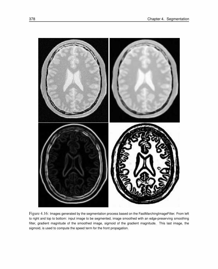
378 Chapter 4. Segmentation
Figure 4.16: Images generated by the segmentation process based on the FastMarchingImageFilter. From left
to right and top to bottom: input image to be segmented, image smoothed with an edge-preserving smoothing
filter, gradient magnitude of the smoothed image, sigmoid of the gradient magnitude. This last image, the
sigmoid, is used to compute the speed term for the front propagation.

4.3. Level Set Segmentation 379
Structure Seed Index σ α β Threshold Output Image from left
Left Ventricle (81,114) 1.0 -0.5 3.0 100 First
Right Ventricle (99,114) 1.0 -0.5 3.0 100 Second
White matter (56,92) 1.0 -0.3 2.0 200 Third
Gray matter (40,90) 0.5 -0.3 2.0 200 Fourth
Table 4.3: Parameters used for segmenting some brain structures shown in Figure 4.17 using the filter Fast-
MarchingImageFilter. All of them used a stopping value of 100.
Figure 4.17: Images generated by the segmentation process based on the FastMarchingImageFilter. From left
to right: segmentation of the left ventricle, segmentation of the right ventricle, segmentation of the white matter,
attempt of segmentation of the gray matter.
of the level set methods when the anatomical structures to be segmented do not occupy extended
regions of the image. This is especially true when the width of the structure is comparable to the size
of the attenuation bands generated by the gradient filter. A possible workaround for this limitation is
to use multiple seeds distributed along the elongated object. However, note that white matter versus
gray matter segmentation is not a trivial task, and may require a more elaborate approach than the
one used in this basic example.
4.3.2 Shape Detection Segmentation
The source code for this section can be found in the file
ShapeDetectionLevelSetFilter.cxx.
The use of the itk::ShapeDetectionLevelSetImageFilter is illustrated in the following exam-
ple. The implementation of this filter in ITK is based on the paper by Malladi et al [39]. In this im-
plementation, the governing differential equation has an additional curvature-based term. This term
acts as a smoothing term where areas of high curvature, assumed to be due to noise, are smoothed
out. Scaling parameters are used to control the tradeoff between the expansion term and the smooth-
ing term. One consequence of this additional curvature term is that the fast marching algorithm is

380 Chapter 4. Segmentation
SigmoidFilter
GradientMagnitude
AnisotropicDiffusion
Inputitk::Image
Iterations Sigma Alpha,Beta
EdgeImage
FastMarching
InputLevelSet
Distance
Seeds
BinaryThreshold
BinaryImage
Threshold
OutputLevelSet
InputLevelSet
EdgePotential
ShapeDetection
Figure 4.18: Collaboration diagram for the ShapeDetectionLevelSetImageFilter applied to a segmentation task.
no longer applicable, because the contour is no longer guaranteed to always be expanding. Instead,
the level set function is updated iteratively.
The ShapeDetectionLevelSetImageFilter expects two inputs, the first being an initial Level Set in
the form of an itk::Image, and the second being a feature image. For this algorithm, the feature
image is an edge potential image that basically follows the same rules applicable to the speed image
used for the FastMarchingImageFilter discussed in Section 4.3.1.
In this example we use an FastMarchingImageFilter to produce the initial level set as the distance
function to a set of user-provided seeds. The FastMarchingImageFilter is run with a constant speed
value which enables us to employ this filter as a distance map calculator.
Figure 4.18 shows the major components involved in the application of the ShapeDetection-
LevelSetImageFilter to a segmentation task. The first stage involves smoothing using the
itk::CurvatureAnisotropicDiffusionImageFilter. The smoothed image is passed as the
input for the itk::GradientMagnitudeRecursiveGaussianImageFilter and then to the
itk::SigmoidImageFilter in order to produce the edge potential image. A set of user-provided

4.3. Level Set Segmentation 381
seeds is passed to an FastMarchingImageFilter in order to compute the distance map. A constant
value is subtracted from this map in order to obtain a level set in which the zero set represents the
initial contour. This level set is also passed as input to the ShapeDetectionLevelSetImageFilter.
Finally, the level set at the output of the ShapeDetectionLevelSetImageFilter is passed to an Binary-
ThresholdImageFilter in order to produce a binary mask representing the segmented object.
Let’s start by including the headers of the main filters involved in the preprocessing.
#include "itkCurvatureAnisotropicDiffusionImageFilter.h"
#include "itkGradientMagnitudeRecursiveGaussianImageFilter.h"
#include "itkSigmoidImageFilter.h"
The edge potential map is generated using these filters as in the previous example.
We will need the Image class, the FastMarchingImageFilter class and the ShapeDetectionLevelSe-
tImageFilter class. Hence we include their headers here.
#include "itkFastMarchingImageFilter.h"
#include "itkShapeDetectionLevelSetImageFilter.h"
The level set resulting from the ShapeDetectionLevelSetImageFilter will be thresholded at the zero
level in order to get a binary image representing the segmented object. The BinaryThresholdImage-
Filter is used for this purpose.
#include "itkBinaryThresholdImageFilter.h"
We now define the image type using a particular pixel type and a dimension. In this case the float
type is used for the pixels due to the requirements of the smoothing filter.
typedef float InternalPixelType;
const unsigned int Dimension = 2;
typedef itk::Image< InternalPixelType, Dimension > InternalImageType;
The output image, on the other hand, is declared to be binary.
typedef unsigned char OutputPixelType;
typedef itk::Image< OutputPixelType, Dimension > OutputImageType;
The type of the BinaryThresholdImageFilter filter is instantiated below using the internal image type
and the output image type.
typedef itk::BinaryThresholdImageFilter< InternalImageType, OutputImageType >
ThresholdingFilterType;
ThresholdingFilterType::Pointer thresholder = ThresholdingFilterType::New();
The upper threshold of the BinaryThresholdImageFilter is set to 0.0 in order to display the zero set
of the resulting level set. The lower threshold is set to a large negative number in order to ensure
that the interior of the segmented object will appear inside the binary region.

382 Chapter 4. Segmentation
thresholder->SetLowerThreshold( -1000.0 );
thresholder->SetUpperThreshold( 0.0 );
thresholder->SetOutsideValue( 0 );
thresholder->SetInsideValue( 255 );
The CurvatureAnisotropicDiffusionImageFilter type is instantiated using the internal image type.
typedef itk::CurvatureAnisotropicDiffusionImageFilter<
InternalImageType,
InternalImageType > SmoothingFilterType;
The filter is instantiated by invoking the New() method and assigning the result to a
itk::SmartPointer.
SmoothingFilterType::Pointer smoothing = SmoothingFilterType::New();
The types of the GradientMagnitudeRecursiveGaussianImageFilter and SigmoidImageFilter are in-
stantiated using the internal image type.
typedef itk::GradientMagnitudeRecursiveGaussianImageFilter<
InternalImageType,
InternalImageType > GradientFilterType;
typedef itk::SigmoidImageFilter<
InternalImageType,
InternalImageType > SigmoidFilterType;
The corresponding filter objects are created with the method New().
GradientFilterType::Pointer gradientMagnitude = GradientFilterType::New();
SigmoidFilterType::Pointer sigmoid = SigmoidFilterType::New();
The minimum and maximum values of the SigmoidImageFilter output are defined with the methods
SetOutputMinimum() and SetOutputMaximum(). In our case, we want these two values to be
0.0 and 1.0 respectively in order to get a nice speed image to feed to the FastMarchingImageFilter.
Additional details on the use of the SigmoidImageFilter are presented in Section 2.3.2.
sigmoid->SetOutputMinimum( 0.0 );
sigmoid->SetOutputMaximum( 1.0 );
We now declare the type of the FastMarchingImageFilter that will be used to generate the initial
level set in the form of a distance map.
typedef itk::FastMarchingImageFilter< InternalImageType, InternalImageType >
FastMarchingFilterType;
Next we construct one filter of this class using the New() method.

4.3. Level Set Segmentation 383
FastMarchingFilterType::Pointer fastMarching
= FastMarchingFilterType::New();
In the following lines we instantiate the type of the ShapeDetectionLevelSetImageFilter and create
an object of this type using the New() method.
typedef itk::ShapeDetectionLevelSetImageFilter< InternalImageType,
InternalImageType > ShapeDetectionFilterType;
ShapeDetectionFilterType::Pointer
shapeDetection = ShapeDetectionFilterType::New();
The filters are now connected in a pipeline indicated in Figure 4.18 with the following code.
smoothing->SetInput( reader->GetOutput() );
gradientMagnitude->SetInput( smoothing->GetOutput() );
sigmoid->SetInput( gradientMagnitude->GetOutput() );
shapeDetection->SetInput( fastMarching->GetOutput() );
shapeDetection->SetFeatureImage( sigmoid->GetOutput() );
thresholder->SetInput( shapeDetection->GetOutput() );
writer->SetInput( thresholder->GetOutput() );
The CurvatureAnisotropicDiffusionImageFilter requires a couple of parameters to be defined. The
following are typical values for 2D images. However they may have to be adjusted depending on
the amount of noise present in the input image. This filter has been discussed in Section 2.7.3.
smoothing->SetTimeStep( 0.125 );
smoothing->SetNumberOfIterations( 5 );
smoothing->SetConductanceParameter( 9.0 );
The GradientMagnitudeRecursiveGaussianImageFilter performs the equivalent of a convolution
with a Gaussian kernel followed by a derivative operator. The sigma of this Gaussian can be used to
control the range of influence of the image edges. This filter has been discussed in Section 2.4.2.
gradientMagnitude->SetSigma( sigma );
The SigmoidImageFilter requires two parameters that define the linear transformation to be applied
to the sigmoid argument. These parameters have been discussed in Sections 2.3.2 and 4.3.1.
sigmoid->SetAlpha( alpha );
sigmoid->SetBeta( beta );
The FastMarchingImageFilter requires the user to provide a seed point from which the level set
will be generated. The user can actually pass not only one seed point but a set of them. Note the
FastMarchingImageFilter is used here only as a helper in the determination of an initial level set.
We could have used the itk::DanielssonDistanceMapImageFilter in the same way.
The seeds are stored in a container. The type of this container is defined as NodeContainer among

384 Chapter 4. Segmentation
the FastMarchingImageFilter traits.
typedef FastMarchingFilterType::NodeContainer NodeContainer;
typedef FastMarchingFilterType::NodeType NodeType;
NodeContainer::Pointer seeds = NodeContainer::New();
Nodes are created as stack variables and initialized with a value and an itk::Index position. Note
that we assign the negative of the value of the user-provided distance to the unique node of the
seeds passed to the FastMarchingImageFilter. In this way, the value will increment as the front is
propagated, until it reaches the zero value corresponding to the contour. After this, the front will
continue propagating until it fills up the entire image. The initial distance is taken from the command
line arguments. The rule of thumb for the user is to select this value as the distance from the seed
points at which the initial contour should be.
NodeType node;
const double seedValue = - initialDistance;
node.SetValue( seedValue );
node.SetIndex( seedPosition );
The list of nodes is initialized and then every node is inserted using InsertElement().
seeds->Initialize();
seeds->InsertElement( 0, node );
The set of seed nodes is now passed to the FastMarchingImageFilter with the method
SetTrialPoints().
fastMarching->SetTrialPoints( seeds );
Since the FastMarchingImageFilter is used here only as a distance map generator, it does not require
a speed image as input. Instead, the constant value 1.0 is passed using the SetSpeedConstant()
method.
fastMarching->SetSpeedConstant( 1.0 );
The FastMarchingImageFilter requires the user to specify the size of the image to be produced as
output. This is done using the SetOutputSize(). Note that the size is obtained here from the output
image of the smoothing filter. The size of this image is valid only after the Update() methods of
this filter have been called directly or indirectly.
fastMarching->SetOutputSize(
reader->GetOutput()->GetBufferedRegion().GetSize() );
ShapeDetectionLevelSetImageFilter provides two parameters to control the competition be-
tween the propagation or expansion term and the curvature smoothing term. The methods
SetPropagationScaling() and SetCurvatureScaling() defines the relative weighting between

4.3. Level Set Segmentation 385
the two terms. In this example, we will set the propagation scaling to one and let the curvature scal-
ing be an input argument. The larger the the curvature scaling parameter the smoother the resulting
segmentation. However, the curvature scaling parameter should not be set too large, as it will draw
the contour away from the shape boundaries.
shapeDetection->SetPropagationScaling( propagationScaling );
shapeDetection->SetCurvatureScaling( curvatureScaling );
Once activated, the level set evolution will stop if the convergence criteria or the maximum number
of iterations is reached. The convergence criteria are defined in terms of the root mean squared
(RMS) change in the level set function. The evolution is said to have converged if the RMS change
is below a user-specified threshold. In a real application, it is desirable to couple the evolution of
the zero set to a visualization module, allowing the user to follow the evolution of the zero set. With
this feedback, the user may decide when to stop the algorithm before the zero set leaks through the
regions of low gradient in the contour of the anatomical structure to be segmented.
shapeDetection->SetMaximumRMSError( 0.02 );
shapeDetection->SetNumberOfIterations( 800 );
The invocation of the Update() method on the writer triggers the execution of the pipeline. As
usual, the call is placed in a try/catch block should any errors occur or exceptions be thrown.
try
{
writer->Update();
}
catch( itk::ExceptionObject & excep )
{
std::cerr << "Exception caught !" << std::endl;
std::cerr << excep << std::endl;
return EXIT_FAILURE;
}
Let’s now run this example using as input the image BrainProtonDensitySlice.png provided in
the directory Examples/Data. We can easily segment the major anatomical structures by providing
seeds in the appropriate locations. Table 4.4 presents the parameters used for some structures. For
all of the examples illustrated in this table, the propagation scaling was set to 1.0, and the curvature
scaling set to 0.05.
Figure 4.19 presents the intermediate outputs of the pipeline illustrated in Figure 4.18. They are from
left to right: the output of the anisotropic diffusion filter, the gradient magnitude of the smoothed
image and the sigmoid of the gradient magnitude which is finally used as the edge potential for the
ShapeDetectionLevelSetImageFilter.
Notice that in Figure 4.20 the segmented shapes are rounder than in Figure 4.17 due to the effects of
the curvature term in the driving equation. As with the previous example, segmentation of the gray
matter is still problematic.
A larger number of iterations is reguired for segmenting large structures since it takes longer for the

386 Chapter 4. Segmentation
Figure 4.19: Images generated by the segmentation process based on the ShapeDetectionLevelSetImage-
Filter. From left to right and top to bottom: input image to be segmented, image smoothed with an edge-
preserving smoothing filter, gradient magnitude of the smoothed image, sigmoid of the gradient magnitude. This
last image, the sigmoid, is used to compute the speed term for the front propagation.

4.3. Level Set Segmentation 387
Structure Seed Index Distance σ α β Output Image
Left Ventricle (81,114) 5.0 1.0 -0.5 3.0 First in Figure 4.20
Right Ventricle (99,114) 5.0 1.0 -0.5 3.0 Second in Figure 4.20
White matter (56,92) 5.0 1.0 -0.3 2.0 Third in Figure 4.20
Gray matter (40,90) 5.0 0.5 -0.3 2.0 Fourth in Figure 4.20
Table 4.4: Parameters used for segmenting some brain structures shown in Figure 4.19 using the filter Sha-
peDetectionLevelSetFilter. All of them used a propagation scaling of 1.0 and curvature scaling of 0.05.
Figure 4.20: Images generated by the segmentation process based on the ShapeDetectionLevelSetImage-
Filter. From left to right: segmentation of the left ventricle, segmentation of the right ventricle, segmentation of
the white matter, attempt of segmentation of the gray matter.
front to propagate and cover the structure. This drawback can be easily mitigated by setting many
seed points in the initialization of the FastMarchingImageFilter. This will generate an initial level
set much closer in shape to the object to be segmented and hence require fewer iterations to fill and
reach the edges of the anatomical structure.
4.3.3 Geodesic Active Contours Segmentation
The source code for this section can be found in the file
GeodesicActiveContourImageFilter.cxx.
The use of the itk::GeodesicActiveContourLevelSetImageFilter is illustrated in the follow-
ing example. The implementation of this filter in ITK is based on the paper by Caselles [11]. This
implementation extends the functionality of the itk::ShapeDetectionLevelSetImageFilter by
the addition of a third advection term which attracts the level set to the object boundaries.
GeodesicActiveContourLevelSetImageFilter expects two inputs. The first is an initial level set in
the form of an itk::Image. The second input is a feature image. For this algorithm, the feature
image is an edge potential image that basically follows the same rules used for the ShapeDetection-
LevelSetImageFilter discussed in Section 4.3.2. The configuration of this example is quite similar to

388 Chapter 4. Segmentation
SigmoidFilter
GradientMagnitude
AnisotropicDiffusion
Inputitk::Image
Iterations Sigma Alpha,Beta
EdgeImage
FastMarching
InputLevelSet
Distance
Seeds
BinaryThreshold
BinaryImage
OutputLevelSet
GeodesicActive
ContoursLengthPenalty
InflationStrength
Figure 4.21: Collaboration diagram for the GeodesicActiveContourLevelSetImageFilter applied to a segmen-
tation task.
the example on the use of the ShapeDetectionLevelSetImageFilter. We omit most of the redundant
description. A look at the code will reveal the great degree of similarity between both examples.
Figure 4.21 shows the major components involved in the application of the GeodesicActiveCon-
tourLevelSetImageFilter to a segmentation task. This pipeline is quite similar to the one used by the
ShapeDetectionLevelSetImageFilter in section 4.3.2.
The pipeline involves a first stage of smoothing using the
itk::CurvatureAnisotropicDiffusionImageFilter. The smoothed image is passed as
the input to the itk::GradientMagnitudeRecursiveGaussianImageFilter and then to the
itk::SigmoidImageFilter in order to produce the edge potential image. A set of user-provided
seeds is passed to a itk::FastMarchingImageFilter in order to compute the distance map. A
constant value is subtracted from this map in order to obtain a level set in which the zero set repre-
sents the initial contour. This level set is also passed as input to the GeodesicActiveContourLevelSe-

4.3. Level Set Segmentation 389
tImageFilter.
Finally, the level set generated by the GeodesicActiveContourLevelSetImageFilter is passed to a
itk::BinaryThresholdImageFilter in order to produce a binary mask representing the seg-
mented object.
Let’s start by including the headers of the main filters involved in the preprocessing.
#include "itkGeodesicActiveContourLevelSetImageFilter.h"
We now define the image type using a particular pixel type and dimension. In this case the float
type is used for the pixels due to the requirements of the smoothing filter.
typedef float InternalPixelType;
const unsigned int Dimension = 2;
typedef itk::Image< InternalPixelType, Dimension > InternalImageType;
In the following lines we instantiate the type of the GeodesicActiveContourLevelSetImageFilter and
create an object of this type using the New() method.
typedef itk::GeodesicActiveContourLevelSetImageFilter< InternalImageType,
InternalImageType > GeodesicActiveContourFilterType;
GeodesicActiveContourFilterType::Pointer geodesicActiveContour =
GeodesicActiveContourFilterType::New();
For the GeodesicActiveContourLevelSetImageFilter, scaling parameters are used to trade off be-
tween the propagation (inflation), the curvature (smoothing) and the advection terms. These
parameters are set using methods SetPropagationScaling(), SetCurvatureScaling() and
SetAdvectionScaling(). In this example, we will set the curvature and advection scales to one
and let the propagation scale be a command-line argument.
geodesicActiveContour->SetPropagationScaling( propagationScaling );
geodesicActiveContour->SetCurvatureScaling( 1.0 );
geodesicActiveContour->SetAdvectionScaling( 1.0 );
The filters are now connected in a pipeline indicated in Figure 4.21 using the following lines:
smoothing->SetInput( reader->GetOutput() );
gradientMagnitude->SetInput( smoothing->GetOutput() );
sigmoid->SetInput( gradientMagnitude->GetOutput() );
geodesicActiveContour->SetInput( fastMarching->GetOutput() );
geodesicActiveContour->SetFeatureImage( sigmoid->GetOutput() );
thresholder->SetInput( geodesicActiveContour->GetOutput() );
writer->SetInput( thresholder->GetOutput() );
The invocation of the Update() method on the writer triggers the execution of the pipeline. As
usual, the call is placed in a try/catch block should any errors occur or exceptions be thrown.

390 Chapter 4. Segmentation
Structure Seed Index Distance σ α β Propag. Output Image
Left Ventricle (81,114) 5.0 1.0 -0.5 3.0 2.0 First
Right Ventricle (99,114) 5.0 1.0 -0.5 3.0 2.0 Second
White matter (56,92) 5.0 1.0 -0.3 2.0 10.0 Third
Gray matter (40,90) 5.0 0.5 -0.3 2.0 10.0 Fourth
Table 4.5: Parameters used for segmenting some brain structures shown in Figure 4.23 using the filter Geodesi-
cActiveContourLevelSetImageFilter.
try
{
writer->Update();
}
catch( itk::ExceptionObject & excep )
{
std::cerr << "Exception caught !" << std::endl;
std::cerr << excep << std::endl;
return EXIT_FAILURE;
}
Let’s now run this example using as input the image BrainProtonDensitySlice.png provided in
the directory Examples/Data. We can easily segment the major anatomical structures by providing
seeds in the appropriate locations. Table 4.5 presents the parameters used for some structures.
Figure 4.22 presents the intermediate outputs of the pipeline illustrated in Figure 4.21. They are from
left to right: the output of the anisotropic diffusion filter, the gradient magnitude of the smoothed
image and the sigmoid of the gradient magnitude which is finally used as the edge potential for the
GeodesicActiveContourLevelSetImageFilter.
Segmentations of the main brain structures are presented in Figure 4.23. The results are quite similar
to those obtained with the ShapeDetectionLevelSetImageFilter in Section 4.3.2.
Note that a relatively larger propagation scaling value was required to segment the white matter. This
is due to two factors: the lower contrast at the border of the white matter and the complex shape of
the structure. Unfortunately the optimal value of these scaling parameters can only be determined
by experimentation. In a real application we could imagine an interactive mechanism by which a
user supervises the contour evolution and adjusts these parameters accordingly.
4.3.4 Threshold Level Set Segmentation
The source code for this section can be found in the file
ThresholdSegmentationLevelSetImageFilter.cxx.
The itk::ThresholdSegmentationLevelSetImageFilter is an extension of the threshold
connected-component segmentation to the level set framework. The goal is to define a range of in-

4.3. Level Set Segmentation 391
Figure 4.22: Images generated by the segmentation process based on the GeodesicActiveContourLevelSe-
tImageFilter. From left to right and top to bottom: input image to be segmented, image smoothed with an edge-
preserving smoothing filter, gradient magnitude of the smoothed image, sigmoid of the gradient magnitude. This
last image, the sigmoid, is used to compute the speed term for the front propagation.

392 Chapter 4. Segmentation
Figure 4.23: Images generated by the segmentation process based on the GeodesicActiveContourImageFilter.
From left to right: segmentation of the left ventricle, segmentation of the right ventricle, segmentation of the white
matter, attempt of segmentation of the gray matter.
tensity values that classify the tissue type of interest and then base the propagation term on the level
set equation for that intensity range. Using the level set approach, the smoothness of the evolving
surface can be constrained to prevent some of the “leaking” that is common in connected-component
schemes.
The propagation term P from Equation 4.3 is calculated from the FeatureImage input g with
UpperThreshold U and LowerThreshold L according to the following formula.
P(x) =
{
g(x)−L if g(x)< (U −L)/2+L
U − g(x) otherwise(4.4)
Figure 4.25 illustrates the propagation term function. Intensity values in g between L and H yield
positive values in P, while outside intensities yield negative values in P.
The threshold segmentation filter expects two inputs. The first is an initial level set in the form of
an itk::Image. The second input is the feature image g. For many applications, this filter requires
little or no preprocessing of its input. Smoothing the input image is not usually required to produce
reasonable solutions, though it may still be warranted in some cases.
Figure 4.24 shows how the image processing pipeline is constructed. The initial surface is
generated using the fast marching filter. The output of the segmentation filter is passed to a
itk::BinaryThresholdImageFilter to create a binary representation of the segmented object.
Let’s start by including the appropriate header file.
#include "itkThresholdSegmentationLevelSetImageFilter.h"
We define the image type using a particular pixel type and dimension. In this case we will use 2D
float images.

4.3. Level Set Segmentation 393
Feature
FastMarching
InputLevelSet
Distance
Seeds
BinaryThreshold
BinaryImage
Inputitk::Image
LevelSetOutputThreshold
Level−setSegmentation
Weight
Curvature
Weight
Figure 4.24: Collaboration diagram for the ThresholdSegmentationLevelSetImageFilter applied to a segmen-
tation task.
ExpandsModelModel
Contracts ContractsModel
UL
g(x)
P
P=0
Figure 4.25: Propagation term for threshold-based level set segmentation. From Equation 4.4.

394 Chapter 4. Segmentation
typedef float InternalPixelType;
const unsigned int Dimension = 2;
typedef itk::Image< InternalPixelType, Dimension > InternalImageType;
The following lines instantiate a ThresholdSegmentationLevelSetImageFilter using the New()
method.
typedef itk::ThresholdSegmentationLevelSetImageFilter< InternalImageType,
InternalImageType > ThresholdSegmentationLevelSetImageFilterType;
ThresholdSegmentationLevelSetImageFilterType::Pointer thresholdSegmentation =
ThresholdSegmentationLevelSetImageFilterType::New();
For the ThresholdSegmentationLevelSetImageFilter, scaling parameters are used to balance the in-
fluence of the propagation (inflation) and the curvature (surface smoothing) terms from Equation 4.3.
The advection term is not used in this filter. Set the terms with methods SetPropagationScaling()
and SetCurvatureScaling(). Both terms are set to 1.0 in this example.
thresholdSegmentation->SetPropagationScaling( 1.0 );
if ( argc > 8 )
{
thresholdSegmentation->SetCurvatureScaling( atof(argv[8]) );
}
else
{
thresholdSegmentation->SetCurvatureScaling( 1.0 );
}
The convergence criteria MaximumRMSError and MaximumIterations are set as in previous exam-
ples. We now set the upper and lower threshold values U and L, and the isosurface value to use in
the initial model.
thresholdSegmentation->SetUpperThreshold( ::atof(argv[7]) );
thresholdSegmentation->SetLowerThreshold( ::atof(argv[6]) );
thresholdSegmentation->SetIsoSurfaceValue(0.0);
The filters are now connected in a pipeline indicated in Figure 4.24. Remember that before calling
Update() on the file writer object, the fast marching filter must be initialized with the seed points
and the output from the reader object. See previous examples and the source code for this section
for details.
thresholdSegmentation->SetInput( fastMarching->GetOutput() );
thresholdSegmentation->SetFeatureImage( reader->GetOutput() );
thresholder->SetInput( thresholdSegmentation->GetOutput() );
writer->SetInput( thresholder->GetOutput() );
Invoking the Update() method on the writer triggers the execution of the pipeline. As usual, the
call is placed in a try/catch block should any errors occur or exceptions be thrown.

4.3. Level Set Segmentation 395
Figure 4.26: Images generated by the segmentation process based on the ThresholdSegmentationLevelSetIm-
ageFilter. From left to right: segmentation of the left ventricle, segmentation of the right ventricle, segmentation
of the white matter, attempt of segmentation of the gray matter. The parameters used in this segmentations are
presented in Table 4.6.
try
{
reader->Update();
const InternalImageType * inputImage = reader->GetOutput();
fastMarching->SetOutputRegion( inputImage->GetBufferedRegion() );
fastMarching->SetOutputSpacing( inputImage->GetSpacing() );
fastMarching->SetOutputOrigin( inputImage->GetOrigin() );
fastMarching->SetOutputDirection( inputImage->GetDirection() );
writer->Update();
}
catch( itk::ExceptionObject & excep )
{
std::cerr << "Exception caught !" << std::endl;
std::cerr << excep << std::endl;
return EXIT_FAILURE;
}
Let’s run this application with the same data and parameters as the example given for
itk::ConnectedThresholdImageFilter in Section 4.1.1. We will use a value of 5 as the initial
distance of the surface from the seed points. The algorithm is relatively insensitive to this initial-
ization. Compare the results in Figure 4.26 with those in Figure 4.1. Notice how the smoothness
constraint on the surface prevents leakage of the segmentation into both ventricles, but also localizes
the segmentation to a smaller portion of the gray matter.
4.3.5 Canny-Edge Level Set Segmentation
The source code for this section can be found in the file
CannySegmentationLevelSetImageFilter.cxx.
The itk::CannySegmentationLevelSetImageFilter defines a speed term that minimizes dis-

396 Chapter 4. Segmentation
Structure Seed Index Lower Upper Output Image
White matter (60,116) 150 180 Second from left
Ventricle (81,112) 210 250 Third from left
Gray matter (107,69) 180 210 Fourth from left
Table 4.6: Segmentation results using the ThresholdSegmentationLevelSetImageFilter for various seed points.
The resulting images are shown in Figure 4.26 .
tance to the Canny edges in an image. The initial level set model moves through a gradient advection
field until it locks onto those edges. This filter is more suitable for refining existing segmentations
than as a region-growing algorithm.
The two terms defined for the CannySegmentationLevelSetImageFilter are the advection term and
the propagation term from Equation 4.3. The advection term is constructed by minimizing the
squared distance transform from the Canny edges.
min
∫D2 ⇒ D∇D (4.5)
where the distance transform D is calculated using a itk::DanielssonDistanceMapImageFilter
applied to the output of the itk::CannyEdgeDetectionImageFilter.
For cases in which some surface expansion is to be allowed, a non-zero value may be set for the
propagation term. The propagation term is simply D. As with all ITK level set segmentation filters,
the curvature term controls the smoothness of the surface.
CannySegmentationLevelSetImageFilter expects two inputs. The first is an initial level set in the
form of an itk::Image. The second input is the feature image g from which propagation and
advection terms are calculated. It is generally a good idea to do some preprocessing of the feature
image to remove noise.
Figure 4.27 shows how the image processing pipeline is constructed. We read two images: the image
to segment and the image that contains the initial implicit surface. The goal is to refine the initial
model from the second input and not to grow a new segmentation from seed points. The feature
image is preprocessed with a few iterations of an anisotropic diffusion filter.
Let’s start by including the appropriate header file.
#include "itkCannySegmentationLevelSetImageFilter.h"
#include "itkGradientAnisotropicDiffusionImageFilter.h"
We define the image type using a particular pixel type and dimension. In this case we will use 2D
float images.
typedef float InternalPixelType;
const unsigned int Dimension = 2;
typedef itk::Image< InternalPixelType, Dimension > InternalImageType;

4.3. Level Set Segmentation 397
Threshold
BinaryThreshold
BinaryImage
AdvectionWeight
MaximumIterations
Inputitk::Image
InitialModel
itk::ImageAnisotropicDiffusion
Gradient
LevelSetOutputThreshold
Level−setSegmentation
CannyVariance
Canny
Figure 4.27: Collaboration diagram for the CannySegmentationLevelSetImageFilter applied to a segmentation
task.
The input image will be processed with a few iterations of feature-preserving diffusion. We create a
filter and set the appropriate parameters.
typedef itk::GradientAnisotropicDiffusionImageFilter< InternalImageType,
InternalImageType> DiffusionFilterType;
DiffusionFilterType::Pointer diffusion = DiffusionFilterType::New();
diffusion->SetNumberOfIterations(5);
diffusion->SetTimeStep(0.125);
diffusion->SetConductanceParameter(1.0);
The following lines define and instantiate a CannySegmentationLevelSetImageFilter.
typedef itk::CannySegmentationLevelSetImageFilter< InternalImageType,
InternalImageType > CannySegmentationLevelSetImageFilterType;
CannySegmentationLevelSetImageFilterType::Pointer cannySegmentation =
CannySegmentationLevelSetImageFilterType::New();
As with the other ITK level set segmentation filters, the terms of the CannySegmentationLevelSe-
tImageFilter level set equation can be weighted by scalars. For this application we will modify the
relative weight of the advection term. The propagation and curvature term weights are set to their
defaults of 0 and 1, respectively.
cannySegmentation->SetAdvectionScaling( ::atof(argv[6]) );
cannySegmentation->SetCurvatureScaling( 1.0 );
cannySegmentation->SetPropagationScaling( 0.0 );

398 Chapter 4. Segmentation
The maximum number of iterations is specified from the command line. It may not be desirable in
some applications to run the filter to convergence. Only a few iterations may be required.
cannySegmentation->SetMaximumRMSError( 0.01 );
cannySegmentation->SetNumberOfIterations( ::atoi(argv[8]) );
There are two important parameters in the CannySegmentationLevelSetImageFilter to control the
behavior of the Canny edge detection. The variance parameter controls the amount of Gaussian
smoothing on the input image. The threshold parameter indicates the lowest allowed value in the
output image. Thresholding is used to suppress Canny edges whose gradient magnitudes fall below
a certain value.
cannySegmentation->SetThreshold( ::atof(argv[4]) );
cannySegmentation->SetVariance( ::atof(argv[5]) );
Finally, it is very important to specify the isovalue of the surface in the initial model input image. In a
binary image, for example, the isosurface is found midway between the foreground and background
values.
cannySegmentation->SetIsoSurfaceValue( ::atof(argv[7]) );
The filters are now connected in a pipeline indicated in Figure 4.27.
diffusion->SetInput( reader1->GetOutput() );
cannySegmentation->SetInput( reader2->GetOutput() );
cannySegmentation->SetFeatureImage( diffusion->GetOutput() );
thresholder->SetInput( cannySegmentation->GetOutput() );
writer->SetInput( thresholder->GetOutput() );
Invoking the Update() method on the writer triggers the execution of the pipeline. As usual, the
call is placed in a try/catch block to handle any exceptions that may be thrown.
try
{
writer->Update();
}
catch( itk::ExceptionObject & excep )
{
std::cerr << "Exception caught !" << std::endl;
std::cerr << excep << std::endl;
return EXIT_FAILURE;
}
We can use this filter to make some subtle refinements to the ventricle segmentation from
the previous example that used the itk::ThresholdSegmentationLevelSetImageFilter.
The application was run using Examples/Data/BrainProtonDensitySlice.png and
Examples/Data/VentricleModel.png as inputs, a threshold of 7.0, variance of 0.1,
advection weight of 10.0, and an initial isosurface value of 127.5. One case was run for 15
iterations and the second was run to convergence. Compare the results in the two rightmost images

4.3. Level Set Segmentation 399
Figure 4.28: Results of applying the CannySegmentationLevelSetImageFilter to a prior ventricle segmentation.
Shown from left to right are the original image, the prior segmentation of the ventricle from Figure 4.26, 15
iterations of the CannySegmentationLevelSetImageFilter, and the CannySegmentationLevelSetImageFilter run
to convergence.
of Figure 4.28 with the ventricle segmentation from Figure 4.26 shown in the middle. Jagged edges
are straightened and the small spur at the upper right-hand side of the mask has been removed.
The free parameters of this filter can be adjusted to achieve a wide range of shape variations from the
original model. Finding the right parameters for your particular application is usually a process of
trial and error. As with most ITK level set segmentation filters, examining the propagation (speed)
and advection images can help the process of tuning parameters. These images are available using
Set/Get methods from the filter after it has been updated.
In some cases it is interesting to take a direct look at the speed image used internally by this filter.
This may help for setting the correct parameters for driving the segmentation. In order to obtain such
speed image, the method GenerateSpeedImage() should be invoked first. Then we can recover the
speed image with the GetSpeedImage() method as illustrated in the following lines.
cannySegmentation->GenerateSpeedImage();
typedef CannySegmentationLevelSetImageFilterType::SpeedImageType
SpeedImageType;
typedef itk::ImageFileWriter<SpeedImageType> SpeedWriterType;
SpeedWriterType::Pointer speedWriter = SpeedWriterType::New();
speedWriter->SetInput( cannySegmentation->GetSpeedImage() );
4.3.6 Laplacian Level Set Segmentation
The source code for this section can be found in the file
LaplacianSegmentationLevelSetImageFilter.cxx.
The itk::LaplacianSegmentationLevelSetImageFilter defines a speed term based on second
derivative features in the image. The speed term is calculated as the Laplacian of the image values.

400 Chapter 4. Segmentation
Laplacian BinaryThreshold
BinaryImage
Inputitk::Image
InitialModel
itk::ImageAnisotropicDiffusion
Gradient
PropagationWeight
MaximumIterations
LevelSetOutput
Level−setSegmentation
Figure 4.29: An image processing pipeline using LaplacianSegmentationLevelSetImageFilter for segmenta-
tion.
The goal is to attract the evolving level set surface to local zero-crossings in the Laplacian image.
Like itk::CannySegmentationLevelSetImageFilter, this filter is more suitable for refining
existing segmentations than as a stand-alone, region growing algorithm. It is possible to perform
region growing segmentation, but be aware that the growing surface may tend to become “stuck” at
local edges.
The propagation (speed) term for the LaplacianSegmentationLevelSetImageFilter is constructed by
applying the itk::LaplacianImageFilter to the input feature image. One nice property of using
the Laplacian is that there are no free parameters in the calculation.
LaplacianSegmentationLevelSetImageFilter expects two inputs. The first is an initial level set in the
form of an itk::Image. The second input is the feature image g from which the propagation term
is calculated (see Equation 4.3). Because the filter performs a second derivative calculation, it is
generally a good idea to do some preprocessing of the feature image to remove noise.
Figure 4.29 shows how the image processing pipeline is constructed. We read two images: the image
to segment and the image that contains the initial implicit surface. The goal is to refine the initial
model from the second input to better match the structure represented by the initial implicit surface
(a prior segmentation). The feature image is preprocessed using an anisotropic diffusion filter.
Let’s start by including the appropriate header files.
#include "itkLaplacianSegmentationLevelSetImageFilter.h"
#include "itkGradientAnisotropicDiffusionImageFilter.h"
We define the image type using a particular pixel type and dimension. In this case we will use 2D
float images.

4.3. Level Set Segmentation 401
typedef float InternalPixelType;
const unsigned int Dimension = 2;
typedef itk::Image< InternalPixelType, Dimension > InternalImageType;
The input image will be processed with a few iterations of feature-preserving diffusion. We create
a filter and set the parameters. The number of iterations and the conductance parameter are taken
from the command line.
typedef itk::GradientAnisotropicDiffusionImageFilter< InternalImageType,
InternalImageType> DiffusionFilterType;
DiffusionFilterType::Pointer diffusion = DiffusionFilterType::New();
diffusion->SetNumberOfIterations( atoi(argv[4]) );
diffusion->SetTimeStep(0.125);
diffusion->SetConductanceParameter( atof(argv[5]) );
The following lines define and instantiate a LaplacianSegmentationLevelSetImageFilter.
typedef itk::LaplacianSegmentationLevelSetImageFilter< InternalImageType,
InternalImageType > LaplacianSegmentationLevelSetImageFilterType;
LaplacianSegmentationLevelSetImageFilterType::Pointer laplacianSegmentation
= LaplacianSegmentationLevelSetImageFilterType::New();
As with the other ITK level set segmentation filters, the terms of the LaplacianSegmentationLevelSe-
tImageFilter level set equation can be weighted by scalars. For this application we will modify the
relative weight of the propagation term. The curvature term weight is set to its default of 1. The
advection term is not used in this filter.
laplacianSegmentation->SetCurvatureScaling( 1.0 );
laplacianSegmentation->SetPropagationScaling( ::atof(argv[6]) );
The maximum number of iterations is set from the command line. It may not be desirable in some
applications to run the filter to convergence. Only a few iterations may be required.
laplacianSegmentation->SetMaximumRMSError( 0.002 );
laplacianSegmentation->SetNumberOfIterations( ::atoi(argv[8]) );
Finally, it is very important to specify the isovalue of the surface in the initial model input image. In a
binary image, for example, the isosurface is found midway between the foreground and background
values.
laplacianSegmentation->SetIsoSurfaceValue( ::atof(argv[7]) );
The filters are now connected in a pipeline indicated in Figure 4.29.
diffusion->SetInput( reader1->GetOutput() );
laplacianSegmentation->SetInput( reader2->GetOutput() );
laplacianSegmentation->SetFeatureImage( diffusion->GetOutput() );
thresholder->SetInput( laplacianSegmentation->GetOutput() );
writer->SetInput( thresholder->GetOutput() );

402 Chapter 4. Segmentation
Figure 4.30: Results of applying LaplacianSegmentationLevelSetImageFilter to a prior ventricle segmentation.
Shown from left to right are the original image, the prior segmentation of the ventricle from Figure 4.26, and the
refinement of the prior using LaplacianSegmentationLevelSetImageFilter.
Invoking the Update() method on the writer triggers the execution of the pipeline. As usual, the
call is placed in a try/catch block to handle any exceptions that may be thrown.
try
{
writer->Update();
}
catch( itk::ExceptionObject & excep )
{
std::cerr << "Exception caught !" << std::endl;
std::cerr << excep << std::endl;
return EXIT_FAILURE;
}
We can use this filter to make some subtle refinements to the ventricle segmentation
from the example using the filter itk::ThresholdSegmentationLevelSetImageFilter.
This application was run using Examples/Data/BrainProtonDensitySlice.png and
Examples/Data/VentricleModel.png as inputs. We used 10 iterations of the diffusion fil-
ter with a conductance of 2.0. The propagation scaling was set to 1.0 and the filter was run
until convergence. Compare the results in the rightmost images of Figure 4.30 with the ventricle
segmentation from Figure 4.26 shown in the middle. Jagged edges are straightened and the small
spur at the upper right-hand side of the mask has been removed.
4.3.7 Geodesic Active Contours Segmentation With Shape Guidance
The source code for this section can be found in the file
GeodesicActiveContourShapePriorLevelSetImageFilter.cxx.

4.3. Level Set Segmentation 403
In medical imaging applications, the general shape, location and orientation of an anatomical struc-
ture of interest is typically known a priori. This information can be used to aid the segmentation
process especially when image contrast is low or when the object boundary is not distinct.
In [34], Leventon et al. extended the geodesic active contours method
with an additional shape-influenced term in the driving PDE. The
itk::GeodesicActiveContourShapePriorLevelSetFilter is a generalization of Leven-
ton’s approach and its use is illustrated in the following example.
To support shape-guidance, the generic level set equation (Eqn( 4.3)) is extended to incorporate a
shape guidance term:
ξ(ψ∗(x)−ψ(x)) (4.6)
where ψ∗ is the signed distance function of the “best-fit” shape with respect to a shape model. The
new term has the effect of driving the contour towards the best-fit shape. The scalar ξ weights the
influence of the shape term in the overall evolution. In general, the best-fit shape is not known ahead
of time and has to be iteratively estimated in conjunction with the contour evolution.
As with the itk::GeodesicActiveContourLevelSetImageFilter, the GeodesicActiveContour-
ShapePriorLevelSetImageFilter expects two input images: the first is an initial level set and the sec-
ond a feature image that represents the image edge potential. The configuration of this example is
quite similar to the example in Section 4.3.3 and hence the description will focus on the new objects
involved in the segmentation process as shown in Figure 4.31.
The process pipeline begins with centering the input image using the the
itk::ChangeInformationImageFilter to simplify the estimation of the pose of the shape,
to be explained later. The centered image is then smoothed using non-linear diffusion to remove
noise and the gradient magnitude is computed from the smoothed image. For simplicity, this
example uses the itk::BoundedReciprocalImageFilter to produce the edge potential image.
The itk::FastMarchingImageFilter creates an initial level set using three user specified
seed positions and a initial contour radius. Three seeds are used in this example to facilitate
the segmentation of long narrow objects in a smaller number of iterations. The output of the
FastMarchingImageFilter is passed as the input to the GeodesicActiveContourShapePriorLevelSe-
tImageFilter. At then end of the segmentation process, the output level set is passed to the
itk::BinaryThresholdImageFilter to produce a binary mask representing the segmented ob-
ject.
The remaining objects in Figure 4.31 are used for shape modeling and estimation. The
itk::PCAShapeSignedDistanceFunction represents a statistical shape model defined by a mean
signed distance and the first K principal components modes; while the itk::Euler2DTransform is
used to represent the pose of the shape. In this implementation, the best-fit shape estimation problem
is reformulated as a minimization problem where the itk::ShapePriorMAPCostFunction is the
cost function to be optimized using the itk::OnePlusOneEvolutionaryOptimizer.
It should be noted that, although particular shape model, transform cost function, and optimizer

404 Chapter 4. Segmentation
Anisotropic Diffusion
Change Information
(Center Image)
Gradient Magnitude
Fast Marching
Bounded Reciprocal
Geodesic ActiveContour
ShapePrior
Input Image
Edge Image
Output Binary Image
Seeds/ Distance
Sigma
Binary Threshold
Prop./ Shape Scaling
PCAShape SignedDistance
Euler2DTransform
ShapePriorMAP CostFunction
OnePlusOne Evolutionary
Optimizer
NormalVariate Generator
Initial LevelSet
Mean Shape Image
Shape Mode
Images
Figure 4.31: Collaboration diagram for the GeodesicActiveContourShapePriorLevelSetImageFilter applied to
a segmentation task.

4.3. Level Set Segmentation 405
are used in this example, the implementation is generic, allowing different instances of these com-
ponents to be plugged in. This flexibility allows a user to tailor the behavior of the segmentation
process to suit the circumstances of the targeted application.
Let’s start the example by including the headers of the new filters involved in the segmentation.
#include "itkGeodesicActiveContourShapePriorLevelSetImageFilter.h"
#include "itkChangeInformationImageFilter.h"
#include "itkBoundedReciprocalImageFilter.h"
Next, we include the headers of the objects involved in shape modeling and estimation.
#include "itkPCAShapeSignedDistanceFunction.h"
#include "itkEuler2DTransform.h"
#include "itkOnePlusOneEvolutionaryOptimizer.h"
#include "itkNormalVariateGenerator.h"
#include "vnl/vnl_sample.h"
#include "itkNumericSeriesFileNames.h"
Given the numerous parameters involved in tuning this segmentation method it is not uncommon
for a segmentation process to run for several minutes and still produce an unsatisfactory result. For
debugging purposes it is quite helpful to track the evolution of the segmentation as it progresses.
The following defines a custom itk::Command class for monitoring the RMS change and shape
parameters at each iteration.

406 Chapter 4. Segmentation
#include "itkCommand.h"
template<class TFilter>
class CommandIterationUpdate : public itk::Command
{
public:
typedef CommandIterationUpdate Self;
typedef itk::Command Superclass;
typedef itk::SmartPointer<Self> Pointer;
itkNewMacro( Self );
protected:
CommandIterationUpdate() {};
public:
void Execute(itk::Object *caller,
const itk::EventObject & event) ITK_OVERRIDE
{
Execute( (const itk::Object *) caller, event);
}
void Execute(const itk::Object * object,
const itk::EventObject & event) ITK_OVERRIDE
{
const TFilter * filter = static_cast< const TFilter * >( object );
if( typeid( event ) != typeid( itk::IterationEvent ) )
{ return; }
std::cout << filter->GetElapsedIterations() << ": ";
std::cout << filter->GetRMSChange() << " ";
std::cout << filter->GetCurrentParameters() << std::endl;
}
};
We define the image type using a particular pixel type and dimension. In this case we will use 2D
float images.
typedef float InternalPixelType;
const unsigned int Dimension = 2;
typedef itk::Image< InternalPixelType, Dimension > InternalImageType;
The following line instantiate a itk::GeodesicActiveContourShapePriorLevelSetImageFilter
using the New() method.
typedef itk::GeodesicActiveContourShapePriorLevelSetImageFilter<
InternalImageType, InternalImageType >
GeodesicActiveContourFilterType;
GeodesicActiveContourFilterType::Pointer geodesicActiveContour =
GeodesicActiveContourFilterType::New();
The itk::ChangeInformationImageFilter is the first filter in the preprocessing stage and is

4.3. Level Set Segmentation 407
used to force the image origin to the center of the image.
typedef itk::ChangeInformationImageFilter<
InternalImageType > CenterFilterType;
CenterFilterType::Pointer center = CenterFilterType::New();
center->CenterImageOn();
In this example, we will use the bounded reciprocal 1/(1+ x) of the image gradient magnitude as
the edge potential feature image.
typedef itk::BoundedReciprocalImageFilter<
InternalImageType,
InternalImageType > ReciprocalFilterType;
ReciprocalFilterType::Pointer reciprocal = ReciprocalFilterType::New();
In the GeodesicActiveContourShapePriorLevelSetImageFilter, scaling parameters are used to
trade off between the propagation (inflation), the curvature (smoothing), the advection, and the
shape influence terms. These parameters are set using methods SetPropagationScaling(),
SetCurvatureScaling(), SetAdvectionScaling() and SetShapePriorScaling(). In this ex-
ample, we will set the curvature and advection scales to one and let the propagation and shape prior
scale be command-line arguments.
geodesicActiveContour->SetPropagationScaling( propagationScaling );
geodesicActiveContour->SetShapePriorScaling( shapePriorScaling );
geodesicActiveContour->SetCurvatureScaling( 1.0 );
geodesicActiveContour->SetAdvectionScaling( 1.0 );
Each iteration, the current “best-fit” shape is estimated from the edge potential image and the current
contour. To increase speed, only information within the sparse field layers of the current contour is
used in the estimation. The default number of sparse field layers is the same as the ImageDimen-
sion which does not contain enough information to get a reliable best-fit shape estimate. Thus, we
override the default and set the number of layers to 4.
geodesicActiveContour->SetNumberOfLayers( 4 );
The filters are then connected in a pipeline as illustrated in Figure 4.31.
center->SetInput( reader->GetOutput() );
smoothing->SetInput( center->GetOutput() );
gradientMagnitude->SetInput( smoothing->GetOutput() );
reciprocal->SetInput( gradientMagnitude->GetOutput() );
geodesicActiveContour->SetInput( fastMarching->GetOutput() );
geodesicActiveContour->SetFeatureImage( reciprocal->GetOutput() );
thresholder->SetInput( geodesicActiveContour->GetOutput() );
writer->SetInput( thresholder->GetOutput() );

408 Chapter 4. Segmentation
Next, we define the shape model. In this example, we use an implicit shape model based on the
principal components such that:
ψ∗(x) = µ(x)+∑k
αkuk(x) (4.7)
where µ(x) is the mean signed distance computed from training set of segmented objects and uk(x)are the first K principal components of the offset (signed distance - mean). The coefficients {αk}form the set of shape parameters.
Given a set of training data, the itk::ImagePCAShapeModelEstimator can be used to obtain the
mean and principal mode shape images required by PCAShapeSignedDistanceFunction.
typedef itk::PCAShapeSignedDistanceFunction<
double,
Dimension,
InternalImageType > ShapeFunctionType;
ShapeFunctionType::Pointer shape = ShapeFunctionType::New();
shape->SetNumberOfPrincipalComponents( numberOfPCAModes );
In this example, we will read the mean shape and principal mode images from file. We will assume
that the filenames of the mode images form a numeric series starting from index 0.
ReaderType::Pointer meanShapeReader = ReaderType::New();
meanShapeReader->SetFileName( argv[13] );
meanShapeReader->Update();
std::vector<InternalImageType::Pointer> shapeModeImages( numberOfPCAModes );
itk::NumericSeriesFileNames::Pointer fileNamesCreator =
itk::NumericSeriesFileNames::New();
fileNamesCreator->SetStartIndex( 0 );
fileNamesCreator->SetEndIndex( numberOfPCAModes - 1 );
fileNamesCreator->SetSeriesFormat( argv[15] );
const std::vector<std::string> & shapeModeFileNames =
fileNamesCreator->GetFileNames();
for (unsigned int k = 0; k < numberOfPCAModes; ++k )
{
ReaderType::Pointer shapeModeReader = ReaderType::New();
shapeModeReader->SetFileName( shapeModeFileNames[k].c_str() );
shapeModeReader->Update();
shapeModeImages[k] = shapeModeReader->GetOutput();
}
shape->SetMeanImage( meanShapeReader->GetOutput() );
shape->SetPrincipalComponentImages( shapeModeImages );
Further we assume that the shape modes have been normalized by multiplying with the correspond-

4.3. Level Set Segmentation 409
ing singular value. Hence, we can set the principal component standard deviations to all ones.
ShapeFunctionType::ParametersType pcaStandardDeviations( numberOfPCAModes );
pcaStandardDeviations.Fill( 1.0 );
shape->SetPrincipalComponentStandardDeviations( pcaStandardDeviations );
Next, we instantiate a itk::Euler2DTransform and connect it to the PCASignedDistanceFunc-
tion. The transform represent the pose of the shape. The parameters of the transform forms the set
of pose parameters.
typedef itk::Euler2DTransform<double> TransformType;
TransformType::Pointer transform = TransformType::New();
shape->SetTransform( transform );
Before updating the level set at each iteration, the parameters of the current best-fit shape is estimated
by minimizing the itk::ShapePriorMAPCostFunction. The cost function is composed of four
terms: contour fit, image fit, shape prior and pose prior. The user can specify the weights applied to
each term.
typedef itk::ShapePriorMAPCostFunction<
InternalImageType,
InternalPixelType > CostFunctionType;
CostFunctionType::Pointer costFunction = CostFunctionType::New();
CostFunctionType::WeightsType weights;
weights[0] = 1.0; // weight for contour fit term
weights[1] = 20.0; // weight for image fit term
weights[2] = 1.0; // weight for shape prior term
weights[3] = 1.0; // weight for pose prior term
costFunction->SetWeights( weights );
Contour fit measures the likelihood of seeing the current evolving contour for a given set of shape/-
pose parameters. This is computed by counting the number of pixels inside the current contour but
outside the current shape.
Image fit measures the likelihood of seeing certain image features for a given set of shape/pose
parameters. This is computed by assuming that ( 1 - edge potential ) approximates a zero-mean,
unit variance Gaussian along the normal of the evolving contour. Image fit is then computed by
computing the Laplacian goodness of fit of the Gaussian:
∑ (G(ψ(x))−|1− g(x)|)2 (4.8)
where G is a zero-mean, unit variance Gaussian and g is the edge potential feature image.
The pose parameters are assumed to have a uniform distribution and hence do not contribute to the
cost function. The shape parameters are assumed to have a Gaussian distribution. The parameters

410 Chapter 4. Segmentation
of the distribution are user-specified. Since we assumed the principal modes have already been
normalized, we set the distribution to zero mean and unit variance.
CostFunctionType::ArrayType mean( shape->GetNumberOfShapeParameters() );
CostFunctionType::ArrayType stddev( shape->GetNumberOfShapeParameters() );
mean.Fill( 0.0 );
stddev.Fill( 1.0 );
costFunction->SetShapeParameterMeans( mean );
costFunction->SetShapeParameterStandardDeviations( stddev );
In this example, we will use the itk::OnePlusOneEvolutionaryOptimizer to optimize the cost
function.
typedef itk::OnePlusOneEvolutionaryOptimizer OptimizerType;
OptimizerType::Pointer optimizer = OptimizerType::New();
The evolutionary optimization algorithm is based on testing random permutations of the parameters.
As such, we need to provide the optimizer with a random number generator. In the following lines,
we create a itk::NormalVariateGenerator, seed it, and connect it to the optimizer.
typedef itk::Statistics::NormalVariateGenerator GeneratorType;
GeneratorType::Pointer generator = GeneratorType::New();
generator->Initialize( 20020702 );
optimizer->SetNormalVariateGenerator( generator );
The cost function has K + 3 parameters. The first K parameters are the principal component multi-
pliers, followed by the 2D rotation parameter (in radians) and the x- and y- translation parameters (in
mm). We need to carefully scale the different types of parameters to compensate for the differences
in the dynamic ranges of the parameters.
OptimizerType::ScalesType scales( shape->GetNumberOfParameters() );
scales.Fill( 1.0 );
for( unsigned int k = 0; k < numberOfPCAModes; k++ )
{
scales[k] = 20.0; // scales for the pca mode multiplier
}
scales[numberOfPCAModes] = 350.0; // scale for 2D rotation
optimizer->SetScales( scales );
Next, we specify the initial radius, the shrink and grow mutation factors and termination criteria of
the optimizer. Since the best-fit shape is re-estimated each iteration of the curve evolution, we do
not need to spend too much time finding the true minimizing solution each time; we only need to
head towards it. As such, we only require a small number of optimizer iterations.
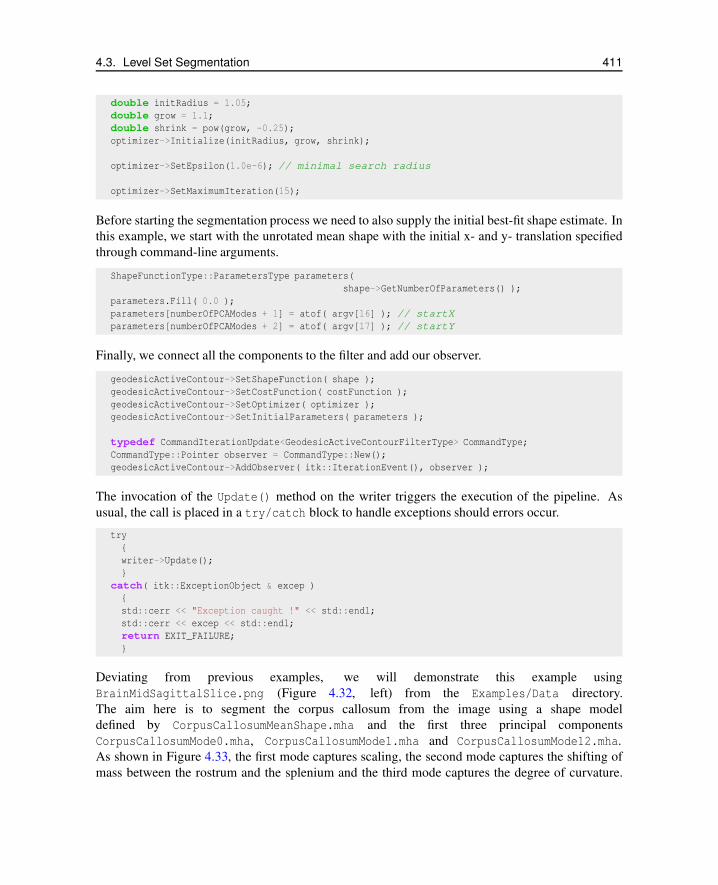
4.3. Level Set Segmentation 411
double initRadius = 1.05;
double grow = 1.1;
double shrink = pow(grow, -0.25);
optimizer->Initialize(initRadius, grow, shrink);
optimizer->SetEpsilon(1.0e-6); // minimal search radius
optimizer->SetMaximumIteration(15);
Before starting the segmentation process we need to also supply the initial best-fit shape estimate. In
this example, we start with the unrotated mean shape with the initial x- and y- translation specified
through command-line arguments.
ShapeFunctionType::ParametersType parameters(
shape->GetNumberOfParameters() );
parameters.Fill( 0.0 );
parameters[numberOfPCAModes + 1] = atof( argv[16] ); // startX
parameters[numberOfPCAModes + 2] = atof( argv[17] ); // startY
Finally, we connect all the components to the filter and add our observer.
geodesicActiveContour->SetShapeFunction( shape );
geodesicActiveContour->SetCostFunction( costFunction );
geodesicActiveContour->SetOptimizer( optimizer );
geodesicActiveContour->SetInitialParameters( parameters );
typedef CommandIterationUpdate<GeodesicActiveContourFilterType> CommandType;
CommandType::Pointer observer = CommandType::New();
geodesicActiveContour->AddObserver( itk::IterationEvent(), observer );
The invocation of the Update() method on the writer triggers the execution of the pipeline. As
usual, the call is placed in a try/catch block to handle exceptions should errors occur.
try
{
writer->Update();
}
catch( itk::ExceptionObject & excep )
{
std::cerr << "Exception caught !" << std::endl;
std::cerr << excep << std::endl;
return EXIT_FAILURE;
}
Deviating from previous examples, we will demonstrate this example using
BrainMidSagittalSlice.png (Figure 4.32, left) from the Examples/Data directory.
The aim here is to segment the corpus callosum from the image using a shape model
defined by CorpusCallosumMeanShape.mha and the first three principal components
CorpusCallosumMode0.mha, CorpusCallosumMode1.mha and CorpusCallosumMode12.mha.
As shown in Figure 4.33, the first mode captures scaling, the second mode captures the shifting of
mass between the rostrum and the splenium and the third mode captures the degree of curvature.

412 Chapter 4. Segmentation
Figure 4.32: The input image to the GeodesicActiveContourShapePriorLevelSetImageFilter is a synthesized
MR-T1 mid-sagittal slice (217× 180 pixels, 1× 1 mm spacing) of the brain (left) and the initial best-fit shape
(right) chosen to roughly overlap the corpus callosum in the image to be segmented.
−3σ mean +3σ
mode 0:
mode 1:
mode 2:
Figure 4.33: First three PCA modes of a low-resolution (58× 31 pixels, 2× 2 mm spacing) corpus callosum
model used in the shape guided geodesic active contours example.
Segmentation results with and without shape guidance are shown in Figure 4.34.
A sigma value of 1.0 was used to compute the image gradient and the propagation and shape prior
scaling are respectively set to 0.5 and 0.02. An initial level set was created by placing one seed
point in the rostrum (60,102), one in the splenium (120,85) and one centrally in the body (88,83)of the corpus callosum with an initial radius of 6 pixels at each seed position. The best-fit shape was
initially placed with a translation of (10,0)mm so that it roughly overlapped the corpus callosum in
the image as shown in Figure 4.32 (right).
From Figure 4.34 it can be observed that without shape guidance (left), segmentation using geodesic
active contour leaks in the regions where the corpus callosum blends into the surrounding brain
tissues. With shape guidance (center), the segmentation is constrained by the global shape model to
prevent leaking.
The final best-fit shape parameters after the segmentation process is:
Parameters: [-0.384988, -0.578738, 0.557793, 0.275202, 16.9992, 4.73473]
and is shown in Figure 4.34 (right). Note that a 0.28 radian (15.8 degree) rotation has been intro-
duced to match the model to the corpus callosum in the image. Additionally, a negative weight for

4.4. Feature Extraction 413
Figure 4.34: Corpus callosum segmentation using geodesic active contours without (left) and with (center)
shape guidance. The image on the right represents the best-fit shape at the end of the segmentation process.
the first mode shrinks the size relative to the mean shape. A negative weight for the second mode
shifts the mass to splenium, and a positive weight for the third mode increases the curvature. It can
also be observed that the final segmentation is a combination of the best-fit shape with additional lo-
cal deformation. The combination of both global and local shape allows the segmentation to capture
fine details not represented in the shape model.
4.4 Feature Extraction
Extracting salient features from images is an important task on image processing. It is typically used
for guiding segmentation methods, preparing data for registration methods, or as a mechanism for
recognizing anatomical structures in images. The following section introduce some of the feature
extraction methods available in ITK.
4.4.1 Hough Transform
The Hough transform is a widely used technique for detection of geometrical features in images.
It is based on mapping the image into a parametric space in which it may be easier to identify if
particular geometrical features are present in the image. The transformation is specific for each
desired geometrical shape.
Line Extraction
The source code for this section can be found in the file
HoughTransform2DLinesImageFilter.cxx.
This example illustrates the use of the itk::HoughTransform2DLinesImageFilter to find
straight lines in a 2-dimensional image.
First, we include the header files of the filter.

414 Chapter 4. Segmentation
#include "itkHoughTransform2DLinesImageFilter.h"
Next, we declare the pixel type and image dimension and specify the image type to be used as input.
We also specify the image type of the accumulator used in the Hough transform filter.
typedef unsigned char PixelType;
typedef float AccumulatorPixelType;
const unsigned int Dimension = 2;
typedef itk::Image< PixelType, Dimension > ImageType;
typedef itk::Image< AccumulatorPixelType, Dimension > AccumulatorImageType;
We setup a reader to load the input image.
typedef itk::ImageFileReader< ImageType > ReaderType;
ReaderType::Pointer reader = ReaderType::New();
reader->SetFileName( argv[1] );
try
{
reader->Update();
}
catch( itk::ExceptionObject & excep )
{
std::cerr << "Exception caught !" << std::endl;
std::cerr << excep << std::endl;
return EXIT_FAILURE;
}
ImageType::Pointer localImage = reader->GetOutput();
Once the image is loaded, we apply a itk::GradientMagnitudeImageFilter to segment edges.
This casts the input image using a itk::CastImageFilter .
typedef itk::CastImageFilter< ImageType, AccumulatorImageType >
CastingFilterType;
CastingFilterType::Pointer caster = CastingFilterType::New();
std::cout << "Applying gradient magnitude filter" << std::endl;
typedef itk::GradientMagnitudeImageFilter<AccumulatorImageType,
AccumulatorImageType > GradientFilterType;
GradientFilterType::Pointer gradFilter = GradientFilterType::New();
caster->SetInput(localImage);
gradFilter->SetInput(caster->GetOutput());
gradFilter->Update();
The next step is to apply a threshold filter on the gradient magnitude image to keep only bright
values. Only pixels with a high value will be used by the Hough transform filter.

4.4. Feature Extraction 415
std::cout << "Thresholding" << std::endl;
typedef itk::ThresholdImageFilter<AccumulatorImageType> ThresholdFilterType;
ThresholdFilterType::Pointer threshFilter = ThresholdFilterType::New();
threshFilter->SetInput( gradFilter->GetOutput());
threshFilter->SetOutsideValue(0);
unsigned char threshBelow = 0;
unsigned char threshAbove = 255;
threshFilter->ThresholdOutside(threshBelow,threshAbove);
threshFilter->Update();
We create the HoughTransform2DLinesImageFilter based on the pixel type of the input image (the
resulting image from the ThresholdImageFilter).
std::cout << "Computing Hough Map" << std::endl;
typedef itk::HoughTransform2DLinesImageFilter<AccumulatorPixelType,
AccumulatorPixelType> HoughTransformFilterType;
HoughTransformFilterType::Pointer houghFilter
= HoughTransformFilterType::New();
We set the input to the filter to be the output of the ThresholdImageFilter. We set also the number
of lines we are looking for. Basically, the filter computes the Hough map, blurs it using a certain
variance and finds maxima in the Hough map. After a maximum is found, the local neighborhood,
a circle, is removed from the Hough map. SetDiscRadius() defines the radius of this disc.
The output of the filter is the accumulator.
houghFilter->SetInput(threshFilter->GetOutput());
houghFilter->SetNumberOfLines(atoi(argv[3]));
if(argc > 4 )
{
houghFilter->SetVariance(atof(argv[4]));
}
if(argc > 5 )
{
houghFilter->SetDiscRadius(atof(argv[5]));
}
houghFilter->Update();
AccumulatorImageType::Pointer localAccumulator = houghFilter->GetOutput();
We can also get the lines as itk::LineSpatialObject . The GetLines() function return a list of
those.
HoughTransformFilterType::LinesListType lines;
lines = houghFilter->GetLines(atoi(argv[3]));
std::cout << "Found " << lines.size() << " line(s)." << std::endl;
We can then allocate an image to draw the resulting lines as binary objects.

416 Chapter 4. Segmentation
typedef unsigned char OutputPixelType;
typedef itk::Image< OutputPixelType, Dimension > OutputImageType;
OutputImageType::Pointer localOutputImage = OutputImageType::New();
OutputImageType::RegionType region(localImage->GetLargestPossibleRegion());
localOutputImage->SetRegions(region);
localOutputImage->CopyInformation(localImage);
localOutputImage->Allocate(true); // initialize buffer to zero
We iterate through the list of lines and we draw them.
typedef HoughTransformFilterType::LinesListType::const_iterator LineIterator;
LineIterator itLines = lines.begin();
while( itLines != lines.end() )
{
We get the list of points which consists of two points to represent a straight line. Then, from these
two points, we compute a fixed point u and a unit vector~v to parameterize the line.
typedef HoughTransformFilterType::LineType::PointListType PointListType;
PointListType pointsList = (*itLines)->GetPoints();
PointListType::const_iterator itPoints = pointsList.begin();
double u[2];
u[0] = (*itPoints).GetPosition()[0];
u[1] = (*itPoints).GetPosition()[1];
itPoints++;
double v[2];
v[0] = u[0]-(*itPoints).GetPosition()[0];
v[1] = u[1]-(*itPoints).GetPosition()[1];
double norm = std::sqrt(v[0]*v[0]+v[1]*v[1]);
v[0] /= norm;
v[1] /= norm;
We draw a white pixels in the output image to represent the line.

4.4. Feature Extraction 417
ImageType::IndexType localIndex;
itk::Size<2> size = localOutputImage->GetLargestPossibleRegion().GetSize();
float diag = std::sqrt((float)( size[0]*size[0] + size[1]*size[1] ));
for(int i=static_cast<int>(-diag); i<static_cast<int>(diag); i++)
{
localIndex[0]=(long int)(u[0]+i*v[0]);
localIndex[1]=(long int)(u[1]+i*v[1]);
OutputImageType::RegionType outputRegion =
localOutputImage->GetLargestPossibleRegion();
if( outputRegion.IsInside( localIndex ) )
{
localOutputImage->SetPixel( localIndex, 255 );
}
}
itLines++;
}
We setup a writer to write out the binary image created.
typedef itk::ImageFileWriter< OutputImageType > WriterType;
WriterType::Pointer writer = WriterType::New();
writer->SetFileName( argv[2] );
writer->SetInput( localOutputImage );
try
{
writer->Update();
}
catch( itk::ExceptionObject & excep )
{
std::cerr << "Exception caught !" << std::endl;
std::cerr << excep << std::endl;
return EXIT_FAILURE;
}
Circle Extraction
The source code for this section can be found in the file
HoughTransform2DCirclesImageFilter.cxx.
This example illustrates the use of the itk::HoughTransform2DCirclesImageFilter to find
circles in a 2-dimensional image.
First, we include the header files of the filter.
#include "itkHoughTransform2DCirclesImageFilter.h"
Next, we declare the pixel type and image dimension and specify the image type to be used as input.

418 Chapter 4. Segmentation
We also specify the image type of the accumulator used in the Hough transform filter.
typedef unsigned char PixelType;
typedef float AccumulatorPixelType;
const unsigned int Dimension = 2;
typedef itk::Image< PixelType, Dimension > ImageType;
ImageType::IndexType localIndex;
typedef itk::Image< AccumulatorPixelType, Dimension > AccumulatorImageType;
We setup a reader to load the input image.
typedef itk::ImageFileReader< ImageType > ReaderType;
ReaderType::Pointer reader = ReaderType::New();
reader->SetFileName( argv[1] );
try
{
reader->Update();
}
catch( itk::ExceptionObject & excep )
{
std::cerr << "Exception caught !" << std::endl;
std::cerr << excep << std::endl;
return EXIT_FAILURE;
}
ImageType::Pointer localImage = reader->GetOutput();
We create the HoughTransform2DCirclesImageFilter based on the pixel type of the input image (the
resulting image from the ThresholdImageFilter).
std::cout << "Computing Hough Map" << std::endl;
typedef itk::HoughTransform2DCirclesImageFilter<PixelType,
AccumulatorPixelType> HoughTransformFilterType;
HoughTransformFilterType::Pointer houghFilter
= HoughTransformFilterType::New();
We set the input of the filter to be the output of the ImageFileReader. We set also the number of
circles we are looking for. Basically, the filter computes the Hough map, blurs it using a certain
variance and finds maxima in the Hough map. After a maximum is found, the local neighborhood,
a circle, is removed from the Hough map. SetDiscRadiusRatio() defines the radius of this disc pro-
portional to the radius of the disc found. The Hough map is computed by looking at the points
above a certain threshold in the input image. Then, for each point, a Gaussian derivative function
is computed to find the direction of the normal at that point. The standard deviation of the deriva-
tive function can be adjusted by SetSigmaGradient(). The accumulator is filled by drawing a line
along the normal and the length of this line is defined by the minimum radius (SetMinimumRa-
dius()) and the maximum radius (SetMaximumRadius()). Moreover, a sweep angle can be defined
by SetSweepAngle() (default 0.0) to increase the accuracy of detection.
The output of the filter is the accumulator.

4.4. Feature Extraction 419
houghFilter->SetInput( reader->GetOutput() );
houghFilter->SetNumberOfCircles( atoi(argv[3]) );
houghFilter->SetMinimumRadius( atof(argv[4]) );
houghFilter->SetMaximumRadius( atof(argv[5]) );
if( argc > 6 )
{
houghFilter->SetSweepAngle( atof(argv[6]) );
}
if( argc > 7 )
{
houghFilter->SetSigmaGradient( atoi(argv[7]) );
}
if( argc > 8 )
{
houghFilter->SetVariance( atof(argv[8]) );
}
if( argc > 9 )
{
houghFilter->SetDiscRadiusRatio( atof(argv[9]) );
}
houghFilter->Update();
AccumulatorImageType::Pointer localAccumulator = houghFilter->GetOutput();
We can also get the circles as itk::EllipseSpatialObject . The GetCircles() function return
a list of those.
HoughTransformFilterType::CirclesListType circles;
circles = houghFilter->GetCircles( atoi(argv[3]) );
std::cout << "Found " << circles.size() << " circle(s)." << std::endl;
We can then allocate an image to draw the resulting circles as binary objects.
typedef unsigned char OutputPixelType;
typedef itk::Image< OutputPixelType, Dimension > OutputImageType;
OutputImageType::Pointer localOutputImage = OutputImageType::New();
OutputImageType::RegionType region;
region.SetSize(localImage->GetLargestPossibleRegion().GetSize());
region.SetIndex(localImage->GetLargestPossibleRegion().GetIndex());
localOutputImage->SetRegions( region );
localOutputImage->SetOrigin(localImage->GetOrigin());
localOutputImage->SetSpacing(localImage->GetSpacing());
localOutputImage->Allocate(true); // initializes buffer to zero
We iterate through the list of circles and we draw them.

420 Chapter 4. Segmentation
typedef HoughTransformFilterType::CirclesListType CirclesListType;
CirclesListType::const_iterator itCircles = circles.begin();
while( itCircles != circles.end() )
{
std::cout << "Center: ";
std::cout << (*itCircles)->GetObjectToParentTransform()->GetOffset()
<< std::endl;
std::cout << "Radius: " << (*itCircles)->GetRadius()[0] << std::endl;
We draw white pixels in the output image to represent each circle.
for(double angle = 0;angle <= 2*vnl_math::pi; angle += vnl_math::pi/60.0 )
{
localIndex[0] =
(long int)((*itCircles)->GetObjectToParentTransform()->GetOffset()[0]
+ (*itCircles)->GetRadius()[0]*std::cos(angle));
localIndex[1] =
(long int)((*itCircles)->GetObjectToParentTransform()->GetOffset()[1]
+ (*itCircles)->GetRadius()[0]*std::sin(angle));
OutputImageType::RegionType outputRegion =
localOutputImage->GetLargestPossibleRegion();
if( outputRegion.IsInside( localIndex ) )
{
localOutputImage->SetPixel( localIndex, 255 );
}
}
itCircles++;
}
We setup a writer to write out the binary image created.
typedef itk::ImageFileWriter< ImageType > WriterType;
WriterType::Pointer writer = WriterType::New();
writer->SetFileName( argv[2] );
writer->SetInput(localOutputImage );
try
{
writer->Update();
}
catch( itk::ExceptionObject & excep )
{
std::cerr << "Exception caught !" << std::endl;
std::cerr << excep << std::endl;
return EXIT_FAILURE;
}

CHAPTER
FIVE
STATISTICS
This chapter introduces the statistics functionalities in Insight. The statistics subsystem’s primary
purpose is to provide general capabilities for statistical pattern classification. However, its use is not
limited for classification. Users might want to use data containers and algorithms in the statistics
subsystem to perform other statistical analysis or to preprocess image data for other tasks.
The statistics subsystem mainly consists of three parts: data container classes, statistical algorithms,
and the classification framework. In this chapter, we will discuss each major part in that order.
5.1 Data Containers
An itk::Statistics::Sample object is a data container of elements that we call measurement
vectors. A measurement vector is an array of values (of the same type) measured on an object (In
images, it can be a vector of the gray intensity value and/or the gradient value of a pixel). Strictly
speaking from the design of the Sample class, a measurement vector can be any class derived from
itk::FixedArray, including FixedArray itself.
ListSample
Sample
ImageToListSampleAdaptor
ScalarImageToListSampleAdaptor JointDomainImageToListSampleAdaptor
ListSampleBase Histogram Subsample MembershipSample
PointSetToListSampleAdaptor
Figure 5.1: Sample class inheritance diagram.

422 Chapter 5. Statistics
5.1.1 Sample Interface
The source code for this section can be found in the file
ListSample.cxx.
This example illustrates the common interface of the Sample class in Insight.
Different subclasses of itk::Statistics::Sample expect different sets of template arguments. In
this example, we use the itk::Statistics::ListSample class that requires the type of measure-
ment vectors. The ListSample uses STL vector to store measurement vectors. This class conforms
to the common interface of Sample. Most methods of the Sample class interface are for retrieving
measurement vectors, the size of a container, and the total frequency. In this example, we will see
those information retrieving methods in addition to methods specific to the ListSample class for data
input.
To use the ListSample class, we include the header file for the class.
We need another header for measurement vectors. We are going to use the itk::Vector class
which is a subclass of the itk::FixedArray class.
#include "itkListSample.h"
#include "itkVector.h"
The following code snippet defines the measurement vector type as a three component float
itk::Vector. The MeasurementVectorType is the measurement vector type in the SampleType.
An object is instantiated at the third line.
typedef itk::Vector< float, 3 > MeasurementVectorType;
typedef itk::Statistics::ListSample< MeasurementVectorType > SampleType;
SampleType::Pointer sample = SampleType::New();
In the above code snippet, the namespace specifier for ListSample is itk::Statistics:: instead
of the usual namespace specifier for other ITK classes, itk::.
The newly instantiated object does not have any data in it. We have two different ways of storing
data elements. The first method is using the PushBack method.
MeasurementVectorType mv;
mv[0] = 1.0;
mv[1] = 2.0;
mv[2] = 4.0;
sample->PushBack(mv);
The previous code increases the size of the container by one and stores mv as the first data element
in it.
The other way to store data elements is calling the Resize method and then calling the
SetMeasurementVector() method with a measurement vector. The following code snippet in-
creases the size of the container to three and stores two measurement vectors at the second and the

5.1. Data Containers 423
third slot. The measurement vector stored using the PushBack method above is still at the first slot.
sample->Resize(3);
mv[0] = 2.0;
mv[1] = 4.0;
mv[2] = 5.0;
sample->SetMeasurementVector(1, mv);
mv[0] = 3.0;
mv[1] = 8.0;
mv[2] = 6.0;
sample->SetMeasurementVector(2, mv);
We have seen how to create an ListSample object and store measurement vectors using the
ListSample-specific interface. The following code shows the common interface of the Sample class.
The Size method returns the number of measurement vectors in the sample. The primary data
stored in Sample subclasses are measurement vectors. However, each measurement vector has its
associated frequency of occurrence within the sample. For the ListSample and the adaptor classes
(see Section 5.1.2), the frequency value is always one. itk::Statistics::Histogram can have a
varying frequency (float type) for each measurement vector. We retrieve measurement vectors us-
ing the GetMeasurementVector(unsigned long instance identifier), and frequency using
the GetFrequency(unsigned long instance identifier).
for ( unsigned long i = 0; i < sample->Size(); ++i )
{
std::cout << "id = " << i
<< "\t measurement vector = "
<< sample->GetMeasurementVector(i)
<< "\t frequency = "
<< sample->GetFrequency(i)
<< std::endl;
}
The output should look like the following:
id = 0 measurement vector = 1 2 4 frequency = 1
id = 1 measurement vector = 2 4 5 frequency = 1
id = 2 measurement vector = 3 8 6 frequency = 1
We can get the same result with its iterator.

424 Chapter 5. Statistics
SampleType::Iterator iter = sample->Begin();
while( iter != sample->End() )
{
std::cout << "id = " << iter.GetInstanceIdentifier()
<< "\t measurement vector = "
<< iter.GetMeasurementVector()
<< "\t frequency = "
<< iter.GetFrequency()
<< std::endl;
++iter;
}
The last method defined in the Sample class is the GetTotalFrequency() method that returns
the sum of frequency values associated with every measurement vector in a container. In the case of
ListSample and the adaptor classes, the return value should be exactly the same as that of the Size()
method, because the frequency values are always one for each measurement vector. However, for the
itk::Statistics::Histogram, the frequency values can vary. Therefore, if we want to develop
a general algorithm to calculate the sample mean, we must use the GetTotalFrequency() method
instead of the Size() method.
std::cout << "Size = " << sample->Size() << std::endl;
std::cout << "Total frequency = "
<< sample->GetTotalFrequency() << std::endl;
5.1.2 Sample Adaptors
There are two adaptor classes that provide the common itk::Statistics::Sample in-
terfaces for itk::Image and itk::PointSet, two fundamental data container classes
found in ITK. The adaptor classes do not store any real data elements themselves. These
data come from the source data container plugged into them. First, we will de-
scribe how to create an itk::Statistics::ImageToListSampleAdaptor and then an
itk::Statistics::PointSetToListSampleAdaptor object.
ImageToListSampleAdaptor
The source code for this section can be found in the file
ImageToListSampleAdaptor.cxx.
This example shows how to instantiate an itk::Statistics::ImageToListSampleAdaptor ob-
ject and plug-in an itk::Image object as the data source for the adaptor.
In this example, we use the ImageToListSampleAdaptor class that requires the input type of Im-
age as the template argument. To users of the ImageToListSampleAdaptor, the pixels of the input
image are treated as measurement vectors. The ImageToListSampleAdaptor is one of two adaptor
classes among the subclasses of the itk::Statistics::Sample. That means an ImageToList-

5.1. Data Containers 425
SampleAdaptor object does not store any real data. The data comes from other ITK data container
classes. In this case, an instance of the Image class is the source of the data.
To use an ImageToListSampleAdaptor object, include the header file for the class. Since we are
using an adaptor, we also should include the header file for the Image class. For illustration, we use
the itk::RandomImageSource that generates an image with random pixel values. So, we need to
include the header file for this class. Another convenient filter is the itk::ComposeImageFilter
which creates an image with pixels of array type from one or more input images composed of pixels
of scalar type. Since an element of a Sample object is a measurement vector, you cannot plug in an
image of scalar pixels. However, if we want to use an image of scalar pixels without the help from the
ComposeImageFilter, we can use the itk::Statistics::ScalarImageToListSampleAdaptor
class that is derived from the itk::Statistics::ImageToListSampleAdaptor . The usage of
the ScalarImageToListSampleAdaptor is identical to that of the ImageToListSampleAdaptor.
#include "itkImageToListSampleAdaptor.h"
#include "itkImage.h"
#include "itkRandomImageSource.h"
#include "itkComposeImageFilter.h"
We assume you already know how to create an image. The following code snippet will create a 2D
image of float pixels filled with random values.
typedef itk::Image<float,2> FloatImage2DType;
itk::RandomImageSource<FloatImage2DType>::Pointer random;
random = itk::RandomImageSource<FloatImage2DType>::New();
random->SetMin( 0.0 );
random->SetMax( 1000.0 );
typedef FloatImage2DType::SpacingValueType SpacingValueType;
typedef FloatImage2DType::SizeValueType SizeValueType;
typedef FloatImage2DType::PointValueType PointValueType;
SizeValueType size[2] = {20, 20};
random->SetSize( size );
SpacingValueType spacing[2] = {0.7, 2.1};
random->SetSpacing( spacing );
PointValueType origin[2] = {15, 400};
random->SetOrigin( origin );
We now have an instance of Image and need to cast it to an Image object with an array pixel
type (anything derived from the itk::FixedArray class such as itk::Vector, itk::Point,
itk::RGBPixel, or itk::CovariantVector).
Since the image pixel type is float in this example, we will use a single element float FixedArray
as our measurement vector type. And that will also be our pixel type for the cast filter.

426 Chapter 5. Statistics
typedef itk::FixedArray< float, 1 > MeasurementVectorType;
typedef itk::Image< MeasurementVectorType, 2 > ArrayImageType;
typedef itk::ComposeImageFilter< FloatImage2DType, ArrayImageType >
CasterType;
CasterType::Pointer caster = CasterType::New();
caster->SetInput( random->GetOutput() );
caster->Update();
Up to now, we have spent most of our time creating an image suitable for the adaptor. Actually, the
hard part of this example is done. Now, we just define an adaptor with the image type and instantiate
an object.
typedef itk::Statistics::ImageToListSampleAdaptor<
ArrayImageType > SampleType;
SampleType::Pointer sample = SampleType::New();
The final task is to plug in the image object to the adaptor. After that, we can use the common
methods and iterator interfaces shown in Section 5.1.1.
sample->SetImage( caster->GetOutput() );
If we are interested only in pixel values, the ScalarImageToListSampleAdaptor (scalar pix-
els) or the ImageToListSampleAdaptor (vector pixels) would be sufficient. However, if
we want to perform some statistical analysis on spatial information (image index or pixel’s
physical location) and pixel values altogether, we want to have a measurement vector
that consists of a pixel’s value and physical position. In that case, we can use the
itk::Statistics::JointDomainImageToListSampleAdaptor class. With this class, when
we call the GetMeasurementVector() method, the returned measurement vector is composed
of the physical coordinates and pixel values. The usage is almost the same as with Image-
ToListSampleAdaptor. One important difference between JointDomainImageToListSampleAdap-
tor and the other two image adaptors is that the JointDomainImageToListSampleAdaptor has the
SetNormalizationFactors() method. Each component of a measurement vector from the Joint-
DomainImageToListSampleAdaptor is divided by the corresponding component value from the sup-
plied normalization factors.
PointSetToListSampleAdaptor
The source code for this section can be found in the file
PointSetToListSampleAdaptor.cxx.
We will describe how to use itk::PointSet as a itk::Statistics::Sample using an adaptor
in this example.
The itk::Statistics::PointSetToListSampleAdaptor class requires a PointSet as input. The
PointSet class is an associative data container. Each point in a PointSet object can have an associated
optional data value. For the statistics subsystem, the current implementation of PointSetToListSam-

5.1. Data Containers 427
pleAdaptor takes only the point part into consideration. In other words, the measurement vectors
from a PointSetToListSampleAdaptor object are points from the PointSet object that is plugged into
the adaptor object.
To use an PointSetToListSampleAdaptor class, we include the header file for the class.
#include "itkPointSetToListSampleAdaptor.h"
Since we are using an adaptor, we also include the header file for the PointSet class.
#include "itkPointSet.h"
#include "itkVector.h"
Next we create a PointSet object. The following code snippet will create a PointSet object that stores
points (its coordinate value type is float) in 3D space.
typedef itk::PointSet< short > PointSetType;
PointSetType::Pointer pointSet = PointSetType::New();
Note that the short type used in the declaration of PointSetType pertains to the pixel
type associated with every point, not to the type used to represent point coordinates. If we
want to change the type of the point in terms of the coordinate value and/or dimension, we
have to modify the TMeshTraits (one of the optional template arguments for the PointSet
class). The easiest way of creating a custom mesh traits instance is to specialize the ex-
isting itk::DefaultStaticMeshTraits. By specifying the TCoordRep template argument,
we can change the coordinate value type of a point. By specifying the VPointDimension
template argument, we can change the dimension of the point. As mentioned earlier, a
PointSetToListSampleAdaptor object cares only about the points, and the type of measurement
vectors is the type of points.
To make the example a little bit realistic, we add two points into the pointSet.
PointSetType::PointType point;
point[0] = 1.0;
point[1] = 2.0;
point[2] = 3.0;
pointSet->SetPoint( 0UL, point);
point[0] = 2.0;
point[1] = 4.0;
point[2] = 6.0;
pointSet->SetPoint( 1UL, point );
Now we have a PointSet object with two points in it. The PointSet is ready to be plugged into the
adaptor. First, we create an instance of the PointSetToListSampleAdaptor class with the type of the
input PointSet object.

428 Chapter 5. Statistics
typedef itk::Statistics::PointSetToListSampleAdaptor<
PointSetType > SampleType;
SampleType::Pointer sample = SampleType::New();
Second, all we have to do is plug in the PointSet object to the adaptor. After that, we can use the
common methods and iterator interfaces shown in Section 5.1.1.
sample->SetPointSet( pointSet );
SampleType::Iterator iter = sample->Begin();
while( iter != sample->End() )
{
std::cout << "id = " << iter.GetInstanceIdentifier()
<< "\t measurement vector = "
<< iter.GetMeasurementVector()
<< "\t frequency = "
<< iter.GetFrequency()
<< std::endl;
++iter;
}
The source code for this section can be found in the file
PointSetToAdaptor.cxx.
We will describe how to use itk::PointSet as a Sample using an adaptor in this example.
itk::Statistics::PointSetToListSampleAdaptor class requires the type of input
itk::PointSet object. The itk::PointSet class is an associative data container. Each
point in a PointSet object can have its associated data value (optional). For the statistics subsys-
tem, current implementation of PointSetToListSampleAdaptor takes only the point part into
consideration. In other words, the measurement vectors from a PointSetToListSampleAdaptor
object are points from the PointSet object that is plugged-into the adaptor object.
To use, an itk::PointSetToListSampleAdaptor object, we include the header file for the class.
#include "itkPointSetToListSampleAdaptor.h"
Since, we are using an adaptor, we also include the header file for the itk::PointSet class.
#include "itkPointSet.h"
We assume you already know how to create an itk::PointSet object. The following code snippet
will create a 2D image of float pixels filled with random values.

5.1. Data Containers 429
typedef itk::PointSet<float,2> FloatPointSet2DType;
itk::RandomPointSetSource<FloatPointSet2DType>::Pointer random;
random = itk::RandomPointSetSource<FloatPointSet2DType>::New();
random->SetMin(0.0);
random->SetMax(1000.0);
unsigned long size[2] = {20, 20};
random->SetSize(size);
float spacing[2] = {0.7, 2.1};
random->SetSpacing( spacing );
float origin[2] = {15, 400};
random->SetOrigin( origin );
We now have an itk::PointSet object and need to cast it to an itk::PointSet object with array
type (anything derived from the itk::FixedArray class) pixels.
Since, the itk::PointSet object’s pixel type is float, We will use single element float
itk::FixedArray as our measurement vector type. And that will also be our pixel type for the
cast filter.
typedef itk::FixedArray< float, 1 > MeasurementVectorType;
typedef itk::PointSet< MeasurementVectorType, 2 > ArrayPointSetType;
typedef itk::ScalarToArrayCastPointSetFilter< FloatPointSet2DType,
ArrayPointSetType > CasterType;
CasterType::Pointer caster = CasterType::New();
caster->SetInput( random->GetOutput() );
caster->Update();
Up to now, we spend most of time to prepare an itk::PointSet object suitable for the adaptor.
Actually, the hard part of this example is done. Now, we must define an adaptor with the image type
and instantiate an object.
typedef itk::Statistics::PointSetToListSampleAdaptor<
ArrayPointSetType > SampleType;
SampleType::Pointer sample = SampleType::New();
The final thing we have to is to plug-in the image object to the adaptor. After that, we can use the
common methods and iterator interfaces shown in 5.1.1.
sample->SetPointSet( caster->GetOutput() );
5.1.3 Histogram
The source code for this section can be found in the file
Histogram.cxx.
This example shows how to create an itk::Statistics::Histogram object and use it.
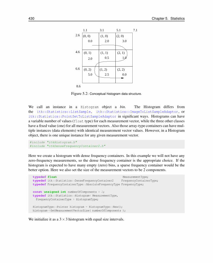
430 Chapter 5. Statistics
(1, 2)
2.6
4.6
0.5
2.5
0.0
2.0
5.0
2.0 3.0
1.0
0.0
3.1 5.1 7.11.1
6.6
8.6
(0, 0)
(2, 2)
(0, 1)
(0, 2)
(1, 0) (2, 0)
(1, 1) (2, 1)
Figure 5.2: Conceptual histogram data structure.
We call an instance in a Histogram object a bin. The Histogram differs from
the itk::Statistics::ListSample , itk::Statistics::ImageToListSampleAdaptor , or
itk::Statistics::PointSetToListSampleAdaptor in significant ways. Histograms can have
a variable number of values (float type) for each measurement vector, while the three other classes
have a fixed value (one) for all measurement vectors. Also those array-type containers can have mul-
tiple instances (data elements) with identical measurement vector values. However, in a Histogram
object, there is one unique instance for any given measurement vector.
#include "itkHistogram.h"
#include "itkDenseFrequencyContainer2.h"
Here we create a histogram with dense frequency containers. In this example we will not have any
zero-frequency measurements, so the dense frequency container is the appropriate choice. If the
histogram is expected to have many empty (zero) bins, a sparse frequency container would be the
better option. Here we also set the size of the measurement vectors to be 2 components.
typedef float MeasurementType;
typedef itk::Statistics::DenseFrequencyContainer2 FrequencyContainerType;
typedef FrequencyContainerType::AbsoluteFrequencyType FrequencyType;
const unsigned int numberOfComponents = 2;
typedef itk::Statistics::Histogram< MeasurementType,
FrequencyContainerType > HistogramType;
HistogramType::Pointer histogram = HistogramType::New();
histogram->SetMeasurementVectorSize( numberOfComponents );
We initialize it as a 3× 3 histogram with equal size intervals.

5.1. Data Containers 431
HistogramType::SizeType size( numberOfComponents );
size.Fill(3);
HistogramType::MeasurementVectorType lowerBound( numberOfComponents );
HistogramType::MeasurementVectorType upperBound( numberOfComponents );
lowerBound[0] = 1.1;
lowerBound[1] = 2.6;
upperBound[0] = 7.1;
upperBound[1] = 8.6;
histogram->Initialize(size, lowerBound, upperBound );
Now the histogram is ready for storing frequency values. We will fill each bin’s frequency according
to the Figure 5.2. There are three ways of accessing data elements in the histogram:
• using instance identifiers—just like any other Sample object;
• using n-dimensional indices—just like an Image object;
• using an iterator—just like any other Sample object.
In this example, the index (0,0) refers the same bin as the instance identifier (0) refers to. The
instance identifier of the index (0, 1) is (3), (0, 2) is (6), (2, 2) is (8), and so on.
histogram->SetFrequency(0UL, static_cast<FrequencyType>(0.0));
histogram->SetFrequency(1UL, static_cast<FrequencyType>(2.0));
histogram->SetFrequency(2UL, static_cast<FrequencyType>(3.0));
histogram->SetFrequency(3UL, static_cast<FrequencyType>(2.0f));
histogram->SetFrequency(4UL, static_cast<FrequencyType>(0.5f));
histogram->SetFrequency(5UL, static_cast<FrequencyType>(1.0f));
histogram->SetFrequency(6UL, static_cast<FrequencyType>(5.0f));
histogram->SetFrequency(7UL, static_cast<FrequencyType>(2.5f));
histogram->SetFrequency(8UL, static_cast<FrequencyType>(0.0f));
Let us examine if the frequency is set correctly by calling the GetFrequency(index) method. We
can use the GetFrequency(instance identifier) method for the same purpose.
HistogramType::IndexType index( numberOfComponents );
index[0] = 0;
index[1] = 2;
std::cout << "Frequency of the bin at index " << index
<< " is " << histogram->GetFrequency(index)
<< ", and the bin’s instance identifier is "
<< histogram->GetInstanceIdentifier(index) << std::endl;
For test purposes, we create a measurement vector and an index that belongs to the center bin.
HistogramType::MeasurementVectorType mv( numberOfComponents );
mv[0] = 4.1;
mv[1] = 5.6;
index.Fill(1);

432 Chapter 5. Statistics
We retrieve the measurement vector at the index value (1, 1), the center bin’s measurement vector.
The output is [4.1, 5.6].
std::cout << "Measurement vector at the center bin is "
<< histogram->GetMeasurementVector(index) << std::endl;
Since all the measurement vectors are unique in the Histogram class, we can determine the index
from a measurement vector.
HistogramType::IndexType resultingIndex;
histogram->GetIndex(mv,resultingIndex);
std::cout << "Index of the measurement vector " << mv
<< " is " << resultingIndex << std::endl;
In a similar way, we can get the instance identifier from the index.
std::cout << "Instance identifier of index " << index
<< " is " << histogram->GetInstanceIdentifier(index)
<< std::endl;
If we want to check if an index is valid, we use the method IsIndexOutOfBounds(index). The
following code snippet fills the index variable with (100, 100). It is obviously not a valid index.
index.Fill(100);
if ( histogram->IsIndexOutOfBounds(index) )
{
std::cout << "Index " << index << " is out of bounds." << std::endl;
}
The following code snippets show how to get the histogram size and frequency dimension.
std::cout << "Number of bins = " << histogram->Size()
<< " Total frequency = " << histogram->GetTotalFrequency()
<< " Dimension sizes = " << histogram->GetSize() << std::endl;
The Histogram class has a quantile calculation method, Quantile(dimension, percent). The
following code returns the 50th percentile along the first dimension. Note that the quantile calcula-
tion considers only one dimension.
std::cout << "50th percentile along the first dimension = "
<< histogram->Quantile(0, 0.5) << std::endl;
5.1.4 Subsample
The source code for this section can be found in the file
Subsample.cxx.
The itk::Statistics::Subsample is a derived sample. In other words, it requires another
itk::Statistics::Sample object for storing measurement vectors. The Subsample class stores a

5.1. Data Containers 433
subset of instance identifiers from another Sample object. Any Sample’s subclass can be the source
Sample object. You can create a Subsample object out of another Subsample object. The Subsample
class is useful for storing classification results from a test Sample object or for just extracting some
part of interest in a Sample object. Another good use of Subsample is sorting a Sample object. When
we use an itk::Image object as the data source, we do not want to change the order of data ele-
ments in the image. However, we sometimes want to sort or select data elements according to their
order. Statistics algorithms for this purpose accepts only Subsample objects as inputs. Changing the
order in a Subsample object does not change the order of the source sample.
To use a Subsample object, we include the header files for the class itself and a Sample class. We
will use the itk::Statistics::ListSample as the input sample.
#include "itkListSample.h"
#include "itkSubsample.h"
We need another header for measurement vectors. We are going to use the itk::Vector class in
this example.
#include "itkVector.h"
The following code snippet will create a ListSample object with three-component float measurement
vectors and put three measurement vectors into the list.
typedef itk::Vector< float, 3 > MeasurementVectorType;
typedef itk::Statistics::ListSample< MeasurementVectorType > SampleType;
SampleType::Pointer sample = SampleType::New();
MeasurementVectorType mv;
mv[0] = 1.0;
mv[1] = 2.0;
mv[2] = 4.0;
sample->PushBack(mv);
mv[0] = 2.0;
mv[1] = 4.0;
mv[2] = 5.0;
sample->PushBack(mv);
mv[0] = 3.0;
mv[1] = 8.0;
mv[2] = 6.0;
sample->PushBack(mv);
To create a Subsample instance, we define the type of the Subsample with the source sample type,
in this case, the previously defined SampleType. As usual, after that, we call the New() method to
create an instance. We must plug in the source sample, sample, using the SetSample() method.
However, with regard to data elements, the Subsample is empty. We specify which data elements,
among the data elements in the Sample object, are part of the Subsample. There are two ways of
doing that. First, if we want to include every data element (instance) from the sample, we simply

434 Chapter 5. Statistics
call the InitializeWithAllInstances() method like the following:
subsample->InitializeWithAllInstances();
This method is useful when we want to create a Subsample object for sorting all the data elements
in a Sample object. However, in most cases, we want to include only a subset of a Sample object.
For this purpose, we use the AddInstance(instance identifier) method in this example. In
the following code snippet, we include only the first and last instance in our subsample object from
the three instances of the Sample class.
typedef itk::Statistics::Subsample< SampleType > SubsampleType;
SubsampleType::Pointer subsample = SubsampleType::New();
subsample->SetSample( sample );
subsample->AddInstance( 0UL );
subsample->AddInstance( 2UL );
The Subsample is ready for use. The following code snippet shows how to use Iterator interfaces.
SubsampleType::Iterator iter = subsample->Begin();
while ( iter != subsample->End() )
{
std::cout << "instance identifier = " << iter.GetInstanceIdentifier()
<< "\t measurement vector = "
<< iter.GetMeasurementVector()
<< "\t frequency = "
<< iter.GetFrequency()
<< std::endl;
++iter;
}
As mentioned earlier, the instances in a Subsample can be sorted without changing the order in the
source Sample. For this purpose, the Subsample provides an additional instance indexing scheme.
The indexing scheme is just like the instance identifiers for the Sample. The index is an integer
value starting at 0, and the last value is one less than the number of all instances in a Subsample.
The Swap(0, 1) method, for example, swaps two instance identifiers of the first data element and
the second element in the Subsample. Internally, the Swap() method changes the instance identifiers
in the first and second position. Using indices, we can print out the effects of the Swap() method.
We use the GetMeasurementVectorByIndex(index) to get the measurement vector at the index
position. However, if we want to use the common methods of Sample that accepts instance iden-
tifiers, we call them after we get the instance identifiers using GetInstanceIdentifier(index)
method.

5.1. Data Containers 435
subsample->Swap(0, 1);
for ( int index = 0; index < subsample->Size(); ++index )
{
std::cout << "instance identifier = "
<< subsample->GetInstanceIdentifier(index)
<< "\t measurement vector = "
<< subsample->GetMeasurementVectorByIndex(index)
<< std::endl;
}
Since we are using a ListSample object as the source sample, the following code snippet will return
the same value (2) for the Size() and the GetTotalFrequency() methods. However, if we used a
Histogram object as the source sample, the two return values might be different because a Histogram
allows varying frequency values for each instance.
std::cout << "Size = " << subsample->Size() << std::endl;
std::cout << "Total frequency = "
<< subsample->GetTotalFrequency() << std::endl;
If we want to remove all instances that are associated with the Subsample, we call the Clear()
method. After this invocation, the Size() and the GetTotalFrequency() methods return 0.
subsample->Clear();
std::cout << "Size = " << subsample->Size() << std::endl;
std::cout << "Total frequency = "
<< subsample->GetTotalFrequency() << std::endl;
5.1.5 MembershipSample
The source code for this section can be found in the file
MembershipSample.cxx.
The itk::Statistics::MembershipSample is derived from the class
itk::Statistics::Sample that associates a class label with each measurement vector. It
needs another Sample object for storing measurement vectors. A MembershipSample object stores
a subset of instance identifiers from another Sample object. Any subclass of Sample can be the
source Sample object. The MembershipSample class is useful for storing classification results from
a test Sample object. The MembershipSample class can be considered as an associative container
that stores measurement vectors, frequency values, and class labels.
To use a MembershipSample object, we include the header files for the class itself and the Sample
class. We will use the itk::Statistics::ListSample as the input sample. We need another
header for measurement vectors. We are going to use the itk::Vector class which is a subclass of
the itk::FixedArray.
#include "itkListSample.h"
#include "itkMembershipSample.h"
#include "itkVector.h"

436 Chapter 5. Statistics
The following code snippet will create a ListSample object with three-component float measure-
ment vectors and put three measurement vectors in the ListSample object.
typedef itk::Vector< float, 3 > MeasurementVectorType;
typedef itk::Statistics::ListSample< MeasurementVectorType > SampleType;
SampleType::Pointer sample = SampleType::New();
MeasurementVectorType mv;
mv[0] = 1.0;
mv[1] = 2.0;
mv[2] = 4.0;
sample->PushBack(mv);
mv[0] = 2.0;
mv[1] = 4.0;
mv[2] = 5.0;
sample->PushBack(mv);
mv[0] = 3.0;
mv[1] = 8.0;
mv[2] = 6.0;
sample->PushBack(mv);
To create a MembershipSample instance, we define the type of the MembershipSample using the
source sample type using the previously defined SampleType. As usual, after that, we call the
New() method to create an instance. We must plug in the source sample, Sample, using the
SetSample() method. We provide class labels for data instances in the Sample object using the
AddInstance() method. As the required initialization step for the membershipSample, we must
call the SetNumberOfClasses() method with the number of classes. We must add all instances in
the source sample with their class labels. In the following code snippet, we set the first instance’
class label to 0, the second to 0, the third (last) to 1. After this, the membershipSample has two
Subsample objects. And the class labels for these two Subsample objects are 0 and 1. The 0 class
Subsample object includes the first and second instances, and the 1 class includes the third instance.
typedef itk::Statistics::MembershipSample< SampleType >
MembershipSampleType;
MembershipSampleType::Pointer membershipSample =
MembershipSampleType::New();
membershipSample->SetSample(sample);
membershipSample->SetNumberOfClasses(2);
membershipSample->AddInstance(0U, 0UL );
membershipSample->AddInstance(0U, 1UL );
membershipSample->AddInstance(1U, 2UL );
The Size() and GetTotalFrequency() returns the same information that Sample does.

5.1. Data Containers 437
std::cout << "Total frequency = "
<< membershipSample->GetTotalFrequency() << std::endl;
The membershipSample is ready for use. The following code snippet shows how to use the
Iterator interface. The MembershipSample’s Iterator has an additional method that returns
the class label (GetClassLabel()).
MembershipSampleType::ConstIterator iter = membershipSample->Begin();
while ( iter != membershipSample->End() )
{
std::cout << "instance identifier = " << iter.GetInstanceIdentifier()
<< "\t measurement vector = "
<< iter.GetMeasurementVector()
<< "\t frequency = "
<< iter.GetFrequency()
<< "\t class label = "
<< iter.GetClassLabel()
<< std::endl;
++iter;
}
To see the numbers of instances in each class subsample, we use the Size() method of the
ClassSampleType instance returned by the GetClassSample(index) method.
std::cout << "class label = 0 sample size = "
<< membershipSample->GetClassSample(0)->Size() << std::endl;
std::cout << "class label = 1 sample size = "
<< membershipSample->GetClassSample(1)->Size() << std::endl;
We call the GetClassSample() method to get the class subsample in the membershipSample.
The MembershipSampleType::ClassSampleType is actually a specialization of the
itk::Statistics::Subsample. We print out the instance identifiers, measurement vectors,
and frequency values that are part of the class. The output will be two lines for the two instances
that belong to the class 0.
MembershipSampleType::ClassSampleType::ConstPointer classSample =
membershipSample->GetClassSample( 0 );
MembershipSampleType::ClassSampleType::ConstIterator c_iter =
classSample->Begin();
while ( c_iter != classSample->End() )
{
std::cout << "instance identifier = " << c_iter.GetInstanceIdentifier()
<< "\t measurement vector = "
<< c_iter.GetMeasurementVector()
<< "\t frequency = "
<< c_iter.GetFrequency() << std::endl;
++c_iter;
}

438 Chapter 5. Statistics
5.1.6 MembershipSampleGenerator
The source code for this section can be found in the file
MembershipSampleGenerator.cxx.
To use, an MembershipSample object, we include the header files for the class itself and a Sample
class. We will use the ListSample as the input sample.
#include "itkListSample.h"
#include "itkMembershipSample.h"
We need another header for measurement vectors. We are going to use the itk::Vector class
which is a subclass of the itk::FixedArray in this example.
#include "itkVector.h"
The following code snippet will create a ListSample object with three-component float measure-
ment vectors and put three measurement vectors in the ListSample object.
typedef itk::Vector< float, 3 > MeasurementVectorType;
typedef itk::Statistics::ListSample< MeasurementVectorType > SampleType;
SampleType::Pointer sample = SampleType::New();
MeasurementVectorType mv;
mv[0] = 1.0;
mv[1] = 2.0;
mv[2] = 4.0;
sample->PushBack(mv);
mv[0] = 2.0;
mv[1] = 4.0;
mv[2] = 5.0;
sample->PushBack(mv);
mv[0] = 3.0;
mv[1] = 8.0;
mv[2] = 6.0;
sample->PushBack(mv);
To create a MembershipSample instance, we define the type of the MembershipSample with
the source sample type, in this case, previously defined SampleType. As usual, after that, we
call New() method to instantiate an instance. We must plug in the source sample, sample ob-
ject using the SetSample(source sample) method. However, in regard to class labels, the
membershipSample is empty. We provide class labels for data instances in the sample object using
the AddInstance(class label, instance identifier) method. As the required initialization
step for the membershipSample, we must call the SetNumberOfClasses(number of classes)
method with the number of classes. We must add all instances in the source sample with their class
labels. In the following code snippet, we set the first instance class label to 0, the second to 0, the
third (last) to 1. After this, the membershipSample has two Subclass objects. And the class labels

5.1. Data Containers 439
for these two Subclass are 0 and 1. The 0 class Subsample object includes the first and second
instances, and the 1 class includes the third instance.
typedef itk::Statistics::MembershipSample< SampleType >
MembershipSampleType;
MembershipSampleType::Pointer membershipSample =
MembershipSampleType::New();
membershipSample->SetSample(sample);
membershipSample->SetNumberOfClasses(2);
membershipSample->AddInstance(0U, 0UL );
membershipSample->AddInstance(0U, 1UL );
membershipSample->AddInstance(1U, 2UL );
The Size() and GetTotalFrequency() methods return the same values as the sample.
std::cout << "Size = " << membershipSample->Size() << std::endl;
std::cout << "Total frequency = "
<< membershipSample->GetTotalFrequency() << std::endl;
The membershipSample is ready for use. The following code snippet shows how to use Iterator
interfaces. The MembershipSample Iterator has an additional method that returns the class label
(GetClassLabel()).
MembershipSampleType::Iterator iter = membershipSample->Begin();
while ( iter != membershipSample->End() )
{
std::cout << "instance identifier = " << iter.GetInstanceIdentifier()
<< "\t measurement vector = "
<< iter.GetMeasurementVector()
<< "\t frequency = "
<< iter.GetFrequency()
<< "\t class label = "
<< iter.GetClassLabel()
<< std::endl;
++iter;
}
To see the numbers of instances in each class subsample, we use the GetClassSampleSize(class
label) method.
std::cout << "class label = 0 sample size = "
<< membershipSample->GetClassSampleSize(0) << std::endl;
std::cout << "class label = 1 sample size = "
<< membershipSample->GetClassSampleSize(0) << std::endl;
We call the GetClassSample(class label) method to get the class subsample in the
membershipSample. The MembershipSampleType::ClassSampleType is actually an specializa-
tion of the itk::Statistics::Subsample. We print out the instance identifiers, measurement
vectors, and frequency values that are part of the class. The output will be two lines for the two

440 Chapter 5. Statistics
instances that belong to the class 0.
MembershipSampleType::ClassSampleType::Pointer classSample =
membershipSample->GetClassSample(0);
MembershipSampleType::ClassSampleType::Iterator c_iter =
classSample->Begin();
while ( c_iter != classSample->End() )
{
std::cout << "instance identifier = " << c_iter.GetInstanceIdentifier()
<< "\t measurement vector = "
<< c_iter.GetMeasurementVector()
<< "\t frequency = "
<< c_iter.GetFrequency() << std::endl;
++c_iter;
}
5.1.7 K-d Tree
The source code for this section can be found in the file
KdTree.cxx.
The itk::Statistics::KdTree implements a data structure that separates samples in a k-
dimension space. The std::vector class is used here as the container for the measurement vectors
from a sample.
#include "itkVector.h"
#include "itkMath.h"
#include "itkListSample.h"
#include "itkWeightedCentroidKdTreeGenerator.h"
#include "itkEuclideanDistanceMetric.h"
We define the measurement vector type and instantiate a itk::Statistics::ListSample object,
and then put 1000 measurement vectors in the object.
typedef itk::Vector< float, 2 > MeasurementVectorType;
typedef itk::Statistics::ListSample< MeasurementVectorType > SampleType;
SampleType::Pointer sample = SampleType::New();
sample->SetMeasurementVectorSize( 2 );
MeasurementVectorType mv;
for (unsigned int i = 0; i < 1000; ++i )
{
mv[0] = (float) i;
mv[1] = (float) ((1000 - i) / 2 );
sample->PushBack( mv );
}
The following code snippet shows how to create two KdTree objects. The first object
itk::Statistics::KdTreeGenerator has a minimal set of information (partition dimension,

5.1. Data Containers 441
partition value, and pointers to the left and right child nodes). The second tree from the
itk::Statistics::WeightedCentroidKdTreeGenerator has additional information such as the
number of children under each node, and the vector sum of the measurement vectors belonging to
children of a particular node. WeightedCentroidKdTreeGenerator and the resulting k-d tree structure
were implemented based on the description given in the paper by Kanungo et al [29].
The instantiation and input variables are exactly the same for both tree generators. Using the
SetSample() method we plug-in the source sample. The bucket size input specifies the limit on
the maximum number of measurement vectors that can be stored in a terminal (leaf) node. A bigger
bucket size results in a smaller number of nodes in a tree. It also affects the efficiency of search.
With many small leaf nodes, we might experience slower search performance because of excessive
boundary comparisons.
typedef itk::Statistics::KdTreeGenerator< SampleType > TreeGeneratorType;
TreeGeneratorType::Pointer treeGenerator = TreeGeneratorType::New();
treeGenerator->SetSample( sample );
treeGenerator->SetBucketSize( 16 );
treeGenerator->Update();
typedef itk::Statistics::WeightedCentroidKdTreeGenerator< SampleType >
CentroidTreeGeneratorType;
CentroidTreeGeneratorType::Pointer centroidTreeGenerator =
CentroidTreeGeneratorType::New();
centroidTreeGenerator->SetSample( sample );
centroidTreeGenerator->SetBucketSize( 16 );
centroidTreeGenerator->Update();
After the generation step, we can get the pointer to the kd-tree from the generator by calling the
GetOutput() method. To traverse a kd-tree, we have to use the GetRoot() method. The method
will return the root node of the tree. Every node in a tree can have its left and/or right child node.
To get the child node, we call the Left() or the Right() method of a node (these methods do not
belong to the kd-tree but to the nodes).
We can get other information about a node by calling the methods described below in addition to the
child node pointers.

442 Chapter 5. Statistics
typedef TreeGeneratorType::KdTreeType TreeType;
typedef TreeType::KdTreeNodeType NodeType;
TreeType::Pointer tree = treeGenerator->GetOutput();
TreeType::Pointer centroidTree = centroidTreeGenerator->GetOutput();
NodeType* root = tree->GetRoot();
if ( root->IsTerminal() )
{
std::cout << "Root node is a terminal node." << std::endl;
}
else
{
std::cout << "Root node is not a terminal node." << std::endl;
}
unsigned int partitionDimension;
float partitionValue;
root->GetParameters( partitionDimension, partitionValue);
std::cout << "Dimension chosen to split the space = "
<< partitionDimension << std::endl;
std::cout << "Split point on the partition dimension = "
<< partitionValue << std::endl;
std::cout << "Address of the left chile of the root node = "
<< root->Left() << std::endl;
std::cout << "Address of the right chile of the root node = "
<< root->Right() << std::endl;
root = centroidTree->GetRoot();
std::cout << "Number of the measurement vectors under the root node"
<< " in the tree hierarchy = " << root->Size() << std::endl;
NodeType::CentroidType centroid;
root->GetWeightedCentroid( centroid );
std::cout << "Sum of the measurement vectors under the root node = "
<< centroid << std::endl;
std::cout << "Number of the measurement vectors under the left child"
<< " of the root node = " << root->Left()->Size() << std::endl;
In the following code snippet, we query the three nearest neighbors of the queryPoint on the two
tree. The results and procedures are exactly the same for both. First we define the point from which
distances will be measured.
MeasurementVectorType queryPoint;
queryPoint[0] = 10.0;
queryPoint[1] = 7.0;
Then we instantiate the type of a distance metric, create an object of this type and set the origin
of coordinates for measuring distances. The GetMeasurementVectorSize() method returns the

5.1. Data Containers 443
length of each measurement vector stored in the sample.
typedef itk::Statistics::EuclideanDistanceMetric< MeasurementVectorType >
DistanceMetricType;
DistanceMetricType::Pointer distanceMetric = DistanceMetricType::New();
DistanceMetricType::OriginType origin( 2 );
for ( unsigned int i = 0; i < sample->GetMeasurementVectorSize(); ++i )
{
origin[i] = queryPoint[i];
}
distanceMetric->SetOrigin( origin );
We can now set the number of neighbors to be located and the point coordinates to be used as a
reference system.
unsigned int numberOfNeighbors = 3;
TreeType::InstanceIdentifierVectorType neighbors;
tree->Search( queryPoint, numberOfNeighbors, neighbors);
std::cout <<
"\n*** kd-tree knn search result using an Euclidean distance metric:"
<< std::endl
<< "query point = [" << queryPoint << "]" << std::endl
<< "k = " << numberOfNeighbors << std::endl;
std::cout << "measurement vector : distance from querry point " << std::endl;
std::vector<double> distances1 (numberOfNeighbors);
for ( unsigned int i = 0; i < numberOfNeighbors; ++i )
{
distances1[i] = distanceMetric->Evaluate(
tree->GetMeasurementVector( neighbors[i] ));
std::cout << "[" << tree->GetMeasurementVector( neighbors[i] )
<< "] : "
<< distances1[i]
<< std::endl;
}
Instead of using an Euclidean distance metric, Tree itself can also return the distance vector. Here
we get the distance values from tree and compare them with previous values.

444 Chapter 5. Statistics
std::vector<double> distances2;
tree->Search( queryPoint, numberOfNeighbors, neighbors, distances2 );
std::cout << "\n*** kd-tree knn search result directly from tree:"
<< std::endl
<< "query point = [" << queryPoint << "]" << std::endl
<< "k = " << numberOfNeighbors << std::endl;
std::cout << "measurement vector : distance from querry point " << std::endl;
for ( unsigned int i = 0; i < numberOfNeighbors; ++i )
{
std::cout << "[" << tree->GetMeasurementVector( neighbors[i] )
<< "] : "
<< distances2[i]
<< std::endl;
if ( itk::Math::NotAlmostEquals( distances2[i], distances1[i] ) )
{
std::cerr << "Mismatched distance values by tree." << std::endl;
return EXIT_FAILURE;
}
}
As previously indicated, the interface for finding nearest neighbors in the centroid tree is very simi-
lar.
std::vector<double> distances3;
centroidTree->Search(
queryPoint, numberOfNeighbors, neighbors, distances3 );
centroidTree->Search( queryPoint, numberOfNeighbors, neighbors );
std::cout << "\n*** Weighted centroid kd-tree knn search result:"
<< std::endl
<< "query point = [" << queryPoint << "]" << std::endl
<< "k = " << numberOfNeighbors << std::endl;
std::cout << "measurement vector : distance_by_distMetric : distance_by_tree"
<< std::endl;
std::vector<double> distances4 (numberOfNeighbors);
for ( unsigned int i = 0; i < numberOfNeighbors; ++i )
{
distances4[i] = distanceMetric->Evaluate(
centroidTree->GetMeasurementVector( neighbors[i]));
std::cout << "[" << centroidTree->GetMeasurementVector( neighbors[i] )
<< "] : "
<< distances4[i]
<< " : "
<< distances3[i]
<< std::endl;
if ( itk::Math::NotAlmostEquals( distances2[i], distances1[i] ) )
{
std::cerr << "Mismatched distance values by centroid tree." << std::endl;
return EXIT_FAILURE;
}
}
KdTree also supports searching points within a hyper-spherical kernel. We specify the radius and

5.2. Algorithms and Functions 445
call the Search() method. In the case of the KdTree, this is done with the following lines of code.
double radius = 437.0;
tree->Search( queryPoint, radius, neighbors );
std::cout << "\nSearching points within a hyper-spherical kernel:"
<< std::endl;
std::cout << "*** kd-tree radius search result:" << std::endl
<< "query point = [" << queryPoint << "]" << std::endl
<< "search radius = " << radius << std::endl;
std::cout << "measurement vector : distance" << std::endl;
for ( unsigned int i = 0; i < neighbors.size(); ++i )
{
std::cout << "[" << tree->GetMeasurementVector( neighbors[i] )
<< "] : "
<< distanceMetric->Evaluate(
tree->GetMeasurementVector( neighbors[i]))
<< std::endl;
}
In the case of the centroid KdTree, the Search() method is used as illustrated by the following
code.
centroidTree->Search( queryPoint, radius, neighbors );
std::cout << "\n*** Weighted centroid kd-tree radius search result:"
<< std::endl
<< "query point = [" << queryPoint << "]" << std::endl
<< "search radius = " << radius << std::endl;
std::cout << "measurement vector : distance" << std::endl;
for ( unsigned int i = 0; i < neighbors.size(); ++i )
{
std::cout << "[" << centroidTree->GetMeasurementVector( neighbors[i] )
<< "] : "
<< distanceMetric->Evaluate(
centroidTree->GetMeasurementVector( neighbors[i]))
<< std::endl;
}
5.2 Algorithms and Functions
In the previous section, we described the data containers in the ITK statistics subsystem. We also
need data processing algorithms and statistical functions to conduct statistical analysis or statistical
classification using these containers. Here we define an algorithm to be an operation over a set of
measurement vectors in a sample. A function is an operation over individual measurement vectors.
For example, if we implement a class ( itk::Statistics::EuclideanDistance) to calculate the
Euclidean distance between two measurement vectors, we call it a function, while if we implemented
a class ( itk::Statistics::MeanCalculator) to calculate the mean of a sample, we call it an
algorithm.

446 Chapter 5. Statistics
5.2.1 Sample Statistics
We will show how to get sample statistics such as means and covariance from the (
itk::Statistics::Sample) classes. Statistics can tells us characteristics of a sample. Such
sample statistics are very important for statistical classification. When we know the form of the
sample distributions and their parameters (statistics), we can conduct Bayesian classification. In
ITK, sample mean and covariance calculation algorithms are implemented. Each algorithm also
has its weighted version (see Section 5.2.1). The weighted versions are used in the expectation-
maximization parameter estimation process.
Mean and Covariance
The source code for this section can be found in the file
SampleStatistics.cxx.
We include the header file for the itk::Vector class that will be our measurement vector template
in this example.
#include "itkVector.h"
We will use the itk::Statistics::ListSample as our sample template. We include the header
for the class too.
#include "itkListSample.h"
The following headers are for sample statistics algorithms.
#include "itkMeanSampleFilter.h"
#include "itkCovarianceSampleFilter.h"
The following code snippet will create a ListSample object with three-component float measurement
vectors and put five measurement vectors in the ListSample object.

5.2. Algorithms and Functions 447
const unsigned int MeasurementVectorLength = 3;
typedef itk::Vector< float, MeasurementVectorLength > MeasurementVectorType;
typedef itk::Statistics::ListSample< MeasurementVectorType > SampleType;
SampleType::Pointer sample = SampleType::New();
sample->SetMeasurementVectorSize( MeasurementVectorLength );
MeasurementVectorType mv;
mv[0] = 1.0;
mv[1] = 2.0;
mv[2] = 4.0;
sample->PushBack( mv );
mv[0] = 2.0;
mv[1] = 4.0;
mv[2] = 5.0;
sample->PushBack( mv );
mv[0] = 3.0;
mv[1] = 8.0;
mv[2] = 6.0;
sample->PushBack( mv );
mv[0] = 2.0;
mv[1] = 7.0;
mv[2] = 4.0;
sample->PushBack( mv );
mv[0] = 3.0;
mv[1] = 2.0;
mv[2] = 7.0;
sample->PushBack( mv );
To calculate the mean (vector) of a sample, we instantiate the
itk::Statistics::MeanSampleFilter class that implements the mean algorithm and plug
in the sample using the SetInputSample(sample*) method. By calling the Update() method,
we run the algorithm. We get the mean vector using the GetMean() method. The output from the
GetOutput() method is the pointer to the mean vector.
typedef itk::Statistics::MeanSampleFilter< SampleType > MeanAlgorithmType;
MeanAlgorithmType::Pointer meanAlgorithm = MeanAlgorithmType::New();
meanAlgorithm->SetInput( sample );
meanAlgorithm->Update();
std::cout << "Sample mean = " << meanAlgorithm->GetMean() << std::endl;
The covariance calculation algorithm will also calculate the mean while performing the covariance
matrix calculation. The mean can be accessed using the GetMean() method while the covariance
can be accessed using the GetCovarianceMatrix() method.

448 Chapter 5. Statistics
typedef itk::Statistics::CovarianceSampleFilter< SampleType >
CovarianceAlgorithmType;
CovarianceAlgorithmType::Pointer covarianceAlgorithm =
CovarianceAlgorithmType::New();
covarianceAlgorithm->SetInput( sample );
covarianceAlgorithm->Update();
std::cout << "Mean = " << std::endl;
std::cout << covarianceAlgorithm->GetMean() << std::endl;
std::cout << "Covariance = " << std::endl;
std::cout << covarianceAlgorithm->GetCovarianceMatrix() << std::endl;
Weighted Mean and Covariance
The source code for this section can be found in the file
WeightedSampleStatistics.cxx.
We include the header file for the itk::Vector class that will be our measurement vector template
in this example.
#include "itkVector.h"
We will use the itk::Statistics::ListSample as our sample template. We include the header
for the class too.
#include "itkListSample.h"
The following headers are for the weighted covariance algorithms.
#include "itkWeightedMeanSampleFilter.h"
#include "itkWeightedCovarianceSampleFilter.h"
The following code snippet will create a ListSample instance with three-component float measure-
ment vectors and put five measurement vectors in the ListSample object.

5.2. Algorithms and Functions 449
typedef itk::Statistics::ListSample< MeasurementVectorType > SampleType;
SampleType::Pointer sample = SampleType::New();
sample->SetMeasurementVectorSize( 3 );
MeasurementVectorType mv;
mv[0] = 1.0;
mv[1] = 2.0;
mv[2] = 4.0;
sample->PushBack( mv );
mv[0] = 2.0;
mv[1] = 4.0;
mv[2] = 5.0;
sample->PushBack( mv );
mv[0] = 3.0;
mv[1] = 8.0;
mv[2] = 6.0;
sample->PushBack( mv );
mv[0] = 2.0;
mv[1] = 7.0;
mv[2] = 4.0;
sample->PushBack( mv );
mv[0] = 3.0;
mv[1] = 2.0;
mv[2] = 7.0;
sample->PushBack( mv );
Robust versions of covariance algorithms require weight values for measurement vectors. We have
two ways of providing weight values for the weighted mean and weighted covariance algorithms.
The first method is to plug in an array of weight values. The size of the weight value array should be
equal to that of the measurement vectors. In both algorithms, we use the SetWeights(weights).

450 Chapter 5. Statistics
typedef itk::Statistics::WeightedMeanSampleFilter< SampleType >
WeightedMeanAlgorithmType;
WeightedMeanAlgorithmType::WeightArrayType weightArray( sample->Size() );
weightArray.Fill( 0.5 );
weightArray[2] = 0.01;
weightArray[4] = 0.01;
WeightedMeanAlgorithmType::Pointer weightedMeanAlgorithm =
WeightedMeanAlgorithmType::New();
weightedMeanAlgorithm->SetInput( sample );
weightedMeanAlgorithm->SetWeights( weightArray );
weightedMeanAlgorithm->Update();
std::cout << "Sample weighted mean = "
<< weightedMeanAlgorithm->GetMean() << std::endl;
typedef itk::Statistics::WeightedCovarianceSampleFilter< SampleType >
WeightedCovarianceAlgorithmType;
WeightedCovarianceAlgorithmType::Pointer weightedCovarianceAlgorithm =
WeightedCovarianceAlgorithmType::New();
weightedCovarianceAlgorithm->SetInput( sample );
weightedCovarianceAlgorithm->SetWeights( weightArray );
weightedCovarianceAlgorithm->Update();
std::cout << "Sample weighted covariance = " << std::endl;
std::cout << weightedCovarianceAlgorithm->GetCovarianceMatrix() << std::endl;
The second method for computing weighted statistics is to plug-in a function that returns a weight
value that is usually a function of each measurement vector. Since the weightedMeanAlgorithm
and weightedCovarianceAlgorithm already have the input sample plugged in, we only need to
call the SetWeightingFunction(weights) method.
ExampleWeightFunction::Pointer weightFunction = ExampleWeightFunction::New();
weightedMeanAlgorithm->SetWeightingFunction( weightFunction );
weightedMeanAlgorithm->Update();
std::cout << "Sample weighted mean = "
<< weightedMeanAlgorithm->GetMean() << std::endl;
weightedCovarianceAlgorithm->SetWeightingFunction( weightFunction );
weightedCovarianceAlgorithm->Update();
std::cout << "Sample weighted covariance = " << std::endl;
std::cout << weightedCovarianceAlgorithm->GetCovarianceMatrix();
std::cout << "Sample weighted mean (from WeightedCovarainceSampleFilter) = "
<< std::endl << weightedCovarianceAlgorithm->GetMean()
<< std::endl;

5.2. Algorithms and Functions 451
5.2.2 Sample Generation
SampleToHistogramFilter
The source code for this section can be found in the file
SampleToHistogramFilter.cxx.
Sometimes we want to work with a histogram instead of a list of measurement vectors (e.g.
itk::Statistics::ListSample, itk::Statistics::ImageToListSampleAdaptor,
or itk::Statistics::PointSetToListSample) to use less memory or to
perform a particular type od analysis. In such cases, we can import data
from a sample type to a itk::Statistics::Histogram object using the
itk::Statistics::SampleToHistogramFiler.
We use a ListSample object as the input for the filter. We include the header files for the ListSample
and Histogram classes, as well as the filter.
#include "itkListSample.h"
#include "itkHistogram.h"
#include "itkSampleToHistogramFilter.h"
We need another header for the type of the measurement vectors. We are going to use the
itk::Vector class which is a subclass of the itk::FixedArray in this example.
#include "itkVector.h"
The following code snippet creates a ListSample object with two-component int measurement vec-
tors and put the measurement vectors: [1,1] - 1 time, [2,2] - 2 times, [3,3] - 3 times, [4,4] - 4 times,
[5,5] - 5 times into the listSample.

452 Chapter 5. Statistics
typedef int MeasurementType;
const unsigned int MeasurementVectorLength = 2;
typedef itk::Vector< MeasurementType , MeasurementVectorLength >
MeasurementVectorType;
typedef itk::Statistics::ListSample< MeasurementVectorType > ListSampleType;
ListSampleType::Pointer listSample = ListSampleType::New();
listSample->SetMeasurementVectorSize( MeasurementVectorLength );
MeasurementVectorType mv;
for (unsigned int i = 1; i < 6; ++i)
{
for (unsigned int j = 0; j < 2; ++j)
{
mv[j] = ( MeasurementType ) i;
}
for (unsigned int j = 0; j < i; ++j)
{
listSample->PushBack(mv);
}
}
Here, we set up the size and bound of the output histogram.
typedef float HistogramMeasurementType;
const unsigned int numberOfComponents = 2;
typedef itk::Statistics::Histogram< HistogramMeasurementType >
HistogramType;
HistogramType::SizeType size( numberOfComponents );
size.Fill(5);
HistogramType::MeasurementVectorType lowerBound( numberOfComponents );
HistogramType::MeasurementVectorType upperBound( numberOfComponents );
lowerBound[0] = 0.5;
lowerBound[1] = 0.5;
upperBound[0] = 5.5;
upperBound[1] = 5.5;
Now, we set up the SampleToHistogramFilter object by passing listSample as the
input and initializing the histogram size and bounds with the SetHistogramSize(),
SetHistogramBinMinimum(), and SetHistogramBinMaximum() methods. We execute the filter
by calling the Update() method.

5.2. Algorithms and Functions 453
typedef itk::Statistics::SampleToHistogramFilter< ListSampleType,
HistogramType > FilterType;
FilterType::Pointer filter = FilterType::New();
filter->SetInput( listSample );
filter->SetHistogramSize( size );
filter->SetHistogramBinMinimum( lowerBound );
filter->SetHistogramBinMaximum( upperBound );
filter->Update();
The Size() and GetTotalFrequency() methods return the same values as the sample does.
const HistogramType* histogram = filter->GetOutput();
HistogramType::ConstIterator iter = histogram->Begin();
while ( iter != histogram->End() )
{
std::cout << "Measurement vectors = " << iter.GetMeasurementVector()
<< " frequency = " << iter.GetFrequency() << std::endl;
++iter;
}
std::cout << "Size = " << histogram->Size() << std::endl;
std::cout << "Total frequency = "
<< histogram->GetTotalFrequency() << std::endl;
NeighborhoodSampler
The source code for this section can be found in the file
NeighborhoodSampler.cxx.
When we want to create an itk::Statistics::Subsample object that includes only
the measurement vectors within a radius from a center in a sample, we can use
the itk::Statistics::NeighborhoodSampler. In this example, we will use the
itk::Statistics::ListSample as the input sample.
We include the header files for the ListSample and the NeighborhoodSampler classes.
#include "itkListSample.h"
#include "itkNeighborhoodSampler.h"
We need another header for measurement vectors. We are going to use the itk::Vector class
which is a subclass of the itk::FixedArray.
#include "itkVector.h"
The following code snippet will create a ListSample object with two-component int measurement
vectors and put the measurement vectors: [1,1] - 1 time, [2,2] - 2 times, [3,3] - 3 times, [4,4] - 4
times, [5,5] - 5 times into the listSample.

454 Chapter 5. Statistics
typedef int MeasurementType;
const unsigned int MeasurementVectorLength = 2;
typedef itk::Vector< MeasurementType , MeasurementVectorLength >
MeasurementVectorType;
typedef itk::Statistics::ListSample< MeasurementVectorType > SampleType;
SampleType::Pointer sample = SampleType::New();
sample->SetMeasurementVectorSize( MeasurementVectorLength );
MeasurementVectorType mv;
for (unsigned int i = 1; i < 6; ++i)
{
for (unsigned int j = 0; j < 2; ++j)
{
mv[j] = ( MeasurementType ) i;
}
for (unsigned int j = 0; j < i; ++j)
{
sample->PushBack(mv);
}
}
We plug-in the sample to the NeighborhoodSampler using the SetInputSample(sample*). The
two required inputs for the NeighborhoodSampler are a center and a radius. We set these two in-
puts using the SetCenter(center vector*) and the SetRadius(double*) methods respectively.
And then we call the Update() method to generate the Subsample object. This sampling procedure
subsamples measurement vectors within a hyper-spherical kernel that has the center and radius spec-
ified.
typedef itk::Statistics::NeighborhoodSampler< SampleType > SamplerType;
SamplerType::Pointer sampler = SamplerType::New();
sampler->SetInputSample( sample );
SamplerType::CenterType center( MeasurementVectorLength );
center[0] = 3;
center[1] = 3;
double radius = 1.5;
sampler->SetCenter( ¢er );
sampler->SetRadius( &radius );
sampler->Update();
SamplerType::OutputType::Pointer output = sampler->GetOutput();
The SamplerType::OutputType is in fact itk::Statistics::Subsample. The following code
prints out the resampled measurement vectors.

5.2. Algorithms and Functions 455
SamplerType::OutputType::Iterator iter = output->Begin();
while ( iter != output->End() )
{
std::cout << "instance identifier = " << iter.GetInstanceIdentifier()
<< "\t measurement vector = "
<< iter.GetMeasurementVector()
<< "\t frequency = "
<< iter.GetFrequency() << std::endl;
++iter;
}
5.2.3 Sample Sorting
The source code for this section can be found in the file
SampleSorting.cxx.
Sometimes we want to sort the measurement vectors in a sample. The sorted vectors may reveal
some characteristics of the sample. The insert sort, the heap sort, and the introspective sort algo-
rithms [43] for samples are implemented in ITK. To learn pros and cons of each algorithm, please
refer to [19]. ITK also offers the quick select algorithm.
Among the subclasses of the itk::Statistics::Sample, only the class
itk::Statistics::Subsample allows users to change the order of the measurement vector.
Therefore, we must create a Subsample to do any sorting or selecting.
We include the header files for the itk::Statistics::ListSample and the Subsample classes.
#include "itkListSample.h"
The sorting and selecting related functions are in the include file itkStatisticsAlgorithm.h.
Note that all functions in this file are in the itk::Statistics::Algorithm namespace.
#include "itkStatisticsAlgorithm.h"
We need another header for measurement vectors. We are going to use the itk::Vector class
which is a subclass of the itk::FixedArray in this example.
We define the types of the measurement vectors, the sample, and the subsample.
#include "itkVector.h"
We define two functions for convenience. The first one clears the content of the subsample and fill
it with the measurement vectors from the sample.

456 Chapter 5. Statistics
void initializeSubsample(SubsampleType* subsample, SampleType* sample)
{
subsample->Clear();
subsample->SetSample(sample);
subsample->InitializeWithAllInstances();
}
The second one prints out the content of the subsample using the Subsample’s iterator interface.
void printSubsample(SubsampleType* subsample, const char* header)
{
std::cout << std::endl;
std::cout << header << std::endl;
SubsampleType::Iterator iter = subsample->Begin();
while ( iter != subsample->End() )
{
std::cout << "instance identifier = " << iter.GetInstanceIdentifier()
<< " \t measurement vector = "
<< iter.GetMeasurementVector()
<< std::endl;
++iter;
}
}
The following code snippet will create a ListSample object with two-component int measurement
vectors and put the measurement vectors: [5,5] - 5 times, [4,4] - 4 times, [3,3] - 3 times, [2,2] - 2
times,[1,1] - 1 time into the sample.
SampleType::Pointer sample = SampleType::New();
MeasurementVectorType mv;
for (unsigned int i = 5; i > 0; --i )
{
for (unsigned int j = 0; j < 2; ++j)
{
mv[j] = ( MeasurementType ) i;
}
for (unsigned int j = 0; j < i; ++j)
{
sample->PushBack(mv);
}
}
We create a Subsample object and plug-in the sample.
SubsampleType::Pointer subsample = SubsampleType::New();
subsample->SetSample(sample);
initializeSubsample(subsample, sample);
printSubsample(subsample, "Unsorted");
The common parameters to all the algorithms are the Subsample object (subsample), the dimension
(activeDimension) that will be considered for the sorting or selecting (only the component belong-
ing to the dimension of the measurement vectors will be considered), the beginning index, and the

5.2. Algorithms and Functions 457
ending index of the measurement vectors in the subsample. The sorting or selecting algorithms are
applied only to the range specified by the beginning index and the ending index. The ending index
should be the actual last index plus one.
The itk::InsertSort function does not require any other optional arguments. The following
function call will sort the all measurement vectors in the subsample. The beginning index is 0, and
the ending index is the number of the measurement vectors in the subsample.
int activeDimension = 0;
itk::Statistics::Algorithm::InsertSort< SubsampleType >( subsample,
activeDimension, 0, subsample->Size() );
printSubsample(subsample, "InsertSort");
We sort the subsample using the heap sort algorithm. The arguments are identical to those of the
insert sort.
initializeSubsample(subsample, sample);
itk::Statistics::Algorithm::HeapSort< SubsampleType >( subsample,
activeDimension, 0, subsample->Size() );
printSubsample(subsample, "HeapSort");
The introspective sort algorithm needs an additional argument that specifies when to stop the intro-
spective sort loop and sort the fragment of the sample using the heap sort algorithm. Since we set the
threshold value as 16, when the sort loop reach the point where the number of measurement vectors
in a sort loop is not greater than 16, it will sort that fragment using the insert sort algorithm.
initializeSubsample(subsample, sample);
itk::Statistics::Algorithm::IntrospectiveSort< SubsampleType >
( subsample, activeDimension, 0, subsample->Size(), 16 );
printSubsample(subsample, "IntrospectiveSort");
We query the median of the measurements along the activeDimension. The last argument tells the
algorithm that we want to get the subsample->Size()/2-th element along the activeDimension.
The quick select algorithm changes the order of the measurement vectors.
initializeSubsample(subsample, sample);
SubsampleType::MeasurementType median =
itk::Statistics::Algorithm::QuickSelect< SubsampleType >( subsample,
activeDimension,
0, subsample->Size(),
subsample->Size()/2 );
std::cout << std::endl;
std::cout << "Quick Select: median = " << median << std::endl;
5.2.4 Probability Density Functions
The probability density function (PDF) for a specific distribution returns the probability density for
a measurement vector. To get the probability density from a PDF, we use the Evaluate(input)
method. PDFs for different distributions require different sets of distribution parameters. Before

458 Chapter 5. Statistics
calling the Evaluate() method, make sure to set the proper values for the distribution parameters.
Gaussian Distribution
The source code for this section can be found in the file
GaussianMembershipFunction.cxx.
The Gaussian probability density function itk::Statistics::GaussianMembershipFunction
requires two distribution parameters—the mean vector and the covariance matrix.
We include the header files for the class and the itk::Vector.
#include "itkVector.h"
#include "itkGaussianMembershipFunction.h"
We define the type of the measurement vector that will be input to the Gaussian membership func-
tion.
typedef itk::Vector< float, 2 > MeasurementVectorType;
The instantiation of the function is done through the usual New() method and a smart pointer.
typedef itk::Statistics::GaussianMembershipFunction< MeasurementVectorType >
DensityFunctionType;
DensityFunctionType::Pointer densityFunction = DensityFunctionType::New();
The length of the measurement vectors in the membership function, in this case a
vector of length 2, is specified using the SetMeasurementVectorSize() method.
densityFunction->SetMeasurementVectorSize( 2 );
We create the two distribution parameters and set them. The mean is [0, 0], and the covariance
matrix is a 2 x 2 matrix:(
4 0
0 4
)
We obtain the probability density for the measurement vector: [0, 0] using the
Evaluate(measurement vector) method and print it out.

5.2. Algorithms and Functions 459
DensityFunctionType::MeanVectorType mean( 2 );
mean.Fill( 0.0 );
DensityFunctionType::CovarianceMatrixType cov;
cov.SetSize( 2, 2 );
cov.SetIdentity();
cov *= 4;
densityFunction->SetMean( mean );
densityFunction->SetCovariance( cov );
MeasurementVectorType mv;
mv.Fill( 0 );
std::cout << densityFunction->Evaluate( mv ) << std::endl;
5.2.5 Distance Metric
Euclidean Distance
The source code for this section can be found in the file
EuclideanDistanceMetric.cxx.
The Euclidean distance function ( itk::Statistics::EuclideanDistanceMetric requires as
template parameter the type of the measurement vector. We can use this function for any subclass of
the itk::FixedArray. As a subclass of the itk::Statistics::DistanceMetric , it has two ba-
sic methods, the SetOrigin(measurement vector) and the Evaluate(measurement vector).
The Evaluate() method returns the distance between its argument (a measurement vector) and the
measurement vector set by the SetOrigin() method.
In addition to the two methods, EuclideanDistanceMetric has two more methods that return the
distance of two measurements — Evaluate(measurement vector, measurement vector) and
the coordinate distance between two measurements (not vectors) — Evaluate(measurement,
measurement). The argument type of the latter method is the type of the component of the mea-
surement vector.
We include the header files for the class and the itk::Vector.
#include "itkVector.h"
#include "itkArray.h"
#include "itkEuclideanDistanceMetric.h"
We define the type of the measurement vector that will be input of the Euclidean distance function.
As a result, the measurement type is float.
typedef itk::Array< float > MeasurementVectorType;
The instantiation of the function is done through the usual New() method and a smart pointer.

460 Chapter 5. Statistics
typedef itk::Statistics::EuclideanDistanceMetric< MeasurementVectorType >
DistanceMetricType;
DistanceMetricType::Pointer distanceMetric = DistanceMetricType::New();
We create three measurement vectors, the originPoint, the queryPointA, and the queryPointB.
The type of the originPoint is fixed in the itk::Statistics::DistanceMetric
base class as itk::Vector< double, length of the measurement vector of the each
distance metric instance>.
The Distance metric does not know about the length of the measurement vectors. We must set it
explicitly using the SetMeasurementVectorSize() method.
DistanceMetricType::OriginType originPoint( 2 );
MeasurementVectorType queryPointA( 2 );
MeasurementVectorType queryPointB( 2 );
originPoint[0] = 0;
originPoint[1] = 0;
queryPointA[0] = 2;
queryPointA[1] = 2;
queryPointB[0] = 3;
queryPointB[1] = 3;
In the following code snippet, we show the uses of the three different Evaluate() methods.
distanceMetric->SetOrigin( originPoint );
std::cout << "Euclidean distance between the origin and the query point A = "
<< distanceMetric->Evaluate( queryPointA )
<< std::endl;
std::cout << "Euclidean distance between the two query points (A and B) = "
<< distanceMetric->Evaluate( queryPointA, queryPointB )
<< std::endl;
std::cout << "Coordinate distance between "
<< "the first components of the two query points = "
<< distanceMetric->Evaluate( queryPointA[0], queryPointB[0] )
<< std::endl;
5.2.6 Decision Rules
A decision rule is a function that returns the index of one data element in a vector of data elements.
The index returned depends on the internal logic of each decision rule. The decision rule is an
essential part of the ITK statistical classification framework. The scores from a set of membership
functions (e.g. probability density functions, distance metrics) are compared by a decision rule and a
class label is assigned based on the output of the decision rule. The common interface is very simple.
Any decision rule class must implement the Evaluate() method. In addition to this method, certain

5.2. Algorithms and Functions 461
decision rule class can have additional method that accepts prior knowledge about the decision task.
The itk::MaximumRatioDecisionRule is an example of such a class.
The argument type for the Evaluate() method is std::vector< double >. The decision rule
classes are part of the itk namespace instead of itk::Statistics namespace.
For a project that uses a decision rule, it must link the itkCommon library. Decision rules are not
templated classes.
Maximum Decision Rule
The source code for this section can be found in the file
MaximumDecisionRule.cxx.
The itk::MaximumDecisionRule returns the index of the largest discriminant score among the
discriminant scores in the vector of discriminant scores that is the input argument of the Evaluate()
method.
To begin the example, we include the header files for the class and the MaximumDecisionRule. We
also include the header file for the std::vector class that will be the container for the discriminant
scores.
#include "itkMaximumDecisionRule.h"
#include <vector>
The instantiation of the function is done through the usual New() method and a smart pointer.
typedef itk::Statistics::MaximumDecisionRule DecisionRuleType;
DecisionRuleType::Pointer decisionRule = DecisionRuleType::New();
We create the discriminant score vector and fill it with three values. The Evaluate(
discriminantScores ) will return 2 because the third value is the largest value.
DecisionRuleType::MembershipVectorType discriminantScores;
discriminantScores.push_back( 0.1 );
discriminantScores.push_back( 0.3 );
discriminantScores.push_back( 0.6 );
std::cout << "MaximumDecisionRule: The index of the chosen = "
<< decisionRule->Evaluate( discriminantScores )
<< std::endl;
Minimum Decision Rule
The source code for this section can be found in the file
MinimumDecisionRule.cxx.
The Evaluate() method of the itk::MinimumDecisionRule returns the index of the smallest

462 Chapter 5. Statistics
discriminant score among the vector of discriminant scores that it receives as input.
To begin this example, we include the class header file. We also include the header file for the
std::vector class that will be the container for the discriminant scores.
#include "itkMinimumDecisionRule.h"
#include <vector>
The instantiation of the function is done through the usual New() method and a smart pointer.
typedef itk::Statistics::MinimumDecisionRule DecisionRuleType;
DecisionRuleType::Pointer decisionRule = DecisionRuleType::New();
We create the discriminant score vector and fill it with three values. The call Evaluate(
discriminantScores ) will return 0 because the first value is the smallest value.
DecisionRuleType::MembershipVectorType discriminantScores;
discriminantScores.push_back( 0.1 );
discriminantScores.push_back( 0.3 );
discriminantScores.push_back( 0.6 );
std::cout << "MinimumDecisionRule: The index of the chosen = "
<< decisionRule->Evaluate( discriminantScores )
<< std::endl;
Maximum Ratio Decision Rule
The source code for this section can be found in the file
MaximumRatioDecisionRule.cxx.
MaximumRatioDecisionRule returns the class label using a Bayesian style decision rule. The dis-
criminant scores are evaluated in the context of class priors. If the discriminant scores are actual
conditional probabilites (likelihoods) and the class priors are actual a priori class probabilities, then
this decision rule operates as Bayes rule, returning the class i if
p(x|i)p(i)> p(x| j)p( j) (5.1)
for all class j. The discriminant scores and priors are not required to be true probabilities.
This class is named the MaximumRatioDecisionRule as it can be implemented as returning the class
i ifp(x|i)p(x| j) >
p( j)
p(i)(5.2)
for all class j.
We include the header files for the class as well as the header file for the std::vector class that
will be the container for the discriminant scores.
#include "itkMaximumRatioDecisionRule.h"
#include <vector>

5.2. Algorithms and Functions 463
The instantiation of the function is done through the usual New() method and a smart pointer.
typedef itk::Statistics::MaximumRatioDecisionRule DecisionRuleType;
DecisionRuleType::Pointer decisionRule = DecisionRuleType::New();
We create the discriminant score vector and fill it with three values. We also create a vector
(aPrioris) for the a priori values. The Evaluate( discriminantScores ) will return 1.
DecisionRuleType::MembershipVectorType discriminantScores;
discriminantScores.push_back( 0.1 );
discriminantScores.push_back( 0.3 );
discriminantScores.push_back( 0.6 );
DecisionRuleType::PriorProbabilityVectorType aPrioris;
aPrioris.push_back( 0.1 );
aPrioris.push_back( 0.8 );
aPrioris.push_back( 0.1 );
decisionRule->SetPriorProbabilities( aPrioris );
std::cout << "MaximumRatioDecisionRule: The index of the chosen = "
<< decisionRule->Evaluate( discriminantScores )
<< std::endl;
5.2.7 Random Variable Generation
A random variable generation class returns a variate when the GetVariate() method is called.
When we repeatedly call the method for “enough” times, the set of variates we will get follows the
distribution form of the random variable generation class.
Normal (Gaussian) Distribution
The source code for this section can be found in the file
NormalVariateGenerator.cxx.
The itk::Statistics::NormalVariateGenerator generates random variables according to the
standard normal distribution (mean = 0, standard deviation = 1).
To use the class in a project, we must link the itkStatistics library to the project.
To begin the example we include the header file for the class.
#include "itkNormalVariateGenerator.h"
The NormalVariateGenerator is a non-templated class. We simply call the New() method to create
an instance. Then, we provide the seed value using the Initialize(seed value).

464 Chapter 5. Statistics
typedef itk::Statistics::NormalVariateGenerator GeneratorType;
GeneratorType::Pointer generator = GeneratorType::New();
generator->Initialize( (int) 2003 );
for ( unsigned int i = 0; i < 50; ++i )
{
std::cout << i << " : \t" << generator->GetVariate() << std::endl;
}
5.3 Statistics applied to Images
5.3.1 Image Histograms
Scalar Image Histogram with Adaptor
The source code for this section can be found in the file
ImageHistogram1.cxx.
This example shows how to compute the histogram of a scalar image. Since the
statistics framework classes operate on Samples and ListOfSamples, we need to intro-
duce a class that will make the image look like a list of samples. This class is the
itk::Statistics::ImageToListSampleAdaptor. Once we have connected this adaptor to an
image, we can proceed to use the itk::Statistics::SampleToHistogramFilter in order to
compute the histogram of the image.
First, we need to include the headers for the itk::Statistics::ImageToListSampleAdaptor
and the itk::Image classes.
#include "itkImageToListSampleAdaptor.h"
#include "itkImage.h"
Now we include the headers for the Histogram, the SampleToHistogramFilter, and the reader
that we will use for reading the image from a file.
#include "itkImageFileReader.h"
#include "itkHistogram.h"
#include "itkSampleToHistogramFilter.h"
The image type must be defined using the typical pair of pixel type and dimension specification.
typedef unsigned char PixelType;
const unsigned int Dimension = 2;
typedef itk::Image<PixelType, Dimension > ImageType;
Using the same image type we instantiate the type of the image reader that will provide the image
source for our example.

5.3. Statistics applied to Images 465
typedef itk::ImageFileReader< ImageType > ReaderType;
ReaderType::Pointer reader = ReaderType::New();
reader->SetFileName( argv[1] );
Now we introduce the central piece of this example, which is the use of the adaptor that will present
the itk::Image as if it was a list of samples. We instantiate the type of the adaptor by using the
actual image type. Then construct the adaptor by invoking its New() method and assigning the result
to the corresponding smart pointer. Finally we connect the output of the image reader to the input
of the adaptor.
typedef itk::Statistics::ImageToListSampleAdaptor< ImageType > AdaptorType;
AdaptorType::Pointer adaptor = AdaptorType::New();
adaptor->SetImage( reader->GetOutput() );
You must keep in mind that adaptors are not pipeline objects. This means that they do not propagate
update calls. It is therefore your responsibility to make sure that you invoke the Update() method
of the reader before you attempt to use the output of the adaptor. As usual, this must be done inside
a try/catch block because the read operation can potentially throw exceptions.
try
{
reader->Update();
}
catch( itk::ExceptionObject & excp )
{
std::cerr << "Problem reading image file : " << argv[1] << std::endl;
std::cerr << excp << std::endl;
return EXIT_FAILURE;
}
At this point, we are ready for instantiating the type of the histogram filter. We must first declare the
type of histogram we wish to use. The adaptor type is also used as template parameter of the filter.
Having instantiated this type, we proceed to create one filter by invoking its New() method.
typedef PixelType HistogramMeasurementType;
typedef itk::Statistics::Histogram< HistogramMeasurementType >
HistogramType;
typedef itk::Statistics::SampleToHistogramFilter<
AdaptorType,
HistogramType>
FilterType;
FilterType::Pointer filter = FilterType::New();
We define now the characteristics of the Histogram that we want to compute. This typically includes
the size of each one of the component, but given that in this simple example we are dealing with a
scalar image, then our histogram will have a single component. For the sake of generality, however,

466 Chapter 5. Statistics
we use the HistogramType as defined inside of the Generator type. We define also the marginal
scale factor that will control the precision used when assigning values to histogram bins. Finally we
invoke the Update() method in the filter.
const unsigned int numberOfComponents = 1;
HistogramType::SizeType size( numberOfComponents );
size.Fill( 255 );
filter->SetInput( adaptor );
filter->SetHistogramSize( size );
filter->SetMarginalScale( 10 );
HistogramType::MeasurementVectorType min( numberOfComponents );
HistogramType::MeasurementVectorType max( numberOfComponents );
min.Fill( 0 );
max.Fill( 255 );
filter->SetHistogramBinMinimum( min );
filter->SetHistogramBinMaximum( max );
filter->Update();
Now we are ready for using the image histogram for any further processing. The histogram is
obtained from the filter by invoking the GetOutput() method.
HistogramType::ConstPointer histogram = filter->GetOutput();
In this current example we simply print out the frequency values of all the bins in the image his-
togram.
const unsigned int histogramSize = histogram->Size();
std::cout << "Histogram size " << histogramSize << std::endl;
for (unsigned int bin=0; bin < histogramSize; ++bin)
{
std::cout << "bin = " << bin << " frequency = ";
std::cout << histogram->GetFrequency( bin, 0 ) <<std::endl;
}
Scalar Image Histogram with Generator
The source code for this section can be found in the file
ImageHistogram2.cxx.
From the previous example you will have noticed that there is a significant number of operations to
perform to compute the simple histogram of a scalar image. Given that this is a relatively common
operation, it is convenient to encapsulate many of these operations in a single helper class.

5.3. Statistics applied to Images 467
The itk::Statistics::ScalarImageToHistogramGenerator is the result of such encapsula-
tion. This example illustrates how to compute the histogram of a scalar image using this helper
class.
We should first include the header of the histogram generator and the image class.
#include "itkScalarImageToHistogramGenerator.h"
#include "itkImage.h"
The image type must be defined using the typical pair of pixel type and dimension specification.
typedef unsigned char PixelType;
const unsigned int Dimension = 2;
typedef itk::Image<PixelType, Dimension > ImageType;
We use now the image type in order to instantiate the type of the corresponding histogram generator
class, and invoke its New() method in order to construct one.
typedef itk::Statistics::ScalarImageToHistogramGenerator<
ImageType > HistogramGeneratorType;
HistogramGeneratorType::Pointer histogramGenerator =
HistogramGeneratorType::New();
The image to be passed as input to the histogram generator is taken in this case from the output of
an image reader.
histogramGenerator->SetInput( reader->GetOutput() );
We define also the typical parameters that specify the characteristics of the histogram to be com-
puted.
histogramGenerator->SetNumberOfBins( 256 );
histogramGenerator->SetMarginalScale( 10.0 );
histogramGenerator->SetHistogramMin( -0.5 );
histogramGenerator->SetHistogramMax( 255.5 );
Finally we trigger the computation of the histogram by invoking the Compute() method of the
generator. Note again, that a generator is not a pipeline object and therefore it is up to you to make
sure that the filters providing the input image have been updated.
histogramGenerator->Compute();
The resulting histogram can be obtained from the generator by invoking its GetOutput() method.
It is also convenient to get the Histogram type from the traits of the generator type itself as shown in
the code below.

468 Chapter 5. Statistics
typedef HistogramGeneratorType::HistogramType HistogramType;
const HistogramType * histogram = histogramGenerator->GetOutput();
In this case we simply print out the frequency values of the histogram. These values can be accessed
by using iterators.
HistogramType::ConstIterator itr = histogram->Begin();
HistogramType::ConstIterator end = histogram->End();
unsigned int binNumber = 0;
while( itr != end )
{
std::cout << "bin = " << binNumber << " frequency = ";
std::cout << itr.GetFrequency() << std::endl;
++itr;
++binNumber;
}
Color Image Histogram with Generator
The source code for this section can be found in the file
ImageHistogram3.cxx.
By now, you are probably thinking that the statistics framework in ITK is too complex for simply
computing histograms from images. Here we illustrate that the benefit for this complexity is the
power that these methods provide for dealing with more complex and realistic uses of image statistics
than the trivial 256-bin histogram of 8-bit images that most software packages provide. One of such
cases is the computation of histograms from multi-component images such as Vector images and
color images.
This example shows how to compute the histogram of an RGB image by using the helper class
ImageToHistogramFilter. In this first example we compute the histogram of each channel inde-
pendently.
We start by including the header of the itk::Statistics::ImageToHistogramFilter, as well
as the headers for the image class and the RGBPixel class.
#include "itkImageToHistogramFilter.h"
#include "itkImage.h"
#include "itkRGBPixel.h"
The type of the RGB image is defined by first instantiating a RGBPixel and then using the image
dimension specification.

5.3. Statistics applied to Images 469
typedef unsigned char PixelComponentType;
typedef itk::RGBPixel< PixelComponentType > RGBPixelType;
const unsigned int Dimension = 2;
typedef itk::Image< RGBPixelType, Dimension > RGBImageType;
Using the RGB image type we can instantiate the type of the corresponding histogram filter and
construct one filter by invoking its New() method.
typedef itk::Statistics::ImageToHistogramFilter<
RGBImageType > HistogramFilterType;
HistogramFilterType::Pointer histogramFilter =
HistogramFilterType::New();
The parameters of the histogram must be defined now. Probably the most important one is the
arrangement of histogram bins. This is provided to the histogram through a size array. The type of
the array can be taken from the traits of the HistogramFilterType type. We create one instance
of the size object and fill in its content. In this particular case, the three components of the size
array will correspond to the number of bins used for each one of the RGB components in the color
image. The following lines show how to define a histogram on the red component of the image
while disregarding the green and blue components.
typedef HistogramFilterType::HistogramSizeType SizeType;
SizeType size( 3 );
size[0] = 255; // number of bins for the Red channel
size[1] = 1; // number of bins for the Green channel
size[2] = 1; // number of bins for the Blue channel
histogramFilter->SetHistogramSize( size );
The marginal scale must be defined in the filter. This will determine the precision in the assignment
of values to the histogram bins.
histogramFilter->SetMarginalScale( 10.0 );
Finally, we must specify the upper and lower bounds for the histogram. This can either be done
manually using the SetHistogramBinMinimum() and SetHistogramBinMaximum() methods or it
can be done automatically by calling SetHistogramAutoMinimumMaximum( true ). Here we use
the manual method.

470 Chapter 5. Statistics
HistogramFilterType::HistogramMeasurementVectorType lowerBound( 3 );
HistogramFilterType::HistogramMeasurementVectorType upperBound( 3 );
lowerBound[0] = 0;
lowerBound[1] = 0;
lowerBound[2] = 0;
upperBound[0] = 256;
upperBound[1] = 256;
upperBound[2] = 256;
histogramFilter->SetHistogramBinMinimum( lowerBound );
histogramFilter->SetHistogramBinMaximum( upperBound );
The input of the filter is taken from an image reader, and the computation of the histogram is trig-
gered by invoking the Update() method of the filter.
histogramFilter->SetInput( reader->GetOutput() );
histogramFilter->Update();
We can now access the results of the histogram computation by declaring a pointer to histogram
and getting its value from the filter using the GetOutput() method. Note that here we use a const
HistogramType pointer instead of a const smart pointer because we are sure that the filter is not
going to be destroyed while we access the values of the histogram. Depending on what you are
doing, it may be safer to assign the histogram to a const smart pointer as shown in previous examples.
typedef HistogramFilterType::HistogramType HistogramType;
const HistogramType * histogram = histogramFilter->GetOutput();
Just for the sake of exercising the experimental method [49], we verify that the resulting histogram
actually have the size that we requested when we configured the filter. This can be done by invoking
the Size() method of the histogram and printing out the result.
const unsigned int histogramSize = histogram->Size();
std::cout << "Histogram size " << histogramSize << std::endl;
Strictly speaking, the histogram computed here is the joint histogram of the three RGB components.
However, given that we set the resolution of the green and blue channels to be just one bin, the
histogram is in practice representing just the red channel. In the general case, we can alway access
the frequency of a particular channel in a joint histogram, thanks to the fact that the histogram class
offers a GetFrequency() method that accepts a channel as argument. This is illustrated in the
following lines of code.

5.3. Statistics applied to Images 471
unsigned int channel = 0; // red channel
std::cout << "Histogram of the red component" << std::endl;
for (unsigned int bin=0; bin < histogramSize; ++bin)
{
std::cout << "bin = " << bin << " frequency = ";
std::cout << histogram->GetFrequency( bin, channel ) << std::endl;
}
In order to reinforce the concepts presented above, we modify now the setup of the histogram filter
in order to compute the histogram of the green channel instead of the red one. This is done by
simply changing the number of bins desired on each channel and invoking the computation of the
filter again by calling the Update() method.
size[0] = 1; // number of bins for the Red channel
size[1] = 255; // number of bins for the Green channel
size[2] = 1; // number of bins for the Blue channel
histogramFilter->SetHistogramSize( size );
histogramFilter->Update();
The result can be verified now by setting the desired channel to green and invoking the
GetFrequency() method.
channel = 1; // green channel
std::cout << "Histogram of the green component" << std::endl;
for (unsigned int bin=0; bin < histogramSize; ++bin)
{
std::cout << "bin = " << bin << " frequency = ";
std::cout << histogram->GetFrequency( bin, channel ) << std::endl;
}
To finalize the example, we do the same computation for the case of the blue channel.
size[0] = 1; // number of bins for the Red channel
size[1] = 1; // number of bins for the Green channel
size[2] = 255; // number of bins for the Blue channel
histogramFilter->SetHistogramSize( size );
histogramFilter->Update();
and verify the output.

472 Chapter 5. Statistics
channel = 2; // blue channel
std::cout << "Histogram of the blue component" << std::endl;
for (unsigned int bin=0; bin < histogramSize; ++bin)
{
std::cout << "bin = " << bin << " frequency = ";
std::cout << histogram->GetFrequency( bin, channel ) << std::endl;
}
Color Image Histogram Writing
The source code for this section can be found in the file
ImageHistogram4.cxx.
The statistics framework in ITK has been designed for managing multi-variate statistics in a natural
way. The itk::Statistics::Histogram class reflects this concept clearly since it is a N-variable
joint histogram. This nature of the Histogram class is exploited in the following example in order to
build the joint histogram of a color image encoded in RGB values.
Note that the same treatment could be applied further to any vector image thanks to the generic
programming approach used in the implementation of the statistical framework.
The most relevant class in this example is the itk::Statistics::ImageToHistogramFilter.
This class will take care of adapting the itk::Image to a list of samples and then to a histogram
filter. The user is only bound to provide the desired resolution on the histogram bins for each one of
the image components.
In this example we compute the joint histogram of the three channels of an RGB image. Our output
histogram will be equivalent to a 3D array of bins. This histogram could be used further for feeding a
segmentation method based on statistical pattern recognition. Such method was actually used during
the generation of the image in the cover of the Software Guide.
The first step is to include the header files for the histogram filter, the RGB pixel type and the Image.
#include "itkImageToHistogramFilter.h"
#include "itkImage.h"
#include "itkRGBPixel.h"
We declare now the type used for the components of the RGB pixel, instantiate the type of the
RGBPixel and instantiate the image type.
typedef unsigned char PixelComponentType;
typedef itk::RGBPixel< PixelComponentType > RGBPixelType;
const unsigned int Dimension = 2;
typedef itk::Image< RGBPixelType, Dimension > RGBImageType;

5.3. Statistics applied to Images 473
Using the type of the color image, and in general of any vector image, we can now instantiate the
type of the histogram filter class. We then use that type for constructing an instance of the filter by
invoking its New() method and assigning the result to a smart pointer.
typedef itk::Statistics::ImageToHistogramFilter<
RGBImageType > HistogramFilterType;
HistogramFilterType::Pointer histogramFilter =
HistogramFilterType::New();
The resolution at which the statistics of each one of the color component will be evaluated is defined
by setting the number of bins along every component in the joint histogram. For this purpose we
take the HistogramSizeType trait from the filter and use it to instantiate a size variable. We set in
this variable the number of bins to use for each component of the color image.
typedef HistogramFilterType::HistogramSizeType SizeType;
SizeType size(3);
size[0] = 256; // number of bins for the Red channel
size[1] = 256; // number of bins for the Green channel
size[2] = 256; // number of bins for the Blue channel
histogramFilter->SetHistogramSize( size );
Finally, we must specify the upper and lower bounds for the histogram using the
SetHistogramBinMinimum() and SetHistogramBinMaximum() methods.
typedef HistogramFilterType::HistogramMeasurementVectorType
HistogramMeasurementVectorType;
HistogramMeasurementVectorType binMinimum( 3 );
HistogramMeasurementVectorType binMaximum( 3 );
binMinimum[0] = -0.5;
binMinimum[1] = -0.5;
binMinimum[2] = -0.5;
binMaximum[0] = 255.5;
binMaximum[1] = 255.5;
binMaximum[2] = 255.5;
histogramFilter->SetHistogramBinMinimum( binMinimum );
histogramFilter->SetHistogramBinMaximum( binMaximum );
The input to the histogram filter is taken from the output of an image reader. Of course, the output
of any filter producing an RGB image could have been used instead of a reader.
histogramFilter->SetInput( reader->GetOutput() );
The marginal scale is defined in the histogram filter. This value will define the precision in the

474 Chapter 5. Statistics
assignment of values to the histogram bins.
histogramFilter->SetMarginalScale( 10.0 );
Finally, the computation of the histogram is triggered by invoking the Update() method of the filter.
histogramFilter->Update();
At this point, we can recover the histogram by calling the GetOutput() method of the filter. The
result is assigned to a variable that is instantiated using the HistogramType trait of the filter type.
typedef HistogramFilterType::HistogramType HistogramType;
const HistogramType * histogram = histogramFilter->GetOutput();
We can verify that the computed histogram has the requested size by invoking its Size() method.
const unsigned int histogramSize = histogram->Size();
std::cout << "Histogram size " << histogramSize << std::endl;
The values of the histogram can now be saved into a file by walking through all of the histogram
bins and pushing them into a std::ofstream.
std::ofstream histogramFile;
histogramFile.open( argv[2] );
HistogramType::ConstIterator itr = histogram->Begin();
HistogramType::ConstIterator end = histogram->End();
typedef HistogramType::AbsoluteFrequencyType AbsoluteFrequencyType;
while( itr != end )
{
const AbsoluteFrequencyType frequency = itr.GetFrequency();
histogramFile.write( (const char *)(&frequency), sizeof(frequency) );
if (frequency != 0)
{
HistogramType::IndexType index;
index = histogram->GetIndex(itr.GetInstanceIdentifier());
std::cout << "Index = " << index << ", Frequency = " << frequency
<< std::endl;
}
++itr;
}
histogramFile.close();
Note that here the histogram is saved as a block of memory in a raw file. At this point you can use
visualization software in order to explore the histogram in a display that would be equivalent to a

5.3. Statistics applied to Images 475
scatter plot of the RGB components of the input color image.
5.3.2 Image Information Theory
Many concepts from Information Theory have been used successfully in the domain of image pro-
cessing. This section introduces some of such concepts and illustrates how the statistical framework
in ITK can be used for computing measures that have some relevance in terms of Information Theory
[58, 59, 33].
Computing Image Entropy
The concept of Entropy has been introduced into image processing as a crude mapping from its
application in Communications. The notions of Information Theory can be deceiving and misleading
when applied to images because their language from Communication Theory does not necessarily
map to what people in the Imaging Community use.
For example, it is commonly said that
“The Entropy of an image is a measure of the amount of information contained in an image”.
This statement is fundamentally incorrect.
The way the notion of Entropy is commonly measured in images is by first assuming that the spatial
location of a pixel in an image is irrelevant! That is, we simply take the statistical distribution
of the pixel values as it can be evaluated in a histogram and from that histogram we estimate the
frequency of the value associated to each bin. In other words, we simply assume that the image
is a set of pixels that are passing through a channel, just as things are commonly considered for
communication purposes.
Once the frequency of every pixel value has been estimated, Information Theory defines that the
amount of uncertainty that an observer will lose by taking one pixel and finding its real value to
be the one associated with the i-th bin of the histogram, is given by − log2 (pi), where pi is the
frequency in that histogram bin. Since a reduction in uncertainty is equivalent to an increase in the
amount of information in the observer, we conclude that measuring one pixel and finding its level to
be in the i-th bin results in an acquisition of − log2 (pi) bits of information1.
Since we could have picked any pixel at random, our chances of picking the ones that are associated
to the i-th histogram bin are given by pi. Therefore, the expected reduction in uncertainty that we
can get from measuring the value of one pixel is given by
1Note that bit is the unit of amount of information. Our modern culture has vulgarized the bit and its multiples, the Byte,
KiloByte, MegaByte, GigaByte and so on as simple measures of the amount of RAM memory and capacity of a hard drive in
a computer. In that sense, a confusion is created between the encoding of a piece of data and its actual amount of information.
For example a file composed of one million letters will take one million bytes in a hard disk, but it does not necessarily have
one million bytes of information, since in many cases parts of the file can be predicted from others. This is the reason why
data compression can manage to compact files.

476 Chapter 5. Statistics
H =−∑i
pi · log2 (pi) (5.3)
This quantity H is what is usually defined as the Entropy of the Image. It would be more accurate to
call it the Entropy of the random variable associated to the intensity value of one pixel. The fact that
H is unrelated to the spatial arrangement of the pixels in an image shows how little of the real Image
Information H actually represents. The Entropy of an image, as measured above, is only a crude
indication of how the intensity values are spread in the dynamic range of intensities. For example,
an image with maximum entropy will be the one that has a large dynamic range and every value in
that range is equally probable.
The common convention of H as a representation of image information has terribly undermined the
enormous potential on the application of Information Theory to image processing and analysis.
The real concepts of Information Theory would require that we define the amount of information in
an image based on our expectations and prior knowledge from that image. In particular, the Amount
of Information provided by an image should measure the number of features that we are not able to
predict based on our prior knowledge about that image. For example, if we know that we are going
to analyze a CT scan of the abdomen of an adult human male in the age range of 40 to 45, there
is already a good deal that we could predict about the content of that image. The real amount of
information in the image is the representation of the features in the image that we could not predict
from knowing that it is a CT scan from a human adult male.
The application of Information Theory to image analysis is still in its early infancy and it is an
exciting and promising field to be explored further. All that being said, let’s now look closer at how
the concept of Entropy (which is not the amount of information in an image) can be measured with
the ITK statistics framework.
The source code for this section can be found in the file
ImageEntropy1.cxx.
This example shows how to compute the entropy of an image. More formally this should be said :
The reduction in uncertainty gained when we measure the intensity of one randomly selected pixel
in this image, given that we already know the statistical distribution of the image intensity values.
In practice it is almost never possible to know the real statistical distribution of intensities and we
are forced to estimate it from the evaluation of the histogram from one or several images of similar
nature. We can use the counts in histogram bins in order to compute frequencies and then consider
those frequencies to be estimations of the probablility of a new value to belong to the intensity range
of that bin.
Since the first stage in estimating the entropy of an image is to compute its histogram,
we must start by including the headers of the classes that will perform such a computa-
tion. In this case, we are going to use a scalar image as input, therefore we need the
itk::Statistics::ScalarImageToHistogramGenerator class, as well as the image class.
#include "itkScalarImageToHistogramGenerator.h"
#include "itkImage.h"

5.3. Statistics applied to Images 477
The pixel type and dimension of the image are explicitly declared and then used for instantiating the
image type.
typedef unsigned char PixelType;
const unsigned int Dimension = 3;
typedef itk::Image< PixelType, Dimension > ImageType;
The image type is used as template parameter for instantiating the histogram generator.
typedef itk::Statistics::ScalarImageToHistogramGenerator<
ImageType > HistogramGeneratorType;
HistogramGeneratorType::Pointer histogramGenerator =
HistogramGeneratorType::New();
The parameters of the desired histogram are defined, including the number of bins and the marginal
scale. For convenience in this example, we read the number of bins from the command line argu-
ments. In this way we can easily experiment with different values for the number of bins and see
how that choice affects the computation of the entropy.
const unsigned int numberOfHistogramBins = atoi( argv[2] );
histogramGenerator->SetNumberOfBins( numberOfHistogramBins );
histogramGenerator->SetMarginalScale( 10.0 );
We can then connect as input the output image from a reader and trigger the histogram computation
by invoking the Compute() method in the generator.
histogramGenerator->SetInput( reader->GetOutput() );
histogramGenerator->Compute();
The resulting histogram can be recovered from the generator by using the GetOutput() method. A
histogram class can be declared using the HistogramType trait from the generator.
typedef HistogramGeneratorType::HistogramType HistogramType;
const HistogramType * histogram = histogramGenerator->GetOutput();
We proceed now to compute the estimation of entropy given the histogram. The first conceptual
jump to be done here is to assume that the histogram, which is the simple count of frequency of
occurrence for the gray scale values of the image pixels, can be normalized in order to estimate the
probability density function PDF of the actual statistical distribution of pixel values.
First we declare an iterator that will visit all the bins in the histogram. Then we obtain the total
number of counts using the GetTotalFrequency() method, and we initialize the entropy variable
to zero.

478 Chapter 5. Statistics
HistogramType::ConstIterator itr = histogram->Begin();
HistogramType::ConstIterator end = histogram->End();
double Sum = histogram->GetTotalFrequency();
double Entropy = 0.0;
We start now visiting every bin and estimating the probability of a pixel to have a value in the
range of that bin. The base 2 logarithm of that probability is computed, and then weighted by the
probability in order to compute the expected amount of information for any given pixel. Note that a
minimum value is imposed for the probability in order to avoid computing logarithms of zeros.
Note that the log(2) factor is used to convert the natural logarithm in to a logarithm of base 2, and
makes it possible to report the entropy in its natural unit: the bit.
while( itr != end )
{
const double probability = itr.GetFrequency() / Sum;
if( probability > 0.99 / Sum )
{
Entropy += - probability * std::log( probability ) / std::log( 2.0 );
}
++itr;
}
The result of this sum is considered to be our estimation of the image entropy. Note that the Entropy
value will change depending on the number of histogram bins that we use for computing the his-
togram. This is particularly important when dealing with images whose pixel values have dynamic
ranges so large that our number of bins will always underestimate the variability of the data.
std::cout << "Image entropy = " << Entropy << " bits " << std::endl;
As an illustration, the application of this program to the image
• Examples/Data/BrainProtonDensitySlice.png
results in the following values of entropy for different values of number of histogram bins.
Number of Histogram Bins 16 32 64 128 255
Estimated Entropy (bits) 3.02 3.98 4.92 5.89 6.88
This table highlights the importance of carefully considering the characteristics of the histograms
used for estimating Information Theory measures such as the entropy.

5.3. Statistics applied to Images 479
Computing Images Mutual Information
The source code for this section can be found in the file
ImageMutualInformation1.cxx.
This example illustrates how to compute the Mutual Information between two images using classes
from the Statistics framework. Note that you could also use for this purpose the ImageMetrics
designed for the image registration framework.
For example, you could use:
• itk::MutualInformationImageToImageMetric
• itk::MattesMutualInformationImageToImageMetric
• itk::MutualInformationHistogramImageToImageMetric
• itk::MutualInformationImageToImageMetric
• itk::NormalizedMutualInformationHistogramImageToImageMetric
• itk::KullbackLeiblerCompareHistogramImageToImageMetric
Mutual Information as computed in this example, and as commonly used in the context of image
registration provides a measure of how much uncertainty on the value of a pixel in one image is
reduced by measuring the homologous pixel in the other image. Note that Mutual Information as
used here does not measure the amount of information that one image provides on the other image;
this would require us to take into account the spatial structures in the images as well as the semantics
of the image context in terms of an observer.
This implies that there is still an enormous unexploited potential on the use of the Mutual Informa-
tion concept in the domain of medical images, among the most interesting of which is the semantic
description of image in terms of anatomical structures.
In this particular example we make use of classes from the Statistics framework in order to compute
the measure of Mutual Information between two images. We assume that both images have the same
number of pixels along every dimension and that they have the same origin and spacing. Therefore
the pixels from one image are perfectly aligned with those of the other image.
We must start by including the header files of the image, histogram filter, reader and Join image
filter. We will read both images and use the Join image filter in order to compose an image of two
components using the information of each one of the input images in one component. This is the
natural way of using the Statistics framework in ITK given that the fundamental statistical classes
are expecting to receive multi-valued measures.
#include "itkImage.h"
#include "itkImageFileReader.h"
#include "itkJoinImageFilter.h"
#include "itkImageToHistogramFilter.h"

480 Chapter 5. Statistics
We define the pixel type and dimension of the images to be read.
typedef unsigned char PixelComponentType;
const unsigned int Dimension = 2;
typedef itk::Image< PixelComponentType, Dimension > ImageType;
Using the image type we proceed to instantiate the readers for both input images. Then, we take
their filenames from the command line arguments.
typedef itk::ImageFileReader< ImageType > ReaderType;
ReaderType::Pointer reader1 = ReaderType::New();
ReaderType::Pointer reader2 = ReaderType::New();
reader1->SetFileName( argv[1] );
reader2->SetFileName( argv[2] );
Using the itk::JoinImageFilter we use the two input images and put them together in an image
of two components.
typedef itk::JoinImageFilter< ImageType, ImageType > JoinFilterType;
JoinFilterType::Pointer joinFilter = JoinFilterType::New();
joinFilter->SetInput1( reader1->GetOutput() );
joinFilter->SetInput2( reader2->GetOutput() );
At this point we trigger the execution of the pipeline by invoking the Update() method on the Join
filter. We must put the call inside a try/catch block because the Update() call may potentially result
in exceptions being thrown.
try
{
joinFilter->Update();
}
catch( itk::ExceptionObject & excp )
{
std::cerr << excp << std::endl;
return EXIT_FAILURE;
}
We now prepare the types to be used for the computation of the joint histogram. For this purpose,
we take the type of the image resulting from the JoinImageFilter and use it as template argument of
the itk::ImageToHistogramFilter. We then construct one by invoking the New() method.
typedef JoinFilterType::OutputImageType VectorImageType;
typedef itk::Statistics::ImageToHistogramFilter<
VectorImageType > HistogramFilterType;
HistogramFilterType::Pointer histogramFilter = HistogramFilterType::New();

5.3. Statistics applied to Images 481
We pass the multiple-component image as input to the histogram filter, and setup the marginal scale
value that will define the precision to be used for classifying values into the histogram bins.
histogramFilter->SetInput( joinFilter->GetOutput() );
histogramFilter->SetMarginalScale( 10.0 );
We must now define the number of bins to use for each one of the components in the joint image.
For this purpose we take the HistogramSizeType from the traits of the histogram filter type.
typedef HistogramFilterType::HistogramSizeType HistogramSizeType;
HistogramSizeType size( 2 );
size[0] = 255; // number of bins for the first channel
size[1] = 255; // number of bins for the second channel
histogramFilter->SetHistogramSize( size );
Finally, we must specify the upper and lower bounds for the histogram using the
SetHistogramBinMinimum() and SetHistogramBinMaximum() methods. The Update() method
is then called in order to trigger the computation of the histogram.
typedef HistogramFilterType::HistogramMeasurementVectorType
HistogramMeasurementVectorType;
HistogramMeasurementVectorType binMinimum( 3 );
HistogramMeasurementVectorType binMaximum( 3 );
binMinimum[0] = -0.5;
binMinimum[1] = -0.5;
binMinimum[2] = -0.5;
binMaximum[0] = 255.5;
binMaximum[1] = 255.5;
binMaximum[2] = 255.5;
histogramFilter->SetHistogramBinMinimum( binMinimum );
histogramFilter->SetHistogramBinMaximum( binMaximum );
histogramFilter->Update();
The histogram can be recovered from the filter by creating a variable with the histogram type taken
from the filter traits.
typedef HistogramFilterType::HistogramType HistogramType;
const HistogramType * histogram = histogramFilter->GetOutput();
We now walk over all the bins of the joint histogram and compute their contribution to the value of
the joint entropy. For this purpose we use histogram iterators, and the Begin() and End() methods.
Since the values returned from the histogram are measuring frequency we must convert them to

482 Chapter 5. Statistics
an estimation of probability by dividing them over the total sum of frequencies returned by the
GetTotalFrequency() method.
HistogramType::ConstIterator itr = histogram->Begin();
HistogramType::ConstIterator end = histogram->End();
const double Sum = histogram->GetTotalFrequency();
We initialize to zero the variable to use for accumulating the value of the joint entropy, and then
use the iterator for visiting all the bins of the joint histogram. For every bin we compute their
contribution to the reduction of uncertainty. Note that in order to avoid logarithmic operations on
zero values, we skip over those bins that have less than one count. The entropy contribution must be
computed using logarithms in base two in order to express entropy in bits.
double JointEntropy = 0.0;
while( itr != end )
{
const double count = itr.GetFrequency();
if( count > 0.0 )
{
const double probability = count / Sum;
JointEntropy +=
- probability * std::log( probability ) / std::log( 2.0 );
}
++itr;
}
Now that we have the value of the joint entropy we can proceed to estimate the values of the entropies
for each image independently. This can be done by simply changing the number of bins and then
recomputing the histogram.
size[0] = 255; // number of bins for the first channel
size[1] = 1; // number of bins for the second channel
histogramFilter->SetHistogramSize( size );
histogramFilter->Update();
We initialize to zero another variable in order to start accumulating the entropy contributions from
every bin.

5.3. Statistics applied to Images 483
itr = histogram->Begin();
end = histogram->End();
double Entropy1 = 0.0;
while( itr != end )
{
const double count = itr.GetFrequency();
if( count > 0.0 )
{
const double probability = count / Sum;
Entropy1 += - probability * std::log( probability ) / std::log( 2.0 );
}
++itr;
}
The same process is used for computing the entropy of the other component, simply by swapping
the number of bins in the histogram.
size[0] = 1; // number of bins for the first channel
size[1] = 255; // number of bins for the second channel
histogramFilter->SetHistogramSize( size );
histogramFilter->Update();
The entropy is computed in a similar manner, just by visiting all the bins on the histogram and
accumulating their entropy contributions.
itr = histogram->Begin();
end = histogram->End();
double Entropy2 = 0.0;
while( itr != end )
{
const double count = itr.GetFrequency();
if( count > 0.0 )
{
const double probability = count / Sum;
Entropy2 += - probability * std::log( probability ) / std::log( 2.0 );
}
++itr;
}
At this point we can compute any of the popular measures of Mutual Information. For example
double MutualInformation = Entropy1 + Entropy2 - JointEntropy;
or Normalized Mutual Information, where the value of Mutual Information is divided by the mean
entropy of the input images.
double NormalizedMutualInformation1 =
2.0 * MutualInformation / ( Entropy1 + Entropy2 );

484 Chapter 5. Statistics
A second form of Normalized Mutual Information has been defined as the mean entropy of the two
images divided by their joint entropy.
double NormalizedMutualInformation2 = ( Entropy1 + Entropy2 ) / JointEntropy;
You probably will find very interesting how the value of Mutual Information is strongly dependent
on the number of bins over which the histogram is defined.
5.4 Classification
In statistical classification, each object is represented by d features (a measurement vector), and
the goal of classification becomes finding compact and disjoint regions (decision regions[19]) for
classes in a d-dimensional feature space. Such decision regions are defined by decision rules that
are known or can be trained. The simplest configuration of a classification consists of a decision
rule and multiple membership functions; each membership function represents a class. Figure 5.3
illustrates this general framework.
Membership function
Membership function A priori knowledgeMea
sure
men
t vec
tor
Decision Rule
Membership score
Class labelMembership function
Figure 5.3: Simple conceptual classifier.
This framework closely follows that of Duda and Hart[19]. The classification process can be de-
scribed as follows:
1. A measurement vector is input to each membership function.
2. Membership functions feed the membership scores to the decision rule.
3. A decision rule compares the membership scores and returns a class label.
This simple configuration can be used to formulated various classification tasks by using different
membership functions and incorporating task specific requirements and prior knowledge into the
decision rule. For example, instead of using probability density functions as membership func-
tions, through distance functions and a minimum value decision rule (which assigns a class from

5.4. Classification 485
Classifier
Membership scores
Parameter Estimation
parameters
Decision Rule
Membership Function Membership Function
Parameter Estimation
Sam
ple
(Tes
t)
Mem
bers
hipS
ampl
e
Figure 5.4: Statistical classification framework.
the distance function that returns the smallest value) users can achieve a least squared error clas-
sifier. As another example, users can add a rejection scheme to the decision rule so that even in a
situation where the membership scores suggest a “winner”, a measurement vector can be flagged as
ill-defined. Such a rejection scheme can avoid risks of assigning a class label without a proper win
margin.
5.4.1 k-d Tree Based k-Means Clustering
The source code for this section can be found in the file
KdTreeBasedKMeansClustering.cxx.
K-means clustering is a popular clustering algorithm because it is simple and usually converges to a
reasonable solution. The k-means algorithm works as follows:
1. Obtains the initial k means input from the user.
2. Assigns each measurement vector in a sample container to its closest mean among the k
number of means (i.e., update the membership of each measurement vectors to the nearest
of the k clusters).
3. Calculates each cluster’s mean from the newly assigned measurement vectors (updates the
centroid (mean) of k clusters).
4. Repeats step 2 and step 3 until it meets the termination criteria.
The most common termination criterion is that if there is no measurement vector that changes its
cluster membership from the previous iteration, then the algorithm stops.

486 Chapter 5. Statistics
The itk::Statistics::KdTreeBasedKmeansEstimator is a variation of this logic. The k-means
clustering algorithm is computationally very expensive because it has to recalculate the mean at each
iteration. To update the mean values, we have to calculate the distance between k means and each
and every measurement vector. To reduce the computational burden, the KdTreeBasedKmeansEs-
timator uses a special data structure: the k-d tree ( itk::Statistics::KdTree) with additional
information. The additional information includes the number and the vector sum of measurement
vectors under each node under the tree architecture.
With such additional information and the k-d tree data structure, we can reduce the computational
cost of the distance calculation and means. Instead of calculating each measurement vector and k
means, we can simply compare each node of the k-d tree and the k means. This idea of utilizing a
k-d tree can be found in multiple articles [2] [45] [29]. Our implementation of this scheme follows
the article by the Kanungo et al [29].
We use the itk::Statistics::ListSample as the input sample, the itk::Vector as the mea-
surement vector. The following code snippet includes their header files.
#include "itkVector.h"
#include "itkListSample.h"
Since our k-means algorithm requires a itk::Statistics::KdTree object as an in-
put, we include the KdTree class header file. As mentioned above, we need a
k-d tree with the vector sum and the number of measurement vectors. There-
fore we use the itk::Statistics::WeightedCentroidKdTreeGenerator instead of the
itk::Statistics::KdTreeGenerator that generate a k-d tree without such additional informa-
tion.
#include "itkKdTree.h"
#include "itkWeightedCentroidKdTreeGenerator.h"
The KdTreeBasedKmeansEstimator class is the implementation of the k-means algorithm. It does
not create k clusters. Instead, it returns the mean estimates for the k clusters.
#include "itkKdTreeBasedKmeansEstimator.h"
To generate the clusters, we must create k instances of
itk::Statistics::DistanceToCentroidMembershipFunction function as the
membership functions for each cluster and plug that—along with a sample—
into an itk::Statistics::SampleClassifierFilter object to get a
itk::Statistics::MembershipSample that stores pairs of measurement vectors and their
associated class labels (k labels).
#include "itkMinimumDecisionRule.h"
#include "itkSampleClassifierFilter.h"
We will fill the sample with random variables from two normal distribution using the
itk::Statistics::NormalVariateGenerator.

5.4. Classification 487
Figure 5.5: Two normal distributions’ probability density plot (The means are 100 and 200, and the standard
deviation is 30 )
#include "itkNormalVariateGenerator.h"
Since the NormalVariateGenerator class only supports 1-D, we define our measurement vector
type as one component vector. We then, create a ListSample object for data inputs. Each measure-
ment vector is of length 1. We set this using the SetMeasurementVectorSize() method.
typedef itk::Vector< double, 1 > MeasurementVectorType;
typedef itk::Statistics::ListSample< MeasurementVectorType > SampleType;
SampleType::Pointer sample = SampleType::New();
sample->SetMeasurementVectorSize( 1 );
The following code snippet creates a NormalVariateGenerator object. Since the random variable
generator returns values according to the standard normal distribution (The mean is zero, and the
standard deviation is one), before pushing random values into the sample, we change the mean
and standard deviation. We want two normal (Gaussian) distribution data. We have two for loops.
Each for loop uses different mean and standard deviation. Before we fill the sample with the sec-
ond distribution data, we call Initialize(random seed) method, to recreate the pool of random
variables in the normalGenerator.
To see the probability density plots from the two distribution, refer to the Figure 5.5.

488 Chapter 5. Statistics
typedef itk::Statistics::NormalVariateGenerator NormalGeneratorType;
NormalGeneratorType::Pointer normalGenerator = NormalGeneratorType::New();
normalGenerator->Initialize( 101 );
MeasurementVectorType mv;
double mean = 100;
double standardDeviation = 30;
for (unsigned int i = 0; i < 100; ++i)
{
mv[0] = ( normalGenerator->GetVariate() * standardDeviation ) + mean;
sample->PushBack( mv );
}
normalGenerator->Initialize( 3024 );
mean = 200;
standardDeviation = 30;
for (unsigned int i = 0; i < 100; ++i)
{
mv[0] = ( normalGenerator->GetVariate() * standardDeviation ) + mean;
sample->PushBack( mv );
}
We create a k-d tree. To see the details on the k-d tree generation, see the Section 5.1.7.
typedef itk::Statistics::WeightedCentroidKdTreeGenerator< SampleType >
TreeGeneratorType;
TreeGeneratorType::Pointer treeGenerator = TreeGeneratorType::New();
treeGenerator->SetSample( sample );
treeGenerator->SetBucketSize( 16 );
treeGenerator->Update();
Once we have the k-d tree, it is a simple procedure to produce k mean estimates.
We create the KdTreeBasedKmeansEstimator. Then, we provide the initial mean values using the
SetParameters(). Since we are dealing with two normal distribution in a 1-D space, the size of
the mean value array is two. The first element is the first mean value, and the second is the second
mean value. If we used two normal distributions in a 2-D space, the size of array would be four, and
the first two elements would be the two components of the first normal distribution’s mean vector.
We plug-in the k-d tree using the SetKdTree().
The remaining two methods specify the termination condition. The estimation process stops when
the number of iterations reaches the maximum iteration value set by the SetMaximumIteration(),
or the distances between the newly calculated mean (centroid) values and previous ones are within
the threshold set by the SetCentroidPositionChangesThreshold(). The final step is to call the
StartOptimization() method.
The for loop will print out the mean estimates from the estimation process.

5.4. Classification 489
typedef TreeGeneratorType::KdTreeType TreeType;
typedef itk::Statistics::KdTreeBasedKmeansEstimator< TreeType >
EstimatorType;
EstimatorType::Pointer estimator = EstimatorType::New();
EstimatorType::ParametersType initialMeans(2);
initialMeans[0] = 0.0;
initialMeans[1] = 0.0;
estimator->SetParameters( initialMeans );
estimator->SetKdTree( treeGenerator->GetOutput() );
estimator->SetMaximumIteration( 200 );
estimator->SetCentroidPositionChangesThreshold(0.0);
estimator->StartOptimization();
EstimatorType::ParametersType estimatedMeans = estimator->GetParameters();
for (unsigned int i = 0; i < 2; ++i)
{
std::cout << "cluster[" << i << "] " << std::endl;
std::cout << " estimated mean : " << estimatedMeans[i] << std::endl;
}
If we are only interested in finding the mean estimates, we might stop. However, to illustrate how
a classifier can be formed using the statistical classification framework. We go a little bit further in
this example.
Since the k-means algorithm is an minimum distance classifier using the estimated k means and the
measurement vectors. We use the DistanceToCentroidMembershipFunction class as membership
functions. Our choice for the decision rule is the itk::Statistics::MinimumDecisionRule that
returns the index of the membership functions that have the smallest value for a measurement vector.
After creating a SampleClassifier filter object and a MinimumDecisionRule object, we plug-in the
decisionRule and the sample to the classifier filter. Then, we must specify the number of classes
that will be considered using the SetNumberOfClasses() method.
The remainder of the following code snippet shows how to use user-specified class labels. The
classification result will be stored in a MembershipSample object, and for each measurement vector,
its class label will be one of the two class labels, 100 and 200 (unsigned int).

490 Chapter 5. Statistics
typedef itk::Statistics::DistanceToCentroidMembershipFunction<
MeasurementVectorType > MembershipFunctionType;
typedef itk::Statistics::MinimumDecisionRule DecisionRuleType;
DecisionRuleType::Pointer decisionRule = DecisionRuleType::New();
typedef itk::Statistics::SampleClassifierFilter< SampleType > ClassifierType;
ClassifierType::Pointer classifier = ClassifierType::New();
classifier->SetDecisionRule( decisionRule );
classifier->SetInput( sample );
classifier->SetNumberOfClasses( 2 );
typedef ClassifierType::ClassLabelVectorObjectType
ClassLabelVectorObjectType;
typedef ClassifierType::ClassLabelVectorType ClassLabelVectorType;
typedef ClassifierType::ClassLabelType ClassLabelType;
ClassLabelVectorObjectType::Pointer classLabelsObject =
ClassLabelVectorObjectType::New();
ClassLabelVectorType& classLabelsVector = classLabelsObject->Get();
ClassLabelType class1 = 200;
classLabelsVector.push_back( class1 );
ClassLabelType class2 = 100;
classLabelsVector.push_back( class2 );
classifier->SetClassLabels( classLabelsObject );
The classifier is almost ready to do the classification process except that it needs two membership
functions that represents two clusters respectively.
In this example, the two clusters are modeled by two Euclidean distance functions. The distance
function (model) has only one parameter, its mean (centroid) set by the SetCentroid() method.
To plug-in two distance functions, we create a MembershipFunctionVectorObject that contains a
MembershipFunctionVector with two components and add it using the SetMembershipFunctions
method. Then invocation of the Update() method will perform the classification.

5.4. Classification 491
typedef ClassifierType::MembershipFunctionVectorObjectType
MembershipFunctionVectorObjectType;
typedef ClassifierType::MembershipFunctionVectorType
MembershipFunctionVectorType;
MembershipFunctionVectorObjectType::Pointer membershipFunctionVectorObject =
MembershipFunctionVectorObjectType::New();
MembershipFunctionVectorType& membershipFunctionVector =
membershipFunctionVectorObject->Get();
int index = 0;
for (unsigned int i = 0; i < 2; i++)
{
MembershipFunctionType::Pointer membershipFunction
= MembershipFunctionType::New();
MembershipFunctionType::CentroidType centroid(
sample->GetMeasurementVectorSize() );
for ( unsigned int j = 0; j < sample->GetMeasurementVectorSize(); j++ )
{
centroid[j] = estimatedMeans[index++];
}
membershipFunction->SetCentroid( centroid );
membershipFunctionVector.push_back( membershipFunction.GetPointer() );
}
classifier->SetMembershipFunctions( membershipFunctionVectorObject );
classifier->Update();
The following code snippet prints out the measurement vectors and their class labels in the sample.
const ClassifierType::MembershipSampleType* membershipSample =
classifier->GetOutput();
ClassifierType::MembershipSampleType::ConstIterator iter
= membershipSample->Begin();
while ( iter != membershipSample->End() )
{
std::cout << "measurement vector = " << iter.GetMeasurementVector()
<< " class label = " << iter.GetClassLabel()
<< std::endl;
++iter;
}
5.4.2 K-Means Classification
The source code for this section can be found in the file
ScalarImageKmeansClassifier.cxx.
This example shows how to use the KMeans model for classifying the pixel of a scalar image.
The itk::Statistics::ScalarImageKmeansImageFilter is used for taking a scalar image and
applying the K-Means algorithm in order to define classes that represents statistical distributions of

492 Chapter 5. Statistics
intensity values in the pixels. The classes are then used in this filter for generating a labeled image
where every pixel is assigned to one of the classes.
#include "itkImage.h"
#include "itkImageFileReader.h"
#include "itkImageFileWriter.h"
#include "itkScalarImageKmeansImageFilter.h"
First we define the pixel type and dimension of the image that we intend to classify. With this image
type we can also declare the itk::ImageFileReader needed for reading the input image, create
one and set its input filename.
typedef signed short PixelType;
const unsigned int Dimension = 2;
typedef itk::Image<PixelType, Dimension > ImageType;
typedef itk::ImageFileReader< ImageType > ReaderType;
ReaderType::Pointer reader = ReaderType::New();
reader->SetFileName( inputImageFileName );
With the ImageType we instantiate the type of the itk::ScalarImageKmeansImageFilter that
will compute the K-Means model and then classify the image pixels.
typedef itk::ScalarImageKmeansImageFilter< ImageType > KMeansFilterType;
KMeansFilterType::Pointer kmeansFilter = KMeansFilterType::New();
kmeansFilter->SetInput( reader->GetOutput() );
const unsigned int numberOfInitialClasses = atoi( argv[4] );
In general the classification will produce as output an image whose pixel values are integers associ-
ated to the labels of the classes. Since typically these integers will be generated in order (0,1,2,...N),
the output image will tend to look very dark when displayed with naive viewers. It is therefore
convenient to have the option of spreading the label values over the dynamic range of the output
image pixel type. When this is done, the dynamic range of the pixels is divided by the number
of classes in order to define the increment between labels. For example, an output image of 8
bits will have a dynamic range of [0:256], and when it is used for holding four classes, the non-
contiguous labels will be (0,64,128,192). The selection of the mode to use is done with the method
SetUseNonContiguousLabels().
const unsigned int useNonContiguousLabels = atoi( argv[3] );
kmeansFilter->SetUseNonContiguousLabels( useNonContiguousLabels );
For each one of the classes we must provide a tentative initial value for the mean of the class. Given
that this is a scalar image, each one of the means is simply a scalar value. Note however that in a
general case of K-Means, the input image would be a vector image and therefore the means will be
vectors of the same dimension as the image pixels.

5.4. Classification 493
for( unsigned k=0; k < numberOfInitialClasses; k++ )
{
const double userProvidedInitialMean = atof( argv[k+argoffset] );
kmeansFilter->AddClassWithInitialMean( userProvidedInitialMean );
}
The itk::ScalarImageKmeansImageFilter is predefined for producing an 8 bits scalar image
as output. This output image contains labels associated to each one of the classes in the K-Means
algorithm. In the following lines we use the OutputImageType in order to instantiate the type of a
itk::ImageFileWriter . Then create one, and connect it to the output of the classification filter.
typedef KMeansFilterType::OutputImageType OutputImageType;
typedef itk::ImageFileWriter< OutputImageType > WriterType;
WriterType::Pointer writer = WriterType::New();
writer->SetInput( kmeansFilter->GetOutput() );
writer->SetFileName( outputImageFileName );
We are now ready for triggering the execution of the pipeline. This is done by simply invoking the
Update() method in the writer. This call will propagate the update request to the reader and then to
the classifier.
try
{
writer->Update();
}
catch( itk::ExceptionObject & excp )
{
std::cerr << "Problem encountered while writing ";
std::cerr << " image file : " << argv[2] << std::endl;
std::cerr << excp << std::endl;
return EXIT_FAILURE;
}
At this point the classification is done, the labeled image is saved in a file, and we can take a look at
the means that were found as a result of the model estimation performed inside the classifier filter.
KMeansFilterType::ParametersType estimatedMeans =
kmeansFilter->GetFinalMeans();
const unsigned int numberOfClasses = estimatedMeans.Size();
for ( unsigned int i = 0; i < numberOfClasses; ++i )
{
std::cout << "cluster[" << i << "] ";
std::cout << " estimated mean : " << estimatedMeans[i] << std::endl;
}
Figure 5.6 illustrates the effect of this filter with three classes. The means were estimated by

494 Chapter 5. Statistics
Figure 5.6: Effect of the KMeans classifier on a T1 slice of the brain.
ScalarImageKmeansModelEstimator.cxx.
5.4.3 Bayesian Plug-In Classifier
The source code for this section can be found in the file
BayesianPluginClassifier.cxx.
In this example, we present a system that places measurement vectors into two Gaussian classes. The
Figure 5.7 shows all the components of the classifier system and the data flow. This system differs
with the previous k-means clustering algorithms in several ways. The biggest difference is that this
classifier uses the itk::Statistics::GaussianDensityFunctions as membership functions in-
stead of the itk::Statistics::DistanceToCentroidMembershipFunction . Since the mem-
bership function is different, the membership function requires a different set of parameters, mean
vectors and covariance matrices. We choose the itk::Statistics::CovarianceSampleFilter
(sample covariance) for the estimation algorithms of the two parameters. If we want a more ro-
bust estimation algorithm, we can replace this estimation algorithm with more alternatives without
changing other components in the classifier system.
It is a bad idea to use the same sample for test and training (parameter estimation) of the parameters.
However, for simplicity, in this example, we use a sample for test and training.
We use the itk::Statistics::ListSample as the sample (test and training). The itk::Vector
is our measurement vector class. To store measurement vectors into two separate sample containers,

5.4. Classification 495
(Par
amet
er e
stim
atio
n)
(Par
amet
er e
stim
atio
n)
Subsample (Class sample) Subsample (Class sample)
CovarianceCalculator
MeanCalculator
Covariance matrix
Mean
CovarianceCalculator
MeanCalculator
Mean
Measurementvectors
Covariance matrix
GaussianDensityFunction GaussianDensityFunction
Probability density
Sample size Sample size
GaussianDensityFunctionIndex of winning
SampleClassifier
Sam
ple
(Tes
t)
MaximumRatioDecisionRule
Sample size
Sample (Training)
Sam
ple
(Lab
eled
)
Figure 5.7: Bayesian plug-in classifier for two Gaussian classes.

496 Chapter 5. Statistics
we use the itk::Statistics::Subsample objects.
#include "itkVector.h"
#include "itkListSample.h"
#include "itkSubsample.h"
The following file provides us the parameter estimation algorithm.
#include "itkCovarianceSampleFilter.h"
The following files define the components required by ITK statistical classification framework: the
decision rule, the membership function, and the classifier.
#include "itkMaximumRatioDecisionRule.h"
#include "itkGaussianMembershipFunction.h"
#include "itkSampleClassifierFilter.h"
We will fill the sample with random variables from two normal distribution using the
itk::Statistics::NormalVariateGenerator.
#include "itkNormalVariateGenerator.h"
Since the NormalVariateGenerator class only supports 1-D, we define our measurement vector type
as a one component vector. We then, create a ListSample object for data inputs.
We also create two Subsample objects that will store the measurement vectors in sample into two
separate sample containers. Each Subsample object stores only the measurement vectors belonging
to a single class. This class sample will be used by the parameter estimation algorithms.
const unsigned int measurementVectorLength = 1;
typedef itk::Vector< double, measurementVectorLength > MeasurementVectorType;
typedef itk::Statistics::ListSample< MeasurementVectorType > SampleType;
SampleType::Pointer sample = SampleType::New();
// length of measurement vectors in the sample.
sample->SetMeasurementVectorSize( measurementVectorLength );
typedef itk::Statistics::Subsample< SampleType > ClassSampleType;
std::vector< ClassSampleType::Pointer > classSamples;
for ( unsigned int i = 0; i < 2; ++i )
{
classSamples.push_back( ClassSampleType::New() );
classSamples[i]->SetSample( sample );
}
The following code snippet creates a NormalVariateGenerator object. Since the random variable
generator returns values according to the standard normal distribution (the mean is zero, and the
standard deviation is one) before pushing random values into the sample, we change the mean and
standard deviation. We want two normal (Gaussian) distribution data. We have two for loops. Each
for loop uses different mean and standard deviation. Before we fill the sample with the second dis-
tribution data, we call Initialize(random seed) method, to recreate the pool of random variables

5.4. Classification 497
in the normalGenerator. In the second for loop, we fill the two class samples with measurement
vectors using the AddInstance() method.
To see the probability density plots from the two distributions, refer to Figure 5.5.
typedef itk::Statistics::NormalVariateGenerator NormalGeneratorType;
NormalGeneratorType::Pointer normalGenerator = NormalGeneratorType::New();
normalGenerator->Initialize( 101 );
MeasurementVectorType mv;
double mean = 100;
double standardDeviation = 30;
SampleType::InstanceIdentifier id = 0UL;
for ( unsigned int i = 0; i < 100; ++i )
{
mv.Fill( (normalGenerator->GetVariate() * standardDeviation ) + mean);
sample->PushBack( mv );
classSamples[0]->AddInstance( id );
++id;
}
normalGenerator->Initialize( 3024 );
mean = 200;
standardDeviation = 30;
for ( unsigned int i = 0; i < 100; ++i )
{
mv.Fill( (normalGenerator->GetVariate() * standardDeviation ) + mean);
sample->PushBack( mv );
classSamples[1]->AddInstance( id );
++id;
}
In the following code snippet, notice that the template argument for the CovarianceCalculator is
ClassSampleType (i.e., type of Subsample) instead of SampleType (i.e., type of ListSample). This
is because the parameter estimation algorithms are applied to the class sample.
typedef itk::Statistics::CovarianceSampleFilter< ClassSampleType >
CovarianceEstimatorType;
std::vector< CovarianceEstimatorType::Pointer > covarianceEstimators;
for ( unsigned int i = 0; i < 2; ++i )
{
covarianceEstimators.push_back( CovarianceEstimatorType::New() );
covarianceEstimators[i]->SetInput( classSamples[i] );
covarianceEstimators[i]->Update();
}
We print out the estimated parameters.

498 Chapter 5. Statistics
for ( unsigned int i = 0; i < 2; ++i )
{
std::cout << "class[" << i << "] " << std::endl;
std::cout << " estimated mean : "
<< covarianceEstimators[i]->GetMean()
<< " covariance matrix : "
<< covarianceEstimators[i]->GetCovarianceMatrix() << std::endl;
}
After creating a SampleClassifier object and a MaximumRatioDecisionRule object, we plug in the
decisionRule and the sample to the classifier. Then, we specify the number of classes that will be
considered using the SetNumberOfClasses() method.
The MaximumRatioDecisionRule requires a vector of a priori probability values. Such a priori
probability will be the P(ωi) of the following variation of the Bayes decision rule:
Decide ωi ifp(−→x |ωi)
p(−→x |ω j)>
P(ω j)
P(ωi)for all j 6= i (5.4)
The remainder of the code snippet shows how to use user-specified class labels. The classification
result will be stored in a MembershipSample object, and for each measurement vector, its class label
will be one of the two class labels, 100 and 200 (unsigned int).

5.4. Classification 499
typedef itk::Statistics::GaussianMembershipFunction< MeasurementVectorType >
MembershipFunctionType;
typedef itk::Statistics::MaximumRatioDecisionRule DecisionRuleType;
DecisionRuleType::Pointer decisionRule = DecisionRuleType::New();
DecisionRuleType::PriorProbabilityVectorType aPrioris;
aPrioris.push_back( (double)classSamples[0]->GetTotalFrequency()
/ (double)sample->GetTotalFrequency() );
aPrioris.push_back( (double)classSamples[1]->GetTotalFrequency()
/ (double)sample->GetTotalFrequency() );
decisionRule->SetPriorProbabilities( aPrioris );
typedef itk::Statistics::SampleClassifierFilter< SampleType > ClassifierType;
ClassifierType::Pointer classifier = ClassifierType::New();
classifier->SetDecisionRule( decisionRule);
classifier->SetInput( sample );
classifier->SetNumberOfClasses( 2 );
typedef ClassifierType::ClassLabelVectorObjectType
ClassLabelVectorObjectType;
typedef ClassifierType::ClassLabelVectorType ClassLabelVectorType;
ClassLabelVectorObjectType::Pointer classLabelVectorObject =
ClassLabelVectorObjectType::New();
ClassLabelVectorType classLabelVector = classLabelVectorObject->Get();
ClassifierType::ClassLabelType class1 = 100;
classLabelVector.push_back( class1 );
ClassifierType::ClassLabelType class2 = 200;
classLabelVector.push_back( class2 );
classLabelVectorObject->Set( classLabelVector );
classifier->SetClassLabels( classLabelVectorObject );
The classifier is almost ready to perform the classification except that it needs two membership
functions that represent the two clusters.
In this example, we can imagine that the two clusters are modeled by two Gaussian distribu-
tion functions. The distribution functions have two parameters, the mean, set by the SetMean()
method, and the covariance, set by the SetCovariance() method. To plug-in two distribution
functions, we create a new instance of MembershipFunctionVectorObjectType and populate
its internal vector with new instances of MembershipFunction (i.e. GaussianMembershipFunc-
tion). This is done by calling the Get() method of membershipFunctionVectorObject to get
the internal vector, populating this vector with two new membership functions and then calling
membershipFunctionVectorObject->Set( membershipFunctionVector ). Finally, the invo-
cation of the Update() method will perform the classification.

500 Chapter 5. Statistics
typedef ClassifierType::MembershipFunctionVectorObjectType
MembershipFunctionVectorObjectType;
typedef ClassifierType::MembershipFunctionVectorType
MembershipFunctionVectorType;
MembershipFunctionVectorObjectType::Pointer membershipFunctionVectorObject =
MembershipFunctionVectorObjectType::New();
MembershipFunctionVectorType membershipFunctionVector =
membershipFunctionVectorObject->Get();
for (unsigned int i = 0; i < 2; ++i)
{
MembershipFunctionType::Pointer membershipFunction =
MembershipFunctionType::New();
membershipFunction->SetMean( covarianceEstimators[i]->GetMean() );
membershipFunction->SetCovariance(
covarianceEstimators[i]->GetCovarianceMatrix() );
membershipFunctionVector.push_back( membershipFunction.GetPointer() );
}
membershipFunctionVectorObject->Set( membershipFunctionVector );
classifier->SetMembershipFunctions( membershipFunctionVectorObject );
classifier->Update();
The following code snippet prints out pairs of a measurement vector and its class label in the sample.
const ClassifierType::MembershipSampleType* membershipSample
= classifier->GetOutput();
ClassifierType::MembershipSampleType::ConstIterator iter
= membershipSample->Begin();
while ( iter != membershipSample->End() )
{
std::cout << "measurement vector = " << iter.GetMeasurementVector()
<< " class label = " << iter.GetClassLabel() << std::endl;
++iter;
}
5.4.4 Expectation Maximization Mixture Model Estimation
The source code for this section can be found in the file
ExpectationMaximizationMixtureModelEstimator.cxx.
In this example, we present an implementation of the expectation maximization (EM) process to
generates parameter estimates for a two Gaussian component mixture model.
The Bayesian plug-in classifier example (see Section 5.4.3) used two Gaussian probability density
functions (PDF) to model two Gaussian distribution classes (two models for two class). However, in
some cases, we want to model a distribution as a mixture of several different distributions. Therefore,
the probability density function (p(x)) of a mixture model can be stated as follows :

5.4. Classification 501
p(x) =c
∑i=0
αi fi(x) (5.5)
where i is the index of the component, c is the number of components, αi is the proportion of the
component, and fi is the probability density function of the component.
Now the task is to find the parameters(the component PDF’s parameters and the proportion values)
to maximize the likelihood of the parameters. If we know which component a measurement vector
belongs to, the solutions to this problem is easy to solve. However, we don’t know the membership
of each measurement vector. Therefore, we use the expectation of membership instead of the exact
membership. The EM process splits into two steps:
1. E step: calculate the expected membership values for each measurement vector to each
classes.
2. M step: find the next parameter sets that maximize the likelihood with the expected member-
ship values and the current set of parameters.
The E step is basically a step that calculates the a posteriori probability for each measurement vector.
The M step is dependent on the type of each PDF. Most of distributions be-
longing to exponential family such as Poisson, Binomial, Exponential, and Nor-
mal distributions have analytical solutions for updating the parameter set. The
itk::Statistics::ExpectationMaximizationMixtureModelEstimator class assumes
that such type of components.
In the following example we use the itk::Statistics::ListSample as the sample (test and
training). The itk::Vector::is our measurement vector class. To store measurement vectors into
two separate sample container, we use the itk::Statistics::Subsample objects.
#include "itkVector.h"
#include "itkListSample.h"
The following two files provides us the parameter estimation algorithms.
#include "itkGaussianMixtureModelComponent.h"
#include "itkExpectationMaximizationMixtureModelEstimator.h"
We will fill the sample with random variables from two normal distribution using the
itk::Statistics::NormalVariateGenerator.
#include "itkNormalVariateGenerator.h"
Since the NormalVariateGenerator class only supports 1-D, we define our measurement vector type
as a one component vector. We then, create a ListSample object for data inputs.
We also create two Subsample objects that will store the measurement vectors in the sample into two

502 Chapter 5. Statistics
separate sample containers. Each Subsample object stores only the measurement vectors belonging
to a single class. This class sample will be used by the parameter estimation algorithms.
unsigned int numberOfClasses = 2;
typedef itk::Vector< double, 1 > MeasurementVectorType;
typedef itk::Statistics::ListSample< MeasurementVectorType > SampleType;
SampleType::Pointer sample = SampleType::New();
sample->SetMeasurementVectorSize( 1 ); // length of measurement vectors
// in the sample.
The following code snippet creates a NormalVariateGenerator object. Since the random variable
generator returns values according to the standard normal distribution (the mean is zero, and the
standard deviation is one) before pushing random values into the sample, we change the mean and
standard deviation. We want two normal (Gaussian) distribution data. We have two for loops. Each
for loop uses different mean and standard deviation. Before we fill the sample with the second
distribution data, we call Initialize() method to recreate the pool of random variables in the
normalGenerator. In the second for loop, we fill the two class samples with measurement vectors
using the AddInstance() method.
To see the probability density plots from the two distribution, refer to Figure 5.5.
typedef itk::Statistics::NormalVariateGenerator NormalGeneratorType;
NormalGeneratorType::Pointer normalGenerator = NormalGeneratorType::New();
normalGenerator->Initialize( 101 );
MeasurementVectorType mv;
double mean = 100;
double standardDeviation = 30;
for ( unsigned int i = 0; i < 100; ++i )
{
mv[0] = ( normalGenerator->GetVariate() * standardDeviation ) + mean;
sample->PushBack( mv );
}
normalGenerator->Initialize( 3024 );
mean = 200;
standardDeviation = 30;
for ( unsigned int i = 0; i < 100; ++i )
{
mv[0] = ( normalGenerator->GetVariate() * standardDeviation ) + mean;
sample->PushBack( mv );
}
In the following code snippet notice that the template argument for the MeanCalculator and Covari-
anceCalculator is ClassSampleType (i.e., type of Subsample) instead of SampleType (i.e., type of
ListSample). This is because the parameter estimation algorithms are applied to the class sample.

5.4. Classification 503
typedef itk::Array< double > ParametersType;
ParametersType params( 2 );
std::vector< ParametersType > initialParameters( numberOfClasses );
params[0] = 110.0;
params[1] = 800.0;
initialParameters[0] = params;
params[0] = 210.0;
params[1] = 850.0;
initialParameters[1] = params;
typedef itk::Statistics::GaussianMixtureModelComponent< SampleType >
ComponentType;
std::vector< ComponentType::Pointer > components;
for ( unsigned int i = 0; i < numberOfClasses; i++ )
{
components.push_back( ComponentType::New() );
(components[i])->SetSample( sample );
(components[i])->SetParameters( initialParameters[i] );
}
We run the estimator.
typedef itk::Statistics::ExpectationMaximizationMixtureModelEstimator<
SampleType > EstimatorType;
EstimatorType::Pointer estimator = EstimatorType::New();
estimator->SetSample( sample );
estimator->SetMaximumIteration( 200 );
itk::Array< double > initialProportions(numberOfClasses);
initialProportions[0] = 0.5;
initialProportions[1] = 0.5;
estimator->SetInitialProportions( initialProportions );
for (unsigned int i = 0; i < numberOfClasses; ++i)
{
estimator->AddComponent( (ComponentType::Superclass*)
(components[i]).GetPointer() );
}
estimator->Update();
We then print out the estimated parameters.

504 Chapter 5. Statistics
for (unsigned int i = 0; i < numberOfClasses; ++i)
{
std::cout << "Cluster[" << i << "]" << std::endl;
std::cout << " Parameters:" << std::endl;
std::cout << " " << (components[i])->GetFullParameters()
<< std::endl;
std::cout << " Proportion: ";
std::cout << " " << estimator->GetProportions()[i] << std::endl;
}
5.4.5 Classification using Markov Random Field
Markov Random Fields are probabilistic models that use the correlation between pixels in a neigh-
borhood to decide the object region. The itk::Statistics::MRFImageFilter uses the maximum
a posteriori (MAP) estimates for modeling the MRF. The object traverses the data set and uses the
model generated by the Mahalanobis distance classifier to gets the the distance between each pixel
in the data set to a set of known classes, updates the distances by evaluating the influence of its
neighboring pixels (based on a MRF model) and finally, classifies each pixel to the class which has
the minimum distance to that pixel (taking the neighborhood influence under consideration). The
energy function minimization is done using the iterated conditional modes (ICM) algorithm [6].
The source code for this section can be found in the file
ScalarImageMarkovRandomField1.cxx.
This example shows how to use the Markov Random Field approach for classifying the pixel of a
scalar image.
The itk::Statistics::MRFImageFilter is used for refining an initial classification by intro-
ducing the spatial coherence of the labels. The user should provide two images as input. The first
image is the one to be classified while the second image is an image of labels representing an initial
classification.
The following headers are related to reading input images, writing the output image, and making the
necessary conversions between scalar and vector images.
#include "itkImage.h"
#include "itkImageFileReader.h"
#include "itkImageFileWriter.h"
#include "itkComposeImageFilter.h"
The following headers are related to the statistical classification classes.
#include "itkMRFImageFilter.h"
#include "itkDistanceToCentroidMembershipFunction.h"
#include "itkMinimumDecisionRule.h"
First we define the pixel type and dimension of the image that we intend to classify. With this image
type we can also declare the itk::ImageFileReader needed for reading the input image, create

5.4. Classification 505
one and set its input filename. In this particular case we choose to use signed short as pixel type,
which is typical for MicroMRI and CT data sets.
typedef signed short PixelType;
const unsigned int Dimension = 2;
typedef itk::Image<PixelType, Dimension > ImageType;
typedef itk::ImageFileReader< ImageType > ReaderType;
ReaderType::Pointer reader = ReaderType::New();
reader->SetFileName( inputImageFileName );
As a second step we define the pixel type and dimension of the image of labels that provides the
initial classification of the pixels from the first image. This initial labeled image can be the output
of a K-Means method like the one illustrated in section 5.4.2.
typedef unsigned char LabelPixelType;
typedef itk::Image<LabelPixelType, Dimension > LabelImageType;
typedef itk::ImageFileReader< LabelImageType > LabelReaderType;
LabelReaderType::Pointer labelReader = LabelReaderType::New();
labelReader->SetFileName( inputLabelImageFileName );
Since the Markov Random Field algorithm is defined in general for images whose pixels have multi-
ple components, that is, images of vector type, we must adapt our scalar image in order to satisfy the
interface expected by the MRFImageFilter. We do this by using the itk::ComposeImageFilter.
With this filter we will present our scalar image as a vector image whose vector pixels contain a
single component.
typedef itk::FixedArray<LabelPixelType,1> ArrayPixelType;
typedef itk::Image< ArrayPixelType, Dimension > ArrayImageType;
typedef itk::ComposeImageFilter<
ImageType, ArrayImageType > ScalarToArrayFilterType;
ScalarToArrayFilterType::Pointer
scalarToArrayFilter = ScalarToArrayFilterType::New();
scalarToArrayFilter->SetInput( reader->GetOutput() );
With the input image type ImageType and labeled image type LabelImageType we instantiate the
type of the itk::MRFImageFilter that will apply the Markov Random Field algorithm in order to
refine the pixel classification.
typedef itk::MRFImageFilter< ArrayImageType, LabelImageType > MRFFilterType;
MRFFilterType::Pointer mrfFilter = MRFFilterType::New();
mrfFilter->SetInput( scalarToArrayFilter->GetOutput() );
We set now some of the parameters for the MRF filter. In particular, the number of classes to be

506 Chapter 5. Statistics
used during the classification, the maximum number of iterations to be run in this filter and the error
tolerance that will be used as a criterion for convergence.
mrfFilter->SetNumberOfClasses( numberOfClasses );
mrfFilter->SetMaximumNumberOfIterations( numberOfIterations );
mrfFilter->SetErrorTolerance( 1e-7 );
The smoothing factor represents the tradeoff between fidelity to the observed image and the smooth-
ness of the segmented image. Typical smoothing factors have values between 1 5. This factor will
multiply the weights that define the influence of neighbors on the classification of a given pixel. The
higher the value, the more uniform will be the regions resulting from the classification refinement.
mrfFilter->SetSmoothingFactor( smoothingFactor );
Given that the MRF filter need to continually relabel the pixels, it needs access to a set of mem-
bership functions that will measure to what degree every pixel belongs to a particular class. The
classification is performed by the itk::ImageClassifierBase class, that is instantiated using the
type of the input vector image and the type of the labeled image.
typedef itk::ImageClassifierBase<
ArrayImageType,
LabelImageType > SupervisedClassifierType;
SupervisedClassifierType::Pointer classifier =
SupervisedClassifierType::New();
The classifier need a decision rule to be set by the user. Note that we must use GetPointer() in the
call of the SetDecisionRule() method because we are passing a SmartPointer, and smart pointer
cannot perform polymorphism, we must then extract the raw pointer that is associated to the smart
pointer. This extraction is done with the GetPointer() method.
typedef itk::Statistics::MinimumDecisionRule DecisionRuleType;
DecisionRuleType::Pointer classifierDecisionRule = DecisionRuleType::New();
classifier->SetDecisionRule( classifierDecisionRule.GetPointer() );
We now instantiate the membership functions. In this case we use the
itk::Statistics::DistanceToCentroidMembershipFunction class templated over the
pixel type of the vector image, that in our example happens to be a vector of dimension 1.

5.4. Classification 507
typedef itk::Statistics::DistanceToCentroidMembershipFunction<
ArrayPixelType >
MembershipFunctionType;
typedef MembershipFunctionType::Pointer MembershipFunctionPointer;
double meanDistance = 0;
MembershipFunctionType::CentroidType centroid(1);
for( unsigned int i=0; i < numberOfClasses; i++ )
{
MembershipFunctionPointer membershipFunction =
MembershipFunctionType::New();
centroid[0] = atof( argv[i+numberOfArgumentsBeforeMeans] );
membershipFunction->SetCentroid( centroid );
classifier->AddMembershipFunction( membershipFunction );
meanDistance += static_cast< double > (centroid[0]);
}
if (numberOfClasses > 0)
{
meanDistance /= numberOfClasses;
}
else
{
std::cerr << "ERROR: numberOfClasses is 0" << std::endl;
return EXIT_FAILURE;
}
We set the Smoothing factor. This factor will multiply the weights that define the influence of
neighbors on the classification of a given pixel. The higher the value, the more uniform will be the
regions resulting from the classification refinement.
mrfFilter->SetSmoothingFactor( smoothingFactor );
and we set the neighborhood radius that will define the size of the clique to be used in the compu-
tation of the neighbors’ influence in the classification of any given pixel. Note that despite the fact
that we call this a radius, it is actually the half size of an hypercube. That is, the actual region of
influence will not be circular but rather an N-Dimensional box. For example, a neighborhood radius
of 2 in a 3D image will result in a clique of size 5x5x5 pixels, and a radius of 1 will result in a clique
of size 3x3x3 pixels.
mrfFilter->SetNeighborhoodRadius( 1 );
We should now set the weights used for the neighbors. This is done by passing an array of values
that contains the linear sequence of weights for the neighbors. For example, in a neighborhood
of size 3x3x3, we should provide a linear array of 9 weight values. The values are packaged in a
std::vector and are supposed to be double. The following lines illustrate a typical set of values

508 Chapter 5. Statistics
for a 3x3x3 neighborhood. The array is arranged and then passed to the filter by using the method
SetMRFNeighborhoodWeight().
std::vector< double > weights;
weights.push_back(1.5);
weights.push_back(2.0);
weights.push_back(1.5);
weights.push_back(2.0);
weights.push_back(0.0); // This is the central pixel
weights.push_back(2.0);
weights.push_back(1.5);
weights.push_back(2.0);
weights.push_back(1.5);
We now scale weights so that the smoothing function and the image fidelity functions have com-
parable value. This is necessary since the label image and the input image can have different
dynamic ranges. The fidelity function is usually computed using a distance function, such as
the itk::DistanceToCentroidMembershipFunction or one of the other membership functions.
They tend to have values in the order of the means specified.
double totalWeight = 0;
for(std::vector< double >::const_iterator wcIt = weights.begin();
wcIt != weights.end(); ++wcIt )
{
totalWeight += *wcIt;
}
for(std::vector< double >::iterator wIt = weights.begin();
wIt != weights.end(); ++wIt )
{
*wIt = static_cast< double > ( (*wIt) * meanDistance / (2 * totalWeight));
}
mrfFilter->SetMRFNeighborhoodWeight( weights );
Finally, the classifier class is connected to the Markof Random Fields filter.
mrfFilter->SetClassifier( classifier );
The output image produced by the itk::MRFImageFilter has the same pixel type as the labeled
input image. In the following lines we use the OutputImageType in order to instantiate the type of
a itk::ImageFileWriter. Then create one, and connect it to the output of the classification filter
after passing it through an intensity rescaler to rescale it to an 8 bit dynamic range
typedef MRFFilterType::OutputImageType OutputImageType;
typedef itk::ImageFileWriter< OutputImageType > WriterType;
WriterType::Pointer writer = WriterType::New();
writer->SetInput( intensityRescaler->GetOutput() );
writer->SetFileName( outputImageFileName );

5.4. Classification 509
Figure 5.8: Effect of the MRF filter on a T1 slice of the brain.
We are now ready for triggering the execution of the pipeline. This is done by simply invoking the
Update() method in the writer. This call will propagate the update request to the reader and then to
the MRF filter.
try
{
writer->Update();
}
catch( itk::ExceptionObject & excp )
{
std::cerr << "Problem encountered while writing ";
std::cerr << " image file : " << argv[2] << std::endl;
std::cerr << excp << std::endl;
return EXIT_FAILURE;
}
Figure 5.8 illustrates the effect of this filter with three classes. In this example the filter was run with
a smoothing factor of 3. The labeled image was produced by ScalarImageKmeansClassifier.cxx and
the means were estimated by ScalarImageKmeansModelEstimator.cxx.


BIBLIOGRAPHY
[1] A. Alexandrescu. Modern C++ Design: Generic Programming and Design Patterns Applied.
Professional Computing Series. Addison-Wesley, 2001. 1.8.3, 1.10, 3.9.1
[2] K. Alsabti, S. Ranka, and V. Singh. An efficient k-means clustering algorithm. In First Work-
shop on High-Performance Data Mining, 1998. 5.4.1
[3] L. Alvarez and J.-M. Morel. A Morphological Approach To Multiscale Analysis: From Princi-
ples to Equations, pages 229–254. Kluwer Academic Publishers, 1994. 2.7.3
[4] ANSI-ISO. Programming Languages - C++. American National Standards Institue, 1998. 1.9
[5] M. H. Austern. Generic Programming and the STL:. Professional Computing Series. Addison-
Wesley, 1999. 1.8.3, 1.10, 3.9.1
[6] J. Besag. On the statistical analysis of dirty pictures. J. Royal Statist. Soc. B., 48:259–302,
1986. 5.4.5
[7] Eric Boix, Mathieu Malaterre, Benoit Regrain, and Jean-Pierre Roux. The GDCM Library.
CNRS, INSERM, INSA Lyon, UCB Lyon, http://www.creatis.insa-lyon.fr/Public/Gdcm/.
1.12.1
[8] R. N. Bracewell. The Fourier Transform and its Applications. McGraw-Hill, 1999. 2.10.1
[9] R. N. Bracewell. Fourier Analysis and Imaging. Plenum US, 2004. 2.10.1
[10] R. H. Byrd, P. Lu, and J. Nocedal. A limited memory algorithm for bound constrained op-
timization. SIAM Journal on Scientific and Statistical Computing, 16(5):1190–1208, 1995.
3.12
[11] V. Caselles, R. Kimmel, and G. Sapiro. Geodesic active contours. International Journal on
Computer Vision, 22(1):61–97, 1997. 4.3.3

512 Bibliography
[12] A. Collignon, F. Maes, D. Delaere, D. Vandermeulen, P. Suetens, and G. Marchal. Automated
multimodality image registration based on information theory. In Information Processing in
Medical Imaging 1995, pages 263–274. Kluwer Academic Publishers, Dordrecht, The Nether-
lands, 1995. 3.5
[13] P. E. Danielsson. Euclidean distance mapping. Computer Graphics and Image Processing,
14:227–248, 1980. 2.8
[14] C. Darwin. On the Origin of Species. http://www.gutenberg.org, sixth edition, 1999. 3.6
[15] M. H. Davis, A. Khotanzad, D. P. Flamig, and S. E. Harms. A physics-based coordinate
transformation for 3-d image matching. IEEE Transactions on Medical Imaging, 16(3), June
1997. 3.9.18
[16] R. Deriche. Fast algorithms for low level vision. IEEE Transactions on Pattern Analysis and
Machine Intelligence, 12(1):78–87, 1990. 2.4.2, 2.7.1, 2.7.1
[17] R. Deriche. Recursively implementing the gaussian and its derivatives. Technical Report 1893,
Unite de recherche INRIA Sophia-Antipolis, avril 1993. Research Repport. 2.4.2, 2.7.1, 2.7.1
[18] C. Dodson and T. Poston. Tensor Geometry: The Geometric Viewpoint and its Uses. Springer,
1997. 3.9.1, 9
[19] Richard O. Duda, Peter E. Hart, and David G. Stork. Pattern classification. A Wiley-
Interscience Publication, second edition, 2000. 5.2.3, 5.4, 5.4
[20] David Eberly. Ridges in Image and Data Analysis. Kluwer Academic Publishers, Dordrecht,
1996. 4.2.1
[21] E. Gamma, R. Helm, R. Johnson, and J. Vlissides. Design Patterns, Elements of Reusable
Object-Oriented Software. Professional Computing Series. Addison-Wesley, 1995. 1.2, 3.4
[22] G. Gerig, O. Kubler, R. Kikinis, and F. A. Jolesz. Nonlinear anisotropic filtering of MRI data.
IEEE Transactions on Medical Imaging, 11(2):221–232, June 1992. 2.7.3
[23] Stephen Grossberg. Neural dynamics of brightness perception: Features, boundaries, diffusion,
and resonance. Perception and Psychophysics, 36(5):428–456, 1984. 2.7.3
[24] J. Hajnal, D. J. Hawkes, and D. Hill. Medical Image Registration. CRC Press, 2001. 3.5,
3.11.4
[25] W. R. Hamilton. Elements of Quaternions. Chelsea Publishing Company, 1969. 3.6.4, 3.9.1,
3.9.11, 3.12
[26] A. Hendersen. The Paraview Guide. Kitware, Inc, 2004. 3.15
[27] B. K. Horn. Closed-form solution of absolute orientation using unit quaternions. Journal of
the Optical Society of America, 4:629–642, April 1987. 3.17

Bibliography 513
[28] C. J. Joly. A Manual of Quaternions. MacMillan and Co. Limited, 1905. 3.6.4, 3.9.11
[29] Tapas Kanungo, David M. Mount, Nathan S. Netanyahu, Christine Piatko, Ruth Silverman,
and Angela Y. Wu. An efficient k-means clustering algorithm: Analysis and implementation.
5.1.7, 5.4.1
[30] J. Koenderink and A. van Doorn. The Structure of Two-Dimensional Scalar Fields with Ap-
plications to Vision. Biol. Cybernetics, 33:151–158, 1979. 4.2.1
[31] J. Koenderink and A. van Doorn. Local features of smooth shapes: Ridges and courses. SPIE
Proc. Geometric Methods in Computer Vision II, 2031:2–13, 1993. 4.2.1
[32] L. Kohn, J. Corrigan, and M.Donaldson, editors. To Err is Human: Building a safer health
system. National Academy Press, 2001. 1.12.4
[33] S. Kullback. Information Theory and Statistics. Dover Publications, 1997. 5.3.2
[34] M. Leventon, W. Grimson, and O. Faugeras. Statistical shape influence in geodesic active
contours. In Proc. IEEE Conference on Computer Vision and Pattern Recognition (CVPR),
volume 1, pages 316–323, 2000. 4.3.7
[35] T. Lindeberg. Scale-Space Theory in Computer Science. Kluwer Academic Publishers, 1994.
2.7.1
[36] H. Lodish, A. Berk, S. Zipursky, P. Matsudaira, D. Baltimore, and J. Darnell. Molecular Cell
Biology. W. H. Freeman and Company, 2000. 3.9.1
[37] W. E. Lorensen and H. E. Cline. Marching cubes: A high resolution 3d surface construction
algorithm. Computer Graphics, 21(4):163–169, July 1987. 2.11.1
[38] F. Maes, A. Collignon, D. Meulen, G. Marchal, and P. Suetens. Multi-modality image regis-
tration by maximization of mutual information. IEEE Trans. on Med. Imaging, 16:187–198,
1997. 3.5
[39] R. Malladi, J. A. Sethian, and B. C. Vermuri. Shape modeling with front propagation: A
level set approach. IEEE Trans. on Pattern Analysis and Machine Intelligence, 17(2):158–174,
1995. 4.3.2
[40] D. Mattes, D. R. Haynor, H. Vesselle, T. K. Lewellen, and W. Eubank. Non-rigid multimodality
image registration. In Medical Imaging 2001: Image Processing, pages 1609–1620, 2001.
3.9.17, 3.11.3
[41] D. Mattes, D. R. Haynor, H. Vesselle, T. K. Lewellen, and W. Eubank. PET-CT image registra-
tion in the chest using free-form deformations. IEEE Trans. on Medical Imaging, 22(1):120–
128, January 2003. 3.5.1, 3.9.17

514 Bibliography
[42] E. H. Meijering, W. J. Niessen, J. P. Pluim, and M. A. Viergever. Quantitative comparison of
sinc-approximating kernels for medical image interpolation. In W. M. Wells, A. Colchester,
and S. Delp, editors, MICCAI’98 First International Conference on Medical Image Comput-
ing and Computer-Assisted Intervention, Lecture Notes in Computer Science, pages 972–980.
Springer Verlag, September 1999. 3.10.4
[43] David R. Musser. Introspective sorting and selection algorithms. Software–Practice and Ex-
perience, 8:983–993, 1997. 5.2.3
[44] NEMA. The dicom standard. Technical report, NEMA, http://medial.nema.org/, 2013. 1.12.1
[45] Dan Pelleg and Andrew Moore. Accelerating exact k -means algorithms with geometric rea-
soning. In Fifth ACM SIGKDD International Conference On Knowledge Discovery and Data
Mining, pages 277–281, 1999. 5.4.1
[46] P. Perona and J. Malik. Scale-space and edge detection using anisotropic diffusion. IEEE
Transactions on Pattern Analysis Machine Intelligence, 12:629–639, 1990. 2.7.3, 2.7.3, 2.7.3
[47] J. P. Pluim, J. B. A. Maintz, and M. A. Viergever. Mutual-Information-Based Registration of
Medical Images: A Survey. IEEE Transactions on Medical Imaging, 22(8):986–1004, August
2003. 3.5, 3.11.3
[48] K. Popper. Open Society and Its Enemies. Princenton University Press, 1971. 3.5.1
[49] K. Popper. The Logic of Scientific Discovery. Routledge, 2002. 3.5.1, 5.3.1
[50] W. H. Press, B. P. Flannery, S. A. Teukolsky, and W. T. Vetterling. Numerical Recipes in C.
Cambridge University Press, second edition, 1992. 3.12
[51] K. Rohr, M. Fornefett, and H. S. Stiehl. Approximating thin-plate splines for elastric regis-
tration: Integration of landmark errors and orientation attributes. In A. Kuba, M. Samal, and
A. Todd-Pkropek, editors, Information Processing in Medical Imaging 1999 (IPMI’99), pages
252–265. Springer, 1999. 3.9.18
[52] K. Rohr, H. S. Stiehl, R. Sprengel, T. M. Buzug, J. Weese, and M. H Kuhn. Landmark-based
elastic registration using approximating thin-plate splines. IEEE Transactions on Medical
Imaging, 20(6):526–534, June 1997. 3.9.18, 3.17
[53] D. Rueckert, L. I. Sonoda, C. Hayes, D. L. G. Hill, M. O. Leach, and D. J. Hawkes. Nonrigid
registration using free-form deformations: Application to breast mr images. IEEE Transaction
on Medical Imaging, 18(8):712–721, 1999. 3.9.17
[54] G. Sapiro and D. Ringach. Anisotropic diffusion of multivalued images with applications to
color filtering. IEEE Trans. on Image Processing, 5:1582–1586, 1996. 2.7.3
[55] W. Schroeder, K. Martin, and B. Lorensen. The Visualization Toolkit, An Object Oriented
Approach to 3D Graphics. Kitware Inc, 1998. 2.11.1

Bibliography 515
[56] J. P. Serra. Image Analysis and Mathematical Morphology. Academic Press Inc., 1982. 2.6.3,
4.2.1
[57] J.A. Sethian. Level Set Methods and Fast Marching Methods. Cambridge University Press,
1996. 4.3
[58] C. E. Shannon. A mathematical theory of communication. Bell System Technical Journal,
27:379–423, July 1948. 2.9.4, 5.3.2
[59] C. E. Shannon and W. Weaver. The Mathematical Theory of Communication. University of
Illinois Press, 1948. 2.9.4, 5.3.2
[60] M. Styner, C. Brehbuhler, G. Szekely, and G. Gerig. Parametric estimate of intensity homo-
geneities applied to MRI. IEEE Trans. Medical Imaging, 19(3):153–165, March 2000. 3.12
[61] Baart M. ter Haar Romeny, editor. Geometry-Driven Diffusion in Computer Vision. Kluwer
Academic Publishers, 1994. 2.7.3
[62] J. P. Thirion. Fast non-rigid matching of 3D medical image. Technical report, Research Report
RR-2547, Epidure Project, INRIA Sophia, May 1995. 3.14
[63] J.-P. Thirion. Image matching as a diffusion process: an analogy with maxwell’s demons.
Medical Image Analysis, 2(3):243–260, 1998. 3.14
[64] P. Viola and W. M. Wells III. Alignment by maximization of mutual information. IJCV,
24(2):137–154, 1997. 3.5
[65] J. Weickert, B.M. ter Haar Romeny, and M.A. Viergever. Conservative image transformations
with restoration and scale-space properties. In Proc. 1996 IEEE International Conference on
Image Processing (ICIP-96, Lausanne, Sept. 16-19, 1996), pages 465–468, 1996. 2.7.3
[66] R. T. Whitaker and G. Gerig. Vector-Valued Diffusion, pages 93–134. Kluwer Academic
Publishers, 1994. 2.7.3, 2.7.3
[67] R. T. Whitaker and X. Xue. Variable-Conductance, Level-Set Curvature for Image Processing.
In International Conference on Image Processing, pages 142–145. IEEE, 2001. 2.7.3
[68] Ross T. Whitaker. Characterizing first and second order patches using geometry-limited diffu-
sion. In Information Processing in Medical Imaging 1993 (IPMI’93), pages 149–167, 1993.
2.7.3
[69] Ross T. Whitaker. Geometry-Limited Diffusion. PhD thesis, The University of North Carolina,
Chapel Hill, North Carolina 27599-3175, 1993. 2.7.3, 2.7.3
[70] Ross T. Whitaker. Geometry-limited diffusion in the characterization of geometric patches in
images. Computer Vision, Graphics, and Image Processing: Image Understanding, 57(1):111–
120, January 1993. 2.7.3

516 Bibliography
[71] Ross T. Whitaker and Stephen M. Pizer. Geometry-based image segmentation using
anisotropic diffusion. In Ying-Lie O, A. Toet, H.J.A.M Heijmans, D.H. Foster, and P. Meer,
editors, Shape in Picture: The mathematical description of shape in greylevel images. Springer
Verlag, Heidelberg, 1993. 2.7.3
[72] Ross T. Whitaker and Stephen M. Pizer. A multi-scale approach to nonuniform diffusion. Com-
puter Vision, Graphics, and Image Processing: Image Understanding, 57(1):99–110, January
1993. 2.7.3
[73] Terry S. Yoo and James M. Coggins. Using statistical pattern recognition techniques to con-
trol variable conductance diffusion. In Information Processing in Medical Imaging 1993
(IPMI’93), pages 459–471, 1993. 2.7.3
[74] T.S. Yoo, U. Neumann, H. Fuchs, S.M. Pizer, T. Cullip, J. Rhoades, and R.T. Whitaker. Direct
visualization of volume data. IEEE Computer Graphics and Applications, 12(4):63–71, 1992.
4.2.1
[75] T.S. Yoo, S.M. Pizer, H. Fuchs, T. Cullip, J. Rhoades, and R. Whitaker. Achieving direct
volume visualization with interactive semantic region selection. In Information Processing in
Medical Images. Springer Verlag, 1991. 4.2.1, 4.2.1
[76] C. Zhu, R. H. Byrd, and J. Nocedal. L-bfgs-b: Algorithm 778: L-bfgs-b, fortran routines for
large scale bound constrained optimization. ACM Transactions on Mathematical Software,
23(4):550–560, November 1997. 3.12

INDEX
Amount of information
Image, 476
Anisotropic data sets, 156
BinaryMask3DMeshSource
Header, 166
Instantiation, 167
SetInput, 167
BSplineInterpolateImageFunction, 264
BSplineTransform, 303
Instantiation, 292, 298, 301, 304
New, 292, 298, 301, 304
Casting Images, 60
CenteredTransformInitializer
GeometryOn(), 215
MomentsOn(), 215
CenteredTransformInitializer
GeometryOn(), 206
MomentsOn(), 206
Complex images
Instantiation, 20
Reading, 20
Writing, 20
CreateStructuringElement()
itk::BinaryBallStructuringElement, 84,
87
DICOM, 30
Changing Headers, 48
Dictionary, 41
GDCM, 41
Header, 41, 44
Introduction, 30
Printing Tags, 41, 44
Series, 30
Standard, 30
Tags, 41, 44
Dicom
HIPPA, 38
Distance Map
itk::SignedDanielssonDistanceMap-
ImageFilter,
129
EllipseSpatialObject
Instantiation, 325
Entropy
Images, 476
What’s wrong in images, 475
GDCM
Dictionary, 41
GDCMImageIO
header, 41
GDCMSeriesFileNames
GetOutputFileNames(), 40
SetOutputDirectory(), 40

518 Bibliography
GetMetaDataDictionary()
ImageIOBase, 42
GroupSpatialObject
Instantiation, 325
HIPAA
Dicom, 38
Privacy, 38
Image
Amount of information, 476
Entropy, 476
Image Series
Reading, 23
Writing, 23
ImageToSpatialObjectMetric
GetValue(), 325
ImageFileRead
Vector images, 18
ImageFileWriter
Vector images, 16
ImageIO
GetMetaDataDictionary(), 46
ImageIOBase
GetMetaDataDictionary(), 42
ImageSeriesWriter
SetFileNames(), 40
Isosurface extraction
Mesh, 166
itk::AddImageFilter
Instantiation, 76
itk::AffineTransform, 219, 259
Composition, 146
header, 132, 219
Image Registration, 231
Instantiation, 220, 233
instantiation, 133, 148
New(), 148, 220
Pointer, 148, 220
resampling, 147
Rotate2D(), 146, 148
SetIdentity(), 138
Translate(), 135, 146, 148, 150
itk::AmoebaOptimizer, 278
itk::ANTSNeighborhoodCorrelationImage-
ToImageMetricv4,
277
itk::BilateralImageFilter, 116
header, 116
instantiation, 116
New(), 116
Pointer, 116
SetDomainSigma(), 117
SetRangeSigma(), 117
itk::BinaryThresholdImageFilter
Header, 51
Instantiation, 51
SetInput(), 52
SetInsideValue(), 53
SetOutsideValue(), 53
itk::BinaryBallStructuringElement
CreateStructuringElement(), 84, 87
SetRadius(), 84, 87
itk::BinaryDilateImageFilter
header, 83
New(), 84
Pointer, 84
SetDilateValue(), 85
SetKernel(), 84
Update(), 85
itk::BinaryErodeImageFilter
header, 83
New(), 84
Pointer, 84
SetErodeValue(), 85
SetKernel(), 84
Update(), 85
itk::BinaryMedianImageFilter, 89
GetOutput(), 89
header, 89
instantiation, 89
Neighborhood, 89
New(), 89
Pointer, 89
Radius, 89
SetInput(), 89
itk::BinomialBlurImageFilter, 99

Bibliography 519
itk::BinomialBlurImageFilter
header, 99
instantiation, 99
New(), 99
Pointer, 99
SetInput(), 100
SetRepetitions(), 100
Update(), 100
itk::BSplineDeformableTransform, 261
itk::BSplineInterpolateImageFunction, 265
itk::BSplineTransform, 292, 297, 301
DeformableRegistration, 292, 297, 301
header, 292, 297, 301
itk::BSplineTransformParametersAdaptor,
297
itk::CannySegmentationLevelSetImageFilter,
395
GenerateSpeedImage(), 399
GetSpeedImage(), 399
SetAdvectionScaling(), 397
itk::CannyEdgeDetectionImageFilter, 57
header, 57
itk::CastImageFilter, 60
header, 60
New(), 60
Pointer, 60
SetInput(), 60
Update(), 61
itk::CenteredRigid2DTransform, 252
itk::CenteredTransformInitializer
header, 214
In 3D, 214
Instantiation, 215
New(), 215
SmartPointer, 215
itk::CenteredRigid2DTransform, 197, 205
header, 197, 205
Instantiation, 197, 205, 206
New(), 198, 206
Pointer, 198, 205
SmartPointer, 206
itk::CenteredSimilarity2DTransform, 210
header, 210
Instantiation, 210
Pointer, 211
SetAngle(), 211
SetScale(), 211
itk::ChangeInformationImageFilter
CenterImageOn(), 407
itk::ComplexToRealImageFilter, 162
itk::ConfidenceConnectedImageFilter, 354
header, 354
SetInitialNeighborhoodRadius(), 356
SetMultiplier(), 355
SetNumberOfIterations(), 356
SetReplaceValue(), 356
SetSeed(), 356
itk::ConjugateGradientLineSearch-
Optimizerv4,
278
itk::ConnectedThresholdImageFilter, 344
header, 344
SetLower(), 345
SetReplaceValue(), 345
SetSeed(), 345
SetUpper(), 345
itk::CorrelationImageToImageMetricv4, 274
itk::CovariantVector
Concept, 244
itk::CurvatureAnisotropicDiffusionImage-
Filter,
108
header, 108
instantiation, 108
New(), 108
Pointer, 108
SetConductanceParameter(), 109
SetNumberOfIterations(), 109
SetTimeStep(), 109
Update(), 109
itk::CurvatureFlowImageFilter, 110
header, 110
instantiation, 110
New(), 111
Pointer, 111
SetNumberOfIterations(), 111

520 Bibliography
SetTimeStep(), 111
Update(), 111
itk::DanielssonDistanceMapImageFilter
GetOutput(), 127
GetVoronoiMap(), 127
Header, 127
Instantiation, 127
instantiation, 127
New(), 127
Pointer, 127
SetInput(), 127
itk::DataObjectDecorator
Get(), 178
Use in Registration, 178
itk::DemonsImageToImageMetricv4, 276
itk::DemonsRegistrationFilter, 309
SetFixedImage(), 309
SetMovingImage(), 309
SetNumberOfIterations(), 309
SetStandardDeviations(), 309
itk::DerivativeImageFilter, 68
GetOutput(), 69
header, 68
instantiation, 69
New(), 69
Pointer, 69
SetDirection(), 69
SetInput(), 69
SetOrder(), 69
itk::DiscreteGaussianImageFilter, 97
header, 97
instantiation, 98
New(), 98
Pointer, 98
SetMaximumKernelWidth(), 98
SetVariance(), 98
Update(), 98
itk::ElasticBodyReciprocalSplineKernel-
Transform,
262
itk::ElasticBodySplineKernelTransform, 262
itk::EllipseSpatialObject
header, 322
SetRadius(), 326
itk::Euler2DTransform, 251
itk::Euler3DTransform, 257
itk::EventObject
CheckEvent, 186
itk::ExhaustiveOptimizerv4, 278
itk::ExtractImageFilter
header, 12
SetExtractionRegion(), 14
itk::FastMarchingImageFilter
Multiple seeds, 376, 383
NodeContainer, 376, 384
Nodes, 376, 384
NodeType, 376, 384
Seed initialization, 376, 384
SetStoppingValue(), 377
SetTrialPoints(), 377, 384
itk::FFTWForwardFFTImageFilter, 161, 164
itk::FileImageReader
GetOutput(), 52, 56, 348
itk::FlipImageFilter, 130
GetOutput(), 131
header, 131
instantiation, 131
Neighborhood, 131
New(), 131
Pointer, 131
Radius, 131
SetInput(), 131
itk::FloodFillIterator
In Region Growing, 344, 354
itk::ForwardFFTImageFilter, 161, 164
itk::GDCMImageIO
header, 34
itk::GDCMSeriesFileNames
GetFileNames(), 36
header, 34
SetDirectory(), 36
itk::GeodesicActiveContourLevelSetImage-
Filter
SetAdvectionScaling(), 389
SetCurvatureScaling(), 389
SetPropagationScaling(), 389

Bibliography 521
itk::GeodesicActiveContourShapePrior-
LevelSetImageFilter
Monitoring, 405
SetAdvectionScaling(), 407
SetCurvatureScaling(), 407
SetPropagationScaling(), 407
itk::GradientAnisotropicDiffusionImage-
Filter,
106
header, 106
instantiation, 106
New(), 106
Pointer, 106
SetConductanceParameter(), 106
SetNumberOfIterations(), 106
SetTimeStep(), 106
Update(), 106
itk::GradientDescentLineSearch-
Optimizerv4,
278
itk::GradientDescentOptimizerv4, 278
itk::GradientDescentOptimizerv4Template
GetCurrentIteration(), 176
SetLearningRate(), 175
SetMinimumStepLength(), 175
SetNumberOfIterations(), 175
SetRelaxationFactor(), 175
itk::GradientMagnitudeRecursiveGaussian-
ImageFilter,
66
header, 67
Instantiation, 67
New(), 67
Pointer, 67
SetSigma(), 67, 375, 383
Update(), 67
itk::GradientRecursiveGaussianImageFilter
header, 16
itk::GradientMagnitudeImageFilter, 64
header, 64
instantiation, 65
New(), 65
Pointer, 65
Update(), 65
itk::GrayscaleDilateImageFilter
header, 86
New(), 87
Pointer, 87
SetKernel(), 87
Update(), 87
itk::GrayscaleErodeImageFilter
header, 86
New(), 87
Pointer, 87
SetKernel(), 87
Update(), 87
itk::GroupSpatialObject
header, 322
New(), 327
Pointer, 327
itk::HistogramMatchingImageFilter, 312
SetNumberOfHistogramLevels(), 313
SetNumberOfMatchPoints(), 313
SetInput(), 312
SetReferenceImage(), 312
SetSourceImage(), 312
ThresholdAtMeanIntensityOn(), 313
itk::HistogramMatchingImageFilter, 294,
308
SetInput(), 295, 309
SetNumberOfHistogramLevels(), 295,
309
SetNumberOfMatchPoints(), 295, 309
SetReferenceImage(), 295, 309
SetSourceImage(), 295, 309
ThresholdAtMeanIntensityOn(), 295,
309
itk::IdentityTransform, 248
itk::Image
Header, 171
Instantiation, 171
itk::ImageRegistrationMethod
Multi-Modality, 189
itk::ImageRegistrationMethodv4
SetMovingInitialTransform(), 232
SetNumberOfLevels(), 227

522 Bibliography
SetShrinkFactorsPerLevel(), 227
SetSmoothingSigmasPerLevel(), 227
itk::ImageToImageMetricv4, 269
GetDerivatives(), 269
GetValue(), 269
GetValueAndDerivatives(), 269
itk::ImageToSpatialObjectMetric
header, 323
Instantiation, 328
itk::ImageToSpatialObjectRegistration-
Method
Instantiation, 328
New(), 328
Pointer, 328
SetFixedImage(), 329
SetInterpolator(), 329
SetMetric(), 329
SetMovingSpatialObject(), 329
SetOptimizer(), 329
SetTransform(), 329
Update(), 330
itk::ImageFileRead
Complex images, 20
Vector images, 14, 22
itk::ImageFileReader, 1
header, 1, 6, 8, 25
Instantiation, 2, 6, 9
New(), 2, 6, 9, 11, 13, 17, 19, 23
RGB Image, 8
SetFileName(), 2, 6, 9, 11, 13, 17, 19,
23
SmartPointer, 2, 6, 9, 11, 13, 17, 19, 23
itk::ImageFileWrite
Complex images, 20
Vector images, 14
itk::ImageFileWriter, 1
header, 1, 6, 8, 34
Instantiation, 2, 6, 9, 24
New(), 2, 6, 9, 11, 13, 17, 19, 23
RGB Image, 8, 28
SetFileName(), 2, 6, 9, 11, 13, 17, 19,
23
SetImageIO(), 7
SmartPointer, 2, 6, 9, 11, 13, 17, 19, 23
UseInputMetaDataDictionaryOff(), 34
itk::ImageMaskSpatialObject
header, 282
Instantiation, 282
New, 282
Pointer, 282
SetImage(), 283
itk::ImageMomentsCalculator, 205
itk::ImageRegistrationMethod
DataObjectDecorator, 178
GetOutput(), 178
Monitoring, 185
Pipeline, 178
Resampling image, 178
itk::ImageRegistrationMethodv4
AffineTransform, 231
GetTransform(), 176
InPlaceOn(), 301
Multi-Modality, 189, 224, 231, 281
Multi-Resolution, 224, 231
Multi-Stage, 231, 239
Scaling parameter space, 231
SetInitialTransform(), 301
itk::ImageSeriesReader
GetMetaDataDictionaryArray(), 40
header, 24, 34
Instantiation, 24
RGB Image, 28
SetFileNames(), 37
itk::ImageSeriesWriter
header, 25
SetMetaDataDictionaryArray(), 40
itk::ImageToImageMetricv4
SetFixedImageMask(), 283
itk::InterpolateImageFunction, 265
Evaluate(), 265
EvaluateAtContinuousIndex(), 265
IsInsideBuffer(), 265
SetInputImage(), 265
itk::IsolatedConnectedImageFilter
AddSeed1(), 359
AddSeed2(), 359

Bibliography 523
GetIsolatedValue(), 360
header, 359
SetLower(), 359
SetReplaceValue(), 360
itk::KernelTransforms, 262
itk::LaplacianSegmentationLevelSetImage-
Filter,
399
SetPropagationScaling(), 401
itk::LaplacianRecursiveGaussianImageFilter,
77
header, 77
New(), 78
Pointer, 78
SetSigma(), 78
Update(), 78
itk::LBFGSOptimizerv4, 278
itk::LBFGSBOptimizerv4, 278
itk::LBFGSBOptimizerv4, 301
header, 301
itk::LBFGSOptimizer
header, 297
itk::LBFGSOptimizerv4, 292, 297
header, 292
itk::LevelSetMotionRegistrationFilter, 295
SetFixedImage(), 295
SetMovingImage(), 295
SetNumberOfIterations(), 295
SetStandardDeviations(), 295
itk::LinearInterpolateImageFunction, 265
header, 323
itk::MaskImageFilter, 164
itk::MattesMutualInformationImageTo-
ImageMetricv4,
276
SetNumberOfHistogramBins(), 189,
276
itk::MeanSquaresImageToImageMetricv4,
271
itk::MeanImageFilter, 80
GetOutput(), 80
header, 80
instantiation, 80
Neighborhood, 80
New(), 80
Pointer, 80
Radius, 80
SetInput(), 80
itk::MeanSquaresImageToImageMetricv4
SetFixedInterpolator(), 172
SetMovingInterpolator(), 172
itk::MedianImageFilter, 81
GetOutput(), 82
header, 81
instantiation, 82
Neighborhood, 82
New(), 82
Pointer, 82
Radius, 82
SetInput(), 82
itk::MinMaxCurvatureFlowImageFilter, 113
header, 113
instantiation, 113
New(), 113
Pointer, 113
SetNumberOfIterations(), 114
SetTimeStep(), 114
Update(), 114
itk::MultiGradientOptimizerv4, 278
itk::MutualInformationImageToImage-
Metricv4
Trade-offs, 191
itk::NearestNeighborInterpolateImage-
Function,
265
header, 132
instantiation, 133
itk::NeighborhoodConnectedImageFilter
SetLower(), 352
SetReplaceValue(), 352
SetSeed(), 352
SetUppder(), 352
itk::NormalizeImageFilter, 60
header, 60
New(), 60
Pointer, 60
524 Bibliography
SetInput(), 60
Update(), 61
itk::NormalVariateGenerator
Initialize(), 281, 329
New(), 281, 329
Pointer, 281, 329
itk::NumericSeriesFileNames
header, 24
itk::ObjectToObjectOptimizer, 278
GetCurrentPosition(), 278
SetMetric(), 278
SetScales(), 278
SetScalesEstimator(), 278
StartOptimization(), 278
itk::OnePlusOneEvolutionaryOptimizer
Instantiation, 328
itk::OnePlusOneEvolutionaryOptimizerv4,
278
itk::OnePlusOneEvolutionaryOptimizer
Initialize(), 410
SetEpsilon(), 410
SetMaximumIteration(), 410
SetNormalVariateGenerator(), 410
SetScales(), 410
itk::OnePlusOneEvolutionaryOptimizerv4
Multi-Modality, 281
itk::Optimizer
MaximizeOff(), 330
MaximizeOn(), 330
itk::OtsuThresholdImageFilter
SetInput(), 348
SetInsideValue(), 348
SetOutsideValue(), 348
itk::OtsuMultipleThresholdsCalculator
GetOutput(), 350
itk::PCAShapeSignedDistanceFunction
New(), 408
SetPrincipalComponentStandard-
Deviations(),
409
SetMeanImage(), 408
SetNumberOfPrincipalComponents(),
408
SetPrincipalComponentsImages(), 408
SetTransform(), 409
itk::Point
Concept, 244
itk::PowellOptimizerv4, 278
itk::QuasiNewtonOptimizerv4, 278
itk::QuaternionRigidTransform, 255
itk::RecursiveGaussianImageFilter, 74, 101
header, 74, 101
Instantiation, 74, 78, 101
New(), 74, 101
Pointer, 74, 101
SetSigma(), 76, 102
Update(), 102
itk::RegionOfInterestImageFilter
header, 10
SetRegionOfInterest(), 11
itk::RegistrationMethod
SetTransform(), 298
itk::RegistrationMethodv4
GetCurrentIteration(), 221
GetValue(), 221
SetFixedImage(), 172
SetMetric(), 172
SetMovingImage(), 172
SetMovingInitialTransform(), 173
SetOptimizer(), 172
SetTransform(), 220
itk::RegularStepGradientDescentOptimizer
SetRelaxationFactor(), 190
itk::RegularStepGradientDescent-
Optimizerv4,
278
itk::ResampleImageFilter, 132
GetOutput(), 134
header, 132
Image internal transform, 138
instantiation, 133
New(), 133
Pointer, 133
SetDefaultPixelValue(), 133, 137, 138,
144
SetInput(), 134

Bibliography 525
SetInterpolator(), 133
SetOutputOrigin(), 133, 138, 139, 142,
146
SetOutputSpacing(), 133, 138, 141,
142, 146
SetSize(), 134, 138, 141, 142, 146
SetTransform(), 133, 138
itk::RescaleIntensityImageFilter, 60
header, 8, 60
New(), 60
Pointer, 60
SetInput(), 60
SetOutputMaximum(), 9, 61
SetOutputMinimum(), 9, 61
Update(), 61
itk::RGBPixel
header, 472
Image, 7, 28
Instantiation, 8, 28
Statistics, 472
itk::Rigid3DPerspectiveTransform, 259
itk::Sample
Histogram, 429
Interfaces, 422
PointSetToListSampleAdaptor, 428
itk::ScaleLogarithmicTransform, 251
itk::ScaleTransform, 249
itk::SegmentationLevelSetImageFilter
SetAdvectionScaling(), 389
SetCurvatureScaling(), 385, 389, 394
SetMaximumRMSError(), 385
SetNumberOfIterations(), 385
SetPropagationScaling(), 385, 389, 394,
401
itk::SegmentationLevelSetImageFilter
GenerateSpeedImage(), 399
GetSpeedImage(), 399
SetAdvectionScaling(), 397
itk::ShapeDetectionLevelSetImageFilter
SetCurvatureScaling(), 385
SetMaximumRMSError(), 385
SetNumberOfIterations(), 385
itk::ShapeDetectionLevelSetImageFilter
SetPropagationScaling(), 385
itk::ShapePriorSegmentationLevelSetImage-
Filter
Monitoring, 405
SetAdvectionScaling(), 407
SetCurvatureScaling(), 407
SetPropagationScaling(), 407
itk::ShapePriorMAPCostFunction
SetShapeParameterMeans(), 410
SetShapeParameterStandardDevia-
tions(),
410
SetWeights(), 409
itk::ShapeSignedDistanceFunction
SetTransform(), 409
itk::ShiftScaleImageFilter, 60
header, 60
New(), 60
Pointer, 60
SetInput(), 60
SetScale(), 61
SetShift(), 61
Update(), 61
itk::SigmoidImageFilter
GetOutput(), 63
header, 62
instantiation, 62
New(), 62
Pointer, 62
SetAlpha(), 62
SetBeta(), 62
SetInput(), 63
SetOutputMaximum(), 62
SetOutputMinimum(), 62
itk::SigmoidImageFilter , 62
itk::SignedDanielssonDistanceMapImage-
Filter
Header, 129
Instantiation, 129
itk::Similarity2DTransform, 254
header, 149
instantiation, 150
New(), 150

526 Bibliography
Pointer, 150
SetAngle(), 150
SetRotationCenter(), 150
SetScale(), 150
itk::Similarity3DTransform, 258
itk::SingleValuedNonLinearVnlOptimizerv4,
278
itk::SpatialObjectToImageFilter
header, 322
Instantiation, 327
itk::SpatialObjectToImageFilter
New(), 327
Pointer, 327
SetInput(), 327
SetSize(), 327
Update(), 327
itk::Statistics
Color Images, 468
itk::Statistics::CovarianceSampleFilter, 446
itk::Statistics::EuclideanDistanceMetric, 459
itk::Statistics::ExpectationMaximization-
MixtureModelEstimator,
500
itk::Statistics::GaussianMixtureModel-
Component,
500
itk::Statistics::GaussianMembershipFunction,
458, 494
itk::Statistics::HeapSort, 455
itk::Statistics::Histogram
GetFrequency(), 470
Iterators, 468
Size(), 470
itk::Statistics::ImageToListAdaptor, 424
itk::Statistics::ImageToHistogramFilter
header, 468, 472
Update(), 470
itk::Statistics::ImageTohistogramFilter
GetOutput(), 470
itk::Statistics::InsertSort, 455
itk::Statistics::IntrospectiveSort, 455
itk::Statistics::JointDomainImageToList-
Adaptor,
424
itk::Statistics::KdTree, 440
itk::Statistics::KdTreeBasedKmeans-
Estimator,
485
itk::Statistics::KdTreeGenerator, 440
itk::Statistics::ListSampleToHistogramFilter,
438, 451
itk::Statistics::ListSampleToHistogram-
Generator,
438
header, 464
itk::Statistics::ListSample, 422
itk::Statistics::MaximumDecisionRule, 461
itk::Statistics::MaximumRatioDecisionRule,
462
itk::Statistics::MeanCalculator, 446
itk::Statistics::MembershipSampleGenerator,
438
itk::Statistics::MembershipSample, 435
itk::Statistics::MinimumDecisionRule, 461
itk::Statistics::NeighborhoodSampler, 438
itk::Statistics::NeighborhoodSampler, 453
itk::Statistics::NormalVariateGenerator, 463,
494
Initialize(), 410
itk::Statistics::PointSetToListSampleAdaptor,
426
itk::Statistics::QuickSelect, 455
itk::Statistics::SampleToHistogramFilter
instantiation, 465
itk::Statistics::SampleToHistogram-
ProjectionFilter,
438
itk::Statistics::SampleClassifier, 494
itk::Statistics::ScalarImageToHistogram-
Generator
Compute(), 467
header, 467
itk::Statistics::ScalarImageToListAdaptor,
424
header, 464
instantiation, 465

Bibliography 527
itk::Statistics::SelectiveSubsampleGenerator,
438
itk::Statistics::Subsample, 432, 455
itk::Statistics::WeightedCentroidKdTree-
Generator,
440
itk::Statistics::WeightedCovariance-
Calculator,
448
itk::Statistics::WeightedMeanCalculator, 448
itk::SymmetricForcesDemonsRegistration-
Filter,
313
SetFixedImage(), 313
SetMovingImage(), 313
SetNumberOfIterations(), 313
SetStandardDeviations(), 313
itk::ThinPlateR2LogRSplineKernel-
Transform,
262
itk::ThinPlateSplineKernelTransform, 262
itk::ThresholdSegmentationLevelSetImage-
Filter,
390
SetCurvatureScaling(), 394
SetPropagationScaling(), 394
itk::ThresholdImageFilter
Header, 55
Instantiation, 55
SetInput(), 56
SetOutsideValue(), 56
ThresholdAbove(), 55
ThresholdBelow(), 55, 56
ThresholdOutside(), 55
itk::Transform, 244
GetJacobian(), 247
SetParameters(), 247
TransformCovariantVector(), 244
TransformPoint(), 244
TransformVector(), 244
itk::TranslationTransform, 248
GetNumberOfParameters(), 173
Instantiation, 231
New(), 232
Pointer, 232
itk::Vector
Concept, 244
itk::VectorConfidenceConnectedImageFilter
SetInitialNeighborhoodRadius(), 362
SetMultiplier(), 362
SetNumberOfIterations(), 362
SetReplaceValue(), 362
SetSeed(), 362
itk::VectorCurvatureAnisotropicDiffusion-
ImageFilter,
120
header, 120, 123
instantiation, 120, 124
New(), 120, 124
Pointer, 120, 124
RGB Images, 123
SetNumberOfIterations(), 121, 125
SetTimeStep(), 121, 125
Update(), 121, 125
itk::VectorGradientAnisotropicDiffusion-
ImageFilter,
118
header, 118, 122
instantiation, 119, 122
New(), 119, 122
Pointer, 119, 122
RGB Images, 122
SetNumberOfIterations(), 119, 123
SetTimeStep(), 119, 123
Update(), 119, 123
itk::VectorIndexSelectionCastImageFilter
header, 22
Instantiation, 22
New(), 22
Pointer, 22
SetIndex(), 22
itk::VectorCastImageFilter
instantiation, 123, 125
New(), 123, 125
Pointer, 123, 125
itk::Versor

528 Bibliography
Definition, 256
itk::VersorRigid3DTransform, 214
header, 214
Instantiation, 215
Pointer, 215
itk::VersorRigid3DTransform, 256
itk::VersorTransform, 256
itk::VersorTransformOptimizer, 256
itk::VnlForwardFFTImageFilter, 161, 164
itk::VolumeSplineKernelTransform, 262
itk::VotingBinaryHoleFillingImageFilter, 90
GetOutput(), 92
header, 90
instantiation, 92
Neighborhood, 92
New(), 92
Pointer, 92
Radius, 92
SetBackgroundValue(), 92
SetForegroundValue(), 92
SetInput(), 92
SetMajorityThreshold(), 92
itk::VotingBinaryIterativeHoleFillingImage-
Filter,
94
GetOutput(), 95
header, 94
instantiation, 94
Neighborhood, 94
New(), 94
Pointer, 94
Radius, 94
SetBackgroundValue(), 95
SetForegroundValue(), 95
SetInput(), 95
SetMajorityThreshold(), 95
SetMaximumNumberOfIterations(), 95
itk::VTKImageIO
header, 6
Instantiation, 6
New(), 6
SetFileTypeToASCII(), 7
SmartPointer, 6
itk::WarpImageFilter
SetInterpolator(), 152
itk::WarpImageFilter, 151, 296, 310, 313
SetDisplacementField(), 296, 310, 314
SetInput(), 296, 310, 313
SetInterpolator(), 296, 310, 313
SetOutputOrigin(), 296, 310, 313
SetOutputSpacing(), 296, 310, 313
itk::WindowedSincInterpolateImage-
Function,
266
itksys
MakeDirectory, 40
SystemTools, 40
Joint Entropy
Statistics, 479
Joint Histogram
Statistics, 479
LandmarkDisplacementFieldSource, 302
LaplacianRecursiveGaussianImageFilter
SetNormalizeAcrossScale(), 78
LinearInterpolateImageFunction, 264
MakeDirectory
itksys, 40
SystemTools, 40
Marching Cubes, 166
Medical Errors, 38
Mesh
Isosurface extraction, 166
MetaDataDictionary, 42, 46
Begin(), 46
ConstIterator, 46
End(), 46
header, 41
Iterator, 46
MetaDataObject, 46
String entries, 46
MetaDataObject
GetMetaDataObjectValue(), 42
header, 41
Strings, 46

Bibliography 529
Model to Image Registration
Observer, 323
Mutual Information
Statistics, 479
NearestNeighborInterpolateImageFunction,
264
Open Science, 193
RecursiveGaussianImageFilter
SetDirection(), 74, 101
SetNormalizeAcrossScale(), 75, 102
SetOrder(), 75, 101
Registration
Finite Element-Based, 287
RegularStepGradientDescentOptimizer
SetLearningRate(), 200
SetMinimumStepLength(), 200
SetNumberOfIterations(), 200
SetRelaxationFactor(), 200
Resampling, 156
RescaleIntensityImageFilter
Instantiation, 19, 22
New(), 19, 22
Pointer, 19, 22
SetOutputMaximum(), 19, 23
SetOutputMinimum(), 19, 23
RGB
reading Image, 7, 28
writing Image, 7, 28
Series
Reading, 23
Writing, 23
SetConductanceParameter()
itk::CurvatureAnisotropicDiffusion-
ImageFilter,
109
SetDilateValue()
itk::BinaryDilateImageFilter, 85
SetDomainSigma()
itk::BilateralImageFilter, 117
SetErodeValue()
itk::BinaryErodeImageFilter, 85
SetFileName()
itk::ImageFileReader, 2, 9, 11, 13, 17,
19, 23
itk::ImageFileWriter, 2, 9, 11, 13, 17,
19, 23
SetInsideValue()
itk::BinaryThresholdImageFilter, 53
itk::OtsuThresholdImageFilter, 348
SetKernel()
itk::BinaryDilateImageFilter, 84
itk::BinaryErodeImageFilter, 84
itk::GrayscaleDilateImageFilter, 87
itk::GrayscaleErodeImageFilter, 87
SetNumberOfIterations()
itk::CurvatureAnisotropicDiffusion-
ImageFilter,
109
itk::CurvatureFlowImageFilter, 111
itk::GradientAnisotropicDiffusion-
ImageFilter,
106
itk::MinMaxCurvatureFlowImageFilter,
114
itk::VectorCurvatureAnisotropic-
DiffusionImageFilter, 121,
125
itk::VectorGradientAnisotropic-
DiffusionImageFilter, 119,
123
SetOutputMaximum()
itk::RescaleIntensityImageFilter, 61
SetOutputMinimum()
itk::RescaleIntensityImageFilter, 61
SetOutsideValue()
itk::BinaryThresholdImageFilter, 53
itk::OtsuThresholdImageFilter, 348
itk::ThresholdImageFilter, 56
SetRadius()
itk::BinaryBallStructuringElement, 84,
87
SetRangeSigma()
itk::BilateralImageFilter, 117

530 Bibliography
SetScale()
itk::ShiftScaleImageFilter, 61
SetShift()
itk::ShiftScaleImageFilter, 61
SetSigma()
itk::GradientMagnitudeRecursive-
GaussianImageFilter,
67
itk::LaplacianRecursiveGaussianImageFilter,
78
itk::RecursiveGaussianImageFilter, 76,
102
SetTimeStep()
itk::CurvatureAnisotropicDiffusion-
ImageFilter,
109
itk::CurvatureFlowImageFilter, 111
itk::GradientAnisotropicDiffusion-
ImageFilter,
106
itk::MinMaxCurvatureFlowImageFilter,
114
itk::VectorCurvatureAnisotropic-
DiffusionImageFilter, 121,
125
itk::VectorGradientAnisotropic-
DiffusionImageFilter, 119,
123
Statistics
Bayesian plugin classifier, 494
Covariance, 446
Expectation maximization, 500
Gaussian (normal) probability density
function, 458
Heap sort, 455
Images, 464
Importing ListSample to Histogram,
451
Insert sort, 455
Introspective sort, 455
Joint Entropy, 479
Joint Histogram, 479
k-means clustering (using k-d tree), 485
Mean, 446
Mixture model estimation, 500
Mutual Information, 479
Order statistics, 455
Quick select, 455
Random number generation
Normal (Gaussian) distribution, 463
Sampling measurement vectors using
radius, 453
Sorting, 455
Weighted covariance, 448
Weighted mean, 448
Subsampling, 156
Supersampling, 156
Surface Extraction, 166
SystemTools, 40
MakeDirectory, 40
Vector
Geometrical Concept, 244
Vector images
Reading, 14
Writing, 14
VectorMagnitudeImageFilter
header, 18
Instantiation, 19
New(), 19
Pointer, 19
Voronoi partitions, 128
itk::DanielssonDistanceMapImage-
Filter,
128
WarpImageFilter, 302
Watersheds, 364
ImageFilter, 366
Overview, 364
WindowedSincInterpolateImageFunction,
264