the investment decision can be viewed as · about a two-asset portfolio as an asset allocation...

OPTIMAL RISKY PORTFOLIOS

PART

II

7

C H A P T E R S E V E N

THE INVESTMENT DECISION can be viewed as

a top-down process: (i) Capital allocation

between the risky portfolio and risk-free

assets, (ii) asset allocation across broad

asset classes (e.g., U.S. stocks, international

stocks, and long-term bonds), and (iii) secu-

rity selection of individual assets within each

asset class.

Capital allocation, as we saw in Chapter

6, determines the investor’s exposure to risk.

The optimal capital allocation is determined

by risk aversion as well as expectations for

the risk–return trade-off of the optimal risky

portfolio. In principle, asset allocation and

security selection are technically identical;

both aim at identifying that optimal risky

portfolio, namely, the combination of risky

assets that provides the best risk–return

trade-off. In practice, however, asset allo-

cation and security selection are typically

separated into two steps, in which the broad

outlines of the portfolio are established first

(asset allocation), while details concerning

specific securities are filled in later (security

selection). After we show how the optimal

risky portfolio may be constructed, we will

consider the cost and benefits of pursuing

this two-step approach.

We first motivate the discussion by illus-

trating the potential gains from simple diver-

sification into many assets. We then proceed

to examine the process of efficient diversifi-

cation from the ground up, starting with an

investment menu of only two risky assets,

then adding the risk-free asset, and finally,

incorporating the entire universe of available

risky securities. We learn how diversification

can reduce risk without affecting expected

returns. This accomplished, we re-examine

the hierarchy of capital allocation, asset allo-

cation, and security selection. Finally, we offer

insight into the power of diversification by

drawing an analogy between it and the work-

ings of the insurance industry.

The portfolios we discuss in this and

the following chapters are of a short-term

horizon—even if the overall investment

horizon is long, portfolio composition can

be rebala nced or updated almost continu-

ously. For these short horizons, the skewness

that characterizes long-term compounded

returns is absent. Therefore, the assumption of

195

normality is sufficiently accurate to describe holding-

period returns, and we will be concerned only with

portfolio means and variances.

In Appendix A, we demonstrate how construc-

tion of the optimal risky portfolio can easily be

accomplished with Excel. Appendix B provides a

review of portfolio statistics with emphasis on the

intuition behind covariance and correlation mea-

sures. Even if you have had a good quantitative

methods course, it may well be worth skimming.

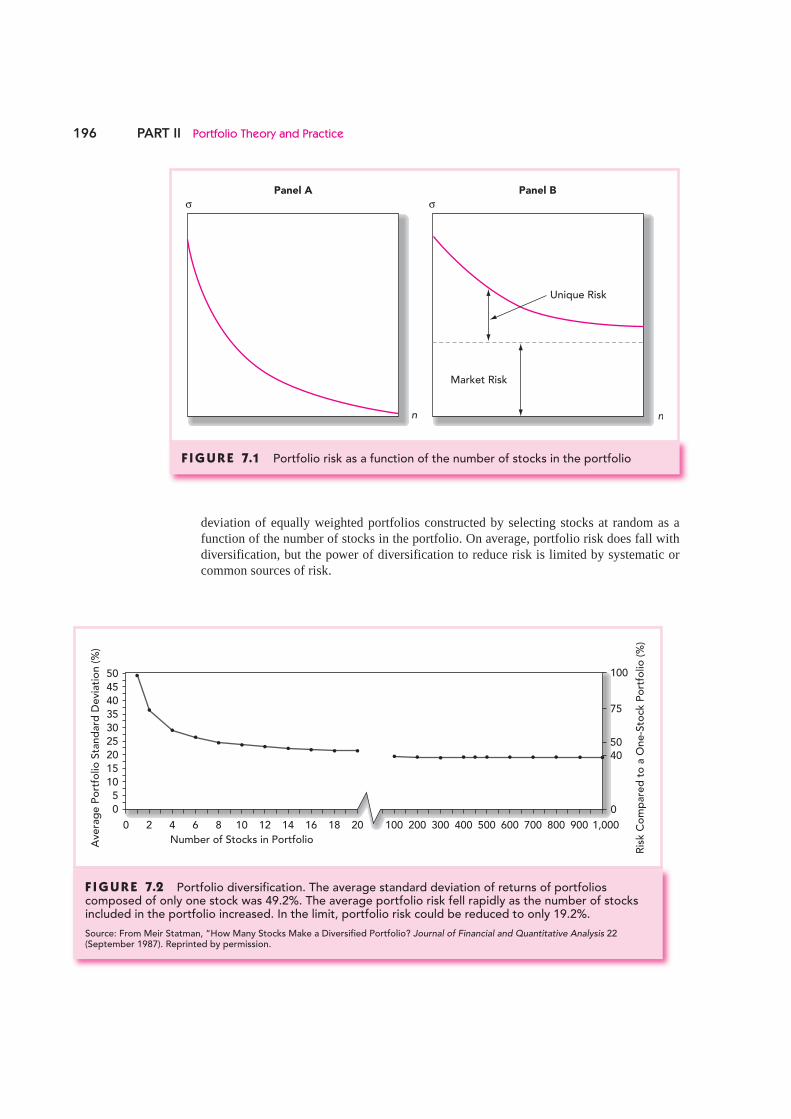
Suppose your portfolio is composed of only one stock, say, Dell Computer Corporation. What would be the sources of risk to this “portfolio”? You might think of two broad sources of uncertainty. First, there is the risk that comes from conditions in the general economy, such as the business cycle, inflation, interest rates, and exchange rates. None of these mac-roeconomic factors can be predicted with certainty, and all affect the rate of return on Dell stock. In addition to these macroeconomic factors there are firm-specific influences, such as Dell’s success in research and development, and personnel changes. These factors affect Dell without noticeably affecting other firms in the economy.

Now consider a naive diversification strategy, in which you include additional securi-ties in your portfolio. For example, place half your funds in ExxonMobil and half in Dell. What should happen to portfolio risk? To the extent that the firm-specific influences on the two stocks differ, diversification should reduce portfolio risk. For example, when oil prices fall, hurting ExxonMobil, computer prices might rise, helping Dell. The two effects are offsetting and stabilize portfolio return.

But why end diversification at only two stocks? If we diversify into many more securi-ties, we continue to spread out our exposure to firm-specific factors, and portfolio volatil-ity should continue to fall. Ultimately, however, even with a large number of stocks we cannot avoid risk altogether, because virtually all securities are affected by the common macroeconomic factors. For example, if all stocks are affected by the business cycle, we cannot avoid exposure to business cycle risk no matter how many stocks we hold.

When all risk is firm-specific, as in Figure 7.1 , panel A, diversification can reduce risk to arbitrarily low levels. The reason is that with all risk sources independent, the exposure to any particular source of risk is reduced to a negligible level. The reduction of risk to very low levels in the case of independent risk sources is sometimes called the insurance principle, because of the notion that an insurance company depends on the risk reduction achieved through diversification when it writes many policies insuring against many inde-pendent sources of risk, each policy being a small part of the company’s overall portfolio. (See Section 7.5 for a discussion of the insurance principle.)

When common sources of risk affect all firms, however, even extensive diversifica-tion cannot eliminate risk. In Figure 7.1 , panel B, portfolio standard deviation falls as the number of securities increases, but it cannot be reduced to zero. The risk that remains even after extensive diversification is called market risk, risk that is attributable to marketwide risk sources. Such risk is also called systematic risk, or nondiversifiable risk. In contrast, the risk that can be eliminated by diversification is called unique risk, firm-specific risk, nonsystematic risk, or diversifiable risk.

This analysis is borne out by empirical studies. Figure 7.2 shows the effect of portfo-lio diversification, using data on NYSE stocks. 1 The figure shows the average standard

1 Meir Statman, “How Many Stocks Make a Diversified Portfolio?” Journal of Financial and Quantitative Analysis 22 (September 1987).

7.1 DIVERSIFICATION AND PORTFOLIO RISK

196 PART II Portfolio Theory and Practice

deviation of equally weighted portfolios constructed by selecting stocks at random as a function of the number of stocks in the portfolio. On average, portfolio risk does fall with diversification, but the power of diversification to reduce risk is limited by systematic or common sources of risk.

Ave

rag

e P

ort

folio

Sta

nd

ard

De

viat

ion

(%

)

50

0 2 4 6 8 10 12 14 16 18 20 100 200 300 400 500 600 700 800 900 1,000

0

100

75

5040

Ris

k C

om

par

ed

to

a O

ne

-Sto

ck P

ort

folio

(%

)

Number of Stocks in Portfolio

4045

353025201510

50

F I G U R E 7.2 Portfolio diversification. The average standard deviation of returns of portfolios composed of only one stock was 49.2%. The average portfolio risk fell rapidly as the number of stocks included in the portfolio increased. In the limit, portfolio risk could be reduced to only 19.2%.

Source: From Meir Statman, “How Many Stocks Make a Diversified Portfolio? Journal of Financial and Quantitative Analysis 22 (September 1987). Reprinted by permission.

F I G U R E 7.1 Portfolio risk as a function of the number of stocks in the portfolio

Panel A

n

Panel B

n

Unique Risk

Market Risk

σ σ

CHAPTER 7 Optimal Risky Portfolios 197

7.2 PORTFOLIOS OF TWO RISKY ASSETS In the last section we considered naive diversification using equally weighted portfolios of several securities. It is time now to study efficient diversification, whereby we construct risky portfolios to provide the lowest possible risk for any given level of expected return. The nearby box provides an introduction to the relationship between diversification and portfolio construction.

Portfolios of two risky assets are relatively easy to analyze, and they illustrate the prin-ciples and considerations that apply to portfolios of many assets. It makes sense to think about a two-asset portfolio as an asset allocation decision, and so we consider two mutual funds, a bond portfolio specializing in long-term debt securities, denoted D, and a stock fund that specializes in equity securities, E. Table 7.1 lists the parameters describing the rate-of-return distribution of these funds.

A proportion denoted by w D is invested in the bond fund, and the remainder, 1 � w D, denoted w E, is invested in the stock fund. The rate of return on this portfolio, r p, will be 2

rp � wDrD � wErE (7.1)

where r D is the rate of return on the debt fund and r E is the rate of return on the equity fund.

The expected return on the portfolio is a weighted average of expected returns on the component securities with portfolio proportions as weights:

E(rp) � wDE(rD) � wEE(rE) (7.2)

The variance of the two-asset portfolio is

� p 2 � w D 2

� D 2 � w E 2

� E 2 � 2wDwE Cov(rD, rE) (7.3)

Our first observation is that the variance of the portfolio, unlike the expected return, is not a weighted average of the individual asset variances. To understand the formula for the portfolio variance more clearly, recall that the covariance of a variable with itself is the variance of that variable; that is

Cov( scenario)[scenarios

r r r E rD D D D, ) Pr( ( )]� �∑ [[ ( )]

Pr( [ ( )

r E r

r E r

D D

D D

�

� �scenarios

scenario)∑ ]]2

2� �D

(7.4)

Therefore, another way to write the variance of the portfolio is

� p 2 � wDwDCov(rD, rD) � wEwECov(rE, rE) � 2wDwECov(rD, rE) (7.5)

2 See Appendix B of this chapter for a review of portfolio statistics.

Debt Equity

Expected return, E(r) 8% 13%Standard deviation, � 12% 20%

Covariance, Cov(rD, rE) 72

Correlation coefficient, �DE .30

TA B L E 7 . 1

Descriptive statistics for two mutual funds

198

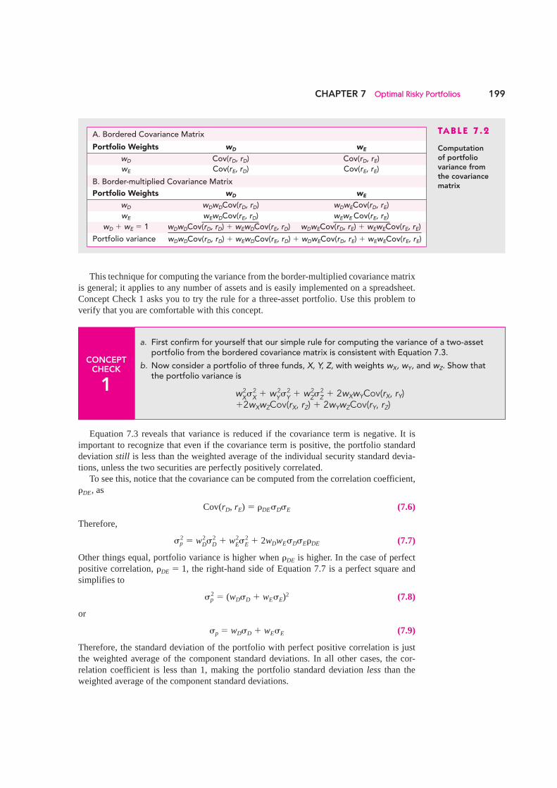
In words, the variance of the portfolio is a weighted sum of covariances, and each weight is the product of the portfolio proportions of the pair of assets in the covariance term.

Table 7.2 shows how portfolio variance can be calculated from a spreadsheet. Panel A of the table shows the bordered covariance matrix of the returns of the two mutual funds. The bordered matrix is the covariance matrix with the portfolio weights for each fund placed on the borders, that is, along the first row and column. To find portfolio variance, multiply each element in the covariance matrix by the pair of portfolio weights in its row and column borders. Add up the resultant terms, and you have the formula for portfolio variance given in Equation 7.5 .

We perform these calculations in panel B, which is the border-multiplied covariance matrix: Each covariance has been multiplied by the weights from the row and the column in the borders. The bottom line of panel B confirms that the sum of all the terms in this matrix (which we obtain by adding up the column sums) is indeed the portfolio variance in Equation 7.5 .

This procedure works because the covariance matrix is symmetric around the diagonal, that is, Cov( r D , r E ) � Cov( r E , r D ). Thus each covariance term appears twice.

INTRODUCTION TO DIVERSIFICATION

Diversification is a familiar term to most investors. In the most general sense, it can be summed up with this phrase: “Don’t put all of your eggs in one basket.” While that sentiment certainly captures the essence of the issue, it provides little guidance on the practical implications of the role diversification plays in an inves-tor’s portfolio and offers no insight into how a diversi-fied portfolio is actually created.

WHAT IS DIVERSIFICATION?

Taking a closer look at the concept of diversification, the idea is to create a portfolio that includes multi-ple investments in order to reduce risk. Consider, for example, an investment that consists of only the stock issued by a single company. If that company’s stock suffers a serious downturn, your portfolio will sustain the full brunt of the decline. By splitting your invest-ment between the stocks of two different companies, you reduce the potential risk to your portfolio.

Another way to reduce the risk in your portfolio is to include bonds and cash. Because cash is generally used as a short-term reserve, most investors develop an asset allocation strategy for their portfolios based primarily on the use of stocks and bonds. It is never a bad idea to keep a portion of your invested assets in cash, or short-term money-market securities. Cash can be used in case of an emergency, and short-term money-market securities can be liquidated instantly in the event your usual cash requirements spike and you need to sell investments to make payments.

Regardless of whether you are aggressive or con-servative, the use of asset allocation to reduce risk through the selection of a balance of stocks and bonds for your portfolio is a more detailed description of how

a diversified portfolio is created than the simplistic eggs in one basket concept. The specific balance of stocks and bonds in a given portfolio is designed to create a specific risk-reward ratio that offers the opportunity to achieve a certain rate of return on your investment in exchange for your willingness to accept a certain amount of risk.

WHAT ARE MY OPTIONS?

If you are a person of limited means or you simply pre-fer uncomplicated investment scenarios, you could choose a single balanced mutual fund and invest all of your assets in the fund. For most investors, this strat-egy is far too simplistic. Furthermore, while investing in a single mutual fund provides diversification among the basic asset classes of stocks, bonds and cash, the opportunities for diversification go far beyond these basic categories. A host of alternative investments provide the opportunity for further diversification. Real estate investment trusts, hedge funds, art and other investments provide the opportunity to invest in vehi-cles that do not necessarily move in tandem with the traditional financial markets.

CONCLUSION

Regardless of your means or method, keep in mind that there is no generic diversification model that will meet the needs of every investor. Your personal time horizon, risk tolerance, investment goals, financial means and level of investment experience will play a large role in dictating your investment mix.

Source: Adapted from Jim McWhinney, Introduction to Diversification, December 16, 2005, www.investopedia.com/articles/basics/05/diversification.asp, retrieved April 25, 2006.

WO

RDS

FRO

M T

HE

STRE

ET


This technique for computing the variance from the border-multiplied covariance matrix is general; it applies to any number of assets and is easily implemented on a spreadsheet. Concept Check 1 asks you to try the rule for a three-asset portfolio. Use this problem to verify that you are comfortable with this concept.

Equation 7.3 reveals that variance is reduced if the covariance term is negative. It is important to recognize that even if the covariance term is positive, the portfolio standard deviation still is less than the weighted average of the individual security standard devia-tions, unless the two securities are perfectly positively correlated.

To see this, notice that the covariance can be computed from the correlation coefficient, � DE, as

Cov(rD, rE) � �DE�D�E (7.6)

Therefore,

� p 2 � w D 2

� D 2 � w E 2

� E 2 � 2wDwE�D�E�DE (7.7)

Other things equal, portfolio variance is higher when � DE is higher. In the case of perfect positive correlation, � DE � 1, the right-hand side of Equation 7.7 is a perfect square and simplifies to

� p 2 � (wD�D � wE�E)2 (7.8)

or

�p � wD�D � wE�E (7.9)

Therefore, the standard deviation of the portfolio with perfect positive correlation is just the weighted average of the component standard deviations. In all other cases, the cor-relation coefficient is less than 1, making the portfolio standard deviation less than the weighted average of the component standard deviations.

CONCEPT CHECK

1

a. First confirm for yourself that our simple rule for computing the variance of a two-asset portfolio from the bordered covariance matrix is consistent with Equation 7.3.

b. Now consider a portfolio of three funds, X, Y, Z, with weights wX, wY, and wZ. Show that the portfolio variance is

w X 2 �

X 2 � w

Y 2 �

Y 2 � w

Z 2 �

Z 2 � 2wXwYCov(rX, rY)

�2wXwZCov(rX, rZ) � 2wYwZCov(rY, rZ)

CONCEPT CHECK

1

a. First confirm for yourself that our simple rule for computing the variance of a two-asset portfolio from the bordered covariance matrix is consistent with Equation 7.3.

b. Now consider a portfolio of three funds, X, Y, Z, with weights wX, wY, and wZ. Show that the portfolio variance is

w X 2 �

X 2 � w

Y 2 �

Y 2 � w

Z 2 �

Z 2 � 2wXwYCov(rX, rY)

�2wXwZCov(rX, rZ) � 2wYwZCov(rY, rZ)

TA B L E 7 . 2

Computation of portfolio variance from the covariance matrix

A. Bordered Covariance Matrix

Portfolio Weights wD wE

wD Cov(rD, rD) Cov(rD, rE)wE Cov(rE, rD) Cov(rE, rE)

B. Border-multiplied Covariance Matrix

Portfolio Weights wD wE

wD wDwDCov(rD, rD) wDwECov(rD, rE)

wE wEwDCov(rE, rD) wEwE Cov(rE, rE)

wD � wE � 1 wDwDCov(rD, rD) � wEwDCov(rE, rD) wDwECov(rD, rE) � wEwECov(rE, rE)

Portfolio variance wDwDCov(rD, rD) � wEwDCov(rE, rD) � wDwECov(rD, rE) � wEwECov(rE, rE)


A hedge asset has negative correlation with the other assets in the portfolio. Equation 7.7 shows that such assets will be particularly effective in reducing total risk. Moreover, Equa-tion 7.2 shows that expected return is unaffected by correlation between returns. Therefore, other things equal, we will always prefer to add to our portfolios assets with low or, even better, negative correlation with our existing position.

Because the portfolio’s expected return is the weighted average of its component expected returns, whereas its standard deviation is less than the weighted average of the component standard deviations, portfolios of less than perfectly correlated assets always offer better risk–return opportunities than the individual component securities on their own. The lower the correlation between the assets, the greater the gain in efficiency.

How low can portfolio standard deviation be? The lowest possible value of the correla-tion coefficient is � 1, representing perfect negative correlation. In this case, Equation 7.7 simplifies to

� p 2 � (wD�D � wE�E)2 (7.10)

and the portfolio standard deviation is

�p � Absolute value (wD�D � wE�E) (7.11)

When � � � 1, a perfectly hedged position can be obtained by choosing the portfolio pro-portions to solve

wD�D � wE�E � 0

The solution to this equation is

w

w w

DE

D E

ED

D ED

��

� ��

��

� �� 1

(7.12)

These weights drive the standard deviation of the portfolio to zero.

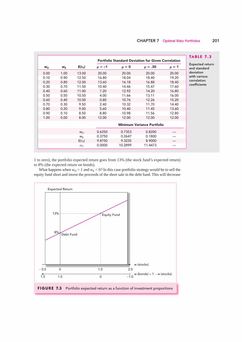
EXAMPLE 7.1 Portfolio Risk and Return

Let us apply this analysis to the data of the bond and stock funds as presented in Table 7.1. Using these data, the formulas for the expected return, variance, and standard deviation of the portfolio as a function of the portfolio weights are

E r w w

w w

p D E

p D E

( )

.

� �

� � � � � � � �

8 13

12 20 2 12 20 32 2 2 2 2 ww w

w w w w

D E

D E D E

p p

� � �

� � �

144 400 1442 2

2

We can experiment with different portfolio proportions to observe the effect on portfo-lio expected return and variance. Suppose we change the proportion invested in bonds. The effect on expected return is tabulated in Table 7.3 and plotted in Figure 7.3 . When the pro-portion invested in debt varies from zero to 1 (so that the proportion in equity varies from


1 to zero), the portfolio expected return goes from 13% (the stock fund’s expected return) to 8% (the expected return on bonds).

What happens when w D > 1 and w E < 0? In this case portfolio strategy would be to sell the equity fund short and invest the proceeds of the short sale in the debt fund. This will decrease

Expected Return

13%

8%

Equity Fund

Debt Fund

w (stocks)

w (bonds) = 1 − w (stocks)

− 0.5 0 1.0 2.0

1.5 1.0 0 −1.0

F I G U R E 7.3 Portfolio expected return as a function of investment proportions

TA B L E 7 . 3

Expected return and standard deviation with various correlation coefficients

Portfolio Standard Deviation for Given Correlation

wD wE E(rP) � � –1 � � 0 � � .30 � � 1

0.00 1.00 13.00 20.00 20.00 20.00 20.000.10 0.90 12.50 16.80 18.04 18.40 19.200.20 0.80 12.00 13.60 16.18 16.88 18.400.30 0.70 11.50 10.40 14.46 15.47 17.600.40 0.60 11.00 7.20 12.92 14.20 16.800.50 0.50 10.50 4.00 11.66 13.11 16.000.60 0.40 10.00 0.80 10.76 12.26 15.200.70 0.30 9.50 2.40 10.32 11.70 14.400.80 0.20 9.00 5.60 10.40 11.45 13.600.90 0.10 8.50 8.80 10.98 11.56 12.801.00 0.00 8.00 12.00 12.00 12.00 12.00

Minimum Variance Portfolio

wD 0.6250 0.7353 0.8200 —wE 0.3750 0.2647 0.1800 —

E(rP) 9.8750 9.3235 8.9000 —�P 0.0000 10.2899 11.4473 —


the expected return of the portfolio. For example, when w D � 2 and w E � � 1, expected portfolio return falls to 2 � 8 � (�1) � 13 � 3%. At this point the value of the bond fund in the portfolio is twice the net worth of the account. This extreme position is financed in part by short-selling stocks equal in value to the portfolio’s net worth.

The reverse happens when w D < 0 and w E > 1. This strategy calls for selling the bond fund short and using the proceeds to finance additional pur-chases of the equity fund.

Of course, varying investment proportions also has an effect on portfolio standard deviation. Table 7.3 presents portfolio standard deviations for different portfolio weights calculated from Equation 7.7 using the assumed value of the cor-relation coefficient, .30, as well as other values of � . Figure 7.4 shows the relationship between standard deviation and portfolio weights. Look first at the solid curve for � DE � .30. The graph shows that as the portfolio weight in the equity fund increases from zero to 1, portfolio standard deviation first falls with the initial diversification from bonds into stocks, but then rises again as the

portfolio becomes heavily concentrated in stocks, and again is undiversified. This pattern will generally hold as long as the correlation coefficient between the funds is not too high. 3 For a pair of assets with a large positive correlation of returns, the portfolio standard devia-tion will increase monotonically from the low-risk asset to the high-risk asset. Even in this case, however, there is a positive (if small) value from diversification.

What is the minimum level to which portfolio standard deviation can be held? For the parameter values stipulated in Table 7.1 , the portfolio weights that solve this minimization problem turn out to be 4

wMin(D) � .82

wMin(E) � 1 � .82 � .18

This minimum-variance portfolio has a standard deviation of

�Min � [(.822 � 122) � (.182 � 202) � (2 � .82 � .18 � 72)]1/2 � 11.45%

as indicated in the last line of Table 7.3 for the column � � .30. The solid colored line in Figure 7.4 plots the portfolio standard deviation when � � .30

as a function of the investment proportions. It passes through the two undiversified portfolios

3 As long as � < � D / � E, volatility will initially f all when we start with all bonds and begin to move into stocks.

4 This solution uses the minimization techniques of calculus. Write out the expression for portfolio variance from Equation 7.3 , substitute 1 � w D for w E, differentiate the result with respect to w D, set the derivative equal to zero, and solve for w D to obtain

w Dr r

r r

E D E

D E D E

Min

2

2 2( )

Cov( )

2Cov( )�

� �

� � � �

,

, Alternatively, with a spreadsheet program such as Excel, you can obtain an accurate solution by using the Solver to minimize the variance. See Appendix A for an example of a portfolio optimization spreadsheet.

ρ = .30

−.50 .500 1.501.0

Weight in Stock Fund

Portfolio Standard Deviation (%)

ρ = −1

ρ = 0

ρ = 1

35

30

25

20

15

10

5

0

F I G U R E 7.4 Portfolio standard deviation as a func-tion of investment proportions


of w D � 1 and w E � 1. Note that the minimum-variance portfolio has a standard deviation smaller than that of either of the individual component assets. This illustrates the effect of diversification.

The other three lines in Figure 7.4 show how portfolio risk varies for other values of the correlation coefficient, holding the variances of each asset constant. These lines plot the values in the other three columns of Table 7.3 .

The solid dark line connecting the undiversified portfolios of all bonds or all stocks, w D � 1 or w E � 1, shows portfolio standard deviation with perfect positive correlation, � � 1. In this case there is no advantage from diversification, and the portfolio standard deviation is the simple weighted average of the component asset standard deviations.

The dashed colored curve depicts portfolio risk for the case of uncorrelated assets, � � 0. With lower correlation between the two assets, diversification is more effective and portfolio risk is lower (at least when both assets are held in positive amounts). The mini-mum portfolio standard deviation when � � 0 is 10.29% (see Table 7.3 ), again lower than the standard deviation of either asset.

Finally, the triangular broken line illustrates the perfect hedge potential when the two assets are perfectly negatively correlated ( � � � 1). In this case the solution for the minimum-variance portfolio is, by Equation 7.12 ,

wMin(D; � � �1) � �E _______

�D � �E � 20 _______

12 � 20 � .625

wMin(E; � � �1) � 1 � .625 � .375

and the portfolio variance (and standard deviation) is zero. We can combine Figures 7.3 and 7.4 to demonstrate the relationship between portfolio

risk (standard deviation) and expected return—given the parameters of the available assets. This is done in Figure 7.5 . For any pair of investment proportions, w D, w E, we read the expected return from Figure 7.3 and the standard deviation from Figure 7.4 . The resulting pairs of expected return and standard deviation are tabulated in Table 7.3 and plotted in Figure 7.5 .

The solid colored curve in Figure 7.5 shows the portfolio opportunity set for � � .30. We call it the portfolio opportunity set because it shows all combinations of portfolio expected return and stan-dard deviation that can be constructed from the two available assets. The other lines show the portfolio opportunity set for other values of the correlation coefficient. The solid black line connecting the two funds shows that there is no benefit from diversifi-cation when the correlation between the two is per-fectly positive ( � � 1). The opportunity set is not “pushed” to the northwest. The dashed colored line demonstrates the greater benefit from diversification when the correlation coefficient is lower than .30.

Finally, for � � � 1, the portfolio opportu-nity set is linear, but now it offers a perfect hedg-ing opportunity and the maximum advantage from diversification.

To summarize, although the expected return of any portfolio is simply the weighted average of the

14

13

12

11

10

9

8

7

6

5

Standard Deviation (%)

0 2 4 6 8 10 12 14 16 18 20

Expected Return (%)

D

E

ρ = −1ρ = 0

ρ = .30 ρ = 1

F I G U R E 7.5 Portfolio expected return as a function of standard deviation


asset expected returns, this is not true of the standard deviation. Potential benefits from diversification arise when correlation is less than perfectly positive. The lower the correla-tion, the greater the potential benefit from diversification. In the extreme case of perfect negative correlation, we have a perfect hedging opportunity and can construct a zero-variance portfolio.

Suppose now an investor wishes to select the optimal portfolio from the opportu-nity set. The best portfolio will depend on risk aversion. Portfolios to the northeast in Figure 7.5 provide higher rates of return but impose greater risk. The best trade-off among

these choices is a matter of personal preference. Investors with greater risk aversion will prefer portfolios to the southwest, with lower expected return but lower risk. 5

In the previous chapter we examined the capital allocation decision, the choice of how much of the portfolio to leave in risk-free money market securities versus in a risky portfo-lio. Now we have taken a further step, specifying that the risky portfolio comprises a stock and a bond fund. We still need to show how investors can decide on the proportion of their risky portfolios to allocate to the stock versus the bond market. This is an asset allocation decision. As the nearby box emphasizes, most investment professionals recognize that “the really critical decision is how to divvy up your money among stocks, bonds and supersafe investments such as Treasury bills.”

In the last section, we derived the properties of portfolios formed by mixing two risky assets. Given this background, we now reintroduce the choice of the third, risk-free, portfolio. This will allow us to complete the basic problem of asset allocation across the three key asset classes: stocks, bonds, and risk-free money market securities. Once you understand this case, it will be easy to see how portfolios of many risky securities might best be constructed.

The Optimal Risky Portfolio with Two Risky Assets and a Risk-Free Asset5

What if our risky assets are still confined to the bond and stock funds, but now we can also invest in risk-free T-bills yielding 5%? We start with a graphical solution. Figure 7.6 shows the opportunity set based on the properties of the bond and stock funds, using the data from Table 7.1 .

5 Given a level of risk aversion, one can determine the portfolio that provides the highest level of utility. Recall from Chapter 6 that we were able to describe the utility provided by a portfolio as a function of its expected return, E ( r p ), and its variance, � p

2 , according to the relationship U � E(rp) � 0.5A � p 2 . The portfolio mean and

variance are determined by the portfolio weights in the two funds, w E and w D, according to Equations 7.2 and 7.3 . Using those equations and some calculus, we find the optimal investment proportions in the two funds. A warn-ing: to use the following equation (or any equation involving the risk aversion parameter, A ), you must express returns in decimal form.

wD � E(rD) � E(rE) � A( �

E 2 � �D�E�DE)

____________________________ A( �

D 2 � �

E 2 � 2�D�E�DE)

wE � 1 � wD

Here, too, Excel’s Solver or similar software can be used to maximize utility subject to the constraints of Equa-tions 7.2 and 7.3 , plus the portfolio constraint that w D � w E � 1 (i.e., that portfolio weights sum to 1).

7.3 ASSET ALLOCATION WITH STOCKS, BONDS, AND BILLS

CONCEPT CHECK

2

Compute and draw the portfolio opportunity set for the debt and equity funds when the correlation coefficient between them is � � .25.

205

Two possible capital allocation lines (CALs) are drawn from the risk-free rate ( r f � 5%) to two feasible portfolios. The first possible CAL is drawn through the minimum-variance portfolio A, which is invested 82% in bonds and 18% in stocks ( Table 7.3 , bottom panel, last column). Portfolio A ’s expected return is 8.90%, and its standard deviation is 11.45%. With a T-bill rate of 5%, the reward-to-volatility (Sharpe) ratio, which is the slope of the CAL combining T-bills and the minimum-variance portfolio, is

SA � E(rA) � r f

_________ �A

� 8.9 � 5 _______ 11.45

� .34

Now consider the CAL that uses portfolio B instead of A. Portfolio B invests 70% in bonds and 30% in stocks. Its expected return is 9.5% (a risk premium of 4.5%), and its standard deviation is 11.70%. Thus the reward-to-volatility ratio on the CAL that is sup-ported by portfolio B is

SB � 9.5 � 5 _______ 11.7

� .38

which is higher than the reward-to-volatility ratio of the CAL that we obtained using the minimum-variance portfolio and T-bills. Hence, portfolio B dominates A.

RECIPE FOR SUCCESSFUL INVESTING:

FIRST, MIX ASSETS WELL

First things first.If you want dazzling investment results, don’t start

your day foraging for hot stocks and stellar mutual funds. Instead, say investment advisers, the really critical decision is how to divvy up your money among stocks, bonds, and supersafe investments such as Treasury bills.

In Wall Street lingo, this mix of investments is called your asset allocation. “The asset-allocation choice is the first and most important decision,” says William Droms, a finance professor at Georgetown University. “How much you have in [the stock market] really drives your results.”

“You cannot get [stock market] returns from a bond portfolio, no matter how good your security selection is or how good the bond managers you use,” says William John Mikus, a managing director of Financial Design, a Los Angeles investment adviser.

For proof, Mr. Mikus cites studies such as the 1991 analysis done by Gary Brinson, Brian Singer and Gilbert Beebower. That study, which looked at the 10-year results for 82 large pension plans, found that a plan’s asset-allocation policy explained 91.5% of the return earned.

DESIGNING A PORTFOLIO

Because your asset mix is so important, some mutual fund companies now offer free services to help inves-tors design their portfolios.

Gerald Perritt, editor of the Mutual Fund Letter, a Chicago newsletter, says you should vary your mix of assets depending on how long you plan to invest. The

further away your investment horizon, the more you should have in stocks. The closer you get, the more you should lean toward bonds and money-market instru-ments, such as Treasury bills. Bonds and money-market instruments may generate lower returns than stocks. But for those who need money in the near future, conserva-tive investments make more sense, because there’s less chance of suffering a devastating short-term loss.

SUMMARIZING YOUR ASSETS

“One of the most important things people can do is summarize all their assets on one piece of paper and figure out their asset allocation,” says Mr. Pond.

Once you’ve settled on a mix of stocks and bonds, you should seek to maintain the target percentages, says Mr. Pond. To do that, he advises figuring out your asset allocation once every six months. Because of a stock-market plunge, you could find that stocks are now a far smaller part of your portfolio than you envis-aged. At such a time, you should put more into stocks and lighten up on bonds.

When devising portfolios, some investment advisers consider gold and real estate in addition to the usual trio of stocks, bonds and money-market instruments. Gold and real estate give “you a hedge against hyper-inflation,” says Mr. Droms. “But real estate is better than gold, because you’ll get better long-run returns.”

Source: Jonathan Clements, “Recipe for Successful Investing: First, Mix Assets Well,” The Wall Street Journal, October 6, 1993. Reprinted by permission of The Wall Street Journal, © 1993 Dow Jones & Com-pany, Inc. All rights reserved worldwide.

WO

RDS FRO

M TH

E STREET


But why stop at portfolio B? We can continue to ratchet the CAL upward until it ultimately reaches the point of tangency with the investment opportunity set. This must yield the CAL with the highest feasible reward-to-volatility ratio. Therefore, the tangency portfolio, labeled P in Figure 7.7 , is the optimal risky portfolio to mix with T-bills. We can read the expected return and standard deviation of portfolio P from the graph in Figure 7.7 :

E(rP) � 11%

�P � 14.2%

In practice, when we try to construct optimal risky portfolios from more than two risky assets, we need to rely on a spreadsheet or another com-puter program. The spreadsheet we present in Appendix A can be used to construct efficient portfolios of many assets. To start, however, we will demonstrate the solution of the portfolio construction problem with only two risky assets (in our example, long-term debt and equity) and a risk-free asset. In this simpler two-asset case, we can derive an explicit formula for the weights of each asset in the optimal portfolio. This will make it easy to illustrate some of the general issues per-taining to portfolio optimization.

The objective is to find the weights w D and w E that result in the highest slope of the CAL (i.e., the weights that result in the risky portfolio with the highest reward-to-volatility ratio). There-fore, the objective is to maximize the slope of the CAL for any possible portfolio, p. Thus our objective function is the slope (equivalently, the Sharpe ratio) S p :

Sp � E(rp) � r f

_________ �p

For the portfolio with two risky assets, the expected return and standard deviation of portfo-lio p are

E r w E r w E r

w w

w w

p D D E E

D E

p D D E

( ) ( ) ( )

[

� �

� �

� � � �

8 132 2 22 2 1 2

2 2

2

144 400 2

� �

� � �

E D E D E

D E

w w r r

w w

Cov( , )]

[ (

/

��72 1 2w wD E )] /


0 5 10 15 20 25 30

Expected Return (%)

D

E

P

rf = 5%

CAL(P)

OpportunitySet of RiskyAssets

2

0

4

6

8

10

12

14

16

18

F I G U R E 7.7 The opportunity set of the debt and equity funds with the optimal CAL and the optimal risky portfolio

13

12

11

10

9

8

7

6

5


0 5 10 15 20 25

Expected Return (%)

D

E

A

B

CAL(A)

CAL(B)

F I G U R E 7.6 The opportunity set of the debt and equity funds and two feasible CALs


When we maximize the objective function, S p, we have to satisfy the constraint that the portfolio weights sum to 1.0 (100%), that is, w D � w E � 1. Therefore, we solve an optimi-zation problem formally written as

Max wi

Sp � E(rp) � r f

________ �p

subject to Σ w i � 1. This is a nonlinear problem that can be solved using standard tools of calculus.

In the case of two risky assets, the solution for the weights of the optimal risky port-folio, P, is given by Equation 7.13. Notice that the solution employs excess rates of return (denoted R) rather than total returns (denoted r).6

wE E

E EDD E E D E

D E E D

��

�

( ) ( ) ( , )

( ) ( )

R R R R

R R

�

� �

2

2

Cov22

1

� �

� �

[ ( ) ( )] ( , )E E

w wD E D E

E D

R R R RCov

(7.13)

EXAMPLE 7.2 Optimal Risky Portfolio

Using our data, the solution for the optimal risky portfolio is

wD ��

� � � � �

( ) ( )

( ) ( ) (

8 5 400 13 5 72

8 5 400 13 5144 8 5��

� � �

13 5 7240

1 40 60

).

. .wE

The expected return and standard deviation of this optimal risky portfolio are

E rP

P

( ) (. ) (. ) %

[(. ) (.

� � � � �

� � � �

4 8 6 13 11

4 144 622�� 400 2 4 6 72 14 21 2) ( . . )] . %/

The CAL of this optimal portfolio has a slope of

SP =

−=

11 5

14 242

..

which is the reward-to-volatility (Sharpe) ratio of portfolio P. Notice that this slope exceeds the slope of any of the other feasible portfolios that we have considered, as it must if it is to be the slope of the best feasible CAL.

In Chapter 6 we found the optimal complete portfolio given an optimal risky portfolio and the CAL generated by a combination of this portfolio and T-bills. Now that we have constructed the optimal risky portfolio, P, we can use the individual investor’s degree of risk aversion, A, to calculate the optimal proportion of the complete portfolio to invest in the risky component.

6 The solution procedure for two risky assets is as follows. Substitute for E ( r P ) from Equation 7.2 and for � P from Equation 7.7 . Substitute 1 � w D for w E. Dif ferentiate the resulting expression for S p with respect to w D, set the derivative equal to zero, and solve for w D.


EXAMPLE 7.3 Optimal Complete Portfolio

An investor with a coefficient of risk aversion A � 4 would take a position in portfolio P of7

y

E r r

AP f

P

��

��

�

��

( ) . .

..2 2

11 05

4 1427439

(7.14)

Thus the investor will invest 74.39% of his or her wealth in portfolio P and 25.61% in T-bills. Portfolio P consists of 40% in bonds, so the fraction of wealth in bonds will be ywD � .4 � .7439 � .2976, or 29.76%. Similarly, the investment in stocks will be ywE � .6 � .7439 � .4463, or 44.63%. The graphical solution of this asset allocation problem is presented in Figures 7.8 and 7.9.

Once we have reached this point, generalizing to the case of many risky assets is straightforward. Before we move on, let us briefly summarize the steps we followed to arrive at the complete portfolio.7

1. Specify the return characteristics of all securities (expected returns, variances, covariances).

2. Establish the risky portfolio:

a. Calculate the optimal risky portfolio, P ( Equation 7.13 ). b. Calculate the properties of portfolio P using the weights determined in step ( a )

and Equations 7.2 and 7.3 .

7Notice that we express returns as decimals in Equation 7.14. This is necessary when using the risk aversion parameter, A, to solve for capital allocation.

F I G U R E 7.9 The proportions of the optimal complete portfolio

Portfolio P74.39%

Stocks44.63%

Bonds29.76%

T-bills25.61%

F I G U R E 7.8 Determination of the optimal complete portfolio


0 5 10 15 20 25 30

Expected Return (%)

D

C

E

P

CAL(P)

OpportunitySet of RiskyAssets

Optimal RiskyPortfolio

Indifference Curve

OptimalCompletePortfolio2

0

4

6

8

10

12

14

16

18

rf = 5%


3. Allocate funds between the risky portfolio and the risk-free asset:

a. Calculate the fraction of the complete portfolio allocated to portfolio P (the risky portfolio) and to T-bills (the risk-free asset) ( Equation 7.14 ).

b. Calculate the share of the complete portfolio invested in each asset and in T-bills.

Recall that our two risky assets, the bond and stock mutual funds, are already diversified portfolios. The diversification within each of these portfolios must be credited for a good deal of the risk reduction compared to undiversified single securities. For example, the standard deviation of the rate of return on an average stock is about 50% (see Figure 7.2 ). In contrast, the standard deviation of our stock-index fund is only 20%, about equal to the historical standard deviation of the S&P 500 portfolio. This is evidence of the importance of diversification within the asset class. Optimizing the asset allocation between bonds and stocks contributed incrementally to the improvement in the reward-to-volatility ratio of the complete portfolio. The CAL with stocks, bonds, and bills ( Figure 7.7 ) shows that the stan-dard deviation of the complete portfolio can be further reduced to 18% while maintaining the same expected return of 13% as the stock portfolio.

CONCEPT CHECK

3

The universe of available securities includes two risky stock funds, A and B, and T-bills. The data for the universe are as follows:

Expected Return Standard Deviation

A 10% 20%

B 30 60

T-bills 5 0

The correlation coefficient between funds A and B is �.2.

a. Draw the opportunity set of funds A and B.

b. Find the optimal risky portfolio, P, and its expected return and standard deviation.

c. Find the slope of the CAL supported by T-bills and portfolio P.

d. How much will an investor with A � 5 invest in funds A and B and in T-bills?

7.4 THE MARKOWITZ PORTFOLIO SELECTION MODEL

Security Selection

We can generalize the portfolio construction problem to the case of many risky securities and a risk-free asset. As in the two risky assets example, the problem has three parts. First, we identify the risk–return combinations available from the set of risky assets. Next, we identify the optimal portfolio of risky assets by finding the portfolio weights that result in the steepest CAL. Finally, we choose an appropriate complete portfolio by mixing the risk-free asset with the optimal risky portfolio. Before describing the process in detail, let us first present an overview.


The first step is to determine the risk–return opportunities available to the investor. These are summarized by the minimum-variance fron-tier of risky assets. This frontier is a graph of the lowest possible variance that can be attained for a given port-folio expected return. Given the input data for expected returns, variances, and covariances, we can calculate the minimum-variance portfolio for any targeted expected return. The plot of these expected return–standard devia-tion pairs is presented in Figure 7.10 .

Notice that all the individual assets lie to the right inside the frontier, at least when we allow short sales in the construction of risky portfolios. 8 This tells us that risky portfolios compris-ing only a single asset are inefficient. Diversifying investments leads to port-folios with higher expected returns and lower standard deviations.

All the portfolios that lie on the minimum-variance frontier from the global minimum-variance portfolio and upward provide the best risk–return combinations and thus are can-didates for the optimal portfolio. The part of the frontier that lies above the global minimum-variance portfolio, therefore, is called the efficient fron-tier of risky assets. For any portfolio on the lower portion of the minimum-variance frontier, there is a portfolio with the same standard deviation and a greater expected return positioned directly above it. Hence the bottom part of the minimum-variance frontier is inefficient.

The second part of the optimiza-tion plan involves the risk-free asset. As before, we search for the capital

allocation line with the highest reward-to-volatility ratio (that is, the steepest slope) as shown in Figure 7.11 .

8 When short sales are prohibited, single securities may lie on the frontier. For example, the security with the high-est expected return must lie on the frontier, as that security represents the only way that one can obtain a return that high, and so it must also be the minimum-variance way to obtain that return. When short sales are feasible, however, portfolios can be constructed that offer the same expected return and lower variance. These portfolios typically will have short positions in low-expected-return securities.

E(r)

Minimum-Variance Frontier

IndividualAssets

GlobalMinimum-VariancePortfolio

Efficient Frontier

σ

F I G U R E 7.10 The minimum-variance frontier of risky assets

E(r)

CAL(P)Efficient Frontier

P

rf

σ

F I G U R E 7.11 The efficient frontier of risky assets with the optimal CAL

211

The CAL that is supported by the optimal portfolio, P, is tangent to the efficient frontier. This CAL dominates all alternative feasible lines (the broken lines that are drawn through the frontier). Portfolio P, therefore, is the optimal risky portfolio.

Finally, in the last part of the problem the individual investor chooses the appropriate mix between the optimal risky portfolio P and T-bills, exactly as in Figure 7.8.

Now let us consider each part of the portfolio construction problem in more detail. In the first part of the problem, risk–return analysis, the portfolio manager needs as inputs a set of estimates for the expected returns of each security and a set of estimates for the covariance matrix. (In Part Five on security analysis we will examine the security valuation techniques and methods of financial analysis that analysts use. For now, we will assume that analysts already have spent the time and resources to prepare the inputs.)

The portfolio manager is now armed with the n estimates of E ( r i ) and the n � n estimates of the covariance matrix in which the n diagonal elements are estimates of the variances, � i

2 , and the n 2 � n � n ( n � 1) off-diagonal elements are the estimates of the covariances between each pair of asset returns. (You can verify this from Table 7.2 for the case n � 2.) We know that each covariance appears twice in this table, so actually we have n ( n � 1)/2 different covariance estimates. If our portfolio management unit covers 50 securities, our security analysts need to deliver 50 estimates of expected returns, 50 estimates of vari-ances, and 50 � 49/2 � 1,225 different estimates of covariances. This is a daunting task! (We show later how the number of required estimates can be reduced substantially.)

Once these estimates are compiled, the expected return and variance of any risky port-folio with weights in each security, w i , can be calculated from the bordered covariance matrix or, equivalently, from the following formulas:

E r w E rp

i

n

i i( ) ( )��1∑

(7.15)

eXcel APPLICATIONS:Two-Security Model

The accompanying spreadsheet can be used to measure the return and risk of a portfolio of two

risky assets. The model calculates the return and risk for varying weights of each security along with the optimal risky and minimum-variance portfo-lio. Graphs are automatically generated for various

model inputs. The model allows you to specify a tar-get rate of return and solves for optimal combina-tions using the risk-free asset and the optimal risky portfolio. The spreadsheet is constructed with the two-security return data from Table 7.1. This spread-sheet is available at www.mhhe.com/bkm.

A B C D E F

1

2 Expected Standard Correlation

3 Return Deviation Coefficient Covariance

4 Security 1

5 Security 2

6 T-Bill

7

8 Weight Weight Expected Standard Reward to

9 Security 1 Security 2 Return Deviation Volatility

10

11

12

13

14

Asset Allocation Analysis: Risk and Return

0.08 0.12 0.3 0.0072

0.13 0.2

0.05 0

1 0 0.08000 0.12000 0.25000

0.9 0.1 0.08500 0.11559 0.30281

0.8 0.2 0.09000 0.11454 0.34922

0.7 0.3 0.09500 0.11696 0.38474

0.6 0.4 0.10000 0.407710.12264

0


0 5

5

11

10 15 20 25 3530

Expected Return (%)


� ��

pi

n

j

n

i j i jw w r r2

1 1∑ ∑ Cov( , ) (7.16)

An extended worked example showing you how to do this using a spreadsheet is presented in Appendix A of this chapter.

We mentioned earlier that the idea of diversification is age-old. The phrase “don’t put all your eggs in one basket” existed long before modern finance theory. It was not until 1952, however, that Harry Markowitz published a formal model of portfolio selection embodying diversification principles, thereby paving the way for his 1990 Nobel Prize in Economics. 9 His model is precisely step one of portfolio management: the identification of the efficient set of portfolios, or the efficient frontier of risky assets.

The principal idea behind the frontier set of risky portfolios is that, for any risk level, we are interested only in that portfolio with the highest expected return. Alternatively, the frontier is the set of portfolios that minimizes the variance for any target expected return.

Indeed, the two methods of computing the efficient set of risky portfolios are equiva-lent. To see this, consider the graphical representation of these procedures. Figure 7.12 shows the minimum-variance frontier.

The points marked by squares are the result of a variance-minimization program. We first draw the constraints, that is, horizontal lines at the level of required expected returns. We then look for the portfolio with the lowest standard deviation that plots on each hori-zontal line—we look for the portfolio that will plot farthest to the left (smallest standard deviation) on that line. When we repeat this for many levels of required expected returns, the shape of the minimum-variance frontier emerges. We then discard the bottom (dashed) half of the frontier, because it is inefficient.

9 Harry Markowitz, “Portfolio Selection,” Journal of Finance, March 1952.

E(r)

E(r3)

E(r2)

E(r1)

σA σB σC

Efficient Frontierof Risky Assets

Global Minimum-Variance Portfolio

σ

F I G U R E 7.12 The efficient portfolio set


In the alternative approach, we draw a vertical line that represents the standard devia-tion constraint. We then consider all portfolios that plot on this line (have the same standard deviation) and choose the one with the highest expected return, that is, the portfolio that plots highest on this vertical line. Repeating this procedure for many vertical lines (levels of standard deviation) gives us the points marked by circles that trace the upper portion of the minimum-variance frontier, the efficient frontier.

When this step is completed, we have a list of efficient portfolios, because the solution to the optimization program includes the portfolio proportions, w i , the expected return, E ( r p ), and the standard deviation, � p .

Let us restate what our portfolio manager has done so far. The estimates generated by the security analysts were transformed into a set of expected rates of return and a cova-riance matrix. This group of estimates we shall call the input list. This input list is then fed into the optimization program.

Before we proceed to the second step of choosing the optimal risky portfolio from the frontier set, let us consider a practical point. Some clients may be subject to additional constraints. For example, many institutions are prohibited from taking short positions in any asset. For these clients the portfolio manager will add to the optimization program constraints that rule out negative (short) positions in the search for efficient portfolios. In this special case it is possible that single assets may be, in and of themselves, efficient risky portfolios. For example, the asset with the highest expected return will be a frontier portfolio because, without the opportunity of short sales, the only way to obtain that rate of return is to hold the asset as one’s entire risky portfolio.

Short-sale restrictions are by no means the only such constraints. For example, some clients may want to ensure a minimal level of expected dividend yield from the optimal portfolio. In this case the input list will be expanded to include a set of expected dividend yields d 1 , . . ., d n and the optimization program will include an additional constraint that ensures that the expected dividend yield of the portfolio will equal or exceed the desired level, d.

Portfolio managers can tailor the efficient set to conform to any desire of the client. Of course, any constraint carries a price tag in the sense that an efficient frontier constructed subject to extra constraints will offer a reward-to-volatility ratio inferior to that of a less constrained one. The client should be made aware of this cost and should carefully con-sider constraints that are not mandated by law.

Another type of constraint is aimed at ruling out investments in industries or countries considered ethically or politically undesirable. This is referred to as socially responsible investing, which entails a cost in the form of a lower reward-to-volatility on the resultant constrained, optimal portfolio. This cost can be justifiably viewed as a contribution to the underlying cause.

Capital Allocation and the Separation Property

Now that we have the efficient frontier, we proceed to step two and introduce the risk-free asset. Figure 7.13 shows the efficient frontier plus three CALs representing various portfo-lios from the efficient set. As before, we ratchet up the CAL by selecting different portfo-lios until we reach portfolio P, which is the tangency point of a line from F to the efficient frontier. Portfolio P maximizes the reward-to-volatility ratio, the slope of the line from F to portfolios on the efficient frontier. At this point our portfolio manager is done. Portfolio P is the optimal risky portfolio for the manager’s clients. This is a good time to ponder our results and their implementation.

214

The most striking conclusion is that a portfolio man-ager will offer the same risky portfolio, P, to all clients regardless of their degree of risk aversion.10 The degree of risk aversion of the client comes into play only in the selection of the desired point along the CAL. Thus the only difference between clients’ choices is that the more risk-averse client will invest more in the risk-free asset and less in the optimal risky portfolio than will a less risk-averse client. However, both will use portfolio P as their optimal risky investment vehicle.

This result is called a separation property; it tells us that the portfolio choice problem may be separated into two independent tasks. 11 The first task, determination of the optimal risky portfolio, is purely technical. Given the manager’s input list, the best risky portfolio is the same for all clients, regardless of risk aversion. The sec-ond task, however, allocation of the complete portfolio to T-bills versus the risky portfolio, depends on personal preference. Here the client is the decision maker.

The crucial point is that the optimal portfolio P that the manager offers is the same for all clients. Put another way, investors with varying degrees of risk aversion would be satis-fied with a universe of only two mutual funds: a money market fund for risk-free invest-ments and a mutual fund that hold the optimal risky portfolio, P, on the tangency point of the CAL and the efficient frontier. This result makes professional management more

10 Clients who impose special restrictions (constraints) on the manager, such as dividend yield, will obtain another optimal portfolio. Any constraint that is added to an optimization problem leads, in general, to a different and inferior optimum compared to an unconstrained program.

11 The separation property was first noted by Nobel laureate James Tobin, “Liquidity Preference as Behavior toward Risk,” Review of Economic Statistics 25 (February 1958), pp. 65–86.

F I G U R E 7.13 Capital allocation lines with various portfolios from the efficient set

E(r)

(Global Minimum-Variance Portfolio)

Efficient Frontierof Risky Assets

CAL(P)

CAL(A)

CAL(G)

A

G

P

F

σ

eXcel APPLICATIONS: Optimal Portfolios

A spreadsheet model featuring optimal risky port-folios is available on the Online Learning Center

at www.mhhe.com/bkm. It contains a template that is similar to the template developed in this section. The model can be used to find optimal mixes of securities for targeted levels of returns for both restricted and

unrestricted portfolios. Graphs of the efficient fron-tier are generated for each set of inputs. The example available at our Web site applies the model to port-folios constructed from equity indexes (called WEBS securities) of several countries.

A B C D E F

1

2

Standard3

Deviation4

5

6

7

8

9

10

11

12

Mean

ReturnWEBS

EWD

EWH

EWI

EWJ

EWL

EWP

EWW

S&P 500

Country

Sweden

Hong Kong

Italy

Japan

Switzerland

Spain

Mexico

15.5393

6.3852

26.5999

1.4133

18.0745

18.6347

16.2243

17.2306

26.4868

41.1475

26.0514

26.0709

21.6916

25.0779

38.7686

17.1944

Efficient Frontier for World Equity Benchmark Securities (WEBS)


efficient and hence less costly. One management firm can serve any number of clients with relatively small incremental administrative costs.

In practice, however, different managers will estimate different input lists, thus deriv-ing different efficient frontiers, and offer different “optimal” portfolios to their clients. The source of the disparity lies in the security analysis. It is worth mentioning here that the universal rule of GIGO (garbage in–garbage out) also applies to security analysis. If the quality of the security analysis is poor, a passive portfolio such as a market index fund will result in a better CAL than an active portfolio that uses low-quality security analysis to tilt portfolio weights toward seemingly favorable (mispriced) securities.

One particular input list that would lead to a worthless estimate of the efficient frontier is based on recent security average returns. If sample average returns over recent years are used as proxies for the true expected return on the security, the noise in those estimates will make the resultant efficient frontier virtually useless for portfolio construction.

Consider a stock with an annual standard deviation of 50%. Even if one were to use a 10-year average to estimate its expected return (and 10 years is almost ancient his-tory in the life of a corporation), the standard deviation of that estimate would still be 50 10 15 8/ . %.� The chances that this average represents expected returns for the com-ing year are negligible. 12 In Chapter 25, we see an example demonstrating that efficient frontiers constructed from past data may be wildly optimistic in terms of the apparent opportunities they offer to improve Sharpe ratios.

As we have seen, optimal risky portfolios for different clients also may vary because of portfolio constraints such as dividend-yield requirements, tax considerations, or other client preferences. Nevertheless, this analysis suggests that a limited number of portfolios may be sufficient to serve the demands of a wide range of investors. This is the theoretical basis of the mutual fund industry.

The (computerized) optimization technique is the easiest part of the portfolio construction problem. The real arena of competition among portfolio managers is in sophisticated secu-rity analysis. This analysis, as well as its proper interpretation, is part of the art of portfolio construction.13

CONCEPT CHECK

4

Suppose that two portfolio managers who work for competing investment management houses each employ a group of security analysts to prepare the input list for the Markowitz algorithm. When all is completed, it turns out that the efficient frontier obtained by portfolio manager A seems to dominate that of manager B. By dominate, we mean that A’s optimal risky portfolio lies northwest of B’s. Hence, given a choice, investors will all prefer the risky portfolio that lies on the CAL of A.

a. What should be made of this outcome?

b. Should it be attributed to better security analysis by A’s analysts?

c. Could it be that A’s computer program is superior?

d. If you were advising clients (and had an advance glimpse at the efficient frontiers of various managers), would you tell them to periodically switch their money to the manager with the most northwesterly portfolio?

12 Moreover, you cannot avoid this problem by observing the rate of return on the stock more frequently. In Chap-ter 5 we showed that the accuracy of the sample average as an estimate of expected return depends on the length of the sample period, and is not improved by sampling more frequently within a given sample period.13You can find a nice discussion of some practical issues in implementing efficient diversification in a white paper prepared by Wealthcare Capital Management at this address: www.financeware.com/ruminations/WP_EfficiencyDeficiency.pdf. A copy of the report is also available at the Online Learning Center for this text, www.mhhe.com/bkm.


The Power of Diversification

Section 7.1 introduced the concept of diversification and the limits to the benefits of diver-sification resulting from systematic risk. Given the tools we have developed, we can recon-sider this intuition more rigorously and at the same time sharpen our insight regarding the power of diversification.

Recall from Equation 7.16 , restated here, that the general formula for the variance of a portfolio is

� ��

pi

n

j

n

i j i jw w r r2

1 1∑ ∑ Cov( , )

(7.16)

Consider now the naive diversification strategy in which an equally weighted portfolio is constructed, meaning that w i � 1/ n for each security. In this case Equation 7.16 may be rewritten as follows, where we break out the terms for which i � j into a separate sum, noting that Cov(r i , r i) � � i

2 :

� �pi

n

ijj i

n

i

n

i jn n nr r2

1

2

1 12

1 1� �

� ��

�

1 ∑ ∑ ∑ Cov( , )

(7.17)

Note that there are n variance terms and n ( n � 1) covariance terms in Equation 7.17 . If we define the average variance and average covariance of the securities as

(7.18)

� �2

1

2

1 1

1

1

�

��

�

��

�

1n

n nr

i

n

i

jj i

n

i

n

i

∑

∑ ∑Cov Cov( )

( ,, )r j

(7.19)

we can express portfolio variance as

� � �

�p n

nn

2 2 11� Cov

(7.20)

Now examine the effect of diversification. When the average covariance among security returns is zero, as it is when all risk is firm-specific, portfolio variance can be driven to zero. We see this from Equation 7.20 . The second term on the right-hand side will be zero in this scenario, while the first term approaches zero as n becomes larger. Hence when security returns are uncorrelated, the power of diversification to reduce portfolio risk is unlimited.

However, the more important case is the one in which economy-wide risk factors impart positive correlation among stock returns. In this case, as the portfolio becomes more highly diversified ( n increases) portfolio variance remains positive. Although firm-specific risk, represented by the first term in Equation 7.20 , is still diversified away, the second term simply approaches

____ Cov as n becomes greater. [Note that ( n � 1)/ n � 1 � 1/ n, which

approaches 1 for large n. ] Thus the irreducible risk of a diversified portfolio depends on the covariance of the returns of the component securities, which in turn is a function of the importance of systematic factors in the economy.

To see further the fundamental relationship between systematic risk and security corre-lations, suppose for simplicity that all securities have a common standard deviation, � , and


all security pairs have a common correlation coefficient, � . Then the covariance between all pairs of securities is � � 2 , and Equation 7.20 becomes

� � �p n

nn

2 2 21 1� �

��

(7.21)

The effect of correlation is now explicit. When � � 0, we again obtain the insurance

principle, where portfolio variance approaches zero as n becomes greater. For � > 0, how-ever, portfolio variance remains positive. In fact, for � � 1, portfolio variance equals � 2 regardless of n, demonstrating that diversification is of no benefit: In the case of perfect correlation, all risk is systematic. More generally, as n becomes greater, Equation 7.21 shows that systematic risk becomes � � 2 .

Table 7.4 presents portfolio standard deviation as we include ever-greater numbers of securities in the portfolio for two cases, � � 0 and � � .40. The table takes � to be 50%. As one would expect, portfolio risk is greater when � � .40. More surprising, perhaps, is that portfolio risk diminishes far less rapidly as n increases in the positive correlation case. The correlation among security returns limits the power of diversification.

Note that for a 100-security portfolio, the standard deviation is 5% in the uncorrelated case—still significant compared to the potential of zero standard deviation. For � � .40, the standard deviation is high, 31.86%, yet it is very close to undiversifiable systematic risk in the infinite-sized security universe, � � � ��2 24 50 31 62. . %. At this point, further diversification is of little value.

Perhaps the most important insight from the exercise is this: When we hold diversified portfolios, the contribution to portfolio risk of a particular security will depend on the covariance of that security’s return with those of other securities, and not on the security’s variance. As we shall see in Chapter 9, this implies that fair risk premiums also should depend on covariances rather than total variability of returns.

CONCEPT CHECK

5

Suppose that the universe of available risky securities consists of a large number of stocks, iden-tically distributed with E(r) � 15%, � � 60%, and a common correlation coefficient of � � .5.

a. What are the expected return and standard deviation of an equally weighted risky portfolio of 25 stocks?

b. What is the smallest number of stocks necessary to generate an efficient portfolio with a standard deviation equal to or smaller than 43%?

c. What is the systematic risk in this security universe?

d. If T-bills are available and yield 10%, what is the slope of the CAL?

Asset Allocation and Security Selection

As we have seen, the theories of security selection and asset allocation are identical. Both activities call for the construction of an efficient frontier, and the choice of a particular portfolio from along that frontier. The determination of the optimal combination of secu-rities proceeds in the same manner as the analysis of the optimal combination of asset classes. Why, then, do we (and the investment community) distinguish between asset allo-cation and security selection?

Three factors are at work. First, as a result of greater need and ability to save (for col-lege educations, recreation, longer life in retirement, health care needs, etc.), the demand


for sophisticated investment management has increased enormously. Second, the widening spectrum of financial markets and financial instruments has put sophisticated investment beyond the capacity of many amateur investors. Finally, there are strong economies of scale in investment analysis. The end result is that the size of a competitive investment company has grown with the industry, and efficiency in organization has become an impor-tant issue.

A large investment company is likely to invest both in domestic and international mar-kets and in a broad set of asset classes, each of which requires specialized expertise. Hence the management of each asset-class portfolio needs to be decentralized, and it becomes impossible to simultaneously optimize the entire organization’s risky portfolio in one stage, although this would be prescribed as optimal on theoretical grounds.

The practice is therefore to optimize the security selection of each asset-class portfolio independently. At the same time, top management continually updates the asset allocation of the organization, adjusting the investment budget allotted to each asset-class portfolio.

TA B L E 7 . 4

Risk reduction of equally weighted portfolios in correlated and uncorrelated universes

� � 0 � � .4

Universe Size n

Portfolio Weights w � 1/n

(%)

Standard Deviation

(%)Reduction

in �

Standard Deviation

(%)Reduction

in �

1 100 50.00 14.64 50.00 8.172 50 35.36 41.835 20 22.36 1.95 36.06 0.706 16.67 20.41 35.36

10 10 15.81 0.73 33.91 0.2011 9.09 15.08 33.7120 5 11.18 0.27 32.79 0.0621 4.76 10.91 32.73

100 1 5.00 0.02 31.86 0.00101 0.99 4.98 31.86

Consider an insurance company that offers a 1-year policy on a residential property valued at $100,000. Suppose the following event tree gives the probability distribution of year-end payouts on the policy:

p = .001

1 − p = .999

Loss: payout = $100,000

No Loss: payout = 0

Assume for simplicity that the insurance company sets aside $100,000 to cover its potential payout on the policy. The funds may be invested in T-bills for the coverage year, earning the

7.5 RISK POOLING, RISK SHARING, AND RISK IN THE LONG RUN


risk-free rate of 5%. Of course, the expected payout on the policy is far smaller; it equals p � potential payout � .001 � 100,000 � $100. The insurer may charge an up-front pre-mium of $120. The $120 yields (with 5% interest) $126 by year-end. Therefore, the insur-er’s expected profit on the policy is $126 � $100 � $26, which makes for a risk premium of 2.6 basis points (.026%) on the $100,000 set aside to cover potential losses. Relative to what appears a paltry expected profit of $26, the standard deviation is enormous, $3,160.70 (try checking this); this implies a standard deviation of return of � � 3.16% of the $100,000 investment, compared to a risk premium of only 0.26%.

By now you may be thinking about diversification and the insurance principle. Because the company will cover many such properties, each of which has independent risk, perhaps the large one-policy risk (relative to the risk premium) can be brought down to a “satisfac-tory” level. Before we proceed, however, we pause for a digression on why this discussion is relevant to understanding portfolio risk. It is because the analogy between the insurance principle and portfolio diversification is essential to understanding risk in the long run.

Risk Pooling and the Insurance Principle

Suppose the insurance company sells 10,000 of these uncorrelated policies. In the context of portfolio diversification, one might think that 10,000 uncorrelated assets would diver-sify away practically all risk. The expected rate of return on each of the 10,000 identical, independent policies is .026%, and this is the rate of return of the collection of policies as well. To find the standard deviation of the rate of return we use Equation 7.20 . Because the covariance between any two policies is zero and � is the same for each policy, the variance and standard deviation of the rate of return on the 10,000-policy portfolio are

� �

��

P

P

n

n

2 21

3 16

10 0000316

�

� � �. %

,. %

(7.22)

Now the standard deviation is of the same order as the risk premium, and in fact could be further decreased by selling even more policies. This is the insurance principle.

It seems that as the firm sells more policies, its risk continues to fall. The standard deviation of the rate of return on equity capital falls relative to the expected return, and the probability of loss with it. Sooner or later, it appears, the firm will earn a risk-free risk premium. Sound too good to be true? It is.

This line of reasoning might remind you of the familiar argument that investing in stocks for the long run reduces risk. In both cases, scaling up the bet (either by adding more policies or extending the investment to longer periods) appears to reduce risk. And, in fact, the flaw in this argument is the same as the one that we encountered when we looked at the claim that stock investments become less risky in the long run. We saw then that the probability of loss is an inadequate measure of risk, as it does not account for the magnitude of the possible loss. In the insurance application, the maximum possible loss is 10,000 � $100,000 � $1 billion, and hence a comparison with a one-policy “portfolio” (with a maximum loss of $100,000) cannot be made on the basis of means and standard deviations of rates of return.

This claim may be surprising. After all, the profits from many policies are normally distributed, 14 so the distribution is symmetric and the standard deviation should be an

14 This argument for normality is similar to that of the newsstand example in Chapter 5. With many policies, the most likely outcomes for total payout are near the expected value. Deviations in either direction are less likely, and the probability distribution of payouts approaches the familiar bell-shaped curve.


appropriate measure of risk. Accordingly, it would seem that the steady decline of the portfolio standard deviation faithfully reflects risk reduction.

The problem with the argument is that increasing the size of the bundle of policies does not make for diversification! Diversifying a portfolio means dividing a fixed investment budget across more assets. If an investment of $100,000 in Microsoft is to be diversified, the same $100,000 must be divided between shares of Microsoft and shares of Wal-Mart and other firms. In contrast, an investor who currently has $100,000 invested in Microsoft does not reduce total risk by adding another $100,000 investment in Wal-Mart.

An investment of $200,000 divided equally between Microsoft and Wal-Mart, cannot be compared to an investment of $100,000 in Microsoft alone using rate of return statis-tics. This is because the scales of the investments are different. Put differently, if we wish to compare these two investments, the distribution of the rate of return is not reliable. We must compare the distribution of dollar profits from the two investments. 15

When we combine n uncorrelated insurance policies, each with an expected profit of $ � , both expected total profit and standard deviation (SD) grow in direct proportion to n. This is so because

E(n�) � nE(�)

Var(n�) � n2Var(�) � n2 �2

SD(n�) � n�

The ratio of mean to standard deviation does not change when n increases. The risk– return trade-off therefore does not improve with the assumption of additional policies. Ironically, the economics of the insurance industry has little to do with what is commonly called the insurance principle. Before we turn to the principle that does drive the industry, let’s first turn back to see what this example suggests about risk in the long run.

Consider the investor with a $100,000 portfolio. Keeping the $100,000 in the risky portfolio for a second year does not diversify the risk associated with the first year invest-ment. Keeping $100,000 in a risky investment for an additional year is analogous to the insurance company selling an additional $100,000 policy. Average rates of return cannot be used to meaningfully compare a 2-year investment in the risky portfolio with a 1-year investment in the same risky portfolio. Instead, we must compare the distribution of termi-nal values (or 2-year HPRs) of alternative 2-year investments: 2 years in the risky portfolio versus 1 year in the risky portfolio and 1 year in a risk-free investment.

Risk Sharing

If risk pooling (the sale of additional independent policies) does not explain the insurance industry, then what does? The answer is risk sharing, the distribution of a fixed amount of risk among many investors.

The birth of the insurance industry is believed to have taken place in Edward Lloyd’s coffee house in the late 1600s. The economic model underlying Lloyd’s underwriters today is quite similar to insurance underwriting when the firm was founded. Suppose a U.S. cor-poration desires to insure the launch of a satellite valued at $100 million. It can contact one of Lloyd’s independent underwriters. That underwriter will contact other underwrit-ers who each will take a piece of the action—each will choose to insure a fraction of the project risk. When the lead underwriter successfully puts together a consortium that is

15 Think back to your corporate finance class and you will see the analogy to ranking mutually exclusive projects of different magnitude. The rate of return, or IRR of two investments, can incorrectly rank the projects because it ignores size; only the net present value criterion can be relied on to correctly rank competing projects. This is so because NPV accounts for the dollar magnitude of the investment and subsequent cash flows.


willing to cover 100% of the risk, a proposal is made to the launch company. Notice that each underwriter has a fixed amount of equity capital. The underwriter diversifies its risk by allocating its investment budget across many projects that are not perfectly correlated, which is why one underwriter will decline to underwrite too large a fraction of any single project. In other words, the underwriters engage in risk sharing. They limit their exposure to any single source of risk by sharing that risk with other underwriters. Each one diversi-fies a largely fixed portfolio across many projects, and the risk of each project is shared with many other underwriters. This is the proper use of risk pooling: pooling many sources of risk in a portfolio of given size. 16

Let’s return to the property insurance. Suppose an insurance entrepreneur can market every year 10,000 policies of the type we discussed (each with $100,000 of coverage), for $1 billion of total coverage. With such prowess, this entrepreneur can go public and sell shares in the enterprise. Let’s say 10,000 investors purchase one share of the billion-dollar company and share equally in the risk premium. If a particular policy pays off, each inves-tor is at risk for only $100,000/10,000 � $10. There is minimal risk from any single policy.

Moreover, even if the insurance company has not pooled many policies, individual investors can still limit their risk by diversifying their own holdings. Shareholders of cor-porations do not look for the corporation to reduce their portfolio risk. Rather, they diver-sify their investment portfolios by divvying them up across stocks of many companies.

Keeping with the assumption that all policies are truly independent, it actually makes no difference how many separate insurance companies cover a given number of policies currently outstanding in an insurance market. Suppose that instead of the billion-dollar com-pany, shares of two $500-million insurance companies trade, each with a “portfolio” of 5,000 policies. The distribution of the aggregate profit of the two companies is identical to that of the billion-dollar company. Therefore, buying one share in the large company pro-vides the same diversification value as buying one share in each of the two smaller firms.

The bottom line is that portfolio risk management is about the allocation of a fixed investment budget to assets that are not perfectly correlated. In this environment, rate of return statistics, that is, expected returns, variances, and covariances, are sufficient to opti-mize the investment portfolio. Choices among alternative investments of a different magni-tude require that we abandon rates of return in favor of dollar profits. This applies as well to investments for the long run.

16 Underwriters that, through successful marketing and efficient administration, can underwrite profitable risks beyond the capacity of their own equity capital may turn to reinsurance companies to cover a fraction of the risk of a large venture. Competition in the reinsurance market keeps rates low and allows the underwriter to keep a good share of the profits of the reinsured risks. This is how insurers can leverage their equity capital.

1. The expected return of a portfolio is the weighted average of the component security expected returns with the investment proportions as weights.

2. The variance of a portfolio is the weighted sum of the elements of the covariance matrix with the product of the investment proportions as weights. Thus the variance of each asset is weighted by the square of its investment proportion. The covariance of each pair of assets appears twice in the covariance matrix; thus the portfolio variance includes twice each covariance weighted by the product of the investment proportions in each of the two assets.

3. Even if the covariances are positive, the portfolio standard deviation is less than the weighted aver-age of the component standard deviations, as long as the assets are not perfectly positively corre-lated. Thus portfolio diversification is of value as long as assets are less than perfectly correlated.

SUMMARY

Vis

it u

s at

ww

w.m

hh

e.c

om

/bkm


4. The greater an asset’s covariance with the other assets in the portfolio, the more it contributes to portfolio variance. An asset that is perfectly negatively correlated with a portfolio can serve as a perfect hedge. The perfect hedge asset can reduce the portfolio variance to zero.

5. The efficient frontier is the graphical representation of a set of portfolios that maximize expected return for each level of portfolio risk. Rational investors will choose a portfolio on the efficient frontier.

6. A portfolio manager identifies the efficient frontier by first establishing estimates for asset expected returns and the covariance matrix. This input list is then fed into an optimization pro-gram that reports as outputs the investment proportions, expected returns, and standard deviations of the portfolios on the efficient frontier.

7. In general, portfolio managers will arrive at different efficient portfolios because of differences in methods and quality of security analysis. Managers compete on the quality of their security analysis relative to their management fees.

8. If a risk-free asset is available and input lists are identical, all investors will choose the same portfolio on the efficient frontier of risky assets: the portfolio tangent to the CAL. All investors with identical input lists will hold an identical risky portfolio, differing only in how much each allocates to this optimal portfolio and to the risk-free asset. This result is characterized as the separation principle of portfolio construction.

9. Diversification is based on the allocation of a fixed portfolio across several assets, limiting the exposure to any one source of risk. Adding additional risky assets to a portfolio, thereby increas-ing the total amounts invested, does not reduce dollar risk, even if it makes the rate of return more predictable. This is because that uncertainty is applied to a larger investment base. Nor does investing over longer horizons reduce risk. Increasing the investment horizon is analogous to investing in more assets. It increases total risk. Analogously, the key to the insurance industry is risk sharing—the spreading of risk across many investors, each of whom takes on only a small exposure to any given source of risk. Risk pooling—the assumption of ever-more sources of risk—may increase rate of return predictability, but not the predictability of total dollar returns.

Related Web sites for

this chapter are available

at www.mhhe.com/bkm

Related Web sites for

this chapter are available

at www.mhhe.com/bkm

diversification insurance principle market risk systematic risk nondiversifiable risk unique risk

firm-specific risk nonsystematic risk diversifiable risk minimum-variance portfolio portfolio opportunity set reward-to-volatility ratio

optimal risky portfolio minimum-variance frontier efficient frontier of risky assets input list separation property

KEY TERMS

1. Which of the following factors reflect pure market risk for a given corporation?

a. Increased short-term interest rates.b. Fire in the corporate warehouse.c. Increased insurance costs.d. Death of the CEO.e. Increased labor costs.

2. When adding real estate to an asset allocation program that currently includes only stocks, bonds, and cash, which of the properties of real estate returns affect portfolio risk? Explain.a. Standard deviation.b. Expected return.c. Correlation with returns of the other asset classes.

3. Which of the following statements about the minimum variance portfolio of all risky securities are valid? (Assume short sales are allowed.) Explain.

a. Its variance must be lower than those of all other securities or portfolios.b. Its expected return can be lower than the risk-free rate.

PROBLEM

SETS

Quiz

Vis

it u

s at

ww

w.m

hh

e.c

om

/bkm

Vis

it u

s at

ww

w.m

hh

e.c

om

/bkm


c. It may be the optimal risky portfolio.d. It must include all individual securities.

The following data apply to Problems 4 through 10: A pension fund manager is consid-ering three mutual funds. The first is a stock fund, the second is a long-term government and corporate bond fund, and the third is a T-bill money market fund that yields a rate of 8%. The probability distribution of the risky funds is as follows:

Expected Return Standard Deviation

Stock fund (S) 20% 30%

Bond fund (B) 12 15

The correlation between the fund returns is .10.

4. What are the investment proportions in the minimum-variance portfolio of the two risky funds, and what is the expected value and standard deviation of its rate of return?

5. Tabulate and draw the investment opportunity set of the two risky funds. Use investment pro-portions for the stock fund of zero to 100% in increments of 20%.

6. Draw a tangent from the risk-free rate to the opportunity set. What does your graph show for the expected return and standard deviation of the optimal portfolio?

7. Solve numerically for the proportions of each asset and for the expected return and standard deviation of the optimal risky portfolio.

8. What is the reward-to-volatility ratio of the best feasible CAL?

9. You require that your portfolio yield an expected return of 14%, and that it be efficient, on the best feasible CAL.a. What is the standard deviation of your portfolio?b. What is the proportion invested in the T-bill fund and each of the two risky funds?

10. If you were to use only the two risky funds, and still require an expected return of 14%, what would be the investment proportions of your portfolio? Compare its standard deviation to that of the optimized portfolio in Problem 9. What do you conclude?

11. Stocks offer an expected rate of return of 18%, with a standard deviation of 22%. Gold offers an expected return of 10% with a standard deviation of 30%.

a. In light of the apparent inferiority of gold with respect to both mean return and volatility, would anyone hold gold? If so, demonstrate graphically why one would do so.

b. Given the data above, reanswer (a) with the additional assumption that the correlation coef-ficient between gold and stocks equals 1. Draw a graph illustrating why one would or would not hold gold in one’s portfolio. Could this set of assumptions for expected returns, standard deviations, and correlation represent an equilibrium for the security market?

12. Suppose that there are many stocks in the security market and that the characteristics of Stocks A and B are given as follows:

Stock Expected Return Standard Deviation

A 10% 5%

B 15 10

Correlation � –1

Suppose that it is possible to borrow at the risk-free rate, rf. What must be the value of the risk-free rate? (Hint: Think about constructing a risk-free portfolio from stocks A and B.)

13. Assume that expected returns and standard deviations for all securities (including the risk-free rate for borrowing and lending) are known. In this case all investors will have the same optimal risky portfolio. (True or false?)

14. The standard deviation of the portfolio is always equal to the weighted average of the standard deviations of the assets in the portfolio. (True or false?)

ProblemsProblems


15. Suppose you have a project that has a .7 chance of doubling your investment in a year and a .3 chance of halving your investment in a year. What is the standard deviation of the rate of return on this investment?

16. Suppose that you have $1 million and the following two opportunities from which to construct a portfolio:a. Risk-free asset earning 12% per year.b. Risky asset with expected return of 30% per year and standard deviation of 40%.

If you construct a portfolio with a standard deviation of 30%, what is its expected rate of return?

The following data are for Problems 17 through 19: The correlation coefficients between pairs of stocks are as follows: Corr(A,B ) � .85; Corr(A,C) � .60; Corr(A,D) � .45. Each stock has an expected return of 8% and a standard deviation of 20%.

17. If your entire portfolio is now composed of stock A and you can add some of only one stock to your portfolio, would you choose (explain your choice):a. B.b. C.c. D.d. Need more data.

18. Would the answer to Problem 17 change for more risk-averse or risk-tolerant investors? Explain.

19. Suppose that in addition to investing in one more stock you can invest in T-bills as well. Would you change your answers to Problems 17 and 18 if the T-bill rate is 8%?

The following table of compound annual returns by decade applies to Challenge Prob-lems 20 and 21.

1920S* 1930s 1940s 1950s 1960s 1970s 1980s 1990s

Small-company stocks �3.72% 7.28% 20.63% 19.01% 13.72% 8.75% 12.46% 13.84%

Large-company stocks 18.36 �1.25 9.11 19.41 7.84 5.90 17.60 18.20

Long-term government 3.98 4.60 3.59 0.25 1.14 6.63 11.50 8.60

Intermediate-term government 3.77 3.91 1.70 1.11 3.41 6.11 12.01 7.74

Treasury bills 3.56 0.30 0.37 1.87 3.89 6.29 9.00 5.02

Inflation �1.00 �2.04 5.36 2.22 2.52 7.36 5.10 2.93

*Based on the period 1926–1929.

20. Input the data from the table into a spreadsheet. Compute the serial correlation in decade returns for each asset class and for inflation. Also find the correlation between the returns of various asset classes. What do the data indicate?

21. Convert the asset returns by decade presented in the table into real rates. Repeat the analysis of Challenge Problem 20 for the real rates of return.

The following data apply to CFA Problems 1 through 3: Hennessy & Associates manages a $30 million equity portfolio for the multimanager Wilstead Pension Fund. Jason Jones, financial vice president of Wilstead, noted that Hennessy had rather consistently achieved the best record among the Wilstead’s six equity managers. Performance of the Hennessy portfolio had been clearly superior to that of the S&P 500 in 4 of the past 5 years. In the one less-favorable year, the shortfall was trivial.

Hennessy is a “bottom-up” manager. The firm largely avoids any attempt to “time the market.” It also focuses on selection of individual stocks, rather than the weighting of favored industries.

There is no apparent conformity of style among the six equity managers. The five manag-ers, other than Hennessy, manage portfolios aggregating $250 million made up of more than 150 individual issues.

Challenge ProblemsChallenge Problems

Vis

it u

s at

ww

w.m

hh

e.c

om

/bkm

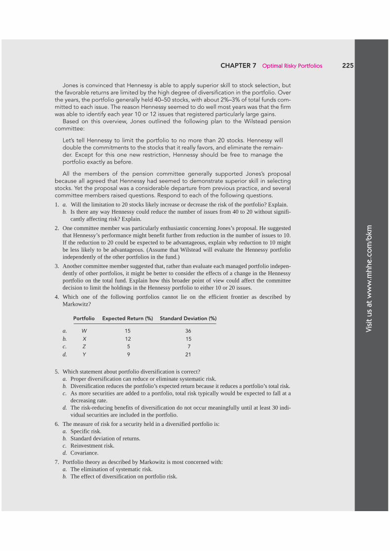
Vis

it u

s at

ww

w.m

hh

e.c

om

/bkm


Jones is convinced that Hennessy is able to apply superior skill to stock selection, but the favorable returns are limited by the high degree of diversification in the portfolio. Over the years, the portfolio generally held 40–50 stocks, with about 2%–3% of total funds com-mitted to each issue. The reason Hennessy seemed to do well most years was that the firm was able to identify each year 10 or 12 issues that registered particularly large gains.

Based on this overview, Jones outlined the following plan to the Wilstead pension committee:

Let’s tell Hennessy to limit the portfolio to no more than 20 stocks. Hennessy will double the commitments to the stocks that it really favors, and eliminate the remain-der. Except for this one new restriction, Hennessy should be free to manage the portfolio exactly as before.

All the members of the pension committee generally supported Jones’s proposal because all agreed that Hennessy had seemed to demonstrate superior skill in selecting stocks. Yet the proposal was a considerable departure from previous practice, and several committee members raised questions. Respond to each of the following questions.

1. a. Will the limitation to 20 stocks likely increase or decrease the risk of the portfolio? Explain.b. Is there any way Hennessy could reduce the number of issues from 40 to 20 without signifi-

cantly affecting risk? Explain.

2. One committee member was particularly enthusiastic concerning Jones’s proposal. He suggested that Hennessy’s performance might benefit further from reduction in the number of issues to 10. If the reduction to 20 could be expected to be advantageous, explain why reduction to 10 might be less likely to be advantageous. (Assume that Wilstead will evaluate the Hennessy portfolio independently of the other portfolios in the fund.)

3. Another committee member suggested that, rather than evaluate each managed portfolio indepen-dently of other portfolios, it might be better to consider the effects of a change in the Hennessy portfolio on the total fund. Explain how this broader point of view could affect the committee decision to limit the holdings in the Hennessy portfolio to either 10 or 20 issues.

4. Which one of the following portfolios cannot lie on the efficient frontier as described by Markowitz?

Portfolio Expected Return (%) Standard Deviation (%)

a. W 15 36

b. X 12 15

c. Z 5 7

d. Y 9 21

5. Which statement about portfolio diversification is correct?a. Proper diversification can reduce or eliminate systematic risk.b. Diversification reduces the portfolio’s expected return because it reduces a portfolio’s total risk.c. As more securities are added to a portfolio, total risk typically would be expected to fall at a

decreasing rate.d. The risk-reducing benefits of diversification do not occur meaningfully until at least 30 indi-

vidual securities are included in the portfolio.

6. The measure of risk for a security held in a diversified portfolio is:a. Specific risk.b. Standard deviation of returns.c. Reinvestment risk.d. Covariance.

7. Portfolio theory as described by Markowitz is most concerned with:a. The elimination of systematic risk.b. The effect of diversification on portfolio risk.

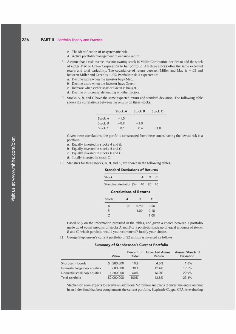
Vis

it u

s at

ww

w.m

hh

e.c

om

/bkm


c. The identification of unsystematic risk.d. Active portfolio management to enhance return.

8. Assume that a risk-averse investor owning stock in Miller Corporation decides to add the stock of either Mac or Green Corporation to her portfolio. All three stocks offer the same expected return and total variability. The covariance of return between Miller and Mac is �.05 and between Miller and Green is �.05. Portfolio risk is expected to:a. Decline more when the investor buys Mac.b. Decline more when the investor buys Green.c. Increase when either Mac or Green is bought.d. Decline or increase, depending on other factors.

9. Stocks A, B, and C have the same expected return and standard deviation. The following table shows the correlations between the returns on these stocks.

Stock A Stock B Stock C

Stock A �1.0

Stock B �0.9 �1.0

Stock C �0.1 �0.4 �1.0

Given these correlations, the portfolio constructed from these stocks having the lowest risk is a portfolio:a. Equally invested in stocks A and B.b. Equally invested in stocks A and C.c. Equally invested in stocks B and C.d. Totally invested in stock C.

10. Statistics for three stocks, A, B, and C, are shown in the following tables.

Standard Deviations of Returns

Stock: A B C

Standard deviation (%): 40 20 40

Correlations of Returns

Stock A B C

A 1.00 0.90 0.50

B 1.00 0.10

C 1.00

Based only on the information provided in the tables, and given a choice between a portfolio made up of equal amounts of stocks A and B or a portfolio made up of equal amounts of stocks B and C, which portfolio would you recommend? Justify your choice.

11. George Stephenson’s current portfolio of $2 million is invested as follows:

Summary of Stephenson’s Current Portfolio

ValuePercent of

TotalExpected Annual

ReturnAnnual Standard

Deviation

Short-term bonds $ 200,000 10% 4.6% 1.6%

Domestic large-cap equities 600,000 30% 12.4% 19.5%

Domestic small-cap equities 1,200,000 60% 16.0% 29.9%

Total portfolio $2,000,000 100% 13.8% 23.1%

Stephenson soon expects to receive an additional $2 million and plans to invest the entire amount in an index fund that best complements the current portfolio. Stephanie Coppa, CFA, is evaluating

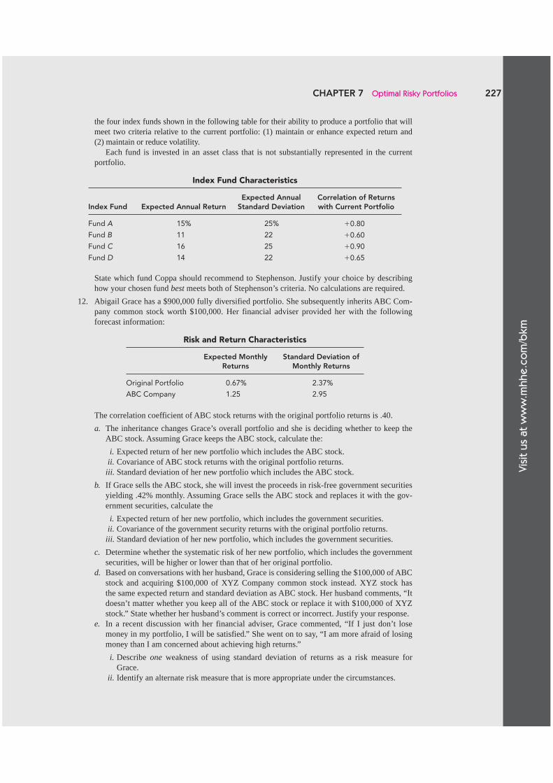
Vis

it u

s at

ww

w.m

hh

e.c

om

/bkm


the four index funds shown in the following table for their ability to produce a portfolio that will meet two criteria relative to the current portfolio: (1) maintain or enhance expected return and (2) maintain or reduce volatility.

Each fund is invested in an asset class that is not substantially represented in the current portfolio.

Index Fund Characteristics

Index Fund Expected Annual ReturnExpected Annual

Standard DeviationCorrelation of Returns with Current Portfolio

Fund A 15% 25% �0.80

Fund B 11 22 �0.60

Fund C 16 25 �0.90

Fund D 14 22 �0.65

State which fund Coppa should recommend to Stephenson. Justify your choice by describing how your chosen fund best meets both of Stephenson’s criteria. No calculations are required.

12. Abigail Grace has a $900,000 fully diversified portfolio. She subsequently inherits ABC Com-pany common stock worth $100,000. Her financial adviser provided her with the following forecast information:

Risk and Return Characteristics

Expected Monthly Returns

Standard Deviation of Monthly Returns

Original Portfolio 0.67% 2.37%

ABC Company 1.25 2.95

The correlation coefficient of ABC stock returns with the original portfolio returns is .40.

a. The inheritance changes Grace’s overall portfolio and she is deciding whether to keep the ABC stock. Assuming Grace keeps the ABC stock, calculate the:

i. Expected return of her new portfolio which includes the ABC stock. ii. Covariance of ABC stock returns with the original portfolio returns.iii. Standard deviation of her new portfolio which includes the ABC stock.

b. If Grace sells the ABC stock, she will invest the proceeds in risk-free government securities yielding .42% monthly. Assuming Grace sells the ABC stock and replaces it with the gov-ernment securities, calculate the

i. Expected return of her new portfolio, which includes the government securities. ii. Covariance of the government security returns with the original portfolio returns.iii. Standard deviation of her new portfolio, which includes the government securities.

c. Determine whether the systematic risk of her new portfolio, which includes the government securities, will be higher or lower than that of her original portfolio.

d. Based on conversations with her husband, Grace is considering selling the $100,000 of ABC stock and acquiring $100,000 of XYZ Company common stock instead. XYZ stock has the same expected return and standard deviation as ABC stock. Her husband comments, “It doesn’t matter whether you keep all of the ABC stock or replace it with $100,000 of XYZ stock.” State whether her husband’s comment is correct or incorrect. Justify your response.

e. In a recent discussion with her financial adviser, Grace commented, “If I just don’t lose money in my portfolio, I will be satisfied.” She went on to say, “I am more afraid of losing money than I am concerned about achieving high returns.”

i. Describe one weakness of using standard deviation of returns as a risk measure for Grace.

ii. Identify an alternate risk measure that is more appropriate under the circumstances.


13. Dudley Trudy, CFA, recently met with one of his clients. Trudy typically invests in a master list of 30 equities drawn from several industries. As the meeting concluded, the client made the following statement: “I trust your stock-picking ability and believe that you should invest my funds in your five best ideas. Why invest in 30 companies when you obviously have stronger opinions on a few of them?” Trudy plans to respond to his client within the context of Modern Portfolio Theory.a. Contrast the concepts of systematic risk and firm-specific risk, and give an example of each

type of risk.b. Critique the client’s suggestion. Discuss how both systematic and firm-specific risk change

as the number of securities in a portfolio is increased.

Diversification

Go to the www.investopedia.com/articles/basics/03/050203.asp Web site to learn more about diversification, the factors that influence investors’ risk preferences, and the types of investments that fit into each of the risk categories. Then check out www.investopedia.com/articles/pf/05/061505.asp for asset allocation guidelines for various types of portfolios from conservative to very aggressive. What do you conclude about your own risk preferences and the best portfolio type for you? What would you expect to happen to your attitude toward risk as you get older? How might your portfolio composition change?

E-Investments

1. a. The first term will be wD � wD � � D 2 , because this is the element in the top corner of the

matrix ( � D 2 ) times the term on the column border (wD) times the term on the row border

(wD). Applying this rule to each term of the covariance matrix results in the sum w D 2 � D 2

� wDwECov(rE, rD) � wEwDCov(rD, rE) � w E 2

� E 2 , which is the same as Equation 7.3, because

Cov(rE, rD) � Cov(rD, rE).

b. The bordered covariance matrix is

wX wY wZ

wX�

X

2Cov(rX, rY) Cov(rX, rZ)

wY Cov(rY, rX) �Y

2Cov(rY, rZ)

wZ Cov(rZ, rX) Cov(rZ, rY) �Z

2

There are nine terms in the covariance matrix. Portfolio variance is calculated from these nine terms:

� � � �P X X Y Y Z Z

X Y X Y Y

w w w

w w r r w w

2

Cov(

� � �

� �

2 2 2 2 2 2

, ) XX Y X

X Z X Z Z X Z X

r r

w w r r w w r r

Cov(

Cov( ) Cov(

, )

, , )� �

�ww w r r w w r r

w w

Y Z Y Z Z Y Z Y

X X Y Y

Cov( , ) Cov(�

� �

, )2 2 2� �22 2 2

2 2 2

�

� � �

w

w w r r w w r rZ Z

X Y X Y X Z X Z

�

Cov( ) Cov( ), , ww w r rY Z Y ZCov( , )

SOLUTIONS TO CONCEPT CHECKS

Vis

it u

s at

ww

w.m

hh

e.c

om

/bkm

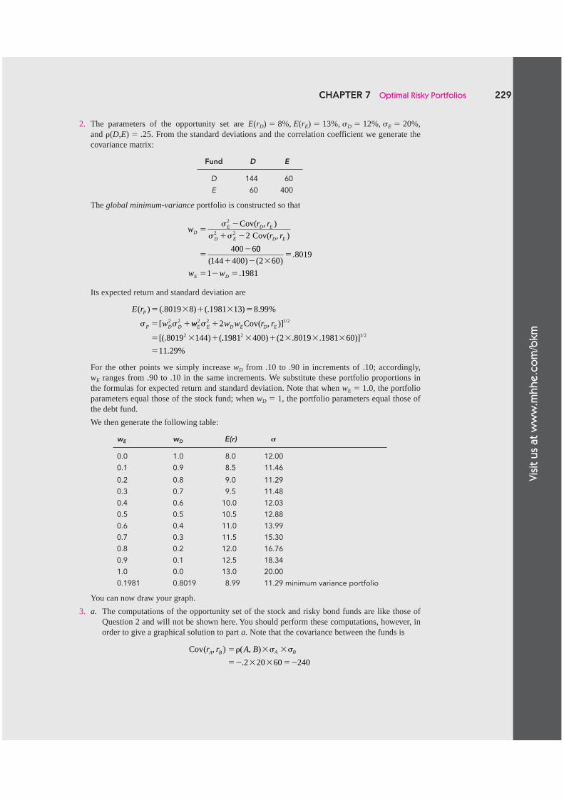
Vis

it u

s at

ww

w.m

hh

e.c

om

/bkm


2. The parameters of the opportunity set are E(rD) � 8%, E(rE) � 13%, �D � 12%, �E � 20%, and �(D,E) � .25. From the standard deviations and the correlation coefficient we generate the covariance matrix:

Fund D E

D 144 60

E 60 400

The global minimum-variance portfolio is constructed so that

wr r

r rDE D E

D E D E

��

� �

��

�

� �

2

2 2 2

400 6

Cov(

Cov(

, )

, )

00

144 400 2 608019

1 1981

( ) ( ).

.

� � ��

� � �w wE D

Its expected return and standard deviation are

E r

w

P

P D D

( ) (. ) (. ) . %

[

� � � � �

� �

8019 8 1981 13 8 992 2� � ww w w r rE E D E D E

2 2 1 2

2

2

8019 144

� �

� � �

Cov( , )]

[(. ) (

/

.. ) ( . . )]

. %

/1981 400 2 8019 1981 60

11 29

2 1 2� � � � �

�

For the other points we simply increase wD from .10 to .90 in increments of .10; accordingly, wE ranges from .90 to .10 in the same increments. We substitute these portfolio proportions in the formulas for expected return and standard deviation. Note that when wE � 1.0, the portfolio parameters equal those of the stock fund; when wD � 1, the portfolio parameters equal those of the debt fund.

We then generate the following table:

wE wD E(r) �

0.0 1.0 8.0 12.00

0.1 0.9 8.5 11.46

0.2 0.8 9.0 11.29

0.3 0.7 9.5 11.48

0.4 0.6 10.0 12.03

0.5 0.5 10.5 12.88

0.6 0.4 11.0 13.99

0.7 0.3 11.5 15.30

0.8 0.2 12.0 16.76

0.9 0.1 12.5 18.34

1.0 0.0 13.0 20.00

0.1981 0.8019 8.99 11.29 minimum variance portfolio

You can now draw your graph.

3. a. The computations of the opportunity set of the stock and risky bond funds are like those of Question 2 and will not be shown here. You should perform these computations, however, in order to give a graphical solution to part a. Note that the covariance between the funds is

Cov( , ) ( , )

.

r r A BA B A B��

��

� �

2 20 60 240

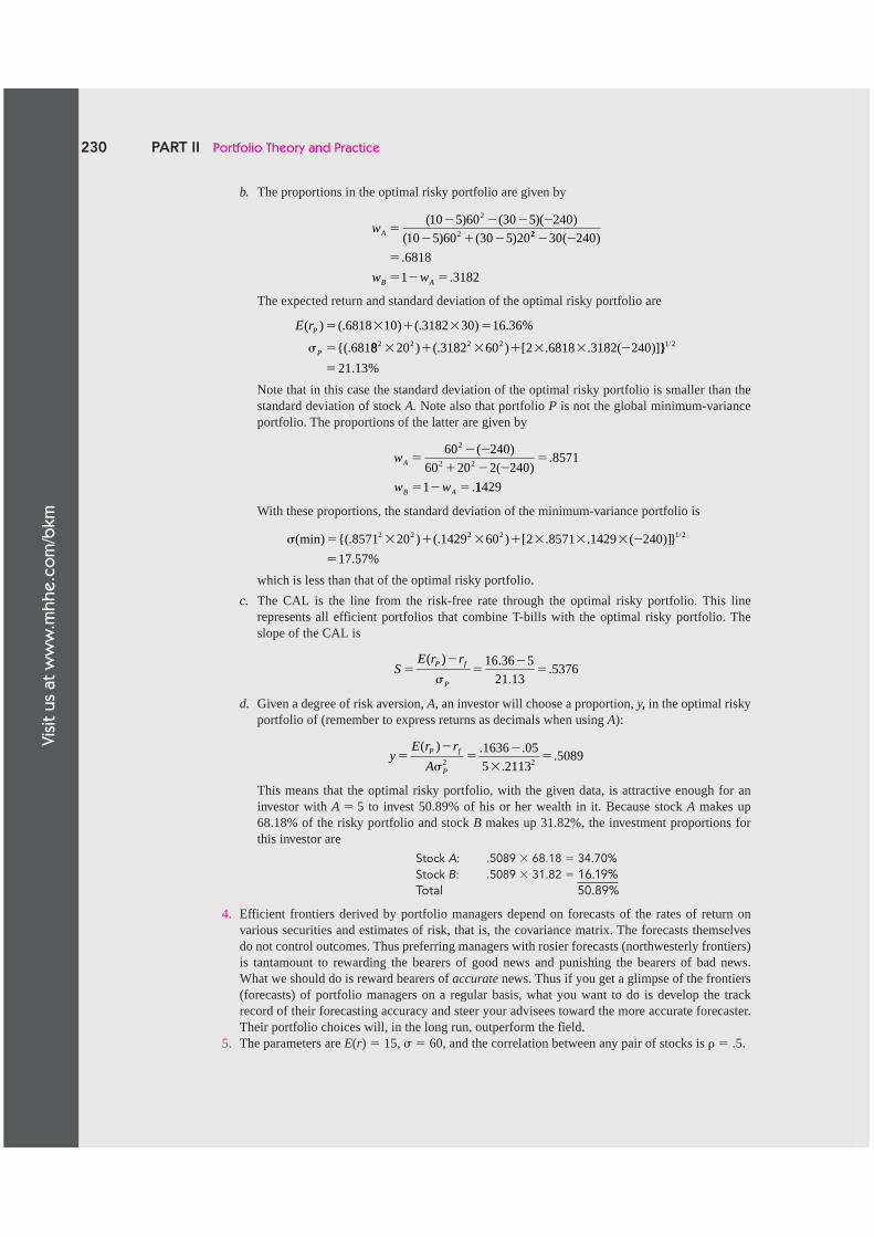
Vis

it u

s at

ww

w.m

hh

e.c

om

/bkm


b. The proportions in the optimal risky portfolio are given by

wA ��

� � �

( ) ( )( )

( ) ( )

10 5 60 30 5 240

10 5 60 30 5 20

2

2 22 30 240

6818

1 3182

� �

�

� � �

( )

.

.w wB A

The expected return and standard deviation of the optimal risky portfolio are

E rP

P

( ) (. ) (. ) . %

{( .

� � � � �

�

6818 10 3182 30 16 36

681� 88 20 3182 60 2 6818 3182 2402 2 2 2� � � � � � �) (. ) [ . . ( )]}}

. %

/1 2

21 13�

Note that in this case the standard deviation of the optimal risky portfolio is smaller than the standard deviation of stock A. Note also that portfolio P is not the global minimum-variance portfolio. The proportions of the latter are given by

w

w w

A

B A

��

� � ��

� � �

60 240

60 20 2 2408571

1

2

2 2

( )

( ).

.11429

With these proportions, the standard deviation of the minimum-variance portfolio is

�( ) { (. ) (. ) [ .min � � � � � � �8571 20 1429 60 2 85712 2 2 2 .. ( ) }

. %

/1429 240

17 57

1 2� �

�

]

which is less than that of the optimal risky portfolio.

c. The CAL is the line from the risk-free rate through the optimal risky portfolio. This line represents all efficient portfolios that combine T-bills with the optimal risky portfolio. The slope of the CAL is

SE r rP f

P

��

��

�( ) .

..

�

16 36 5

21 135376

d. Given a degree of risk aversion, A, an investor will choose a proportion, y, in the optimal risky portfolio of (remember to express returns as decimals when using A):

yE r r

AP f

P

��

��

��

( ) . .

..

�2 2

1636 05

5 21135089

This means that the optimal risky portfolio, with the given data, is attractive enough for an investor with A � 5 to invest 50.89% of his or her wealth in it. Because stock A makes up 68.18% of the risky portfolio and stock B makes up 31.82%, the investment proportions for this investor are

Stock A: .5089 � 68.18 � 34.70%

Stock B: .5089 � 31.82 � 16.19%

Total 50.89%

4. Efficient frontiers derived by portfolio managers depend on forecasts of the rates of return on various securities and estimates of risk, that is, the covariance matrix. The forecasts themselves do not control outcomes. Thus preferring managers with rosier forecasts (northwesterly frontiers) is tantamount to rewarding the bearers of good news and punishing the bearers of bad news. What we should do is reward bearers of accurate news. Thus if you get a glimpse of the frontiers (forecasts) of portfolio managers on a regular basis, what you want to do is develop the track record of their forecasting accuracy and steer your advisees toward the more accurate forecaster. Their portfolio choices will, in the long run, outperform the field.

5. The parameters are E(r) � 15, � � 60, and the correlation between any pair of stocks is � � .5.


a. The portfolio expected return is invariant to the size of the portfolio because all stocks have identical expected returns. The standard deviation of a portfolio with n � 25 stocks is

� � � ��

� � � �

P n n n[ / ( ) / ]

[ / . /

/2 2 1 2

2 2

1

60 25 5 60 24 225 43 271 2] . %/ �

b. Because the stocks are identical, efficient portfolios are equally weighted. To obtain a standard deviation of 43%, we need to solve for n:

4360

560 1

1 849 3 600 1 800 1

22 2

� � ��

� � �

n

n

nn n

.( )

, , , ,8800

1 800

4936 73n� �

,.

Thus we need 37 stocks and will come in with volatility slightly under the target.

c. As n gets very large, the variance of an efficient (equally weighted) portfolio diminishes, leaving only the variance that comes from the covariances among stocks, that is

� � �� P2 25 60 42 43. . %

Note that with 25 stocks we came within .84% of the systematic risk, that is, the nonsystematic risk of a portfolio of 25 stocks is only .84%. With 37 stocks the standard deviation is 43%, of which nonsystematic risk is .57%.

d. If the risk-free is 10%, then the risk premium on any size portfolio is 15 � 10 � 5%. The standard deviation of a well-diversified portfolio is (practically) 42.43%; hence the slope of the CAL is

S � 5/42.43 � .1178

APPENDIX A: A Spreadsheet Model for Efficient Diversification

Several software packages can be used to generate the efficient frontier. We will dem-onstrate the method using Microsoft Excel. Excel is far from the best program for this purpose and is limited in the number of assets it can handle, but working through a simple portfolio optimizer in Excel can illustrate concretely the nature of the calculations used in more sophisticated “black-box” programs. You will find that even in Excel, the computa-tion of the efficient frontier is fairly easy.

We apply the Markowitz portfolio optimization program to a practical problem of inter-national diversification. We take the perspective of a portfolio manager serving U.S. clients, who wishes to construct for the next year an optimal risky portfolio of large stocks in the U.S and six developed capital markets (Japan, Germany, U.K., France, Canada, and Australia). First we describe the input list: forecasts of risk premiums and the covariance matrix. Next, we describe Excel’s Solver, and finally we show the solution to the manager’s problem.

The Covariance Matrix

To capture recent risk parameters the manager compiles an array of 60 recent monthly (annualized) rates of return, as well as the monthly T-bill rates for the same period.

The standard deviations of excess returns are shown in Table 7A.1 (column C). They range from 14.93% (U.K. large stocks) to 22.7% (Germany). For perspective on how these

Vis

it u

s at

ww

w.m

hh

e.c

om

/bkm

Vis

it u

s at

ww

w.m

hh

e.c

om

/bkm


parameters can change over time, standard deviations for the period 1991–2000 are also shown (column B). In addition, we present the correlation coefficient between large stocks in the six foreign markets with U.S. large stocks for the same two periods. Here we see that cor-relations are higher in the more recent period, consistent with the process of globalization.

The covariance matrix shown in Table 7A.2 was estimated from the array of 60 returns of the seven countries using the COVARIANCE function from the dialog box of Data Analysis in Excel’s Tools menu. Due to a quirk in the Excel software, the covariance matrix is not corrected for degrees-of-freedom bias; hence, each of the elements in the matrix was multiplied by 60/59 to eliminate downward bias.

Expected Returns

While estimation of the risk parameters (the covariance matrix) from excess returns is a simple technical matter, estimating the risk premium (the expected excess return) is a daunting task. As we discussed in Chapter 5, estimating expected returns using histori-cal data is unreliable. Consider, for example, the negative average excess returns on U.S. large stocks over the period 2001–2005 (cell G6) and, more generally, the big differences in average returns between the 1991–2000 and 2001–2005 periods, as demonstrated in columns F and G.

In this example, we simply present the manager’s forecasts of future returns as shown in column H. In Chapter 8 we will establish a framework that makes the forecasting process more explicit.

The Bordered Covariance Matrix and Portfolio Variance

The covariance matrix in Table 7A.2 is bordered by the portfolio weights, as explained in Section 7.2 and Table 7.2 . The values in cells A18–A24, to the left of the covariance matrix, will be selected by the optimization program. For now, we arbitrarily input 1.0 for the U.S. and zero for the others. Cells A16–I16, above the covariance matrix, must be set equal to the column of weights on the left, so that they will change in tandem as the column weights are changed by Excel’s Solver. Cell A25 sums the column weights and is used to force the optimization program to set the sum of portfolio weights to 1.0.

Cells C25–I25, below the covariance matrix, are used to compute the portfolio variance for any set of weights that appears in the borders. Each cell accumulates the contribution to portfolio variance from the column above it. It uses the function SUMPRODUCT to accomplish this task. For example, row 33 shows the formula used to derive the value that appears in cell C25.

Finally, the short column A26–A28 below the bordered covariance matrix presents port-folio statistics computed from the bordered covariance matrix. First is the portfolio risk premium in cell A26, with formula shown in row 35, which multiplies the column of port-folio weights by the column of forecasts (H6–H12) from Table 7A.1 . Next is the portfolio standard deviation in cell A27. The variance is given by the sum of cells C25–I25 below the bordered covariance matrix. Cell A27 takes the square root of this sum to produce the standard deviation. The last statistic is the portfolio Sharpe ratio, cell A28, which is the slope of the CAL (capital allocation line) that runs through the portfolio constructed using the column weights (the value in cell A28 equals cell A26 divided by cell A27). The opti-mal risky portfolio is the one that maximizes the Sharpe ratio.

Using the Excel Solver

Excel’s Solver is a user-friendly, but quite powerful, optimizer. It has three parts: (1) an objective function, (2) decision variables, and (3) constraints. Figure 7A.1 shows three pictures of the Solver. For the current discussion we refer to picture A.

Vis

it u

s at

ww

w.m

hh

e.c

om

/bkm


A B C D E F G H

1

2

7A.1 Country Index Statistics and Forecasts of Excess Returns

Correlation with the

U.S. Average Excess Return Forecast

3

4

Country

−0.0148

0.0094

0.0247

0.0209

0.1225

0.0398

0.1009

0.1108

0.0536

0.0837

0.0473

0.0468

−0.0177

0.0727

1

0.83

0.83

0.85

0.81

0.43

0.79

1

0.64

0.54

0.53

0.52

0.41

0.72

Standard Deviation

1991–2000

0.1295

0.1466

0.1741

0.1538

0.1808

0.2432

0.1687

0.1495

0.1493

0.2008

0.2270

0.1617

0.1878

0.1727

2001–2005 1991–2000 2001–2005

US

UK

France

Germany

Australia

Japan

Canada

5

6

7

8

9

10

11

12

1991–2000 2001–2005 2006

0.0600

0.0530

0.0700

0.0800

0.0580

0.0450

0.0590

A B C D E F G H I

7A.2 The Bordered Covariance Matrix

Portfolio

Weights 1.0000 0.0000 0.0000 0.0000

1.0000

0.0000

0.0000

0.0000

0.0000

0.0000

0.0000

1.0000

0.0600

0.1495

0.4013

Cell A18 - A24 A18 is set arbitrarily to 1 while A19 to A24 are set to 0

Formula in cell C16 =A18 ... Formula in cell I16 = A24

Formula in cell A25 =SUM(A18:A24)

Formula in cell C25 =C16*SUMPRODUCT($A$18:$A$24,C18:C24)

Formula in cell D25-I25 Copied from C25 (note the absolute addresses)

Formula in cell A26 =SUMPRODUCT($A$18:$A$24,H6:H12)

Formula in cell A27 =SUM(C25:I25)^0.5

Formula in cell A28 =A26/A27

0.0224

0.0184

0.0250

0.0288

0.0195

0.0121

0.0205

0.0224

0.0184

0.0223

0.0275

0.0299

0.0204

0.0124

0.0206

0.0000

0.0288

0.0299

0.0438

0.0515

0.0301

0.0183

0.0305

0.0000

0.0121

0.0124

0.0177

0.0183

0.0147

0.0353

0.0158

0.0000

US UK

0.0000

0.0250

0.0275

0.0403

0.0438

0.0259

0.0177

0.0273

0.0000

France Germany

0.0000

0.0195

0.0204

0.0259

0.0301

0.0261

0.0147

0.0234

0.0000

Australia Japan

US

UK

France

Germany

Australia

Japan

Canada

0.0000

0.0205

0.0206

0.0273

0.0305

0.0234

0.0158

0.0298

0.0000

Canada

13

14

15

16

17

18

19

20

21

22

23

24

25

26

27

28

29

30

31

32

33

34

35

36

37

38

A B C D E F G H I J K L

US

Mean

SD 0.1

Min Var Optimum

0.0383

0.1132

0.3386

0.6112

0.8778

−0.2140

−0.5097

0.0695

0.2055

−0.0402

0.0465

0.0400

0.1135

0.3525

0.6195

0.8083

−0.2029

−0.4610

0.0748

0.1987

−0.0374

0.0466

0.0450

0.1168

0.3853

0.6446

0.5992

−0.1693

−0.3144

0.0907

0.1781

−0.0288

0.0480

0.0500

0.1238

0.4037

0.6696

0.3900

−0.1357

−0.1679

0.1067

0.1575

−0.0203

0.0509

0.0550

0.1340

0.4104

0.6947

0.1809

−0.1021

−0.0213

0.1226

0.1369

−0.0118

0.0550

0.0564

0.1374

0.4107

0.7018

0.1214

−0.0926

0.0205

0.1271

0.1311

−0.0093

0.0564

0.0575

0.1401

0.4106

0.7073

0.0758

−0.0852

0.0524

0.1306

0.1266

−0.0075

0.0575

0.0600

0.1466

0.4092

0.7198

−0.0283

−0.0685

0.1253

0.1385

0.1164

−0.0032

0.0602

0.0700

0.1771

0.3953

0.7699

−0.4465

−0.0014

0.4185

0.1704

0.0752

0.0139

0.0727

0.0800

0.2119

0.3774

0.8201

−0.8648

0.0658

0.7117

0.2023

0.0341

0.0309

0.08710.0411

Slope

UK

France

Germany

Australia

Japan

Canada

CAL*

*Risk premium on CAL = SD × slope of optimal risky portfolio

44

45

46

47

48

49

50

51

52

53

54

55

43

Cell to store constraint on risk premium

7A.3 The Efficient Frontier39

40

41

42

0.0400

Mean

SD

Slope

TA B L E 7 A . 1 , 7 A . 2 , 7 A . 3

Spreadsheet model for international diversification

eXce lPlease visit us at

www.mhhe.com/bkm

Vis

it u

s at

ww

w.m

hh

e.c

om

/bkm


The top panel of the Solver lets you choose a target cell for the “objective function,” that is, the variable you are trying to optimize. In picture A, the target cell is A27, the portfo-lio standard deviation. Below the target cell, you can choose whether your objective is to maximize, minimize, or set your objective function equal to a value that you specify. Here we choose to minimize the portfolio standard deviation.

The next panel contains the decision variables. These are cells that the Solver can change in order to optimize the objective function in the target cell. Here, we input cells A18–A24, the portfolio weights that we select to minimize portfolio volatility.

The bottom panel of the Solver can include any number of constraints. One constraint that must always appear in portfolio optimization is the “feasibility constraint,” namely, that portfolio weights sum to 1.0. When we bring up the constraint dialogue box, we spec-ify that cell A25 (the sum of weights) be set equal to 1.0.

Finding the Minimum Variance Portfolio

It is helpful to begin by identifying the global minimum variance portfolio ( G ). This pro-vides the starting point of the efficient part of the frontier. Once we input the target cell, the decision variable cells, and the feasibility constraint, as in picture A, we can select “solve” and the Solver returns portfolio G. We copy the portfolio statistics and weights to our output Table 7A.3 . Column C in Table 7A.3 shows that the lowest standard deviation (SD) that can be achieved with our input list is 11.32%. Notice that the SD of portfolio G is considerably lower than even the lowest SD of the individual indexes. From the risk premium of portfolio G (3.83%) we begin building the efficient frontier with ever-larger risk premiums.

B

C

A

F I G U R E 7 A . 1 Solver dialog box

Vis

it u

s at

ww

w.m

hh

e.c

om

/bkm


Charting the Efficient Frontier of Risky Portfolios

We determine the desired risk premiums (points on the efficient frontier) that we wish to use to construct the graph of the efficient frontier. It is good practice to choose more points in the neighborhood of portfolio G because the frontier has the greatest curvature in that region. It is sufficient to choose for the highest point the highest risk premium from the input list (here, 8% for Germany). You can produce the entire efficient frontier in minutes following this procedure.

1. Input to the Solver a constraint that says: Cell A26 (the portfolio risk premium) must equal the value in cell E41. The Solver at this point is shown in picture B of Figure 7A.1 . Cell E41 will be used to change the required risk premium and thus generate different points along the frontier.

2. For each additional point on the frontier, you input a different desired risk premium into cell E41, and ask the Solver to solve again.

3. Every time the Solver gives you a solution to the request in (2), copy the results into Table 7A.3 , which tabulates the collection of points along the efficient frontier. For the next step, change cell E41 and repeat from step 2.

Finding the Optimal Risky Portfolio on the Efficient Frontier

Now that we have an efficient frontier, we look for the portfolio with the highest Sharpe ratio (i.e., reward-to-volatility ratio). This is the efficient frontier portfolio that is tangent to the CAL. To find it, we just need to make two changes to the Solver. First, change the target cell from cell A27 to cell A28, the Sharpe ratio of the portfolio, and request that the value in this cell be maximized. Next, eliminate the constraint on the risk premium that may be left over from the last time you used the Solver. At this point the Solver looks like picture C in Figure 7A.1 .

The Solver now yields the optimal risky portfolio. Copy the statistics for the optimal portfolio and its weights to your Table 7A.3 . In order to get a clean graph, place the column of the optimal portfolio in Table 7A.3 so that the risk premiums of all portfolios in the table are steadily increasing from the risk premium of portfolio G (3.83%) all the way up to 8%.

The efficient frontier is graphed using the data in cells C45–I45 (the horizontal or x -axis is portfolio standard deviation) and C44–I44 (the vertical or y -axis is portfolio risk premium). The resulting graph appears in Figure 7A.2 .

The Optimal CAL

It is instructive to superimpose on the graph of the efficient frontier in Figure 7A.2 the CAL that identifies the optimal risky portfolio. This CAL has a slope equal to the Sharpe ratio of the optimal risky portfolio. Therefore, we add at the bottom of Table 7A.3 a row with entries obtained by multiplying the SD of each column’s portfolio by the Sharpe ratio of the optimal risky portfolio from cell H46. This results in the risk premium for each port-folio along the CAL efficient frontier. We now add a series to the graph with the standard deviations in B45–I45 as the x -axis and cells B54–I54 as the y -axis. You can see this CAL in Figure 7A.2 .

The Optimal Risky Portfolio and the Short-Sales Constraint

With the input list used by the portfolio manager, the optimal risky portfolio calls for sig-nificant short positions in the stocks of France and Canada (see column H of Table 7A.3 ). In many cases the portfolio manager is prohibited from taking short positions. If so, we need to amend the program to preclude short sales.


To accomplish this task, we repeat the exercise, but with one change. We add to the Solver the following constraint: Each element in the column of portfolio weights, A18–A24, must be greater than or equal to zero. You should try to produce the short-sale constrained efficient frontier in your own spreadsheet. The graph of the constrained fron-tier is also shown in Figure 7A.2 .

.0900

.0800

.0700

.0600

.0500

.0400

.0300.1000 .1200 .1400 .1600 .1800 .2000 .2200 .2400

Standard Deviation

Ris

k P

rem

ium

Risk premium SD Slope

Efficient PfNo short

No shortMin. Var pf

0.05640.05750.03830.0540

0.13740.14010.11320.1350

0.41070.41040.33860.3960

Eff frontier — No short sales

Efficient frontierCapital allocation line

F I G U R E 7 A . 2 Efficient frontier and CAL for country stock indexes

APPENDIX B: Review of Portfolio Statistics

We base this review of scenario analysis on a two-asset portfolio. We denote the assets D and E (which you may think of as debt and equity), but the risk and return parameters we use in this appendix are not necessarily consistent with those used in Section 7.2.

Expected Returns

We use “expected value” and “mean” interchangeably. For an analysis with n scenarios, where the rate of return in scenario i is r ( i ) with probability p ( i ), the expected return is

E r p i r i

i

n

( ) ( ) ( )��1∑

(7B.1)

If you were to increase the rate of return assumed for each scenario by some amount , then the mean return will increase by . If you multiply the rate in each scenario by a fac-tor w, the new mean will be multiplied by that factor:

i

n

i

n

i

n

p i r i p i r i p i� � �

� � � � �1 1 1

∑ ∑ ∑( ) [ ( ) ] ( ) ( ) ( )) ( )

( ) [ ( )] ( ) ( )

� �

� � � ��

E r

p i wr i w p i r ii

n

i

n

1 1

∑ ∑ wwE r( )

(7B.2)

Vis

it u

s at

ww

w.m

hh

e.c

om

/bkm

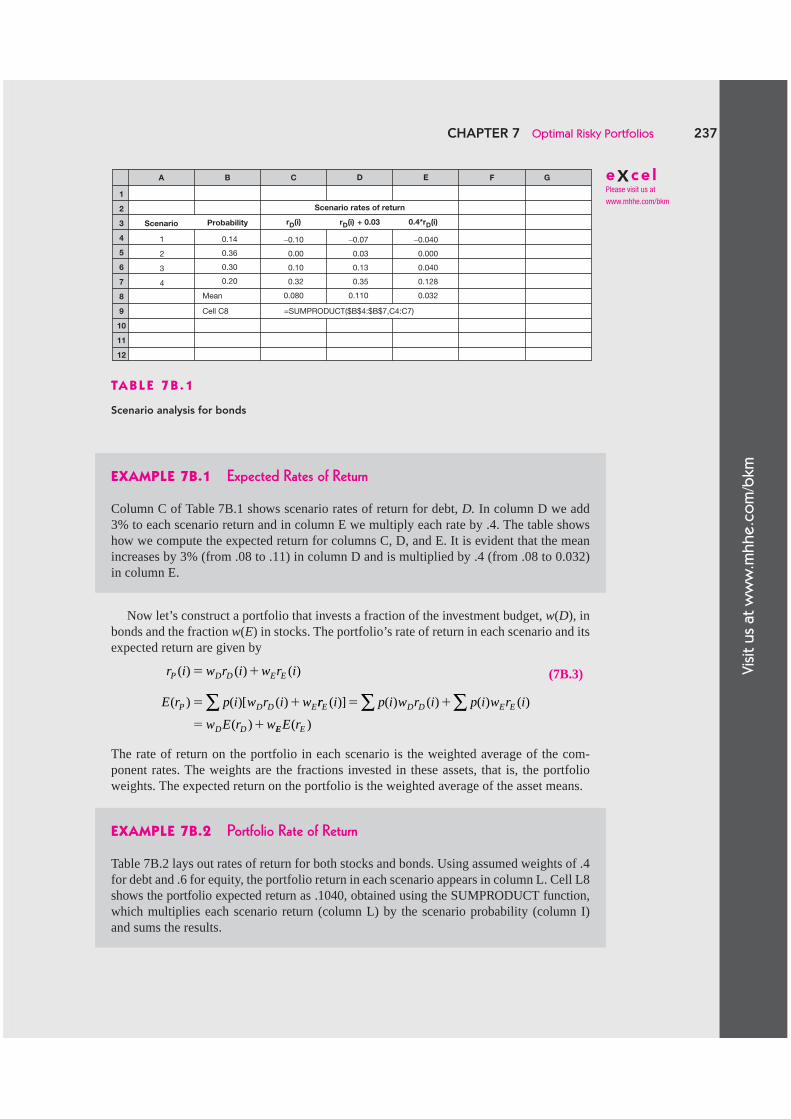
Vis

it u

s at

ww

w.m

hh

e.c

om

/bkm


Now let’s construct a portfolio that invests a fraction of the investment budget, w ( D ), in bonds and the fraction w ( E ) in stocks. The portfolio’s rate of return in each scenario and its expected return are given by

r i w r i w r i

E r p i w r i w

P D D E E

P D D E

( ) ( ) ( )

( ) ( )[ ( )

� �

� �∑ rr i p i w r i p i w r i

w E r w

E D D E E

D D

( )] ( ) ( ) ( ) ( )

( )

� �

� �

∑ ∑EE EE r( )

(7B.3)

The rate of return on the portfolio in each scenario is the weighted average of the com-ponent rates. The weights are the fractions invested in these assets, that is, the portfolio weights. The expected return on the portfolio is the weighted average of the asset means.

EXAMPLE 7B.1 Expected Rates of Return

Column C of Table 7B.1 shows scenario rates of return for debt, D. In column D we add 3% to each scenario return and in column E we multiply each rate by .4. The table shows how we compute the expected return for columns C, D, and E. It is evident that the mean increases by 3% (from .08 to .11) in column D and is multiplied by .4 (from .08 to 0.032) in column E.


www.mhhe.com/bkm

A B C D E GF

1

2

3

4

5

6

7

8

9

10

11

12

Scenario rates of return

rD(i) rD(i) + 0.03 0.4*rD(i)

Mean

Cell C8

−0.10

0.00

0.10

0.32

0.080

=SUMPRODUCT($B$4:$B$7,C4:C7)

−0.07

0.03

0.13

0.35

0.110

−0.040

0.000

0.040

0.128

0.032

0.14

0.36

0.30

0.20

Probability

1

2

3

4

Scenario

TA B L E 7 B . 1

Scenario analysis for bonds

EXAMPLE 7B.2 Portfolio Rate of Return

Table 7B.2 lays out rates of return for both stocks and bonds. Using assumed weights of .4 for debt and .6 for equity, the portfolio return in each scenario appears in column L. Cell L8 shows the portfolio expected return as .1040, obtained using the SUMPRODUCT function, which multiplies each scenario return (column L) by the scenario probability (column I) and sums the results.

Vis

it u

s at

ww

w.m

hh

e.c

om

/bkm


Variance and Standard Deviation

The variance and standard deviation of the rate of return on an asset from a scenario analy-sis are given by 17

� � ��

2

1

2( ) ( )[ ( ) ( )]r p i r i E ri

n

∑

� � �( ) ( )r r2

(7B.4)

Notice that the unit of variance is percent squared. In contrast, standard deviation, the square root of variance, has the same dimension as the original returns, and therefore is easier to interpret as a measure of return variability.

When you add a fixed incremental return, , to each scenario return, you increase the mean return by that same increment. Therefore, the deviation of the realized return in each scenario from the mean return is unaffected, and both variance and SD are unchanged. In contrast, when you multiply the return in each scenario by a factor w, the variance is mul-tiplied by the square of that factor (and the SD is multiplied by w ):

SD( ) ( )wr w w r� � � �2 2

Var( ) ( ) [ ( ) ( )] (wr p i wr i E wr w p ii

n

i

n

� � � �= =∑ ∑

1

2 2

1

))[ ( ) ( )]r i E r� � �2 2 2w

(7B.5)

Excel does not have a direct function to compute variance and standard deviation for a scenario analysis. Its STDEV and VAR functions are designed for time series. We need to calculate the probability-weighted squared deviations directly. To avoid having

17 Variance (here, of an asset rate of return) is not the only possible choice to quantify variability. An alternative would be to use the absolute deviation from the mean instead of the squared deviation. Thus, the mean absolute deviation (MAD) is sometimes used as a measure of variability. The variance is the preferred measure for several reasons. First, it is mathematically more difficult to work with absolute deviations. Second, squaring deviations gives more weight to larger deviations. In investments, giving more weight to large deviations (hence, losses) is compatible with risk aversion. Third, when returns are normally distributed, the variance is one of the two param-eters that fully characterize the distribution.

H I J K L

1

2

3

4

5

6

7

8

9

10

11

12

Scenario rates of return Portfolio return

0.4*rD(i)+0.6*rE(i)rD(i) rE(i)

0.14

0.36

0.30

0.20

−0.10

0.00

0.10

0.32

0.08Mean

Cell L4 =0.4*J4+0.6*K4

Cell L8 =SUMPRODUCT($I$4:$I$7,L4:L7)

−0.35

0.20

0.45

−0.19

0.12

−0.2500

0.1200

0.3100

0.0140

0.1040

1

2

3

4

ProbabilityScenario

TA B L E 7 B . 2

Scenario analysis for bonds and stocks


www.mhhe.com/bkm

Vis

it u

s at

ww

w.m

hh

e.c

om

/bkm


to first compute columns of squared deviations from the mean, however, we can simplify our problem by expressing the variance as a difference between two easily computable terms:

� � � � � �

�

2( ) [ ( )] { [ ( )] ( )}

( )

r E r E r E r E r rE r

E r

2 2 2

2

2

��

� � �

[ ( )] ( ) ( )

( ) [ ( )] ( ) ( )

E r E r E r

E r E r p i r i

2

2 2 2

2

��

p i r ii

n

i

n( ) ( )

11

2

∑

∑

(7B.6)


www.mhhe.com/bkm

A B C D E F G

13

14

15

16

17

18

19

20

21

22

23

24


rD(i) rD(i) + 0.03 0.4*rD(i)

0.14

0.36

0.30

0.20

Mean

Cell C21

Variance

SD

−0.10

0.00

0.10

0.32

0.0800

0.0185

0.1359

=SUMPRODUCT($B$16:$B$19,C16:C19,C16:C19)−C20^2

Cell C22 =C21^0.5

−0.07

0.03

0.13

0.35

0.1100

0.0185

0.1359

−0.040

0.000

0.040

0.128

0.0240

0.0034

0.0584

1

2

3

4

ProbabilityScenario

TA B L E 7 B . 3

Scenario analysis for bonds

EXAMPLE 7B.3 Calculating the Variance of a Risky Asset in Excel

You can compute the first expression, E(r2), in Equation 7B.6 using Excel’s SUMPROD-UCT function. For example, in Table 7B.3, E(r2) is first calculated in cell C21 by using SUMPRODUCT to multiply the scenario probability times the asset return times the asset return again. Then [E(r)]2 is subtracted (notice the subtraction of C20^2 in cell C21), to arrive at variance.

The variance of a portfolio return is not as simple to compute as the mean. The portfolio variance is not the weighted average of the asset variances. The deviation of the portfolio rate of return in any scenario from its mean return is

r E r w r i w r i w E r w E rP P D D E E D D E E� � � � �

�

( ) ( ) ( ) [ ( ) ( )]

ww r i E r w r i E r

w d i w eD D D E E E

D E

[ ( ) ( )] [ ( ) ( )]

( )

� � �

� � (( )i

(7B.7)

where the lowercase variables denote deviations from the mean:

d(i r i E r

e i r i E rD D

E E

) ( ) ( )

( ) ( ) ( )

� �

� �

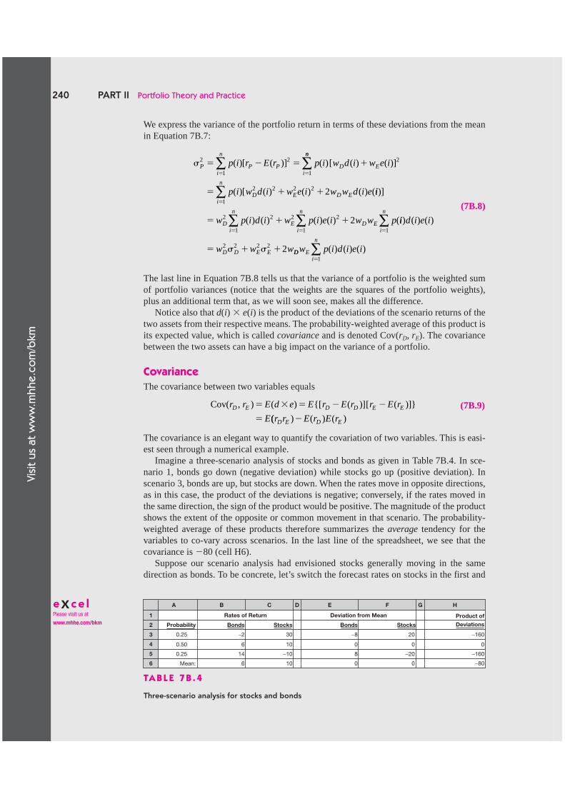
Vis

it u

s at

ww

w.m

hh

e.c

om

/bkm


We express the variance of the portfolio return in terms of these deviations from the mean in Equation 7B.7 :

� � � � ��

P2 2 2p i r E r p i w d i w e iP P D E

i

( )[ ( )] ( )[ ( ) ( )]1

nn

i

n

D E D Ep i w d i w e i w w d i e

∑∑�

� � �

1

2( )[ ( ) ( ) ( ) (2 2 2 2 ii

w p i d i w p i e i w w p

i

n

D E D

)]

( ) ( ) ( ) ( ) (

�

� � �

1

2 2

∑

2 2 2E ii d i e i

w w w

i

n

i

n

i

n

D D E E

) ( ) ( )��

� � � � �

111

2

∑∑∑

2 2 2 2DD E

i

n

w p i d i e i( ) ( ) ( )�1∑

(7B.8)

The last line in Equation 7B.8 tells us that the variance of a portfolio is the weighted sum of portfolio variances (notice that the weights are the squares of the portfolio weights), plus an additional term that, as we will soon see, makes all the difference.

Notice also that d ( i ) � e ( i ) is the product of the deviations of the scenario returns of the two assets from their respective means. The probability-weighted average of this product is its expected value, which is called covariance and is denoted Cov( r D, r E ). The covariance between the two assets can have a big impact on the variance of a portfolio.

Covariance

The covariance between two variables equals

Cov( , ) ( ) {[ ( )][ ( )]}r r E d e E r E r r E r

ED E D D E E� � � � �

� (( ) ( ) ( )r r E r E rD E D E�

(7B.9)

The covariance is an elegant way to quantify the covariation of two variables. This is easi-est seen through a numerical example.

Imagine a three-scenario analysis of stocks and bonds as given in Table 7B.4 . In sce-nario 1, bonds go down (negative deviation) while stocks go up (positive deviation). In scenario 3, bonds are up, but stocks are down. When the rates move in opposite directions, as in this case, the product of the deviations is negative; conversely, if the rates moved in the same direction, the sign of the product would be positive. The magnitude of the product shows the extent of the opposite or common movement in that scenario. The probability-weighted average of these products therefore summarizes the average tendency for the variables to co-vary across scenarios. In the last line of the spreadsheet, we see that the covariance is � 80 (cell H6).

Suppose our scenario analysis had envisioned stocks generally moving in the same direction as bonds. To be concrete, let’s switch the forecast rates on stocks in the first and

TA B L E 7 B . 4

Three-scenario analysis for stocks and bonds

A

Bonds

Rates of Return Deviation from Mean

Stocks Bonds Stocks

Product of

Deviations

B C D E F G H

1

2

3 0.25

0.50

0.25

Mean:

−2

6

14

6

30

10

−10

10

−8

0

8

0

20

0

−20

0

−160

0

−160

−80

4

5

6

Probability


www.mhhe.com/bkm

Vis

it u

s at

ww

w.m

hh

e.c

om

/bkm


third scenarios, that is, let the stock return be � 10% in the first scenario and 30% in the third. In this case, the absolute value of both products of these scenarios remains the same, but the signs are positive, and thus the covariance is positive, at � 80, reflecting the ten-dency for both asset returns to vary in tandem. If the levels of the scenario returns change, the intensity of the covariation also may change, as reflected by the magnitude of the prod-uct of deviations. The change in the magnitude of the covariance quantifies the change in both direction and intensity of the covariation.

If there is no comovement at all, because positive and negative products are equally likely, the covariance is zero. Also, if one of the assets is risk-free, its covariance with any risky asset is zero, because its deviations from its mean are identically zero.

The computation of covariance using Excel can be made easy by using the last line in Equation 7B.9 . The first term, E ( r D � r E ), can be computed in one stroke using Excel’s SUMPRODUCT function. Specifically, in Table 7B.4 , SUMPRODUCT(A3:A5, B3:B5, C3:C5) multiplies the probability times the return on debt times the return on equity in each scenario and then sums those three products.

Notice that adding to each rate would not change the covariance because deviations from the mean would remain unchanged. But if you multiply either of the variables by a fixed factor, the covariance will increase by that factor. Multiplying both variables results in a covariance multiplied by the products of the factors because

Cov( , ) {[ ( )][ (w r w r E w r w E r w r w E rD D E E D D D D E E E E� � � ))]}

( , )� w w r rD E D ECov (7B.10)

The covariance in Equation 7B.10 is actually the term that we add (twice) in the last line of the equation for portfolio variance, Equation 7B.8 . So we find that portfolio variance is the weighted sum (not average) of the individual asset variances, plus twice their covariance weighted by the two portfolio weights ( w D � w E ).

Like variance, the dimension (unit) of covariance is percent squared. But here we can-not get to a more easily interpreted dimension by taking the square root, because the aver-age product of deviations can be negative, as it was in Table 7B.4 . The solution in this case is to scale the covariance by the standard deviations of the two variables, producing the correlation coefficient.

Correlation Coefficient

Dividing the covariance by the product of the standard deviations of the variables will gen-erate a pure number called correlation. We define correlation as follows:

Corr

Cov( , )

( , )r r

r rD E

D

D E

E��

(7B.11)

The correlation coefficient must fall within the range [�1, 1]. This can be explained as follows. What two variables should have the highest degree comovement? Logic says a variable with itself, so let’s check it out.

Cov(r r E r E r r E r

E r E

D D D D D D

D

, ) { [ ( )] [ ( )]}

[ (

� � � �

� � rr

r rr r

D D

D DD D

D D

D

D

)]

, )( , )

2 2

2

2

� �

��

��

�Corr(

Cov��1

(7B.12)

Similarly, the lowest (most negative) value of the correlation coefficient is � 1. (Check this for yourself by finding the correlation of a variable with its own negative.)

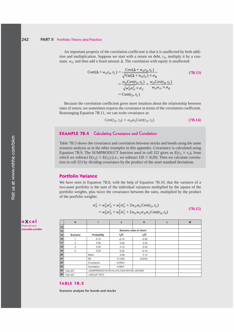
Vis

it u

s at

ww

w.m

hh

e.c

om

/bkm


An important property of the correlation coefficient is that it is unaffected by both addi-tion and multiplication. Suppose we start with a return on debt, r D, multiply it by a con-stant, w D, and then add a fixed amount . The correlation with equity is unaffected:

Corr(Cov(

Var(� �

�

� ��w r r

w r r

w rD D E

D D E

D D

, ), )

) EE

D D E

D D E

D D E

D D

w r r

w

w r r

w�

� ��

� ��

Cov( Cov(, ) , )2 2

EE

D Er r� Corr( , )

(7B.13)

Because the correlation coefficient gives more intuition about the relationship between rates of return, we sometimes express the covariance in terms of the correlation coefficient. Rearranging Equation 7B.11 , we can write covariance as

Cov(rD, rE) � �D�ECorr(rD, rE) (7B.14)

EXAMPLE 7B.4 Calculating Covariance and Correlation

Table 7B.5 shows the covariance and correlation between stocks and bonds using the same scenario analysis as in the other examples in this appendix. Covariance is calculated using Equation 7B.9. The SUMPRODUCT function used in cell J22 gives us E(rD � rE), from which we subtract E(rD) � E(rE) (i.e., we subtract J20 � K20). Then we calculate correla-tion in cell J23 by dividing covariance by the product of the asset standard deviations.

Portfolio Variance

We have seen in Equation 7B.8 , with the help of Equation 7B.10 , that the variance of a two-asset portfolio is the sum of the individual variances multiplied by the square of the portfolio weights, plus twice the covariance between the rates, multiplied by the product of the portfolio weights:

� � � � � �

� � �

P D D E E D E D E

D D E

2 2 2 2 2

2

w w w w r r

w w

22

Cov( , )22 2� � � �E D E D E D E2w w r rCorr( , )

(7B.15)

H I J K L M

13

14

15

16

17

18

19

20

21

22

23

24

25


rD(i) rE(i)

0.14

0.36

0.30

0.20

−0.10

0.00

0.10

0.32

0.08

0.1359

−0.0034

−0.0847

Mean

SD

Covariance

Correlation

Cell J22

Cell J23

=SUMPRODUCT(I16:I19,J16:J19,K16:K19)−J20*K20

=J22/(J21*K21)

−0.35

0.20

0.45

−0.19

0.12

0.2918

1

2

3

4

ProbabilityScenario

TA B L E 7 B . 5



www.mhhe.com/bkm

Vis

it u

s at

ww

w.m

hh

e.c

om

/bkm


EXAMPLE 7B.5 Calculating Portfolio Variance

We calculate portfolio variance in Table 7B.6. Notice there that we calculate the portfolio standard deviation in two ways: once from the scenario portfolio returns (cell E35) and again (in cell E36) using the first line of Equation 7B.15. The two approaches yield the same result. You should try to repeat the second calculation using the correlation coef-ficient from the second line in Equation 7B.15 instead of covariance in the formula for portfolio variance.

TA B L E 7 B . 6


A B C D E F G

25

26

27

28

29

30

31

32

33

34

35

36

37

38

39

Cell E35 =SUMPRODUCT(B30:B33,E30:E33,E30:E33)−E34^2)^0.5

Cell E36 =(0.4*C35)^2+(0.6*D35)^2+2*0.4*0.6*C36)^0.5

Scenario rates of return Portfolio return

rD(i) rE(i) 0.4*rD(i)+0.6rE(i)

0.14

0.36

0.30

0.20

Mean

SD

Covariance

Correlation

−0.10

0.00

0.10

0.32

0.08

0.1359

−0.0034

−0.0847

−0.35

0.20

0.45

−0.19

0.12

0.2918

SD:

−0.25

0.12

0.31

0.014

0.1040

0.1788

0.1788

1

2

3

4

ProbabilityScenario


www.mhhe.com/bkm

Suppose that one of the assets, say, E, is replaced with a money market instrument, that is, a risk-free asset. The variance of E is then zero, as is the covariance with D. In that case, as seen from Equation 7B.15 , the portfolio standard deviation is just w D � D. In other words, when we mix a risky portfolio with the risk-free asset, portfolio standard deviation equals the risky asset’s standard deviation times the weight invested in that asset. This result was used extensively in Chapter 6.

the investment decision can be viewed as · about a two-asset portfolio as an asset allocation...

Documents