BIS WORKING PAPERS

No. 59 – November 1998

PORTFOLIO SELECTION

USING FUZZY DECISION THEORY

by

Srichander Ramaswamy

BANK FOR INTERNATIONAL SETTLEMENTSMonetary and Economic Department

Basle, Switzerland

BIS Working Papers are written by members of the Monetary and Economic Department of the Bank forInternational Settlements, and from time to time by other economists, and are published by the Bank. The papersare on subjects of topical interest and are technical in character. The views expressed in them are those of theirauthors and not necessarily the views of the BIS.

Copies of publications are available from:

Bank for International SettlementsInformation, Press & Library ServicesP.O. BoxCH-4002 Basle, Switzerland

Fax: +41 61 / 280 91 00 and +41 61 / 280 81 00

The present publication is also available on the BIS Web site (www.bis.org).

© Bank for International Settlements 1998.All rights reserved. Brief excerpts may be reproduced or translated provided the source is stated.

ISSN 1020-0959

BIS WORKING PAPERS

No. 59 – November 1998

PORTFOLIO SELECTION

USING FUZZY DECISION THEORY

by

Srichander Ramaswamy *

Abstract

This paper presents an approach to portfolio selection using fuzzy decision theory.The approach is such that a given target rate of return is achieved for an assumedmarket scenario. If the assumed market scenario turns out to be incorrect, theportfolio is guaranteed to secure a given minimum rate of return. The methodologyis useful in the management of assets against given liabilities or in formingstructured portfolios that guarantee a minimum rate of return.

* I would like to thank Gabriele Galati for many thoughtful comments on an earlier version of the paper. Helpfulsuggestions from Greg Sutton, Henri Pagès and Joe Bisignano are very much appreciated. I am also indebted to LynnKirman and Nigel Hulbert for proof-reading and Stephan Arthur for overseeing the publication.

Contents

Introduction ............................................................................................................................ 1

1. Motivation .................................................................................................................... 2

2. Fuzzy decision theory .................................................................................................. 4

2.1 Fuzzy multi-criteria optimisation ...................................................................... 6

3. Structured portfolio ...................................................................................................... 8

4. Numerical example ...................................................................................................... 12

4.1 Yield curve scenarios ......................................................................................... 12

Conclusions ............................................................................................................................ 19

References .............................................................................................................................. 20

1

Introduction

Fund managers are constantly faced with the dilemma of guessing the direction of market

moves in order to meet the return target for assets under management. Given the uncertainty inherent

in financial markets, fund managers are very cautious in expressing their market views. The

information content in such cautious views can be best described as being “fuzzy” or vague, in terms

of both the direction and the size of market moves. Nevertheless, such fuzzy views are the ones needed

to structure portfolios so that the target return, which is assumed to be higher than the risk-free rate, is

met. In general, achieving returns higher than the risk-free rate requires taking either market or credit

risk. In this paper we will propose a methodology using fuzzy decision theory to select optimal

portfolios that target returns above the risk-free rate by taking only market risk.

As suggested above, generating returns higher than the risk-free rate requires fund

managers to hold a portfolio of risky assets. Such portfolios may be structured around imprecise and

potentially incorrect views of asset managers regarding the size and direction of market moves.

Additionally, fund managers may operate under strict guidelines requiring a minimum rate of return

for the assets being managed. Under such a constraint, fund managers are forced to examine the

performance of the risky portfolio they hold under various possible market scenarios. The risky

portfolio frequently has to be structured so that the return from holding the portfolio meets the target

rate of return for those scenarios deemed most probable by the fund manager and the minimum rate of

return is achieved for other scenarios.

In general, the target rate of return and the minimum rate of return for the portfolio will

be a function of the investment horizon, the risk preference of the investor and the nature of assets that

can be included in the portfolio. In this paper we will assume that the investment horizon is typically

one to three months and the investment universe consists of government debt securities and plain

vanilla options on these securities. The target rate of return will be assumed to be a certain number of

basis points above Libor over the given investment horizon. Such an investment horizon and security

selection could be ideally suited for central banks managing their short-term liquidity portfolio. This is

particularly true for those central banks that try to target returns above the money market rate for the

liquidity portfolio without taking additional credit risk. Seen in a broader perspective, the target

audience for the investment objective stated above could be asset liability management groups who

seek to meet a given target return by choosing an optimal portfolio that best replicates their liabilities.

Further, since liabilities can be interpreted as a short position on assets, the proposed methodology is

also applicable to proprietary trading groups who hold risky portfolios funded at Libor in order to

generate returns above the risk-free rate.

Structuring a portfolio along the lines described above is a difficult exercise using

existing techniques for portfolio selection. For instance, the approach using mean-variance

2

optimisation to structure the portfolio may be inappropriate. This is because the joint distribution of

returns for the assets in the investment universe considered here is usually not computable with any

degree of confidence. For the same reason many other techniques for portfolio selection, such as the

average shortfall approach (J.P. Morgan (1993)) or asymmetric risk measures for portfolio

optimisation under uncertainty (King (1993)) are also not useful because they assume that the return

distribution of the portfolio can be computed. In order to solve the portfolio selection problem

described here, one has to apply techniques that do not require the estimation of the joint distribution

of asset returns. In this paper, the problem is addressed using fuzzy decision theory since it satisfies

this requirement. The numerical results suggest that when holding the optimal portfolio consisting of

US treasury securities and plain vanilla options on them, it is possible to generate above 100 basis

points (bps) excess return over Libor on an annualised basis with a 99.5% confidence level. This is

confirmed by carrying out a Monte Carlo simulation of potential yield curve scenarios and computing

the annualised excess return over Libor for the given investment period. However, it is important to

note that in general the excess return distribution will depend on the shape of the yield curve, repo

rates and bond market volatility.

The rest of the paper is organised in the following manner. Section 1 provides the

motivation for posing the portfolio selection problem in the fuzzy decision theory framework. Section

2 gives an overview of fuzzy decision theory and fuzzy multi-criteria optimisation. Section 3 describes

the formulation of the portfolio selection problem under multiple scenarios as a multi-objective linear

programming problem. It is shown that a satisfactory solution to this problem can be easily determined

using fuzzy decision theory. Section 4 presents a numerical example to illustrate the various issues. It

is assumed in Section 4 that the allowable asset class for the structured portfolio consists of

government bonds and plain vanilla options on them. The final section concludes.

1. Motivation

In a capitalist economy, individuals and business firms make portfolio and investment

decisions with the objective of maximising the expected income over a given time horizon. Such

decisions are based on the subjective evaluation of income expectations over the chosen time horizon

and the risk preferences of the individuals or institutions taking these decisions. However, when one is

faced with uncertainty in the sense of Keynes (see Minsky (1975)), there is no scientific basis on

which one could compute the relevant probabilities for various propositions that determine the income

distribution. The subjective estimates of the relevant probabilities and the confidence with which they

are held are themselves subject to substantial changes during emerging events such as crises.

Nevertheless, individuals and investment firms must take decisions under imperfect knowledge by

3

forming subjective views that help to forecast changes to those factors that influence their end-of-

period wealth.

In the classical approach to portfolio selection, one often applies the theory of expected

utility that is derived from a set of axioms concerning investor behaviour as regards the ordering

relationship for deterministic and random events in the choice set. The specific nature of the axioms

that characterise the utility function is based on the assumption that a probability measure can be

defined on the random outcomes. However, if we assume that the origins of these random events are

not well known, then the theory of probability proves inadequate because of a lack of experimental

information. In such instances, one has to approach the decision theory problem under uncertainty

using different mathematical tools. Further, the preference function that describes the utility of the

investor may itself be changing with the degree of uncertainty. Moreover, one could postulate that the

investor has multiple preference functions each of which corresponds to a particular view on various

factors that influence the future state of the economy and the confidence with which it is held. Under

these conditions, the existing literature in the field of economic theory does not provide the investor

with sufficient tools to address the portfolio selection problem.

The discussion above highlighted potential difficulties one would encounter when

addressing the portfolio selection problem under uncertainty. It was postulated that under uncertainty

the investor would be confronted with multiple utility functions. Each one of these utility functions

may be attributed to a particular market view being held and can be broadly described as capturing the

investor’s level of satisfaction if it turns out to be true. For instance, a fund manager structuring a

fixed-income portfolio may have only vague views regarding future interest rate scenarios and these

can broadly be described as being “bullish”, “bearish” or “neutral”. Such views may arise out of the

subjective and/or intuitive opinion of the decision-maker on the basis of information available at the

given point in time. Under these circumstances, one might try to characterise the range of acceptable

solutions to the portfolio selection problem as a fuzzy set (see Bellman and Zadeh (1970)). In simple

terms, a fuzzy set is a class of objects in which there is no clear distinction between those objects that

belong to the class and those that do not. Further, associated with each object is a membership

function that defines the degree of membership of the object in the set. In this respect, fuzzy set theory

provides a framework to deal with problems in which the source of imprecision is the absence of

sharply defined criteria of class membership rather than the presence of random variables. This

provides the point of departure from probability theory, where the uncertainty arises from the random

nature of the environment rather than from any vagueness of human reasoning.

In the context of choosing optimal portfolios that target returns above the risk-free rate

for certain market scenarios while at the same time guaranteeing a minimum rate of return, fuzzy

decision theory provides an excellent framework for analysis. This is because the nature of the

problem requires one to examine various market scenarios, and each such scenario will in turn give

4

rise to an objective function. In the face of uncertainty, one will not be able to assign a numerical value

to the probability of these scenarios occurring. Under this constraint, it is not clear how a suitable

weighting vector can be determined to solve the multi-objective optimisation problem. One way to

overcome this difficulty is to use the membership function that arises in fuzzy decision theory to serve

as a suitable preference function for finding an ordering relation for the uncertain events. In fact, one

can describe the membership function as the fuzzy utility of the investor, which describes the

behaviour of indifference, preference or aversion towards uncertainty (Mathieu-Nicot (1990)). The

advantage of using the membership function is that it does not rely necessarily on the existence of a

probability measure but rather on the existence of relative preference between the uncertain events.

The above arguments show how the portfolio selection problem under uncertainty can be

transformed into a problem of decision-making in a fuzzy environment (see Bellman and Zadeh

(1970)). To do this, one has to model the aspirations of the investor on the basis of the strength of the

views held on various market scenarios through suitable membership functions of a fuzzy set. For

instance, a fund manager structuring a fixed-income portfolio may have aspiration levels as to what

the portfolio’s acceptable excess return over the risk-free rate should be for those scenarios he/she

considers more likely. For other scenarios deemed less likely in the fund manager’s view, returns

lower than the risk-free rate may be considered acceptable for the structured portfolio. In such

circumstances, it is rather easy for the fund manager to describe the goals so as to target 50-100 bps

excess return over the liabilities or risk-free rate for the more likely market scenarios. Such a

characterisation of the aspiration levels will allow one to model the fuzzy preferences of the fund

manager through a suitable membership function of the fuzzy subset. Once this is done, the portfolio

selection problem can be easily tackled in the framework of fuzzy decision theory. This will be

described in Section 3. In the section that follows, the concepts of fuzzy sets, fuzzy goals and fuzzy

decision will be introduced and a fuzzy multi-criteria optimisation problem will be formulated.

2. Fuzzy decision theory

Many decision-making problems in the real world take place in a framework where the

goals and/or constraints are imprecisely defined. The source of imprecision in such problems is the

absence of sharply defined criteria of class membership rather than the presence of random variables.

In order to deal quantitatively with imprecision, the notion of fuzzy sets was introduced by Zadeh

(1965). This section presents the concepts of fuzzy sets, fuzzy goals and fuzzy decision and formulates

a fuzzy multi-criteria optimisation problem. We refer the reader to Zimmermann (1985) for a more

detailed description of these concepts.

In simple terms a fuzzy set is a class of objects in which there is no sharp boundary

5

between those objects that belong to the class and those that do not. If, for instance, }{xX = denotes a

collection of objects, then a fuzzy set A in X is a set of ordered pairs

( ){ } XxxxA A ∈µ= ,)(, (1)

where )(xAµ is called the grade of membership of x in A, and ZXA →µ : is a function from X to a

space Z called the membership space. Note that when Z contains only two points, 0 and 1, then the set

A is non-fuzzy and its membership function is identical to the characteristic function of a non-fuzzy

set. Again, if }{xX = denotes a set of alternatives to a decision-making problem, then a fuzzy goal G

in X will be identified with a given fuzzy set G in X. For example, if one considers X to denote the set

of real numbers, then the fuzzy goal expressed in words as “x should be considerably larger than 10”

can be represented as a fuzzy set whose membership function is subjectively given by

( ) 10,)10(1

10,0)(11 ≥−+=

<=µ−− xx

xxG (2)

Similarly, the goal “x should be in the vicinity of 15” can be interpreted as a fuzzy set with a

membership function of the form

( ) 12)15(1)(−

−+=µ xxG (3)

In a similar manner, one can define a fuzzy constraint C in X as a fuzzy set in X.

Given the above notion of fuzzy goals and fuzzy constraints, one can define the decision-

making problem in a fuzzy environment as the intersection of goals and constraints. Specifically, if we

are given a space of alternatives X, then the fuzzy decision D is defined as a fuzzy set in X given by

CGD ∩= where the symbol ∩ denotes the intersection of sets. The corresponding membership

function of the fuzzy set D is given by

[ ])(),()( xxMinx CGD µµ=µ (4)

More generally, if there are n goals nGG ,,1 L and m constraints mCC ,,1 L , then the decision D is a

fuzzy set given by

mn CCGGGD ∩∩∩∩= LL 121 (5)

with the membership function

[ ])(),(),(,),()(11

xxxxMinxmn CCGGD µµµµ=µ LL (6)

Further, if D is a fuzzy decision represented by its membership function )(xDµ , then the non-fuzzy

subset GD of D defined by

6

)()( xMaxx DDG µ=µ (7)

is said to be the optimal decision and the corresponding state Xx∈ will be the maximising decision.

To illustrate the above concepts, let us consider the simple example with two fuzzy goals

1G and 2G and one fuzzy constraint 1C characterised by the fuzzy sets given in Table 1. The fuzzy

decision D is characterised by the fuzzy set arising from the intersection of the goals and constraints

and is again given in Table 1 by the membership function )(xDµ . The maximising decision in this

case is the state x = 4 which maximises the membership function in the fuzzy decision set.

Table 1

Fuzzy membership function

x 1 2 3 4 5

)(1

xGµ 0.0 0.1 0.3 0.6 1.0

)(2

xGµ 0.1 0.4 1.0 0.8 0.6

)(1

xCµ 0.2 0.6 0.7 1.0 0.5

)(xDµ 0.0 0.1 0.3 0.6 0.5

2.1 Fuzzy multi-criteria optimisation

In any decision-making framework, the term optimisation is associated with the process

of choosing a specific set of actions from a class of possible actions such that a predefined utility or

preference function of the decision-maker is maximised. The solution to this problem involves

ordering the scalar values arising from the mapping of the set of possible actions using the utility

function and choosing the one that maximises the utility of the decision-maker. However, on a number

of occasions the decision-maker may not be able to define a utility function crisply. Such a problem

arises in particular when the decision-maker has multiple utilities or objectives to maximise. Under the

assumption that the utility function is not crisply defined, it is not obvious how the set of possible

actions can be mapped to find an ordering relation for the set of alternatives. In such instances, fuzzy

decision theory provides a framework to find an ordering relation for the set of possible actions using

a fuzzy membership function that characterises the degree of satisfaction of the decision-maker. Such

a membership function can be interpreted as the fuzzy utility of the decision-maker (Mathieu-Nicot

(1990)). Moreover, multiple objectives are easy to handle in this framework, since finding the optimal

solution to such a problem only involves computing the intersection of fuzzy sets and choosing the

state that maximises the fuzzy membership function. In this section, we will describe a multi-objective

linear programming problem formulation where the objective functions are considered to be fuzzy.

The transformation of the fuzzy objectives using a suitable membership function in order to

7

characterise the degree of satisfaction of the decision-maker with respect to the given objective will

also be described.

In general, any optimisation problem in which the objective function and the constraints

in the space of the decision variables are linear is said to be a linear programming problem. In

addition, if there are multiple objectives, then the optimisation problem will be called a multi-objective

linear programming problem. Such an optimisation problem can be characterised by:

MkxcxfMaximize i

N

iikk ,,2,1 ,)(

1

L== ∑=

(8)

subject to

Pjbxab ji

N

iijj ,,2,1 ,max

1

min L=≤≤ ∑=

(9)

In the context of decision-making in a fuzzy environment, several modifications to the above

optimisation problem formulation are possible. For instance, the decision-maker may not really be

interested in maximising the objective function in a strict sense. Rather, the decision-maker may only

be interested in reaching certain aspiration levels for the various objective functions. If, for instance,

one of the objective functions represents the net profit of the firm, the decision-maker may be

interested in achieving “good” profits above a given minimum level. Another possible modification to

the classical linear programming problem is to consider the constraints as soft constraints so that one

may wish to attach different degrees of importance to violations of various constraints.

In this paper, we will consider the case where the decision-maker has multiple objectives

each of which is formulated so as to achieve certain goals that are not crisply defined. To solve

problems of this nature, each of the objectives has to be transformed using a membership function so

as to characterise the degree of satisfaction to the decision-maker with respect to the particular

objective. There are many possible choices to such a membership function depending on the nature of

the decision-maker's objective (see Sakawa (1993)). We will consider in this paper linear membership

functions which are appropriate to transform goals expressed in the form “the objective function

should be considerably larger than a given value”. Such linear membership functions will also

preserve the linearity of the original problem and the resulting optimisation problem can be solved

using linear programming methods. Moreover, when drawing comparisons with utility functions, a

linear membership function can be interpreted as the fuzzy utility of a risk-neutral investor. By

choosing a membership function that is either concave or convex, one could model the fuzzy utility of

a risk-averse or risk-seeking investor, respectively.

Let us now consider the case of a decision-maker who has a fuzzy goal such as “the

objective function )(xf k should be much greater than minkp ”. Further, let us assume that the degree of

satisfaction of the decision-maker with respect to achieving the objective does not change beyond the

8

level maxkp . Then the corresponding linear membership function that characterises the fuzzy goal of

the decision-maker is given by:

( )

>

≤<−−

≤

=µ

max

maxminminmax

min

min

)(;1

)(;

)(;0

)(

kk

kkkkk

kk

kk

kk

pxf

pxfppp

p(x)f

pxf

xf (10)

Given the membership functions for the various objectives of the decision-maker, the maximising

decision can be computed by solving the following optimisation problem:

( ))(,,2,1

xfMk

MinMaximize kkµ

= L (11)

subject to

Pjbxab ji

N

iijj ,,2,1 ,max

1

min L=≤≤ ∑=

(12)

%\� LQWURGXFLQJ� WKH� DX[LOLDU\� YDULDEOH� �� WKH� DERYH� RSWLPLVDWLRQ� SUREOHP� FDQ� EH� UHGXFHG� WR� WKH

following conventional linear programming problem:

λ Maximize (13)

subject to

( ) Mkxfkk ,,2,1 ,)( L=λ≥µ (14)

Pjbxab ji

N

iijj ,,2,1 ,max

1

min L=≤≤ ∑=

(15)

In the next section we will describe how fuzzy decision theory can be used to structure

portfolios that meet multiple objectives of the investor arising from the uncertainty inherent in

quantifying future market moves. In particular, we will pose an optimal portfolio selection problem

with the asset class comprising bonds and plain vanilla options on them as a multi-objective

optimisation problem. Each of the objective functions in this optimisation problem will correspond to

a particular membership function of a fuzzy set for a given yield curve scenario.

3. Structured portfolio

In an efficient market, investors who hold a risky portfolio are on average compensated

with returns above the risk-free rate. However, over the short to medium-term horizon (typically less

than a couple of years) there is no guarantee that holding a risky portfolio of assets will produce

9

returns above the risk-free rate. Investors who have to meet liabilities over the short term (assumed

here to be above the risk-free rate) are usually interested in structuring their risky portfolio of assets

such that the downside risk of holding the portfolio is relatively small in adverse market conditions.

Further, under favourable market conditions the investor would like to target returns well in excess of

the liabilities. Clearly, with respect to the portfolio of assets being held, one needs to define what

characterises such adverse and favourable market conditions. In the context of the optimal portfolio

selection problem of interest in this paper, such adverse and favourable market conditions will give

rise to multiple objectives. In this section, we will illustrate how the multiple scenario portfolio

optimisation problem can be formulated so that the resulting structured portfolio meets the multiple

goals of the investor.

Let us consider the case of a fund manager who has to choose a structured portfolio from

an investment universe of N assets with miniX and max

iX being the minimum and maximum weight of

the ith asset in the portfolio. In order to select the structured portfolio, the fund manager may examine

M potential market scenarios, and for each of these scenarios he/she may wish to maximise the

portfolio return. To achieve the return objective the fund manager could formulate the following

optimisation problem:

MkxrxRMaximizeN

iiikk ,,2,1 ,)(

1

L== ∑=

(16)

subject to

∑=

=N

iix

1

1 (17)

NiXxX iii ,,2,1 ,maxmin L=≤≤ (18)

In equation (16), ikr denotes the return from the ith asset for the kth market scenario at

the end of the investment period and )(xRk the portfolio return for the kth scenario. Since the above

optimisation problem has multiple objective functions, one has to compute a Pareto optimal solution

for the problem (see Sakawa (1993)). For instance, one could characterise the set of Pareto optimal

solutions using the weighted minimax method and select one solution from this set. The set of Pareto

optimal solutions to the above optimisation problem is characterised by:

λ Maximize (19)

subject to

MkxRw kk ,,2,1 ,)( L=λ≥ (20)

∑=

=N

iix

1

1 (21)

NiXxX iii ,,2,1 ,maxmin L=≤≤ (22)

10

,Q�WKH�DERYH�UHODWLRQV�� �LV�DQ�DX[LOLDU\�YDULDEOH�DQG� Mkwk ,2,1 ,0 L=> are any arbitrarily chosen

weights. Given any suitable weighting vector, one can determine the Pareto optimal solution. Here, we

assume without loss of generality that ,0)( >xRk .maxmin XxX ≤≤ If this is not the case, the

objective functions can be rewritten as

MkCxRxR kk ,,2,1 ,)()(ˆ L=−= (23)

where C is a suitable constant that ensures kxRk ∀> ,0)(ˆ . Incorporating this change in equation (20),

one can compute the Pareto optimal solution.

The optimisation problem formulated above is a linear programming problem and can be

easily solved using standard algorithms. However, finding a satisfactory Pareto optimal solution

requires one to define the a priori probabilities of various scenarios that incorporate the market views.

In the face of uncertainty these a priori probabilities are not computable, and hence it is difficult to

compute a Pareto optimal solution that can be characterised as being satisfactory. Moreover, the fund

manager may like to structure the portfolio such that the return targets are different for each market

scenario, for instance with those scenarios that he/she considers more likely to occur (although no

experimental evidence is available) being targeted to achieve greater return. Transforming such goals

into suitable weights Mkwk ,2,1 ,0 L=> for the various scenarios is not obvious from the fund

manager’s perspective.

The notion of uncertainty and the process of decision-making under uncertainty were

long-standing intellectual interests of Keynes. In Keynes’s view, when investors make decisions under

imperfect knowledge they are faced with changing preference functions. Moreover, the relevant

probabilistic propositions and the weight attached to such propositions also change in response to

emerging events. One way to characterise such subjective probability assignments to emerging events

and the confidence with which they are held is through the use of fuzzy sets. For instance, let us

consider the case of an investor structuring a fixed-income portfolio who defines the objectives

vaguely such as to target a “good” return above the risk-free rate for “bullish” yield curve scenarios. In

this case the investor expresses a subjective view that the market will rally and targets a “good” return

that describes his/her preference function if the view turns out to be true. Since such an objective is not

crisply defined, it is appropriate to address the portfolio selection problem in the fuzzy decision theory

framework. In other words, it is assumed here that the motivation for solving the optimal portfolio

selection problem in the fuzzy decision theory framework is the absence of crisply defined objectives

when the investor’s knowledge of emerging events is uncertain. Such an assumption is quite realistic

given that investors usually have only an intuitive feeling as to how the market will perform, and

hence to define crisply the return objectives for such market scenarios may be unrealistic.

11

Let us now consider a fund manager structuring a portfolio based on M potential market

scenarios. For each such scenario, the fund manager may have a target range for the expected return

over the investment period. We will denote by minkp and max

kp the minimum and maximum expected

return for the kth market scenario. Note that it is quite easy for the fund manager to provide

information on the expected target range of return for various scenarios rather than to define the a

priori probabilities for different scenarios. Using the linear membership function given in equation

(10) it is possible to compute the degree of satisfaction ))(( xRkkµ for any given portfolio x for the kth

market scenario. Given that the degree of satisfaction to the fund manager for the kth market scenario

is ))(( xRkkµ , the structured portfolio can be computed by solving the following optimisation

problem:

λ Maximize (24)

subject to

( ) MkxRkk ,,2,1 ,)( L=λ≥µ (25)

∑=

=N

iix

1

1 (26)

NiXxX iii ,,2,1 ,maxmin L=≤≤ (27)

It is easy to show that the solution to the above optimisation problem (if one exists) will

be Pareto optimal (see Sakawa (1993)). It is again useful to remind the reader that one can interpret the

membership function ))(( xRkkµ for the kth market scenario in (25) as modelling the fuzzy utility of

the investor for the given scenario. In this case, the structured portfolio computed by solving the above

optimisation problem maximises the fuzzy utility of the investor. For a choice of the membership

function as in equation (10), Figure 1 shows the fuzzy utility of the investor for the kth scenario under

Figure 1

Fuzzy utility of risk-neutral investor

0

0.2

0.4

0.6

0.8

1

1.2

0.00% 0.50% 1.00% 1.50% 2.00% 2.50% 3.00% 3.50% 4.00%

Annualised return

Fuzz

y ut

ilit

y

12

the assumption %5.0min =kp and %5.2max =kp . As pointed out in Section 2.1, the linear membership

function can be interpreted as the fuzzy utility of a risk-neutral investor. In the next section we will

consider a numerical example to illustrate the portfolio selection problem using fuzzy decision theory.

4. Numerical example

In this section we will illustrate the use of fuzzy decision theory to structure portfolios by

considering the case of a fund manager who is allowed to hold only government bonds and plain

vanilla options on them. Further, we will assume that borrowing at Libor finances both the bond

position and any option premium paid for a given investment period and that there is no foreign

exchange risk. The objective of the fund manager is to select a structured portfolio in the given asset

class such that, under a variety of yield curve scenarios, the portfolio return is greater than a given

minimum. For yield curve scenarios deemed more likely in the fund manager’s view, the portfolio is

structured to target a return considerably higher than the Libor rate of return. The details of

formulating such a multiple scenario optimisation problem are given below.

4.1 Yield curve scenarios

In order to formulate a suitable optimisation problem for selecting the structured bond

portfolio, one needs to consider potential market scenarios and their impact on the portfolio being

held. Let us again consider the case of a fund manager holding a portfolio of bonds. In order to hedge

against a potential capital loss due to the yield curve shifting up, the fund manager could buy a put

option on the bond portfolio over the time horizon of interest. However, the premium paid for buying

this put option will result in a loss if the market rallies or if the yield curve is unchanged at the end of

the investment horizon. Although in a rallying market there is capital appreciation of the bond

portfolio which would compensate for the premium lost on the put option, this is not the case if the

yield curve remains unchanged. For such a market scenario, the investor could finance part or most of

the put option premium by selling call options on the bonds. Clearly, this simple analysis shows that a

well-structured portfolio for the example considered would consist of holding a portfolio of bonds and

buying put options and selling call options on the same portfolio in some suitable proportion. The

individual weights for the various assets in such a structured portfolio can be computed by formulating

a suitable optimisation problem. In this section we will illustrate the formulation of such an

optimisation problem that meets the multiple goals of the fund manager.

It will be assumed here for the purposes of illustrating the methodology of structuring

portfolios based on fuzzy decision theory that the fund manager holds a portfolio of US treasuries

consisting of the current two, five and ten-year bonds. Using the current yield to maturity of these

13

bonds and the yield of the one-year T-bill it is possible to construct the linearly interpolated par yield

curve. Under the assumption that the par yield curve remains constant over the investment period, it is

possible to compute the total return from holding the bond portfolio. This return comprises two parts,

one arising from the roll-down along the yield curve and the other from the accrued interest over the

investment period. In case the par yield curve shifts up or down, the total return would include another

component which is the capital loss or gain resulting from the yield curve move. It is important to note

that, for any given yield curve scenario, it is possible to compute the price of a coupon bond, and

hence the pay-off from an option on the bond at the maturity date. Clearly, the total return over the

investment period from a portfolio of bonds and plain vanilla options on them can be computed for

any given yield curve scenario.

Let us now consider the portfolio of current two, five and ten-year bonds and plain vanilla

options with strike prices both at-the-money and out-of-the-money on these securities. We will denote

by ,1x 2x and 3x the weights of the two, five and ten-year bonds in the portfolio. The portfolio

weights of at-the-money put options bought on these bonds will be denoted ,4x 5x and 6x , and the

portfolio weights of out-of-the-money put options bought will be denoted ,7x 8x and 9x . Similarly,

let ,10x 11x and 12x denote the portfolio weights of at-the-money call options sold on these bonds and

,13x 14x and 15x denote the portfolio weights of out-of-the-money call options sold. For any given

par yield curve on the maturity date of the investment, it is possible to compute the return from each

asset in the portfolio by repricing the bonds using the par yield curve. We will denote the annualised

return from the ith asset in the portfolio for the kth yield curve scenario as ikr The various yield curve

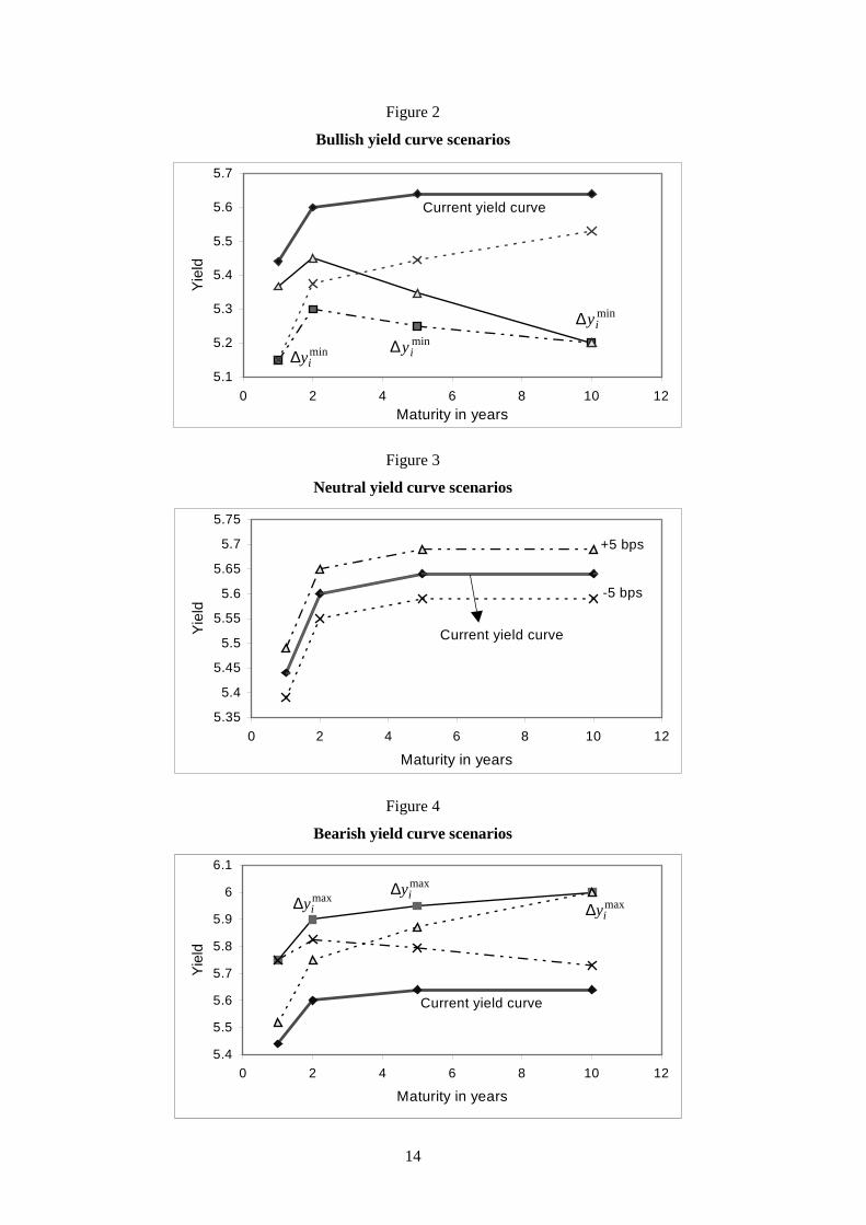
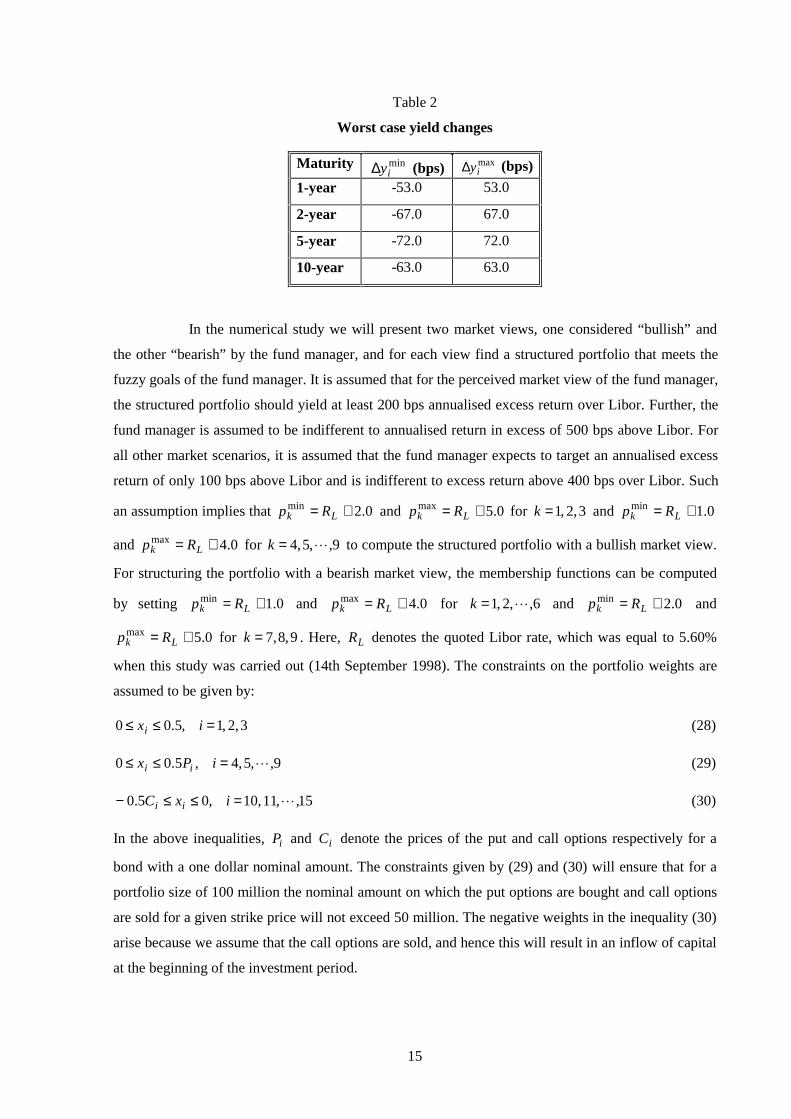
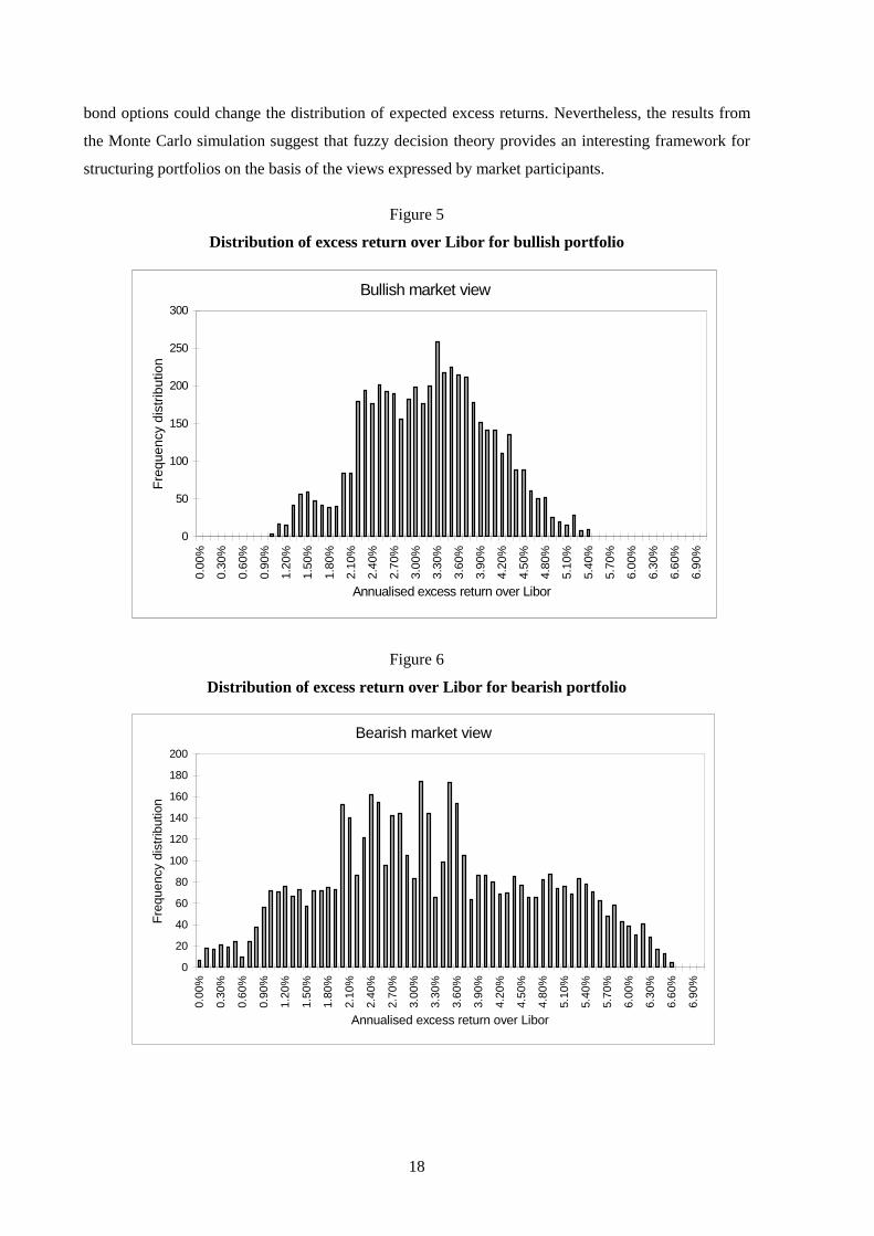
scenarios will be described as “bullish”, “neutral” or “bearish”. For each such scenario, we will

consider three potential par yield curves that describe the scenario; these are shown graphically in

Figures 2-4. For the constraint functions of the optimisation problem given by (25), 3,2,1=k will

denote bullish scenarios, 6,5,4=k will denote neutral scenarios and 9,8,7=k will denote bearish

scenarios. We note here that there are in total M = 9 market scenarios to be considered.

The minimum and maximum yield curve shifts given by miniy∆ and max

iy∆ respectively

in the above figures were computed from constant maturity yields over the previous two years for the

given investment horizon. For instance, assuming that the investment horizon is one month, max2y∆ is

computed from the constant maturity two-year yields using a one-month rolling window and choosing

the worst case absolute yield change over the previous two years. In the numerical study presented

here, the investment horizon of interest was assumed to be one month, and Table 2 shows the values

used for miniy∆ and max

iy∆ in the study.

14

Figure 2

Bullish yield curve scenarios

Figure 3

Neutral yield curve scenarios

Figure 4

Bearish yield curve scenarios

5.4

5.5

5.6

5.7

5.8

5.9

6

6.1

0 2 4 6 8 10 12

Maturity in years

Yie

ld

Current yield curve

maxiy∆

maxiy∆

maxiy∆

5.1

5.2

5.3

5.4

5.5

5.6

5.7

0 2 4 6 8 10 12Maturity in years

Yie

ldCurrent yield curve

miniy∆

miniy∆

miniy∆

5.35

5.4

5.45

5.5

5.55

5.6

5.65

5.7

5.75

0 2 4 6 8 10 12

Maturity in years

Yie

ld

Current yield curve

+5 bps

-5 bps

15

Table 2

Worst case yield changes

Maturity miniy∆ (bps) max

iy∆ (bps)

1-year -53.0 53.0

2-year -67.0 67.0

5-year -72.0 72.0

10-year -63.0 63.0

In the numerical study we will present two market views, one considered “bullish” and

the other “bearish” by the fund manager, and for each view find a structured portfolio that meets the

fuzzy goals of the fund manager. It is assumed that for the perceived market view of the fund manager,

the structured portfolio should yield at least 200 bps annualised excess return over Libor. Further, the

fund manager is assumed to be indifferent to annualised return in excess of 500 bps above Libor. For

all other market scenarios, it is assumed that the fund manager expects to target an annualised excess

return of only 100 bps above Libor and is indifferent to excess return above 400 bps over Libor. Such

an assumption implies that 0.2min += Lk Rp and 0.5max += Lk Rp for 3,2,1=k and 0.1min += Lk Rp

and 0.4max += Lk Rp for 9,,5,4 L=k to compute the structured portfolio with a bullish market view.

For structuring the portfolio with a bearish market view, the membership functions can be computed

by setting 0.1min += Lk Rp and 0.4max += Lk Rp for 6,,2,1 L=k and 0.2min += Lk Rp and

0.5max += Lk Rp for 9,8,7=k . Here, LR denotes the quoted Libor rate, which was equal to 5.60%

when this study was carried out (14th September 1998). The constraints on the portfolio weights are

assumed to be given by:

3,2,1,5.00 =≤≤ ixi (28)

9,,5,4,5.00 L=≤≤ iPx ii (29)

15,,11,10,05.0 L=≤≤− ixC ii (30)

In the above inequalities, iP and iC denote the prices of the put and call options respectively for a

bond with a one dollar nominal amount. The constraints given by (29) and (30) will ensure that for a

portfolio size of 100 million the nominal amount on which the put options are bought and call options

are sold for a given strike price will not exceed 50 million. The negative weights in the inequality (30)

arise because we assume that the call options are sold, and hence this will result in an inflow of capital

at the beginning of the investment period.

16

Using the fuzzy goals of the fund manager given above, it is easy to compute the

membership functions ))(( xRkkµ for each yield curve scenario. The resulting optimisation problem

given by (24)-(27) in Section 3 can then be used to compute the optimal portfolio that meets the goals

of the fund manager. Table 3 gives the details of the bonds in the portfolio including the one-year

T-bill used to construct the par yield curve. Table 4 shows the prices of put and call options maturing

in one month on these bonds. The optimal structured portfolio for a “bullish” market view for a one-

month investment period is given in Table 5. In this table, all figures refer to a nominal amount of

bond holdings where the size of the portfolio is assumed to be 100 million. The amounts shown

against the put and call options refer to the nominal amount on which the put options should be bought

and call options sold respectively. Since the call options are sold, the nominal amounts against call

Table 3

Details of bond and T-bill prices

Instrument Maturity Coupon rate Quoted price

1-year T-bill 19.08.99 – 95.082

2-year note 31.08.00 5.125 100.813

5-year note 15.08.03 5.250 102.625

10-year note 15.05.08 5.625 106.125

Table 4

Details of one-month option prices

Underlying Option type Strike price Option price

2-year note Put 100.813 0.15625

2-year note Put 100.547 0.05468

2-year note Call 100.813 0.26560

2-year note Call 101.313 0.07810

2-year note Put 102.625 0.40625

5-year note Put 101.938 0.13280

5-year note Call 102.625 0.55470

5-year note Call 103.625 0.20310

10-year note Put 106.125 0.67187

10-year note Put 105.000 0.22660

10-year note Call 106.125 1.03125

10-year note Call 107.969 0.37500

17

options are given with a negative sign. Table 6 shows the optimal structured portfolio assuming that

the fund manager has a “bearish” market view.

Table 5

Structured portfolio for bullish market view

Bond issue 2-year 5-year 10-year

Nominal bond holding (mn) 0.28 48.51 46.29

At-the-money put on nominal (mn) 50.0 8.91 50.0

Out-of-money put on nominal (mn) 0.0 6.52 7.61

At-the-money call on nominal (mn) -50.0 -15.60 -50.0

Out-of-money call on nominal (mn) 0.0 0.0 -7.33

Table 6

Structured portfolio for bearish market view

Bond issue 2-year 5-year 10-year

Nominal bond holding (mn) 0.24 48.51 46.29

At-the-money put on nominal (mn) 50.0 29.95 50.0

Out-of-money put on nominal (mn) 0.0 0.0 0.0

At-the-money call on nominal (mn) -50.0 -19.77 -50.0

Out-of-money call on nominal (mn) 0.0 0.0 -5.30

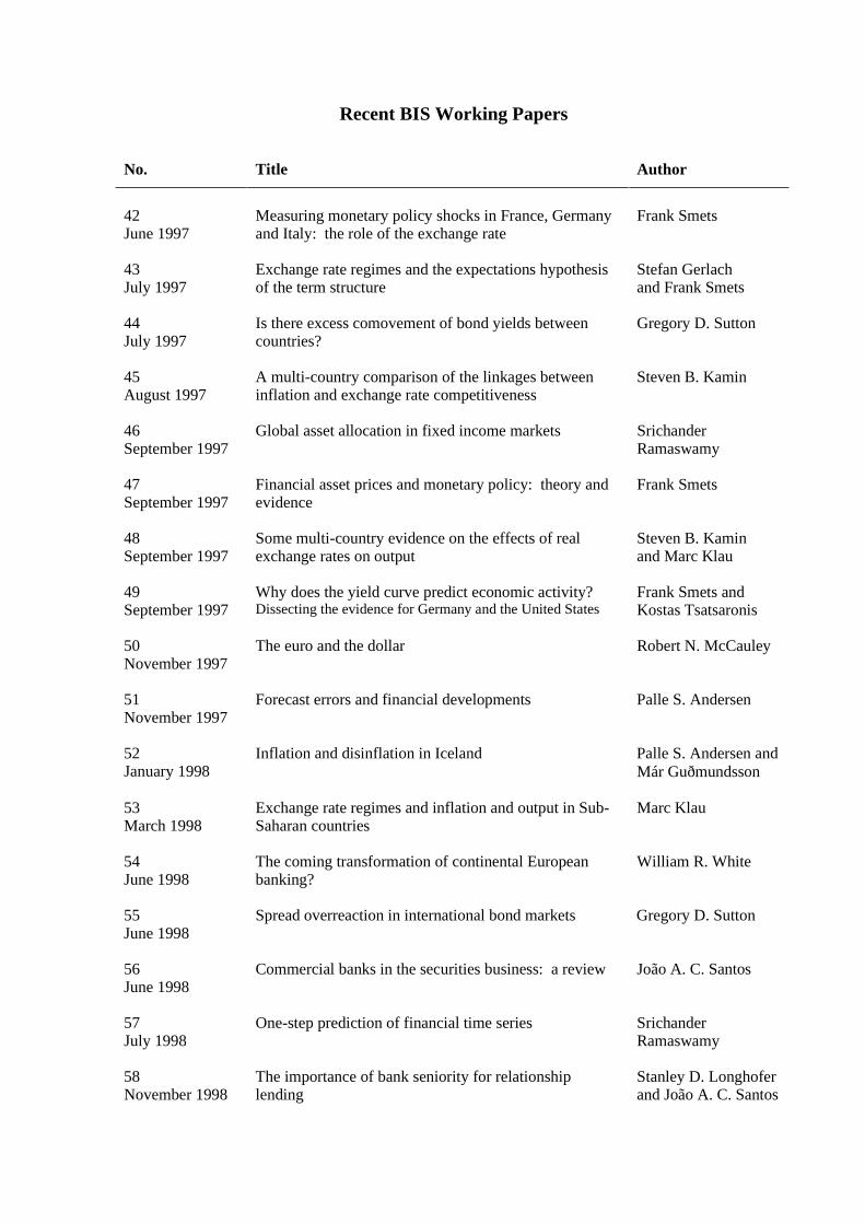
In order to investigate whether the portfolio returns do guarantee the minimum return

targeted by the fund manager, a Monte Carlo simulation was carried out to generate a total of 5,000

yield curve scenarios. The various yield curve scenarios considered were a parallel shift, downward-

sloping and upward-sloping yield curves with respect to the current par yield curve. The distributions

of the annualised excess returns against Libor are shown in Figures 5 and 6 for the structured

portfolios with bullish and bearish market views respectively. It can be inferred from these figures that

although only nine yield curve scenarios were modelled to structure the portfolio, there is practically

no downside risk for the portfolios constructed on the basis of either a bearish or bullish market view

for the scenarios simulated. Using the distribution of excess returns over Libor generated by the Monte

Carlo simulation, the excess return over Libor of the structured portfolio constructed using a bullish

market view is found to lie above 100 bps with a 99.5% confidence level. In the case of the portfolio

structured using the bearish market view, there is a 100 bps excess return over Libor with a 95%

confidence level. However, it is important to stress that the results presented here are based on one

particular yield curve environment. A different yield curve shape, repo rate or implied volatility for the

18

bond options could change the distribution of expected excess returns. Nevertheless, the results from

the Monte Carlo simulation suggest that fuzzy decision theory provides an interesting framework for

structuring portfolios on the basis of the views expressed by market participants.

Figure 5

Distribution of excess return over Libor for bullish portfolio

Figure 6

Distribution of excess return over Libor for bearish portfolio

Bullish market view

0

50

100

150

200

250

300

0.00

%

0.30

%

0.60

%

0.90

%

1.20

%

1.50

%

1.80

%

2.10

%

2.40

%

2.70

%

3.00

%

3.30

%

3.60

%

3.90

%

4.20

%

4.50

%

4.80

%

5.10

%

5.40

%

5.70

%

6.00

%

6.30

%

6.60

%

6.90

%

Annualised excess return over Libor

Fre

quen

cy d

istr

ibut

ion

Bearish market view

0

20

40

60

80

100

120

140

160

180

200

0.00

%

0.30

%

0.60

%

0.90

%

1.20

%

1.50

%

1.80

%

2.10

%

2.40

%

2.70

%

3.00

%

3.30

%

3.60

%

3.90

%

4.20

%

4.50

%

4.80

%

5.10

%

5.40

%

5.70

%

6.00

%

6.30

%

6.60

%

6.90

%

Annualised excess return over Libor

Fre

quen

cy d

istr

ibut

ion

19

Conclusions

In this paper we examined the problem of forming structured portfolios under uncertainty

in order to meet a given target return. It was shown that this could be posed as a fuzzy multi-criteria

optimisation problem. Using concepts from fuzzy decision theory, it was shown how one could

compute a membership function that describes the subjective views of the fund manager under

uncertainty in a quantitative manner. The advantage of the problem formulation presented here is that

it does not entail computing the return distribution of the assets. For purposes of illustration, a linear

membership function was used to compute a structured portfolio that meets the fund manager’s

objectives. It was argued that the membership function can be interpreted as modelling the fuzzy

utility of the investor, and hence the chosen optimal portfolio will maximise the fuzzy utility.

However, it is important to point out that for some choices of the membership function there may be

no solution to the portfolio selection problem. In such instances, one will have to modify the aspiration

levels for the various scenarios to find a satisfactory solution. Structuring portfolios using the

optimisation framework presented in this paper will be useful in the context of asset liability

management where fund managers have specific return targets. In such cases, it is easy to express the

goals in terms of an expected range for the target return for a variety of market scenarios. Moreover,

this methodology could also be potentially useful to proprietary trading groups who can finance

portfolios at Libor to target return in excess of the borrowing costs.

20

References

Bellman, R. and L.A. Zadeh (1970): “Decision-Making in a Fuzzy Environment”, ManagementScience, Vol. 17, pp. 141-64.

J.P. Morgan (1993): “Average Shortfall: A New Approach to Asset Allocation”, J.P. MorganSecurities European Fixed Income Research.

King, A.L. (1993): “Asymmetric Risk Measures and Tracking Models for Portfolio OptimizationUnder Uncertainty”, Annals of Operations Research, Vol. 45, pp. 165-77.

Mathieu-Nicot, B. (1990): “Determination and Interpretation of the Fuzzy Utility of an Act in anUncertain Environment”, in J. Kacprzyk and M. Fedrizzi (eds.) Multiperson DecisionMaking Using Fuzzy Sets and Possibility Theory, Kluwer Academic Publishers, pp. 90-7.

Minsky, H.P. (1975): John Maynard Keynes, Columbia University Press, New York.

Sakawa, M. (1993): Fuzzy Sets and Interactive Multiobjective Optimisation, Plenum Press, London.

Zadeh, L.A. (1965): “Fuzzy Sets”, Information and Control, Vol. 8, pp. 338-53.

Zimmermann, H.J. (1985): Fuzzy Set Theory and Its Applications, Kluwer Academic Publishers,Dordrecht.

Recent BIS Working Papers

No. Title Author

42June 1997

Measuring monetary policy shocks in France, Germanyand Italy: the role of the exchange rate

Frank Smets

43July 1997

Exchange rate regimes and the expectations hypothesisof the term structure

Stefan Gerlachand Frank Smets

44July 1997

Is there excess comovement of bond yields betweencountries?

Gregory D. Sutton

45August 1997

A multi-country comparison of the linkages betweeninflation and exchange rate competitiveness

Steven B. Kamin

46September 1997

Global asset allocation in fixed income markets SrichanderRamaswamy

47September 1997

Financial asset prices and monetary policy: theory andevidence

Frank Smets

48September 1997

Some multi-country evidence on the effects of realexchange rates on output

Steven B. Kaminand Marc Klau

49September 1997

Why does the yield curve predict economic activity?Dissecting the evidence for Germany and the United States

Frank Smets andKostas Tsatsaronis

50November 1997

The euro and the dollar Robert N. McCauley

51November 1997

Forecast errors and financial developments Palle S. Andersen

52January 1998

Inflation and disinflation in Iceland Palle S. Andersen andMár Guðmundsson

53March 1998

Exchange rate regimes and inflation and output in Sub-Saharan countries

Marc Klau

54June 1998

The coming transformation of continental Europeanbanking?

William R. White

55June 1998

Spread overreaction in international bond markets Gregory D. Sutton

56June 1998

Commercial banks in the securities business: a review João A. C. Santos

57July 1998

One-step prediction of financial time series SrichanderRamaswamy

58November 1998

The importance of bank seniority for relationshiplending

Stanley D. Longhoferand João A. C. Santos