the international workshop on agromet and gis applications ... · agromet and gis applications for...
TRANSCRIPT

StatisticalDownscaling Tutorial
Korea MeteorologicalAdministration
The International Workshop onAgromet and GIS Applicationsfor Agricultural Decision Making
Date : December 5(Mon)~9(Fri), 2016 Place : MSTAY Hotel JEJU Hosted by : Korea Meteorological Administration(KMA) Organized by : National Institute of Meteorological Sciences(NIMS) Sponsored by : WMO CAgM / NCAM / APCC / OSGeo / PKNU / DU

2 | Statistical Downscaling Tutorial

2 | Statistical Downscaling Tutorial Statistical Downscaling Tutorial | 3
contents1. The Background and Goals
2. Programs
3. Abstracts
4. Participant List
5. Logistic Information
05
11
21
25
50

4 | Statistical Downscaling Tutorial
4 | Statistical Downscaling Tutorial Statistical Downscaling Tutorial | 5
Introduction to Spatial Data in R

6 | Statistical Downscaling Tutorial
6 | Statistical Downscaling Tutorial Statistical Downscaling Tutorial | 7
Why spatial data in R?
What is R, and why should we pay the price of using it?
How does the community around R work, what are its sharedprinciples?
How does applied spatial data analysis fit into R?
But I have a non-standard research question . . .
Spatial Data in R 2 / 72
Introduction to Spatial Data in R
based on work by Roger S. Bivand, Edzer Pebesma and H. Rue
Spatial Data in R 1 / 72
8 | Statistical Downscaling Tutorial
Applied spatial data analysis with R
R can be used to tackle most of these problems, at least initially...
Packages for importing commonly encountered spatial data formats
Range of contributed packages in spatial statistics and increasingawareness of the importance of spatial data analysis in the broadercommunity
Current contributed packages with spatial statistics applications (seeR spatial projects):
point patterns: spatstat, VR:spatial, splancs;geostatistics: gstat, geoR, geoRglm, fields, spBayes, RandomFields,
VR:spatial, sgeostat, vardiag;lattice/area data: spdep, DCluster, spgwr, ade4.modelling tools: mgcv, INLA, R2WinBUGS, R2BayesX.
Spatial Data in R 4 / 72
Where do we find spatial problems?
Geography How are settlements located according to the presence ofnatural resources, mountains, rivers, etc?
Econometrics Where are flats more expensive in a city?
Ecology How are different species of trees distributed in a forest?
Epidemiology How does the risk of suffering from a particular diseasechange with location? Is high risk linked to the presence ofsome pollution sources?
Environmetrics How can we produce an estimation of the pollution in theair from samples obtanied at a set of stations?
Public Pollicy Where is unemployment higher? What regions shouldbenefit from certain types of pollicies?
Spatial Data in R 3 / 72
8 | Statistical Downscaling Tutorial Statistical Downscaling Tutorial | 9
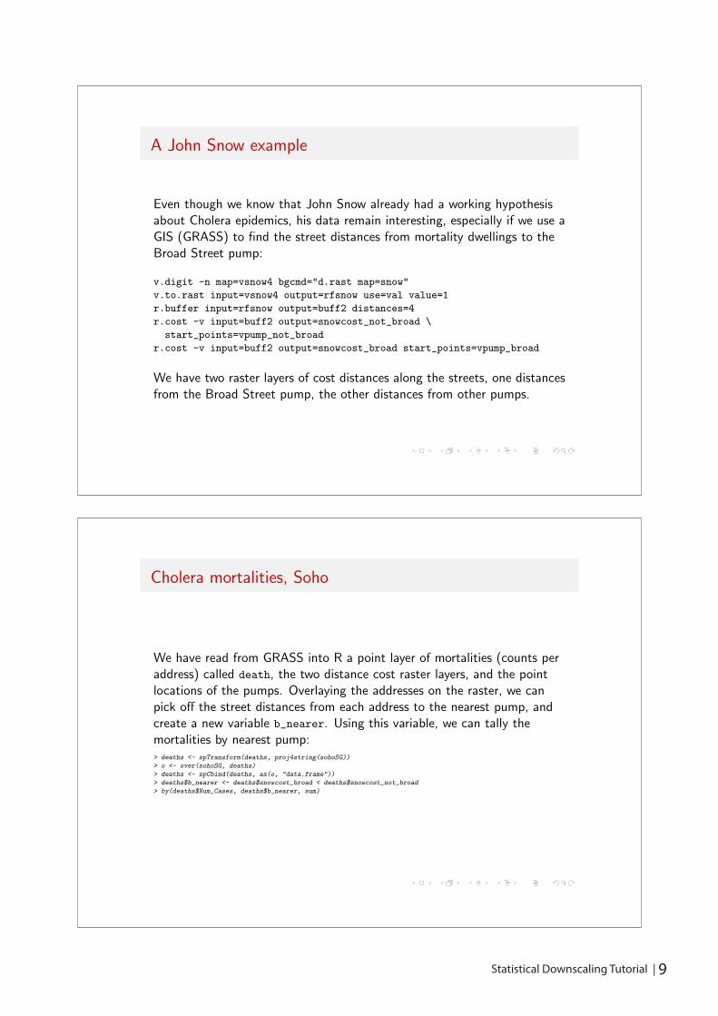
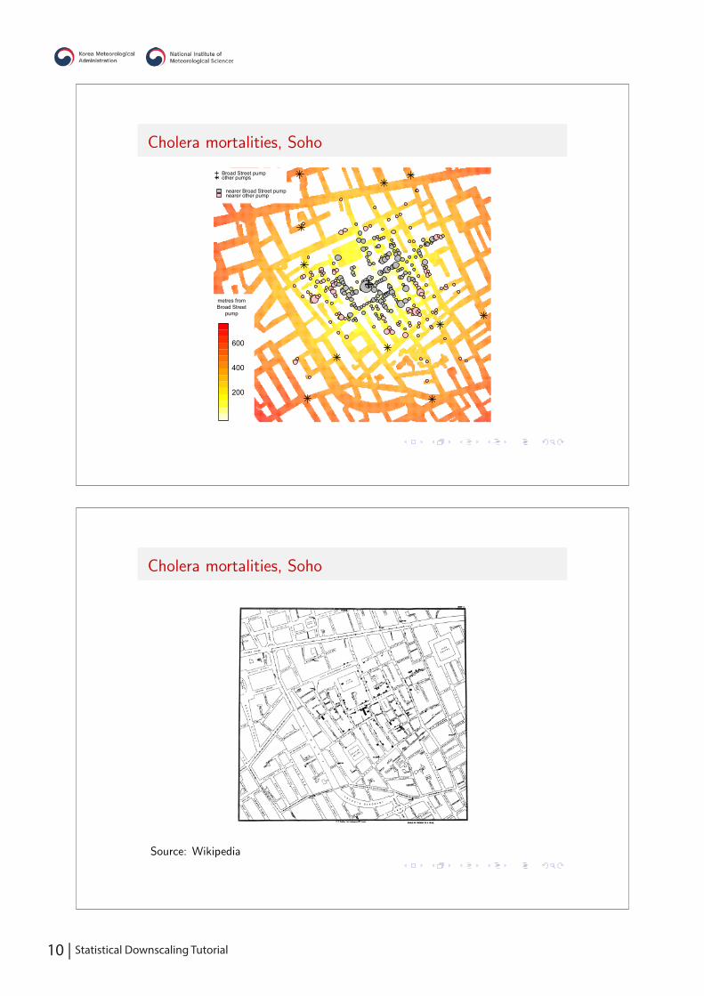
Cholera mortalities, Soho
We have read from GRASS into R a point layer of mortalities (counts peraddress) called death, the two distance cost raster layers, and the pointlocations of the pumps. Overlaying the addresses on the raster, we canpick off the street distances from each address to the nearest pump, andcreate a new variable b_nearer. Using this variable, we can tally themortalities by nearest pump:> deaths <- spTransform(deaths, proj4string(sohoSG))
> o <- over(sohoSG, deaths)
> deaths <- spCbind(deaths, as(o, "data.frame"))
> deaths$b_nearer <- deaths$snowcost_broad < deaths$snowcost_not_broad
> by(deaths$Num_Cases, deaths$b_nearer, sum)
A John Snow example
Even though we know that John Snow already had a working hypothesisabout Cholera epidemics, his data remain interesting, especially if we use aGIS (GRASS) to find the street distances from mortality dwellings to theBroad Street pump:
v.digit -n map=vsnow4 bgcmd="d.rast map=snow"
v.to.rast input=vsnow4 output=rfsnow use=val value=1
r.buffer input=rfsnow output=buff2 distances=4
r.cost -v input=buff2 output=snowcost_not_broad \
start_points=vpump_not_broad
r.cost -v input=buff2 output=snowcost_broad start_points=vpump_broad
We have two raster layers of cost distances along the streets, one distancesfrom the Broad Street pump, the other distances from other pumps.
10 | Statistical Downscaling Tutorial
Cholera mortalities, Soho
Source: Wikipedia
Cholera mortalities, Soho
●
●●
●
●
●
●
●
●
●
●
●
●
●●
●
●●
●●
●●
●
●●●●●
●●
●
●
●
●
●
●●●
●
●
●
●
●
●
●
●
●
●
●
●
●
●●
●
●
●
●
●
●
●
●●
●●
●
●
●
●
●
●
●
●●
●
●
●
●
●
●
●
●
●
●
●
●●
●
●
●
●
●
●
●
●
●
●●
●
●
●
●
●
●
●
●
●
●
●
●
●
●
●●
●
●
●
●●
●
●
●
●
●
●
●
●
●
●
●
●
●
●
●
●
●
●
●
●
●●
●
●
●
●
●
●
●
●
●
●
●
●
●
●
●
●
●
●
●
●
●
●
●
●
●
●
●
●
●
●
●
●
●
●
●
●
●
●
●
●
●
●
●
●
●
●
●
●
●
●●
●
●●
●
●
●
●
●
●
●
●
●
●
●
●
●
●
●
●
●
●
●
●
●
●
●
●
●
●
●
●
●
●
●
●
●
●
●
●
●
●
●
●
●
●
●
●●
●
●
●
●
●
●
●
●
●
●
●
●
●
●
●
●
●
●
●
●
●
●
●
●
●
●
●
●
●
●
●
●
●
●
●
●
●
●
●
●
●
●
●
●●
●
●
●
●
●
●
●
●
●
●
●
●●
●
●
●
●
●
●●
●
●●
●●
●●
●
●●
●
●● ●
●
●●
●
metres fromBroad Street
pump
200
400
600
Broad Street pumpother pumps
nearer Broad Street pumpnearer other pump

10 | Statistical Downscaling Tutorial Statistical Downscaling Tutorial | 11
Workshop framework
Workshop infrastructure
Task views are one of the nice innovations on CRAN that helpnavigate in the jungle of contributed packages — the Spatial taskview is a useful resource
The task view is also a point of entry to the Rgeo website hosted offCRAN, and updated quite often; it tries to mention in more detailcontributed packages for spatial data analysis
It also provides a link to the sp development area on Sourceforge,with CVS access to sp
Finally, it links to the R-sig-geo mailing list, which is the preferedplace to ask questions about analysing spatial/geographical data
Additional resources can be found at web site related to the book byBivand et al. (2013):http://www.asdar-book.org
Spatial Data in R 10 / 72
Workshop framework
Analysing Spatial Data in R
The background for the tutorial is provided in the R News note byRoger Bivand and Edzer Pebesma, November 2005, pp. 9–13 and thebook by Bivand et al. (2013)
First we’ll look at the representation of spatial data in R, with stresson the classes provided in the sp package
After that, we’ll see how to read and write spatial data incommonly-used exchange formats, and how to handle coordinatereference systems
An introduction to spatial analysis using some spatial econometricswill be given and disease mapping models will come next
Then we will see how to work with point data and analyse pointpatterns
We’ll show how analysis packages for geostatistics are being adaptedto use these representations directly
Finally, we will move on to the spatio-temporal case
9 / 72
12 | Statistical Downscaling Tutorial
Introduction
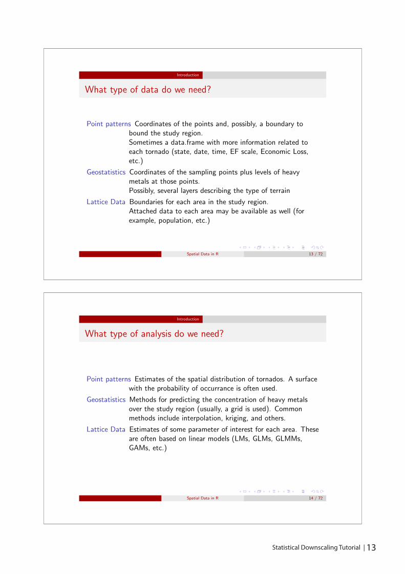
Let’s start with 3 examples...
Point patterns Location of the starting point of tornados in the US in2009. Where do tornados tend to appear more often?
Geostatistics Study of the distribution of heavy metals around the Meuseriver (in the border between Belgium and the Netherlands)
Lattice Data Analysis of the cases of sudden infant death syndrome inNorth Carolina and its possible link to the ethnic distributionof the population
Spatial Data in R 12 / 72
Workshop framework
Analysing Spatial Data in R: Representing Spatial Data
Spatial Data in R 11 / 72
12 | Statistical Downscaling Tutorial Statistical Downscaling Tutorial | 13
Introduction
What type of analysis do we need?
Point patterns Estimates of the spatial distribution of tornados. A surfacewith the probability of occurrance is often used.
Geostatistics Methods for predicting the concentration of heavy metalsover the study region (usually, a grid is used). Commonmethods include interpolation, kriging, and others.
Lattice Data Estimates of some parameter of interest for each area. Theseare often based on linear models (LMs, GLMs, GLMMs,GAMs, etc.)
Spatial Data in R 14 / 72
Introduction
What type of data do we need?
Point patterns Coordinates of the points and, possibly, a boundary tobound the study region.Sometimes a data.frame with more information related toeach tornado (state, date, time, EF scale, Economic Loss,etc.)
Geostatistics Coordinates of the sampling points plus levels of heavymetals at those points.Possibly, several layers describing the type of terrain
Lattice Data Boundaries for each area in the study region.Attached data to each area may be available as well (forexample, population, etc.)
Spatial Data in R 13 / 72
14 | Statistical Downscaling Tutorial
Introduction
Spatial objects
The foundation object is the Spatial class, with just two slots(new-style class objects have pre-defined components called slots)
The first is a bounding box, and is mostly used for setting up plots
The second is a CRS class object defining the coordinate referencesystem, and may be set to CRS(as.character(NA)), its default value.
Operations on Spatial* objects should update or copy these values tothe new Spatial* objects being created
Spatial Data in R 16 / 72
Introduction
Object framework
To begin with, all contributed packages for handling spatial data in Rhad different representations of the data.
This made it difficult to exchange data both within R betweenpackages, and between R and external file formats and applications.
The result has been an attempt to develop shared classes to representspatial data in R, allowing some shared methods and many-to-one,one-to-many conversions.
Bivand and Pebesma chosed to use new-style classes (S4) torepresent spatial data, and are confident that this choice was justified.
Spatial Data in R 15 / 72
14 | Statistical Downscaling Tutorial Statistical Downscaling Tutorial | 15
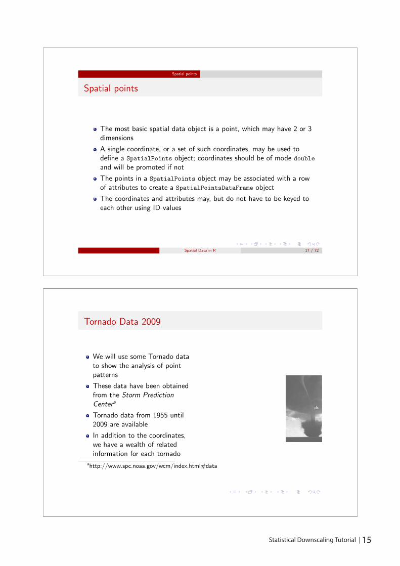
Tornado Data 2009
We will use some Tornado datato show the analysis of pointpatterns
These data have been obtainedfrom the Storm PredictionCentera
Tornado data from 1955 until2009 are available
In addition to the coordinates,we have a wealth of relatedinformation for each tornado
ahttp://www.spc.noaa.gov/wcm/index.html#data
Spatial points
Spatial points
The most basic spatial data object is a point, which may have 2 or 3dimensions
A single coordinate, or a set of such coordinates, may be used todefine a SpatialPoints object; coordinates should be of mode double
and will be promoted if not
The points in a SpatialPoints object may be associated with a rowof attributes to create a SpatialPointsDataFrame object
The coordinates and attributes may, but do not have to be keyed toeach other using ID values
Spatial Data in R 17 / 72
16 | Statistical Downscaling Tutorial
Spatial points
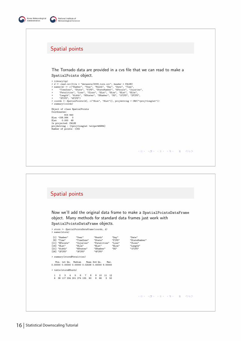
Now we’ll add the original data frame to make a SpatialPointsDataFrame
object. Many methods for standard data frames just work withSpatialPointsDataFrame objects.> storn <- SpatialPointsDataFrame(coords, d)
> names(storn)
[1] "Number" "Year" "Month" "Day" "Date"
[6] "Time" "TimeZone" "State" "FIPS" "StateNumber"
[11] "EFscale" "Injuries" "Fatalities" "Loss" "CLoss"
[16] "SLat" "SLon" "ELat" "ELon" "Length"
[21] "Width" "NStates" "SNumber" "SG" "1FIPS"
[26] "2FIPS" "3FIPS" "4FIPS"
> summary(storn$Fatalities)
Min. 1st Qu. Median Mean 3rd Qu. Max.
0.00000 0.00000 0.00000 0.02538 0.00000 8.00000
> table(storn$Month)
1 2 3 4 5 6 7 8 9 10 11 12
6 38 117 234 201 274 125 60 8 66 3 50
Spatial points
The Tornado data are provided in a cvs file that we can read to make aSpatialPoints object.> library(sp)
> d <- read.csv(file = "datasets/2009_torn.csv", header = FALSE)
> names(d) <- c("Number", "Year", "Month", "Day", "Date", "Time",
+ "TimeZone", "State", "FIPS", "StateNumber", "EFscale", "Injuries",
+ "Fatalities", "Loss", "CLoss", "SLat", "SLon", "ELat", "ELon",
+ "Length", "Width", "NStates", "SNumber", "SG", "1FIPS", "2FIPS",
+ "3FIPS", "4FIPS")
> coords <- SpatialPoints(d[, c("SLon", "SLat")], proj4string = CRS("+proj=longlat"))
> summary(coords)
Object of class SpatialPoints
Coordinates:
min max
SLon -158.064 0
SLat 0.000 49
Is projected: FALSE
proj4string : [+proj=longlat +ellps=WGS84]
Number of points: 1182
16 | Statistical Downscaling Tutorial Statistical Downscaling Tutorial | 17
Spatial polygons
Spatial lines and polygons
A Line object is just a spaghetti collection of 2D coordinates; aPolygon object is a Line object with equal first and last coordinates
A Lines object is a list of Line objects, such as all the contours at asingle elevation; the same relationship holds between a Polygons
object and a list of Polygon objects, such as islands belonging to thesame county
SpatialLines and SpatialPolygons objects are made using lists ofLines or Polygons objects respectively
SpatialLinesDataFrame and SpatialPolygonsDataFrame objects aredefined using SpatialLines and SpatialPolygons objects andstandard data frames, and the ID fields are here required to match thedata frame row names
Spatial Data in R 22 / 72
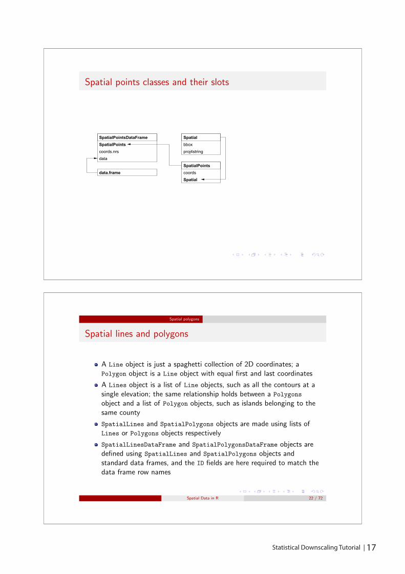
Spatial points classes and their slots
coordsSpatial
coords.nrsdata
SpatialPoints bboxproj4string
SpatialPointsDataFrame
data.frame
Spatial
SpatialPoints
18 | Statistical Downscaling Tutorial
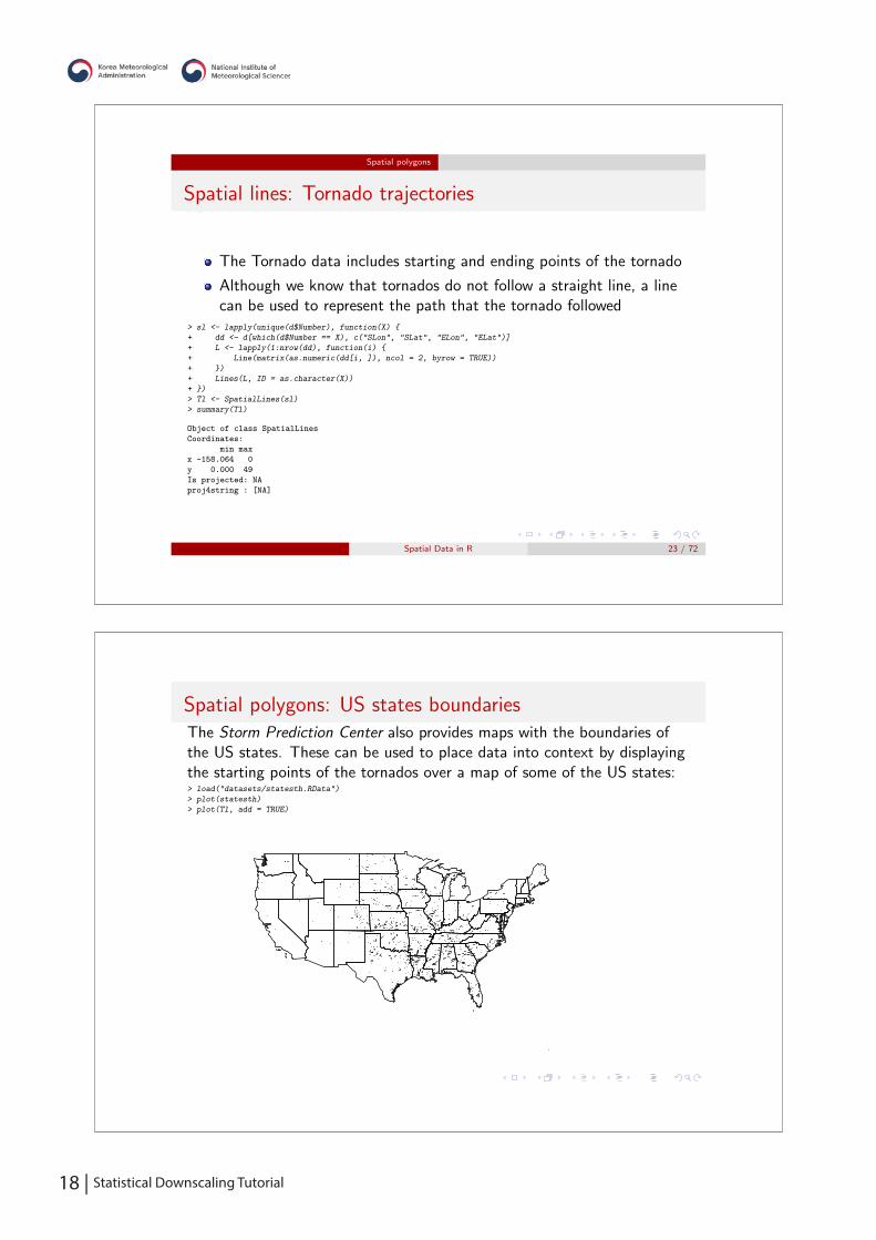
Spatial polygons: US states boundariesThe Storm Prediction Center also provides maps with the boundaries ofthe US states. These can be used to place data into context by displayingthe starting points of the tornados over a map of some of the US states:> load("datasets/statesth.RData")
> plot(statesth)
> plot(Tl, add = TRUE)
Spatial polygons
Spatial lines: Tornado trajectories
The Tornado data includes starting and ending points of the tornado
Although we know that tornados do not follow a straight line, a linecan be used to represent the path that the tornado followed
> sl <- lapply(unique(d$Number), function(X) {
+ dd <- d[which(d$Number == X), c("SLon", "SLat", "ELon", "ELat")]
+ L <- lapply(1:nrow(dd), function(i) {
+ Line(matrix(as.numeric(dd[i, ]), ncol = 2, byrow = TRUE))
+ })
+ Lines(L, ID = as.character(X))
+ })
> Tl <- SpatialLines(sl)
> summary(Tl)
Object of class SpatialLines
Coordinates:
min max
x -158.064 0
y 0.000 49
Is projected: NA
proj4string : [NA]
Spatial Data in R 23 / 72
18 | Statistical Downscaling Tutorial Statistical Downscaling Tutorial | 19
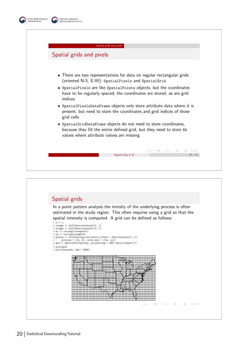
Spatial Polygons classes and slots
coordsSpatiallines
plotOrderSpatial
polygons
bboxproj4string
LineLines
ID
Polygons
plotOrderlabptIDarea
SpatialLines
Spatial
Lines
Polygons
Polygon
coords
labptareaholeringDir
SpatialPolygons
Spatial lines
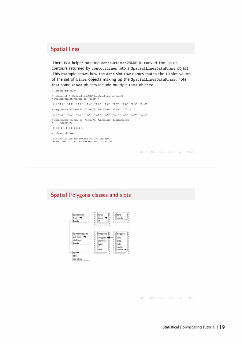
There is a helper function contourLines2SLDF to convert the list ofcontours returned by contourLines into a SpatialLinesDataFrame object.This example shows how the data slot row names match the ID slot valuesof the set of Lines objects making up the SpatialLinesDataFrame, notethat some Lines objects include multiple Line objects:> library(maptools)
> volcano_sl <- ContourLines2SLDF(contourLines(volcano))
> row.names(slot(volcano_sl, "data"))
[1] "C_1" "C_2" "C_3" "C_4" "C_5" "C_6" "C_7" "C_8" "C_9" "C_10"
> sapply(slot(volcano_sl, "lines"), function(x) slot(x, "ID"))
[1] "C_1" "C_2" "C_3" "C_4" "C_5" "C_6" "C_7" "C_8" "C_9" "C_10"
> sapply(slot(volcano_sl, "lines"), function(x) length(slot(x,
+ "Lines")))
[1] 3 4 1 1 1 2 2 3 2 1
> volcano_sl$level
[1] 100 110 120 130 140 150 160 170 180 190
Levels: 100 110 120 130 140 150 160 170 180 190
20 | Statistical Downscaling Tutorial
Spatial gridsIn a point pattern analysis the intnsity of the underlying process is oftenestimated in the study region. This often requires using a grid so that thespatial intensity is computed. A grid can be defined as follows:> h <- 1
> xrange <- diff(bbox(statesth)[1, ])
> yrange <- diff(bbox(statesth)[2, ])
> nx <- ceiling((xrange/h))
> ny <- ceiling(yrange/h)
> grdtop <- GridTopology(cellcentre.offset = bbox(statesth)[, 1],
+ cellsize = c(h, h), cells.dim = c(nx, ny))
> grd <- SpatialGrid(grdtop, proj4string = CRS("+proj=longlat"))
> plot(grd)
> plot(statesth, add = TRUE)
Spatial grids and pixels
Spatial grids and pixels
There are two representations for data on regular rectangular grids(oriented N-S, E-W): SpatialPixels and SpatialGrid
SpatialPixels are like SpatialPoints objects, but the coordinateshave to be regularly spaced; the coordinates are stored, as are gridindices
SpatialPixelsDataFrame objects only store attribute data where it ispresent, but need to store the coordinates and grid indices of thosegrid cells
SpatialGridDataFrame objects do not need to store coordinates,because they fill the entire defined grid, but they need to store NA
values where attribute values are missing
Spatial Data in R 27 / 72
20 | Statistical Downscaling Tutorial Statistical Downscaling Tutorial | 21
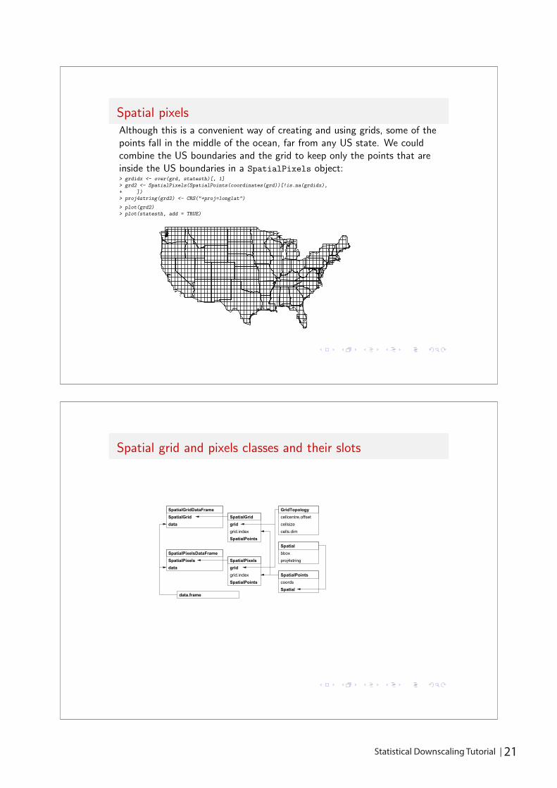
Spatial grid and pixels classes and their slots
SpatialPixelsDataFrame
dataSpatialPixels
SpatialGriddata grid
grid.indexSpatialPoints
gridgrid.indexSpatialPoints
cellcentre.offsetcellsizecells.dim
coordsSpatial
bboxproj4string
data.frame
Spatial
GridTopology
SpatialPoints
SpatialGridDataFrameSpatialGrid
SpatialPixels
Spatial pixelsAlthough this is a convenient way of creating and using grids, some of thepoints fall in the middle of the ocean, far from any US state. We couldcombine the US boundaries and the grid to keep only the points that areinside the US boundaries in a SpatialPixels object:> grdidx <- over(grd, statesth)[, 1]
> grd2 <- SpatialPixels(SpatialPoints(coordinates(grd))[!is.na(grdidx),
+ ])
> proj4string(grd2) <- CRS("+proj=longlat")
> plot(grd2)
> plot(statesth, add = TRUE)
22 | Statistical Downscaling Tutorial
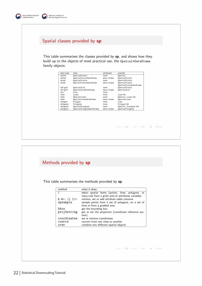
Methods provided by sp
This table summarises the methods provided by sp:
method what it does[ select spatial items (points, lines, polygons, or
rows/cols from a grid) and/or attributes variables$, $<-, [[, [[<- retrieve, set or add attribute table columnsspsample sample points from a set of polygons, on a set of
lines or from a gridded areabbox get the bounding boxproj4string get or set the projection (coordinate reference sys-
tem)coordinates set or retrieve coordinatescoerce convert from one class to anotherover combine two different spatial objects
Spatial classes provided by sp
This table summarises the classes provided by sp, and shows how theybuild up to the objects of most practical use, the Spatial*DataFrame
family objects:
data type class attributes extendspoints SpatialPoints none Spatial
points SpatialPointsDataFrame data.frame SpatialPoints
pixels SpatialPixels none SpatialPoints
pixels SpatialPixelsDataFrame data.frame SpatialPixels
SpatialPointsDataFrame
full grid SpatialGrid none SpatialPixels
full grid SpatialGridDataFrame data.frame SpatialGrid
line Line nonelines Lines none Line listlines SpatialLines none Spatial, Lines listlines SpatialLinesDataFrame data.frame SpatialLines
polygon Polygon none Line
polygons Polygons none Polygon listpolygons SpatialPolygons none Spatial, Polygons listpolygons SpatialPolygonsDataFrame data.frame SpatialPolygons

22 | Statistical Downscaling Tutorial Statistical Downscaling Tutorial | 23
Spatial grids and pixels
Using Spatial family objects
Very often, the user never has to manipulate Spatial family objectsdirectly, as we have been doing here, because methods to create themfrom external data are also provided
Because the Spatial*DataFrame family objects behave in most caseslike data frames, most of what we are used to doing with standarddata frames just works — like "[" or $ (but no merge, etc., yet)
These objects are very similar to typical representations of the samekinds of objects in geographical information systems, so they do notsuit spatial data that is not geographical (like medical imaging) assuch
They provide a standard base for analysis packages on the one hand,and import and export of data on the other, as well as sharedmethods, like those for visualisation we turn to now
Spatial Data in R 34 / 72
Spatial grids and pixels
Overlying tornados and US states
The Tornado data comprises tornados occurred in Puerto Rico, Alaska andother regions or states. In order to select only those tornados found in themain continental region of the US, we can do an overlay:> sidx <- over(storn, statesth)[, 1]
> storn2 <- storn[!is.na(sidx), ]
> plot(storn2)
> plot(statesth, add = TRUE)
Spatial Data in R 33 / 72
24 | Statistical Downscaling Tutorial
Introduction
Vizualising Spatial Data
Displaying spatial data is one of the chief reasons for providing waysof handling it in a statistical environment
Of course, there will be differences between analytical andpresentation graphics here as well — the main point is to get a usabledisplay quickly, and move to presentation quality cartography later
In general, maintaining aspect is vital, and that can be done in bothbase and lattice graphics in R (note that both sp and maps displaymethods for spatial data with geographical coordinates“stretch” they-axis)
We’ll look at the basic methods for displaying spatial data in sp;other packages have their own methods, but the next unit will showways of moving data from them to sp classes
Spatial Data in R 36 / 72
Spatial grids and pixels
Analysing Spatial Data in R: Vizualising Spatial Data
Spatial Data in R 35 / 72

24 | Statistical Downscaling Tutorial Statistical Downscaling Tutorial | 25
Plotting a SpatialPoints object
120°W 110°W 100°W 90°W 80°W 70°W
20°N
30°N
40°N
50°N
While plotting the SpatialPointsobject would have called the plotmethod for Spatial objects internallyto set up the axes, we start by doingit separately:> library(sp)
> plot(as(storn2, "Spatial"), axes = TRUE)
> plot(storn2, add = TRUE)
> plot(storn2[storn2$EFscale == 4, ], col = "red",
+ add = TRUE)
Then we plot the points with thedefault plotting character, andsubset, overplotting points with EFscale of 4 in red, using the [ method
Just spatial objects
Just spatial objects
There are base graphics plot methods for the key Spatial* classes,including the Spatial class, which just sets up the axes
In base graphics, additional plots can be added by overplotting asusual, and the locator() and identify() functions work as expected
In general, most par() options will also work, as will the full range ofgraphics devices (although some copying operations may disturbaspect)
First we will display the positional data of the objects discussed in thefirst unit
Spatial Data in R 37 / 72

26 | Statistical Downscaling Tutorial
Plotting a SpatialPixels object
102°W 100°W 98°W 96°W 94°W
36°N
37°N
38°N
39°N
40°N
41°N
Both SpatialPixels and SpatialGridobjects are plotted like SpatialPointsobjects, with plotting characters> library(sp)
> kansas <- statesth[statesth$NAME ==
+ "Kansas", ]
> plot(statesth, axes = TRUE, xlim = c(-103,
+ -94), ylim = c(36, 41))
> plot(statesth[statesth$NAME == "Kansas",
+ ], col = "azure2", add = TRUE)
> box()
> plot(grd2, add = TRUE)
While points, lines, and polygons areoften plotted without attributes, thisis rarely the case for gridded objects
Plotting a SpatialPolygons object
102°W 100°W 98°W 96°W 94°W
36°N
37°N
38°N
39°N
40°N
41°N
In plotting the SpatialPolygonsobject, we use the xlim= and ylim=arguments to restrict the display areato match the soil sample points.> library(sp)
> kansas <- statesth[statesth$NAME ==
+ "Kansas", ]
> plot(statesth, axes = TRUE, xlim = c(-103,
+ -94), ylim = c(36, 41))
> plot(statesth[statesth$NAME == "Kansas",
+ ], col = "azure2", add = TRUE)
> box()
If the axes= argument is FALSE oromitted, no axes are shown — thedefault is the opposite from standardbase graphics plot methods

26 | Statistical Downscaling Tutorial Statistical Downscaling Tutorial | 27
Points of the grid inside kansas
●●●●●●●●●●●●●●●●●●●●●●●●●●●●●●●●●●●●●●●●●●●●●●●●●●●●●●●●●●●●●●●●●●●●●●●●●●●●●●●●●●●●●●●●●●●●●●● ● ●●●●●●●●●●●●●●●●●●●●●●●●●●●●●●●●●●●●●●● ●● ●●●●●●●●●●●●●●●●●●●●●●●●●●●●●●●●●●●●●●● ●●● ●●●●●●●●●●●●●●●●●●●●●●●●●●●●●●●●●●●●●●●●●●●●● ●● ●●●●●●●●●●●●●●●●●●●●●●●●●●●●●●●●●●●●●●●●●●● ●●●● ●●●●●●●●●●●●●●●●●●●●●●●●●●●●●●●●●●●●●●●●●●●●● ●●● ●●●●●●●●●●●●●●●●●●●●●●●●●●●●●●●●●●●●●●●●●●●●●●●●●●●●●●●●●●●●●●●●●●●●●●●●●●●●●●●●●●●●●●●●●●●●●●●●●●●●●●●●●●●●●●●●●●●●●●●●●●●●●●●●●●●●●●●●●●●●●●●●●●●●●●●●●●●●●●●●●●●●●●●●●●●●●●●●●●●●●●●●●●●●●●●●●●●●●●●●●●●●●●●●●●●●●●●●●●●●●●●●●●●●●●●●●●●●●●●●●●●●●●●●●●●●●●●●●●●●●●●●●●●●●●●●●●●●●●●●●●●●●●●●●●●●●●●●●●●●●●●●●●●●●●●●●●●●●●●●●●●●●●●●●●●●●●●●●●●●
●●●●●●●●●●●●●●●●●●●●●●●●●●●●●●●●●●●●●●●●●●●●●●●●●●●●●●●●●●●●●●●●●●●●●●●●●●●●●●
●●●●●●●●●●●●●●●●●●●●●●●●●●●●●●●●●●●●●●●●●●●●●●●●●●●●●●●●●●●●●●●●●●●●●● ●●●●
●●●●● ●●●● ●●●●● ●
●
●
●
OFF KANSASIN KANSAS
We will usually need to get thecategory levels and match them tocolours (or plotting characters) “byhand”> kidx <- over(grd2, kansas)[, 1]
> grd2df <- SpatialPointsDataFrame(grd2,
+ data.frame(KANSAS = as.factor(!is.na(kidx))))
> plot(grd2df, col = grd2df$KANSAS,
+ pch = 19)
> labs <- c("OFF KANSAS", "IN KANSAS")
> cols <- 1:2
> legend("topleft", legend = labs, col = cols,
+ pch = 19, bty = "n")
It is also typical that the legend()involves more code than everythingelse together, but very often thesame vectors are used repeatedly andcan be assigned just once
Including attributes
Including attributes
To include attribute values means making choices about how torepresent their values graphically, known in some GIS as symbology
It involves choices of symbol shape, colour and size, and of whichobjects to differentiate
When the data are categorical, the choices are given, unless there areso many different categories that reclassification is needed for cleardisplay
Once we’ve looked at some examples, we’ll go on to see how classintervals may be chosen for continuous data
Spatial Data in R 41 / 72
28 | Statistical Downscaling Tutorial
Including attributes Class intervals
Class intervals
Class intervals can be chosen in many ways, and some have beencollected for convenience in the classInt package
The first problem is to assign class boundaries to values in a singledimension, for which many classification techniques may be used,including pretty, quantile, natural breaks among others, or even simplefixed values
From there, the intervals can be used to generate colours from acolour palette, using the very nice colorRampPalette() function
Because there are potentially many alternative class membershipseven for a given number of classes (by default from nclass.Sturges),choosing a communicative set matters
Spatial Data in R 44 / 72
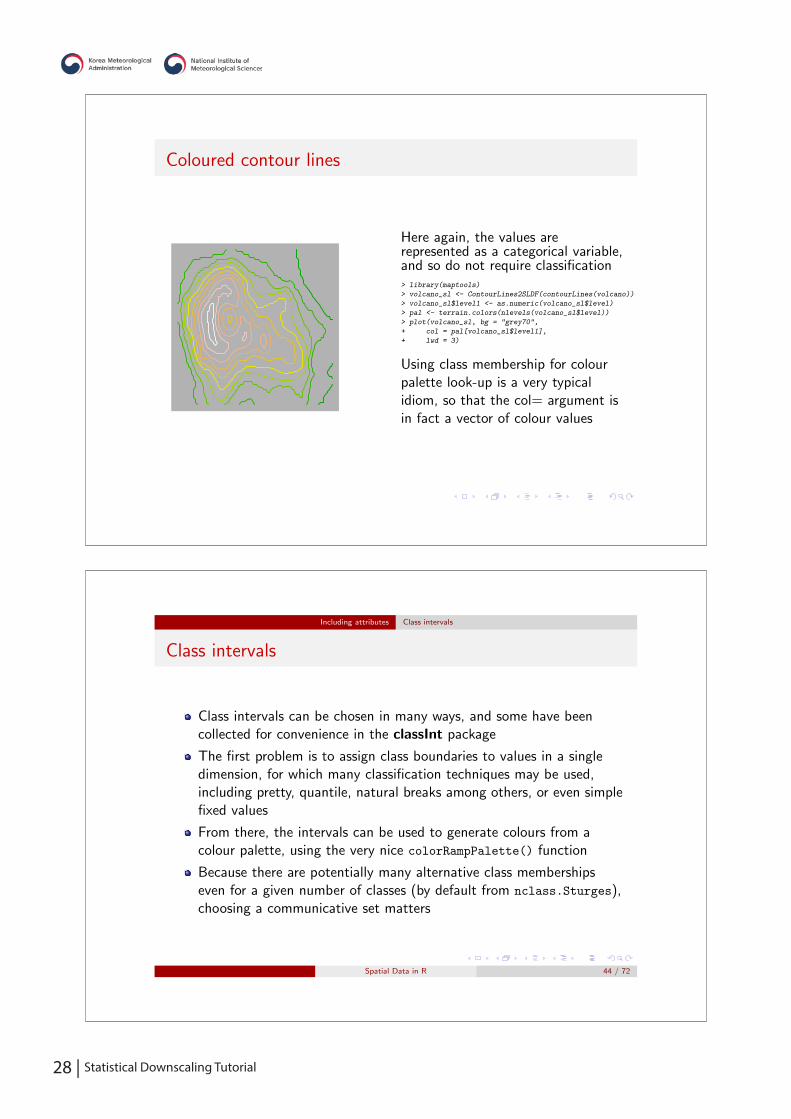
Coloured contour lines
Here again, the values arerepresented as a categorical variable,and so do not require classification> library(maptools)
> volcano_sl <- ContourLines2SLDF(contourLines(volcano))
> volcano_sl$level1 <- as.numeric(volcano_sl$level)
> pal <- terrain.colors(nlevels(volcano_sl$level))
> plot(volcano_sl, bg = "grey70",
+ col = pal[volcano_sl$level1],
+ lwd = 3)
Using class membership for colourpalette look-up is a very typicalidiom, so that the col= argument isin fact a vector of colour values
28 | Statistical Downscaling Tutorial Statistical Downscaling Tutorial | 29
Class interval plots
−10 −5 0 5
0.0
0.2
0.4
0.6
0.8
1.0
Quantile
●● ●●●
●●●●
●●●●●●●●●●●●●●●●●●●
●●●●●●●●●●●●●●●●
●●●●●●●●●●●●●●●●●●●●●●●●●●●●●●●
●●●●●●●●●●●●●●●●●●●●●●●●
●●●●●●●●●●●●●●●● ●●●● ● ●●
−10 −5 0 5
0.0
0.2
0.4
0.6
0.8
1.0
Fisher−Jenks natural breaks
●● ●●●
●●●●
●●●●●●●●●●●●●●●●●●●
●●●●●●●●●●●●●●●●
●●●●●●●●●●●●●●●●●●●●●●●●●●●●●●●
●●●●●●●●●●●●●●●●●●●●●●●●
●●●●●●●●●●●●●●●● ●●●● ● ●●
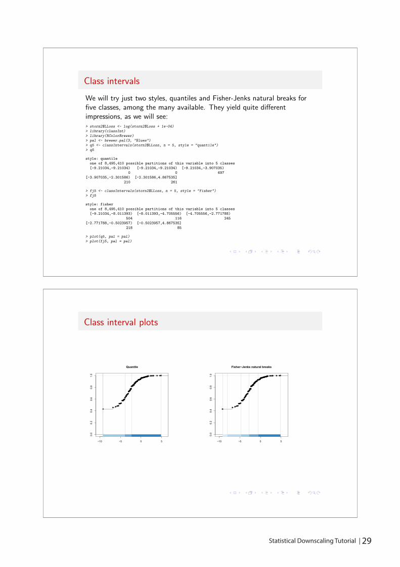
Class intervals
We will try just two styles, quantiles and Fisher-Jenks natural breaks forfive classes, among the many available. They yield quite differentimpressions, as we will see:> storn2$LLoss <- log(storn2$Loss + 1e-04)
> library(classInt)
> library(RColorBrewer)
> pal <- brewer.pal(3, "Blues")
> q5 <- classIntervals(storn2$LLoss, n = 5, style = "quantile")
> q5
style: quantile
one of 8,495,410 possible partitions of this variable into 5 classes
[-9.21034,-9.21034) [-9.21034,-9.21034) [-9.21034,-3.907035)
0 0 697
[-3.907035,-2.301586) [-2.301586,4.867535]
210 261
> fj5 <- classIntervals(storn2$LLoss, n = 5, style = "fisher")
> fj5
style: fisher
one of 8,495,410 possible partitions of this variable into 5 classes
[-9.21034,-8.011393) [-8.011393,-4.705556) [-4.705556,-2.771788)
504 116 245
[-2.771788,-0.5023957) [-0.5023957,4.867535]
218 85
> plot(q5, pal = pal)
> plot(fj5, pal = pal)
30 | Statistical Downscaling Tutorial
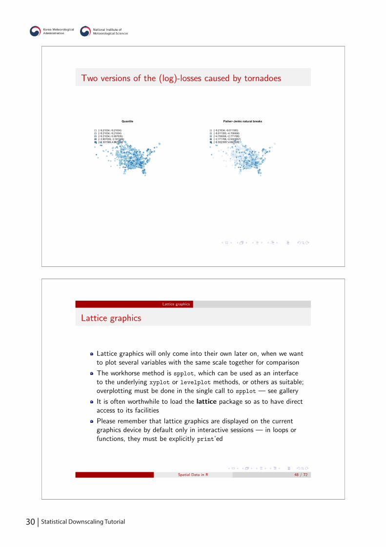
Lattice graphics
Lattice graphics
Lattice graphics will only come into their own later on, when we wantto plot several variables with the same scale together for comparison
The workhorse method is spplot, which can be used as an interfaceto the underlying xyplot or levelplot methods, or others as suitable;overplotting must be done in the single call to spplot — see gallery
It is often worthwhile to load the lattice package so as to have directaccess to its facilities
Please remember that lattice graphics are displayed on the currentgraphics device by default only in interactive sessions — in loops orfunctions, they must be explicitly print’ed
Spatial Data in R 48 / 72
Two versions of the (log)-losses caused by tornadoes
●
●
●●●
●
●
●●●●●
●●●●●
●
● ●
●
●
●
●●●●●●● ●●● ●
●●●
●●● ●●●
●●●●●●●●
●●●●●●●
●●●●●●●●●
●
●●●
●●
●
●
● ●
●●
●
● ●●●
●●●●●
●●●●
●
●●●●●
●
● ●● ●●●●
●●●
●●
●
●
●
●●
●●
●●●● ●●
●●
●
●
●
●●
●
●●●●
●● ● ●
●
●
●●
●●●
●●● ●●
●
●
●
●●●
●
●●●●●
●●●
●
●
●●●●
●
●●●
●
●
●
●
●
●●●●●●
●●●●●●
●
●●●●
●●●●●●●●●●
●
●●●●●●●
●●●●●
●
●
●
●●
●●●●●●●●●●●
●
●●
●
●●●
●●●●●●●
●●
●●●●●●
●●●
●●
●●
●●●●●
●
●
●
●●●●
●
●● ●
●●●●●●
●
●
●●
●●●●●●
●●
●
●●●●●
●●
●
●●
●
●
●●●
●
●●●
●●
●
●
●●●●
●●●
●
●
●●●
●
●●●●●●
●●
●
●
●
●
●
●
●●
●●
●●
●
●●●●●●●
●●●●●
●
●●●●●●●●
●●●●●
●●
●●●●●
●●●
●●●●●●
● ● ●●●●●
●
●●●●●●●●●●
●●●●●●
●●
●●
●
●●
●●
●
●●●●●●●●
●●●● ●●●
●●●
●●
●●●●●●
●●
●
●
●●●
●
●●●●●●●●●●●●●●●●●●●●●●●●●●●
●
●●
●
●●
●
●●●●●●●
●
●●●●●
●●
●
●●
●
●●
●
●
●
●
●●
●●●
●●
●
●
●
●
●
●●●●●
●
●
●
●●
●
●
●
●
●
●
●●●
●●●
●●
●
●
●●
●● ●
●
●
●
●
●
●
●●
●
●
●
●●
●
●●●
●●●
●
●
●●
●
●●
● ●
●●
●
●
●
●
●
●
●●
●
●
●●●
●
●●
●
●
●●●●
●●
●
●
●●●●
●●
●●●
●
●●●●●
●●
●●
●●
●●●
●
●
●
●
●●
●●●●
●●
●●●
●●●●●●
●●
● ●●
●●
●
●●
●●●
●
●●●●
●
●
●
●
●
●
●
●
● ●●● ● ●
●●●●
●
●●●●●●●
●
●●●●●●●●● ●●
●●
●
●●●
●
●
●
●●●●
●
●
●●
●
●
●
●●
●
●●
●●
●
●
●●●
●●
●●●●
●
●
●
●●
●●
●
●
●●●
●● ●
●●
● ●●●
●●
●●
●●● ●● ●●●●
●●
● ●●
●●●●●●●
●●●●
●●
●
●
●●
●●
●
●●
●●
●●●●●●●●
●
●
●
●
● ●●●●●
●●
●●
●●
●●●●●
●●
●
●
●
●
●
●●●
●
●
●
●●
●
●
●
●
●●
●●
●
●●●●
●●
●
●
●
●
●
●●
●●
●
●●●
●
●
●
●●●
●
●
●
●
●
●
●●●●
●
●
●●
●●●
●●
●
●
●
●●
●●
●●●
● ●
●
●●
●
●
●
●●
●●●●●●
●
●
●
●
● ●●
●●●●●●
●
●●●●●
●●
●
●●●●
●●
●●●●
●
●●
●
●
●●
●
●
●●
●●
●
●
●
●
●
●
●
●
●
●
●
●
●●
●
●●●
●
●●
●
●●
●
●
●
●
●
●
●
●
●
●●
●●
●
●
●
●
●
●
●
●
●
●
●
●
●
●
●
●
●
●
●
●
●●●
●●●●
●
●●●●●
● ●
●
●
●●●●
●
●●
●
●●
●
●●●●
●
●●●●
●●●
●●
●●
●●
●●●
●
●●
●●●●●
●●● ●
●
●
●
●●●
●●●●
●●●●
●
●
●
●
●●●●●●
●●●●●●●●●●●●●●●●●●●●●●●●●
●
●
Quantile
[−9.21034,−9.21034)[−9.21034,−9.21034)[−9.21034,−3.907035)[−3.907035,−2.301586)[−2.301586,4.867535]
●
●
●●●
●
●
●●●●●
●●●●●
●
● ●
●
●
●
●●●●●●● ●●● ●
●●●
●●● ●●●
●●●●●●●●
●●●●●●●
●●●●●●●●●
●
●●●
●●
●
●
● ●
●●
●
● ●●●
●●●●●
●●●●
●
●●●●●
●
● ●● ●●●●
●●●
●●
●
●
●
●●
●●
●●●● ●●
●●
●
●
●
●●
●
●●●●
●● ● ●
●
●
●●
●●●
●●● ●●
●
●
●
●●●
●
●●●●●
●●●
●
●
●●●●
●
●●●
●
●
●
●
●
●●●●●●
●●●●●●
●
●●●●
●●●●●●●●●●
●
●●●●●●●
●●●●●
●
●
●
●●
●●●●●●●●●●●
●
●●
●
●●●
●●●●●●●
●●
●●●●●●
●●●
●●
●●
●●●●●
●
●
●
●●●●
●
●● ●
●●●●●●
●
●
●●
●●●●●●
●●
●
●●●●●
●●
●
●●
●
●
●●●
●
●●●
●●
●
●
●●●●
●●●
●
●
●●●
●
●●●●●●
●●
●
●
●
●
●
●
●●
●●
●●
●
●●●●●●●
●●●●●
●
●●●●●●●●
●●●●●
●●
●●●●●
●●●
●●●●●●
● ● ●●●●●
●
●●●●●●●●●●
●●●●●●
●●
●●
●
●●
●●
●
●●●●●●●●
●●●● ●●●
●●●
●●
●●●●●●
●●
●
●
●●●
●
●●●●●●●●●●●●●●●●●●●●●●●●●●●
●
●●
●
●●
●
●●●●●●●
●
●●●●●
●●
●
●●
●
●●
●
●
●
●
●●
●●●
●●
●
●
●
●
●
●●●●●
●
●
●
●●
●
●
●
●
●
●
●●●
●●●
●●
●
●
●●
●● ●
●
●
●
●
●
●
●●
●
●
●
●●
●
●●●
●●●
●
●
●●
●
●●
● ●
●●
●
●
●
●
●
●
●●
●
●
●●●
●
●●
●
●
●●●●
●●
●
●
●●●●
●●
●●●
●
●●●●●
●●
●●
●●
●●●
●
●
●
●
●●
●●●●
●●
●●●
●●●●●●
●●
● ●●
●●
●
●●
●●●
●
●●●●
●
●
●
●
●
●
●
●
● ●●● ● ●
●●●●
●
●●●●●●●
●
●●●●●●●●● ●●
●●
●
●●●
●
●
●
●●●●
●
●
●●
●
●
●
●●
●
●●
●●
●
●
●●●
●●
●●●●
●
●
●
●●
●●
●
●
●●●
●● ●
●●
● ●●●
●●
●●
●●● ●● ●●●●
●●
● ●●
●●●●●●●
●●●●
●●
●
●
●●
●●
●
●●
●●
●●●●●●●●
●
●
●
●
● ●●●●●
●●
●●
●●
●●●●●
●●
●
●
●
●
●
●●●
●
●
●
●●
●
●
●
●
●●
●●
●
●●●●
●●
●
●
●
●
●
●●
●●
●
●●●
●
●
●
●●●
●
●
●
●
●
●
●●●●
●
●
●●
●●●
●●
●
●
●
●●
●●
●●●
● ●
●
●●
●
●
●
●●
●●●●●●
●
●
●
●
● ●●
●●●●●●
●
●●●●●
●●
●
●●●●
●●
●●●●
●
●●
●
●
●●
●
●
●●
●●
●
●
●
●
●
●
●
●
●
●
●
●
●●
●
●●●
●
●●
●
●●
●
●
●
●
●
●
●
●
●
●●
●●
●
●
●
●
●
●
●
●
●
●
●
●
●
●
●
●
●
●
●
●
●●●
●●●●
●
●●●●●
● ●
●
●
●●●●
●
●●
●
●●
●
●●●●
●
●●●●
●●●
●●
●●
●●
●●●
●
●●
●●●●●
●●● ●
●
●
●
●●●
●●●●
●●●●
●
●
●
●
●●●●●●
●●●●●●●●●●●●●●●●●●●●●●●●●
●
●
Fisher−Jenks natural breaks
[−9.21034,−8.011393)[−8.011393,−4.705556)[−4.705556,−2.771788)[−2.771788,−0.5023957)[−0.5023957,4.867535]
30 | Statistical Downscaling Tutorial Statistical Downscaling Tutorial | 31
Level plots
●
●
●●●
●
●
●●●●●
●●●●●
●
● ●
●
●
●
●●●●●●● ●●● ●
●●●
●●● ●●●
●●●●●●●●
●●●
●●●●
●●●●●●●●●
●
●●●
●●
●
●
● ●
●●
●
● ●●●
●●●●●
●●●●
●
●●●●●
●
● ●● ●●●●
●●
●
●●
●
●
●
●●
●●
●●●● ●●
●●
●
●
●
●●
●
●●●●
●● ● ●
●
●
●●
●●●
●●● ●●
●
●
●
●●●
●
●●●●●
●●●
●
●
●●●●
●
●●●
●
●
●
●
●
●●●●●●
●●●●●●
●
●●●●
●●●●●●●
●●●
●
●●●●●●●
●●●●●
●
●
●
●●
●●●●●●●●●●●
●
●●
●
●●●
●●●●●●●
●●
●●●●●●
●●●
●●
●●
●●●●●
●
●
●
●●●●
●
●● ●
●●●●●●
●
●
●●
●●●●●●
●●
●
●●●●●
●
●
●
●●
●
●
●●●
●
●
●
●
●●
●
●
●●●●
●●●
●
●
●●●
●
●●●●
●●
●●
●
●
●
●
●
●
●●
●●
●●
●
●●●●●●●
●●●●●
●
●●
●●●
●●
●
●●●●●
●●
●●●●●
●●●
●●
●●●●● ● ●●●●●
●
●●●●●● ●●●●
●●●●●●
●
●
●●
●
●●
●●
●
●●●●●●●●
●●●● ●●●
●
●
●●●
●●●●●●
●●
●
●
●●●
●
●●●●●●●●●●●●●●●●●●●●
●●●●●●●
●
●●
●
●●
●
●●●●●●●
●
●●●●●
●●
●
●●
●
●●
●
●
●
●
●●
●●●
●●
●
●
●
●
●
●●●●●
●
●
●
●●
●
●
●
●
●
●
●●●
●●●
●●
●
●
●●
●● ●
●
●
●
●
●
●
●●
●
●
●
●●
●
●●●
●●●
●
●
●●
●
●●
● ●
●●
●
●
●
●
●
●
●●
●
●
●●●
●
●●
●
●
●●●●
●●
●
●
●●●●
●●
●●●
●
●●●●●
●●
●●
●●
●●
●
●
●
●
●
●●
●●●●
●●
●●●
●●●●●●
●●
● ●●
●●
●
●●
●●●
●
●●●●
●
●
●
●
●
●
●
●
● ●●● ● ●
●●●
●
●
●●●●●●●
●
●●●●●●●●● ●●
●●
●
●●●
●
●
●
●●●●
●
●
●●
●
●
●
●●
●
●●
●●
●
●
●●●
●●
●●●●
●
●
●
●●
●●
●
●
●●●
●● ●
●●
● ●●●
●●
●●
●●● ●● ●●●●
●●
● ●●
●●●●●●●
●●●●
●●
●
●
●●
●●
●
●●
●●
●●●●●●●●
●
●
●
●
● ●●●●●
●●
●●
●●
●●●●●
●
●
●
●
●
●
●
●●●
●
●
●
●●
●
●
●
●
●●
●●
●
●●●●
●●
●
●
●
●
●
●
●
●●
●
●●●
●
●
●
●●●
●
●
●
●
●
●
●●●●
●
●
●●
●●●
●●
●
●
●
●●
●●
●●●
● ●
●
●●
●
●
●
●●
●●●●●●
●
●
●
●
● ●●
●
●●●●●
●
●●●●●
●●
●
●●●●
●●
●●●●
●
●●
●
●
●●
●
●
●●
●●
●
●
●
●
●
●
●
●
●
●
●
●
●●
●
●●●
●
●●
●
●●
●
●
●
●
●
●
●
●
●
●●
●●
●
●
●
●
●
●
●
●
●
●
●
●
●
●
●
●
●
●
●
●
●●●
●●●●
●
●●●●●
● ●
●
●
●●●●
●
●●
●
●●
●
●●●●
●
●●●●
●●●
●●
●●
●●
●●●
●
●●
●●●●●
●●● ●
●
●
●
●●●
●●●
●
●●●●
●
●
●
●
●●●●●●
●●●
●●●●●●●
●●●●●●●●●●●●●●●
●
●
●
●
●
●
●
[−9.21,−6.395](−6.395,−3.579](−3.579,−0.7636](−0.7636,2.052](2.052,4.868]
The use of lattice plotting methodsyields easy legend generation, whichis another attraction> bpal <- colorRampPalette(pal)(6)
> print(spplot(storn2, "LLoss",
+ col.regions = bpal, cuts = 5))
Here we are showing the distancesfrom the river of grid points in thestudy area; we can also pass inintervals chosen previously
Bubble plots
Loss
●
●
●
●
●
●
●
●
●●
●
●
●
●
●
●
●
●
●
● ●
●
●
● ●
● ●
●● ●
●
●
●
●
●
●
●
●
● ● ●
●
●
●●
● ●
●
●
●
●
●
●
●
●
●
●
●
●
●
●
●
● ●
●
●
●
●●
●
●
●
●
●
●
●
●
●
●
●
●
●
●
●
●
●
●
●
●
●
●
●
●
●
●
●
●●
●
●
●
●
●
●
●
●
●
●
●
●
●
●
●
●
●
●
●
●
●
●
●
●
●
●
●
●
●● ●
●
●●
●●
●
●
●
●●
●
● ●●
●
●
●
●● ●
●
●● ●
●
● ● ●
●●
● ●
●
●
●
●
●
●● ●
● ●
●
●
●
●●
●
●
●●
●
●
●
●
●●
●
●
●
●
●●●
●
●
●●
●
●
●
●●
●●
●
●
●
●
●
●
●
●●
●
●
●
●
●
●●
●
●
●
●
●
●
●
●
●
●
●
●
●
●
●
● ●
●
●
●
●
●●●
●
●
●
●
●
●
●
●●
●
●●
●
●
●
●
●
●
●
●
●●●●
●
●
●
●
●
●
●
● ● ● ●
●
●
●
●
●●
●
●●
●
●
●
●
● ● ●
●
●
●
●
●
●
●
●
●
●
●
●
●
● ●●
●
●
●
●
●
● ●●
●
●
●
●
●
●
●●
● ●
●
●
●
●
●
●
●
●
●
●●
●
●
●●
●
●
●
●
●
●
●●●
●
●
●
●
●
●
●
●
●
●
●●
●
●
●
●
●
●
●
● ●
●
●
●
●
●
●
●
●
●
●
●
●
●
●
● ●
●
●
●
●
●
●
●
●
●
●
●
●
●
●
●
●
●
●
●
●
●
●
● ●
●
●
●
●
●
●
●
●
●
● ●
●
●●
●
●
●
●●
●
●
●
●
●
●
●
●
●●
●
●
●
●
●
●
●
●
● ● ●
●
●
●
●
●
●
●
●
●
●
●
●
● ●
● ●
●
●
●
●
●
●
● ● ●
●
● ●
●
●
●
●
●
●
●
●
●
●
●
●
●
●
● ● ●
●
●
●
●
●
●
●
●
●
●
●
●
●
●●
●
●●
●
●
●●
●
●●●
●
●
●
●●
●
●●
●
●●
●
●
● ●
●
●
●
●
● ●
●
●
●
●
●
●
●● ●
●
●
●
●
●
●
●
●
●
●
●
●
●
●
●
●
●
●
●
●
●
●
●
●
●
●
●
●
●
●
●
●
●
●
●
●
●
●
●
●
●
●
● ●
●
●
● ●
●
●
●●
●
●
●
●
●
●
●
●
●
●
●
●
●
●
●
●●
●
●
●
●
●
● ●
●
●
●
●
●
●
●
●
●
●
●
●
●
●
●
●
●
●
●
●
● ●●
●
●●
●
●
●
●
●
●
●
●
●
●
●●
2550100200400
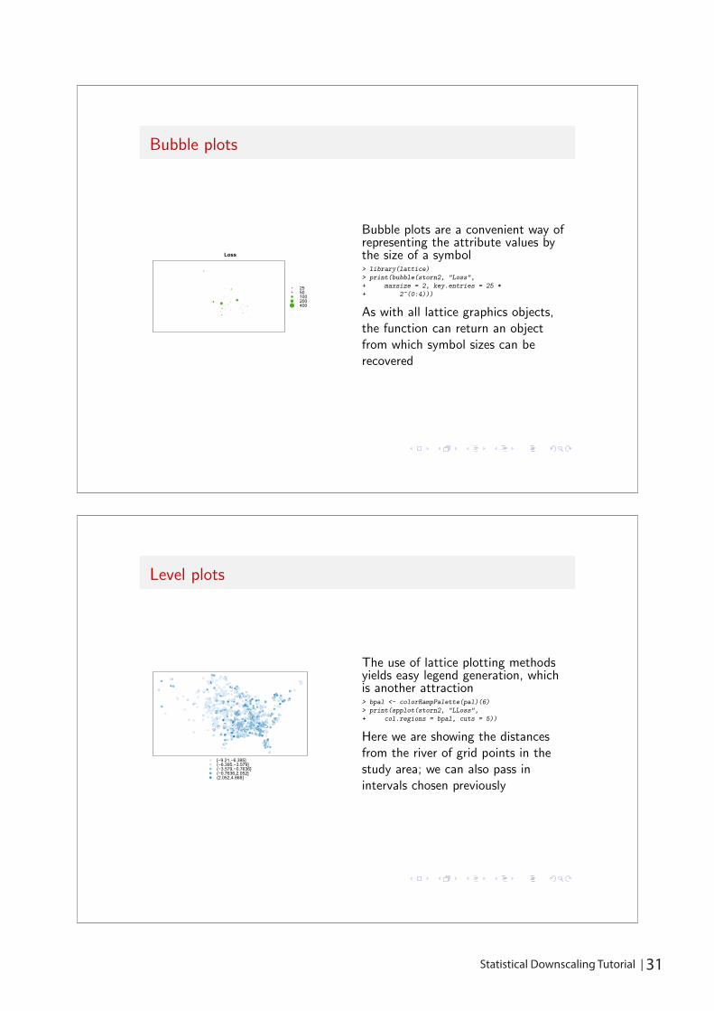
Bubble plots are a convenient way ofrepresenting the attribute values bythe size of a symbol> library(lattice)
> print(bubble(storn2, "Loss",
+ maxsize = 2, key.entries = 25 *
+ 2^(0:4)))
As with all lattice graphics objects,the function can return an objectfrom which symbol sizes can berecovered
32 | Statistical Downscaling Tutorial
Lattice graphics
Analysing Spatial Data in R: Accessing spatial data
Spatial Data in R 52 / 72
Lattice graphics
More realism
So far we have just used canned data and spatial objects rather thananything richer
The vizualisation methods are also quite flexible — both the basegraphics and lattice graphics methods can be extensively customised
It is also worth recalling the range of methods available for sp objects,in particular the overlay and spsample methods with a range ofargument signatures
These can permit further flexibility in display, in addition to theirprimary uses
Spatial Data in R 51 / 72
32 | Statistical Downscaling Tutorial Statistical Downscaling Tutorial | 33
Introduction
Creating objects within R
As mentioned previously, maptools includes ContourLines2SLDF() toconvert contour lines to SpatialLinesDataFrame objects
maptools also allows lines or polygons from maps to be used as sp objects
maptools can export sp objects to PBSmapping
maptools uses gpclib to check polygon topology and to dissolve polygons
maptools converts some sp objects for use in spatstat
maptools can read GSHHS high-resolution shoreline data intoSpatialPolygon objects
Spatial Data in R 54 / 72
Introduction
Introduction
Having described how spatial data may be represented in R, and howto vizualise these objects, we need to move on to accessing user data
There are quite a number of packages handling and analysing spatialdata on CRAN, and others off-CRAN, and their data objects can beconverted to or from sp object form
We need to cover how coordinate reference systems are handled,because they are the foundation for spatial data integration
Both here, and in relation to reading and writing various file formats,things have advanced a good deal since the R News note
Spatial Data in R 53 / 72
34 | Statistical Downscaling Tutorial
Introduction Coordinates
Coordinate reference systems
Coordinate reference systems (CRS) are at the heart of geodetics andcartography: how to represent a bumpy ellipsoid on the plane
We can speak of geographical CRS expressed in degrees andassociated with an ellipse, a prime meridian and a datum, andprojected CRS expressed in a measure of length, and a chosenposition on the earth, as well as the underlying ellipse, prime meridianand datum.
Most countries have multiple CRS, and where they meet there isusually a big mess — this led to the collection by the EuropeanPetroleum Survey Group (EPSG, now Oil & Gas Producers (OGP)Surveying & Positioning Committee) of a geodetic parameter dataset
Spatial Data in R 56 / 72
Using maps data: Illinois counties
92°W 90°W 88°W 86°W
37°N
38°N
39°N
40°N
41°N
42°N
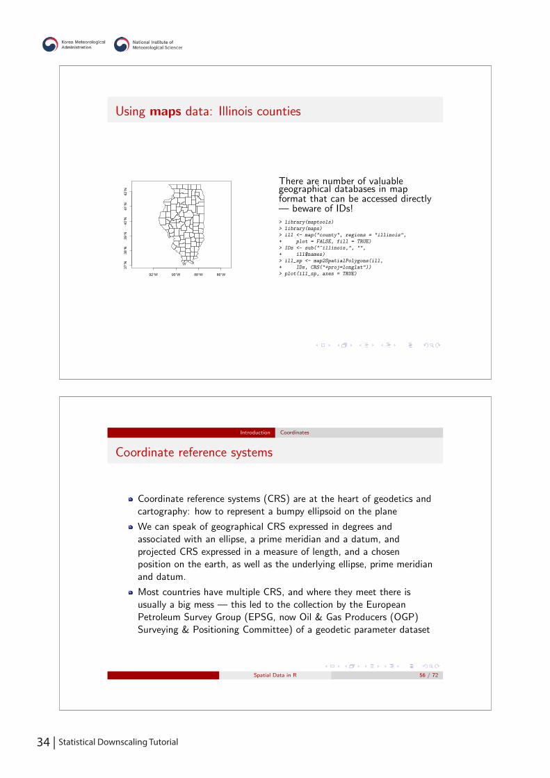
There are number of valuablegeographical databases in mapformat that can be accessed directly— beware of IDs!> library(maptools)
> library(maps)
> ill <- map("county", regions = "illinois",
+ plot = FALSE, fill = TRUE)
> IDs <- sub("^illinois,", "",
+ ill$names)
> ill_sp <- map2SpatialPolygons(ill,
+ IDs, CRS("+proj=longlat"))
> plot(ill_sp, axes = TRUE)
34 | Statistical Downscaling Tutorial Statistical Downscaling Tutorial | 35
Here: neither here nor there
In a Dutch navigation example, a chart position in the ED50 datum has to be compared
with a GPS measurement in WGS84 datum right in front of the jetties of IJmuiden,
both in geographical CRS. Using the spTransform method makes the conversion, using
EPSG and external information to set up the ED50 CRS. The difference is about 124m;
lots of details about CRS in general can be found in Grids & Datums.
> library(rgdal)
> ED50 <- CRS(paste("+init=epsg:4230", "+towgs84=-87,-96,-120,0,0,0,0"))
> IJ.east <- as(char2dms("4d31 00\"E"), "numeric")
> IJ.north <- as(char2dms("52d28 00\"N"), "numeric")
> IJ.ED50 <- SpatialPoints(cbind(x = IJ.east, y = IJ.north),
+ ED50)
> res <- spTransform(IJ.ED50, CRS("+proj=longlat +datum=WGS84"))
> spDistsN1(coordinates(IJ.ED50), coordinates(res),
+ longlat = TRUE) * 1000
[1] 124.0994
Introduction Coordinates
Coordinate reference systems
The EPSG list among other sources is used in the workhorse PROJ.4library, which as implemented by Frank Warmerdam handlestransformation of spatial positions between different CRS
This library is interfaced with R in the rgdal package, and the CRS
class is defined partly in sp, partly in rgdal
A CRS object is defined as a character NA string or a valid PROJ.4CRS definition
The validity of the definition can only be checked if rgdal is loaded
Spatial Data in R 57 / 72

36 | Statistical Downscaling Tutorial
Reading vectors
Reading vectors
GIS vector data are points, lines, polygons, and fit the equivalent spclasses
There are a number of commonly used file formats, all or mostproprietary, and some newer ones which are partly open
GIS are also handing off more and more data storage to DBMS, andsome of these now support spatial data formats
Vector formats can also be converted outside R to formats that areeasier to read
Spatial Data in R 60 / 72
Introduction Coordinates
CRS are muddled
If you think CRS are muddled, you are right, like time zones anddaylight saving time in at least two dimensions
But they are the key to ensuring positional interoperability, and“mashups”— data integration using spatial position as an index mustbe able to rely on data CRS for integration integrity
The situation is worse than TZ/DST because there are lots of oldmaps around, with potentially valuable data; finding correct CRSvalues takes time
On the other hand, old maps and odd choices of CRS origins canhave their charm . . .
Spatial Data in R 59 / 72

36 | Statistical Downscaling Tutorial Statistical Downscaling Tutorial | 37
Reading vectors Reading shapefiles
Reading shapefiles
The ESRI ArcView and now ArcGIS standard(ish) format for vectordata is the shapefile, with at least a DBF file of data, an SHP file ofshapes, and an SHX file of indices to the shapes; an optional PRJ fileis the CRS
Many shapefiles in the wild do not meet the ESRI standardspecification, so hacks are unavoidable unless a full topology is built
Both maptools and shapefiles contain functions for reading andwriting shapefiles; they cannot read the PRJ file, but do not dependon external libraries
There are many valid types of shapefile, but they sometimes occur instrange contexts — only some can be happily represented in R so far
Spatial Data in R 62 / 72
Reading vectors
Reading vectors
GIS vector data can be either topological or spaghetti — legacy GISwas topological, desktop GIS spaghetti
sp classes are not bad spaghetti, but no checking of lines or polygonsis done for errant topology
A topological representation in principal only stores each point once,and builds arcs (lines between nodes) from points, polygons from arcs— GRASS 6 has a nice topological model
Only RArcInfo tries to keep some traces of topology in importinglegacy ESRI ArcInfo binary vector data (or e00 format data) — mapsuses topology because that was how things were done then
Spatial Data in R 61 / 72

38 | Statistical Downscaling Tutorial
Reading vectors: rgdal
> US1 <- readOGR(dsn = "datasets", layer = "s_01au07")
OGR data source with driver: ESRI Shapefile
Source: "datasets", layer: "s_01au07"
with 57 features
It has 5 fields
> cat(strwrap(proj4string(US1)), sep = "\n")
+proj=longlat +datum=NAD83 +no_defs +ellps=GRS80
+towgs84=0,0,0
Using the OGR vector part of the
Geospatial Data Abstraction Library lets us
read shapefiles like other formats for which
drivers are available. It also supports the
handling of CRS directly, so that if the
imported data have a specification, it will
be read. OGR formats differ from platform
to platform — the next release of rgdal will
include a function to list available formats.
Use FWTools to convert between formats.
Reading shapefiles: maptools
> library(maptools)
> getinfo.shape("datasets/s_01au07.shp")
Shapefile type: Polygon, (5), # of Shapes: 57
> US <- readShapePoly("datasets/s_01au07.shp")
There are readShapePoly, readShapeLines,
and readShapePoints functions in the
maptools package, and in practice they now
handle a number of infelicities. They do
not, however, read the CRS, which can
either be set as an argument, or updated
later with the proj4string method

38 | Statistical Downscaling Tutorial Statistical Downscaling Tutorial | 39
Reading rasters: rgdal> getGDALDriverNames()$name
[1] AAIGrid ACE2 ADRG AIG AirSAR
[6] ARG BAG BIGGIF BLX BMP
[11] BSB BT CEOS COASP COSAR
[16] CPG CTable2 CTG DIMAP DIPEx
[21] DODS DOQ1 DOQ2 DTED E00GRID
[26] ECRGTOC EHdr EIR ELAS ENVI
[31] EPSILON ERS ESAT FAST FIT
[36] FujiBAS GenBin GFF GIF GMT
[41] GRASSASCIIGrid GRIB GS7BG GSAG GSBG
[46] GSC GTiff GTX GXF HDF4
[51] HDF4Image HDF5 HDF5Image HF2 HFA
[56] HTTP IDA ILWIS INGR IRIS
[61] ISIS2 ISIS3 JAXAPALSAR JDEM JP2OpenJPEG
[66] JPEG JPEG2000 KMLSUPEROVERLAY KRO L1B
[71] LAN LCP Leveller LOSLAS MAP
[76] MBTiles MEM MFF MFF2 MSGN
[81] NDF netCDF NGSGEOID NITF NTv2
[86] NWT_GRC NWT_GRD OGDI OZI PAux
[91] PCIDSK PCRaster PDF PDS PNG
[96] PNM PostGISRaster R Rasterlite RIK
[101] RMF RPFTOC RS2 RST SAGA
[106] SAR_CEOS SDTS SGI SNODAS SRP
[111] SRTMHGT Terragen TIL TSX USGSDEM
[116] VRT WCS WEBP WMS XPM
[121] XYZ ZMap
122 Levels: AAIGrid ACE2 ADRG AIG AirSAR ARG BAG BIGGIF BLX BMP BSB BT CEOS COASP COSAR ... ZMap
> list.files()
[1] "SP27GTIF.TIF"
> SP27GTIF <- readGDAL("SP27GTIF.TIF")
SP27GTIF.TIF has GDAL driver GTiff
and has 929 rows and 699 columns
Reading rasters
Reading rasters
There are very many raster and image formats; some allow only oneband of data, others think data bands are RGB, while yet others areflexible
There is a simple readAsciiGrid function in maptools that readsESRI Arc ASCII grids into SpatialGridDataFrame objects; it does nothandle CRS and has a single band
Much more support is available in rgdal in the readGDAL function,which — like readOGR — finds a usable driver if available andproceeds from there
Using arguments to readGDAL, subregions or bands may be selected,which helps handle large rasters
Spatial Data in R 65 / 72

40 | Statistical Downscaling Tutorial
Reading rasters: rgdal
> summary(SP27GTIF)
Object of class SpatialGridDataFrame
Coordinates:
min max
x 681480 704407.2
y 1882579 1913050.0
Is projected: TRUE
proj4string :
[+proj=tmerc +lat_0=36.66666666666666 +lon_0=-88.33333333333333 +k=0.9999749999999999
+x_0=152400.3048006096 +y_0=0 +datum=NAD27 +units=us-ft +no_defs +ellps=clrk66
+nadgrids=@conus,@alaska,@ntv2_0.gsb,@ntv1_can.dat]
Grid attributes:
cellcentre.offset cellsize cells.dim
x 681496.4 32.8 699
y 1882595.2 32.8 929
Data attributes:
band1
Min. : 4.0
1st Qu.: 78.0
Median :104.0
Mean :115.1
3rd Qu.:152.0
Max. :255.0
Reading rasters: rgdal
680000 685000 690000 695000 700000 705000
1885
000
1895
000
1905
000
This is a single band GeoTiff, mostlyshowing downtown Chicago; a lot of data isavailable in geotiff format from US publicagencies, including Shuttle radartopography mission seamless data — we’llget back to this later> image(SP27GTIF, col = grey(1:99/100),
+ axes = TRUE)

40 | Statistical Downscaling Tutorial Statistical Downscaling Tutorial | 41
Writing objects GIS interfaces
GIS interfaces
GIS interfaces can be as simple as just reading and writing files — loosecoupling, once the file formats have been worked out, that is
Loose coupling is less of a burden than it was with smaller, slower machines,which is why the GRASS 5 interface was tight-coupled, with R functionsreading from and writing to the GRASS database directly
The GRASS 6 interface spgrass6 on CRAN also runs R within GRASS, butuses intermediate temporary files; the package is under development but isquite usable
Use has been made of COM and Python interfaces to ArcGIS; typical use isby loose coupling except in highly customised work situations
Carson Farmer has developed a plug-in for QGis (manageR) to provide abridge between R and QGis
Spatial Data in R 70 / 72
Writing objects
Writing objects
In rgdal, writeGDAL can write for example multi-band GeoTiffs, butthere are fewer write than read drivers; in general CRS andgeogreferencing are supported — see gdalDrivers
The rgdal function writeOGR can be used to write vector files,including those formats supported by drivers, including now KML —see ogrDrivers
External software (including different versions) tolerate output objectsin varying degrees, quite often needing tricks - see mailing list archives
In maptools, there are functions for writing sp objects to shapefiles— writePolyShape, etc., as Arc ASCII grids — writeAsciiGrid, andfor using the R PNG graphics device for outputting image overlays forGoogle Earth
Spatial Data in R 69 / 72
42 | Statistical Downscaling Tutorial
Using Google Maps
●
●
●●
●
●
●
●●●●●
●●●●
●
●
●●
●
●
●
●●
●●●●
● ●●● ●
●●●
●●● ●●●
●●●●
●●●●
●●●
●●
●●
●●●●
●
●●●●
●
●●●
●●
●
●
●●
●●
●
●●●●
●●●●●
●●●●
●
●
●●●●
●
● ●●
●●●●
●●
●
●●
●
●
●
●●
●●
●● ●● ● ●
●●
●
●
●
●●
●
●●●●
●●
● ●
●
●
●●
●●●
●●● ●●
●
●
●●
●
●●
●
●●
●●●
●●
●
●
●
●●●●
●
●● ●
●
●
●
●
●
●●●●●●
●
●●●●
●
●
●
●●
●
●●●●●●
●●●● ●
●
●●●●●●●
●●●●●
●
●
●
●●
●
●●●
● ● ●●● ●●
●
●●
●
●●●
●●●● ●●
●
●
●
●
●●●●●
●●
●
●
●
●
●
●
●●●●
●
●
●
●● ● ●
●
●
●● ●
●●●●●●
●
●
●●
●●
●● ●●
●●
●
●●●●●
●
●
●
●●
●
●
●●
●
●
●
●
●
●●
●
●
●●●
●
●●●
●
●
●●●
●
●●●●
●●
●●
●
●
●
●
●
●
●●
●●
●●
●
●●●●●●
●
●●●
●●
●
●●
●●●
●●
●
●●●●●
●●
●
●●
●●
●●●
●●
●●●●
● ● ●●●●●
●
●●●● ●● ●●●●
●
●●●●
●
●
●
●●
●
●●
●●
●
●●●●● ●● ●
●●●●
●●●
●
●
●
●●
●
●●●●●
● ●
●
●
●●●
●
●●●●●●●●●●●●●●●●●●● ●
●●●●●●●
●
●
●●
●
●
●
●●●●● ●
●
●
●●●●●
●●
●
●●
●
●●
●
●
●
●
●●
●●●
●●
●
●
●
●
●
●●●●●
●
●
●
●●
●
●
●
●
●
●
●●●
●●●
●●
●
●
●●
●● ●
●
●
●
●
●
●
●●
●
●
●
●●
●
●●●
●●●
●
●
●●
●
●●
●●
●●
●
●
●
●
●
●
●●
●
●
●●●
●
●●
●
●
●●●●
●●
●
●
●●●●
● ●
●●●
●
●●●●●
●
●
●
●
●
●
●●
●
●
●
●
●
●●
●●●●
●●
●●●
●●●●●●
●●
● ●●
●●
●
●●
●●●
●
●●
●●
●
●
●
●
●
●
●
●
●●
●● ●●
●●●
●
●
●●●●●●●
●
●●●●●●●●● ●●
●●
●
●●●
●
●
●
●
●●
●
●
●
●●
●
●
●
●●
●
●●
●●
●
●
●●●
●●
●●●●
●
●
●
●●
●●
●
●
●●●
●
●●
●●
● ●●●
●●
●●
●●
●●● ● ●●●
●●
●●
●
●●●●●●●
●●●●
●●
●
●
●
●
●
●
●
●
●●
●
●
●●●●●●●
●
●
●
●
●
● ●●●●
●
●
●●●
●●
●●●
●●
●
●
●
●
●
●
●
●●●
●
●
●
●●
●
●
●
●
●●
●●
●
●●●●
●●
●
●
●
●
●
●
●
●●
●
●●●
●
●
●
●●●
●●
●
●
●
●
●
●●
●●
●
●
●●
●●
●
●● ●
●
●
●
●
●
●●
●●●
●
●●
●
●
●
●
●
●
●●
●●●●●
●
●
●
●
●
●
● ●●
●
●●●●●
●
●●● ●●
●●
●
●●●●
●●
●●●●
●
●●
●
●
●●
●
●
●●
●
●
●
●
●
●
●
●
●
●
●
●
●
●
●●
●
●●●
●
●●
●
●●
●
●
●
●
●
●
●
●
●
●●
●●
●
●
●
●
●
●
●
●
●
●
●
●
●
●
●
●
●
●
●
●
●
●
●●
●
●●
●
●
● ●●●●
● ●
●
●
●●●●
●
●●
●
●●
●
●●●●
●
●
●●●●●
●●
●
●●
●●
●●●
●
●
●
●
●●
●●
●
●
● ●
●
●
●
●●●
●●●
●
●
●●●
●
●
●
●
●
●●●●
●●
●●●
●●●●●●●
●●●●●●●●●●●●●●●
●
●
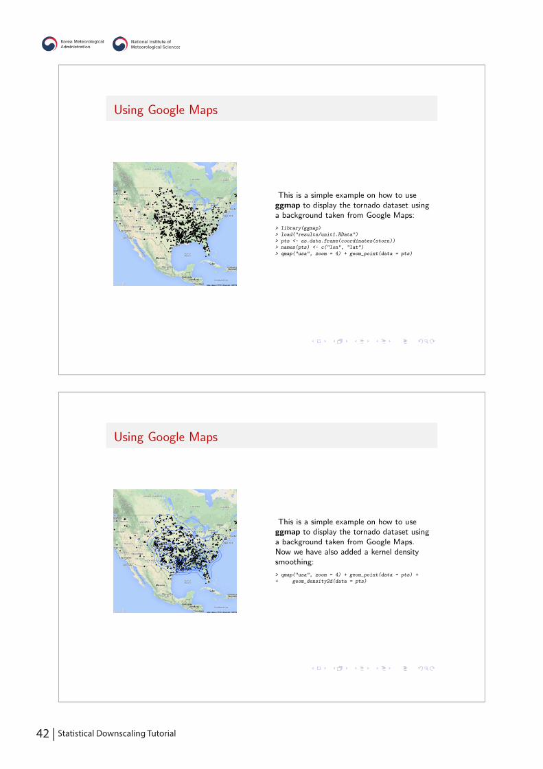
This is a simple example on how to useggmap to display the tornado dataset usinga background taken from Google Maps.Now we have also added a kernel densitysmoothing:
> qmap("usa", zoom = 4) + geom_point(data = pts) +
+ geom_density2d(data = pts)
Using Google Maps
●
●
●●
●
●
●
●●●●●
●●●●
●
●
●●
●
●
●
●●
●●●●
● ●●● ●
●●●
●●● ●●●
●●●●
●●●●
●●●
●●
●●
●●●●
●
●●●●
●
●●●
●●
●
●
●●
●●
●
●●●●
●●●●●
●●●●
●
●
●●●●
●
● ●●
●●●●
●●
●
●●
●
●
●
●●
●●
●● ●● ● ●
●●
●
●
●
●●
●
●●●●
●●
● ●
●
●
●●
●●●
●●● ●●
●
●
●●
●
●●
●
●●
●●●
●●
●
●
●
●●●●
●
●● ●
●
●
●
●
●
●●●●●●
●
●●●●
●
●
●
●●
●
●●●●●●
●●●● ●
●
●●●●●●●
●●●●●
●
●
●
●●
●
●●●
● ● ●●● ●●
●
●●
●
●●●
●●●● ●●
●
●
●
●
●●●●●
●●
●
●
●
●
●
●
●●●●
●
●
●
●● ● ●
●
●
●● ●
●●●●●●
●
●
●●
●●
●● ●●
●●
●
●●●●●
●
●
●
●●
●
●
●●
●
●
●
●
●
●●
●
●
●●●
●
●●●
●
●
●●●
●
●●●●
●●
●●
●
●
●
●
●
●
●●
●●
●●
●
●●●●●●
●
●●●
●●
●
●●
●●●
●●
●
●●●●●
●●
●
●●
●●
●●●
●●
●●●●
● ● ●●●●●
●
●●●● ●● ●●●●
●
●●●●
●
●
●
●●
●
●●
●●
●
●●●●● ●● ●
●●●●
●●●
●
●
●
●●
●
●●●●●
● ●
●
●
●●●
●
●●●●●●●●●●●●●●●●●●● ●
●●●●●●●
●
●
●●
●
●
●
●●●●● ●
●
●
●●●●●
●●
●
●●
●
●●
●
●
●
●
●●
●●●
●●
●
●
●
●
●
●●●●●
●
●
●
●●
●
●
●
●
●
●
●●●
●●●
●●
●
●
●●
●● ●
●
●
●
●
●
●
●●
●
●
●
●●
●
●●●
●●●
●
●
●●
●
●●
●●
●●
●
●
●
●
●
●
●●
●
●
●●●
●
●●
●
●
●●●●
●●
●
●
●●●●
● ●
●●●
●
●●●●●
●
●
●
●
●
●
●●
●
●
●
●
●
●●
●●●●
●●
●●●
●●●●●●
●●
● ●●
●●
●
●●
●●●
●
●●
●●
●
●
●
●
●
●
●
●
●●
●● ●●
●●●
●
●
●●●●●●●
●
●●●●●●●●● ●●
●●
●
●●●
●
●
●
●
●●
●
●
●
●●
●
●
●
●●
●
●●
●●
●
●
●●●
●●
●●●●
●
●
●
●●
●●
●
●
●●●
●
●●
●●
● ●●●
●●
●●
●●
●●● ● ●●●
●●
●●
●
●●●●●●●
●●●●
●●
●
●
●
●
●
●
●
●
●●
●
●
●●●●●●●
●
●
●
●
●
● ●●●●
●
●
●●●
●●
●●●
●●
●
●
●
●
●
●
●
●●●
●
●
●
●●
●
●
●
●
●●
●●
●
●●●●
●●
●
●
●
●
●
●
●
●●
●
●●●
●
●
●
●●●
●●
●
●
●
●
●
●●
●●
●
●
●●
●●
●
●● ●
●
●
●
●
●
●●
●●●
●
●●
●
●
●
●
●
●
●●
●●●●●
●
●
●
●
●
●
● ●●
●
●●●●●
●
●●● ●●
●●
●
●●●●
●●
●●●●
●
●●
●
●
●●
●
●
●●
●
●
●
●
●
●
●
●
●
●
●
●
●
●
●●
●
●●●
●
●●
●
●●
●
●
●
●
●
●
●
●
●
●●
●●
●
●
●
●
●
●
●
●
●
●
●
●
●
●
●
●
●
●
●
●
●
●
●●
●
●●
●
●
● ●●●●
● ●
●
●
●●●●
●
●●
●
●●
●
●●●●
●
●
●●●●●
●●
●
●●
●●
●●●
●
●
●
●
●●
●●
●
●
● ●
●
●
●
●●●
●●●
●
●
●●●
●
●
●
●
●
●●●●
●●
●●●
●●●●●●●
●●●●●●●●●●●●●●●
●
●
This is a simple example on how to useggmap to display the tornado dataset usinga background taken from Google Maps:
> library(ggmap)
> load("results/unit1.RData")
> pts <- as.data.frame(coordinates(storn))
> names(pts) <- c("lon", "lat")
> qmap("usa", zoom = 4) + geom_point(data = pts)
42 | Statistical Downscaling Tutorial Statistical Downscaling Tutorial | 43
Analysing Spatial Data in R: Worked example: geostatistics

44 | Statistical Downscaling Tutorial
44 | Statistical Downscaling Tutorial Statistical Downscaling Tutorial | 45
Worked example: geostatistics
� Geostatistics is a bit like the alchemy of spatial statistics,focussed more on prediction than model fitting
� Since the reason for modelling is chiefly prediction inpre-model-based geostatistics, and to a good extent inmodel-based geostatistics, we’ll also keep to interpolation here
� Interpolation is trying to make as good guesses as possible ofthe values of the variable of interest for places where there areno observations (can be in 1, 2, 3, . . . dimensions)
� These are based on the relative positions of places withobservations and places for which predictions are required, andthe observed values at observations
Analysing Spatial Data in R: Worked example:geostatistics
46 | Statistical Downscaling Tutorial
Meuse soil data
� The Maas river bank soil pollution data (Limburg, TheNetherlands) are sampled along the Dutch bank of the riverMaas (Meuse) north of Maastricht; the data are those used inBurrough and McDonnell (1998, pp. 309–311)
� These are a subset of the data provided with gstat and sp,but here we use the same subset as the very well regarded GIStextbook, in case cross-checking is of interest
� The data used here are a shapefile named BMcD.shp with itsdata table with the zinc ppm measurements we are interestedin interpolating, and an ASCII grid of flood frequencies for thepart of the river bank we are interested in, giving theprediction locations
Geostatistics packages
� The gstat package provides a wide range of functions forunivariate and multivariate geostatistics, also for largerdatasets, while geoR and geoRglm contain functions formodel-based geostatistics
� A similar wide range of functions is to be found in the fieldspackage. The spatial package is available as part of the VRbundle (shipped with base R), and contains several corefunctions
� The RandomFields package provides functions for thesimulation and analysis of random fields. For diagnostics ofvariograms, the vardiag package can be used
� The sgeostat package is also available; within the samegeneral topical area are the tripack for triangulation and theakima package for spline interpolation
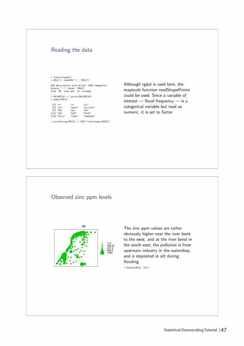
46 | Statistical Downscaling Tutorial Statistical Downscaling Tutorial | 47
Observed zinc ppm levels
Zn
●●●
●●
●●●●●
●
●●●
●●
●
●●●
●●●
●
●●
●
●
●
●●
●
●
●●
●●●
●
●
●
●
●
●
●
●
●
●
●
●
●
●●
●
●●
●●
●
●
●
●
●
●
●
●●●
●
●
●
●
●●
●
●
●●
●
●
●●●
●
●
●
●●
●
●
●
●
●
●●
● ●
●●
●
●
●●
113186.25307.5698.51839
The zinc ppm values are ratherobviously higher near the river bankto the west, and at the river bend inthe south east; the pollution is fromupstream industry in the watershep,and is deposited in silt duringflooding> bubble(BMcD, "Zn")
Reading the data
> library(rgdal)
> BMcD <- readOGR(".", "BMcD")
OGR data source with driver: ESRI Shapefile
Source: ".", layer: "BMcD"
with 98 rows and 15 columns
> BMcD$Fldf <- factor(BMcD$Fldf)
> names(BMcD)
[1] "x" "y" "xl"
[4] "yl" "elev" "d_river"
[7] "Cd" "Cu" "Pb"
[10] "Zn" "LOI" "Fldf"
[13] "Soil" "lime" "landuse"
> proj4string(BMcD) <- CRS("+init=epsg:28992")
Although rgdal is used here, themaptools function readShapePointscould be used. Since a variable ofinterest — flood frequency — is acategorical variable but read asnumeric, it is set to factor
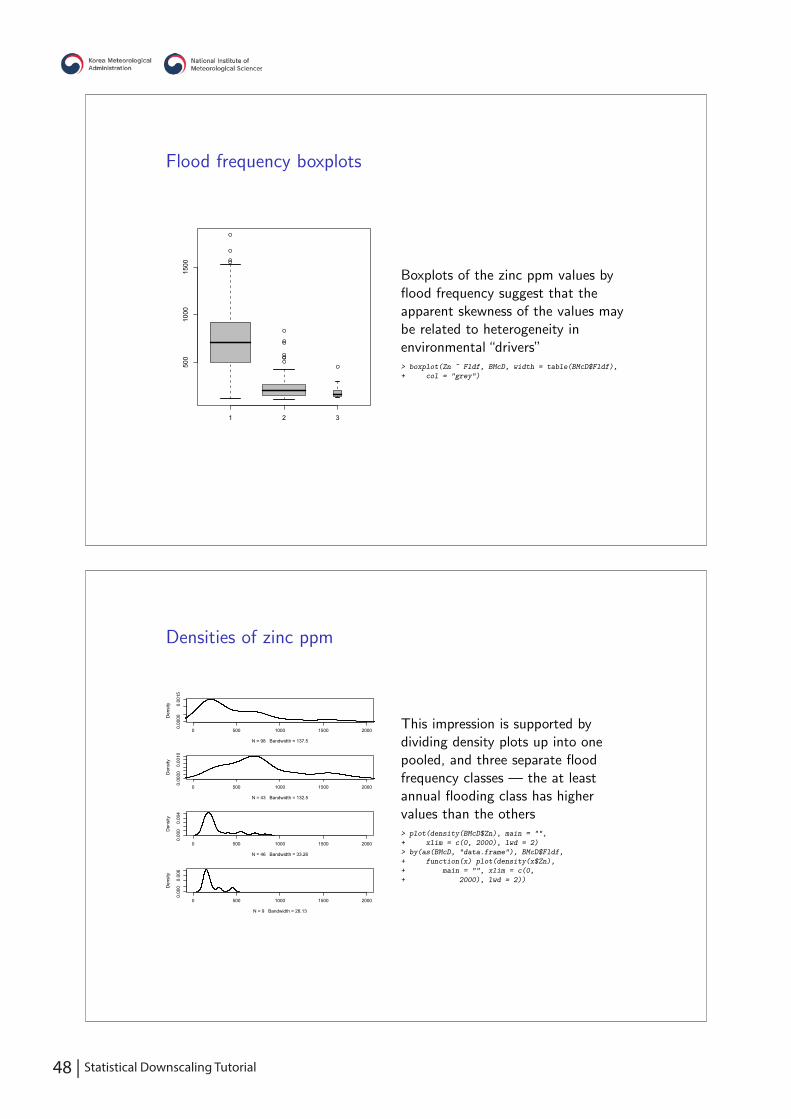
48 | Statistical Downscaling Tutorial
Densities of zinc ppm
0 500 1000 1500 2000
0.00
000.
0015
N = 98 Bandwidth = 137.5
Den
sity
0 500 1000 1500 2000
0.00
000.
0010
N = 43 Bandwidth = 132.5
Den
sity
0 500 1000 1500 2000
0.00
00.
004
N = 46 Bandwidth = 33.26
Den
sity
0 500 1000 1500 2000
0.00
00.
006
N = 9 Bandwidth = 28.13
Den
sity
This impression is supported bydividing density plots up into onepooled, and three separate floodfrequency classes — the at leastannual flooding class has highervalues than the others> plot(density(BMcD$Zn), main = "",
+ xlim = c(0, 2000), lwd = 2)
> by(as(BMcD, "data.frame"), BMcD$Fldf,
+ function(x) plot(density(x$Zn),
+ main = "", xlim = c(0,
+ 2000), lwd = 2))
Flood frequency boxplots
1 2 3
500
1000
1500
Boxplots of the zinc ppm values byflood frequency suggest that theapparent skewness of the values maybe related to heterogeneity inenvironmental “drivers”> boxplot(Zn ~ Fldf, BMcD, width = table(BMcD$Fldf),
+ col = "grey")
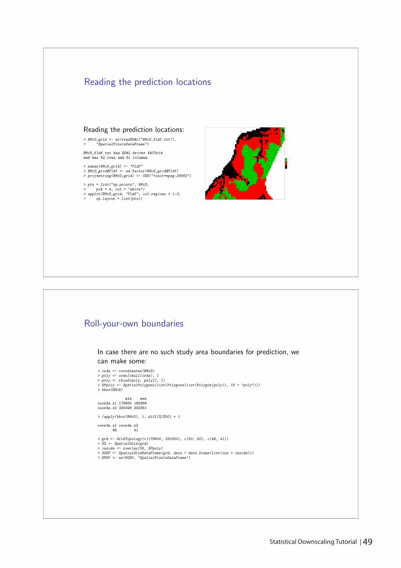
48 | Statistical Downscaling Tutorial Statistical Downscaling Tutorial | 49
Roll-your-own boundaries
In case there are no such study area boundaries for prediction, wecan make some:> crds <- coordinates(BMcD)
> poly <- crds[chull(crds), ]
> poly <- rbind(poly, poly[1, ])
> SPpoly <- SpatialPolygons(list(Polygons(list(Polygon(poly)), ID = "poly")))
> bbox(BMcD)
min max
coords.x1 178605 180956
coords.x2 330349 332351
> (apply(bbox(BMcD), 1, diff)%/%50) + 1
coords.x1 coords.x2
48 41
> grd <- GridTopology(c(178600, 330300), c(50, 50), c(48, 41))
> SG <- SpatialGrid(grd)
> inside <- overlay(SG, SPpoly)
> SGDF <- SpatialGridDataFrame(grd, data = data.frame(list(ins = inside)))
> SPDF <- as(SGDF, "SpatialPixelsDataFrame")
Reading the prediction locations
Reading the prediction locations:> BMcD_grid <- as(readGDAL("BMcD_fldf.txt"),
+ "SpatialPixelsDataFrame")
BMcD_fldf.txt has GDAL driver AAIGrid
and has 52 rows and 61 columns
> names(BMcD_grid) <- "Fldf"
> BMcD_grid$Fldf <- as.factor(BMcD_grid$Fldf)
> proj4string(BMcD_grid) <- CRS("+init=epsg:28992")
> pts = list("sp.points", BMcD,
+ pch = 4, col = "white")
> spplot(BMcD_grid, "Fldf", col.regions = 1:3,
+ sp.layout = list(pts))
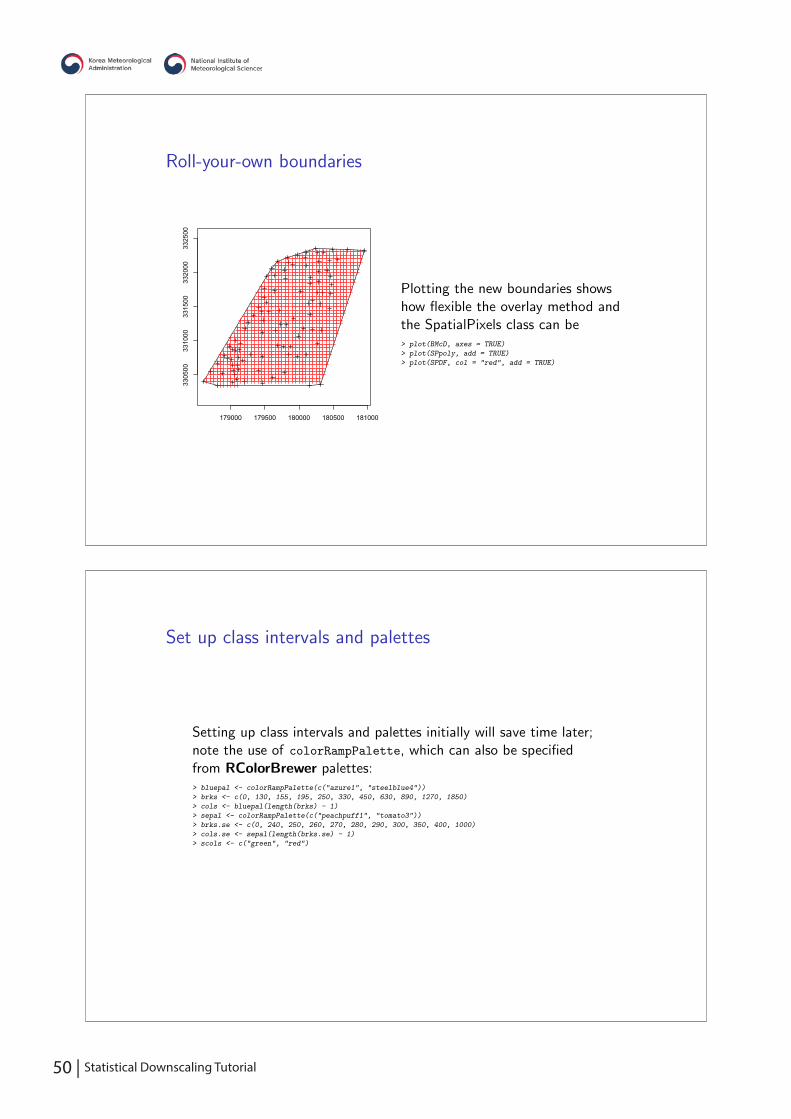
50 | Statistical Downscaling Tutorial
Set up class intervals and palettes
Setting up class intervals and palettes initially will save time later;note the use of colorRampPalette, which can also be specifiedfrom RColorBrewer palettes:> bluepal <- colorRampPalette(c("azure1", "steelblue4"))
> brks <- c(0, 130, 155, 195, 250, 330, 450, 630, 890, 1270, 1850)
> cols <- bluepal(length(brks) - 1)
> sepal <- colorRampPalette(c("peachpuff1", "tomato3"))
> brks.se <- c(0, 240, 250, 260, 270, 280, 290, 300, 350, 400, 1000)
> cols.se <- sepal(length(brks.se) - 1)
> scols <- c("green", "red")
Roll-your-own boundaries
179000 179500 180000 180500 181000
3305
0033
1000
3315
0033
2000
3325
00
Plotting the new boundaries showshow flexible the overlay method andthe SpatialPixels class can be> plot(BMcD, axes = TRUE)
> plot(SPpoly, add = TRUE)
> plot(SPDF, col = "red", add = TRUE)

50 | Statistical Downscaling Tutorial Statistical Downscaling Tutorial | 51
Aspatial flood frequency model
Flood frequency model interpolation
●
●
●
●
●
●●
●
●
●
●
●
●●
●
●
●
●
●
●
●
●
●
●
●
●
●
●
●
●
●
●
●
●
●
●
●
●
●
●
●
●
●
●
●
●
●
●
●
●
●
●
●
●
●●
●
●
●
●
●
●
●
●
●
●●
●
●
●
●
●
●
●
●
●
●
●
●
●
●
●
●
●
●
●
●
●
●
●
●
●
●
●
●
● ●
●
under 130130 − 155155 − 195195 − 250250 − 330330 − 450450 − 630630 − 890890 − 1270over 1270
And the messy bits (once):> library(maptools)
> BMcD_grid$lm_pred <- predict(fres,
+ newdata = BMcD_grid)
> image(BMcD_grid, "lm_pred",
+ breaks = brks, col = cols)
> title("Flood frequency model interpolation")
> pe <- BMcD$Zn - eres$predictions
> symbols(coordinates(BMcD), circles = sqrt(abs(pe)),
+ fg = "black", bg = scols[(pe <
+ 0) + 1], inches = FALSE,
+ add = TRUE)
> legend("topleft", fill = cols,
+ legend = leglabs(brks),
+ bty = "n", cex = 0.8)
Aspatial flood frequency modelSince we have seen how the zinc ppm values seem to bedistributed in relationship to flood frequencies, and because wehave flood frequencies for the prediction locations, we can startwith a null model, then an aspatial model (using leave-one-outcross validation to show us how we are doing):> library(ipred)
> res <- errorest(Zn ~ 1, data = as(BMcD, "data.frame"), model = lm,
+ est.para = control.errorest(k = nrow(BMcD), random = FALSE,
+ predictions = TRUE))
> round(res$error, 2)
[1] 400.86
> fres <- lm(Zn ~ Fldf, data = BMcD)
> anova(fres)
Analysis of Variance Table
Response: Zn
Df Sum Sq Mean Sq F value Pr(>F)
Fldf 2 6413959 3206979 33.8 8.196e-12
Residuals 95 9013656 94881
> eres <- errorest(Zn ~ Fldf, data = as(BMcD, "data.frame"), model = lm,
+ est.para = control.errorest(k = nrow(BMcD), random = FALSE,
+ predictions = TRUE))
> round(eres$error, 2)
[1] 310.74
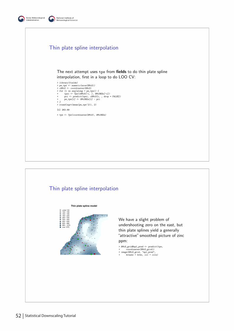
52 | Statistical Downscaling Tutorial
Thin plate spline interpolation
Thin plate spline model
●
●
●
●
●
●●
●
●
●
●
●
●
●
●
●
●
●
●
●
●
●
●
●
●
●
●
●
●
●
●
●
●
●
●
●
●
●
●
●
●
●
●
●
●
●
●
●
●
●
●
●
●
●
●
●
●
●
●
●
●
●
●
●
●
●
●
●
●
●
●
●
●
●
●
●
●●
●
●
●
●
●
●
●
●
●
●
●
●
●
●
●
●
●
● ●
●
under 130130 − 155155 − 195195 − 250250 − 330330 − 450450 − 630630 − 890890 − 1270over 1270
We have a slight problem ofundershooting zero on the east, butthin plate splines yield a generally“attractive” smoothed picture of zincppm:> BMcD_grid$spl_pred <- predict(tps,
+ coordinates(BMcD_grid))
> image(BMcD_grid, "spl_pred",
+ breaks = brks, col = cols)
Thin plate spline interpolation
The next attempt uses tps from fields to do thin plate splineinterpolation, first in a loop to do LOO CV:> library(fields)
> pe_tps <- numeric(nrow(BMcD))
> cBMcD <- coordinates(BMcD)
> for (i in seq(along = pe_tps)) {
+ tpsi <- Tps(cBMcD[-i, ], BMcD$Zn[-i])
+ pri <- predict(tpsi, cBMcD[i, , drop = FALSE])
+ pe_tps[i] <- BMcD$Zn[i] - pri
+ }
> round(sqrt(mean(pe_tps^2)), 2)
[1] 263.69
> tps <- Tps(coordinates(BMcD), BMcD$Zn)
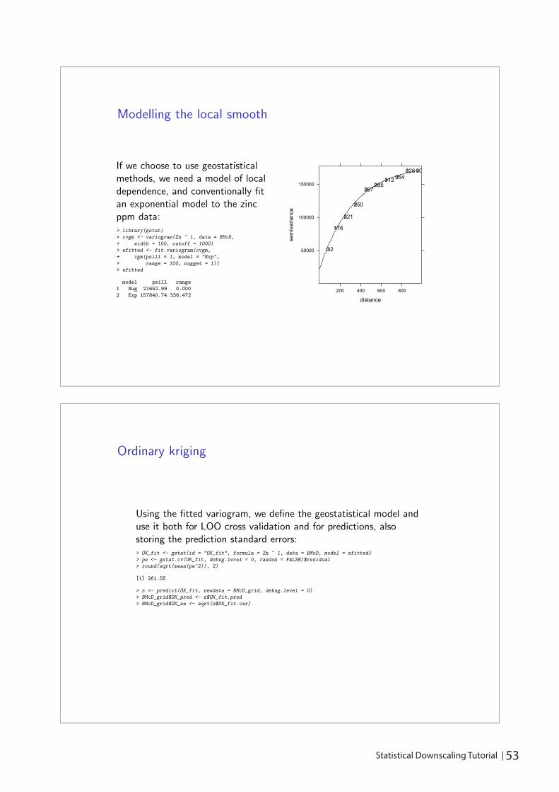
52 | Statistical Downscaling Tutorial Statistical Downscaling Tutorial | 53
Ordinary kriging
Using the fitted variogram, we define the geostatistical model anduse it both for LOO cross validation and for predictions, alsostoring the prediction standard errors:> OK_fit <- gstat(id = "OK_fit", formula = Zn ~ 1, data = BMcD, model = efitted)
> pe <- gstat.cv(OK_fit, debug.level = 0, random = FALSE)$residual
> round(sqrt(mean(pe^2)), 2)
[1] 261.55
> z <- predict(OK_fit, newdata = BMcD_grid, debug.level = 0)
> BMcD_grid$OK_pred <- z$OK_fit.pred
> BMcD_grid$OK_se <- sqrt(z$OK_fit.var)
Modelling the local smooth
If we choose to use geostatisticalmethods, we need a model of localdependence, and conventionally fitan exponential model to the zincppm data:> library(gstat)
> cvgm <- variogram(Zn ~ 1, data = BMcD,
+ width = 100, cutoff = 1000)
> efitted <- fit.variogram(cvgm,
+ vgm(psill = 1, model = "Exp",
+ range = 100, nugget = 1))
> efitted
model psill range
1 Nug 21652.99 0.000
2 Exp 157840.74 336.472distance
sem
ivar
ianc
e
50000
100000
150000
200 400 600 800
32
176
221
250
267285
312 354328 306

54 | Statistical Downscaling Tutorial
Ordinary kriging standard errors
Fitted exponential OK standard errors
●
●
●
●
●
●●
●
●
●
●
●
●
●
●
●
●
●
●
●
●
●
●
●
●
●
●
●
●
●
●
●
●
●
●
●
●
●
●
●
●
●
●
●
●
●
●
●
●
●
●
●
●
●
●●
●
●
●
●
●
●
●
●
●
●
●
●
●
●
●
●
●
●
●
●
●●
●
●
●
●
●
●
●
●
●
●
●
●
●
●
●
●
●
● ●
●
under 240240 − 250250 − 260260 − 270270 − 280280 − 290290 − 300300 − 350350 − 400over 400 For the standard errors, we use a
different palette, but the procedure isthe same:> image(BMcD_grid, "OK_se", breaks = brks.se,
+ col = cols.se)
Ordinary kriging predictions
Fitted exponential OK model
●
●
●
●
●
●●
●
●
●
●
●
●
●
●
●
●
●
●
●
●
●
●
●
●
●
●
●
●
●
●
●
●
●
●
●
●
●
●
●
●
●
●
●
●
●
●
●
●
●
●
●
●
●
●●
●
●
●
●
●
●
●
●
●
●
●
●
●
●
●
●
●
●
●
●
●●
●
●
●
●
●
●
●
●
●
●
●
●
●
●
●
●
●
● ●
●
under 130130 − 155155 − 195195 − 250250 − 330330 − 450450 − 630630 − 890890 − 1270over 1270
By now, the typical idiom of addingconstructed variables to theSpatialPixels data frame object, anddisplaying them by name, should befamiliar:> image(BMcD_grid, "OK_pred",
+ breaks = brks, col = cols)
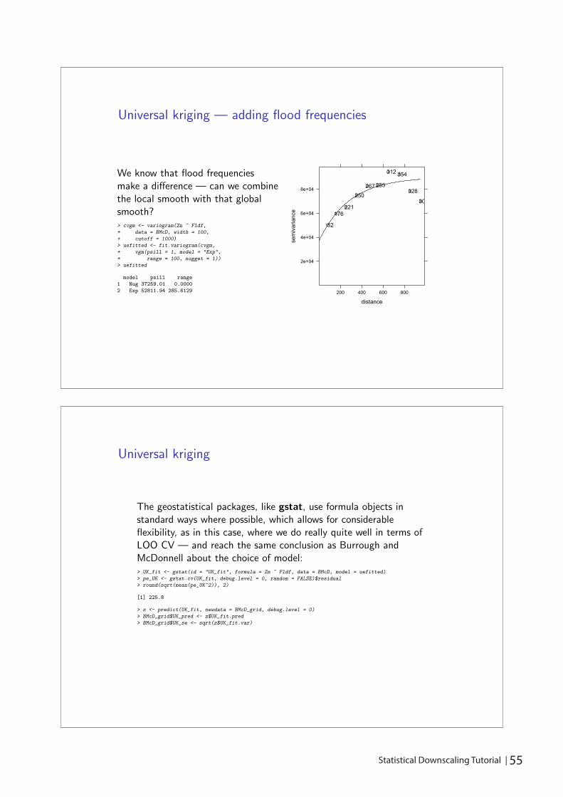
54 | Statistical Downscaling Tutorial Statistical Downscaling Tutorial | 55
Universal kriging
The geostatistical packages, like gstat, use formula objects instandard ways where possible, which allows for considerableflexibility, as in this case, where we do really quite well in terms ofLOO CV — and reach the same conclusion as Burrough andMcDonnell about the choice of model:> UK_fit <- gstat(id = "UK_fit", formula = Zn ~ Fldf, data = BMcD, model = uefitted)
> pe_UK <- gstat.cv(UK_fit, debug.level = 0, random = FALSE)$residual
> round(sqrt(mean(pe_UK^2)), 2)
[1] 225.8
> z <- predict(UK_fit, newdata = BMcD_grid, debug.level = 0)
> BMcD_grid$UK_pred <- z$UK_fit.pred
> BMcD_grid$UK_se <- sqrt(z$UK_fit.var)
Universal kriging — adding flood frequencies
We know that flood frequenciesmake a difference — can we combinethe local smooth with that globalsmooth?> cvgm <- variogram(Zn ~ Fldf,
+ data = BMcD, width = 100,
+ cutoff = 1000)
> uefitted <- fit.variogram(cvgm,
+ vgm(psill = 1, model = "Exp",
+ range = 100, nugget = 1))
> uefitted
model psill range
1 Nug 37259.01 0.0000
2 Exp 52811.94 285.6129
distancese
miv
aria
nce
2e+04
4e+04
6e+04
8e+04
200 400 600 800
32
176221
250267 285
312 354
328
306
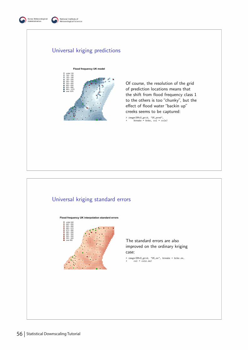
56 | Statistical Downscaling Tutorial
Universal kriging standard errors
Flood frequency UK interpolation standard errors
●
●
●
●
●
●●
●
●
●
●
●
●●
●
●
●
●
●
●
●
●
●
●
●
●
●
●
●
●
●
●
●
●
●
●
●
●
●
●
●
●
●
●
●
●
●
●
●
●
●
●
●
●
●●
●
●
●
●
●
●
●
●
●
●
●
●
●
●
●
●
●
●
●
●
●●
●
●
●
●
●
●
●
●
●
●
●
●
●
●
●
●
●
● ●
●
under 240240 − 250250 − 260260 − 270270 − 280280 − 290290 − 300300 − 350350 − 400over 400 The standard errors are also
improved on the ordinary krigingcase:> image(BMcD_grid, "UK_se", breaks = brks.se,
+ col = cols.se)
Universal kriging predictions
Flood frequency UK model
●
●
●
●
●
●●
●
●
●
●
●
●●
●
●
●
●
●
●
●
●
●
●
●
●
●
●
●
●
●
●
●
●
●
●
●
●
●
●
●
●
●
●
●
●
●
●
●
●
●
●
●
●
●●
●
●
●
●
●
●
●
●
●
●
●
●
●
●
●
●
●
●
●
●
●●
●
●
●
●
●
●
●
●
●
●
●
●
●
●
●
●
●
● ●
●
under 130130 − 155155 − 195195 − 250250 − 330330 − 450450 − 630630 − 890890 − 1270over 1270
Of course, the resolution of the gridof prediction locations means thatthe shift from flood frequency class 1to the others is too“chunky”, but theeffect of flood water“backin up”creeks seems to be captured:> image(BMcD_grid, "UK_pred",
+ breaks = brks, col = cols)

56 | Statistical Downscaling Tutorial Statistical Downscaling Tutorial | 57
Exporting a completed prediction
We will finally try to export the universal kriging predictions as aGeoTiff file, and read it into ArcGIS. In practice, this requires usingToolbox → Raster → Calculate statistics, and then right-clickingon the layer: Properties → Symbology → Classified:> writeGDAL(BMcD_grid["UK_pred"], "UK_pred.tif")
Putting it all together
lm_pred spl_pred
OK_pred UK_pred
0
200
400
600
800
1000
1200
1400
1600
1800
Using spplot, we can display all thepredictions together, to give a viewof our progress:> pts = list("sp.points", BMcD,
+ pch = 4, col = "black",
+ cex = 0.5)
> spplot(BMcD_grid, c("lm_pred",
+ "spl_pred", "OK_pred", "UK_pred"),
+ at = brks, col.regions = cols,
+ sp.layout = list(pts))
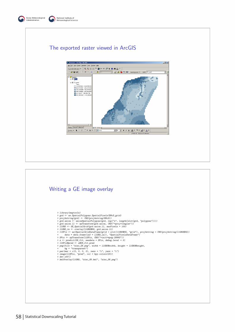
58 | Statistical Downscaling Tutorial
Writing a GE image overlay
> library(maptools)
> grd <- as.SpatialPolygons.SpatialPixels(BMcD_grid)
> proj4string(grd) <- CRS(proj4string(BMcD))
> grd.union <- unionSpatialPolygons(grd, rep("x", length(slot(grd, "polygons"))))
> grd.union.ll <- spTransform(grd.union, CRS("+proj=longlat"))
> llGRD <- GE_SpatialGrid(grd.union.ll, maxPixels = 100)
> llGRD_in <- overlay(llGRD$SG, grd.union.ll)
> llSPix <- as(SpatialGridDataFrame(grid = slot(llGRD$SG, "grid"), proj4string = CRS(proj4string(llGRD$SG)),
+ data = data.frame(in0 = llGRD_in)), "SpatialPixelsDataFrame")
> SPix <- spTransform(llSPix, CRS("+init=epsg:28992"))
> z <- predict(OK_fit, newdata = SPix, debug.level = 0)
> llSPix$pred <- z$OK_fit.pred
> png(file = "zinc_OK.png", width = llGRD$width, height = llGRD$height,
+ bg = "transparent")
> par(mar = c(0, 0, 0, 0), xaxs = "i", yaxs = "i")
> image(llSPix, "pred", col = bpy.colors(20))
> dev.off()
> kmlOverlay(llGRD, "zinc_OK.kml", "zinc_OK.png")
The exported raster viewed in ArcGIS
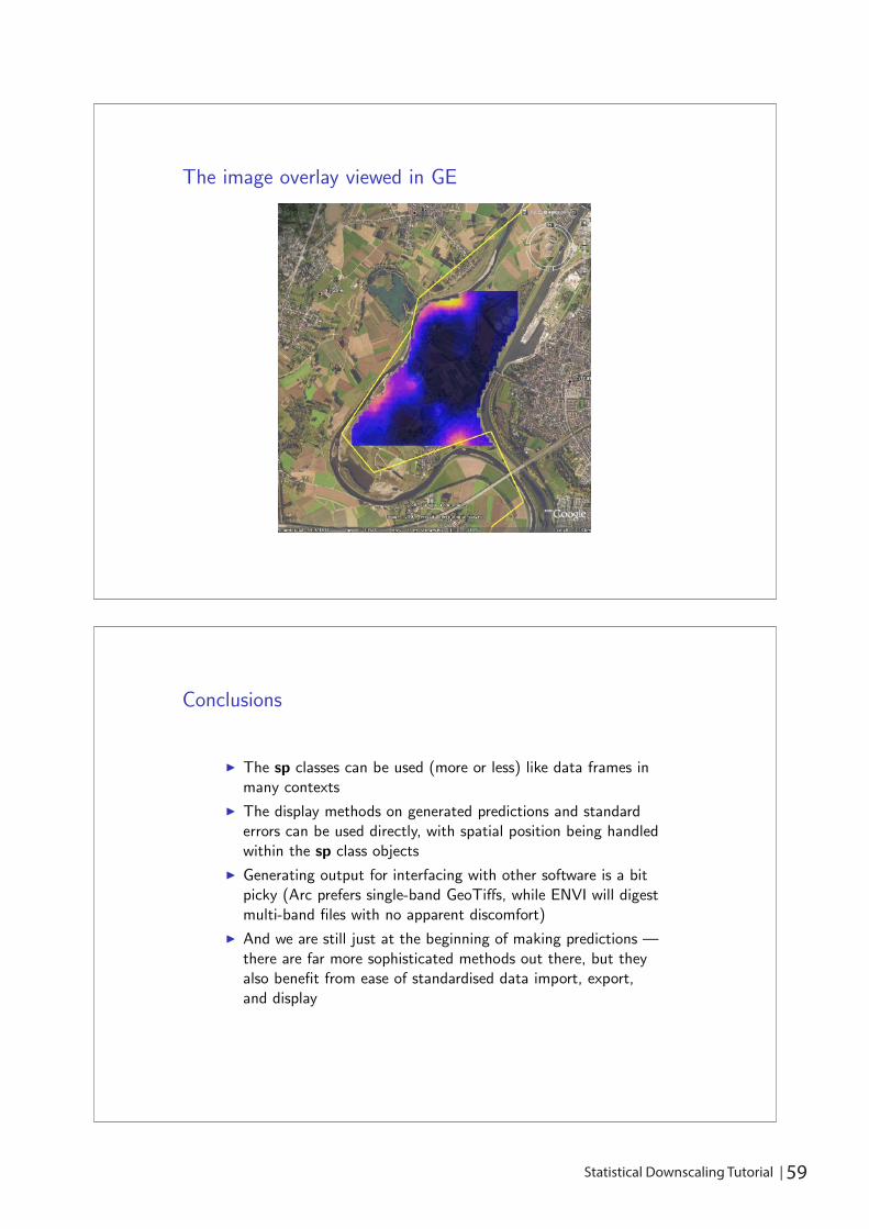
58 | Statistical Downscaling Tutorial Statistical Downscaling Tutorial | 59
Conclusions
� The sp classes can be used (more or less) like data frames inmany contexts
� The display methods on generated predictions and standarderrors can be used directly, with spatial position being handledwithin the sp class objects
� Generating output for interfacing with other software is a bitpicky (Arc prefers single-band GeoTiffs, while ENVI will digestmulti-band files with no apparent discomfort)
� And we are still just at the beginning of making predictions —there are far more sophisticated methods out there, but theyalso benefit from ease of standardised data import, export,and display
The image overlay viewed in GE

example of korean daily mean data

62 | Statistical Downscaling Tutorial

62 | Statistical Downscaling Tutorial Statistical Downscaling Tutorial | 63
구성
1. 소개
2. 자료
3. 통계모형
4. 결과
5. 결론및향후연구
통계적 보간법을 이용한
일별 평균기온 추정
대구대학교
전산통계학과
윤상후

64 | Statistical Downscaling Tutorial
통계적보간법 (통계적상세화기법)
inverse distance weighted interpolation, artificial neural network, canonical correlation analysis,
hidden Markov model, partial least squares regression, spline interpolation, parameter-elevation
Regressions on independent slopes Model, PRISM 등이존재
Linear model 모형 :이해하기쉬운직관적모형으로상대적으로쉽게모형과가능
일반선형모형 (General linear model)
일반화가법모형 (Generalized linear model)
공간선형모형 (Spatial regression model)
베이지안공간선형 (Bayesian spatial regression model)
1. 소개
• 다양한분야(농업, 수문등)에서고해상도격자기상정보의활용성과중요성증가
• 관측된자료로부터고르게분포된장기간의고해상도격자기상정보생산이필요
• 스케일상세화기법은통계적상세화기법과역학적상세화기법이존재
• 역학적상세화기법 :산지효과와같은물리적요소에대한대기과정을현실적으로모의가능
하지만상당한계산시간과방대한저장공간이요구됨
• 통계적상세화기법 :계산부하가작고모델앙상블전망을통해예측의불확실성평가
• 격자형국지기후자료 : 격자와관측지점간거리와지형학적환경을모두고려해야함
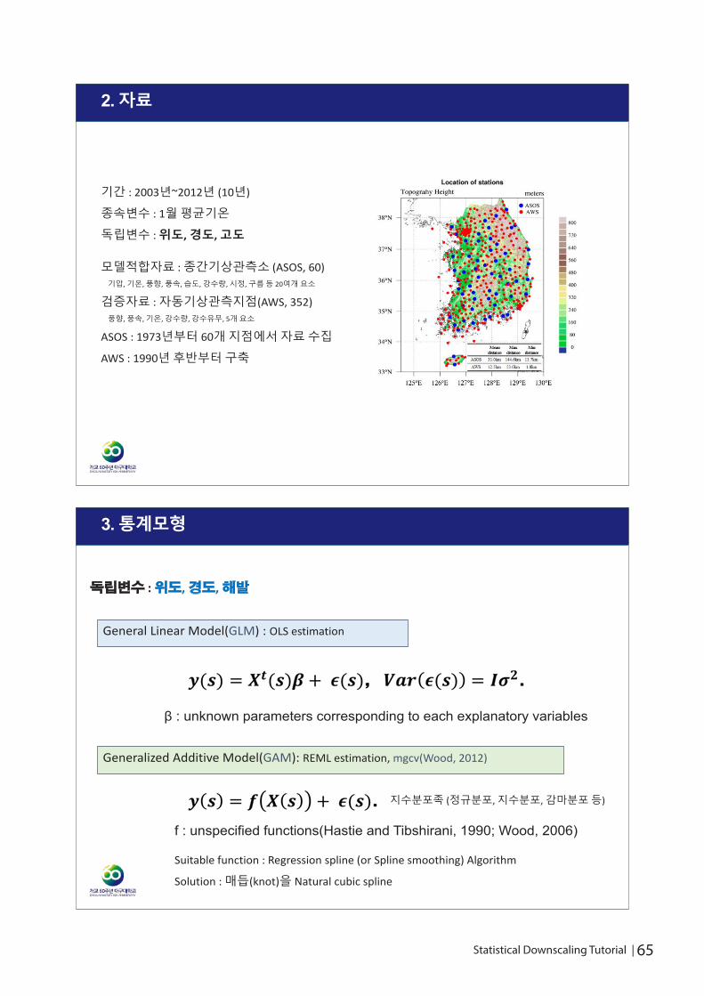
64 | Statistical Downscaling Tutorial Statistical Downscaling Tutorial | 65
3. 통계모형
General Linear Model(GLM) : OLS estimation
Generalized Additive Model(GAM): REML estimation, mgcv(Wood, 2012)
f : unspecified functions(Hastie and Tibshirani, 1990; Wood, 2006)
β : unknown parameters corresponding to each explanatory variables
독립변수 : 위도, 경도, 해발
지수분포족 (정규분포, 지수분포, 감마분포등)
Suitable function : Regression spline (or Spline smoothing) Algorithm
Solution : 매듭(knot)을 Natural cubic spline
2. 자료
기간 : 2003년~2012년 (10년)
종속변수 : 1월평균기온
독립변수 : 위도, 경도, 고도
모델적합자료 : 종간기상관측소 (ASOS, 60)기압, 기온, 풍향, 풍속, 습도, 강수량, 시정, 구름등 20여개요소
검증자료 : 자동기상관측지점(AWS, 352)풍향, 풍속, 기온, 강수량, 강수유무, 5개요소
ASOS : 1973년부터 60개지점에서자료수집
AWS : 1990년후반부터구축
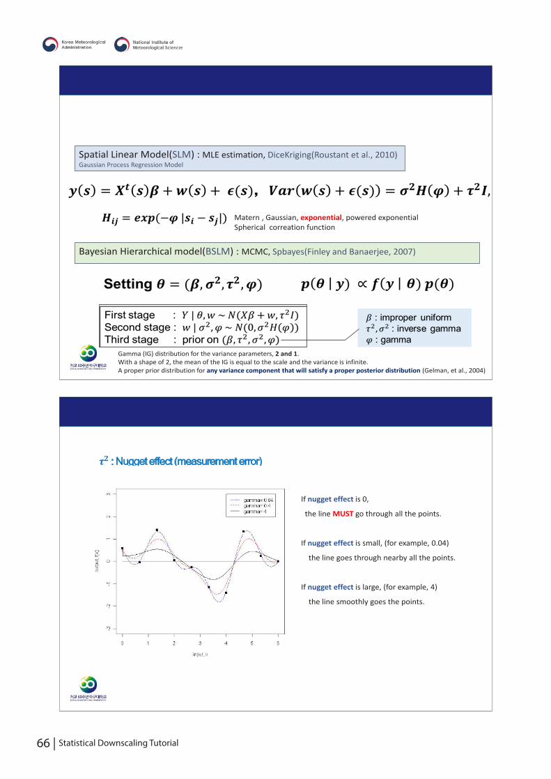
66 | Statistical Downscaling Tutorial
𝝉𝝉𝝉𝝉𝟐𝟐𝟐𝟐 : Nugget effect (measurement error)
If nugget effect is 0,
the line MUST go through all the points.
If nugget effect is small, (for example, 0.04)
the line goes through nearby all the points.
If nugget effect is large, (for example, 4)
the line smoothly goes the points.
Spatial Linear Model(SLM) : MLE estimation, DiceKriging(Roustant et al., 2010)Gaussian Process Regression Model
Bayesian Hierarchical model(BSLM) : MCMC, Spbayes(Finley and Banaerjee, 2007)
Matern , Gaussian, exponential, powered exponentialSpherical correation function
Gamma (IG) distribution for the variance parameters, 2 and 1.With a shape of 2, the mean of the IG is equal to the scale and the variance is infinite. A proper prior distribution for any variance component that will satisfy a proper posterior distribution (Gelman, et al., 2004)
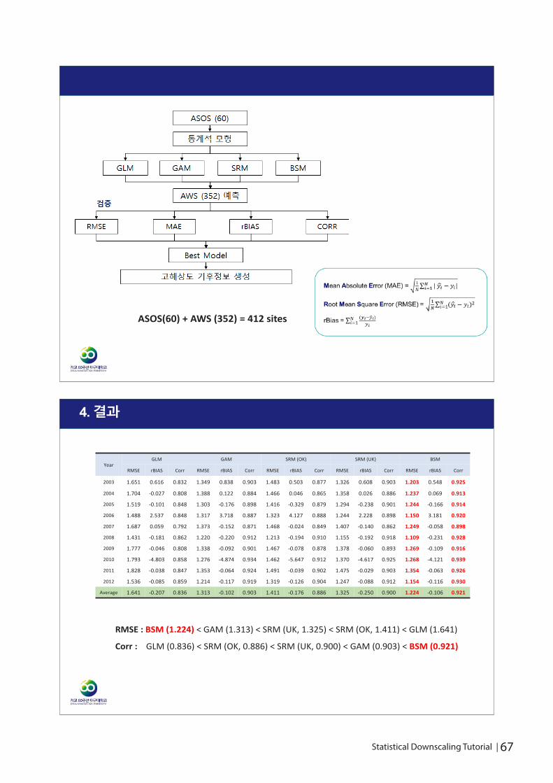
66 | Statistical Downscaling Tutorial Statistical Downscaling Tutorial | 67
4. 결과
YearGLM GAM SRM (OK) SRM (UK) BSM
RMSE rBIAS Corr RMSE rBIAS Corr RMSE rBIAS Corr RMSE rBIAS Corr RMSE rBIAS Corr
2003 1.651 0.616 0.832 1.349 0.838 0.903 1.483 0.503 0.877 1.326 0.608 0.903 1.203 0.548 0.925
2004 1.704 -0.027 0.808 1.388 0.122 0.884 1.466 0.046 0.865 1.358 0.026 0.886 1.237 0.069 0.913
2005 1.519 -0.101 0.848 1.303 -0.176 0.898 1.416 -0.329 0.879 1.294 -0.238 0.901 1.244 -0.166 0.914
2006 1.488 2.537 0.848 1.317 3.718 0.887 1.323 4.127 0.888 1.244 2.228 0.898 1.150 3.181 0.920
2007 1.687 0.059 0.792 1.373 -0.152 0.871 1.468 -0.024 0.849 1.407 -0.140 0.862 1.249 -0.058 0.898
2008 1.431 -0.181 0.862 1.220 -0.220 0.912 1.213 -0.194 0.910 1.155 -0.192 0.918 1.109 -0.231 0.928
2009 1.777 -0.046 0.808 1.338 -0.092 0.901 1.467 -0.078 0.878 1.378 -0.060 0.893 1.269 -0.109 0.916
2010 1.793 -4.803 0.858 1.276 -4.874 0.934 1.462 -5.647 0.912 1.370 -4.617 0.925 1.268 -4.121 0.939
2011 1.828 -0.038 0.847 1.353 -0.064 0.924 1.491 -0.039 0.902 1.475 -0.029 0.903 1.354 -0.063 0.926
2012 1.536 -0.085 0.859 1.214 -0.117 0.919 1.319 -0.126 0.904 1.247 -0.088 0.912 1.154 -0.116 0.930
Average 1.641 -0.207 0.836 1.313 -0.102 0.903 1.411 -0.176 0.886 1.325 -0.250 0.900 1.224 -0.106 0.921
RMSE : BSM (1.224) < GAM (1.313) < SRM (UK, 1.325) < SRM (OK, 1.411) < GLM (1.641)
Corr : GLM (0.836) < SRM (OK, 0.886) < SRM (UK, 0.900) < GAM (0.903) < BSM (0.921)
ASOS(60) + AWS (352) = 412 sites
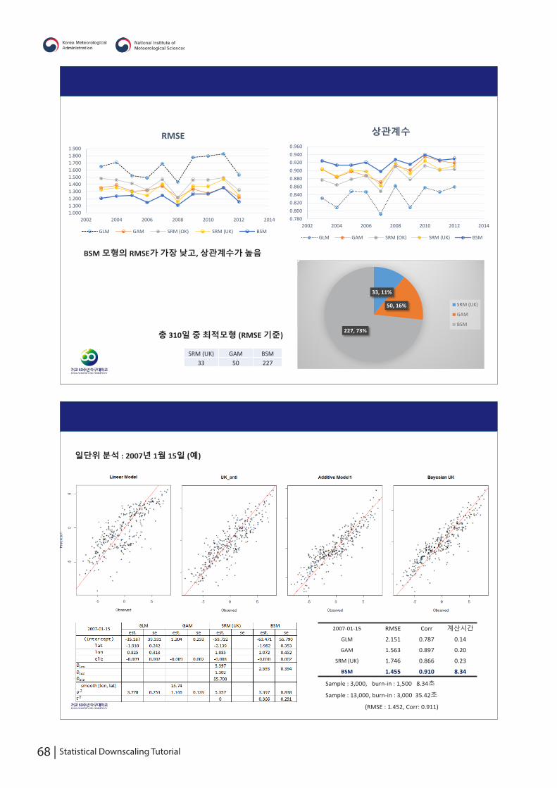
68 | Statistical Downscaling Tutorial
2007-01-15 RMSE Corr 계산시간
GLM 2.151 0.787 0.14
GAM 1.563 0.897 0.20
SRM (UK) 1.746 0.866 0.23
BSM 1.455 0.910 8.34
Sample : 3,000, burn-in : 1,500 8.34초
Sample : 13,000, burn-in : 3,000 35.42초
(RMSE : 1.452, Corr: 0.911)
일단위분석 : 2007년 1월 15일 (예)
0.7800.8000.8200.8400.8600.8800.9000.9200.9400.960
2002 2004 2006 2008 2010 2012 2014
상관계수
GLM GAM SRM (OK) SRM (UK) BSM
1.0001.1001.2001.3001.4001.5001.6001.7001.8001.900
2002 2004 2006 2008 2010 2012 2014
RMSE
GLM GAM SRM (OK) SRM (UK) BSM
BSM 모형의 RMSE가가장낮고, 상관계수가높음
33, 11%
50, 16%
227, 73%
SRM (UK)
GAM
BSM
SRM (UK) GAM BSM33 50 227
총 310일중최적모형 (RMSE 기준)
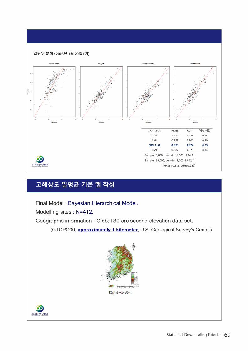
68 | Statistical Downscaling Tutorial Statistical Downscaling Tutorial | 69
고해상도일평균기온맵작성
Final Model : Bayesian Hierarchical Model.Modelling sites : N=412.Geographic information : Global 30-arc second elevation data set.
(GTOPO30, approximately 1 kilometer, U.S. Geological Survey’s Center)
2008-01-20 RMSE Corr 계산시간
GLM 1.419 0.775 0.14
GAM 0.977 0.900 0.20
SRM (UK) 0.876 0.924 0.23
BSM 0.887 0.921 8.34
Sample : 3,000, burn-in : 1,500 8.34초
Sample : 13,000, burn-in : 3,000 35.42초
(RMSE : 0.885, Corr: 0.922)
일단위분석 : 2008년 1월 20일 (예)
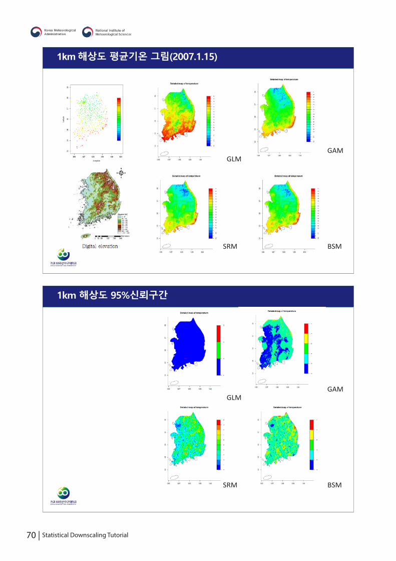
70 | Statistical Downscaling Tutorial
1km 해상도 95%신뢰구간
SRM
GAMGLM
BSM
1km 해상도평균기온그림(2007.1.15)
SRM
GAMGLM
BSM

70 | Statistical Downscaling Tutorial Statistical Downscaling Tutorial | 71
향후연구
독립변수 : 위도, 경도, 해발, 지향면, 해양도
2007-01-15 RMSE CorrGLM 2.151 0.787GAM 1.563 0.897
SRM (UK) 1.746 0.866BSM 1.455 0.910
2007-01-15 RMSE CorrGLM 1.945 0.859GAM 1.871 0.878
SRM (UK) 1.998 0.861BSM 1.697 0.911
최적예측을위해변수선택알고리즘필요
Kriging (Variogram model), MK-PRISM 등다른방법과예측성능비교
5. 결론
• 선형기반통계적보간법을이용한고해상도기후자료생성연구• GLM, GAM, SRM, BSM.
• 베이지안선형모형이일평균기온의공간적패턴을잘반영
• 통계적보간법은:• 기온, 강수량, 상대습도, 바람세기, 시나리오결과등다양하게적용가능.
• GAM과 SRM은베이지안선형모형에비해상대적으로계산시간은저렴하면서성능은우수함.
• 베이지안선형모형의경우 iteration이증가할수록정확도는향상되나, 계산시간이비싸지는단점이존재.

72 | Statistical Downscaling Tutorial