the international workshop on agromet and gis … · · 2017-12-18qgis tutorial for...
TRANSCRIPT
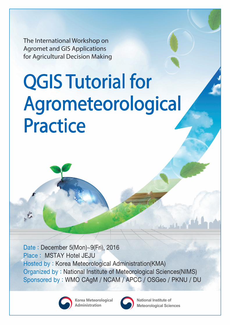
QGIS Tutorial for Agrometeorological Practice
Korea MeteorologicalAdministration
The International Workshop onAgromet and GIS Applicationsfor Agricultural Decision Making
Date : December 5(Mon)~9(Fri), 2016 Place : MSTAY Hotel JEJU Hosted by : Korea Meteorological Administration(KMA) Organized by : National Institute of Meteorological Sciences(NIMS) Sponsored by : WMO CAgM / NCAM / APCC / OSGeo / PKNU / DU

2 | QGIS Tutorial for Agrometeorological Practice

2 | QGIS Tutorial for Agrometeorological Practice QGIS Tutorial for Agrometeorological Practice | 3
contents1. The Background and Goals
2. Programs
3. Abstracts
4. Participant List
5. Logistic Information
05
11
21
25
50

4 | QGIS Tutorial for Agrometeorological Practice

4 | QGIS Tutorial for Agrometeorological Practice QGIS Tutorial for Agrometeorological Practice | 5
International Workshop on Agromet and GIS Applications 8
05~09 December 2016, Jeju Korea
QGIS Tutorial for Agrometeorological Practice
Organized by Dr. PAEK, Doojin and Dr. LEE, Seongkyu
Instructor Dr. PAEK, Doojin (Seoul Housing and Community Corporation), [email protected]
Dr. LEE, Seongkyu (APEC Climate Center), [email protected]
Who is for Anyone who is interested in GIS application for Agro-meteorology and this
program is for beginner and low intermediate. It will be a good starting point
for those who want to know how to apply climate/weather data with GIS tool to
their own fields, especially agriculture field.
Prerequisite The following items must be brought to the tutorial session :
1. His/her own notebook computer
Contents The detailed programs are as follows:
1. GIS training beginning – 1
- Introduction for OSGEO Korean Chapter
- Introduction for FOSS4G (Free and Open Sources Softwares (FOSS) for
Geospatial
- Overview of GIS (Geographic Information System)
- QGIS installation: program and example data
2. GIS training beginning – 2
- QGIS’ practice : introduction for GIS data (vector & raster etc)
3. GIS training intermediate – 1
- QGIS spatial analysis I
4. GIS training intermediate – 2
- QGIS spatial analysis II with agrometeorological example
Remarks The contents may be subject to change without notification. The text book and
sample data for GIS tutorial will be distributed in the tutorial session. Dr.
CHUNG, Uran (APEC Climate Center) will support agrometeorological practice.

6 | QGIS Tutorial for Agrometeorological Practice

6 | QGIS Tutorial for Agrometeorological Practice QGIS Tutorial for Agrometeorological Practice | 7
Introduction to QGIS - Using QGIS and ISCGM Global Map -

8 | QGIS Tutorial for Agrometeorological Practice
8 | QGIS Tutorial for Agrometeorological Practice QGIS Tutorial for Agrometeorological Practice | 9
I. Overview –QGIS
Doojin Paek([email protected])
Introduction to QGIS- Using QGIS and ISCGM Global Map -
Korean Chapter

10 | QGIS Tutorial for Agrometeorological Practice
I-1. QGIS OverviewI. Overview – QGIS & Global Map
4
QGIS
Desktop
QGIS
Desktop
QGIS
Browser
QGIS
Browser
QGIS
Client
QGIS
Client
QGIS
Server
QGIS
Server
QGIS Library Desktop GIS for
querying, creating, editing, analyzing geospatial data
Browser for spatial data
Web Mapping Framework based on QGIS Server and GeoExt
WMS 1.3.0, 1.1.1 Server FastCGI/CGI Program SLD Support
I-1. QGIS OverviewI. Overview – QGIS & Global Map
3
QGIS Free & Open Source Geographic Information System
OS
MS Windows Mac OSX Linux, Unix
License
GPL
Language
C++, Python, …
Release Date Version CodenameJul-02 0.0.1-Alpha Start!!!
3-May-08 0.1 "Io"21-Jul-08 0.11.0 "Metis"5-Jan-09 1.0.0 "Kore"1-Sep-09 1.2.0 "Daphnis"10-Jan-10 1.4.0 "Enceladus"29-Jul-10 1.5.0 "Tethys"27-Nov-10 1.6.0 "Copiapó"19-Jun-11 1.7.0 "Wrocław"21-Jun-12 1.8.0 "Lisboa"8-Sep-13 2.0.0-2.0.1 "Dufour"26-Feb-14 2.2 "Valmiera"27-June-14 2.4 "Chugiak"
31-October-14 2.6 “Brighton”20-Febrary-15 2.8 “Wein”26-June-15 2.10 “Pisa”
23-October-15 2.12 “Lyon”29-February-16 2.14 “Essen”
08-Jul-16 2.16 “Nødebo”

10 | QGIS Tutorial for Agrometeorological Practice QGIS Tutorial for Agrometeorological Practice | 11
6
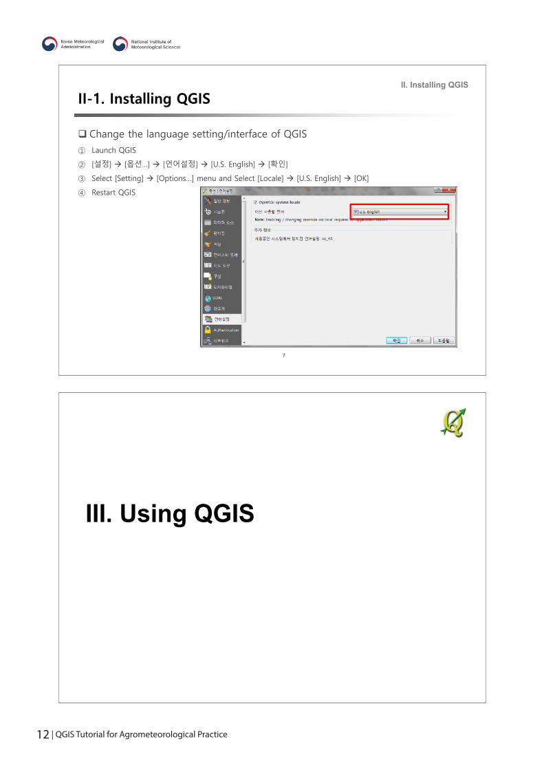
II-1. Installing QGISII. Installing QGIS
Install QGIS Essen (2.14.5, LTR Version) on Windows OS
① Download latest QGIS Standalone Installer Version 2.14 from http://www.qgis.org/
② Save the File to your machine and double click on the .exe file to install
③ Accept the install defaults to complete the process
④ Launch QGIS
II. Installing QGIS
12 | QGIS Tutorial for Agrometeorological Practice
III. Using QGIS
7
II-1. Installing QGISII. Installing QGIS
Change the language setting/interface of QGIS
① Launch QGIS
② [설정] [옵션…] [언어설정] [U.S. English] [확인]
③ Select [Setting] [Options…] menu and Select [Locale] [U.S. English] [OK]
④ Restart QGIS
12 | QGIS Tutorial for Agrometeorological Practice QGIS Tutorial for Agrometeorological Practice | 13
10
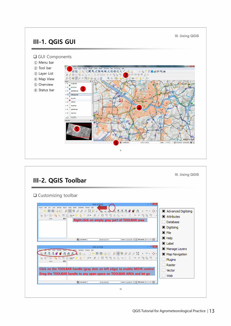
III-2. QGIS ToolbarIII. Using QGIS
Customizing toolbar
Right-click on empty gray part of TOOLBAR areaRight-click on empty gray part of TOOLBAR area
Click on the TOOLBAR handle (gray dots on left edge) to enable MOVE control
Drag the TOOLBAR handle to any open space on TOOLBAR AREA and let go
Click on the TOOLBAR handle (gray dots on left edge) to enable MOVE control
Drag the TOOLBAR handle to any open space on TOOLBAR AREA and let go
9
III-1. QGIS GUIIII. Using QGIS
GUI Components① Menu bar
② Tool bar
③ Layer List
④ Map View
⑤ Overview
⑥ Status bar
1122
33
44
55
66
14 | QGIS Tutorial for Agrometeorological Practice
12
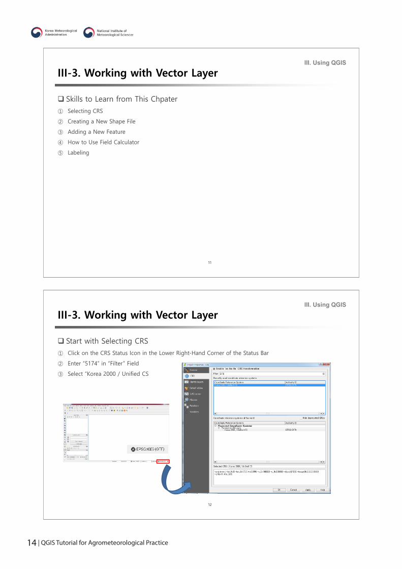
III-3. Working with Vector LayerIII. Using QGIS
Start with Selecting CRS
① Click on the CRS Status Icon in the Lower Right-Hand Corner of the Status Bar
② Enter “5174” in “Filter” Field
③ Select “Korea 2000 / Unified CS
11
III-3. Working with Vector LayerIII. Using QGIS
Skills to Learn from This Chpater
① Selecting CRS
② Creating a New Shape File
③ Adding a New Feature
④ How to Use Field Calculator
⑤ Labeling

14 | QGIS Tutorial for Agrometeorological Practice QGIS Tutorial for Agrometeorological Practice | 15
14
III-3. Working with Vector LayerIII. Using QGIS
Add a New Feature
① Click on the “Toggle Editing” Icon
② Click on the “Adding Feature” Icon
③ Click on Any Place on the Canvas
④ Fill in “id”, “High” and “Low” Fields
⑤ Add 2 More New Features on the Canvas (3 New Features Total)
⑥ Finish Editing by Clicking on the “Toggle Editing” Icon and “Save”
When a Prompt Window Pops Up
13
III-3. Working with Vector LayerIII. Using QGIS
New Shapefile Layer
① Layer Create Layer New Shapefile Layer…
② Add a New Field Named “High”
③ Add a New Field Named “Low”
④ Click “OK” and Save Layer as “temperature”

16 | QGIS Tutorial for Agrometeorological Practice
16
III-3. Working with Vector LayerIII. Using QGIS
Calculate Growing Degree-Day for Rice (Baseline = 10˚C)
① Fill in “Output field name” as “gdd”
② Select “Output field type” as “Decimal number(real)”
③ Input “10” into Precision Field
④ Type in a Formula for “gdd”
15
III-3. Working with Vector LayerIII. Using QGIS
Field Calculator
① Right Click on the “temperature” Layer on the Layers Panel
② Select “Open Attribute Table”
③ Click on “Open field calculator” Icon

16 | QGIS Tutorial for Agrometeorological Practice QGIS Tutorial for Agrometeorological Practice | 17
18
III-3. Working with Vector LayerIII. Using QGIS
Updating Existing Field
① Click Again on “Open field calculator” Icon
② Check “Update Existing Field”
③ Change the formula Using “Max” Function in “Math” Section
max( ( "High" + "Low")/2 - 10,0)Use “Recent” FunctionTo Bring up a Recently
Used Formula
17
III-3. Working with Vector LayerIII. Using QGIS
Field Calculator - Result
① Right Click on the “temperature” Layer on the Layers Panel
② Select “Open Attribute Table”
③ Click on “Open field calculator” Icon
The Result Can be Below “0”

18 | QGIS Tutorial for Agrometeorological Practice
20
III-3. Working with Vector LayerIII. Using QGIS
Labeling
① Right Click on the “temperature” Layer on the Layers Panel
② Select “Properties”
③ “Labels” “Show labels for this layer” Label with “High” “OK”
19
III-3. Working with Vector LayerIII. Using QGIS
Result

18 | QGIS Tutorial for Agrometeorological Practice QGIS Tutorial for Agrometeorological Practice | 19
22
III-4. InterpolationIII. Using QGIS
Skills to Learn from This Chapter
① Capturing Coordinate
② Calculating Distance from Field Calculator
③ Using Field Calculator Built-in Functions
④ Built-in Interpolation Tool
⑤ How to Style a Raster Layer
21
III-3. Working with Vector LayerIII. Using QGIS
Result
20 | QGIS Tutorial for Agrometeorological Practice
24
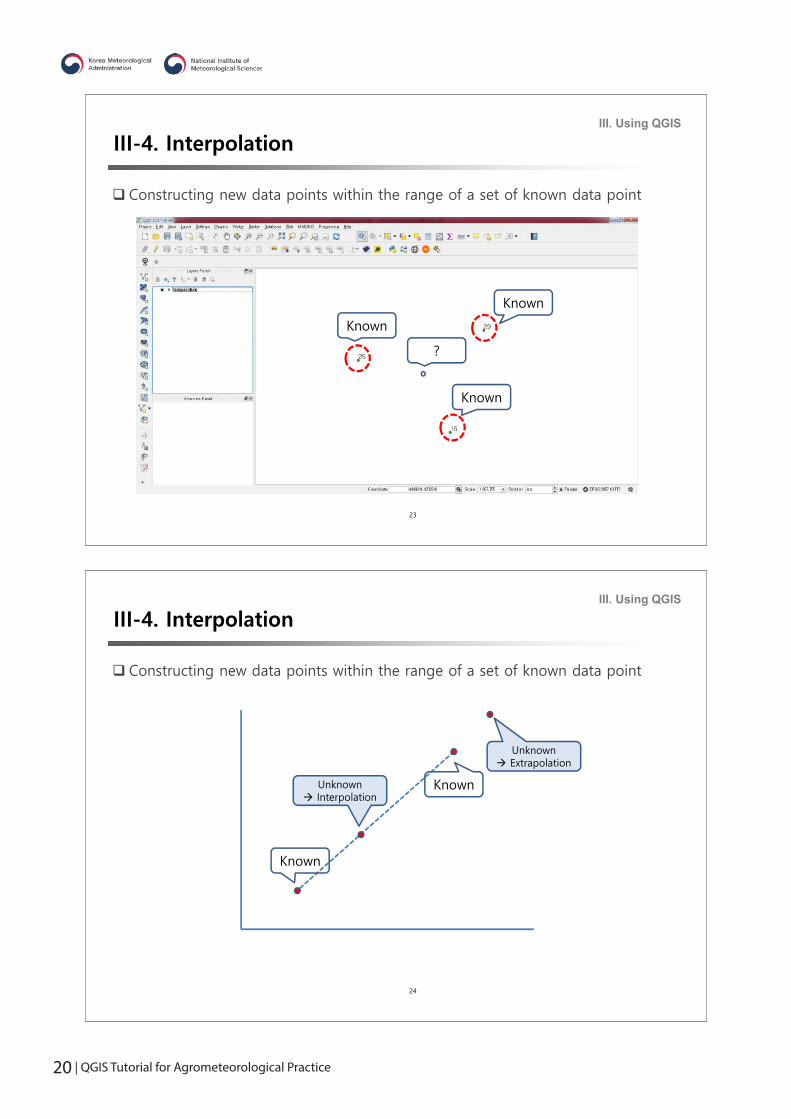
III-4. InterpolationIII. Using QGIS
Constructing new data points within the range of a set of known data point
Known
KnownUnknown Interpolation
Unknown Extrapolation
23
III-4. InterpolationIII. Using QGIS
Constructing new data points within the range of a set of known data point
Known
Known
Known
?

20 | QGIS Tutorial for Agrometeorological Practice QGIS Tutorial for Agrometeorological Practice | 21
26
III-4. InterpolationIII. Using QGIS
Constructing new data points within the range of a set of known data point
Known
Known
Polynomial
25
III-4. InterpolationIII. Using QGIS
Constructing new data points within the range of a set of known data point
Known
KnownLineal
22 | QGIS Tutorial for Agrometeorological Practice
28
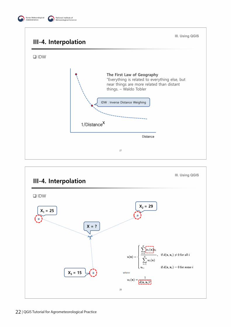
III-4. InterpolationIII. Using QGIS
IDW
X = ?
X1 = 25
X3 = 15
X2 = 29
27
III-4. InterpolationIII. Using QGIS
IDW
IDW : Inverse Distance Weighing
Distance
1/Distancex
The First Law of Geography“Everything is related to everything else, but near things are more related than distant things. – Waldo Tobler
22 | QGIS Tutorial for Agrometeorological Practice QGIS Tutorial for Agrometeorological Practice | 23
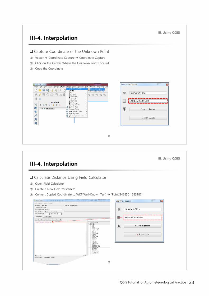
III-4. InterpolationIII. Using QGIS
Calculate Distance Using Field Calculator
① Open Field Calculator
② Create a New Field “distance”
③ Convert Copied Coordinate to WKT(Well-Known Text) ‘Point(948850 1653187)’
30
III-4. InterpolationIII. Using QGIS
Capture Coordinate of the Unknown Point
① Vector Coordinate Capture Coordinate Capture
② Click on the Canvas Where the Unknown Point Located
③ Copy the Coordinate
29

24 | QGIS Tutorial for Agrometeorological Practice
III-4. InterpolationIII. Using QGIS
Calculate Distance Using Field Calculator⑤ Calculate Distances Between X and (X1, X2, and X3)
distance($geometry, geom_from_wkt('Point(948850 1653187)'))
32
III-4. InterpolationIII. Using QGIS
Calculate Distance Using Field Calculator
④ Convert WKT to Geometry geom_from_wkt('Point(9488850 1653187)')
(Now, the Field Calculator Can Identify “X”)
31

24 | QGIS Tutorial for Agrometeorological Practice QGIS Tutorial for Agrometeorological Practice | 25
III-4. InterpolationIII. Using QGIS
Calculate Inverse Distance Weight Using Field Calculator
① Open Field Calculator
② Create a New Field “weight”
③ Calculate weight 1 / "distance" ^2
④ Click “OK”
34
III-4. InterpolationIII. Using QGIS
Calculate Distance Using Field Calculator⑥ Result
41481.2957
38561.0067
47249.3635
33
26 | QGIS Tutorial for Agrometeorological Practice
III-4. InterpolationIII. Using QGIS
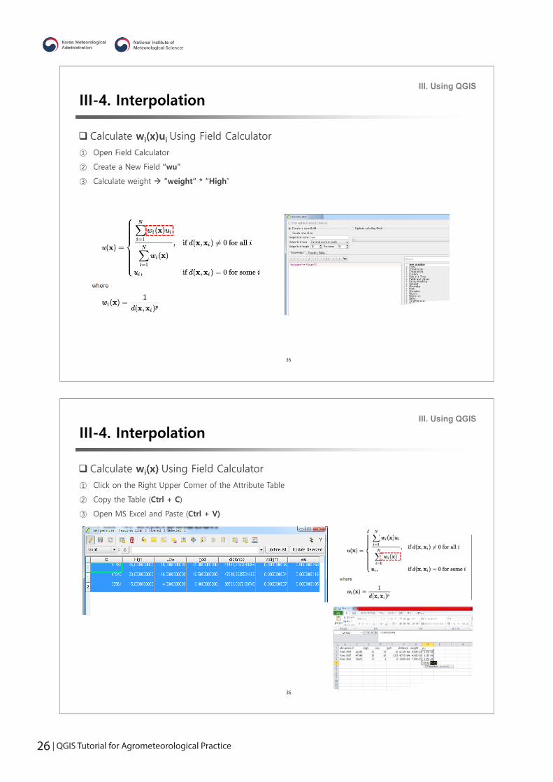
Calculate wi(x) Using Field Calculator
① Click on the Right Upper Corner of the Attribute Table
② Copy the Table (Ctrl + C)
③ Open MS Excel and Paste (Ctrl + V)
36
III-4. InterpolationIII. Using QGIS
Calculate wi(x)ui Using Field Calculator
① Open Field Calculator
② Create a New Field “wu”
③ Calculate weight “weight“ * “High”
35
26 | QGIS Tutorial for Agrometeorological Practice QGIS Tutorial for Agrometeorological Practice | 27
III-4. InterpolationIII. Using QGIS
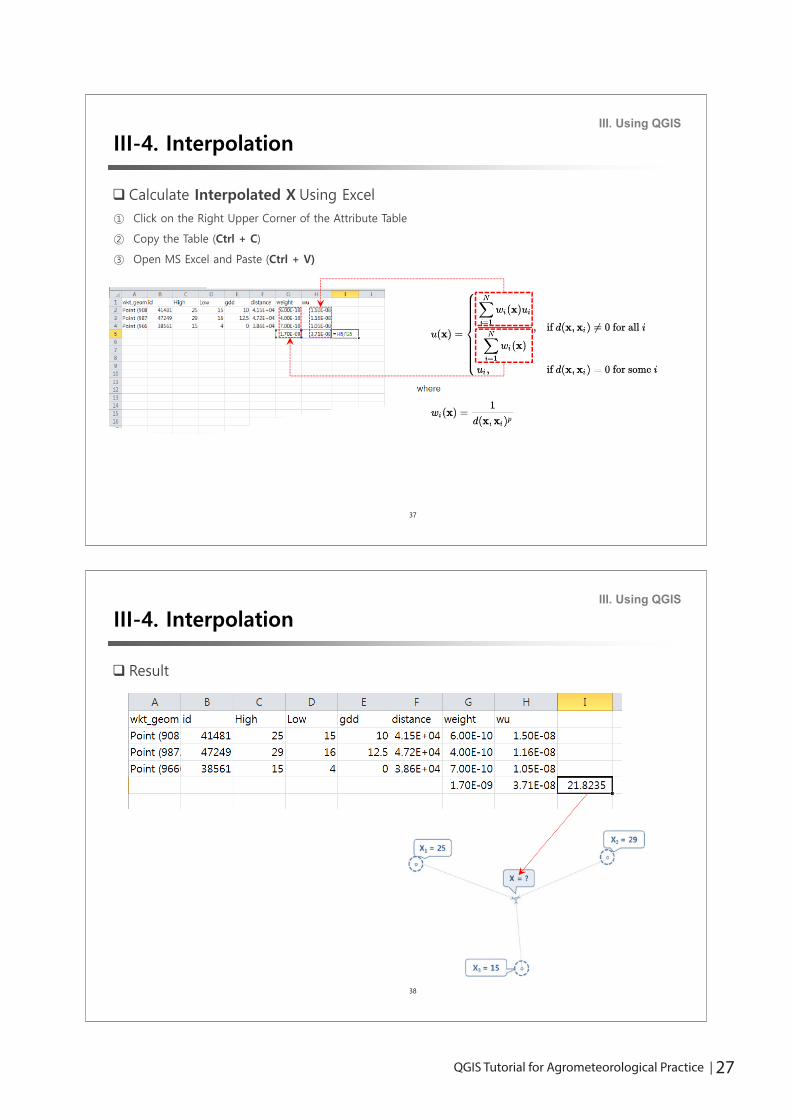
Result
38
III-4. InterpolationIII. Using QGIS
Calculate Interpolated X Using Excel
① Click on the Right Upper Corner of the Attribute Table
② Copy the Table (Ctrl + C)
③ Open MS Excel and Paste (Ctrl + V)
37

28 | QGIS Tutorial for Agrometeorological Practice
III-4. InterpolationIII. Using QGIS
Built-In Interpolation Tool
40
① Result
② Properties Style Render type(single band pseudocolor)
III-4. InterpolationIII. Using QGIS
Built-In Interpolation Tool
39
① Raster Interpolation Interpolation
② Select Vector Layer and Attribute
③ Click on “Add“ Button
④ Select Interpolation Method IDW
⑤ Click on “Set to current extent” Button
⑥ Save

28 | QGIS Tutorial for Agrometeorological Practice QGIS Tutorial for Agrometeorological Practice | 29
III-4. InterpolationIII. Using QGIS
Built-In Interpolation Tool
42
⑥ Zoom-In
⑦ Identify Feature
⑧ Click on Any Place on the Canvas
III-4. InterpolationIII. Using QGIS
Built-In Interpolation Tool
41
③ Check “Invert”
④ Click on “Classify” Button
⑤ Click on “OK” Button

30 | QGIS Tutorial for Agrometeorological Practice
44
III-5. Modeling with Vector GridIII. Using QGIS
Object
Modeling a process using vector grid
Advanced use of field calculator
Visualization of a process
Presentation of deterministic model
43
III-5. Modeling with Vector GridIII. Using QGIS
Scenario
Chemicals leaked from a special vehicle that was carrying toxic substance.
This chemical is a colorless and odorless that diffuses into the air
It is not a problem if it is exposed to less than 11,900 nanograms, but exposed to more than
that, the exposed need to be examined.
Thus, the authority made the following request to you.
What is the range of areas exposed above 11,900 nanograms?
This tutorial is inspired by Barry Rowlingson’s online R workshop linked below.
Barry Rowlingson. 2012. Geospatial Data in R and Beyond. Available at: http://www.maths.lancs.ac.uk/~rowlings/Teaching/UseR
2012/plume.html

30 | QGIS Tutorial for Agrometeorological Practice QGIS Tutorial for Agrometeorological Practice | 31
46
III-5. Modeling with Vector GridIII. Using QGIS
Basic Information
Information on the situation at the time of exposure was obtained below.
o α = Exposure level = 12,000o d = ?o β = 400o κ = Eccentricity (=strength of the wind = 5)o θ = Wind direction = North East = 45º (1/4pi)
Leak
A point “d” distance away from the leak point in the direction of θ
45
III-5. Modeling with Vector GridIII. Using QGIS
Basic Information
When chemicals are diffused into the air at a certain point, chemical exposure in the area is
expressed as a function of the following.
o α = Exposure levelo d = Distance from the release to a certain pointo β = Distance scale factoro κ = Eccentricity (=strength of the wind)o θ = Wind direction
Leak
A point “d” distance away from the leak point in the direction of θ
32 | QGIS Tutorial for Agrometeorological Practice
48
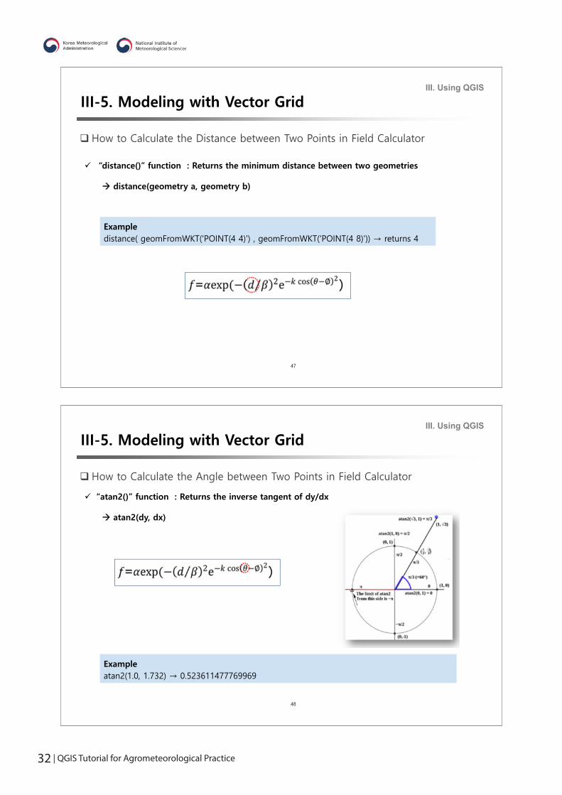
III-5. Modeling with Vector GridIII. Using QGIS
How to Calculate the Angle between Two Points in Field Calculator
“atan2()” function : Returns the inverse tangent of dy/dx
atan2(dy, dx)
Exampleatan2(1.0, 1.732) → 0.523611477769969
47
III-5. Modeling with Vector GridIII. Using QGIS
How to Calculate the Distance between Two Points in Field Calculator
“distance()” function : Returns the minimum distance between two geometries
distance(geometry a, geometry b)
Exampledistance( geomFromWKT('POINT(4 4)') , geomFromWKT('POINT(4 8)')) → returns 4

32 | QGIS Tutorial for Agrometeorological Practice QGIS Tutorial for Agrometeorological Practice | 33
50
III-5. Modeling with Vector GridIII. Using QGIS
Procedure
① Create a grid in the scope of analysis.
Initial Leak12,000 nanograms
49
III-5. Modeling with Vector GridIII. Using QGIS
How to Calculate a Centroid of a Polygon in Field Calculator
“centroid()” function : Returns the geometric center of a geometry
centroid(geom)
Examplecentroid($geometry) → returns geometry

34 | QGIS Tutorial for Agrometeorological Practice
52
III-5. Modeling with Vector GridIII. Using QGIS
Procedure
③ Adjust the color according to the function result.
10,500 10,000 9,500
11,500 11,000 10,000
11,500 10,500
51
III-5. Modeling with Vector GridIII. Using QGIS
Procedure
② Fill each grid with a function result.
10,500 10,000 9,500
11,500 11,000 10,000
11,500 10,500
Initial Leak12,000 nanograms

34 | QGIS Tutorial for Agrometeorological Practice QGIS Tutorial for Agrometeorological Practice | 35
54
III-5. Modeling with Vector GridIII. Using QGIS
Exercise
② Add a Vector Grid and Save as grid.shp
53
III-5. Modeling with Vector GridIII. Using QGIS
Exercise
① Add a leak point layer (release.shp) and a background map(EPSG=3857)
Google Satellite can be imported by
Web Openlayers Plugin Google Maps
Google Satellite
Plugins can be installed from Plugins Manage and Install Plugins …
36 | QGIS Tutorial for Agrometeorological Practice
56
III-5. Modeling with Vector GridIII. Using QGIS
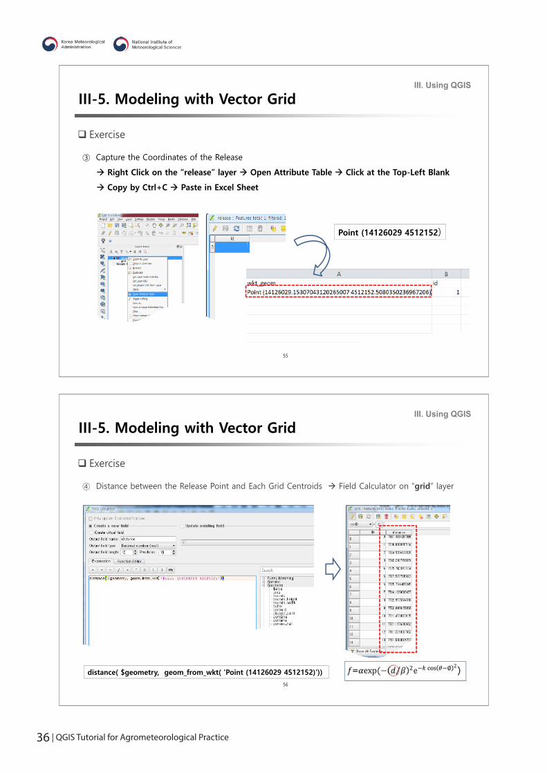
Exercise
④ Distance between the Release Point and Each Grid Centroids Field Calculator on “grid” layer
distance( $geometry, geom_from_wkt( 'Point (14126029 4512152)'))
55
III-5. Modeling with Vector GridIII. Using QGIS
Exercise
③ Capture the Coordinates of the Release
Right Click on the “release” layer Open Attribute Table Click at the Top-Left Blank
Copy by Ctrl+C Paste in Excel Sheet
Point (14126029 4512152)

36 | QGIS Tutorial for Agrometeorological Practice QGIS Tutorial for Agrometeorological Practice | 37
58
III-5. Modeling with Vector GridIII. Using QGIS
Exercise
⑥ Calculating Exposure Level of Each Grid Cell
12000*exp(-(("distance"/400)^2*exp(-5*cos("angle" - pi()/4))^2))
57
III-5. Modeling with Vector GridIII. Using QGIS
Exercise
⑤ Angle between the Release Point and Each Grid Centroids
distance( $geometry, geom_from_wkt( 'Point (14126029 4512152)'))

38 | QGIS Tutorial for Agrometeorological Practice
60
III-5. Modeling with Vector GridIII. Using QGIS
Exercise
⑧ Result
59
III-5. Modeling with Vector GridIII. Using QGIS
Exercise
⑦ Visualize Exposure Level of Each Grid Cell
Right Click on “grid” Layer Properties Style Graduated
38 | QGIS Tutorial for Agrometeorological Practice QGIS Tutorial for Agrometeorological Practice | 39
Thank youQ&A
61
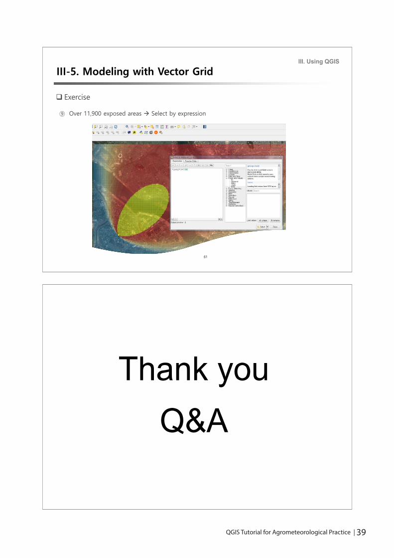
III-5. Modeling with Vector GridIII. Using QGIS
Exercise
⑨ Over 11,900 exposed areas Select by expression

40 | QGIS Tutorial for Agrometeorological Practice

40 | QGIS Tutorial for Agrometeorological Practice QGIS Tutorial for Agrometeorological Practice | 41
Exercise 1
Calculation of GDD from the digital map of temperature

42 | QGIS Tutorial for Agrometeorological Practice 42 | QGIS Tutorial for Agrometeorological Practice
42 | QGIS Tutorial for Agrometeorological Practice QGIS Tutorial for Agrometeorological Practice | 4342 | QGIS Tutorial for Agrometeorological Practice
페이지 1 / 24
Exercise 1 – Calculation of GDD from the digital map of temperature
Objectives: The goal of the first exercise for Agro-meteorology is to generate the
digital map of growing degree day (GDD) from the digital map of temperature. In order
to create the digital map of temperature, we first need to join CSV/Text file which has
temperature information (i.e., maximum temperature or minimum temperature) to vector
data (i.e., shape file) having coordination such as latitude and longitudes and interpolate.
In particular, we need the base temperature to calculate GDD of crops; in case of rice, a
summer crop, it starts growing at 10 Celsius degree.
1. Open the weather shape file. You can open the shape file from two ways. First one is
using the menu and the other one is just adding layers from “Drag and Drop from
Window Explorer” (see Note 1, Fig. 3).
- go to the file menu “Layer” >> click “Add Layer” >> select “Add Vector Layer”
(Fig. 1)
- click “Browse” button in ‘Add vector layer’ box and find the shape file: (Fig.2)
- file location: QGIS Tutorial – Data – Tutorial Session 2 – ASOS Observation:
kma_asos58.shp
Fig. 1.

44 | QGIS Tutorial for Agrometeorological Practice
페이지 2 / 24
Fig. 2.
Note 1: the way of “Drag and Drop”
Drag a shape file from the Windows Explorer and drop it on the ‘Layers Panel’.
Fig. 3.
2. Open the text file which has the monthly maximum temperature of Normal (1981-
2010).
- go to file menu “Layer” >> click “Add Layer‘ >> Select “Add Delimited Text Layer”
(Fig. 4)

44 | QGIS Tutorial for Agrometeorological Practice QGIS Tutorial for Agrometeorological Practice | 45
페이지 3 / 24
- click “Browse” button in ‘Create a Layer from a Delimited Text File’ box and find
the text file. In addition, should select the options of ‘CSV’ and ‘No geometry’ (Fig.
5)
- file location: QGIS Tutorial – Data – Tutorial Session 2 – ASOS Observation:
m30avg_tx8110.csv
Fig. 4.
Fig. 5.
3. In order to Join the text file to the vector. First of all, select ‘kma_asos58.shp’ on the

46 | QGIS Tutorial for Agrometeorological Practice
페이지 4 / 24
‘Layers Panel’ and click the right button of Mouse to open properties box.
- click the right button of Mouse and select “Properties” (Fig. 6)
- click the ‘Joins’ tab in the left contents’ list of ‘Layer Properties – kma_asos58’
box (Fig. 7)
Fig. 6.
Fig. 7.
4. Select the icon (cross symbol) in the ‘Lay properties – kma_asos58’ box and
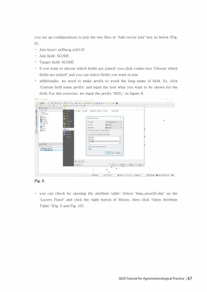
46 | QGIS Tutorial for Agrometeorological Practice QGIS Tutorial for Agrometeorological Practice | 47
페이지 5 / 24
you set up configurations to join the two files in ‘Add vector join’ box as below (Fig.
8).
- Join layer: m30avg_tx8110
- Join field: SCODE
- Target field: SCODE
- if you want to choose which fields are joined: you click combo box ‘Choose which
fields are joined’ and you can select fields you want to join
- additionally, we need to make prefix to avoid the long name of field. So, click
‘Custom field name prefix’ and input the text what you want to be shown for the
field. For this exercise, we input the prefix ‘M30_’ as figure 8.
Fig. 8.
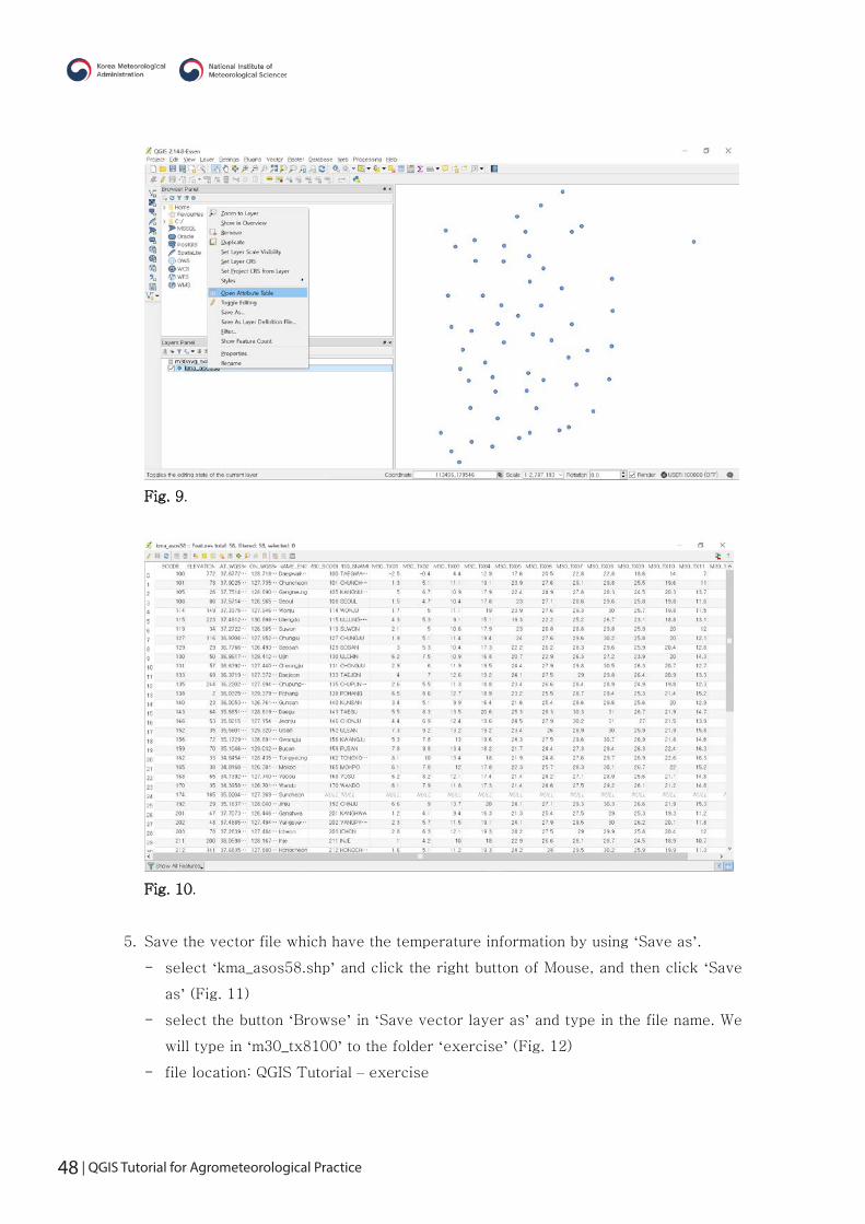
- you can check by opening the attribute table: Select ‘kma_asos58.shp’ on the
‘Layers Panel’ and click the right button of Mouse, then click ‘Open Attribute
Table’ (Fig. 9 and Fig. 10).
48 | QGIS Tutorial for Agrometeorological Practice
페이지 6 / 24
Fig. 9.
Fig. 10.
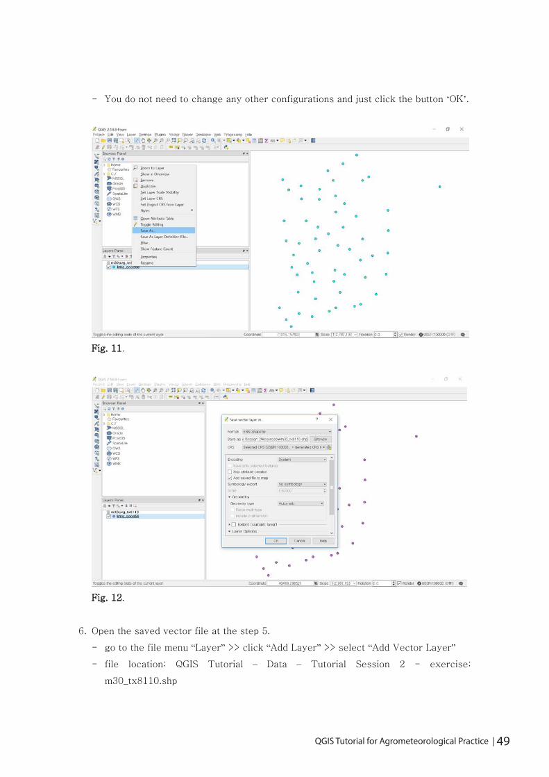
5. Save the vector file which have the temperature information by using ‘Save as’.
- select ‘kma_asos58.shp’ and click the right button of Mouse, and then click ‘Save
as’ (Fig. 11)
- select the button ‘Browse’ in ‘Save vector layer as’ and type in the file name. We
will type in ‘m30_tx8100’ to the folder ‘exercise’ (Fig. 12)
- file location: QGIS Tutorial – exercise
48 | QGIS Tutorial for Agrometeorological Practice QGIS Tutorial for Agrometeorological Practice | 49
페이지 7 / 24
- You do not need to change any other configurations and just click the button ‘OK’.
Fig. 11.
Fig. 12.
6. Open the saved vector file at the step 5.
- go to the file menu “Layer” >> click “Add Layer” >> select “Add Vector Layer”
- file location: QGIS Tutorial – Data – Tutorial Session 2 - exercise:
m30_tx8110.shp

50 | QGIS Tutorial for Agrometeorological Practice
페이지 8 / 24
- this shape file would be that you saved at the step 5. (Fig. 13)
Fig. 13.
7. We will interpolate with the temperature information. First, go to the menu ‘Raster’
and click ‘Interpolation’ and then click again “Interpolation” at the extended pull-
down menu (Fig. 14).
Fig. 14.
8. Set up the configurations as below (Fig. 15):

50 | QGIS Tutorial for Agrometeorological Practice QGIS Tutorial for Agrometeorological Practice | 51
페이지 9 / 24
- first, look at ‘Input’ panel in the left of ‘Interpolation plugin’ box, then
- click the combo box at ‘Vector layers’ and choose ‘m30_tx8110’
- again click the combo box at ‘Interpolation attribute’ and choose ‘M30_TX01’
- click the button ‘Add’ to input the selected field to the text box
- look at ‘Output’ panel in the right of ‘Interpolation plugin’ box,
- select ‘Inverse Distance Weighting (IDW)’ in ‘Interpolation method’
- type in ‘400’ for ‘Number of columns’ and ‘427’ for ‘Number of rows’,
respectively.
- we need to setup extent of map, type in X min and Y min, respectively: 51832.3
for X min,-33145 for Y min
- additionally, 546767.24 for X max, 569052.49 for Y max
(see Extent_Interpolation.txt file in DATA – Tutorial Session 2 folder)
- type in ‘m30_tx01’ in the folder ‘exercise’ to save the interpolation.
- file location: QGIS Tutorial – Data – Tutorial Session 2 - exercise (Fig. 15)
Fig. 15.

52 | QGIS Tutorial for Agrometeorological Practice
페이지 10 / 24
Fig. 16.
9. You can make interpolation from February to December
- file names for saving: m30_tx02 ~ m30_tx12
10. Likewise, you open the text file which has the minimum temperature and the shape
file. You interpolate then them. Remember from the step 2 to 9. So, you can have
24 digital temperature maps to calculate GDD of crop.
- file location to open the text file: QGIS Tutorial – Data – Tutorial Session 2 -
ASOS Observation: m30avg_tn8110.csv
- file location to open the shape file: QGIS Tutorial – Data – Tutorial Session 2 -
ASOS Observation: kma_asos58.shp
- file location and file name to save the vector file joined with the minimum
temperature: QGIS Tutorial – Data – Tutorial Session 2 – exercise:
m30_tn8110.shp
- then, save the interpolations as those filenames: m30_tn01 ~ m30_tn12
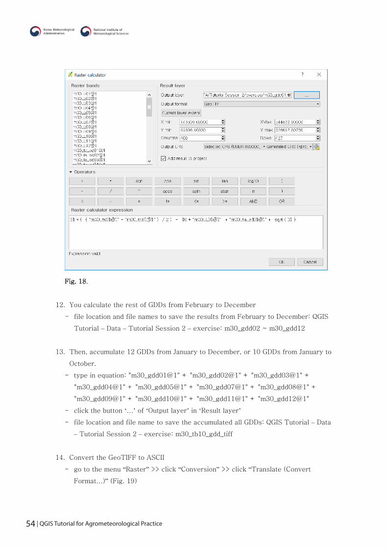
11. Now, you can calculate GDD by using ‘Raster calculator’ if you have 24 digital
temperature maps. Go to the menu ‘Raster Calculation” and open ‘Raster calculator’
box. (Fig. 17 and Fig. 18)
We will GDD equation as below (Kim et al., 2008):
GDD = N × ��(𝑇𝑇𝑇𝑇𝑥𝑥𝑥𝑥 − 𝑇𝑇𝑇𝑇𝑛𝑛𝑛𝑛)
2� − 𝑇𝑇𝑇𝑇𝑏𝑏𝑏𝑏 + 𝐿𝐿𝐿𝐿 × 𝜎𝜎𝜎𝜎 × √𝑁𝑁𝑁𝑁�
N: the number of month, Tx: the maximum temperature, Tn: the minimum

52 | QGIS Tutorial for Agrometeorological Practice QGIS Tutorial for Agrometeorological Practice | 53
페이지 11 / 24
temperature, Tb: the base temperature of crop, L: constant, σ: the standard
deviation of the average temperature
You can refer Thom (1954) since the constant L was calculated from that.
- should open the raster, constant L and standard deviation:
file location to open the raster, constant L: QGIS Tutorial – GDD – Constant L:
m30_L01 ~ m30_L12
file location to open the raster, standard deviation of the average temperature:
QGIS Tutorial – GDD – SD Tavg: m30_ta_sd01 ~ m30_ta_sd12
- type in equitation for January GDD as below, click operators as well (Fig. 17),
31 * ( ( "m30_tx01@1" + "m30_tn01@1" ) / 2 ) - 10 + "m30_L@1" *
"m30_ta_sd01@1" * sqrt ( 31 )
- click the button ‘…’ of ‘Output layer’ in ‘Result layer’
- file location and file name to save the calculated GDD: QGIS Tutorial – Data –
Tutorial Session 2 – exercise: m30_gdd01
- just check ‘GeoTIFF’ of ‘Output format’
Fig. 17.
54 | QGIS Tutorial for Agrometeorological Practice
페이지 12 / 24
Fig. 18.
12. You calculate the rest of GDDs from February to December
- file location and file names to save the results from February to December: QGIS
Tutorial – Data – Tutorial Session 2 – exercise: m30_gdd02 ~ m30_gdd12
13. Then, accumulate 12 GDDs from January to December, or 10 GDDs from January to
October.
- type in equation: "m30_gdd01@1" + "m30_gdd02@1" + "m30_gdd03@1" +
"m30_gdd04@1" + "m30_gdd05@1" + "m30_gdd07@1" + "m30_gdd08@1" +
"m30_gdd09@1" + "m30_gdd10@1" + "m30_gdd11@1" + "m30_gdd12@1"
- click the button ‘…’ of ‘Output layer’ in ‘Result layer’
- file location and file name to save the accumulated all GDDs: QGIS Tutorial – Data
– Tutorial Session 2 – exercise: m30_tb10_gdd_tiff
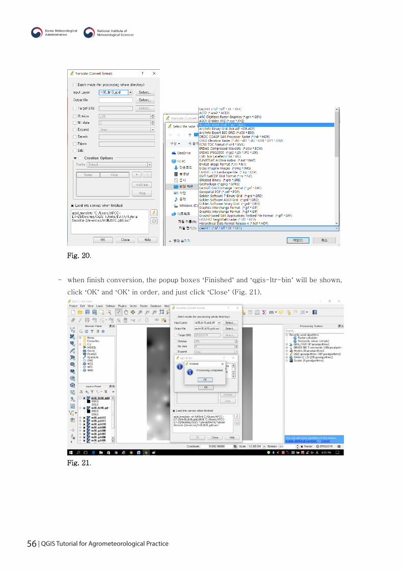
14. Convert the GeoTIFF to ASCII
- go to the menu “Raster” >> click “Conversion” >> click “Translate (Convert
Format…)” (Fig. 19)

54 | QGIS Tutorial for Agrometeorological Practice QGIS Tutorial for Agrometeorological Practice | 55
페이지 13 / 24
- if you want to translate the files are not in ‘Layers Panel’, can click the button
‘Select’ in ‘Translate (Convert format)’ box.
- but, we will translate the file which already opened in ‘Layers Panel’, so just click
the combo box and click ‘m30_tb10_gdd_tiff’ (Fig. 20).
- select the format ‘Arc/Info ASCII Grid (*.asc *.ASC)’ in the list and type in the file
name to save (Fig. 20).
- if finish type in the file name, do not change any options, and click ‘OK’.
Fig. 19.
56 | QGIS Tutorial for Agrometeorological Practice
페이지 14 / 24
Fig. 20.
- when finish conversion, the popup boxes ‘Finished’ and ‘qgis-ltr-bin’ will be shown,
click ‘OK’ and ‘OK’ in order, and just click ‘Close’ (Fig. 21).
Fig. 21.

56 | QGIS Tutorial for Agrometeorological Practice QGIS Tutorial for Agrometeorological Practice | 57
페이지 15 / 24
Reference:
Thom, H. C. S., 1954: The relationship between heating degree-days and temperature.
Monthly Weather Review, 82(9), 1-6.
Kim, J. H., J. I. Yun, 2008: On mapping growing degree-Days (GDD) from monthly digital
climatic surfaces for South Korea. Korean Journal of Agricultural and Forest
Meteorology, 10 (1), 1~8.
58 | QGIS Tutorial for Agrometeorological Practice
페이지 16 / 24
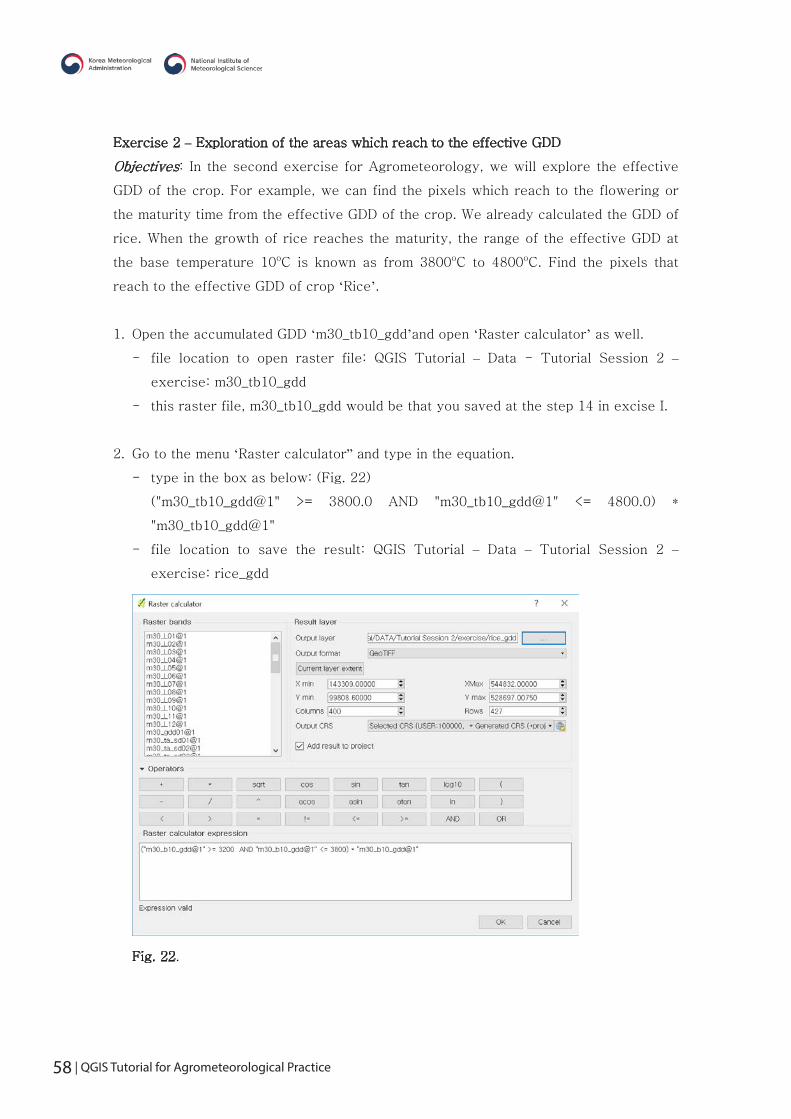
Exercise 2 – Exploration of the areas which reach to the effective GDD
Objectives: In the second exercise for Agrometeorology, we will explore the effective
GDD of the crop. For example, we can find the pixels which reach to the flowering or
the maturity time from the effective GDD of the crop. We already calculated the GDD of
rice. When the growth of rice reaches the maturity, the range of the effective GDD at
the base temperature 10oC is known as from 3800oC to 4800oC. Find the pixels that
reach to the effective GDD of crop ‘Rice’.
1. Open the accumulated GDD ‘m30_tb10_gdd’and open ‘Raster calculator’ as well.
- file location to open raster file: QGIS Tutorial – Data - Tutorial Session 2 –
exercise: m30_tb10_gdd
- this raster file, m30_tb10_gdd would be that you saved at the step 14 in excise I.
2. Go to the menu ‘Raster calculator” and type in the equation.
- type in the box as below: (Fig. 22)
("m30_tb10_gdd@1" >= 3800.0 AND "m30_tb10_gdd@1" <= 4800.0) *
"m30_tb10_gdd@1"
- file location to save the result: QGIS Tutorial – Data – Tutorial Session 2 –
exercise: rice_gdd
Fig. 22.

58 | QGIS Tutorial for Agrometeorological Practice QGIS Tutorial for Agrometeorological Practice | 59
페이지 17 / 24
Exercise 3 – Presentation of layout GDD
Objectives: We will make presentation with your results in the last exercise. First,
change legend and color scheme using ‘Style layer’ in properties of the raster, and then
make layout from “Map composer” (you already practiced at Introduction part of QGIS –
day I (7 December)).
1. Select the raster file, ‘m30_tb10_gdd’ in ‘Layers Panel’, click the right button of
Mouse and ‘Properties’ (Fig. 23).
- click ‘Style’ in ‘Layer Properties – m30_tb10_gdd’ box.
- click ‘Singleband pseudocolor’ of ‘Render type’ in the combo box.
- select ‘Classify’ of ‘Generate new color map’ in the right.
- if you change mode of classification, there two modes ‘Continuous’ and ‘Equal
Interval’.
- let’s change ‘Continuous’ to ‘Equal Interval’, then change 5 to 8 in Classes.
- lastly, select ‘Apply’ and ‘OK’.
Fig. 23.
60 | QGIS Tutorial for Agrometeorological Practice
페이지 18 / 24
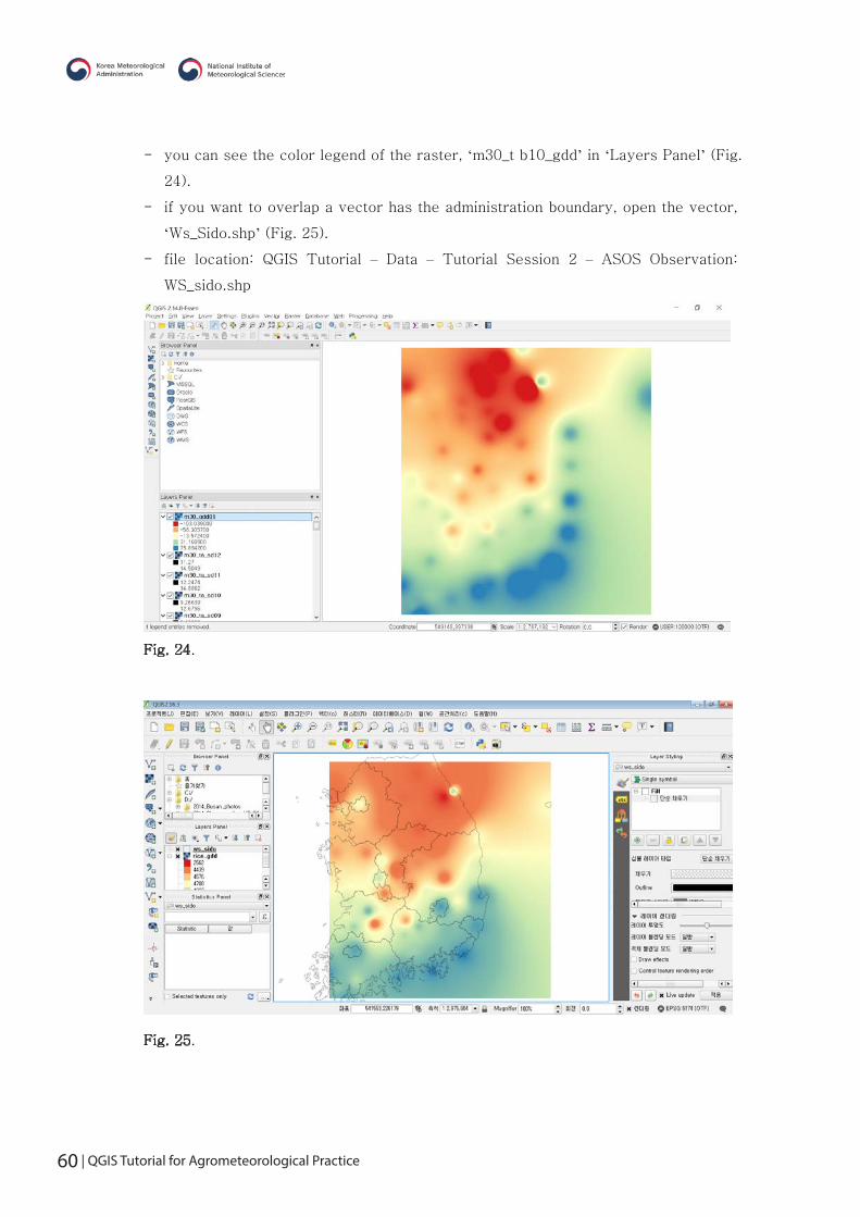
- you can see the color legend of the raster, ‘m30_t b10_gdd’ in ‘Layers Panel’ (Fig.
24).
- if you want to overlap a vector has the administration boundary, open the vector,
‘Ws_Sido.shp’ (Fig. 25).
- file location: QGIS Tutorial – Data – Tutorial Session 2 – ASOS Observation:
WS_sido.shp
Fig. 24.
Fig. 25.

60 | QGIS Tutorial for Agrometeorological Practice QGIS Tutorial for Agrometeorological Practice | 61
페이지 19 / 24
2. Go to the menu ‘Project’ and select ‘Composer manager’ (Fig. 26).
- Click ‘ADD’ button in ‘Composer manager’, and in order to create map, type in the
name of map: Rice_GDD in ‘Composer title’ box and click ‘OK’ (Fig. 27 and Fig.
28)
Fig. 26.
Fig. 27.

62 | QGIS Tutorial for Agrometeorological Practice
페이지 20 / 24
Fig. 28.
- You can see a new window ‘Rice_GDD’ (Fig. 29).
Fig. 29.
- go to the menu ‘Layout’ and click ‘Add Map’ in the pull-down menu (Fig. 30).
- you can check the figure of mouse pointer ‘+’ (cross). So, you drag the box in the
white box, then the map will be shown (Fig. 31).
- in addition, you can make other components of map, in instance legend, scale-bar,
and labels such as text (Fig. 32).
- click ‘Add Scalebar’ and drag the box to make scalebar.
- click ‘Add Legend’ and drag the box to make legend.

62 | QGIS Tutorial for Agrometeorological Practice QGIS Tutorial for Agrometeorological Practice | 63
페이지 21 / 24
Fig. 30.
Fig. 31.
64 | QGIS Tutorial for Agrometeorological Practice
페이지 22 / 24
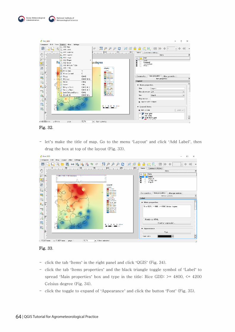
Fig. 32.
- let’s make the title of map. Go to the menu ‘Layout’ and click ‘Add Label’, then
drag the box at top of the layout (Fig. 33).
Fig. 33.
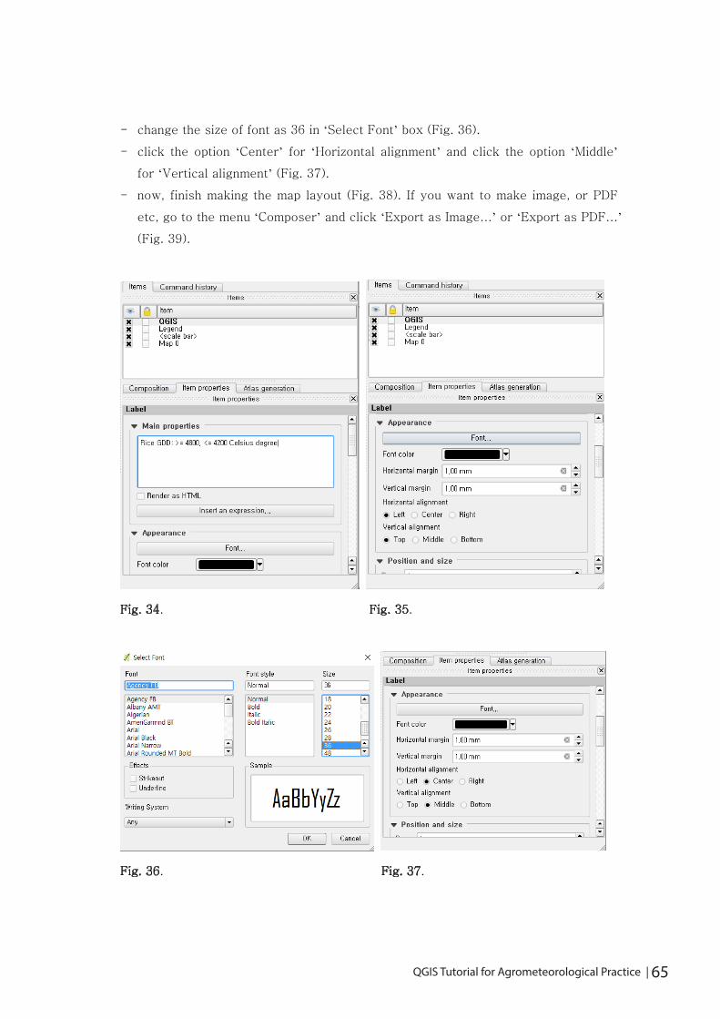
- click the tab ‘Items’ in the right panel and click ‘QGIS’ (Fig. 34).
- click the tab ‘Items properties’ and the black triangle toggle symbol of ‘Label’ to
spread ‘Main properties’ box and type in the title: Rice GDD: >= 4800, <= 4200
Celsius degree (Fig. 34).
- click the toggle to expand of ‘Appearance’ and click the button ‘Font’ (Fig. 35).
64 | QGIS Tutorial for Agrometeorological Practice QGIS Tutorial for Agrometeorological Practice | 65
페이지 23 / 24
- change the size of font as 36 in ‘Select Font’ box (Fig. 36).
- click the option ‘Center’ for ‘Horizontal alignment’ and click the option ‘Middle’
for ‘Vertical alignment’ (Fig. 37).
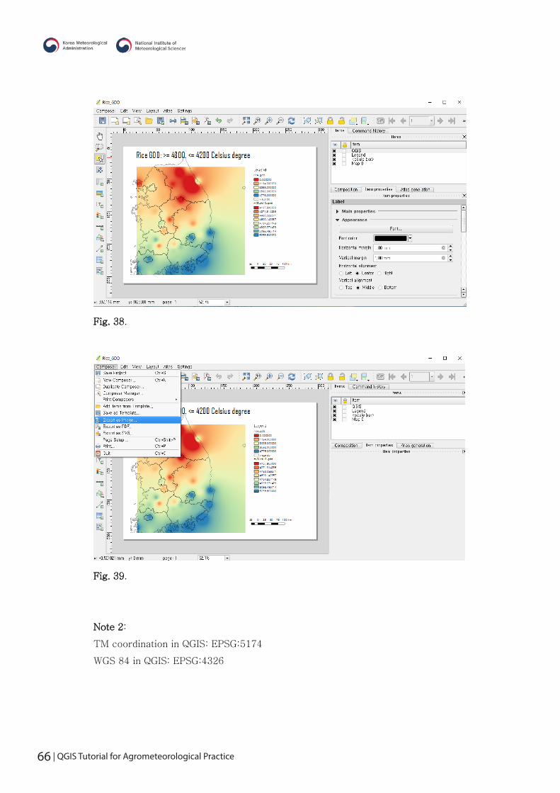
- now, finish making the map layout (Fig. 38). If you want to make image, or PDF
etc, go to the menu ‘Composer’ and click ‘Export as Image…’ or ‘Export as PDF…’
(Fig. 39).
Fig. 34. Fig. 35.
Fig. 36. Fig. 37.
66 | QGIS Tutorial for Agrometeorological Practice
페이지 24 / 24
Fig. 38.
Fig. 39.
Note 2:
TM coordination in QGIS: EPSG:5174
WGS 84 in QGIS: EPSG:4326