HAL Id: hal-02505669https://hal-mines-paristech.archives-ouvertes.fr/hal-02505669

Submitted on 11 Mar 2020

HAL is a multi-disciplinary open accessarchive for the deposit and dissemination of sci-entific research documents, whether they are pub-lished or not. The documents may come fromteaching and research institutions in France orabroad, or from public or private research centers.

L’archive ouverte pluridisciplinaire HAL, estdestinée au dépôt et à la diffusion de documentsscientifiques de niveau recherche, publiés ou non,émanant des établissements d’enseignement et derecherche français ou étrangers, des laboratoirespublics ou privés.

The Influx Management Envelope Considering RealFluid Behaviour Drilling Controls

Christian Berg, Geir Arne Evjen, Naveen Velmurugan, Martin Culen

To cite this version:Christian Berg, Geir Arne Evjen, Naveen Velmurugan, Martin Culen. The Influx Management En-velope Considering Real Fluid Behaviour Drilling Controls. SPE Drilling and Completion, Society ofPetroleum Engineers, 2019, 10.2118/198916-PA. hal-02505669

SPE xxxxxxApril 3, 2019

The Influx Management Envelope Considering Real Fluid BehaviourChristian Berg, University of South-Eastern Norway, Kelda Drilling Controls Geir Arne Evjen, Kelda Drilling Controls

Naveen Velmurugan, MINES ParisTech and Martin Culen, SPE, Blade Energy Partners

Abstract

The Influx Management Envelope (IME) Culen et al. (2016), is a decision making tool for how to deal with a influx during

managed pressure drilling (MPD) operations that offers a substantial improvement over the traditional MPD Well Control

Matrix (WCM). However, in the case study by Gabaldon et al. (2017), it has been found that the simplified analytical solution

introduced by Culen et al. (2016) makes the IME inaccurate for many real-world applications. This paper extends the original

IME that considers the gas migration in the annulus as a single bubble, without making the simplifying assumptions that are

required to make the equations explicit and analytically solvable. The underlying equations that are required to develop the

IME is derived from first principles and it is shown that using realistic equations of state (EOS) for gas, and a single-bubble

type model, the equations for the IME can be numerically solved yielding less conservative limits. The proposed approach is

significantly faster than constructing the IME through high-fidelity simulations. The proposed method allows the calculation

of peak circulating pressure at the surface and the maximum weak point pressure for a given kick size and initial shut-in

pressure, as well as a kick envelope with respect to formation limits. This makes the contributions of this paper relevant for

traditional well control decision making as well. The effect of considering various simplifying assumptions on the resulting

IME is studied and different scenarios that compare the results of the proposed approach with that of the original single

bubble equation for the IME by Culen et al. (2016) is presented.

Introduction

Managed Pressure Drilling (MPD) The main objective of Surface Back Pressure (SBP) MPD is to maintain the pressure

at a pre-determined anchor point (position) in the annulus constant, irrespective of pump flow. This is achieved using a

Rotating Control Device (RCD) that seals the annulus and diverts the return flow to the choke valves at the surface. As

mud pump flow rate changes, different back pressure can be applied from the surface, counteracting the changes in frictional

pressure at a given annulus location and thus keeping the pressure at that location constant. That is, counteracting changes

in pfriction (or phydrostatic if mud weight is changed) by psurface applied by the MPD chokes in Eq.1 where pap is the pressure

at the anchor point.

pap = phydrostatic + pfriction + psurface (1)

With a sealed annulus and chokes, the fundamental configuration on the surface when using MPD techniques is very

similar to a conventional drilling operation doing well control with a shut blowout preventer (BOP) and circulating through

well control chokes. This make MPD systems able handle a minor influx of gas in MPD operations without resorting

1

to traditional well control if the operational pressure limits for the RCD and MPD choke manifold are respected. Most

MPD operations have a sensitive return flow measurement available, allowing to detect influxes earlier than in conventional

operations (Willersrud et al. 2015), (Karimi Vajargah, Hoxha, and van Oort 2014) . The possibility of changing surface

pressure and thus affecting the bottomhole pressure in seconds allows MPD operations to suppress an influx more quickly

and with less influx volume than a conventional hard shut-in, (Zhou, Aamo, and Kaasa 2011), (Kinik, Gumus, and Osayande

2014). Some commercial automated MPD systems have built-in “kick detection” and “kick suppression” modes, see Kinik,

Gumus, and Osayande (2014)) that makes it possible to not only detect a kick earlier than with conventional methods, but

also to effectively suppress it without operator intervention.

MPD and well control Managed pressure drilling is defined by the IADC as: ”an adaptive drilling process used to

precisely control the annular pressure profile throughout the wellbore. The objectives are to ascertain the downhole pressure

environment limits and to manage the annular hydraulic pressure profile accordingly. It is the intention of MPD to avoid

continuous influx of formation fluid to the surface. Any influx incidental to the operation will be safely contained using

an appropriate process” In the above definition, MPD is an overbalanced drilling operation, and MPD equipment is not

well control equipment. The equipment available when during MPD operations still makes it possible to have a less clear

definition than for conventional drilling of when an influx should be considered a ”well control” situation. When using MPD

techniques the ”appropriate process” might be to carry on operations as normal in the case of a small gas influx. If a kick is

encountered and after the initial kick detection and suppression is finished a range of possible paths forward is possible.

• Circulate out the kick using the MPD line-up using the MPD equipment.

• The BOP can be shut, and then the kick can be circulated out below the shut BOP, through the secondary MPD flow

line and through MPD chokes with MPD chokes managing the back pressure. This enables a very rapid transition to

conventional well control if required.

• Ramp down the pumps while adding surface pressure like for a normal MPD connection, and then perform a hard shut

in and conventional well control.

Deciding what is the best option of all the alternatives for a given kick is no straight forward task, depending on a number

of factors. It is important to note that the time involved in circulating the gas out, which is Non-Productive Time (NPT), is

different for all the alternatives, from low to high from the first to last alternative. It is also worth noting that transitioning

between the above alternatives could also be performed when the gas is closer to surface instead of right after the initial kick,

thus reducing the time required to circulate the gas out.

The MPD “well control matrix” WCM shown in Fig.1 was introduced to help deal with this decision making specifically.

The WCM is the preferred industry tool today and is required by regulators in several regions for using MPD techniques,

(Mir Rajabi, Hannegan, and Moore 2014). The WCM is typically developed and agreed upon during planning of the MPD

operation for each hole section drilled. The limits set in the WCM is a combination of barrier limits (max allowable back

pressure at surface) and kick detection accuracy. Although a significant improvement over ”nothing” when it comes to well

control decision making during MPD, the WCM still have some limitations, and the actual severity of a kick as reflected

2

Figure 1: Example of the MPD Well Control Matrix

by the WCM is unclear. For instance, weak point fracture pressure is not reflected in the WCM. In the example of Fig.1 if

operating close to formation limits with respect to kick tolerance any influx might become challenging with respect to well

control, while the WCM would indicate ”all green”. Combining traditional kick tolerance calculations, with the barrier limits

from the WCM in a continuous and data driven manner while maintaining the operational simplicity of the WCM is the

main goal of the IME. As the initial goal of the WCM was to bridge traditional well control with the possibilities presented

by MPD, the IME aims to improve this coupling by also considering kick tolerance, and to set less arbitrary limits on when

to transition to conventional well control. This is achieved through quantifying kick volume vs peak surface- and weak point

pressure.

Influx Management Envelope (IME) The fundamental idea of the IME is using traditional single bubble kick tolerance

calculations for correlating kick size, initial shut in pressure and peak surface- and weak point- pressure while circulating

gas to surface. Using this approach, a more “data-driven” approach to the WCM limits can be achieved. Maximum surface

pressure that will be encountered while circulating out the influx is a function of the initial surface pressure and a given

kick volume. In the IME, the limit for deciding whether to circulate a kick out using conventional well control or MPD is

calculated as a combination of initial shut in surface pressures and kick volumes, giving a kick envelope. The concept of

considering a kick envelope and comparing the link between this and the WCM was performed by Mir Rajabi, Hannegan,

and Moore 2014 using a high fidelity simulator. In the original IME paper, Culen et al. (2016) does simplifications to make

calculation of this kick envelope curve explicit and analytically solvable. Gabaldon et al. (2017) shows that this approach

might be overly conservative by comparing this to a high fidelity simulator.

Fig.2 shows how the output of the IME calculations are presented. The IME chart aims to replicate the original WCM

in its basic form, but with the post influx surface pressure and influx volume being continuous inputs. The line separating

the red and yellow region is the combination of post influx pressure and influx volume that would lead to surface pressure

being exactly the set limit pressure when the kick reach the surface. The calculation of this ”limit line” is the core of the

IME, and the position of the limit line will be significantly affected by the chosen simplifications. The equation presented in

3

Culen et al. (2016), Eq.2 assumes ideal gas, gas kick at the bottom and incompressible liquid. Eq. 2 will be derived in detail

later in this article.

Vkick =psurf − psbp,i

g

κsurfκdhpsurfTdh

(ρl − ρg)(pdhTsurfκdh − cos(θ)psurfTdhκsurf)(2)

If setting psurf as the maximum pressure to put on the well using MPD, Vkick is calculated as a function of psbp,i, the post

influx surface pressure right after the kick is suppressed. Setting psbp,i to the post influx surface pressure and Vkick for a

given influx, the peak surface pressure for the given kick can be calculated as psurf . The Influx detection limit that defines

the green region is set at an value chosen from experience.

After the IME limits are calculated the chart is prepared for field use. In operation if a kick is encountered the MPD

operator can plot the post influx surface pressure and kick volume as a point in the chart. Depending on the position of the

”dot” in the chart the IME gives information about whether the maximum surface pressure limit will be violated if circulating

the kick using the MPD system while maintaining bottomhole pressure constant.

Figure 2: Influx management envelope, extending the WCM concept, Culen et al. 2016

4

Extending the single bubble IME

A

z1

z0

Bz0

z1

zB

Cz0

z1

zC1

zC2

Dz0

z1

zD

Liquid

Gas

Figure 3: Schematic representation of the stages of influx circulation considered

Fig. 3 illustrates a wellbore at four different time instances. Symbol z is vertical depth, where z1 is at the bottom and

z0 is at the top. Symbols A, B, C and D denotes points in time from before the influx has occurred to it has been observed

and finally circulated out of the wellbore. The time instances can be explained as follows: (A) No indication of kick; (B)

influx has been observed and suppressed by applying additional surface pressure (C) influx is just below a formation weak

point at depth zC1 and (D) when the kick has reached the surface. In situation (A) no gas has entered the wellbore, i.e

the wellbore is filled with mud and there are no surface indications of a kick. At time (B), the operator has encountered

an increase in return flow and stopped the kick by increasing the surface back pressure. When the kick has been stopped,

the flow rate stabilizes and returns back to the flow rate at the point before the kick was observed. From this point on,

the bottomhole pressure must be kept constant while circulating the gas up annulus. At time (C) the influx is just below a

formation weakpoint. The gas has expanded and surface pressure is increased to keep bottomhole pressure constant. Finally,

at time (D) the gas has expanded and reached the surface, here illustrated with a gas pocket at the top of the wellbore. Note

that, in order to maintain a constant downhole pressure, the surface pressure at (D) must be higher than at time (C), and

at time (C) must be higher than at time (B). In all following derivations, pB , pC and pD is the pressure profile as a function

of depth Z in the three cases (B), (C) and (D) respectively. In all cases the surface pressure must not exceed any surface

equipment pressure limits, i.e. pA(z0) ≤ pB(z0) ≤ pC(z0) ≤ pmax(z0) and the weak point formation pressure limit should not

5

be exceeded pC(zC1) < pmax(zC1).

Fundamental assumptions The goal of the following derivations is to find a relation between the post influx surface

pressure pB(z0) and the initial influx size (Vg) at time (B) where the expanded influx at the weak-point at time (C) and

surface at time (D) do not violate the pressure limits when keeping bottomhole pressure constant. The calculation of the

limit line in the IME is based primarily on two main assumptions:

1. The downhole pressure is kept constant during circulation of the influx

2. The mass of gas in the system is constant

The wellbore is considered an open system, where mud can enter and leave. It is assumed that the mud enters at the bottom

and leaves at the top; the typical flow direction of the wellbore. The mass of the system is distributed as a volumetric mix

of mud and gas along the wellbore where the volumetric fraction of gas α can vary from 0 to 1 where α = 1 is pure gas and

α = 0 is pure mud. Single bubble of gas is not assumed in the initial derivation and the introduction of this assumption is

done in detail.

Constant bottomhole pressure Downhole pressure at any location z is the sum of a hydrostatic and a frictional pressure

component. The downhole pressure at any time and location z can then be found from Eq. (3):

p(z) = p(z0) + g

∫ z

0

[[1− α(T, p)]ρl(T, p) + α(T, p)ρg(T, p)] dZ +∆pf (z) (3)

where ρl and ρg is density of the liquid and gas respectively, p(z0) is the surface pressure and ∆pf (Z) is the friction as a

function of depth due to flow in the wellbore. Note that temperature T and pressure p depends on depth Z. Densities of

mud and gas can be found from simple density relations to more accurate PVT1 calculations using a real-gas Equation of

State (EOS). In either case, the proceeding derivation makes no assumptions on the EOS, other than that it is continuous in

temperature and pressure.

After an influx has been detected (A) and subsequently suppressed (B) by applying an additional surface pressure, the

downhole pressure is kept constant while circulating the influx up and out of the wellbore. When the influx is just below

a formation weak point (C) the required surface pressure is pc(z0) (pC(z0) > pB(z0)). When the influx has arrived at the

surface (D), the required surface pressure is pD(z0) (pD(z0) > pC(z0)). Equations for the downhole pressure is given in Eq.(4)

with i ∈ [B,C,D] representing time instances (B), (C) and (D).

pi(z1) = pi(z0) + g

∫ z1

0

[[1− αi(T, pi(Z))]ρl(T, pi(Z)) + αi(T, pi(Z))ρg(T, pi(Z))] dZ +∆pfi(z1)(4)

Note that the volume fraction distributions αB , αC and αD differ since the influx is higher up in the annulus for case

(C) than (B) and for case (D) than (C).

Constant influx mass The second assumption is that the mass of the influx must remain constant from time (B) through

(D). This follows from the assumption that the bottomhole pressure is kept constant2, and from conservation of mass. The1Pressure-Volume-Temperature2It is assumed that there is no secondary influx when circulating the gas out

6

integrated mass of gas from location V0 = 0 to V (Z) at any given time is given by Eq.(5)

m =

∫ V

0

ρg(T, p)α(T, p)dV (5)

Defining the mapping between vertical depth Z and measured depth L as h : Z 7→ L and assuming that h(Z) is Lipschitz

continuous then its differential is

dL =∂h

∂ZdZ (6)

Defining hzdef= ∂h

∂Z and inserting into Eq. (5), differential annuluar volume of the wellbore is given by

dV = A(L)dL = A(h(Z))hzdZ (7)

where A(L) is the area of the annulus at any measured depth L. The total mass of gas in the system will be given as

m =

∫ Z

0

ρg(T, p)α(T, p)A(h(Z))hzdZ (8)

where the integral is formulated in vertical depth Z. Accumulated gas in the wellbore at times i ∈ [B,C,D] is then given as

Eq. (9).

mi =

∫ z1

0

ρg(T, pi)αi(T, pi)hzA(h(Z))dZ (9)

Single bubble assumption The volumetric gas distribution αB , αC and αD can be used to define any distribution of the

influx gas in the wellbore. The most common and simplest form of this is to sum up all the gas into one gas volume with

α = 1 and place the volume at the top, below the weak point and at the bottom of the wellbore, to represent times (D),

(C) and (B) respectively. Mathematically a single bubble can be defined using a piecewise function for αB , αC and αD but

limited by the boundaries zB , zC1, zC2 and zD such that 0 < zB < zC2 − zC1 < zD < z1:

αB =

0 0 ≤ Z ≤ zB

1 zB < Z ≤ z1(10)

αC =

0 0 ≤ Z ≤ zC1

1 zC1 < Z < zC2

0 zC2 ≤ Z ≤ z1

(11)

and

αD =

1 0 ≤ Z ≤ zD

0 zD < Z ≤ z1(12)

Fig. 4 illustrates the gas bubbles for time instances (B), (C) and (D), one at the top of the wellbore, one below the formation

weak point and one at the bottom. Note that the length of the intervals are set different, as one expect that the volume of

gas is larger at the top then at the bottom, but that the exact size are for illustrative purposes only.

7

0 ZD ZC1 ZC2 ZB Z

0

1 αCαDαB

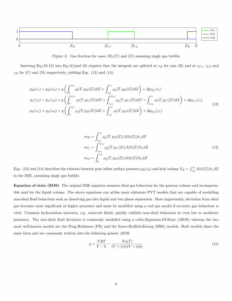
Figure 4: Gas fraction for cases (B),(C) and (D) assuming single gas bubble

Inserting Eq.(10-12) into Eq.(4))and (9) requires that the integrals are splitted at zB for case (B) and at zC1, zC2 and

zD for (C) and (D) respectively, yielding Eqs. (13) and (14).

pB(z1) = pB(z0) + g

(∫ zB

0

ρl(T, pB(Z))dZ +

∫ z1

zB

ρg(T, pB(Z))dZ

)+∆pfB (z1)

pC(z1) = pC(z0) + g

(∫ zC1

0

ρl(T, pC(Z))dZ +

∫ zC2

zC1

ρg(T, pC(Z))dZ +

∫ z1

zC2

ρl(T, pC(Z))dZ

)+∆pfC (z1)

pD(z1) = pD(z0) + g

(∫ zD

0

ρg(T, pD(Z))dZ +

∫ z1

zD

ρl(T, pD(Z))dZ

)+∆pfD (z1)

(13)

mB =

∫ z1

zB

ρg(T, pB(Z))A(h(Z))hzdZ

mC =

∫ zC2

zC1

ρg(T, pC(Z))A(h(Z))hzdZ

mD =

∫ zD

0

ρg(T, pD(Z))A(h(Z))hzdZ

(14)

Eqs. (13) and (14) describes the relation between post influx surface pressure pB(z0) and kick volume VB =∫ z1zB

A(h(Z))hzdZ

in the IME, assuming single gas bubble.

Equation of state (EOS) The original IME equation assumes ideal gas behaviour for the gaseous volume and incompress-

ible mud for the liquid volume. The above equations can utilise more elaborate PVT models that are capable of modelling

non-ideal fluid behaviour such as dissolving gas into liquid and two phase separation. Most importantly, deviation from ideal

gas becomes more significant at higher pressures and must be modelled using a real gas model if accurate gas behaviour is

vital. Common hydrocarbon mixtures, e.g. reservoir fluids, quickly exhibits non-ideal behaviour at even low to moderate

pressures. The non-ideal fluid deviation is commonly modelled using a cubic-Equation-Of-State (cEOS) whereas the two

most well-known models are the Peng-Robinson (PR) and the Soave-Redlich-Kwong (SRK) models. Both models share the

same form and are commonly written into the following generic cEOS

p =NRT

V − b− Na(T )

(V + δ1b)(V + δ2b)(15)

8

Table 1: Parameters for generic cEOS

SRK PRδ1 1

√2 + 1

δ2 0√2− 1

Ωa 0.42747 0.45724Ωb 0.08664 0.07780m 0.480 + 1.574ω − 0.175ω2 0.37464 + 1.54226ω − 0.26992ω2

where the constants a and b are computed using the following expressions

a(T ) =Ωa

ΩbbRTcγ(T ) (16)

b = ΩbRTc

pc(17)

γ(T ) = (1 +m[1−√T/Tc])

2 (18)

and Tc, pc and ω are critical temperature, critical pressure and acentric factor of the molecule respectively. The expressions

for the m-factor are the original expressions published by Soave (1972) and Peng and Robinson (1976). The cEOS model

is easily extended to model mixtures and has successfully been used to model complex hydrocarbon mixtures with high

accuracy, Whitson and Brulé (2000).

The cEOS equation can give up to three volume roots, one liquid volume, one gaseous volume and one non-physical

volume. The equation is typically solved for pressure using a numerical method and initialized using ideal gas volume for

the gaseous root and V = 1.1b for the liquid root which ensures successful convergence at all conditions. The non-physical

volume is easily rejected since ( ∂p∂V )T < 0 must hold for the converged volume.

Numerical solution Note that Eq. (13) and (14) assumes single bubble of gas, but the following derivation and numerical

solution can be performed without that simplification if Eq.(4), and (9) is used. For finding the limit lines for the surface-

and weak point- pressure, two independent cases are solved. For finding the limit line for the surface pressure, state D is

subtracted from state B in Eq.(13) and (14) yielding (19).

pB(z0)− pD(z0) + g

(∫ zB

0

ρl(T, pB(Z))dZ +

∫ z1

zB

ρg(T, pB(Z))dZ −∫ zD

0

ρg(T, pD(Z))dZ . . .

−∫ z1

zD

ρl(T, pD(Z))dZ

)+∆pfB (z1)−∆pfD (z1) = 0∫ z1

zB

ρg(T, pB(Z))A(h(Z))hzdZ −∫ zD

0

ρg(T, pD(Z))A(h(Z))hzdZ = 0

(19)

In order to find the limit line for formation weak point pressure, state C is subtracted from state B in Eqs.(13) and (14)

9

yielding Eq.(20)

pB(z0)− pC(z0) + g

(∫ zB

0

ρl(T, pB(Z))dZ +

∫ z1

zB

ρg(T, pB(Z))dZ . . .

−∫ zC1

0

ρl(T, pC(Z))dZ −∫ zC2

zC1

ρg(T, pC(Z))dZ −∫ z1

zC2

ρl(T, pC(Z))dZ

)+∆pfB (z1)−∆pfC (z1) = 0∫ z1

zB

ρg(T, pB(Z))A(h(Z))hzdZ −∫ zC2

zC1

ρg(T, pC(Z))A(h(Z))hzdZ = 0

(20)

Note that zC1 is the true vertical depth at the formation weak point whereas pC(z0) is still referenced at the surface. The

pressure at the formation weak point is given as pC(zC1)

pC(zC1) = pC(z0) + g

∫ zC1

0

ρl(pC(Z))dZ +∆pfC (zC1) (21)

Substituting for pC(zC1) into Eq. (20), the equation for weak point pressure now become

pB(z0)− pC(zC1)) + g

(∫ zB

0

ρl(T, pB(Z))dZ +

∫ z1

zB

ρg(T, pB(Z))dZ −∫ zC2

zC1

ρg(T, pC(Z))dZ . . .

−∫ z1

zC2

ρl(T, pC(Z))dZ

)+∆pfB (z1)−∆pfC (z1) + ∆pfC (zC1) = 0∫ z1

zB

ρg(T, pB(Z))A(h(Z))hzdZ −∫ zC2

zC1

ρg(T, pC(Z))A(h(Z))hzdZ = 0

(22)

Eqs. (19) and (22) are solved independently in the variables zB , zD and zB , zC2 respectively, using a Newton-Raphson solver

where pB(z0) is the post influx surface pressure and pD(z0) is set to the maximum surface pressure pmax(z0). Weak point

pressure pC(zC1) and its depth zC1 is specified and pi for B,C,D is found from Eq.(13). All the integrals is approximated

using the left sided rectangle method, that is∫ b

af(x)dx = f(a)(b− a). Note that here, higher accuracy could be achieved by

using a higher order numerical method, such as trapezoidal rule∫ b

af(x)dx = f(a)+f(b)

2 )(b − a). The initial kick volume can

be found as Vkick =∫ z1zB

A(h(Z))hzdZ where A(h(Z))hz is known functions from specified geometry and the integral can be

solved exactly.

Geometric simplifications The area function A(h(Z)) and measured depth function L = h(Z) are generic and easily

adopted to simpler geometric cases. The original paper by Culen et al. 2016 derives the IME equations using a vertical

section for the cased section and a deviated one, defined by θ, the angle between the vertical and the horizontal displacement.

Annular area for the cased and open hole sections are different but constant over the entire section. Using the subscript 0

for the cased hole and 1 for the drilled section the annular area at any location L can then be written as

A(L) =

π4 (D

2a,0 −D2

d,0) 0 ≤ L ≤ l2

π4 (D

2a,1 −D2

d,1) l2 < L ≤ l1(23)

where Da and Dd are the wellbore diameter and drillstring outer diameter. The function L = h(Z) which maps the vertical

depth Z to measured depth L is the piece-wise function for the deviated open hole section and the cased hole section:

L = h(Z) =

Z 0 ≤ Z ≤ z2Z−z2cos θ + z2 z2 < Z ≤ z1

(24)

10

Note that the above functions are not continuous at location z2. Differentiation with of h(Z) with respect to Z yields

hz =

1 0 ≤ Z ≤ z2

1cos θ z2 < Z ≤ z1

(25)

Defining the annular capacities κ0 = π4 (D

2a,0 − D2

d,0) and κ1 = π4 (D

2a,1 − D2

d,1) and inserting into Eq. (14) the integrated

mass of gas for cases (B), (C) and (D) yields the equations

mB =κ1

cos θ

∫ z1

zB

ρg(T, pB)dZ

mC =κ1

cos θ

∫ zC2

zC1

ρg(T, pC)dZ

mD = κ0

∫ zD

0

ρg(T, pD)dZ

(26)

Original IME equations Here the equation for the kick envelope from Culen et al. 2016 in Eq.(2) is found. Equating mB

and mD of Eq. (26) and together with the pressure equation given in Eq. (19) yields the following equation set that can be

solved in the variables zB and zD

pB(z0)− pD(z0) + g

(∫ zB

0

ρl(T, pB(Z))dZ +

∫ z1

zB

ρg(T, pB(Z))dZ −∫ zD

0

ρg(T, pD(Z))dZ . . .

−∫ z1

zD

ρl(T, pD(Z))dZ

)+∆pfB −∆pfD = 0

κ1

κ0 cos θ

∫ z1

zB

ρg(T, pB(Z))dZ −∫ zD

0

ρg(T, pD(Z))dZ = 0

(27)

The original IME paper by Culen et al. (2016) assumes ideal gas in the mass balance equation, this is to account for the gas

expansion in the gas bubble. Second, for the pressure equation, gas and liquid densities are assumed to be constant such

that ρg = ρg(pB) = ρg(pD) = const and ρl = ρl(pB) = ρl(pD) = const. It is worth noting that the assumption of constant

gas density contradicts the assumption of ideal gas in the mass balance equation, and can lead to a less conservative IME

depending on the gas density used. The density expression of the first equation is then moved out of the integrand hence

yielding the following integrated solution.

pB(z0)− pD(z0) + g(zD(ρl − ρg) + zB(ρl − ρg) + z1(ρg − ρl)) + ∆pfB −∆pfD = 0

pB(z0)− pD(z0) + g(ρl − ρg)(zD + zB − z1) + ∆pfB −∆pfD = 0(28)

The density of ideal gas can be formulated as ρg = RgTp where Rg = RM , M is molecular weight and R is the universal gas

constant. Assuming that temperatures of the cased and open hole sections are constants given by T0 and T1 and inserting

the ideal gas expression into the second equation in Eq. 27

κ1

T1κ0 cos θ

∫ z1

zB

pB(Z)dZ − 1

T0

∫ zD

0

pD(Z)dZ = 0 (29)

The pressure at surface when the gas has been circulated up the wellbore is pD(z0) whereas the constant downhole pressure

at times (B) and (D) is assumed to be the same as the initial bottomhole pressure. pB(z1) = pC(z1) = p1. Approximating

the first integral in Eq.(29) by the right sided rectangle rule∫ b

af(x)dx = f(b)(b−a) and the second by the left sided rectangle

11

rule∫ b

af(x)dx = f(a)(b− a).

κ1p1T1κ0 cos θ

(z1 − zB)−pD(z0)zD

T0= 0 (30)

Introducing the temporary parameter η

η =T0κ1p1

T1κ0pD(z0)(31)

then the latter expression becomes

zD =η

cos θ(z1 − zB) (32)

Assuming that the frictional pressures∆pfB and∆pfD are identical and inserting the above expression into Eq. (28). Variable

ZD can be eliminated

η(z1 − zB)

cos θ− (z1 − zB) =

pD(z0)− pB(z0)

g(ρl − ρg)(33)

(z1 − zB)(η

cos θ− 1) =

pD(z0)− pB(z0)

g(ρl − ρg)(34)

z1 − zB =pD(z0)− pB(z0)

g(ρl − ρg)(η

cos θ − 1)(35)

since the vertical height of the influx gas is z1 − zB . The influx volume Vg,B at instance (B) is given by Vg,B = κ1(l1 − lB) =

κ1

cos θ (z1 − zB). Multiplying into the above equation yields

Vg,B =κ1

cos θ

pD(z0)− pB(z0)

g(ρl − ρg)(η

cos θ − 1)(36)

=κ1(pD(z0)− pB(z0))

g(ρl − ρg)(η − cos θ)(37)

Re-inserting the parameter η yields the original IME given in Eq. (2)

Vg,B =(pD(z0)− pB(z0))

g

κ0κ1T1pD(ρl − ρg)(T0κ1p1 − T1κ0pD cos θ)

(38)

Practical considerations As noted by Patil et al. (2018) there are some practical considerations to take into account when

using and generating a IME. The above derivations assume constant flow throughout the time from (B) to (D), and the influx

volume Vkick is assumed to be accurate. Here possible modifications to the above derivations is covered to capture two of the

important points given by Patil et al. (2018), namely the ability to shut in with the MPD equipment in the case of a pump

failure and the accuracy of Vkick used in the IME chart.

Ability to shut in In the case of a pump failure while circulating, surface pressure must be added to compensate for lost

friction if aiming to keep bottomhole pressure constant. The worst case with respect to surface pressure would be if this

happens exactly at the point in time when the gas is at the surface, state (D). If setting ∆pfD = 0 in Eq. (13), (19) this case

is captured, that is, zero flow is assumed at the point when the gas is in the top of the annulus. This will lead to a slightly

conservative IME, but with the ability to stop pumps and adding surface pressure to compensate for friction at any time,

without violating maximum surface pressure.

12

Influx volume and liquid compressibility Normally Vkick would be found from surface measurements. If pressure is

increased significantly to suppress influx, the liquid in the wellbore will compress, leading to a higher actual Vkick than what

is measured at surface. If the actual pressure increase is known, an estimate for the real Vkick can be calculated before using

the IME. An approximate for the actual Vkick could be found based on Eq.(39) where Vkicksurface is the measured surface kick

volume, V is the well fluid volume ∆p is the pressure increase to suppress the influx and β is the system bulk modulus before

the kick is taken. The last term in Eq.(39) represent the volume change of liquid due to compression from the increased

surface pressure.

Vkick = Vkicksurface +V − Vkick

β∆p (39)

Solving Eq. (39) with respect to Vkick yields

Vkick =Vkicksurfaceβ + V∆p

β −∆p(40)

If data from for instance Formation Integrity Tests (FIT) with surface pressure vs active volume is available, β can be fitted

to these from ∆V = Vβ ∆p or the FIT data can be used directly to estimate Vkick. Experience shows that a system bulk

modulus of about 1.2e9 − 1.5e9[Pa] fits well with data from a range of MPD wells. Using a compressibility modulus in the

lower end of this would be conservative. (Overestimating influx size Vkick)

Results

In the following section, results of the numerical solution of the systems in Eqs. (19) and (22) is presented. Sensitivity

to depth, temperature, friction and the equation of state is studied. The liquid is assumed to be incompressible, that is

ρl(p) = constant in all cases. For the calculations using the original IME equation gas density is assumed to be ρg = 2 ppg

and pdh is calculated as the downhole pressure after the kick but neglecting the gas bubble (that is, assuming liquid all the

way to the bottom).

Effect of the equation of state In the following section the effect of the equation of state vs depth and temperature is

shown. For simple comparison two test cases is chosen. Maximum surface pressure is set to 1000 psi. For comparisons in

the following section the maximum kick volume Vkick is found for a initial post-influx surface pressure of 100 psi, this to

study the influence of other parameters than the post-influx surface pressure. The effect of post-influx surface pressure on

the maximum influx volume, (the full IME) is shown in the end of the results chapter.

• 12 1/4” section with casing set at 4000 ft total vertical depth (TVD) and drilled to 7000 ft TVD

• 8 1/2” section with casing set at 7000 ft TVD and drilled to 10 000 ft TVD

For all results field units are used. It is worth noting that all derivations in the previous chapters assume compatible

units and thus SI units should be used in equations. A unit conversion table from SI to field units is given in Appendix A.

To reduce complexity and make for simpler comparison both wells are assumed vertical and with no annulus friction. The

effect of friction is studied independently. Well configuration for the two test wells are summarized in Table 2.

13

Test well 1, 12 1/4” Test well 2, 8 1/2”

Casing depth 4000 ft 7000 ft

Open hole depth 4000-7000 ft 7000-10 000 ft

Inclination Vertical Vertical

Casing diameter 12.375 in 8.625 in

Open hole diameter 12.25 in 8.5 in

Drill string diameter top 5 in 5 in

Drill string diameter bottom 6 in 6 in

Return flow temperature 150 °F 150 °F

Bottomhole temperature Case specific Case specific

Liquid density 13 ppg 13 ppg

Maximum surface pressure 1000 psi 1000 psi

Table 2: Test well-sections considered in results

EOS vs depth In the following case the effect of the equation of state vs depth is shown for both of the test wells as well as

the result of the original IME equation given in Eq.(2) by Culen et al. (2016). Bottomhole temperature is set to 250 °F and

return flow temperature to 150 °F for all cases. In reality temperature will increase with depth, but is kept constant here to

illustrate one effect at the time. Sensitivity to temperature will be covered independently. Depth is varied from 5500-7000ft

for test well 1 and 8000-10 000ft for test well 2. This to avoid the complication of the kick displacing into the cased hole,

something that is not covered in the original IME equations. In reality an IME will probably be prepared for the largest

planned depth for the section, as this will be the most conservative. Another option could be to have two charts prepared

for a section, with one being at the shoe and one at target depth.

As seen in Fig. 5, the real-gas EOS give a higher acceptable kick size then for the ideal gas case for both test wells. The

two real-gas EOS give similar but not exactly equal results, both having a higher maximum influx volume then for ideal gas

and the original IME equations.

In Fig. 6 methane density is plotted vs depth, assuming vertical well, 13 ppg mud and temperature varying linearly

from 150 °F at surface to 250 °F at 10 000 ft. Fig. 6 indirectly shows why the real-gas EOS give a higher acceptable kick

size for a given post influx- and max surface- pressure compared to calculations using ideal gas. As seen in the ”normalized

gas density” plot, both PR and SRK have a lower gas density then ideal gas if depths are higher than 6000-8000 ft in this

example case. A lower density than ideal gas, will lead to a lower mass of gas in the well for a given kick volume in the

kick envelope calculations, thus giving more margins. Both real-gas EOS have a higher density than ideal gas closer to the

surface, this will lead to less gas volume for a given mass of gas, increasing the kick tolerance as compared to ideal gas.

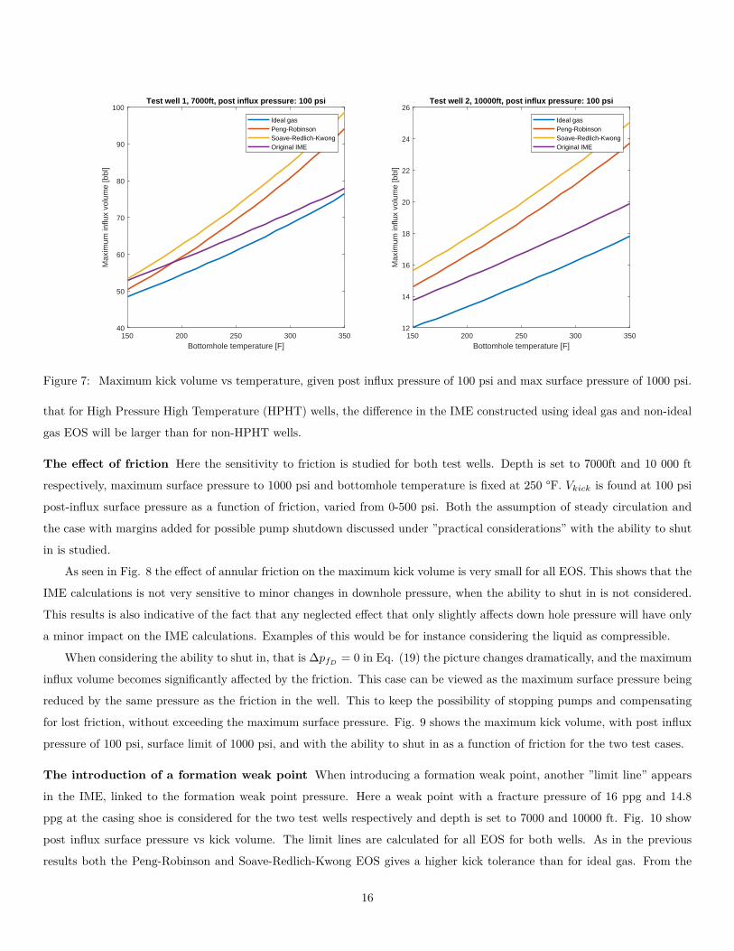
EOS vs temperature Here the effect of bottomhole temperature vs equation of state for the two test wells is studied.

The depth for the two test cases is set to 7000 ft and 10000 ft respectively and bottomhole temperature is varied from 150

°F to 400 °F As seen from Fig. 7 temperature significantly affects the maximum kick size for both test wells, with the real

gas EOS giving higher margins than for ideal gas in both cases. The results show that the difference between the ideal gas

14

5500 6000 6500 7000

Depth [ft]

60

70

80

90

100

110

120

130M

axim

um in

flux

volu

me

[bbl

]Test well 1, post influx pressure:100 psi

Ideal gasPeng-RobinsonSoave-Redlich-KwongOriginal IME

8000 8500 9000 9500 10000

Depth [ft]

14

16

18

20

22

24

26

28

Max

imum

influ

x vo

lum

e [b

bl]

Test well 2, post influx pressure: 100 psi

Ideal gasPeng-RobinsonSoave-Redlich-KwongOriginal IME

Figure 5: Maximum kick volume vs depth, given post influx pressure of 100 psi and max surface pressure of 1000 psi

0 2000 4000 6000 8000 10000

Depth [ft]

0

0.2

0.4

0.6

0.8

1

1.2

1.4

1.6

1.8

2

Den

sity

[ppg

]

Gas density vs depth, Methane

Ideal gasPeng-RobinsonSoave-Redlich-Kwong

0 2000 4000 6000 8000 10000

Depth [ft]

0.85

0.9

0.95

1

1.05

1.1

1.15

Den

sity

/Den

sity

idea

l [-]

Normalized gas density vs depth, Methane

Ideal gasPeng-RobinsonSoave-Redlich-Kwong

Figure 6: Methane density vs depth for vertical well, 13 ppg mud mud. Quite significant (+-10%) deviation is seen vs ideal

gas over the depth considered

and non ideal gas cases become larger with higher downhole temperature. An important point to note is that the maximum

acceptable kick volume increase with down hole temperature. This effect becomes more significant for the SRK and PR EOS

IME, than for ideal gas and original IME. The temperature dependence on the original IME equation is very similar to the

one using the ideal gas EOS. The fact that the maximum kick volume increases with temperature can be explained as follows:

At higher down hole temperatures the gas density will be lower, such that the total mass of gas (what actually causes the

required increase in pressure when it reach the surface) will be lower for a given kick volume. Another important point is

15

150 200 250 300 350

Bottomhole temperature [F]

40

50

60

70

80

90

100M

axim

um in

flux

volu

me

[bbl

]Test well 1, 7000ft, post influx pressure: 100 psi

Ideal gasPeng-RobinsonSoave-Redlich-KwongOriginal IME

150 200 250 300 350

Bottomhole temperature [F]

12

14

16

18

20

22

24

26

Max

imum

influ

x vo

lum

e [b

bl]

Test well 2, 10000ft, post influx pressure: 100 psi

Ideal gasPeng-RobinsonSoave-Redlich-KwongOriginal IME

Figure 7: Maximum kick volume vs temperature, given post influx pressure of 100 psi and max surface pressure of 1000 psi.

that for High Pressure High Temperature (HPHT) wells, the difference in the IME constructed using ideal gas and non-ideal

gas EOS will be larger than for non-HPHT wells.

The effect of friction Here the sensitivity to friction is studied for both test wells. Depth is set to 7000ft and 10 000 ft

respectively, maximum surface pressure to 1000 psi and bottomhole temperature is fixed at 250 °F. Vkick is found at 100 psi

post-influx surface pressure as a function of friction, varied from 0-500 psi. Both the assumption of steady circulation and

the case with margins added for possible pump shutdown discussed under ”practical considerations” with the ability to shut

in is studied.

As seen in Fig. 8 the effect of annular friction on the maximum kick volume is very small for all EOS. This shows that the

IME calculations is not very sensitive to minor changes in downhole pressure, when the ability to shut in is not considered.

This results is also indicative of the fact that any neglected effect that only slightly affects down hole pressure will have only

a minor impact on the IME calculations. Examples of this would be for instance considering the liquid as compressible.

When considering the ability to shut in, that is ∆pfD = 0 in Eq. (19) the picture changes dramatically, and the maximum

influx volume becomes significantly affected by the friction. This case can be viewed as the maximum surface pressure being

reduced by the same pressure as the friction in the well. This to keep the possibility of stopping pumps and compensating

for lost friction, without exceeding the maximum surface pressure. Fig. 9 shows the maximum kick volume, with post influx

pressure of 100 psi, surface limit of 1000 psi, and with the ability to shut in as a function of friction for the two test cases.

The introduction of a formation weak point When introducing a formation weak point, another ”limit line” appears

in the IME, linked to the formation weak point pressure. Here a weak point with a fracture pressure of 16 ppg and 14.8

ppg at the casing shoe is considered for the two test wells respectively and depth is set to 7000 and 10000 ft. Fig. 10 show

post influx surface pressure vs kick volume. The limit lines are calculated for all EOS for both wells. As in the previous

results both the Peng-Robinson and Soave-Redlich-Kwong EOS gives a higher kick tolerance than for ideal gas. From the

16

0 100 200 300 400 500

Annulus friction [psi]

60

62

64

66

68

70

72

74M

axim

um in

flux

volu

me

[bbl

]Test well 1, 7000ft, post influx pressure: 100 psi

Ideal gasPeng-RobinsonSoave-Redlich-Kwong

0 100 200 300 400 500

Annulus friction [psi]

14

15

16

17

18

19

20

Max

imum

influ

x vo

lum

e [b

bl]

Test well 2, 10000ft, post influx pressure: 100 psi

Ideal gasPeng-RobinsonSoave-Redlich-Kwong

Figure 8: Friction vs maximum kick volume with post influx pressure of 100 psi, and surface pressure limit of 1000 psi.

0 100 200 300 400 500

Annulus friction [psi]

25

30

35

40

45

50

55

60

65

70

75

Max

imum

influ

x vo

lum

e [b

bl]

Test well 1, 7000ft, post influx pressure: 100 psi

Ideal gasPeng-RobinsonSoave-Redlich-Kwong

0 100 200 300 400 500

Annulus friction [psi]

6

8

10

12

14

16

18

20

Max

imum

influ

x vo

lum

e [b

bl]

Test well 2, 10000ft, post influx pressure: 100 psi

Ideal gasPeng-RobinsonSoave-Redlich-Kwong

Figure 9: Friction vs maximum kick volume with post influx pressure of 100 psi, surface pressure limit of 1000 psi, and with

the ability to shut in.

weak point limit line it is seen that for both wells, if having a high post influx pressure, ”any” kick will exceed the weak point

pressure. This fact can be described as follows; at surface pressures above 600 psi the weak point pressure will be exceeded

for the considered limits with just liquid in the well, so that even pre-kick, the weak point pressure is exceeded.

Influx management envelope Here a sample IME chart is prepared for test well 2 with depth set to 10 000 ft and

considering weak point limit of 14.8 ppg at the shoe with a shoe depth of 7000ft. Surface pressure limit is set to 1000psi.

17

100 200 300 400 500 600 700 800 900 1000 1100

Post influx surface pressure [psi]

0

10

20

30

40

50

60

70

Max

imum

influ

x vo

lum

e [b

bl]

Test well 1, 7000ft

Ideal gas, surface limitIdeal gas, weak point limitPeng-Robinson, surface limitPeng-Robinson, weak point limitSoave-Redlich-Kwong, surface limitSoave-Redlich-Kwong, weak point limit

100 200 300 400 500 600 700 800 900 1000 1100

Post influx surface pressure [psi]

0

2

4

6

8

10

12

14

16

18

20

Max

imum

influ

x vo

lum

e [b

bl]

Test well 2, 10000ft

Ideal gas, surface limitIdeal gas, weak point limitPeng-Robinson, surface limitPeng-Robinson, weak point limitSoave-Redlich-Kwong, surface limitSoave-Redlich-Kwong, weak point limit

Figure 10: Influx management envelopes with weak point for well 1 and 2 for all EOS. Note that the y axis is reversed so

that it takes the same basic form as the well control matrix

Kick detection limit has been specified to 4 bbl, adding a new region in the IME. The IME is calculated using the Soave-

Redlich-Kwong EOS. The resulting color coded IME can be seen in Fig. 11.

Figure 11: Final influx management envelope well 2 calculated using the Soave-Redlich-Kwong EOS.

The different regions in Fig. 11 can be explained as follows:

18

I. Below influx detection limit, no influx is detected and operation continues as normal

II. Influx detected and suppressed. Combinations of post influx surface pressure and kick volume in this region will not

exceed the specified surface pressure limit. Influx can be circulated out using MPD. Combinations of post influx pressure

and kick volume that is exactly on the line separating this region and region IV will reach a peak surface pressure of

1000 psi (the specified limit) when circulated to the surface.

III. Influx/ post influx pressure combinations in this region will exceed the specified weak point pressure when circulated

to the surface. The criticality of this depends on how the weak point limit has been found, and the likelihood of a

underground blowout if the limit is exceeded.

IV. Combinations of post influx pressure and kick volume in this region will exceed the specified maximum surface pressure

when circulated out (1000psi), and should be managed by conventional well control. The kick will not violate the weak

point pressure limit.

V. Combinations of post influx pressure and kick volume in this region will exceed both the MPD surface pressure limit,

and violate the weak point pressure limit. The criticality of exceeding the weak point limit depends on how the weak

point limit has been found, and the likelihood of a underground blowout if the limit is exceeded. A kick in this region

might prove challenging, even when doing conventional well control

Discussion

Through the derivations it is shown how the limit line for surface and weak point pressure can be calculated using

any equation of state. The final derivation of the IME equations assumes single bubble of gas. Although gas solubility

and distribution is not considered, the initial derivation makes no assumptions on this, leaving significant room for future

work. In the results liquid density ρl is assumed independent of pressure, but Eq. (19) and (22) opens up for considering

compressible liquid as well. As shown in the results of sensitivity to friction without the ability to shut in Fig. 8, the IME

calculations is not very sensitive to minor variations in down hole pressure such that the effect of considering compressible

liquid is likely minor.

The integrals in (19) and (22) are solved using a simple low order numerical integrator and although the possibility of

using other numerical integrators are touched upon briefly, the sensitivity to the numerical method used are not covered. As

the results in Fig. 8 show that the IME calculations is not very sensitive to minor changes in downhole pressure, the effect

of this is likely small.

A systematic study comparing the proposed method of solving the IME limit line equations vs high fidelity simulations

following the approach of Gabaldon et al. (2017) should be performed.

Although the resulting IME from the proposed method show more margins with respect to acceptable kick size than

the original IME equations by Culen et al. (2016) if using a real-gas EOS, it is not the authors belief that the result is

un-conservative, especially if a methane gas kick at bottom and single bubble is assumed. The main reason for having more

margins is the inclusion of a real gas EOS. Although making the solution of the equations simpler, the assumption of ideal gas

is inaccurate even at moderate pressures. At the pressures experienced in drilling and production a real gas EOS is required

19

for any significant accuracy.

The sensitivity to gas composition is not studied, and in general considering pure methane is likely the most conservative.

The use of SRK and PR equations of state make the calculation of the IME using most gas compositions straight forward,

in general yielding IME curves with more margins.

Conclusion

It is shown that the calculation of the limit lines for the IME can be performed along the lines of the initial IME paper,

without assuming ideal gas through numerical methods, and that this gives higher kick tolerance than for the equation

presented by Culen et al. (2016). The initial derivation of the IME equations makes it possible to consider gas distribution

and gas dissolving into the mud. The limit line for formation weakpoint pressure is introduced in the same framework.

When solved for different equations of state, the ideal gas IME is found to be similar to that of Culen et al. (2016),

depending on the gas density used in Eq.2. The Peng-Robinson (PR) and Soave-Redlich-Kwong (SRK) equations of state

give very similar results for calculation of the IME, something that is as expected as both EOS are considered to be relatively

good and of comparable accuracy for most systems. Using a PR- or SRK- EOS to build an IME results in more kick tolerance

then for a IME based on ideal gas, a kick tolerance that is likely more realistic.

The calculation of the IME by using the proposed method will be significantly faster than building an IME based on high

fidelity simulations, provided code for the numerical solution is implemented, comparable to the time and effort required by

the equation suggested presented by Culen et al. (2016).

The solution of the equations used to generate the IME can also be used to calculate a peak surface- and weakpoint-

pressure for a given kick size and post influx pressure, something that is relevant to conventional well control as well as

for the generation of a IME for MPD operations. The IME weak point limit line and the concept of presenting this as a

”kick envelope” is relevant for conventional well control as well as MPD, being a natural and more continuous extension of

considering just Maximum Allowable Annulus Surface Pressure (MAASP) with respect to a formation weak point.

Acknowledgment

This research has been partially funded by the the Norwegian Research Council in the Industrial PhD project ”Modeling

for automatic control and estimation of influx and loss in drilling operations” Project no 241586 and Oslofjordfondet project

”Autonomous pressure control” Project no 272044.

References

Culen, M. S., et al. 2016. “Evolution of the MPD Operations Matrix: The Influx Management Envelope”. In SPE/IADC

Managed Pressure Drilling and Underbalanced Operations Conference and Exhibition. Galveston, Texas, USA: Society of

Petroleum Engineers. doi: http://doi.org/10.2118/179191-MS.

Gabaldon, O. R., et al. 2017. “Case Study: First Experience of Developing an Influx Management Envelope IME for a Deep-

water MPD Operation”. In IADC/SPE Managed Pressure Drilling & Underbalanced Operations Conference & Exhibition.

Rio de Janeiro, Brazil: Society of Petroleum Engineers. doi: http://doi.org/10.2118/185289-MS.

20

Karimi Vajargah, Ali, Besmir Buranaj Hoxha, and Eric van Oort. 2014. “Automated Well Control Decision-Making during

Managed Pressure Drilling Operations”. In SPE-170324-MS. SPE: Society of Petroleum Engineers. isbn: 978-1-61399-

326-2. doi: http://doi.org/10.2118/170324-MS.

Kinik, Koray, Ferhat Gumus, and Nadine Osayande. 2014. “A Case Study: First Field Application of Fully Automated

Kick Detection and Control by MPD System in Western Canada”. Kinik2014: Society of Petroleum Engineers. isbn:

1-61399-319-6.

Mir Rajabi, Mehdi, Don M Hannegan, and Dennis Derrick Moore. 2014. “The MPD Well Control Matrix; What Is Actually

Happening”. In SPE Annual Technical Conference and Exhibition. Amsterdam, The Netherlands: Society of Petroleum

Engineers. doi: http://doi.org/10.2118/170684-MS.

Patil, Harshad, et al. 2018. “Advancing the MPD Influx Management Envelope IME: A Comprehensive Approach to Assess

the Factors That Affect the Shape of the IME”. In SPE/IADC Managed Pressure Drilling and Underbalanced Operations

Conference and Exhibition. New Orleans, Louisiana, USA: Society of Petroleum Engineers. doi: http://doi.org/10.

2118/189995-MS.

Peng, Ding-Yu, and Donald B. Robinson. 1976. “A New Two-Constant Equation of State”. Industrial & Engineering Chemistry

Fundamentals 15 (1): 59–64. issn: 0196-4313, 1541-4833. doi: http://doi.org/10.1021/i160057a011.

Soave, Giorgio. 1972. “Equilibrium Constants from a Modified Redlich-Kwong Equation of State”. Chemical Engineering

Science 27 (6): 1197–1203. issn: 0009-2509. doi: http://doi.org/10.1016/0009-2509(72)80096-4.

Whitson, Curtis H., and Michael R. Brulé. 2000. Phase Behavior. In collab. with Society of Petroleum Engineers (U.S.)

Monograph / SPE ; Henry L. Doherty Series v. 20. OCLC: ocm46488305. Richardson, Tex: Henry L. Doherty Memorial

Fund of AIME, Society of Petroleum Engineers. isbn: 978-1-55563-087-4.

Willersrud, Anders, et al. 2015. “Early Detection and Localization of Downhole Incidents in Managed Pressure Drilling”.

Willersrud2015: Society of Petroleum Engineers. doi: http://doi.org/10.2118/173816-MS.

Zhou, Jing, Ole Morten Aamo, and Glenn-Ole Kaasa. 2011. “Switched Control for Pressure Regulation and Kick Attenuation

in a Managed Pressure Drilling System”. Control Systems Technology, IEEE Transactions on 19 (2): 337–350. issn:

1063-6536.

Appendix A: Unit Conversion table

21

SI Field unit

1 m3 6.2898 bbl

1 m2 1 550.0 in2

1 Pa 1.4503e-04 psi

1 Pa 1e-5 bar

1 kgm3 8.3454e-3 ppg

1 m 3.2808 ft

1 m 39.3701 in

1 C 1.80*C+32.00 F

1 rad 57.2958 degree

Christian Berg holds a B.Sc. degree in Gas and Energy Technology and M.Sc. degree in Process Technology from Telemark

University-College in Porsgrunn, Norway. He was awarded the price for the best average grade of all engineering students

during his B.Sc. He also holds a trade certificate as Laboratory Technician. From 2014 he has been working at Kelda Drilling

Controls as a Research Engineer while doing an Industrial PhD with the University of South-Eastern Norway on the topic

of modelling for control and estimation of influx and loss during drilling operations. In this work he is developing software

systems for pressure control in drilling, and has experience from deployment, commissioning and operating MPD control

systems in the field. His main interests include mathematical modelling and numerical solutions within the field of of fluid

dynamics.

Geir Arne Evjen holds a M.Sc. in Process Technology and is working on a PhD in thermodynamics. He comes from a

position as principal researcher in Statoil R&D with a background from process modelling, multiphase flow, fluid modelling

and flow-assurance. He has been system architect in several R&D projects on advanced software for estimation and data

reconciliation. Partner and full-time employee in Kelda Drilling Controls. His main research interest is computational

thermodynamics and behaviour of complex fluids and mixtures.

Naveen Velmurugan holds a M.Sc.in Petroleum (Drilling) Engineering from the Norwegian University of Science and

Technology in Trondheim, Norway. He is currently pursuing his industrial PhD in Mathematics and Control at MINES

ParisTech in Paris, France (in association with Kelda Drilling Controls). His research interests include well control, multiphase

fluid flow modelling and dynamic systems with applications to drilling. His current research focuses on state and parameter

estimation of partial differential equations (PDEs), with applications to distributed pressure dynamics within the wellbore

and the reservoir during MPD operations.

Martin Culen holds a Mechanical Engineering degree from the University of Alberta, Canada and has over 24 years of

energy industry experience specializing in Underbalanced and Managed Pressure Drilling. He is currently a Principal with

Blade Energy Partners, Director of Blade Energy’s offices in Dubai. In addition to his involvement with MPD and UBD

projects, Martin develops training material and is an instructor for Blade’s MPD and UBD courses. Martin is actively

involved with the IADC UBO-MPD Committee, having served as the Chairman for the UBD and Training sub-committees,

most recently committee Chairman, and head of the the API 16RCD task group. He has also served as chair and co-chair for

numerous SPE workshops and conferences. Martin is the author of 13 technical papers and holds a patent related to MPD.

22