The impact of hypoxia on tumour controlprobability in the high-dose range used in

stereotactic body radiation therapy

A MASTER THESIS BY

Emely Lindblom

Medical Radiation Physics, Department of Physics, StockholmUniversity

Spring term, 2012

Abstract

The use of stereotactic body radiation therapy employing few large fractionsof radiation dose for the treatment of non-small cell lung cancer has been

proven very successful, high values of tumour control probability (TCP)being clinically achieved. In spite of the success of the fractionation

schedules currently used, there is a tendency towards reducing the numberof fractions for economical and practical reasons, and also for maximizing

the comfort of the patients. It is therefore the main aim of this thesis toinvestigate the impact of a severely reduced number of fractions on thetumour control probability for tumours that contain hypoxic areas. The

impact on TCP of other factors such as hypoxic fraction, distribution of theoxygen partial pressure and location of the hypoxic volume within the

tumour were also investigated. The effect of tumour motion due tobreathing was included and evaluated using Cone Beam Computed

Tomography (CBCT) data from patients imaged with internal markers in theliver and pancreas. The results clearly showed that in the presence ofhypoxia, TCP is seriously compromised if there is not enough time for

reoxygenation between fractions. A reduction in the number of fractions ofjust one fraction may require an increase of several Gy per fraction to obtain

a similar TCP. The diaphragmatic tumour motion range showed littleinfluence on TCP provided that the PTV encompassed all tumour positions.

The dose delivered to the PTV margin was found not to be the only factorthat is significant for local control, the average dose correlated better with

TCP. The agreement of the results of this work with clinical results also serveas a strong indicator that inter-fraction reoxygenation is an important

process in real-life patients treated with stereotactic body radiotherapy.

2

Sammanfattning

Stereotaktisk stralbehandling av patienter med icke-smacelligalungcarcinom har resulterat i framgansrika kliniska utfall. Det finns en

tendens att ytterligare reducera antalet fraktioner som den totala dosen skadelas i, vilken drivs av ekonomiska och praktiska skal. Syftet med detta

arbete var framfor allt att undersoka hur sannolikheten att uppnatumorkontroll paverkas av en kraftig reduktion i antalet fraktioner for

tumorer med hypoxiska regioner. Paverkan av andra faktorer som andelensyrebrist, fordelningen av syret i tumoren samt positionen av regioner med

syrebrist i tumoren studerades ocksa. Effekten av rorelse utvarderadesgenom att data fran patienter med interna markorer i lever och

bukspottkortel som undergatt Cone Beam Computed Tomography (CBCT)anvandes. Simuleringar och berakningar utfordes i mjukvarorna MATLAB

och Origin. Resultaten pavisar tydligt att sannolikheten att uppna kontroll avsjukdomen minskar kraftigt nar dosen ges i farre fraktioner for tumorer med

syrebrist. Om antalet fraktioner reduceras med endast en fraktion kan detkrava en dosokning om flera Gy per fraktion for att uppna liknande

sannolikhet for kontroll. Utstrackningen av den longitudinella rorelsen hostumoren visade sig ha liten paverkan pa sannolikheten for tumorkontroll,forutsatt att rorelsen i huvudsak tacktes in i PTV:t. Dosen till periferin av

PTV:t visade sig inte vara den avgorande faktorn for att uppnatumorkontroll. Medeldosen till PTV visade battre korrelation med

sannolikheten for att uppna kontroll. Overensstammelsen av resultaten frandetta arbete med kliniska utfall pavisar tydligt att omfordelningen av syremellan fraktioner ar en viktigt process i verkliga patienter som behandlas

med stereotaktisk stralbehandling.

3

Acknowledgements

I would like to thank Dr. Alexandru Dasu for his help, guidance and usefuldiscussions. I would also like to thank Drs. Margareta Edgren, Ingmar Lax

and Peter Wersall for willingly and knowledgeably answering my questionsrelated to this work. Thanks also goes to Elias Lindback for providing me

with the CBCT-data necessary for parts of the work, and for usefuldiscussions. I would also like to thank Marie Huss, Tor Kjellsson and Dr.

Peter Lindblom for their thoughtful advice and the useful discussions weshared. Last but not least, I would like to thank my supervisor, Dr. IulianaToma-Dasu for her highly knowledgeable and inspirational way of guiding

me through this work.

4

Contents

1 Introduction 8

2 Background 82.1 The microenvironment in NSCLC tumours . . . . . . . . . . . . 92.2 The tumour vascularity . . . . . . . . . . . . . . . . . . . . . . . . 92.3 Tumour hypoxia . . . . . . . . . . . . . . . . . . . . . . . . . . . . 92.4 Stereotactic body radiation therapy . . . . . . . . . . . . . . . . . 14

2.4.1 Dose prescription schemes . . . . . . . . . . . . . . . . . 172.5 The impact of fractionation . . . . . . . . . . . . . . . . . . . . . 172.6 Choice of radiobiological model . . . . . . . . . . . . . . . . . . . 18

3 Methods and Materials 203.1 Calculation of tumour control probability . . . . . . . . . . . . . 20

3.1.1 Modelling the tumour . . . . . . . . . . . . . . . . . . . . 203.1.2 Modelling the oxygen partial pressure . . . . . . . . . . . 203.1.3 Determining the surviving fraction . . . . . . . . . . . . . 213.1.4 Modelling the dose distribution . . . . . . . . . . . . . . . 213.1.5 Incorporating tumour movement . . . . . . . . . . . . . . 22

3.2 Dose fractionation schemes . . . . . . . . . . . . . . . . . . . . . 243.3 Planned simulations . . . . . . . . . . . . . . . . . . . . . . . . . 26

3.3.1 The relevant dose parameter for predicting the TCP . . . 263.3.2 The TCP dependence on the oxygen partial pressure dis-

tribution . . . . . . . . . . . . . . . . . . . . . . . . . . . . 283.3.3 The TCP dependence on the hypoxic fraction . . . . . . . 293.3.4 The TCP dependence on the position of the hypoxic island 293.3.5 The influence on TCP of tumour movement during irra-

diation . . . . . . . . . . . . . . . . . . . . . . . . . . . . . 313.4 Analysis of uncertainties . . . . . . . . . . . . . . . . . . . . . . . 34

4 Results 344.1 The relevant dose parameter for predicting the TCP . . . . . . . 364.2 The TCP dependence on the oxygen partial pressure distribution 404.3 The TCP dependence on the hypoxic fraction . . . . . . . . . . . 414.4 The TCP dependence on the position of the hypoxic island . . . 434.5 The influence on TCP of tumour movement during irradiation . 454.6 Analysis of uncertainties . . . . . . . . . . . . . . . . . . . . . . . 47

5 Discussion 475.1 Discussion of the results . . . . . . . . . . . . . . . . . . . . . . . 47

5.1.1 The relevant dose parameter for predicting the TCP . . . 485.1.2 The TCP dependence on the oxygen partial pressure dis-

tribution . . . . . . . . . . . . . . . . . . . . . . . . . . . . 495.1.3 The TCP dependence on the hypoxic fraction . . . . . . . 505.1.4 The TCP dependence on the position of the hypoxic island 515.1.5 The influence on TCP of tumour movement during irra-

diation . . . . . . . . . . . . . . . . . . . . . . . . . . . . . 525.2 Analysis of uncertainties . . . . . . . . . . . . . . . . . . . . . . . 535.3 The model for cell survival . . . . . . . . . . . . . . . . . . . . . . 54

5

5.4 Dosimetric aspects . . . . . . . . . . . . . . . . . . . . . . . . . . 55

6 Conclusions 57

A Appendix 58

6

Acronyms

3D-CRT - Three-dimensional conformal radiotherapyBOLD - Blood oxygen level dependentCBCT - Cone-beam computed tomographyCC - Collapsed coneCTV - Clinical target volumeDVH - Dose volume histogramGTV - Gross target volumeHF - Hypoxic fractionHI - Hypoxic islandIVD - Inter-vessel distanceLQ - Linear-quadraticMRI - Magnetic resonance imagingMV - Mega voltNSCLC - Non-small cell lung cancerOER - Oxygen enhancement ratioPB - Pencil beamPTV - Planning target volumeRCR - Repairable-conditionally repairableSBRT - Stereotactic body radiation therapyTCP - Tumour control probabilityUSC - Universal survival curve

7

1 Introduction

Patients with non-small cell lung cancer (NSCLC) are possible candidates forstereotactic body radiation therapy (SBRT). The clinical experience of treat-ing these patients with few fractions of high doses is generally good, and thereis a trend towards reducing the number of fractions for several reasons. Fewerfractions would for example be beneficial from an economical and practicalviewpoint, but it would also be more convenient for the patients who are of-ten elderly. This work aims to investigate mainly the impact of an extremelyreduced number of fractions on the tumour control probability (TCP) for typ-ical tumours that contain hypoxic areas. The impact on TCP of other factorssuch as hypoxic fraction, distribution of the oxygen partial pressure and loca-tion of the hypoxic volume are also investigated. The effect of tumour motiondue to breathing is also included in the analysis. This work will focus on treat-ment methods used in the SBRT of NSCLC. The report is written with respectto this specific cancer, even though some results and corresponding discus-sion are applicable to SBRT of other types of tumours as well.

2 Background

Lung cancer is one of the most common cancer types in both men and womenand the number one cancer-related cause of death in the world [1]. The Amer-ican Cancer Society estimates that 28% of all cancer-related deaths in the USin 2012 will be due to lung cancer. They also report that the number of peopledying from lung cancer each year is larger than the number of deaths due tocolon, breast and prostate cancers combined [2]. Starting in the bronchioles,alveoli or inner bronchial lining, the lung cancer can not be seen on x-raysin its earlier phase and is thus usually not discovered until it is too late forcure. Likewise, symptoms do not generally occur until the cancer is ratheradvanced and even then, the symptoms may be mistaken as indicators forother diseases. This is made even more relevant by the fact that most peopleaffected by lung cancer have a history of smoking. Shortness of breath, a per-sistent cough and chest pain are examples of lung cancer symptoms whichmay very well be present without any tumour. Therefore, it is likely that ittakes some time before patients suffering from lung cancer contact a physi-cian [2].

Lung cancer can be divided into small-cell lung cancer (SCLC) and non-small cell lung cancer (NSCLC). Non-small cell lung cancer constitutes 80-95% of lung cancer cases and can be divided into three smaller groups:

• Adenocarcinoma, (40 % of lung cancers), occurs in the distal part of thelung in secretory cells;

• Squamous cell carcinoma, (25-30 % of lung cancers), occurs on the in-ner lining of the airways. The disease is normally located adjacent to abronchus, in the central part of the lungs;

• Large cell carcinoma, (10-15 % of lung cancers), can develop in any partof the lung.

8

Unlike adenocarcinoma, which grows slowly and is more likely to have a pos-itive outcome for the patient, large cell carcinoma is an aggressive tumourtype which grows fast and also tends to metastasise quickly. Common treat-ments of NSCLC include surgery, radiotherapy and chemotherapy among oth-ers. It is not unusual to combine different treatment modalities [2].

2.1 The microenvironment in NSCLC tumours

The tumour microenvironment in NSCLC can be spatially varying, a result ofthe irregular blood supply characteristic of tumours (as shown in one of theearly papers by Tomlinson and Gray (1955) [3]). The blood supplies not onlyoxygen, but also other nutrients to the cells. An impaired blood supply thusresults not only in deprivation of oxygen, but also in a lack of nutrients im-portant for the tissue. It is, however, the oxygen that is of greatest concernfor radiation therapy. As is discussed later in this report, tumour hypoxia hasgreat influence on the effect of radiation therapy. In general, the tumour mi-croenvironment has a large impact on the success or failure of several formsof cancer treatment, the key issue being the distinctive nature of the tumourvascularity [4].

2.2 The tumour vascularity

The growth of solid tumours is sustained through the creation of new bloodvessels to supply the tumour with nutrients and oxygen and remove wasteproducts. This process is called angiogenesis. In normal tissues, the processof angiogenesis results in a fine distribution of vessels that provide sufficientoxygen to the tissue, and is driven by highly organized molecular and cel-lular chain of events. In tumours however, this process does not take placeto the same extent and such (normal) blood vessel formation is not possi-ble [5]. Solid tumours often derive their blood supply from the venous side ofthe vasculature in the surrounding normal tissue. This neovasculature is thusdeprived of the oxygen and nutrients carried by the blood in the arteries [6].The vessels supplying tumours are often thick and bulky resulting in an evenpoorer oxygen supply to some parts of the tissue [7]. The resulting lack ofoxygen causes the cell to over-express factors which promote further angio-genesis, ultimately leading to additional formation of abnormal vessels [5].The growing tumour cells push the vessels apart, further increasing the dis-tance that the oxygen has to diffuse to reach all cells [6]. The tumour can thusbe said to continuously outgrow its own blood supply.

2.3 Tumour hypoxia

The inadequate blood vessel formation in tumours leads to the formationof hypoxic and possibly even necrotic areas. Hypoxia in tumours occurs intwo forms; chronic (diffusion-limited) and acute (perfusion-limited) hypoxia.Chronic hypoxia is a result of the coarse blood vessel distribution, leavingsome cells outside the oxygen diffusion range, deprived of oxygen. Acute hy-poxia is the result of temporarily closed vessels, which may reopen and reoxy-genate the cells [6]. As mentioned in the previous section, hypoxia affects the

9

tumour response to cancer treatment. It has however also been noted thathypoxia in tumours is strongly correlated with the progression of the diseaseas well as the creation and spread of metastases [8]. Several other importanttumour characteristics associated with hypoxia are briefly mentioned below.

• Proliferation. Although hypoxic cells proliferate less than well oxygena-ted cells, hypoxia plays an important role in the proliferation of cancercells because it triggers some known growth factors [7].

• Progression. Several studies have reported a correlation between the ex-pression of the hypoxic response factor HIF-1α and the progression ofhuman tumours [7].

• Metabolism. As the availability of oxygen is reduced, cells begin to de-rive their energy from the process of glycolysis which thus becomesthe main source of ATP, (adenosine triphosphate, involved in the cellu-lar metabolism where it works as a source of energy). The an-aerobicglycolysis is a fast anabolic process that results in a net-production oftwo ATP molecules. Under normoxic conditions it is a part of the cell’smetabolism and is followed by the aerobic processes citric acid cycleand oxidative phosphorylation, which produce an additional 36 addi-tional ATP molecules [7, 9].

• Immortalization. At the end of the chromosomes, the DNA is arrangedin a special way forming the telomeres which work as a protective cap,among other things preventing the chromosome ends from sticking toeach other. Another important function is to prevent DNA from beinglost at cell division [10]. As the cell divides, the telomeres are shortened,and as a result, the cell can only divide a limited number of times beforeentering senescence, meaning it looses its ability to divide. This problemcan be avoided by the enzyme telomerase, activated by some stem cellsand cancer cells. With the help of this, the chromosome ends are ableto rebuild themselves, counter-acting the degradation caused by cell di-vision resulting in a cell that is immortal [9]. Seimiya et al. found thathypoxia further promotes the telomerase activity in solid tumours [11].

• pH. The metabolic process of glycolysis mentioned above, produces lac-tic acid which lowers the pH in the cell below values found in normal tis-sues. Tumours have however shown to be able to adapt to pH changesand grow in spite of the more acidic milieu [7].

The regions of low oxygen partial pressure or lacking oxygen resulting fromthe impaired blood supply are heterogeneously distributed in solid tumoursand can be found very close to normoxic areas [8]. Drugs used in the treat-ment of cancer are hampered by the hypoxia itself, but also by the very causeleading to it - the vascular structure in the tumour. The drugs are admin-istered via the blood, which means that the chemicals are prevented fromreaching hypoxic areas as they are, by definition, out of reach from the ves-sels [12]. Hypoxia thus play an important role in chemotherapy, and, as willbe seen, in radiotherapy as well.

10

The oxygen effect

The cell is damaged by all ionizing radiations but the amount of damage andits clustering of damage depends on the linear energy transfer (LET) of theradiation type. Sparsely ionizing radiations, such as x-rays and electrons,have a low LET and produce fast, secondary charged particles in the tissue.These charged particles in turn create short-lived ion pairs which react toproduce free radicals which are responsible for the damage inflicted to thecell through chemical reactions with, for example, molecular oxygen. Theamount of damage is therefore largely determined by the amount of molec-ular oxygen present at the time, (during irradiation or within microsecondsafter) [13].

The presence of oxygen molecules near or at the site of damage enablesthe formation of a DNA radical, resulting from a reaction between the DNAand a free radical produced by the sparsely ionizing radiation traversing thebiologic material. An organic peroxide can then be formed which makes theDNA radical permanent, as opposed to the DNA radical returning to its stableform in case of an oxygen-deprived milieu. The formation of the organic per-oxide is not restorable, and the chemical composition is thus permanentlyaltered. This is referred to as the oxygen fixation hypothesis [13]. This fixa-tion could in turn lead to dangerous consequences, such as the initiation ofa tumour, as the DNA of that particular cell is modified. The phenomenon ofoxygen fixation and its consequences fundamentally affects the way in whichradiotherapy should be executed in the ideal way.

Hypoxia and radiation therapy

The major benefits from conventionally fractionated radiotherapy, (for exam-ple 2 Gy per fraction during a couple of weeks), are normal tissue repair andreoxygenation. Dividing the total dose into smaller fractions delivered witha certain time-interval in between allows for more repair in the normal tis-sues than in tumours. This net benefit in repair for the normal tissue is dueto its greater ability to recover from DNA damage compared to most tumourcells [14, 15]. Another advantage of fractionated radiotherapy is the possibil-ity for the hypoxic cells to reoxygenate between fractions. This is importantsince the absence of oxygen makes cells more radio-resistant [16], as previ-ously mentioned.

The phenomenon of reoxygenation was discussed by Kallman in 1972 [17].He concluded that the hypoxic fraction in a tumour is an important predic-tor of how well the tumour will respond to a fractionated treatment regimengiven the difference in radio-sensitivity between well oxygenated and hypoxiccells. Irradiation of a tumour with a hypoxic region will thus result in a selec-tive exhaustion of the well oxygenated cells, leading to an increase in the hy-poxic fraction. Kallman found that the larger the initial hypoxic fraction, thelarger the hypoxic fraction resulting from the preferential exhaustion of theradio-sensitive cells was. For example, irradiating a tumour with an initial hy-poxic fraction of 1% with 10 Gy resulted in a new hypoxic fraction of just over1%, while a tumour with an initial 20% hypoxic cells ended up with 25% hy-poxia after being given the same dose. Thus irradiation immediately causespartially hypoxic tumours to increase their radio-resistance. If the tumour

11

would maintain this oxygen distribution, every fraction of radiation wouldincrease the radio-resistance of the tumours, hampering the success of ra-diotherapy. As stated by Kallman, this is not the case as is evident from clin-ical observations and the success of fractionated radiotherapy. Somethingis thus bound to happen between fractions, causing the tumour hypoxia tosuccessively decrease. Kallman concluded that this process is due to that thepreviously hypoxic cells surviving irradiation become reoxygenated and thusmore radio-sensitive than before [17].

The term reoxygenation could imply two scenarios: a global improvementin the oxygen status of the tissue or an alteration on a more local level, notresulting in any overall change in the hypoxic fraction of the tumour. Thom-linson and Gray (1955) discussed the effect of radiotherapy on tumours con-taining hypoxic centres. They proposed that as cells in the peripheral partof the tumour tissue will be fully supplied with oxygen and other nutrients,they are fully capable of proliferation, further increasing the distance fromthe blood supply to the centrally located, hypoxic cells which then risk dy-ing. Irradiation could counteract this by killing the outer, well-oxygenatedcells, allowing the hypoxic regions to come within a distance from the stromathat ensures their survival. Provided that their ability to reproduce has beenkept in spite of being under-nourished, these cells may proliferate again [3].Hence during fractionated radiotherapy, hypoxic regions may be re-suppliedwith oxygen and thus reduced, ultimately increasing the effect of the irradia-tion (as a larger part of the tumour becomes well supplied with oxygen). Thiswould represent the global case of reoxygenation.

In an article from 2012, Toma-Dasu et al. concluded that there are indeedchanges in the oxygenation of the tumour on a microscopic level during atreatment course, based on the clinical and experimental outcomes reportedby other authors [18]. This is another possible scenario; that there is a localredistribution of the oxygen partial pressure, not connected to the effect ofirradiation. Cells within and nearby the hypoxic region may thus alter theiroxygenation status, so that previously hypoxic cells become oxygenated andvice versa. This is an example of local reoxygenation.

Kallman (1972) commented on the theory that reoxygenation occurs asa result of tumour shrinkage, decreasing the distance from the capillariesto the hypoxic cells as a possible, but not major contributor to the reoxy-genation process. He proposed some other mechanisms possibly respon-sible for the reoxygenation that is obviously happening. For one, the cellsthat have been severely damaged by the radiation could reduce their oxygenmetabolism, allowing a greater potency for the oxygen to diffuse to formerlypoorly oxygenated cells. Another suggestion is that surviving cells residing inthe previously hypoxic region could migrate into better oxygenated areas [17].Whether local or global, and regardless of the underlying mechanisms, re-oxygenation does indeed play an important role in the success or failure of aradiotherapy course.

Measurements of oxygenation

As the oxygenation status of the tumour is an important factor influencingthe outcome of different forms of cancer therapy, it is crucial to estimate theoxygen distribution in a tumour in order to deliver the optimal treatment to

12

each individual patient. In order to achieve this and treat patients in the bestway, in vivo measurements of the hypoxic status of the tumour is a prerequi-site [19].

The golden standard for assessing the hypoxia in a tumour in a quanti-tative manner is by measuring it with a polarographic micoelectrode. Thismethod is invasive, as the microelectrode needs to be inserted into the tis-sue to be measured, and it is therefore limited to studies on tumours that areeasily accessed [19]. Early-stage NSCLC are often deeply located and thus notthat easily accessible as there is a risk of initiating complications through di-rect measurements [20]. In 2006, Le and colleagues reported the results frommeasuring the oxygen partial pressure in resectable NSCLC tumours and nor-mal lung tissue in twenty patients using the Eppendorf polarographic elec-trode. The median tumour pO2 was 16.6 mmHg (0.7-56 mmHg) while themedian lung pO2 was 42.8 mmHg (23-656 mmHg). The range in size of theinvestigated tumours was quite big; between 0.1 and 144.4 ml, (median 10.8ml), of which ten were larger than 10 ml [20].

Another problem associated with the polarographic microelectrode is thatthe measurements obtained only represent the oxygen partial pressure at thesite where the sample was taken. Given the heterogeneous oxygen distribu-tion obtained in hypoxic tumours, this poses a problem as one ideally de-sires to know the overall pressure distribution [19]. This could be addressedthrough non-invasive techniques such as magnetic resonance imaging (MRI)for example. In blood oxygen level dependent (BOLD) MRI, de-oxygenatedhaemoglobin can be distinguished from oxygenated haemoglobin, providinga qualitative evaluation of alterations in the oxygenation [21]. Other non-invasive techniques involve utilizing certain molecules known to accumulatein hypoxic cells. These could thus be labelled with a radioactive isotope suit-able for positron emission tomography (PET) and an image of the tumour oxy-genation could be obtained. For an imaging agent to be suitable, it shouldhave a small molecular size and a lipophilicty that allows it to pass throughcell membranes easily [22].

In 1997, Fujibayashi et al. reported the results from incubating a coppercomplex (62Cu-ATSM) with rat mitochondria and measuring the reduction ofCu(II) to Cu(I). They found that the reduction occurred in hypoxic mitochon-dria but not in normal ones, which is a clear implication for the ability toimage hypoxia. An example of a PET-agent utilized in cases of lung cancer is18F-fluoromisonidazole (18F-FMISO) [19]. 18F-FMISO is the most commonlyused PET-agent for the imaging of regional hypoxia. The tissue-blood-ratioin hypoxic tissues result in increased pixel values compared to normoxic tis-sues. This means that hypoxic areas can be clearly distinguished (by lookingfor pixels with values above a certain threshold) from normoxic areas. A draw-back of 18F-FMISO is its slow clearance, resulting in a rather low contrast inthe unprocessed image. In this aspect, 62Cu-ATSM appears to be superior to18F-FMISO, due to its more rapid uptake and bigger ratio between normoxicand hypoxic regions, (as summarized by Krohn et al., 2008 [21]).

The crucial difference between the invasive microelectrode measurementtechnique and the non-invasive molecular imaging of PET is the difficultyof quantification in the latter. PET images provide maps of the relative oxy-genation status, but they do not provide numbers of the oxygen levels in thetumour. Toma-Dasu et al. proposed in 2012 the incorporation 18F-FMISO-

13

PET in the treatment planning and dose prescription process through thedetermination of the relative radio-resistance of hypoxic compared to bet-ter oxygenated areas in the tumour. This was possible through a non-linearscaling of tumour uptake-values based on the average uptake-value in thewell oxygenated area outside the tumour, (assumed to be 60 mmHg). In thisway, a quasi-quantitative estimation of the hypoxia on a voxel level in the tu-mour could be established. The necessary dose to be prescribed could thusbe calculated using an algorithm that determines the minimum dose levelsrequired based on the radio-resistance of the tumour [18].

2.4 Stereotactic body radiation therapy

Since 1974, the Gamma-knife has been used at Karolinska Hospital to treatsmall volumes in the brain with high-dose radiation therapy given in a singlefraction. This is only possible as the treatment volume margins are reducedthrough immobilization of the head. A stereotactic frame is screwed into theskull, preventing the patient from moving during irradiation. A single dose of10 to 30 Gy is typically prescribed to the 50% isodose line encompassing thetarget, resulting in a maximum dose of up to 60 Gy and thus a very heteroge-neous dose distribution [23].

This form of stereotactic treatment works well in the head since the skull iseasily fixated and the brain does not move. The dose can thus successfully bedelivered with high accuracy to the intended target. In 1994, Lax et al. aimedto extend this treatment modality to regions outside the head, to extracranialsites, starting with the abdomen. While normal liver tissue has a low toler-ance to irradiation, the liver is able to function even if a large part of it is in-activated, (as will be discussed below). For these reasons, liver tumours wereconsidered in the study by Lax et al. [23]. The liver is thus an organ which ben-efits from reduced margins, as can be achieved in stereotactic radiotherapy.In order to immobilize the patient, a stereotactic body frame made of woodand plastic was used. In order to define the stereotactic system, the framewas equipped with indicators suitable either for CT or MR imaging [24]. Theframe contained a vacuum pillow to closely follow the contours of the patient,extending from the head to the thighs.

One big difference between treating the head and the abdomen is organmotion, which will be a significant problem in the latter case. Lax and col-leagues tried to minimize the diaphragmatic movement by applying a con-stant pressure to the abdomen. The diaphragmatic movement was thus re-duced from 1.5-2.5 cm to 0.5-1.0 cm. The irradiation was delivered throughmultiple accelerator arcs, unlike the ≈ 200 60Co-sources used in the modernGamma Knife units. The dose of 7.7-30 Gy per fraction (prescribed to thePTV) was delivered in 1-4 fractions. In 93% of the 28 cases, tumour positiondeviations in the transversal plane was restricted to 5 mm or less. In the lon-gitudinal plane, the deviation was within 8 mm in 88% of the cases [23]. In1995, Blomgren and Lax et al. reported the first results of stereotactic radio-therapy applied to extracranial sites. They observed a local control of 80% (32of 40 tumours) in the cases suited for evaluation, and concluded that stereo-tactic radiotherapy could indeed be of clinical significance for treating otherparts of the body than the brain.

14

About the same time, in October 1994 in Japan, Uematsu et al. began aclinical study on patients with primary or metastatic lung carcinomas treatedwith modified stereotactic radiotherapy. The 45 patients studied were pre-scribed doses of 30-75 Gy in 5-15 fractions to the 80% isodose supplied withan oxygen mask to aid in the breathing instructions. If deemed necessary, anabdominal belt was used as well and the resulting motions were monitored.No stereotactic frame was thus used. Of the 66 lesions treated, all respondedto treatment and only two showed local progression [25].

To summarize, the idea of stereotactic body radiotherapy is to reduce thetreatment volume, by performing a more careful treatment-setup. This willbe more time-consuming, so the number of fractions is reduced comparedto conventionally fractionated radiotherapy. As the irradiated volume is re-duced, a dose-escalation to the target is possible, not resulting in an increaseddose-penalty to normal tissues. Thereby, it is possible to obtain better localcontrol and survival, without risking additional normal tissue complications.

The radiobiology of SBRT

In 1982, Wolbarst et al. described a patient to be irradiated as consistingof physiological elements or sub-units organized in compartments. Thesesub-units constituting a compartment, (e.g. a part of an organ), are assumedidentical and radiobiologically independent of one another. This means thatpossible damage inflicted to one sub-unit can have no secondary effects onadjacent sub-units which will continue to function as normal. The spatialdistribution of the damage could thus be considered irrelevant, the remain-ing, healthy sub-units will continue performing the tasks of the organ, albeitwith decreased efficiency. Tissues with this structure are known as parallelltissues. However, there are examples of serially organized tissues, in whichthe location of the damage is crucial. The spinal cord is one such example, inwhich the sub-units work as a chain; serious damage to one part could havefatal consequences for everything that comes next [26].

Serially organized structures are said to have a small volume effect, thedominating factor is mainly how much damage has been inflicted and nothow large the damaged volume is. In so-called parallell tissues, (where thesub-units perform their tasks independently, ”side-by-side”), it is the size ofthe damaged volume that has the largest impact. The volume effect is there-fore said to be small in serial organs and strong in parallell organs. Paral-lell organs are typically large, such as the peripheral kidney and peripherallungs [27]. Due to the strong volume effect, these organs would especiallybenefit from reducing the treatment volume in radiotherapy. This is the veryaim of stereotactic radiotherapy; to escalate the target dose without increas-ing the normal tissue dose through reducing the set-up margins and thus thetarget volume [28].

When delivering the dose in one or a few fractions as in SBRT, the pro-cess of reoxygenating hypoxic cells as a result of killing off the peripherally lo-cated, well-oxygenated cells as discussed by Thomlinson et al. [3] is unlikelyto occur. On the other hand, local reoxygenation takes place for these shorttreatments, a process not dependent on the radiotherapy delivery technique.The impact of this type of reoxygenation, which occurs between irradiations,will of course decrease with the number of fractions, as discussed previously.

15

In 2008, Brown and Koong commented on the results of Garcia-Barrioset al. (2003) who irradiated mice and came to the conclusion that endothe-lial apoptosis plays a significant role in the dose-response of a tumour [29].Brown and Koong discussed this and proposed that cell kill after a singlehigh-dose fraction is not only due to the direct action of the ionizing radia-tion on the tumour cells. Referring to the results of Garcia-Barrios et al. whofound that endothelial apoptosis takes place at doses above 8-11 Gy, Brownand Koong proposed that the endothelial apoptosis of the tumour vasculatureposes a secondary effect contributing to tumour cell kill as the blood supplyis reduced. Brown and Koong further reasoned that this is an effect that onlytakes place in SBRT, as the doses required are high and that the possibly dam-aged endothelium would have time to repair in conventionally fractionatedradiotherapy [30]. This very interesting aspect of a potential secondary effectcaused by a depleted vascularity was brought up by Denekamp et al. in 1998,(however not directly associated with SBRT). She and her colleagues statedthat instead of viewing the limited blood supply in tumours as an obstacle,(due to for example the limited ability for anti-tumoural drugs to reach all tu-mour cells), it could be interpreted as a weakness and targeted instead [6].Perhaps delivering single high-dose fractions is doing just that.

SBRT in NSCLC

Patients with early-stage, (single tumour, no distant metastases or lymph nodeinvolvement), non-small-cell lung cancer (NSCLC) are generally treated withsurgery. However, about 25% of patients diagnosed with this disease are re-fusing surgery or are medically inoperable due to co-existing disease suchas cardiovascular disease (CVD) or chronic obstructive pulmonary disorder(COPD) [31], and for them radiotherapy is an option.

Inoperable patients treated with conventional radiotherapy have shownlocal control between 40 and 70% and 5-year survival of only 5-35% [32]. Ithas thus been suggested that doses used for these schedules are too low toachieve local control and hence need to be escalated. This has not been pos-sible with conventional fractionation since the effect on the normal tissueand risk organs would be too severe. To overcome this problem, the radio-therapy can be delivered in a stereotactic manner, reducing the irradiatedvolume and hence make the required dose escalation possible. This is espe-cially beneficial for the lung due to the parallel organization of the peripherallung tissue [27]. Stereotactic body radiation therapy (SBRT) is today used as atreatment modality for patients suffering from early-stage NSCLC.

In the Japanese study by Onishi et al., 245 patients with stage I NSCLCwere treated with different fractionation schemes in 13 institutions between1995 and 2003. They reported a local control of 91.9% for a BED≥ 100 Gy andthat exceeding 120 or 140 Gy in BED did not improve the local control ratesignificantly, (not even for patients with Stage IB disease, whose local controlrate is much lower for BED < 100 Gy). Typical fractionation schemes achiev-ing a desired BED are 5×10 Gy (BED=100 Gy10) and 4×12 Gy (BED = 105.6Gy10). The conclusion was thus that a BED of around 100 Gy10 is required toachieve local control in patients with stage I NSCLC [32].

In 2011, Lanni and co-workers reported an advantage in survival of SBRT(4×12 Gy and 5×12 Gy) over three-dimensional conformal radiotherapy (3D-

16

CRT) given in 1.8-2 Gy per fraction [33]. In addition, they also found that therecould be a substantial economic benefit from using SBRT, as treating patientswith 3D-CRT could result in as much as a 22% higher cost compared to SBRT.They also concluded that using a smaller number of fractions to deliver SBRTwould reduce the cost even more. The possible economic benefit of reducingthe number of fractions of course has to be viewed in the light of the medicaloutcome of such an alteration. This will be investigated and discussed in thepresent report.

2.4.1 Dose prescription schemes

The number of fractions used in stereotactic radiotherapy is significantly re-duced compared to conventionally fractionated radiotherapy. There is how-ever no golden standard, and the numbers of fractions used today generallyrange from one to eight and even more.

As previously mentioned, it is important to ensure a target environmentthat is as static as possible in SBRT. Targets in the lung are naturally subjectto a marked movement due to the inherent breathing during irradiation. Var-ious authors report on methods to reduce the breathing motions as much aspossible. In addition to the individually made vacuum pillows, (which areplaced in the outer, fixed frame), abdominal pressure can be applied. Onesuch example comes from Hof et al. who applied abdominal pressure aimingat a tumour motion due to breathing of less than 1 cm [34].

The definition of the planning target volume (PTV) also differs somewhatbetween authors. Zimmermann et al. defined the PTV as the clinical tar-get volume (CTV) with an additional margin which was determined individ-ually, ranging between 6 and 22 mm depending on the tumour location [35].A common example of target volume definition is that described by Ricardi etal., who added 5 mm to the CTV in the axial direction and 10 mm in the longi-tudinal direction. Palma et al. used four-dimensional computed tomography(4D-CT) to create an internal target volume (ITV) accounting for all tumourmotion. The PTV was then defined as the ITV with an additional, uniformmargin of 5 mm [36].

Doses are typically prescribed to the PTV-encompassing isodose or, insome cases, to the isocenter. Examples for NSCLC patients include singlefractions of 19 to 30 Gy to the isocenter, (with the 80% isodose encompass-ing the PTV) [34], and multifraction-schemes such as 3×12.5 Gy to the 60%isodose [35] and 5×11 Gy to the 80% isodose [36].

2.5 The impact of fractionation

As is evident from the papers by Thomlinson and Gray [3] and Kallman [17],reoxygenation is a crucial element in the course of radiotherapy. Thus al-lowing for fractionation could improve reoxygenation as has been discussed.However, in stereotactic radiotherapy, the aim is to reduce the number of frac-tions and allowing a larger dose per fraction, enabled by the more carefuldelivery of the dose, (reduced target margins). The question is though howefficient this really is - especially if the case of tumours with hypoxic regionsis considered.

17

In 2010, Ruggieri and colleagues published a study investigating the matter ofhypofractionation and hypoxia. Using theoretical simulations, they found asignificant gain in the therapeutic ratio (TR) when comparing SBRT-like dosedelivery with CFRT for hypoxic tumours. They further concluded that the rea-son for this result is that the dose-boosting performed in SBRT is sufficient tocounteract the loss in reoxygenation capacity when the number of fractions isreduced [37]. In 2011, Carlson et al. recognized the possible handicap of SBRTfor hypoxic tumours due to the severely reduced reoxygenation possibilitiesduring the treatment course. Through theoretical simulations, they foundthat hypofractionation results in a severe increase in cell survival comparedto conventionally fractionated regimens for hypoxic tumours; increasing thedose per fraction from 2.0-2.2 Gy to 18.3-23.8 Gy (single fraction) resulted ina cell kill reduction of up to three logs. They attributed this to variations inthe α/β-ratio for tumours with heterogeneous oxygen distributions as well asthe loss of reoxygenation potential between fractions. They also stated thatas a result of delivering the dose in fewer fractions, the fraction of maximallyresistant cells has a bigger impact on tumour control [38].

These two papers are thus contradicting each other. Only one can, (strictlyspeaking), be correct. There are of course differences in the way the simula-tions have been carried out, and there is no doubt that the results of eachpaper indicate what is stated respectively, (i.e. for or against hypofraction-ation for hypoxic tumours). However, it is of great importance to elucidatewhether hypoxic tumours are suitable for hypofractionation or not. The ma-jor aim of this work is to investigate this, through theoretical simulations andcalculations of the tumour control probability.

2.6 Choice of radiobiological model

Tumour control probability (TCP) is a highly relevant indicator of the successor failure of a treatment scheme as it literally represents the probability toachieve local control of the disease. According to the Poisson formulationTCP is given as:

TCP = exp(−N · SF) (1)

where N is the number of clonogenic cells and SF is the surviving fraction [4].In order to determine the TCP, a radiobiological model to describe cell sur-vival is thus necessary. The most straightforward choice would be the linear-quadratic (LQ) model as it is widely used and generally accepted as a goodmodel in the scientific community of this field. There has however been somecriticism of the validity of the LQ-model to accurately describe cell survival inthe high-dose range used in SBRT. There is an ongoing debate about whichmodel is the most suitable to use for this purpose, (see for example [39–42]).In the following sections, the LQ-model and its most quoted alternative, theuniversal survival curve (USC) are described.

18

The linear-quadratic model

The LQ-model describes survival as:

SF = exp(−α ·D − β ·D2) (2)

where α, (Gy−1), and β, (Gy−2), are parameters describing the intrinsic ra-diosensitivity of the irradiated tissue.

In 1973, Chadwick and Leenhouts published a paper in which they de-scribed a molecular theory of cell survival, ultimately deriving the LQ-model.In this way, the parameters α and β are given mechanistic explanations. Theaim of their model was to connect the physical process of energy absorp-tion associated with ionizing radiation with the biological and chemical af-termath. In their model, the cell is thought to contain a number of criticalmolecules (DNA) which determine its reproductive potential. Ionizing radi-ation produces damage in the cell, described by Chadwick and Leenhouts asbreaks in the molecular bonds of the DNA strands, which may be repaired. Adouble strand break (DSB) can be caused either by a single radiation event orby two separate events (single strand breaks, SSBs) occurring close enough intime and space to each other to equal a DSB. By designing expressions for thenumber of DSBs caused directly or by two separate SSBs, Poisson statisticsis used to obtain an expression for the cell survival. This expression can beexpressed as Equation 2, with:

• α, consisting of a proportionality factor that connects DSBs and celldeath, the number of locations for direct DSBs, the probability that aDSB is caused, the dose spent at this type of action and the number ofDSBs not repaired;

• β, consisting of a proportionality factor that connects DSBs and celldeath, the number of critical bonds on the respective strands, the prob-ability that a bond is broken, the dose spent at this type of action, thenumber of broken bonds not repaired as well as a factor accounting forthe association of two SSBs to form a DSB.

The authors further concluded that the effect of oxygen will be evident in thesecond mode of action, i.e. two SSBs forming a DSB. This is because the oxy-gen will affect the factors describing the SSBs not repaired or returned to theirunharmed state [43].

According to the theory by Chadwick and Leenhouts, the LQ-model is atruly mechanistic model, a mathematical expression which can be fully ac-counted for in the physical and biological processes taking place. This is ofcourse highly favourable as the aim is to describe the biological course ofevents. In the past decades the LQ-model has been shown to be capable todescribe a broad range of clinical and experimental data. The LQ-model hashowever been questioned at high doses.

The universal survival curve

In 2008, Park an colleagues proposed a new model for cell survival intended tobetter fit the cell behaviour in the high-dose range. They advocated a merge

19

of the LQ-model and the single hit multitarget (SHMT) model into one sin-gle curve to describe cell survival. The purpose of doing so was to keep thestrengths of the LQ-model in the low dose range while straightening the curveat higher doses, where the SHMT model has proven to work better accord-ing to the authors. The universal survival curve (USC) thus consists of theLQ-model in the low-dose region that transforms into the SHMT-model forhigher doses. A threshold dose, DT , was introduced at which this transfor-mation takes place. In vitro data from a NSCLC H460 cell line was then usedto check the quality of the fit of the USC curve [39].

3 Methods and Materials

3.1 Calculation of tumour control probability

The goal of this work is to estimate the tumour control probability that couldbe achieved for a hypoxic tumour treated with dose fractionation schemesrelevant for stereotactic body radiotherapy. To be able to do so, a numberof simulations are performed. The general details of the simulations are de-scribed below as well as the different simulations performed.

In this work, the MATLAB Software, version 7.10 (R2010a) and Origin 7have been used. A code previously used to calculate TCP, (using Equation 1),for conventionally fractionated treatment schemes was employed. This codewas modified for SBRT-prescription schemes and to include motion of the tu-mour. In Sections 3.1.1-3.1.3, the details of the initial code are described. InSections 3.1.4-3.1.5, the modifications made to simulate the SBRT treatmentof NSCLC incorporating tumour motion due to breathing are accounted for.

3.1.1 Modelling the tumour

The tumour considered has a diameter of 2 cm, (GTV+CTV), and contains ahypoxic core, the size of which will vary between simulations. The tumouris assumed to contain 108 clonogenic cells [44], rendering a clonogenic celldensity of 2.4·107 cm−3.

3.1.2 Modelling the oxygen partial pressure

In 2003, Dasu et al. published results on theoretical simulations of tumouroxygenation for tissues with various inter-vessel distance (IVD) distributions.The normal tissue vascularity can for example be described by a rather nar-row IVD distribution, while tumours have broader IVD distances and largermean IVDs. Dasu et al. concluded that to fully describe the oxygenation ofa tissue, information on both the average and the width of the distributionis necessary [16]. Simulations were used to determine distributions of tis-sue oxygenations for a broad range of cases with respect to IVD distributions.These were subsequently used to model oxygen partial pressure in tumoursfor the present study using a specially designed code. Different distributionswere considered for the hypoxic island of the tumour and for the rim of thetumour.

20

3.1.3 Determining the surviving fraction

To calculate the TCP, the surviving fraction is determined with the linear-quadratic model:

ln(SF) = −α ·D − β ·D2 (3)

The justification for the use of the LQ-model in spite of the criticism regard-ing its applicability in the high dose range will be discussed thoroughly inSection 5.3 and Appendix A. In 1999, Martel et al. reported values of D50, (thedose required to obtain 50% tumour control probability), and the γ50, (thenormalized slope of the dose-response curve at 50% tumour control proba-bility), that they calculated based on clinical observations of NSCLC-patientstreated with SBRT [45]. In 2001, Mehta et al. used these values, (γ50 = 1.5 andD50 = 84.5 Gy), to construct a dose-response curve for survival at 30 monthsfor NSCLC patients. Based on this, they reported a value of the intrinsic ra-diosensitivity α of 0.35 Gy−1 for NSCLC [46]. This value, together with thecommonly used α/β-ratio of 10 Gy is used in the calculations in this work.

As previously discussed, the absence of oxygen makes cells more radiore-sistant. The increased radiation resistance of the hypoxic cells in comparisonto the well oxygenated state can be quantified with a dose modifying factor(DMF) as originally proposed by Alper et al. in 1956 [47]:

DMF =OERmax · (2.5 + pO2)

2.5 + OERmax · pO2

(4)

where pO2 is the oxygen partial pressure and OER is the oxygen enhancementratio. The OER is a measure of the relative increase in the effect of ioniz-ing radiation in the presence of oxygen. For sparsely ionizing radiations itis between 2.5 and 3.5 at high doses. For densely ionizing radiations, (e.g.α-particles), the OER is close to unity, meaning the oxygen effect is almostabsent [13].

To model the effect of hypoxia, the DMF is incorporated into Equation 3as follows:

ln(SF) = −α · D

DMF− β ·

(D

DMF

)2

(5)

where the value of OERmax used is 3 [6, 17].

3.1.4 Modelling the dose distribution

Dose distributions in SBRT are calculated by the treatment planning systems.However, the dose in and around PTV can be empirically described as:

D = D100 ·Dmax

1 + ( rXhalf

)3.5(6)

21

whereD100 is the dose at the 100% isodose line,Dmax is the ratio between themaximum dose andD100, r is the distance from the center of the distributionandXhalf is the distance at which the dose is reduced to half of the maximumvalue. This distance is adjusted in the calculations as described in the para-graph below so that the prescription for the present fractionation scheme isfulfilled. The power is kept at 3.5 in all calculations.

Let rPTV be the radius of the PTV and let IPTV be the percentage isodoseline encompassing the PTV. To meet the desired criteria of the dose prescrip-tion, the dose at the distance rPTV from the center of the PTV is given by:

DrPTV= D100 ·

IPTV

100(7)

DrPTVis thus the dose prescribed to the margin of the PTV, (or, equally, to

the isodose line encompassing the PTV). The sought Xhalf is now found asfollows:

DrPTV= D100 ·

Dmax

1 + ( rPTV

Xhalf)3.5

(8)

⇐⇒

D100 ·IPTV

100= D100 ·

Dmax

1 + ( rPTV

Xhalf)3.5

(9)

Thus Xhalf is ultimately given by:

Xhalf =rPTV(

100·Dmax

IPTV− 1) 1

3.5

(10)

3.1.5 Incorporating tumour movement

To take the motion of the tumour into account, data from patients with radio-graphic markers implanted into their liver or pancreas is used1. The longitu-dinal movement of the marker, (position versus time), was obtained throughcone beam computed tomography (CBCT) imaging. The diaphragmatic move-ment was monitored and the motion in the corresponding direction is con-sidered in this work.

1Personal communication with Dr. Ingemar Lax and Elias Lindback

22

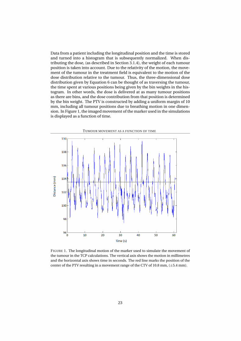
Data from a patient including the longitudinal position and the time is storedand turned into a histogram that is subsequently normalized. When dis-tributing the dose, (as described in Section 3.1.4), the weight of each tumourposition is taken into account. Due to the relativity of the motion, the move-ment of the tumour in the treatment field is equivalent to the motion of thedose distribution relative to the tumour. Thus, the three-dimensional dosedistribution given by Equation 6 can be thought of as traversing the tumour,the time spent at various positions being given by the bin weights in the his-togram. In other words, the dose is delivered at as many tumour positionsas there are bins, and the dose contribution from that position is determinedby the bin weight. The PTV is constructed by adding a uniform margin of 10mm, including all tumour positions due to breathing motion in one dimen-sion. In Figure 1, the imaged movement of the marker used in the simulationsis displayed as a function of time.

TUMOUR MOVEMENT AS A FUNCTION OF TIME

FIGURE 1. The longitudinal motion of the marker used to simulate the movement ofthe tumour in the TCP calculations. The vertical axis shows the motion in millimetresand the horizontal axis shows time in seconds. The red line marks the position of thecenter of the PTV resulting in a movement range of the CTV of 10.8 mm, (±5.4 mm).

23

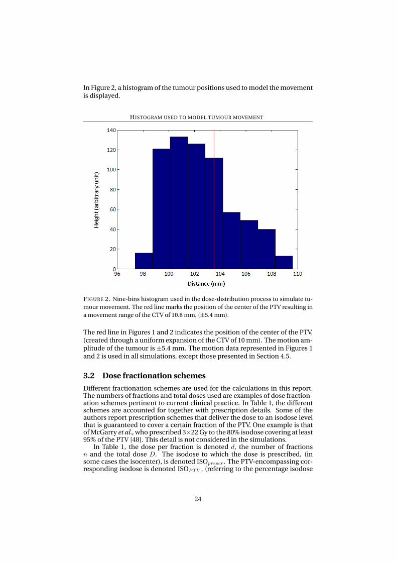
In Figure 2, a histogram of the tumour positions used to model the movementis displayed.

HISTOGRAM USED TO MODEL TUMOUR MOVEMENT

FIGURE 2. Nine-bins histogram used in the dose-distribution process to simulate tu-mour movement. The red line marks the position of the center of the PTV resulting ina movement range of the CTV of 10.8 mm, (±5.4 mm).

The red line in Figures 1 and 2 indicates the position of the center of the PTV,(created through a uniform expansion of the CTV of 10 mm). The motion am-plitude of the tumour is ±5.4 mm. The motion data represented in Figures 1and 2 is used in all simulations, except those presented in Section 4.5.

3.2 Dose fractionation schemes

Different fractionation schemes are used for the calculations in this report.The numbers of fractions and total doses used are examples of dose fraction-ation schemes pertinent to current clinical practice. In Table 1, the differentschemes are accounted for together with prescription details. Some of theauthors report prescription schemes that deliver the dose to an isodose levelthat is guaranteed to cover a certain fraction of the PTV. One example is thatof McGarry et al., who prescribed 3×22 Gy to the 80% isodose covering at least95% of the PTV [48]. This detail is not considered in the simulations.

In Table 1, the dose per fraction is denoted d, the number of fractionsn and the total dose D. The isodose to which the dose is prescribed, (insome cases the isocenter), is denoted ISOprescr. The PTV-encompassing cor-responding isodose is denoted ISOPTV , (referring to the percentage isodose

24

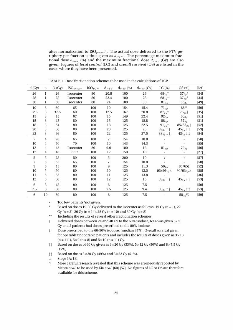
after normalization to ISOprescr). The actual dose delivered to the PTV pe-riphery per fraction is thus given as dPTV . The percentage maximum frac-tional dose dmax (%) and the maximum fractional dose dmax (Gy) are alsogiven. Figures of local control (LC) and overall survival (OS) are listed in thecases where they have been presented.

TABLE 1. Dose fractionation schemes to be used in the calculations of TCP.

d (Gy) n D (Gy) ISOprescr ISOPTV dPTV dmax (%) dmax (Gy) LC (%) OS (%) Ref

26 1 26 Isocenter 80 20.8 100 26 683y* 373y* [34]28 1 28 Isocenter 80 22.4 100 28 683y* 373y* [34]30 1 30 Isocenter 80 24 100 30 813y 533y [49]

10 3 30 65 100 10 154 15.4 712y 68** [50]12.5 3 37.5 60 100 12.5 167 20.8 872y† 752y† [35]15 3 45 67 100 15 149 22.4 923y 603y [51]15 3 45 80 100 15 125 18.8 883y 573y [31]18 3 54 80 100 18 125 22.5 912y‡ 85/652y‡ [52]20 3 60 80 100 20 125 25 893y † † 453y † † [53]22 3 66 80 100 22 125 27.5 883y ‡ ‡ 433y ‡ ‡ [54]

7 4 28 65 100 7 154 10.8 - - [50]10 4 40 70 100 10 143 14.3 - - [55]12 4 48 Isocenter 80 9.6 100 12 813y 793y [56]12 4 48 66.7 100 12 150 18 - - [27]

5 5 25 50 100 5 200 10 g g [57]7 5 35 65 100 7 154 10.8 - - [50]9 5 45 80 100 9 125 11.3 502y 85/65‡ [52]

10 5 50 80 100 10 125 12.5 93/963yf 90/633yf [58]11 5 55 80 100 11 125 13.8 - - [36]12 5 60 80 100 12 125 15 893y † † 453y † † [53]

6 8 48 80 100 6 125 7.5 - - [50]7.5 8 60 80 100 7.5 125 9.4 893y † † 453y † † [53]

6 10 60 80 100 6 125 7.5 - 582y% [59]

- Too few patients/not given.* Based on doses 19-30 Gy delivered to the isocenter as follows: 19 Gy (n = 1), 22

Gy (n = 2), 26 Gy (n = 14), 28 Gy (n = 10) and 30 Gy (n = 8).** Including the results of several other fractionation schemes.† Delivered doses between 24 and 40 Gy to the 60% isodose, 69% was given 37.5

Gy and 2 patients had doses prescribed to the 80% isodose.‡ Dose prescribed to the 60-90% isodose, (median 84%). Overall survival given

for operable/inoperable patients and includes the results of doses given as 3×18(n = 111), 5×9 (n = 8) and 5×10 (n = 11) Gy.

†† Based on doses of 60 Gy given as 3×20 Gy (33%), 5×12 Gy (50%) and 8×7.5 Gy(17%).

‡‡ Based on doses 3×20 Gy (49%) and 3×22 Gy (51%).f Stage 1A/1B.g More careful research revealed that this scheme was erroneously reported by

Mehta et al. to be used by Xia et al. [60] [57]. No figures of LC or OS are thereforeavailable for this scheme.

25

3.3 Planned simulations

This section describes the specific details of the simulations and calculationsperformed. Tumour motion is incorporated in all simulations using data froma patient CBCT-examination, as described in Section 3.1.5.

3.3.1 The relevant dose parameter for predicting the TCP

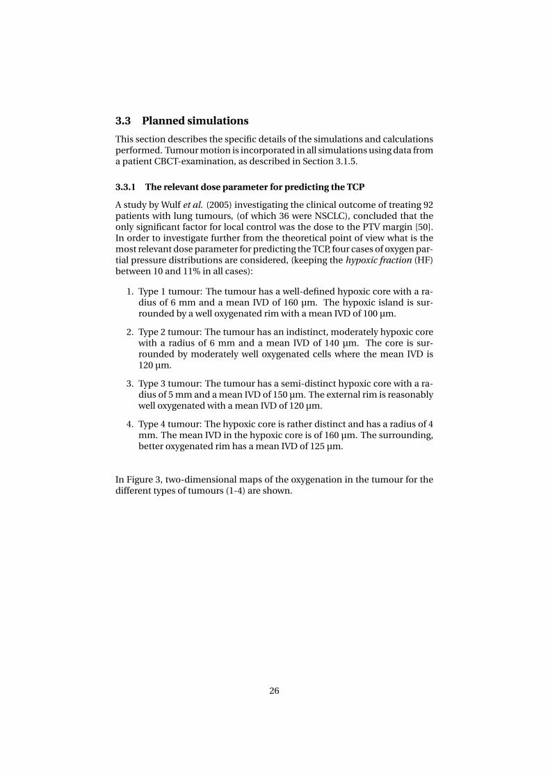
A study by Wulf et al. (2005) investigating the clinical outcome of treating 92patients with lung tumours, (of which 36 were NSCLC), concluded that theonly significant factor for local control was the dose to the PTV margin [50].In order to investigate further from the theoretical point of view what is themost relevant dose parameter for predicting the TCP, four cases of oxygen par-tial pressure distributions are considered, (keeping the hypoxic fraction (HF)between 10 and 11% in all cases):

1. Type 1 tumour: The tumour has a well-defined hypoxic core with a ra-dius of 6 mm and a mean IVD of 160 µm. The hypoxic island is sur-rounded by a well oxygenated rim with a mean IVD of 100 µm.

2. Type 2 tumour: The tumour has an indistinct, moderately hypoxic corewith a radius of 6 mm and a mean IVD of 140 µm. The core is sur-rounded by moderately well oxygenated cells where the mean IVD is120 µm.

3. Type 3 tumour: The tumour has a semi-distinct hypoxic core with a ra-dius of 5 mm and a mean IVD of 150 µm. The external rim is reasonablywell oxygenated with a mean IVD of 120 µm.

4. Type 4 tumour: The hypoxic core is rather distinct and has a radius of 4mm. The mean IVD in the hypoxic core is of 160 µm. The surrounding,better oxygenated rim has a mean IVD of 125 µm.

In Figure 3, two-dimensional maps of the oxygenation in the tumour for thedifferent types of tumours (1-4) are shown.

26

VARIOUS OXYGEN PARTIAL PRESSURE DISTRIBUTIONS FOR ≈10% HYPOXIA

FIGURE 3. Two-dimensional maps of the oxygen partial pressure distribution in mmHgfor various combinations of inter-vessel distances. 1) Type 1 tumour; 2) Type 2 tu-mour; 3) Type 3 tumour; 4) Type 4 tumour.

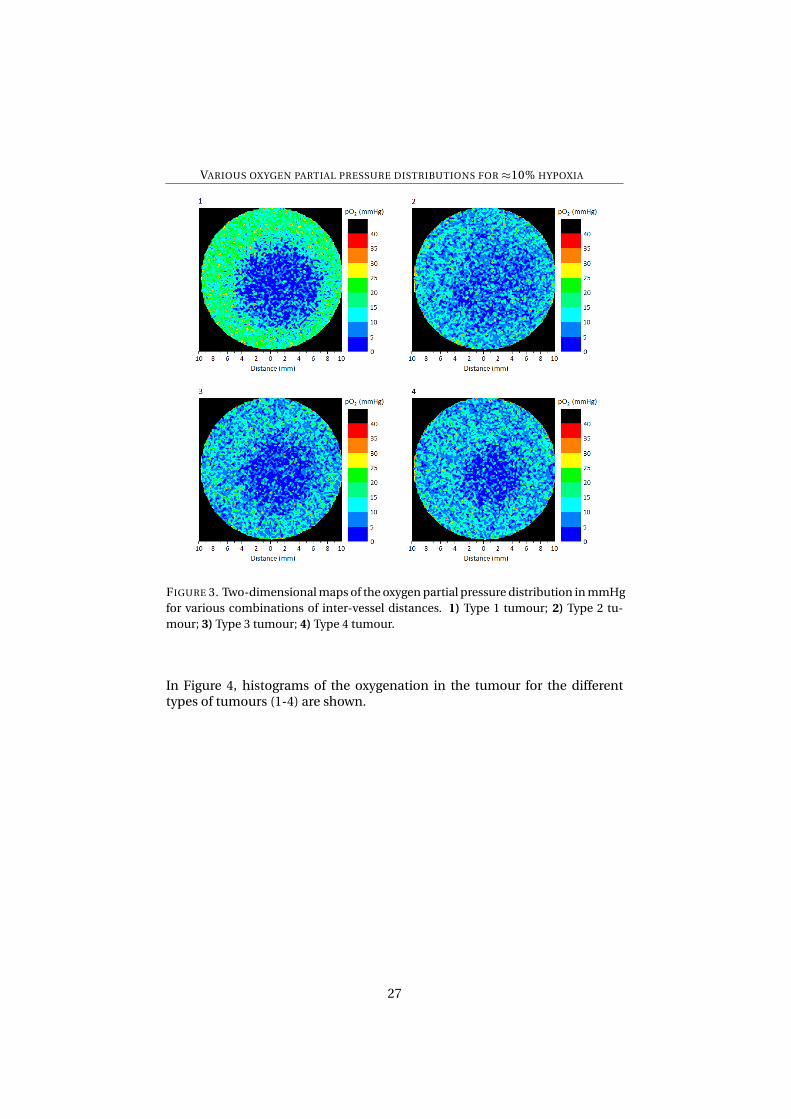
In Figure 4, histograms of the oxygenation in the tumour for the differenttypes of tumours (1-4) are shown.

27

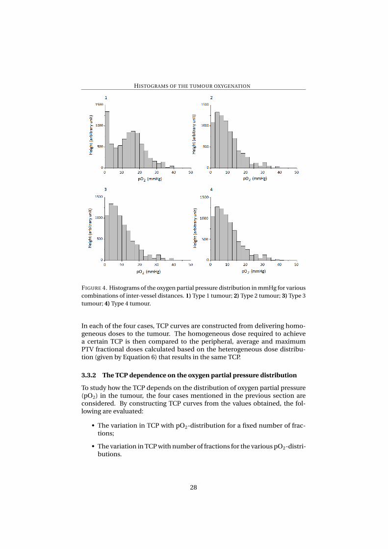
HISTOGRAMS OF THE TUMOUR OXYGENATION

FIGURE 4. Histograms of the oxygen partial pressure distribution in mmHg for variouscombinations of inter-vessel distances. 1) Type 1 tumour; 2) Type 2 tumour; 3) Type 3tumour; 4) Type 4 tumour.

In each of the four cases, TCP curves are constructed from delivering homo-geneous doses to the tumour. The homogeneous dose required to achievea certain TCP is then compared to the peripheral, average and maximumPTV fractional doses calculated based on the heterogeneous dose distribu-tion (given by Equation 6) that results in the same TCP.

3.3.2 The TCP dependence on the oxygen partial pressure distribution

To study how the TCP depends on the distribution of oxygen partial pressure(pO2) in the tumour, the four cases mentioned in the previous section areconsidered. By constructing TCP curves from the values obtained, the fol-lowing are evaluated:

• The variation in TCP with pO2-distribution for a fixed number of frac-tions;

• The variation in TCP with number of fractions for the various pO2-distri-butions.

28

3.3.3 The TCP dependence on the hypoxic fraction

For constant values of the inter-vessel distances in the well-oxygenated andhypoxic tumour tissues, (100 and 160 µm respectively), the dependence ofTCP on the hypoxic fraction is investigated. This is done by simulating thetumour with different sizes of the hypoxic core resulting in HF≈10, 6, 3 and1%. By constructing TCP curves from the values obtained, the following areevaluated:

• The variation in TCP with HF for a fixed number of fractions;

• The variation in TCP with number of fractions for the various HFs.

3.3.4 The TCP dependence on the position of the hypoxic island

For constant values of the inter-vessel distances in the well-oxygenated andhypoxic tumour tissues, (100 and 160 µm respectively), and a constant hy-poxic fraction (≈10% and≈1%), the dependence of TCP on the position of thehypoxic island is investigated. The hypoxic island is placed near the center ofthe tumour and near the periphery of the CTV whereupon by constructingTCP curves from the values obtained, the following are evaluated:

• The variation in TCP with hypoxic island location for a fixed number offractions;

• The variation in TCP with number of fractions for the various locationsof the hypoxic island.

In Figure 5, examples of two-dimensional cross sections through the tumourshowing the two different locations of the hypoxic island, (central and pe-ripheral), for the two hypoxic fractions, (10 and 1%), are shown.

29

VARIOUS OXYGEN PARTIAL PRESSURE DISTRIBUTIONS FOR DIFFERENT HYPOXIC

FRACTIONS AND POSITIONS OF THE HYPOXIC ISLAND

FIGURE 5. Two-dimensional maps of the oxygen partial pressure distribution for var-ious hypoxic fractions (HFs) and positions of the hypoxic island (HI). A) Central loca-tion, rHI = 6 mm, HF≈10%; B) Peripheral location, rHI = 6 mm, HF≈10%; C) Centrallocation, rHI = 3 mm, HF≈1%; D) Peripheral location, rHI = 3 mm, HF≈1%.

In Figure 6, histograms of the oxygen partial pressure in the tumour showingthe two different locations of the hypoxic island, (central and peripheral), forthe two hypoxic fractions, (10 and 1%), are shown.

30

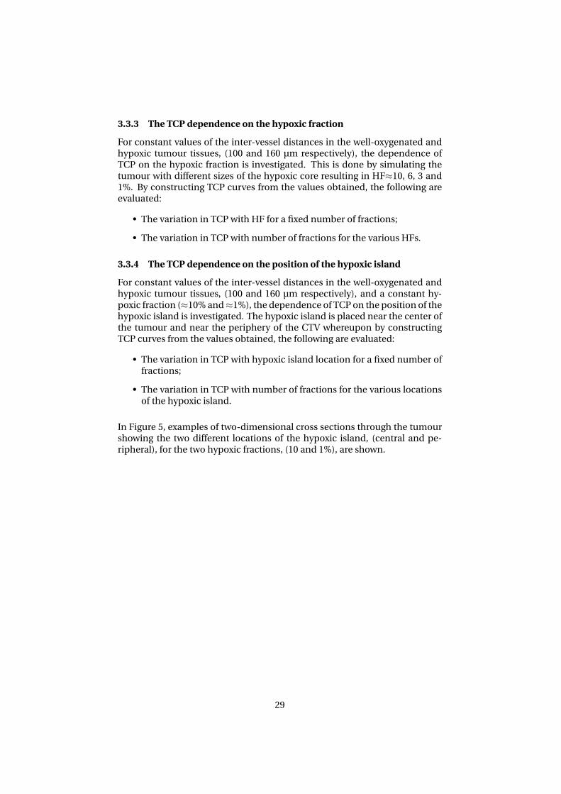
HISTOGRAMS OF THE TUMOUR OXYGENATION FOR DIFFERENT HYPOXIC FRACTIONS AND

POSITIONS OF THE HYPOXIC ISLAND

FIGURE 6. Histograms of the oxygenation for various hypoxic fractions (HFs) and po-sitions of the hypoxic island (HI). A) Central location, rHI = 6 mm, HF≈10%; B) Pe-ripheral location, rHI = 6 mm, HF≈10%; C) Central location, rHI = 3 mm, HF≈1%; D)Peripheral location, rHI = 3 mm, HF≈1%.

3.3.5 The influence on TCP of tumour movement during irradiation

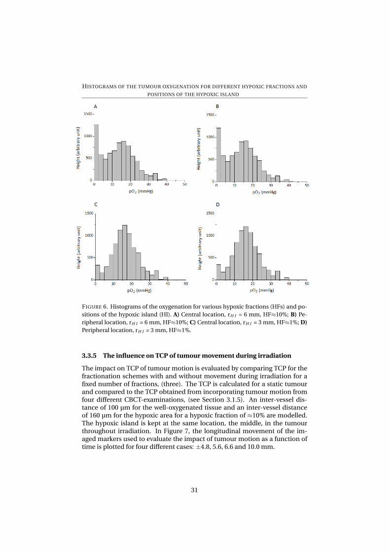
The impact on TCP of tumour motion is evaluated by comparing TCP for thefractionation schemes with and without movement during irradiation for afixed number of fractions, (three). The TCP is calculated for a static tumourand compared to the TCP obtained from incorporating tumour motion fromfour different CBCT-examinations, (see Section 3.1.5). An inter-vessel dis-tance of 100 µm for the well-oxygenated tissue and an inter-vessel distanceof 160 µm for the hypoxic area for a hypoxic fraction of ≈10% are modelled.The hypoxic island is kept at the same location, the middle, in the tumourthroughout irradiation. In Figure 7, the longitudinal movement of the im-aged markers used to evaluate the impact of tumour motion as a function oftime is plotted for four different cases: ±4.8, 5.6, 6.6 and 10.0 mm.

31

TUMOUR MOVEMENT AS A FUNCTION OF TIME

FIGURE 7. The longitudinal motion in four different cases. A) Movement±4.8 mm; B)Movement±5.6 mm; C) Movement±6.6 mm; D) Movement±10.0 mm. The positionof the PTV center is indicated with a red, horizontal line.

32

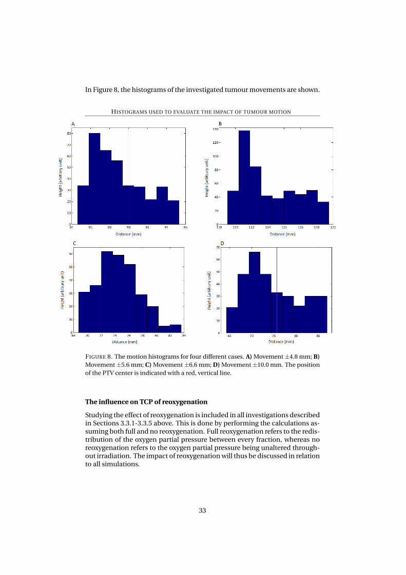
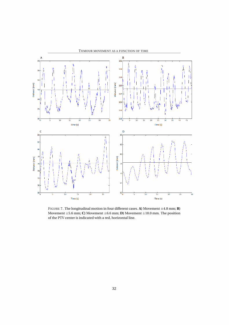
In Figure 8, the histograms of the investigated tumour movements are shown.

HISTOGRAMS USED TO EVALUATE THE IMPACT OF TUMOUR MOTION

FIGURE 8. The motion histograms for four different cases. A) Movement±4.8 mm; B)Movement±5.6 mm; C) Movement±6.6 mm; D) Movement±10.0 mm. The positionof the PTV center is indicated with a red, vertical line.

The influence on TCP of reoxygenation

Studying the effect of reoxygenation is included in all investigations describedin Sections 3.3.1-3.3.5 above. This is done by performing the calculations as-suming both full and no reoxygenation. Full reoxygenation refers to the redis-tribution of the oxygen partial pressure between every fraction, whereas noreoxygenation refers to the oxygen partial pressure being unaltered through-out irradiation. The impact of reoxygenation will thus be discussed in relationto all simulations.

33

3.4 Analysis of uncertainties

To estimate the uncertainty in the TCP, the standard deviation is calculated asfollows [61]:

σx =

√1

N − 1

∑(xi − x)2 (11)

where x and xi represent the TCP and x represent the mean of the TCP. Forthree dose-schemes, 3×15 to the 67% isodose [51], 4×12 to the 66.7% iso-dose [27] and 5×11 to the 80% isodose [36], the TCP is calculated ten timeseach. The resulting values serve as xi and the mean TCP as x in Equation11. To make a connection between the uncertainty in TCP (σTCP) and hypoxia,Equation 11 is also used to calculate the uncertainty in the hypoxic fraction(σHF) in the same way. In addition to the calculated sample uncertainties,other sources of error and uncertainty will be discussed.

4 Results

In Table 2, the results of calculating the TCP using the fractionation schemespresented in Table 1 are presented. Values of the TCP in per cent are displayedboth for no and full reoxygenation. The calculations have been performed fora tumour with a 12 mm hypoxic island located centrally, and inter-vessel dis-tances of IVDox = 100 µm and IVDhyp = 160 µm for the well oxygenated andhypoxic parts respectively. The fractional dose is denoted d, the number offractions n and the resulting total dose D. For each scheme, the fractionaldose to the PTV margin dPTV , the fractional maximum percentage and abso-lute dose to the PTV dmax and the average CTV fractional dose dave are dis-played.

34

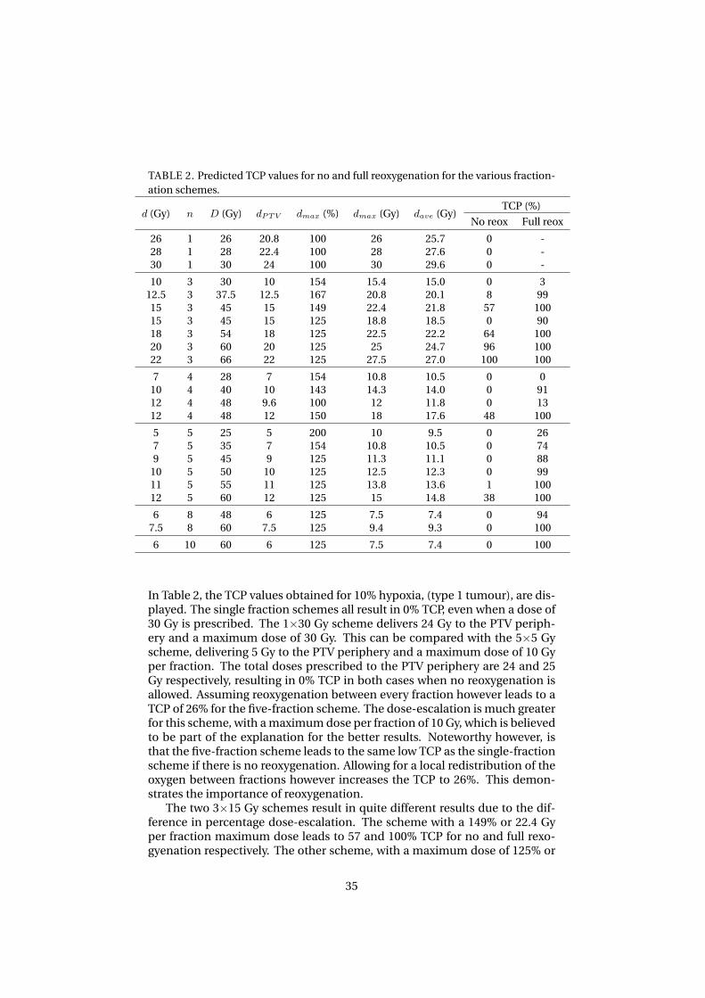
TABLE 2. Predicted TCP values for no and full reoxygenation for the various fraction-ation schemes.

TCP (%)d (Gy) n D (Gy) dPTV dmax (%) dmax (Gy) dave (Gy)

No reox Full reox

26 1 26 20.8 100 26 25.7 0 -28 1 28 22.4 100 28 27.6 0 -30 1 30 24 100 30 29.6 0 -

10 3 30 10 154 15.4 15.0 0 312.5 3 37.5 12.5 167 20.8 20.1 8 9915 3 45 15 149 22.4 21.8 57 10015 3 45 15 125 18.8 18.5 0 9018 3 54 18 125 22.5 22.2 64 10020 3 60 20 125 25 24.7 96 10022 3 66 22 125 27.5 27.0 100 100

7 4 28 7 154 10.8 10.5 0 010 4 40 10 143 14.3 14.0 0 9112 4 48 9.6 100 12 11.8 0 1312 4 48 12 150 18 17.6 48 100

5 5 25 5 200 10 9.5 0 267 5 35 7 154 10.8 10.5 0 749 5 45 9 125 11.3 11.1 0 88

10 5 50 10 125 12.5 12.3 0 9911 5 55 11 125 13.8 13.6 1 10012 5 60 12 125 15 14.8 38 100

6 8 48 6 125 7.5 7.4 0 947.5 8 60 7.5 125 9.4 9.3 0 100

6 10 60 6 125 7.5 7.4 0 100

In Table 2, the TCP values obtained for 10% hypoxia, (type 1 tumour), are dis-played. The single fraction schemes all result in 0% TCP, even when a dose of30 Gy is prescribed. The 1×30 Gy scheme delivers 24 Gy to the PTV periph-ery and a maximum dose of 30 Gy. This can be compared with the 5×5 Gyscheme, delivering 5 Gy to the PTV periphery and a maximum dose of 10 Gyper fraction. The total doses prescribed to the PTV periphery are 24 and 25Gy respectively, resulting in 0% TCP in both cases when no reoxygenation isallowed. Assuming reoxygenation between every fraction however leads to aTCP of 26% for the five-fraction scheme. The dose-escalation is much greaterfor this scheme, with a maximum dose per fraction of 10 Gy, which is believedto be part of the explanation for the better results. Noteworthy however, isthat the five-fraction scheme leads to the same low TCP as the single-fractionscheme if there is no reoxygenation. Allowing for a local redistribution of theoxygen between fractions however increases the TCP to 26%. This demon-strates the importance of reoxygenation.

The two 3×15 Gy schemes result in quite different results due to the dif-ference in percentage dose-escalation. The scheme with a 149% or 22.4 Gyper fraction maximum dose leads to 57 and 100% TCP for no and full rexo-gyenation respectively. The other scheme, with a maximum dose of 125% or

35

18.8 Gy per fraction leads to 0 and 90% TCP for no and full reoxygenation re-spectively. Given identical doses to the PTV, the TCP may thus vary by up to57 percentage points if different maximum doses are allowed. This indicatesthat the dose to the PTV periphery is not enough information to predict theTCP for a certain scheme.

What is also interesting is the differences in TCPnoreox and TCPfullreox be-tween the two schemes. The difference in TCP is 57% if there is no reoxy-genation but only 10% if reoxygenation takes place. The dose-escalation thushas a bigger impact on TCP if no reoxygenation is allowed. This demonstratesthe power and importance of the process of reoxygenation between fractions.High values of TCP without reoxygenation are generally hard to obtain unlessthe fractional dose is rather high. TCP values as high as 96 and 100% are ac-quired only for the 3×20 and 22 Gy respectively, (in the case of no reoxygena-tion).

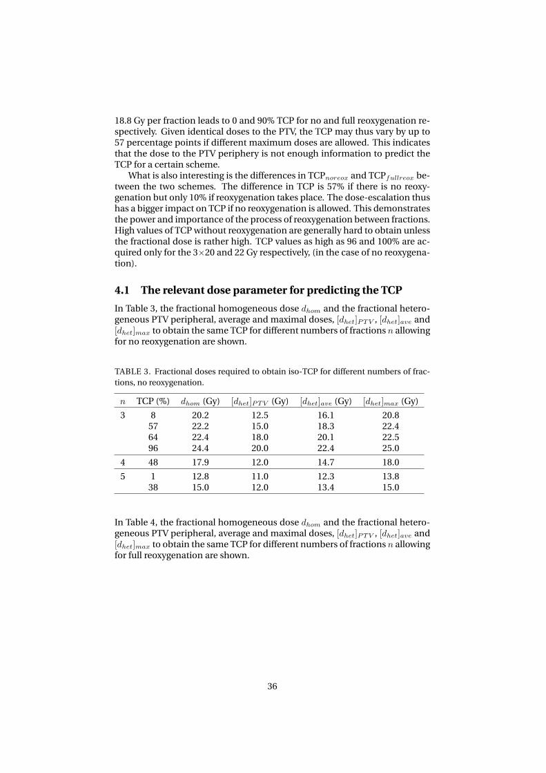
4.1 The relevant dose parameter for predicting the TCP

In Table 3, the fractional homogeneous dose dhom and the fractional hetero-geneous PTV peripheral, average and maximal doses, [dhet]PTV , [dhet]ave and[dhet]max to obtain the same TCP for different numbers of fractions n allowingfor no reoxygenation are shown.

TABLE 3. Fractional doses required to obtain iso-TCP for different numbers of frac-tions, no reoxygenation.

n TCP (%) dhom (Gy) [dhet]PTV (Gy) [dhet]ave (Gy) [dhet]max (Gy)

3 8 20.2 12.5 16.1 20.857 22.2 15.0 18.3 22.464 22.4 18.0 20.1 22.596 24.4 20.0 22.4 25.0

4 48 17.9 12.0 14.7 18.0

5 1 12.8 11.0 12.3 13.838 15.0 12.0 13.4 15.0

In Table 4, the fractional homogeneous dose dhom and the fractional hetero-geneous PTV peripheral, average and maximal doses, [dhet]PTV , [dhet]ave and[dhet]max to obtain the same TCP for different numbers of fractions n allowingfor full reoxygenation are shown.

36

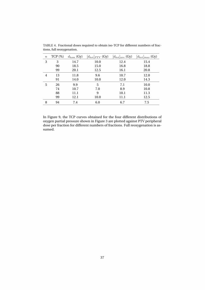
TABLE 4. Fractional doses required to obtain iso-TCP for different numbers of frac-tions, full reoxygenation.

n TCP (%) dhom (Gy) [dhet]PTV (Gy) [dhet]ave (Gy) [dhet]max (Gy)

3 3 14.7 10.0 12.4 15.490 18.5 15.0 16.8 18.899 20.1 12.5 16.1 20.8

4 13 11.8 9.6 10.7 12.091 14.0 10.0 12.0 14.3

5 26 9.9 5 7.1 10.074 10.7 7.0 8.9 10.888 11.1 9 10.1 11.399 12.1 10.0 11.1 12.5

8 94 7.4 6.0 6.7 7.5

In Figure 9, the TCP curves obtained for the four different distributions ofoxygen partial pressure shown in Figure 3 are plotted against PTV peripheraldose per fraction for different numbers of fractions. Full reoxygenation is as-sumed.

37

TCP CURVES FOR VARIOUS OXYGEN PARTIAL PRESSURE DISTRIBUTIONS AS A FUNCTION

OF PTV PERIPHERAL DOSE PER FRACTION

FIGURE 9. TCP curves for various oxygen partial pressure distributions in mmHg anddifferent combinations of inter-vessel distances achieving the same hypoxic fraction,plotted against the fractional PTV peripheral dose for 3, 4 and 5 fractions. 1) Type 1tumour; 2) Type 2 tumour; 3) Type 3 tumour; 4) Type 4 tumour. Full reoxygenation isassumed.

In Figure 10, the TCP curves obtained for the four different distributions ofoxygen partial pressure shown in Figure 3 are plotted against the average doseper fraction to the CTV for different numbers of fractions. Full reoxygenationis assumed.

38

TCP CURVES FOR VARIOUS OXYGEN PARTIAL PRESSURE DISTRIBUTIONS AS A FUNCTION

OF AVERAGE DOSE PER FRACTION TO THE CTV

FIGURE 10. TCP curves for various oxygen partial pressure distributions in mmHg anddifferent combinations of inter-vessel distances achieving the same hypoxic fraction,plotted against the average fractional dose to the CTV for 3, 4 and 5 fractions. 1) Type1 tumour; 2) Type 2 tumour; 3) Type 3 tumour; 4) Type 4 tumour. Full reoxygenationis assumed.

In Figure 9, TCP is plotted as a function of PTV peripheral dose while in Fig-ure 10, the average CTV dose is on the horizontal axis. What can be seenis the better consistency of TCP with the average heterogeneous CTV doserather than the peripheral PTV dose. In order to make the fit so that the greencurves predict zero TCP at zero dose, the point (d, TCP ) = (0, 0) had to beadded in the fitting process. One of the points on the green curves representthe TCP obtained by prescribing 5×5 Gy to the 50% isodose. Thus, the PTVperipheral dose is 5 Gy while the maximum dose is 10 Gy. This is an exam-ple of a peripheral dose that poorly represents the dose actually delivered tothe tumour, (the average dose being 9.5 Gy). For the five-fractions schemes,

39

the rather broad dose range resulting in high TCP values severely affects theappearance of the curves. In the limit d → 0, the TCP curve should asymp-totically approach zero, which is not achieved in panels 2, 3 and 4 in Figure9. Furthermore, the blue curves representing the four-fractions schemes inpanels 3 and 4 look very strange in relation to the data points. Part of the ex-planation for this lies in the two mid-data points being very similar in PTVperipheral dose (9.6 and 10 Gy respectively) but differing significantly in pre-dicted TCP (64 and 98% in panel 3 and 54 and 97% in panel 4). The schemeprescribing 9.6 Gy per fraction delivers a maximum dose of 12 Gy per fractionand the scheme prescribing 10 Gy per fraction delivers a maximum dose ofmore than 14 Gy per fraction. This difference in dose-escalation between theclosely located data points forces the steep slope of the TCP curve leading toits overall strange shape. All these serve as a strong indicators that presentingTCP as a function of PTV peripheral dose could be highly misrepresentative.

Looking instead at Figure 10 where TCP is plotted as a function of averagedose per fraction, the curves have a nice shape as a result of the better agree-ment of the average fractional dose with predicted TCP. These plots show fur-ther indication, in accordance with the values in Tables 3-4, that the averagedose is a more relevant factor to estimate local control. To conclude this on amore general level, a multivariate analysis of the most relevant factor to ob-tain local control is suggested.

4.2 The TCP dependence on the oxygen partial pressure dis-tribution

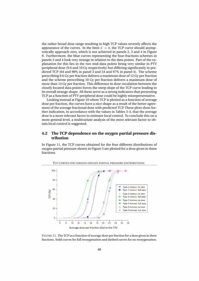
In Figure 11, the TCP curves obtained for the four different distributions ofoxygen partial pressure shown in Figure 3 are plotted for a dose given in threefractions.

TCP CURVES FOR VARIOUS OXYGEN PARTIAL PRESSURE DISTRIBUTIONS

FIGURE 11. The TCP as a function of average dose per fraction for a dose given in threefractions. Solid curves for full reoxygenation and dashed curves for no reoxygenation.

40

From the curves in Figure 11, it can be seen that in the case of full reoxygena-tion, the biggest difference in TCP is between the cases of spread-out hypoxia,(type 2 tumour, green solid curve), and a more concentrated hypoxia, (type 1tumour, blue solid curve).

In Figure 12, the TCP curves obtained for the four different distributionsof oxygen partial pressure shown in Figure 3 are plotted for a dose given in 3,4 and 5 fractions. Full reoxygenation is assumed.

TCP CURVES FOR VARIOUS OXYGEN PARTIAL PRESSURE DISTRIBUTIONS AND NUMBERS

OF FRACTIONS

FIGURE 12. The TCP as a function of average dose per fraction for a dose given in 3, 4and 5 fractions for various oxygen partial pressure distributions. All curves representfull reoxygenation.

4.3 The TCP dependence on the hypoxic fraction

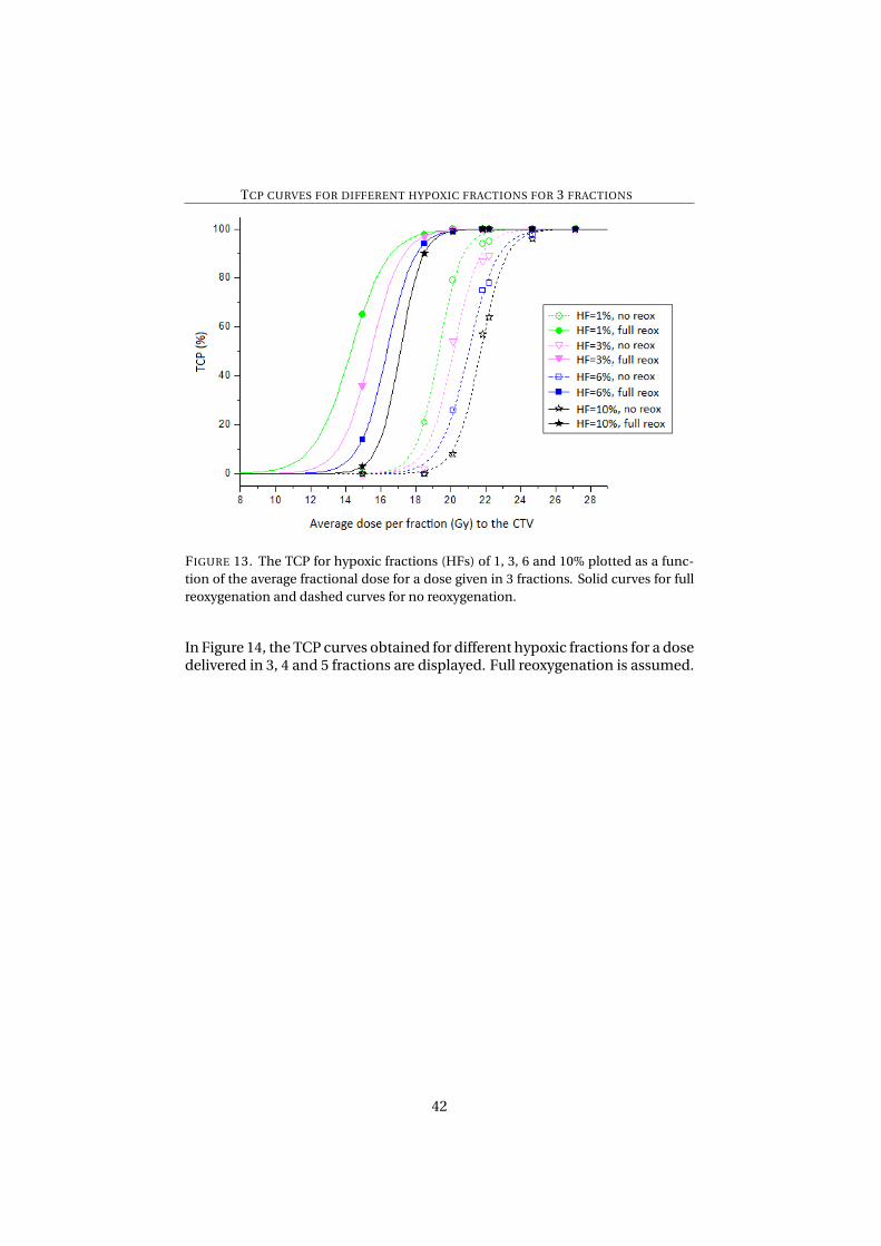
In Figure 13, the TCP curves obtained for different hypoxic fractions for a dosedelivered in three fractions are displayed.

41

TCP CURVES FOR DIFFERENT HYPOXIC FRACTIONS FOR 3 FRACTIONS

FIGURE 13. The TCP for hypoxic fractions (HFs) of 1, 3, 6 and 10% plotted as a func-tion of the average fractional dose for a dose given in 3 fractions. Solid curves for fullreoxygenation and dashed curves for no reoxygenation.

In Figure 14, the TCP curves obtained for different hypoxic fractions for a dosedelivered in 3, 4 and 5 fractions are displayed. Full reoxygenation is assumed.

42

TCP CURVES FOR DIFFERENT HYPOXIC FRACTIONS FOR DIFFERENT NUMBERS OF

FRACTIONS

FIGURE 14. The TCP for hypoxic fractions of 1, 3, 6 and 10% plotted as a function of theaverage dose per fraction for a dose given in 3, 4 and 5 fractions. All curves representfull reoxygenation.

4.4 The TCP dependence on the position of the hypoxic is-land

In Figure 15, the TCP curves obtained for different positions of the hypoxicisland for hypoxic fractions of 10 and 1% respectively are shown. The dose isgiven in three fractions.

43

TCP CURVES FOR DIFFERENT POSITIONS OF THE HYPOXIC ISLAND FOR THREE

FRACTIONS

FIGURE 15. The TCP for different positions of the hypoxic island plotted as a functionof the average dose for a dose given in 3 fractions. A) HF=10%; B) HF=1%. Solid curvesfor full reoxygenation and dashed curves for no reoxygenation.

The results displayed in Figure 15 demonstrate that, assuming full reoxygena-tion, there is a slight increase in TCP when the hypoxic island is located cen-trally compared to peripherally for both 10 and 1% hypoxia. This increase ismore significant for a smaller hypoxic fraction of ≈1%. If no reoxygenationtakes place, there is virtually no difference in TCP depending on where thehypoxic island is located. A small increase in TCP for high doses per fractionis seen for the central location of the smaller hypoxic island compared to thelarger one. This is another case in which the importance of reoxygenation isdemonstrated.

In Figure 16, the TCP curves obtained for different positions of the hypoxicisland for hypoxic fractions of 10 and 1% respectively are shown. The dose isgiven in 3, 4 and 5 fractions. Full reoxygenation is assumed.

44

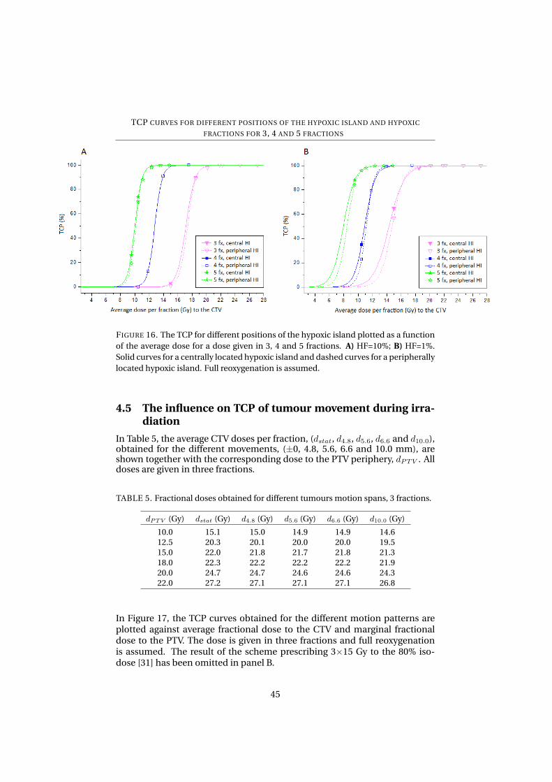
TCP CURVES FOR DIFFERENT POSITIONS OF THE HYPOXIC ISLAND AND HYPOXIC

FRACTIONS FOR 3, 4 AND 5 FRACTIONS

FIGURE 16. The TCP for different positions of the hypoxic island plotted as a functionof the average dose for a dose given in 3, 4 and 5 fractions. A) HF=10%; B) HF=1%.Solid curves for a centrally located hypoxic island and dashed curves for a peripherallylocated hypoxic island. Full reoxygenation is assumed.

4.5 The influence on TCP of tumour movement during irra-diation

In Table 5, the average CTV doses per fraction, (dstat, d4.8, d5.6, d6.6 and d10.0),obtained for the different movements, (±0, 4.8, 5.6, 6.6 and 10.0 mm), areshown together with the corresponding dose to the PTV periphery, dPTV . Alldoses are given in three fractions.

TABLE 5. Fractional doses obtained for different tumours motion spans, 3 fractions.

dPTV (Gy) dstat (Gy) d4.8 (Gy) d5.6 (Gy) d6.6 (Gy) d10.0 (Gy)

10.0 15.1 15.0 14.9 14.9 14.612.5 20.3 20.1 20.0 20.0 19.515.0 22.0 21.8 21.7 21.8 21.318.0 22.3 22.2 22.2 22.2 21.920.0 24.7 24.7 24.6 24.6 24.322.0 27.2 27.1 27.1 27.1 26.8

In Figure 17, the TCP curves obtained for the different motion patterns areplotted against average fractional dose to the CTV and marginal fractionaldose to the PTV. The dose is given in three fractions and full reoxygenationis assumed. The result of the scheme prescribing 3×15 Gy to the 80% iso-dose [31] has been omitted in panel B.

45

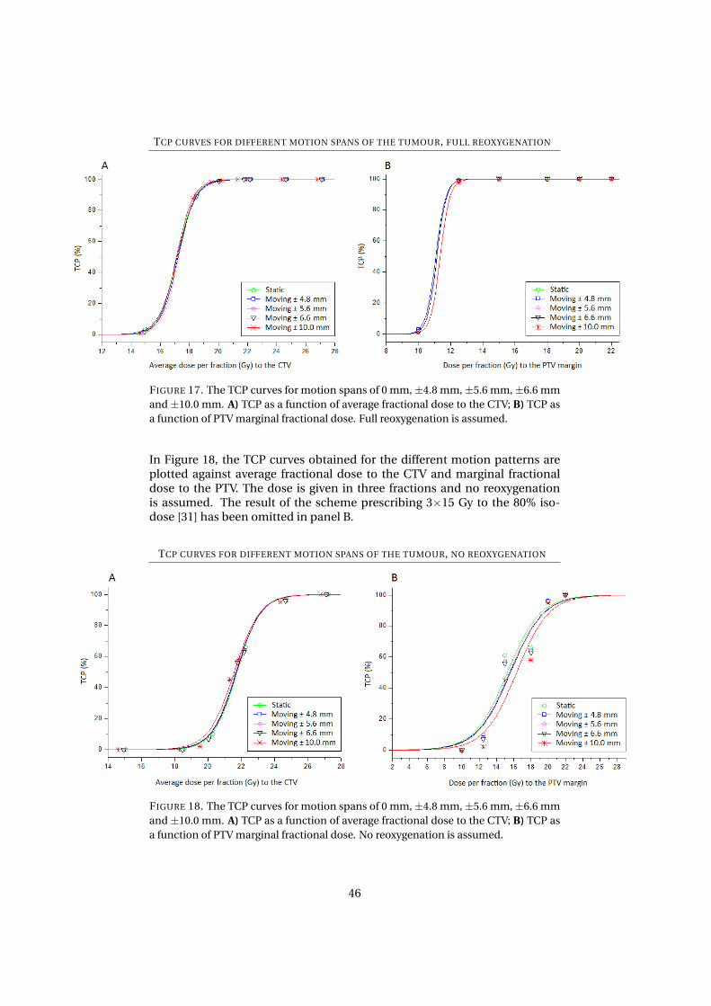
TCP CURVES FOR DIFFERENT MOTION SPANS OF THE TUMOUR, FULL REOXYGENATION

FIGURE 17. The TCP curves for motion spans of 0 mm,±4.8 mm,±5.6 mm,±6.6 mmand ±10.0 mm. A) TCP as a function of average fractional dose to the CTV; B) TCP asa function of PTV marginal fractional dose. Full reoxygenation is assumed.

In Figure 18, the TCP curves obtained for the different motion patterns areplotted against average fractional dose to the CTV and marginal fractionaldose to the PTV. The dose is given in three fractions and no reoxygenationis assumed. The result of the scheme prescribing 3×15 Gy to the 80% iso-dose [31] has been omitted in panel B.

TCP CURVES FOR DIFFERENT MOTION SPANS OF THE TUMOUR, NO REOXYGENATION

FIGURE 18. The TCP curves for motion spans of 0 mm,±4.8 mm,±5.6 mm,±6.6 mmand ±10.0 mm. A) TCP as a function of average fractional dose to the CTV; B) TCP asa function of PTV marginal fractional dose. No reoxygenation is assumed.

46

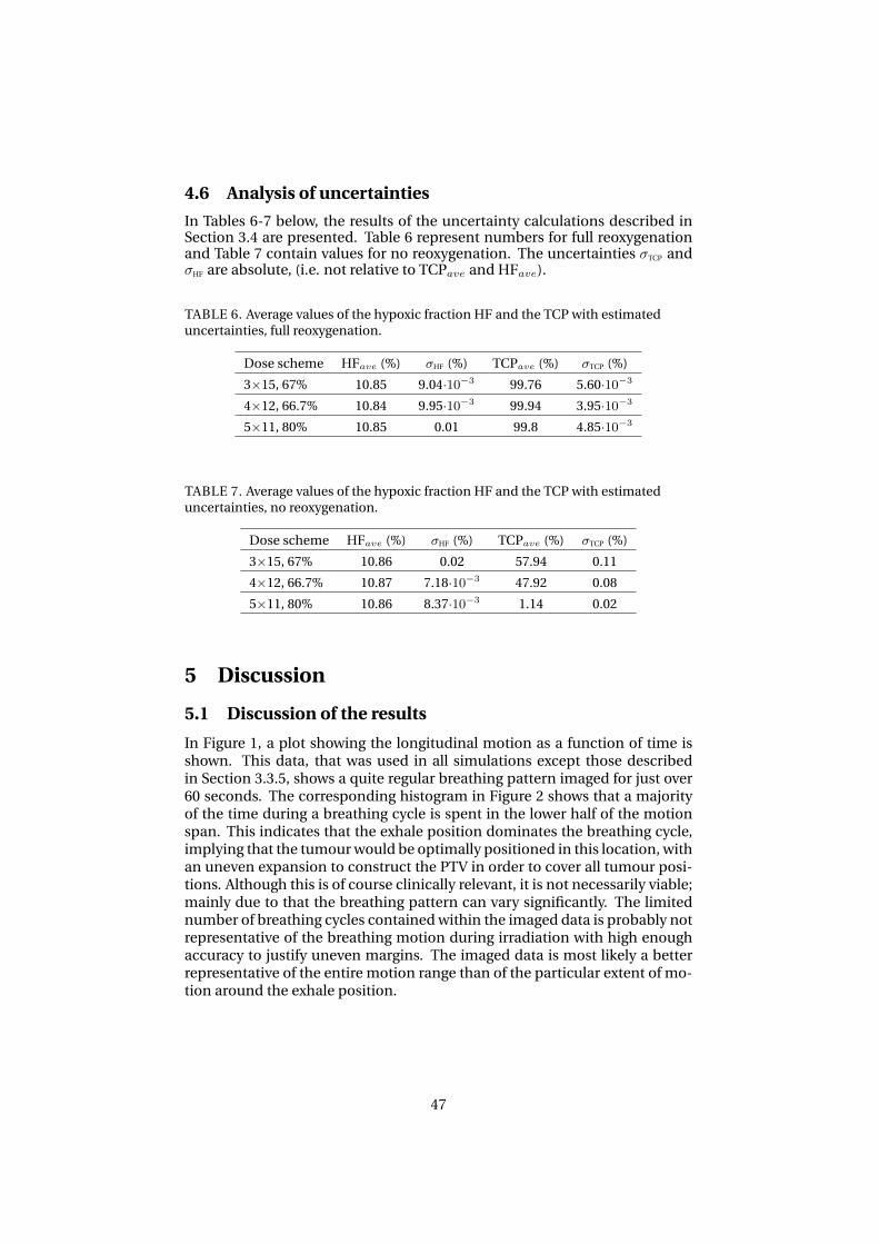
4.6 Analysis of uncertainties

In Tables 6-7 below, the results of the uncertainty calculations described inSection 3.4 are presented. Table 6 represent numbers for full reoxygenationand Table 7 contain values for no reoxygenation. The uncertainties σTCP andσHF are absolute, (i.e. not relative to TCPave and HFave).

TABLE 6. Average values of the hypoxic fraction HF and the TCP with estimateduncertainties, full reoxygenation.

Dose scheme HFave (%) σHF (%) TCPave (%) σTCP (%)

3×15, 67% 10.85 9.04·10−3 99.76 5.60·10−3

4×12, 66.7% 10.84 9.95·10−3 99.94 3.95·10−3

5×11, 80% 10.85 0.01 99.8 4.85·10−3

TABLE 7. Average values of the hypoxic fraction HF and the TCP with estimateduncertainties, no reoxygenation.

Dose scheme HFave (%) σHF (%) TCPave (%) σTCP (%)

3×15, 67% 10.86 0.02 57.94 0.11

4×12, 66.7% 10.87 7.18·10−3 47.92 0.08

5×11, 80% 10.86 8.37·10−3 1.14 0.02

5 Discussion

5.1 Discussion of the results

In Figure 1, a plot showing the longitudinal motion as a function of time isshown. This data, that was used in all simulations except those describedin Section 3.3.5, shows a quite regular breathing pattern imaged for just over60 seconds. The corresponding histogram in Figure 2 shows that a majorityof the time during a breathing cycle is spent in the lower half of the motionspan. This indicates that the exhale position dominates the breathing cycle,implying that the tumour would be optimally positioned in this location, withan uneven expansion to construct the PTV in order to cover all tumour posi-tions. Although this is of course clinically relevant, it is not necessarily viable;mainly due to that the breathing pattern can vary significantly. The limitednumber of breathing cycles contained within the imaged data is probably notrepresentative of the breathing motion during irradiation with high enoughaccuracy to justify uneven margins. The imaged data is most likely a betterrepresentative of the entire motion range than of the particular extent of mo-tion around the exhale position.

47

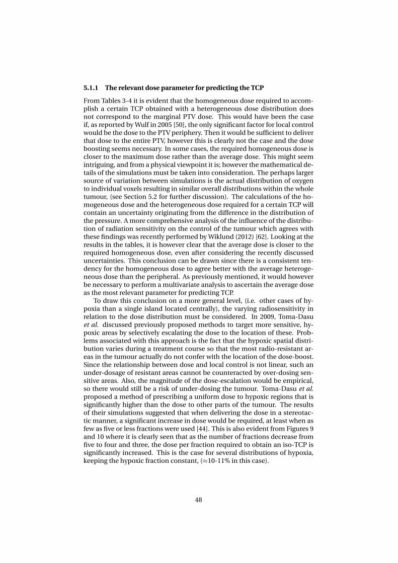
5.1.1 The relevant dose parameter for predicting the TCP

From Tables 3-4 it is evident that the homogeneous dose required to accom-plish a certain TCP obtained with a heterogeneous dose distribution doesnot correspond to the marginal PTV dose. This would have been the caseif, as reported by Wulf in 2005 [50], the only significant factor for local controlwould be the dose to the PTV periphery. Then it would be sufficient to deliverthat dose to the entire PTV, however this is clearly not the case and the doseboosting seems necessary. In some cases, the required homogeneous dose iscloser to the maximum dose rather than the average dose. This might seemintriguing, and from a physical viewpoint it is; however the mathematical de-tails of the simulations must be taken into consideration. The perhaps largersource of variation between simulations is the actual distribution of oxygento individual voxels resulting in similar overall distributions within the wholetumour, (see Section 5.2 for further discussion). The calculations of the ho-mogeneous dose and the heterogeneous dose required for a certain TCP willcontain an uncertainty originating from the difference in the distribution ofthe pressure. A more comprehensive analysis of the influence of the distribu-tion of radiation sensitivity on the control of the tumour which agrees withthese findings was recently performed by Wiklund (2012) [62]. Looking at theresults in the tables, it is however clear that the average dose is closer to therequired homogeneous dose, even after considering the recently discusseduncertainties. This conclusion can be drawn since there is a consistent ten-dency for the homogeneous dose to agree better with the average heteroge-neous dose than the peripheral. As previously mentioned, it would howeverbe necessary to perform a multivariate analysis to ascertain the average doseas the most relevant parameter for predicting TCP.

To draw this conclusion on a more general level, (i.e. other cases of hy-poxia than a single island located centrally), the varying radiosensitivity inrelation to the dose distribution must be considered. In 2009, Toma-Dasuet al. discussed previously proposed methods to target more sensitive, hy-poxic areas by selectively escalating the dose to the location of these. Prob-lems associated with this approach is the fact that the hypoxic spatial distri-bution varies during a treatment course so that the most radio-resistant ar-eas in the tumour actually do not confer with the location of the dose-boost.Since the relationship between dose and local control is not linear, such anunder-dosage of resistant areas cannot be counteracted by over-dosing sen-sitive areas. Also, the magnitude of the dose-escalation would be empirical,so there would still be a risk of under-dosing the tumour. Toma-Dasu et al.proposed a method of prescribing a uniform dose to hypoxic regions that issignificantly higher than the dose to other parts of the tumour. The resultsof their simulations suggested that when delivering the dose in a stereotac-tic manner, a significant increase in dose would be required, at least when asfew as five or less fractions were used [44]. This is also evident from Figures 9and 10 where it is clearly seen that as the number of fractions decrease fromfive to four and three, the dose per fraction required to obtain an iso-TCP issignificantly increased. This is the case for several distributions of hypoxia,keeping the hypoxic fraction constant, (≈10-11% in this case).

48

5.1.2 The TCP dependence on the oxygen partial pressure distribution

As it could be seen in Figure 11, given a hypoxic fraction of ≈10% it is bet-ter to have an evenly distributed oxygenation in the tumour than having onepart that is well oxygenated and one that is severely hypoxic. This is not sostrange, given the mechanisms of reoxygenation and its influence on TCP aspreviously discussed. To obtain a certain hypoxic fraction, a more evenly dis-tributed hypoxia implies that the tumour is generally less radio-resistant, asthe difference between the well and poorly oxygenated areas has to decreasecompared to the case of a more concentrated hypoxia. A less well-oxygenatedarea will contain cells that are even less sensitive to irradiation, and as thepersistence of clonogenic potential of one or a few malignant cells is enoughto cause treatment failure, this scenario poses a bigger threat to obtain localcontrol. Thus to obtain a certain level of TCP the average dose per fractionneeds to be higher if the hypoxia is more concentrated.

The impact of local reoxygenation between fractions is also evident fromcomparing the dashed and solid curves in Figure 11. The doses required toobtain a certain TCP is markedly increased if full reoxygenation is not al-lowed. Provided that reoxygenation does indeed take place, the oxygen par-tial pressure distribution has a larger impact on TCP, compared to the case ofno reoxygenation. This is evident from comparing the horizontal distancebetween the dashed (no reoxygenation) and the solid (full reoxygenation)curves in the figure. This demonstrates the power of reoxygenation; if theoxygen environment remains static throughout a treatment course, the doseper fraction needs to be higher, with little dependence on the pressure distri-bution. To obtain a TCP of 80% for example, the difference in required doseper fraction in the case of spread-out versus concentrated hypoxia is≈0.5 Gyin the case of no reoxygenation. If reoxygenation is allowed however, the cor-responding dose-difference is≈3 Gy.

The results shown in Figure 11 are also a strong indicator that reoxygena-tion is actually happening in patients. For example, the 3×12.5 Gy-scheme,(⇔ 20.1 Gy average fractional dose), would maximally lead to a TCP of lessthan 40% in the absence of inter-fraction reoxygenation. Zimmerman et al.,who used this fractionation scheme for a majority of patients in their studyfrom 2005, obtained an overall survival at 1 and 2 years of 80 and 75%, (Kaplan-Meier), respectively [35]. It is of course theoretically possible that all of thosepatients had well-oxygenated NSCLC, but most likely, the conclusion to bedrawn is that the tumours do indeed have an oxygen distribution that variesspatially during a radiotherapy course. It should however be mentioned thatthere are of course other factors in the complex nature of human tumoursand the process of radiotherapy that could produce these results.

In Figure 12 the TCP curves for a total dose given in 3, 4 and 5 fractionsare plotted against average dose per fraction for the four pO2-distributions.From this plot, it is once again evident that as the number of fractions is de-creased, the dose per fraction required for a certain level of TCP is signifi-cantly increased. In all of the three cases (3, 4 and 5 fractions) the best TCPis obtained for a spread-out hypoxia (type 2 tumour), while the lowest TCPresults from the most concentrated form of hypoxia (type 1 tumour). An-other tendency that might be discerned is that as the number of fractionsincreases, the spread in TCP obtained with the different pO2-distributions

49

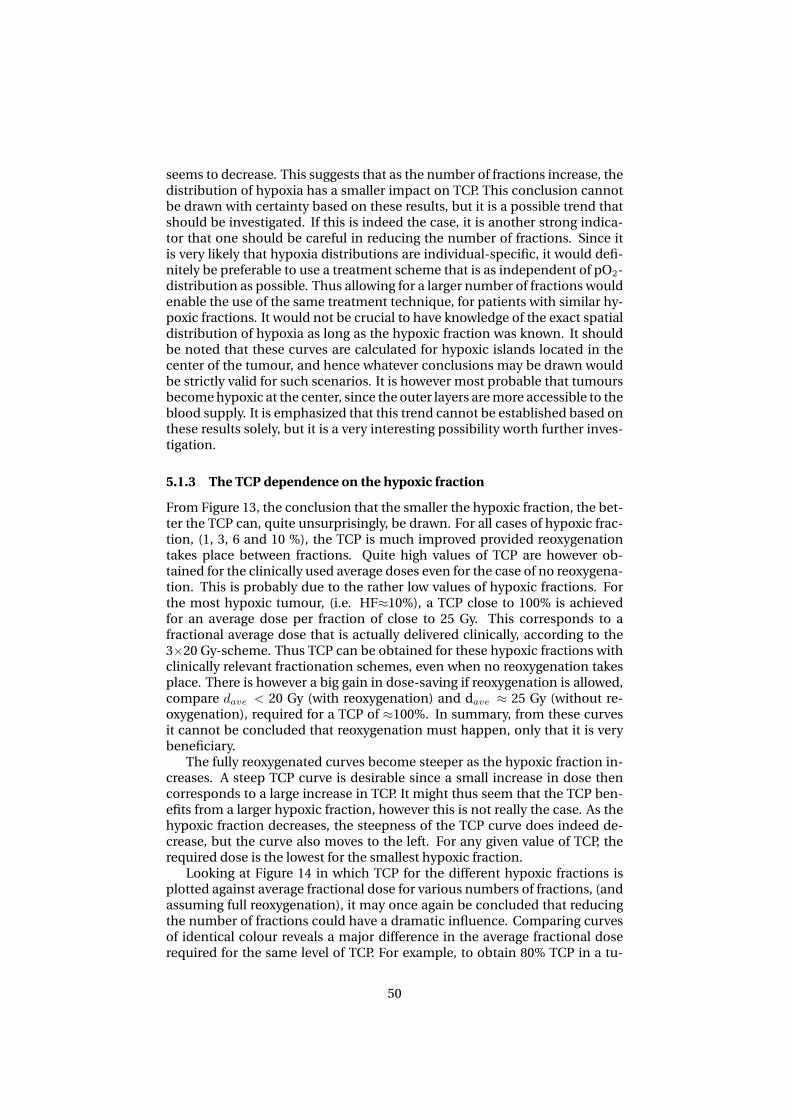
seems to decrease. This suggests that as the number of fractions increase, thedistribution of hypoxia has a smaller impact on TCP. This conclusion cannotbe drawn with certainty based on these results, but it is a possible trend thatshould be investigated. If this is indeed the case, it is another strong indica-tor that one should be careful in reducing the number of fractions. Since itis very likely that hypoxia distributions are individual-specific, it would defi-nitely be preferable to use a treatment scheme that is as independent of pO2-distribution as possible. Thus allowing for a larger number of fractions wouldenable the use of the same treatment technique, for patients with similar hy-poxic fractions. It would not be crucial to have knowledge of the exact spatialdistribution of hypoxia as long as the hypoxic fraction was known. It shouldbe noted that these curves are calculated for hypoxic islands located in thecenter of the tumour, and hence whatever conclusions may be drawn wouldbe strictly valid for such scenarios. It is however most probable that tumoursbecome hypoxic at the center, since the outer layers are more accessible to theblood supply. It is emphasized that this trend cannot be established based onthese results solely, but it is a very interesting possibility worth further inves-tigation.

5.1.3 The TCP dependence on the hypoxic fraction

From Figure 13, the conclusion that the smaller the hypoxic fraction, the bet-ter the TCP can, quite unsurprisingly, be drawn. For all cases of hypoxic frac-tion, (1, 3, 6 and 10 %), the TCP is much improved provided reoxygenationtakes place between fractions. Quite high values of TCP are however ob-tained for the clinically used average doses even for the case of no reoxygena-tion. This is probably due to the rather low values of hypoxic fractions. Forthe most hypoxic tumour, (i.e. HF≈10%), a TCP close to 100% is achievedfor an average dose per fraction of close to 25 Gy. This corresponds to afractional average dose that is actually delivered clinically, according to the3×20 Gy-scheme. Thus TCP can be obtained for these hypoxic fractions withclinically relevant fractionation schemes, even when no reoxygenation takesplace. There is however a big gain in dose-saving if reoxygenation is allowed,compare dave < 20 Gy (with reoxygenation) and dave ≈ 25 Gy (without re-oxygenation), required for a TCP of ≈100%. In summary, from these curvesit cannot be concluded that reoxygenation must happen, only that it is verybeneficiary.

The fully reoxygenated curves become steeper as the hypoxic fraction in-creases. A steep TCP curve is desirable since a small increase in dose thencorresponds to a large increase in TCP. It might thus seem that the TCP ben-efits from a larger hypoxic fraction, however this is not really the case. As thehypoxic fraction decreases, the steepness of the TCP curve does indeed de-crease, but the curve also moves to the left. For any given value of TCP, therequired dose is the lowest for the smallest hypoxic fraction.

Looking at Figure 14 in which TCP for the different hypoxic fractions isplotted against average fractional dose for various numbers of fractions, (andassuming full reoxygenation), it may once again be concluded that reducingthe number of fractions could have a dramatic influence. Comparing curvesof identical colour reveals a major difference in the average fractional doserequired for the same level of TCP. For example, to obtain 80% TCP in a tu-

50

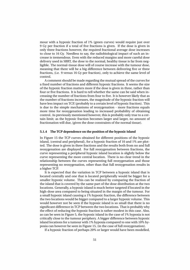
mour with a hypoxic fraction of 1% (green curves) would require just over9 Gy per fraction if a total of five fractions is given. If the dose is given inonly three fractions however, the required fractional average dose increasesto close to 16 Gy. Needless to say, the radiobiological impact of such an in-crease is tremendous. Even with the reduced margins and more careful dosedelivery used in SBRT, the dose to the normal, healthy tissue is far from neg-ligible. The normal-tissue dose will of course increase with the tumour dose,meaning that there will be a big difference between delivering five or threefractions, (i.e. 9 versus 16 Gy per fraction), only to achieve the same level ofcontrol.

A comment should be made regarding the mutual spread of the curves fora fixed number of fractions and different hypoxic fractions. It seems the sizeof the hypoxic fraction matters more if the dose is given in three, rather thanfour or five fractions. It is hard to tell whether the same can be said when in-creasing the number of fractions from four to five. It is however likely that asthe number of fractions increases, the magnitude of the hypoxic fraction willhave less impact on TCP, (probably to a certain level of hypoxic fraction). Thisis due to the simple mechanisms of reoxygenation - more fractions equalsmore time for reoxygenation leading to increased probability of obtainingcontrol. As previously mentioned however, this is probably only true to a cer-tain limit; as the hypoxic fraction becomes larger and larger, no amount offractionation will due, (given the dose constraints of the normal tissue).

5.1.4 The TCP dependence on the position of the hypoxic island

In Figure 15 the TCP curves obtained for different positions of the hypoxicisland, (central and peripheral), for a hypoxic fraction of 10 and 1% are plot-ted. The dose is given in three fractions and the results both from no and fullreoxygenation are displayed. For full reoxygenation between fractions, thecurve representing a peripheral hypoxic island location is slightly below thecurve representing the more central location. There is no clear trend in therelationship between the curves representing full reoxygenation and thoserepresenting no reoxygenation, other than that full reoxygenation results ina higher TCP.

It is expected that the variation in TCP between a hypoxic island that islocated centrally and one that is located peripherally would be bigger for asmaller hypoxic volume. This can be realized by comparing the fraction ofthe island that is covered by the same part of the dose distribution at the twolocations. Generally, a hypoxic island is much better targeted if located in thehigh-dose area compared to being situated in the margin of the tumour. Fora small hypoxic island causing a 1% hypoxic fraction, the difference betweenthe two locations would be bigger compared to a larger hypoxic volume. Thiswould however not be seen if the hypoxic island is so small that there is nosignificant difference in TCP between the two locations. That is probably whythe effect of reducing the hypoxic fraction is rather modest in this case. Also,as can be seen in Figure 5, the hypoxic island in the case of 1% hypoxia is notcritically close to the tumour periphery. A bigger difference between hypoxicisland locations for a tumour with 1% hypoxia compared to one with 10% hy-poxia can however be seen in Figure 15, (in the case of full reoxygenation).

If a hypoxic fraction of perhaps 20% or larger would have been modelled,

51

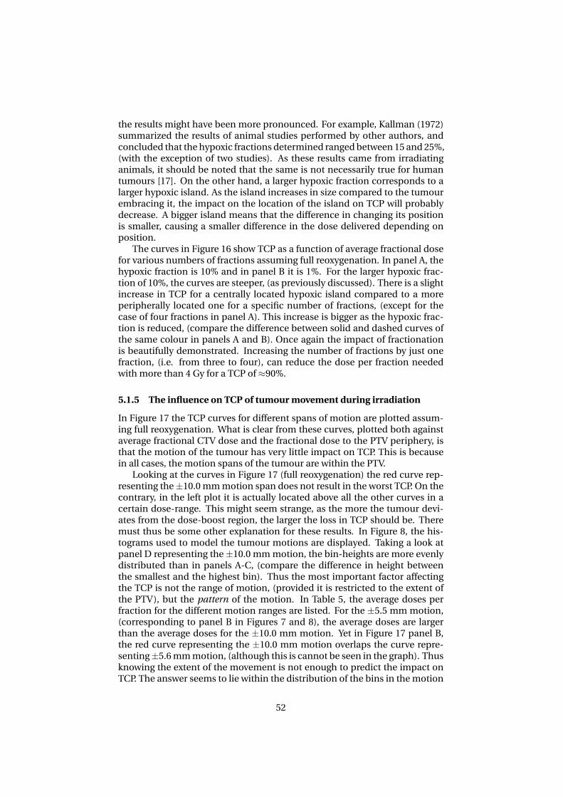
the results might have been more pronounced. For example, Kallman (1972)summarized the results of animal studies performed by other authors, andconcluded that the hypoxic fractions determined ranged between 15 and 25%,(with the exception of two studies). As these results came from irradiatinganimals, it should be noted that the same is not necessarily true for humantumours [17]. On the other hand, a larger hypoxic fraction corresponds to alarger hypoxic island. As the island increases in size compared to the tumourembracing it, the impact on the location of the island on TCP will probablydecrease. A bigger island means that the difference in changing its positionis smaller, causing a smaller difference in the dose delivered depending onposition.

The curves in Figure 16 show TCP as a function of average fractional dosefor various numbers of fractions assuming full reoxygenation. In panel A, thehypoxic fraction is 10% and in panel B it is 1%. For the larger hypoxic frac-tion of 10%, the curves are steeper, (as previously discussed). There is a slightincrease in TCP for a centrally located hypoxic island compared to a moreperipherally located one for a specific number of fractions, (except for thecase of four fractions in panel A). This increase is bigger as the hypoxic frac-tion is reduced, (compare the difference between solid and dashed curves ofthe same colour in panels A and B). Once again the impact of fractionationis beautifully demonstrated. Increasing the number of fractions by just onefraction, (i.e. from three to four), can reduce the dose per fraction neededwith more than 4 Gy for a TCP of≈90%.

5.1.5 The influence on TCP of tumour movement during irradiation

In Figure 17 the TCP curves for different spans of motion are plotted assum-ing full reoxygenation. What is clear from these curves, plotted both againstaverage fractional CTV dose and the fractional dose to the PTV periphery, isthat the motion of the tumour has very little impact on TCP. This is becausein all cases, the motion spans of the tumour are within the PTV.

Looking at the curves in Figure 17 (full reoxygenation) the red curve rep-resenting the±10.0 mm motion span does not result in the worst TCP. On thecontrary, in the left plot it is actually located above all the other curves in acertain dose-range. This might seem strange, as the more the tumour devi-ates from the dose-boost region, the larger the loss in TCP should be. Theremust thus be some other explanation for these results. In Figure 8, the his-tograms used to model the tumour motions are displayed. Taking a look atpanel D representing the±10.0 mm motion, the bin-heights are more evenlydistributed than in panels A-C, (compare the difference in height betweenthe smallest and the highest bin). Thus the most important factor affectingthe TCP is not the range of motion, (provided it is restricted to the extent ofthe PTV), but the pattern of the motion. In Table 5, the average doses perfraction for the different motion ranges are listed. For the ±5.5 mm motion,(corresponding to panel B in Figures 7 and 8), the average doses are largerthan the average doses for the ±10.0 mm motion. Yet in Figure 17 panel B,the red curve representing the ±10.0 mm motion overlaps the curve repre-senting±5.6 mm motion, (although this is cannot be seen in the graph). Thusknowing the extent of the movement is not enough to predict the impact onTCP. The answer seems to lie within the distribution of the bins in the motion

52

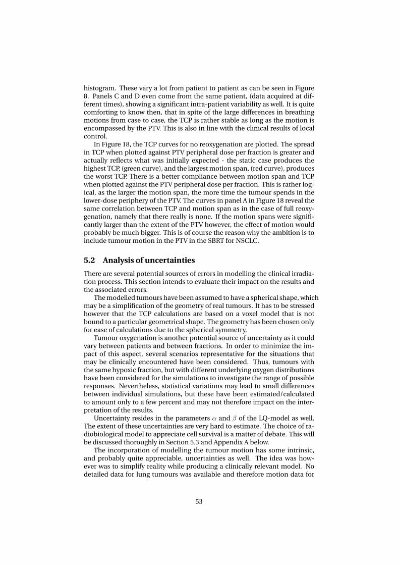
histogram. These vary a lot from patient to patient as can be seen in Figure8. Panels C and D even come from the same patient, (data acquired at dif-ferent times), showing a significant intra-patient variability as well. It is quitecomforting to know then, that in spite of the large differences in breathingmotions from case to case, the TCP is rather stable as long as the motion isencompassed by the PTV. This is also in line with the clinical results of localcontrol.

In Figure 18, the TCP curves for no reoxygenation are plotted. The spreadin TCP when plotted against PTV peripheral dose per fraction is greater andactually reflects what was initially expected - the static case produces thehighest TCP, (green curve), and the largest motion span, (red curve), producesthe worst TCP. There is a better compliance between motion span and TCPwhen plotted against the PTV peripheral dose per fraction. This is rather log-ical, as the larger the motion span, the more time the tumour spends in thelower-dose periphery of the PTV. The curves in panel A in Figure 18 reveal thesame correlation between TCP and motion span as in the case of full reoxy-genation, namely that there really is none. If the motion spans were signifi-cantly larger than the extent of the PTV however, the effect of motion wouldprobably be much bigger. This is of course the reason why the ambition is toinclude tumour motion in the PTV in the SBRT for NSCLC.

5.2 Analysis of uncertainties

There are several potential sources of errors in modelling the clinical irradia-tion process. This section intends to evaluate their impact on the results andthe associated errors.

The modelled tumours have been assumed to have a spherical shape, whichmay be a simplification of the geometry of real tumours. It has to be stressedhowever that the TCP calculations are based on a voxel model that is notbound to a particular geometrical shape. The geometry has been chosen onlyfor ease of calculations due to the spherical symmetry.

Tumour oxygenation is another potential source of uncertainty as it couldvary between patients and between fractions. In order to minimize the im-pact of this aspect, several scenarios representative for the situations thatmay be clinically encountered have been considered. Thus, tumours withthe same hypoxic fraction, but with different underlying oxygen distributionshave been considered for the simulations to investigate the range of possibleresponses. Nevertheless, statistical variations may lead to small differencesbetween individual simulations, but these have been estimated/calculatedto amount only to a few percent and may not therefore impact on the inter-pretation of the results.

Uncertainty resides in the parameters α and β of the LQ-model as well.The extent of these uncertainties are very hard to estimate. The choice of ra-diobiological model to appreciate cell survival is a matter of debate. This willbe discussed thoroughly in Section 5.3 and Appendix A below.

The incorporation of modelling the tumour motion has some intrinsic,and probably quite appreciable, uncertainties as well. The idea was how-ever was to simplify reality while producing a clinically relevant model. Nodetailed data for lung tumours was available and therefore motion data for

53

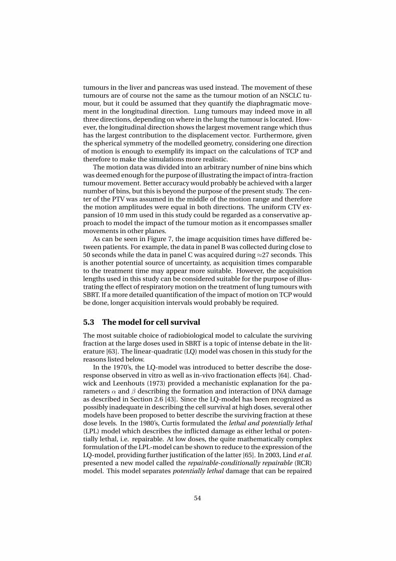
tumours in the liver and pancreas was used instead. The movement of thesetumours are of course not the same as the tumour motion of an NSCLC tu-mour, but it could be assumed that they quantify the diaphragmatic move-ment in the longitudinal direction. Lung tumours may indeed move in allthree directions, depending on where in the lung the tumour is located. How-ever, the longitudinal direction shows the largest movement range which thushas the largest contribution to the displacement vector. Furthermore, giventhe spherical symmetry of the modelled geometry, considering one directionof motion is enough to exemplify its impact on the calculations of TCP andtherefore to make the simulations more realistic.

The motion data was divided into an arbitrary number of nine bins whichwas deemed enough for the purpose of illustrating the impact of intra-fractiontumour movement. Better accuracy would probably be achieved with a largernumber of bins, but this is beyond the purpose of the present study. The cen-ter of the PTV was assumed in the middle of the motion range and thereforethe motion amplitudes were equal in both directions. The uniform CTV ex-pansion of 10 mm used in this study could be regarded as a conservative ap-proach to model the impact of the tumour motion as it encompasses smallermovements in other planes.

As can be seen in Figure 7, the image acquisition times have differed be-tween patients. For example, the data in panel B was collected during close to50 seconds while the data in panel C was acquired during ≈27 seconds. Thisis another potential source of uncertainty, as acquisition times comparableto the treatment time may appear more suitable. However, the acquisitionlengths used in this study can be considered suitable for the purpose of illus-trating the effect of respiratory motion on the treatment of lung tumours withSBRT. If a more detailed quantification of the impact of motion on TCP wouldbe done, longer acquisition intervals would probably be required.

5.3 The model for cell survival

The most suitable choice of radiobiological model to calculate the survivingfraction at the large doses used in SBRT is a topic of intense debate in the lit-erature [63]. The linear-quadratic (LQ) model was chosen in this study for thereasons listed below.

In the 1970’s, the LQ-model was introduced to better describe the dose-response observed in vitro as well as in-vivo fractionation effects [64]. Chad-wick and Leenhouts (1973) provided a mechanistic explanation for the pa-rameters α and β describing the formation and interaction of DNA damageas described in Section 2.6 [43]. Since the LQ-model has been recognized aspossibly inadequate in describing the cell survival at high doses, several othermodels have been proposed to better describe the surviving fraction at thesedose levels. In the 1980’s, Curtis formulated the lethal and potentially lethal(LPL) model which describes the inflicted damage as either lethal or poten-tially lethal, i.e. repairable. At low doses, the quite mathematically complexformulation of the LPL-model can be shown to reduce to the expression of theLQ-model, providing further justification of the latter [65]. In 2003, Lind et al.presented a new model called the repairable-conditionally repairable (RCR)model. This model separates potentially lethal damage that can be repaired

54

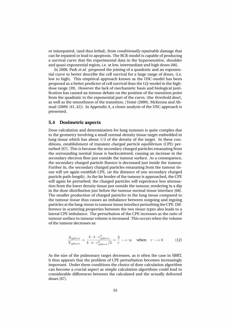
or misrepaired, (and thus lethal), from conditionally repairable damage thatcan be repaired or lead to apoptosis. The RCR-model is capable of producinga survival curve that fits experimental data in the hypersensitive, shoulderand quasi-exponential region, i.e. at low, intermediate and high doses [66].

In 2008, Park et al. proposed the joining of a quadratic and an exponen-tial curve to better describe the cell survival for a large range of doses, (i.e.low to high). This empirical approach known as the USC-model has beenproposed as a better predictor of cell survival than the LQ-model in the high-dose range [39]. However the lack of mechanistic basis and biological justi-fication has caused an intense debate on the position of the transition pointfrom the quadratic to the exponential part of the curve, (the threshold dose),as well as the smoothness of the transition, (Tome (2009), McKenna and Ah-mad (2009) [41, 42]). In Appendix A, a closer analysis of the USC approach ispresented.

5.4 Dosimetric aspects

Dose calculation and determination for lung tumours is quite complex dueto the geometry involving a small normal-density tissue target embedded inlung tissue which has about 1/3 of the density of the target. In these con-ditions, establishment of transient charged particle equilibrium (CPE) per-turbed [67]. This is because the secondary charged particles emanating fromthe surrounding normal tissue is backscattered, causing an increase in thesecondary electron flow just outside the tumour surface. As a consequence,the secondary charged particle fluence is decreased just inside the tumour.Further in, the secondary charged particles emanating from the tumour tis-sue will yet again establish CPE, (at the distance of one secondary chargedparticle path-length). As the far border of the tumour is approached, the CPEwill again be perturbed; the charged particles will experience less attenua-tion from the lower density tissue just outside the tumour, rendering in a dipin the dose-distribution just before the tumour-normal tissue interface [68].The smaller production of charged particles in the lung tissue compared tothe tumour tissue thus causes an imbalance between outgoing and ingoingparticles at the lung-tissue to tumour tissue interface perturbing the CPE. Dif-ference in scattering properties between the two tissue types also leads to alateral CPE imbalance. The perturbation of the CPE increases as the ratio oftumour surface to tumour volume is increased. This occurs when the volumeof the tumour decreases as:

Asphere

Vsphere=

4 · π · r2sphere4 · π · r3sphere/3

=3

r−→∞ when r −→ 0 (12)

As the size of the pulmonary target decreases, as is often the case in SBRT,it thus appears that the problem of CPE perturbation becomes increasinglyimportant. Under these conditions the choice of dose calculation algorithmcan become a crucial aspect as simple calculation algorithms could lead toconsiderable differences between the calculated and the actually delivereddoses [67].

55

While documenting the fractionation schedules and the doses prescribed anal-ysed in this work, it has become clear that there are considerable differencesbetween the dose calculation algorithms used in the treatment planning ofSBRT for NSCLC. For example, Ricardi et al. used the collapsed-cone (CC)algorithm [31] that better accounts for the lateral scattering in dose calcula-tions, while Baba et al. and Hof et al. used the pencil-beam (PB) convolutionalgortihm that provides a more simple approach to dose calculation in het-erogeneous media. There are also publications in which the dose calculationalgorithm is not specifically stated, see for example Onishi et al. (2004) [32].

If all algorithms performed in a similar way, comparison between the re-sults of different calculation algorithms would be simple and adequate. How-ever, these algorithms lead to different results for targets situated in the lungwhich makes the comparison of the results of a certain dose scheme reportedby authors using different algorithms difficult to interpret, as differences intarget coverage add an unnecessary uncertainty factor. This has been illus-trated in the study by Haedinger et al. comparing the PTV- and CTV dosevolume histograms (DVHs) resulting from planning the SBRT-treatment of 33pulmonary targets with the PB algorithm and the CC algorithm. Photon en-ergies of both 6 and 18 MV were used. The authors found a significant over-estimation of the dose by the PB algorithm at the tumour-lung tissue inter-face. This was especially valid for smaller targets of ≤100 cm3 in volume ir-radiated with 18 MV beams. An average reduction in PTV dose coverage of7% was found using the CC algorithm compared to the PB algorithm. Com-paring the results to Monte-Carlo (MC) calculations, it was shown that the CCalgorithm lead to closer-to-reality results than the PB algorithm especially inthe high-dose range between 100 and 150% dose. The differences betweenthe two calculation algorithms were found to increase with decreasing targetvolume, due to the increase in target surface-to-volume ratio. These resultssuggest that the accuracy of the number of calculated monitor units (MUs)decreases when the PB algorithm is used for dose calculations in small targetvolumes in the lung [67].

These results indicate that the differences in dose calculation may hamperthe comparison of results from studies employing different algorithms sincethe reported doses delivered will differ from the actually delivered doses tovarious extents. Furthermore, not reporting the dose calculation algorithmused in a study adds a further layer of uncertainty that might even lead to theexclusion of the said study from analyses. All these should therefore be takenas a strong encouragement for a more coherent use and recording of the dosecalculation algorithms used in SBRT.

56

6 Conclusions

Clinical studies have shown that the dose fractionation schemes currentlyused in SBRT for NSCLC could lead to high values of TCP. The aim to furtherreduce the number of fractions might be beneficial from an economical andpractical viewpoint as more patients could be treated and patients would faceshorter treatments. This should however be pursued with caution in the lightof the possible existence of hypoxic cells in the tumours. In the presence ofhypoxia, TCP is seriously compromised if there is not enough time for rexoy-genation between fractions. The results of this study showed that if hypoxiais present in NSCLC tumours, the TCP might be seriously compromised ifnot enough reoxygenation is allowed between fractions. In these conditions,reducing the number of fractions to just one fraction may lead to a consider-able increase in the required prescription dose to maintain the same TCP asobtained from a multi-fraction schedule. The good agreement between theresults of this simulation study and the clinical results serve as a strong in-dicator that inter-fraction reoxygenation is an important process that mighttake place in clinical patients treated with SBRT.

The results also showed that the diaphragmatic tumour motion appears tohave little influence on TCP provided that the PTV encompasses all tumourpositions during the breathing cycle. Furthermore, the results also suggestedthat the dose delivered to the PTV margin might not be the only factor that issignificant for local control. Instead, the heterogeneity of tumour radiosensi-tivities should be considered in relation to the heterogeneity of the calculateddose distribution.

57

A Appendix

Analysis of the universal survival curve

The USC-model originally proposed by Park et al. (2008) was based on ananalysis of the cell survival data of a NSCLC H460 cell line irradiated withdoses up to 16 Gy. By fitting the survival data with both the USC- and theLQ-model, Park et al. thus compared the two models. The results show arather poor fit of the LQ-model at doses above≈10 Gy whereas the USC followthe data more closely [39]. The superiority of the USC over the LQ-modelis demonstrated by comparing the sum of squares from the fits; 0.0168 forUSC and 5.08 for the LQ-model. These figures support the idea that the USCis indeed a much better choice than the LQ-model in the high-dose range.Interestingly enough, the curve representing the LQ-model was constructedbased on a fit to data ≤8 Gy and extrapolated for higher doses. Furthermore,in the original publication it is stated that if the LQ-model was fitted over theentire dose range (i.e., up to 16 Gy) the resulting sum of squares would beonly 0.285. While this value is still higher than the corresponding value givenby the USC, it is a very small fraction (≈6%) of the originally stated value of5.08. These discrepancies have determined us to perform an own analysis ofH460 cell survival data. The Advanced Fitting Tool for a non-linear curve fitin Origin 7 has been used for this purpose. A fit of the form:

y = P1 · x+ P2 · x2 (13)

is made. Thus y corresponds to ln(SF), P1 to −α, P2 to −β and x to the dose.The raw cell survival data was not included in the original paper, but Park etal. published these one year after the first publication, (Park et al. (2009) [69]).The data is given as ”log SF” although the base of the logarithm is unclear. Ithas been assumed that the data represent log10(SF) as this is a usual repre-sentation of cell survival data, (Table 8). In Table 8, values of ln(SF) calculatedfrom the original data are also presented.

58

TABLE 8. Survival data from Park et al. for the given doses.

D (Gy) log10(SF) ln(SF)

0.5 -0.0101 -0.02331 -0.0137 -0.0315

1.5 -0.21 -0.48352 -0.19 -0.43753 -0.395 -0.90954 -0.526 -1.21125 -0.791 -1.8213

7.5 -1.863 -4.289710 -3.387 -7.798912 -4.534 -10.439914 -5.592 -12.876116 -6.76 -15.5655

In an attempt to reproduce the fit in the original article, the data was fit withP1 fixed at -0.33 (⇔ α = 0.33 Gy−1) whileP2 was allowed to vary. The resultingcurve (Figure 17) has the following expression:

y = −0.33 · x− 0.04132 · x2 (14)

⇐⇒

ln(SF) = −0.33 ·D − 0.04132 ·D2 (15)

In Figure A1 below, the curve fit obtained is displayed together with the sur-vival data.

59

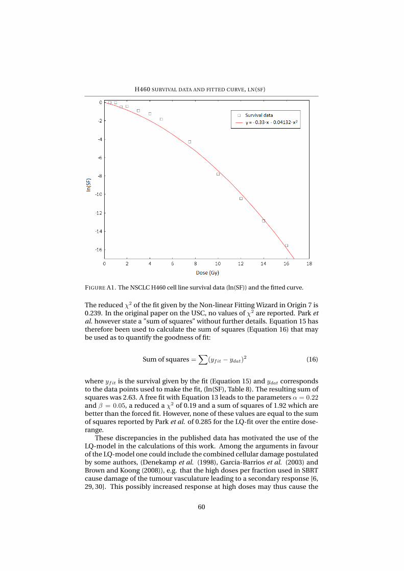
H460 SURVIVAL DATA AND FITTED CURVE, LN(SF)

FIGURE A1. The NSCLC H460 cell line survival data (ln(SF)) and the fitted curve.

The reduced χ2 of the fit given by the Non-linear Fitting Wizard in Origin 7 is0.239. In the original paper on the USC, no values of χ2 are reported. Park etal. however state a ”sum of squares” without further details. Equation 15 hastherefore been used to calculate the sum of squares (Equation 16) that maybe used as to quantify the goodness of fit:

Sum of squares =∑

(yfit − ydat)2 (16)

where yfit is the survival given by the fit (Equation 15) and ydat correspondsto the data points used to make the fit, (ln(SF), Table 8). The resulting sum ofsquares was 2.63. A free fit with Equation 13 leads to the parameters α = 0.22and β = 0.05, a reduced a χ2 of 0.19 and a sum of squares of 1.92 which arebetter than the forced fit. However, none of these values are equal to the sumof squares reported by Park et al. of 0.285 for the LQ-fit over the entire dose-range.

These discrepancies in the published data has motivated the use of theLQ-model in the calculations of this work. Among the arguments in favourof the LQ-model one could include the combined cellular damage postulatedby some authors, (Denekamp et al. (1998), Garcia-Barrios et al. (2003) andBrown and Koong (2008)), e.g. that the high doses per fraction used in SBRTcause damage of the tumour vasculature leading to a secondary response [6,29, 30]. This possibly increased response at high doses may thus cause the

60

in-vivo survival curve to continuously bend, serving as another argument forthe validity of using the LQ-model in the high-dose range.

A better fit could theoretically be obtained by considering a third orderpolynomial relationship, (Equation 17):

ln(SF) = −α ·D − β ·D2 + γ ·D3 (17)

According to this expression, the low- and medium-dose survival would begoverned by the α and β parameters, while at the high doses, the term γ ·D3

would dominate. It should be noted that Fowler and Stern (1960) discussedthe inclusion of higher-order terms in the LQ-model more than 15 years be-fore the LQ-model was introduced for clinical applications. In their originalpublication, they chose to exclude terms with a higher power than two, as aknown mechanistic justification for the γ parameter was lacking [70].

61

References

[1] www.medscape.com.

[2] American Cancer Society.

[3] Thomlinson R H, Gray L H. The histological structure of some humanlung cancers and the possible implications for radiotherapy. British Jour-nal of Cancer, 9(4):539–549, 1955.

[4] Dasu A, Toma-Dasu I, Karlsson M. The effects of hypoxia on the theoret-ical modelling of tumour control probability. Acta Oncologica, 44:563–571, 2005.

[5] Leite de Oliviera R, Hamm A, Mazzone M. Growing tumor vessels: morethan one way to skin a cat - implications of angiogenesis targeted cancertherapies. Molecular Aspects of Medicine, 32:71–87, 2011.

[6] Denekamp J, Dasu A, Waites A. Vasculature and microenvironmentalgradients: the missing links in novel approaches to cancer therapy? Ad-van Enzyme Regul, 38:281–299, 1998.

[7] Harris A L. Hypoxia - a key regulatory factor in tumour growth. Nature,2:38–47, 2002.

[8] Hockel M, Vaupel P. Tumor hypoxia: definitions and current clinical, bi-ologic, and molecular aspects. Journal of the National Cancer Institute,93(4):266–276, 2001.

[9] Sonesson B, Sonesson G. Anatomi och fysiologi. Liber, 2006.

[10] Department of Biology, Lund University.

[11] Seimiya H, Tanji M, Oh-Hara T et al. Hypoxia up-regulates telomeraseactivity via mitogen-activated protein kinase signaling in human solidtumor cells. Biochemical and Biophysical Research Communications,260:365–370, 1999.

[12] Brown J M, Giaccia A J. The unique physiology of solid tumors: opportu-nities (and problems) for cancer therapy. Cancer Research, 58:1408–1416,1998.

[13] Hall E, Giaccia A. Radiobiology for the radiologist, 6th edition. LippincottWilliams & Wilkins, 2006.

[14] Mayles P, Nahum A, Rosenwald J C. Handbook of radiotherapy physics:theory and practice. Taylor & Francis, 2007.

[15] Fuks Z, Kolesnick R. Engaging the vascular component of the tumor re-sponse. Cancer Cell, 8:89–91, 2005.

[16] Dasu A, Toma-Dasu I, Karlsson M. Theoretical simulation of tumouroxygenation and results from acute and chronic hypoxia. Physics inMedicine and Biology, 48:2829–2842, 2003.

62

[17] Kallman R. The phenomenon of reoxygenation and its implications forfractionated radiotherapy. Radiology, 105:135–142, 1972.

[18] Toma-Dasu I, Uhrdin J, Antonovic A, Dasu A et al. Dose prescription andtreatment planning based on FMISO-PET hypoxia. Acta Oncologica,51:222–230, 2012.

[19] Meng X, Kong F-M, Yu J. Implementation of hypoxia measurement intolung cancer therapy. Lung Cancer, 75:146–150, 2012.

[20] Le Q-T, Chen E, Salim A, Chao H et al. An evaluation of tumor oxygena-tion and gene expression in patients with early stage non-small cell lungcancers. Clin Cancer Res, 12(5):1507–1513, 2006.

[21] Krohn K, Link J, Mason R. Molecular imaging of hypoxia. The Journal ofNuclear Medicine, 49(6) (Suppl):129S–148S, 2008.

[22] Fujibayashi Y, Taniuchi H, Yonekyra Y, Ohtani H et al. Copper-62-ATSM:a new hypoxia imaging agent with high membrane permeability and lowredox potential. The Journal of Nuclear Medicine, 38(7):1155–1160, 1997.

[23] Lax I, Blomgren H, Naslund I, Svanstrom R. Stereotactic radiotherapy ofmalignancies in the abdomen. Acta Oncologica, 33(6):677–683, 1994.

[24] Blomgren H, Lax I, Naslund I, Svanstrom R. Stereotactic high dose frac-tion radiation therapy of extracranial tumors using an accelerator. ActaOncologica, 34(6):861–870, 1995.

[25] Uematsu M, Shioda A, Tahara K, Fukui T et al. Focal, high dose and frac-tionated modified stereotactic radiation therapy for lung carcinoma pa-tients: a preliminary experience. Cancer, 82(6):1062–1070, 1998.

[26] Wolbarst A B, Chin L M, Svensson G K. Optimization of radiation ther-apy: integral-response of a model biological system. Int J Radiation On-cology Biol Phys, 8:1761–1769, 1982.

[27] Pia Baumann. Stereotactic body radiotherapy in non-small cell lung can-cer. PhD thesis, Stockholm University, 2009.

[28] Lo S S, Fakiris A J, Chang E L, Mayr N A et al. Stereotactic body radiationtherapy: a novel treatment modality. Nat rev Clin Oncol, 7:44–54, 2010.

[29] Garcia-Barros M, Paris F, Cordon-Cardo C, Lyden D et al. Tumor re-sponse to radiotherapy regulated by endothelial cell apoptosis. Science,300:1155–1159, 2003.

[30] Brown J M, Koong A C. High-dose single-fraction radiotherapy: exploit-ing a new biology? Int J Radiation Oncology Biol Phys, 71(2):324–325,2008.

[31] Ricardi U, Riccardo Filipp A, Guarneri A, Giglioli F R et al. Stereotacticbody radiation therapy for early stage non-small cell lung cancer: resultsof a prospective trial. Lung Cancer, 68:72–77, 2010.

63

[32] Onishi H, Araki T, Shirato H, Nagata Y et al. Stereotactic hypofraction-ated high-dose irradiation for stage i nonsmall cell lung carcinoma. Can-cer, 101(7):1623–1631, 2004.

[33] Lanni T, Grills I, Kestin L, Robertson J. Stereotactic radiotherapy reducestreatment cost while improving overall survival and local control overstandard fractionated radiation therapy for medically inoperable non-small-cell lung cancer. Am J Clin Oncol, 34:494–498, 2011.

[34] Hof H, Muenter M, Oetzel D et al. Stereotactic single-dose radiotherapy(radiosurgery) of early-stage nonsmall-cell lung cancer (NSCLC). Can-cer, 110(1):148–155, 2007.

[35] Zimmermann F, Geinitz H, Schill S, Grosu A et al. Stereotactic hypofrac-tionated radiation therapy for stage I non-small cell lung cancer. LungCancer, 48:107–114, 2005.

[36] Palma D, van Sornsen de Koste J, Verbakel W, Vincent A, Senan S. Lungdensity changes after stereotactic radiotherapy: a quantitative analysisin 50 patients. Int J Radiation Oncology Biol Phys., 300:1155–1159, 2010.

[37] Ruggieri R, Naccarato S, Nahum A. Severe hypofractionation: Non-homogeneous tumour dose delivery can counteract tumour hypoxia.Acta Oncologica, 49:1304–1314, 2010.

[38] Carlson D, Keall P, Loo B, Chen Z, Brown M. Hypofractionation resultsin redcued tumor cell kill compared to conventional fractionation fortumors with regions of hypoxia. Int J Radiation Oncology Biol Phys,79(4):1188–1195, 2011.

[39] Park C, Papiez L, Zhang S, Story M, Timmerman R D. Universal survivalcurve and single fraction equivalent dose: useful tools in understand-ing potency of ablative radiotherapy. Int J Radiation Oncology Biol Phys,70(3):847–852, 2008.

[40] Fowler J. Linear quadratics is alive and well: in regard to park et al. Int JRadiation Oncology Biol Phys, 72(3):957, 2008.

[41] McKenna F, Ahmad S. Toward a unified surival curve: in regard toKavanagh and Newman (Int J Radiat Oncol Biol Phys 2008;71:958-959)and Park et al. (Int J Radiat Oncol Biol Phys 2008;70:847-852). Int J Ra-diation Oncology Biol Phys, 73(2):640, 2009.

[42] Tome W. Universal survival curve and single fraction equivalent dose:useful tools in understanding potency of ablative radiotherapy: in re-gards to parks et al. (Int J Radiat Oncol Biol Phys 2008;72:1620-1621. IntJ Radiation Oncology Biol Phys, 73(4):1286, 2009.

[43] Chadwick K, Leenhouts H. A molecular theory of cell survival. Phys.Med. Biol., 18(1):78–87, 1973.

[44] Toma-Dasu I, Dasu A, Brahme A. Dose prescription and optimisationbased on tumour hypoxia. Acta Oncologica, 48:1181–1192, 2009.

64

[45] Martel M K, Ten Haken R K, Hazuka M B, Kessler M L et al. Estimationof tumor control probability model parameters from 3-D dose distri-butions of non-small cell lung cancer patients. Lung Cancer, 24:31–37,1999.

[46] Mehta M, Scrimger R, Mackie R, Paliwal B et al. A new approach to doseescalation in non-small-cell lung cancer. Int J Radiation Oncology BiolPhys, 49(1):23–33, 2001.

[47] Alper T, Howard-Flanders P. Role of oxygen in modifying the radiosen-sitivity of E. Coli B. Nature, 178(4540):978–979, 1956.

[48] McGarry R C, Papiez L, Williams M, Whitford T, Timmerman R D.Stereotactic body radiation therapy of early-stage non-small-celllung carcinoma: phase I study. Int J Radiation Oncology Biol Phys.,63(4):1010–1015, 2005.

[49] Fritz P, Kraus H-J, Blaschke T, Mohlnickel W et al. Stereotactic, highsingle-dose irradiation of stage I non-small cell lung cancer (NSCLC)using four-dimensional CT scans for treatment planning. Lung Cancer,60:193–199, 2008.

[50] Wulf J, Baier K, Mueller G, Flentje M P. Dose-response in stereotactic ir-radiation of lung tumours. Radiotherapy and Oncology, 77:83–87, 2005.

[51] Baumann P, Nyman J, Hoyer M et al.. Outcome in a prospective phase iitrial of medically inoperable stage i non-small-cell lung cancer patientstreated with stereotactic body radiotherapy. Journal of Clinical Oncol-ogy, 27:20, 2009.

[52] Olsen J R, Robinson C G, El Naqa I, Creach K M et al. Dose-response forstereotactic body radiotherapy in early-stage non-small-cell lung cancer.Int J Radiation Oncology Biol Phys., 81(4):e299–e303, 2011.

[53] Haasbeek C, Lagerwaard F, Antonisse M et al. Stage I nonsmall cell lungcancer in patients aged≥75 years: outcomes after stereotactic radiother-apy. Cancer, 116(2):406–414, 2010.

[54] Fakiris A J, McGarry R C, Yiannoutsos C T, Papiez L et al. Stereotacticbody radiation therapy for early-stage non-small-cell lung carcinoma:four-year results of a prospective phase II study. Int J Radiation Oncol-ogy Biol Phys, 75(3):677–682, 2011.

[55] Salazar O M, Sandhu T S, Lattin P B et al. Once-weekly, high-dosestereotactic body radiotherapy for lung cancer: 6-year analysis of 60early stage, 42 locally advanced, and 7 metastatic lung cancers. Int JRadiation Oncology Biol Phys, 72:707–715, 2008.

[56] Baba F, Shibamoto Y, Tomita N, Ikeya-Hashizume C et al. Stereotacticbody radiotherapy for stage I lung cancer and small lung metastasis:evaluation of an immobilization system for suppression of respiratorytumor movement and preliminary results. Radiation Oncology, 4(15):,2009.

65

[57] Xia T, Li H, Sun Q et al. Promising clinical outcome of stereotactic bodyradiation therapy for patients with inoperable stage I/II non-small-celllung cancer. Int J Radiation Oncology Biol Phys, 66:117–125, 2006.

[58] Takeda A, Sanuki N, Kunieda E et al. Stereotactic body radiotherapy forprimary lung cancer at a dose of 50 Gy total in five fractions to the pe-riphery of the planning target volume calculated using a superpositionalgorithm. Int J Radiation Oncology Biol Phys, 73:442–448, 2009.

[59] Onishi H, Kuriyama K, Komiyama T et al. Clinical outcomes of stereo-tactic radiotherapy for stage i non-small cell lung cancer using a novelirradiation technique: patient self-controlled breath-hold and beamswitching using a combination of linear accelerator and ct scanner. LungCancer, 45(1):45–55, 2004.

[60] Mehta N, King C, Agazaryan N et al.. Stereotactic body radiation ther-apy and 3-dimensional conformal radiotherapy for stage i non-small celllung cancer: A pooled analysis of biological equivalent dose and localcontrol. Practical Radiation Oncology, 2011.

[61] Taylor J R. An introduction to error analysis. University Science Books,1997, Second edition.

[62] Wiklund K. Modeling of dose and sensitivity heterogeneities in radiationtherapy. PhD thesis, Stockholm University, 2012.

[63] Kirkpatrick J, Brenner D. The linear-quadratic model is inappropriateto model high dose per fraction effects in radiosurgery. Med Phys,36(8):366–375, 2009.

[64] Fowler J. Development of radiobiology for oncology - a personal view.Phys. Med. Biol., 51:R263–R286, 2006.

[65] Curtis S. Lethal and potentially lethal lesions induced by radiation-a uni-fied repair model. Radiation Research, 106:252–270, 1986.

[66] Lind B, Persson L, Edgren M, Brahme A. Repairable-conditionally re-pairable damage model based on dual poisson processes. Radiat Res,160(3):366–375, 2003.

[67] Haedinger U, Krieger T, Flentje M, Wulf J. Influence of calculationmodel on dose distribution in stereotactic radiotherapy for pulmonarytargets. Int J Radiation Oncology Biol Phys, 61(1):239–249, 2005.

[68] Introduction to radiological physics and radiation dosimetry. Wiley-VCHVerlag GmbH, 1991.

[69] Park C, Papiez L, Timmerman R D. In reply to Drs. McKenna andAhmad. Int J Radiation Oncology Biol Phys, 73(2):641, 2009.

[70] Fowler J, Stern B. Dose-rate effects: some theoretical and practical con-siderations. British Journal of Radiobiology, 33(390):389–395, 1960.

66