Roberto J. Galván Madrid

The Formation of the Most Massive Stars in the Galaxy

La formación de las estrellas másmasivas de la Galaxia

Universidad Nacional Autónoma de México

Dr. Enrique Luis Graue WiechersRector

Dr. Leonardo Lomelí VanegasSecretario General

Dr. Alberto Ken Oyama NakagawaSecretario de Desarrollo Institucional

Dr. Javier Nieto GutiérrezCoordinador General de Estudios de Posgrado

Dr. Laurent R. LoinardCoordinador del Programa de Posgrado en Astrofísica

Dra. Cecilia Silva GutiérrezSubdirectora Académica

de la Coordinación General de Estudios de Posgrado

Lic. Lorena Vázquez RojasCoordinación Editorial

The FormaTion oF The mosT massive sTars in The Galaxy

la Formación de las esTrellas más masivas de la Galaxia

Universidad Nacional Autónoma de México

Coordinación General deEstudios de Posgrado

Programa de Posgrado en Astrofísica

La Colección Posgrado publica, desde 1987, las tesis de maestría y docto­rado que presentan, para obtener el grado, los egresados de los programas del Sistema Universitario de Posgrado de la unam.

El conjunto de obras seleccionadas, además de su originalidad, ofrecen al lector el tratamiento de temas y problemas de gran relevancia que con­tribuyen a la comprensión de los mismos y a la difusión del pensamiento universitario.

Colección Posgrado

universidad nacional auTónoma de méxico

méxico, 2019

Roberto J. Galván Madrid

The Formation of the Most Massive Stars in the Galaxy

La formación de las estrellas másmasivas de la Galaxia

Galván Madrid, Roberto J.The formation of the most massive stars in the galaxy = La formación de las estrellas más masivas de la galaxia / Roberto J. Galván Madrid. ­­ Primera edición. ­­ México : UNAM, Coordinación de Estudios de Posgrado, 2013. 272 p. : il., mapas ; 21 cm. – – (Colección posgrado) Bibliografía: p. 225­245 ISBN (Impreso) 978­607­02­4179­6 1. Estrellas – Formación. 2. Estrellas – Cúmulos. 3. Estrellas – Evolución. I. Universidad Nacional Autónoma de México. Coordinación de Estudios de Posgrado. II. título. III. título: La formación de las estrellas más masivas de la galaxia.

523.88­scdd21 Biblioteca Nacional de México

Formación en Latex: Mtra. Silvia Zueck González y Dr. Alejandro Lara SánchezDiseño de portada: Columba Citlali Bazán LechugaCorrección de estilo y lectura de pruebas: Lorena Vázquez Rojas

Primera edición PDF: 27 de agosto de 2019

D.R. © Universidad Nacional Autónoma de México Coordinación General de Estudios de Posgrado Ciudad Universitaria, 04510, Coyoacán, Ciudad de MéxicoD.R. © Roberto J. Galván Madrid

ISBN (PDF) 978-607-30-2146-3

DOI: https://doi.org/10.22201/cgep.9786073021463e.2019

Prohibida la reproducción total o parcial por cualquier medio sin la autorización escrita del titular de los derechos patrimoniales.

Esta edición y sus características son propiedad de la Universidad Nacional Autónoma de México.

Impreso y hecho en México

Indice general

1. Introduction to the Scientific Problem 23

1.1. Introduccion al Problema

Cientıfico . . . . . . . . . . . . . . . . . . . 23

1.2. Star Formation . . . . . . . . . . . . . . . . 27

1.2.1. Stars in Context . . . . . . . . . . . 27

1.2.2. From Clouds to Clumps to Cores . . 28

1.2.3. Disk-Jet Mediated Accretion . . . . 32

1.3. Massive-Star Formation . . . . . . . . . . . 37

1.3.1. Properties of Massive Star Formation

Regions . . . . . . . . . . . . . . . . 37

1.3.2. Disk-Outflow Accretion in Massive

Star Formation . . . . . . . . . . . . 40

1.4. The Formation of the Most

Massive Stars . . . . . . . . . . . . . . . . . 45

1.4.1. From Massive to Very Massive . . . 45

1.4.2. Ultracompact and Hypercompact

HII Regions . . . . . . . . . . . . . . 46

10

1.4.3. Accretion and Ionization . . . . . . . 47

1.5. Goals . . . . . . . . . . . . . . . . . . . . . 49

2. A MSFR at the Onset of Ionization: W33A 51

2.1. Resumen . . . . . . . . . . . . . . . . . . . . 51

2.2. Summary . . . . . . . . . . . . . . . . . . . 53

2.3. Introduction . . . . . . . . . . . . . . . . . . 55

2.4. Observations . . . . . . . . . . . . . . . . . 57

2.4.1. SMA . . . . . . . . . . . . . . . . . . 57

2.4.2. VLA . . . . . . . . . . . . . . . . . . 59

2.5. Results . . . . . . . . . . . . . . . . . . . . . 60

2.5.1. Continuum Emission . . . . . . . . . 60

2.5.2. Molecular Line Emission . . . . . . . 66

2.6. Discussion . . . . . . . . . . . . . . . . . . . 80

2.6.1. Star Formation from Converging

Filaments . . . . . . . . . . . . . . . 80

2.6.2. Cores at Different Evolutionary Stages 85

2.6.3. A Rotating Disk/Outflow System in

MM1-Main . . . . . . . . . . . . . . 88

2.7. Conclusions . . . . . . . . . . . . . . . . . . 92

3. A MSFR with young UC and HC HII

Regions: G20.08N 97

3.1. Resumen . . . . . . . . . . . . . . . . . . . . 97

3.2. Summary . . . . . . . . . . . . . . . . . . . 99

3.3. Introduction . . . . . . . . . . . . . . . . . . 101

3.4. Observations . . . . . . . . . . . . . . . . . 105

11

3.4.1. SMA . . . . . . . . . . . . . . . . . . 105

3.4.2. VLA . . . . . . . . . . . . . . . . . . 107

3.5. Results and Discussion . . . . . . . . . . . . 108

3.5.1. The Continuum Emission . . . . . . 108

3.5.2. The Large-Scale Molecular Cloud . . 114

3.5.3. Molecular Gas in The Inner 0.1 pc . 121

3.5.4. The Ionized Gas: Radio

Recombination Lines . . . . . . . . . 138

3.5.5. Outflow Tracers . . . . . . . . . . . 142

3.5.6. A New NH3 (3,3) Maser . . . . . . . 142

3.6. Hierarchical Accretion in

G20.08N . . . . . . . . . . . . . . . . . . . . 146

3.6.1. The Observations . . . . . . . . . . . 146

3.6.2. Resupply of the Star-Forming Cores 149

3.6.3. Accretion Rate . . . . . . . . . . . . 150

3.6.4. Transfer of Angular Momentum . . . 151

3.7. Conclusions . . . . . . . . . . . . . . . . . . 153

4. Time Variability of HII Regions:

A Signature of Accretion? 159

4.1. Resumen . . . . . . . . . . . . . . . . . . . . 159

4.2. Summary . . . . . . . . . . . . . . . . . . . 161

4.3. Introduction . . . . . . . . . . . . . . . . . . 162

4.4. Observations . . . . . . . . . . . . . . . . . 165

4.5. Discussion . . . . . . . . . . . . . . . . . . . 168

4.5.1. The Expected Variation Trend . . . 168

12

4.5.2. The Observed Variation . . . . . . . 170

4.5.3. Is G24 A1 Accreting? . . . . . . . . 171

4.6. Conclusions . . . . . . . . . . . . . . . . . . 172

5. Time Variability of HII Regions in

Numerical Simulations of MSFR 177

5.1. Resumen . . . . . . . . . . . . . . . . . . . . 177

5.2. Summary . . . . . . . . . . . . . . . . . . . 179

5.3. Introduction . . . . . . . . . . . . . . . . . . 181

5.4. Methods . . . . . . . . . . . . . . . . . . . . 185

5.4.1. The Numerical Simulations . . . . . 185

5.4.2. Data Sets . . . . . . . . . . . . . . . 186

5.5. Results . . . . . . . . . . . . . . . . . . . . . 187

5.5.1. Variable HII Regions . . . . . . . . . 187

5.5.2. Global Temporal Evolution . . . . . 190

5.5.3. Comparison to Surveys . . . . . . . 196

5.5.4. Long-Term Variation Probabilities . 197

5.5.5. Short-Term Variation Probabilities . 202

5.5.6. Variations in other properties of the

HII regions . . . . . . . . . . . . . . 206

5.6. Discussion . . . . . . . . . . . . . . . . . . . 209

5.6.1. A new view of early H II region

evolution . . . . . . . . . . . . . . . 209

5.6.2. Observational Signatures . . . . . . 211

5.6.3. Caveats and limitations . . . . . . . 214

5.7. Conclusions . . . . . . . . . . . . . . . . . . 216

13

6. Conclusions 219

6.1. Conclusiones Generales . . . . . . . . . . . . 219

6.2. General Conclusions . . . . . . . . . . . . . 222

Bibliography 225

I. Radio and (Sub)millimeter Interferometers 247

I.a. Aperture Synthesis . . . . . . . . . . . . . . 248

I.b. Visibility Calibration . . . . . . . . . . . . . 251

II. Molecular-line Emission 255

II.a. Molecular Transitions . . . . . . . . . . . . 256

II.b. Carbon Monoxide . . . . . . . . . . . . . . . 257

II.c. Ammonia Inversion Transitions . . . . . . . 259

II.d. Methyl Cyanide Transitions . . . . . . . . . 263

III.Ionized-Gas Emission 267

III.a.Free-free Continuum Emission . . . . . . . . 268

III.b.Radio Recombination Lines . . . . . . . . . 269

Acknowledgements

A lot of people have been important for the comple-

tion of the work presented in this thesis. I am deeply gra-

teful to my advisor at CRyA-UNAM and mentor Luis F.

Rodrıguez. I worked with him for the first time as a sum-

mer undergraduate in 2003. Since then, he keeps teaching

me valuable things for work and providing personal encou-

ragement.

During most of the thesis work, I was based at the

Harvard-Smithsonian Center for Astrophysics (CfA) as an

Smithsonian Predoctoral Fellow of the Submillimeter Array

(SMA) project. The CfA has a challenging intellectual envi-

ronment and it has been a pleasure to work in such a place.

I have been greatly enriched in talks, lunches, and conversa-

tions with fellow students, postdocs, and senior staff. I am

indebted to my CfA advisors Qizhou Zhang and Paul Ho.

Qizhou has always been there to answer even the smallest

16

question, and Paul has provided me with encouragement

and interesting research ideas. I am also grateful to Eric

Keto, who has been a very important collaborator since I

arrived to the CfA. I also want to thank Nimesh Patel, Mark

Gurwell, Ray Blundell, Ken “Taco”Young, Shelbi Hostler,

Erin Brassfield, Anil Dosaj, Ryan Howie, Jennifer Barnett,

Margaret Simonini, Steve Longmore, Ke Wang, Thomas

Peters, Mordecai Mac Low, Karin Hollenberg, Stan Kurtz,

and Enrique Vazquez.

I could not have done this thesis without the distant

but continuous support from my friends from life. Thank

you, Karina Arjona, Nila Chargoy, Gabriela Montes, Rosy

Torres, Martın Avalos, Jesus Toala, Vicente Hernandez,

Carlos Carrasco, Karla Alamo, David Medellın, Raul La-

madrid, Eduardo Montemayor, and Arturo Montemayor. I

am also grateful to the friends I have made in Cambrid-

ge/Boston, Jaime Pineda, Diego Munoz, Arielle Moullet,

Vivian U, Sophia Dai, Jan Forbrich, Sergio Martın, Alexa

Hart, Dave Riebel, Mayumi Sato, Natasa Tsitali, Kathari-

na Immer, Molly Wasser, Apple Hsu, Ibon Santiago, and

last but not least, Baobab Liu. Most of this thesis was as-

sembled while visiting Academia Sinica in Taiwan. Thanks

to Satoko Takahashi, Anli Tsai, Pei-Ying Hsieh, Huan-Ting

Peng, and Alfonso Trejo for a wonderful stay.

Finally, I want to thank my mother, I wish I could be at

home more often, my brothers Pedro and Andres, and the

17

rest of my family. Thanks to my uncle Pepe for supporting

me during my college years when I started this adventure

in Physics, I hope you get better soon. To my aunt Eloisa,

to Brenda, and Valeria.

Agradecimientos

Mucha gente ha sido importante para poder hacer esta

tesis. Estoy profundamente agradecido a mi asesor y mentor

en el CRyA-UNAM Luis F. Rodrıguez. Trabaje con el por

primera vez como un estudiante de verano de licenciatura

en 2003, y desde ese tiempo me ha ensenado cosas valiosas

no solo en asuntos del trabajo.

Durante la mayor parte del trabajo para esta tesis estu-

ve en el Centro de Astrofısica (CfA) Harvard-Smithsoniano

como un estudiante predoctoral trabajando para el Arreglo

Submilimetrico (SMA). El CfA tiene un ambiente intelec-

tual muy rico y ha sido un placer trabajar ahı. Las plati-

cas, almuerzos, y conversaciones con estudiantes, postdocs,

y el personal del centro han sido muy enriquecedoras. Es-

toy agradecido con mis asesores en el CfA Qizhou Zhang y

Paul Ho. Qizhou siempre ha estado disponible incluso para

responder la duda mas pequena, y Paul siempre fue fuente

20

de motivacion y de ideas interesantes. Tambien estoy agra-

decido con Eric Keto por haber sido un colaborador muy

importante desde que llegue al CfA. Tambien quiero agra-

decer a Nimesh Patel, Mark Gurwell, Ray Blundell, Ken

“Taco”Young, Shelbi Hostler, Erin Brassfield, Anil Dosaj,

Ryan Howie, Jennifer Barnett, Margaret Simonini, Steve

Longmore, Ke Wang, Thomas Peters, Mordecai Mac Low,

Karin Hollenberg, Stan Kurtz y Enrique Vazquez.

No hubiera podido hacer este trabajo sin mis amigos de

la vida que me han apoyado constantemente a pesar de la

distancia. Gracias a Karina Arjona, Nila Chargoy, Gabriela

Montes, Rosy Torres, Martın Avalos, Jesus Toala, Vicente

Hernandez, Carlos Carrasco, Karla Alamo, David Medellın,

Raul Lamadrid, Eduardo Montemayor y Arturo Montema-

yor. Tambien agradezco a los amigos que hecho en Cambrid-

ge/Boston, Jaime Pineda, Diego Munoz, Arielle Moullet,

Vivian U, Sophia Dai, Jan Forbrich, Sergio Martın, Alexa

Hart, Dave Riebel, Mayumi Sato, Natasa Tsitali, Kathari-

na Immer, Molly Wasser, Apple Hsu, Ibon Santiago, y por

supuesto, Baobab Liu. La mayorıa de esta tesis fue puesta

en forma durante una estancia en la Academia Sınica en

Taiwan. Quiero agradecer a Satoko Takahashi, Anli Tsai,

Pei-Ying Hsieh, Huan-Ting Peng y Alfonso Trejo por una

estancia maravillosa.

Finalmente, quiero agradecer a mi mama, quisiera po-

der estar en casa mas seguido, a mis hermanos Pedro y

21

Andres, y al resto de mi familia. Gracias en particular a

mi tıo Pepe por apoyarme cuando empece esta aventura en

la Fısica durante mi carrera en Monterrey, espero te mejo-

res pronto. Gracias tambien a mi tıa Eloisa y a mis primas

Brenda y Valeria.

1

Introduction to the

Scientific Problem

1.1. Introduccion al Problema

Cientıfico

Las estrellas son los bloques fundamentales que consti-

tuyen el Universo. Aunque la materia oscura y la energıa

oscura acaparan la mayor parte del contenido total de

materia-energıa (23 % y 72 % respectivamente [191]), la pri-

mera solo interacciona gravitacionalmente, mientras que de

la segunda se sabe muy poco. En contraste, la pequena

fraccion de atomos “normales” es el principal agente de la

evolucion cosmica. La formacion de las estrellas es por lo

24

tanto uno de los topicos mas importantes en la astronomıa

moderna.

El modelo estandar de la formacion de estrellas de baja

masa (tipo solar) consiste en acrecion de material a traves

de un disco circunestelar y la expulsion de jets perpendi-

culares al disco debido a procesos magnetohidrodinamicos

[183]. No esta claro si los mismos procesos estan presentes

en la formacion de estrellas masivas, aquellas que tienen

mas de 8 M aproximadamente. Las estrellas masivas son

importantes porque su efecto en el ambiente Galactico, a

traves de sus vientos, radiacion, ionizacion, etc., es mucho

mayor que el de las estrellas de baja masa [143]. Sin em-

bargo, estudiar la formacion de estrellas masivas es difıcil

porque se forman en menor cantidad, mas rapido, en gru-

pos mas numerosos, y estan mas embebidas que las estrellas

de baja masa [237]. Observaciones en el espectro infrarrojo,

(sub)milimetrico, y centimetrico a alta resolucion angular1

son necesarias para este tipo de estudios.

En las ultimas dos decadas se ha hecho mucha investiga-

cion sobre la formacion de estrellas masivas; sin embargo,

la mayorıa de los estudios se han enfocado en las etapas

mas tempranas e intermedias, es decir, cuando la estrella

en formacion todavıa no es muy masiva (equivalente a una

estrella en secuencia principal de tipo B, con una masa

menor a 15 o 20 M). Estrellas mas masivas (tipo O en

secuencia principal) producen suficientes fotones UV para

25

fotoionizar su ambiente y producir una region H II que tien-

de a expulsar al gas circundante y a detener la acrecion. Sin

embargo, sabemos que las estrellas mas masivas que 15 o

20 M deben obtener su masa de alguna manera.

Nuestra tesis pretende estudiar el proceso de formacion

de las estrellas mas masivas de la Galaxia. Hemos usado dos

interferometros que cubren diferentes regiones del espec-

tro: el Very Large Array (VLA) y el Submillimeter Array

(SMA). El VLA observa ondas centimetricas que son muy

utiles para trazar gas ionizado tanto en continuo como en

lıneas de recombinacion del hidrogeno, ası como gas molecu-

lar usando amoniaco NH3 como trazador. El SMA observa

ondas (sub)milimetricas que trazan polvo y gas ionizado en

el continuo, y gran variedad de lıneas moleculares (CH3CN,

CO, etc) y de recombinacion. Tambien hemos usado mode-

los y detalladas simulaciones numericas hechas por colabo-

radores para comparar con nuestras observaciones.

La tesis consiste en seis capıtulos mas apendices. Cada

capıtulo tiene un breve resumen en espanol. El primer y el

sexto capıtulo son la introduccion y las conclusiones genera-

les respectivamente. Los resultados son presentados en los

cuatro capıtulos intermedios que corresponden a cada uno

de los cuatro artıculos arbitrados que han sido publicados

sobre la tesis. Los primeros dos son estudios del gas molecu-

lar y ionizado a diferentes escalas en regiones de formacion

de estrellas masivas de muy alta luminosidad L > 105 L.

26

Las dos regiones difieren en la evolucion de su ionizacion,

mientras el gas ionizado en W33A (capıtulo 2) es apenas

detectable, G20.08N (capıtulo 3) tiene ya un pequeno grupo

de regiones H II hipercompactas. Los capıtulos 4 y 5 tra-

tan sobre un fenomeno que apenas esta empezando a ser

reconocido: la variabilidad en la emision del gas ionizado

de las regiones H II mas jovenes, desde el punto de vista

observacional y de simulaciones respectivamente.

27

1.2. Star Formation

1.2.1. Stars in Context

Stars are the basic building blocks that drive the evolu-

tion of the Universe. Although dark matter and dark energy

possess the largest share of energy-matter content at pre-

sent – 23 % and 72 % respectively [191] – the former only

interacts gravitationally and its effects are negligible on sca-

les relevant to the interior of galaxies, while very little is

known about the latter. On the other hand, the much sma-

ller share of “normal” atoms in the Universe is the main

agent responsible for driving its evolution.

Star formation, the process by which gas is transfor-

med into stars, is one of the two reciprocal agents that

control the evolution of galaxies [143]. The other process is

feedback from the formed/forming stars: gas is transformed

into stars that through outflows, winds, H II regions, and

radiation shape the galactic ecosystems that will form the

next generation of stars (figure 1.1). The more massive the

star is, the greater the feedback is. The first generation of

stars that formed from primordial elements (H, He, and Li)

in the Universe was responsible for its reionization during

redshift z ∼ 5 to 10 [1, 34]. Heavier elements are formed

either by nucleosynthesis in the interior of stars or from

supernova explosions [37]. Elements heavier than oxygen

28

up to iron are synthesized exclusively by the most massive

stars, while elements heavier than iron are synthesized in

supernova explosions (Type II and Type Ib) [214], which

are the explosive ending of the rapid life of a massive star.

Therefore, the composition of the Universe as we see it is a

byproduct of stars, and in particular the heavy elements so

necessary to life could not exist if it were not for massive

stars.

The process by which stars form is itself deeply connec-

ted to life. During their formation, stars gain mass through

accretion from a disk of dust and gas that results from

the collapse of the parental “core” [183, 143]. It is in these

dusty disks that planet formation occurs. Therefore, star

and planet formation are intimately tied to one another.

1.2.2. From Clouds to Clumps to Cores

Stars form within Giant Molecular Clouds (GMCs) that

have sizes up to several ×10 pc 2 and masses up to several

×104 M. GMCs have multiple levels of sub-structure and

it has been found that at the sites relevant to star forma-

tion, smaller scales correspond to denser, more quiescent

structures, at least before important feedback has taken

place. Table 1.1 summarizes the basic terminology and sca-

les relevant to our discussion.

29

Figura 1: Illustration of stellar life cycle as a function of time(x-axis) and mass (y-axis). Stars of all masses are formed fromthe collapse of interstellar gas. During their lives and deaths theysynthesize elements that end up forming part of new gas cloudsthat form new generations of stars. Credit NASA/CXC/SAO.

30

Larson [129] found the following scaling relations bet-

ween density ρ, size R, and velocity dispersion δv in GMCs:

ρ ∝ R−1, (1.1)

δv ∝ R1/2. (1.2)

The second relation (equation 1.2) has been more widely

confirmed than the first one, and it is naturally expected if

GMCs are a turbulent, compressible fluid subject to shocks

[143]. The role of turbulence in star formation is believed to

be two-fold [137, 16]: on the one hand, it supports GMCs

against global collapse; on the other hand, it is responsible

for creating localized density enhancements that constitute

the clumps and cores from which stars form [208, 74].

Once a local density enhancement becomes gravitatio-

nally bound it collapses into a point in a “free-fall time” tff

in the absence of any other opposing force:

tff =

(3π

32Gρ

)1/2

, (1.3)

However, more factors are usually at play, in particular

thermal/turbulent support at core/clump scales and mag-

netic fields. For the formation of low- and intermediate-

mass stars (M? < 8 M, see section 1.3) it appears that at

small-enough scales (R < 0,1 pc) cores are reasonably well

31

decoupled from their environment, and that magnetic [80]

and thermal pressure [127] are important in delaying co-

llapse. The turbulent linewidths at core scales for low-mass

star formation are subsonic, which is often interpreted as

turbulence being unimportant at core and smaller scales.

However, there is still considerable debate about the rela-

tive importance of these agents in collapse [16]. One of the

results of our thesis is that for the case of the most massive

stars, star-forming cores do not appear to be fixed during

protostellar accretion, but may continuously accrete from

their environment.

Cuadro 1.1: Properties of Star-Forming Clouds, Clumps, andCoresa

Property Cloudsb Clumpsb Coresb

Mass (M) 103 to 104 50 to 500 0.5 to 5Size (pc) 2 to 15 0.3 to 3 0.03 to 0.2

Mean density (cm−3) 50 to 500 103 to 104 104 to 105

Velocity extent km s−1 2 to 5 0.3 to 3 0.1 to 0.3

a: adapted from Bergin & Tafalla [25]. b: values are typical for low-mass

star formation regions before significant feedback has occurred. They scale

up for high-mass protostars (except for core and clump size).

More recently, another ingredient has been recognized

as important in the picture for the initial conditions of

star formation: the ubiquity of filaments (see figure 1.2).

The advent of Galactic-scale surveys at infrared (IR) and

millimeter (mm) wavelengths has shown that most often,

32

star-forming cores are embedded in structures that are fila-

mentary [147]. Moreover, sensitive observations of low-mass

protostars have shown that also at core scales there are sig-

nificant departures from simple spherical or axisymmetric

structures [200]. All this evidence points toward a new pic-

ture of star formation in which the initial conditions are

non-equilibrium structures.

1.2.3. Disk-Jet Mediated Accretion

On scales smaller than 0.01 pc and once a protostellar

object has formed, a wide body of observations and theory

has convincingly shown that low-mass stars gain mass th-

rough a circumstellar accretion disk [182, 172]. During the

stages in which accretion is strong, a jet is often observed

perpendicular to the disk [171]. Such a jet is launched via

magnetohydrodynamical processes [38] and entrains part of

the circumstellar envelope producing spectacular molecular

outflows [10]. There is increasing evidence that this picture

partially applies to the formation of massive stars (see figu-

re 1.3). One of the results of this thesis is that for the most

massive stars the presence of significant ionization must be

taken into account.

During the most embedded stages of the formation of

low-mass stars (class 0 and Class I protostars, see Adams

et al. [3] and Ward-Thompson et al. [212]) it is difficult to

33

Figura 2: Filamentary structures at scales from ∼ 1 pc to ∼ 10pc in the massive star formation region G10,6 − 0,4. Magentacontours show the dust continuum at 1.2 mm (IRAM 30m teles-cope). Blue contours show the combined single dish (IRAM 30m)and interferometer (SMA) high-resolution image of the centralcluster. Several massive clumps in the peripheral filaments arelabeled. Credit Liu et al. [131]. Reproduced by permission of theAAS.

disentangle the emission from the envelope and from the

disk, but the advent of (sub)millimeter interferometers has

alleviated this situation [100]. The least embedded Class

II protostars and T Tauri stars exhibit naked disks that

can be characterized in exquisite detail via molecular-line

spectroscopy and resolved imaging in the mm [6]. Another

34

valuable tool to characterize disks in low-mass protostars

is IR spectroscopy. While mm observations trace the bulk

of dust and gas, the near (NIR) to mid (MIR) infrared are

the main tools to characterize the warm dust in the inner

accretion disk [52].

Accretion onto the stellar surface is believed to be me-

diated by the stellar magnetosphere [182]. The stellar mag-

netic field truncates the inner disk and accretion from the

disk onto the star proceeds through the magnetic-field lines.

The accretion shock formed at the stellar surface dissipates

copious amounts of energy in X-rays and the UV. Recom-

bination lines such as Brγ are widely used to estimate ac-

cretion rates for low-mass protostars [151]. Unfortunately,

these lines are not detectable for deeply-embedded, massive

protostars, so the way in which material is finally accreted

by a massive star remains an unexplored topic.

More recently, IR surveys of large numbers of protostars

have revealed that low-mass protostars are less luminous

than they are expected to be from models and our know-

ledge of their timescales [61]. The most appealing solution

to this “low-luminosity problem” is episodic accretion [60],

i.e., that protostars spend a large fraction of their lifetimes

in a low-accretion mode with interspersed large accretion

bursts. Evidence for variable accretion in a selected num-

ber of sources also comes from multi-epoch observations of

free-free radio jets, both for low- and high-mass stars. The-

35

se jets show variability of the jet cores and motions of the

knotty ejections [141, 70, 47]. Since outflow and accretion

are thought to be correlated, variable accretion seems to be

a key element in the formation of stars of all masses. Detai-

led numerical simulations and models also show that when

non-axisymmetric effects in 3D and disk instabilities are ta-

ken into account, variable accretion appears to be universal

[236, 121, 161]. One of the results of this thesis is that varia-

bility in the inner ionized gas (the so-called hypercompact

H II region) surrounding protostars with masses larger than

about 15 to 20 M appears to be a signature of active and

variable accretion.

36

Figura 3: Disk-jet system in the high-mass protostar IRAS18162–2048 (HH 80–81). The left panel shows the envelope+disktraced by dust continuum at 860 µm (color) and the free-free ra-dio jet seen at 3.6 cm (contours). The right panel shows in colorthe velocity field of the rotating disk+envelope traced by the SOmolecule overplotted on the radio jet. Credit Carrasco-Gonzalezet al. (in preparation).

37

1.3. Massive-Star Formation

1.3.1. Properties of Massive Star Formation

Regions

Few massive stars are born compared to their low-mass

counterparts. The number of stars N(M) that are formed

within a mass range dM is given by the initial mass function

(IMF) of stars [178]:

N(M)dM ∝M−α, (1.4)

where α = 2,3 for stars more massive than about half a

solar mass. Per unit of mass range, for every 30 M star

that forms, 13 stars with an initial mass of 10 M and 3000

solar-mass stars are born.

Typically, studies aimed at the formation of massive

stars need to target regions that are located at distances

of several kpc from the Sun. Two other factors that cons-

pire to hamper the study of massive star formation (MSF)

are that massive stars form within more clustered environ-

ments than low-mass stars [237, 126], and that massive pro-

tostars are more deeply embedded, making the use of radio,

(sub)mm, and IR techniques necessary for their study.

Several theories have been put forward to explain the

properties of massive star formation regions (MSFRs). The

38

IMF is probably the key aspect they all try to explain. One

such theory labeled as “core accretion” or “monolithic co-

llapse” assumes the existence of a massive prestellar core

that will end up forming a single massive star [144, 120].

This model was mainly motivated by observations of the

distribution of masses of low-mass prestellar cores that in-

dicate it follows a power law with a slope close to that of

the IMF (equation 1.4) [149]. A second popular model for

MSF and the origin of the IMF is so-called “competitive

accretion” [18, 31]. In this model the distribution of core

masses is not so important because cores are not well deco-

upled from their environment. Rather, the molecular cloud

collapses in a lot of fragments with a Jeans mass:

MJ ∝ T 3/2/ρ1/2, (1.5)

where T and ρ are the gas temperature and density respec-

tively. Once this initial fragmentation is set, the accreting

protostars compete with each other for their common gas

reservoir.

Much research by numerous groups has been devoted

in the last decade to test the above mentioned models (see

Zinnecker & Yorke [237], and references therein), and mo-

dels have been refined as well (see McKee & Ostriker [143],

and references therein). Although still not fully recogni-

zed, models are converging to a compromise point. One

39

key improvement has been the inclusion of radiative and

gas feedback and the treatment of radiative transfer in nu-

merical simulations [49, 120, 121, 211, 161], which yields a

more realistic cloud fragmentation at different MJ for diffe-

rent subregions, unlike that expected from simpler versions

of competitive accretion. Similarly, the more recent core-

accretion simulations show that feedback limits, but does

not suppress, fragmentation at core (see table 1.1) and disk

(∼ 1000 AU or less) scales [121], unlike the original moti-

vation for a single-core to single-star scenario.

Observations, some of them presented in this thesis, im-

pose important constraints on these models. Some cores de-

tected in single-dish surveys have been thought to be pro-

genitors of single massive stars because they have masses of

a few ×100 M, however, when observed with interferome-

ters (figure 1.4) they break into several cores with masses of

at most several ×10 M [235, 75, 234]. Also, observations

show that at least for some very massive SFRs, the cores

are still embedded in larger-scale accretion flows (clump

and cloud scale) that appear to be undergoing global co-

llapse and keep feeding the cores they harbor [106, 71, 132].

Therefore, the cores that form massive stars cannot be con-

sidered isolated.

40

Figura 4: Fragmentation in the massive star forming cores withinthe infrared dark cloud (IRDC) G28.34+0.06. The dust emissionthat in single-dish observations appears as a single core is resol-ved into multiple components. Credit Zhang et al. [235]. Repro-duced by permission of the AAS.

1.3.2. Disk-Outflow Accretion in Massive Star

Formation

It is well established that in low-mass protostars accre-

tion proceeds through a circumstellar disk [172, 6] accom-

panied by the ejection of magnetically driven jets [171, 38]

that entrain the material seen as outflows [10] (see section

1.2.3). In the past decade, evidence has gathered to assert

that similar processes are present in the formation of high-

41

mass stars, but at the same time there seem to be some

important differences [26, 42].

It appears that outflows from massive protostars are wi-

der and less collimated, although this may be partly due to

the poorer angular resolution of observations compared to

nearby low-mass SFRs [27, 10]. If massive outflows are not

collimated, it is possible that they are not magnetohydro-

dinamically launched as their low-mass counterparts, ho-

wever, a few observations have found that magnetic fields

are important in massive star forming cores [79] and a mag-

netized jet has been directly observed in one MSFR [38].

It is still unknown if this is widespread in MSF. Also, it

has been found that massive outflows increase their energe-

tics (mechanical luminosity Lmech, mechanical force Fmech,

and mass-loss rate M) with increasing luminosity of the

powering source(s), Lbol, following the same power laws as

low-mass outflows [29, 222, 133]. This suggests that the

launching mechanism is the same for protostars of all mas-

ses.

The free-free emission from radio jets at the base of mo-

lecular outflows has also been observed for some high-mass

protostars with up to M? ∼ 15 to 20 M (corresponding to

B-type stars) [47, 174] (see figure 1.5). When detected, this

emission appears to trace collimated jets as in low-mass

protostars. However, it is not clear how frequent these ra-

dio jets are in MSF regions, and what is their relation with

42

other sources of ionization like the UV-photon induced io-

nization expected for masses larger than about 15 M (see

section 1.4). The case for the existence of accretion disks

in high-mass protostars appears to be clear [181, 157, 113],

but the definition of “disk” may need to be relaxed (see

Cesaroni et al. [42], and references therein, see also figure

1.3). If massive protostellar disks are rotationally suppor-

ted and stable they should present rotation profiles close to

Keplerian

Vrot(r) ∝ r−1/2, (1.6)

as has been found in a few disks around high-mass protos-

tars [42]. However, in most MSFRs, the rotating structures

appear to have messier velocity fields, and infall motions

appear to be Vinf ∼ Vrot, which suggests that these disks

are not rotationally-supported, flat structures, but rather

spiraling-in “toroids”. This may well be caused by angular

resolution limitations3 and contamination from the dense

envelope in the selected dust/gas tracer. The initial angu-

lar momentum of the collapsing envelope is also important

in determining the radius at which the rotating structure

becomes a rotationally supported disk [108]. Therefore, the

aspect ratio, size, and velocity field of an envelope+disk

that is not fully resolved is biased by observational limita-

tions (resolution and tracer) and the real physical condi-

tions of the collapsing core.

43

Figura 5: Free-free radio jet in the high-mass protostar IRAS16547−4247. The arc-shaped lobes may be due to precession ofthe disk-jet system. Credit Rodrıguez et al. [174]. Reproduced bypermission of the AAS.

44

Another aspect that appears to be key in massive pro-

tostellar disks is their gravitational (in)stability. Equation

(1.6) is only valid if the disk mass is much smaller than

the stellar mass Mdisk << M?. However, it has been found

that the masses of the rotating structures that surround

high-mass stars are comparable or even much larger than

the stellar mass. Still, it is difficult to determine what frac-

tion of this mass corresponds to the true disk (see above).

Recent models and numerical simulations of MSF indicate

that these disks are unstable and prone to fragment due to

their own gravity [121, 119, 162], which actually helps to ex-

plain the higher fraction of multiple systems for high-mass

stars [126].

To avoid confusing the discussion during the rest of this

thesis, in most times we will use the term “accretion flow”

to refer to the rotating/infalling structures around high-

mass protostars.

45

1.4. The Formation of the Most

Massive Stars

1.4.1. From Massive to Very Massive

Early calculations of star formation showed that for sp-

herical accretion, the radiation pressure exerted by a mas-

sive protostar of about M? ∼ 8 M was enough to stop

further accretion [101, 219], leading to an apparent con-

tradiction with the observation that stars as massive as

M? ∼ 100 M do exist. As mentioned in previous sections,

both observations and theory have concurred in that geo-

metry is not spherical: the presence of disks focuses radia-

tion pressure in the polar directions and permits accretion

in the disk plane [223, 120].

As the stellar mass keeps growing, a new ingredient may

need to be taken into account: photoionization. The amount

of UV photons produced by a star increases very rapidly

with mass [202]. Therefore, while stars with masses in the

range M? ∼ 5 to 15 M are not able to photoionize enough

hydrogen to detectable levels4, stars with M? roughly grea-

ter than 15 M start to photoionize their own accretion

flow [102]. It is to these O-type stars that in the rest of this

thesis we refer to as “the most” or “very” massive stars.

46

1.4.2. Ultracompact and Hypercompact HII

Regions

Observationally, the existence of a class of very small

(R < 0,1 pc) and dense (n > 104 cm−3) H II regions,

the so-called ultracompact (UC) and hypercompact (HC)

H II regions (see table 1.2) has been known for two de-

cades [220, 125, 56]. In the simplest interpretation, they

are often thought to be freely expanding into their su-

rrounding medium at the sound speed of the ionized gas

cHII ∼ 10 km s−1. Such expectation comes from extrapo-

lating the knowledge that larger H II regions (from compact

to giant) do expand hydrodynamically due to the pressu-

re contrast of the hot ionized gas (THII ∼ 10 000 K) with

the surrounding neutral gas (Tneut ∼ 10 K) [192]. Howe-

ver, since their discovery, it has been known that there are

too many UC and HC H II regions compared to the num-

ber expected if they are freely expanding [220, 125, 45].

Another piece of the puzzle is that UC and HC H II

regions have varied morphologies (see figure 1.6): sphe-

rical/unresolved, cometary, core-halo, shell-like, irregular,

and bipolar [220, 125, 56].

Many ideas have been put forward that partially explain

the varied morphologies and long lifetimes of UC and HC

H II regions. In the most promising analytical models, some

47

of the bipolar and unresolved H II regions may result from

the ionized gas expelled by accretion disks that are being

photoevaporated [92, 136], while some of the cometary H

II regions may be “champagne flows”, i.e., ionized gas that

is expelled from a neutral cloud in a preferential direction

due to the presence of an initial density gradient [197, 12].

Cuadro 1.2: Properties of HII Regionsa

Class Size (pc) Density (cm−3) Ionized Mass (M)Hypercompact (HC) < 0,02 > 105 ∼ 10−3

Ultracompact (UC) . 0,1 > 104 ∼ 10−2

Compact . 0,5 & 103 ∼ 1Classical ∼ 10 ∼ 100 ∼ 105

Giant ∼ 100 ∼ 10 103 to 106

Supergiant > 100 ∼ 10 106 to 108

a: adapted from Kurtz [123]. The separation between UC and HC HII regions

is loosely defined. It may be better to use size to define them, since density

and ionized-mass estimations are model dependent (see, e.g., chapter 3).

1.4.3. Accretion and Ionization

If the gravity of the star(s) is taken into account, HC

H II regions can be gravitationally trapped [107, 102] when

they have a radius smaller than the gravitational radius

Rg ≈ GM?/c2HII, (1.7)

48

where cHII ∼ 10 km s−1 is the speed of sound in the ioni-

zed gas. Rg ∼ 100 AU for a star with mass M? = 20 M.

In trapped H II regions, the accretion flows continue and

gas accretes onto the star in spite of being ionized. Most of

the well studied HC and UC H II regions have observed si-

zes larger than their gravitational radius, however this does

not mean that they cannot harbor stars that are still accre-

ting. Considering that geometry is unlikely to be spherical,

it may be the case that in some solid angles the H II region

has a radius RHII > Rg and therefore there is an ionized

outflow, while in some other solid angles (e.g., the disk pla-

ne) RHII < Rg and accretion proceeds onto the star [108].

In this thesis we have observed MSFRs that may harbor

very massive stars that are still accreting in spite of having

a small H II region. We have found, both from observa-

tions (chapters 2, 3, and 4) and from analyzing numerical

simulations (chapter 5) that this is a very feasible idea. Ob-

servations with the next generation of interferometers like

the Expanded Very Large Array (EVLA) and the Atacama

Large Millimeter/submillimeter Array (ALMA) are needed

to test this model further, and to get to an evolutionary

picture where both the observations of shock-ionized jets

and photoionized regions can be understood within a uni-

fied framework.

49

1.5. Goals

It is the purpose of this thesis to improve our understan-

ding of the formation of the most massive (O-type) stars in

our Galaxy. To achieve this, we have made extensive use of

the Submillimeter Array (SMA) in Mauna Kea, Hawaii, and

of the Very Large Array (VLA) in Socorro, New Mexico.

We have also compared our results with analytical models

and state-of-the-art numerical simulations. Two important

questions that need to be answered to achieve our goal are:

Does photoionization stop accretion? or does mass

growth continue after the onset of an H II region?

What is the relation of the ionized and molecular

gas from disk (∼ 1000 AU) scales to core (0.1 pc)

to clump (1 pc) scales?

The next four chapters describe the main results of this

thesis. Chapter 2 and chapter 3 are case studies of two

very luminous L > 105 L MSFRs. The first one, W33A

has only very faint free-free emission, indicating that ioni-

zation has just started. The second one, G20.08N, has a

more developed cluster of UC and HC H II regions at the

center. Both regions have indications of active accretion at

disk and core scales. Also, both regions have indications of

large-scale (pc) collapse and converging motions that in-

50

dicate that the clump-scale gas is actively participating in

star formation. Chapter 4 reports the detection of a flux

decrement in the HC H II region G24.78 A1. This results

indicates that the H II region contracted in a period of seve-

ral years, a result inconsistent with the simple expectation

of ever expanding H II regions. Rather, we interpret this

result as evidence for density changes in the inner (ionized)

accretion flow and active accretion in the HC H II region

stage. Chapter 5 is an analysis of the properties as a fun-

ction of time of the H II regions in the cluster formation

simulation recently presented by Peters et al. [161]. Varia-

bility and size changes (including negative variations) are a

natural result in these simulations due to the constant evo-

lution of the partially-ionized accretion flow. We quantify

the variability in the simulations and give predictions for

future surveys looking for variability.

Notes

1One arcsec equivale 5000 AU a una distancia de 5 kpc.2One parsec (pc) is equivalent to 206 264.806 astronomical units

(AU), or to 3,086 × 1018 cm.3The highest angular resolution achieved by current mm interfero-

meters is ∼ 0,5”, or 5000 AU at a distance of 5 kpc.4When observed, the ionization in these sources may arise from

shock-induced ionization as in low-mass jets.

2

A MSFR at the Onset

of Ionization: W33A

2.1. Resumen

Se presentan observaciones interferometricas de la re-

gion de formacion de estrellas masivas W33A, hechas con

el VLA y el SMA con resoluciones angulares de 5”(≈ 0,1

pc) a 0.5”(≈ 0,01 pc) . Nuestros principales resultados son:

(1) Detectamos estructuras filamentarias de gas molecular

con escalas de pc. Dos de estos filamentos separados en ve-

locidad por ≈ 2,5 km s−1 se intersectan donde la formacion

de estrellas masivas esta ocurriendo. Este resultado sugiere

que la formacion estelar ha sido iniciada por la convergen-

52

cia (interaccion) de los filamentos, como ha sido sugerido

por algunas simulaciones numericas. (2) Los nucleos de gas

y polvo (MM1 y MM2) en la interseccion de los filamentos

parecen estar en diferentes estados evolutivos, y cada uno

de ellos esta compuesto por multiples condensaciones. MM1

y MM2 tienen diferentes temperaturas, indıces espectrales,

espectros moleculares, y masas en forma de gas y estrellas.

(3) La dinamica del nucleo caliente MM1 indica la presencia

de un disco en rotacion en su centro (MM1-Main) alrededor

de una fuente debil de gas ionizado. Se observa que un flujo

bipolar masivo es expulsado perpendicular al disco.

Estos resultados han sido publicados en: Galvan-

Madrid, Roberto, Zhang, Qizhou, Keto, Eric R., Ho Paul T.

P., Zapata, Luis A., Rodrıguez, Luis F., Pineda, Jaime E.,

& Vazquez-Semadeni, Enrique. The Astrophysical Journal,

725, 17 (Diciembre 2010).

53

2.2. Summary

Interferometric observations of the W33A massive star-

formation region, using the Submillimeter Array (SMA)

and the Very Large Array (VLA) at resolutions from 5”(≈0,1 pc) to 0.5”(≈ 0,01 pc) are presented. Our main findings

are: (1) we detected parsec-scale filaments of cold molecu-

lar gas. Two filaments at different velocities intersect in the

zone where the star formation is occurring, consistent with

triggering of the star-formation activity by the convergen-

ce of such filaments. This has been predicted by numerical

simulations of star formation initiated by converging flows.

(2) The two dusty cores (MM1 and MM2) at the intersec-

tion of the filaments are found to be at different evolutio-

nary stages. Each of them is resolved into multiple conden-

sations. MM1 and MM2 have different temperatures, con-

tinuum spectral indices, molecular-line spectra, and masses

of both stars and gas. (3) The dynamics of the “hot-core”

MM1 indicates the presence of a rotating disk in its center

(MM1-Main) around a faint peak of ionized-gas emission.

The stellar mass is estimated to be ∼ 10 M. A massive

molecular outflow is observed to emanate perpendicular to

the disk.

These results have been published in Galvan-Madrid,

Roberto, Zhang, Qizhou, Keto, Eric R., Ho Paul T. P.,

54

Zapata, Luis A., Rodrıguez, Luis F., Pineda, Jaime E., &

Vazquez-Semadeni, Enrique. “From the Convergence of Fi-

laments to Disk-Outflow Accretion: Massive-Star Forma-

tion in W33A”. The Astrophysical Journal, 725, 17 (De-

cember 2010) [75].

55

2.3. Introduction

Stars form by accretion of gas in dense molecular-cloud

cores. However, the differences, if any, in the details of

the formation process of massive stars (those with roughly

M? > 8 M) compared to low-mass stars are not well un-

derstood. Recent reviews on the topic are those by Beuther

et al. [26] and Zinnecker & Yorke [237].

Our program is aimed at studying how the formation of

massive stars in clusters proceeds in the presence of diffe-

rent levels of ionization, from the onset of detectable free–

free emission to the presence of several bright ultracom-

pact (UC) H II regions. In this chapter we present our first

results on the massive star-formation region W33A (also

known as G12.91-0.26), at a kinematic distance of 3.8 kpc

[95]. W33A is part of the W33 giant H II region complex

[213]. It was recognized as a region with very high far in-

frared luminosity (≈ 1 × 105 L ), but very faint radio-

continuum emission by Stier et al. [195]. van der Tak et

al. [205] modeled the large-scale (arcminute) cloud as a sp-

herical envelope with a power-law density gradient, based

on single-dish mm/submm observations. Those authors al-

so presented mm interferometric observations at several-

arcsecond resolution that resolved the central region into

two dusty cores separated by ∼ 20, 000 AU. The brigh-

56

test mm core contains faint (∼ 1 mJy at cm wavelengths)

radio-continuum emission [168] resolved at 7 mm into pos-

sibly three sources separated by less than 1” (≈ 4000 AU)

from each other [203]. These radio sources were interpre-

ted by van der Tak & Menten [203] as the gravitationally

trapped H II regions set forth by Keto [102]. However, the

earlier detection by Bunn et al. [36] of near-infrared recom-

bination line (Brα) emission with FWHM = 155 km s−1

suggests that at least some of the radio free–free emission

is produced by a fast ionized outflow. More recently, Davies

et al. [54] reported spectroastrometry observations of Brγ

emission toward W33A. The Brγ emission appears to be

produced by at least two physical components: broad line

wings extending to a few hundreds of kilometers per second

from the systemic velocity appear to trace a bipolar jet on

scales of a few AU, while the narrow-line emission may be

attributed to a dense H II region [54]. Being a bright mid-

and far-infrared source, W33A has also been target of inter-

ferometry experiments at these wavelengths, which reveal

density gradients and non-spherical geometry in the warm

dust within the inner few hundred AU [58, 57].

In this chapter we report on millimeter and centimeter

interferometric observations performed with the Submilli-

meter Array (SMA) and the Very Large Array (VLA) at

angular resolutions from ∼ 5” to 0,5”. We find a massive

star-forming cluster embedded in a parsec-scale filamentary

57

structure of cold molecular gas. The dense gas is hierarchi-

cally fragmented into two main dusty cores, each of them

resolved into more peaks at our highest angular resolution.

The main cores appear to be at different evolutionary sta-

ges, as evidenced from their differing spectra, masses, tem-

peratures, and continuum spectral indices. The warmer core

harbors faint free–free emission centered on a rotating disk

traced by warm molecular gas. The disk powers a massive

molecular outflow, indicating active accretion. In Section 2

of this chapter, we describe the observational setup. 2.3 3

we list our results, in Section 4 we present a discussion of

our findings, and in Section 5 we give our conclusions.

2.4. Observations

2.4.1. SMA

We observed the W33A region with the Submillimeter

Array1 in the 1.3-mm (230 GHz) band using two different

array configurations. Compact-array observations were ta-

ken on 2007 July 17, and covered baselines with lengths

between 7 and 100 Kλ (detecting spatial structures in the

range of 29,5” to 2,1”). Very Extended (VEX) configuration

data were taken on 2008 August 2, with baseline lengths

from 23 to 391 Kλ (9,0” to 0,5”). For both observations, the

two sidebands covered the frequency ranges of 219,3−221,3

58

and 229,3 − 231,3 GHz with a uniform spectral resolution

of ≈ 0,5 km s−1.

We also report on the continuum emission from archi-

val observations taken in the 0.9-mm (336 GHz) band on

2006 May 22. The array was in its Extended configuration,

with baseline lengths from 18 to 232 Kλ (11,4” to 0,8”).

These data were used to constrain the spectral index of the

continuum sources.

The visibilities of each data set were separately calibra-

ted using the SMA’s data calibration program, MIR. We

used Callisto to obtain the absolute amplitude and qua-

sars to derive the time-dependent phase corrections and

frequency-dependent bandpass corrections. Table 2.1 lists

relevant information on the calibrators. We estimate our

flux-scale uncertainty to be better than 15 %. Further ima-

ging and processing was done in MIRIAD and AIPS.

The continuum was constructed in the (u, v) domain

from the line-free channels. The line-free continuum in the

1.3-mm Compact-configuration data was bright enough to

perform phase self-calibration. The derived gain corrections

were applied to the respective line data. No self-calibration

was done for the higher angular resolution data sets.

59

2.4.2. VLA

We observed the (J,K) = (1, 1) and (2, 2) inversion

transitions of NH3 with the Very Large Array2. Observa-

tions were carried out on 2004 June 14 and 15 (project

AC733). The array was in its D configuration, with base-

line lengths in the range of 3 to 79 Kλ (detecting scales

from 68.7”to 2.6”). The correlator was set to the 4-IF mo-

de. Each of the IF pairs was tuned to the (1,1) and (2,2)

lines, respectively, covering a bandwidth of 3.1 MHz (39

km s−1) at a spectral resolution of 0.6 km s−1.

The data were calibrated and imaged using standard

procedures in the AIPS software. Table 2.1 lists the quasars

used to derive the absolute flux scale, the time-dependent

gain corrections, and the frequency-dependent passband ca-

libration. The absolute flux scale is accurate within a few

percent. No self-calibration was performed.

60

2.5. Results

2.5.1. Continuum Emission

Morphology

Our observations at 1.3 mm resolve each of the two mm

cores reported by [205] into multiple continuum sources.

The concatenation of Compact- and VEX-configuration da-

ta permits us to simultaneously resolve the structures at

≈ 0,5” resolution and to be sensitive to relatively exten-

ded structures. Figure 2.1 (left) shows the 1.3-mm conti-

nuum map. It is seen that MM1 and MM2 are resolved

into at least three and two smaller mm peaks respectively

(marked by crosses in Fig. 2.1). Only MM1 is associated

with the cm emission detected by [168]. Two of the th-

ree faint 7-mm sources (S7mm ∼ 1 mJy) reported by [203]

toward MM1 at a resolution of ∼ 0,05” (marked by trian-

gles in Fig. 2.1) are counterparts of the 1.3-mm peaks. The

faintest 7-mm source has no association in our continuum

or line data. In addition to the clearly identified 1.3-mm

peaks, the northeast-southwest large-scale continuum rid-

ge appears to have more fainter sources. Another possible

source is well separated from the ridge, at≈ 8” to the south-

west of MM1. More sensitive observations are necessary to

investigate their nature.

61

We label the identified mm peaks as MM1-Main (the

brightest source of MM1), MM1-NW (for northwest),

MM1-SE (for southeast), MM2-Main, and MM2-NE. Table

2.2 lists the peak positions and peak intensities measured in

the mm map of Fig. 2.1 left. The sums of the 1.3-mm fluxes

of the components that we obtain from multi-component

Gaussian fits to the sources comprising MM1 and MM2 are

robust, and consistent with the fluxes measured by integra-

ting the intensity over the areas of interest. However, the

sizes and fluxes of the individual components in the fits are

not accurate, mainly because of insufficient angular resolu-

tion. Table 2.2 lists the added flux of the subcomponents of

MM1 and MM2. The ratio of the 1.3-mm flux of MM1 to

that of MM2 in our data is 1.2, very close to that reported

by [205]: 1.3. The fluxes that we report are 88 % to 106 %

larger than those in [205], probably due to differences in

(u, v) coverage and flux-scale uncertainties.

Only the bright, compact sources are detected in the

0.9-mm continuum image (Fig. 2.1 right). This single-

configuration data set has a more modest (u, v) coverage

than the concatenated 1.3-mm data and is less sensitive to

extended structures.

62

Figura 6: (Sub)millimeter continuum emission in W33A. Theleft panel shows the 231 GHz (1.3 mm) continuum from theSMA Compact+VEX data (HPBW = 0,63” × 0,43”, P.A. =30,7). Contours are at −5, 5, 7, 10, 15, 20, 30, and 40 times thenoise of 1.5 mJy beam−1. The right panel shows the 336GHz (0.9 mm) continuum from the Extended-configurationdata (HPBW = 0,88” × 0,83”, P.A. = 275,1), with con-tours at −5, 5, 7, 10, 15, 20, 30, and 39 times the rms noise of 6mJy beam−1. The cores MM1 and MM2 are labeled, and the

sources into which they fragment are marked by crosses. Trian-gles mark the positions of the faint 7 mm sources reported byvan der Tak & Menten (2005). 1 arcsec corresponds to 3800 AU(0.018 pc).

63

Nature of the Continuum

To set an upper limit to the free–free contribution at

1.3-mm we extrapolate the 8.4 to 43.3-GHz free–free spec-

tral index α = 1,03±0,08 (where the flux goes as Sν ∝ να),

calculated from the fluxes reported by [203] and [168]. This

is a reasonable assumption since α for free–free sources with

moderate optical depths, either jets [e.g., 35, 90, 78] or H

II regions [e.g., 65, 105, 71], is approximately in the range

from 0.5 to 1.

For MM1 with a 7-mm flux of S7mm ≈ 4,3 mJy, the

maximum free–free flux at 1.3-mm is 28 mJy. The 1.3-mm

flux integrated over MM1 is S1,3mm ≈ 357± 25 mJy (Table

2.2). Therefore, the free–free contribution to the 1.3-mm

flux is at most ∼ 8 %. No cm continuum has been detected

toward MM2 or in the rest of the field, thus, the 1.3-mm

emission outside MM1 is most probably produced entirely

by dust. Using the same considerations, the free–free flux

of MM1 at 0.9 mm is less than 42 mJy. The integrated flux

of MM1 at this wavelength is S0,9mm ∼ 612 mJy, then the

free–free emission is at most ∼ 7 %. Because the data are

taken at different epochs, the possibility of radio variability

[see 67, 204, 73, for reports on other targets] adds to the

uncertainty. The 0.9-mm data may suffer from missing flux,

making the fractional free–free contribution at this wave-

64

length even smaller. In the rest of this study, we consider

the (sub)mm free–free emission to be negligible.

To compare the 0.9-mm and 1.3-mm fluxes in a con-

sistent way, we produced images with a uniform (u, v) co-

verage (using only baselines with lengths from 30 to 230

Kλ), without self-calibration (using only the VEX data

at 1.3 mm and the Extended data at 0.9 mm), and a

common circular synthesized beam (HPBW = 0,85”). The

average spectral indices of the two main mm cores are

〈αMM1〉 = 3,3±0,3 and 〈αMM2〉 = 2,5±0,4. In the Rayleigh–

Jeans (R-J) approximation (hν kBT ), the spectral index

of thermal dust emission is α = 2 + β, where β is the

exponent of the dust absorption coefficient. The fiducial

interstellar–medium (ISM) value of β is 2, while for hot co-

res in massive star-forming regions (MSFRs) typical values

are β ≈ 1−2 [40, 231]. Therefore, MM1 has β ≈ 1,3 typical

of a hot core, but MM2 has β ≈ 0,5. In Section 2.5.2 we

show that the kinetic temperature of MM2 is ≈ 46 K, then

the R-J limit is not a good approximation at 0.9 mm for

MM2.

Without using the assumption of being in the R-J li-

mit, the gas mass Mgas derived from optically–thin dust

emission at 1.3-mm can be obtained from Kirchhoff’s law:

65

[Mgas

M

]= (26,6)×

(exp

(11,1

[Tdust/K]

)− 1

)

×

([F1,3mm/Jy][d/kpc]2

[κ1,3mm/cm2g−1]

), (2.1)

where Tdust is the dust temperature, F1,3mm is the 1.3-mm

flux density, d is the distance to the object, and κ1,3mm is

the dust absorption coefficient. Assuming coupling between

gas and dust, the dust temperature in MM1 is ≈ 347 K in

the inner arcsecond (obtained from fits to CH3CN lines, see

Section 2.5.2) and > 100 K at larger scales (obtained from

NH3 lines, see Section 2.5.2). For this range of temperature,

using an opacity κ1,3mm = 0,5 cm2 g−1 [155], Equation 2.1

gives a mass for MM1 in the range MMM1 = [9, 32] M. For

MM2 with a temperature of 46 K (Section 2.5.2), the mass

is MMM2 ∼ 60 M. MM2 then appears to be much colder

and more massive (in gas) than MM1. The uncertainties in

opacity make the mass estimation accurate to only within

a factor of a few.

66

2.5.2. Molecular Line Emission

The Parsec-scale Gas

The large-scale gas within an area of ∼ 1′ × 1′ (or ∼ 1

pc) can be divided into quiescent gas and high-velocity gas.

The quiescent gas is best traced by the VLA NH3 data. The

high-velocity gas is seen in the SMA CO (2–1) maps.

Morphology and Velocity Structure

There is a clear morphological difference between the

quiescent and the high-velocity gas. Figure 2.2 shows mo-

ment maps of the NH3 (2,2) line overlaid with the high-

velocity CO gas. The NH3 moment maps were integrated

in the [31, 43] km s−1 LSR velocity range. The blueshifted

CO gas was integrated in the range [0, 22] km s−1, and the

redshifted CO was integrated in [62, 98] km s−1. The syste-

mic velocity of the gas closer to MM1 is Vsys ≈ 38,5 km s−1

(Section 2.5.2). The quiescent NH3 emission is composed of

one prominent filamentary structure in the east-west direc-

tion that peaks toward the MM1 region (Fig. 2.2), plus

another filamentary structure that extends to the south

of MM1 and MM2, and some fainter clumps toward the

northwest of MM2. The high-velocity CO traces at least

two molecular outflows that expand outward off the quies-

67

cent filaments. The lobes of the most prominent outflow are

centered in MM1, and extend toward the northwest (reds-

hifted gas) and southeast (blueshifted) at a position angle

P.A. ≈ 133. The observed size of this outflow is about

0.4 pc. The redshifted lobe of a second high-velocity out-

flow extends ≈ 0,5 pc to the north-northeast of the cores

at P.A. ≈ 19, and appears to be originated in MM2. The

blueshifted side of this outflow does not appear at high ve-

locities. The P.A. that we find for the main outflow agrees

very well with the P.A. ≈ 135 of the outflow as seen at 2.2

µm reported by Davies et al. [54, see their Figure 1], which

matches an elongated 4,5 µm structure in Spitzer images

[Figure 12 of 48]. However, the infrared emission is three to

four times larger. Also, using single-dish observations, [57]

reported a CO J = 3 − 2 outflow whose orientation mat-

ches those of both the SMA and the near IR outflows. The

low-velocity CO (2–1) gas could not be properly imaged

because of the lack of short (u, v) spacings3.

The large-scale quiescent gas has two velocity compo-

nents, which appear to be two different structures of gas at

different velocities, as can be seen in Fig. 2.2. The gas asso-

ciated with MM1 and MM2 (center of the main filament),

as well as the western part of the main filament and the

north–south extensions appears to be at ≈ 38,5 km s−1,

with a typical mean-velocity dispersion of 0,4 km s−1. The

eastern part of the main filament appears blueshifted, with

68

a mean centroid velocity of ≈ 35,9 km s−1 and a disper-

sion of the centroid velocity of 0,4 km s−1. The two gas

structures overlap in space toward the MM1/MM2 region,

which suggests that the star formation activity in these mm

cores was triggered by the convergence of the filaments of

molecular gas. Fig. 2.2 shows a three-dimensional rende-

ring of the same data that better illustrates this result. At

the position of the mm cores, the filamentary structures

do not merely superpose in position-position-velocity spa-

ce, but merge into a region that suddenly extends to higher

velocities. The larger velocity range at the center (see also

Fig. 2.2) is found to be due to coherent velocity structures

(disk and outflows in the dense gas) with the SMA data

(Section 2.5.2).

Physical Parameters

Now we derive the temperature structure of the parsec-

scale filaments and lower limits to the outflow parameters.

Most of the gas in the pc-scale filaments, including the

gas associated with MM2, is cold, with a kinetic tempera-

ture Tkin = [20, 50] K. Tkin rises significantly only toward

MM1. A temperature map at the resolution of the NH3 da-

ta (Fig. 2.4) was obtained by fitting the (1,1) and (2,2) line

profiles as described in [176]. The errors in the temperatu-

re determination are in general ∼ 3 K, but get too large

69

Figura 7: Parsec-scale gas structure toward W33A. The co-lor scale shows the quiescent gas components as detected inthe NH3 (2,2) data (HPBW = 6,0” × 2,6”, PA = 2). Theblue solid contours show the high-velocity gas as detected inCO (2–1) (HPBW = 3,0” × 2,0”, PA = 56) integratedin the range [0,22] km s−1. The red dashed contours showthe high-velocity CO gas in the range [62,98] km s−1. Con-tour levels are −5, 5, 7, 10, 15, 20, 25, 30, 35, 40, 50, and 60 × 0,7Jy beam−1 km s−1. The mm continuum sources identified in thisstudy are marked with stars. The top frame shows the integratedNH3 (2,2) intensity (moment 0, in mJy beam−1 km s−1). Themiddle panel shows the intensity-weighted mean velocity (mo-ment 1, in km s−1 with respect to the LSR). The bottom panelshows the velocity dispersion with respect to the mean velocity(moment 2, FWHM/2.35 in km s−1). The direction of the iden-tified outflows are marked with arrows in the top panel. 10 arcseccorrespond to 38 000 AU (0.184 pc).

70

Figura 8: Three-dimensional (position–position–velocity) rende-ring of the NH3 (2,2) data. Every voxel in the data cube withintensity > 20 mJy beam−1 (5σ) has been included. The ver-tical axis is color-coded according to VLSR. It is seen that thetwo filamentary structures at different velocities do not merelysuperpose at the center position, but merge in position–position–velocity space, suggesting interaction of the filaments.

toward MM14. We determine the temperature of MM2 to

be TMM2 ≈ 46 K. The temperature of MM1 is constrained

to TMM1 > 100 K.

For the CO (2–1) line, the interferometric data suffer

from missing flux for the more extended emission close to

Vsys. We set the following limits to the outflow parameters:

mass Mout > 27 M, momentum Pout > 233 M km s−1,

71

and kinetic energy Eout > 3×1046 erg s−1, where we correc-

ted for the optical depth at each velocity bin using the 13CO

(2–1) line. We refer the reader to [166] for a description of

the procedure to calculate the aforementioned quantities.

The momentum and especially the energy estimations are

less affected by missing flux since they depend more on the

high-velocity channels. [57] estimated the inclination an-

gle of the inner-cavity walls of the outflow to be i ∼ 50,

by radiative-transfer modeling of the mid-IR emission. Co-

rrecting by inclination, the lower limits to the momentum

and energy of the outflow are Pout > 362 M km s−1 and

Eout > 7× 1046 erg s−1.

The Inner 0.1 pc

Morphology and Velocity Structure

The SMA data permit us to study the molecular gas

at a resolution of ≈ 1500 AU (0,4”). Some molecular lines

trace relatively cold gas, while some other lines trace the

warmer gas closer to the heating sources. Figure 2.5 shows

the spectra over the entire sidebands from the pixels at

the positions of the mm peaks MM1-Main and MM2-Main.

The prominent lines are labeled, and listed along with their

upper-level energy in Table 2.3. Lines with a peak intensity

below 20 K are not listed. A complete inventory of the

molecular lines in W33A will be presented in the future.

72

Figura 9: Map of the kinetic temperature Tkin at large scalesobtained from the NH3 (1,1) and (2,2) data. It is seen that thepc-scale filaments are cold, with Tkin = [20, 50] K. Only towardMM1 Tkin rises significantly, but the errors toward this regionincrease up to ≈ 40 K. Symbols are as in Fig 2.1.

It is immediately seen that MM1 has a “hot-core” spec-

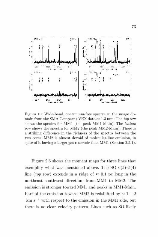
trum, while MM2 is almost devoid of molecular emission,

if not for the CO, 13CO and C18O J = 2− 1, and faint SO

J(K) = 6(5) − 5(4) emission. We interpret this difference

as a signature of the evolutionary stage of the cores, MM1

being more evolved than MM2.

73

Figura 10: Wide-band, continuum-free spectra in the image do-main from the SMA Compact+VEX data at 1.3 mm. The top rowshows the spectra for MM1 (the peak MM1-Main). The bottomrow shows the spectra for MM2 (the peak MM2-Main). There isa striking difference in the richness of the spectra between thetwo cores. MM2 is almost devoid of molecular-line emission, inspite of it having a larger gas reservoir than MM1 (Section 2.5.1).

Figure 2.6 shows the moment maps for three lines that

exemplify what was mentioned above. The SO 6(5)–5(4)

line (top row) extends in a ridge of ≈ 0,1 pc long in the

northeast–southwest direction, from MM1 to MM2. The

emission is stronger toward MM1 and peaks in MM1-Main.

Part of the emission toward MM2 is redshifted by ∼ 1− 2

km s−1 with respect to the emission in the MM1 side, but

there is no clear velocity pattern. Lines such as SO likely

74

have large optical depths and trace only the surface of the

emitting region, where clear velocity gradients, especially of

rotation, may not be expected. From the SO data we cons-

train any velocity difference between the MM1 and MM2

cores to ∆V < 2 km s−1.

For a given molecule, the isotopologue lines and the li-

nes with upper energy levels well above 100 K trace the

more compact gas, closer to the heating sources. Figure 2.6

shows the examples of 13CS J = 5 − 4 (middle panel) and

CH3CN J(K) = 12(3) − 11(3) (bottom). Both of them are

only visible toward MM1, and peak in MM1-Main. These

lines trace a clear velocity gradient centered on MM1-Main,

the blueshifted emission is toward the southwest, and the

redshifted emission toward the northeast, perpendicular to

the main bipolar CO outflow. We interpret this as rota-

tion. The emission tracing this velocity gradient is not iso-

lated, there is also emission coming from MM1-NW and

MM1-SE. Especially in the CH3CN lines, this extra emis-

sion appears to trace redshifted and blueshifted emission

respectively. One possibility is that MM1-NW and MM2-

SE are separate protostars from MM1-Main. However, the

orientation of the lobes in the high-velocity outflow is the

same. Therefore, we prefer the interpretation that MM1-

NW and MM2-SE are not of protostellar nature, but emis-

sion enhancements (both in continuum and line emission)

from the hot base of the powerful molecular outflow driven

75

by the disk-like structure surrounding MM1-Main. In this

scenario, the other 7-mm sources reported by [203] (or at

least the counterpart of MM1-NW) can be interpreted as

shocked free–free enhancements in a protostellar jet, simi-

lar to those observed in the high-mass star formation region

IRAS 16547− 4247 [174, 66].

Figure 2.7 shows the position–velocity (PV) diagrams

of the CH3CN K = 3 line shown in Fig. 2.6, centered at

the position of MM1-Main perpendicular to the rotation

axis (top frame) and along it (bottom frame). The rota-

tion pattern is similar to those observed in objects that

have been claimed to be Keplerian disks, i.e., structures

where the mass of the central object is large compared to

the mass of the gas, rotating with a velocity Vrot ∝ r−0,5

[232, 44, 98]. The large velocity dispersion closest to MM1-

Main (Figs. 2.6 and 2.7) ought to be caused by unresolved

motions in the inner disk, since velocity dispersions well

above 1 km s−1 cannot be due to the gas temperature.

Recently, [54] reported a possible disk-jet system cen-

tered in W33A MM1-Main. The jet, observed in the Brγ

line, extends up to ±300 km s−1 in velocity at scales ∼ 1

AU, with a similar orientation and direction to the mole-

cular outflow reported in this study. However, the velocity

structure of what [54] interpret as a rotating disk has a si-

milar orientation but opposite sense of rotation as the disk

that we report. They used CO absorption lines with upper

76

Figura 11: Hot-core molecules toward the center of W33A. Thetop row shows the SO 6(5)–5(4) line. The middle row shows the13CS 5–4 line. The bottom row shows the CH3CN 12(3)–11(3)line. Contours show the moment 0 maps at 5, 15, 30, 50, 100, 150,and 200×0,05 Jy beam−1 km s−1. The color scale shows the mo-ment 1 maps (left column) and moment 2 maps (right column).Symbols are as in Fig. 2.1. While the SO traces an extendedenvelope reaching MM2, the other molecules trace a clear velo-city gradient indicative of rotation centered in MM1-Main. Thevelocity dispersion also peaks in MM1-Main.

77

energy levels Eu ∼ 30 K, while we use emission lines like

those of CH3CN, with Eu > 100 K (Table 2.3). If an ex-

tended screen of cold gas with a negligible velocity gradient

is between the observer and the inner warm gas with a ve-

locity gradient, it is possible that the absorption lines are

partially filled with emission, mimicking a velocity gradient

with the opposite sense to that seen in the emission lines.

Physical Parameters

Now we derive the temperature and column density of

the hot-core emission, and constrain the stellar mass, gas

mass, and CH3CN abundance in MM1.

The kinetic temperature of the innermost gas can be

obtained from the K lines of CH3CN J = 12 − 11. To

avoid the simplification of considering optically-thin emis-

sion assumed in a population-diagram analysis, we fit all

the K lines assuming LTE, while simultaneously solving

for the temperature Tkin, column density of CH3CN mole-

cules NCH3CN, and line width at half-power FWHM. The

procedure to obtain the level populations can be found in

[8].

Figure 2.8 shows the results of our fits to the CH3CN

spectra. The systemic velocity Vsys ≈ 38,5 km s−1 was

found to be optimal. The data outside the lines of inter-

est have been suppressed for clarity, and the fit was done

78

Figura 12: Position–Velocity (PV) diagrams for the CH3CNJ = 12−11 K = 3 data. The center is the position of MM1-Main(Table 2.2). Top: PV diagram at P.A. = 39. A clear velocity gra-dient is seen from the southwest (blueshifted, negative position)to the northeast (redshifted, positive position). At the angle ofthis cut the velocity gradient has maximum symmetry. Bottom:PV diagram at P.A. = 39 + 90 = 129. Negative positions areto the northwest, and positive positions to the southeast. Thereis emission in the range [36, 41] km s−1 at all positions. Closerto the center position, the velocity dispersion increases rapidly.

79

in the frequency windows where only the lines of interest

are present. The gas is warmer (by 18 %) and denser (by

415 % in column) toward the peak MM1-Main (bottom fra-

me) than in the average of the sources composing MM1 (top

frame). This makes the case for the internal heating and a

centrally-peaked density gradient in MM1-Main, as well as

for its protostellar nature. Some lines are not completely

well fit under the assumption of a single value for the pa-

rameters. On the one hand, the bright K = 7 and 8 lines

indicate the presence of some column of very warm gas; on

the other hand, the K = 3 is not brighter than the K < 3

lines within the uncertainties, indicating that some column

of gas is below 200 K. Two-component fits do not give bet-

ter results. The reported values should be interpreted as an

average along the line of sight. Detailed radiative transfer

in the context of a physical model is currently under way.

Under the interpretation of edge-on rotation as the cau-

se of the velocity gradient observed in Figs. 2.6 and 2.7,

the dynamical mass in MM1-Main (stars plus gas) is about

9 M, where a mean-velocity offset of 2.0 km s−1 with res-

pect to Vsys ≈ 38,5 km s−1 was taken at a radius of 0,5”.

Assuming that the disk is perpendicular to the outflow, and

correcting for the outflow inclination angle i = 50 estima-

ted by [57], the enclosed dynamical mass is Mdyn ∼ 15 M.

Given that W33A is fragmented into multiple sources,

a strict upper limit to the stellar mass in MM1-Main is

80

< 20 M, the mass necessary to account for the total lumi-

nosity (∼ 105 L) of W33A. Also, the total gas mass in the

MM1 sources inferred from dust emission is ∼ 10 M, the-

refore the gas mass in the rotating structure around MM1-

Main should be a fraction of it. For a gas mass in the rota-

ting structure Mgas ∼ 5 M, the mass of the protostar(s)

in MM1-Main amounts to M? ∼ 10 M. MM1-Main ap-

pears to be B-type protostar still accreting from a rotating

disk-like structure.

From the ∼ [9, 32] M gas-mass range in MM1 we deri-

ve an average column density of molecular gas of about

[1, 4] × 1023 cm−2 . For an average CH3CN column of

∼ 8× 1015 cm−2 , a CH3CN abundance with respect to H2

of X(CH3CN) ∼ [2, 8] × 10−8 is derived, similar estimates

in other regions of high-mass star formation [216, 167, 71].

2.6. Discussion

2.6.1. Star Formation from Converging

Filaments

In W33A, two localized regions of star formation (MM1

and MM2) separated by 0.1 pc are surrounded by a common

filamentary structure of ∼ 1 pc in length (Section 2.5.2).

The two velocity components of this filamentary structu-

81

Figura 13: Simultaneous fits to the CH3CN J = 12− 11 K lines.The dashed gray line is the data. The solid black line is thefit. The data outside the lines of interest have been set to zeroto avoid contamination by other molecular lines. Top: Averagespectra over the entire MM1 region. Bottom: Spectra toward thefew central pixels at the peak position (MM1-Main). The gas iswarmer, denser, and has a larger line width toward this position.

82

re are separated by ≈ 2,6 km s−1 in line-of-sight velocity

and intersect in projection right at the position of the star

formation activity (Fig. 2.2). The velocity components are

not a mere superposition in position–position–velocity spa-

ce, but they merge into a structure with larger motions

(Fig. 2.3, Section 2.5.2), resolved into a disk/outflow sys-

tem by subarcsecond resolution observations (Figs. 2.6 and

2.7, Section 2.5.2). This suggests that star formation in

W33A was triggered by the convergence of molecular fila-

ments. Such a scenario has been suggested for the region

W3 IRS 5 by [170]. More recently, the merging of filaments

has also been claimed by [97] in the infrared dark cloud

G35.39–0.33 and by [39] in the MSFR W75.

This mode of star formation is predicted by numerical

simulations of star formation triggered by converging flows

[15, 84, 206]. In those simulations, the formation of molecu-

lar clouds itself is a product of the convergence of streams of

neutral gas. Later in the evolution of the molecular clouds,

filaments of molecular gas can converge (merge) with each

other, leading to the formation of cores and stars.

We present here a simple comparison with a region

found in the numerical simulation recently reported by

[207]. This simulation represents the formation of a giant

molecular complex from the convergence of two streams of

warm neutral gas, at the scale of tens of parsecs. Specifica-

lly, the simulation was performed using the smoothed par-

83

ticle hydrodynamics (SPH) code GADGET [193], including

sink-particle and radiative cooling prescriptions [96, 206].

The convergence of the warm diffuse-gas streams triggers a

thermal instability in the gas, which causes it to undergo a

transition to the cold atomic phase, forming a cloud. The

latter soon becomes gravitationally unstable, begins con-

tracting, and undergoes hierarchical fragmentation. During

the contraction, the density of isolated clumps increases and

they can reach physical conditions corresponding to those

of molecular clumps. Finally, the global collapse reaches the

center of mass of the cloud, at which point a region with

physical conditions corresponding to those of MSFRs forms.

The simulation box has 256 pc per side, and the converging

flows have a length of 112 pc, and a radius of 32 pc. Ho-

wever, after the gravitational contraction, the clumps are

only a few parsecs across. Since SPH is essentially a Lagran-

gian method, it allows sufficient resolution in these dense

regions. We refer the reader to [206, 207] for details of the

simulation. Here we focus on the region called “Cloud 1” in

[207], albeit roughly 1.5 Myr later than the time examined

in that paper.

Figure 2.9 shows two snapshots of column density sepa-

rated by 0.133 Myr (the time interval between successive

data dumps of the simulation). The column density is com-

puted by integrating the density along the x-direction over

the 10 pc path 123 ≤ x ≤ 133 pc, which is centered at the

84

midplane of the simulation, where the (sheet-like) cloud is

located. In this region and epoch of the simulation, the two

leftmost filaments in the top panel of Fig. 2.9 converge to

form the boomerang-shaped filament seen in the bottom pa-

nel. Note that the simulation was not designed to simulate

the observed filaments. The comparison is only intended to

show that some of observed properties of W33A can arise

naturally in the context of a simulation of the formation of

a large molecular complex that contains a filament system.

The peaks of two filaments of gas are initially separated

by 0.4 pc (top frame of Fig. 2.9) and then merge at a projec-

ted velocity of 3± 1,5 km s−1, measured directly from the

displacement observed between the two panels. The column

density of the filaments is in the range [103, 104] code units

(Fig. 2.9), or NH2 = [0,5 × 1024, 0,5 × 1025] cm−2. For an

NH3 abundance with respect to H2 in the range X(NH3) =

[10−8, 10−7] [e.g., 71], the column density of the cold fila-

ments in our observations is NH2 = [1,1 × 1024, 1,1 × 1025]

cm−2. Figure 2.10 shows the volume density (color scale)

and y–z plane velocity (arrows) in a slice trough the fila-

ments. It is seen that the filaments reach densities typical

of MSFRs (peak n ∼ 105 cm−3) and that their velocity

field presents fast jumps of a few km s−1 in the interaction

zones, comparable to our observations. We conclude that

some of the properties of the observed filaments such as

sizes, column densities, and velocities agree within a factor

85

of 2 with those from the simulation. This rough comparison

illustrates that our interpretation of convergence between

the observed filaments is feasible.

2.6.2. Cores at Different Evolutionary Stages

The star-forming cores in W33A appear to be at mar-

kedly different evolutionary stages (Section 2.5.2). The first

piece of evidence for this is the clear difference in the ri-

chness of the molecular-line emission from MM1 to MM2

(see Fig. 2.5). MM1 has molecular emission typical of a

“hot-core” [124], with a prominent CH3CN J = 12 − 11

“K-forest” that can be detected up to the K = 8 line, with

upper-level energy Eu = 525,5 K (see Table 2.3). The avera-

ge gas temperature of MM1 is ∼ 347 K. In contrast, MM2 is

almost devoid of “hot-core” emission, and is only detected

in a few molecules. MM2 is much colder than MM1, with a

temperature TMM2 ≈ 46 K. The second piece of evidence is

the mass content of the cores. MM1 has only ∼ [9, 32] M

of gas, while MM2 has ∼ 60 M. This could naively be in-

terpreted as MM2 having a much larger gas reservoir than

MM1, but it should be kept in mind that both cores are

part of a common parsec-scale structure. Clump infall at pc

scales has been reported from single-dish [221] and interfe-

rometric [71] observations. Also, numerical simulations of

parsec-sized clumps show that the star-forming cores that

86

Figura 14: Snapshots of molecular filaments merging with eachother extracted from the simulation presented by Vazquez-Semadeni et al. (2009). The time interval between the first (top)and second (bottom) frames is 0.133 Myr. The units of the z- andy-axes are pc. The color scale shows the column density in codeunits, equivalent to 4,9× 1020 H2 particles per square cm.

87

Figura 15: Snapshots of molecular filaments merging with eachother extracted from the simulation presented by Vazquez-Semadeni et al. (2009). The time interval between the first (top)and second (bottom) frames is 0.133 Myr. The units of the z- andy-axes are pc. The color scale shows the volume density (cm−3)in a slice passing through the merging filaments. The arrows in-dicate the velocity of the gas in the y–z plane. In the secondframe (bottom), the two merged filaments have velocities roughlyopposing each other by a few km s−1.

88

give birth to massive stars are continuously fed from gas in

the environment at the clump scales [e.g., 32, 185, 207, 161].

There are two possibilities that we briefly discuss here:

(1) the prestellar cores that were the precursors to MM1

and MM2 appeared at the same time and then MM1 evol-

ved faster to produce a ∼ 10 M star (Section 2.5.2), whi-

le MM2 only produced at most an intermediate mass star

(MM2 is not prestellar, since it has some internal heating

and appears to power an outflow, see Section 2.5.2), or (2)

the prestellar core precursor to MM2 formed later and has

yet to form at least one massive star. Our observations can-

not tell these options apart. A measurement of the accre-

tion rate in both cores would be helpful. Sources at diffe-

rent evolutionary stages within a single star-forming clus-

ter have also been reported recently for AFGL 5142 [231],

G28.34+0.06 [235], and AFGL 961 [215].

2.6.3. A Rotating Disk/Outflow System in

MM1-Main

In the past decade, the question of whether massi-

ve stars form by disk-outflow mediated accretion similar

to low-mass stars has been the subject of intensive re-

search. The answer is positive: they definitely do. Some

of the massive protostars that have been shown to har-

bor disk/outflow systems are G192.16-3.82 [181], Cepheus

89

A HW2 [157], IRAS 20126+4104 [44], and IRAS 16547-

4247 [66]. All these relatively clean disk examples, howe-

ver, do not have stars more massive than 15 to 20 M.

More massive (O-type) stars have also been shown to form

via disk-mediated accretion. However, the innermost part

of the accretion flow is often (at least partially) ionized and

is observed as a hypercompact (HC) H II region. Also, the

gas in these more massive regions is warmed up to farther

distances, and very massive rotating structures of size up to

0.1 pc are typically observed. Examples are G10.6-0.4 [104],

G24.78+0.08 [20], W51e2 [116], and G20.08-0.14 N [71], all

of which have stellar masses above 20M. A possible excep-

tion to this scenario is W51 North, where [227, 226] claims

to have found a protostar with M? > 60 M and without a

“bright” (with flux above tens of mJy at wavelengths ∼ 1

cm) H II region. This apparent discrepancy is solved if mul-

tiple, lower-mass stars account for the mass in W51 North

or if the H II region in this source is gravitationally trapped

as currently observed. Indeed, detailed simulations of the

evolution of HC H II regions within accretion flows show

that their radio-continuum emission flickers significantly in

timescales from 10 to 104 yr [161].

In this chapter we report on the existence of a rotating

disk centered on MM1-Main in W33A (Section 2.5.2). To

our sensitivity, the radius of the disk is R . 4000 AU.

The warm-gas emission does not come only from the disk,

90

but also from an structure elongated perpendicular to it,

coincident with the other mm peaks (MM1-NW and MM1-

SE) along the direction of the outflow (see Figs. 2.6 and

2.7). We propose that the secondary mm peaks in MM1 are

not of protostellar nature, but regions where the emission

is enhanced due to the interaction of the outflow with the

disk and its inner envelope. Indeed, the two brightest 7-

mm detections of [203] are counterparts of MM1-Main (Q1,

Sν ≈ 1,7 mJy at 7 mm) and MM1-SE (Q2, Sν ≈ 0,6 mJy

at 7 mm).

The free–free emission from the 7 mm source Q1 should

be a combination of photoionization by the central protos-

tar and shock-induced ionization of material due to the jet

observed by [54], likely dominated by the latter. The ori-

gin of the free–free emission from Q2 could also be shocks,

although deeper 7 mm observations are needed to con-

firm this source. Q3 does not have a mm/submm coun-

terpart and may not be a distinct source. The radio con-

tinuum sources of W33A could then be analogs of those

in IRAS 16547–4247 [173, 174], which have fluxes a fac-

tor of a few larger at 0.75 times the distance to W33A.

Indeed, we find that the radio-continuum emission from

Q1 (MM1-Main) agrees with the correlation found for low-

mass jets between the radio-continuum luminosity of the jet

and the momentum rate of the associated molecular out-

flow: P = 10−2,5(Sνd2)1,1 [7], where the radio luminosity

91

has units of mJy kpc2 and the momentum rate has units of

M yr−1 km s−1. For W33A with a radio flux S3,6cm = 0,79

mJy [168], and a distance d = 3,8 kpc [95], the expected

momentum rate is P = 0,046 M yr−1 km s−1, while the

observed momentum rate (lower limit) is P = 0,040 M

yr−1 km s−1 (obtained dividing the momentum of the mo-

lecular outflow by its length, including the inclination co-

rrection). This correlation was found to hold for three well-

studied massive protostars (IRAS 16547–4247, HH 80–81,

and Cep A HW2) by [174]. In this study we report that it al-

so holds for W33A, which constitutes further evidence for a

common accretion mechanism between low- and high-mass

protostars, at least to the stage prior to the development

of a brighter H II region.

Comparing the ratio of the radio luminosity to the IR

luminosity L(8 GHz)/L(IR) with the recombination-line li-

ne width may be a useful criterion to distinguish between a

source ionized by shocks (jet or stellar wind) or by photoio-

nization (what usually is called an H II region). In Fig. 2.6

of the review by [89], it is seen that UC H II regions have

the largest L(8 GHz)/L(IR) and the smallest line width, jet

sources have the smallest L(8 GHz)/L(IR) and the largest

line width, and HC H II regions fall in between the pre-

vious two. For W33A, log(L(8 GHz)/L(IR)) ≈ 7,1, and the

FWHM of the IR recombination lines is of several hundreds

km s−1, again consistent with a jet source.

92

The star(s) at the center of MM1-Main (with M? ∼10 M) appears to dominate the dynamics of the disk, but

we cannot rule out the existence of additional, less massive

objects within it. Indeed, models of massive protostellar

disks predict their fragmentation and the formation of a

few lower mass companions within it [118, 121, 161].

2.7. Conclusions

In this chapter we presented for the first time resol-

ved observations in both mm continuum and molecular-line

emission for the massive star formation region W33A, cha-

racterized by a very high luminosity (L ∼ 105 L) and

very low radio-continuum emission (∼ 1 mJy). Both of the

previously known mm cores (MM1 and MM2) are resol-

ved into multiple peaks, and appear to be at very different

evolutionary stages, as indicated by their molecular spec-

tra, masses, temperatures, and continuum spectral indices.

The brightest core (MM1-Main at the center of MM1) is

centered on a very faint free–free source and the gas dy-

namics up to a few thousand AU of it indicates the pre-

sence of a circumstellar disk rotating around a stellar mass

of M? ∼ 10 M. MM1-Main also drives a powerful, high-

velocity molecular outflow perpendicular to the disk. MM2,

the coldest and most massive core, is not detected in hot-

93

core lines but appears to drive a more modest outflow. Both

MM1 and MM2 are located at the intersection of parsec-

scale filamentary structures with line-of-sight velocity off-

set by ≈ 2,6 km s−1. Analysis of the position–position–

velocity structure of these filaments and a comparison with

recent numerical simulations suggests that star formation

in W33A was triggered by the convergence of filaments of

cold molecular gas.

Notes

1The Submillimeter Array is a joint project between the Smithso-

nian Astrophysical Observatory and the Academia Sinica Institute of

Astronomy and Astrophysics and is funded by the Smithsonian Insti-

tution and the Academia Sinica. See Ho et al. [86].2 The National Radio Astronomy Observatory is operated by As-

sociated Universities, Inc., under cooperative agreement with the Na-

tional Science Foundation.3Single-dish data were taken for this purpose but these were co-

rrupted due to a bad off position and could not be used.4The (2,2) to (1,1) ratio is not sensitive to temperatures much

larger than 50 K, but we confirm the large temperatures in MM1 at

smaller scales using the CH3CN lines, see Section 2.5.2. The errors in

the fits also increase toward MM1 due to its wider velocity structure.

94

Cu

adro

2.1:

Obse

rvat

ion

alP

aram

eter

s

Ep

och

Arr

ay

Ph

ase

Cen

tera

Ban

dp

ass

Flu

xP

hase

α(J

2000)

δ(J

2000)

Calib

rato

rC

alib

rato

rC

alib

rato

r2004

06

14+

15

VL

A-D

18

14

39.5

00

−17

51

59.8

00

3C

273

3C

286

1851

+005

2006

05

22

SM

A-E

xte

nd

ed18

14

39.5

09

−17

51

59.9

99

3C

273

Callis

to1733−

130

2007

07

17

SM

A-C

om

pact

18

14

39.4

95

−17

51

59.8

00

3C

454.3

Callis

to1733−

130

2008

08

02

SM

A-V

EX

18

14

39.4

95

−17

51

59.8

00

3C

454.3

Callis

to1733−

130

a:

un

its

of

R.A

.are

hou

rs,

min

ute

s,an

dse

con

ds.

Un

its

of

dec

l.are

deg

rees

,arc

min

ute

s,an

darc

seco

nd

s.

95

Cu

adro

2.2:

Milli

met

erC

onti

nu

um

Sou

rces

Core

aC

om

pon

entb

α(J

2000)c

δ(J

2000)c

I peak(1

.3m

m)d

S(1

.3m

m)d

(hrs

,min

,sec

)(d

eg,a

rcm

in,a

rcse

c)(

mJy

bea

m−1)

(mJy)

MM

1-N

W18

14

39.4

7−

17

51

59.7

31

357

MM

1M

M1-M

ain

18

14

39.5

1−

17

52

00.0

65

357

MM

1-S

E18

14

39.5

5−

17

52

00.4

25

357

MM

2M

M2-M

ain

18

14

39.2

4−

17

52

01.9

43

289

MM

2-N

E18

14

39.3

1−

17

52

00.6

22

289

a:m

ain

core

as

lab

eled

inF

ig.2.1

,le

ftp

an

el.b

:cl

earl

yd

isti

nct

sub

com

pon

ents

ofth

em

ain

core

sas

mark

edin

Fig

.2.1

.

c:p

osi

tion

of

pea

k.d

:p

eak

inte

nsi

ty±

1,5

mJy

bea

m−1.H

PB

W=

0,6

3”×

0,4

3”.e:

ad

ded

flu

xof

the

sub

com

pon

ents

of

each

core

.T

he

un

cert

ain

ties

inth

efl

uxes

of

MM

1an

dM

M2

are±

20

mJy

an

d±

25

mJy

resp

ecti

vel

y.

96

Cuadro 2.3: Bright Molecular Linesa

Species Transition ν0 Eu

(GHz) (K)C18O 2–1 219.5603 15.8

HNCO 10(2,9)–9(2,8) 219.7338 228.4– 10(2,8)–9(2,7) 219.7371 228.2– 10(0,10)–9(0,9) 219.7982 58.0

H213CO 3(1,2)–2(1,1) 219.9084 32.9SO 6(5)–5(4) 219.9494 34.9

CH3OH 8(0,8)–7(1,6) E 220.0784 96.613CO 2–1 220.3986 15.86

CH3CN 12(8)-11(8) 220.4758 525.5– 12(7)-11(7) 220.5393 418.6

HNCO 10(1,9)–9(1,8) 220.5847 101.5CH3CN 12(6)-11(6) 220.5944 325.8

– 12(5)-11(5) 230.6410 247.3– 12(4)-11(4) 220.6792 183.1– 12(3)-11(3) 220.7090 133.1– 12(2)-11(2) 220.7302 97.4– 12(1)-11(1) 220.7430 76.0– 12(0)-11(0) 220.7472 68.8

CH3OH 15(4,11)–16(3,13) E 229.5890 374.4– 8(-1,8)–7(0,7) E 229.7588 89.1– 3(-2,2)–4(-1,4) E 230.0270 39.8

12CO 2–1 230.5380 16.5OCS 19–18 231.0609 110.813CS 5–4 231.2207 26.6

CH3OH 10(2,9)–9(3,6) A− 231.2811 165.3

a: molecular lines with peak TB ≥ 20 K. The first column refers to the mole-

cule tag, the second column to the transition, the third to its rest frequency

as found in Splatalogue (http://www.splatalogue.net/), and the fourth to

the upper-level energy. Data used from Splatalogue are compiled from the

CDMS catalog [150] and the NIST catalog [135].

3

A MSFR with young

UC and HC HII

Regions: G20.08N

3.1. Resumen

Se presentan observaciones espectrales y de continuo

en G20.08–0.14 N, las cuales exploran la dinamica del gas

ionizado y molecular a varias escalas espaciales en esta re-

gion de formacion de estrellas masivas. Observaciones de

la molecula NH3 usando el VLA con una resolucion de 4”

revelan un flujo de acrecion con un radio de ≈ 0,5 pc que

rodea un grupo de tres regiones H II muy pequenas. Es-

98

te flujo parece estar rotando y colapsando. Observaciones

de moleculas que trazan gas denso y caliente hechas con el

SMA (CH3CN, OCS, and SO2) y con el VLA (NH3) con

una resolucion de 0,4” muestran que dos de las regiones H II

tienen gas colapsando hacia ellas en escalas de ∼ 0,05 pc y

una de ellas tiene un flujo de acrecion con rotacion alineada

con la rotacion del flujo a escalas de pc. Este alineamiento,

ası como las escalas temporales para la contraccion de la

nube (0.1 Myr) y de los nucleos densos (0.01 Myr), sugie-

ren que el flujo de acrecion a escalas de 1 pc es continuo

hasta escalas de 0.1 pc y que el material continua fluyendo

de las escalas grandes a las escalas chicas.

Observaciones de lıneas de recombinacion milimetricas

a una resolucion de 0,4” sugieren que la dinamica del gas

ionizado en la region H II mas brillante es una combina-

cion de rotacion y flujo eyectado. Las anchas lıneas de re-

combinacion y la distribucion espectral de energıa sugieren

la presencia de gradientes de densidad en el gas ionizado

y flujos supersonicos respectivamente. Estas observaciones

son consistentes con fotoevaporacion (fotoionizacion) de la

parte interna de un flujo de acrecion molecular que ha sido

aplanado por rotacion.

Estos resultados han sido publicados en: Galvan-

Madrid, Roberto, Keto, Eric R., Zhang, Qizhou, Kurtz,

Stan, Rodrıguez, Luis F., & Ho Paul T. P. The Astrophy-

sical Journal, 706, 1036 (Diciembre 2009).

99

3.2. Summary

Spectral line and continuum observations of the molecu-

lar and ionized gas in G20.08–0.14 N explore the dynamics

over a range of spatial scales in this massive star-forming

region. Observations of NH3 performed with the Very Large

Array at 4” angular resolution show a large-scale (∼ 0,5 pc

radius) molecular accretion flow around and into a star clus-

ter with three small H II regions. Higher resolution (0,4”)

Submillimeter Array and VLA observations in hot core mo-

lecules (CH3CN, OCS, and SO2, NH3) show that the two

brightest and smallest H II regions are themselves surroun-

ded by smaller scale (∼ 0,05 pc radius) accretion flows. The

rotation of the large-scale flow is aligned with the small sca-

le, and the timescale for the contraction of the cloud is short

enough, 0.1 Myr, for the large-scale flow to deliver signifi-

cant mass to the smaller scales within the star formation

timescale. The flow structure appears to be continuous and

hierarchical from larger to smaller scales.

Millimeter recombination line (RL) observations at 0,4”

angular resolution indicate rotation and outflow of the io-

nized gas within the brightest H II region (A). The broad

recombination lines suggest supersonic flows. A continuum

spectral energy distribution (SED) that rises from cm to

mm wavelengths indicates a density gradient inside this H

100

II region. These observations are consistent with photoe-

vaporation of the inner part of the rotationally flattened

accretion flow.

These results have been published in Galvan-Madrid,

Roberto, Keto, Eric R., Zhang, Qizhou, Kurtz, Stan,

Rodrıguez, Luis F., & Ho Paul T. P. “Formation of an O-

Star Cluster by Hierarchical Accretion in G20.08–0.14 N”.

The Astrophysical Journal, 706, 1036 (December 2009) [71].

101

3.3. Introduction

Massive star-forming regions (MSFRs) with O stars are

usually identified by a group of hypercompact (HC) H II

or ultracompact (UC) H II regions found together, deeply

embedded in a dense molecular cloud [76, 45, 89]. That

several H II regions are typically found within each star-

forming region indicates that massive stars form together

in small clusters. Furthermore, the infrared luminosity and

radio continuum brightness of the individual H II regions

suggest that some of them may themselves contain more

than one massive star. Thus, the spatial structure of mas-

sive star-forming regions is clustered and hierarchical: the

star-forming regions contain a number of separate HC and

UC H II regions, each of which may in turn contain a few

massive stars.

Low angular resolution, single-dish, molecular line sur-

veys of MSFRs show evidence for large scale contraction of

the embedding molecular clouds [221, 115]. Higher angu-

lar resolution observations of some of these regions iden-

tify velocity gradients consistent with rotation and in-

flow. In addition to the accretion flows seen on the large-

scale (∼ 0,3 − 1 pc) of the embedding molecular cloud

(G10.6–0.4 [85, 109, 106]; G29.96–0.02 [154]), accretion

flows are also seen on smaller (≤ 0,1 pc) scales around

102

individual HC and UC H II regions (G10.6–0.4 [110, 188];

W3(OH) [111, 112]; W51e2 [229, 225]; G28.20–0.05 [189];

G24.78+0.08 [23, 24, 20, 73]; G29.96–0.02 [26]).

It is unclear how the flows on different length scales are

related. In the case of G10.6–0.4, the cluster-scale accre-

tion flow can be traced down from the largest cloud scale

to the small scale of the brightest H II region, but it is not

known whether this holds for other objects. For example,

in a survey of MSFRs, selected on the basis of IRAS colors

and specifically excluding those with H II regions, multiple

bipolar molecular outflows (implying the presence of ac-

cretion flows) are seen in random orientations [28, 29, 30].

The different orientations of these smaller-scale flows sug-

gest separate, individual centers of collapse. This compari-

son raises the question whether a large-scale coherent flow

is required for the formation of the most massive stars, O

stars (M? > 20 M) capable of producing bright H II re-

gions, whereas B stars require only smaller scale flows.

It is also unclear what happens in an accretion flow

when the inflowing molecular gas reaches the boundary

of an embedded H II region. Previous observations sug-

gest that the H II regions in an MSFR that are surroun-

ded by accretion flows, may be best understood as deri-

ving from the continuous ionization of the accretion flow

[107, 102, 108], rather than as a dynamically separate ex-

panding bubble of ionized gas within the flow. Part of the

103

ionized gas may continue to the central star or stars and

part escapes off the rotationally flattened accretion flow as

a photoevaporative outflow perpendicular to the plane of

rotation [92, 224, 99, 136]. The outflow is accelerated to su-

personic speeds by the density gradient maintained by the

stellar gravity [108]. Because the extent of an ionized out-

flow is generally larger than the region of ionized inflow, in

most cases the outflow should be detected more easily than

the inflow. H II regions classified as “broad recombination

line objects”(BRLO) [94, 179] show steep density gradients

and supersonic flows [105], consistent with photoevapora-

tion and acceleration. It is not known whether all BRLO are

associated with accretion. If the accretion surrounding an

O star cluster is continuous from the largest to the smallest

scales, this must be the case.

There are only a handful of radio recombination line

(RRL) observations that spatially resolve the ionized flow

within an HC H II region. Velocity gradients consistent with

outflow and rotation in the ionized gas have been previously

reported for W3(OH) [112], W51e2 [103], and G28.20–0.05

[180]. Observations of the very massive and spatially lar-

ge G10.6–0.4 H II region made at the VLA in the highest

possible angular resolution are able to map the inflowing

ionized gas [104].

In order to study the accretion dynamics over a range of

scales in a MSFR, from the cluster scale down to the scale

104

of individual HC H II regions and within the ionized gas, we

set up a program of radio frequency molecular line, recom-

bination line, and continuum observations at two telesco-

pes and with several different angular resolutions. For the

study presented in this chapter, we chose the massive star

formation region G20.08–0.14 North (hereafter G20.08N),

identified by three UC and HC H II regions detected in the

cm continuum by Wood and Churchwell [220]. The total

luminosity of the region is L ∼ 6,6× 105 L for a distance

of 12.3 kpc.1

Previous observations suggest accretion in the G20.08N

cluster. Molecular-line observations show dense gas embed-

ding the H II regions [201, 164]. Molecular masers, gene-

rally associated with ongoing massive-star formation, have

been detected in a number of studies (OH [88]; H2O [91];

and CH3OH [209]). Klaassen & Wilson [114, 115] obser-

ved large-scale inward motions consistent with an overall

contraction of the embedding molecular cloud. Those aut-

hors also observed SiO line profiles suggestive of massive

molecular outflows, further evidence for accretion and star

formation. The recombination line spectra show broad li-

nes [77, 179], presumably due to large, organized motions in

the ionized gas. However, the previous observations do not

have the angular resolution and the range of spatial scales

needed to confirm the presence of accretion flows and study

them in detail.

105

In this chapter we present several observations of

G20.08N and discuss our findings. We confirm active ac-

cretion within the cluster. Furthermore, we find that the

parsec-scale accretion flow fragments into smaller flows

around the individual HC H II regions, and that the gas

probably flows from the largest scale down to the smallest

scale. This continuous and hierarchical accretion may be

necessary to supply enough mass to the small-scale flows

to form O-type stars, in contrast to low- and intermediate-

mass star-forming regions with stars no more massive than

∼ 20 M, where isolated accretion flows around individual

protostars may be sufficient.

3.4. Observations

3.4.1. SMA

We observed G20.08N on 2006 June 25 and July 6 with

the Submillimeter Array2 [86] in its very extended (VEX)

configuration. Two sidebands covered the frequency ranges

of 220,3 − 222,3 GHz and 230,3 − 232,3 GHz with a spec-

tral resolution of ≈ 0,5 km s−1. The H30α recombination

line (ν0 = 231,9009 GHz) was positioned in the upper si-

deband3. The observations sampled baseline lengths from

≈ 50 to . 400 kλ, sensitive to a range of spatial scales from

≈ 0,5” to ≈ 4,1”.

106

The visibilities of each observation were separately ca-

librated using the SMA’s data calibration program, MIR.

Table 3.1 lists relevant information on the calibrators. We

used quasars for the absolute amplitude scale as well as the

time-dependent phase corrections and frequency-dependent

bandpass corrections. Inspection of the quasar fluxes and

comparison with their historical flux densities in the SMA

database4 suggest that flux calibration is accurate to better

than 20 %. The calibrated data were exported to MIRIAD

for further processing and imaging.

There were enough line-free channels in the 2-GHz pass-

band to subtract the continuum in the (u, v) domain. The

line-free continuum was self-calibrated in phase, and the

gain solutions were applied to the spectral line data. We

list all the identified lines in Table 3.2. Figure 3.1 shows

the continuum-free spectra across both sidebands at the

position of the 1.3-mm peak.

To improve the sensitivity, the data were smoothed to

a spectral resolution of 2 km s−1. The rms noise in our

natural-weighted maps, made from the combined observa-

tions of both days, is ∼ 2 mJy beam−1 for the single-

sideband continuum and ∼ 30 mJy beam−1 per channel

(2 km s−1 wide) for the line data.

107

3.4.2. VLA

Spectral line observations of NH3 (J,K) = (2, 2) and

(3,3) at two different angular resolutions were obtained

with the Very Large Array5 in the D and BnA configura-

tions (projects AS749, AS771, and AS785). Partial results

from these observations were presented in Sollins [186]. All

the observations, except the VLA-D (3,3), were done with

a bandwidth of 3.125 MHz (≈ 39 km s−1) divided in 64

spectral channels, each 0,6 km s−1 wide. The VLA-D (3,3)

observation was done with the same bandwidth divided in

128 spectral channels, each 0,3 km s−1 wide. The band-

width covers the main hyperfine line and one line from the

innermost satellite pair6. The NH3 data are presented at a

spectral resolution of 0.6 km s−1. The noise per channel in

the final images was in the range of 1,0−1,5 mJy beam−1.

In addition to the molecular line observations, we obser-

ved the ionized gas in the H66α recombination line in the

VLA B configuration. The correlator was set up to cover

a bandwidth of 12.5 MHz (≈ 166 km s−1) divided in 64

channels of 2.6 km s−1 each. The rms noise per channel in

the final image was ≈ 1 mJy beam−1.

All three VLA data sets were calibrated using standard

procedures in the AIPS software. Tables 3.1 and 3.2 sum-

marize the relevant observational parameters. The conti-

108

nuum was constructed in the (u, v) domain from line-free

channels and was then self-calibrated. The gain solutions

from self-calibration were applied to the line data.

3.5. Results and Discussion

3.5.1. The Continuum Emission

Morphology

Figure 3.2 shows the 1.3-cm continuum (contours) ob-

tained from the VLA-BnA observations overlaid with the

1.3-mm continuum from the SMA-VEX data (color scale).

At 1.3 cm we resolve the G20.08N system into the three

components reported by [220]. H II region A is the brigh-

test, westernmost peak. H II region B is the slightly broader

peak ≈ 0,7” to the SE of A. H II region C is the more ex-

tended UC H II further to the SE. Its brightest, eastern rim

is detected at the ∼ 10 mJy beam−1 level in our 1.3-mm

observations.

The continuum of H II region A is unresolved at 1.3

cm; at 1.3 mm it shows a core-halo morphology. The 1.3-

mm core is unresolved (Gaussian fits yield a deconvolved

size at half power FWHM . 0,4”). The low-intensity halo

has a diameter of ≈ 1” (see Fig. 3.2). The H30α emission

is confined to the unresolved core (Section 3.5.4) and the

109

warm molecular gas (Section 3.5.3) coincides with the ex-

tended continuum halo. This indicates that the unresolved

H II region A is surrounded by a dust cocoon. H II region B

is barely resolved in the 1.3-cm VLA BnA map (deconvol-

ved FWHM ≈ 0,6”). The peak position of H II region A is

identical at 1.3 cm and 1.3 mm: α(J2000) = 18h 28m 10.s30,

δ(J2000) = −11 28′ 47.′′8, within the positional uncertainty

of the reference quasars (in the range 0,01”− 0,1”).

SED and the Nature of the Millimeter Emission

Previous observations of the recombination lines at 2

and 6 cm [179] put the H II regions in G20.08N in the

class known as “broad recombination line objects” (alt-

hough those observations did not have sufficient angular

resolution to separate H II regions A, B, and C). The lar-

ge widths in cm-wavelength recombination lines are due

to pressure broadening at high gas densities (> 105 cm−3)

as well as unresolved supersonic motions [105]. These H II

regions also have continuum spectral energy distributions

(SEDs) that increase with frequency through the mm wave-

lengths, evidence for a steep density gradient in the ionized

gas [65, 102, 14, 13, 105]. Our new VLA and SMA observa-

tions, at 1.3 cm and 1.3 mm respectively, extend the SED

to millimeter wavelengths. We find that the flux density of

H II region A continues to rise from cm to mm wavelengths

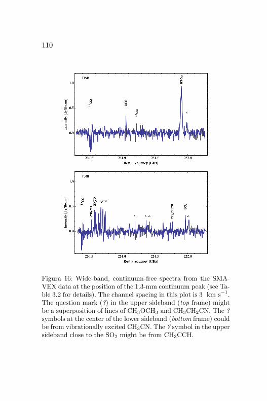
110

Figura 16: Wide-band, continuum-free spectra from the SMA-VEX data at the position of the 1.3-mm continuum peak (see Ta-ble 3.2 for details). The channel spacing in this plot is 3 km s−1.The question mark (?) in the upper sideband (top frame) mightbe a superposition of lines of CH3OCH3 and CH3CH2CN. The ?symbols at the center of the lower sideband (bottom frame) couldbe from vibrationally excited CH3CN. The ? symbol in the uppersideband close to the SO2 might be from CH3CCH.

111

Figura 17: VLA-BnA 1.3-cm continuum (red contours) overlaidon the SMA-VEX 1.3-mm continuum (color scale) toward theG20.08N complex. From west to east: H II region A is the com-pact, strongest peak at both wavelengths. H II region B is the lessbright H II region at . 1” to the SE of A. H II region C is the mo-re extended emission to the SE of B. The color scale goes linearlyfrom 8 to 430 mJy beam−1 (the rms noise in the mm image is2 mJy beam−1). Contours are placed at −5, 5, 10, 20, 40, 80, 150× 1 mJy beam−1, the noise of the cm image. The SMA-VEXbeam (empty ellipse) encircles the VLA-BnA beam (filled ellipse)at the bottom-left of the image.

112

(Fig. 3.2), and we analyze this characteristic in detail be-

low. The flux densities of H II region B at 1.3 mm (≈ 93

mJy) and 1.3 cm (≈ 202 mJy) imply a spectral index (α,

where Sν ∝ να) of α ∼ −0,3, roughly consistent with the

expected index of −0,1 of optically thin gas. H II region C

is more extended and most of the 1.3-mm flux is resolved

out.

At wavelengths shorter than 1 mm, thermal dust emis-

sion contributes significantly to the continuum. We esti-

mate the relative contributions of dust and free-free emis-

sion at 1.3 mm from our recombination line observations

(described in Section 3.5.4) and the theoretically expected

line-to-continuum ratio. In the optically thin limit (a good

approximation at 1.3 mm) the free-free line-to-continuum

flux ratio SL/SC is given by the ratio of the opacities κL/κC

[82]:

[κL

cm−1

]=

πh3e2

(2πmek)3/2mecn2

1fn1,n2φνneni

T 3/2

× exp

(En1

kT

)(1− e−hν/kT

), (3.1)[

κCcm−1

]= 9,77× 10−3 neni

ν2T 3/2

[17,72 + ln

T 3/2

ν

], (3.2)

where all the units are in cgs, the physical constants ha-

ve their usual meanings, n1 = 30 for H 30α, fn1,n2 ≈

113

0,1907n1(1 + 1,5/n1) for α lines, ne = ni for hydrogen,

T ≈ 8000− 10 000 K, and φν is the normalized line profile.

The main source of uncertainty in equations (1a) and (1b)

is the temperature of the ionized gas. Assuming that the

line profile is Gaussian and correcting for 8 % helium in the

gas, the expected ratio at the line center is SL,0/SC ≈ 3,0

for T = 8000 K, or SL,0/SC ≈ 2,3 for T = 10 000 K. The

observed ratio is SL,0/SC ≈ 1,8. Therefore, assuming that

the RRLs are in LTE, the free-free contribution to the 1.3-

mm flux of H II region A is ≈ 60 %− 80 % for the assumed

temperature range.

Figure 3.3 shows a model SED for H II region A in which

70 % (355 mJy) of the 1.3-mm flux is produced by free-free

from an H II region with a density gradient and 30 % (142

mJy) by warm dust. Assuming radiative equilibrium, we set

the dust temperature Td to 230 K, the average temperature

of the dense gas at the same scales (Section 3.5.3). The mo-

deling procedure is described in Keto [102] and Keto et al.

[105]. Table 3.3 summarizes the model. The total gas mass

inferred from the dust emission is too large (M ∼ 35 − 95

M) for the H II region alone, so most of the dust must be

in the cocoon around the H II region. The calculated mass

range takes into account uncertainties in the dust emissi-

vity, but not in the temperature.

The density gradient derived for the ionized gas in H II

region A is ne ∝ r−γ , with γ = 1,3. Equilibrium between

114

recombination and ionization in this model H II region re-

quires an ionizing flux equivalent to an O7.5 star (using the

computations of Vacca [202]), although this ionizing flux

could be made up of several stars of slightly later spectral

type. The model for the SED assumes spherical geometry

and a static H II region with no inflow of neutral gas into

the H II region. In contrast, H II region A is embedded in

a rotationally flattened accretion flow (see Section 3.5.3),

so the determination of the stellar spectral type is only ap-

proximate.

3.5.2. The Large-Scale Molecular Cloud

The large-scale molecular cloud is detected by the NH3

VLA-D observations. From these data we find the presence

of a parsec-scale accretion flow surrounding the cluster of

H II regions. In the following sections we first estimate the

systemic velocity Vsys of the cloud with respect to the local

standard of rest (LSR), and then analyze the line veloci-

ties to determine rotation and infall following the procedu-

re used in measuring accretion flow velocities by previous

studies [e.g., 85, 109, 229, 225]. We also derive the physi-

cal properties of the cloud: temperature, mass, ammonia

abundance, and density.

115

Figura 18: Radio-to-millimeter SED of G20.08N A. The 6-cmand 2-cm measurements were obtained from Wood & Church-well [220]. The 1.3-cm and 1.3-mm points were obtained fromGaussian fits to our VLA-BnA and SMA-VEX data, respecti-vely. Crosses are the data points. The error bars correspond tothe 10 % and 20 % uncertainty expected in the VLA and SMAflux measurements, respectively. The red dashed line shows theflux of an H II region with a density gradient. The black dottedline is the flux from the warm dust component. The solid blueline is the sum of the two components. The relative contributionsof free-free (70 %) and dust (30 %) to the 1.3-mm flux were esti-mated from the observed H30α line-to-continuum ratio, and aremarked with diamonds.

116

Dynamics

Figure 3.4 shows the channel maps of the (J,K) = (3, 3)

main hyperfine line. The most notable feature is a velocity

gradient along the major axis of the cloud, consistent with

rotation. The redshifted emission is toward the NE, while

the blueshifted gas is toward the SW. Also, there is strong

absorption against the free-free background of the H II re-

gions at the center of the cloud, which are unresolved at

∼ 4” resolution. The separation between the emission peaks

on either side of the absorption is≈ 10”, or 0.6 pc. The sym-

metry of the channel maps suggests a systemic velocity of

about 42 km s−1. A Gaussian fit to the emission spectrum

integrated in a box covering the entire cloud, and clipping

out the redshifted absorption, gives a centroid velocity of

42,3 ± 0,4 km s−1. We adopt a systemic velocity for the

parsec-scale cloud of Vsys = 42 km s−1, in agreement with

that reported by Plume et al. [164] (41.9 km s−1) based

on observations of CS J = 7− 6.

Figure 3.5 shows position-velocity (PV) diagrams across

cuts at PA = 45 (SW-NE, major axis) and PA = 135

(NW-SE, minor axis). The rotation is seen in the SW-NE

cut as a shift in the velocity of the emission contours from

one side of the absorption to the other. The velocity offset

with respect to Vsys seen in the emission contours increases

117

inward, suggesting that the gas rotates faster with decrea-

sing radius.

Under the assumption that the velocity gradient seen in

emission along the major axis is dominated by rotation, the

redshifted absorption in the PV diagrams (Fig. 3.5) is also

evidence for inward flow toward the central H II regions,

as there is an excess of redshifted absorption. This is mo-

re clearly seen in Fig. 3.6, which shows the spectra toward

the absorption center. The NH3 (2,2) main hyperfine absor-

ption peak is redshifted by 2.3 kms−1 with respect to the

systemic velocity. An infall velocity Vinf ≈ 2 km s−1 is also

seen in the NH3 (3,3) line, although the spectrum is con-

taminated by an NH3 (3,3) maser (see description in Fig.

3.6). The maser is confirmed by our high angular resolution

NH3 observations (Section 3.5.6).

If the rotation were seen edge-on, there would not be a

velocity gradient across the H II region along the minor axis

(NW-SE). At an oblique viewing angle a velocity gradient

along the minor axis is created by the inflow. The velocity

gradient along both the minor and major axes (Fig. 3.5)

implies that the rotationally flattened flow is tipped with

respect to the line of sight.

118

Figura 19: Channel maps of the VLA-D NH3 (3,3) observations.Emission is in solid contours and absorption in dashed contours.The star covers the H II regions shown in Fig. 3.1. Contourlevels are at −35,−25,−15,−10,−7,−5, 5, 7, 10, 15, 25, 35 × 2mJy beam−1. A clear velocity gradient in emission is seen from

one side of the absorption to the other. The LSR systemic ve-locity of the molecular gas is Vsys = 42,0 km s−1. The originalmaps at 0.3 km s−1 spectral resolution were smoothed to 0.6km s−1 for clarity.

119

Figura 20: Position-velocity diagrams of NH3 (2,2) and (3,3)from the VLA-D data. The cuts were done at PA=45

(bottom row) and PA=135 (top row). Dashed contours areabsorption, solid contours are emission. Contouring is at−168,−144,−120,−96,−72,−48,−36,−24,−12, −4, 4, 8, 12,16, 24, 32, 40, 48, 56, 64 × 1 mJy beam−1. Only one inner sa-tellite line is covered in the velocity range. In the SW-NE cuts(across the major axis of the cloud) the difference in the velocityof the emission with respect to Vsys = 42 km s−1 increases closerto the position center. This can be interpreted as spin up withdecreasing distance from the center. However, the same trend ispresent in the NW-SE cuts (along the minor axis of the cloud),although only in the stronger, blueshifted side of the emission.This suggests that besides rotation, radial motions in the frameof the central stars are also present.

120

Cloud Parameters

The optical depth of the gas can be determined from the

brightness ratios of the hyperfine lines. From their optical

depth ratio the rotational temperature between the (2, 2)

and (3, 3) transitions can be determined (see Keto et al.

[109] and Mangum et al. [140] for details of the procedure).

This temperature can be considered as a first-order appro-

ximation to the kinetic temperature (Tk) of the molecular

gas. Danby et al. [53] suggest that an improved estimate

of the kinetic temperature (Tk) is obtained by accounting

for the populations in the upper states of the K-ladders

rather than assuming that all states above the lowest are

negligibly populated. Including this correction, we obtain

an average kinetic temperature Tk ∼ 22 K for the parsec-

scale cloud. The high-resolution data discussed in Section

3.5.3 show that higher gas temperatures are found closer to

the H II regions.

The mean column density of NH3 is NNH3 ∼ 2,3 ×1016 cm−2. We can determine the abundance of ammo-

nia X(NH3) by comparing the NH3 and H2 column den-

sities. The mass of the cloud can be estimated from the

observed velocity dispersion (σV ∼ 3,5 kms−1), the radius

of the cloud (R ∼ 100 000 AU), and the virial theorem:

Mvir = (5/3G)Rσ2V ∼ 2300 M. Similarly, from the ob-

121

served velocity gradient, the rotation velocity is Vrot ∼ 4

km s−1 at a radius R ∼ 100 000 AU. Equating the cen-

tripetal and gravitational forces, the gas mass inside R is

M = (RV 2rot)/G ∼ 1800 M. Therefore, we estimate the

average column density of H2 to be NH2 ∼ 5 × 1022 cm−2

and X(NH3) ∼ 5 × 10−7, within a factor of three of the

value estimated for G10.6–0.4 [106]. The mean H2 density

in the large-scale cloud is nH2 ∼ 104 cm−3 .

3.5.3. Molecular Gas in The Inner 0.1 pc

Our SMA Very Extended (VEX) and VLA-BnA obser-

vations provide a rich view of the molecular environment

close to the H II regions. The lines detected with the SMA

that have peak intensities > 300 mJy beam−1 and are not

blended with any other line are listed in the top part of

Table 3.2. We follow a similar outline as for the large-scale

cloud.

Dynamics

Figures 3.7 to 3.10 show the channel maps of OCS

J = 19−18, SO2 J(Ka,Kb) = 11(1, 11)−10(0, 10), CH3CN

J(K) = 12(3)− 11(3), and CH3CN J(K) = 12(4)− 11(4).

These maps show that the line emission from these hot-core

122

Figura 21: NH3 spectra from the VLA-D observations toward thecenter of the absorption in G20.08N. The vertical line marks thesystemic velocity (Vsys = 42 km s−1). The small peak near themiddle of the (3,3) absorption is due to maser emission (confir-med in the high-resolution, VLA-BnA data, see Section 3.5.6).The absorption peaks in the main (2,2) and (3,3) lines are reds-hifted with respect to Vsys, indicating the presence of inflow inthe kinematics of the parsec-scale molecular cloud. The otherweak absorption component seen in the (2,2) spectrum is one ofthe inner satellites. The absorption component at ≈ 22 km s−1

in the (3,3) spectrum is also an inner satellite. The weaker absor-ption at 30−37 km s−1 in the (3,3) spectrum may arise from anoutflow. The blueshifted absorption in the main lines closest toVsys might arise from blending with the rotation seen in emission.

123

molecules is considerably brighter around H II region A. All

the molecules show a velocity gradient across this source,

from the southwest to northeast, in a similar orientation as

the larger, cluster-scale flow. We do not detect molecular

emission around H II region B. At this high angular resolu-

tion we are not sensitive to brightness temperatures of less

than ∼ 10 K (3σ) for the mm lines.

Figure 3.11 shows the velocity-integrated intensity (mo-

ment 0) and the intensity-weighted mean velocity (moment

1) maps of the four lines previously shown in Figs. 3.7 to

3.10. The integrated emission of CH3CN 12(4) − 11(4) is

brightest in front of the H II region, while for the other mo-

lecules the brightness peak is slightly offset from the con-

tinuum. These differences reflect the relative brightness of

each molecule with respect to the continuum emission of H

II region A. The velocity gradient across H II region A is al-

so seen. Figure 3.12 shows the velocity-integrated (moment

0) and velocity dispersion (moment 2) maps for the same

lines as Fig. 3.11. The line widths increase toward the con-

tinuum peak, indicating that unresolved motions increase

closer to the H II region.

Figure 3.13 shows the position-velocity (PV) diagrams

for the lines of Figure 3.10 in cuts at position angles PA =

45 and PA = 135 across the continuum peak of HII region

A. The cuts at 45 show the velocity gradient also seen in

the channel maps of OCS and both of the CH3CN lines. The

124

Figura 22: Channel maps of OCS J = 19 − 18 fromthe SMA-VEX observations. Contours are −4, 4, 6, 8, 10, 12, 14× 30 mJy beam−1 (negative in dashed, and positive in solid).The peak intensity is 423 mJy beam−1. The numbers in the up-per left corner indicate the central LSR velocity of the channel.The two stars mark the positions of H II regions A (west) and B(east).

125

Figura 23: Channel maps of SO2 J(Ka,Kb) = 11(1, 11) −10(0, 10) from the SMA-VEX observations. Contours are−4, 4, 6, 8, 10, 12, 14, 16, 18, 20 × 30 mJy beam−1 (negativein dashed, and positive in solid). The peak intensity is612 mJy beam−1.

PV diagram of CH3CN 12(4)-11(4) has a feature suggestive

of a velocity gradient in the perpendicular direction PA

= 135, with an excess of redshifted emission toward the

NW. Consistent with our interpretation of the NH3 VLA-D

data, this suggests inward motion in a rotationally-flattened

126

Figura 24: Channel maps of CH3CN J(K) = 12(3)− 11(3) fromthe SMA-VEX observations. Contours are −4, 4, 6, 8, 10, 12, 14× 30 mJy beam−1 (negative in dashed, and positive in solid).The peak intensity is 440 mJy beam−1.

flow that is seen not quite edge-on. The same redshifted

feature is also marginally detected in the lower excitation

CH3CN transition as well as the OCS line. However, the

infall signature in emission is only tentative, and a clearer

indication of infall at small scales comes from the redshifted

NH3 absorption in the VLA-BnA data (see below).

127

Figura 25: Channel maps of CH3CN J(K) = 12(4)− 11(4) fromthe SMA-VEX observations. Contours are −4, 4, 6, 8, 10, 12, 13× 30 mJy beam−1 (negative in dashed, and positive in solid).The peak intensity is 401 mJy beam−1.

In general, observational experience suggests that

CH3CN, along with NH3, is a reliable tracer of high-density

molecular mass and accretion flows [41, 230, 233, 157].

CH3CN has recently been detected in the outflow of the

nearby low-mass star L1157 [9], but at a very low bright-

ness (< 0,03 K). The distribution of the OCS molecule in

128

Figura 26: Velocity-integrated emission (moment 0, contours)and intensity-weighted mean velocity (moment 1, color scale)maps from hot-core molecules toward G20.08N. The Top Leftpanel shows the OCS J = 19− 18 (contours are −5, 5, 9, 13, 17×0,15 Jy beam−1 km s−1). The Top Right panel correspondsto the SO2 J(Ka,Kb) = 11(1, 11) − 10(0, 10) (contours are−5, 5, 8, 12, 15 × 0,25 Jy beam−1 km s−1). The Bottom Left pa-nel shows the CH3CN J(K) = 12(3) − 11(3) (contours are−5, 5, 8, 12, 15 × 0,15 Jy beam−1 km s−1). The Bottom Rightpanel plots the CH3CN J(K) = 12(4) − 11(4) (contours are−5, 5, 9, 14, 19×0,1 Jy beam−1 km s−1). Negative contours are indashed style, and positive contours in solid. Only the continuumH II region A is associated with warm gas in our SMA-VEX da-ta. The extent of the line emission is similar in all the tracers,although for the SO2 it is more extended toward the northwestand more absorbed toward the continuum peak. The velocitygradient seen in the channel maps for each molecule is also seenhere. The color scale is the same in all the frames.

129

Figura 27: Velocity-integrated emission (moment 0, contours)and velocity dispersion with respect to moment-1 velocity(moment 2, gray scale) maps from hot-core molecules towardG20.08N. Contours are the same as in Fig. 3.11. The plottedvelocity dispersion is σ = FWHM/2(2 ln 2)1/2. σ increases to-ward the center of H II region A, possibly caused by unresolvedmotions toward the center.

130

our observations is very similar to the CH3CN, but the SO2

velocities do not show the same pattern, and are more dif-

ficult to interpret. The SO2 may be more easily affected by

the excitation conditions, and part of the observed emission

could arise from the shocked boundaries of outflows. From

Gaussian fits to the CH3CN K = 2, 3, and 4 emission lines

at the position of the continuum peak, the systemic velocity

at small scales is estimated to be Vsys = 41,8±0,3 km s−1.

Figure 3.14 shows the CH3CN spectra and their Gaussian

fits.

At subarcsecond angular resolution, our NH3 observa-

tions are sensitive to emission of brightness temperature

above ∼ 200 K. Therefore the thermal NH3 is detected only

in absorption against the bright continuum. As in Section

3.5.2, a comparison between the NH3 absorption line velo-

city and Vsys shows an inward velocity of ≈ 2 km s−1 in

front of H II region A (Figure 3.15). The NH3 (2,2) absor-

ption line in front of H II region B is redshifted by ∼ 2,0

km s−1 with respect to Vsys, implying inward motion and

accretion toward H II region B as well (Figure 3.15). The

(3,3) absorption in front of H II region B is mixed with NH3

maser emission (Section 3.5.6), and the determination of

the inward velocity is uncertain. More sensitive observa-

tions are needed to constrain the properties of the molecu-

lar gas around H II region B.

131

Figura 28: Position-velocity diagrams of the SMA-VEX observa-tions. The left column is for a cut at PA= 45 (SW-NE). Theright column is at PA= 135 (NW-SE). Cuts are centered at theposition of the continuum peak of H II region A. Contours arethe same as in Fig. 3.7. The velocity gradient interpreted as ro-tation from SW to NE is clearly seen in OCS and CH3CN. TheSO2 features are more complex.

132

Figura 29: Spectra (points) and Gaussian fits (lines) to theCH3CN J = 12 − 11, K = 2, 3, and 4 lines at the position ofH II region A. Error bars denote the 1σ noise in the 2 km s−1-wide channels.

133

Core Parameters

We estimate the dynamical mass M (gas plus stars) wit-

hin the smaller accretion flow in the same way as with the

large-scale flow (see Section 3.5.2). At a radius R ∼ 5000

AU the rotation velocity is Vrot ∼ 3−4 km s−1. Therefore,

M ∼ 50 − 90 M. This is consistent with the lower limit

to the stellar mass, M? ≈ 35 M, required for ionization

equilibrium (Section 3.5.1). The estimate is also consistent

with the gas mass derived from the mm continuum on-

ce the free-free contribution has been properly subtracted,

Mgas ∼ 35− 95M (Section 3.5.1). The mean H2 density is

nH2 ∼ 106 cm−3 .

We derive the temperature in the dense gas surrounding

H II region A from the rotational energy diagram of the li-

nes of the CH3CN J = 12−11 K-ladders (see e.g., Loren &

Mundy [134] and Zhang et al. [230]). Figure 3.16 shows this

diagram for two cases: one considering all the K = 0, ..., 7

lines, and the other including only the K = 4, ..., 7 lines,

which have lower optical depths than the low-number K

lines (also, the K = 0, 1 lines are blended, separated by

only 5.8 km s−1). The rotational temperature obtained for

the former case is Trot ∼ 403 K, while for the latter it is

Trot ∼ 230 K. The difference between the two values given

above appears to be caused by optical depth effects (the

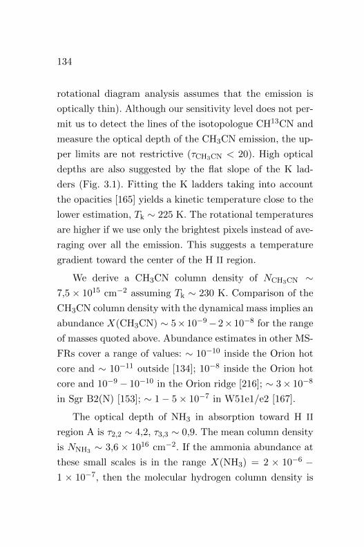
134

rotational diagram analysis assumes that the emission is

optically thin). Although our sensitivity level does not per-

mit us to detect the lines of the isotopologue CH13CN and

measure the optical depth of the CH3CN emission, the up-

per limits are not restrictive (τCH3CN < 20). High optical

depths are also suggested by the flat slope of the K lad-

ders (Fig. 3.1). Fitting the K ladders taking into account

the opacities [165] yields a kinetic temperature close to the

lower estimation, Tk ∼ 225 K. The rotational temperatures

are higher if we use only the brightest pixels instead of ave-

raging over all the emission. This suggests a temperature

gradient toward the center of the H II region.

We derive a CH3CN column density of NCH3CN ∼7,5 × 1015 cm−2 assuming Tk ∼ 230 K. Comparison of the

CH3CN column density with the dynamical mass implies an

abundance X(CH3CN) ∼ 5× 10−9− 2× 10−8 for the range

of masses quoted above. Abundance estimates in other MS-

FRs cover a range of values: ∼ 10−10 inside the Orion hot

core and ∼ 10−11 outside [134]; 10−8 inside the Orion hot

core and 10−9 − 10−10 in the Orion ridge [216]; ∼ 3× 10−8

in Sgr B2(N) [153]; ∼ 1− 5× 10−7 in W51e1/e2 [167].

The optical depth of NH3 in absorption toward H II

region A is τ2,2 ∼ 4,2, τ3,3 ∼ 0,9. The mean column density

is NNH3 ∼ 3,6 × 1016 cm−2. If the ammonia abundance at

these small scales is in the range X(NH3) = 2 × 10−6 −1 × 10−7, then the molecular hydrogen column density is

135

Figura 30: Top and middle panels: NH3 (2,2) and (3,3) spec-tra toward the absorption peak of H II region A in the VLA-BnA observations. The vertical line marks the systemic velocity(Vsys = 41,8 km s−1) of the molecular gas at scales comparableto the H II region. The centers of the absorption lines are redshif-ted with respect to Vsys, indicating inflow of molecular gas towardH II region A at small scales. The (3,3) absorption is broader(FWHM ≈ 6,5 km s−1) than the (2,2) (FWHM ≈ 5,6 km s−1),probably caused by larger motions closer to the center. Bottompanel: NH3 (2,2) spectrum toward H II region B. The absorption,considerably fainter than for H II region A, is also redshifted.

136

NH2 ∼ 2× 1022 − 4× 1023 cm−2. This implies a molecular

gas mass of Mgas ∼ 2 − 40 M. The kinetic temperature

obtained from the NH3 is Tk ∼ 50 K, considerably cooler

than that obtained for CH3CN and implying that most of

the NH3 column density is further away from the H II region

than the CH3CN.

The distribution of the warm molecular gas around H

II region A appears to be rotationally flattened (Figs. 3.7

to 3.12), but the observed size is slightly larger than the

radius at which the accretion flow is expected to become

centrifugally supported (i.e., a “disk”), Rd = GM/V 2rot ∼

2000− 3000 AU for a star of mass M? = 35 M and Vrot =

3 − 4 km s−1. Actually, the disk scale matches the size of

the H II region (Table 3.3, Section 3.5.4).

The mass-inflow rate toward H II region A can be esti-

mated from the high-resolution NH3 absorption. From an

inflow velocity of Vinf ≈ 2 km s−1 and spherical geometry,

the mass-inflow rate is M ∼ 1× 10−3 − 2× 10−2 M yr−1

(for the 2 − 40 M of molecular gas detected in ammonia

absorption). This estimate may be an upper limit because

the hot molecular core is flattened rather than spherical.

137

Figura 31: Rotation diagram for the CH3CN J = 12 − 11. Thetop panel is a fit of all the K = 0, ..., 7 lines. The bottom paneluses only the K = 4, ..., 7 lines, which have lower optical depths.Error bars are 3σ values. Lines are the linear fits to the data.

138

3.5.4. The Ionized Gas: Radio

Recombination Lines

In Section 3.5.1 we inferred a density gradient inside the

HC H II region A. In this section, we derive the internal dy-

namics of this H II region based on multifrequency RRLs.

The mm/sub-mm lines are especially important because

they are much less affected by pressure broadening and pre-

ferentially trace denser gas. While subarcsecond resolution

studies at wavelengths longer than 7 mm have been avai-

lable for many years [55, 56, 175], similar studies at shor-

ter wavelengths have had limited angular resolution (e.g.,

[94]). Keto et al. [105] presented the first results of high-

frequency, high-resolution (∼ 1”), multifrequency RRL ob-

servations in a sample of 5 MSFRs with similar characteris-

tics to G20.08N A. They were able to separate the contri-

butions of pressure broadening and large-scale motions to

the line width, even when the H II regions were unresolved.

We follow their procedure to analyze our RRL data.

We observed the H30α (ν0 = 231,90 GHz) and H66α

(ν0 = 22,36 GHz) lines at subarcsecond angular resolution

(see Table 3.2). Because both the line-to-continuum ratio

and the continuum intensity are lower at 22 GHz than at

231 GHz, the H66α line is much weaker than the H30α li-

ne. This is somewhat alleviated by the better sensitivity of

139

the VLA, but the signal-to-noise ratio (S/N) in the high-

frequency line is still better. Figure 3.17 shows the moment

0 and moment 1 maps of the H30α line. Although the emis-

sion is unresolved at half power, there is a slight indication

of a velocity gradient in the ionized gas that agrees (not per-

fectly) with the rotation seen in CH3CN and OCS. Figure

3.18 shows the H30α and H66α spectra toward H II region

A and their Gaussian fits. The H66α line shows evidence

of a blueshifted wing, suggesting either inflow or outflow in

addition to rotation. Within the uncertainties of the fits,

both the H66α and H30α lines have the same line width

(Table 3.4).

Assuming that the dynamical broadening ∆vD (caused

by turbulence and ordered motions) and the thermal broa-

dening ∆vT are Gaussian, and that the pressure broadening

∆vL is Lorentzian, the RRL has a Voigt profile with line

width [82]:

∆vV(ν) ≈ 0,534∆vL(ν)

+ (∆v2D + ∆v2

T + 0,217∆v2L(ν))1/2, (3.3)

where all the widths are FWHM.

For the H30α line at 231.9 GHz the pressure broadening

is less than the thermal broadening at electron densities be-

low 2× 108 cm−3 [105]. Our SED modeling indicates lower

140

densities over most of the HII region. Therefore, the obser-

ved line width can be attributed to thermal plus dynamical

broadening. The electron temperature Te in UC H II regions

is typically Te = 8000−10 000 K, with a small gradient as a

function of Galactocentric radius [4]. We adopt Te = 9000 K

(TB < 100 K for H30α because of the low optical depth and

. 1 filling factor), which translates into a thermal FWHM

of ∆vT = 20,9 km s−1. Therefore, from Eq. 3.3, we obtain

a dynamical width of ∆vD = 24,8 km s−1. From the velo-

city gradient (Fig. 3.17) it is seen that ∼ 6 km s−1 of ∆vD

can be in the form of rotation. The rest could be caused

by inflowing or outflowing ionized gas, as suggested by the

blueshifted (∼ 2− 3 km s−1) mean velocities of the RRLs,

and by the blue wing in the H66α spectrum (Fig. 3.18).

Most of the ionized gas that we see should be outflow.

Inflow inside the H II region is expected within the radius

where the escape velocity from the star exceeds the sound

speed of the ionized gas. This is approximately the Bondi-

Parker transonic radius [108], Rb = GM?/2c2s = 5,5 AU

M?/M, or about 190 AU for H II region A, assuming a

sound speed cs = 9 kms−1 and stellar mass M? = 35 M.

H II region A extends out to ∼ 2500 AU, so most of the gas

is not gravitationally bound to the star and flows outward.

In this model, the outflow is continuously supplied by pho-

toevaporation off the rotationally flattened accretion flow.

The somewhat misaligned velocity gradient in the ionized

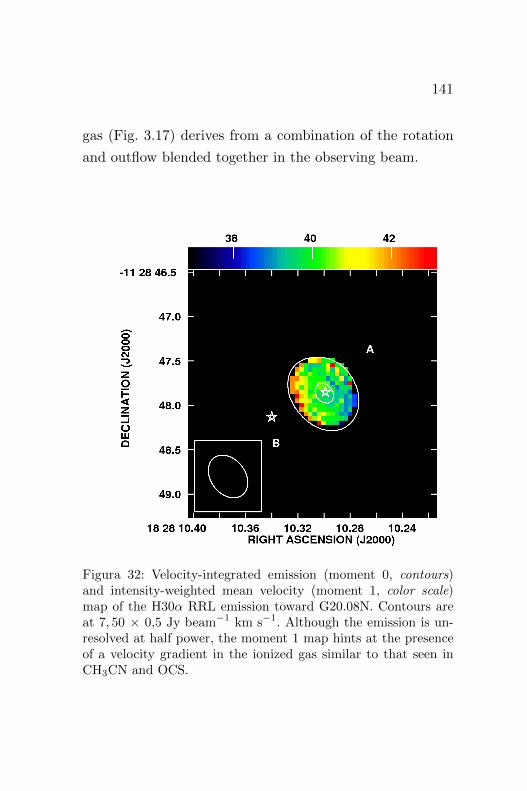
141

gas (Fig. 3.17) derives from a combination of the rotation

and outflow blended together in the observing beam.

Figura 32: Velocity-integrated emission (moment 0, contours)and intensity-weighted mean velocity (moment 1, color scale)map of the H30α RRL emission toward G20.08N. Contours areat 7, 50 × 0,5 Jy beam−1 km s−1. Although the emission is un-resolved at half power, the moment 1 map hints at the presenceof a velocity gradient in the ionized gas similar to that seen inCH3CN and OCS.

142

3.5.5. Outflow Tracers

Low angular resolution (HPBW = 14”), single-dish

(JCMT) observations of SiO (8–7) show evidence for large-

scale molecular outflows in G20.08N [115]. Although the

standard outflow tracers 12CO J = 2−1 and 13CO J = 2−1

are in our passband, we do not detect any CO in emis-

sion. The (u, v) coverage of our SMA-VEX observations is

incapable of imaging structures larger than ∼ 4”; there-

fore, the CO emission from the molecular cloud and mo-

lecular outflow must be on larger scales. 12CO and 13CO

are seen in our data in absorption at the position of H

II region A, at several different velocities in the range

VLSR = 42− 84 km s−1. Some CO absorption features are

at the same velocities as the HI absorption features of Fish

et al. [64] and are therefore due to foreground gas that is

not related to G20.08N but rather to intervening Galactic

spiral arms.

3.5.6. A New NH3 (3,3) Maser

A handful of NH3 masers have been reported in the

literature, always associated with massive star formation

(e.g., [210]). Many of the known NH3 masers are from non-

metastable (J > K) transitions. The first clear detection

143

Figura 33: Spectra (points) and Gaussian fits (lines) to the H30α(top panel) and H66α (bottom panel) lines toward G20.08N A.Error bars denote the 1σ noise in the channels. The channel spa-cing is 2 km s−1 for H30α and 5,2 km s−1 for H66α. The fluxwas integrated over a 0.5” square box centered on H II region A.

144

of a metastable (J = K) NH3 (3,3) maser was reported

by Mangum & Wootten toward DR 21(OH) [139]. Most

of the detections point toward a shock excitation origin

for the population inversion, inasmuch as the maser spots

are invariably associated with outflow indicators such as

bipolar CO and/or SiO structures, class I methanol masers,

and/or water masers [139, 117, 228].

We report the serendipitous detection of a new NH3

(3,3) maser toward G20.08N. The maser spot is rela-

tively weak, and is spatially centered at α(J2000) =

18h 28m 10.s346, δ(J2000) = −11 28′ 47.′′93, close in pro-

jection to the center of H II region B. The maser spot is

spatially unresolved even in uniform weighting maps of the

VLA-BnA data (HPBW = 0,48” × 0,26”, PA = −0,8).

If the deconvolved source size is limited to half the beam

size, then the peak brightness temperature of the spot is

constrained to TB > 7 × 103 K. The high intensity, toget-

her with the absence of similar emission in our (2,2) maps

at high angular resolution, confirm the maser nature of the

(3,3) emission. The spectral feature is also very narrow (Fig.

3.16), typical of maser emission, although it shows evidence

of line wings. From a Gaussian fit to the line profile, the

velocity of the maser is Vmaser ∼ 44,7 km s−1 (accurate

only to 20 % − 40 %). The FWHM is ∼ 0,7 km s−1, after

deconvolving the channel width of 0,6 km s−1. Owing to

its position, it is probable that the maser is excited by H II

145

region B. We do not have sufficient data, however, to assert

that it is excited in a shock.

Figura 34: VLA-BnA spectrum of the NH3 (3,3) maser spot to-ward G20.08N. The brightness temperature TB scale assumes anangular size equal to half the uniform-weighted beam dimensions.

146

3.6. Hierarchical Accretion in

G20.08N

3.6.1. The Observations

One of the central questions in star formation is whet-

her star formation is “bimodal”, i.e., whether high-mass

and low-mass stars form in a different way [183]. Analysis

of recent observations suggests that accretion flows around

protostars of up to M? ∼ 10 M can be explained wit-

hin the standard model of star formation as a combina-

tion of a thin disk inside a rotationally flattened envelope

[122, 146, 113]. Of course, once a protostar gains the mass

and temperature of an O star, the formation of an H II

region within the accretion flow introduces new phenome-

na [107, 104, 108, 161]. Yet not all molecular clouds form

massive stars. In a comprehensive survey, Solomon et al.

[190] found that clouds that form low-mass stars are uni-

formly distributed throughout the Galactic disk, but those

that form the clusters of the most massive stars, O stars

capable of producing significant H II regions, are associa-

ted with the galactic spiral arms. If the formation process is

very similar (with the addition of significant ionization for

M? > 20M), then the difference may be found in the con-

ditions of the parent molecular clouds. The observations of

147

G20.08N reported in this chapter and of G10.6–0.4 repor-

ted previously [106, 104] suggest that one difference is that

the molecular clouds surrounding young clusters of O stars

are in a state of overall collapse whereas in star-forming

regions without H II regions we see only localized collapse.

In G20.08N the H II regions A, B, and C are surroun-

ded by a common molecular cloud of radius ∼ 0,5 pc and

mass M ∼ 2000 M, which is rotating with a velocity of

∼ 4 km s−1 and contracting with an inward velocity of ∼ 2

km s−1. This rotation and contraction constitute a large-

scale accretion flow. The velocity of the inward flow is about

equal to the rotational velocity implying that the gas is ap-

proximately in free-fall and not constrained by centrifugal

force. Within this larger flow are at least two smaller ac-

cretion flows around H II regions A and B. The molecular

core around H II region A is bright enough to be detected

in hot-core molecules in emission at subarcsecond angular

resolution. The radius and mass of this core are 0.05 pc

and ∼ 20 M. Accretion in the core is indicated by rota-

tion at a velocity of 3 or 4 km s−1 and contraction of ∼ 2

km s−1. We do not detect molecular emission around H

II region B, but the accretion inflow is inferred from NH3

absorption that is redshifted by ∼ 2 km s−1 with respect

to the systemic velocity.

In contrast, star-forming regions that contain only low

mass stars or even stars as massive as type B do not ap-

148

pear to have this global collapse of the entire parent cloud.

The observations of these regions suggest only localized ac-

cretion flows within individual clumps. For example, star-

forming regions such as IRAS 19410+2336 [194, 29, 30],

IRAS 05358+3543 [28, 130], and AFGL 5142 [233, 231],

have bolometric luminosities of at most a few times 104

L, consistent with type B protostars. There are a number

of cores of size similar to those in G20.08N, but there is no

reported evidence of a larger parsec-scale, accretion flow.

In an analysis of a recent numerical simulation,

Vazquez-Semadeni et al. [207] also find that the formation

of massive stars or clusters is associated with large-scale

collapse involving thousands of M and accretion rates of

10−3 M yr−1. In contrast, low- and intermediate-mass

stars or clusters in their simulation are associated with iso-

lated accretion flows that are a factor of 10 smaller in size,

mass, and accretion rate.

If global collapse of the host molecular cloud is neces-

sary for the formation of O stars in clusters, then the as-

sociation of O stars with galactic spiral arms may imply

that compression of giant molecular clouds as they pass th-

rough galactic spiral arms may be the primary mechanism

for initiating global collapse [169, 184, 142]. The low-mass

star-forming regions found by Solomon et al. [190] to be

spread throughout the Galaxy may not need such large-

scale compression.

149

3.6.2. Resupply of the Star-Forming Cores

The orientations of the large cloud-scale accretion flow

and the core-scale flow around H II region A are similar and

the flows could be continuous (we do not know the orien-

tation of the flow around H II region B because we cannot

detect the surrounding molecular emission). The molecu-

lar core around H II region A contains only a few tens of

M, similar to the mass of a single O star. If the core is

to form one or more O stars at less than 100 % efficiency,

its mass must be resupplied by the larger scale accretion

flow. Resupply is also suggested by the short dynamical or

crossing timescale, given by the ratio of the size to the in-

fall velocity, ∼ 104 yrs. If the core is to last more than this,

it must be resupplied by the larger scale flow, which has a

dynamical timescale of ∼ 105 yrs. If the core is not resup-

plied then the growing protostar may simply run out of gas

before reaching the mass of an O star.

A similar process of resupply is suggested in recent theo-

retical work. Analytic arguments show that as an unstable

cloud fragments, there should be a continuous cascade of

mass from larger to smaller fragments as well as a cascade of

kinetic energy [63, 152]. In recent numerical simulations of

high mass star formation, Wang et al. [211] find that most

of the mass is supplied from outside a 0.1 pc core around

150

the protostar. Vazquez-Semadeni et al. [207] and Peters et

al. [161] also find in their simulations that as a massive core

is consumed from the inside by an accreting protostar, the

core continues to accrete mass from the outside.

3.6.3. Accretion Rate

The accretion rate within the small-scale flow around

H II region A is M ∼ 1 × 10−3 to 2 × 10−2 M. Similar

accretion rates are reported for flows around other H II

regions such as G10.6–0.4, 8 × 10−4 M yr−1 [106], and

W51e2, 3 × 10−3 to 1 × 10−2 M yr−1 [225]. In contrast,

the accretion rates estimated for the cores in these MSFRs

without bright H II regions are generally lower by one or

two orders of magnitude, ∼ 10−4 M yr−1 [28, 29].

A high accretion rate is necessary to form an O star.

Because accreting massive protostars begin core hydro-

gen burning well before reaching the mass of an O star,

they evolve essentially as main-sequence stars of equiva-

lent mass. Numerical simulations of stellar evolution that

include accretion predict that unless the accretion rate is

high enough, a growing massive protostar will evolve off

the main-sequence and explode before it reaches the mass

of an O star [104]. For a protostar to gain the mass of an

O star, the rate at which accretion supplies fresh hydrogen

to the growing protostar must be greater than the rate at

151

which the star burns the hydrogen. At the upper end of the

mass spectrum, M? > 40 M, this rate is > 10−3 M yr−1.

The accretion flows in G20.08N are capable of supplying

gas at the rate necessary to form massive O stars. In MS-

FRs without O stars, the accretion rates may be too low

for the stars to achieve the mass of an O star within their

hydrogen-burning lifetimes.

3.6.4. Transfer of Angular Momentum

If the flow in G20.08N is continuous, then the observa-

tions show that the flow spins up as it contracts. Ignoring

projection effects, the magnitude of the specific angular mo-

mentum on the large scale is L/m ∼ 0,6 km s−1 pc at

r ≈ 0,2 pc, from the VLA-D NH3 data, while from the

VEX SMA data it is L/m ∼ 0,1 km s−1 pc at r ≈ 0,02 pc

around H II region A. From these estimates ∼ 85 % of the

specific angular momentum in the large-scale flow is lost.

In previous observations of G10.6–0.4 [106], it was found

that 97 % of the angular momentum in that flow is lost

between 1.5 and 0.02 pc. Evidently, angular momentum is

efficiently transferred outward and does not prevent collap-

se of the cloud.

Magnetic fields may be important in this process [79].

Although there are no observations of the magnetic field in

G20.08N, the field direction has been mapped in another

152

MSFR with HC H II regions, W51e1/e2. Here, observations

show that the magnetic field is uniform on the larger scale,

0.5 pc [128], while on the smaller scale, 0.03 pc, of the accre-

tion flow onto W51e2, the field is pinched into an hourglass

shape with the accretion flow at the waist [196]. Thus or-

dered field lines extend from the H II region-scale accretion

flow to the large-scale molecular cloud, and if the field has

enough strength, angular momentum could be transferred

outward by the field. However, dust polarization observa-

tions do not give a direct estimate of the field strength, and

it is also possible that the field is essentially passive and just

carried along by the flow. The observation that the clouds

in both W51e1/e2 and G20.08N are close to free-fall collap-

se implies that the magnetic field is not strong enough to

support the clouds. In other words, these clouds are mag-

netically supercritical.

Numerical simulations of star formation that do not in-

clude magnetic forces show that angular momentum can

be transferred by hydrodynamics alone. Abel et al. [1] find

that at any radius, there is both low and high angular mo-

mentum gas, and that pressure forces or shock waves can

redistribute the angular momentum between fluid elements.

Lower angular momentum gas sinks inward and displaces

higher angular momentum gas outward, resulting in a net

outward flow of angular momentum.

153

Whether the specific angular momentum is transferred

by hydrodynamics or magnetic forces, observations and si-

mulations show that angular momentum is not conserved

as a function of radius, and does not prevent the gas from

flowing continuously from large to small scales in a rotating

flow.

3.7. Conclusions

We report radio and mm observations of the molecular

and ionized gas toward the O-star cluster G20.08N, made

with an angular resolution from ∼ 0,1 pc to ∼ 0,01 pc. Our

main findings can be summarized as follows:

1. We find a large-scale (∼ 0,5 pc) accretion flow around

and into a star cluster with several O-type stars, iden-

tified by one UC and two HC H II regions. This flow is

rotating and infalling towards its center. The two HC

H II regions are surrounded by smaller accretion flows

(∼ 0,05 pc), each of them with the signature of infall

too. The brightest (toward H II region A) is detec-

ted in mm emission lines, and rotates in concordance

with the large-scale flow.

2. The similar orientations of the flows at small and lar-

ge scales, as well as their dynamical timescales (∼ 104

154

yrs and ∼ 105 yrs respectively), and masses (∼ 10 M

and ∼ 103 M respectively), suggest that, if O stars

are forming in G20.08N (as it is observed), then the

smaller scales ought to be resupplied from the lar-

ger scales. The same result has been found in recent

numerical simulations of massive star formation in

clusters.

3. The brightest HC H II region (A) has a rising SED

from cm to mm wavelengths and broad hydrogen re-

combination lines. Both characteristics suggest den-

sity gradients and supersonic flows inside the H II

region. A velocity gradient is tentatively detected in

the recombination line emission of this source, sug-

gesting rotation and outflow in the ionized gas at the

innermost scales. H II region A can be interpreted as

the inner part of the surrounding molecular accretion

flow, with the observed ionization being produced by

photoevaporation.

Notes

1 Both near and far kinematic distances have been reported for

G20.08N. The near value given by Downes et al. [59] (d ≈ 4,1 kpc)

is the most commonly quoted in the previous literature. In contrast,

Fish et al. [64] and Anderson & Bania [5] report that this region is

at the far kinematic distance (d ≈ 12,3 kpc). We will assume the

far distance throughout the rest of this study. For reference, a scale

155

of 0,5” corresponds to ≈ 6000 AU (0.03 pc). The total luminosity

of the region was estimated to be L ∼ 7,3 × 104 L assuming the

near kinematic distance [220]. Correcting for the location at the far

distance, the luminosity is L ∼ 6,6 × 105 L.2The Submillimeter Array is a joint project between the Smithso-

nian Astrophysical Observatory and the Academia Sinica Institute of

Astronomy and Astrophysics and is funded by the Smithsonian Insti-

tution and Academia Sinica.3In “chunk”20 of the SMA correlator setup.4http://sma1.sma.hawaii.edu/callist/callist.html5 The National Radio Astronomy Observatory is operated by As-

sociated Universities, Inc., under cooperative agreement with the Na-

tional Science Foundation.6The NH3 molecule is symmetric top with inversion, see Ho &

Townes [87] for details.

156

Cu

adro

3.1:

Obse

rvat

ion

alP

aram

eter

s

Ep

och

Arr

ay

Ph

ase

Cen

tera

Ban

dp

ass

Ph

ase

Flu

xα

(J2000)

δ(J

2000)

Calib

rato

rC

alib

rato

rC

alib

rato

r2003

Ap

r28

VL

A-D

18

28

10.3

84

−11

28

48.6

53C

454.3

1833−

210

0137

+331

2003

May

13

VL

A-D

18

28

10.3

84

−11

28

48.6

53C

454.3

1851

+005

1331

+305

2003

Oct

09

VL

A-B

nA

18

28

10.3

84

−11

28

48.6

53C

454.3

1851

+005

1331

+305

2003

Oct

10

VL

A-B

nA

18

28

10.3

84

−11

28

48.6

53C

454.3

1851

+005

1331

+305

2006

Ju

n25

SM

A-V

EX

18

28

10.3

8−

11

28

48.6

03C

273

1830

+063

1830

+063

2006

Ju

n25

SM

A-V

EX

18

28

10.7

6−

11

29

27.6

03C

273

1830

+063

1830

+063

2006

Ju

l06

SM

A-V

EX

18

28

10.3

8−

11

28

48.6

03C

454.3

1751

+096

1751

+096

2006

Ju

l06

SM

A-V

EX

18

28

10.7

6−

11

29

27.6

03C

454.3

1751

+096

1751

+096

2007

Oct

26

VL

A-B

18

28

10.4

00

−11

28

49.0

03C

454.3

1743−

038

1331

+305

2007

Oct

27

VL

A-B

18

28

10.4

00

−11

28

49.0

03C

454.3

1743−

038

1331

+305

a:

un

its

of

R.A

.are

hou

rs,

min

ute

s,an

dse

con

ds.

Un

its

of

dec

l.are

deg

rees

,arc

min

ute

s,an

darc

seco

nd

s.

157C

uad

ro3.

2:L

ines

a

Sp

ecie

sT

ran

siti

on

ν0

Arr

ay

HP

BW

(GH

z)(a

rcse

c×

arc

sec;

deg

)H

66α

22.3

64178

VL

A-B

0,4

7×

0,3

4;

3N

H3

(2,2

)23.7

22633

VL

A-D

4,6

8×

2,9

3;

236

NH

3(3,3

)23.8

70129

VL

A-D

4,5

0×

3,3

2;

8N

H3

(2,2

)23.7

22633

VL

A-B

nA

0,3

7×

0,2

8;

343

NH

3(3,3

)23.8

70129

VL

A-B

nA

0,7

1×

0,3

4;

013C

O2–1

220.3

98681

SM

A-V

EX

0,5

5×

0,4

1;

32

CH

3C

N12(4

)–11(4

)220.6

79297

SM

A-V

EX

0,5

5×

0,4

1;

32

CH

3C

N12(3

)–11(3

)220.7

09024

SM

A-V

EX

0,5

5×

0,4

1;

32

CH

3C

N12(2

)–11(2

)220.7

30266

SM

A-V

EX

0,5

5×

0,4

1;

32

SO

211(1

,11)–

10(0

,10)

221.9

65200

SM

A-V

EX

0,5

4×

0,4

1;

32

CO

2–1

230.5

38000

SM

A-V

EX

0,5

3×

0,3

9;

37

OC

S19–18

231.0

60991

SM

A-V

EX

0,5

3×

0,3

9;

37

H30α

231.9

009

SM

A-V

EX

0,5

3×

0,3

9;

37

CH

3C

N12(7

)–11(7

)220.5

39340

SM

A-V

EX

0,5

5×

0,4

1;

32

HN

CO

10(1

,9)–

9(1

,8)

220.5

84762

SM

A-V

EX

0,5

4×

0,4

1;

32

CH

3C

N12(6

)–11(6

)220.5

94438

SM

A-V

EX

0,5

5×

0,4

1;

32

CH

3C

N12(5

)–11(5

)220.6

41096

SM

A-V

EX

0,5

5×

0,4

1;

32

CH

3C

N12(1

)–11(1

)220.7

43015

SM

A-V

EX

0,5

5×

0,4

1;

32

CH

3C

N12(0

)–11(0

)220.7

47265

SM

A-V

EX

0,5

5×

0,4

1;

32

CH

2C

HC

N24(0

,24)–

23(0

,23)

221.7

6598

SM

A-V

EX

0,5

5×

0,4

1;

32

13C

S5–4

231.2

20768

SM

A-V

EX

0,5

2×

0,3

9;

37

a:

lin

esd

etec

ted

at

S/N>

6.

Th

etop

part

of

the

tab

lelist

sth

eli

nes

wit

hS

/N>

10

(exce

pt

the

H66α

lin

e)an

d

clea

rly

isola

ted

infr

equ

ency

.T

hebottom

part

of

the

tab

lelist

sth

elin

esd

etec

ted

at

S/N<

10

or

ble

nd

ed.

Som

e

spec

tral

featu

res

(see

Fig

.3.1

)th

at

wer

en

ot

pro

per

lyid

enti

fied

du

eto

low

S/N

(≈5)

an

db

len

din

gare

not

list

ed.

158

Cuadro 3.3: Model for the H II Region G20.08N A

Parametera ValueHII Radius (AU) 2530

Electron densityb (105 cm−3 ) 1.4Exponentc 1.3

Gas Massd (M) 35 to 95Spectral Type O7.5

Stellar Mass (M) 34HII Mass (M) 0.05

a: the independent parameters are the first four rows. b: electron density

at the HII radius. c: exponent γ of the power-law density gradient in the

ionized gas, where n ∝ r−γ . d: mass of molecular gas obtained from the

dust emission. Assuming dust temperature Td = 230 K and a gas-to-dust

ratio of 100. The range is caused by the dust emissivity coefficient β used

(see Keto et al. [105]), from β = 1 to β = 1,5.

Cuadro 3.4: Emission Line Parameters Toward H II Region Aa

Species Transition VLSR FWHM TB,peak( km s−1) ( km s−1) (K)

H 66α 39,3± 1,1 34,1± 2,5 190± 13H 30α 40,3± 0,4 32,5± 0,9 89± 2

CH3CN 12(4)–11(4) 42,7± 0,3 5,8± 0,7 32± 4CH3CN 12(3)–11(3) 41,4± 0,2 5,3± 0,5 41± 4CH3CN 12(2)–11(2) 41,4± 0,2 4,9± 0,5 32± 3

a: from Gaussian fits. 1σ statistical errors are quoted.

4

Time Variability of

HII Regions:

A Signature of

Accretion?

The Ionized Gas: Radio Recombination Lines

4.1. Resumen

En una escala de tiempo de anos, un cambio en el flujo

de radio continuo en longitudes de onda en las cuales la

emision es opticamente gruesa puede indicar si una region

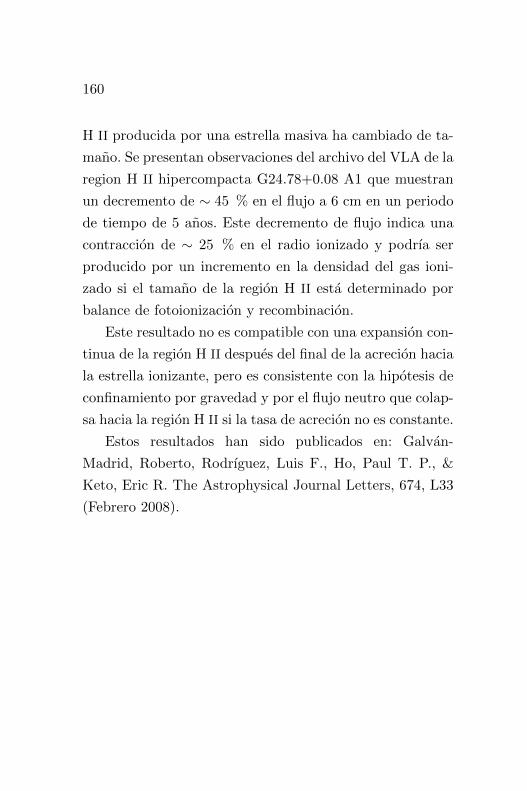
160

H II producida por una estrella masiva ha cambiado de ta-

mano. Se presentan observaciones del archivo del VLA de la

region H II hipercompacta G24.78+0.08 A1 que muestran

un decremento de ∼ 45 % en el flujo a 6 cm en un periodo

de tiempo de 5 anos. Este decremento de flujo indica una

contraccion de ∼ 25 % en el radio ionizado y podrıa ser

producido por un incremento en la densidad del gas ioni-

zado si el tamano de la region H II esta determinado por

balance de fotoionizacion y recombinacion.

Este resultado no es compatible con una expansion con-

tinua de la region H II despues del final de la acrecion hacia

la estrella ionizante, pero es consistente con la hipotesis de

confinamiento por gravedad y por el flujo neutro que colap-

sa hacia la region H II si la tasa de acrecion no es constante.

Estos resultados han sido publicados en: Galvan-

Madrid, Roberto, Rodrıguez, Luis F., Ho, Paul T. P., &

Keto, Eric R. The Astrophysical Journal Letters, 674, L33

(Febrero 2008).

161

4.2. Summary

Over a timescale of years, an observed change in the

optically thick radio continuum flux can indicate whether

an unresolved H II region around a newly formed massive

star is changing in size. In this chapter we present a study

of archival VLA observations of the hypercompact H II re-

gion G24.78+0.08 A1. We found a decrease of ∼ 45 % in

its 6-cm flux over a five year period. Such a decrease in-

dicates a contraction of ∼ 25 % in the ionized radius and

could be caused by an increase in the ionized gas density

if the size of the H II region is determined by a balance

between photoionization and recombination. This finding

is not compatible with continuous expansion of the H II

region after the end of accretion onto the ionizing star, but

is consistent with the hypothesis of gravitational trapping

and (partially) ionized accretion flows if the mass-accretion

rate is not steady.

These results have been published in Galvan-Madrid,

Roberto, Rodrıguez, Luis F., Ho, Paul T. P., & Keto, Eric

R. “Time Variation in G24.78+0.08 A1: Evidence for an

Accretion Hypercompact H II Region?”The Astrophysical

Journal Letters, 674, L33 (February 2008) [73].

162

4.3. Introduction

The formation of massive stars (M? > 8 M) by ac-

cretion presents a number of theoretical difficulties; among

them, that once a star attains a sufficient mass its surface

temperature is high enough to produce a small H II re-

gion (see the reviews on ultracompact and hypercompact

H II regions by Churchwell [45]; Kurtz [123]; and Hoare et

al. [89]). The thermal pressure differential between the hot

(∼ 104 K) ionized gas and the cold (∼ 100 K) molecular

gas can potentially reverse the accretion flow of molecular

gas and prevent the star from ever reaching a higher mass.

However, models that include the effects of gravity [102]

have shown that if the H II region is small enough (ionized

diameter ≤ 1000 AU for total stellar mass ≥ 350 M), the

gravitational attraction of the star(s) is greater than the

thermal pressure of the ionized gas, permitting the mole-

cular accretion flow to cross the ionization boundary and

proceed toward the star as an ionized accretion flow wit-

hin the H II region. In this stage the H II region is said to

be gravitationally trapped by the star. Of course, geome-

try does not need to be spherical, rather, the accretion flow

is expected to be flattened. Models that take into account

the effects of the geometry of accretion show that the H II

region can be outflowing in the polar directions, where the

163

parental accretion flow is less dense, while it can be gra-

vitationally trapped along the plane of the accretion flow

(disk).

Previous studies have demonstrated a number of ob-

servational techniques bearing on the evolution of small H

II regions around newly formed stars. Accretion flows on-

to and through H II regions can be directly observed by

mapping molecular and radio recombination lines (RRLs)

at very high angular resolution [188, 104]. If the H II region

is too small to be spatially resolved, the frequency depen-

dence of the velocities and widths of RRLs can be used to

infer steep density gradients and supersonic velocities wit-

hin the H II regions [105], as expected from the presence

of ionized accretion flows or bipolar outflows. Radio conti-

nuum observations at very high angular resolution, made

at two epochs some years apart, can also be used to directly

observe changes in size of small H II regions [67]. Changes

in size indicate whether the evolution of the H II region is

consistent with pressure-driven expansion or gravitational

trapping.

In this chapter we present a study that demonstrates

yet another technique – how a comparison of radio conti-

nuum observations at different epochs can be used to infer

size changes in H II regions even if the observations do not

spatially resolve them. At optically thick frequencies the ra-

dio continuum flux depends to first approximation only on

164

the size of an H II region and is independent of its internal

density structure. Therefore, even if the size is not known,

a change in the flux over time still indicates a change in the

size of the H II region. This technique is particularly valua-

ble because it can be used on the smallest and youngest H

II regions, and because lower angular resolution radio con-

tinuum observations generally require less observing time

than spectral line and high angular resolution observations.

For this study we selected the hypercompact (HC) H II

region G24.78+0.08 A1 which lies at the center of a massive

molecular accretion flow [23, 20] and also has multi-epoch

6 cm radio continuum observations in the VLA archive.

G24.78+0.08 was detected in the centimetric (cm) conti-

nuum by Becker et al. [19], and later resolved by Codella et

al. [46] into a compact (A) and an extended (B) component.

A millimeter (mm) interferometric study [23] revealed the

presence of two massive rotating toroids centered in res-

pective dust cores (A1 and A2). The compact cm emission

comes from the mm component A1 (hereafter G24 A1), and

has recently been resolved by Beltran et al. [21]. If G24 A1

is ionized by a single star, its spectral type should be ear-

lier than O9 [46]. Also, G24 A1 likely powers a massive CO

outflow [69].

The infalling and rotating molecular gas and bipolar

outflow all suggest ongoing accretion. However, based on

proper motions of H2O masers around the H II region,

165

Beltran et al. [21] and Moscadelli et al. [148] proposed that

at the present time, the H II region is expanding into the

accretion flow. The suggested timescale for the expansion is

short enough that we should be able to detect a correspon-

ding increase in the optically thick radio continuum flux

within a few years.

4.4. Observations

We searched the VLA1 archive for multi-epoch observa-

tions centered in the G24 A1 region at optically thick fre-

quencies (below 23 GHz for G24 A1). Since in the optically

thick part of the spectrum the flux density of the source

scales as the angular size squared, flux density variations

corresponding to size variations can be detected even in

observations of modest angular resolution. We chose three

data sets of 6-cm observations in the C configuration, two

from 1984 and one from 1989 (see Table 4.1).

The observations were made in both circular polariza-

tions with an effective bandwidth of 100 MHz. The ampli-

tude scale was derived from observations of the absolute

amplitude calibrator 3C286. This scale was transferred to

the phase calibrator and then to the source. We estimate

an error not greater than 10 % for the flux densities of the

sources.

166

We edited and calibrated each epoch separately follo-

wing the standard VLA procedures using the reduction

software AIPS. Precession to J2000 coordinates was per-

formed running the task UVFIX on the (u, v) data. After

self-calibration, we made CLEANed images with uniform

weighting and cutting the short spacings (up to 10 Kλ) to

minimize the presence of extended emission at scales larger

than ∼ 20”.

Before subtraction, we made the images as similar as

possible. We restored the CLEAN components with an

identical Gaussian beam HPBW 4.′′79 × 3.′′38, PA= −15.

We applied primary beam corrections and aligned the

maps. No significant differences were found in the difference

image between the 1984 May 11 and 14 images, as expected

for such a small time baseline. We therefore averaged the

two 1984 epochs into a single data set. In subtracting the fi-

nal maps we allowed the 1984 image to have small (' 0,1′′)

shifts in position as well as a scaling of ' 10 % in ampli-

tude. This was done in order to minimize the rms residuals

of the difference image in the region of interest. A similar

procedure was used by Franco-Hernandez & Rodrıguez [67]

to detect a variation in the lobes of the bipolar UC H II re-

gion NGC 7538 IRS1. The individual maps, as well as the

final difference image between 1984 and 1989 are shown in

Figure 4.1.

167

Figura 35: VLA images of G24.78+0.08 for 1984.36 (top), 1989.48(middle), and the difference of 1989.48 – 1984.36 (bottom). Thecontours are -10, -8, -6, -5, -4, 4, 5, 6, 8, 10, 12, 15, 20, 30, 40,and 60 times 0.57 mJy beam−1. The half power contour of thesynthesized beam (4.′′79× 3.′′38 with a position angle of −15) isshown in the bottom left corner of the images. The crosses indica-te the positions of the components A1 and B from our Gaussianfits to the 1984.36 image. The negative residuals observed in thedifference image indicate a decrease of ∼ 45 %in the flux densityof component A1.

168

4.5. Discussion

4.5.1. The Expected Variation Trend

If G24 A1 Is Expanding

Beltran et al. [21] suggested that the 7 mm and

1.3 cm continuum morphologies are consistent with limb-

brightening from a thin, ionized-shell structure. Based on

H2O maser proper motions [148, 21] they also suggested an

expansion speed of ∼ 40 km s−1. The increase in flux co-

rresponding to the increase in size due to expansion ought

to be detectable in a few years.

If G24 A1 Is Accreting

If G24 A1 is the ionized inner portion of the star for-

ming accretion flow, the long-term growth of the H II region

due to the increasing ionizing flux of the star should be im-

perceptible. However, the H II region could change in size

over an observable timescale if the gas density in the ac-

cretion flow is time variable. Because the mass of ionized

gas within the H II region is very small compared to the

mass of the accretion flow, even a small change in the flow

density could affect the size of the H II region.

169

For example, we can obtain a lower limit for the ionized

mass of G24 A1MHII from a measurement of its flux density

at a frequency for which its emission is optically thin, and

assuming that it is spherical and homogeneous. From the

equations of Mezger & Henderson [145] we have that:

[MHII

M

]= 3,7× 10−5

[Sν

mJy

]0,5[ Te104 K

]0,175

×[

ν

4,9 GHz

]0,05[ Dkpc

]2,5[ θsarcsec

]1,5

, (4.1)

where the flux density is Sν , Te is the electron temperature,

D is the distance to the region, and θs is its FWHP. Taking

Sν = 101 mJy, D = 7,7 kpc, and θs = 0.′′17 at 7 mm

[21], and assuming Te = 104 K, the ionized mass in G24

A1 would be MHII ∼ 5 × 10−3M. A higher limit to the

mass can be obtained considering that HC H II regions

should have density gradients (n ∝ rα, with α = −1,5 to

−2,5) rather than being homogeneous [108]. In this case we

obtain ionized masses between MHII ∼ 1 × 10−2 M and

MHII ∼ 3 × 10−2 M, a factor of 2 − 6 higher than under

the assumption of homogeneity, but still very small when

compared to that of the surrounding molecular material or

the ionizing star itself.

170

4.5.2. The Observed Variation

Figure 4.1 shows the individual maps of the 1984 May

11 + 14 (1984.36) and 1989 June 23 (1989.48) epochs, as

well as the difference image. Sources A1 and B (the former

labeled A by Codella et al. [46]) are unresolved (θs ≤ 2′′),

and the total emission is dominated by component B. Ho-

wever, the flux decrease is centered at the position of A1.

We performed Gaussian fits to both components using the

task JMFIT in AIPS, and the results are summarized in

Table 4.2. We have checked the reliability of the fits to the

image by making direct fits to the (u, v) data. The values

obtained from both techniques are entirely consistent but

suggest that the errors given by the tasks used in the ima-

ge (JMFIT) and (u, v) (UVFIT) fittings are underestimated

by a factor of 2. The errors given in Table 4.2 have been

corrected by this factor.

The decrease in the flux density of G24 A1 between

1989.48 and 1984.36 is 5,1± 1,1 mJy, or 45± 10 %. Com-

ponent B shows no evidence of time variability, as expected

for a more evolved H II region not associated with signs

of current star-forming activity such as H2O or OH masers

[46]. We set an upper limit of 2 % to the circularly-polarized

emission of the sources, which indicates that we are not dea-

ling with variable gyrosynchrotron emission from an active

stellar magnetosphere.

171

4.5.3. Is G24 A1 Accreting?

The ∼ 45 % flux decrease (i.e., a contraction of ∼ 25

% in the ionized radius) we have detected at 6 cm toward

G24 A1 is not consistent with the hypothesis that this H

II region is expanding rapidly into the molecular accretion

flow. Assuming a radius R ∼ 500 AU and an expansion

velocity v ∼ 40 km s−1 [21], a flux increase of ∼ 20 %

should have been observed between the compared epochs.

We attribute the contraction of the H II region to an

increase in its density produced by the enhancement of

accretion, either caused by an isotropic increment in the

mass-accretion rate or by the sudden accretion of a locali-

zed clump in the neutral inflow (for example, clumps have

been observed in the accretion flow onto the UC H II re-

gion G10.6–0.4 [187, 104]). Our data do not allow us to

distinguish between these two possibilities.

The additional mass required to increase the density can

be estimated. The ionized radius rS scales roughly with the

density n as rs ∝ n−2/3 (if the radius of the H II region is set

by a balance between photoionization and recombination)

and at optically thick frequencies the flux density scales as

Sν ∝ r2s . The ionized mass within G24 A1 is MHII ∼ 1 ×

10−2 M (Section 4.5.1). Therefore, the sudden accretion of

∼ 5×10−3 M into the H II region would suffice to explain

172

the observed 45 % flux decrease. The molecular accretion

flow around this H II region has a mass of ∼ 130 M [23].

Thus, the required variation, 50 % of the mass of the H II

region, is only of the order of 0.001 % of the total mass of

the accretion flow.

Finally, we shall mention that even when the observa-

tions here presented are not consistent with a simple, con-

tinuous expansion of G24 A1, our result does not mean

that this H II region does not expand at all, or that it is

contracting continuously. As will be shown in the following

chapter, an emerging model of the early evolution of H II

regions embedded in massive accretion flows indicates that

H II region variability is a common signature of the inter-

action of the neutral and ionized portions of the accretion

flow in which clusters of massive stars form.

4.6. Conclusions

Our analysis of archival VLA observations of the HC

H II region G24.78+0.08 A1 indicates a contraction of its

radius between 1984.36 and 1989.48. This finding is con-

sistent with the hypothesis that this HC H II is the inner,

ionized part of the larger scale accretion flow seen in the

molecular line observations of Beltran et al. [23, 20].

173

Notes

1The National Radio Astronomy Observatory is operated by As-

sociated Universities, Inc., under cooperative agreement with the Na-

tional Science Foundation.

174

Cu

adro

4.1:

Obse

rvat

ion

alP

aram

eter

s

Ep

och

Ph

ase

Cen

tera

Am

plitu

de

Ph

ase

Boots

trap

ped

Flu

xB

eam

α(J

2000)

δ(J

2000)

Calib

rato

rC

alib

rato

rD

ensi

ty(J

y)

(arc

sec×

arc

sec;

deg

)1984

May

11

18

36

12.1

45−

07

11

28.1

73C

286

1743−

038

2,4

14±

0,0

05

5,3

8×

3,4

4;−

29

1984

May

14

18

36

12.1

45−

07

11

28.1

73C

286

1743−

038

2,4

64±

0,0

07

4,7

8×

3,3

4;

+03

1989

Ju

n23

18

36

10.6

82−

07

11

19.8

73C

286

1834−

126

0,1

53±

0,0

01

4,5

0×

3,3

1;−

10

a:

un

its

of

right

asc

ensi

on

are

hou

rs,

min

ute

s,an

dse

con

ds.

Un

its

of

dec

lin

ati

on

are

deg

rees

,arc

min

ute

s,an

d

arc

seco

nd

s.

175

Cuadro 4.2: Gaussian Fit Results

Epoch Component Positiona,b Flux Densityα(J2000) δ(J2000) (mJy)

1984.36 A1 18 36 12.545 −07 12 10.87 11,4± 0,81984.36 B 18 36 12.668 −07 12 15.37 31,4± 1,01989.48 A1 18 36 12.545 −07 12 10.87 06,3± 0,81989.48 B 18 36 12.668 −07 12 15.37 32,8± 0,8

a: units of right ascension are hours, minutes, and seconds. Units of declina-

tion are degrees, arcminutes, and arcseconds. b: For the 1989.48 epoch, the

centers of the Gaussians were fixed to those obtained for the 1984.36 epoch.

5

Time Variability of

HII Regions in

Numerical Simulations

of MSFR

Time Variability of HII Regions in Numerical Simula-

tions of MSFR

5.1. Resumen

Las regiones H II ultracompactas e hipercompactas apa-

recen cuando una estrella con una masa mayor a aproxima-

178

damente 15 M empieza a ionizar su ambiente. Observa-

ciones recientes de variaciones temporales en la emision de

radio continuo de estos objetos son una de las piezas de

evidencia que sugieren que al menos una fraccion de estas

regiones H II contienen estrellas que continuan acretando

del flujo neutro y en colapso que las rodea. Presentamos

un analisis de las propiedades como funcion del tiempo de

las regiones H II formadas en las simulaciones radiativo-

hidrodinamicas en 3D presentadas por Peters et al. Las

regiones H II en estas simulaciones “parpadean”. Sus flujos

de radio continuo, ası como sus variaciones en flujo y ta-

manos son consistentes con las observaciones disponibles.

De nuestras mediciones en las simulaciones, estimamos que

una pequena fraccion (∼ 10 %) de las regiones H II ob-

servadas deben presentar variaciones de flujo detectables

(> 10 %) en escalas de tiempo de ∼ 10 anos. Las varia-

ciones positivas son ligeramente mas probables que las ne-

gativas en estas escalas temporales. Un resultado novedoso

es que decrementos en flujo suceden, en contraste con el

modelo mas simple de regiones H II que se expanden sin

interrupcion. Tambien exploramos las correlaciones tempo-

rales entre propiedades que son directamente observables

(flujos y tamanos) y cantidades derivadas (densidades y ta-

zas de ionizacion).

Estos resultados han sido publicados en: Galvan-

Madrid, Roberto, Peters, Thomas, Keto, Eric, Mac

179

Low, Mordecai-Mark, Banerjee, Robi, & Klessen, Ralf S.

Monthly Notices of the Royal Astronomical Society, 416,

1033 (Septiembre 2011).

5.2. Summary

Ultracompact and hypercompact H II regions appear

when a star with a mass larger than about 15 solar masses

starts to ionize its own environment. Recent observations

of their time variability, like the one presented in the pre-

vious chapter, are one of the pieces of evidence that suggest

that at least some of them harbor stars that are still accre-

ting from an infalling neutral accretion flow that becomes

ionized in its innermost part. We present an analysis of

the properties of the H II regions that are formed in the 3D

radiation-hydrodynamic simulations presented by Peters et

al. (2010) as a function of time. Flickering of the H II regions

is a natural outcome of this model. The radio-continuum

fluxes of the simulated H II regions, as well as their flux

and size variations are in agreement with the available ob-

servations. From the simulations, we estimate that a small

but non-negligible fraction (∼ 10 %) of observed H II re-

gions should have detectable flux variations (larger than

10 %) on timescales of ∼ 10 years, with positive variations

being more likely to happen than negative variations. A no-

180

vel result of these simulations is that negative flux changes

do happen, in contrast to the simple expectation of ever

growing H II regions. We also explore the temporal corre-

lations between properties that are directly observed (flux

and size) and other quantities like density and ionization

rates.

These results have been published in Galvan-Madrid,

Roberto, Peters, Thomas, Keto, Eric, Mac Low, Mordecai-

Mark, Banerjee, Robi, & Klessen, Ralf S. “Time variabi-

lity in simulated ultracompact and hypercompact HII re-

gions.”Monthly Notices of the Royal Astronomical Society,

416, 1033 (Septiembre 2011) [72].

181

5.3. Introduction

The most massive stars in the Galaxy, O-type stars with

masses M? > 20 M, emit copious amounts of UV photons

[202] that ionize part of the dense gas from which they

form. The resulting H II regions are visible via their free-

free continuum and recombination line radiation [145, 220].

H II regions span orders of magnitude in size, from giant

(D ∼ 100 pc) bubbles, to “ultracompact”(UC) and “hyper-

compact”(HC) H II regions, loosely defined as those with

sizes of ∼ 0,1 pc and ∼ 0,01 pc (or less), respectively (see

the reviews by Churchwell [45], Kurtz [123], and Hoare et

al. [89]). UC and HC H II regions are the most deeply em-

bedded, and so are best observed at radio wavelengths.

Large, rarefied H II regions expand without interruption

within the surrounding medium due to the high pressure

contrast between the ionized and neutral phases [192]. This

simple model was extrapolated to the ever smaller objects

recognized later and is widely used to interpret observations

of UC and HC H II regions. Common assumptions about

these objects are: i) They are steadily expanding within

their surrounding medium at the sound speed of the ioni-

zed gas, ∼ 10 km s−1. ii) The ionizing star(s) is already

formed, i.e., accretion to the massive star(s) powering the

H II region has stopped.

182

However, evidence has accumulated that suggests a re-

vision of these assumptions:

1. The hot molecular cores embedding UC and HC H

II regions are often rotating and infalling [106, 43,

20, 22, 116], sometimes from parsec scales all the way

to the immediate surroundings of the ionized region

[71, 17].

2. Infall of gas at velocities of a few km s−1 directly

toward the ionized center has also been observed in

UC and HC H II regions [229, 20, 71].

3. The inner ionized gas has been resolved in a few cases,

and it also shows accretion dynamics (outflow, infall,

and rotation [104, 180, 71]).

4. The spectral index α (where the flux goes as Sν ∝ να)

of some UC and HC H II regions is ∼ 1 from cm to

mm wavelengths, indicating density gradients and/or

clumpiness inside the ionized gas [65, 93, 105, 13].

5. A few UC and HC H II regions have been shown to

have variations on timescales of years [2, 67, 204, 73].

These variations indicate that UC and HC H II re-

gions sometimes expand [2], and sometimes contract

[73]. Some other ionized regions around massive pro-

tostars have been shown to remain approximately

constant in flux [81].

183

All these observations strongly suggest that UC and

HC H II regions are not homogeneous spheres of gas freely

expanding into a quiescent medium, but rather that the-

se small H II regions are intimately related to the accretion

processes forming the massive stars. Simple analytic models

show that the observed H II regions can be either the ioni-

zed, inner part of the inflowing accretion flow [107, 102] or

the ionized photoevaporative outflow [92] fed by accretion

[108].

Numerical simulations of the formation and expansion

of H II regions in accretion flows around massive stars ha-

ve only recently become possible with three-dimensional

radiation-hydrodynamics. Studies that simulate the expan-

sion of H II regions have focussed on larger-scale effects on

the parental molecular cloud [49, 50, 51, 159, 83, 11]. Howe-

ver, in none of those simulations was the ionizing radiation

produced by the massive stars dynamically forming through

gravitational collapse in the molecular cloud. Recent simu-

lations by Peters et al. [161] include a more realistic treat-

ment of the formation of the star cluster. Radio-continuum

images generated from the output of those simulations show

time variations in the morphology and flux from the H II

regions produced by the massive stars in formation. The-

se changes are the result of the complex interaction of the

massive filaments of neutral gas infalling to the central stars

with the ionized regions produced by some of them. A sta-

184

tistical analysis of the H II region morphologies [163] con-

sistently reproduces the relatively high fraction of spheri-

cal and unresolved regions found in observational surveys.

Thus, the non-monotonic expansion of H II regions, or flic-

kering, appears able to resolve the excess number of obser-

ved UC and HC H II regions with respect to the expectation

if they expand uninterrupted (the so-called lifetime problem

put forward by Wood & Churchwell [220]). Furthermore,

the ionizing radiation is unable to stop protostellar growth

when accretion is strong enough. Instead, accretion is stop-

ped by the fragmentation of the gravitationally unstable

accretion flow in a process called “fragmentation-induced

starvation”, a theoretical discussion of which can be found

in Peters et al. [162].

In this chapter we present a more detailed analysis of

the flux variability in the simulations presented in Peters

et al. [161]. In Section 2 of this chapter we describe the

set of numerical simulations and the methods of analysis.

In Section 3 we present our results. Section 4 discusses the

implications of our findings. In Section 5 we present our

conclusions.

185

5.4. Methods

5.4.1. The Numerical Simulations

Our study uses the highest resolution simulations of tho-

se presented in Peters et al. [161]. The simulations use a

modified version of the adaptive-mesh code FLASH [68],

including self-gravity and radiation feedback. They include

for the first time a self-consistent treatment of gas heating

by both ionizing and non-ionizing radiation. Peters et al.

[161] describes in detail the numerical methods. The initial

conditions are a cloud mass of 1000 M with an initial tem-

perature of 30 K. The initial density distribution is a flat

inner region of 0.5 pc radius surrounded by a region with

a decreasing density ∝ r−1,5. The density in the homoge-

neous volume is 1,27× 10−20 g cm−3 . The simulation box

has a length of 3.89 pc. The size and mass of the cloud are

in agreement with those of star-formation regions that are

able to produce at least one star with M? > 20 M [71].

Run A (as labeled in Peters et al. [161]) has a maximum

cell resolution of 98 AU and only the first collapsed object

is followed as a sink particle [62]. In this run, the formation

of additional stars (the sink particles) is suppressed using a

density-dependent temperature floor (see Peters et al. [161]

for details). On the other hand, in Run B additional collap-

se events are permitted and a star cluster is formed, each

186

star being represented by a sink particle. The maximum

resolution in Run B is also 98 AU.

5.4.2. Data Sets

For the entire time span of Run A (single sink) and Run

B (multiple sink), radio-continuum maps at a wavelength

of 2 cm were generated from the simulation output every

∼ 300 yr by integrating the radiative transfer equation for

free-free radiation while neglecting scattering [82]. Follo-

wing Mac Low et al. [138], each intensity map was then con-

volved to a circular Gaussian beam with half-power beam

width HPBW = 0,14” (assuming a source distance of 2.65

kpc). A noise level of 10−3 Jy was added to each image.

Further details are given in Peters et al. [161]. These maps

were used to explore the behavior of the free-free continuum

from the H II region over the entire time evolution of the

simulations. For Run B, sometimes the H II regions overlap

both physically in space and/or in appearance in the line of

sight. Therefore, the presented time analysis refers to the

entire star cluster unless otherwise specified.

To compare more directly to available observations,

which span at most a couple of decades in time, each of

Run A and B were re-run in four time intervals for which

a flux change was observed in the radio-continuum images

mentioned above. Data dumps and radio-continuum maps

187

were generated at every simulation time step (∼ 10 yr). The

analysis performed in the low time-resolution maps was al-

so done in these high time-resolution data. For Run B, the

intervals for the high time-resolution data were also selec-

ted such that the H II region powered by the most massive

star is reasonably isolated from fainter H II regions ionized

by neighboring sink particles, both in real space and in the

synthetic maps.

5.5. Results

5.5.1. Variable HII Regions

Real UC and HC H II regions, as well as those that

result from the simulations presented here, are far from the

ideal cases described by, e.g., Spitzer [192]. However, it is

instructive to discuss the limiting ideal cases to show that

their variability is a natural consequence of their large to

moderate optical depth.

The flux density Sν of an ionization-bounded1 H II re-

gion is

S =2kν2

c2

∫ΩTBdΩ, (5.1)

where k is the Boltzmann constant, c is the speed of light,

ν is the frequency, and the brightness temperature TB is

integrated over the angular area Ω of the H II region.

188

In the limit of very low free-free optical depths (τff 1),

TB along a line of sight l goes as

TB ∝ T−0,35e ν−2,1

∫ln2dl, (5.2)

where Te and n are the electron temperature and density

respectively.

Combining equations (1) and (2) we have that for a

given ν and constant Te:

S(τff 1) ∝ n2R3 ∝ N , (5.3)

where the last proportionality comes from the Stromgren

relation N ∝ n2R3 (N is the ionizing-photon rate and R is

the ‘radius’ of the H II region). Equation (3) shows that in

the optically-thin limit the H II -region flux only depends on

N . For time intervals of a few ×10 yr the mass and ionizing

flux of an accreting protostar remain almost constant, and

so does the flux of an associated optically-thin H II region.

On the other hand, for very high optical depths (τff 1) TB = Te. For a given frequency and constant Te, equation

(1) becomes:

S(τff 1) ∝ R2 ∝ N2/3n−4/3, (5.4)

therefore, the flux of an optically thick H II region is pro-

portional to its area, and both flux and area decrease with

189

density.

This analysis is valid for time intervals larger than the

recombination timescale (∼ 1 month for n ∼ 106 cm−3, see

e.g., Osterbrock [156]) and as long as the growth of N is

negligible.

However, the H II regions in the simulations are clumpy

and have subregions of high and low free-free optical depth.

Their flux during the accretion stage (while they flicker) is

dominated by the denser, optically thicker (τff > 1) subre-

gions, so their behaviour is closer to eq. (4) than to eq. (3).

The on-line version of this paper contains a movie of τff for

Run B as viewed from the Z-axis (line of sight perpendicu-

lar to the plane of the accretion flow). The clumpiness and

intermediate-to-large optical depth of these H II regions are

also the reasons behind their rising spectral indices up to

relatively large frequencies (ν > 100 GHz) without a signi-

ficant contribution from dust emission (see the analytical

discussions of Ignace & Churchwell [93] and Keto et al.

[105], or the analysis of these simulations in Peters et al.

[163]). As for the variability, the large optical depths cause

the size and flux of the simulated H II regions to be well

correlated with each other, and anticorrelated with the den-

sity of the central ionized gas (see Section 3.6). The neutral

accretion flow in which the ionizing sources are embedded is

filamentary and prone to gravitational instability (further

discussion is in Peters et al. [163, 162]). The changes in the

190

density of the H II regions are a consequence of their pas-

sage through density enhancements in the quickly evolving

accretion flow.

5.5.2. Global Temporal Evolution

Figure 5.1 shows the global temporal evolution of the

H II region in Run A (single sink particle). The 2-cm flux

(S2cm) observed from orthogonal directions and the mass of

the ionizing star (M?) are plotted against time. The global

temporal trend of the H II region is to expand and become

brighter. However, fast temporal variations are seen at all

the stages of the evolution. The fluxes in the projections

along the three different cartesian axes follow each other

closely. For the rest of the analysis, the Z-axis projection,

a line of sight perpendicular to the plane of the accretion

flow, is used.

The H II region is always faint (S2cm < 1 Jy at the

assumed distance of 2.65 kpc) for M? < 25 M. Past this

point, the H II region is brighter than 1 Jy 86 % of the time

(Fig. 5.1).

A similar analysis of the H II region around the most

massive star in Run B (multiple sinks) is shown in Fig. 5.2.

Only the Z-axis projection, i.e., a line of sight perpendicular

to plane of the accretion flow is used, since only from this

viewing angle the brightest H II region is well separated

191

Figura 36: 2-cm flux (S2cm, filled black squares) and stellar mass(M?, gray circles) as a function of time (t) for Run A. Althoughthe long-term trend of the H II region is to increase in flux, itconstantly flickers during its evolution. The fluxes at the differentprojections (X-axis top, Y-axis middle, Z-axis bottom), thoughnot the same, follow each other closely.

192

from other H II regions at all times (the flux movies are

presented in Peters et al. [161]). The extra fragmentation

in Run B translates into a weaker accretion flow and a

lower-mass ionizing star as compared to that of Run A, a

process referred to as “fragmentation-induced starvation”(a

theoretical discussion of this process in presented in Peters

et al. [162]). Therefore, the brightest H II region in Run B

(Fig. 5.2) is weaker than the H II region in Run A (Fig.

5.1). Figures 5.1 and 5.2 do not show times later than t =

100 kyr in order to facilitate their comparison. Both runs

continue past this time, but in Run B accretion onto the

most massive star stops at t = 109 kyr, while in Run A

the artificial suppression of the fragmentation leads to an

unrealistically large mass for the ionizing star at later times.

H II regions are highly variable both in Run A and Run

B. However, since the suppression of fragmentation in Run

A produces a larger accretion flow and a most massive io-

nizing star, Run A presents larger flux variations than Run

B. Figure 5.3 shows the flux changes over the evolution of

the H II regions in both runs. A comparison of the fractio-

nal variations of the H II regions shows that, though more

similar between runs, they are still larger in Run A (Figure

5.4). For consecutive data points, in Run A positive flux

variations are 56 % of the events and the flux increment is

+74 % on average, while negative changes are 44 % of the

events and have an average magnitude of −27 %. Similarly,

193

Figura 37: 2-cm flux (S2cm, filled black squares) of the H II regionformed by the most massive star and its stellar mass (M?, graycircles) as a function of time (t) for Run B. Although the long-term trend of the H II region is to increase in flux, it constantlyflickers during its evolution. Only the Z-axis projection is usedbecause from this viewing angle, perpendicular to the plane ofthe accretion flow, the brightest H II region can be distinguishedfrom other H II regions at all times.

for Run B, positive changes (52 % of the events) have an

average magnitude of +42 %, while the average flux decre-

ment (48 % of the events) is −18 %.

194

Figura 38: 2-cm flux variations (∆S2cm) for Run A (top panel)and Run B (bottom) panel.

195

Figura 39: Fractional flux variations (∆S2cm/S2cm,0) for Run A(top panel) and Run B (bottom) panel.

196

5.5.3. Comparison to Surveys

We present a comparison with the ionized-gas surveys of

UC and HC H II regions by Wood & Churchwell [220] and

Kurtz et al. [125]2. Figure 5.5 shows normalized histograms

of 2-cm luminosity (S2cmd2) obtained for both runs using

the time steps previously shown in figures 5.1 to 5.4 and the

co-added observed samples from Wood & Churchwell [220]

and Kurtz et al. [125], taking the 81 sources for which they

report a 2-cm flux and a distance. Simulation and observa-

tions roughly agree, but neither Run A nor B can reproduce

the high-luminosity end of the observed distribution: 20 %

of the observed sources have S2cmd2 > 50 Jy kpc2, while

only 1 % of the H II regions in the simulation steps of Run

A and in no step in Run B have luminosities above this

threshold. These bright UC H II regions likely correspond

to stages in which accretion to the ionizing protostar(s) is

completely shut off, therefore they do not correspond to the

analyzed H II regions from the simulation in which the pro-

tostars are still accreting. In the range 20 < S2cmd2 < 50

Jy kpc2, Run A matches better than Run B the observed

luminosities. This may be because Run B does not produce

any star with a mass M? > 30 M. Simulations identical to

Run B produce higher-mass stars in the presence of mag-

netic fields [160] and may also produce more massive stars

in the purely radiation-hydrodynamical case with higher-

197

mass initial clumps. We plan to perform in the future a

study on the robustness of our results for different initial

conditions. For the smallest luminosities, Run B matches

better than Run A the observed 55 % of H II regions that

have S2cmd2 < 5 Jy kpc2, but over-estimates (35 %) the ob-

served fraction (14 %) of H II regions with 5 < S2cmd2 < 10.

Peters et al. [163] presented statistics of the morphologies

of the H II regions in Run A and Run B and found that

Run B agrees better with observed surveys. Although Run

A can be interpreted as a mode of isolated massive star

formation, the treatment of fragmentation is more realistic

in Run B. Moreover, most high-mass stars form in clusters

[237].

5.5.4. Long-Term Variation Probabilities

We address the question of the flux variability expec-

ted from the simulations by calculating the probability of

variations larger than a given threshold as a function of

time difference between steps. The low time-resolution da-

ta has the advantage of spanning the entire runs, but is

not useful to predict the expected variations on timescales

shorter than 102 yr. We use the high time-resolution data

sets to make an estimate of the flux variations over shorter

timescales, but we caution that the analyzed time intervals

may not be representative of the entire simulation. We use

198

Figura 40: Histograms of 2-cm luminosities (S2cmd2) for the glo-

bal temporal evolution of the simulated H II regions (dashed li-nes) and the co-added samples of Wood & Churchwell [220] andKurtz et al. [125] (solid lines). The top and bottom frames corres-pond to Run A and Run B respectively.

this approach because re-running the entire simulations to

produce data at ∼ 10 yr resolution is not feasible.

Figure 5.6 shows the probabilities of flux increments

larger than a given threshold for time differences between 1

199

and 60 kyr for Run A (left column)and Run B (right). The

top panels correspond to flux increments larger than 10 %,

the middle panels correspond to 50 %, and the bottom pa-

nels to 90 %. On average, H II regions tend to expand,

making a given flux increment to be more likely to happen

for larger time intervals than for shorter ones.

Figure 5.7 show the probabilities of flux decrements lar-

ger than a given threshold (in modulus) for Run A (left co-

lumn) and Run B (right) respectively. The top to bottom

order of the thresholds is as in Fig. 5.6. At ∆t > 30 kyr

the negative-change probabilities decrease and reach ∼ 0

at about ∆t > 40 kyr for any threshold. This is caused by

the eventual growth of the H II regions in spite of the flic-

kering. There is some indication that the probabilities for

negative changes also decrease at timescales shorter than 1

kyr, specially for flux-change thresholds larger than 50 %

(see Fig. 5.7). This is also suggested from the analysis of

the high temporal-resolution data in the next section. Alt-

hough flux increments are more likely than decrements for

any given threshold and time lag, a novel result of the-

se simulations is that negative flux changes do happen, in

contrast with the simple expectation of ever growing H II

regions.

200

Figura 41: Left column: probabilities for flux increments largerthan 10 (top), 50 (middle), and 90 % (bottom) as a function oftime difference for the long-term evolution of the H II region inRun A. The error bars indicate the 1σ statistical uncertainty fromthe number of counts in each bin 1000-yr wide. Right column:same for the H II regions in Run B.

201

Figura 42: Left column: probabilities for flux decrements largerthan 10 (top), 50 (middle), and 90 % (bottom) as a function oftime difference for the long-term evolution of the H II region inRun A. The error bars indicate the 1σ statistical uncertainty fromthe number of counts in each bin 1000-yr wide. Right column:same for the H II regions in Run B.

202

5.5.5. Short-Term Variation Probabilities

We re-ran four time intervals in each of Run A and Run

B, spanning a few hundred years each, and producing data

dumps at each simulation step (∼ 10 yr). These time in-

tervals were selected to contain a pair of negative/positive

flux changes to investigate the correlation of flux variations

with physical changes in the H II region, like size and den-

sity (next section). Therefore, they may not be representa-

tive of the entire simulation, but since it is not feasible to

re-run the entire simulations producing data dumps at the

highest temporal resolution, we use these data to constrain

the expected flux variations in observable timescales. We

argue that the close match at scales of ∆t ∼ 500 yr between

the probabilities obtained from the low temporal-resolution

(previous section) and the high temporal-resolution data

(this section) indicates that the results presented here are

meaningful.

Figure 5.8 shows the probabilities for flux increments

larger than the specified threshold as a function of time lag.

This figure is the analog of Fig. 5.6 for the high temporal-

resolution data. The slight probability decrements after

∆t ∼ 300 yr, especially at low thresholds, are an arti-

fact caused by the fact that the data sets include a ne-

gative/positive flux-change pair. Still, the probabilities at

203

∆t = 490 yr match within 20 % to 80 % with the probabili-

ties at ∆t = 500 yr from the low-temporal resolution data.

On observable timescales, ∆t = 0 to 40 yr, a small but

non-zero fraction of H II regions is expected to have detec-

Figura 43: Left column: probabilities for flux increments largerthan 10 (top), 50 (middle), and 90 % (bottom) as a function oftime difference for the sample intervals at high time resolution.The error bars indicate the 1σ statistical uncertainty from thenumber of counts in each bin 20-yr wide. Right column: same forthe H II region around the most massive star in Run B.

204

table flux increments. For two observations separated by 10

yr, Run A gives a prediction of 16,7±2,9 % of H II regions

having flux increments larger than 10 %, 6,8 ± 1,9 % with

flux increments larger than 50 %, and 4,7±1,6 % with incre-

ments larger than 90 %. The more realistic Run B predicts

a smaller fraction of variable H II regions: 6,9 ± 1,6 %,

0,3 ± 0,3 %, and 0 % of them are expected to have flux

increments larger than 10 %, 50 %, and 90 % over a time

interval of 10 yr, respectively.

Figure 5.9 show the probabilities for flux decrements lar-

ger than a given threshold obtained with the high temporal-

resolution data. The probabilities obtained at ∆t = 490

yr from the high temporal-resolution data roughly match

with those at ∆t = 500 yr obtained from the low temporal-

resolution data, within a factor of 1 to 3.

Negative variations should also be detectable in a non-

negligible fraction of H II regions. Run A predicts that

5,7 ± 1,7 %, 2,6 ± 1,2 %, and 1,6 ± 0,1 % of H II regions

should present flux decrements larger than 10 %, 50 %, and

90 % respectively, when observed in two epochs separated

by 10 yr. Run B predicts a smaller fraction of H II regions

with negative flux variations: 3,3± 1,1 %, 1,5± 0,7 %, and

0 % for thresholds at 10 %, 50 %, and 90 % respectively. We

emphasize that negative variations are not expected in clas-

sical models of monotonic H II region growth, while they

are a natural outcome of the model presented here. Mo-

205

reover, these variations should be detectable with current

telescopes.

Figura 44: Left column: probabilities for flux decrements largerthan 10 (top), 50 (middle), and 90 % (bottom) as a function oftime difference for the sample intervals at high time resolution.The error bars indicate the 1σ statistical uncertainty from thenumber of counts in each bin 20-yr wide. Right column: same forthe H II region around the most massive star in Run B.

206

5.5.6. Variations in other properties of the HII

regions

Because Run B is more realistic in the treatment of frag-

mentation (see Peters et al. [161]), we use the time intervals

of Run B with data at high temporal resolution to inves-

tigate the correlations of sudden flux changes with other

properties of the H II regions.

Let the scale length LHII of the H II region of interest

be defined as

LHII = 2(A/π)1/2, (5.5)

where A is the area in the synthetic image where the H II

region is brighter than three times the rms noise. Figure

5.10 compares the time evolution of LHII, the ionized-gas

density ρHII within the H II region, and the rate of ioniza-

tion of neutral gas M→HII.

Figure 5.11 further compares the time evolution of the

2-cm flux S2cm, the total ionized-gas mass MHII in the H II

region, and the ionized-gas mass within the same volume

with density ρHII > 10−17 g cm−3, the typical peak density

reached when the H II region gets denser immediately after

the flickering events (see Fig. 5.10).

The flux-size correlation, as well as the size-density anti-

correlation are a consequence of the relatively large optical

207

Figura 45: Variation at high temporal resolution in Run B of thescale length LHII (filled black circles) of the H II region aroundthe most massive sink particle, its density ρHII (filled black squa-res), and its rate of ionization of neutral gas M→HII (filled blackdiamonds).

208

depths of the H II regions (see Section 3.1). The “quen-

ching” events, when an H II region has a large, sudden

drop in flux and size, are coincident with large increments

in the ionized density. The H II region rapidly reaches a

state close to ionization equilibrium at its new size after

the quenching instability. In Fig. 5.10 it is seen that at the

moment of the quenching, the ionization rate has a sharp

decrement immediately followed by an even faster incre-

ment that marks the initial re-growth of the H II region.

Shortly afterwards, the ionization rate stabilizes again and

the H II region grows hydrodynamically, gradually beco-

ming larger and less dense.

The ionized mass of the H II regions follows the flux

and size closely (Fig. 5.11), since this is the gas responsible

for the free-free emission. However, if only the denser gas is

taken into account, the amount of this dense ionized gas is

particularly high in the initial re-growth of the H II region

immediately after the quenching event (Fig. 5.11). There-

fore the rapid quenching events are marked by the presence

of denser gas around the accreting massive protostar.

209

5.6. Discussion

5.6.1. A new view of early H II region

evolution

Until recently, H II regions have been modeled as (of-

ten spherical) bubbles of ionized gas freely expanding into

a quiescent medium. However, this paradigm fails to ex-

plain observations of some UC and HC H II regions (see

Section 1). There is enough evidence to assert that mas-

sive stars form in clusters by accretion of gas from their

complex environment (reviews have been presented by Ga-

ray & Lizano [76], Mac Low & Klessen [137], Beuther et

al. [26], and Zinnecker & Yorke [237]). Centrally peaked,

anisotropic density gradients are expected at the moment

an accreting massive star starts to ionize its environment.

Therefore, the earliest H II regions should not be expected

to be the aforementioned bubbles, but more complex sys-

tems where ionized gas that is outflowing, rotating, or even

infalling may coexist. The feasibility of this scenario has

been shown by analytic models [92, 107, 102, 108, 136] and

recent numerical simulations [161, 163, 162]. In these nume-

rical models, the inner part of the accretion flow is mostly

ionized, while the outer part is mostly neutral. The neutral

accretion flow continuously tries to feed the central stars.

The interaction of this infalling neutral gas with the ionized

210

Figura 46: Variation at high temporal resolution in Run B of the2-cm flux S2cm (filled black circles) of the H II region around themost massive sink particle, its ionized mass MHII (filled blacksquares), and its dense-gas ionized mass MHII,dense (filled blackdiamonds).

211

region has a remarkable observational effect: the flickering

of the free-free emission from the H II region.

We stress that the flickering is not a gasdynamical ef-

fect. Instead, it is a non-local result of the shielding of the

ionizing source by its own accretion flow. Hence, variations

in the ionization state of the gas inside the H II region are

not limited by the speed of sound but can happen on the

much shorter recombination timescale of the ionized gas,

rendering direct observation of this flickering effect feasi-

ble.

5.6.2. Observational Signatures

Time-variation effects are expected in the ionized gas

but not in the molecular gas, since small clumps of molecu-

lar gas that become ionized and/or recombine have a much

larger effect on the emission of the < 1 M of ionized gas

than on the tens to hundreds of M of molecular gas in

the accretion flow. One observational example is the HC H

II region G20.08N A, for which Galvan-Madrid et al. [71]

reports an ionized mass of 0,05 M and a mass of warm

molecular gas in the inner 0.1 pc of 35 to 95 M (another

well studied example is G10.6–0.4, with more than 1000 M

in the pc-scale molecular flow surrounding the H II regions

[106, 104, 132]). The H II regions in the simulations also

have masses of ionized gas in the range 10−3 to 10−1 M

while the stars are still accreting.

212

In sections 3.4 and 3.5 we have attempted to quantify

the expected flux variations in the radio continuum of H II

regions for massive stars forming in isolation (Run A) and,

more realistically, in clusters (Run B). The accretion flow

in Run A is stronger than in Run B (actually the star in

Run A never stops accreting, see Peters et al. [161]), which

leads to a brighter and more variable H II region.

For a given run, flux variation threshold, and time dif-

ference, positive variations are more likely to happen than

negative ones, i.e., there is a constant struggle between the

H II region trying to expand and the surrounding neutral

gas trying to confine it, with a statistical bias toward ex-

pansion.

Monitoring H II regions for thousands of years is not

possible, but a few observations of rapid flux changes over

timescales of ∼ 10 yr have been presented in the litera-

ture [2, 67, 204, 73]. Comparing multi-epoch images made

with radio-interferometers can be challenging: even if the

absolute flux scale of the standard quasars is known to bet-

ter than 2 %, slight differences in observational parameters

between observations (mainly the Fourier-space sampling,

see Perley [158]) make questionable any observed change

smaller than 10 %. We have therefore measured the varia-

tion probabilities in the simulations at thresholds starting

at 10 %. Considering this detection limit for the more rea-

listic case of Run B, we have estimated that about 7 % of

213

UC and HC H II regions observed at two epochs separated

by about 10 years should have detectable flux increments,

and that about 3 % should have detectable decrements. In

total, ∼ 10 % of H II regions should have detectable flux

variations in a period of 10 years. Dedicated observations

of as many sources as possible are now needed to test this

model.

Our long timescale data can only be constrained by ob-

servational surveys, not by time monitoring. In Section 3.3

we have shown that the radio luminosities (i.e., distance-

corrected flux) in the long-term evolution of the simulated

H II regions are consistent with major surveys, except for

the most luminous H II regions, in which likely accretion

has stopped and which therefore do not correspond with

our data. The hypothesis that a considerable fraction of

observed UC and HC H II regions may harbor stars that

are still accreting material still needs more convincing evi-

dence in addition to matching the model here presented.

For most cases the dynamics of the surrounding molecular

gas and of the ionized gas have not been studied at high

angular resolution, and such studies in many sources are

key to test this idea. From available observations, almost

all of the massive star formation regions with signatures of

active accretion and in which the mass of the protostar is

estimated from dynamics to be M? > 20 M have a rela-

tively bright H II region (with at least ∼ 100 mJy at short

214

cm wavelenghts, e.g., Beltran et al. [21] and Galvan-Madrid

et al. [71]). To our knowledge, the only clear exception is

the recent report by Zapata et al. [226] of an accreting pro-

tostar in W51 N with an estimated mass of M? ∼ 60 M

and only 17 mJy at 7 mm. This object can be understood

in the context of these simulations if it is in a quenched,

faint state as currently observed.

5.6.3. Caveats and limitations

As mentioned in Peters et al. [161, 163, 162] the simu-

lations here presented do not include the effects of stellar

winds and magnetically-driven jets originating from within

100 AU, which would produce outflows that are more po-

werful than the purely pressure-driven outflows that appear

in Runs A and B.

The inclusion of stellar winds and jets may affect the

results presented in this paper only quantitatively. Peters

et al. [160] have shown that magnetically driven outflows

from radii beyond 100 AU do not stop accretion and even

channel more material to the central most massive protos-

tars. The simulations of Wang et al. [211] also indicate that

collimated outflows may be an important regulator of star

formation by slowing the accretion rate but without impe-

ding accretion. Observationally, molecular outflows tend to

be less collimated for the more massive O-type protostars

215

capable of producing H II regions than for B-type protos-

tars [10]. Regarding the radio-continuum, it is unknown if

the free-free emission from the photoionized H II regions

produced by O-type protostars can coexist with the free-

free emission from (partially) ionized, magnetically driven

jets. Before the appearance of an H II region, these jets are

detected in protostars less massive than ∼ 15 M [38], and

even though their radio emission also appears to be variable

(due to motions and interactions with the medium, see e.g.,

Curiel et al. [47]), their typical centimeter flux is ∼ 1 mJy,

one to two orders of magnitude fainter than the typical flux

of UC and HC H II regions (except maybe for the youngest

gravitationally-trapped H II regions [102]). Therefore, the

relative effect of any variation in a hypothetical radio jet

should be small compared with the variations in the H II

region flux.

A further limitation of this study is that accretion onto

the protostars is not well resolved, since the maximum cell

resolution (98 AU) corresponds to a scale of the order of

the inner accretion disk [161].

216

5.7. Conclusions

We performed an analysis of the radio-continuum va-

riability in H II regions that appear in the radiation-

hydrodynamic simulations of massive-star formation pre-

sented in Peters et al. [161]. The ultimate fate of ultra-

compact and hypercompact H II regions is to expand, but

during their evolution they flicker due to the complex in-

terplay of the inner ionized gas and the outer neutral gas.

The radio-luminosities of the H II regions formed by the ac-

creting protostars in our simulations are in agreement with

those of observational radio surveys, except for the most

luminous of the observed H II regions. We show that H

II regions are highly variable in all timescales from 10 to

104 yr, and estimate that at least 10 % of observed ultra-

compact and hypercompact H II regions should exhibit flux

variations larger than 10 % for time intervals longer than

about 10 yr.

Notes

1For H II regions that are embedded in their parental cloud, the

ionization-bounded approximation is better than the density-bounded

approximation. The analysis here presented can be derived from, e.g.,

Mezger & Henderson [145], Spitzer [192], Rybicki & Lightman [177],

and Keto [102].

217

2 The relation of the surrounding molecular gas to the ionized gas

has not been explored in detail for many of their sources, which makes

difficult to assess whether they are candidates to harbor accreting

protostars.

6

Conclusions

6.1. Conclusiones Generales

En esta tesis presentamos observaciones interferometri-

cas a longitudes de onda de radio y (sub)milimetricas

(capıtulos 2 y 3). Se observo el continuo de gas ionizado

y polvo, ası como lıneas moleculares y de recombinacion

de hidrogeno, las cuales revelan la estructura y dinamica

de dos regiones de formacion de estrellas masivas de muy

alta luminosidad (L > 105 L) que estan en el proceso de

formar estrellas de las mas masivas. En esta tesis tambien

se analizaron observaciones de archivo en un tercer objeto

(capıtulo 4) que revelan que su emision de radio continuo

es variable. Por ultimo (capıtulo 5), se presenta un analisis

220

de la emsion sintetica de regiones H II producidas en deta-

lladas simulaciones numericas de la formacion de grupos de

estrellas masivas, el cual permite explicar y dar predicciones

de algunas observables como la variabilidad.

Nuestras conclusiones principales se resumen como si-

gue:

1. Parece ser que las estrellas mas masivas en la Galaxia

(M? > 15 M) se forman por procesos similares a los

que estan presentes en la formacion de estrellas de ba-

ja masa, es decir, acrecion del gas en el ambiente. Sin

embargo, la ionizacion tiene que tomarse en cuenta.

2. La aparicion de ionizacion parece no detener a la acre-

cion inicialmente. El colapso y la rotacion en estruc-

turas similares a un disco o toro continuan durante

parte de le etapa de region H II hipercompacta. Mo-

delos analıticos y simulaciones numericas sugieren que

el gas acretable puede llegar hasta la estrella en un

flujo de acrecion que esta parcialmente ionizado. Sin

embargo, observaciones definitivas todavıa no existen.

3. Independientemente de si el gas acretable llega a la

estrella o no. Las observaciones y modelos muestran

que las regiones H II mas jovenes no son esferas de

Stromgren, sino la parte interior, ionizada de un flujo

de acrecion a escalas mas grandes.

221

4. Los nucleos moleculares (escalas de ∼ 0,1 pc) que

guardan a los discos, toros, y regiones H II hipercom-

pactas parecen no estar aislados de su ambiente, como

es considerado en los modelos de formacion de estre-

llas masivas mediante colapso monolıtico. En cambio,

los nucleos moleculares parecen estar acoplados a su

medio ambiente en escalas de pc o mayores. No es

posible decir sin lugar a dudas si el gas que esta en

escalas de pc eventualmente llega a la estrella, pero

las observaciones sugieren que la acrecion competiti-

va puede tener un papel significativo, al menos en la

formacion de grupos con estrellas muy masivas.

222

6.2. General Conclusions

In this thesis we have performed radio to (sub)mm ob-

servations (chapters 2 and 3) in continuum, molecular lines,

and hydrogen recombination lines that reveal the structu-

re and dynamics of two MSFRs with very high luminosities

(L > 105 L) that are in the process of forming stars at the

upper end of the mass function. We have also analyzed ar-

chive observations in a third object (chapter 4) that reveal

that its radio-continuum emission is variable, and analyzed

state-of-the-art numerical simulations of the formation of

massive stars in clusters (chapter 5) that explain several of

the observed features.

Our main conclusions can be summarized as follows:

1. It appears that the most massive stars in the Ga-

laxy (M? > 15 M) form by similar processes than

low-mass stars, i.e., accretion of environment gas. Ho-

wever, ionization needs to be taken into account.

2. The onset of ionization does not appear to stop accre-

tion initially. Infall and rotation in disk-like structu-

res continues during part of the HC H II region sta-

ge. Analytical models and simulations suggest that

accretion may continue all the way to the star in a

partially-ionized accretion flow. However, conclusive

observations are still not available.

223

3. Regardless of whether accretion continues to the star

or not. Observations and models show that the youn-

gest H II regions are not freely-expanding Stromgren

spheres, but the inner, ionized part of a larger-scale

accretion flow.

4. The molecular cores (scales of ∼ 0,1 pc) that harbor

disks, toroids, and HC H II regions do not appear

to be isolated from their environment as considered

in the so-called monolithic-collapse models of massive

star formation. Rather, they appear to be coupled to

their clump (pc-scale) environment. It is not possible

to say without doubt that the clump-scale gas even-

tually reaches the star, but observations suggest that

competitive accretion may play a significant role, at

least in MSFRs that are forming very massive stars.

Bibliografıa

[1] T. Abel, G. L. Bryan, and M. L. Norman. Science,295:93, 2002.

[2] J. M. Acord, E. Churchwell, and D. O. S. Wood. ApJLetters, 495:107, 1998.

[3] F. C. Adams, C. J. Lada, and F. H. Shu. ApJ,312:788, 1987.

[4] A. Afflerbach, E. Churchwell, J. M. Acord, P. Hof-ner, S. Kurtz, and C. G. Depree. ApJ Supplement,106:423, 1996.

[5] L. D. Anderson and T. M. Bania. ApJ, 690:706, 2009.

[6] S. M. Andrews, D. J. Wilner, A. M. Hughes, C. Qi,and C. P. Dullemond. ApJ, 700:1502, 2009.

[7] G. Anglada, E. Villuendas, R. Estalella, M. T.Beltran, L. F. Rodrıguez, J. M. Torrelles, and S. Cu-riel. AJ, 116:2953, 1998.

[8] E. Araya, P. Hofner, S. Kurtz, L. Bronfman, andS. DeDeo. ApJ Supplement, 157:279, 2005.

225

226

[9] H. G. Arce, J. Santiago-Garcıa, J. K. Jørgensen,M. Tafalla, and R. Bachiller. ApJ Letters, 681:21,2008.

[10] H. G. Arce, D. Shepherd, F. Gueth, C.-F. Lee, R. Ba-chiller, A. Rosen, and H. Beuther. In B. Reipurth, D.Jewitt, & K. Keil, editor, Protostars and Planets V,page 245, 2007.

[11] S. J. Arthur, W. J. Henney, G. Mellema, F. De Colle,and E. Vazquez-Semadeni. MNRAS, 414:1747, 2011.

[12] S. J. Arthur and M. G. Hoare. ApJ Supplement,165:283, 2006.

[13] M. Avalos, S. Lizano, R. Franco-Hernandez, L. F.Rodrıguez, and J. M. Moran. ApJ, 690:1084, 2009.

[14] M. Avalos, S. Lizano, L. F. Rodrıguez, R. Franco-Hernandez, and J. M. Moran. ApJ, 641:406, 2006.

[15] J. Ballesteros-Paredes, L. Hartmann, andE. Vazquez-Semadeni. ApJ, 527:285, 1999.

[16] J. Ballesteros-Paredes, R. S. Klessen, M.-M.Mac Low, and E. Vazquez-Semadeni. In B.Reipurth, D. Jewitt, & K. Keil, editor, Protostarsand Planets V, page 63, 2007.

[17] H. Baobab Liu, P. T. P. Ho, Q. Zhang, E. Keto, J. Wu,and H. Li. ApJ, 722:262, 2010.

[18] M. R. Bate and I. A. Bonnell. MNRAS, 356:1201,2005.

227

[19] R. H. Becker, R. L. White, D. J. Helfand, and S. Zoo-nematkermani. ApJ Supplement, 91:347, 1994.

[20] M. T. Beltran, R. Cesaroni, C. Codella, L. Testi, R. S.Furuya, and L. Olmi. Nature, 443:427, 2006.

[21] M. T. Beltran, R. Cesaroni, L. Moscadelli, and C. Co-della. A&A, 471:L13, 2007.

[22] M. T. Beltran, R. Cesaroni, R. Neri, and C. Codella.A&A, 525:151, 2011.

[23] M. T. Beltran, R. Cesaroni, R. Neri, C. Codella, R. S.Furuya, L. Testi, and L. Olmi. ApJ Letters, 601:187,2004.

[24] M. T. Beltran, R. Cesaroni, R. Neri, C. Codella, R. S.Furuya, L. Testi, and L. Olmi. A&A, 435:901, 2005.

[25] E. A. Bergin and M. Tafalla. ARA&A, 45:339, 2007.

[26] H. Beuther, E. B. Churchwell, C. F. McKee, and J. C.Tan. In B. Reipurth, D. Jewitt, & K. Keil, editor,Protostars and Planets V, page 165, 2007.

[27] H. Beuther and Shepherd D. In M.S. Nanda Kumar,editor, Cores to Clusters: Star Formation with NextGeneration Telescopes, page 105, 2005.

[28] H. Beuther, P. Schilke, F. Gueth, M. McCaughrean,M. Andersen, T. K. Sridharan, and K. M. Menten.A&A, 387:931, 2002.

[29] H. Beuther, P. Schilke, T. K. Sridharan, K. M. Men-ten, C. M. Walmsley, and F. Wyrowski. A&A,383:892, 2002.

228

[30] H. Beuther, P. Schilke, and T. Stanke. A&A, 408:601,2003.

[31] I. A. Bonnell and M. R. Bate. MNRAS, 370:488, 2006.

[32] I. A. Bonnell, M. R. Bate, and S. G. Vine. MNRAS,343:413, 2003.

[33] D. Boucher, J. Burie, A. Bauer, A. Dubrulle, andJ. Demaison. J. Phys. Chem. Ref. Data, 9:659, 1980.

[34] V. Bromm and R. B. Larson. ARA&A, 42:79, 2004.

[35] K. J. Brooks, G. Garay, M. Voronkov, and L. F.Rodrıguez. ApJ, 669:459, 2007.

[36] J. C. Bunn, M. G. Hoare, and J. E. Drew. MNRAS,272:346, 1995.

[37] E. M. Burbidge, G. R. Burbidge, W. A. Fowler, andF. Hoyle. Reviews of Modern Physics, 29:547, 1957.

[38] C. Carrasco-Gonzalez, L. F. Rodrıguez, G. Anglada,J. Martı, J. M. Torrelles, and M. Osorio. Science,330:1209, 2010.

[39] C. Carrasco-Gonzalez, L. F. Rodrıguez, J. M. To-rrelles, G. Anglada, and O. Gonzalez-Martın. AJ,139:2433, 2010.

[40] R. Cesaroni, M. Felli, T. Jenness, R. Neri, L. Olmi,M. Robberto, L. Testi, and C. M. Walmsley. A&A,345:949, 1999.

[41] R. Cesaroni, M. Felli, L. Testi, C. M. Walmsley, andL. Olmi. A&A, 325:725, 1997.

229

[42] R. Cesaroni, D. Galli, G. Lodato, C. M. Walmsley,and Q. Zhang. In B. Reipurth, D. Jewitt, & K. Keil,editor, Protostars and Planets V, page 197, 2007.

[43] R. Cesaroni, P. Hofner, C. M. Walmsley, and E. Chur-chwell. A&A, 331:709, 1998.

[44] R. Cesaroni, R. Neri, L. Olmi, L. Testi, C. M. Walms-ley, and P. Hofner. A&A, 434:1039, 2005.

[45] E. Churchwell. ARA&A, 40:27, 2002.

[46] C. Codella, L. Testi, and R. Cesaroni. A&A, 325:282,1997.

[47] S. Curiel, P. T. P. Ho, N. A. Patel, J. M. Torre-lles, L. F. Rodrıguez, M. A. Trinidad, J. Canto,L. Hernandez, J. F. Gomez, G. Garay, and G. An-glada. ApJ, 638:878, 2006.

[48] C. J. Cyganowski, B. A. Whitney, E. Holden, E. Bra-den, C. L. Brogan, E. Churchwell, R. Indebetouw,D. F. Watson, B. L. Babler, R. Benjamin, M. Gomez,M. R. Meade, M. S. Povich, T. P. Robitaille, andC. Watson. AJ, 136:2391, 2008.

[49] J. E. Dale, I. A. Bonnell, C. J. Clarke, and M. R.Bate. MNRAS, 358:291, 2005.

[50] J. E. Dale, I. A. Bonnell, and A. P. Whitworth. MN-RAS, 375:1291, 2007a.

[51] J. E. Dale, P. C. Clark, and I. A. Bonnell. MNRAS,377:535, 2007b.

230

[52] P. D’Alessio, L. Hartmann, N. Calvet, R. Franco-Hernandez, W. J. Forrest, B. Sargent, E. Furlan,K. Uchida, J. D. Green, D. M. Watson, C. H. Chen,F. Kemper, G. C. Sloan, and J. Najita. ApJ, 621:461,2005.

[53] G. Danby, D. R. Flower, P. Valiron, P. Schilke, andC. M. Walmsley. MNRAS, 235:229, 1988.

[54] B. Davies, S. L. Lumsden, M. G. Hoare, R. D. Oud-maijer, and W.-J. de Wit. MNRAS, 402:1504, 2010.

[55] C. G. de Pree, D. M. Mehringer, and W. M. Goss.ApJ, 482:307, 1997.

[56] C. G. De Pree, D. J. Wilner, A. J. Mercer, L. E. Davis,W. M. Goss, and S. Kurtz. ApJ, 600:286, 2004.

[57] W. J. de Wit, M. G. Hoare, R. D. Oudmaijer, andS. L. Lumsden. A&A, 515:45, 2010.

[58] W. J. de Wit, M. G. Hoare, R. D. Oudmaijer, andJ. C. Mottram. ApJ Letters, 671:169, 2007.

[59] D. Downes, T. L. Wilson, J. Bieging, and J. Wink.A&A Supplement, 40:379, 1980.

[60] M. M. Dunham, N. J. Evans, S. Terebey, C. P. Du-llemond, and C. H. Young. ApJ, 710:470, 2010.

[61] N. J. Evans and the Spitzer c2d Legacy Team. ApJSupplement, 181:321, 2009.

[62] C. Federrath, R. Banerjee, P. C. Clark, and R. S.Klessen. ApJ, 713:269, 2010.

231

[63] G. B. Field, E. G. Blackman, and E. R. Keto. MN-RAS, 385:181, 2008.

[64] V. L. Fish, M. J. Reid, D. J. Wilner, and E. Church-well. ApJ, 587:701, 2003.

[65] J. Franco, S. Kurtz, P. Hofner, L. Testi, G. Garcıa-Segura, and M. Martos. ApJ Letters, 542:143, 2000.

[66] R. Franco-Hernandez, J. M. Moran, L. F. Rodrıguez,and G. Garay. ApJ, 701:974, 2009.

[67] R. Franco-Hernandez and L. F. Rodrıguez. ApJ Let-ters, 604:105, 2004.

[68] B. Fryxell, K. Olson, P. Ricker, F. X. Timmes, M. Zin-gale, D. Q. Lamb, P. MacNeice, R. Rosner, J. W. Tru-ran, and H. Tufo. ApJ Supplement, 131:273, 2000.

[69] R. S. Furuya, R. Cesaroni, C. Codella, L. Testi, R. Ba-chiller, and M. Tafalla. A&A, 390:L1, 2002.

[70] R. Galvan-Madrid, R. Avila, and L. F. Rodrıguez.Rev. Mex. AA, 40:31, 2004.

[71] R. Galvan-Madrid, E. Keto, Q. Zhang, S. Kurtz, L. F.Rodrıguez, and P. T. P. Ho. ApJ, 706:1036, 2009.

[72] R. Galvan-Madrid, T. Peters, E. R. Keto, M.-M.Mac Low, R. Banerjee, and R. S. Klessen. MNRAS,416:1033, 2011.

[73] R. Galvan-Madrid, L. F. Rodrıguez, P. T. P. Ho, andE. Keto. ApJ Letters, 674:33, 2008.

232

[74] R. Galvan-Madrid, E. Vazquez-Semadeni, J. Kim,and J. Ballesteros-Paredes. ApJ, 670:480, 2007.

[75] R. Galvan-Madrid, Q. Zhang, E. R. Keto, P. T. P.Ho, L. A. Zapata, L. F. Rodrıguez, J. E. Pineda, andE. Vazquez-Semadeni. ApJ, 725:17, 2010.

[76] G. Garay and S. Lizano. PASP, 111:1049, 1999.

[77] G. Garay, M. J. Reid, and J. M. Moran. ApJ, 289:681,1985.

[78] A. G. Gibb and M. G. Hoare. MNRAS, 380:246, 2007.

[79] J. M. Girart, M. T. Beltran, Q. Zhang, R. Rao, andR. Estalella. Science, 324:1408, 2009.

[80] J. M. Girart, R. Rao, and D. P. Marrone. Science,313:812, 2006.

[81] C. Goddi, E. M. L. Humphreys, L. J. Greenhill, C. J.Chandler, and L. D. Matthews. ApJ, 728:15, 2011.

[82] Gordon, M. A. and Sorochenko, R. L. Radio Recom-bination Lines. Their Physics and Astronomical Ap-plications. Astrophysics and Space Science Library,2002.

[83] M. Gritschneder, T. Naab, S. Walch, A. Burkert, andF. Heitsch. ApJ Letters, 694:26, 2009.

[84] F. Heitsch, L. W. Hartmann, A. D. Slyz, J. E. G.Devriendt, and A. Burkert. ApJ, 674:316, 2008.

[85] P. T. P. Ho and A. D. Haschick. ApJ, 304:501, 1986.

233

[86] P. T. P. Ho, J. M. Moran, and K. Y. Lo. ApJ Letters,616:1, 2004.

[87] P. T. P. Ho and C. H. Townes. ARA&A, 21:239, 1983.

[88] P. T. P. Ho, S. N. Vogel, M. C. H. Wright, and A. D.Haschick. ApJ, 265:295, 1983.

[89] M. G. Hoare, S. E. Kurtz, S. Lizano, E. Keto, andP. Hofner. In B. Reipurth, D. Jewitt, & K. Keil,editor, Protostars and Planets V, page 181, 2007.

[90] P. Hofner, R. Cesaroni, L. Olmi, L. F. Rodrıguez,J. Martı, and E. Araya. A&A, 465:197, 2007.

[91] P. Hofner and E. Churchwell. A&A Supplement,120:283, 1996.

[92] D. Hollenbach, D. Johnstone, S. Lizano, and F. Shu.ApJ, 428:654, 1994.

[93] R. Ignace and E. Churchwell. ApJ, 610:351, 2004.

[94] D. T. Jaffe and J. Martın-Pintado. ApJ, 520:162,1999.

[95] D. T. Jaffe, M. T. Stier, and G. G. Fazio. ApJ,252:601, 1982.

[96] A.-K. Jappsen, R. S. Klessen, R. B. Larson, Y. Li,and M.-M. Mac Low. A&A, 435:611, 2005.

[97] I. Jimenez-Serra, P. Caselli, J. C. Tan, A. K.Hernandez, F. Fontani, M. J. Butler, and S. van Loo.MNRAS, 406:187, 2010.

234

[98] I. Jimenez-Serra, J. Martın-Pintado, P. Caselli,S. Martın, A. Rodrıguez-Franco, C. Chandler, andJ. M. Winters. ApJ Letters, 703:157, 2009.

[99] D. Johnstone, D. Hollenbach, and J. Bally. ApJ,499:758, 1998.

[100] J. K. Jorgensen, T. L. Bourke, P. C. Myers,J. Di Francesco, E. F. van Dishoeck, C.-F. Lee,N. Ohashi, F. L. Schoier, S. Takakuwa, D. J. Wilner,and Q. Zhang. ApJ, 659:479, 2007.

[101] F. D. Kahn. A&A, 37:149, 1974.

[102] E. Keto. ApJ, 599:1196, 2003.

[103] E. Keto and P. Klaassen. ApJ Letters, 678:109, 2008.

[104] E. Keto and K. Wood. ApJ, 637:850, 2006.

[105] E. Keto, Q. Zhang, and S. Kurtz. ApJ, 672:423, 2008.

[106] E. R. Keto. ApJ, 355:190, 1990.

[107] E. R. Keto. ApJ, 580:980, 2002.

[108] E. R. Keto. ApJ, 666:976, 2007.

[109] E. R. Keto, P. T. P. Ho, and A. D. Haschick. ApJ,318:712, 1987a.

[110] E. R. Keto, P. T. P. Ho, and A. D. Haschick. ApJ,324:920, 1988.

[111] E. R. Keto, P. T. P. Ho, and M. J. Reid. ApJ Letters,323:117, 1987b.

235

[112] E. R. Keto, W. J. Welch, M. J. Reid, and P. T. P.Ho. ApJ, 444:765, 1995.

[113] E. R. Keto and Q. Zhang. MNRAS, 406:102.

[114] P. D. Klaassen and C. D. Wilson. ApJ, 663:1092,2007.

[115] P. D. Klaassen and C. D. Wilson. ApJ, 684:1273,2008.

[116] P. D. Klaassen, C. D. Wilson, E. R. Keto, andQ. Zhang. ApJ, 703:1308, 2009.

[117] K. E. Kraemer and J. M. Jackson. ApJ Letters, 439:9,1995.

[118] K. M. Kratter and C. D. Matzner. MNRAS, 373:1563,2006.

[119] K. M. Kratter, C. D. Matzner, M. R. Krumholz, andR. I. Klein. ApJ, 708:1585, 2010.

[120] M. R. Krumholz, R. I. Klein, and C. F. McKee. ApJ,656:959, 2007.

[121] M. R. Krumholz, R. I. Klein, C. F. McKee, S. S. R.Offner, and A. J. Cunningham. Science, 323:754,2009.

[122] M. S. N. Kumar and J. M. C. Grave. A&A, 472:155,2007.

[123] S. Kurtz. In R. Cesaroni, M. Felli, E. Churchwell,& M. Walmsley, editor, Massive Star Birth: A Cross-roads of Astrophysics, IAU Symposium 227, page 111,2005.

236

[124] S. Kurtz, R. Cesaroni, E. Churchwell, P. Hofner, andC. M. Walmsley. In V. Mannings, A.P. Boss, & S. S.Russell, editor, Protostars and Planets IV, page 299,2000.

[125] S. Kurtz, E. Churchwell, and D. O. S. Wood. ApJSupplement, 91:659, 1994.

[126] C. J. Lada and E. A. Lada. ARA&A, 41:57, 2003.

[127] C. J. Lada, A. A. Muench, J. Rathborne, J. F. Alves,and M. Lombardi. ApJ, 672:410, 2008.

[128] S.-P. Lai, R. M. Crutcher, J. M. Girart, and R. Rao.ApJ, 561:864, 2001.

[129] R. B. Larson. MNRAS, 194:809, 1981.

[130] S. Leurini, H. Beuther, P. Schilke, F. Wyrowski,Q. Zhang, and K. M. Menten. A&A, 475:925, 2007.

[131] H. B. Liu, G. Quintana-Lacaci, K. Wang, P. T. P. Ho,Z.-Y. Li, Q. Zhang, and Z. Zhang. The Origin of OBClusters: From 10 pc to 0.1 pc. ArXiv e-prints, 2011.

[132] H.-B. Liu, Q. Zhang, and P. T. P. Ho. ApJ, 729:100,2011.

[133] A. Lopez-Sepulcre, C. Codella, R. Cesaroni, N. Mar-celino, and C. M. Walmsley. A&A, 499:811, 2009.

[134] R. B. Loren and L. G. Mundy. ApJ, 286:232, 1984.

[135] F. J. Lovas. Journal of Physical and Chemical Refe-rence Data, 33:177, 2004.

237

[136] J. Lugo, S. Lizano, and G. Garay. ApJ, 614:807, 2004.

[137] M. Mac Low and Klessen R. Reviews of Modern Phy-sics, 76:125, 2004.

[138] M. Mac Low, D. van Buren, D. O. S. Wood, andE. Churchwell. ApJ, 369:395, 1991.

[139] J. G. Mangum and A. Wootten. ApJ Letters, 428:33,1994.

[140] J. G. Mangum, A. Wootten, and L. G. Mundy. ApJ,388:467, 1992.

[141] J. Martı, L. F. Rodrıguez, and B. Reipurth. ApJ,502:337, 1998.

[142] E. E. Martınez-Garcıa, R. A. Gonzalez-Lopezlira, andG. Bruzual-A. ApJ, 694:512, 2009.

[143] C. F. McKee and E. C. Ostriker. ARA&A, 45:565,2007.

[144] C. F. McKee and J. C. Tan. ApJ, 585:850, 2003.

[145] P. G. Mezger and A. P. Henderson. ApJ, 147:471,1967.

[146] S. Molinari, S. Pezzuto, R. Cesaroni, J. Brand,F. Faustini, and L. Testi. A&A, 481:345, 2008.

[147] S. Molinari and the Herschel Hi-GAL Consortium.A&A, 518:L100, 2010.

[148] L. Moscadelli, C. Goddi, R. Cesaroni, M. T. Beltran,and R.S. Furuya. A&A, 472:867, 2007.

238

[149] F. Motte, P. Andre, and R. Neri. A&A, 336:150, 1998.

[150] H. S. P. Muller, F. Schloder, J. Stutzki, and G. Win-newisser. Journal of Molecular Structure, 742:215,2005.

[151] J. Muzerolle, L. Hartmann, and N. Calvet. ApJ,116:2965, 1998.

[152] W. I. Newman and I. Wasserman. ApJ, 354:411, 1990.

[153] A. Nummelin, P. Bergman, A. Hjalmarson, P. Fri-berg, W. M. Irvine, T. J. Millar, M. Ohishi, andS. Saito. ApJ Supplement, 128:213, 2000.

[154] L. Olmi, R. Cesaroni, P. Hofner, S. Kurtz, E. Chur-chwell, and C. M. Walmsley. A&A, 407:225, 2003.

[155] V. Ossenkopf and T. Henning. A&A, 291:943, 1994.

[156] D. E. Osterbrock, editor. Astrophysics of Ga-seous Nebulae and Active Galactic Nuclei., UniversityScience Books, 1989.

[157] N. A. Patel, S. Curiel, T. K. Sridharan, Q. Zhang,T. R. Hunter, P. T. P. Ho, J. M. Torrelles, J. M. Mo-ran, J. F. Gomez, and G. Anglada. Nature, 437:109,2005.

[158] R. A. Perley, F. R. Schwab, and A. H. Bridle, editors.volume 6 of ASP Conference Series., 1989.

[159] T. Peters, R. Banerjee, and R. S. Klessen. Phys. Scr.,T132:014026, 2008.

239

[160] T. Peters, R. Banerjee, R. S. Klessen, and M.-M.Mac Low. ApJ, 729:72, 2011.

[161] T. Peters, R. Banerjee, R. S. Klessen, M.-M.Mac Low, R. Galvan-Madrid, and E. R. Keto. ApJ,711:1017, 2010.

[162] T. Peters, R. S. Klessen, M.-M. Mac Low, and R. Ba-nerjee. ApJ, 725:134, 2010c.

[163] T. Peters, M.-M. Mac Low, R. Banerjee, R. S. Kles-sen, and C. P. Dullemond. ApJ, 719:831, 2010b.

[164] R. Plume, D. T. Jaffe, and N. J. Evans, II. ApJ Sup-plemet, 78:505, 1992.

[165] K. Qiu and Q. Zhang. ApJ Letters, 702:66, 2009.

[166] K. Qiu, Q. Zhang, J. Wu, and H.-R. Chen. ApJ,696:66, 2009.

[167] A. Remijan, E. C. Sutton, L. E. Snyder, D. N. Friedel,S.-Y. Liu, and C.-C. Pei. ApJ, 606:917, 2004.

[168] T. N. Rengarajan and P. T. P. Ho. ApJ, 465:363,1996.

[169] W. W. Roberts. ApJ, 158:123, 1969.

[170] J. A. Rodon, H. Beuther, S. T. Megeath, and F. F. S.van der Tak. A&A, 490:213, 2008.

[171] L. F. Rodrıguez. In B. Reipurth & C. Bertout, edi-tor, Herbig-Haro Flows and the Birth of Stars., IAUSymposium 182, page 83, 1997.

240

[172] L. F. Rodrıguez, P. D’Alessio, D. J. Wilner, P. T. P.Ho, J. M. Torrelles, S. Curiel, Y. Gomez, S. Lizano,A. Pedlar, J. Canto, and A. C. Raga. Nature, 395:355,1998.

[173] L. F. Rodrıguez, G. Garay, K. J. Brooks, and D. Mar-dones. ApJ, 626:953, 2005.

[174] L. F. Rodrıguez, J. M. Moran, R. Franco-Hernandez,G. Garay, K. J. Brooks, and D. Mardones. AJ,135:2370, 2008.

[175] L. F. Rodrıguez, L. A. Zapata, and P. T. P. Ho. ApJ,692:162, 2009.

[176] E. W. Rosolowsky, J. E. Pineda, J. B. Foster, M. A.Borkin, J. Kauffmann, P. Caselli, P. C. Myers, andA. A. Goodman. ApJ Supplement, 175:509, 2008.

[177] Rybicki, G. B. and Lightman A. P. Radiative Proces-ses in Astrophysics. Wiley, New York, 1979.

[178] E. E. Salpeter. ApJ, 121:161, 1955.

[179] M. Sewilo, E. Churchwell, S. Kurtz, W. M. Goss, andP. Hofner. ApJ, 605:285, 2004.

[180] M. Sewilo, E. Churchwell, S. Kurtz, W. M. Goss, andP. Hofner. ApJ, 681:350, 2008.

[181] D. S. Shepherd, M. J. Claussen, and S. E. Kurtz.Science, 292:1513, 2001.

[182] F. Shu, J. Najita, E. Ostriker, F. Wilkin, S. Ruden,and S. Lizano. ApJ, 429:781, 1994.

241

[183] F. H. Shu, F. C. Adams, and S. Lizano. ARA&A,25:23, 1987.

[184] F. H. Shu, V. Milione, W. Gebel, C. Yuan, D. W.Goldsmith, and W. W. Roberts. ApJ, 173:557, 1972.

[185] R. J. Smith, S. Longmore, and I. Bonnell. MNRAS,400:1775, 2009.

[186] P. K. . Sollins. Accretion and outflow in massive starformation: Observational studies at high angular re-solution. PhD thesis, Harvard University, United Sta-tes – Massachusetts, 2005.

[187] P. K. Sollins and P. T. P. Ho. ApJ, 630:987, 2005.

[188] P. K. Sollins, Q. Zhang, E. Keto, and P. T. P. Ho.ApJ Letters, 624:49, 2005.

[189] P. K. Sollins, Q. Zhang, E. Keto, and P. T. P. Ho.ApJ, 631:399, 2005.

[190] P. M. Solomon, A. R. Rivolo, J. Barrett, and A. Yahil.ApJ, 319:730, 1987.

[191] D. N. Spergel, L. Verde, H. V. Peiris, E. Komatsu,M. R. Nolta, C. L. Bennett, M. Halpern, G. Hinshaw,N. Jarosik, A. Kogut, M. Limon, S. S. Meyer, L. Page,G. S. Tucker, J. L. Weiland, E. Wollack, and E. L.Wright. ApJ Supplement, 148:175, 2003.

[192] Spitzer, L. Physical Processes in the Interstellar Me-dium. Wiley, New York, 1978.

[193] V. Springel, N. Yoshida, and S. D. M. White. NewAstronomy, 6:79, 2001.

242

[194] T. K. Sridharan, H. Beuther, P. Schilke, K. M. Men-ten, and F. Wyrowski. ApJ, 566:931, 2002.

[195] M. T. Stier, D. T. Jaffe, T. N. Rengarajan, G. G. Fa-zio, C. W. Maxson, B. McBreen, L. Loughran, S. Se-rio, and S. Sciortino. ApJ, 283:573, 1984.

[196] Y.-W. Tang, P. T. P. Ho, P. M. Koch, J. M. Girart,S.-P. Lai, and R. Rao. ApJ, 700:251, 2009.

[197] G. Tenorio-Tagle. A&A, 71:59, 1979.

[198] A. R. Thompson, J. M. Moran, and Jr. Swenson,G. W., editors. Interferometry and Synthesis in RadioAstronomy, 2nd Edition, 2001.

[199] A. G. G. M. Tielens, editor. The Physics and Che-mistry of the Interstellar Medium, 2005.

[200] J. J. Tobin, L. Hartmann, L. W. Looney, and H.-F.Chiang. ApJ, 712:1010, 2010.

[201] B. E. Turner. A&A Supplement, 37:1, 1979.

[202] W. D. Vacca, C. D. Garmany, and J. M. Shull. ApJ,460:914, 1996.

[203] F. F. S. van der Tak and K. M. Menten. A&A,437:947, 2005.

[204] F. F. S. van der Tak, P. G. Tuthill, and W. C. Danchi.A&A, 431:993, 2005.

[205] F. F. S. van der Tak, E. F. van Dishoeck, N. J. Evans,II, and G. A. Blake. ApJ, 537:283, 2000.

243

[206] E. Vazquez-Semadeni, G. C. Gomez, A. K. Japp-sen, J. Ballesteros-Paredes, R. F. Gonzalez, and R. S.Klessen. ApJ, 657:870, 2007.

[207] E. Vazquez-Semadeni, G. C. Gomez, A.-K. Japp-sen, J. Ballesteros-Paredes, and R. S. Klessen. ApJ,707:1023, 2009.

[208] E. Vazquez-Semadeni, J. Kim, M. Shadmehri, andJ. Ballesteros-Paredes. ApJ, 618:344, 2005.

[209] A. J. Walsh, M. G. Burton, A. R. Hyland, and G. Ro-binson. MNRAS, 301:640, 1998.

[210] A. J. Walsh, S. N. Longmore, S. Thorwirth, J. S. Ur-quhart, and C. R. Purcell. MNRAS, 382:L35, 2007.

[211] P. Wang, Z.-Y. Li, T. Abel, and F. Nakamura. ApJ,709:27, 2010.

[212] D. Ward-Thompson, P. Andre, R. Crutcher,D. Johnstone, T. Onishi, and C. Wilson. In B.Reipurth, D. Jewitt, & K. Keil, editor, Protostarsand Planets V, page 33, 2007.

[213] G. Westerhout. Bull. Astron. Inst. Neth., 14:215,1958.

[214] J. C. Wheeler, C. Sneden, and J. W. Jr. Truran.ARA&A, 27:279, 1989.

[215] J. P. Williams, R. K. Mann, C. N. Beaumont, J. J.Swift, J. D. Adams, J. Hora, M. Kassis, E. A. Lada,and C. G. Roman-Zuniga. ApJ, 699:1300, 2009.

244

[216] D. J. Wilner, M. C. H. Wright, and R. L. Plambeck.ApJ, 422:642, 1994.

[217] T. L. Wilson, K Rohlfs, Huttemeister, and S., editors.Tools of Radio Astronomy, 2009.

[218] T. L. Wilson and R. Rood. ARA&A, 32:191, 1994.

[219] M. G. Wolfire and J. P. Cassinelli. ApJ, 319:850,1987.

[220] D. O. S. Wood and E. Churchwell. ApJ Supplement,69:831, 1989.

[221] J. Wu and N. J. Evans, II. ApJ Letters, 592:79, 2003.

[222] Y. Wu, Y. Wei, M. Zhao, Y. Shi, W. Yu, S. Qin, andM. Huang. A&A, 426:503, 2004.

[223] H. W. Yorke and C. Sonnhalter. ApJ, 569:846, 2002.

[224] H. W. Yorke and A. Welz. A&A, 315:555, 1996.

[225] L. M. Young, E. Keto, and P. T. P. Ho. ApJ, 507:270,1998.

[226] L. A. Zapata, P. T. P. Ho, P. Schilke, L. F. Rodrıguez,K. Menten, A. Palau, and R. T. Garrod. ApJ,698:1422, 2009.

[227] L. A. Zapata, A. Palau, P. T. P. Ho, P. Schilke, R. T.Garrod, L. F. Rodrıguez, and K. Menten. A&A,479:L25, 2008.

[228] Q. Zhang and P. T. P. Ho. ApJ Letters, 450:63, 1995.

[229] Q. Zhang and P. T. P. Ho. ApJ, 488:241, 1997.

[230] Q. Zhang, P. T. P. Ho, and N. Ohashi. ApJ, 494:636,1998.

[231] Q. Zhang, T. R. Hunter, H. Beuther, T. K. Sridharan,S.-Y. Liu, Y.-N. Su, H.-R. Chen, and Y. Chen. ApJ,658:1152, 2007.

[232] Q. Zhang, T. R. Hunter, and T. K. Sridharan. ApJLetters, 505:151, 1998.

[233] Q. Zhang, T. R. Hunter, T. K. Sridharan, and P. T. P.Ho. ApJ, 566:982, 2002.

[234] Q. Zhang and K. Wang. ApJ, 733:26, 2011.

[235] Q. Zhang, Y. Wang, T. Pillai, and J. Rathborne. ApJ,696:268, 2009.

[236] Z. Zhu, L. Hartmann, and C. Gammie. ApJ, 694:1045,2009.

[237] H. Zinnecker and H. W. Yorke. ARA&A, 45:481,2007.

Appendix I

Radio and

(Sub)millimeter

Interferometers

247

248

I.a. Aperture Synthesis

The angular resolution θ of a diffraction-limited telesco-

pe of diameter D at wavelength λ is θ ≈ λ/D. A 10-m class

optical telescope can in principle achieve an angular resolu-

tion as good as θ ≈ 0,01”. However, in the radio regime (cm

wavelengths) such a telescope would only have θ > 100”.

This problem can be circumvented with interferometry, in

which each telescope can be considered as a small section

in the aperture of a telescope of diameter B, the separation

between elements. The technique of combining several te-

lescopes into an interferometer and producing images from

it is known as “aperture synthesis”, or “synthesis imaging”,

and was developed first in the radio part of the spectrum

because of the feasibility of combining signals electronically.

Further discussion of this technique can be found in Wilson

et al. [217] and Thompson et al. [198].

Consider a plane electromagnetic wave of amplitude E

from a very distant source. This wave induces the voltages

U1 and U2 in two antennae

U1 ∝ E exp[iωt], (I.1)

U2 ∝ E exp[iω(t− τ)], (I.2)

where τ is the delay caused by extra path δl that the wave

needs to travel to reach the second antenna. A schematic of

249

Figura 47: Schematic of a two-element radio interferometer.

a two-element interferometer is in figure I.1. In a correlator

the two signals are convolved (multiplied and integrated in

time) producing an output:

R(τ) ∝∫ T

0U1U2dt ∝ E2 exp[iωτ ]. (I.3)

For astronomical observations, τ varies with time due to

Earth’s rotation.

250

Now lets consider an object with a vector direction s

from the antennae to its position on the sky, and a bright-

ness distribution Iν(s). The collecting area is A(s), and B

is the baseline vector joining the two antennae. The output

from the correlator when the two-element interferometer

stares at the source centered in s and covering the angle Ω

is

R(B) =

∫ΩA(s)Iν(s) exp

[i2πν

(1

cB · s− τ

)]dΩ∆ν, (I.4)

R(B) is known as the visibility function. In an array of

many elements, every element pair with baseline Bi,j pro-

duces a visibility measurement Ri,j per integration time.

A convenient coordinate system in the plane of the sky

can be defined. Let σ = (x, y) be a vector with origin in

some reference within the source s0, then the normalized

projection of B on the source plane is the (u, v) vector

(u, v) =B · σλ

, (I.5)

and the complex visibility function I.4 can be rewritten as:

V (u, v) =

∫ ∫A(x, y)I(x, y) exp[i2π(ux+ vy)]dxdy (I.6)

251

Finally, the brightness distribution of the source on the

sky is obtained from the Fourier transform of the visibility

function V (u, v) and dividing by the beam response A(x, y):

I(x, y) =1

A(x, y)

∫ ∫V (u, v) exp[−i2π(ux+ vy)]dudv

(I.7)

I.b. Visibility Calibration

Visibilities need to be calibrated to remove instrumental

and atmospheric effects. These factors usually depend on

individual antennae or in antenna pairs. The relation of

the uncalibrated visibility V (u, v)uncal to the true visibility

V (u, v)true is :

V (u, v)uncal = Gi,j(t)V (u, v)true, (I.8)

where the complex gain factor Gi,j(t) for each (u, v) mea-

surement for each baseline defined by antennae i and j may

depend on time t.

To calibrate Gi,j(t), a calibrator source of known struc-

ture and flux is observed interspersed in time altogether

with the target source. It is convenient to pick as calibrator

a point-like, bright source, because the phase of an unresol-

252

ved source at the phase center is zero. Unresolved quasars

are typically a good choise to calibrate phases. If the se-

lected quasar is not variable on the time-scale of a single

observing run, it is also useful to calibrate the variation on

the amplitude of Gi,j(t) with time. However, the absolu-

te amplitude scale still needs to be derived from either a

source that is known to have a fixed flux on timescales of

years to decades, or from a source for which a very relia-

ble model of the emission exists. The flux scale in mm and

submm observations is usually derived from models of the

thermal emission of bodies in the Solar system. For cen-

timeter observations, standard flux quasars are typically

used, but their flux is ultimately derived from observations

of Solar-system objects.

The visibility of a point-like calibrator source with flux

Ss at the phase center is

Vc(u, v) = Gi,j(t)Ss (I.9)

Once the complex gain factors from equation I.9 are

known, they are applied using equation I.8 to retrieve the

true visibility of the target source.

The baseline-based gain factor can be decomposed in

antenna gain factors as

Gi,j(t) = gi(t)g∗j (t) (I.10)

253

The more antennae an interferometer has, the more re-

dundancy there is for determining the individual-antenna

gains, facilitating calibration.

Appendix II

Molecular-line

Emission

255

256

II.a. Molecular Transitions

Molecules are more complex than atoms and their line

emission can be produced by several different processes.

The three main classes of molecular transitions are:

Transitions between electronic levels. The correspon-

ding spectral lines are typically in the visual and UV

wavelength range.

Vibrational transitions that arise from oscillations of

the nuclei. These lines are typically in the IR.

Rotational transitions that arise from rotational mo-

tions of the nuclei. Lines are mostly at sub(mm) and

cm wavelengths. These are the transitions that are

relevant to the instruments used in this thesis.

The energy levels Erot of rotational transitions are de-

fined by the rotational quantum number J = 0, 1, 2, ...:

Erot =~2

2ΘJ(J + 1), (II.1)

where ~ is the reduced Planck constant and Θ is the mo-

ment of inertia of the molecule. Equation II.1 is only valid

for rigid linear molecules. If a molecule can be centrifugally

stretched the energy levels also depend on the stretching

constant D as:

257

Erot =~2

2ΘJ(J + 1)− hD[J(J + 1)]2 (II.2)

Since dipole radiative transitions between rotational le-

vels only occur in molecules with a permanent dipole mo-

ment, non-polar molecules like H2, N2, and O2 are typically

difficult to detect.

The structure of energy levels is more complicated (“hy-

perfine splitting”) for molecules that have a non-zero elec-

tric dipole or magnetic quadrupole. A new quantum num-

ber F = J + I is conserved, where I is the nuclear spin.

Examples are molecules containing a 14N atom such as

HCN, HNC, HC3N.

II.b. Carbon Monoxide

Carbon Monoxide (CO) is the most abundant linear

molecule and it is widely used to trace molecular gas across

the Universe. In this thesis we have observed the J = 2− 1

transition at ν = 230,538 GHz. The column density in the

lower level of a linear molecule is given by [199, 217]:

N(J) = 93,5gJν

3

gJ+1AJ+1,J

1

1− exp[−4,80× 10−2ν/Tex]

∫τdν,

(II.3)

258

where the frequency ν is in GHz, the linewidth dν in

km s−1, gJ and gJ+1 are the statistical weights of the lower

and upper levels respectively, AJ+1,J is the spontaneous-

emission Einstein coefficient, Tex is the excitation tempera-

ture between the energy levels, and τ is the optical depth.

If the level populations are in LTE, the total CO column

density is given by the Boltzmann equation:

N(tot) = N(J)Z

2J + 1exp

[hBeJ(J + 1)

kT

], (II.4)

where Be is is the rotational constant and the partition

function Z can be approximated by

Z ≈ kT/hBe, for hBe << kT (II.5)

Once the column density of CO is known, the column

of molecular hydrogen can be estimated if the so-called

X(CO) conversion factor is known. It is usually assumed

that there are ≈ 104 H2 molecules for every CO molecule.

For massive star formation regions, CO is often optically

thick at least in the central part of the spectrum. The same

CO transition in an isotopologue like 13CO or C18O can be

used to measure τ by means of the ratio of line intensities:

I(12CO)

I(13CO)=

1− exp[−τJ+1,J ]

1− exp[−τJ+1,J ]/χ, (II.6)

259

where the abundance ratio of 12CO to 13CO, χ, is of order

102 and known to vary with Galactocentric radius [218].

II.c. Ammonia Inversion Transitions

One of the molecules used through this thesis is am-

monia (NH3). This molecule is a “symmetric top”, i.e., the

molecule is symmetric in two of its three principal axes (see

Fig. II.1). Taking z as the symmetry axis, and the angular

momentum J = (Jx, Jy, Jz), a symmetric-top molecule will

have Θx = Θy = Θpp and Θz = Θpl. Its energy eigenvalues

are:

E(J,K) = J(J + 1)~2

2Θpp+K2~2

( 1

2Θpl− 1

2Θpp

), (II.7)

where K is the eigenvalue of Jz, J = 0, 1, 2, ..., and K =

0,±1,±2, ... ± J . The transitions that we use in this work

are the hyperfine transitions where (J,K) remains constant

after the N nucleus tunnels across the H ring. This so-called

“inversion”transitions are at wavelengths of around 1.3 cm

and are observable with the Very Large Array (VLA). Each

(J,K) main line is accompanied by two pairs of hyperfine

satellite components.

When at least one satellite line is detected in addition to

the main line for a given NH3 hyperfine transition (either in

260

Figura 48: 3D structure of the ammonia NH3 molecule. Nitrogenis in blue and Hydrogen in white. Credit Ben Mills.

emission or absorption), the optical depth of the gas can be

calculated. Assuming LTE, as well as a single filling factor

and excitation temperature for either two main/satellite or

two main(J,K)/main(J ′,K ′) pairs, the column density of

ammonia NNH3 and the rotational temperature of the gas

Trot can be estimated. Further details can be found in Ho

& Townes [87] and Mangum & Wooten [140].

The optical depth of the main line τ(J,K,m) in a given

channel is obtained by solving the equation:

TB(J,K,m)

TB(J,K, s)=

1− exp [−τ(J,K,m)]

1− exp [−aτ(J,K,m)], (II.8)

where a is the intrinsic relative intensity of the satellite (s)

with respect to the main (m) line and TB are the brightness

temperatures.

261

The column density N(J,K) of ammonia molecules in

a given (J,K) state is related to the velocity-integrated

optical depth by:

N(J,K) =3hJ(J + 1)

8π3µ2K2

[1 + exp(−hν/kTex)

1− exp(−hν/kTex)

]∫τ(J,K)dv

(II.9)

Given that hν << kTex, and introducing IJ,K as a fac-

tor to correct for the total optical depth of the main plus

satellite lines τ(J,K) = IJ,Kτ(J,K,m), equation II.9 can

be re-expressed as

[N(J,K)

cm−2

]= 1,65× 1014J(J + 1)[Tex/K]

K2[ν/GHz]

×IJ,Kτp(J,K,m)

[∆V

km s−1

], (II.10)

where τp(J,K,m) is the peak optical depth of the main line

for the (J,K) transition and ∆V is its FWHM, assuming

a gaussian profile.

The total ammonia column density NNH3 is then cal-

culated by solving the equation:

262

N(J,K)

NNH3

=(2J + 1)S(J,K)

Zexp

[− E(J,K)

Tex(J ′,K ′; J,K)

],

(II.11)

where the partition function Z is approximated by Z '1,78×106[T 3

ex/C0B20 ]1/2, with B0 and C0 being the rotatio-

nal constants of ammonia, and S(J,K) is the nuclear spin

statistical weight.

By combining the Boltzmann equation with Eq. II.10,

the rotational temperature (i.e., the excitation temperature

between K ladders) is obtained:

Trot(J′,K ′; J,K) = −∆E(J ′,K ′; J,K)×[

ln

((2J + 1)J ′(J ′ + 1)K2IJ ′,K′τp(J

′,K ′,m)∆V (J ′,K ′)

(2J ′ + 1)J(J + 1)K ′2IJ,Kτp(J,K,m)∆V (J,K)

)]−1

,(II.12)

Trot gives a rough approximation to the kinetic temperature

Tk of the molecular gas if collisions between the K ladders

of ammonia can be ignored. However, to estimate Tk we

apply the correction given by Danby et al. [53], where the

collisional excitation of para- and ortho-NH3 by para-H2

(J = 0) was considered.

263

Figura 49: 3D structure of the methyl cyanide CH3CN molecule.Nitrogen is in blue, Carbon in black, and Hydrogen in white.Credit Ben Mills.

II.d. Methyl Cyanide Transitions

Methyl Cyanide (CH3CN) is a symmetric-top molecu-

le (see Fig. II.2) that is very useful to probe the physical

conditions of dense molecular gas because it has groups of

closely spaced lines with very different excitation. Given

that for CH3CN the different K ladders are radiatively iso-

lated (i.e., the relative populations of the K ladders are set

by collisions), lines between them can provide us with a

good estimate of the actual kinetic temperature of the gas

at the observed scales. Since we have several lines and we

are in the Rayleigh-Jeans regime, assuming LTE and low

optical depth, we can obtain an estimate of the CH3CN co-

lumn density by the method outlined in the following para-

graphs. For a more detailed discussion we refer the reader

to Loren & Mundy [134] and Zhang et al. [230].

264

Making the assumptions mentioned above, the column

density of CH3CN molecules in the (J,K) (the upper J level

of the emission line) state NJ,K is related to the velocity-

integrated line intensity by:

NJ,K =

(3

16π3

)(π

ln 2

)1/2(2J + 1)

S(J,K)

(k

νµ2

)∫TBdV ,

(II.13)

where S(J,K) is the nuclear spin statistical weight and µ

is the dipole moment of the molecule.

We have observed the J = 12 − 11 K-transitions of

CH3CN in the 1.3-mm band. In appropriate units Equation

II.13 is rewritten as:

[NJ,K

cm−2

]=

3,49× 1015

(ν/GHz)(144−K2)

∫TBdV

K km s−1 (II.14)

The relation between the population in a specific level

and the total population is determined by the rotational

temperature Trot as given by:

ln

[NJ,K

gJ,K

]= ln

[NCH3CN

Z(Trot)

]−EJ,Kk

1

Trot, (II.15)

265

where Z is the partition function and gJ,K is the statistical

weight of the (J,K) level. The molecular parameters used

are those of Boucher et al. [33]. Equation can be plotted in

a “population diagram”for K = 0, 1, 2, 3, 4, ..... Then Trot

is determined from the slope of the fit, and NCH3CN is

obtained from the intersection with the ordinate axis.

The procedure outlined above is only valid if lines are

optically thin, which is often not the case at least for the

low K numbers. One solution is to make the fit of the popu-

lation diagram only using the higher K components [71]. A

better solution is to drop off the assumption that lines are

optically thin and fit simultaneously the multiple K lines

solving for NCH3CN and Trot, and taking into account the

optical depth τν

τν =c2NJ,KAJ,K

8πν20

(exp[hν0/kTrot]− 1

)φ(ν), (II.16)

where ν0 is the rest frequency of the transition, and φ(ν)

is the line profile function, which we assume Gaussian. The

Einstein spontaneous-emission coefficient of the upper level

AJ,K for rotational transitions of symmetric-top molecules

is given by:

AJ,K =64π4ν3

0µ2

3hc3

J2 −K2

J(2J + 1)(II.17)

266

Finally, in LTE, the level populations follow a Boltz-

mann distribution and the total column density NCH3CN

is

NJ,K

NCH3CN=

gJ,KZ(Trot)

exp[−EJ,K/kTrot] (II.18)

Following Araya et al. [8], we use the partition function

Z(Trot)

Z(T ) =3,89[T/K]1,5(

1− exp[−524,8/[T/K]])2 , (II.19)

which includes contributions to the total population from

the first vibrationaly-excited mode and full spin degeneracy

factors [33].

Appendix III

Ionized-Gas Emission

267

268

III.a. Free-free Continuum Emission

An ionized plasma emits continuum radiation due to

accelerations caused by Coulomb interactions in an ensem-

ble of charged particles. For typical interstellar conditions

only the electrons suffer significant acceleration and radia-

te. A detailed derivation of the results used here can be

found in Rybicki & Lightman [177]. The optical depth of

this “free-freeradiation at frequency ν is given by

τν ∼ 8,2× 10−2

[TeK

]−1,35[ ν

GHz

]−2,1[ EM

pc cm−6

], (III.1)

where Te is the electron temperature and EM , the the emis-

sion measure, is the integral of the electron density squared

along the line of sight EM =∫n2edl. Note that the free-free

emission gets optically thinner at higher frequencies.

Since for H II regions Te ∼ 104 K, the Rayleigh-Jeans li-

mit hν << kT is valid from radio to (sub)mm wavelengths.

The intensity of an ionization-bounded (i.e., the ionization

does not get to infinity) H II region along any given line of

sight is

Iν =2ν2

c2kTB, (III.2)

where TB = Te(1− exp[−τν ]) is the brightness temperature

of the radiation.

269

Integrating over the solid angle Ω subtended by the H II

region. The free-free continuum has the following spectral

indices with frequency

Sν ∝ ν−0,1, for τν << 1, (III.3)

Sν ∝ ν2, for τν >> 1 (III.4)

Compact and most UC H II regions show this spectral break

at frequencies ranging from 1 to 10 GHz. However, some

UC H II regions and most HC H II regions with ne > 105

cm−3 are partially optically thick due to density gradients

and/or clumpiness (see discussions in chapters 2 and 4),

causing intermediate spectral indices Sν ∼ 1 all the way

from 1 GHz to frequencies above 100 GHz.

III.b. Radio Recombination Lines

In a plasma of ionized hydrogen, electrons recombine

with nuclei and get ionized back again continuously. Whi-

le recombining, electrons cascade down from energy levels

with higher principal quantum numbers n to lower levels.

Transitions from n + 1 → n have the highest probability.

From n ∼ 20 to infinity they appear at sub(mm) to radio

frequencies, producing the so-called radio recombination li-

nes (RRLs).

270

The profiles of RRLs are given by three processes: ther-

mal broadening due to the gas temperature Te, “pressu-

re”broadening due to distortion of the quantized energy

levels caused by collisions, and dynamical broadening due

to spatially unresolved motions in the form of either turbu-

lence or ordered flows.

Pressure broadening hampers the understanding of the

dynamics from RRLs, but the line-width due to this effect

decreases rapidly with frequency as ∆νpr ∝ ν−4 [105]. Ther-

mal broadening also makes dynamical studies difficult, but

the thermal linewidth is fixed with frequency at ∆νth ≈ 19

km s−1 for Te = 8000 K. Therefore, the best way to obtain

the dynamics of the ionized gas is through a combination of

continuum and line measurements, where at least one line

observation is done at high frequencies (e.g., with the VLA

at 7mm, or with the SMA). This method is employed and

further discussed in chapter 2.

The Formation of the Most Massive Stars in the GalaxyLa formación de las estrellas más masivas de la Galaxia

—editado por la Coordinación General de Estudios de Posgrado y el Programa de Posgrado en Astrofísica de la Universidad Nacional Autónoma de México—

El cuidado de la edición y coordinación editorial estuvo a cargo de:Soc. Lorena Vázquez Rojas

Diseño de portada: D.G. Citlali Bazán Lechuga

Formación en Latex: Mtra. Silvia Zueck González y Dr. Alejandro Lara Sánchez