the forecasting performance of single equation models of inflation

JEL classifications: C53, E31Correspondence: David Norman, GPO Box 2633,

THE ECONOMIC RECORD, VOL. 88, NO. 280, MARCH, 2012, 64–78

Adelaide 5001. Email: [email protected]

The Forecasting Performance of Single EquationModels of Inflation

DAVID NORMAN and ANTHONY RICHARDS

Reserve Book of Australia

� 2011 The AuthorsEconomic Record �doi: 10.1111/j.1475

In the US academic literature, it is now widely accepted that itis difficult to generate a more accurate forecast of inflation than asimple autoregressive model, following Atkeson and Ohanian’sseminal work. In central banks, however, the conventional viewthat inflation is ultimately determined by excess demand in theeconomy is still widely accepted, and research into activity-basedmodels has continued. We add to this research by examining arange of activity-based models, with the aim being to determinewhether any of these can outperform the autoregressive bench-mark, and if so, which performs best. Our results show that anexpectations-augmented, unemployment-based Phillips Curve canproduce significantly superior forecasts of Australian trimmedmean inflation to both the autoregressive benchmark and others ata range of forecast horizons, while mark-up type models also pro-duce superior results at longer horizons. This outperformance isshown to come from the period in which inflation rose to rela-tively high rates. These results do not, however, translate to head-line consumer price index inflation, suggesting that inflation in theitems that are ‘trimmed’ largely reflects ‘noise’, as opposed toany signal of trend inflation.

I IntroductionThere is now a considerable literature inves-

tigating the relative forecast performance ofvarious models of inflation. A particularlyinfluential paper for the USA is that of Atkesonand Ohanian (2001), which forcefully makes theargument that it has been very difficult to gener-ate a model that will forecast better, on averagesince 1984, than a model which includes only asingle lag of four-quarter-ended inflation and aconstant as its independent variables. Despite

64

and Reserve Bank of Australia2012 The Economic Society of Australia

-4932.2011.00781.x

this finding, which has been broadly affirmed inmany US papers since (see Stock and Watson,2009 for a survey of this literature), policy-makers generally continue to employ forecastingmodels where inflation is related in some way toexcess demand in the economy. This in partreflects a belief that Atkeson and Ohanian’sresults may be sample-dependent; that is, theymay only be true on average during a period inwhich the economy has been very stable. Stockand Watson (2009) find some support for thisview by noting that their Phillips Curve modelproduces better forecasts than the Atkeson andOhanian (univariate) model at extreme values(both positive and negative) of the unemploy-ment gap.

2012 FORECASTING PERFORMANCE OF SINGLE EQUATION MODELS OF INFLATION 65

With the intellectual foundation for monetarypolicy resting on there being a relationshipbetween excess demand and inflation, and someindication that Phillips Curve–type models areimportant for forecasting at particular times inthe business cycle, it seems unwise to give up onthe search for better activity-based models withwhich to forecast inflation. This article attemptsto do that by pursuing two questions. The first isthe same as that posed by Atkeson and Ohanian –can we improve on the forecasts of a univariatemodel using lagged inflation? The second is,within the class of multivariate (fundamental)models, which perform better than others? Weinvestigate four alternative fundamental modelsof inflation. The first is a (standard and hybrid)New Keynesian Phillips Curve (NKPC; see Galıand Gertler, 1999 and Jaaskela and Nimark, 2011for an Australian perspective), which is the work-horse of dynamic stochastic general equilibrium(DSGE) models that are now widely used incentral banks and academia. The second is amark-up model (de Brouwer & Ericsson, 1998;B _ardsen et al., 2007), which models inflation as afunction of the deviation of the mark-up of priceover marginal cost from its steady state, thoughwe modify this to incorporate a role for forward-looking behaviour. Our third model – a distri-buted lag model – is closely related to themark-up, with the main difference being that itmodels inflation as a function of growth inmarginal costs without specifying some steady-state equilibrium for the mark-up. The fourthmodel is an unemployment-based Phillips Curveas per Gruen et al. (1999).

Our results using Australian data providesome evidence in support of Stock and Watson’sclaim that the Atkeson and Ohanian results maynot be general. In particular, we find that these‘fundamental’ models of inflation often outper-form the univariate benchmark model whenforecasting trimmed mean inflation in Australiaover the latter half of the last decade; in someinstances, the improvement is as large as 30per cent. These results do not, however, holdfor forecasts of consumer price index (CPI)inflation, where our fundamental models onlyoccasionally outperform the univariate model,suggesting that downweighting extreme valuesin the cross-sectional distribution of pricechanges in any period can be useful inmodelling and forecasting inflation. In relationto our second question, we find that the unem-ployment-based Phillips Curve model outper-

� 2011 The Authors and Reserve Bank of AustraliaEconomic Record � 2012 The Economic Society of Austra

forms all others in regards to both in-sampleand out-of-sample fit when using trimmed meaninflation as the dependent variable. The mark-upand distributed lag models, unsurprisingly, per-form quite similarly to each other and a littleworse than the Phillips Curve model. However,our NKPC model provides a weak representationof inflation, with most of its coefficientsinsignificant, and its in-sample and out-of-sam-ple performance poor. This is partly due to itstreatment of inflation expectations and is cor-rected by including a direct measure of inflationexpectations, thus overcoming the weak instru-ments problem identified by (among others)Mavroeidis (2005). Nonetheless, the perfor-mance of this alternative (OLS) NKPC remainsinferior, suggesting that the use of real marginalcosts, instead of nominal marginal costs or theunemployment rate, as the driving variable maynot be suitable in Australia.

Our article is structured as follows. Section 2looks at the time series properties of inflationand introduces the derivation of each of ourmodels. Section 3 then discusses the approachused and decisions taken as part of the estima-tion. We present both our in-sample and out-of-sample results in Section 4, before finishingwith a conclusion.

II Modelling Structure and Theory

(i) Time Series Properties of InflationThe first question to address in modelling

inflation is what measure of inflation we wish tomodel.

There are two obvious candidates: CPI infla-tion; and some measure of underlying consumerprice inflation. There are several advantages inmodelling CPI inflation: the Reserve Bank ofAustralia’s (RBA) mandate is to target CPIinflation; it is a simple and all-inclusive measureof consumer price inflation; and the results fromsuch an exercise can easily be compared withthe international academic literature, which lar-gely uses CPI inflation as the dependent vari-able. There are, however, also good argumentsin favour of using a measure of underlying infla-tion. For one, the RBA gives considerable atten-tion to measures of underlying inflation(Richards & Rosewall, 2010), including thosethat exclude a fixed set of volatile items (typi-cally known as ‘core’ measures) and those thatdownweight particular items based on statisti-cal considerations (such as the ‘trimmed mean’

lia

0

1

2

3

0

1

2

3

0

3

6

9

12

0

3

6

9

12

0

3

6

9

12

0

3

6

9

12

CPI

Quarterly%

% %

%

Year-ended

1984 1989 1994 1999 20092004

Trimmed mean

FIGURE 1Australian Inflation

Notes: Excluding mortgage interest charges prior to Septem-ber quarter 1998. Trimmed mean also excludes deposit &loan facilities prices since September 2005. Both measuresare adjusted for the effects of tax changes of 1999–2000.Sources: ABS; RBA.

66 ECONOMIC RECORD MARCH

and ‘weighted median’). Underlying measures(in particular trimmed measures) have also beenshown to reduce the ‘noise’ component in CPIinflation, without removing any informationabout its medium-term trend. For example, Rob-erts (2005) shows that these measures Granger-cause CPI inflation, but that the reverse is nottrue, while Brischetto and Richards (2007) findthat trimmed mean inflation is a better fore-caster of both trend and headline CPI inflationthan CPI inflation itself.1 Ball and Mazumder(2011) also find that using weighted median,rather than CPI or core, inflation enables themto account for about half of the apparent break-down in the US Phillips Curve relationship dur-ing the recent recession. Given all this, it seemsplausible that underlying measures are more rel-evant when the purpose is forecasting.

In light of these considerations, we havechosen to model both CPI and an underlyingmeasure of inflation, although we focus mainlyon the latter. Within the suite of underlyingmeasures, we use the trimmed mean measure(with a 15 per cent trim by weight on either sideof the distribution of quarterly price changes).This statistical measure of underlying inflationdoes not suffer from many of the recent criti-cisms of ‘core’ measures, regarding their useful-ness at times of persistent changes in relativeprices (such as a rise in commodity prices whilemanufactures prices are falling).

Figure 1 shows the profile of both CPI andtrimmed mean inflation over the period from1982 to 2009. Visual inspection of the datastrongly suggests the presence of a break in themean rate of inflation around the early 1990s,associated with the early 1990s recession andthe introduction of the inflation targeting frame-work in 1993. The data also hint at the possibil-ity that inflation was non-stationary prior to thistime. Since the early 1990s, however, it appearslikely that inflation has been stationary.

These visual conclusions are supported by theresults of statistical tests. Using the Bai–Perrontest (Bai & Perron, 1998) to check for the pres-

1 Consistent with this, our own investigations showthat lagged year-ended trimmed mean inflation canbeat the Atkeson and Ohanian benchmark as a predic-tor of future CPI inflation. We find that, based on datafrom 1982, lagged core and (especially) trimmedmean inflation are both superior predictors of headlineinflation relative to a forecast based on lagged head-line inflation.

Econo

ence of multiple structural breaks in the meanrate of both CPI and trimmed mean inflation, wefind that there is one break in the mean rate ofeither measure of inflation, which is estimatedto occur in the December quarter of 1990.(The 95 per cent confidence interval around thisbreak point, however, extends from 1990 to1993.) Accordingly, any model that is estimatedover this break period would need to include anintercept dummy to ensure that the estimatedcoefficients are not biased upwards (Perron,1990).

In addition to a test of structural breaks in themean rate of inflation, we also considered thepossibility of breaks in the relationship betweeninflation and its determinants, using a rollingChow test. This exercise is motivated by a num-ber of well-documented changes in the inflationprocess over time, including an apparent flatten-ing of the Phillips Curve (Kuttner & Robinson,2010) and a decline in the sensitivity of inflationto movements in import prices (Dwyer & Leong,2001). We do indeed find a single break in theinflation process, using the critical valuesderived by Andrews (1993), which is datedaround 1989 in most specifications.

Given these findings, we choose to estimateall models with a start date of March quarter1990. The choice of this date allows us toavoid the need to control for any breaks in themodel using intercept or slope dummies, and

� 2011 The Authors and Reserve Bank of Australiamic Record � 2012 The Economic Society of Australia

2 The mark-up is not typically included in thestandard set-up, as it is generally assumed to be con-stant and so is deleted. We include it at this stage toallow the possibility that it may be time-varying, asdiscussed below.


ensures that our coefficients are not biased (inthe sense of Perron, 1990). Another implicationof this choice, as discussed in Russell et al.(2010), is that we model only the (stationary)short-run Phillips Curve, and do not captureany information about the (potentially non-stationary) long-run Phillips Curve. Accord-ingly, we do not constrain any of our models tohave a unit root.

(ii) Model StructureThe long literature on models of inflation pro-

vides a myriad of possible specifications, begin-ning with the Friedman–Phelps expectations-augmented Phillips Curve (see Phelps, 1967;Friedman, 1968) and extending to its most recentvariant, the NKPC (see Galı & Gertler, 1999).This section establishes the relationship betweenfour different specifications of the inflation pro-cess: the NKPC; a mark-up model; a distributedlag model; and an unemployment-based PhillipsCurve.

New Keynesian Phillips CurveWe start with the NKPC, which is now the

workhorse of most DSGE models and has beenwidely documented in recent years. Given therelatively high share of imports to Australia,we use the Galı and Monacelli (2005) openeconomy NKPC model as our starting point.Under this framework, and with all variables inlog-levels, the aggregate price level at time t(Pt) is determined as a weighted average ofdomestic and imported inflation (Ph

t and Pft

respectively):

Pt ¼ ð1� aÞPht þ aPf

t ; ð1Þ

where a is the share of imports in domestic con-sumption, Pf

t ¼ e þ P�, and e and P* are thenominal exchange rate and foreign price level,respectively. Equation (1) can be rearranged toexpress aggregate inflation (pt) as a function ofdomestic inflation (ph

t ) and real import prices(Pf;real

t ¼ Pft � Ph

t ):

pt ¼ ph;t þ aDPf;realt : ð2Þ

The derivation of domestic inflation followsthe standard sticky-price set-up commonly seenin the literature: a proportion of (randomlyselected) firms re-set prices each quarter, withtheir optimal reset price determined as a mark-up over the discounted present value of currentand expected future marginal costs. This results


in the following standard NKPC for domesticinflation:

pht ¼ bEt

dphtþ1 þ kdmct þ Dlt; ð3Þ

where b is the firm’s discount rate, mct repre-sents its marginal cost and lt is its desiredmark-up, while Et is the expectation operatorand a b over a variable represents deviationsfrom its steady-state value.2

As discussed in Galı and Monacelli (2005),the determination of marginal costs is somewhatdifferent in an open economy setting to that ofthe standard closed economy setting presentedin most textbooks, due to the use of imports inproduction. In particular, the use of imports inproduction means that domestic marginal cost isdetermined as a function of both real unit labourcosts (ulcreal

t ¼ wt � at � Pt) and real importprices:

mct ¼ ð1� aÞðwt � at � PtÞ þ aðPft � PtÞ

¼ ð1� aÞðwt � at � PtÞ þ að1� aÞPf;realt

¼ ð1� aÞðwt � at � Pt þ aPf;realt Þ: ð4Þ

Combining equations (2–4), we get the follow-ing specification for our open-economy NKPC:

pt ¼ bEtdph

tþ1 þ ð1� aÞkculcrealt þ að1� aÞk dPf;real

t

þ Dlt þ aD dPf;realt : ð5Þ

We make one additional modification to thisspecification, to allow for the possibility that theoutput gap may influence inflation over andabove its indirect influence through unit labourcosts. There are various motivations for thisaddition. One possible motivation is given byLeith and Malley (2007), who argue that non-wage costs are more pro-cyclical than unitlabour costs, so that the latter do not fullycapture the pro-cyclicality of marginal costs. Analternative motivation is to assume that thedesired mark-up is time-varying and related tothe business cycle (as done in Batini et al.,2005), either because the elasticity of consumerdemand is inversely related to incomes or

lia


because oligopolistic firms deviate from collusionduring booms; see Rotemberg and Saloner,19863). Regardless of the motivation, it isstraightforward to include the output gap as apossible determinant, to be dropped if it is foundto be empirically irrelevant. This is done byspecifying the change in the mark-up as a func-tion of the output gap (~yt):

Dlt ¼ c~yt ð6Þ

which implies that our final specification of theopen-economy NKPC is:

pt ¼ bEtbphtþ1 þ ð1� aÞkculcreal

t þ að1� aÞk dPf;realt

þ c~yt þ aD dPf;realt : ð7Þ

Mark-up modelThe second model that we estimate is a mark-

up model, which uses an error-correction speci-fication to model inflation as a function of themark-up. Examples of this type of model can befound in de Brouwer and Ericsson (1998), Heathet al. (2004) and B _ardsen et al. (2007). How-ever, in keeping with the assumption that agentsare forward looking, we add an expected infla-tion term to the de Brouwer–Ericsson specifi-cation. This addition, and our mark-up approachmore generally, can easily be derived from are-parameterisation of the NKPC.

To see this, replace Pf,real with ð1=ð1 � aÞÞ�ðPf

t � PtÞ (using equation 1) to produce

pt ¼ bEtphtþ1 þ kulct þ

ka1� a

ðPft � PtÞ

þ a1� a

DðPft � PtÞ þ c~yt: ð8Þ

Rearranging this, and lagging a number of vari-ables by one period to avoid endogeneity, wearrive at the following specification for ourmark-up model:

3 There is also an empirical literature on whethermark-ups are pro- or counter-cyclical. This literatureseems to find opposing conclusions for different coun-tries: Rotemberg and Woodford (1999) argue thatmark-ups are counter-cyclical using US data; Maca-llan et al. (2008) find that mark-ups are pro-cyclicalin the UK; and McDonald (1999) argues that they arecounter-cyclical in Australia for competitive firms butpro-cyclical for firms with a high degree of marketpower.

Econo

pt¼ð1�aÞbEtphtþ1�kðPt�1�ð1�aÞulct�1�aPf

t�1ÞþaDPf

t�1þð1�aÞc~yt�1; ð9Þ

where Pt�1 � ð1�aÞulct�1 � aPft�1 captures the

mark-up of price over marginal cost in anopen economy, and the inflation expectationsterm reflects the presence of sticky prices andforward-looking firms.

Distributed lag modelOur third model – the distributed lag – clo-

sely follows the mark-up model in terms ofspecifying inflation as a function of marginalcosts, although the driving variables in the dis-tributed lag model are expressed in growthrates, rather than levels. (Brayton et al., 1999provides an example of such a model.) It canbe easily derived from the mark-up model bytaking the first difference of equation (9), toproduce:

pt ¼ð1� aÞbEtphtþ1 � kð1� aÞDulct�1 � kaDPf

t�1

þ aD2Pft�1 þ ð1� aÞcD~yt�1 � kpt�1

� ð1� aÞbEt�1pt: ð10Þ

Rearranging this, and adding (1 ) a)bpt to eachside of the equation, leaves us with the follow-ing specification for the distributed lag model:

pt ¼ð1� aÞb1Etphtþ1 � ð1� aÞk1Dulct�1

þ k1aDPft�1 þ a1D

2Pft�1 þ ð1� aÞc1D~yt�1

� k1pt�1 þ g1; ð11Þ

where the subscript 1 on a coefficient indicatesthat it is divided by (1 + (1 ) a)b), and g ¼b(1 ) a)(pt ) Et)1pt) is a white noise process bythe assumption of rational expectations.

Phillips CurveOur final model is an expectations-augmented

Phillips Curve that has the unemployment rateas its driving variable (rather than the marginalcost-based approach of the three previous mod-els). The origins of this model date back toPhelps (1967) and Friedman (1968), while amore recent example of the model can be foundin Gruen et al. (1999).

There are various ways to derive this model(see, for example, Gruen et al., 1999 for analternative), but we choose to derive it from theNKPC presented in equation (7) to show thedifferent assumptions employed in all four


FIGURE 2Time Profile of the Determinants of Inflation

Sources: ABS; RBA.


models. To do this, we start with equation (11)(which is itself derived from equation 7), andmake two assumptions:

Ut ¼ /~yt ð12Þ

and

Dulct ¼ ~btptþ1 þ hUt; ð13Þ

where Ut is the unemployment rate. The firstassumption is a standard Okun’s law (on theassumption that the natural rate of unemploy-ment is constant, an assumption which is dis-cussed later), while the second assumption isbased on the notion that firms and workers agreeto fix nominal wages for a number of periodsbased on their expectation of inflation over thelife of the contract and adjusted for the tightnessof the labour market at the time of bargaining.(This assumption can be found in Gruen et al.,1999.)

Combining these two assumptions with equa-tion (11), we get the following equation:

pt ¼ð1� aÞb1Etphtþ1 � ð1� aÞk1ð~bEt�1pt þ hUt�1Þ

þ k1aDPft�1 þ a1D

2Pft�1 � k1pt�1 þ g1 ð14Þ

which can be rearranged to produce the PhillipsCurve model used in this article:

pt ¼ð1� aÞb1Etphtþ1 � ð1� aÞðk1hþ c1/ÞUt�1

� ð1� aÞc1/Ut�2 þ k1aDPft�1 þ a1D

2Pft�1

� k1ð1� ~bÞpt�1 þ g2; ð15Þ

where g2 ¼ ð1 � aÞðb1 � k~bÞðpt � Et�1ptÞ isanother white noise process (along the lines of g1).

A quick word on nomenclature may be use-ful here. It is now standard to speak of a Phil-lips Curve that includes both expected andlagged inflation – as does our unemployment-based Phillips Curve – as a ‘hybrid’ NKPC,while the NKPC includes only expected infla-tion and the ‘Friedman–Phelps’ Phillips Curveincludes only lagged inflation. However, werefrain from using these technical distinctionson the basis that our estimate of the PhillipsCurve derived in equation (15) uses a measureof inflation expectations that is derived fromfinancial markets. This means that we do notknow how the inflation expectations we use inour model are formed; it may be that theexpectations that are consistent with this seriesare fully rational (as assumed by the NKPC) or


purely adaptive (as per Friedman and Phelps).Nonetheless, to avoid confusion with the litera-ture we will use the term ‘GPT’ Phillips Curveto described equation (15), and we present ourestimates (where relevant) of the hybrid andstandard NKPC and the Friedman–Phelps Phil-lips Curve.

III Estimation

(i) Data and EstimationWe now turn to a description of the data used

in our models, and the constraints that we foundnecessary to keep our estimation tractable. Agraph of the main series used as regressors canbe found in Figure 2.

The details of the inflation variables that wechoose to model have already been discussed inSection 2.1. In regards to inflation expectations,the measure that we use in the mark-up, dis-tributed lag and GPT Phillips Curve models isderived from pricing in the bond market (asnoted above), and is calculated as the differ-ence between standard and indexed bonds at amaturity of approximately 10 years. (Alternativemeasures are considered in Section 4.2, while inthe NKPC we instrument for inflation expecta-tions, as is standard.) There are problems withthis measure, including the fact that it includesany shifts in liquidity premia, its long duration(ideally we would use a 1- or 2-year aheadexpectation) and the fact that it is not directlyobserved from financial prices prior to 1993

lia


(see Gruen et al., 2005).4 However, there are noobviously superior alternatives and it proves tohave some empirical power. Our derivationimplies that we should also strictly include ameasure of expected domestic inflation, butgiven the absence of any such variable we proxydomestic inflation expectations with this bondmarket measure of expected total inflation.

For nominal unit labour costs, we estimatethem as total labour costs divided by real GDP.For real unit labour costs, we deviate from thestandard practice used in the international litera-ture of using labour’s share of total income,given the substantial influence that commodityprices have on the GDP deflator (and hencelabour’s share) in Australia. Instead, we calcu-late real unit labour costs by deflating nominalunit labour costs by either trimmed mean or CPIinflation.

Data on import prices are in local currencyand are sourced from the ABS Balance of Pay-ments release, but are adjusted in three ways.First, we remove ‘lumpy’ imported goods (largeone-off imports such as civil aircraft) and oil(due to its volatility) from the calculation toproduce an underlying measure of import prices.Second, we remove automated data processingequipment imports due to concerns about thetreatment of quality changes when measuringthe price of such goods. Third, we adjust theacross-the-docks import price data to includethe effect of changes in tariff rates. Real importprices are deflated in the same way as real unitlabour costs; in theory we should be deflatingthem by a measure of domestic inflation, but, inline with the discussion surrounding inflationexpectations, the use of aggregate inflationinstead is a more practical option.

Estimates of the output gap are based on aproduction function approach, in line with thepractice favoured by the Organisation for Eco-nomic Co-operation and Development (OECD).This approach involves calculating potentialoutput growth as a weighted average ofsmoothed growth in the net capital stock andlabour inputs (where the weight on each is thecapital and labour share of total factor income,respectively) plus smoothed growth in multifac-

4 Prior to 1993, inflation expectations are estimatedas the nominal bond yield less an assumed real bondyield based on data for other OECD countries (seeGruen et al., 2005).

Econo

tor productivity. This potential growth rate isthen converted to a level of potential GDP byassuming that potential GDP was equal to actualGDP on average between 1998 and 2001 (inother words, that the output gap averaged zeroover this time); the latter assumption has noeffect on the regression results since the outputgap is demeaned in each case.

Estimates of the unemployment rate are takendirectly from the ABS Labour Force release. Wechose not to allow for a time-varying non-accel-erating rate of unemployment (NAIRU), andinstead assume that it has been constant since1990. This decision largely reflects our viewthat including a time-varying NAIRU would addsubstantial complexity to the estimation, butthat the gains from this would be limited due tothe considerable imprecision involved in esti-mating NAIRUs. As an indication of the extentof imprecision, it is notable that recent estimatesof the time-varying NAIRU in Australia producewidely contrasting estimates: the differencebetween the estimates of Kennedy et al. (2008)and Lim et al. (2009), for example, looks to bearound 3–4 percentage points through most ofthe 1990s, before gradually converging over the2000s, and Chen-Yu Leu and Sheen (2011) findthat the 95 per cent confidence interval aroundtheir estimate of the time-varying NAIRU typi-cally spans 3–4 1

2 percentage points. In addition,it is not clear from these papers that there hasbeen great change in the NAIRU over our sam-ple. In view of these arguments, we believe thatincluding such a time-varying NAIRU in ourmodel would not add enough to outweigh theadditional complexity it brings.

When determining the exact structure of theestimated models, we use the Akaike Informa-tion Criteria (AIC) to determine the appropriatenumber of lags. (The exception is for theNKPC, where the theory is more definitiveabout the appropriate lag structure, and so theonly change we make to equation 7 is toinclude lagged inflation, thus creating a hybridNKPC.) Having determined the appropriate lagstructure, we then imposed some constraint onvariables for which a long lag structure is sug-gested, to preserve degrees of freedom; ourmethod for this is to use the polynomial dis-tributed lag (or Almon lag) structure. We alsoexclude some variables that are suggested asregressors by our derivation but which do notadd to the explanatory power of the models(in particular, the change in import prices is



excluded from the mark-up model, and so wealso drop the acceleration in imports pricesthat is derived from this in the distributed lagand GPT Phillips Curve models, while laggedinflation is not significant in either of theselatter two models). Finally, we include theinverse, as opposed to level, of the unemploy-ment rate in the GPT Phillips Curve model dueto its superior fit and theoretical consistencywith a given change in unemployment having alarger effect at lower levels of unemployment.Given these decisions, the exact models thatare estimated for trimmed mean inflation arerepresented by:

pt ¼ bEtbptþ1 þ qbpt�1 þ kculcrealt þ c dPf;real

t þ /~yt�1

þ vD dPf;realt ð16Þ

pt ¼ bEt�1ptþs � wðPt�1 � ð1� kÞulct�1 � aPft�1Þ

þ cDPft�1 þ /~yt�1 ð17Þ

X9 X12f
pt ¼ bEt�1ptþs �
j¼1

kjDulct�j þk¼1

ckDPt�k

þ /~yt�1 ð18Þ

1 4X12

f

5 One reviewer raised the question of whether oilprice shocks are collinear with import price shocks, inwhich case our conclusions could be biased. However,this is unlikely to be a critical issue since our measureof import prices excludes oil, and movements in theexchange rate (which affect both variables) tend to beswamped by movements in global oil prices. As aresult, the correlation between quarterly movementsin the two is only )0.24.

pt ¼ bEt�1ptþs � /Ut�2

� dD Ut�3 þk¼1

ckDPt�k;

ð19Þ

where equations (16)–(19) represent our esti-mated hybrid NKPC, mark-up, distributed lagand GPT Phillips Curve models respectively.The last three of these are estimated usingOLS, while the hybrid NKPC is estimatedusing GMM, with four lags of inflation and twolags of real unit labour costs as instruments.However, to correct for the possibility that ourNKPC could suffer from the weak instrumentsissue identified by (among others) Mavroeidis(2005), we also estimate a version of thehybrid NKPC that includes the bond marketmeasure of inflation expectations directly,negating the need to instrument for it andallowing us to estimate the model with OLS.(This approach is used in Henzel and Wol-lmershauser, 2008, and we refer to this hereafteras the ‘OLS NKPC’.) For this specification, weinclude the prior period’s expectation of futureinflation and the first lag of all other variablesto prevent endogeneity, resulting in the follow-ing specification:


pt ¼ bEt�1bptþs þ qpt�1 þ kculcrealt�1 þ c dPf;real

t�1

þ /~yt�1 þ vD dPf;realt�1 : ð20Þ

All variables are included in log or log-differ-ence form in our regressions, except theunemployment rate which is in levels.

(ii) The Role of Oil PricesThus far, we have ignored the role that oil

prices play in influencing inflation. For CPI infla-tion, the link between changes in oil prices andinflation is direct, in that shocks to oil pricesboost CPI inflation in proportion to the weight ofautomotive fuel in the CPI. Given this, we augmenteach of our models with the contemporaneousand one-period lagged change in Australian-dollar crude oil prices when CPI inflation is ourdependent variable. (For the NKPC and OLSNKPC, both the level of real oil prices andthe contemporaneous change in oil prices isincluded.) For trimmed mean inflation, the influ-ence of oil prices is less clear, since large shocksto oil prices will typically be ‘trimmed’ out of theunderlying inflation measure, while second roundeffects (including through higher transport costs)will be retained; as such, there could be a slower,but still important effect on underlying inflationfrom shocks to oil prices.

To investigate whether there is a role for oilprices in explaining underlying inflation in Aus-tralia, we tested whether augmenting our regres-sions with lagged growth in crude oil prices (orthe level of oil prices for the NKPC and OLSNKPC) improved the fit of our models. However,we found mixed results for such a role, with somemodels displaying significant coefficients but oth-ers suggesting no effect. For those models thatdisplayed significant coefficients, the results sug-gested that oil prices feed into underlying infla-tion very slowly (over approximately 3–4 years),which seems implausibly long. Accordingly, wedecided to not include oil prices as a regressor inany of our trimmed mean models.5

lia

TABLE 1Trimmed Mean Inflation Model Estimates

Hybrid

NKPC

OLS

NKPC Mark-up DL

GPT

PC

Constant 0.000 1.244* 0.012***)0.009**

pe 0.840*** 0.145 0.433*** 0.309*** 0.403***

pt)1 0.212* 0.194*

pt)1 )0.072**

ulc 0.469**

Dulc 0.172*

ulcreal 0.000 0.141**

Pf 0.172

DPf )0.009** 0.000 0.107*** 0.079***

Pf,real )0.004 0.018*

Output

gap

)0.048 0.258*** 0.146* 0.178***

UR 0.142***

DUR )0.003***

Trend 0.015***

�R2 0.408 0.585 0.625 0.618 0.648

AIC )9.244 )9.748 )9.849 )9.810 )9.913

In-sample

RMSE

0.233 0.154 0.148 0.153 0.143

Notes: ***, ** and * represent significance at the 1, 5 and10 per cent level. Where multiple lags are included,coefficients shown are the sum of the lags, and Wald testsare used to determine significance. Coefficients on theoutput gap, level and change in the unemployment rate, realunit labour costs, real import prices and trend aremultiplied by 4 to represent annualised effects. The changein import prices is specified in real terms for the NewKeynesian Phillips Curve (NKPC) and OLS NKPC, andnominal otherwise.

6 Indeed, our estimates of a pure NKPC are signifi-cantly inferior to the hybrid version, and so are notpresented. However, this does not imply that theFriedman-Phelps Phillips Curve is a better representa-tion, since using only lagged inflation, with the bondmarket measure of inflation expectations, producesnotably worse results than the (forward-looking) GPTPhillips Curve (as discussed in Section 4.2).

7 The 95 per cent confidence interval around thissum, based on the standard errors from a Wald test, is0.82 to 1.31.

8 It has been suggested to us that this latter resultmight reflect the parsimony of our NKPC model,which does not include, among other things, employ-ment adjustment costs (as per Batini et al., 2005).However, when we include expected changes inemployment as a proxy for such employment adjust-ment costs – as per Batini et al. – we find an insignif-icant coefficient, and our other results are littlechanged.

9 The insignificance of real unit labour costs in theNKPC may partly reflect the restriction (implied byusing real marginal costs) that the mark-up has notrend (at least no trend other than that in the outputgap). In contrast, we have relaxed this restriction inthe mark-up and distributed lag models by not requir-ing the sum of the coefficients on unit labour costsand import prices to sum to 1. This cannot provide acomplete explanation, however, since the OLS NKPCalso contains the restriction of no trend.


IV Results

(i) In-Sample FitWe begin our discussion of the results with

an assessment of the model coefficients andin-sample fit. Looking firstly at the models oftrimmed mean inflation, these generally appearto fit the data quite well: the adjusted-R2s aretypically at or above 0.60, and the in-sampleroot mean squared errors (RMSE) calculatedsince 1993 are at or below 0.15 percentagepoints per quarter (Table 1; Fig. 3 shows thefitted values). (By way of comparison, averagequarterly trimmed mean inflation over thistime was 0.66 per cent.) The notable excep-tion to this is the hybrid NKPC, which has amuch poorer fit than others. Since the in-sam-ple performance of the OLS NKPC is compar-able to (though slightly worse than) the othermodels, we take this to be a reflection ofthe weak-instrument problem that has been

Econo

well documented by Mavroeidis (2005), amongothers.6

Looking at the individual coefficients, thecoefficient on inflation expectations is signifi-cant and between 0.3 and 0.4 for the mark-up,distributed lag and GPT Phillips Curve models,while the sum of the coefficients on laggedand future inflation is of a similar magnitudein the OLS NKPC. These results are starklydifferent from that of the hybrid NKPC, wherethe sum of the coefficients on lagged andfuture inflation is slightly larger than 1.7 Thisdifference in part reflects theory (the coeffi-cient on inflation expectations in the last threemodels are all scaled by 1 minus the importshare according to our derivation), but this the-oretical explanation seems insufficient toexplain such a large difference. Turning to themarginal cost variables, unit labour costs arefound to be a significant explanator of inflationin all models in which they are included,except the hybrid NKPC.8,9 The coefficienton the level of real unit labour costs in theOLS NKPC is broadly similar to what is foundin the international literature. However, the


FIGURE 3Fitted Values of Trimmed Mean Inflation Models

Notes: †Estimated using closed form, corresponding to Galıand Gertler (1999) graph of ‘fundamental inflation’.

TABLE 2CPI Inflation Model Estimates

Hybrid

NKPC

OLS

NKPC Mark-up DL

GPT

PC

Constant )0.077** 1.638 0.012*** 0.001

pe 0.337 0.322 0.399 0.255 0.388***

pt)1 0.275* )0.184

pt)1 )0.096

ulc 0.292

Dulc 0.183

ulcreal 0.009** 0.063

Pf 0.133

DPf )0.017* )0.012 0.104 0.068

Pf,real 0.018 0.058**

Output

gap

)0.096 0.150 )0.004 0.027

UR 0.071

D UR )0.002

Trend 0.019**

Oil price 0.014** 0.022**

DOil 0.010* 0.017*** 0.022*** 0.022*** 0.022***

�R2 0.033 0.366 0.363 0.324 0.341

AIC )7.827 )8.252 )8.259 )8.178 )8.226

In-sample

RMSE

1.773 0.315 0.313 0.322 0.317

Notes: ***, ** and * represent significance at the 1, 5 and 10per cent level. Where multiple lags are included, coefficientsshown are the sum of the lags, and Wald tests are used todetermine significance. Coefficients on the output gap, leveland change in the unemployment rate, real unit labour costs,real import prices, oil price level and trend are multiplied by4 to represent annualised effects. The change in importprices is specified in real terms for the New KeynesianPhillips Curve (NKPC) and OLS NKPC, and nominalotherwise.


coefficients on growth in unit labour costs inthe mark-up and distributed lag models do dif-fer substantially, with that in the mark-upmodel almost three times larger. Likewise, thecoefficient on growth in import prices isaround 0.1 in the distributed lag and GPT Phil-lips Curve models but 0.17 in the mark-upmodel.10 The coefficients on the level of realimport prices is small in the OLS NKPC andinsignificant in the hybrid NKPC, possibly dueto the downward trend in real import pricesover the full sample.

The coefficients on the output gap and unem-ployment rate are also all significant (again withthe exception of the hybrid NKPC). For the out-put gap, the coefficients imply that a 1 percent-age point output gap boosts annual inflation byaround 0.15–0.25 percentage points, while a1 percentage point fall in unemployment (from5 per cent) induces a rise in inflation that isalmost three times larger. This difference seemsbroadly consistent with a standard Okun coeffi-cient of 0.5, once we recognise that the effect of

10 There is some theoretical basis for these differ-ences between the coefficients in the mark-up modeland those in the distributed lag and GPT PhillipsCurve models, in that the marginal cost coefficients inthe latter are scaled by 1/(1 + (1 ) a)b), which isalways <1. This may reconcile the differencesbetween the import price coefficients, but seems unli-kely to do so for unit labour costs using plausibleestimates of a and b.


the output gap on inflation also works partlythrough higher unit labour costs growth.11

Turning to the results with CPI inflation, themost important observation is that the modelsperform considerably worse than those usingtrimmed mean. The fit of the models unsur-prisingly falls, given the greater volatility inCPI inflation than trimmed mean inflation(Table 2). More concerning, though, is that alarge number of coefficients are no longerfound to be significant. This largely reflectsmuch higher standard errors on these estimates,since the point estimates are broadly similar tothose presented in Table 1. The clearest excep-tion to this is for the output gap and unem-ployment rate coefficients, where the point

11 Dixon and Thomson (2000), however, estimatethat the Okun coefficient for Australia is lower at0.22.

lia

12 To conserve degrees of freedom, only one lag ofeach endogenous variable (inflation, inflation expecta-tions, the output gap and quarterly growth in unitlabour costs) is included, but the model is augmentedwith various lags of four-quarter-ended unit labourcosts and import price growth to capture the same laglengths as in the distributed lag model.

13 There are a few gaps in the sample of forecastsfrom the Melbourne Institute. For the four or fiveperiods in which we do not have such an estimate, weassume that its forecast is the same as that of theautoregressive benchmark, implying that the relativeRMSFE shown in Table 3 for this model are mildlybiased towards 1. The published forecasts also do notallow us to compare the 1 quarter ahead forecast orthose using CPI inflation.


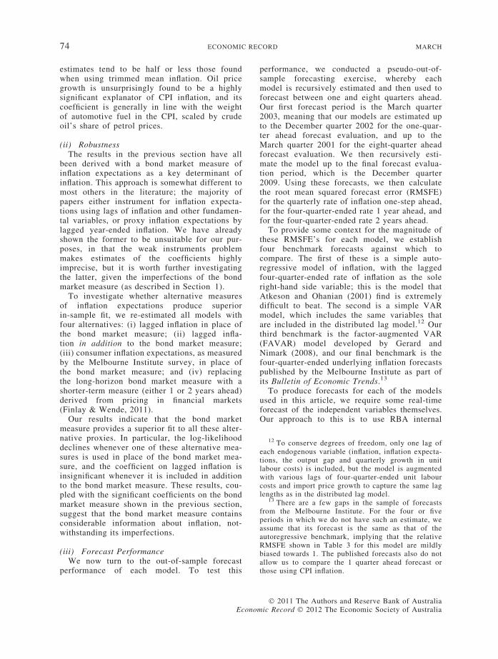
estimates tend to be half or less those foundwhen using trimmed mean inflation. Oil pricegrowth is unsurprisingly found to be a highlysignificant explanator of CPI inflation, and itscoefficient is generally in line with the weightof automotive fuel in the CPI, scaled by crudeoil’s share of petrol prices.

(ii) RobustnessThe results in the previous section have all

been derived with a bond market measure ofinflation expectations as a key determinant ofinflation. This approach is somewhat different tomost others in the literature; the majority ofpapers either instrument for inflation expecta-tions using lags of inflation and other fundamen-tal variables, or proxy inflation expectations bylagged year-ended inflation. We have alreadyshown the former to be unsuitable for our pur-poses, in that the weak instruments problemmakes estimates of the coefficients highlyimprecise, but it is worth further investigatingthe latter, given the imperfections of the bondmarket measure (as described in Section 1).

To investigate whether alternative measuresof inflation expectations produce superiorin-sample fit, we re-estimated all models withfour alternatives: (i) lagged inflation in place ofthe bond market measure; (ii) lagged infla-tion in addition to the bond market measure;(iii) consumer inflation expectations, as measuredby the Melbourne Institute survey, in place ofthe bond market measure; and (iv) replacingthe long-horizon bond market measure with ashorter-term measure (either 1 or 2 years ahead)derived from pricing in financial markets(Finlay & Wende, 2011).

Our results indicate that the bond marketmeasure provides a superior fit to all these alter-native proxies. In particular, the log-likelihooddeclines whenever one of these alternative mea-sures is used in place of the bond market mea-sure, and the coefficient on lagged inflation isinsignificant whenever it is included in additionto the bond market measure. These results, cou-pled with the significant coefficients on the bondmarket measure shown in the previous section,suggest that the bond market measure containsconsiderable information about inflation, not-withstanding its imperfections.

(iii) Forecast PerformanceWe now turn to the out-of-sample forecast

performance of each model. To test this

Econo

performance, we conducted a pseudo-out-of-sample forecasting exercise, whereby eachmodel is recursively estimated and then used toforecast between one and eight quarters ahead.Our first forecast period is the March quarter2003, meaning that our models are estimated upto the December quarter 2002 for the one-quar-ter ahead forecast evaluation, and up to theMarch quarter 2001 for the eight-quarter aheadforecast evaluation. We then recursively esti-mate the model up to the final forecast evalua-tion period, which is the December quarter2009. Using these forecasts, we then calculatethe root mean squared forecast error (RMSFE)for the quarterly rate of inflation one-step ahead,for the four-quarter-ended rate 1 year ahead, andfor the four-quarter-ended rate 2 years ahead.

To provide some context for the magnitude ofthese RMSFE’s for each model, we establishfour benchmark forecasts against which tocompare. The first of these is a simple auto-regressive model of inflation, with the laggedfour-quarter-ended rate of inflation as the soleright-hand side variable; this is the model thatAtkeson and Ohanian (2001) find is extremelydifficult to beat. The second is a simple VARmodel, which includes the same variables thatare included in the distributed lag model.12 Ourthird benchmark is the factor-augmented VAR(FAVAR) model developed by Gerard andNimark (2008), and our final benchmark is thefour-quarter-ended underlying inflation forecastspublished by the Melbourne Institute as part ofits Bulletin of Economic Trends.13

To produce forecasts for each of the modelsused in this article, we require some real-timeforecast of the independent variables themselves.Our approach to this is to use RBA internal


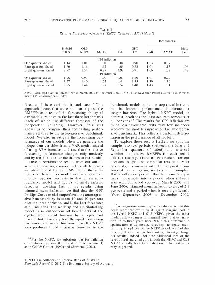
TABLE 3Relative Forecast Performance (RMSE, Relative to AR(4) Model)

HybridNKPC

OLSNKPC Mark-up DL

GPTPC

Benchmarks

VAR FAVARMelb.Inst.

TM inflationOne quarter ahead 1.14 1.01 1.07 1.04 0.90 1.03 0.97Four quarters ahead 1.66 1.16 1.12 1.06 0.82 1.01 1.13 1.06Eight quarters ahead 2.77 1.34 0.87 0.92 0.71 1.06 1.08 1.48

CPI inflationOne quarter ahead 1.76 0.93 1.00 1.03 1.10 1.01 0.97Four quarters ahead 3.77 1.40 1.52 1.44 1.45 1.30 1.10Eight quarters ahead 3.85 1.64 1.27 1.59 1.40 1.43 1.01

Notes: Calculated over the forecast period March 2003 to December 2009. NKPC, New Keynesian Phillips Curve; TM, trimmedmean; CPI, consumer price index.

15 A suggestion raised by some referees is that thiscould reflect the exclusion of lags of marginal cost inthe hybrid NKPC and OLS NKPC, given the othermodels allow changes in marginal cost to affect infla-tion up to three years later. While this difference inspecification is deliberate, reflecting the tighter theo-retical priors placed on the NKPC model, we find that


forecast of these variables in each case.14 Thisapproach means that we cannot strictly use theRMSFEs as a test of the forecasting ability ofour models, relative to the last three benchmarks(each of which use different forecasts of theindependent variables). However, this stillallows us to compare their forecasting perfor-mance relative to the autoregressive benchmarkmodel. We also investigate the forecasting per-formance of our models when we generate theindependent variables from a VAR model insteadof using RBA forecasts, and find that the relativeforecasting performance changes only modestlyand by too little to alter the themes of our results.

Table 3 contains the results from our out-of-sample forecasting exercise, where all forecastsare standardised by the RMSFEs of the auto-regressive benchmark model so that a figure <1implies superior forecasts to that of an auto-regressive model and figures >1 imply inferiorforecasts. Looking first at the results usingtrimmed mean inflation, we find that the GPTPhillips Curve model outperforms the autoregres-sive benchmark by between 10 and 30 per centover the three horizons, and is the best forecasterat all horizons. The mark-up and distributed lagmodels also outperform all benchmarks at theeight-quarter ahead horizon by a significantmargin, but have only broadly equal forecastingperformance at nearer horizons. The OLS NKPCalso produces broadly similar forecasts to the

14 For the NKPC, we substitute out for inflationexpectations by using the closed form of the model,as in Galı & Gertler (1999) and Sbordone (2002).


benchmark models at the one-step ahead horizon,but its forecast performance deteriorates atlonger horizons. The hybrid NKPC model, incontrast, produces the least accurate forecasts atall horizons.15 The results for CPI inflation aremuch less favourable, with very few instanceswhereby the models improve on the autoregres-sive benchmark. This reflects a uniform deterio-ration in the performance of all models.

To explore these results further, we split thesample into two periods (between the June andSeptember quarters of 2006) and assessedwhether the relative RMSFEs for each perioddiffered notably. There are two reasons for ourdecision to split the sample at this date. Mostobviously, it coincides with the mid-point of ourforecast period, giving us two equal samples.But equally as important, this date broadly sepa-rates the sample into a period when inflationwas well contained (between March 2003 andJune 2006, trimmed mean inflation averaged 2.6per cent) and a period when it rose significantly(from September 2006 to December 2009,

relaxing this restriction does not significantly changeour results. Indeed, including additional lags of thelevel of real marginal cost in both the NKPC and OLSNKPC actually lead to a reduction in forecast accu-racy in general.

lia


trimmed mean inflation averaged 3.4 per cent),providing us with an indication of how our mod-els perform in each state.

While the results must be tentative, giventhey are derived using only 7 years of forecasts,the results of this split-sample exercise provideevidence consistent with a view that the type ofmodels studied in this article are most useful attimes of significant fluctuations in inflation. Inrelation to trimmed mean inflation, we find thatour models tend to perform worse than both theautoregressive and FAVAR benchmark modelsin the first half of our forecast sample. (Theexception is the hybrid NKPC, augmented withadditional lags of real marginal cost, whichforecasts very accurately during this period.)However, there is a sizeable deterioration in theforecasting performance of the benchmark mod-els in the second half of our forecast period thatis not matched by an equal-sized deteriorationin the forecasting performance of our models;indeed, the forecast errors from the GPT Phil-lips Curve barely increase in the second sample,despite the greater variance in inflation. As aresult, the OLS NKPC, mark-up, distributed lagand GPT Phillips Curve models all outperformthe autoregressive model at at least one horizonover this period. (The performance of the hybridNKPC declines significantly from the first sam-ple.) A similar result is found for CPI inflation;in the latter sample, the forecasting performanceof the autoregressive model deteriorates morenotably than that of our models, and as a resultthey have somewhat better forecasting per-formance than the autoregressive benchmark(though the results are somewhat patchy and theperformance of the other benchmark models isbroadly equal to those of our main models overthis time). These result is consistent with theargument in Stock and Watson (2009), that theAtkeson and Ohanian (2001) results are over-turned during periods when activity deviatessignificantly from its potential level.

V ConclusionThis article has sought to answer two ques-

tions – using Australian data, can we find anactivity-based model of inflation that improveson the Atkeson and Ohanian (2001) benchmarkautoregressive model in forecasting inflation,and if so, what form of activity-based modelperforms best. In relation to the first ques-tion, our answer appears to be yes, at least fortrimmed mean inflation and in periods that

Econo

include some significant movement in inflation.These results are in line with Stock and Watson’s(2009) suggestion that the Atkeson and Ohanianresults are overturned in periods where the unem-ployment gap is large (in absolute terms). How-ever, our results are much less favourable foractivity-based models when headline CPI infla-tion is the dependent variable; in this case, theautoregressive model displays superior perfor-mance over the full sample and at least as goodperformance during the period in which inflationrose. We interpret this deterioration in forecastperformance (and the associated decline in preci-sion of our estimates) as implying that the tailsof the price distribution that are downweightedby the trimmed mean measure do not contain anysignal of trend inflation.

In regards to the second question, our resultssuggest that the expectations-augmented PhillipsCurve has displayed the best forecasting (and in-sample) performance in recent years. Of the mod-els that we assess, its forecast performance issuperior at all horizons and has been 10–20 percent better than that of the mark-up and distrib-uted lag models, which in turn have producedsuperior forecasts to a range of benchmarks atlonger horizons. In contrast, the forecast perfor-mance of the NKPC is very poor, and is onlypartly corrected when we avoid the problem ofinstrumenting for inflation expectations. We takethis finding to imply that inflation is betterexplained by either the unemployment rate orgrowth in nominal marginal costs, rather than bythe level of real marginal costs.

Our findings lend support to the ongoingsearch for activity-based models that canexplain and forecast inflation. Importantly, theevidence in this article for the superior perfor-mance of such models comes largely from a per-iod when inflation began to deviate notablyfrom its trend rate, which is the type of episodewhen it is most important to be able to forecastinflation well. More generally, our results sug-gest scope for further research on the transmis-sion of excess demand into inflation, includingwhy the unemployment rate provides a betterread on inflation than unit labour costs.

Supporting InformationAdditional supporting information may be

found in the online version of this article:DATA S1 Datasets and CodesPlease note: Wiley-Blackwell is not responsible

for the content or functionality of any supporting



materials supplied by the authors. Any queries(other than missing material) should be directedto the corresponding author for the article.

REFERENCES

Andrews, D. (1993), ‘Tests for Parameter Instabilityand Structural Change with Unknown ChangePoint’, Econometrica, 61 (4), 821–56.

Atkeson, A. and Ohanian, L. (2001), ‘Are PhillipsCurves Useful for Forecasting Inflation?’, FederalReserve Bank of Minneapolis Quarterly Review, 25 (1),2–11.

Bai, J. and Perron, P. (1998), ‘Estimating and TestingLinear Models with Multiple Structural Changes’,Econometrica, 66 (1), 47–78.

Ball, L. and Mazumder, S. (2011), ‘Inflation Dynam-ics and the Great Recession’, National Bureau ofEconomic Research Working Paper No. 17044,NBER, Cambridge, MA.

B _ardsen, G., Hurn, S. and McHugh, Z. (2007),‘Modelling Wages and Prices in Australia’, Eco-nomic Record, 83 (261), 143–58.

Batini, N., Jackson, B. and Nickell, S. (2005), ‘An Open-Economy New Keynesian Phillips Curve for the UK’,Journal of Monetary Economics, 52 (6), 1061–71.

Brayton, F., Roberts, J. and Williams, J. (1999),‘What’s Happened to the Phillips Curve?’ Financeand Economics Discussion Paper No. 1999-49,Board of Governors of the Federal Reserve System,Washington, DC.

Brischetto, A. and Richards, A. (2007), ‘The Perfor-mance of Trimmed Mean Measures of UnderlyingInflation’, Paper presented at the Conference onPrice Measurement for Monetary Policy sponsored bythe Federal Reserve Banks of Cleveland and Dallas,Dallas.

Chen-Yu Leu, S. and Sheen, J. (2011), ‘A Small NewKeynesian State-Space Model of the AustralianEconomy’, Economic Modelling, 28 (1–2), 672–84.

De Brouwer, G. and Ericsson, N. (1998), ‘ModellingInflation in Australia’, Journal of Business and Statis-tics, 164 (4), 443–9.

Dixon, R. and Thomson, J. (2000), ‘Okun’s Law andMovements over Time in the Unemployment Ratein Australia’, Department of Economics ResearchPaper No. 741, University of Melbourne.

Dwyer, J. and Leong, K. (2001), ‘Changes in theDeterminants of Inflation in Australia’, ReserveBank of Australia Research Discussion Paper No.2001-02, Sydney, Australia.

Finlay, R. and Wende, S. (2011), ‘Estimating InflationExpectations with a Limited Number of InflationIndexed Bonds’, Reserve Bank of AustraliaResearch Discussion Paper No. 2011-01, Sydney,Australia.

Friedman, M. (1968), ‘The Role of Monetary Policy’,American Economic Review, 58 (1), 1–17.


Galı, J. and Gertler, M. (1999), ‘Inflation Dynamics:A Structural Econometric Analysis’, Journal ofMonetary Economics, 44 (2), 195–222.

Galı, J. and Monacelli, T. (2005), ‘Monetary Policy andExchange Rate Volatility in a Small Open Economy’,Review of Economics and Statistics, 72 (3), 707–34.

Gerard, H. and Nimark, K. (2008), ‘Combining Multi-variate Density Forecasts using Predictive Criteria’,Reserve Bank of Australia Research DiscussionPaper No. 2008-02, Sydney, Australia.

Gruen, D., Pagan, A. and Thompson, C. (1999), ‘ThePhillips Curve in Australia’, Journal of MonetaryEconomics, 44 (2), 223–58.

Gruen, D., Robinson, T. and Stone, A. (2005), ‘OutputGaps in Real Time: How Reliable are They?’, Eco-nomic Record, 81 (252), 6–18.

Heath, A., Roberts, I. and Bulman, T. (2004), ‘Infla-tion in Australia: Measurement and Modelling’, inKent, C. and Guttman, S. (eds), The Future of Infla-tion Targeting. Reserve Bank of Australia, Sydney;167–207.

Henzel, S. and Wollmershauser, T. (2008), ‘The NewKeynesian Phillips Curve and the Role ofExpectations: Evidence from the CESifo World Eco-nomic Survey’, Economic Modelling , 25 (5), 811–32.

Jaaskela, J. and Nimark, K. (2011), ‘A Medium ScaleNew Keynesian Open Economy Model of Austra-lia’, Economic Record, 87 (276), 11–36.

Kennedy, S., Luu, N. and Goldbloom, A. (2008),‘Examining Full Employment in Australia using thePhillips and Beveridge Curves’, The Australian Eco-nomic Review, 41 (3), 286–97.

Kuttner, K. and Robinson, T. (2010), ‘Understandingthe Flattening Phillips Curve’, The North AmericanJournal of Economics and Finance, 21 (2), 110–25.Special Issue: 50 Years of the Phillips Curve.

Leith, C. and Malley, J. (2007), ‘Estimated OpenEconomy New Keynesian Phillips Curves for theG7’, Open Economies Review, 18 (4), 405–26.

Lim, G., Dixon, R. and Tsiaplias, S. (2009), ‘PhillipsCurve and the Equilibrium Unemployment Rate’,Econommic Record, 85 (271), 371–82.

Macallan, C., Millard, S. and Parker, M. (2008), ‘TheCyclicality of Mark-Ups and Profit Margins for theUnited Kingdom: Some New Evidence’, Bank ofEngland Working Paper No. 351, London, UK.

Mavroeidis, S. (2005), ‘Identification Issues in For-ward-Looking Models Estimated by GMM, with anApplication to the Phillips Curve’, Journal ofMoney, Credit and Banking, 37 (3), 421–48.

McDonald, J. (1999), ‘The Determinants of Firm Prof-itability in Australian Manufacturing’, EconomicRecord, 72 (2), 115–26.

Perron, P. (1990), ‘Testing for a Unit Root in a TimeSeries Regression with a Changing Mean’, Journalof Business and Economic Statistics, 8 (2), 153–62.

Phelps, E. (1967), ‘Phillips Curves, Expectations ofInflation and Optimal Unemployment over Time’,Economica, 34 (3), 254–81.

lia


Richards, A. and Rosewall, T. (2010), ‘Measures ofUnderlying Inflation’, Reserve Bank of AustraliaBulletin, March 7–12.

Roberts, I. (2005), ‘Underlying Inflation: Concepts,Measurement and Performance’, Reserve Bank ofAustralia Research Discussion Paper No. 2005-05, Sydney, Australia.

Rotemberg, J. and Saloner, G. (1986), ‘A Supergame-Theoretic Model of Price Wars during Booms’,American Economic Review, 76 (3), 390–407.

Rotemberg, J. and Woodford, M. (1999), The CyclicalBehaviour of Prices and Costs. Elsevier Science,Amsterdam, Netherlands.

Econo

Russell, B., Banerjee, A., Malki, I. and Ponomareva,N. (2010), ‘A Multiple Break Panel Approach toEstimating United States Phillips Curves’, Depart-ment of Economics Discussion Paper No. 10-14,University of Birmingham.

Sbordone, A. M. (2002), ‘Prices and Unit LaborCosts: A New Test of Price Stickiness’, Journal ofMonetary Economics, 49 (2), 265–92.

Stock, J. and Watson, M. (2009), ‘Phillips CurveInflation Forecasts’, in Fuhrer, J., Kodrzyckim, Y.,Little, J. and Olivei, G. (eds), Understanding Infla-tion and the Implications for Monetary Policy,Chapter 3. MIT Press, Cambridge; 101–86.


the forecasting performance of single equation models of inflation

Documents