learning from errors while forecasting inflation: a case

Malik and Hanif-Learning from Errors While Forecasting Inflation: A Case for Intercept Correction

24

Learning from Errors While Forecasting Inflation: A Case for Intercept Correction

Muhammad Jahanzeb Malik and Muhammad Nadim Hanif

State Bank of Pakistan and State Bank of Pakistan

Received: 07.04.2017 Accepted: 05.09.2018 Published: 05.04.2019

doi:10.33818/ier.304468

ABSTRACT

Structural changes are quite common in macroeconomic time series. Moreover, any

underlying macroeconomic relationship cannot be correctly specified unless we know the

true model. Structural changes in time series and misspecification in empirical model are

observed as shifts in the constant of the underlying relationship between the subject

variables of interest. Forecasting from such a model assuming ‘no structural break’ and

‘correct model’ is tantamount to ignoring important aspects of underlying economy and

mostly results in forecast failure(s). Intercept correction (IC) is a method for

accommodating such ignored structural break(s) and omitted variable(s). We use a simple

model (for July 1991 to March 2016) to forecast inflation for 25 countries and compare its

performance with a) the same model with optimal IC, b) the same model with half IC, and

c) a random walk model. Optimal IC approach, though computational intensive,

outperforms in forecasting next period inflation compared to one from a) the same model

without IC, b) the same model with half intercept correction, and c) random walk model

without IC. For the particular class of inflation models under study, over the time period

specified, ‘quarter IC’ works best among the fixed IC rules.

Key words: Forecasting, Structural changes, Intercept correction, Misspecification,

Inflation models

JEL Classifications: C01, C52, C53

1. INTRODUCTION

The forward-looking nature of monetary policy highlights the importance of inflation

forecasting. Accordingly, we need to be aware of the main factors behind the forecast failures.

Mean shift or intercept change is considered as the biggest enemy of forecasts Clements and

Hendry (1999). This study primarily highlights the importance of intercept correction (IC) and

describes a framework for its implementation for details; see Clements and Hendry (1999). For

illustration, we use a simple model of inflation (as a function of lagged broad money supply

growth). Even though this appears to be a naïve model, the intercept correction method protects

against various forms of mis-specification errors in complex models and compensates for the

effects of missing variables. Thus, it can prove to be a strong competitor to sophisticated

models. However, what should be the degree of IC, between zero IC to unit IC, is the research

question of this study.

Muhammad Nadim Hanif, (email: [email protected]), Tel: +923212436714.

Muhammad Jahanzeb Malik, (email: [email protected]), Tel: +923215018594.

Authors belong to State Bank of Pakistan. The views expressed in this study are those of the authors and need not

necessarily be associated with their employer. Authors are thankful to the Editor for his insightful comments on

earlier version of this study which helped improved this a lot.

mailto:[email protected]

International Econometric Review (IER)

25

We estimate a simple inflation forecasting model (which is equivalent to ‘zero intercept

correction’ or ZIC) and compare its performance with a random walk model (RWM) as

benchmark. We also compare the performance of ZIC with the same but allowing for some

non-zero fraction of IC. The degree of IC could be incorporated in different ways. First,

arbitrarily selecting a fraction of previous forecast error (PFE) which is obviously the simple

and stable approach to decide a fraction of error to be corrected. Second, an optimal selection

of a fraction of PFE which is a sophisticated way to estimate a fraction of error to be corrected

but may vary with the sample. We explore both of these ways for IC in this study. For an

arbitrary selection of the ‘fraction’ or ‘weight’ (w) of the PFE, we choose it to be 0.5. This we

call half intercept correction (HIC) rule. Similarly, one may have a quarter intercept correction

(QIC) rule or three-quarters intercept correction rule. For optimal selection of this weight (w),

we search for the one which minimizes the root mean squared error (RMSE) of in-sample

inflation forecasts. We denote this correction by OIC.

For this study we select 25 countries (including Pakistan). In case of Pakistan we also make

such comparisons (forecasting with and without IC) for a larger set of inflation forecasting

models which we studied in Hanif and Malik (2015).

For all 25 countries, OIC beats ZIC, HIC as well as RW model (of inflation). In case of Pakistan,

OIC based forecasting beats all 9 inflation forecasting models in Hanif and Malik (2015)

including highly technical models of inflation with seemingly strong theoretical background.

While selecting the optimal degree of intercept correction (w) we observe that a higher intercept

correction is needed for the countries where inflation is volatile (and high). For the particular

class of inflation forecasting models under investigation, over the period studied in this paper,

‘quarter intercept correction (QIC)’ works best among the fixed intercept correction rules.

In the next section, we explain the data and the methodology we use. In section 3 we provide

empirical evidence in accordance with the methodology outlined. Last section is for concluding

remarks.

2. METHODOLOGY AND DATA

A variant of the quantity theory of money suggests inflation (deflation) results from expansion

(contraction) in money supply in an economy. In order to demonstrate the usefulness of

intercept correction see Clements and Hendry (1999), we start with this simple relationship to

forecast inflation while considering other competing determinants of inflation including global

commodity prices (which we proxy by international prices of crude oil), nominal exchange rate,

and real economic activity in the country. We model general level of price change (measured

by CPI) as a function of optimal lag(s) of inflation itself and optimal lags of broad money supply

growth, international crude oil price change, change in nominal exchange rate, and a proxy for

changes in real economic activity. We collect monthly data for all the variables from

International Financial Statistics of IMF for 25 countries. The change can be monthly (i.e.

month on month, denoted by MoM) or annual (i.e. year on year denoted by YoY). For MoM

case, as an example, let us denote yt = log (CPIt / CPIt–1) and xt = log (M2t / M2t–1). Similarly, we

can define the other set of variables zt, if any, such as log (EXCRt / EXCRt–1) for exchange rate,

and so on; zt could be different from the true model (as we do not know the true model).

Dividing the available dataset into two halves, we run the simple linear regression [using linest,

in Excel] without any constant as in equation (2.1), i.e.,

yt = b0yt−i + c0xt−j+d0zt−k + ⋯ +∈t (2.1)


26

and thus,

yt = b0yt−i + c0xt−j+d0zt−k + ⋯ +∈t

or,

yt − {b0yt−i + c0xt−j+d0zt−k + ⋯ } =∈t (2.2)

where i, j, and k can be chosen on the basis of either some lag selection criterion or some prior

information or a combination of both approaches. Since our focus here is not lag selection and

we want to explore the merits of IC only, we do not go into lag selection related details here.

However, even if the lag selection is neither optimal nor based upon any prior information,

intercept correction takes care of lag selection related misspecification, in addition to omitted

variable(s) bias, at least partially (because the misspecification can all be considered as a

fluctuation in the constant intercept, to a first order of approximation).

For this study, we use dataset from July 1991 to March 2016. If we denote the sample size used

in this estimation as T* (which is half of the overall sample size T), we can see that the

prediction error at t = T* from equation (2) is as below:

yt = b0yt−i + c0xt−j+d0zt−k + ⋯ +∈t

The intercept correction method uses the forecast error from the current period to adjust the

forecast in the next period by a fraction, say, w0. The adjusted forecast at t = T* + 1, i.e., yT*+1 is

𝑦𝐹𝑇∗+1

= ��0𝑦𝑇∗ + ��0𝑥𝑇∗ + ��0𝑧𝑇∗ + ⋯ + ��0 ∈𝑇∗ (2.3)

This has the forecast error: 𝑦𝑇∗+1 − 𝑦𝑇∗+1𝐹 = ∈𝐹

𝑇∗+1. When 𝑤0 = 0, this is the usual forecast,

without intercept correction. If it is anticipated that the next period forecast will contain an error

close to quarter, half, or three-quarters of the error made in the previous period then quarter,

half, or three-quarters fraction of PFE can be adjustment respectively to account for the

‘anticipated’ error.

The above process is repeated by adding one observation and so on. We go until t = T i.e. from

T* to T. Forecast 𝑦𝐹𝑇∗+2

and the corresponding forecast errors are ∈𝐹𝑇∗+2 and so on are

obtained accordingly.

Using ∈𝐹𝑇∗+1 … … … … … … … … … … ∈𝐹

𝑇, ee calculate root mean square error (RMSE) of

forecasts as

𝑅𝑀𝑆𝐸 (𝑦) = √∑ (∈𝐹𝑡)𝑇

𝑡=𝑇∗2

𝑇−𝑇∗

In order to judge if quarter, half, or three-quarters1 intercept correction should be adopted as a

fractional intercept correction rule, we should see which fractional adjustment results in RMSE

within, say, 10% of the minimum RMSE to forecast inflation rate for a given country.

For optimal intercept correction, we repeat the above procedure for 𝑤0 =0, 0.01, … … … … … … … ,0.99, 1.0 and look for the degree of interception that yields minimum

RMSE.

For the case of empirical exercise in this study, Model (2.1) is estimated using data from July

1991 to October 2003 (first half of dataset), we then recursively forecast inflation from

November 2003 to March 2016 (second half of dataset). At each step one observation is

1 Or, any arbitrary value that can be fixed as a rule for fractional intercept correction.


27

increased in the estimation sample and PFE is added with some coefficient “w0” in the model

and we estimate model represented in equation (2.3). This process is repeated for all

observations till final forecast of March 2016 is obtained. In order to find out the optimal value

of w0, RMSE is calculated for 𝑤0 = 0, 0.01, … … … … … … … ,0.99, 1.0. Optimal value of “w0”

is obtained where RMSE of forecasts is minimized and is called OIC fraction.

3. ESTIMATION AND RESULTS

Since we are working with growth data (of prices and money), we do not expect our variables

of interest to be non-stationary and thus do not test for unit roots. Moreover, the benchmark

forecasting model (RW or AR1) works with and without unit roots and thus we need not worry

about stationarity. As discussed, we estimate i) a benchmark model, ii) simple inflation

forecasting model (without intercept), iii) an inflation forecasting model with adding back half

of the forecasting error in underlying ZIC model (ii), and iv) an inflation forecasting model with

the addition of an optimal degree of intercept correction back to the underlying ZIC model. For

benchmarking purpose we estimate a random walk model of inflation with drift as found to be

the best benchmarking model in forecasting inflation in Pakistan by Hanif and Malik (2015).

Table 3.1 Relative RMSE of OIC model with respect to i) random walk with drift and ii) HIC model

Note: These results pertain to MoM dataset.

In Table 3.1, we report the relative RMSE of an inflation forecasting model, as in (2.1), with

optimal value of w0 for all countries. We study RMSE relative to RMSE of RW model with

drift and HIC model. Optimal intercept corrected version performs well in all cases. These

results are robust to whether we consider MoM or YoY style of calculating the growth. More

importantly, these results are robust to whether or not we use the additional set of potential

Country Optimal degree of IC RRMSE

(viz a viz RW WD)

RRMSE

(viz a viz HIC)

Bolivia 0.52 0.50 0.50

Colombia 0.89 0.65 0.68

Costa Rica 0.46 0.50 0.50

Denmark 0.23 0.52 0.53

Dominica 0.00 0.39 0.44

Fiji 0.00 0.38 0.43

Grenada 0.29 0.44 0.45

Japan 0.28 0.50 0.51

Jordan 0.21 0.44 0.46

Malaysia 0.41 0.52 0.52

Mexico 0.79 0.61 0.63

Pakistan 0.13 0.43 0.45

Paraguay 0.16 0.41 0.43

Singapore 0.00 0.40 0.43

South Africa 0.38 0.52 0.53

St Kitts & Nevis 0.04 0.42 0.45

St Lucia 0.04 0.40 0.44

St Vincent & Grenadines 0.00 0.39 0.43

Swaziland 0.19 0.37 0.39

Switzerland 0.11 0.46 0.47

Tonga 0.07 0.42 0.45

Trin/Tobago 0.14 0.45 0.47

Turkey 0.59 0.54 0.54

U.S. 0.65 0.59 0.60

Uruguay 0.49 0.52 0.52


28

explanatory variables (𝑧𝑡) of inflation2 simply because when we omit some of the relevant

explanatory variable(s) their changes reflect in the intercept and intercept correction (partially)

compensates for the omitted variable(s).

In all above analysis pertaining to performance of inflation forecasting models with intercept

correction, we have quite interesting observations: The optimal degree of intercept correction

is different for different countries (Table 3.2a). It suggests exploring which type of countries

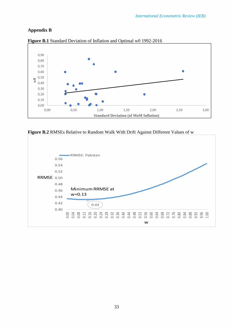
requires relatively a higher degree of intercept correction. On plotting the optimal degree of

intercept correction with the degree of volatility in inflation we observe that both are directly

related – higher the volatility in inflation, higher would be the required optimal degree of

intercept correction in order to forecast inflation best (Figure B.1). It highlights the importance

of using intercept correction in inflation forecasting particularly for high inflation countries

because countries with volatile inflation are usually the high inflation countries. For each

country the OIC does not vary much over extending the sample period as is clear from the last

column of Table 3.2a. It shows very low standard deviations of OICs for different samples –

barring for pre global commodity prices shock of 2007-08. This is also clear from ‘closeness’

of country wise OICs plotted in Figure B.6 (Appendix B) for different samples.

Country 1992-

2008

1992-

2012

1992-

2013

1992-

2014

1992-

2015

1992-

2016

(March)

Average

(columns

2 to 8)

Standard

Deviation

(columns

2 to 8)

Standard

Deviation

(columns

3 to 8)

(1) (2) (3) (4) (5) (6) (7) (8) (9) (9)

Bolivia 0.21 0.39 0.38 0.40 0.45 0.52 0.39 0.10 0.10

Colombia 0.71 0.83 0.81 0.87 0.87 0.89 0.83 0.07 0.07

Costa Rica 0.23 0.42 0.40 0.41 0.44 0.46 0.39 0.08 0.08

Denmark 0.05 0.27 0.22 0.25 0.20 0.23 0.20 0.08 0.08

Dominica 0.16 0.00 0.00 0.00 0.00 0.00 0.03 0.07 0.07

Fiji 0.16 0.00 0.00 0.00 0.00 0.00 0.03 0.07 0.07

Grenada 0.06 0.34 0.36 0.34 0.34 0.29 0.29 0.11 0.11

Japan 0.13 0.27 0.26 0.28 0.31 0.28 0.26 0.06 0.06

Jordan 0.13 0.19 0.23 0.23 0.24 0.21 0.21 0.04 0.04

Malaysia 0.33 0.36 0.39 0.38 0.41 0.41 0.38 0.03 0.03

Mexico 0.52 0.77 0.79 0.78 0.77 0.79 0.74 0.11 0.11

Pakistan 0.26 0.13 0.12 0.09 0.11 0.13 0.14 0.06 0.06

Paraguay 0.29 0.21 0.20 0.20 0.18 0.16 0.21 0.04 0.04

Singapore 0.00 0.00 0.00 0.00 0.00 0.00 0.00 0.00 0

South Africa 0.42 0.38 0.31 0.31 0.33 0.38 0.36 0.05 0.05

St Kitts & Nevis 0.27 0.12 0.11 0.04 0.04 0.04 0.10 0.09 0.09

St Lucia 0.03 0.01 0.00 0.00 0.00 0.00 0.01 0.01 0.01

St Vincent & Gr. 0.00 0.00 0.03 0.00 0.00 0.00 0.01 0.01 0.01

Swaziland 0.37 0.20 0.19 0.09 0.15 0.19 0.20 0.09 0.09

Switzerland 0.00 0.00 0.00 0.06 0.08 0.11 0.04 0.05 0.05

Tonga 0.00 0.05 0.09 0.14 0.07 0.07 0.07 0.05 0.05

Trin/Tobago 0.00 0.20 0.14 0.13 0.14 0.14 0.13 0.07 0.07

Turkey 0.63 0.62 0.61 0.60 0.62 0.59 0.61 0.01 0.01

U.S. 0.52 0.59 0.59 0.60 0.64 0.65 0.60 0.05 0.05

Uruguay 0.91 0.60 0.57 0.53 0.51 0.49 0.60 0.16 0.16

Table 3.2a Optimal degree of intercept correction estimated for different time periods


For the case of Pakistan specifically, we also compare the performance of optimal intercept

correcting the inflation-forecasting model of this study with a number of inflation forecasting

2 𝑧𝑡 includes global commodity prices, nominal exchange rate, and real economic activity. Results pertaining to case without

𝑧𝑡 can be obtained from the corresponding author, if needed.


29

models estimated by Hanif and Malik (2015). In Table 3.3, we report the RMSE of 9 inflation

forecasting models of Hanif and Malik (2015) relative to RMSE of OIC model of this study.

Thus, study’s OIC inflation forecasting model performs better compared to all the models we

considered from Hanif and Malik (2015).

Country OIC groups 1992-

2008

1992-

2012

1992-

2013

1992-

2014

1992-

2015

1992-

2016 (March)

1

0

0 0 0 0 0 0

2 0 0 0 0 0 0

3 0 0 0 0 0 0

4 0 0 0 0 0 0

5 0 0 0 0 0 0

6

Above 0 but below 0.25

0.03 0.01 0.03 0.04 0.04 0.04

7 0.05 0.05 0.09 0.06 0.07 0.07

8 0.06 0.12 0.11 0.09 0.08 0.11

9 0.13 0.13 0.12 0.09 0.11 0.13

10 0.13 0.19 0.14 0.13 0.14 0.14

11 0.16 0.2 0.19 0.14 0.15 0.16

12 0.16 0.2 0.2 0.2 0.18 0.19

13 0.21 0.21 0.22 0.23 0.2 0.21

14 0.23 0.23 0.25 0.24 0.23

14

Above 0.25 but below 0.50

0.27

15 0.26 0.27 0.26 0.28 0.31 0.28

16 0.27 0.34 0.31 0.31 0.33 0.29

17 0.29 0.36 0.36 0.34 0.34 0.38

18 0.33 0.38 0.38 0.38 0.41 0.41

19 0.37 0.39 0.39 0.4 0.44 0.46

20 0.42 0.42 0.4 0.41 0.45 0.49

21

Above 0.50 but below 0.75

0.52 0.59 0.57 0.53 0.51 0.52

22 0.52 0.6 0.59 0.6 0.62 0.59

23 0.63 0.62 0.61 0.6 0.64 0.65

24 0.71

24 Above 0.75

0.77 0.79 0.78 0.77 0.79

25 0.91 0.83 0.81 0.87 0.87 0.89

Table 3.2b Distribution of Optimal degree of intercept correction estimated for different time periods


Models Relative RMSE

ARIMA 0.76

MVAR 0.87

EVAR-1 0.20

EVAR-2 0.58

CVAR 0.31

MVAR (Bayesian) 0.75

EVAR (Bayesian) 0.73

CVAR (Bayesian) 0.71

ARDL 0.96

Table 3.3 Relative Forecast Performance (Relative to Intercept Correction Model)

When we compare the performance of different fixed intercept correction rules (like HIC), we

find that QIC works best amongst quarter, half and three-quarters intercept correction.

4. CONCLUSION

We use a simple model of inflation consisting of lag(s) of inflation along with lags of broad

money supply growth to forecast next period inflation. We evaluate forecasting performance of

this model in comparison with a random walk model of inflation. Then we see if intercept


30

correction (IC) helps improve the inflation forecasting performance of this model in comparison

with the performance of the same model with no IC. An IC can also be applied arbitrarily like

half intercept correction (HIC). However, we think a ‘root mean squared error (RMSE)

minimizing approach’ can be adopted to decide for the desired degree of IC rather than no or

arbitrary IC. We call such degree of IC as an optimal intercept correction (OIC). ‘Is really the

idea of OIC worthwhile compared to no or arbitrarily selected degree of IC’ is the one of the

two question of this study. The other question is which degree of interception correction works

best from among the different fixed intercept correction rules like quarter, half, etc.

We carry out an exercise for 25 countries over a period from July 1991 to March 2016 during

which we know inflation rate series are characterized by different structural breaks (including

the one during 2008). The simple model of inflation works for all countries against random

walk model as there is no such country for which relative RMSE is greater than unity (Figure

B.2-B.5 of Appendix B) irrespective of fraction of IC– like no, half or optimal.

Three main results are interesting.

No intercept correction is not an option as we can see that zero IC is not optimal for 20 out of

25 countries. In other words, minimum relative RMSE is achieved only for 5 out of 25 countries

(Dominica, Fiji, Singapore, and St. Vincent and Grenadines) when no IC is applied. There can

be a couple of countries for which minimum relative RMSE occurs for fraction of IC which

may be statistically not different from zero (like 0.04 in the cases of St. Kitts and Nevis and St.

Lucia). One can interpret this result as if intercept correction does not really help improve the

inflation forecast for these 7 countries. However, the proportion of such countries where no

intercept correction is required is found to be small. In most of the cases improving inflation

forecast needs intercept correction. Likewise, complete or full intercept correction is also not

an option as we cannot found even a single country where unit IC is optimal.

OIC works for most of the countries against no or half intercept correction model of inflation

forecasting (Figure B.2-B.5 of Appendix B). The value of OIC found stable for respective

countries when we estimate it by increasing the sample size for one year over a period of four

years (from 1992-2012 to 2008-2013, 2008-2014, 2008-2015 and 2008-2016) as shown in

Table 3.2a. The idea of OIC is worthwhile for forecasting purpose that too with or without

inclusion of available relevant explanatory variable(s) for the variable of interest (inflation in

this study). Once we observe different optimal degree of IC for different countries, we also

observe that higher degree of IC is required for better forecasts of inflation rate in economies

with relatively volatile inflation rate. OIC based simple inflation forecasting model for Pakistan

also performs best compared to all the relatively sophisticated models we estimated in Hanif

and Malik (2015) for inflation forecasting purpose.

In case one thinks selecting an OIC is estimation intensive, s/he may use the simplest approach

of selecting an arbitrary fraction of IC. From among the various options of fixing the fraction

of intercept correction, say one quarter, half or three quarters, different fractions perform

differently. HIC does not produce minimum RMSE for 22 out 25 countries. Minimum RMSE

is achieved only for 3 out of 25 countries (Bolivia, Costa Rica and Japan) when HIC is applied.

Again, there can be a couple of countries for which minimum relative RMSE occurs for fraction

of IC which may be statistically not different from half (like 0.52 for the cases of South Africa

and Uruguay). Based on our observation in this study - that in most of the cases OIC falls close

to 0.25 (Table 3.2b) compared to only a few (a couple of) cases falling close to half (three-

fourths) intercept correction – QIC may be a preferred choice to create a fixed IC rule.


31

In the end, we would like to lodge a caveat. Our study is based upon one relationship only and

there is need to attempt this investigation for some other relationships as well.

REFERENCES

Castle, J.L., M.P. Clements and D.F. Hendry (2016). An Overview of Forecasting Facing

Breaks. Journal of Business Cycle Research, 12, 3-23.

Clements, M.P. and D.F. Hendry (1996). Intercept Correction and Structural Change. Journal

of Applied Econometrics, 11, 475-494.

Hanif, M.N. and M.J. Malik (2015). Evaluating Performance of Inflation Forecasting Models

of Pakistan. SBP Research Bulletin. 11 (1).

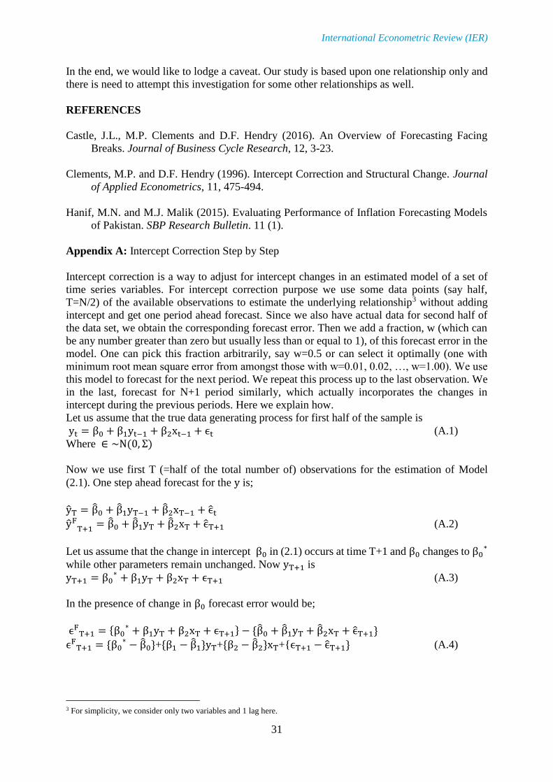
Appendix A: Intercept Correction Step by Step

Intercept correction is a way to adjust for intercept changes in an estimated model of a set of

time series variables. For intercept correction purpose we use some data points (say half,

T=N/2) of the available observations to estimate the underlying relationship3 without adding

intercept and get one period ahead forecast. Since we also have actual data for second half of

the data set, we obtain the corresponding forecast error. Then we add a fraction, w (which can

be any number greater than zero but usually less than or equal to 1), of this forecast error in the

model. One can pick this fraction arbitrarily, say w=0.5 or can select it optimally (one with

minimum root mean square error from amongst those with w=0.01, 0.02, …, w=1.00). We use

this model to forecast for the next period. We repeat this process up to the last observation. We

in the last, forecast for N+1 period similarly, which actually incorporates the changes in

intercept during the previous periods. Here we explain how.

Let us assume that the true data generating process for first half of the sample is

yt = β0 + β1yt−1 + β2xt−1 + ϵt (A.1)

Where ∈ ~N(0, Σ)

Now we use first T (=half of the total number of) observations for the estimation of Model

(2.1). One step ahead forecast for the y is;

yT = β0 + β1yT−1 + β2xT−1 + ϵt

yFT+1

= β0 + β1yT + β2xT + ϵT+1 (A.2)

Let us assume that the change in intercept β0 in (2.1) occurs at time T+1 and β0 changes to β0∗

while other parameters remain unchanged. Now yT+1 is

yT+1 = β0∗ + β1yT + β2xT + ϵT+1 (A.3)

In the presence of change in β0 forecast error would be;

ϵFT+1 = {β0

∗ + β1yT + β2xT + ϵT+1} − {β0 + β1yT + β2xT + ϵT+1}

ϵFT+1 = {β0

∗ − β0}+{β1 − β1}yT+{β2 − β2}xT+{ϵT+1 − ϵT+1} (A.4)

3 For simplicity, we consider only two variables and 1 lag here.


32

In equation (A4) there are four components of ϵFT+1 particularly {β0

∗ − β0} could be due to

[wrong] assumption that β0 is constant over the forecast horizon. It results in forecast failure4.

Other three components are just due to the estimation of true parameters.

In the following we illustrate the implementation of intercept correction procedure and the way

it helps reduce the forecast error in (A.4).

We use first half observations for the estimation of model (A.1) but without intercept. One step

ahead forecast for the y is;

yT = β1yT−1 + β2xT−1 + ϵt

yFT+1

= β1yT + β2xT + ϵT+1 (A.5)

Assuming that the change in intercept in (A.1), β0 occurred at T+1 and it became β0∗ all other

parameters remain unaffected. Now yT+1 would be;

yT+1 = β0∗ + β1yT + β2xT + ϵT+1 (A.6)

In the presence of change in β0 forecast error would be;

ϵFT+1 = {β0

∗ + β1yT + β2xT + ϵT+1} − {β1yT + β2xT + ϵT+1}

ϵFT+1 = {β0

∗}+{β1 − β1}yT+{β2 − β2}xT+{ϵT+1 − ϵT+1} (A.7)

In equation (A.7) the component of error “{β0∗}” could be due to [wrongly] omitting intercept

in the estimation. We repeat the above procedure up to all the observations in last half of the

data set. Now we have the last N/2 forecast errors and corresponding observations.

In the following we illustrate how to incorporate intercept change by including the forecast

error at ϵFN as a regressor in the model. In doing so we will be ignoring β0 in the regression on

last N/2 observations;

yN = β1yN−1 + β2xN−1 + w0ϵFN−1 + ϵN (A.8)

One step ahead forecast would be,

yFN+1

= β1yN + β2xN + w0ϵFN + ϵN+1 (A.9)

Substituting ϵFN in (A9) we have;

yFN+1

= β1yN + β2xN + w0[{β0∗}+{β1 − β1}yN−1+{β2 − β2}xN−1+{ϵN − ϵN}] + ϵN+1

yFN+1

= (w0(β0∗)) + β1yN+w0(β1 − β1)yN−1 + β2xN + w0{β2 − β2}xN−1 + w0{(ϵN −

ϵN) + ϵN+1

Above equation shows that intercept change at T+1 is incorporated in forecasting yN+1.

Since the above procedure is recursive so we can incorporate the changes occurring at different

time periods in our forecast for the variable of interest.

4 In contrast to forecast failure due to shift in long run mean of the explained variable, change in any (or all) of the other

parameters (causes no systematic bias but) increases forecast variance only (Castle et al, 2016).


33

Appendix B

Figure B.1 Standard Deviation of Inflation and Optimal w0 1992-2016

Figure B.2 RMSEs Relative to Random Walk With Drift Against Different Values of w

0,00

0,10

0,20

0,30

0,40

0,50

0,60

0,70

0,80

0,90

0,00 0,50 1,00 1,50 2,00 2,50 3,00

w0

Standard Deviation (of MoM Inflation)

0.43

0.40

0.42

0.44

0.46

0.48

0.50

0.52

0.54

0.56

0.00

0.04

0.08

0.12

0.16

0.20

0.24

0.28

0.32

0.36

0.40

0.44

0.48

0.52

0.56

0.60

0.64

0.68

0.72

0.76

0.80

0.84

0.88

0.92

0.96

1.00

RRMSE: Pakistan

Minimum RRMSE at w=0.13

RRMSE

w


34

Figure B.3 RMSEs Relative to Random Walk Model with Drift Against different values of w.

0.500.480.490.500.510.520.530.540.550.560.57

RRMSE: Bolivia

RRMSE

w


0.650.60

0.65

0.70

0.75

0.80

0.85RRMSE: Colambia

RRMSE

w


0.500.48

0.49

0.50

0.51

0.52

0.53

0.54

0.55

0.56RRMSE: Costa Rica

RRMSE

w


0.390.380.400.420.440.460.480.500.520.540.56

RRMSE: Dominica

RRMSE

w

Minimum RRMSE at w=0

0.38

0.380.400.420.440.460.480.500.520.540.56

RRMSE: Fiji

RRMSE

w


0.440.41

0.43

0.45

0.47

0.49

0.51

0.53

0.55RRMSE: Grenada

RRMSE

w


0.52

0.51

0.52

0.53

0.54

0.55

0.56

0.57

0.0

0

0.0

5

0.1

0

0.1

5

0.2

0

0.2

5

0.3

0

0.3

5

0.4

0

0.4

5

0.5

0

0.5

5

0.6

0

0.6

5

0.7

0

0.7

5

0.8

0

0.8

5

0.9

0

0.9

5

1.0

0

RRMSE: Denmark


RRMSE

w

0.500.49

0.50

0.51

0.52

0.53

0.54

0.55

0.56

0.57

0.58

0.59

0.0

0

0.0

5

0.1

0

0.1

5

0.2

0

0.2

5

0.3

0

0.3

5

0.4

0

0.4

5

0.5

0

0.5

5

0.6

0

0.6

5

0.7

0

0.7

5

0.8

0

0.8

5

0.9

0

0.9

5

1.0

0

RRMSE: Japan


RRMSE

w


35


0.520.51

0.52

0.53

0.54

0.55

0.56

0.57

0.58

0.59RRMSE: South Africa

RRMSE

w


0.400.39

0.41

0.43

0.45

0.47

0.49

0.51

RRMSE: Singapore

RRMSE

w

Minimum RRMSE at w=0.380.440.43

0.45

0.47

0.49

0.51

0.53

0.55

0.57RRMSE: Jordan

RRMSE

w


0.520.510.520.530.540.550.560.570.580.590.600.61

RRMSE: Malaysia

RRMSE

w


0.610.60

0.62

0.64

0.66

0.68

0.70

0.72

0.74

0.76RRMSE: Mexico

RRMSE

w


0.410.40

0.42

0.44

0.46

0.48

0.50

0.52

0.54

0.56RRMSE: Paraguay

RRMSE

w


0.42

0.38

0.40

0.42

0.44

0.46

0.48

0.50

0.52

0.54

0.56

0.58

0.00

0.04

0.08

0.12

0.16

0.20

0.24

0.28

0.32

0.36

0.40

0.44

0.48

0.52

0.56

0.60

0.64

0.68

0.72

0.76

0.80

0.84

0.88

0.92

0.96

1.00

RRMSE: St Kitts and Nevis


RRMSE

w

0.400.36

0.38

0.40

0.42

0.44

0.46

0.48

0.50

0.52

0.54

0.56

0.00

0.04

0.08

0.12

0.16

0.20

0.24

0.28

0.32

0.36

0.40

0.44

0.48

0.52

0.56

0.60

0.64

0.68

0.72

0.76

0.80

0.84

0.88

0.92

0.96

1.00

RRMSE: St Lucia


RRMSE

w


36


0.390.380.400.420.440.460.480.500.520.540.56

RRMSE: St Vincent and Grenadines

RRMSE

w


0.370.36

0.38

0.40

0.42

0.44

0.46

0.48

0.50RRMSE: Swaziland

RRMSE

w


0.460.45

0.46

0.47

0.48

0.49

0.50

0.51

0.52

0.53RRMSE: Switzerland

RRMSE

w


0.45

0.44

0.46

0.48

0.50

0.52

0.54

0.56

0.58

0.60RRMSE: Trin/Tobago

RRMSE

w


0.540.53

0.55

0.57

0.59

0.61

0.63

0.65RRMSE: Turkey

RRMSE

w


0.59

0.58

0.60

0.62

0.64

0.66

0.68

0.70RRMSE: U.S.

RRMSE

w


0.52

0.50

0.51

0.52

0.53

0.54

0.55

0.56

0.57

0.00

0.04

0.08

0.12

0.16

0.20

0.24

0.28

0.32

0.36

0.40

0.44

0.48

0.52

0.56

0.60

0.64

0.68

0.72

0.76

0.80

0.84

0.88

0.92

0.96

1.00

RRMSE: Uruguay

Minimum RRMSE at w=0.04RRMSE

w

0.42

0.36

0.41

0.46

0.51

0.56

0.61

0.00

0.04

0.08

0.12

0.16

0.20

0.24

0.28

0.32

0.36

0.40

0.44

0.48

0.52

0.56

0.60

0.64

0.68

0.72

0.76

0.80

0.84

0.88

0.92

0.96

1.00

RRMSE: Tonga


RRMSE

w


37

Figure B.6 Country-wise OIC for Different Samples

0

0,25

0,5

0,75

1

Bo

livia

Co

lom

bia

Co

sta

Ric

a

Den

mar

k

Do

min

ica

Fiji

Gre

nad

a

Jap

an

Jord

an

Mal

aysi

a

Mex

ico

Pak

ista

n

Par

agu

ay

Sin

gap

ore

Sou

th A

fric

a

St K

itts

& N

evis

St L

uci

a

St V

ince

nt

& G

ren

adin

es

Swaz

ilan

d

Swit

zerl

and

Ton

ga

Trin

/To

bag

o

Turk

ey

U.S

.

Uru

guay

1992-2008 1992-2012 1992-2013

1992-2014 1992-2015 1992-2016

learning from errors while forecasting inflation: a case

Documents