new perspectives on forecasting inflation in emerging...
TRANSCRIPT
Federal Reserve Bank of Dallas Globalization and Monetary Policy Institute
Working Paper No. 338 https://doi.org/10.24149/gwp338
New Perspectives on Forecasting Inflation in Emerging Market Economies: An Empirical Assessment*
Roberto Duncan Enrique Martínez-García Ohio University Federal Reserve Bank of Dallas and SMU
January 2018
Abstract We use a broad-range set of inflation models and pseudo out-of-sample forecasts to assess their predictive ability among 14 emerging market economies (EMEs) at different horizons (1 to 12 quarters ahead) with quarterly data over the period 1980Q1-2016Q4. We find, in general, that a simple arithmetic average of the current and three previous observations (the RW-AO model) consistently outperforms its standard competitors - based on the root mean squared prediction error (RMSPE) and on the accuracy in predicting the direction of change. These include conventional models based on domestic factors, existing open-economy Phillips curve-based specifications, factor-augmented models, and time-varying parameter models. Often, the RMSPE and directional accuracy gains of the RW-AO model are shown to be statistically significant. Our results are robust to forecast combinations, intercept corrections, alternative transformations of the target variable, different lag structures, and additional tests of (conditional) predictability. We argue that the RW-AO model is successful among EMEs because it is a straightforward method to downweight later data, which is a useful strategy when there are unknown structural breaks and model misspecification. JEL codes: E31, F41, F42, F47.
* We would like to thank Christiane Baumeister, Claudio Borio, Andrea Civelli, Neil Ericsson, Andrew Filardo, Gloria González-Rivera, Evan Koenig, Prakash Loungani, María Teresa Martínez-García, Xuguang Sheng, Tara Sinclair, Patricia Toledo, seminar participants at Ohio University and at the Workshop on Forecasting Issues in Developing Economies (April 26-27, 2017, Washington, D.C.), and two anonymous referees for helpful suggestions and comments. We also acknowledge the excellent research assistance provided by Bikash Bhattarai, Valerie Grossman, Emily Schueller, and Shaibu Yahaya. All remaining errors are ours alone. Contacting author: Roberto Duncan, Department of Economics, Ohio University. Office: 349 Bentley Annex. Phone: +1 (740) 597-1264. E-mail: [email protected]. Enrique Martínez-García, Federal Reserve Bank of Dallas and Southern Methodist University (SMU), 2200 N. Pearl Street, Dallas, TX 75201. Phone: +1 (214) 922-5262. Fax: +1 (214) 922-5194. E-mail: [email protected]. Webpage: https://sites.google.com/view/emgeconomics. The views in this paper are those of the authors and do not necessarily reflect the views of the Federal Reserve Bank of Dallas or the Federal Reserve System.

1 Introduction
Understanding what helps forecast inflation is important for any modern economy. However, systematic
explorations of inflation prediction for emerging market economies (EMEs) are rather limited and generally
showcase apparent discrepancies with the inflation dynamics in the U.S. and other advanced economies
(Pincheira and Medel (2015), Pincheira and Gatty (2016), Mandalinci (2017)). During the last decades,
EMEs have witnessed great changes in their macroeconomic dependencies– some are attributed to changes
in policies (inflation-targeting), some to globalization, and some to other factors. All these changes pose a
significant challenge for forecasters interested in predicting key macroeconomic variables like inflation.
The existing literature focusing on inflation forecasting for EMEs has produced few studies with only a
limited cross-section and time-series dimension in some cases. Often those studies tend to cover one to three
countries (Liu and Gupta (2007), Aron and Muellbauer (2012), Ögünç et al. (2013), Chen et al. (2014),
Balcilar et al. (2015), Medel et al. (2016), Altug and Çakmakli (2016)), the exception being Mandalinci
(2017) that covers 9 EMEs. The time coverage also tends to be limited with some of them restricted to
exploring experiences during the 2000s (Pincheira and Medel (2015), Altug and Çakmakli (2016)).
This strand of the literature on inflation forecasting for EMEs mostly ignores the variant of the random
walk model proposed by Atkeson and Ohanian (2001) (RW-AO, henceforth), and used by Stock and Watson
(2007) and Faust and Wright (2013), among others, as an important benchmark model. Many studies use
instead the naïve random walk model without good results, except for Ögünç et al. (2013) and Altug and
Çakmakli (2016). However, Ögünç et al. (2013) and Altug and Çakmakli (2016) are focused on one or two
countries and, in general, they do not find that the RW-AO is successful or the best model.1 Not surprisingly,
the RW-AO specification does not appear in the list of forecasting tools used by central banks around the
world– many in EMEs– that use inflation targeting either (see Hammond (2012)).
Here, we show that it is diffi cult for a forecaster to provide value added with conventional model-based
predictions beyond the simple univariate RW-AO model unless he/she incorporates subjective judgement
to identify structural shifts in the data. We therefore argue that inflation among EMEs appears easier to
forecast with the RW-AO model, and yet harder to interpret (in the sense that the RW-AO model does not
arise from economic theory and yet its performance is quite robust in practice).
Our paper explores a broad sample of EMEs with ample cross-sectional coverage and an extensive time
series encompassing a number of business cycles (going, in most cases, back to the 1980s). We study
empirically the forecasting performance over a cross-section of 14 EMEs and establish that the variant of the
random walk model along the lines of Atkeson and Ohanian (2001) and Faust and Wright (2013) (the RW-AO
model) outperforms more complex and developed models for inflation forecasting. If we rank those models
beaten by the RW-AO in terms of predictability, factor-augmented models show up at the top of the list as
second-best. Based on this evidence, we argue that the RW-AO model constitutes the empirically-relevant
benchmark to beat in forecasting inflation for EMEs.
This is a novel set of results that appear to challenge well-known economic-based models for inflation
forecasting– even Phillips-curve-based specifications which otherwise are shown to perform well for many
1Ögünç et al. (2013) investigate the case of Turkey while Altug and Çakmakli (2016) explore Turkey as well as Brazil.Our country sample of EMEs does not include Brazil, but for Turkey we find the RW-AO’s performance to be relativelyreasonable (particularly at 4-quarter horizons). Moreover, we show that there is significant cross-country variation in the RW-AO’s performance among EMEs in our sample– Turkey, in fact, does not feature as one of the countries where we uncover thestronger statistical significance in favor of the RW-AO model.
1

advanced economies (as seen in Duncan and Martínez-García (2015) and Kabukcuoglu and Martínez-García
(2018)).
For our investigation, we focus on headline CPI inflation as our measure of inflation– as it is less subject to
revisions and more timely than, for example, the GDP deflator– and run a very extensive model comparison
exercise including up to 9 different specifications widely-used in the literature. We collect quarterly data on
headline CPI inflation, real GDP, industrial production, and on several other indicators (bilateral exchange
rates with the U.S. dollar, commodity prices) for 14 EMEs plus 18 advanced economies with consistent,
reliable, and longer-coverage time series from the sources documented in Grossman et al. (2014).
The main results of our inflation forecast evaluation can be summarized as follows:
First, we establish that the RW-AO model generally outperforms a large selection of the existing inflation
forecasting models. In general, the RW-AO model tends to produce a lower root mean square prediction
error (RMSPE) than its competitors. The gains in smaller RMSPEs are statistically significant in a number
of interesting cases, across models and countries.
Second, we also consider the performance of the forecasting models with an alternative measure of
predictive success. The RW-AO model produces success ratios– assessing the ability of the forecast to
correctly anticipate the direction of change in inflation– that are comparable with or higher than those
of their competitors. For most countries, our findings suggest those improvements in the accuracy of the
direction of change forecasted for inflation are statistically significant.
Third, we view the RW-AO specification as an important empirical benchmark for forecasting inflation
across a diverse group of EMEs around the world. Among the competing models defeated by the RW-
AO, factor-augmented models can be regarded as second-best options under the same metrics of predictive
accuracy.
Fourth, we find that certain variables driven by foreign developments such as exchange rates and com-
modity prices do not seem to contribute much to predict inflation in the small open economies of our sample.
Fifth, we show that our results are mostly robust in a number of dimensions. We explore forecast
combinations, intercept corrections, alternative transformations of the target variable, and different lags
in the RW-AO model. Usually, the RW-AO tends to beat its competitors. A test of equal predictability
across countries that takes into account cross-sectional dependence suggests that the RW-AO beats the most
competitive models, particularly in the short- to medium-term.
Finally, in a comparison with subjective predictions from Consensus ForecastsTM , we find that these tend
to produce lower or similar RMSPEs than does the RW-AO in most of the EMEs in our sample (although
the time dimension is significantly shorter than that of our baseline exercises). Potentially, this implies that
the combination of subjective forecasts and inflation forecasting models can be a fruitful avenue of future
research. It also suggests that professional forecasters, who are able to use their own judgment to identify
structural shifts, have an advantage helping them outperform RW-AO forecasts.
In this paper we also provide a discussion of the implications of our findings for inflation modeling and
forecasting. Atkeson and Ohanian (2001), among others, have argued that the empirical evidence on the
validity of Phillips curve-based models is weak for forecasting U.S. inflation. Atkeson and Ohanian (2001)
show that during the Great Moderation period Phillips curve-based models often underperform naïve models
(in particular, the RW-AO model based on past realizations of inflation alone). The more recent literature,
in turn, casts the Phillips curve and its predictions on a more positive light among advanced economies–
e.g. Ball and Mazumder (2014) and Coibion and Gorodnichenko (2015) considering the role of (anchored)
2

inflation expectations, and Duncan and Martínez-García (2015) and Kabukcuoglu and Martínez-García
(2018) exploring the open-economy dimension of Phillips-curve-based models.
We take a somewhat more sanguine view of the forecasting evidence than Atkeson and Ohanian (2001),
particularly as it relates to the experiences of many EMEs. We recognize the potential misspecification of
conventional Phillips-curve-based specifications in a world that has become increasingly more integrated–
through trade in goods, capital, labor, information, among others. We suggest however that even richer
specifications incorporating the open-economy dimension may underperform among EMEs due to unmodelled
parameter instability and ancillary assumptions that are violated in the data.
We note that time-variation in the parameters (in particular, on the central bank’s inflation target) can
partly account for the varied experiences of a number of EMEs. We also propose that monetary policy
credibility and the formation of expectations can play a role as well. Allowing processes for the formation of
expectations that are not fully rational and policy frameworks where the inflation target is not fully credible–
as it seems plausible in the case of a number of EMEs in our dataset– may go a long way to explain the
limited forecasting success among EMEs of conventional model-based specifications when compared with the
simpler RW-AO model.
Finally, we argue that the success of the RW-AO in practice arises also from the diffi culties of modeling
all the relevant features of the economy and tracking all relevant changes and structural breaks over time.
Our findings, in fact, illustrate that simpler adaptive forecasting strategies like the RW-AO model can be
preferable because they are robust to many different forms of misspecification and unmodelled structural
breaks (Giraitis et al. (2013)). We show that forecasting by averaging or appropriately downweighting past
data as we do with the RW-AO model, without engaging in further modeling, appears to be a viable strategy
for predicting inflation among EMEs. Moreover, this break-robust strategy can provide a general approach
for handling trends of any nature: stochastic, linear or nonlinear deterministic trends, and structural breaks
without knowledge of the nature of the trend. This strategy applies whether the series is stationary or
non-stationary. For all those reasons, we view the RW-AO model as the empirically-relevant benchmark to
beat in modeling inflation for forecasting among EMEs.
The rest of the paper proceeds as follows. In Section 2, we report the key forecasting models and describe
our pseudo-out-of-sample forecasting strategy. In Section 3, we present and discuss the main results and
robustness checks comparing our preferred model specification against a broad range of current models
for inflation forecasting. Section 4 provides a discussion of the implications of our main findings and the
recommendations we draw from our forecasting exercise. Section 5 concludes with some final remarks. The
Appendix provides all the relevant tables and figures as well as details on the open-economy New Keynesian
model that we use to frame our discussion.
2 Models and Forecast Evaluation
Our sample consists of seasonally-adjusted, average-quarterly series for 14 EMEs (Chile, China, Colom-
bia, Hungary, Indonesia, India, Malaysia, Mexico, Nigeria, Peru, Philippines, South Africa, Thailand, and
Turkey) over the 1980Q1-2016Q4 period. We also include a sample of 18 advanced economies obtained
from the dataset of Grossman et al. (2014) in order to estimate static factors and use them to forecast
domestic inflation in each EME. We focus on headline Consumer Price Index (CPI) as measured by the
3

quarter-over-quarter inflation rate (πt). For every country and quarter t in our sample we construct:
πt ≡ 100
[(CPItCPIt−1
)4− 1
]. (1)
Table 1.A reports the data sources for the different forecasting models. Further details on the variables used
in each model are included in the next subsection below. Table 1.B provides descriptive statistics for the
main variable of interest, πt, for the EMEs considered in our paper. Across time, the majority of these EMEs
have experienced significant falls in both the level and volatility of inflation. However, Table 1.B suggests
that there are also significant differences across countries– reflecting policy shifts (most EMEs adopted
inflation-targeting during this period) and structural differences, as well as the timing and composition of
shocks.
We follow Faust and Wright (2013) and evaluate directly a number of models usually suggested by the
literature on inflation forecasting in advanced and developing economies. Aside from univariate specifications
and frequentist techniques, we consider other elements and methods that have proved to be useful in inflation
forecasting, such as factor components (Stock and Watson (2002), Ciccarelli and Mojon (2010)), standard
Phillips-curve-type specifications (Stock and Watson (1999), Stock and Watson (2007)), Phillips-curve-type
open-economy specifications using the real exchange rate (Kabukcuoglu and Martínez-García (2016)), com-
modity price indexes (Chen et al. (2014)), Bayesian VARs (Doan et al. (1984), Litterman (1986)), and
time-varying coeffi cient models (Primiceri (2005), Mandalinci (2017)).
Random Walk (RW-AO).We consider a variant of the random walk model along the lines of Atkeson
and Ohanian (2001) and Faust and Wright (2013) as our benchmark model:2
M0 : πt+h =1
4
∑4
i=1πt+1−i + εt+h
The set of competing models is the following:
1. Recursive autoregression, AR(p) model (RAR) (M1).
M1 : πt+h = φ0 + Φ (L)πt + εt+h
where Φ(L) = φ1L+ ...+ φpLp and we set p = 2 in this lag polynomial.
2. Direct forecast, AR(2) model (DAR) (M2).
M2 : πt+h = φ0,h + Φ (L, h)πt + εt+h
where h denotes the forecast horizon, Φ(L, h) = φ1,h + φ2,hL+ ...+ φp,hLp−1, and we set p = 2 in the
lag polynomial for a given horizon h.
3. Direct forecast, AR(4) model (DAR4) (M3).
M3 : πt+h = φ0,h + Φ (L, h)πt + εt+h
2We describe here our forecasting equations (not exactly the forecasting models), so we interpret εt+h as a (population)forecast error.
4

as before but we set p = 4 in the lag polynomial for a given horizon h.
4. Factor-Augmented AR(p) model (FAR) (M4).
M4 : πt+h = φ0,h + Φ (L, h)πt + Θ (L, h) Ft + εt+h
where Ft denotes an estimated static factor component of the inflation rates of the countries in the full
sample (the static factor is computed using data for the 14 EMEs investigated here plus 18 advanced
economies).
5. Augmented Phillips Curve (APC) (M5).
M5 : πt+h = φ0,h + Φ (L, h)πt +A (L, h) yt +B (L, h) et + C (L, h) pct + εt+h
where yt, et, and pct denote the percent change in the industrial production index, the real exchange
rate, and the commodity price index, respectively.3 The commodity price index is the simple average
of the price indexes of agricultural raw materials, beverages, food, metals, and crude oil produced by
the International Monetary Fund (IMF).
6. Bivariate BVAR (BVAR2) (M6). Let Xt =(πt, Ft
)′, then the VAR model can be written as
M6 : Xt+h = Φ0,h + Φ (L, h)Xt + εt+h
where Φ0,h is a vector of parameters, and Φ (L, h) denotes in this case a matrix of lag polynomials that
depends on h. Following Sims and Zha (1998), the VAR is estimated using Minnesota priors.4
7. Multivariate BVAR (BVAR4) (M7). Redefining Xt = (πt, yt, et, pct)′, an analogous version of the
previous VAR model is estimated using Minnesota priors.
8. Bivariate BVAR with commodity price indexes (BVAR2-COM) (M8). An analogous version
of the VAR model above is estimated using Minnesota priors and Xt = (πt, pct)′.
9. Time-Varying Parameter (TVP) specification (M9).
M9 : πt+h = φ0h,t + φ1h,tπt + εt+h
where φ0h,t and φ1h,t are random walk coeffi cients such that
φ0h,t+h = φ0h,t + ν0.t+h
φ1h,t+h = φ1h,t + ν1,t+h
and ν0.t+h and ν1.t+h are uncorrelated i.i.d. shocks.
3Following Stock and Watson (1999), we prefer to forecast with a Phillips curve based on measures of real aggregate activity(e.g., industrial production index) to the use of unemployment rates.
4The hyper-parameters used in all the BVARs were µ1 = 1 (AR (1) coeffi cient dummies), λ1 = 0.5 (overall tightness), λ2 = 1(relative cross-variable weight), and λ3 = 1 (lag decay).
5

We calculate pseudo out-of-sample forecasts by recursive estimation. The number of lags used in the
baseline exercise for the competing models is 2.5 The exception is the DAR4 model (M4) that has the same
lag structure as the RW-AO for comparison purposes. The forecast horizons are h = 1, 4, 8, and 12 quarters.
The prediction error is defined as the difference between actual and predicted values. The training sample
is 1980Q2-2000Q2. For h = 1, for instance, the first forecast is made in 2000Q3 and the last one is made
in 2016Q4. The root mean squared prediction error (RMSPE) is computed for each country, model, and
forecast horizon.
The Theil-U statistic (relative RMSPE), that is, the ratio of the RMSPE of our RW-AO relative to the
RMSPE of each competitor model (M1−M9) is summarized in Table 2. Values less than one imply that the
RW-AO model has a lower RMSPE than does the competing model. To assess the statistical significance
of the difference of the Theil’s U-statistics from one, we use a simple one-sided Diebold-Mariano-West test
and adjust the statistic if the models are nested according to Clark and West (2007). In addition, we use
the adjustment proposed by Harvey et al. (1997) for small samples. The test statistics are constructed
using heteroscedasticity and autocorrelation robust (HAC) standard errors. Values of the corresponding
t-statistics larger than 1.282 indicate that the null hypothesis of equal predictive accuracy is rejected at the
10% significance level.
Additionally, we assess the directional accuracy of each competing specification including the benchmark
RW-AO model– summarized in Table 3.6 We construct success ratios as estimates of the probability with
which the forecast produced by a given model correctly anticipates the direction of change in inflation at
a given forecast horizon. Tossing a fair coin on a suffi ciently long sample already predicts the direction
of change correctly about 50% of the time. Hence, a model needs to attain a success ratio greater than
0.5 to provide an improvement in directional accuracy over pure chance. The statistical significance of the
directional accuracy relative to pure chance is determined via the test of Pesaran and Timmermann (2009).
3 Empirical Results
3.1 Main Findings
The ratios of RMSPEs for our set of forecasting models are summarized in Table 2 (for each of the forecast
horizons 1, 4, 8, and 12, respectively). We consider eight different 1-quarter ahead forecasts only because, as
it is well known, the iterated and direct methods are equivalent when h = 1. Similarly, the success ratios to
assess the directional accuracy of the forecasts are summarized in Table 3 (for each of the forecast horizons
considered). Our main conclusions are as follows:
1. Overall, the RW-AOmodel mostly produces lower RMSPEs than its competitors at any forecast horizon
(the average median of the relative RMSPE is generally smaller than one, see Figure 1 and Table 2).5The specification of M9 is motivated by the solution of the workhorse New Keynesian model in Martínez-García (2017)
allowing for time-variation in the coeffi cients arising from structural change (on the inflation target, but perhaps also on thedegree of openness, etc.). See the Appendix on conditions under which this solution may no longer be well-defined having to dowith the credibility of monetary policy and the formation of expectations. The lag value is the same used by Faust and Wright(2013) for advanced economies and Mandalinci (2017) for EMEs. In fact, the conventional lag length used in the literature oninflation forecasting in EMEs is also 2. In addition, we analyze the sensitivity of our results to this lag structure by using anautoregressive model with 4 lags (DAR4, M3). We find that this specification provides lower forecast accuracy measured bythe RMSPE and the directional accuracy ratios (see the ranking of models provided in Table 5).
6Supplementary materials are available in the Supplemental Appendix with additional information on the results reportedhere in Table 2 and Table 3, detailed by country.
6

In a number of cases, the gains in smaller RMSPEs are statistically significant (Table 2).7 The RW-AO
also produces success ratios generally above the 0.5 threshold and, very often, statistically significant
at all forecasting horizons (see Figure 2 and Table 3). The likelihood with which the RW-AO correctly
anticipates the direction of change in inflation tends to be comparable with or better than that of its
competitors, and in the 0.58−0.68 range of medians (Table 3). The median success ratio of the RW-AO
tends to be close to or above the maximum attained by any model for each forecasting horizon.
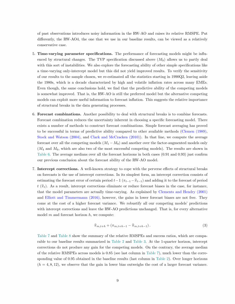
2. Across countries, the RW-AO model outperforms the rest of the models with statistically significant
gains for Mexico, Peru, and Hungary at almost every forecast horizon (Table 4). The case of Peru
is interesting because of the minuscule relative RMSPEs for most of the alternative models except
the TVP. It is worth recalling that the Peruvian is the only economy in our sample that faced a
hyperinflationary episode in the period under study (as illustrated in Table 1.B). Regarding the rest of
countries, the statistical differences over the rest of the competing models are also notable for Colombia,
Nigeria, and Philippines (especially at 4- and 8-quarter horizons). In the rest of the sample, the RW-
AO’s performance is relatively reasonable with the exceptions of China, Malaysia, Thailand (1-quarter
horizon), and South Africa (1-, 8-, 12-quarter horizons).
3. Considering all the forecast horizons and countries, the RW-AO outperforms– or at least shows similar
predictive ability to– univariate and multivariate factor-augmented models (M4, M6) in forecasting
the inflation rate among EMEs. In terms of directional accuracy, the RW-AO seems to be better or
as competitive as those models as well. In Table 5, we sort the alternative models per the number
of countries in which the relative RMSPE of the RW-AO is lower than one, but considering only the
statistically significant cases. Factor-augmented models show up at the top of the list which suggests
they could constitute a reasonable second-best alternative. The models more frequently beaten by the
RW-AO are the DAR4 (M3), the Augmented Phillips Curve (M5), and the BVAR4 (M7). The RW-AO
model also clearly dominates all its competitors in terms of directional accuracy (see average medians
over all horizons in Table 3).
4. The time-varying parameter (TVP) specification (M9) allows us to partly address the concern that
the performance of alternative forecasting models might be influenced by structural change over the
sample period. Our results generally show that the RW-AO specification tends to outperform model
M9, suggesting that such a type of parameter instability may not be the only reason explaining the
success of the RW-AO model among EMEs.
5. We also learn that there are certain international macro variables that do not contribute (or at least
do not contribute much) to predicting inflation among EMEs such as:8 (i) the exchange rate (unlike instudies such as Kabukcuoglu and Martínez-García (2016) that find some predictive power for advanced
economies), but more in line with the findings of Frankel et al. (2012) who show that EMEs have
experienced a downward trending pass-through since the 1990s;9 (ii) global factors (in contrast to what
7The RW-AO often does better at long horizons rather than at the very short one (h = 1).8We have also considered different specifications of Phillips-curve-based models like the NOEM-BVAR proposed by Duncan
and Martínez-García (2015). Our findings with this alternative specification do not overturn the main results in support ofthe RW-AO model among EMEs. The NOEM-BVAR results are not reported here, but are available upon request from theauthors.
9Fluctuations in the exchange rate can affect inflation through direct and indirect channels. The direct effect arises from
7

Ciccarelli and Mojon (2010) and Duncan and Martínez-García (2015) find for advanced economies);
and (iii) commodities prices (as argued by Chen et al. (2014)).
3.2 Robustness Checks and Other Exercises
We perform a number of robustness checks, whose results are available upon request, as well as forecast
combinations and intercept corrections. Some conclusions from such analysis are worth mentioning here:
1. Among the Factor Augmented (M4,M6) and Augmented Phillips Curve (M5) models, we also evaluate
some alternatives modeling the first difference of the inflation rate without obtaining superior results.
The lack of complete data on monetary aggregates for most of the EMEs prevents us from testing
Phillips Curve specifications with money components on a comparable footing. The use of GDP
instead of the industrial production indexes leads to similar statistics for the Augmented Phillips Curve
(M5) models. Open-economy Phillips-Curve-based specifications like the ones proposed in Duncan and
Martínez-García (2015) for advanced economies do not appear to perform all that much better than
the RW-AO among EMEs either.
2. We have checked the BVAR forecasts using normal-flat priors. Overall, the results are qualita-
tively similar or moderately better with Minnesota priors. Additionally, we use alternative vectors:
(πt, π∗t , yt, y
∗t )′, (πt, yt, et)
′, and (πt, y∗t , et)
′, where ∗ denotes rest-of-the-world (advanced economies)values. However, we did not obtain any noticeable improvement in predictive ability with those alter-
native vectors of variables.
3. The RW-AO model usually outperforms the naïve random-walk specification, with or without drift, in
our sample.10
4. Different RW-AO specifications. We vary the degree of smoothing of the RW-AO model by
increasing the number of observations into the moving average. Aside from our baseline RW-AO
model with 4 lags used in our main results, we introduce three additional variants that include 8, 12,
and 16 past values of the inflation rate. That is, the forecasting functions are
πt+h =1
q
∑q
i=1πt+1−i + εt+h, (2)
with q = 4, 8, 12, 16. We label them RW-AO4 (or simply RW-AO), RW-AO8, RW-AO12, and RW-
AO16, respectively. We repeat the baseline exercise using the direct method and calculating the
RMSPEs. Figure 3 shows the averages of the median ratios of RMSPE of each RW-AO model relative
to the RMSPE of a competing forecasting model calculated over the 14 EMEs and the 9 competing
models for a given forecast horizon. Again, values less than one indicate a higher predictive ability
for the RW-AO compared to the alternative model. We find that the RW-AO8 minimizes the relative
RMSPE, on average, and provides a suitable degree of smoothing. As Figure 3 shows, a higher number
pass-through into import prices. The indirect effect occurs because real exchange rate movements contribute to shift aggregatedemand across countries.10We refer to the naïve random-walk specification without drift as a special case of the general-form of the RW-AO model
in (2) where only the first lag is included (q = 1). We introduce the case of the naïve random-walk with drift by adding aconstant.
8
of past observations introduces noisy information in the RW-AO and raises its relative RMSPE. Put
differently, the RW-AO4, the one that we use in our baseline results, can be viewed as a relatively
conservative case.
5. Time-varying parameter specifications. The performance of forecasting models might be influ-enced by structural changes. The TVP specification discussed above (M9) allows us to partly deal
with this sort of instabilities. We also explore the forecasting ability of other simple specifications like
a time-varying only-intercept model but this did not yield improved results. To verify the sensitivity
of our results to the sample chosen, we re-estimated all the statistics starting in 1990Q2, leaving aside
the 1980s, which is a decade characterized by high and volatile inflation rates across many EMEs.
Even though, the same conclusions hold, we find that the predictive ability of the competing models
is somewhat improved. That is, the RW-AO is still the preferred model but the alternative competing
models can exploit more useful information to forecast inflation. This suggests the relative importance
of structural breaks in the data generating processes.
6. Forecast combinations. Another possibility to deal with structural breaks is to combine forecasts.Forecast combination reduces the uncertainty inherent in choosing a specific forecasting model. There
exists a number of methods to construct forecast combinations. Simple forecast averaging has proved
to be successful in terms of predictive ability compared to other available methods (Clemen (1989),
Stock and Watson (2004), and Clark and McCracken (2010)). In that line, we compute the average
forecast over all the competing models (M1−M9) and another over the factor-augmented models only
(M4 and M6, which are also two of the most successful competing models). The results are shown in
Table 6. The average medians over all the forecast horizons in both cases (0.91 and 0.93) just confirm
our previous conclusion about the forecast ability of the RW-AO model.
7. Intercept corrections. A well-known strategy to cope with the perverse effects of structural breakson forecasts is the use of intercept corrections. In its simplest form, an intercept correction consists of
estimating the forecast error of certain period t−1 (πt−1− πt−1) and adding it to the forecast of periodt (πt). As a result, intercept corrections eliminate or reduce forecast biases in the case, for instance,
that the model parameters are actually time-varying. As explained by Clements and Hendry (2001)
and Elliott and Timmermann (2016), however, the gains in lower forecast biases are not free. They
come at the cost of a higher forecast variance. We robustify all our competing models’predictions
with intercept corrections and leave the RW-AO predictions unchanged. That is, for every alternative
model m and forecast horizon h, we compute:
πm,t+h + (πm,t+h−1 − πm,t+h−1) . (3)
Table 7 and Table 8 show the summary of the relative RMSPEs and success ratios, which are compa-
rable to our baseline results summarized in Table 2 and Table 3. At the 1-quarter horizon, intercept
corrections do not produce any gain for the competing models. On the contrary, the average median
of the relative RMSPEs across models is 0.85 (see last column in Table 7), much lower than the corre-
sponding value of 0.95 obtained in the baseline results (last column in Table 2). Over longer horizons
(h = 4, 8, 12), we observe that the gain in lower bias outweighs the cost of a larger forecast variance.
9

The largest improvement, from 0.75 (baseline) to 0.85 (Table 7), is observed at the 12-quarter hori-
zon. This outcome favors the alternative models, but it does not seem to be suffi cient to prefer them
over the RW-AO. Table 8 shows an analogous story. The average of the median success ratio of the
competing models falls at the 1-quarter horizon but improves at longer forecast horizons. The median
success ratio averaged over all the horizons and the nine robustified models is 0.63 (see last column,
last row in Table 8) and very close to the value produced by the RW-AO (0.65). In sum, we notice that
intercept-corrected models yield some but not substantial gains in predictive ability thanks to lower
forecast biases.
8. Different transformation of the target variable. Overall, the findings are robust to the transfor-mation of the target variable. In addition to the exact quarter-over-quarter inflation rate annualized
used in the baseline exercises (πt; as in (1)), we construct the approximate quarter-over-quarter inflation
rate annualized in logs (πa,qoq), the exact year-over-year inflation rate (πe,yoyt ), and the approximate
year-over-year inflation rate in logs (πa,yoy; as in Atkeson and Ohanian (2001)):
πa,qoqt ≡ 400
[ln
(CPItCPIt−1
)], (4)
πe,yoyt ≡ 100
[(CPItCPIt−4
)− 1
], (5)
πa,yoyt ≡ 100
[ln
(CPItCPIt−4
)]. (6)
Table 9 shows the averages of the median ratios of the RMSPE of each RW-AO model relative to
the RMSPE of a competing forecasting model calculated over the 14 EMEs and the 9 competing
models for a given forecast horizon. On average, the use of approximate inflation rates tends to
benefit the competitive models relative to the RW-AO more than the use of exact inflation rates.
This difference becomes more noteworthy for year-over-year rates. Logged CPI series smooth sharp
fluctuations observed in EMEs and the smoothing turns stronger for the fourth difference filter. The
predictive ability of the RW-AO model relative to its competitors remains, especially at 4-, 8-, and
12-quarter horizons.
9. Another test for differences in predictive ability.11 We estimate an only-intercept model for
each of the 14 EMEs using SUR-GLS, where the dependent variable is the difference between the
squared forecast error of an alternative model and the squared forecast error of the RW-AO model.
A rolling-window estimation using a width of 75 observations generates the forecasts. Hence, this
can be viewed as a type of Giacomini and White (2006) test in which we address the cross-sectional
dependence by using SUR-GLS. We choose the three most competitive models according to Table 5:
M4 (FAR), M6 (BVAR2), and M8 (BVAR2). Table 10 reports the results and statistics. A positive
(negative) intercept indicates that the RW-AO model shows higher (lower) predictive ability than does
the alternative model. The null hypothesis is that all the constants are jointly equal to zero. That
is, for a given forecast horizon and alternative model, we evaluate the equal predictive ability across
countries. We mostly reject the null hypothesis. We conclude that the RW-AO beats those three
competing models at the 4-, 8-, and 12-quarter horizons, but not at the 1-quarter horizon.11We thank an anonymous reviewer for suggesting this to us.
10

10. Conditional predictability. We find similar performance of the RW-AO model in EMEs as for
developed economies. We use the conditional predictability test by Giacomini and White (2006) to
explore differences in predictability among EMEs relative to the U.S. (where the U.S. is viewed as
representative of the advanced economies). For each country (including the U.S.) and each forecast
horizon, we generate forecasts from a rolling-window estimation using a width of 75 observations and
construct the difference, dt, between the squared forecast error of an alternative model i (e2i,t) and the
squared forecast error of the RW-AO model (e2RW−AO,t). We regress that indicator on its first two lags
(dt−1, dt−2), a measure of the GDP cycle (yt; the year-over-year growth rate of GDP), and a proxy of
a high-inflationary regime (ht; an indicator function that takes the value of 1 if the current inflation
rate is higher than the median inflation rate, 5% approximately, and 0 otherwise). That is, for each
economy we estimate
dt = α0 + α1dt−1 + α2dt−2 + α3yt + α4ht + εt (7)
where dt ≡ e2i,t − e2RW−AO,t for i = {M4,M6,M8}. Again, we focus on three of the most competitivemodels (FAR, BVAR2, and BVAR2). Table 11 reports the p-values associated with the joint null
hypothesis that all non-intercept coeffi cients are zero (α1 = α2 = α3 = α4 = 0) and the percentage
of economies in which we reject the null hypothesis at 10% using a Wald test. We reject the null
hypothesis for the U.S. and most of the EMEs. Our interpretation is that the U.S. and many EMEs in
our sample are not very different in terms of this sort of conditional predictability. Past predictability,
the business cycle and the high- or low-inflationary regime seem to be statistically related to the current
predictability of the best competing models relative to the RW-AO.
4 Discussion
4.1 Policy Implications
There are a number of insights and policy recommendations that arise from our empirical results on inflation
forecasting for EMEs:
First, since monetary policy transmission is associated with significant lags, optimal policy needs to be
forward-looking which underscores the importance of obtaining accurate forecasts. The central banks among
many EMEs seem to be making an important omission for inflation forecasting by setting aside the model
proposed by Atkeson and Ohanian (2001). In fact, no variant of the RW-AO model is mentioned in the
survey of forecasting methods for inflation-targeting central banks reported by Hammond (2012). However,
as we show in the paper, the RW-AO specification has excellent predictive power, especially in the medium
and long term (h > 1) and, therefore, we argue that it should be part of the forecasting toolbox when it
comes to predicting inflation in those economies as well as for policy analysis.
Second, most of the studies that investigate how to better predict inflation in EMEs have virtually
ignored the RW-AO model specification. The exceptions being Ögünç et al. (2013) and Altug and Çakmakli
(2016), but they look at one or two country experiences and often do not find strong evidence in favor of
the RW-AO model. Our empirical results, in turn, would lead us to recommend the RW-AO specification
as an additional benchmark to those already commonly used in the literature (standard random walk,
autoregressive processes, etc.). We believe this new benchmark is a harder yardstick to overcome for any
11

proposed model of inflation forecasting for EMEs.
Third, we argue that parameter instability and model misspecification can contribute to explain the
relative failure of competing economic models for the forecasting of inflation among EMEs. The challenge
is to find a general framework for forecasting where the model structure and even the presence and type of
structural change are all unknown and may vary both within the estimation sample and over the forecast
period. In this vein, Rossi (2012) argued that widespread forecast breakdowns make it all the more pressing
to develop robust forecasting models.12 Instead of attempting to identify such breaks (which is hardly an easy
task in the presence of recent and ongoing structural change), break-robust adaptive forecasting strategies
have been studied by Pesaran and Pick (2009), Eklund et al. (2013), and Giraitis et al. (2013), among
others, which downweight data from older periods deemed to be less relevant to predict the current dynamic
behavior of the variable of interest.
Finally, we argue that understanding the dynamics of inflation requires a deeper exploration of the
reasons why existing economic models appear to perform so poorly for the forecast of inflation in economies
such as those of EMEs. As noted before, model misspecification, parameter instability, and even sampling
error can contribute to the poor forecasting performance of most of the existing economic models. Future
research along these lines can lead in our view to a better understanding of the inflation process and to the
development of novel approaches to resolve this apparent empirical puzzle. We emphasize here, instead, the
key idea that simpler adaptive strategies like the RW-AO model can be preferable in practice as they are
robust to many different forms of misspecification and structural breaks.13
4.2 Structural Breaks
The key implications of our analysis on inflation forecasting among EMEs shed some light on adaptive
forecasting with parameter instability and potential misspecification and can be summarized as follows:
• Intercept corrections. Our results with model predictions enhanced by intercept corrections suggestthat structural breaks might be playing a role, although partial, in the relative failure of the competing
models. When we include intercept corrections, we observe a clear gain due to the lower bias reflected
especially in increased directional accuracy.
• Forecast combination. We observe that the predictability of inflation models changes over time.Subsampling appears to be useful in practice to deal with the possibility of unobserved structural breaks
and unmodelled (time-varying) features in forecasting inflation. As mentioned in Section 3.2, when we
leave aside the 1980s, a decade characterized by high and volatile inflation rates across many EMEs,
we still find robust support for the RW-AO specification, but find that the predictive ability of the
12 Interestingly, this is related to other areas of empirical forecasting such as the Meese-Rogoff puzzle on exchange ratepredictability. In assessing the success of the standard random walk model to predict the exchange rate, Meese and Rogoff(1983a), Meese and Rogoff (1983b) conjectured that model misspecification, parameter instabilities, and even small sampleestimation bias could potentially explain the poor forecasting performance of economic models of the exchange rate (a pointdiscussed more recently in Bacchetta et al. (2009) and Rossi (2013)). The Meese-Rogoff literature has also postulated thatnear-random walk behavior may emerge naturally whenever the fundamentals are I (1) and the discount factor is near one(Engel and West (2005)).13More generally, appropriately downweighting the past– as the RW-AO model does– can be a robust strategy for handling
trends of any nature as well as structural breaks without requiring further modeling. Giraitis et al. (2013) show that such anadaptive approach generally works well for stochastic, linear or nonlinear deterministic trends, and structural breaks withoutknowledge of the nature of the trend. This approach also continues to be valid whether the time series is stationary ornon-stationary.
12

competing models is somewhat improved. An alternative to dealing with this can be achieved through
forecast combination, which we explore in this paper. Our results largely confirm the finding that the
RW-AO model tends to outperform many competing economic models and the forecast combination
that can be obtained from them, which perform well only occasionally. Also, what our exercise with
forecast combination might be suggesting is, again, that we are dealing with important parameter
instabilities.
• Time-varying specifications. A time-varying parameter (TVP) specification (M9, motivated by
the empirical work of Mandalinci (2017)) can also partly address the concern that the performance
of our alternative forecasting models might be influenced by structural change over the sample period
under consideration, although our results show that the RW-AO specification still tends to outperform
the TVP model. In other words, the evidence suggests that parameter instability, as modelled by the
proposed TVP specification, may account only in part for the success of the RW-AO model among
EMEs. A puzzling result arises here whereby the TVP model specification does not appear very
successful in improving our predictive ability for inflation forecasting among EMEs. In our view, the
proposed TVP specification does not fully capture the effect of structural change in forecasting across
EMEs, perhaps for at least two reasons. One reason is that there are many non-linear functional forms,
many forms of structural breaks (in intercepts, slopes, and variances), and that breaks can be of different
magnitudes (some relevant, some not), discrete and continuous, occurring within the estimation period
and within the prediction period, etc. All of this makes it challenging to model them in the estimation
within the sample. Another reason is that there are different prediction methods with nonlinear models
such as TVP for horizons greater than a period. We use the direct method for the TVP to be consistent
with the other models, but there are also methods that use Monte Carlo simulations or bootstrapping
that could be used and would give less bias than the direct method (Granger and Terasvirta (1993)).
In any event, all of this implies that the forecaster should be monitoring for changes in the specification
(including breaks) by country and adjusting his/her methods once change has been detected. Since
detecting shifts often involves a substantial time lag and comes at a cost in terms of modeling effort,
our evidence favoring the RW-AO specification suggests a simpler (less costly) alternative that is
robust across many different country experiences among EMEs and sample periods. In other words,
we show that forecasters can be quite successful– without attempting to identify breaks– simply using
break-robust forecasting strategies like the RW-AO model.
• Role of judgment. We compare the RW-AO forecasts to the professional forecasts obtained from
Consensus ForecastsTM to assess the significance of subjective judgement over simple break-robust
strategies like the RW-AO model. The Consensus ForecastsTM data we use covers the period 2006Q4-
2016Q4 for 12 of the 14 EMEs in our sample– predictions for Nigeria and South Africa are not avail-
able.14 These are average predictions of a panel of professional forecasters for each country that produce
14Forecasts start in 2006Q4 for China, India, Indonesia, Malaysia, and Thailand; in 2007Q1 for Chile, Colombia, Hungary,Mexico, Peru, and Turkey; and in 2009Q3 for Phillipines. Our approach to calculate the implicit forecasts for the quarter-over-quarter growth rates (SAAR, %) involves: first, transforming the forecasts for the reported year-over-year exact growth
rates (SA, %) into their corresponding log-approximations (πa,yoyt = 100[ln(1 +
πe,yoyt100
)]); second, using the additivity of
the log-approximation to the year-over-year growth rate (πa,yoyt = 14
(πa,qoqt + πa,qoqt−1 + πa,qoqt−2 + πa,qoqt−3
)), we infer the log-
approximation of the quarter-over-quarter growth rate for any forecasting horizon h ≥ 0 (πa,qoqt+h ) netting out the known (eitherdirectly observed date or recursively implied forecasts) log-approximation of the quarter-over-quarter growth rates over the
13

quarterly forecasts of year-over-year growth rates (these quarterly forecasts are regularly released at a
quarterly frequency for Indonesia, Philippines, India, China, Thailand, and Malaysia and bi-annually
for Mexico, Peru, Hungary, Colombia, Turkey, and Chile). These forecasts on the inflation rate in the
current quarter relative to the same quarter of last year can be used together with the observed data to
infer the quarter-over-quarter annualized inflation rates implicit in Consensus ForecastsTM predictions.
To the best of our knowledge, this is the first paper to employ the quarterly forecasts from Consensus
ForecastsTM among EMEs to investigate their predictive ability. Our main findings are summarized in
Table 12 which shows that professional forecasts tend to be superior to RW-AO-based forecasts for the
majority of EMEs. However, the RW-AO remains competitive when forecasting quarter-over-quarter
growth rates (particularly at shorter horizons).15 These findings suggest that the incorporation of
subjective judgement and perhaps the use of other ancillary sources beyond what a given model would
rely on in order to identify structural shifts can improve inflation forecasts relative to our preferred
benchmark (outperforming the RW-AO forecasts).16
4.3 The Role of Central Bank’s Credibility
The success of the RW-AO model arises in practice from the diffi culties of incorporating all the relevant
features of the economy in a forecasting model while tracking changes over time. For instance, we know
that we may have more or less persistence in inflation with Phillips-curve-based models when heterogenous
beliefs and imperfect credibility about the inflation target are considered. We provide a more detailed
theoretical argument for this in the Appendix based on a modified version of the workhorse open-economy
New Keynesian model. We see this modification of the model as providing some contextualization for the
claim that the current crop of economic forecasting models– more specifically, those based on the Phillips
curve– might be misspecified for the case of EMEs and subject to structural shifts like those affecting central
bank’s credibility.
This theoretical framework accommodates the possibility of change or instability in parameters more
broadly. For instance, we could consider that it is the changes in the credibility parameter and/or the central
bank’s time-varying (explicit or implicit) inflation target, which generally are diffi cult to observe and measure
but appear plausibly time-varying for EMEs, what lies behind model instability and misspecification. This,
in turn, is what may explain the relatively poor performance of economic models compared to the RW-AO
model.
In Section 3, we point out that the RW-AO model outperforms the rest of the competing models especially
in economies such as Hungary, Mexico, and Peru at almost every forecast horizon (Table 4). In contrast,
preceding three quarters from the forecasts of the log-approximated year-over-year growth rate (πa,qoqt+h = 4πa,yoyt+h − πa,qoqt+h−1 −πa,qoqt+h−2−π
a,qoqt+h−3); finally, we recover the implicit forecasts of the exact quarter-over-quarter growth rates (SAAR, %) from the
derived log-approximation (πt = 100[(exp
(πa,qoqt100
))4− 1]). We use these implicit forecasts in our evaluation exercise here.
15 In terms of directional accuracy, we find somewhat stronger support for the RW-AO model against Consensus ForecastsTM .Similarly, we also explore the predictive ability of the RW-AO model with annual inflation rates compared to that of both privateforecasts from Consensus ForecastsTM and institutional forecasts from the International Monetary Fund’s World EconomicOutlook (IMF WEO) database. Results are available from the authors upon request– a summary of those findings can befound in the Supplemental Appendix of this paper.16Faust and Wright (2013) suggest that subjective forecasts are often superior to model-based forecasts for inflation among
advanced economies. Related to this point, see also Mandalinci (2017) who finds institutional forecasts to be superior to model-based forecasts for many EMEs (where his institutional forecasts are from the International Monetary Fund’s World EconomicOutlook (IMF-WEO)).
14

the RW-AO predictor does not produce such an outstanding performance in countries like Malaysia, South
Africa, and Thailand. We explore the reason suggested in the theory laid out in the Appendix with the
aid of Figure 4. This figure plots the average of the ratios of RMSPEs of the RW-AO model relative to
the competing models in the vertical axes. This average is calculated over the 9 alternative models and the
4 forecast horizons for each economy. On the horizontal axes, we measure four different proxies of lack of
credibility in the monetary policy.
We plot the average relative RMSPE against: the number of years under an inflation targeting scheme
(Figure 4A; based on information from Roger (2010) and Hammond (2012)), an index of central bank inde-
pendence (Figure 4B; using the index proposed by Garriga (2016)17), the median inflation rate computed
over annualized quarter-over-quarter inflation rates between 1980Q2 and 1989Q4 (Figure 4C), and the coef-
ficient of variation of the annualized quarter-over-quarter inflation rates calculated over the 1980Q2-1989Q4
period as well (Figure 4D).
The lack of credibility in the central bank’s policies during the 1980s is reflected in high inflation levels
and highly volatile inflation rates. Likewise, the poor credibility in the past has probably induced central
banks to adopt, sooner or later, institutional changes such as inflation-targeting schemes or statutory im-
provements that seek independence from central governments or other external influences. In the absence
of accurate indicators, these variables relating to the adoption of an inflation-targeting and gains in central
bank independence work as imperfect measures of lack of credibility. Our interpretation is that the higher
the values of any of these proxies, the lower the degree of credibility in the central bank’s monetary policy.
Given this and the period we study here, the low credibility in the past might be what prompts the adoption
of inflation targeting or greater central bank independence aimed at improving the central bank’s credibility.
Figure 4 provides the sign of the correlations between these proxies for past credibility and the forecasting
performance of the RW-AO model, and the corresponding p-values. Even though there are some influential
observations and the sample size is small, the relationships depicted are suggestive and consistent with the
implications of the theoretical model we discuss in the Appendix. The predictive ability that the RW-AO
offers relative to its competitors is better in economies that experienced low credibility in the past. This
is the case of Peru, Mexico, and Hungary, which ranked at the top of Table 4. These economies tend to
appear with relatively high values for our proxies of lack of policy credibility. The opposite is observed for
Malaysia, South Africa, and Thailand. These countries usually appear in the upper left corner of the scatter
plots, indicating relatively high credibility jointly with low relative predictive ability of the RW-AO model.
In sum, this piece of evidence supports the idea that the lack of credibility might be behind the relative
success of the RW-AO in some countries compared to others.
Finally, we show in the Appendix that structural breaks can arise in theory from changes in the credibility
of the central bank’s inflation target or from shifts in the inflation target itself. The limitations to measure
the policy credibility and implicit targets make the task of inflation forecasting in EMEs a challenging one.
Professional forecasters (Consensus ForecastsTM ) tend to produce lower or similar RMSPEs than the RW-AO
model suggesting that subjective judgement can improve over such break-robust forecasts by incorporating
ancillary information about– among other things– any significant structural shifts (in particular in the
monetary policy framework) quickly into their own predictions.
17Garriga (2016)’s dataset codes all relevant statutory reforms affecting central bank independence. The data indicate theoccurence of central bank reforms, their direction, and also incorporate all the attributes necessary to build the well-knownCukierman et al. (1992) index for 182 countries between 1970 and 2012.
15

5 Concluding Remarks
Our empirical findings, based on a varied cross-section of country experiences among EMEs, show that a
parsimonious forecasting model of inflation (the RW-AO model) outperforms other forecasting models of
inflation. Overall, the RW-AO model mostly produces lower RMSPEs than its competitors and success
ratios generally above the 0.5 threshold at any forecast horizon and, often, they are statistically significant.
We view the RW-AO specification as an important empirical benchmark for forecasting inflation across
a diverse group of EMEs. Among the competing models beaten by the RW-AO, univariate and multivariate
factor-augmented models can be regarded as second-best options under the same metrics of predictive accu-
racy. We find that certain variables driven by foreign factors such as exchange rates and commodity prices
do not seem to contribute much to predict inflation in the small open economies of our sample.
The time-varying parameter specification allows us to partly address the concern that the performance of
alternative forecasting models might be influenced by structural change or time-varying parameters (like the
inflation target) over the sample period. Our results generally show that the RW-AO specification tends to
outperform the time-varying specification as well, indicating that such a type of parameter instability may
not be the only reason explaining the success of the RW-AO model among EMEs.
Finally, our findings motivate us to look for alternative ways to model inflation among EMEs. We suggest
that understanding the process that leads to the formation of expectations and the appropriate conduct of
monetary policy under different credibility scenarios can be important. Incorporating inflation expectations
explicitly into our forecasting models is therefore a promising research avenue which– although complicated
due to data availability– we aim to investigate further in the future. Even more, if we consider the favorable
results from comparing the subjective predictions from Consensus ForecastsTM with those from the RW-AO
model.
Under lack of credibility in the inflation target, a Phillips curve can imply inflation dynamics that produce
permanent (or near-permanent) effects in the inflation rate from otherwise transitory changes in output slack
that resemble those observed in many EMEs during the 1980s and part of the 1990s. The gradual recovery of
the confidence on the central bank’s policies and its commitment with an inflation target lead to stationary
processes that probably are more similar to those that work better from the late 1990s on. The inability
of the forecaster to observe sudden shifts in credibility or frequent changes in the implicit target makes the
empirical modeling and forecasting of inflation a diffi cult task, particularly among EMEs. We leave this task
also for future research.
16

Appendix
A Phillips-Curve-Based Models: A Closer Inspection
The influential work of Atkeson and Ohanian (2001) documents a break in the performance of Phillips-
curve-based forecasting models during the Great Moderation period. These authors suggest the RW-AO
model as an alternative (theory-agnostic) forecasting benchmark and find evidence that it outperforms
standard Phillips-curve-based specification. In this sense, the empirical Phillips curve relationship between
domestic inflation and domestic economic activity no longer seems to work as a tool for inflation forecasting.
More recently, Duncan and Martínez-García (2015) have argued that the closed-economy Phillips curve has
limited value for forecasting inflation partly due to misspecification, as it ignores the international linkages
affecting the dynamics of inflation. Furthermore, they show that open-economy Phillips curve-based models
can describe domestic inflation dynamics more accurately– a finding that appears ubiquitous across many
developed economies. The Phillips curve appears to be alive and well– albeit in its open-economy form.
The main empirical finding of this paper is to show that the RW-AO model appears as the more relevant
benchmark for inflation forecasting for many EMEs. We argue that the RW-AO is successful because is a
method to downweight past data, which is a good strategy when there are instabilities/structural breaks. We
argue that the open-economy Phillips curve that emerges from the workhorse two-country New Keynesian
model is still helpful to understand the dynamics of inflation and that, in principle, it also aids us to think
about the potential factors explaining the empirical evidence of parameter instability on EMEs documented
in this paper. We argue that unmodelled parameter instability in the open-economy Phillips curve (time-
varying inflation targets) as well as some restrictive assumptions underlying the conventional specification
of the New Keynesian model are challenged by the experience of many EMEs in our sample. This can
partly explain why simpler, break-robust forecasting models like the RW-AO predictor outperform other
more complex (model-based) alternatives.
The reminder of this Appendix articulates this point introducing explicitly a time-varying inflation target
and highlighting the significance of assumptions like full rational expectations (with homogenous beliefs) and
perfect credibility of the inflation target.
The Standard Open-Economy Phillips Curve. We adopt the workhorse open-economy New Keyne-
sian model of Martínez-García and Wynne (2010), further developed in Martínez-García (2017). The model
includes two countries which are symmetric, but with local-product bias in their respective consumption
baskets. The share of Foreign (Home) goods in the Home (Foreign) consumption basket given by the para-
meter 0 ≤ ξ ≤ 12 determines the degree of trade openness. All goods are traded internationally. We assume
for simplicity that the trade elasticity of substitution between Home and Foreign goods σ > 0 satisfies that
σγ = 1 where γ refers to the inverse of the intertemporal elasticity of substitution (this case implies that
international financial markets become irrelevant and has been considered by Cole and Obstfeld (1991),
among others).
Monetary non-neutrality arises from monopolistic competition and producer currency pricing under stag-
gered price-setting behavior à la Calvo (1983), as is conventional in the open-economy literature. We extend
17

the model of Martínez-García (2017) with Yun (1996)-price indexation where firms that do not re-optimize
their prices in a given period increase them at the trend inflation rate of the country where they sell their
variety. Furthermore, we assume that each country’s central bank responds to local conditions– that is, to
deviations of local inflation from target and to the country’s own slack– as implied by the Taylor (1993)
rule. The Home country’s monetary policy rule is
it ≈ πTt + ψπ
(πt − πTt
)+ ψxxt + ϑt, (8)
where the short-term nominal interest rate is given by it, inflation is πt ≡ pt − pt−1, the inflation target isdenoted πTt , and the output gap (actual output minus the output potential under flexible prices) is given
by xt. The policy response to inflation deviations from target is given by the parameter ψπ > 0 while the
response to slack is determined by ψx > 0.
We assume that central banks’adjust their policy rates to track changes in their country’s natural rate
of interest. Hence, we state– as most of the literature implicitly does– that ϑt ≡ rt + mt, where mt are
zero-mean (unanticipated) innovations on the stance of Home monetary policy. The central bank’s (time-
varying) inflation target, πTt , is assumed to follow a random walk– that is, πTt = πTt−1 + επt , where επt are
the corresponding zero-mean i.i.d. Home inflation target innovations. Similarly we describe the monetary
policy rule of the Foreign country.18
Under purely rational expectations, the inflation target set by the central bank anchors inflation expec-
tations in equilibrium whenever this target is perfectly credible. Then, the long-run trend inflation rate
prevailing in each country must be equal to the country’s inflation target set by their own central bank, i.e.,
πt must be equal to πTt (and similarly for the foreign country). To see this, we can interpret the long-run
trend inflation rate as the (stochastic) trend of the corresponding inflation process, i.e.,
πt = limh→∞
Et (πt+h) . (9)
The inflation rate πt fluctuates around the country’s stochastic inflation target, πTt , whenever credibly set
by the central bank.19 It follows that Et(πTt+h
)= πTt at any period h > 0 and as h goes to infinity. In that
sense, (9) implies that πt = πTt – hence validating the initial conjecture that the trend inflation and target
inflation must be the same in equilibrium (also noted in Woodford (2008)). The same logic applies to equate
the Foreign trend inflation and target inflation rates.
The open-economy Phillips curve for the Home country can be written for inflation in deviations from
18The assumption is that Home and Foreign monetary policy shocks can be described as in Martínez-García (2017), i.e.,(mtm∗t
)≈(
δm 00 δm
)(mt−1m∗t−1
)+
(εmtεm∗t
),(
εmtεm∗t
)∼ N
((00
),
(σ2m ρm,m∗σ2m
ρm,m∗σ2m σ2m
)).
For the inflation target innovations, we simply assume that(επtεπ∗t
)∼ N
((00
),
(σ2π 00 σ2π
)).
19The inflation target is explicitly announced under an inflation-targeting regime, which is the prevailing framework for mon-etary policy among many of the EMEs in our sample (Hammond (2012)). However, a target for inflation can be communicated(implicitly or explicitly) to the public even without the trappings of inflation-targeting as it happens for some of the EMEs inour sample.
18

the inflation target directly (i.e., πt − πTt ) in the following form (Martínez-García (2017)):
πt − πTt ≈ βEt(πt+1 − πTt+1
)+ k
[xWt + vt
], (10)
where xt = yt − yt and x∗t = y∗t − y∗t define the Home and Foreign slack– that is, the deviations of out-
put, yt and y∗t respectively, from output potential under flexible prices and perfect competition, yt and y∗t
respectively– and xWt ≡ (1− ξ) xt + ξx∗t is the corresponding trade-weighted measure of global slack. Here
trade weights are determined by the share of imported goods in the consumption basket 0 ≤ ξ ≤ 12 .20 An
analogous expression can be derived for the Foreign country.
As in Kabukcuoglu and Martínez-García (2018), we abstract from the changes in the Phillips curve
functional form arising when the Calvo (1983) pricing equation is log-linearized around a non-zero inflation
rate (discussed elsewhere by Ascari (2004) and Sahuc (2006)). The intertemporal discount factor is 0 < β < 1,
while the composite coeffi cient k ≡((1−α)(1−βα)
α
)(ϕ+ γ) is the slope of the Phillips curve which depends on
the Calvo price stickiness parameter 0 < α < 1, the inverse of the Frisch elasticity of labor supply ϕ > 0, and
the intertemporal elasticity of substitution, γ > 0. The term vt captures other transient factors and shocks to
the open-economy Phillips curve such as cost-push shocks. The structure of the workhorse two-country New
Keynesian model is then completed with an open-economy investment-savings (IS) curve for each country
(see, e.g., the derivation in Martínez-García (2017)).
This log-linear system characterizes the dynamics of output, inflation, and the short-term nominal interest
rate around the steady state for the Home and Foreign economies. Hence, a straightforward forecasting model
based on full rationality and perfect credibility for(πt − πTt , yt, π
∗t − π
T∗t , y∗t
)can be characterized in VAR
form and suffi ces to effi ciently forecast the cyclical component of inflation, πt − πTt , among most advancedeconomies– as shown in the related work of Duncan and Martínez-García (2015).
Whenever we abstract from vt in the specification of the open-economy Phillips curve (i.e., in equation
(10)), a straightforward representation of the cyclical component of inflation arises that depends solely on
monetary shocks. We retain the assumption that (mt, m∗t ) follows a random bivariate process that captures
possibly-persistent and unanticipated shocks to monetary policy in both countries and, hence, whenever a
solution exists and is unique, the characterization of inflation for the Home country implied by the results
of Martínez-García (2017) can be expressed in the following terms,
πt = πTt +k
1− βδmxWt , (11)
where,
πTt = πTt−1 + επt , επt ∼ N
(0, σ2π
), (12)
xWt = δmxWt−1 + ηWt , η
Wt ∼ N
(0, σ2W
), (13)
where σ2W is a composite coeffi cient that depends on the parameters for the exogenous monetary shock
process as well as on deep structural parameters of the model.
20This specification can also be recast in terms of domestic slack (xt) and the real exchange rate gap, as explained in Martínez-García and Wynne (2010). That transformation is used for inflation forecasting by Kabukcuoglu and Martínez-García (2016),among others, and also motivates the APC (M5) and BVAR4 (M7) specifications of our empirical work.
19

If we assume (time-varying) stochastic volatility for σ2π and σ2W , this simple representation of the solution
is in line with the unobserved components model of inflation with stochastic volatility (UC-SV) proposed by
Stock and Watson (2007) albeit with a more general autoregressive specification for the cyclical component
(given by k1−βδm x
Wt ). Whenever we assume a constant inflation target (i.e., whenever σ
2π = 0), this solution
reduces to the autoregressive specification RAR (M1) and to related specifications such as DAR and DAR4
(M2 and M3). The solution in (11) is also related to the more general TVP representation allowing for
the coeffi cients to vary over time (M9). The TVP representation is more flexible and permits a random
walk (RW) for the inflation target (πTt ) as well as exogenous structural shifts (partly on account of greater
opennes (globalization)). In order to capture more general dynamics closer in spirit to the general solution
postulated by Duncan and Martínez-García (2015), we analyze the specifications in M4 − M8 with the
addition of additional economic regressors for forecasting motivated by the New Keynesian model.
Imperfect Credibility and Deviations from Rational Expectations. As shown in (10), standard
open-economy Phillips curve-based models treat the cyclical component of inflation (inflation in deviations
from its target) as determined by three factors: expected inflation, global slack, and structural shocks that
exogenously shift the open-economy Phillips curve. We should note that even though the inflation process
may be decoupled effectively into two components (a random walk inflation target plus a stationary cyclical
component) as suggested by equation (11), such a model solution is hard to use to predict inflation among
emerging economies. This is the case because: (a) the inflation target is diffi cult to observe and diffi cult
to estimate (due to, among other reasons, the fact that inflation targets are sometimes implicit); and (b)
credibility plays also a role and its changes are hard to identify and quantify.
Well-anchored inflation expectations are thought to be a reflection of credible monetary policy. In that
sense, an important departure from that benchmark of credible monetary policies which underlies the inflation
solution in (11) is to consider the role of imperfect credibility on the inflation target as a potential source of
misspecification. While rational (forward-looking) expectations remain predominant in the New Keynesian
literature (with only limited attention being paid to surveys of inflation forecasts for EMEs due to data
availability), we argue that the mechanism for the formation of expectations should receive more attention.
Hence, we allow for deviations from rational expectations as well– using the conventional form of adaptive
expectations.
We argue that deviations from fully rational expectations together with imperfect credibility of the
monetary policy play an important role in bringing the predictions of the open-economy New Keynesian
model closer to the empirical findings among EMEs. Under lack of credibility in the inflation target, a
Phillips-curve-based model can imply inflation dynamics that produce permanent (or near-permanent) effects
in the inflation rate from otherwise transitory changes in output slack– inflation patterns that resemble those
observed in many EMEs during the 1980s and part of the 1990s. The improved confidence on the central
bank’s policies and its commitments under explicit or implicit policy frameworks for inflation targeting lead
to stationary processes that probably are more similar to those given by (11) that appear to work better
from the late 1990s on.
Hence, a departure from the standard open-economy New Keynesian model that introduces adaptive
expectations together with partial credibility (or imperfect credibility) of the central bank’s inflation target
can be both consistent with the open-economy Phillips curve and with our evidence suggesting that near-
random walk models like the RW-AO can be better suited to forecast inflation among many EMEs. For
20

tractability, let us also suppose that the central bank’s inflation target is constant (i.e., σ2π = 0 and πTt = πT )
and that monetary shocks are i.i.d. (i.e., non-persistent with δm = 0). Then, the open-economy Phillips
curve in (10) can be re-written as follows:
πt − πT ≈ β[(
(1− θ) πqt−1 + θπT)− πT
]+ k
[xWt + vt
], (14)
where next period inflation expectations are based on a weighted average of past inflation and on the central
bank’s inflation target, i.e., Et (πt+1) = (1− θ) πqt−1 + θπT . The parameter 0 ≤ θ ≤ 1 in equation (14) is the
corresponding weight on the inflation target and (1− θ) the weight on past inflation. We introduce adaptiveexpectations with the average q−period inflation rate from t + 1 − q to t (πqt ) which can be written as π
qt
≈ 1q
∑q
j=1πt+1−j for some q ≥ 1. The timing of this moving average πqt−1 incorporated in the inflation
expectations for (14) corrects for the publication lags in the inflation data.
The parameter θ can be interpreted as a measure of the credibility of the central bank’s inflation target
with θ = 1 indicating full credibility of the target, θ = 0 representing the case of no credibility, and 0 < θ < 1
indicating partial credibility.21 The parameter θ can be more also defined as the fraction of agents that do
believe in the central bank’s inflation target while (1− θ) is the fraction of agents that do not find monetarypolicy credible and rely on adaptive expectations to form their predictions about future inflation. This
specification is related to a growing literature on the role of heterogenous beliefs in the New Keynesian
model (Lansing (2009), Assenza et al. (2013), Di Bartolomeo et al. (2016), Gibbs (2017), and Pecora and
Spelta (2017)).
The q−period moving average of the inflation rate given by πqt ≈ 1q
∑q
j=1πt+1−j permits us to consider
a number of alternative specifications. One possibility is that the forecast of one-period-ahead inflation at
time t is given by the observed inflation rate the prior period πt−1 (which is the case when q = 1). Another
conventional possibility is that adaptive expectations be based on π4t instead, which is approximately equal
to the observed rate of inflation over the previous four periods (a four-quarter moving average). This measure
alone captures well the inflation tendency and constitutes, in fact, the basis of the RW-AO forecasting model
(M0).
Case 1: Perfect credibility. Let us suppose that inflation expectations are firmly anchored and fully
rational as is often assumed to be the case for advanced economies. Then, theory suggests that inflationary
expectations are pinned down by the central bank’s target and θ = 1. From here it follows that (14) implies:22
πt ≈ πT + k[xWt + vt
]→ ∆qπt ≈ k
[∆qxWt + ∆q vt
], (15)
where xW,qt ≈ 1q
∑q
j=1xWt+1−j and v
qt ≈ 1
q
∑q
j=1vt+1−j . Here, we define the inflation deviations operator
as follows: ∆qπt ≡ πt − πqt−1, which corresponds to a conventional first-difference operator whenever q = 1.
Similarly, we define the slack deviations operator and the cost-push shock operator as follows: ∆qxWt ≡xt − xW,qt−1 and ∆q vt ≡ vt − vqt−1, respectively.The expression in (15) is consistent with the solution under rational expectations given in equation
21We use this special case with constant θ for illustration purposes. For details on generalizing the specification to allow forstate-dependent changes in the perceptions of how credible monetary policy is and their linkage to inflation expectations, werefer the interested reader to Mehrotra and Yetman (2014).
22Here, we note that πqt ≈ πT + k
[1q
∑q
j=1xWt+1−j +
1q
∑q
j=1vt+1−j
]= πT + k
[xW,qt + vqt
].
21

(11)– albeit the rational expectations solution in (11) is derived abstracting from the cost-push shock vt, yet
allowing persistent monetary shocks and some time-variation in the inflation target (δm > 0 and σ2π > 0).
This is to be expected because in the rational expectations equilibrium, inflation expectations are anchored
by the inflation target (as implied by equation (11)). The implication of the open-economy Phillips curve in
this case is rather standard.
A shock that produces a positive global output gap increases inflation above the central bank’s target,
but does not unleash an inflationary spiral as those shocks are inherently transitory. If the global output gap
stabilizes– even when it is still positive and quite sizable– inflation will also stabilize. Hence, a shock that
pushes output above its potential, has only a limited impact in raising inflation. In other words, a credible
inflation target is a powerful anchor for actual inflation– something that appears to be corroborated in the
evidence for most advanced countries presented in Duncan and Martínez-García (2015).
Case 2: No credibility with adaptive expectations. Let us assume now that inflationary expectations
are purely backward-looking (adaptive expectations), so that θ = 0 and economic agents put no weight on
the offi cial inflation target. Hence, it follows from here that (14) implies:
πt ≈ βπqt−1 + (1− β) πT + k[xWt + vt
]→ ∆qπt ≈ (1− β)
(πT − πqt−1
)+ k
[xWt + vt
], (16)
which appears to behave like a near-unit-root autoregressive process with a residual term that bundles the
endogenous global slack component as well as the exogenous cost-push shock term. If the discount factor
satisfies that β → 1, a structural shock that produces a positive global output gap leads to steadily increasing
inflation (i.e., πt > πqt−1). The only way to stabilize inflation in that case is to push output back to potential.
However, in order to lower above-target inflation back to target, the central bank needs to push output below
potential (possibly causing a recession in the process). Global slack, therefore, can lead to inflationary and
deflationary spirals in this context and policy must respond accordingly. In addition, we recognize that
those patterns may emerge even when the local economy is operating below potential, because– owing to
above-potential output in the rest of the world– it finds itself drawn into this spirals.
Not surprisingly, if the true data-generating process (DGP) is given by the specification where agents
do not believe in the inflation target (and expectations are adaptive) as in equation (16), trying to predict
inflation based on the alternative specification like that of equation (15) which assumes full credibility and
rational expectations is likely to underperform. Hence, we argue that model misspecification in terms of
monetary policy credibility and full rational expectations formation rather than the underlying open-economy
Phillips curve may explain why simpler models like the RW-AO (M0) appear to work well empirically among
many EMEs.
Case 3: Partial credibility with adaptive expectations. Finally, we consider the intermediate case
in which inflationary expectations are partly anchored and inflation dynamics depend on both the central
bank’s inflation target and past inflation. In this case, we have 0 < θ < 1 and that implies:
πt ≈ β(
(1− θ) πqt−1 +
(θ +
(1− ββ
))πT)
+k[xWt + vt
]→ ∆qπt ≈ (1− β (1− θ))
(πT − πqt−1
)+k[xWt + vt
].
(17)
22

Hence, inflation tends to converge towards the central bank’s inflation target. This specification can be
cast in the form of an error correction-type model for changes in inflation (even in the limit case where the
discount factor satisfies that β → 1). The inflation process also tends to increase/decrease in the direction
of global slack. As a result, inflation stabilizes in the short-run whenever those forces offset each other in
(17), i.e., whenever:
∆qπt = 0→ πt = πqt−1 = πT +k
1− β (1− θ)[xWt + vt
]. (18)
Even partial credibility suffi ces to avoid the inflationary/deflationary spirals of the case where monetary
policy is not credible– i.e., whenever θ = 0.
Here, a comparison with the case where inflation expectations are well-anchored (θ = 1, equation (15)) is
very useful as it reveals that inflation quickly becomes unanchored whenever θ 6= 1. This implies much larger
differences between actual and target inflation (∆qπt) for a corresponding amount of global slack (xWt ) than
under full credibility as θ → 0. Consistent with this logic, a number of recent studies argue that improved
credibility of the central bank’s inflation target helps explain the failure of inflation to keep falling despite the
apparent persistence of large negative output gaps in the aftermath of the 2008-09 global recession among
many advanced countries (Meier (2010), IMF WEO (2013)).
Much less work has been done exploring the role of credibility for EMEs. Our paper is– to the best
of our knowledge– one of the first to explicitly propose that the credibility of the inflation target and
deviations from rational expectations can help align the predictions of the open-economy Phillips curve
with the findings reported for many EMEs (notably those documented in this paper). We leave for future
research the estimation of the model with imperfect credibility of the inflation target and the recovery of
the parameter θ associated with the credibility of monetary policy. We note again that deviations from
full rationality are also important to take under consideration. Hence, we plan to incorporate explicitly–
whenever available– surveys or data on the inflation target for the central bank in the future estimation and
forecasting of such a model with imperfect credibility.
We believe that our paper also makes a novel contribution to the literature by taking some first steps
towards developing variants of the open-economy Phillips-curve-based model that can encompass experiences
as different as those of the EMEs in our sample. We believe this can ultimately equip us with a more unified
framework with which to explore inflation across many countries around the world.
23

B Tables and Figures
24

Table 1.A - Data Sources for the Different Forecasting ModelsConcept Data Sources Main TransformationHeadline CPI National statistical offi ces and central banks; OECD; Quarter-over-quarter (SAAR, %)
Grossman et al. (2014)Real GDP National statistical offi ces and central banks; OECD; Quarter-over-quarter (SAAR, %)
Grossman et al. (2014)Industrial production National statistical offi ces and central banks; Quarter-over-quarter (SAAR, %)
OECD; IMF; Grossman et al. (2014)Nominal exchange rate Central banks; Wall Street Journal; Financial Times; IMF; Quarter-over-quarter (SAAR, %)
Grossman et al. (2014)Commodity price index IMF Quarter-over-quarter (SAAR, %)Inflation forecasts Consensus ForecastsTM : Quarterly year-over-year inflation (SA, %) forecasts Quarterization
This table reports the main sources of the data used in our forecasting exercises. The EME countries included in our forecasting evaluation are: Chile, China, Colombia,Hungary, Indonesia, India, Malaysia, Mexico, Nigeria, Peru, Philippines, South Africa, Thailand, and Turkey. The time series coverage spans the period between1980Q1 and 2016Q4 across all variables and countries, with few exceptions. China’s headline CPI data starts in 1984Q1. For Nigeria, we use GDP data only becausethe industrial production series was not available for the whole period.
The commodity price index is computed as a simple average of the price indexes of agricultural raw materials, food, beverages, metals, and crude oil from the IMF. Thereal exchange rate used in augmented Phillips curve models is defined as the bilateral nominal exchange rate (U.S. dollars per unit of foreign currency) times the CPIof the EME divided by the U.S. CPI. We also compute static factors with an expanded country sample that includes the 14 EMEs investigated in the paper togetherwith the following 18 advanced economies: Australia, Austria, Belgium, Canada, France, Germany, Greece, Italy, Japan, Korea, Netherlands, Portugal, Spain, Sweden,Switzerland, Taiwan, U.K., and U.S.All series are seasonally adjusted. SAAR denotes seasonally-adjusted (SA), annualized rate computations of the quarter-over-quarter growth rate. Quarterization refersto the procedure whereby we derive quarter-over-quarter growth rates (SAAR, %) based on quarterly data reported in the form of year-over-year growth rates (SA,%). Our approach to calculate the implicit forecasts for the quarter-over-quarter growth rates (SAAR, %) involves three straightforward steps: first, we transform theforecasts for the reported year-over-year exact growth rates (SA, %) into their corresponding log-approximations; second, using the additivity of the log-approximationto the year-over-year growth rate, we infer the log-approximation of the quarter-over-quarter growth rate for any forecasting horizon netting out the observed or impliedforecasts for the log-approximation of the quarter-over-quarter growth rate over the preceding three quarters; finally, we exponentiate the log-approximation of thequarter-over-quarter growth rates appropriately to recover the exact growth rate (SAAR, %). We use these implicit forecasts in our evaluation exercise with datacovering the period 2006Q4-2016Q4 for 12 out of the 14 EMEs in our sample—predictions for Nigeria and South Africa are not available.
25

Country Region Mean Std. Dev. Q1 Q2 Q3
Mexico LA 26.79 38.88 4.06 9.26 28.51Peru LA 2428.33 26247.78 2.90 6.42 70.21Hungary EE 10.52 9.73 3.62 7.70 16.43Colombia LA 14.47 10.07 5.14 11.74 23.33Nigeria AA 20.84 24.36 7.52 12.67 28.52Indonesia AP 9.98 14.18 4.39 6.76 11.11Philippines AP 8.57 11.10 3.09 6.14 10.53Turkey EE 41.64 36.30 10.02 35.37 65.87Chile LA 10.05 9.94 3.00 5.73 14.31India AP 7.98 4.64 5.01 7.57 10.41China AP 5.47 7.57 1.22 2.90 7.56Thailand AP 3.64 3.92 1.65 3.05 5.13Malaysia AP 2.96 2.86 1.34 2.73 4.19South Africa AA 9.25 5.69 5.20 8.08 13.09
Country Region Mean Std. Dev. Q1 Q2 Q3 Mean Std. Dev. Q1 Q2 Q3 Mean Std. Dev. Q1 Q2 Q3
Mexico LA 68.41 49.29 28.48 59.36 88.52 16.12 14.16 7.81 12.71 19.87 3.97 1.40 2.93 3.86 4.83Peru LA 7576.85 46334.02 67.43 113.06 367.26 15.53 24.25 3.52 6.80 11.86 3.01 1.95 1.70 2.90 4.39Hungary EE 11.50 9.76 4.19 9.21 16.94 17.41 9.64 9.06 16.59 23.48 3.86 3.42 1.46 3.84 5.69Colombia LA 24.23 6.56 21.30 24.50 28.53 17.26 7.69 9.67 18.75 23.22 4.58 2.22 2.82 4.56 5.79Nigeria AA 23.30 30.95 6.82 11.50 38.44 28.80 27.64 8.92 17.86 41.67 12.15 7.78 7.48 10.79 16.07Indonesia AP 9.14 5.34 5.97 8.06 12.03 14.55 22.89 5.90 8.64 12.76 6.72 5.91 3.87 5.32 7.22Philippines AP 15.32 17.76 6.92 11.85 16.14 7.38 5.10 4.58 6.58 8.86 4.40 3.02 2.39 3.80 5.74Turkey EE 49.31 25.72 31.47 44.85 57.37 72.72 34.11 58.50 71.54 81.41 9.12 5.76 5.87 8.53 10.75Chile LA 10.05 9.94 3.00 5.73 14.31 7.71 5.13 3.54 5.63 10.75 3.34 2.97 1.77 3.05 4.84India AP 9.23 3.79 6.93 8.88 10.96 8.14 5.99 4.98 7.10 10.87 6.88 3.60 4.77 6.38 9.43China AP 9.78 9.73 3.62 5.99 13.27 6.18 8.85 -0.59 2.30 9.97 2.79 2.65 1.37 2.17 3.66Thailand AP 5.00 4.90 2.13 3.95 6.41 3.82 3.16 2.02 3.67 5.37 2.45 3.33 0.43 2.47 4.02Malaysia AP 3.40 3.62 1.42 3.03 4.60 3.15 1.78 1.81 2.96 4.10 2.44 2.92 1.05 2.22 3.56South Africa AA 14.84 5.27 12.31 13.70 17.02 8.70 4.46 5.65 8.25 11.73 5.43 2.88 3.92 5.40 6.45
Panel II. 1980Q2-1990Q4 Panel III. 1991Q1-2002Q4 Panel IV. 2003Q1-2016Q4
Notes: LA refers to Latin America, EE is for Eastern Europe and the MENA countries (the Middle East and North Africa region), AA stands for Sub-Saharan Africa, and AP for the Asia-Pacific Region. Std. Dev. refers to the standard deviation. Q1, Q2, and Q3 denote the first quartile (25%), the second quartile (50%) or median, and the third quartile (75%) of the distribution, respectively. SAAR denotes seasonally-adjusted, annualized rate computations of the quarter-over-quarter growth rate.
Panel I. Full SampleTable 1.B - Descriptive Statistics: Quarter-over-Quarter Inflation Rate (SAAR, %)
26

M1 M2 M3 M4 M5 M6 M7 M8 M9 AverageRAR DAR DAR4 FAR APC BVAR2 BVAR4 BVAR2-COM TVP M1-M9
One-quarter aheadMean 0.898 0.898 0.892 0.912 0.810 0.929 0.824 0.846 1.055 0.896Median 0.993 0.993 0.967 0.965 0.808 0.990 0.834 0.898 1.065 0.946#<1 7 7 8 8 11 7 10 10 5 8#pv<0.1 3 3 8 4 7 4 6 6 2 5Four-quarter aheadMean 0.700 0.714 0.754 0.754 0.657 0.812 0.726 0.729 0.830 0.742Median 0.760 0.760 0.831 0.815 0.610 0.891 0.785 0.789 0.839 0.787#<1 12 12 11 10 12 12 13 14 14 12#pv<0.1 9 9 11 8 9 6 10 9 10 9Eight-quarter aheadMean 0.636 0.697 0.716 0.767 0.666 0.788 0.763 0.773 0.838 0.738Median 0.662 0.702 0.766 0.919 0.717 0.885 0.828 0.861 0.812 0.795#<1 12 11 11 10 13 13 12 13 14 12#pv<0.1 8 8 11 6 9 9 11 9 11 9Twelve-quarter aheadMean 0.620 0.675 0.689 0.775 0.651 0.764 0.786 0.814 0.868 0.738Median 0.563 0.637 0.658 0.826 0.600 0.854 0.879 0.880 0.860 0.751#<1 11 10 10 9 11 14 14 14 14 12#pv<0.1 9 9 10 6 9 7 6 5 6 7Averages (all horizons)Mean 0.713 0.746 0.763 0.802 0.696 0.823 0.775 0.791 0.898 0.778Median 0.745 0.773 0.806 0.881 0.684 0.905 0.831 0.857 0.894 0.820#<1 11 10 10 9 12 12 12 13 12 11#pv<0.1 7 7 10 6 9 7 8 7 7 8
Notes: Rows for means and medians report the average/median ratio of root mean squared prediction error (RMSPE) from the RW-AO model relative to the RMSPE of competing forecasting models calculated over the 14 countries. Values less than one imply that the RW-AO model has a lower RMSPE than does the competitive benchmark. The row #<1 reports the number of economies that show relative RMSPE lower than 1 for a particular model. The row #pv<0.1 reports the number of economies that show a p-value lower than 0.1 for the null of equal predictive accuracy measured by the RMSPEs of the RW-AO and the alternative model. We use the Diebold-Mariano-West statistic or the adjusted Clark-West statistic when models are nested. See Tables 1.A and 1.B for the data sources. RAR and DAR denote the AR(2) model using the iterative and direct methods to forecast, DAR4 is the AR(4) model, FAR is the Factor-Augmented AR(2) model, APC is the Augmented Phillips Curve, BVAR2 is the bivariate Bayesian VAR(2), BVAR4 is the 4-variable Bayesian VAR(2), BVAR2-COM is the bivariate Bayesian VAR(2) with commodity price indexes, and TVP is the time-varying parameter specification.
Table 2 - RMSPE of the RW-AO Model Relative to Competing Models (Summary)
27

M0 M1 M2 M3 M4 M5 M6 M7 M8 M9 AverageRW-AO RAR DAR DAR4 FAR APC BVAR2 BVAR4 BVAR2-COM TVP M1-M9
One-quarter aheadMean 0.608 0.563 0.563 0.573 0.581 0.542 0.580 0.553 0.556 0.527 0.560Median 0.583 0.561 0.561 0.591 0.576 0.568 0.561 0.561 0.568 0.545 0.566#>0.5 14 9 9 10 11 9 11 9 9 9 10Four-quarter aheadMean 0.673 0.582 0.590 0.599 0.587 0.593 0.599 0.586 0.582 0.517 0.582Median 0.683 0.571 0.571 0.579 0.595 0.587 0.627 0.571 0.579 0.508 0.577#>0.5 14 13 13 14 12 13 11 12 11 7 12Eight-quarter aheadMean 0.668 0.552 0.568 0.580 0.611 0.562 0.621 0.564 0.584 0.530 0.575Median 0.669 0.551 0.568 0.585 0.653 0.559 0.627 0.576 0.644 0.517 0.587#>0.5 14 10 9 10 9 8 12 10 8 9 9Twelve-quarter aheadMean 0.668 0.548 0.556 0.557 0.583 0.564 0.551 0.569 0.581 0.540 0.561Median 0.664 0.564 0.582 0.573 0.627 0.591 0.555 0.582 0.591 0.545 0.579#>0.5 14 10 10 10 9 10 12 11 13 10 11Averages (all horizons)Mean 0.654 0.561 0.569 0.577 0.591 0.565 0.588 0.568 0.575 0.529 0.569Median 0.650 0.562 0.570 0.582 0.613 0.576 0.592 0.573 0.596 0.529 0.577#>0.5 14 11 10 11 10 10 12 11 10 9 10
Table 3 - Directional Accuracy: Success Ratios (Summary)
Notes: Rows for means and medians report the average and median ratio of success in directional accuracy over the 14 countries. The row #>0.5 reports the number of economies that show a success ratio higher than 0.5 for a particular model. See Tables 1.A and 1.B for the data sources. RW-AO stands for the random walk model proposed by Atkeson and Ohanian (2001), RAR and DAR denote the AR(2) model using the iterative and direct methods to forecast, DAR4 is the AR(4) model, FAR is the Factor-Augmented AR(2) model, APC is the Augmented Phillips Curve, BVAR2 is the bivariate Bayesian VAR(2), BVAR4 is the 4-variable Bayesian VAR(2), BVAR2-COM is the bivariate Bayesian VAR(2) with commodity price indexes, and TVP is the time-varying parameter (TVP) specificcation.
28
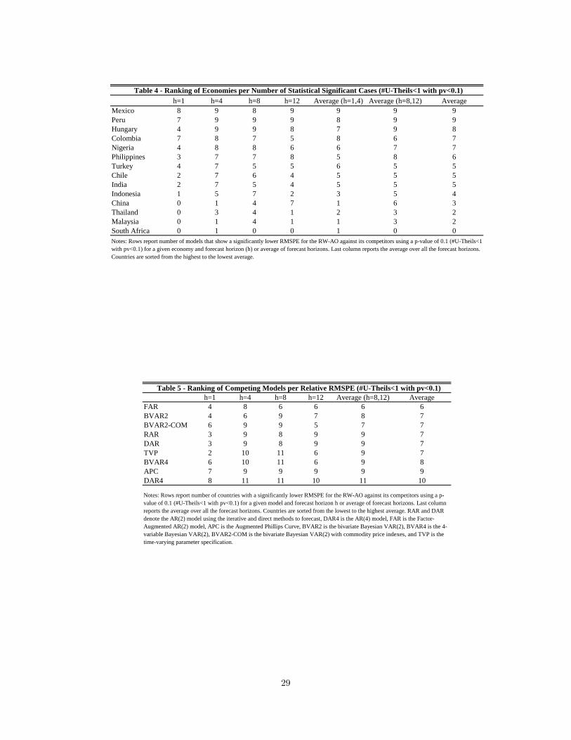
h=1 h=4 h=8 h=12 Average (h=1,4) Average (h=8,12) AverageMexico 8 9 8 9 9 9 9Peru 7 9 9 9 8 9 9Hungary 4 9 9 8 7 9 8Colombia 7 8 7 5 8 6 7Nigeria 4 8 8 6 6 7 7Philippines 3 7 7 8 5 8 6Turkey 4 7 5 5 6 5 5Chile 2 7 6 4 5 5 5India 2 7 5 4 5 5 5Indonesia 1 5 7 2 3 5 4China 0 1 4 7 1 6 3Thailand 0 3 4 1 2 3 2Malaysia 0 1 4 1 1 3 2South Africa 0 1 0 0 1 0 0
Table 4 - Ranking of Economies per Number of Statistical Significant Cases (#U-Theils<1 with pv<0.1)
Notes: Rows report number of models that show a significantly lower RMSPE for the RW-AO against its competitors using a p-value of 0.1 (#U-Theils<1 with pv<0.1) for a given economy and forecast horizon (h) or average of forecast horizons. Last column reports the average over all the forecast horizons. Countries are sorted from the highest to the lowest average.
h=1 h=4 h=8 h=12 Average (h=8,12) AverageFAR 4 8 6 6 6 6BVAR2 4 6 9 7 8 7BVAR2-COM 6 9 9 5 7 7RAR 3 9 8 9 9 7DAR 3 9 8 9 9 7TVP 2 10 11 6 9 7BVAR4 6 10 11 6 9 8APC 7 9 9 9 9 9DAR4 8 11 11 10 11 10
Table 5 - Ranking of Competing Models per Relative RMSPE (#U-Theils<1 with pv<0.1)
Notes: Rows report number of countries with a significantly lower RMSPE for the RW-AO against its competitors using a p-value of 0.1 (#U-Theils<1 with pv<0.1) for a given model and forecast horizon h or average of forecast horizons. Last column reports the average over all the forecast horizons. Countries are sorted from the lowest to the highest average. RAR and DAR denote the AR(2) model using the iterative and direct methods to forecast, DAR4 is the AR(4) model, FAR is the Factor-Augmented AR(2) model, APC is the Augmented Phillips Curve, BVAR2 is the bivariate Bayesian VAR(2), BVAR4 is the 4-variable Bayesian VAR(2), BVAR2-COM is the bivariate Bayesian VAR(2) with commodity price indexes, and TVP is the time-varying parameter specification.
29

M1-M9 M4 and M6 M1-M9 M4 and M6
Average Average Average AverageOne-quarter aheadMean 0.950 0.920 0.566 0.584Median 1.024 0.972 0.561 0.576#<1; #>0.5 6 7 9 11#pv<0.1 2 4 8 8Four-quarter aheadMean 0.769 0.797 0.591 0.595Median 0.834 0.888 0.571 0.611#<1; #>0.5 11 11 13 12#pv<0.1 8 7 7 8Eight-quarter aheadMean 0.785 0.818 0.568 0.619Median 0.884 0.953 0.576 0.669#<1; #>0.5 11 11 9 9#pv<0.1 6 6 9 9Twelve-quarter aheadMean 0.821 0.820 0.573 0.587Median 0.926 0.920 0.609 0.600#<1; #>0.5 9 10 10 10#pv<0.1 5 5 8 8Averages (all horizons)Mean 0.831 0.839 0.574 0.596Median 0.917 0.933 0.579 0.614#<1; #>0.5 9 10 10 11#pv<0.1 5 6 8 8
Notes: First and third columns report statistics for the forecast average of models M1 through M9 (M1-M9 Average). Second and fourth columns report the forecast average of models M4 and M6 only (M4 and M6 Average). Mean/median report those statistics for the ratio of the root mean squared prediction error (RMSPE) of the corresponding forecast average relative to the RW-AO model over the 14 countries, for a given forecast horizon. Values less than one imply that the RW-AO model has a lower RMSPE than does the forecast average. The row #<1; #>0.5 reports the number of economies that show relative RMSPE lower than 1 in the first and second columns, and the number of economies that show a success ratio higher than 0.5 in the last two columns. The row #pv<0.1 reports the number of economies that show a p-value lower than 00.1 for the null of equal predictive accuracy measured by the RMSPEs of the RW-AO and the corresponding forecast average, using the Diebold-Mariano-West statistic.
Table 6 - Forecast AveragesRelative RMSPE Directional accuracy
30

M1 M2 M3 M4 M5 M6 M7 M8 M9 AverageRAR DAR DAR4 FAR APC BVAR2 BVAR4 BVAR2-COM TVP M1-M9
One-quarter aheadMean 0.856 0.856 0.881 0.807 0.712 0.819 0.705 0.792 0.762 0.799Median 0.947 0.947 0.950 0.836 0.763 0.857 0.753 0.802 0.751 0.845#<1 9 9 8 12 14 12 14 12 14 12#pv<0.1 6 6 8 8 11 9 11 10 12 9Four-quarter aheadMean 0.897 0.925 0.942 0.799 0.742 0.755 0.694 0.727 0.673 0.795Median 0.983 1.013 1.020 0.885 0.779 0.822 0.765 0.783 0.675 0.858#<1 9 6 5 8 11 14 14 14 14 11#pv<0.1 3 2 5 4 5 6 6 5 7 5Eight-quarter aheadMean 0.993 0.965 0.966 0.817 0.707 0.700 0.674 0.700 0.698 0.802Median 1.034 1.030 1.019 0.955 0.796 0.753 0.754 0.775 0.703 0.869#<1 4 5 6 10 14 14 14 14 14 11#pv<0.1 1 1 6 2 5 8 8 8 7 5Twelve-quarter aheadMean 1.007 0.982 0.944 0.740 0.700 0.696 0.692 0.702 0.721 0.798Median 1.052 1.048 0.994 0.787 0.755 0.766 0.758 0.769 0.737 0.852#<1 4 3 8 9 10 14 14 14 14 10#pv<0.1 1 1 8 4 4 5 3 4 5 4Averages (all horizons)Mean 0.938 0.932 0.933 0.791 0.715 0.742 0.692 0.730 0.714 0.799Median 1.004 1.009 0.996 0.866 0.773 0.799 0.758 0.782 0.717 0.856#<1 7 6 7 10 12 14 14 14 14 11#pv<0.1 3 3 7 5 6 7 7 7 8 6
Table 7 - RMSPE of the RW-AO Model Relative to Competing Models with Intercept Corrections (Summary)
Notes: Forecasts of competing models include intercept corrections. Rows for means and medians report the average/median ratio of root mean squared prediction error (RMSPE) from the RW-AO model relative to the RMSPE of competing forecasting models with intercept corrections calculated over the 14 countries. Values less than one imply that the RW-AO model has a lower RMSPE than does the competitive benchmark. The row #<1 reports the number of economies that show relative RMSPE lower than 1 for a particular model. The row #pv<0.1 reports the number of economies that show a p-value lower than 00.1 for the null of equal predictive accuracy measured by the RMSPEs of the RW-AO and the alternative model. We use the Diebold-Mariano-West statistic or the adjusted Clark-West statistic when models are nested. See Tables 1.A and 1.B for the data sources. RAR and DAR denote the AR(2) model using the iterative and direct methods to forecast, DAR4 is the AR(4) model, FAR is the Factor-Augmented AR(2) model, APC is the Augmented Phillips Curve, BVAR2 is the bivariate Bayesian VAR(2), BVAR4 is the 4-variable Bayesian VAR(2), BVAR2-COM is the bivariate Bayesian VAR(2) with commodity price indexes, and TVP is the time-varying parameter specificcation.
31

M0 M1 M2 M3 M4 M5 M6 M7 M8 M9 Average
RW-AO RAR DAR DAR4 FAR APC BVAR2 BVAR4 BVAR2-COM TVP M1-M9One-quarter aheadMean 0.608 0.425 0.425 0.447 0.454 0.432 0.453 0.447 0.455 0.415 0.439Median 0.583 0.431 0.431 0.446 0.446 0.431 0.446 0.446 0.454 0.423 0.439#>0.5 14 1 1 3 4 1 5 3 1 1 2Four-quarter aheadMean 0.673 0.690 0.714 0.722 0.690 0.689 0.657 0.665 0.681 0.630 0.682Median 0.683 0.702 0.726 0.742 0.694 0.710 0.661 0.653 0.669 0.645 0.689#>0.5 14 13 13 13 13 14 12 14 14 14 13Eight-quarter aheadMean 0.668 0.720 0.722 0.729 0.703 0.685 0.643 0.637 0.649 0.621 0.679Median 0.669 0.750 0.750 0.759 0.759 0.672 0.664 0.655 0.681 0.638 0.703#>0.5 14 13 13 13 13 13 13 12 12 11 13Twelve-quarter aheadMean 0.668 0.737 0.735 0.728 0.681 0.677 0.659 0.661 0.660 0.663 0.689Median 0.664 0.722 0.750 0.759 0.694 0.704 0.667 0.667 0.667 0.685 0.702#>0.5 14 13 13 13 14 14 14 13 13 13 13Averages (all horizons)Mean 0.654 0.643 0.649 0.657 0.632 0.621 0.603 0.603 0.611 0.582 0.622Median 0.650 0.651 0.664 0.676 0.648 0.629 0.609 0.605 0.618 0.598 0.633#>0.5 14 10 10 11 11 11 11 11 10 10 10
Table 8 - Directional Accuracy: Success Ratios of the RW-AO and Competing Models with Intercept Corrections (Summary)
Notes: Forecasts of competing models (M1-M9) include intercept corrections. Rows for means and medians report the average and median ratio of success in directional accuracy over the 14 countries. The row #>0.5 reports the number of economies that show a success ratio higher than 0.5 for a particular model. See Tables 1.A and 1.B for the data sources. RW-AO stands for the random walk model proposed by Atkeson and Ohanian (2001), RAR and DAR denote the AR(2) model using the iterative and direct methods to forecast, DAR4 is the AR(4) model, FAR is the Factor-Augmented AR(2) model, APC is the Augmented Phillips Curve, BVAR2 is the bivariate Bayesian VAR(2), BVAR4 is the 4-variable Bayesian VAR(2), BVAR2-COM is the bivariate Bayesian VAR(2) with commodity price indexes, and TVP is the time-varying parameter specificcation.
32

Exact q-o-q inflation Approximate q-o-q inflation Exact y-o-y inflation Approximate y-o-y inflationAverage M1-M9 Average M1-M9 Average M1-M9 Average M1-M9
One-quarter aheadMean 0.896 0.949 1.501 1.574Median 0.946 1.002 1.580 1.636#<1 8 7 2 2#pv<0.1 5 4 2 2Four-quarter aheadMean 0.742 0.778 0.812 0.851Median 0.787 0.817 0.870 0.899#<1 12 12 10 9#pv<0.1 9 9 6 5Eight-quarter aheadMean 0.738 0.771 0.766 0.795Median 0.795 0.829 0.840 0.862#<1 12 12 11 11#pv<0.1 9 9 7 7Twelve-quarter aheadMean 0.738 0.771 0.759 0.787Median 0.751 0.788 0.770 0.802#<1 12 12 11 11#pv<0.1 7 7 6 6Averages (all horizons)Mean 0.778 0.817 0.959 1.002Median 0.820 0.859 1.015 1.050#<1 11 11 8 8#pv<0.1 8 7 5 5
Table 9. RMSPE of the RW-AO Model Relative to Competing Models, Different Measures of Inflation
Notes: The exact quarter-over-quarter inflation (used in baseline exercises) is calculated as 100((CPI(t)/CPI(t-1))4-1), the approximate quarter-on-quarter inflation is 400(log(CPI(t))-log(CPI(t-1))), the exact year-on-year inflation is (CPI(t)/CPI(t-4)-1), and the approximate year-on-year inflation is 100(log(CPI(t))-log(CPI(t-4))). Rows for means and medians report the average of the mean/median ratio of root mean squared prediction error (RMSPE) from the RW-AO model relative to the RMSPE of competing forecasting models calculated over the 14 countries and over the 9 models. Values less than one imply that the RW-AO model has, on average, a lower RMSPE than does the competitive benchmarks. The row #<1 reports the average number of cases (out of 14 EMEs) that show an average of the relative RMSPE lower than 1 over the 9 competing models. The row #pv<0.1 reports the average number of cases (out of 14 EMEs) that show a p-value lower than 0.1 for the null of equal predictive accuracy measured by the RMSPEs of the RW-AO and over the 9 competing models. We use the Diebold-Mariano-West statistic or the adjusted Clark-West statistic when models are nested.
33

M4 M6 M8
FAR BVAR2 BVAR2-COMOne-quarter ahead#Intercept>0 6 6 7Median (Intercept) -1.18 -1.33 -0.05Chi-square statistic 48.17 50.10 80.09P-value 0.00 0.00 0.00
Four-quarter ahead#Intercept>0 12 12 11Median (Intercept) 10.84 2.89 5.21Chi-square statistic 106.03 41.77 70.17P-value 0.00 0.00 0.00
Eight-quarter ahead#Intercept>0 12 13 13Median (Intercept) 9.19 5.03 5.06Chi-square statistic 84.18 82.80 77.74P-value 0.00 0.00 0.00
Twelve-quarter ahead#Intercept>0 10 14 14Median (Intercept) 17.13 5.23 4.09Chi-square statistic 177.30 105.70 61.01P-value 0.00 0.00 0.00
Table 10 - Statistics for the Test of Joint Predictive Ability Across Countries
Notes: We estimate an only-intercept model for each of the 14 EMEs using SUR-GLS estimation, where the regressand is the difference between the squared forecast error of the alternative model (M4, M6, and M8) and the squared forecast error of the RW-AO model. Squared forecast errors are generated from a rolling-window estimation using a width of 75 observations. The number of observations is 70 (h=1), 67 (h=4), 63 (h=8), and 59 (h=12). A positive (negative) intercept indicates that the RW-AO model shows higher(lower) predictive ability than the alternative model. #Intercept>0 is the number of countries/equations that show a positive intercept, given a forecast horizon and an alternative model. The median of all the intercepts is reported as well. The null hypothesis is that all the intercepts are jointly equal to zero (equal predictive ability across countries). The p-value and chi-square statistic are related to that null hypothesis and the statistic is compared to a critical value with 14 degrees of freedom. FAR is the Factor-Augmented AR(2) model, BVAR2 is the bivariate Bayesian VAR(2), and BVAR2-COM is the bivariate Bayesian VAR(2) with commodity price indexes.
34

M4 M6 M8
FAR BVAR2 BVAR2-COMOne-quarter ahead%EMEs with P-value(Wald test)>0.1 50% 57% 86%US P-value(Wald test) 0.04 0.01 0.00
Four-quarter ahead%EMEs with P-value(Wald test)>0.1 86% 71% 86%US P-value(Wald test) 0.07 0.00 0.17
Eight-quarter ahead%EMEs with P-value(Wald test)>0.1 86% 71% 71%US P-value(Wald test) 0.04 0.00 0.00
Twelve-quarter ahead%EMEs with P-value(Wald test)>0.1 100% 64% 71%US P-value(Wald test) 0.04 0.00 0.00
Averages (all horizons)%EMEs with P-value(Wald test)>0.1 80% 66% 79%US P-value(Wald test) 0.05 0.00 0.04
Table 11 - Tests of Conditional Predictive Ability
Notes: For each country including the US and each forecast horizon, we generate forecasts from a rolling-window estimation using 75 observations and construct the difference between the squared forecast error of an alternative model and the squared forecast error of the RW-AO model. We regress that indicator on its first two lags, a measure of the GDP cycle (year-on-year GDP growth rate) and a proxy of a high-inflationary regime (an indicator function that takes the value of 1 if the current inflation rate is higher than the median inflation rate, approximately 5%, and 0 otherwise). The number of observations is 68 (h=1), 65 (h=4), 61 (h=8), and 57 (h=12). We use the conditional predictability (Wald) test by Giacomini and White (2006). %EMEs with P-value(Wald test)>0.1 reports the percentage of the 14 economies in which we reject at 10% the joint null hypothesis that all non-intercept coefficients are zero. US P-value(Wald test) reports the p-value associated with an analogous joint hypothesis for the US. FAR is the Factor-Augmented AR(2) model, BVAR2 is the bivariate Bayesian VAR(2), and BVAR2-COM is the bivariate Bayesian VAR(2) with commodity price indexes.
35
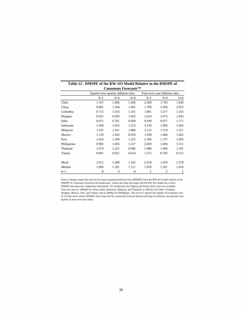
h=1 h=4 h=6 h=1 h=4 h=6Chile 1.167 1.406 1.266 2.508 1.793 1.640China 0.881 1.564 1.402 1.780 1.950 2.023Colombia 0.713 1.353 1.161 1.801 1.317 1.355Hungary 0.931 0.930 1.022 1.634 1.073 1.043India 0.671 0.781 0.958 0.938 0.977 1.171Indonesia 1.309 1.655 1.223 3.539 1.983 1.663Malaysia 1.355 1.161 1.080 2.123 1.519 1.211Mexico 1.139 1.043 0.918 1.938 1.484 1.465Peru 1.018 1.509 1.323 2.369 1.737 1.693Philippines 0.982 1.045 1.317 2.029 1.694 1.511Thailand 1.074 1.221 0.946 1.980 1.404 1.191Turkey 0.891 0.831 0.614 1.575 0.783 0.572
Mean 1.011 1.208 1.102 2.018 1.476 1.378Median 1.000 1.191 1.121 1.959 1.501 1.410#<1 6 3 4 1 2 1
Table 12 - RMSPE of the RW-AO Model Relative to the RMSPE of Consensus Forecasts™
Quarter-over-quarter inflation rates Year-over-year inflation rates
Notes: Columns report the ratio of root mean squared prediction error (RMSPE) from the RW-AO model relative to the RMSPE of Consensus Forecast (CF) predictions. Values less than one imply that the RW-AO model has a lower RMSPE than does the competitive benchmark. CF's predictions for Nigeria and South Africa were not available. Forecasts start in: 2006Q4 for China, India, Indonesia, Malaysia, and Thailand; in 2007Q1 for Chile, Colombia, Hungary, Mexico, Peru, and Turkey; and in 2009Q3 for Phillipines. The row #<1 reports the number of economies (out of 12) that show relative RMSPE lower than one for a particular forecast horizon and type of inflation rate (quarter-over-quarter or year-over-year rates).
36

Figure 1. RMSPE of the RW-AO Relative to Competing Models (Medians)
Notes: Medians of ratio of root mean squared prediction error (RMSPE) from the RW-AO model relative to the RMSPE of competing forecasting models calculated over the 14 countries for a given forecast horizon (h). Values less than one imply that the RW-AO model has a lower RMSPE than does the competitive benchmark. RAR and DAR denote the AR(2) model using the iterative and direct methods to forecast, DAR4 is the AR(4) model, FAR is the Factor-Augmented AR(2) model, APC is the Augmented Phillips Curve, BVAR2 is the bivariate Bayesian VAR(2), BVAR4 is the 4-variable Bayesian VAR(2), BVAR2-COM is the bivariate Bayesian VAR(2) with commodity price indexes, and TVP is the time-varying parameter specificcation.
0.0
1.0
RAR DAR DAR4 FAR
h=1 h=4 h=8 h=12
0.0
1.0
APC BVAR2 BVAR4 BVAR2-COM TVP
h=1 h=4 h=8 h=12
37

Figure 2. Directional Accuracy: Success Ratios (Medians)
Notes: Medians of ratio of success in directional accuracy over the 14 countries for a given forecast horizon (h). RW-AO stands for the random walk model proposed by Atkeson and Ohanian (2001), RAR and DAR denote the AR(2) model using the iterative and direct methods to forecast, DAR4 is the AR(4) model, FAR is the Factor-Augmented AR(2) model, APC is the Augmented Phillips Curve, BVAR2 is the bivariate Bayesian VAR(2), BVAR4 is the 4-variable Bayesian VAR(2), BVAR2-COM is the bivariate Bayesian VAR(2) with commodity price indexes, and TVP is the time-varying parameter (TVP) specificcation.
0.50
0.60
0.70
RW-AO RAR DAR DAR4 FAR
h=1 h=4 h=8 h=12
0.50
0.60
0.70
APC BVAR2 BVAR4 BVAR2-COM TVP
h=1 h=4 h=8 h=12
38

Figure 3. RMSPE for Different RW-AO Models Relative to Competing Models (Average Medians)
Notes: RW-AO models with averages over the past 4, 8, 12 and 16 inflation values. Average of medians of ratio of root mean squared prediction error (RMSPE) from the RW-AO model relative to the RMSPE of competing forecasting models calculated over the 14 countries and the 9 competing models for a given forecast horizon (h). Values less than one imply that, on average, the RW-AO model has a lower RMSPE than does the competitive benchmark.
0.6
0.7
0.8
0.9
1.0
h = 1 h = 4 h = 8 h = 12 Average
RWAO4 RWAO8 RWAO12 RWAO16
39

Notes: The average RMSPE of the RW-AO model relative to competing models is calculated over the 9 alternative models and 4 forecast horizons for each economy. Values less than one imply that, on average, the RW-AO model has a lower RMSPE than does the competitive model. The number of years under inflation targeting is calculated from 1999 to 2016 (the forecast period) using information from Hammond (2012) and Roger (2010). The index of central bank independence is an average for each country using data from Garriga (2016). The median inflation rate and the coefficient of variation are computed over the quarter-over-quarter inflation rates between 1980Q2 and 1989Q4 for each economy. Labels in graphs correspond to Hungary, Mexico, Peru (economies at the top of the ranking in Table 4) as well as Malaysia, South Africa, and Thailand (economies at the bottom of the ranking in Table 4).
0.00
0.20
0.40
0.60
0.80
1.00
1.20
0 2 4 6 8 10 12 14 16 18 20
Figure 4A. Average RMSPE of the RW-AO Model Relative to Competing Models and Years with Inflation Targeting
Regime
Corr = -0.305(p-value=0.29) PER
MEX
ZAFMYS
HUN
THA
0.00
0.20
0.40
0.60
0.80
1.00
1.20
0.20 0.30 0.40 0.50 0.60 0.70 0.80 0.90
Figure 4B. Average RMSPE of the RW-AO Model Relative to Competing Models and Index of Central Bank
Independence
Corr = -0.480(p-value=0.08) PER
ZAFMYS
HUN
THA
0.00
0.20
0.40
0.60
0.80
1.00
1.20
0.0 10.0 20.0 30.0 40.0 50.0 60.0 70.0
Figure 4C. Average RMSPE of the RW-AO Model Relative to Competing Models and Median Inflation Rate (1980-1990)
Corr = -0.739(p-value=0.00)
PER
MEX
ZAFMYS
HUN
THA
0.00
0.20
0.40
0.60
0.80
1.00
1.20
0.0 1.0 2.0 3.0 4.0 5.0 6.0 7.0 8.0 9.0
Figure 4D. Average RMSPE of the RW-AO Model Relative to Competing Models and Coefficient of Variation of
Inflation Rate (1980-1990)
Corr = -0.741(p-value=0.00)
PER
MEX
THA
MEX
ZAF MYS
HUN
40

References
Altug, S. and C. Çakmakli (2016). Forecasting Inflation Using Survey Expectations and Target Inflation:
Evidence for Brazil and Turkey. International Journal of Forecasting 32, 138—153.
Aron, J. and J. Muellbauer (2012). Improving Forecasting in an Emerging Economy, South Africa: Chang-
ing Trends, Long Run Restrictions and Disaggregation. International Journal of Forecasting 28, 456—
476.
Ascari, G. (2004). Staggered Prices and Trend Inflation: Some Nuisances. Review of Economic Dynam-
ics 7 (3), 642—667.
Assenza, T., P. Heemeijer, C. H. Hommes, and D. Massaro (2013). Individual Expectations and Aggregate
Macro Behavior. Tinbergen Institute Discussion Paper 13-016/II .
Atkeson, A. and L. E. Ohanian (2001). Are Phillips Curves Useful for Forecasting Inflation? Federal
Reserve Bank of Minneapolis Quarterly Review, 25 (1), 2—11. Winter.
Bacchetta, P., E. van Wincoop, and T. Beutler (2009). Can Parameter Instability Explain the Meese-
Rogoff Puzzle? NBER International Seminar on Macroeconomics 6 (1), 125—173.
Balcilar, M., R. Gupta, and K. Kotzé (2015). Forecasting Macroeconomic Data for an Emerging Market
with a Nonlinear DSGE Model. Economic Modelling 44, 215—228.
Ball, L. and S. Mazumder (2014). A Phillips Curve with Anchored Expectations and Short-Term Unem-
ployment. Working Paper 20715, National Bureau of Economic Research..
Calvo, G. A. (1983). Staggered Prices in a Utility-Maximizing Framework. Journal of Monetary Eco-
nomics 12 (3), 383—398.
Chen, Y.-c., S. J. Turnovsky, and E. Zivot (2014). Forecasting Inflation Using Commodity Price Aggre-
gates. Journal of Econometrics 183, 117—134.
Ciccarelli, M. and B. Mojon (2010). Global Inflation. The Review of Economics and Statistics 92 (3),
524—535.
Clark, T. E. and M. W. McCracken (2010). Averaging Forecasts from VARs with Uncertain Instabilities.
Journal of Applied Econometrics 25 (1), 5—29.
Clark, T. E. and K. D. West (2007). Approximately Normal Tests for Equal Predictive Accuracy in Nested
Models. Journal of Econometrics 138 (1), 291—311.
Clemen, R. T. (1989). Combining Forecasts: A Review and Annotated Bibliography. International Journal
of Forecasting 5 (4), 559—583.
Clements, M. P. and D. F. Hendry (2001). Forecasting Non-stationary Economic Time Series. MIT Press.
Coibion, O. and Y. Gorodnichenko (2015). Is the Phillips Curve Alive and Well after All? Inflation
Expectations and the Missing Disinflation. American Economic Journal: Macroeconomics 7 (1), 197—
232.
Cole, H. L. and M. Obstfeld (1991). Commodity Trade and International Risk Sharing. How Much Do
Financial Markets Matter? Journal of Monetary Economics 28 (1), 3—24.
41

Cukierman, A., S. B. Webb, and B. Neyapti (1992). Measuring the independence of central banks and its
effect on policy outcomes. The World Bank Economic Review 6, 353—398.
Di Bartolomeo, G., M. Di Pietro, and B. Giannini (2016). Optimal Monetary Policy in a New Keynesian
Model with Heterogeneous Expectations. Journal of Economic Dynamics and Control 73 (C), 373—387.
Doan, T., R. B. Litterman, and C. A. Sims (1984). Forecasting and Conditional Projections Using Realistic
Prior Distributions. Econometric Reviews 3 (1), 1—100.
Duncan, R. and E. Martínez-García (2015). Forecasting Local Inflation with Global Inflation: When
Economic Theory Meets the Facts. Federal Reserve Bank of Dallas Globalization and Monetary Policy
Institute Working Paper No. 235 .
Eklund, J., G. Kapetanios, and S. Price (2013). Robust Forecast Methods and Monitoring During Struc-
tural Change. The Manchester School 81 (S3), 3—27.
Elliott, G. and A. Timmermann (2016). Economic Forecasting. Princeton University Press.
Engel, C. and K. D. West (2005). Exchange Rates and Fundamentals. Journal of Political Economy 113 (3),
485—517.
Faust, J. and J. H. Wright (2013). Forecasting Inflation, Volume 2A of Handbook of Economic Forecasting,
Chapter 1, pp. 2—56. Elsevier.
Frankel, J., D. Parsley, and S.-J. Wei (2012). Slow Pass-Through Around the World: A New Import for
Developing Countries? Open Economies Review 23 (2), 213—251. April.
Garriga, A. C. (2016). Central Bank Independence in the World: A New Dataset. International Interac-
tions 42 (5), 849—868. https://sites.google.com/site/carogarriga/cbi-data-1.
Giacomini, R. and H. White (2006). Tests of Conditional Predictive Ability. Econometrica 74, 1545—1578.
Gibbs, C. G. (2017). Forecast Combination, Non-linear Dynamics, and the Macroeconomy. Economic
Theory 63 (3), 653—686.
Giraitis, L., G. Kapetanios, and S. Price (2013). Adaptive Forecasting in the Presence of Recent and
Ongoing Structural Change. Journal of Econometrics 177 (2), 153—170.
Granger, C. W. J. and T. Terasvirta (1993).Modelling Nonlinear Economic Relationships. Oxford: Oxford
University Press.
Grossman, V., A. Mack, and E. Martínez-García (2014). A New Database of Global Economic Indicators.
The Journal of Economic and Social Measurement 39 (3), 163—197.
Hammond, G. (2012). State of the Art of Inflation Targeting - 2012. Centre for Central Banking Studies.
Handbook - No. 29 .
Harvey, D., S. Leybourne, and P. Newbold (1997). Testing the Equality of Prediction Mean Squared
Errors. International Journal of Forecasting 13 (2), 281—291.
IMF WEO (2013). The Dog that Didn’t Bark: Has Inflation Been Muzzled or Was it Just Sleeping?
Chapter 3. World Economic Outlook (IMF), April 2013.
Kabukcuoglu, A. and E. Martínez-García (2016). What Helps Forecast U.S. Inflation? - Mind the Gap!
Koç University-TUSIAD Economic Research Forum Working Papers (No. 1615).
42
Kabukcuoglu, A. and E. Martínez-García (2018). Inflation as a Global Phenomenon—Some Implications
for Inflation Modelling and Forecasting. Journal of Economic Dynamics and Control 87 (2), 46—73.
Lansing, K. J. (2009). Time-Varying U.S. Inflation Dynamics and the New Keynesian Phillips Curve.
Review of Economic Dynamics 12 (2), 304—326.
Litterman, R. B. (1986). Forecasting with Bayesian Vector Autoregressions: Five Years of Experience.
Journal of Business and Statistics 4 (1), 25—38.
Liu, G. D. and R. Gupta (2007). A Small-Scale DSGE Model for Forecasting the South African Economy.
South African Journal of Economics 75 (2), 179—193.
Mandalinci, Z. (2017). Forecasting Inflation in Emerging Markets: An Evaluation of Alternative Models.
International Journal of Forecasting 33 (4), 1082—1104.
Martínez-García, E. (2017). Good Policies or Good Luck? New Insights on Globalization and the Inter-
national Monetary Policy Transmission Mechanism. Computational Economics, 1—36, September 15,
2017.
Martínez-García, E. and M. A. Wynne (2010). The Global Slack Hypothesis. Federal Reserve Bank of
Dallas Staff Papers, 10. September.
Medel, C. A., M. Pedersen, and P. M. Pincheira (2016). The Elusive Predictive Ability of Global Inflation.
International Finance 19 (2), 120—146.
Meese, R. A. and K. S. Rogoff (1983a). Empirical Exchange Rate Models of the Seventies: Do They Fit
Out of Sample? Journal of International Economics 14 (1-2), 3—24.
Meese, R. A. and K. S. Rogoff (1983b). The Out-of-Sample Failure of Empirical Exchange Rate Mod-
els: Sampling Error or Misspecification? In J. A. Frenkel (Ed.), Exchange Rates and International
Macroeconomics, pp. 67—112. University of Chicago Press. Chicago and London.
Mehrotra, A. and J. Yetman (2014). Decaying Expectations: What Inflation Forecasts Tell Us About the
Anchoring of Inflation Expectations. BIS Working Papers No. 464 .
Meier, A. (2010). Still Minding the Gap– Inflation Dynamics during Episodes of Persistent Large Output
Gaps. IMF Working Paper WP/10/189 .
Pecora, N. and A. Spelta (2017). Managing Monetary Policy in a New Keynesian Model with Many Beliefs
Types. Economics Letters 150 (C), 53—58.
Pesaran, M. H. and A. Pick (2009). Forecasting Random Walks Under Drift Instability. DNB Working
Papers 207, Netherlands Central Bank, Research Department .
Pesaran, M. H. and A. Timmermann (2009). Testing Dependence Among Serially Correlated Multicate-
gory Variables. Journal of the American Statistical Association 104 (485), 325—337.
Pincheira, P. M. and A. Gatty (2016). Forecasting Chilean Inflation with International Factors. Empirical
Economics 51, 981—1010.
Pincheira, P. M. and C. A. Medel (2015). Forecasting Inflation with a Simple and Accurate Benchmark:
The Case of the U.S. and a Set of Inflation Targeting Countries. Czech Journal of Economics and
Finance 65 (1), 2—29.
43
Primiceri, G. E. (2005). Time-varying Structural Vector Autoregressions and Monetary Policy. The Review
of Economic Studies 72 (3), 821—852.
Roger, S. (2010). Inflation Targeting Turns 20. Finance & Development 47 (1), 46—49.
Rossi, B. (2012). Advances in Forecasting under Instability. In G. Elliott and A. Timmerman (Eds.),
Handbook of Economic Forecasting. Elsevier, North Holland.
Rossi, B. (2013). Exchange Rate Predictability. Journal of Economic Literature 51 (4), 1063—1119.
Sahuc, J.-G. (2006). Partial Indexation, Trend Inflation, and the Hybrid Phillips Curve. Economics Let-
ters 90 (1), 42—50.
Sims, C. A. and T. Zha (1998). Bayesian Methods for Dynamic Multivariate Models. International Eco-
nomic Review 39 (4), 949—968.
Stock, J. H. and M. W. Watson (1999). Forecasting Inflation. Journal of Monetary Economics 44 (2),
293—335.
Stock, J. H. and M. W. Watson (2002). Macroeconomic Forecasting Using Diffusion Indexes. Journal of
Business and Economic Statistics 20 (2), 147—162.
Stock, J. H. and M. W. Watson (2004). Combination Forecasts of Output Growth in a Seven-Country
Data Set. Journal of Forecasting 23 (6), 405—430.
Stock, J. H. and M. W. Watson (2007). Why Has U.S. Inflation Become Harder to Forecast? Journal of
Money, Credit and Banking 39 (02), 3—34.
Taylor, J. B. (1993). Discretion versus Policy Rules in Practice. Carnegie-Rochester Conference Series on
Public Policy 39, 195—214.
Woodford, M. (2008). How Important Is Money in the Conduct of Monetary Policy? Journal of Money,
Credit and Banking 40 (8), 1561—1598.
Yun, T. (1996). Nominal Price Rigidity, Money Supply Endogeneity, and Business Cycles. Journal of
Monetary Economics 37 (2), 345—370.
Ögünç, F., K. Akdogan, S. Baser, M. G. Chadwick, D. Ertug, T. Hülagü, S. Kösem, M. U. Özmen, and
N. Tekatli (2013). Short-term Inflation Forecasting Models for Turkey and a Forecast Combination
Analysis. Economic Modelling 33, 312—325.
44

Supplementary Tables
45

M1 M1/M2 M3 M4 M5 M6 M7 M8 M9RAR or DAR DAR4 FAR APC BVAR2 BVAR4 BVAR2-COM TVP
Chile 1.033 0.966 * 0.914 0.786 * 0.967 0.850 0.930 1.240China 1.178 1.220 1.187 1.161 1.186 1.222 1.146 1.153Colombia 0.814 * 0.969 * 0.714 * 0.702 * 0.740 * 0.774 * 0.779 * 1.165Hungary 0.928 1.007 0.935 0.799 * 0.944 0.750 * 0.796 * 1.007India 0.953 0.898 * 1.024 0.954 1.042 0.981 0.984 0.900 *Indonesia 0.938 0.911 * 0.874 0.992 0.892 0.979 0.911 0.900Malaysia 1.107 1.110 1.094 1.123 1.103 1.114 1.123 0.953Mexico 0.374 * 0.320 * 0.621 * 0.348 * 0.631 * 0.358 * 0.371 * 0.817 *Nigeria 1.038 1.028 0.995 0.757 * 1.012 0.818 * 0.885 * 0.985Peru 0.001 * 0.001 * 0.000 * 0.001 * 0.000 * 0.001 * 0.001 * 1.136Philippines 1.096 0.868 * 1.305 0.818 * 1.333 0.719 * 0.852 1.195South Africa 1.037 1.074 1.130 0.936 1.154 1.092 1.020 1.191Thailand 1.194 1.196 1.183 1.173 1.200 1.125 1.190 1.091Turkey 0.882 0.920 * 0.788 * 0.786 0.796 * 0.752 0.861 * 1.040
Mean #DIV/0! 0.898 0.892 0.912 0.810 0.929 0.824 0.846 1.055Median #NUM! 0.993 0.967 0.965 0.808 0.990 0.834 0.898 1.065#<1 0 7 8 8 11 7 10 10 5#pv<0.1 3 8 4 7 4 6 6 2Notes: Columns report the ratio of root mean squared prediction error (RMSPE) from the RW-AO model relative to the RMSPE of standard forecasting models. Values less than one imply that the RW-AO model has a lower RMSPE than does the competitive benchmark. Values in bold indicate that the null hypothesis of equal predictive accuracy is rejected at 10% level using the Diebold-Mariano-West statistic or the adjusted Clark-West statistic when models are nested. See Tables 1.A and 1.B for the data sources. RAR and DAR denote AR(2) model using the iterative and direct methods to forecast, DAR4 is the AR(4) model, FAR is the Factor-Augmented AR(2) model, APC is the Augmented Phillips Curve, BVAR2 is the bivariate Bayesian VAR(2), BVAR4 is the 4-variable Bayesian VAR(2), BVAR2-COM is the bivariate Bayesian VAR(2) with commodity price indexes, and TVP is the time-varying parameter specification.
Table S1 - One-Quarter Ahead RMSPE of the RW-AO Model Relative to Competing Models
46

M1 M2 M3 M4 M5 M6 M7 M8 M9RAR DAR DAR4 FAR APC BVAR2 BVAR4 BVAR2-COM TVP
Chile 0.725 * 0.691 * 0.843 * 0.792 * 0.610 * 0.996 0.807 * 0.817 * 0.932China 0.945 0.933 0.924 * 1.032 1.063 1.052 1.026 0.964 0.927Colombia 0.473 * 0.663 * 0.872 * 0.664 * 0.535 * 0.837 * 0.763 * 0.750 * 0.907Hungary 0.592 * 0.751 * 0.790 * 0.789 * 0.575 * 0.833 * 0.720 * 0.724 * 0.868 *India 0.852 * 0.770 * 0.818 * 0.839 0.773 * 0.948 0.859 * 0.867 * 0.755 *Indonesia 1.046 0.987 0.972 * 0.642 * 0.839 0.815 * 0.879 * 0.934 0.815 *Malaysia 1.096 1.117 1.126 1.083 1.075 0.947 0.971 0.984 0.747 *Mexico 0.136 * 0.119 * 0.118 * 0.280 * 0.113 * 0.429 * 0.153 * 0.159 * 0.834 *Nigeria 0.756 * 0.779 * 0.737 * 0.848 * 0.605 * 0.857 0.738 * 0.760 * 0.762 *Peru 0.001 * 0.001 * 0.001 * 0.001 * 0.000 * 0.002 * 0.000 * 0.000 * 0.866 *Philippines 0.764 * 0.568 * 0.528 * 0.887 0.502 * 0.968 0.661 * 0.648 * 0.845 *South Africa 0.898 0.993 1.059 1.118 0.956 1.052 0.999 0.994 0.884 *Thailand 0.996 1.018 1.058 1.024 0.935 0.925 0.843 * 0.935 0.732 *Turkey 0.513 * 0.608 * 0.715 * 0.559 * 0.610 * 0.702 * 0.740 0.672 * 0.740
Mean 0.700 0.714 0.754 0.754 0.657 0.812 0.726 0.729 0.830Median 0.760 0.760 0.831 0.815 0.610 0.891 0.785 0.789 0.839#<1 12 12 11 10 12 12 13 14 14#pv<0.1 9 9 11 8 9 6 10 9 10Notes: Columns report the ratio of root mean squared prediction error (RMSPE) from the RW-AO model relative to the RMSPE of standard forecasting models. Values less than one imply that the RW-AO model has a lower RMSPE than does the competitive benchmark. Values in bold indicate that the null hypothesis of equal predictive accuracy is rejected at 10% level using the Diebold-Mariano-West statistic or the adjusted Clark-West statistic when models are nested. See Tables 1.A and 1.B for the data sources. RAR and DAR denote AR(2) model using the iterative and direct methods to forecast, DAR4 is the AR(4) model, FAR is the Factor-Augmented AR(2) model, APC is the Augmented Phillips Curve, BVAR2 is the bivariate Bayesian VAR(2), BVAR4 is the 4-variable Bayesian VAR(2), BVAR2-COM is the bivariate Bayesian VAR(2) with commodity price indexes, and TVP is the time-varying parameter specification.
Table S2 - Four-Quarters Ahead RMSPE of the RW-AO Model Relative to Competing Models
47

M1 M2 M3 M4 M5 M6 M7 M8 M9RAR DAR DAR4 FAR APC BVAR2 BVAR4 BVAR2-COM TVP
Chile 0.538 * 0.891 0.965 * 0.913 0.743 * 0.915 0.872 * 0.863 * 0.813 *China 0.813 0.714 * 0.677 * 0.976 0.973 0.932 0.874 * 0.984 0.834 *Colombia 0.375 * 0.690 * 0.851 * 0.576 * 0.566 * 0.900 * 0.966 0.958 0.928 *Hungary 0.467 * 0.589 * 0.639 * 0.646 * 0.475 * 0.746 * 0.704 * 0.702 * 0.766 *India 0.954 0.932 0.919 * 0.944 0.929 0.891 * 0.903 * 0.905 * 0.797 *Indonesia 0.916 0.888 0.896 * 0.657 * 0.690 * 0.818 * 0.794 * 0.822 * 0.751 *Malaysia 1.044 1.059 1.070 1.026 1.022 0.807 * 0.827 * 0.832 * 0.738 *Mexico 0.088 * 0.083 * 0.099 * 0.185 * 0.083 * 0.390 * 0.280 * 0.248 * 0.919Nigeria 0.709 * 0.651 * 0.680 * 0.926 0.618 * 0.882 * 0.830 * 0.860 * 0.811 *Peru 0.001 * 0.001 * 0.001 * 0.001 * 0.000 * 0.001 * 0.001 * 0.001 * 0.839 *Philippines 0.614 * 0.473 * 0.475 * 1.007 0.450 * 0.888 0.729 * 0.793 * 0.791 *South Africa 0.843 1.075 1.067 1.216 0.994 1.016 1.033 1.036 0.958Thailand 1.033 1.051 1.008 1.028 0.967 0.858 * 0.826 * 0.903 0.792 *Turkey 0.501 * 0.659 * 0.681 * 0.645 * 0.808 * 0.989 1.044 0.909 0.995
Mean 0.636 0.697 0.716 0.767 0.666 0.788 0.763 0.773 0.838Median 0.662 0.702 0.766 0.919 0.717 0.885 0.828 0.861 0.812#<1 12 11 11 10 13 13 12 13 14#pv<0.1 8 8 11 6 9 9 11 9 11Notes: Columns report the ratio of root mean squared prediction error (RMSPE) from the RW-AO model relative to the RMSPE of standard forecasting models. Values less than one imply that the RW-AO model has a lower RMSPE than does the competitive benchmark. Values in bold indicate that the null hypothesis of equal predictive accuracy is rejected at 10% level using the Diebold-Mariano-West statistic or the adjusted Clark-West statistic when models are nested. See Tables 1.A and 1.B for the data sources. RAR and DAR denote AR(2) model using the iterative and direct methods to forecast, DAR4 is the AR(4) model, FAR is the Factor-Augmented AR(2) model, APC is the Augmented Phillips Curve, BVAR2 is the bivariate Bayesian VAR(2), BVAR4 is the 4-variable Bayesian VAR(2), BVAR2-COM is the bivariate Bayesian VAR(2) with commodity price indexes, and TVP is the time-varying parameter specification.
Table S3 - Eight-Quarters Ahead RMSPE of the RW-AO Model Relative to Competing Models
48

M1 M2 M3 M4 M5 M6 M7 M8 M9RAR DAR DAR4 FAR APC BVAR2 BVAR4 BVAR2-COM TVP
Chile 0.482 * 0.644 * 0.734 * 0.978 0.586 * 0.959 0.950 0.970 0.933China 0.590 * 0.492 * 0.438 * 0.535 * 0.830 0.711 * 0.570 * 0.858 0.808 *Colombia 0.302 * 0.610 * 0.630 * 0.560 * 0.565 * 0.821 0.885 0.921 0.933Hungary 0.430 * 0.488 * 0.497 * 0.475 * 0.418 * 0.842 * 0.817 * 0.816 * 0.916India 1.057 1.087 1.076 1.009 1.027 0.848 * 0.873 * 0.875 * 0.848 *Indonesia 0.961 0.955 0.967 * 0.831 0.792 * 0.847 0.837 0.868 0.845Malaysia 1.096 1.108 1.078 1.105 1.103 0.868 0.884 0.886 0.836Mexico 0.081 * 0.111 * 0.135 * 0.224 * 0.118 * 0.246 * 0.632 * 0.654 * 0.870 *Nigeria 0.695 * 0.652 * 0.622 * 0.773 0.613 * 0.860 * 0.907 0.903 0.850 *Peru 0.001 * 0.001 * 0.001 * 0.000 * 0.000 * 0.001 * 0.001 * 0.002 * 0.757 *Philippines 0.536 * 0.509 * 0.570 * 1.006 0.534 * 0.865 * 0.861 * 0.823 * 0.790 *South Africa 0.795 1.005 1.063 1.342 0.926 0.951 0.954 0.950 0.886Thailand 1.168 1.161 1.151 1.198 1.061 0.944 0.910 0.984 0.910Turkey 0.490 * 0.629 * 0.686 * 0.820 * 0.541 * 0.926 0.923 0.890 0.975
Mean 0.620 0.675 0.689 0.775 0.651 0.764 0.786 0.814 0.868Median 0.563 0.637 0.658 0.826 0.600 0.854 0.879 0.880 0.860#<1 11 10 10 9 11 14 14 14 14#pv<0.1 9 9 10 6 9 7 6 5 6Notes: Columns report the ratio of root mean squared prediction error (RMSPE) from the RW-AO model relative to the RMSPE of standard forecasting models. Values less than one imply that the RW-AO model has a lower RMSPE than does the competitive benchmark. Values in bold indicate that the null hypothesis of equal predictive accuracy is rejected at 10% level using the Diebold-Mariano-West statistic or the adjusted Clark-West statistic when models are nested. See Tables 1.A and 1.B for the data sources. RAR and DAR denote AR(2) model using the iterative and direct methods to forecast, DAR4 is the AR(4) model, FAR is the Factor-Augmented AR(2) model, APC is the Augmented Phillips Curve, BVAR2 is the bivariate Bayesian VAR(2), BVAR4 is the 4-variable Bayesian VAR(2), BVAR2-COM is the bivariate Bayesian VAR(2) with commodity price indexes, and TVP is the time-varying parameter specification.
Table S4 - Twelve-Quarters Ahead RMSPE of the RW-AO Model Relative to Competing Models
49

M0 M1/M2 M3 M4 M5 M6 M7 M8 M9
RW-AO RAR or DAR DAR4 FAR APC BVAR2 BVAR4 BVAR2-COM TVP
Chile 0.61 * 0.52 † 0.52 † 0.56 0.48 † 0.56 0.55 0.56 * 0.56China 0.58 * 0.65 † 0.70 * 0.71 * 0.58 * 0.67 * 0.62 * 0.61 0.47Colombia 0.59 * 0.56 † 0.64 * 0.53 0.56 † 0.53 0.56 0.58 0.44Hungary 0.56 * 0.44 † 0.47 0.39 0.39 † 0.42 0.44 0.38 0.50India 0.76 * 0.65 * 0.62 * 0.71 * 0.74 * 0.70 * 0.70 * 0.70 * 0.59 *Indonesia 0.58 * 0.56 * 0.58 * 0.56 * 0.61 * 0.56 * 0.61 * 0.58 * 0.50Malaysia 0.61 * 0.68 * 0.70 * 0.62 * 0.64 * 0.65 * 0.56 0.68 * 0.55 *Mexico 0.70 * 0.47 † 0.47 † 0.55 0.53 0.55 0.50 0.47 † 0.56Nigeria 0.68 * 0.59 * 0.62 * 0.59 * 0.58 0.56 0.59 * 0.56 0.52Peru 0.58 * 0.47 † 0.47 † 0.47 0.42 0.48 0.47 † 0.47 † 0.56Philippines 0.56 * 0.65 * 0.61 † 0.70 * 0.64 * 0.71 * 0.65 * 0.67 * 0.45South Africa 0.55 0.50 * 0.55 * 0.61 * 0.39 0.61 * 0.42 0.41 0.56Thailand 0.64 * 0.65 * 0.62 * 0.65 * 0.64 * 0.64 * 0.61 * 0.65 * 0.55Turkey 0.55 0.48 † 0.47 † 0.48 0.39 0.48 † 0.47 0.48 † 0.58
Mean 0.61 0.56 0.57 0.58 0.54 0.58 0.55 0.56 0.53Median 0.58 0.56 0.59 0.58 0.57 0.56 0.56 0.57 0.55#>0.5 14 9 10 11 9 11 9 9 9
Notes: Columns report the ratio of success in directional accuracy. Values in bold (*) indicate that the null hypothesis of no dependence between sign(forecast change) and sign(actual change) is rejected at 10% level using the Pesaran and Timmermann (2009) test. A "†" symbol at the right of each value indicates that the test statistic is undefined due to the presence of many forecasts in one direction. The row #>0.5 reports the number of economies that show a success ratio higher than 0.5 for a particular model. See Tables 1.A and 1.B for the data sources. RW-AO stands for the random walk model proposed by Atkeson and Ohanian (2001), RAR and DAR denote AR(2) model using the iterative and direct methods to forecast, DAR4 is the AR(4) model, FAR is the Factor-Augmented AR(2) model, APC is the Augmented Phillips Curve, BVAR2 is the bivariate Bayesian VAR(2), BVAR4 is the 4-variable Bayesian VAR(2), BVAR2-COM is the bivariate Bayesian VAR(2) with commodity price indexes, and TVP is the time-varying parameter (TVP) specification.
Table S5 - Directional Accuracy: Success Ratio of One-Quarter-Ahead Forecasts
50

M0 M1 M2 M3 M4 M5 M6 M7 M8 M9RW-AO RAR DAR DAR4 FAR APC BVAR2 BVAR4 BVAR2-COM TVP
Chile 0.59 * 0.57 † 0.56 † 0.59 0.56 0.59 † 0.67 * 0.57 † 0.59 † 0.44China 0.59 * 0.62 † 0.65 † 0.65 † 0.65 * 0.62 * 0.70 * 0.56 0.63 * 0.46Colombia 0.59 * 0.54 † 0.57 * 0.54 0.51 0.54 † 0.51 0.56 0.56 † 0.48Hungary 0.63 * 0.41 † 0.49 † 0.56 * 0.48 0.44 † 0.48 * 0.46 * 0.40 † 0.56India 0.78 * 0.60 * 0.60 * 0.62 * 0.68 * 0.62 * 0.68 * 0.60 * 0.60 * 0.57 *Indonesia 0.60 * 0.62 * 0.62 * 0.60 * 0.52 † 0.59 * 0.49 † 0.54 * 0.60 * 0.62 *Malaysia 0.73 * 0.79 * 0.79 * 0.76 * 0.81 * 0.81 * 0.78 * 0.78 * 0.79 * 0.49Mexico 0.71 * 0.51 † 0.51 † 0.51 † 0.54 0.52 † 0.59 * 0.52 † 0.54 † 0.49Nigeria 0.70 * 0.57 * 0.57 * 0.57 * 0.63 * 0.59 * 0.62 * 0.60 * 0.57 * 0.52Peru 0.75 * 0.54 † 0.54 † 0.54 † 0.32 0.54 0.37 0.60 * 0.49 0.48Philippines 0.67 * 0.56 * 0.52 † 0.51 † 0.63 * 0.52 0.63 * 0.49 0.49 † 0.60 *South Africa 0.62 * 0.67 * 0.67 * 0.71 * 0.67 * 0.68 * 0.70 * 0.68 * 0.70 * 0.43Thailand 0.71 * 0.63 * 0.65 * 0.70 * 0.67 * 0.67 * 0.67 * 0.67 * 0.67 * 0.56Turkey 0.76 * 0.51 † 0.51 † 0.52 † 0.56 † 0.57 * 0.51 † 0.57 0.51 † 0.54
Mean 0.67 0.58 0.59 0.60 0.59 0.59 0.60 0.59 0.58 0.52Median 0.68 0.57 0.57 0.58 0.60 0.59 0.63 0.57 0.58 0.51#>0.5 14 13 13 14 12 13 11 12 11 7
Table S6 - Directional Accuracy: Success Ratio of Four-Quarters-Ahead Forecasts
Notes: Columns report the ratio of success in directional accuracy. Values in bold (*) indicate that the null hypothesis of no dependence between sign(forecast change) and sign(actual change) is rejected at 10% level using the Pesaran and Timmermann (2009) test. A "†" symbol at the right of each value indicates that the test statistic is undefined due to the presence of many forecasts in one direction. The row #>0.5 reports the number of economies that show a success ratio higher than 0.5 for a particular model. See Tables 1.A and 1.B for the data sources. RW-AO stands for the random walk model proposed by Atkeson and Ohanian (2001), RAR and DAR denote AR(2) model using the iterative and direct methods to forecast, DAR4 is the AR(4) model, FAR is the Factor-Augmented AR(2) model, APC is the Augmented Phillips Curve, BVAR2 is the bivariate Bayesian VAR(2), BVAR4 is the 4-variable Bayesian VAR(2), BVAR2-COM is the bivariate Bayesian VAR(2) with commodity price indexes, and TVP is the time-varying parameter specification.
51

M0 M1 M2 M3 M4 M5 M6 M7 M8 M9RW-AO RAR DAR DAR4 FAR APC BVAR2 BVAR4 BVAR2-COM TVP
Chile 0.63 * 0.54 † 0.69 * 0.69 * 0.64 * 0.56 † 0.71 * 0.64 * 0.66 † 0.49China 0.69 * 0.56 † 0.56 † 0.58 † 0.71 * 0.71 * 0.75 * 0.59 * 0.69 * 0.53Colombia 0.58 * 0.47 † 0.47 0.54 0.41 0.44 0.53 † 0.56 0.66 * 0.49Hungary 0.64 * 0.37 † 0.41 † 0.47 * 0.47 0.41 † 0.44 * 0.39 † 0.37 † 0.61India 0.71 * 0.76 * 0.78 * 0.78 * 0.73 * 0.80 * 0.75 * 0.81 * 0.80 * 0.58 *Indonesia 0.73 * 0.53 * 0.53 * 0.54 * 0.44 * 0.44 * 0.53 * 0.42 0.46 * 0.63Malaysia 0.68 * 0.71 * 0.73 * 0.73 * 0.75 * 0.71 * 0.75 * 0.66 * 0.73 * 0.47Mexico 0.64 * 0.32 † 0.32 † 0.32 † 0.59 * 0.37 0.64 0.34 † 0.36 † 0.59Nigeria 0.66 * 0.58 * 0.58 * 0.59 * 0.66 * 0.63 * 0.66 * 0.61 * 0.66 * 0.56 *Peru 0.71 * 0.59 † 0.59 † 0.59 † 0.46 0.56 0.59 † 0.47 0.47 0.47Philippines 0.75 * 0.51 * 0.47 † 0.49 † 0.69 * 0.47 † 0.61 * 0.51 * 0.46 † 0.51South Africa 0.54 0.64 * 0.63 * 0.61 * 0.81 * 0.68 * 0.61 * 0.71 * 0.63 * 0.46Thailand 0.80 * 0.68 * 0.73 * 0.71 * 0.71 * 0.61 * 0.68 * 0.61 * 0.76 * 0.53Turkey 0.59 * 0.46 † 0.46 † 0.46 † 0.47 0.47 0.46 0.56 † 0.46 † 0.51
Mean 0.67 0.55 0.57 0.58 0.61 0.56 0.62 0.56 0.58 0.53Median 0.67 0.55 0.57 0.58 0.65 0.56 0.63 0.58 0.64 0.52#>0.5 14 10 9 10 9 8 12 10 8 9
Table S7 - Directional Accuracy: Success Ratio of Eight-Quarters-Ahead Forecasts
Notes: Columns report the ratio of success in directional accuracy. Values in bold (*) indicate that the null hypothesis of no dependence between sign(forecast change) and sign(actual change) is rejected at 10% level using the Pesaran and Timmermann (2009) test. A "†" symbol at the right of each value indicates that the test statistic is undefined due to the presence of many forecasts in one direction. The row #>0.5 reports the number of economies that show a success ratio higher than 0.5 for a particular model. See Tables 1.A and 1.B for the data sources. RW-AO stands for the random walk model proposed by Atkeson and Ohanian (2001), RAR and DAR denote AR(2) model using the iterative and direct methods to forecast, DAR4 is the AR(4) model, FAR is the Factor-Augmented AR(2) model, APC is the Augmented Phillips Curve, BVAR2 is the bivariate Bayesian VAR(2), BVAR4 is the 4-variable Bayesian VAR(2), BVAR2-COM is the bivariate Bayesian VAR(2) with commodity price indexes, and TVP is the time-varying parameter specification.
52

M0 M1 M2 M3 M4 M5 M6 M7 M8 M9RW-AO RAR DAR DAR4 FAR APC BVAR2 BVAR4 BVAR2-COM TVP
Chile 0.56 0.56 † 0.60 † 0.60 † 0.65 * 0.56 † 0.55 * 0.67 * 0.58 * 0.62 *China 0.80 * 0.58 * 0.60 * 0.60 * 0.73 * 0.71 * 0.53 † 0.53 † 0.56 0.64 *Colombia 0.60 * 0.40 † 0.45 0.49 0.40 0.36 0.60 † 0.60 † 0.60 † 0.65 *Hungary 0.51 0.35 † 0.35 † 0.38 † 0.36 0.38 † 0.40 0.35 † 0.35 † 0.56India 0.69 * 0.73 * 0.67 * 0.65 * 0.65 * 0.69 * 0.53 * 0.53 * 0.53 * 0.51Indonesia 0.60 * 0.64 * 0.64 * 0.67 * 0.58 * 0.60 * 0.60 * 0.56 0.62 * 0.47Malaysia 0.71 * 0.64 * 0.64 * 0.58 0.67 * 0.64 * 0.62 * 0.62 * 0.62 * 0.47Mexico 0.73 * 0.44 † 0.44 † 0.44 † 0.49 0.47 0.56 † 0.56 0.56 0.56Nigeria 0.69 * 0.55 * 0.55 * 0.53 * 0.60 0.64 * 0.53 0.65 * 0.69 * 0.55Peru 0.84 * 0.53 † 0.53 † 0.53 † 0.36 0.51 0.53 † 0.49 0.55 0.44Philippines 0.78 * 0.56 * 0.56 * 0.56 * 0.71 * 0.58 * 0.65 * 0.64 * 0.62 * 0.53South Africa 0.56 0.62 * 0.67 * 0.67 * 0.82 * 0.67 * 0.58 * 0.71 * 0.67 * 0.47Thailand 0.64 * 0.67 * 0.67 * 0.67 * 0.73 * 0.65 * 0.60 * 0.45 0.65 * 0.55Turkey 0.64 * 0.42 † 0.42 † 0.42 † 0.40 0.42 0.44 0.60 † 0.53 * 0.55
Mean 0.67 0.55 0.56 0.56 0.58 0.56 0.55 0.57 0.58 0.54Median 0.66 0.56 0.58 0.57 0.63 0.59 0.55 0.58 0.59 0.55#>0.5 14 10 10 10 9 10 12 11 13 10
Notes: Columns report the ratio of success in directional accuracy. Values in bold (*) indicate that the null hypothesis of no dependence between sign(forecast change) and sign(actual change) is rejected at 10% level using the Pesaran and Timmermann (2009) test. A "†" symbol at the right of each value indicates that the test statistic is undefined due to the presence of many forecasts in one direction. The row #>0.5 reports the number of economies that show a success ratio higher than 0.5 for a particular model. See Tables 1.A and 1.B for the data sources. RW-AO stands for the random walk model proposed by Atkeson and Ohanian (2001), RAR and DAR denote AR(2) model using the iterative and direct methods to forecast, DAR4 is the AR(4) model, FAR is the Factor-Augmented AR(2) model, APC is the Augmented Phillips Curve, BVAR2 is the bivariate Bayesian VAR(2), BVAR4 is the 4-variable Bayesian VAR(2), BVAR2-COM is the bivariate Bayesian VAR(2) with commodity price indexes, and TVP is the time-varying parameter specification.
Table S8 - Directional Accuracy: Success Ratio of Twelve-Quarters-Ahead Forecasts
53

h=1 h=2 h=3 h=4 h=5 h=6 h=1 h=2 h=3 h=4 h=5 h=6Chile 1.167 1.176 1.373 1.406 1.287 1.266 2.508 2.689 2.118 1.793 1.681 1.640China 0.881 1.147 1.610 1.564 1.211 1.402 1.780 1.918 1.891 1.950 2.016 2.023Colombia 0.713 1.001 0.981 1.353 0.896 1.161 1.801 1.685 1.449 1.317 1.331 1.355Hungary 0.931 1.011 0.862 0.930 0.933 1.022 1.634 1.343 1.119 1.073 1.054 1.043India 0.671 0.821 0.875 0.781 0.775 0.958 0.938 0.953 0.930 0.977 1.072 1.171Indonesia 1.309 1.197 1.394 1.655 1.348 1.223 3.539 3.161 2.361 1.983 1.850 1.663Malaysia 1.355 1.190 1.123 1.161 1.061 1.080 2.123 1.934 1.674 1.519 1.344 1.211Mexico 1.139 1.062 1.078 1.043 0.832 0.918 1.938 1.583 1.717 1.484 1.448 1.465Peru 1.018 1.114 1.627 1.509 1.394 1.323 2.369 2.632 2.093 1.737 1.694 1.693Philippines 0.982 1.062 1.128 1.045 1.170 1.317 2.029 2.302 1.924 1.694 1.608 1.511Thailand 1.074 1.053 1.240 1.221 0.950 0.946 1.980 2.030 1.694 1.404 1.271 1.191Turkey 0.891 1.078 1.054 0.831 0.678 0.614 1.575 1.594 1.193 0.783 0.585 0.572
Mean 1.011 1.076 1.195 1.208 1.045 1.102 2.018 1.985 1.680 1.476 1.413 1.378Median 1.000 1.070 1.125 1.191 1.005 1.121 1.959 1.926 1.706 1.501 1.396 1.410#<1 6 1 3 3 6 4 1 1 1 2 1 1
Table S9 - RMSPE of the RW-AO Model Relative to the RMSPE of Consensus Forecasts™Quarter-over-quarter inflation rates Year-over-year inflation rates
Notes: Columns report the ratio of root mean squared prediction error (RMSPE) from the RW-AO model relative to the RMSPE of Consensus Forecast (CF) predictions. Values less than one imply that the RW-AO model has a lower RMSPE than does the competitive benchmark. CF's predictions for Nigeria and South Africa were not available. Forecasts start in: 2006Q4 for China, India, Indonesia, Malaysia, and Thailand; in 2007Q1 for Chile, Colombia, Hungary, Mexico, Peru, and Turkey; and in 2009Q3 for Phillipines. The row #<1 reports the number of economies (out of 12) that show relative RMSPE lower than 1 for a particular forecast horizon and type of inflation rate (quarter-over-quarter or year-over-year rates).
54
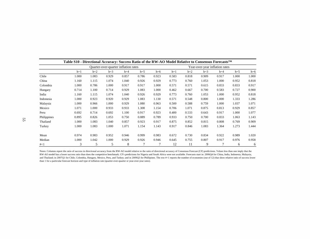
h=1 h=2 h=3 h=4 h=5 h=6 h=1 h=2 h=3 h=4 h=5 h=6Chile 1.000 1.083 0.929 0.857 0.786 0.923 0.583 0.818 0.909 0.917 1.000 1.000China 1.160 1.115 1.074 1.040 0.926 0.929 0.773 0.760 1.053 1.000 0.952 0.818Colombia 1.000 0.786 1.000 0.917 0.917 1.000 0.571 0.571 0.615 0.833 0.833 0.917Hungary 0.714 1.100 0.714 0.929 1.083 1.000 0.462 0.667 0.700 0.583 0.727 0.900India 1.160 1.115 1.074 1.040 0.926 0.929 0.773 0.760 1.053 1.000 0.952 0.818Indonesia 1.000 0.923 0.920 0.929 1.083 1.130 0.571 0.548 0.800 1.000 1.333 1.286Malaysia 1.000 0.966 1.000 0.929 1.080 0.963 0.500 0.588 0.759 1.000 1.037 1.071Mexico 1.071 1.000 0.933 0.933 1.308 1.154 0.706 1.071 0.875 0.813 0.929 0.857Peru 0.692 0.714 0.692 1.100 0.917 0.923 0.400 0.533 0.643 0.917 1.000 1.077Philippines 0.895 0.826 1.053 0.750 0.889 0.789 0.933 0.750 0.700 0.833 1.063 1.143Thailand 1.000 1.083 1.040 0.857 0.923 0.917 0.875 0.852 0.815 0.808 0.769 0.909Turkey 1.000 1.083 1.000 1.071 1.154 1.143 0.917 0.846 1.083 1.364 1.273 1.444
Mean 0.974 0.983 0.952 0.946 0.999 0.983 0.672 0.730 0.834 0.922 0.989 1.020Median 1.000 1.042 1.000 0.929 0.926 0.946 0.645 0.755 0.807 0.917 0.976 0.958#<1 3 5 5 8 7 7 12 11 9 7 6 6
Table S10 - Directional Accuracy: Success Ratio of the RW-AO Model Relative to Consensus Forecasts™Quarter-over-quarter inflation rates Year-over-year inflation rates
Notes: Columns report the ratio of success in directional accuracy from the RW-AO model relative to the ratio of directional accuracy of Consensus Forecast (CF) predictions. Values less than one imply that the RW-AO model has a lower success ratio than does the competitive benchmark. CF's predictions for Nigeria and South Africa were not available. Forecasts start in: 2006Q4 for China, India, Indonesia, Malaysia, and Thailand; in 2007Q1 for Chile, Colombia, Hungary, Mexico, Peru, and Turkey; and in 2009Q3 for Phillipines. The row #<1 reports the number of economies (out of 12) that show relative ratio of success lower than 1 for a particular forecast horizon and type of inflation rate (quarter-over-quarter or year-over-year rates).
55

Study Best forecasting model EMEs in the sample Data frequency Full sample Forecasting period Is the RW-AO considered?
Main statistic for forecast evaluation
Altug and Cakmakli (2016) Models with survey expectations Brazil, Turkey M 2001-2014 2007.1-2014.1 Yes RMSPEAron and Muellbauer (2012) Multivariate equilibrium correction models South Africa Q 1979-2007 2002.3-2007.4 No RMSPEBalcilar et al. (2015) Non linear DSGE model South Africa Q 1960-2011 2001.1-2011.4 No RMSPEChen et al. (2014) Model with world commodity prices South Africa, Chile Q 1983-2010 2000.4-2010.3 No RMSPEGupta et al. (2011) Factor models South Africa Q 1980-2000 2001.1-2006.4 No RMSPEMandalinci (2017) UCSV and TVPVAR models 9 EMEs Q 1979-2014 2001.1-2014.3 No RMSPE, Log scoresOgunc et al. (2013) BVAR and combination of different forecast model Turkey Q 2003-2011 2009.4-2011.2 Yes RMSPEPincheira and Gaty (2016) International inflation factor augmented model Chile M 1995-2013 2001.9-2013.3 No RMSPEPincheira and Medel (2015) DESARIMA model 6 EMEs M 1990-2011 1999.2-2011.12 No RMSPENotes: UCSV stands for unobserved component model with stochastic volatiliy. TVP-VAR denotes the time-varying parameter VAR model. DESARIMA denotes the Driftless Extended Seasonal ARIMA model. RW-AO is the random walk model proposed by Atkeson and Ohanian (2001). M, Q and A denote monthly, quarterly, annual data frequency, respectively.
56
Table S11 - A (Non-Exhastive) Literature Review of Inflation Forecasting for EMEs

Figure S1. Quarter-over-Quarter Headline CPI Inflation Rate (SAAR, %) Across EMEs
Notes: SAAR denotes seasonally-adjusted, annualized rate computations of the quarter-over-quarter growth rate. The shaded area defines the period each country operated under a de jure or de facto infl�ation-targeting scheme based on information from Roger (2010) and Hammond (2012). We also include a value corresponding to the index of central bank independence (CBI) proposed by Garriga (2016) for each country whereby a higher value closer to one by this measure indicates a more independent monetary policy framework. We follow the convention on hyperinflations in the literature introduced in Phillip Cagan's 1956 book The Monetary Dynamics of Hyperinflation : we define an episode of hyperinflation as the period when inflation is above 50% monthly (which corresponds to approximately 250% at quarterly frequency) and cap the vertical axis of each subplot accordingly. The only country in our sample that shows a distinct episode of hyperinflation in our sample is Peru during the late 1980s and early 1990s.
0
50
100
150
200
250
1980 1985 1990 1995 2000 2005 2010 2015
Turkey
CBI = 0.866
%
-15
-10
-5
0
5
10
15
20
25
1980 1985 1990 1995 2000 2005 2010 2015
Thailand
CBI = 0.230
%
-5
0
5
10
15
20
25
30
35
1980 1985 1990 1995 2000 2005 2010 2015
South Africa
CBI = 0.352
%
-10
0
10
20
30
40
50
60
70
80
90
1980 1985 1990 1995 2000 2005 2010 2015
Philippines
CBI = 0.634
%
-50
0
50
100
150
200
250
1980 1985 1990 1995 2000 2005 2010 2015
Peru
CBI = 0.798
%
-40
-20
0
20
40
60
80
100
120
140
1980 1985 1990 1995 2000 2005 2010 2015
Nigeria
CBI = 0.572
%
0
50
100
150
200
250
1980 1985 1990 1995 2000 2005 2010 2015
Mexico
CBI = 0.638
%
-10
-5
0
5
10
15
20
1980 1985 1990 1995 2000 2005 2010 2015
Malaysia
CBI = 0.505
%
-20
0
20
40
60
80
100
120
1980 1985 1990 1995 2000 2005 2010 2015
Indonesia
CBI = 0.864
%
-10
-5
0
5
10
15
20
25
30
1980 1985 1990 1995 2000 2005 2010 2015
India
CBI = 0.295
%
-10
0
10
20
30
40
50
1980 1985 1990 1995 2000 2005 2010 2015
Hungary
CBI = 0.827
%
-10
0
10
20
30
40
50
1980 1985 1990 1995 2000 2005 2010 2015
China
CBI = 0.601
%
-10
0
10
20
30
40
50
60
1980 1985 1990 1995 2000 2005 2010 2015
Chile
CBI = 0.819
%
0
5
10
15
20
25
30
35
40
1980 1985 1990 1995 2000 2005 2010 2015
Colombia
CBI = 0.693
%
57