inflation forecasting rbi

8/2/2019 Inflation Forecasting Rbi

http://slidepdf.com/reader/full/inflation-forecasting-rbi 1/32

W P S (DEPR): 01 / 2012

RBI WORKING PAPER SERIES

Inflation Forecasting: Issues

and Challenges in India

Muneesh Kapur

DEPARTMENT OF ECONOMIC AND POLICY RESEARCH

JANUARY 2012



The Reserve Bank of India (RBI) introduced the RBI Working Papers series in

March 2011. These papers present research in progress of the staff members

of RBI and are disseminated to elicit comments and further debate. The

views expressed in these papers are those of authors and not that

of RBI. Comments and observations may please be forwarded to authors.

Citation and use of such papers should take into account its provisional

character.

Copyright: Reserve Bank of India 2012



Inflation Forecasting: Issues and Challenges in India

Muneesh Kapur 1

This paper focuses on modelling and forecasting inflation in India using an augmented Phillips curve framework. Both demand and supply factors are seen as drivers of inflation. Demand conditions are found to have a stronger impact on

non-food manufactured products inflation (NFMP) vis-a-vis headline WPI inflation; moreover, NFMP is found to be more persistent than headline inflation. Both these findings support the use of NFMP as a core measure of inflation. But, the impact of global non-fuel commodities on NFMP is found to be substantial. Inflation in non- fuel commodities is seen as a more important driver of domestic inflation rather than fuel inflation. The exchange rate pass-through coefficient is found to be modest, but nonetheless sharp depreciation in a short period of time can add to inflationary pressures. The estimated equations show a satisfactory in-sample as well as out-of-sample performance based on dynamic simulations. Nonetheless,forecasting challenges emanate from volatility in international oil and other commodity prices and domestic food supply dynamics.

JEL Classification Numbers: E31; E32; E52; E58.

Keywords: Exchange Rate Pass-through, India, Inflation, Monetary Policy, PhillipsCurve..

Maintenance of price stability, defined as low and stable inflation, is the best

way through which monetary policy can contribute to sustained and high growth.

Post the recent global financial crisis, it is now recognized that price stability may

not, however, ensure financial stability. While price stability is a necessary

condition, it is not a sufficient condition for financial stability. Nonetheless, price

stability continues to remain a necessary pre-requisite for financial stability and

growth.

High inflation has an adverse impact on growth through a variety of

channels. First, high inflation leads to uncertainty which impacts investment and

growth. As it is, investment decisions are subject to a lot of uncertainties. High and

volatile inflation adds further to these uncertainties. Second, high inflation makes

banks deposits less attractive and encourages investment in physical assets and

speculative activities, which leads to diversion of savings away from formal

1 Director, Monetary Policy Department, Reserve Bank of India (E-mail). The views

expressed in the paper are those of the author and do not necessarily represent those of the institution to which he belongs.

1

mailto:[email protected]

mailto:[email protected]



financial savings channels such as bank deposits. These developments lead to

reduction in financial savings. Thus, high inflation has an adverse impact on both

savings and investment. Finally, high inflation has a particular more severe impact

on the poor and other vulnerable segments of the society in developing economies

like India, with high poverty levels. Thus, low and stable inflation is desirable from

a number of perspectives.

Low and stable inflation, therefore, remains a key objective of monetary

policy for central banks, whether inflation targeting or otherwise. However,

achievement of low and stable inflation is quite challenging. It is well-known that

monetary policy affects output and prices with lags, which are both long and

variable. Accordingly, monetary policy has to be forward-looking, i.e., monetary

policy needs to act today in anticipation of future growth and inflation trajectory.

Therefore, forecasts of growth and inflation play a critical role in the conduct and

formulation of monetary policy and its ultimate success in achieving price stability.This, in turn, depends upon success in modelling and forecasting inflation and

growth.

In India, low and stable inflation remains a key objective of monetary policy

along with growth and financial stability. Inflation dynamics in emerging economies

like India are, however, relatively more complex than advanced economies in view

of recurrent supply shocks and large weight of volatile components such as food

items in the various price indices. This makes inflation modelling and forecasting

more challenging in countries like India.

Inflation in India has remained persistently high since early 2010, with

headline WPI moving in a range of 9-10 per cent till October 2011, significantly

above its average of around 5 per cent recorded during the 2000s. Non-food

manufactured products inflation, a measure of underlying inflation, has also

increased over the course of 2011 and has moved in a range of 7-8 per cent

during 2011. What explains these inflation dynamics? Can these be explained by

standard models and approaches such as the Philips curve framework?

Against this backdrop, this paper begins with a brief overview of alternate

modelling approaches for inflation (Section I). The following section (Section II)

undertakes a review of the Phillips curve approach to modelling and forecasting

inflation and discusses both the traditional Phillips curve and the New Keynesian

Phillips Curve (NKPC) approaches. This section also assesses the available

2



cross-country empirical evidence for or against the Phillips curve. Section III then

attempts to model inflation in India based on a Phillips curve framework and

assesses the forecasting performance of this approach. Section IV concludes.

I. Approaches to Modelling and Forecasting Inflation

A number of approaches are available for modelling inflation. The first

approach to modelling inflation is provided by estimating a short-run aggregate

supply curve, i.e., an augmented Phillips curve which relates inflation to demand

pressures and supply shocks in the economy. A more detailed discussion of the

Phillips curve modelling and forecasts in the Indian context is taken up in the next

section.

The second approach is the use of time series econometrics such as

univariate autoregressive moving average (ARMA) models or multivariate Vector Autoregressive (VAR) models, which provide relatively good forecasts at short

horizons. Illustratively, Biswas et al. (2010) model inflation as well as industrial

growth for India in a VAR as well as Bayesian VAR (BVAR) framework and found

that the BVAR model out-performed the VAR model in case of forecasts for both

inflation and industrial growth.

The third approach is based upon the recognition that inflation is ultimately

a monetary phenomenon and there exists a long-run stable relationship between

money and inflation. Although the Phillips Curve framework does not have money

supply variables explicitly, this does not mean that money supply is not important.

While money demand may be unstable in the short-run because of financial

innovations, it is found to be reasonably stable over the long run (Lucas, 1988;

Ball, 1998). Short-run inflation dynamics are largely dependent on supply-demand

conditions, but monetary expansion influences inflationary conditions in the long-

run. Prior to the global financial crisis, monetary and credit aggregates were de-

emphasised in major advanced economies, with the notable exception of the

European Central Bank. Post the financial crisis, there is a greater recognition that

monetary and credit factors need to be monitored and efforts are also on to

incorporate such factors in modern models. Explicit attention to the long-run

relationship between money growth and inflation may be valuable (Goodhart

3



2007). Thus, monetary aggregates continue to be an important information

variable in the context of inflation dynamics.

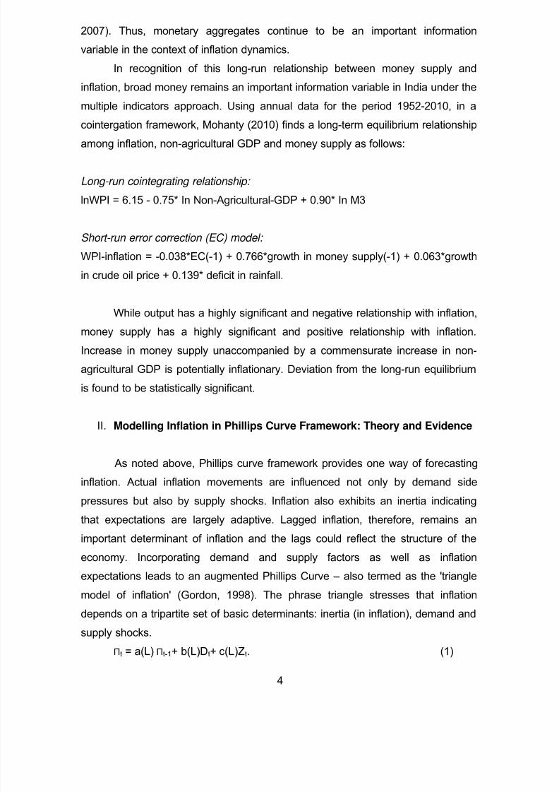
In recognition of this long-run relationship between money supply and

inflation, broad money remains an important information variable in India under the

multiple indicators approach. Using annual data for the period 1952-2010, in a

cointergation framework, Mohanty (2010) finds a long-term equilibrium relationship

among inflation, non-agricultural GDP and money supply as follows:

Long-run cointegrating relationship:

lnWPI = 6.15 - 0.75* In Non-Agricultural-GDP + 0.90* In M3

Short-run error correction (EC) model:

WPI-inflation = -0.038*EC(-1) + 0.766*growth in money supply(-1) + 0.063*growth

in crude oil price + 0.139* deficit in rainfall.

While output has a highly significant and negative relationship with inflation,

money supply has a highly significant and positive relationship with inflation.

Increase in money supply unaccompanied by a commensurate increase in non-

agricultural GDP is potentially inflationary. Deviation from the long-run equilibrium

is found to be statistically significant.

II. Modelling Inflation in Phillips Curve Framework: Theory and Evidence

As noted above, Phillips curve framework provides one way of forecasting

inflation. Actual inflation movements are influenced not only by demand side

pressures but also by supply shocks. Inflation also exhibits an inertia indicating

that expectations are largely adaptive. Lagged inflation, therefore, remains an

important determinant of inflation and the lags could reflect the structure of the

economy. Incorporating demand and supply factors as well as inflation

expectations leads to an augmented Phillips Curve – also termed as the 'triangle

model of inflation' (Gordon, 1998). The phrase triangle stresses that inflation

depends on a tripartite set of basic determinants: inertia (in inflation), demand and

supply shocks.

Πt = a(L) Πt-1+ b(L)Dt+ c(L)Zt. (1)

4



where, Πt, Dt and Zt denote inflation, a measure of excess demand (unemployment

gap or output gap) and supply shocks (imported inflation or exchange rate

movements), respectively; a(L), b(L) and c(L) are lag polynomials.

New Keynesian Phillips Curve

As against the above traditional backward-looking ad hoc Phillips curve, in

recent years, the Phillips curve has been derived from micro-foundations, with

optimal price setting by forward-looking monopolistically competitive firms. Such a

formulation leads to a New Keynesian Phillips Curve (NKPC), a purely forward-

looking Phillips curve: in this specification, inflation depends inter alia upon

expected future inflation (Et Πt+1); in contrast, inflation depends on expected

current inflation (Et-1 Πt) in the traditional expectations-augmented standard Phillips

curve. The purely forward-looking Phillips curve, however, does not get muchempirical support. Lagged inflation remains an important determinant of inflation,

and in fact, a purely backward-looking Phillips curve seems to be preferred by the

data, which has led to ad hoc hybrid Phillips curve – with both forward- and

backward-looking inflation components (Gali et al ., 2005). Gali et al. (2005) find

that the coefficient on expected inflation is higher than that of lagged inflation,

which they argue as evidence in favour of NKPC.

However, the NKPC and its empirical estimates are subject to serious

identification issues as these specifications do not allow to distinguish forward-

looking models from backward-looking models; the higher weight on expected

inflation may be due to misspecification resulting from omission of explanatory

variables from the main equation. Typically, expected inflation is instrumented

through lagged inflation amongst the instrument set and this can bias the

coefficient on expected inflation to be higher and NKPC can yield large estimates

of the coefficient on expected inflation even when forward-looking behaviour is

completely absent (Rudd and Whelan, 2007). Moreover, while many studies find

that the forward-looking behaviour dominates, the robust confidence intervals are

so wide that the results are consistent both with no backward-looking dynamics as

well as very substantial backward-looking behavior (Kleibergen and Mavroeidis,

2009).

5



Philips Curve Forecasts: An Assessment

While Phillips curve framework remains the workhorse model for modelling

inflation and thinking about policy issues, question marks have been raised over

its forecasting abilities. According to Atkeson and Ohanian (2001), random walk

(naive) forecasts beat (backward-looking) Phillips curve forecasts. In a similar

vein, Stock and Watson (2008) note that, while Phillips Curve forecasts are better

than other multivariate forecast, but their performance is episodic, sometimes

better than and sometimes worse than a good univariate benchmark. Peach et al.

(2010) find threshold effects in the Philips curve, i.e., if output gap (or

unemployment gap) is within a certain threshold, the relationship between inflation

and activity is weak, but when the output gap is outside these thresholds, there is

a significant impact of economic activity on inflation. For the US, they estimate the

threshold in terms of unemployment gap to be 1.56 per cent; thus, if the

unemployment gap is within +/- 1.56 per cent, there is no impact of unemploymenton inflation, and the effect on inflation is significant only when the unemployment

gap is outside this threshold of +/- 1.56 per cent. Meyer and Pasaogullari (2010)

find that no single specification outperforms all others over all time periods; for

example, for the US, they find that the median and 16 percent trimmed-mean

measures outperform all other specifications during the 1990s, and survey-based

inflation expectations seem to do better during volatile periods. On the other hand,

Fuhrer et al. (2009a) find that the forecasting performance of Phillips curve is

better if changing dynamics of inflation, in particular the weakening impact of oil

prices on inflation, are taken into account.

Between the backward-looking and the forward-looking specifications,

micro-founded versions of the Phillips curve can be viewed as complementary to

standard backward-looking specifications and there is little evidence suggesting

that forward-looking Phillips curve specifications provide more accurate inflation

forecasts than a standard backward-looking specification (Fuhrer, 2009b).

According to Gordon (2011), the triangle model outperforms the NKPC variant by

orders of magnitude, not only in standard goodness-of-fit statistics, but also in

post-sample dynamic simulations. Similarly, Ball and Mazumder (2011) find the

Great Recession of 2009-10 provides evidence against the NKPC. As a result, the

traditional backward-looking specification, augmented to account for supply

6



shocks, continues to play a role in shaping the inflation outlook and the conduct of

monetary policy.

Phillips Curve Studies for India

In the Indian context, previous attempts to model inflation using Phillips

curve framework include Dholakia (1990), RBI (2001, 2004), Kapur and Patra

(2002), Srinivasan et al. (2006), Dua and Gaur (2009), Paul (2009), Patra and Ray

(2010), Patra and Kapur (2010), Singh et al. (2011), and Mazumder (2011). RBI

(2001, 2004) and Kapur and Patra (2002), using annual data, found evidence for a

Phillips curve relationship in India, with role for both excess demand conditions

(output gap) and supply shocks (food inflation and import prices). Srinivasan et al.

(2006) do not find support for Phillips curve with coefficients on output gap terms

being insignificant (although positive) with headline inflation as the dependent

variable; the coefficient on output gap was found to be negative withmanufacturing headline inflation as the dependent variable. Their analysis is

based on monthly data for the period April 1994-March 2005 and industrial

production as the activity variable. Using annual data, Paul (2009) is able to find

support in favour of a Phillips curve only when industrial production is used as an

indicator of economic activity (instead of overall GDP) and data are re-arranged on

a crop year basis (instead of fiscal year basis). Dua and Gaur (2009) investigate

Phillips curve relationship for a number of Asian economies (both developing and

developed) and find support for the existence of Phillips curve in India (sample

period 1996-2005 using quarterly data) as well as other economies in their study;

while they include import inflation as an explanatory variable for the developed

countries in their sample, it is not included in their developing countries sample.

Patra and Ray (2010) employ Phillips curve framework in the context of

modeling inflation expectations and find support in favour of the relationship using

monthly data for the period 1997-2008. Patra and Kapur (2010) estimated a range

of Philips curves in the context of a new Keynesian model using quarterly data for

1996-2009. They estimate traditional backward-looking Philips curve as well as

purely forward-looking NKPC and hybrid NKPC, while controlling for supply shocks

and using overall GDP as the activity variable. While Patra and Kapur (2010)

found some support for the NKPC and the hybrid version of the same, the

estimated equations suffered from serial correlation. Moreover, in the hybrid

7



NKPC, the coefficient on lagged inflation was found to be higher than that of the

expected inflation. The backward-looking Philips curve satisfied the various

diagnostics. Singh et al. (2011) are able to find a Phillips curve relationship in the

latter part (2004:Q2 to 2009: Q4) but not in the first part (1997:Q4 to 2004:Q1) of

their sample. Supply shocks are captured rather crudely by looking at the outlier

point in the contemporaneous relationship between inflation and output gap.

Mazumder (2011) finds support for the Phillips curve relationship for India using

quarterly data for the period 1970-2008 with economic activity proxied by industrial

production and movements in oil prices as a control for supply shock; the

relationship is found to be stable across various monetary regimes proxied by the

terms of various Governors. All the above mentioned studies use output gap

based on Hodrick-Prescott filter, except for Singh et al. (2011) who use Kalman

filter. Bhalla (2011) focuses on the role of minimum support prices in driving

inflation dynamics in a simple bi-variate framework, regressing headline inflationon minimum support prices.

A review of the existing studies in the Indian context shows a number of

limitations. First, a number of studies use industrial production as the activity

variable to measure demand pressures. Overall inflation in an economy reflects

aggregate demand pressures and these are best captured by excess demand

measures based on overall activity. Industrial activity accounts for less than a fifth

of the Indian GDP and captures the overall demand pressures rather imperfectly.

Services sector now accounts for two-thirds of GDP and its exclusion may give a

misleading picture. Second, a number of studies are based on annual data, which

reduces their relevance for policy purposes and moreover, such studies cannot

capture inflation dynamics appropriately. Third, in almost all studies, the role of

external supply shocks is limited to international crude oil prices. In recent years,

non-oil commodity prices have also witnessed a significant jump amidst elevated

volatility. Moreover, while the domestic fuel prices are administered in India as is

the case in many other EMEs, domestic non-oil prices are relatively freely

determined. In this context, global non-oil commodity inflation trends are

potentially important determinants of inflation and their role needs to be assessed.

Fourth, in the recent period, the Reserve Bank has articulated non-food

manufactured products WPI inflation as an indicator of demand-side pressures

(RBI, 2011). According to Raj and Misra (2011), who examine a host of core

8



measures of inflation, non-food manufactured products inflation is the only

measure which satisfies all the properties of a core measure. None of the existing

studies have modeled this component of inflation. Fifth, the role of minimum

support prices is tested in a bivariate framework in Bhalla (2011), but not in a

multivariate framework. Sixth, given the continued dependence of agriculture on

monsoon conditions, rainfall conditions remain a key determinant of domestic food

and overall inflation. Finally, the sharp depreciation of the rupee during July-

September 2011 again brought into focus the role of exchange rate pass-through.

Existing studies have focused on movements in nominal exchange rate of the

rupee vis-à-vis the US dollar, but sensitivity analysis to nominal effective exchange

rate is missing. This issue is found to be important in the context of modeling non-

food manufactured products inflation, as discussed in a later section. Overall, the

various existing studies touch upon some aspects of the determinants of inflation,

but a comprehensive assessment taking into account all potential determinants ismissing. This paper, therefore, attempts to overcome these limitations of the

existing studies and attempts to provide a comprehensive approach to inflation

dynamics in India.

III. Phillips Curve Modelling for India

Methodology and Data

Given the empirical superiority of the traditional Phillips curve over the

NKPC, this paper uses the former framework, following Gordon (1998), to model

inflation in India. In India, wholesale price index (WPI) inflation is the headline

measure of inflation, although the Reserve Bank also takes into account trends in

other inflation indicators such as consumer prices and GDP deflator. As noted

earlier, the Reserve Bank has recently emphasized non-food manufactured

products WPI inflation as an indicator of demand-side pressures; we, therefore,

model both headline WPI inflation and the non-food manufactured products

inflation group within the WPI. Based on the discussion in the preceding section,

apart from the demand conditions, the potential explanatory variables are a host of

supply shocks such as global commodity inflation, rainfall conditions, minimum

support prices and the exchange rate. In the context of high food and fuel inflation,

9



an issue of topical interest is the extent of spillover from food and fuel prices to

non-food manufactured products inflation. The paper attempts to address this

issue also. The impact of demand conditions on inflation may be non-linear which

can be studied by including square of output gap terms or separate variables for

positive and negative output gaps (Dolado et al, 2005); the impact could also be

asymmetric depending upon whether output gap is positive or negative.

Drawing from the discussion above, variants of the following general

specification of Phillips curve are estimated:

INFWPIt = a0 + a1*YGAPt + a2*Et-1 INFWPIt + a3*INFGLt + a4*INFCRt + a5*EXCHAt (or,

a5*NEERt) + a6*RAIN t + a7*MSP t + a8*YGAP2t + vt (2)

INFMPNFt = a0 + a1*YNGAPt + a2*Et-1 INFMPNFt + a3*INFGLt + a4*INFCRt + a5*EXCHA t (or,

a5*NEERt) + a6*INFFOODt + a7*YNGAP2t + vt (3)

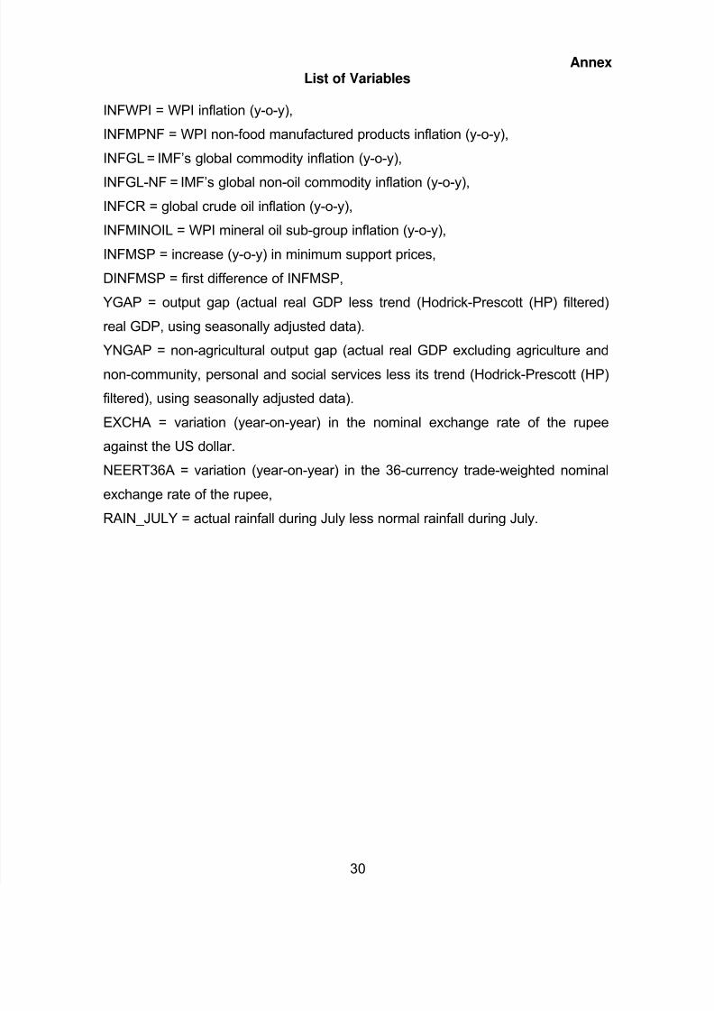
The variables are defined in Annex. All the data series are stationary, with

some ambiguity about MSP inflation2. All data are measured in per cent terms.

Output gap (YGAP) is computed as actual real GDP less trend (Hodrick-Prescott

(HP) filtered) real GDP, using seasonally adjusted data3. In the case of non-food

manufactured products inflation equation, output gap is based on non-agricultural

real GDP and the relevant output gap (YNGAP) is computed as actual real non-

agricultural GDP less its trend (Hodrick-Prescott (HP) filtered), using seasonally

adjusted data. Et-1INFWPIt and Et-1INFMPNFt denote expected inflation in period

t-1 for the next period. Inflation expectations are assumed to be adaptive and are

captured through lags of inflation following Gordon (1998) and others. Two lags of

inflation are included in the equations to ensure no residual autocorrelation. The

equations are estimated using quarterly data for the period 1996-2011 (April-June

1996 to January-March 2011).

Empirical Results

2Unit root tests (Augmented Dickey-Fuller tests, with lag selection based on BIC criteria) indicate

that all data series are stationary except for MSP inflation. However, the KPSS test cannot rejectthe null of stationarity for MSP inflation.3

Results are robust to the computation of output gap using the Baxter-King band-pass filter.

10



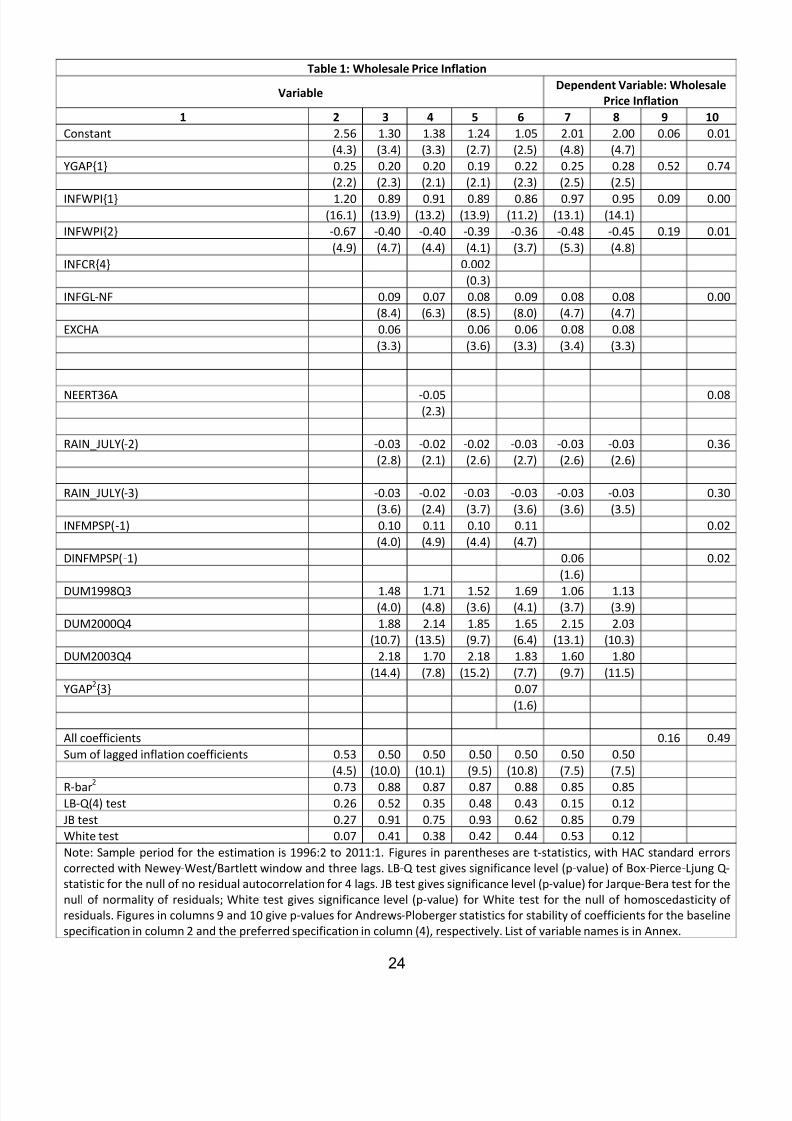
Results for headline WPI inflation are set in Table 1 and those for non-food

manufactured products inflation are in Table 2. The estimated coefficients are on

the expected lines. Column 2 in both tables reports results for the baseline Phillips

curve without supply shocks. Subsequent columns in both the tables estimate the

augmented Phillips curve by adding various supply shocks, followed by testing for

non-linearity.

Headline WPI Inflation

Beginning with the specification for the headline inflation, the key features

of the estimates are, first, excess demand conditions have an upward pressure on

inflation, while deficiency in demand pulls down inflation: the estimates indicate

that if output gap is one per cent (i.e., actual output is one per cent above the

potential output level), then inflation increases by 19-25 basis points with a lag of

one quarter and the long-run impact is 40-53 basis points (Table 1, columns 2-6). According to the linear specifications in these columns, the impact is symmetric

and therefore, a negative output gap (deficit demand conditions) leads to an

equivalent reduction in inflation. The demand variable is significant even in the

baseline specification that does not incorporate supply shocks (Table 1, column 2).

Thus, contrary to Paul (2009) and some other studies, the Phillips curve relation

for India exists without the need to incorporate supply shocks and other

adjustments.

Second, the inflation process is persistent, with the sum of lagged

coefficients being around 0.5 and highly significant (Table 1, columns 2-6). Third,

global commodity prices have a strong and quick pass-through (Table 1, columns

3-6). An increase of 10 per cent in global non-fuel commodity prices increases

headline WPI inflation by 70-90 basis points in the same quarter, with the long-run

impact being double (140-180 basis points); the coefficient needs to be juxtaposed

with the large volatility in international commodity prices witnessed in the recent

years. Fourth, when we add international crude oil prices to the equation (column

5), the coefficient is found to be positive but statistically insignificant. This could be

reflecting delayed and incomplete pass-through of high international crude oil

prices to domestic prices in view of the administered nature of domestic fuel

prices. The Government has also modulated the taxes and duties on petroleum

products to smoothen the impact of volatility in international crude prices on

11



domestic inflation. These factors create a wedge between movements in

international crude oil prices and domestic fuel prices, which make it difficult to

estimate the impact in the equation. Similar findings are reported by Dua and Gaur

(2009) on the role of oil prices in the inflation process for India as well as the other

three developing Asian countries (China, Philippines and Thailand) in their sample.

Mohanty and Klau (2001) too report a similar finding – in only 5 out of 14 EMEs in

their sample, oil prices are found to have a significant impact on inflation.

Fifth, the coefficient on the exchange rate indicates that the exchange rate

pass-through is 0.06 in the short-run and 0.12 in the long-run, i.e., 10 per cent

appreciation (deprecation) of rupee vis-à-vis the US dollar reduces (increases)

inflation by 60 basis points in the same quarter, while the long-run pass-through is

120 basis points. The results are broadly similar when we use the NEER instead

of the nominal exchange rate. The signs on the exchange rate (positive) and the

NEER (negative) variables differ because of the measurement issues: while anincrease in the nominal exchange rate denotes depreciation of the rupee, an

increase in the NEER denotes appreciation of the rupee. The exchange rate pass-

through coefficient is thus relatively low and is consistent with other estimates (for

example, Khundrakpam, 2008; Patra and Kapur, 2010). The exchange rate pass-

through for India is close to that of low inflation countries (0.16) (Choudhri and

Hakura, 2001). The Indian rupee depreciated by around 10 per cent vis-a-vis the

US dollar during July-September 2011 and the pass-through estimates in this

paper suggest that this depreciation could add almost 120 basis points to headline

inflation in the long-run.

Sixth, given the importance of the south-west monsoon, rainfall shortage

during the month of July – the critical month for kharif sowing - is found to have an

adverse impact on inflation, with a lag of 2-3 quarters. A deficiency of 10 per cent

in the rainfall in July increases headline inflation by 60 basis points with a lag of

three quarters and the long-run impact turns out to be 120 basis points. Seventh,

minimum support prices have a substantial impact: 10 per cent increase in

minimum support prices increase headline WPI inflation by 100 basis points with

lag of a quarter, and the long-run impact is 200 basis points. At the same time,

minimum support prices are also found to respond to headline WPI inflation with a

lag. However, as noted earlier, the unit root tests provide conflicting results

regarding MSP inflation: while the ADF tests cannot reject the null hypothesis of

12



unit root, the KPSS test accepts the null of stationarity. Therefore, in order to

check the robustness of the results, Table 1 (column 7) reports results when first

difference of minimum support prices inflation (DINFMSP) is used, while column 8

reports results when MSP inflation is dropped from the specification. In both

cases, the results are broadly the same. When the first difference of MSOP

inflation is used, the coefficient is found to be positive and somewhat lower, but it

is significant only at slightly below 10 per cent. When the MSP inflation variable is

dropped, the results are qualitatively similar as in the baseline (column 3); the only

difference is that the coefficient on output gap and the exchange rate are

somewhat higher.

Finally, on the issue of whether there is a differential impact of excess v/s

deficient demand on inflation, there is some evidence of asymmetry. We test for

asymmetry by adding squared output gap term to the linear specification of column

3. The coefficient on the squared output gap term is found to be positive, but it isweakly significant at 10 per cent (Table 1, column 6). Subject to this caveat, the

point estimates indicate that a positive output gap (actual output above the

potential) of one per cent increases headline inflation by 36 basis points in the

short-run and by 72 basis points in the long-run, whereas a negative output gap

(actual output below the potential) of one per cent reduces headline inflation by

only 8 basis points and 16 basis points in the short-and long-run; by contrast, the

corresponding linear model (column 3), the impact of output gap on inflation is 20

and 40 basis points.

Diagnostic tests are satisfactory and indicate residuals are normally

distributed, free from serial correlation and are homoscedastic (Table 1)4. The

various equations have good explanatory power with R-bar 2 of 0.87-0.88. Formal

stability tests - Andrews-Ploberger tests - indicate that the estimated specifications

are stable and Table 1 (columns 7-8) report these tests for the baseline

specification (column 2) and the preferred specification (column 4). According to

the tests, the null of coefficient stability cannot be rejected for individual

coefficients as well as all coefficients together for the baseline specification in

column 2. For the augmented and the preferred specification in column 4, there is

4Unit root tests for residuals (not reported) both for headline inflation (Table 1) and non-food

manufactured products inflation (Table 2) indicate that these are stationary.

13



some evidence of instability in some of the individual coefficients; however, the

null of stability for all coefficients jointly cannot be rejected.

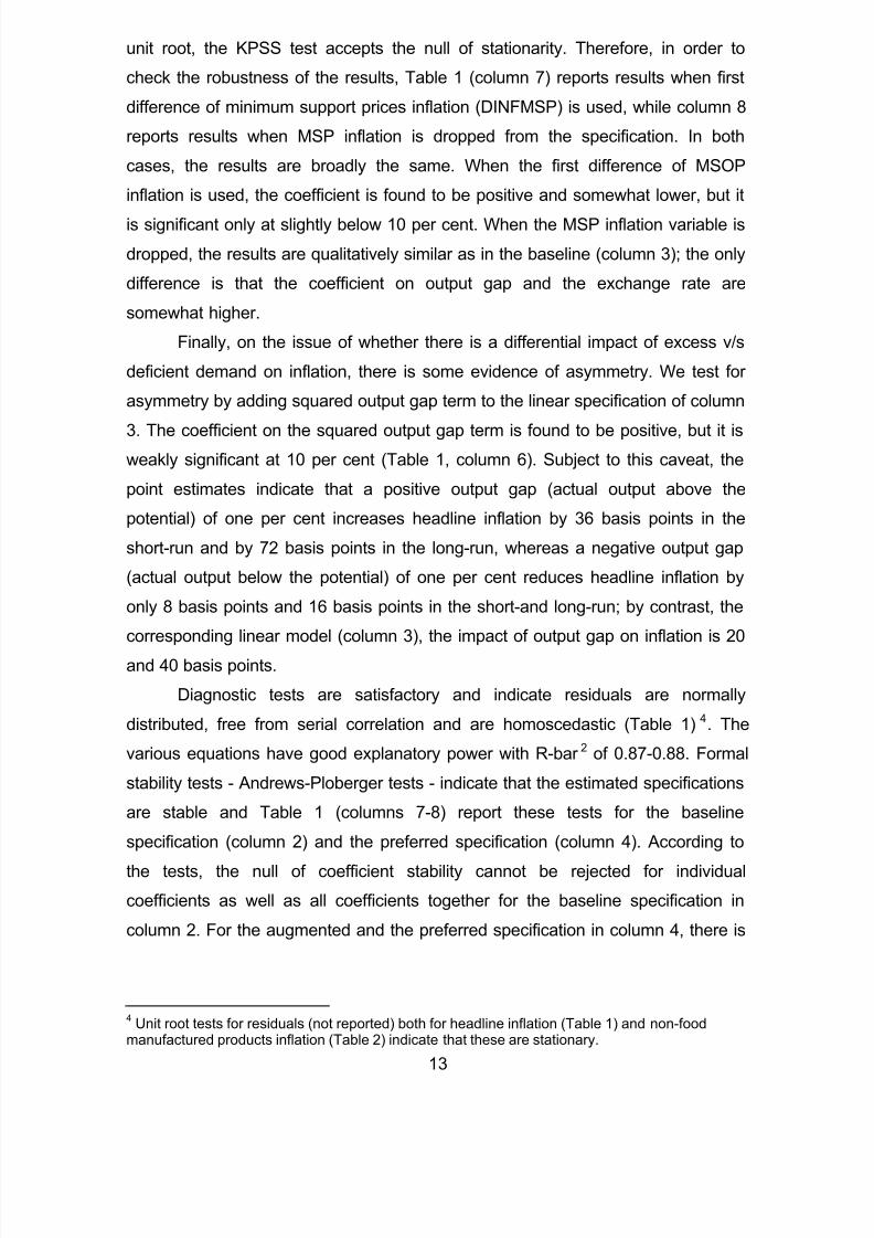
The preferred equation (column 4) has a good explanatory power and

captures the turning points in inflation relatively well, although there are periods of

deviations. These are partly due to movements in domestic fuel and food prices,

which are not explicitly modeled in the equation to avoid over-fitting.

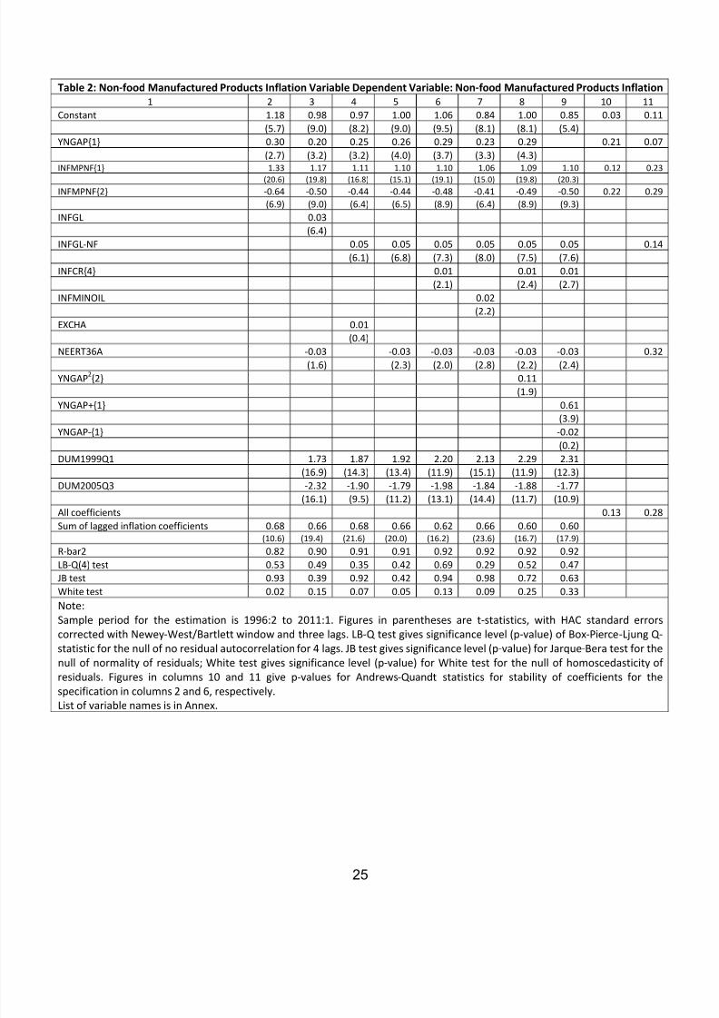
Non-food Manufactured Products Inflation

Turning to non-food manufactured products (NFMP) inflation (Table 2), the

results are qualitatively the same as in the headline inflation case. There are a few

notable differences from the estimates in Table 1. First, the impact of demand

conditions on inflation is now higher than that in the headline inflation case. A

positive (negative) non-agricultural GDP gap of one per cent increases (reduces)

NFMP inflation by 20-30 basis point with a lag of one quarter, and the long-run

impact is 59-94 basis points (Table 2, columns 2 to 9). The long-run impact of

demand conditions on NFMP inflation is twice the estimates in the corresponding

specifications in the headline WPI inflation case. This finding of demand conditions

having a relatively stronger impact on NFMP inflation vis-a-vis headline inflation

supports the RBI’s policy focus on NFMP as an indicator of demand pressures in

the economy.

Second, NFMP inflation is more persistent compared to headline inflation,

as may be seen from the sum of lagged inflation coefficients (0.60-0.68 in the case

of NFMP and around 0.50 in the case of headline inflation). The relatively sticker

14



nature of NFMP also extends support to NFMP being used as a core measure of

inflation or an indicator of underlying inflation pressures. As Woodford (2003) has

noted, it is the stickiness in prices or the persistence in inflation that leads to

deviation of actual output from its natural (potential) level of output. As all goods

prices are not sticky, central banks should target a measure of core inflation that

places greater weight on those prices which are stickier.

Third, global commodity inflation remains an important driver of NFMP

inflation: the coefficient estimates indicate that an increase of 10 per cent in global

non-fuel prices increases NFMP inflation by 50 basis points in the same quarter

and 130-160 basis points in the long-run. Both the immediate and the long-run

impact of global non-fuel inflation on NFMP inflation (50 and 130-160 basis points)

is somewhat less than that on headline inflation (70-90 and 140-180 basis points).

Nonetheless, the impact of global inflation on NFMP inflation is substantial – this

finding does not lend support to NFMP being a core indicator of inflation. Thus,whereas the first two findings of strong demand impact and more persistent nature

support the case of NFMP as a core indicator of inflation, the continued large

impact of global commodity shocks on NFMP inflation raises the question as to

whether NFMP is imported inflation (Mohanty, 2011). We revert to this issue later.

Fourth, international crude oil prices are found to have a statistically

significant impact on NFMP inflation, but the impact is quite modest vis-a-vis non-

fuel commodity prices. An increase of 10 per cent in international crude oil prices

increases NFMP inflation by only 10 basis points and that too with a lag of four

quarters; the long-run impact is 30 basis points (Table 2, column 6). The modest

impact can be attributed to delayed and incomplete pass-through to domestic

prices, as noted earlier. When we use the WPI mineral group inflation as an

indicator of oil inflation (in lieu of international crude oil inflation), the impact is

somewhat stronger as well as quicker. An increase of 10 per cent in WPI mineral

oil group inflation increases NFMP inflation by 20 basis points in the same quarter

and 60 basis points in the long-run (Table 2, column 7).

Fifth, the exchange rate coefficient surprisingly is not found to be significant

when we use the nominal exchange rate of the rupee (Table 2, column 4).

However, when we use the movements in the NEER as an indicator of the

exchange rate, the coefficient is found to be statistically significant. As noted

earlier, given the measurement practices, the coefficient on the NEER is negative:

15



an increase in the NEER indicates appreciation and vice versa. The exchange rate

pass-through coefficient is 0.03 and 0.08-0.09 in the short-run and long-run,

respectively (Table 2, columns 5-9). Thus, 10 per cent depreciation of the NEER

leads to an increase of 30 basis points in the WPI-NFMP inflation in the same

quarter and 80-90 basis points in the long-run. The difference in the results

between using the nominal exchange rate and the NEER is due to the fact that

there have been some periods when the two measures indicate contradictory

movements.

Finally, as in the case of headline inflation, there is some evidence of

asymmetric impact of demand conditions (Table 2, column 8). A positive output

gap of one per cent increases NFMP inflation by 51 basis points with a lag of

quarter and 128 basis points in the long-run; the impact of negative output gap on

NMFMP inflation is substantially muted – it reduces NFMP inflation by 7 and 18

basis points in the short- and long-run, respectively. Alternatively, if we drop theoutput gap variable altogether from the specification and enter positive and

negative output gap variables as separate coefficients, the results are even

stronger (Table 2, column 9). While deficient demand conditions do not seem to

have any impact on inflation, strong demand conditions have more significant

impact. However, given the limited sample size, such results need to be

corroborated with alternative approaches.

Diagnostic tests indicate no residual serial correlation, and the residuals are

normally distributed. The null of homoscedastic errors cannot be rejected for

various specifications (except column 2) (Table 2). The alternative specifications

have high explanatory power (with R-bar 2 of 0.91-0.92). We chose the

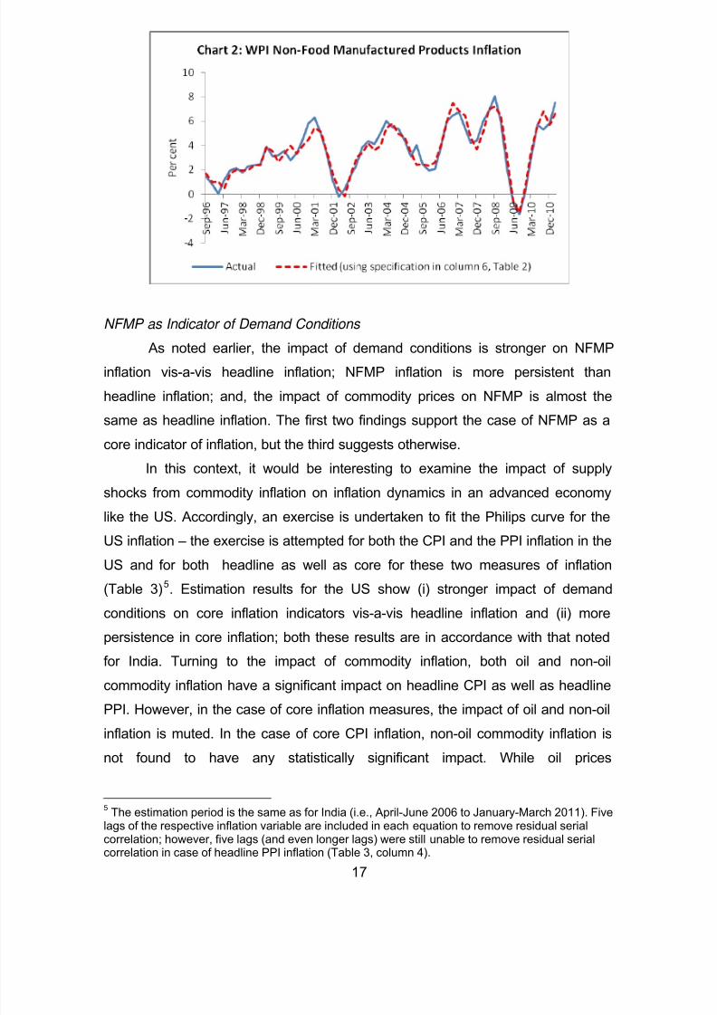
specification in column 6 as the preferred specification and this has a relatively

good fit (Chart 2). Andrews-Ploberger tests (reported in columns 8 and 9) for the

baseline (column 2) and the preferred (column 6) specifications cannot reject the

null of coefficient stability for the individual as well as all coefficients taken

together. Thus, the results are more robust vis-a-vis the headline inflation case,

where the stability tests were unable to reject the null in the case of some

individual variables.

16



NFMP as Indicator of Demand Conditions

As noted earlier, the impact of demand conditions is stronger on NFMPinflation vis-a-vis headline inflation; NFMP inflation is more persistent than

headline inflation; and, the impact of commodity prices on NFMP is almost the

same as headline inflation. The first two findings support the case of NFMP as a

core indicator of inflation, but the third suggests otherwise.

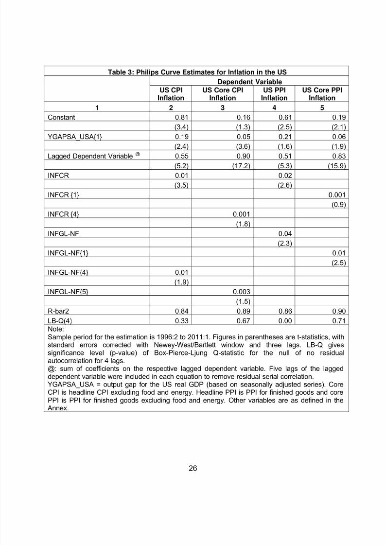
In this context, it would be interesting to examine the impact of supply

shocks from commodity inflation on inflation dynamics in an advanced economy

like the US. Accordingly, an exercise is undertaken to fit the Philips curve for the

US inflation – the exercise is attempted for both the CPI and the PPI inflation in the

US and for both headline as well as core for these two measures of inflation

(Table 3)5. Estimation results for the US show (i) stronger impact of demand

conditions on core inflation indicators vis-a-vis headline inflation and (ii) more

persistence in core inflation; both these results are in accordance with that noted

for India. Turning to the impact of commodity inflation, both oil and non-oil

commodity inflation have a significant impact on headline CPI as well as headline

PPI. However, in the case of core inflation measures, the impact of oil and non-oil

inflation is muted. In the case of core CPI inflation, non-oil commodity inflation is

not found to have any statistically significant impact. While oil prices

5The estimation period is the same as for India (i.e., April-June 2006 to January-March 2011). Five

lags of the respective inflation variable are included in each equation to remove residual serialcorrelation; however, five lags (and even longer lags) were still unable to remove residual serialcorrelation in case of headline PPI inflation (Table 3, column 4).

17



contemporaneously impact on headline CPI inflation, the impact on core CPI is

with a lag of four quarters; moreover, the long-run impact is only a third of the

impact on the headline inflation. Moving to core PPI inflation, oil inflation is not

found to have any statistical significant impact. On the other hand, non-oil

commodity inflation impacts core PPI inflation with a lag of a quarter (the impact

on headline PPI was contemporaneous). Moreover, the long-run impact of non-oil

commodity inflation on core PPI is lower than that on headline PPI. Overall, the

core measure of inflation in India scores well on the first two of the three

parameters of the core measure – stronger impact of demand conditions, more

persistence and lower impact of supply shocks - whereas the US core measures

seem to satisfy all the three.

Dynamic Forecasting Performance: In Sample and Out of Sample

How good is the forecasting performance of the estimated Phillips curves

perform in the Indian context? This section assesses both in sample and out of

sample forecasting performance.

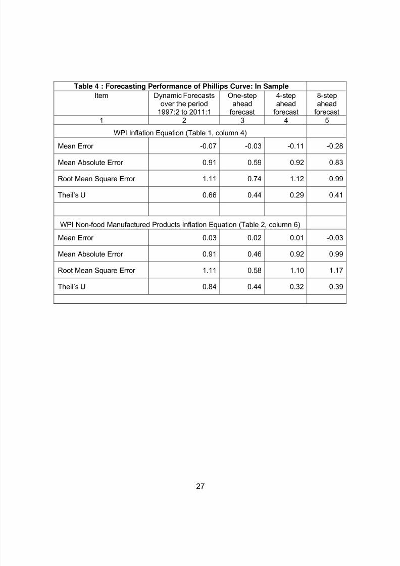
As regards in sample dynamic forecasting, the results are based on the

respective equations estimated over the full sample period (i.e., upto the quarter

ended March 2011). Various simulation statistics indicate a reasonably good

performance of the estimated equation (Table 4). Dynamic forecasts over the full

sample period (June 1997-March 2011) indicate that the root mean squared error

(RMSE) of the estimated equation to be 66 per cent of the random walk model in

the case of headline inflation and 84 per cent in the case of non-food

manufactured products inflation. The dynamic forecasting evaluation over the full

sample period is a relatively stringent test since it takes forecasted values of

inflation at each iteration. This generates predictions of equations with the lagged

dependent variable generated endogenously rather than taking the actual values

of lagged inflation. If we focus on 4 and 8 quarters ahead forecast, the typical

policy focus horizon, the Phillips curve performs much better than a random walk.

The Theil’s U falls to 0.29-0.41 for headline inflation, i.e., the RMSE of the

estimated equations is only 29-41 per cent of a random walk model. For NFMP,

Theil’s U falls to 0.32-0.39.

18



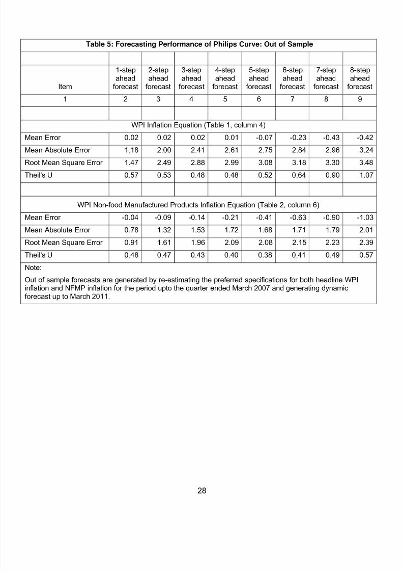
Turning to out of sample forecasts, the preferred specifications of Tables 1

and 2 are re-estimated for the period just prior to the onset of the global financial

crisis, i.e., for the period upto the quarter ended March 2007 and then dynamic

forecasts are generated for various horizons up to the quarter ended March 2011.

The results indicate that the Philips curve specifications outperform the random

walk model for all horizons in the case of non-food manufactured products inflation

and for upto seven quarters in the case of headline WPI inflation. Unlike Atkeson

and Ohanian (2001) finding in the US context, Phillips curve forecasts are found to

outperform a random walk model over the sample period.

The better performance of the estimated Phillips curve vis-a-vis the random

walk, however, benefits from the fact that this exercise uses actual realised values

of other explanatory variables like output growth, global commodity inflation and

movements in the exchange rate. Global commodity inflation exhibits a significant

quarter-to-quarter volatility, relatively difficult to forecast and often the source of actual inflation deviating from the forecasted inflation on a real time basis. In

addition, food prices exhibit significant volatility depending upon weather

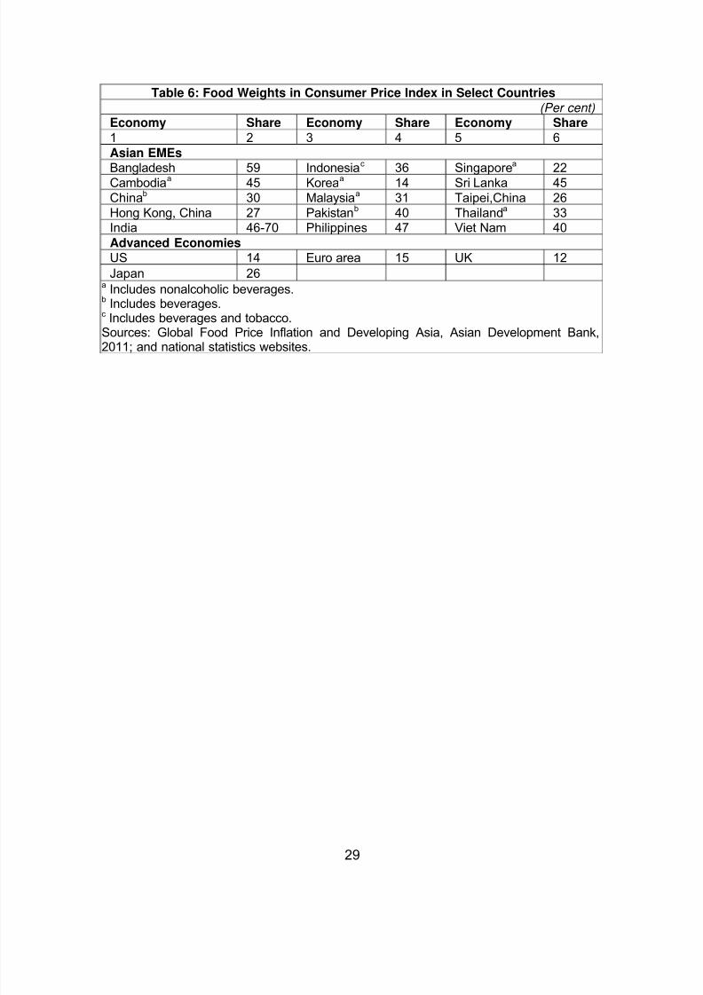
conditions and these add further volatility to headline inflation. Moreover, the

weight of food items in the price indices in India is significantly higher than

advanced economies and even many other emerging market economies (Table 6).

Higher food weights coupled with more volatility in food inflation, therefore, lead to

more volatility in headline inflation. With half the basket on account of food items,

core measures of inflation have limitations. Overall, while Phillips curve framework

provides a useful way to forecast inflation, the volatility in global commodity prices

and domestic agricultural shocks makes accurate forecasts a challenging job.

IV. Conclusion

In view of long and variable transmission lags, it is important for monetary

policy to respond to expected inflation and output dynamics. Reliable forecasts of

growth and inflation are, therefore, important for effective monetary management.

This paper focussed on modelling and forecasting inflation in India using an

augmented Phillips curve framework. Both demand and supply factors are seen as

drivers of inflation. Demand conditions are found to have a stronger impact on

non-food manufactured products inflation (NFMP) vis-a-vis headline WPI inflation;

moreover, NFMP is found to be more persistent than headline inflation. Both these

19



findings support the use of NFMP as a core measure of inflation. But, the impact of

global non-fuel commodities on NFMP is found to be substantial, which tempers

the case for using NFMP as a core measure. Inflation in non-fuel commodities is

seen as a more important driver of domestic inflation rather than fuel inflation,

although most of the focus is typically on fuel prices.

The exchange rate pass-through coefficient is found to be modest, but

nonetheless sharp depreciation in a short period of time, as it occurred during

July-September 2011, can add to inflationary pressures. The estimated equations

show a satisfactory in-sample performance based on dynamic simulations.

Nonetheless, forecasting challenges emanate from volatility in international oil and

other commodity prices and domestic food supply dynamics. These supply-side

factors have exhibited significant volatility in the recent years and add complexity

to inflation dynamics and its forecasting. Finally, structural food inflation emanating

from protein-rich items and fruits and vegetables has emerged as a key driver of domestic inflation (Gokarn, 2010; Subbarao, 2011). This factor has not been

considered in this paper and it would be useful to incorporate them in the

modelling framework for a better understanding of inflation dynamics.

References

Atkeson, Andrew and Lee Ohanian (2001), “Are Phillips Curves Useful for Forecasting Inflation?”, Federal Reserve Bank of Minneapolis Quarterly Review ,

Vol. 25(1), Winter, pp.2-11.

Ball, Laurence and Sandeep Mazumder (2011), “Inflation Dynamics and the GreatRecession”, Working Paper 17044, National Bureau of Economic Research.

Bhalla, Surjit (2011), “Populism, Politics and Procurement”, Financial Express ,September 13.

Biswas, Dipankar , Sanjay Singh and and Arti Sinha (2010), “Forecasting Inflationand IIP Growth: Bayesian Vector Autoregressive Model”, Occasional Papers, Vol.31 (2), Monsoon, Reserve Bank of India, pp. 31-48.

Choudhri, E.U. and D.S.Hakura (2001), “Exchange Rate Pass-through toDomestic Prices: Does the Inflationary Environment Matter?”, Working Paper 194,International Monetary Fund.

Choudhri, E.U., H.Faruqee and D.S.Hakura (2005), “Explaining the ExchangeRate Pass-through in Different Prices”, Journal of International Economics , Vol.65, pp. 349-374.

20



Dholakia, R. H. (1990), “Extended Phillips Curve for the Indian Economy”, Indian Economic Journal , Vol. 38 (1), pp. 69–78.

Dolado, Juan, Ramon Maria-Dolores and Manueal Naveira (2005), “Are MonetaryPolicy Reaction Functions Asymmetric? The Role of Nonlinearity in the PhillipsCurve”, European Economic Review , Vol. 49, pp.485-503.

Dua, Pammi and Upasna Gaur (2009), “Determination of Inflation in an OpenEconomy Phillips Curve Framework: The Case for Developed and DevelopingEconomies”, Working Paper 178, Centre for Development Economics, DelhiSchool of Economics.

Fuhrer, Jeff, Giovanni Olivei and Geoffrey Tootel (2009a), “Empirical Estimates of Changing Inflation Dynamics”, Working Paper 09-4, Federal Reserve Bank of Boston.

Fuhrer, Jeff, Yolanda Kodryzycki, Jane Little and Giovanni Olivei (2009b), “ThePhillips Curve in Historical Context” in Fuhrer, Jeff, Yolanda Kodryzycki, Jane Littleand Giovanni Olivei (ed.), Understanding Inflation and the Implications for Monetary Policy: A Phillips Curve Retrospective”, MIT Press, Cambridge, MA:London, pp.3-68.

Gali, Jordi and Mark Gertler (1999), "Inflation Dynamics: A Structural Econometric Analysis", Journal of Monetary Economics , Vol. 44, pp. 195-222.

Gali, Jordi, Mark Gertler and David Lopez-Salido (2005), “Robustness of theEstimates of the Hybrid New Keynesian Phillips Curve”, Journal of Monetary Economics , Vol.52(6), pp. 1107-18.

Gokarn, Subir (2010), “The Price of Protein”, Reserve Bank of India Bulletin ,

November

Gordon, Robert (1998), “Foundations of the Goldilocks Economy: Supply Shocksand the Time-varying NAIRU”, Brookings Papers on Economic Activity , Vol. 29,pp.297–333.

---- (2011), “The History of the Phillips Curve: Consensus and Bifurcation”,Economica , Vo. 78, January, pp.10-50.

Kapur, Muneesh and Michael Patra (2000), “The Price of Low Inflation”,Occasional Papers , Vol. 21 (2 and 3), Reserve Bank of India, pp. 191-233.

Khundrakpam, Jeevan Kumar (2008), “Have Economic Reforms AffectedExchange Rate Pass-Through to Prices in India”, Economic and Political Weekly ,Vol.43 (16), April 19, 2008, pp.71-79.

Kleibergen, Frank and Sophocles Mavroeidis (2009), “Weak Instrument RobustTests in GMM and the New Keynesian Phillips Curve”, Journal of Business &Economic Statistics, Vol. 27(3), July, pp.293-311.

21



Mazumder, Sandeep (2011), “The Stability of the Phillips Curve in India: Does theLucas Critique Apply?”, Journal of Asian Economics (forthcoming).

Meyer, Brent H. and Mehmet Pasaogullari (2010), “Simple Ways to ForecastInflation: What Works Best?”, Economic Commentary , available athttp://www.clevelandfed.org/research/commentary/2010/2010-17.cfm

Mohanty, Deepak (2010), Inflation Dynamics in India: Issues and Concerns,Reserve Bank of India Bulletin , April.

--- (2011), “Changing Inflation Dynamics in India”, Reserve Bank of India Bulletin ,September.

Mohanty, M.S. and Marc Klau (2001), “What Determines Inflation in EmergingMarket Countries?”, in “Modeling Aspects of the Inflation Process and MonetaryTransmission Mechanism in Emerging Market Countries”, BIS Papers 8 , Bank for International Settlements.

Patra, M.D. and Partha Ray (2010), “Inflation Expectations and Monetary Policy in

India: An Empirical Exploration”, Working Paper WP/10/84, International MonetaryFund.

Patra, M.D. and Muneesh Kapur (2010), “A Monetary Policy Model Without Moneyfor India”, Working Paper WP/10/183, International Monetary Fund.

Peach, Richard, Robert Rich and Anna Cororation (2010), “How Does SlackInfluence Inflation?”, Current Issues in Economic and Finance , Vol. 17, No.3,Federal Reserve Bank of New York

Paul, Biru Paksha (2009), “In search of the Phillips Curve for India”, Journal of

Asian Economics , Vol. 20, pp. 479-488.

Raj, Janak and Sangita Misra (2011), “Measures of Core Inflation in India – AnEmpirical Evaluation”, Working Paper (DEPR) 16/2011, Reserve Bank of India.

Reserve Bank of India (2002), Report on Currency and Finance 2000-01.

---- (2004), Report on Currency and Finance 2003-04.

---- (2011), Monetary Policy Statement 2011-12.

Rudd, J. and Whelan (2007), “Modelling Inflation Dynamics: A Critical Review of Recent Research“, Journal of Money, Credit and Banking , Supplement toVol.39(1), pp.155-170.

Singh, B. Karan, A. Kanakaraj , and T.O. Sridevi (2011), “Revisiting the EmpiricalExistence of the Phillips Curve for India”, Journal of Asian Economics , Vol.22,pp.247-258.

22

http://www.clevelandfed.org/research/commentary/2010/2010-17.cfm

http://www.clevelandfed.org/research/commentary/2010/2010-17.cfm



Srinivasan, Naveen, Vidya Mahambare and M.Ramachandra (2006), “ModellingInflation in India: Critique of the Structuralist Approach”, Journal of Quantitative Economics , New Series, Vol. 4 (2), pp.45–58.

Subbarao, D. (2011), “Monetary Policy Dilemmas: Some RBI Perspectives”, Reserve Bank of India Bulletin , October.

Woodford, Michael (2003), Interest and Prices: Foundations of a Theory of Monetary Policy, Princeton University Press, Princeton.

23



Table 1: Wholesale Price Inflation

Variable

Dependent Variable: Wholesale

Price Inflation

1 2 3 4 5 6 7 8 9 10

Constant 2.56 1.30 1.38 1.24 1.05 2.01 2.00 0.06 0.01

(4.3) (3.4) (3.3) (2.7) (2.5) (4.8) (4.7)

YGAP{1} 0.25 0.20 0.20 0.19 0.22 0.25 0.28 0.52 0.74

(2.2) (2.3) (2.1) (2.1) (2.3) (2.5) (2.5)

INFWPI{1}

1.20

0.89

0.91

0.89

0.86

0.97

0.95

0.09

0.00

(16.1) (13.9) (13.2) (13.9) (11.2) (13.1) (14.1)

INFWPI{2} ‐0.67 ‐0.40 ‐0.40 ‐0.39 ‐0.36 ‐0.48 ‐0.45 0.19 0.01

(4.9) (4.7) (4.4) (4.1) (3.7) (5.3) (4.8)

INFCR{4} 0.002

(0.3)

INFGL‐NF 0.09 0.07 0.08 0.09 0.08 0.08 0.00

(8.4) (6.3) (8.5) (8.0) (4.7) (4.7)

EXCHA 0.06 0.06 0.06 0.08 0.08

(3.3) (3.6) (3.3) (3.4) (3.3)

NEERT36A‐0.05

0.08

(2.3)

RAIN_JULY(‐2) ‐0.03 ‐0.02 ‐0.02 ‐0.03 ‐0.03 ‐0.03 0.36

(2.8) (2.1) (2.6) (2.7) (2.6) (2.6)

RAIN_JULY(‐3) ‐0.03 ‐0.02 ‐0.03 ‐0.03 ‐0.03 ‐0.03 0.30

(3.6) (2.4) (3.7) (3.6) (3.6) (3.5)

INFMPSP(‐1) 0.10 0.11 0.10 0.11 0.02

(4.0) (4.9) (4.4) (4.7)

DINFMPSP(‐1) 0.06 0.02

(1.6)

DUM1998Q3

1.48

1.71

1.52

1.69

1.06

1.13

(4.0) (4.8) (3.6) (4.1) (3.7) (3.9)

DUM2000Q4 1.88 2.14 1.85 1.65 2.15 2.03

(10.7) (13.5) (9.7) (6.4) (13.1) (10.3)

DUM2003Q4 2.18 1.70 2.18 1.83 1.60 1.80

(14.4) (7.8) (15.2) (7.7) (9.7) (11.5)

YGAP2{3} 0.07

(1.6)

All coefficients 0.16 0.49

Sum of lagged inflation coefficients 0.53 0.50 0.50 0.50 0.50 0.50 0.50

(4.5) (10.0) (10.1) (9.5) (10.8) (7.5) (7.5)

R‐bar2 0.73

0.88

0.87

0.87

0.88

0.85

0.85

LB‐Q(4) test 0.26 0.52 0.35 0.48 0.43 0.15 0.12

JB test 0.27 0.91 0.75 0.93 0.62 0.85 0.79

White test 0.07 0.41 0.38 0.42 0.44 0.53 0.12

Note: Sample period for the estimation is 1996:2 to 2011:1. Figures in parentheses are t‐statistics, with HAC standard errors

corrected with Newey‐West/Bartlett window and three lags. LB‐Q test gives significance level (p‐value) of Box‐Pierce‐Ljung Q ‐

statistic for the null of no residual autocorrelation for 4 lags. JB test gives significance level (p‐value) for Jarque‐Bera test for the

null of normality of residuals; White test gives significance level (p‐value) for White test for the null of homoscedasticity of

residuals. Figures in columns 9 and 10 give p‐values for Andrews‐Ploberger statistics for stability of coefficients for the baseline

specification in column 2 and the preferred specification in column (4), respectively. List of variable names is in Annex.

24



Table 2: Non‐food Manufactured Products Inflation Variable Dependent Variable: Non‐food Manufactured Products Inflation

1 2 3 4 5 6 7 8 9 10 11

Constant 1.18 0.98 0.97 1.00 1.06 0.84 1.00 0.85 0.03 0.11

(5.7) (9.0) (8.2) (9.0) (9.5) (8.1) (8.1) (5.4)

YNGAP{1} 0.30 0.20 0.25 0.26 0.29 0.23 0.29 0.21 0.07

(2.7) (3.2) (3.2) (4.0) (3.7) (3.3) (4.3)

INFMPNF{1} 1.33 1.17 1.11 1.10 1.10 1.06 1.09 1.10 0.12 0.23

(20.6)

(19.8)

(16.8)

(15.1)

(19.1)

(15.0)

(19.8)

(20.3)

INFMPNF{2} ‐0.64 ‐0.50 ‐0.44 ‐0.44 ‐0.48 ‐0.41 ‐0.49 ‐0.50 0.22 0.29

(6.9) (9.0) (6.4) (6.5) (8.9) (6.4) (8.9) (9.3)

INFGL 0.03

(6.4)

INFGL‐NF 0.05 0.05 0.05 0.05 0.05 0.05 0.14

(6.1) (6.8) (7.3) (8.0) (7.5) (7.6)

INFCR{4} 0.01 0.01 0.01

(2.1) (2.4) (2.7)

INFMINOIL 0.02

(2.2)

EXCHA 0.01

(0.4)

NEERT36A ‐0.03 ‐0.03 ‐0.03 ‐0.03 ‐0.03 ‐0.03 0.32

(1.6) (2.3) (2.0) (2.8) (2.2) (2.4)

YNGAP2{2} 0.11

(1.9)

YNGAP+{1} 0.61

(3.9)

YNGAP‐{1} ‐0.02

(0.2)

DUM1999Q1 1.73 1.87 1.92 2.20 2.13 2.29 2.31

(16.9) (14.3) (13.4) (11.9) (15.1) (11.9) (12.3)

DUM2005Q3 ‐2.32 ‐1.90 ‐1.79 ‐1.98 ‐1.84 ‐1.88 ‐1.77

(16.1) (9.5) (11.2) (13.1) (14.4) (11.7) (10.9)

All coefficients 0.13 0.28

Sum of lagged inflation coefficients 0.68 0.66 0.68 0.66 0.62 0.66 0.60 0.60

(10.6)

(19.4)

(21.6)

(20.0)

(16.2)

(23.6)

(16.7)

(17.9)

R‐bar2 0.82 0.90 0.91 0.91 0.92 0.92 0.92 0.92

LB‐Q(4) test 0.53 0.49 0.35 0.42 0.69 0.29 0.52 0.47

JB test 0.93 0.39 0.92 0.42 0.94 0.98 0.72 0.63

White test 0.02 0.15 0.07 0.05 0.13 0.09 0.25 0.33

Note:

Sample period for the estimation is 1996:2 to 2011:1. Figures in parentheses are t‐statistics, with HAC standard errors

corrected with Newey‐West/Bartlett window and three lags. LB‐Q test gives significance level (p‐value) of Box‐Pierce‐Ljung Q ‐

statistic for the null of no residual autocorrelation for 4 lags. JB test gives significance level (p‐value) for Jarque‐Bera test for the

null of normality of residuals; White test gives significance level (p‐value) for White test for the null of homoscedasticity of

residuals. Figures in columns 10 and 11 give p‐values for Andrews‐Quandt statistics for stability of coefficients for the

specification in columns 2 and 6, respectively.

List of variable names is in Annex.

25



Table 3: Philips Curve Estimates for Inflation in the US

Dependent Variable US CPI

Inflation US Core CPI

Inflation US PPI

Inflation US Core PPI

Inflation 1 2 3 4 5

Constant 0.81 0.16 0.61 0.19

(3.4) (1.3) (2.5) (2.1)

YGAPSA_USA{1} 0.19 0.05 0.21 0.06

(2.4) (3.6) (1.6) (1.9)

Lagged Dependent Variable @ 0.55 0.90 0.51 0.83

(5.2) (17.2) (5.3) (15.9)

INFCR 0.01 0.02

(3.5) (2.6)

INFCR {1} 0.001

(0.9)

INFCR {4} 0.001

(1.8)

INFGL-NF 0.04

(2.3)

INFGL-NF{1} 0.01

(2.5)

INFGL-NF{4} 0.01

(1.9)

INFGL-NF{5} 0.003

(1.5)

R-bar2 0.84 0.89 0.86 0.90

LB-Q(4) 0.33 0.67 0.00 0.71Note:Sample period for the estimation is 1996:2 to 2011:1. Figures in parentheses are t-statistics, withstandard errors corrected with Newey-West/Bartlett window and three lags. LB-Q givessignificance level (p-value) of Box-Pierce-Ljung Q-statistic for the null of no residualautocorrelation for 4 lags.@: sum of coefficients on the respective lagged dependent variable. Five lags of the laggeddependent variable were included in each equation to remove residual serial correlation. YGAPSA_USA = output gap for the US real GDP (based on seasonally adjusted series). CoreCPI is headline CPI excluding food and energy. Headline PPI is PPI for finished goods and corePPI is PPI for finished goods excluding food and energy. Other variables are as defined in the

Annex.

26



Table 4 : Forecasting Performance of Phillips Curve: In Sample

Item Dynamic Forecastsover the period1997:2 to 2011:1

One-step ahead forecast

4-step aheadforecast

8-step aheadforecast

1 2 3 4 5

WPI Inflation Equation (Table 1, column 4)

Mean Error -0.07 -0.03 -0.11 -0.28

Mean Absolute Error 0.91 0.59 0.92 0.83

Root Mean Square Error 1.11 0.74 1.12 0.99

Theil’s U 0.66 0.44 0.29 0.41

WPI Non-food Manufactured Products Inflation Equation (Table 2, column 6)

Mean Error 0.03 0.02 0.01 -0.03

Mean Absolute Error 0.91 0.46 0.92 0.99

Root Mean Square Error 1.11 0.58 1.10 1.17

Theil’s U 0.84 0.44 0.32 0.39

27



Table 5: Forecasting Performance of Philips Curve: Out of Sample

Item

1-stepahead

forecast

2-stepahead

forecast

3-stepahead

forecast

4-stepahead

forecast

5-stepahead

forecast

6-stepahead

forecast

7-stepahead

forecast

8-stepahead

forecast

1 2 3 4 5 6 7 8 9

WPI Inflation Equation (Table 1, column 4)

Mean Error 0.02 0.02 0.02 0.01 -0.07 -0.23 -0.43 -0.42

Mean Absolute Error 1.18 2.00 2.41 2.61 2.75 2.84 2.96 3.24

Root Mean Square Error 1.47 2.49 2.88 2.99 3.08 3.18 3.30 3.48

Theil's U 0.57 0.53 0.48 0.48 0.52 0.64 0.90 1.07

WPI Non-food Manufactured Products Inflation Equation (Table 2, column 6)

Mean Error -0.04 -0.09 -0.14 -0.21 -0.41 -0.63 -0.90 -1.03

Mean Absolute Error 0.78 1.32 1.53 1.72 1.68 1.71 1.79 2.01

Root Mean Square Error 0.91 1.61 1.96 2.09 2.08 2.15 2.23 2.39

Theil's U 0.48 0.47 0.43 0.40 0.38 0.41 0.49 0.57

Note:

Out of sample forecasts are generated by re-estimating the preferred specifications for both headline WPIinflation and NFMP inflation for the period upto the quarter ended March 2007 and generating dynamic

forecast up to March 2011.

28



Table 6: Food Weights in Consumer Price Index in Select Countries (Per cent)

Economy Share Economy Share Economy Share 1 2 3 4 5 6 Asian EMEs

Bangladesh 59 Indonesia

c

36 Singapore

a

22 Cambodiaa 45 Koreaa 14 Sri Lanka 45 Chinab 30 Malaysiaa 31 Taipei,China 26 Hong Kong, China 27 Pakistanb 40 Thailanda 33 India 46-70 Philippines 47 Viet Nam 40 Advanced Economies US 14 Euro area 15 UK 12 Japan 26

a Includes nonalcoholic beverages. b Includes beverages. c Includes beverages and tobacco. Sources: Global Food Price Inflation and Developing Asia, Asian Development Bank,

2011; and national statistics websites.

29



AnnexList of Variables

INFWPI = WPI inflation (y-o-y),

INFMPNF = WPI non-food manufactured products inflation (y-o-y),

INFGL = IMF’s global commodity inflation (y-o-y),

INFGL-NF = IMF’s global non-oil commodity inflation (y-o-y),

INFCR = global crude oil inflation (y-o-y),

INFMINOIL = WPI mineral oil sub-group inflation (y-o-y),

INFMSP = increase (y-o-y) in minimum support prices,

DINFMSP = first difference of INFMSP,

YGAP = output gap (actual real GDP less trend (Hodrick-Prescott (HP) filtered)

real GDP, using seasonally adjusted data).

YNGAP = non-agricultural output gap (actual real GDP excluding agriculture andnon-community, personal and social services less its trend (Hodrick-Prescott (HP)

filtered), using seasonally adjusted data).

EXCHA = variation (year-on-year) in the nominal exchange rate of the rupee

against the US dollar.

NEERT36A = variation (year-on-year) in the 36-currency trade-weighted nominal

exchange rate of the rupee,

RAIN_JULY = actual rainfall during July less normal rainfall during July.

inflation forecasting rbi

Documents