the euv imaging spectrometer for hinode - rxollc · the euv imaging spectrometer for hinode 21 2....
TRANSCRIPT
Solar Phys (2007) 243: 19–61DOI 10.1007/s01007-007-0293-1
The EUV Imaging Spectrometer for Hinode
J.L. Culhane · L.K. Harra · A.M. James · K. Al-Janabi · L.J. Bradley ·R.A. Chaudry · K. Rees · J.A. Tandy · P. Thomas · M.C.R. Whillock · B. Winter ·G.A. Doschek · C.M. Korendyke · C.M. Brown · S. Myers · J. Mariska · J. Seely ·J. Lang · B.J. Kent · B.M. Shaughnessy · P.R. Young · G.M. Simnett · C.M. Castelli ·S. Mahmoud · H. Mapson-Menard · B.J. Probyn · R.J. Thomas · J. Davila · K. Dere ·D. Windt · J. Shea · R. Hagood · R. Moye · H. Hara · T. Watanabe · K. Matsuzaki ·T. Kosugi · V. Hansteen · Ø. Wikstol
Received: 15 August 2006 / Accepted: 18 January 2007 /Published online: 22 March 2007© Springer 2007
T. Kosugi deceased 2006 November 26.
J.L. Culhane (�) · L.K. Harra · A.M. James · K. Al-Janabi · L.J. Bradley · R.A. Chaudry ·K. Rees · J.A. Tandy · P. Thomas · M.C.R. Whillock · B. WinterMullard Space Science Laboratory, University College London, Holmbury St Mary, Dorking,Surrey, RH5 6NT, UKe-mail: [email protected]
G.A. Doschek · C.M. Korendyke · C.M. Brown · S. Myers · J. Mariska · J. SeelyNaval Research Laboratory, E.O. Hulburt Centre for Space Research, Washington, DC 20375-5320,USA
J. Lang · B.J. Kent · B.M. Shaughnessy · P.R. YoungSpace Science and Technology Department, Rutherford Appleton Laboratory, Chilton, Didcot,Oxfordshire, OX11 0QX, UK
G.M. Simnett · C.M. Castelli · S. Mahmoud · H. Mapson-Menard · B.J. ProbynSpace Research Group, School of Physics and Space Research, University of Birmingham,Birmingham, UK
R.J. Thomas · J. DavilaNASA Goddard Space Flight Centre, Code 682, Greenbelt, MD 20771, USA
K. DereSchool of Computational Sciences, George Mason University, 4400 University Drive, Fairfax,VA 22030, USA
D. WindtPupin Physics Laboratories, Department of Astronomy, Columbia University, 550 West 120thStreet, New York, 10027, USA
J. SheaPerdix Corporation, P.O. Box 23, 35 Howard Street, Wilton, NH 03086, USA
R. HagoodSwales Aerospace, 5050 Powder Mill Road, Beltsville, MD 20705, USA
20 J.L. Culhane et al.
Abstract The EUV Imaging Spectrometer (EIS) on Hinode will observe solar corona andupper transition region emission lines in the wavelength ranges 170 – 210 Å and 250 – 290 Å.The line centroid positions and profile widths will allow plasma velocities and turbulent ornon-thermal line broadenings to be measured. We will derive local plasma temperatures anddensities from the line intensities. The spectra will allow accurate determination of differ-ential emission measure and element abundances within a variety of corona and transitionregion structures. These powerful spectroscopic diagnostics will allow identification andcharacterization of magnetic reconnection and wave propagation processes in the upper so-lar atmosphere. We will also directly study the detailed evolution and heating of coronalloops. The EIS instrument incorporates a unique two element, normal incidence design.The optics are coated with optimized multilayer coatings. We have selected highly effi-cient, backside-illuminated, thinned CCDs. These design features result in an instrumentthat has significantly greater effective area than previous orbiting EUV spectrographs withtypical active region 2 – 5 s exposure times in the brightest lines. EIS can scan a field of6 × 8.5 arc min with spatial and velocity scales of 1 arc sec and 25 km s−1 per pixel. Theinstrument design, its absolute calibration, and performance are described in detail in thispaper. EIS will be used along with the Solar Optical Telescope (SOT) and the X-ray Tele-scope (XRT) for a wide range of studies of the solar atmosphere.
1. Introduction
The Hinode mission will study the Sun at visible, EUV and X-ray wavelengths. Visibleobservations will be made with a 0.5 m diffraction-limited telescope — the largest solaroptical instrument yet deployed in space. The Solar Optical Telescope (SOT), constructedby NAOJ and Lockheed-Martin, will investigate photospheric dynamics and make vectormagnetogram maps at ≈0.25 arc sec (175 km) resolution.
X-ray observations will be made with a grazing incidence X-Ray Telescope (XRT) hav-ing 2 arc sec spatial resolution. Constructed by Smithsonian Astrophysical Observatory andNAOJ, it images the entire solar atmosphere in the temperature range 1 MK < T < 30 MK.
The UK-led EUV Imaging Spectrometer (EIS) will observe the emission lines of highlyionized elements in two carefully chosen wavelength bands so as to measure detailed plasmaproperties with special emphasis on flow velocities and on non-thermal plasma processesover a wide range of plasma temperatures (0.04 MK, 0.25 MK, 1.0 MK < T < 20 MK).This paper outlines the scientific goals of the EIS and discusses the properties, calibrationand performance of the instrument in detail within the context of the overall Hinode mission.
R. MoyeArtep Inc., 2922 Excelsior Spring Ct., Ellicott City, MD 21042, USA
H. Hara · T. WatanabeNational Astronomical Observatory of Japan, Mitaka, Tokyo, 181, Japan
K. Matsuzaki · T. KosugiInstitute of Space and Astronautical Science, Sagamihara, Kanagawa 229, Japan
V. Hansteen · Ø. WikstolInstitute of Theoretical Astrophysics, University of Oslo, P.O. Box 1029, Blindern, 0315, Oslo,Norway
The EUV Imaging Spectrometer for Hinode 21
2. Scientific Aims
The scientific aims of the Hinode mission are focused on three main goals:
– Determine the mechanisms responsible for heating the corona in active regions and thequiet Sun.
– Establish the mechanisms that cause transient phenomena, e.g., flares, CMEs.– Investigate processes for energy transfer from photosphere to corona.
The instruments have been designed to achieve these goals. Instrument operations and sci-ence analysis will concentrate on understanding how changes in the magnetic field impactthe solar atmosphere in terms of slow evolutionary behavior, small-scale heating, or throughmore catastrophic events. In pursuing the mission science goals, recognition of magneticreconnection-based physical processes and their quantitative description will be of consid-erable importance for understanding the responsive behavior of the solar atmosphere. An-other important area is the identification and description of wave propagation modes andany related energy dissipation.
The EIS contribution to the mission aims involves the measurement of line intensities,Doppler velocities, line widths, temperatures and densities for the plasma in the Sun’s at-mosphere. From these measurements, EIS will probe the physical processes that are preva-lent on widely different size scales on the Sun. With the availability of suitable multilayercoatings, the design goals of EIS for operation at λ < 300 Å were to substantially increasethe photon throughput and enhance spectral and spatial resolution over previous spectrome-ters that had operated at these wavelengths. These improvements have led to an instrumentthat can obtain useful images of an active region (4 × 8 arc min) at 2 arc sec resolutionin around 1 – 2 minutes for 12 suitable emission lines. For a flaring active region loop, a50 Mm section of emitting plasma can be scanned at 2 arc sec resolution in a time of oneminute while achieving plasma velocity and line profile width estimates with precisionsof ±5 km s−1 and ±25 km s−1 respectively. A selection from the many topics that will bepursued with EIS is indicated below:
Coronal/Photospheric velocity field comparison in active regions: On active region (AR)spatial scales, the visible filter images from the solar optical telescope (SOT) will providedetailed information on photospheric velocities and their time variation. Both vector andline-of-sight magnetograms will also be available. The detailed observation of related inten-sity, velocity and magnetic configuration changes in the coronal active region plasma has notpreviously been possible and will be undertaken with EIS observations of loops and otherAR magnetic structures.
Coronal AR heating: dynamic phenomena in loops: The understanding of this topic remainselusive. There is evidence for reconnection in loops (e.g. Harra, Mandrini, and Matthews,2004). Much time will be devoted to the detection and characterization of small brighteningsby both the EIS and the XRT. EIS in particular will observe any changes in temperature,density and velocity that occur as a result of small events and will obtain evidence of relatedplasma flows. In addition, the spatially resolved loop temperature and density measurementsthat EIS will obtain will allow comparison with the output of increasingly sophisticatedMHD models (Klimchuk, 2006).
Evolution of trans-equatorial loops: These structures have by definition a significant rolefor the understanding of large-scale coronal activity. While they appear to participate inlarge-scale reconnection (Tsuneta, 1996), many of their properties are similar to those of the
22 J.L. Culhane et al.
smaller loops found in active regions (Pevtsov, 2000). Following their recognition in full-Sun XRT images, EIS will study their foot points in an effort to understand their energeticsin relation to the underlying magnetic field.
Coronal seismology: waves in AR structures: Waves are observed on all size and time scaleson the Sun — from the 5 minute oscillations in the chromosphere to the large-scale shockwaves related to flares and coronal mass ejections. They may have a key role in the supplyof the energy to the corona and have been demonstrated to exist in coronal structures (e.g.,Williams et al., 2002). It is also clear that their detection and mode identification will allowthe measurement of important coronal parameters, e.g., magnetic field (Nakariakov and Of-man, 2001). Spectroscopic observations of oscillations in coronal loops have been made inflaring and post flare conditions (Wang et al., 2002, 2003), while on a larger scale spectro-scopic observations of EIT waves in the corona have been pioneered by Harra and Sterling(2003). Progress in these important areas requires observations at the better cadence thatEIS will provide.
CME onsets and signatures: CMEs almost certainly involve reconnection. Magnetic break-out scenarios (e.g., Antiochos, DeVore, and Klimchuk, 1999), require the removal of over-lying magnetic field structures. In the case of eruption of twisted flux ropes (Williams et al.,2005), this removal process permits an eruption that is driven by the energy stored in thetwisted field. So far, CMEs have largely been studied with limb observations by corona-graphs. Velocity measurements by EIS will allow the early stages of the field removal tobe identified on the disc and the degree of twist in the erupting material to be assessed.Current CME models predict different plasma dynamic signatures. Here again, EIS velocitymeasurements will have a key role in testing model validities.
Flare produced plasma: source, location and triggering: The production of high temperatureplasma in the corona following solar flares continues to be controversial. Bragg spectrome-ter observations of flare plasma with good spectral resolution by the Yohkoh BCS (Culhaneet al., 1991) have had poor spatial resolution. However Warren and Doschek (2005) havereported a hydrodynamic model that involves energy release in successive sub-resolutionthreads within loops and appears consistent with the plasma velocities observed by theYohkoh BCS. EIS will image flare lines from e.g. Fe XXIV, with good spatial and tempo-ral resolution which, together with XRT context observations, should clarify the plasmaproduction questions.
Flare reconnection: inflow and outflow: While there has been a lot of observational evidencefor reconnection in flares (e.g., Masuda et al., 1994; Tsuneta, 1995), there remain inconsis-tencies in detail. In particular, spectroscopic data are lacking on outflow and inflow veloc-ities. Much evidence for reconnection has been based on imaging alone (e.g., Yokoyamaet al., 2001). We require spectral images with high temporal resolution in the corona. EIS isdesigned to address this difficult problem.
Quiet Sun transient events: network, network boundaries, Coronal Hole boundaries: Evi-dence has also been found for reconnection in the quiet Sun, around convective cell bound-aries (e.g., Innes et al., 1997) and at coronal hole boundaries (e.g., Madjarska, Doyle, andvan Driel-Gesztelyi, 2004), resulting in bi-directional jets. Heating has been observed atthe cell boundaries (e.g., Harrison, 1997) and even within the cells themselves (Harra, Gal-lagher, and Phillips, 2000). There is some dispute as to the cause of the bi-directional jets(often termed explosive events) and of the events that are registered through heating or den-sity change (often referred to as blinkers). EIS will enable us to distinguish between theseand determine whether they are indeed different phenomena.
The EUV Imaging Spectrometer for Hinode 23
The coronal emission lines registered in the two EUV pass bands of the EIS instrumentalong with the magnetic field data provided by the SOT and the structural context informa-tion from the XRT, will allow significant advances to be achieved in the above areas and inmany other facets of solar coronal physics.
3. Instrument Overview
Previous spectrometers designed to operate in orbit in the 50 to 500 Å wavelength rangehave employed grazing incidence optical systems (mirrors and diffraction gratings) sincethe normal incidence reflectivity at these wavelengths is vanishingly small for the usualoptical materials (e.g., SOHO CDS; Harrison et al., 1995). In addition, the microchannelplate array detectors commonly used, although providing good spatial resolution, exhibitedquantum efficiencies (QE) ≤ 20% and required hygroscopic coatings, e.g., KBr. Uncoatedmicrochannel plates have substantially lower QE values. The design of the EIS instrumentallows normal incidence operation of the optical elements through the use of multilayercoatings applied to both mirror and grating. In addition, the use of thinned back-illuminatedCCDs to register the diffracted photons allows QE values to be achieved that are two tothree times greater than for microchannel plate systems. A disadvantage stems from thecomparatively narrow passband achievable with an individual multilayer. At the time theinstrument was designed, the wavelength range obtainable from available multilayers was80 Å < λ < 350 Å. However, enhanced knowledge of the coronal emission line spectrummeans that these limitations can be tolerated in the interest of achieving high throughput.
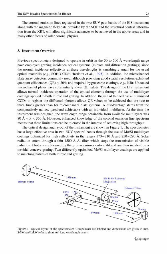
The optical design and layout of the instrument are shown in Figure 1. The spectrometerhas a large effective area in two EUV spectral bands through the use of Mo/Si multilayercoatings optimized for high reflectivity in the ranges 170 – 210 Å and 250 – 290 Å. Solarradiation enters through a thin 1500 Å Al filter which stops the transmission of visibleradiation. Photons are focused by the primary mirror onto a slit and are then incident on atoroidal concave grating. Two differently optimized Mo/Si multilayer coatings are appliedto matching halves of both mirror and grating.
Figure 1 Optical layout of the spectrometer. Components are labeled and dimensions are given in mm.S/SW and L/LW refer to short and long wavelength bands.
24 J.L. Culhane et al.
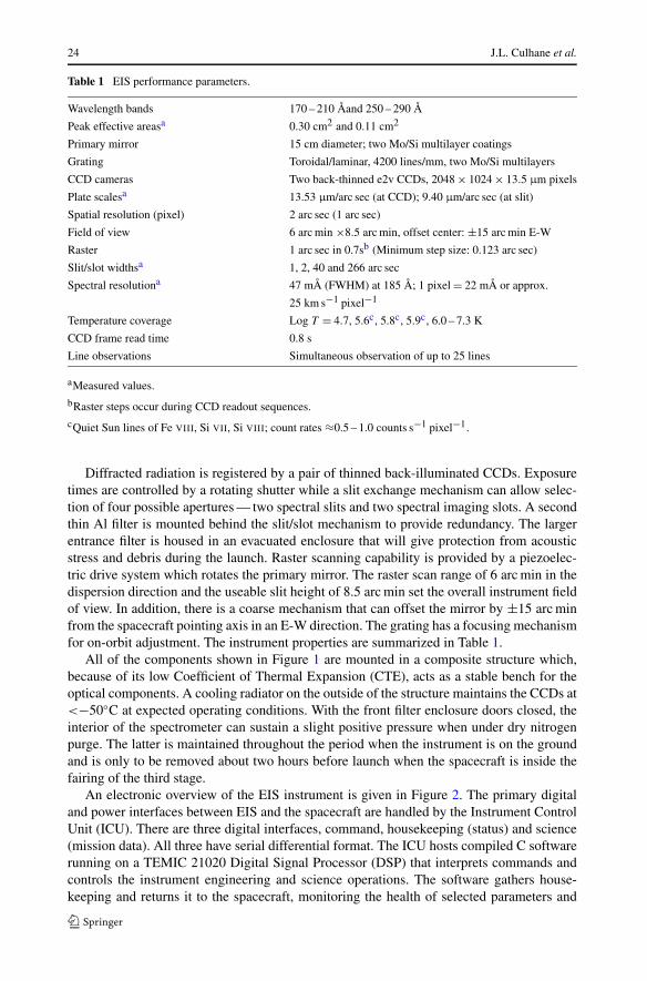
Table 1 EIS performance parameters.
Wavelength bands 170 – 210 Åand 250 – 290 Å
Peak effective areasa 0.30 cm2 and 0.11 cm2
Primary mirror 15 cm diameter; two Mo/Si multilayer coatings
Grating Toroidal/laminar, 4200 lines/mm, two Mo/Si multilayers
CCD cameras Two back-thinned e2v CCDs, 2048 × 1024 × 13.5 μm pixels
Plate scalesa 13.53 μm/arc sec (at CCD); 9.40 μm/arc sec (at slit)
Spatial resolution (pixel) 2 arc sec (1 arc sec)
Field of view 6 arc min ×8.5 arc min, offset center: ±15 arc min E-W
Raster 1 arc sec in 0.7sb (Minimum step size: 0.123 arc sec)
Slit/slot widthsa 1, 2, 40 and 266 arc sec
Spectral resolutiona 47 mÅ (FWHM) at 185 Å; 1 pixel = 22 mÅ or approx.
25 km s−1 pixel−1
Temperature coverage Log T = 4.7, 5.6c, 5.8c, 5.9c, 6.0 – 7.3 K
CCD frame read time 0.8 s
Line observations Simultaneous observation of up to 25 lines
aMeasured values.
bRaster steps occur during CCD readout sequences.
cQuiet Sun lines of Fe VIII, Si VII, Si VIII; count rates ≈0.5 – 1.0 counts s−1 pixel−1.
Diffracted radiation is registered by a pair of thinned back-illuminated CCDs. Exposuretimes are controlled by a rotating shutter while a slit exchange mechanism can allow selec-tion of four possible apertures — two spectral slits and two spectral imaging slots. A secondthin Al filter is mounted behind the slit/slot mechanism to provide redundancy. The largerentrance filter is housed in an evacuated enclosure that will give protection from acousticstress and debris during the launch. Raster scanning capability is provided by a piezoelec-tric drive system which rotates the primary mirror. The raster scan range of 6 arc min in thedispersion direction and the useable slit height of 8.5 arc min set the overall instrument fieldof view. In addition, there is a coarse mechanism that can offset the mirror by ±15 arc minfrom the spacecraft pointing axis in an E-W direction. The grating has a focusing mechanismfor on-orbit adjustment. The instrument properties are summarized in Table 1.
All of the components shown in Figure 1 are mounted in a composite structure which,because of its low Coefficient of Thermal Expansion (CTE), acts as a stable bench for theoptical components. A cooling radiator on the outside of the structure maintains the CCDs at<−50◦C at expected operating conditions. With the front filter enclosure doors closed, theinterior of the spectrometer can sustain a slight positive pressure when under dry nitrogenpurge. The latter is maintained throughout the period when the instrument is on the groundand is only to be removed about two hours before launch when the spacecraft is inside thefairing of the third stage.
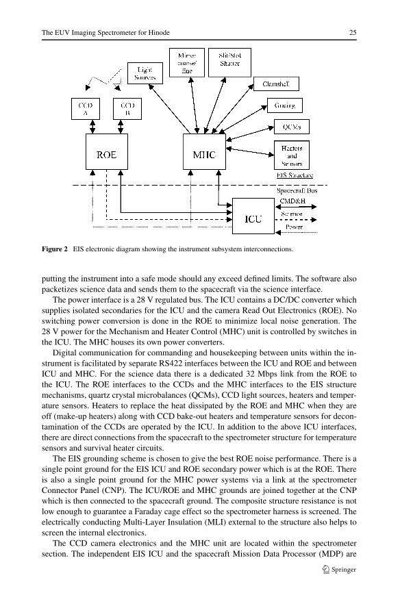
An electronic overview of the EIS instrument is given in Figure 2. The primary digitaland power interfaces between EIS and the spacecraft are handled by the Instrument ControlUnit (ICU). There are three digital interfaces, command, housekeeping (status) and science(mission data). All three have serial differential format. The ICU hosts compiled C softwarerunning on a TEMIC 21020 Digital Signal Processor (DSP) that interprets commands andcontrols the instrument engineering and science operations. The software gathers house-keeping and returns it to the spacecraft, monitoring the health of selected parameters and
The EUV Imaging Spectrometer for Hinode 25
Figure 2 EIS electronic diagram showing the instrument subsystem interconnections.
putting the instrument into a safe mode should any exceed defined limits. The software alsopacketizes science data and sends them to the spacecraft via the science interface.
The power interface is a 28 V regulated bus. The ICU contains a DC/DC converter whichsupplies isolated secondaries for the ICU and the camera Read Out Electronics (ROE). Noswitching power conversion is done in the ROE to minimize local noise generation. The28 V power for the Mechanism and Heater Control (MHC) unit is controlled by switches inthe ICU. The MHC houses its own power converters.
Digital communication for commanding and housekeeping between units within the in-strument is facilitated by separate RS422 interfaces between the ICU and ROE and betweenICU and MHC. For the science data there is a dedicated 32 Mbps link from the ROE tothe ICU. The ROE interfaces to the CCDs and the MHC interfaces to the EIS structuremechanisms, quartz crystal microbalances (QCMs), CCD light sources, heaters and temper-ature sensors. Heaters to replace the heat dissipated by the ROE and MHC when they areoff (make-up heaters) along with CCD bake-out heaters and temperature sensors for decon-tamination of the CCDs are operated by the ICU. In addition to the above ICU interfaces,there are direct connections from the spacecraft to the spectrometer structure for temperaturesensors and survival heater circuits.
The EIS grounding scheme is chosen to give the best ROE noise performance. There is asingle point ground for the EIS ICU and ROE secondary power which is at the ROE. Thereis also a single point ground for the MHC power systems via a link at the spectrometerConnector Panel (CNP). The ICU/ROE and MHC grounds are joined together at the CNPwhich is then connected to the spacecraft ground. The composite structure resistance is notlow enough to guarantee a Faraday cage effect so the spectrometer harness is screened. Theelectrically conducting Multi-Layer Insulation (MLI) external to the structure also helps toscreen the internal electronics.
The CCD camera electronics and the MHC unit are located within the spectrometersection. The independent EIS ICU and the spacecraft Mission Data Processor (MDP) are
26 J.L. Culhane et al.
located in the spacecraft service or bus section at ≈2.5 m from the spectrometer. Obser-vation tables, loaded in the EIS ICU from the MDP, organize the readout of data from theCCD cameras with a maximum of 25 user-selected spectral windows being allowed by thesoftware. The ICU also generates commands for operating the scanning, shutter, and slitinterchange mechanisms to execute appropriate sets of observing sequences or studies. Thespacecraft mass memory has a total capacity of 7 Gbits for the instruments and the nominalEIS share of this is 15%. Thus instrument data throughput is set by the number of groundstation contacts per day. Provision of access to the Norwegian Svalbard ground station byESA and the Norwegian Space Agency will allow at least 15 ground station contacts eachday in addition to the four daily contacts with the JAXA station at the Uchinoura SpaceCentre (USC). Thus EIS, using lossless data compression, will be able to operate at a datarate of ≈100 kb/s.
Following the SOHO CDS instrument, EIS will provide the next steps in EUV spectralimaging of the solar corona and upper transition region. It will have approximately a factorof ten enhancement in effective area due to the use of multilayer coated optics and back-illuminated CCDs. Spectral resolution is also improved by a factor of ten in the wavelengthranges being observed. While at 2 arc sec, the spatial resolution is a factor two to three betterthan that of CDS.
4. Optical Design and Instrument Components
An optical schematic of EIS which gives the locations of the components is shown in Fig-ure 1 and has been briefly discussed in the previous section. A detailed account of the in-strument’s optics and mechanisms is given by Korendyke et al. (2006). The telescope pri-mary mirror images EUV radiation from the Sun onto the spectrograph slit. Light passingthrough the slit is dispersed and stigmatically re-imaged by the toroidal grating onto two1024 × 2048 pixel CCD detectors, each with 2048 pixels in the dispersion direction. Inflight, the mirror can be rotated in ≈0.125 arc sec steps about the Y axis (solar N-S) to sam-ple different solar structures with the slit. High-resolution spectroheliograms (raster images)are formed by steadily moving the solar image in fine increments on the spectrograph slitand taking repeated exposures. An interchange mechanism allows selection among two slits(1 and 2 arc sec width) and two slots (40 and 266 arc sec width). The slot observations of thesolar disk obtain images of large areas in bright solar emission lines with a single exposure.For the 40 arc sec slot, spectrally pure images are available for several strong lines in eachpassband. The slot images exhibit a modest spatial blur along the dispersion direction.
Both mirror and grating operate at near normal incidence. To broaden the spectral range,the multilayer-coated optical elements were divided into two D-shaped sectors; each sectorwas coated with a multilayer tuned to produce high reflectivity in its wavelength band. Thesecoatings achieved peak reflectivities of 32% and 23% in the 170 – 210 Å and 250 – 290 Åbands, respectively. Optimum response is achieved for each band by careful selection ofthickness for the individual Si and Mo layers (Seely et al., 2004). The telescope mirror is asuperpolished off-axis parabola with a focal length of 1939 mm, a measured figure accuracy<λ/47 rms at 6328 Å and a microroughness of <4 Å rms. The 160 mm diameter mirrorwas fabricated from Zerodur by Tinsley Laboratories, Inc. and has a usable diameter of150 mm. The flight grating is specified to be a toroid (Beutler, 1945; Haber, 1950) with radiiof 1182.98 mm in the dispersion direction and 1178.28 mm in the perpendicular directionwith a figure slope error <0.5 arc sec RMS. The grating microroughness is <2.5 Å RMS.The gratings were fabricated by Carl Zeiss Laser Optics GmbH from 100 mm diameterfused silica blanks and have a usable area of 90 mm diameter.
The EUV Imaging Spectrometer for Hinode 27
4.1. Entrance Filter and Housing
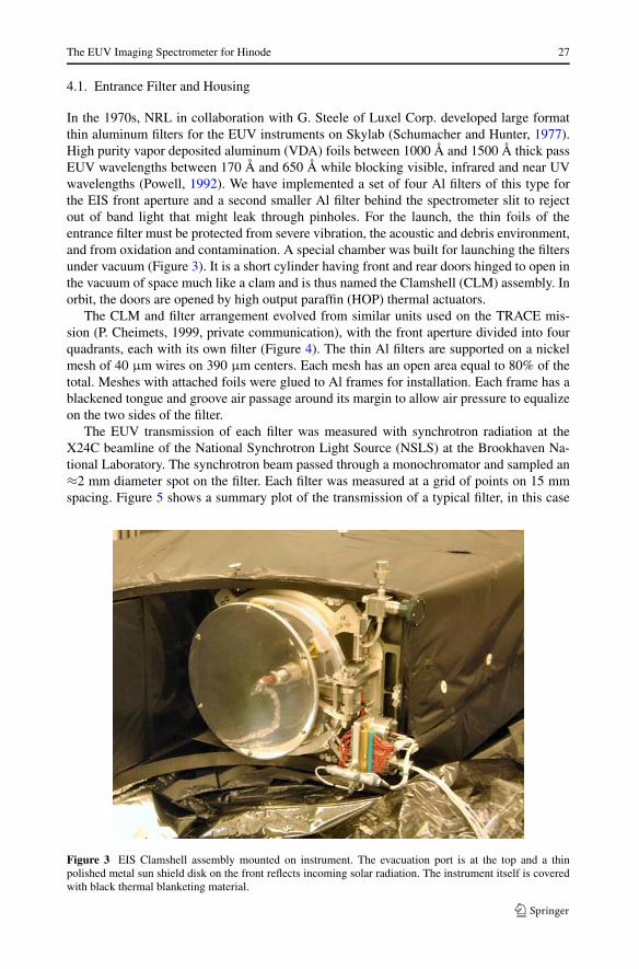
In the 1970s, NRL in collaboration with G. Steele of Luxel Corp. developed large formatthin aluminum filters for the EUV instruments on Skylab (Schumacher and Hunter, 1977).High purity vapor deposited aluminum (VDA) foils between 1000 Å and 1500 Å thick passEUV wavelengths between 170 Å and 650 Å while blocking visible, infrared and near UVwavelengths (Powell, 1992). We have implemented a set of four Al filters of this type forthe EIS front aperture and a second smaller Al filter behind the spectrometer slit to rejectout of band light that might leak through pinholes. For the launch, the thin foils of theentrance filter must be protected from severe vibration, the acoustic and debris environment,and from oxidation and contamination. A special chamber was built for launching the filtersunder vacuum (Figure 3). It is a short cylinder having front and rear doors hinged to open inthe vacuum of space much like a clam and is thus named the Clamshell (CLM) assembly. Inorbit, the doors are opened by high output paraffin (HOP) thermal actuators.
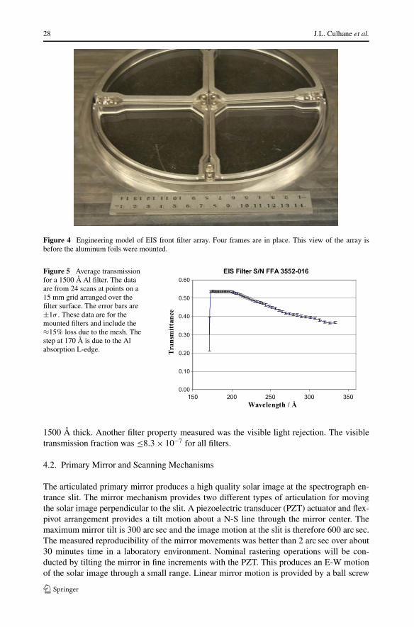
The CLM and filter arrangement evolved from similar units used on the TRACE mis-sion (P. Cheimets, 1999, private communication), with the front aperture divided into fourquadrants, each with its own filter (Figure 4). The thin Al filters are supported on a nickelmesh of 40 μm wires on 390 μm centers. Each mesh has an open area equal to 80% of thetotal. Meshes with attached foils were glued to Al frames for installation. Each frame has ablackened tongue and groove air passage around its margin to allow air pressure to equalizeon the two sides of the filter.
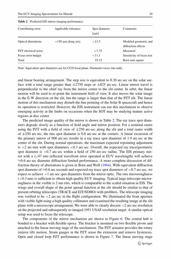
The EUV transmission of each filter was measured with synchrotron radiation at theX24C beamline of the National Synchrotron Light Source (NSLS) at the Brookhaven Na-tional Laboratory. The synchrotron beam passed through a monochromator and sampled an≈2 mm diameter spot on the filter. Each filter was measured at a grid of points on 15 mmspacing. Figure 5 shows a summary plot of the transmission of a typical filter, in this case
Figure 3 EIS Clamshell assembly mounted on instrument. The evacuation port is at the top and a thinpolished metal sun shield disk on the front reflects incoming solar radiation. The instrument itself is coveredwith black thermal blanketing material.
28 J.L. Culhane et al.
Figure 4 Engineering model of EIS front filter array. Four frames are in place. This view of the array isbefore the aluminum foils were mounted.
Figure 5 Average transmissionfor a 1500 Å Al filter. The dataare from 24 scans at points on a15 mm grid arranged over thefilter surface. The error bars are±1σ . These data are for themounted filters and include the≈15% loss due to the mesh. Thestep at 170 Å is due to the Alabsorption L-edge.
1500 Å thick. Another filter property measured was the visible light rejection. The visibletransmission fraction was ≤8.3 × 10⁻⁷ for all filters.
4.2. Primary Mirror and Scanning Mechanisms
The articulated primary mirror produces a high quality solar image at the spectrograph en-trance slit. The mirror mechanism provides two different types of articulation for movingthe solar image perpendicular to the slit. A piezoelectric transducer (PZT) actuator and flex-pivot arrangement provides a tilt motion about a N-S line through the mirror center. Themaximum mirror tilt is 300 arc sec and the image motion at the slit is therefore 600 arc sec.The measured reproducibility of the mirror movements was better than 2 arc sec over about30 minutes time in a laboratory environment. Nominal rastering operations will be con-ducted by tilting the mirror in fine increments with the PZT. This produces an E-W motionof the solar image through a small range. Linear mirror motion is provided by a ball screw
The EUV Imaging Spectrometer for Hinode 29
Table 2 Predicted EIS mirror imaging performance.
Contributing error Applicable tolerance Spot diameter Comments
[μm]
Optical aberrations <150 μm along axis <13.5 Modeled geometric and
diffraction effects
PZT electrical noise <7.75 Measured
Focus error budget <11.1 Sensitivity of focus test
Total 19.12 Root sum square
Note: Equivalent spot diameters are for CCD focal plane. Diameters twice rms radii.
and linear bearing arrangement. The step size is equivalent to 0.30 arc sec on the solar sur-face with a total range greater than ±2750 steps or ±825 arc sec. Linear mirror travel isperpendicular to the chief ray from the mirror center to the slit center. In orbit, the linearmotion will be used to re-point the instrument field of view. It also moves the solar imagein the E-W direction on the slit, but the range is larger than that of the PZT tilt. The linearmotion of this mechanism may disturb the fine pointing of the Solar B spacecraft and henceits operation is restricted. However, the EIS instrument can use this mechanism to observeemerging activity at the limbs on occasions when the SOT may be studying mature activeregions at disc center.
The predicted image quality of the mirror is shown in Table 2. The ray trace spot diam-eters degrade slowly as a function of field angle and mirror position. For a nominal rasterusing the PZT with a field of view of ±250 arc sec along the slit and a total raster widthof ±250 arc sec, the rms spot diameter is 0.8 arc sec at the corners. A linear excursion ofthe primary mirror of 900 arc sec results in a ray trace spot diameter of 1.9 arc sec at thecenter of the slit. During normal operations, the maximum expected repointing adjustmentis <2 arc min with spot diameters <0.3 arc sec. Overall, the expected ray trace/geometricspot diameter is <0.7 arc sec within a field of 250 arc sec radius. The EIS primary mir-ror with a λ/47 rms reflected wavefront error operated at EUV wavelengths will achieve≈0.6 arc sec diameter diffraction limited performance. A more complete discussion of dif-fraction theory of aberrations is given in Born and Wolf (1964). With equivalent diffractionspot diameter of ≈0.6 arc seconds and expected ray trace spot diameters of <0.7 arc sec, weexpect to achieve <1 arc sec spot diameters from the mirror optic. The rms microroughness(<0.3 nm) is sufficient to obtain high quality EUV imaging. Typical large telescope micror-oughness in the visible is 2 nm rms, which is comparable to the scaled situation in EIS. Thewings and overall shape of the point spread function at the slit should be similar to that ofpresent orbiting telescopes (TRACE and EIT/SOHO) with prefilters. The telescope imagingwas verified to be <2 arc sec in the flight configuration. We illuminated the front aperturewith visible light using a high quality collimator and examined the resulting image at the slitplane with a microscope arrangement. We were able to clearly discern <2 arc sec resolutionon the projected and subsequently re-imaged 1951 USAF resolution target. A similar opticalsetup was used to focus the telescope.
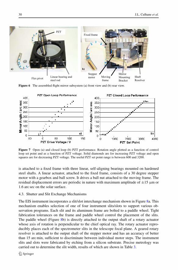
The components of the mirror mechanism are shown in Figure 6. The central hub isbonded to a bracket with flexible epoxy. The bracket is mounted on two flexible pivots andattached to the linear moving stage of the mechanism. The PZT actuator provides the rotary(mirror tilt) motion. Strain gauges in the PZT sense the extension and remove hysteresis.Open and closed loop PZT performance is shown in Figure 7. The linear moving stage
30 J.L. Culhane et al.
Figure 6 The assembled flight mirror subsystem (a) front view and (b) rear view.
Figure 7 Open (a) and closed loop (b) PZT performance. Rotation angle plotted as a function of controlloop set point and as a function of PZT voltage. Solid diamonds are for increasing PZT voltage and opensquares are for decreasing PZT voltage. The useful PZT set point range is between 600 and 3200.
is attached to a fixed frame with three linear, self-aligning bearings mounted on hardenedsteel shafts. A linear actuator, attached to the fixed frame, consists of a 30 degree steppermotor with a gearbox and ball screw. It drives a ball nut attached to the moving frame. Theresidual displacement errors are periodic in nature with maximum amplitude of ±15 μm or1.6 arc sec on the solar surface.
4.3. Shutter and Slit Exchange Mechanisms
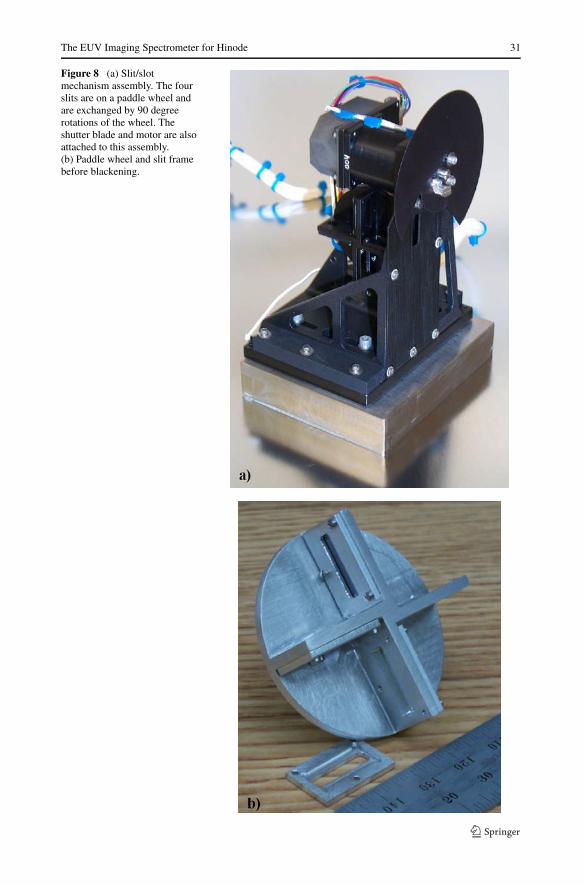
The EIS instrument incorporates a slit/slot interchange mechanism shown in Figure 8a. Thismechanism enables selection of one of four instrument slits/slots to support various ob-servation programs. Each slit and its aluminum frame are bolted to a paddle wheel. Tightfabrication tolerances on the frame and paddle wheel control the placement of the slits.The paddle wheel (Figure 8b) is directly attached to the output shaft of a rotary actuatorwhose axis of rotation is perpendicular to the chief optical ray. The rotary actuator repro-ducibly places each of the spectrometer slits in the telescope focal plane. A geared rotaryresolver is attached to the output shaft of the stepper motor and has an accuracy of betterthan 15 arc min, sufficient to discriminate between individual motor steps. The instrumentslits and slots were fabricated by etching from a silicon substrate. Precise metrology wascarried out to determine the slit width, results of which are shown in Table 3.
The EUV Imaging Spectrometer for Hinode 31
Figure 8 (a) Slit/slotmechanism assembly. The fourslits are on a paddle wheel andare exchanged by 90 degreerotations of the wheel. Theshutter blade and motor are alsoattached to this assembly.(b) Paddle wheel and slit framebefore blackening.
32 J.L. Culhane et al.
Table 3 EIS slit width summary.
Note: Measured accuracies are±0.5 μm for the 1 and 2 arc secslits and ±2 μm for the 40 and266 arc sec slots.
Nominal width Serial number Measured width Measured width
[arc sec] [μm] [arc sec]
1 101C 9.5 1.01
2 102A 19.0 2.02
40 103A 384 40.9
266 104D 2506 266.6
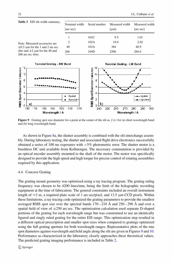
Figure 9 Grating spot size diameter for a point at the center of the slit as f (λ) for (a) short wavelength bandand (b) long wavelength band.
As shown in Figure 8a, the shutter assembly is combined with the slit interchange assem-bly. During laboratory testing, the shutter and associated flight drive electronics successfullyobtained a series of 100 ms exposures with <5% photometric error. The shutter motor is abrushless DC unit available from Kollmorgen. The necessary commutation is provided byan optical encoder assembly mounted to the shaft of the motor. The motor was specificallydesigned to provide the high speed and high torque for precise control of rotating assembliesrequired by this application.
4.4. Concave Grating
The grating mount geometry was optimized using a ray tracing program. The grating rulingfrequency was chosen to be 4200 lines/mm, being the limit of the holographic recordingequipment at the time of fabrication. The general constraints included an overall instrumentlength of ≈3 m, a required plate scale of 1 arc sec/pixel, and 13.5 μm CCD pixels. Withinthese limitations, a ray tracing code optimized the grating parameters to provide the smallestaveraged RMS spot size over the spectral bands 170 – 210 Å and 250 – 290 Å and over aspatial field of view of ±250 arc sec. The optimization calculation used separate D-shapedportions of the grating for each wavelength range but was constrained to use an identicallyfigured and singly ruled grating for the entire EIS range. This optimization step resulted ina different optical prescription and smaller spot sizes when compared to gratings optimizedusing the full grating aperture for both wavelength ranges. Representative plots of the rmsspot diameters against wavelength and field angle along the slit are given in Figures 9 and 10.Performance as characterized in the laboratory closely approaches these theoretical values.The predicted grating imaging performance is included in Table 2.
The EUV Imaging Spectrometer for Hinode 33
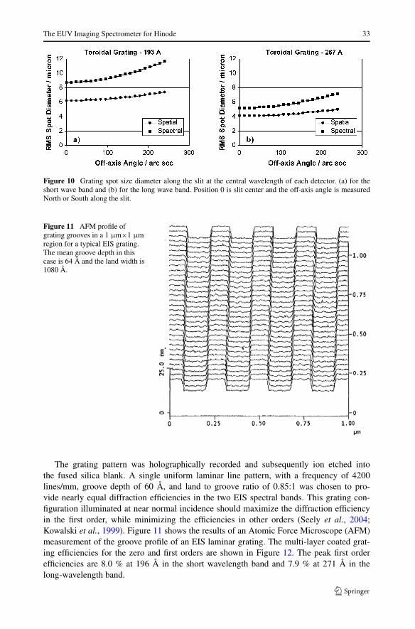
Figure 10 Grating spot size diameter along the slit at the central wavelength of each detector. (a) for theshort wave band and (b) for the long wave band. Position 0 is slit center and the off-axis angle is measuredNorth or South along the slit.
Figure 11 AFM profile ofgrating grooves in a 1 μm×1 μmregion for a typical EIS grating.The mean groove depth in thiscase is 64 Å and the land width is1080 Å.
The grating pattern was holographically recorded and subsequently ion etched intothe fused silica blank. A single uniform laminar line pattern, with a frequency of 4200lines/mm, groove depth of 60 Å, and land to groove ratio of 0.85:1 was chosen to pro-vide nearly equal diffraction efficiencies in the two EIS spectral bands. This grating con-figuration illuminated at near normal incidence should maximize the diffraction efficiencyin the first order, while minimizing the efficiencies in other orders (Seely et al., 2004;Kowalski et al., 1999). Figure 11 shows the results of an Atomic Force Microscope (AFM)measurement of the groove profile of an EIS laminar grating. The multi-layer coated grat-ing efficiencies for the zero and first orders are shown in Figure 12. The peak first orderefficiencies are 8.0 % at 196 Å in the short wavelength band and 7.9 % at 271 Å in thelong-wavelength band.
34 J.L. Culhane et al.
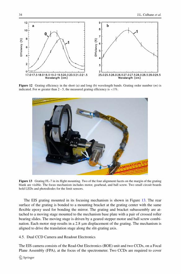
Figure 12 Grating efficiency in the short (a) and long (b) wavelength bands. Grating order number (m) isindicated. For m greater than 2 – 5, the measured grating efficiency is <1%.
Figure 13 Grating FL-7 in its flight mounting. Two of the four alignment facets on the margin of the gratingblank are visible. The focus mechanism includes motor, gearhead, and ball screw. Two small circuit boardshold LEDs and photodiodes for the limit sensors.
The EIS grating mounted in its focusing mechanism is shown in Figure 13. The rearsurface of the grating is bonded to a mounting bracket at the grating center with the sameflexible epoxy used for bonding the mirror. The grating and bracket subassembly are at-tached to a moving stage mounted to the mechanism base plate with a pair of crossed rollerbearing slides. The moving stage is driven by a geared stepper motor and ball screw combi-nation. Each motor step results in a 2.8 μm displacement of the grating. The mechanism isaligned to drive the translation stage along the slit-grating axis.
4.5. Dual CCD Camera and Readout Electronics
The EIS camera consists of the Read-Out Electronics (ROE) unit and two CCDs, on a FocalPlane Assembly (FPA), at the focus of the spectrometer. Two CCDs are required to cover
The EUV Imaging Spectrometer for Hinode 35
both the short (170 to 210 Å) and long (250 to 290 Å) wavelength ranges. Radiation fromthe solar region of interest is focused and dispersed by the EIS optics (Figure 1) into thesetwo wavelength ranges and imaged by the two CCDs.
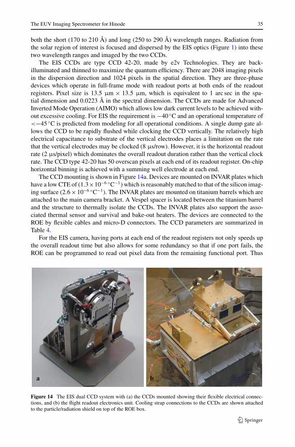
The EIS CCDs are type CCD 42-20, made by e2v Technologies. They are back-illuminated and thinned to maximize the quantum efficiency. There are 2048 imaging pixelsin the dispersion direction and 1024 pixels in the spatial direction. They are three-phasedevices which operate in full-frame mode with readout ports at both ends of the readoutregisters. Pixel size is 13.5 μm × 13.5 μm, which is equivalent to 1 arc sec in the spa-tial dimension and 0.0223 Å in the spectral dimension. The CCDs are made for AdvancedInverted Mode Operation (AIMO) which allows low dark current levels to be achieved with-out excessive cooling. For EIS the requirement is −40 ◦C and an operational temperature of<−45 ◦C is predicted from modeling for all operational conditions. A single dump gate al-lows the CCD to be rapidly flushed while clocking the CCD vertically. The relatively highelectrical capacitance to substrate of the vertical electrodes places a limitation on the ratethat the vertical electrodes may be clocked (8 μs/row). However, it is the horizontal readoutrate (2 μs/pixel) which dominates the overall readout duration rather than the vertical clockrate. The CCD type 42-20 has 50 overscan pixels at each end of its readout register. On-chiphorizontal binning is achieved with a summing well electrode at each end.
The CCD mounting is shown in Figure 14a. Devices are mounted on INVAR plates whichhave a low CTE of (1.3×10⁻⁶ ◦C−1) which is reasonably matched to that of the silicon imag-ing surface (2.6×10⁻⁶ ◦C−1). The INVAR plates are mounted on titanium barrels which areattached to the main camera bracket. A Vespel spacer is located between the titanium barreland the structure to thermally isolate the CCDs. The INVAR plates also support the asso-ciated thermal sensor and survival and bake-out heaters. The devices are connected to theROE by flexible cables and micro-D connectors. The CCD parameters are summarized inTable 4.
For the EIS camera, having ports at each end of the readout registers not only speeds upthe overall readout time but also allows for some redundancy so that if one port fails, theROE can be programmed to read out pixel data from the remaining functional port. Thus
Figure 14 The EIS dual CCD system with (a) the CCDs mounted showing their flexible electrical connec-tions, and (b) the flight readout electronics unit. Cooling strap connections to the CCDs are shown attachedto the particle/radiation shield on top of the ROE box.
36 J.L. Culhane et al.
Table 4 Summary of CCDparameters.
aSee Section 7.2. Full calibrationresults suggest that ≈60% maybe more appropriate.
Wavelength range CCD A CCD B
250 – 290 Å 170 – 210 Å
Device type CCD 42-20
Array size 2048 × 1024
Pixel size 13.5 μm × 13.5 μm
Readout rate 2 μs/pixel
Full well capacity 90k electrons
Charge transfer efficiency 0.999996
Quantum efficiencya 39 ± 4% 44 ± 4%
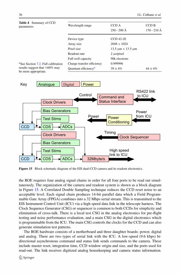
Figure 15 Block schematic diagram of the EIS dual-CCD camera and its readout electronics.
the ROE requires four analog signal chains in order for all four ports to be read out simul-taneously. The organization of the camera and readout system is shown as a block diagramin Figure 15. A Correlated Double Sampling technique reduces the CCD reset noise to anacceptable level. Each signal chain produces 14-bit parallel data which a Field Program-mable Gate Array (FPGA) combines into a 32 Mbps serial stream. This is transmitted to theEIS Instrument Control Unit (ICU) via a high-speed data link in the telescope harness. TheClock Sequence Generator (CSG) or sequencer is common to both CCDs for simplicity andelimination of cross-talk. There is a local test CSG in the analog electronics for pre-flighttesting and noise performance evaluation, and a main CSG in the digital electronics whichis programmable from the ICU. The main CSG controls the clocks for the CCD and can alsogenerate stimulation test patterns.
The ROE hardware consists of a motherboard and three daughter boards: power, digitaland analog. There are two types of serial link with the ICU. A low-speed (9.6 kbps) bi-directional asynchronous command and status link sends commands to the camera. Theseinclude master reset, integration time, CCD window origin and size, and the ports used forread-out. The link receives digitized analog housekeeping and camera status information.
The EUV Imaging Spectrometer for Hinode 37
A high-speed link (32 Mbps) using Low Voltage Differential Signaling technology passesthe CCD image data to the ICU. The 14-bit data from the four CCD signal chains plus a2-bit CCD port ID header for each is concatenated into a contiguous 64-bit serial word.
The full well capacity of the CCDs is approximately 90k electrons. With 14-bit Analogto Digital Converters (ADCs), the amplifier gain was set to 6.6 ± 0.03 electrons per DataNumber (DN). The full well capacity of the CCD in the long-wavelength range correspondsto ≈7500 photons. Due to the photoelectric effect, an incident photon will be converted intoa variable number of photoelectrons. At 170 Å, each photon will generate about 20 photo-electrons, while at 290 Å, one photon will generate about 12 photoelectrons. The minimumsignal detectable by the CCDs should correspond to one photon which in turn correspondsto 12 photoelectrons at the long-wavelength limit. Thus, the minimum “shot” noise on thedetected signal should also correspond to 12 photoelectrons or one photon. To maximize thesignal-to-noise ratio, the quantization and read noise values should be below the signal shotnoise. Since these terms add in quadrature, there is little advantage in having quantizationor read noise values which are substantially below the photon shot noise.
The thermal noise generated at the expected nominal CCD operating temperature of−50 ◦C will be minimal (≈0.005 electrons pixel−1 s−1) except for very long integrationtimes, and will even then still be significantly below the signal shot noise. An amplifier gainof ≈6.5 electrons/DN means that the quantization noise is well below the signal shot noise.A readout noise of ≈50% of the signal shot noise would correspond to about 6 electronsrms, suggesting a readout time of around 2 μs/pixel.
Subsets of the CCD frames can be selected in hardware for readout. Definable regions onthe CCDs are in the form of rectangles selectable up to the full CCD width. Both CCDs musthave identical windows which can be up to 1024 pixels wide for two readout nodes or upto 2048 pixels if only one readout node is available. Thus either two or four identical hard-ware windows can be selected. In the four-window case, pairs of windows must be locatedsymmetrically about column number 1024 on each CCD. The available height is 512 rows.Charge from outside these windows will not be read and can be quickly dumped. A commonClock Sequence Generator leads to the use of identical hardware windows on both CCDs.However, this gives a major benefit of minimizing cross talk on the digitized signal as pixelsare clocked out at the same time. Flexible software windows, up to a maximum of 25 intotal, can be set to further reduce the pixel data for transmission to the ground. The configu-ration of these software windows can be independent of CCD and at any location within theframes. Thus particular EUV spectral regions of interest may be selected.
5. Mechanical and Thermal Design
5.1. Mechanical Design
The mechanical design requirements were (a) total structure mass of less than 23 kg set bythe capacity of the M-V launcher; (b) high stiffness with a first resonance mode frequency>60 Hz; (c) dimensional stability to maintain spectral and spatial resolution over a broadtemperature range and to minimize motion of the spectra on the detectors; and (d) structuralthree-year condensable molecular fluence of 2.7 × 10⁻⁶ g cm−2. This strict fluence require-ment restricted the selection of materials within the optics cavity, mandated extensive vac-uum conditioning of the EIS structure, and required assembly in a carefully controlled cleanenvironment. The assembled instrument was double bagged and purged during instrumentand spacecraft level integration and test.
38 J.L. Culhane et al.
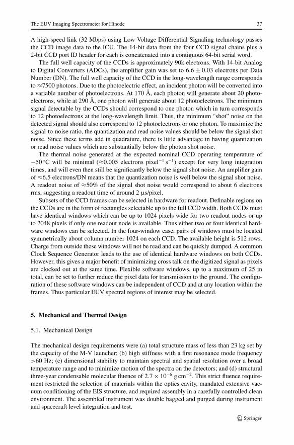
Figure 16 Diagram of the EIS spectrometer structure showing the locations of the principal elements.
The structure chosen used honeycomb sandwich panels with aluminum core materialand face sheets made from Carbon Fiber Reinforced Plastic (CFRP). The selected fiber resincombination is M55 with RS3 cyanate ester resin. M55/RS3 has been used extensively in theaerospace industry and shows impressive stiffness to mass ratios with excellent dimensionalstability and acceptably low outgassing properties.
The layout of the instrument is shown in Figure 16. EIS measures 3.54 m from the tipof the entrance baffle to the rear bulkhead carrying the mirror. The instrument base panelconsists of a 20-mm-thick Al core with nominal 1-mm-thick face sheets and 1-mm reinforce-ment patches near the instrument interface points. The EIS is mounted on a semi-kinematictitanium suspension between the instrument interface points (titanium inserts) and the cen-tral cylinder of the payload module. The width at the widest point of the instrument is 0.55 mand the height is 0.25 m.
The effective CTE of the optical bench was measured using coupon samples and is lessthan 0.4 ppm/◦C. The allowed thermal gradient variation in orbit with this CTE is 10 ◦C. Thebulkhead skins consist of balanced quasi-isotropic layers of 0/+60/-60 deg orientation. Theinstrument sidewalls and bulkheads consist of 10-mm-thick core with 0.6-mm-thick facesheets. The mass of the bare structure totals just below 23 kg which is 40% of the overallinstrument mass (including all optical units, electronics boxes, wiring harness and thermalhardware).
The assembly of the instrument’s panels was done in stages to ensure proper cleanli-ness and stress relief before final integration. All panels including the base panel or opticalbench were thoroughly cleaned as parts and then “dry” assembled leaving small clearancesbetween the internal bolted faces and edges. All edges were capped with CFRP U-shapedstrips to close the vented aluminum honeycomb core. The face sheets facing outwards wereall perforated with a rectangular pattern of small holes. This is to ensure that all gas trappedinside the sandwich was vented directly to the outside of the instrument. The Al honeycombmaterial was also perforated to permit venting of the individual cells.
The EUV Imaging Spectrometer for Hinode 39
The dry assembly was thermally cycled in a vacuum chamber to stress-relieve the struc-ture. Following this step, all strength- and stiffness-critical bulkheads were bonded togetherwith strips of L-shaped CFRP. The edges that were prone to rubbing due to mechanicalloading were coated with adhesive to seal the fiber particles on the machined edges. Thestructure was then returned to the bake-out chamber for a six-week vacuum bake-out withconstant QCM monitoring, to clear all outgassing species. After verification and confirma-tion that the structure met the outgassing fluence requirements, the optical components andelectronics boxes were mounted. These were all baked out separately prior to final assembly.
Following final integration and alignment verification the instrument was kept purgedduring all stages, except during mechanical acceptance, thermal balance and thermal vac-uum testing. The purge lines are integrated in the structure and inject ultra-clean nitrogennear all optical components (mirror, grating and CCDs). Vent ports located in the lid of theinstrument away from these injection points allow rapid evacuation and ensure flow awayfrom the optical surfaces. The instrument entrance is blocked by the clamshell doors sealingthe 1500 Å Al filters and keeping them under vacuum.
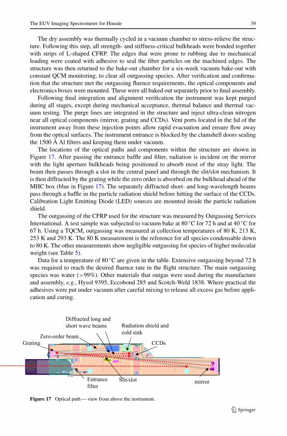
The locations of the optical paths and components within the structure are shown inFigure 17. After passing the entrance baffle and filter, radiation is incident on the mirrorwith the light aperture bulkheads being positioned to absorb most of the stray light. Thebeam then passes through a slot in the central panel and through the slit/slot mechanism. Itis then diffracted by the grating while the zero order is absorbed on the bulkhead ahead of theMHC box (blue in Figure 17). The separately diffracted short- and long-wavelength beamspass through a baffle in the particle radiation shield before hitting the surface of the CCDs.Calibration Light Emitting Diode (LED) sources are mounted inside the particle radiationshield.
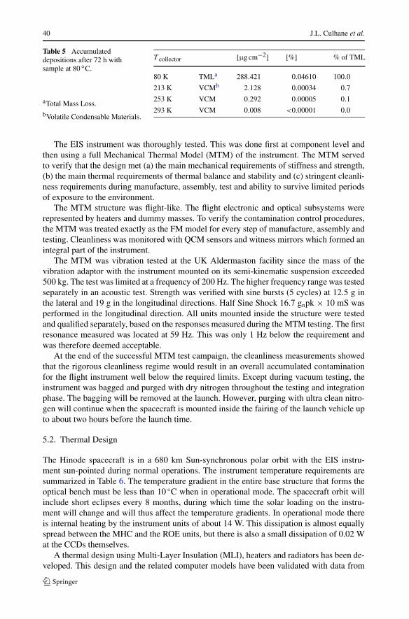
The outgassing of the CFRP used for the structure was measured by Outgassing ServicesInternational. A test sample was subjected to vacuum bake at 80 ◦C for 72 h and at 40 ◦C for67 h. Using a TQCM, outgassing was measured at collection temperatures of 80 K, 213 K,253 K and 293 K. The 80 K measurement is the reference for all species condensable downto 80 K. The other measurements show negligible outgassing for species of higher molecularweight (see Table 5).
Data for a temperature of 80 ◦C are given in the table. Extensive outgassing beyond 72 hwas required to reach the desired fluence rate in the flight structure. The main outgassingspecies was water (>99%). Other materials that outgas were used during the manufactureand assembly, e.g., Hysol 9395, Eccobond 285 and Scotch-Weld 1838. Where practical theadhesives were put under vacuum after careful mixing to release all excess gas before appli-cation and curing.
Figure 17 Optical path — view from above the instrument.
40 J.L. Culhane et al.
Table 5 Accumulateddepositions after 72 h withsample at 80 ◦C.
aTotal Mass Loss.
bVolatile Condensable Materials.
T collector [μg cm−2] [%] % of TML
80 K TMLa 288.421 0.04610 100.0
213 K VCMb 2.128 0.00034 0.7
253 K VCM 0.292 0.00005 0.1
293 K VCM 0.008 <0.00001 0.0
The EIS instrument was thoroughly tested. This was done first at component level andthen using a full Mechanical Thermal Model (MTM) of the instrument. The MTM servedto verify that the design met (a) the main mechanical requirements of stiffness and strength,(b) the main thermal requirements of thermal balance and stability and (c) stringent cleanli-ness requirements during manufacture, assembly, test and ability to survive limited periodsof exposure to the environment.
The MTM structure was flight-like. The flight electronic and optical subsystems wererepresented by heaters and dummy masses. To verify the contamination control procedures,the MTM was treated exactly as the FM model for every step of manufacture, assembly andtesting. Cleanliness was monitored with QCM sensors and witness mirrors which formed anintegral part of the instrument.
The MTM was vibration tested at the UK Aldermaston facility since the mass of thevibration adaptor with the instrument mounted on its semi-kinematic suspension exceeded500 kg. The test was limited at a frequency of 200 Hz. The higher frequency range was testedseparately in an acoustic test. Strength was verified with sine bursts (5 cycles) at 12.5 g inthe lateral and 19 g in the longitudinal directions. Half Sine Shock 16.7 gnpk × 10 mS wasperformed in the longitudinal direction. All units mounted inside the structure were testedand qualified separately, based on the responses measured during the MTM testing. The firstresonance measured was located at 59 Hz. This was only 1 Hz below the requirement andwas therefore deemed acceptable.
At the end of the successful MTM test campaign, the cleanliness measurements showedthat the rigorous cleanliness regime would result in an overall accumulated contaminationfor the flight instrument well below the required limits. Except during vacuum testing, theinstrument was bagged and purged with dry nitrogen throughout the testing and integrationphase. The bagging will be removed at the launch. However, purging with ultra clean nitro-gen will continue when the spacecraft is mounted inside the fairing of the launch vehicle upto about two hours before the launch time.
5.2. Thermal Design
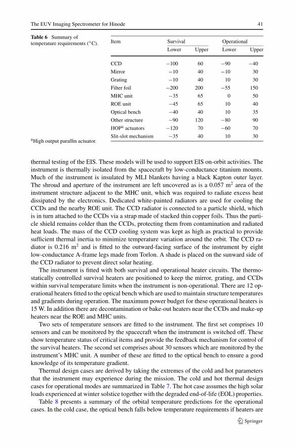
The Hinode spacecraft is in a 680 km Sun-synchronous polar orbit with the EIS instru-ment sun-pointed during normal operations. The instrument temperature requirements aresummarized in Table 6. The temperature gradient in the entire base structure that forms theoptical bench must be less than 10 ◦C when in operational mode. The spacecraft orbit willinclude short eclipses every 8 months, during which time the solar loading on the instru-ment will change and will thus affect the temperature gradients. In operational mode thereis internal heating by the instrument units of about 14 W. This dissipation is almost equallyspread between the MHC and the ROE units, but there is also a small dissipation of 0.02 Wat the CCDs themselves.
A thermal design using Multi-Layer Insulation (MLI), heaters and radiators has been de-veloped. This design and the related computer models have been validated with data from
The EUV Imaging Spectrometer for Hinode 41
Table 6 Summary oftemperature requirements (◦C).
aHigh output paraffin actuator.
Item Survival Operational
Lower Upper Lower Upper
CCD −100 60 −90 −40
Mirror −10 40 −10 30
Grating −10 40 10 30
Filter foil −200 200 −55 150
MHC unit −35 65 0 50
ROE unit −45 65 10 40
Optical bench −40 40 10 35
Other structure −90 120 −80 90
HOPa actuators −120 70 −60 70
Slit-slot mechanism −35 40 10 30
thermal testing of the EIS. These models will be used to support EIS on-orbit activities. Theinstrument is thermally isolated from the spacecraft by low-conductance titanium mounts.Much of the instrument is insulated by MLI blankets having a black Kapton outer layer.The shroud and aperture of the instrument are left uncovered as is a 0.057 m2 area of theinstrument structure adjacent to the MHC unit, which was required to radiate excess heatdissipated by the electronics. Dedicated white-painted radiators are used for cooling theCCDs and the nearby ROE unit. The CCD radiator is connected to a particle shield, whichis in turn attached to the CCDs via a strap made of stacked thin copper foils. Thus the parti-cle shield remains colder than the CCDs, protecting them from contamination and radiatedheat loads. The mass of the CCD cooling system was kept as high as practical to providesufficient thermal inertia to minimize temperature variation around the orbit. The CCD ra-diator is 0.216 m2 and is fitted to the outward-facing surface of the instrument by eightlow-conductance A-frame legs made from Torlon. A shade is placed on the sunward side ofthe CCD radiator to prevent direct solar heating.
The instrument is fitted with both survival and operational heater circuits. The thermo-statically controlled survival heaters are positioned to keep the mirror, grating, and CCDswithin survival temperature limits when the instrument is non-operational. There are 12 op-erational heaters fitted to the optical bench which are used to maintain structure temperaturesand gradients during operation. The maximum power budget for these operational heaters is15 W. In addition there are decontamination or bake-out heaters near the CCDs and make-upheaters near the ROE and MHC units.
Two sets of temperature sensors are fitted to the instrument. The first set comprises 10sensors and can be monitored by the spacecraft when the instrument is switched off. Theseshow temperature status of critical items and provide the feedback mechanism for control ofthe survival heaters. The second set comprises about 30 sensors which are monitored by theinstrument’s MHC unit. A number of these are fitted to the optical bench to ensure a goodknowledge of its temperature gradient.
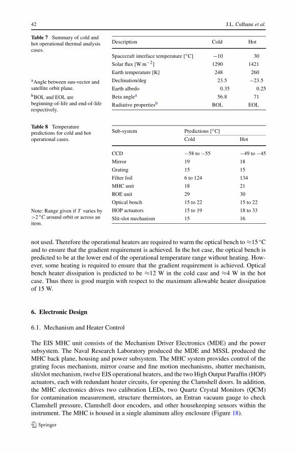
Thermal design cases are derived by taking the extremes of the cold and hot parametersthat the instrument may experience during the mission. The cold and hot thermal designcases for operational modes are summarized in Table 7. The hot case assumes the high solarloads experienced at winter solstice together with the degraded end-of-life (EOL) properties.
Table 8 presents a summary of the orbital temperature predictions for the operationalcases. In the cold case, the optical bench falls below temperature requirements if heaters are
42 J.L. Culhane et al.
Table 7 Summary of cold andhot operational thermal analysiscases.
aAngle between sun-vector andsatellite orbit plane.bBOL and EOL arebeginning-of-life and end-of-liferespectively.
Description Cold Hot
Spacecraft interface temperature [◦C] −10 30
Solar flux [W m−2] 1290 1421
Earth temperature [K] 248 260
Declination/deg 23.5 −23.5
Earth albedo 0.35 0.25
Beta anglea 56.8 71
Radiative propertiesb BOL EOL
Table 8 Temperaturepredictions for cold and hotoperational cases.
Note: Range given if T varies by>2 ◦C around orbit or across anitem.
Sub-system Predictions [◦C]
Cold Hot
CCD −58 to −55 −49 to −45
Mirror 19 18
Grating 15 15
Filter foil 6 to 124 134
MHC unit 18 21
ROE unit 29 30
Optical bench 15 to 22 15 to 22
HOP actuators 15 to 19 18 to 33
Slit-slot mechanism 15 16
not used. Therefore the operational heaters are required to warm the optical bench to ≈15 ◦Cand to ensure that the gradient requirement is achieved. In the hot case, the optical bench ispredicted to be at the lower end of the operational temperature range without heating. How-ever, some heating is required to ensure that the gradient requirement is achieved. Opticalbench heater dissipation is predicted to be ≈12 W in the cold case and ≈4 W in the hotcase. Thus there is good margin with respect to the maximum allowable heater dissipationof 15 W.
6. Electronic Design
6.1. Mechanism and Heater Control
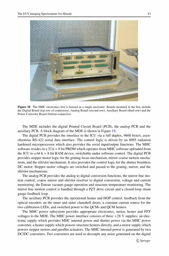
The EIS MHC unit consists of the Mechanism Driver Electronics (MDE) and the powersubsystem. The Naval Research Laboratory produced the MDE and MSSL produced theMHC back plane, housing and power subsystem. The MHC system provides control of thegrating focus mechanism, mirror coarse and fine motion mechanisms, shutter mechanism,slit/slot mechanism, twelve EIS operational heaters, and the two High Output Paraffin (HOP)actuators, each with redundant heater circuits, for opening the Clamshell doors. In addition,the MHC electronics drives two calibration LEDs, two Quartz Crystal Monitors (QCM)for contamination measurement, structure thermistors, an Entran vacuum gauge to checkClamshell pressure, Clamshell door encoders, and other housekeeping sensors within theinstrument. The MHC is housed in a single aluminum alloy enclosure (Figure 18).
The EUV Imaging Spectrometer for Hinode 43
Figure 18 The MHC electronics box is housed in a single enclosure. Boards mounted in the box includethe Digital Board (top row of connectors), Analog Board (second row), Auxiliary Board (third row) and thePower Converter Board (bottom connector).
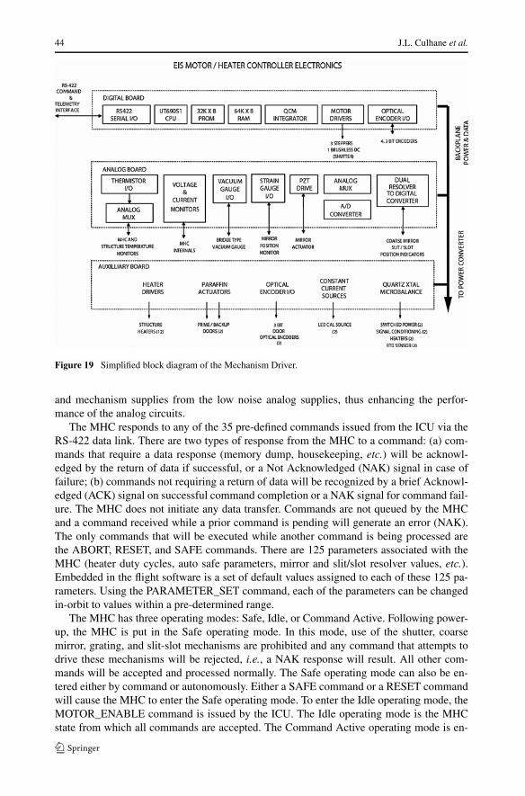
The MDE includes the digital Printed Circuit Board (PCB), the analog PCB and theauxiliary PCB. A block diagram of the MDE is shown in Figure 19.
The digital PCB provides the interface to the ICU via a full duplex, 9600 byte/s, asyn-chronous RS-422 serial data interface. The control logic is driven by an 8085 radiationhardened microprocessor which also provides the serial input/output functions. The MHCsoftware resides in a 32 k ×8 bit PROM which operates from MHC software uploaded fromthe ICU to a 64 k × 8 bit RAM device, switchable under software control. The digital PCBprovides stepper motor logic for the grating focus mechanism, mirror coarse motion mecha-nism, and the slit/slot mechanism. It also provides the control logic for the shutter brushlessDC motor. Stepper motor voltages are switched and passed to the grating, mirror, and theslit/slot mechanisms.
The analog PCB provides the analog to digital conversion functions, the mirror fine mo-tion control, coarse mirror and slit/slot resolver to digital conversion, voltage and currentmonitoring, the Entran vacuum gauge operation and structure temperature monitoring. Themirror fine motion control is handled through a PZT drive circuit and a closed-loop straingauge feedback loop.
The auxiliary PCB provides the operational heater and HOP control, feedback from theoptical encoders on the inner and outer clamshell doors, a constant current source for thetwo calibration LEDs, and switched power to the QCMs and QCM heaters.
The MHC power subsystem provides appropriate electronics, motor, heater and PZTvoltages to the MDE. The MHC power interface consists of three +28 V supplies: an elec-tronic supply which provides MHC internal power and shutter power via the MHC powerconverter, a heater supply which powers structure heaters directly, and a motor supply whichpowers stepper motors and paraffin actuators. The MHC internal power is generated by twoDC/DC converters. Two converters are used to decouple any noise generated on the digital
44 J.L. Culhane et al.
Figure 19 Simplified block diagram of the Mechanism Driver.
and mechanism supplies from the low noise analog supplies, thus enhancing the perfor-mance of the analog circuits.
The MHC responds to any of the 35 pre-defined commands issued from the ICU via theRS-422 data link. There are two types of response from the MHC to a command: (a) com-mands that require a data response (memory dump, housekeeping, etc.) will be acknowl-edged by the return of data if successful, or a Not Acknowledged (NAK) signal in case offailure; (b) commands not requiring a return of data will be recognized by a brief Acknowl-edged (ACK) signal on successful command completion or a NAK signal for command fail-ure. The MHC does not initiate any data transfer. Commands are not queued by the MHCand a command received while a prior command is pending will generate an error (NAK).The only commands that will be executed while another command is being processed arethe ABORT, RESET, and SAFE commands. There are 125 parameters associated with theMHC (heater duty cycles, auto safe parameters, mirror and slit/slot resolver values, etc.).Embedded in the flight software is a set of default values assigned to each of these 125 pa-rameters. Using the PARAMETER_SET command, each of the parameters can be changedin-orbit to values within a pre-determined range.
The MHC has three operating modes: Safe, Idle, or Command Active. Following power-up, the MHC is put in the Safe operating mode. In this mode, use of the shutter, coarsemirror, grating, and slit-slot mechanisms are prohibited and any command that attempts todrive these mechanisms will be rejected, i.e., a NAK response will result. All other com-mands will be accepted and processed normally. The Safe operating mode can also be en-tered either by command or autonomously. Either a SAFE command or a RESET commandwill cause the MHC to enter the Safe operating mode. To enter the Idle operating mode, theMOTOR_ENABLE command is issued by the ICU. The Idle operating mode is the MHCstate from which all commands are accepted. The Command Active operating mode is en-

The EUV Imaging Spectrometer for Hinode 45
tered following the receipt of a valid command from either the Safe or Idle modes. When theMHC is in the Command Active mode, only the ABORT, RESET, or SAFE commands areaccepted, all others are rejected. The MHC will transition from the Command Active modeto the Idle or Safe mode following completion of the current command.
The MHC supports two memory modes; Programmable Read Only Memory (PROM)mode and Random Access Memory (RAM) mode. In PROM mode, the baseline code resid-ing in a PROM is executed. In RAM mode, the program currently loaded in a RAM is exe-cuted. The baseline code is copied from PROM to RAM at power-up. On power-up, the de-fault is PROM mode. Switching between modes is accomplished via the MEMORY_MODEcommand and always results in a return to the SAFE operating mode. Updated MHC oper-ating code can be uplinked from the ICU to the MHC RAM using the MEMORY_UPLOADcommand.
6.2. On-Board Data Processing Unit
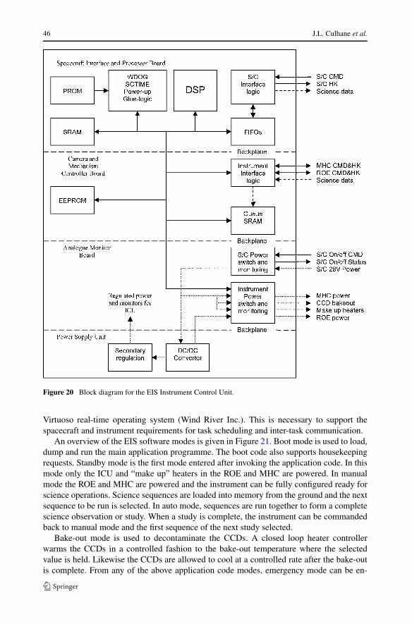
The ICU is an on-board processor that controls the entire EIS instrument. Located in thespacecraft bus section, it also handles interfacing between the EIS spectrometer and thespacecraft. Figure 20 gives an overview of the ICU electronics. The circuitry is located onfive printed circuit boards: spacecraft interface and processor board, camera and mechanismcontroller board, analog monitor board, power supply unit and a backplane. The spacecraftinterface and processor board is based around a TEMIC 21020 Digital Signal Processor(DSP) running at a clock speed of 20 MHz. There are two FPGAs, a Static RAM (SRAM;1 Mb) and a boot PROM of 8 kb to support the DSP. One FPGA decodes the address spacefor the memory and I/O. It also implements the Watch Dog and Spacecraft timer functionsand a “boot-strap” code power-up function. The second FPGA deals with the spacecraftdigital interfaces.
The spacecraft interface is based on three links, command and housekeeping or sta-tus, both 62.5 kbps and science mission data transfer at 2 Mbps. Each of the interfacesincorporates First In First Out (FIFO) buffers. The camera and mechanism controller boardcontains onboard application code storage in 1 Mb of Electrically Eraseable PROM (EEP-ROM) which can hold two versions of the code, CCD image buffers in 4 Mb of SRAMfor the raw science data and two further FPGAs. One FPGA handles the 32 Mbps highspeed link between the ROE and the ICU while the second controls the RS422 9.6 kbpsinterfaces between the ICU and the ROE and MHC. The analog monitor contains the pri-mary power interface and current limiter for the instrument. It is responsible for temper-ature, current and voltage monitoring, primary and secondary line switching and heaterswitching. FET switches are used to switch primary power to the MHC, bake-out andsubstitution heaters and secondary unregulated power to the ROE. An FPGA is used forcontrol of the monitoring function and bus interface along with an ADC, analog multi-plexers and operational amplifiers. Secondary power line conditioning is provided by thepower supply unit board. There are regulated power lines for the ICU and unregulatedones for the ROE. The backplane provides the interface connections between the aboveboards.
Buffer logic on the daughter boards for the backplane is included in the FPGAs but isnot shown in the diagram. The bootstrap code in PROM is written in assembly language andsupports the loading and dumping of the operational code from either bank of the EEPROMor spacecraft to RAM, as commanded. In order to facilitate the software development theoperational code is designed to be modular. This code is written in C operating under the
46 J.L. Culhane et al.
Figure 20 Block diagram for the EIS Instrument Control Unit.
Virtuoso real-time operating system (Wind River Inc.). This is necessary to support thespacecraft and instrument requirements for task scheduling and inter-task communication.
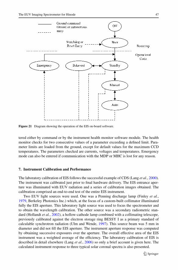
An overview of the EIS software modes is given in Figure 21. Boot mode is used to load,dump and run the main application programme. The boot code also supports housekeepingrequests. Standby mode is the first mode entered after invoking the application code. In thismode only the ICU and “make up” heaters in the ROE and MHC are powered. In manualmode the ROE and MHC are powered and the instrument can be fully configured ready forscience operations. Science sequences are loaded into memory from the ground and the nextsequence to be run is selected. In auto mode, sequences are run together to form a completescience observation or study. When a study is complete, the instrument can be commandedback to manual mode and the first sequence of the next study selected.
Bake-out mode is used to decontaminate the CCDs. A closed loop heater controllerwarms the CCDs in a controlled fashion to the bake-out temperature where the selectedvalue is held. Likewise the CCDs are allowed to cool at a controlled rate after the bake-outis complete. From any of the above application code modes, emergency mode can be en-
The EUV Imaging Spectrometer for Hinode 47
Figure 21 Diagram showing the operation of the EIS on-board software.
tered either by command or by the instrument health monitor software module. The healthmonitor checks for two consecutive values of a parameter exceeding a defined limit. Para-meter limits are loaded from the ground, except for default values for the maximum CCDtemperatures. The parameters checked are currents, voltages and temperatures. Emergencymode can also be entered if communication with the MDP or MHC is lost for any reason.
7. Instrument Calibration and Performance
The laboratory calibration of EIS follows the successful example of CDS (Lang et al., 2000).The instrument was calibrated just prior to final hardware delivery. The EIS entrance aper-ture was illuminated with EUV radiation and a series of calibration images obtained. Thecalibration comprised an end-to-end test of the entire EIS instrument.
Two EUV light sources were used. One was a Penning discharge lamp (Finley et al.,1979, Berkeley Photonics Inc.) which, at the focus of a custom-built collimator illuminatedfully the EIS aperture. This laboratory light source was used to focus the spectrometer andto obtain the wavelength calibration. The other source was a secondary radiometric stan-dard (Hollandt et al., 2002), a hollow-cathode lamp combined with a collimating telescope,previously calibrated against the electron storage ring BESSY I as a primary standard ofcalculable synchrotron radiation (Ulm and Wende, 1997). This source beam was 5 mm indiameter and did not fill the EIS aperture. The instrument aperture response was computedby obtaining successive exposures over the aperture. The overall effective area of the EISinstrument was a weighted average of the efficiency. The laboratory calibration of EIS isdescribed in detail elsewhere (Lang et al., 2006) so only a brief account is given here. Thecalculated instrument response to three typical solar coronal spectra is also presented.
48 J.L. Culhane et al.
7.1. Wavelength Calibration
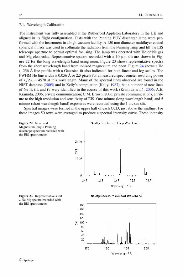
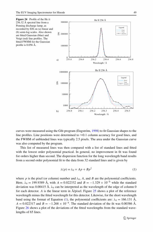
The instrument was fully assembled at the Rutherford Appleton Laboratory in the UK andaligned in its flight configuration. Tests with the Penning EUV discharge lamp were per-formed with the instrument in a high vacuum facility. A 150 mm diameter multilayer coatedspherical mirror was used to collimate the radiation from the Penning lamp and fill the EIStelescope aperture to permit optimal focusing. The lamp was operated with He or Ne gasand Mg electrodes. Representative spectra recorded with a 10 μm slit are shown in Fig-ure 22 for the long wavelength band using neon. Figure 23 shows representative spectrafrom the short wavelength band from ionized magnesium and neon. Figure 24 shows a HeII 256 Å line profile with a Gaussian fit also indicated for both linear and log scales. TheFWHM He line width is 0.056 Å or 2.5 pixels for a measured spectrometer resolving powerof λ/�λ = 4570 at this wavelength. Many of the spectral lines observed are found in theNIST database (2005) and in Kelly’s compilation (Kelly, 1987), but a number of new linesof Ne II, III, and IV were identified in the course of this work (Kramida et al., 2006; A.E.Kramida, 2006, private communication; C.M. Brown, 2006, private communication), a trib-ute to the high resolution and sensitivity of EIS. One minute (long wavelength band) and 5minute (short wavelength band) exposures were recorded using the 1 arc sec slit.
Spectral images were formed in the upper half of each CCD, just above the midline. Forthese images 50 rows were averaged to produce a spectral intensity curve. These intensity
Figure 22 Neon andMagnesium long λ Penningdischarge spectrum recorded withthe EIS spectrometer.
Figure 23 Representative shortλ Ne-Mg spectra recorded withthe EIS spectrometer.
The EUV Imaging Spectrometer for Hinode 49
Figure 24 Profile of the He II
256.32 Å spectral line from aPenning discharge lamp, asrecorded by EIS on (a) linear and(b) semi-log scales. Also shownare fitted Gaussian (blue) andVoigt (red) line profiles. Thefitted FWHM for the Gaussianprofile is 0.056 Å.
curves were measured using the Gfit program (Engström, 1998) to fit Gaussian shapes to theline profiles. Line positions were determined to ≈0.1 column accuracy for good lines, andthe FWHM of unblended lines was typically 2.5 pixels. The area under the Gaussian curvewas also computed by the program.
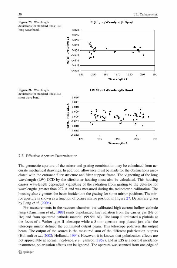
This list of measured lines was then compared with a list of standard lines and fittedwith the lowest order polynomial practical. In general, no improvement in fit was foundfor orders higher than second. The dispersion function for the long wavelength band resultsfrom a second order polynomial fit to the data from 32 standard lines and is given by
λ(p) = λ0 + Ap + Bp2 (1)
where p is the pixel (or column) number and λ0, A, and B are the polynomial coefficients.Here, λ0 = 199.9389 Å, with A = 0.022332 and B = −1.329 × 10⁻⁸ while the standarddeviation was 0.00415 Å. λ0 can be interpreted as the wavelength of the edge of column 0for each detector. A is the linear term in Å/pixel. Figure 25 shows a plot of the referencewavelength minus the fitted wavelength for this detector. Likewise, for the short wavelengthband using the format of Equation (1), the polynomial coefficients are: λ0 = 166.131 Å,A = 0.022317 and B = −1.268 × 10⁻⁸. The standard deviation of the fit was 0.00386 Å.Figure 26 shows a plot of the deviations of the fitted wavelengths from the standard wave-lengths of 65 lines.
50 J.L. Culhane et al.
Figure 25 Wavelengthdeviations for standard lines; EISlong wave band.
Figure 26 Wavelengthdeviations for standard lines; EISshort wave band.
7.2. Effective Aperture Determination
The geometric aperture of the mirror and grating combination may be calculated from ac-curate mechanical drawings. In addition, allowance must be made for the obstructions asso-ciated with the entrance filter structure and filter support frame. The vignetting of the longwavelength (LW) CCD by the slit/shutter housing must also be calculated. This housingcauses wavelength dependent vignetting of the radiation from grating to the detector forwavelengths greater than 272 Å and was measured during the radiometric calibration. Thehousing also vignettes the beam incident on the grating for some mirror positions. The mir-ror aperture is shown as a function of coarse mirror position in Figure 27. Details are givenby Lang et al. (2006).
For measurements in the vacuum chamber, the calibrated high current hollow cathodelamp (Danzmann et al., 1988) emits unpolarized line radiation from the carrier gas (Ne orHe) and from sputtered cathode material (99.5% Al). The lamp illuminated a pinhole atthe focus of a Wolter type II telescope while a 5 mm aperture stop placed just after thetelescope mirror defined the collimated output beam. This telescope polarizes the outputbeam. The output of the source is the measured sum of the different polarization outputs(Hollandt et al., 2002; Hollandt, 1994). However, it is known that polarization effects arenot appreciable at normal incidence, e.g., Samson (1967), and as EIS is a normal incidenceinstrument, polarization effects can be ignored. The aperture was scanned from one edge of
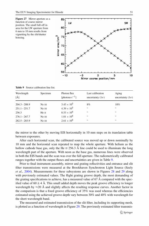
The EUV Imaging Spectrometer for Hinode 51
Figure 27 Mirror aperture as afunction of coarse mirrorposition. The small fall-off inarea for the LW aperture from6 mm to 10 mm results fromvignetting by the slit/shutterhousing.
Table 9 Source calibration line list.
Wavelength Spectrum Photon flux Last calibration Aging
[Å] [photons s−1] uncertainty (1σ ) uncertainty (1σ )
204.3 – 208.9 Ne III 3.43 × 10⁵ 8% 10%
251.1 – 251.7 Ne III 4.39 × 10⁵ “ “
256.3 He II 8.53 × 10⁶ “ “
276.1 – 267.7 Ne III 1.01 × 10⁶ “ “
282.5 – 283.9 Ne III 2.61 × 10⁶ “ “
the mirror to the other by moving EIS horizontally in 10 mm steps on its translation tablebetween exposures.
After each horizontal scan, the calibrated source was moved up or down nominally by10 mm and the horizontal scan repeated to map the whole aperture. With helium as thehollow cathode base gas, only the He II 256.3 Å line could be used to illuminate the longwavelength part of the aperture. With neon as the base gas, numerous lines were observedin both the EIS bands and the scan was over the full aperture. The radiometrically calibratedranges together with the output fluxes and uncertainties are given in Table 9.
Prior to final instrument assembly, mirror and grating reflectivities and entrance and slitfilter transmissions were measured at the Brookhaven Synchrotron Light Source (Seelyet al., 2004). Measurements for these subsystems are shown in Figures 28 and 29 alongwith previously estimated values. The flight grating groove depth, the most demanding ofthe grating specifications to achieve, has a measured value of 67 Å compared with the spec-ified value of 60 ± 4 Å. This small added depth moves the peak groove efficiency to longerwavelength by ≈20 Å and slightly affects the resulting response curves. Another factor inthe comparison is that a fixed groove efficiency of 35% was used whereas the efficienciesestimated using the achieved groove depth vary between 30% and 40% with wavelength forthe short wavelength band.
The measured and estimated transmission of the slit filter, including its supporting mesh,is plotted as a function of wavelength in Figure 29. The previously estimated filter transmis-
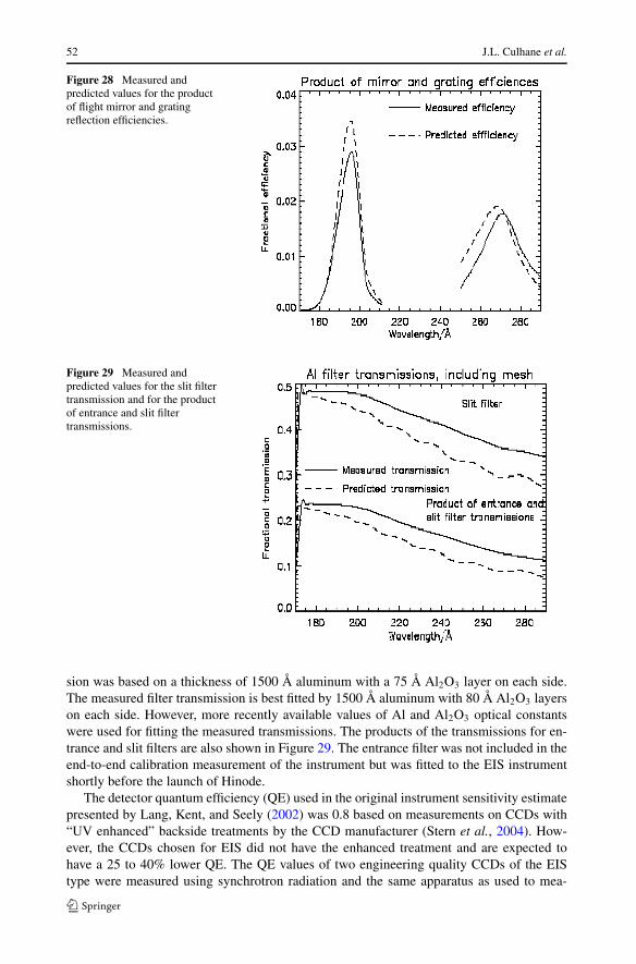
52 J.L. Culhane et al.
Figure 28 Measured andpredicted values for the productof flight mirror and gratingreflection efficiencies.
Figure 29 Measured andpredicted values for the slit filtertransmission and for the productof entrance and slit filtertransmissions.
sion was based on a thickness of 1500 Å aluminum with a 75 Å Al2O3 layer on each side.The measured filter transmission is best fitted by 1500 Å aluminum with 80 Å Al2O3 layerson each side. However, more recently available values of Al and Al2O3 optical constantswere used for fitting the measured transmissions. The products of the transmissions for en-trance and slit filters are also shown in Figure 29. The entrance filter was not included in theend-to-end calibration measurement of the instrument but was fitted to the EIS instrumentshortly before the launch of Hinode.
The detector quantum efficiency (QE) used in the original instrument sensitivity estimatepresented by Lang, Kent, and Seely (2002) was 0.8 based on measurements on CCDs with“UV enhanced” backside treatments by the CCD manufacturer (Stern et al., 2004). How-ever, the CCDs chosen for EIS did not have the enhanced treatment and are expected tohave a 25 to 40% lower QE. The QE values of two engineering quality CCDs of the EIStype were measured using synchrotron radiation and the same apparatus as used to mea-
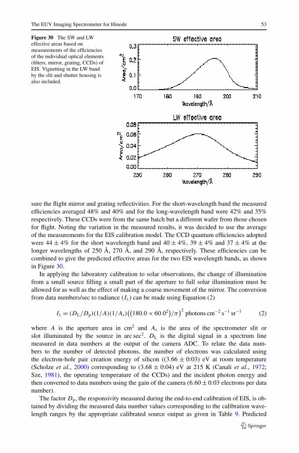
The EUV Imaging Spectrometer for Hinode 53
Figure 30 The SW and LWeffective areas based onmeasurements of the efficienciesof the individual optical elements(filters, mirror, grating, CCDs) ofEIS. Vignetting in the LW bandby the slit and shutter housing isalso included.
sure the flight mirror and grating reflectivities. For the short-wavelength band the measuredefficiencies averaged 48% and 40% and for the long-wavelength band were 42% and 35%respectively. These CCDs were from the same batch but a different wafer from those chosenfor flight. Noting the variation in the measured results, it was decided to use the averageof the measurements for the EIS calibration model. The CCD quantum efficiencies adoptedwere 44 ± 4% for the short wavelength band and 40 ± 4%, 39 ± 4% and 37 ± 4% at thelonger wavelengths of 250 Å, 270 Å, and 290 Å, respectively. These efficiencies can becombined to give the predicted effective areas for the two EIS wavelength bands, as shownin Figure 30.
In applying the laboratory calibration to solar observations, the change of illuminationfrom a small source filling a small part of the aperture to full solar illumination must beallowed for as well as the effect of making a coarse movement of the mirror. The conversionfrom data numbers/sec to radiance (Iλ) can be made using Equation (2)
Iλ = (DL/Dp)(1/A)(1/As)((
180.0 × 60.02)/π
)2photons cm−2 s−1 sr−1 (2)
where A is the aperture area in cm2 and As is the area of the spectrometer slit orslot illuminated by the source in arc sec2. DL is the digital signal in a spectrum linemeasured in data numbers at the output of the camera ADC. To relate the data num-bers to the number of detected photons, the number of electrons was calculated usingthe electron-hole pair creation energy of silicon ((3.66 ± 0:03) eV at room temperature(Scholze et al., 2000) corresponding to (3.68 ± 0:04) eV at 215 K (Canali et al., 1972;Sze, 1981), the operating temperature of the CCDs) and the incident photon energy andthen converted to data numbers using the gain of the camera (6.60 ± 0.03 electrons per datanumber).
The factor Dp, the responsivity measured during the end-to-end calibration of EIS, is ob-tained by dividing the measured data number values corresponding to the calibration wave-length ranges by the appropriate calibrated source output as given in Table 9. Predicted
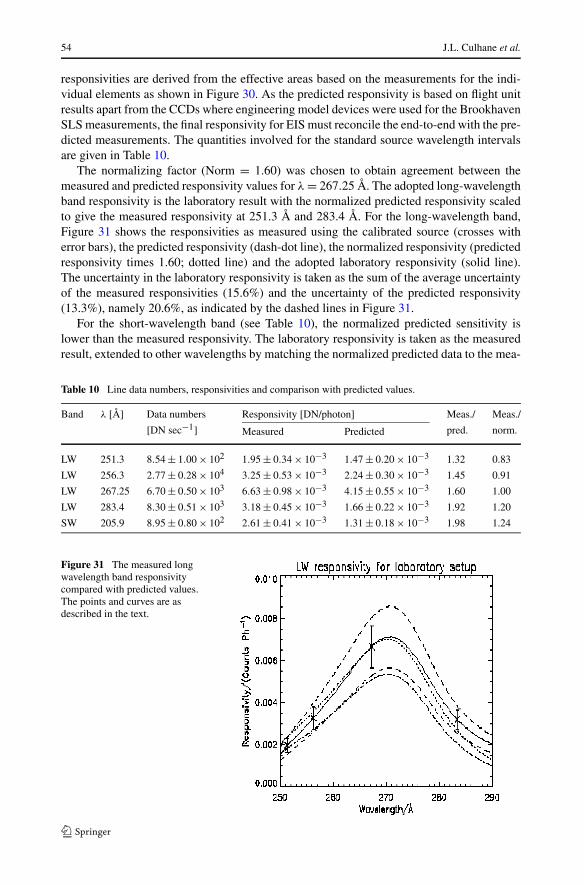
54 J.L. Culhane et al.
responsivities are derived from the effective areas based on the measurements for the indi-vidual elements as shown in Figure 30. As the predicted responsivity is based on flight unitresults apart from the CCDs where engineering model devices were used for the BrookhavenSLS measurements, the final responsivity for EIS must reconcile the end-to-end with the pre-dicted measurements. The quantities involved for the standard source wavelength intervalsare given in Table 10.
The normalizing factor (Norm = 1.60) was chosen to obtain agreement between themeasured and predicted responsivity values for λ = 267.25 Å. The adopted long-wavelengthband responsivity is the laboratory result with the normalized predicted responsivity scaledto give the measured responsivity at 251.3 Å and 283.4 Å. For the long-wavelength band,Figure 31 shows the responsivities as measured using the calibrated source (crosses witherror bars), the predicted responsivity (dash-dot line), the normalized responsivity (predictedresponsivity times 1.60; dotted line) and the adopted laboratory responsivity (solid line).The uncertainty in the laboratory responsivity is taken as the sum of the average uncertaintyof the measured responsivities (15.6%) and the uncertainty of the predicted responsivity(13.3%), namely 20.6%, as indicated by the dashed lines in Figure 31.
For the short-wavelength band (see Table 10), the normalized predicted sensitivity islower than the measured responsivity. The laboratory responsivity is taken as the measuredresult, extended to other wavelengths by matching the normalized predicted data to the mea-
Table 10 Line data numbers, responsivities and comparison with predicted values.
Band λ [Å] Data numbers Responsivity [DN/photon] Meas./ Meas./
[DN sec−1] pred. norm.Measured Predicted
LW 251.3 8.54 ± 1.00 × 10² 1.95 ± 0.34 × 10⁻³ 1.47 ± 0.20 × 10⁻³ 1.32 0.83
LW 256.3 2.77 ± 0.28 × 10⁴ 3.25 ± 0.53 × 10⁻³ 2.24 ± 0.30 × 10⁻³ 1.45 0.91
LW 267.25 6.70 ± 0.50 × 10³ 6.63 ± 0.98 × 10⁻³ 4.15 ± 0.55 × 10⁻³ 1.60 1.00
LW 283.4 8.30 ± 0.51 × 10³ 3.18 ± 0.45 × 10⁻³ 1.66 ± 0.22 × 10⁻³ 1.92 1.20
SW 205.9 8.95 ± 0.80 × 10² 2.61 ± 0.41 × 10⁻³ 1.31 ± 0.18 × 10⁻³ 1.98 1.24
Figure 31 The measured longwavelength band responsivitycompared with predicted values.The points and curves are asdescribed in the text.
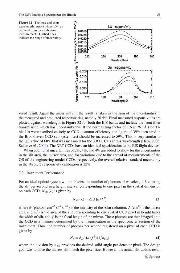
The EUV Imaging Spectrometer for Hinode 55
Figure 32 The long and shortwavelength responsivities, Dp, asdeduced from the calibrationmeasurements. Dashed linesindicate the range of uncertainty.
sured result. Again the uncertainty in the result is taken as the sum of the uncertainties inthe measured and predicted responsivities, namely 20.5%. Final measured responsivities areplotted against wavelength in Figure 32 for both the EIS bands and include the front filtertransmission which has uncertainty 5%. If the normalizing factor of 1.6 at 267 Å (see Ta-ble 10) were ascribed entirely to CCD quantum efficiency, the figure of 39% measured inthe Brookhaven CCD sub-system test should be increased to 59%. This is very similar tothe QE value of 60% that was measured for the XRT CCDs at this wavelength (Hara, 2003;Sakao et al., 2004). The XRT CCDs have an identical specification to the EIS flight devices.
When additional uncertainties of 2%, 4%, and 4% are added to allow for the uncertaintiesin the slit area, the mirror area, and for variations due to the spread of measurements of theQE of the engineering model CCDs, respectively, the overall relative standard uncertaintyin the absolute responsivity calibration is 22%.
7.3. Instrument Performance
For an ideal optical system with no losses, the number of photons of wavelength λ enteringthe slit per second in a height interval corresponding to one pixel in the spatial dimensionon each CCD, N slit(λ) is given by
N slit(λ) = φλA(a/f 2
)(3)
where φ (photons cm−2 s−1 sr−1) is the intensity of the solar radiation, A (cm2) is the mirrorarea, a (cm2) is the area of the slit corresponding to one spatial CCD pixel in height timesthe width of slit, and f is the focal length of the mirror. These photons are then imaged ontothe CCD in a manner determined by the magnification in the spectrometer section of theinstrument. Thus, the number of photons per second registered on a pixel of each CCD isgiven by
Nλ = φλA(a/f 2
)(1/npix) (4)
where the division by npix provides the desired solid angle per detector pixel. The designgoal was to have the narrow slit match the pixel size. However, the actual slit widths result
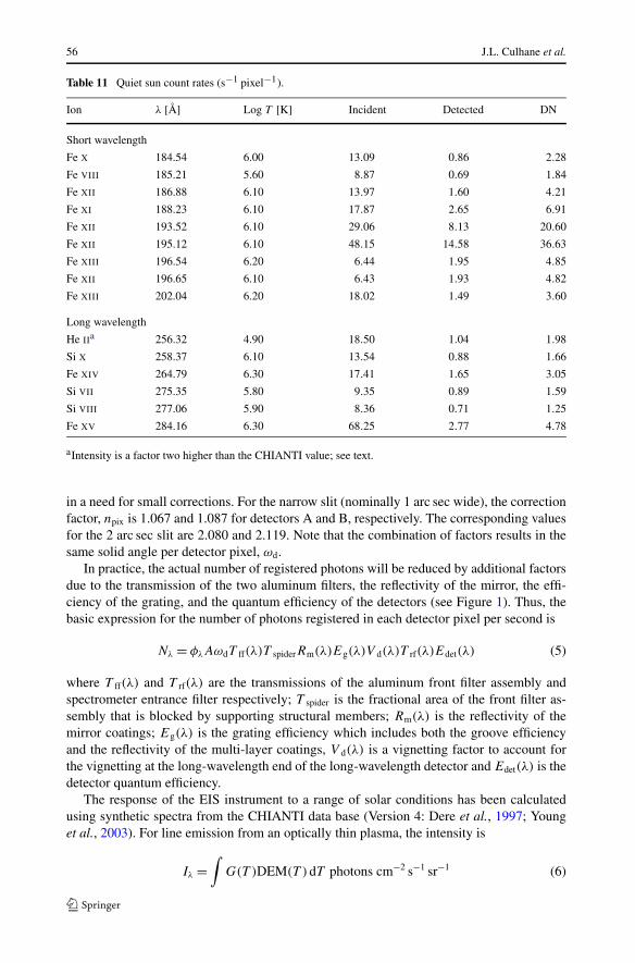
56 J.L. Culhane et al.
Table 11 Quiet sun count rates (s−1 pixel−1).
Ion λ [Å] Log T [K] Incident Detected DN
Short wavelength
Fe X 184.54 6.00 13.09 0.86 2.28
Fe VIII 185.21 5.60 8.87 0.69 1.84
Fe XII 186.88 6.10 13.97 1.60 4.21
Fe XI 188.23 6.10 17.87 2.65 6.91
Fe XII 193.52 6.10 29.06 8.13 20.60
Fe XII 195.12 6.10 48.15 14.58 36.63
Fe XIII 196.54 6.20 6.44 1.95 4.85
Fe XII 196.65 6.10 6.43 1.93 4.82
Fe XIII 202.04 6.20 18.02 1.49 3.60
Long wavelength
He IIa 256.32 4.90 18.50 1.04 1.98
Si X 258.37 6.10 13.54 0.88 1.66
Fe XIV 264.79 6.30 17.41 1.65 3.05
Si VII 275.35 5.80 9.35 0.89 1.59
Si VIII 277.06 5.90 8.36 0.71 1.25
Fe XV 284.16 6.30 68.25 2.77 4.78
aIntensity is a factor two higher than the CHIANTI value; see text.
in a need for small corrections. For the narrow slit (nominally 1 arc sec wide), the correctionfactor, npix is 1.067 and 1.087 for detectors A and B, respectively. The corresponding valuesfor the 2 arc sec slit are 2.080 and 2.119. Note that the combination of factors results in thesame solid angle per detector pixel, ωd.
In practice, the actual number of registered photons will be reduced by additional factorsdue to the transmission of the two aluminum filters, the reflectivity of the mirror, the effi-ciency of the grating, and the quantum efficiency of the detectors (see Figure 1). Thus, thebasic expression for the number of photons registered in each detector pixel per second is
Nλ = φλAωdT ff(λ)T spiderRm(λ)Eg(λ)V d(λ)T rf(λ)Edet(λ) (5)
where T ff(λ) and T rf(λ) are the transmissions of the aluminum front filter assembly andspectrometer entrance filter respectively; T spider is the fractional area of the front filter as-sembly that is blocked by supporting structural members; Rm(λ) is the reflectivity of themirror coatings; Eg(λ) is the grating efficiency which includes both the groove efficiencyand the reflectivity of the multi-layer coatings, V d(λ) is a vignetting factor to account forthe vignetting at the long-wavelength end of the long-wavelength detector and Edet(λ) is thedetector quantum efficiency.
The response of the EIS instrument to a range of solar conditions has been calculatedusing synthetic spectra from the CHIANTI data base (Version 4: Dere et al., 1997; Younget al., 2003). For line emission from an optically thin plasma, the intensity is
Iλ =∫
G(T )DEM(T )dT photons cm−2 s−1 sr−1 (6)
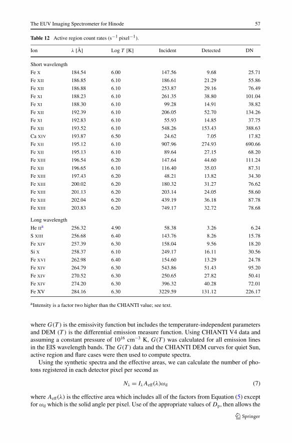
The EUV Imaging Spectrometer for Hinode 57
Table 12 Active region count rates (s−1 pixel−1).
Ion λ [Å] Log T [K] Incident Detected DN
Short wavelength
Fe X 184.54 6.00 147.56 9.68 25.71
Fe XII 186.85 6.10 186.61 21.29 55.86
Fe XII 186.88 6.10 253.87 29.16 76.49
Fe XI 188.23 6.10 261.35 38.80 101.04
Fe XI 188.30 6.10 99.28 14.91 38.82
Fe XII 192.39 6.10 206.05 52.70 134.26
Fe XI 192.83 6.10 55.93 14.85 37.75
Fe XII 193.52 6.10 548.26 153.43 388.63
Ca XIV 193.87 6.50 24.62 7.05 17.82
Fe XII 195.12 6.10 907.96 274.93 690.66
Fe XII 195.13 6.10 89.64 27.15 68.20
Fe XIII 196.54 6.20 147.64 44.60 111.24
Fe XII 196.65 6.10 116.40 35.03 87.31
Fe XIII 197.43 6.20 48.21 13.82 34.30
Fe XIII 200.02 6.20 180.32 31.27 76.62
Fe XIII 201.13 6.20 203.14 24.05 58.60
Fe XIII 202.04 6.20 439.19 36.18 87.78
Fe XIII 203.83 6.20 749.17 32.72 78.68
Long wavelength
He IIa 256.32 4.90 58.38 3.26 6.24
S XIII 256.68 6.40 143.76 8.26 15.78
Fe XIV 257.39 6.30 158.04 9.56 18.20
Si X 258.37 6.10 249.17 16.11 30.56
Fe XVI 262.98 6.40 154.60 13.29 24.78
Fe XIV 264.79 6.30 543.86 51.43 95.20
Fe XIV 270.52 6.30 250.65 27.82 50.41
Fe XIV 274.20 6.30 396.32 40.28 72.01
Fe XV 284.16 6.30 3229.59 131.12 226.17
aIntensity is a factor two higher than the CHIANTI value; see text.
where G(T ) is the emissivity function but includes the temperature-independent parametersand DEM (T ) is the differential emission measure function. Using CHIANTI V4 data andassuming a constant pressure of 1016 cm−3 K, G(T ) was calculated for all emission linesin the EIS wavelength bands. The G(T ) data and the CHIANTI DEM curves for quiet Sun,active region and flare cases were then used to compute spectra.
Using the synthetic spectra and the effective areas, we can calculate the number of pho-tons registered in each detector pixel per second as
Nλ = IλAeff(λ)ωd (7)
where Aeff(λ) is the effective area which includes all of the factors from Equation (5) exceptfor ωd which is the solid angle per pixel. Use of the appropriate values of Dp, then allows the
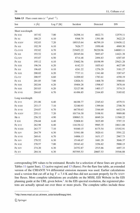
58 J.L. Culhane et al.
Table 13 Flare count rates (s−1 pixel−1).
Ion λ [Å] Log T [K] Incident Detected DN
Short wavelength
Fe XXI 187.92 7.00 34298.14 4822.71 12579.11
Fe XI 188.23 6.10 9368.79 1391.00 3622.25
Fe XXIV 192.03 7.20 189315.64 46799.19 119458.12
Fe XII 192.39 6.10 7626.77 1950.48 4969.30
Ca XVII 192.82 6.70 219452.22 58220.96 148003.11
Fe XII 193.52 6.10 20345.04 5693.67 14421.38
Ca XIV 193.87 6.50 8714.48 2494.83 6307.85
Fe XII 195.12 6.10 33682.56 10198.99 25621.28
Fe XIII 196.54 6.20 6142.33 1855.63 4627.89
Fe XII 196.65 6.10 4241.22 1276.29 3181.27
Fe XIII 200.02 6.20 7737.11 1341.60 3287.67
Ca XV 200.97 6.60 14209.02 1783.61 4350.19
Fe XX 201.05 7.00 12026.51 1468.70 3580.81
Fe XIII 202.04 6.20 19404.28 1598.67 3878.44
Fe XIII 203.83 6.20 32127.88 1403.17 3374.33
Fe XVII 204.65 6.70 61496.85 2164.85 5185.02
Long wavelength
Fe XVI 251.06 6.40 66188.77 2345.63 4579.51
Fe XXII 253.17 7.10 32180.93 1399.04 2708.70
Fe XVII 254.87 6.70 66730.63 3344.69 6432.54
Fe XXIV 255.11 7.20 101716.30 5198.91 9989.00
He II 256.32 4.90 108063.31 6049.24 11568.22
S XIII 256.68 6.40 52808.81 3035.89 5797.33
Fe XVI 262.98 6.40 116130.12 9985.35 18611.88
Fe XXIII 263.77 7.10 91040.15 8175.54 15192.91
Fe XIV 264.79 6.30 31941.00 3020.41 5591.22
Fe XVII 269.41 6.70 14806.13 1631.17 2967.73
Fe XIV 270.52 6.30 15148.67 1681.29 3046.37
Fe XXI 270.57 7.00 29343.42 3256.82 5900.15
Fe XIV 274.20 6.30 24752.87 2515.86 4497.33
Fe XV 284.16 6.30 507595.53 20607.53 35546.88
corresponding DN values to be estimated. Results for a selection of these lines are given inTables 11 (quiet Sun), 12 (active region) and 13 (flares). For the flare line table, an extendedversion of the CHIANTI V4 differential emission measure was used. Earlier calculationsused a version that cut off at log T = 7.4 K and thus did not account properly for Fe XXIV
line fluxes. More complete tabulations are available on the MSSL EIS Website in the EISplanning guide at the URL given below.1 At the EIS spectral resolution, the registered pho-tons are actually spread out over three or more pixels. The complete tables include those
1http://www.mssl.ucl.ac.uk/www_solar/solarB/espg.html.
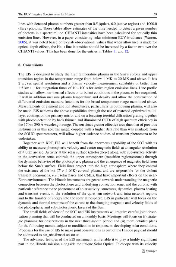
The EUV Imaging Spectrometer for Hinode 59
lines with detected photon numbers greater than 0.5 (quiet), 6.0 (active region) and 1000.0(flare) photons. These tables allow estimates of the time needed to detect a given numberof photons in a spectrum line. CHIANTI intensities have been calculated for optically thinemission lines. However, in a paper considering solar minimum EUV irradiance (Warren,2005), it was noted based on Skylab observational values that when allowance is made foroptical depth effects, the He II line intensities should be increased by a factor two over theCHIANTI values. This has been done for the entries in Tables 11 and 12.
8. Conclusions
The EIS is designed to study the high temperature plasma in the Sun’s corona and uppertransition region in the temperature range from below 1 MK to 20 MK and above. It has2 arc sec spatial resolution and a plasma velocity measurement capability of better than±5 km s−1 for integration times of 10 – 100 s for active region emission lines. Line profilestudies will allow non-thermal effects or turbulent conditions in the plasma to be recognized.It will in addition measure plasma temperature and density and allow the construction ofdifferential emission measure functions for the broad temperature range mentioned above.Measurements of element and ion abundances, particularly in outflowing plasma, will alsobe made. EIS achieves the above capabilities through the use of matched optimized multi-layer coatings on the primary mirror and on a focusing toroidal diffraction grating togetherwith photon detection by back thinned and illuminated CCDs of high quantum efficiency inthe 170 to 290 Å wavelength range. The ten times greater effective area than that of previousinstruments in this spectral range, coupled with a higher data rate than was available fromthe SOHO spectrometers, will allow higher cadence studies of transient phenomena to beundertaken.
Together with XRT, EIS will benefit from the enormous capability of the SOT with itsability to measure photospheric velocity and vector magnetic fields at an angular resolutionof ≈0.25 arc sec. Activity at the solar surface (photosphere) along with sub-surface activityin the convection zone, controls the upper atmosphere (transition region/corona) throughthe dynamic behavior of the photospheric plasma and the emergence of magnetic field frombelow the Sun’s surface. Field lines project into the high atmosphere where they controlthe existence of the hot (T > 1 MK) coronal plasma and are responsible for the violenttransient phenomena, e.g., solar flares and CMEs, that have important effects on the near-Earth environment. The Hinode instruments are geared towards understanding the magneticconnection between the photosphere and underlying convection zone, and the corona, withparticular reference to the phenomena of solar activity: structures, dynamics, plasma heatingand transient events, to the evolution of the quiet sun network and intra-network regionsand to the transfer of energy into the solar atmosphere. EIS in particular will focus on thedynamic and thermal response of the corona to the changing magnetic and velocity fields ofthe photospheric and sub-photospheric layers of the Sun.
The small fields of view of the SOT and EIS instruments will require careful joint obser-vation planning that will be conducted on a monthly basis. Meetings will focus on (i) strate-gic planning for observations in the next three-month period and (ii) more detailed plansfor the following month, subject to modification in response to developing solar conditions.Proposals for the use of EIS to make joint observations as part of the Hinode payload shouldbe addressed to [email protected].
The advanced features of the EIS instrument will enable it to play a highly significantpart in the Hinode mission alongside the unique Solar Optical Telescope with its velocity
60 J.L. Culhane et al.
and magnetic field observing capability together with the full-Sun context view provided athigh time cadence by the high resolution X-ray telescope.
Acknowledgements Hinode is a Japanese mission constructed and launched by JAXA/ISAS, collaborat-ing with NAOJ as a domestic partner, NASA (USA) and PPARC (UK) as international partners. Scientificoperation of the Hinode mission is conducted by the Hinode science team organized at ISAS/JAXA. Thisteam mainly consists of scientists from institutes in the partner countries. Support for the EIS constructionand post-launch operation program is provided by PPARC (UK), NASA (USA), the Ministry of Educationand Culture (Japan), the European Space Agency and the Norwegian Space Centre.
We would like to thank Sue Horne and Rosemary Young for their management of the PPARC funding.Among the MSSL staff, the contributions of Alec McCalden and Chris McFee are gratefully acknowledged.Work at the Naval Research Laboratory and Goddard Space Flight Center was supported by the NASA Mar-shall Space Flight Center (MSFC). In particular, we would like to thank MSFC’s Hinode Program Manager,Larry Hill, for his support and guidance during the development, testing and integration of the EIS instru-ment. The authors wish to acknowledge the staff of JAXA/ISAS and NAOJ, along with the engineers of thecompanies involved in this project. Among them are K. Minesugi for mechanical design; A. Onishi and K.Hiraide for thermal design; M. Noguchi and M. Nakagiri for EIS testing at ISAS. We are particularly gratefulto Bo Andersen of the Norwegian Space Centre for his efforts both on behalf of EIS and of the Hinode mis-sion. JLC thanks the Leverhulme Foundation for the award of an Emeritus Fellowship. Finally we would liketo acknowledge the substantial effort by the teams at MSSL, NRL, RAL, Birmingham, NAOJ, ISAS/JAXAand the University of Oslo who made the EIS instrument a reality.
References
Antiochos, S., DeVore, C.R., Klimchuk, J.: 1999, Astrophys. J. 510, 485.Beutler, H.G.: 1945, J. Opt. Soc. Am. 35, 311.Born, M., Wolf, E.: 1964, Principles of Optics, 2nd edn., MacMillan, New York, p. 469.Canali, C., Martini, M., Ottavani, G., Alberigi Quaranta, A.: 1972, IEEE Trans. Nucl. Sci. NS-19.Culhane, J.L., et al.: 1991, Solar Phys. 136, 89.Danzmann, K., Günther, M., Fischer, J., Kock, M., Kühne, M.: 1988, Appl. Opt. 27, 4947.Dere, K.P., Landi, E., Mason, H.E., Monsignori Fossi, B.C., Young, P.R.: 1997, Astron. Astrophys. Suppl.
125, 149.Engström, L.: 1998, GFit Version 10.0. Lund Reports on Atomic Physics, LRAP-232, LTH, Lund. http://
kurslab-atom.fysik.lth.se/Lars/Gfit/html/index.html.Finley, D.S., Bowyer, C.S., Paresce, F., Malina, R.F.: 1979, Appl. Opt. 18, 649.Haber, H.J.: 1950, J. Opt. Soc. Am. 40, 153.Hara, H.: 2003, FM XRT-S Calibration, National Astronomical Observatory of Japan.Harra, L.K., Sterling, A.: 2003, Astrophys. J. 587, 429.Harra, L.K., Gallagher, P.T., Phillips, K.J.H.: 2000, Astron. Astrophys. 362, 371.Harra, L.K., Mandrini, C.H., Matthews, S.A.: 2004, Solar Phys. 223, 57.Harrison, R.A.: 1997, Solar Phys. 175, 467.Harrison, R.A., et al.: 1995, Solar Phys. 162, 233.Hollandt, J.: 1994, Strahlungsnormale für die solare Spektroradiometrie im Vakuum-UV, Ph.D. dissertation,
Technischen Universität, Berlin.Hollandt, J., Kühne, M., Huber, M.C.E., Wende, B.: 2002, In: Pauluhn, A., Huber, M.C.E., von Steiger, R.
(eds.) The Radiometric Calibration of SOHO, International Space Science Institute Report SR-002, ESA,Nordwijk, p. 51.
Innes, D.E., Inhester, B., Axford, W.I., Willhelm, K.: 1997, Nature 386, 811.Kelly, R.L.: 1987, J. Chem. Phys. Ref. Data 16 (Suppl. No. 1).Klimchuk, J.A.: 2006, Solar Phys. 234, 41.Korendyke, C.M., et al.: 2006, Appl. Opt. 45, 8674.Kowalski, M.P., et al.: 1999, Appl. Opt. 38, 6487.Kramida, A.E., Brown, C.M., Feldman, U., Reader, J.: 2006, Phys. Scr. 74, 156.Lang, J., Kent, B.J., Seely, J.F.: 2002, In: Pauluhn, A., Huber, M.C.E., von Steiger, R. (eds.) The Radiometric
Calibration of SOHO, International Space Science Institute Report SR-002, ESA, Nordwijk, p. 337.Lang, J., et al.: 2000, J. Opt. A: Pure Appl. Opt. 2, 88.Lang, J., et al.: 2006, Appl. Opt. 45, 8689.Madjarska, M.S., Doyle, J.G., van Driel-Gesztelyi, L.: 2004, Astrophys. J. 603, L57.

The EUV Imaging Spectrometer for Hinode 61
Masuda, S., Kosugi, T., Hara, H., Tsuneta, S., Ogawara, Y.: 1994, Nature 371, 495.Nakariakov, V.M., Ofman, L.: 2001, Astron. Astrophys. 372, L53.NIST Atomic Spectral Data Base: 2005, http://physics.nist.gov/cgi-bin/asd.Pevtsov, A.A.: 2000, Astrophys. J. 531, 553.Powell, F.: 1992, In: Bennett, H.E., Chase, L.L., Guenther, A.H., Newman, B., Soileau, M.J. (eds.) Laser-
Induced Damage in Optical Materials, Proc. SPIE 1848, 503.Sakao, T., et al.: 2004, In: Mather, J.C. (ed.) Optical, Infrared, and Millimeter Space Telescopes, Proc. SPIE
5487, 1189.Samson, J.A.R.: 1967, Vacuum Ultraviolet Spectroscopy Techniques, Wiley, New York, p. 315.Scholze, F., Henneken, H., Kuschnerus, P., Rabus, H., Richter, M., Ulm, G.: 2000, Nucl. Instrum. Methods
39, 208.Schumacher, R.J., Hunter, W.R.: 1977, Appl. Opt. 16, 904.Seely, J.F., Brown, C.M., Windt, D.L., Donguy, S., Kjonrattanawanich, B.: 2004, Appl. Opt. 43, 1463.Stern, R.A., et al.: 2004, In: Fineschi, S., Gummin, M.A. (eds.) Telescopes and Instrumentation for Solar
Astrophysics, Proc. SPIE 5171, 77.Sze, S.M.: 1981, Physics of Semiconductor Devices, 2nd edn., Wiley, New York, p. 754.Tsuneta, S.: 1995, Publ. Astron. Soc. Japan 47, 691.Tsuneta, S.: 1996, Astrophys. J. 456, L63.Ulm, G. Wende, B.: 1997, In: Haase, A., Landwehr, G., Umbach, E. (eds.) Röntgen Centennial, World Sci-
entific, Singapore, p. 81.Wang, T.J., Solanki, S.K., Curdt, W., Innes, D.E., Dammasch, I.E.: 2002, Astrophys. J. 574, L101.Wang, T.J., Solanki, S.K., Curdt, W., Innes, D.E., Dammasch, I.E., Kliem, B.: 2003, Astron. Astrophys. 402,
L17.Warren, H.: 2005, Astrophys. J. Suppl. 157, 147.Warren, H., Doschek, G.A.: 2005, Astrophys. J. 618, L157.Williams, D.R., et al.: 2002, Mon. Not. Roy. Astron. Soc. 336, 747.Williams, D.R., Török, T., Démoulin, P., van Driel-Gesztelyi, L., Kliem, B.: 2005, Astrophys. J. 628, L163.Yokoyama, T., Akita, K., Morimoto, T., Inoue, K., Newmark, J.: 2001, Astrophys. J. 546, L69.Young, P.R., Del Zanna, G., Landi, E., Dere, K.P., Mason, H.E., Landini, M.: 2003, Astrophys. J. Suppl. 144,
135.