•

THE ERROR~IN~VARIABLES PROBLEM IN THE LOGISTIC REGRESSION MODEL

by

Rhonda Robinson Clark

Department of·RiostatisticsUniversity of North Carolina at Chapel Hill

Ins·titute of Statistics Mimeo Series No. 1407

July 1982

--

THE ERROR-IN-VARIABLES PROBLEM

IN THE LOGISTIC REGRESSION MODEL

by

. Rhonda Robinson Clark

A Dissertation submitted to the faculty of the University ofNorth Carolina at Chapel Hill in partial fulfillment of therequirements for the degree of Doctor of PhilosophY in theDepartment of Biostatistics.

Chapel Hill

JULY 1982

ii

ABSTRACT

RHONDA ROBINSON CLARK. The Error-in-Variables Problem in theLogistic Regression Model. (Under the direction of ClarenceE. Davis.)

It is well known that when the independent variable in simple

linear regression is measured with error that least squaresesti­

mates are not unbiased. This is also true for logistic regression

and the magnitude of the bias is demonstrated through simulation

studies.

Estimators are presented as possible solutions to the 'error­

in-variables' problem; that is, the problem of obtaining consistent

estimators of model parameters when measurement error is present in

the independent variable. Two solutions require an external esti­

mate of the variance of the measurement error, two require multiple

measures on the independent variable, while two others are exten­

sions of the method of grouping, and the instrumental variable ap­

proach. Simulation studies show that the use of an external esti-

mate of the error variance or multiple measures on the independent

variable leads to estimators with substantially lower mean square

error than the least squares estimate. For the grouping and instru­

mental variable approaches, the proposed estimators have lower mean

square error under some but not all conditions.

The methods discussed are applied to data from the Lipid

Research Clinics Program Prevalence Study.

ACKNOWLEDGEMENTS

I wish to thank the chairman of my Doctoral Committee,

Dr. Clarence E. Davis, for his guidance, encouragement, and

never-ending optimism. Without his support this work could

not have been completed. I am also grateful to Drs. G. Koch,

M. Symons, J. Hosking, and G. Heiss for their suggestions and

participation on the committee.

I would also like to take this opportunity to thank my

friends and family for their love and support throughout my

years in this program.

Finally, I would like to thank Ms. Ernestine Bland for

the excellent and speedy job that she performed in typing the

manuscript.

i. i i

iv

TABLE OF CONTENTS

CHAPTER PAGE

I INTRODUCTION AND REVIEW OF THE LITERATURE............. 1

1.1 The Error-in-Variabl es Problem in LinearRegression;...... . .. ... . .. . .. ... .. . . .. .... . .. .. . . .. 31•1•1 In:troduct ;on . . . . .. . . . . . . . . . . . . . . . . . . . . . . . . 31.1. 2 Classical Approaches to the Error-in-

Variables Problem · 51.1.3 Alternatives to the Classical Approaches .. 8

1.1.3.1 The Method of Grouping ...•.•..... 81.1.3.2 The Use of Instrumental

Varia'b1e-s ••••••••••• _. • • • • • • • • •• 101.1.3.3 Replication of Observations .•.... 11

1.2 The Use of the Logistic Regression Model inEpidemiologic Research ...•....................... 151. 2. 1 Int roduc t 1on .- . • . . . • . . . . . . . . . • . . . . . .. 151.2.2 Discriminant Function Approach•.•......... 161.2.3 Weighted Least Squares/Maximum

Li kel i hood Approach....... .... . . . . .. .. . .. 171.2.4 Comparison of the Approaches ..•.•...•..... 20

1.3 Outl ineof the Research 21

11. DESCRIPTION OF THE BIAS DUE TO MEASUREMENT ERROR...... 23

2.1 A Review of the Simple Linear and MultipleLinear Regression Cases .•......••••.......•.....• 242.1.1 Simple Linear Regression Case ........•.... 242.1.2 Multiple Linear Regression Case 25

2.2 Mathematical Descriptions of the Bias Underthe Logistic Regression Model ......•............. 28

2.3 Description of the Bias Under the LogisticRegression Model Using Simulation 302.3.1 Description of the Simulation

Pr-ocedure. . . . . . . . . . . . . . . . . . .. . . . . . . . . . . .. 312.3.2 Simple Logistic Regression Case ..•........ 332.3.3 Multiple Logistic Regression Case.•....... 342.3.4 Summary:of Results 35

CHAPTER

III ALTERNATIVE ESTIMATES OF S WHEN MEASUREMENTERROR IS PRESENT IN THE SIMPLE LOGISTIC RE-

v

PAGE

GRESS ION MODEL........................................ 37

3.1 Modified Discriminant Function Estimator •..••.•.. 37

3.2 An Estimator Based on the Method of Grouping ..... 383.2. 1 The Method........... . . . . . ... . . . . . . . . . . . . .. 393.2.2 Rationale Behind the Method .......•....... 40

3.3 Use of an Instrumental Variable to Estimate S.••• 433.3.1 Iterative Instrumental Variable

Estimator 433.3.2 Two-Stage Least Squares Estimator 47

3.4 Another Two-Stage Estimator of B••••••••••••••••• 49

3.5 Comparison of the Alternative Estimators 51

IV USE OF MULTIPLE MEASUREMENTS IN THE ESTIMATIONOF 13 ......•...••....•.•........_.......•.•....•........ 57

4.1 The Mean of mIndependent Measurements as ethe Independent Variabl e 57

4.2 Further Reduction of the Bias When m isSmall -. 59

4.3 Use of the James-Stein Estimator of Ui asthe Independent Va ri ab1e.. . . . . . . . . . . . . . .. . .. •.... 61

4.4 Estimation of 0 2 When mMeasurements aretaken on a SUbsampl e 63

4.5' Results of Simulation Study 63

V APPLICATION OF METHODS TO THE LIPID RESEARCHCLINICS DATA .........................•..... It •••••••••• 67

5.1 Description of the Data Set 67

5.2 Computation of the Estimates and TheirVariances - 68

5.3 Comparison of the Estimates 74

5.4 Conclusions ; 77

vi

CHAPTER PAGE

VI SUMMARY AND SUGGESTIONS FOR FURTHER RESEARCH •••••••••• 84

5.2

vi i

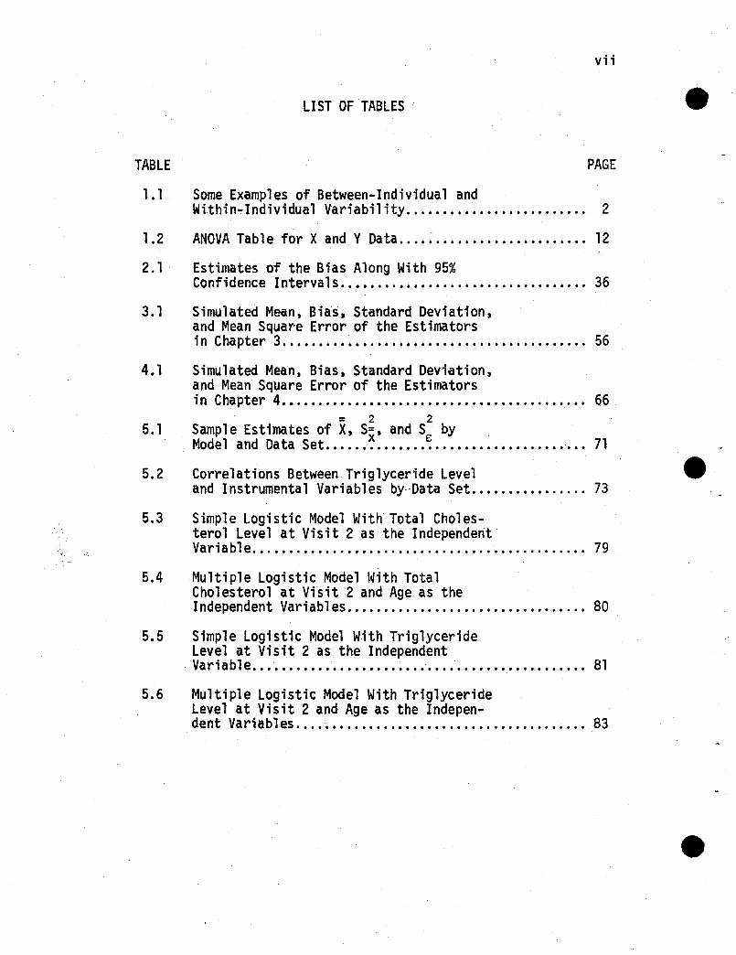
LIST OF TABLES

TABLE PAGE

1.1 Some Examples of Between-Individual andWithin,,:,Individual Variability ...........•..........•.. 2

1.2 ANOVA Table for Xand Y Data 12

2.1 Estimates of the Bias Along With 95%Confidence Interva"l s. . . . . . . . . . . . . . . . . . . . . . . . . . . . . . . . .. 36

3.1 Simulated Mean, Bias, Standard Deviation,and Mean Square Error of the Estimatorsin, Chapter 3 56

4.1 Simulated Mean, Bias, Standard Deviation,and Mean Square Error of the Estimatorsin Chapter 4...................•...................... 66

2 25.1 Sample Estimates of X, Sx' and SE by

Model and DataSet....................•.........•.."... 71

Correlations Between Triglyceride Leveland Instrumental Variables by~~Data Set .•.............. 73

5.3 Simple Logistic Model With Total Choles­terol Level at Visit 2 as the IndependentVar ; ab1e••••••••••••••••••••••••••••• '. • • • • • • • • • • • • • • •• 7·9

5.4 Multiple Logistic Model With TotalCholesterol at Visit 2 and Age as theIndependent Variabl es 80

5.5 Simple Logistic Model With TriglycerideLevel at Visit 2 as the Independent

. Variable • .••••••••••••••••••••••-.•.•••••••.••••.••..••• 81

5.6 Multiple Logistic Model With TriglycerideLevel at Visit 2 and Age as the Indepen-dent Variables '. . . . . . . . .83

CHAPTER r

INTRODUCTION AND REVIEW OF THE LITERATURE

Epidemiologic data collected from prospective studies are often

used to model the incidence of disease as a·function of one or more

independent variables. A commonly employed statistical procedure

for such studies is multiple logistic regression. For example, in a

prospective study of coronary heart disease in Framingham (Truett,

Cornfield and Kannel (1967», the variation in the incidence of

disease as a function of serum cholesterol, systolic blood pressure,

age, relative weight, hemoglobin, cigarettes/day, and ECG measured

on the initial examination was investigated. The probability, P,

of developing the disease during the 12-year time interval was esti­

mated for each individual using the logistic regression model:

In the standard linear regression problem one assumes that the

independent variable is measured without error and that the values

of the dependent variable deviate from their true values only by a

random error component representing explanatory variables excluded

from the model or sampling error. Under these assumptions the

ordinary least squares (OLS) estimates of the parameters are

2

unbiased with minimum variance. Violation of these assumptions in

the linear regression model leads to an underestimate of the ex­

pected magnitude of the regression coefficients (Snedecor and

Cochran (1967)).

It is well known from epidemiologic 1iterature that variables

such as systolic blood pressure and serum cholesterol level are

subject to possible "errors" or variation in measurement. Two recog­

nized sources of this variation are within-individual variability

and observer (interviewer, laboratory) error. Gardner and Heady

(1973) give the following examples of within-individual variability

o~ and between-individual variability o~:

TABLE 1.1 Some Examples of Between-Individual and Within­Individual Variability

Variabl e Mean ~ ~

Cholesterol (mg %) 215 25 40

Blood Pressure (mmHg) 141 9. 1 13.6

Calories (per day) 2846 370 406

Often these errors are combined with sampling error and forgotten.

The purpose of this research is to study the effect of measurement

error on the estimated logistic regression model coefficients and

to propose methods of producing consistent estimates of these regres­

sion coefficients when error in the independent variable is present.

3

1.1 The Error-in-Variables Problem in Linear Regression

1.1.1 Introduction

There are several possible situations out of which the finite

set of independent pairs of observations (Xl'Yl ), (XZ,YZ)' ...

(Xn,Yn) might arise. In each of the situations that will be dis­

cussed, there is a corresponding set of true values that will be

denoted as (Ul ' Vl ), (UZ' VZ), ••. (Un' Vn) . In the regress ion

situation the following linear relationship between the true vari-

ables Uand V holds:

V= ex + I3U + t

E(V IU) = ex + I3U

where V is a random variable, Umay be fixed or random, and t has

mean 0 and variance at. In the particular' case where Uand Vare

bivariate normal, this is the correlation model andE{UIV) =y + oV.

If V and Uare linearly related as follows:

V= ex + I3U

and if both Vand Uare fixed, the relationship between thevari­

ables is called functional. If the above relationship holds, but

Vand Uare random variables, we have a structural relationship

between Vand U. If we fail to observe the true variables Uand

V in any of the above situations, and instead observe X =U + E

and Y = V+ n, we have what is known as the error-in-variables

problem or measurement error. For the remainder of this study we

shall concern ourselves with the error-in-variables problem when

4

the relationship between the true unobserved variables is structural.

Suppose that only V is subject to error, then V=ex + au be-

comes

v - n =a + eu

v =a + eu + n

where E(n) =0, n has variance 0 2 and is independent of U. Thus then .relationship between the observed values is a regression type rela-

tionship with

E(V\U) = a + eu

The ordinary least squares COLS) estimators are, in this case, both

consistent and unbiased.

If V is not subject to error, but U is, then

V = a + e(X - E)

x = -ala + 1Ie V + E

= a* + (3* V + E

E(XIV) =a* + e*V

where E{E) = 0, Ehas variance 0 2 and is independent of V.Again,E

we have a regression type relation with the OLS estimators being

consistent estimators of a and S. (S = 1/S*, ~ = -~*/~*).

If both Uand Vare subject to error the problem becomes com­

plicated. The relationship between the observed variables is

v = a + eX + n - eE.

The error term is now n - (3E and is no longer independent of X

since X =U + ~ The OLS technique in this situation leads to

..

..

5

biased and inconsistent estimates of the regression parameters.

That is, if b is the OLS estimator of S, then

where cr~ is the variance of U.

In another model proposed by Berkson (1950), observations are

made on V for a given X. Here again X= U+ E and Y = V+ n. We

are no longer trying to observe a given U, but for each fixed X

there are a number of U·s which could have given rise to that par­

ticular observed X. Also for each U there is a probability that

the observed fixed X is an observation on that Uwith error E. The

U·s are now random variables distributed about the fixed Xwith

error E. Now E is independent of X (but not of U), and

Y= a + eX + n - SE

E(Y IX) = a + (3X

where X is fixed, and we again have a situation in which the OLS

estimator of S is unbiased and consistent.

1.1.2 Classical Approaches to the Error-in-Variables Problem

A number of approaches have been proposed for dealing with the

error-in-variables problem under the structural model. We will

begin with the classical approaches discussed by Moran (1971) and

Madansky (1959).

Let the relationship between the unobserved true variables be

6

V. =a + (3U.1 1

1. ni and Ei are normally and independently distributed with

means equal to 0 and variances O"~ and O'~ respectively,

2. Ui is normally distributed with mean l.l and variance O"~,

3. Ui , ni and Ei are mutually independent,

the observed variables X and Yare jointly distributed in a bivariate

normal distribution with parameters lJ, 0u2 , 0 2 , 0 2 , Ct and (3, where.E n

•

E(X) =l.l

Var(X)

E(Y) =a + BJ.l

Var(Y) = (32 0 2 + 02U n

CoV(X,Y) = f3 0 2U

(1.1.2.1)

The following quantities are jointly sufficient for the equations

in (1.1.2.1):

nX = !

i=lv = f Yi

i=l n

n (y._y)2Sy.y = I 1n

i=l

(1.1.2~2)•

The maximum likelihood equations are derived by setting the quanti­

ties in (.1.1.2.1) equal to those in (1.1.2.2) if we can assume that

the latter five quantities are functionally independent.

7

The fact that we have five equations and six unknowns makes

the parameters O'~, O'~, O'~, a, and f3 unidentifiable. In order to

avoid this problem we need to change some of our assumptions or

obtain additional information. In particular, if we knew O'~, O'~,

or O'~/O'~ and were sure that cov( E,n) = 0, we coul d estimate Band

subsequentlya. Both Moran (1971) and Madansky (1959) give the

following estimates of B when additional information is available.

1. 0'2 known:n

Syy - 0 2A n(31 =

Sxy

2. 0 2 known:E

4. When both O'~ and O'~ are known, we are confronted with an

over-identification situation. We now have four parameters

and five equations. As a result we arrive at inconsisten­

cies. That is

8

are both derived from the same system of equations. In

large samples these two estimates will become asymptoti­

cally equivalent. Because of the inconsistencies s a

maximum 1i kelihood sol ution cannot be arrived at by

equating (1.1.2.1) to (1.1.2.2). Kiefer (1964) points

out that under these circumstances the proper procedure

is to write out the likelihood and maximize it with respect

to the four unknown parameters as as ~s and cr~. Barnett

(1967) gives the resu1 ting equations.

5. The previous four estimators are derived upon the assump­

tion that cOv(Esn) = O. If cov(Esn) ; Os then cov(xsY) =cOv(Esn) + acr~. Therefore if both cr~ and o~ are known and ~

we assume that COV(Esn) is not equal to Os we have five

unknowns and five equations. The estimate of a is

= sign[J xiYi,=1

1.1.3 Alternatives to the Classical Approaches

1.1.3.1 The Method of Grouping

Several methods of solving the error-in-variables problem when

no additional information about variances is available have been

proposed. These methods do not require any distributional assumptions.

9

One such method is known as the method of grouping. The method con­

sists of ordering the observed pairs (Xi,V i ), selecting proportions

Pl and P2 such that Pl + P2 <= 1. placing the first nPl pairs in

groupGl , and the last nP2 pairs in another group G3, and discarding

G2, the middle group of observations (if Pl + P2 < 1).

" . V, - V3 b2e = =-6 Xl - X3 b,

Wald (1940) states that 66 is a consistent estimate of (3 if:

1. the grouping is independent of the errors E:i and ni;

2. as n ~ co. b, does not approach 0, namely lim inf!Xl-Xjl > o.J'I-HO

In order to determine when conditions (l) and (2) are satisfied we

consider several possible procedures for assigning observations to

the groups. It is obvious that if the observations are assigned

to the groups randomly, condition (1) would be satisfied but not

condition (2) since then

If the magnitude of the Ui's were known, it would be possible

to rank the observations by their corresponding magnitude of Ui •

This grouping procedure would satisfy both conditions. However, it

is unlikely that infonnation on the magnitude of the Ui's would be

available without the actual values. Another possibility is to

order the observations (Xi,V i ) by the magnitude of the observed Xi 's.

This procedure will not guarantee consistency since the ordering

may be dependent on the error .. Neyman and Scott (1951) give the

10

following necessary and sufficient condition for the cons.istency of

S6 when the observations are grouped according to the magnitude of

the observed Xi's:

S6 is a consistent estimate ofa if and only

if the range of U has 'gaps' of 'sufficient

length' at 'appropriate places' (determined

by P1 and P2) where U has probability zero

of occurring.

This condition guarantees that, as n -+ 00, the misgrouped observa-A

tions with respect to Udo not contribute to plim a6 tending away~

from S.

1.1.3.2 The Use of Instrumental Variables

Asecond method of obtaining consistent estimates of a involves

the use of instrumental variables. Suppose that in addition to

having observations on the variables Xi and Vi' we also observe

another variable Zi which is known to be correlated with Ui and Vi'

but is independent of Ei and ni' Then

~ (Z.-Z)(V.-Y)A i=l' ,f37 = """--n"--------

L (Z.-Z)(X.-'X)i=l' ,

nis a consistent estimate of f3 provided I (.z.-Z)(X.-X) does noti=l . , ,approach zero and n -+ co (i.e., cov(Z,X) r} 0). It should be noted

that the effectiveness of this method depends on one's ability to

find a variable which is independent of the error and correlated

11

with Uand on the strength of that correlation. Letting Zi take

the values -1. O. 1 depending on i. where i is independent of the

'" '"error. reduces f3] to f36. Also Durbin (1954) suggests that Zi = i

is a better instrumental variable if the rank order of the X; 's is

the same as the tank order of the Ui's. That is. it leads to a

more efficient estimate than the method of grouping.

1.1.3.3 Replication of Observations

We have seen that in the classical case we can estimate f3

when we know 0 2 • 0 2 • or 0 2/02 • This naturally leads to the consid-E nnEeration of the estimation of e when we can estimate one or more of

these quantities. This is possible if for each (.UpVi ) there is

more than one corresponding. value of (X p Vi).

Assume that we have n pairs of values (Ui,Vi ) and Ni observa­

tions on each pa ir. That is

V•• = V. + n· .lJ 1 lJ .

j = 1.2•••••Ni

; = 1.2••.••n

If the usual assumptions of independence are made. a one-way

analysis of variance can be carried out on the XiS and V's and an

estimate of f3 computed. Madansky describes the procedure by using

the following ANOVA table ..

TABLE 1.2 ANOVA Table for Xand Y Data

Source

I

BETWEEN SETS{ II

tIll

IV

Mean Square

nLN. (x .• -x )2;=1 1 1 ••.

n-1

n (- - ) - -N. x. -x . - .L ' 1· •• (y,. y•• );=1 n-1

n N (- - 2\' ,. y. -y )L 1· '• •;=1 n-1

n N; - 2L ~ (x;j-X;'>

;=1 j=l N-n

Expected Mean Square

n0 2 + [(N2 - L N~)/N(n-1)] a~

e: ;=1

n .cov(e:,n) + [(N2 - L. N~)/N(n-1)] B 0 2

;=1 u

n0 2 + [(N2 - L N~)/N(n-1)] B2 0 2n ;=1 ' u

0 2e:

WITHIN "SETS

e

V

VI

N.n 1 ( -)( -\' \' X'.J.-X1· y .. -y. )l. l • 'J , •

i=l j=l N-n

N.n 1 ( .- 2\' \' y .. -y. )l. L. 'J' .

;=1 j=l N-n

e

cov(£,n)

0 2n

e

..J

N

13

whereNi N;

x. = 2 xij/Ni Y;. =j~l

y . ./N.1· j=l 1J 1

n Ni n Nix = .L j~l x. ·/N y•• == .L j~l yij/N•• 1=1 1J 1=1

nN = r N•

. 1 11=

Tukey (1951) proposes the following estimates of 13:

A

(II -V)/(I -IV)138 =

A

(III-VI)/(II-V)139 =

A

13'0 = I( III -vI}/(I -IV)

It is easily seen that these estimates converge to S as n ~ 00 and

N. ~ 00 for some i.1

Housner and Brennan (1948) also give an estimate of S when there

are multiple measurements on Uand V. They consider the expression

y. '-Yk ob - _l.;..'llJ~-:;,("._

ij kl - xij-Xkl

Y1" =() + ax.. + T).. - f3 t· .J 1J lJ 1Jthen

(x . .-x"o) b. '1,0 = 13(x . .-x"o) + (n· ·-n"o) - S( e;•• -e:.,,). 1J ~ 1J~ 1J ~lJ ~ 1J ~

so that

14

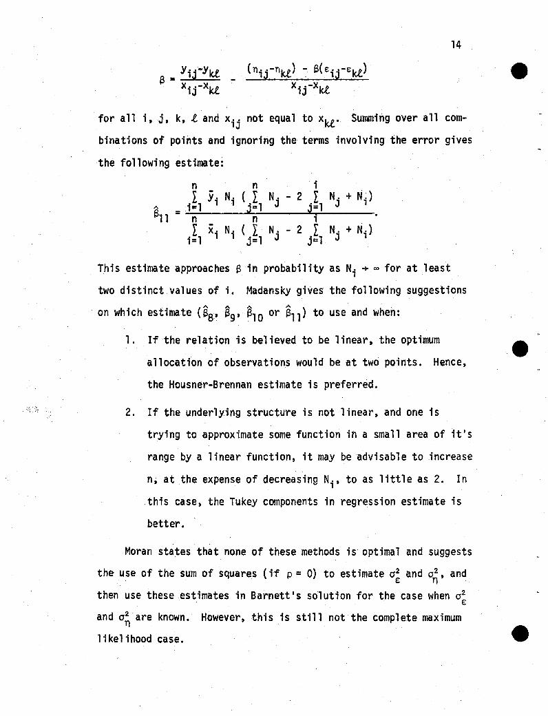
for all i, j, k,.e. and xij not equal to xkl . Summing over all com­

binations of points and ignoring the terms involving the error gives

the following estimate:

n n i

1.=L

1Yi Ni ( L N. - 2 L N. + N.)

J'=l J j=l J 1=~~__....l_~ ~-'-- _

n n iI ii Ni ( L N. - 2 L N. + Ni )

i=l j=l J j=l J

This estimate approaches ain probability as Ni ~ ~ for at least

two distinct values of i. Madansky gives the following suggestionsA A A A

on which estimate (SS-' 139,1310 or all) to use and when:

1. If the relation is believed to be linear, the optimum

allocation of observations would be at two points. Hence,

the Housner-Brennan estimate is preferred.

2. If the underlying structure is not linear, and one is

trying to approximate some function in a small area of it's

range by a linear function, it may be advisable to increase

n, at the expense of decreasing Ni' to as little as 2. In

this case, the Tukey components in regression estimate is

better.

Moran states that none of these methods is optimal and suggests

the use of the sum of squares (if p = 0) to estimate a2 and 0 2 , and. E n

then use these estimates in Barnett's solution for the case when a~

and a~ are known. However, this is still not the complete maximum

likelihood case.

15

Many of the ideas and results discussed above in reference to

the error-in-variab1es problem with one independent variable extend

to the multivariate situation. A brief discussion is given by

Moran (1971).

1.2 Use of the Logistic Regression Model in Epidemiologic Research

1.2.1 Introduction

One of the most often used indicators of disease frequency in

epidemiology is the incidence rate. Theoretically this rate esti­

mates the probability of disease or death for a particUlar population

over a fixed time period. It is possible to model this probability

as a fUnction of one or more independent variables. The logistic

function is a commonly used model for this purpose. Although this

study mainly involves the univariate logistic function,we note here

that it is in the multivariate case that this function is most often

used. This is because most chronic diseases are effected by multiple

factors simultaneously.

There are two methods used to estimate a and ~ in the logistic

regression model

1Vi =------- + n··

1 + e - ea + au i ) 1

One proposed by Truett, Cornfield and Kannel (1967) uses a linear

discriminant analysis approach. The other method, proposed by Walker

and Duncan (1967), uses an iterative procedure to obtain maximum

likelihood estimates of the parameters.

16

1.2.2 Discriminant Function Approach

Assume that we follow N individuals over a fixed time period.

Also assume that this sample is derived from two populations: 0

(those who would develop the disease), and NO (those who would not

develop the disease). The respective sample sizes being n, and nO'

Suppose also that there exists a variable U having a normal distri­

bution with mean ~1 in the diseased population and mean ~O in the

non-diseased population. Finally, we assume that the variance of U

is the same in each population.

Let

P{DIU)

P{NDI U)

P{D) = P

= probability of disease for an individual charac­terized by U.

= probability of not having the disease given U.

= unconditional probability of disease.

P{ND) = 1-p = unconditional probability of not having the disease.

fO{U)=P{UIND)= probability of Ugiven the individual does not. have the disease. .

f,(U)=P(U!D) = probability of Ugiven the individual does havethe disease.

From Bayes' Theorem:

In partic~lar, if the distribution of fO(U)· and f1{U) are univariate

normals with means ~1 and ~O respectively, and with the same vari­

ance a~, then

P{Dlu) = 11 + e -(et + aU)

17

where CI. = - log 1pP - 20J (lll-llO)(lll+lJO)u

s =lJ1-lJO0 2u

The following samp1 e estimates of ex and t3 are derived by in­

serting maximum likelihood estimates of 111' 1l0' p, and o~ into the

above equations.

A nO 1 A(_ -)CI. = - log n - 2" t3 u1+u0

1

2 22 (nO-1)50 + (n1- l )51where 5 =-=--.--.;~-~-~u n1 + nO - 2

5~ and 5i are sample variances of Ugiven y = 0, y = 1,respectively.

An estimate of risk can be computed for each individual conditional

upon his value ofU as

A 1.P(DIU) = --...:----

1 + e -(~ +SU)

1.2.3 Weighted Least Squares/Maximum Likelihood Approach

Walker and Duncan (1967) assume that the logistic function is

an appropriate model for the probabil ity that an individual will

develop a particular disease conditional upon the risk factor U.

They proceed from that assumption to use weighted least squares

estimation to obtain estimates of the coefficients of the model:

18

where

E(ViIUi ) = 1. =p~1 + e - (a + au i )

is the probability that the ith individual in the sample acquires

the disease within the follow-up period given Ui •

They approximate the function f(Ui ,a,8) using a first order

Taylor Series Expansion around initial values aOand So as

af(U i ,aO,(0

) af(U i ,aO,(0)f(Ui,a,S) ~ f(Ui,aO,BO) + aa (a-aO) + dS (8-80)

Letting

Yi is approximated as

Y* ! U*(B - 00) + n*

The iterative weighted least squares estimate of °= (a,S) is then

A _ A .. ( 'W )-1 'W· ·Y *0r+l - Or + U rU U r r .

where U is a nx2 matrix having as its ith row (l,Ui ), Wr is a

diagonal weight matrix detennined as the inverse of the variance

matrix of n*, and Y* is a nxl vector of rescaled observations

where e = (a,S).

19

The previous results are identical to those obtained by using

maximum likelihood equations. Given a sample of n individuals free

of disease who are followed for a fixed period of time and identi­

fied at the end of the period as having developed the disease or not,

then the probability of disease given the variableUi is

where Yi = 1 if the ith individual has the disease and Yi = 0 other­

wise. The likelihood of the sample of n individuals is given by

n y. l-Y.L(a,S) = 'IT P. 1 (l-P.) 1

i=l 1 1

The likelihood equations are then

n nl Yi - i~l

P. =0i=l 1

n nl Y.U; - l PiU i = o.

i=l 1 1 i=l

Because of the nonlinearity of the above equations, this method re­

quires the use of an iterative computing technique. The most often

used iterative method is the Newton-Raphson technique, which is

based on the first order Taylor Series Expansion of

. T(0) = d l~eL(e)

(e-e )2T(e) = T{e ) + T'{e )(e-e ) +. T"(00) 2.10 +. 0 00

20

T(0) ! T(00) + TI'(00)(0-eO)

Setting T(,e) = 0 and solving for 0 gives us the MLE of e•.

In practice the initial estimates are the discriminant function esti­

mates. The right side gives a new trial value for which the process

is repeated until successive o estimates agree to a specified extent

and T(0) =0 at convergence. This method works well if T{e) is

stable over a range of values near e (i.e., if the likelihood func­

tion is close to normal in shape). Asymptotic likelihood theory

guarantees this for large samples. The method fails if the likeli­

hood is multimodal.

1.2.4 Comparison of the Approaches

One of the major drawbacks of the discriminant function approach

is its requirement that U be normally distributed. This requirement

is rarely satisfied, even approximately, although in some cases the

appropriate transformation can be made to normalize the variable.

Truett, Cornfield and Kannel's results do however show that despite

extreme non-normality of U the agreement between observation and

expectation is quite good.

The Walker-Duncan weighted least squares approach makes no such

assumptions about the distribution of the independent variable. Also

this approach forces the total number of expected cases to equal the

total number of observed cases. This is a desirable property for any

smoothing procedure. As stated previously, this procedure is iterative

21

and therefore computationally more difficult than the discriminant

function approach.

Halperin, Blackwelder and Verter (1970) prefer the weighted

least squares approach on theoretical grounds since it does not

assume any particular distribution of U and it gives results which

asymptotically converge to the proper value if the logistic model

holds.

1.3 Outline of the Research

The purpose of this research is to study the effect of measure­

ment error in the independent variable on the estimated logistic

regression model coefficients and to propose methods of producing

consistent estimates of the coefficients. The main focus of this

study is the univariate logistic regression model:

Vi = 1 + n.1 + e -(a + eU i ) 1

In Chapter II the bias in the estimated coefficients of the

univariate logistic model is described for several different distri­

butions of the unobserved independent variable, Ui • Also, a

description of the bias is given for the multivariate logistic

regression model with two independent variables, one measured with­

out error and the other measured·with error.

In Chapter III we investigate as possible solutions to the

error-in-variables problem under the logistic regression model: an

adaptation of the method of grouping, the use of instrumental vari­

ables, and solutions when certain variances are known. The criteria

22

for comparison between these methods and the iterative weighted

. least squares method is the simulated bias and MSE of the estimated

coefficient.

In Chapter IV the use of mUltiple measures of the independent

variable is investigated. Acomparison is .made between the use of

one measurement, the mean of mmeasurements, and the James-Stein

estimate of the independent variable as the independent variable in

the model. Again the criteria for comparison are the simulated bias

and MSE.

Finally, in Chapter Vthe methods discussed are applied to a

data set from the Lipid Research Clinics Program Prevalence Study.

That data set contains observations on 4171 men and women. The

variables of interest are cholesterol level, triglyceride level, and

age, with the outcome variable being mortality status at 5.7 years

after the measurements are taken. Other variables brought into the

study and used as instrumental variables are HDL cholesterol level

and Quetelet index (weight/height2).

A surrmary of the results and recommendations for further re­

search are given in Chapter VI.

. I

CHAPTER II

DESCRIPTION OF THE BIAS DUE TO MEASUREMENT ERROR

Before investigating possible solutions to the error-in-variables

problem under the logistic regression model, it is important to make

two determinations. We must first determine whether there is a bias

under this model. Secondly, we must determine the direction and mag­

nitude of the bias given that it exists. If there is no bias or if

the bias is always small and/or away from the null, there would be

1ittle need for this study. It is al so of interest to describe the

Mas for different di.stributions of the independent variable and to

determine whether the distribution of the independent variable has an

effect on the bias. Therefore, in this chapter the bias is described

for the following cases:

1. Simple linear regression;

2. MUltiple linear regression (two independent variables);

3. Simple logistic regression where the independent variableis

a) conditionally normal;

b) conditionally exponential;

c) unconditionally normal;

d) unconditionally exponential.

24

4. Multiple logistic regression where the independent variablesare

a) conditionally bivariate normal;

b) unconditionally bivariate normal.

2.1 A Review of the Simple Linear and MUltiple Linear RegressionCases

2.1.1 Simple Linear Regression Case

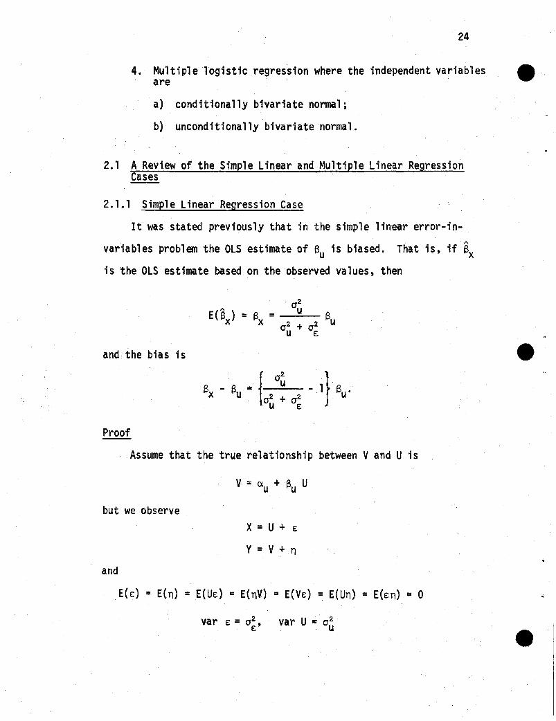
It was stated previously that in the simple linear error-in-A

variables problem the OLS estimate of au is biased. That is, if ax

is the OLS estimate based on the observed values, then

and the bias is

Proof

Assume that the true relationship between Vand U is

v = ex + a Uu u

but we observex = U + E

y =V + nand

E(E} = E(n} = E(UE) = E{nV) =E(VE} = E(Un) =E(En) = 0

var E =0 2 , var U :: 0 2E U

.25

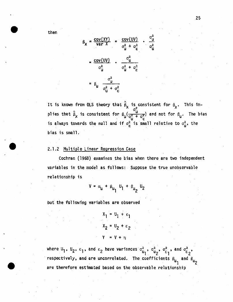
then

a =cov(XY)x var X

=cov(UV}0 2

U

= cov(UV)0 2 + 0 2U E

where Ul t U2t

respectively,

;;..

It is known from OLS theory that ax is consistent for Bx• Thisim-0 2

plies that ax is consistent fO,r Bu{o~ ~ o~} and not for Bu. The bias

is always towards the null and if o~ is small relative to O~t the

biasis sma11 .

2.1.2 Multiple Linear Regression Case

Cochran (l968) examines the bias when there are two independent

Viariables in the model as follows: Suppose the true unobservable

relationship is

but the following variables are observed

Xl = Ul + El

X2 = U2 + E 2

Y = V+ n

d h . ·22 2 d 2El t an E:2 ave vanances 0u t au tat ano t1 2 El E2

and are uncorrelated. The coefficients au and au·12

are therefore estimated based on the observable relationship

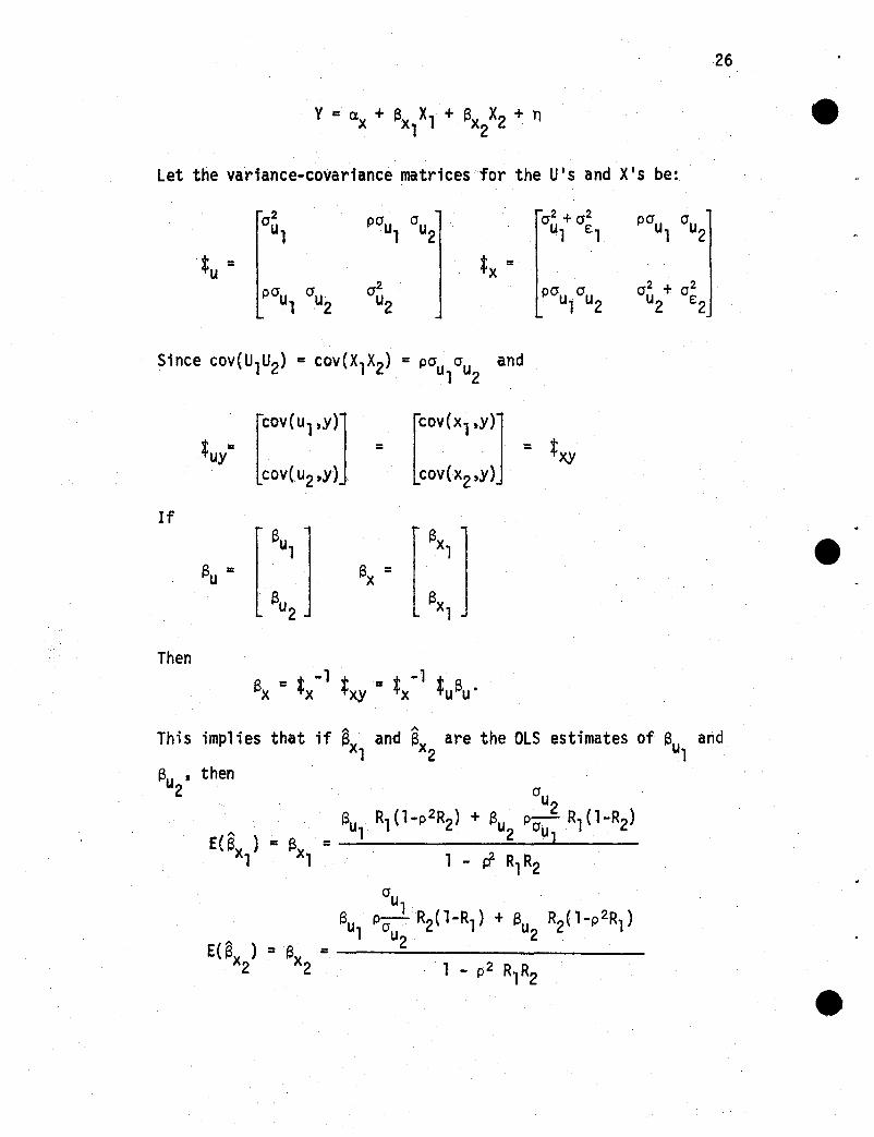
26

Y= a . + ~ Xl· + ~ X2 + nX xl· x2

Let the variance-covariance matrices for the U's and XIS be:

ThenQ - + -1 +- + -1 + 13~x -'x +xy -'x +u u·

This implies that if ax and ex are theOLS estimates of Su and121

Q then~u '2

27

If the correlation between Ul and U2 is zero (i .e." P = 0), then

which is identical to the results in the univariate case.

If only one variable is subject to measurement error, for

example U2, then

Even though U1 is measured without error there is a bias in the

estimation of l3u •. This bias may be negative or positive, depending. 1

on the signs of l3u ,13 ,and p. It is possible to produce situations1 u2

in which l3u < l3u ' but E(~x ) > E(~x). Since f < 1 we observe a1 2 1 2

larger bias in ~x for the multiple regression case than for the2

simple linear regression case. Also as p increases to 1, the bias

in the multiple linear regression case increases.

28

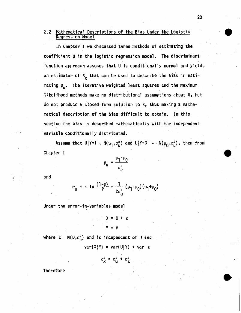
2.2 Mathematical Descriptions of the Bias Under the LogisticRegression Model

In Chapter I we discussed three methods of estimating the

coefficient 6 in the logistic regression model. The discriminant

function approach assumes that Uis conditionally normal and yields

an estimator of 6x that can be used to describe the bias in esti­

mating Suo The iterative weighted least squares and the maximum

likelihood methods make no distributional assumptions about U, but

do not produce a closed-form solution to 6, thus making a mathe­

matical description of the bias difficult to obtain. In this

section the bias is described mathematically with the independent

variable conditionally distributed.

Assume that UIV=l_ N(lll'O'~) and U!V=O - N(l1O'O~), then from

Chapter I

and

Ctu = - 1n (1pp) - 2:2

(l1l-lJO) (111 +110)u

Under the error-in-variab1es model

x = U + E

v =V

where E - N(O,o~) and is independent of Uand

var(XIV) = var(UIV) + var E

Therefore

29

These results are identical to those obtained in the simple linear

case. We conclude that when the true independent variable comes

from a mixture of two nonna1s with equal variance and measurement

error exists in the independent variable, the discriminant function

estimate of the coefficients using the observed data is not unbiased.

The bias is always towards the null and is dependent upon the mag­

nitude of cr~ relative to that of cr~.

Next we investigate the bias when UIY=l ... Exponential (A1) and

UIY=o - Exponential (:>.'0). In this case

P(Y=ll U) = ----:..1 _

1 + exp[- (-1 n~ (l-p)AO P.

= ---=-1 _

-(ex + S U)1 + e u U

whereA (1) A -A

ex = - Tn _1 -p ,13 = 1 0U AO P u AOA1

If we observe X= U+ e: where e: ... N(O,cr2 ) and E is independent of U,E

thenvar(XIV=O) =var(UIV=O) + var €

30

var(.XI Y=l) = var(UI Y=l) + var(e:)

As a result

We conclude in this case that there is a bias in the estimation of

eu when measurement error is present and the independent variable

is conditionally exponential. Again the bias is towards the nUll.

We conclude this section by considering the bias in the multiple

logistic model when (Ul ,U2) is conditionally multivariate normal.

Assume that

~IY=o - MN(~O'*u)

~IY=l ... MN(~l'*u)

where

U= [~:]and

~O = ['lJ10

]'lJ20

If we observe

then ~IY=o - MN(~ot~x)

~IY=l - MN(~lt;x)

31

where

The expected value of the estimator of au that we would obtain by

using the discriminant function approach on the observed XiS is:

This result is also identical to the multiple linear regression case

and the conclusions made in that case also apply here.

2.3 Description of the Bias Under the Logistic Regression ModelUsing Simulation "

In this section we study the bias when the iterative weighted

least squares or maximum likelihood methods are used and no distri­

butional assumptions about the independent variable are necessary.

2.3.1 Description of the Simulation Procedure

General Model:

1Yi lUi =-----T(-a-+---,..,SU..,.........) + nl

1 + e 1

where1

with probability Pi = -(a + SU.)1 + e 1

with probabilityl-Pi

32

i.e•• YilUi is Bernoulli (Pi)'

We begi"n the simulation by generating val ues of Ui under the

following distributions:

1. . U; 1Yi Normal

2. UilYi Exponential

3. Ui ... Nonnal

4. Ui ... Exponential

Next, the error values, £1' are generated from a N(O,1) distribution.

The observed values, Xi. are then computed as

X.=U.+£ .•, ,. ,After assigning values to ~ and a, values of the dependent variable

Vi are derived by computing

1P. = ), -{a + a u.

l+e u ,u,

and 1etting

1 if ~i < Pi

where.;,.... Unifonn (0.1). For each sample of values (Y.,X.), i = 1,2,, ,.•. ,500, the SAS procedure Logist was used to produce the iterative

weighted least squares estimate of au. The bias was then computed as"-

a-suo This procedure was followed for 150 samples of size 500. This

33

resulted in 150 estimates of au. The mean and standard deviation of

these estimates were computed along with 95% confidence intervals.

2.3.2 Simple Logistic Regression Case

Simulations in which the independent variable is conditionally

distributed were done as a check on the simulation procedure, since

we know mathematically what the results should be. The results are

summarized in Table 2.1. We selected 150 samples of size 500 from

a mixture of two normal populations. The conditional normal distri­

butions were:

UIV=l N(2,1)

ulv=o NO,l)

with p =P(V=l) =~ and a = ~l-~O = 1. If the simulation is per-c. U 0 2

fonning as expected, then

. A .,..,

Our results are good with E(Bx) =0.5109.

Next we checked the simulation procedure whenU was conditionally

exponentiaL We let p = ~, AO = 1, A1 =2 and Bu = A~-~O = 0.5. In1 0

this case

A A

Again the results are good with E(Bx) = 0.3201. Based on these re-

sults, we feel confident that the simulations are performing as

desired.

The simulations show that when Ui is distributed as a N(O,l)

variable, the estimated bias is -0.5377 when Bu=land 0.5338 when

34

au = -1. The bias for this case is towards the null and sl ightly

greater in magnitude than the bias that results when Ui comes from

a mixture of two normals. When Ui is exponential (ft=l) and Su=l,

the bias is -0.6825. This is much larger than the bias in the normal

case.

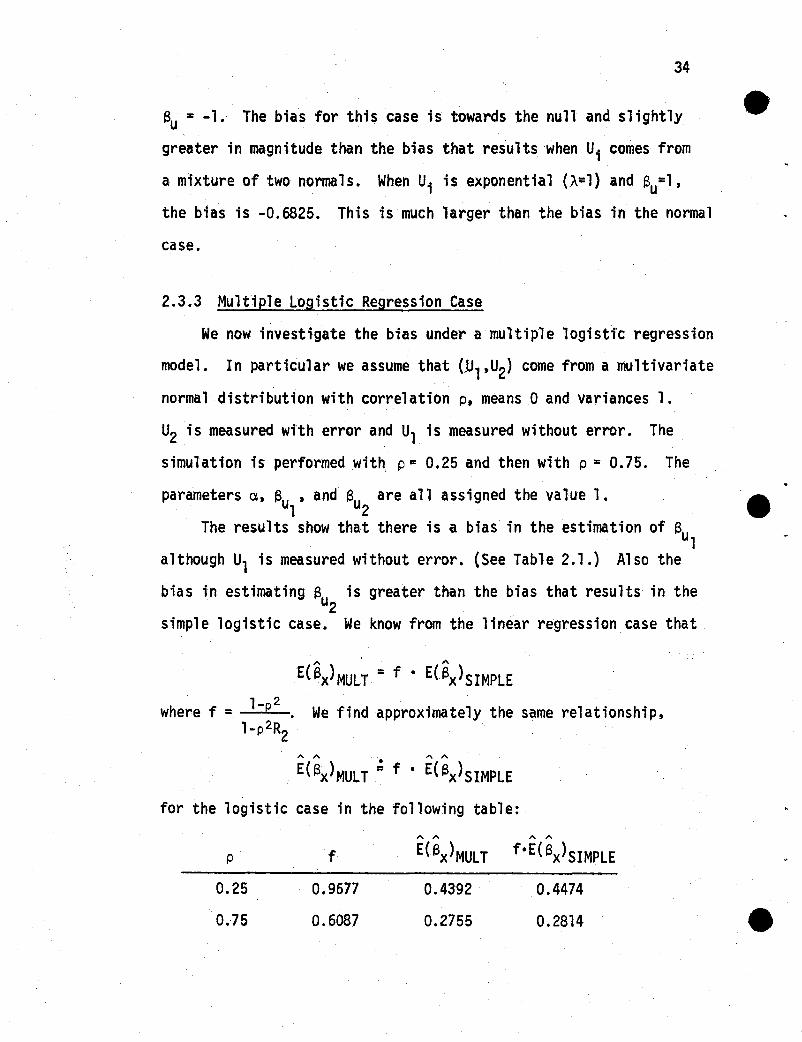
2.3.3 Multiple Logistic Regression Case

We now investigate the bias under a multiple logistic regression

model. In particular we assume that (~1,U2) come from a multivariate

normal distribution with correlation P. means 0 and variances 1.

U2 is measured with error and Ul is measured without error. The

simulation is performed with, P = 0.25 and then with P = 0.75. The

parameters a, au ' and Su are all assigned the value 1.1 2

The results show that there is a bias in the estimation of au1

although Ul is measured without error. (See Table 2.1.) Also the

bias in estimating a is greater than the bias that results in theu2simple logistic case. We know from the linear regression case that

,,' _ A

E(aX)MULT = f e E(aX)SIMPLE

where f = l-p2. We findapproxirnately the same relationship,l-p2R2

A A A A

E(Sx)MULT .~ f e E(Sx)SIMPLE

for the logistic case in the following table:

p

0.25

0 ..75

f

0.9677

0.6087

A A A A

E(Sx)MULT feE(Sx)SIMPLE

0.4392 0.4474

0.2755 0.2814

35

The simulations also show that as p increases the bias increases.

36

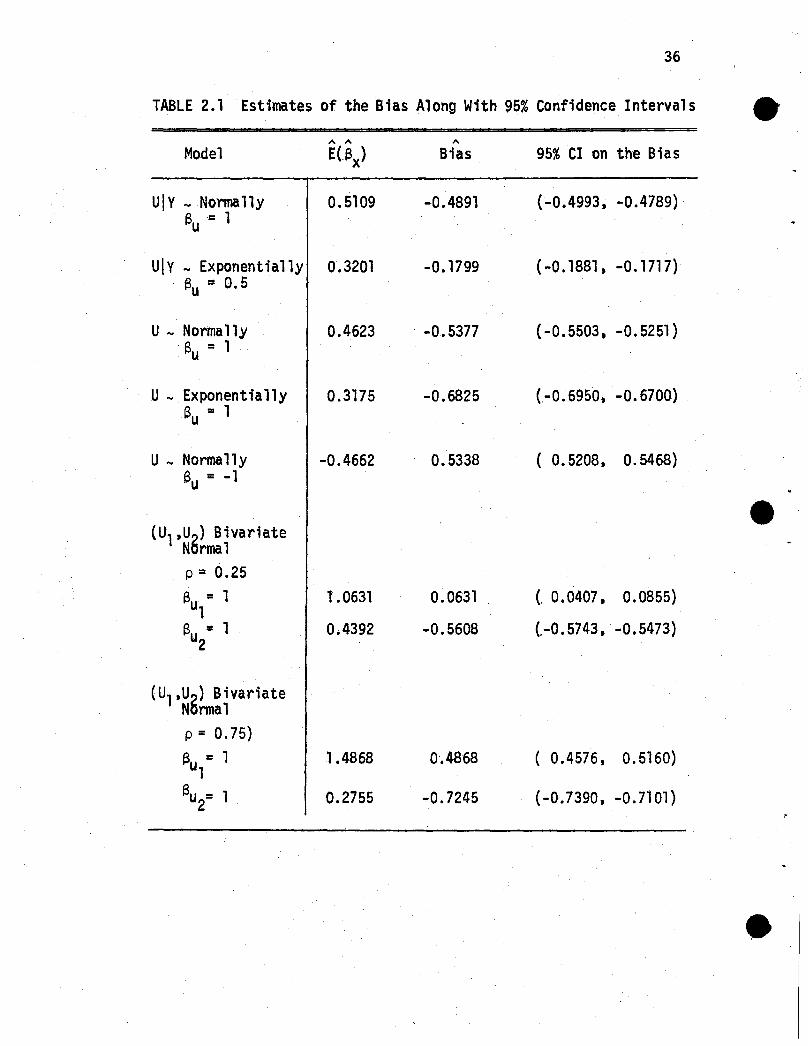
TABLE 2.1 Estimates of the Bias Along With 95% Confidence Intervals eA A A

Model E(.I\) Bias 95% CIon the Bias

Ulv ... Normally 0.5109 -0.4891 (-0.4993. -0.4789)e= 1u

U\V ... Exponentially 0.3201 -0.1799 (-0.1881. -0.1717). au = 0.5

U... Normally 0.4623 -0.5377 (-0.5503, -0.5251)a = 1u

U... Exponentially 0.3175 -0.6825 (.-0.6950. -0.6700)6 = 1u

U... Normally -0.4662 0.5338 ( 0.5208, 0.5468)e =-1·u

e(Ul,U~)Bivariate

N rmalp = 0.25a =1 1.0631 0.0631 ( 0.0407, 0.0855)u1e =1 0.4392 -0.5608 (-0.5743, -0.5473)u2

(U1,Ug) BivariateN nnalp = 0.75)e = 1 1.4868 0·.4868 ( 0.4576, 0.5160)u1au = 1 0.2755 -0.7245 (-0.7390, -0.7101)2

CHAPTER III

ALTERNATIVE ESTIMATES OF a WHEN MEASUREMENT ERRORIS PRESENT IN THE SIMPLE LOGISTIC REGRESSION MODEL

3.1 Modified Discriminant Function Estimator

Recall that the discriminant function estimator of the coeffi-

cients iOn the logistic model is appropriate when one can assume that

the conditional distribution of the independent variable, Ugiven Y,

is normal. That is, if

and

then

where

ul V=O '" N(llO'O~)

UIV=l N(lll o~}

1P.(Y =11 U) =---,---,-~.......-(et+ au)

1 + e

(3.1.1)

Suppose measurement error is present; that is, we observe

X=U+ e:, where Uand e: are independent with variances o~ and o~,

respectively. Since the variance of X is 0x2 = 0 2 + 0 2 , by substi-u e:

tuting o~ - o~ for o~ in equation (3.1.1), S can be rewritten as:

{3.1.2}

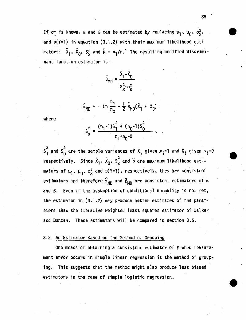
38

If o~ is known, ex and a can be estimated by replacing 'Ill' 1l0' o~,

and p(Y=l) in equation (3.1.2) with their maximum likelihood esti-- - ' I'\.

mators: Xl' XO' Si and p = nl/n. The resulting modified discrimi-

nant function estimator is:

where

2 2Sl and So are the sample variances of Xi given Yi=l and Xi given Yi=O

respectively. Since Xl' Xo' S~ and pare maximum likelihood esti­

mators of 'Ill' llO' o~ and p(Y=l), respectively, they are consistent

estimators and therefore ~D and SMD are consistent estimators of ex

and a. Even if the assumption of conditional normality is not met,

the estimator in (3.1.2) may produce better estimates of the param­

eters than the iterative weighted least squares estimator of Walker

and Duncan. These estimators will be compared in section 3.5.

3.2 An Estimator Based on the Method of Grouping

One means of obtaining a consistent estimator of e when measure­

ment error occurs in simple linear regression is the method of group·

ing. This suggests that the method might also produce less biased

estimators in the case of simple logistic regression.

39

3.2.1 The Method

Suppose one has available a grouping criterion, l, that is cor­

related with the true unobserved independent variable, U, but is not

correlated with the error term, E. The method would consist of rank­

ing the observations based upon the magnitude of their corresponding

l values. Those with the smallest nl l values would be classified

into group 1. The middle values would be classified into group 2,

and discarded. Those observations with the largest n3 l values would

be classified into group 3. The group sizes are nl =n2 =n3 =n/3.

An ideal situation would be to have a grouping criterion that would

correctly group all of the observed Xi values into the same group

that their corresponding Ui values belong. The following quantities

are computed for groups 1 and 3:

- Xia• Xg = ~ n; 9 = 1,3

9 g

'" y.b. Pg =~ n;; 9 =1,3

9

c• ~g = Log [p~ j; 9 = 1,3l-P

9

The parameters, a and S, are then estimated as

/

40

3.2.2 Rationale Behind the Method

We first transform the model

1P. = P(V.=lIU.) =--~--1 1 1 _(ct + au.)

1 +e 1

into the following linear form:

PiAi = Log ----- =a + aUi •

l-P.1

(3.2.2.1)

P.~ince Vi is a dichotomous va,riable, an observed value of log 1_

1-P.cannot be computed unless it can be assumed that Pi is equal 1

to some value Pg for all Ui's, a member of group g; therefore we

can pool the corresponding Vi's and estimate Pg, where

(3.2.2.2)

for i = l,2, •.. ,ngg = 1,2,3.

As a result, equation (3.2.2.1) becomes

A =ex + au.g. 19

and

where

- -A =A =a + au9 9 9

~ =} ~ =A9 G n9 9

g

- UiUg =6 n .

9 g

(3.2.2.3)

In this form we recognize a as the slope of the line in equation

(3.2.2.3). Therefore, a can be written as

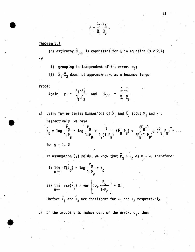
41

Theorem 3.1

'"The estimatorBGRP is consistent for S in equation (3.2.2.4)

if

i) grouping is independent of the error, E. ;1- -ii) X1-X3 does not approach zero as n becomes large.

Proof:

Again and'" '"Al-A

= - -X1-X3

A A

a) Using Taylor Series Expansions of Al and A3 about Pl and P3~

respectively, we haveA

A P P . 1 A 2P -1 '" 2A = log -+ = log~ + (P -P ) + z 9 2 (pg-Pg) +g l-Pg l-Pg Pg(l-Pg) 9 9 2Pg(1-Pg)

for 9 = 1, 3

A

If assumption (2) holds, we know that Pg -+- Pg as n -+- 00, therefore

'" P1) 1im E(A

g·) =1og~ = A

n+oo l-P g9

ii) lim var(~g) =var [109--'1J =O.n+oo l-Pg

'" '"Thefore Al and A3 are consistent for Al and A3 respectively.

b) If the grouping is independent of the error, Eit then

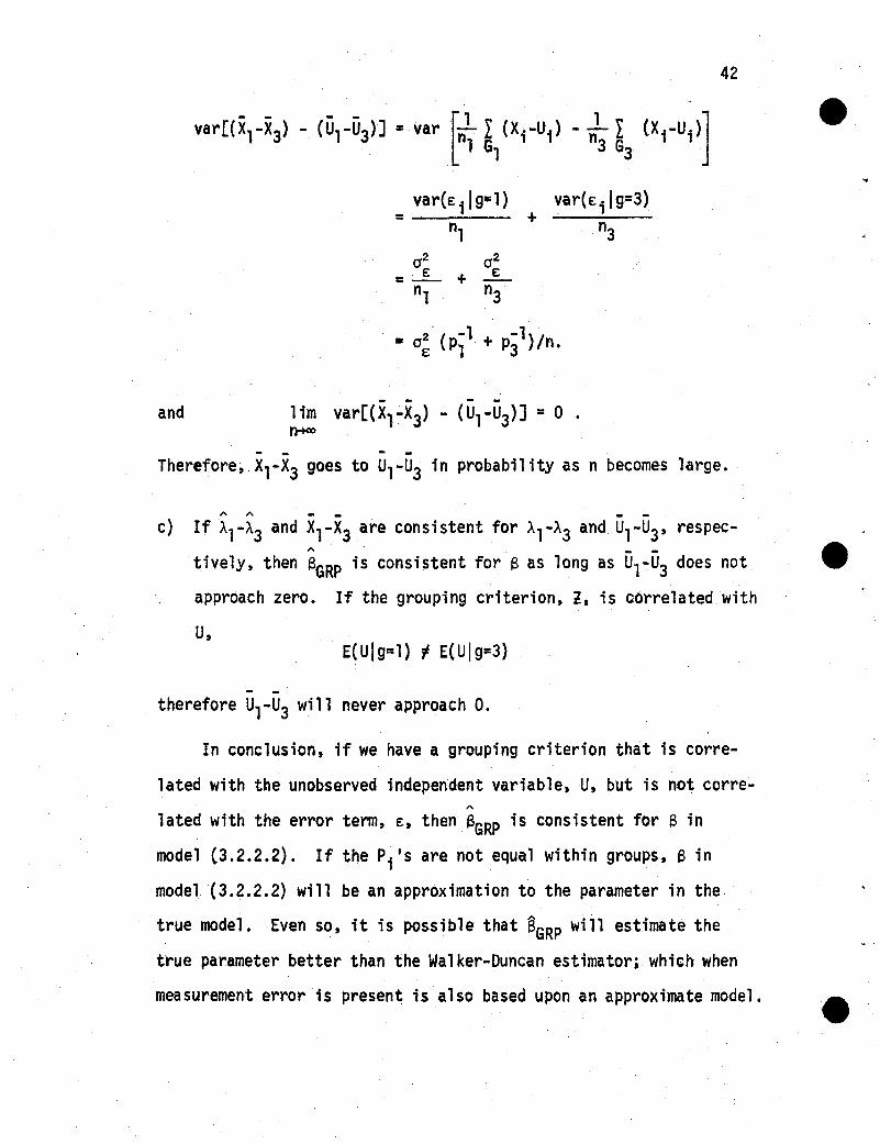
42

- - - - 'r1 1 ]var[(X1-X3) - (U1-U3)] =var --- L (X.-Ui ) - --" L (X.-U.)" n1 G

11 n3 G

31 1.

__ var(E i Ig=l)+n1

0 2 0 2

=....f..- + En1 n3

var(Ei Ig=3}n3

and

=02' (p-l + p-1)/nE 1 3 .

- - --lim var[(X1-X3) - (Ul -U3)} = 0 •~

- -Therefore, X1-X3 goes to U1-U3 in probabil ity as n becomes large.

" '"c) If Al-A3 and X1-X3 are consistent for Al-A3 and Ul -U3, respec-

tively, then SGRP is consistent for e as long as 01-03 does not ~approach zero. If the grouping criterion, ~, is correlated with

U,E(Ulg=l) ; E(Ulg=3)

therefore Ul -U3 will never approach O.

In conclusion, if we have a grouping criterion that is corre­

lated with the unobserved independent variable, U, but is not corre-'"lated with the error tenn, E, then SGRP is consistent for S in

model (.3.2.2.2). If the Pi's are not equal within groups, S in

model (3.2.2.2) will be an approximation to the parameter in the

true model. Even so, it is possible that ~GRP will estimate the

true parameter better than the Walker-Duncan estimator; which when

measurement error is present is also based upon an approximate model.

43

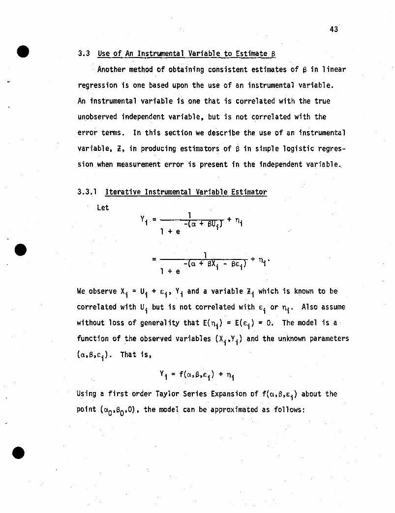
3.3 Use of An Instrumental Variable to Estimate f3

Another method of obtaining consistent estimates of f3 in linear

regression is one based upon the use of an instrumental variable.

An instrumental variable is one that is correlated with the true

unobserved independent variable, but is not correlated with the

error terms. In this section we describe the use of an instrumental

variable, l, in producing estimators of e in simple logistic regres­

sion when measurement error is present in the independent variable ..

3.3.1 Iterative Instrumental Variable Estimator

Let1V" = + n~(cx + SU.) i

1 + e '

1=-----,(-cx-+~~f3r.X-.---e='"e:-1

."T'") + ni ·1 +e 1

Vi = f(cx,e,e: i ) +ni

Using a first order Taylor Series Expansion of f(a,8,e:i) about the

point (cxo'So'O), the model can be approximated as follows:

44

=

+

let

then

e -faa +saXi) e -faa + SOX;)

-(a + S X.)-:; Xi(S-Sa) - ----T"'(a-a-+-:--:::S-;aX.,-;"T"")-2 Sc;.[1 + e . a a 1 J2 [1 + e . ]

(3.3.1.1)

p = 1 and Qai

=1-Pa.;a. -(aa + SOX.) •1 1 + e 1

Next, let

As a result,

(3 .. 3.1.2)

If one observes an instrumental variable, f;., that is correlated

with Ui but is not correlated with ni or Ei' then

*a) cov{n ,f) =0, since n is independent of Xand f,

b) cOV(S£,l) ~ BCOV(E,l) =0,

45

and

c} cov{X,l} = cov(U,l} ~o.

Using equation {3.3.1.2}, a can be written as:

cov{Y*,l} + So cov{X,l) ~ S cov{X,l).

. (3.3.1.3)

A natural estimator ofa* is

{3.3.1.4}

Next we derive an estimator of a. Taking the expected value of the

terms in equation (3.3.1.2), we have

Since E(Ei ) = E(.ni) =0,

Anatural estimator of a* is1'\ A _ A '" _

ar+l =ar + Y~ - (Sr+l-Sr) X • (3. 3.1. 5)

Initial values, aOand SO' are assigned and equations (3.3.1.4)·

and (3.3.1.5) computed iteratively until the solution converges.

For example, until 16r+1 - erl is less than some prespecified amount

(ex., .0005).

46

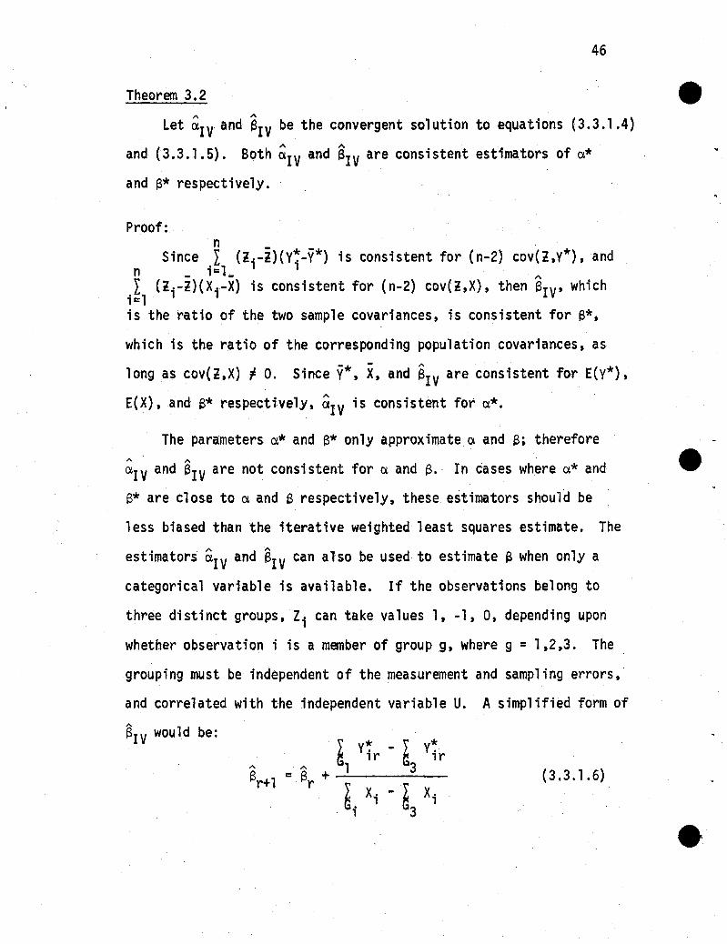
Theorem 3.2A A

Let alV and SIV be the convergent solution to equations (3.3.1.4)

and (3.3.1.5). Both ~IV and SIV are consistent estimators of a*

and a* respectively.

Proof:

(3.3.1.6)

) * ) *~ Vir - ~ Vir=8 + 1 3

r ~. x. -I x.1 G 1

i 3

n _Since.~ (li-l)(V~-Y*) is consistent for (n-2) cov(ltV*) tand

n _ 1-L A

.L (li-l)(Xi-X) is consistent for (n-2) cov(ltX)t then aIVt which1=1is the ratio of the two sample covariances t is consistent for a*t

which is the ratio of the corresponding population covariances. as

long as cov(ltX) r O. Since Y*t Xt and eIV are consistent for E(V*)t

E(X)t and 6* respectivelYt &IV is consistent fot a*.

The parameters a* and a* only approximate a and a; thereforeA A -alV and SIV are not consistent for a and a. In cases where a* and ..

a* are close to a and a respectivelYt these estimators should be

less biased than the iterative weighted least squares estimate. The

estimators &IV and8IV can also be used to estimate f3 when only a

categorical variable is available. If the observations belong to

three distinct groupst Zi can take values It -It Ot depending upon

whether observation i is a member of group gt where g = lt2 t3. The

grouping must be independent of the measurement and sampling errors t

and correlated with the independent variable U. A simplified form of

SIV would be:

47

where G1, G2 and G3 are the three groups with n/3 observations in

each group. If more than three groups exist, say g, then values 1,

2, ••. ,g could be assigned to Zi,and a computed using equation

(3.3.1.4) •

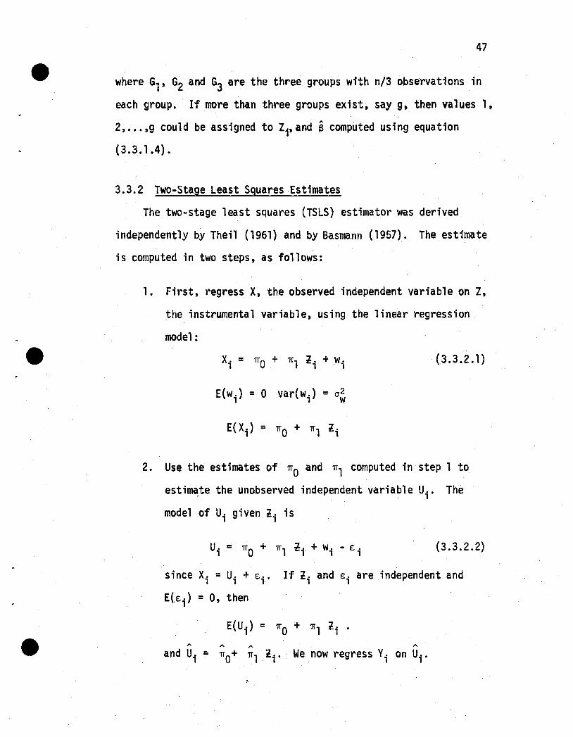
3.3.2 Two-Stage Least Squares Estimates

The two-stage least squares (TSLS) estimator was derived

independently by Theil (1961) and by Basmann (1957}.The estimate

is computed in two steps, as follows:

1. First, regress X, the observed independent variable on Z,

the instrumental variable, using the linear regression

model:

x. = 'ITO + 'IT1 ~. + W.1.11

E(Wi ) = a var(wi} = o~

{3.3.2.1}

2. Use the estimates of 'ITO and 'lTl computed in step 1 to

estirna;te the unobserved independent variable Ui . The

model of Ui given li is

(3.3.2.2)

since X. = U. + E.. If l,. and E,' are independent and, , 1

E(Ei} =0, then

E(U i } = 'ITO + 'IT1 li •A A A A

and Ui = 'lTO+ 'lTl lie We now regress Vi on Uf .

48

In simple linear regression the TSLS estimator and the instru­

mental variable estimator are identical. Let

V. =a + eu. + n·111

Xi = U. + e:.1 1

a) U. n, e: are independent and E(n) =E(e:) =O.

b) cov(l,X) =cov(l,U), andcov(l,n) =cov(l,e:) = O.

If X is regressed on l the estimates of lTO and ITl aren _ _

_f (li-i)(Xi-X)ITl - . - 2

I (fri )

and

A

The estimate of 13 that results from regressing Vi on Ui using the

modelA

Vi =a + I3U. + n~1 1

is n A A-

I (U.-D)(V.-Y)A 1 1

'!3rSLS = n A A 2

L (u.-D)1 '

In the case of logistic regression, the model in step 2 is:

49

1 **Yi =--_"":"'-_-;:-"- + ni .-(a + BU.)

1 + e 1

The iterative weighted least squares estimator of f3 using the above

. model is:

" "where U 1'5 an nx2 matrix with [l Ui] as the ith row, Wr is the

diagonal weight matrix with {Pu. QQ. } on the diagonal, v; is an1,r 1,r

nxl vector with elements

V. - pI'.1 ui,r 1

t(-------.;~-)o, p" =--_"":"'-_-1'.-1'.- ,fA Q" Ui,r -(ar + f3rU,.)u. u. 1 +1,r l,r e

This estimator can be derived in practice by using SAS's PROC. A

LOGIST on the values of (Vi,Ui ), i =l,2, •.. ,n. The resulting esti-. "mator w,ll be referred to as BrSLS'

3.3.3 Another Two-Stage Estimator of f3

In previous sections, Xi and ftO + ftl Zi were used as estimates

of the unobserved independent variable Ui . In this section the use

of the Bayes or James-Stein estimate of Ui is discussed.

If Xi = U; + Ei is observed, where Ui - N(~,cr~) and Ei - N(O,o~),

then (Xi,Ui ) is distributed as a bivariate normal with

and

var(.Xi ) = cr~ + o~, var(Ui ) =cr~

cov( Xi ,Ui ) = cr~

50

ifE(E i ) =0 and Ui , Ei are independent.- Also the conditional0 2

distribution of Ui given Xi is N(ll + P(X1.-ll), (XJ2) wher~ p = uE 02+02

The Bayes estimate of Ui is that function of the observations U E

that minimizes the conditional expectation of the loss function

2L = (Ui - f(X i )) .

- . 2E[( Ui - f(X i )) IXi] is minimum when ftXi) = E( Ui IXi)' if a minimum

exists. Therefore

Proof: eLet Yi =~ + SQU i + ni

cov(Yi,lJ + p(Xi-lJ))

var(ll + p(Xi-u))

p cov(Yi ,Xi) 1= = -sp2 var Xi p x

0 2 + 0 2

= U £ f\ = l3u .0 2

U

Since So is equal to l3u' any consistent estimator of (3a is a consis­

tent estimator of l3u' and it is well known that the OLS estimatorA

using the values (Yi'Ui ) is consistent for l3u. Whether a similar

relationship exists in the logistic case is investigated by means of

51

simulation in the next section.

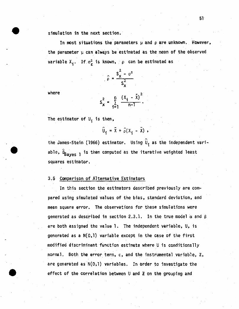
In most situations the parameters l.l and p are unknown. However,

the parameter 1.1 can always be estimated as the mean of the observed

variabl e Xi. If cr~ is known, p can be estimated as

2 2A Sx - cr

. p = 2Sx

where - 22 n (Xi - X)

Sx =.L1

n-11=

The estimator of Ui is then,

'" - AU. = X + p( X. - x) ,1 1

A

the James-Stein (1966) estimator. Using Ui as the independent vari-

able, Ssayes 1 is then computed as the iterative weighted least

squares estimator.

3.5 Comparison of Alternative Estimators

In this section the estimators described previously are com­

pared using simulated values of the bias, standard deviation, and

mean square error. The observations for these simulations were

generated as described in section 2.3.1. In the true model ex and 6

are both assigned the value 1. The independent variable, U, is

generated asa N(O,l) variable except in the case of the first

modified discriminant function estimate whereU is conditionally

normal. Both the error term, e:, and the instrumental variable, l,

are generated as N(O,l) variables. In order to investigate the

effect of the correlation between Uand! on the grouping and

52

instrumental variable estimators, we generated three sets of l

values for each sample. The sets differ only in the value of

corr(U,l). The correlations are 0.2, 0.5 and 0.9. Two additional

'"sets of l values were generated for simulation of s,-5L5' with

corr(U,l) =0.3 and 0.4.

The following estimators were computed for 150 samples of size

500:

1. MOdified Discriminant Function Estimator, 0'2 knownE

a) Uconditionally normal with means III = 2, 110 = 1

b) U", N(O,l)

2. The Iterative Weighted Least Squares Estimator with

2 2'" - (5x- 0'e) -U. = X+ (X. - X)1 52 1

X

'"as the independent variable, Saayes l'

3. The Grouping Estimator,

'"4. The Iterative Instrumental Variable Estimator, SIVn _L (li-l)(Y~ -y*)

'" i=l lr r= Sr + -n"--------

I (lr"~)( X.-x)i=l 1

0.2,

0.3,

53

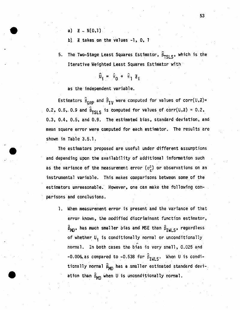
a) l - N(O,l)

bl l takes on the values -1, 0, 1

A

5. The Two-Stage Least Squares Estimator, !3rSLS' which is the

Iterative Weighted Least Squares Estimator with

A " "U. = 7T0 + 7T 1 ~.·1, 1

as the independent variable.

" AEstimators BGRP and B1V were computed for values of corr(U,~)::

A

0.5,.0.9 and a,-SLS is computed for values of,corr(U,~) :: 0.2,

0.4, 0.5, and 0.9. The estimated bias, standard deviation, and

mean square error were computed for each estimator. The resu1 ts are

shown in Table 3.5.1.

The estimators proposed are useful under different assumptions

and depending upon the availabil ity of additional information such

as the variance of 'the measurement error (C1~) or observations on an

instrumental variable. This makes comparisons between some of the

estimators unreasonable. However, one can make the following com­

parisons and conclusions.

1. When measurement error is present and the variance of that

error known, the modified discriminant function estimator,A • _ A

SND' has much smaller blas and MSE than SrWLS' regardless

of whether Ui is conditionally normal or unconditionally, A

normal. 1n both cases the bias is very small, 0.025 and

-O.OOSt as compared to -0.538 for SIWLS. When U is condi-. A

tionally normal SMD has asrnaller estimated standard devi-A,,'

ation than SMD when U is unconditionally normal.

54

2. When ~ 1s known and one cannot assume conditional normal­

ity of Up then the use of the Bayes estimate of Ui as the

independent variable produces an estimator of e with

smaller MSE than when using SMD' See lines 2 and 3 of

Table 3.1.

....3. The method of grouping estimator, f3GRP ' the iterative instru-

mental variable estimator, SIV' and the TSLS estimator,....SrSLS' vary in quality relative to the value of the corre-

lation between the instrumental variable (or grouping cri­

terion) and the independent variable, U. Both the bias and

the standard deviation of the estimators increase as the

correlation, PU~' decreases.

4. The rate of convergence for SIV is also a function of PU~'

For example, when PU~ =0.2, only 108 out of 150 samples

provided solutions within 30 iterations. In contrast, when

PU~ = 0.9 all but two samples converged to a solution within

30 iterations. This problem is due to the large variance of

the estimator when the correlation is small. It is well

known that inefficient/unstable estimators have convergence

probl ems.

5. The bias in 6GRP ' 6IV and STSLS is smaller than the bias....

in f3 IWLS ' although the standard deviation of these esti-

mators is always larger than the standard deviation of

'"f3IWLS ' For values of PU~· > 0.2 the MSE's of these estimators

are smaller than the MSE of SIWLS'

55

6. In terms of bias and MSE. there appears to be little. A A A

difference in the performances of f3GRp • f3IV and !3rSLS."However. !3rSLS is preferred over the other two because of

"the convergence probl an of f3rv and the necessary model" Aassumptions of SGRp. Also. !3rSLS and its variance are

easy to compute using SAS's PROC LOGIST.

56

TABLE 3.1 Simulated Mean, Bias, Standard Deviation and Mean"SquareError of the Estimators

A A A A

~SEEstimators Mean Bias STD(t3)

A ulY ... Normally 1.025 0.166 0.168SMD: 0.025A

U ... Normally 0.994 -0.006 0.203 0.203Ssayesl : 0.936 -0.064 0.163 0.175

A

SGRp: PU:t =0.2 0.835 -0.165 0.691 0.7100.5 0.914 -0.086 0.260 0.2740.9 0.958 -0.042 0.154 0.160

A

SIV: :t ... N(O,1)

PU:t =0.2, n = 108 0.605 -0.395 0.371 0.5420.5, 136 0.845 -0.155 0.209 0.2600.9, 148 0.885 -0.115 0.158 0.195

A

SIV: :t =-1, 0, 1 ePU~ =0.2, n = 100 0.524 -0.476 0.380 0.609

0.5, 135 0.813 -0.187 0.200 0.2740.9, 147 0.867 -0.133 0.152 0.202

~SLS: PU:t = 0.2 0.911 -0.089 0.911 0.915*0.3 0.856 -0.144 0.398 0.4230.4 0.857 -0.143 0.286 0.3200.5 0.866 -0.134 0.230 0.2660.9 0.956 -0.044 0.148 0.154

A

SIWLS(Wa1ker-Duncan) 0.462 -0.538 0.079 0.544

*After removal of the extreme value, 9.39, the starred line becomes:

0.855 -0.145 0.588 0.606

CHAPTER IV

USE OF MULTIPLE MEASUREMENTS IN THE ESTIMATION OFe

4.1 The Mean of MIndependent Measurements as the IndependentVariable

In previous sections it has been assumed that the measurement·

error, Ei , has a mean value of zero and is independent of the un­

observed variable Ui , for all values of i. If under these assump­

tions, m independent measurements are made on each,of the n

independent sample units with the observed variable being

X•• =U.+E ..1J 1 'J

i = 1,2, ... ,nj =1,2, .. .,m

then

E(X. ·IU.) = U.'J 1 ,

and var(X .. IU.) =var(E .. Iu.) =0 2 •'J 1 'J' , E

_ m

Therefore, Xi _ = .r XiJ·/m, which estimates E(XiJ·IUi ) a1 so estimatesJ=l ' . _

Ui . Also as the number of repeated measurements increases, Xi_ con-

verges to Ui . This suggests the use of Xi_ in place of the unknown

independent variable Ui when estimating e.In the case of simple 1inear regression, if

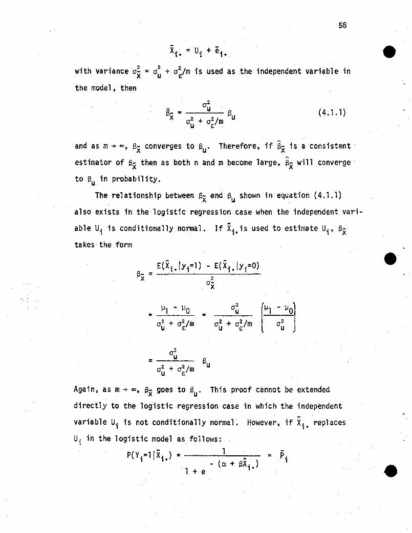
58

Xi. = Ui + ei .

with variance 0i =o~+ o~/m is used as the independent variable in

the model, then

(4.1.1)

and as m-+ eo, Bx converges to Bu. Therefore, if Sx is a consistent

estimator of Bx then as both nand m become large, Sse will converge

to au in probabi1 ity.

The relationship between Bx- and B shown in equation (4.1.1)u .also exists in the logistic regression case when the independent vari-

able Ui is conditionally normal. If Xi. is used to estimate Ui , Bxtakes· the form

lJl - lJO= =0 2 + 02/mu £:

Again, as m-+ eo, ax goes to au. This proof cannot be extended

directly to the logistic regression case in which the independent-variable Ui is not conditionally normal. However, if Xi. replaces

Ui in the logistic model as follows:

P{ Yi=ll Xi J = ...:...1----(et+BX.)

·1 +e ,.

= .pi

59

then the iterative weighted least squares OWLS) estimator is

(4.1.2)

where X is an nx2 matrix with i th row (1 ,Xi'>' Wr is a diagonal

weight matrix with elements" {PirQir}' and v; is an nxl vector with.th "- - - ", element {Yi-Pir/PirQir}.

As m~ 00, Xi. ~ Ui and equation (.4.1.2) becomes

e =s + (U'W U)-l U'W V*r+lr r r r

The nx2 matrix U has i th row (l,Ui ), Wr is diagonal with element

{PiQi}' v; is an nxl vector with elements {Yi-p;lPiQi}' and

1Pi =------,(;-a-+~SU:-:-.-.-) •

1 + e . ,

It is well known that Sus the IWLS estimator without measure-\

ment error (i.e .. Ui observable) converges to S as n ~ 110. Therefore,

'"Sx converges to S as both m~ 00 and n .~ 00.

4.2 Further Reduction of the Bias when m is Small

Another advantage of having multiple measurements on each

sample unit is that one can now estimate the variance of the measure- "

i = 1,2, ... ,n2 m

SXIU,. = Ij=l

ment error. Since var(XijIUi) = var(e:ij!Ui ) = ai, o~ can be esti­

mated by pool ing the estimated va lues of var( Xij IUi) as follows:

- 2(X•• - X" ).'J .. •m-l

and

- 2n m (X .• - X. )S2 = L l 'J ,.

E i=l j=l n(m-l}

An estimate of q~ can be computed as

. - - 2n (X. - X )S! ~ I .,. ..

x i=l n-l

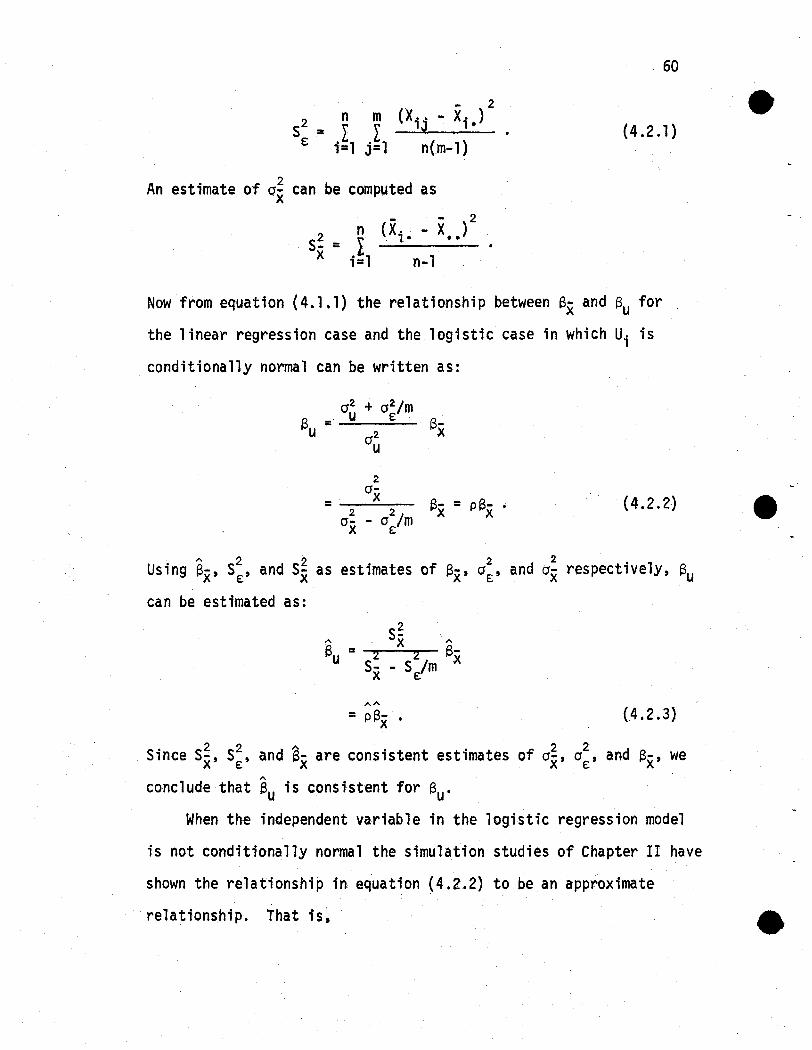
60

(4.2.1)

Now from equation (4.1.1) the relationship between 13,X and l3u for

the linear regression case and the logistic case in which Ui is

conditionally normal can be written as:

13- = p 13-x x (4.2.2)

A 2 2 2 2 .1Using I3x' SE' and S,X as estimates of I3x' 0E' and Ox respectlve y, l3ucan be estimated as:

2f' . Sx A

l3u = z z 13,XS- - S 1mx E

(4.2.3)

2 2 ~ 2 2Since Sx' SE' and P,X are consistent estimates of ox' 0E' and I3x' weA

conclude that l3u is consistent for Bu.

When the independent variable in the logistic regression model

is not conditionally normal the simulation studies of Chapter II have

shown the relationship in equation (4.2.2) to be an approximate

relationship~ That is~

61

where

Therefore2o­x

2 2(j- - (j 1mx E

13­x

in the logistic case. Still the estimator in equ~tion (4.2.3) isA

expected to be less biased than 13x when m is small.

4.3 Use of the James-Stein Estimator of Uias the Independent

Variabl e

If more than one measurement is available for each sample unit,

one can compute the James-Stein estimator of Ui (discussed previously

in section 3.4) when both p and o~ are u~known. In the case of m.

measurements on each sampling unit, one observes

X. = U. + E.1 • 1 1

where (Xi.,Ui ) is bivariate nonna1 with E(X i .) = E(Ui ) =}.I, var(Xi.l =

o~ + (j~/m, var(Ui ) = o~, and cov(X;.Ui ) =o~.Also,

= }.I + p*(X. - }.I)'1 •

The Bayes estimator of Ui is again that function of the observations

that minimizes the conditional expectation of the loss function,2

L = (Ui - f(X i )) , which is

fr. = }.I + p*(i. - ~).1 1 •

62

Since l.l and p* are unknown, we estimate them using

A = n mJl =X =.r .I XiJ·/nm

,=1 J=l

2 2 •where Sx and SE are def,ned in equation (4.2.1). The estimator of

Ui isA _ A _ _

U. =X+ p*{X,' - X)., . .A

Using Ui above as the independent variable, S is estimated usingA

the IWLS estimator. The result is SSayes 2'A

In the case of linear regression, this estimator, SBayeS 2 isAA

identical to the estimator derived in section 4.2, pSx'

Proof:

A

Ssayes 2

A _ _

HUi-U)(Y i-V)= A _ 2

HUi-U)

A L{Xi-~)(Yi-Y) 1 A AA

= P* _ _ =-:;::-- 13- = p (3-p*2 L{X

i-X)2 p* X X

A

since Ui- U= p*(Xi - X)

andA _ 1p - -.A*P

Whether this is true in the case of logistic regression is investi­

gated in section 4.5 by means of simulation.

63

4.4 Estimation of 0 2 When m Measurements are Taken on a Subsamplee; .

It is not always economically feasible to take more than one

measurement on each sample unit. However, one can take mmeasure-

k mS~ = L .L

i=l J=l

ments on a subsample of k units and estimate o~. Since Ui is fixed

for each unit and independent of e: l' an estimate of a~ would be

- 2(X .. - x. )'J ,.

k(m-l)

andS2

X

2 A

whereSx and (3IWLS are based on a single measurement. For example,

for sample unit with mmeasurements use only the first in computing

4.5 Results of Simulation Study

Simulated values of the following estimators were produced for

150 samples of size 500.

The IWLS estimator with Xi as the independentvariable. •

1.A

ex:

2.AApax: The estimator in (1) adjusted by the factor

S~A xP = 22

Sj( - Se:/m

3. Saayes 2: The IWLS estimator with

A _ [.S~ -S2/m.]U. =.~ + X E (i,..- ~), S~

x

64

as the independent variable.

The IWL5 estimator with Xi as the independent vari­able adjusted by the factor

52x

where 52 is based on mmeasurements made on a sub­sample of k units.

Different estimates of"Sx. pSx. and SSayes 2 were computed for

values of m= 2.4.6. and 8. where m is the number of repeated measure­

ments. The estimated mean. bias. and mean square error of the

estimators are shown in Table 4.1.

As expected. the bias in the estimators decreases as m increases.

Even when m is as small as 2. the reduction in the bias and MSE ;s

large. The actual reduction in bias from SIWLS to Sx when m= 2 is

'" '"29.4%. Adjustment of the estimator Sx by the factor p decreases the

bias even more significantly. In the case of m= 2. there is an 87.9%

'" "''''reduction in the bias from SIWLS to pax when m=2. A similar reduc-" "tion in bias occurs with the use of ass a"nd aBayes 2. As shown in

the linear regression case. ~Sx and Ssayes 2 are identical estimators.

There is an increase in the standard deviation of these estimators

over that of SIWL5. However. the YMSE is largest for the IWl5 e~ti­

mator. Another point worth noting is that the use of p does not

affect the results of the test of the Ho: S=O since the t-statistic

for this test is invariant under scale transformation. That is.

t =

65

66

TABLE 4.1 Simulated Values of the Mean, Standard Deviation, andMean Square Error of the Estimators

A A A -",-

Estimator Mean Bias STD .; MSE

A

(3x: m=2 0.620 -0.380 0.092 0.3914 0.776 -0.224 0.105 0.2476 0.829 -0.171 0.122 0.2108 0.874 -0.126 0.125 0.178

AA

PSi: m = 2 0.935 -0.065 0.146 0.1604 0.969 -0.031 0.131 0.1356 0.968 -0.032 0.143 0.1478 0.984 -0.016 0.140 0.140

A

SBayes 2: m= 2 0.935 -0.065 0.146 0.1604 0.969 -0.031 0.131 0.1356 0.968 -0.032 0.143 0.1478 0.984 -0.016 0.140 0.140 e

A

k=50, m = 2(3ss' 0.942 -0.068 0.247 0.256

0.462 -0.538 0.079 0.544

CHAPTER V

APPLICATION OF METHODS TO THE LIPID RESEARCH CLINICS DATA

5.1 Description of the Data Set

In this chapter the application of methods discussed previously

will be applied to data collected as part of the Lipid Research

Clinics (LRC) Program Prevalence Study. Detailed descriptions of

the LRC Prevalence Study can be found el sewhere (Hei ss, et a1. (J 980)) .

The data used fn this demonstration consist of observations on 4171

white men and women, age 30 and above. After participation in

Visit 1 of the Prevalence Study these individuals were randomly

selected, as part of a 15% sample of Visit 1 participants, to par­

ticipate in Visit 2. As a result, we have available two determina­

tions of plasma cholesterol and triglyceride levels, one taken at

each visit, along with other sociodemographic data. Other variables

used in this study are HDL cholesterol level measured at Visit 2,

and Quetelet index (weight/height2). The outcome variable for this

demonstration is mortality status at an average of 5.7 years after

the measurements were taken. Mortality status is modeled asa func­

tion of either total cholesterol or triglyceride level. Because of

the influences of sex and age on mortality, separate logistic models

were fit for each sex and when p.ossible, age was included in the

model as an additional independent variable. Both males and females

68

using hormones or having a missing value for that variable were

eliminated from the demonstration because of the influence of sex

hormone usage on lipid and lipoprotein levels (Heiss, et al. (1980)).

5.2 Computation of the Estimators and Their Variances

The following estimators were computed by model and data set,

along with their standard deviations and p-values corresponding to

the test of the Ho: 6=0:

1. eIWLS 1s the iterative weighted least squares estimate

with a single measurement of either cholesterol or triglyc­

eride as the independent variable. Both the estimate and

its variance were computed using SAS's PROC LOGIST.

A

2. 6MO is the modified discriminant function estimate using

an external estimate of the variance of the measurement

error. The estimate is computed as described in Chapter III.

A Taylor Series Approximation is used to derive the follow-

'"ing large sample estimate of the variance of f3MO :

When there is more than one independent variable, the

variance of the rth coefficient can be estimated as

VA{SMo,r) = S;l (l/nl + l/nO)

where s;l is the rth diagonal element of the inverse co­

variance matrix.

,

69

A

3. Ssayes 1 is the iterative weighted least square estimate

which uses

A

Ui = X +

as the first stage estimate of Ui . Again, cr~ is an ex­

ternal estimate of the variance of the measurement error.A A

After computing the Ui's, both the estimate ~Bayes 1 and

its variance are computed using SAS's PROC LOGIST on theA

Ui's and the dependent variable.

A

4. I3GRP is the grouping estimate in which observations are

grouped according to the magnitude of an instrumental

variable. The estimate is computed as described in

Chapter III. The large sample approximation to its vari­

ance using a Taylor Series Approximation of the estimator

is

2A A

;\1 - 1.3- -Xl - X3

+

5. SIV is the iterative instrumental varlable estimate. Its

variance is computed for fixed values of the ·observed

70

independent variable Xi and for fixed values of the instru­

mental variable li as

6. s,.SLS is the two-stage iterative weighted least squares'" '" '"estimate which uses Ui = 'ITO + 'ITl li as the first stage

A

estimate of U. li is an instrumental variable and 'ITO'

;1 result from the linear regression of the observedA

independent variable Xon l. Both the estimate 6-rSLS and

its variance are computed using SAS's PROC LOG1ST on the'"dependent variable and Ui •

7. ex is the iterative weighted least squares estimate which

uses the mean of the two measurements of cholesterol (or

triglyceride) as an estimate of the true independent vari-

able (PROC LOGIST).

'"8. aBayes 2 is the iterative weighted least squares estimate

which uses

A _

Ui =X+

as the independent variable (PROC LOGIST).

= 2 2The sample estimates of X, S-, and S by model and by data set arex E

shown in Table 5.1.

71

= 2 . 2TABLE 5.1 Sample Estimates of X, Sx' and SE by Model and Data Set

Independent VariableMeasured with Error

Total Cholesterol

Triglyceride=X

2s­X

52E

Males

206.1

1258.4

256.2

140.3

9086.4

3092.6

Females

205.4

1622.8

258.3

103.3

4673.1

815.6

All of the estimators listed above were not computed for all

models. Estimators requiring an external estimate of the variance

of the measurement error (SMD and Ssayes 1) could only be computed

for models in which total cholesterol was the independent variable.

A relatively good estimate of the within-individual variabil ity of

total cholesterol was found in a paper by Ederer (1972). He ob­

served, using data from the National Diet-Heart Study based on a

sample of 1000 men~ that in the absence of dietary change the

between-visit correlation was about 0.85 when measurements of total

chol esterol were taken one to two weeks apart. He a1so reports a

within-visit between-individual standard deviation of 38 (ax) for

cholesterol. Given two measurements of cholesterol for each individ­

ual

72

where var(Xi ) = var(X i ) = o~, Uiis the true value of cholesterol,1 2

and Ei and E; are error terms, we have1 2

0 2

corr(X,' ,X,, ) = u1 2 o~ + o~

Therefore, o~ = [1 - corr(xil

,xi2

)] o~. Using Ederer's values for

corr(xi1

,xi2

) and o~ we computed o~ using the above equation to be

216.6. No estimate of the variance of the measurement error in

triglyceride level of reasonable quality could be found.A A

Those estimators requiring an instrumental variable (SGRP' SIV' eSTSLS) were demonstrated for models in which triglyceride level was

the independent variable of interest. None of the variables observed

in this study were adequately correlated with total cholesterol, By

'adequately' we mean having a correlation greater than 0.2. Our

simulations in Chapter III showed that estimators requiring an instru-

mental variable perform poorly when the correlation between the

instrumental variable and the independent variable measured with

error is less than or equal to 0.2. Therefore, we did not attempt

to demonstrate the use of these estimators with total cholesterol

as the independent variable. Our data set contained two variables

adequately correlated with triglyceride level. They were HDL choles-

terol level at Visit 2, and Quetelet index (weightlheight2). It

was also observed that the correlation between log(HDL) and triglyceride e

73

was even higher than the correlation between HOL and triglyceride.

Therefore, using HOL, 10g(HOL), and Quetelet index, estimators re­

quiring instrumental variables were computed. Table 5.2 shows the

correlations between triglyceride level and HOL, 10g(HOL), and

Quetelet index. Correlations adjusted for age are also given.

TABLE 5.2 Correlations Between Triglyceride Level and InstrumentalVariables by Data Set

Instrumental Variable

HOL

(Adj. for Age)

log(HOL)

(Adj. for Age)

Quetelet Index

(Adj. for Age)

Males

-0.3134

-0.3209

-0.3565

-0.3628

0.2483

0.2496

Females

-0.3265

-0.3639

-0.3589

-0.3917

0.2557

0.2344

In using an instrumental variable to estimate model coeffi­

cients it is necessary to assume that the error in measuring the

instrumental variable is independent of the error in measuring

triglyceride level. This appears to be a reasonable assumption

given the mechanisms. for measuring HOL cholesterol and triglyceride

levels. Obviously there is no relationship between errors in the

measurement of triglyceride level and errors in measuring height or

weight.

74

A

The grouping estimator, SGRP' and the instrumental variable...

estimator, elY' are demonstrated only for the simple logistic case.

Extensions of these estimators to the multiple logistic case was

not attempted as a part of this research.

Tables 5.3-5.6 show the estimators computed by model and data

set along with their standard deviations and p-values corresponding

to the test of the Ho: 13=0.

5.3 Comparison of the Estimates

Comparisons of the estimates are made within model and within

data set.

1. In the simple logistic model with total cholesterol as

the independent variable we observe that

a) The magnitude of the estimate increases from SIWLS

t06MD to 6x. The increase in magnitude from 6lWLSA At.'"

to ex is about 58.3%. Also, SBayes 1 and ~ayes 2

are larger 1n magnitude than SIWLS and ~x respectively ....

The largest increase 1n magnitude is from SIWLS to

BBayeS 2' a 76.4% increase.Al though the model coeffi­

cient corresponding to total cholesterol is not signif­

icantly different from zero (a =0.05) regardless of

the estimator used, there is a decrease in the p-valueA A A

from SIWlS to eMD to ax'b) For females, the largest increase in magnitude is

... ...froms IWLS toSMD , a 41.9% increase. Other patterns

mentioned for males in (a) also occur for females

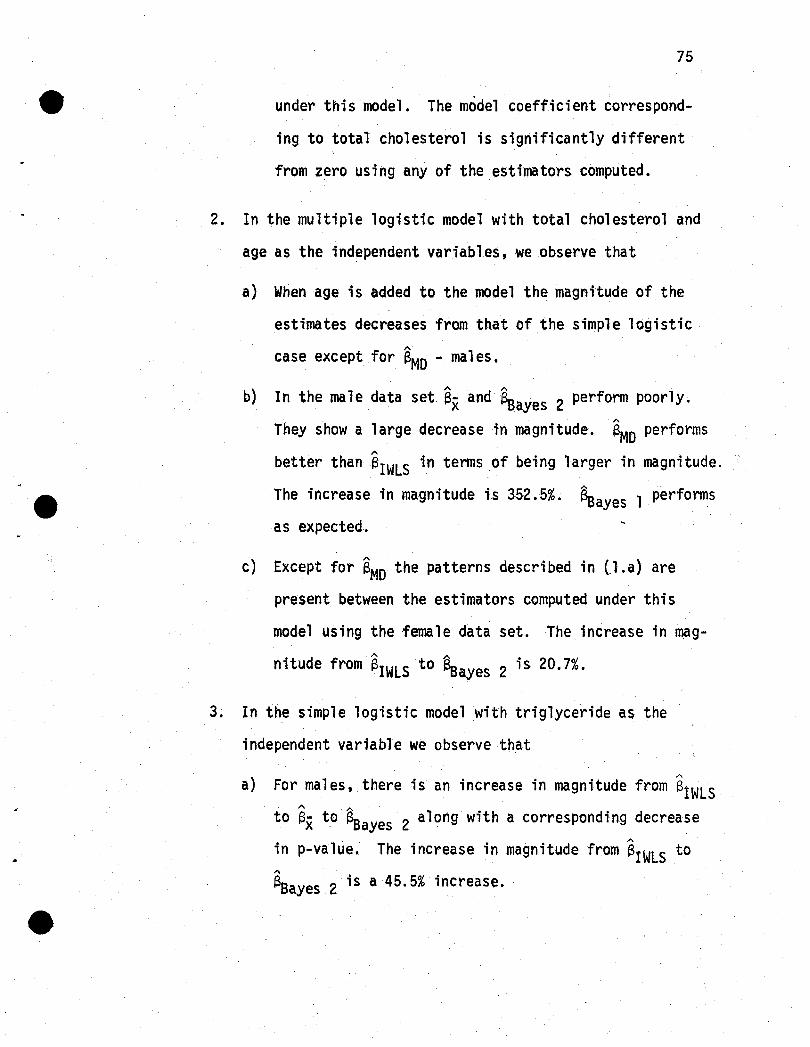
75

under this model. The model coefficient correspond­

ing to total cholesterol is significantly different

from zero using any of the estimators computed.

2. In the multiple logistic model with total cholesterol and

age as the independent variables, we observe that

a) When age is added to the model the magnitude of the

estimates decreases from that of .the simple logistic

"case except for SMD - males.

)" Ab In the male data set ex and (3Bayes 2 perform poorly.

They show a large decrease in magnitude. SMD performs

"better than (3IWLS in tennsof being larger in magnitude.

The increase in magnitude is 352.5%. ~ayes 1 performs

as expected.

c) Except for SMD the patterns described in (.1.a) are

present between the estimators computed under this

model using the female data set. The increase in mag-

nitude from SIWLS to ~ayes 2 is 20.7%.

3. In the simple logistic model with triglyceride as the

independent variable we observe that

a} For males, there is an increase in magnitude from BIWLS

. to ax to Saayes 2 along with a corresponding decrease

in p-value. The increase in magnitude from SIWLS to"SBayes 2 is a 45.5% increase ..

76

b) For females, there exists a smallet increase in mag­

nitude (11.9%) from eIWLS to aBayeS 2 than for males.

'" '"Also the p-value increases from f3 IWLS ·to f3Bayes 2·

c) For both males and females the model coefficient is

significantly different from zero (a = .05) using

'" '" '"SIWLS' ex or f3Bayes 2.

'"d) For the female data set the s,.SLS estimates are larger

in magnitude than BIWLS ' but have increased p-values,

although they remain significant. For the male data

'"set, the !3rSLS estimates are larger in magnitude than

'"the SIWLS estimates except for the case in which HDL

is the instrumental variable. None of the TSLS esti­

mates suggest that the model coefficient fortriglyc­

eride is significant using the male data set.

e) The grouping and instrumental variable estimators

perform poorly for both the male and female data sets~

'"For SIV-males, there is no gain in magnitude. There'" "-is a gain in magnitude from eIWLS to SGRP and from

BIWLS to eIV (in the female data set). These gains

are offset by large increases in variance.

4. In the multiple logistic model with triglyceride level

and age as the independent variabl es, we observe that·

'" '"a) There is an increase in magnitude fromsIWLS to STSLS

for both data sets except when Quetelet index is used

77

as the instrumental variable (male data set). ThereA A

is also an increase in magnitude from ~IWLS to ~x toA

~Bayes 2·

A . _ . A

b) Except for ~SLS (.HDL,QI)-ma1es, l3x - females, and

~ayes 2 - females, the coefficient corresponding to

triglyceride in the model is significantly different

from zero Ca =0.05).

5.4 Conclusions

The simulation studies of the previous chapters showed that onA A A A

the average ~D' SBayes l' l3x' and 13Bayes 2 perform better thanA

13IWLS • They also showed that if the correlation between the inde-

pendent variable and an instrumental variable was high enough, SGRP'A A

13Iv , and SrSLS would perform well. By 'perform well' we mean have

reduced bias and MSE. Since the bias was shown in Chapter II to

always be towards the null, we demonstrate the reduction in bias

offered by the proposed alternative estimators as an increase inA

their magnitude over tbat of 13IWLS • We also expected, based on,

simulation results, to demonstrate situations in which the p-value

corresponding to the Ho: 13=0 decreases when one uses the alternative

estimators rather than SIWLS. We were able to demonstrate this inA A A A

most cases for 13MD , 13Bayes l' ex and f13ayes 2· However, when look-

ing at the estimators requiring an instrumental variable, the p-value

actually increased. This probably a result of one or more of the

following:

78

1. The correlation between triglyceride and the instrumental

variables was too small; therefore:. resulting in a large

estimated variance.

A

2. The variance used for l3IV in this demonstration is con-

ditional on the observed value of triglyceride and con~

ditional on the instrumental variable. This may not be

an appropriate estimate of the variance.

79

TABLE 5.3 Simple Logistic Model With Total Cholesterol Level atVisit 2 as the Independent Variable

Estimators Males Females(n=2508) (n=1663)

"f3 IWLS 0.00254 0.01381Std. Error 0.00247 0.00277P-value (0.30) «0.0001)

"f3MDStd. ErrorP-va1ue

0.003080.00275(0.26)

0.019590.00356

«0.0001)

"f3Bayes 1 0.00301 0.01575Std. Error 0.00292 0.00316P-va1ue (0.30) «0.0001)e"f3x 0.00402 0.01489Std. Error 0.00258 0.00284P-va1ue CO.12) (:<0.0001)

•

•

"f3Bayes 2Std. ErrorP-value

0.004480.00287(0.12)

0.016170.00309

(<0.000l)

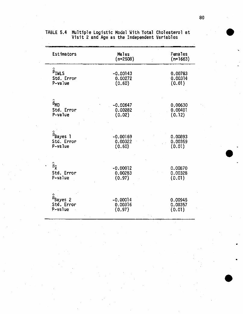
TABLE 5.4 Multiple Logistic Model With Total Cholesterol atVisit 2 and Age as the Independent Variables

Estimators Males Females(n=2508) (n=1663)

A

SIWLS -0.00143 0.00783Std. Error 0.00272 0.00314P-va1ue (0.60) (0.0l)

80

A

(3MDStd. ErrorP-va1ue

A

13Bayes 2Std. ErrorP-value

-0.006470.00282(0.02)

-0.000140.00316(0.97)

0.006300.00401(0.12)

0.009450.00357(0.01 )

•

TABLE 5.5 Simple Logistic Model with Triglyceride Level atVisit 2 as the Independent Variable

81

SGRPtHDLStd. ErrorP-value

Srv tHDLStd. ErrorP-value

A

SrvtLHDLStd. ErrorP-value

A

SIV tQIStd. ErrorP-value

0.001850.00488(0.70)

-0.000430.00288(0.88)

0.000950.00254(0.71)

-0.001140.00392(0.77)

0.009010.00644(0.16)

0.006010.00681(0.38)

0.006010.00619(0.33)

0.006420.00959(0.50)

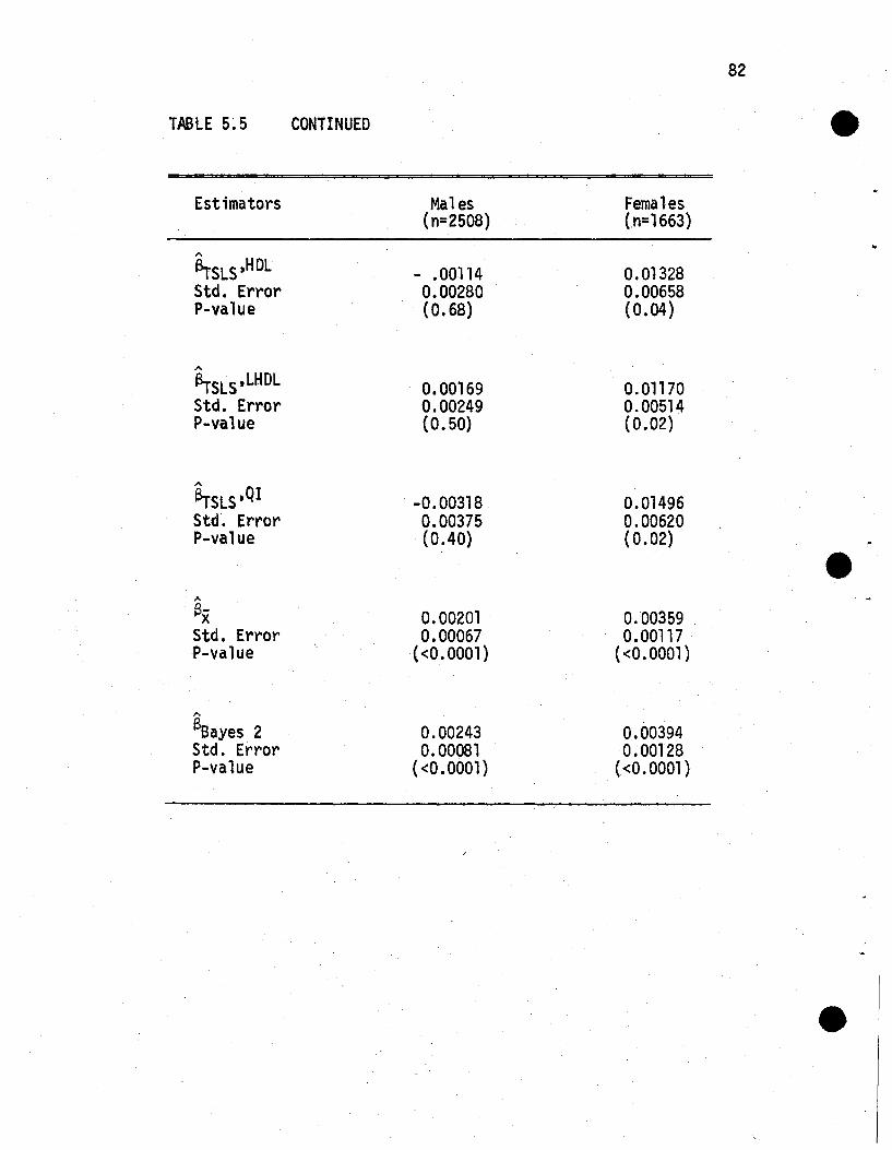
TABLE 5~ 5 CONTINUED

82

Estimators Males Females(n=2508) (.n=1663)

.."~SLS,HDL - .00114 0.01328Std. Error 0.00280 0.00658P-value (0.68) (0.04)

"erSLS,LHDLStd. ErrorP-value

"eBayes 2Std. ErrorP-value

0.001690.00249(0.50)

0.002430.00081

«0.0001 )

0.011700.00514(0.02)

0.003940.00128

«0.0001)

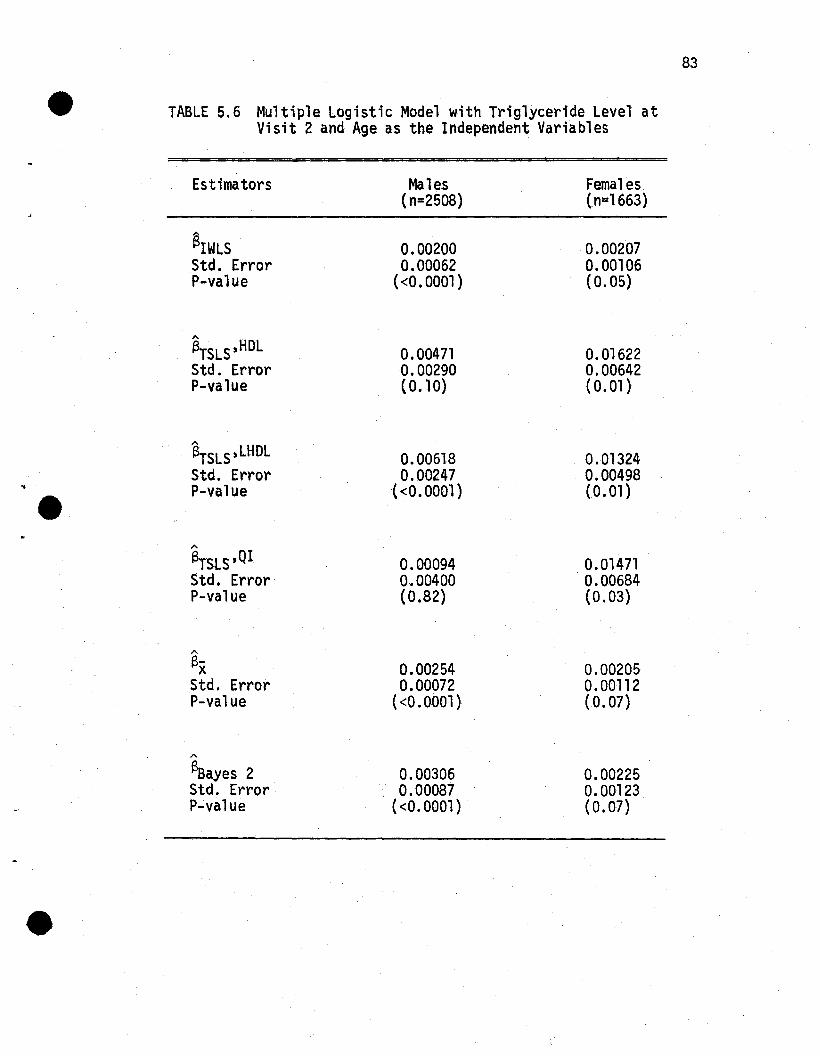
TABLE 5.6 Multiple Logistic Model with Triglyceride Level atVisit 2 and Age as the Independent Variables

Estimators Males Females(n=2508) (n=1663)

~IWLS 0.00200 0.00207Std. Error 0.00062 0.00106P-value «0.0001) (0.05)

83

"SrSLS,HDLStd. ErrorP-value

0.004710.00290(0.10)

0.016220.00642(0.01 )

SrSLS,LHDL 0.00618 0.01324Std. Error 0.00247 0.00498

"l P-va1ue «0.0001) (0.01)e"!3rSLS,QI 0.00094 0.01471Std. Error 0.00400 0.00684P-value (0.82) (0.03)

"e­xStd. ErrorP-value

A

eBayes 2Std. ErrorP-value

0.002540.00072

«0.0001)

0.003060.00087

«0.0001)

0.002050.00112(0.07)

0.002250.00123(0.07)

CHAPTER VI

SUMMARY AND SUGGESTIONS FOR FURTHER RESEARCH

In this work it has been determined that the iterative weighted

least squares (IWLS) estimator of the model coefficients in logistic

regression is not unbiased when measurement error is present in the

independent variable. Several estimators have been proposed as

alternatives to the IWLS estimator. Of the estimators discussed,

the ones requiring an external estimate of the variance of the

measurement error and the.ones requiring multiple measurements of

the independent variable performed best in termS of having smaller

bias and MSE than the IWLS estimator. The estimators requiring an

instrumental variable perform well only if t~e correlation between

the instrumental variable and the independent variable is high. The

application of the instrumental variables and grouping estimates

also demonstrate that they are not likely to be very useful in

practice.

The major focus of this work has been the simple logistic re­

gression model, although some mention of bias in the multiple

logistic regression model was made. Amore complete investigation

of the effect of measurement error on the estimation of coefficients

in the multiple logistic regression model would be of value,

r

\

•

85

especially when some t but not all t variables are measured without

error. Most of the estimators discussed can also be used in the

multiple case; however t further work is needed to extend the

iterative1nstrumental variable estimator to the multiple case .

It would also be worthwhile to develop an unconditional estimate

of the variance of this estimator.

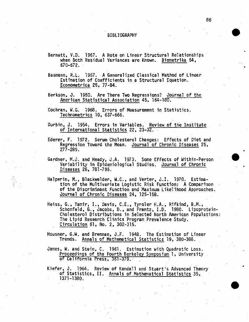
86

BIBLIOGRAPHY

Barnett, V.D. 1967. A Note on Linear Structural Relationshipswhen Both Residual Variances are Known. Biometrika 54,670-672 ..

Basmann, R.L. 1957. A Generalized Classical Method of LinearEstimation of Coefficients in a Structural Equation.Econometrica 25, 77-84.

Berkson, J. 1950. Are There Two Regressions? Journal of theAmerican Statistical Association 45, 164-180.

Cochran, W.G. 1968. Errors of Measurement in Statistics.Technometrics 10, 637-666.

Durbin, J. 1954. Errors in Variables. Review of th'e Instituteof International Statistics 22, 23-32.

Ederer, F. 1972. Serum Cholesterol Changes: Effects of Diet andRegression Toward the Mean. Journal of Chronic Diseases 25,277-289.

Gardner, M.J. and Heady, J.A. 1973. Some Effects of Within-PersonVariability in Epidemiological Studies. Journal of ChronicDiseases 26, 781-795.

Halperin, M., Blackwelder, W.C., and Verter, J.I. 1970. Estima­tion of the Multivariate Logistic Risk Function: A Comparisonof the Discriminant Function and Maximum Likelihood Approaches.Journal of Chronic Diseases 24, 125-158.

Heiss, G., Tamir, I., Davis, C.E., Tyroler H.A., Rifkind, B.M.,Schonfeld, Got Jacobs, D., and Frantz, I.D. 1980. Lipoprotein­Cholesterol Distributions in Selected North American Populations:The Li pid Research Clinics Program Prevalence Study.Circulation 61, No.2, 302-315.

Housner, G.W. and Brennan, J.F. 1948. The Estimation of LinearTrends. Annals of Mathematical Statistics 19, 380-388.

James, W. and Stein, C. 1961. Estimation with Q~adratic Loss.Proceedings of the Fourth Berkeley Symposium' 1, Universityof California Press, 361-379.. '

Kiefer, J. 1964. Review of Kendall and Stuart's Advanced Theoryof Statistics, II. Annals of Mathematical Statistics 35,1371-1380.

..

87

Kleijnen, J.P.C. 1974. Statistical Techniques in Simulation:Part 1. Marcel Dekker, Inc., New York. .

Lindley, D.V. and Smith, A.F.M. 1972. Bayes Estimates for LinearModels. Journal of the Royal Statistical Society B, 34, 1-41.

Madansky, A. 1959. The Fitting of Straight Lines when BothVariables are Subject to Error. Journal of the AmericanStatistical Association 54, 173-205.

Moran, P.A.P. 1971. Estimating Structural and Functional Relation­ships. Journal of Multivariate Analysis I, 232-255.

Neyman, J. and Scott, E. 1951. On Certain Methods of Estimatingthe Linear Structural Relationship. Annals of MathematicalStatistics 22, 352-361. (Correction 23, 135) ... .. .

Snedecor, G.W. and Cochran, W.G. 1967. Statistical Methods. 6thEdition, Tbe Iowa State University Press, Ames, Iowa.

Theil, H. 1961. Econometric Forecasts and Policy. 2nd Edition,North-Holland PUblishing Company, Amsterdam.

Truett, J., Cornfield, J., and Kannel, W. 1967. AMultivariateAnalysis of the Risk of Coronary Heart Disease in Framingham.Journal of Chronic Diseases 20, 511-524 .

Tukey, J.W. 1951. Components in Regression. Biometrics 7,33-69.

Wald, A. 1940. The Fitting of Straight Lines if Both Variablesare Subject to Error. Annals of Mathematical Statistics 11,

Walker, S.H. and Duncan, D.B. 1967. Estimation of the Probabilityof an Event as a Function of Several Independent Variables.Biometrika 54, 167-179.

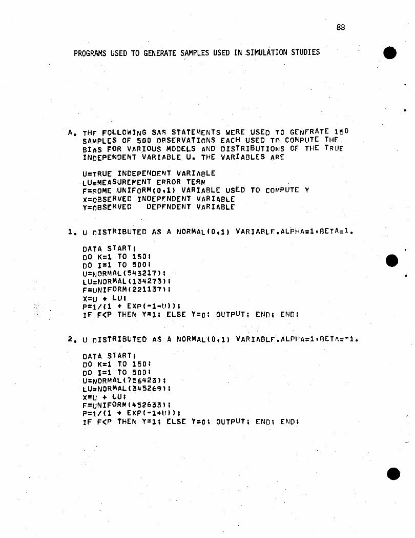
88

PROGRAMS USED TO GENERATE SAMPLES USED IN SIMULATION STUDIES

A. THr FOLLOWING S~~ STATEMENTS WERE USED TO GfNrRATE 15 0SA~PLES OF 500 OBSERVATIONS EACH USED Tn COMPUTE THFBIAS FOR VARIOUS MODELS AND DISTRIBUTIONS or THE TRUEHJOEPENDENT VARII\BLE U. THE VARIAOLES ARE

U=TRUE INDEPENDENT VARIABLELU=MEASURE"ENT ERROR TERMF=~OME ~NIFoRM(O,l) VARIABLE USED TO COMPUTE VX=OBSERVEDINDEPrNDENT VARIABLEV=OsSERVEO OEPrNOENT VARIABLE

1. U nISTRIBUTED AS A NORMALCO,l) VARIABLr.AL~HA=1.8ETA=1.

DATA START;00 K=l TO 150;DO 1=1 TO 500;U=NORMALCSQ3211);LU=NORMAL C13Q213) ;F=UNIFORMC221131l;X=U + LU;P=l/Cl + EXPC-l-U»;IF F(PTHEN V=l; ELSE V=O; OUTPUT; END; END;

2. U nISTRIBUTEO AS A NORMALCO.l) VARII\BLr.ALPt'A=1.8ETfI=-1.

DATA START;DO K=l TO 150;DO 1=1 TO 500;U=NORMALC7~6q23)1

LU=NORMALC!45269);X=U + LUIF=UNIFORMCQ52633);p=t/Cl + EXPC-l+U»;IF F(P THEN V=11 ELSE V=O; OUTPUT; END; END;

..

..

•

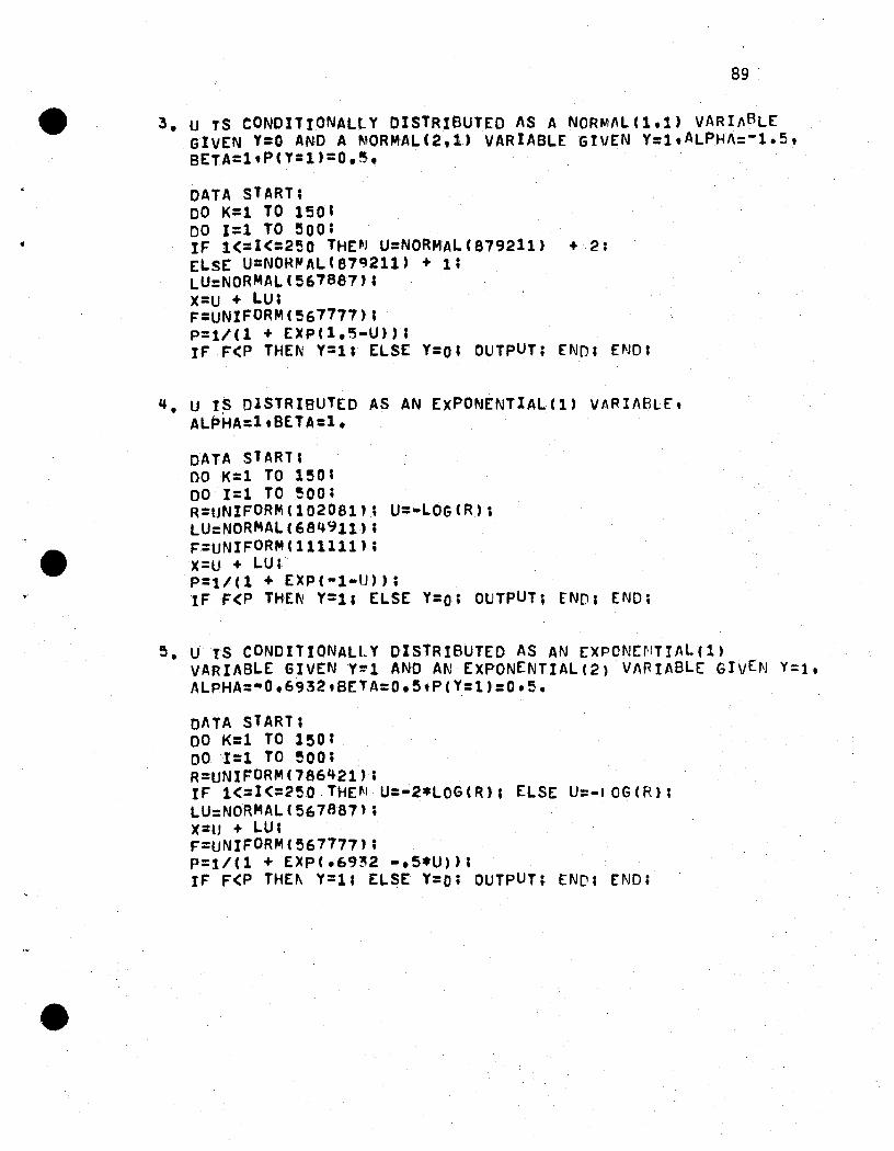
89

3. U TS CONDITIONALLY DISTRIBUTED AS A NORMALC1.1) VARIABLEGIVEN Y=O AND A NORMALC2,1) VARIABLE GIVEN Y=1,ALPHA:-l.5.BETA=1,PCY=1)=O.~.

DATA START;00 K=1 TO 150;00 1=1 TO 500;IF 1(=1<=250 THEN U=NORMAL(879211) + 2:ELSE U=NOR~ALCe79211) + 1;lU=NORMAL(567887);x=u + LU;F=UNIFORM(567777);p=t/C1 + EXPC1.5-U»;IF F(P THEN Y=1; ELSE Y=Ol OUTPUT; END; END;

~. U IS DISTRIBUTED AS AN EXPONENTIAL(1) VARIABLE,ALPHA=ltBETA=l.

DATA START;DO K=l TO 150;DO· 1=1 TO 500;R=UNIFORMCI02081); U=-LOGCR);LU=NORMAL(684911);F=UNIFORMC111111';x=u + LU;P=t/C1 + EXPC-1-U»;IF F(P THE~ Y=1; ELSE Y=o; OUTPUT; END; END;

5. UtS CONDITIONALl.Y OIsTRIBUTED AS AN EXPONEf'ITIAL(1)VARIABLE GIVENY~l AND AN EXPONENTIAL(2) VA~IJ\BLE GIVEN Y=1,ALPHA=-O.6932.BETA=O.5tP(Y=1)=O.S.

DATA START;DO K=l TO 150;001=1 TO 500;R=UNIFORMC786421';IF 1(=1<=250 THE'" U=-2*LOG CR); ELSE U=-I OG CR) ;LU:NORMALC567887';x=u + LU;F=UNIFORMC567777';P=t/Cl + EXPC.69~2 -.5*U»;IF F(P TH£~ Y=1; ELSE Y=O; OUTPUT; END; END;

90

6, U1.U2 ARE 8IVARIl\TE NORMALS WITH MEANS n. VARIANCES 1ANn CORREL~TION=O,25.ALPHA=1.BETA1=1.BrTA2=1.

DATA SlART;00 K=l TO 150;00 1=1 TO ~oo;

U1=NORMALCQ29673);C=NORMALC7e23~7);

u2=.25*U1 + .9683*C;LU2=NORMAL(23781 Q);Xl=U1;X2=U2 + LU2;F=uNIFORM(543221);p=t/(l + EXPC-1-UI-U2»;IF F(P THEN Y=l; ELSE Y=O; OUTPUT; END; END;

7. U1,U2 ARE BIVARIATE NORMALS WITH MEANS n. VARIANCES 1ANn CORREL~TION=O.75.ALPHA=1,BETA1=1.Br.TA2=1.

DATA START;00 K=1 TO 150;DO 1=1 TO 500;U1=NORMAL(Q29673);C=NOR~AL(1e2347);

u2=,75*Ul + .6614*C;LU2=NOKMAL(23781Q);xl=Ul;X2=U2 + LU2;F=UNIFORM(543221);p=t/(1 + EXPC-l-U1-U2»;IF F(P THENY=l; ELSE Y=o; OUTPUT; END; END;

8, THr FOLLOWING SA~ STATEMENTS WERE USED TO GENERATE150 SAMPLES OF 500 OBSERVATIONS EACH usre TO COMpUTETHr VARIOUS ESTTMATORS OF BETA. THE VARIABLES AREDE~CRIBED IN A, WITH THE FOLLOWING ADDITIONS:

W=A NORMALCO.l) VARIABLE USED TO COMPUTr Z.Z=THE INS1RUMENTAL VARIABLERHo=CQRRELATION RETWEEN U AND Z

.. I

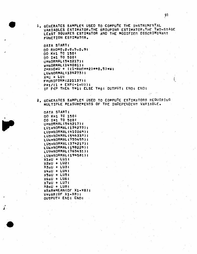
J

.J

91,

1. GENERATES SAMPLES USED TO COMPUTE THE INSTRUMENTALVARIABLES E~TIMATOR,THE GROUPING ESTIMATOR,THE TWO-STAGELEAST SQUARES ESTIMATOR AND THE MOOIFIEn DISCRIMINANTFUNCTION ESTIMATOR.

DATA START;00 RHO=0.2,O.5,O.9;00 K=1 TO 150;00 1=1 TO 500;U=NORMALCS~3217);

W=NORMAL(1~q081);

Z=RHO*U + (Cl-RHO*.2)**O.S).W;LU=NORMAL(134273);x=u + LU;F=UNIFORM(221137);P=t/(l + EXPC-l-Ut);IF F<P THEN Y=l; ELSE Y=o; OUTPUT; END; END;

2, GENERATES SAMPLE~ USED TO COMPUTE ESTIMftTORS REQUIRINGMULTIPLE MEASURr.~ENTS OF THE INDEPENDENT VARI~8LE,

DATA START;00 K=l TO 150;DO 1=1 TO sao;U=NORMAL(5~3217);

LU1=NORMALC13~273);

LU,=NOMMAL(41006Q );

LU~=NOHMAL(5~633~);

LU~=NORMALC7S5~5!\);

LUS=NORMAL(374211);LU6=NORMAL(1 98229);LU7=NORMAL(765431);LUa=NORMAL(1 94581);Xl=U + LU1;x2=U + LU2:X3=U + LU3;X4=U + LU~;

xS=U + LUS;X6=U + LU6;x7=U + LU7:X8=U + LU8:X8AR=~EAN(OF Xl-X8);V=VARCOF Xl-X8);OUTPUT; E~C; END;

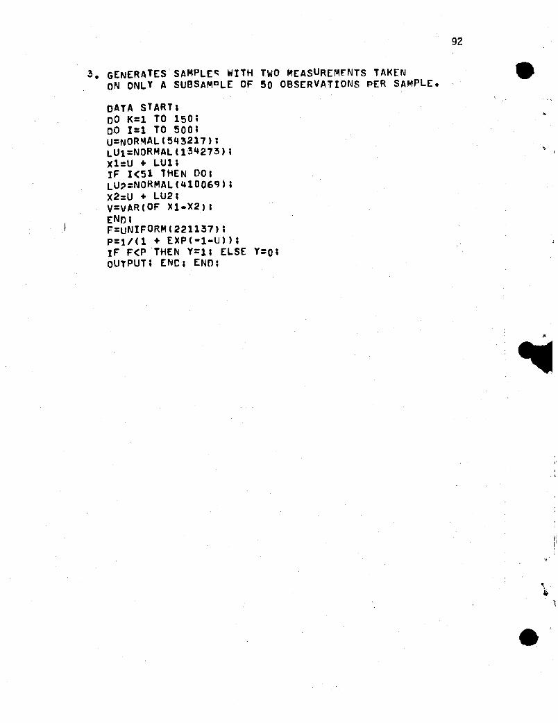
3. GENERATES SAMPLE~ WITH TWO MEASUREMENTS TAKENON ONLY A SUBSAMDLE OF 50 OBSERVATIONS PER SAMPLE.

DATA START;00 K=l TO 150;00 1=1 TO 500;U=NORMALC5~3217);

LU1=NORMALC1~4273);

XI=U + LUI;IF 1<51 THEN 00;LU,=NORMAL(410069);X2=U + LU2;V=VARCOF X1-X2)1END;F=UNIFORM(221137);p=t/Cl + EXPC-I-U));IF F<PTHEN Y=1; ELSE Y=o;OUTPUT; ENe; END;

92