the effect of ceiling configurations on indoor air motion ... for orbi.pdf · natural ventilation...

Published in : Building & Environment 46 (2011)1211-1222

Status : Postprint (Author’s version)

The effect of ceiling configurations on indoor air motion and ventilation

flow rates

Anh Tuan Nguyen, Sigrid Reiter

Local Environment Management and Analysis (LEMA), University of Liège, Belgium

ABSTRACT

The purpose of this paper is to evaluate the effects of a building parameter, namely ceiling configuration, on

indoor natural ventilation. The computational fluid dynamics (CFD) code Phoenics was used with the RNG k-ε

turbulence model to study wind motion and ventilation flow rates inside the building. All the CFD boundary

conditions were described. The simulation results were first validated by wind tunnel experiment results in

detail, and then used to compare rooms with various ceiling configurations in different cases. The simulation

results generated matched the experimental results confirming the accuracy of the RNG k-ε turbulence model to

successfully predict indoor wind motion for this study. Our main results reveal that ceiling configurations have

certain effects on indoor airflow and ventilation flow rates although these effects are fairly minor.

Keywords : Natural ventilation ; Ceiling configurations ; RNG k-ε ; turbulence model ; Ventilation flow rates

1. Introduction

In architecture, natural ventilation is often used as a low-energy environmental solution to improve indoor

microclimates and thermal comfort in buildings. In hot and humid tropical climates natural ventilation is

particularly effective as it maintains the equilibrium of relative humidity inside and outside buildings, and

prevents indoor humidity from condensing. Most folk and traditional architectures in many parts of the world

have successfully applied natural ventilation solutions to solve various indoor environmental problems.

In the formation of an architectural space, the ceiling and floor are the two factors that are absolutely

indispensable. In the indoor spaces of folk or traditional architecture, the ceilings are generally consistent with

the roofs and therefore varied and often dependent on roof forms. A certain typical type of ceiling and roof in a

specific region is often influenced by the natural environment, climate, culture, religion, local materials and

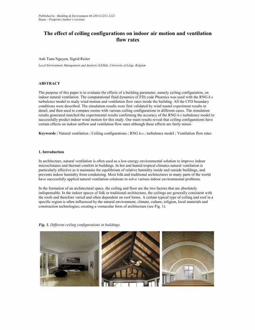
construction technologies; creating a vernacular form of architecture (see Fig. 1).

Fig. 1. Different ceiling configurations in buildings.



Natural ventilation is the process of air exchange between an indoor and outdoor space by natural mechanisms.

According to CIBSE [1], besides mechanically assisted ventilation, there are three types of natural ventilation in

buildings: cross ventilation; single-side ventilation and stack ventilation. Cross ventilation and single-side

ventilation, which are generally called wind driven ventilation, are caused by natural wind while stack

ventilation is driven by the increased buoyancy of air as it warms up. The majority of buildings employing

natural ventilation rely mainly on wind driven ventilation. However, stack ventilation has many advantages,

especially in moderate and cold climates. Ideal designs for naturally ventilated buildings should take full

advantage of both types of ventilation.

Khan et al. [2] made an extensive investigation and reported seven passive ventilation strategies, including:

(1) window openings,

(2) atria and courtyards,

(3) wing walls,

(4) chimney cowls/exhaust cowls,

(5) wind towers,

(6) wind catchers and

(7) wind floor — air inlet system.

We also assume

(8) solar chimneys and

(9) underground ventilation ducts

as two other ventilation strategies which were not mentioned by these authors.

Natural ventilation is obviously an important architectural feature in hot humid climates as wind motion removes

heat concentration and humidity thereby improving thermal comfort.

ASHRAE standard 55 [3] reported that an air speed of 0.8 m/s would reduce operative temperature by 2.6 °C, on

condition that air temperature is equal to radiant temperature, on human thermal sensation.

It is obvious that natural ventilation in a building is affected by many building related parameters. The results of

various studies on how different architectural elements affect natural ventilation generally show a strong

correlation between indoor wind motion and building parameters such as the size and type of window [4,5], roof

style and height [6], shade panels — roof eaves — balcony [7], atria — courtyard [8,9], building arrangement

[10] and environment density [11 . The study carried out by Kato et al. [12] on cross ventilation in cubic models

using a wind tunnel and Large Eddy Simulation also confirmed that indoor configurations strongly effect wind

motion and flow rate.

Chen [13] carried out a review study on the method of ventilation performance prediction for buildings. Seven

methods were examined, including:

(1) analytical models,

(2) empirical models,

(3) small-scale experimental models,

(4) full-scale experimental models,

(5) multi-zone models,

(6) zonal models, and

(7) CFD (Computational Fluid Dynamics) models.

He also emphasized that CFD models have accounted for 70% of the ventilation performance studies published

in the past year.

In this study, we analyzed naturally driven air motion measured inside buildings by using a CFD model in order

to explain the effects of ceiling configurations on wind flow patterns and volumetric flow rates. The latest

version of Phoenics code [14] was employed to handle the problem. With Fluent code, Phoenics is currently one

of the mostly used codes in academic CFD research [15-17].



2. The choice of turbulence model

The standard k-ε model has been proven effective for various engineering applications and it is widely used in

the industrial sector. Barbason and Reiter [18] compared various turbulence models and reported that the choice

of k-ε was a good compromise except for natural ventilation with significant indoor thermal loads. However,

certain characteristics of wind flow, such as the creation of regions with very low velocities and thus low

Reynolds numbers, particularly in near-wall regions, could not be accurately predicted by standard k-ε. This

requirement led to the formulation of a modified k-ε turbulence model, which is expected to be more effective

and more accurate for such regions. These models are the low-Reynolds number k-ε model (LR k-ε), the RNG k-

ε model and Reynolds stress model (RSM) [16].

A basic characteristic of the RNG k-ε [19] turbulence model is that it involves an analytically derived differential

formula for effective viscosity that accounts for low-Reynolds number effects. This feature of the RNG k-ε

model combined with appropriate treatment of the near-wall region gives better prediction of indoor airflow

applications than that of the standard k-ε model [16].

Gebremedhin and Wu [20] examined five RANS models (the standard k-ε, the RNG k-ε, the LR k-ε, the k-ω and

the RSM) using Phoenics code for a space occupied by 10 cows. Based on convergence and computational

stability criteria, they stated that the RNG k-ε model "was found to be the most appropriate model to characterise

the flow field in a ventilated space".

Gloria Gomes et al. [21] carried out some experiments and numerical simulations on Phoenics code to

investigate the effect of different irregular-plan shapes on airflow. They reported that the RNG k-ε model results

matched the experimental results quite accurately.

Chen [22] compared five different k-ε models, including a standard k-ε model, a low Reynolds number k-ε

model, a two-layer k-ε model, a two-scale k-ε model, and a renormalisation group (RNG) k-ε model.

Corresponding experimental data from relevant literature on the subject were used for validation. He found the

RNG k-ε model is slightly better than the standard k-ε model and is therefore recommended for simulations of

indoor airflow and stated that the performance of the other models was not stable.

The results mentioned above show that the RNG k-ε model gives fairly good results and is an appropriate

turbulence model for the simulation of indoor airflow. Therefore, RNG k-ε was chosen for this study.

3. Validation of CFD numerical results

Validation demonstrates the ability of both the user and the CFD code in accurately predicting representative

indoor environmental applications for which some form of reliable data is available. In this study, the numerical

results were compared with similar experiments performed by Jiang et al. [23] to validate reliability of the RNG

k-ε turbulence model.

3.1. Experimental data

Jiang et al. [23] carried out a wind tunnel experiment at Cardiff University to study the flow field in and around a

cubic model which allowed cross ventilation. The wind tunnel had a cross section dimension of 2 m in width and

1 m in height. The maximum wind speed in the tunnel was about 12.0 m/s and its variation between

measurement runs was within 2%. A 6.0 m upstream fetch in the tunnel used a combination of blockage, fences

and surface roughness (Lego Duplo blocks) to simulate the lower part of an urban atmospheric boundary layer.

The cubic model was 250 mm × 250 mm × 250 mm in dimension with a 84 mm × 125 mm opening in both

windward and leeward wall. The wall thickness was 6 mm evenly. Wind velocities were measured along 9

vertical lines at the center section of the model with 18 measurement points on each line (see Fig. 2).



Fig. 2. Locations of wind velocity measurement on the symmetrical section of the model (thick dark block) and

model configurations (all dimensions in mm).

4. The numerical scheme

4.1. Governing equations

The RNG k-ε model [24] is a two-equation turbulence model, similar to the standard k-ε model, which is derived

by using Renormalisation Group methods. This model differs from the standard k-ε model only due to the

modification of ε to the equation. The governing equations are the time-averaged continuity (1), momentum (2)

and transport equations for k (3) and ε (4), as follows:

where ui, uj are the mean and fluctuating velocity components in the xi, xj direction, respectively; p is the mean

pressure; ρ is the fluid density; k and ε stand for the turbulence kinetic energy and its rate of dissipation,

respectively; vt = Cµk2/ε (isotropic eddy viscosity), η = kS/ε, S = (2SijSij)

1/2 and Sij = (∂ui/∂xj + ∂uj/∂xi)/2 (mean

strain tensor).

The turbulence constants are: σk = 0.7179; σe = 0.7179; Cµ = 0.085; cε1 = 1.42; cε2 = 1.68; η0 = 4.38; β =

0.015.

4.2. =ear-wall treatment

The k-ε model is not able to predict the flow in the near-wall region due to the viscous effect and low Reynolds

number within this region. Two available methods are proposed for near-wall modeling: the Low Reynolds

number model [25] and the wall-function method [26].

In this study, the near-wall boundary layer was treated by employing the equilibrium Logarithmic wall-function

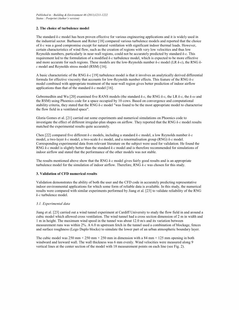
method: for the viscous (laminar) sublayer and log-law sublayer [27]. These layers are presented in Fig. 3. This

method is reported to be the most suitable solution for isothermal simulation [28] and may be written as follows:



Strictly this law should be applied to a point whose y+ value is in the range 30 < y

+ < 130

Strictly this law should be applied to a point whose y+ value is in the range 0 < y

+ < 5

where:

• u+ is dimensionless velocity

• ur is the absolute value of the resultant velocity parallel to the wall at the first grid node,

• uτ is the resultant friction velocity uτ =

• y is the normal distance of the first grid point from the wall,

• y+ is the dimensionless wall distance y+ = ρuτy/µ,

• Cµ is a constant equal to 0.085 in the RNG k-ε model,

• κ is the von Karman constant equal to 0.42

• E is a function of the wall roughness parameter (in Phoenics, for smooth wall, E = 8.6).

Fig. 3. Typical velocity distribution in near-wall region (after Wilcox [29]).

4.3. Discretisation technique

The finite volume method was implemented for the spatial discretisation of the research domain by applying 3-D

structured Cartesian mesh. As reported by Loomans [30] and Phoenics [28] as well as by grid testing, grid

distribution must be continuous to reduce the rate of change of grid size across region boundaries. The size of

adjacent cells should be equal or as close to equal as possible to avoid serious numerical errors during

simulation. Besides, Grid merge tolerance must be less than or equal to the thickness of the smallest component.

Power-law distribution method [28] was exploited to ensure high grid density around the object without

increasing the total number of cells in the domain. A finer mesh was imposed in the near-wall regions in order to

accurately resolve the high-gradient regions of the flow field. After some grid dependency tests to verify the

influence of grid discretisation on numerical results, the final simulation used a non-uniform structured grid of



97 × 47 × 55 cells with the domain dimension of 121 (length) × 41 (height) × 81 (width), where L is the

reference size of the cubic model (see Fig. 2).

4.4. Time step, iteration number, and convergence criteria

In this validation simulation, we chose the Upwind scheme to discretise the convection term in the governing

equation. The SIMPLEST [28] (Semi-Implicit Method for Pressure-Linked Equations — Shortened) algorithm

which is a variant of SIMPLE algorithm was used for the solution of the systems of algebraic equations for

velocity components and pressure. The iteration uses the false-time step relaxation for the velocities u, v and w

and linear method for all other variables.

The simulation achieved convergence when the mass balance was accurate within 1% of the mass flow rate for

the whole domain. Furthermore, the variation of flow variables (u, v, w) at specified positions in the flow field

had to be less than 1% over the last 100 time steps for absolute values larger than 0.01. Convergence was

controlled by three simultaneous factors: spot monitor (unchanged values) at probe location, variables' error

(under 1%), and mass conservation (mass in - mass out = 0). In the validating simulation, the solution achieved

convergence after 2270 iterations, equal to 7 h47' CPU time (2 × 1.46 GHz, 2 Gb RAM).

4.5. Boundary conditions

We ensured the homogeneity between numerical simulation conditions and those of the wind tunnel experiment.

The variation of wind velocity with the height of the inlet follows logarithmic law, which was the case in our

experiment, and the effective roughness height was 0.003 m. The building model in the simulation was placed at

the same location as in the experiment conducted by Yiang et al. The model surface roughness was assigned to

be zero as the experimental model was made of Perspex. At the ground wall boundary, the wall-function method

was adopted with a roughness of 5 × 10-5 m. At the side and upper boundaries, the full-slip velocity condition

was adopted. The simulation was assumed to be isothermal. Details of boundary conditions are reported in Table

1.

Table 1 Details of the boundary conditions and computational parameters for the simulation.

P u V w k ε

Inflow - Uref = 10 m/s; (uz/U*) =

(1/κ)ln(z/z0)

0 0 k = 3Uref2it

2/2 ε = Cµk3/2/l

Outflow Zero external u, v, w, k, e: ∂/∂x = 0

ambient

pressure

Upper and side faces of

computational domain - (ιιn) = 0; (ui), k, ε: ∂/∂x = 0

Solid wall - 0 0 0 ∂k/∂n = 0 Equation

(8)

Relaxation method Linear False-time step False-time

step

False-time

step

Linear Linear

Relaxation factor 0.5 1 1 1 0.5 0.5

Convergence criterion 1% 1% 1% 1% 1% 1% where Uref is reference inflow velocity at height 500 mm; it is turbulence intensity; l is characteristic length; Cµ is constant equal 0.085, u2 is

wind velocity at height z; z0 is aerodynamic roughness length; U* is total friction velocity [U* = Urκ/ln(zr/z0)] ; (un), (ui) are normal and

tangential velocity component at 1st grid cell adjacent to upper and side wall; n is local coordinate normal to the wall.

A further problem needed to be resolved. The results of many studies [31-33] have pointed out that the k-ε

turbulence model does not accurately predict the flow field above a cube due to an incorrect prediction of

turbulence kinetic energy k at the frontal sharp edge, that might interfere with the pressure distribution behind the

object. To obtain a better prediction of the recirculation flow at the top of the cube, this study adopted the

suggestion of Gao and Chow [34] by limiting the longitudinal velocities in the first cell adjacent to the sharp

edge of the cube, and setting appropriate wall functions at the intersection cells for the velocity components (see

Fig. 4).



Fig. 4. The incorrect prediction of recirculation above a cube by the k-ε model (a); compares with its correction

by Gao and Chow's method (b); and wind tunnel experiment (c).

Fig. 5. Mean velocity U/Uref on 9 vertical lines at center section of the model (Black dots: experiment; solid line:

R=G k-ε model simulation in this study).



Fig. 6. Mean velocity V/Uref on 9 vertical lines at center section of the model (Black dots: experiment; solid line:

R=G k-ε model simulation in this study).

5. Validation of the results

This section will compare the experimental results and the numerical simulation in detail. First, the mean

velocity distributions outside and inside the model will be analyzed and then the wind flow pattern on the model

will be discussed.

Figs. 5 and 6 show comparisons of the mean velocity U/Uref and V/Uref distributions on 9 vertical lines at the

center of the section of the model (U, V are mean velocities on x and y axes, respectively). With the same inlet

wind profile at x = -3H, it is clear that results generated by the RNG k-ε model generally matched those from the

experiment. It is notable that this agreement is even better inside the model (0 < x < H, y < 0.25).



Fig. 7 illustrates the wind flow pattern around the model both generated by the simulation and in the practical

experiment. Similar wind distribution was obtained, especially inside the model where the velocity vectors'

distribution was almost the same.

Even so, some discrepancies between experimental and numerical results exist. The simulation generally seems

to underestimate the wind speed above the top of the model in both x and y directions (y > 0.25). As can be seen

from Fig. 7, the recirculation area above the roof of the model is higher and a little bigger in the simulation

which leads to the underestimation of the wind velocity. As reported above, the k-ε model does not accurately

predict the flow field above the cube although a correction of the boundary condition was established. Near the

ground boundary, small discrepancies may be attributed to coarseness of the mesh dividing near the floor.

Discrepancies might also come from the differences in boundary conditions present during the two studies that

are very difficult to eliminate such as inlet turbulence intensity, the effect of heat transfer, errors in measurement

etc. during the experiment.

Generally the comparisons correlated confirming the reliability of the RNG k-ε model in accurately predicting

the airflow field in and around the building. Therefore, the RNG k-ε model can be used for other simulations

with confidence for similar model configurations.

Fig. 7. Wind velocity distribution around the model by R=G k-ε simulation in this study (left) and in the practical

experiment (right).

Fig. 8. Configurations of the ceiling shapes. The 3-D models are presented from left to right in order from 1 to 6.



6. 3-D simulation settings and results of the present study

6.1. Model configurations

This study concentrates on the effect of ceiling shape on indoor ventilation. Six different typical cross section

types were investigated (see Fig. 8). All the models were cubes with identical dimensions of 5 m in order to

eliminate the effect of outside shape on the indoor wind distributions. All the walls were set identically to be 0.2

m thick. On the windward wall of each model, there was a window measuring 1.2 m × 2 m with a sill height of

0.9 m while on leeward wall there was a door measuring 0.8 m × 2.1 m located near an edge. All the models had

different cross section types, but the same volume of 74.06 m3 in cases 1, 1*, 3 and 64.51 m3 in case 2, which

also means they had the same average height of 3.5 m in cases 1, 1*, 3 and 2.8 m in case 2. Models 4 and 5 had

similar configurations on the cross sections, but the difference is that model 4 had a two-slope ceiling while

model 5 had a four-slope ceiling in the form of a pyramid.

Four cases were investigated as shown in Table 2 (case 1*, using the wind profile of an open flat terrain in

Hanoi, Vietnam, in order to compare the influence of a different wind profile on numerical results).

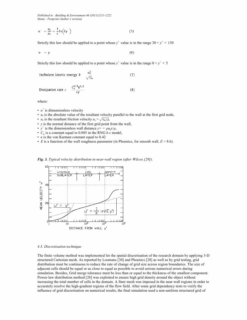
Table 2 Wind incident angles, reference velocity and average ceiling heights of the cases.

Number of

models

investigated

Wind incident

angle α

Average ceiling

height (m)

Uref at inlet (m/s) Note

Case 1 6 0° 3.5 10 Wind profile of validation case

Case 1* 6 0° 3.5 1.85 Wind profile of an open flat terrain in Hanoi -

Vietnam



6.2. Grid and numerical parameters dependency test

A comparative study on the dependence of the results on the initial numerical settings was implemented. We

made a comparative study on model 1 of case 1 in two steps: a grid dependency test (step 1) and other

parameters dependency test (step 2). In step 1, six different grid densities were tested. These settings and test

results are listed in Table 3.

From Table 3, it is clear that the three grid settings with the highest densities (D, E and F) gave stable and similar

results as the maximum discrepancy was only 0.47%. Among them, grid setting D required less CPU time, so it

was adopted in step 2. In step 2, four discretisation schemes available in Phoenics (Upwind, Hybrid, Smart,

Quick) and two convergence criterions (1% and 0.1%) were tested for their influences on results' stability by

running seven other simulations. These combinations and results are shown in Table 4.

The flow rates and velocities shown in Table 4 reveal that differences between these combinations were very

small — under 1% (Quick and Smart scheme could not give a converged solution). A low convergence criterion

(0.1%) did not considerably change the solution but was much more time consuming.

Based on the results of this test, all subsequent simulations applied the following combination: a high grid

density (250,745 cells); Upwind scheme and a 1% convergence criterion. Other boundary conditions were set to

be the same as those of the validation case mentioned above (see Fig. 9).



Table 3 Grid dependency test.

Grid density Number of

grid cells

Iteration at

convergence

CPU time Flow rate (m3/s) Velocity at the center of the window (m/s)

A. Lowesta 90,400 2460 3h1 7' 8.972 4.181

B. Low 126,000 2511 5h30' 9.399 4.189

C. Medium 191,634 2452 6h56' 10.157 4.214

D. High 250,745 2645 8h46' 10.978 4.638

E. Very high 304,980 2762 11h11' 10.931 4.660

F. Highestb 352,512 3300 16h20' 10.968 4.643

a Lower grid densities were not suitable because the wall thickness of the models was 0.2 m. b Higher grid density would make the solution difficult to converge.

Table 4 Other parameters dependency test.

Discretisation

scheme

Convergence criterion

(%)

Iteration at

convergence

CPU time Flow rate (m3/s) Velocity at window center (m/s)

Upwind 1 2645 8h46' 10.978 4.638

0.1 2800 9h02' 10.978 4.639

Hybrid 1 3105 10h10' 10.968 4.689

0.1 4269 15h58' 11.050 4.689

Quick 1 Solution did not

converge

0.1

Smart 1 Solution did not

converge

0.1

Fig. 9. Center section of the numerical domain shows model's position and grid distribution.

6.3. Calculation method

To compare the numerical results of different models and cases, ventilation flow rates and wind distributions

were analyzed in the following ways.

6.3.3. Ventilation flow rate

Volumetric flow rate Q is obtained by several methods. In simple design calculations, flow rate through the

cross-ventilated model was computed by an empirical method based on the Bernoulli equation:

where Cd is the discharge coefficient of the openings; A is opening area ((1/A2) = (1/Ain2) + (1/Aout

2)); ∆CP is

mean pressure coefficient across the openings.



In this study, Q was calculated by using a definition equation. In cross-ventilated cases with the fluid assumed

incompressible (ρ = const), given an opening area A at the inlet, and a fluid flowing through it with uniform

velocity U and an angle θ away from the perpendicular direction to A, the flow rate is:

For a non-uniform flow, considering the mean velocity in the direction perpendicular to the area A, equation

(10) becomes:

A is the area of the windward window equal to 2.4 m2; ui indicates the velocity magnitude in one of the small

parts of A, Ai refers to the area of a part of A; was computed by a supplemental tool named INFORM in

Phoenics (higher CFD grid resolution on the window area will give a more accurate value). Therefore, Q can

easily be calculated with high accuracy.

6.3.2. Wind distribution

In order to evaluate the differences of indoor wind motion, this study used the approach of Kindangen et al. [6]

in which the following non-dimensional indoor air motion parameters were computed, based on 81 grid points in

each model:

where v,· is the mean velocity at interior location i (m/s); Uref is the reference free-stream velocity at the height of

10 m (10 m/s); n is the number of points measured in each model (n = 81 ); σs(vi/Uref) is the standard deviation of

(vi/Uref), with the standard deviation defined as:

Cv is a wind flow parameter used to indicate the relative average velocity magnitude of indoor wind movement,

in this case on two plane heights 0.9 m (working plane) and 1.75 m (mid-room height). Csv is a coefficient used

to evaluate the homogeneity of indoor wind distribution. A low Csv value means wind distribution is uniform and

vice versa. A high flow rate with a low Csv (explained later) is a sign which confirms good ventilation.

6.4. Results and discussion

In Fig. 10, the ventilation flow rates of the six models are compared. In all cases, model 3 generally performed

better while ventilation rates of the other models were unstable. Nevertheless, disparity between the six models

was not significant due to the small difference of average velocities at the window. The largest difference

occurred in case 3 between model 2 (which had the lowest flow rate) and model 3 (which had the highest flow

rate) and was equal to 0.45 m3/s (4% of Qmax in case 3). Case 1 had the smallest difference between the six

models.

The comparison of ventilation flow rates between cases 1 and 1* demonstrates that the different wind profiles

did not make any changes to the ventilation performance between models.



As reported by Kato et al. [12] and Kobayashi et al. [35], a significant static pressure drop usually occurs across

the windward opening; and the cross ventilation flow rate is directly related to indoor pressure (see equation (9))

caused by the interaction between airflow and interior enclosure. Behind the "vena contracta" point (point at

which the diameter of the air stream is smallest) near the windward opening, the kinetic energy of the airflow is

diffused into the room space. If there is no wind-blockage and the airflow is smoothly exhausted from the room,

it will preserve most of its kinetic energy and thus the ventilation flow rate will be higher. If the airflow has to

change its direction, more kinetic energy will be transformed into turbulence kinetic energy through Reynolds

stress and mean strain interaction. Consequently, a smaller static pressure drop across the inlet opening is

obtained which leads to a lower ventilation flow rate. Thus, the following considerations were derived from

these principles:

- A lower Csv, is synonymous with homogeneous wind distribution whereby more kinetic energy of the airflow is

transformed to turbulence kinetic energy leading to a lower ventilation flow rate (see Figs. 10 and 11a).

- The difference of flow rates between models was small due to the short distance between the inlet (window)

and outlet (door), and the small room volume of these models, especially as the openings were comparatively

large. These settings caused small differences in indoor dissipation of kinetic energy between models and small

differences of indoor static pressure, and thus small differences of flow rate.

As shown in Fig. 11a, model 5 seems to have a more homogeneous wind distribution than the others since it had

the lowest Csv values in both plane heights, whereas model 3 had the peak Csv, which means a non-uniform wind

distribution inside. This result once again, shows that disparities of Csv between these models were not

significant in each case, but between cases, Csv fluctuated.

In the case with the wind incident angle of 45° the direction of the incoming air stream nearly coincides with the

line connecting the window and the door (case 3), Csv significantly increased whereas ventilation flow rate was

almost unchanged (see Fig. 10). These signs clearly indicate that only the space between inlet and outlet of the

room was well-ventilated, wind motion in other parts might be very limited. In other words, wind distribution in

case 3 was not homogeneous. In this case, the airflow went smoothly from inlet to outlet and then discharged

without losing much kinetic energy, which is required to avoid stagnation of the air indoors.

This phenomenon was relatively consistent with Givoni's finding [36] that better ventilation conditions are

obtained when the air stream has to change direction within the room, than when the flow goes directly from

inlet to outlet.

As shown in Fig. 11b, it is clear that different models have different average velocity coefficients which means

ceiling configurations have certain effects on indoor air motion although these effects are minor. Fig. 11b shows

that disparities of Cv between the six models in three cases were not significant. Besides, almost no agreement of

Cv between the two plane heights of 0.9 m and 1.75 m was obtained. Thus, it is difficult to draw any conclusions

about which models provide better ventilation in the cases we studied.

From the simulations, we found that the maximum velocities usually occurred at an inlet or outlet at the heights

of 0.9 m and 1.75 m. The comparison of the Cvmax of the six models shows that the peak Cvmax was usually

obtained in model 3 (Fig. 11e). This supports the previous finding that model 3 achieved the highest flow rate in

comparison to the other models.

However, in case 3, the Cvmax of the six models is almost equal. It is noteworthy that the ventilation flow rate of

the six models in case 3 was different. Thus, it is impossible to draw the conclusion that different flow rates lead

to different maximum velocities, and vice versa.



Fig. 10. Comparison of ventilation flow rate in cases 1, 2, 3 (left) and case 1* (right).

Fig. 11. Comparison of Csv (a); C„ (b) and Cvmax (c) of six models in three cases.



6.4.1. The role of ceiling height

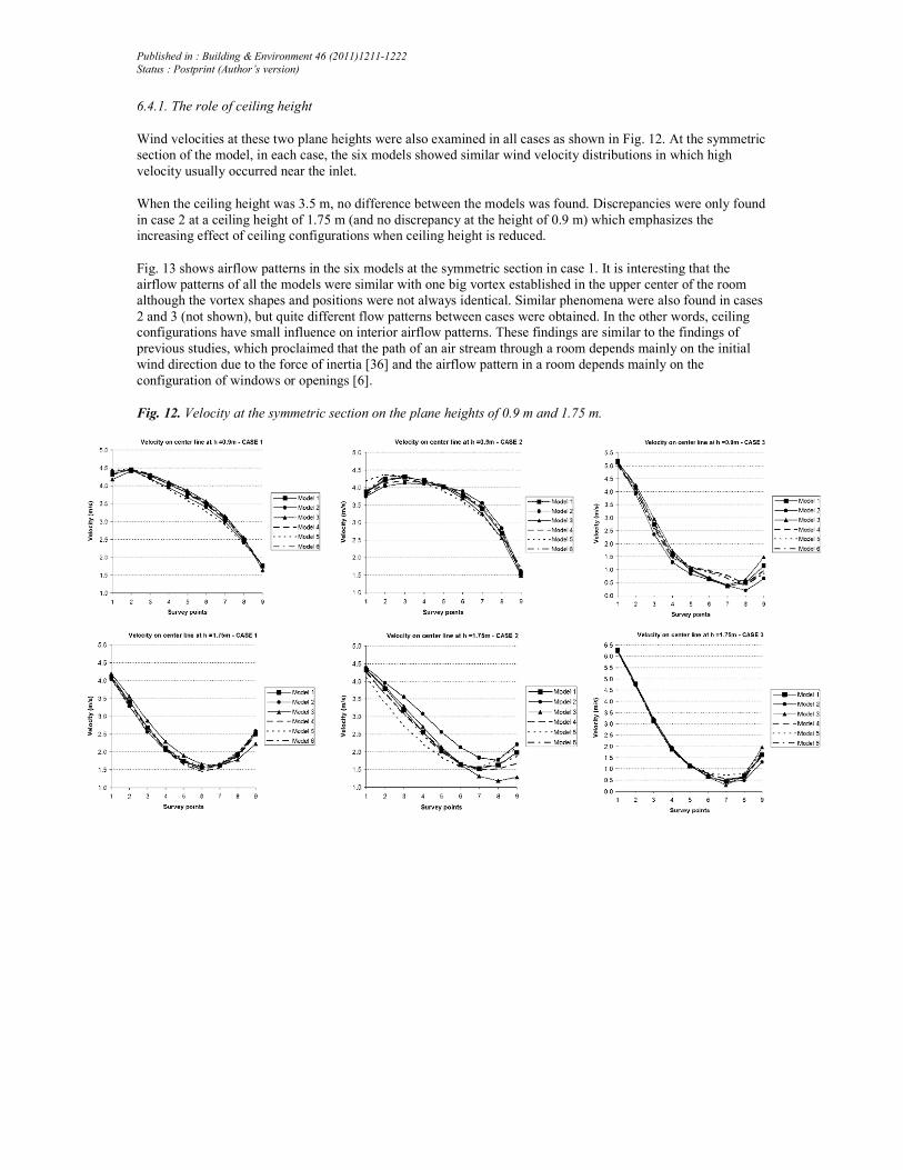
Wind velocities at these two plane heights were also examined in all cases as shown in Fig. 12. At the symmetric

section of the model, in each case, the six models showed similar wind velocity distributions in which high

velocity usually occurred near the inlet.

When the ceiling height was 3.5 m, no difference between the models was found. Discrepancies were only found

in case 2 at a ceiling height of 1.75 m (and no discrepancy at the height of 0.9 m) which emphasizes the

increasing effect of ceiling configurations when ceiling height is reduced.

Fig. 13 shows airflow patterns in the six models at the symmetric section in case 1. It is interesting that the

airflow patterns of all the models were similar with one big vortex established in the upper center of the room

although the vortex shapes and positions were not always identical. Similar phenomena were also found in cases

2 and 3 (not shown), but quite different flow patterns between cases were obtained. In the other words, ceiling

configurations have small influence on interior airflow patterns. These findings are similar to the findings of

previous studies, which proclaimed that the path of an air stream through a room depends mainly on the initial

wind direction due to the force of inertia [36] and the airflow pattern in a room depends mainly on the

configuration of windows or openings [6].

Fig. 12. Velocity at the symmetric section on the plane heights of 0.9 m and 1.75 m.



Fig. 13. Wind flow pattern inside six models in case 1.

6.4.2. Influence of wind incident angle

In this study, two angles of attack were used. Comparison of wind distribution and velocity magnitude in Figs.

11 and 12 shows that the angle of attack had a great influence on these variables. The comparison of Csv between

case 1 and case 3 (Fig. 11a) revealed that the angle of attack strongly affects indoor wind uniformity, especially

when the flow stream is coincided with the inlet-outlet route. However, when changing the angle of attack, no

significant disparity between models was recorded.

7. Conclusions

The present paper discusses a study on the influence of different ceiling configurations on wind induced air

motion inside a building. The goal of this study is to examine whether ceiling shape can improve natural

ventilation. The methods employed were CFD simulations on six basic models in three cases and wind tunnel

experiments from related literature for CFD validation. Parametric studies included air change rate, wind

velocity, wind distribution and its homogeneity. Results from this study revealed the following:

- The fact that CFD predictions were reasonably close to the experimental results suggests that the RNG k-ε

model performed well in predicting airflow in and around buildings with simple configurations.

- Ceiling configurations have certain effects on wind induced and indoor airflow patterns although these effects

are not significant. Comparison of indoor wind velocity, wind distribution and airflow rate showed small

disparities between the models used. When room volumes are the same, the largest disparity of flow rate found

between models was only 4% of the highest flow rate in each case.

- Ceiling height plays an important role in this study. When the ceiling height of a room decreases, the airflow

rate increases and the effect of ceiling configurations on wind motion is clearer.

- Indoor airflow depends on various building parameters as well as the characteristics of the incoming airflow.

Studies on indoor airflow should simultaneously analyse many design variables, such as the cooling potential of

natural ventilation.

In the present study, although only volumetric ventilation rates and velocity-related parameters were

investigated, the findings revealed that ceiling shape could be temporarily overlooked in the first stage of natural



ventilation design due to its relatively minor effect.

Acknowledgments

This study was financially supported by the Ministry of Education and Training of Vietnam (Grant No 624/QD-

BGDDT: 9th Feb. 2010) and partly by Wallonie Bruxelles International (Grant No 23478/AMG/BE.VN/JP/jp).

We would like to thank Dr. Jiang Yi for his support of experimental settings and results. The authors greatly

appreciate comments from the reviewers and the valuable input from Mathieu Barbason and Sébastien Erpicum.

References

[1] CIBSE. Natural ventilation in non-domestic buildings. Applications manual AM10. London: The Chartered Institution of Building

Services Engineers; 1997.

[2] Khan N, Su Y, Riffat FB. A review on wind driven ventilation techniques. Energy and Buildings 2008;40:1586-604.

[3] ANSI/ASHRAE Standard 55-2004. Thermal environmental conditions for human occupancy. Atlanta: ASHRAE Inc.; 2005.

[4] Amador AG, Lopez FA. Ventilation performance in a funneling window. Conference on passive and low energy architecture, Dublin;

2008.

[5] Heiselberg P, Bjorn E, Nielsen PV. Impact of open windows on room airflow and thermal comfort. International Journal of Ventilation

2001;1(2):91-100.

[6] Kindangen J, Krauss G, Depecker P. Effects of roof shapes on wind-induced air motion inside buildings. Building and Environment

1997;32(1):1-11.

[7] Prianto E, Depecker P. Characteristic of airflow as the effect of balcony, opening design and internal division on indoor velocity. Energy and Buildings 2002;34:401-9.

[8] Sharpies S, Bensalem R. Airflow in courtyard and atrium buildings in the urban environment: a wind tunnel study. Solar Energy

2001;70(3):237-44.

[9] Tablada de la Torre AE. Shape of new residential buildings in the historical centre of old Havana to favour natural ventilation and thermal

comfort. PhD thesis. Leuven: Katholieke Universiteit Leuven; 2006.

[10] Bady M, Kato S, Takahashi T, Huang H. Experimental investigations of the indoor natural ventilation for different building configurations and incidences. Building and Environment 2011;46:65-74.

[11] Moeseke GV, Gratia E, Reiter S, De Herde A. Wind pressure distribution influence on natural ventilation for different incidences and

environment densities. Energy and Buildings 2005;37:878-89.

[12] Kato S, Murakami S, Mochida A, Akabayashi S, Tominaga Y. Velocity pressure field of cross ventilation with open windows analyzed

by wind tunnel and numerical simulation. Journal of Wind Engineering and Industrial Aerodynamics 1992;41-44:2575-86.

[13] Chen Q, Ventilation performance prediction for buildings: a method overview and recent applications. Building and Environment

2009;44:848-58.

[14] PHOENICS 2009. Available from:. Cham Co.Ltd. http://www.cham.co.uk/; 2010.06-11-21.

[15] Nyuk HW, Heryanto S. The study of active stack effect to enhance natural ventilation using wind tunnel and computational fluid

dynamics (CFD) simulations. Energy and Buildings 2004;36:668-78.

[16] Stamou A, Katsiris I. Verification of a CFD model for indoor airflow and heat transfer. Building and Environment 2006;41:1171-81.

[17] Xu W, Chen Q. A two-layer turbulence model for simulating indoor airflow, part II. Applications. Energy and Buildings 2001;33:627-

39.

[18] Barbason M, Reiter S. About the choice of turbulence model in building physics simulation. In: 7th international conference on indoor

air quality, ventilation and energy conservation in buildings, Syracuse, New York; 2010.

[19] Yakhot V, Orszag SA. Renormalization group analysis of turbulence. I. Basic theory. Journal of Scientific Computing 1986;1(1):3-51.

[20] Gebremedhin KG, Wu BX. Characterization of flow field in a ventilated space and simulation of heat exchange between cows and their

environment. Journal of Thermal Biology 2003;28(4):301-19.



[21] Gloria Gomes M, Rodrigues AM, Mendes P. Experimental and numerical study of wind pressures on irregular-plan shapes. Journal of

Wind Engineering and Industrial Aerodynamics 2005;93:741-56.

[22] Chen Q. Comparison of different k-ε models for indoor airflow computations. Part B, Fundamentals. Numerical Heat Transfer

1995;28(3):353-69.

[23] Jiang Y, Alexander D, Jenkins H, Arthur R, Chen Q. Natural ventilation in buildings: measurement in a wind tunnel and numerical

simulation with large-eddy simulation. Journal of Wind Engineering and Industrial Aerodynamics 2003;91:331-53.

[24] Yakhot V, Orszag SA, Thangam S, Gatski TB, Speziale CG. Development of turbulence models for shear flows by a double expansion

technique. Physics of Fluids 1992;A4:1510-20.

[25] Patel VC, Rodi W, Scheuere G. Turbulence models for near-wall and low Reynolds number flows - a review. AIAA Journal

1985;23(9):1308-19.

[26] Launder BE, Spalding DB. The numerical computation of turbulent flows. Computer Methods in Applied Mechanics and Engineering

1974;3:269-89.

[27] ASHRAE. Handbook of fundamentals 2005. Atlanta: ASHRAE Inc; 2005.

[28] Spalding DB. The phoenics encyclopedia 2009. Available from: http://www. cham.co.uk/phoenics/d_polis/d_enc/encindex.htm; 2010.

06-25-19.

[29] Wilcox DC. Turbulence modeling for CFD. 2nd ed. La Canada: DCW Industries; 1998.

[30] Loomans M. The measurement and simulation of indoor air flow. PhD thesis. Eindhoven: Eindhoven University of Technology; 1998.

[31] Murakami S. Overview of turbulence models applied in CWE-1997. Journal of Wind Engineering and Industrial Aerodynamics 1998;74-76:1-24.

[32] Tsuchiya M, Murakami S, Mochida A, Kondo K, Ishida Y. Development of a new k-ε model for flow and pressure fields around bluff

body. Journal of Wind Engineering and Industrial Aerodynamics 1997;67-68:169-82.

[33] Thomas TG, Williams JJR. Simulation of skewed turbulent flow past a surface mounted cube. Journal of Wind Engineering and

Industrial Aerodynamics 1999;81:347-60.

[34] Gao Y, Chow WK. Numerical studies on air flow around a cube. Journal of Wind Engineering and Industrial Aerodynamics

2005;93:115-35.

[35] Kobayashi T, Sagara K, Yamanaka T, Kotani H, Sandberg M. Stream tube analysis of cross-ventilated simple-shaped model and

detached house. In: Proceedings of 6th international conference on indoor air quality, ventilation and energy conservation in buildings,

Sendai, Japan; 2007.

[36] Givoni B. Man climate and architecture. Amsterdam: Elsevier publishing Co. Ltd; 1969. p. 260-261.

the effect of ceiling configurations on indoor air motion ... for orbi.pdf · natural ventilation...

Documents