the e ect of electoral systems on voter turnout: evidence ... · the e ect of electoral systems on...

The Effect of Electoral Systems on Voter Turnout:

Evidence from a Natural Experiment

Carlos Sanz∗

Princeton University

May 26, 2015

Accepted for publication in Political Science Research and Methods

Abstract

I exploit the unique institutional framework of Spanish local elections, where municipalitiesfollow different electoral systems depending on their population size, as mandated by a nationallaw. Using a regression discontinuity design, I compare turnout under closed list proportionalrepresentation and under an open list, plurality-at-large system where voters can vote forindividual candidates from the same or different party lists. I find that the open list systemincreases turnout by between one and two percentage points. The results suggest that open listsystems, which introduce competition both across and within parties, are conducive to morevoter turnout.

∗I thank Marco Battaglini and Thomas Fujiwara for their guidance and support. I also thank Jorge Alvarez,Jesus Fernandez-Villaverde, Federico Huneeus, Matias Iaryczower, John Londregan, Fernanda Marquez-Padilla, JoseMiguel Rodrıguez, and seminar participants in Princeton University for their thoughtful comments and suggestions.I am solely responsible for any remaining errors.

1

1 Introduction

Voter turnout varies widely across countries. How much of that variation can be explained bydifferences in the electoral system? What is the causal effect of the electoral system on voterturnout? Do citizens participate more when they are allowed to decide which individual candidatesget elected (open list systems), than in elections where they vote for a party-list (closed list systems)?These questions have attracted the attention of economists and political scientists for a long time(see Blais, 2006; Blais and Aarts, 2006; and Geys, 2006 for reviews of the literature).

There are two main characteristics of electoral systems: the degree of proportionality, determinedmainly by the electoral formula and the district magnitude, and the ballot structure (open vs.closedlists). While the literature has extensively studied the former and generally agreed that moreproportionality increases voter turnout (see, for example, Blais and Dobrzynska, 1998; Bowler etal., 2003; Fornos et al., 2004; Jackman and Miller, 1995; Ladner and Milner, 1999; Milner andLadner, 2006; Schram and Sonnemans, 1996; Selb, 2009; St-Vincent, 2013), little is known aboutthe effects of the ballot structure.1 This is unfortunate, as changes between closed and open listshave been debated in several countries.2 Understanding their influence on voter turnout is crucialto enlighten that debate and to the design of electoral systems.

Previous empirical evidence on this issue is mostly based on cross-country regressions, wheresmall sample sizes and the endogeneity of electoral rules raise concerns about the causal interpreta-tion of the estimates, as it is difficult to isolate the effect of the voting systems from other economic,cultural or institutional variables that may also affect voter turnout.3 To the best of my knowledge,this is the first paper to use a quasi-experimental design to estimate how open list systems affectvoter turnout. I focus on a previously unexplored setting in which electoral systems are exogenouslyassigned. In Spain, municipalities with more than 250 inhabitants elect a city council by closed listproportional representation while municipalities with 250 or fewer inhabitants elect a city council ina plurality-at-large, open list election, in which voters can vote for up to four individual candidatesfrom the same or different party-lists. While the two systems differ in both proportionality andballot structure (open vs. closed lists), in Section 5 I show that the difference in proportionalityis small and provide evidence that the effect on turnout is driven by the difference in the ballotstructure.

The institutional framework of Spanish local elections is a unique opportunity to study thecausal effect of the electoral system on voter turnout for several reasons. First, the electoral systema municipality has to follow is determined by a national law as a function of the population size ofthe municipality, which reduces endogeneity concerns. Second, the number of observations is veryhigh (around 72,000), as there are more than 8,000 municipalities in Spain and election results bymunicipality are available for 9 election years. Furthermore, there are many municipalities with apopulation size close to the population threshold that separates the two electoral systems (around700 municipalities in a window of 50 inhabitants around the threshold). Third, all the municipalitiesunder any of the electoral systems follow the exact same electoral system. This is in opposition tocross-country studies, where it is inevitable to pool into the same electoral system a set of systemsthat are only somewhat similar. Fourth, unlike what is often the case in situations where a policychanges at a municipal population threshold (Campa, 2012; Eggers, 2013; Grembi et al., 2012), noother rule changes at the threshold. Therefore, we can be confident in attributing the differencesin outcomes between municipalities at each side of the threshold to the electoral system and not tosome other regulation.

To carry out the analysis, I have collected a rich dataset with results from all elections held inSpain since the restoration of democracy in 1977. Combining regression discontinuity design and

1As Blais and Aarts (2006) put it, ”one aspect of electoral systems that has been neglected is the ballot structure”and ”we know preciously little about the impact of ballot structure on turnout”.

2For example, Japan introduced an open list preference vote in elections for the upper house in 2001, while Italyabandoned an open list proportional representation system in 1993.

3Countries that use open list systems include Belgium, Brazil, Chile, Colombia, Denmark, Finland, Indonesia,Iraq, Ireland, Italy, Japan, the Netherlands, Slovakia, Sweden and Switzerland.

2

fixed effects estimation, I find that the open list system increases voter turnout with respect tothe closed list system by between one and two percentage points. There are many channels thatmay be conducive to these results - e.g. rational-choice calculations about the pivotality of votesor perceived fairness of the systems. I provide evidence that the differences in turnout are at leastpartially driven by the number of parties that enter competition. A higher number of parties incompetition may in turn affect voter turnout by increased aggregate mobilization efforts and byproviding voters with a more compelling set of options. I find that the open list system increasesby 0.35 the average number of lists in competition. This effect is most likely driven by the fact thatthe open list system makes it much easier for popular candidates from small parties to get elected,as voters can choose individual candidates from the same or different party lists.

An issue that requires special attention is that there exists some evidence that municipalities maybe able to partially control their population size, as some sorting is observed around the threshold.I carefully study this question in Section 6, assessing the validity of the empirical strategy andchecking the robustness of the results to donut-regression discontinuity design estimation in thespirit of Barreca et al. (2011), by dropping observations within a window where the sorting is mostlikely to occur.

The rest of the paper is organized as follows. Section 2 reviews the literature on the impactof electoral systems on voter turnout, analyzing both theoretical predictions and the availableempirical evidence. Section 3 provides background on the Spanish electoral systems. The data andempirical strategy are laid out in Section 4. Section 5 presents the main results and looks into themechanisms at work. The robustness of the results is analyzed in Section 6. Section 7 concludes.

2 Literature Review

This paper contributes to the literature that tries to explain voter turnout (see, for example, Downs,1957, and Riker and Ordeshook, 1968) and, in particular, to the literature that studies the linkbetween the electoral system and voter turnout. The electoral systems that I compare in this paperdiffer mainly in their ballot structure. In this section, I review the theoretical arguments and theprevious empirical evidence on the effect of the ballot structure on voter turnout.

In some elections, voters can express a preference for candidates within the party lists (open listsystems, OL), while in others they are limited to choose between different lists (closed list systems,CL). There are opposing views in the literature about how the use of OL vs. CL systems shouldaffect voter turnout.

On the one hand, it has been argued that OL systems should increase turnout. Mattila (2003)argues that since voters can choose the candidate they wish to vote for, they are likely to feelmore satisfied with the act of voting. Along the same lines, Karvonen (2004) indicates that votingfor individual candidates makes the election more personal and concrete and that both elementsshould provide a stimulus for active electoral participation. Supporting this hypothesis, Hix andHagemann (2009) find that citizens in EU states who use OL are almost five percent more likely tobe contacted by candidates or parties than citizens in member states with CL systems. They arealso more than 20 percent more likely to be contacted by candidates or parties and about 15 percentmore likely to feel well informed about the elections than citizens in states with CL systems.

On the other hand, Robbins (2010) hypothesizes that turnout should be higher in CL systems.His argument is that in OL systems parties may not exert the same level of resources to solicitsupport or mobilize voters as in CL systems. Individual candidates, for their part, will appeal totheir supporters but will likely avoid mobilization strategies that involve the entire population. InCL systems, on the contrary, ”parties place greater emphasis on mobilizing voters everywhere inhopes of soliciting additional support. After all, if they construct the list, then they are responsiblefor the success of their candidates and will devote more time, energy and resources calling individualsto the polls”.

The empirical evidence for the effect of the ballot structure is scarce, probably due to limitedcross-country variation. Hix and Hagemann (2009) find that voters are almost 10 percent more

3

likely to cast their votes on election day in OL systems. Robbins (2010), on the contrary, finds thatOL decreases turnout levels. Mattila’s (2003) empirical findings, with data from elections to theEuropean Parliament, show that a variable indicating a CL system is not significant. The empiricalanalyses in Blais and Aarts (2006), Dos Santos (2007) and Karvonen (2004) also conclude that thereis not sufficient evidence to support the hypothesis of a positive correlation between preferentialvoting and electoral participation. Eggers (2013) uses a discontinuity in the electoral rules of Frenchlocal elections and finds that a closed list proportional representation system leads to more turnoutthan an open list plurality system, but he attributes the effect to the different proportionality ofthe systems. In sum, the empirical evidence is non-conclusive: the effect of the ballot structure onturnout is still an open question.

Finally, another strand of literature has studied the effects of OL systems on other outcomes.4

Farrell and McAllister (2006) find that preferential voting systems where voters are given morefreedom in completing the ballot paper lead to higher satisfaction with democracy. Other papershave found that OL systems increase the value of personal reputation with respect to party repu-tation by enhancing intra-party competition and electoral uncertainty (Carey and Shugart, 1995,Chang, 2005) or by inducing voters to focus more on candidates’ characteristics and less on parties’positions (Shugart et al., 2005). Ames (1995a, 1995b) studies the use of OL elections in Brazil andsupports these conclusions by highlighting the very weak role played by national parties in the coun-try. Persson et al. (2003) find that OL systems reduce corruption, while Chang and Golden (2007)find the opposite effect. Negri (2014) develops a theoretical model and predicts that, in general,CL proportional representation is associated to lower minority representation within Parliamentsthan OL systems.

3 Spanish Electoral Systems

Spain is politically decentralized in 17 regions and more than 8,000 municipalities. Each munic-ipality elects a local government in free elections. A national law requires local governments toprovide a variety of services, including public lighting, waste collection, cemeteries, street cleaningand road pavement (see Table 1 for a comprehensive list). In addition, municipalities are allowed toprovide any other service that they consider useful to the municipality. For example, it is commonthat they provide touristic information to visitors and organize local festivities. Municipalities canlevy a number of taxes and charges (most importantly, a property tax) and receive transfers fromregional and national governments to finance some of their expenditures. Approximately 55 percentof their revenues come from the taxes imposed by themselves (Sweeting, 2009).

Local elections are held simultaneously in all municipalities in Spain every fourth year.5 Theelections follow one of three electoral systems, depending upon the population size of the munici-pality.

Municipalities with more than 250 inhabitants use a closed list proportional representationsystem (henceforth, the CL system).6 They elect a city council in a single-district, closed listelection, where each party presents a list of candidates and citizens can vote for one of the party lists.The size of the council increases with population at certain population cutoffs but all municipalitiesin the CL system used for identification elect a 7-member council (as the empirical strategy relieson municipalities close to the threshold). The conversion from votes to seats is done according tothe D’Hondt rule.7 The council elects a mayor among its members and is entitled to approve thebudget, decide on expenditure in various fields, control the governing bodies and to the roll-call

4This discussion is partially based on the literature review in Negri (2014).5Local elections coincide with regional elections in 13 of the 17 Spanish regions and in one year (1999) they also

coincided with elections for the European Parliament. The implications of this are studied in the empirical strategy.6The population size that determines the electoral system is the official population in the municipal register

(padron municipal) the 1st of January of the year before the elections.7There is an electoral threshold at 5 percent, i.e. parties need to get at least 5 percent of the votes to enter the

D’Hondt distribution of seats. However, given the size of the council of the municipalities we are studying, thatthreshold does not play an important role in these elections.

4

Table 1: Services of Spanish municipalities by population

Municipalities ServicesAll Public lighting, cemeteries, waste collection, street

cleaning household water supply, sewerage, access tovillages, paving roads, food and beverage control

> 5000 Public park, public library, waste treatment,organization of markets

> 10000 Civil protection, social services, prevention andfire-fighting, sports facilities for public use

> 20000 Urban public passenger transport and environmentalprotection

Note: The table shows the services that Spanish municipalities are required to

provide, as a function of population size. Source: Law 5/1985 and Campa (2012).

vote of confidence on the mayor. The mayor chairs the meetings of the council, casts the decisivevote in the event of a tie, decides on some expenditures, heads the local police and appoints mayoraldeputies and cabinet members, among other responsibilities.

Municipalities with a population between 100 and 250 inhabitants follow an open list, plurality-at-large system (henceforth, the OL system). Under this system, a council of five members iselected. Political parties can present candidate-lists of up to five candidates and voters can votefor up to four candidates from the same or different party lists. The five most voted candidatesare elected members of the council.8 As in the CL system, the council elects a mayor among itsmembers and the responsibilities of the council and mayor are identical under the two systems.

Finally, municipalities with fewer than 100 inhabitants directly elect a mayor in a simple plu-rality, first-past-the-post election, i.e. each political party can present one candidate and the mostvoted candidate is elected mayor. These municipalities follow a direct democracy system in whichthe role of the council is played by open meetings that any citizen in the municipality can attend.9

The paper focuses on the 250-inhabitant threshold and compares voter turnout under the CLand OL systems, as only the electoral system changes at that threshold. The results for the 100-inhabitant threshold are discussed in Section 5.

The CL and OL systems differ in two main dimensions. First, the electoral formula differsas under the OL system seats are allocated by plurality to the most voted individual candidates,while under CL they are allocated to parties according to the D’Hondt rule. Both the change inthe electoral formula and the increase in the council size (from 5 to 7 members) imply that theCL is a more proportional system at the party level. Second, the two systems differ on the ballotstructure: while the CL system is a closed list system where competition is limited to across-partiescompetition, the OL system allows voters to express their preferences for individual candidates,making it easier for popular candidates from small parties to get a seat in the council and introducingcompetition both across and within parties. In Section 5, I provide evidence that the difference inproportionality is small in practice, and that it is the difference in ballot structure what drives theresults, with open lists increasing voter turnout.

8The fact that candidates can vote for fewer candidates than there are seats to elect means that it is a limitedvoting system.

9Municipalities with more than 100 inhabitants could decide to adopt this system. In order to do that, a majorityof the citizens of the municipality had to sign a petition and two thirds of the members of the council and the regionalgovernment had to approve it. To the best of my knowledge, no municipality ever used this procedure. Therefore,the regression discontinuity design can be sharp, as the probability of treatment jumps from 0 to 1 at the threshold.

5

4 Empirical Strategy and Data

4.1 Empirical Strategy

To estimate the effect of the electoral system on voter turnout, I combine regression discontinuityand fixed-effects estimation. In particular, I consider the following estimating equation:

ymt = αm + γt + βDmt + f(xmt − x∗) + umt, (1)

where ymt is the outcome of interest (in the main specifications, voter turnout), Dmt is a treatmentdummy that captures the electoral system municipality m is required to follow in election year t,xmt is the assignment variable (log population the year before the elections)10, x∗ is log of thepopulation threshold (250 inhabitants), so that treatment status depends on whether xmt is biggeror smaller than x∗, f is a smooth function of the assignment variable, αm is a municipality fixedeffect, γt is a year fixed effect and umt is an error term. The parameter of interest is β.11

To estimate f , I use non-parametric estimation (local linear regression). A key ingredientto this approach is the bandwidth. There is a trade-off between precision and bias: a biggerbandwidth increases precision at the cost of more bias. I choose a baseline bandwidth according tothe procedure suggested by Imbens and Kalyanaraman (2012) and provide the results at differentfractions of that bandwidth to see how sensitive the results are to bandwidth choice. Notice thatwe may not want the bandwidth to be bigger than 150 inhabitants (remember that municipalitieswith fewer than 100 inhabitants follow a different system), as if that happened we would be mixingoutcomes from the three electoral systems in the same specification. For that reason, I restrict theanalysis to bandwidths of less than 150 inhabitants. I use a rectangular kernel, as recommended byImbens and Lemieux (2008) and Lee and Lemieux (2010). This is equivalent to estimating standardlinear regressions over the interval of the selected bandwidth on both sides of the cutoff point. Icluster the standard errors at the municipality level.

A possible cause of concern in a pure regression discontinuity framework would be that a discon-tinuity in the density of population size is observed at the threshold (Lee and Lemieux, 2010) (seeFigure 1).12 To deal with that issue, I add municipality and year fixed effects to the basic regressiondiscontinuity framework. The identification assumption is that there are no unobservable factorsthat may simultaneously affect voter turnout and whether a municipality’s population is just aboveor just below the threshold, conditional on municipality and year fixed effects. The identificationtherefore relies on switchers: intuitively, the regressions do not compare municipalities just aboveand just below the threshold but municipalities that switch from one system to another with thosethat remain in the same system.13 If the factors that make municipalities sort around the thresholdare time invariant, β will identify the average treatment effect of the electoral system on voterturnout for municipalities close to the threshold.14

Although the identification assumption is fundamentally untestable, in Section 6 I present threesets of tests to address the validity of the strategy. First, I test whether municipalities at each side

10Geys (2006) recommends using log population for turnout studies.11Similar strategies to the one used in this paper have been used by Almunia and Lopez-Rodriguez (2012), Grembi

et al (2012), Lemieux and Milligan (2008) and Pettersson-Lidbom (2012). More generally, population thresholdshave been widely used in recent years as a way to get a credible estimation of causal effects (Arnold and Freier, 2013;Bordignon et al, 2013; Brollo et al, 2009; Campa, 2012; Casas-Arce and Saiz, 2012; Egger and Koethenbuerger, 2010;Eggers, 2013; Ferraz and Finan, 2009; Fujiwara, 2011; Fujiwara, 2015; Gagliarducci and Nannicini, 2013; Hinnerichand Pettersson-Lidbom, 2014; Hirota and Yunoue, 2013; Litschig and Morrison, 2013; Petterson-Lidbom, 2006).

12The discontinuity is significant using McCrary’s (2008) test in a pooled cross section of all the municipality-years,but not if each election-year is considered separately. In Section 7 I describe in detail why and how that discontinuityappears.

13The inclusion of fixed effects implies that municipalities just above and just below the threshold can differ inother factors that affect voter turnout.

14The use of fixed effects implies that it is not possible to provide a graphical representation of the results, as thecomparison of municipalities above and below the threshold is conditioned on the municipality and year fixed effects.(See Pettersson-Lidbom (2012) for a paper that combines regression discontinuity and fixed effects and can’t providea graphical analysis.)

6

Figure 1: Histogram of population size

020

040

060

0N

umbe

r of

Mun

icip

aliti

es

100 250 400Population

of the threshold differ, conditional on the fixed effects, in other variables that may themselves affectthe outcomes of interest. Second, I estimate a dynamic model to test for pretrends: in particular,I study whether this period’s electoral system has an effect on previous period’s turnout. Third,I consider donut regressions to examine the robustness of the results to the exclusion of someobservations where any problem of self-selection that might remain after the inclusion of the fixedeffects is likely to be concentrated.

Another issue that requires some consideration is that local elections are held on the same dayas regional elections in 13 of the 17 Spanish regions. In 1999, local elections also coincided withelections to the European Parliament. This can be analyzed as a measurement error issue. Observedturnout tmt, is measured with error as it differs from the ”true” turnout t∗mt, which is the turnoutthat would have been observed if local elections had been the only elections on election day. Let theerror be emt = tmt−t∗mt. If (1) captures the true relationship between the outcome and independentvariables, then ymt = t∗mt.

Thus, the estimated model is

tmt = αm + γt + βDmt + f(xmt − x∗) + umt + emt. (2)

If the new error term umt + emt is uncorrelated with the regressors, the estimators will beunbiased and consistent. Thus, if emt is not correlated with the electoral system (and there is noreason to think it is, because the population threshold does not play any role in regional or Europeanelections), measurement error will not affect the unbiasedness and consistency of the estimators.15

4.2 Data

I have collected data from all local elections that have taken place in Spain since the restorationof democracy after General Franco’s death in 1975. In this period, local elections have been heldin 9 years (1979, 1983, 1987, 1991, 1995, 1999, 2003, 2007, 2011) in all municipalities in thecountry (around 8000).16 In addition to the data from local elections, I have collected data at the

15The estimators will nonetheless be inefficient, but the big sample size helps to overcome that problem.16Due to some missing values or errors in the official elections data, the final dataset used in this paper contains

observations for 71,780 out of the approximately 73,026 local elections in this period, i.e. 98.6 percent of the elections.I cannot know the number of total elections because for the first years in the sample I only observe municipalitieswith elections data, so I do not know how many municipalities held elections that are not in my sample. I calculated73,026 by assuming that the number of municipalities remained constant over time.

7

municipality level from all national Congress elections in that period.17 These data will be usedin Section 6 to analyze the validity of the identification strategy. All data are from the NationalStatistics Institute (INE) and are publicly available.

Table 2 presents summary statistics for the variables used in the paper. The main outcome ofinterest is Turnout, defined as the number of votes cast divided by the electoral census. That is,Turnout measures the proportion of citizens that cast a vote over the set of potential voters (theelectoral census). There is no voter registration in Spain: potential voters are all citizens from Spain,EU countries and countries under Reciprocity Treaties, older than 18 and not disenfranchised bycourt order.18 The other outcome variable of interest is Lists, defined as the number of party-liststhat run for election.

I consider six variables from Congress elections: the percent of voter turnout (N turnout), definedanalogously to the one for local elections, the percent of blank (N blank) and spoilt (N spoilt) votes,defined as the number of blank and spoilt votes divided by the number of votes cast, and the shareof votes for the three main parties in Spain: the right-wing Popular Party (N right), the left-wingSocialist Party (N left) and the far-left United Left (N far left)19, defined as the votes for theseparties divided by the number of valid votes.20

5 Results

5.1 Main Results

Table 3 presents the main estimates of the impact of the electoral system on voter turnout. Thetable shows the results of estimating equation (1) by local linear regression, using Turnout as thedependent variable. The treatment variable is OL, which takes the value of 1 if the municipalityfollows the OL system and 0 if it follows the CL system. The coefficient on OL therefore capturesthe effect on turnout of using the OL system in relation to the CL system, i.e. it measures theeffect on turnout of crossing the threshold from right to left.

Column (1) provides the estimated effect based on the preferred specification, which uses thebandwidth suggested by Imbens and Lemieux (2008). Under that specification, the OL systemincreases turnout in relation to the CL system by one percentage point, and the effect is statisticallysignificant at the 1 percent level. The rest of the columns show the results for different fractions ofthat bandwidth. The effect is statistically significant and quantitatively similar across bandwidths,ranging from one to two percentage points, suggesting that the effect is not driven by the choice ofthe bandwidth. In conclusion, the results imply that the OL system leads to more voter turnoutthan the CL system.

5.2 Additional Results: Mechanism

The OL and CL systems differ in two main dimensions. First, the electoral formula differs as underthe OL system seats are allocated by plurality to the most voted individual candidates, while underthe CL system they are allocated to parties according to the D’Hondt rule. Both the change in theelectoral formula and the increase in the council size (from 5 to 7 members) imply that the CL is amore proportional system at the party level. Second, the two systems differ on the ballot structure:

17Spain is a bicameral parliamentary system. The national elections data are for elections to the Lower House(Congreso), which concentrates most of the political power. Throughout the paper, ”national elections” refer tothese elections.

18Disenfrachisement is mostly for disability reasons. In 2011 the figure of disenfranchised individuals was 79398(including individuals younger than 18), or around 0.18 percent of the population.

19United Left (Izquierda Unida) is a coalition of parties created in 1986 whose main party is the Communist Party.For elections before that date, votes for the Communist Party are considered. The sample size is smaller than forthe main parties because, in some years, the coalition did not run in some regions.

20Valid votes include votes for candidates and blank votes, but not spoilt votes. I use this denominator because itis the relevant one for the allocation of seats, as it is used to determine whether parties reach the election thresholdto get seats (3 percent in Congress elections). Accordingly, it is the one that is normally reported by the media.

8

Table 2: Summary Statistics

mean sd min p10 p50 p90 max countAll municipalitiesturnout (%) 75.4 12.1 0.90 59.6 77.4 88.7 100 71780lists (%) 2.90 1.56 1.00 1 3 5 25 71780n turnout (%) 77.2 8.97 0.80 66.0 78.4 87.0 100 63478n blank (%) 0.88 1.23 0.00 0 0.59 1.99 50 63478n spoilt (%) 1.07 1.93 0.00 0 0.62 2.45 84.6 63478n right (%) 39.5 19.5 0.00 12.4 40.1 64.5 100 63478n left (%) 37.3 15.8 0.00 15.9 37.8 57.5 100 63478n far left (%) 3.73 4.51 0.00 0 2.43 8.54 66.7 56233OL municipalities (100 ≤ population ≤ 250).turnout (%) 77.4 11.9 0.90 61.5 79.7 90.1 100 13496lists (%) 2.19 0.91 1.00 1 2 3 6 13496n turnout (%) 77.9 8.65 2.11 67.1 79.0 87.6 100 11941n blank (%) 1.02 1.46 0.00 0 0.71 2.68 50 11941n spoilt (%) 1.15 2.18 0.00 0 0 3.23 45.0 11941n right (%) 45.8 20.5 0.00 14.6 48.1 71.3 97.5 11941n left (%) 31.2 14.8 0.00 11.9 30.8 50.5 87.9 11941n far left (%) 2.68 3.16 0.00 0 1.72 6.52 43.8 10515CL municipalities (251 ≤ population ≤ 400).turnout (%) 76.6 14.0 6.54 56.2 80.4 90.3 100 8059lists (%) 2.08 0.77 1.00 1 2 3 6 8059n turnout (%) 77.5 8.85 13.31 66.1 78.9 87.2 99.3 7009n blank (%) 0.89 0.96 0.00 0 0.61 2.11 11.0 7009n spoilt (%) 1.11 1.94 0.00 0 0.55 2.68 52.4 7009n right (%) 40.7 19.5 0.00 11.3 43.1 64.6 91.4 7009n left (%) 34.6 15.1 0.00 14.0 35.4 53.4 81.0 7009n far left (%) 2.68 2.98 0.00 0 1.88 6.06 50 6237

The first panel shows summary statistics for all municipalities.

The second panel shows summary statistics for municipalities under the OL system.

The third panel, for those under the CL system and fewer than 400 inhabitants,

which is the biggest bandwidth in the regressions.

9

Table 3: Effect of Ballot Structure on Voter Turnout: Open vs. Closed List

(1) (2) (3) (4) (5) (6)turnout turnout turnout turnout turnout turnout

OL 1.031∗∗∗ 1.237∗∗∗ 1.156∗∗∗ 1.547∗∗∗ 1.844∗∗∗ 1.308∗∗

(0.381) (0.395) (0.407) (0.431) (0.491) (0.641)Observations 15954 13556 11226 8798 6404 3976Municipalities 2826 2597 2343 2079 1803 1512Bandwidth IK .85*IK .70*IK .55*IK .40*IK .25*IK

Standard errors clustered by municipality in parentheses.

All regressions include municipality and year fixed effects.

IK refers to the minimum of Imbens and Kalyanaraman’s (2012) bandwidth and 250 inhabitants.∗ p < 0.10, ∗∗ p < 0.05, ∗∗∗ p < 0.01.

while the CL system is a closed list system where competition is limited to competition acrosspolitical parties, the OL system allows voters to express their preferences for individual candidates,introducing competition both across and within parties. In this section, I provide evidence that theballot structure difference is more relevant and the one that drives the results.

First, although the CL system is formally a proportional representation system, in practice it isonly slightly more proportional than the OL system. Under the OL system, only in 3.5 percent ofthe elections doesn’t the most voted party get an absolute majority (3/5 or more) of the seats (andtherefore most of the political power, including the possibility of appointing the mayor).21 But thecases in which no party has an absolute majority of seats in the council are also rare under the CLsystem, around 7 percent of the elections. That is because the number of seats is small (7) and theD’Hondt rule is used, which favors the most voted parties when the district size is small.

Second, I study whether the electoral system also has an effect on the number of party-listsrunning in the election. Panel A of Table 4 shows that the OL system increases the number of listsby around 0.35, which suggests that at least part of the change in voter turnout might be driven byentry decisions of candidates. A higher number of parties in competition may in turn affect voterturnout by increased aggregate mobilization efforts and by providing voters with a more compellingset of options.22

Panel B of Table 4 shows the results for voter turnout after a control for the number of lists isincluded in the main regression. The coefficient on Lists indicates that one more party running inthe election increases turnout by around six percentage points. But the more interesting result isthat the estimated effect of the electoral system reverses when the control for the number of lists is

21To see why that is the case, consider a scenario in which there are three parties, A, B and C, and that 40% of theelectorate prefers party A, 35% party B and 25% party C. Assume that voters are indifferent between the two partiesother than their preferred party and, to focus on across-parties competition, that they do not care about individualcandidates but only about their preferred party getting the mayor. In this case, party A can present a list of fourcandidates and its supporters give their four votes to those four candidates. This guarantees 4 seats to party A, nomatter how many candidates parties B and C decide to include on their lists. Party B will get the other seat unlessit decides to include 5 candidates on its list. Thus, even with a minor advantage in terms of votes, the leading partygets 4 out of 5 seats and therefore the mayor. If the advantage is sufficiently big, it may get the 5 seats by presenting5 candidates if voters split their votes sufficiently across candidates.

22It has also been argued that a higher number of parties could decrease voter turnout as it usually producescoalition governments, which make elections less decisive (Jackman, 1987). However, that is unlikely to play a bigrole in the case studied in this paper because coalition governments are rare in the two systems that I compare, asis explained above.

10

introduced: conditional on the number of lists, turnout is higher under the CL system. Of course,this does not mean that the causal effect is actually positive. The number of lists is an endogenousor ”bad” control in a regression whose goal is to find the true causal effect, as it is also an outcomeof the electoral system (see Angrist and Pischke (2008) on bad controls). However, this exercisereinforces the argument that the reason why the OL system leads to more turnout than the CLsystem is that it encourages more parties to enter competition.

It is hard to explain the difference in number of parties as being driven by the different propor-tionality of the systems: if voters care only about party-level competition, the CL system makes iteasier for small parties to get some representation so we should expect more parties to run underthe CL system.23 The change in the number of parties is most likely driven by the different ballotstructure of the systems, as the OL system makes it easier for individual candidates in small partiesto get elected to the council. For example, assume there are three main parties A, B and C, and asmall party D that has a very popular leader, and that voters care both about parties and individ-ual candidates. Suppose that if voters can only vote for one party-list, as in the CL system, mostindividuals prefer to vote for parties A, B and C, so these three parties share the 7 seats. That is,although D has a very popular leader, most voters prefer to vote for their preferred parties A, Band C if they can only vote for one party-list. In this scenario, party D will not enter competitionif there is a cost of running. On the other hand, under the OL system, voters are allowed to votefor four individual candidates, from the same or different party-lists. Thus, voters could give threeof their votes for candidates of their preferred party and one vote for the leader of party D. Underthis system, party D will enter competition if the benefit of getting a seat is bigger than the cost ofrunning. This argument suggests that the ballot structure of the OL system, which allows votersto choose among candidates from different party-lists, should lead to more parties in competition.

Third, I compare the OL system with a third electoral system, exploiting a discontinuity inelectoral systems at a different threshold: municipalities with 100 or more inhabitants (but with notmore than 250) follow the OL system, while those with fewer than 100 inhabitants elect a mayor ina first-past-the-post (FPTP) election, i.e. each political party can present one candidate and themost voted candidate is elected mayor. These municipalities follow a direct democracy system inwhich the role of the council is played by open meetings that any citizen in the municipality canattend.24 Although the estimates for this threshold should be interpreted with caution, as in the100-inhabitant threshold there is a change in the government system in addition to the change inthe electoral system, the evidence presented here reinforces some of the conclusions drawn from themain results from the 250-inhabitant threshold. In particular, if it is the ballot structure and notthe proportionality of the systems what drives the increased turnout under the OL with respect tothe CL system, we would also expect that effect to be present when we compare the OL systemwith FPTP, as these two systems also differ on the ballot structure but are both plurality (and notproportional representation) systems.

To study turnout at this threshold, I follow the same empirical strategy described in the previoussection. The treatment variable is (slightly abusing notation) again OL, which takes the value of 1if the municipality follows the OL system and 0 if it follows the FPTP system. The results in PanelA of Table 5 show that the OL system increases voter turnout by between two and three percentagepoints with respect to FPTP.25 It also increases the number of lists in competition, although by a

23Indeed, it has been generally accepted that proportional representation systems increase the number of partiesin competition (Blais and Aarts, 2006).

24Sanz (2014) uses the change in the government system at the 100-inhabitant threshold to study how directdemocracy, as opposed to representative democracy, affects public finances.

25For this threshold I exclude the observations from 1979, 1983 and 2011 because the threshold was not relevantto the electoral system in those years. In 1979 and 1983, the threshold for electing a mayor by FPTP was at25 inhabitants rather than at 100, so that system was virtually not used (there was only one municipality with apopulation of fewer than 25 inhabitants in those two years). A change in the electoral law in 2011 determined that allmunicipalities had to elect a council in the 2011 election so no FTPT elections were held that year. I also exclude theobservations from 1987. These were the first elections in which all the municipalities with fewer than 100 inhabitantswere required to follow the FPTP system and in the majority of municipalities only one list ran for the election,probably as a consequence of parties not having time to adapt to the new system. To prevent these transitionaleffects from affecting the results I do not include observations from 1987 in the estimation. In any case, the results

11

Table 4: Effect of Ballot Structure on Number of Party-Lists and on Voter Turnout When Control-ling for Party-Lists

Panel A: Party-Lists

(1) (2) (3) (4) (5) (6)lists lists lists lists lists lists

OL 0.314∗∗∗ 0.317∗∗∗ 0.331∗∗∗ 0.355∗∗∗ 0.387∗∗∗ 0.382∗∗∗

(0.0292) (0.0304) (0.0321) (0.0341) (0.0402) (0.0511)Observations 17693 15148 12517 9845 7114 4472Municipalities 2993 2744 2483 2196 1885 1577

Panel B: Turnout When Controlling For Party-Lists


lists 6.042∗∗∗ 5.979∗∗∗ 5.916∗∗∗ 6.063∗∗∗ 5.937∗∗∗ 5.956∗∗∗

(0.152) (0.169) (0.189) (0.216) (0.256) (0.319)

OL -0.860∗∗ -0.708∗∗ -0.857∗∗ -0.655 -0.578 -0.944(0.343) (0.359) (0.373) (0.403) (0.453) (0.597)

Observations 15954 13556 11226 8798 6404 3976Municipalities 2826 2597 2343 2079 1803 1512Bandwidth IK .85*IK .70*IK .55*IK .40*IK .25*IK




12

Table 5: Effect of Ballot Structure on Voter Turnout and Party-Lists: Open List vs. FPTP (100-inhabitant threshold)

Panel A: Turnout


OL 2.811∗∗∗ 2.808∗∗∗ 2.566∗∗∗ 2.447∗∗∗ 2.474∗∗∗ 2.243∗∗∗


Panel B: Party-Lists


OL 0.0761∗ 0.0764∗ 0.0808∗ 0.0462 0.0764 0.143∗





13

modest amount (0.1) (Panel B). Therefore, the results from this threshold go in the same directionas those obtained from the main threshold: not only does the OL system lead to more turnout andmore lists in competition than the CL system, but the OL system also produces the same effectswhen we compare it with FPTP.26

6 Robustness

As explained in Section 4, a discontinuity in the density of population sizes is observed at thethreshold. In the first part of this section, I review how that discontinuity arises. In the subsequentparts of the section present three sets of robustness checks to assess the validity of the empiricalstrategy.

6.1 Sorting around the Threshold: Process

The official population size of a municipality is given by the number of citizens who are registeredin the municipal register (padron municipal). Municipalities keep track of all the variations inthe population (births, deaths, registrations and unregistrations) in the public register and reportperiodically the data to the National Statistics Institute (INE). The INE validates the informationit receives, checking that there is no fraud –for example, it makes sure that for every sign-in in amunicipality there is a corresponding sign-out in another- and yearly makes the final populationfigures public. Given the mechanics of the process, it is hard to believe that there is outrightmanipulation of the population figures. Instead, the discontinuity at the threshold arises becauseindividuals that have dwellings in more than one municipality can in practice decide in which ofthem to register.27 In particular, the mayor or other local politicians may be interested in theelectoral system that the municipality follows and may make an effort to persuade some individualsto register in the municipality so that it keeps the preferred electoral system.28 Therefore, someindividuals that would have registered in another municipality if there was no change of rules atthe threshold, decide to register in the municipality.

Although the identification assumption is fundamentally untestable, I now present three sets oftests to assess the validity of the strategy. First, I test whether municipalities at each side of thethreshold differ, conditional on the fixed effects, in other variables that may themselves affect theoutcomes of interest. Second, I estimate a dynamic model to test for pretrends: in particular, I studywhether this period’s electoral system has an effect on previous period’s turnout. Third, I considerdonut regressions to examine the robustness of the results to the exclusion of some observationswhere any problem of self-selection that might remain after the inclusion of the fixed effects is likelyto be concentrated.

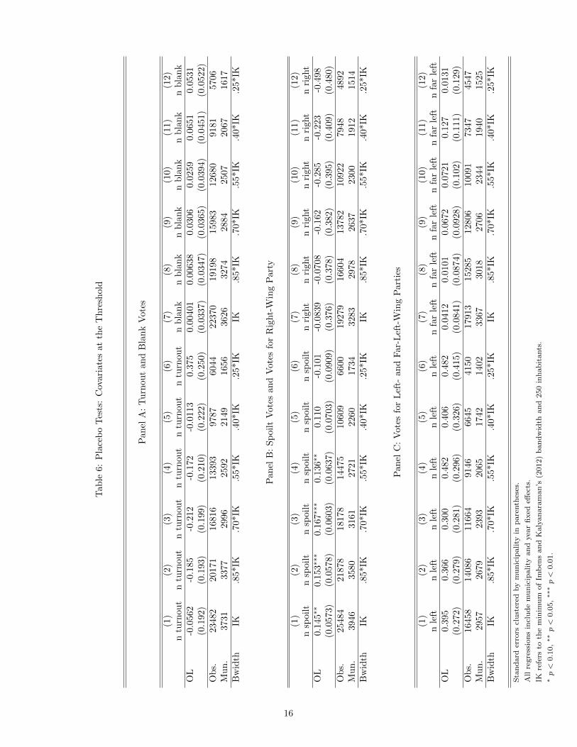
6.2 Placebo Tests: Covariates at the Thresholds

The identification strategy requires municipalities that municipalities that switch into the OL systembe comparable with those that stay in the same system and with those that switch out of theOL system. In other words, municipalities just above and just below the threshold should notdiffer, conditional on the fixed effects, in other variables that may themselves have an effect onvoter turnout. Here I use national Congress election variables and test whether they change at

are still significant (and in general even bigger in magnitude) if that year is included in the estimation.26The robustness checks for the results from this threshold are presented in the Appendix.27Although individuals who live in more than one municipality are required to register in the municipality in which

they spend more time, that requirement is almost impossible to monitor and not enforced in practice.28In particular, the spike of the distribution of population sizes suggests that there is a preference to fall under

the CL system. A possible reason for this preference is that the number of seats increases at the threshold, thereforeleading to more political positions available. Indeed, similar spikes on the distribution are observed at other thresholdswhere the council size increases, although it is not possible to know whether the spike is entirely caused by the councilsize as more regulations change at the other thresholds.

14

the thresholds by including them as dependent variables in equation (1).29 These covariates areespecially suited to this context because if municipalities differ in some unobservable factors thataffect voter turnout at local elections, it is likely that those unobservable variable affect turnout atnational elections too. Furthermore, Congress elections are the most important elections in Spainand turnout is typically very high (78 percent in the average municipality during the sample period)so they are likely to capture any political differences across municipalities.30

As pointed out by Lee and Lemieux (2010), it is important that the covariates are determinedprior to the present period’s realization of the running and treatment variables if they can be affectedby treatment.31 I merge local elections data with data from the most recent previous Congresselections at the municipality level.32 I consider the percent of voter turnout in (N turnout), blank(N blank) and spoilt votes (N spoilt) in Congress elections and the percent of votes for the threemain parties in Spain (N right, N left and N far left).33 If the empirical strategy is valid, thereshould be no effect of the electoral system on these variables.

The results from these tests are shown in Table 6. Among the six variables considered, only inone (the share of spoilt votes) there seems to be some difference between municipalities, but theeffect is quantitatively small and only significant in some specifications. Overall, the results suggestthat, conditional on the fixed effects, municipalities just above and just below the threshold do notdiffer sistematically along these variables: while municipalities operating under open and closed listsbehave differently in local elections, they do not do so in national elections.

29Note that the inclusion of the fixed effects implies that to test the robustness of the strategy we need variablesthat change over time.

30Spain follows a parliamentary system, so there are no elections for the executive branch. Citizens elect theCongress, which in turn elects the Prime Minister.

31Although the population threshold does not play any role in national elections, behavior at subsequent nationalelections could be affected if, for example, the electoral system influences voters’ political views.

32Thus, I estimate equation (1) where instead of turnout at the 1983 (1987, 1991, 1995, 1999, 2003, 2007, 2011)local elections I include turnout at the 1982 (1986, 1989, 1993, 1996, 2000, 2004, 2008) national elections as thedependent variable.

33The other parties represented in Congress during the whole period are regional parties that do not run in thewhole country.

15

Tab

le6:

Pla

ceb

oT

ests

:C

ovari

ate

sat

the

Th

resh

old

Pan

elA

:T

urn

ou

tan

dB

lan

kV

ote

s

(1)

(2)

(3)

(4)

(5)

(6)

(7)

(8)

(9)

(10)

(11)

(12)

ntu

rnou

tn

turn

out

ntu

rnou

tn

turn

ou

tn

turn

ou

tn

turn

ou

tn

bla

nk

nb

lan

kn

bla

nk

nb

lan

kn

bla

nk

nb

lan

kO

L-0

.056

2-0

.185

-0.2

12-0

.172

-0.0

113

0.3

75

0.0

0401

0.0

0638

0.0

306

0.0

259

0.0

651

0.0

531

(0.1

92)

(0.1

93)

(0.1

99)

(0.2

10)

(0.2

22)

(0.2

50)

(0.0

337)

(0.0

347)

(0.0

365)

(0.0

394)

(0.0

451)

(0.0

522)

Ob

s.23

482

2017

116

816

13393

9787

6044

22370

19198

15983

12680

9181

5706

Mu

n.

3731

3377

2996

2592

2149

1656

3626

3274

2884

2507

2067

1617

Bw

idth

IK.8

5*IK

.70*

IK.5

5*IK

.40*IK

.25*IK

IK.8

5*IK

.70*IK

.55*IK

.40*IK

.25*IK

Pan

elB

:S

poilt

Vote

san

dV

ote

sfo

rR

ight-

Win

gP

art

y

(1)

(2)

(3)

(4)

(5)

(6)

(7)

(8)

(9)

(10)

(11)

(12)

nsp

oilt

nsp

oilt

nsp

oilt

nsp

oil

tn

spoil

tn

spoil

tn

right

nri

ght

nri

ght

nri

ght

nri

ght

nri

ght

OL

0.14

5∗∗

0.15

3∗∗∗

0.16

7∗∗

∗0.1

36∗

∗0.1

10

-0.1

01

-0.0

839

-0.0

708

-0.1

62

-0.2

85

-0.2

23

-0.4

98

(0.0

573)

(0.0

578)

(0.0

603)

(0.0

637)

(0.0

703)

(0.0

909)

(0.3

76)

(0.3

78)

(0.3

82)

(0.3

95)

(0.4

09)

(0.4

80)

Ob

s.25

484

2187

818

178

14475

10609

6600

19279

16604

13782

10922

7948

4892

Mu

n.

3946

3580

3161

2721

2260

1734

3283

2978

2637

2300

1912

1514

Bw

idth

IK.8

5*IK

.70*

IK.5

5*IK

.40*IK

.25*IK

IK.8

5*IK

.70*IK

.55*IK

.40*IK

.25*IK

Pan

elC

:V

ote

sfo

rL

eft-

an

dF

ar-

Lef

t-W

ing

Part

ies

(1)

(2)

(3)

(4)

(5)

(6)

(7)

(8)

(9)

(10)

(11)

(12)

nle

ftn

left

nle

ftn

left

nle

ftn

left

nfa

rle

ftn

far

left

nfa

rle

ftn

far

left

nfa

rle

ftn

far

left

OL

0.39

50.

366

0.30

00.4

82

0.4

06

0.4

82

0.0

412

0.0

101

0.0

672

0.0

721

0.1

27

0.0

131

(0.2

72)

(0.2

79)

(0.2

81)

(0.2

96)

(0.3

26)

(0.4

15)

(0.0

841)

(0.0

874)

(0.0

928)

(0.1

02)

(0.1

11)

(0.1

29)

Ob

s.16

458

1408

611

664

9146

6645

4150

17913

15285

12806

10091

7347

4547

Mu

n.

2957

2679

2393

2065

1742

1402

3367

3018

2706

2344

1940

1525

Bw

idth

IK.8

5*IK

.70*

IK.5

5*IK

.40*IK

.25*IK

IK.8

5*IK

.70*IK

.55*IK

.40*IK

.25*IK

Sta

nd

ard

erro

rscl

ust

ered

by

mu

nic

ipali

tyin

pare

nth

eses

.

All

regre

ssio

ns

incl

ud

em

un

icip

ality

an

dyea

rfi

xed

effec

ts.

IKre

fers

toth

em

inim

um

of

Imb

ens

an

dK

aly

an

ara

man

’s(2

012)

ban

dw

idth

an

d250

inh

ab

itants

.∗p<

0.1

0,∗∗

p<

0.0

5,∗∗

∗p<

0.0

1.

16

6.3 Pretrends in the Outcomes of Interest

The longitudinal structure of the data can be used to estimate dynamic causal effects. This subsec-tion studies the timing of the effect of the electoral system on the outcomes of interest by estimatingthe following model:

ymt = αm + γt + β1Dmt + β2Dm,t+1 + f1(xmt − x∗) + f2(xm,t+1 − x∗) + umt. (3)

If, conditional on the fixed effects, next period’s electoral system is as good as random forthose municipalities sufficiently close to the threshold, next period’s electoral system should nothelp predict this period’s outcome variable.34 Thus, the coefficient β2 serves as a robustness check:β2 6= 0 would suggest an endogeneity problem that may raise concerns about the validity of theapproach of the paper. Alternatively, we can think of (3) as testing whether treatment and controlmunicipalities were on different trends before the realization of this period’s variables.35

Table 7 shows the results. The estimates for β2 are not statistically significant for Turnout. Forsome bandwidth choices, the coefficients for Lists are significant but they are small and have theopposite sign to the contemporaneous effect, suggesting that, if there is any difference, OL munic-ipalities had fewer lists in the previous election. Moreover, β1, the contemporaneous effect of theelectoral system on the outcomes, remains similar to the one obtained in the baseline specifications,for the three outcome variables. That implies that previous trends in the outcome variables are notdriving the results.

6.4 Donut Regressions

This subsection considers donut regressions in the spirit of Barreca et al. (2011). The idea of thistechnique is to exclude observations very close to the thresholds, where sorting is more likely tooccur. Given the nature of the sorting process of Spanish municipalities, it is likely that the sortingof municipalities is limited to a small window around the threshold: since the discontinuity in thedensity appears not because of outright manipulation of the population data, but as a consequence ofregistration decisions of citizens, it does not seem plausible that the population size of municipalitiesthat are self-selecting into treatment is much bigger than what is strictly necessary to be above thethreshold, or that municipalities with a population size far below the threshold attempt to cross it.Thus, finding a similar effect after municipalities close to the threshold are excluded would reinforcethe credibility of the estimates.

For each outcome variable and bandwidth choice, I consider four specifications. The first one isthe benchmark regression, in which no observations are excluded. The second excludes observationswithin a window of six inhabitants around the threshold (three at each side of the threshold), thethird excludes those within an interval of 10 inhabitants and the fourth those within an interval of20 inhabitants.

The results (see Table 8) show that excluding observations very close to the threshold does notaffect the results, as they are remarkably similar in magnitude to the ones obtained in the baselinespecifications. For voter turnout, the results are significant when up to 10 inhabitants around thethreshold are excluded.36 For a bandwidth of half that length, the results are significant evenwhen municipalities with a population within a 20 inhabitants around the threshold are excluded.For the number of lists, the coefficients remain significant across all specifications. These resultssuggest that the findings of the paper are not being driven by municipalities of which concernsabout self-selection could still persist.

34According to Lee and Lemieux (2010), ”finding a discontinuity in ymt but not in ym,t−1 would be a strong pieceof evidence supporting the validity of the RD design”.

35It is necessary to flexibly control for population in both periods (i.e. to include the functions f1and f2) to capturethe effect of the electoral system and not of changes in population size.

36When 20 inhabitants are excluded the results are not significant but the point estimate remains similar: it is theincreased standard errors due the decrease in sample size that makes the coefficient lose significance.

17

Table 7: Robustness: Testing for Pretrends in the Outcomes of Interest

Panel A: Turnout


OL 1.628∗∗∗ 1.792∗∗∗ 1.754∗∗∗ 2.014∗∗∗ 2.251∗∗∗ 1.620∗∗

(0.410) (0.425) (0.443) (0.471) (0.548) (0.762)

OL(+1) -0.259 -0.302 -0.313 -0.191 -0.150 0.563(0.437) (0.455) (0.474) (0.495) (0.545) (0.713)


Panel B: Lists


OL 0.349∗∗∗ 0.360∗∗∗ 0.374∗∗∗ 0.385∗∗∗ 0.398∗∗∗ 0.358∗∗∗

(0.0308) (0.0319) (0.0340) (0.0366) (0.0432) (0.0576)

OL(+1) -0.0458 -0.0619∗∗ -0.0776∗∗ -0.0877∗∗∗ -0.104∗∗∗ -0.0736(0.0281) (0.0292) (0.0308) (0.0337) (0.0382) (0.0501)





18

Table 8: Robustness: Donut Regressions

Panel A: Turnout

(1) (2) (3) (4) (5) (6) (7) (8)turnout turnout turnout turnout turnout turnout turnout turnout

OL 1.031∗∗∗ 0.925∗∗ 0.920∗∗ 0.754 1.676∗∗∗ 1.546∗∗∗ 1.689∗∗∗ 1.876∗∗∗

(0.381) (0.419) (0.440) (0.494) (0.445) (0.517) (0.583) (0.710)Observations 15954 15531 15249 14583 8039 7616 7334 6668Municipalities 2826 2825 2825 2825 2002 1994 1991 1976Bandwidth IK IK IK IK .50*IK .50*IK .50*IK .50*IKExcluded 0 6 10 20 0 6 10 20

Panel B: Lists

(1) (2) (3) (4) (5) (6) (7) (8)lists lists lists lists lists lists lists lists

OL 0.314∗∗∗ 0.307∗∗∗ 0.288∗∗∗ 0.282∗∗∗ 0.361∗∗∗ 0.357∗∗∗ 0.333∗∗∗ 0.353∗∗∗

(0.0292) (0.0312) (0.0321) (0.0351) (0.0353) (0.0389) (0.0415) (0.0486)Observations 17693 17270 16988 16322 9000 8577 8295 7629Municipalities 2993 2992 2992 2992 2102 2096 2093 2084Bandwidth IK IK IK IK .50*IK .50*IK .50*IK .50*IKExcluded 0 6 10 20 0 6 10 20




19

7 Conclusion

By exploiting the unique institutional framework of Spanish local elections, I have shown thatthe electoral system has an effect on voter turnout. In particular, an open list, plurality-at-largesystem increases turnout by between one and two percentage points with respect to a closed listproportional representation system. The results suggest that open list systems where parties runin candidate lists but voters can express their preferences for individual candidates are conduciveto more voter turnout.

Working on understanding this type of electoral systems better could be a fruitful avenue forfuture research. Economists and political scientists have extensively worked on voter turnout andthe motivations for the decision of voting or abstaining (Battaglini et al., 2010; Feddersen andPesendorfer, 1996; Feddersen and Sandroni, 2006; Ledyard, 1984; Palfrey and Rosenthal, 1985),and this is still an active area of research (DellaVigna et al., 2013; Fujiwara et al., 2014; Gerberet al., 2008; Herrera et al., 2013; Kartal, 2013; Nickerson, 2008). However, to the best of myknowledge, we still do not have a theoretical framework to think about voter turnout in open listelections, in which there is competition both across and within parties.

References

Ames, B. 1995a. ”Electoral rules, constitutency pressures, and pork barrel: Bases of voting inthe Brazilian congress. The Journal of Politics, 57 (4), 324-343.

Ames, B. 1995b. Electoral strategies under open-list proportional representation. AmericanJournal of Political Science, 39 (2), 406-433.

Angrist, J. D. and Pischke, J. S. 2008. Mostly harmless econometrics: An empiricist’s compan-ion. Princeton University Press.

Arnold, F., and Freier, R. 2013. Signature requirements and citi-zen initatives: Quasi-experimental evidence from Germany. Available athttp://www.diw.de/documents/publikationen/73/diw 01.c.424904.de/dp1311.pdf.

Barreca, A. I., Guldi, M., Lindo, J. M., and Waddell, G. R. 2011. Saving Babies? Revisitingthe effect of very low birth weight classification. The Quarterly Journal of Economics, 126(4),2117-2123.

Battaglini, Marco, Rebecca B. Morton, and Thomas R. Palfrey. 2010. The swing voter’s cursein the laboratory. The Review of Economic Studies, 77(1), 61-89.

Blais, A. 2006. What affects voter turnout? Annual Review of Political Science, 9, 111-125.

Blais, A., and Aarts, K. 2006. Electoral systems and turnout. Acta Politica, 41(2), 180-196.

Blais, A., and Dobrzynska, A. 1998. Turnout in electoral democracies. European Journal ofPolitical Research, 33(2), 239-261.

Bordignon, M., Nannicini, T., and Tabellini, G. 2013. Moderating political extremism: Singleround vs runoff elections under plurality rule. IZA Discussion Paper.

Bowler, S., Donovan, T., and Brockington, D. 2003. Electoral reform and minority representa-tion: Local experiments with alternative elections. Ohio State University Press.

Brollo, F., Nannicini, T., Perotti, R., and Tabellini, G. 2013. The political resource curse. TheAmerican Economic Review, 103(5), 1759-1796.

20

Campa, P. 2012. Gender quotas, female politicians and public expenditures: quasi-experimentalevidence. ECONPUBBLICA Working Paper No. 157.

Carey, J. M. and Shugart, M. S. 1995. Incentives to cultivate a personal vote: A rank orderingof electoral formulas. Electoral Studies, 14 (4), 417-439.

Casas-Arce, P., and Saiz, A. 2012. Women and power: Unwilling, ineffective, or held back?IZA Discussion Paper.

Chang, E. C. C. 2005. Electoral incentives for political corruption under open-list proportionalrepresentation. The Journal of Politics, 67 (3), 716-730.

Chang, E. C. C. and Golden, M. A. 2007. Electoral systems, district magnitude and corruption.British Journal of Political Science, 37 (1), 115-137.

DellaVigna, S., J. List, U. Malmendier, and G. Rao. 2013. “Voting to tell others.” Mimeo,U.C. Berkeley.

Dos Santos, A. M. 2007. Do electoral rules matter? Electoral list modelsand their effects on party competition and institutional performance. Available athttp://socialsciences.scielo.org/pdf/s dados/v3nse/scs a06.pdf.

Downs, A. 1957. An economic theory of democracy. New York: Harper.

Egger, P., and Koethenbuerger, M. 2010. Government spending and legislative organization:Quasi-experimental evidence from Germany. American Economic Journal: Applied Economics,200-212.

Eggers, A. C. 2013. Proportionality and turnout: Evidence from French municipalities. Avail-able at http://andy.egge.rs/papers/Eggers ProportionalityTurnoutFrance.pdf.

Farrell, D. M., and McAllister, I. 2006. Voter satisfaction and electoral systems: Does prefer-ential voting in candidate-centred systems make a difference? European Journal of PoliticalResearch, 45(5), 723-749.

Feddersen, Timothy J., and Wolfgang Pesendorfer. 1996. The swing voter’s curse. The Ameri-can Economic Review, 86(3), 408-424.

Feddersen, T., and Sandroni, A. 2006. A theory of participation in elections. The AmericanEconomic Review, 96(4), 1271-1282.

Ferraz, C., and Finan, F. 2009. Motivating politicians: The im-pacts of monetary incentives on quality and performance. Available athttp://eml.berkeley.edu/˜ffinan/Finan MPoliticians.pdf.

Fornos, C. A., Power, T. J., and Garand, J. C. 2004. Explaining voter turnout in Latin America,1980 to 2000. Comparative Political Studies, 37(8), 909-940.

Fujiwara, T. 2011. A Regression Discontinuity Test of Strategic Voting and Duverger’s Law.Quarterly Journal of Political Science, 6(3-4), 197-233.

Fujiwara, T. 2015. Voting Technology, Political Responsiveness, and Infant Health: EvidenceFrom Brazil. Econometrica, 83: 423464.

Fujiwara, T., Meng, K. C., and Vogl, T. 2014. Estimating habit formation in voting. Availableat http://www.princeton.edu/˜fujiwara/papers/fmv habit formationvoting feb2014.pdf.

Gagliarducci, S., and Nannicini, T. 2013. Do better paid politicians perform better? Disentan-gling incentives from selection. Journal of the European Economic Association, 11, 369-398.

21

Gerber, A.S., D.P. Green, and C.W. Larimer. 2008. “Social pressure and voter turnout: Evi-dence from a large-scale field experiment.” American Political Science Review, 102(1), 33-48.

Geys, B. 2006. Explaining voter turnout: A review of aggregate-level research. Electoral Studies,25(4), 637-663.

Grembi, V., Nannicini, T., and Troiano, U. 2012. Policy responses to fiscal restraints: Adifference-in-discontinuities design. Available at http://www.igier.unibocconi.it/files/397.pdf.

Herrera, H., Morelli, M., and Palfrey, T. R. 2013. Turnout and power sharing. The EconomicJournal, 124 (574), F131–F162.

Hinnerich, B. T. and P. Pettersson-Lidbom. 2014. Democracy, redistribution, and politicalparticipation: Evidence from Sweden 1919-1938. Econometrica 82 (3), 961{993.

Hirota, H., and Yunoue, H. 2013. Does local council size affect land development expenditure?Quasi-experimental evidence from Japanese municipal data. Available at http://mpra.ub.uni-muenchen.de/43723/.

Hix, S., and Hagemann, S. 2009. Could changing the electoral rules fix European parliamentelections? Politique europeenne, (2), 37-52.

Imbens, G., and Kalyanaraman, K. 2012. Optimal bandwidth choice for the regression discon-tinuity estimator. The Review of Economic Studies, 79(3), 933-959.

Imbens, G. W. and T. Lemieux (2008). Regression discontinuity designs: A guide to practice.Journal of econometrics, 142 (2), 615-635.

Jackman, R. W. 1987. Political institutions and voter turnout in the industrial democracies.The American Political Science Review, 81(2), 405-423.

Jackman, R. W., and Miller, R. A. 1995. Voter turnout in the industrial democracies duringthe 1980s. Comparative Political Studies, 27(4), 467-492.

Kartal, M. 2013. Welfare comparison of proportional representation and majoritarian rule withendogenous turnout. Available at https://files.nyu.edu/mk2672/public/.

Karvonen, L. 2004. Preferential voting: incidence and effects. International Political ScienceReview, 25(2), 203-226.

Ladner, A., and Milner, H. 1999. Do voters turn out more under proportional than majoritariansystems? The evidence from Swiss communal elections. Electoral Studies, 18(2), 235-250.

Ledyard, J. O. 1984. The pure theory of large two-candidate elections. Public Choice, 44(1),7-41.

Lee, D. S., and Lemieux, T. 2010. Regression discontinuity designs in economics. The Journalof Economic Literature, 48(2), 281-355.

Lemieux, T., and Milligan, K. 2008. Incentive effects of social assistance: A regression discon-tinuity approach. Journal of Econometrics, 142(2), 807-828.

Litschig, S., and Morrison, K. 2013. The Impact of Intergovernmental Transfers on EducationOutcomes and Poverty Reduction. AEJ: Applied Economics, 5(4): 206-240.

Mattila, M. 2003. Why bother? Determinants of turnout in the European elections. ElectoralStudies, 22(3), 449-468.

McCrary, J. 2008. Manipulation of the running variable in the regression discontinuity design:A density test. Journal of Econometrics, 142(2), 698-714.

22

Milner, H., and Ladner, A. 2006. Can PR voting serve as a shelter against declining turnout?Evidence from Swiss municipal elections. International Political Science Review, 27(1), 29-45.

Negri, M. 2014. Minority representation in proportional representation systems. Avail-able at http://margheritanegri.files.wordpress.com/2013/03/minority-representation-in-pr-systems-negri1.pdf.

Nickerson, D.W. 2008. “Is voting contagious? Evidence from two field experiments.” AmericanPolitical Science Review, 102(1), 49-57.

Palfrey, Thomas R., and Howard Rosenthal. 1985. Voter participation and strategic uncertainty.The American Political Science Review (1985): 62-78.

Persson, T., Tabellini, G., and Trebbi, F. 2003. Electoral rules and corruption. Journal of theEuropean Economic Association, 1(4), 958-989.

Pettersson-Lidbom, P. 2012. Does the size of the legislature affect the size of government:Evidence from two natural experiments. Journal of Public Economics, Volume 96, Issues 3–4,269-278.

Riker, W. H., and Ordeshook, P. C. 1968. A theory of the calculus of voting. The AmericanPolitical Science Review, 25-42.

Robbins, J. W. 2010. The personal vote and voter turnout. Electoral Studies, 29(4), 661-672.

Sanz, C. 2014. Does direct democracy reduce deficits? Evidence from Spain. Princeton Uni-versity Working Paper.

Schram, A., and Sonnemans, J. 1996. Voter turnout as a participation game: An experimentalinvestigation. International Journal of Game Theory, 25(3), 385-406.

Shugart, M. S., M. E. Valdini, and Suominen, K. 2005. Looking for locals: Voter informationdemands and personal vote-earning attributes of legislators under proportional representation.American Journal of Political Science, 49 (2), 437-449.

Selb, P. 2009. A deeper look at the proportionality-turnout nexus. Comparative Political Stud-ies, 42(4), 527-548.

St-Vincent, S. L. 2013. An experimental test of the pivotal voter model under plurality andPR elections. Electoral Studies, 32(4), 795–806.

Sweeting, D. 2009. The institutions of strong local political leadership in Spain. Environmentand planning C: government and policy 27.

A Robustness Checks for the 100-inhabitant Threshold

In this appendix I show robustness checks for the results at the 100-inhabitant threshold. Table 9tests for pretrends and Table 10 shows the results of the donut regression discontinuity design.

23

Table 9: 100-Inhabitant Threshold Robustness: Pretrends in the Outcomes of Interest

Panel A: Turnout


OL 3.177∗∗∗ 3.195∗∗∗ 3.082∗∗∗ 2.974∗∗∗ 2.796∗∗∗ 2.159∗∗

(0.588) (0.600) (0.621) (0.672) (0.764) (0.978)

OL(+1) 0.152 0.300 0.235 0.285 0.450 0.192(0.544) (0.563) (0.577) (0.626) (0.661) (0.774)

Observations 8742 7555 6263 4915 3588 2242Municipalities 2504 2220 1921 1588 1256 931Bandwidth IK 85% 70% 55% 40% 25%

Panel B: Lists


OL 0.100∗∗ 0.0927∗∗ 0.0827∗ 0.0538 0.0679 0.223∗∗

(0.0439) (0.0463) (0.0496) (0.0555) (0.0657) (0.0981)

OL(+1) -0.0554 -0.0452 -0.0592 -0.0653 -0.000580 0.0453(0.0434) (0.0468) (0.0486) (0.0533) (0.0583) (0.0718)

Observations 5401 4596 3813 2999 2146 1341Municipalities 1694 1513 1316 1117 911 677Bandwidth IK 85% 70% 55% 40% 25%




24

Table 10: 100-Inhabitant Threshold Robustness: Donut Regressions

Panel A: Turnout

(1) (2) (3) (4) (5) (6) (7) (8)turnout turnout turnout turnout turnout turnout turnout turnout

OL 2.811∗∗∗ 2.947∗∗∗ 2.983∗∗∗ 3.448∗∗∗ 2.487∗∗∗ 2.555∗∗∗ 2.484∗∗∗ 3.679∗∗∗

(0.521) (0.578) (0.639) (0.803) (0.595) (0.696) (0.804) (1.074)Obs. 11161 10739 10493 9871 5737 5315 5069 4447Mun. 2621 2621 2621 2608 1603 1603 1603 1589Bw. IK IK IK IK 50% 50% 50% 50%Excluded 0 6 10 20 0 6 10 20

Panel B: Party-Lists

(1) (2) (3) (4) (5) (6) (7) (8)lists lists lists lists lists lists lists lists

OL 0.0778∗∗ 0.0818∗ 0.101∗∗ 0.147∗∗ 0.0517 0.0506 0.0941 0.187(0.0390) (0.0475) (0.0482) (0.0669) (0.0506) (0.0730) (0.0827) (0.145)

Obs. 6907 6485 6239 5617 3571 3149 2903 2281Mun. 1823 1823 1823 1810 1190 1184 1180 1144Bw. IK IK IK IK 50% 50% 50% 50%Excluded 0 6 10 20 0 6 10 20




25

the e ect of electoral systems on voter turnout: evidence ... · the e ect of electoral systems on...

Documents