the compiler design handbook
TRANSCRIPT


TheCOMPILERDESIGN
Optimizations andMachine CodeGeneration
S E C O N D E D I T I O N
Handbook


CRC Press is an imprint of theTaylor & Francis Group, an informa business
Boca Raton London New York
TheCOMPILERDESIGN
Optimizations andMachine CodeGeneration
S E C O N D E D I T I O N
E d i t e d b y
Y.N. SrikantPriti Shankar
Handbook

CRC PressTaylor & Francis Group6000 Broken Sound Parkway NW, Suite 300Boca Raton, FL 33487‑2742
© 2008 by Taylor & Francis Group, LLC CRC Press is an imprint of Taylor & Francis Group, an Informa business
No claim to original U.S. Government worksPrinted in the United States of America on acid‑free paper10 9 8 7 6 5 4 3 2 1
International Standard Book Number‑13: 978‑1‑4200‑4382‑2 (Hardcover)
This book contains information obtained from authentic and highly regarded sources. Reprinted material is quoted with permission, and sources are indicated. A wide variety of references are listed. Reasonable efforts have been made to publish reliable data and information, but the author and the publisher cannot assume responsibility for the validity of all materials or for the consequences of their use.
No part of this book may be reprinted, reproduced, transmitted, or utilized in any form by any electronic, mechanical, or other means, now known or hereafter invented, including photocopying, microfilming, and recording, or in any informa‑tion storage or retrieval system, without written permission from the publishers.
For permission to photocopy or use material electronically from this work, please access www.copyright.com (http://www.copyright.com/) or contact the Copyright Clearance Center, Inc. (CCC) 222 Rosewood Drive, Danvers, MA 01923, 978‑750‑8400. CCC is a not‑for‑profit organization that provides licenses and registration for a variety of users. For orga‑nizations that have been granted a photocopy license by the CCC, a separate system of payment has been arranged.
Trademark Notice: Product or corporate names may be trademarks or registered trademarks, and are used only for identification and explanation without intent to infringe.
Library of Congress Cataloging‑in‑Publication Data
The Compiler design handbook : optimizations and machine code generation / edited by Y.N. Srikant and Priti Shankar. ‑‑ 2nd ed.
p. cm.Includes bibliographical references and index.ISBN 978‑1‑4200‑4382‑2 (alk. paper)1. Compilers (Computer programs) 2. Code generators. I. Srikant, Y. N. II. Shankar, P. (Priti) III.
Title.
QA76.76.C65C35 2007005.4’53‑‑dc22 2007018733
Visit the Taylor & Francis Web site athttp://www.taylorandfrancis.com
and the CRC Press Web site athttp://www.crcpress.com

Table of Contents
1 Worst-Case Execution Time and Energy AnalysisTulika Mitra, Abhik Roychoudhury . . . . . . . . . . . . . . . . . . . . . . . . . . . . . . . . . . . . . . . . . . . . . . . . . . 1-1
2 Static Program Analysis for SecurityK. Gopinath . . . . . . . . . . . . . . . . . . . . . . . . . . . . . . . . . . . . . . . . . . . . . . . . . . . . . . . . . . . . . . . . . . . . . . . . . 2-1
3 Compiler-Aided Design of Embedded ComputersAviral Shrivastava, Nikil Dutt . . . . . . . . . . . . . . . . . . . . . . . . . . . . . . . . . . . . . . . . . . . . . . . . . . . . . . . 3-1
4 Whole Execution Traces and Their Use in DebuggingXiangyu Zhang, Neelam Gupta, Rajiv Gupta . . . . . . . . . . . . . . . . . . . . . . . . . . . . . . . . . . . . . . . . 4-1
5 Optimizations for Memory HierarchiesEaswaran Raman, David I. August . . . . . . . . . . . . . . . . . . . . . . . . . . . . . . . . . . . . . . . . . . . . . . . . . . 5-1
6 Garbage Collection TechniquesAmitabha Sanyal, Uday P. Khedker . . . . . . . . . . . . . . . . . . . . . . . . . . . . . . . . . . . . . . . . . . . . . . . . . . 6-1
7 Energy-Aware Compiler OptimizationsY. N. Srikant, K. Ananda Vardhan . . . . . . . . . . . . . . . . . . . . . . . . . . . . . . . . . . . . . . . . . . . . . . . . . . . 7-1
8 Statistical and Machine Learning Techniques in Compiler DesignKapil Vaswani . . . . . . . . . . . . . . . . . . . . . . . . . . . . . . . . . . . . . . . . . . . . . . . . . . . . . . . . . . . . . . . . . . . . . . . 8-1
9 Type Systems: Advances and ApplicationsJens Palsberg, Todd Millstein . . . . . . . . . . . . . . . . . . . . . . . . . . . . . . . . . . . . . . . . . . . . . . . . . . . . . . . . . 9-1
10 Dynamic CompilationEvelyn Duesterwald . . . . . . . . . . . . . . . . . . . . . . . . . . . . . . . . . . . . . . . . . . . . . . . . . . . . . . . . . . . . . . . . 10-1
11 The Static Single Assignment Form: Construction and Applicationto Program OptimizationJ. Prakash Prabhu, Priti Shankar, Y. N. Srikant . . . . . . . . . . . . . . . . . . . . . . . . . . . . . . . . . . . . . 11-1
12 Shape Analysis and ApplicationsThomas Reps, Mooly Sagiv, Reinhard Wilhelm . . . . . . . . . . . . . . . . . . . . . . . . . . . . . . . . . . . . . 12-1
v

13 Optimizations for Object-Oriented LanguagesAndreas Krall, Nigel Horspool . . . . . . . . . . . . . . . . . . . . . . . . . . . . . . . . . . . . . . . . . . . . . . . . . . . . . . 13-1
14 Program SlicingG. B. Mund, Rajib Mall . . . . . . . . . . . . . . . . . . . . . . . . . . . . . . . . . . . . . . . . . . . . . . . . . . . . . . . . . . . . 14-1
15 Computations on Iteration SpacesSanjay Rajopadhye, Lakshminarayanan Renganarayana, Gautam Gupta,Michelle Mills Strout . . . . . . . . . . . . . . . . . . . . . . . . . . . . . . . . . . . . . . . . . . . . . . . . . . . . . . . . . . . . . . . 15-1
16 Architecture Description Languages for Retargetable CompilationWei Qin, Sharad Malik . . . . . . . . . . . . . . . . . . . . . . . . . . . . . . . . . . . . . . . . . . . . . . . . . . . . . . . . . . . . . 16-1
17 Instruction Selection Using Tree ParsingPriti Shankar . . . . . . . . . . . . . . . . . . . . . . . . . . . . . . . . . . . . . . . . . . . . . . . . . . . . . . . . . . . . . . . . . . . . . . . 17-1
18 A Retargetable Very Long Instruction Word Compiler Frameworkfor Digital Signal ProcessorsSubramanian Rajagopalan, Sharad Malik . . . . . . . . . . . . . . . . . . . . . . . . . . . . . . . . . . . . . . . . . . 18-1
19 Instruction SchedulingR. Govindarajan . . . . . . . . . . . . . . . . . . . . . . . . . . . . . . . . . . . . . . . . . . . . . . . . . . . . . . . . . . . . . . . . . . . 19-1
20 Advances in Software PipeliningHongbo Rong, R. Govindarajan . . . . . . . . . . . . . . . . . . . . . . . . . . . . . . . . . . . . . . . . . . . . . . . . . . . . 20-1
21 Advances in Register Allocation TechniquesV. Krishna Nandivada . . . . . . . . . . . . . . . . . . . . . . . . . . . . . . . . . . . . . . . . . . . . . . . . . . . . . . . . . . . . . . 21-1
Index . . . . . . . . . . . . . . . . . . . . . . . . . . . . . . . . . . . . . . . . . . . . . . . . . . . . . . . . . . . . . . . . . . . . . . . . . . . . . . . . . . . . . I-1
vi

1Worst-Case Execution
Time and EnergyAnalysis
Tulika MitraandAbhik RoychoudhuryDepartment of Computer Science,School of Computing,National University of Singapore,[email protected] [email protected]
1.1 Introduction . . . . . . . . . . . . . . . . . . . . . . . . . . . . . . . . . . . . . . . . . .1-11.2 Programming-Language-Level WCET Analysis . . . . . . . . .1-4
WCET Calculation • Infeasible Path Detection andExploitation
1.3 Micro-Architectural Modeling . . . . . . . . . . . . . . . . . . . . . . . . .1-16Sources of Timing Unpredictability • Timing Anomaly• Overview of Modeling Techniques • Integrated ApproachBased on ILP • Integrated Approach Based on Timing Schema• Separated Approach Based on Abstract Interpretation• A Separated Approach That Avoids State Enumeration
1.4 Worst-Case Energy Estimation . . . . . . . . . . . . . . . . . . . . . . . .1-35Background • Analysis Technique • Accuracy and Scalability
1.5 Existing WCET Analysis Tools . . . . . . . . . . . . . . . . . . . . . . . . .1-411.6 Conclusions . . . . . . . . . . . . . . . . . . . . . . . . . . . . . . . . . . . . . . . . . .1-42
Integration with Schedulability Analysis • System-LevelAnalysis • Retargetable WCET Analysis • Time-PredictableSystem Design • WCET-Centric Compiler Optimizations
References . . . . . . . . . . . . . . . . . . . . . . . . . . . . . . . . . . . . . . . . . . . . . . . . . .1-44
1.1 Introduction
Timing predictability is extremely important for hard real-time embedded systems employed in applicationdomains such as automotive electronics and avionics. Schedulability analysis techniques can guaranteethe satisfiability of timing constraints for systems consisting of multiple concurrent tasks. One of the keyinputs required for the schedulability analysis is the worst-case execution time (WCET) of each of thetasks. WCET of a task on a target processor is defined as its maximum execution time across all possibleinputs.
Figure 1.1a and Figure 1.2a show the variation in execution time of a quick sort program on asimple and complex processor, respectively. The program sorts a five-element array. The figures show thedistribution of execution time (in processor cycles) for all possible permutations of the array elementsas inputs. The maximum execution time across all the inputs is the WCET of the program. This simpleexample illustrates the inherent difficulty of finding the WCET value:
1-1

1-2 The Compiler Design Handbook: Optimizations and Machine Code Generation
12
10
8
6
Nu
mb
er o
f In
pu
ts4
2
03000 3010 3020 3030 3040 3050 3060 3070 3080
Execution Time (cycles)(a)
16
14
12
10
Nu
mb
er o
f In
pu
ts
8
6
4
2
0660 670 680 690 700
Energy (× 10 nJ)
710 720 730
(b)
FIGURE 1.1 Distribution of time and energy for different inputs of an application on a simple processor.
� Clearly, executing the program for all possible inputs so as to bound its WCET is not feasible. Theproblem would be trivial if the worst-case input of a program is known a priori. Unfortunately, formost programs the worst-case input is unknown and cannot be derived easily.� Second, the complexity of current micro-architectures implies that the WCET is heavily influencedby the target processor. This is evident from comparing Figure 1.1a with Figure 1.2a. Therefore, thetiming effects of micro-architectural components have to be accurately accounted for.
Static analysis methods estimate a bound on the WCET. These analysis techniques are conservativein nature. That is, when in doubt, the analysis assumes the worst-case behavior to guarantee the safetyof the estimated value. This may lead to overestimation in some cases. Thus, the goal of static anal-ysis methods is to estimate a safe and tight WCET value. Figure 1.3 explains the notion of safety andtightness in the context of static WCET analysis. The figure shows the variation in execution time ofa task. The actual WCET is the maximum possible execution time of the program. The static analysismethod generates the estimated WCET value such that estimated WCET ≥ actual WCET. The differencebetween the estimated and the actual WCET is the overestimation and determines how tight the estima-tion is. Note that the static analysis methods guarantee that the estimated WCET value can never be lessthan the actual WCET value. Of course, for a complex task running on a complex processor, the actualWCET value is unknown. Instead, simulation or execution of the program with a subset of possible in-puts generates the observed WCET, where observed WCET ≤ actual WCET. In other words, the observedWCET value is not safe, in the sense that it cannot be used to provide absolute timing guarantees forsafety-critical systems. A notion related to WCET is the BCET (best-case execution time), which representsthe minimum execution time across all possible inputs. In this chapter, we will focus on static analysis

Worst-Case Execution Time and Energy Analysis 1-3
16
14
12
10
Nu
mb
er o
f In
pu
ts
8
6
2
4
02690 2700 2710 2720
Execution Time (cycles)
2730 2740 2750
(a)
14
12
Nu
mb
er o
f In
pu
ts 10
8
6
4
2
01060 1080 1100 1120 1140
Energy (× 10 nJ)
1160 1180 1200
(b)
FIGURE 1.2 Distribution of time and energy for different inputs of the same application on a complex processor.
techniques to estimate the WCET. However, the same analysis methods can be easily extended to estimatethe BCET.
Apart from timing, the proliferation of battery-operated embedded devices has made energy consump-tion one of the key design constraints. Increasingly, mobile devices are demanding improved functionalityand higher performance. Unfortunately, the evolution of battery technology has not been able to keepup with performance requirements. Therefore, designers of mission-critical systems, operating on limitedbattery life, have to ensure that both the timing and the energy constraints are satisfied under all possible
Estimated
BCET
Actual
BCET
Observed
BCETObserved
WCET
Over estimation
Actual
WCET
Estimated
WCET
Execution Time
Observed
Actual
Dis
trib
uti
on
of
Ex
ecu
tio
n T
ime
FIGURE 1.3 Definition of observed, actual, and estimated WCET.

1-4 The Compiler Design Handbook: Optimizations and Machine Code Generation
scenarios. The battery should never drain out before a task completes its execution. This concern leads tothe related problem of estimating the worst-case energy consumption of a task running on a processor forall possible inputs. Unlike WCET, estimating the worst-case energy remains largely unexplored even thoughit is considered highly important [86], especially for mobile devices. Figure 1.1b and Figure 1.2b showthe variation in energy consumption of the quick sort program on a simple and complex processor,respectively.
A natural question that may arise is the possibility of using the WCET path to compute a bound on theworst-case energy consumption. As energy = average power × execution time, this may seem like a viablesolution and one that can exploit the extensive research in WCET analysis in a direct fashion. Unfortunately,the path corresponding to the WCET may not coincide with the path consuming maximum energy. Thisis made apparent by comparing the distribution of execution time and energy for the same program andprocessor pair as shown in Figure 1.1 and Figure 1.2. There are a large number of input pairs 〈I1, I2〉 in thisprogram, where time(I1) < time(I2), but energy(I1) > energy(I2). This happens as the energy consumedbecause of the switching activity in the circuit need not necessarily have a correlation with the executiontime. Thus, the input that leads to WCET may not be identical to the input that leads to the worst-caseenergy.
The execution time or energy is affected by the path taken through the program and the underlyingmicro-architecture. Consequently, static analysis for worst-case execution time or energy typically consistsof three phases. The first phase is the program path analysis to identify loop bounds and infeasible flowsthrough the program. The second phase is the architectural modeling to determine the effect of pipeline,cache, branch prediction, and other components on the execution time (energy). The last phase, estimation,finds an upper bound on the execution time (energy) of the program given the results of the flow analysisand the architectural modeling.
Recently, there has been some work on measurement-based timing analysis [6, 17, 92]. This line of workis mainly targeted toward soft real-time systems, such as multimedia applications, that can afford to missthe deadline once in a while. In other words, these application domains do not require absolute timingguarantees. Measurement-based timing analysis methods execute or simulate the program on the targetprocessor for a subset of all possible inputs. They derive the maximum observed execution time (see thedefinition in Figure 1.3) or the distribution of execution time from these measurements. Measurement-based performance analysis is quite useful for soft real-time applications, but they may underestimate theWCET, which is not acceptable in the context of safety-critical, hard real-time applications. In this article,we only focus on static analysis techniques that provide safe bounds on WCET and worst-case energy.The analysis methods assume uninterrupted program execution on a single processor. Furthermore, theprogram being analyzed should be free from unbounded loops, unbounded recursion, and dynamicfunction calls [67].
The rest of the chapter is organized as follows. We proceed with programming-language-level WCETanalysis in the next section. This is followed by micro-architectural modeling in Section 1.3. We present astatic analysis technique to estimate worst-case energy bound in Section 1.4. A brief description of existingWCET analysis tools appears in Section 1.5, followed by conclusions.
1.2 Programming-Language-Level WCET Analysis
We now proceed to discuss static analysis methods for estimating the WCET of a program. For WCETanalysis of a program, the first issue that needs to be determined is the program representation on whichthe analysis will work. Earlier works [73] have used the syntax tree where the (nonleaf) nodes correspondto programming-language-level control structures. The leaves correspond to basic blocks — maximalfragments of code that do not involve any control transfer. Subsequently, almost all work on WCETanalysis has used the control flow graph. The nodes of a control flow graph (CFG) correspond to basicblocks, and the edges correspond to control transfer between basic blocks. When we construct the CFG of aprogram, a separate copy of the CFG of a function f is created for every distinct call site of f in the program

Worst-Case Execution Time and Energy Analysis 1-5
sum = 0; i = 0
sum = 0; i = 0 FOR
sum += i
sum += i
. . .
. . .
6
5
4
i++
(b)(a) (c)
i++
7
1A sum = 0;
B for (i = 0; i < 10; i++){
C if (i % 2 == 0)
D sum += i;
E if (sum < 0)
F . . .
G }
H return sum;
i < 10
i < 10
sum < 0
sum < 0 IF IF
2
i%2 == 0
i%2 == 0
3
8
SEQUENCE
SEQUENCE
return
sum
return
sum
FIGURE 1.4 (a) A code fragment. (b) Control flow graph of the code fragment. (c) Syntax tree of the code fragment.
such that each call transfers control to its corresponding copy of CFG. This is how interprocedural analysiswill be handled. Figure 1.4 shows a small code fragment as well as its syntax tree and control flow graphrepresentations.
One important issue needs to be clarified in this regard. The control flow graph of a program can beeither at the source code level or at the assembly code level. The difference between the two comes fromthe compiler optimizations. Our program-level analysis needs to be hooked up with micro-architecturalmodeling, which accurately estimates the execution time of each instruction while considering the timingeffects of underlying microarchitectural features. Hence we always consider the assembly-code-level CFG.However, while showing our examples, we will show CFG at the source code level for ease of exposition.
1.2.1 WCET Calculation
We explain WCET analysis methods in a top-down fashion. Consequently, at the very beginning, wepresent WCET calculation — how to combine the execution time estimates of program fragments to getthe execution time estimate of a program. We assume that the loop bounds (i.e., the maximum numberof iterations for a loop) are known for every program loop; in Section 1.2.2 we outline some methods toestimate loop bounds.
In the following, we outline the three main categories of WCET calculation methods. The path-basedand integer linear programming methods operate on the program’s control flow graph, while the tree-basedmethods operate on the program’s syntax tree.
1.2.1.1 Tree-Based Methods
One of the earliest works on software timing analysis was the work on timing schema [73]. The techniqueproceeds essentially by a bottom-up pass of the syntax tree. During the traversal, it associates an executiontime estimate for each node of the tree. The execution time estimate for a node is obtained from theexecution time estimates of its children, by applying the rules in the schema. The schema prescribes

1-6 The Compiler Design Handbook: Optimizations and Machine Code Generation
rules — one for each control structure of the programming language. Thus, rules corresponding to asequence of statements, if-then-else and while-loop constructs, can be described as follows.� Time(S1; S2) = Time(S1) + Time(S2)� Time(if (B) { S1 } else { S2} ) = Time(B) + max(Time(S1), Time(S2))� Time (while (B) { S1} ) = (n + 1)*Time(B) + n*Time(S1)
Here, n is the loop bound. Clearly, S1, S2 can be complicated code fragments whose execution timeestimates need to obtained by applying the schema rules for the control structures appearing in S1, S2.Extensions of the timing schema approach to consider micro-architectural modeling will be discussed inSection 1.3.5.
The biggest advantage of the timing schema approach is its simplicity. It provides an efficient compo-sitional method for estimating the WCET of a program by combining the WCET of its constituent codefragments. Let us consider the following schematic code fragment P g m. For simplicity of exposition, wewill assume that all assignments and condition evaluations take one time unit.
i = 0; while (i<100) {if (B’) S1 else S2; i++;}
If Time(S1) > Time(S2), by using the rule for if-then-else statements in the timing schema we get
Time(if (B') S1 else S2 ) = Time(B') + Time(S1) = 1 + Time(S1)
Now, applying the rule for while-loops in the timing schema, we get the following. The loop bound in thiscase is 100.
Time(while (i<100) {if(B') S1 else S2}) = 101 ∗ Time(i < 100)+100 ∗ Time(if (B') S1 else S2)
= 101 ∗ 1 + 100 ∗ (1 + Time(S1))= 201 + 100 ∗ Time(S1)
Finally, using the rule for sequential composition in the timing schema we get
Time(P g m) = Time(i = 0) + Time(while (i<100) {if (B') S1 else S2})= 1 + 201 + 100 ∗ Time(S1) = 202 + 100 ∗ Time(S1)
The above derivation shows the working of the timing schema. It also exposes one of its major weaknesses.In the timing schema, the timing rules for a program statement are local to the statement; they do notconsider the context with which the statement is arrived at. Thus, in the preceding we estimated themaximum execution time of if (B’) S1 else S2 by taking the execution time for evaluating Band the time for executing S1 (since time for executing S1 is greater than the time for executing S2).As a result, since the if-then-else statement was inside a loop, our maximum execution time estimate forthe loop considered the situation where S1 is executed in every loop iteration (i.e., the condition B’ isevaluated to true in every loop iteration).
However, in reality S1 may be executed in very few loop iterations for any input; if Time(S1) issignificantly greater than Time(S2), the result returned by timing schema will be a gross overestimate.More importantly, it is difficult to extend or augment the timing schema approach so that it can returntighter estimates in such situations. In other words, even if the user can provide the information that “it isinfeasible to execute S1 in every loop iteration of the preceding program fragment P g m,” it is difficult toexploit such information in the timing schema approach. Difficulty in exploiting infeasible program flowsinformation (for returning tighter WCET estimates) remains one of the major weaknesses of the timingschema. We will revisit this issue in Section 1.2.2.
1.2.1.2 Path-Based Methods
The path-based methods perform WCET calculation of a program P via a longest-path search over thecontrol flow graph of P . The loop bounds are used to prevent unbounded unrolling of the loops. The

Worst-Case Execution Time and Energy Analysis 1-7
biggest disadvantage of this method is its complexity, as in the worst-case it may amount to enumerationof all program paths that respect the loop bounds. The advantage comes from its ability to handle variouskinds of flow information; hence, infeasible path information can be easily integrated with path-basedWCET calculation methods.
One approach for restricting the complexity of longest-path searches is to perform symbolic stateexploration (as opposed to an explicit path search). Indeed, it is possible to cast the path-based searchesfor WCET calculation as a (symbolic) model checking problem [56]. However, because model checkingis a verification method [13], it requires a temporal property to verify. Thus, to solve WCET analysisusing model-checking-based verification, one needs to guess possible WCET estimates and verify thatthese estimates are indeed WCET estimates. This makes model-checking-based approaches difficult to use(see [94] for more discussion on this topic). The work of Schuele and Schneider [72] employs a symbolicexploration of the program’s underlying transition system for finding the longest path, without resortingto checking of a temporal property. Moreover, they [72] observe that for finding the WCET there is noneed to (even symbolically) maintain data variables that do not affect the program’s control flow; thesevariables are identified via program slicing. This leads to overall complexity reduction of the longest-pathsearch involved in WCET calculation.
A popular path-based WCET calculation approach is to employ an explicit longest-path search, butover a fragment of the control flow graph [31, 76, 79]. Many of these approaches operate on an acyclicfragment of the control flow graph. Path enumeration (often via a breadth-first search) is employed tofind the longest path within the acyclic fragment. This could be achieved by a weighted longest-pathalgorithm (the weights being the execution times of the basic blocks) to find the longest sequence of basicblocks in the control flow graph for a program fragment. The longest-path algorithm can be obtained bya variation of Djikstra’s shortest-path algorithm [76]. The longest paths obtained in acyclic control flowgraph fragments are then combined with the loop bounds to yield the program’s WCET. The path-basedapproaches can readily exploit any known infeasible flow information. In these methods, the explicit pathsearch is pruned whenever a known infeasible path pattern is encountered.
1.2.1.3 Integer Linear Programming (ILP)
ILP combines the advantages of the tree and path-based approaches. It allows (limited) integration ofinfeasible path information while (often) being much less expensive than the path-based approaches.Many existing WCET tools such as aiT [1] and Chronos [44] employ ILP for WCET calculation.
The ILP approach operates on the program’s control flow graph. Each basic block B in the control flowgraph is associated with an integer variable NB , denoting the total execution count of basic block B . Theprogram’s WCET is then given by the (linear) objective function
maximize∑B∈B
NB ∗ c B
where B is the set of basic blocks of the program, and c B is a constant denoting the WCET estimate ofbasic block B . The linear constraints on NB are developed from the flow equations based on the controlflow graph. Thus, for basic block B ,∑
B ′→B
E B ′→B = NB =∑
B→B ′′E B→B ′′
where E B ′→B (E B→B ′′ ) is an ILP variable denoting the number of times control flows through the controlflow graph edge B ′ → B (B → B ′′). Additional linear constraints are also provided to capture loopbounds and any known infeasible path information.
In the example of Figure 1.4, the control flow equations are given as follows. We use the numbering ofthe basic blocks 1 to 8 shown in Figure 1.4. Let us examine a few of the control flow equations. For basicblock 1, there are no incoming edges, but there is only one outgoing edge 1 → 2. This accounts for theconstraint N1 = E 1→2; that is, the number of executions of basic block 1 is equal to the number of flows

1-8 The Compiler Design Handbook: Optimizations and Machine Code Generation
from basic block 1 to basic block 2. In other words, whenever basic block 1 is executed, control flows frombasic block 1 to basic block 2. Furthermore, since basic block 1 is the entry node, it is executed exactlyonce; this is captured by the constraint N1 = 1. Now, let us look at the constraints for basic block 2; theinflows to this basic block are the edges 1 → 2 and 7 → 2 and the outflows are the edges 2 → 3 and2 → 8. This means that whenever block 2 is executed, control must have flown in via either the edge1 → 2 or the edge 7 → 2; this accounts for the constraint E 1→2 + E 7→2 = N2. Furthermore, wheneverblock 2 is executed, control must flow out via the edge 2 → 3 or the edge 2 → 8. This accounts for theconstraint N2 = E 2→3 + E 2→8. The inflow/outflow constraints for the other basic blocks are obtained ina similar fashion. The full set of inflow/outflow constraints for Figure 1.4 are shown in the following.
N1 = 1 = E 1→2
E 1→2 + E 7→2 = N2 = E 2→3 + E 2→8
E 2→3 = N3 = E 3→4 + E 3→5
E 3→4 = N4 = E 4→5
E 4→5 + E 3→5 = N5 = E 5→6 + E 5→7
E 5→6 = N6 = E 6→7
E 6→7 + E 5→7 = N7 = E 7→2
E 2→8 = N8 = 1
The execution time of the program is given by the following linear function in Ni variables (ci is aconstant denoting the WCET of basic block i).
8∑i=1
Ni ∗ ci
Now, if we ask the ILP solver to maximize this objective function subject to the inflow/outflow constraints,it will not succeed in producing a time bound for the program. This is because the only loop in the programhas not been bounded. The loop bound information itself must be provided as linear constraints. In thiscase, since Figure 1.4 has only one loop, this accounts for the constraint
E 7→2 ≤ 10
Using this loop bound, the ILP solver can produce a WCET bound for the program. Of course, the WCETbound can be tightened by providing additional linear constraints capturing infeasible path information;the flow constraints by default assume that all paths in the control flow graph are feasible. It is worthwhileto note that the ILP solver is capable of only utilizing the loop bound information and other infeasible pathinformation that is provided to it as linear constraints. Inferring the loop bounds and various infeasiblepath patterns is a completely different problem that we will discuss next.
Before moving on to infeasible path detection, we note that tight execution time estimates for basicblocks (the constants ci appearing in the ILP objective function) are obtained by micro-architecturalmodeling techniques described in Section 1.3. Indeed, this is how the micro-architectural modeling andprogram path analysis hook up in most existing WCET estimation tools. The program path analysis is doneby an ILP solver; infeasible path and loop bound information are integrated with the help of additionallinear constraints. The objective function of the ILP contains the WCET estimates of basic blocks asconstants. These estimates are provided by micro-architectural modeling, which considers cache, pipeline,and branch prediction behavior to tightly estimate the maximum possible execution time of a basic blockB (where B is executed in any possible hardware state and/or control flow context).

Worst-Case Execution Time and Energy Analysis 1-9
1.2.2 Infeasible Path Detection and Exploitation
In the preceding, we have described WCET calculation methods without considering that certain sequencesof program fragments may be infeasible, that is, not executed on any program input. Our WCET calculationmethods only considered the loop bounds to determine a program’s WCET estimate. In reality, the WCETcalculation needs to consider (and exploit) other information about infeasible program paths. Moreover,the loop bounds also need to be estimated through an off-line analysis. Before proceeding further, wedefine the notion of an infeasible path.
Definition 1.1Given a program P , let BP be the set of basic blocks of P . Then, an infeasible path of P is a sequence of basicblocks σ over the alphabet BP , such that σ does not appear in the execution trace corresponding to any inputof P .
Clearly, knowledge of infeasible path patterns can tighten WCET estimates. This is simply because thelongest path determined by our favorite WCET calculation method may be an infeasible one. Our goal isto efficiently detect and exploit infeasible path information for WCET analysis. The general problem ofinfeasible path detection is NP-complete [2]. Consequently, any approach toward infeasible path detectionis an underapproximation — any path determined to be infeasible is indeed infeasible, but not vice versa.
It is important to note that the infeasible path information is often given at the level of source code,whereas the WCET calculation is often performed at the assembly-code-level control flow graph. Becauseof compiler optimizations, the control flow graph at the assembly code level is not the same as the controlflow graph at the source code level. Consequently, infeasible path information that is (automatically)inferred or provided (by the user) at the source code level needs to be converted to a lower level within aWCET estimation tool. This transformation of flow information can be automated and integrated withthe compilation process, as demonstrated in [40].
In the following, we discuss methods for infeasible path detection. Exploitation of infeasible path in-formation will involve augmenting the WCET calculation methods we discussed earlier. At this stage, itis important to note that infeasible path detection typically involves a smart path search in the program’scontrol flow graph. Therefore, if our WCET calculation proceeds by path-based methods, it is difficult toseparate the infeasible path detection and exploitation. In fact, for many path-based methods, the WCETdetection and exploitation will be fused into a single step. Consequently, we discuss infeasible path detec-tion methods and along with it exploitation of these in path-based WCET calculation. Later on, we alsodiscuss how the other two WCET calculation approaches (tree-based methods and ILP-based methods)can be augmented to exploit infeasible path information. We note here that the problem of infeasible pathdetection is a very general one and has implications outside WCET analysis. In the following, we onlycapture some works as representatives of the different approaches to solving the problem of infeasible pathdetection.
1.2.2.1 Data Flow Analysis
One of the most common approaches for infeasible path detection is by adapting data flow analysis [21, 27].In this analysis, each control location in the program is associated with an environment. An environmentis a mapping of program variables to values, where each program variable is mapped to a set of values,instead of a single value. The environment of a control location L captures all the possible values that theprogram variables may assume at L ; it captures variable valuations for all possible visits to L . Thus, if x isan integer variable, and at line 70 of the program, the environment at line 70 maps x to [0.5], this meansthat x is guaranteed to assume an integer value between 0 and 5 when line 70 is visited. An infeasible pathis detected when a variable is mapped to the empty set of values at a control location.
Approaches based on data flow analysis are often useful for finding a wide variety of infeasible pathsand loop bounds. However, the environments computed at a control location may be too approximate. Itis important to note that the environment computed at a control location C L is essentially an invariant

1-10 The Compiler Design Handbook: Optimizations and Machine Code Generation
property — a property that holds for every visit to C L . To explain this point, consider the example programin Figure 1.4a. Data flow analysis methods will infer that in line E of the program sum ∈ [0..20], that is,0 ≤ sum≤ 20. Hence we can infer that execution of lines E, F in Figure 1.4a constitutes an infeasible path.However, by simply keeping track of all possible variable values at each control location we cannot directlyinfer that line D of Figure 1.4a cannot be executed in consecutive iterations of the loop.
1.2.2.2 Constraint Propagation Methods
The above problem is caused by the merger of environments at any control flow merge point in thecontrol flow graph. The search in data flow analysis is not truly path sensitive — at any control loca-tion C L we construct the environment for C L from the environments of all the control locations fromwhich there is an incoming control flow to C L . One way to solve this problem is to perform constraintpropagation [7, 71] (or value propagation as in [53]) along paths via symbolic execution. Here, instead ofassigning possible values to program variables (as in flow analysis), each input variable is given a specialvalue: unknown. Thus, if nothing is known about a variable x, we simply represent it as x. The opera-tions on program variables will then have to deal with these symbolic representations of variables. Thesearch then accumulates constraints on x and detects infeasible paths whenever the constraint store be-comes unsatisfiable. In the program of Figure 1.4a, by traversing lines C,D we accumulate the constrainti % 2 = 0. In the subsequent iteration, we accumulate the constraint i+1 % 2 = 0. Note that via sym-bolic execution we know that the current value of i is one greater than the value in the previous iteration,so the constraint i+1 % 2 = 0. We now need to show that the constraint i % 2 = 0 ∧ i+1 % 2 = 0is unsatisfiable in order to show that line D in Figure 1.4a cannot be visited in subsequent loop iterations.This will require the help of external constraint solvers or theorem provers such as Simplify [74]. Whetherthe constraint in question can be solved automatically by the external prover, of course, depends on theprover having appropriate decision procedures to reason about the operators appearing in the constraint(such as the addition [+] and remainder [%] operators appearing in the constraint i % 2 = 0 ∧ i+1 % 2 = 0).
The preceding example shows the plus and minus points of using path-sensitive searches for infeasiblepath detection. The advantage of using such searches is the precision with which we can detect infeasibleprogram paths. The difficulty in using full-fledged path-sensitive searches (such as model checking) is, ofcourse, the huge number of program paths to consider.1
In summary, even though path-sensitive searches are more accurate, they suffer from a huge complexity.Indeed, this has been acknowledged in [53], which accommodates specific heuristics to perform pathmerging. Consequently, using path-sensitive searches for infeasible path detection does not scale up tolarge programs. Data flow analysis methods fare better in this regard since they perform merging at controlflow merge points in the control flow graph. However, even data flow analysis methods can lead to full-fledged loop unrolling if a variable gets new values in every iteration of a loop (e.g., consider the programwhile (...){ i++ } ).
1.2.2.3 Heuristic Methods
To avoid the cost of loop unrolling, the WCET community has studied techniques that operate on the acyclicgraphs representing the control flow of a single loop iteration [31, 76, 79]. These techniques do not detector exploit infeasible paths that span across multiple loop iterations. The basic idea is to find the weightedlongest path in any loop iteration and multiply its cost with the loop bound. Again, the complicationarises from the presence of infeasible paths even within a loop iteration. The work of Stappert et al. [76]finds the longest path π in a loop iteration and checks whether it is feasible; if π is infeasible, it employs
1Furthermore, the data variables of a program typically come from unbounded domains such as integers. Thus,use of a finite-state search method such as model checking will have to either employ data abstractions to constructa finite-state transition system corresponding to a program or work on symbolic state representations representinginfinite domains (possibly as constraints), thereby risking nontermination of the search.

Worst-Case Execution Time and Energy Analysis 1-11
graph-theoretic methods to remove π from the control flow graph of the loop. The longest-path calculationis then run again on the modified graph. This process is repeated until a feasible longest path is found.Clearly, this method can be expensive if the feasible paths in a loop have relatively low execution times.
To address this gap, the recent work of Suhendra et al. [79] has proposed a more “infeasible path aware”search of the control flow graph corresponding to a loop body. In this work, the infeasible path detectionand exploitation proceeds in two separate steps. In the first step, the work computes “conflict pairs,” that is,incompatible (branch, branch) or (assignment, branch) pairs. For example, let us consider the followingcode fragment, possibly representing the body of a loop.
1 if (x > 3)2 z = z + 1;3 else4 x = 1;5 if (x < 2)6 z = z/2;7 else8 z = z -1;
Clearly, the assignment at line 4 conflicts with the branch at line 5 evaluating to false. Similarly, the branchat line 1 evaluating to true conflicts with the branch at line 5 evaluating to true. Such conflicting pairs aredetected in a traversal of the control flow directed acyclic graph (DAG) corresponding to the loop body.Subsequently, we traverse the control flow DAG of the loop body from sink to source, always keepingtrack of the heaviest path. However, if any assignment or branch decision appearing in the heaviest pathis involved in a conflict pair, we also keep track of the next heaviest path that is not involved in such a pair.Consequently, we may need to keep track of more than one path at certain points during the traversal;however, redundant tracked paths are removed as soon as conflicts (as defined in the conflict pairs) areresolved during the traversal. This produces a path-based WCET calculation method that detects andexploits infeasible path patterns and still avoids expensive path enumeration or backtracking.
We note that to scale up infeasible path detection and exploitation to large programs, the notion ofpairwise conflicts is important. Clearly, this will not allow us to detect that the following is an infeasiblepath:
x = 1; y = x; if (y > 2){...
However, using pairwise conflicts allows us to avoid full-fledged data flow analysis in WCET calculation.The work of Healy and Whalley [31] was the first to use pairwise conflicts for infeasible path detection andexploitation. Apart from pairwise conflicts, this work also detects iteration-based constraints, that is, thebehavior of individual branches across loop iterations. Thus, if we have the following program fragment,the technique of Healy and Whalley [31] will infer that the branch inside the loop is true only for theiterations 0..24.
for (i = 0; i < 100; i++){if (i < 25)
{ S1; }else { S2;}
}
If the time taken to execute S1 is larger than the time taken to execute S2, we can estimate the costof the loop to be 25 ∗ Time(S1) + 75 ∗ Time(S2). Note that in the absence of a framework for usingiteration-based constraints, we would have returned the cost of the loop as 100 ∗ Time(S1).
In principle, it is possible to combine the efficient control flow graph traversal in [79] with the frameworkin [31], which combines branch constraints as well as iteration-based constraints. This can result in a path-based WCET calculation that performs powerful infeasible path detection [31] and efficient infeasible pathexploitation [79].

1-12 The Compiler Design Handbook: Optimizations and Machine Code Generation
for (i = 1; i <= 100; i++){for (j = i; j <= 100; j++){
...
FIGURE 1.5 A nonrectangular loop nest.
1.2.2.4 Loop Bound Inferencing
An important part of infeasible path detection and exploitation is inferencing and usage of loop bounds.Without sophisticated inference of loop bounds, the WCET estimates can be vastly inflated. To see thispoint, we only need to examine a nested loop of the form shown in Figure 1.5. Here, a naive method willput the loop bound of the inner loop as 100 ∗ 100 = 10, 000, which is a gross overestimate over the actualbound of 1 + 2 + . . . + 100 = 5050.
Initial work on loop bounds relied on the programmer to provide manual annotations [61]. Theseannotations are then used in the WCET calculation. However, giving loop bound annotations is in generalan error-prone process. Subsequent work has integrated automated loop bound inferencing as part ofinfeasible path detection [21]. The work of Liu and Gomez [52] exploits the program structure forhigh-level languages (such as functional languages) to infer loop bounds. In this work, from the recursivestructure of the functions in a functional program, a cost function is constructed automatically. Solving thiscost-bound function can then yield bounds on loop executions (often modeled as recursion in functionalprograms). However, if the program is recursive (as is common for functional programs), the cost boundfunction is also recursive and does not yield a closed-form solution straightaway. Consequently, thistechnique [52] (a) performs symbolic evaluation of the cost-bound function using knowledge of programinputs and then (b) transforms the symbolically evaluated function to simplify its recursive structure.This produces the program’s loop bounds. The technique is implemented for a subset of the functionallanguage Scheme.2
For imperative programs, the work of Healy et al. [30] presents a comprehensive study for inferringloop bounds of various kinds of loops. It handles loops with multiple exits by automatically identifyingthe conditional branches within a loop body that may affect the number of loop iterations. Subsequently,for each of these branches the range of loop iterations where they can appear is detected; this informationis used to compute the loop bounds. Moreover, the work of Healy et al. [30] also presents techniques forautomatically inferring bounds on loops where loop exit/entry conditions depend on values of programvariables. As an example, let us consider the nonrectangular loop nest shown in Figure 1.5. The techniqueof Healy et al. [30] will automatically extract the following expression for the bound on the number ofexecutions of the inner loop.
Ninner =100∑i=1
100∑j=i
1 =100∑i=1
(100∑j=1
1 −i−1∑j=1
1
)=
100∑i=1
(100 − (i − 1))
We can then employ techniques for solving summations to obtain Ninner .
1.2.2.5 Exploiting Infeasible Path Information in Tree-Based WCET Calculation
So far, we have outlined various methods for detecting infeasible paths in a program’s control flow graph.These methods work by traversing the control flow graph and are closer to the path-based methods.
2Dealing loops as recursive procedures has also been studied in [55] but in a completely different context. Thiswork uses context-sensitive interprocedural analysis to separate out the cache behavior of different executions of therecursive procedure corresponding to a loop, thereby distinguishing, for instance, the cache behavior of the first loopiteration from the remaining loop iterations.
Worst-Case Execution Time and Energy Analysis 1-13
If the WCET calculation is performed by other methods (tree based or ILP), how do we even integratethe infeasible path information into the calculation? In other words, if infeasible path patterns have beendetected, how do we let tree-based or ILP-based WCET calculation exploit these patterns to obtain tighterWCET bounds? We first discuss this issue for tree-based methods and then for ILP methods.
One simple way to exploit infeasible path information is to partition the set of program inputs. For eachinput partition, the program is partially evaluated to remove the statements that are never executed (forinputs in that partition). Timing schema is applied to this partially evaluated program to get its WCET. Thisprocess is repeated for every input partition, thereby yielding a WCET estimate for each input partition.The program’s WCET is set to the maximum of the WCETs for all the input partitions. To see the benefitof this approach, consider the following schematic program with a boolean input b.
If Stmt1 : if (b == 0) { S1;} else {S2;}If Stmt2 : if (b == 1) { S3;} else {S4;}
Assume that
Time(S1) > Time(S2) and Time(S3) > Time(S4)
Then using the rules of timing schema we have the following. For convenience, we call the first (second)if statement in the preceding schematic program fragment If Stmt1 (If Stmt2).
Time(If Stmt1) = Time(b == 0) + Time(S1)Time(If Stmt2) = Time(b == 1) + Time(S3)Time(If Stmt1; If Stmt2) = Time(If Stmt1) + Time(If Stmt2) =
Time(b == 0) + Time(b == 1) + Time(S1) + Time(S3)
We now consider the execution time for the two possible inputs and take their maximum. Let us nowconsider the program for input b = 0. Since statements S1 and S4 are executed, we have:
Time(If Stmt1; If Stmt2)b=0 = Time(b == 0) + Time(b == 1) + Time(S1) + Time(S4)
Similarly, S2 and S3 are executed for b = 1. Thus,
Time(If Stmt1; If Stmt2)b=1 = Time(b == 0) + Time(b == 1) + Time(S2) + Time(S3)
The execution time estimate is set to the maximum of Time(If Stmt1; If Stmt2)b=0 and Time(If Stmt1;If Stmt2)b=1. Both of these quantities are lower than the estimate computed by using the default timingschema rules. Thus, by taking the maximum of these two quantities we will get a tighter estimate than byapplying the vanilla timing schema rules.
Partitioning the program inputs and obtaining the WCET for each input partition is a very simple, yetpowerful, idea. Even though it has been employed for execution time analysis and energy optimizationin the context of timing schema [24, 25], we can plug this idea into other WCET calculation methodsas well. The practical difficulty in employing this idea is, of course, computing the input partitions ingeneral. In particular, Gheorghita et al. [25] mention the suitability of the input partitioning approach formultimedia applications performing video and audio decoding and encoding; in these applications thereare different computations for different types of input frames being decoded and encoded. However, ingeneral, it is difficult to partition the input space of a program so that inputs with similar execution timeestimates get grouped to the same partition. As an example, consider the insertion sort program wherethe input space consists of the different possible ordering of the input elements in the input array. Thus,in an n-element input array, the input space consists of the different possible permutations of the arrayelement (the permutation a[1], a[3], a[2] denoting the ordering a[1] < a[3] < a[2]). First, getting such apartitioning will involve an expensive symbolic execution of the sorting program. Furthermore, even after

1-14 The Compiler Design Handbook: Optimizations and Machine Code Generation
i = 0 B1
i < 100 B2
a[i] < 0 B3
S1B4 B5
B6i++
S2
FIGURE 1.6 Example control flow graph.
we obtain the partitioning we still have too many input partitions to work with (the number of partitionsfor the sorting program is the number of permutations, that is, n!). In the worst case, each program inputis in a different partition, so the WCET estimation will reduce to exhaustive simulation.
A general approach for exploiting infeasible path information in tree-based WCET calculation has beenpresented in [61]. In this work, the set of all paths in the control flow graph (taking into account the loopbounds) is described as a regular expression. This is always possible since the set of paths in the control flowgraph (taking into account the loop bounds) is finite. Furthermore, all of the infeasible path informationgiven by the user is also converted to regular expressions. Let Paths be the set of all paths in the controlflow graph and let I1, I2 be certain infeasible path information (expressed as a regular expression). We canthen safely describe the set of feasible paths as Paths ∩ (¬I1) ∩ (¬I2); this is also a regular expression sinceregular languages are closed under negation and intersection. Timing schema now needs to be employedin these paths, which leads to a practical difficulty. To explain this point, consider the following simpleprogram fragment.
for (i=0; i <100; i++){if (a[i] < 0) { S1;}else { S2;}
}
We can draw the control flow graph of this program and present the set of paths in the control flow graph(see Figure 1.6) as a regular expression over basic block occurrences. Thus, the set of paths in the controlflow graph fragment of Figure 1.6 is
B1(B2B3B4B6 + B2B3B5B6)100
Now, suppose we want to feed the information that the block B4 is executed at least in one iteration. Ifa[i] is an input array, this information can come from our knowledge of the program input. Alternatively,if a[i] was constructed via some computation prior to the loop, this information can come from ourunderstanding of infeasible program paths. In either case, the information can be encoded as the regularexpression ¬B1(B2B3B5B6)∗ = �∗ B4�∗, where � = {B1, B2, B3, B4, B5, B6} is the set of all basicblocks. The set of paths that the WCET analysis should consider is now given by
B1(B2B3B4B6 + B2B3B5B6)100 ∩ �∗ B4�∗

Worst-Case Execution Time and Energy Analysis 1-15
The timing schema approach will now remove the intersection by unrolling the loop as follows.
B1(B2B3B4B6)(B2B3B4B6 + B2B3B5B6)99∪B1(B2B3B4B6 + B2B3B5B6)(B2B3B4B6)(B2B3B4B6 + B2B3B5B6)98∪B1(B2B3B4B6 + B2B3B5B6)2(B2B3B4B6)(B2B3B4B6 + B2B3B5B6)97 ∪ . . .
For each of these sets of paths (whose union we represent above) we can employ the conventional timingschema approach. However, there are 100 sets to consider because of unrolling a loop with 100 iterations.This is what makes the exploitation of infeasible paths difficult in the timing schema approach.
1.2.2.6 Exploiting Infeasible Path Information in ILP-Based WCET Calculation
Finally, we discuss how infeasible path information can be exploited in the ILP-based approach for WCETcalculation. As mentioned earlier, the ILP-based approach is the most widely employed WCET calculationapproach in state-of-the-art WCET estimation tools. The ILP approach reduces the WCET calculation to aproblem of optimizing a linear objective function. The objective function represents the execution time ofthe program, which is maximized subject to flow constraints (in the control flow graph) and loop boundconstraints. Note that the variables in the ILP problem correspond to execution counts of control flowgraph nodes (i.e., basic blocks and edges).
Clearly, integrating infeasible path information will involve encoding knowledge of infeasible programpaths as additional linear constraints [49, 68]. Introducing such constraints will make the WCET estimate(returned by the ILP solver) tighter. The description of infeasible path information as linear constraintshas been discussed in several works. Park proposes an information description language (IDL) for describ-ing infeasible path information [62]. This language provides convenient primitives for describing pathinformation through annotations such as samepath(A,C), where A, C can be lines in the program. Thisessentially means than whenever A is executed, C is executed and vice versa (note that A, C can be executedmany times, as they may lie inside a loop). In terms of execution count constraints, such information canbe easily encoded as NBA = NBC , where BA and BC are the basic blocks containing A, C , and NBA andNBC are the number of executions of BA and BC .
Recent work [e.g., 20] provides a systematic way of encoding path constraints as linear constraints onexecution counts of control flow graph nodes and edges. In this work, the program’s behavior is describedin terms of “scopes”; scope boundaries are defined by loop or function call entry and exit. Within eachscope, the work provides a systematic syntax for providing path information in terms of linear constraints.
For example, let us consider the control flow graph schematic denoting two if-then-else statementswithin a loop shown in Figure 1.7. The path information is now given in terms of each/all iterations ofthe scope (which in this case is the only loop in Figure 1.7). Thus, if we want to give the information thatblocks B2 and B6 are always executed together (which is equivalent to using the samepath annotationdescribed earlier) we can state it as NB2 = NB6 . On the other hand, if we want to give the information thatB2 and B6 are never executed together (in any iteration of the loop), this gets converted to the followingformat
for each iteration NB2 + NB6 ≤ 1
Incorporating the number of loop iterations in the above constraints, one can obtain the linear constraintNB2 + NB6 ≤ 100 (assuming that the loop bound is 100). This constraint is then fed to the ILP solveralong with the flow constraints and loop bounds (and any other path information).
In conclusion, we note that the ILP formulation for WCET calculation relies on aggregate executioncounts of basic blocks. As any infeasible path information involves sequences of basic blocks, the encodingof infeasible path information as linear constraints over aggregate execution counts can lose information(e.g., it is possible to satisfy NB2 + NB6 ≤ 100 in a loop with 100 iterations even if B2 and B6 are executedtogether in certain iterations). However, encoding infeasible path information as linear constraints providesa safe and effective way of ruling out a wide variety of infeasible program flows. Consequently, in mostexisting WCET estimation tools, ILP is the preferred method for WCET calculation.

1-16 The Compiler Design Handbook: Optimizations and Machine Code Generation
B1B1, B2, B4, B6 may be an infeasible path, to
be represented as a linear constraint.
B2 B3
B4
B5 B6
B7
FIGURE 1.7 A control flow graph fragment for illustrating infeasible path representation.
1.3 Micro-Architectural Modeling
The execution time of a basic block B in a program executing on a particular processor depends on (a) thenumber of instructions in B , (b) the execution cycles per instruction in B , and (c) the clock period of theprocessor. Let a basic block B contain the sequence of instructions 〈I1, I2, . . . , IN〉. For a simple micro-controller (e.g., TI MSP430), the execution latency of any instruction type is a constant. Let latency(Ii )be a constant denoting the execution cycles of instruction Ii . Then the execution time of the basic blockB can be expressed as
time(B) =(
N∑i=1
latency(Ii )
)× period (1.1)
where period is the clock period of the processor. Thus, for a simple micro-controller, the executiontime of a basic block is also a constant and is trivial to compute. For this reason, initial work on timinganalysis [67, 73] concentrated mostly on program path analysis and ignored the processor architecture.
However, the increasing computational demand of the embedded systems led to the deployment ofprocessors with complex micro-architectural features. These processors employ aggressive pipelining,caching, branch prediction, and other features [33] at the architectural level to enhance performance.While the increasing architectural complexity significantly improves the average-case performance of anapplication, it leads to a high degree of timing unpredictability. The execution cycle latency(Ii ) of aninstruction Ii in Equation 1.1 is no longer a constant; instead it depends on the execution context of theinstruction. For example, in the presence of a cache, the execution time of an instruction depends onwhether the processor encounters a cache hit or a cache misses while fetching the instruction from thememory hierarchy. Moreover, the large difference between the cache hit and miss latency implies thatassuming all memory accesses to be cache misses will lead to overly pessimistic timing estimates. Anyeffective estimation technique should obtain a safe but tight bound on the number of cache misses.

Worst-Case Execution Time and Energy Analysis 1-17
IFTH IFTH
PDC0 PDCD
Decode Queue (0–3) DISS
LRACC
L-pipe J-pipe I-pipe CRD/EXE2
WB
GPR IRACC RACC
AGEN/EXE1
PDC1
I-cache
D-cache
FIGURE 1.8 The IBM PowerPC 440 CPU Pipeline.
1.3.1 Sources of Timing Unpredictability
We first proceed to investigate the sources of timing unpredictability in a modern processor architectureand their implications for timing analysis. Let us use the IBM PowerPC (PPC) 440 embedded core [34]for illustration purposes. The PPC 440 is a 32-bit RISC CPU core optimized for embedded applications. Itintegrates a superscalar seven-stage pipeline, with support for out-of-order issue of two instructions perclock to multiple execution units, separate instruction and data caches, and dynamic branch prediction.
Figure 1.8 shows the PPC 440 CPU pipeline. The instruction fetch stage (IFTH) reads a cache line(two instructions) into the instruction buffer. The predecode stage (PDCD) partially decodes at most twoinstructions per cycle. At this stage, the processor employs a combination of static and dynamic branchprediction for conditional branches. The four-entry decode queue accepts up to two instructions per cyclefrom the predecode stage and completes the decoding. The decode queue always maintains the instructionsin program order. An instruction waits in the decode queue until its input operands are ready and thecorresponding execution pipeline is available. Up to two instructions can exit the decode queue per cycleand are issued to the register access (RACC) stage. Instruction can be issued out-of-order from the decodequeue. After register access, the instructions proceed to the execution pipelines. The PPC 440 containsthree execution pipelines: a load/store pipe, a simple integer pipe, and a complex integer pipe. The firstexecute stage (AGEN/EXE1) completes simple arithmetics and generates load/store addresses. The secondexecute stage (CRD/EXE2) performs data cache access and completes complex operations. The write back(WB) stage writes back the results into the register file.
Ideally, the PPC 440 pipeline has a throughput of two instructions per cycle. That is, the effectivelatency of each individual instruction is 0.5 clock cycle. Unfortunately, most programs encounter multiplepipeline hazards during execution that introduce bubbles in the pipeline and thereby reduce the instructionthroughput:
Cache miss: Any instruction may encounter a miss in the instruction cache (IFTH stage) and theload/store instructions may encounter a miss in the data cache (CRD/EXE2 stage). The executionof the instruction gets delayed by the cache miss latency.
Data dependency: Data dependency among the instructions may introduce pipeline bubbles. An in-struction I dependent on another instruction J for its input operand has to wait in the decodequeue until J produces the result.

1-18 The Compiler Design Handbook: Optimizations and Machine Code Generation
Control dependency: Control transfer instructions such as conditional branches introduce controldependency in the program. Conditional branch instructions cause pipeline stalls, as the processordoes not know which way to go until the branch is resolved. To avoid this delay, dynamic branchprediction in the PPC 440 core predicts the outcome of the conditional branch and then fetchesand executes the instructions along the predicted path. If the prediction is correct, the executionproceeds without any delay. However, in the event of a misprediction, the pipeline is flushed and abranch misprediction penalty is incurred.
Resource contention: The issue of an instruction from the decode queue depends on the availabil-ity of the corresponding execution pipeline. For example, if we have two consecutive load/storeinstructions in the decode queue, then only one of them can be issued in any cycle.
Pipeline hazards have significant impact on the timing predictability of a program. Moreover, certainfunctional units may have variable latency, which is input dependent. For example, the PPC 440 core canbe complemented by a floating point unit (FPU) for applications that need hardware support for floatingpoint operations [16]. In that case, the latency of an operation can be data dependent. For example, tomitigate the long latency of the floating point divide (19 cycles for single precision), the PPC 440 FPUemploys an iterative algorithm that stops when the remainder is zero or the required target precision hasbeen reached. A similar approach is employed for integer divides in some processors. In general, any unitthat complies with the IEEE floating point standard [35] introduces several sources for variable latency(e.g., normalized versus denormalized numbers, exceptions, multi-path adders, etc.).
A static analyzer has to take into account the timing effect of these various architectural features toderive a safe and tight bound on the execution time. This, by itself, is a difficult problem.
1.3.2 Timing Anomaly
The analysis problem becomes even more challenging because of the interaction among the differentarchitectural components. These interactions lead to counterintuitive timing behaviors that essentiallypreclude any compositional analysis technique to model the components independently.
Timing anomaly is a term introduced to define the counterintuitive timing behavior [54]. Let us assumea sequence of instructions executing on an architecture starting with an initial processor state. The latencyof the first instruction is modified by an amount �t. Let �C be the resulting change in the total executiontime of the instruction sequence.
Definition 1.2A timing anomaly is a situation where one the following cases becomes true:
� �t > 0 results in (�C > �t) or (�C < 0)� �t < 0 results in (�C < �t) or (�C > 0)
From the perspective of WCET analysis, the cases of concern are the following: (a) The (local) worst-caselatency of an instruction does not correspond to the (global) WCET of the program (e.g., �t > 0 resultsin �C < 0), and (b) the increase in the global execution time exceeds the increase in the local instructionlatency (e.g., �t > 0 results in �C > �t). Most analysis techniques implicitly assume that the worst-caselatency of an instruction will lead to safe WCET estimates. For example, if the cache state is unknown, itis common to assume a cache miss for an instruction. Unfortunately, in the presence of a timing anomaly,assuming a cache miss may lead to underestimation.
1.3.2.1 Examples
An example where the local worst case does not correspond to the global worst case is illustrated inFigure 1.9. In this example, instructions A, E execute on functional unit 1 (FU1), which has variablelatency. Instructions B, C, and D execute on FU2, which has a fixed latency. The arrows on the timeline show when each instruction becomes ready and starts waiting for the functional unit. The processor

Worst-Case Execution Time and Energy Analysis 1-19
A
A B C D E
FU1
FU1
FU2
FU2
A
D
Longer Latency for A
Shorter Latency for A
Time
E
E
C
B
B
C D
FIGURE 1.9 An example of timing anomaly.
allows out-of-order issue of the ready instructions to the functional units. The dependencies among theinstructions are shown in the figure. In the first scenario, instruction A has a shorter latency, but theschedule leads to longer total execution time, as it cannot exploit any parallelism. In the second scenario,A has longer latency, preventing B from starting execution earlier (B is dependent on A). However, thisdelay opens up the opportunity for D to start execution earlier. This in turn allows E (which is dependenton D) to execute in parallel with B and C. The increased parallelism results in shorter overall executiontime for the second scenario even though A has longer latency.
The second example illustrates that the increase in the global execution time may exceed the increasein the local instruction latency. In the PPC 440 pipeline, the branch prediction can indirectly affectinstruction cache performance. As the processor caches instructions along the mispredicted path, theinstruction cache content changes. This is called wrong-path instructions prefetching [63] and can haveboth constructive and destructive effects on the cache performance. Analyzing each feature individuallyfails to model this interference and therefore risks missing out on corner cases where branch mispredictionintroduces additional cache misses.
This is illustrated in Figure 1.10 with an example control flow graph. For simplicity of exposition, letus assume an instruction cache with four lines (blocks) where each basic block maps to a cache block(in reality, a basic block may get mapped to multiple cache blocks or may occupy only part of a cacheblock). Basic block B1 maps to the first cache block, B4 maps to the third cache block, and B2 and B3both map to the second cache block (so they can replace each other). Suppose the execution sequence isB1 B2 B4 B1 B2 B4 B1 B2 B4. . . . That is, the conditional branch at the end of B1 is always taken; however,it is always mispredicted. The conditional branch at the end of B4, on the other hand, is always correctlypredicted. If we do not take branch prediction into account, any analysis technique will conclude a cachehit for all the basic blocks for all the iterations except for the first iteration (which encounters cold misses).Unfortunately, this may lead to underestimation in the presence of branch prediction. The cache statebefore the prediction at B1 is shown in Figure 1.10. The branch is mispredicted, leading to instructionfetch along B3. Basic block B3 incurs a cache miss and replaces B2. When the branch is resolved, however,B2 is fetched into the instruction cache after another cache miss. This will result in two additional cachemisses per loop iteration. In this case, the total increase in execution time exceeds the branch mispredictionpenalty because of the additional cache misses. Clearly, separate analysis of instruction caches and branchprediction cannot detect these additional cache misses.
Interested readers can refer to [54] for additional examples of timing anomalies based on a simplifiedPPC 440 architecture. In particular, [54] presents examples where (a) a cache hit results in worst-case

1-20 The Compiler Design Handbook: Optimizations and Machine Code Generation
B1
T N
B2 B3
B4
B1
B2
B4
B1
B3
B4
B1
B2
B4
Before
Prediction
After Non-Taken
Prediction
(Cache Miss B3)
After Branch
Resolution as Taken
(Cache Miss B2)
FIGURE 1.10 Interference between instruction cache and branch prediction.
timing, (b) a cache miss penalty can be higher than expected, and (c) the impact of a timing anomaly onWCET may not be bounded. The third situation is the most damaging, as a small delay at the beginning ofexecution may contribute an arbitrarily high penalty to the overall execution time through a domino effect.
Identifying the existence and potential sources of a timing anomaly in a processor architecture remainsa hard problem. Lundqvist and Stenstrom [54] claimed that no timing anomalies can occur if a processorcontains only in-order resources, but Wenzel et al. [91] constructed an example of a timing anomaly inan in-order superscalar processor with multiple functional units serving an overlapping set of instructiontypes. A model-checking-based automated timing anomaly identification method has been proposed [18]for a simplified processor. However, the scalability of this method for complex processors is not obvious.
1.3.2.2 Implications
Timing anomalies have serious implications for static WCET analysis. First, the anomaly caused by schedul-ing (as shown in Figure 1.9) implies that one has to examine all possible schedules of a code fragment toestimate the longest execution time. A sequence of n instructions, where each instruction can have k possi-ble latency values, generates kn schedules. Any static analysis technique that examines all possible scheduleswill have prohibitive computational complexity. On the other hand, most existing analysis methods relyon making safe local decisions at the instruction level and hence run the risk of underestimation.
Second, many analysis techniques adopt a compositional approach to keep the complexity of the mod-eling architecture under control [29, 81]. These approaches model the timing effects of the differentarchitectural features in separation. Counterintuitive timing interference among the different features(e.g., cache and branch prediction in Figure 1.10 or cache and pipeline) may render the compositionalapproaches invalid. For example, Healy et al. [29] performed cache analysis followed by pipeline analysis.Whenever a memory block cannot be classified as a cache hit or miss, it is assumed to be a cache miss. Thisis a conservative decision in the context of cache modeling and works perfectly for the in-order processorpipeline modeled in that work. However, if it is extended to out-of-order pipeline modeling, the cache hitmay instead result in worst-case timing, and the decision will not be safe.
Lundqvist and Stenstrom [54] propose a program modification method that enforces timing predictabil-ity and thereby simplifies the analysis. For example, any variable latency instruction can be preceded and

Worst-Case Execution Time and Energy Analysis 1-21
succeeded by “synchronization” instructions to force serialization. Similarly, synchronization instructionsand/or software-based cache prefetching can be introduced at program path merging points to ensureidentical processor states, but this approach has a potentially high performance overhead and requiresspecial hardware support.
An architectural approach to avoid complex analysis due to timing anomalies has been presented in [3].An application is divided into multiple subtasks with checkpoints to monitor the progress. The checkpointsare inserted based on a timing analysis of a simple processor pipeline (e.g., no out-of-order execution,branch prediction, etc.). The application executes on a complex pipeline unless a subtask fails to completebefore its checkpoint (which is rare). At this point, the pipeline is reconfigured to the simple mode so thatthe unfinished subtasks can complete in a timely fashion. However, this approach requires changes to theunderlying processor micro-architecture.
1.3.3 Overview of Modeling Techniques
The micro-architectural modeling techniques can be broadly divided into two groups:
� Separated approaches� Integrated approaches
The separated approaches work on the control flow graph, estimating the WCET of each basic block byusing micro-architectural modeling. These WCET estimates are then fed to the WCET calculation method.Thus, if the WCET calculation proceeds by ILP, only the constants in the ILP problem corresponding tothe WCET of the basic blocks are obtained via micro-architectural modeling.
In contrast, the integrated approaches work by augmenting a WCET calculation method with micro-architectural modeling. In the following we see at least two such examples — an augmented ILP modelingmethod (to capture the timing behavior of caching and branch prediction) and an augmented timingschema approach that incorporates cache/pipeline modeling. Subsequently, we will discuss two examplesof separated approaches, one of them using abstract interpretation for the micro-architectural modelingand the other one using a customized fixed-point analysis over the time intervals at which events (changingpipeline state) can occur. In both examples of the separated approach, the program path analysis proceedsby ILP.
In addition, there exist static analysis methods based on symbolic execution of the program [53]. This isan integrated method that extends cycle-accurate architectural simulation to perform symbolic executionwith partially known operand values. The downside of this approach is the slow simulation speed that canlead to long analysis time.
1.3.4 Integrated Approach Based on ILP
An ILP-based path analysis technique has been described in Section 1.2. Here we present ILP-basedmodeling of micro-architectural components. In particular, we will focus on ILP-based instruction cachemodeling proposed in [50] and dynamic branch prediction modeling proposed in [45]. We will also lookat modeling the interaction between the instruction cache and the branch prediction [45] to capture thewrong-path instruction prefetching effect discussed earlier (see Figure 1.10).
The main advantage of ILP-based WCET analysis is the integration of path analysis and micro-architectural modeling. Identifying the WCET path is clearly dependent on the timing of each individualbasic block, which is determined by the architectural modeling. On the other hand, behavior of instructioncache and branch prediction depends heavily on the current path. In other words, unlike pipeline, timingeffects of cache and branch prediction cannot be modeled in a localized manner. ILP-based WCET analysistechniques provide an elegant solution to this problem of cyclic dependency between path analysis andarchitectural modeling. The obvious drawback of this method is the long solution time as the modelingcomplexity increases.
1-22 The Compiler Design Handbook: Optimizations and Machine Code Generation
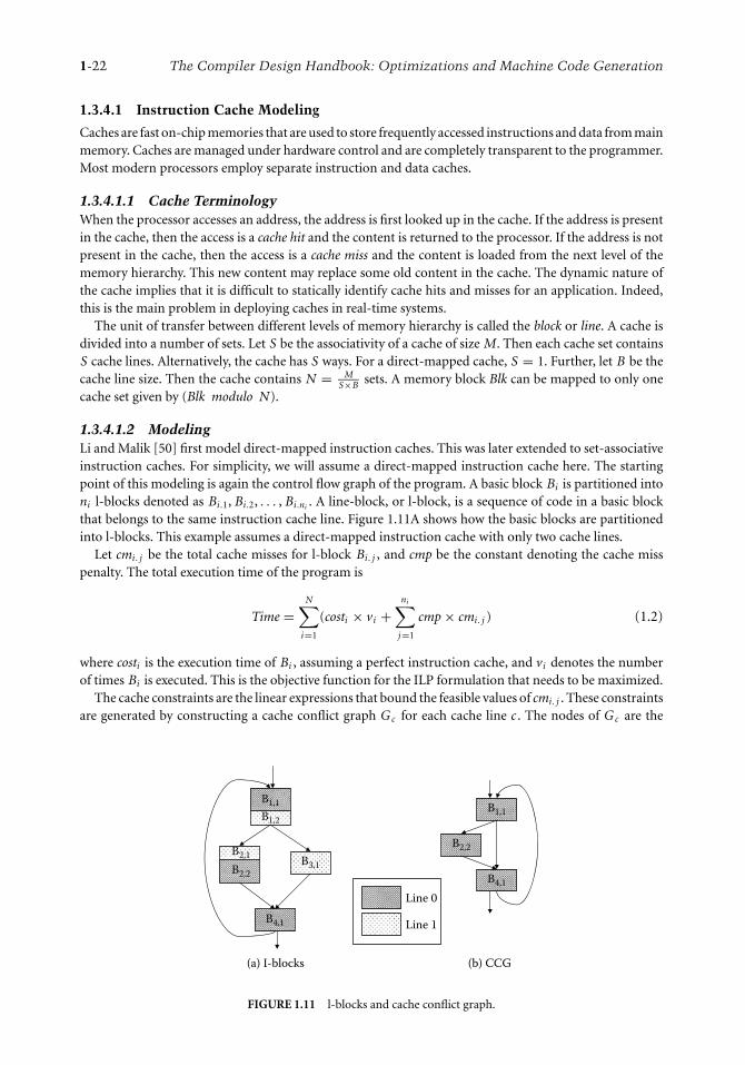
1.3.4.1 Instruction Cache Modeling
Caches are fast on-chip memories that are used to store frequently accessed instructions and data from mainmemory. Caches are managed under hardware control and are completely transparent to the programmer.Most modern processors employ separate instruction and data caches.
1.3.4.1.1 Cache TerminologyWhen the processor accesses an address, the address is first looked up in the cache. If the address is presentin the cache, then the access is a cache hit and the content is returned to the processor. If the address is notpresent in the cache, then the access is a cache miss and the content is loaded from the next level of thememory hierarchy. This new content may replace some old content in the cache. The dynamic nature ofthe cache implies that it is difficult to statically identify cache hits and misses for an application. Indeed,this is the main problem in deploying caches in real-time systems.
The unit of transfer between different levels of memory hierarchy is called the block or line. A cache isdivided into a number of sets. Let S be the associativity of a cache of size M. Then each cache set containsS cache lines. Alternatively, the cache has S ways. For a direct-mapped cache, S = 1. Further, let B be thecache line size. Then the cache contains N = M
S×B sets. A memory block Blk can be mapped to only onecache set given by (Blk modulo N).
1.3.4.1.2 ModelingLi and Malik [50] first model direct-mapped instruction caches. This was later extended to set-associativeinstruction caches. For simplicity, we will assume a direct-mapped instruction cache here. The startingpoint of this modeling is again the control flow graph of the program. A basic block Bi is partitioned intoni l-blocks denoted as Bi.1, Bi.2, . . . , Bi.ni . A line-block, or l-block, is a sequence of code in a basic blockthat belongs to the same instruction cache line. Figure 1.11A shows how the basic blocks are partitionedinto l-blocks. This example assumes a direct-mapped instruction cache with only two cache lines.
Let cmi. j be the total cache misses for l-block Bi. j , and cmp be the constant denoting the cache misspenalty. The total execution time of the program is
Time =N∑
i=1
(costi × vi +ni∑
j=1
cmp × cmi. j ) (1.2)
where costi is the execution time of Bi , assuming a perfect instruction cache, and vi denotes the numberof times Bi is executed. This is the objective function for the ILP formulation that needs to be maximized.
The cache constraints are the linear expressions that bound the feasible values of cmi. j . These constraintsare generated by constructing a cache conflict graph G c for each cache line c . The nodes of G c are the
B1,1
B2,1
B2,2
B3,1
B2,2
B1,1
B4,1
(b) CCG
B4,1
Line 0
Line 1
(a) I-blocks
B1,2
FIGURE 1.11 l-blocks and cache conflict graph.

Worst-Case Execution Time and Energy Analysis 1-23
l-blocks mapped to cache line c . An edge Bi. j → Bu.v exists in G c if there exists a path in the control flowgraph such that control flows from Bi. j to Bu.v without going through any other l-block mapped to c . Inother words, there is an edge between l-blocks Bi. j to Bu.v if Bi. j can be present in the cache when controlreaches Bu.v . Figure 1.11b shows the cache conflict graph corresponding to cache line 0 for the controlflow graph in Figure 1.11a mapped to a cache with two lines.
Let ri. j→u.v be the execution count of the edge between l-blocks Bi. j and Bu.v in a cache conflict graph.Now the execution count of l-block Bi. j equals the execution count of basic block Bi . Also, at each nodeof the cache conflict graph, the inflow equals the outflow and both equal the execution count of the node.Therefore,
vi =∑u.v
ri. j→u.v =∑u.v
ru.v→i. j (1.3)
The cache miss count cmi. j equals the inflow from conflicting l-blocks in the cache conflict graph. Anytwo l-blocks mapped to the same cache block are conflicting if they have different address tags. Two l-blocksmapped to the same cache block do not conflict when the basic block boundary is not aligned with thecache block boundary. For example, l-blocks B1,2 and B2,1 in Figure 1.11a occupy partial cache blocks andhave the same address tags. They do not conflict with each other. Thus, we have
cmi. j =∑u.v
Bu.v conflicts Bi. j
ru.v→i. j (1.4)
1.3.4.2 Dynamic Branch Prediction Modeling
Modern processors employ branch prediction to avoid performance loss due to control dependency [33].Branch prediction schemes can be broadly categorized as static and dynamic. In the static scheme, a branchis predicted in the same direction every time it is executed. Though simple, static schemes are much lessaccurate than dynamic schemes.
1.3.4.2.1 Branch TerminologyDynamic schemes predict a branch depending on the execution history. They use a 2n entry branchprediction table to store past branch outcomes. When the processor encounters a conditional branchinstruction, this prediction table is looked up using some index, and the indexed entry is used as prediction.When the branch is resolved, the entry is updated with the actual outcome. In practice, two-bit saturatingcounters are often used for prediction.
Different branch prediction schemes differ in how they compute an n-bit index to access this table. Incase of simplest prediction scheme, the index is n lower-order bits of the branch address. More complexschemes use a single shift register called a branch history register (BHR) to record the outcomes of the nmost recent branches called history π . The prediction table is looked up either using the BHR directly orexclusive or (XOR)-ed with the branch address. Considering the outcome of the neighboring branchesexploits the correlation among consecutive branch outcomes.
Engblom [19] investigated the impact of dynamic branch prediction on the predicability of real-timesystems. His experiments on a number of commercial processors indicate that dynamic branch predictionleads to high degree of execution time variation even for simple loops. In some cases, executing moreiterations of a loop takes less time than executing fewer iterations. These results reaffirm the need to modelbranch prediction for WCET analysis.
1.3.4.2.2 ModelingLi et al. [45] model dynamic branch predictors through ILP. The modeling is quite general and canbe parameterized with respect to various prediction schemes. Modeling of dynamic branch predictionis somewhat similar to cache modeling. This is because they both use arrays (branch prediction tableand cache) to maintain information. However, two crucial differences make branch prediction modelingsignificantly harder. First, a given branch instruction may use different entries of the prediction table

1-24 The Compiler Design Handbook: Optimizations and Machine Code Generation
at different points of execution (depending on the outcome of previous branches). However, an l-blockalways maps to the same cache block. Second, the flow of control between two conflicting l-blocks alwaysimplies a cache miss, but the flow of control between two branch instructions mapped to the same entryin the prediction table may lead to correct or incorrect prediction depending on the outcome of the twobranches.
To model branch prediction, the objective function given in Equation 1.2 is modified to the following:
Time =N∑
i=1
(costi ∗ vi + bmp ∗ bmi ) (1.5)
where bmp is a constant denoting the penalty for a single branch misprediction, and bmi is the numberof times the branch in Bi is mispredicted. The constraints now need to bound feasible values of bmi . Forsimplicity, let us assume that the branch prediction table is looked up using the history π as the index.
First, a terminating least-fixed-point analysis on the control flow graph identifies the possible values ofhistory π for each conditional branch. The flow constraints model the change in history along the controlflow graph and thereby derive the upper bound on bmπ
i — the execution count of the conditional branchat the end of basic block Bi with history π . Next, a structure similar to a cache conflict graph is used tobound the quantity pπ
i→ j denoting the number of times control flows from Bi to B j such that the π thentry of the prediction table is used for branch prediction at Bi and B j and is never accessed in between.Finally, the constraints on the number of mispredictions are derived by observing the branch outcomesfor consecutive accesses to the same prediction table entry as defined by pπ
i→ j .
1.3.4.3 Interaction between Cache and Branch Prediction
Cache and branch prediction cannot be modeled individually because of the wrong-path instructionprefetching effect (see Figure 1.10). An integrated modeling of these two components through ILP tocapture the interaction has been proposed in [45]. First, the objective function is modified to include thetiming effect of cache misses as well as branch prediction.
Time =N∑
i=1
(costi ∗ vi + bmp ∗ bmi +ni∑
j=1
cmp × cmi. j ) (1.6)
If we assume that the processor allows only one unresolved branch at any time during execution, thenthe number of branch mispredictions bmi is not affected by instruction cache. However, the values of thenumber of cache misses cmi. j may change because of the instruction fetches along the mispredicted path.The timing effects due to these additional instruction fetches can be categorized as follows:
� An l-block Bi. j misses during normal execution since it is displaced by another conflicting l-blockBu.v during speculative execution (destructive effect).� An l-block Bi. j hits during normal execution, since it is prefetched during speculative execution(constructive effect).� A pending cache miss of Bi. j during speculative execution along the wrong path causes the processorto stall when the branch is resolved. How long the stall lasts depends on the portion of cache misspenalty that is masked by the branch misprediction penalty. If the speculative fetching is completelymasked by the branch penalty, then there is no delay incurred.
Both the constructive and destructive effects of branch prediction on cache are modeled by modifyingthe cache conflict graph. The modification adds nodes to the cache conflict graph corresponding to thel-blocks fetched along the mispredicted path. Edges are added among the additional nodes as well asbetween the additional nodes and the normal nodes depending on the control flow during misprediction.The third factor (delay due to incomplete cache miss when the branch is resolved) is taken care of byintroducing an additional delay term in Equation 1.6.

Worst-Case Execution Time and Energy Analysis 1-25
1.3.4.4 Data Cache and Pipeline
So far we have discussed instruction cache and branch prediction modeling using ILP. Data caches areharder to model than instruction caches, as the exact memory addresses accessed by load/store instructionsmay not be known. A simulation-based analysis technique for data caches has been proposed in [50]. Aprogram is broken into smaller fragments where each fragment has only one execution path. For example,even though there are many possible execution paths in a JPEG decompression algorithm, the executionpaths of each computational kernel such as inverse discrete cosine transform (DCT), color transformation,and so on are simple. Each code fragment can therefore be simulated to determine the number of datacache hits and misses. These numbers can be plugged into the ILP framework to estimate the WCET ofthe whole program. For the processor pipeline, [50] again simulates the execution of a basic block startingwith an empty pipeline state. The pipeline state at the end of execution of a basic block is matched againstthe instructions in subsequent basic blocks to determine the additional pipeline stalls during the overlap.These pipeline stalls are added up to the execution time of the basic block. It should be obvious that thisstyle of modeling for data cache and pipeline may lead to underestimation in the presence of a timinganomaly.
Finally, Ottosson and Sjodin [60] propose a constraint-based WCET estimation technique that extendsthe ILP-based modeling. This technique takes the context, that is, the history, of execution into account.Each edge in the control flow graph now corresponds to multiple variables each representing a particularprogram path. This allows accurate representation of the state of the cache and pipeline before a basicblock is executed. A constraint-based modeling propagates the cache states across basic blocks.
1.3.5 Integrated Approach Based on Timing Schema
As mentioned in Section 1.2, one of the original works on software timing analysis was based on timingschema [73]. In the original work, each node of the syntax tree is associated with a simple time bound.This simple timing information is not sufficient to accurately model the timing variations due to pipelinehazards, caches, and branch prediction. The timing schema approach has been extended to model apipeline, instruction cache, and data cache in [51].
1.3.5.1 Pipeline Modeling
The execution time of a program construct depends on the preceding and succeeding instructions on apipelined processor. A single time bound cannot model this timing variation. Instead a set of reservationtables associated with each program construct represents the timing information corresponding to differentexecution paths. A pruning strategy is used to eliminate the execution paths (and their correspondingreservation tables) that can never become the worst-case execution path of the program construct. Theremaining set of reservation tables is called the worst-case timing abstraction (WCTA) of the programconstruct.
The reservation table represents the state of the pipeline at the beginning and end of execution ofthe program construct. This helps analyze the pipelined execution overlap among consecutive programconstructs. The rows of the reservation table represent the pipeline stages and the columns represent time.Each entry in the reservation table specifies whether the corresponding pipeline stage is in use at the giventime slot. The execution time of a reservation table is equal to its number of columns. Figure 1.12 showsa reservation table corresponding to a simple five-stage pipeline.
The rules corresponding to the sequence of statements and if-then-else and while-loop constructs canbe extended as follows. The rule for a sequence of statements S: S1; S2 is given by
W(S) = W(S1) ⊕ W(S2)
where W(S), W(S1), and W(S2) are the WCTAs of S, S1, and S2, respectively. The operator ⊕ isdefined as
W1 ⊕ W2 = {w1 ⊕ w2|w1 ∈ W1, w2 ∈ W2}

1-26 The Compiler Design Handbook: Optimizations and Machine Code Generation
X
1 2 3 4 5 11 12 13 14 15
IF
ID
EX
MEM
WB
X X
X X X
X X
X X
X
X X X
X X X
X
Time
X X X
FIGURE 1.12 Reservation table.
where w1 and w2 are reservation tables, and ⊕ represents the concatenation of two reservation tablesfollowing the pipelined execution model. Similarly, the timing schema rule for S: if (exp) thenS1 else S2 is given by
W(S) = (W(exp) ⊕ (W(S1) ∪ W(S2))
where ∪ is the set union operation. Finally, the rule for the construct S: while (exp) S1 isgiven by
W(S) =(
N⊕i=1
(W(exp) ⊕ W(S1))
)⊕ W(exp)
whereN is the loop bound. In all the cases, a reservation tablew can be eliminated from the WCTA W if it canbe guaranteed that w will never lead to the WCET of the program. For example, if the worst-case scenario(zero overlap with neighboring instructions) involving w ∈ W is shorter than the best-case scenario (com-plete overlap with neighboring instructions) involving w ′ ∈ W, then w can be safely eliminated from W.
1.3.5.2 Instruction Cache Modeling
To model the instruction cache, the WCTA is extended to maintain the cache state information for aprogram construct. The main observation is that some of the memory accesses can be resolved locally(within the program construct) as cache hit/miss. Each reservation table should therefore include (a) thefirst reference to each cache block as its hit or miss depends on the cache content prior to the programconstruct (first reference) and (b) the last reference to each cache block (last reference). The latter affectsthe timing of the successor program construct(s).
The timing rules are structurally identical to the pipeline modeling, but the semantics of the ⊕ operatoris modified. Let us assume a direct-mapped instruction cache. Then w1 ⊕ w2 inherits for a cache block cthe first reference of w1 except when w1 does not have any access to c . In that case, w1 ⊕ w2 inherits thefirst reference of w2. Similarly, for a cache block c , w1 ⊕ w2 inherits the last reference of w2 except whenw2 does not have a last reference to c . In this case, the last reference to c is inherited from w1. Finally, thenumber of additional cache hits for w2 can be determined by comparing the first references of w2 withthe last references of w1. The execution time of w1 ⊕ w2 can be determined by taking into account thepipelined execution across w1, w2 and the additional cache hits. As before, a pruning strategy is employedto safely eliminate WCTA elements that can never contribute to the WCET path of the program.
1.3.5.3 Data Cache Modeling
Timing analysis of the data cache is similar to that of the instruction cache. The major difficulty, however,is that the addresses of some data references may not be known at compile time. A global data flowanalysis [38] is employed to resolve the data references of load/store instructions as much as possible. Aconservative approach is then proposed [38] where two cache miss penalties are assumed for each datareference whose memory address cannot be determined at compile time. The data reference is then ignored

Worst-Case Execution Time and Energy Analysis 1-27
in the rest of the analysis. The first penalty accounts for the cache miss possibility of the data reference. Thesecond penalty covers for the possibility that the data reference may replace some memory block (fromthe cache) that is considered as cache hit in the analysis. Finally, data dependence analysis is utilized tominimize the WCET overestimation resulting from the conservative assumption of two cache misses perunknown reference.
1.3.6 Separated Approach Based on Abstract Interpretation
ILP-based WCET analysis methods can model the architectural components and their interaction in anaccurate fashion, thereby yielding tight estimates. However, ILP solution time may increase considerablywith complex architectural features. To circumvent this problem, Theiling et al. [82] have proposed aseparated approach where abstract interpretation is employed for micro-architectural modeling followedby ILP for path analysis. As there is a dependency between the two steps, micro-architectural modeling hasto produce conservative estimates to ensure safety of the result. This overestimation is offset by significantlyfaster analysis time.
Abstract interpretation [15] is a theory for formally constructing conservative approximations of thesemantics of a programming language. A concrete application of abstract interpretation is in static programanalysis where a program’s computations are performed using abstract values in place of concrete values.Abstract interpretation is used in WCET analysis to approximate the “collecting semantics” at a programpoint. The collecting semantics gives the set of all program states (cache, pipeline, etc.) for a given programpoint. In general, the collecting semantics is not computable. In abstract interpretation, the goal is toproduce an abstract semantics which is less precise but effectively computable. The computation of theabstract semantics involves solving a system of recursive equations/constraints. Given a program, we canassociate a variable [[ p]] to denote the abstract semantics at program point p. Clearly, [[ p]] will dependon the abstract semantics of program points preceding p. Since programs have loops, this will lead to asystem of recursive constraints. The system of recursive constraints can be iteratively solved via fixed-pointcomputation. Termination of the fixed-point computation is guaranteed only if (a) the domain of abstractvalues (which is used to define the abstract program semantics) is free from infinite ascending chains and(b) the iterative estimates of [[ p]] grow montonically. The latter is ensured if the semantic functions in theabstract domain, which show the effect of the programming language constructs in the abstract domainand are used to iteratively estimate [[p]], are monotonic.
Once the fixed-point computation terminates, for every program point p, we obtain a stable estimatefor [[ p]] — the abstract semantics at p. This is an overapproximation of all the concrete states with which pcould be reached in program executions. Thus, for cache behavior modeling, [[p]] could be used to denotean overapproximation of the set of concrete cache states with which program point p could be reachedin program executions. This abstract semantics is then used to conservatively derive the WCET boundsfor the individual basic blocks. Finally, the WCET estimates of basic blocks are combined with ILP-basedpath analysis to estimate the WCET of the entire program.
1.3.6.1 Cache Modeling
To illustrate AI-based cache modeling, we will assume a fully associative cache with a set of cache linesL = {l1, . . . , ln} and least recently used replacement policy. Let {s1, . . . , sm} denote the set of memoryblocks. The absence of any memory block in a cache line is indicated by a new element I ; thus, S ={s1, . . . , sm} ∪ {I }.
Let us first define the concrete semantics.
Definition 1.3A concrete cache state is a function c : L → S.
If c(lx ) = s for a concrete cache state c , then there are x − 1 elements (c(l1), . . . , c(lx−1)) that are morerecently used than s . In other words, x is the relative age of s . Cc denotes the set of all concrete cache states.

1-28 The Compiler Design Handbook: Optimizations and Machine Code Generation
Definition 1.4A cache update functionU : Cc × S → Cc describes the new cache state for a given cache state and a referencedmemory block.
Let s = c(lx ) be the referenced memory block. The cache update function shifts the memory blocksc(l1), . . . , c(lx−1), which have been more recently used than s , by one position to the next cache line. If swas not in the cache, then all the memory blocks are shifted by one position, and the least recently usedmemory block is evicted from the cache state (if the cache was full). Finally, the update function puts thereferenced memory block s in the first position l1.
The abstract semantics defines the abstract cache states, the abstract cache update function, and thejoin function.
Definition 1.5An abstract cache state c : L → 2S maps cache lines to sets of memory blocks.
Let C denote the set of all abstract cache states. The abstract cache update function U : C × S �→ Cis a straightforward extension of the function U (which works on concrete cache states) to abstract cachestates.
Furthermore, at control flow merge points, join functions are used to combined the abstract cachestates. That is, join functions approximate the collecting semantics depending on program analysis.
Definition 1.6A join function J : C × C �→ C combines two abstract cache states.
Since L is finite and S is finite, clearly the domain of abstract cache states is finite and hence freefrom any infinite ascending chains. Furthermore, the update and join functions U and J are monotonic.This ensures termination of a fixed-point computation-based analysis over the above-mentioned abstractdomain. We now discuss two such analysis methods.
The program analysis mainly consists of must analysis and may analysis. The must analysis determinesthe set of memory blocks that are always in the cache at a given program point. The may analysis deter-mines the memory blocks that may be in the cache at a given program point. The may analysis can beused to determine the memory blocks that are guaranteed to be absent in the cache at a given programpoint.
The must analysis uses abstract cache states with upper bounds on the ages of the memory blocks inthe concrete cache states. That is, if s ∈ c(lx ), then s is guaranteed to be in the cache for at least the nextn − x memory references (n is the number of cache lines). Therefore, the join function of two abstractcache states c1 and c2 puts a memory block s in the new cache state if and only if s is present in both c1
and c2. The new age of s is the maximum of its ages in c1 and c2. Figure 1.13 shows an example of the joinfunction for must and may analysis.
The may analysis uses abstract cache states with lower bounds on the ages of the memory blocks.Therefore, the join function of two abstract cache states c1 and c2 puts a memory block s in the new cachestate if s is present in either c1 or c2 or both. The new age of s is the minimum of its ages in c1 and c2.
At a program point, if a memory block s is present in the abstract cache state after must analysis, thena memory reference to s will result in a cache hit (always hit). Similarly, if a memory block s is absent inthe abstract cache state after may analysis, then a memory reference to s will result in a cache miss (alwaysmiss). The other memory references cannot be classified as hit or miss. To improve the accuracy, a furtherpersistence analysis can identify memory blocks for which the first reference may result in either hit ormiss, but the remaining references will be hits.
These categorization of memory references is used to define the WCET for each basic block. To improvethe accuracy, the WCET of a basic block is determined under different calling contexts. Thus, the objective

Worst-Case Execution Time and Energy Analysis 1-29
{a}
{a}
{ }
{b}
{b}
{c, d}
{a}
{ }
{b}
{c, d}
{ }
Young
Old
Young
Old
Age
{ }
{a, b}
{c}
{c}
{b}
{c}
{a}
{d}
Join for May AnalysisJoin for Must Analysis
{ }
{ }
{a, b}
{c}
{d}
FIGURE 1.13 Join for must and may analysis.
function can be defined as
Time =N∑
i=1
∑x∈τ (Bi )
(costx
i × vix)
(1.7)
where τ (Bi ) denotes the set of all calling contexts for basic block Bi . The bounds on execution counts v xi
can be derived by ILP-based path analysis.An extension for data cache modeling using abstract interpretation has been proposed in [23]. The basic
idea is to extend the cache update function such that it can handle cases where not all addresses referencedby a basic block are known.
Another technique for categorizing cache access references into always hit, always miss, first miss, andfirst hit has been proposed by the group at Florida State University [4, 57, 93]. They perform categorizationthrough static cache simulation, which is essentially an interprocedural data flow analysis. This catego-rization is subsequently used during pipeline analysis [29]. Pipeline analysis proceeds by determining thetotal number of cycles required to execute each path, where a path consists of all the instructions thatcan be executed during a single iteration of a loop. The data hazards and the structural hazards acrosspaths are determined by maintaining the first and last use of each pipeline stage and register within a path.As mentioned before, this separation of cache analysis from the pipeline analysis may not be safe in thepresence of a timing anomaly.
1.3.6.2 Pipeline Modeling
To model a pipeline with abstract interpretation [41], concrete execution on a concrete pipeline can beviewed as applying a function. This function takes as input a concrete pipeline state s and a sequenceof instructions in a basic block b. It produces a sequence of execution states, called a trace, and a finalconcrete state when executing b. The length of the trace determines the number of cycles the execution takes.The concept of trace is similar to the reservation table described in the context of timing-schema-basedanalysis.
However, in the presence of incomplete information, such as nonclassified cache accesses, the concreteexecution is not feasible. Therefore, pipeline analysis employs an abstract execution of the sequence ofinstructions in a basic block starting with an abstract pipeline state s [41]. This modeling defines anabstract pipeline state as a set of concrete pipeline states, and pipeline states with identical timing behaviorare grouped together. Now, suppose that in an abstract pipeline state s an event occurs that changes thepipeline states, such as the issue/execution of an instruction I in a basic block. If the latency of this eventcan be statically determined, s has only one successor state. However, if the latency of I ’s execution cannotbe statically determined, a pipeline state will have several successor states resulting from the executionof I corresponding to the various possible latencies of I (thereby causing state space explosion). In this

1-30 The Compiler Design Handbook: Optimizations and Machine Code Generation
way, reachable pipeline states within a basic block will be enumerated (while grouping together states withidentical timing behavior) in order to determine the basic block’s WCET.
For a processor without a timing anomaly [41], the abstract execution can be employed to each ba-sic block starting with the empty pipeline state. The abstract execution exploits the memory referencecategorization (obtained through cache modeling) to determine memory access delays during pipelineexecution. Therefore, abstract execution of a basic block should happen under different contexts. In thepresence of a timing anomaly, cache and pipeline analysis cannot be separated [32]. Hence the abstractstates now consist of pairs of abstract pipeline states and abstract cache states. Moreover, the final abstractstates of a basic block will be passed on to the successor basic block(s) as initial states. Clearly, this can leadto an exponential number of abstract states for complex processor pipelines.
1.3.6.3 Branch Prediction Modeling
Colin and Puaut [14] propose abstract-interpretation-based branch prediction modeling. They assumethat the branch prediction table (see Section 1.3.4.2.1) is indexed using the address of the conditionalbranch instruction. This prediction scheme is simpler and hence easier to model than the BHR-basedpredictors modeled using ILP [45]. Colin and Puaut use the term branch target buffer (BTB) instead ofprediction table, as it stores the target address in addition to the branch history. Moreover, each entry inthe BTB is tagged with the address of the conditional branch instruction whose history and target addressare stored in that entry. When a conditional branch is encountered, if its address is in the BTB, then it ispredicted based on the history stored in the BTB. Otherwise, the default prediction of the branch not takenis used. The BTB is quite similar to instruction cache and indeed can be organized as direct-mapped ors-way set associative caches.
The abstract execution defines the abstract buffer state (ABS) corresponding to the BTB. Each basicblock Bi is associated with two ABS: AB Sin
i and AB Souti , representing the BTB state before and after Bi ’s
execution. An ABS indicates for each BTB entry which conditional branch instructions can be in the BTBat that time. At program merge points, a set union operation is carried out. Thus,
AB Sini =
⊎B j ∈ Pred Bi
AB Soutj
where PredB(i) is the set of basic blocks preceding Bi in the control flow graph. Assuming a set-associativeBTB, the union operator � is defined as follows:
AB Si � AB S j = ∀x∀y AB Si [x , y] ∪ AB S j [x , y]
where AB Si [s , k] is a set containing all the branch instructions that could be in the yth entry of the set x .AB Sout
i is derived from AB Sini by taking into account the conditional branch instruction in Bi .
Given AB Sini , the conditional branch instruction can be classified as history predicted if it is present in
the BTB and default predicted otherwise. However, a history-predicted instruction does not necessarilylead to correct prediction. Similarly, a default-predicted instruction does not always lead to misprediction.This is taken into account by considering the behavior of the conditional branch instruction. For example,a history-predicted loop instruction is always correctly predicted except for loop exit.
The modeling in [14] was later extended to more complex branch predictors such as bimodal and global-history branch prediction schemes [5, 11]. The semantic context of a branch instruction in the source codeis taken into account to classify a branch as easy to predict or hard to predict. Easy-to-predict branchesare analyzed, while conservative misprediction penalties are assumed for hard-to-predict branches. Thedownside of these techniques is that they make a restrictive assumption of each branch instruction mappingto a different branch table entry (i.e., no aliasing).

Worst-Case Execution Time and Energy Analysis 1-31
1.3.7 A Separated Approach That Avoids State Enumeration
The implication of a timing anomaly (see Section 1.3.2) is that all possible schedules of instructions haveto be considered to estimate the WCET of even a basic block. Moreover, all possible processor states atthe end of the preceding and succeeding basic blocks have to be considered during the analysis of a basicblock. This can result in state space explosion for analysis techniques, such as abstract-interpretation-basedmodeling, that are fairly efficient otherwise [83].
A novel modeling technique [46] obtains safe and tight estimates for processors with timing anomalieswithout enumerating all possible executions corresponding to variable latency instructions (owing tocache miss, branch misprediction, and variable latency functional units). In particular, [46] models afairly complex out-of-order superscalar pipeline with instruction cache and branch prediction. First, theproblem is formulated as an execution graph capturing data dependencies, resource contentions, and degreeof superscalarity — the major factors dictating instruction executions. Next, based on the execution graph,the estimation algorithm starts with very coarse yet safe timing estimates for each node of the executiongraph and iteratively refines the estimates until a fixed point is reached.
1.3.7.1 Execution Graph
Figure 1.14 shows an example of an execution graph. This graph is constructed from a basic block with fiveinstructions as shown in Figure 1.14a; we assume that the degree of superscalarity is 2. The processor hasfive pipeline stages: fetch (IF), decode (ID), execute (EX), write back (WB), and commit (CM). A decodedinstruction is stored in the re-order buffer. It is issued (possibly out of order) to the correspondingfunctional unit for execution when the operands are ready and the functional unit is available.
Let CodeB = I1 . . . In represent the sequence of instructions in a basic block B . Then each node vin the corresponding execution graph is represented by a tuple: an instruction identifier and a pipelinestage denoted as stage(instruction id). For example, the node v = IF(Ii ) represents the fetch stage of theinstruction Ii . Each node in the execution graph is associated with the latency of the corresponding pipelinestage. For a node u with variable latency min latu ∼ max latu , the node is annotated with an interval[min latu , max latu]. As some resources (e.g., floating point multiplier) in modern processors are fullypipelined, such resources are annotated with initiation intervals. The initiation interval of a resource isdefined as the number of cycles that must elapse between issuing two instructions to that resource. Forexample, a fully pipelined floating point multiplier can have a latency of six clock cycles and an initiationinterval of one clock cycle. For a nonpipelined resource, the initiation interval is the same as latency. Also,if there exist multiple copies of the same resource (e.g., two arithmetic logical units (ALUs)), then oneneeds to define the multiplicity of that resource.
IF(I1)I1: mult r6 r10 4
IF(I2)I2: mult r1 r10 r1
IF(I3)I3: sub r6 r6 r2
IF(I4)I4: mult r4 r8 r4
IF(I5)I5: add r1 r1 r4
(a) Code Example (b) Execution Graph
ID(I1)
ID(I2)
ID(I3)
ID(I4)
ID(I5)
EX(I1)
EX(I2)
EX(I3)
EX(I4)
EX(I5)
WB(I1)
WB(I2)
WB(I3)
WB(I4)
WB(I5)
CM(I1)
CM(I2)
CM(I3)
CM(I4)
CM(I5)
FIGURE 1.14 A basic block and its execution graph. The solid directed edges represent dependencies and the dashedundirected edges represent contention relations. From Li et al. [46] c© 2006 Springer.

1-32 The Compiler Design Handbook: Optimizations and Machine Code Generation
The dependence relation from node u to node v in the execution graph denotes that v can start executiononly after u has completed execution; this is indicated by a solid directed edge from u to v in the executiongraph. The analysis models the following dependencies:� Dependencies among pipeline stages of the same instruction.� Dependencies due to finite-sized buffers and queues such as I-buffer or ROB. For example, assuming
a four-entry I-buffer, there will be no entry available for IF(Ii+4) before the completion of ID(Ii )(which removes Ii from the I-buffer). Therefore, there should be a dependence edge ID(Ii ) →IF(Ii+4).� Dependencies due to in-order execution in IF, ID, and CM pipeline stages. For example, in a scalarprocessor (i.e., degree of superscalarity = 1) there will be dependence edges IF(Ii ) → IF(Ii+1)because IF(Ii+1) can only start after IF(Ii ) completes. For a superscalar processor with n-way fetch(i.e., degree of superscalarity = n), there are dependence edges IF(Ii ) → IF(Ii+n). This capturesthe fact that Ii+n cannot be fetched in the same cycle as Ii .� Data dependencies among instructions. If instruction Ii produces a result that is used by instructionI j , then there should be a dependence edge WB(Ii ) → EX(I j ).
Apart from the dependence relation among the nodes in an execution graph (denoted by solid edges),there also exist contention relations among the execution graph nodes. Contention relations model struc-tural hazards in the pipeline. A contention relation exists between two nodes u and v if they can delayeach other by contending for a resource, for example, functional unit or register write port. The con-tention between u and v is shown as an undirected dashed edge in the execution graph. A contentionrelation makes it possible for an instruction later in the program order to delay the execution of an earlierinstruction.
Finally, a parallelism relation is defined to model superscalarity, for example, multiple issues and multipledecodes. Two nodes u and v participate in a parallelism relation iff (a) nodes u and v denote the samepipeline stage (call it s tg ) of two different instructions Ii and I j and (b) instructions Ii and I j can startexecution of this pipeline stage s tg in parallel.
1.3.7.2 Problem Definition
Let B be a basic block consisting of a sequence of instructions CodeB = I1 . . . In. Estimating the WCET ofB can be formulated as finding the maximum (latest) completion time of the node CM(In), assuming thatIF(I1) starts at time zero. Note that this problem is not equivalent to finding the longest path from IF(I1)to CM(In) in B ’s execution graph (taking the maximum latency of each pipeline stage). The executiontime of a path in the execution graph is not a summation of the latencies of the individual nodes for tworeasons:� The total time spent in making the transition from ID(Ii ) to EX(Ii ) is dependent on the contentions
from other ready instructions.� The initiation time of a node is computed as the max of the completion times of its immedi-ate predecessors in the execution graph. This models the effect of dependencies, including datadependencies.
1.3.7.3 Estimation Algorithm
The timing effects of the dependencies are accounted for by using a modified longest-path algorithm thattraverses the nodes in topologically sorted order. This topological traversal ensures that when a node isvisited, the completion times of all its predecessors are known. To model the effect of resource contentions,the algorithms conservatively estimate an upper bound on the delay due to contentions for a functionalunit by other instructions. A single pass of the modified longest-path algorithm computes loose boundson the lifetime of each node. These bounds are used to identify nodes with disjoint lifetimes. These

Worst-Case Execution Time and Energy Analysis 1-33
Prologue
Body
IF(I–5)
IF(I–4)
IF(I–3)
IF(I–2)
IF(I–1)
IF(I0)
IF(I1)
ID(I–5)
ID(I–4)
ID(I–3)
ID(I–2)
ID(I–1)
ID(I0)
ID(I1)
EX(I–5)
EX(I–4)
EX(I–3)
EX(I–2)
EX(I–1)
EX(I0)
EX(I1)
WB(I–5)
WB(I–4)
WB(I–3)
WB(I–2)
WB(I–1)
WB(I0)
WB(I1)
CM(I–5)
CM(I–4)
CM(I–3)
CM(I–2)
CM(I–1)
CM(I0)
CM(I1)
FIGURE 1.15 An example prologue. From Li et al. [46] c© 2006 Springer.
nodes are not allowed to contend in the next pass of the longest-path search to get tighter bounds. Thesetwo steps repeat until there is no change in the bounds. Termination is guaranteed for the followingreasons:� The algorithm starts with all pairs of instructions in the contention relation (i.e., every instruction
can delay every other instruction).� At every step of the fixed-point computation, pairs are removed from this set — those instructionpairs that are shown to be separated in time.
As the number of instructions in a basic block is finite, the number of pairs initially in the contentionrelation is also finite. Furthermore, the algorithm removes at least one pair in every step of the fixed-pointcomputation, so the fixed-point computation must terminate in finitely many iterations; if the numberof instructions in the basic block being estimated is n, the number of fixed-point iterations is boundedby n2.
1.3.7.3.1 Basic Block ContextIn the presence of a timing anomaly, a basic block cannot be analyzed in isolation by assuming an emptypipeline at the beginning. The instructions before (after) a basic block B that directly affect the executiontime of B constitute the contexts of B and are called the prologue (epilogue) of B . As processor buffersizes are finite, the prologue and epilogue contain finite number of instructions. Of course, a basic blockB may have multiple prologues and epilogues corresponding to the different paths along which B can beentered or exited. To capture the effects of contexts, the analysis technique constructs execution graphscorresponding to all possible combinations of prologues and epilogues. Each execution graph consists ofthree parts: the prologue, the basic block itself (called the body), and the epilogue.
The executions of two or more successive basic blocks have some overlap due to pipelined execution. Theoverlap δ between a basic block B and its preceding basic block B ′ is the period during which instructionsfrom both the basic blocks are in the pipeline, that is,
δ = tfinishCM(I0) − t
readyIF(I1) (1.8)
where I0 is the last instruction of block B ′ (predecessor) and I1 is the first instruction of block B . To avoidduplicating the overlap in time estimates of successive basic blocks, the execution time tB of a basic blockB is defined as the interval from the time when the instruction immediately preceding B has finished

1-34 The Compiler Design Handbook: Optimizations and Machine Code Generation
committing to the time when B ’s last instruction has finished committing, that is,
tB = tfinishCM(In) − t
finishCM(I0) (1.9)
where I0 is the instruction immediately prior to B and In is the last instruction of B .The execution time for basic block B is estimated with respect to (w.r.t.) the time at which the first
instruction I1 of B is fetched, i.e., treadyIF(I1) = 0. Thus,
tB = tfinishCM(In) − δ (1.10)
tB can be conservatively estimated by finding the largest value of tfinishCM(In) and the smallest value of δ.
1.3.7.3.2 Overall Pipeline AnalysisThe execution time estimate tB of a basic block B is obtained for a specific prologue and a specific epilogue ofB . A basic block B in general has multiple choices of prologues and epilogues. Thus, B ’s execution time isestimated under all possible combinations of prologues and epilogues. The maximum of these estimatesis used as B ’s WCET c B . Let P and E be the set of prologues and epilogues for B .
c B = maxp∈P , e∈E
(tB with prologue p and epilogue e)
c B is used in defining the WCET of the program as the following objective function:
maximize∑B∈B
NB ∗ c B
The quantity NB denotes the execution count of basic block B and is a variable. B is the set of all basicblocks in the program. This objective function is maximized over the constraints on NB given by ILP-basedpath analysis.
1.3.7.4 Integrating Cache and Branch Prediction Analysis
The basic idea is to define different scenarios for a basic block corresponding to cache miss and branchmisprediction. If these scenarios are defined suitably, then we can estimate a constant that bounds theexecution time of a basic block corresponding to each scenario. Finally, the execution frequencies of thesescenarios are defined as ILP variables and are bounded by additional linear constraints.
Scenarios corresponding to cache misses are defined as follows. Given a cache configuration, a basicblock BB can be partitioned into a fixed number of memory blocks, with instructions in each memoryblock being mapped to the same cache block (cache accesses of instructions other than the first one in amemory block are always hits). A cache scenario of BB is defined as a mapping of hit or miss to each ofthe memory blocks of BB. The memory blocks are categorized into always hit, always miss, or unknown,using abstract interpretation-based modeling (see Section 1.3.6.1). The upper bounds on the executiontime of BB are computed w.r.t. each of the possible cache scenarios. For the first instructions in memoryblocks with unknown categorization, the latency of the fetch stage is assumed to be [1, penal ty] wherepenal ty is the cache miss penalty.
Similarly, the scenarios for branch prediction are defined as the two branch outcomes (correct predictionand misprediction) corresponding to each of the predecessor basic blocks. The execution time of the basicblock is estimated w.r.t. both the scenarios by adding nodes corresponding to the wrong-path instructionsto the execution graph of a basic block.
Considering the possible cache scenarios and correct or wrong prediction of the preceding branch fora basic block, the ILP objective function denoting a program’s WCET is now written as follows.
Maximize T =N∑
i=1
∑j→i
∑ω∈i
tc ,ωj→i ∗ E c ,ω
j→i + tm,ωj→i ∗ E m,ω
j→i (1.11)

Worst-Case Execution Time and Energy Analysis 1-35
TABLE 1.1 Accuracy and analysis time of WCET estimation technique [46]
Benchmark WCET (cycles) Analysis time (sec)
Estimated Observed Ratio ILP formulation ILP solutionadpcm 139,346 227,134 1.32 3.41 9.90dhry 275,177 436,610 1.53 1.84 0.10fdct 15,006 16,956 1.13 0.08 0.01fft 944,397 1,146,474 1.14 0.44 0.01fir 77,004 101,333 1.26 0.79 0.31ludcmp 17,617 23,818 1.28 0.43 0.12matsum 62,138 62,734 1.01 0.07 0.01minver 14,221 21,315 1.33 1.28 0.98qurt 4,114 6,464 1.45 0.85 0.62whet 760,010 950,818 1.14 1.24 0.01
where tc ,ωj→i is the WCET of Bi executed under the following context: (a) Bi is reached from a preceding
block B j , (b) the branch prediction at the end of B j is correct or B j does not have a conditional branch,and (c) Bi is executed under a cache scenario ω ∈ i . i is the set of all cache scenarios of block Bi . Thebounds on number of scenarios with correct and mispredicted branch instructions are obtained usingILP-based analysis [45] (see Section 1.3.4.2).
Finally, to extend the above approach for modeling data caches, one can adapt the approach of [69].This work augments the cache miss equation framework of Ghosh et al. [26] to generate accurate hit andmiss patterns corresponding to memory references at different loop levels.
1.3.7.5 Accuracy and Scalability
To give the readers a feel of the accuracy and scalability of the WCET analysis techniques, we present inTable 1.1 the experimental results from [46]. The processor configuration used here is fairly sophisticated:a 2-way superscalar out-of-order pipeline with 5 stages containing a 4-entry instruction fetch buffer, an8-entry re-order buffer, 2 ALUs, variable latency multiplication and floating point units, and 1 load/storeunit; perfect data cache; gshare branch predictor with a 128-entry branch history table; a 1-KB 2-way setassociative instruction cache with 16 sets, 32 bytes line size, and 30 cycles cache miss penalty. The analysiswas run on a 3-GHz Pentium IV PC with 2 GB main memory.
Table 1.1 presents the estimated WCET obtained through static analysis and the observed WCET ob-tained via simulation (see Figure 1.3 for the terminology). The estimated WCET is quite close to theobserved WCET. Also, the total estimation time (ILP formulation + ILP solving) is less than 15 secondsfor all the benchmarks.
1.4 Worst-Case Energy Estimation
In this section, we present a static analysis technique to estimate safe and tight bounds for the worst-caseenergy consumption of a program on a particular processor. The presentation in this section is basedon [36].
Traditional power simulators, such as Wattch [9] and SimplePower [96], perform cycle-by-cycle powerestimation and then add them up to obtain total energy consumption. Clearly, we cannot use cycle-accurate estimation to compute the worst-case energy bound, as it would essentially require us to simulateall possible scenarios (which is too expensive). The other method [75, 88] is to use fixed per-instructionenergy but it fails to capture the effects of cache miss and branch prediction. Instead, worst-case energyanalysis is based on the key observation that the energy consumption of a program can be separated outinto the following time-dependent and time-independent components:

1-36 The Compiler Design Handbook: Optimizations and Machine Code Generation
Instruction-specific energy: The energy that can be attributed to a particular instruction (e.g., energyconsumed as a result of the execution of the instruction in the ALU, cache miss, etc.). Instruction-specific energy does not have any relation with the execution time.
Pipeline-specific energy: The energy consumed in the various hardware components (clock networkpower, leakage power, switch-off power, etc.) that cannot be attributed to any particular instruction.Pipeline-specific energy is roughly proportional to the execution time.
Thus, cycle-accurate simulation is avoided by estimating the two energy components separately. Pipeline-specific energy estimation can exploit the knowledge of WCET. However, switch-off power and clocknetwork power make the energy analysis much more involved — we cannot simply multiply the WCETby a constant power factor. Moreover, cache misses and overlap among basic blocks due to pipelining andbranch prediction add significant complexity to the analysis.
1.4.1 Background
Power and energy are terms that are often used interchangeably as long as the context is clear. For batterylife, however, the important metric is energy rather than power. The energy consumption of a task runningon a processor is defined as Energy = P × t, where P is the average power and t is the execution time.Energy is measured in Joules, whereas power is measured in Watts (Joules/second). Power consumptionconsists of two main components: dynamic power and leakage power P = Pdynamic + Pleakage.
Dynamic power is caused by the charging and discharging of the capacitive load on each gate’s outputdue to switching activity. It is defined as Pdynamic = 1
2 AV 2ddCf , where A is the switching activity, Vdd is the
supply voltage, C is the capacitance, and f is the clock frequency. For a given processor architecture, Vdd
and f are constants. The capacitance value for each component of the processor can be derived throughregister-capacitor (RC)-equivalent circuit modeling [9].
Switching activity A is dependent on the particular program being executed. For circuits that chargeand discharge every cycle, such as double-ended array bitlines, an activity factor of 1.0 can be used.However, for other circuits (e.g., single-ended bitlines, internal cells of decoders, pipeline latches, etc.), anaccurate estimation of the activity factor requires examination of the actual data values. It is difficult, ifnot impossible, to estimate the activity factors through static analysis. Therefore, an activity factor of 1.0(i.e., maximum switching) is assumed conservatively for each active processor component.
Modern processors employ clock gating to save power. This involves switching off clock signals to theidle components so they do not consume dynamic power in the unused cycles. Jayaseelan et al. [36] modelthree different clock gating styles. For simplicity, let us assume a realistic gating style where idle units andports dissipate 10% of the peak power. A multi-ported structure consumes power proportional to thenumber of ports accessed in a given cycle. The power consumed in the idle cycles is referred to as switch-offpower.
A clock distribution network consumes a significant fraction of the total energy. Without clock gating,clock power is independent of the characteristics of the applications. However, clock gating results in powersavings in the clock distribution network. Whenever the components in a portion of the chip are idle, theclock network in that portion of the chip can be disabled, reducing clock power.
Leakage power captures the power lost from the leakage current irrespective of switching activity. Theanalysis uses the leakage power model proposed in [98]: Pleakage = Vdd × N × kd × Ileakage, where Vdd
is the supply voltage and N is the number of transistors. Ileakage is a constant specifying the leakagecurrent corresponding to a particular process technology. kd is an empirically determined design parameterobtained through SPICE simulation corresponding to a particular device.
1.4.2 Analysis Technique
The starting point of the analysis is the control flow graph of the program. The first step of the analysisestimates an upper bound on the energy consumption of each basic block. Once these bounds are known,the worst-case energy of the entire program can be estimated through path analysis.

Worst-Case Execution Time and Energy Analysis 1-37
1.4.2.1 Energy Estimation for a Basic Block
The goal here is to estimate a tight upper bound on the total energy consumption ener g yBB of a basicblock BB through static analysis. From the discussion in Section 1.4.1,
energyBB = dynamicBB + switchoff BB
+ leakageBB + clockBB (1.12)
where dynamicBB is the instruction-specific energy component, that is, the energy consumed as a resultof switching activity as an instruction goes through the pipeline stages. switchoff BB, leakageBB, and clockBB
are defined as the energy consumed as a result of the switch-off power, leakage power, and clock power,respectively, during wcetBB, where wcetBB is the WCET of the basic block BB. The WCET (wcetBB) isestimated using the static analysis techniques. Now we describe how to define bounds for each energycomponent.
1.4.2.1.1 Dynamic EnergyThe instruction-specific energy of a basic block is the dynamic power consumed as a result of the switchingactivity generated by the instructions in that basic block.
dynamicBB =∑
instr ∈ BB
dynamicinstr (1.13)
where dynamicinstr is the dynamic power consumed by an instruction instr. Now, let us analyze the energyconsumed by an instruction as it travels through the pipeline:
1. Fetch and decode: The energy consumed here is due to fetch, decode, and instruction cache access.This stage needs feedback from cache analysis.
2. Register access: The energy consumed for the register file access because of reads/writes can varyfrom one class of instructions to another. The energy consumption in the register file for aninstruction is proportional to the number of register operands.
3. Branch prediction: The energy consumption in this stage needs feedback from branch predictionmodeling.
4. Wakeup logic: When an operation produces a result, the wakeup logic is responsible for makingthe dependent instructions ready, and the result is written onto the result bus. An instruction placesthe tag of the result on the wakeup logic and the actual result on the result bus exactly once, andthe corresponding energy can be easily accounted for. The enery consumed in the wakeup logic isproportional to the number of output operands.
5. Selection logic: Selection logic is interesting from the point of view of energy consumption. Theselection logic is responsible for selecting an instruction to execute from a pool of ready instructions.Unlike the other components discussed earlier, an instruction may access the selection logic morethan once. This is because an instruction can request a specific functional unit and the request mightnot be granted, in which case it makes a request in the next cycle. However, we cannot accuratelydetermine the number of times an instruction would access the selection logic. Therefore, it isconservatively assumed that the selection logic is accessed every cycle.
6. Functional units: The energy consumed by an instruction in the execution stage depends on thefunctional unit it uses and its latency. For variable latency instructions, one can safely assume themaximum energy consumption. The energy consumption for load/store units depends on datacache modeling.
Now, Equation 1.13, corresponding to dynamic energy consumed in a basic block BB, is redefined as
dynamicBB = selection powercycle × wcetBB
+∑
instr ∈ BB
dynamicinstr (1.14)

1-38 The Compiler Design Handbook: Optimizations and Machine Code Generation
where selection powercycle is a constant defining the power consumed in the selection logic per cycle. wcetBB
is the WCET of BB. Note that dynamicinstr is redefined as the power consumed by instr in all the pipelinestages except for selection logic.
As mentioned before, pipeline-specific energy consists of three components: switch-off energy, clockenergy, and leakage energy. All three energy components are influenced by the execution time of the basicblock.
1.4.2.1.2 Switch-off EnergyThe switch-off energy refers to the power consumed in an idle unit when it is disabled through clockgating. Let accessBB(C ) be the total number of accesses to a component C by the instructions in basic blockBB. Let ports(C ) be the maximum number of allowed accesses/ports for component C per cycle. Then,switch-off energy for component C in basic block BB is
switchoff BB(C ) =(
wcetBB − accessBB(C)ports(C)
)× full powercycle(C) × 10% (1.15)
where full powercycle(C ) is the full power consumption per cycle for component C . The switch-off energycorresponding to a basic block can now be defined as
switchoff BB =∑
C∈components
switchoff BB(C) (1.16)
where components is the set of all hardware components.
1.4.2.1.3 Clock Network EnergyTo estimate the energy consumed in the clock network, clock gating should be taken into account.
clockBB = non gated clockBB ×(
circuitBB
non gated circuitBB
)(1.17)
where non gated clockBB is the clock energy without gating and can be defined as
non gated clockBB = clock powercycle × wcetBB (1.18)
where clock powercycle is the peak power consumed per cycle in the clock network. circuitBB is definedas the power consumed in all the components except clock network in the presence of clock gating.That is,
circuitBB = dynamicBB + switchoff BB + leakageBB (1.19)
non gated circuitBB, however, is the power consumed in all the components except clock network in theabsence of clock gating. It is simply defined as
non gated circuitBB = circuit powercycle × wcetBB (1.20)
circuit powercycle is a constant defining the peak dynamic plus leakage power per cycle excluding the clocknetwork.
1.4.2.1.4 Leakage EnergyThe leakage energy is simply defined as leakageBB = Pleakage × wcetBB, where Pleakage is the power lostper processor cycle from the leakage current regardless of the circuit activity. This quantity, as defined inSection 1.4.1, is a constant given a processor architecture. wcetBB is, as usual, the WCET of BB.

Worst-Case Execution Time and Energy Analysis 1-39
B1 B120
BB WCETBB BB50
B3B3
50
30 B2t1Time
t2
t3
t4t5
FIGURE 1.16 Illustration of overlap.
1.4.2.2 Estimation for the Whole Program
Given the energy bounds for the basic blocks, we can now estimate the worst-case energy consumptionof a program using an ILP formulation. The ILP formulation is similar to the one originally proposedby Li and Malik [50] to estimate the WCET of a program. The execution times of the basic blocks arereplaced with the corresponding energy consumptions. Let energyBi
be the upper bound on the energyconsumption of a basic block Bi . Then the total energy consumption of the program is given by
Total energy =N∑
i=1
energyBi× count Bi (1.21)
where the summation is taken over all the basic blocks in the program. The worst-case energy consumptionof the program can be derived by maximizing the objective function under the flow constraints throughan ILP solver.
1.4.2.3 Basic Block Context
A major difficulty in estimating the worst-case energy arises from the overlapped execution of basic blocks.Let us illustrate the problem with a simple example. Figure 1.16 shows a small portion of the control flowgraph. Suppose we are interested in estimating the energy bound for basic block BB. The annotation foreach basic block indicates the maximum execution count. This is just to show that the execution counts ofoverlapped basic blocks can be different. As the objective function (defined by Equation 1.21) multiplieseach energyBB with its execution count countBB, we cannot arbitrarily transfer energy between overlappingbasic blocks. Clearly, instruction-specific energy of BB should be estimated based on only the energyconsumption of its instructions. However, we cannot take such a simplistic view for pipeline-specificenergy. Pipeline-specific energy depends critically on wcetBB.
If we define wcetBB without considering the overlap, that is, wcetBB = t5 − t2, then it results in excessiveoverestimation of the pipeline-specific energy values as the time intervals t3 − t2 and t5 − t4 are accountedfor multiple times. To avoid this, we can redefine the execution time of BB as the time difference betweenthe completion of execution of the predecessor (B1 in our example) and the completion of execution ofBB, that is, wcetBB = t5 − t3. Of course, if BB has multiple predecessors, then we need to estimate wcetBB
for each predecessor and then take the maximum value among them.This definition of execution time, however, cannot be used to estimate the pipeline-specific energy of
BB in a straightforward fashion. This is because switch-off energy and thus clock network energy dependon the idle cycles for hardware ports/units. As we are looking for worst-case energy, we need to estimate anupper bound on idle cycles. Idle cycle estimation (see Equation 1.15) requires an estimate of accessBB(C),which is defined as the total number of accesses to a component C by the instructions in basic block BB.Now, with the new definition of wcetBB as the interval t5 − t3, not all these accesses fall within wcetBB,and we run the risk of underestimating idle cycles. To avoid this problem, accessBB(C) in Equation 1.15 is

1-40 The Compiler Design Handbook: Optimizations and Machine Code Generation
BB´ BB´
BB BBBX
BX
t1Time
t2
t3
FIGURE 1.17 Illustration of branch misprediction.
replaced with accessWCETBBBB (C ), which is defined as the total number of accesses to a component C by the
instructions in basic block BB that are guaranteed to occur within wcetBB.The number of accesses according to this new definition is estimated during the WCET analysis of a basic
block. The energy estimation techniques use the execution-graph-based WCET analysis technique [46]discussed in Section 1.3.7. Let t3 be the latest commit time of the last instruction of the predecessor nodeB1 and let t5 be the earliest commit time of the last instruction of BB. Then, for each pipeline stage of thedifferent instructions in BB, the algorithm checks whether its earliest or latest start time falls within theinterval t5 − t3. If the answer is yes, then the accesses corresponding to that pipeline stage are guaranteedto occur within wcetBB and are included in accessWCETBB
BB (C). The pipeline-specific energy is now estimatedw.r.t. each of BB’s predecessors, and the maximum value is taken.
1.4.2.4 Integrating Cache and Branch Prediction Analysis
Integration of cache and branch prediction modeling is similar to the method described in the contextof execution-graph-based WCET analysis (Section 1.3.7). For each cache scenario, the analysis adds thedynamic energy due to cache misses defined as
mem energyωBB = missωBB × access energy (1.22)
where mem energyωBB is the main memory energy for BB corresponding to cache scenario ω, missωBB is the
number of cache misses in BB corresponding to cache scenario ω, and access energy is a constant definingthe energy consumption per main memory access.
The additional instruction-specific energy due to the execution of speculative instructions is estimatedas follows. Let BB be a basic block with BB′ as the predecessor (see Figure 1.17). If there is a mispredictionfor the control flow BB′ → BB, then instructions along the basic block BX will be fetched and executed.The executions along this mispredicted path will continue till the commit of the branch in BB′. Let t3 bethe latest commit time of the mispredicted branch in BB′. For each of the pipeline stages of the instructionsalong the mispredicted path (i.e., BX), the algorithm checks if its earliest start time is before t3. If theanswer is yes, then the dynamic energy for that pipeline stage is added to the branch misprediction energyof BB. In this fashion, the worst-case energy of a basic block BB corresponding to all possible scenarioscan be estimated, where a scenario consists of a preceding basic block BB′ and correct/wrong predictionof the conditional branch in BB′ and the cache scenario of BB.
1.4.3 Accuracy and Scalability
To give the readers a feel of the accuracy and scalability of the worst-case energy estimation technique, wepresent in Table 1.2 the experimental results from [36]. The processor configuration used here is as follows:an out-of-order pipeline with five stages containing a 4-entry instruction fetch buffer, an 8-entry re-orderbuffer, an ALU, variable latency multiplication and floating point units, and a load/store unit; perfect datacache; a gshare branch predictor with a 16-entry branch prediction table; a 4-KB 4-way set associativeinstruction cache, 32 bytes line size, and a 10-cycle cache miss penalty; 600 MHz clock frequency; and asupply voltage of 2.5 V.
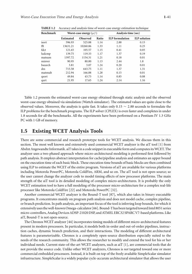
Worst-Case Execution Time and Energy Analysis 1-41
TABLE 1.2 Accuracy and analysis time of worst-case energy estimation technique
Benchmark Worst-case energy (μJ ) Analysis time (sec)
Estimated Observed Ratio ILP formulation ILP solutionisort 596.93 525.88 1.14 2.88 0.15fft 13631.21 10260.86 1.33 1.11 0.25fdct 121.65 105.57 1.15 0.41 0.05ludcmp 139.75 119.33 1.17 1.37 0.19matsum 1397.72 1154.31 1.21 0.18 0.01minver 90.95 80.80 1.13 2.44 1.8bsearch 3.81 3.07 1.24 0.20 0.01des 715.58 643.75 1.11 1.37 1.31matmult 212.94 166.88 1.28 0.15 0.01qsort 49.84 43.73 1.14 0.85 0.08qurt 21.95 17.65 1.24 2.14 1.16
Table 1.2 presents the estimated worst-case energy obtained through static analysis and the observedworst-case energy obtained via simulation (Wattch simulator). The estimated values are quite close to theobserved values. Moreover, the analysis is quite fast. It takes only 0.15 ∼ 2.88 seconds to formulate theILP problems for the benchmark programs. The ILP solver (CPLEX) is even faster and completes in under1.8 seconds for all the benchmarks. All the experiments have been performed on a Pentium IV 1.3 GHzPC with 1 GB of memory.
1.5 Existing WCET Analysis Tools
There are some commercial and research prototype tools for WCET analysis. We discuss them in thissection. The most well known and extensively used commercial WCET analyzer is the aiT tool [1] fromAbsInt Angewandte Informatik. aiT takes in a code snippet in executable form and computes its WCET. Theanalyzer uses a two-phased approach where micro-architectural modeling is performed first followed bypath analysis. It employs abstract interpretation for cache/pipeline analysis and estimates an upper boundon the execution time of each basic block. These execution time bounds of basic blocks are then combinedusing ILP to estimate the WCET of the entire program. Versions of aiT are available for various platformsincluding Motorola PowerPC, Motorola ColdFire, ARM, and so on. The aiT tool is not open-source; sothe user cannot change the analyzer code to model timing effects of new processor platforms. The mainstrength of the aiT tool is its detailed modeling of complex micro-architectures. It is probably the onlyWCET estimation tool to have a full modeling of the processor micro-architecture for a complex real-lifeprocessor like Motorola ColdFire [22] and Motorola PowerPC [32].
Another commercial WCET analyzer is the Bound-T tool [87], which also takes in binary executableprograms. It concentrates mainly on program path analysis and does not model cache, complex pipeline,or branch prediction. In path analysis, an important focus of the tool is inferring loop bounds, for which itextensively uses the well-known Omega-calculator [66]. Bound-T has been targeted toward Intel 8051 seriesmicro-controllers, Analog Devices ADSP-21020 DSP, and ATMEL ERC32 SPARC V7-based platforms. LikeaiT, Bound-T is not open-source.
The Chronos WCET analyzer [44] incorporates timing models of different micro-architectural featurespresent in modern processors. In particular, it models both in-order and out-of-order pipelines, instruc-tion caches, dynamic branch prediction, and their interactions. The modeling of different architecturalfeatures is parameterizable. Chronos is a completely open-source distribution especially suited to theneeds of the research community. This allows the researcher to modify and extend the tool for his or herindividual needs. Current state-of-the-art WCET analyzers, such as aiT [1], are commercial tools that donot provide the source code. Unlike other WCET analyzers, Chronos is not targeted toward one or morecommercial embedded processors. Instead, it is built on top of the freely available SimpleScalar simulatorinfrastructure. SimpleScalar is a widely popular cycle-accurate architectural simulator that allows the user

1-42 The Compiler Design Handbook: Optimizations and Machine Code Generation
to model a variety of processor platforms in software [10]. Chronos targets its analyzer to processor mod-els supported by SimpleScalar. This choice of platform ensures that the user does not need to purchasea particular embedded platform and its associated compiler, debugger, and other tools (which are oftenfairly expensive) to conduct research in WCET analysis using Chronos. Also, the flexibility of SimpleScalarenables development and verification of modeling a variety of micro-architectural features for WCET anal-ysis. Thus, Chronos provides a low-overhead, zero-cost, and flexible infrastructure for WCET research.However, it does not support as detailed micro-architectural modeling as is supported by the commercialaiT analyzer; in particular, certain processor features such as data cache are not modeled in Chronos.
Among the research prototypes, HEPTANE [64] is an open-source WCET analyzer. HEPTANE modelsin-order pipeline, instruction cache, and branch prediction, but it does not include any automated programflow analysis. Symta/P [77] is another research prototype that estimates WCET for C programs. It modelscaches and simple pipelines but does not support modeling of complex micro-architectural features such asout-of-order pipelines and branch prediction. Cinderella [48] is an ILP-based research prototype developedat Princeton University. The main distinguishing feature of this tool is that it performs both program pathanalysis and micro-architectural modeling by solving an ILP problem. However, this formulation makesthe tool less scalable because the ILP solving time does not always scale up for complex micro-architectures.Also, Cinderella mostly concentrates on program path analysis and cache modeling; it does not analyzetiming effects of complex pipelines and branch prediction. The SWEET analyzer from Paderborn, Uppsala,and Malarden Universities focuses mostly on program flow analysis and does not model complex micro-architectures (such as out-of-order pipelines). The program flow analysis proceeds by abstract executionwhere variable values are abstracted to intervals. However, the abstraction in the flow analysis is limited todata values; the control flow is not abstracted. Consequently, abstract execution in the SWEET tool [27]may resort to a complete unrolling of the program loops.
In addition to the above-mentioned tools, several other research groups have developed their own in-house timing analysis prototypes incorporating certain novel features. One notable effort is by the researchgroup at Florida State University. Their work involves sophisticated flow analysis for inferring infeasiblepath patterns and loop bounds [31] — features that are not commonly present in many WCET analyzers.However, the tool is currently not available for use or download; it is an in-house research effort.
1.6 Conclusions
In this chapter, we have primarily discussed software timing and energy analysis of an isolated task executingon a target processor without interruption. This is an important problem and forms the building blocksof more complicated performance analysis techniques. As we have seen, the main steps of software timingand energy analysis are (a) program path analysis and (b) micro-architectural modeling. We have alsodiscussed a number of analysis methods that either perform an integrated analysis of the two steps orseparate the two steps. It has been observed that integrated analysis methods are not scalable to largeprograms [94], and hence separated approaches for timing analysis may have a better chance of beingintegrated into compilers. Finally, we outline here some possible future research directions.
1.6.1 Integration with Schedulability Analysis
The timing and energy analysis methods discussed in this chapter assume uninterrupted execution of aprogram. In reality, a program (or “task,” using the terminology of the real-time systems community) mayget preempted because of interrupts. The major impact of task preemption is on the performance of theinstruction and data caches. Let Tl be a lower-priority task that gets preempted by a higher-priority taskTh . When Tl resumes execution, some of its cache blocks have been replaced by Th . Clearly, if the WCETanalysis does not anticipate this preemption, the resulting timing guarantee will not be safe. Cache-relatedpreemption delay [42, 58] analysis derives an upper bound on the number of additional cache misses perpreemption. This information is integrated in the schedulability analysis [37] to derive the maximumnumber of possible preemptions and their effect on the worst-case cache performance.

Worst-Case Execution Time and Energy Analysis 1-43
1.6.2 System-Level Analysis
In a system-on-chip device consisting of multiple processing elements (typically on a bus), a system-wideperformance analysis has to be built on top of task-level execution time analysis [70, 85]. Integrating thetiming effects of shared bus and complex controllers in the WCET analysis is quite involved. In a recent work,Tanimoto et al. [80] model the shared bus on a system-on-chip device by defining bus scenario as represent-ing a set of possible execution sequences of tasks and bus transfers. They use the definition of bus scenario toautomatically derive the deadline and period for each task starting with high-level real-time requirements.
1.6.3 Retargetable WCET Analysis
Retargetability is one of the major issues that needs to be resolved for WCET analysis tools to gain wideracceptability in industry [12]. Developing a complex WCET analyzer for a new platform requires extensivemanual effort. Unfortunately, the presence of a large number of platforms available for embedded softwaredevelopment implies that we cannot ignore this problem. The other related problem is the correctnessof the abstract processor models used in static timing analysis. The manual abstraction process cannotguarantee the correctness of the models. These two problems can be solved if the static timing analyzercan be generated (semi-)automatically from a formal description of the processor.
One possibility in this direction is to start with the processor specification in some architecture de-scription language (ADL). ADLs precisely describe the instruction-set architecture as well as the micro-architecture of a given processor platform. Certain architectural features are highly parameterizable andhence easy to retarget from a WCET analysis point of view, but other features such as out-of-order pipelinesare not easily parameterizable. Li et al. [47] propose an approach to automatically generate static WCETanalyzers starting from ADL descriptions for complex processor pipelines. On the other end of the spec-trum, we can start with processor specification in hardware description languages (HDLs) such as Verilogor VHDL. The timing models have to be obtained from this HDL specification via simplification andabstraction. Thesing [84] takes this approach for timing models of a system controller. It remains to beseen whether this method scales to complex processor pipelines.
1.6.4 Time-Predictable System Design
The increasing complexity of systems and software leads to reduced timing predictability, which in turncreates serious difficulties for static analysis techniques [86]. An alternative is to design systems and softwarethat are inherently more predictable in terms of timing without incurring significant performance loss.The Virtual Simple Architecture (VISA) approach [3] counters the timing anomaly problem in complexprocessor pipelines by augmenting the processor micro-architecture with a simpler pipeline. Proposalsfor predictable memory hierarchy include cache locking [65, 89], cache partitioning [39, 95], as well asreplacing cache with scratchpad memory [78, 90] such that WCET analysis is simplified. At the softwarelevel, the work in [28, 59] discusses code transformations to reduce the number of program paths consideredfor WCET analysis. Moreover, Gustafsson et al. [28] also propose WCET-oriented programming to producecode with a very simple control structure that avoids input-data-dependent control flow decisions as faras possible.
1.6.5 WCET-Centric Compiler Optimizations
Traditional compiler optimization techniques guided by profile information focus on improving theaverage-case performance of a program. In contrast, the metric of importance to real-time systems is theworst-case execution time. Compiler techniques to reduce the WCET of a program have started to receiveattention very recently. WCET-centric optimizations are more challenging, as the worst-case path changesas optimizations are applied.
Lee et al. [43] have developed a code generation method for dual-instruction-set ARM processorsto simultaneously reduce the WCET and code size. They use a full ARM instruction set along the WCETpath to achieve faster execution and at the same time use reduced Thumb instructions along the noncriticalpaths to reduce code size. Bodin and Puaut [8] designed a customized static branch prediction scheme

1-44 The Compiler Design Handbook: Optimizations and Machine Code Generation
for reducing a program’s WCET. Zhao et al. [99] present a code positioning and transformation methodto avoid the penalties associated with conditional and unconditional jumps by placing the basic blockson WCET paths in contiguous positions whenever possible. Suhendra et al. [78] propose WCET-directedoptimal and near-optimal variable allocation strategies to scratchpad memory. Finally, Yu and Mitra [97]exploit application-specific extensions to the base instruction set of a processor for reducing the WCETof real-time tasks. Clearly, there are many other contexts where WCET-guided compiler optimization canplay a critical role.
Acknowledgments
Portions of this chapter were excerpted from R. Jayaseelan, T. Mitra, and X. Li, 2006, “Estimating the worst-case energy consumption of embedded software,” in Proceedings of the 12th IEEE Real-Time and EmbeddedTechnology and Applications Symposium (RTAS), pages 81–90, and adapted from X. Li, A. Roychoudhury,and T. Mitra, 2006, “Modeling out-of-order processors for WCET analysis,” Real-Time Systems, 34(3):195–227.
The authors would like to acknowledge Ramkumar Jayaseelan for preparing the figures in the introduc-tion section.
References
1. AbsInt Angewandte Informatik GmbH. aiT: Worst case execution time analyzer. http://www.absint.com/ait/.
2. P. Altenbernd. 1996. On the false path problem in hard real-time programs. In Proceedings of theEighth Euromicro Workshop on Real-Time Systems (ECRTS), 102–07.
3. A. Anantaraman, K. Seth, K. Patil, E. Rotenberg, and F. Mueller. 2003. Virtual simple architecture(VISA): Exceeding the complexity limit in safe real-time systems. In Proceedings of the 30th IEEE/ACMInternational Symposium on Computer Architecture (ISCA), 350–61.
4. R. Arnold, F. Mueller, D. B. Whalley, and M. G. Harmon. 1994. Bounding worst-case instructioncache performance. In Proceedings of the 15th IEEE Real-Time Systems Symposium (RTSS), 172–81.
5. I. Bate and R. Reutemann. 2004. Worst-case execution time analysis for dynamic branch predictors.In Proceedings of the 16th Euromicro Conference on Real-Time Systems (ECRTS), 215–22.
6. G. Bernat, A. Colin, and S. M. Petters. 2002. WCET analysis of probabilistic hard real-time systems.In Proceedings of the 23rd IEEE Real-Time Systems Symposium (RTSS), 279–88.
7. R. Bodik, R. Gupta, and M. L. Soffa. 1997. Refining data flow information using infeasible paths.In Proceedings of the 6th European Software Engineering Conference held jointly with the 5th ACMSIGSOFT International Symposium on Foundations of Software Engineering ESEC/FSE, Vol. 1301 ofLecture Notes in Computer Science, 361–77. New York: Springer.
8. F. Bodin and I. Puaut. 2005. A WCET-oriented static branch prediction scheme for real-time systems.In Proceedings of the 17th Euromicro Conference on Real-Time Systems, 33–40.
9. D. Brooks, V. Tiwari, and M. Martonosi. 2000. Wattch: A framework for architectural-level poweranalysis and optimizations. In Proceedings of the 27th Annual ACM/IEEE International Symposiumon Computer Architecture (ISCA), 83–94.
10. D. Burger and T. Austin. 1997. The SimpleScalar tool set, version 2.0. Technical Report CS-TR-1997-1342, University of Wisconsin, Madison.
11. C. Burguiere and C. Rochange. 2005. A contribution to branch prediction modeling in WCETanalysis. In Proceedings of the IEEE Design, Automation and Test in Europe Conference and Exposition,Vol. 1, 612–17.
12. K. Chen, S. Malik, and D. I. August. 2001. Retargetable static timing analysis for embedded software.In Proceedings of IEEE/ACM International Symposium on System Synthesis (ISSS).
13. E. M. Clarke, E. A. Emerson, and A. P. Sistla. 1986. Automatic verification of finite-state concurrentsystems using temporal logic specifications. ACM Transactions on Programming Languages andSystems 8(2):244–63.

Worst-Case Execution Time and Energy Analysis 1-45
14. A. Colin and I. Puaut. 2000. Worst case execution time analysis for a processor with branchprediction. Real-Time Systems 18(2):249–74.
15. P. Cousot and R. Cousot. 1977. Abstract interpretation: A unified lattice model for static analysis ofprograms by construction or approximation of fixpoints. In Proceedings of the Fourth Annual ACMSymposium on Principles of Programming Languages (POPL), 238–52.
16. K. Dockser. 2001. “Honey, I shrunk the supercomputer!” — The PowerPC 440 FPU brings super-computing to IBM blue logic library. IBM MicroNews 7(4):27–29.
17. S. Edgar and A. Burns. 2001. Statistical analysis of WCET for scheduling. In Proceedings of the 22ndIEEE Real-Time Systems Symposium (RTSS), 215–24.
18. J. Eisinger, I. Polian, B. Becker, A. Metzner, S. Thesing, and R. Wilhelm. 2006. Automatic identificationof timing anomalies for cycle-accurate worst-case execution time analysis. In Proceedings of the NinthIEEE Workshop on Design and Diagnostics of Electronic Circuits and Systems (DDECS), 15–20.
19. J. Engblom. 2003. Analysis of the execution time unpredictability caused by dynamic branch predic-tion. In Proceedings of the 9th IEEE Real-Time and Embedded Technology and Applications Symposium(RTAS), 152–59.
20. J. Engblom and A. Ermedahl. 2000. Modeling complex flows for worst-case execution time analysis.In Proceedings of IEEE Real-Time Systems Symposium (RTSS).
21. A. Ermedahl and J. Gustafsson. 1997. Deriving annotations for tight calculation of execution time.In Third International Euro-Par Conference on Parallel Processing (Euro-Par). Vol. 1300 of LectureNotes in Computer Science, 1298–307. New York: Springer.
22. C. Ferdinand, R. Heckmann, M. Langenbach, F. Martin, M. Schmidt, H. Theiling, S. Thesing, andR. Wilhelm. 2001. Reliable and precise WCET determination for a real-life processor. In Proceedingsof International Workshop on Embedded Software (EMSOFT), 469–85.
23. C. Ferdinand and R. Wilhelm. 1998. On predicting data cache behavior for real-time systems. InProceedings of the ACM SIGPLAN Workshop on Languages, Compilers, and Tools for Embedded Systems(LCTES), 16–30.
24. S. V. Gheorghita, T. Basten, and H. Corporaal. 2005. Intra-task scenario-aware voltage scheduling.In International Conference on Compiler, Architectures and Synthesis for Embedded Systems (CASES).
25. S. V. Gheorghita, S. Stuijk, T. Basten, and H. Corporaal. 2005. Automatic scenario detection forimproved WCET estimation. In ACM Design Automation Conference (DAC).
26. S. Ghosh, M. Martonosi, and S. Malik. 1999. Cache miss equations: A compiler framework foranalyzing and tuning memory behavior. ACM Transactions on Programming Languages and Systems,21(4):707–46.
27. J. Gustafsson. 2000. Eliminating annotations by automatic flow analysis of real-time programs. InProceedings of the Seventh International Conference on Real-Time Computing Systems and Applications(RTCSA), 511–16.
28. J. Gustafsson, B. Lisper, R. Kirner, and P. Puschner. 2006. Code analysis for temporal predictability.Real-Time Systems 32:253–77.
29. C. Healy, R. Arnold, F. Mueller, D. Whalley, and M. Harmon. 1999. Bounding pipeline and instruc-tion cache performance. IEEE Transactions on Computers 48(1):53–70.
30. C. Healy, M. Sjodin, V. Rustagi, D. Whalley, and R. van Englen. 2000. Supporting timing analysis byautomatic bounding of loop iterations. Real-Time Systems 18:129–56.
31. C. A. Healy and D. B. Whalley. 2002. Automatic detection and exploitation of branch constraintsfor timing analysis. IEEE Transactions on Software Engineering 28(8):763–81.
32. R. Heckmann, M. Langenbach, S. Thesing, and R. Wilhelm. 2003. The influence of processor archi-tecture on the design and the results of WCET tools. Proceedings of the IEEE, 91(7):1038–054.
33. J. L. Hennessy and D. A. Patterson. 2003. Computer architecture — a quantitative approach. 3rd ed.San Francisco: Morgan Kaufmann.
34. IBM Microelectronics Division. 1999. The PowerPC 440 core.35. Institute of Electrical and Electronics Engineers. 1985. IEEE 754: Standard for binary floating-point
arithmetic.

1-46 The Compiler Design Handbook: Optimizations and Machine Code Generation
36. R. Jayaseelan, T. Mitra, and X. Li. 2006. Estimating the worst-case energy consumption of embeddedsoftware. In Proceedings of the 12th IEEE Real-Time and Embedded Technology and ApplicationsSymposium (RTAS), 81–90.
37. L. Ju, S. Chakraborty, and A. Roychoudhury. 2007. Accounting for cache-related preemption delayin dynamic priority schedulability analysis. In Proceedings of Design Automation and Test in Europe(DATE).
38. S.-K. Kim, S. L. Min, and R. Ha. 1996. Efficient worst case timing analysis of data caching. InProceedings of the Second IEEE Real-Time Technology and Applications Symposium (RTAS), 230–40.
39. D. B. Kirk. 1989. SMART (strategic memory allocation for real-time) cache design. In Proceedingsof the Real-Time Systems Symposium (RTSS), 229–39.
40. R. Kirner. 2003. Extending optimizing compilation to support worst-case execution time analysis.PhD thesis, T. U. Vienna.
41. M. Langenbach, S. Thesing, and R. Heckmann. Pipeline modeling for timing analysis. In Proceedingsof the 9th International Symposium on Static Analysis (SAS). Vol. 2477 of Lecture Notes in ComputerScience, 294–309. New York: Springer.
42. C.-G. Lee, H. Hahn, Y.-M. Seo, S. L. Min, R. Ha, S. Hong, C. Y. Park, M. Lee, and C. S. Kim.1998. Analysis of cache-related preemption delay in fixed-priority preemptive scheduling. IEEETransactions on Computers 47(6):700–13.
43. S. Lee et al. 2004. A flexible tradeoff between code size and WCET using a dual instruction setprocessor. In Proceedings of the 8th International Workshop on Software and Compilers for EmbeddedSystems (SCOPES). Vol. 3199 of Lecture Notes in Computer Science, 244–58. New York: Springer.
44. X. Li, Y. Liang, T. Mitra, and A. Roychoudhury. Chronos: A timing analyzer for embedded software.Science of Computer Programming, special issue on Experiment Software and Toolkit 2007 (toappear), http://www.comp.nus.edu.sg/∼rpembed/chronos/.
45. X. Li, T. Mitra, and A. Roychoudhury. 2005. Modeling control speculation for timing analysis.Real-Time Systems 29(1):27–58.
46. X. Li, A. Roychoudhury, and T. Mitra. 2006. Modeling out-of-order processors for WCET analysis.Real-Time Systems 34(3):195–227.
47. X. Li, A. Roychoudhury, T. Mitra, P. Mishra, and X. Cheng. 2007. A retargetable software timinganalyzer using architecture description language. In Proceedings of the 12th Asia and South PacificDesign Automation Conference (ASP-DAC), 396–401.
48. Y.-T. S. Li. Cinderella 3.0 WCET analyzer. http://www.princeton.edu/∼yauli/cinderella-3.0/.49. Y.-T. S. Li and S. Malik. 1997. Performance analysis of embedded software using implicit path
enumeration. IEEE Transactions on Computer-Aided Design of Integrated Circuits and Systems (TCAD)16(12):1477–87.
50. Y.-T. S. Li and S. Malik. 1998. Performance analysis of real-time embedded software. New York:Springer.
51. S.-S. Lim, Y. H. Bae, G. T. Jang, B-D. Rhee, S. L. Min, C. Y. Park, H. Shin, K. Park, S.-M. Moon, andC. S. Kim. 1995. An accurate worst case timing analysis for RISC processors. IEEE Transactions onSoftware Engineering 21(7):593–604.
52. Y. A. Liu and G. Gomez. 2001. Automatic accurate cost-bound analysis for high-level languages.IEEE Transactions on Computers 50(12):1295–309.
53. T. Lundqvist and P. Stenstrom. 1999. An integrated path and timing analysis method based oncycle-level symbolic execution. Real-Time Systems 17(2/3):183–207.
54. T. Lundqvist and P. Stenstrom. 1999. Timing anomalies in dynamically scheduled microprocessors.In Proceedings of the 20th IEEE Real-Time Systems Symposium (RTSS), 12–21.
55. F. Martin, M. Alt, R. Wilhelm, and C. Ferdinand. 1998. Analysis of loops. In Compiler Construction(CC). New York: Springer.
56. A. Metzner. 2004. Why model checking can improve WCET analysis. In Proceedings of the 16thInternational Conference on Computer Aided Verification (CAV). Vol. 3114 of Lecture Notes inComputer Science, 361–71. New York: Springer.

Worst-Case Execution Time and Energy Analysis 1-47
57. F. Mueller. 2000. Timing analysis for instruction caches. Real-Time Systems 18:217–47.58. H. S. Negi, T. Mitra, and A. Roychoudhury. 2003. Accurate estimation of cache-related preemp-
tion delay. In Proceedings of the 1st IEEE/ACM/IFIP International Conference on Hardware/SoftwareCodesign and System Synthesis (CODES+ISSS), 201–06.
59. H. S. Negi, A. Roychoudhury, and T. Mitra. 2004. Simplifying WCET analysis by code transfor-mations. In Proceedings of the 4th International Workshop on Worst-Case Execution Time Analysis(WCET).
60. G. Ottosson and M. Sjodin. 1997. Worst-case execution time analysis for modern hardware ar-chitectures. In Proceedings of the ACM SIGPLAN Workshop on Languages, Compilers, and Tools forReal-Time Systems (LCT-RTS).
61. C. Y. Park. 1993. Predicting program execution times by analyzing static and dynamic programpaths. Real-time Systems 5(1):31–62.
62. C. Y. Park. 1992. Predicting deterministic execution times of real-time programs. PhD thesis,University of Washington, Seattle.
63. J. Pierce and T. Mudge. 1996. Wrong-path instruction prefetching. In Proceedings of the 29th AnnualIEEE/ACM International Symposium on Microarchitectures (MICRO), 165–75.
64. I. Puaut. HEPTANE static WCET analyzer. http://www.irisa.fr/aces/work/heptane-demo/heptane.html.
65. I. Puaut and D. Decotigny. 2002. Low-complexity algorithms for static cache locking in multi-tasking hard real-time systems. In Proceedings of the 23rd IEEE Real-Time Systems Symposium (RTSS),114–23.
66. W. Pugh. 1991. The omega test: A fast and practical integer programming algorithm for dependenceanalysis. In ACM/IEEE Conference on Supercomputing.
67. P. Puschner and C. Koza. 1989. Calculating the maximum execution time of real-time programs.Real-Time Systems 1(2):159–76.
68. P. Puschner and A. Schedl. 1997. Computing maximum task execution times: A graph based ap-proach. Real-Time Systems 13(1):67–91.
69. H. Ramaprasad and F. Mueller. Bounding worst-case data cache behavior by analytically deriv-ing cache reference patterns. In IEEE Real-Time Technology and Applications Symposium (RTAS),148–57.
70. K. Richter, D. Ziegenbein, M. Jersak, and R. Ernst. 2002. Model composition for scheduling analysisin platform design. In Proceedings of the 39th Annual ACM/IEEE Design Automation Conference(DAC), 287–92.
71. A. Roychoudhury, T. Mitra, and H. S. Negi. 2005. Analyzing loop paths for execution timeestimation. In Lecture Notes in Computer Science. Vol. 3816, 458–69. New York: Springer.
72. T. Schuele and K. Schneider. 2004. Abstraction of assembler programs for symbolic worst caseexecution time analysis. In Proceedings of the 41st ACM/IEEE Design Automation Conference (DAC),107–12.
73. A. C. Shaw. 1989. Reasoning about time in higher-level language software. IEEE Transactions onSoftware Engineering 1(2):875–89.
74. Simplify. Simplify theorem prover. http://www.research.compaq.com/SRC/esc/Simplify.html.75. A. Sinha and A. P. Chandrakasan. 2001. Jouletrack: A web based tool for software energy profiling.
In Proceedings of the Design Automation Conference (DAC).76. F. Stappert, A. Ermedahl, and J. Engblom. 2001. Efficient longest executable path search for programs
with complex flows and pipeline effects. In Proceedings of the First International Conference onCompilers, Architecture, and Synthesis for Embedded Systems (CASES), 132–40.
77. J. Staschulat. Symta/P: Symbolic timing analysis for processes. http://www.ida.ing.tu-bs.de/research/projects/symta/home.e.shtml.
78. V. Suhendra, T. Mitra, A. Roychoudhury, and T. Chen. 2005. WCET centric data allocationto scratchpad memory. In Proceedings of the 26th IEEE Real-Time Systems Symposium (RTSS),223–32.
1-48 The Compiler Design Handbook: Optimizations and Machine Code Generation
79. V. Suhendra, T. Mitra, A. Roychoudhury, and T. Chen. 2006. Efficient detection and exploitationof infeasible paths for software timing analysis. In Proceedings of the 43rd ACM/IEEE DesignAutomation Conference (DAC), 358–63.
80. T. Tanimoto, S. Yamaguchi, A. Nakata, and T. Higashino. 2006. A real time budgeting method formodule-level-pipelined bus based system using bus scenarios. In Proceedings of the 43rd ACM/IEEEDesign Automation Conference (DAC), 37–42.
81. H. Theiling and C. Ferdinand. 1998. Combining abstract interpretation and ILP for microarchi-tecture modelling and program path analysis. In Proceedings of the 19th IEEE Real-Time SystemsSymposium (RTSS), 144–53.
82. H. Theiling, C. Ferdinand, and R. Wilhelm. 2000. Fast and precise WCET prediction by separatedcache and path analyses. Real-Time Systems 18(2/3):157–79.
83. S. Thesing. Safe and precise worst-case execution time prediction by abstract interpretation ofpipeline models. PhD thesis, University of Saarland, Germany.
84. S. Thesing. 2006. Modeling a system controller for timing analysis. In Proceedings of the 6th ACM/IEEEInternational Conference on Embedded Software (EMSOFT), 292–300.
85. L. Thiele, S. Chakraborty, M. Gries, A. Maxiaguine, and J. Greutert. 2001. Embedded software innetwork processors — models and algorithms. In Proceedings of the First International Workshop onEmbedded Software (EMSOFT). Vol. 2211 of Lecture Notes in Computer Science, 416–34. New York:Springer.
86. L. Thiele and R. Wilhelm. 2004. Design for timing predictability. Real-Time Systems, 28(2/3):157–77.87. Tidorum Ltd. Bound-T execution time analyzer. http://www.bound-t.com.88. V. Tiwari, S. Malik, and A. Wolfe. 1994. Power analysis of embedded software: A first step towards
software power minimization. IEEE Transactions of VLSI Systems 2(4):437–45.89. X. Vera, B. Lisper, and J. Xue. 2003. Data cache locking for higher program predictability. In
Proceedings of the International Conference on Measurements and Modeling of Computer Systems(SIGMETRICS), 272–82.
90. L. Wehmeyer and P. Marwedel. 2005. Influence of memory hierarchies on predictability for timeconstrained embedded software. In Proceedings of the Conference on Design, Automation and Test inEurope (DATE), 600–605.
91. I. Wenzel, R. Kirner, P. Puschner, and B. Rieder. 2005. Principles of timing anomalies in superscalarprocessors. In Proceedings of the Fifth International Conference on Quality Software (QSIC), 295–303.
92. I. Wenzel, R. Kirner, B. Rieder, and P. Puschner. Measurement-based worst-case execution timeanalysis. In Proceedings of the Third IEEE Workshop on Software Technologies for Future Embeddedand Ubiquitous Systems (SEUS), 7–10.
93. R. White, F. Mueller, C. Healy, D. Whalley, and M. Harmon. 1997. Timing analysis for data cachesand set-associative caches. In Proceedings of the Third IEEE Real-Time Technology and ApplicationsSymposium (RTAS), 192–202.
94. R. Wilhelm. 2004. Why AI+ ILP is good for WCET, but MC is not, nor ILP alone. In Proceedings of the5th International Conference on Verification, Model Checking, and Abstract Interpretation (VMCAI).Vol. 2937 of Lecture Notes in Computer Science, 309–22. New York: Springer.
95. A. Wolfe. 1994. Software-based cache partitioning for real-time applications. Journal of Computerand Software Engineering, Special Issue on Hardware-Software Codesign, 2(3):315–27.
96. W. Ye et al. 2000. The design and use of simplepower: A cycle-accurate energy estimation tool. InProceedings of the ACM/IEEE Design Automation Conference (DAC).
97. P. Yu and T. Mitra. 2005. Satisfying real-time constraints with custom instructions. In Proceed-ings of the ACM International Conference on Hardware/Software Codesign and System Synthesis(CODES+ISSS), 166–71.
98. Y. Zhang et al. 2003. Hotleakage: A temperature-aware model of subthreshold and gate leakage forarchitects. Technical Report CS-2003-05, University of Virginia.
99. W. Zhao, D. Whalley, C. Healy, and F. Mueller. 2004. WCET code positioning. In Proceedings of the25th IEEE Real-Time Systems Symposium (RTSS), 81–91.

2Static Program
Analysis for Security
K. GopinathDepartment of Computer Scienceand Automation,Indian Institute of Science,Bangalore, [email protected]
2.1 Introduction . . . . . . . . . . . . . . . . . . . . . . . . . . . . . . . . . . . . . . . . . .2-1A Dramatic Failure of Static Analysis: Ken Thompson’s TrojanHorse • Detecting Viruses • A Case Study for Static Analysis:GSM Security Hole • Obfuscation
2.2 Static Analysis of Buffer Overflows . . . . . . . . . . . . . . . . . . . . .2-82.3 Static Analysis of Safety of Mobile Code . . . . . . . . . . . . . . . .2-92.4 Static Analysis of Access Control Policies . . . . . . . . . . . . . . .2-9
Case Studies • Dynamic Access Control • Retrofitting SimpleMAC Models for SELinux • Model Checking Access Control onthe Internet: Trust Management
2.5 Language-Based Security . . . . . . . . . . . . . . . . . . . . . . . . . . . . . .2-15The Type-Based Approach • Java Information Flow (Jif)Language • A Case Study: VSR
2.6 Future Work . . . . . . . . . . . . . . . . . . . . . . . . . . . . . . . . . . . . . . . . . .2-24References . . . . . . . . . . . . . . . . . . . . . . . . . . . . . . . . . . . . . . . . . . . . . . . . . .2-25
AbstractIn this chapter, we discuss static analysis of the security of a system. First, we give a brief background onwhat types of static analysis are feasible in principle and then move on to what is practical. We next discussstatic analysis of buffer overflow and mobile code, followed by access control. Finally, we discuss staticanalysis of information flow expressed in a language that has been annotated with flow policies.
2.1 Introduction
Analyzing a program for security holes is an important part of the current computing landscape, as securityhas not been an essential ingredient in a program’s design for quite some time. With the critical importanceof a secure program becoming clearer in the recent past, designs based on explicit security policies arelikely to gain prominence.
Static analysis of a program is one technique to detect security holes. Compared to monitoring an execu-tion at runtime (which may not have the required coverage), a static analysis — even if incomplete becauseof loss of precision — potentially gives an analysis on all runs possible instead of just the ones seen so far.
However, security analysis of an arbitrary program is extremely hard. First, what security means is oftenunspecified or underspecified. The definition is either too strict and cannot cope with the “commonsense”requirement or too broad and not useful. For example, one definition of security involves the notion of“noninterference” [24]. If it is very strict, even cryptoanalytically strong encryption and decryption does
2-1

2-2 The Compiler Design Handbook: Optimizations and Machine Code Generation
not qualify as secure, as there is information flow from encrypted text to plain text [59]. If it is not verystrict, by definition, some flows are not captured that are important in some context for achieving securityand hence, again, not secure. For example, if electromagnetic emissions are not taken into account, thekey may be easily compromised [50]. A model of what security means is needed, and this is by no meansan easy task [8]. Schneider [28] has a very general definition: a security policy defines a binary partition ofall (computable) sets of executions — those that satisfy and those that do not. This is general enough tocover access control policies (a program’s behavior on an arbitrary individual execution for an arbitraryfinite period), availability policies (behavior on an arbitrary individual execution over an infinite period),and information flow (behavior in terms of the set of all executions).
Second, the diagonalization trick is possible, and many analyses are undecidable. For example, there areundecidable results with respect to viruses and malicious logic [16]: it is undecidable whether an arbitraryprogram contains a computer virus. Similarly, viruses exist for which no error-free detection algorithmexists.
Recently, there have been some interesting results on computability classes for enforcement mecha-nisms [28] with respect to execution monitors, program rewriting, and static analysis. Execution monitorsintervene whenever execution of an untrusted program is about to violate the security policy being en-forced. They are typically used in operating systems using structures such as access control lists or usedwhen executing interpreted languages by runtime type checking. It is possible to rewrite a binary so thatevery access to memory goes through a monitor. While this can introduce overhead, optimization tech-niques can be used to reduce the overhead. In many cases, the test can be determined to be not necessaryand removed by static analysis. For example, if a reference to a memory address m has already been checked,it may not be necessary for a later occurrence.
Program rewriting modifies the untrusted program before execution to make it incapable of violatingthe security policy. An execution monitor can be viewed as a special case of program rewriting, but Hamlenet al. [28] point out certain subtle cases. Consider a security policy that makes halting a program illegal;an execution monitor cannot enforce this policy by halting, as this would be illegal! There are also classesof policies in certain models of execution monitors that cannot be enforced by any program rewriter.
As is to be expected, the class of statically enforceable policies is the class of recursively decidableproperties of programs (class �0 of the arithmetic hierarchy): a static analysis has to be necessarily total(i.e., terminate) and return safe or unsafe. If precise analysis is not possible, we can relax the requirementby being conservative in what it returns (i.e., tolerate false positives). Execution monitors are the class ofco-recursively enumerable languages (class �1 of the arithmetic hierarchy).1
A system’s security is specified by its security policy (such as access control or information flow model)and implemented by mechanisms such as physical separation or cryptography.2 Consider access control. Anaccess control system guards access to resources, whereas an information flow model classifies informationto prevent disclosure. Access control is a component of security policy, while cryptography is one technicalmechanism to effect the security policy. Systems have employed basic access control since timesharingsystems began (1960) (e.g., Multics, Unix). Simple access control models for such “stand-alone” machinesassumed the universe of users known, resulting in the scale of the model being “small.” A set of accesscontrol moves can unintentionally leak a right (i.e., give access when it should not). If it is possible to analyzethe system and ensure that such a result is not possible, the system can be said to be secure, but theoreticalmodels inspired by these systems (the most well known being the Harrison, Ruzzo, Ullman [HRU] model)showed “surprising” undecidability results [29], chiefly resulting from the unlimited number of subjectsand objects possible. Technically, in this model, it is undecidable whether a given state of a given protection
1A security policy P is co-recursively enumerable if there exists a Turing machine M that takes an arbitrary executionmonitor E M as an input and rejects it in finite time if ∼ P (E M); otherwise M(E M) loops forever.
2While cryptography has rightfully been a significant component in the design of large-scale systems, its relationto security policy, especially its complementarity, has not often been brought out in full. “If you think cryptography isthe solution to your problem, you don’t know what your problem is” (Roger Needham).

Static Program Analysis for Security 2-3
system is safe for a given generic right. However, the need for automated analysis of policies was small inthe past, as the scale of the systems was small.
Information flow analysis, in contrast to access control, concerns itself with the downstream use ofinformation once obtained after proper access control. Carelessness in not ensuring proper flow modelshas resulted recently in the encryption system in HD-DVD and BluRay disks to be compromised (the keyprotecting movie content is available in memory).3
Overt models of information flow specify the policy concerning how data should be used explicitly,whereas covert models use “signalling” of information through “covert” channels such as timing, elec-tromagnetic emissions, and so on. Note that the security weakness in the recent HD-DVD case is due toimproper overt information flow. Research on some overt models of information flow such as Bell andLaPadula’s [6] was initiated in the 1960s, inspired by the classification of secrets in the military. Since oper-ating systems are the inspiration for work in this area, models of secure operating systems were developedsuch as C2 and B2 [57]. Work on covert information flow progressed in the 1970s. However, the work oncovert models of information flow in proprietary operating systems (e.g., DG-UNIX) was expensive andtoo late, so late that it could not be used on the by then obsolescent hardware. Showing that Trojan horsesdid not use covert channels to compromise information was found to be “ultimately unachievable” [27].
Currently, there is a considerable interest in studying overt models of information flow, as the extensiveuse of distributed systems and recent work with widely available operating systems such as SELinux andOpenSolaris have expanded the scope of research. The scale of the model has become “large,” with theneed for automated analysis of policies being high.
Access control and information flow policies can both be statically analyzed, with varying effectivenessdepending on the problem. Abstract interpretation, slicing, and many other compiler techniques can alsobe used in conjunction. Most of the static analyses induce a constraint system that needs to be solved to seeif security is violated. For example, in one buffer overflow analysis [23], if there is a solution to a constraintsystem, then there is an attack. In another analysis in language-based security, nonexistence of a solutionto the constraints is an indication of a possible leak of information.
However, static analysis is not possible in many cases [43] and has not yet been used on large piecesof software. Hence, exhaustive checking using model checking [14] is increasingly being used when onewants to gain confidence about a piece of code. In this chapter, we consider model checking as a form ofstatic analysis. We will discuss access control on the Internet that uses model checking (Section 2.4.4). Wewill also discuss this approach in the context of Security-Enhanced Linux (SELinux) where we check if alarge application has been given only sufficient rights to get its job done [31].
In spite of the many difficulties in analyzing the security of a system, policy frameworks such as accesscontrol and information flow analysis and mechanisms such as cryptography have been used to makesystems “secure.” However, for any such composite solution, we need to trust certain entities in the systemsuch as the compiler, the BIOS, the (Java) runtime system, the hardware, digital certificates, and so on —essentially the “chain of trust” problem. That this is a tricky problem has been shown in an interestingway by Ken Thompson [53]; we will discuss it below. Hence, we need a “small” trusted computing base(TCB): all protection mechanisms within a system (hardware, software, firmware) for enforcing securitypolicies.
In the past (early 1960s), operating systems were small and compilers larger in comparison. The TCBcould justifiably be the operating system, even if uncomfortably larger than one wished. In today’s context,the compilers need not be as large as current operating systems (for example, Linux kernel or Windows ismany millions of lines of code), and a TCB could profitably be the compiler. Hence, a compiler analysis ofsecurity is meaningful nowadays and likely to be the only way large systems (often a distributed system)can be crafted in the future. Using a top-level security policy, it may be possible to automatically partitionthe program so that the resulting distributed system is secure by design [60].
3The compromise of the security system DeCSS in DVDs was due to cryptanalysis, but in the case of HD-DVD itwas simply improper information flow.

2-4 The Compiler Design Handbook: Optimizations and Machine Code Generation
To illustrate the effectiveness of static security analysis, we first discuss a case where static analysis failscompletely (Ken Thomson’s Trojan horse). We then outline some results on the problem of detectingviruses and then discuss a case study in which static analysis can in principle be very hard (equivalent tocryptanalysis in general) but is actually much simpler because of a critical implementation error. We willalso briefly touch upon obfuscation that exploits difficulty of analysis.
We then discuss static analysis of buffer overflows, loading of mobile code, and access control andinformation flow, illustrating the latter using Jif [35] language on a realistic problem. We conclude withlikely future directions in this area of research.
2.1.1 A Dramatic Failure of Static Analysis: Ken Thompson’s Trojan Horse
Some techniques to defeat static analysis can be deeply effective; we summarize Ken Thompson’s ingeniousTrojan horse trick [53] in a compiler that uses self-reproduction, self-learning, and self-application. Wefollow his exposition closely.
First, self-reproduction is possible; for example, one can construct a self-reproducing program suchas ((lambda x. (list x x)) (lambda x. (list x x))). Second, it is possible to teacha compiler (written in its own language) to compile new features (the art of bootstrapping a compiler):this makes self-learning possible. We again give Ken Thompson’s example to illustrate this. Let us saythat a lexer knows about '\n' (newline) but not '\v' (vertical tab). How does one teach it to compile'\v' also? Let the initial source be:
c=next();if (c !='\\') return(c);c=next();if (c !='\\') return('\\')if (c ='n') return('\n')
Adding to the compiler source
if (c ='v') return('\v') //error
and using previous compiler binary does not work, as that binary does not know about '\v'. However,the following works:
if (c ='v') return(11)
Now a new binary (from the new source using the old compiler binary) knows about '\v' in a portableway. Now we can use it to compile the previously uncompilable statement:
if (c ='v') return('\v')
The compiler has “learned.” Now, we can introduce a Trojan horse into the login program that has abackdoor to allow a special access to log in as any user:
compile(char *s) {(* compiler main that accepts s as input (a program)*)if match(s, "pattern_login") {
(* "Trojan" compile for a login program in the system*)compile("bug_login"); return
}... (* normal compile *)
}
However, this is easily detectable (by examining the source). To make this not possible, we can add a secondTrojan horse aimed at the compiler:

Static Program Analysis for Security 2-5
if match(s, "pattern_compiler") {(* "Trojan" compile for a compiler program in the system*)compile("bug_compiler"); return
}
Now we can code a self-reproducing program that reintroduces both Trojan horses into the compilerwith a learning phase where the buggy compiler binary with two Trojan horses now reinserts it into anynew compiler binary compiled from a clean source! The detailed scheme is as follows: first a clean compilerbinary (A) is built from a clean compiler source (S). Next, as part of the learning phase, a modified compilersource (S′) can be built that incorporates the bugs. The logic in S′ looks at the source code of any programsubmitted for compilation and, say by pattern matching, decides whether a program submitted is a loginor a compiler program. If it decides that it is one of these special programs, it reproduces4 one or moreTrojan horses (as necessary) when presented with a clean source. Let the program S′ be compiled with A.We have a new binary A′ that reinserts the two Trojans on any clean source!
The virus exists in the binary but not in the source. This is not possible to discern unless the history ofthe system (the sequence of compilations and alterations) is kept in mind. Static analysis fails spectacularly!
2.1.2 Detecting Viruses
As discussed earlier, the virus detection problem is undecidable. A successful virus encapsulates itself sothat it cannot be detected — the opposite of “self-identifying data.” For example, a very clever virus wouldput logic in I/O routines so that any read of suspected portions of a disk returns the original “correct”information! A polymorphic virus inserts “random” data to vary the signature. More effectively, it cancreate a random encryption key to encrypt the rest of the virus and store the key with the virus.
2.1.2.1 Cohen’s Results
Cohen’s impossibility result states that it is impossible for a program to perfectly demarcate a line, en-closing all and only those programs that are infected with some virus: no algorithm can properly de-tect all possible viruses [16]: ∀Alg .∃Virus.Alg does not detect Virus. For any candidate computer virusdetection algorithm A, there is a program p(pgm): if A(pgm) then exit; else spread.Here, spread means behave like a virus. We can diagonalize this by setting pgm=p and a contradictionfollows immediately as p spreads iff not A(p).
Similarly, Chess and White [11] show there exists a virus that no algorithm perfectly detects, i.e., onewith no false positives: ∃Virus.∀Alg .Alg does not detect Virus. Also, there exists a virus that no algorithmloosely detects, i.e., claims to find the virus but is infected with some other virus: ∃Virus.∀Alg .Alg does notloosely-detect Virus. In other words, there exist viruses for which, even with the virus analyzed completely,no program detects only that virus with no false positives. Further, another Chess and White’s impossibilityresult states that there is no program to classify programs (only those) with a virus V and not include anyprogram without any virus.
Furthermore, there are interesting results concerning polymorphic viruses: these viruses generate a setof other viruses that are not identical to themselves but are related in some way (for example, are able toreproduce the next one in sequence). If the size of this set is greater than 1, call the set of viruses generatedthe viral set S.
An algorithm A detects a set of viruses S iff for every program p, A(p) terminates and returns TRUEiff p is infected with some virus V in S. If W is a polyvirus, for any candidate W-detection algorithm C ,there is a program s (pgm) that is an instance of W:
4It is easiest to do so in the binary being produced as the compiled output.

2-6 The Compiler Design Handbook: Optimizations and Machine Code Generation
if subroutine_one(pgm) then exit, else {replace text of subroutine_one with a random program;spread; exit; }
subroutine_one: return C(argument)
This can be diagonalized by pgm=s, resulting in a contradiction: if C(s) true exit; other-wise polyvirus.
Hence, it is clear that static analysis has serious limits.
2.1.3 A Case Study for Static Analysis: GSM Security Hole
We will now attempt to situate static analysis with other analyses, using the partitioning attack [50] on GSMhashing on a particular implementation as an example. GSM uses the COMP128 algorithm for encryption.A 16B (128b) key of subscriber (available with the base station along with a 16B challenge from the basestation is used to construct a 12B (96b) hash. The first 32b is sent as a response to the challenge, and theremaining 64b is used as the session key. The critical issue is that there should be no leakage of the keyin any of the outputs this includes any electromagnetic (EM) leakages during the computation of the hash.The formula for computation of the hash it has a butterfly structure) is as follows:
//X is 32B (16B key || 16B challenge)//Tj[r] is a lookuptable of 8-j bits value with r rows://alg uses T0[512], T1[256], T2[128], T3[64], T4[32]for j=0..4
for k=0..2^j -1for l=0..2^(4-j) -1
m=l+k*2^(5-j)n=m+2^(4-j)y=(X[m]+2*X[n]) mod 2^(9-j)z=(2*X[m]+X[n]) mod 2^(9-j)X[m]=Tj[y]X[n]=Tj[z]
If we expand y in the expression for X[m], we have
X[m]=Tj[(X[m]+2*X[n]) mod 2^(9-j)]
A simple-minded flow analysis will show that there is direct dependence of the EM leakage on thekey; hence, this is not information flow secure. However, cryptographers, using the right “confusion” and“diffusion” operators such as the above code, have shown that the inverse can be very difficult to compute.Hence, even if very simple static analysis clearly points out the flow dependence of the EM leakage onthe key, it is not good enough to crack the key. However, even if the mapping is cryptanalytically strong,“implementation” bugs can often give away the key. An attack is possible if one does not adhere to thefollowing principle [50] of statistical independence (or more accurately noninterference, which will bediscussed later): relevant bits of all intermediate cycles and their values should be statistically independent ofthe inputs, outputs, and sensitive information.
Normally, those bits that emit high EM are good candidates for analysis. One set of candidates are thearray and index values, as they need to be amplified electrically for addressing memory. They are thereforeEM sensitive, whereas other internal values may not be so.
Because of the violation of this principle, a cryptographically strong algorithm may have an implemen-tation that leaks secrets. For example, many implementations use 8b microprocessors, as COMP128 isoptimized for them, so the actual implementation for T0 is two tables, T00 and T01 (each 256 entries):

Static Program Analysis for Security 2-7
//X is 32B (16B key || 16B challenge)//Tj[r] is a lookuptable of 8-j bits value with r rows://alg uses T0[512], T1[256], T2[128], T3[64], T4[32]for j=0..4
for k=0..2^j -1for l=0..2^(4-j) -1
m=l+k*2^(5-j)n=m+2^(4-j)y=(X[m]+2*X[n]) mod 2^(9-j)z=(2*X[m]+X[n]) mod 2^(9-j)if (y<256) X[m]=Tj0[y] else Tj1[y-256] // old: X[m]=Tj[y]if (z<256) X[m]=Tj0[z] else Tj1[z-256] // old: X[n]=Tj[z]
If the number of intermediate lookups from tables T00 or T01 have statistical significance, thenbecause of the linearity of the indexywith respect toR for the first round, some information can be gleanedabout the key. The technique of differential cryptanalysis is based on such observations. In addition, if itis possible to know when access changes from one table (say, T00) to another (T01) by changing R, thenthe R value where it changes is given by K + 2*R=256, from which X, the first byte of the GSM key, can bedetermined.
In general, we basically have a set of constraints, such as
0 ≤ x + 2y1 ≤ 127
128 ≤ x + 2y2 ≤ 256
where y1 and y2 are two close values that map the index into different arrays (T0 or T1).5
If there is a solution to these Diophantine equations, then we have an attack. Otherwise, no. Since thecryptographic confusion and diffusion operations determine the difficulty (especially with devices such asS-boxes in DES), in general the problem is equivalent to the cryptanalysis problem. However, if we assumethat the confusion and diffusion operations are linear in subkey and other parameters (as in COMP128),we just need to solve a set of linear Diophantine equations [39].
What we can learn from the above is the following: we need to identify EM-sensitive variables. Othervalues can be “declassified”; even if we do not take any precautions, we can assume they cannot be observedfrom an EM perspective. We need to check the flow dependence of the EM-sensitive variables (i.e., externallyvisible) on secrets that need to be safeguarded.
Recently, work has been done that implies that success or failure of branch prediction presentsobservable events that can be used to crack encryption keys.
The above suggests the following problems for study:� Automatic downgrading of “insensitive” variables� Determination of the minimal declassification to achieve desired flow properties
2.1.4 Obfuscation
Given that static analyses are often hard, some applications use them to good effect. An example is the newarea of “obfuscation” of code so that it cannot be reverse-engineered easily. Obfuscation is the attemptto make code “unreadable” or “unintelligible” in the hope that it cannot be used by competitors. This iseffected by performing semantic-preserving transformations so that automatic static analysis can revealnothing useful. In one instance, control flow is intentionally altered so that it is difficult to understand or
5In general, l ≤ f (a , b) ≤ u, . . . , with f being an affine function for tractability.

2-8 The Compiler Design Handbook: Optimizations and Machine Code Generation
use it by making sure that any analysis that can help in unravelling code is computationally intractable (forexample, PSPACE-hard or NP-hard). Another example is intentionally introducing aliases, as certain aliasanalysis problems are known to be hard (if not undecidable), especially in the interprocedural context.Since it has been shown that obfuscation is, in general, impossible [4], static analysis in principle could beadopted to undo obfuscation unless it is computationally hard.
2.2 Static Analysis of Buffer Overflows
Since the advent of the Morris worm in 1988, buffer overflow techniques to compromise systems havebeen widely used. Most recently, the SQL slammer worm in 2003, using a small UDP packet (376B),compromised 90% of all target machines worldwide in less than 10 minutes.
Since buffer overflow on a stack can be avoided, for example, by preventing the return address frombeing overwritten by the “malicious” input string, array bounds checking the input parameters by thecallee is one technique. Because of the cost of this check, it is useful to explore compile time approachesthat eliminate the check through program analysis. Wagner et al. [56] use static analysis (integer rangeanalysis), but it has false positives due to imprecision in pointer analysis, interprocedural analysis, and soon and a lack of information on dynamically allocated sizes.
CCured [46] uses static analysis to insert runtime checks to create a type-safe version of C program.CCured classifies C pointers into SAFE, SEQ, or WILD pointers. SAFE pointers require only a null check.SEQ pointers require a bounds check, as these are involved in pointer arithmetic, but the pointed object isknown statically, while WILD ones require a bounds check as well as a runtime check, as it is not knownwhat type of objects they point to at runtime. For such dynamically typed pointers, we cannot rely on thestatic type; instead, we need, for example, runtime tags to differentiate pointers from nonpointers.
Ganapathy et al. [23] solve linear programming problems arising out of modeling C string programsas linear programs to identify buffer overruns. Constraints result from buffer declarations, assignments,and function call/returns. C source is first analyzed by a tool that builds a program-dependence graphfor each procedure, an interprocedural CFG, ASTs for expressions, along with points-to and side-effectinformation. A constraint generator then generates four constraints for each pointer to a buffer (betweenmax/min buffer allocation and max/min buffer index used), four constraints on each index assignment(between previous and new values as well as for the highest and lowest values), two for each bufferdeclaration, and so on. A taint analysis next attempts to identify and remove any uninitialized constraintvariables to make it easy for the constraint solvers.
Using LP solvers, the best possible estimate of the number of bytes used and allocated for each bufferin any execution is computed. Based on these values, buffer overruns are inferred. Some false positivesare possible because of the flow-insensitive approach followed; these have to be manually resolved. Sinceinfeasible linear programs are possible, they use an algorithm to identify irreducibly inconsistent sets.After such sets of constraints are removed, further processing is done before solvers are employed. Thisapproach also employs techniques to make program analysis context sensitive.
Engler et al. [19] use a “metacompilation” (MC) approach to catch potential security holes. For ex-ample, any use of “untrusted input”6 could be a potential security hole. Since a compiler potentially hasinformation about such input variables, a compiler can statically infer some of the problematic uses andflag them. To avoid hardwiring some of these inferences, the MC approach allows implementers to addrules to the compiler in the form of high-level system-specific checkers. Jaeger et al. [31] use a similarapproach to make SELinux aware of two trust levels to make information flow analysis possible; as of now,it is not possible. We will discuss this further in Section 2.4.3.
6Examples in the Linux kernel code are system call parameters, routines that copy data from user space, and networkdata.

Static Program Analysis for Security 2-9
2.3 Static Analysis of Safety of Mobile Code
The importance of safe executable code embedded in web pages (such as Javascript), applications (asmacros in spreadsheets), OS kernel (such as drivers, packet filters [44], and profilers such as DTrace [51]),cell phones, and smartcards is increasing every day. With unsafe code (especially one that is a Trojan), it ispossible to get elevated privileges that can ultimately compromise the system. Recently, Google Desktopsearch [47] could be used to compromise a machine (to make all of its local files available outside, forexample) in the presence of a malicious Java applet, as Java allows an applet to connect to its originatinghost.
The most simple model is the “naive” sandbox model where there are restrictions such as limited accessto the local file system for the code, but this is often too restrictive. A better sandbox model is that ofexecuting the code in a virtual machine implemented either as an OS abstraction or as a software isolationlayer and using emulation. In the latter solution, the safety property of the programming language andthe access checks in the software isolation layer are used to guarantee security.
Since object-oriented (OO) languages such as Java and C# have been designed for making possible“secure” applets, we will consider OO languages here. Checking whether a method has access permissionsmay not be local. Once we use a programming language with function calls, the call stack has information onthe current calling sequence. Depending on this path, a method may or may not have the permissions. Stackinspection can be carried out to protect the callee from the caller by ensuring that the untrusted caller has theright credentials to call a higher-privileged or trusted callee. However, it does not protect the caller from thecallee in the case of callback or event-based systems. We need to compute the intersection of permissions ofall methods invoked per thread and base access based on this intersection. This protects in both directions.
Static analysis can be carried out to check security loopholes introduced by extensibility in OO languages.Such holes can be introduced through subclassing that overrides methods that check for corner casesimportant for security. We can detect potential security holes by using a combination of model checkingand abstract interpretation: First, compute all the possible execution histories; pushdown systems can beused for representation. Next, use temporal logic to express properties of interest (for example, a methodfrom an applet cannot call a method from another applet). If necessary, use abstract interpretation andmodel checking to check properties of interest.
Another approach is that of the proof-carrying code (PCC). Here, mobile code is accompanied by aproof that the code follows the security policy. As a detailed description of the above approaches for thesafety of mobile code is given in the first edition of this book [36], we will not discuss it here further.
2.4 Static Analysis of Access Control Policies
Lampson [38] introduced access control as a mapping from {entity, resource, op} to {permit, deny} (ascommonly used in operating systems). Later models have introduced structure for entities such as roles(“role-based access control”) and introduced a noop to handle the ability to model access control modularlyby allowing multiple rules to fire: {role, resource, op} to {permit, deny, noop}. Another significantadvance is access control with anonymous entities: the subject of trust management, which we discuss inSection 2.4.4.
Starting from the early simple notion, theoretical analysis in the HRU system [29] of access control hasthe following primitives:
� Create subject s : creates a new row, column in the access control matrix (ACM)� Create object o: creates a new column in the ACM� Destroy subject s : deletes a row, column from the ACM� Destroy object o: deletes a column from the ACM� Enter r into A[s , o]: adds r rights for subject s over object o� Delete r from A[s , o]: removes r rights from subject s over object o

2-10 The Compiler Design Handbook: Optimizations and Machine Code Generation
Adding a generic right r where there was not one is “leaking.” If a system S, beginning in initial state s 0,cannot leak right r , it is safe with respect to the right r . With the above primitives, there is no algorithmfor determining whether a protection system S with initial state s 0 is safe with respect to a generic right r .A Turing machine can be simulated by the access control system by the use of the infinite two-dimensionalaccess control matrix to simulate the infinite Turing tape, using the conditions to check the presence of aright to simulate whether a symbol on the Turing tape exists, adding certain rights to keep track of wherethe end of the corresponding tape is, and so on.
Take grant models [7], in contradistinction to HRU models, are decidable in linear time [7]. Insteadof generic analysis, specific graph models of granting and deleting privileges and so on are used. Kochet al. [37] have proposed an approach in which safety is decidable in their graphical model if each graphrule either deletes or adds graph structure but not both. However, the configuration graph is fixed.
Recently, work has been done on understanding and comparing the complexity of discretionary accesscontrol (DAC) (Graham–Denning) and HRU models in terms of state transition systems [42]. HRUsystems have been shown to be not as expressive as DAC. In the Graham–Denning model, if a subjectis deleted, the objects owned are atomically transferred to its parent. In a highly available access controlsystem, however, there is usually more than one parent (a DAG structure rather than a tree), and we needto decide how the “orphaned” objects are to be shared. We need to specify further models (for example,dynamic separation of duty). If a subject is the active entity or leader, further modeling is necessary. Thesimplest model usually assumes a fixed static alternate leader, but this is inappropriate in many criticaldesigns. The difficulty in handling a more general model is that leader election also requires resources thatare subject to access control, but for any access control reconfiguration to take place, authentications andauthorizations have to be frozen for a short duration until the reconfiguration is complete. Since leaderelection itself requires access control decisions, as it requires network, storage, and other resources, weneed a special mechanism to keep these outside the purview of the freeze of the access control system. Themodeling thus becomes extremely complex. This is an area for investigation.
2.4.1 Case Studies
2.4.1.1 Firewalls
Firewalls are one widely known access control mechanism. A firewall examines each packet that passesthrough the entry point of a network and decides whether to accept the packet and allow it to proceedor to discard the packet. A firewall is usually designed as a sequence of rules; each rule is of the form<pred> → <decision>, where <pred> is a boolean expression over the different fields of a packet, andthe <decision> is either accept or discard. Designing the sequence of rules for a firewall is not an easy task,as it needs to be consistent, complete, and compact. Consistency means the rules are ordered correctly,completeness means every packet satisfies at least one rule in the firewall, and compactness means thefirewall has no redundant rules. Gouda and Liu [25] have examined the use of “firewall decision diagrams”for automated analysis and present polynomial algorithms for achieving the above desirable goals.
2.4.1.2 Setuid Analysis
The access control mechanism in Unix-based systems is based critically on the setuid mechanism. This isknown to be a source of many privilege escalation attacks if this feature is not used correctly. Since there aremany variations of setuid in different Unix versions, the correctness of a particular application using thismechanism is difficult to establish across multiple Unix versions. Static analysis of an application alongwith the model of the setuid mechanism is one attempt at checking the correctness of an application.
Chen et al. [10] developed a formal model of transitions of the user IDs involved in the setuid mechanismas a finite-state automaton (FSA) and developed techniques for automatic construction of such models.The resulting FSAs are used to uncover problematic uses of the Unix API for uid-setting system calls, toidentify differences in the semantics of these calls among various Unix systems, to detect inconsistency inthe handling of user IDs within an OS kernel, and to check the proper usage of these calls in programs

Static Program Analysis for Security 2-11
automatically. As a Unix-based system maintains per-process state (e.g., the real, effective, and saveduids) to track privilege levels, a suitably abstracted FSA (by mapping all user IDs into a single “nonroot”composite ID) can be devised to maintain all such relevant information per state. Each uid-setting systemcall then leads to a number of possible transitions; FSA transitions are labeled with system calls. Let thisFSA be called the setuid-FSA. The application program can also be suitably abstracted and modeled as anFSA (the program FSA) that represents each program point as a state and each statement as a transition.By composing the program FSA with the setuid-FSA, we get a composite FSA. Each state in the compositeFSA is a pair of one state from the setuid-FSA (representing a unique combination of the values in the realuid, effective uid, and saved uid) and one state from the program FSA (representing a program point).Using this composite FSA, questions such as the following can be answered:� Can the setuid system call fail? This is possible if an error state in the setuid-FSA part in a composite
state can be reached.� Can the program fail to drop the privilege? This is possible if a composite state can be reached thathas a privileged setuid-FSA state, but the program state should be unprivileged at that programpoint.� Which parts of an application run at elevated privileges? By examining all the reachable compositestates, this question can be answered easily.
2.4.2 Dynamic Access Control
Recent models of access control are declarative, using rules that encode the traditional matrix model. Anaccess request is evaluated using the rules to decide whether access is to be provided or not. It also helpsto separate access control policies from business logic.
Dougherty et al. [18] use Datalog to specify access control policies. At any point in the evolution of thesystem, facts (“ground terms”) interact with the policies (“datalog rules”); the resulting set of deductionsis a fixpoint that can be used to answer queries whether an access is to be allowed or not. In many systems,there is also a temporal component to access control decisions. Once an event happens (e.g., a paperis assigned to reviewer), certain accesses get revoked (e.g., the reviewer cannot see the reviews of otherreviewers of the same paper until he has submitted his own) or allowed. We can therefore construct atransition system with edges being events that have a bearing on the access control decisions. The goal ofanalysis is now either safety or availability (a form of liveness): namely, is there some accessible state inthe dynamic access model that satisfies some boolean expression over policy facts? These questions canbe answered efficiently, as any fixed Datalog query can be computed in polynomial time in the size ofthe database, and the result of any fixed conjunctive query over a database Q can be computed in spaceO(log| Q |) [18, 54].
Analysis of access control by abstract interpretation is another approach. Given a language for accesscontrol, we can model leakage of a right as an abstract interpretation problem. Consider a simple languagewith assignments, conditionals, and sequence (“;”). If A is a user, let [A, stmt]s represent whether A canexecute stmt in state s . Let r (q ,A)s mean that A can read q in state s and w( p,A)s means A can write pin state s . Then we have the following interpretation:
[A, p = q]s = r (q ,A)s and w(p,A)s
[A, if c then p else q]s = r (c ,A)s and ((c and [A,p]s ) or (not c and [A,q]s ))
[A, (a ; b)]s = [A, a]s and [A, b]s ′
where s ′ is the new state after executing a .Here, A can be a set of users also. Next, if [A, prog](startstate) = 1, then A can execute prog. The access
control problem now becomes: Is there a program P that A can execute and that computes the value ofsome‚ forbidden‚ value and writes it to a location that A can access? With HRU-type models, the set ofprograms to be examined is essentially unbounded, and we have undecidability. However, if we restrictthe programs to be finite, decidability is possible.

2-12 The Compiler Design Handbook: Optimizations and Machine Code Generation
It is also possible to model dynamic access control by other methods such as using pushdown sys-tems [34], graph grammars [5], but we will only discuss the access control problem on the Internet thatcan be modeled using pushdown systems.
2.4.3 Retrofitting Simple MAC Models for SELinux
Since SELinux is easily available, we will use it as an example for discussing access control. In the past, thelack of such operating systems made research difficult; they were either classified or very expensive.
Any machine hosting some services on the net should not get totally compromised if there is a break-in.Can we isolate the breach to those services and not let it affect the rest of the system? It is possible to doso if we can use mandatory access policies (MACs) rather than the standard DACs. In a MAC the systemdecides how you share your objects, whereas in a DAC you can decide how you share your objects. Abreak-in into a DAC system has the potential to usurp the entire machine, whereas in a MAC system thekernel or the system still validates each access according to a policy loaded beforehand.
For example, in some recent Linux systems (e.g., Fedora Core 5/6, which is based on SELinux) that employMAC, there is a “targeted” policy where every access to a resource is allowed implicitly, but deny rules can beused to prevent accesses. By default, most processes run in an “unconfined” domain, but certain daemonsor processes7 (targeted ones) run in “locked-down” domains after starting out as unconfined. If crackerbreaks into apache and gets a shell account, it can run only with the privileges of the locked-down daemon,and the rest of the system is usually safe. The rest of the system is not safe only if there is a way to effecta transition into the unconfined domain. With the more stringent “strict policy,” also available in FedoraCore 5/6, that implicitly denies everything and “allow” rules are used to enable accesses, it is even moredifficult.
Every subject (process) and object (e.g., file, socket, IPC object, etc.) has a security context that isinterpreted only by a security server. Policy enforcement code typically handles security identifiers (SIDs);SIDs are nonpersistent and local identifiers. SELinux implements a combination of:
� Type enforcement and (optional) multilevel security: Typed models have been shown to be moretractable for analysis. Type enforcement requires that the type of domains and objects be respectedwhen making transitions to other domains or when acting on objects of a certain type. It also offerssome preliminary support for models that have information at different levels of security. The bulkof the rules in most policies in SELinux are for type enforcement.� Role-based access control (RBAC): Roles for processes. Specifies domains that can be entered byeach role and specifies roles that are authorized for each user with an initial domain associated witheach user role. It has the ease of management of RBAC with fine granularity of type enforcement.
The security policy is specified through a set of configuration files.Overt flows transfer data directly; these are often high bandwidth and easily controllable by a policy.
Covert flows are indirect (e.g., file existence or CPU usage); these are often low bandwidth and difficult tocontrol in SELinux. Examples of overt flows are:
� Direct information flow: For example, allow subject t object t:file write. Here,the domain subject t is being given the permission to write to a file of type object t.� Transitive information flow: For example, allow subject a t object t:file write;allow subject b t object t:file read. Here, one domain is writing to an objectof type file that is being read by another domain.
7httpd, dhcpd, mailman, mysqld, named, nscd, ntpd, portmap, postgresql, squid, syslogd, winbind, and snmpd.

Static Program Analysis for Security 2-13
However, one downside is that very fine level control is needed. Every major component such as NFSor X needs extensive work on what permissions need to be given before it can do its job. As the defaultassumption is “deny,” there could be as many as 30,000 allow rules. There is a critical need for automatedanalysis. If the rules are too lax, we can have a security problem. If we have too few rules (too strict),a program can fail at runtime, as it does not have enough permissions to carry out its job. Just as insoftware testing, we need to do code coverage analysis. In the simplest case, without alias analysis orinterprocedural analysis, it is possible to look at the static code and decide what objects are needed to beaccessed. Assuming that all the paths are possible, one can use abstract interpretation or program slicingto determine the needed rules. However, these rules will necessarily be conservative. Without proper aliasanalysis in the presence of aliasing, we will have to be even more imprecise; similar is the case in the contextof interprocedural analysis.
Ganapathy et al. [22] discuss automated authorization policy enforcement for user-space servers andthe Linux kernel. Here, legacy code is retrofitted with calls to a reference monitor that checks permissionsbefore granting access (MAC). For example, information “cut” from a sensitive window in an X servershould not be allowed to be “pasted” into an ordinary one. Since manual placing of these calls is errorprone, an automated analysis based on program analysis is useful. First, security-sensitive operations tobe checked (“MACed”) are identified. Next, for each such operation, the code-level constructs that mustbe executed are identified by a static analysis as a conjunction of several code-level patterns in terms oftheir ASTs. Next, locations where these constructs are potentially performed have to be located and, wherepossible, the “subject” and “object” identified. Next the server or kernel is instrumented with calls to areference monitor with subject, object, and op triple as the argument, with a jump to the normal code onsuccess or with call to a code that handles the failure case.
We now discuss the static analysis for automatic placement of authorization hooks, given, for example,the kernel code and the reference monitor code [21]. Assuming no recursion, the call graph of the referencemonitor code is constructed. For each node in the call graph, a summary is produced. A summary of afunction is the set of (pred, op) pairs that denotes the condition under which op can be authorized bythe function. For computing the summary, a flow and context-sensitive analysis is used that propagatesa predicate through the statements of the function. For example, at a conditional statement with q as thecondition, the “if” part is analyzed with pred∧q , and the “then” part by pred∧¬q . At a call site, each pair inthe summary of the function is substituted with the actuals of the call, and the propagation of the predicatecontinues. When it terminates, we have a set of pairs as summary. Another static analysis on the kernelsource recovers the set of conceptual operations that may be performed by each kernel function. This is doneby searching for combinations of code patterns in each kernel function. For each kernel function, it thensearches through a set of idioms for these code patterns to determine if the function performs a conceptualoperation; an idiom is a rule that relates a combination of code patterns to conceptual operations.
Once the summary of each function h in the reference monitor code and the set of conceptual operations(S) for each kernel function k is available, finding the set of functions hi in the monitor code that guardsk reduces to finding a cover for the set S using the summary of functions hi .
Another tractable approach is for a less granular model but finer than non-MAC systems. For example,it is typically the case in a large system that there are definitely forbidden accesses and allowable accessesbut also many “gray” areas. “Conflicting access control subspaces” [32] result if assignments of permissionsand constraints that prohibit access to a subject or a role conflict. Analyzing these conflicts and resolvingthem, an iterative procedure, will result in a workable model.
2.4.4 Model Checking Access Control on the Internet: Trust Management
Access control is based on identity. However, on the Internet, there is usually no relationship betweenrequestor and provider prior to request (though cookies are one mechanism used). When users areunknown, we need third-party input so that trust, delegation, and public keys can be negotiated. With

2-14 The Compiler Design Handbook: Optimizations and Machine Code Generation
public key cryptography, it becomes possible to deal with anonymous users as long as they have a publickey: authentication/authorization is now possible with models such as SPKI/SDSI (simple public keyinfrastructure/simple distributed security infrastructure) [15] or trust management. An issuer authorizesspecific permissions to specific principals; these credentials can be signed by the issuer to avoid tampering.We can now have credentials (optionally with delegation) with the assumption that locally generatedpublic keys do not collide with other locally generated public keys elsewhere. This allows us to exploitlocal namespaces: any local resource controlled by a principal can be given access permissions to others bysigning this grant of permission using the public key.
We can now combine access control and cryptography into a larger framework with logics forauthentication/authorization and access control. For example, an authorization certificate (K, S, D, T, V)in SPKI/SDSI can be viewed as an ACL entry, where keys or principals represented by the subject S aregiven permission, by a principal with public key K, to access a “local” resource T in the domain of theprincipal with public key K. Here, T is the set of authorizations (operations permitted on T), D is thedelegation control (whether S can in turn give permissions to others), and V is the duration during whichthe certificate is valid.
Name certificates define the names available in an issuer’s local namespace, whereas authorizationcertificates grant authorizations or delegate the ability to grant authorizations. A certificate chain providesproof that a client’s public key is one of the keys that has been authorized to access a given resourceeither directly or transitively, via one or more name definition or authorization delegation steps. A setof SPKI/SDSI name and authorization certificates defines a pushdown system [34], and one can “modelcheck” many of the properties in polynomial time. Queries in SPKI/SDSI [15] can be as follows:
� Authorized access: Given resource R and principal K, is K authorized to access R? Given resourceR and name N (not necessarily a principal), is N authorized to access R? Given resource R, whatnames (not necessarily principals) are authorized to access R?� Shared access: For two given resources R1 and R2, what principals can access both R1 and R2? Fortwo given principals K1 and K2, what resources can be accessed by both K1 and K2?� Compromisation assessment: Due (solely) to the presence of maliciously or accidentally issuedcertificate set C0 ⊂ C, what resources could principal K have gained access to? What principalscould have gained access to resource R?� Expiration vulnerability: If certificate set C0 ⊂ C expires, what resources will principal K be pre-vented from accessing? What principals will be excluded from accessing resource R?� Universally guarded access: Is it the case that all authorizations that can be issued for a given resourceR must involve a cert signed by principal K? Is it the case that all authorizations that grant a givenprincipal K0 access to some resource must involve a cert signed by K?
Other models of trust management such as RBAC-based trust management (RT) [41] are also possible.The following rules are available in the base model RT[]:
� Simple member: A.r → D. A asserts that D is a member of A’s r role.� Simple inclusion: A.r → B .r 1. This is delegation from A to B.
The model RT[∩] adds to RT[] the following intersection inclusion rule: A.r → B1.r 1 and B2.r 2. Thisadds partial delegations from A to B1 and to B2. The model RT[⇐] adds to RT[] the following linkinginclusion rule: A.r → A.r 1.r 2. This adds delegation from A to all the members of the role A.r 1. RT[∩, ⇐]is all of the above four rules. The kinds of questions we would like to ask are:
� Simple safety (existential): Does a principal have access to some resource in some reachable state?� Simple availability: In every state, does some principal have access to some resource?� Bounded safety: In every state, is the number of principals that have access to some resourcebounded?� Liveness (existential): Is there a reachable state in which no principal has access to a given resource?

Static Program Analysis for Security 2-15
� Mutual exclusion: In every reachable state, are two given properties (or two given resources) mu-tually exclusive (i.e., no principal has both properties [or access to both resources] at the sametime)?� Containment: In every reachable state, does every principal that has one property (e.g., has accessto a resource) also have another property (e.g., is an employee)? Containment can express safetyor availability (e.g., by interchanging the two example properties in the previous sentence).
The complexity of queries such as simple safety, simple availability, bounded safety, liveness, and mutualexclusion analysis for RT[∩, ⇐] is decidable in poly time in size of state. For containment analysis [41],it is P for RT[], coNP-complete for RT[∩], PSPACE-complete for RT[⇐], and decidable in coNEXP forRT[∩, ⇐].
However, permission-based trust management cannot easily authorize principals with a certain property.For example [41], to give a 20% discount to students of a particular institute, the bookstore can delegatediscount permission to the institute key. The institute has to delegate its key to each student with respect to“bookstore” context; this can be too much burden on the institute. Alternatively, the institute can create anew group key for students and delegate it to each student key, but this requires that the institute create a keyfor each meaningful group; this is also too much burden. One answer to this problem is an attribute-basedapproach, which combines RBAC and trust management.
The requirements in an attribute-based system [40] are decentralization, provision of delegation ofattribute authority, inference, attribute-based delegation of attribute authority, conjunction of attributes,attributes with fields (expiry, age, etc.) with the desirable features of expressive power, declarative semantics,and tractable compliance checking. Logic programming languages such as Prolog or, better, Datalog canbe used for a delegation logic for ABAC: this combines logic programming with delegation and possiblywith monotonic or nonmonotonic reasoning. With delegation depth and complex principals such as k outof n (static/dynamic) thresholds, many more realistic situations can be addressed.
Related to the idea of attribute-based access control and to allow for better interoperability acrossadministrative boundaries of large systems, an interesting approach is the use of proof-carrying authenti-cation [2]. An access is allowed if a proof can be constructed for an arbitrary access predicate by locatingand using pieces of the security policy that have been distributed across arbitrary hosts. It has been imple-mented as modules that extend a standard web server and web browser to use proof-carrying authorizationto control access to web pages. The web browser generates proofs mechanically by iteratively fetching proofcomponents until a proof can be constructed. They provide for iterative authorization, by which a servercan require a browser to prove a series of challenges.
2.5 Language-Based Security
As discussed earlier, current operating systems are much bigger than current compilers, so it is worthwhileto make the compiler part of the TCB rather than an OS. If it is possible to express security policies using aprogramming language that can be statically analyzed, a compiler as part of a TCB makes eminent sense.
The main goal of language-based security is to check the noninterference property, that is, to detect allpossible leakages of some sensitive information through computation, timing channels, termination chan-nels, I/O channels, and so on. However, the noninterference property is too restrictive to express securitypolicies, since many programs do leak some information. For example, sensitive data after encryption canbe leaked to the outside world, which is agreeable with respect to security as long as the encryption iseffective. Hence, the noninterference property has to be relaxed by some mechanisms like declassification.
Note that static approaches cannot quantify the leakage of information, as the focus is on whether aprogram violated some desired property with respect to information flow. It is possible to use a dynamic ap-proach that quantifies the amount of information leaked by a program as the entropy of the program’s out-puts as a distribution over the possible values of the secret inputs, with the public inputs held constant [43].Noninterference has an entropy of 0. Such a quantitative approach will often be more useful and flexiblethan a strict static analysis approach, except that analysis has to be repeated multiple times for coverage.

2-16 The Compiler Design Handbook: Optimizations and Machine Code Generation
One approach to static analysis for language-based security has been to use type inference techniques,which we discuss next.
2.5.1 The Type-Based Approach
Type systems establish safety properties (invariants) that hold throughout the program, whereas nonin-terference requires that two programs give the same output in spite of different input values for their “low”values. Hence, a noninterference proof can be viewed as a bisimulation. For simpler languages (discussedbelow), a direct proof is possible, but for languages with advanced features such as concurrency and dy-namic memory allocation, noninterference proofs are more complex. Before we proceed to discuss thetype-based approach, we will briefly describe the lattice model of information flow.
The lattice model of information flow started with the work of Bell and LaPadula [6] and Denningand Denning [17]. Every program variable has a static security class (or label); the security label of eachvariable can be global (as in early work) or local for each owner, as in the decentralized label model (DLM)developed for Java in Jif [45].
If x and y are variables, and there is (direct) information flow from x to y, it is permissible iff thelabel of x is less than that of y. Indirect flows arise from control flow such as if (y=1) then x=1else x=2. If the label of x ≤ the label of y, some information of y flows into x (based on whether x is1 or 2) and should be disallowed. Similarly, if (y=z) then x=1 else w=2, the lub of the levelsof y and z should be ≤ g lb of the levels of x and w . To handle this situation, we can assign a label to theprogram counter (pc). In the above example, we can assign the label of the lub to pc just after evaluatingthe condition; the condition now that needs to be satisfied is that both the arms of the if should have atleast the same level as the pc .
Dynamic labels are also possible. A method may take parameters, and the label of the parameter itselfcould be an another formal. In addition, array elements could have different labels based on index, andhence an expression could have a dynamic label based on the runtime value of its index.
Checking that the static label of an expression is at least as restrictive as the dynamic label of any value itmight produce is now one goal of analysis (preferably static). Similarly, in the absence of declassification,we need to check that the static label of a value is at least as restrictive as the dynamic label of any valuethat might affect it. Because of the limitations of analysis, static checking may need to use conservativeapproximations for tractability.
Denning and Denning proposed program certification as a lattice-based static analysis method [17] toverify secure information flow. However, soundness of the analysis was not addressed. Later work suchas that of Volpano and colleagues [55] showed that a program is secure if it is “typable,” with the “types”being labels from a security lattice. Upward flows are handled through subtyping. In addition to checkingcorrectness of flows, it is possible to use type inference to reduce the need to annotate the security levelsby the programmer. Type inference computes the type of any expression or program. By introducing typevariables, a program can be checked if it can be typed by solving the constraint equations (inequalities)induced by the program. In general, simple type inference is equivalent to first-order unification, whereasin the context of dependent types it is equivalent to higher-order unification.
For example, consider a simple imperative language with the following syntax [55]:
(phrases) p::= e | c(expr) e::= x | l | n | e arith e' | e relop e'(cmds) c::= e:=e' | c; c' | if e then c else c' |
while e do c | let var x:=e in c
Here, l denotes locations (i.e., program counter values), n integers, x variables, and c constants. Thetypes in this system are types of variables, locations, expressions, and commands; these are given by oneof the partially ordered security labels of the security system. A cmd has a type tcmd only if it is guaranteed

Static Program Analysis for Security 2-17
that every assignment in cmd is made to a variable whose security class is t or higher. The type system forsecurity analysis is as follows (L and T are location and type environments, respectively):
L ; T � n : t An integer constant can be typed
L ; T � x : t if T(x) = t
L ; T � l : t if L (l) = t
L ; T � e : t L ; T � e ′ : t
L ; T � e relop e ′ : t
L ; T � x : t L ; T � e ′ : t
L ; T � x := e : tcmd
L ; T � c : tcmd L ; T � c ′ : tcmd
L ; T � c ; c ′ : tcmd
L ; T � e : t L ; T � c : t L ; T � c ′ : t
L ; T � i f e then c else c ′ : t
L ; T � e : t L ; T � c : t
L ; T � while e do c : t
Consider the rules for assignment above. In order for information to flow from e ′ to e , both have tobe at the same security level. However, upward flow is allowed, for secrecy, for example, if e is at a higherlevel and e ′ is at a lower level. This is handled by extending the partial order by subtyping and coercion:the low level (derived type) is smaller (for secrecy) in this extended order than the high level (base type).Note that the extended relation has to be contravariant in the types of commands tcmd .
It can be proved [55] that if an expression e can be given a type t in the above type system, then, forsecrecy, only variables at level t or lower in e will have their contents read when e is evaluated (no readup). For integrity, every variable in e stores information at integrity level t. If a command has the propertythat every assignment within c is made to a variable whose security class is at least t, then the confinementproperty for secrecy says that no variable below level t is updated in c (no write down). For integrity, everyvariable assigned in c can be updated by a type t variable.
Soundness of the type system induces the noninterference property, that is, a high value cannot influenceany lower value (or information does not leak from high values to low values).
Smith and Volpano [53] have studied information flow in multithreaded programs. The above typesystem does not guarantee noninterference; however, by restricting the label of all the while-loops and itsguards to low, the property is restored. Abadi has modeled encryption as declassification [1] and presentedthe resulting type system.
Myers and colleagues have developed static checking for DLM-based Jif language [12, 16], while Pottierand colleagues [49] have developed OCaml-based FlowCAML. We discuss the Jif approach in some detail.
2.5.2 Java Information Flow (Jif) Language
Jif is a Java-based information flow programming language that adds static analysis of information flowfor improved security assurance. Jif is mainly based on static type checking. Jif also performs some runtimeinformation flow checks.
Jif is based on decentralized labels. A label in Jif defines the security level, represented by a set ofpolicy expressions separated by semicolons. A policy expression {owner : reader1, reader2, . . .} means theprincipal owner wants to allow labeled information to flow to at most the principal’s readeri . Unlike the

2-18 The Compiler Design Handbook: Optimizations and Machine Code Generation
MAC model, these labels contain fine-grained policies, which have an advantage of being able to representdecentralized access control. These labels are called decentralized labels because they enforce security onbehalf of the owning principals, not on behalf of an implicitly centralized policy specifier. The policy{o1 : r1, r2; o2 : r2, r3} specifies that both o1 and o2 own the information with each allowing either r1, r2 orr2, r3, respectively. For integrity, another notation is adopted.
Information can flow from label L 1 to label L 2 only if L 1 L 2 (i.e., L 1 is less restrictive than L 2),where defines a preorder on labels in which the equivalence classes form a join semilattice. To labelan expression (such as w + x), a join operator is defined as the lub of the labels of the operands, as ithas to have a secrecy as strong as any of them. In the context of control flow, such as if cond thenx=... else x=..., we also need the join operator. To handle implicit flows through control flow,each program visible location is given an implicit label.
A principal hierarchy allows one principal to actfor another. This helps in simplifying the policy state-ments in terms of representation of groups or roles. For example, suppose principal Alice actsfor Adm andprincipal Bob actsfor Adm; thus, in the following code whatever value Adm has is also readable by Aliceand Bob.
void examplePrincipalHierarchy(){int{Alice:} a;int{Bob:} b;int{Adm:} c = 10;a = c; /* is valid stmt */b = c; /* is valid stmt */
}
The declassification mechanism gives the programmer an explicit escape hatch for releasing informationwhenever necessary. The declassification is basically carried out by relaxing the policies of some labels byprincipals having sufficient authority. For example,
void exampleDeclassification() where authority (Alice) {int{Alice:} x;int{Alice:Bob} y;int{Bob:} a;int{Bob:Alice} b;/*Here PC has label {}*/
if (x > 10) {/*Here PC has label {Alice:}*/declassify(y = 25, {Alice:Bob});/*stmt ``y = 25" is declassified from {Alice:} to {Alice:Bob}*//*valid because has Alice's authority*/
}/*Here PC has again the label {}*/b = declassify(a, {Bob:Alice});/*invalid because doesn't have Bob's authority*/
}
Jif has label polymorphism. This allows the expression of code that is generic with respect to the securityclass of the data it manipulates. For example,
void exampleLP(int{Alice:;Bob:}i){.../*Assures a security level upto {Alice:;Bob:}*/
}

Static Program Analysis for Security 2-19
To the above function (which assures a security level up to {Alice:;Bob:}) one can pass any integer variablehaving one of the following labels:
� {}� {Alice:Bob}� {Alice:}� {Bob:}� {Alice:;Bob:}
Jif has automatic label inference. This makes it unnecessary to write many type-annotations. For example,suppose the following function is called (which can only be called from a program point with label at most{Alice:;Bob:}) from a valid program point; “a” will get a default label of {Alice:;Bob:}.
void exampleALI{Alice:;Bob:}(int i){int a;/* Default label of ``a"' is {Alice:;Bob:}*/
}
Runtime label checking and first-class label values in Jif make it possible to discover and define newpolicies at runtime. Runtime checks are statically checked to ensure that information is not leaked by thesuccess or failure of the runtime check itself. Jif provides a mechanism for comparing runtime labels andalso a mechanism for comparing runtime principals. For example,
void m(int{Alice:pr} i, principal{} pr){int{Alice:Bob} x;if (Bob actsfor pr) {x = i;/* OK, since {Alice:pr} <= {Alice:Bob}*/
}else {x = 0;
}}void n(int{*lbl} i, label{} lbl){
int{Alice:} x;if (lbl <= new label {Alice:}) {x = i;/* OK, since {*lbl} <= {Alice:Bob}*/
}else {x = 0;
}}
Note that in the above function n(. . . ), *lbl represents an actual label held by the variable lbl, whereasjust lbl inside a label represents the label of the variable lbl (i.e., {} here).
Labels and principals can be used as first-class values represented at runtime. These dynamic labels andprincipals can be used in the specification of other labels and used as the parameters of parameterizedclasses. Thus, Jif ’s type system has dependent types. For example,

2-20 The Compiler Design Handbook: Optimizations and Machine Code Generation
class C[label L] { ... }...void m() {
final label lb = new label {Alice: Bob};int{*lb; Bob:} x = 4;C[lb] foo = null;/*Here ``lb" acts as first-class label*/
C[{*lb}] bar = foo;}
Note that, unlike in Java, method arguments in Jif are always implicitly final. Some of the limitations ofJif are that there is no support for Java Threads, nested classes, initializer blocks, or native methods.
Interaction of Jif with existing Java classes is possible by generating Jif signatures for the interfacecorresponding to these Java classes.
2.5.3 A Case Study: VSR
The context of this section8 is the security of archival storage. The central objective usually is to guaranteethe availability, integrity, and secrecy of a piece of data at the same time. Availability is usually achievedthrough redundancy, which reduces secrecy (it is sufficient for the adversary to get one copy of the secret).Although the requirements of availability and secrecy seem to be in conflict, an information-theoreticsecret sharing protocol was proposed by Shamir in 1979 [51], but this algorithm does not provide dataintegrity. Loss of shares can be tolerated up to a threshold but not to arbitrary modifications of shares.
A series of improvements have therefore been proposed over time to build secret sharing protocolsresistant to many kinds of attacks. The first one takes into account the data-integrity requirement andleads to verifiable secret sharing (VSS) algorithms [20, 48]. The next step is to take into account mobileadversaries that can corrupt any number of parties given sufficient time. It is difficult to limit the number ofcorrupted parties on the large timescales over which archival systems are expected to operate. An adversarycan corrupt a party, but redistribution can make that party whole again (in practice, this happens, forexample, following a system re-installation). Mobile adversaries can be tackled by means of proactivesecret sharing (PSS), wherein redistributions are performed periodically. In one approach, the secret isreconstructed and then redistributed. However, this causes extra vulnerability at the node of reconstruction.Therefore, another approach, redistribution without reconstruction, is used [33]. A combination of VSSand PSS is verifiable secret redistribution (VSR); one such protocol is proposed in [58]. In [26] we proposedan improvement of this protocol, relaxing some of the requirements.
Modeling the above protocol using Jif can help us understand the potential and the difficulties of Jifstatic analysis. We now discuss the design of a simplified VSR [58] protocol:� Global values: This class contains the following variables that are used for generation and verifica-
tion of shares and subshares during reconstruction and redistribution phases.
(m,n): m is the threshold number of servers required for reconstruction of a secret, and n isthe total number of servers to which shares are distributed.
p: The prime used for Z p ; r is the prime used for Zr .
g: The Diffie–Hellman exponentiator.
KeyID: Unique for each secret across all clients.
ClientID: ID of the owner of the secret.� Secret: This class contains secret’s value (i.e., the secret itself), the polynomial used for distributionof shares, N[] — the array of server IDs to which the shares are distributed.
8This is joint work with a former student, S. Roopesh.

Static Program Analysis for Security 2-21
� Points2D: This class contains two values x and f(x), where f is the polynomial used for generatingthe shares (or subshares). It is used by Lagrangian interpolator to reconstruct the secret (or sharesfrom subshares).� Share: This class contains an immutable original share value (used to check whether shares areuncorrupted or not) and a redistributing polynomial (used for redistribution of this share to a newaccess structure).� SubShare: This is the same as the Share class, except that the share value actually contains a subsharevalue and no redistributing polynomial.� SubShareBox: This class keeps track of the subshares from a set of valid servers (i.e., B[] servers)in the redistribution phase. This is maintained by all servers belonging to the new (m′,n′)-accessstructure to which new shares are redistributed.� Client: This class contains zero or more secrets and is responsible for initial distribution of sharesand reconstruction of secrets from valid sets of servers.� Server: This class maintains zero or more shares from different clients and is responsible forredistribution of shares after the client (who is the owner of the secret corresponding to this share)has approved the redistribution.� Node: Each node contains two units, one Client and the other Server (having the same IDs asthis node). On message reception from the reliable communication (group communication system[GCS]) interface GCSInterface, this node extracts the information inside the message and gives itto either the client or the server, based on the message type.� GCSInterface: This communication interface class is responsible for acting as an interface betweenunderlying reliable messaging systems (e.g., the Ensemble GCS [30] system), user requests, andClient and Server.� UserCommand (Thread): This handles three types of commands from the user:
Distribution of the user’s secret S to (m,n)-access structure
Redistribution from (m,n)-access structure to (m′,n′)-access structure
Reconstruction of secret S� SendMessage (Thread): This class packetizes the messages (from Node) (depends on the commu-nication interface), then either sends or multicasts these packets to the destination node(s).� Attacker: This class is responsible for attacking the servers, getting their shares, and corrupting alltheir valid shares (i.e., changing the y values in the Points2D class to arbitrary values). This classalso keeps all valid shares it got by attacking the servers. It also reconstructs all possible secrets fromthe shares collected. Without loss of generality, we assume that at most one attacker can be runningin the whole system.� AttackerNode: This is similar to Node, but instead of Client and Server instances, it contains onlyone instance of the Attacker class.� AttackerGCSInterface: Similar to the GCSInterface class.� AttackerUserCommand: This handles two types of commands from the attacker:
Attack server Si
Construct all possible secrets from collected valid shares
We do not dwell on some internal bookkeeping details during redistribution and reconstruction phases.Figure 2.1 gives the three phases of the simplified VSR protocol. The distribution and reconstruction phasesalmost remain the same. Only the redistribution phase is slightly modified, where the client acts as themanager of the redistribution process. The following additional assumptions are also made:
� There are no “Abort” or “Commit” messages from servers.� In the redistribution phase, the client, who is the owner of the secret corresponding to this redistri-bution process, will send the “commit” messages instead of the redistributing servers.

2-22 The Compiler Design Handbook: Optimizations and Machine Code Generation
User CommandLine Inputs
Client
Server 1
Server n
Server 2
1) {Secret, (m,n), N[]}
2) Share 1
2) Share 2
2) Share n
3) {gk, ga1, ga2, ... gam1}
User CommandLine Inputs
Client
Server 1
Server n
Server 2
1) Share 1
1) Share 2
1) Share n
Distribution Phase
Reconstruction Phase
Redistribution Phase
Server 1
Server n
User CommandLine Inputs
Client
Server 1
Server n´
Server 2
6) Got All
Subshares
6) Got All
Subshares
6) Got AllSubshares
Server 2
B[]-Valid
Servers
new
(m, n´)-access
structure
(m,n)-access
structure
3) Redistribute to
(m, n´)-access
structure
4) Subshares
4) Subshares
4) Subshares
5) Diffie Hellman
Values
7) Commit(Store) Share
2) Get Ready to
Get Subshares
from B[] Servers
1) { (m, n´), N´[] , B[]}
2) { Secret/“Irrecoverable Secret”}
FIGURE 2.1 Simplified VSR protocol.
� Attacker is restricted to only attacking the servers and thereby getting all the original shares, whichare held by the servers, and corrupting them.� There are no “reply and DoS attacks” messages.
2.5.3.1 Jif Analysis of Simplified VSR
In this section, we discuss an attempt to do a Jif analysis on a simplified VSR implementation and itsdifficulties. As shown in Figure 2.2, every Node (including the AttackerNode) runs with “root” authority(who is above all and can actfor all principals). Every message from and out of the network will have anempty label (as we rely on underlying Java Ensemble for cryptographically perfect end-to-end and multicastcommunication). The root (i.e., Node) receives the message from the network. Based on the message type,

Static Program Analysis for Security 2-23
Node 1authority(root)
Client 1authority
(Client 1)
Server 1authority
(Server 1)
Attacker Nodeauthority(root)
Attacker (0)authority(Attacker)
GCS Communication System(No JIF Analysis)
Node 2authority(root)
Client 2authority
(Client 2)
Server 2authority
(Server 2)
Client nauthority
(Client n)
Server nauthority
(Server n)
JIF Analysis
EnvironmentMessage{Server 1:}
Message {} Message {} Message {} Message {}
Message{Attacker:}
Message{Client 2:}
Message{Server 2:}
Message{Client n:}
Message{Server n:}
Node nauthority(root)
Message{Client 1:}
FIGURE 2.2 Jif analysis on VSR.
root will appropriately (classify or) declassify the contents of the message and handles them by givingthem to either the client or server. Similarly, all outgoing messages from Client/Server to communicationnetwork would be properly declassified.
First, the communication interface (Java Ensemble) uses some native methods to contact ensemble-server.9 To do asynchronous communication we use threads in our VSR implementation. Since Jif doesnot support Java Threads and native methods, Jif analysis cannot be done at this level. Hence, we have torestrict the Jif analysis above the communication layer.10
Next, let us proceed to do static analysis on the remaining part using the Jif compiler. Consider theAttacker Node (see Figure 2.2). The attacker node (running with root authority) classifies all content goingto the principal Attacker with the label-{Attacker :}. If the attacker has compromised some server, it wouldget all the valid shares belonging to that server. Hence, all shares of a compromised server output from thecommunication interface (GCS) go to the attacker node first. Since it is running with root authority andsees that shares are semi-sensitive, it (de)classifies these shares to {Server:}. For these shares to be read bythe attacker, the following property should hold: {Server:} {Attacker:}.
However, since the Attacker principal does not actsfor this Server (principal), the above relation doesnot hold, so the attacker cannot read the shares. The Jif compiler detected this as an error. However, if weadd an actsfor relation from Attacker (principal) to this Server (principal) (i.e., Attacker actsfor Server), itcould read the shares. In this case, the Jif compiler does not report any error, implying that the informationflow from {Server:} to {Attacker:} is valid (since {Server:} {Attacker:} condition holds).
VSR has a threshold property: if the number of shares (or subshares) is more than the threshold, thesecret can be reconstituted. This implies that any computation knowing less than the threshold numberof shares cannot interfere with any computation that has access to more than this threshold. We need athreshold set noninterference property. This implies that we can at most declassify less than any set of athreshold number of shares. Since such notions are not expressible in Jif, even if mathematically provedas in [58], more powerful dependent-type systems have to be used in the analysis. Since modern typeinference is based on explicit constraint generation and solving, it is possible to model the thresholdproperty through constraints, but solving such constraints will have a high complexity. Fundamentally,we have to express the property that any combination of subshares less than the threshold number cannot
9ensemble-server is a daemon serving group communication.10Because of this separation, we encounter a problem with the Jif analysis even if we want to abstract out the lower
GCS layer. Some of the classes (such as the Message class) are common to both upper and lower layers, but they arecompiled by two different compilers (Jif and Java) that turn out to have incompatible .class files for the common classes.

2-24 The Compiler Design Handbook: Optimizations and Machine Code Generation
interfere (given that the number of subshares available is more than this number); either every case hasto be discharged separately or symmetry arguments have to be used. Approaches such as model checking(possibly augmented with symmetry-based techniques) are indicated.
There is also a difficulty in Jif in labeling each array element with different values. In the Client class,there is a function that calculates and returns the shares of a secret. Its skeleton code is as follows:
1 Share[] getShares(int[] ServerID){
2 Share{Client:}[]{Client:} shares = new Share{Client:}[]{Client:};3 int n = ServerIDs.length;4 for (int i = 0 ; i < n ; i++){5 shares[i] = {Client:ServerServerID[i]} polynomial(ServerID[i]);6 }7 return shares;8 }
In line 2, “shares” is an array of type “Share” with a label of {Client:} for both array variable and individualelements of this array. Line 5 calculates different shares for different servers based on ServerIDs and assignsa different label of {Client: ServerServerID[i]} for each of these shares. However, Jif does not allow for differentlabels for different elements of an array; it only allows a common label for all elements of an array. If this ispossible, we should ensure that accessing some array element does not itself leak some information aboutthe index value.
There are currently many other difficulties in using Jif to do analysis such as the need to recode a programin Jif. The basic problem is the (post hoc) analysis after an algorithm has already been designed. What islikely to be more useful11 is an explicit security policy before the code is developed [60] and then use ofJif or a similar language to express and check these properties where possible. McCamant and Ernst [43]argue that Jif-type static analysis is still relatively rare and no “large” programs have yet been ported to Jifor FlowCaml. They instead use a fine-grained dynamic bit-tracking analysis to measure the informationrevealed during a particular execution.
2.6 Future Work
Current frameworks such as Jif have not been sufficiently developed. We foresee the following evolution:
� The analysis in Section 2.5.1 assumed that typing can reveal interesting properties. This needs tobe extended to a more general static analysis that deals with values in addition to types as well aswhen the language is extended to include arrays and so on. Essentially, the analysis should be ableto handle array types with affine index functions. This goes beyond the analysis possible with typeanalysis.� Incorporate pointers and heaps in the analysis. Use dataflow analysis on lattices but with complexlattice values (such as regular expressions, etc.) or use shape analysis techniques.� Integrate static analysis (such as abstract interpretation and compiler dataflow analysis) with modelchecking to answer questions such as: What is the least/most privilege a variable should have to satisfysome constraint? This may be coupled with techniques such as counterexample guided abstractionrefinement [13]. This, however, requires considerable machinery. Consider, for example, a fullydeveloped system such as the SLAM software model checking [3]. It uses counterexample-driven
11In the verification area, it is increasingly becoming clear that checking the correctness of finished code is an orderof magnitude more difficult than intervening in the early phases of the design.

Static Program Analysis for Security 2-25
abstraction of software through “boolean” programs (or abstracted programs) using model creation(c2bp), model checking (bebop), and model refinement (newton). SLAM builds on the OCamlprogramming language and uses dataflow and pointer analysis, predicate abstraction and symbolicmodel checking, and tools such as CUDD, a SAT solver, and an SMT theorem prover [3]. Manysuch analyses have to be developed for static analysis of security properties.
References
1. Martn Abadi. Secrecy by Typing in Security Protocols. TACS 1997.2. Andrew W. Appel and Edward W. Felten. 1999. Proof-carrying authentication. Proceedings of the
6th ACM Conference on Computer and Communications Security, 52–62. New York: ACM Press.3. Thomas Ball and Sriram K. Rajamani. 2002. The SLAM project: debugging system software via static
analysis. In Proceedings of the 29th ACM SIGPLAN-SIGACT Symposium on Principles of ProgrammingLanguages, 1–3.
4. B. Barak, O. Goldreich, R. Impagliazzo, S. Rudich, A. Sahai, S. Vadhan, and K. Yang. 2001. Onthe (im)possibility of obfuscating programs. In Advances in cryptology (CRYPTO’01). Vol. 2139 ofLecture notes in computer science, 1–18, New York: Springer.
5. Jorg Bauer, Ina Schaefer, Tobe Toben, and Bernd Westphal. 2006. Specification and verification ofdynamic communication systems. In Proceedings of the Sixth International Conference on Applicationof Concurrency to System Design, 189–200. Washington, DC: IEEE Computer Society.
6. D. Elliott Bell and Leonard J. LaPadula. 1973. Secure computer systems: Mathematical foundations.MITRE Corporation.
7. Matt Bishop. 2002. Computer security: Art and science. Reading, MA: Addison-Wesley.8. R. Canetti. 2001. Universally composable security: A new paradigm for cryptographic protocols.
42nd FOCS, 2001. Revised version (2005). Online: http://eprint.iacr.org/2000/0679. Bryan M. Cantrill, Michael W. Shapiro, and Adam H. Leventhal. 2004. Dynamic instrumentation
of production systems. In Proceedings of the 2004 USENIX Annual Technical Conference.10. Hao Chen, David Wagner, and Drew Dean. 2002. Setuid demystified. In Proceedings of the 11th
USENIX Security Symposium, 171–90. Berkeley, CA: USENIX Assoc.11. David M. Chess and Steve R. White. 2000. An undetectable computer virus. Virus Bulletin
Conference.12. S. Chong, A. C. Myers, K. Vikram, and L. Zheng. Jif reference manual. http://www.cs.cornell.edu/
jif/doc/jif-3.0.0/manual.html.13. Edmund M. Clarke, Orna Grumberg, Somesh Jha, Yuan Lu, and Helmut Veith. 2000.
Counterexample-guided abstraction refinement. In Proceedings of the 12th International Confer-ence on Computer Aided Verification, 154–69. London: Springer Verlag.
14. Edmund M. Clarke, Orna Grumberg, and Doron A. Peled. 2000. Model checking. Cambridge, MA:MIT Press.
15. P. Clarke, J. E. Elien, C. Ellison, M. Fridette, A. Morcos, and R. L. Rivest. 2001. Certificate chaindiscovery in SPKI? SDSI. J. Comp. Security 9:285–332.
16. Fred Cohen. 1987. Computer viruses: Theory and experiments. Comp. Security 6, Vol 6(1), pp. 22–35.17. Dorothy E. Denning and Peter J. Denning. 1977. Certification of programs for secure information
flow. Commun. ACM 20(7):504–13.18. D. Dougherty, K. Fisler, and S. Krishnamurthi. 2006. Specifying and reasoning about dynamic access-
control policies. International Joint Conference on Automated Reasoning (IJCAR), August 2006.19. Dawson Engler, Benjamin Chelf, Andy Chou, and Seth Hallem. Checking system rules using system-
specific, programmer-written compiler extensions. In Proceedings of the 4th Symposium on OperatingSystem Design and Implementation, San Diego, CA, October 2000.
20. P. Feldman. 1987. A practical scheme for non-interactive verifiable secret sharing. In Proceedings ofthe 28th IEEE Annual Symposium on Foundations of Computer Science, 427–37.

2-26 The Compiler Design Handbook: Optimizations and Machine Code Generation
21. Vinod Ganapathy, Trent Jaeger, and Somesh Jha. 2005. Automatic placement of authorization hooksin the Linux security modules framework. In Proceedings of the 12th ACM Conference on Computerand Communications Security, 330–39. New York: ACM Press.
22. Vinod Ganapathy, Trent Jaeger, and Somesh Jha. 2006. Retrofitting legacy code for authorizationpolicy enforcement. Proceedings of the 2006 Symposium on Security and Privacy, 214–29. Washington,DC: IEEE Computer Society.
23. V. Ganapathy, S. Jha, D. Chandler, D. Melski, and D. Vitek. 2003. Buffer overrun detection usinglinear programming and static analysis. In Proceedings of the 10th ACM Conference on Computer andCommunications Security (CCS), 345–54. New York: ACM Press.
24. Joseph A. Goguen and Jos Meseguer. 1982. Security policies and security models. In Proceedings ofthe 1982 IEEE Symposium on Security and Privacy, 11–20. Los Alamitos, CA: CS Press.
25. Mohamed G. Gouda and Alex X. Liu. 2004. Firewall design: Consistency, completeness, and com-pactness. In Proceedings of the 24th International Conference on Distributed Computing Systems,320–27. Washington, DC: IEEE Computer Society.
26. V. H. Gupta and K. Gopinath. 2006. An extended verifiable secret redistribution protocol for archivalsystems. In International Conference on Availability, Reliability and Security, 100–107. Los Alamitos,CA: IEEE Computer Society.
27. Joshua D. Guttman, Amy L. Herzog, and John D. Ramsdel. 2003. Information flow in operatingSystems: Eager formal methods. WITS2003.
28. K. W. Hamlen, Greg Morrisett, and F. B. Schneider. 2005. Computability classes for enforcementmechanisms. ACM TOPLAS 28:175–205.
29. M. A. Harrison, W. L. Ruzzo, and J. D. Ullman. 1976. Protection in operating systems. Commun.ACM 19:461–71.
30. Mark Hayden and Ohad Rodeh. 2004. Ensemble reference manual. Available online: http://dsl.cs.technion.ac.il/projects/Ensemble/doc/ref.pdf
31. Trent Jaeger, Reiner Sailer, and Xiaolan Zhang. 2003. Analyzing integrity protection in the SELinuxexample policy. In Proceedings of the 11th USENIX Security Symposium. USENIX.
32. Trent Jaeger, Xiaolan Zhang, and Fidel Cacheda. 2003. Policy management using access controlspaces. ACM Trans. Inf. Syst. Security. 6(3):327–64.
33. Sushil Jajodia and Yvo Desmedt. 1997. Redistributing secret shares to new access structures and itsapplications. Tech. Rep. ISSE TR-97-01, George Mason University.
34. S. Jha and T. Reps. 2002. Analysis of SPKI/SDSI certificates using model checking. In Proceedings ofthe 15th IEEE Workshop on Computer Security Foundations, 129. Washington, DC: IEEE ComputerSociety.
35. Jif: Java + information flow. www.cs.cornell.edu/jif/.36. R. B. Keskar and R. Venugopal. 2002. Compiling safe mobile code. In The compiler design handbook.
Boca Raton, FL: CRC Press.37. M. Koch, L. V. Mancini, and F. Parisi-Presicce. 2002. Decidability of safety in graph-based models
for access control. In Proceedings of the 7th European Symposium on Research in Computer Security,229–43. London: Springer-Verlag.
38. Butler W. Lampson. 1973. A note on the confinement problem. Commun. ACM 16(10):613–15.39. Felix Lazebnik. 1996. On systems of linear Diophantine equations. Math. Mag. 69(4).40. N. Li, B. N. Grosof, and J. Feigenbaum. 2003. Delegation logic: A logic-based approach to distributed
authorization. ACM Trans. Inf. Syst. Security 6:128–171.41. Ninghui Li, John C. Mitchell, and William H. Winsborough. 2005. Beyond proof-of-compliance:
Security analysis in trust management. J. ACM 52:474–514.42. Ninghui Li and Mahesh V. Tripunitara. 2005. Safety in discretionary access control. In Proceedings of
the 2005 IEEE Symposium on Security and Privacy, 96–109. Washington, DC: IEEE Computer Society.43. Stephen McCamant and Michael D. Ernst. 2006. Quantitative information-flow tracking for C
and related languages. MIT Computer Science and Artificial Intelligence Laboratory Tech. Rep.MIT-CSAIL-TB-2006-076, Cambridge, MA.

Static Program Analysis for Security 2-27
44. Steven McCanne and Van Jacobson. 1993. The BSD packet filter: A new architecture for user-levelpacket capture. In Proceedings of the Winter Usenix Technical Conference, 259–69.
45. Andrew C. Meyers. 1999. Mostly-static decentralized information flow control. MIT Laboratoryfor Computer Science, Cambridge, MA.
46. George C. Necula, Scott McPeak, and Westley Weimer. 2002. CCured: Type-safe retrofitting of legacycode. In Annual Symposium on Principles of Programming Languages, 128–39. New York: ACM Press.
47. Seth Nielson, Seth J. Fogarty, and Dan S. Wallach. 2004. Attacks on Local Searching Tools. Tech.Rep. TR04-445, Department of Computer Science, Rice University, Honston, TX.
48. T. P. Pedersen. 1991. Non-interactive and information theoretic secure verifiable secret sharing. InProceedings of CRYPTO 1991, the 11th Annual International Cryptology Conference, 129–40. London:Springer Verlag.
49. Franois Pottier and Vincent Simonet. 2003. Information flow inference for ML. ACM Transac.Programming Languages Syst. 25(1):117–58.
50. J. Rao, P. Rohatgi, H. Scherzer, and S. Tinguely. 2002. Partitioning attacks: Or how to rapidly clonesome GSM cards. In Proceedings of the 2002 IEEE Symposium on Security and Privacy, 31. Washington,DC: IEEE Computer Society.
51. A. Shamir. 1979. How to share a secret. Commun. ACM, 22(11):612–13.52. Geoffrey Smith and Dennis M. Volpano. 1998. Secure information flow in a multi-threaded im-
perative language. In Proceedings of the 25th ACM SIGPLAN-SIGACT Symposium on Principles ofProgramming Languages, 355–64. New York: ACM Press.
53. Ken Thompson. 1984. Reflections on trusting trust. Commun. ACM, 27(8): 761–63.54. M. Y. Vardi. 1982. The complexity of relational query languages (extended abstract). In Proceedings
of the 14th Annual Symposium on the Theory of Computing, 137–46. New York: ACM Press.55. Dennis M. Volpano, Cynthia E. Irvine, and Geoffrey Smith. 1996. A sound type system for secure
flow analysis. J. Comput. Security 4(2/3):167–88.56. D. Wagner, J. Foster, E. Brewer, and A. Aiken. 2000. A first step towards automated detection of
buffer overrun vulnerabilities. In Symposium on Network and Distributed Systems Security (NDSS00),February 2000, San Diego, CA.
57. Wlkipedia. Trusted Computer System evaluation criteria. http://en.wikipedia.org/wiki/TrustedComputer System Evaluation.
58. Theodore M. Wong, Chenxi Wang, and Jeannette M. Wing. 2002. Verifiable secret redistributionfor archival systems. In Proceedings of the First IEEE Security in Storage Workshop, 94. Washington,DC: IEEE Computer Society.
59. Steve Zdancewic and Andrew C. Myers. 2001. Robust declassification. In Proceedings of the 2001IEEE Computer Security Foundations Workshop.
60. Steve Zdancewic, Lantian Zheng, Nathaniel Nystrom, and Andrew C. Myers. 2001. Untrusted hostsand confidentiality: Secure program partitioning. In ACM Symposium on Operating Systems Princi-ples. New York: ACM Press.


3Compiler-Aided
Design of EmbeddedComputers
Aviral ShrivastavaDepartment of Computer Science andEngineering,School of Computing and Informatics,Arizona State University, Tempe, [email protected]
Nikil DuttCenter for Embedded Computer Systems,Donald Bren School of Informatics andComputer Sciences,University of California, Irvine, [email protected]
3.1 Introduction . . . . . . . . . . . . . . . . . . . . . . . . . . . . . . . . . . . . . . . . . .3-13.2 Compiler-Aided Design of Embedded Systems . . . . . . . . .3-2
Design Constraints on Embedded Systems • Highly CustomizedDesigns of Embedded Systems • Compilers for EmbeddedSystems • Compiler-Assisted Embedded System Design
3.3 Horizontally Partitioned Cache . . . . . . . . . . . . . . . . . . . . . . . .3-83.4 Compiler for Horizontally Partitioned Cache . . . . . . . . . . .3-9
HPC Compiler Framework • Experimental Framework• Simple Greedy Heuristics Work Well for Energy Optimization• Optimizing for Energy Is Different Than Optimizing forPerformance
3.5 Compiler-in-the-Loop HPC Design. . . . . . . . . . . . . . . . . . . .3-17Exhaustive Exploration • HPC CIL DSE Heuristics• Importance of Compiler-in-the-Loop DSE
3.6 Summary . . . . . . . . . . . . . . . . . . . . . . . . . . . . . . . . . . . . . . . . . . . . .3-24References . . . . . . . . . . . . . . . . . . . . . . . . . . . . . . . . . . . . . . . . . . . . . . . . . .3-24
3.1 Introduction
Embedded systems are computing platforms that are used inside a product whose main function is differentthan general-purpose computing. Cell phones and multipoint fuel injection systems in cars are examplesof embedded systems. Embedded systems are characterized by application-specific and multidimensionaldesign constraints. While decreasing time to market and the need for frequent upgrades are pushingembedded system designs toward programmable implementations, these stringent requirements demandthat designs be highly customized. To customize embedded systems, standard design features of general-purpose processors are often omitted, and several new features are introduced in embedded systems tomeet all the design constraints simultaneously.
Consequently, software development for embedded systems has become a very challenging task. Tra-ditionally humans used to code for embedded systems directly in assembly language, but now with thesoftware content reaching multimillion lines of code and increasing at the rate of 100 times every decade,compilers have the onus of generating code for embedded systems. With embedded system designs stillbeing manually customized, compilers have a dual responsibility: first to exploit the novel architecturalfeatures in the embedded systems, and second to avoid the loss due to missing standard architecturalfeatures. Existing compiler technology falls tragically short of these goals.
3-1

3-2 The Compiler Design Handbook: Optimizations and Machine Code Generation
While the task of the compiler is challenging in embedded systems, it has been shown time and againthat whenever possible, a compiler can have a very significant impact on the power, performance, andso on of the embedded system. Given that the compiler can have a very significant impact on the designconstraints of embedded systems. Consequently, it is only logical to include the compiler during the designof the embedded system. Existing embedded system design techniques do not include the compiler duringthe design space exploration. While it is possible to use ad hoc methods to include the compiler’s effectsduring the design of a processor, a systematic methodology to perform compiler-aware embedded systemsdesign is needed. Such design techniques are called compiler-aided design techniques.
This chapter introduces our compiler-in-the-loop (CIL) design methodology, which systematically in-cludes compiler effects to design embedded processors. The core capability in this methodology is a designspace exploration (DSE) compiler. A DSE compiler is different from a normal compiler in that a DSE com-piler has heuristics that are parameterized on the architectural parameters of the processor architecture.While typical compilers are built for one microarchitecture, a DSE compiler can generate good-qualitycode for a range of architectures. A DSE compiler takes the architecture description of the processor as aninput, along with the application source code, and generates an optimized executable of the applicationfor the architecture described.
The rest of the chapter is organized as follows. In Section 3.2, we describe our whole approach of usinga compiler for processor design. In particular, we attempt to design the popular architectural feature, inembedded processors, called horizontally partitioned cache (HPC), using our CIL design methodology.Processors with HPC have two caches at the same level of memory hierarchy, and wisely partitioning thedata between the two caches can achieve significant energy savings. Since there is no existing effectivecompiler technique to achieve energy reduction using HPCs, in Section 3.4, we first develop a compilertechnique to partition data for HPC architectures to achieve energy reduction. The compilation techniqueis generic, in the sense that it is not for specific HPC parameters but works well across HPC parameters.Being armed with a parametric compilation technique for HPCs, Section 3.5 embarks upon the questdesigns an embedded processor by choosing the HPC parameters using inputs from the compiler.
Finally, Section 3.6 summarizes this chapter.
3.2 Compiler-Aided Design of Embedded Systems
The fundamental difference between an embedded system and a general-purpose computer system is inthe usage of the system. An embedded system is very application specific. Typically a set of applicationsare installed on an embedded system, and the embedded system continues to execute those applicationsthroughout its lifetime, while general-purpose computing systems are designed to be much more flexible toallow and enable rapid evolution in the application set. For example, the multipoint fuel injection systemsin automobiles are controlled by embedded systems, which are manufactured and installed when the caris made. Throughout the life of the car, the embedded system performs no other task than controllingthe multipoint fuel injection into the engine. In contrast, a general-purpose computer performs a varietyof tasks that change very frequently. We continuously install new games, word processing software, textediting software, movie players, simulation tools, and so on, on our desktop PCs. With the popularityof automatic updating features in PCs, upgrading has become more frequent than ever before. It is theapplication-specific nature of embedded systems that allows us to perform more aggressive optimizationsthrough customization.
3.2.1 Design Constraints on Embedded Systems
Most design constraints on the embedded systems come from the environment in which the embeddedsystem will operate. Embedded systems are characterized by application-specific, stringent, and multidi-mensional design constraints:
Application-specific design constraints: The design constraints on embedded systems differ widely;they are very application specific. For instance, the embedded system used in interplanetary
Compiler-Aided Design of Embedded Computers 3-3
surveillance apparatus needs to be very robust and should be able to operate in a much widerrange of temperatures than the embedded system used to control an mp3 player.
Multidimensional design constraints: Unlike general-purpose computer systems, embedded systemshave constraints in multiple design dimensions: power, performance, cost, weight, and even form.A new constraint for handheld devices is the thickness of handheld electronic devices. Vendors onlywant to develop sleek designs in mp3 players and cell phones.
Stringent design constraints: The constraints on embedded systems are much more stringent than ongeneral-purpose computers. For instance, a handheld has much tighter constraint on weight of thesystem than a desktop system. This comes from the portability requirements of handhelds such asmp3 players. While people want to carry their mp3 players everywhere with them, desktops are notsupposed to be moved very often. Thus, even if a desktop weighs a pound more, it does not mattermuch, while in an mp3 player every once matters.
3.2.2 Highly Customized Designs of Embedded Systems
Owing to the increasing market pressures of short time to market and frequent upgrading, embeddedsystem designers want to implement their embedded systems using programmable components, whichprovide faster and easier development and upgrades through software. The stringent, multidimensional,and application-specific constraints on embedded systems force the embedded systems to be highly cus-tomized to be able to meet all the design constraints simultaneously. The programmable component inthe embedded system (or the embedded processor) is designed very much like general-purpose processorsbut is more specialized and customized to the application domain. For example, even though registerrenaming increases performance in processors by avoiding false data dependencies, embedded processorsmay not be able to employ it because of the high power consumption and the complexity of the logic.Therefore, embedded processors might deploy a “trimmed-down” or “light-weight” version of registerrenaming, which provides the best compromise on the important design parameters.
In addition, designers often implement irregular design features, which are not common in general-purpose processors but may lead to significant improvements in some design parameters for the relevantset of applications. For example, several cryptography application processors come with hardware acceler-ators that implement the complex cryptography algorithm in the hardware. By doing so, the cryptographyapplications can be made faster and consume less power but may not have any noticeable impact on nor-mal applications. Embedded processor architectures often have such application-specific “idiosyncratic”architectural features.
Last, some design features that are present in general-purpose processors may be entirely missing inembedded processors. For example, support for prefetching is now a standard feature in general-purposeprocessors, but it may consume too much energy and require too much extra hardware to be appropriatein an embedded processor.
To summarize, embedded systems are characterized by application-specific, multidimensional, and strin-gent constraints, which result in the embedded system designs being highly customized to meet all thedesign constraints simultaneously.
3.2.3 Compilers for Embedded Systems
High levels of customization and the presence of idiosyncratic design features in embedded processorscreate unique challenges for their compilers. This leaves the compiler for the embedded processor in a verytough spot. Compilation techniques for general-purpose processors may not be suitable for embeddedprocessors for several reasons, some of which are listed below:
Different ISA: Typically, embedded processors have different instruction set architectures (ISAs) thangeneral-purpose processors. While IA32 and PowerPC are the most popular ISAs in the general-purpose processors, ARM and MIPS are the most popular instruction sets in embedded processors.

3-4 The Compiler Design Handbook: Optimizations and Machine Code Generation
The primary reason for the difference in ISAs is that embedded processors are often built fromthe ground up to optimize for their design constraints. For instance, the ARM instruction set hasbeen designed to reduce the code size. The code footprint of an application compiled in ARMinstructions is very small.
Differentoptimizationgoals: Even if compilers can be modified to compile for a different instruction set,the optimization goals of the compilers for general-purpose processors and embedded processorsare different. Most general-purpose compiler technology aims toward high performance and lesscompile time. However, for many embedded systems, energy consumption and code size may veryimportant goals. For battery-operated handheld devices energy consumption is very importantand, due to the limited amount of RAM size in the embedded system, the code size may be veryimportant. In addition, for most embedded systems compile time may not be an issue, since theapplications are compiled on a server—somewhere other than the embedded system—and onlythe binaries are loaded on the embedded system to execute as efficiently as possible.
Limited compiler technology: Even though techniques may be present to exploit the regular designfeatures in general-purpose processors, compiler technology to exploit the “customized” versionof the architectural technique may be absent. For example, predication is a standard architecturalfeature employed in most high-end processors. In predication, the execution of each instructionis conditional on the value of a bit in the processor state register, called the condition bit. Thecondition bit can be set by some instructions. Predication allows a dynamic decision about whetherto execute an instruction. However, because of the architectural overhead of implementing pred-ication, sometimes very limited support for predication is deployed in embedded processors. Forexample, in the Starcore architecture [36], there is no condition bit, there is just a special conditionalmove instruction (e.g., cond move R1 R2, R3 R4), whose semantics are: if (R1 > 0) move R1 R3,else move R1 R4. To achieve the same effect as predication, the computations should be performedlocally, and then the conditional instruction can be used to dynamically decide to commit the resultor not. In such cases, the existing techniques and heuristics developed for predication do not work.New techniques have to be developed to exploit this “flavor” of predication in the architecture.The first challenge in developing compilers for embedded processors is therefore to enhance thecompiler technology to exploit novel and idiosyncratic architectural features present in embeddedprocessors.
Avoid penalty due to missing design features: Several embedded systems simply omit some archi-tectural features that are common in general-purpose processors. For example, the support forprefetching may be absent in an embedded processor. In such cases, the challenge is to minimizethe power and performance loss resulting from the missing architectural feature.
To summarize, code generation for embedded processors is extremely challenging because of theirnonregular architectures and their stringent multidimensional constraints.
3.2.4 Compiler-Assisted Embedded System Design
While code generation for embedded systems is extremely challenging, a good compiler for an embeddedsystem can significantly improve the power, performance, etc. of the embedded system. For example, acompiler technique to support partial predication can achieve almost the same performance as completepredication [13]. Compiler-aided prefetching in embedded systems with minimal support for prefetchingcan be almost as effective as a complete hardware solution [37].
3.2.4.1 Compiler as a CAD Tool
Given the significance of the compiler on processor power and performance, it is only logical that thecompiler must play an important role in embedded processor design. To be able to use compilers to

Compiler-Aided Design of Embedded Computers 3-5
Application
TraditionalCompiler
Executable
Application
Executable
ArchitectureDescription
DSECompiler
(b) DSE Compiler(a) Traditional Compiler
FIGURE 3.1 Traditional and DSE compiler.
design processors, the key capability required is an architecture-sensitive compiler, or what we call a DSEcompiler. It should be noted here that the DSE compiler we use and need here is conceptually different thana normal compiler. As depicted in Figure 3.1, a normal compiler is for a specific processor; it takes the sourcecode of the application and generates code that is as fast as possible, as low-power consuming as possible,and so on for that specific processor. A DSE compiler is more generic; it is for a range of architectures.A DSE compiler takes the source code of the application, and the processor architecture description asinput, and generates code for the processor described. The main difference between a normal compilerand a DSE compiler is in the heuristics used. The heuristics deployed in a traditional compiler may nothave a large degree of parameterization. For example, the register allocator in the compiler for a machinethat has 32 registers needs to be efficient in allocating just 32 registers, while a DSE compiler should beable to efficiently register allocate using any number of registers. One example is that the instructionscheduling heuristic of a DSE compiler will be parameterized on the processor pipeline description, whilein a normal compiler, it can be fixed. Another example is the register allocation heuristic in the compiler.The register allocation algorithm in a compiler for a machine that has 32 registers needs to be efficientin allocating just 32 registers, while a DSE compiler should be able to efficiently register allocate usingany number of registers. No doubt, all compilers have some degree of parameterizations that allow somedegree of compiler code reuse when developing a compiler for a different architecture. DSE compilers havean extremely high degree of parametrization and allow large-scale compiler code reuse.
Additionally, while a normal compiler can have ad hoc heuristics to generate code, a DSE compilerneeds to truthfully and accurately model the architecture and have compilation heuristics that are param-eterized on the architecture model. For example, simple scheduling rules are often used to generate codefor a particular bypass configuration. The scheduling rules, for example, a dependent load instructionshould always be separated by two or more cycles after the add instruction, work for the specific bypassconfiguration. A DSE compiler will have to model the processor pipeline and bypasses as a graph or agrammar and generate code that selects instructions that form a path in the pipeline or a legitimate wordin the grammar.
The DSE compiler gets the processor description in Architecture Description Language (ADL). Whilethere is a significant body of research in developing ADLs[1, 4, 5, 8, 9, 20, 21, 38] to serve as golden specifica-tion for simulation, verification, synthesis, and so on, here we need an ADL that can describe the processorat an abstraction that the compiler needs. We use the EXPRESSION ADL [10, 25] to parameterize ourDSE compiler that we call EXPRESS [13].
3.2.4.2 Traditional Design Space Exploration
Figure 3.2 models the traditional design methodology for exploring processor architectures. In the tra-ditional approach, the application is compiled once to generate an executable. The executable is then

3-6 The Compiler Design Handbook: Optimizations and Machine Code Generation
Compiler
Processor
Description
ADL
Application Executable Simulator Report
FIGURE 3.2 Traditional simulation-only design space exploration.
simulated over various architectures to choose the best architecture. We call such traditional design method-ology simulation-only (SO) DSE. The SO DSE of embedded systems does not incorporate compiler effectsin the embedded processor design. However, the compiler effects on the eventual power and performancecharacteristics can be incorporated in embedded processor design in an ad hoc manner in the existingmethodology. For example, the hand-generated code can be used to reflect the code the actual compilerwill eventually generate. This hand-generated code can be used to evaluate the architecture. However, sucha scheme may be erroneous and result in suboptimal design decisions. A systematic way to incorporatecompiler hints while designing the embedded processor is needed.
3.2.4.3 Compiler-in-the-Loop Exploration
Figure 3.3 describes our proposed CIL schema for DSE. In this scheme, for each architectural variation,the application is compiled (using the DSE compiler), and the executable is simulated on a simulator ofthe architectural variation. Thus, the evaluation of the architecture incorporates the compiler effects in asystematic manner. The overhead CIL DSE is the extra compilation time during each exploration step, butthat is insignificant relative to the simulation time.
We have developed various novel compilation techniques to exploit architectural features present inembedded processors and demonstrate the need and usefulness of CIL DSE at several abstractions ofprocessor design, as shown in Figure 3.4: at the processor instruction set design abstraction, at the processorpipeline design abstraction, at the memory design abstraction, and at the processor memory interactionabstraction.
At the processor pipeline design abstraction, we developed a novel compilation technique for generatingcode for processors with partial bypassing. Partial bypassing is a popular microarchitectural feature presentin embedded systems because although full bypassing is the best for performance, it may have significantarea, power, and wiring complexity overheads. However, partial bypassing in processors poses a challengefor compilers, as no techniques accurately detect pipeline hazards in partially bypassed processors. Ouroperation-table-based modeling of the processor allows us to accurately detect all kinds of pipeline hazardsand generates up to 20% better performing code than a bypass-insensitive compiler [23, 32, 34].
Compiler
Processor
Description
ADL
Application Executable Simulator Report
FIGURE 3.3 Compiler-in-the-loop design space exploration.

Compiler-Aided Design of Embedded Computers 3-7
Instruction SetProcessor
PipelineMemory
Design
Processor Pipeline -
Memory Interface
FIGURE 3.4 Processor design abstractions.
During processor design, the decision to add or remove a bypass is typically made by designer’s intu-ition or SO DSE. However, since the compiler has significant impact on the code generated for a bypassconfiguration, the SO DSE may be significantly inaccurate. The comparison of our CIL with SO DSEdemonstrates that not only do these two explorations result in significantly different evaluations of eachbypass configuration, but they also exhibit different trends for the goodness of bypass configurations.Consequently, the traditional SO DSE can result in suboptimal design decisions, justifying the need andusefulness of our CIL DSE of bypasses in embedded systems [26, 31].
At the instruction set design abstraction, we first develop a novel compilation technique to generate codeto exploit reduced bit-width instruction set architectures (rISAs). rISA is a popular architectural feature inwhich the processor supports two instruction sets. The first instruction set is composed of instructions thatare 32 bits wide, and the second is a narrow instruction set composed of 16-bit-wide instructions. rISAswere originally conceived to reduce the code size of the application. If the application can be expressedin the narrow instructions only, then up to 50% code compression can be achieved. However, since thenarrow instructions are only 16 bits wide, they implement limited functionality and can access only asmall subset of the architectural registers. Our register pressure heuristic consistently achieves 35% codecompression as compared to 14% achieved by existing techniques [12, 30].
In addition, we find out that the code compression achieved is very sensitive on the narrow instructionset chosen and the compiler. Therefore, during processor design, the narrow instruction set should bedesigned very carefully. We employ our CIL DSE technique to design the narrow instruction set. We findthat correctly designing the narrow instruction set can double the achievable code compression [9, 29].
At the processor pipeline–memory interface design abstraction, we first develop a compilation techniqueto aggregate the processor activity and therefore reduce the power consumption when the processor isstalled. Fast and high-bandwidth memory buses, although best for performance, can have very highcosts, energy consumption, and design complexity. As a result, embedded processors often employ slowbuses. Reducing the speed of the memory bus increases the time a processor is stalled. Since the energyconsumption of the processor is lower in the stalled state, the power consumption of the processor decreases.However, there is further scope for power reduction of the processor by switching the processor to IDLEstate while it is stalled. However, switching the state of the processor takes 180 processor cycles in theIntel XScale, while the largest stall duration observed in the qsort benchmark of the MiBench suite is lessthan 100 processor cycles. Therefore, it is not possible to switch the processor to a low-power IDLE stateduring naturally occurring stalls during the application execution. Our technique aggregates the memorystalls of a processor into a large enough stall so that the processor can be switched to the low-power IDLEstate. Our technique is able to aggregate up to 50,000 stall cycles, and by switching the processor to thelow-power IDLE state, the power consumption of the processor can be reduced by up to 18% [33].
There is a significant difference in the processor power consumption between the SO DSE and CILDSE. SO DSE can significantly overestimate the processor power consumption for a given memory bus

3-8 The Compiler Design Handbook: Optimizations and Machine Code Generation
configuration. This bolsters the need and usefulness of including compiler effects during the explorationand therefore highlights the need for CIL DSE.
This chapter uses a very simple architectural feature called horizontally partitioned caches (HPCs) todemonstrate the need and usefulness of CIL exploration design methodology. HPC is a popular memoryarchitectural feature present in embedded systems in which the processors have multiple (typically two)caches at the same level of memory hierarchy. Wisely partitioning data between the caches can result inperformance and energy improvements. However, existing techniques target performance improvementsand achieve energy reduction only as a by-product. First we will develop energy-oriented data partitioningtechniques to achieve high degrees of energy reduction, with a minimal hit on performance [35], andthen we show that compared to SO DSE of HPC configurations, CIL DSE results in discovering HPCconfigurations that result in significantly less energy consumption.
3.3 Horizontally Partitioned Cache
Caches are one of the major contributors of not only system power and performance, but also of theembedded processor area and cost. In the Intel XScale [17], caches comprise approximately 90% ofthe transistor count and 60% of the area and consume approximately 15% of the processor power [3].As a result, several hardware, software, and cooperative techniques have been proposed to improve theeffectiveness of caches.
Horizontally partitioned caches are one such feature. HPCs were originally proposed in 1995 by Gonzalezet al. [6] for performance improvement. HPCs are a popular microarchitectural feature and have beendeployed in several current processors such as the popular Intel StrongArm [16] and the Intel XScale [17].However, compiler techniques to exploit them are still in their nascent stages.
A horizontally partitioned cache architecture maintains multiple caches at the same level of hierarchy,but each memory address is mapped to exactly one cache. For example, the Intel XScale contains twodata caches, a 32KB main cache and a 2KB mini-cache. Each virtual page can be mapped to either of thedata caches, depending on the attributes in the page table entry in the data memory management unit.Henceforth in this paper we will call the additional cache the mini-cache and the original cache the maincache.
The original idea behind such cache organization is the observation that array accesses in loops oftenhave low temporal locality. Each value of an array is used for a while and then not used for a longtime. Such array accesses sweep the cache and evict the existing data (like frequently accessed stackdata) out of the cache. The problem is worse for high-associativity caches that typically employ first-in-first-out page replacement policy. Mapping such array accesses to the small mini-cache reduces thepollution in the main cache and prevents thrashing, leading to performance improvements. Thus, ahorizontally partitioned cache is a simple, yet powerful, architectural feature to improve performance.Consequently, most existing approaches for partitioning data between the horizontally partitioned cachesaim at improving performance.
In addition to performance improvement, horizontally partitioned caches also result in a reduction inthe energy consumption due to two effects. First, reduction in the total number of misses results in reducedenergy consumption. Second, since the size of the mini-cache is typically small, the energy consumed peraccess in the mini-cache is less than that in the large main cache. Therefore, diverting some memoryaccesses to the mini-cache leads to a decrease in the total energy consumption. Note that the first effectis in line with the performance goal and was therefore targeted by traditional performance improvementoptimizations. However, the second effect is orthogonal to performance improvement. Therefore, energyreduction by the second effect was not considered by traditional performance-oriented techniques. As weshow in this paper, the second effect (of a smaller mini-cache) can lead to energy improvements even in thepresence of slight performance degradation. Note that this is where the goals of performance improvementand energy improvement diverge.

Compiler-Aided Design of Embedded Computers 3-9
Compiler
Executable
Embedded
Platform
Data Partitioning
Heuristic
Page Access Info.
Extractor
Page
Mapping
Application
Performance/Energy
Estimator
Data Partitioning Framework
FIGURE 3.5 Compiler framework.
3.4 Compiler for Horizontally Partitioned Cache
3.4.1 HPC Compiler Framework
The problem of energy optimization for HPCs can be translated into a data partitioning problem. Thedata memory that the program accesses is divided into pages, and each page can be independently andexclusively mapped to exactly one of the caches. The compiler’s job is then to find the mapping of the datamemory pages to the caches that leads to minimum energy consumption.
As shown in Figure 3.5, we first compile the application and generate the executable. The page accessinformation extractor calculates the number of times each page is accessed during the execution of theprogram. Then it sorts the pages in decreasing order of accesses to the pages. The complexity of simulationused to compute the number of accesses to each page and sorting the pages is O[n + m log(m)], where nis the number of data memory accesses, and m is the number of pages accessed by the application.
The data partitioning heuristic finds the best mapping of pages to the caches that minimizes the energyconsumption of the target embedded platform. The data partitioning heuristic can be tuned to obtainthe best-performing, or minimal energy, data partition by changing the cost function performance/energyestimator.
The executable together with the page mapping are then loaded by the operating system of the targetplatform for optimized execution of the application.
3.4.2 Experimental Framework
We have developed a framework to evaluate data partitioning algorithms to optimize the memory latencyor the memory subsystem energy consumption of applications. We have modified sim-safe simulator fromthe SimpleScalar toolset [2] to obtain the number of accesses to each data memory page. This implementsour page access information extractor in Figure 3.5. To estimate the performance/energy of an applicationfor a given mapping of data memory pages to the main cache and the mini-cache, we have developedperformance and energy models of the memory subsystem of a popular PDA, the HP iPAQ h4300 [14].
Figure 3.6 shows the memory subsystem of the iPAQ that we have modeled. The iPAQ uses the IntelPXA255 processor [15] with the XScale core [17], which has a 32KB main cache and 2KB mini-cache.PXA255 also has an on-chip memory controller that communicates with PC100-compatible SDRAMs

3-10 The Compiler Design Handbook: Optimizations and Machine Code Generation
SDRAM
SDRAM
32 KB Main Cache
Processor
Core Memory
Controller
XScale PXA255
2 KBMini-cache
FIGURE 3.6 Modeled memory subsystem.
via an off-chip bus. We have modeled the low-power 32MB Micron MT48V8M32LF [24] SDRAM as theoff-chip memory. Since the iPAQ has 64MB of memory, we have modeled two SDRAMs.
We use the memory latency as the performance metric. We estimate the memory latency as (Am +AM) + M P × (Mm + MM), where Am and AM are the number of accesses, and Mm and MM are thenumber of misses in the mini-cache and the main cache, respectively. We obtain these numbers using thesim-cache simulator [2], modified to model HPCs. The miss penalty M P was estimated as 25 processorcycles, taking into account the processor frequency (400 MHz), the memory bus frequency (100 MHz),the SDRAM access latency in power-down mode (6 memory cycles), and the memory controller delay(1 processor cycle).
We use the memory subsystem energy consumption as the energy metric. Our estimate of memoryenergy consumption has three components: energy consumed by the caches, energy consumed by off-chipbusses, and energy consumed by the main memory (SDRAMs). We compute the energy consumed in thecaches using the access and miss statistics from the modified sim-cache results. The energy consumedper access for each of the caches is computed using eCACTI [23]. Compared to CACTI [28], eCACTIprovides better energy estimates for high-associativity caches, since it models sense-amps more accuratelyand scales device widths according to the capacitive loads. We have used linear extrapolation on cache sizeto estimate energy consumption of the mini-cache, since neither CACTI nor eCACTI model caches withless than eight sets.
We use the Printed Circuit Board (PCB) and layout recommendations of the PXA255 and Intel 440MXchipset [18, 16] and the relation between Zo , Co , and εr [19] to compute the the energy consumed by theexternal memory bus in a read/write burst as shown in Table 3.1.
We used the parameters shown in Table 3.2 from the MICRON MT48V8M32LF SDRAM to compute theenergy consumed by the SDRAM per read/write burst operation (cache line read/write), shown in Table 3.2.
We perform our experiments on applications from the MiBench suite [7] and an implementation ofthe H.263 encoder [22]. To compile our benchmarks we used GCC with all optimizations turned on.
TABLE 3.1 External Memory Bus Parameters
Input pin capacitance 3.5 pFInput/output pin capacitance 5 pFBus wire length 2.6 in.PCB characterisitc impedance, Zo 60 �
Relative permitivity of PCB dielectric, εr 4.4
Capacitance per unit length, Co 2.34 pF/in.Capacitance per trace 6.17 pFBus energy per burst 9.46 nJ

Compiler-Aided Design of Embedded Computers 3-11
TABLE 3.2 SDRAM Energy Parameters
SDRAM current Idd 100 mASDRAM supply voltage Vdd 2.5 VMemory bus frequency fmem 100 MHzNumber of memory cycles/burst Ncyc 13
SDRAM energy per read/write burst E mbst 32.5 nJ
3.4.3 Simple Greedy Heuristics Work Well for Energy Optimization
In this section, we develop and explore several data partitioning heuristics with the aim of reducing thememory subsystem energy consumption.
3.4.3.1 Scope of Energy Reduction
To study the maximum scope of energy reduction achievable by page partitioning, we try all possible pagepartitions and estimate their energy consumption. Figure 3.7 plots the maximum energy reduction that weachieved by exhaustive exploration of all possible page mappings. We find the page partition that results inthe minimum energy consumption by the memory subsystem and plot the reduction obtained comparedto the case when all the pages are mapped to the main cache. Since the number of page partitions possibleis exponential on the number of pages accessed by the application, it was not possible to complete thesimulations for all the benchmarks. Exhaustive exploration was possible only for the first five benchmarks.The plot shows that compared to the case when all pages are mapped to the main cache, the scope of energyreduction is 55% on this set of benchmarks.
Encouraged by the effectiveness of page mapping, we developed several heuristics to partition the pagesand see if it is possible to achieve high degrees of energy reduction using much faster techniques.
3.4.3.2 Complex Page Partitioning Heuristic: OM2N
The first technique we developed and examined is the heuristic OM2N, which is a greedy heuristic withone level of backtracking. Figure 3.8 describes the OM2N heuristic. Initially, M (list of pages mapped to themain cache) and m (list of pages mapped to the mini-cache) are empty. All the pages are initially undecided
70%Scope of Energy Savings (OPT)
60%
50%
% E
ner
gy
Sav
ing
s
Benchmarks
40%
30%
20%
10%
0%
susa
n
adpcm
_enc
adpcm
_dec
gsm
_enc
gsm
_dec
jpeg
lam
eh263
blow
fish_e
nc
blow
fish_d
ec
dijkst
ra
aver
age
FIGURE 3.7 Maximum scope of energy reduction possible by page mapping.

3-12 The Compiler Design Handbook: Optimizations and Machine Code Generation
Heuristic OM2N(Pages P)01: M = φ , m = φ , U = P02: while (U �= φ)03: p = U.pop()04: M1 = M + p, m1 = m, U 1 = U05: while (U 1 �= φ)06: p′ = U 1.pop()07: cost1′ = evaluatePartitionCost(M1 + p′, m1)08: cost2′ = evaluatePartitionCost(M1, m1 + p′)09: if (cost1′ ≤ cost2′) M1+ = p′ else m1+ = p′
10: endwhile11: M2 = M, m2 = m + p, U 2 = U12: while (U 2 �= φ)13: p′ = U 2.pop()14: cost1′ = evaluatePartitionCost(M2 + p′, m2)15: cost2′ = evaluatePartitionCost(M2, m2 + p′)16: if (cost1′ ≤ cost2′) M2+ = p′ else m2+ = p′
17: endwhile18: cost1 = evaluatePartitionCost(M1, m1)19: cost2 = evaluatePartitionCost(M2, m2)20: if (cost1 ≤ cost2) M+ = p else m+ = p21: endwhile22: return M, m
FIGURE 3.8 Heuristic OM2N.
and are in U (line 01). U is a list containing pages sorted in decreasing order of accesses. The heuristicpicks the first page in U and tries both the mappings of this page — first to the main cache (line 04) andthen to the mini-cache (line 11). In lines 05 to 10, after mapping the first page to the main cache, the whileloop tries to map each of the remaining pages one by one into the main cache (line 07) and the mini-cache(line 08) and keeps the best solution. Similarly, it tries to find the best page partition in lines 12 to 17 afterassuming that the first page is mapped to the mini-cache and remembers the best solution. In lines 18 to20 it evaluates the energy reduction achieved by the two assumptions. The algorithm finally decides onthe mapping of the first page in line 20 by mapping the first page into the cache that leads to lesser energyconsumption.
The function evaluatePartitionCost(M, m) uses simulation to estimate the performance or the energyconsumption of a given partition. The simulation complexity, and therefore the complexity of the functionevaluatePartitionCost(M, m), is O(N). In each iteration of the topmost while loop in lines 02 to 21, themapping of one page is decided. Thus, the topmost while loop in lines 02 to 21 is executed at most M times.In each iteration of the while loop, the two while loops in lines 05 to 10 and lines 12 to 17 are executed.Each of these while loops may call the function evaluatePartitionCost(M, m) at most M times. Thus, thetime complexity of heuristic OM2N is O(M2 N).
Figure 3.9 plots the energy reduction achieved by the minimum energy page partition found by ourheuristic OM2N compared to the energy consumption when all the pages are mapped to the main cache.The main observation from Figure 3.9 is that the minimum energy achieved by the exhaustive and theOM2N is almost the same. On average, OM2N can achieve a 52% reduction in memory subsystem energyconsumption.
3.4.3.3 Simple Page Partitioning Heuristic: OMN
Encouraged by the fact the algorithm of complexity O(M2 N) can discover page mappings that result innear-optimal energy reductions, we tried to develop simpler and faster algorithms to partition the pages.Figure 3.10 is a greedy approach for solving the data partitioning problem. The heuristic picks the first

Compiler-Aided Design of Embedded Computers 3-13
Energy Reduction Achieved by OPT and OM2N
OM2N
OPT
% E
ner
gy
Sav
ing
s
Benchmarks
70%
60%
50%
40%
30%
20%
10%
0%
susa
n
adpcm
_enc
adpcm
_dec
gsm
_enc
gsm
_dec
jpeg
lam
e
h263
blow
fish_e
nc
blow
fish_d
ec
dijkst
ra
aver
age
FIGURE 3.9 Energy reduction achieved by OM2N.
page in U and evaluates the cost of the partition when the page is mapped to the main cache (line 04)and when it is mapped to the mini-cache (line 05). The heuristic finally maps a page to the partition thatresults in minimum cost (line 06). There is only one while loop in this algorithm (lines 02 to 07), andin each step it decides upon the mapping of one page. Thus, it performs at most M simulations, each ofcomplexity O(N). Thus, the complexity of this heuristic OMN is O(MN).
The leftmost bars in Figure 3.11 plot the energy reduction achieved by the minimum energy pagepartition found by our heuristic OMN compared to the energy consumption when all the pages aremapped to the main cache. On average, OMN can discover page mappings that result in a 50% reductionin memory subsystem energy consumption.
3.4.3.4 Very Simple Page Partitioning Heuristic: ON
Figure 3.12 shows a very simple single-step heuristic. If we define k = mini−cache sizepage size , then the first k pages
with the maximum number of accesses are mapped to the mini-cache, and the rest are mapped to the maincache. This partition aims to achieve energy reduction while making sure there is no performance loss (forhigh-associativity mini-caches). Note that for this heuristic we do not need to sort the list of all the pages.Only k pages with the highest number of accesses are required. If the number of pages is m, then the timecomplexity of selecting the k pages with highest accesses is O(km). Thus, the complexity of the heuristicis only O(n + km), which can be approximated to O(n), since both k and m are very small compared to n.
Heuristic OMN(Pages P)01: M = φ , m = φ , U = P02: while (U �= φ)03: p = U.pop()04: cost1 = evaluatePartitionCost(M + p, m)05: cost2 = evaluatePartitionCost(M, m + p)06: if (cost1 ≤ cost2) M+ = p else m+ = p07: endwhile08: return M, m
FIGURE 3.10 Heuristic OMN.
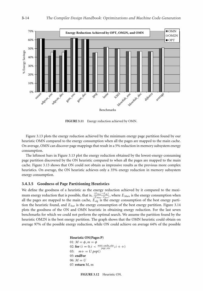
3-14 The Compiler Design Handbook: Optimizations and Machine Code Generation
Energy Reduction Achieved by OPT, OM2N, and OMN OMN
OM2N
OPT
% E
ner
gy
Sav
ing
s
Benchmarks
70%
60%
50%
40%
30%
20%
10%
0%
susa
n
adpcm
_enc
adpcm
_dec
gsm
_enc
gsm
_dec
jpeg
lam
eh263
blow
fish_e
nc
blow
fish_d
ec
dijkst
ra
aver
age
FIGURE 3.11 Energy reduction achieved by OMN.
Figure 3.13 plots the energy reduction achieved by the minimum energy page partition found by ourheuristic OMN compared to the energy consumption when all the pages are mapped to the main cache.On average, OMN can discover page mappings that result in a 5% reduction in memory subsystem energyconsumption.
The leftmost bars in Figure 3.13 plot the energy reduction obtained by the lowest-energy-consumingpage partition discovered by the ON heuristic compared to when all the pages are mapped to the maincache. Figure 3.13 shows that ON could not obtain as impressive results as the previous more complexheuristics. On average, the ON heuristic achieves only a 35% energy reduction in memory subsystemenergy consumption.
3.4.3.5 Goodness of Page Partitioning Heuristics
We define the goodness of a heuristic as the energy reduction achieved by it compared to the maxi-
mum energy reduction that is possible, that is,(E Main−E alg )(E Main−E best )
, where E Main is the energy consumption whenall the pages are mapped to the main cache, E alg is the energy consumption of the best energy parti-tion the heuristic found, and E best is the energy consumption of the best energy partition. Figure 3.14plots the goodness of the ON and OMN heuristic in obtaining energy reduction. For the last sevenbenchmarks for which we could not perform the optimal search. We assume the partition found by theheuristic OM2N is the best energy partition. The graph shows that the OMN heuristic could obtain onaverage 97% of the possible energy reduction, while ON could achieve on average 64% of the possible
Heuristic ON(Pages P)01: M = φ , m = φ
02: for (i = 0; i < mini−cache sizepage size
; i + +)
03: m+ = U.pop()05: endFor06: M = U07: return M, m
FIGURE 3.12 Heuristic ON.

Compiler-Aided Design of Embedded Computers 3-15
Energy Reduction Achieved by OPT, OM2N, OMN, and ON ON
OMN
OM2N
OPT
% E
ner
gy
Sav
ing
s
Benchmarks
70%
60%
50%
40%
30%
20%
10%
0%
susa
n
adpcm
_enc
adpcm
_dec
gsm
_enc
gsm
_dec
jpeg
lam
eh263
blow
fish_e
nc
blow
fish_d
ec
dijkst
ra
aver
age
FIGURE 3.13 Energy reduction achieved by ON.
energy reduction. It is important to note that the GCC compiler for XScale does not exploit the mini-cacheat all. The ON heuristic provides a simple yet effective way to exploit the mini-cache without incurringany performance penalty (for a high-associativity mini-cache).
3.4.4 Optimizing for Energy Is Different Than Optimizing for Performance
This experiment investigates the difference in optimizing for energy and optimizing for performance. Wefind the partition that results in the least memory latency and the partition that results in the least energyconsumption. Figure 3.15a plots E br −E be
E be, where E br is the memory subsystem energy consumption of the
Goodness of Heuristics ON
OMN
Go
od
nes
s
Benchmarks
120%
100%
80%
60%
40%
20%
0%
susa
n
adpcm
_enc
adpcm
_dec
gsm
_enc
gsm
_dec
jpeg
lam
eh263
blow
fish_e
nc
blow
fish_d
ec
dijkst
ra
aver
age
FIGURE 3.14 Goodness of heuristics.

3-16 The Compiler Design Handbook: Optimizations and Machine Code Generation
7%Increase in Runtime by Choosing Best Energy Partition
Instead of the Best Runtime Partition
% D
iffer
ence
in
Mem
ory
Lat
ency 6%
5%
4%
3%
2%
1%
0%
Benchmarks
susa
n
adpcm
_enc
adpcm
_dec
gsm
_enc
gsm
_dec
jpeg
lam
eh263
blow
fish_e
nc
blow
fish_d
ec
dijkst
ra
aver
age
140%
Decrease in Energy when Choosing the Best Energy Partition Instead of theBest Runtime Partition
% E
ner
gy
Diff
eren
ce
120%
100%
80%
60%
40%
20%
0%
Benchmarks
susa
n
adpcm
_enc
adpcm
_dec
gsm
_enc
gsm
_dec
jpeg
lam
eh263
blow
fish_e
nc
blow
fish_d
ec
dijkst
ra
aver
age
FIGURE 3.15 Optimizing for energy is better than optimizing for performance. (a) Increase in runtime, when wechoose the best. energy partition instead of the best performance partition. (b) Decrease in energy consumption, whenwe choose the best energy partition instead of the best performance partition.
partition that results in the least memory latency, and E be is the memory subsystem energy consumption bythe partition that results in the least memory subsystem energy consumption. For the first five benchmarks(susan to gsm dec), the number of pages in the footprint were small, so we could explore all the partitions.For the last seven benchmarks (jpeg to dijkstra), we took the partition found by the OM2N heuristic asthe best partition, as OM2N gives close-to-optimal results in cases when we were able to search optimally.The graph essentially plots the increase in energy if you choose the best performance partition as yourdesign point. The increase in energy consumption is up to 130% and on average is 58% for this set ofbenchmarks.

Compiler-Aided Design of Embedded Computers 3-17
Figure 3.15b plots Rbe −Rbr
Rbe, where Rbe is the memory latency (in cycles) of the best energy partition, and
Rbr is the memory latency of the best-performing partition. This graph shows the increase in memorylatency when you choose the best energy partition compared to using the best performance partition. Theincrease in memory latency is on average 1.7% and is 5.8% in the worst case for this set of benchmarks. Thus,choosing the best energy partition results in significant energy savings at a minimal loss in performance.
3.5 Compiler-in-the-Loop HPC Design
So far we have seen that HPC is a very effective microarchitectural technique to reduce the energy con-sumption of the processor. The energy savings achieved are very sensitive to the HPC configuration; thatis, if we change the HPC configuration, the page partitioning should also change.
In the traditional DSE techniques, for example, SO DSE, the binary and the page mapping are kept thesame, and the binary with the page mapping is executed on different HPC configurations. This strategyis not useful for HPC DSE, since it does not make sense to use the same page mapping after changing theHPC parameters. Clearly, the HPC parameters should be explored with the CIL during the exploration.To evaluate HPC parameters, the page mapping should be set to the given HPC configuration.
Our CIL DSE framework to explore HPC parameters is depicted in Figure 3.16. The CIL DSE frameworkis centered around a textual description of the processor. For our purposes, the processor descriptioncontains information about (a) HPC parameters, (b) the memory subsystem energy models, and (c) theprocessor and memory delay models.
We use the OMN page partitioning heuristic and generate a binary executable along with the pagemapping. The page mapping specifies to which cache (main or mini) each data memory page is mapped.The compiler is tuned to generate page mappings that lead to the minimum memory subsystem energyconsumption. The executable and the page mapping are both fed into a simulator that estimates theruntime and the energy consumption of the memory subsystem.
The Design Space Walker performs HPC design space exploration by updating the HPC design parame-ters in the processor description. The mini-cache, which is configured by Design Space Walker, is specifiedusing two attributes: the mini-cache size and the mini-cache associativity. For our experiments, we varycache size from 256 bytes to 32 KB, in exponents of 2. We explore the whole range of mini-cache associa-tivities, that is, from direct mapped to fully associative. We do not model the mini-cache configurations
HPC Compiler
Application
Executable
Simulator
Design Space
Walker
Page Mapping
Report Runtime
Energy
ProcessorDescription
Energy Model
Delay Model
mini-cacheparams
FIGURE 3.16 Compiler-in-the-loop methodology to explore the design space of HPCs.

3-18 The Compiler Design Handbook: Optimizations and Machine Code Generation
ExhaustiveExploration()01: minEnergy = MAX ENERGY02: foreach (c ∈ C )03: energy = estimateEnergy(c)04: if (energy < minEnergy)05: minEnergy = energy06: endIf07: endFor08: return minEnergy
FIGURE 3.17 Exhaustive exploration algorithm.
for which eCACTI [23] does not have a power model. We set the cache line size to be 32 bytes, as in theIntel XScale architecture. In total we explore 33 mini-cache configurations for each benchmark.
3.5.1 Exhaustive Exploration
We first present experiments to estimate the importance of exploration of HPCs. To this end, we performexhaustive CIL exploration of HPC design space and find the minimum-energy HPC design parameters.Figure 3.17 describes the exhaustive exploration algorithm. The algorithm estimates the energy consump-tion for each mini-cache configuration (line 02) and keeps track of the minimum energy. The functionestimate energy estimates the energy consumption for a given mini-cache size and associativity.
Figure 3.18 compares the energy consumption of the memory subsystem with three cache designs. Theleftmost bar represents the energy consumed by the memory subsystem when the system has only a 32KB
Memory Subsystem Energy Consumption 32K
32K + 2K
Exhaust
No
rmal
ized
En
erg
y
Benchmarks
300%
250%
200%
150%
100%
50%
0%
adpcm
_enc
adpcm
_dec
blow
fish_e
nc
blow
fish_d
ec
dijkst
ra
gsm
_enc
gsm
_dec
h263jp
egla
me
susa
n
aver
age
FIGURE 3.18 Energy savings achieved by exploration.

Compiler-Aided Design of Embedded Computers 3-19
TABLE 3.3 Optimal Mini-cache Parameters
Benchmark Mini-cache Parameters
adpcm dec 8K, direct mappedadpcm enc 4K, 2-waydijkstra 8K, 2-wayblowfish dec 16K, 2-wayblowfish enc 16K, 2-waygsm dec 2K, direct mappedgsm enc 2K, direct mappedh263 8K, 2-wayjpeg 16K, 2-waylame 8K, 2-waysusan 2K, 4-way
main cache (no mini-cache is present.) The middle bar shows the energy consumed when there is a 2KBmini-cache in parallel with the 32KB cache, and the application is compiled to achieve minimum energy.The rightmost bar represents the energy consumed by the memory subsystem, when the mini-cacheparameters (size and associativity) are chosen using exhaustive CIL exploration. All the energy values arenormalized to the case when there is a 2KB mini-cache (the Intel XScale configuration). The last set ofbars is the average over the applications.
We make two important observations from this graph. The first is that HPC is very effective in reducingthe memory subsystem energy consumption. Compared to not using any mini-cache, using a default mini-cache (the default mini-cache is 2KB, 32-way set associative) leads to an average of a 2 times reduction inthe energy consumption of the memory subsystem. The second important observation is that the energyreduction obtained using HPCs is very sensitive to the mini-cache parameters. Exhaustive CIL explorationof the mini-cache DSE to find the minimum-energy mini-cache results in an additional 80% energyreduction, thus reducing the energy consumption to just 20% of the case with a 2KB mini-cache.
Furthermore, the performance of the energy-optimal HPC configuration is very close to the performanceof the best-performing HPC configuration. The performance degradation was no more than 5% and was2% on average. Therefore, energy-optimal HPC configuration achieves high energy reductions at minimalperformance cost. Table 3.3 shows the energy-optimal mini-cache configuration for each benchmark. Thetable suggests that low-associativity mini-caches are good candidates to achieve low-energy solutions.
3.5.2 HPC CIL DSE Heuristics
We have demonstrated that CIL DSE of HPC design parameters is very useful and important to achievesignificant energy savings. However, since the mini-cache design space is very large, exhaustive explorationmay consume a lot of time. In this section we explore heuristics for effective and efficient HPC DSE.
3.5.2.1 Greedy Exploration
The first heuristic we develop for HPC CIL DSE is a pure greedy algorithm, outlined in Figure 3.19. Thegreedy algorithm first greedily finds the cache size (lines 02 to 04) and then greedily finds the associativity(lines 05 to 07). The function betterNewConfiguration tells whether the new mini-cache parameters resultin lower energy consumption than the old mini-cache parameters.
Figure 3.20 plots the energy consumption when the mini-cache configuration is chosen by the greedyalgorithm compared to when using the default 32KB main cache and 2KB mini-cache configuration. Theplot shows that for most applications, greedy exploration is able to achieve good results, but for blowfishand susan, the greedy exploration is unable to achieve any energy reduction; in fact, the solution it hasfound consumes even more energy than the base configuration. However, on average, the greedy CIL HPCDSE can reduce the energy consumption of the memory subsystem by 50%.

3-20 The Compiler Design Handbook: Optimizations and Machine Code Generation
GreedyExploration()01: size = MIN SIZE, assoc = MIN ASSOC
// greedily find the size02: while (betterNewConf (size × 2, assoc, size, assoc))03: size = size × 204: endWhile
// greedily find the assoc05: while (betterNewConf (size, assoc × 2, size, assoc))06: assoc = assoc × 207: endWhile
08: return estimateEnergy(size, assoc)
betterNewConf(size′, assoc′, size, assoc)01: if (!existsCacheConfig(size′, assoc′))02: return false03: energy = estimateEnergy(size, assoc)04: energy′ = estimateEnergy(size′, assoc′)05: return (energy′ < energy)
FIGURE 3.19 Greedy exploration.
Energy Consumption Achieved by the Greedy Heuristic Greedy
Exhaust
En
erg
y C
on
sum
pti
on
(%
)
Benchmarks
120%
100%
80%
60%
40%
20%
0%
adpcm
_enc
adpcm
_dec
blow
fish_e
nc
blow
fish_d
ec
dijkst
ra
gsm
_enc
gsm
_dec
h263jp
egla
me
susa
n
aver
age
FIGURE 3.20 Energy reduction achieved by the greedy exploration.

Compiler-Aided Design of Embedded Computers 3-21
HybridExploration()01: size = MIN SIZE, assoc = MIN ASSOC
// greedily find the size02: while (betterNewConf (size × 4, assoc, size, assoc))03: size = size × 404: endWhile
// search in the neighborhood05: done = false06: while (!done)07: if (betterNewConf (size × 2, assoc, size, assoc))08: size = size × 209: else if (betterNewConf (size, assoc × 2, size, assoc))10: assoc = assoc × 211: else if (betterNewConf (size ÷ 2, assoc, size, assoc))12: size = size ÷ 213: else if (betterNewConf (size ÷ 2, assoc ÷ 2, size, assoc))14: size = size ÷ 2, assoc = assoc ÷ 215: else if (betterNewConf (size ÷ 2, assoc × 2, size, assoc))16: size = size ÷ 2, assoc = assoc × 217: else18: done = true19: endWhile
08: return estimateEnergy(size, assoc)
FIGURE 3.21 Hybrid exploration.
3.5.2.2 Hybrid Exploration
To achieve energy consumption close to the optimal configurations, we developed a hybrid algorithm,outlined in Figure 3.21. The hybrid algorithm first greedily searches for the optimal mini-cache size (lines02 to 04). Note, however, that it tries every alternate mini-cache size. The hybrid algorithm tries mini-cache sizes in exponents of 4, rather than 2 (line 03). Once it has found the optimal mini-cache size, itexplores exhaustively in the size-associativity neighborhood (lines 07 to 15) to find a better size-associativityconfiguration.
The middle bar in Figure 3.22 plots the energy consumption of the optimal configuration comparedto the energy consumption when the XScale default 32-way, 2K mini-cache is used and compares theenergy reductions achieved with the greedy and exhaustive explorations. The graph shows that the hybridexploration can always find the optimal HPC configuration for our set of benchmarks.
3.5.2.3 Energy Reduction and Exploration Time Trade-Off
There is a clear trade-off between the energy reductions achieved by the exploration algorithms and thetime required for the exploration. The rightmost bar in Figure 3.23 plots the time (in hours) requiredto explore the design space using the exhaustive algorithm. Although the exhaustive algorithm is able todiscover extremely low energy solutions, it may take tens of hours to perform the exploration. The leftmostbar in Figure 3.23 plots the time that greedy exploration requires to explore the design space of the mini-cache. Although the greedy algorithm reduces the exploration time on average by a factor of 5 times, theenergy consumption is on average 2 times more than what is achieved by the optimal algorithm.

3-22 The Compiler Design Handbook: Optimizations and Machine Code Generation
Energy Consumption Achieved by Exploration Algorithms Greedy
Hybrid
Exhaust
En
erg
y C
on
sum
pti
on
(%
)
Benchmarks
120%
100%
80%
60%
40%
20%
0%
adpcm
_enc
adpcm
_dec
blow
fish_e
nc
blow
fish_d
ec
dijkst
ra
gsm
_enc
gsm
_dec
h263jp
egla
me
susa
n
aver
age
FIGURE 3.22 Relative energy reduction achieved by exploration algorithms.
Exploration Time of Exploration Algorithms Greedy
Hybrid
Exhaust
Ex
plo
rati
on
Tim
e (h
ou
rs)
Benchmarks
70
60
50
30
40
20
10
0
adpcm
_enc
adpcm
_dec
blow
fish_e
nc
blow
fish_d
ec
dijkst
ra
gsm
_enc
gsm
_dec
h263jp
egla
me
susa
n
aver
age
FIGURE 3.23 Exploration time of exploration algorithms.

Compiler-Aided Design of Embedded Computers 3-23
Finally, the middle bar in Figure 3.23 plots the time required to find the mini-cache configuration whenusing the hybrid algorithm. Our hybrid algorithm is able to find the optimal mini-cache configuration inall of our benchmarks, while it takes about 3 times less time than the optimal algorithm. Thus, we believethe hybrid exploration is a very effective and efficient exploration technique.
3.5.3 Importance of Compiler-in-the-Loop DSE
Our next set of experiments show that although SO DSE can also find HPC configurations with lessmemory subsystem energy consumption, it does not do as well as CIL DSE. To this end, we performedSO DSE of HPC design parameters. We compile once for the 32KB/2KB (i.e., the original XScale cacheconfiguration) to obtain an executable and the minimum energy page mapping. While keeping thesetwo the same, we explored all the HPC configurations to find the HPC design parameters that minimizethe memory subsystem energy consumption. Figure 3.24 plots the the energy consumption of the HPCconfiguration found by the SO DSE (middle bar) and CIL DSE (right bar) and the original Intel XScaleHPC configuration (left bar) for each benchmark. The rightmost set of bars represents the average overall the benchmarks. All the energy consumption values are normalized to energy consumption of the32KB/2KB configuration.
It should be noted that the overhead of compilation time in CIL DSE is negligible, because simulationtimes are several orders of magnitude more than compilation times. The important observation to makefrom this graph is that although even SO DSE can find HPC configurations that result in, on average,a 57% memory subsystem energy reduction, CIL DSE is much more effective and can uncover HPCconfigurations that result in a 70% reduction in the memory subsystem energy reduction.
Compiler-in-the-Loop vs. Simulation-Only Exploration 32K + 2K
SOE-Opt
CIL-Opt
% E
ner
gy
Red
uct
ion
Benchmarks
120%
100%
80%
60%
40%
20%
0%
adpcm
_enc
adpcm
_dec
blow
fish_e
nc
blow
fish_d
ec
dijkst
ra
gsm
_enc
gsm
_dec
h263jp
egla
me
susa
n
aver
age
FIGURE 3.24 CIL versus SO exploration.

3-24 The Compiler Design Handbook: Optimizations and Machine Code Generation
3.6 Summary
Embedded systems are characterized by stringent, application-specific, multidimensional constraints ontheir designs. These constraints, along with the shrinking time to market and frequent upgrade needs ofembedded systems, are responsible for programmable embedded systems that are highly customized. Whilecode generation for these highly customized embedded systems is a challenge, it is also very rewarding inthe sense that an architecture-sensitive compilation technique can have significant impact on the systempower, performance, and so on. Given the importance of the compiler on the system design parameters,it is reasonable for the compiler to take part in designing the embedded system. While it is possible to usead hoc methods to include the compiler effects while designing an embedded system, a systematic method-ology to design embedded processors is needed. This chapter introduced the CIL design methodology,which systematically includes the compiler in the embedded system DSE. Our methodology requires anarchitecture-sensitive compiler. To evaluate a design point in the embedded system design space, the ap-plication code is first compiled for the embedded system design and is then executed on the embeddedsystem model to estimate the various design parameters (e.g., power, performance, etc.). Owing to thelack of compiler technology for embedded systems, most often, first an architecture-sensitive compilationtechnique needs to be developed, and only then can it be used for CIL design of the embedded processor.In the chapter we first developed a compilation technique for HPCs, which can result in a 50% reduc-tion in the energy consumption of the memory subsystem. When we use this compilation technique inour CIL approach, we can come up with HPC parameters that result in an 80% reduction in the energyconsumption by the memory subsystem, demonstrating the need and usefulness of our approach.
References
1. M. R. Barbacci. 1981. Instruction set processor specifications (ISPS): The notation and its applica-tions. IEEE Transactions on Computing C-30(1):24–40. New York: IEEE Press.
2. D. Burger and T. M. Austin. 1997. The SimpleScalar tool set, version 2.0. SIGARCH ComputerArchitecture News 25(3):13–25.
3. L. T. Clark, E. J. Hoffman, M. Biyani, Y. Liao, S. Strazdus, M. Morrow, K. E. Velarde, and M. A. Yarch.2001. An embedded 32-b microprocessor core for low-power and high-performance applications.IEEE J. Solid State Circuits 36(11):1599–608. New York: IEEE Press.
4. Paul C. Clements. 1996. A survey of architecture description languages. In Proceedings of InternationalWorkshop on Software Specification and Design (IWSSD), 16–25.
5. A. Fauth, M. Freericks, and A. Knoll. 1993. Generation of hardware machine models from instructionset descriptions. In IEEE Workshop on VLSI Signal Processing, 242–50.
6. A. Gonzalez, C. Aliagas, and M. Valero. 1995. A data cache with multiple caching strategies tunedto different types of locality. In ICS ’95: Proceedings of the 9th International Conference on Supercom-puting, 338–47. New York: ACM Press.
7. M. R. Guthaus, J. S. Ringenberg, D. Ernst, T. M. Austin, T. Mudge, and R. B. Brown. 2001. MiBench:A free, commercially representative embedded benchmark suite. In IEEE Workshop in WorkloadCharacterization.
8. J. Gyllenhaal, B. Rau, and W. Hwu. 1996. HMDES version 2.0 specification. Tech. Rep. IMPACT-96-3,IMPACT Research Group, Univ. of Illinois, Urbana.
9. G. Hadjiyiannis, S. Hanono, and S. Devadas. 1997. ISDL: An instruction set description languagefor retargetability. In Proceedings of Design Automation Conference (DAC), 299–302. New York: IEEEPress.
10. A. Halambi, P. Grun, V. Ganesh, A. Khare, N. Dutt, and A. Nicolau. 1999. EXPRESSION: A languagefor architecture exploration through compiler/simulator retargetability. In Proceedings of DesignAutomation and Test in Europe. New York: IEEE Press.
11. A. Halambi, A. Shrivastava, P. Biswas, N. Dutt, and A. Nicolau. 2002. A design space explorationframework for reduced bit-width instruction set architecture (risa) design. In ISSS ’02: Proceedingsof the 15th International Symposium on System Synthesis, 120–25. New York: ACM Press.

Compiler-Aided Design of Embedded Computers 3-25
12. A. Halambi, A. Shrivastava, P. Biswas, N. Dutt, and A. Nicolau. 2002. An efficient compiler techniquefor code size reduction using reduced bit-width isas. In Proceedings of the Conference on Design,Automation and Test in Europe. New York: IEEE Press.
13. A. Halambi, A. Shrivastava, N. Dutt, and A. Nicolau. 2001. A customizable compiler framework forembedded systems. In Proceedings of SCOPES.
14. Hewlett Packard. HP iPAQ h4000 series-system specifications. http://www.hp.com.15. Intel Corporation. Intel PXA255 processor: Developer’s manual. http://www.intel.com/design/pca/
applicationsprocessors/manuals/278693.htm.16. Intel Corporation. Intel StrongARM* SA-1110 microprocessor brief datasheet. http://download.
intel.com/design/strong/datashts/27824105.pdf.17. Intel Corporation. Intel XScale(R) Core: Developer’s manual. http://www.intel.com/design/
intelxscale/273473.htm.18. Intel Corporation. LV/ULV Mobile Intel Pentium III Processor-M and LV/ULV Mobile Intel Celeron
Processor (0.13u)/Intel 440MX Chipset: Platform design guide. http://www.intel.com/design/mobile/desguide/251012.htm.
19. IPC-D-317A: Design guidelines for electronic packaging utilizing high-speed techniques. 1995. Institutefor Interconnecting and Packaging Electronic Circuits.
20. D. Kastner. 2000. TDL: A hardware and assembly description language. Tech. Rep. TDL 1.4, SaarlandUniversity, Germany.
21. R. Leupers and P. Marwedel. 1998. Retargetable code generation based on structural processordescriptions. Design Automation Embedded Syst. 3(1):75–108. New York: IEEE Press.
22. K. Lillevold et al. 1995. H.263 test model simulation software. Telenor R&D.23. M. Mamidipaka and N. Dutt. 2004. eCACTI: An enhanced power estimation model for on-chip
caches. Tech. Rep. TR-04-28, CECS, UCI.24. Micron Technology, Inc. MICRON Mobile SDRAM MT48V8M32LF datasheet. http://www.micron.
com/products/dram/mobilesdram/.25. P. Mishra, A. Shrivastava, and N. Dutt. 2004. Architecture description language (adl)-driven
software toolkit generation for architectural exploration of programmable socs. In DAC ’04:Proceedings of the 41st Annual Conference on Design Automation, 626–58. New York: ACM Press.
26. S. Park, E. Earlie, A. Shrivastava, A. Nicolau, N. Dutt, and Y. Paek. 2006. Automatic generation ofoperation tables for fast exploration of bypasses in embedded processors. In DATE ’06: Proceedingsof the Conference on Design, Automation and Test in Europe, 1197–202. Leuven, Belgium: EuropeanDesign and Automation Association. New York: IEEE Press.
27. S. Park, A. Shrivastava, N. Dutt, A. Nicolau, Y. Paek, and E. Earlie. 2006. Bypass aware instructionscheduling for register file power reduction, In LCTES 2006: Proceedings of the 2006 ACM SIG-PLAN/SIGBED conference on language, compilers, and tool support for embedded systems, 173–81.New York: ACM Press.
28. P. Shivakumar and N. Jouppi. 2001. Cacti 3.0: An integrated cache timing, power, and area model.WRL Technical Report 2001/2.
29. A. Shrivastava, P. Biswas, A. Halambi, N. Dutt, and A. Nicolau. 2006. Compilation framework forcode size reduction using reduced bit-width isas (risas). ACM Transaction on Design Automation ofElectronic Systems 11(1):123–46. New York: ACM Press.
30. A. Shrivastava and N. Dutt. 2004. Energy efficient code generation exploiting reduced bit-widthinstruction set architecture. In Proceedings of The Asia Pacific Design Automation Conference(ASPDAC). New York: IEEE Press.
31. A. Shrivastava, N. Dutt, A. Nicolau, and E. Earlie. 2005. Pbexplore: A framework for compiler-in-the-loop exploration of partial bypassing in embedded processors. In DATE ’05: Proceedings of theConference on Design, Automation and Test in Europe, 1264–69. Washington, DC: IEEE ComputerSociety.
32. A. Shrivastava, E. Earlie, N. D. Dutt, and A. Nicolau. 2004. Operation tables for scheduling in thepresence of incomplete bypassing. In CODES+ISSS, 194–99. New York: IEEE Press.

3-26 The Compiler Design Handbook: Optimizations and Machine Code Generation
33. A. Shrivastava, E. Earlie, N. Dutt, and A. Nicolau. 2005. Aggregating processor free time for energyreduction. In CODES+ISSS ’05: Proceedings of the 3rd IEEE/ACM/IFIP International Conference onHardware/Software Codesign and System Synthesis, 154–59. New York: ACM Press.
34. A. Shrivastava, E. Earlie, N. Dutt, and A. Nicolau. 2006. Retargetable pipeline hazard detection forpartially bypassed processors, In IEEE Transactions on Very Large Scale Integrated Circuits, 791–801.New York: IEEE Press.
35. A. Shrivastava, I. Issenin, and N. Dutt. 2005. Compilation techniques for energy reduction inhorizontally partitioned cache architectures. In CASES ’05: Proceedings of the 2005 InternationalConference on Compilers, Architectures and Synthesis for Embedded Systems, 90–96. New York: ACMPress.
36. Starcore LLC. SC1000-family processor core reference.37. S. P. Vanderwiel and D. J. Lilja. 2000. Data prefetch mechanisms. ACM Computing Survey (CSUR)
32(2):174–99. New York: ACM Press.38. V. Zivojnovic, S. Pees, and H. Meyr. 1996. LISA — Machine description language and generic
machine model for HW/SW co-design. In IEEE Workshop on VLSI Signal Processing, 127–36.

4Whole ExecutionTraces and Their
Use in Debugging
Xiangyu ZhangDepartment of Computer Sciences,Purdue University,West Lafayette, [email protected]
Neelam GuptaDepartment of Computer Sciences,University of Arizona, Tuscon, [email protected]
Rajiv GuptaDepartment of Computer Scienceand Engineering,University of California, Riverside, [email protected]
4.1 Introduction . . . . . . . . . . . . . . . . . . . . . . . . . . . . . . . . . . . . . . . . . .4-14.2 Whole Execution Traces . . . . . . . . . . . . . . . . . . . . . . . . . . . . . . .4-2
Timestamped WET Representation • Compressing WholeExecution Traces
4.3 Using WET in Debugging . . . . . . . . . . . . . . . . . . . . . . . . . . . . .4-8Dynamic Program Slicing • Dynamic Matching of ProgramVersions
4.4 Concluding Remarks . . . . . . . . . . . . . . . . . . . . . . . . . . . . . . . . . .4-16References . . . . . . . . . . . . . . . . . . . . . . . . . . . . . . . . . . . . . . . . . . . . . . . . . .4-16
AbstractProfiling techniques have greatly advanced in recent years. Extensive amounts of dynamic information canbe collected (e.g., control flow, address and data values, data, and control dependences), and sophisticateddynamic analysis techniques can be employed to assist in improving the performance and reliability ofsoftware. In this chapter we describe a novel representation called whole execution traces that can holda vast amount of dynamic information in a form that provides easy access to this information duringdynamic analysis. We demonstrate the use of this representation in locating faulty code in programsthrough dynamic-slicing- and dynamic-matching-based analysis of dynamic information generated byfailing runs of faulty programs.
4.1 Introduction
Program profiles have been analyzed to identify program characteristics that researchers have thenexploited to guide the design of superior compilers and architectures. Because of the large amountsof dynamic information generated during a program execution, techniques for space-efficient represen-tation and time-efficient analysis of the information are needed. To limit the memory required to storedifferent types of profiles, lossless compression techniques for several different types of profiles have beendeveloped. Compressed representations of control flow traces can be found in [15, 30]. These profiles canbe analyzed for the presence of hot program paths or traces [15] that have been exploited for performingpath-sensitive optimization and prediction techniques [3, 9, 11, 21]. Value profiles have been compressedusing value predictors [4] and used to perform code specialization, data compression, and value encoding[5, 16, 20, 31]. Address profiles have also been compressed [6] and used for identifying hot data streams that
4-1

4-2 The Compiler Design Handbook: Optimizations and Machine Code Generation
exhibit data locality, which can help in finding cache-conscious data layouts and developing data prefetch-ing mechanisms [7, 13, 17]. Dependence profiles have been compressed in [27] and used for computatingdynamic slices [27], studying the characteristics of performance-degrading instructions [32], and studyinginstruction isomorphism [18]. More recently, program profiles are being used as a basis for the debuggingof programs. In particular, profiles generated from failing runs of faulty programs are being used to helplocate the faulty code in the program.
In this chapter a unified representation, which we call whole execution traces (WETs), is described, andits use in assisting faulty code in a program is demonstrated. WETs provide an ability to relate differenttypes of profiles (e.g., for a given execution of a statement, one can easily find the control flow path, datadependences, values, and addresses involved). For ease of analysis of profile information, WET is con-structed by labeling a static program representation with profile information such that relevant and relatedprofile information can be directly accessed by analysis algorithms as they traverse the representation. Aneffective compression strategy has been developed to reduce the memory needed to store WETs.
The remainder of this chapter is organized as follows. In Section 4.2 we introduce the WET represen-tation. We describe the uncompressed form of WETs in detail and then briefly outline the compressionstrategy used to greatly reduce its memory needs. In Section 4.3 we show how the WETs of failing runscan be analyzed to locate faulty code. Conclusions are given in Section 4.4.
4.2 Whole Execution Traces
WET for a program execution is a comprehensive set of profile data that captures the complete functionalexecution history of a program run. It includes the following dynamic information:
Control flow profile: The control flow profile captures the complete control flow path taken during asingle program run.
Value profile: This profile captures the values that are computed and referenced by each executedstatement. Values may correspond to data values or addresses.
Dependence profile: The dependence profile captures the information about data and control depen-dences exercised during a program run. A data dependence represents the flow of a value from thestatement that defines it to the statement that uses it as an operand. A control dependence betweentwo statements indicates that the execution of a statement depends on the branch outcome of apredicate in another statement.
The above information tells what statements were executed and in what order (control flow profile),what operands and addresses were referenced as well as what results were produced during each statementexecution (value profile), and the statement executions on which a given statement execution is data andcontrol dependent (dependence profile).
4.2.1 Timestamped WET Representation
WET is essentially a static representation of the program that is labeled with dynamic profile information.This organization provides direct access to all of the relevant profile information associated with everyexecution instance of every statement. A statement in WET can correspond to a source-level statement,intermediate-level statement, or machine instruction.
To represent profile information of every execution instance of every statement, it is clearly necessaryto distinguish between execution instances of statements. The WET representation distinguishes betweenexecution instances of a statement by assigning unique timestamps to them [30]. To generate the timestampsa time counter is maintained that is initialized to one and each time a basic block is executed, the currentvalue of time is assigned as a timestamp to the current execution instances of all the statements withinthe basic block, and then time is incremented by one. Timestamps assigned in this fashion essentiallyremember the ordering of all statements executed during a program execution. The notion of timestampsis the key to representing and accessing the dynamic information contained in WET.
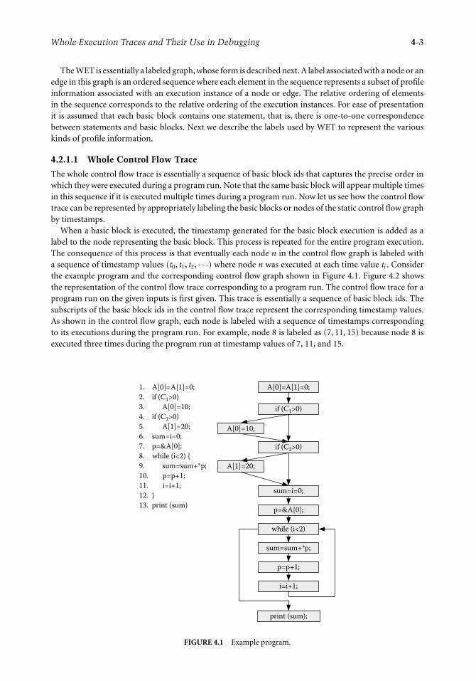
Whole Execution Traces and Their Use in Debugging 4-3
The WET is essentially a labeled graph, whose form is described next. A label associated with a node or anedge in this graph is an ordered sequence where each element in the sequence represents a subset of profileinformation associated with an execution instance of a node or edge. The relative ordering of elementsin the sequence corresponds to the relative ordering of the execution instances. For ease of presentationit is assumed that each basic block contains one statement, that is, there is one-to-one correspondencebetween statements and basic blocks. Next we describe the labels used by WET to represent the variouskinds of profile information.
4.2.1.1 Whole Control Flow Trace
The whole control flow trace is essentially a sequence of basic block ids that captures the precise order inwhich they were executed during a program run. Note that the same basic block will appear multiple timesin this sequence if it is executed multiple times during a program run. Now let us see how the control flowtrace can be represented by appropriately labeling the basic blocks or nodes of the static control flow graphby timestamps.
When a basic block is executed, the timestamp generated for the basic block execution is added as alabel to the node representing the basic block. This process is repeated for the entire program execution.The consequence of this process is that eventually each node n in the control flow graph is labeled witha sequence of timestamp values (t0, t1, t2, · · ·) where node n was executed at each time value ti . Considerthe example program and the corresponding control flow graph shown in Figure 4.1. Figure 4.2 showsthe representation of the control flow trace corresponding to a program run. The control flow trace for aprogram run on the given inputs is first given. This trace is essentially a sequence of basic block ids. Thesubscripts of the basic block ids in the control flow trace represent the corresponding timestamp values.As shown in the control flow graph, each node is labeled with a sequence of timestamps correspondingto its executions during the program run. For example, node 8 is labeled as (7, 11, 15) because node 8 isexecuted three times during the program run at timestamp values of 7, 11, and 15.
A[0]=A[1]=0;1. A[0]=A[1]=0;
2. if (C1>0)
3. A[0]=10;
4. if (C2>0)
5. A[1]=20;
6. sum=i=0;
7. p=&A[0];
8. while (i<2) {
9. sum=sum+*p;
10. p=p+1;
11. i=i+1;
12. }
13. print (sum)
A[0]=10;
A[1]=20;
sum=i=0;
p=&A[0];
p=p+1;
i=i+1;
print (sum);
while (i<2)
sum=sum+*p;
if (C1>0)
if (C2>0)
FIGURE 4.1 Example program.

4-4 The Compiler Design Handbook: Optimizations and Machine Code Generation
1. A[0]=A[1]=0;
With input C1=1 and C2=0, the execution trace is:
11 22 33 44 65 76 87 98 109 1110 811 912 1013 1114 815 1316
[1]
2. if (C1>0) [2]
3. A[0]=10; [3]
4. if (C2>0) [4]
5. A[1]=20;
6. sum=i=0;
7. p=&A[0];
[5]
[6]
8. while (i<2) [7,11,15]
10. p=p+1; [9,13]
11. i=i+1; [10,14]
13. print (sum); [16]
9. sum=sum+*p; [8,12]
FIGURE 4.2 Timestamped control flow representation.
Let’s see how the above timestamped representation captures the complete control flow trace. The pathtaken by the program can be generated from a labeled control flow graph using the combination of staticcontrol flow edges and the sequences of timestamps associated with nodes. If a node n is labeled withtimestamp value t, the node that is executed next must be the static control flow successor of n that islabeled with timestamp value t + 1. Using this observation, the complete path or part of the program pathstarting at any execution point can be easily generated.
4.2.1.2 Whole Value Trace
The whole value trace captures all values and addresses computed and referenced by executed statements.Instrumentation code must be introduced for each instruction in the program to collect the value trace fora program run. To represent the control flow trace, with each statement, we already associate a sequence oftimestamps (t0, t1, t2, · · ·) corresponding to the statement execution instances. To represent the value trace,we also associate a sequence of values (v0, v1, v2, · · ·) with the statement. These are the values computedby the statement’s execution instances. Hence, there is one-to-one correspondence between the sequenceof timestamps and the sequence of values.
Two points are worth noting here. First, by capturing values as stated above, we are actually capturingboth values and addresses, as some instructions compute data values while others compute addresses.Second, with each statement, we only associate the result values computed by that statement. We do notexplicitly associate the values used as operands by the statement. This is because we can access the operandvalues by traversing the data dependence edges and then retrieving the values from the value traces ofstatements that produce these values.
Now let us illustrate the above representation by giving the value traces for the program run considered inFigure 4.2. The sequence of values produced by each statement for this program run is shown in Figure 4.3.For example, statement 11 is executed twice and produces values 1 and 2 during these executions.

Whole Execution Traces and Their Use in Debugging 4-5
1. A[0]=A[1]=0; [0]
2. if (C1>0) [True]
3. A[0]=10; [10]
4. if (C2>0) [False]
5. A[1]=20;
6. sum=i=0;
7. p=&A[0];
[0]
[A]
8. while (i<2) [True, True, False]
10. p=p+1; [A+1,A+2]
11. i=i+1; [1,2]
13. print (sum); [10]
9. sum=sum+*p; [10,10]
FIGURE 4.3 Value trace representation.
4.2.1.3 Whole Dependence Trace
A dependence occurs between a pair of statements; one is the source of the dependence and the other is thedestination. Dependence is represented by an edge from the source to the destination in the static controlflow graph. There are two types of dependences:
Static data dependence: A statement d is statically data dependent upon statement s if a value computedby statement s may be used as an operand by statement d in some program execution.
Static control dependence: A statement d is statically control dependent upon a predicate s if theoutcome of predicate s can directly determine whether d is executed in some program execution.
The whole data and control dependence trace captures the dynamic occurrences of all static data andcontrol dependences during a program run. A static edge from the source of a dependence to its destinationis labeled with dynamic information to capture each dynamic occurrence of a static dependence duringthe program run. The dynamic information essentially identifies the execution instances of the sourceand destination statements involved in a dynamic dependence. Since execution instances of statementsare identified by their timestamps, each dynamic dependence is represented by a pair of timestamps thatidentify the execution instances of statements involved in the dynamic dependence. If a static dependenceedge s → d is exercised multiple times during a program run, it will be labeled by a sequence of timestamppairs ([t0
s , t0d ], [t1
s , t1d ], · · ·) corresponding to multiple occurrences of the dynamic dependence observed
during the program run.Let us briefly discuss how dynamic dependences are identified during a program run. To identify dynamic
data dependences, we need to further process the address trace. For each memory address the executioninstance of an instruction that was responsible for the latest write to the address is remembered. When anexecution instance of an instruction uses the value at an address, a dynamic data dependence is establishedbetween the execution instance of the instruction that performed the latest write to the address and theexecution instance of the instruction that used the value at the address. Dynamic control dependencesare also identified. An execution instance of an instruction is dynamically control dependent upon theexecution instance of the predicate that caused the execution of the instruction. By first computing the static

4-6 The Compiler Design Handbook: Optimizations and Machine Code Generation
1. A[0]=A[1]=0;
2. if (C1>0)
3. A[0]=10;
[(2,3)]
4. if (C2>0)
5. A[1]=20;
6. sum=i=0;
7. p=&A[0];
[(7,11)(11,15)]
[(7,9)(11,13)]
8. while (i<2)
[(7,10)(11,14)]10. p=p+1;
11. i=i+1;
13. print (sum);
9. sum=sum+*p;[(7,8)(11,12)]
FIGURE 4.4 Timestamped control dependence trace representation.
control predecessors of an instruction, and then detecting which one of these was the last to execute prior toa given execution of the instruction from the control flow trace, dynamic control dependences are identified.
Now let us illustrate the above representation by giving the dynamic data and control dependences forthe program run considered in Figure 4.2. First let’s consider the dynamic control dependences shown inFigure 4.4. The control dependence edges in this program include 2 → 3, 4 → 5, 8 → 9, 8 → 10, and8 → 11. These edges are labeled with timestamp pairs. The edge 2 → 3 is labeled with ([2, 3]) becausethis dependence is exercised only once and the timestamps of the execution instances involved are 2 and3. The edge 4 → 5 is not labeled because it is not exercised in the program run. However, edge 8 → 9is labeled with ([7, 8], [11, 12]), indicating that this edge is exercised twice. The timestamps in each pairidentify the execution instances of statements involved in the dynamic dependences.
Next let us consider the dynamic data dependence edges shown in Figure 4.5. The darker edges cor-respond to static data dependence edges that are labeled with sequences of timestamp pairs that capturedynamic instances of data dependences encountered during the program run. For example, edge 11 → 8shows the flow of the value of variable i from its definition in statement 11 to its use in statement 8. Thisedge is labeled ([10, 11], [14, 15]) because it is exercised twice in the program run. The timestamps in eachpair identify the execution instances of statements involved in the dynamic dependences.
4.2.2 Compressing Whole Execution Traces
Because of the large amount of information contained in WETs, the storage needed to hold the WETs isvery large. In this section we briefly outline a two-tier compression strategy for greatly reducing the spacerequirements.
The first tier of our compression strategy focuses on developing separate compression techniques foreach of the three key types of information labeling the WET graph: (a) timestamps labeling the nodes,(b) values labeling the nodes, and (c) timestamp pairs labeling the dependence edges. Let us briefly considerthese compression techniques:
Timestamps labeling the nodes: The total number of timestamps generated is equal to the number ofbasic block executions, and each of the timestamps labels exactly one basic block. We can reduce the

Whole Execution Traces and Their Use in Debugging 4-7
1. A[0]=A[1]=0;
2. if (C1>0)
3. A[0]=10;
4. if (C2>0)
5. A[1]=20;
6. sum=i=0;
7. p=&A[0];
[(1,8)]
[(5,8)]
[(6,9)]
[(10,11)(14,15)]
8. while (i<2)
[(12,16)]
10. p=p+1;
11. i=i+1;
13. print (sum);
9. sum=sum+*p;
[(5,7)]
[(5,10)]
[(10,14)]
[(9,13)]
[(6,8)]
[(10,14)]
[(9,12)]
[(8,12)]
FIGURE 4.5 Timestamped data dependence trace representation.
space taken up by the timestamp node labels as follows. Instead of having nodes that correspondto basic blocks, we create a WET in which nodes can correspond to Ball Larus paths [2] that arecomposed of multiple basic blocks. Since a unique timestamp value is generated to identify theexecution of a node, now fewer timestamps will be generated. In other words, when a Ball Larus pathis executed, all nodes in the path share the same timestamp. By reducing the number of timestamps,we save space without having any negative impact on the traversal of WET to extract the controlflow trace.
Values labeling the nodes: It is well known that subcomputations within a program are often performedmultiple times on the same operand values. This observation is the basis for widely studied tech-niques for reuse-based redundancy removal [18]. This observation can be exploited in devising acompression scheme for sequence of values associated with statements belonging to a node in theWET. The list of values associated with a statement is transformed such that only a list of uniquevalues produced by it is maintained along with a pattern from which the exact list of values canbe generated from the list of unique values. The pattern is often shared across many statements.The above technique yields compression because by storing the pattern only once, we are able toeliminate all repetitions of values in value sequences associated with all statements.
Timestamp pairs labeling the dependence edges: Each dependence edge is labeled with a sequenceof timestamp pairs. Next we describe how the space taken by these sequences can be reduced.Our discussion focuses on data dependences; however, similar solutions exist for handling controldependence edges [27]. To describe how timestamp pairs can be reduced, we divide the datadependences into two categories: edges that are local to a Ball Larus path and edges that are nonlocalas they cross Ball Larus path boundaries.
Let us consider a node n that contains a pair of statements s1 and s2 such that a local data dependenceedge exists due to flow of values from s1 to s2. For every timestamp pair (ts1 , ts2 ) labeling the edge, it isdefinitely the case that ts1 = ts2 . In addition, if s2 always receives the involved operand value from s1,then we do not need to label this edge with timestamp pairs. This is because the timestamp pairs thatlabel the edge can be inferred from the labels of node n. If node n is labeled with timestamp tn, under

4-8 The Compiler Design Handbook: Optimizations and Machine Code Generation
TABLE 4.1 WET Sizes
Stmts. Executed Orig. WET Comp. WET Orig./
Benchmark Input (Millions) (MB) (MB) Comp.
099.go training 685.28 10369.32 574.65 18.04126.gcc ref/insn-emit.i 364.80 5237.89 89.03 58.84130.li ref 739.84 10399.06 203.01 51.22164.gzip training 650.46 9687.88 537.72 18.02181.mcf testing 715.16 10541.86 416.21 25.33197.parser training 615.49 8729.88 188.39 46.34255.vortex training/lendian 609.45 8747.64 104.59 83.63256.bzip2 training 751.26 11921.19 220.70 54.02300.twolf training 690.39 10666.19 646.93 16.49Avg. n/a 646.90 9588.99 331.25 41.33
the above conditions, the data dependence edge must be labeled with the timestamp pair < tn, tn >. Itshould be noted that by creating nodes corresponding to Ball Larus paths, opportunities for eliminationof timestamp pair labels increase greatly. This is because many nonlocal edges get converted to local edges.
Let us consider nonlocal edges next. Often multiple data dependence edges are introduced between apair of nodes. It is further often the case that these edges have identical labels. In this case we can save spaceby creating a representation for a group of edges and save a single copy of the labels.
For the second-tier compression we view the information labeling the WET as consisting of streams ofvalues arising from the following sources: (a) a sequence of < t, v > pairs labeling a node gives rise totwo streams, one corresponding to the timestamps (ts) and the other corresponding to the values (vs),and (b) a sequence of < ts1 , ts2 > pairs labeling a dependence edge also gives rise to two streams, onecorresponding to the first timestamps (ts1 s) and the other corresponding to the second timestamps (ts2 s).Each of the above streams is compressed using a value-prediction-based algorithm [28].
Table 4.1 lists the benchmarks considered and the lengths of the program runs, which vary from365 and 751 million intermediate-level statements. WETs could not be collected for complete runs formost benchmarks even though we tried using Trimaran-provided inputs with shorter runs. The effectof our two-tier compression strategy is summarized in Table 4.1. While the average size of the originaluncompressed WETs (Orig. WET) is 9589 megabytes, after compression their size (Comp. WET) is reducedto 331 megabytes, which represents a compression ratio (Orig./Comp.) of 41. Therefore, on average, ourapproach enables saving of the whole execution trace corresponding to a program run of 647 millionintermediate statements using 331 megabytes of storage.
4.3 Using WET in Debugging
In this section we consider two debugging scenarios and demonstrate how WET-based analysis can beemployed to assist in fault location in both scenarios. In the first scenario we have a program that fails toproduce the correct output for a given input, and it is our goal to assist the programmer in locating thefaulty code. In the second scenario we are given two versions of a program that should behave the samebut do not do so on a given input, and our goal is to help the programmer locate the point at which thebehavior of the two versions diverges. The programmer can then use this information to correct one ofthe versions.
4.3.1 Dynamic Program Slicing
Let us consider the following scenario for fault location. Given a failed run of a program, our goal is toidentify a fault candidate set, that is, a small subset of program statements that includes the faulty codewhose execution caused the program to fail. Thus, we assume that the fact that the program has failed isknown because either the program crashed or it produced an output that the user has determined to be

Whole Execution Traces and Their Use in Debugging 4-9
incorrect. Moreover, this failure is due to execution of faulty code and not due to other reasons (e.g., faultyenvironment variable setting).
The statements executed during the failing run can constitute a first conservative approximation ofthe fault candidate set. However, since the user has to examine the fault candidate set manually to locatefaulty code, smaller fault candidate sets are desirable. Next we describe a number of dynamic-slicing-basedtechniques that can be used to produce a smaller fault candidate set than the one that includes all executedstatements.
4.3.1.1 Backward Dynamic Slicing
Consider a failing run that produces an incorrect output value or crashes because of dereferencing of anillegal memory address. The incorrect output value or the illegal address value is now known to be relatedto faulty code executed during this failed run. It should be noted that identification of an incorrect outputvalue will require help from the user unless the correct output for the test input being considered is alreadyavailable to us. The fault candidate set is constructed by computing the backward dynamic slice starting atthe incorrect output value or illegal address value. The backward dynamic slice of a value at a point in theexecution includes all those executed statements that effect the computation of that value [1, 14]. In otherwords, statements that directly or indirectly influence the computation of faulty value through chains ofdynamic data and/or control dependences are included in the backward dynamic slices. Thus, the backwardreachable subgraph forms the backward dynamic slice, and all statements that appear at least once in thereachable subgraph are contained in the backward dynamic slice. During debugging, both the statementsin the dynamic slice and the dependence edges that connect them provide useful clues to the failure cause.
We illustrate the benefit of backward dynamic slicing with an example of a bug that causes a heap overflowerror. In this program, a heap buffer is not allocated to be wide enough, which causes an overflow. Thecode corresponding to the error is shown in Figure 4.6. The heap array A allocated at line 10 overflowsat line 51, causing the program to crash. Therefore, the dynamic slice is computed starting at the addressof A[i] that causes the segmentation fault. Since the computation of the address involves A[] and i, bothstatements at lines 10 and 50 are included in the dynamic slice. By examining statements at lines 10 and50, the cause of the failure becomes evident to the programmer. It is easy to see that although a countentries have been allocated at line 10, b count entries are accessed according to the loop bounds of the forstatement at line 50. This is the cause of the heap overflow at line 51. The main benefit of using dynamicslicing is that it focuses the attention of the programmer on the two relevant lines of code (10 and 50),enabling the fault to be located.
We studied the execution times of computing backward dynamic slices using WETs. The results of thisstudy are presented in Figure 4.7. In this graph each point corresponds to the average dynamic slicing timefor 25 slices. For each benchmark 25 new slices are computed after an execution interval of 15 millionstatements. These slices correspond to 25 distinct memory references. Following each execution intervalslices are computed for memory addresses that had been defined since the last execution interval. Thiswas done to avoid repeated computation of the same slices during the experiment. The increase in slicingtimes is linear with respect to the number of statements executed. More importantly, the slicing times arevery promising. For 9 out of 10 benchmarks the average slicing time for 25 slices computed at the end ofthe run is below 18 seconds. The only exception is 300.twolf, for which the average slicing time at the
. . .
10. A = (int *) malloc(a count * sizeof(int));. . .
50. for (i=0; i < b count; i++)51. A[i] = NULL;. . .
FIGURE 4.6 Understanding a heap overflow bug using backward slice.

4-10 The Compiler Design Handbook: Optimizations and Machine Code Generation
0
5
10
15
20
25
30
35
40
Statements Executed (millions)
Sli
cin
g T
ime
(sec
.)099.go 126.gcc130.li 134.perl164.gzip 181.mcf197.parser 255.vortex256.bzip2 300.twolf
0 15 30 45 60 75 90 105 120 135 150
FIGURE 4.7 Dynamic slicing times using WETs.
end of the program run is roughly 36 seconds. We noted that the compression algorithm did not reducethe graph size for this program as much as many of the other benchmarks. Finally, at earlier points duringprogram runs the slicing times are even lower.
4.3.1.2 Forward Dynamic Slicing
Zeller introduced the term delta debugging [22] for the process of determining the causes of programbehavior by looking at the differences (the deltas) between the old and new configurations of the programs.Hildebrandt and Zeller [10, 23] then applied the delta debugging approach to simplify and isolate thefailure-inducing input difference. The basic idea of delta debugging is as follows. Given two program runsrs and r f corresponding to the inputs Is and I f , respectively, such that the program fails in run r f andcompletes execution successfully in run rs , the delta debugging algorithm can be used to systematicallyproduce a pair of inputs I ′
s and I ′f with a minimal difference such that the program fails for I ′
f and executessuccessfully for I ′
s . The difference between these two inputs isolates the failure-inducing difference partof the input. These inputs are such that their values play a critical role in distinguishing a successful runfrom a failing run.
Since the minimal failure-inducing input difference leads to the execution of faulty code and hencecauses the program to fail, we can identify a fault candidate set by computing a forward dynamic slicestarting at this input. In other words, all statements that are influenced by the input value directly orindirectly through a chain of data or control dependences are included in the fault candidate set. Thus,now we have a means for producing a new type of dynamic slice that also represents a fault candidate set.We recognized the role of forward dynamic slices in fault location for the first time in [8].
Let us illustrate the use of forward dynamic slicing using the program in Figure 4.8. In this program ifthe length of the input is longer than 1,024, the writes to Buffer[i] at line 6 overflow the buffer corruptingthe pointer stored in CorruptPointer. As a result, when we attempt to execute the free at line 9, the programcrashes.
Let us assume that to test the above program we picked the following two inputs: the first input is′aaaaa′, which is a successful input, and the second input is ′a < repeated 2000 times >′, which is a failinginput because the length is larger than 1,024. After applying the s ddmin algorithm in [23] on them, wehave two new inputs: the new successful input is ′a < repeated 1024 times >′ and the new failing input is′a < repeated 1025 times >′. The failure-inducing input difference between them is the last character ′a ′
in the new failed input.Now we compute the forward dynamic slice of 1,025th ′a ′ in the failing input. The resulting dynamic
slice consists of a data dependence chain originating at statement INPUT[i] at line 5, leading to the write to

Whole Execution Traces and Their Use in Debugging 4-11
1. char * CorruptPointer;2. char Buffer[1024];3. CorruptPointer = (char *) malloc( . . . );4. i = 0;5. while (INPUT[i]) {6. Buffer[i] = INPUT[i];7. i++;8. }9. free(CorruptPointer);
FIGURE 4.8 Understanding a buffer overflow bug using a forward slice.
Buffer[i] at line 6, and then leading to the statement free(CorruptPointer) at line 9. When the programmerexamines this data dependence chain, it becomes quite clear that there is an unexpected data dependencefrom Buffer[i] at line 6 to free(CorruptPointer) at line 9. Therefore, the programmer can conclude thatBuffer[i] has overflowed. This is the best result one can expect from a fault location algorithm. This isbecause, other than the input statement, the forward dynamic slice captures exactly two statements. Theseare the two statements between which the spurious data dependence was established, and hence they mustbe minimally present in the fault candidate set.
4.3.1.3 Bidirectional Dynamic Slicing
Given an erroneous run of the program, the objective of this method is to explicitly force the control flowof the program along an alternate path at a critical branch predicate such that the program produces thecorrect output. The basic idea of this approach is inspired by the following observation. Given an input onwhich the execution of a program fails, a common approach to debugging is to run the program on thisinput again, interrupt the execution at certain points to make changes to the program state, and then seethe impact of changes on the continued execution. If we can discover the changes to the program state thatcause the program to terminate correctly, we obtain a good idea of the error that otherwise was causing theprogram to fail. However, automating the search of state changes is prohibitively expensive and difficult torealize because the search space of potential state changes is extremely large (e.g., even possible changes forthe value of a single variable are enormous if the type of the variable is integer or float). However, changingthe outcomes of predicate instances greatly reduces the state search space since a branch predicate has onlytwo possible outcomes: true or false. Therefore, we note that through forced switching of the outcomes ofsome predicate instances at runtime, it may be possible to cause the program to produce correct results.
Having identified a critical predicate instance, we compute a fault candidate set as the bidirectionaldynamic slice of the critical predicate instance. This bidirectional dynamic slice is essentially the union ofthe backward dynamic slice and the forward dynamic slice of the critical predicate instance. Intuitively,the reason the slice must include both the backward and forward dynamic slice is as follows. Consider thesituation in which the effect of executing faulty code is to cause the predicate to evaluate incorrectly. In thiscase the backward dynamic slice of the critical predicate instance will capture the faulty code. However, itis possible that by changing the outcome of the critical predicate instance we avoid the execution of faultycode, and hence the program terminates normally. In this case the forward dynamic slice of the criticalpredicate instance will capture the faulty code. Therefore, the faulty code will be in either the backwarddynamic slice or the forward dynamic slice. We recognized the role of bidirectional dynamic slices in faultlocation for the first time in [26], where more details on identification of the critical predicate instancecan also be found.
Next we present an example to illustrate the need for bidirectional dynamic slices. We consider a simpleprogram shown in Figure 4.9 that sums up the elements of an array (A[1] + A[2] + · · · + A[N]). Whilethis is the correct version of the program, next we will create three faulty versions of this program. In eachof these versions the critical predicate instance can be found. However, the difference in these versions

4-12 The Compiler Design Handbook: Optimizations and Machine Code Generation
1. Start = 1;2. End = N;3. Sum = 0;4. i = Start;5. while (i <= End) {6. Sum = Sum + A[i];7. i = i + 1;8. }9. print(Sum);
FIGURE 4.9 Correct version: Sum = A[1] + A[2] + · · · + A[N].
is where in the bidirectional dynamic slice the faulty code is present, that is, the critical predicate, thebackward dynamic slice of the critical predicate, and the forward dynamic slice of the critical predicate:
Fault in the critical predicate: Figure 4.10 shows a faulty version of the program from Figure 4.9. Inthis faulty version, the error in the predicate of the while loop results in the loop executing forone fewer iterations. As a result, the value of A[N] is not added to Sum, producing an incorrectoutput. The critical predicate instance identified for this program run is the last execution instanceof the while loop predicate. This is because if the outcome of the last execution instance of the whileloop predicate is switched from false to true, the loop iterates for another iteration and the outputproduced by the program becomes correct. Given this information, the programmer can ascertainthat the error is in the while loop predicate, and it can be corrected by modifying the relationaloperator from < to <=.
Fault in the backward dynamic slice of the critical predicate instance: In the previous faulty version,the critical predicate identified was itself faulty. Next we show that in a slightly altered version of thefaulty version, the fault is not present in the critical predicate but rather in the backward dynamicslice of the critical predicate. Figure 4.11 shows this faulty version. The fault is in the initializationof End at line 3, and this causes the while loop to execute for one fewer iterations. Again, the value ofA[N] is not added to Sum, producing an incorrect output. The critical predicate instance identifiedfor this program run is the last execution instance of the while loop predicate. This is because if theoutcome of the last execution instance of the while loop predicate is switched from false to true,the loop iterates for another iteration and the output produced by the program becomes correct.However, in this situation the programmer must examine the backward dynamic slice of the criticalpredicate to locate the faulty initialization of End at line 3.
Fault in the forward dynamic slice of the critical predicate instance: Finally, we show a faulty versionin which the faulty code is present in the forward dynamic slice of the critical predicate instance.Figure 4.12 shows this faulty version. The fault is at line 6, where reference to A[i + 1] should be
1. Start = 1;2. End = N;3. Sum = 0;4. i = Start;5. while (i < End) { – faulty statement6. Sum = Sum + A[i];7. i = i + 1;8. }9. print(Sum);
FIGURE 4.10 Fault in the critical predicate.

Whole Execution Traces and Their Use in Debugging 4-13
1. Start = 1;2. End = N-1; – faulty statement3. Sum = 0;4. i = Start;5. while (i <= End) {6. Sum = Sum + A[i];7. i = i + 1;8. }9. print(Sum);
FIGURE 4.11 Fault in backward dynamic slice of critical predicate instance.
replaced by reference to A[i]. When this faulty version is executed, let us consider the situationin which when the last loop iteration is executed, the reference to A[N + 1] at line 6 causes theprogram to produce a segmentation fault. The most recent execution instance of the while looppredicate is evaluated to true. However, if we switch this evaluation to false, the loop executes forone fewer iterations, causing the program crash to disappear. Note that the output produced is stillincorrect because the value of A[1] is not added to Sum. However, since the program no longercrashes, the programmer can analyze the program execution to understand why the program crash isavoided. By examining the forward dynamic slice of the critical predicate instance, the programmercan identify the statements, which when not executed avoid the program crash. This leads to theidentification of reference to A[i + 1] as the fault.
In the above discussion we have demonstrated that once the critical predicate instance is found, thefault may be present in the critical predicate, its backward dynamic slice, or its forward dynamic slice. Ofcourse, the programmer does not know beforehand where the fault is. Therefore, the programmer mustexamine the critical predicate, the statements in the backward dynamic slice, and the statements in theforward dynamic slice one by one until the faulty statement is found.
4.3.1.4 Pruning Dynamic Slices
In the preceding discussion we have shown three types of dynamic slices that represent reduce faultcandidate sets. In this section we describe two additional techniques for further pruning the sizes of thefault candidate sets:
Coarse-grained pruning: When multiple estimates of fault candidate sets are found using backward,forward, and bidirectional dynamic slices, we can obtain a potentially smaller fault candidate setby intersecting the three slices. We refer to this simple approach as the coarse-grained pruningapproach. In [24] we demonstrate the benefits of this approach by applying it to a collection of realbugs reported by users. The results are very encouraging, as in many cases the fault candidate setcontains only a handful of statements.
1. Start = 0;2. End = N;3. Sum = 0;4. i = Start;5. while (i <= End) {6. Sum = Sum + A[i+1]; – faulty statement7. i = i + 1;8. }9. print(Sum);
FIGURE 4.12 Fault in forward dynamic slice of critical predicate instance.

4-14 The Compiler Design Handbook: Optimizations and Machine Code Generation
Fine-grained pruning: In general, it is not always possible to compute fault candidate sets using back-ward, forward, and bidirectional dynamic slices. For example, if we fail to identify a minimalfailure-inducing input difference and a critical predicate instance, then we cannot compute theforward and bidirectional dynamic slices. As a result, coarse-grained pruning cannot be applied. Toperform pruning in such situations we developed a fine-grained pruning technique that reduces thefault candidate set size by eliminating statements in the backward dynamic slice that are expectednot to be faulty.
The fine-grained pruning approach is based upon value profiles of executed statements. The main ideabehind this approach is to exploit correct outputs produced during a program run before an incorrectoutput is produced or the program terminates abnormally. The executed statements and their value profilesare examined to find likely correct statements in the backward slice. These statements are such that if theyare altered, they will definitely cause at least one correct output produced during the program run tochange. All statements that fall in this category are marked as likely correct and thus pruned from thebackward dynamic slice. The detailed algorithm can be found in [25] along with experimental data thatshow that this pruning approach is highly effective in reducing the size of the fault candidate set. It should benoted that this fine-grained pruning technique makes use of both dependence and value traces containedin the WET.
4.3.2 Dynamic Matching of Program Versions
Now we consider a scenario in which we have two versions of a program such that the second versionhas been derived through application of transformations to the first version. When the two versions areexecuted on an input, it is found that while the first version runs correctly, the second version does not.In such a situation it is useful to find out the execution point at which the dynamic behavior of the twoversions deviates, since this gives us a clue to the cause of differing behaviors.
The above scenario arises in the context of optimizing compilers. Although compile-time optimizationsare important for improving the performance of programs, applications are typically developed with theoptimizer turned off. Once the program has been sufficiently tested, it is optimized prior to its deployment.However, the optimized program may fail to execute correctly on an input even though the unoptimizedprogram ran successfully on that input. In this situation the fault may have been introduced by the optimizerthrough the application of an unsafe optimization, or a fault present in the original program may havebeen exposed by the optimizations. Determining the source and cause of the fault is therefore important.
In [12] a technique called comparison checking was proposed to address the above problem. A compar-ison checker executes the optimized and unoptimized programs and continuously compares the resultsproduced by corresponding instruction executions from the two versions. At the earliest point during ex-ecution at which the results differ, they are reported to the programmer, who can use this informationto isolate the cause of the faulty behavior. It should be noted that not every instruction in one versionhas a corresponding instruction in the other version because optimizations such as reassociation maylead to instructions that compute different intermediate results. While the above approach can be usedto test optimized code thoroughly and assist in locating a fault if one exists, it has one major drawback.For the comparison checker to know which instruction executions in the two versions correspond to eachother, the compiler writer must write extra code that determines mappings between execution instancesof instructions in the two program versions. Not only do we need to develop a mapping for each kind ofoptimization to capture the effect of that optimization, but we must also be able to compose the map-pings for different optimizations to produce the mapping between the unoptimized and fully optimizedcode. The above task is not only difficult and time consuming, but it must be performed each time a newoptimization is added to the compiler.
We have developed a WET-based approach for automatically generating the mappings. The basic ideabehind our approach is to run the two versions of the programs and regularly compare their executionhistories. The goal of this comparison is to find matches between the execution history of each instructionin the optimized code with execution histories of one or more instructions in the unoptimized code.

Whole Execution Traces and Their Use in Debugging 4-15
If execution histories match closely, it is extremely likely that they are indeed the corresponding instructionsin the two program versions. At each point when executions of the programs are interrupted, their historiesare compared with each other. Following the determination of matches, we determine if faulty behaviorhas already manifested itself, and accordingly potential causes of faulty behavior are reported to the userfor inspection. For example, instructions in the optimized program that have been executed numeroustimes but do not match anything in the unoptimized code can be reported to the user for examination. Inaddition, instructions that matched each other in an earlier part of execution but later did not match canbe reported to the user. This is because the later phase of execution may represent instruction executionsafter faulty behavior manifests itself. The user can then inspect these instructions to locate the fault(s).
The key problem we must solve to implement the above approach is to develop a matching process thatis highly accurate. We have designed a WET-based matching algorithm that consists of the following twosteps: signature matching and structure matching. A signature of an instruction is defined in terms of thefrequency distributions of the result values produced by the instruction and the addresses referenced by theinstruction. If signatures of two instructions are consistent with each other, we consider them to tentativelymatch. In this second step we match the structures of the data dependence graphs produced by the twoversions. Two instructions from the two versions are considered to match if there was a tentative signaturematch between them and the instructions that provided their operands also matched with each other.
In the Trimaran system [19] we generated two versions of very long instructional word (VLIW) machinecode supported under the Trimaran system by generating an unoptimized and an optimized version ofprograms. We ran the two versions on the same input and collected their detailed whole execution traces.The execution histories of corresponding functions were then matched. We found that our matchingalgorithm was highly accurate and produced the matches in seconds [29]. To study the effectiveness ofmatching for comparison checking as discussed above, we created another version of the optimized codeby manually injecting an error in the optimized code. We plotted the number of distinct instructions forwhich no match was found as a fraction of distinct executed instructions over time in two situations:when the optimized program had no error and when it contained an error. The resulting plot is shownin Figure 4.13. The points in the graph are also annotated with the actual number of instructions in theoptimized code for which no match was found. The interval during which an error point is encounteredduring execution is marked in the figure.
Compared to the optimized program without error, the number of unmatched instructions increasessharply after the error interval point is encountered. The increase is quite sharp — from 3 to 35%. Whenwe look at the actual number of instructions reported immediately before and after the execution intervalduring which the error is first encountered, the number reported increases by an order of magnitude.
Twolf
0
0.05
0.1
0.15
0.2
0.25
0.3
0.35
0.4
0 10 20 30 40 50 60 70
Execution Length (millions)
Rep
ort
ed
w/o ERROR w/ERROR
192 211 278 293 293 293 293
3
3
21282417
3334 3354 3364 3371 3381
Error Interval
FIGURE 4.13 Unmatched statements over time.

4-16 The Compiler Design Handbook: Optimizations and Machine Code Generation
By examining the instructions in the order they are executed, erroneous instructions can be quickly isolated.Other unmatched instructions are merely dependent upon the instructions that are the root causes of theerrors. Out of the over 2,000 unmatched instructions at the end of the second interval, we only need toexamine the first 15 unmatched instructions in temporal order to find an erroneous instruction.
4.4 Concluding Remarks
The emphasis of earlier research on profiling techniques was separately studying single types of profiles(control flow, address, value, or dependence) and capturing only a subset of profile information of agiven kind (e.g., hot control flow paths, hot data streams). However, recent advances in profiling enableus to simultaneously capture and compactly represent complete profiles of all types. In this chapter wedescribed the WET representation that simultaneously captures complete profile information of severaltypes of profile data. We demonstrated how such rich profiling data can serve as the basis of powerfuldynamic analysis techniques. In particular, we described how dynamic slicing and dynamic matchingcan be performed efficiently and used to greatly assist a programmer in locating faulty code under twodebugging scenarios.
References
1. H. Agrawal and J. Horgan. 1990. Dynamic program slicing. In ACM SIGPLAN Conference onProgramming Language Design and Implementation, 246–56. New York, NY: ACM Press.
2. T. Ball and J. Larus. 1996. Efficient path profiling. In IEEE/ACM International Symposium onMicroarchitecture, 46–57. Washington, DC, IEEE Computer Society.
3. R. Bodik, R. Gupta, and M. L. Soffa. 1998. Complete removal of redundant expressions. In ACM SIG-PLAN Conference on Programming Language Design and Implementation, 1–14, Montreal, Canada.New York, NY: ACM Press.
4. M. Burtscher and M. Jeeradit. 2003. Compressing extended program traces using value predictors. InInternational Conference on Parallel Architectures and Compilation Techniques, 159–69. Washington,DC, IEEE Computer Society.
5. B. Calder, P. Feller, and A. Eustace. 1997. Value profiling. In IEEE/ACM International Symposium onMicroarchitecture, 259–69. Washington, DC, IEEE Computer Society.
6. T. M. Chilimbi. 2001. Efficient representations and abstractions for quantifying and exploiting datareference locality. In ACM SIGPLAN Conference on Programming Language Design and Implemen-tation, 191–202, Snowbird, UT. New York, NY: ACM Press.
7. T. M. Chilimbi and M. Hirzel. 2002. Dynamic hot data stream prefetching for general-purposeprograms. In ACM SIGPLAN Conference on Programming Language Design and Implementation,199–209. New York, NY: ACM Press.
8. N. Gupta, H. He, X. Zhang, and R. Gupta. 2005. Locating faulty code using failure-inducing chops.In IEEE/ACM International Conference on Automated Software Engineering, 263–72, Long Beach,CA. New York, NY: ACM Press.
9. R. Gupta, D. Berson, and J. Z. Fang. 1998. Path profile guided partial redundancy eliminationusing speculation. In IEEE International Conference on Computer Languages, 230–39, Chicago, IL.Washington, DC, IEEE Computer Society.
10. R. Hildebrandt and A. Zeller. 2000. Simplifying failure-inducing input. In International Symposiumon Software Testing and Analysis, 135–45. New York, NY: ACM Press.
11. Q. Jacobson, E. Rotenberg, and J. E. Smith. 1997. Path-based next trace prediction. In IEEE/ACMInternational Symposium on Microarchitecture, 14–23. Washington, DC, IEEE Computer Society.
12. C. Jaramillo, R. Gupta, and M. L. Soffa. 1999. Comparison checking: An approach to avoid debuggingof optimized code. In ACM SIGSOFT 7th Symposium on Foundations of Software Engineering and8th European Software Engineering Conference. LNCS 1687, 268–84. Heidelberg, Germany: Springer-Verlag. New York, NY: ACM Press.

Whole Execution Traces and Their Use in Debugging 4-17
13. D. Joseph and D. Grunwald. 1997. Prefetching using Markov predictors. In International Symposiumon Computer Architecture, 252–63. New York, NY: ACM Press.
14. B. Korel and J. Laski. 1988. Dynamic program slicing. Information Processing Letters, 29(3): 155–63.Amsterdam, The Netherlands: Elsevier North-Holland, Inc.
15. J. R. Larus. 1999. Whole program paths. In ACM SIGPLAN Conference on Programming LanguageDesign and Implementation, 259–69, Atlanta, GA. New York, NY: ACM Press.
16. M. H. Lipasti and J. P. Shen. 1996. Exceeding the dataflow limit via value prediction. In IEEE/ACMInternational Symposium on Microarchitecture, 226–37. Washington, DC, IEEE Computer Society.
17. S. Rubin, R. Bodik, and T. Chilimbi. 2002. An efficient profile-analysis framework for data layoutoptimizations. In ACM SIGPLAN-SIGACT Symposium on Principles of Programming Languages,140–53, Portland, OR. New York, NY: ACM Press.
18. Y. Sazeides. 2003. Instruction-isomorphism in program execution. Journal of Instruction LevelParallelism, 5:1–22.
19. L. N. Chakrapani, J. Gyllenhaal, W. Hwu, S. A. Mahlke, K. V. Palem, and R. M. Rabbah, Trimaran:An infrastructure for research in instruction-level parallelism, languages, and compliers for highperformance computing 2004, LNCS 8602, 32–41, Berlin: Springer/Heidlberg.
20. J. Yang and R. Gupta. 2002. Frequent value locality and its applications. ACM Transactions onEmbedded Computing Systems, 1(1):79–105. New York, NY: ACM Press.
21. C. Young and M. D. Smith. 1998. Better global scheduling using path profiles. In IEEE/ACM Inter-national Symposium on Microarchitecture, 115–23. Washington, DC, IEEE Computer Society.
22. A. Zeller. 1999. Yesterday, my program worked. Today, it does not. Why? In ACM SIGSOFT SeventhSymposium on Foundations of Software Engineering and Seventh European Software EngineeringConference, 253–67. New York, NY: ACM Press.
23. A. Zeller and R. Hildebrandt. 2002. Simplifying and isolating failure-inducing input. IEEE Transac-tions on Software Engineering, 28(2):183–200. Washington, DC, IEEE Computer Society.
24. X. Zhang, N. Gupta, and R. Gupta. Locating Faulty Code by Multiple Points Slicing. Software -Practice & Experience, vol 37, Issue 9, pp. 935–961, July 2007. New York, NY: John Wiley & Sons, Inc.
25. X. Zhang, N. Gupta, and R. Gupta. 2006. Pruning dynamic slices with confidence. In ACM SIGPLANConference on Programming Language Design and Implementation, 169–80, Ottawa, Canada. NewYork, NY: ACM Press.
26. X. Zhang, N. Gupta, and R. Gupta. 2006. Locating faults through automated predicate switching.In International Conference on Software Engineering, 272–81, Shanghai, China. New York, NY: ACMPress.
27. X. Zhang and R. Gupta. 2004. Cost effective dynamic program slicing. In ACM SIGPLAN Conferenceon Programming Language Design and Implementation, 94–106, Washington, DC. New York, NY:ACM Press.
28. X. Zhang and R. Gupta. 2005. Whole execution traces and their applications. ACM Transactions onArchitecture and Code Optimization, 2(3):301–34. New York, NY: ACM Press.
29. X. Zhang and R. Gupta. 2005. Matching execution histories of program versions. In Joint 10thEuropean Software Engineering Conference and ACM SIGSOFT 13th Symposium on Foundations ofSoftware Engineering, 197–206, Lisbon, Portugal. New York, NY: ACM Press.
30. Y. Zhang and R. Gupta. 2001. Timestamped whole program path representation and its applica-tions. In ACM SIGPLAN Conference on Programming Language Design and Implementation, 180–90,Snowbird, UT. New York, NY: ACM Press.
31. Y. Zhang and R. Gupta. 2002. Data compression transformations for dynamically allocated datastructures. In International Conference on Compiler Construction, Grenoble, France. London, UK:Springer–Verlag.
32. C. B. Zilles and G. Sohi. 2000. Understanding the backward slices of performance degradinginstructions. In ACM/IEEE 27th International Symposium on Computer Architecture, 172–81. NewYork, NY: ACM Press.


5Optimizations for
Memory Hierarchies
Easwaran RamanandDavid I. AugustDepartment of Computer Science,Princeton University, Princeton, [email protected]@cs.princeton.edu
5.1 Introduction . . . . . . . . . . . . . . . . . . . . . . . . . . . . . . . . . . . . . . . . . .5-15.2 Background . . . . . . . . . . . . . . . . . . . . . . . . . . . . . . . . . . . . . . . . . . .5-3
Dependence in Loops • Reuse and Locality • QuantifyingReuse and Locality
5.3 Loop Interchange . . . . . . . . . . . . . . . . . . . . . . . . . . . . . . . . . . . . .5-6Legality of Loop Interchange • Dependent Loop Indices •
Profitability of Loop Interchange • A Loop PermutationAlgorithm
5.4 Loop Blocking . . . . . . . . . . . . . . . . . . . . . . . . . . . . . . . . . . . . . . . .5-11Legality of Strip-Mine and Interchange • Profitability ofStrip-Mine and Interchange • Blocking with Skewing
5.5 Other Loop Transformations . . . . . . . . . . . . . . . . . . . . . . . . . .5-15Loop Fusion • Loop Fission
5.6 Data Prefetching . . . . . . . . . . . . . . . . . . . . . . . . . . . . . . . . . . . . . .5-16Hardware Support • Profitability of Prefetching • PrefetchingAffine Array Accesses • Prefetching Other Accesses
5.7 Data Layout Transformations . . . . . . . . . . . . . . . . . . . . . . . . . .5-22Field Layout • Data Object Layout
5.8 Optimizations for Instruction Caches . . . . . . . . . . . . . . . . . .5-24Code Layout in Procedures • Procedure Splitting • Cache LineColoring
5.9 Summary and Future Directions . . . . . . . . . . . . . . . . . . . . . . .5-275.10 References . . . . . . . . . . . . . . . . . . . . . . . . . . . . . . . . . . . . . . . . . . . .5-28References . . . . . . . . . . . . . . . . . . . . . . . . . . . . . . . . . . . . . . . . . . . . . . . . . .5-28
5.1 Introduction
Since the advent of microprocessors, the clock speeds of CPUs have increased at an exponential rate. Whilethe speed at which off-chip memory can be accessed has also increased exponentially, it has not increasedat the same rate. A memory hierarchy is used to bridge this gap between the speeds of the CPU and thememory. In a memory hierarchy, the off-chip main memory is at the bottom. Above it, one or more levelsof memory reside. Each level is faster than the level below it but stores a smaller amount of data. Sometimesregisters are considered to be the topmost level of this hierarchy.
There are two ways in which the intermediate levels of this hierarchy can be organized.
The most popular approach, used in most general-purpose processors, is to use cache memory. A cachecontains some frequently accessed subset of the data in the main memory. When the processorwants to access a piece of data, it first checks the topmost level of the hierarchy and goes down until
5-1

5-2 The Compiler Design Handbook: Optimizations and Machine Code Generation
the data sought is found. Most current processors have either two or three levels of caches on topof the main memory. Typically, the hardware controls which subset of state of one level is stored ina higher level. In a cache-based memory hierarchy, the average time to access a data item dependsupon the probability of finding the data at each level of the hierarchy.
Embedded systems use scratch pad memory in their memory subsystems. Scratch pads are smaller andfaster addressable memory spaces. The compiler or the programmer directs where each data itemshould reside.
In this chapter, we restrict our attention to cache-based memory hierarchies. This chapter discussescompiler transformations that reduce the average access latency of accessing data and instructions frommemory. The average latency of accesses can be reduced in several ways. The first approach is to reducethe number of cache misses. There are three types of cache misses. Cold misses are the misses that areseen when a data item is accessed for the first time in the program and hence is not found in the cache.Capacity misses are caused when the current working set of the program is greater than the size of thecache. Conflict misses happen when more than one data item maps to the same cache line, thereby evictingsome data in the current working set from the cache, but the current working set itself fits within thecache. The second approach is to reduce the average number of cycles needed to service a cache miss.The optimizations discussed later in this chapter reduce the average access latency by reducing the cachemisses, by minimizing the access latency on a miss, or by a combination of both.
In many processor architectures, the compiler cannot explicitly specify which data items should be placedat each level of the memory hierarchy. Even in architectures that support such directives, the hardware stillmaintains primary control. In either case, the compiler performs various transformations to reduce theaccess latency:
1. Code restructuring optimizations: The order in which data items are accessed highly influenceswhich set of data items are available in a given level of cache hierarchy at any given time. Inmany cases, the compiler can restructure the code to change the order in which data items areaccessed without altering the semantics of the program. Optimizations in this category includeloop interchange, loop blocking or tiling, loop skewing, loop fusion, and loop fission.
2. Prefetching optimizations: Some architectures do provide support in the instruction set thatallows the compiler some explicit control of what data should be in a particular level of the hierarchy.This is typically in the form of prefetch instructions. As the name suggests, a prefetch instructionallows a data item to be brought into the upper levels of the hierarchy before the data is actuallyused by the program. By suitably inserting such prefetch instructions in the code, the compiler candecrease the average data access latency.
3. Data layout optimizations: All data items in a program have to be mapped to addresses in thevirtual address space. The mapping function is often irrelevant to the correctness of the program,as long as two different items are with overlapping lifetimes not mapped to overlapping addressranges. However, this can have an effect on which level of the hierarchy a data item is found andhence on the execution time. Optimizations in this category include structure splitting, structurepeeling, and stack, heap, and global data object layout.
4. Code layout optimizations: The compiler has even more freedom in mapping instructions toaddress ranges. Code layout optimizations use this freedom to ensure that most of the code isfound in the topmost level of the instruction cache.
While the compiler can optimize for the memory hierarchies in many ways, it also faces some significantchallenges. The first challenge is in analyzing and understanding memory access patterns of applications.While significant progress has been made in developing better memory analyses, there remain many caseswhere the compiler has little knowledge of the memory behavior of applications. In particular, irregularaccess patterns such as traversals of linked data structures still thwart memory optimization efforts on thepart of modern compilers. Indeed, most of the optimizations for memory performance are designed tohandle regular access patterns such as strided array references. The next challenge comes from the fact

Optimizations for Memory Hierarchies 5-3
that many optimizations for memory hierarchies are highly machine dependent. Incorrect assumptionsabout the underlying memory hierarchy often reduce the benefits of these optimizations and may evendegrade the performance. An optimization that targets a cache with a line size of 64 bytes may not besuitable for processors with a cache line size of 128 bytes. Thus, the compiler needs to model the memoryhierarchy as accurately as possible. This is a challenge given the complex memory subsystem found inmodern processors. In Intel’s Itanium®, for example, the miss latency of first-level and second-level cachesdepends upon on factors such as the occupancy of the queue that contains the requests to the second-level cache. Despite these difficulties, memory optimizations are worthwhile, given how much memorybehavior dictates overall program performance.
The rest of this chapter is organized as follows. Section 5.2 provides some background on the notion ofdependence within loops and on locality analysis that is needed to understand some of the optimizations.Sections 5.3, 5.4, and 5.5 discuss some code restructuring optimizations. Section 5.6 deals with dataprefetching, and data layout optimizations are discussed in Section 5.7. Optimizations for the instructioncache are covered in Section 5.8. Section 5.9 briefly summarizes the optimizations and discusses somefuture directions, and Section 5.10 discusses references to various works in this area.
5.2 Background
Code restructuring and data prefetching optimizations typically depend on at least partial regularity indata access patterns. Accesses to arrays within loops are often subscripted by loop indices, resulting invery regular patterns. As a result, most of these techniques operate at the granularity of loops. Hence,we first present some theory on loops that will be used in subsequent sections. A different approach tounderstanding loop accesses by using the domain of Z-polyhedra to model the loop iteration space isdiscussed by Rajopadhye et al. [24].
5.2.1 Dependence in Loops
Any compiler transformation has to preserve the semantics of the original code. This is ensured by preserv-ing all true dependences in the original code. Traditional definitions of dependence between instructionsare highly imprecise when applied to loops. For example, consider the loop in Figure 5.1 that computes therow sums of a matrix. By the traditional definition of true dependence, the statement row sum[i]+=matrix[i][j] in the inner loop has a true dependence on itself, but this is an imprecise statementsince this is true only for statements within the same inner loop. In other words, row sum[i+1] doesnot depend on row sum[i], and both can be computed in parallel. This shows the need for a moreprecise definition of dependence within a loop. While a detailed discussion of loop dependence is beyondthe scope of this chapter, we briefly discuss loop dependence theory and refer readers to Kennedy andAllen [13].
An important drawback of the traditional definition of dependences when applied to loops is that theydo not have any notion of loop iteration. As the above example suggests, if a statement is qualified by itsloop iteration, the dependence definitions will be more precise. The following definitions help preciselyspecify a loop iteration:
for (i=0; i< m; i++){for(j = 0; j< n; j++){
row_sum[i] += matrix[i][j]}
}
FIGURE 5.1 Matrix row sum computation.

5-4 The Compiler Design Handbook: Optimizations and Machine Code Generation
Normalized iteration number: If a loop index I has a lower bound of L and a step size of S, then thenormalized iteration number of an iteration is given by I−L
S + 1.Iteration vector: An iteration vector of a loop nest is a vector of integers representing loop iterations
in which the value of the kth component denotes the normalized iteration number of the kthoutermost loop. As an example, for the loop shown above, the iteration vector i = (1, 2) denotesthe second iteration of the j loop within the first iteration of the i loop.
Using iteration vectors, we can define statement instances. A statement instance S(i) denotes the state-ment S executed on the iteration specified by the iteration vector i. Defining the dependence relations onstatement instances, rather than just on the statements, makes the dependence definitions precise. Thus,if S denotes the statement row sum[i] += matrix[i][j], then there is true dependence betweenS(i, j1) and S(i, j2), where j1 < j2 <= n. In general, there can be a dependence between two statement in-stances S1(i1) and S2(i2) only if the statement S2 is dependent on S1 and the iteration vector i1 is lexicograph-ically less than or equal to i2. To specify dependence between statement instances, we define two vectors:
Dependence distance vector: If there is a dependence from statement Si in iteration i to statementS j in iteration j, then the dependence distance vector d(i, j) is a vector of integers defined asd(i, j) = j-i.
Dependence direction vector: If d(i, j) is a dependence distance vector, then the corresponding directionvector D(i, j) is defined as
D(i, j ) = (D(i, j )0, D(i, j )1, . . . D(i, j )n), where,
D(i, j )k =
⎧⎪⎨⎪⎩<, if d(i, j )k > 0
=, if d(i, j )k = 0
>, if d(i, j )k < 0
In any valid dependence, the leftmost non = component of the direction vector must be <. The looptransformations described in this chapter are known as reordering transformations. A reordering transfor-mation is one that does not add or remove statements from a loop nest and only reorders the executionof the statements that are already in the loop. Since reordering transformations do not add or removestatements, they do not add or remove any new dependences. A reordering transformation is valid if itpreserves all existing dependences in the loop.
5.2.2 Reuse and Locality
Most compiler optimizations for memory hierarchies rely on the fact that programs reuse the same datarepeatedly. There are two types of data reuse:
Temporal reuse: When a program accesses a memory location more than once, it exhibits temporalreuse.
Spatial reuse: When a program accesses multiple memory locations within the same cache line, itexhibits spatial reuse.
These reuses can be due to the same reference or a group of data references. In the former case, the reuseis known as self reuse, and in the latter case, it is known as group reuse. In the loop
// even_sum and odd_sum are global variables
for (i=0; i<m; i+=2){even_sum += a[i];odd_sum += a[i+1];
}

Optimizations for Memory Hierarchies 5-5
even sum and odd sum exhibit self-temporal reuse. The references to a[i] and a[i+1] showself-spatial reuse individually and exhibit group-spatial reuse together.
Data reuse is beneficial since a reused data item is likely to be found in the caches and hence incur a lowaverage access latency. If the caches are infinitely large, then all reused data would be found in the cache,but since the cache sizes are finite, a data objectD in the cache may be replaced by some other data betweentwo uses of D.
5.2.3 Quantifying Reuse and Locality
The compiler must be able to quantify reuse and locality in order to exploit them. Reuse resulting fromarray accesses in loops whose subscripts are affine functions of the loop indices can be modeled usinglinear algebra. Consider an n-dimensional array X accessed inside a loop nest N = (L 1, L 2, . . . L m) mloops. Let the loop indices be represented by an n × 1 matrix i . Then each access to X can be representedas X[Ai + C ], where A is an m × n matrix that applies a linear transformation on i , and C is an m × 1constant vector. For example, an access X[0][i-j] in a loop nest with two loops, whose indices are iand j, is represented as X[Ai + C ], where
A =(
0 01 −1
), i =
(ij
), and C =
(00
)This access exhibits self-temporal reuse if it accesses the same memory location in two iterations of
the loop. If, in iterations i1 and i2, the reference to X accesses the same location, then Ai1 + C must beequal to Ai2 + C . Let d = i1 − i2. The vector d is known as the reuse distance vector. If a non-null valueof d satisfyies the equation A × d = 0, then the reference exhibits self-temporal reuse. In other words,if the kernel of the vector space given by A is non-null, then the reference exhibits self-temporal reuse.For the above example, there is a non-null d satisfying the equation since A × (
kk
) = (00
). This implies
that the location accessed in iteration (i1, j1) is also accessed in iteration (i1 + k, j1 + k) for any valueof k. Group-temporal reuse is identified in a similar manner. If two references Ai1 + C1 and Ai2 + C2
to the same array in iterations i1 and i2, respectively, access the same location, then Ai1 + C1 must beequal to Ai2 + C2. In other words, if a non-null d satisfies A × d = (C1 − C2), the pair of referencesexhibit group-temporal reuse. If an entry of the d vector is 0, then the corresponding loop carries temporalreuse. The amount of reuse is given by the product of the iteration count of those loops that have a 0entry in d .
An access exhibits self-spatial reuse if two references access different locations that are in the same cacheline. We define the term contiguous dimension to mean the dimension of the array along which two adjacentelements of the array are in adjacent locations in memory. In this chapter, all the code examples are in C,where arrays are arranged in row-major order and hence the nth dimension of an n-dimensional array isthe contiguous dimension. For simplicity, it is assumed that two references exhibit self-spatial reuse onlyif they have the same subscripts in all dimensions except the contiguous dimension. This means the firsttest for spatial reuse is similar to that of temporal reuse ignoring the contiguous dimension subscript. Thesecond test is to ensure that the subscripts of the last contiguous dimension differ by a value that is lessthan the cache line size. Given an access X[Ai + C ], the entries of the last row of matrix A are coefficientsof the affine function used as a subscript in the contiguous dimension. We define a new matrix As thatis obtained by setting all the columns in the last row of A to 0. If the kernel of As is non-null and thesubscripts of the contiguous dimension differ by a value less than the cache line size, then the referenceexhibits self-spatial reuse. Similarly, group-spatial reuse is present between two references Ai1 + C1 andAi2 +C2 if there is a solution to As ×d = (C1 −C2). Let i c1, i c2, . . . i ck denote the iteration counts of loopsthat carry temporal reuse in all but the contiguous dimension. Let s be the stride along the contiguousdimension and cls be the cache line size. Then, the total spatial reuse is given by
∏i i c i × cls
s .As described earlier, reuse does not always translate to locality. The term data footprint of a loop
invocation refers to the total amount of data accessed by an invocation of the loop. It is difficult to exactlydetermine the size of data accessed by a set of loops, so it is estimated based on factors such as estimated

5-6 The Compiler Design Handbook: Optimizations and Machine Code Generation
iteration count. The term localized iteration space [21] refers to the subspace of the iteration space whosedata footprint is smaller than the cache size. Reuse translates into locality only if the intersection of thereuse distance vector space with the localized iteration vector space is not empty.
5.3 Loop Interchange
Loop interchange changes the order of loops in a perfect loop nest to improve spatial locality. Considerthe loop in Figure 5.2. This loop adds two m × n matrices. Since multidimensional arrays in C are storedin row-major order, two consecutive accesses to the same array are spaced far apart in memory. If all thethree matrices do not completely fit within the cache, every access to a, b, and c will miss in the cache,but a compiler can transform the loop into the following equivalent loop:
for (i=0; i< m; i++){for(j = 0; j< n; j++){
c[i][j] = a[i][j] + b[i][j];}
}
The above loop is semantically equivalent to the first loop but results in fewer conflict misses.As this example illustrates, the order of nesting may be unimportant for correctness and yet may have
a significant impact on the performance. The goal of loop interchange is to find a suitable nesting orderthat reduces memory access latency while retaining the semantics of the original loop. Loop interchangecomes under a category of optimizations known as unimodular transformations. A loop transformation iscalled unimodular if it transforms the dependences in a loop by multiplying it with a matrix, whose deter-minant has a value of either −1 or 1. Other unimodular transformations include loop reversal, skewing,and so on.
5.3.1 Legality of Loop Interchange
It is legal to apply loop interchange on a loop nest if and only if all dependences in the original loopare preserved after the interchange. Whether an interchange preserves dependence can be determinedby looking at the direction vectors of the dependences after interchange. Consider a loop nest N =(L 1, L 2, . . . L n). Let D(i, j) be the direction vector of a dependence in this loop nest. If the order of loopsin the loop nest is permuted by some transformation, then the direction vector corresponding to thedependence in the permuted loop nest can be obtained by permuting the entries of D(i, j). To understandthis, consider the iteration vectors i and j corresponding to the source and sink of the dependence. Apermutation of the loop nest results in a corresponding permutation of the components of i and j . Thispermutes the distance vector d(i, j) and hence the direction vector D(i, j). To determine whether N canbe permuted to N ′ = (L i1 , L i2 , . . . L in ), the same permutation is applied to the direction vectors of alldependences, and the resultant direction vectors are checked for validity.
for (j=0; j< n; j++){for(i = 0; i< m; i++){
c[i][j] = a[i][j] + b[i][j];}
}
FIGURE 5.2 A suboptimal loop ordering.

Optimizations for Memory Hierarchies 5-7
As an example, consider the loop
for(i=1; i<m; i++){for(j=1; j<n; j++){
a[i][j] = a[i][j-1] + a[i-1][j+1];}
}
This loop nest has two dependences:� Dependence from a[i][j-1] to a[i][j], represented by the distance vector (0, 1) and thedirection vector (=, <)� Dependence from a[i-1][j+1] to a[i][j], represented by the distance vector (1, −1) andthe direction vector (<, >)
Loop interchange would permute a direction vector by swapping its two components. While the directionvector (=, <) remains valid after this permutation, the vector (<, >) gets transformed to (>, <), which isan invalid direction vector. Hence, the loop nest above cannot be interchanged.
5.3.2 Dependent Loop Indices
Even if interchange does not violate any dependence, merely swapping the loops may not be possible if theloop indices are dependent on one another. For example, the loop in Figure 5.1 can be rewritten as
for (j=0; j<n; j++){for(i=j; i<j+m; i++){
row_sum[i-j] += matrix[i-j][j];}
}
Except for the change in the bounds of the inner loop index, the loop is semantically identical to the one inFigure 5.1. It has the same dependence vectors, so it must be legal to interchange the loops. However, sincethe inner loop index is dependent on the outer loop index, the two loops cannot simply be swapped. Theindices of the loops need to be adjusted after interchange. This can be done by noting that loop interchangetransposes the iteration space of the loop. Figure 5.3 shows the iterations of the original loop for n = 3 andm = 4. In Figure 5.4, the iteration space is transposed. This corresponds to the following interchangedloop.
for(i=0; i < m+n-1 ; i++){for(j=max(0, i-m+1); j < min(n, i+1); j++){
row_sum[i-j] += matrix[i-j][j];}
}
5.3.3 Profitability of Loop Interchange
Even if loop interchange can be performed on a loop nest, it is not always profitable to do so. In theexample shown in Figure 5.2, it is obvious that traversing the matrices first along the rows and then alongthe columns is optimal, but when the loop body accesses multiple arrays, each of the accesses may prefera different loop order. For example, in the following loop,

5-8 The Compiler Design Handbook: Optimizations and Machine Code Generation
j = 0 j = 2j = 1
i = 0
i = 2
i = 3
i = 4
i = 5
i = 1
FIGURE 5.3 Iteration space before interchange.
for (j=0; j<m; j++){for(i=0; i<n; i++){
sum += (matrix[i][j]*row[j]);}
}
the loop order is suboptimal for accesses to the matrix array. However, this is the best loop orderto access the row array. In this loop nest, the element row[j] shows self-temporal reuse between theiterations of the inner loop. Hence, it needs to be accessed just once per iteration of the outer loop. If theloops are interchanged, this array is accessed once per iteration of the inner loop. If the size of the rowarray is much larger than the size of the cache, then there is no reuse across outer loop iterations.
For this loop nest:
� Number of misses to matrix = n × m� Number of misses to row = ncls� Total number of misses = n × m + n
cls
i = 0 i = 1 i = 2 i = 3 i = 4 i = 5
j = 1
j = 0
j = 2
FIGURE 5.4 Iteration space after interchange.

Optimizations for Memory Hierarchies 5-9
If the loops are interchanged, then� Number of misses to matrix = n×mcls� Number of misses to row = m×n
cls� Total number of misses = 2 × n×mcls
In the above equations, cls denotes the size of the cache line in terms of elements of the two arrays. Fromthis set of equations, it is clear that the interchanged loop is better only when the cache line can hold morethan two elements of the two arrays.
5.3.4 A Loop Permutation Algorithm
In theory, one could similarly determine the right order for any given loop nest, but when the maximumdepth of a perfect loop nest is n, the number of possible loop orderings is n!, and computing the totalnumber of misses for those n! loops is prohibitive for a large value of n. Instead, we can use some simpleset of heuristics to determine an order that is likely to be profitable.
The algorithm in Figure 5.5 computes a good order of loops for the given loop nest N. For every loop inN, it computes cache misses(L), which is the estimated number of cache misses when the loop L is madethe inner loop. To compute cache misses(L), the algorithm first computes a set. Each element of this setis either a single array reference or a group of array references that have group reuse. For instance, in thefollowing loop,
for (i=0; i<N; i++)sum += A[i] + A[i+1];
Input: Loop nest N = (L 1, L 2, . . . , L n)Output: Good loop order N ′ = (L g1 , L g2 , . . . , L gn )
for every loop L i in N docache misses(L i ) = 0RGSet = { reuse groups in N }for every access group RG in RGSet do
A = leading reference in RGif index of L i is not in A’s subscripts then
cache misses(L i , A) = 1else
if stride(A, L i ) > cls thencache misses(L i , A) = # iterations of L i
elsecache misses(L i , A) = # iterations of L i * stride(A,L i )
clsend iffor L j in N, L i �= L j do
cache misses(L i ,A) *= # iterations of L j
end forend ifcache misses(L i ) += cache misses(L i , A)
end forend for
N′ = {L i in N sorted by cache misses(L i )}
FIGURE 5.5 An algorithm to obtain a good permutation of a loop nest.

5-10 The Compiler Design Handbook: Optimizations and Machine Code Generation
array references A[i] and A[i+1] belong to the same reuse group. Only the leading array reference in areuse group is used for calculating cache misses. If a reference does not have L i in the subscripts, its costis considered as 1. This is because such a reference will correspond to the same memory location for alliterations of L i and will therefore miss only once during the first access. If a reference has the index of L i inone of its subscripts, the stride of the reference is first computed. stride(A, L i ) is defined as the differencein address in accesses of A in two consecutive iterations of L i , where the i th component of the iterationvector differs by 1. As an example, stride(X[i][ j ], i) is 256 in the following code:
char X[128][128];for (i=0; i<128; i+=2){
for(j=0; j<128; j++){sum += X[i][j];
}}
If the stride is greater than the cache line size, then every reference to A will miss in the cache, socache misses is incremented by the number of iterations of L i . If the stride is less than cache line size, thenonly one in every cls
stride accesses will miss in the cache. Hence, the number of iterations of L i is dividedby cls
stride and added to cache misses(L i ). Then, for each reference, cache misses(L i ) is multiplied by theiteration counts of other loops whose indices are used as some subscript of A. Finally, the cache misses forall references are added together.
After cache misses(L i ) for each loop L i is computed, the loops are sorted by cache misses in descendingorder, and this is to obtain a good loop order. In other words, the loop with the lowest estimated cachemisses is a good candidate for the innermost loop, the loop with the next lowest cache misses is a goodcandidate for the next innermost loop, and so on.
To see how this algorithm works, it is applied to the loop
double matrix[m][n], row[m];for (j=0; j<n; j++){
for(i=0; i<m; i++){sum += (matrix[i][j]*row[j]);
}}
Let L i denote the loop with induction variable i and L j denote the loop with induction variable j. Forthe loop nest with i as the induction variable:
1. cache misses(L i , row) = n, since i is not a subscript in row.2. cache misses(L i , matrix) = m∗n. Here we assume that n is a large enough number so that
stride(n, L i ) is greater than the cache line size.3. cache misses(L i ) = n + n∗m.
For the loop L j :
1. cache misses(L j , row) = m∗n∗sizeof(double)/cls2. cache misses(L j , matrix) = m∗n∗sizeof(double)/cls3. cache misses(L j ) = 2∗m∗n∗sizeof(double)/cls
If the cache line can hold at least two doubles, cache misses(L j ) is less than cache misses(L i ), andtherefore L j is the candidate for the inner loop position.
While the algorithm in Figure 5.5 determines a good loop order in terms of profitability, it is notnecessarily a valid order, as some of the original dependences may be violated in the new order. The orderproduced by the algorithm is therefore used as a guide to obtain a good legal order. This can be done inthe following manner:

Optimizations for Memory Hierarchies 5-11
1. Pick the best candidate for the outermost loop among the loops that are not yet in the best legalorder.
2. Assign it to the outermost legal position in the best legal order.3. Repeat steps 1 and 2 until all loops are assigned a place in the best legal order.
Kennedy and Allen [13] show why the resulting order is always a legal order.
5.4 Loop Blocking
A very common operation in many scientific computations is matrix multiplication. The code shownbelow is a simple implementation of the basic matrix multiplication algorithm.
double a[m1][n1], b[n1][n2], c[m1][n2];for (i=0; i<m1; i++){
for(j=0; j<n2; j++){c[i][j] = 0;for (k=0; k < n1; k++){
c[i][j] += a[i][k]*b[k][j];}
}}
This code has a lot of data reuse. For instance, every row of matrix a is used to compute n2 differentelements of the product matrix c. However, this reuse does not translate to locality if the matrices do notfit in the cache. If the matrices do not fit in the cache, the loop also suffers from capacity misses that arenot eliminated by loop interchange. In this case, the following transformed loop improves locality:
for(i=0; i<m1; i++){for(j=0; j<n2; j++){
c[i][j]=0;}
}for(i1=0; i1<m1; i1 += block_size){
for(j1=0; j1<n2; j1 += block_size){for(k1=0; k1<n1; k1 += block_size){
for (i=i1; i<min(m1, i1+block_size); i++){for(j=j1; j<min(n2, j1+block_size); j++){
for (k=k1; k < min(n1, k1+block_size); k++){c[i][j] += a[i][k]*b[k][j];
}}
}}
}}
First the initialization of the matrix c is separated out from the rest of the loop. Then, a transformationknown as blocking or tiling is applied. If the value of block size is chosen carefully, the reuse inthe innermost three loops translates to locality. Figures 5.6 and 5.7 show the iteration space of a two-dimensional loop nest before and after blocking. In this example, the original iteration space has beencovered by using four nonoverlapping rectangular tiles or blocks. In general, the tiles can take the shape ofa parallelepiped for an n-dimensional iteration space. A detailed discussion of tiling shapes can be foundin Rajopadhye [24].

5-12 The Compiler Design Handbook: Optimizations and Machine Code Generation
j
i
FIGURE 5.6 Iteration space before blocking.
The basic transformation used in blocking is called strip-mine and interchange. Strip mining transformsa loop into two nested loops, with the inner loop iterating over a small strip of the original loop and theouter loop iterating across strips. Strip mining the innermost loop in the matrix multiplication exampleresults in the following loop nest:
for (i=0; i<m1; i++){for(j=0; j<n2; j++){
for (k1=0; k1 < n1; k1 += block_size){for (k=k1; k < min(n1, k1+block_size); k++){
c[i][j] += a[i][k]*b[k][j];}
}}
}
Assuming block size is smaller than n1, the innermost loop now executes fewer iterations thanbefore, and there is a new loop with index k1. After strip mining, the loop with index k1 is interchangedwith the two outer loops, resulting in blocking along one dimension:
for (k1=0; k1 < n1; k1 += block_size){for (i=0; i<m1; i++){
for(j=0; j<n2; j++){for (k=k1; k < min(n1, k1+block_size); k++){
c[i][j] += a[i][k]*b[k][j];}
}}
}
j
i
FIGURE 5.7 Iteration space after blocking.

Optimizations for Memory Hierarchies 5-13
Doing strip-mine and interchange on thei andj loops also results in the blocked matrix multiplicationcode shown earlier. An alternative approach to understand blocking in terms of clustering and tilingmatrices is discussed by Rajopadhye [24].
5.4.1 Legality of Strip-Mine and Interchange
Let L k be a loop which is to be strip mined into an outer loop L ′k and an inner loop L ′′
k . Let L j be the loopwith which the loop L ′′
k is to be interchanged. Strip mining L k is always a legal transformation since it doesnot alter any of the existing dependences and only relabels the iteration space of the loop. Thus, the legalityof blocking depends on the legality of the interchange of L ′
k and L j , but determining the legality of thisinterchange requires strip mining L k , which necessitates the recomputation of the direction vectors of allthe dependences. A faster alternative is to test the legality of interchanging L j with L k instead. While thelegality of this interchange ensures the correctness of blocking, this test is conservative and may preventvalid strip-mine and interchange in some cases [13].
5.4.2 Profitability of Strip-Mine and Interchange
We now discuss the conditions under which strip-mine and interchange transformation is profitable,given the strip sizes, which determine the block size. For a discussion of optimal block sizes refer toRajopadhye [24] (Chapter 15 in this text).
Given a loop nest N = (L 1, L 2 . . . L n), a loop L k and another loop L j , where L k is nested within L j ,the profitability of strip mining L k and interchanging the by-strip loop with L j depends on the following:
� The reuse carried by L j� The data footprint of all inner loops of L k� The cost of strip mining L k
The goal of strip mining L k and interchanging the by-strip loop with L j is to ensure that reuse carriedby L j is translated into locality. For this to happen, L j must carry reuse between its iterations. This canhappen under any of the following circumstances:
� There is some dependence carried by L j . If L j carries some dependence, it means an iteration ofL j reuses a location accessed by some earlier iteration of L j .� There is an array index that does not have the index of L j in any of its subscripts.� The index of L j is used as a subscript in the contiguous dimension, resulting in spatial reuse.
The data footprint of L j must be larger than the cache size, as otherwise the reuse carried by L j lieswithin the localized iteration space. The data footprint of L k must also be larger than the cache size, asotherwise it is sufficient to strip-mine some other loop between L j and L k . Finally, the benefits of reusemust still outweigh the cost of strip mining L k . Strip mining can cause a performance penalty in two ways:
� If the strips are not aligned to cache line boundaries, it would reduce the spatial locality of arrayaccesses that have the index of L k as the subscript in the contiguous dimension.� Every dependence carried by the loop L k shows decreased temporal locality.
Typically, the cost of doing strip-mine and interchange is small and is often outweighed by the benefits.
5.4.3 Blocking with Skewing
In loop nests where interchange violates dependences, loop skewing can be applied first to enable loopinterchange. Consider the loop iteration shown in Figure 5.8. The outer loop of this nest is indexed by i,and the inner loop by j. Even if it is profitable, the diagonal edges from iteration vector (i, j) to (i + 1, j − 1)

5-14 The Compiler Design Handbook: Optimizations and Machine Code Generation
j
i
(0,1) (0,4)
(3,1) (3,4)
FIGURE 5.8 Dependences before skewing.
prevent loop interchange, but the same loop can be transformed to the one in Figure 5.9, which allowsloop interchange. This transformation is known as loop skewing.
Given two loops, the inner loop can be skewed with respect to the outer loop by adding the outerloop index to the inner loop index. Consider a dependence with direction vector (<, >). This pair ofloops does not permit loop interchange. Consider two iteration vectors (i1, j1) and (i2, j2), which are thesource and target, respectively, of the dependence. Let (d1, d2) be the distance vector corresponding tothis dependence, where (d1, d2) = (i1 − i2, j1 − j2). The goal is to transform this distance vector into(d1, d2 + f × d1), where f × d1 >= |d2|, so that the direction vector becomes either (<, <) or (<, =),which permits loop interchange. This can be achieved by multiplying the outer loop index and adding theproduct to the inner loop index. Thus, the two iteration vectors become (i1, j1 + f.i1) and (i2, j2 + f.i2),and the distance vector becomes (i1 − i2, j1 − j2 + f.(i1 − i2)), which is equal to (d1, d2 + f.d1).
The loop shown in Figure 5.8 applies an averaging filter m times on an array as shown below:
for (i=0; i<m; i++){for(j=1; j<n-1; j++){
a[j] = (a[j-1]+a[j]+a[j+1])/3;}
}
The dependences in this loop are characterized by three dependence distance vectors (0, 1), (1, 0), and(1, −1), which are depicted in Figure 5.8, for the case where m takes a value of 4 and n takes a value of 6.While the j loop can be strip mined into two loops with induction variables j1 and j, the j1 loop cannotbe interchanged with the i loop because of the dependence represented by (−1, 1). We skew the inner j
j
i
(0,1)
(3,7)
FIGURE 5.9 Dependences after skewing.

Optimizations for Memory Hierarchies 5-15
loop with respect to the outer i loop. Since a distance vector of (1, 0) allows interchange, the value of f ischosen as 1. Figure 5.9 shows the dependences in the loop after applying skewing. This corresponds to thefollowing loop:
for(i=0; i<m; i++){for(j=i+1; j<i+n-1; j++){
a[j-i] = (a[j-i-1]+a[j-i]+a[j-i+1])/3;}
}
Strip mining the loop with index j results in the following code:
for(i=0; i<m; i++){for(j1=i+1; j1<i+n-1; j1+=block_size){
for(j=j1; j<min(i+n-1, j1+block_size); j++){a[j-i] = (a[j-i-1]+a[j-i]+a[j-i+1])/3;
}}
}
The outer two loops can now be interchanged after suitably adjusting the bounds. This results in thetiled loop:
for(j1=1; j1< m+n-2; j1+= block_size){for(i=max(0, j1-n+2); i< min(j1, m-1); i++){
for(j=j1; j<min(i+n-1, j1+block_size); j++){a[j-i] = (a[j-i-1]+a[j-i]+a[j-i+1])/3;
}}
}
5.5 Other Loop Transformations
5.5.1 Loop Fusion
When there is reuse of data across two independent loops, the loops can be fused together, provided theirindices are compatible. For example, the following set of loops:
max = a[0];for(i=1; i<N; i++){
if (a[i] > max)max = a[i];
}min = a[0];for(i=1; i<N; i++){
if (a[i] < min)min = a[i];
}
can be fused together into a single loop:

5-16 The Compiler Design Handbook: Optimizations and Machine Code Generation
max = a[0];min = a[0];for(i=1; i<N; i++){
if (a[i] > max)max = a[i];
if (a[i] < min)min = a[i];
}
If the value of N is large enough that the array does not fit in the cache, the original loop suffers fromconflict misses that are minimized by the fused loop. Loop fusion is often combined with loop alignment.Two loops may have compatible loop indices, but the bounds may be different. For example, if the firstloop computes the maximum of all N elements and the second loop computes the minimum of only thefirst N/2 elements, the indices have to be aligned. This is done by first splitting the max loop into two, oneiterating over the first N/2 elements and the other over the rest of the elements. Then the loop computingthe minimum can be fused with the first portion of the loop computing the maximum.
5.5.2 Loop Fission
Loop fission or loop distribution is a transformation that does the opposite of loop fusion by transforminga loop into multiple loops such that the the body of the original loop is distributed across those loops. Todetermine whether the body can be distributed, the program dependence graph (PDG) of the loop bodyis constructed first. Different strongly connected components of the PDG can be distributed into differentloops, but all nodes in the same strongly connected component have to be in the same loop. For example,the following loop,
for (i=0; i<n; i++){a[i] = a[i-1]+b[i-1];b[i] = k*a[i];c[i] = c[i-1]+1;
}
can be distributed into
for (i=0; i<n; i++){a[i] = a[i-1]+b[i-1];b[i] = k*a[i];
}
for (i=0; i<n; i++){c[i] = c[i-1]+1;
}
since the statementc[i] = c[i-1]+1 is independent of the other two statements, which are dependenton each other. Loop fission reduces the memory footprint of the original loop. This is likely to reduce thecapacity misses in the original loop.
5.6 Data Prefetching
Data prefetching differs from the other loop optimizations discussed above in some significant aspects:� Instead of transforming the data access pattern of the original code, prefetching introducesadditional code that attempts to bring in the cache lines that are likely to be accessed in thenear future.

Optimizations for Memory Hierarchies 5-17
� Data prefetching can reduce all three types of misses. Even when it is unable to avoid a miss, it canreduce the time to service that miss.� While the techniques described above are applicable only for arrays, data prefetching is a muchmore general technique.� Prefetching requires some form of hardware support.
Consider the simple loop
for (i=0; i<N; i++){sum = sum + A[i];
}
This loop computes the sum of the elements of the array A. The cache misses to the array A are all coldmisses. To avoid these misses, prefetching code is inserted in the loop to bring into the cache an elementthat is required some pd iterations later:
for (i=0; i<N; i++){prefetch(A[i+pd]);sum = sum + A[i];
}
The value pd above is referred to as the prefetch distance, which specifies the number of iterationsbetween the prefetching of a data element and its actual access. If the value of pd is carefully chosen, thenon most iterations of the loop, the array element that is accessed in that iteration would already be availablein the cache, thereby minimizing cold and capacity misses.
5.6.1 Hardware Support
In the above example, we have shown prefetch as a function routine. In practice, prefetch corre-sponds to some machine instruction. The simplest option is to use the load instruction to do the prefetch.By loading the value to some unused register or a register hardwired to a particular value and making surethe instruction is not removed by dead code elimination, the array element is brought into the cache. Whilethis has the advantage of requiring no additional support in the instruction set architecture (ISA), thisapproach has some major limitations. First, the load instructions have to be nonblocking. A load instructionis nonblocking if the load miss does not stall other instructions in the pipeline that are independent of theload. If the load blocks the pipeline, the prefetches themselves would suffer cache misses and block thepipeline, defeating the very purpose of prefetching. This is not an issue in most modern general-purposeprocessors, where load instructions are nonblocking. The second, and major, limitation is that since exe-cuting loads can cause exceptions, prefetches might introduce new exceptions in the transformed code thatwere not there in the original code. For instance, the code example shown earlier might cause an exceptionwhen it tries to access an array element beyond the length of the array. This can be avoided by making surean address is prefetched only if it is guaranteed not to cause an exception, but this would severely limitthe applicability of prefetching. To avoid such issues, some processors have special prefetch instructionsin their instruction set architecture. These instructions do not block the pipeline and silently ignore anyexceptions that are raised during their execution. Moreover, they typically do not use any destinationregister, thereby improving the register usage in code regions with high register pressure.
5.6.2 Profitability of Prefetching
Introducing data prefetching does not affect the correctness of a program, except for the possibility ofspurious exceptions discussed above. When there is suitable ISA support to prevent such exceptions, thecompiler has to consider only the profitability aspect when inserting prefetches. For a prefetch instructionto be profitable, it has to satisfy two important criteria: accuracy and timeliness.

5-18 The Compiler Design Handbook: Optimizations and Machine Code Generation
Accuracy refers to the fact that a prefetched cache line is actually accessed later by the program. Prefetchesmay be inaccurate because of the compiler’s inability to determine runtime control flow. Consider thefollowing loop:
for (i=0; i<N; i++){if (A[foo(i)] > 100)
sum = sum+B[i];}
A prefetch for the array B inserted at iteration i is accurate only if the element B[i+pd] is accessedlater, but this depends on A[foo(i+pd)], and it may not always be safe to compute foo(i+pd).Even if it is safe to do so, the cost of invoking foo may far outweigh the potential benefits of prefetching,forcing the compiler to insert prefetches unconditionally for every future iteration. As will be describedlater, prefetching of a loop traversing a recursive data structure could also be inaccurate. The accuracyof a prefetch is important because useless prefetches might evict useful data — data that will definitelybe accessed in the future — from the cache line and increase the memory traffic, thereby degrading theperformance.
Accuracy alone does not guarantee that a prefetch is beneficial. If we set the value of pd to be 0, then wecan guarantee that the prefetch is accurate by issuing it right before the access, but this obviously does notresult in any benefit. A prefetch is timely if it is issued at the right time, so that, when the access happens, itfinds the data in the cache. The prefetch distance determines the timeliness of a prefetch for a given loop.Let h be the average schedule height of a loop iteration and pd be the prefetch distance. Then the numberof cycles separating the prefetch and the actual access is roughly pd ∗h. This value must be greater than theaccess latency without prefetch for the access to be a hit in the L1 cache. At the same time, if this value is toohigh, the probability of the prefetched cache line being displaced subsequently, before the actual access,increases, thereby reducing the benefits of the prefetch. Thus, determining the right prefetch distance fora given loop is a crucial step in prefetching implementations.
A third factor that determines the benefits of prefetching is the overhead involved in prefetching. Thefollowing example shows how the prefetching overhead could negate the benefits of prefetching. Considerthe code fragment
char c[MAX];for(i=0; i<MAX; i++){
prefetch(c[i+pd]);sum += c[i];
}
This code is the same as the example shown earlier, except that it sums up an array of chars. Assumethat this code is executed on a machine with an issue width of 1, and the size of the L1 cache line is 64bytes. Let c be the number of cycles required to service a cache miss. Under this scenario,
Number of cache misses in the absence of prefetching = ⌈MAX
64
⌉Prefetching overhead = MAX cycles
Even if all the misses are prefetched,
Cycles saved by prefetching = ⌈MAX
64
⌉ × c
For prefetching to be beneficial, ⌈MAX
64
⌉× c > MAX
⇒ c > 64

Optimizations for Memory Hierarchies 5-19
Input: Loop nest NOutput: Loop nest N with prefetches inserted if profitable
perform locality analysisidentify leading referencesfor every leading reference lref do
pred(lref) = compute prefetch predicate(lref)end fordecompose loops based on pred(lref)schedule prefetches
FIGURE 5.10 A loop prefetching algorithm.
If the miss latency for this access without prefetching is <64 cycles, then the overhead of prefetchingoutweighs its benefits. In such cases, optimizations such as loop splitting or loop unrolling can makeprefetching still be profitable. If the value of MAX is determined, either statically or using profiling, to bea large number, unrolling the loop 64 times will make prefetching profitable. After unrolling, only oneprefetch is issued per iteration of the unrolled loop, and hence the prefetching overhead reduces to MAX
64cycles. For prefetching to be beneficial in this unrolled loop,⌈
MAX
64
⌉× c >
MAX
64(5.1)
⇒ c > 1 (5.2)
Thus, as long as the cost of a cache miss is more than one cycle, prefetching will be beneficial.
5.6.3 Prefetching Affine Array Accesses
Figure 5.10 outlines an algorithm by Mowry et al. [21] that issues prefetches for array accesses within aloop.
The prefetching algorithm consists of the following steps:
1. Perform locality analysis. The first step of the algorithm is to obtain reuse distance vectors andintersect them with the localized iteration space to determine the locality exhibited by the accessesin the loop.
2. Identify accesses requiring prefetches. All accesses exhibiting self-reuse are candidates for prefetch-ing. When accesses exhibit group reuse, only one of the accesses needs to be prefetched. Amongreferences that exhibit group reuse, the one that is executed first is called the leading reference. It issufficient to prefetch only the leading reference of each group.
3. Compute prefetch predicates. When a reference has spatial locality, multiple instances of thatreference access the same cache line, so only one of them needs to be prefetched. To identify this,every instance of an access is associated with a prefetch predicate. An instance of a reference isprefetched only if the predicate associated with it is 1. Since all references are affine array accesses,the predicates are some functions of the loop indices. As an example, consider the following loopnest:
for (i=0; i<m; i++){sum[0] += a[i];
}
Assuming that the arrays are aligned to cache line boundaries, the prefetch predicate for sum is(i==0) and for a is (a mod n)==0, where n is the number of elements of a in a cache line.

5-20 The Compiler Design Handbook: Optimizations and Machine Code Generation
4. Perform loop decomposition. One way to ensure that a prefetch is inserted only when the predicateis true is to use a conditional statement based on the prefetch predicate or, if the architecturesupports it, use predicate registers to guard the execution of the prefetch. This requires computingthe predicate during every iteration of the loop, which takes some cycles, and issuing the prefetch onevery iteration, which takes up issue slots. Since the prefetch predicates are well-defined functionsof the loop indices, a better approach is to decompose the loop into sections such that all iterationsin a particular section either satisfy the predicate or do not satisfy the predicate. The code above,with respect to the reference to array a, satisfies the predicate in iterations 0, n, 2n, and so on anddoes not satisfy the predicates in the rest of the iterations. There are many ways to decompose theloops into such sections. If a prefetch is required only during the first iteration of a loop, then thefirst iteration can be peeled out of the loop and the prefetch inserted only in the peeled portion. Ifthe prefetch is required once in every n iterations, the loop can be unrolled n times so that in theunrolled iteration space, every iteration satisfies the predicate. However, depending on the unrollfactor and the size of the loop body, unrolling might degrade the instruction cache behavior. Inthose cases, the original iterations that do not satisfy the prefetching predicate can be rerolled back.For instance, if the loop above is transformed into
for (i=0; i<m; i+=n){sum[0] += a[i];for(i1 = i+1; i1 < min(m, i+n); i1++){
sum[0] += a[i1];}
}
all iterations of the inner loop do not satisfy the predicate, while all iterations of the outer loopsatisfy the predicate. This process is known as loop splitting. This is performed for all distinct prefetchpredicates.
5. Schedule the prefetches. A prefetch has to be timely to be effective. If cyclesmiss denotes the cachemiss penalty in terms of cycles, then the prefetch has to be inserted that many cycles before thereference to completely eliminate the miss penalty. This can be achieved by software pipelining theloop, assuming that the latency of the prefetch instruction is cyclesmiss. This will have the effect ofmoving the prefetch instruction cyclesmiss
cyclesloopiterations ahead of the corresponding access in the software
pipelined loop.
Certain architecture-specific features can also be used to enhance the last two steps above. For example,the Intel Itanium® architecture has a feature known as rotating registers. This allows registers used in a loopbody to be efficiently renamed after every iteration of a counted loop such that the same register nameused in the code refers to two different physical registers in two consecutive iterations of the loop. The useof rotating registers to produce better prefetching code is discussed in [8].
5.6.4 Prefetching Other Accesses
Programs often contain other references that are predictable. These include:� Arrays with subscripts that are not affine functions of the loop indices but still show some pre-dictability of memory accesses� Traversal of a recursive data structure such as a linked list, where all the nodes in the list are allocatedtogether and hence are placed contiguously� Traversal of a recursive data structure allocated using a custom allocator that allocates objects ofsimilar size or type together
A compiler cannot statically identify and prefetch such accesses and usually relies on some form ofruntime profiling to analyze these accesses. A technique known as stride profiling [35] is often used to identifysuch patterns. The goal of stride profiling is to find whether the addresses produced by a static load/store

Optimizations for Memory Hierarchies 5-21
instruction exhibit any exploitable pattern. Let a1, a2, a3 . . . an, an+1 denote the addresses generated by astatic load/store instruction. Then s1 = a2 − a1, s2 = a3 − a2, . . . sn = an+1 − an denote the access strides.An instruction is said to be strongly single strided if most of the si s are equal to some S. In other words,
there is some S such that
∑n
1(si ==S)
n is close to 1. This profiled stride S is used in computing the prefetchpredicate and scheduling of the prefetch. Some instructions may not have a single dominant stride but stillshow regularity. For instance, a long sequence of si may all be equal to S1, followed by a long sequence of si
being all equal to S2, and so on. In other words, an access has a particular stride in one phase, followed by adifferent stride in the next phase, and so on. Such accesses are called strongly multi-strided. The followingexample illustrates how a strongly multi-strided access can be prefetched:
while (ptr != NULL){sum += *ptr;ptr = ptr->next;
}
If ptr is found to be strongly multi-strided, it can be prefetched as follows:
while (ptr != NULL){sum += *ptr;stride = ptr - prev;prefetch(ptr+k*stride);prev = ptr;ptr = ptr->next;
}
The loop contains code to dynamically calculate the stride. Assuming that phases with a particularstride last for a long time, the current observed stride is used to prefetch the pointer that is likely to beaccessed k iterations later. Since the overhead of this prefetching is high, it must be employed judiciouslyafter considering factors such as the iteration count of the loop, the average access latency of the load thatis prefetched, and the length of the phases with a single stride.
Another type of access that is useful to prefetch is indirect access. In the code fragment
for (i=0; i<n; i++){box[i]->area = box[i]->length * box[i]->breadth;
}
the references to the array box can be prefetched. However, the references to area, length, andbreadthmay cause a large number of cache misses if the pointers stored in the box array do not point tocontiguous memory locations. Profile-based prefetching techniques are also not helpful in this case. Thesolution is to perform indirect prefetching. After applying indirect prefetching, the loop would look like
for (i=0; i<n; i++){temp = box[i+pd];prefetch(temp);box[i]->area = box[i]->length * box[i]->breadth;
}
The pointer that would be dereferenced pd iterations later is loaded into a temporary variable, and aprefetch is issued for that address. The new loop requires a prefetch to box[i+pd], as otherwise the loadto temp could result in stalls that may negate any benefits from indirect prefetching.

5-22 The Compiler Design Handbook: Optimizations and Machine Code Generation
5.7 Data Layout Transformations
The techniques discussed so far transform the code accessing the data so as to decrease the memory accesslatency. An orthogonal approach to reduce memory access latency is to transform the layout of data inmemory. For example, if two pieces of data are always accessed close to each other, the spatial localitycan be improved by placing those two pieces of data in the same cache line. Data layout transformationsare a class of optimization techniques that optimize the layout of data to improve spatial locality. Thesetransformations can be done either within a single aggregate data type or across data objects.
5.7.1 Field Layout
The fields of a record type can be classified as hot or cold depending on their access counts. It is oftenbeneficial to group hot fields together and separate them from cold fields to improve cache utilization.Consider the following record definition:
struct S1 {char hot[4];char cold[60];
};S1 s1[512];
Each instance of S1 occupies a single cache line, and the entire array s1 occupies 512 cache lines. Thetotal size of this array is well above the size of L1 cache in most processors, but only 4 bytes of the aboverecord type are used frequently. If the struct consists of only the field hot, then the entire array fitswithin an L1 cache.
Structure splitting involves separating a set of fields in a record type into a new type and inserting apointer to this new type in the original record type. Thus, the above struct can be transformed to:
struct S1_cold {char cold[60];
};
struct S1 {char hot[4];struct S1_cold *cold_link;
};
S1 s1[512];
After the transformation, the array s1 fits in L1 cache of most processors. While this increases the costof accessing cold, as it requires one more indirection, this does not hurt much because it is accessedinfrequently. However, even this cost can be eliminated for the struct defined above, by transformingS1, as follows:
struct S1_cold {char cold[60];
};
struct S1_hot {char hot[4];
};S1_hot s1_hot[512];S1_cold s1_cold[512];

Optimizations for Memory Hierarchies 5-23
The above transformation is referred to as structure peeling. While peeling is always better than splittingin terms of access costs, it is sometimes difficult to peel a record type. For instance, if a record type haspointers to itself, then peeling becomes difficult.
While merely grouping the hot fields together is often useful, this method suffers from performancepenalties when the size of the record is large. As an example, consider the following record definition andsome code fragments that use the record:
struct S2 {char hot1[32];char hot2[32];char not_so_hot[32];
};
struct S2 s2[128];...for (i = 0; i<128; i++) // Invoked N times
x += foo (s2[i].hot1);...for (i = 0; i<128; i++) // Invoked N times
x += foo(s2[i].hot2);...for (i = 0; i<128; i++) // Invoked N/10 times
sum3 += foobar(s2[i].not_so_hot) + foo(s2[i].hot1);...
The fields hot1 and hot2 are more frequently accessed than not so hot, but not so hot isalways accessed immediately before hot1. Hence placing not so hot together with hot1 improvesspatial locality and reduces the misses tohot1. This fact is captured by the notion of reference affinity. Twofields have a high reference affinity if they are often accessed close to each other. In the above example, wehave considered accesses within the same loop as affine. One could also consider other code granularitiessuch as basic block, procedure, arbitrary loop nest, and so on.
Structure splitting, peeling, and re-layout involve the following steps:
1. Determine if it is safe to split a record type. Some examples of the unsafe behaviors include:
(a) Implicit assumptions on offset of fields. This typically involves taking the address of a fieldwithin the record.
(b) Pointers passed to external routines or library calls. This can be detected using pointer escapeanalysis.
(c) Casting from or to the record type under consideration. Casting from type A to type Bimplicitly assumes a particular relative ordering of the fields in both A and B.
If a record type is subjected to any of the above, it is deemed unsafe to transform.2. Classify the fields of a record type as hot or cold. This involves computing the dynamic access counts
of the structure fields. This can be done either using static heuristics or using profiling. Then fieldswhose access counts are above a certain threshold are labeled as hot and the other fields are labeledas cold.
3. Move the cold fields to a separate record and insert a pointer to this cold record type in the originaltype.
4. Determine an ordering of the hot fields based on the reference affinity between them. This involvesthe following steps:
(a) Compute reference affinity between all pairs of fields using some heuristic.
(b) Group together fields that have high affinity between them.

5-24 The Compiler Design Handbook: Optimizations and Machine Code Generation
5.7.2 Data Object Layout
Data object layout attempts to improve the layout of data objects in stack, heap, or global data space. Someof the techniques for field layout are applicable to data object layout as well. For instance, the local variablesin a function can be treated as fields of a record, and techniques for field layout can be applied. Similarly,all global variables can likewise be considered as fields of a single record type.
However, additional aspects of the data object layout problem add to its complexity. One such aspect isthe issue of cache line conflicts. Two distinct cache lines containing two different data objects may conflictin the cache. If those two data objects are accessed together frequently, a large number of conflict missesmay result. Conflicts are usually not an issue in field layout because the size of structures rarely exceedsthe size of the cache, while global, stack, and heap data exceed the cache size more often.
Heap layout is usually more challenging because the objects are allocated dynamically. Placing a particu-lar object at some predetermined position relative to some other object in the heap requires the cooperationof the memory allocator. Thus, all heap layout techniques focus on customized memory allocation thatuses runtime profiles to guide allocation. The compiler has little role to play in most of these techniques.
A different approach to customized memory allocation, known as pool allocation, has been proposedby Lattner and Adve[14]. Pool allocation identifies the data structure instances used in the program. Theallocator then tries to allocate each data structure instance in its own pool. Consider the following codeexample:
struct list;struct tree;struct linked_list{
int n;struct linked_list *next;
};struct tree{
int n;struct tree *left;struct tree *right;
};struct linked_list *l1, *l2;struct tree *t;...
Assume that after the necessary dynamic allocations, the pointer l1 points to the head of a linked list,l2 points to the head of a different linked list, and t points to the root of a binary tree. The memory foreach of these three distinct data structure instances in the program would be allocated in three distinctpools. Thus, if a single data structure instance is traversed repeatedly without accessing the other instances,the cache will not be polluted by unused data, thereby improving the cache utilization. The drawback tothis technique is that it does not profile the code to identify the access patterns and hence may cause severeperformance degradation when two instances, such as l1 and l2 above, are concurrently accessed.
5.8 Optimizations for Instruction Caches
Modern processors issue multiple instructions per clock cycle. To efficiently utilize this ability to issuemultiple instructions per cycle, the memory system must be able to supply the processor with instructionsat a high rate. This requires that the miss rate of instructions in the instruction cache be very low. Severalcompiler optimizations have been proposed to decrease the access latency for instructions in the instructioncache.

Optimizations for Memory Hierarchies 5-25
B1
B2 B3
B4
1 999
1 999
FIGURE 5.11 Control flow graph.
5.8.1 Code Layout in Procedures
A procedure consists of a set of basic blocks. The mapping from the basic blocks to the virtual addressspace can have a big impact on the instruction cache performance. Consider the section of control flowgraph in Figure 5.11 that corresponds to an if-then-else statement. The numbers on the edges denote thefrequency of execution of the edges. Thus, most of the time, the basic block B3 is executed after B1, andB2 is seldom executed. It is not desirable to place B2 after B1, as that could fill the cache line containingB1 with infrequently used code. The code layout algorithms use profile data to guide the mapping of basicblocks to the address space.
Figure 5.12 shows an algorithm proposed by Pettis and Hansen [22] to do profile-guided basic blocklayout. The algorithm sorts the edges of the control flow graph by the frequency of execution. Initially,every basic block is assumed to be in a chain containing just itself. A chain is simply a straight line path
Input: control flow graph CFG of procedure POutput: relative order of basic blocks
sort edges of the CFG by edge weight in descending orderfor every edge E in the sorted list do
B1 = Src(E)B2 = Dest(E)if B1 and B2 are not part of any chains then
form a chain B1-B2else if if B1 is the tail of a chain C1 and B2 is the head of a chain C2 then
append C2 to C1end if
end forbreak cycles in CFG and perform a topological sortfor every node B of CFG in topological sort order do
C = chain containing Bif basic blocks in C are not laid out then
lay out basic blocks of C in orderend if
end for
FIGURE 5.12 Code layout algorithm.

5-26 The Compiler Design Handbook: Optimizations and Machine Code Generation
in the control flow graph. The algorithm tries to merge the chains into longer chains by looking at eachedge, starting from the one with the highest frequency. If the source of the edge is the tail node of achain and the destination is the head node of a chain, the chains are merged. This process continuesuntil all edges are processed. Then the algorithm does a topological sort of the control flow graph afterbreaking cycles. The chains corresponding to the nodes in the topological order are laid out consecutivelyin memory.
5.8.2 Procedure Splitting
While the above algorithm separates hot blocks from cold blocks within a procedure, a poor instructioncache performance still might result. To see this, consider a program with two procedures P1 and P2. Letthe hot basic blocks in each procedure occupy one cache line and the cold basic blocks occupy one cacheline. If the size of the cache is two cache lines, using the layout produced by the previous algorithm mightresult in the hot blocks of the two procedures getting mapped to the same cache line, producing a largenumber of cache misses.
A simple solution to this problem is to place the hot basic blocks of different procedures close to eachother. In the above example, this will avoid conflict between the hot basic blocks of the two procedures.Procedure splitting [22] is a technique that splits a procedure into hot and cold sections. Hot sections ofall the procedures are placed together, and the cold sections are placed far apart from the hot sections.If the size of the entire program exceeds the cache size, while the hot sections alone fit within the cache,then procedure splitting will result in the cache being occupied by hot code for a large fraction of time.This results in very few misses during the execution of the hot code, resulting in considerable performanceimprovement.
Procedure splitting simply classifies the basic blocks as hot or cold based on some threshold and movesthe cold basic blocks to a distant memory location. For processors that require a special instruction tojump beyond a particular distance, all branches that conditionally jump to a cold basic block are redirectedto a stub code, which jumps to the actual cold basic block. Thus, the transitions between hot and coldregions have to be minimal, as they require two control transfer instructions including the costlier specialjump instruction.
5.8.3 Cache Line Coloring
Another technique known to improve placement of blocks across procedures is cache line coloring [9].Cache line coloring attempts to place procedures that call each other in such a way that they do not mapto the same set of cache blocks.
Consider the following code fragment:
void foo(){bar();...
}int foobar(){
for (i=0; i<n; i++)foo();
...}
The procedure foobar contains a loop in which foo is called and foo calls bar. The proceduresfoo and bar must not map to the same cache line, as that will result in a large number of misses. If itis assumed that the size of the hot code blocks in the program exceeds the size of the instruction cache,

Optimizations for Memory Hierarchies 5-27
procedure splitting might still result in the code blocks of foo and bar being mapped to the same set ofcache lines.
The input to cache line coloring is the call graph of a program with weighted undirected edges, where theweight on the edge connecting P1 and P2 denotes the number of times P1 calls P2 or vice versa. The nodesare labeled with the number of cache lines required for that procedure. The output of the technique is amapping between procedures to a set of cache lines. The algorithm tries to minimize the cache line conflictsbetween nodes that are connected by edges with high edge weights. The edges in the call graph are firstsorted by their weights, and each edge is processed in the descending order of weights. If both the nodesconnecting an edge have not been assigned to any cache lines, they are assigned nonconflicting cache lines.If one of the nodes is unassigned, the algorithm tries to assign nonconflicting cache lines to the unassignednode without changing the assignment of the other node. If nonconflicting colors cannot be found, it isassigned a cache line close to the other node. If both nodes have already been assigned cache lines, thetechnique tries to reassign colors to one of them based on several heuristics, which try to minimize theedge weight of edges connected to conflicting nodes.
The main drawback of this technique is that it only considers one level of the call depth. If there is along call chain, the technique does not attempt to minimize conflicts between nodes in this chain that areadjacent to each other. In addition, the technique assumes that the sizes of procedures are multiples ofcache line sizes, which may result in holes between procedures.
5.9 Summary and Future Directions
The various optimizations for memory hierarchies described in this chapter are essential components ofoptimizing compilers targeting modern architectures. While no single technique is a silver bullet for bridg-ing the processor–memory performance gap, many of these optimizations complement each other, andtheir combination helps a wide range of applications. Table 5.1 summarizes how each of the optimizationsachieve improved memory performance.
While these optimizations were motivated by the widening performance gap between the processorand the main memory, the recent trend of stagnant processor clock frequencies may narrow this gap.However, the stagnation of clock frequencies is accompanied by another trend — the prevalence of chipmultiprocessors (CMPs). CMPs pose a new set of challenges to memory performance and increase theimportance of compiler-based memory optimizations. Compiler techniques need to focus on multi-threaded applications, as more applications will become multi-threaded to exploit the parallelism offeredby CMPs. Compilers also have to efficiently deal with the changes in the memory hierarchy that may havesome levels of private caches and some level of caches that are shared among the different cores. The localityin the shared levels of the hierarchy for an application is influenced by applications that are running in theother cores of the CMP.
TABLE 5.1 Classification of optimizations for memory hierarchies
Optimization Performance improvement
Loop interchange Fewer conflict missesLoop blocking Fewer capacity missesLoop fusion Fewer capacity missesLoop fission Fewer conflict missesData prefetching Fewer cold, capacity, and conflict misses
Misses partially hiddenData layout Fewer conflict misses, improved cache utilizationInstruction cache optimizations Fewer conflict misses, improved cache utilization

5-28 The Compiler Design Handbook: Optimizations and Machine Code Generation
5.10 References
The work of Abu-Sufah et al. [1] was among the first to look at compiler transformations to improve mem-ory locality. Allen and Kennedy [3] proposed the technique of automatic loop interchange. Loop tiling wasproposed by Wolfe [32, 33], who also proposed loop skewing [31]. Several enhancements to tiling includingtiling at the register level [11], tiling for imperfectly nested loops [2], and other improvements [12, 27]have been proposed in the literature. Wolf and Lam [29, 30] proposed techniques for combining variousunimodular transformations and tiling to improve locality. Detailed discussion of various loop restruc-turing techniques can be found in textbooks written by Kennedy and Allen [13] and Wolfe [34] and in thedissertations of Porterfield [23] and Wolf [28].
Software prefetching was first proposed by Callahan et al. [5] and Mowry et al. [19–21]. Machine-specific enhancements to software prefetching have been proposed by Santhanam et al. [26] and Doshiet al. [8]. Luk and Mowry [15] proposed some compiler techniques to prefetch recursive data structuresthat may not have a strided access pattern. Saavedra-Barrera et al. [25] discuss the combined effects ofunimodular transformations, tiling, and software prefetching. Mcintosh [17] discusses various compiler-based prefetching strategies and evaluates them.
Hundt et al. [10] developed an automatic compiler technique for structure layout optimizations. Calderet al. [4] and Chilimbi et al. [6, 7] proposed techniques for data object layout that require some level ofprogrammer intervention or library support. Mcintosh et al. [18] describe an interprocedural optimiza-tion technique for placement of global values. Lattner and Adve [14] developed compiler analysis andtransformation for pool allocation based on the types of data objects.
McFarling [16] first proposed optimizations targeting instruction cache performances. He gave resultson optimal performance under certain assumptions. Pettis and Hansen [22] proposed several profile-guided code positioning techniques including basic block ordering, basic block layout, and proceduresplitting. Hashemi et al. [9] proposed the coloring-based approach to minimize cache line conflicts ininstruction caches.
References
1. W. Abu-Sufah, D. J. Kuck, and D. H. Lawrie. 1979. Automatic program transformations for virtualmemory computers. In Proceedings of the National Computer Conference, 1979.
2. Nawaaz Ahmed, Nikolay Mateev, and Keshav Pingali. 2000. Tiling imperfectly-nested loop nests.In Supercomputing ’00: Proceedings of the 2000 ACM/IEEE Conference on Supercomputing 31–34.Washington, DC: IEEE Computer Society.
3. John R. Allen and Ken Kennedy. 1984. Automatic loop interchange. SIGPLAN Notices 19(6):233–46,New York, NY: ACM Press.
4. Brad Calder, Chandra Krintz, Simmi John, and Todd Austin. 1998. Cache-conscious data placement.In ASPLOS-VIII: Proceedings of the Eighth International Conference on Architectural Support forProgramming Languages and Operating Systems, 139–49. New York: ACM Press.
5. David Callahan, Ken Kennedy, and Allan Porterfield. 1991. Software prefetching. SIGARCHComputer Architecture News 19(2):40–52. In ASPLOS-IV: Proceedings of the Fourth InternationalConference on Architectural Support for Programming Languages and Operating Systems, New York,NY: ACM Press.
6. Trishul M. Chilimbi, Bob Davidson, and James R. Larus. 1999. Cache-conscious structure definition.In PLDI ’99: Proceedings of the ACM SIGPLAN 1999 Conference on Programming Language Designand Implementation, Vol. 34, 13–24. New York: ACM Press.
7. Trishul M. Chilimbi, Mark D. Hill, and James R. Larus. 1999. Cache-conscious structure layout. InPLDI ’99: Proceedings of the ACM SIGPLAN 1999 Conference on Programming Language Design andImplementation, Vol. 34, 1–12. New York: ACM Press.

Optimizations for Memory Hierarchies 5-29
8. G. Doshi, R. Krishnaiyer, and K. Muthukumar. 2001. Optimizing software data prefetches withrotating registers, 257–67. In PACT 2001: Proceedings of the Tenth International Conference on ParallelArchitectures and Compilation Techniques, New York, NY: ACM Press.
9. Amir H. Hashemi, David R. Kaeli, and Brad Calder. 1997. Efficient procedure mapping using cacheline coloring. In PLDI ’97: Proceedings of the ACM SIGPLAN 1997 Conference on ProgrammingLanguage Design and Implementation, 171–82. New York: ACM Press.
10. Robert Hundt, Sandya Mannarswamy, and Dhruva Chakrabarti. 2006. Practical structure layoutoptimization and advice. In CGO ’06: Proceedings of the International Symposium on Code Generationand Optimization, 233–44. Washington, DC: IEEE Computer Society.
11. M. Jimnez, J. M. Llabera, A. Fernandez, and E. Morancho. 1998. A general algorithm for tiling theregister level. In ICS ’98: Proceedings of the 12th International Conference on Supercomputing, 133–40.New York: ACM Press.
12. Guohua Jin, John Mellor-Crummey, and Robert Fowler. 2001. Increasing temporal locality withskewing and recursive blocking. In Supercomputing ’01: Proceedings of the 2001 ACM/IEEE Conferenceon Supercomputing (CDROM), 43–43. New York: ACM Press.
13. Ken Kennedy and John R. Allen. 2002. Optimizing compilers for modern architectures: A dependence-based approach. San Francisco: Morgan Kaufmann.
14. Chris Lattner and Vikram Adve. 2005. Automatic pool allocation: Improving performance by con-trolling data structure layout in the heap. In PLDI ’05: Proceedings of the 2005 ACM SIGPLANConference on Programming Language Design and Implementation, Vol. 40, 129–42. New York:ACM Press.
15. Chi-Keung Luk and Todd C. Mowry. 1996. Compiler-based prefetching for recursive data structures.In ASPLOS-VII: Proceedings of the Seventh International Conference on Architectural Support forProgramming Languages and Operating Systems, 222–33. New York: ACM Press.
16. S. Mcfarling. 1989. Program optimization for instruction caches. In ASPLOS-III: Proceedings of theThird International Conference on Architectural Support for Programming Languages and OperatingSystems, 183–91. New York: ACM Press.
17. Nathaniel Mcintosh. 1998. Compiler support for software prefetching. PhD thesis Rice University,Houston, TX.
18. Nathaniel Mcintosh, Sandhya Mannarswamy, and Robert Hundt. 2006. Whole-program optimiza-tion of global variable layout. In PACT 2006: Proceedings of the Fifteenth International Conference onParallel Architectures and Compilation Techniques, 164–172, New York: ACM Press.
19. Todd C. Mowry. 1995. Tolerating latency through software-controlled data prefetching. PhD thesis,Stanford University, Stanford, CA.
20. Todd Mowry and Anoop Gupta. 1991. Tolerating latency through software-controlled prefetchingin shared-memory multiprocessors. J. Parallel Distrib. Comput. 12(2):87–106. In ASPLOS-V: Pro-ceedings of the Fifth International Conference on Architectural Support for Programming Languagesand Operating Systems, 62–73. New York: ACM Press.
21. Todd C. Mowry, Monica S. Lam, and Anoop Gupta. 1992. Design and evaluation of a compileralgorithm for prefetching. SIGPLAN Notices 27(9):62–73.
22. Karl Pettis and Robert C. Hansen. 1990. Profile guided code positioning. SIGPLAN Notices25(6):16–27, In PLDI ’90: Proceedings of the 2005 ACM SIGPLAN Conference on ProgrammingLanguage Design and Implementation, 16–27, New York: ACM Press.
23. Allan K. Porterfield. 1989. Software methods for improvement of cache performance on supercom-puter applications. PhD thesis, Rice University, Houston, TX.
24. Sanjay Rajopadhye, Lakshminarayanan Renganarayana, Gautam Gupta, and Michelle Strout. 2007.Computations on iteration spaces. In The compiler design handbook: Optimizations and machinecode generation, 2nd ed. Boca Raton, FL: CRC Press.
25. Rafael H. Saavedra-Barrera, Weihua Mao, Daeyeon Park, Jacqueline Chame, and Sungdo Moon.1996. The combined effectiveness of unimodular transformations, tiling, and software prefetching.

5-30 The Compiler Design Handbook: Optimizations and Machine Code Generation
In IPPS ’96: Proceedings of the 10th International Parallel Processing Symposium, 39–45. Washington,DC: IEEE Computer Society.
26. Vatsa Santhanam, Edward H. Gornish, and Wei-Chung Hsu. 1997. Data prefetching on the hppa-8000. In ISCA ’97: Proceedings of the 24th Annual International Symposium on Computer Archi-tecture, 264–73. New York: ACM Press.
27. Yonghong Song and Zhiyuan Li. 1999. New tiling techniques to improve cache temporal locality. InPLDI ’99: Proceedings of the ACM SIGPLAN 1999 Conference on Programming Language Design andImplementation, 215–28. New York: ACM Press.
28. Michael E. Wolf. 1992. Improving locality and parallelism in nested loops. PhD thesis, StanfordUniversity, Stanford, CA.
29. Michael E. Wolf and M. S. Lam. 1991. A loop transformation theory and an algorithm to maximizeparallelism. IEEE Trans. Parallel Distrib. Syst. 2(4):452–71, Washington, DC: IEEE Computer Society.
30. Michael E. Wolf and Monica S. Lam. 1991. A data locality optimizing algorithm. In PLDI ’91: Proceed-ings of the ACM SIGPLAN 1991 Conference on Programming Language Design and Implementation,30–44. New York: ACM Press.
31. Michael J. Wolfe. 1986. Loops skewing: The wavefront method revisited. Int. J. Parallel Programming15(4):279–93, Norwell, MA: Kluwer Academic Publishers.
32. Michael J. Wolfe. 1987. Iteration space tiling for memory hierarchies. In Proceedings of the ThirdSIAM Conference on Parallel Processing for Scientific Computing, 357–61. Philadelphia, PA: Societyfor Industrial and Applied Mathematics.
33. Michael J. Wolfe. 1989. More iteration space tiling. In Supercomputing ’89: Proceedings of the 1989ACM/IEEE Conference on Supercomputing, 655–64. New York: ACM Press.
34. Michael J. Wolfe. 1995. High performance compilers for parallel computing. Boston: Addison-WesleyLongman Publishing.
35. Youfeng Wu. 2002. Efficient discovery of regular stride patterns in irregular programs and its use incompiler prefetching. In PLDI ’02: Proceedings of the ACM SIGPLAN 2002 Conference on Program-ming Language Design and Implementation, 210–21. New York: ACM Press.

6Garbage Collection
Techniques
Amitabha SanyalandUday P. KhedkerDepartment of Computer Sciences& Engineering,IIT Bombay, Mumbai, [email protected]@cse.iitb.ac.in
6.1 Introduction . . . . . . . . . . . . . . . . . . . . . . . . . . . . . . . . . . . . . . . . . .6-1The Need for Garbage Collection • Features of GarbageCollection Methods • Effectiveness of Garbage Collection• The Pragmatics of Garbage Collection • Locality of ProgramExecution
6.2 Basic Methods of Garbage Collection . . . . . . . . . . . . . . . . . .6-6Reference Counting-Based Collectors • Mark-Sweep Collectors• Mark-Compact Collectors
6.3 Copying Collectors . . . . . . . . . . . . . . . . . . . . . . . . . . . . . . . . . . . .6-12Cheney’s Copying Collector • Performance of CopyingCollectors • Locality Issues
6.4 Generational Collectors . . . . . . . . . . . . . . . . . . . . . . . . . . . . . . .6-16The Basic Design • Tenuring Policy • Recording Agesof Objects • Recording of Intergenerational Pointers
6.5 Incremental and Concurrent Collectors . . . . . . . . . . . . . . . .6-23Incremental and Concurrent Non-Moving Collectors• Incremental and Concurrent Moving Collectors
6.6 Conclusions . . . . . . . . . . . . . . . . . . . . . . . . . . . . . . . . . . . . . . . . . .6-31References . . . . . . . . . . . . . . . . . . . . . . . . . . . . . . . . . . . . . . . . . . . . . . . . . .6-32
This chapter provides a comprehensive discussion of various garbage collection methods. The goal ofthis chapter is to highlight fundamental concepts rather than cover all the details. After introducing theunderlying issues in garbage collection, the basic methods of garbage collection are described. This isfollowed by their generational, incremental, and concurrent versions.
6.1 Introduction
This section examines the need for garbage collection and introduces the basic concepts related to garbagecollection. It also establishes several metrics on the basis of which garbage collectors are evaluated andidentifies the distinguishing features of garbage collectors.
6.1.1 The Need for Garbage Collection
A program in execution needs memory to store the data manipulated by it. The data is named by variablesin the program. Memory is allocated in various ways that differ from each other in their answers to thefollowing questions: At what point of time is a variable bound to a chunk of memory, and how long doesthe binding last?
6-1

6-2 The Compiler Design Handbook: Optimizations and Machine Code Generation
In the earliest form of memory allocation, called static allocation, the binding is established at compiletime and does not change throughout the program execution. In the case of stack allocation, the bindingis created during the invocation of the function that has the variable in its scope and lasts for the lifetimeof the function. In heap allocation, the binding is created explicitly by executing a statement that allocatesa chunk of memory and explicitly binds an access expression to it. An access expression is a generalizationof a variable and denotes an address. In its general form, it is a reference or a pointer variable followedby a sequence of field names. One of the ways in which the binding can be undone is by disposing of theactivation record that contains the pointer beginning the access expression. Then the access expressionceases to have any meaning. The other way is to execute an assignment statement that will bind the accessexpression to a different memory chunk.
After a binding is changed, the chunk of memory may be inaccessible. An important issue here is thereclamation of such unreachable memory. The reclaimed memory can be subsequently allocated to adifferent access expression. This is especially important in the cases of stack and heap allocation because itis not possible to place a bound on the memory requirement under these allocation policies. In the case ofstack allocation, reclamation takes place at the end of a function invocation by adjusting the stack pointer.This reflects the fact that the space occupied by the local variables of the function is now free. This spaceis then allocated to the variables of the next function invoked.
In the case of heap allocation, reclamation is easy if it is done explicitly through a deallocation statement.However, a misjudgment by the programmer in inserting such a statement may lead to a reachable memorycell being reclaimed. To free the programmer from concerns of memory management, it is important touse an automatic tool that can detect unreachable memory and reclaim it. In the context of heap allocation,an unreachable memory chunk is called garbage, and a tool that detects and collects garbage is called agarbage collector. The executing program whose memory requirements are being serviced by the garbagecollector is called the mutator.
Most garbage collectors base their collection on reachability; that is, they collect memory that cannot bereached by the program in the rest of the execution. However, one can also have memory that is reachablebut not live, that is, memory that will not be accessed in further execution of the program. A garbagecollector working on the basis of liveness instead of reachability may collect more garbage. Since it isdifficult to detect memory that is not live, most collectors approximate liveness by reachability. We shalluse the terms reachable and unreachable instead of the terms live and dead, which are more popular ingarbage collection literature.
Following normal conventions, we shall identify a memory chunk with its contents, which we shall callan object from now on. All further discussion will be in terms of objects. For example, the phrase “pointerpointing to an object” will refer to a variable holding the address of the memory chunk containing theobject. Similarly, “an object is garbage collected” will mean the memory chunk occupied by the object isgarbage collected.
The concepts discussed above are illustrated through a program that creates the graph shown inFigure 6.1b. This graph is represented as the adjacency list shown in Figure 6.1c. The stack and heapconfigurations are shown in Figure 6.1d. If the node with label 4 is deleted from the graph by deletingthe pointers from B to E and G to I and changing the pointer from B to D to point to G, then the objectsE, D, F, and I become unreachable. The space occupied by these objects could be reclaimed by a garbagecollector and used for further allocation. The pointers in the stack area, static area, and address registersform the entry points from where all the reachable objects in a heap can be accessed by the program. Thisset of pointers is called the root set. Starting from the root set, if we trace the objects and their connectivity,the resulting graph is called a reachability graph.
6.1.2 Features of Garbage Collection Methods
Most garbage collection methods can be distinguished by the following features that offer various designchoices:

Garbage Collection Techniques 6-3
void CreateGraph(void){ int source, target; Graph * graph; source = NIL; while ((target = readNextNode()) != NIL) { if (source == NIL);/* This is the first node */ graph = createGraph(target); else { if (!nodeInGraph (graph, target)) insertNode (graph, target); updateSuccList (graph, source, target); } source = target; }}
1
2 3
4
Subgraph for Path
1 2 4 1 3 4
(b) An input path
A 1
B 2
D 4
G 3
C2
H3
E
4
I
4
F
1
Nodes Successor Lists
A
1
B
2
C
2
D
4
E
4
F
1
G
3H3
I
4
Gar
hptegraT
ecruoS
4 NIL
StackHeap
(c) Graph data structure
using adjacency lists
(d) Actual data in the memory
(a) A program to construct a subgraph corresponding
to a path by reading the path as a list of nodes
FIGURE 6.1 Motivating example.
� Tracing vs. nontracing collectors: Tracing1 collectors traverse the data of the mutator and treatthe left out objects as unreachable. In the case of nontracing collection, the reachability informationis explicitly recorded during mutator execution. This information is encoded within the objectsthemselves. A nontracing collector updates the reachability information of an object only whenthe object is manipulated. Thus, it has a local view of the reachability graph. In contrast, a tracingcollector traverses the entire reachable data structure in memory. This requires knowledge of theroot set, which contains the entry points of the data structures used by the mutator. After tracing,a garbage collector may either directly collect garbage cells or preserve reachable cells, therebycollecting garbage indirectly. The process of preserving reachable cells is also called scavenging.� Moving vs. nonmoving collectors: When garbage is reclaimed for allocation, a moving collectorreorganizes reachable data to reduce fragmentation and to increase locality. For example, reachableobjects are moved toward one end of the memory, freeing the rest of the memory for allocation.The contiguous grouping of reachable data is called compaction. Since some objects may remainreachable for a long time, they may be repeatedly moved across partitions. This problem is alleviatedby maintaining objects of different ages in separate partitions, so that partitions containing long-lived objects are not garbage collected frequently.
1When memory is traversed by following the links of a data structure, it is called tracing. In contrast, scanning is thetraversal of contiguous memory by following addresses sequentially.
6-4 The Compiler Design Handbook: Optimizations and Machine Code Generation
� Exhaustive collectors vs. collectors with interleaved detection and collection: Once garbage col-lection starts in an exhaustive collector, control is not returned to the mutator until all objectsdetected as garbage are collected. As a consequence, exhaustive collection methods may be consid-ered disruptive. Often, collectors are used in situations where long pauses due to garbage collectionare considered unacceptable. In such situations, collection is interleaved with mutator execution;that is, the mutator may resume execution before the entire garbage is collected. In incrementalcollectors the interleaving is within a single thread of execution, whereas in concurrent collectorsthe mutator and the collector run concurrently as separate threads. Reference counting, which isalso incremental, attempts to reduce pause times by disallowing accumulation of large amountsof garbage. This is done by invoking the collector as soon as garbage is created. This is differentfrom all other methods that perform garbage collection only when an allocation request cannotbe fulfilled. In effect, reference counting performs garbage collection continuously on very smallamounts of data.
6.1.3 Effectiveness of Garbage Collection
The effectiveness of garbage collection can be assessed in terms of the following:� Space overheads: Space is required by garbage collectors to maintain information of various kinds.Most collectors require objects to carry information about types and sizes of objects and tagsto distinguish pointer fields from nonpointer fields. Some garbage collection methods such asreference counting require reachability information to be encoded within objects. Moving garbagecollection methods (Section 6.1.2) have an overhead of keeping some free space to allow movementof data for compaction, and generational collectors (Section 6.4) have to maintain informationregarding intergenerational pointers.� Time overheads: A garbage collector may incur the following time overheads:
CPU time: This is the actual time spent in garbage collection activity. It also includes thecosts of recording old to new generation pointers in generational collectors and various syn-chronization costs in incremental and concurrent collectors (Section 6.5). The mutator mayalso have to bear some cost of garbage collection. For example, in incremental collectors, themutator has to execute some additional code in the form of write-barriers and read-barriers.
Overheads due to virtual memory: This is the time required to service cache misses or pagefaults. Cache misses and page faults can effect the execution of the garbage collector as wellas the mutator.� Pause times: The performance of garbage collectors is also judged by the lengths of pauses noticed
by users. Minimizing pause times to make them imperceptible to users is a key design goal ofgarbage collection methods. Real-time garbage collectors are even required to offer a guarantee onthe upper bound on the lengths of pauses.
6.1.4 The Pragmatics of Garbage Collection
Garbage collectors need to cooperate with not only the compiler that is used to produce the executableversion of the mutator but also the underlying operating system. A garbage collector provides an interfacebetween the operating system (or the virtual machine) and the user program for allocation and deallo-cation of heap memory. All other interactions between the operating system and user programs remainunchanged. Typically, a garbage collector seeks a large chunk of memory from the operating system andservices all allocation requests by the mutator.
Garbage collectors also need to have information about the sizes of the objects, the layout of fieldswithin the objects, and whether each field is a pointer. In languages with flow-sensitive and dynamicallychecked types such as Lisp or Smalltalk, the field of an object can contain both a pointer and a nonpointerat different times during execution. For such languages, each field must be tagged. At any time during
Garbage Collection Techniques 6-5
execution, this tag identifies whether a field contains a pointer. Other information such as size and layoutmust also be encoded explicitly within objects.
For languages with flow-insensitive, statically checked types such as Java and Haskell, each object isequipped with a header that has complete information about the object. This header remains unchangedthroughout the execution of the program. Tags identifying pointer fields are not necessary. With closecooperation between the compiler and the garbage collector, even the header information can be eliminated.If the garbage collector can be made aware of the types in the mutator, and if the types of the stack variablesare known during a collection, then complete information about every object in the heap required forgarbage collection can be deduced. However, this detection entails runtime overheads, so explicit headersare preferred.
In some methods, type information is not associated with a single object, but with a page containingobjects of the same type. Thus, every page constituting the heap has associated type information. In thesemethods, every pointer access is processed to find the page containing the pointed object, and the typeinformation associated with it is used for garbage collection.2
The real challenge is to design garbage collectors that work in environments in which the compileris oblivious of the collector and objects do not carry the runtime type information that is required forgarbage collection. The Boehm–Demers–Weiser collector [13, 16] is an example of such a collector. Thesegarbage collectors resort to conservative pointer-finding, that is, they regard anything that can possibly bea pointer as a pointer. While this strategy may also preserve memory cells that are actually garbage, it issafe for nonmoving collectors. In a moving collector, this technique may result in overwriting an integerby a pointer value during compaction.
Another issue where a garbage collector needs to cooperate with the compiler is in deciding whengarbage collection can be performed. Among the possible alternatives, the restrictive strategy is calledsafe-points gc [62], where the compiler designates certain program points as safe for garbage collection.It is ensured that such points occur frequently during execution. The advantage is that in the rest of theprogram, the compiler is free to perform optimizations of the kind that can make garbage collection unsafe.The unrestricted strategy is called any-time gc, where the compiler ensures that garbage collection can beperformed any time without affecting the working of the mutator.
In the context of object-oriented languages, objects may represent resources other than heap memory.For example, objects may represent file handles, graphics contexts, network connections, and so on. Whensuch objects are reclaimed, procedures to release the resources must be invoked. The action taken by theseprocedures is called finalization. The mutator registers such finalizable objects with the garbage collector.During tracing, if a finalizable object is marked as reachable, it is scavenged as any other object. Otherwisethe procedure for finalization is invoked before reclamation.
6.1.5 Locality of Program Execution
This section defines the concepts related to the effect of memory hierarchy on garbage collection andmutator execution. Every page fault or cache miss during the execution of a program extracts a performancepenalty. A program has good locality if the number of page faults or cache misses for a given number ofmemory accesses is small. There are two notions of locality:
� Temporal locality: Temporal locality captures the intuitive idea of clustering in time. If a programhas good temporal locality, a data item that has been referenced in the immediate past has a highprobability of being referenced in the immediate future.� Spatial locality: Spatial locality captures clustering in space. In a program with good spatial locality,a data item located physically near an item that has been referenced in the immediate past has ahigh probability of being referenced in the immediate future. An example of data items that arephysically close is adjacent nodes in a graph.
2This technique is called BIBOP (big bag of pages).

6-6 The Compiler Design Handbook: Optimizations and Machine Code Generation
If a program has good temporal locality, then, in the best case, the pages containing all the data itemsreferred may be in the main memory, and there may be no page fault. Even if there is a page fault, arecency-based policy for eviction such as least recently used (LRU) works well if the program has goodtemporal locality. Spatial locality suggests which pages could be loaded together to reduce the number ofpage faults. Fetch or prefetch policies that bring in pages containing physically adjacent items along withthe item requested appeal to spatial locality. In the context of garbage collection, it is desirable that thecollector has good locality. Furthermore, the mutator should have good locality even if its data is movedaround by the collector. Indeed, some authors [14, 43] suggest that an appropriately designed garbagecollector could even improve the locality of the mutator.
6.2 Basic Methods of Garbage Collection
In this section, we describe the early collectors called reference counting and mark-sweep. Both thesecollectors were designed for Lisp implementations around 1960. We also describe the mark-compactmethod, which is a later refinement of mark-sweep incorporating compaction.
6.2.1 Reference Counting-Based Collectors
The reference counting method [26, 37] stores in each object a count of the number of pointers pointingto the object. Each pointer assignment also involves manipulation of these counts. When a new object isallocated, the count is initialized to 1. Let pointers p and q hold the addresses of objects A and B beforethe assignment p = q. When the assignment is executed, both p and q point to B. These assignments areexecuted through the garbage collector, which decrements the reference count of A by 1 and incrementsthe reference count of B by 1. If the reference count of an object becomes 0, the object is detected as garbageand the space occupied by it is added to a list of free cells. If the reclaimed object contains pointers toother objects, then the reference counts of these objects are also decremented. Clearly, this method isincremental, nontracing, and nonmoving.
This method requires additional space for storing reference counts and additional time for manipulatingthese counts. In particular, most pointer assignments require two counts to be adjusted rather than one.The limitations of this method are:� The objects that are a part of a cyclic data structure continue to have nonzero counts even if they
are unreachable. Thus, cyclic data structures cannot be garbage collected.� A chain of reclamations increases pause times, affecting the almost-real-time behavior of the method.
Several variants of reference counting have been proposed to reduce its overheads and overcome itslimitations. The space overheads can be overcome by using reference counts saturating at small values.When the maximum value is reached, the counts are neither decremented nor incremented. Such objectscan then be garbage collected by a tracing method and their counts reset to 0. By resorting to a tracingmethod, this approach also overcomes the limitation of not being able to garbage collect cyclic datastructures. In the extreme form of this method, one-bit counts can be used. The bit value, in combinationwith an incoming pointer, captures three states of an object, as illustrated in Figure 6.2. There are variationsof this approach in which the bit is stored in the objects themselves [68], or as a tag within pointers [57].The latter has the advantage that the cell pointed to by a pointer need not be read during garbage collection.This may improve the cache and paging behavior of the mutator.
While most approaches use mark-sweep collectors for garbage collecting shared objects with saturatedcounts, some use mark-compact collectors [66] or even copying collectors [67]. A further variation triesto extend the range of single bit counts to accurately determine up to two or more pointers over shortprogram fragments [47].
The time overheads can be reduced by deferred reference counting [27]. This method avoids adjusting thecounts for objects pointed to by parameters and local variables. This is done on the basis that the countsof such objects will eventually have to be decremented at the end of the procedure. For these objects, the

Garbage Collection Techniques 6-7
New
Bit Value 0 and
a Unique Pointer
Pointing to the Cell
Garbage
Bit Value 0 and no
Pointer Pointing
to the Cell
Shared and Stuck
Bit Value 1 and Possibly
Multiple Pointers Pointing
to the Cell
Pointer Is Reassigned
to Some Other Cell
Additional Pointer IsAssigned to the Same Cell
Pointer Is Reassigned
OR
Additional Pointer Is Assigned
FIGURE 6.2 A single bit reference count captures three states of an object.
counts indicate the number of global pointers only. They may be pointed to by local pointers even whentheir counts have reduced to zero. Such objects are added to a zero count table (ZCT). If an object that isalready in a ZCT is assigned to a global pointer during mutator execution, its count is incremented and itis removed from the ZCT. To collect those objects in the ZCT that are actually unreachable, the followingprocedure is applied periodically: All objects that are directly pointed to by the stack are marked. Theunmarked objects in the ZCT are freed, and the marked objects are unmarked.
The Brownbridge–Salkild [18, 48] variant of reference counting tries to perform garbage collection inthe presence of cyclic data structures. In this method, all pointers are characterized as either weak or strong,based on the following invariant properties:
� Every reachable object is reachable from the root set through a chain of strong pointers.� There is no cycle consisting only of strong pointers.
For every object, separate counts of the number of incoming strong pointers and weak pointers aremaintained. These are called strong reference count (SRC) and weak reference count (WRC). If the SRC ofan object becomes 0, it indicates the possibility that the object may be unreachable. In the examples inFigure 6.3, weak pointers are shown as dotted arrows.
A pointer assigned to point to a newly created object is characterized as strong. This makes the newobject reachable through a chain of strong pointers, satisfying the first invariant. Moreover, since thispointer cannot create a cycle, the second invariant is also satisfied. Similarly a pointer assigned to point toan old object is characterized as a weak pointer. It is easy to verify that as a result of this characterization,both the invariants are satisfied. In both cases, the WRC and SRC of the relevant objects are suitablyupdated.
Root Set
O A B
CD
×
Root Set
O A B
CD
×
Root Set
O A B
CD
×
(a) Unreachable Cycle (b) Cycle Reachable from a
Strong External Pointer
(c) Cycle Reachable from a
Weak External Pointer
FIGURE 6.3 Different possibilities in Brownbridge–Salkild algorithm. The reference counts of an object are foundby simply counting the incoming pointers.

6-8 The Compiler Design Handbook: Optimizations and Machine Code Generation
The critical operation is the removal of a pointer pointing to an object, for instance, O. If this is a weakpointer, then WRC(O) is decreased by 1. However, if this is a strong pointer whose removal brings bothWRC(O) and SRC(O) down to 0, then O is unreachable and can be reclaimed. The most critical case is whenas a result of removing the pointer, O is pointed to by weak pointers only. The different possibilities are:
1. O may be a part of an unreachable cycle. This is illustrated in Figure 6.3a. Because of the twoinvariants, in this situation only the last pointer in the cycle (from D to O) can be a weak pointer.This situation is detected by a traversal starting with and ending at O. The entire cycle is thenreclaimed.
2. O may be part of a reachable cycle, but the external pointer to this cycle points to some other objectbelonging to the cycle as shown in Figure 6.3b.3 This situation is detected by a traversal starting atO and ending at B, whose SRC is more than 1. To satisfy the first invariant, the weak pointer D to Ois made strong. However, to satisfy the second invariant, the pointer from A to B is made weak.
3. O is reachable but not in a cycle. The action taken is the same as the action in the previous caseexcept that the weakening of the cycle-closing pointer is not required.
The algorithm wrongly detects the cycle in Figure 6.3c as being unreachable, because it relies on theexternal pointer being strong. Salkild [48] suggests a remedy in which the pointer from A to B is madeweak and the pointers from the root to B and D to O are made strong. Furthermore, just as it was done forthe object O, a traversal from B is started to ensure that the invariants are satisfied. However, the result-ing algorithm does not terminate in some cases [45]. The termination issue was addressed by Pepels etal. [45], but the algorithm that results is complex and inefficient [37]. Axford [5] avoids the problem byassuming that every cycle has a unique entry. This assumption may not be restrictive in certain situations.Implementations of functional programming languages, for example, involve construction of such graphs.
6.2.2 Mark-Sweep Collectors
The reference-counting method has space and time overheads of maintaining counts. In addition, it has thelimitation of not being directly able to reclaim cyclic data structures. The space overheads can be reducedby using one-bit counts, and the overheads of maintaining counts at each pointer update can be eliminatedby tracing the reachability graph starting from root variables. Conceptually, this results in the mark-sweepmethod [41]. In this method, detection consists of a marking phase in which, starting with root variables,the data structures created by the mutator are traced, and the objects that are reached are marked. Thus,the method requires a bit for each object. Collection consists of a sweeping phase in which the entire heap isscanned sequentially, and the garbage is collected by adding the unmarked objects to a free list. Detectionand collection are not interleaved — sweeping should begin only after the completion of marking. Duringtracing, the mutator’s execution is suspended, at least until marking is over. Therefore, this is an exhaustivemethod. Since reclamation adds the garbage cells to the free list in situ, this is a nonmoving collection.
The space overheads of the mark-sweep method are not high except that explicit recursion may causestack overflows. Additionally, if the memory residency of data is high (i.e., a large part of data remainsreachable and very little garbage is created), this method may have to be called very frequently with very littleprogress in mutator execution between consecutive runs of the collector. This will reduce the effectivenessof the collection still further, as the mutator will not have the opportunity to make a significant numberof objects unreachable. This repeated and ineffective execution of the garbage collector is called thrashing.Since this method is disruptive, thrashing is particularly undesirable.
The time overheads of the mark-sweep method are:� If an object is reachable, its mark bit must be set. If mark bits are allocated in objects, setting themark bit dirties the page containing the object. During eviction, the operating system must writethis page back to the disk. This affects the virtual memory performance of the collector.
3This situation is possible only if B is also a part of another cycle. This is not shown in the figure.

Garbage Collection Techniques 6-9
� Although the effort required for detection is proportional to the size of reachable data, collectionrequires the entire heap to be traversed.� If tracing is performed using recursive functions, the overheads of function calls can be significant.
The nonmoving nature of this method causes two problems. The first problem is that the collectedmemory may be fragmented. Therefore, if allocation requests are made for objects of different sizes, itbecomes necessary to find a good fit for each object to prevent further fragmentation. This can be timeconsuming. Moreover, requests for large objects may fail even if the total available memory exceeds thesize requested. Second, because of noncontiguous free space, closely related objects may be separatedduring allocation. This may affect the locality of the mutator. These limitations are reduced by compactingthe space occupied by reachable objects. The resulting moving collector is called mark-compact and isdescribed in Section 6.2.3.
Some of the overheads of the mark-sweep method can be reduced as described below:� The adverse effect on the virtual memory performance due to distributed mark bits can be alleviatedby storing the mark bits in a bitmap [16]. Then no page other than the bitmap page needs to bewritten back during detection. However, the efficiency of this technique requires that the mappingbetween the bit position and the address that it corresponds to be simple. Furthermore, it is desirablethat the bitmap be memory resident. This may require special support from the operating system.� The effect of traversing the entire heap during collection can be somewhat mitigated by prefetchingpages, thanks to a predictable order of traversal. It is also possible to perform lazy collection bydistributing it over several allocation requests in the mutator [13, 35, 72]. Thus, after markingis over, any allocation request is served with the explicit involvement of the sweeping phase. Thesweeping phase ensures that allocation is performed only from the area that has already been swept.Since the mutator cannot access garbage cells, sweeping is unaffected. Allocation of unswept cellsis prohibited, so there is no fear of freshly allocated (and hence unmarked) objects being collectedas garbage.� The overheads of recursive function calls can be reduced by replacing recursion with iteration andby explicit management of the stack required for traversal [11]. Effectively, the stack of activationrecords is replaced by a stack of marked nodes. Since the amount of data on the stack reduces, bothspace and time are saved. However, the marking stack may still be deep and require a substantialamount of memory. An elegant solution to the problem of large size of stack is the Deutsch–Schorr–Waite pointer reversal algorithm [31, 50, 58], illustrated in Figure 6.4. This algorithm traverses theheap in depth-first order and simulates the stack of nodes in the heap itself. The stack top is availablethrough the curr pointer. The deeper nodes can be accessed through a chain of reversed pointersreachable through the prev pointer. There is no pointer between the top element and the elementbelow it. There are three phases of the traversal:
• When the traversal advances on an edge X → Y, X is the stack top. Its forward pointer to Yis reversed and made to point to the first element of the chain of reversed pointers reachablethrough prev. prev is then made to point to X, and a new stack top is created by making currpoint to Y.
• When the traversal switches from the left child Y of X to its right child Z, Y is the stack top and Xis the previous element. Since the forward pointer in X should now be restored to Y, the reversedpointer in X is copied from its left field to the right field. Z is held in curr, the new top.
• When the traversal retreats from Y to X, Y is the stack top and X is the previous element. Theforward pointer from X to Y should now be restored. Hence, curr is made to point to X, and thereversed pointer in X is replaced by a forward pointer to Y.� This method has been extended to general n-nary nodes [58] by storing an additional field con-
taining the number of children of a node.� While the pointer reversal algorithm saves on additional stack space, it requires enough extra bitsin each object to store the number of its children. These bits are used to decide the next step

6-10 The Compiler Design Handbook: Optimizations and Machine Code Generation
A
B C
D E
PrevCurr Prev
Curr Prev
Prev
Curr
CurrPrev
PrevCurr
Curr
A
B C
D E
A
B C
D E
(a) Advancing from A to B (b) Advancing from B to D (c) Switching from D to E
A
B C
D E
A
B C
D E
A
B C
D E
(d) Retreating from E to B (e) Switching from B to C (f) Retreating from C to A
FIGURE 6.4 Depth-first traversal using Deutsch–Schorr–Waite pointer reversal algorithm.
during traversal. Further, unlike the methods that use a stack, every step in this method requiresmanipulation of three pointers. Hence, this method turns out to be considerably worse in terms oftime than the method that maintains an explicit stack of nodes.
6.2.3 Mark-Compact Collectors
Mark-compact is a moving collection technique. It detects reachable objects by tracing data structures,marks objects that are reachable, and then rearranges the reachable objects so that they occupy a contiguousarea in the heap. This also makes the free area contiguous. Though the method avoids fragmentation, itmay affect locality if the relative order of reachable objects (in terms of addresses) is not preserved.
The compaction may be performed either by “folding” the heap so that reachable objects from one endof the heap are copied into the free cells at the other end or by “sliding” all reachable objects to one side,thereby squeezing out the free cells. The folding-based method was developed by Edwards [39, 49]. It isillustrated in Figure 6.5. In the first pass of this method, reachable objects are marked. In the second pass,two pointers are used to scan reachable objects and free cells. The free pointer points to free cells at oneend of the heap, and the live pointer points to reachable objects at the other end. The reachable objectsat one end are copied into the free cells at the other. For each object relocated, a forwarding address isrecorded in the original space occupied by the object. The two pointers are advanced toward each other.The free pointer is advanced until the next free cell is reached, and the live pointer is advanced until the nextreachable object is reached. The process is repeated until the two pointers meet. Finally, in a single pass,the reachable objects are scanned and pointers are updated by copying the forwarding addresses recordedin the first pass.
Free Live
FIGURE 6.5 Two pointer algorithm “folds” the heap memory by relocating reachable objects (indicated by cross-hatching) from one end of the heap into free cells at the other end of the heap.

Garbage Collection Techniques 6-11
A w B x
C y
D z
A B C D D
A w B x
C y
D z
A AB C´ D´
A w B x
C y
D z
A w B B x C C y
D z
(a) Marking (b) Placing Forwarding
Pointers
(c) Updating Pointers (d) Moving Objects
FIGURE 6.6 Marking followed by three passes of the Lisp 2 algorithm of compaction.
This method does not directly work for variable-sized data. One solution to this problem is to divide theheap into different regions, each region occupying data of a certain size. Another alternative is to allocatevariable-sized data in a variable number of fixed-sized chunks [10].
An additional limitation of the two-pointer method is that it disturbs the relative order of the objects,thereby disturbing locality. Sliding algorithms relocate all objects starting from one end. They allow forvariable-sized data by first calculating the new position of each reachable object. This is also the forwardingaddress of the object. Two additional passes are required, the first for updating the pointers in the reachableobjects to reflect the forwarding addresses and the other for relocating the objects to their new addresses.
The Lisp 2 algorithm [22, 23, 25] uses an additional pointer space in each memory cell to store theforwarding address. As illustrated in Figure 6.6, after the marking phase is over, the first pass of compactioncomputes and places the forwarding addresses in each cell. Let the new address of A be denoted by A′.This is placed in A as its forwarding address. In the second pass, all the pointers are updated by theircorresponding forwarding addresses. For example, since A points to D, A is made to point to D′. Theobjects are relocated in the third pass. Note that this movement of objects does not affect the pointerscontained, as they move along with the objects. For example, A continues to point to D. Although we haveshown all objects of the same size, this method handles variable sizes also.
The main disadvantage of the Lisp 2 algorithm is the space overhead for storing forwarding addresses inthe objects. Instead, it is possible to collect the forwarding addresses in a separate table and view the slidingof reachable objects as the relocation performed by a relocating loader while loading a program. The maindifference between the two is that a sliding compactor has to deal with a much larger number of entitiesthat need relocation. The relocation table [25, 32] can be created in the first free location discovered. Asreachable objects are moved, this table must be slid to the other end of the heap. Since the table shouldremain sorted, sliding may require special care.
Jonker’s algorithm [38] uses a completely different approach based on threading all parents of anobject [30]. In the first pass, all reachable objects are marked. In the second pass, the heap is scanned, andwhen an object is reached, its new address is calculated. Simultaneously, its parents that have already beenvisited and have been remembered through a thread of pointers are updated to point to the new locationof the object. However, if some parents of this object are discovered later in the scan, they are threadedback to the object. In the third pass, all objects are moved to their new locations, and parents in the threadare updated to point to the new location.
The threading performed in the second pass is illustrated in Figure 6.7. When object A is visited, it isdiscovered to be a parent of D, and D does not have any threaded back pointer. Hence, the data of D iscopied in A, thereby making a place for a pointer to A in D. Then B is scanned, the data of its child C iscopied in B, and a threading pointer to B is stored in C. Whenever a reachable object is visited, its newaddress is calculated. When C is visited, its parent node B is reached via the threaded pointer. This allowsthe data in C to be restored, and the pointer in B is made to point to C′. Note that C is not moved to C′
in this pass. Since C has a child D that has a threaded pointer, it is traversed, and the node reached (A) isthe node to which C is made to point, whereas D is made to point to C. When D is scanned, all its parents

6-12 The Compiler Design Handbook: Optimizations and Machine Code Generation
A wB x
C y
D z
A
A w zB x
C y
D
A
B
A w zB x y
C
D
A
B
CA w zB x
C y
D
A
B
CA w zB x
C y
D
A
B
C
D
A wB x
C y
D z
(a) (b) (c) (d) (e) (f)
FIGURE 6.7 A trace of the threading used by Jonker’s compactor. Objects are scanned in the order A, B, C, D, andE. C and D represent the addresses where X will be moved after compaction.
(A and C) are available through the thread. They are made to point to the new address D′, and the data inD, which is available in the last parent in the thread (A), is restored in D.
Note that D may have a parent that may be visited after D is scanned. In such a case a backward threadis created in the second pass (after the situation in Figure 6.7f), which chains such parents of D. If thealgorithm could update the pointers in the objects reachable through the forward thread of D (i.e., objectsthat were scanned before D was reached), why can it not do the same for the objects included in thebackward thread? The answer is that to save space, the algorithm does not record the new addresses of theobjects. The new address D′ is calculated only when D is reached. At this point, its parents, which arereachable through the forward thread, can be updated to point to D′. However, when a parent is includedin the backward thread, there is no record of the fact that the new address of D is D′. Hence, these parentscan be updated in a subsequent pass only. In the third pass, all reachable objects are be moved to their newlocations by scanning the heap and calculating the new addresses. Simultaneously, the remaining parentsare also updated.
Jonker’s method also does not require objects to be of the same size. However, it requires the data to belarge enough to be overwritten by a pointer and some way of distinguishing between data and pointers.Its main drawback is that it has the overheads of threading and unthreading pointers.
6.3 Copying Collectors
Similar to mark-compact collectors, copying collectors are also tracing collectors that scavenge and compactreachable objects. However, instead of using the same space for both allocation and compaction, copyingcollectors use a separate empty space for compaction. This makes compaction easy, since the marked datais just laid contiguously starting from one end of this empty space. Tracing and copying in a copyingcollector requires a single traversal over all reachable objects. The earliest copying collector with bothsemi-spaces in memory was proposed by Fenichel and Yochelson [29].4 However, their formulation of thetracing traversal was recursive and thus consumed stack space. The first practical copying collector wassuggested by Cheney [20]. Cheney’s formulation is nonrecursive and uses a part of the space taken by thecopied objects as a replacement for the stack.
6.3.1 Cheney’s Copying Collector
The copying collector divides the heap into two semi-spaces. The mutator uses just one of the two semi-spaces between consecutive garbage collections. The semi-spaces are traditionally called FromSpace andToSpace because the garbage collector scavenges reachable data from FromSpace and copies them to ToSpace.
4An earlier copying collector proposed by Minsky [43] had one of the semi-spaces on disk.

Garbage Collection Techniques 6-13
ToSpace
FromSpace
Scan Free
Root Set
A
B C
D E
FIGURE 6.8 Heap configuration during program execution. The two spaces are flipped prior to garbage collection.
Assume that the program is running and using memory from ToSpace as shown in Figure 6.8. Alsoassume that there is a single variable in the root set pointing to the object labeled A. When ToSpacebecomes full, a request for memory by the mutator triggers a garbage collection. At this point, the rolesof the two spaces are reversed — ToSpace becomes the new FromSpace and FromSpace becomes the newToSpace. This action is known in the garbage collection literature as a flip. Two pointers, scan and free, areset to the beginning of ToSpace. FromSpace is now scavenged by starting from each pointer in the root set,collecting all reachable data, and copying them in ToSpace. This is explained with the example shown inFigure 6.9.
Starting at the lowest address A′, the object A is first copied into ToSpace. We shall use A′ to refer to boththe copied object and its address. To redirect future references to A to the copied object, the forwardingaddress A′ is recorded in the first field of A. The pointer free is moved to the first free address after theobject A′. During garbage collection, scan and free are positioned in such a manner that copied objectswhose children have also been copied occur between the beginning of ToSpace and scan. Similarly, theobjects that have been copied but all of whose children have not been copied occur between scan and free.The configuration after A has been copied is shown in Figure 6.9a.
Now the pointers in the fields of A′ are used to copy the objects B and C at B′ and C′. The forwardingaddresses are recorded in B and C, and scan and free are moved to the first addresses after A′ and C′. Nowthe processing of A is complete. The objects that have been processed completely, in this case A′, have beenshaded black in the figure. In contrast, B′ and C′ are gray since their children have not been copied yet.These are copied next, using the pointer fields of B′ and C′. When E is reached a second time from the objectC′, the forwarding address indicates that E does not have to be copied, and only the forwarding addressis copied into C′. The final configuration is indicated in Figure 6.9d. When scan catches up with free, itindicates that the entire reachable data starting from the root set has been copied. The control is passedto the mutator, and subsequent allocations are done from ToSpace starting at the location pointed to byfree. Since the mutator is stopped until the current round of garbage collection is over, copying collectorsin this form are also called stop-and-copy collectors.
6.3.2 Performance of Copying Collectors
We shall first look at the CPU cost of garbage collection using copying collectors. Recollect that the CPUcost only considers the time expended by the CPU and does not take into account the time requiredfor servicing cache misses and page faults. The CPU cost of collection and allocation is low. There isno marking and consequently no bit manipulation as in the case of mark-sweep and mark-compactalgorithms. Since copied objects occupy memory from one end of a contiguous address space, they are

6-14 The Compiler Design Handbook: Optimizations and Machine Code Generation
FromSpace
Root Set
A A
C
D E
A
Scan Free
FromSpace
ToSpace
Root Set
A A
B C C
D E
A B C
Scan Free
(a) A is copied to A in ToSpace and a forward-
ing address is placed in A in FromSpace. Its
children are yet to be copied.
(b) A’s children B and C are copied in ToSpace.
All children of A have been copied but the
children of B and C are yet to be copied.
FromSpace
Root Set
A A
B C C
D E
A B C
E
Free
Scan
FromSpace
Root Set
A A
B B C C
D E
A B C D
E
Scan Free
(c) D and E are copied in ToSpace. Thus all
children of B and C are in ToSpace. The
children of D and E are yet to be examined.
(d) Since D and E have no children, this com-
pletes the copying of live objects.
ToSpace
B
ToSpace
B
ToSpace
B
D
FIGURE 6.9 Snapshots of heap during garbage collection.
automatically compacted. A copying collector thus enjoys all the benefits of compaction — there are nofree lists to be maintained for allocation and, since there is no fragmentation, it is not required to find agood fit for variable-sized objects.
One can define the efficiency of a garbage collector as the average cost of scavenging a single object.Appel [1] has argued that increasing the size of the memory results in an increase in the efficiency of thecopying collector. If we assume that the number of reachable objects at every garbage collection is roughlythe same, then the cost of garbage collection is constant and does not increase with the size of the heap. Thisis borne out in Appel’s experiments. However, increasing the heap size results in fewer garbage collections.Thus, the efficiency of a copying collector increases with an increase in memory size.
The CPU cost of memory allocation is very low. It merely consists of checking whether there is enoughmemory in ToSpace and then advancing the free pointer to reflect the allocation. The check for sufficiencyof memory can be eliminated by having a write-protected page at the end of ToSpace [1]. The resulting

Garbage Collection Techniques 6-15
page fault raises an exception that is handled by the collector code. After collection, program control ishanded back to the instruction that caused the page fault.
Since the copying collector collects reachable objects, there is a situation that can cause a possible risein CPU costs. If an object is long-living, it gets copied from one semi-space to the other for a large numberof garbage collection cycles. A solution is to identify objects that have survived a certain number of cyclesand copy them into a separate long-living area. This area is garbage collected through an alternate schemesuch as mark-sweep instead of copying collection. However, the objects in the long-living area may havepointers back to the main heap. Such pointers have to be treated as root set pointers while collecting themain heap. A generalization of this scheme is to keep objects in separate spaces according to their ages.These spaces are called generations, and the scheme is called generational garbage collection (Section 6.4).
6.3.3 Locality Issues
The memory in Appel’s argument [1] refers to physical memory. The argument may not hold for virtualmemory because, beyond a certain point, the advantages of increasing the heap size will be nullified bythe number of page faults. In general, if the system on which the mutator and the collector are runninghas a hierarchy of memories, then their performance will be affected by their locality. Poor locality willshow up in the form of page faults or cache misses. Page faults can be very costly. Servicing a page fault cancost up to a million cycles.
Some of the locality issues associated with garbage collection that have been identified by Wilson [62]are:
� Locality of the collector itself� Effects of the collection process on the locality of the mutator
During tracing, all reachable data will be touched very few times, most often only once. Similarly, whilecopying, the ToSpace versions of the objects will be touched only once. Thus, the copying collector haslittle temporal locality — there are no repeated touches to the same object. However, copying collectorsmay show significant spatial locality. The tracing process successively touches closely linked objects, andsuch objects may be laid out closely in memory (see discussion below). Similarly, copying lays out thecopied objects successively in ToSpace.
Studies by Hayes [33] have shown that objects created by programs show considerable spatial locality;that is, objects closely related in a data structure are also created and therefore reside close to each otherin memory. A problem with copying collectors is that while copying, they alter the original layout of thedata created by the mutator, thus degrading its spatial locality. To improve the locality of the mutator,several copying strategies have been tried. Moon [43] has shown that depth-first copying results in betterspatial locality for the mutator than breadth-first copying. Since Cheney’s collector copies objects in abreadth-first manner, Moon has suggested a copying strategy called approximately depth-first, which is amodification of the strategy in Cheney’s collector. In this strategy, the last partially filled page in ToSpaceis selected for scanning. Stamos [53, 54] and Blau [12] have shown that both breadth-first and depth-firstcopying result in better locality than random copying.
According to Wilson [62], the feature of a copying collector that has the most effect on the temporallocality of both the mutator and the collector is the alternate reuse of memory among two large semi-spaces. The size of the semi-spaces cannot be reduced beyond a point, since it will result in frequentcollections during which long-living objects will be repeatedly copied from one semi-space to another.Furthermore, because of the alternate use of the semi-spaces, the next page in ToSpace that will be accessedduring either copying or allocation is likely to be among the least recently used and will probably resultin a page fault. As a contrast, consider a scheme in which allocation is done from a single space, which weshall call the creation space. When this space is full, objects are scavenged into a separate space called theold space, and the creation space can be used once again for allocation. The old space is garbage collectedinfrequently by a noncopying scheme. The locality of such a system will be much better than a copyingcollector, especially if the creation space is small in size. However, there is the danger that short-living

6-16 The Compiler Design Handbook: Optimizations and Machine Code Generation
objects may be scavenged into the old area and die soon after but continue to be resident and occupy heapspace for a long time.
Thus, to improve locality of the system, there is a need to distinguish between short-living and long-living objects. The short-living objects should be allocated in an address space that is of relatively smallsize. Because of frequent reuse, this space will remain resident in physical memory, resulting in fewer pagefaults. This forms the basis for generational garbage collectors.
6.4 Generational Collectors
There is a mismatch between the demographic behavior of objects and the strategy employed by tracingcollectors. If all objects are collected with the same frequency, objects that survive a number of collectionswill be repeatedly traced. This represents unremunerative work for the garbage collector. Baker [8] hasexpressed the cost per allocated object of a garbage collection as the mark/cons5 ratio, which should beas low as possible. Generational collectors [40, 43, 59] decrease the mark/cons ratio by putting objects ofdifferent lifetimes in separate collection spaces.
The basis of the generational collectors is the weak generational hypothesis, which states that youngerobjects have a shorter life expectancy than older objects. This hypothesis seems to be true in practice [33, 56].Generational collectors take advantage of this by having more than one collection space, which are collectedat varying frequencies. The youngest collection space is collected most often. Objects that survive theyoungest collection for a certain amount of time are promoted to an older generation, which is collectedless often. The object continues in the older generation for some time before it either dies and is garbagecollected or is promoted to the next generation. Thus, to recover the same amount of garbage as anongenerational garbage collector, the generational collector incurs fewer tracing and copying costs.
The central idea of generational garbage collection is to collect different generations at different fre-quencies. The weak generational hypothesis only makes it profitable to collect younger generations morefrequently than older generations. As a theoretical exercise, Baker [8] has considered a model of life ex-pectancy of objects in which the fraction of objects expected to survive a period t is given by 2−t/τ , whereτ is a constant. In this exponential decay model, the life expectancy of an object does not depend on itsage. Using this model, it has been shown [24, 33, 56] that older generations will have fewer survivors thanyoung ones, so it will be profitable to collect older generations more frequently than younger generations.
In summary, the advantages of the generational scheme are the following:� Because of the decreased mark/cons ratio, the time taken by the generational collector over theentire program execution is smaller.� Since the younger generation has fewer survivors, its collection is faster and the pauses experiencedby the mutator are shorter.� The size of each generation is made considerably smaller than the next. Thus, the size of theyoungest generation is quite small. Since most of the activities of the collector are limited to theyoungest generation, the locality of the collector and possibly the mutator is improved. Indeed,some authors [64] think this is the real reason for the effectiveness of generational collectors.
6.4.1 The Basic Design
We shall consider a generational extension of a copying collector with two generations. Generalization tomore than two generations does not pose any additional conceptual problems. Assume that the state ofToSpace after two rounds of garbage collection is as shown in Figure 6.10. We shall assume for now thateach object has an extra field to record its age in terms of the number of collections it has survived.
5cons has its origins in the language Lisp, where it is used for allocating a new object. In the context of a copyingcollector, mark will also include the cost of copying.

Garbage Collection Techniques 6-17
ToSpace
Root Set
A 0 B 2
C 1 D 2
E 1 F 1 G 2
FIGURE 6.10 Young generation before promotion.
After an object has survived a certain number of collections called the tenuring threshold (three in thiscase), it is considered to be a long-living object. It is now promoted to a separate space called the oldgeneration space; the earlier space is called the young generation space. Since the number of survivors inthe young generation is low, the older generation will fill up slowly and will be collected less often thanthe younger generation. In general, there will be a number of generations of increasing ages and withdecreasing frequencies of collection. A collection of the young generation is called a minor collection, whilethat of an old generation is called a major collection.
Figure 6.11 shows the state of ToSpace of both generations after tenuring. The objects B and D, whichhave survived three collections, are now tenured into the older generation, while the object G has beencollected away. The tenuring ages of the remaining objects in the younger generation have been updated.In addition, the mutator has allocated a new object H, and the sole pointer pointing to H is from B. Notethat the tenuring ages of the objects in the oldest generation are irrelevant.
We now mention the issues that could arise in a generational scheme. Some of these issues are laterdescribed in detail.� The size of the younger generation and the tenuring threshold together determine how quickly an
object will be promoted. The effectiveness of generational collection depends on whether objectsare promoted at the right time. A delay in promoting a long-lived object causes the object to becopied repeatedly during minor collections. However, a short-lived object promoted to the oldergeneration prematurely may become unreachable soon after promotion. Since older generationsare collected infrequently, such an object may continue to occupy heap space for a long time.Worse still, objects in the younger generation that are pointed to solely by such objects will also beconsidered to be reachable and will be repeatedly copied from one semi-space to another duringminor collections.� The size of the younger generation also affects the length of the pause during a minor collection andthe localities of the collector and the mutator. A smaller size results in shorter pauses and improvedlocality.� The number of generations is also important for generational collectors. The reason for havingseveral generations is that if a short-lived object survives a collection and then becomes unreachable,
ToSpaceYoung Generation Old Generation
ToSpace
Root Set
A 1 B -
C 2 D -
E 2 F 2
H 0
FIGURE 6.11 Young and old generations.

6-18 The Compiler Design Handbook: Optimizations and Machine Code Generation
there is still the possibility that its space will be recovered soon enough in a major collection. Thestrong generational hypothesis [24, 33, 59] says that even among generations containing long-livedobjects, the relatively younger generations have fewer survivors than older generations. While thismight justify the use of several generations, the strong generational hypothesis itself is more anarticle of faith and is not supported by empirical data [37]. Thus, while there have been collectorswith as many as seven generations [19], most generational collectors have two to three generations.� The recording of the age of objects is another concern. The example described above seems tosuggest that an extra field is added to each object to record its age. This is expensive and almostnever done. Instead, objects whose ages are close are approximated to the same age. There is a trade-off between expending space to record ages precisely and risking repeated copying or prematurepromotion of objects due to approximate recording.� The final issue is that of intergenerational pointers. As can be seen in Figure 6.11, the objectH is reachable only through the older generation. To prevent reclamation of H during a minorcollection, the pointer from B to H has to be considered as a root set pointer. Pointers can becomeintergenerational during promotion (D to A) or be created by the mutator through an assignment(B to H). Intergenerational pointers from the older to the younger generation have to be recorded.However, if we collect the young generation whenever the old generation is collected, then theyoung-to-old pointers do not have to be recorded during creation, because they will be identifiedduring the minor collection.
6.4.2 Tenuring Policy
The tenuring threshold can either be decided a priori or be dynamically decided during garbage collection.In the first case, the tenuring policy is called fixed, and in the second, adaptive.
6.4.2.1 Fixed Tenuring
The main issue here is to decide the tenuring threshold a priori. For a given environment in which thegarbage collector has to operate, the lifetime behavior of objects suggests a tenuring threshold. The originalSML/NJ collector [2] had a tenuring threshold of one, since only about 2% of the objects survived a minorcollection. However, Wilson and Moher [65] have studied the lifetime behavior of objects in Smalltalkand Lisp systems. They have found that, of the objects allocated at a certain time, the fraction that survivesubsequent collections has the characteristics shown in Figure 6.12. The figure shows that a tenure thresholdof one will lead to premature tenuring, as there are many survivors (the entire hatched region) after the firstscavenge. However, few (the cross-hatched region) survive the second scavenge, and a tenure threshold oftwo is more appropriate.6
6.4.2.2 Adaptive Tenuring
A fine interplay occurs between the size of the new generation, the tenure threshold, and the numberof generations on one hand and pause times and effective utilization of the heap space on the other.As a way of changing the tenuring policy dynamically, Zorn [72] has argued against having fixed-sizedsemi-spaces. If the birth rate of objects becomes more than the death rate, each collection results in ahigh number of survivors, and collections become frequent. In such situations, instead of waiting for thesemi-space to be full, a better policy is to trigger collections only if the volume of data allocated sincethe last collection reaches a certain threshold and to grow the heap otherwise. This amortizes the cost ofthe garbage collection.
6In fact, Wilson and Moher’s collector has provisions for tuning the tenure threshold to a value between oneand two.

Garbage Collection Techniques 6-19
4%
8%
12%
16%
20%
24%
4%
8%
12%
16%
20%
24%
4%
8%
12%
16%
20%
24%
copied twice
copied oncebut not twice
never copied
% of objects survivinguntil scavenge 2
% of objects survivinguntil scavenge 3
%of
obje
cts
surv
ivin
gsu
bseq
uent
scav
enge
s
scavenge 1 scavenge 2 scavenge 3
time of data allocation
FIGURE 6.12 Fraction of objects surviving subsequent scavenges. (Reproduced with the permission of ACM.)
Ungar and Jackson [60, 61] have extensively studied the garbage collector of a Smalltalk-80 system.Their main goal was to reduce pause times to acceptably low levels. They have identified the limitationsof fixed tenuring threshold due to dynamic variations in the lifetime behavior of objects. In particular, ifa large number of objects are younger than the threshold, pauses will be long. Furthermore, if very fewobjects are being scavenged, there is no need to tenure any object, but a fixed-threshold policy will stilltenure objects that are old. Since pause times are related to the volume of data surviving a collection,7 theysuggest that the volume of data surviving should decide the tenuring threshold in the next collection:
� If the volume of surviving data is less than a predetermined value, the pause time in the nextcollection is judged to be acceptable, and the tenuring threshold is set to infinity, so that there is notenuring in the next collection.� If the volume of surviving data is greater than the predetermined value, then the tenuring thresholdis adjusted to tenure enough objects to bring down the volume of surviving data to acceptablelevels. The value of the new tenuring threshold is decided using a table that records the volume ofsurviving data of each age. This table is updated at each collection.
Other tenuring policies that bring an already tenured object back to the younger generation have alsobeen considered [9].
6.4.3 Recording Ages of Objects
A generational collector has to keep track of the ages of objects to decide when to promote them to thenext generation. However, maintaining the ages of individual objects is costly in terms of both space andtime. Therefore, age is recorded for groups of objects whose ages are close to each other. The generational
7For various reasons, the method is actually based not on the number of objects, but on the space consumed bythese objects.

6-20 The Compiler Design Handbook: Optimizations and Machine Code Generation
space that an object is currently residing in gives an indication of its age. We now discuss how the heapcan be organized into different generational spaces to achieve different tenuring thresholds.
In the simplest case, a generation can have only one space (instead of two semi-spaces) called creationspace. During garbage collection, objects can be promoted en masse to the next generation, thus obviatingthe need of a ToSpace. An advantage of this method is that the creation space is fully used betweenconsecutive collections. Therefore, this method shows better locality than methods that use only one oftwo semi-spaces at a time. While en masse promotion also has the problem of premature tenuring, it canbe alleviated by having more than one generation.
An improvement over this method developed by Ungar [59] is to have a creation space and an agingspace that consists of two semi-spaces. At garbage collection time, the creation space and the currentlyused semi-space of the aging space are scavenged into the other semi-space. This solves the problem ofpremature tenuring, since a prematurely tenured object can still be collected in the aging space. However,it has the problem of long-living objects being repeatedly garbage collected.
The methods discussed so far have a tenure threshold of one. We can also have a tenure threshold of morethan one. In Shaw’s method [51], the younger generation consists of a number of buckets. Each bucketis garbage collected with the same frequency. After a predetermined number of collections, survivors ofa bucket are promoted to the next bucket, and the oldest bucket is promoted to the next generation. Forexample, if the number of buckets and the number of collections per bucket are both two, the methodguarantees that an object survives at least three collections (at least one in the first bucket and two in thesecond) before it is promoted to the old generation. By choosing the number of collections appropriately,the collector can be tuned to a particular lifetime characteristic of objects.
Wilson and Moher [65] have combined the single semi-space of Ungar’s method with Shaw’s greater-than-one tenuring threshold. In their method, the younger generation consists of a creation space and anaging space made up of two semi-spaces. There is also an old generation. At every collection, survivorsof the creation space are promoted to the ToSpace of the aging space, and the survivors of FromSpace inthe aging space are promoted to the old generation. Thus, the method in this form has an effective tenurethreshold of two.
The method incorporates a modification of what has been described before, to adjust the tenure thres-hold to a value between one and two. Instead of promoting all the survivors of the creation space to theaging space, only objects below a certain age are transferred. The rest of the objects are directly promotedto the old generation. Detecting all objects below a threshold age is possible because objects are allocatedsequentially in the creation space. The threshold gives a handle to tune the tenure threshold to a valuebetween one and two.
6.4.4 Recording of Intergenerational Pointers
It is important to record intergenerational pointers from the old to the young generation. An object inthe young generation may only be reachable through an object in the old generation. In such a situation,the young generation object should be detected as being reachable through the intergenerational pointerduring a minor collection.
Intergenerational pointers can be discovered by explicitly scanning the older generation during a minorcollection. However, this is expensive, and most methods use a write-barrier instead. A write-barrier is afragment of code that is added to the mutator around pointer assignments. This code checks whether theassignment will create an intergenerational pointer and, if it does, records this information. The issuesthat arise in handling intergenerational pointers are:
� The overhead to the mutator due to the write-barrier.� The space overhead for recording the intergenerational pointer.� The overhead to the collector during scavenge time.
Fortunately, the number of intergenerational pointer stores is a small fraction of the total number ofinstructions. Of all pointer stores, the stores to registers and the stack can be ignored. The initializing stores

Garbage Collection Techniques 6-21
ToSpaceYoung Generation Old Generation
ToSpace
Root Set
A B
C D
E F
H
Entry Table
FIGURE 6.13 Entry tables.
(for example, to cons cells in Lisp) can be ignored because they cannot introduce old-to-young generationpointers. The number of old-to-young generation pointer assignments in Lisp or ML that have to be trappedthrough write-barriers have been estimated as being about 1% of the total number of instructions [37].However, if each write-barrier consists of 10 instructions, the mutator execution time increases by 10%.While static analysis techniques have been suggested to reduce the number of barriers required [71], thereis still a need to optimize recording of intergenerational pointers. We now describe some of the methodsused to record intergenerational pointers.
6.4.4.1 Entry Tables
This technique was used as a part of the first generational collector by Lieberman and Hewitt [40]. Themethod uses a table, called the entry table, for each generation except the oldest. If the execution of themutator results in the potential creation of an old-to-new pointer, then the object in the old generation ismade to point instead to a new slot in the entry table for the young generation. The slot contents, in turn,are made to point to the original destination, the object in the younger generation. The scheme for twogenerations is illustrated in Figure 6.13.
During a collection of the younger generation, the entry table of this generation also forms a part ofthe root set. Collection under this method is fast; the only cause of inefficiency is possible duplicationof pointers from the entry table to the same object. This makes the cost of scanning the entry tableproportional to the number of assignments creating intergenerational pointers. However, the mutatormay be slowed down considerably, because an original reference from an old object to a new object nowinvolves an indirection through the entry table.
6.4.4.2 Remembered Sets
Unlike entry tables, in this method [59] the old object containing the intergenerational pointer is itselfrecorded. This is shown in Figure 6.14. Each object has a bit in the header indicating whether it is in the
ToSpaceYoung Generation Old Generation
ToSpace
Root Set
A - B 1
C - D 1
E - F -
H -
Remembered Set
FIGURE 6.14 Remembered set.

6-22 The Compiler Design Handbook: Optimizations and Machine Code Generation
remembered set. When an intergenerational pointer is stored in an old object, the object is recorded in theremembered set if the bit in its header is not already set. These objects in the remembered set are treatedas part of the root set during a minor collection.
The cost at collection time is proportional to the number of intergenerational pointers and not to thenumber of stores. However, all the fields of a remembered object have to be scanned. If the object is large,this represents a substantial overhead. The added cost to the mutator is high, since every pointer storeinvolves a checking of whether the pointer is intergenerational and whether the header bit of the object inwhich the pointer is being stored is set.
Appel’s SML/NJ collector [2] has a fast implementation of the remembered set. The remembered setrecords every pointer store, including those to objects that are already present in the remembered set, andstores of pointers from new generations to old generations. At collection time, the irrelevant pointers inthe remembered set are filtered out. This strategy is effective for a language such as ML in which mostof the stores are initializing stores and there are very few old-to-young intergenerational pointers. Thisalso works well for collectors that perform en masse promotion. After the en masse promotion, the entireremembered set is cleared.
Approximating the recording of intergenerational pointers results in less overhead for the mutator, butthe collector’s overhead increases because it has to filter out the wrong kind of pointers. Hudson andDiwan [34] extend Appel’s idea by storing intergenerational pointer information at two levels. Duringmutator execution, addresses of objects that may have intergenerational pointers are quickly recordedin a sequential buffer without any checks. To avoid checking for overflow at every write, the buffer has awrite-protected page at the end. During garbage collection, the information in the buffer is transferred tothe remembered set after filtering. For example, duplicate entries in the sequential buffer are filtered outby implementing the remembered set as a hash table.
The techniques discussed above mark individual objects. The next few techniques described approximateobject marking at larger levels of granularity.
6.4.4.3 Page Marking
Instead of recording individual objects that contain intergenerational pointers, this technique recordspages that contain intergenerational pointers. In its simplest form, one can have a bit for every virtual page.Whenever an intergenerational pointer is stored in a page, the event is trapped and the bit correspondingto the page is set. During collection of a younger generation, every page whose bit is set is scanned for thepresence of an intergenerational pointer from an older generation to this generation.
The problem with the approach in this form is that pages that have been swapped out may be broughtin and then searched to discover that they do not contain intergenerational pointers to the generationconcerned. The cost of such an eventuality is very high, so a bitmap is maintained for every swapped outpage. This bitmap contains a bit for every generation. Whenever a page is swapped out, it is scanned, andif a generation has a pointer from this page, the corresponding bit is set. During a collection of the i thgeneration, a swapped out page is brought in only if the i th bit of the bitmap of the page is set.
The Ephemeral Garbage Collector [43] built for the Lisp implementation on top of the Symbolics 3600machine employed this scheme with minor variations. The garbage collector was aided by the specializedhardware of this machine:
� The write-barrier was implemented in hardware.� The page size was small, and the presence of an intergenerational pointer was detected by hard-ware [52]. Therefore, pages could be scanned very quickly.� The machine had a tagged architecture that allowed the hardware to differentiate between wordscontaining pointers and words containing nonpointers. Because of this, one could scan withouttaking into account object boundaries and yet not run the risk of interpreting a pointer field as anonpointer field. This also added to the speed of scanning.

Garbage Collection Techniques 6-23
6.4.4.4 Card Marking
Unlike page marking, this technique is designed to work on stock hardware. The memory is divided intocards. The size of the cards is appropriately chosen. If the card is too big, the cost of scanning is large. Ifthe card size is small, the number of cards is large, and the per-card information to be maintained alsobecomes large. In the design described [52], the card size was 256 words. Thus, the granularity of objectmarking in this technique is between page marking and word marking.
The card marking scheme works much like the page marking scheme. There is a primary card-marktable that contains a bit for every card. The bit records whether a pointer has been stored in the card. Thereis also a secondary card mark table that contains a bitmap for every card. The i th bit of this bitmap recordswhether the card contains a pointer to an object in the i th generation.
During the execution of the mutator, if a pointer is stored in a card, the primary card-mark of the cardis set. Garbage collection now proceeds as follows: Suppose the i th generation is being garbage collected.Every card whose bitmap in the secondary card-mark table has the i th bit set is scanned. This involveschecking each word to determine whether it contains a pointer to the generation being garbage collectedand, in that case, treating the pointer as a root set pointer and performing a scavenging. After a scan, ifa card contains a pointer to a younger generation, the secondary card-mark table for that generation isreset. The bit in the primary card-mark table is cleared for the card.
Next, the cards whose bits in the primary card-mark table are set are scanned. These are the cards thatdid not have any pointers to the generation being collected at the end of the last collection but have hada pointer stored during the last round of mutator execution. These cards are also scanned in the mannerdescribed above. At the end of this, the scavenging of the current generation is complete. Clearly, theinformation in the card-mark tables of the cards in the generation being collected are now meaningless,so they are cleared.
Scanning a card in software requires a solution to the following problem. The header contains theinformation distinguishing pointer from nonpointer fields. Since a card could begin in the middle of anobject, the pointer information of the remaining part of the object is not available. The solution in [52]was to maintain information to determine the nearest preceding card that starts with an object header.Starting with this object, the sequence of objects is followed until the object whose fields begin the currentcard is reached. This object header is examined to determine whether the words beginning the card arepointers.
6.5 Incremental and Concurrent Collectors
In some applications large pauses cannot be tolerated. Such applications are mostly interactive andin some instances rely on a guarantee of a bound on the length of pauses. While running such ap-plications, it may not be possible to allow the associated garbage collector to run until the end of around of collection. Hence, one has to use garbage collectors that are incremental, that is, collectors inwhich a single round of garbage collection is interspersed with mutator execution. The reference count-ing method described earlier is, in its natural form, incremental. However, reference counting has itsown limitations of not being able to handle cycles naturally and of uneven distribution of pause times(Section 6.2.1). Therefore, it becomes necessary to think of incremental versions of other kinds of garbagecollectors.
A garbage collector is said to be incremental if garbage collection is interleaved with mutator execution ina single thread of execution. It is said to be concurrent if the collector and the mutator can run concurrentlyon multiple threads. In effect, this means the interleaving between the collector and the mutator is welldefined in the case of incremental collectors and arbitrary in the case of concurrent collectors. Finally, agarbage collector is said to be real-time if it can guarantee a bound on the length of pauses.
The central issue with incremental collectors is that because of the interleaving of mutator and collector,their views of the reachability graph may be different. Instead of trying to make the two views identical,the collector’s view of the reachability graph is made an overapproximation of the mutator’s view. Thus,

6-24 The Compiler Design Handbook: Optimizations and Machine Code Generation
Root Set
ToSpace A
B C
D E
Root Set
ToSpace A
B C
D E
(a) Initial reachability graph (b) After changes brought about by the mutator
FIGURE 6.15 Situation in which a reachable object can be wrongly reclaimed.
the collector may conservatively preserve an object that is unreachable. However, it will never discard anobject that is reachable.
In the context of incremental and concurrent collectors, Dijkstra et al. [28] have introduced a tricolorabstraction for indicating the state of tracing of objects. We used this coloring scheme for explaining copyingcollectors in Figure 6.9. In this scheme, a black object indicates that the collector has traced the object,as well as all its immediate descendants. A gray object indicates that the collector has traced the objectbut not its descendants. Finally, a white object indicates that the object has not been traced at all. Someincremental collectors explicitly maintain the color of objects. More often, the tricolor abstraction is usedas a conceptual mechanism to reason about properties of collectors. It is used in soundness arguments toshow that the collector does not wrongly claim any reachable object and in monotonicity arguments toprove the termination of tracing.
Consider the following example, which illustrates conditions under which an incremental or concurrentcollector could go wrong. Figure 6.15a shows the state of tracing in the reachability graph recorded by thecollector. Assume that the mutator now makes the changes shown in Figure 6.15b. In particular, the linkfrom B to E is severed, and the link from A to C is made to point to E. Since A continues to be labeledblack, it will be assumed by the collector that its descendants have been traced. Since there is no path froma gray object to E, it will never be traced and consequently will be collected as garbage. This illustrates thefollowing necessary and sufficient conditions for the garbage collector to fail to preserve a reachable whiteobject O:
� A black object directly points to O.� There is no path from any gray object to O.
An incremental garbage collector ensures safety by trying to prevent either of the two conditions. This isdone by the use of barriers. A barrier is an extra fragment of code that is wrapped around certain criticalmutator actions. In the incremental versions of nonmoving collectors, a barrier is wrapped around pointerstores, while for moving collectors, it is wrapped around pointer reads. We first discuss the algorithms thatuse write-barriers.
6.5.1 Incremental and Concurrent Nonmoving Collectors
We first discuss incremental mark-sweep algorithms. In the case of mark-sweep algorithms, the tricolorabstraction during tracing is to be interpreted as follows. Objects with incoming pointers from the markstack are considered gray. Black objects are those whose children are either black or gray. The rest of theobjects are white. Thus, for an object, its mark bit and the presence of an incoming pointer from stack cantogether be considered as an implicit coding of its color.
There are two kinds of incremental mark-sweep techniques which use the write-barrier in different ways.These are the snapshot-at-beginning and incremental update techniques. Snapshot-at-beginning techniquesensure correctness by preventing the second condition, whereas incremental update techniques ensurecorrectness by preventing the first condition.

Garbage Collection Techniques 6-25
Root Set
ToSpace A B
C D
E F
Root Set
ToSpace A B
C D
E F
(a) Initial reachability graph (b) After changes brought about by the mutator
FIGURE 6.16 The need of scanning root set as an atomic action.
6.5.1.1 Snapshot-at-Beginning
We describe a well-known technique proposed by Yuasa [69]. The name snapshot-at-beginning derivesfrom the fact that the reachability graph at the beginning of a collection phase is retained in spite ofmutator interference. This algorithm prevents the second condition as follows: During a collection phase,if the mutator tries to change8 a pointer to a white object, a write-barrier is invoked and the pointer ispushed on the mark-stack. For example, in Figure 6.15a, when the pointer from B is changed from E toC, it is first pushed on the mark-stack before the mutator is allowed to continue its normal actions. Sinceobjects pointed by the mark stack will be taken out and traced later by the collector, they will not be lost.Also, every newly allocated object during the collection phase is colored black by setting its mark bit.
The collection starts with a scanning of the root set as an atomic action. The reason scanning needs tobe atomic is shown in Figure 6.16. Assume that scanning is incremental, the portion of the root set thathas already been scanned is shown in black in Figure 6.16a. If the mutator now takes over and makes thechanges as shown in Figure 6.16b, the object D, which is pointed from an already scanned stack slot, willnot be marked. Though reachable, the cell will be collected away. The cell could have been preserved if awrite-barrier had been used for stack entries. However, this would have resulted in a prohibitively largeoverhead. The method developed by Yuasa et al. [70] suggests a possible solution to this problem.
The snapshot-at-beginning algorithm is conservative. In Figure 6.15, if the only pointer to E had beenfrom B, then changing this pointer would have resulted in E becoming garbage. However, the pointer toE would have still been recorded on the mark stack and prevented E from being collected in this round.In fact, all the objects that become unreachable during a round of collection will be collected only duringthe next round. Also note that while snapshot-at-beginning algorithm prevents the second condition, theymay allow the first condition to arise. For example, the scenario in Figure 6.15b is allowed.
6.5.1.2 Incremental Update Methods
Incremental update methods ensure correctness by preventing any pointer to a white object from beingstored in a black object. Dijkstra et al.’s method [28] conservatively approximates this idea by using awrite-barrier to trap the store of a pointer to a white object in an object of any color. The white object iscolored gray and thus cannot be garbage collected. Because of the store of the pointer to E in A as shownin Figure 6.15b, the object E will be colored gray. This is shown in Figure 6.17a.
Steele’s [55] write-barrier, however, changes the color of the object into which the pointer to the whiteobject was being stored to gray. In Figure 6.17b, object A turns from black to gray. Since this object, whichwas originally black, has now turned gray, there will be a second round of tracing starting with this object.During this tracing the white object will be marked and thus not be collected.
After changing the color of E to gray under Dijkstra’s method, even if the mutator deletes the pointerfrom A to E, making E unreachable, it will not be reclaimed during this collection. Under Steele’s method,
8A change includes deletion.

6-26 The Compiler Design Handbook: Optimizations and Machine Code Generation
Root Set Root Set
ToSpace A
B C
D E
ToSpace A
B C
D E
(a) Dijkstra’s write-barrier (b) Steele’s write-barrier
FIGURE 6.17 Write-barriers.
however, if the mutator deletes the pointer from A to E while E is still white, it will be reclaimed in the currentround of garbage collection. Thus, Dijkstra’s method is more conservative than Steele’s method. Note thatboth these methods assume a fixed root set, unlike the Doligez–Leroy–Gonthier method (Section 6.5.2).Moreover, in both these collectors, the mutator and the collector are largely independent. Therefore, theycan be viewed as concurrent collectors.
The collectors described so far are incremental or concurrent versions of mark-sweep. We now describea different kind of incremental nonmoving collector.
6.5.1.3 Baker’s Treadmill Noncopying Collector
Many of the drawbacks of copying collectors arise because objects are copied from one semi-space toanother. As a result of copying, read-barriers, which are costly, have to be used in incremental versions ofcopying collectors. The noncopying collector suggested by Baker [7] retains the major advantage of copyingcollectors, that is, the collection effort is proportional to the number of reachable objects. Additionally,since it does not move objects, there are no forwarding pointers, and there is only one version of an object.Thus, the mutator does not have to be protected from the changes brought about by the collector, ashappens in moving collectors (see Section 6.5.2).
Any incremental tracing collector has to distinguish between four sets of objects: black objects, grayobjects, white objects, and free objects. New objects are allocated by the mutator from the set of free objects.The incremental versions of mark-sweep and copying collectors maintain and identify these sets as shownin Figure 6.18.
As shown in Figure 6.19, Baker’s noncopying collector explicitly maintains the four sets by chainingthem in a circular doubly linked list. Within the list, the sets are demarcated by the four pointers bottom,top, scan, and allocate. Free objects are hatched. As explained below, this method only needs to distinguishbetween white and nonwhite objects, and a single bit is sufficient for this purpose. The other colors aremerely conceptual and have been used for purposes of exposition.
When the mutator allocates a new object, the allocate pointer is advanced clockwise and the allocatedobject is colored black. The method is practical only when all objects are of the same size. The mutator
Mark-sweep Copying
White objects Mark bit of the object is clearand object is not in stack
Object is in FromSpace
Black objects Mark bit of the object is set andand the object is not in stack
Object is between one end of ToSpaceand the scan pointer
Gray objects Mark bit of object is setand object is in stack
Object is between scan and freepointers in ToSpace
Free objects Object is in free list Object is at the other end of ToSpace
FIGURE 6.18 Identification of objects of different colors.

Garbage Collection Techniques 6-27
Bottom
Scan
Top
Allocate
FreeSpace
NewSpace
ToSpace
FromSpace
FIGURE 6.19 Baker’s treadmill noncopying collector.
can also interfere with the collector by storing a pointer to a white object in a black object. Though Bakersuggests the use of a read-barrier, it is enough to use a write-barrier to trap such writes and convert thewhite object to a gray object. The collector scans by repeatedly selecting the gray object next to the scanpointer. If a child of this object is black or gray, then nothing is done. If it is white, it is unlinked from itsplace and linked at the beginning of the region of gray objects. This is the only step that requires explicitcolor information. An object is colored black after all its children are processed.
When scan meets top, the current collection round is complete. At this point there are just black andwhite objects, and the roles of the two spaces between the bottom and the top pointers are reversed byswapping the two pointers. The black segment can now be seen as white and the white segment as thehatched segment consisting of free objects.
This method avoids the use of a read-barrier. Furthermore, such nonmoving collectors can work innoncooperative environments such as compilers that do not identify pointer variables [36, 62]. Baker alsoclaims that the space required for the extra links is compensated for small objects by the absence of amark stack or separate FromSpace and ToSpace versions of reachable objects. For large objects, the spacerequired by the noncopying collector compares favorably with noncopying versions, and the time requiredfor unlinking and linking is also significantly less than for copying the object.
The main problem with this method is regarding allocation of new objects when the sizes of objects aredifferent. Then the allocation process has to search the free memory region for a chunk of memory thatfits the object size. Wilson and Johnstone [63] suggest a variation of the method where the free memoryregion consists of a number of lists of objects segregated by their sizes. An object of a certain size is quicklyapproximated to the list of the right size, and a chunk of free memory is allocated from the list.
6.5.2 Incremental and Concurrent Moving Collectors
We have seen that in a mark-sweep collector, changes made by the mutator can affect the collector’s viewof the reachability graph. A moving collector has an additional concern — the collector actions can alsoaffect the mutator’s view of the reachability graph. In the context of a copying collector, for example, whenthe mutator tries to read the field of an object, the object may be just a copy in FromSpace, and the fieldmay contain a forwarding address to the actual object that has been copied into ToSpace. Thus, even read

6-28 The Compiler Design Handbook: Optimizations and Machine Code Generation
Scan Free Allocate
ToSpace
FIGURE 6.20 ToSpace in Baker’s copying method.
actions of the mutator should be trapped to ensure the validity of the data that is read. We now look at thebetter-known incremental moving collectors.
6.5.2.1 Baker’s Copying Method
Like Cheney’s method, Baker’s copying method [6] also consists of two semi-spaces — FromSpace andToSpace. Garbage collection begins with flipping the two semi-spaces, following which reachable objectsare copied from FromSpace to ToSpace. However, since the collector can be interrupted by the mutatorbefore collection is over, the space from which new cells are to be allocated by the mutator is an issue. Ifobjects are copied at one end of ToSpace, allocation is done at the other end as shown in Figure 6.20.
Correctness is ensured by using read-barriers to trap the mutator when it tries to read objects throughpointers. The read-barrier checks whether the object that is being read through the pointer has alreadybeen copied into ToSpace. In this case, the forwarding address stored in the object is returned. Otherwise,the object is copied into ToSpace in the manner of a Cheney collector, and the address at which it is copiedis returned. In effect, if the mutator tries to read a white object, it is made gray.9 Thus, the mutator isprotected from the changes made by the collector, since it only reads the ToSpace version of any object.The collector is also protected from the mutator. Since the mutator cannot read a pointer to a white object,it cannot store such a pointer in a black object. Thus, the second condition is prevented, and the collectordoes not mistakenly collect a reachable object.
Another issue has to be handled by Baker’s copying collector. Since the mutator may interrupt thecollector, the mutator may run out of space for allocation before collection is completed. The system thencomes to a standstill. To prevent such a situation, the amount of work done by the collector is tied to theamount of allocation of new space. Whenever new space is allocated by the mutator, control is transferredto the collector. The collector does a predetermined amount of copying and scanning and passes controlback to the mutator.
Baker’s method is conservative. Objects allocated during a collection round are assumed to be blackand are not collected, even if they die during the current round. Similarly, an object that has already beentraversed will not be collected during the current round of collection, even if it is made unreachable afterthe traversal.
One of the drawbacks of Baker’s method is the cost of the read-barrier, in terms of both space and time.Zorn [73] reports that pointer reads from about 15% of the total number of instructions. Inlining theread-barrier would cause the mutator code size to become unacceptably large. Zorn also reports a 20%time overhead for read-barriers implemented in software.
6.5.2.2 Brooks’ Variation of Baker’s Copying Method
Brooks [17] introduced a write-barrier variation of Baker’s scheme. The idea is to eliminate the check inBaker’s read-barrier that determines whether an object needs to be forwarded to ToSpace. In this method,every object comes armed with an indirection pointer. If a FromSpace object has already been copied,the indirection pointer points to the ToSpace version as usual; otherwise the indirection pointer points to
9For the interpretation of colors in a copying collector, refer to Figure 6.18.

Garbage Collection Techniques 6-29
itself. Thus, the method does unconditional single-level dereferencing, which, on average, is assumed tobe cheaper than checking. The indirection can also be regarded as a simpler form of read-barrier.
Unlike Baker’s method, Brooks’ method allows the mutator to see both white and gray objects. To ensurecorrectness of the collector, the method uses a write-barrier to detect the setting of a black-to-white pointerand moves the white object to ToSpace. This is similar to the snapshot-at-beginning algorithms.
6.5.2.3 Appel--Ellis--Li Collector
Without hardware support, Baker’s copying method is very inefficient. Moreover, it is inherently se-quential. The Appel–Ellis–Li [3] collector is efficient and concurrent. Instead of using a read-barrier totrap access of individual objects through pointers, the method uses virtual-memory page protection todetect access of pages in FromSpace. The method makes use of the fact that most operating systemsprovide two modes of execution — user mode and kernel mode. Page protection applies only to usermode.
The ToSpace is organized as in Baker’s copying collector. The only difference is that the page occupied bya gray object is write protected. When the mutator tries to access a gray object, a trap is raised. In responseto this, the collector runs a thread in the kernel mode, scans the entire page, and converts every gray objectin the page to a black object by bringing its children into ToSpace. The write protection of the page isremoved after scanning. The mutator and the collector then run concurrently, with the collector scanningpages containing gray objects. Since the mutator does not see a pointer to a white object, it cannot storeone in a black object. Thus, safety of garbage collection is ensured. New objects are allocated at the otherend of ToSpace.
Thus, the virtual memory hardware forms an efficient medium-grained synchronization between thecollector and the mutator. One of the reasons for the large latency in Baker’s collector was that following aflip, the root set, which could be very large, was scanned atomically. The Appel–Ellis–Li collector, however,write protects the root set and then scans it incrementally, thus decreasing the latency. However, it hasbeen claimed [38, 65] that both Baker’s and the Appel–Ellis–Li collector fail to provide the bounds onlatency that are required of real-time collectors.
The methods described earlier restrict mutator access to ToSpace objects only. The replication methods,however, do quite the opposite. They restrict the mutator access to FromSpace objects. The collectorreplicates the latest version of FromSpace objects into ToSpace. When this replication is complete, FromSpaceis discarded and the mutator switches over to ToSpace.
6.5.2.4 Nettles’ Replicating Collector
In this method [44], collection starts by copying objects into ToSpace, but the root set continues to pointto the objects in FromSpace. For the mutator to be able to execute by seeing FromSpace objects only,forwarding of objects by the collector must be nondestructive, that is, the forwarding address must notoverwrite the data in the object as in a normal copying collector. This is done by having a separate spacein the object for the forwarding address. Therefore, until the FromSpace objects are discarded at the endof the collection, the mutator sees a correct and updated view of the reachability graph.
If the mutator changes an object after it is copied, its ToSpace version has to be updated. To do this,a write-barrier is used to log all mutator changes during collection. The collector periodically uses themutator log to update the ToSpace objects. Since the updated objects could be pointing to new objects inFromSpace, they are rescanned so that the new objects are also copied. At the end of the collection phase,the root set is updated to point directly to ToSpace objects. As in other incremental methods, the amountof work done during each incremental round of collection is linked to the amount of allocation of newcells during the previous mutator round. This ensures that the mutator does not run out of memory beforecopying is complete.
Nettles’ collector can also be made concurrent. Notice that one of the ways in which the collector andmutator may interfere with each other is that an object that is being read by the collector can be writtenby the mutator. However, this write will appear in the mutator log and will be updated in the future toits correct value. Thus, the mutator and the collector are largely independent. However synchronizations

6-30 The Compiler Design Handbook: Optimizations and Machine Code Generation
MutatorThread
Root Set
MutatorThread
Root Set
MutatorThread
Root Set
Local HeapLocal HeapLocal Heap
Global CollectorThread
Shared Heap
FIGURE 6.21 Outline of the Doligez–Leroy–Gonthier collector. Each mutator thread also includes a collector for thelocal heap.
are required around the accesses of the mutator log and the root set, since they are written by both themutator and the collector.
Trapping each mutator write and updating ToSpace objects through the mutator log is expensive.Therefore, the method is effective for functional or near-functional languages, in which the number ofmutator writes are very few.
6.5.2.5 The Doligez--Leroy--Gonthier Collector
This is a near-real-time concurrent garbage collector for Concurrent Caml Light. The collector is shownin Figure 6.21. Each mutator thread has a local heap, which is also its young generation space. A sharedheap forms a common old generation space for all threads. Every mutator thread also includes a fastasynchronous copying collector to collect its young generation. The shared heap is collected using amark-sweep collector activated as a concurrent thread.
Each thread allocates immutable objects in its local heap and mutable objects in the shared heap.Distinguishing immutable and mutable objects is easy in Caml because they have different types. Whenthe local heap of a thread becomes full, the mutator is stopped and a copying collector scavenges survivorsin the local heap into the shared heap. It is ensured that there are no pointers from the shared heap tothe local heaps or from one local heap to another. If an assignment causes an object in the shared heap topoint to an object O in the local heap, then O and all objects in the local heap reachable from O are copiedto the shared heap. Thus, the local root set of a thread is enough to scavenge the local heap.
The Doligez–Leroy–Gonthier collector uses a variant of Dijkstra’s method. It performs minor collectionsalong with a major collection. A fundamental assumption in the design of the collector is that a thread cantrack its own root set only. Therefore, the global collector thread does not have access to any root variable.Hence, it requests each mutator to shade objects directly reachable from its roots as gray. Following this,the collector repeatedly scans and marks the local heaps and global heaps, as long as there are gray objectsin the heaps. At the beginning of the sweep phase, there are no gray objects — only black and white ones.The sweep phase returns the white objects to a free list and converts the black objects to white. This endsa round of garbage collection.
If an object is newly allocated by the mutator, it is colored black as usual. To prevent black objects frompointing to white ones, when the mutator changes a pointer from A to B to A to C, the object C is markedas in Dijkstra’s method. Where this method differs from Dijkstra’s method is that because of the absenceof the assumption of a fixed root set, the object B also has to be marked. The reason for this is shown inFigure 6.22. Let us say a marking request by the collector has resulted in the marking of A and C. Now the

Garbage Collection Techniques 6-31
Root Set
A
B C
Root Set
A
B C
(a) (b)
FIGURE 6.22 Old objects need to be marked during a change of pointer.
mutator expands its root set by writing the value in the first field of A to a register and then changes thepointer from A to point to C. The old object B will remain white and will be incorrectly reclaimed.
Most incremental copying collectors copy an object as an atomic action. If the object is large, this canresult in large pauses. Ungar and Jackson [61] suggest ways to avoid copying large objects by separatingthe objects into a short header and a body. The header is treated like any other object, whereas the bodyis allocated space in a separate large object area. Very often, such large objects are strings and bitmaps ofimages and do not contain pointers. In such cases, the problem of handling intergenerational pointers alsodoes not arise.
6.6 Conclusions
We have reviewed some basic garbage collection strategies along with their generational and incrementalversions. Zorn’s [74] empirical studies with the Boehm–Weiser collector have shown that, in some aspects,the performance of programs with even a basic collector such as mark-sweep is comparable to thatof programs with explicit memory management. For example, the CPU costs of execution under theBoehm–Weiser collector are often comparable to and sometimes better than the costs of execution underexplicitly managed memory. However, their memory requirements are high. One of the reasons for this isthe conservative nature of the Boehm–Weiser collector. The page and cache faults are also higher comparedto programs with explicit memory management.
An important shortcoming of the basic collectors is their large pause times. This is a serious concern ininteractive and multimedia applications. Both incremental and generational techniques reduce pause times.Generational collectors also result in better locality of references. Zorn [72] has found the time overheads ofgenerational collection over explicit memory management to be within 20%. While generational collectorsseem to perform well on the whole, our review suggests that the choice of a collector is highly dependenton the context of its usage.
We now describe the directions of current work on garbage collection. Some of these developments areattempts to improve existing ideas, while others are new developments.� Garbage collection in uncooperative environments: Garbage collectors that do not depend on
information from the compiler are useful, because they can be made to work with already exist-ing systems without modifications. However, because of incomplete information, these collectorshave to be conservative and therefore preserve significant amounts of garbage. Thus, their mem-ory requirement is higher than that of collectors that work in more cooperative environments.Boehm [13, 15] describes methods that increase precision by avoiding misidentification of pointers.� Parallel garbage collection: One of the ways of using a multiprocessor environment effectively isto use a concurrent collector, that is, a collector that consists of several mutator threads runningconcurrently with a single collector thread. However, even in such configurations, the collectormay become a bottleneck. To increase the throughput of the collector, it should be parallelized andrun on more than one thread. It is not difficult to identify collector activities that can be done in

6-32 The Compiler Design Handbook: Optimizations and Machine Code Generation
parallel. Tracing, for example, is easily parallelizable. However, the challenges are in load balancingand minimizing synchronization overheads. Attanasio et al. [4] have evaluated the performance offive parallel garbage collectors. Most of the collectors scale linearly up to eight processors, showingthe effectiveness of parallelization.� Distributed garbage collection: An interesting extension of basic garbage collection is to distributeit across multiple networked computers. Just as distributed systems allow transparent placement andinvocation of local and remote objects, the idea behind distributed garbage collectors is transparentmanagement of object spaces. One of the difficulties is to provide a consistent view of objectreferences that keep changing in different local spaces. The distributed collector should also be ableto tolerate failures of the components of the distributed system and the communication links. Thechallenge is to build a scalable and fault-tolerant system overcoming these difficulties. Plainfosseand Shapiro [46] have surveyed different techniques for distributed systems.� Cache-conscious garbage collectors: Modern architectures organize their memory in a hierarchyof increasing access speeds. Since the fastest of these is the cache, it is necessary that the garbagecollector and the mutator find most of the data in the cache. The penalty of a cache miss runsinto hundreds of cycles. Chilimbi and Larus [21] show how a generational collector can be usedto organize the data layout to improve the cache behavior of the mutator. Boehm [14], however,suggests methods of improving the cache behavior of the collector itself.� Garbage collection for persistent object stores: Objects are called persistent when they outlive theexecution of the program that created them. Typically, such objects are written into nonvolatilememory such as disks by tedious and error-prone input–output routines. Persistent object stores area natural extension of the memory hierarchy to include such nonvolatile memory. Thus, persistentobjects can be written into and read from nonvolatile memory in a transparent manner, as if suchmemory were part of the memory hierarchy. This also means that persistent object stores have tobe garbage collected periodically; otherwise they tend to accumulate unreclaimed garbage.
On the whole, garbage collection is an extremely successful technology. Implementations of almost alldeclarative languages have been accompanied by garbage collectors, as have implementations of Smalltalkand scripting languages such as Perl, Ruby, and Python. Furthermore, even implementations of procedurallanguages such as C and C++, which do not have automatic memory management as a part of their languagedefinitions, are being supported by external garbage collectors. In the modern era, the Java Virtual Machineand the .NET common language runtime, the virtual machines for Java and C#, both support garbagecollectors. It is expected that the future will see more programming environments where garbage collectorswill free programmers from concerns of memory management.
References
1. Andrew W. Appel. 1987. Garbage collection can be faster than stack allocation. Information ProcessingLetters 25(4):275–79.
2. Andrew W. Appel. 1989. Simple generational garbage collection and fast allocation. Software Practiceand Experience 19(2):171–83.
3. Andrew W. Appel, John R. Ellis, and Kai Li. 1988. Real-time concurrent collection on stock multi-processors. ACM SIGPLAN Notices 23(7):11–20.
4. Clement R. Attanasio, David F. Bacon, Anthony Cocchi, and Stephen Smith. 2001. A comparativeevaluation of parallel garbage collectors. In Fourteenth Annual Workshop on Languages and Com-pilers for Parallel Computing. Lecture Notes in Computer Science. Heidelberg, Germany: Springer-Verlag.
5. Thomas H. Axford. 1990. Reference counting of cyclic graphs for functional programs. ComputerJournal 33(5):466–70.
6. Henry G. Baker. 1978. List processing in real-time on a serial computer. Communications of the ACM21(4):280–94.

Garbage Collection Techniques 6-33
7. Henry G. Baker. 1992. The treadmill, real-time garbage collection without motion sickness. ACMSIGPLAN Notices 27(3):66–70.
8. Henry G. Baker. 1993. ‘Infant mortality’ and generational garbage collection. ACM SIGPLAN Notices28(4):55–57.
9. David A. Barrett and Benjamin G. Zorn. Using lifetime predictors to improve memory allocationperformance. In Proceedings of the ACM SIGPLAN Conference on Programming Language Designand Implementation, 187–96. New York: ACM Press.
10. Joel F. Bartlett. 1989. SCHEME->C: A portable scheme-to-C compiler. Technical report, DECWestern Research Laboratory, Palo Alto, CA.
11. F. L. Bauer and H. Wossner. 1982. Algorithmic language and program development. Heidelberg,Germany: Springer-Verlag.
12. Ricki Blau. 1983. Paging on an object-oriented personal computer for Smalltalk. In ACM SIG-METRICS Conference on Measurement and Modeling of Computer Systems, Minneapolis. New York:ACM Press.
13. Hans-Juergen Boehm. Space efficient conservative garbage collection. In Proceedings of the ACMSIGPLAN Conference on Programming Language Design and Implementation, 197–206. New York:ACM Press.
14. Hans-Juergen Boehm. 2001. Reducing garbage collector cache misses. ACM SIGPLAN Notices36(1):59–64.
15. Hans-Juergen Boehm. 2002. Bounding space usage of conservative garbage collectors. ACM SIG-PLAN Notices 37(1):93–100.
16. Hans-Juergen Boehm and Mark Weiser. 1988. Garbage collection in an uncooperative environment.Software Practice and Experience 18(9):807–20.
17. Rodney A. Brooks. Trading data space for reduced time and code space in real-time garbage collec-tion on stock hardware. In Conference record of the 1984 ACM Symposium on Lisp and FunctionalProgramming, 256–62. New York: ACM Press.
18. David R. Brownbridge. 1985. Cyclic reference counting for combinator machines. In Record of the1985 Conference on Functional Programming and Computer Architecture, ed. Jean-Pierre Jouannaud.Vol. 201 of Lecture Notes in Computer Science. Heidelberg, Germany: Springer-Verlag.
19. Patrick J. Caudill and Allen Wirfs-Brock. 1986. A third-generation Smalltalk-80 implementation.ACM SIGPLAN Notices 21(11):119–30.
20. C. J. Cheney. 1970. A nonrecursive list compacting algorithm. Communications of the ACM13(11):677–78.
21. Trishul M. Chilimbi and James R. Larus. 1999. Using generational garbage collection to implementcache-conscious data placement. ACM SIGPLAN Notices 34(3):37–48.
22. Douglas W. Clark. 1979. Measurements of dynamic list structure in Lisp. ACM Transactions onSoftware Engineering 5(1):51–59.
23. Douglas W. Clark and C. Cordell Green. 1977. An empirical study of list structure in Lisp. Commu-nications of the ACM 20(2):78–86.
24. William D. Clinger and Lars T. Hansen. 1997. Generational garbage collection and the radioactivedecay model. ACM SIGPLAN Notices 32(5):97–108.
25. Jacques Cohen and Alexandru Nicolau. 1983. Comparison of compacting algorithms for garbagecollection. ACM Transactions on Programming Languages and Systems 5(4):532–53.
26. George E. Collins. 1960. A method for overlapping and erasure of lists. Communications of the ACM3(12):655–57.
27. L. Peter Deutsch and Daniel G. Bobrow. 1976. An efficient incremental automatic garbage collector.Communications of the ACM 19(9):522–26.
28. Edsgar W. Dijkstra, Leslie Lamport, A. J. Martin, C. S. Scholten, and E. F. M. Steffens. 1978. On-the-flygarbage collection: An exercise in cooperation. Communications of the ACM 21(11):965–75.
29. Robert R. Fenichel and Jerome C. Yochelson. 1969. A Lisp garbage collector for virtual memorycomputer systems. Communications of the ACM 12(11):611–12.

6-34 The Compiler Design Handbook: Optimizations and Machine Code Generation
30. David A. Fisher. 1974. Bounded workspace garbage collection in an address order preserving listprocessing environment. Information Processing Letters 3(1):25–32.
31. David Gries. 1979. The Schorr–Waite graph marking algorithm. Acta Informatica 11(3):223–32.32. B. K. Haddon and W. M. Waite. 1967. A compaction procedure for variable length storage elements.
Computer Journal 10:162–65.33. Barry Hayes. 1991. Using key objects opportunism to collect old objects. ACM SIGPLAN Notices
26(11):33–46.34. Richard L. Hudson and Amer Diwan. 1990. Adaptive garbage collection for Modula-3 and Smalltalk.
In OOPSLA/ECOOP ’90 Workshop on Garbage Collection in Object-Oriented Systems, ed. Eric Juland Niels-Christian Juul.
35. R. John M. Hughes. 1982. A semi-incremental garbage collection algorithm. Software Practice andExperience 12(11):1081–84.
36. Mark S. Johnstone. 1997. Noncompacting memory allocation and real-time garbage collection. PhDthesis, University of Texas at Austin.
37. Richard Jones and Rafael Lins. 1996. Garbage collection algorithms for automatic memory manage-ment, 1st ed. New York: John Wiley & Sons.
38. H. B. M. Jonkers. 1979. A fast garbage compaction algorithm. Information Processing Letters9(1):25–30.
39. Donald E. Knuth. 1973. The art of computer programming, Vol. I, Fundamental algorithms, 2nd ed.,chapter 2. Reading, MA: Addison-Wesley.
40. Henry Lieberman and Carl E. Hewitt. 1983. A real-time garbage collector based on the lifetimes ofobjects. Communications of the ACM 26(6):419–29.
41. John McCarthy. 1960. Recursive functions of symbolic expressions and their computation by ma-chine. Communications of the ACM 3:184–95.
42. Marvin L. Minsky. 1963. A Lisp garbage collector algorithm using serial secondary storage. TechnicalReport Memo 58 (rev.), Project MAC, MIT, Cambridge, MA.
43. David A. Moon. 1984. Garbage collection in a large LISP system. In Conference Record of the 1984Symposium on Lisp and Functional Programming, 235–45. New York: ACM Press.
44. Scott M. Nettles, James W. O’Toole, David Pierce, and Nicholas Haines. 1992. Replication-basedincremental copying collection. In Proceedings of International Workshop on Memory Management,ed. Yves Bekkers and Jacques Cohen. Vol. 637 of Lecture Notes in Computer Science. Heidelberg,Germany: Springer-Verlag.
45. E. J. H. Pepels, M. C. J. D. van Eekelen, and M. J. Plasmeijer. 1988. A cyclic reference countingalgorithm and its proof. Technical Report 88–10, Computing Science Department, University ofNijmegen, The Netherlands.
46. David Plainfosse and Marc Shapiro. 1991. Distributed garbage collection in the system is good. InInternational Workshop on Object Orientation in Operating Systems, ed. Luis-Felipe Cabrera, VincentRusso, and Marc Shapiro, 94–99. Washington, DC: IEEE Press.
47. David J. Roth and David S. Wise. 1998. One-bit counts between unique and sticky. ACM SIGPLANNotices 34(3):49–56.
48. Jon D. Salkild. 1987. Implementation and analysis of two reference counting algorithms. Master’sthesis, University College, London.
49. Robert A. Saunders. 1974. The LISP system for the Q–32 computer. In E. C. Berkeley. The program-ming language LISP: Its operation and applications, ed. E. C. Berkeley and Daniel G. Bobrow, 220–31.Cambridge, MA: Information International.
50. H. Schorr and W. Waite. 1967. An efficient machine independent procedure for garbage collectionin various list structures. Communications of the ACM 10(8):501–506.
51. Robert A. Shaw. 1988. Empirical analysis of a Lisp system. Technical Report CSL–TR–88–351, PhDthesis, Stanford University, Stanford, CA.
52. Patrick Sobalvarro. 1988. A lifetime-based garbage collector for Lisp systems on general-purposecomputers. Technical Report AITR-1417, Bachelor of Science thesis, MIT AI Lab, Cambridge, MA.

Garbage Collection Techniques 6-35
53. James W. Stamos. 1982. A large object-oriented virtual memory: Grouping strategies, measurements,and performance. Technical Report SCG-82-2, Xerox PARC, Palo Alto, CA.
54. James W. Stamos. 1984. Static grouping of small objects to enhance performance of a paged virtualmemory. ACM Transactions on Computer Systems 2(3):155–80.
55. Guy L. Steele. 1975. Multiprocessing compactifying garbage collection. Communications of the ACM18(9):495–508.
56. Darko Stefanovic and J. Eliot B. Moss. 1994. Characterisation of object behaviour in Standard ML ofNew Jersey. In Conference Record of the 1994 ACM Symposium on Lisp and Functional Programming,43–54. New York: ACM Press.
57. Will R. Stoye, T. J. W. Clarke, and Arthur C. Norman. 1984. Some practical methods for rapid com-binator reduction. In Conference Record of the 1984 Symposium on Lisp and Functional Programming,ed. Guy L. Steele, 159–66. New York: ACM Press.
58. Lars-Erik Thorelli. Marking algorithms. BIT 12(4):555–68.59. David M. Ungar. 1984. Generation scavenging: A nondisruptive high performance storage reclama-
tion algorithm. ACM SIGPLAN Notices 19(5):157–67.60. David M. Ungar and Frank Jackson. 1988. Tenuring policies for generation-based storage reclama-
tion. ACM SIGPLAN Notices 23(11):1–17.61. David M. Ungar and Frank Jackson. 1992. An adaptive tenuring policy for generation scavengers.
ACM Transactions on Programming Languages and Systems 14(1):1–27.62. Paul R. Wilson. 1994. Uniprocessor garbage collection techniques. Technical report, University of
Texas.63. Paul R. Wilson and Mark S. Johnstone. 1993. Truly real-time noncopying garbage collection. In
OOPSLA/ECOOP ’93 Workshop on Garbage Collection in Object-Oriented Systems, ed. Eliot Moss,Paul R. Wilson, and Benjamin Zorn, New York: ACM Press.
64. Paul R. Wilson, Mark S. Johnstone, Michael Neely, and David Boles. 1995. Dynamic storage alloca-tion: A survey and critical review. In Proceedings of International Workshop on Memory Management,ed. Henry Baker. Vol. 986 of Lecture Notes in Computer Science. Heidelberg, Germany: Springer-Verlag.
65. Paul R. Wilson and Thomas G. Moher. 1989. Design of the opportunistic garbage collector. ACMSIGPLAN Notices, 24(10):23–35.
66. David S. Wise. 1979. Morris’ garbage compaction algorithm restores reference counts. ACM Trans-actions on Programming Languages and Systems 1:115–20.
67. David S. Wise. 1993. Stop-and-copy and one-bit reference counting. Technical Report 360, IndianaUniversity, Computer Science Department.
68. David S. Wise and Daniel P. Friedman. 1977. The one-bit reference count. BIT 17(3):351–59.69. Taichi Yuasa. 1990. Real-time garbage collection on general-purpose machines. Journal of Software
and Systems 11(3):181–98.70. Taichi Yuasa, Yuichiro Nakagawa, Tsuneyasu Komiya, and Masahiro Yasugi. 2002. Return barrier: In-
cremental stack scanning for snapshot real-time GC. In International Lisp Conference, San Francisco,California, Heidelberg: Springer Verlag.
71. Karen Zee and Martin Rinard. Write barrier removal by static analysis. ACM SIGPLAN Notices37(11):191–210.
72. Benjamin G. Zorn. 1989. Comparative performance evaluation of garbage collection algorithms.Technical Report UCB/CSD 89/544, PhD thesis, University of California at Berkeley.
73. Benjamin Zorn. 1990. Barrier methods for garbage collection. Technical Report CU-CS-494-90,University of Colorado, Boulder.
74. Benjamin Zorn. 1993. The measured cost of conservative garbage collection. Software Practice andExperience 23:733–56.

7Energy-Aware
CompilerOptimizations
Y. N. Srikant andK. Ananda VardhanDepartment of Computer Scienceand Automation,Indian Institute of Science,Bangalore, [email protected]@csa.iisc.ernet.in
7.1 Introduction . . . . . . . . . . . . . . . . . . . . . . . . . . . . . . . . . . . . . . . . . .7-17.2 Power and Energy Models . . . . . . . . . . . . . . . . . . . . . . . . . . . . .7-27.3 Dynamic Voltage Scaling (DVS) . . . . . . . . . . . . . . . . . . . . . . .7-3
Region-Based Compiler Algorithm for DVS • Finding Regions• Integer Linear Program–Based Compiler Algorithm for DVS• DVS Algorithm for a Dynamic Compiler
7.4 Optimizations for Leakage Energy Reduction . . . . . . . . . .7-13Transition-Aware Scheduling
7.5 Compile-Time Allocation for Scratchpad Memory . . . . .7-21The Static Allocation Algorithm
7.6 Conclusions and Future Directions . . . . . . . . . . . . . . . . . . . .7-23References . . . . . . . . . . . . . . . . . . . . . . . . . . . . . . . . . . . . . . . . . . . . . . . . . .7-24
7.1 Introduction
The demands of modern society on computing technology are very severe. Its productivity is closelylinked to availability of inexpensive and energy-efficient computing devices. While battery technology isdeveloping at a slow pace, the demands of sophisticated mobile computing systems that require to bepowered for several hours by batteries without recharging them require novel techniques to be devised toutilize the available energy efficiently. Similarly, large data centers that support complex Web searches andonline purchases house thousands of servers that guzzle power. Any energy saved by the microprocessorswill lower electricity bills. Under these circumstances, it is no surprise that modern microprocessor designconsiders energy efficiency as a first-class design constraint [31].
Apart from the above extremely important reasons, there are other technical reasons for consider-ing power dissipation seriously. According to Pollack [35], the power densities in microprocessors arerapidly approaching that of a nuclear reactor. High power dissipation produces excessive heat and lowersreliability and lifetimes of chips. It increases production cost due to complex cooling and packagingrequirements, impacts our environment, and may endanger the human body.
There are many ways to save power and energy in a computing system. Some are hardware-based and theothers are software-based techniques. The major subsystems of a computing system that can benefit frompower- and energy-aware designs are the disk, the memory, the CPU, and the communication subsystems.Energy-saving schemes could be built into the hardware, the operating system, or the device drivers orinserted by the compiler into the application program itself. Various proposals have been made to reduce
7-1

7-2 The Compiler Design Handbook: Optimizations and Machine Code Generation
power consumption from both the micro-architecture community as well as the compiler community.As in performance-oriented optimizations, both techniques follow a similar process of analyzing andunderstanding the program’s behavior, either empirically or analytically, converting this behavior intorequirements and mapping these requirements onto the processor’s capabilities, thus enabling the programto run with more power efficiency. Even though the two techniques have a similar goal and a similar process,they adopt different approaches to achieve it. The difference is due to the levels at which they analyze theprogram and, more importantly, how the analysis information is related to power consumption. Micro-architectural techniques normally use simple program properties within a narrow window of time, such asusage of a function unit or cache line in the last few cycles. Compiler techniques consider global programproperties, such as profile information, data flow analysis information, and so on and therefore can dobetter in several cases.
A compiler writer’s interpretation of the program behavior from the point of view of power consump-tion is different from that of a person designing a compiler that would produce time-efficient code. Thisinvolves mapping program properties such as resource usage, memory accesses, maximum InstructionLevel Parallelism (ILP), availability of slack, and so on onto a power model and estimating the powerconsumption. This requires a very intricate and detailed analysis. For example, from the memory perspec-tive, once the sequence of blocks being accessed is analyzed, designing a fast prefetching algorithm is notsufficient. The requirement to control power consumption brings a need to understand information suchas at what rate the prefetching should be done, because this value directly impacts the power consumption.Even though analysis at such a detailed level is not feasible at the micro-architecture level, controllingpower consumption dynamically using the first hand knowledge available at runtime is possible in thiscase and is quite attractive in certain cases. Using the performance counters in Intel processors for dynamicvoltage scaling in just-in-time compilers, as in Section 7.3.4, is such an example.
This chapter discusses a few energy-saving optimizations that can be implemented in a compiler. Thediscussion will be limited to CPU and memory subsystems. The major advantage of using the compilationapproach is that the techniques can be automated. It should be emphasized here that hardware-based andoperating system–based techniques increase the effectiveness of the compiler optimizations.
The chapter begins with a brief discussion of power models used in compilers [8, 17, 24], followedby a discussion of the various optimization techniques. Among the major optimization techniques thatan energy-aware compiler can implement, dynamic voltage scaling of the CPU [21, 52, 53], instructionscheduling for leakage energy reduction [46], and scratchpad memory allocation [2, 41] are the most importantones, and sufficient attention will be paid to these techniques in this chapter. For a more extensive discussionon power models, the reader is referred to [7, 8, 11, 12, 17, 23, 26, 31, 35, 47, 50]. Other techniques fordynamic voltage scaling are discussed in [3, 36, 38, 45]. Additional instruction scheduling techniques arereported in [27, 32–34, 37, 51, 54–56]. A variety of other scratchpad allocation strategies are available in[1, 5, 16, 28, 48].
Apart from the optimizations discussed in this chapter, other compiler optimization techniques forsaving energy have been reported in the literature. Allocation of variables to memory banks is discussedin [6, 13–15, 19, 25, 29, 42], and compiler-controlled cache management is discussed in [39, 57, 58].
7.2 Power and Energy Models
It is essential to understand the models for power and energy consumption in CMOS chips in order todesign any energy-saving optimization in compilers or operating systems. Since energy is the product ofpower and time, it may seem that optimizing one will automatically optimize the other. This is not true.For example, the power consumed by a computer system can be reduced by halving the clock frequency,but if the computer takes twice as long to complete the same task, the total energy consumed may notbe lower. Energy optimization seems more important in mobile systems because it makes the battery runlonger. Servers, however, need power optimization so that instantaneous power consumption and hencetemperature are within limits, with energy consumption taking the back seat.

Energy-Aware Compiler Optimizations 7-3
Several simple equations that govern the behavior of power dissipation in a CMOS device, as supplyvoltage and/or frequency are varied, are well known in the literature [8, 17, 24]. Three of these equationsare presented below. The relation governing frequency is
f ∝ (V − Vth)α/V (7.1)
where V is the device’s supply voltage, Vth is its threshold or switching voltage, f is its operating frequency,and α is a technology-dependent constant, which has been experimentally determined to be about 1.3. Asvoltage is reduced to the level of Vth, f decreases to zero. This equation can be approximated by a linearrelationship:
Vn = β + (1 − β) ∗ fn (7.2)
where Vn = V/Vmax, fn = f/ fmax, and β = 0.3 for today’s technology. Vmax and fmax are the maximumpossible device supply voltage and operating frequency, respectively. Substituting for β in Equation 7.2,assuming V >> Vth, Vmax >> Vth, and simplifying, Equation 7.2 becomes
f = kV (7.3)
where k = fmax/Vmax is a constant within the operating range of voltage and frequency. Power dissipationin a device is given by
Pdevice = 1
2C V Vswinga f + IleakageV + Ishort V (7.4)
where Pdevice is the power dissipation of the device, C is the output capacitance, a is the activity factor(0 < a < 1), Vswing is the voltage swing across C , Ileakage is the leakage current in the device, and Ishort isthe average short-circuit current when the device switches, short-circuiting the drain and the source. Thethree terms in Equation 7.4 correspond to switching power loss (dynamic power loss), leakage power loss,and short-circuit power loss, respectively. With today’s technology, switching power loss is the dominatingterm in Equation 7.4, Vswing ≈ V . Assuming C to be the average over all devices in the chip, and summingover all the blocks on the chip, an equation for Pchip, the power dissipation of the chip, is obtained:
Pchip = 1
2
∑all blocks i
C V 2i ai fi (7.5)
Making a first-order approximation that ai = 1, fi and Vi are the same for all the blocks i on the chip,and using Equation 7.3, Equation 7.5 simplifies to
Pchip = Kv V 3 = K f f 3 (7.6)
where Kv and K f are constants. Equation 7.6 is the so-called cube root rule. It is clear from Equation 7.6that changing the chip voltage or frequency is one of the most effective and powerful methods of reducingdynamic power and energy consumption. Leakage power and energy loss cannot be reduced by dynamicvoltage scaling, but can be controlled by voltage gating of function units, memory, and cache. Short-circuitpower loss cannot be controlled by software, but only by superior VLSI technology.
7.3 Dynamic Voltage Scaling (DVS)
It is well known that Dynamic Random Access Memory (DRAM) is slower than the CPU by at least a factorof 3. Caches are used to offset this incompatibility. However, in the case of programs that use memoryheavily and whose data do not fit into the cache, the CPU stalls to let memory catch up and to ensure thatdata dependencies are honored. It is easy to come to the conclusion that the CPU can use a lower clockfrequency in certain parts of the program that are memory bound and thereby save power and energy.

7-4 The Compiler Design Handbook: Optimizations and Machine Code Generation
Memory
Operation
Tmem
Noverlap
f
CPU
Operation
CPU Slack Time = Tmem − Toverlap
Execution
Time
= Toverlap
Nnon-overlap
f= Tnon-overlap
FIGURE 7.1 Illustration of CPU slack time.
This may increase the execution time of the program if not done carefully. Figure 7.1 (adapted from [52])helps illustrate the concept of DVS more clearly.
The basic assumption here is that the memory is asynchronous, has a clock and power supply that isindependent of the CPU, and is much slower than the CPU. Therefore, the CPU stalls in memory-boundapplications, and CPU slack time can identified as shown in Figure 7.1. In Figure 7.1, Tmem is the time formemory operations, f is the CPU clock frequency, Noverlap is the number of cycles of CPU operation thatcan be overlapped with the memory operation without requiring the result of memory operations, andNnonoverlap is the number of cycles of CPU operation that require the result of pending memory operations.The CPU is idle in the CPU slack time period. Therefore, it is possible to reduce the operating voltage andfrequency of the CPU in the overlap region such that Toverlap stretches and reduces the CPU slack timeclose to zero. The CPU voltage and frequency may have to be changed again for the nonoverlap region sothat there is no performance penalty.
DVS is a hardware-based technique that allows a CPU to change its operating voltage (and therebyfrequency) using a program instruction. Currently a number of processors from Intel, AMD, Transmeta, TI,and so on used in laptops and handheld devices provide this facility. Voltage-frequency settings are availableas a set of pairs of discrete values, with a particular voltage setting tied to a fixed frequency. Furthermore,switching from the current voltage-frequency setting to a new one requires time equivalent to approximately100 memory transactions (typically, 20 μs). A good DVS algorithm should consider all these factors.
Program analysis can be used to determine when to change the current CPU voltage-frequency settingand which setting to use, so that considerable savings in energy can be obtained with not much impact onperformance. Such analysis uses program profile information and other program properties to make thesedecisions. Compiler analysis is only one of the ways in which DVS can be implemented. Interval-based,intertask, and intratask approaches are the other techniques, and a survey of these techniques is foundin [47]. The next two sections (7.3.1 and 7.3.3) contain descriptions of a region-based algorithm [21] andan integer-linear-programming–based algorithm [53], respectively, both of which can be incorporatedinto a compiler. Both these algorithms are static in nature and cannot be used in dynamic compilers.A DVS algorithm suitable for use in dynamic compilers [52] is presented in Section 7.3.4.
7.3.1 Region-Based Compiler Algorithm for DVS
This algorithm works well only with memory-bound programs. It partitions a given program into tworegions, one of them running at (Vmax, fmax), the maximum voltage-frequency pair for the CPU, and theother running at a lower voltage-frequency pair, for instance, (V, f ). The constraints on this partitioning

Energy-Aware Compiler Optimizations 7-5
process are on the overall performance and the size of the region running at (V, f ). Formally, the problemcan be stated as follows.
minR, f
{Wf · τ (R, f ) + Wfmax · τ (P − R, fmax) + Wtrans · 2 · n(R)} (7.7)
subject to
τ (R, f ) + τ (P − R, fmax) + τtrans · 2 · n(R) ≤ (1 + r ) · τ (P , fmax) (7.8)
and
τ (R, fmax)/τ (P , fmax) ≥ ρ (7.9)
where
P : Given programR: Region within P that is to be foundP − R: Part of P , leaving out Rfmax: Maximum frequency of operation of the CPUf : Operating frequency of region RWfmax : Power dissipation of the whole system at frequency fmax
Wf : Power dissipation of the whole system at frequency fWtrans: Power dissipation during a single voltage-frequency switchτ (R, f ): Total execution time of region R running at frequency fτ (P − R, fmax): Total execution time of region P − R running at frequency fmax
τ (P , fmax): Total execution time of program P running at frequency fmax
τtrans: Performance (time) overhead during a single voltage-frequency switchn(R): Number of times region R is executedr : Percentage of performance loss (due to DVS) that is toleratedρ: Compiler design parameter, controlling the size of R
In words, the problem statement can be explained thus. Given a program P , carve out a region R fromit and find a frequency f , such that when R is run at the frequency f and the rest of the program, P − R, isrun at the frequency fmax, the total energy usage is minimized, and the total execution time, including theswitching overhead, is not increased more than r % of the original execution time (P running at fmax). Thestructure of the region R and its determination are explained in Section 7.3.2. It suffices to say at this pointthat R is a single-entry, single-exit program structure. It is necessary to put a lower bound on the size ofregion R (see Equation 7.9), to ensure that the execution time of region R is more than the time overheadof a single voltage-frequency switch. This is controlled by the factor ρ and can be set by experimentation.Its value is usually 0.2 to 0.3.
After the region R is found, the compiler introduces two DVS calls, one just before entry into R, tochange the frequency to f , and another just after exit from R, to change the frequency back to fmax.
7.3.2 Finding Regions
A program region R is a single-entry and single-exit program structure. Loop nests, function and procedurecall sites, procedures and functions, sequences of statements, or even the whole program, can all beconsidered as regions. This definition ensures that all the top-level statements inside a region are executedthe same number of times. This in turn implies that the number of times the program executes DVScalls (voltage-frequency change settings) is precisely 2 · N(R). Regions are classified as basic regions andcomposite regions. Tightly nested loops, and call sites of functions and procedures, are basic regions.Composite regions are formed from basic regions by the rules of composition given in Figure 7.2. Anyother type of statement, such as an assignment (with no function call in it) or an if-then-else (with no

7-6 The Compiler Design Handbook: Optimizations and Machine Code Generation
if-then-else statement:R: if () R1; else R2
τ (R, f ) = τ (R1, f ) + τ (R2, f )n(R) = n(R1) + n(R2)
Either one of R1 or R2 is definitely executed; hence additionLoop structure with imperfect nesting:R: for () R1
τ (R, f ) = τ (R1, f )n(R) is obtained by profiling
τ (R1, f ) takes care of the count of the for-loop as wellWhile-loop is similar to the above for-loopFunction call site:R: F ()
τ (R, f ) = τ (F , f ) · n(R)/n(F )n(R) is obtained by profiling
Sequence of regions:R: {R1; R2; · · · Rn}
τ (R, f ) =∑
1≤i≤n
τ (Ri , f )
n(R1) = n(R2) = · · · = n(Rn)Function:F : < type o f F > F () R
τ (F , f ) = τ (R, f )
n(F ) =∑
Ri i s a call s i te to F ()
n(Ri )
FIGURE 7.2 Rules for combining basic regions to form composite regions. Syntax of constructs is as in the language C.
call site or loop within), is treated as a part of the region following it. An example of regions is given inFigure 7.3.
In Figure 7.3, C1, C2, C3, L2, L3 (together with L4), L5, and L6 (together with L7) are all basic regions.S1 is treated as a part of the region L1. Region L1 is treated as a composite region consisting of regions C2and L2. Similarly, I1 consists of L3-L4 and C3; F1 consists of C1, S1-L1, and I1; F2 consists of L5; and F3consists of L6.
The DVS algorithm consists of the following steps:
1. Identify the basic and composite regions in the source code. An abstract syntax tree (AST) repre-sentation of the source code will be useful here.
2. Instrument the source code by inserting book-keeping code at the beginning of each region (basicand composite). This book-keeping code is in the form of a system call that takes an index forthe region R, for which it carries out book-keeping. At the time of profiling, it counts n(R) foreach basic region R and for imperfect loops as shown in Figure 7.2. It also records τ (R, f ) for aloop-nest basic region during profiling.
3. Profile the instrumented code and compute n(R) and τ (R, f ) for basic regions and a few otherregions, for all the frequencies, f , that are permitted in the target system. The power dissipationof the system should be measured either with a digital power meter as in [21] or with a simulatorsuch as Wattch [8]. Suitable values for τtrans and Wtrans must be chosen ([21] used values of 20 μsand 0 W, respectively, for these two quantities).
4. Compute n(R) and τ (R, f ) for the composite regions using the rules shown in Figure 7.2. Thisstep requires interprocedural analysis. A call graph is needed along with the AST. Only regions at

Energy-Aware Compiler Optimizations 7-7
F1: main(){C1: init();S1: i=1; y=10;L1: while (i<100){C2: x=func1();L2: for(int j=0; j<M; j++) { · · · }I1: if(x>y)L3: for(int j=0; j<N; j++)L4: for(int k=0; k<P; k++) {· · ·}C3: else y=func1();
}}
F2: void init(){L5: for(int i=0; i<20; i++){· · ·}
}F3: int func1(){L6: while(a>b)L7: for(int j=100; j>5; j−−){· · ·}
}
FIGURE 7.3 An example of regions.
the same level of nesting can be considered for composition. For example, C1 cannot be composedwith C2, and L2 cannot be composed with L3.
5. Solve the minimization problem stated in Equation 7.7 by considering all possible candidate regions(basic and composite), which can be considered as R and P − R, and find R and f . This steprequires the values of r and ρ to be specified ([21] used values of 5 and 20%, respectively, for thesetwo quantities).
6. Insert DVS calls at the entry and exit points of the region R to change the voltage and frequency.For example, in Figure 7.3, if region L3-L4 is chosen as R during the minimization phase, and f isthe associated frequency, L3-L4 will operate at f , and the rest of the program will operate at fmax.To facilitate this, a DVS call is inserted just before the region L3-L4 to change the frequency to f(since the program would have started to execute with the frequency fmax), and another DVS callis inserted just after the region L3-L4 to change the frequency back to fmax.
7.3.2.1 An Example for Region Computation
Only one of the many regions in a program can be active at any time. Code instrumentation can beimplemented through a system call that carries a region identifier as a parameter. For each execution, thissystem call increments n(R) once for its parameter region R (as per Figure 7.2). Thus, n(R) accumulatesthe required count of the number of times the region R is executed. This system call also records the timetaken to execute basic loop-nest regions. This is done by recording the value of a high-precision timerin τ (R, f ) for the basic loop-nest region R and updating it once another such system call for a differentregion is executed.
For example, in Figure 7.4, once the execution of the instrumentation code for the region L2 has begun,τ (L2, f ) records the timer value at that time. As soon as the instrumentation code for region L3-L4 hasbegun, not only is the timer value recorded for L3-L4, but τ (L2, f ) is updated with the difference in timervalues (current value and old value in τ [L2, f ]). This difference is the time spent in the execution ofregion L2. The basic assumption here is that straight line code that is executed only once consumes muchless time than loops and hence can be either neglected or assigned a small constant value as its time of

7-8 The Compiler Design Handbook: Optimizations and Machine Code Generation
F1: main(){instrumentation code for C1
C1: init();instrumentation code for S1-L1
S1: i=1; y=10;L1: while (i<100){
instrumentation code for C2C2: x=func1();
instrumentation code for L2L2: for(int j=0; j<M; j++) { · · · }I1: if(x>y)
instrumentation code for L3-L4L3: for(int j=0; j<N; j++)L4: for(int k=0; k<P; k++) {· · ·}
instrumentation code for C3C3: else y=func1();
}}
F2: void init(){instrumentation code for L5
L5: for(int i=0; i<20; i++){· · ·}}
F3: int func1(){instrumentation code for L6-L7
L6: while(a>b)L7: for(int j=100; j>5; j−−){· · ·}
}
FIGURE 7.4 An example of code instrumentation for regions.
execution. Recursive functions are handled correctly by the above procedure. n(R) gets incremented foreach call (as in a loop), and timer value will get updated correctly on termination of the recursive call. Thefinal recorded value of τ (R, f ) will be the time of execution of the call that terminates recursion, eventhough its intermediate values are not meaningful. All the vaues are averaged over several sets of inputs(as is usual in profiling).
After the profiling operation is complete, n(R) and τ (R, f ) for all the composite regions are computedusing the equations shown in Figure 7.2. Sample values of n(R) and τ (R, f ) for the regions in Figure 7.3are shown in Figure 7.5. The computations are carried out during a traversal of the call graph in reversetopological order. The members of a mutually recursive set of functions can be traversed in any order. TheASTs of each function and procedure are traversed in a bottom-up fashion. The entire set of operationsis repeated for the various frequencies available in the target system. Examples of computing n(R) andτ (R, f ) are provided in Figure 7.6 (for some of the entries in Figure 7.5).
7.3.3 Integer Linear Program--Based Compiler Algorithm for DVS
Section 7.3.1 described a DVS algorithm that minimizes total energy consumption. It uses a clever regioncomposition heuristic, which works very well in practice. It also uses coarse-grain profiling (at the levelof loop nests and function calls) to enable accurate power and time measurements during executions of

Energy-Aware Compiler Optimizations 7-9
R (basic) n(R) τ(R, f)C1 1+ 30C2 99+ 262.8C3 14+ 37.2L2 99+ 8+
L3-L4 85+ 200+
L5 1+ 30+
L6-L7 113+ 300+
R (composite) n(R) τ(R, f)S1-L1 1+ 508
I1 99 237.2F2=init 1 30
F3=func1 113 300F1=main 1 538
FIGURE 7.5 Sample values of n(R) and τ (R, f ) for the regions in Figure 7.3. Numbers flagged with + indicateprofiled values.
basic regions. It is also possible to use an energy simulator such as Wattch [9] to perform cycle-accuratesimulation to get these figures for the purposes of DVS. However, such simulations do not considerpower dissipation in the complete computer system. They consider only the CPU and memory and leaveout input–output (I/O) controllers, disks, and so on from the simulation. The figures obtained from suchsimulations are still useful in performing DVS, since present-day I/O controllers and disks are power-awareand minimize power dissipation independently on their own.
The advantage in using such simulators to get the execution time and energy dissipation figures is thatthese figures can be obtained at a very fine grain level (for example, basic blocks). Therefore, it is possibleto perform DVS in a better fashion with finer control. However, at this grain size, voltage transition timeand energy become significant when compared to the power dissipation and time consumption figuresfor basic blocks and cannot be ignored. Trying all possible region combinations by enumerating them asin Section 7.3.1 can be extremely time consuming when the number of regions is very large (as is the casewhen a region is a basic block). In such cases, the problem of DVS can also be formulated using mixedinteger linear programming (MILP) to produce better results [36, 53]. MILP formulations produce optimalresults, and their accuracy is limited only by the accuracy of profiling and the time available to solve theproblem. Several commercial packages such as CPLEX (from ILOG) are available to solve MILP problems,and these produce results in a very reasonable amount of time. An MILP formulation of the DVS problemadapted from [53] is presented in Section 7.3.3.1.
τ (F 2, f ) = τ (L5, f ) = 30n(F 2) = 1 (only one call site)τ (F 3, f ) = τ (L6 − L7, f ) = 300n(F 3) = n(C2) + n(C3) = 99 + 14 = 113τ (C1, f ) = τ (F 2, f ) · n(C1)/n(F 2) = 30 × 1/1 = 30τ (C2, f ) = τ (F 3, f ) · n(C2)/n(F 3) = 300 × 99/113 = 262.8τ (C3, f ) = τ (F 3, f ) · n(C3)/n(F 3) = 300 × 14/113 = 37.2τ (S1 − L1, f ) = τ (C2, f ) + τ (L2, f ) + τ (I 1, f ) = 262.8 + 8 + 237.2 = 508τ (I 1, f ) = τ (L3 − L4, f ) + τ (C3, f ) = 200 + 37.2 = 237.2n(I 1) = n(L3 − L4) + n(C3) = 85 + 14 = 99τ (F 1, f ) = τ (C1, f ) + τ (S1 − L1, f ) = 30 + 508 = 538n(F 1) = 1 (main is called only once)
FIGURE 7.6 Examples of computing τ (R, f ) and n(R) for the values shown in Figure 7.5.

7-10 The Compiler Design Handbook: Optimizations and Machine Code Generation
A
CB
D
E
FIGURE 7.7 Control flow graph and DVS call placement.
7.3.3.1 An MILP Formulation of the DVS Problem
This algorithm requires the control flow graph of the program along with profiling information on thenumber of times each edge is executed. The energy consumption and execution time for each basic blockare also needed. The algorithm places DVS calls to change the voltage along chosen edges, rather than atthe beginning and end of regions. Consider Figure 7.7. Depending on the execution time of the blocks andthe criticality of paths, the voltage setting for block E may depend on the edge through which it is entered,viz., CE or DE. It uses a similar target architectural model as the algorithm in Section 7.3.1.
Burd and Broderson [10] have given precise equations to account for the transition time and energy fora transition from voltage Vi to voltage Vj . The larger the voltage change, the larger are the transition timeand energy values.
τtrans = 2 · C
Imax· |Vi − Vj | (7.10)
E trans = (1 − η) · C ·∣∣V 2
i − V 2j
∣∣ (7.11)
where
τtrans: Time for transition from voltage Vi to Vj
E trans: Energy consumed in transition from voltage Vi to Vj
C : Voltage regulator capacitanceImax: Maximum allowed output current of the voltage regulator
Typical values are C = 10 μF, τtrans = 12 μs, and, E trans = 1.2 μJ for a voltage change from Vi = 1.3 V,to Vj = 0.7 V. The optimization problem can be stated as follows.
Minimize
r∑i=1
r∑j=1
v∑k=1
ni j E j ksi j k +r∑
p=1
r∑i=1
r∑j=1
n pi j epi j Ce (7.12)
subject to the constraints
r∑i=1
r∑j=1
v∑k=1
ni j Tj ksi j k +r∑
p=1
r∑i=1
r∑j=1
n pi j tpi j Ct ≤ (1 + α)τ (7.13)
v∑k=1
si j k = 1 (7.14)

Energy-Aware Compiler Optimizations 7-11
Basic Block p
Basic Block j
npijnij
npi nki
niq
npiq
Basic Block k
Basic Block q
Basic Block i
FIGURE 7.8 Edge graph to illustrate definitions in MILP formulation of DVS.
−epij ≤v∑
k=1
(spikV 2
k − sijkV 2k
) ≤ epij (7.15)
−tpij ≤v∑
k=1
(spikVk − sijkVk) ≤ tpij (7.16)
where (see Figure 7.8 for illustrations)
r : Number of regions in the program (i.e., basic blocks)v : Number of available levels of voltage changenij: Number of times region j is entered through edge (i, j )E jk: Energy consumed by region j at voltage level kepij: Transition energy consumed by a voltage change (if any) when passing from edge ( p, i) to (i, j )
during executionTjk: Time for execution of region j at voltage level ktpij: Transition time for a voltage change (if any) when passing from edge ( p, i) to (i, j ) during executionsijk: 0-1 integer variable; sijk = 1 if a DVS call sets the voltage level along edge (i, j ) to k; otherwise 0npij: Number of times region i is entered through edge ( p, i) and exited through edge (i, j )Ce : Equals C · (1 − η), a constant for a given voltage regulatorCt : Equals 2·C
Imax, a constant for a given voltage regulator
τ : Time of execution of the whole program at maximum permitted voltage with no DVSα: Tolerance in reduction of performance (time)Vk : Supply voltage at voltage level k
The two terms in the objective function in Equation 7.12 correspond to the total energy consumedby all the regions in the program and the total energy cost for voltage level changes, respectively. Sim-ilarly, the two terms on the left side of the inequality in Equation 7.13 represent the total executiontime of the regions and the total time for voltage transitions, respectively. The variables epij and tpij
have been introduced in the constraints to eliminate the absolute value terms that would otherwise

7-12 The Compiler Design Handbook: Optimizations and Machine Code Generation
be introduced into the function to be minimized, viz., Equation 7.12. It must be noted that the vari-ables spik and sijk can have a value of 1 for at most one value of k (by definition). After finding thevalues of variables sijk for all the edges (i, j ) in the control flow graph, a pass over the control flowgraph inserts appropriate DVS calls on the edges by breaking the edge and introducing the instruc-tion in between. More details are available in [53]. It is not yet known whether the MILP-based DVSscheme offers substantial improvement over the region-based scheme presented earlier in real-lifeapplications.
7.3.4 DVS Algorithm for a Dynamic Compiler
The two DVS algorithms presented in Sections 7.3.1 and 7.3.3 are both static. They do not adapt to differentprogram conditions, such as different input sets, or different target machine parameters. For example,the memory requirements of several programs go up as the input size increases [52]. This results in morecache misses and more memory boundedness for programs and more opportunities for DVS to changeover the CPU to a much lower voltage and save more energy. In other words, for smaller input sizes,the program may have to run at a higher voltage compared to that for larger input sizes, so as to haveacceptable performance penalties due to DVS. Similarly, machines with more cache memory and/or withfaster DRAM will have fewer opportunities for DVS compared to machines with less cache and/or slowermemory. Such variations cannot be accommodated with a static DVS scheme that inserts DVS calls intocode at compile time, but can be handled by dynamic compilers [18] very well.
A dynamic compiler is a much more generalized software system than a just-in-time compiler. Itrecompiles, modifies, and optimizes parts or all of a program as it runs. It refers to techniques for runtimegeneration of executable code. A dynamic compiler uses runtime information of a program to exploitoptimization opportunities not available to a static compiler. Two good examples are loop unrolling basedon runtime information regarding loop limits and optimizations performed across dynamic binding. Italso presents a good opportunity to enable legacy executable code produced using outdated compilertechnology and currently running on outdated hardware to run on present-day hardware with goodspeedup. The most important disadvantage of a dynamic compiler is that all the time spent in carryingout optimizations is added to the execution time. Hence, all optimizations and transformations must bevery lightweight in nature.
A DVS scheme built into a dynamic compiler measures the slack available because of the differencein the speed of memory and CPU and makes decisions regarding DVS. Such measurements are madebased on the frequency of execution of code regions and whether the regions are memory bound. Theyuse the hardware performance counters (HPCs) available in several modern-day processors and verylittle computation to estimate the slack. Such a scheme, based on [52], is explained in the next fewsections.
7.3.4.1 An Overview of the Scheme
The first step in the DVS algorithm is to identify the so-called hot regions. Since it is profitable to optimizeonly long-running code, loops and functions qualify as code regions to be monitored for hotness. Thelightweight profiling mechanisms available in dynamic compilers can be used for this purpose [18]. Nocode regions will be hot at program start time. Once hot regions are identified, the usual optimizationsof the dynamic compiler are applied on them, and segments of test code to collect runtime informationfrom HPCs, such as the number of memory bus transactions, are inserted at the entry and exit points ofa hot region. After collecting sufficient information, the DVS decision algorithm decides the appropriatevoltage/frequency setting for the hot region, removes the test code, and inserts the required DVS code atthe entry and exit points of the hot region. While permitting multiple DVS regions may sound natural ina dynamic compilation framework, permitting nested DVS regions may increase the overheads beyondthe permitted limit. Furthermore, if a region changes its hotness, then the applied DVS will have to bechanged after a reevaluation.

Energy-Aware Compiler Optimizations 7-13
7.3.4.2 The DVS Decision Algorithm
As in any DVS scheme, the assumptions made in Section 7.3 hold here, and the terminology of Figure 7.1will be used in this section. A new term, relative CPU slack time, can be defined as
relative CPU slack time = Tmem − Toverlap
Ttotal(7.17)
where Ttotal is defined as Tmem + Tnonoverlap. If β f is the new CPU frequency, (1 − β) is the reductionin frequency. It can be observed from Figure 7.1 that the larger the CPU slack time (and relative CPUslack time), the larger is the frequency reduction (i.e., [1 − β]) that can be achieved. If η is the toleratedperformance loss, then
(1 − β) = c0 · η ·(
Tmem
Ttotal− Toverlap
Ttotal
)(7.18)
where c0 is a constant. Simplifying Equation 7.18, an equation for β is obtained:
β = 1 − c1Tmem
Ttotal+ c2
Toverlap
Ttotal(7.19)
The second and third terms in Equation 7.19 can be expressed using information available in HPC events.
Tmem
Ttotal� k1
#mem bus transactions
#μops retired(7.20)
Toverlap
Ttotal� k2
#FP INT instructions
#μops retired(7.21)
For an x86 processor, the quantities in Equations 7.20 and 7.21 are directly available through HPCevents, and hence β in Equation 7.19 is inexpensive to compute. More details regarding HPC events andperformance monitoring are available in [22, 40, 52]. However, this method may not be very accuratein practice. More precise computation of β in Equation 7.19 enables better DVS but will perhaps bemore expensive in time and may affect performance considerably. According to [52], DVS in a dynamiccompilation environment may offer more than two times the energy savings compared to DVS in a staticcompilation environment.
7.4 Optimizations for Leakage Energy Reduction
Power consumption in processor cores has become an important concern in architectural design as well incompiler construction. In older technologies, as indicated in Equation 7.4 and the associated discussion,dynamic energy dissipation was the dominating factor. The leakage energy consumption correspondingto the inactive state of the circuits was negligible. This assumption will no longer hold in the near future.
Static energy dissipation results from leakage current (see Equation 7.4), which in turn is very sensitiveto increases in threshold voltage, Vt . As integrated circuit technology improves and scales to smallerdimensions, supply voltages are reduced, and this in turn decreases Vt . With the threshold voltages reachinglow values, the leakage energy is estimated to be on par with the dynamic switching energy in all the unitsof the processor, with the forthcoming 70-nm technology. Studies show that with the technology trend,leakage power consumption is going to increase linearly, whereas dynamic power consumption is goingto remain almost constant [42], the former thereby constituting a significant portion of the total powerconsumption. In the literature, the terms static energy and leakage energy are used interchangeably, andthey will be used similarly in this chapter. Leakage power consumption can be reduced if the number of idlecycles is increased. This can be done automatically by circuit-level switching techniques or by explicitely

7-14 The Compiler Design Handbook: Optimizations and Machine Code Generation
Power
Consumption
High Power
Te–Transition Energy
Td–Transition Delay
Te
Td Cycles
Low Power
FIGURE 7.9 Behavior of a functional unit. This shows the transition from a high-power mode to a low-power mode.
gating the supply voltage of devices or function units through program instructions, thereby placing thefunction units in low-power mode. Static power consumption in low-power mode is negligible comparedto that in the active mode of the unit.
7.4.1 Transition-Aware Scheduling
Figure 7.9 shows the behavior of a unit with a circuit-level switching technique. In [17, 20, 43] it is shownthat transition energy, depending on the controlling technique, varies between 1 and 10% of the activeenergy. Moreover, the transition delay ranges from 3 to 30 cycles in 70-nm technology [20, 43]. The greaterthe transition delay, the greater is the performance penalty, but a smaller transition delay (sharp transition)requires more transition energy. If the transition delay is critical and is made very small, the transitionenergy loss can be up to 50% of the dynamic energy consumption. The break-even time period is calculatedas the minimum time that a circuit should be in the idle state so that the energy overhead of transition isnullified. The break-even time is estimated to be anywhere between 10 and 30 cycles.
If the number of transitions between active and idle modes can be reduced, the saved transition delay canbe added to the idle period of the functional unit. This reduces the frequent discharging and charging ofthe capacitance in the circuits of functional units, thereby reducing the power consumed due to transitionsas well. It also increases the chances of the function unit staying in an idle period or in an active periodcontinuously for longer durations, thus using the resources more efficiently, from both the performance andpower point of view. Circuit-level switching techniques on their own do not take any program parametersinto account and hence can cause a certain amount of performance impact too. Transition-aware scheduling[46], an instruction scheduling technique, can aid such hardware mechanisms by reordering instructionssuch that the function units that are in active mode can continue to be in active mode, and once theybecome idle, they remain so for several cycles. The number of transitions of the function units from activeto low power and vice versa is reduced by this intelligent scheduling. This reduction not only saves power,but also improves performance. The presentation in the next few sections is based on [46].
7.4.1.1 An Example
Let us take the code segment in Figure 7.10, possibly generated by a traditional scheduler. The figure alsoshows how different functional units, ALU, MUL, and memory Read Ports (RP) are used. It must be notedthat the functional unit usage in each line is the cumulative demand of the previous instruction(s) and thecurrent instruction. The load instruction scheduled in the cycle i will use an ALU in the first cycle and aread port RP in the next cycle. The initial stages of the pipeline that are common to all the instructionsare not modeled. A switch from 1 to 0 and 0 to 1 indicates a transition from the active mode to the idlemode and vice versa, respectively. The add instruction scheduled in the i +1 cycle and the mul instructionscheduled in i +2 force a transition in the ALU. Figure 7.11 shows how to rearrange these instructions such

Energy-Aware Compiler Optimizations 7-15
Cycle Instruction ALU MUL RPi ld r1, 10[r2] 1 0 0
i+1 add r1,r1,r4 1 0 1i+2 mul r3,r1,r3 0 1 0i+3 ld r5,10[r2] 1 0 0i+4 add r4,r1,0x04 1 0 1i+5 mul r4,r1,r4 0 1 0i+6 add r1,r5,r3 1 0 0
FIGURE 7.10 This is a valid schedule generated by a traditional scheduler.
that the number of transitions decreases and the continuous idle period in each functional unit increases.The schedule in Figure 7.11 has been generated by a transition-aware scheduler. The heuristics adoptedby a traditional scheduler suit well if the aim is to just avoid stalls and improve the total execution time.However, in addition to these requirements, the new transition-aware scheduler schedules instructionsthat use the same set of functional units.
7.4.1.2 Dynamic Resource Usage
Figures 7.12 and 7.13 show plots of continuous idle periods (Y-axis) in ALU with and without transition-aware scheduling applied. The figures are the snapshots of the continuous idle periods in a window of100,000 transitions (X-axis). The total number of execution cycles with and without optimization differby only 0.6%. This indicates that in the window that has been captured, both programs are executingalmost the same part of the program. Short durations and fewer idle cycles are observed in Figure 7.12.The behavior has been transformed, for the same number of transitions, into longer and more numerouscontinous idle cycles after applying the optimization, as shown in Figure 7.13. This indicates that there isan opportunity to create extra idle periods in functional units.
7.4.1.3 The Target Machine Architecture
The different functional units considered to be a part of the target machine are ALU, MUL, FPU, and amemory port. Single-issue processors, such as most of the present-day embedded processors, and a singleinstance of each functional unit, are assumed. These units are exposed to the compiler through a machinedescription of the target machine. The other units, which are implicitly affected by accessing these units, arethe write buffer, the memory buses, and the buses that connect MAC and FPU co-processors. A transitionfrom active to idle mode can take place if there is an idle period of more than one cycle. The reverse transitionfrom idle to active mode takes place when the unit is accessed for use. Both transitions are handled bythe hardware. The reason for a functional unit being idle can be a cache miss, a branch misprediction,functional unit unavailability being ahead of it, or a dependent instruction being blocked in the pipeline.The machine description associates an instruction with a set of functional units and the time for whicheach functional unit is used. Thus, an instruction can access any subset of these components during anycycle of its operation in the pipeline. A transition-aware scheduler is a modified form of the standard
Cycle Instruction ALU MUL RPi ld r1, 10[r2] 1 0 0
i+1 ld r5,10[r2] 1 0 1i+2 add r1,r1,r4 1 0 1i+3 add r4,r1,0x04 1 0 0i+4 add r1,r5,r4 1 0 0i+5 mul r3,r1,r3 0 1 0i+6 mul r4,r1,r4 0 1 0
FIGURE 7.11 Scheduling instructions with a transition-aware scheduler.

7-16 The Compiler Design Handbook: Optimizations and Machine Code Generation
4.99 4.991 4.992 4.993 4.994 4.995 4.996 4.997 4.998 4.999 5
×106
0
5
10
15
20
25
30
35
FIGURE 7.12 A snapshot of continuous idle periods (Y-axis) without transition-aware scheduling. Note the shortand small number of continuous idle periods (sparse).
4.99 4.991 4.992 4.993 4.994 4.995 4.996 4.997 4.998 4.999 5
×106
0
5
10
15
20
25
30
35
FIGURE 7.13 A snapshot of continuous idle periods (Y-axis) with transition-aware scheduling. Note the long andlarge number of continuous idle periods (dense).

Energy-Aware Compiler Optimizations 7-17
automaton-based instruction scheduler [4] that, while scheduling a basic block, schedules instructionsthat use similar resources together, so that the resources need not be switched on and off frequently.
7.4.1.4 The Energy Model
An energy model aiming to capture the total power consumption in functional units should take intoconsideration the following parameters:
1. Number of active cycles and idle cycles of different functional units2. Static idle energy, transition energy, and dynamic energy that vary with the circuit-level control
techniques used3. The number of transitions in the functional unit
In addition to functional units, the energy leakage in the read ports and write ports of the data cache canbe modeled, and their usage information can be provided to the compiler. The power model appropriateto this discussion is derived from [17]. The model estimates the energy dissipation using different policiesof a circuit-level leakage reduction scheme with various design- and technology-dependent constants. Themodel captures the dynamic behavior of a functional unit through the state of each functional unit andthe changes in the access pattern of the unit. Energy dissipations in the various states of a functional unit,viz., E total, E dynamic, E leakage, E transition, and E sleep, are given by the following equations:
E total = E dynamic + E leakage + E transition + E sleep (7.22)
E dynamic = Nactive(α + (1 − D)p) (7.23)
E leakage = (Nactive · D + Nuncontr idle)(α · s · p + (1 − α) p) (7.24)
E transition = Ntransitions
((1 − α) + E sl signal
E active
)(7.25)
E sleep = Nsleep · s · p (7.26)
N = Nactual + Nsleep + Ntransitions (7.27)
where
N: Total number of cycles in which the unit is used.Nactive: Number of cycles in which the unit is in active mode.Nuncont idle: Number of cycles in which the unit is in active mode but idle.Ntransitions: Number of transitions of the unit.Nsleep: Number of cycles in which the unit is in low-power sleep mode.α: Activity factor; that is, the fraction of cells discharged in the functional unit. This factor is dependent
on the application.D: Duty cycle of the clock.p: Leakage energy factor; fraction of static leakage in active but idle mode to the static leakage in the
active mode.s : Leakage energy factor; fraction of the energy dissipated in sleep mode to the static leakage in active
but idle mode.E sl signal: Energy consumed in putting a unit into sleep mode.E active: Energy consumed in the active mode.
The parameters p, s , E sleep, and E active are dependent on the technology and design of the logic. Typicalvalues for the various parameters are α = 0.25 − 0.75, p = 0.05, s = 0.01, and E sleep/E active = 0.001.With a value of 1, Nuncontr idle can be ignored when compared to (Nactive · D). More discussion on this topicis available in [17].

7-18 The Compiler Design Handbook: Optimizations and Machine Code Generation
Input:A Basic block in the form of a datadependency graphOutput: Scheduled sequence of instructions
begininit(Readylist);schedtime=0;while(!all insns in BB have been scheduled)
doGlobal=GetGlobal (PresentState)
while (!ReadyList)do
for(each element in ReadyList)do
op=Element of ReadyList;Closeness=Close(op,Global);ChangePriority(op,Closeness);
doneinsn=ChooseInsn(ReadyList)
if(insn)ScheduleInstruction(schedtime,insn)
schedtime=schedtime+1;update(Readylist);
donedone
end
FIGURE 7.14 The list scheduler is modified to incorporate the information of global resource usage and computethe closeness of an instruction with respect to the global usage.
7.4.1.5 The Scheduling Algorithm
The list scheduling algorithm for basic blocks achieves reduction in the number of transitions in functionalunits. The modified problem of the scheduling can be stated as follows:
Given an instruction sequence as a data dependence graph and the resource usage informationin the form of bit vectors (resource reservation tables), minimize the number of bit transitionsacross the usage vectors of the scheduled instruction sequence generated.
The algorithm shown in Figure 7.14 provides a mechanism for fetching the global resource usage vectorby querying the scheduling automaton [4] that is constructed from the machine description provided.Then it computes the “closeness” between the vectors and assigns priorities to each instruction. The readylist is sorted based on the priorities of the instructions. The scheduler uses the scheduling automatonto choose suitable instructions (no resource conflicts), one at a time from the ready list, and schedulesthem in successive time slots. If no operation is ready, then no-ops are introduced until some instructionbecomes ready. The scheduler tries to avoid introducing no-ops as in a traditional scheduler.
7.4.1.6 Global Resource Usage Vector
An important part of the algorithm is to obtain the global resource usage vector (GRV), which containsinformation on the usage of each of the functional units during the present scheduling cycle. Someinstructions scheduled in the previous cycles continue to consume different resources during the currentcycle, thus changing the global usage in every cycle. To obtain this vector, the pipeline description model thatis used to detect structural hazards during scheduling has been modified. The pipeline description modelcan be in any form, viz., a global resource reservation table or an automaton-based model. An automaton

Energy-Aware Compiler Optimizations 7-19
000
S1i1
i1
i1
i1
S2S3
S5
S4i2
i2
i2i3
i3
i1
Unit 1
Cycle 1
i1 i2 i3
Cycle 2
Unit 2
Unit 3
1
0
0
0
0
0
Cycle 1 Cycle 2
0
1
0
0
1
0
Cycle 1 Cycle 2
0
1
0
0
1
0
i2 i3
i3
i3
i3
S7 S6
000
100
001
011
010
110
001
010
010
100
000 1
10
000
101
000
FIGURE 7.15 A scheduling automaton.
model has been used here. This model implicitly captures the global resource usage that is needed duringthe construction of the automaton, and this reduces the scheduling time. It is also easy to specify newresources other than function units that are used by a traditional scheduler. For example, memory porthas been added as another resource component. The number of states increases with the addition ofnew components to the description. Every state has a GRV, and it is updated during the building of theautomaton. The modified algorithm to build the automaton is described in the paragraph below.
The two-column matrix in each state is the resource usage matrix in that state (for two cycles). Thefirst column of this matrix is the GRV for the current cycle. Since our machine model is a single-issuemodel, each state is a cycle-advancing state, so the second column is inspected for any resource conflictswhile deciding which instruction arcs to add to the state during the automaton building process. If thereare no conflicts, the state matrix is shifted left by one column and OR-ed with the reservation table of aninstruction to generate the matrix for the new state. The rest of the procedure is the same as in [4]. Figure7.15 shows a snapshot of an automaton to model a pipeline. The figure shows three instruction classesi1, i2, and i3, with their reservation tables and the automaton built using these classes.
7.4.1.7 Closeness Heuristic
The next part of the algorithm calculates the closeness between the instructions in the ready list and theGRV. Each instruction class is associated with a resource usage vector (RUV). The RUV is a weightedvector in which each element corresponds to the number of cycles for which a particular unit is used byan instruction in the associated class. It is computed by summing up all the entries in each row of thereservation table for the corresponding instruction. For example, in Figure 7.15, the RUVs are i1: 100,i2: 020, i3: 101. The closeness of the RUVs of two instructions x and y indicates the number of transitionsthat may occur if the instructions x and y are scheduled in consecutive cycles. During every iteration of thescheduling process, the GRV is OR-ed with the RUV of the last scheduled instruction. In this operation,a bit version of an RUV (BRUV) that contains 1’s for its nonzero elements is used. By OR-ing the two
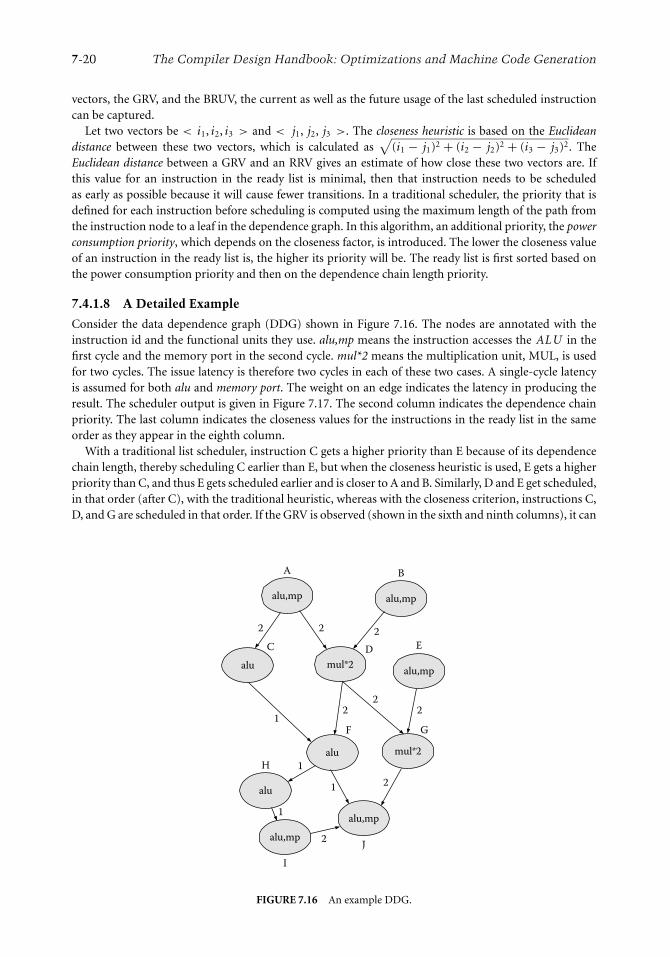
7-20 The Compiler Design Handbook: Optimizations and Machine Code Generation
vectors, the GRV, and the BRUV, the current as well as the future usage of the last scheduled instructioncan be captured.
Let two vectors be < i1, i2, i3 > and < j1, j2, j3 >. The closeness heuristic is based on the Euclideandistance between these two vectors, which is calculated as
√(i1 − j1)2 + (i2 − j2)2 + (i3 − j3)2. The
Euclidean distance between a GRV and an RRV gives an estimate of how close these two vectors are. Ifthis value for an instruction in the ready list is minimal, then that instruction needs to be scheduledas early as possible because it will cause fewer transitions. In a traditional scheduler, the priority that isdefined for each instruction before scheduling is computed using the maximum length of the path fromthe instruction node to a leaf in the dependence graph. In this algorithm, an additional priority, the powerconsumption priority, which depends on the closeness factor, is introduced. The lower the closeness valueof an instruction in the ready list is, the higher its priority will be. The ready list is first sorted based onthe power consumption priority and then on the dependence chain length priority.
7.4.1.8 A Detailed Example
Consider the data dependence graph (DDG) shown in Figure 7.16. The nodes are annotated with theinstruction id and the functional units they use. alu,mp means the instruction accesses the ALU in thefirst cycle and the memory port in the second cycle. mul*2 means the multiplication unit, MUL, is usedfor two cycles. The issue latency is therefore two cycles in each of these two cases. A single-cycle latencyis assumed for both alu and memory port. The weight on an edge indicates the latency in producing theresult. The scheduler output is given in Figure 7.17. The second column indicates the dependence chainpriority. The last column indicates the closeness values for the instructions in the ready list in the sameorder as they appear in the eighth column.
With a traditional list scheduler, instruction C gets a higher priority than E because of its dependencechain length, thereby scheduling C earlier than E, but when the closeness heuristic is used, E gets a higherpriority than C, and thus E gets scheduled earlier and is closer to A and B. Similarly, D and E get scheduled,in that order (after C), with the traditional heuristic, whereas with the closeness criterion, instructions C,D, and G are scheduled in that order. If the GRV is observed (shown in the sixth and ninth columns), it can
alu,mp alu,mp
alu,mp
alu,mp
alu,mp
mul*2
mul*2
alu
2 2 2
222
2
1
1
1 2
1
I
J
GF
E
BA
C D
Halu
alu
FIGURE 7.16 An example DDG.

Energy-Aware Compiler Optimizations 7-21
Insn Priority Cycle Insn List GRV Insn List GRV Closeness
A 5 i A B,E 100 A B,E 100 0,0
B 5 i+1 B C,E 101 B E,C 101 0.1
C 4 i+2 C D,E 101 E C,D 101 1, √3
D 4 i+3 D E 010 C D 101 √3
E 2 i+4 E F 110 D 010
F 3 i+5 F H,G 100 G 010 0
G 1 i+6 H G,I 100 G F 010 √2
H 2 i+7 I G,J 100 F H 110 0
I 1 i+8 G J 010 H I 100 1
J 0 i+10 J 110 I J 100 0
i+11 001 J 101
i+12 001 101
FIGURE 7.17 Scheduler output using traditional heuristics and closeness heuristics.
be seen that the continuous idle cycles of ALU, MP, and MUL have increased. The number of transitionsin ALU and MUL has been reduced from four to two, and in the memory port from five to three. However,with the closeness heuristic there is a no-op in the sequence after D (in column 7). This is because noother instructions in the ready list can be scheduled at that point in time. This is the performance penalty(execution cycles) that is paid when the closeness heuristic is used. However, simulation studies show thatthis impact is not so significant when compared to the power consumption benefits.
Experimental results and more details are available in [46]. Modifications to the above scheme andapplication to clustered VLIW architectures are described in [30, 31].
7.5 Compile-Time Allocation for Scratchpad Memory
It is well known that off-chip memory is the slowest and most energy consuming type of memory in thememory hierarchy. Cache memories are much smaller than off-chip main memories and are much faster.They are used to keep frequently used code blocks or variables and thereby reduce the number of mainmemory accesses. Caches are well known and are used in most processors. Caches have a tag memory tostore valid addresses and extra hardware for a fast comparison of addresses with the contents of tag memory.These are needed to detect hits and misses, but they consume energy continuously since comparisons aremade during each memory access. Caches integrate very well with software and are transparent to thesoftware in their operation. This has made caches very popular with hardware designers. However, cachehits and misses bring a certain amount of nondeterminism to the execution time and its estimation. Mostworst-case execution time (WCET) estimation software ignores the presence of caches and regards the timeof execution of each instruction assuming a cache miss. WCET estimation in the presence of cache is a hotresearch topic [30].
Scratchpad memories have been proposed not only to make WCET estimation more accurate, butalso to reduce the energy consumption in memory hierarchies. Scratchpad memories are as fast as cachememories but do not have the tag memory and address comparison hardware. Therefore, they consumeless energy than caches but require the services of a compiler or the programmer to fill it with code and/orvariables. Letting programmers handle scratchpad memories is not desirable since the allocation canbecome quite complex and may lead to inefficient allocation and possible program errors. Compile-timealgorithms based on integer linear programming have been proposed for scratchpad memory allocation.The discussion in the sections that follow is based on such algorithms described in [2, 41, 44, 49].
7.5.1 The Static Allocation Algorithm
A typical embedded system contains several types of memories, and each type has its own advantagesand disadvantages. Cache, on-chip scratchpad Static Random Access Memory (SRAM), off-chip SRAM,

7-22 The Compiler Design Handbook: Optimizations and Machine Code Generation
on-chip DRAM, off-chip DRAM, ROM, and external flash memory are among the most common ones.The speeds of these memories decrease approximately in the same order as mentioned above. It is possibleto consider the entire memory hierarchy in the allocation algorithm, but for clarity, only off-chip DRAMand on-chip scratchpad SRAM are considered here. Avissar et al. [2] present such an extension.
The allocation algorithm should consider the energy benefits obtained by placing frequently accesseddata variables and frequently executed code segments in the scratchpad. The size of scratchpad memoryis much smaller than that of main memory and therefore cannot accommodate all the variables andcode segments. Therefore, it is necessary to profile the program for which scratchpad allocation is tobe performed and determine the counts of execution of basic blocks and the number of accesses to eachvariable. While entire functions and basic blocks are both considered as program memory object candidatesfor scratchpad allocation, individual scalar and nonscalar global variables are considered as data memoryobject candidates for the same purpose. Local variables (stack variables) and dynamically allocated objectsare not considered for allocation on scratchpad. The allocation is purely static, and there is no dynamicreloading of objects. These extensions are discussed in the literature suggested in Section 7.1. The followingdiscussion considers the savings or gain in energy consumption obtained by allocating an object to thescratchpad. For example, if E m and E s are the energy consumptions for a data access to the main memoryand scratchpad, respectively, (E m − E s ) is the savings in energy.
7.5.1.1 Energy Savings for a Complete Function
It is assumed that functions are single-entry, single-exit entities. Therefore, moving the complete codefor a function into scratchpad requires changing none of the instructions in the function body or thecorresponding function calls. The savings or gain in energy consumption of a function f can be computedusing the following equation:
E g ( f ) =∑
i
ni · E ginstr−fetch (7.28)
where
E g ( f ): Gain in energy consumed by the function fn f
i : Number of times instruction i in the function f is executedE g
instr−fetch: Gain in energy consumed for a single instruction fetch
n fi can be computed easily using profiling information for basic blocks.
7.5.1.2 Energy Savings for a Basic Block
Similarly, the energy consumed by a single basic block can also be computed. When a basic block is movedto scratchpad, jump instructions to jump from a basic block in regular memory to the basic block inscratchpad and perhaps back are required. These constitute an extra overhead and can be expensive in thepresence of small basic blocks. It is preferrable to move consecutive basic blocks to minimize the overhead.The gain in energy consumption of a basic block b can be computed using the following equation:
E g (b) = Ib · nb · E ginstr−fetch − J b · E g
jump (7.29)
where
E g (b): Gain in energy consumed by the basic block bnb : Number of times the basic block b is executed (from profiling)Ib : Number of instructions in the basic block bE g
instr−fetch: Gain in energy consumed for a single instruction fetchJ b : Number of jumps from main memory to block b in scratchpad or vice versaE g
jump: Energy consumed for a single jump instruction

Energy-Aware Compiler Optimizations 7-23
7.5.1.3 Energy Savings for Data Memory Objects
Each global scalar and nonscalar variable is considered a data memory object. Local variables are notconsidered here. The number of times a global variable v is accessed (including both reads and writes)and the total energy consumed by all the accesses are computed as follows.
nv =∑
b
refb(v) · nb (7.30)
E g (v) = nv · E gls (7.31)
where
nv : Total number of accesses to variable vrefb(v): Number of static references to variable v in basic block bnb : Number of times the basic block b is executed (from profiling)E g (v): Total gain in energy consumed due to variable vE g
ls : Average gain in energy consumed by a memory access (read or write)
7.5.1.4 The Integer Linear Programming Formulation
Maximize
E gtotal =
∑f ∈F
x( f ) · E g ( f ) +∑b∈B
x(b) · E g (b) +∑v∈V
x(v) · E g (v) (7.32)
where F , B , and V are the total number of functions, basic blocks, and global variables, in the program,respectively. x(i) is the integer programming 0-1 variable, taking a value of 1 if the object i (function, basicblock, or variable) is allocated to the scratchpad, and 0 otherwise. The size constraint can be stated as
∑f ∈F
x( f ) · size( f ) +∑b∈B
x(b) · size(b) +∑v∈V
x(v) · size(v) ≤ scratchpadsize (7.33)
where size(i) is the size of object i . The size of a basic block includes the size of the jump instruction aswell. Minor optimizations to this scheme to avoid counting jumps to consecutive basic blocks that areboth moved scratchpad are described in [41].
7.6 Conclusions and Future Directions
This chapter considered a few energy-saving compiler optimizations in detail. Dynamic voltage scaling,which reduces the dynamic energy consumption in processors, was formulated as a minimization prob-lem, and transition-aware scheduling, which reduces leakage energy consumption, was formulated as aninstruction scheduling problem. Scratchpad memories, which are an alternative to cache memories inembedded processors, require the compiler to perform the allocation of code and data objects onto them,and this problem was formulated as an integer linear programming problem.
The last word on energy-aware compiler optimizations has hardly been said. The processors used insensor networks and other embedded systems need aggressive energy optimizations. No professionalcompilers incorporate all the energy-aware optimizations such as DVS, instruction scheduling, memorybank allocation, scratchpad allocation, cache management, and communication reduction (in clusters),and building such a compiler is an interesting research project. Furthermore, the interaction of variousenergy-saving optimizations with performance-improving optimizations has not been studied thoroughly.Integration of optmizations possible at the operating system level into a compiler framework and designof a programming framework to develop power- and energy-aware applications would be other researchpossibilities. In addition, innovations in architecture are introducing novel features into hardware to

7-24 The Compiler Design Handbook: Optimizations and Machine Code Generation
save power and energy, and future compilers would be challenged to use such features effectively. Theproblem of reducing power consumption can be more effectively solved by designing hybrid algorithms thatcombine micro-architectural techniques and compiler techniques such that they complement each other.For example, rather than controlling cache configurations dynamically, the same can be achieved throughannotations inserted into programs after a compiler analysis. This would reduce the burden on the hardwareat runtime.
References
1. Absar, M. J., and Catthoor, F. 2005. Compiler-based approach for exploiting scratchpad in pres-ence of irregular array access. In ACM Conference on Design, Automation and Test in Europe,1162–67.
2. Avissar, O., Barua, R., and Steware, D. 2002. An optimal memory allocation scheme for scratch-pad-based embedded systems. ACM TECS 1:6–26.
3. Azvedo, A., Issenin, I., Cornea, R., Gupta, R., Dutt, N., Veidenbaum, A., and Nicolau, A. 2002.Profile-based dynamic voltage scheduling using program checkpoints. In ACM Conference on Design,Automation and Test in Europe, 168–75.
4. Bala, V., and Rubin, N. 1995. Efficient instruction scheduling using finite state automata. In ACMInternational Symposium on Microarchitecture (MICRO-29), 46–56.
5. Banakar, R., Steinke, S., Lee, B.-S., Balakrishnan, M., and Marwedel, P. 2002. Scratchpad memory:A design alternative for cache on-chip memory in embedded systems. In ACM InternationalConference on Hardware Software Codesign (CODES), 73–78.
6. Benini, L., Macii, A., and Poncino, M. 2000. A recursive algorithm for low-power memory parti-tioning. In ACM International Symposium on Low Power Electronics and Design (ISLPED), 78–83.
7. Borkar, S. 1999. Design challenges of technology scaling. IEEE Micro 19(4):23–29.8. Brooks, D. M., Bose, P., Schuster, S. E., Jacobson, H., Kudva, P. N., Buyuktosunoglu, A., Wellman,
J.-D., Zyuban, V., Gupta, M., and Cook, P. W. 2000. Power-aware microarchitecture: Design andmodelling challenges for next-generation microprocessors. IEEE Micro 20(6):26–44.
9. Brooks, D. M., Tiwari, V., and Martonosi, M. 2000. Wattch: A framework for architectural-level poweranalysis and optimizations. In ACM International Conference on Computer Architecture (ISCA),83–94.
10. Burd, T., and Broderson, R. 2000. Design issues for dynamic voltage scaling. In ACM InternationalSymposium on Low Power Electronics and Design (ISLPED), 9–14.
11. Butts, J. A., and Sohi, G. S. 2000. A static power model for architects. In ACM/IEEE InternationalSymposium on Microarchitecture (MICRO-33), 191–201.
12. De, V., and Borkar, S. 1999. Technology and design challenges for low power and high performance.In ACM International Symposium on Low Power Electronics and Design (ISLPED ’99), 163–68.
13. De La Luz, V., Kandemir, M., Vijayakrishnan, N., Sivasubramaniam, A., and Irwin, M. J. 2001.Hardware and software techniques for controlling DRAM power modes. IEEE Trans. Comput.50(11):1154–73.
14. De La Luz, V., Kandemir, M., and Kolcu, I. 2002. Automatic data migration for reducing energyconsumption in multi-bank memory systems. In ACM/IEEE Conference on Design Automation(DAC), 213–18.
15. De La Luz, V., Sivasubramaniam, A., Kandemir, M., Vijayakrishnan, N., and Irwin, M. J. 2002.Scheduler-based DRAM energy management. In ACM/IEEE Conference on Design Automation(DAC), 697–702.
16. Dominguez, A., Udayakumaran, S., and Barua, R. 2005. Heap data allocation to scratchpad memoryin embedded systems. J. Embedded Comput. 1(4):1–17.
17. Dropsho, S., Kursun, V., Albonesi, D. H., Dwarkadas, S., and Friedman, E. G. 2002. Managing staticleakage energy in microprocessor functional units. In ACM International Symposium on Microar-chitecture (MICRO-35), 321–32.

Energy-Aware Compiler Optimizations 7-25
18. Duesterwald, E. 2007. Dynamic compilation. In The compiler design handbook: Optimizations andmachine code generation, ed. Srikant, Y. N. and Shankar, P. Boca Raton, FL: CRC Press.
19. Falk, H., and Verma, M. 2004. Combined data partitioning and loop nest splitting for energyconsumption minimization. In International Workshop on Software and Compilers for EmbeddedSystems (SCOPES), 137–51. Heidelberg, Germany: Springer Verlag.
20. Heo, S., Barr, K., Hampton, M., and Arisovic, K. 2002. Dynamic fine-grain leakage reduction usingleakage-biased bitlines. In ACM International Conference on Computer Architecture (ISCA), 137–47.
21. Hsu, C.-H., and Kremer, U. 2003. The design, implementation, and evaluation of a compiler al-gorithm for CPU energy reduction. In ACM Conference on Programming Language Design andImplementation (PLDI), 38–48.
22. Isci, C., and Martonosi, M. 2003. Runtime power monitoring in high-end processors: Methodologyand empirical data. In ACM International Symposium on Microarchitecture (MICRO-36), 93–104.
23. Iyer, A., and Marculescu, D. 2002. Microarchitecture-level power management. IEEE Trans. VLSISyst. 10(3):230–39.
24. Kim, N. S., Austin, T., Blaauw, D., Mudge, T., Flautner, K., Hu, J. S., Irwin, M. J., Kandemir, M., andNarayanan, V. 2003. Leakage current: Moore’s law meets static power. IEEE Comput. 36(12):68–75.
25. Koc, H., Ozturk, M., Kandemir, M., Narayanan, S. H. K., and Ercanli, E. 2006. Minimizing energyconsumpton of banked memories using data recomputation. In ACM International Symposium onLow Power Electronics and Design (ISLPED), 358–62.
26. Kursun, V., and Friedman, E. G., 2002. Low swing dual threshold voltage domino logic. ACM GreatLakes Symposium GLVLSI, 47–52.
27. Lee, C., Lee, J. K., and Hwang, T. 2003. Compiler optimization on VLIW instruction scheduling forlow power. ACM TODAES 8(2):252–68.
28. Li, L., Gao, L., and Xue, J. 2005. Memory coloring: A compiler approach for scratchpad memorymanagement. In ACM Conference on Parallal Architectures and Compilation Techniques (PACT),329–38.
29. Lyuh, C.-G., and Kim, T. 2004. Memory access scheduling and binding considering energy mini-mization in multi-bank memory systems. In ACM/IEEE Conference on Design Automation (DAC),81–86.
30. Mitra, T., and Roychoudhury, A. 2007. Worst-case execution time and energy analysis. In Thecompiler design handbook: Optimizations and machine code generation, ed. Srikant, Y. N. and Shankar,P. Boca Raton FL: CRC Press.
31. Mudge, T. 2001. Power: A first-class architectural design constraint. IEEE Comput. 34(4):52–58.32. Nagpal, R., and Srikant, Y. N. 2006. Compiler-assisted leakage energy optimization for clustered
VLIW architectures. In ACM International Conference on Embedded Software (EMSOFT), 233–41.33. Nagpal, R., and Srikant, Y. N. 2006. Exploring energy-performance tradeoffs for heterogeneous in-
terconnect clustered VLIW processors. In International Conference on High Performance Computing(HiPC), 497–508, Springer-Verlag.
34. Pokam, G., Rochecouste, O., Seznec, A., and Bodin, F. 2004. Speculative software management ofdatapath-width for energy optimization. In ACM International Conference on Language, Compilerand Tool Support for Embedded Systems (LCTES), 78–87.
35. Pollack, F. 1999. New microarchitecture challenges in the coming generations of CMOS processtechnologies. Keynote at the ACM International Symposium of Microarchitecture (MICRO-32).http://www.intel.com/research/mrl/Library/micro32Keynote.pdf.
36. Saputra, H., Kandemir, M., Vijaykrishnan, N., Irwin, M. J., Hu, J. S., Hsu, C.-H., and Kremer, U.2002. Energy-conscious compilation based on voltage scaling. In ACM International Conference onLCTES/SCOPES, 2–11.
37. Sharkey, J. J., Ponomarev, D. V., Ghose, K., and Ergin, O. 2006. Instruction packing: Toward fast andenergy-efficient instruction scheduling. ACM TACO 3(2):158–81.
38. Shin, D., Kim, J., and Lee, S. 2001. Low-energy intra-task voltage scheduling using static timinganalysis. In ACM International Conference on Design Automation (DAC), 438–43.

7-26 The Compiler Design Handbook: Optimizations and Machine Code Generation
39. Shrivastava, A., Issenin, I., and Dutt, N. 2005. Compilation techniques for energy reduction in hori-zontally partitioned cache architectures. In ACM International Conference on Compilers, Architectureand Synthesis for Embedded Systems (CASES), 90–96.
40. Sprunt, B. 2002. Pentium 4 performance-monitoring features. IEEE Micro 22(4):72–82.41. Steinke, S., Wehmeyer, L., Lee, B.-S., and Marwedel, P. 2002. Assigning program and data objects
to scratchpad for energy reduction. In ACM Conference on Design, Automation and Test in Europe,409–17.
42. Sudarsanam, A., and Malik, S. 2000. Simultaneous reference allocation in code generation for dualmemory bank ASIPs. ACM TODAES 5:242–64.
43. Tsai, Y. F., Duarte, D., Vijayakrishnan, N., and Irwin, M. J. 2004. Impact of process scaling onefficacy of leakage reduction schemes. In IEEE International Conference on IC Design and Technology(ICICDT), 3–11.
44. Udayakumaran, S., Dominguez, A., and Barua, R. 2006. Dynamic allocation for scratch-pad memoryusing compile-time decisions. ACM TECS 5(2):472–511.
45. Unnikrishnan, P., Chen, G., Kandemir, M., and Mudgett, D. R. 2002. Dynamic compilation forenergy adaptation. In IEEE Conference on Computer-Aided Design, 158–63.
46. Vardhan, K. A., and Srikant, Y. N. 2005. Transition aware scheduling: Increasing continuous idleperiods in resource units. In ACM International Conference on Computing Frontiers, 189–98.
47. Venkatachalam, V., and Franz, M. 2005. Power reduction techniques for microprocessor systems.ACM Comput. Surveys 37(3):195–237.
48. Verma, M., Wehmeyer, L., and Marwedel, P. 2004. Cache-aware scratchpad allocation algorithm. InACM Conference on Design, Automation and Test in Europe, 21264–69.
49. Verma, M., and Marwedel, P. 2006. Overlay techniques for scratchpad memories in low powerembedded systems. IEEE Trans. VLSI Syst. 14(8):802–15.
50. Vijayakrishnan, N., Kandemir, M., Irwin, M. J., Kim, H. S., and Yei, W. 2000. Energy-driven inte-grated hardware-software optimizations using simpower. In International Conference on ComputerArchitecture (ISCA), 95–106.
51. Wang, Z., and Hu, X. S. 2005. Energy-aware variable partitioning and instruction scheduling formultibank memory architectures. ACM TODAES 10(2):369–88.
52. Wu, Q., Martonosi, M., Clark, D. W., Reddi, V. J., Connors, D., Wu, Y., Lee, J., and Brooks, D. 2005. Adynamic compilation framework for controlling microprocessor energy and performance. In ACMInternational Conference on Microarchitecture (MICRO-38), 271–82.
53. Xie, F., Martonosi, M., and Malik, S. 2004. Intraprogram dynamic voltage scaling: Bounding op-portunities with analytic modeling. ACM TACO 1(3):323–67.
54. Yang, H., Govindarajan, R., Gao, G. R., Cai, G., and Hu, Z. 2002. Exploiting schedule slacks for rate-optimal power-minimum software pipelining. In Workshop on Compilers and Operating Systems forLow Power (COLP), COLP Workshop Proceedings.
55. You, Y.-P., Lee, C., and Lee, J. K. 2006. Compilers for leakage power reduction. ACM TODAES11(1):147–64.
56. Zhang, W., Vijaykrishnan, N., Kandemir, M., Irwin, M. J., Duarte, D., and Tsai, Y.-F. 2001. ExploitingVLIW schedule slacks for dynamic and leakage energy reduction. In ACM International Symposiumon Microarchitecture (MICRO-34), 102–13.
57. Zhang, W., Hu, J. S., Degalahal, V., Kandemir, M., Vijayakrishnan, N., and Irwin, M. J. 2002.Compiler-directed instruction cache leakage optimization. In ACM International Conference onMicroarchitecture (MICRO-35), 208–18.
58. Zhang, W., Karakoy, M., Kandemir, M., and Chen, G. 2003. A compiler approach for reducing datacache energy. In ACM International Conference on Supercomputing (ICS), 76–85.

8Statistical and
Machine LearningTechniques in
Compiler Design
P.J. JosephFreescale Semiconductor India Pvt. Ltd.,Noida, [email protected]
Matthew T. Jacob,Y.N. Srikant, andKapil VaswaniDepartment of Computer Scienceand Automation,Indian Institute of Science,Bangalore, [email protected]@[email protected]
8.1 Introduction . . . . . . . . . . . . . . . . . . . . . . . . . . . . . . . . . . . . . . . . . .8-1Motivation • Classical Solutions
8.2 Adaptive Compilers . . . . . . . . . . . . . . . . . . . . . . . . . . . . . . . . . . .8-78.3 Characterizing Compiler Interactions . . . . . . . . . . . . . . . . . .8-8
Empirical Regression Models
8.4 Heuristic Selection . . . . . . . . . . . . . . . . . . . . . . . . . . . . . . . . . . . .8-14Deciding Best Loop Unroll Factors • Learning PriorityFunctions
8.5 Phase Ordering . . . . . . . . . . . . . . . . . . . . . . . . . . . . . . . . . . . . . . .8-21Characterizing Phase Ordering Space • Search Techniques• Focused Search Techniques
8.6 Optimization Flags and Parameter Selection . . . . . . . . . . .8-27Optimization Flag Selection Using Inferential Statistics
8.7 Conclusions . . . . . . . . . . . . . . . . . . . . . . . . . . . . . . . . . . . . . . . . . .8-28Appendix A: Optimality in Program Compilation . . . . . . . . . . . .8-29References . . . . . . . . . . . . . . . . . . . . . . . . . . . . . . . . . . . . . . . . . . . . . . . . . .8-30
8.1 Introduction
In computer science, the word optimize refers to the process of modifying to achieve maximum efficiency instorage capacity or time or cost. True to their name, optimizing compilers transform computer programs intosemantically equivalent programs with the objective of maximizing performance. The transformation isachieved using a set of optimizations. Each optimization usually consists of an analysis component thatidentifies specific performance anomalies and a transformation component that eliminates the anomaliesvia a series of code transformations.
Despite significant advances in compilation techniques and numerous compiler optimizations thathave been proposed over the years, the goal of building optimizing compilers that deliver optimal oreven near-optimal performance1 is far from being achieved. For instance, it has been observed thatperformance of compiler-generated code falls far short of hand-optimized code in certain applicationdomains [1]. One might argue that the superiority of hand-optimized code is due to domain knowledgeor special insights into the functioning of code that programmers may have, which allows them to make
1Refer to Appendix A for a formal description of the notion of optimality in program compilation.
8-1

8-2 The Compiler Design Handbook: Optimizations and Machine Code Generation
program/hardware-specific transformations. Even if we discount such transformations, optimizing com-pilers have been shown to fall short in several other ways. For instance, recent research has shown thatthe sequence in which compiler optimizations are applied to a program has a significant bearing on itsexecution time and that the performance of the default optimization sequence in most compilers is farbelow that of the best program-specific optimization sequence [2]. It has also been observed that mostprograms perform better if some of the optimizations are disabled [3, 4]. These observations suggest thatcompilers may not be exploiting the power of existing optimizations to the fullest.
In this chapter, we examine the reasons behind these apparent shortcomings of compilers. Not surpris-ingly, we find that compilers are replete with inherently hard problems and complex interactions betweenoptimizations that are difficult for compiler writers to comprehend. We show that the key to solving theseproblems and building high-performance compilers lies in adaptability, that is, the ability to reconfigureparts of the compiler to the requirements of the program being compiled and the target platform. Wediscuss how statistical and machine learning techniques can help address some of the complex issues thatarise in building adaptive compilers. In particular, we show that problems such as identifying compilerinteractions, design of efficient heuristics, finding program-specific optimization sequences, and selectionof program-specific optimization flags can be formulated as problems in learning and statistical inference,and near-optimal solutions to these problems can be found efficiently and automatically. This automatedapproach greatly simplifies the design of performance-critical components of an optimizing compiler,letting compiler writers focus on other important aspects such as correctness and retargetability.
8.1.1 Motivation
Let us start by examining some of the reasons compilers fail to deliver optimal performance.
8.1.1.1 Inherently Hard Problems
Compiler optimizations are the source of some of the hardest and most challenging problems in computerscience. This is specially the case with architecture-dependent optimizations such as register allocation,instruction scheduling, and data layout. Since finding optimal solutions to these problems is provablyhard, compiler writers are forced to develop heuristics to find approximate solutions to these problems.Consider register allocation, for instance. It has been shown that optimal register allocation can be reducedto the problem of determining whether a graph can be k-colored [5] (refer to [6] for details). Therefore, acoloring-based register allocator uses heuristics to select variables for spilling when the interference graphcannot be k-colored (where k is the number of unallocated registers). For some compiler optimizations,heuristics can be designed to guarantee solutions that are within a constant factor of the optimal solution,but more often than not, heuristics are designed for the average case, and there are no guarantees of howwell the heuristics perform for a given program and target platform.
8.1.1.2 Interactions between Optimizations
It is well known that most compiler optimizations interact, that is, the effect of any given optimization on theperformance may depend on the presence or absence of other optimizations in the compilation sequence.Furthermore, the nature of the interaction may also depend on the order in which the optimizations areapplied. For example, loop unrolling is known to interact with global common subexpression elimination,in other words, (GCSE). This implies that, the benefits of unrolling depend on whether GCSE is appliedand on the order in which unrolling and GCSE are applied.
Interactions between optimizations can be positive or negative. A positive interaction usually occurswhen one optimization enables or creates opportunities for another optimization. Negative interactionsoccur when one optimization restricts the applicability of another optimization. A good example of anegative interaction is the one between register allocation and instruction scheduling, which we discussin detail later in this section.
Apart from interacting with other optimizations, compiler optimizations also interact with the hardware.This is inherently true for architecture-dependent optimizations such as loop optimizations, prefetch-ing, basic block reordering, and instruction scheduling. Despite years of research, the nature of these

Statistical and Machine Learning Techniques in Compiler Design 8-3
interactions is only partially understood. Consequently, few interactions are taken into account whiledesigning optimizations.
8.1.1.3 Multiple Objective Functions
As if optimizing programs for performance was not hard enough, modern compilers are routinely ex-pected to generate code that is simultaneously optimized for multiple objective functions. For example,in embedded systems such as mobile devices or sensor networks, the compiler must satisfy additionalconstraints on metrics such as code size and power consumption. In several cases, some of the objectivefunctions may be at odds with each other, that is, optimizations that improve the quality of code withrespect to one objective function may adversely influence the other. Designing optimizations that meetthese stringent requirements is a complex task.
8.1.2 Classical Solutions
Having examined some of the problems that plague optimizing compilers, let us review some of thestrategies that existing compiler implementations use to deal with these problems. We primarily focus ontechniques that deal with interactions between compiler optimizations and interactions with the architec-ture. The general strategy adopted by compiler writers can be summarized as follows:� Identify and characterize specific interactions: The presence of interactions is usually detected by
manually inspecting the semantics of optimizations and architectural specifications. Alternatively,some simple interactions can be automatically detected if the compiler writer is willing to specifythe semantics of optimizations in specification languages such as Gospel [7–9].� Adapt the optimizations involved: Compiler optimizations may require restructuring if they areinvolved in strong interactions. In the simplest of cases, the heuristics that drive the optimizationare changed to deal with the interaction [10, 11]. In other cases, two or more optimizations may becombined and performed together [12–15].
We illustrate this process using two specific instances, namely, the interaction between instructionscheduling and register allocation, and the interactions between various loop transformations and thehardware.
8.1.2.1 Interaction between Instruction Scheduling and Register Allocation
Instruction scheduling is a compiler optimization that rearranges instructions in a given code sequencewith the goal of reducing the execution latency of the sequence. If sufficient parallelism is available inthe code sequence, instruction scheduling can hide functional unit latencies, memory latencies, and otherdelays such as pipeline interlocks. However, a deeper analysis of the effects of instruction scheduling showsthe presence of a complex interaction with register allocation [14]. The nature of this interaction dependson the order in which scheduling and register allocation are performed. If scheduling is performed beforeregister allocation (known as the prepass strategy), the scheduler can utilize full parallelism in the codesequence and generate a compact schedule by interleaving the execution of independent instructions.However, in this process, the scheduler can potentially increase the maximum number of live variables andcause the register allocator to generate more spill code. If register allocation is performed before scheduling(known as the postpass strategy), the scheduler may not see the full parallelism available in code because offalse dependencies induced by the reuse of registers. This may limit the extent to which the scheduler canreorder instructions and result in a suboptimal schedule with unnecessary stalls. The following exampleillustrates this interaction.
8.1.2.2 Example
Consider the code snippet shown in Figure 8.1 (adapted from [14]). The figure also shows the intermediatecode before register allocation and scheduling and the corresponding dependence graph. Assume that thearchitecture has two registers, r 1 and r 2. Figure 8.2 shows the schedule and live ranges of virtual variablesif instruction scheduling is performed before register allocation. For this code sequence, the scheduler

8-4 The Compiler Design Handbook: Optimizations and Machine Code Generation
Source Code
IR
z = x[i]tmp = x[i+1+n]
i3
i2
i1
i4
0 0
01
1
i5
i6
i1: v1 = addr(x) + Ii2: v2 = load @(v1)i3: z = v2i4: v3 = v1 + 1i5: v4 = load ni6: v5 = load @(v3+v4)
Data Dependence Graph
FIGURE 8.1 Example illustrating the interaction between instruction scheduling and register allocation.
generates an optimal schedule that executes in six cycles with no stalls. The scheduler hides latencies ofthe loads i2 and i5 by separating them from their respective uses. Although this schedule is optimal, theseparation of dependent instructions causes an increase in the number of simultaneously live ranges. Inthis case, the register allocator is forced to spill one of the variables because there are three live ranges atcycles 3 and 4 and only two registers available for allocation.
Now consider the scenario where register allocation is performed before scheduling. The live rangesseen by the allocator are shown in Figure 8.3. Observe that at no time in this code sequence are more thantwo variables live, and the register allocator is able to allocate registers to all variables (v1 → r 1, v2 →r 2, v3 → r 2, v4 → r 1) without spilling. However, the false dependencies introduced because of the reuseof registers (both r 1 and r 2) limit the parallelism seen by the scheduler. Consequently, the scheduler isunable to hide load latencies and is forced to introduce stalls in the final schedule, which now runs intoeight cycles.
Both these scenarios illustrate the presence of a negative interaction between instruction schedulingand register allocation, irrespective of the order in which the optimizations are applied. An interactionwith similar characteristics also occurs between partial redundancy elimination (PRE) and register allo-cation [9, 16]. More precisely, the code-hoisting step in PRE might increase the live ranges of variablesinvolved in the redundant expression, resulting in increased register pressure and possible spilling.
Once an interaction is identified, the optimizations involved in the interaction may be reformulatedto ensure that the interaction does not result in suboptimal code. Several such formulations for registerallocation and instruction scheduling have been proposed. While the specific details may vary, the formu-lations seek to make the optimizations aware of their influence on each other. This is achieved indirectlyby introducing some means of communication between the optimizations [9, 17] or directly by integrat-ing the optimizations into a single pass [18]. For instance, Motwani et al. [14] formulate the combinedscheduling and register allocation as a single optimization problem, show that the combined problem isNP-hard but approximable, and propose a combined parameterized heuristic that can be used to weighthe conflicting considerations of register pressure and parallelism.
Interestingly, while most of these formulations have been proposed for in-order, VLIW processors,it has been observed that for out-of-order (OoO) superscalar processors, register pressure is often agreater concern than exploiting parallelism and creating better schedules [19, 20]. This is due to severalfeatures supported by OoO processors such as register renaming, which eliminates false dependencies
1 i1: v1 = addr (x) + I2 i2: v2 = load @(v1)3 i5: v4 = load n4 i3: z = v25 i4: v3 = v1 + 16 i6: v5 = load @(v3+v4)
v1 v2
v3
v4
FIGURE 8.2 The schedule generated by a prepass scheduler and the live ranges of virtual registers.

Statistical and Machine Learning Techniques in Compiler Design 8-5
i1: v1 = addr(x) + Ii2: v2 = load @(v1)i3: z = v2i4: v3 = v1 + 1i5: v4 = load ni6: v5 = load @(v3+v4)
12345678
i1:i2:
i3:i4:i5:
i6:
r1r2
zr2r1
r1
==
===
=
addr(x) + Iload @(r1)
r2r1 + 1load n
load @(r2+r1)
v1 v2
v3 v4
FIGURE 8.3 The live ranges seen by the register allocator and the schedule generated by the postpass scheduler.
introduced by register reuse, and dynamic scheduling with large instruction windows and speculation,which allow out-of-order processors to exploit instruction-level parallelism across large code sequences.Consequently, formulations that assign a higher weight to the register allocator (e.g., postpass strategy) arelikely to perform better on OoO processors. This observation shows that interactions may involve moreoptimizations than anticipated (hardware optimizations in this case) and may be more complex than whatmeets the eye. Therefore, it is critical for compiler writers to characterize these interactions in their entiretyand ensure that all factors that can influence the nature of the interactions are accounted for. The absenceof a comprehensive characterization may lead to wrong conclusions and adversely affect performance.
8.1.2.3 Interactions between Loop Transformations and Caches
High-level loop transformations such as unrolling, tiling, fission, fusion, and interchange have individuallyproved to be some of the most effective compiler optimizations, especially in loop-dominated scientific,media, and graphics programs. Apart from exposing instruction-level parallelism, reducing loop overheads,and increasing functional-unit utilization, these transformations are especially useful in improving theloop’s memory behavior. The potential of these optimizations is best illustrated using an example (adaptedfrom [15]). Consider the MATLAB code in Listing 8.1, which contains a simple loop that multiplies thematrix b with an array c and stores the results in an array a .
Listing 8.1: MATLAB code for multiplying an array with a matrix% a, c are arrays of size 1000% b is a matrix of size 1000x1000for i =1:1000,
for j =1:1000,a( i ) = a( i ) + b(i , j )∗c( i )
endend
If the matrix b were stored in column major order (which is the case in MATLAB), the accesses to theelements of matrix b would incur a cache miss in each iteration of the loop (because the matrix is accessedrow-wise). Loop interchange [21] can be used to avoid this performance anomaly. Assuming a cache blocksize of 32 bytes, the interchanged loop shown in Listing 8.2 incurs a cache miss once every four iterations.
Listing 8.2: Source code after loop interchange has been appliedfor j =1:1000,
for i =1:1000,a( i ) = a( i ) + b(i , j )∗c( i )
endend
However, this transformation comes at a cost. In the original loop, the computation in each iterationcan be expressed using one mutliply-and-add instruction (supported on several current processors suchas the PowerPC and Itanium), whereas in the transformed loop, two extra loads (for elements of arrays aand c) and an extra store (to array a) are required in the inner loop. Depending on the cache miss latency,

8-6 The Compiler Design Handbook: Optimizations and Machine Code Generation
loop interchange may either improve or hurt performance. Hence, cache latency must be factored into theheuristic that evaluates the benefit of loop interchange.
This interaction with cache latency is just one of the many interactions that affect loop interchange.In general, loop transformations are known to interact strongly with each other. Consider the loop inListing 8.3, which is obtained after applying loop unrolling and interchange to the loop in the previousexample. Unrolling this loop amortizes the cost of the extra load and store instructions inserted because ofloop interchange. Elements of arrays a and c are now loaded once in every iteration of the inner loop, andtheir values are reused across four computations. This version of the loop enjoys the benefits of interchange(i.e., reduced cache misses) while minimizing the runtime cost of additional instructions. This exampleshows that loop unrolling can interact positively with loop interchange, assuming that other side effectsof unrolling, such as the increase in code size and register pressure, are ignored.
Listing 8.3: Source code after loop unrolling and interchange has been appliedfor j =1:1000:4,
for i =1:1000,a( i ) = a( i ) + b(i , j )∗c( i )a( i ) = a( i ) + b(i , j+1)∗c(i)a( i ) = a( i ) + b(i , j+2)∗c(i)a( i ) = a( i ) + b(i , j+3)∗c(i)
endend
The story about interactions in loop transformations does not quite end here. In our example, we onlyconsidered the effect of the transformations on the cache. The transformations may affect other aspectsof code such as register pressure, functional unit utilization, and code size. Adding other transformationssuch as loop tiling, fission, and fusion to the mix further complicates matters. Finding the right sequencein which to apply these transformations and selecting the right parameters for each transformation aredifficult tasks, and a method that determines the most effective loop optimization strategy for any givenprogram and platform continues to elude researchers.
Several researchers have explored the possibility of combining two or more loop transformations[15, 22, 23] to deal with interactions. Wolf et al. [15] propose an algorithm that combines several looptransformations. The goal of their algorithm is to find a loop transformation strategy (combination of theorder in which loop transformations are applied and the manner in which each transformation is used)that exploits positive interactions between these transformations. Since the number of potential looptransformation strategies is large, their approach uses heuristics to narrow the search space. Within thisspace, each strategy is evaluated using simple static cost models for caches, registers, and computational re-sources. Interestingly, their experimental evaluation shows that the combined analysis and transformationresults in significant gains over a baseline implementation for a number of programs, with one exception,where the combined analysis performs significantly worse. In this program, some of the loops generatedby the combined loop transformations were too complex for the software prefetching optimization toanalyze. Hence, no prefetch instructions are generated, leading to a significant performance loss. Thisobservation illustrates the complexity of identifying interactions in compilers and the pitfalls of ignoringkey interactions while designing optimizations.
8.1.2.4 Discussion
Our discussion in this section can be summarized as follows. We find that hard problems and complexinteractions are pervasive in compilers. More importantly, solutions to these problems are dependenton the program and the intricacies of the target platform. A solution that is best for one program orplatform is not necessarily the best for the other. This leads us to the conclusion that compilers must beflexible enough to adapt to the requirements of specific programs and hardware configurations. Aspectsof compilation such as the compilation sequence and optimization heuristics must be adaptable by designif high performance is to be achieved.

Statistical and Machine Learning Techniques in Compiler Design 8-7
Source
Code Compiler
Front-end
Architecture
Description
IR
Ph
ase
1
Ph
ase
2
Ph
ase
n
BinaryHardware
FIGURE 8.4 The structure of a typical optimizing compiler.
8.2 Adaptive Compilers
Let us first review the structure of existing optimizing compilers and see how they fare in terms of flexibilityand adaptability. Figure 8.4 illustrates the architecture of a typical optimizing compiler. The back-end ofthe compiler consists of a set of optimizations or phases. These phases are applied to an intermediaterepresentation of the program in a predetermined sequence, irrespective of the program being optimized.Each phase is almost always designed independently, and interactions between optimizations are oftenignored. Coarse models of the underlying hardware are sometimes employed to guide optimizations, withthe aim of reducing the influence of negative interactions between the optimizations and the hardware. Itis easy to see that the structure of a modern optimizing compiler is more or less rigid. This lack of flexibilityis one of the key reasons that optimizing compilers fail to deliver optimal performance.
In light of these shortcomings of conventional compilers, many in the compiler community havefavored the idea of building compilers that adapt to the program and the hardware [24]. Although theidea of an adaptive compiler sounds compelling, several concerns need to be addressed before an actualimplementation can be envisaged. For example, what are the necessary building blocks of an adaptivecompiler? How is the compiler structured? What are the compile time requirements of the compiler? Whatperformance guarantees can the compiler make? In the rest of this section, we attempt to answer some ofthese questions.
Figure 8.5 illustrates the proposed architecture of an adaptive compiler [24]. This architecture dif-fers from the traditional compiler on several counts. An adaptive compiler consists of some form anadaptation unit, which controls the entire optimization process. The adaption unit uses a combination of
Program Profile
Source
Code Compiler
Front-end
Adaptation
Unit
Architecture
Description
BinaryHardware
Compilation Strategies
IR
FIGURE 8.5 The architecture of an adaptive optimizing compiler.

8-8 The Compiler Design Handbook: Optimizations and Machine Code Generation
program analysis and abstract architecture descriptions to evaluate different compilation strategies andselect a strategy that is best suited to the program and a target platform. More precisely, the adaption unitselects (a) a custom compilation sequence and (b) custom heuristics for each optimization. Additionally,the adaptation unit may use a representative program profile provided by the programmer to tune thecompilation strategy to the program and a specific class of inputs. This can be seen as an advanced formof profile-guided optimization that involves restructuring the compiler itself. Once a compilation strategyis chosen, compilation proceeds as normal and an optimized binary is generated. We now outline some ofthe challenges that must be addressed by any implementation that adheres to this conceptual design:
1. Identify and characterize compiler interactions and design synergetic optimization phases.2. Design an adaptation unit that can automatically:
• Explore the space of compilation sequences and determine the best compilation sequence fora given program and architecture. This is known as the phase ordering problem.
• For each optimization in the compilation sequence that is driven by a heuristic, select thebest heuristic for the given program and platform. We refer to this problem as one of heuristicselection.
In the rest of this chapter, we consider these problems in detail. In addition, we consider the problemof selecting the best compiler optimization flags and parameters for a given program. Optimization flagselection is relevent for conventional compilers where the phase ordering is fixed but the compiler allowsuser control over individual optimization flags and parameters. We show how some of these hard problemsare naturally expressed as problems in inference and learning, and well-known statistical and machinelearning techniques can be employed to find effective solutions to these problems automatically.
8.3 Characterizing Compiler Interactions
We have already seen that compiler interactions play a crucial role in determining the eventual performanceof a compiler. Understanding these interactions is critical to problems such as phase ordering and thedesign of interaction-sensitive compiler optimizations and heuristics. Traditionally, the task identifyingand characterizing key interactions has been performed manually by compiler writers and researchers.Given a set of compiler optimizations, compiler writers are expected to analyze the optimizations anddetermine if (a) two or more optimizations interact and (b) any of the optimizations interact with thearchitecture. However, the manual nature of this task leaves open the possibility of oversights. It is possiblethat the compiler writer may have misread or even overlooked some important interactions. We have alreadyseen an example of an unexpected and complex interaction register allocation, instruction scheduling,and OoO processors that are usually overlooked by compiler writers [20]. The following example furtherillustrates this possibility.
Function inlining is a transformation that replaces the call-site with the body of the callee. The trans-formation also replaces the formal arguments in the callee with the actual arguments. This optimizationreduces the overheads of the call by eliminating the need for setting up a stack frame and allows the calleeto be optimized in the context of the caller. However, inlining leads to an increase in code size and a possibleincrease in register pressure. It is therefore natural to expect inlining to interact positively with classicaloptimizations such as common subexpression elimination, PRE, and so on and interact negatively withregister allocation and the instruction cache. Hence, virtually all optimizing compilers use heuristics tolimit the amount of code growth due to inlining, and some compilers also consider the impact on registerpressure before making inlining decisions. However, it was recently shown [4] that on OoO superscalarprocessors, inlining interacts negatively with the size of the reorder buffer. In other words, the efficacyof inlining is reduced on OoO superscalar processors with large reorder buffers. If this interaction is notconsidered by the inlining heuristic, excessive inlining may result, which may even hurt performance.

Statistical and Machine Learning Techniques in Compiler Design 8-9
The reasons behind this interaction are easily understood. Modern OoO processors with branch pre-diction and large reorder buffers are capable of predicting targets of call-sites and fetching instructionsacross call-sites. This enables the processor to exploit parallelism across call boundaries and hide the la-tency of instructions that set up the call stack. It would be unfair to expect compiler writers to detect,characterize, and model these intricate interactions. In fact, the difficulty of this task can only increasewith the increasing number of compiler optimizations and the complexity of modern processors.
To address these problems, we require a method that automatically detects and quantifies the degreeof interactions between any given set of optimizations. It turns out that the problem of detecting andquantifying interactions is not unique to compiler optimizations. Interactions between components existin most natural and artificial systems. Consequently, there exist a number of automatic techniques to studyand quantify interactions. One such class of techniques, known as empirical regression models, has beenwell studied in the statistical and machine learning literature and has found widespread use. In the restof this section, we describe various regression modeling techniques and evaluate the applicability of thesetechniques to compiler optimizations.
8.3.1 Empirical Regression Models
Regression modeling refers to a class of methods used for building black box models of systems. Say we aregiven a system defined by a set of input parameters and an output variable (also known as the response).Assume that the system is described by some mathematical function, which represents the relationshipbetween the inputs and the response. In regression modeling, we want to find an approximation of thisfunction solely by observing the response of the system for different inputs.
Let us state this notion formally. We are given a system S with n input parameters {xi | 1 ≤ i ≤ n} anda response variable y. We are also given a set of observations {(X1, y1), (X2, y2), . . . , (Xm, ym)}, where eachXi is an n-dimensional vector and represents an assignment of values to the input parameters, and yi isthe response of the system for the input Xi . Also assume that the system is characterized by the followingequation:
y = f (x1, x2, . . . , xn)
In regression modeling, we use the observations to learn a function f that satisfactorily approximates f .Formally,
y = f (X) = f (X) + ε
where ε represents the approximation error. One can think of regression modeling as the process ofsearching for a function that best explains the observations. However, since there are infinitely manyfunctions, the search for the closest approximation may never terminate. Regression modeling techniquesrestrict the search space by making some assumptions about the structure and form of the approximationfunction f . We now describe two techniques, linear regression models [25] and multivariate adaptiveregression splines (MARS) [26], that are commonly used for building regression models.
8.3.1.1 Linear Regression Models
Linear regression models are the simplest and perhaps the most commonly used regression modelingtools. In linear modeling, we want to find the closest linear approximation of the relationship betweenthe inputs and the response. In the simplest case, we assume that the approximation function f takes thefollowing form:
y = β0 +n∑
i=1
βi xi + ε
Here, the approximation function is a weighted sum of the input parameters plus a constant and theapproximation error. The unknown weights {βi | 1 ≤ i ≤ n} are known as partial regression coefficients.These coefficients represent the expected change in the response per unit change in the corresponding

8-10 The Compiler Design Handbook: Optimizations and Machine Code Generation
input. In situations where we anticipate the presence of interactions between input variables, we can extendlinear models to incorporate interactions. For example, the following equation represents a linear modelfor a system with two input parameters and an interaction term.
y = β0 + β1x1 + β2x2 + β12x1x2 + ε
For generality, we can also represent this model as follows:
y = β0 + β1x1 + β2x2 + β3x3 + ε
where x3 = x1x2 is an interaction term. Similarly, linear models can be extended to model interactionsbetween three or more variables. In general, a complete linear model for a system with n input variableshas 2n terms and 2n + 1 unknown partial regression coefficients, the values for which must be determinedfrom the observations.
8.3.1.1.1 Building Linear ModelsBecause of their simplicity, building linear models from a set of observations is relatively straightforward.Let {(X1, y1), (X2, y2), . . . , (Xm, ym)} be a given set of observations. Let us assume that we are interestedin building a linear model of the form shown in Equation 8.1.
y = β0 +k∑
i=1
βi xi + ε (8.1)
Here, the model consists of k terms. Each term xi represents an input variable or an interaction betweentwo or more input variables. We now wish to determine the values of the partial regression coefficients thatminimize the approximation error. First, we substitute the m observations in Equation 8.1 and representthe resulting m equations in a matrix form as follows:
y = Xβ + ε (8.2)
Here, the vector y = {y1, y2, . . . , ym} is a vector of responses from the observations, the matrix X ={X1; X2; . . . ; Xm} represents the set of inputs (also known as the design or model matrix), and β is avector representing the unknown partial regression coefficients. Since there are many solutions to thisset of equations, a unique solution is obtained by defining an error metric and finding partial regressioncoefficients that minimize the specified error metric. For instance, the sum of squares error defined asfollows is a commonly used error metric.
S S E =n∑
i=1
(yi − f (xi ))2 (8.3)
This metric is the cumulative sum of squared differences between the observed response values and thevalues predicted by the linear model. Partial regression coefficients that minimize this metric are easilycomputed as follows:
β = (X′X)−1X′y (8.4)
For obvious reasons, this estimate of the partial regression coefficients is known as the least squares estimate.These values of β can be substituted in Equation 8.1 to obtain the linear model f (X).
8.3.1.1.1.1 ExampleThe utility of linear models in analyzing performance of complex systems is best illustrated using anexample. Consider the well-known matrix multiplication program shown in Listing 8.4. If the cumulativesize of the matrices a , b, and c is large, the working set of the program may not fit into the cache, causingcache misses. Loop tiling is a loop transformation that increases the efficiency of loops by partitioning theloops working set into smaller chunks or blocks such that each block stays in the cache while it is beingused. Listing 8.5 shows the same program after tiling has been performed.

Statistical and Machine Learning Techniques in Compiler Design 8-11
Listing 8.4: Matrix multiply
1 float a[SIZE][SIZE], b[SIZE][SIZE], c[SIZE][SIZE];2 for( i=0; i < SIZE; i++)3 for( j=0; i < SIZE; j++)4 for(k=0; k < SIZE; k++)5 c[ i ][ j ] = c[ i ][ j ] + a[ i ][k] x b[k][ j ];
Listing 8.5: Matrix multiply after loop tiling has been applied
1 float a[SIZE][SIZE], b[SIZE][SIZE], c[SIZE][SIZE];2 for( ii =0; ii < SIZE; ii = ii + BLOCK)3 for( jj =0; jj < SIZE; jj = jj + BLOCK)4 for(kk=0; kk < SIZE; kk = kk + BLOCK)5 for( i = 0; i < MIN(SIZE, ii + BLOCK − 1); i++)6 for( j = 0; j < MIN(SIZE, jj + BLOCK − 1); j++)7 for(k = 0; k < MIN(SIZE, kk + BLOCK −1); k++)8 c[ i ][ j ] = c[ i ][ j ] + a[ i ][k] ∗ b[k][ j ];
Deciding the best blocking factor for arbitrary loops is hard because it requires reasoning about the sizeof the loop’s working set and knowledge about the target platform’s cache size hierarchy. An idea of howcritical this decision is can be gauged from Figure 8.6a, which shows the variation in execution time (inseconds) of this program (SIZE = 1,024, measured using a cycle accurate simulator) for various blockingfactors ranging from 8 to 128 and L1 data cache sizes ranging from 8 to 128KB. The plot shows that smallblocking factors are preferable, irrespective of the cache size. A sharp increase in execution time is observedfor high blocking factors, especially on platforms with small caches.
Based on these observations, we can build a linear model that approximately represents the relationshipbetween the execution time of the program, the blocking factor, and the cache size. Equation 8.5 repre-sents the linear model we obtain. The model suggests that the blocking factor has a higher influence onperformance than the size of the data cache. As expected, the high value of the coefficient associated withthe product terms indicates the presence of a strong interaction between the blocking factor and the cachesize. The signs of the coefficients also reveal that increasing the blocking factor hurts performance, whereasthe converse is true for the cache size. The sign of the interaction coefficient suggests that performanceimproves if both the blocking factor and cache size are increased together.
y = 6.20 + 4.46 ∗ blocking f ac tor (8.5)
− 1.79 ∗ cache s i ze
− 1.85 ∗ blocking f ac tor ∗ cache s i ze
Figure 8.6b graphically illustrates the execution time predicted by the model. Although the linear modeldoes not exactly fit all observations (especially the performance variations for large blocking factors andsmall cache sizes), it captures the overall performance trends.
Apart from the model itself, most linear modeling tools also provide as output a number of statistics thatestimate the accuracy of the linear model. These include the mean squared error, R2 statistic, and residu-als [25]. If these statistics suggest that the linear model is not a reasonable approximation of the underlyingsystem (because of nonlinear variations), other modeling techniques such as MARS may be employed.
8.3.1.2 Multivariate Adaptive Regression Splines (MARS)
MARS [26] belongs to a class of recursive-partitioning-based regression techniques that use a divide-and-conquer strategy to find functions that approximate arbitrarily complex relationships. Instead of attemptingto find one global function that explains the response (like linear models), MARS recursively partitions the

8-12 The Compiler Design Handbook: Optimizations and Machine Code Generation
20
15
10
Ex
ecu
tio
n T
ime
5
0
64 KB32 KB
16 KBL1 Data Cache Size
8 KB
4 KB0 8
1632
64128
Blocking Factor
256512
1024
64 KB
20
Exe
cuti
on
Tim
e
15
10
5
0
32 KB16 KB
L1 Data Cache Size Blocking Factor8 KB4 KB
816
3264
128256
5121024
FIGURE 8.6 (a) Variation in execution time of matrix multiply for different blocking factors and L1 data cache sizes.(b) A linear model for the execution time of matrix multiply with blocking factor and L1 data cache size as inputparameters. The linear model captures the high-level trends in execution time but is unable to capture sharp, nonlinearvariations in the space defined by small cache sizes and high blocking factors.
domain of input variables into disjoint regions until the response in each region can be accurately describedusing simple functions. The final MARS model is simply a linear combination of these functions.
Let us formally state the basic ideas behind MARS models. Assume that the input variables {xi | 1 ≤ i ≤n} ∈ D, where the domain D defines the input space. The MARS algorithm starts by considering the wholedomain as one region and uses a simple function (typically a simple spline function [26]) to model theresponse in the region. If this simple model is not accurate enough (results in a high approximation error),

Statistical and Machine Learning Techniques in Compiler Design 8-13
the algorithm partitions the current region (D) into two disjoint regions, for example, R1 and R2, alongthe axis of one of the input variables. It then tries to model the regions R1 and R2 using simple functions.This process repeats until the response in each region {Ri |1 ≤ i ≤ m} can be adequately modeled usingsimple functions. If Bm(x) denotes the function the describes the response in region Rm, then the overallmodel is represented as
if x ∈ Rm, then f (x) = w0 + wm Bm(x) (8.6)
Here, the functions Bm are known as the basis functions and wm are the regression coefficients. The modelcan also be represented as
f (x) = w0 +M∑
m=1
wm Bm(x)Im(x) (8.7)
where Im(x) is an indicator function that assumes a value 1 if x ∈ Rm and 0 otherwise.The key aspect of the MARS algorithm is that all parameters of the model, that is, the regions Rm,
unknown parameters of the basis functions Bm, and the regression coefficients wm, are determined usingexperimental data. Furthermore, a MARS model (Equation 8.7) can be rewritten in a form in which theterms corresponding to input variables and their interactions are associated with their own coefficients(much like Equation 8.1). Because of these features, models produced by MARS are not only more accuratethan simple linear models but are also interpretable (partial regression coefficients obtained using theMARS model also indicate the influence of the corresponding term on the response).
8.3.1.3 Case Study: Detecting Interactions in the gcc Compiler
Vaswani et al. [4] consider the problem of identifying interactions in the gcc compiler using regressionmodels. The system they model (Figure 8.7) is a combination of the compiler and the target platform. Thecompiler is parameterized by a set of optimization flags (one for each optimization) that control whetherthe corresponding optimization is applied. Also included as inputs are the settings on heuristics such asthe maximum unroll factor and the maximum code growth due to function inlining. The platform ismodeled as a generic OoO superscalar processor parameterized by a micro-architectural configuration,which includes variables such as the issue width, reorder buffer size, cache sizes, memory latency, branchpredictor configuration, and the number of functional units.
The modeling technique proceeds as follows. For each program/input pair, a set of observations iscollected at carefully selected points in the input space. Each observation is a pair (Xi , yi ), where the inputvector Xi is an assignment of values to compiler optimization flags, heuristics, and the micro-architecturalparameters. Each yi is the execution time (in cycles) of the program generated using the flag and heuristicsettings specified by Xi and executed on a target machine whose configuration is specified by the micro-architectural parameter settings in Xi . The execution time is measured using a detailed cycle-accurate
Optimizing
Compiler
Target
Platform
Execution
Time
Program Input
Binary
Settings of Heuristics
Source
Program
Compiler
Optimization
Flags
Micro-architectural
Parameters
FIGURE 8.7 Components and parameters of the system considered for regression modeling.

8-14 The Compiler Design Handbook: Optimizations and Machine Code Generation
processor simulator. A MARS model is built based on these observations. The model relates the executiontime of the program to the optimization flags, heuristics, micro-architectural parameters, and interactionsbetween these variables. The partial regression coefficients of these models tell us how significant each ofthese variables and their interactions are.
An analysis of the regression coefficients obtained for a set of benchmark programs yields some inter-esting insights. The coefficients reveal that performance is by far determined by the micro-architecturalconfiguration and that conventional compiler optimizations have a relatively smaller role to play. Amongcompiler optimizations, function inlining and omitting the frame pointer are found to be the most effectiveacross benchmarks. More importantly, the model identifies several interesting positive and negative inter-actions. For instance, the reorder buffer size, a parameter that is hard to analytically model and hence isignored by most static modeling techniques, interacts negatively with function inlining but positively withthe maximum unroll factor heuristic. The latter interaction, coupled with the observation that increasingthe maximum unroll factor tends to hurt performance, suggests that loops should be aggressively unrolledon machines with larger reorder buffers. These important insights into the inner workings of compileroptimizations would have been hard to derive without the assistance of empirical models.
8.4 Heuristic Selection
It is common for a compiler optimization to find itself in situations where it must choose from one ofthe several ways it can affect a code transformation (which may include the option of not affecting thetransformation). Ideally, we would like a model of the system that accurately computes the costs and benefitsof applying each transformation. The compiler would then be able to evaluate each of the options andpick the optimal transformation to apply. However, this approach is generally not feasible for two reasons.(a) The number of possible transformations may be too large to enumerate. (b) Building models thataccurately compute the costs and benefits of transformations on modern platforms is difficult. For thesereasons, compiler optimizations are forced to rely on heuristics to guide decision making. Optimizationsmay use heuristics to narrow the space of transformations to evaluate and estimate the costs and benefitsof each transformation. In essence, heuristics make compiler optimizations tractable at the cost of optimaldecision making.
This leads us to the following important question: How do we design good heuristics? This question hasplagued compiler writers for several years. The difficulty in designing good heuristics is best illustrated byan example. Consider function inlining and the problem of determining whether to inline a given call-site.The costs and benefits of inlining depend on a host of factors including:� Static parameters such as the function sizes (both caller and callee), number and type of arguments,
depth in the call tree, available parallelism, dependence relationships, etc.� The target platform configuration, which includes parameters such as issue width, cache sizes,reorder buffer size, number of functional units, branch predictor configuration, etc.� Other optimizations in the compilation sequence that may interact with inlining
Our goal is to derive an inlining heuristic that considers all these factors and determines whether the call-site in question should be inlined. We require that the heuristic make the right decisions across differentprograms and different target platforms. Designing such a heuristic is a challenge. Not surprisingly, theapproach taken by compiler writers is one of trial and error. Compiler writers are usually adept at identifyingprogram features that should be considered in the heuristic; deriving the heuristic itself is, however, basedon experience and repeated experiments.
In this section, we consider the problem of automatically deriving good heuristics. It has been shownthat in many cases, heuristic selection can be reduced to well-known problems in machine learning suchas supervised classification [27, 28], function approximation [29, 30], and function selection [31]. The keyidea behind the learning-based approach is to consider a heuristic as a function that takes as input variousfactors that influence the effectiveness of an optimization and outputs a metric that reflects the goodness

Statistical and Machine Learning Techniques in Compiler Design 8-15
of each candidate transformation. This reduction from heuristics to functions enables the use of standardmachine learning techniques such as support vector machines (SVMs) [32] and genetic programming [33]to automatically learn heuristics using training data generated by running a set of representative programson the target platform. We illustrate this approach with two specific examples, namely, the problemof determining the best unroll factors for loops and a more general problem of learning good priorityfunctions for optimizations such as function inlining and instruction scheduling.
8.4.1 Deciding Best Loop Unroll Factors
Loop unrolling is a loop transformation that replicates the body of a loop several times. Listing 8.3 showsan unrolled version of the loop in Listing 8.1. Loop unrolling reduces the overheads of instructions thatcheck for loop termination. Other important benefits of unrolling include (a) the increase in integer linearprogramming (ILP) that may help generate better schedules, (b) positive interactions with classical opti-mizations and other loop transformations [15], and (c) exposing regular memory access patterns [34, 35].However, loop unrolling has several undesired side effects such as increase in code size and register pressure,which can neutralize the benefits of unrolling and even hurt performance. The task of a compiler writeris to design a heuristic function that considers these factors and determines if a loop should be unrolledand the best unroll factor for the loop.
Monsifrot et al. [27] proposed the use of supervised classification to infer unroll heuristic functionsfor a given target platform. Their approach focuses on the problem of finding a heuristic that determinesif a given loop should be unrolled. Stephenson and Amarasinghe [28] extended this approach to findheuristics that predict the best unroll factor for a loop. Before discussing these approaches, we introducesome of the basic concepts of supervised classification.
8.4.1.1 Supervised Classification
Consider a set of objects, each characterized by a finite number of measurable quantities or features.Also assume that there exists an equivalence relation that partitions these objects into a finite number ofequivalence classes. Supervised classification [32] is a machine learning technique that automatically findsan approximation to this equivalence relation from training data. The training data consists of a subsetof the objects (represented using feature vectors), each associated with an equivalence class (representedusing class labels). If the approximate equivalence relation inferred from the training data resembles theactual relation, it will classify “unseen” objects (objects not part of the training data) correctly with highprobability. This approximate relation can then be used as a proxy for the actual equivalence relation.
8.4.1.2 Loop Unrolling and Supervised Classification
Let us formulate the problem of finding loop unrolling heuristics for a given target platform in thesupervised classification framework. Consider loops as the objects of interest and assume that there existsan equivalence relation that partitions all loops into equivalence classes such that two loops L 1 and L 2
belong to the same equivalence class if they have the same best loop unroll factor. Since this equivalencerelation is unknown, we use supervised classification to learn an approximate relation, which will be ourunrolling heuristic. In other words, if the heuristic we learn is a close approximation of the unknownequivalence relation, the result of classifying an unseen loop using this heuristic is likely to give the bestunroll factor for that loop.
The procedure for using supervised classification to find the best loop unrolling heuristic consists ofthe following steps:
Feature extraction: Identify a set of static loop features that are likely to determine the costs andbenefits of loop unrolling. Stepehenson and Amarasinghe [28] propose to use 38 loop features intheir classification scheme; a subset of these 38 features is listed in Table 8.1.
Generating training data: The training data consist of pairs {(L i , ui ) | 1 ≤ i ≤ n}, where L i is thefeature vector and ui is the best unroll factor for loop i . The training data is generated by first

8-16 The Compiler Design Handbook: Optimizations and Machine Code Generation
TABLE 8.1 Subset of loop features considered forsupervised classification
Loop characteristicsLoop nest levelNumber of operandsNumber of operationsNumber of floating point operationsNumber of memory operationsNumber of branchesInstruction fan-in in DAGLive range sizeCritical path lengthKnown trip countNumber of parallel computations in loopThe min. memory to memory loop carried dependencyThe language (C or Fortran)Number of indirect references in loop bodyThe max dependence height of computations
selecting a set of benchmark programs. The compiler then identifies loops in these programs andstatically analyzes the loop bodies to generate feature vectors. Finding the best unroll factor for eachloop in the training programs is also relatively straightforward. For each loop in the training dataset, the execution time of the loop is measured on the target platform for all unroll factors (below areasonable upper bound), and the loop is labeled with the unroll factor that results in the smallestexecution time. This assignment partitions the training data into as many classes as the number ofunroll factors considered for evaluation.
Feature selection: Based on the training data, feature selection techniques [32] such as mutual infor-mation score and greedy feature selection are used to reduce the dimensionality of the feature space.These techniques identify and eliminate redundant features and only retain the most informativeones. Using smaller feature vectors for training is recommended, both for accuracy and efficiencyreasons.
Select a classification technique: The choice of the classification technique is typically governed byfactors such as accuracy, efficiency, and interpretability. Monsifrot et al. [27] use decision trees [36]for classification for their efficiency and interpretability. A decision-tree-based approach recursivelypartitions the feature space into regions, much like MARS. The nodes of the decision tree are simpleconditions over one or more features, which can be easily read and interpreted by compiler writers.However, Stephenson and Amarasinghe [28] prefer more accurate but less interpretable methodssuch as nearest-neighbor classification and support vector machines.
The result of this exercise is an unrolling heuristic customized for a given target platform. Stephensonand Amarasinghe [28] found that the heuristic learned using supervised classification outperforms ahighly tuned, manually developed heuristic in several cases, and unlike the manual heuristic that tookseveral years to develop, the classifier-based heuristic was obtained in a matter of days, including the timeto generate the training data. Interestingly, they also found that the loop unroll factors suggested by theclassifier for unseen loops are almost always the same as the optimal unroll factors obtained using anoracle.
8.4.2 Learning Priority Functions
In several optimizations, compiler heuristics are structured as priority functions [31, 37]. A priorityfunction is used when a compiler must choose one from among several code transformations it caneffect. The priority function considers several program characteristics and assigns a weight to each

Statistical and Machine Learning Techniques in Compiler Design 8-17
candidate transformation, which reflects the potential gains of applying the transformation. The natureand importance of priority functions is best illustrated using examples:� Function inlining: Inlining a function at a call-site can improve performance by eliminating the
overheads of setting up a stack frame and by allowing the callee’s code to be optimized in thecontext of the caller. However, unconstrained inlining and the resulting increase in code size andregister pressure can adversely affect performance. Therefore, it is not uncommon for compilers tocontrol the increase in code size using a tunable threshold. Given this threshold, inliners typicallyuse a priority function to choose the most profitable call-sites in the program. An example priorityfunction is shown below.
P (c) = (level(c) + 1) ∗ largestSize
size(c)(8.8)
Here c refers to a callee function being considered for inlining, level(c) is the call depth of the callee,size(c) is the size of the callee (typically measured in the number of IR (intermediate) instructions),largestSize represents the size of the largest function in the program, and P (c) is the priority valueassigned to the callee c . This priority function assigns a higher priority to callees that have relativelysmall code size and are deeper in the call-graph.� List scheduling: A list scheduler first creates a dependence graph of instructions in the optimizationunit (typically a basic block). In each subsequent step, the scheduler identifies a set of ready instruc-tions, that is, instructions whose input dependencies have been resolved and micro-architecturalconstraints (such as the availability of functional units) have been satisfied. The scheduler thenselects one of the ready instructions for scheduling. The selection is typcially based on a priorityfunction, which estimates the potential benefit of scheduling each of the ready instructions next.Equation 8.9 shows a typical list scheduling priority function P (i) for instruction i that prioritizesinstructions that head long-latency dependence chains. Here, latency(i) is the estimated latency ofthe instruction (in cycles).
P (i) = latency(i) : if i is independent
maxi depends on j latency(i) + P ( j ) : otherwise (8.9)
These two examples are by no means exhaustive; priority functions are integral to several other opti-mizations such as register allocation [10, 38], hyperblock formation [39, 40], software pipelining [11], anddata prefetching [31, 41]. It has been shown that priority functions play a critical role in determining theeventual effectiveness of an optimization.
Unfortunately, effective priority functions are hard to engineer. In the absence of a systematic process forderiving good priority functions, compiler writers manually design and evaluate priority functions via adhoc experimentation. For some optimizations, priority functions may be found using an approach basedon supervised learning (Section 8.4.1). However, for optimizations like instruction scheduling and registerallocation, where the difference in execution time between good and bad individual choices may not bediscernible, supervised learning may not be the best alternative (although efforts along those lines havebeen made [29]). Stephenson et al. [31] propose an alternate and rather interesting approach to solvingthis problem. They show that effective priority functions may be found using an unsupervised learningtechnique known as genetic programming [33]. In this formulation, the best priority function is found bysearching through the space of priority functions and evaluating each candidate function by executing oneor more representative programs on the target platform and measuring the execution time. Let us try to un-derstand how genetic programming can search this potentially infinite space automatically and efficiently.
8.4.2.1 Genetic Programming
Genetic programming (GP) [33] is a machine learning technique that attempts to find a program thatoptimally solves a given problem by mimicking the evolutionary behavior of a natural population. Just asa population consists of a set of individuals, a GP population consists of a set of programs, represented

8-18 The Compiler Design Handbook: Optimizations and Machine Code Generation
Create Initial
Population;
gen = 0
Evaluate Fitness of
Each Individual
gen > LIMIT?
No
YesEnd
Perform Evolutionary
Operations;
gen++
FIGURE 8.8 The sequence of operations in a genetic programming-based algorithm.
using parse trees. Each program is also associated with a fitness function, which is an estimate of howwell the program solves the given problem. GP algorithms start with an initial population of programs(usually randomly generated). Each step in the algorithm (illustrated in Figure 8.8) corresponds to ageneration in the evolutionary process of the natural population. During each generation, programs evolvevia mechanisms analogous to natural selection, reproduction (cross-over), and mutation amongst others,while following the principle of survival of the fittest. In a mechanism analogous to natural selection, apredetermined number of programs are randomly chosen to die in each generation. The probability of aprogram being selected for dying is inversely proportional to its fitness. Hence, programs that are relativelyfitter (i.e., solve the problem better) are more likely to survive and remain a part of the population afterselection. In cross-over, a predetermined number of offsprings are produced by a cross-over of randomindividuals in the current population. Again, the likelihood of a program being chosen for cross-overis proportional to its fitness. This strategy ensures that features of good programs survive through thegenerations, while features that cause programs to perform poorly die out. Programs may also mutateby randomly changing into other programs. Mutation ensures that an algorithm does not get stuck withlocally optimal programs and that the algorithm eventually finds the globally optimal program for thegiven problem. The algorithm usually terminates when the number of generations reaches a user-specifiedlimit. At this point, the fittest function in the current population is returned as the best solution.
8.4.2.2 Priority Functions and GP
Priority functions can be thought of as programs that assign weights to code transformations. We nowoutline a GP-based technique [31] that exploits this correspondence between priority functions andprograms and finds effective priority functions for a given target platform. The technique relies on geneticprogramming for searching through the space of priority functions. To use GP, we must resolve thefollowing issues: (a) identify the set of program features to be included in the priority function, (b) decidehow priority functions can be represented, (c) define the space of valid priority functions that the geneticalgorithm is allowed to explore, (d) define a fitness function, and (e) define evolutionary operations overpriority functions. Let’s take a closer look at each of these tasks:
Feature extraction: Given an optimization, we must first identify a set of measurable code characteristicsthat are likely to influence the costs and benefits of the optimization. This task is similar to thefeature extraction procedure discussed in Section 8.4.1.

Statistical and Machine Learning Techniques in Compiler Design 8-19
size
largestSize
1level
+
×
/
FIGURE 8.9 Parse tree representation of the inlining priority function.
Representing priority functions: Priority functions can be represented using parse trees [33]. For exam-ple, Figure 8.9 shows the parse tree corresponding to the inlining priority function (Equation 8.8).The inner nodes of the parse tree are operations, and the leaves correspond to features.
Priority function space: The priority function space represents all functions that GP is allowed togenerate and explore. A function space is defined by the set of operators that may be used togenerate expressions. A simple set of operators over real-valued and boolean-valued features usedby Stephenson et al. [31] are listed in Table 8.2. In general, a larger number of operators allowsthe GP to explore a larger function space and enhances the GP’s ability to express good priorityfunctions. However, allowing a larger number of operators may adversely affect the time taken byGP to converge to a locally optimal priority function.
Fitness functions: We require a fitness function that estimates a priority function’s ability to recognizeand prioritize profitable transformations over unprofitable ones. One way of assessing the fitnessof a priority function is to build the function into the optimization, compile a set of benchmarkprograms, run the programs on the target platform, and measure the total execution time. The bestpriority function obtained by GP using this fitness function will be tuned for the class of applicationsthat the benchmarks represent. Alternatively, if the goal is to obtain a customized fitness functionfor a given program (and perhaps a given input), the execution time of that program on the targetplatform may be used as the fitness value. The latter can also be seen as a profile-driven optimization.
Evolutionary operations: As shown in Figure 8.8, the GP uses one or more evolutionary operationsduring each generation to evolve the population. We define these operations over parse trees.Figure 8.10 shows the priority functions that may be produced after a cross-over is performedbetween two priority functions. Here, two subtrees of the parents are randomly selected and swappedto produce new individuals. Similarly, mutation may be defined as an operation in which a subtreeof an individual is randomly selected and replaced with another randomly generated expression(Figure 8.11).
TABLE 8.2 Real-valued and Boolean-valued operators used forconstructing priority functions
Real-valued operators
Real1 + Real2
Real1 − Real2
Real1 × Real2
Real1/Real2 if Real2 �= 0, 0 otherwise√Real1
Real1 : if Bool1
Real2 : if not Bool1
const Real1
Boolean-valued operators
Bool1 and Bool2
Bool1 or Bool2
not Bool1
Real1 < Real2
Real1 > Real2
Real1 = Real2
const Bool1

8-20 The Compiler Design Handbook: Optimizations and Machine Code Generation
size
largestSize
1level
+
×
/
size
# arguments
*
2
level
+
/
size
# arguments
*
2
largestSize
+
/
/
×+
level largestSize
level12# arguments
+*
FIGURE 8.10 Figure illustrating the cross-over operation. If the subtrees rooted at gray-color-nodes in expressions(a) and (b) are selected for cross-over and swapped, one of the resulting offspring is shown in (c). If the subtrees rootedat the blue-colored nodes are chosen and swapped, the offspring shown in (d) may result.
Once the problem of finding an effective priority function is reduced to the GP framework, one of themany GP implementations may be used. The result of running a GP over the program feature space is aparse tree, which can be embedded in a compiler and used as a priority function.
8.4.2.3 Implementation Issues
Having established the connection between priority functions and GP, we can use one of the many readilyavailable GP implementations to find effective priority functions. However, depending on the optimizationat hand and the GP implementation used, one or more of the following implementation issues mayarise.

Statistical and Machine Learning Techniques in Compiler Design 8-21
/
size×
+ has loop?
1level
FIGURE 8.11 Priority function produced after mutating the function in Figure 8.10(a). The subtree rooted at nodelargestSize has been replaced with a randomly generated subtree representing the expression has loop?.
First, note that expressions created via the evolutionary operations are not bounded in size. If left toits own devices, GP may create arbitrarily large expressions. However, if one assumes that Occam’s razorholds and most priority functions are likely to be simple, a GP implementation may place some form ofexternal bounds on the size of the expressions. For instance, larger priority functions could be penalizedby using the function size in computing the expression’s fitness. Such a fitness function would ensure thatlarge expressions are not likely to survive unless they are significantly better. Stephenson et al. [31] use asimpler version of this strategy.
The efficacy and running time of genetic programming has been shown to depend significantly on thedegree to which each evolutionary operator is applied. Most GP implementations take input parameterssuch as the population size, number of generations, number of expressions replaced in each generation,mutation rate, and so on. Policies like elitism, which ensures that the fittest member of each generationis not replaced, may also be used. Finding the best values for these parameters will usually require someexperimentation. Finally, note that in the specific instance of finding priority functions, the running timeof the GP is dominated by the time spent in evaluating the fitness of priority functions in each generation.This comprises the time spent in compiling the benchmark program(s) using each priority functionand executing the program(s) on the target platform. However, this process can be entirely automated,eliminating the manual search process that compiler writers currently employ.
8.5 Phase Ordering
In discussions leading up this section, we observed that the nature of interactions between optimizationsdepends on the program being compiled and the order of applying the optimizations. We also observed thatapplying optimizations in the right order is likely to yield significant benefits. These observations naturallylead us to the problem of finding the sequence of applying optimizations that results in “optimal” code.This problem, also known as the phase ordering problem, has intrigued researchers for several years.
The complex nature of the phase ordering problem has been recognized for several years. Althoughfew in number, attempts have been made to analytically infer phase orderings for specific classes ofoptimizations. For instance, Whitfield and Soffa [7, 8] proposed a framework for specifying optimizations.The formal specifications are used to automatically identify potential interactions, which in turn could beused to select local phase orderings. Long and Fursin [42] consider the special class of iteration reorderingloop transformations and show that the phase ordering problem for this class of optimizations can betransformed to one of searching over a polyhedral space. These methods are unfortunately restricted to aselect set of optimizations, restricting their use in practice.
Because of these limitations of analytical methods, researchers have tended to favor empirical techniquessuch as iterative compilation [43] for finding effective solutions to the phase ordering problem. Unlike ana-lytical methods, empirical techniques [2, 44–48] evaluate different phase orderings by executing programson the target platform. Since each phase ordering is evaluated based on its execution time on the targetplatform, all intricacies of the hardware are automatically accounted for, eliminating the need for complex

8-22 The Compiler Design Handbook: Optimizations and Machine Code Generation
hardware models. Hence, the empirical approach produces high-quality phase orderings, tuned for a givenprogram(s) and target platform. However, empirical methods are inherently associated with significantlyhigh compilation costs. The compilation time, which now includes the time spent compiling programswith each phase ordering and executing the programs on the target platform, depends on the number ofphase orderings evaluated before a satisfactory solution is found. This in turn depends on the techniqueused to search the phase ordering space and the characteristics of the space itself. In the rest of this section,we take a closer look at these two aspects vital to the feasibility of empirical approaches.
8.5.1 Characterizing Phase Ordering Space
The phase ordering space is a discrete space consisting of all possible phase orderings. This space isobviously infinite because each optimization may be occur infinitely many times in a phase ordering.2
For the purpose of characterizing and searching, it is usual practice to restrict the space by imposingconstraints, such as imposing an upper bound on the length of the phase orderings. However, even aconstrained phase ordering space can be huge if a nontrivial number of optimizations are considered. Acompiler with 16 optimizations and a maximum length of 10 results in a space of 1610 phase orderings [2].Therefore, most studies that characterize phase orderings are limited to a much smaller phase orderingspace.
Interestingly, Kulkarni et al. [50, 51] consider the problem of finding optimal phase orderings forindividual procedures. Their studies show that for simple procedures and a typical set of optimizations,the effective phase ordering space is finite in practice. They argue that for most procedures, the phaseordering space can be reduced to a finite set of phase orderings such that each phase ordering in theoriginal infinite space is functionally equivalent (i.e., produces the same optimized procedure) to at leastone phase ordering in the finite set. If a finite phase ordering space does exist, an exhaustive characterizationand search may be possible [52].
We now discuss conclusions from two separate attempts at characterizing the phase ordering space [2, 52].These conclusions are critical to our understanding of the phase ordering space and to the design of efficientsearch techniques employed for finding the optimal phase ordering.
Almagor et al. [2] experimentally characterized a 10-of-5 space (sequences of length 5 drawn from 10optimizations) with close to 10 million points for a set of small programs. The programs were compiled foreach of these 10 million points, and the number of instructions executed was used as the fitness metric. Twopoints in this space are said to be adjacent if the Hamming distance between them is 1. An analysis of theresults shows that the phase ordering space is all but smooth. The surface of the fitness metric in this spaceresembles a heavily cracked glacier. The surface does not reveal any relationships or correlations betweenthe optimizations. Also, the difference between the best- and the worst-performing phase ordering wassometimes found to be 100% or larger. This confirms the importance of finding the right phase orderingfor programs. A more detailed analysis of the surface reveals the existence of several local minima (alladjacent phase orderings perform worse) and at times several global minima. Furthermore, the distancebetween a randomly chosen point in the space and the closest local minima tends to be small (a Hammingdistance of 16 or less in most cases). This property was shown to hold for a larger 10-of-16 phase orderingspace as well. However, the analysis also finds that both good and bad local minima exist. In other words,some of the local minima are fairly close to the global optimal (within 5%), wheres other local minimaare farther away (20% or more). Furthermore, the distribution of the local minima in space is heavilydependent on the program and the set of transformations considered. These observations suggest thatsimple search techniques like hill climbing [53] may reach a local minima in a small number of steps andbetter solutions may be obtained using adaptive techniques like genetic algorithms [54].
While Almagor et al. [2] characterized spaces with a fixed phase ordering length, Kulkarni et al. [52]evaluated phase ordering spaces without a bound on the length. Their study reveals a correlation between
2Touati and Barthou [49] formalize this notion and prove that the phase ordering problem is undecidable in general.

Statistical and Machine Learning Techniques in Compiler Design 8-23
the length of the phase orderings and performance. They observe that as the length of the phase orderingsconsidered increases, the average difference between the local minima for that length and the globalminima decreases. However, increasing the length beyond a threshold does not result in proportionalbenefits. Since searching in spaces with longer phase orderings is expensive, efficient search algorithmsmust strike a balance between the time taken for searching and the quality of the search results.
8.5.2 Search Techniques
We now describe two general search techniques that have been shown to be very effective in findingclose-to-optimal phase orderings:
Hill climbing: Hill climbing [53] is a simple search technique that attempts to find a local optimum ofa function over a discrete space. There are several versions of this search technique. In the simplestversion of hill climbing, the search starts at an initial point (usually randomly selected) and in eachsubsequent step moves to a neighboring point with a better fitness value (lower execution time inour case). The search terminates at a point where no neighboring point has a better fitness value,that is, a locally optimal point is reached. In steepest descent hill climbing, the algorithm evaluatesthe fitness of all neighboring points and moves to the point with the best fitness value. An impatientversion of steepest descent restricts the number of neighbors it evaluates before making a decision tomove. The version of hill climbing commonly used for finding effective phase orderings is randomresearch hill climbing. Here, one of the basic versions of hill climbing is performed multiple timeswith different randomly selected initial points. Most studies [2, 52] indicate that random researchhill climbing finds phase orderings that are very close to the global optimum within a small numberof steps. This result follows from some of the characteristics of the search space.
Genetic algorithms: A genetic algorithm (GA) [54] is a search technique that belongs to the classof evolutionary algorithms. GAs are a generalized form of GP. In GAs, the input space is anabstract representation called chromosomes of possible solutions. Traditionally, the solutions orchromosomes are represented as binary strings. However, many other representations of the solutionspace are also possible. Furthermore, evolutionary operators such as cross-over and mutation arealso defined over chromosomes. Much like GPs, the randomness in the evolutionary operatorsensures that the GA does not get stuck in locally optimal solutions and reaches the global optimalif run for a sufficient number of generations. In our problem, a phase ordering naturally maps tothe notion of a chromosome and is easily represented as a string over the alphabet of compileroptimizations. Cooper et al. [44] first proposed the use of GAs for finding phase orderings thatreduce the size of optimized code. Kulkarni et al. [52] show that GAs are very effective in findingphase orderings close to the global optimum within a reasonable number of generations. They alsofind that the maximum length of the phase orderings considered is an important parameter in theperformance of the GA. As the length of the phase ordering is increased, the difference between theGA solution and the global optimum decreases.
8.5.3 Focused Search Techniques
The search techniques discussed above address the problem of finding good phase orderings automatically.However, the techniques have found limited use in practice because of the large amounts of time theyincur in finding good phase orderings. Even with the most efficient search techniques, finding an effectivephase ordering could take several hours, if not days [47, 48]. For instance, Kulkarni et al. [47] reportedthat finding phase orderings for a jpeg implementation using a conventional genetic algorithm requiresover 20 hours. Similarly, Agakov et al. [48] found that over 100 phase ordering evaluations are requiredto find a locally optimal phase ordering using random search. The search time is dominated by the timespent in compiling and evaluating each phase ordering. While this effort may be justified in some settings,faster searching algorithms are essential for a wider acceptance and use of compilers that adapt phaseorderings.

8-24 The Compiler Design Handbook: Optimizations and Machine Code Generation
Sn
/2...
Sn
S1S2...Sn/2
a
b
FIGURE 8.12 Graphical illustration of a phase ordering space. The shaded areas represent near-optimal phaseorderings for two programs.
There are several ways of improving the efficiency of the search process. For instance, Cooper et al. [55]proposed methods for reducing the amount of time spent in evaluating each phase ordering. The speed ofsearching could also be improved by caching the results of phase orderings as they are evaluated and reusingthe results from the cache when a redundant phase ordering is detected. A phase ordering is said to beredundant if (a) it is syntactically the same as a phase ordering that has previously been searched andevaluated or (b) it is functionally equivalent to the previously evaluated phase orderings. This may happenbecause of the presence of dormant optimizations or two different phase orderings producing the samecode or two phase orderings producing equivalent code [47]. An orthogonal approach is to reduce thenumber of phase orderings considered for evaluation by focusing the search techniques to regions ofthe phase ordering space where the optimal points are more likely to occur [45, 47, 48]. For illustrativepurposes, let us consider a focused search technique based on predictive modeling [48].
8.5.3.1 Focused Search Using Predictive Models
The search techniques we have discussed so far are generic techniques that do not require any priorknowledge of the programs or optimizations under consideration. As a result, these techniques apply to awide variety of programs and optimizations. However, the generic nature of these techniques comes at thecost of increased search times. This is because in the absence of any prior information about the natureof the search space, generic search techniques must start by considering all phase orderings as potentialcandidates and slowly narrow down the search to regions of the phase ordering space that yield the mostbenefit.
In light of this shortcoming, researchers have considered the possibility of using more specializedsearch techniques for increasing the efficiency of the search process. Agakov et al. [48] propose one suchspecialized search technique based on machine learning. The technique relies on the assumption that“similar” programs are likely to respond in a similar fashion to different phase orderings. In other words,a phase ordering that is beneficial for one program is likely to be beneficial for all similar programs. Thisassumption also implies that the best phase orderings for similar programs are likely to occur in the sameregions of the phase ordering space. Therefore, if the regions that contain effective phase orderings for oneprogram are known a priori, the process of finding the best phase orderings for similar programs can bespeeded up by biasing the search toward these regions.
Figure 8.12 illustrates the basis of this search technique graphically. Consider a set � of m optimizations{o1, . . . , om}. The bounded area in Figure 8.12 represents a constrained phase ordering space in whicheach phase ordering is a sequence s1s2 . . . sn of length n, where each si ∈ �. To simplify the visualization,

Statistical and Machine Learning Techniques in Compiler Design 8-25
the phase ordering space is flattened out into two dimensions. The x-axis represents the first half of thesequence s1s2 . . . sn/2, and the y-axis represents the second half sn/2 . . . sn. The figure also shows regions(shaded with plain gray) that contain phase orderings that result in a significant speedup for program aand other regions (shaded in hatched gray) that benefit program b. The best phase orderings for anotherprogram c similar to b are more likely to be found in regions that benefit b.
We now describe the search technique in more detail. The proposed methodology involves an offlinetraining step, in which a mapping between a set of training programs and regions of the phase orderingspace that yield significant benefits is learned. Then, given a new program, the technique finds the closestprogram in the training set and initiates a conventional search from regions that are known to benefit theclosest training program. Let us take a closer look at each of these steps.
8.5.3.1.1 Offline TrainingIn this offline step, we want to learn a mapping between a set of training programs and regions in the phaseordering space that yield significant performance benefits for these programs. There are several ways oflearning such a mapping. In the simplest of strategies, we could run the training programs for a randomlyselected set of phase orderings and associate each training program with its own best phase ordering(s).Then an effective phase ordering for a new program may be found simply by finding a program in thetraining set that is most similar to the new program, evaluating its best phase ordering(s) and pickingthe best ordering among them. While this focused search technique is extremely quick, it constrains thesearch space to a very small set of phase orderings. As a result, it lacks the ability to generalize beyond theset of programs in the training data set and may not yield the best phase orderings for sufficiently differentprograms.
Let us now consider an alternate strategy that generalizes to a larger class of programs while retainingmuch of the performance advantages of the previous strategy. The key to the alternate approach lies inrealizing that the previous strategy assigns an equal, nonzero probability to phase orderings that wereeffective for the most similar program in the training set and a probability of 0 to all other phase orderings.In the alternate approach, we try to assign high probabilities to phase orderings that were effective for theprogram in the training set and progressively lower (nonzero) probabilities to other phase orderings. Ineffect, such a probability assignment ensures that given a new program, the search procedure evaluatesphase orderings that were beneficial for similar programs in the training set and hence are more likely tobenefit the new program, before evaluating other phase orderings.
We are now left with the task of assigning probabilities to phase orderings for each of the programs inthe training data set. Ideally, the probability assigned to each phase ordering should reflect the likelihoodof the phase ordering being effective for similar programs. There are several ways to compute such anassignment. For instance, if we assume that the individual optimizations are independent, each phaseordering could be assigned a probability equal to the product of the probabilities of the optimizations inthat sequence being effective (Equation 8.10).
P (s1s2 . . . sn) =n∏
i=1
P (si ) (8.10)
Here, P (si ) is the probability that the optimization si occurs in effective phase orderings. This probabilityis easily computed by running the training program for a randomly generated set of phase orderings andcounting the number of times the optimization appears in an effective phase ordering. Here, an effectivephase ordering is defined as a phase ordering that achieves at least a certain fraction of the performanceachieved by the best phase ordering.
This simple method of assigning probabilities to phase orderings ignores the presence of interactions. Aswe have already seen, interactions between optimizations are pervasive. For example, some optimizationsare most effective in the presence of other optimizations. In such scenarios, a simple product of theindividual probabilities is not a good measure of the effectiveness of the phase ordering. To account for

8-26 The Compiler Design Handbook: Optimizations and Machine Code Generation
TABLE 8.3 Some of the features usedto classify programs
Features
loop nest depthare loop bounds constant?number of array references within loopsnumber of load/store instructions in loopsnumber of integer variables in loopsnumber of floating point variables in loopsnumber of call instructions in loopsnumber of branch instructions in loops
interactions between optimizations, phase orderings can be modeled as Markov chains [56]. A Markovchain for phase orderings is defined as follows:
P (s1s2 . . . sn) = P (s1)n∏
i=2
P (si | si−1) (8.11)
This richer characterization of phase orderings assumes that the effectiveness of an optimization dependsonly on the previous optimization in the phase ordering. Since this model accounts for some of theinteractions between optimizations, the resulting probability assignment more accurately reflects thepotential benefits of phase orderings. Consequently, a search guided by this model is likely to find effectivephase orderings quickly.
8.5.3.1.2 Program ClassificationThe focused search technique we have discussed hinges on the notion of similarity of programs. Givena new program, we want to identify a program in the training set that responds in the same fashion tochanges in phase orderings. This problem can be cast as an unsupervised classification problem. Here, eachprogram is represented using a set of measurable features that characterize the way the program respondsto different phase orderings. We first collect the feature vectors of all training programs. Given the featurevector of a new program, any unsupervised classification technique like nearest neighbors can be used tofind the program most similar to the new program. The subset of features used by Agakov et al. is listed inTable 8.3; a detailed listing can be found elsewhere [48].
8.5.3.1.3 Focused SearchAfter identifying the training program most similar to the given program, we drive one of the manyconventional search techniques using the probability model associated with the training program. Forinstance, in random search, phase orderings are selected based on the probability model of the trainingprogram instead of the original method of selecting phase orderings at random. In case of a GA, the initialpopulation of phase orderings is selected using the probability model of the training program instead ofa randomly generated set of phase orderings.
The focused search technique we have discussed has shown a lot of promise [48]. These techniques arriveat the best phase orderings using a fraction of the number of evaluations incurred by the correspondingconventional search techniques. However, just like other learning techniques, it has been found that theeffectiveness of focused search depends on the quality and the amount of training data, which in thiscase equates to the number of different programs included in the training data and the number of phaseorderings evaluated for learning the probability models. The latter is especially important if we use richermodels such as Markov chains. Here, the number of unknown probabilities that must be learned fromtraining data is O(m2), where m is the number of optimizations. It has been found that the simplerproduct of probabilities model may outperform Markov chains if the amount of training data available isnot sufficient to accurately learn all the unknown probabilities in the chain.

Statistical and Machine Learning Techniques in Compiler Design 8-27
8.6 Optimization Flags and Parameter Selection
The selection of optimization flags is probably the only form of (manual) adaptation built into a conven-tional compiler. Most compilers allow users to choose their own optimization settings by providing flags thatcan be used to enable or disable optimizations individually. However, developers and compilation toolsrarely exercise this option and rely on the default settings instead (typically the -Ox settings, where x is thelevel of optimization). Recent research has shown that the use of default settings often leads to suboptimalperformance [3, 4]. This is because compiler writers usually choose the default settings based on the averageperformance measured over a number of benchmark programs on a limited number of platforms. There-fore, these settings are not guaranteed to deliver the best performance for a given program on a given targetplatform. For instance, it is not uncommon for some of the aggressive optimizations like loop unrolling to beturned off by default [57] because the optimization was found to hurt average performance, probably dueto negative interactions and/or ineffective heuristics. These optimizations are not used (unless explicitlyturned on by the user), even when the program being compiled may have benefited from the optimizations.
Ideally, we would like the compiler to automatically select the best set of optimization flags for eachprogram, probably by performing a cost-benefit analysis based on an accurate model of all optimizationsand the target platform. Such analysis is beyond the capabilities of existing analytical modeling techniques.As an alternate approach, researchers have proposed a number of automatic techniques based on statis-tics and machine learning to address this problem [3, 4, 58, 59]. Let us consider the technique based oninferential statistics [3] in some detail.
8.6.1 Optimization Flag Selection Using Inferential Statistics
In this approach, compiler optimizations are considered as factors that influence the performance of thegiven program. We design a set of experiments to test whether each of the factors has a significant positiveeffect on performance. Here, each experiment involves measuring the execution time of the programcompiled using one of the 2k possible settings of the optimization flags. For the moment, assume that weare interested in determining whether one of the optimizations A is effective for the program. We candesign a set of experiments G , which can be split into two equal groups G 0 and G 1 with N experimentseach. The group G 0 consists of experiments in which the optimization A is turned off, and G 1 consistsof experiments where A is turned on. All other optimization flags are randomly selected. A statistical testknown as the Mann–Whitney test [60] can be used to analyze the data collected by measuring the executiontimes of the given program for each of these experiments and determine whether the optimization A iseffective. Informally, the test is based on the observation that if optimization A is effective, the performanceof experiments in group G 1 should be better than the performance of experiments in group G 0. Note thatsimply comparing the average execution times of experiments in G 0 with the average of experiments inG 1 may lead to false conclusions because this comparison does not take the variance into account.
The Mann–Whitney test works as follows. The test ranks each of the experiments in G based on themeasured execution time. The experiment with the smallest execution time is assigned rank 1, and theexperiment with the highest time is assigned rank 2N. Then the test computes statistics S0 and S1, where S0
and S1 are the sums of ranks of all experiments in groups G 0 and G 1, respectively. Consider the statistic S1.This statistic can have a minimum value (1+2+· · ·+ N) and a maximum value ([N +1]+· · ·+2N). Thefirst value occurs when all the experiments in group G 1 have execution times smaller than the experimentsin group G 0, and the second values occurs in the opposite case. It can be shown that if the optimizationA is not effective for the program, the statistic S1 is normally distributed with mean
μ = N(N + 1)
2(8.12)
and standard deviation
σ =√
N2(2N + 1)
12(8.13)

8-28 The Compiler Design Handbook: Optimizations and Machine Code Generation
Since the statistic S1 is normally distributed, one can use ordinary statistics to determine the probability ofa specific value of S1 as originating from this distribution. If this probability is small (less than a threshold,typically 5%), we can conclude that the optimization A is effective for the program.
So far, we have discussed the scenario where we are interested in testing for the significance of oneoptimization. Although this test can be independently repeated for each optimization, it would requirea large number of experiments. An experimental design technique known as orthogonal arrays [61] maybe used to design a single set of experiments that can be reused for all optimizations. Using orthogonalarrays, Haneda et al. [3] show that a set of 48 experiments is sufficient to select the best optimization flagsettings for 23 optimizations in gcc.
Several other techniques may be employed to select optimization flags. For instance, Cavazos et al. [58]use logistic regression [62] for selecting method-specific optimization flags for compilation in a Javaruntime system. Vaswani et al. [4] use neural network models to select both optimization flags andoptimization parameters and find that performance can be improved by as much as 20% by using program-specific optimization settings. Cavazos and O’Boyle [59] propose the use of regression models to selectoptimization flags from data obtained using hardware performance counters. It is important to note thatthese techniques are statisitcally rigorous, completely automatic, and require no prior knowledge of theoptimizations involved.
8.7 Conclusions
Optimizing compilers were originally conceived as tools that would free programmers from the burdenof manually optimizing and tuning programs for performance, allowing them to focus on writing correctand modular code instead. It is therefore ironic that compiler writers find themselves in a similar situationtoday. Writing high-performance optimizing compilers is becoming an increasingly difficult and tedioustask because of the sheer number and nature of compiler optimizations, complex interactions, multiple(often conflicting) objective functions, and the complexity of modern hardware. Therefore, tools andtechniques that automatically address these concerns and allow compiler writers to focus on the task ofwriting correct and retargetable optimizations are desirable.
In this chapter, we observe that the key to high performance lies in flexible and adaptable compilationstrategies, a feature missing in conventional compilers. Through a series of examples, we show that effectivecompilation strategies can be automatically learned using statistical and machine learning techniques. Inthis model of compilation (illustrated in Figure 8.13), the compiler learns a mapping between different
Source
Code Compiler
Front-end
IR Adaptation
Unit
Program Profile
BinaryHardware
Compilation Strategies
FIGURE 8.13 An adaptive compilation model that uses feedback from the target platform to search and evaluatecompilation strategies.

Statistical and Machine Learning Techniques in Compiler Design 8-29
types of programs and effective compilation strategies, which includes aspects such as phase ordering,optimization flags, and heuristics. The learning process is based entirely on experimental data collectedby observing the behavior of compiler optimizations for a set of representative programs on the targetplatform. Note that this model of adaptive compilation differs slightly from the model shown in Figure 8.5in the use of an architecture description for driving optimizations. Researchers have preferred using thetarget platform as the hardware model rather than relying on an abstract model of the hardware. This is adirect consequence of the fact that existing techniques for modeling the hardware [9] are not accurate orflexible enough to drive adaptation. The design of techniques that can quickly and accurately predict theperformance implications of compiler optimizations continues to be an area of active research.
This black-box approach to the design of compiler optimizations has several advantages over traditionalanalytical approaches. The approach does not rely on a compiler writer’s knowledge of the optimizations oron the availability of detailed hardware models; the approach is targeted at complex systems like compilerswhere human understanding is often limited. For instance, empirical modeling techniques offer insightsinto the inner workings of compiler optimizations that are hard to infer otherwise. Furthermore, somestatistical and learning techniques often find optimal or close-to-optimal solutions to hard problems.Finally, the empirical approach also automates tedious tasks such as heuristic selection, often resulting insignificant savings in design and development time.
We conclude our discussion with a brief mention of some of the shortcomings of statistical and machinelearning techniques. First, these techniques rely on the availability of adequate training data, which must becollected by executing programs on the target platform or via simulation. This results in a significant, oftenintolerable increase in compilation time. Consequently, the use of learning-based adaptive compilationtechniques has been restricted to environments such as embedded systems, where large compilation timesare acceptable. Second, most learning techniques are heavily parameterized and cannot be used out ofthe box. For instance, the efficiency of a GA relies heavily on a number of tunable parameters such as theinitial population size, the fraction of population selected for mutation and cross-over, and the maximumnumber of generations the GA is allowed to run. Tuning these parameters often requires a certain amountof trial and error. Addressing these shortcomings is critical for the feasibility and wider acceptability ofadaptive compilers.
Appendix A: Optimality in Program Compilation
In the absolute sense, a program Pabs is said to be optimal if there exists no semantically equivalent programP ′ that executes faster than Pabs for any input of the program. Therefore, given an arbitrary program, wewould ideally like an optimizing compiler to generate the corresponding optimal program. It turns outthat this notion of optimality is only of theoretical interest and cannot be realized in practice. In fact, thereare simple programs for which an equivalent optimal program does not exist [63]. For instance, considerprograms that contain loops with branches conditioned on input variables. The execution paths of theseprograms clearly depend on the input data. For such programs, one requires the notion of an unboundedspeculative window to express or execute an equivalent optimal program.
Since this notion of optimality is not practical, it is relaxed by restricting our reasoning to the performanceof the program on a given input [49]. Formally, a program PI can be considered optimal if there exists nosemantically equivalent program P ′ that executes faster for a given input I . Note that although optimalityis defined in terms of the program’s performance over a specific input, the optimal program is stillrequired to execute correctly for all other inputs. It turns out that even this notion of optimality is hardto achieve because it requires reasoning over a large (potentially infinite) number of possible compileroptimizations (those that exist or may exist in the future). Therefore, it makes practical sense to restrictthe notion of optimality to a given set of compiler optimizations. Thus, from the perspective of programcompilation, a program PMI is considered optimal [49] if there exists no semantically equivalent programthat executes faster than PMI for a given input data set I , and PMI is obtained using compiler optimizationsfrom some finite set M.

8-30 The Compiler Design Handbook: Optimizations and Machine Code Generation
References
1. Kamen Yotov, Xiaoming Li, Gang Ren, Michael Cibulskis, Gerald DeJong, Maria Garzaran, DavidPadua, Keshav Pingali, Paul Stodghill, and Peng Wu. 2003. A comparison of empirical andmodel-driven optimization. In Proceedings of the Conference on Programming Languages Designand Implementation.
2. L. Almagor, Keith D. Cooper, Alexander Grosul, Timothy J. Harvey, Steven W. Reeves, De-vika Subramanian, Linda Torczon, and Todd Waterman. 2004. Finding effective compilation se-quences. In Proceedings of the Symposium on Languages, Compilers and Tool Support for EmbeddedSystems.
3. M. Haneda, P. M. W. Knijnenburg, and H. A. G. Wijshoff. 2005. Automatic selection of compileroptions using non-parametric inferential statistics. In Proceedings of the International Conference onParallel Architectures and Compilation Techniques.
4. Kapil Vaswani, P. J. Joseph, Matthew J. Thazhuthaveetil, and Y. N. Srikant. 2007. Microarchitecturesensitive empirical models for compiler optimizations. In Proceedings of the International Symposiumon Code Generation and Optimization.
5. G. J. Chaitin, M. A. Auslander, A. K. Chandra, J. Cocke, M. E. Hopkins, and P. W. Markstein. 1981.Register allocation via coloring. Computer Languages 6:47–57.
6. Florent Bouchez, Alain Darte, Fabrice Rastello, and Christophe Guillon. 2006. Register allocation:What does the np-completeness proof of Chaitin et al. really prove? In Workshop on Duplicating,Deconstructing, and Debunking.
7. D. Whitfield and M. L. Soffa. 1990. An approach to ordering optimizing transformations. InProceedings of the ACM SIGPLAN Symposium on Principles & Practice of Parallel Programming.
8. Deborah L. Whitfield and Mary Lou Soffa. 1997. An approach for exploring code improving trans-formations. ACM Transactions on Programming Languages and Systems 19(6):1053–84.
9. B. R. Childers, M. L. Soffa, and M. Zhao. 2005. A model-based framework: An approach forprofit-driven optimization. In Proceedings of the International Symposium on Code Generation andOptimization.
10. D. Bernstein and D. Goldin. 1989. Spill code minimization techniques for optimizing compilers. InProceedings of the Conference on Programming Language Design and Implementation, 258–63.
11. B. R. Rau. 1994. Iterative modulo scheduling: An algorithm for software pipelining loops. InProceedings of the International Symposium on Microarchitecture.
12. Cliff Click and Keith D. Cooper. 1995. Combining analyses, combining optimizations. ACMTransactions on Programing Languages and Systems 17(2):181–96.
13. Sorin Lerner, David Grove, and Craig Chambers. 2002. Composing dataflow analyses and trans-formations. In Proceedings of the International Symposium on Principles of Programming Languages,270–82.
14. Rajeev Motwani, Krishna V. Palem, Vivek Sarkar, and Salem Reyen. 1995. Combining registerallocation and instruction scheduling. Technical Report TR 698, Courant Institute.
15. Michael E. Wolf, Dror E. Maydan, and Ding-Kai Chen. 1996. Combining loop transformationsconsidering caches and scheduling. In Proceedings of the 29th Annual ACM/IEEE InternationalSymposium on Microarchitecture, 274–86.
16. Rajiv Gupta and Rastislav Bodik. 1999. Register pressure sensitive redundancy elimination. InProceedings of the International Conference on Compiler Construction, 107–21. Heidelberg, Germany:Springer-Verlag.
17. Shlomit S. Pinter. 1993. Register allocation with instruction scheduling: A new approach. In ACMSIGPLAN Conference on Programming Language Design and Implementation, 248–57.
18. David G. Bradlee, Susan J. Eggers, and Robert R. Henry. 1991. Integrating register allocation andinstruction scheduling for RISCS. ACM SIGOPS Operating Systems Review 25, 122–131.
19. R. Silvera, J. Wang, G. Gao, and R. Govindarajan. 1997. A register pressure sensitive instructionscheduler for dynamic issue processors. In Proceedings of the International Conference on ParallelArchitectures and Compilation Techniques, 78–89.

Statistical and Machine Learning Techniques in Compiler Design 8-31
20. Madhavi Gopal Valluri and R. Govindrajan. 1999. Evaluating register allocation and instructionscheduling techniques in out-of-order issue processors. In Proceedings of the International Conferenceon Parallel Architectures and Compilation Techniques.
21. Ken Kennedy and Randy Allen. 2001. Optimizing compilers for modern architectures: A dependence-based approach. San Francisco: Morgan Kaufmann.
22. Stephanie Coleman and Kathryn S. McKinley. 1995. Tile size selection using cache organization anddata layout. In Proceedings of the Conference on Programming Language Design and Implementation,279–90.
23. Apan Qasem and Ken Kennedy. 2006. Profitable loop fusion and tiling using model-driven empiricalsearch. In Proceedings of International Conference on Supercomputing.
24. Keith D. Cooper, Devika Subramaniam, and Linda Torczon. 2002. Adaptive compilers of the 21stcentury. Journal of Supercomputing 23:7–22.
25. D. C. Montgomery. 2001. Design and analysis of experiments, 5th ed. New York: Wiley.26. J. H. Friedman. 1991. Multivariate adaptive regression splines. Annals of Statistics 19:1–141.27. Antoine Monsifrot, Francois Bodin, and Rene Quiniou. 2002. A machine learning approach to
the automatic production of compiler heuristics. In Lecture Notes on Artificial Intellegence, 41–50,Springer-Verlag.
28. Mark Stephenson and Saman Amarasinghe. 2005. Predicting unroll factors using supervisedclassification. In Proceedings of the Symposium on Code Generation and Optimization.
29. E. Moss, P. Utgoff, J. Cavazos, D. Precup, D. Stefanovi, C. Brodley, and D. Scheeff. 1997. Learning toschedule straight line code. In Proceedings of Neural Information Processing Symposium.
30. A. McGovern and E. Moss. 1998. Scheduling straight-line code using reinforcement learning androllouts. In Proceedings of Neural Information Processing Symposium.
31. Mark Stephenson, Saman Amarasinghe, Martin Martin, and Una-May O’Reilly. 2003. Meta opti-mization: Improving compiler heuristics with machine learning. In Proceedings of the Symposiumon Programming Languages Design and Implementation.
32. R. Duda, P. Hart, and D. Stork. 2001. Pattern classification. New York: Wiley.33. J. Koza. 1992. Genetic programming: On the programming of computers by means of natural selection.
Cambridge, MA: MIT Press.34. J. W. Davidson and S. Jinturkar. 1994. Memory access coalescing: A technique for eliminating
redundant memory accesses. In Proceedings of the Conference on Programming Language Design andImplementation, 186–95.
35. S. Larsen and S. Amarasinghe. 2000. Exploiting superword level parallelism with multimediainstruction sets. In Proceedings of the Conference on Programming Language Design and Implemen-tation, 145–56.
36. J. R. Quinlan. 1987. Simplifying decision trees. International Journal of Man-Machine Studies27(3):221–34.
37. E. Ozer, S. Banerjia, and T. Conte. 1998. Unified assign and schedule: A new approach to schedul-ing for clustered register file microarchitectures. In Proceedings of the 27th Annual InternationalSymposium on Microarchitecture, 308–15.
38. F. C. Chow and J. L. Hennessey (1990). The priority-based coloring approach to register allocation.ACM Transactions on Programming Languages and Systems, 501–36.
39. S. A. Mahlke. 1996. Exploiting instruction level parallelism in the presence of branches. PhDthesis, Department of Electrical and Computer Engineering, University of Illinois at Urbana-Champaign.
40. S. A. Mahlke, D. Lin, W. Chen, R. Hank, and R. Bringmann. 1992. Effective compiler supportfor predicated execution using the hyperblock. In Proceedings of the International Symposium onMicroarchitecture, Vol. 25, 45–54.
41. Open research compiler. http://ipf-orc.sourceforge.net.42. Shun Long and Grigori Fursin. 2005. A heuristic search algorithm based on unified transformation
framework. In Workshop on High Performance Scientific and Engineering Computing.

8-32 The Compiler Design Handbook: Optimizations and Machine Code Generation
43. T. Kisuki, P. M. W. Knijnenburg, M. F. P. Boyle, and H. A. G. Wijshoff. 2000. Iterative compilationin program optimization. In Workshop on Compilers for Parallel Computers.
44. Keith D. Cooper, Philip J. Schielke, and Devika Subrarnanian. 1999. Optimizing for reduced codespace using genetic algorithms. In Proceedings of the Symposium on Languages, Compilers and ToolSupport for Embedded Systems.
45. Spyridon Triantafyllis, Manish Vachharajani, Neil Vachharajani, and David I. August. 2003. Compileroptimization-space exploration. In Proceedings of the International Symposium on Code Generationand Optimization.
46. Prasad Kulkarni, Wankang Zhao, Hwashin Moon, Kyunghwan Cho, David Whalley, Jack Davidson,Mark Bailey, Yunheung Paek, and Kyle Gallivan. Finding effective optimization phase sequences. InProceedings of the Symposium on Languages, Compilers and Tool Support for Embedded Systems.
47. Prasad Kulkarni, Stephen Hines, Jason Hiser, David Whalley, Jack Davidson, and Douglas Jones.2004. Fast searches for effective optimization phase sequences. In Proceedings of the Conference onProgramming Language Design and Implementation, 171–82.
48. F. Agakov, E. Bonilla, J. Cavazos, B. Franke, G. Fursin, M. F. P. O’Boyle, J. Thomson, M. Toussaint,and C. K. I. Williams. 2006. Using machine learning to focus iterative compilation. In Proceedingsof the International Symposium on Code Generation and Optimization.
49. Sid-Ahmed-Ali Touati and Denis Barthou. 2006. On the decidability of phase ordering problem inoptimizing compilation. In Proceedings of the International Conference on Computing Frontiers.
50. Prasad Kulkarni, David Whalley, Gary Tyson, and Jack Davidson. 2006. In search of near-optimaloptimization phase orderings. In Proceedings of the Conference on Language, Compilers and ToolSupport for Embedded Systems.
51. P. Kulkarni, D. Whalley, G. Tyson, and J. Davidson. 2006. Exhaustive optimization phase order spaceexploration. In Proceedings of the International Symposium on Code Generation and Optimization.
52. Prasad A. Kulkarni, David B. Whalley, Gary S. Tyson, and Jack W. Davidson. 2007. Evaluatingheuristic optimization phase order search algorithms. In Proceedings of the International Symposiumon Code Generation and Optimization.
53. Stuart Russell and Peter Norvig. 1995. Artificial intelligence: A modern approach, chapter 4. New York:Prentice Hall.
54. David E. Goldberg. 1989. Genetic algorithms in search, optimization and machine learning. Dordrecht,The Netherlands: Kluwer Academic.
55. K. D. Cooper, A. Grosul, T. J. Harvey, S. Reeves, D. Subramanian, L. Torczon, and T. Waterman.2005. Acme: Adaptive compilation made efficient. In Proceedings of the Conference on Language,Compilers and Tool Support for Embedded Systems.
56. J. L. Doob. 1953. Stochastic processes. New York: John Wiley & Sons.57. GNU gcc compiler. http://gcc.gnu.org.58. J. Cavazos and Michael F. P. O’Boyle. 2006. Method specific dynamic compilation using logistic
regression. In Proceedings of the International Conference on Object Oriented Programming Systems,Languages and Architecture.
59. John Cavazos, Grigori Fursin, Felix Agakov, Edwin Bonilla, Michael F. P. O’Boyle, and OlivierTemam. 2007. Rapidly selecting good compiler optimizations using performance counters. InProceedings of the International Symposium on Code Generation and Optimization.
60. Myles Hollander and Douglas A. Wolfe. 1999. Nonparametric statistical methods. Wiley Series inProbability and Statistics. New York: Wiley.
61. A. S. Hedayat, N. J. A. Sloane, and J. Stufken. 1999. Orthogonal arrays: The theory and applications.Springer-Verlag Series in Statistics. Heidelberg, Germany: Springer-Verlag.
62. C. Bishop. 2005. Neural networks for pattern recognition. Oxford: Oxford University Press.63. U. Schwiegelshohn, F. Gasperoni, and K. Ebcioglu. 1991. On optimal parallelization of arbitrary
loops. Journal of Parallel and Distributed Computing 11(2):130–34.

9Type Systems:Advances andApplications
Jens PalsbergandTodd MillsteinUCLA Computer Science Department,University of California, Los Angeles, [email protected]@cs.ucla.edu
9.1 Introduction . . . . . . . . . . . . . . . . . . . . . . . . . . . . . . . . . . . . . . . . . .9-19.2 Types for Confinement . . . . . . . . . . . . . . . . . . . . . . . . . . . . . . . .9-2
Background • Static Analysis • Confined Types • RelatedWork on Alias Control
9.3 Type Qualifiers . . . . . . . . . . . . . . . . . . . . . . . . . . . . . . . . . . . . . . . .9-12Background • Static Analysis • A Type System for Qualifiers• Related Work on Type Refinements
References . . . . . . . . . . . . . . . . . . . . . . . . . . . . . . . . . . . . . . . . . . . . . . . . . .9-19
9.1 Introduction
This chapter is about the convergence of type systems and static analysis. Historically, these two approachesto reasoning about programs have had different purposes. Type systems are developed to catch commonkinds of programming errors early in the software development cycle. In contrast, static analyses weredeveloped to automatically optimize the code generated by a compiler. The two fields also have differenttheoretical foundations: type systems are typically formalized as logical inference systems [61], while staticanalyses are typically formalized as abstract program executions [20, 46].
Recently, however, there has been a convergence of the objectives and techniques underlying type systemsand static analysis [42, 55, 57, 58]. On the one hand, static analysis is increasingly being used for programunderstanding and error detection, rather than purely for code optimization. For example, the LCLinttool [30] uses static analysis to detect null-pointer dereferences and other common errors in C programs,and it relies on type-system-like program annotations for efficiency and precision. As another example,the Error Detection via Scalable Program Analysis (ESP) tool [21] uses static analysis to detect violationsof Application Programming Interface (API) usage protocols, for example, that a file can only be read orwritten after it has been opened.
On the other hand, type systems have become a mature and widely accepted technology. Programmerswrite most new software in languages such as C [45], C++ [29], Java [39], and C# [49], which all featurevarying degrees of static type checking. For example, the Java type system guarantees that if a programcalls a method on some object, at runtime the object will actually have a method of that name, expectingthe proper number and kind of arguments. Types are also used in the intermediate languages of compilersand even in assembly languages [51], such as the typed assembly language for x86 called TALx86 [50].
With this success, researchers have been motivated to explore the potential to extend traditional typesystems to detect a variety of interesting classes of program errors. This exploration has shown type systemsto be a robust approach to static reasoning about programs and their properties. For example, type systemshave been used recently to ensure the safety of manual memory management (e.g., [40, 53, 65]), to track and
9-1

9-2 The Compiler Design Handbook: Optimizations and Machine Code Generation
restrict the aliasing relationships among pointers (e.g., [1, 11, 17, 31]), and to ensure the proper interactionof threads in concurrent programs (e.g., [9, 32, 33]).
These new uses of type systems have brought type systems closer to the domain of static analysis, interms of both objectives and techniques. For example, reasoning about aliasing is traditionally done via astatic analysis to compute the set of may-aliases, rather than via a type system. As another example, somesophisticated uses of type systems have required making types flow sensitive [23, 37], whereby the type ofan expression can change at each program point (e.g., a file’s type might denote that the file is open at onepoint but closed at another point). This style of type system has a natural relationship to traditional staticanalysis, where the set of “flow facts” can change at each program point.
In this chapter, we describe two type systems that have a strong relationship to static analysis. Each of thetype systems is a refinement of an existing and well-understood type system: the first refines a subset of theJava type system, while the second refines a system of simple types for the lambda calculus. The refinementsare done via annotations that refine existing types to specify and check finer-grained properties. Many ofthe sophisticated type systems mentioned above can be viewed as refinements of existing types and typesystems. Such type systems are examples of type-based analyses [56]; that is, they assume and leverage theexisting type system and they provide information only for programs that type check with the existingtype system.
In the following section we describe a type system that ensures a strong form of encapsulation in object-oriented languages. Namely, the analysis guarantees that an object of a class declaredconfinedwill neverdynamically escape the class’s scope. Object confinement goes well beyond the guarantees of traditionalprivacy modifiers such asprotected andprivate, and it bears a strong relationship to standard staticanalyses.
Language designers cannot anticipate all of the refinements that will be useful for programmers or allof the ways in which these refinements can be used to practically check programs. Therefore, it is desirableto provide a framework that allows programmers to easily augment a language’s type system with newrefinements of interest for their applications. In Section 9.3 we describe a representative framework ofthis kind, supporting programmer-defined type qualifiers. A type qualifier is a simple but useful kind oftype refinement consisting solely of an uninterpreted “tag.” For example, C’s const qualifier refines anexisting type to further indicate that values of this type are not modifiable, and a nonnull qualifier couldrefine a pointer type to further indicate that pointers of this type are never null.
9.2 Types for Confinement
In this section we will use types to ensure that an object cannot escape the scope of its class. Our presentationis based on results from three papers on confined types [8, 41, 72].
9.2.1 Background
Object-oriented languages such as Java provide a way of protecting the name of a field but not the contentsof a field. Consider the following example.
package p;
public class Table {private Bucket[] buckets;public Object[] get(Object key) { return buckets; }
}
class Bucket {Bucket next;Object key, val;
}

Type Systems: Advances and Applications 9-3
The hash table class Table is a public class that uses a package-scoped class Bucket as part of itsimplementation. The programmer has declared the field buckets to be private and intends the hash-table-bucket objects to be internal data structures that should not escape the scope of the Bucket class.The declaration of Bucket as packaged scoped ensures that the Bucket class is not visible outside thepackage p. However, even the combination of a private field and a package-scoped class does not preventBucket objects from being accessible outside the scope of the Bucket class. To see why, notice thatthe public get method in class Table has body return buckets; that provides an array of bucketobjects to any client, including clients outside the package p. Any client can now update the array andthereby change the behavior of the hash table.
The example shows how an object reference can leak out of a package. Such leakage is a problem because(a) the object may represent private information such as a private key and (b) code outside the package mayupdate the object, making it more difficult for programmers to reason about the program. The problemstems from a combination of aliasing and side effects. Aliasing occurs when an object is accessible throughdifferent access paths. In the above example, code outside the package can access bucket objects and updatethem.
How can we ensure that an object cannot escape the scope of its class? We will briefly discuss how onecan solve the problem using static analysis and then proceed to show a type-based solution.
9.2.2 Static Analysis
Static analysis can be used to determine whether an object can escape the scope of its class. We will explaina whole-program analysis, that is, an approach that requires access to all the code in the application andits libraries.
Assuming that we have the whole program, let U be the set of class names in the program. The basicidea is to statically compute, for each expression e in the program, a subset of U that conservatively ap-proximates the possible values of e . We will call that set the flow set for e . For example, if the flow setfor e is the set {A, B , C }, that means the expression e will evaluate to either an A-object, a B-object, ora C -object. Notice that we allow the set to be a conservative approximation; for example, e might neverevaluate to a C -object. All we require is that if e evaluates to an X-object, then X is a member of the flowset for e .
Researchers have published many approaches to statically computing flow sets for expressions in object-oriented programs; see, for example, [2, 22, 59, 64, 67] for some prominent and efficient whole-programanalyses. For the purposes of this discussion, all we rely on is that flow sets can be computed statically.
Once we have computed flow sets, for each package-scoped class C we can determine whether C everappears in the flow set for an expression outside the package of C . For each class that never appears in flowsets outside its package, we know its objects do not escape its package in this particular program.
The whole-program-analysis approach has several drawbacks:
Bug finding after the program is done: The approach finds bugs after the whole program is done.While that is useful, we would like to help the programmer find bugs while he or she is writing theprogram.
No enforcement of discipline: The static analysis does not enforce any discipline on the programmer. Aprogrammer can write crazy code, and the static analysis may then simply report that every objectcan escape the scope of its class. While that should be a red flag for the programmer, we would liketo help the programmer determine which lines of code to fix to avoid some of the problems.
Fragility: The static analysis tends to be sensitive to small changes in the program text. For one versionof a program, a static analysis may find no problems with escaping objects, and then after a fewlines of changes, suddenly the static analysis finds problems all over the place. We would like to helpthe programmer build software in a modular way such that changes in one part of the program donot affect other parts of the program.
The type-based approach in the next section has none of these three drawbacks.

9-4 The Compiler Design Handbook: Optimizations and Machine Code Generation
The static-analysis approach in this section is one among many static analyses that solve the same orsimilar problems. For example, researchers have published powerful escape analyses [5–7, 27] some ofwhich can be adapted to the problem we consider in this chapter.
9.2.3 Confined Types
We can use types to ensure that an object cannot escape the scope of its class. We will show an approachfor Java that extends Java with the notions of confined type and anonymous method. The idea is that if wedeclare a class to be confined, the type system will enforce rules that ensure that an object of the classcannot escape the scope of the class. If a program type checks in the extended type system, an object cannotescape the scope of its class.
Confinement can be enforced using two sets of constraints. The first set of constraints, confinementrules, applies to the classes defined in the same package as the confined class. These rules track values ofconfined types and ensure that they are neither exposed in public members nor widened to nonconfinedtypes. The second kind of constraints, anonymity rules, applies to methods inherited by the confinedclasses, potentially including library code, and ensures that these methods do not leak a reference to thedistinguished variable this, which may refer to an object of confined type.
We will discuss the confinement and anonymity rules next and later show how to formalize the rulesand integrate them into the Java type system.
9.2.3.1 Confinement Rules
The following confinement rules must hold for all classes of a package containing confined types.� C1: A confined type must not appear in the type of a public (or protected) field or the return typeof a public (or protected) method.� C2: A confined type must not be public.� C3: Methods invoked on an expression of confined type must either be defined in a confined classor be anonymous.� C4: Subtypes of a confined type must be confined.� C5: Confined types can be widened only to other confined types.� C6: Overriding must preserve anonymity of methods.
Rule C1 prevents exposure of confined types in the public interface of the package, as client code couldbreak confinement by accessing values of confined types through a type’s public interface. RuleC2 is neededto ensure that client code cannot instantiate a confined class. It also prevents client code from declaringfield or variables of confined types. The latter restriction is needed so that code in a confining packagewill not mistakenly assign objects of confined types to the fields or variables outside that package. RuleC3 ensures that methods invoked on an object enforce confinement. In the case of methods defined in theconfining package, this ensues from the other confinement rules. Inherited methods defined in anotherpackage do not have access to any confined fields, since those are package scoped (rule C1). However,an inherited method of confined class may leak the this reference, which is implicitly widened to themethod’s declaring class. To prevent this, rule C3 requires these methods to be anonymous (as explainedbelow). Rule C4 prevents the declaration of a public subclass of a confined type. This prevents spoofingleaks, where a public subtype defined outside of the confined package is used to access private fields [18].Rule C5 prevents code within confining packages from assigning values of confined types to fields orvariables of public types. Finally, rule C6 allows us to statically verify the anonymity of the methods thatare invoked on expressions of confined types.
9.2.3.2 Anonymity Rule
The anonymity rule applies to inherited methods that may reside in classes outside of the enclosingpackage. This rule prevents a method from leaking the this reference. A method is anonymous if it hasthe following property.

Type Systems: Advances and Applications 9-5
� A1: The this reference is used only to select fields and as the receiver in the invocation of otheranonymous methods.
This prevents an inherited method from storing or returning this as well as using it as an argumentto a call. Selecting a field is always safe, as it cannot break confinement because only the fields visible inthe current class can be accessed. Method invocation (on this) is restricted to other methods that areanonymous as well. Note that we check this constraint assuming the static type of this, and rule C6ensures that the actual method invoked on this will also be anonymous. Thus, rule C6 ensures that theanonymity of a method is independent of the result of method lookup.
Rule C6 could be weakened to apply only to methods inherited by confined classes. For instance, if ananonymous method m of class A is overridden in both class B and C, and B is extended by a confined classwhile C is not, then the method m in B must be anonymous while m of C need not be. The reason is that themethod m of C will never be invoked on confined objects, so there is no need for it to be anonymous.
9.2.3.3 Confined Featherweight Java
Confined Featherweight Java (ConfinedFJ) is a minimal core calculus for modeling confinement for aJava-like object-oriented language. ConfinedFJ extends Featherweight Java (FJ), which was designed byIgarashi et al. [43] to model the Java type system. It is a core calculus, as it limits itself to a subset of the Javalanguage with the following five basic expressions: object construction, method invocation, field access,casts, and local variable access. This spartan setting has proved appealing to researchers. ConfinedFJ staystrue to the spirit of FJ. The surface differences lie in the presence of class- and method-level visibilityannotations. In ConfinedFJ, classes can be declared to be either public or confined, and methods canoptionally be declared as anonymous. One further difference is that ConfinedFJ class names are pairs ofidentifiers bundling a package name and a class name just as in Java.
9.2.3.4 Syntax
Let metavariable L range over class declarations, C, D, E range over a denumerable set of class identifiers,K, M range over constructor and method declarations, respectively, and f and x range over field names andvariables (including parameters and the pseudo-variable this), respectively. Lete, d range over expressionsand u, v, w range over values.
We adopt FJ notational idiosyncrasies and use an overbar to represent a finite (possibly empty)sequence. We write f to denote the sequence f1, . . . , fn and similarly for e and v. We write C f todenote C1 f1, . . . Cn fn, C <: D to denote C1 <: D1, . . . , Cn <: Dn, and finally this.f = f to denotethis.f1 = f1, . . . , this.fn = fn.
The syntax of ConfinedFJ is given in Figure 9.1. An expression e can be either one of a variable x
(including this), a field access e.f, a method invocation e.m(e), a cast (C) e, or an object new C(e). SinceConfinedFJ has a call-by-value semantics, it is expedient to add a special syntactic form for fully evaluatedobjects, denoted new C(v).
Class identifiers are pairs p.q such that p and q range over denumerable disjoint sets of names. ForConfinedFJ class name p.q, p is interpreted as a package name and q as a class name. In ConfinedFJ, classidentifiers are fully qualified. For a class identifier C, packof (C) denotes the identifier’s package prefix, so,for example, the value of packof (p.O) is p.
C ::= p.q
L ::= [public|conf] class C � D {C f; K M }K ::= C(C f) {super(f); this.f = f; }M ::= [anon] C m(C x) {returne; }e ::= x | e.f | e.m(e) | (C) e | new C(e)v ::= new C(v)
FIGURE 9.1 ConfinedFJ: Syntax.

9-6 The Compiler Design Handbook: Optimizations and Machine Code Generation
Each class declaration is annotated with one of the visibility modifiers public, conf, or none; a publicclass is declared by public class C � D {. . .}, a package-scoped, confined class is conf class C � D{. . .},and a package-scoped, nonconfined class is class C � D{. . .}. Methods can be annotated with the optionalanon modifier to denote anonymity.
We will not formalize the dynamic semantics of ConfinedFJ (for full details, see [75]). We assume aclass table CT that stores the definitions of all classes of the ConfinedFJ program such that CT(C) is thedefinition of class C. The subtyping relation C <: D denotes that class C is a subtype of class D; <: is thesmallest reflexive and transitive class ordering that has the property that if C extends D, then C <: D. Everyclass is a subtype of l.Object. The function fields(C) returns the list of all fields of the class C includinginherited ones; methods(C) returns the list of all methods in the class C; mdef (m) returns the identifier ofdefining class for the method m.
9.2.3.5 Type Rules
Figure 9.2 defines relations used in the static semantics. The predicate conf (C) holds if the class table mapsC to a class declared as confined. Similarly, the predicate public(C) holds if the class table maps C to aclass declared as public. The function mtype(m, C) yields the type signature of a method. The predicateoverride(m, C, D) holds if m is a valid, anonymity-preserving redefinition of an inherited method or if this isthe method’s original definition. Class visibility, written visible(C, D), states that a class C is visible from D
if C is public or if both classes are in the same package.The safe subtyping relation, written C � D, is a confinement-preserving restriction of the subtyping
relation <:. A class C is a safe subtype of D if C is a subtype of D and either C is public or D is confined. Thisrelation is used in the typing rules to prevent widening a confined type to a public type; confinement-preserving widening requires safe subtyping to hold. The type system further constrains subtyping byenforcing that all subclasses of a confined class must belong to the same package (see the T-CLASS rule andthe definition of visibility in Figure 9.4). Notice that safe subtyping is reflexive and transitive.
Figure 9.3 defines constraints imposed on anonymous methods. A method m is anonymous in classC, written anon(m, C), if its declaration is annotated with the anon modifier. The following syntacticrestrictions are imposed on the body of an anonymous method. An expression e is anonymous in class C,written anon(e, C), if the pseudo-variable this is used solely for field selection and anonymous methodinvocation. (C) e is anonymous if e is anonymous. new C(e) and e.m(e) are anonymous if e �= this and
Confined types, type visibility, and safe subtyping:
C T(C) = conf class C� D{. . .}con f (C)
public (C)
visible (C, D)
packof (C) = packof (D)
visible(C, D)
C <: D conf (C) ⇒ conf (D)
C ≺ D
Method type lookup:
mdef (m, C) = D [anon] B m(B x {returne; } ∈ methods (D)
mtype (m, C) = B → B
Valid method overriding:
either m is not defined in D or any of its parents, or
mtype (M, C) = C → C0 mtype (m, D) = C → C0 (anon(m, D) ⇒ anon (m, C))
override (m, C, D)
FIGURE 9.2 ConfinedFJ: Auxiliary definitions.

Type Systems: Advances and Applications 9-7
Anonymous method:
mdef (m, C0) = C′0 anon C m (C x {. . .} ∈ methods (C′
0)
anon(m, C0)
Anonymity constraints:
anon (e, C)
anon ((C′) e, C)
anon (e, C)
anon (new C′ (e), C)
x �= this
anon (x, C)
anon (e, C)
anon (e, f, C)
anon (e, C) anon (e, C)
anon (e.m(e), C)
anon(this.f, C)
anon(m, C) anon (e, C)
anon (this.m(e), C)
FIGURE 9.3 ConfinedFJ: Syntactic anonymity constraints.
e, e are anonymous. With the exception of this all variables are anonymous. this.f is always anonymous,and this.m(e) is anonymous in C if m is anonymous in C and e is anonymous. We write anon(e, C) todenote that all expressions in e are anonymous.
9.2.3.6 Expression Typing Rules
The typing rules for ConfinedFJ are given in Figure 9.4, where type judgments have the form � e : C,in which � is an environment that maps variables to their types. The main difference with FJ is that theserules disallow unsafe widening of types. This is captured by conditions of the form C � D that enforcesafe subtyping:� Rules T-VAR and T-FIELD are standard.� Rule T-NEW prevents instantiating an object if any of the object’s fields with a public type is given a
confined argument. That is, for fields with declared types D and argument types C, relation C � D
must hold. By definition of Ci � Di, if Ci is confined, then Di is confined as well.� Rule T-INVK prevents widening of confined arguments to public parameters by enforcing safesubtyping of argument types with respect to parameter types. To prevent implicit widening of thereceiver, we consider two cases. Assume that the receiver has type C0 and the method m is definedin D0; then it must be the case either that C0 is a safe subtype of D0 or that m has been declaredanonymous in D0.� Rule T-UCAST prevents casting a confined type to a public type. Notice that a down cast preservesconfinement because by rule T-CLASS a confined class can only have confined subclasses.
9.2.3.7 Typing Rules for Methods and Classes
Figure 9.4 also gives rules for typing methods and classes:� Rule T-METHOD places the following constraints on a method m defined in class C0 with body e.The type D of e must be a safe subtype of the method’s declared type C. The method must preserveanonymity declarations. If m is declared anonymous, emust comply with the corresponding restric-tions. The most interesting constraint is the visibility enforced on the body by � visible(e, C0),which is defined recursively over the structure of terms. It ensures that the types of all subexpres-sions of e are visible from the defining class C0. In particular, the method parameters used in themethod body e must have types visible in C0.� Rule T-CLASS requires that if class C extends D, then D must be visible in C, and if D is confined, thenso is C. Rule T-CLASS allows the fields of a class C to have types not visible in C, but the constraintof � visible(e, C) in rule T-METHOD prohibits the method of C from accessing such fields.

9-8 The Compiler Design Handbook: Optimizations and Machine Code Generation
Expression typing:
� x : � (x) (T-VAR)
� e : C fields (C) = (C f)
T e.f1 : Ci(T-FIELD)
� e : C0 � e : C mtype (m, C0) = D → C C≺ D
mdef (m, C0) = D0 (C0 � D0∨ anon(m, D0))
� e.m(e) : C(T-INVK )
fields(C) = (D f) � e : C C ≺ D
� new C(e) : C(T-NEW)
� e : D conf (D) ⇒ conf (C)
� (C) e : C(T-UCAST)
Method typing:
x : C, this : C0 e : D D� C override (m, C0, D0)x : C, this : C0 visible (e, C0) (anon(m, C0) ⇒ anon(e, C0))
[anon] C m(C x) {returne; } OK IN C0�D0 (T-METHOD)
Class typing:
fields(D) = (D g) K = C (D g, C f) {super (g); this.f = f; }visible (D, C) (conf (D) ⇒ conf (C)) M OK IN C�D
[public|conf] class C � D {C f; K M } OK (T-CLASS)
Static expression visibility:
visible (� (x), C)
� visible (x, C)
� e.fi : C′ visible (C′, C) � visible (e, C)
� visible (e.fi, C)
visible (C′, C) � visible (e, C)
� visible ((C′) e, C)
visible (C′, C) ∀i, � visible (ei , C)
� visible (new C′ (e), C)
� e.m(e) : C′ visible(C′, C) � visible (e, C) ∀i, � visible (ei, C)
� visible (e.m)(e), C)
FIGURE 9.4 ConfinedFJ: Typing rules.
The class table CT is well-typed if all classes in CT are well-typed. For the rest of this paper, we assumeCT to be well-typed.
9.2.3.8 Relation to the Informal Rules
We now relate the confinement and anonymity rules with the ConfinedFJ type system. The effect of ruleC1, which limits the visibility of fields if their type is confined, is obtained as a side effect of the visibilityconstraint as it prevents code defined in another package from accessing a confined field. ConfinedFJcould be extended with a field and method access modifier without significantly changing the type system.The expression typing rules enforce confinement rules C3 and C5 by ensuring that methods invoked onan object of confined type are either anonymous or defined in a confined class and that widening isconfinement preserving. Rule C2 uses access modifiers to limit the use of confined types, and the sameeffect is achieved by the visibility constraint � visible(e, C) on the expression part of T-METHOD. Rule

Type Systems: Advances and Applications 9-9
C4, which states that subclassing is confinement preserving, is enforced by T-CLASS. Rule C6, which statesthat overriding is anonymity preserving, is enforced by T-METHOD. Finally, the anonymity constraint ofrule A1 is obtained by the anon predicate in the antecedent of T-METHOD.
9.2.3.9 Two ConfinedFJ Examples
Consider the following stripped-down version of a hash table class written in ConfinedFJ. The hash tableis represented by a class p.Table defined in some package p that holds a single bucket of class p.Buck.The bucket can be obtained by calling the method get() on a table, and the bucket’s data can then beobtained by calling getData(). In this example, buckets are confined, but they extend a public classp.Cell. The interface of p.Table.get() specifies that the method’s return type is p.Cell; thisis valid, as that class is public. In this example a factory class, named p.Factory, is needed to createinstances of p.Table. because the table’s constructor expects a bucket and since buckets are confined,they cannot be instantiated outside of their defining package.
class p.Table � l.Object {p.Buck buck;
Table(p.Buck buck) { super(); this.buck = buck; }p.Cell get() { return this.buck; }
}
class p.Cell � l.Object {l.Object data;
l.Object getData() { return this.data; }}
conf class p.Buck � p.Cell {p.Buck() { super(); }
}
class p.Factory � l.Object {p.Factory() { super(); } }p.Table table() { return new p.Table( new p.Buck() ); }
}
This program does not preserve confinement as the body of the p.Table.get()method returns aninstance of a confined class in violation of the widening rule. The breach can be exhibited by constructinga class o.Breach in package o that creates a new table and retrieves its bucket.
class o.Breach � l.Object {l.Object main () { return new p.Factory().table().get(); }
}
The expression new o.Breach().main() eventually evaluates to new p.Buck(), exposingthe confined class to code defined in another package. This example is not typable in the ConfinedFJ typesystem. The method p.Table.get() does not type-check because rule T-METHOD requires the typeof the expression returned by the method to be a safe subtype of the method’s declared return type. Theexpression has the confined type p.Buck, while the declared return type is the public type p.Cell.

9-10 The Compiler Design Handbook: Optimizations and Machine Code Generation
In another prototypical breach of confinement, consider the following situation in which the confinedclass p.Self extends a Broken parent class that resides in package o. Assume further that the classinherits its parent’s code for the reveal() method.
conf class p.Self � o.Broken {p.Self() { super(); }
}
class p.Main � l.Object {p.Main() { super(); }l.Object get() { return new p.Self().reveal(); }
}
Inspection of this code does not reveal any breach of confinement, but if we widen the scope of our analysisto the o.Broken class, we may see
class o.Broken � l.Object {o.Broken() { super(); }l.Object reveal() { return this; }
}
Invoking reveal() on an instance of p.Self will return a reference to the object itself. This does nottype-check because the invocation of reveal() in p.Main.get() violates the rule T-INVK (becausethe non-anonymous method reveal(), inherited from a public class o.broken, is invoked on anobject of a confined type p.Self). The method reveal() cannot be declared anonymous, as themethod returns this directly.
9.2.3.10 Type Soundness
Zhao et al. [72] presented a small-step operational semantics of ConfinedFJ, which is a computation-steprelation P → P ′ on program states P , P ′. They define that a program state satisfies confinement if everyobject is in the scope of its defining class. They proceed to prove the following type soundness result (fora version of ConfinedFJ without downcast).
Theorem (confinement) [72]: If P is well-typed, satisfies confinement, and P →∗ P ′, then P ′ satisfiesconfinement.
The confinement theorem states that a well-typed program that initially satisfies confinement preservesconfinement. Intuitively, this means that during the execution of a well-typed program, all the objectsthat are accessed within the body of a method are visible from the method’s defining package. The onlyexception is for anonymous methods, as they may have access to this, which can evaluate to an instanceof a class confined in another package, and if this occurs the use of this is restricted to be a receiverobject.
Confined types have none of the three drawbacks of whole-program static analysis: we can type-checkfragments of code well before the entire program is done, the type system enforces a discipline that canhelp make many types confined, and a change to a line of code only affects types locally.
9.2.3.11 Confinement Inference
Every type-correct FJ program can be transformed into a type-correct ConfinedFJ program by putting allthe classes into the same package. Conversely, every type-correct ConfinedFJ program can be transformed

Type Systems: Advances and Applications 9-11
into a type-correct Java program by removing all occurrences of the modifiers conf and anon. (The originalversion of FJ does not have packages.)
The modifiers conf and anon can help enforce more discipline than Java does. If we begin with aprogram in FJ extended with packages and want to enforce the stricter discipline of ConfinedFJ, we facewhat we call the confinement inference problem.
The confinement inference problem: Given a Java program, find a subset of the package-scoped classes that we can make confined and find a subset of the methods that we can makeanonymous.
The confinement inference problem has a trivial solution: make no classes confined and make no methodanonymous. In practice we may want the largest subsets we can get.
Grothoff et al. [41] studied confinement inference for a variant of the confinement and anonymityrules in this chapter. They used a constraint-based program analysis to infer confinement and methodanonymity. Their constraint-based analysis proceeds in two steps: (a) generate a system of constraints fromprogram text and then (b) solve the constraint system. The constraints are of the following six forms:
A ::= not-anon(methodId)
T ::= not-conf(classId)
C ::= A | T | T ⇒ A | A ⇒ A | A ⇒ T | T ⇒ T
A constraint not-anon(methodId) asserts that the method methodId is not anonymous; similarly,not-conf(classId) asserts that the class classId is not confined. The remaining four forms of constraintsdenote logical implications. For example, not-anon(A.m()) ⇒ not-conf(C) is read “if method m in classA is not anonymous, then class C will not be confined.”
From each expression in a program, we generate one or more constraints. For example, for a typecast expression (C) e for which the static Java type of e is D, we generate the constraint not-conf(C) ⇒not-conf(D), which represents the condition from the T-UCAST rule that conf (D) ⇒ conf (C).
All the constraints are ground Horn clauses. The solution procedure computes the set of clausesnot-conf(classId) that are either immediate facts or derivable via logical implication. This compu-tation can be done in linear time [28] in the number of constraints, which, in turn, is linear in the size ofthe program.
A solution represents a set of classes that cannot be confined and a set of methods that are not anonymous.The complements of those sets represent a maximal solution to the confinement inference problem.
Grothoff et al. [41] presented an implementation of their constraint-based analysis. They gathered asuite of 46,000 Java classes and analyzed them for confinement. The average time to analyze a class file is lessthan 8 milliseconds. The results show that, without any change to the source, 24% of the package-scopedclasses (exactly 3,804 classes, or 8% of all classes) are confined. Furthermore, they found that by usinggeneric container types, the number of confined types could be increased by close to 1,000 additionalclasses. Finally, with appropriate tool support to tighten access modifiers, the number of confined classescan be well over 14,500 (or over 29% of all classes) for that same benchmark suite.
9.2.4 Related Work on Alias Control
The type-based approach in this chapter is one among many type-based approaches that solve the sameor similar problems. For example, a popular approach is to use a notion of ownership type [1, 3, 4, 9,10, 11, 16, 19, 26, 52, 62] for controlling aliasing. The basic idea of ownership types is to use the conceptof domination on the dynamic object graph. (In a graph with a starting vertex s , a vertex u dominatesanother vertex v if every path from s to v must pass through u.) In a dynamic object graph, we may havean object we think of as owning several representation objects. The goal of ownership types is to ensurethat the owner object dominates the representation objects. The dominance relation guarantees that the

9-12 The Compiler Design Handbook: Optimizations and Machine Code Generation
only way we can access a representation object is via the owner. An ownership type system has type rulesthat are quite different than the rules for confined types.
9.3 Type Qualifiers
In this section we will use types to allow programmers to easily specify and check desired properties of theirapplications. This is achieved by allowing programmers to introduce new qualifiers that refine existingtypes. For example, the type nonzero int is a refinement of the type int that intuitively denotes thesubset of integers other than zero.
9.3.1 Background
Static type systems are useful for catching common programming errors early in the software developmentcycle. For example, type systems can ensure that an integer is never accidentally used as a string and thata function is always passed the right number and kinds of arguments. Unfortunately, language designerscannot anticipate all of the program errors that programmers will want to statically detect, nor can theyanticipate all of the practical ways in which such errors can be detected.
As a simple example, while most type systems in mainstream programming languages can distinguishintegers from strings and ensure that each kind of data is used in appropriate ways, these type systemstypically cannot distinguish positive from negative integers. Such an ability would enable stronger assur-ances about a program, for example, that it never attempts to take the square root of a negative number.As another example, most type systems cannot distinguish between data that originated from one sourceand data that originated from a different source within the program. Such an ability could be useful totrack a form of value flow, for example, to ensure that a string that was originally input from the user istreated as tainted and therefore given restricted capabilities (e.g., such a string should be disallowed as theformat-string argument to C’s printf function, since a bad format string can cause program crashesand worse).
Without static checking for these and other kinds of errors, programmers have little recourse. They canuse assert statements, which catch errors, but only as they occur in a running system. They can specifydesired program properties in comments, which are useful documentation but need have no relation tothe actual program behavior. In the worst case, programmers simply leave the desired program propertiescompletely implicit, making these properties easy to misunderstand or forget entirely.
9.3.2 Static Analysis
Static analysis could be used to ensure desired program properties and thereby guarantee the absence ofclasses of program errors. Indeed, generic techniques exist for performing static analyses of programs (e.g.,[20, 46]), which could be applied to the properties of interest to programmers. As with confinement, onestandard approach is to compute a flow set for each expression e in the program, which conservativelyoverapproximates the possible values of e . However, instead of using class names as the elements of a flowset, each static analysis defines its own domain of flow facts.
For example, to track positive and negative integers, a static analysis could use a domain of signs [20],consisting of the three elements +, 0, and − with the obvious interpretations. If the flow set computedfor an expression e contains only the element +, we can be sure that e will evaluate to a positive integer.In our format-string example, a static analysis could use a domain consisting of the elements taintedand untainted, representing, respectively, data that do and do not come from the user. If the flow setcomputed for an expression e contains only the element untainted, we can be sure that e does notcome from the user.
While this approach is general, it suffers from the drawbacks discussed in Section 9.2.2. First, whole-program analysis is typically required for precision, so errors are only caught once the entire programhas been implemented. Second, the static analysis is descriptive, reporting the properties that are true of

Type Systems: Advances and Applications 9-13
τ ::= int |τ → τ
e ::= n |e1 + e2|x|λx : τ.e|e1e2
FIGURE 9.5 The syntax of the simply typed lambda calculus.
a given program, rather than prescriptive, providing a discipline to help programmers achieve the desiredproperties. Finally, the results of a static analysis can be sensitive to small changes in the program.
The type-based approach described next is less precise than some static analyses but has none of theabove drawbacks.
9.3.3 A Type System for Qualifiers
We now develop a type system that supports programmer-defined type qualifiers. After a brief review ofthe simply typed lambda calculus, types are augmented with user-defined tags and language support fortag checking. A notion of subtyping for tagged types provides a natural form of type qualifiers. Finally,more expressiveness is achieved by allowing users to provide specialized typing rules for qualifier checking.
9.3.3.1 Simply Typed Lambda Calculus
We assume familiarity with the simply typed lambda calculus and briefly review the portions that arerelevant for the rest of the section. Many other sources contain fuller descriptions of the simply typedlambda calculus, for example, the text by Pierce [61].
Figure 9.5 shows the syntax for the simply typed lambda calculus augmented with integers and integeraddition. The metavariable τ ranges over types, and e ranges over expressions. The syntax τ1 → τ2
denotes the type of functions with argument type τ1 and result type τ2. The metavariable n ranges overinteger constants, and x ranges over variable names. The syntax λx : τ.e represents a function with formalparameter x (of type τ ) and body e , and the syntax e1e2 represents application of the function expressione1 to the actual argument e2.
Figure 9.6 presents static typechecking rules for the simply typed lambda calculus. The rules define ajudgment of the form � e : τ . The metavariable � ranges over type environments, which are finitemappings from variables to types. Informally, the judgment � e : τ says that expression e is well-typedwith type τ under the assumption that free variables in e have the types associated with them in �. Therules in Figure 9.6 are completely standard.
Static type-checking enforces a notion of well-formedness on programs at compile time, thereby pre-venting some common kinds of runtime errors. For example, the rules in Figure 9.6 ensure that a well-typedexpression (with no free variables) will never attempt to add an integer to a function at runtime. A type sys-tem’s notion of well-formedness is formalized by a type soundness theorem, which specifies the properties
� e : τ
� n : int (T-INT)
� e1 : int � e2 : int
� e1 + e2 : int(T-PLUS)
�(x) = τ
� x : τ(T-VAR)
�, x : τ1 e : τ2
� λx : τ1.e : τ1 → τ2(T-ABS)
� e1 : τ2 → τ � e2 : τ2
� e1e2 : τ(T-APP)
FIGURE 9.6 Static type-checking for the simply typed lambda calculus.

9-14 The Compiler Design Handbook: Optimizations and Machine Code Generation
τ ::= q ν
ν ::= int|τ → τ
e ::= . . . |annot(e , q) | assert (e , q)
FIGURE 9.7 Adding user-defined tags to the syntax.
of well-typed programs. Intuitively, type soundness for the simply typed lambda calculus says that theevaluation of well-typed expressions will not “get stuck,” which happens when an operation is attemptedwith operand values of the wrong types.
A type soundness theorem relies on a formalization of a language’s evaluation semantics. There are manystyles of formally specifying language semantics and of proving type soundness, and common practicetoday is well described by others [61, 68]. These topics are beyond the scope of this chapter.
9.3.3.2 Tag Checking
One way to allow programmers to easily extend their type system is to augment the syntax for typeswith a notion of programmer-defined type tags (or simply tags). The new syntax of types is shown inFigure 9.7. The metavariable q ranges over an infinite set of programmer-definable type tags. Each typeis now augmented with a tag. For example, positive int could be a type, where positive is aprogrammer-defined tag denoting positive integers. Function types include a top-level tag as well as tagsfor the argument and result types.
For programmers to convey the intent of a type tag, the language is augmented with two new expressionforms, as shown in Figure 9.7. Our presentation follows that of Foster et al. [35, 36]. The expressionannot(e , q) evaluates e and tags the resulting value with q . For example, if the expression e evaluates toa string input by the user, one can use the expression annot(e, tainted) to declare the intention toconsider e ’s value as tainted [54, 63]. The expressionassert(e , q) evaluates e and checks that the resultingvalue is tagged with q . For example, the expression assert(e, untainted) ensures that e ’s valuedoes not originate from the user and is therefore an appropriate format-string argument to printf. Afailed assert causes the program to terminate erroneously.
Just as our base type system in Figure 9.6 statically tracks the type of each expression, so does ouraugmented type system, using the augmented syntax of types. The rules are shown in Figure 9.8. Forsimplicity, the rules are set up so that each runtime value created during the program’s execution will have
� e : ν
� n : int (Q-INT)
� e1 : q1 int � e2 : q2 int
� e1 + e2 : int(Q-PLUS)
�, x : τ1 e : τ2
� λx : τ1.e : τ1 → τ2(Q-ABS)
� e : τ�(x) = τ
� x : τ(Q-VAR)
� e1 : τ2 → τ � e2 : τ2
� e1e2 : τ(Q-APP)
� e : ν
� annot (e , q) : q ν(Q-ANNOT)
� e : q ν
� assert (e , q) : q ν(Q-ASSERT)
FIGURE 9.8 Adding user-defined tags to the type system.

Type Systems: Advances and Applications 9-15
exactly one tag (a conceptually untagged value can be modeled by tagging it with a distinguished notagtag). This invariant is achieved via two interrelated typing judgments. The judgment � e : ν determinesan untagged type for a given expression. This judgment is only defined for constructor expressions, whichare expressions that dynamically create new values. The judgment � e : τ is the top-level type-checkingjudgment. It is defined for all other kinds of expressions. The Q-ANNOT rule provides a bridge between thetwo judgments, requiring each constructor expression to be tagged in order to be given a complete type τ .
Intuitively, the type system conservatively ensures that if � e : q ν holds, the value of e at runtime will be tagged with q . The rules for annot(e , q) and assert(e , q) are straightforward: Q-ANNOT
includes q as the tag on the type of e , while Q-ASSERT requires that e ’s type already includes the tag q . Therest of the rules are unchanged from the original simply typed lambda calculus, except that the premisesof Q-PLUS allow for the tags on the types of the operands. Nonetheless, these unchanged rules have exactlythe desired effect. For example, Q-APP requires the actual argument’s type in a function application tomatch the formal argument type, thereby ensuring that the function only ever receives values tagged withthe expected tag.
Together the rules in Figure 9.8 provide a simple form of value-flow analysis, statically ensuring thatvalues of a given tag will flow at runtime only to places where values of that tag are expected. For example,a programmer can define a square-root function of the form
λx : positive int.e
and the type system guarantees that only values explicitly tagged as positivewill be passed to the func-tion. As another example, the programmer can statically detect possible division-by-zero errors by replacingeach divisor expression e (assuming our language included integer division) with the expressionassert(e ,nonzero). Finally, the type of the following function has type tainted int→untainted intwhich ensures that although the function accepts a tainted integer as an argument, this integer does notflow to the return value:
λx : tainted int.annot(0,untainted)
However, the following function, which returns the given tainted argument, is forced to record this fact inits type, tainted int→tainted int:
λx : tainted int.x
9.3.3.2.1 Type SoundnessThe notion of type soundness in the presence of tags is a natural extension of that of the simply typedlambda calculus. Type soundness still ensures that well-typed expressions will not get stuck, but the notionof stuckness now includes failed asserts. This definition of stuckness formalizes the idea that taggedvalues will only flow where they are expected. Type soundness can be proven using standard techniques.
9.3.3.2.2 Tag InferenceIt is possible to consider tag inference for our language. Constructor expressions are no longer explicitlyannotated via annot, and formal argument types no longer include tags. Tag inference automaticallydetermines the tag of each constructor expression and the tags on each formal argument or determinesthat the program cannot be typed. Programmers still must employassert explicitly to specify constraintson where values of particular tags are expected.
As with confinement inference, a constraint-based program analysis can be used for tag inference.Conceptually, each subexpression in the program is given its own tag variable, and the analysis thengenerates equality constraints based on each kind of expression. For example, in a function application,the tag of the actual argument is constrained to match the tag of the formal argument type. The simpleequality constraints generated by tag inference can be solved in linear time [60, 66]. Furthermore, if theconstraints have a solution, there exists a principal solution, which is more general than every other solution.Intuitively, this is the solution that produces the largest number of tags.

9-16 The Compiler Design Handbook: Optimizations and Machine Code Generation
For example, consider the following function:
λx : int.λy : int.assert(x ,tainted)
One possible typing for the function gives both x and y the type tainted int. However, a moreprecise typing gives y’s type a fresh tag qy , since the function’s constraints do not require it to have the tagtainted. This new typing encodes that fact as well as the fact that x and y flow to disjoint places in theprogram. Finally, the following program generates constraints that have no solution, since x is requiredto be both tainted and untainted:
(λx : int.assert(x ,tainted)) assert(e ,untainted)
9.3.3.3 Qualifier Checking
While the type system in the previous subsection allows programmers to specify and check new propertiesof interest via tags, its expressiveness is limited because tags are completely uninterpreted. For example,the type system does not “know” the intent of tags such as positive, nonzero, tainted, anduntainted; it only knows that these tags are not equivalent to one another. However, tags often havenatural relationships to one another. For example, intuitively it should be safe to pass a positive intwhere a nonzero int is expected, since a positive integer is also nonzero. Similarly, we may want toallow untainted data to be passed where tainted data is expected, since allowing that cannot cause tainteddata to be improperly used. The type system of the previous section does not permit such flexibility.
Foster et al. observed that this expressiveness can be naturally achieved by allowing programmers tospecify a partial order � on type tags [35, 36]. Intuitively, if q1 � q2, then q1 denotes a stronger constraintthan q2. The programmer can now declare positive � nonzero and, similarly, untainted �tainted, where untainted denotes the set of values that are definitely untainted, and tainted nowdenotes the set of values that are possibly tainted. The programmer-defined partial order naturally inducesa subtyping relation among tagged types. For example, given the above partial order, positive intwould be considered a subtype of nonzero int, which therefore allows a value of the former type tobe passed where a value of the latter type is expected.
With this added expressiveness, type tags can be considered full-fledged type qualifiers. For example, acanonical example of a type qualifier is C’s const annotation, which indicates that the associated valuecan be initialized but not later updated. C allows a value of type int* to be passed where a (constint)* is expected. This is safe because it simply imposes an extra constraint on the given pointer value,namely, that its contents are never updated. However, a value of type (const int)* cannot safely bepassed where an int* is expected, since this would allow the pointer value’s constness to be forgotten,allowing its contents to be modified. Another useful example qualifier is nonnull for pointers, wherebyit is safe to pass a nonnull pointer where an arbitrary pointer is expected, but not vice versa.
Figure 9.9 shows the extension of the rules in the previous subsection to support qualifiers, adaptedfrom [36]. Q-SUB is a subsumption rule, which allows an expression’s type to be promoted to any supertype.
τ ≤ τ ′
q � q ′
qint ≤ q ′int(S-INT)
q � q ′ τ ′1 ≤ τ1 τ2 ≤ τ ′
2
q(τ1 → τ2) ≤ q ′(τ ′1 → τ ′
2)(S-FUN)
� e : τ� e : τ ′ τ ′ ≤ τ
� e : τ(Q-SUB)
FIGURE 9.9 Adding subtyping to the type system.

Type Systems: Advances and Applications 9-17
The subtyping relation ≤ depends on the partial order � among qualifiers in a straightforward way. Asusual, subtyping is contravariant on function argument types for soundness [13].
As an example of this type system in action, consider an expression e of type positive int.Assuming that the programmer specifies positive � nonzero, then by S-INT we have positiveint ≤ nonzero int and by Q-SUB e we have nonzero int. Therefore, by the Q-App rule fromFigure 9.8, e may be passed to a function expecting an argument of type nonzero int.
As an aside, the addition of subtyping makes our formal system expressive enough to encode multiplequalifiers per type. For example, to encode a type like untainted positive int, one can definea new qualifier, untainted positive, along with the partial-order untainted positive �untainted and untainted positive � positive. Then the subtyping and subsumption rulesallow an untainted positive value to be treated as being both untainted and positive, asdesired.
As before, type soundness says that the type system guarantees that allasserts will succeed at runtime,where the runtime assertion check now requires a value’s associated qualifier to be “less than” the specifiedqualifier, according to the declared partial order. The type soundness proof again uses standard techniques.It is also possible to generalize tag inference to support qualifier inference. The approach is similar tothat described above, although the generated constraints are now subtype constraints instead of equalityconstraints.
Foster’s thesis discusses type soundness and qualifier inference in detail [34]. It also discusses CQUAL, animplementation of programmer-defined type qualifiers that adapts the described theory to the C language.CQUAL has been used successfully for a variety of applications, including inference of constness [36],detection of format-string vulnerabilities [63], detection of user/kernel pointer errors [44], validation ofthe placement of authorization hooks in the Linux kernel [71], and the removal of sensitive informationfrom crash reports [12].
9.3.3.4 Qualifier-Specific Typing Rules
The � partial order allows programmers to specify more information about each qualifier, making theoverall type system more flexible. However, most of the intent of a qualifier must still be conveyed indirectlyviaannots, which is tedious and error prone. For example, the programmer must useannot to explicitlyannotate each constructor expression that evaluates to a positive integer as being positive, or else itwill not be considered as such by the type system. Therefore, the programmer has the burden of manuallyfiguring out which expressions are positive and which are not. Furthermore, if the programmer accidentallyannotates an expression such as-34 + 5as positive, the type system will happily allow this expressionto be passed to a square-root function expecting a positive int, even though that will likely cause aruntime error.
Qualifier inference avoids the need for explicit annotations using annot. However, qualifier inferencesimply determines which expressions must be treated as positive to satisfy a program’s asserts.There is no guarantee that these expressions actually evaluate to positive integers, and many expressionsthat do evaluate to positive integers will not be found to be positive by the inferencer.
To address the burden and fragility of qualifier annotations, we consider an alternate approach toexpressing a qualifier’s intent. Instead of relying on program annotations, we require qualifier designers tospecify a programming discipline for each qualifier, which indicates when an expression may be given thatqualifier. For example, a programming discipline for positive might say that all positive constants canbe considered positive and that an expression of the form e1 + e2 can be considered positive ifeach operand expression can itself be considered positive according to the discipline. In this way, thediscipline declaratively expresses the fact that 34 + 5 can be considered positive, while -34 + 5cannot.
The approach described is used by the Clarity framework for programmer-defined type qualifiers inC [14]. Clarity provides a declarative language for specifying programming disciplines. For example,Figure 9.10 shows how the discipline informally described above for positive would be specified inClarity. The figure declares a new qualifier named positive, which refines the type int. It then uses

9-18 The Compiler Design Handbook: Optimizations and Machine Code Generation
qualifier positive(int Expr E)case E of
dec1 int Const C:C, where C>0
| dec1 int Expr E1, E2:E1 + E2, where positive(E1) && positive(E2)
FIGURE 9.10 A programming discipline for positive in Clarity.
pattern matching to specify two ways in which an expression E can be given the qualifier positive.The Clarity framework includes an extensible type-checker, which employs user-defined disciplines toautomatically type-check programs.
Formally, consider the type system consisting of the rules in Figures 9.8 and 9.9. We remove all therules of the form � e : ν, which perform type-checking on constructor expressions, and we removethe annot expression form along with its type-checking rule Q-ANNOT. When a programmer introducesa new qualifier, he or she must also augment the type system with new inference rules indicating theconditions under which each constructor expression may be given this qualifier. For example, the rules inFigure 9.10 are formally represented by adding the following two rules to the type system:
n > 0
� n : positive int[P-INT]
� e1 : positive int � e2 : positive int
� e1 + e2 : positive int(P-PLUS)
Assuming that the programmer also declares positive � nonzero, the subtyping and subsumptionrules in Figure 9.9 allow the above rules to be used to give the qualifier nonzero to an expression as well.
Not all qualifiers have natural rules associated with them. For example, the programming disciplinesassociated with qualifiers such as tainted and untainted could be program dependent and/or quitecomplicated. Therefore, in practice both the Clarity and CQUAL approaches are useful.
9.3.3.4.1 Type SoundnessA type soundness theorem analogous to that for traditional type qualifiers, which guarantees thatassertssucceed at runtime, can be proven in this setting. In addition, it is possible to prove a stronger notionof type soundness. Clarity allows the programmer to optionally specify the set of values associated witha particular qualifier. For example, the programmer could associate the set of positive integers with thepositive qualifier. Given this information, type soundness says that a well-typed expression with thequalifier positive will evaluate to a member of the specified set.
To ensure this form of type soundness, Clarity generates one proof obligation per programmer-definedrule. For example, the second rule for positive above requires proving that the sum of two integersgreater than zero is also an integer greater than zero. Clarity discharges proof obligations automaticallyusing off-the-shelf decision procedures [25], but in general these may need to be manually proven by thequalifier designer.
This form of type soundness validates the programmer-defined rules. For example, if the second rulefor positive above were erroneously defined for subtraction rather than addition, the error would becaught because the associated proof obligation is not valid: the difference between two positive integers isnot necessarily positive. In this way, programmers obtain a measure of confidence that their qualifiers andassociated inference rules are behaving as intended.
9.3.3.4.2 Qualifier InferenceQualifier inference is also possible in this setting and is implemented in Clarity, allowing the qualifiersfor variables to be inferred rather than declared by the programmer. Similar to qualifier inference in the

Type Systems: Advances and Applications 9-19
previous subsection, a set of subtype constraints is generated and solved. However, handling programmer-defined inference rules requires a form of conditional subtype constraints to be solved [15].
9.3.4 Related Work on Type Refinements
Work on refinement types for the ML language allows programmers to create subtypes of data type defini-tions [38], each denoting a subset of the values of the data type. For example, a standard list data type couldbe refined to define a type of nonempty lists. The language for specifying these refinements is analogousto the language for programmer-defined inference rules in Clarity.
Other work has shown how to make refinement types and type qualifiers flow sensitive [23, 24, 37, 47],which allows the refinement of an expression to change over time. For example, a file pointer could havethe qualifier closed upon creation and the qualifier open after it has been opened. In this way, typerefinements can be used to track temporal protocols, for example, that a file must be opened before it canbe read or written.
Finally, others have explored type refinements through the notion of dependent types [48], in whichtypes can depend on program expressions. An instance of this approach is Dependent ML [69, 70], whichallows types to be refined through their dependence on linear arithmetic expressions. For example, thetype int list(5) represents integer lists of length 5, and a function that adds an element to an integerlist would be declared to have the argument type int list(n) for some integer n and to return avalue of type int list(n+1). These kinds of refinements are targeted at qualitatively different kindsof program properties from those targeted by type qualifiers.
References
1. Jonathan Aldrich, Valentin Kostadinov, and Craig Chambers. 2002. Alias annotations for programunderstanding. In Proceedings of the 17th ACM SIGPLAN Conference on Object-Oriented Program-ming, Systems, Languages, and Applications, 311–30. New York: ACM Press.
2. David F. Bacon and Peter F. Sweeney. 1996. Fast static analysis of C++ virtual function calls. SIGPLANNotices 31(10): 324–41.
3. Anindya Banerjee and David A. Naumann. 2002. Representation independence, confinement andaccess control. In Proceedings of POPL’02, SIGPLAN–SIGACT Symposium on Principles of Program-ming Languages, 166–77.
4. Mike Barnett, Robert DeLine, Manuel Faahndrich, K. Rustan M. Leino, and Wolfram Schulte. 2003.Verification of object-oriented programs with invariants. In Fifth Workshop on Formal Techniquesfor Java-Like Programs.
5. Bruno Blanchet. 1999. Escape analysis for object oriented languages. Application to Java. SIGPLANNotices 34(10):20–34.
6. Bruno Blanchet. 2003. Escape analysis for Java: Theory and practice. ACM Transactions onProgramming Languages and Systems 25(6):713–75.
7. Jeff Bogda and Urs Holzle. 1999. Removing unnecessary synchronization in Java. SIGPLAN Notices34(10): 35–46.
8. Boris Bokowski and Jan Vitek. 1999. Confined types. In Proceedings of the Fourteenth AnnualConference on Object-Oriented Programming Systems, Languages, and Applications (OOPSLA’99),82–96.
9. Chandrasekhar Boyapati, Robert Lee, and Martin Rinard. 2002. Ownership types for safe program-ming: Preventing data races and deadlocks. In Proceedings of the 17th ACM SIGPLAN Conference onObject-Oriented Programming, Systems, Languages, and Applications, 211–30. New York: ACM Press.
10. Chandrasekhar Boyapati, Alexandru Salcianu, William Beebee, and Martin Rinard. 2003. Owner-ship types for safe region-based memory management in real-time Java. In ACM Conference onProgramming Language Design and Implementation, 324–37.
11. John Boyland. 2001. Alias burying: Unique variables without destructive reads. Software Practiceand Experience, 31(6):533–53.

9-20 The Compiler Design Handbook: Optimizations and Machine Code Generation
12. Pete Broadwell, Matt Harren, and Naveen Sastry. 2003. Scrash: A system for generating secure crashinformation. In USENIX Security Symposium.
13. Luca Cardelli. 1988. A semantics of multiple inheritance. Information and Computation 76(2/3):138–64.
14. Brian Chin, Shane Markstrum, and Todd Millstein. 2005. Semantic type qualifiers. In PLDI ’05:Proceedings of the 2005 ACM SIGPLAN Conference on Programming Language Design and Implemen-tation, 85–95. New York: ACM Press.
15. Brian Chin, Shane Markstrum, Todd Millstein, and Jens Palsberg. 2006. Inference of user-definedtype qualifiers and qualifier rules. In European Symposium on Programming.
16. David Clarke. 2001. Object ownership and containment. PhD thesis, School of Computer Scienceand Engineering, University of New South Wales, Sydney, Australia.
17. David G. Clarke, John M. Potter, and James Noble. 1998. Ownership types for flexible alias protection.In Proceedings of the 13th ACM SIGPLAN Conference on Object-Oriented Programming, Systems,Languages, and Applications, 48–64. New York: ACM Press.
18. Dave Clarke, Michael Richmond, and James Noble. 2003. Saving the world from bad beans:Deployment-time confinement checking. In Proceedings of the ACM Conference on Object-OrientedProgramming, Systems, Languages, and Applications (OOPSLA), 374–87.
19. David Clarke and Tobias Wrigstad. 2003. External uniqueness. In 10th Workshop on Foundations ofObject-Oriented Languages (FOOL).
20. Patrick Cousot and Radhia Cousot. 1977. Abstract interpretation: A unified lattice model for staticanalysis of programs by construction or approximation of fixpoints. In Fourth ACM Symposium onPrinciples of Programming Languages, 238–52.
21. Manuvir Das, Sorin Lerner, and Mark Seigle. 2002. Esp: Path-sensitive program verification inpolynomial time. In PLDI ’02: Proceedings of the ACM SIGPLAN 2002 Conference on ProgrammingLanguage Design and Implementation, 57–68. New York: ACM Press.
22. J. Dean, D. Grove, and C. Chambers. 1995. Optimization of object-oriented programs using staticclass hierarchy analysis. In Proceedings of the Ninth European Conference on Object-Oriented Pro-gramming (ECOOP’95), ed. W. Olthoff, 77–101. Aarhus, Denmark: Springer-Verlag.
23. Robert DeLine and Manuel Fahndrich. 2001. Enforcing high-level protocols in low-level software.In Proceedings of the ACM SIGPLAN 2001 Conference on Programming Language Design and Imple-mentation, 59–69. New York: ACM Press.
24. Robert DeLine and Manuel Fahndrich. 2004. Typestates for objects. In Proceedings of the 2004European Conference on Object-Oriented Programming, LNCS 3086. Heidelberg, Germany: Springer-Verlag.
25. David Detlefs, Greg Nelson, and James B. Saxe. 2005. Simplify: A theorem prover for programchecking. Journal of the ACM 52(3):365–473.
26. David Detlefs, K. Rustan, M. Leino, and Greg Nelson. 1996. Wrestling with rep exposure. Technicalreport, Digital Equipment Corporation Systems Research Center.
27. Alain Deutsch. 1995. Semantic models and abstract interpretation techniques for inductive datastructures and pointers. In Proceedings of the ACM SIGPLAN Symposium on Partial Evaluation andSemantics-Based Program Manipulation, 226–229.
28. William F. Dowling and Jean H. Gallier. 1984. Linear-time algorithms for testing the satisfiability ofpropositional horn formulae. Journal of Logic Programming 1(3):267–84.
29. Margaret A. Ellis and Bjarne Stroustrup. 1990. The annotated C++ reference manual. Reading, MA:Addison-Wesley.
30. David Evans. 1996. Static detection of dynamic memory errors. In PLDI ’96: Proceedings of the ACMSIGPLAN 1996 Conference on Programming Language Design and Implementation, 44–53. New York:ACM Press.
31. Manuel Fahndrich, K. Rustan, and M. Leino. 2003. Declaring and checking non-null types in anobject-oriented language. In Proceedings of the 18th ACM SIGPLAN Conference on Object-OrientedPrograming, Systems, Languages, and Applications, 302–12. New York: ACM Press.

Type Systems: Advances and Applications 9-21
32. Cormac Flanagan and Stephen N. Freund. 2000. Type-based race detection for Java. In Proceedings ofthe ACM SIGPLAN 2000 Conference on Programming Language Design and Implementation, 219–32.New York: ACM Press.
33. Cormac Flanagan and Shaz Qadeer. 2003. A type and effect system for atomicity. In Proceedings ofthe ACM SIGPLAN 2003 Conference on Programming Language Design and Implementation, 338–49.New York: ACM Press.
34. Jeffrey S. Foster. 2002. Type qualifiers: Lightweight specifications to improve software quality. PhDdissertation, University of California, Berkeley.
35. Jeffrey S. Foster, Manuel Fahndrich, and Alexander Aiken. 1999. A theory of type qualifiers. InProceedings of the 1999 ACM SIGPLAN Conference on Programming Language Design and Implemen-tation, 192–203. New York: ACM Press.
36. Jeffrey S. Foster, Robert Johnson, John Kodumal, and Alex Aiken. 2006. Flow-insensitive type qual-ifiers. ACM Transactions on Programming Languages and Systems 28(6):1035–87.
37. Jeffrey S. Foster, Tachio Terauchi, and Alex Aiken. 2002. Flow-sensitive type qualifiers. In Proceedingsof the ACM SIGPLAN 2002 Conference on Programming Language Design and Implementation, 1–12.New York: ACM Press.
38. Tim Freeman and Frank Pfenning. 1991. Refinement types for ML. In PLDI ’91: Proceedings of theACM SIGPLAN 1991 Conference on Programming Language Design and Implementation, 268–77.New York: ACM Press.
39. James Gosling, Bill Joy, and Guy Steele. 1996. The Java language specification. Reading, MA:Addison-Wesley.
40. Dan Grossman, Greg Morrisett, Trevor Jim, Michael Hicks, Yanling Wang, and James Cheney.2002. Region-based memory management in Cyclone. In Proceedings of the ACM SIGPLAN2002 Conference on Programming Language Design and Implementation, 282–93. New York: ACMPress.
41. Christian Grothoff, Jens Palsberg, and Jan Vitek. 2001. Encapsulating objects with confined types.In ACM Transactions on Programming Languages and Systems. Proceedings of OOPSLA’01, ACMSIGPLAN Conference on Object-Oriented Programming Systems, Languages and Applications,241–53 (to appear in 2007).
42. Nevin Heintze. 1995. Control-flow analysis and type systems. In Proceedings of SAS’95, InternationalStatic Analysis Symposium, 189–206. Heidelberg, Germany: Springer-Verlag.
43. Atsushi Igarashi, Benjamin C. Pierce, and Philip Wadler. 2001. Featherweight Java: a minimal corecalculus for Java and GJ. ACM Transactions on Programming Languages and Systems 23(3):396–450.
44. Rob Johnson and David Wagner. 2004. Finding user/kernel pointer bugs with type inference. InProceedings of the 13th USENIX Security Symposium, 119–34.
45. Brian W. Kernighan and Dennis M. Ritchie. 1978. The C programming language. New York: Prentice-Hall.
46. Gary A. Kildall. 1973. A unified approach to global program optimization. In Conference Record ofthe ACM Symposium on Principles of Programming Languages, 194–206.
47. Yitzhak Mandelbaum, David Walker, and Robert Harper. 2003. An effective theory of typerefinements. In Proceedings of the Eighth ACM SIGPLAN International Conference on FunctionalProgramming, 213–25. New York: ACM Press.
48. Per Martin-Lof. 1982. Constructive mathematics and computer programming. In Sixth InternationalCongress for Logic, Methodology, and Philosophy of Science, 153–75. Amsterdam: North-Holland.
49. Microsoft. Microsoft Visual C#. http://msdn.microsoft.com/vcsharp.50. Greg Morrisett, Karl Crary, Neal Glew, Dan Grossman, Richard Samuels, Frederick Smith, David
Walker, Stephanie Weirich, and Steve Zdancewic. 1999. Talx86: A realistic typed assembly language.Presented at 1999 ACM Workshop on Compiler Support for System Software, May 1999.
51. Greg Morrisett, David Walker, Karl Crary, and Neal Glew. 1998. From system F to typed assemblylanguage. In Proceedings of POPL’98, 25th Annual SIGPLAN–SIGACT Symposium on Principles ofProgramming Languages, 85–97.

9-22 The Compiler Design Handbook: Optimizations and Machine Code Generation
52. Peter Muller and Arnd Poetzsch-Heffter. 1999. Universes: A type system for controlling represen-tation exposure. In Programming Languages and Fundamentals of Programming, ed. A. Poetzsch-Heffter and J. Meyer. Fernuniversitat Hagen.
53. George C. Necula, Scott McPeak, and Westley Weimer. 2002. CCured: Type-safe retrofitting of legacycode. In Proceedings of the 29th ACM SIGPLAN-SIGACT Symposium on Principles of ProgrammingLanguages, 128–39. New York: ACM Press.
54. Peter Ørbæk and Jens Palsberg. 1995. Trust in the λ-calculus. Journal of Functional Programming7(6):557–91.
55. Jens Palsberg. 1998. Equality-based flow analysis versus recursive types. ACM Transactions onProgramming Languages and Systems 20(6):1251–64.
56. Jens Palsberg. 2001. Type-based analysis and applications. In Proceedings of PASTE’01, ACMSIGPLAN/SIGSOFT Workshop on Program Analysis for Software Tools and Engineering, 20–27.
57. Jens Palsberg and Patrick M. O’Keefe. 1995. A type system equivalent to flow analysis. ACM Trans-actions on Programming Languages and Systems 17(4):576–99.
58. Jens Palsberg and Christina Pavlopoulou. 2001. From polyvariant flow information to intersectionand union types. Journal of Functional Programming, 11(3):263–17.
59. Jens Palsberg and Michael I. Schwartzbach. 1991. Object-oriented type inference. In Proceedingsof OOPSLA’91, ACM SIGPLAN Sixth Annual Conference on Object-Oriented Programming Systems,Languages and Applications, 146–61.
60. M. S. Paterson and M. N. Wegman. 1978. Linear unification. Journal of Computer and System Sciences16:158–67.
61. Benjamin C. Pierce. 2002. Types and programming languages. Cambridge MA: MIT Press.62. K. Rustan, M. Leino, and Peter Muller. 2004. Object invariants in dynamic contexts. In Proceedings
of ECOOP’04, 16th European Conference on Object-Oriented Programming, 491–516.63. Umesh Shankar, Kunal Talwar, Jeffrey S. Foster, and David Wagner. 2001. Detecting format string
vulnerabilities with type qualifiers. In Proceedings of the 10th Usenix Security Symposium.64. Frank Tip and Jens Palsberg. 2000. Scalable propagation-based call graph construction algorithms.
In Proceedings of OOPSLA’00, ACM SIGPLAN Conference on Object-Oriented Programming Systems,Languages and Applications, 281–93.
65. Mads Tofte and Jean-Pierre Talpin. 1994. Implementation of the typed call-by-value λ-calculususing a stack of regions. In Proceedings of the 21st ACM SIGPLAN-SIGACT Symposium on Principlesof Programming Languages, 188–201. New York: ACM Press.
66. Mitchell Wand. 1987. A simple algorithm and proof for type inference. Fundamentae InformaticaeX:115–22.
67. John Whaley and Monica Lam. 2004. Cloning-based context-sensitive pointer alias analysis usingbinary decision diagrams. In Proceedings of PLDI’04, ACM SIGPLAN Conference on ProgrammingLanguage Design and Implementation.
68. Andrew K. Wright and Matthias Felleisen. 1994. A syntactic approach to type soundness. Informationand Computation 115(1):38–94.
69. Hongwei Xi and Frank Pfenning. 1998. Eliminating array bound checking through dependent types.In Proceedings of ACM SIGPLAN Conference on Programming Language Design and Implementation,249–57.
70. Hongwei Xi and Frank Pfenning. 1999. Dependent types in practical programming. In Proceedingsof the 26th ACM SIGPLAN Symposium on Principles of Programming Languages, 214–27.
71. Xiaolan Zhang, Antony Edwards, and Trent Jaeger. 2002. Using cqual for static analysis of autho-rization hook placement. In USENIX Security Symposium, ed. Dan Boneh, 33–48.
72. Tian Zhao, Jens Palsberg, and Jan Vitek. 2006. Type-based confinement. Journal of FunctionalProgramming 16(1):83–128.

10Dynamic Compilation
Evelyn DuesterwaldIBM T.J. Watson Research Center,Yorktown Heights, [email protected]
10.1 Introduction . . . . . . . . . . . . . . . . . . . . . . . . . . . . . . . . . . . . . . . . .10-110.2 Approaches to Dynamic Compilation . . . . . . . . . . . . . . . . .10-310.3 Transparent Binary Dynamic Optimization . . . . . . . . . . .10-4
Fragment Selection • Fragment Optimization • FragmentLinking • Code Cache Management • Handling Exceptions• Challenges
10.4 Dynamic Binary Translation . . . . . . . . . . . . . . . . . . . . . . . . .10-1410.5 Just-in-Time Compilation . . . . . . . . . . . . . . . . . . . . . . . . . . . .10-1510.6 Nontransparent Approach: Runtime Specialization . . . .10-1710.7 Summary . . . . . . . . . . . . . . . . . . . . . . . . . . . . . . . . . . . . . . . . . . . .10-19References . . . . . . . . . . . . . . . . . . . . . . . . . . . . . . . . . . . . . . . . . . . . . . . . . .10-19
10.1 Introduction
The term dynamic compilation refers to techniques for runtime generation of executable code. The idea ofcompiling parts or all the application code while the program is executing challenges our intuition aboutoverheads involved in such an endeavor, yet recently a number of approaches have evolved that effectivelymanage this challenging task.
The ability to dynamically adapt executing code addresses many of the existing problems with tra-ditional static compilation approaches. One such problem is the difficulty for a static compiler to fullyexploit the performance potential of advanced architectures. In the drive for greater performance, today’smicroprocessors provide capabilities for the compiler to take on a greater role in performance delivery,ranging from predicated and speculative execution (e.g., for the Intel Itanium processor) to various powerconsumption control models. To exploit these architectural features, the static compiler usually has to relyon profile information about the dynamic execution behavior of a program. However, collecting validexecution profiles ahead of time may not always be feasible or practical. Moreover, the risk of performancedegradation that may result from missing or outdated profile information is high.
Current trends in software technology create additional obstacles to static compilation. These are exem-plified by the widespread use of object-oriented programming languages and the trend toward shippingsoftware binaries as collections of dynamically linked libraries instead of monolithic binaries. Unfortu-nately, the increased degree of runtime binding can seriously limit the effectiveness of traditional staticcompiler optimization, because static compilers operate on the statically bound scope of the program.
Finally, the emerging Internet and mobile communications marketplace creates the need for the compilerto produce portable code that can efficiently execute on a variety of machines. In an environment ofnetworked devices, where code can be downloaded and executed on the fly, static compilation at thetarget device is usually not an option. However, if static compilers can only be used to generate platform-independent intermediate code, their role as a performance delivery vehicle becomes questionable.
10-1

10-2 The Compiler Design Handbook: Optimizations and Machine Code Generation
Compiler
High-Level
Language
Program
Linker Loader Dynamic
Compiler
Object
Code
Executable
Code
Loaded
Image
Feedback
FIGURE 10.1 Dynamic compilation pipeline.
This chapter discusses dynamic compilation, a radically different approach to compilation that ad-dresses and overcomes many of the preceding challenges to effective software implementation. Dynamiccompilation extends our traditional notion of compilation and code generation by adding a new dynamicstage to the classical pipeline of compiling, linking, and loading code. The extended dynamic compilationpipeline is depicted in Figure 10.1.
A dynamic compiler can take advantage of runtime information to exploit optimization opportuni-ties not available to a static compiler. For example, it can customize the running program according toinformation about actual program values or actual control flow. Optimization may be performed acrossdynamic binding, such as optimization across dynamically linked libraries. Dynamic compilation avoidsthe limitations of profile-based approaches by directly utilizing runtime information. Furthermore, with adynamic compiler, the same code region can be optimized multiple times should its execution environmentchange. Another unique opportunity of dynamic compilation is the potential to speed up the executionof legacy code that was produced using outdated compilation and optimization technology.
Dynamic compilation provides an important vehicle to efficiently implement the “write-once-run-anywhere” execution paradigm that has recently gained a lot of popularity with the Java programminglanguage [22]. In this paradigm, the code image is encoded in a mobile platform-independent format(e.g., Java bytecode). Final code generation that produces native code takes place at runtime as part of thedynamic compilation stage.
In addition to addressing static compilation obstacles, the presence of a dynamic compilation stage cancreate entirely new opportunities that go beyond code compilation. Dynamic compilation can be used totransparently migrate software from one architecture to a different host architecture. Such a translation isachieved by dynamically retargeting the loaded nonnative guest image to the host machine native format.Even for machines within the same architectural family, a dynamic compiler may be used to upgradesoftware to exploit additional features of the newer generation.
As indicated in Figure 10.1, the dynamic compilation stage may also include a feedback loop. Withsuch a feedback loop, dynamic information, including the dynamically compiled code itself, may be savedat runtime to be restored and utilized in future runs of the program. For example, the FX!32 system foremulating x86 code on an Alpha platform [27] saves runtime information about executed code, whichis then used to produce translations offline that can be incorporated in future runs of the program. Itshould be noted that FX!32 is not strictly a dynamic compilation system, in that translations are producedbetween executions of the program instead of online during execution.
Along with its numerous opportunities, dynamic compilation also introduces a unique set of chal-lenges. One such challenge is to amortize the dynamic compilation overhead. If dynamic compilation issequentially interleaved with program execution, the dynamic compilation time directly contributes tothe overall execution time of the program. Such interleaving greatly changes the cost-benefit compilationtrade-off that we have grown accustomed to in static compilation. Although in a static compiler increasedoptimization effort usually results in higher performance, increasing the dynamic compilation time mayactually diminish some or all of the performance improvements that were gained by the optimization inthe first place. If dynamic compilation takes place in parallel with program execution on a multiprocessorsystem, the dynamic compilation overhead is less important, because the dynamic compiler cannot di-rectly slow down the program. It does, however, divert resources that could have been devoted to execution.Moreover, long dynamic compilation times can still adversely affect performance. Spending too much time

Dynamic Compilation 10-3
on compilation can delay the employment of the dynamically compiled code and diminish the benefits.To maximize the benefits, dynamic compilation time should therefore always be kept to a minimum.
To address the heightened pressure for minimizing overhead, dynamic compilers often follow an adaptiveapproach [23]. Initially, the code is optimized with little or no optimization. Aggressive optimizations areconsidered only later, when more evidence has been found that added optimization effort is likely to be ofuse.
A dynamic compilation stage, if not designed carefully, can also significantly increase the space require-ment for running a program. Controlling additional space requirements is crucial in environments wherecode size is important, such as embedded or mobile systems. The total space requirements of executionwith a dynamic compiler include not only the loaded input image but also the dynamic compiler itself,plus the dynamically compiled code. Thus, care must be taken to control both the footprint of the dynamiccompiler and the size of the currently maintained dynamically compiled code.
10.2 Approaches to Dynamic Compilation
A number of approaches to dynamic compilation have been developed. These approaches differ in severalaspects, including the degree of transparency, the extent and scope of dynamic compilation, and theassumed encoding format of the loaded image. On the highest level, dynamic compilation systems canbe divided into transparent and nontransparent systems. In a transparent system, the remainder of thecompilation pipeline is oblivious to the fact that a dynamic compilation stage has been added. Theexecutable produced by the linker and loader is not specially prepared for dynamic optimization, andit may execute with or without a dynamic compilation stage. Figure 10.2 shows a classification of thevarious approaches to transparent and nontransparent dynamic compilation.
Transparent dynamic compilation systems can further be divided into systems that operate on binaryexecutable code (binary dynamic compilation) and systems that operate on an intermediate platform-independent encoding (just-in-time [JIT] compilation). A binary dynamic compiler starts out with aloaded fully executable binary. In one scenario, the binary dynamic compiler recompiles the binary codeto incorporate native-to-native optimizing transformations. These recompilation systems are also referredto as dynamic optimizers [3, 5, 7, 15, 36]. During recompilation, the binary is optimized by customizingthe code with respect to specific runtime control and data flow values. In dynamic binary translation, the
Dynamic Compilation
Transparent Nontransparent
“Hardwired” into Executable
Runtime Specialization
Intermediate Virtual Machine Code
Just-in-Time Compilation
Native-to-Native
Dynamic Optimization Nonnative
Binary Translation
Binary Code
FIGURE 10.2

10-4 The Compiler Design Handbook: Optimizations and Machine Code Generation
loaded input binary is in a nonnative format, and dynamic compilation is used to retarget the code to adifferent host architecture [19, 35, 39]. The dynamic code translation may also include optimization.
JIT compilers present a different class of transparent dynamic compilers [11, 12, 18, 28, 29]. The input toa JIT compiler is not a native program binary; instead, it is code in an intermediate, platform-independentrepresentation that targets a virtual machine. The JIT compiler serves as an enhancement to the virtualmachine to produce native code by compiling the intermediate input program at runtime, instead ofexecuting it in an interpreter. Typically, semantic information is attached to the code, such as symboltables or constant pools, which facilitates the compilation.
The alternative to transparent dynamic compilation is the nontransparent approach, which integrates thedynamic compilation stage explicitly within the earlier compilation stages. The static compiler cooperateswith the dynamic compiler by delaying certain parts of the compilation to runtime, if their compilationcan benefit from runtime values. A dynamic compilation agent is compiled (i.e., hardwired) into theexecutable to fill and link in a prepared code template for the delayed compilation region. Typically, theprogrammer indicates adequate candidate regions for dynamic compilation via annotations or compilerdirectives. Several techniques have been developed to perform runtime specialization of a program in thismanner [9, 23, 31, 33].
Runtime specialization techniques are tightly integrated with the static compiler, whereas transparentdynamic compilation techniques are generally independent of the static compiler. However, transparentdynamic compilation can still benefit from information that the static compiler passes down. Semanticinformation, such as a symbol table, is an example of compiler information that is beneficial for dynamiccompilation. If the static compiler is made aware of the dynamic compilation stage, more targeted infor-mation may be communicated to the dynamic compiler in the form of code annotations to the binary [30].
The remainder of this chapter discusses the various dynamic compilation approaches shown inFigure 10.2. We first discuss transparent binary dynamic optimization as a representative dynamic com-pilation system. We discuss the mechanics of dynamic optimization systems and their major components,along with their specific opportunities and challenges. We then discuss systems in each of the remainingdynamic compilation classes and point out their unique characteristics.
Also, a number of hardware approaches are available to dynamically manipulate the code of a runningprogram, such as the hardware in out-of-order superscalar processors or hardware dynamic optimizationin trace cache processors [21]. However, in this chapter, we limit the discussion to software dynamiccompilation.
10.3 Transparent Binary Dynamic Optimization
A number of binary dynamic compilation systems have been developed that operate as an optional dynamicstage [3, 5, 7, 15, 35]. An important characteristic of these systems is that they take full control of theexecution of the program. Recall that in the transparent approach, the input program is not speciallyprepared for dynamic compilation. Therefore, if the dynamic compiler does not maintain full controlover the execution, the program may escape and simply continue executing natively, effectively bypassingdynamic compilation altogether. The dynamic compiler can afford to relinquish control only if it canguarantee that it will regain control later, for example, via a timer interrupt.
Binary dynamic compilation systems share the general architecture shown in Figure 10.3. Input to thedynamic compiler is the loaded application image as produced by the compiler and linker. Two maincomponents of a dynamic compiler are the compiled code cache that holds the dynamically compiled codefragments and the dynamic compilation engine. At any point in time, execution takes place either in thedynamic compilation engine or in the compiled code cache. Correspondingly, the dynamic compilationengine maintains two distinct execution contexts: the context of the dynamic compilation engine itselfand the context of the application code.
Execution of the loaded image starts under control of the dynamic compilation engine. The dynamiccompiler determines the address of the next instruction to execute. It then consults a lookup table todetermine whether a dynamically compiled code fragment starting at that address already exists in the

Dynamic Compilation 10-5
Compiled Code Cache
Loaded Code Image
Interpret
Fragment
Exists?
Construct
Fragment?
Optimize
Select
Link
Emit
Dynamic Compilation Engine
Yes
YesNo
No
Exception
Handler
Exception
Next
Address
Control Transfer
Code Transfer
Miss
Context Switch
FIGURE 10.3
code cache. If so, a context switch is performed to load the application context and to continue executionin the compiled code cache until a code cache miss occurs. A code cache miss indicates that no compiledfragment exists for the next instruction. The cache miss triggers a context switch to reload the dynamiccompiler’s context and reenter the dynamic compilation engine.
The dynamic compiler decides whether a new fragment should be compiled starting at the next address.If so, a code fragment is constructed based on certain fragment selection policies, which are discussed inthe next section. The fragment may optionally be optimized and linked with other previously compiledfragments before it is emitted into the compiled code cache.
The dynamic compilation engine may include an instruction interpreter component. With an interpretercomponent, the dynamic compiler can choose to delay the compilation of a fragment and instead interpretthe code until it has executed a number of times. During interpretation, the dynamic compiler can profilethe code to focus its compilation efforts on only the most profitable code fragments [4]. Without aninterpreter, every portion of the program that is executed during the current run can be compiled into thecompiled code cache.
Figure 10.3 shows a code transfer arrow from the compiled code cache to the fragment selectioncomponent. This arrow indicates that the dynamic compiler may choose to select new code fragmentsfrom previously created code in the compiled code cache. Such fragment reformation may be performedto improve fragment shape and extent. For example, several existing code fragments may be combinedto form a single new fragment. The dynamic compiler may also reselect an existing fragment for moreaggressive optimization. Reoptimization of a fragment may be indicated if profiling of the compiled codereveals that it is a hot (i.e., frequently executing) fragment.
In the following sections, we discuss the major components of the dynamic compiler in detail: frag-ment selection, fragment optimization, fragment linking, management of the compiled code cache, andexception handling.
10.3.1 Fragment Selection
The fragment selector proceeds by extracting code regions and passing them to the fragment optimizer foroptimization and eventual placement in the compiled code cache. The arrangement of the extracted code

10-6 The Compiler Design Handbook: Optimizations and Machine Code Generation
A A True
F
B
C Call
E
D
B
C
D
E
(a) Control flow graph (b) Memory layout (c) Trace layout
Return Return
A False
B
C
D
Exit Stub
E
Call
True False
F
FIGURE 10.4
regions in the compiled code cache leads to a new code layout, which has the potential of improving theperformance of dynamically compiled code. Furthermore, by passing isolated code regions to the optimizer,the fragment selector dictates the scope and kind of runtime optimization that may be performed. Thus,the goal of fragment selection is twofold: to produce an improved code layout and to expose dynamicoptimization opportunities.
New optimization opportunities or improvements in code layout are unlikely if the fragment selectormerely copies static regions from the loaded image into the code cache. Regions such as basic blocks orentire procedures are among the static regions of the original program and have been already exposedto, and possibly optimized by, the static compiler. New optimization opportunities are more likely to befound in the dynamic scope of the executing program. Thus, it is crucial to incorporate dynamic controlflow into the selected code regions.
Because of the availability of dynamic information, the fragment selector has an advantage over a staticcompiler in selecting the most beneficial regions to optimize. At the same time, the fragment selectoris more limited because high-level semantic information about code constructs is no longer available.For example, without information about procedure boundaries and the layout of switch statements, it isgenerally impossible to discover the complete control flow of a procedure body in a loaded binary image.
In the presence of these limitations, the units of code commonly used in a binary dynamic compilationsystem are a partial execution trace, or trace for short BD [4, 7]. A trace is a dynamic sequence ofconsecutively executing basic blocks. The sequence may not be contiguous in memory; it may even beinterprocedural, spanning several procedure boundaries, including dynamically linked modules. Thus,traces are likely to offer opportunities for improved code layout and optimization. Furthermore, traces donot need to be computed; they can be inferred simply by observing the runtime behavior of the program.
Figure 10.4 illustrates the effects of selecting dynamic execution traces. The graph in Figure 10.4a showsa control flow graph representation of a trace, consisting of blocks A, B, C, D, and E that form a loopcontaining a procedure call. The graph in Figure 10.4b shows the same trace in a possible noncontiguousmemory layout of the original loaded program image. The graph in Figure 10.4c shows a possible improvedlayout of the looping trace in the compiled code cache as a contiguous straight-line sequence of blocks.The straight-line layout reduces branching during execution and offers better code locality for the loop.
10.3.1.1 Adaptive Fragment Selection
The dynamic compiler may select fragments of varying shapes. It may also stage the fragment selection ina progressive fashion. For example, the fragment selector may initially select only basic block fragments.Larger composite fragments, such as traces, are selected as secondary fragments by stringing togetherfrequently executing block fragments [4]. Progressively larger regions, such as tree regions, may then beconstructed by combining individual traces [19]. Building composite code regions can result in poten-tially large amounts of code duplication because code that is common across several composite regions

Dynamic Compilation 10-7
is replicated in each region. Uncontrolled code duplication can quickly result in excessive cache size re-quirements, the so-called code explosion problem. Thus, a dynamic compiler has to employ some formof execution profiling to limit composite region construction to only the (potentially) most profitablecandidates.
10.3.1.2 Online Profiling
Profiling the execution behavior of the loaded code image to identify the most frequently executing regionsis an integral part of dynamic compilation. Information about the hot spots in the code is used in fragmentselection and for managing the compiled code cache space. Hot spots must be detected online as theyare becoming hot, which is in contrast to conventional profiling techniques that operate offline and donot establish relative execution frequencies until after execution. Furthermore, to be of use in a dynamiccompiler, the profiling techniques must have very low space and time overheads.
A number of offline profiling techniques have been developed for use in feedback systems, such as profile-based optimization. A separate profile run of the program is conducted to accumulate profile informationthat is then fed back to the compiler. Two major approaches to offline profiling are statistical PC samplingand binary instrumentation for the purpose of branch or path profiling. Statistical PC sampling [1, 10, 40]is an inexpensive technique for identifying hot code blocks by recording program counter hits. AlthoughPC sampling is efficient for detecting individual hot blocks, it provides little help in finding larger hot coderegions. One could construct a hot trace by stringing together the hottest code blocks. However, such atrace may never execute from start to finish because the individual blocks may have been hot along disjointexecution paths. The problem is that individually collected branch frequencies do not account for branchcorrelations, which occur if the outcome of one branch can influence the outcome of a subsequent branch.
Another problem with statistical PC sampling is that it introduces nondeterminism into the dynamiccompilation process. Nondeterministic behavior is undesirable because it greatly complicates developmentand debugging of the dynamic compiler.
Profiling techniques based on binary instrumentation record information at every execution instance.They are more costly than statistical sampling, but can also provide more fine-grained frequency infor-mation. Like statistical sampling, branch profiling techniques suffer the same problem of not adequatelyaddressing branch correlations. Path-profiling techniques overcome the correlation problem by directlydetermining hot traces in the program [6]. The program binary is instrumented to collect entire path (i.e.,trace) frequency information at runtime in an efficient manner.
A dynamic compiler could adopt these techniques by inserting instrumentation in first-level codefragments to build larger composite secondary fragments. The drawback of adapting offline techniques isthe large amount of profile information that is collected and the overhead required to process it. Existingdynamic compilation systems have employed more efficient, but also more approximate, profiling schemesthat collect a small amount of profiling information, either during interpretation [5] or by instrumentingfirst-level fragments [19]. Ephemeral instrumentation is a hybrid profiling technique [37] based on theability to efficiently enable and disable instrumentation code.
10.3.1.3 Online Profiling in the Dynamo System
As an example of a profiling scheme used in a dynamic compiler, we consider the next executing tail(NET) scheme used in the Dynamo system [16]. The objective of the NET scheme is to significantly reduceprofiling overhead while still providing effective hot path predictions. A path is divided into a path head(i.e., the path starting point) and a path tail, which is the remainder of the path following the starting point.For example, in path ABCDE in Figure 10.4a, block A is the path head and BCDE is the path tail. The NETscheme reduces profiling cost by using speculation to predict path tails, while maintaining full profilingsupport to predict hot path heads. The rationale behind this scheme is that a hot path head indicates thatthe program is currently executing in a hot region, and the next executing path tail is likely to be part ofthat region.
Accordingly, execution counts are maintained only for potential path heads, which are the targets ofbackward taken branches or the targets of cache exiting branches. For example, in Figure 10.4a, one

10-8 The Compiler Design Handbook: Optimizations and Machine Code Generation
profiling count is maintained for the entire loop at the single path head at the start of block A. Once thecounter at block A has exceeded a certain threshold, the next executing path is selected as the hot path forthe loop.
10.3.2 Fragment Optimization
After a fragment has been selected, it is translated into a self-contained location-independent intermediaterepresentation (IR). The IR of a fragment serves as a temporary vehicle to transform the original instructionstream into an optimized form and to prepare it for placement and layout in the compiled code cache.To enable fast translation between the binary code and the IR, the abstraction level of the IR is kept closeto the binary instruction level. Abstraction is introduced only when needed, such as to provide locationindependence through symbolic labels and to facilitate code motion and code transformations throughthe use of virtual registers.
After the fragment is translated into its intermediate form, it can be passed to the optimizer. A dynamicoptimizer is not intended to duplicate or replace conventional static compiler optimization. On the con-trary, a dynamic optimizer can complement a static compiler by exploiting optimization opportunitiesthat present themselves only at runtime, such as value-based optimization or optimization across theboundaries of dynamically linked libraries. The dynamic optimizer can also apply path-specific optimiza-tion that would be too expensive to apply indiscriminately over all paths during static compilation. Ona given path, any number of standard compiler optimizations may be performed, such as constant andcopy propagation, dead code elimination, value numbering, and redundancy elimination [4, 15]. However,unlike in static compiler optimization, the optimization algorithm must be optimized for efficiency insteadof generality and power. A traditional static optimizer performs an initial analysis phase over the code tocollect all necessary data flow information that is followed by the actual optimization phase. The cost ofperforming multiple passes over the code is likely to be prohibitive in a runtime setting. Thus, a dynamicoptimizer typically combines analysis and optimization into a single pass over the code [4]. During thecombined pass all necessary data flow information is gathered on demand and discarded immediately if itis no longer relevant for current optimization [17].
10.3.2.1 Control Specialization
The dynamic compiler implicitly performs a form of control specialization of the code by producinga new layout of the running program inside the compiled code cache. Control specialization describesoptimizations whose benefits are based on the execution taking specific control paths. Another example ofcontrol specialization is code sinking [4], also referred to as hot–cold optimization [13]. The objective ofcode sinking is to move instructions from the main fragment execution path into fragment exits to reducethe number of instructions executed on the path. An instruction can be sunk into a fragment exit blockif it is not live within the fragment. Although an instruction appears dead on the fragment, it cannot beremoved entirely because it is not known whether it is also dead after exiting the fragment.
An example of code sinking is illustrated in Figure 10.5. The assignment X: = Y in the first block infragment 1 is not live within fragment 1 because it is overwritten by the read instruction in the next block.To avoid useless execution of the assignment when control remains within fragment 1, the assignment canbe moved out of the fragment and into a so-called compensation block at every fragment exit at which theassigned variable may still be live, as shown in Figure 10.5i. Once the exit block is linked to a target fragment(fragment 2 in Figure 10.5) the code inside the target fragment can be inspected to determine whetherthe moved assignment becomes dead after linking. If it does, the moved assignment in the compensationblock can safely be removed, as shown in Figure 10.5ii.
Another optimization is prefetching, which involves the placement of prefetch instructions alongexecution paths prior to the actual usage of the respective data to improve the memory behavior ofthe dynamically compiled code. If the dynamic compiler can monitor data cache latency, it can easilyidentify candidates for prefetching. A suitable placement of the corresponding prefetch instructions canbe determined by consulting collected profile information.

Dynamic Compilation 10-9
Fragment 1
(i)
Code Block Compensation
Block
Exit Stub
X:= Y
If (F(Y) exit
X:= f(Y)If (F(Y) exit
X:= f(Y)
Fragment 2 Fragment 1 Fragment 2
X:= Y
Read X Read X
(ii)
FIGURE 10.5
10.3.2.2 Value Specialization
Value specialization refers to an optimization that customizes the code according to specific runtime valuesof selected specialization variables. The specialization of a code fragment proceeds like a general form ofconstant propagation and attempts to simplify the code as much as possible.
Unless it can be established for certain that the specialization variable is always constant, the executionof the specialized code must be guarded by a runtime test. To handle specialization variables that takeon multiple values at runtime, the same region of code may be specialized multiple times. Several tech-niques, such as polymorphic in-line caches [25], have been developed to efficiently select among multiplespecialization versions at runtime.
A number of runtime techniques have been developed that automatically specialize code at runtime,given a specification of the specialization variables [9, 23, 31]. In code generated from object-orientedlanguages, virtual method calls can be specialized for a common receiver class [25]. In principle, any code re-gion can be specialized with respect to any number of values. For example, traces may be specialized accord-ing to the entry values of certain registers. In the most extreme case, one can specialize individual instruc-tions, such as complex floating point instructions, with respect to selected fixed-input register values [34].
The major challenge in value specialization is to decide when and what to specialize. Overspecializationof the code can quickly result in code explosion and may severely degrade performance. In techniquesthat specialize entire functions, the programmer typically indicates the functions to specialize throughcode annotations prior to execution [9, 23]. Once the specialization regions are determined, the dynamicspecializer monitors the respective register values at runtime to trigger the specialization. Runtime special-ization is the primary optimization technique employed by nontransparent dynamic compilation systems.We revisit runtime specialization in the context of nontransparent dynamic compilation in Section 10.6.
10.3.2.3 Binary Optimization
The tasks of code optimization and transformation are complicated by having to operate on executablebinary code instead of a higher-level intermediate format. The input code to the dynamic optimizer haspreviously been exposed to register allocation and possibly also to static optimization. Valuable semanticinformation that is usually incorporated into compilation and optimization, such as type informationand information about high-level constructs (i.e., data structures), is no longer available and is generallydifficult to reconstruct.
An example of an optimization that is relatively easy to perform on intermediate code but difficult onthe binary level is procedure inlining. To completely inline a procedure body, the dynamic compiler has to

10-10 The Compiler Design Handbook: Optimizations and Machine Code Generation
reverse engineer the implemented calling convention and stack frame layout. Doing this may be difficult,if not impossible, in the presence of memory references that cannot be disambiguated from stack framereferences. Thus, the dynamic optimizer may not be able to recognize and entirely eliminate instructionsfor stack frame allocation and deallocation or instructions that implement caller and callee register savesand restores.
The limitations that result from operating on binary code can be partially lifted by making certainassumptions about compiler conventions. For example, assumptions about certain calling or registerusage conventions help in the procedure inlining problem. Also, if it can be assumed that the stack is onlyaccessed via a dedicated stack pointer register, stack references can be disambiguated from other memoryreferences. Enhanced memory disambiguation may then in turn enable more aggressive optimization.
10.3.3 Fragment Linking
Fragment linking is the mechanism by which control is transferred among fragments without exitingthe compiled code cache. An important performance benefit of linking is the elimination of unnecessarycontext switches that are needed to exit and reenter the code cache.
The fragment-linking mechanism may be implemented via exit stubs that are initially inserted at everyfragment exiting branch, as illustrated in Figure 10.6. Prior to linking, the exit stubs direct control to thecontext switch routine to transfer control back to the dynamic compilation engine. If a target fragmentfor the original exit branch already exists in the code cache, the dynamic compiler can patch the exitingbranch to jump directly to its target inside the cache. For example, in Figure 10.6, the branches A to Eand G to A have been directly linked, leaving their original exit stubs inactive. To patch exiting branches,some information about the branch must be communicated to the dynamic compiler. For example, todetermine the target fragment of a link, the dynamic compiler must know the original target address ofthe exiting branch. This kind of branch information may be stored in a link record data structure, and apointer to it can be embedded in the exit stub associated with the branch [4].
The linking of an indirect computed branch is more complicated. If the fragment selector has collecteda preferred target for the indirect branch, it can be inlined directly into the fragment code. The indirecttarget is inlined by converting the indirect branch into a conditional branch that tests whether the currenttarget is equal to the preferred target. If the test succeeds, control falls through to the preferred target insidethe fragment. Otherwise, control can be directed to a special lookup routine that is permanently residentin the compiled code cache. This routine implements a lookup to determine whether a fragment for theindirect branch target is currently resident in the cache. If so, control can be directed to the target fragmentwithout having to exit the code cache [4].
Although its advantages are obvious, linking also has some disadvantages that need to be kept in balancewhen designing the linker. For example, linking complicates the effective management of the code cache,
A
B
C
D
E
Code Block
Active Exit Stub
Inactive Exit StubF
G
FIGURE 10.6

Dynamic Compilation 10-11
which may require the periodic removal or relocation of individual fragments. The removal of a fragmentmay be necessary to make room for new fragments, and fragment relocation may be needed to periodicallydefragment the code cache. Linking complicates both the removal and relocation of individual fragmentsbecause all incoming fragment links have to be unlinked first. Another problem with linking is that itmakes it more difficult to limit the latency of asynchronous exception handling. Asynchronous exceptionsarise from events such as keyboard interrupts and timer expiration. Exception handling is discussed inmore detail in Section 10.3.5.
Linking may be performed on either a demand basis or a preemptive basis. With on-demand linking,fragments are initially placed in the cache with all their exiting branches targeting an exit stub. Individ-ual links are inserted as needed each time control exits the compiled code cache via an exit stub. Withpreemptive linking, all possible links are established when a fragment is first placed in the code cache.Preemptive linking may result in unnecessary work when links are introduced that are never executed.On the other hand, demand-based linking causes additional context switches and interruptions of cacheexecution each time a delayed link is established.
10.3.4 Code Cache Management
The code cache holds the dynamically compiled code and may be organized as one large contiguous areaof memory, or it may be divided into a set of smaller partitions. Managing the cache space is a crucial taskin the dynamic compilation system. Space consumption is primarily controlled by a cache allocation anddeallocation strategy. However, it can also be influenced by the fragment selection strategy. Cache spacerequirements increase with the amount of code duplication among the fragments. In the most conservativecase, the dynamic compiler selects only basic block fragments, which avoids code duplication altogether.However, the code quality and layout in the cache is likely to be unimproved over the original binary.A dynamic compiler may use an adaptive strategy that permits unlimited duplication if sufficient spaceis available but moves toward shorter, more conservatively selected fragments as the available space inthe cache diminishes. Even with an adaptive strategy, the cache may eventually run out of space, and thedeallocation of code fragments may be necessary to make room for future fragments.
10.3.4.1 Fragment Deallocation
A fragment deallocation strategy is characterized by three parameters: the granularity, the timing, andthe replacement policy that triggers deallocation. The granularity of fragment deallocation may rangefrom an individual fragment deallocation to an entire cache flush. Various performance tradeoffs are tobe considered in choosing the deallocation granularity. Individual fragment deallocation is costly in thepresence of linking because each fragment exit and entry has to be individually unlinked. To reduce thefrequency of cache management events, one might choose to deallocate a group of fragments at a time.A complete flush of one of the cache partitions is considerably cheaper because individual exit and entrylinks do not have to be processed. Moreover, complete flushing does not incur fragmentation problems.However, uncontrolled flushing may result in loss of useful code fragments that may be costly to reacquire.
The timing of a deallocation can be demand or preemptive based. A demand-based deallocation occurssimply in reaction to an out-of-space condition of the cache space. A preemptive strategy is used in theDynamo system for cache flushing [4]. The idea is to time a cache flush so that the likelihood of losingvaluable cache contents is minimized. The Dynamo system triggers a cache flush when it detects a phasechange in the program behavior. When a new program phase is entered, a new working set of fragmentsis built, and it is likely that most of the previously active code fragments are no longer relevant. Dynamopredicts phase changes by monitoring the fragment creation rate. A phase change is signaled if a suddenincrease in the creation rate is detected.
Finally, the cache manager has to implement a replacement policy. A replacement policy is particularlyimportant if individual fragments are deallocated. However, even if an entire cache partition is flushed,a decision has to be made as to which partition to free. The cache manager can borrow simple common

10-12 The Compiler Design Handbook: Optimizations and Machine Code Generation
replacement policies from memory paging systems, such as first-in, first-out (FIFO) or least recently used(LRU). Alternatively, more advanced garbage collection strategies, such as generational garbage collectionstrategies, can be adopted to manage the dynamic compilation cache.
Besides space allocation and deallocation, an important code cache service is the fast lookup of fragmentsthat are currently resident in the code cache. Fragment lookups are needed throughout the dynamiccompilation system and even during the execution of cached code fragments when it is necessary to lookup an indirect branch target. Thus, fast implementation of fragment lookups, for example, via hash tables,is crucial.
10.3.4.2 Multiple Threads
The presence of multithreading can greatly complicate the cache manager. Most of the complication frommultithreading can simply be avoided by using thread-private caches. With thread-private caches, eachthread uses its own compiled code cache, and no dynamically compiled code is shared among threads.However, the lack of code sharing with thread-private caches has several disadvantages. The total codecache size requirements are increased by the need to replicate thread-shared code in each private cache.Besides additional space requirements, the lack of code sharing can also cause redundant work to be carriedout when the same thread-shared code is repeatedly compiled.
To implement shared code caches, every code cache access that deletes or adds fragment code mustbe synchronized. Operating systems usually provide support for thread synchronization. To what extentthreads actually share code and, correspondingly, to what extent shared code caches are beneficial arehighly dependent on the application behavior.
Another requirement for handling multiple threads is the provision of thread-private state. Storage forthread-private state is needed for various tasks in the dynamic compiler. For example, during fragmentselection a buffer is needed to hold the currently collected fragment code. This buffer must be threadprivate to avoid corrupting the fragment because multiple threads may be simultaneously in the processof creating fragments.
10.3.5 Handling Exceptions
The occurrence of exceptions while executing in the compiled code cache creates a difficult issue for adynamic compiler. This is true for both user-level exceptions, such as those defined in the Java language,and system-level exceptions, such as memory faults. An exception has to be serviced as if the originalprogram is executing natively. To ensure proper exception handling, the dynamic compiler has to interceptall exceptions delivered to the program. Otherwise, the appropriate exception handler may be directlyinvoked, and the dynamic compiler may lose control over the program. Losing control implies that theprogram has escaped and can run natively for the remainder of the execution.
The original program may have installed an exception handler that examines or even modifies theexecution state passed to it. In binary dynamic compilation, the execution state includes the contentsof machine registers and the program counter. In JIT compilation, the execution state depends on theunderlying virtual machine. For example, in Java, the execution state includes the contents of the Javaruntime stack.
If an exception is raised when control is inside the compiled code cache, the execution state maynot correspond to any valid state in the original program. The exception handler may fail or operateinadequately when an execution state has been passed to it that was in some way modified through dynamiccompilation. The situation is further complicated if the dynamic compiler has performed optimizationson the dynamically compiled code.
Exceptions can be classified as asynchronous or synchronous. Synchronous exceptions are associatedwith a specific faulting instruction and must be handled immediately before execution can proceed.Examples of synchronous exceptions are memory or hardware faults. Asynchronous exceptions do not

Dynamic Compilation 10-13
require immediate handling, and their processing can be delayed. Examples of asynchronous exceptionsinclude external interrupts (e.g., keyboard interrupts) and timer expiration.
A dynamic compiler can deal with asynchronous exceptions by delaying their handling until a safeexecution point is reached. A safe point describes a state at which the precise execution state of the originalprogram is known. In the absence of dynamic code optimization, a safe point is usually reached whencontrol is inside the dynamic compilation engine. When control exits the code cache, the original executionstate is saved by the context switch routine prior to reentering the dynamic compilation engine. Thus, thesaved context state can be restored before executing the exception handler.
If control resides inside the code cache at the time of the exception, the dynamic compiler can delayhandling the exception until the next code cache exit. Because the handling of the exception must not bedelayed indefinitely, the dynamic compiler may have to force a code cache exit. To force a cache exit, thefragment that has control at the time of the exception is identified, and all its exit branches are unlinked.Unlinking the exit branches prevents control from spinning within the code cache for an arbitrarily longperiod of time before the dynamic compiler can process the pending exception.
10.3.5.1 Deoptimization
Unfortunately, postponing the handling of an exception until a safe point is reached is not an optionfor synchronous exceptions. Synchronous exceptions must be handled immediately, even if control is at apoint in the compiled code cache. The original execution state must be recovered as if the original programhad executed unmodified. Thus, at the very least, the program counter address, currently a cache address,has to be set to its corresponding address in the original code image.
The situation is more complicated if the dynamic compiler has applied optimizations that change theexecution state. This includes optimizations that eliminate code, remap registers, or reorder instructions.In Java JIT compilation, this also includes the promotion of Java stack locations to machine registers.To reestablish the original execution state, the fragment code has to be deoptimized. This problem ofdeoptimization is similar to one that arises with debugging optimized code, where the original unoptimizeduser state has to be presented to the programmer when a break point is reached.
Deoptimization techniques for runtime compilation have previously been discussed for JIT compilation[26] and binary translation [24]. Each optimization requires its own deoptimization strategy, and not alloptimizations are deoptimizable. For example, the reordering of two memory load operations cannot beundone once the reordered earlier load has executed and raised an exception. To deoptimize a transforma-tion, such as dead code elimination, several approaches can be followed. The dynamic compiler can storesufficient information at every optimization point in the dynamically compiled code. When an exceptionarises, the stored information is consulted to determine the compensation code that is needed to undo theoptimization and reproduce the original execution state. For dead code elimination, the compensationcode may be as simple as executing the eliminated instruction. Although this approach enables fast staterecovery at exception time, it can require substantial storage for deoptimization information.
An alternative approach, which is better suited if exceptions are rare events, is to retrieve the necessarydeoptimization information by recompiling the fragment at exception time. During the initial dynamiccompilation of a fragment, no deoptimization information is stored. This information is recorded onlyduring a recompilation that takes place in response to an exception.
It may not always be feasible to determine and store appropriate deoptimization information, forexample, for optimizations that exploit specific register values. To be exception-safe and to faithfullyreproduce original program behavior, a dynamic compiler may have to suppress optimizations that cannotbe deoptimized if an exception were to arise.
10.3.6 Challenges
The previous sections have discussed some of the challenges in designing a dynamic optimization system.A number of other difficult issues still must be dealt with in specific scenarios.

10-14 The Compiler Design Handbook: Optimizations and Machine Code Generation
10.3.6.1 Self-Modifying and Self-Referential Code
One such issue is the presence of self-modifying or self-referential code. For example, self-referential codemay be inserted for a program to compute a check sum on its binary image. To ensure that self-referentialbehavior is preserved, the loaded program image should remain untouched, which is the case if the dynamiccompiler follows the design illustrated in Figure 10.3.
Self-modifying code is more difficult to handle properly. The major difficulty lies in the detection of codemodification. Once code modification has been detected, the proper reaction is to invalidate all fragmentscurrently resident in the cache that contain copies of the modified code. Architectural support can makethe detection of self-modifying code easy. If the underlying machine architecture provides page–writeprotection, the pages that hold the loaded program image can simply be write protected. A page protectionviolation can then indicate the occurrence of code modification and can trigger the corresponding fragmentinvalidations in the compiled code cache. Without such architectural support, every store to memory mustbe intercepted to test for self-modifying stores.
10.3.6.2 Transparency
A truly transparent dynamic compilation system can handle any loaded executable. Thus, to qualifyas transparent a dynamic compiler must not assume special preparation of the binary, such as explicitrelinking or recompilation with dynamic compilation code. To operate fully transparently, a dynamiccompiler should be able to handle even legacy code. In a more restrictive setting, a dynamic compiler maybe allowed to make certain assumptions about the loaded code. For example, an assumption may be madethat the loaded program was generated by a compiler that obeys certain software conventions. Anotherassumption could be that it is equipped with symbol table information or stack unwinding information,each of which may provide additional insights into the code that can be valuable during optimization.
10.3.6.3 Reliability
Reliability and robustness present another set of challenges. If the dynamic compiler acts as an optionaltransparent runtime stage, robust operation is of even greater importance than in static compilation stages.Ideally, the dynamic compilation system should reach hardware levels of robustness, though it is not clearhow this can be achieved with a piece of software.
10.3.6.4 Real-Time Constraints
Handling real-time constraints in a dynamic compiler has not been sufficiently studied. The executionspeed of a program that runs under the control of a dynamic compiler may experience large variations.Initially, when the code cache is nearly empty, dynamic compilation overhead is high and execution progressis correspondingly slow. Over time, as a program working set materializes in the code cache, the dynamiccompilation overhead diminishes and execution speed picks up. In general, performance progress is highlyunpredictable because it depends on the code reuse rate of the program. Thus, it is not clear how any kindof real-time guarantees can be provided if the program is dynamically compiled.
10.4 Dynamic Binary Translation
The previous sections have described dynamic compilation in the context of code transformation forperformance optimization. Another motivation for employing a dynamic compiler is software migration.In this case, the loaded image is native to a guest architecture that is different from the host architecture,which runs the dynamic compiler. The binary translation model of dynamic compilation is illustrated inFigure 10.7. Caching instruction set simulators [8] and dynamic binary translation systems [19, 35, 39]are examples of systems that use dynamic compilation to translate nonnative guest code to a native hostarchitecture.
An interesting aspect of dynamic binary translation is achieving separation of the running softwarefrom the underlying hardware. In principle, a dynamic compiler can provide a software implementation

Dynamic Compilation 10-15
Loaded Guest Image
Host Architecture
Binary Translator Code Cache
Guest Architecture Code
Host Architecture Code
FIGURE 10.7
of an arbitrary guest architecture. With the dynamic compilation layer acting as a bridge, software andhardware may evolve independently. Architectural advances can be hidden and remain transparent to theuser. This potential of dynamic binary translation has recently been commercially exploited by Transmeta’scode morphing software [14] and Transitive’s emulation software layer [38].
The high-level design of a dynamic compiler, if used for binary translation, remains the same as illustratedin Figure 10.3, with the addition of a translation module. This additional module translates fragmentsselected from guest architecture code into fragments for the host architecture, as illustrated in Figure 10.8.
To produce a translation from one native code format to another, the dynamic compiler may chooseto first translate the guest architecture code into an intermediate format and then generate the final hostarchitecture instructions. Going through an intermediate format is especially helpful if the differences inhost and guest architecture are large. To facilitate the translation of instructions, it is useful to establish afixed mapping between guest and host architecture resources, such as machine registers [19].
Although the functionality of the major components in the dynamic compilation stage, such as fragmentselection and code cache management, is similar to the case of native dynamic optimization, a number ofimportant challenges are unique to binary translation.
If the binary translation system translates code not only across different architectures but also acrossdifferent operating systems, it is called full system translation. The Daisy binary translation system thattranslates from code for the PowerPC under IBM’s UNIX system, AIX, to a customized very long instructionword (VLIW) architecture is an example of full system translation [19]. Full system translation may befurther complicated by the presence of a virtual address space in the guest system. The entire virtual memoryaddress translation mechanism has to be faithfully emulated during the translation, which includes thehandling of such events as page faults. Furthermore, low-level boot code sequences must also be translated.Building a dynamic compiler for full system translation requires in-depth knowledge of both the guestand host architectures and operating systems.
10.5 Just-in-Time Compilation
JIT compilation refers to the runtime compilation of intermediate virtual machine code. Thus, unlikebinary dynamic compilation, the process does not start out with already compiled executable code. JITcompilation was introduced for Smalltalk-80 [18] but has recently been widely popularized with theintroduction of the Java programming language and its intermediate bytecode format [22].
The virtual machine environment for a loaded intermediate program is illustrated in Figure 10.9. Asin binary dynamic compilation, the virtual machine includes a compilation module and a compiled codecache. Another core component of the virtual machine is the runtime system that provides various systemservices that are needed for the execution of the code. The loaded intermediate code image is inherently
Select
FragmentTranslate Optimize Link
Emit into
Code Cache
FIGURE 10.8 Dynamic translation pipeline.
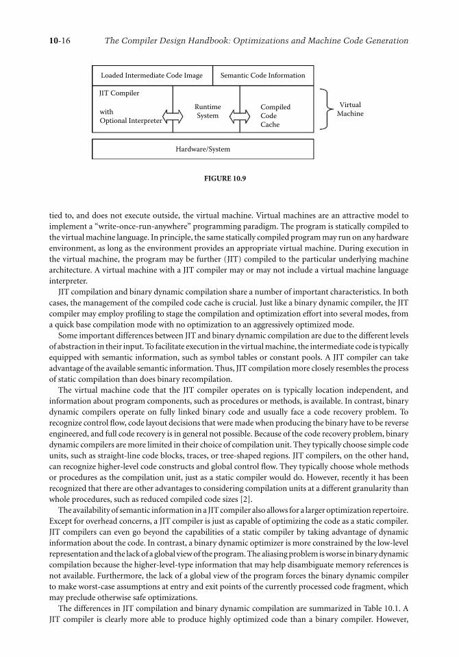
10-16 The Compiler Design Handbook: Optimizations and Machine Code Generation
Loaded Intermediate Code Image Semantic Code Information
JIT Compiler
Runtime
System
Hardware/System
Compiled
Code
Cache
Virtual
Machine with
Optional Interpreter
FIGURE 10.9
tied to, and does not execute outside, the virtual machine. Virtual machines are an attractive model toimplement a “write-once-run-anywhere” programming paradigm. The program is statically compiled tothe virtual machine language. In principle, the same statically compiled program may run on any hardwareenvironment, as long as the environment provides an appropriate virtual machine. During execution inthe virtual machine, the program may be further (JIT) compiled to the particular underlying machinearchitecture. A virtual machine with a JIT compiler may or may not include a virtual machine languageinterpreter.
JIT compilation and binary dynamic compilation share a number of important characteristics. In bothcases, the management of the compiled code cache is crucial. Just like a binary dynamic compiler, the JITcompiler may employ profiling to stage the compilation and optimization effort into several modes, froma quick base compilation mode with no optimization to an aggressively optimized mode.
Some important differences between JIT and binary dynamic compilation are due to the different levelsof abstraction in their input. To facilitate execution in the virtual machine, the intermediate code is typicallyequipped with semantic information, such as symbol tables or constant pools. A JIT compiler can takeadvantage of the available semantic information. Thus, JIT compilation more closely resembles the processof static compilation than does binary recompilation.
The virtual machine code that the JIT compiler operates on is typically location independent, andinformation about program components, such as procedures or methods, is available. In contrast, binarydynamic compilers operate on fully linked binary code and usually face a code recovery problem. Torecognize control flow, code layout decisions that were made when producing the binary have to be reverseengineered, and full code recovery is in general not possible. Because of the code recovery problem, binarydynamic compilers are more limited in their choice of compilation unit. They typically choose simple codeunits, such as straight-line code blocks, traces, or tree-shaped regions. JIT compilers, on the other hand,can recognize higher-level code constructs and global control flow. They typically choose whole methodsor procedures as the compilation unit, just as a static compiler would do. However, recently it has beenrecognized that there are other advantages to considering compilation units at a different granularity thanwhole procedures, such as reduced compiled code sizes [2].
The availability of semantic information in a JIT compiler also allows for a larger optimization repertoire.Except for overhead concerns, a JIT compiler is just as capable of optimizing the code as a static compiler.JIT compilers can even go beyond the capabilities of a static compiler by taking advantage of dynamicinformation about the code. In contrast, a binary dynamic optimizer is more constrained by the low-levelrepresentation and the lack of a global view of the program. The aliasing problem is worse in binary dynamiccompilation because the higher-level-type information that may help disambiguate memory references isnot available. Furthermore, the lack of a global view of the program forces the binary dynamic compilerto make worst-case assumptions at entry and exit points of the currently processed code fragment, whichmay preclude otherwise safe optimizations.
The differences in JIT compilation and binary dynamic compilation are summarized in Table 10.1. AJIT compiler is clearly more able to produce highly optimized code than a binary compiler. However,

Dynamic Compilation 10-17
TABLE 10.1 Differences in JIT Compilation and Binary Dynamic Compilation
JIT Compilation Dynamic Binary Compilation
Semantic information available Lack of semantic informationFull code recovery Limited code recovery; limited choice in compilation unitFull optimization repertoire Limited optimization potential
consider a scenario where the objective is not code quality but compilation speed. Under these conditions,it is no longer clear that the JIT compiler has an advantage. A number of compilation and code generationdecisions, such as register allocation and instruction selection, have already been made in the binary codeand can often be reused during dynamic compilation. For example, binary translators typically constructa fixed mapping between guest and host system machine registers. Consider the situation where the guestarchitecture has fewer registers, for instance, 32, than the host architecture, for instance, 64, so that the32 guest registers can be mapped to the first 32 host registers. When translating an instruction opcode,op1,op2, the translator can use the fixed mapping to directly translate the operands from guest to hostmachine registers. In this fashion, the translator can produce code with globally allocated registers withoutany analysis, simply by reusing register allocation decisions from the guest code.
In contrast, a JIT compiler that operates on intermediated code has to perform a potentially costly globalanalysis to achieve the same level of register allocation. Thus, what appears to be a limitation may proveto have its virtues depending on the compilation scenario.
10.6 Nontransparent Approach: Runtime Specialization
A common characteristic among the dynamic compilation systems discussed so far is transparency. Thedynamic compiler operates in complete independence from static compilation stages and does not makeassumptions about, or require changes to, the static compiler.
A different, nontransparent approach to dynamic compilation has been followed by staged runtimespecialization techniques [9, 31, 33]. The objective of these techniques is to prepare for dynamic compilationas much as possible at static compilation time. One type of optimization that has been supported in thisfashion is value-specific code specialization. Code specialization is an optimization that produces anoptimized version by customizing the code to specific values of selected specialization variables.
Consider the code example shown in Figure 10.10. Figure 10.5i shows a dot product function that iscalled from within a loop in the main program, such that two parameters are fixed (n = 3 and row = [5,0, 3]) and only a third parameter (col) may still vary. A more efficient implementation can be achieved byspecializing the dot function for the two fixed parameters. The resulting function spec doc, which retainsonly the one varying parameter, is shown in Figure 10.10ii.
In principle, functions that are specialized at runtime, such as spec dot, could be produced in a JITcompiler. However, code specialization requires extensive analysis and is too costly to be performed fullyat runtime. If the functions and the parameters for specialization are fixed at compile time, the staticcompiler can prepare the runtime specialization and perform all the required code analyses. Based on theanalysis results, the compiler constructs code templates for the specialized procedure. The code templatesfor spec dot are shown in Figure 10.11ii in C notation. The templates may be parameterized with respectto missing runtime values. Parameterized templates contain holes that are filled in at runtime with therespective values. For example, template T2 in Figure 10.11ii contains two holes for the runtime parametersrow[0]. . . row[2] (hole h1) and the values 0, . . . , (n−1)(hole h2).
By moving most of the work to static compile time, the runtime overhead is reduced to initializationand linking of the prepared code templates. In the example from Figure 10.10, the program is staticallycompiled so that in place of the call to routine dot, a call to a specialized dynamic code generation agent isinserted. The specialized code generation agent for the example from Figure 10.10, make spec dot, is shownin Figure 10.11i. When invoked at runtime, the specialized dynamic compiler looks up the appropriate

10-18 The Compiler Design Handbook: Optimizations and Machine Code Generation
dot (inf n, int row[ ], intcol [ ]){
int i, sum;sum = 0;
for (i = 0; i<n; i++)sum + = row (i)* col (i);
return sum;}
main ( ) {read (&n, row);. . .while (. . .) {/* n=3, row = {5, 0, 3} */dot (n, row, col);. . .
}}
spec dot (int col [ ]){int sum = 0;sum += 5* col [0];sum += 3* col [2];return sum;
}
main {} {read (&n, row);make spec dot (n,
row);. . .while (. . . ) {spec dot (col);. . .
}}
(i) (ii)
FIGURE 10.10 Code specialization example. A dot–product function before (i) and after (ii) specialization.
code templates for spec dot, fills in the holes for parameters n and row with their runtime values, andpatches the original main routine to link in the new specialized code.
The required compiler support renders these runtime specialization techniques less flexible than trans-parent dynamic compilation systems. The kind, scope, and timing of dynamic code generation are fixed atcompile time and hardwired into the code. Furthermore, runtime code specialization techniques usuallyrequire programmer assistance to choose the specialization regions and variables (e.g., via code annotationsor compiler directives). Because overspecialization can easily result in code explosion and performancedegradation, the selection of beneficial specialization candidates is likely to follow an interactive approach,
make spec dot (int n, int row [ ] ) {buf = alloc ( ); /* allocate buffer space for spec dot */
copy temp (buf, T1); /* copy template T1 into buffer */for (i=0; i<n; i++) {
copy temp (buf, T2); /* copy template T2 */fill hole (buf, h1, row [i]); /* fill hole h1 in T2 */fill hole (buf, h2, i); /* file hole h2 in T2 */
}copy temp (buf, T3); /* copy template T3 */return buf;
}(i)
Template T1: spec dot (int col []) { int sum = 0;Template T2: sum += {hole h1} * col [ {hole h2}];Template T3: return sum; }
(ii)
FIGURE 10.11 Runtime code generation function (i) and code templates (ii) for specializing function dot fromFigure 10.10.

Dynamic Compilation 10-19
where the programmer explores various specialization opportunities. Recently, a system has been devel-oped toward automating the placement of compiler directives for dynamic code specialization [32].
The preceding techniques for runtime specialization are classified as declarative. Based on the program-mer declaration, templates are produced automatically by the static compiler. An alternative approach isimperative code specialization. In an imperative approach, the programmer explicitly encodes the run-time templates. C is an extension of the C languages that allows the programmer to specify dynamic codetemplates [33]. The static compiler compiles these programmer specifications into code templates that areinitiated at runtime in a similar way to the declarative approach. Imperative runtime specialization is moregeneral because it can support a broader range of runtime code generation techniques. However, it alsorequires deeper programmer involvement and is more error prone, because of the difficulty of specifyingthe dynamic code templates.
10.7 Summary
Dynamic compilation is a growing research field fueled by the desire to go beyond the traditional com-pilation model that views a compiled binary as a static immutable object. The ability to manipulate andtransform code at runtime provides the necessary instruments to implement novel execution services.This chapter discussed the mechanisms of dynamic compilation systems in the context of two applica-tions: dynamic performance optimization and transparent software migration. However, the capabilitiesof dynamic compilation systems can go further and enable such services as dynamic decompression anddecryption or the implementation of security policies and safety checks.
Dynamic compilation should not be viewed as a technique that competes with static compilation.Dynamic compilation complements static compilation, and together they make it possible to move towarda truly write-once-run-anywhere paradigm of software implementation.
Although dynamic compilation research has advanced substantially in recent years, numerous challengesremain. Little progress has been made in providing effective development and debugging support fordynamic compilation systems. Developing and debugging a dynamic compilation system is particularlydifficult because the source of program bugs may be inside transient dynamically generated code. Breakpoints cannot be placed in code that has not yet materialized, and symbolic debugging of dynamicallygenerated code is not an option. The lack of effective debugging support is one of the reasons the engineeringof dynamic compilation systems is such a difficult task. Another area that needs further attention is codevalidation. Techniques are needed to assess the correctness of dynamically generated code. Unless dynamiccompilation systems can guarantee high levels of robustness, they are not likely to achieve widespreadadoption.
This chapter surveys and discusses the major approaches to dynamic compilation with a focus ontransparent binary dynamic compilation. For more information on the dynamic compilation systems thathave been discussed, we encourage the reader to explore the sources cited in the References section.
References
1. L. Anderson, M. Berc, J. Dean, M. Ghemawat, S. Henzinger, S. Leung, L. Sites, M. Vandervoorde,C. Waldspurger, and W. Weihl. 1977. Continuous profiling: Where have all the cycles gone? InProceedings of the 16th ACM Symposium of Operating Systems Principles, 14.
2. D. Bruening and E. Duesterwald. 2000. Exploring optimal compilation unit shapes for an embed-ded just-in-time compiler. In Proceedings of the 3rd Workshop on Feedback-Directed and DynamicOptimization.
3. D. Bruening, E. Duesterwald, and S. Amarasinghe. 2001. Design and implementation of a dynamicoptimization framework for Windows. In Proceedings of the 4th Workshop on Feedback-Directed andDynamic Optimization.
4. V. Bala, E. Duesterwald, and S. Banerjia. 1999. Transparent dynamic optimization: The design andimplementation of Dynamo. Hewlett-Packard Laboratories Technical Report HPL-1999–78.

10-20 The Compiler Design Handbook: Optimizations and Machine Code Generation
5. V. Bala, E. Duesterwald, and S. Banerjia. 2000. Dynamo: A transparent runtime optimizationsystem. In Proceedings of the SIGPLAN ’00 Conference on Programming Language Design andImplementation, 1–12.
6. T. Ball and J. Larus. 1996. Efficient path profiling. In Proceedings of the 29th Annual InternationalSymposium on Microarchitecture (MICRO-29), 46–57.
7. W. Chen, S. Lerner, R. Chaiken, and D. Gillies. 2000. Mojo: A dynamic optimization system. InProceedings of the 3rd Workshop on Feedback-Directed and Dynamic Optimization.
8. R. F. Cmelik and D. Keppel. 1993. Shade: A fast instruction set simulator for execution profiling.Technical Report UWCSE-93-06-06, Department of Computer Science and Engineering, Universityof Washington, Seattle.
9. C. Consel and F. Noel. 1996. A general approach for run-time specialization and its application toC. In Proceedings of the 23rd Annual Symposium on Principles of Programming Languages, 145–56.
10. T. Conte, B. Patel, K. Menezes, and J. Cox. 1996. Hardware-based profiling: an effective techniquefor profile-driven optimization. Int. J. Parallel Programming 24:187–206.
11. C. Chambers and D. Ungar. 1989. Customization: Optimizing compiler technology for SELF, adynamically-typed object-oriented programming language. In Proceedings of the SIGPLAN ’89Conference on Programming Language Design and Implementation, 146–60.
12. Y. C. Chung and Y. Byung-Sun. The Latte Java Virtual Machine. Mass Laboratory, Seoul NationalUniversity, Korea. latte.snu.ac.kr/manual/html mono/latte.html.
13. R. Cohn and G. Lowney. 1996. Hot cold optimization of large Windows/NT applications. InProceedings of the 29th Annual International Symposium on Microarchitecture, 80–89.
14. D. Ditzel. 2000. Transmeta’s Crusoe: Cool chips for mobile computing. In Proceedings of Hot Chips12, Stanford University, Stanford, CA.
15. D. Deaver, R. Gorton, and N. Rubin. 1999. Wiggins/Redstone: An online program specializer. InProceedings of Hot Chips 11, Palo Alto, CA.
16. E. Duesterwald and V. Bala. 2000. Software profiling for hot path prediction: Less is more. InProceedings of 9th International Conference on Architectural Support for Programming Languages andOperating Systems, 202–211.
17. E. Duesterwald, R. Gupta, and M. L. Soffa. 1995. Demand-driven computation of interproceduraldata flow. In Proceedings of the 22nd ACM Symposium on Principles on Programming Languages.37–48.
18. L. P. Deutsch and A. M. Schiffman. 1994. Efficient implementation of the Smalltalk-80 system. InConference Record of the 11th Annual ACM Symposium on Principles of Programming Languages,297–302.
19. K. Ebcioglu and E. Altman. 1997. DAISY: Dynamic compilation for 100% architectural compatibility.In Proceedings of the 24th Annual International Symposium on Computer Architecture, 26–37.
20. D. R. Engler. 1996. VCODE: A retargetable, extensible, very fast dynamic code generation system. InProceedings of the SIGPLAN ’96 Conference on Programming Language Design and Implementation(PLDI ’96), 160–70.
21. D. H. Friendly, S. J. Patel, and Y. N. Patt. 1998. Putting the fill unit to work: Dynamic optimizationsfor trace cache microprocessors. In Proceedings of the 31st Annual International Symposium onMicroarchitecture (MICRO-31), 173–81.
22. J. Gosling, B. Joy, and G. Steele. 1999. The Java language specification. Reading, MA: Addison-Wesley.
23. B. Grant, M. Philipose, M. Mock, C. Chambers, and S. Eggers. 1999. An evaluation of stagedrun-time optimizations in DyC. In Proceedings of the SIGPLAN ’99 Conference on ProgrammingLanguage Design and Implementation, 293–303.
24. M. Gschwind and E. Altman. 2000. Optimization and precise exceptions in dynamic compilation.In Proceedings of Workshop on Binary Translation.

Dynamic Compilation 10-21
25. U. Hoelzle, C. Chambers, and D. Ungar. 1991. Optimizing dynamically-typed object-orientedlanguages with polymorphic inline caches. In Proceedings of ECOOP 4th European Conference onObject-Oriented Programming, 21–38.
26. U. Hoelzle, C. Chambers, and D. Ungar. 1992. Debugging optimized code with dynamic deop-timization. In Proceedings of the SIGPLAN ’92 Conference on Programming Language Design andImplementation, 32–43.
27. R. J. Hookway and M. A. Herdeg. 1997. FX!32: Combining emulation and binary translation. DigitalTech. J. 0(1):3–12.
28. IBM Research. The IBM Jalapeno Project. www.research.ibm.com/jalapeno/.29. Intel Microprocessor Research Lab. Open Runtime Platform. www.intel.com/research/mrl/orp/.30. C. Krintz and B. Calder. 2001. Using annotations to reduce dynamic optimization time. In Proceedings
of the SIGPLAN ’01 Conference on Programming Language Design and Implementation, 156–67.31. M. Leone and P. Lee. 1996. Optimizing ML with run-time code generation. In Proceedings of the
SIGPLAN ’96 Conference on Programming Language Design and Implementation, 137–48.32. M. Mock, M. Berryman, C. Chambers, and S. Eggers. 1999. Calpa: A tool for automatic dynamic
compilation. In Proceedings of the 2nd Workshop on Feedback-Directed and Dynamic Optimization.33. M. Poletta, D. R. Engler, and M. F. Kaashoek. 1997. TCC: A system for fast flexible, and high-level
dynamic code generation. In Proceedings of the SIGPLAN ’97 Conference on Programming LanguageDesign and Implementation, 109–21.
34. S. Richardson. 1993. Exploiting trivial and redundant computation. In Proceedings of the 11thSymposium on Computer Arithmetic.
35. K. Scott and J. Davidson. 2001. Strata: A software dynamic translation infrastructure. In Proceedingsof the 2001 Workshop on Binary Translation.
36. A. Srivastava, A. Edwards, and H. Vo. 2001. Vulcan: Binary translation in a distributed environment.Technical Report MSR-TR-2001-50, Microsoft Research.
37. O. Taub, S. Schechter, and M. D. Smith. 2000. Ephemeral instrumentation for lightweight programprofiling. Technical report, Harvard University.
38. Transitive Technologies. www.transitives.com/.39. D. Ung and C. Cifuentes. 2000. Machine-adaptable dynamic binary translation. ACM Sigplan Notices
35(7):41–51.40. X. Zhang, Z. Wang, N. Gloy, J. Chen, and M. Smith. 1997. System support for automatic profiling
and optimization. In Proceedings of the 16th ACM Symposium on Operating Systems Principles, 15–26.


11The Static Single
Assignment Form:Construction and
Application toProgram Optimization
J. Prakash Prabhu1,Priti Shankar,andY. N. SrikantDepartment of Computer Scienceand Automation,Indian Institute of Science,Bangalore, [email protected]@[email protected]
11.1 Introduction . . . . . . . . . . . . . . . . . . . . . . . . . . . . . . . . . . . . . . . . .11-111.2 The Static Single Assignment Form . . . . . . . . . . . . . . . . . . .11-2
Construction of the SSA Form • A Linear Time Algorithmfor Placing φ-Nodes
11.3 Variants of the SSA Form . . . . . . . . . . . . . . . . . . . . . . . . . . . . .11-17Pruned SSA • Semi-Pruned SSA
11.4 Conditional Constant Propagation . . . . . . . . . . . . . . . . . . . .11-20The Lattice of Constants • The CCP Algorithm: Flow GraphVersion • The CCP Algorithm: SSA Version
11.5 Value Numbering . . . . . . . . . . . . . . . . . . . . . . . . . . . . . . . . . . . .11-25Hashing-Based Value Numbering: Basic Block Version• Value Numbering with Hashing and SSA Forms
11.6 Partial Redundancy Elimination . . . . . . . . . . . . . . . . . . . . .11-36Partial Redundancy Elimination on the SSA Form• The SSAPRE Algorithm
11.7 Translation from SSA Form to Executable Form . . . . . . .11-47The Lost Copy Problem • The Swap Problem
11.8 Discussion and Conclusions . . . . . . . . . . . . . . . . . . . . . . . . . .11-50References . . . . . . . . . . . . . . . . . . . . . . . . . . . . . . . . . . . . . . . . . . . . . . . . . .11-51
11.1 Introduction
The emergence of the static single assignment (SSA) form as an important intermediate representationfor compilers has resulted in considerable research in algorithms to compute this form efficiently. TheSSA representation is an example of a sparse representation where definition sites are directly associatedwith use sites. Analysis of sparse representations has the advantage of being able to directly access pointswhere relevant data flow information is available. Therefore, one can profitably use this property in im-proving algorithms for optimizations carried out on older, more traditional intermediate representations.
1Presently at Bell Laboratories, Bangalore.11-1

11-2 The Compiler Design Handbook: Optimizations and Machine Code Generation
Read A, B , Cif (A > B)
if (A > C) max = Aelse max = C
else if (B > C) max = Belse max = C
Print max
FIGURE 11.1 Program in non-SSA form.
In this chapter we present the original construction [18], some recent improvements [19, 51], andapplications to some specific optimizations. We discuss conditional constant propagation [44, 45, 55],global value numbering [4, 10, 16, 44, 45], and partial redundancy elimination [33, 38, 43–45, 48]. Sev-eral other algorithms for optimizations such as dead code elimination [6, 18, 44], strength reduction[17, 20, 34, 36, 44, 46, 58], array bound check elimination [6, 7, 27, 39], and liveness analysis [5] on sparserepresentations have not been included because of space constraints.
Section 11.2 discusses the SSA form and its construction. Some variants of the SSA form proposed byBriggs et al. [9] are described in Section 11.3. Section 11.4 contains a detailed presentation of conditionalconstant propagation algorithms on the the SSA representation. This is followed by a description of value-numbering algorithms in Section 11.5 and partial redundancy elimination algorithms in Section 11.6.Some issues involved in back translation of the SSA form to executable form are discussed in Section 11.7.Section 11.8 concludes this chapter with a discussion. We assume that the reader is familiar with the notionof control flow graphs, basic blocks, paths, and so forth. These definitions are available in [3, 6, 18, 44].
11.2 The Static Single Assignment Form
A program is in SSA form if each of its variables has exactly one definition, which implies that each useof a variable is reached by exactly one definition. The control flow remains the same as in a traditional(non-SSA) program. A special merge operator, denoted φ, is used for the selection of values in join nodes.The SSA form is usually augmented with use–definition and/or definition–use chains in its data structurerepresentation to facilitate design of faster algorithms.
Figures 11.1 and 11.4 show two non-SSA form programs, Figures 11.2 and 11.5 show their SSA forms,and Figures 11.3 and 11.6 show the flowcharts of the SSA form.
The program in Figure 11.1 is not in SSA form because there are several assignments to the variablemax. In the program in Figure 11.2 (with the accompanying flowchart in Figure 11.6), each assignmentis made to a different variable, maxi . The variable max5 is assigned the correct value by the φ-function,which takes the value maxi , if the control reaches it via the i th incoming branch from left to right.
The φ-functions in the two blocks B1 and B5 in Figure 11.6 are meant to choose the appropriate valuebased on the control flow. For example, the φ-assignment to RSR5 in the block B5 in Figure 11.6 selectsone of RSR3, RSR2, or RSR4 based on the execution following the arc B2 → B5, B3 → B5, or B4 → B5,respectively.
Read A, B , Cif (A > B)
if (A > C) max1 = Aelse max2 = C
else if (B > C) max3 = Belse max4 = C
max5 = φ(max1, max2, max3, max4)Print max5
FIGURE 11.2 Program of Figure 11.1 in SSA form.

The Static Single Assignment Form 11-3
Start
A > BT
TF FT
F
A > C
Stop
B > C
Read
A, B, C
Printmax5
max5 = φ(max1, max2, max3, max4)
max1 = A max2 = C max3 = B max4 = C
FIGURE 11.3 Flowchart of program in Figure 11.2.
Usually, compilers construct a control flow graph representation of a program first and then convert it toSSA form. The conversion process involves the introduction of statements with assignment to φ-functionsin several join nodes and renaming of variables that are targets of more than one definition. Of course, theusages of such variables will also be changed appropriately. Not every join node needs a φ-function forevery variable in the program. Algorithms for the suitable placement of φ-functions to ensure a minimalSSA form are described in the next section.
A reader unfamiliar with the SSA form may wonder about the role of φ-functions in the final machinecode of the program. Since there is no direct translation of a φ-function to machine code, a copy instructionneeds to be inserted at the end of each predecessor block of the block containing a φ-function. Thisintroduces some inefficiency into machine code, which can be compensated for, to some extent, by goodregister allocation [18]. Carrying out dead code elimination before φ-conversion is also required to removeredundant assignment statements.
Read A; LSR = 1; RSR = A; LSR = (LSR + RSR)/2;
Repeat
T = SR ∗ SR;
if (T > A) RSR = SRelse if (T < A) LSR = SR
else begin LSR = SR; RSR = SR; end
SR = (LSR + RSR)/2;
until (LSR �= RSR)
Print SR
FIGURE 11.4 Another program in non-SSA form.

11-4 The Compiler Design Handbook: Optimizations and Machine Code Generation
Read A; LSR1 = 1; RSR1 = A; SR1 = (LSR1 + RSR1)/2;
Repeat
LSR2 = φ(LSR5, LSR1);RSR2 = φ(RSR5, RSR1);SR2 = φ(SR3, SR1);T = SR2 ∗ SR2;
if (T > A) RSR3 = SR2
else if (T < A) LSR3 = SR2
else begin LSR4 = SR2; RSR4 = SR2; end
LSR5 = φ(LSR2, LSR3, LSR4);RSR5 = φ(RSR3, RSR2, RSR4);SR3 = (LSR5 + RSR5)/2;
until (LSR5 �= RSR5)
Print SR3
FIGURE 11.5 Program in Figure 11.4 in SSA form.
T < A
T > A T F
F T
Print SR3
Stop
T F
B2
B3 B4
Start
Read A
LSR1 = 1; RSR1 = A
SR1 = (LSR1 + RSR1)/2
RSR2 = φ(RSR5, RSR1)
T = SR2 *SR2
SR2 = φ(SR3, SR1)
LSR2 = φ(LSR5, LSR1)
RSR3 = SR2
LSR3 = SR2 LSR4 = SR2
RSR4 = SR2
LSR5 ! = RSR5
LSR5 = φ(LSR2, LSR3, LSR4)
RSR5 = φ(RSR3, RSR2, RSR4)
SR3 = (LSR5 + RSR5)/2
B1
B5
FIGURE 11.6 Flowchart of program in Figure 11.5.

The Static Single Assignment Form 11-5
Start
A > B
A > C
Stop
B > C
Read
A, B, C
max1 = A
t = max1
max2 = C
t = max2
max3 = B
t = max3
max5 = t
Print max5
max4 = C
t = max4
FIGURE 11.7 φ-Conversion on program in Figure 11.3.
Figure 11.7 shows a simple example of the effect of φ-conversion. During register allocation, the sameregister would be assigned to t, max1, max2, max3, max4, and max5, and thereby copying is eliminated.
11.2.1 Construction of the SSA Form
We now discuss the construction of an SSA form from a flow graph. We consider only scalars and referthe reader to [18, 35] for details on how structures, pointers, and arrays are handled. Our presentation isbased on the material in [18].
11.2.1.1 Conditions on the SSA Form
After a program has been translated to SSA form, the new form should satisfy the following conditions forevery variable v in the original program:
1. If two paths from nodes with a definition of v converge at a node p, then p contains a trivialφ-function of the form v = φ(v , v , . . . , v), with the number of arguments equal to the in-degreeof v .
2. Each appearance of v in the original program or a φ-function in the new program has been replacedby a new variable vi , leaving the new program in SSA form.
3. Any use of a variable v along any control path in the original program and the corresponding useof vi in the new program yield the same value for both v and vi .
Condition 1 above is recursive. It implies that φ-assignments introduced by the translation procedurewill also qualify as assignments to v , and this in turn may lead to introduction of more φ-assignments atother nodes.
11.2.1.2 The Join Set and φ-Nodes
Given a set S of flow graph nodes, we define the set JOIN(S) of nodes from the flow graph to be the setof all nodes n, such that there are at least two nonnull paths in the flow graph that start at two distinctnodes in S and converge at n. The iterated join set, JOIN+(S) is the limit of the monotonic nondecreasing

11-6 The Compiler Design Handbook: Optimizations and Machine Code Generation
Start
i = 0;
read n
n <> 1
even(n) print i
n = n/2 n = 3*n + 1 Stop
i = i + 1
B1
B2
B3 B4
B5 B6
N Y
Y N
Start
B1
B2
B3 B4
B5 B6 B7 Stop
{}
{}
{}
{} {}
{B7} {B7} {B2}
{}
Flow Graph
Dominator Tree with Dominance Frontier
B7
FIGURE 11.8 Example flow graph for SSA form construction.
sequence of sets of nodes
JOIN(1)(S) = JOIN(S)
JOIN(i+1)(S) = JOIN(S ∪ JOIN(i)(S))
If S is defined to be the set of assignment nodes for a variable v , then JOIN+(S) is precisely the setof flow graph nodes, where φ-functions are needed (for v). See [18] for proofs. The set JOIN+(S) istermed the iterated dominance frontier, DF+(S), which can be computed efficiently in a manner to bedescribed shortly.
11.2.1.3 Dominator Tree
Given two nodes x and y in a flow graph, x dominates y if x appears in all paths from the Start node to y.The node x strictly dominates y if x dominates y and x �= y. x is the immediate dominator of y (denotedidom[y]) if x is the closest strict dominator of y. A dominator tree shows all the immediate dominatorrelationships. Figure 11.8 shows a flow graph and its dominator tree. Dominator trees can be constructedin time almost linear in the number of edges of a flow graph [42] (see [29] for a linear time but morecomplicated algorithm).
11.2.1.4 Dominance Frontier
For a flow graph node x , the set of all flow graph nodes y, such that x dominates a predecessor of y butdoes not strictly dominate y, is called the dominance frontier of x and is denoted by DF(x). The followingredefinition of DF(x) makes it simple to compute in linear time.
DF(x) = DFlocal(x) ∪⋃
z ∈ children(x)
DFup(z)
DFlocal(x) = {y ∈ successor(x) | idom(y) �= x}DFup(x) = {y ∈ D F (x) | idom(y) �= parent(x)}

The Static Single Assignment Form 11-7
function dominance frontier(n) // n is a node in the dominator tree
begin
for all children c of n in the dominator tree do
dominance frontier(n.c);
end for
DF(n) = ∅;
// DFlocal computation
for all successors of n in the flow graph do
if (idom(s ) �= n) then DF(n) = DF(n) ∪ {s };end for
// DFup computation
for all children c of n in the dominator tree do
for all p ∈ DF(c) do
if (idom( p) �= n) then DF(n) = DF(n) ∪ {p};end for
end for
end
FIGURE 11.9 Dominance frontier computation.
Here, children(x) and parent(x) are defined over the dominator tree and successor(x) is defined overthe flow graph. The algorithm in Figure 11.9 computes the dominance frontier based on the definitionsgiven above. It is called on the root of the dominator tree, and the tree is traversed in postorder. Figure 11.8shows the DF sets as annotations on the nodes of the dominator tree.
We now extend the definition of DF to act on sets and define the iterated dominance frontier on linessimilar to JOIN+(S).
DF(S) = ∪x ∈ SDF(x)
DF(1)(S) = DF(S)
DF(i+1)(S) = DF(S ∪ DF(i)(S))
For each variable v , the set of flow graph nodes that need φ-functions is DF+(S), where S is the setof nodes containing assignments to v . We do not construct DF+(S) explicitly. It is computed implicitlyduring the placement of φ-functions.
11.2.1.5 Minimal SSA Form Construction
There are three steps in the construction of the minimal SSA form:
1. Compute DF sets for each node of the flow graph using the algorithm in Figure 11.9.2. Place trivial φ-functions for each variable in the nodes of the flow graph using the algorithm in
Figure 11.10.3. Rename variables using the algorithm in Figure 11.11.
The function place-phi-function(v) is called once for each variable v . It can be made more efficient byusing integer flags instead of boolean flags as described in [18]. Our presentation uses boolean flags tomake the algorithm simpler to understand.
The renaming algorithm in Figure 11.11 performs a top-down traversal of the dominator tree. Itmaintains a version stack V , whose top element is always the version to be used for a variable usageencountered (in the appropriate range, of course). A counter v is used to generate a new version number.It is possible to use a separate stack for each variable as in [18], so as to reduce the overheads a bit. However,we believe our presentation is simpler to comprehend.

11-8 The Compiler Design Handbook: Optimizations and Machine Code Generation
function Place-phi-function(v) // v is a variable
// This function is executed once for each variable in the flow graph
begin
// has-phi(B) is true if a φ-function has already
// been placed in B// processed(B) is true if B has already been processed once
// for variable vfor all nodes B in the flow graph do
has-phi(B) = false; processed(B) = false;
end for
W = ∅; // W is the work list
// Assignment-nodes(v) is the set of nodes containing
// statements assigning to vfor all nodes B ∈ Assignment-nodes(v) do
processed(B) = true; Add(W, B);
end for
while W �= ∅ do
begin
B = Remove(W);
for all nodes y ∈ DF(B) do
if (not has-phi(y)) then
begin
place < v = φ(v , v , ..., v) > in y;
has-phi(y) = true;if (not processed(y)) then
begin processed(y) = true; Add(W, y); end
end
end for
end
end
FIGURE 11.10 Minimal SSA construction.
Let us trace the steps of the SSA construction algorithm with the help of the example in Figure 11.12. Letus concentrate on the variable n. Blocks B1, B5, and B6 have assignments to n. (Read n is also consideredas an assignment.) The dominance frontier of B1 being null, no φ-function is introduced while processingit. A φ-function is introduced for n in B7 while processing B5 (this will not be repeated while processingB6). B2 gets a φ-function for n when B7 is handled.
Let us now understand how different instances of n are renamed. The instruction read n in B1 becomesread n0 while processing B1. At the same time, the second parameter of the φ-function for n in block B2
is changed to n0. Processing B2 in the top-down order results in changing the statement n = φ(n, n0) ton1 = φ(n, n0), and the new version number 1 is pushed onto the version stack V . This results in changingthe comparisons n �= 1 to n1 �= 1 in block B2 and even(n) to even(n1) in block B3. The expressions n/2in block B5 and 3 ∗ n + 1 in block B6 also change to n1/2 and 3 ∗ n1 + 1, respectively. A new version of n,viz., n2 (or n3, respectively) is created while processing the assignment in block B5 (or B6, respectively).The version number 2 (or 3, respectively) is pushed onto V . This results in changing the parameters ofthe φ-function in block B7 as shown in Figure 11.12. After finishing with B5 (or B6, respectively), V ispopped to remove 2 (or 3, respectively), before processing B7. A new version n4 is created while processingthe φ-statement in B7, which in turn changes the first parameter of the φ-function for n in block B2, fromn to n4. V is then popped and recursion unwinds. The variable i is treated in a similar manner.

The Static Single Assignment Form 11-9
function Rename-variables(x , B) // x is a variable and B is a block
begin
ve = Top(V); // V is the version stack of xfor all statements s ∈ B do
if s is a non-φ statement then
replace all uses of x in the R H S(s ) with Top(V);if s defines x then
begin
replace x with xv in its definition; push xv onto V ;
// xv is the renamed version of x in this definition
v = v + 1; // v is the version number counter
end
end for
for all successors s of B in the flow graph do
j = predecessor index of B with respect to sfor all φ-functions f in s which define x do
replace the j th operand of f with Top(V);end for
end for
for all children c of B in the dominator tree do
Rename-variables(x , c);
end for
repeat Pop(V); until (Top(V) == ve);
end
begin // calling program
for all variables x in the flow graph do
V = ∅; v = 1; push 0 onto V ; // end-of-stack marker
Rename-variables(x , Start);end for
end
FIGURE 11.11 Renaming variables.
11.2.1.6 Complexity of SSA Graph Construction
We define R, the size of a flow graph, as follows.
R = max{N f , E f , A, M},
where
N f is the number of nodes in the flow graph.
E f is the number of edges in the flow graph.
A is the number of assignments in the flow graph.
M is the number of uses of variables in the flow graph.
The construction of the dominance frontier and the SSA form in theory take O(R2) and O(R3) time,respectively. However, according to [18], measurements on programs show that the size of dominancefrontiers in practice is small, and hence the entire construction, including the construction of dominancefrontiers, has complexity O(R) in practice.

11-10 The Compiler Design Handbook: Optimizations and Machine Code Generation
Start
even (n1) print i1
Stopn2 = n1/2
B1
B4
B6n3 = 3 *n1 + 1
n4 = φ(n2, n3)
i2 = i1 + 1B7
B2
B3
B5
i0 = 0
read n0
i1 = φ(i2, i0)
n1 = φ(n4, n0)
n1 <> 1
FIGURE 11.12 SSA form construction for the flow graph in Figure 11.8.
11.2.1.7 A Note on the Size of SSA Graphs
An SSA form is usually augmented with links from every unique definition of a variable to its uses(corresponding to d-u information). Some algorithms need SSA forms augmented with links that gofrom every use of a variable to its unique definition (corresponding to u-d information). If there are ndefinitions in a program, and each of these could reach n uses, then both d-u and u-d chains will haveO(n2) links. However, an SSA graph with d-u or u-d information will have only O(n) links because of thefactoring carried out by φ-functions. This is illustrated in Figures 11.13 and 11.14. In Figure 11.13, thed-u chain of each definition of i contains all three uses of i in the second switch statement. However, inFigure 11.14, because of the factoring introduced by the φ-function, each definition reaches only one use.
switch( j )case 1: i=10; break;
case 2: i=20; break;
case 3: i=30; break;
end
switch(k)
case 1: x = i ∗ 3 + 5; break;
case 2: y = i ∗ 6 + 15; break;
case 3: z = i ∗ 9 + 25; break;
end
FIGURE 11.13 Program in non-SSA form.

The Static Single Assignment Form 11-11
switch( j )case 1: i1=10; break;
case 2: i2=20; break;
case 3: i3=30; break;
end
i4 = φ(i1, i2, i3);switch(k)
case 1: x = i4 ∗ 3 + 5; break;
case 2: y = i4 ∗ 6 + 15; break;
case 3: z = i4 ∗ 9 + 25; break;
end
FIGURE 11.14 Program in Figure 11.13 in SSA form.
The renaming algorithm of Figure 11.11 can be augmented to establish d-u and u-d links. This requiresevery statement to be a separate node in the flow graph. It also requires keeping a pointer to the nodedefining a variable on the version stack along with the name of the variable. The rest of the process issimple.
The SSA form increases the number of variables. If there are n variables in a program and each of thesehas k definitions, then the SSA form would have nk variables to take care of the nk definitions. It may notbe possible to map these nk variables back to n variables during machine code generation because of codemovements that could have taken place as a result of optimization.
11.2.2 A Linear Time Algorithm for Placing φ-Nodes
In this section, we describe a simple linear time algorithm for computing φ-nodes developed by Sreedharand Gao [51]. This algorithm is based on a new data structure, called the DJ-graph, which is basically thedominator tree augmented with edges called “join” edges, which may lead to nodes where data flow infor-mation is merged. Cytron’s original algorithm [18] for computing φ-nodes precomputes the dominancefrontier for every node in the flow graph. In some cases this precomputation takes time quadratic in thenumber of nodes of the flow graph. For example, consider the “ladder graph” shown in Figure 11.15a. Tocompute DF(2), we use the expression
DF(2) = DFup(4) ∪ {3}
Computing the set DFup(4) involves first computing DF(4) and then selecting those nodes in DF(4) thatare not dominated by node 2 and thus require time linear in the size of DF(4). Similarly, computing DF(4)requires time linear in the size of DF(6):
DF(4) = DFup(6) ∪ {5}DF(6) = DFup(8) ∪ {7}DF(8) = {9}
Every step in the dominance frontier computation adds a new node to the dominance frontier (DFlocal)and examines all the nodes in the dominance frontier of the node(s) it immediately dominates. In general,a ladder graph with n nodes, computing the dominance frontier for a node placed similarly to node 2above, takes time
1 + 2 + · · · + n
2= O(n2)

11-12 The Compiler Design Handbook: Optimizations and Machine Code Generation
7
2
0 1
3
4 5
6
8 9
10
(a) “Ladder” graph
D-edge
0
1 2 5 7
4
6
3 9
10
8
J-edge
(b) DJ-graph
FIGURE 11.15 The “ladder” graph and its DJ-graph.
However, as can be seen from Table 11.1, the maximum number of φ-nodes required for this laddergraph (for a single variable) is linear in the number of nodes of the graph. While the example abovemay seem contrived, there are examples of nested repeat-until loops for which the dominance frontiercomputation takes quadratic time [18]. In the following section, we will see a data structure called theDJ-graph that is used to compute the iterated dominance frontier without precomputing the dominancefrontier of every node.
11.2.2.1 The DJ-Graph and Its Properties
The DJ-graph is a directed graph whose nodes are the nodes of the control flow graph. There are twokinds of edges between the nodes, called the D-edges (dominator edges) and J-edges (join edges). Theconstruction of the DJ-graph is performed in two steps:

The Static Single Assignment Form 11-13
TABLE 11.1 Dominancefrontiers for the “ladder”graph shown in Figure 11.15
n DF(n)0 {}1 {3}2 {3,5,7,9}3 {5}4 {5,7,9}5 {7}6 {7,9}7 {9}8 {9}9 {}10 {}
1. Build the dominator tree of the control flow graph. The edges in the dominator tree constitute theD-edges of the DJ-graph.
2. Add the J-edges to the dominator tree to obtain the complete DJ-graph. A J-edge is an edge x → yfrom the control flow graph such that x does not strictly dominate y. In other words, y is a controlflow join point and x is a predecessor of y. The time complexity of adding the J-edges to theDJ-graph from the control flow graph is O(E), where E is the number of edges in the control flowgraph.
The total time for constructing the DJ-graph is linear in the size of the control flow graph since thedominator tree can be contructed in linear time [29]. The DJ-graph for the ladder graph of Figure 11.15ais shown in Figure 11.15b. The solid edges represent the D-edges, while dotted ones represent J-edges. AnyDJ-graph has the following three key properties:
1. The number of edges in the DJ-graph is less than the total number of nodes and edges in thecorresponding control flow graph. This can be shown as
Number of edges in DJ-graph = |D-edges| + |J-edges|≤ N f − 1 + E f
< N f + E f
2. If a node y has to be in the DF(x), then there should be a J-edge from some node z ∈ SubTree(x)to y. Subtree(x) is subtree rooted at x in the dominator tree and hence is the set of all the nodesdominated by x .Proof: Let z be any node in SubTree(x) and y ∈ DF(x). Suppose there exists no J-edge z → y.Case 1: There is a D-edge z → y. Then (x dom z ∧ z dom y) ⇒ (x dom y) ⇒ [y /∈ DF(x)], giving
a contradiction.Case 2: There is no D-edge z → y. Since y ∈ DF(x), x dominates a predecessor of y but does
not strictly dominate y. Let pred(y) be z. Since (x dom z), [z ∈ Subtree(x)]. Now thereare two cases: (a) (z dom y) ⇒ (x sdom y) ⇒ y /∈ DF(x), giving a contradiction, and(b) (z !dom y). By definition of a J-edge, there should exist a J-edge from z to y.
Thus to compute DF(x), we do not need to look beyond those nodes y, which are connectedby means of a J-edge to a node z in the SubTree(x).
3. Let W be the set of nodes y such that there exists a J-edge from a node z ∈ SubTree(x) to y.The DF(x) is composed of exactly those set of those nodes y ∈ W such that level(y) ≤ level(x).The level of a node is the depth of the node in the dominator tree with the level of root being definedas 0.

11-14 The Compiler Design Handbook: Optimizations and Machine Code Generation
For every z ∈ SubTree(x)if ((z → y is a J-edge) ∧ (level(y) ≤ level(x)))
DF(x) = DF(x) ∪ {y}
FIGURE 11.16 Computing the dominance frontier of single node x .
Proof: Let w ∈ W and z → w be a J-edge. There are two cases to consider with respect to thelevels of w and x :
Case 1: level(w) ≤ level(x). Now [z ∈ pred(w)] and (x dom z). Also [level(w) ≤ level(x)] ⇒ (x!sdom w). From this, it follows that x dominates a predecessor of w and does not strictlydominate w . Hence w ∈ DF(x).
Case 2: level(w) > level(x). Now there are two possibilities: (a) [w ∈ SubTree(x)] ⇒ (x sdom w)⇒ [w /∈ DF(x)]. (b) [w /∈ SubTree(x)]. Let u = idom(w) . Now since level(w) > level(x),level(u) ≥ level(x) ⇒ (u !dom x) . This means there exists a path (in the flow graph) fromstart node to w through x and z that does not pass through u, which implies (u !dom w),which is a contradiction. Thus, [w ∈ SubTree(x)], which reduces to case 1.
11.2.2.2 Dominance Frontier of a Single Node Using a DJ-Graph
The algorithm shown in Figure 11.16 computes DF(x) for a given node x . It directly follows from properties2 and 3 where two conditions are checked for every node in the SubTree(x) to determine membership inDF(x). For example, to compute DF(2), only the join edges 8 → 9, 6 → 7, 4 → 5, and 2 → 3 are considered.Since the heads of all these J-edges are at the same level as 2, DF(2) = {3, 5, 7, 9}.
To compute the dominance frontier of a set of nodes, we can call the above algorithm for every node inthe set and take the union of the resulting dominance frontiers. However, this could result in redundantcomputation and lead to quadratic behavior. For example, to compute DF({4, 2}), since DF({4, 2}) = DF(4)∪ DF(2), we can compute DF(4) and DF(2) individually and take their union. Assume we call DF(4) firstand then DF(2). While computing DF(2), we would visit the subtree rooted at node 4 again, even thoughit has been processed by the first call to DF(4). To prevent this reprocessing, the nodes have to be properlyordered by their levels, and state has to be maintained about the visits that have already been made.
11.2.2.3 Dominance Frontier for a Set of Nodes Nα
The algorithm given in Figures 11.17, 11.18, and 11.19 computes the dominance frontier of a set of nodesNα . The algorithm is based on two observations:
1. Before computing DF(x), if the DF(z) for some node z ∈ SubTree(x) has already been computed,it is not recomputed while finding DF(x).
Compute IDF(Nα)For every x ∈ Nα ,
next(x) = DAT[level(x)]DAT[level(x)] = x
endforwhile ( x = Next Bottom Up Node() != NULL )
CurrentRoot = xMark x as visitedTop Down Visit(x)
endwhile
FIGURE 11.17 Dominance frontier computation of set of nodes Nα .
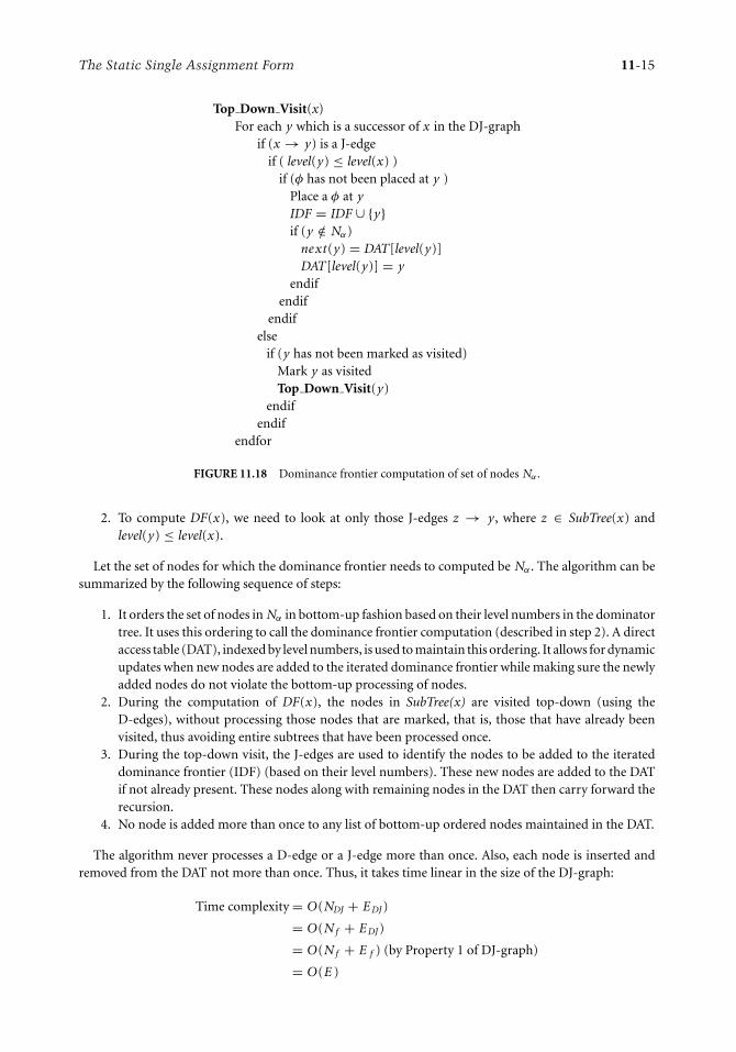
The Static Single Assignment Form 11-15
Top Down Visit(x)For each y which is a successor of x in the DJ-graph
if (x → y) is a J-edgeif ( level(y) ≤ level(x) )
if (φ has not been placed at y )Place a φ at yIDF = IDF ∪ {y}if (y /∈ Nα)
next(y) = DAT[level(y)]DAT[level(y)] = y
endifendif
endifelse
if (y has not been marked as visited)Mark y as visitedTop Down Visit(y)
endifendif
endfor
FIGURE 11.18 Dominance frontier computation of set of nodes Nα .
2. To compute DF(x), we need to look at only those J-edges z → y, where z ∈ SubTree(x) andlevel(y) ≤ level(x).
Let the set of nodes for which the dominance frontier needs to computed be Nα . The algorithm can besummarized by the following sequence of steps:
1. It orders the set of nodes in Nα in bottom-up fashion based on their level numbers in the dominatortree. It uses this ordering to call the dominance frontier computation (described in step 2). A directaccess table (DAT), indexed by level numbers, is used to maintain this ordering. It allows for dynamicupdates when new nodes are added to the iterated dominance frontier while making sure the newlyadded nodes do not violate the bottom-up processing of nodes.
2. During the computation of DF(x), the nodes in SubTree(x) are visited top-down (using theD-edges), without processing those nodes that are marked, that is, those that have already beenvisited, thus avoiding entire subtrees that have been processed once.
3. During the top-down visit, the J-edges are used to identify the nodes to be added to the iterateddominance frontier (IDF) (based on their level numbers). These new nodes are added to the DATif not already present. These nodes along with remaining nodes in the DAT then carry forward therecursion.
4. No node is added more than once to any list of bottom-up ordered nodes maintained in the DAT.
The algorithm never processes a D-edge or a J-edge more than once. Also, each node is inserted andremoved from the DAT not more than once. Thus, it takes time linear in the size of the DJ-graph:
Time complexity = O(NDJ + E DJ)
= O(N f + E DJ)
= O(N f + E f ) (by Property 1 of DJ-graph)
= O(E )

11-16 The Compiler Design Handbook: Optimizations and Machine Code Generation
Next Bottom Up Node()if (DAT[CurrentLevel] != NULL)
x = DAT[CurrentLevel]DAT[CurrentLevel]=next(x)return x
endiffor i = CurrentLeveldownto1 do
if (DAT[i]! = NULL)CurrentLevel = ix = DAT[i]DAT[i] = next(x)return x
endifendfor
FIGURE 11.19 Dominance frontier computation of set of nodes Nα .
The algorithm thus runs in time linear in the number of edges of the control flow graph. The key tothis linear time complexity is the direct access table. Each element of the table is a linked list that containsnodes that are at the same level (the corresponding index into the table). Insertion and deletion of a nodefrom the DAT take constant time.
An application of the above algorithm on the DJ-graph of Figure 11.15b for Nα = {0, 2} is traced inFigure 11.20. It shows the direct access table at various points in the algorithm. Initially, the two nodes areinserted into DAT and aligned in bottom-up order. A call to Top Down Visit(2) is placed that first examinesthe J-edge 2 → 3, adds 3 to the iterated dominance frontier IDF and to DAT. It goes on to examine edges4 → 5, 6 → 7, and 8 → 9 while adding 5, 7, and 9 to IDF and DAT. Note that this top-down traversalvisits the D-edges of SubTree(2) exactly once. The process is then carried out with Top Down Visit(9),Top Down Visit(7), and Top Down Visit(5), none of them contributing anything more to IDF. The finalcall to Top Down Visit(0) does not visit the subtrees rooted at 2, 3, 5, 7, and 9 since they have alreadybeen visited once. This avoids the recomputation that leads to quadratic behavior in Cytron’s algorithm.The J-edges correspond to the DFlocal relation used in Cytron’s dominance frontier computation. In theDJ-graph, the DFlocal relation is explicitly represented with join edges that help in getting a linear timealgorithm for placing φ-nodes.
The algorithms for φ-function placement seen in this section were recursive in nature. Das and Ramakr-ishna [19] proposed an efficient iterative algorithm for φ-function computation based on the computationof merge set of the nodes in the control flow graph [8]. The merge set of a node n is the set of nodes whereφ-functions may have to be placed if a variable definition is placed in n. The algorithm precomputes themerge set for every node in the control flow graph and later uses them for actual φ-function placement.The merge sets are computed using the DJ-graph structure. This algorithm is especially advantageouswhen the basic blocks are very dense, that is, when they have a lot of variable definitions. The earlierapproaches to finding φ-functions computed the φ-points for every variable definition. This implies thatif two or more variable definitions are in the same basic block, although the φ-function placement maybe at the same location, it is still recomputed. However, in the new approach, the φ-function is computedwith respect to a basic block instead of a variable definition. Once the merge sets have been precom-puted, to find the nodes at which a φ-function has to be placed because of variable definitions in a set ofnodes Nα , it is sufficient to take the union of merge sets of nodes in Nα . Details of the algorithm can befound in [19].

The Static Single Assignment Form 11-17
00
1
2
2
3
00
1
2
3
3
Top_Down_Visit(2)
CurrentLevel = 1
IDF = {3}
Top_Down_Visit(3)
(after 9, 10, 7, 5)
CurrentLevel = 1
IDF = {3, 5, 7, 9}
Top_Down_Visit(6)
CurrentLevel = 1
IDF = {3, 5, 7}
Top_Down_Visit(8)
CurrentLevel = 1
IDF = {3, 5, 7, 9}
Top_Down_Visit(0)
CurrentLevel = 0
IDF = {3, 5, 7, 9}
Top_Down_Visit(1)
CurrentLevel = 1
IDF = {3, 5, 7, 9}
Top_Down_Visit(4)
CurrentLevel = 1
IDF = {3,5}
0
3
0
1
2
3
5
0
5
0
57 37 3
0
1
2
3
9
1
0
Nα = {0, 2}
CurrentLevel = 1
IDF = {}
Level
0
1
2
3
0
1
2
3
0
1
2
3
0
1
2
3
FIGURE 11.20 Trace of DAT during IDF computation of Nα = {0, 2}.
11.3 Variants of the SSA Form
The dominance frontier algorithm developed by Cytron et al. [18], called the “minimal” SSA form, caninsert a φ-function for a variable at a program flow point where the variable is not live; that is, it can inserta φ-function at a point even if the corresponding variable is not used later in the program.
Consider the example program skeleton shown in Figure 11.21a. Of the three variables x, y, and zdefined and used in the program, x is defined and used wholly in blocks B1 and B2; y is defined in blocksB1 and B2 and used only in blocks B3 and B4; z is defined in blocks B1 and B2 and used only in block B5.As shown in Figure 11.21b, the minimal SSA form would insert a φ for both x and y in B5 even thoughthey are no longer used after B5.
11.3.1 Pruned SSA
Choi et al. [12] proposed a variant form of SSA called pruned SSA. In this form, once the dominancefrontiers have been computed, a live variable analysis is done to find the set of variables that are live at theentry of a basic block. Pruned SSA would then insert a φ-function for a variable v in a basic block b onlyif v is live at the entry of b. The pruned SSA form for the example program of Figure 11.21a is shown inFigure 11.22a. While pruned SSA may insert fewer φ-functions than minimal SSA, it is expensive becauseof the need for a global data flow analysis.

11-18 The Compiler Design Handbook: Optimizations and Machine Code Generation
x ...x
y ...z
y y
B1 B2
B4
B5
B3
x ...x
y ...z
z
(a) Original program
y1 y2
B1 B2
B4
φ(x1, x2)
φ(y1, y2)
φ(z1, z2)B5
B3
x1...x1y1 ...
z1
x2...x2y2 ...
z2
x3
y3
z3z3
(b) SSA form of program
FIGURE 11.21 Example program and its minimal SSA form.
11.3.2 Semi-Pruned SSA
Briggs et al. [9] suggested another variant of SSA called semi-pruned SSA based on the observation thatmany temporary variables have very short lifetimes, that is, they are defined and used only within a singlebasic block. These variables would not require φ-functions at the join points. Semi-pruned SSA computesthat set of variables that are live on entry to some basic block. These variables are named non-locals, thatis, those that have definitions outside the current basic block. Semi-pruned SSA computes the iterateddominance frontier only for the definitions in non-locals. Thus, the number of φ-functions insertedwould be between that for minimal and pruned SSA. The cost of computing non-locals is less than thatof a full-blown live-variable analysis since it does not involve any iteration or elimination. Figure 11.23gives the algorithm for computing non-locals. The semi-pruned SSA form for the example program ofFigure 11.21a is shown in Figure 11.22b. Since x is not live at the entry of any of the blocks (it is definedand used wholly within B1 and B2), a φ is not placed at B5 for x , whereas a φ is placed for y, as it is liveacross a basic block.
Briggs et al. [9] also noted that different SSA-based optimizations may require different flavors of SSA.For example, the extra φ-functions of minimal SSA may help value numbering discover congruences thatare usually not found in their absence [18]. However, if SSA is used for finding live ranges during register

The Static Single Assignment Form 11-19
y1 y2
B1 B2
B4
φ(z1, z2)B5
B3
x1...x1y1 ...
z1
x2...x2y2 ...
z2
z3z3
(a)
y1 y2
B1 B2
B4
φ(y1, y2)
φ(z1, z2)B5
B3
x1...x1y1 ...
z1
x2...x2y2 ...
z2
y3
z3z3
(b)
FIGURE 11.22 Pruned and semi-pruned SSA forms. (a) Pruned SSA form for example in Figure 11.21(a).(b) Semi-pruned SSA form for example in Figure 11.21(a).
allocation, pruned and semi-pruned SSA forms are more useful since the extra φ can cause the lifetime ofits argument variables to be extended unnecessarily. Results of constant propagation are not affected byany specific flavor of SSA.
We next discuss some optimizations that can be carried out on the SSA form.
Compute Non LocalsFor every block B
killed = φ
For each instruction v ← x op y in Bif x /∈ killed then
non locals ← non locals ∪ {x}if y /∈ killed then
non locals ← non locals ∪ {y}killed ← killed ∪ {v}
FIGURE 11.23 Algorithm for computing the “non-locals” set.

11-20 The Compiler Design Handbook: Optimizations and Machine Code Generation
11.4 Conditional Constant Propagation
Constant propagation is a well-known compiler optimization during which variables that can be deter-mined to contain only constant values at runtime in all possible executions of the program are discovered.These values are propagated throughout the program, and expressions whose operands can be determinedto be only constants are also discovered and evaluated. In effect, there is a symbolic execution of theprogram with the limited purpose of discovering constant values. The following examples help explainthe intricacies of constant propagation.
The simplest case is that of straight line code without any branches, as in a basic block. This re-quires only one pass through the code, with forward substitutions and no iteration. However, such aone-pass strategy cannot discover constants in conditionals and loops. For such cases we need to carryout data flow analysis involving work-lists and iterations. A simple algorithm of this kind adds succes-sor nodes to the work-list as symbolic execution proceeds. Nodes are removed one at a time from thework-list and executed. If the new value at a node is different from the old value, all the successors ofthe node are added to the work-list. The algorithm stops when the work-list becomes empty. Such analgorithm can catch constants in programs such as program A but not in programs such as program B inFigure 11.24.
Conditional constant propagation handles programs such as program B in Figure 11.24 by evaluatingall conditional branches with only constant operands. This uses a work-list of edges (instead of nodes)from the flow graph. Furthermore, neither successor edge of a branch node is added to the work-list whenthe branch condition evaluates to a constant value (true or false); only the relevant successor (true or false)is added.
Conditional constant propagation algorithms on SSA graphs are faster and more efficient than theones on flow graphs. They find at least as many constants as the algorithms on flow graphs (even withd-u chains, this efficiency cannot be achieved with flow graphs; see [55]). In the following sections, weillustrate the conditional constant propagation algorithms on flow graphs by means of an example andfollow it up with a detailed explanation of the algorithm on SSA graphs. Our description is based onthe algorithms presented in [55]. We assume that each node contains exactly one instruction and thatexpressions at nodes can contain at most one operator and two operands (except for φ-functions). Thegraphs are supposed to contain N nodes, E f flow edges, E s SSA edges (corresponding to d-u information),and V variables.
FIGURE 11.24 Limitations of various CP algorithms.

The Static Single Assignment Form 11-21
False True ...c1 c2 c3
FIGURE 11.25 The lattice of constants.
any � = anyany ⊥ = ⊥
Ci C j = ⊥, if i �= jCi C j = Ci, if i = j
FIGURE 11.26 The meet operator.
11.4.1 The Lattice of Constants
The infinite lattice of constants used in the constant propagation algorithms is a flat lattice as shown inFigure 11.25. � stands for an as yet undetermined constant, ⊥ for a nonconstant, and Ci for a constantvalue. The meet operator is defined as in Figure 11.26. The symbol any stands for any lattice value inFigure 11.26.
11.4.2 The CCP Algorithm: Flow Graph Version
All variables are supposed to be used only after they are defined and are initialized by the ConditionalConstant Propagation (CCP) algorithm to � at every node. This is a special feature of the Wegman–Zadeckalgorithm, which enables it to find more constants than other algorithms (in programs with loops). Fordetails of this effect, the reader is referred to [55]. Each node is supposed to have two lattice cells pervariable, one to store the incoming value and the other to store the computed value (exit value). There arealso two lattice cells at each node to store the old and new values of the expression. All the edges goingout of the start node are initially put on the work-list and marked as executable. The algorithm does notprocess any edges that are not so marked. A marked edge is removed from the work-list, and the node atthe target end of the edge is symbolically executed. This execution involves computing the lattice value ofall variables (not just the assigned variable). The incoming value of a variable x at a node y is computedas the meet of the exit values of x at the preceding nodes of y, and the values are stored in the incominglattice cells of the respective variables at the node.
Now the expression at the node is evaluated according to the rules given in Figure 11.28. If the nodecontains an assignment statement, and if the new value of the expression is lower (in lattice value) thanthe existing value of the assignment target variable, then all outgoing edges of the node are marked asexecutable and added to the work-list. The new value is also stored in the exit lattice cell of the assignmenttarget variable.
If the node contains a branch condition, and if the new value of the expression is lower than its existingvalue, then one of the following two actions is taken. If the new value is ⊥, both the successor edgesof the node are marked and added to the work-list. If the new value is a constant (true or false), onlythe corresponding successor edge is marked and added to the work-list. This step enables elimination ofunreachable code. The new value of the expression is also stored in a lattice cell at the node.

11-22 The Compiler Design Handbook: Optimizations and Machine Code Generation
OUT = {a = 30, b = 20, d = 30}
d = a
a = 30
if (b == 20)
b = 20
a = 10
Executable
Executable
OUT = {a = 10, b = 20, d = T} Executable
IN = {a = T, b = T, d = T}
OUT = {a = 10, b = 20, d = T}
IN = {a = 10, b = 20, d = T}
IN = {a = 10, b = 20, d = T}
1
2
3
4
OUT = {a = 30, b = 20, d = T}
IN = {a = 30, b = 20, d = T}
FIGURE 11.27 Example illustrating CCP on the flow graph.
In both these cases, note that no action is taken if the value of the expression does not change fromone visit to the next. There is also a copying of all incoming lattice cells apart from the target variable ofthe assignment to their exit cells to enable the successor nodes to pick up values of variables. Figure 11.27gives the trace of this algorithm on the example seen earlier in Figure 11.24. All edges except 2 → 4 aremarked executable. This helps in determining that d is always assigned a value of 30 and helps eliminatethe if statement.
However, this algorithm is too slow in practice and hence is not used as it is in any compiler. It is usedwith d-u information that helps in eliminating most of the lattice cell copy operations. The major sourceof inefficiency is that it uses the flow graph edges for both propagation of values and tracking reachablecode. The SSA-based algorithm does this more efficiently because it uses different types of edges for eachtask. We present this version now.
val(a op b) = ⊥, if either or both of a and b is ⊥= Ci op C j , if val(a) and val(b) are constants, Ci and C j , respectively
= �, otherwise
Special rules for ∨ and ∧any stands for an element of {true,false,⊥, �}These rules indicate that if one of the operands is known in the
shown cases, then the other operand is irrelevant
any ∨ true = true
true ∨ any = true
any ∧ false = false
false ∧ any = false
FIGURE 11.28 Expression evaluation.

The Static Single Assignment Form 11-23
// G = (N ,E f ,Es ) is the SSA graph, with flow edges and SSA edges,
// and V is the set of variables used in the SSA graph
begin
Flowpile = {(Start → n) | (Start → n) ∈ E f };SSApile = ∅;
for all e ∈ E f do e.executable = false; end for
v .cell is the lattice cell associated with the variable vfor all v ∈ V do v .cell = �; end for
// y.oldval and y.newval store the lattice values of expressions at node yfor all y ∈ N do
y.oldval = �; y.newval = �;
end for
while (Flowpile �= ∅) or (SSApile �= ∅) do
begin
if (Flowpile �= ∅) then
begin
(x , y) = remove(Flowpile);if (not (x , y).executable) then
begin
(x , y).executable = true;
if (φ-pr es ent(y)) then visit-φ(y)
else if (first-time-visit(y)) then visit-expr(y);
// visit-expr is called on y only on the first visit
// to y through a flow edge; subsequently, it is called
// on y on visits through SSA edges only
if (flow-outdegree(y) == 1) then
// Only one successor flow edge for y
Flowpile = Flowpile ∪ {(y, z) | (y, z) ∈ E f };end
// if the edge is already marked, then do nothing
end
FIGURE 11.29 CCP algorithm with SSA graphs.
11.4.3 The CCP Algorithm: SSA Version
SSA forms along with extra edges (SSA edges) corresponding to d-u information enable efficient algorithmsfor constant propagation of the flow graph. We add an edge from every definition to each of its uses inthe SSA form. The new algorithm uses both flow graph and SSA edges and maintains two work-lists, onefor each. Flow graph edges are used to keep track of reachable code, and SSA edges help in propagation ofvalues. Flow graph edges are added to the flow work-list whenever a branch node is symbolically executedor whenever an assignment node has a single successor (all this is subject to value changes as before). SSAedges coming out of a node are added to the SSA work-list whenever there is a change in the value of theassigned variable at the node. This ensures that all uses of a definition are processed whenever a definitionchanges its lattice value. This algorithm needs only one lattice cell per variable (globally, not on a pernode basis) and two lattice cells per node to store expression values. Conditional expressions at branchnodes are handled as before. However, at any join node, the meet operation considers only those prede-cessors that are marked executable. The SSA-based algorithm is presented in Figures 11.29, 11.30, 11.31,and 11.32.

11-24 The Compiler Design Handbook: Optimizations and Machine Code Generation
if (SSApile �= ∅) then
begin
(x , y) = remove(SSApile);if (φ-present(y)) then visit-φ(y)
else if (alr eady-visited(y)) then visit-expr(y);
// A false returned by alr eady-visited implies that y// is not yet reachable through flow edges
end
end // Both piles are empty
end
function φ-present(y) // y ∈ Nbegin
if y is a φ-node then return trueelse return false
end
function visit-φ(y) // y ∈ Nbegin
y.newval = �;
// ‖y.instruction.inputs‖ is the number of parameters of the φ-instruction at node yfor i = 1 to ‖y.instruction.inputs‖ do
Let pi be the i th predecessor of y ;
if ((pi , y).executable) then
begin
Let ai = y.instruction.inputs[i];// ai is the i th input and ai .cell is the lattice cell associated with that variable
y.newval = y.newval ai .cell ;end
end for
if (y.newval < y.instruction.output.cell) then
begin
y.instruction.output.cell = y.newval;SSApile = SSApile ∪ {(y, z) | (y, z) ∈ Es };
end
end
FIGURE 11.30 CCP algorithm with SSA graphs cont’d.
11.4.3.1 An Example
Consider program C in Figure 11.24. The flow graph and the SSA graph for this program are shown inand Figures 11.33 and 11.34. It is clear that at node B5, a cannot be determined to be a constant by theCCP algorithm using a flow graph because of the two definitions of a reaching B5. The problem is dueto the meet operation executed at B5 using both its predecessors while determining the lattice value ofa . This problem is avoided by the CCP algorithm using the SSA graph. It uses only those predecessorsthat have edges to the current node marked as executable. In this example, only C4 would be consideredwhile performing the meet operation to compute the new value for a3, because the other edge (C3, C5) isnot marked executable. As shown in Figure 11.24, the SSA version of the algorithm determines a3 to be aconstant (of the same value as a2), and assigns its value to d .

The Static Single Assignment Form 11-25
function visit-expr(y) // y ∈ Nbegin
Let input1 = y.instruction.inputs[1];Let input2 = y.instruction.inputs[2];if (input1.cell == ⊥ or input2.cell == ⊥) then
y.newval = ⊥else if (input1.cell == � or input2.cell == �) then
y.newval = �else // evaluate expression at y as in Figure 11.20
y.newval = evaluate(y);
It is easy to handle instructions with one operand
if y is an assignment node then
if (y.newval < y.instruction.output.cell) then
begin
y.instruction.output.cell = y.newval;SSApile = SSApile ∪ {(y, z) | (y, z) ∈ Es };
end
else if y is a branch node then
begin
if (y.newval < y.oldval) then
begin
y.oldval = y.newval;switch(y.newval)
case ⊥: // Both true and false branches are equally likely
Flowpile = Flowpile ∪ {(y, z) | (y, z) ∈ E f };case true: Flowpile = Flowpile ∪ {(y, z) | (y, z) ∈ E f and
(y, z) is the true branch edge at y };case false: Flowpile = Flowpile ∪ {(y, z) | (y, z) ∈ E f and
(y, z) is the false branch edge at y };end switch
end
end
end
FIGURE 11.31 CCP algorithm with SSA graphs cont’d.
11.4.3.2 Asymptotic Complexity
Each SSA edge will be examined at least once and at most twice because the lattice value of each variablecan be lowered only twice. Each flow graph edge will be examined only once. During a visit to a node,all operations take constant time. As before, the time for adding an edge (either flow or SSA) to a pileis charged to the edge removal operation. Thus, the total time taken by the algorithm is O(E f + E s ).Theoretically, E s can be as large as O(max{E f , N})2 [18], and thus, this algorithm can become O(E f
2).However, in practice, E s is usually O(max{E f , N}), so the time for constant propagation with the SSAgraph is practically linear in the size of the program (max{E f , N}).
11.5 Value Numbering
Value numbering is one of the oldest and still a very effective technique that is used for performing severaloptimizations in compilers [3, 4, 10, 15, 16, 46, 49]. The central idea of this method is to assign numbers(called value numbers) to expressions in such a way that two expressions receive the same number if

11-26 The Compiler Design Handbook: Optimizations and Machine Code Generation
function first-time-visit(y) // y ∈ N// This function is called when processing a flow graph edge
begin // Check in-coming flow graph edges of yfor all e ∈ {(x , y) | (x , y)∈ E f }
if e.executable is true for more than one edge ethen return false else return true
end for
// At least one in-coming edge will have executable true
// because the edge through which node y is entered is
// marked as executable before calling this function
end
function already-visited(y) // y ∈ N// This function is called when processing an SSA edge
begin // Check in-coming flow graph edges of yfor all e ∈ {(x , y) | (x , y)∈ E f }
if e.executable is true for at least one edge ethen return true else return false
end for
end
FIGURE 11.32 CCP algorithm with SSA graphs cont’d.
B1
B0
B2
B3
B4
B5
B6
no
yes
Start
a = 10
b = 20
b == 20
a = 30
d = a
Stop
FIGURE 11.33 Flow graph of program C in Figure 11.24.
the compiler can prove that they are equal for all possible program inputs. This technique is useful infinding redundant computations and folding constants. Even though it was originally proposed as a localoptimization technique applicable to basic blocks, it can be modified to operate globally. We assume thatexpressions in basic blocks have at most one operator (except for φ-functions in SSA forms). There aretwo principal techniques to prove equivalence of expressions: hashing and partitioning.

The Static Single Assignment Form 11-27
Start
no
yes
a3 = φ(a2, a1)
C0
C1
C2
C3
C4
C6
C7
C5
a1 = 10
b == 20
b = 20
a2 = 30
Stop
d = a3
Solid edges are
flow edges
Dashed edges are
SSA edges
FIGURE 11.34 SSA graph of program C in Figure 11.24.
The hashing scheme is simple and easy to understand. It uses a hashing function that combines theoperator and the value numbers of operands of an expression (assume non-φ, for the present) contained inthe instruction and produces a unique value number for the expression. If this number is already containedin the hash table, the name corresponding to this existing value number refers to an earlier computationin the block. This name holds the same value as the expression for all inputs, so the expression can bereplaced by the name. Any operator with known constant values is evaluated, and the resulting constantvalue is used to replace any subsequent references. It is easy to adapt this algorithm to apply commutativityand simple algebraic identities without increasing its complexity.
The partitioning method operates on SSA forms and uses the technique of Deterministic Finite Automa-ton (DFA) minimization [1] to partition the values into congruence classes. Two expressions or computa-tions are congruent to each other if their operators are identical and their operands are congruent to eachother. Two constants are congruent to each other if their values are the same. Two variables are congruentto each other if the computations defining them are congruent to each other. The process starts by puttingall expressions with the same operator into the same class and then refining the classes based on the equiv-alence of operands. The partitioning-based technique is described in [4, 10, 14, 45]. Partitioning-basedmethods are global techniques that operate on the whole SSA graph, unlike hash-based methods. Weprovide a sample of the partitioning method through an example (see Figures 11.35 and 11.36).
The initial and final value partitions are as shown in Figure 11.35. To begin with, variables that havebeen assigned constants with the same value are put in the same partition (P1 and P5), and so arevariables assigned expressions with the same operator (P3). φ-instructions of the same block are alsobundled together (P2 and P4). Now we start examining instructions in each partition pairwise and splitthe partition if the operands of the instructions are not in the same partition. For example, we splitP3 into Q3 and Q4, because x2 + 2 is not equivalent to x2 + 3 (constants 2 and 3 are not equivalent).The partitioning technique splits partitions only when necessary, whereas the hashing technique com-bines partitions whenever equivalence is found. Continuing the example, we do not split x2 and y2 into

11-28 The Compiler Design Handbook: Optimizations and Machine Code Generation
FIGURE 11.35 Initial and final value partitions for the SSA graph in Figure 11.36
Start
x2 = φ(x4, x1, x3)
y2 = φ(y4, y1, y3)
x4 = φ(x5, x6)
y4 = φ(y3, y6)
x5 = x2 + 2
y5 = y2 + 2
x6 = x2 + 3
y6 = y2 + 3
x3 = 6
y3 = 6
x1 = 4
y1 = 4
Stop
B2
B1
B3 B4
B5
B6
FIGURE 11.36 SSA graph for value numbering with the partitioning technique.
different classes because their corresponding inputs, viz., (x1, y1), (x3, y3), and (x4, y4), belong to identicalequivalent classes, P1, P5, and P4, respectively. A similar argument holds for x4 and y4 as well. Afterpartitioning, this information may be used for several optimizations such as common subexpressionelimination, invariant code motion, and so on as explained in [4].
Even though there are programs on which partitioning is more effective than hashing (and vice-versa),partitioning is not as effective as hashing on real-life programs [10]. Hashing is the method of choice formost compilers. We informally describe the local hashing-based value numbering on basic blocks in thenext section and then go on to describe the global algorithm on SSA graphs in detail in the followingsections. Our presentation is based on the techniques described in [10, 15, 45, 46].
11.5.1 Hashing-Based Value Numbering: Basic Block Version
We briefly describe the data structures used in the basic block version of value numbering using hashing andillustrate the algorithm with an example. The basic block version uses three tables: HashTable, ValnumTable,and NameTable. HashTable is indexed using the output of a hashing function that takes an expression (with

The Static Single Assignment Form 11-29
Value Number
Expression Value Number
Constant Value
ValnumTable entry
(indexed by name hash value)
Name
Name List Constflag
NameTable entry
(indexed by value number)
HashTable entry
(indexed by expression hash value)
FIGURE 11.37 Data structures for value numbering with basic blocks.
value numbers of its operands replacing the operands themselves) as a parameter. It stores expressionsand their value numbers. ValnumTable is indexed using another hashing function that takes a variablename (a string) as a parameter. It stores variable names and their value numbers. NameTable is indexedusing a value number, and it stores the variable names (a list) corresponding to this value number and theconstant value associated with this variable, if any, indicated by the field Constflag. The first name in thename list always corresponds to the first definition for the corresponding value number. A counter is usedto generate new value numbers by simple incrementing. The array B, of size n, stores the n instructions ofa basic block. Any good hashing scheme presented in books on data structures and algorithms can be usedfor the hashing functions [2, 53]. The data structures used in value numbering are shown in Figure 11.37.
We illustrate the hashing algorithm on flow graphs by means of an example. Source-level languagestatements and the corresponding intermediate code in the form of quadruples are shown in Figure 11.38,along with the final transformed code. Let us run through the instructions in the basic block one at a timeand observe how value numbering works on them. Processing the first instruction, a = 10, results in abeing entered into ValnumTable and NameTable with a value number of, for instance, 1, along with itsconstant value. When handling instruction 2, a is looked up in the ValnumTable, and its constant valueis fetched from NameTable. Constant folding results in b getting a constant value of 40. The name b isentered into ValnumTable and NameTable with a new value number of, for instance, 2, and its constantvalue of 40.
HLL Program Quadruples before Quadruples afterValue Numbering Value Numbering
a = 10 1. a = 10 1. a = 10b = 4∗a 2. b = 4∗a 2. b = 40c = i∗ j +b 3. t1 = i∗ j 3. t1 = i∗ jd = 15∗a∗ c 4. c = t1+b 4. c = t1+40e = i 5. t2 = 15∗a 5. t2 = 150c = e∗ j + i∗a 6. d = t2∗ c 6. d = 150∗ c
7. e = i 7. e = i8. t3 = e∗ j 8. t3 = i∗ j9. t4 = i∗a 9. t4 = i∗10
10. c = t3+ t4 10. c = t1+ t4(Instructions 5 and 8can be deleted)
FIGURE 11.38 Example of value numbering.

11-30 The Compiler Design Handbook: Optimizations and Machine Code Generation
HashTable
Expression Value Number
i * j 5
t1 + 40 6
150 * c 8
i * 10 9
t1 + t4 10
ValNumTable
Name Value Number
a 1
b 2
i 3
j 4
t1 5
c 10
t2 7
d 8
e 3
t3 5
t4 9
FIGURE 11.39 The HashTable and ValNumTable for the example in Figure 11.38.
The names i and j are entered into the two tables with new value numbers when processing instruction3. The expression i ∗ j is searched in HashTable (with the value numbers of i and j used during hashing).Since it is not found there, it is entered into HashTable with a new value number. The name t1 is also enteredinto ValnumTable and NameTable with the same value number. The constant value of b, viz., 40, replacesb in instruction 4 and is inserted into HashTable with a new value number, and c enters the tables withthis value number. Instructions 5, 6, and 7 are processed in a similar way. The name t2 becomes a constantof value 150, and this value of 150 replaces t2 in instruction 6. During the processing of instruction 8,e is replaced by i , and the expression i ∗ j is found in HashTable. NameTable gives the name of the firstdefinition corresponding to it as t1. Therefore, t1 replaces t3 in instruction 10. Contents of the three tablesare shown in Figures 11.39 and 11.40. Instructions 5 and 8 can be deleted, since the holding variables, t2and t3, have already been replaced by 150 and t1, respectively, in instructions referencing them.
11.5.2 Value Numbering with Hashing and SSA Forms
In this section, we describe the value numbering algorithm on the SSA form of a program using hashing.The local value numbering algorithm for basic blocks can be applied on the SSA form of a program toobtain a global value numbering algorithm. We use a reverse postorder over the SSA flow graph to guidetraversals over the dominator tree. One of the reasons for choosing a reverse postorder over the SSA flowgraph is to ensure that all the predecessors of a block are processed before the block is processed (thisis obviously not possible in the presence of loops, and the effect of loops will be explained later). Thedominator tree for a flow graph is shown in Figure 11.43, along with a depth-first tree for the same flow
NameTable
Name ConstantValue Constant Flag
a 10 T
b 40 T
e, ijt3, t1t2 150 T
dc
FIGURE 11.40 The NameTable for the example in Figure 11.38.

The Static Single Assignment Form 11-31
function SSA Value Numbering(B) // B is a basic block
begin
scope = new HashTable Scope
Push scope onto the Scope Stack
for i = 1 to n // n = number of statements in B
begin
Let s be the statement at B[i]
if s is an assignment of the form x = y op z in B
expr = ValNum(y) op ValNum(z)
// Apply algebraic laws here to simplify expr
v = Hash(expr) // Apply the hash function to expr
if Present Hash(v)
w = Get Defining Var(v)
Insert ValNum(x, v, w)
Remove s from B
else
Insert ValNum(x, v, x)
Insert Hash(expr, v, x)
endif
endif
if s is an assignment of the form x = y in B
w = Get Replacing Var(y)
v = ValNum(y)
Insert ValNum(x, v, w)
endif
if s is φ-function of the form x ← φ(y1, y2, ...)
if s is meaningless
Insert ValNum(x, ValNum(y1), y1)
Remove s from B
else if s is redundant
Let w be the defining variable of the earlier non-redundant φ
Insert ValNum(x, ValNum(w), w)
Remove s from B
else
v = Hash(φ(y1, y2, ...))
Insert ValNum(x, v, x)
Insert Hash(φ(y1, y2, ...), v, x)
endif
endif
endfor
for i = 1 to | succ(B) |Let Ci be a successor of B at index i
Update the φ function inputs in Ci
endfor
// Note that in the following for loop, the recursive calls on
// the children of B are performed in reverse postorder
for i = 1 to | Children(B) | in the Dominator Tree
Let Ci be a child of B at index i
SSA Value Numbering(Ci )
endfor
Pop the top of the Scope Stack
end
FIGURE 11.41 Value numbering with SSA form.

11-32 The Compiler Design Handbook: Optimizations and Machine Code Generation
function ValNum(x)
Returns the Value Number corresponding to variable x from the ValumTablefunction Hash(expr)
Applies the hashing function on expr and returns the result
function Present Hash(v)
Returns true is an entry indexed by v exists in Hashtable else returns falsefunction Get Defining Var(v)
Returns the defining variable corresponding to an entry indexed by v in HashTablefunction Insert Valnum(x, v, y)
Inserts an entry in ValnumTable at index given by value number v for variable xand sets the replacing variable as y
function Insert Hash(expr, v, x)
Inserts an entry in Hashtable at index given by value number v for an expression expr
and sets the defining variable as xfunction Get Replacing Var(v)
Returns the replacing variable corresponding to an entry indexed by v in Valnumtable
FIGURE 11.42 Value numbering with SSA form cont’d.
graph and traversal orders on these. The algorithm requires a scoped HashTable similar to one used in theprocessing of symbol tables for lexically scoped languages. The scope of the tables extends along the pathsin the dominator tree. Every time a basic block is visited during the traversal of the dominator tree, newtable entries corresponding to the block’s scope are added to the table. These entries are removed whena basic block has completed processing. The SSA form used here does not need any additional edges inthe form of u-d or d-u information. The structure of the tables used in this algorithm is shown inFigure 11.44.
The SSA form introduces some specialties in instruction processing. There will be no “hangingexpressions” (expressions not attached to any variable), because no definition is killed in the SSA form.
Stop
B1
Start
B6
B5
B4
B2 B3
Start
B1
B2 B3
B4
B5
B6 Stop
Start
B1
B2 B3 B4
B5
Stop B6
Flow Graph Depth-first Tree
(DFST)
Dominator Tree
Postorder on DFST: B6, Stop, B5, B4, B2, B3, B1, Start
Reverse postorder on DFST: Start, B1, B3, B2, B4, B5, Stop, B6
Visit order on dominator tree is same as reverse postorder
FIGURE 11.43 Flowchart, DFST, and dominator tree.

The Static Single Assignment Form 11-33
Parameters for
φ-functionExpression Value Number
Defining
Variable
Constant ValueVariable
NameValue Number
Replacing
Variable
ValnumTable
(indexed by name hash value)
HashTable entry
(indexed by expression hash value)
FIGURE 11.44 Data structures for value numbering with SSA forms.
This also means there is no need to restore any old entries in tables when the processing of a block iscompleted. It is enough if the new entries are deleted. This reduces the overheads in managing scopedtables. We do not need the NameTable here. The SSA names of the variables themselves can be used asvalue numbers.
A computation C (e.g., of the form a = b op c) becomes redundant if b op c has already been computed inone of the nodes dominating the node containing C . If the defining variable of the dominating computationis x , then C can be deleted, and all occurrences of a can be replaced by x . This is recorded in the ValnumTableby entering a and the value number of x into it and setting the field replacing-variable to x . From nowon, whenever an expression involving a is to be processed, we search for a in the ValnumTable and getits replacing-variable field (which contains x). This replaces a in the expression being processed. Whileprocessing an instruction of the form p = q , we take the replacing-variable of q (e.g., r ) and enter it alongwith p in the ValnumTable. This ensures that any future references of p are also replaced by r .
We maintain a global ValnumTable and a scoped HashTable as before, but over the dominator tree(ValnumTable is not scoped). For example, in Figure 11.43, a computation in block B5 can be replaced bya computation in block B1 or B4, since the tables for B1, B4, and B5 will be together while processing B5.It is possible that no such previous computations are found in the HashTable, in which case we generate anew value number and store the expression in the computation along with the new value number in theHashTable. The defining variable of the computation is also stored in the global ValnumTable along withthe new value number. A global table is needed for ValnumTable while processing φ-instructions.
Processing φ-instructions is slightly more complicated. A φ-instruction receives inputs from severalvariables along different predecessors of a block. The inputs need not be defined in the immediate prede-cessors or dominators of the current block. They may be defined in any block that has a control path tothe current block. For example, in Figure 11.45, while processing block B9, we need definitions of a2, a6,and so on, which are not in the same scope as B9 (over the dominator tree). However, each incoming arccorresponds to exactly one input parameter of the φ-instruction. This global nature of inputs requires aglobal ValnumTable, containing all the variable names in the SSA graph.
During the processing of a φ-instruction, it is possible that one or more of its inputs are not yet definedbecause the corresponding definitions reach the block through back arcs. Such entries will not be foundin the ValnumTable. In such a case, we simply assign a new value number to the φ-expression and recordthe defining variable of the φ-instruction along with this new value number in the global ValnumTable.The φ-expression is also stored with the new value number in the scoped HashTable. It may not be outof place to mention here that value numbering based on partitioning can handle some of the cases wheredefinitions reach through back arcs. For details, refer to [10, 45] and the example discussed later in thissection.
If all the input variables are found in the global ValnumTable, then we first replace the inputs of theφ-instruction by the entries found in the ValnumTable and then go on to check whether the φ-expressionis either meaningless or redundant. If neither of these is true, a new value number is generated, and thesimplified φ-expression and its defining variable are entered into the tables as explained before.

11-34 The Compiler Design Handbook: Optimizations and Machine Code Generation
a1 = u1 + v1
b1 = u2 + v2
a4 = u1 + v1
a3 = u3 + v3a2 = u2 + v2
b2 = u3 + v3
a6 = u1 + v1
a5 = φ(a4, a1)
b5 = u2 + v2
B1
B2
B4 B5 B6
B3
B7
B8
B9
b3 = a2
Start
Stop
b4 = φ(a2, a6, b5)
b6 = φ(b1, a1, b1)
FIGURE 11.45 Example of value numbering with SSA forms.
A φ-expression is meaningless if all its inputs are identical. In such a case, the correspondingφ-instruction can be deleted, and all occurrences of the defining variable of the φ-instruction can bereplaced by the input parameter. This is recorded in the global ValnumTable along with the value numberof the input parameter. For example, the instruction u = φ(a , b, c) may become u = φ(x , x , x) if a , b, andc are all equivalent to x , as determined from the entries in ValnumTable. In such a case, we delete theinstruction and record u in ValnumTable along with x and its value number, so that future occurrences ofu can be replaced by x .
A φ-expression is redundant if there is another φ-expression in the same basic block with exactly thesame parameters. Note that we cannot use another φ-expression from a dominating block here becausethe control conditions for the blocks may be different. For example, the blocks B1 and B4 in Figure 11.43may have the same φ-expression, but they may yield different values at runtime depending on the controlflow. HashTable can be used to check the redundancy of a φ-expression in the block. If a φ-expression isindeed redundant, then the corresponding φ-instruction can be deleted and all occurrences of the definingvariable in the redundant φ-instruction can be replaced by the earlier nonredundant one. This informationis recorded in the tables. The complete algorithm is shown in Figures 11.41 and 11.42.
Figures 11.45 and 11.46 show an SSA graph before and after value numbering. Figure 11.47 shows thedominator tree and a reverse postorder for the same SSA graph. Block B8 has a meaningless φ-instruction,and block B9 has a redundant φ-instruction. Instructions such as a2 = b1 in block B2 can perhapsbe deleted but are shown in Figure 11.46 to explain the functioning of the algorithm. The SSA graph inFigure 11.45 has not been obtained by translation from a flow graph; it has been constructed to demonstratethe features of the algorithm.
As another example, consider the SSA graph shown in Figure 11.36. Hashing-based techniques discoverfewer equivalences as shown below.
{x1, y1}, {x3, y3}, {x2}, {x4}, {x5}, {x6}, {y2}, {y4}, {y5}, {y6}

The Static Single Assignment Form 11-35
a2 = b1
b2 = u3 + v3
a4 = a1a6 = a1
a5 = a1
b3 = b1b5 = b1
B1
B2
B4 B5 B6
B3
B7
B8
B9
Stop
Start
a1 = u1 + v1
b1 = u2 + v2
a3 = u3 + v3
b4 = φ(b1, a1, b1)
FIGURE 11.46 Example of value numbering with SSA forms cont’d.
This is partly because of the back arcs. x2 and y2 will always be assigned different value numbers, becausethe values of x3, x4, y3, and y4 reach the block B2 through back edges, and their corresponding instructionswould not have been processed (present in blocks B5 and B6) while block B2 was being processed. x5 andy5 are not assigned the same value number because x2 and y2 do not have the same value number. Thesame is true of x6 and y6.
B1
B2 B3 B9
B4 B5 B8 B6 B7
Start
Stop
Reverse postorder on the SSA graph that is used with
the dominator tree above:
Start, B1, B3, B7, B6, B2, B5, B4, B8, B9, Stop
FIGURE 11.47 Dominator tree and reverse postorder for Figure 11.45.

11-36 The Compiler Design Handbook: Optimizations and Machine Code Generation
11.6 Partial Redundancy Elimination
Partial redundancy elimination (PRE) is a powerful compiler optimization that subsumes global commonsubexpression elimination and loop-invariant code motion and can be modified to perform additionalcode improvements such as strength reduction as well. PRE was originally proposed by Morel and Renvoise[43]. They showed that elimination of redundant computations and the moving of invariant computationsout of loops can be combined by solving a more general problem, that is, the elimination of computationsperformed twice on a given execution path. Such computations were termed partially redundant. PRE per-forms insertions and deletions of computations on a flow graph in such a way that after the transformation,each path, in general, contains fewer occurrences of such computations than before. Most compilers todayperform PRE. It is regarded as one of the most important optimizations, and it has generated substantialinterest in the research community [13, 20–24, 33, 34, 36–38, 45, 46, 48].
In spite of its benefits, Morel and Renvoise’s algorithm has some shortcomings. It is not optimal in thesense that it does not eliminate all partial redundancies that exist in a program, and it performs redundantcode motion. It involves performing bidirectional data flow analysis, which, some claim, is in general morecomplex than unidirectional analysis [38]. Knoop et al. decomposed the bidirectional structure of the PREalgorithm into a sequence of unidirectional analyses and proposed an optimal solution to the problemwith no redundant code motion [37, 38].
In this section, we informally describe a simple algorithm for partial redundancy elimination for aprogram not in the SSA form [48]. It is based on well-known concepts, namely, availability, anticipa-bility, partial availability, and partial anticipability. The algorithm is computationally and lifetime op-timal. Its essential feature is the integration of the notion of safety into the definition of partial avail-ability and partial anticipability. It requires four unidirectional bit vector analyses. A special feature ofthis algorithm is that it does not require edge-splitting transformation to be done before application ofthe algorithm.
An informal description of the idea behind the algorithm follows. We say an expression is available ata point if it has been computed along all paths reaching this point with no changes to its operands sincethe computation. An expression is said to be anticipable at a point if every path from this point has acomputation of that expression with no changes to its operands in between. Partial availability and partialanticipability are weaker properties with the requirement of a computation along “at least one path” asagainst “all paths” in the case of availability and anticipability.
We say a point is safe for an expression if it is either available or anticipable at that point. Safe partialavailability (anticipability) at a point differs from partial availability (anticipability) in that it requiresall points on the path along which the computation is partially available (anticipable) to be safe. In theexample given in Figure 11.48, partial availability at the entry of node 4 is true, but safe partial availabilityat that point is false, because the entry and exit points of node 3 are not safe. In Figure 11.49, safe partialavailability at the entry of node 4 is true. We say a computation is safe partially redundant in a node if it islocally anticipable and is safe partially available at the entry of the node. In Figure 11.49, the computationin node 4 is safe partially redundant.
The basis of the algorithm is to identify safe partially redundant computations and make them totallyredundant by the insertion of new computations at proper points. The totally redundant computationsafter the insertions are then replaced. If a + b is the expression of interest, then by insertion we meaninsertion of the computation h = a + b, where h is a new variable; replacement means substitution of acomputation, such as x = a + b, by x = h.
Given a control flow graph, we compute availability, anticipability, safety, safe partial availability, andsafe partial anticipability at the entry and exit points of all the nodes in the graph. We then mark all pointsthat satisfy both safe partial availability and safe partial anticipability. Now we note that the points ofinsertion for the transformation are the entry points of all nodes containing the computation whose exitpoint is marked but whose entry point is not, as well as all edges whose heads are marked but whose tailsare not. We also note that replacement points are the nodes containing the computation whose entry orexit point is marked.

The Static Single Assignment Form 11-37
5a + b
a + b 1 2
3
4
FIGURE 11.48 Node 4: a + b not safe partially available.
a + b
a + b
1
3
4
2
FIGURE 11.49 Node 4: a + b is safe partially redundant.
x = a + b
y = a + b
1
3
4
2
FIGURE 11.50 Before PRE.
Alternatively, if we consider the paths formed by connecting all the adjacent points that are marked, weobserve that the points of insertion are the nodes corresponding to the starting points of such paths andthe edges that enter junction nodes on these paths. The computations to be replaced are the ones appearingon these paths. For the example in Figure 11.50, small circles correspond to marked points. Based on theabove observation, we see that node 1 and edge (2, 3) are the points of insertion, and nodes 1 and 4 arethe points of replacement. The graph after the transformation is shown in Figure 11.51.

11-38 The Compiler Design Handbook: Optimizations and Machine Code Generation
y = h
1 2
3
4
h = a + b
x = h
h = a + b
FIGURE 11.51 After PRE.
In the next section, we will describe in detail an algorithm for performing PRE on the SSA form of aprogram [33].
11.6.1 Partial Redundancy Elimination on the SSA Form
Most optimizations that use the SSA form are based on variables and do not act on program expressions.In this section, we describe SSAPRE [33], an algorithm for performing PRE based entirely on the SSAform. In the absence of SSAPRE, to do PRE on any program in SSA form, the program first needs tobe translated out of SSA, and then a traditional bit-vector-based PRE is performed on the program andthe result back-converted into SSA form to continue performing other SSA-based optimizations. SSAPREavoids this conversion back and forth between SSA and non-SSA forms.
A distinctive feature of any SSA-based optimization is that it does not require an iterative data flow anal-ysis, unlike traditional optimizations that operate on the control flow graph. This is because informationcan be represented only at those points where it changes in the SSA graph and hence can be propagatedfaster. Also, SSA-based optimizations do not need to distinguish between global and local versions ofproblems (inter- and intra-basic block), which is necessary in case of bit-vector problems on the controlflow graph. Both these features are present in SSAPRE.
The main challenge in performing PRE on the SSA form is to identify expressions that may have differentinstances of variables as operands but that are potentially redundant. For example, consider the examplein Figure 11.52. Although a3 +b1 seems to be computationally different from a1 +b1, it is actually partiallyredundant with respect to a1 + b1.
a3 φ(a1, a2)
a2 ...
a3 + b1
a1 + b1
FIGURE 11.52 Partially redundant expressions having different SSA variable instances.

The Static Single Assignment Form 11-39
11.6.2 The SSAPRE Algorithm
The SSAPRE algorithm works by representing the computation of an expression exp by a hypotheticaltemporary h, for instance, the redundancy class variable (RCV). A definition of exp corresponds to a storeof exp into h. The use of exp corresponds to a load from h. It then applies the analysis of PRE on theSSA form of h to introduce full redundancies. Finally, compiler temporaries are introduced to removethese redundancies by saving expressions into temporaries and reusing them. The program in its finalrepresentation will be in SSA form.
The algorithm assumes that all the critical edges in the control flow graph have been split. A criticaledge is an edge from a node with more than one successor (for instance, a) to a node with more than onepredecessor (for instance, b). Usually these edges are points that act as bottlenecks for code hoisting (outof nodes like b). By splitting this edge (and inserting a node, for instance, c , on this edge), code can stillbe hoisted out of b and placed at the new node c , thereby eliminating a partial redundancy.
The SSAPRE algorithm is performed in six steps. Before applying these six steps, it performs a singlepass on the SSA program to identify lexically identical expressions. These are expressions whose operatorsand operands are the same, ignoring the SSA versions. For example, a3 + b1 and a1 + b2 are lexicallyidentical. The algorithm uses a �-operator similar to φ of SSA computation for representing the merge ofthe redundancy class variables.
The first two steps of the algorithm correspond to the SSA computation algorithm of [18], the onlydifference being that here both these steps work on the expressions (i.e., the RCVs) instead of the originalvariables of the program. The steps involved in SSAPRE, in order, are:
1. �-insertion: Inserts a �-operator for the RCVs at specific merge points in the program. The �
insertions are not necessarily minimal.2. Rename: Gives SSA versions to the occurrences of RCVs in the program. After this step, all occur-
rences of an expression a +b represented by the same SSA version of RCV compute the same value.It also renames the operands of the �-function. Some �-operands correspond to paths along whicha + b does not occur but that are merge points for operands of the expression. These operandsare represented by ⊥. After this step, the SSA graph is very dense because of introduction of RCVinstances and their corresponding �-operators.
3. Down-safety: Identifies �s that are down-safe, that is, �-blocks at which the expression a + brepresented by RCV h is fully anticipable. This is done by a backward analysis on the SSA graph.
4. WillBeAvail: Identifies �s at which the expression a + b is available assuming PRE insertions willbe performed on appropriate incoming edges to the �-block.
5. Finalize: Uses the results of the previous step to insert computations of a +b into h on an incomingedge to the �-block to ensure a +b is available at �. It then links up uses of h to the definitions thathave been newly inserted. Finally, it removes extraneous �s and gets the SSA form of h in minimalform.
6. Code Motion: Introduces real temporaries to eliminate redundant computations of a+b by walkingover the SSA graph of h, introducing the store of a + b into t and giving each t its unique SSAversion. The �s for h are translated into φ for the temporaries.
Figure 11.53 shows the candidate SSA program that we will use to illustrate the application of theSSAPRE algorithm. The final result after application of SSAPRE on this program is shown in Figure 11.58,below. In the following subsections, we give a detailed description of each of the six steps. Before thealgorithm begins, it assumes that the critical edges have already been split and that the dominance treeand dominance frontier relations have been computed.
11.6.2.1 Φ-Insertion
A � for an expression is required whenever two different values of an expression merge at a common pointin the program. There are two different conditions for the placement of �:

11-40 The Compiler Design Handbook: Optimizations and Machine Code Generation
1
3 4
76
98
10 11
15
13
14
17
12
2
5
16
a1 + b1
a1 + b1 a1 + b1
a6 φ(a5, a4)
a5 + b1
a5 φ(a6, a1)
a4 φ(a2, a3)
a3a2
a1
b1
FIGURE 11.53 Example program for application of SSAPRE.
� Wherever an expression exp occurs, a � has to be inserted at its iterated dominance frontier. Thisis similar to a definition for h, its RCV.� Wherever there is a φ for a variable that is an operand of exp, a corresponding � has to be placedthere. This is because a φ indicates a changed value of exp reaching the block because of differentvalues of the operand along its incoming edges. Also, a � is inserted only if exp is used after that(i.e., it is not dead). This may require precomputation of points of last use for exp using a deadvariable analysis.
The �s are placed by a single pass through the program, during which both the IDF of the nodes whereexp is defined and the IDF of the definition points of variables that are operands of exp (with RCV h) aretaken into account. Figure 11.54 shows the program after �-insertion. Here h is the RCV for the expressiona + b. The �s placed in nodes 10 and 11 are due to these nodes being in the IDF of nodes 5 and 6, wherethe expression a + b is defined, while the � placed in node 12 is due to the presence of φ for a in thatnode, which is an operand in a + b. A �-operator is not inserted at node 15 since the expression is deadat this node.

The Static Single Assignment Form 11-41
1
3 4
10 11
15
13
14
17
12
2
5
16
a1
b1
a1 + b1
a1 + b1a1 + b1
76
a3a2h Φ(h, h)h Φ(h, h)
h Φ(h, h)
a4 φ(a2, a3)
a5 + b1
h Φ(h, h)
a6 φ(a5, a4)
h Φ(h, h, h)
a5 φ(a6, a1)
98
FIGURE 11.54 Program after � insertion.
11.6.2.2 Rename
The rename step assigns SSA versions to the RCV h. After this step, the SSA instances of h have twoproperties:
1. Identical SSA instances of h represent identical expression values for the expression exp that theRCV represents.
2. A control flow path with two different instances of h has to cross either an assignment to anoperand of exp or a � of h.
Renaming is achieved by a preorder traversal on the dominator tree, similar to the scalar SSA variablerenaming step [18]. Here a renaming stack for every expression exp is maintained along with the renamingstack for each variable at the same time. Entries are popped off the expression stack when backing out ofthe current basic block. At every block, three kinds of expressions can be encountered:
1. Real occurrences, that is, exp’s that were present in the original program.2. Operators � inserted in the insertion step.3. Operands of a �-operator.

11-42 The Compiler Design Handbook: Optimizations and Machine Code Generation
1
3 4
6 7
8 9
10 11
15
13
14
17
12
2
5
16
h6 Φ(h2, h4, h7)
a1 + b1[h3]
a1 + b1[h1] a1 + b1[h3]
h2 Φ(h1, ) h4 Φ(h3, h3)
h7 Φ(h6, h5)
a6 φ(a5, a4)
a5 φ(a6, a1)
a6 + b1[h7]
a1
b1
a2 a3
h5 Φ( , )a4 φ(a2, a3)
FIGURE 11.55 SSA graph of program after rename.
When an expression occurrence q is encountered:� If q = h is the result of the �-function, a new version is assigned to h.� In case of a real occurrence q = exp, the versions of occurrence of every variable v in exp on thetop of v ’s stack are compared with the corresponding version of v on the top of exp’s stack:
• If there is a match for all such vs in exp, q = exp is assigned the same version as the version expon the top of exp’s stack.
• If there is a mismatch for at least one variable v , assign a new version to exp (i.e., the correspondingRCV).� In case of a �-operand, the same process of trying to match the versions of the variables on the
top of renaming stacks of the variables and the expression is carried out. The only difference hereis that if there is a mismatch, a special version ⊥ is assigned to the �-operand. This indicates thatthere is no valid computation of exp along that incoming edge.
Every time a new version is assigned, it is pushed onto the expression renaming stack. After the preordertraversal is completed, all dead �s are eliminated.
Figure 11.55 shows the SSA graph of the program after the renaming step. The results of all the�-operators in nodes 10, 11, 12, 13, and 14 get new SSA versions since the � might represent a merge pointwhere two or more instances of a +b meet. The two real occurrences of a +b in nodes 3 and 6 get assigned

The Static Single Assignment Form 11-43
the same SSA version for h since there is no change in either of the operands between the two nodes. Oneof the �-operands for the � in node 10 is assigned the ⊥ element since there is no valid instance of a + balong the corresponding incoming edge. The same holds for both operands of the � in node 12.
11.6.2.3 Down-Safety
Whenever an expression is inserted at a program point, it has to be down-safe, that is, it should notintroduce a new computation along a path on which it was not originally present. In SSAPRE, the expressioninsertions are required only at the�-operands. Since there are no critical edges, down-safety at a�-operandis equivalent to down-safety at the � itself [33]. A �-block is not down safe if:
1. There is a path to exit from the �-block along which the � result is not used.2. There is a path to exit from the �-block along which the only use of � is as an operand of another
� that itself is not down-safe.
Down-safety is computed as follows:
1. Initially, all �s from which there is a path to exit, along which the � result is not used, are markedas not down-safe. The remaining �s are marked as down-safe. This can be done during the renamestep itself. (When the exit block is reached during the pre-order traversal, the instance of exp on topof the expression stack is examined. If it is a �, then that � is marked as not down-safe.) Also, all�-operands that are real occurrences are marked with the flag has real use (this can also be doneduring the rename step [33]). The rest of the �-operands are either ⊥ or are � themselves.
2. All �s from which there is a path to exit, along which the only use of the � is as an operand ofanother � that itself is not down-safe, are marked as not down-safe. This is achieved by backwardpropagation along the use-def edges of the SSA graph: if the operand of a � (which is alreadymarked as not down-safe) is not a real occurrence and not a ⊥, then the operand (which is a �) ismarked as not down-safe, and this procedure recursed.
Figure 11.56 shows the result of the down-safety step on the SSA graph of the candidate program. Theonly node marked as not being down-safe is 10 since there is a direct path from 10 to the exit where h2,the result of the �, is not used. The rest of the �s are marked as down-safe.
11.6.2.4 WillBeAvail
This step has two forward propagation passes, performed one after the other, to compute the set of pointswhere an expression exp can be inserted to make the partially redundant expression fully redundant.
The first pass computes a predicate called can be avail: At the end of this computation, all �s for whichcan be avail is true are: (a) those that are down-safe for insertion of exp along with (b) those that arenot down-safe but where exp is fully available. The first pass begins with the set of �-nodes that are notdown-safe and for which one of the operands is ⊥. It sets the can be avail of such �s to false. It thenforward propagates this value along the chain of def-use edges to all �s for which the former � is anoperand (excluding edges along which has real use is set to true). Once such �s are found, the operandcorresponding to the former � is set to ⊥, the can be avail of this � is set to false, and the procedurerecursed.
The second pass computes a predicate called later: �-nodes at which later is true belong to the set of�s beyond which insertions cannot be postponed without introducing a new unnecessary redundancy. Itworks within the region computed by the first pass. Initially, later is set to true wherever can be avail istrue. This pass then assigns a false value for �s with at least one operand with has real use set to true andforward propagates this value to other �-nodes similar to can be avail.
At the end of the two passes, the will be avail predicate is computed:
will be avail = can be avail ∧ ¬later
The can be avail portion of the predicate represents the computational optimality condition of PRE,while the later predicate represents the lifetime optimality criterion.

11-44 The Compiler Design Handbook: Optimizations and Machine Code Generation
later = 0 wba = 0
cba = 0 dsafe = 0
later = 1 wba = 0
cba = 1 dsafe = 1
later = 0 wba = 1
cba = 1 dsafe = 1
later = 0 wba = 1
cba = 1 dsafe = 1
later = 0 wba = 1
cba = 1 dsafe = 1
1
3 4
6 7
15
14
17
12
8 9
2
5
16
h6 Φ(h2, h4, h7)
a4 φ(a2, a3)
a6 φ(a5, a4)
φ(a6, a1)
a6 + b1 [h7]
13
10
11
h7 Φ(h6, h5)
a1
b1
a1 + b1[h3]
a1 + b1[h3]
a1 + b1[h1]
h2 Φ(h1, )
a5
h4 Φ(h3, h3) a2 a3
h5 Φ( , )
FIGURE 11.56 SSA graph of program after down-safe and WillBeAvail computations.
At the end of this phase, the insertion points are computed. These insertion points are indicated by apredicate called insert. Insertions are done for �-operands that satisfy insert, that is, along the predecessoredge corresponding to the �-operand. The predicate insert holds for a �-operand if:
1. will be avail(�) = true and2. (� operand =⊥) ∨ (has real use [�-operand] = false ∧ operand is defined by a � that does not
satisfy will be avail)
Figure 11.56 shows the values of can be avail and later computed for the different �-nodes in the SSAgraph. The points of insertion are shown in Figure 11.57 indicated by the predicate insert being set to true.
11.6.2.5 Finalize
The finalize phase transforms the program with RCVs into a valid SSA form that is suitable for insertionsof expressions and in which no �-operand is a ⊥. This phase does the following:� For every real occurrence of an expression exp, finalize decides whether it should be computed
and stored into a temporary t (saved) or whether it should be reloaded from an already savedtemporary t.

The Static Single Assignment Form 11-45
reload = 0
save = 1
reload = 1
save = 0
reload = 1
save = 0
reload = 0
save = 1
1
3
6 7
8 9
10 11
15
13
14
17
12
2
5
16
a1 + b1[h3]
a1 + b1[h3]
a1 + b1[h1]
a4 φ(a2, a3)
insert = 1
insert = 1
4
a1
b1
a2 a3h2 Φ(h1, ) h4 Φ(h3, h3)
h6 Φ(h2, h4, h7)
a5 φ(a6, a1)
h7 Φ(h6, h5)
a6 φ(a5, a4)
a6 + b1[h7]
h5 Φ( , )
FIGURE 11.57 SSA graph of program after finalize.
� For every � for which will be avail is true, an insertion of exp is performed on every incomingedge that corresponds to a �-operand at which the exp is not available (whose insert flag has beenset to true).� All the �s for which will be avail is true become φs of the temporary t of the SSA form. The other�s for which will be avail is false are not a part of the SSA form for t.� All extraneous �s are removed.
The finalize phase performs a preorder traversal on the dominator tree of the control flow graph. Itmaintains a table AvailDef indexed by the SSA subscript of the RCV hx . The entry AvailDef [x] points tothe defining occurrence of the expression expi . This can either be a real occurrence of the expression expor a � for which will be avail is true.
During the preorder traversal, three kinds of expressions may be visited:
� �: If the will be avail flag has not been set, the � is ignored and is not a part of the final SSA form.Otherwise, AvailTable[x] is set to this � where hx is the left hand side (lhs) variable of the �.� Real occurrence of expi : Assuming expi is represented by the RCV hx , if AvailTable[x] is set to ⊥ orsome expression that does not dominate expi , then AvailTable[x] is set to expi . Otherwise, the saveflag of entry pointed to by AvailTable[x] and the reload flag of expi is set to true.

11-46 The Compiler Design Handbook: Optimizations and Machine Code Generation
1
3 4
6 7
8 9
10 11
15
13
14
17
12
2
5
16
a1
b1
a2 a3
t3
a4 φ(a2, a3)
t3 a1 + b1
t1 a1 + b1
t2 a1 + b1
t5 a4 + b1
t7 φ(t2, t3, t7)
a5 φ(a6, a1)
t7
t6 φ(t6, t5)
a6 φ(a5, a4)
FIGURE 11.58 Program after the code motion phase.
� Operand of a � that is in a successor block: Three cases arise depending on the flags will be availof � and the insert flag of the �-operand:
• If the will be avail of the � is set to false, nothing is done.
• If the will be avail of the � is set to true and the insert flag of the �-operand is set to true, acomputation of expi is inserted at the exit of the current block.
• If the will be avail of the � is set to true and the insert flag of the �-operand is set to false, thesave flag of the entry pointed to by AvailTable[x] is set to true and the �-operand is updated torefer to that entry.
The extraneous �s do not affect the correctness of the algorithm but do consume some space. Theminimization of �s thus improves the efficiency of SSA-based optimizations that are done after SSAPRE.Removal of extraneous �s involves one more pass over the program [33].
Figure 11.57 shows the program after the finalize phase along with the reload and save flags.
11.6.2.6 Code Motion
The final phase of the SSAPRE algorithm is code motion. It involves introducing the temporary t toeliminate redundant computations. It is done by the following steps:

The Static Single Assignment Form 11-47
� At a real occurrence of an expression exp, if the save flag is set, the result of the computation isstored into a new version of the temporary t. However, if the reload flag is set, the computation ofexp is replaced by a use of the current version of t.� At an inserted occurrence of expression, the value of the inserted computation is stored into a newversion of t.� At a �, a corresponding φ is generated for t.
The final result of the algorithm after application of all six steps is given in Figure 11.58. The partiallyredundant computations of a +b from nodes 6 and 14 have been replaced by loads from a saved temporary.
11.7 Translation from SSA Form to Executable Form
Once optimizations have been performed on the SSA form, the SSA form of code has to be converted backto the executable form, replacing the hypothetical φ-functions by commonly implemented instructions.One way of removing the φ-functions while still preserving program semantics is to insert a copy state-ment at the end of each predecessor block of the φ-node, corresponding to each φ-node’s argument.Figure 11.59b shows the result of copy insertion applied to the SSA program of Figure 11.59a.
An optimization that is frequently used to reduce the number of SSA variable instances is copy folding.It is usually coupled with the SSA renaming step. At a copy or assign statement y ← x , instead of pushingthe new version of y (for instance, yi ) onto the renaming stack of y, copy folding can be achieved bypushing the current version of x (for instance, x j ) onto the renaming stack of y. This step would makesure that subsequent uses of yi are directly replaced by x j since they would see x j on the top of y’s stackinstead of yi . Figure 11.60 illustrates the effect of copy folding y with x .
Copy folding can result in the live ranges of different instances of a variable to overlap with each other.In the example shown in Figure 11.60, the live ranges of x2 get extended because of copy folding andnow interfere with the live range of x3. Briggs et al. [9] point out two problems that might arise in theback-translated code when the original algorithm of inserting copies for back-translation is performed inthe presence of copy folding.
x2 φ(x0, x1)
x0 ... x1 ...
... x2
(a)
x1x2 x1
...
...
x0x2 x0
...
x2
(b)
FIGURE 11.59 Back-translation and copy insertion. (a) Candidate program for back-translation. (b) Result of back-translation using copy insertion.

11-48 The Compiler Design Handbook: Optimizations and Machine Code Generation
x2 φ(x1, x3)x3 x2 + 1
if p then
return y
y x
if p thenx x + 1
x1 1x 1
return x2
FIGURE 11.60 Copy folding during SSA renaming.
11.7.1 The Lost Copy Problem
This problem is illustrated in Figure 11.61a, which shows the result of back-translation of the program inFigure 11.60. A naive insertion of copy instructions in the predecessor blocks results in a lost copy. Forprogram correctness, the value of x2 should be returned before it is overwritten by x3 in the last iteration.The main cause of this problem is the use of x2 beyond the scope of the φ-function that defined it. It canbe solved by splitting the critical edge as shown in Figure 11.62 or by saving x2 into a temporary t beforeit is overwritten by x3 and then replacing all subsequent references to x2 by t (Figure 11.61b).
if p then
x2 x1
x2 x3
x1 1
x3 x2 + 1
return x2
(a)
x2 x1
x1 1
if p thenx2 x3
t x2
x3 x2 + 1
return t
(b)
FIGURE 11.61 Lost copy problem and a solution. (a) The lost copy problem. (b) Solving the lost copy problem byintroduction of a temporary solution.

The Static Single Assignment Form 11-49
if p then
return x2
x2 x1
x1 1
x3 x2 + 1x2 x3
FIGURE 11.62 Solving the lost copy problem by critical edge splitting.
11.7.2 The Swap Problem
Another problem that arises when back-translation is performed on SSA code that has been copy folded iscalled the swap problem. For example, when copy folding is done during SSA conversion on the programsnippet shown in Figure 11.63a, it results in the code shown in Figure 11.63b. In the translated code, thereis now a cyclic dependency between the results of φ-nodes; each of a2 and b2 is used as an argument tothe φ-function that defines the other variable. A naive back-translation would result in the code shownin Figure 11.64a. This code is incorrect since on the first iteration a2 is overwritten by b2 when actually it
if p then
... a
a 1b 1
x aa bb x
(a)
if p then
b1 1
a1 1
b2 φ(b1, a2)
a2 φ(a1, b2)
... a2
(b)
FIGURE 11.63 The swap problem. (a) Program to illustrate the swap problem. (b) Program segment after SSAconversion with copy folding.

11-50 The Compiler Design Handbook: Optimizations and Machine Code Generation
if p then
b1 ...a1 ...
a2b2
a1b1
a2
b2
b2
b1
... a2
(a)
if p then
b1 ...a1 ...
a2b2
a1b1
a2
b2
t
t b2
a2
... a2
(b)
FIGURE 11.64 The swap problem. (a) Result of naive translation by inserting copy instructions. (b) One solution tothe swap problem.
should have been assigned the value of a1. One way of solving of this problem is by splitting the criticaledge and using a temporary as shown in Figure 11.64b.
Briggs et al. give an algorithm for translation of SSA back to normal code without splitting the criticaledge. More details can be found in [9].
11.8 Discussion and Conclusions
In this chapter, we have discussed in detail several algorithms on the traditional flow graph and on thestatic single assignment form. These algorithms demonstrate how the features of SSA graphs such asφ-functions, single assignment to variables, and SSA edges (corresponding to d-u information) facilitatefaster operation of algorithms for some global optimizations. For example, conditional constant propaga-tion operates much faster on SSA graphs and discovers at least the same set of constants as the algorithmon the flow graph. In the case of value numbering, the SSA version is not only faster and simpler, butalso global, because of the single assignment property. For partial redundancy elimination the benefitsstem from enabling PRE to be seamlessly integrated into a global optimizer that uses SSA as its internalrepresentation.
As a consequence of its practical advantages, several well-known compilers have adopted the SSA formfor code optimizations. The latest version of the GNU compiler collection (GCC) uses a form of SSA

The Static Single Assignment Form 11-51
based on its internal tree intermediate representation, called the Tree SSA [47]. Tree SSA is designed to belanguage and target machine independent so that high-level transformations that cannot be performedover the register transfer language (GCC’s low-level representation) can be easily done.
The Jalapeno virtual machine for Java, now known as Jikes RVM (Research Virtual Machine), isanother compiler that uses the SSA form [11]. It makes use of a variant of SSA for carrying outoptimizations on object fields and arrays, called the heap array SSA [26]. Some optimizations that areperformed are intraprocedural flow-sensitive optimizations, anticipatory SSAPRE [54], conditional con-stant propagation for scalars and arrays, global value numbering, redundant load elimination, and deadstore elimination [26].
The SUIF 2 Compiler System [57] constructs the SSA form using the techniques of [9]. It providesoptions to construct semi-pruned, minimal, or pruned SSA forms and construct use-def and def-usechains [32]. The relevant optimizations that are supported include eliminating copy instructions anduseless φ-nodes and dead code elimination [44].
Investigations on whether optimizations can be combined on the lines of [14] and on alternativeSSA forms [31, 56] on which more optimization algorithms can operate are needed. The issue of usingdependence information in SSA forms also arises while tackling parallelization transformations. Knobeand Sarkar [35] discuss the array SSA form and its use in parallelization. Lapowski and Hendren [40]extend SSA to pointers. Hasti and Horwitz [30] show that SSA helps convert flow-insensitive analysis toflow-sensitive analysis. Concurrent SSA has been addressed by Srinivisan et al. [52], Lee et al. [41], andNovillo et al. [47].
The static single information (SSI) form is a recently proposed extension of SSA [5] that has yetto be widely adopted by the static analysis community. Some comparisons of SSI and SSA have beenpresented in [50] along with algorithms for some analyses. Applications of SSA to compiler back-endproblems such as register allocation and code generation have been attempted. Hack et al. [28] use theSSA form for register allocation, and Eckstein et al. [25] use SSA graphs for instruction selection. Thus,back-end problems also can be profitably addressed using SSA.
References
1. Alfred V. Aho and John E. Hopcroft. 1974. The design and analysis of computer algorithms. Boston,MA: Addison-Wesley Longman.
2. Alfred V. Aho, John E. Hopcroft, and Jeffrey Ullman. 1983. Data structures and algorithms. Boston,MA: Addison-Wesley Longman.
3. Alfred V. Aho, Ravi Sethi, and Jeffrey D. Ullman. 1986. Compilers: Principles, techniques, and tools.Boston, MA: Addison-Wesley Longman.
4. B. Alpern, M. N. Wegman, and F. K. Zadeck. 1988. Detecting equality of variables in programs. InPOPL ’88: Proceedings of the 15th ACM SIGPLAN-SIGACT Symposium on Principles of ProgrammingLanguages, 1–11. New York: ACM Press.
5. C. Ananian. 1999. The static single information form. Master’s thesis, Tech. Rep. MIT-LCS-TR-801,MIT, Cambridge, MA.
6. Andrew W. Appel. 1997. Modern compiler implementation in Java: Basic techniques. New York:Cambridge University Press.
7. Jonathan M. Asuru. 1992. Optimization of array subscript range checks. ACM Lett. Program. Lang.Syst. 1(2):109–18.
8. Gianfranco Bilardi and Keshav Pingali. 2003. Algorithms for computing the static single assignmentform. J. ACM 50(3):375–425.
9. Preston Briggs, Keith D. Cooper, Timothy J. Harvey, and L. Taylor Simpson. 1998. Practical im-provements to the construction and destruction of static single assignment form. Softw. Pract.Exper. 28(8):859–81.
10. Preston Briggs, Keith D. Cooper, and L. Taylor Simpson. 1997. Value numbering. Softw. Pract. Exper.27(6):701–24.

11-52 The Compiler Design Handbook: Optimizations and Machine Code Generation
11. Michael G. Burke, Jong-Deok Choi, Stephen Fink, David Grove, Michael Hind, Vivek Sarkar,Mauricio J. Serrano, V. C. Sreedhar, Harini Srinivasan, and John Whaley. 1999. The JalapenoDynamic Optimizing Compiler for Java. In JAVA ’99: Proceedings of the ACM 1999 Conferenceon Java Grande, 129–41. New York: ACM Press.
12. Jong-Deok Choi, Ron Cytron, and Jeanne Ferrante. 1991. Automatic construction of sparse dataflow evaluation graphs. In POPL ’91: Proceedings of the 18th ACM SIGPLAN-SIGACT Symposiumon Principles of Programming Languages, 55–66. New York: ACM Press.
13. F. Chow. A portable machine independent optimizer — Design and implementation. PhD thesis,Dept. of Electrical Engineering, Stanford University, Stanford, CA.
14. Cliff Click and Keith D. Cooper. 1995. Combining analyses, combining optimizations. ACM Trans.Program. Lang. Syst. 17(2):181–96.
15. John Cocke. 1969. Programming languages and their compilers: Preliminary notes. Courant Instituteof Mathematical Sciences, New York University.
16. K. Cooper and Taylor Simpson. 1995. SCC-based value numbering. Tech. Rep. CRPC-TR95636-S,Rice University, Houston, TX.
17. Keith D. Cooper, L. Taylor Simpson, and Christopher A. Vick. 2001. Operator strength reduction.ACM Trans. Program. Lang. Syst. 23(5):603–25.
18. Ron Cytron, Jeanne Ferrante, Barry K. Rosen, Mark N. Wegman, and F. Kenneth Zadeck. 1991.Efficiently computing static single assignment form and the control dependence graph. ACM Trans.Program. Lang. Syst. 13(4):451–90.
19. Dibyendu Das and U. Ramakrishna. 2005. A practical and fast iterative algorithm for φ functioncomputation using DJ graphs. ACM Trans. Program. Lang. Syst. 27(3):426–40.
20. D. Dhamdhere. 1989. A new algorithm for composite hoisting and strength reduction. Int. J. Comput.Math. 27:1–14.
21. D. M. Dhamdhere. 1988. A fast algorithm for code movement optimisation. SIGPLAN Notices23(10):172–80.
22. D. M. Dhamdhere. 1991. Practical adaption of the global optimization algorithm of Morel andRenvoise. ACM Trans. Program. Lang. Syst. 13(2):291–94.
23. V. M. Dhaneshwar and D. M. Dhamdhere. 1995. Strength reduction of large expressions. J. Program.Lang. 3:95–120.
24. Karl-Heinz Drechsler and Manfred P. Stadel. 1993. A variation of Knoop, Ruthing, and Steffen’s lazycode motion. SIGPLAN Notices 28(5):29–38.
25. Erik Eckstein, Oliver Konig, and Bernhard Scholz. 2003. Code instruction selection based onSSA-graphs. In Software and Compilers for Embedded Systems, 49–65. Heidelberg, Germany:Springer-Verlag.
26. Stephen J. Fink, Kathleen Knobe, and Vivek Sarkar. 2000. Unified analysis of array and objectreferences in strongly typed languages. In SAS ’00: Proceedings of the Ninth International StaticAnalysis Symposium, 155–74. Heidlberg, Germany: Springer-Verlag.
27. Rajiv Gupta. 1993. Optimizing array bound checks using flow analysis. ACM Lett. Program. Lang.Syst. 2(1–4):135–50.
28. Sebastian Hack, Daniel Grund, and Gerhard Goos. 2006. Register allocation for programs in ssa-form. In CC ’06: Proceedings of the Fifteenth International Conference on Compiler Construction,247–62.
29. D. Harel. 1985. A linear algorithm for finding dominators in flow graphs and related problems. InSTOC ’85: Proceedings of the Seventeenth Annual ACM Symposium on Theory of Computing, 185–94.New York: ACM Press.
30. Rebecca Hasti and Susan Horwitz. 1998. Using static single assignment form to improveflow-insensitive pointer analysis. In PLDI ’98: Proceedings of the ACM SIGPLAN 1998 Conferenceon Programming Language Design and Implementation, 97–105. New York: ACM Press.

The Static Single Assignment Form 11-53
31. Paul Havlak. 1994. Construction of thinned gated single-assignment form. In Proceedings of the6th International Workshop on Languages and Compilers for Parallel Computing, 477–99. London:Springer-Verlag.
32. Glenn Holloway. 2001. The Machine-SUIF static single assignment library. http://www.eecs.harvard.edu/hobe/software/nei/ssa.pdf
33. Robert Kennedy, Sun Chan, Shin-Ming Liu, Raymond Lo, Peng Tu, and Fred Chow. 1999.Partial redundancy elimination in SSA form. ACM Trans. Program. Lang. Syst. 21(3): 627–76.
34. Robert Kennedy, Fred C. Chow, Peter Dahl, Shin-Ming Liu, Raymond Lo, and Mark Streich. 1998.Strength reduction via ssapre. In CC ’98: Proceedings of the 7th International Conference on CompilerConstruction, 144–58. London: Springer-Verlag.
35. Kathleen Knobe and Vivek Sarkar. 1998. Array SSA form and its use in parallelization. In POPL ’98:Proceedings of the 25th ACM SIGPLAN-SIGACT Symposium on Principles of Programming Languages,107–20. New York: ACM Press.
36. J. Knoop, O. Ruthing, and B. Steffen. 1993. Lazy strength reduction. J. Program. Lang. 1:71–91.37. Jens Knoop, Oliver Ruthing, and Bernhard Steffen. 1992. Lazy code motion. In PLDI ’92: Proceed-
ings of the ACM SIGPLAN 1992 Conference on Programming Language Design and Implementation,224–34. New York: ACM Press.
38. Jens Knoop, Oliver Ruthing, and Bernhard Steffen. 1994. Optimal code motion: Theory and practice.ACM Trans. Program. Lang. Syst. 16(4):1117–55.
39. Priyadarshan Kolte and Michael Wolfe. 1995. Elimination of redundant array subscript range checks.In PLDI ’95: Proceedings of the ACM SIGPLAN 1995 Conference on Programming Language Designand Implementation, 270–78. New York: ACM Press.
40. Christopher Lapkowski and Laurie J. Hendren. 1996. Extended SSA numbering: Introducing SSAproperties to languages with multi-level pointers. In CASCON ’96: Proceedings of the 1996 Con-ference of the Centre for Advanced Studies on Collaborative Research, Toronto, Ontario, Canada, 23.IBM Press.
41. Jaejin Lee, Samuel P. Midkiff, and David A. Padua. 1997. Concurrent static single assignmentform and constant propagation for explicitly parallel programs. In Proceedings of the 10th Inter-national Workshop on Languages and Compilers for Parallel Computing. Vol. 1366 of Lecture Notes inComputer Science, 114–30. New York: Springer.
42. Thomas Lengauer and Robert Endre Tarjan. 1979. A fast algorithm for finding dominators in aflowgraph. ACM Trans. Program. Lang. Syst. 1(1):121–41.
43. E. Morel and C. Renvoise. 1979. Global optimization by suppression of partial redundancies.Commun. ACM 22(2):96–103.
44. Robert Morgan. 1998. Building an optimizing compiler. Newton, MA: Digital Press.45. Steven S. Muchnick. 1997. Advanced compiler design and implementation. San Francisco: Morgan
Kaufmann.46. Steven S. Muchnick and Neil D. Jones. 1981. Program flow analysis: Theory and application. New
York: Prentice Hall Professional Technical Reference.47. Diego Novillo, Ronald C. Unrau, and Jonathan Schaeffer. 1998. Concurrent SSA form in the pres-
ence of mutual exclusion. In ICPP ’98: Proceedings of the 1998 International Conference on ParallelProcessing, 356. Washington, DC: IEEE Computer Society.
48. V. K. Paleri, Y. N. Srikant, and P. Shankar. 2003. Partial redundancy elimination: a simple, pragmatic,and provably correct algorithm. Sci. Comput. Program. 48(1):1–20.
49. B. K. Rosen, M. N. Wegman, and F. K. Zadeck. 1988. Global value numbers and redundant com-putations. In POPL ’88: Proceedings of the 15th ACM SIGPLAN-SIGACT Symposium on Principles ofProgramming Languages, 12–27. New York: ACM Press.
50. Jeremy Singer. 2005. Static program analysis based on virtual register renaming. PhD thesis, Christ’sCollege, University of Cambridge, Cambridge, UK.

11-54 The Compiler Design Handbook: Optimizations and Machine Code Generation
51. Vugranam C. Sreedhar and Guang R. Gao. 1995. A linear time algorithm for placing φ-nodes. InPOPL ’95: Proceedings of the 22nd ACM SIGPLAN-SIGACT Symposium on Principles of ProgrammingLanguages, 62–73. New York: ACM Press.
52. Harini Srinivasan, James Hook, and Michael Wolfe. 1993. Static single assignment for explicitlyparallel programs. In Proceedings of the 20th ACM SIGPLAN-SIGACT Symposium on Principles ofProgramming Languages, 260–72.
53. Ronald L. Rivest, Thomas Cormen, and Charles E. Leiserson. 1990. Introduction to algorithms.New York: McGraw-Hill.
54. Thomas VanDrunen and Antony L. Hosking. 2004. Anticipation-based partial redundancy elimi-nation for static single assignment form. Softw. Pract. Exper. 34(15):1413–39.
55. Mark N. Wegman and F. Kenneth Zadeck. 1991. Constant propagation with conditional branches.ACM Trans. Program. Lang. Syst. 13(2):181–210.
56. Daniel Weise, Roger F. Crew, Michael Ernst, and Bjarne Steensgaard. 1994. Value dependencegraphs: representation without taxation. In POPL ’94: Proceedings of the 21st ACM SIGPLAN-SIGACT Symposium on Principles of Programming Languages, 297–310. New York: ACM Press.
57. Robert P. Wilson, Robert S. French, Christopher S. Wilson, Saman P. Amarasinghe, Jennifer-Ann M.Anderson, Steven W. K. Tjiang, Shih-Wei Liao, Chau-Wen Tseng, Mary W. Hall, Monica S. Lam,and John L. Hennessy. 1994. SUIF: An infrastructure for research on parallelizing and optimizingcompilers. SIGPLAN Notices 29(12):31–37.
58. Michael Wolfe. 1992. Beyond induction variables. In PLDI ’92: Proceedings of the ACM SIGPLAN1992 Conference on Programming Language Design and Implementation, 162–174. New York: ACMPress.

12Shape Analysis
and Applications1
Thomas Reps2
Computer Sciences Department,University of Wisconsin-Madison, [email protected]
Mooly SagivDepartment of Computer Science,School of Mathematics and Science,Tel Aviv University, Tel Aviv, [email protected]
Reinhard WilhelmFachbereich Informatik,Universitaet des Saarlandes,Saarbruecken, [email protected]
12.1 Introduction . . . . . . . . . . . . . . . . . . . . . . . . . . . . . . . . . . . . . . . . .12-2Structure of the Chapter
12.2 Questions about the Heap Contents . . . . . . . . . . . . . . . . . .12-3Traditional Compiler Analyses • Analyzing Programs forShapes • Answers as Given by Shape Analysis
12.3 Shape Analysis . . . . . . . . . . . . . . . . . . . . . . . . . . . . . . . . . . . . . . .12-9Summarization • Parametric Shape Analysis • AbstractionFunctions • Designing a Shape Abstraction
12.4 An Overview of a Shape-Analysis Framework . . . . . . . . .12-13Representing Stores via 2-Valued and 3-Valued LogicalStructures • Extraction of Store Properties • Expressing theSemantics of Program Statements • Abstraction viaTruth-Blurring Embeddings • Conservative Extraction of StoreProperties • Abstract Interpretation of Program Statements
12.5 Applications . . . . . . . . . . . . . . . . . . . . . . . . . . . . . . . . . . . . . . . . .12-32Identifying May- and Must-Aliases • Constructing ProgramDependences • Other Applications
12.6 Extensions . . . . . . . . . . . . . . . . . . . . . . . . . . . . . . . . . . . . . . . . . . .12-38Interprocedural Analysis • Computing Intersections ofAbstractions • Efficient Heap Abstractions and Representations• Abstracting Numeric Values • Abstraction Refinement
12.7 Related Work . . . . . . . . . . . . . . . . . . . . . . . . . . . . . . . . . . . . . . . .12-4012.8 Conclusions . . . . . . . . . . . . . . . . . . . . . . . . . . . . . . . . . . . . . . . . .12-41References . . . . . . . . . . . . . . . . . . . . . . . . . . . . . . . . . . . . . . . . . . . . . . . . . .12-41
Abstract
A shape-analysis algorithm statically analyzes a program to determine information about the heap-allocated data structures that the program manipulates. The results can be used to understand programs orto verify properties of programs. Shape analysis also recovers information that is valuable for debugging,compile-time garbage collection, instruction scheduling, and parallelization.
1Portions of this paper were adapted from [65] (© Springer-Verlag) and excerpted from [58] (© ACM).2Supported in part by NSF Grants CCR-9619219, CCR-9986308, CCF-0540955, and CCF-0524051; by ONR Grants N00014-
01-1-0796 and N00014-01-1-0708; by the Alexander von Humboldt Foundation; and by the John Simon Guggenheim Memo-rial Foundation. Address: Comp. Sci. Dept.; Univ. of Wisconsin; 1210 W. Dayton St.; Madison, WI 53706.
3Address: School of Comp. Sci.; Tel Aviv Univ.; Tel Aviv 69978; Israel.4Address: Fachrichtung Informatik, Univ. des Saarlandes; 66123 Saarbrucken; Germany.
12-1

12-2 The Compiler Design Handbook: Optimizations and Machine Code Generation
12.1 Introduction
Pointers and heap-allocated storage are features of all modern imperative programming languages. How-ever, they are ignored in most formal treatments of the semantics of imperative programming languagesbecause their inclusion complicates the semantics of assignment statements: an assignment through apointer variable (or through a pointer-valued component of a record) may have far-reaching side effects.Works that have treated the semantics of pointers include [5, 42, 43, 45].
These far-reaching side effects also make program dependence analysis harder, because they make itdifficult to compute the aliasing relationships among different pointer expressions in a program. Havingless precise program dependence information decreases the opportunities for automatic parallelizationand for instruction scheduling.
The usage of pointers is error prone. Dereferencing NULL pointers and accessing previously deallocatedstorage are two common programming mistakes. The usage of pointers in programs is thus an obstacle forprogram understanding, debugging, and optimization. These activities need answers to many questionsabout the structure of the heap contents and the pointer variables pointing into the heap.
By shapes, we mean descriptors of heap contents. Shape analysis is a generic term denoting staticprogram-analysis techniques that attempt to determine properties of the heap contents relevant for theapplications mentioned above.
12.1.1 Structure of the Chapter
Section 12.2 lists a number of questions about the contents of the heap. Figure 12.1 presents a programthat will be used as a running example, which inserts an element into a singly linked list. Section 12.2.3shows how shape analysis would answer the questions about the heap contents produced by this program.Section 12.3 then informally presents a parametric shape-analysis framework along the lines of [58], whichprovides a generative way to design and implement shape-analysis algorithms. The “shape semantics” —plus some additional properties that individual storage elements may or may not possess — are specified inlogic, and the shape-analysis algorithm is automatically generated from such a specification. Section 12.4shows how the informal treatment from Section 12.3 can be made precise by basing it on predicate logic.In particular, it is shown how a 2-valued interpretation and a 3-valued interpretation of the same set of
/* list.h */typedef struct node {struct node *n;int data;
} *List;(a)
/ * insert.c */#include ''list.h''void insert (List x, int d) {List y, t, e;assert(acyclic list (x) && x != NULL);y = x;while (y->n ! = NULL && ...) {y = y->n;
}t = malloc( );t->data = d;e = y->n;t->n = e;y->n = t;
}(b)
FIGURE 12.1 (a) Declaration of a linked-list data type in C. (b) A C function that searches a list pointed to byparameter x, and splices in a new element.

Shape Analysis and Applications 12-3
formulas can be used to define the concrete and abstract semantics, respectively, of pointer-manipulatingstatements. Section 12.5 lists some applications of shape analysis. Section 12.6 briefly describes severalextensions of the shape-analysis framework that have been investigated. Section 12.7 discusses relatedwork. Section 12.8 presents some conclusions.
12.2 Questions about the Heap Contents
Shape analysis has a somewhat constrained view of programs. It is not concerned with numeric or stringvalues that programs compute, but exclusively with the linked data structures they build in the heap andthe pointers into the heap from the stack, from global memory, or from cells in the heap.5 We will thereforeuse the term execution state to mean the set of cells in the heap, the connections between them (via pointercomponents of heap cells), and the values of pointer variables in the store.
12.2.1 Traditional Compiler Analyses
We list some questions about execution states that a compiler might ask at points in a program, togetherwith (potential) actions enabled by the respective answers:
NULL pointers: Does a pointer variable or a pointer component of a heap cell contain NULL at theentry to a statement that dereferences the pointer or component?
Yes (for every state): Issue an error message.No (for every state): Eliminate a check for NULL.Maybe: Warn about the potential NULL dereference.
Alias: Do two pointer expressions reference the same heap cell?
Yes (for every state): Trigger a prefetch to improve cache performance, predict a cache hitto improve cache-behavior prediction, or increase the sets of uses and definitions for animproved liveness analysis.
No (for every state): Disambiguate memory references and improve program dependence in-formation [11, 55].6
Sharing: Is a heap cell shared?7
Yes (for some state): Warn about explicit deallocation, because the memory manager may runinto an inconsistent state.
No (for every state): Explicitly deallocate the heap cell when the last pointer to it ceases to exist.
Reachability: Is a heap cell reachable from a specific variable or from any pointer variable?
Yes (for every state): Use this information for program verification.No (for every state): Insert code at compile time that collects unreachable cells at runtime.
Disjointness: Do two data structures pointed to by two distinct pointer variables ever have commonelements?
No (for every state): Distribute disjoint data structures and their computations to differentprocessors [24].
5However, the shape-analysis techniques presented in Sections 12.3 and 12.4 can be extended to account for bothnumeric values and heap-allocated objects. See Section 12.6.4 and [20, 21, 28].
6The answer “yes (for some state)” indicates the case of a may-alias. This answer prevents reordering or parallelizingtransformations from being applied.
7Later in the chapter, the sharing property that is formalized indicates whether a cell is “heap-shared,” that is, pointedto by two or more pointer components of heap cells. Sharing due to two pointer variables or one pointer variable andone heap cell component pointing to the same heap cell is also deducible from the results of shape analysis.

12-4 The Compiler Design Handbook: Optimizations and Machine Code Generation
Cyclicity: Is a heap cell part of a cycle?
No (for every state): Perform garbage collection of data structures by reference counting. Processall elements in an acyclic linked list in a doall–parallel fashion.
Memory leak: Does a procedure or a program leave behind unreachable heap cells when it returns?
Yes (in some state): Issue a warning.
The questions in this list are ones for which several traditional compiler analyses have been designed,motivated by the goal of improving optimization and parallelization methods. The may-alias-analysisproblem, which seeks to find out whether the answer to the alias question is “yes (in some state)” is ofparticular importance in compiling. The goal of providing better may-alias information was the motivationfor our work that grew into shape analysis.
Alias, sharing, and disjointness properties are related but different. To appreciate the difference, it sufficesto see that they are defined on different domains and used in different types of compiler tasks. Alias relationsconcern pairs of pointer expressions; they are relevant for disambiguating memory references. Sharingproperties concern the organization of neighboring heap cells; they are relevant for compile-time memorymanagement. Disjointness relations concern pairs of data structures; they are relevant for determiningwhether traversals of two data structures can be parallelized. The relations between these properties are asfollows:
Disjointness-aliasing: Two data structures D1 and D2 are disjoint in every state if there exist no twopointer expressions e1, referring to D1, and e2, referring to D2, that may be aliased in any state.
Disjointness-sharing: If two data structures D1 and D2 are not disjoint in some state, at least one ofthe common elements of D1 and D2 is shared in this state.
Aliasing-sharing: If two different pointer expressions e1 and e2 reference the same heap cell in somestate, then this cell or one of its “predecessors” must be shared in this state. However, the oppositeneed not hold because not all heap cells are necessarily reachable from a variable.
Some of the other questions in the list given earlier concern memory-cleanness properties [14], forexample, no NULL-dereferences, no deallocation of shared cells, and no memory leaks.
12.2.1.1 Memory Disambiguation
Many compiler transformations and their enabling analyses are based on information about the inde-pendence of program statements. Such information is used extensively in compiler optimizations, auto-matic program parallelizations, code scheduling for instruction-level parallel machines, and in software-engineering tools such as code slicers. The concept of program dependence is based on the notions ofdefinition and use of resources. Such analyses can be performed at the source-language level, where resourcesare mostly program variables, as well as at the machine-language level, where resources are registers, mem-ory cells, status flags, and so on. For source-level analysis, these notions have been generalized from scalarvariables to array components. Definitions and uses, in the form of indexed array names, now denote re-sources that are subsections of an array. Definitions and uses, which were uniquely determining resourcesin the case of scalar variables, turn into potential definitions (respectively uses) of sets of resources. Usingthese sets in the computation of dependences may induce spurious dependences. Many alias tests havebeen developed to ascertain whether two sets of potentially referenced resources are actually disjoint, thatis, whether two given references to the same array never access the same element [66].
The same is overdue for references to the heap through pointer expressions. However, pointer expressionsmay refer to an unbounded amount of storage that is located in the heap. Appropriate analyses of pointerexpressions should find information about:
Must-aliases: Two pointer expressions refer to the same heap cell on all executions that reach a givenprogram point.
May-aliases: Two pointer expressions may refer to the same heap cell on an execution that reaches agiven program point.
Shape Analysis and Applications 12-5
Approaches that attempt to identify may-aliases and must-aliases have traditionally used path expres-sions [27]. In Section 12.5.1 we provide a new approach based on shape analysis, which yields very preciseresults.
12.2.2 Analyzing Programs for Shapes
Several of the properties listed above can be combined to formulate more complex properties of heapcontents:
Shape: What is the “shape” of (some part of) the contents of the heap? Shapes (or, more precisely,shape descriptors) characterize data structures. A shape descriptor could indicate whether the heapcontains a singly linked list, potentially with (or definitely without) a cycle, a doubly linked list, abinary tree, and so on. The need to track many of the properties listed above, for example, sharing,cyclicity, reachability, and disjointness, is an important aspect of many shape-analysis algorithms.Shape analysis can be understood as an extended type analysis; its results can be used as an aid inprogram understanding and debugging [13].
Nonstructural properties: In addition to the shape of some portions of the contents of the heap, whatproperties hold among the value components of a data structure? These combined properties canbe used to prove the partial correctness of programs [35].
History properties: These track where a heap cell was allocated and what kinds of operations have beenperformed on it. This kind of information can be used to identify dependences between points inthe program (see Section 12.5.2).
12.2.2.1 Shape Descriptors and Data Structures
We claimed above that shape descriptors can characterize data structures. The constituents of shapedescriptors that can be used to characterize a data structure include:
i. Root pointer variables, that is, information about which pointer variables point from the stack orfrom the static memory area into a data structure stored in the heap
ii. The types of the data-structure elements and, in particular, which fields hold pointersiii. Connectivity properties, such as:
Whether all elements of the data structure are reachable from a root pointer variableWhether any data-structure elements are sharedWhether there are cycles in the data structureWhether an element v pointed to by a “forward” pointer of another element v ′ has its “backward”
pointer pointing to v ′
iv. Other properties, for instance, whether an element of an ordered list is in the correct position
Each data structure can be characterized by a certain set of such properties.Most semantics track the values of pointer variables and pointer-valued fields using a pair of functions,
often called the environment and the store. Constituents i and ii above are parts of any such semantics;consequently, we refer to them as core properties.
Connectivity and other properties, such as those mentioned in iii and iv, are usually not explicitly partof the semantics of pointers in a language but instead are properties derived from this core semantics. Theyare essential ingredients in program verification, however, as well as in our approach to shape analysis ofprograms. Noncore properties will be called instrumentation properties (for reasons that will become clearshortly).
Let us start by taking a Platonic view, namely that ideas exist without regard to their physical realization.Concepts such as “is shared,” “lies on a cycle,” and “is reachable” can be defined either in graph-theoreticterms, using properties of paths, or in terms of the programming-language concept of pointers. Thedefinitions of these concepts can be stated in a way that is independent of any particular data structure;for instance:

12-6 The Compiler Design Handbook: Optimizations and Machine Code Generation
Example 12.1
A heap cell is heap-shared if it is the target of two pointers — either from two different heap cells or fromtwo different pointer components of the same heap cell.
Data structures can now be characterized using sets of such properties, where “data structure” is stillindependent of a particular implementation; for instance:
Example 12.2
An acyclic singly linked list is a set of objects, each with one pointer field. The objects are reachable from aroot pointer either directly or by following pointer fields. No object lies on a cycle, that is, is reachable fromitself by following pointer fields.
To address the problem of verifying or analyzing a particular program that uses a certain data structure,we have to leave the Platonic realm and formulate shape invariants in terms of the pointer variables anddata-type declarations from that program.
Example 12.3
Figure 12.1a, above, shows the declaration of a linked-list data type in C, and Figure 12.1b shows a Cprogram that searches a list and splices a new element into the list. The characterization of an acyclic singlylinked list in terms of the properties “is reachable from a root pointer” and “lies on a cycle” can now bespecialized for that data-type declaration and that program as follows:
� “Is reachable from a root pointer” means “is reachable fromx, or is reachable fromy, or is reachablefrom t, or is reachable from e.”� “Lies on a cycle” means “is reachable from itself following one or more n-fields.”
This chapter deals with analyses that attempt to determine the shapes of all data structures in the heap.To obtain shape descriptors, these analyses track many of the properties that have been discussed above.Looking at things in the other direction, however, once such shape descriptors have been obtained, answersto many of the above questions can merely be “read off” of the shape descriptors.
12.2.3 Answers as Given by Shape Analysis
This section discusses the results obtained by analyzing insert using a particular shape-analysis algo-rithm designed to analyze programs that manipulate singly linked lists. In this case, the analysis ofinserthas been carried out under the assumption that the inputs toinsert are a nonempty, acyclic singly linkedlist and an integer. The former requirement is captured by the shape descriptors shown in Figure 12.2,which are provided as input to the shape-analysis algorithm.
x xn u uu0
(a) (b)
rx,n rx,n rx,n
n
FIGURE 12.2 Shape descriptors that describe the input to insert. (a) Represents acyclic lists of length at least 2.(b) Represents acyclic lists of length 1.

Shape Analysis and Applications 12-7
x, y
x x
n n n
n n n n n
n
(a)
rx,n, ry,n rx,n, ry,n
(c)
rx,n y, rx,n, ry,n
x n
x n n n n n n
n
(e)
(g)
rx,n
x n n n
n
rx,n rx,n
rx,n y, rx,n, ry,n
(f )
rx,n rx,n y, rx,n, ry,n
rx,n, ry,n
rx,n, ry,n
y, rx,n, ry,n
(h)
x n n n
n n
n
rx,n rx,n y, rx,n, ry,n
(d)
rx,n y, rx,n, ry,n rx,n, ry,n
x, y n
n
(b)
rx,n, ry,n rx,n, ry,n
FIGURE 12.3 The eight shape graphs that arise at the beginning of the while-loop body in the program ofFigure 12.1.
The shape-analysis algorithm produces information for each program point that describes the lists thatcan arise there. At the entry to the while-loop body some of the properties are:� Pointer variables x and y point into the same list: x always points to the head; y points to either
the head of the x-list or some tail of the x-list.� All other pointer variables of the program have the value NULL.� The list is acyclic.� No memory leaks occur.
In addition, the information obtained by the shape-analysis algorithm shows that no attempt to deref-erence a NULL-valued pointer is ever made. Figure 12.3 shows the eight shape graphs produced by theanalysis for the program point at the entry to the loop body.
Each shape graph represents a set of concrete memory configurations. In insert, the loop body isexecuted when the argument list is of length 2 or greater, and it advances variable y along the list that ispointed to by x. The shape-analysis algorithm is able to discover eight shape graphs that represent all suchmemory configurations. The graphs represent lists of various lengths, with various numbers of list cellsbetween the list cells pointed to by x and y: Figure 12.3a and 12.3b represent lists in which x and y pointto the same list cell; Figure 12.3c and 12.3d represent lists in which x and y point to list cells that are oneapart; Figure 12.3e and 12.3f represent lists in which x and y point to list cells that are two apart; Figure12.3g and 12.3h represent lists in which x and y point to list cells that are three or more apart.

12-8 The Compiler Design Handbook: Optimizations and Machine Code Generation
Heap cells and their properties in the represented heaps can be read off from a shape graph in thefollowing way:
� The name p represents pointer variable p. For instance, two of the pointer variables of programinsert, namely x and y, appear in the shape graphs in Figures 12.2 and 12.3. The absence ofthe name p in a shape graph means that, in the stores represented by the shape graph, programvariable p definitely has the value NULL. In Figure 12.3a, the absence of the name t means that tdefinitely has the value NULL in the stores that the shape graph represents.� Circles stand for abstract nodes. A solid circle stands for an abstract node that represents exactlyone heap cell. In Figure 12.2b, the circle u represents the one cell of an input list of length 1. Solidcircles could be viewed as abstract nodes with the property “uniquely representing.” (This is thecomplement of the “summary” property sm that is introduced later on.)� A dotted circle stands for an abstract node that may represent one or more heap cells; inFigure 12.2a, the dotted circle u represents the cells in the tail of the input list.� A solid edge labeled c between abstract nodes m and m′ represents the fact that the c-field of theheap cell represented by m points to the heap cell represented by m′. Figure 12.3a indicates that then-field of the first list cell points to the second list cell.� A dotted edge labeled c between abstract nodes m and m′ tells us that the c-field of one of the heapcells represented by m may point to one of the heap cells represented by m′. When m and m′ arethe same abstract nodes, this edge may or may not represent a cycle. In Figure 12.3b, the dottedself-cycle on the dotted circle represents n-fields of heap cells represented by this abstract nodepossibly pointing to other heap cells represented by the dotted circle. Additional information aboutnoncyclicity (see below) implies that, in this case, the dotted self-cycle does not represent a cycle inthe heap.� A unary property q that holds for all heap cells represented by an abstract node is representedin the graph by having a solid arrow from the property name q to that node. (These names aretypically subscripted, such as rx ,n or cn.) For example, the property “reachable-from-x-via-n,”denoted in the graph by rx ,n, means that the heap cells represented by the corresponding abstractnodes are (transitively) reachable from pointer variable x via n-fields. Both nodes in Figure 12.3bare the targets of a solid edge from an instance of property name rx ,n. This means the concrete cellrepresented by the first abstract node and all concrete cells represented by the second abstract nodeare reachable from x via n-fields.� A dotted arrow from a property name p to an abstract node represents the fact that p may be truefor some of the heap cells represented by the abstract node and may be false for others. The absenceof an arrow from p to an abstract node means that none of the represented heap cells has propertyp. (Examples with dotted edges are given in Section 12.3.4.)
In summary, the shape graphs portray information of three kinds:
� Solid, meaning “always holds” for properties (including “uniquely representing”)� Absent, meaning “never holds” for properties� Dotted, meaning “don’t know” for properties (including “uniquely representing”)
Shape analysis associates sets of shape graphs with each program point. They describe (a superset of) allthe execution states that can occur whenever execution reaches that program point. To determine whethera property always (ever) holds at a given program point, we must check that it holds for all (some) of theshape graphs for that point.
With this interpretation in mind, all of the claims about the properties of the heap contents at the entryto the while-loop body listed at the beginning of this subsection can be checked by verifying that they holdfor all of the graphs shown in Figure 12.3.

Shape Analysis and Applications 12-9
12.3 Shape Analysis
The example program insertworks for lists of arbitrary lengths. However, as described in the precedingsection (at least for one program point), the description of the lists that occur during execution is finite. Asshown in Figure 12.3, eight shape graphs are sufficient to describe all of the execution states that occur atthe entry of the loop body in insert. This is a general requirement for shape analysis. Although the datastructures that a program builds or manipulates are in general of unbounded size, the shape descriptors,manipulated by a shape-analysis algorithm, have to have bounded size.
This representation of the heap contents has to be conservative in the sense that whoever asks forproperties of the heap contents — for example, a compiler, a debugger, or a program-understandingsystem — receives a reliable answer. The claim that “pointer variable p or pointer field p->c never hasthe value NULL at this program point” may only be made if this is indeed the case for all executions of theprogram and all program paths leading to the program point. It may still be the case that in no programexecution p (respectively p->c) will be NULL at this point but that the analysis will be unable to derivethis information. In the field of program analysis, we say that program analysis is allowed to (only) err onthe safe side.
In short, shape analysis computes for a given program and each point in the program:
a finite, conservative representation of the heap-allocated data structures that could arise whena path to this program point is executed.
12.3.1 Summarization
The constraint that we must work with a bounded representation implies a loss of information about theheap contents. Size information, such as the lengths of lists or the depths of trees, will in general be lost.However, structural information may also be lost because of the chosen representation. Thus, a part ofthe execution state (or some of its properties) is exactly represented, and some part of the execution state(or some of its properties) is only approximately represented. The process leading to the latter is calledsummarization. Summarization intuitively means the following:� Some heap cells will lose their identity, that is, will be represented together with other heap cells by
one abstract node.� The connectivity among those jointly represented heap cells will be represented conservatively; thatis, each pointer in the heap will be represented, but several such pointers (or the absence of suchpointers) may be represented jointly.� Properties of these heap cells will also be represented conservatively. This means the following:
• A property that holds for all (for none of the) summarized cells will be found to hold (not tohold) for their summary node.
• A property that holds for some but not all of the summarized cells will have the value “don’tknow” for the summary node.
12.3.2 Parametric Shape Analysis
Shape analysis is a generic term representing a whole class of algorithms of varying power and complexitythat try to answer questions about the structure of heap-allocated storage. In our setting, a particularshape-analysis algorithm is determined by a set of properties that heap cells may have and by relations thatmay or may not hold between heap cells.
First, there are the aforementioned core properties, for example, the “pointed-to-by- p” propertyfor each program pointer variable p, and the property “connected-through-c ,” which pairs of heapcells (l1, l2) possess if the c-field of l1 points to l2 (see Table 12.1). These properties are part of anypointer semantics. The core properties in the particular shape analysis of the insert program are

12-10 The Compiler Design Handbook: Optimizations and Machine Code Generation
TABLE 12.1 Predicates used for representing thestores manipulated by programs that use the Listdata-type declaration from Figure 12.1(a)
Predicate Intended Meaning
q(v) Does pointer variable q point to cells v?n(v1, v2) Does the n-field of v1 point to v2?
“pointed-to-by-x,” denoted by x , “pointed-to-by-y,” denoted by y, “pointed-to-by-t,” denoted by t,“pointed-to-by-e,” denoted by e , and “connected-through-n,” denoted by n(·, ·).
The instrumentation properties [58], denoted by I , together with the core properties determine what theanalysis is capable of observing. These are expressed in terms of the core properties. Our example analysisis designed to identify properties of programs that manipulate acyclic singly linked lists. Reachabilityproperties from specific pointer variables have the effect of keeping disjoint sublists summarized separately.This is particularly important when analyzing a program in which two pointers are advanced along disjointsublists.
Therefore, the instrumentation properties in our example analysis are “is-on-an-n-cycle,” denoted bycn, “reachable-from-x-via-n,” denoted by rx ,n, “reachable-from-y-via-n,” denoted by r y,n, and “reachable-from-t-via-n,” denoted by rt,n. For technical reasons, a property that is part of every shape analysis is“summary,” denoted by sm(·).
12.3.3 Abstraction Functions
The abstraction function of a particular shape analysis is determined by a distinguished subset of the setof all unary properties, the so-called abstraction properties, A. Given a set A of abstraction properties,the corresponding abstraction function will be called A-abstraction function (and the act of applying it,A-abstraction). If the set W = I −A is not empty, that is, if there are instrumentation predicates that arenot used as abstraction predicates, we will call the abstraction A-abstraction with W .
The principle of abstraction is that heap cells that have the same definite values for the abstractionproperties are summarized to the same abstract node. Thus, if we view the set of abstraction properties asour means of observing the contents of the heap, the heap cells summarized by one summary node haveno observable difference.
All concrete heap cells represented by the same abstract heap cells agree on their abstraction properties;that is, either they all have these abstraction properties, or none of them have them. Thus, summarynodes inherit the values of the abstraction properties from the nodes they represent. For nonabstractionproperties, their values are computed in the following way: if all summarized cells agree on this property —that is, they have the same value — the summary node receives this value. If not all summarized cells agreeon a property, their summary node will receive the value “don’t know.” The values of binary properties arecomputed the same way.
From what has been said above, it is clear that there is a need for three values: two definite values,representing 0 (false) and 1 (true), and an additional value, 1/2, representing uncertainty. This abstractionprocess is called truth-blurring embedding (see also Section 12.4.4).
Example 12.4
The shape graphs in Figure 12.2 and the ones in Figure 12.3 are obtained using the {x , y, t, e , rx ,n, r y,n, rt,n,re ,n, cn}-abstraction function. In Figure 12.2a, all the cells in the tail of an input list of length at least 2 aresummarized by the abstract node u, because they all have the property rx ,n and do not have the propertiesx , y, t, e , r y,n, rt,n, re ,n, and cn. The abstract node u0 represents exactly one cell — the first cell of the inputlist. It has the properties x and rx ,n and none of the other properties.
Now consider how the value of the property n is computed for the summary node u. The different listcells that are summarized by u do not have the same values for n, because at any one time a pointer field

Shape Analysis and Applications 12-11
S4
Name Graphical Representation
x u1
u1
u1
u1
u2
u2
n
n n
n n nu2
u3
u3 u4
x
x
x
S0
S1
S2
S3
FIGURE 12.4 Concrete lists pointed to by x of length ≤4.
may point to at most one heap cell. Thus, the connected-by-n-field properties of the resulting summarynodes have the value 1/2.
12.3.4 Designing a Shape Abstraction
This section presents a sequence of example shape abstractions to demonstrate how the precision of ashape abstraction can be changed by changing the properties used — both abstraction and nonabstractionproperties. Here precision refers to the set of concrete heap structures that each abstract shape descriptorrepresents; a more precise shape descriptor represents a smaller set of concrete structures. One abstractionis more precise than another if it yields more precise shape descriptors. All examples treat singly linkedlists of the type declared in Figure 12.1. The core properties are x , later also y, and n.
Example 12.5
Consider the case of {x}-abstraction; that is, the only abstraction property is x . Figure 12.4 depicts fourlists of length 1 to 4 pointed to by x and the empty list. Figure 12.5 shows the shape graphs obtained byapplying {x}-abstraction to the concrete lists of Figure 12.4. In addition to the lists of length 3 and 4 fromFigure 12.4 (i.e., S�
3 and S�4), the shape graph S3 also represents:� The acyclic lists of length 5, 6, and so on that are pointed to by x� The cyclic lists of length 3 or more that are pointed to by x, such that the backpointer is not to the
head of the list, but to the second, third, or later element
Thus, S3 is a finite shape graph that captures an infinite set of (possibly cyclic) concrete lists. The exampleshows that a “weak” abstraction may lose valuable information: even when only acyclic lists are abstracted,the result of the abstraction is a shape graph that also represents cyclic lists.
Name Graphical Representation
S0
S1 x u1
S2 x u1n u
S3 x u1n u
n
FIGURE 12.5 Shape graphs that are obtained by applying {x}-abstraction to the concrete lists that appear inFigure 12.4.

12-12 The Compiler Design Handbook: Optimizations and Machine Code Generation
x
x
u1
u1
Sacyclic
Scyclic
Name Graphical Representation
u
u
cn n cn
nn
nn
FIGURE 12.6 The shape graphs that are obtained by applying {x}-abstraction with {cn} to acyclic lists (top) andcyclic lists (bottom).
Example 12.6
The next example uses {x}-abstraction with {cn}; that is, it is uses cyclicity properties in addition to theabstraction property x . Figure 12.6 shows two shape graphs: Sacyclic, the result of applying this abstractionto acyclic lists, and Scyclic, the result of applying it to cyclic lists. Although Sacyclic, which is obtained by {x}-abstraction with {cn}, looks just like S3 in Figure 12.5, which is obtained just by {x}-abstraction (without{cn}), Sacyclic describes a smaller set of lists than S3, namely only acyclic lists of length at least 3. The absenceof a cn-arrow to u1 expresses the fact that none of the heap cells summarized by u1 lie on a cycle.
In contrast, Scyclic describes lists in which the heap cells represented both by u1 and by u definitely lieon a cycle. These are lists in which the last list element has a backpointer to the head of the list.
Example 12.7
This example shows what it means to make an instrumentation property an abstraction property. {x , cn}-abstraction and {x}-abstraction with {cn} are applied to cyclic lists, that is, lists that have a backpointerinto the middle of the list. Figure 12.7 shows how the additional abstraction property cn causes there tobe two different summary nodes.
Instrumentation properties that track information about reachability from pointer variables are partic-ularly important for avoiding a loss of precision, because they permit the abstract representations of datastructures — and different parts of the same data structure — that are disjoint in the concrete world tobe kept separate [57, p. 38]. A reachability property rq ,n(v) captures whether a heap cell v is (transitively)reachable from pointer variable q along n-fields.
Example 12.8
The power of reachability information is illustrated in our next example. Figures 12.8 and 12.9 show howa concrete list in which x points to the head and y points into the middle is mapped to two different shapegraphs, depending on whether {x , y, rx ,n, r y,n}-abstraction or just {x , y}-abstraction is used.
x nn
nn
cn
x nn
cn(a) (b)
FIGURE 12.7 (a) {x , cn}-abstraction and (b) {x}-abstraction with {cn}. The two abstractions have been applied to alist of length at least 5, with a backpointer into the middle of the list. The ≥5 elements of the lists represented by shapegraph (a) are distributed as follows: at least three of them form the acyclic prefix of the list, and at least two of themform the cycle.

Shape Analysis and Applications 12-13
u1x
Name Graphical Representation
n n n n nu2
y
u3 u4 u5 u6S6
FIGURE 12.8 A concrete list pointed to by x, where y points into the middle of the list.
Name
Sreach
Smiddle
x
x
u1 u2 u
u1 u2
yn
nn
n
nn
n nn
u
u
Graphical Representation
rx,n rx,n y, rx,n, ry,n rx,n, ry,n
FIGURE 12.9 The shape graphs that are obtained by applying {x , y, rx ,n , r y,n}-abstraction and {x , y}-abstraction,respectively, to the list S�
6 from Figure 12.8.
Note that the situation depicted in Figure 12.8 occurs in insert as y is advanced down the list; thereachability abstraction properties play a crucial role in developing a shape-analysis algorithm that iscapable of obtaining precise shape information for insert.
12.4 An Overview of a Shape-Analysis Framework
This section provides an overview of the formal underpinnings of the shape-analysis framework presentedin [58]. The framework is parametric; that is, it can be instantiated in different ways to create a variety ofspecific shape-analysis algorithms. The framework is based on 3-valued logic. In this paper, the presentationis at a semi-technical level; for a more detailed treatment of this material, as well as several elaborationson the ideas covered here, the reader should refer to [58].
To be able to perform shape analysis, the following concepts need to be formalized:� An encoding (or representation) of stores, so that we can talk precisely about store elements andthe relationships among them.� A language in which to state properties that store elements may or may not possess.� A way to extract the properties of stores and store elements.� A definition of the concrete semantics of the programming language, in particular, one that makesit possible to track how properties change as the execution of a program statement changes thestore.� A technique for creating abstractions of stores so that abstract interpretation can be applied.
In our approach, the formalization of each of these concepts is based on predicate logic.
12.4.1 Representing Stores via 2-Valued and 3-Valued Logical Structures
To represent stores, we work with what logicians call logical structures. A logical structure is associated witha vocabulary of predicate symbols (with given arities). So far we have talked about properties of different

12-14 The Compiler Design Handbook: Optimizations and Machine Code Generation
classes, that is, core, instrumentation, and abstraction properties. Properties in our specification language,predicate logic, correspond to predicates.
Each logical structure S, denoted by 〈U S , ιS〉, has a universe of individuals U S . In a 2-valued logicalstructure, ιS maps each arity-k predicate symbol p and possible k-tuple of individuals (u1, . . . , uk), whereui ∈ U S , to the value 0 or 1 (i.e., false and true, respectively). In a 3-valued logical structure, ιS maps pand (u1, . . . , uk) to the value 0, 1, or 1/2 (i.e., false, true, and unknown, respectively).
2-valued logical structures will be used to encode concrete stores; 3-valued logical structures will be usedto encode abstract stores; members of these two families of structures will be related by “truth-blurringembeddings” (explained in Section 12.4.4).
2-valued logical structures are used to encode concrete stores as follows: individuals represent memorylocations in the heap; pointers from the stack into the heap are represented by unary “pointed-to-by-variable-q” predicates; and pointer-valued fields of data structures are represented by binary predicates.
Example 12.9
Table 12.1 lists the predicates used for representing the stores manipulated by programs that use theList data-type declaration from Figure 12.1a. In the case of insert, the unary predicates x , y, t, ande correspond to the program variables x, y, t, and e, respectively. The binary predicate n corresponds tothe n-fields of List elements.
Figure 12.10 illustrates the 2-valued logical structures that represent lists of length ≤4 that are pointedto by program variable x. Column 3 of Figure 12.10 gives a graphical rendering of these 2-valued logicalstructures; note that these graphs are identical to those depicted in Figure 12.4:
� Individuals of the universe are represented by circles with names inside.� A unary predicate p is represented in the graph by having a solid arrow from the predicate namep to node u for each individual u for which ι( p)(u) = 1 and no arrow from predicate name p tonode u′ for each individual u′ for which ι(p)(u′) = 0. (If ι(p) is 0 for all individuals, the predicatename p will not be shown.)� A binary predicate q is represented in the graph by a solid arrow labeled q between each pair ofindividuals ui and u j for which ι(q)(ui , u j ) = 1 and no arrow between pairs u′
i and u′j for which
ι(q)(u′i , u′
j ) = 0.
Name Logical Structure
unary preds. binary preds.
unary preds. binary preds.
unary preds. binary preds.
unary preds. binary preds.
unary preds. binary preds.
indiv. x y t e n
x xy t e n u1 u1
x u1 u2n
x u1 u2n u3
n
x u1 u2n u3
n u4n
x y t e n u1 u2
u1 u11 0 0 0 0
u1u2
u1u2
1 0 0 00 0 0 0
0 10 0
indiv.
indiv.
x y t e n u1 u2 u3u1u2
u3
1 0 0 00 0 0 00 0 0
u1u2
u3
0 1 00 0 10 0 00
indiv.
x y t e n u1 u2 u3u1u2
u3
1 0 0 00 0 0 00 0 0
u1u2
u3
0 1 00 0 10 0 00
u4 0 0 0 u4 0 0 0
u4
00100
indiv.
Graphical Representation
S0
S1
S2
S3
S4
FIGURE 12.10 The 2-valued logical structures that represent lists of length ≤4.

Shape Analysis and Applications 12-15
Thus, in structure S�2, pointer variable x points to individual u1, whose n-field points to individual u2. The
n-field of u2 does not point to any individual (i.e., u2 represents a heap cell whose n-field has the valueNULL).
12.4.2 Extraction of Store Properties
2-valued structures offer a systematic way to answer questions about properties of the concrete stores theyencode. For example, consider the formula
ϕis(v)def= ∃v1, v2 : n(v1, v) ∧ n(v2, v) ∧ v1 = v2 (12.1)
which expresses the “is-shared” property. Do two or more different heap cells point to heap cell v viatheir n-fields? For instance, ϕis(v) evaluates to 0 in S�
2 for the assignment [v �→ u2], because there is
no assignment of the form [v1 �→ ui , v2 �→ u j ] such that ιS�
2 (n)(ui , u2), ιS�
2 (n)(u j , u2), and ui = u j
all hold.As a second example, consider the formula
ϕcn (v)def= n+(v , v) (12.2)
which expresses the property of whether a heap cell v appears on a directed n-cycle. Here n+ denotesthe transitive closure of the n-relation. Formula ϕcn (v) evaluates to 0 in S�
2 for the assignment [v �→ u2],
because the transitive closure of the relation ιS�
2 (n) does not contain the pair (u2, u2).The preceding discussion can be summarized as the following principle:
Observation 12.1 (Property-Extraction Principle). By encoding stores as logical structures, questionsabout properties of stores can be answered by evaluating formulas. The property holds or does not hold,depending on whether the formula evaluates to 1 or 0, respectively, in the logical structure.
The language in which queries are posed is standard first-order logic with a transitive-closure operator.The notion of evaluating a formula ϕ in logical structure S with respect to assignment Z (where Z assignsindividuals to the free variables of ϕ) is completely standard (e.g., see [17, 58]). We use the notation[[ϕ]]S
2 (Z) to denote the value of ϕ in S with respect to Z.
12.4.3 Expressing the Semantics of Program Statements
Our tool for expressing the semantics of program statements is also based on evaluating formulas:
Observation 12.2 (Expressing the Semantics of Statements via Logical Formulas). Suppose that σ isa store that arises before statement st, that σ ′ is the store that arises after st is evaluated on σ , and that S is thelogical structure that encodes σ . A collection of predicate-update formulas — one for each predicate p inthe vocabulary of S — allows one to obtain the structure S ′ that encodes σ ′. When evaluated in structure S,the predicate-update formula for a predicate p indicates what the value of p should be in S ′.
In other words, the set of predicate-update formulas captures the concrete semantics of st.This process is illustrated in Figure 12.11 for the statement y = y->n, where the initial structure S�
a
represents a list of length 4 that is pointed to by both x and y. Figure 12.11 shows the predicate-updateformulas for the five predicates of the vocabulary used in conjunction with insert: x , y, t, e , and n; thesymbols x ′, y ′, t ′, e ′, and n′ denote the values of the corresponding predicates in the structure that arisesafter execution of y = y->n. Predicates x ′, t ′, e ′, and n′ are unchanged in value by y = y->n. Thepredicate-update formula y ′(v) = ∃v1 : y(v1) ∧ n(v1, v) expresses the advancement of program variabley down the list.

12-16 The Compiler Design Handbook: Optimizations and Machine Code Generation
unary preds. binary preds.
x u1 u2n
y
u3n u4
n
x y t eu1u2
u3
1 0 0 00 1 0 00 0 0 0
u4 0 0 0 0
u1n u2 u3 u4
u1u2
u3
0 1 0 00 0 1 00 0 0 1
u4 0 0 0 0
indiv.
unary preds.
Structure
Before
Statement
Structure
After
Predicate
Update
Formulae
binary preds.
x u1
Sa
u2n
yy = y –>n
x´(v) = x(v)y´(v) = v1
t´(v) = t(v)
e´(v) = e(v)
: y(v1) n(v1, v)
n´(v1, v2) = n(v1, v2)
u3n u4
n
x y t eu1u2
u3
1 1 0 00 0 0 00 0 0 0
u4 0 0 0 0
u1n u2 u3 u4
u1u2
u3
0 1 0 00 0 1 00 0 0 1
u4 0 0 0 0
indiv.
Sb
FIGURE 12.11 The given predicate-update formulas express a transformation on logical structures that correspondsto the semantics of y = y->n.
12.4.4 Abstraction via Truth-Blurring Embeddings
The abstract stores used for shape analysis are 3-valued logical structures that, by the construction discussedbelow, are a priori of bounded size. In general, each 3-valued logical structure corresponds to a (possiblyinfinite) set of 2-valued logical structures. Members of these two families of structures are related bytruth-blurring embeddings.
The principle behind truth-blurring embedding is illustrated in Figure 12.12, which shows how2-valued structure S�
a is abstracted to 3-valued structure Sa when we use {x , y, t, e}-abstraction.Abstraction is driven by the values of the “vector” of unary predicate values that each individual u has —that is, for S�
a , by the values ι(x)(u), ι(y)(u), ι(t)(u), and ι(e)(u) — and, in particular, by the equivalence
unary preds. binary preds.unary preds. binary preds.
abstractsto
xxu1
u1
u1
u1
u2
u2
u2
u3
u3
u3
u4
u4
u4
yy
SaSa
n n nn
n
indiv.indiv.
x y t ex y t e sm
nu1
u1
u234
u234
u234
u234
n1 1 0
000
0
0
000 0
000 0
u1
u2
u3
u4
0 1 0
100
0u1 1 1 0 0 0 0
0 0 0 0 00
000 1
000 0
1/2 1/2
1/2
FIGURE 12.12 The abstraction of 2-valued structure S�a to 3-valued structure Sa when we use {x , y, t, e}-abstraction.
The boxes in the tables of unary predicates indicate how individuals are grouped into equivalence classes; the boxes inthe tables for predicate n indicate how the quotient of n with respect to these equivalence classes is performed.

Shape Analysis and Applications 12-17
TABLE 12.2 Kleene’s 3-valued interpretation of thepropositional operators
∧ 0 1 1/2 ∨ 0 1 1/2 ¬0 0 0 0 0 0 1 1/2 0 11 0 1 1/2 1 1 1 1 1 0
1/2 0 1/2 1/2 1/2 1/2 1 1/2 1/2 1/2
classes formed from the individuals that have the same vector for their unary predicate values. In S�a , there
are two such equivalence classes: (a) {u1}, for which x , y, t, and e are 1, 1, 0, and 0, respectively, and(b) {u2, u3, u4}, for which x , y, t, and e are all 0. (The boxes in the table of unary predicates for S�
a showhow individuals of S�
a are grouped into two equivalence classes.)All members of such equivalence classes are mapped to the same individual of the 3-valued structure.
Thus, all members of {u2, u3, u4} from S�a are mapped to the same individual in Sa , called u234;8 similarly,
all members of {u1} from S�a are mapped to the same individual in Sa , called u1.
For each non-unary predicate of the 2-valued structure, the corresponding predicate in the 3-valuedstructure is formed by a truth-blurring quotient. For instance:
� In S�a , ιS�
a (n) evaluates to 0 for the only pair of individuals in {u1}× {u1}. Therefore, in Sa the valueof ιSa (n)(u1, u1) is 0.� In S�
a , ιS�a (n) evaluates to 0 for all pairs from {u2, u3, u4} × {u1}. Therefore, in Sa the value of
ιSa (n)(u234, u1) is 0.� In S�a , ιS�
a (n) evaluates to 0 for two of the pairs from {u1} × {u2, u3, u4} (i.e., ιS�a (n)(u1, u3) = 0
and ιS�a (n)(u1, u4) = 0), whereas ιS�
a (n) evaluates to 1 for the other pair (i.e., ιS�a (n)(u1, u2) = 1);
therefore, in Sa the value of ιSa (n)(u1, u234) is 1/2.� In S�a , ιS�
a (n) evaluates to 0 for some pairs from {u2, u3, u4} × {u2, u3, u4} (e.g., ιS�a (n)(u2, u4) = 0),
whereas ιS�a (n) evaluates to 1 for other pairs (e.g., ιS�
a (n)(u2, u3) = 1); therefore, in Sa the value ofιSa (n)(u234, u234) is 1/2.
In Figure 12.12, the boxes in the tables for predicate n indicate these four groupings of values.An additional unary predicate, called sm (standing for “summary”), is added to the 3-valued structure
to capture whether individuals of the 3-valued structure represent more than one concrete individual. Forinstance, ιSa (sm)(u1) = 0 because u1 in Sa represents a single individual of S�
a . However, u234 representsthree individuals of S�
a . For technical reasons, sm can be 0 or 1/2, but never 1; therefore, ιSa (sm)(u234) = 1/2.
12.4.5 Conservative Extraction of Store Properties
Questions about properties of 3-valued structures can be answered by evaluating formulas using Kleene’ssemantics of 3-valued logic (see [58]). The value of a formula is obtained in almost exactly the sameway that it is obtained in ordinary 2-valued logic, except that the propositional operators are given theinterpretations shown in Table 12.2. (The evaluation rules for ∃, ∀, and transitive closure are adjustedaccordingly; that is, ∃ and ∀ are treated as indexed-∨ and indexed-∧ operators, respectively.) We usethe notation [[ϕ]]S
3 (Z) to denote the value of ϕ in 3-valued logical structure S with respect to 3-valuedassignment Z.
We define a partial order � on truth values to reflect their degree of definiteness (or information content):l1 � l2 denotes that l1 is at least as definite as l2.
8The reader should bear in mind that the names of individuals are completely arbitrary. u234 could have been calledu17 or u99 and so on; in particular, the subscript “234” is used here only to remind the reader that, in this example,u234 of Sa is the individual that represents {u2, u3, u4} of S�
a . (In many subsequent examples, u234 will be named u.)

12-18 The Compiler Design Handbook: Optimizations and Machine Code Generation
u1 u1
x y t e nsmS0
S1
S2
S3
1 0 0 0 0 0 1
u11 0 0 0 0 0
u 0 0 u 0 00 0 0
indiv.
x y t e n u1
u1
smindiv.
x y t e n uu1smindiv.
unary preds.
u1 1 0 0 0 0
u 0 0 0 0 1/2
x y t e smindiv.
unary preds.
binary preds.
u1 0 1/2
u 0 1/2
n uu1
binary preds.
binary preds.
binary preds.
unary preds.
unary preds.
Name Logical Structure Graphical Representation
x u1
x u1
un
x u1 unn
FIGURE 12.13 The 3-valued logical structures that are obtained by applying truth-blurring embedding to the2-valued structures that appear in Figure 12.10.
Definition 12.1 (Information Order). For l1, l2 ∈ {0, 1/2, 1}, we define the information order ontruth values as follows: l1 � l2 if l1 = l2 or l2 = 1/2. The symbol � denotes the least-upper-bound operationwith respect to �:
� 0 1/2 10 0 1/2 1/2
1/2 1/2 1/2 1/2
1 1/2 1/2 1
The 3-valued semantics is monotonic in the information order (see Table 12.2).In [58] the embedding theorem states that the 3-valued Kleene interpretation in S of every formula is
consistent with (i.e., �) the formula’s 2-valued interpretation in every concrete store S� that S represents.Consequently, questions about properties of stores can be answered by evaluating formulas using Kleene’ssemantics of 3-valued logic:
� If a formula evaluates to 1, then the formula holds in every store represented by the 3-valuedstructure S.� If a formula evaluates to 0, then the formula does not hold in any store represented by S.� If a formula evaluates to 1/2, then we do not know if this formula holds in all stores, does not holdin any store, or holds in some stores and does not hold in some other stores represented by S.
Consider the formula ϕcn (v) defined in Equation 12.2. (Does heap cell v appear on a directed cycle ofn-fields?) Formula ϕcn (v) evaluates to 0 in structure S3 from Figure 12.13 for the assignment [v �→ u1],because n+(u1, u1) evaluates to 0 in Kleene’s semantics.
Formula ϕcn (v) evaluates to 1/2 in S3 for the assignment [v �→ u], because ιS3 (n)(u, u) = 1/2, and thusn+(u, u) evaluates to 1/2 in Kleene’s semantics. Because of this, we do not know whether S3 represents aconcrete store that has a cycle; this uncertainty implies that (the tail of) the list pointed to by x might becyclic.
In many situations, however, we are interested in analyzing the behavior of a program under theassumption, for example, that the program’s input is an acyclic list. If an abstraction is not capable ofexpressing the distinction between cyclic and acyclic lists, an analysis algorithm based on that abstractionwill usually be able to recover only very imprecise information about the actions of the program.

Shape Analysis and Applications 12-19
For this reason, we are interested in having our parametric framework support abstractions in which, forinstance, the acyclic lists are distinguished from the cyclic lists. Our framework supports such distinctionsby using instrumentation predicates.
The preceding discussion illustrates the following principle:
Observation 12.3 (Instrumentation Principle). Suppose that S is a 3-valued structure that representsthe 2-valued structure S�. By explicitly “storing” in S the values that a formula ϕ has in S�, it is sometimespossible to extract more precise information from S than can be obtained just by evaluating ϕ in S.
In our experience, we have found three kinds of instrumentation predicates to be useful:
� Nullary predicates record Boolean information (and are similar to the “predicates” in predicateabstraction [3, 22]). For example, to distinguish between cyclic and acyclic lists, we can define aninstrumentation predicate c0 by the formula
ϕc0
def= ∃v : n+(v , v) (12.3)
which expresses the property that some heap cell v lies on a directed n-cycle. Thus, when ιS (c0) is 0,we know that S does not represent any memory configurations that contain cyclic data structures.� Unary instrumentation predicates record information for unbounded sets of objects. Examples ofsome unary instrumentation predicates are given in Section 12.3.4. Notice that the unary cyclicitypredicate cn (defined by an open formula [see Equation 12.2]) allows finer distinctions than arepossible with the nullary cyclicity predicate (defined by a closed formula [see Equation 12.3]).Unary cyclicity predicate cn records information about the cyclicity properties of individual nodes —namely, cn(v) records whether node v lies on a cycle; nullary cyclicity predicate c0 records a propertyof the heap as a whole — namely, whether the heap contains any cycle.� Binary instrumentation predicates record relationships between unbounded sets of objects. For
example, the instrumentation predicate t[n](v1, v2)def=n+(v1, v2) records the existence of n-paths
from v1 to v2.
Moreover, instrumentation predicates that are unary can also be used as abstraction predicates.In Section 12.3.4, we saw how it is possible to change the shape abstraction in use by changing the set of
instrumentation predicates in use and/or by changing which unary instrumentation predicates are used asabstraction predicates. By using the right collection of instrumentation predicates and abstraction predi-cates, shape-analysis algorithms can be created that, in many cases, determine precise shape informationfor programs that manipulate several (possibly cyclic) data structures simultaneously. The informationobtained is more precise than that obtained from previous work on shape analysis.
In Section 12.5, several other instrumentation predicates are introduced that augment shape descriptorswith auxiliary information that permits flow-dependence information to be read off from the results ofshape analysis.
12.4.6 Abstract Interpretation of Program Statements
The goal of a shape-analysis algorithm is to associate with each vertex v of control-flow graph G , a finite setof 3-valued structures that “describes” all of the 2-valued structures that can arise at v (and possibly more).The abstract semantics can be expressed as the least fixed point (in terms of set inclusion) of a system ofequations over variables that correspond to vertices in the program. The right-hand side of each equationis a transformer that represents the abstract semantics for an individual statement in the program.
The most complex issue we face is the definition of the abstract semantics of program statements. Thisabstract semantics has to (a) be conservative, that is, must account for every possible runtime situation,and (b) should not yield too many “unknown” values.

12-20 The Compiler Design Handbook: Optimizations and Machine Code Generation
The fact that the concrete semantics of statements can be expressed via logical formulas (Observa-tion 12.2), together with the fact that the evaluation of a formula ϕ in a 3-valued structure S is guar-anteed to be safe with respect to the evaluation of ϕ in any 2-valued structure that S represents (theembedding theorem), means that one abstract semantics falls out automatically from the concrete se-mantics. One merely has to evaluate the predicate-update formulas of the concrete semantics on 3-valuedstructures.
Observation 12.4 (Reinterpretation Principle). Evaluation of the predicate-update formulas for a state-ment st in 2-valued logic captures the transfer function for st of the concrete semantics. Evaluation of the sameformulas in 3-valued logic captures a sound transfer function for st of the abstract semantics.
If st is a statement, [[st]]3 denotes the transformation on 3-valued structures that is defined by evaluatingin 3-valued logic the predicate-update formulas that represent the concrete semantics of st.
Figure 12.14 combines Figures 12.11 and 12.12 (see column 2 and row 1, respectively, of Figure 12.14).Column 4 of Figure 12.14 illustrates how the predicate-update formulas that express the concrete seman-tics for y = y->n also express a transformation on 3-valued logical structures — that is, an abstractsemantics — that is safe with respect to the concrete semantics (cf. S�
a → S�b versus Sa → Sb).9
As we will see, this approach has a number of good properties:
� Because the number of elements in the 3-valued structures that we work with is bounded, theabstract-interpretation process always terminates.� The embedding theorem implies that the results obtained are conservative.� By defining appropriate instrumentation predicates, it is possible to emulate some previous shape-analysis algorithms (e.g., [8, 25, 30, 33]).10
Unfortunately, there is also bad news: the method described above and illustrated in Figure 12.14 canbe very imprecise. For instance, the statement y = y->n illustrated in Figure 12.14 sets y to the value ofy->n; that is, it makes y point to the next element in the list. In the abstract semantics, the evaluation instructure Sa of the predicate-update formula y ′(v) = ∃v1 : y(v1) ∧ n(v1, v) causes ιSb (y)(u234) to be set to1/2. When ∃v1 : y(v1)∧n(v1, v) is evaluated in Sa , we have ιSa (y)(u1)∧ ιSa (n)(u1, u234) = 1∧1/2 = 1/2.
9The abstraction of S�
b , as described in Section 12.4.4, is Sc . Figure 12.14 illustrates that in the abstract semanticswe also work with structures that are even further “blurred.” We say that Sc embeds into Sb ; u1 in Sc maps to u1 inSb ; u2 and u34 in Sc both map to u234 in Sb ; the n predicate of Sb is the truth-blurring quotient of n in Sc underthis mapping.
Our notion of the 2-valued structures that a 3-valued structure represents is based on this more general notion ofembedding [58]. Note that in Figure 12.13, S2 can be embedded into S3; thus, structure S3 also represents the acycliclists of length 2 that are pointed to by x.
10The discussion above ignores the fact that for every statement and condition in the program, we also need todefine how to update each instrumentation predicate p. That is, if p is defined by ϕp , an update formula is needed fortransformation [[st]]3(S) to produce an appropriate set of values for predicate p.
The simplest way is to reevaluate ϕp on the core predicates produced by [[st]]3(S). In practice, however, thisapproach does not work very well because information will be lost under abstraction. As observed elsewhere [58],when working in 3-valued logic, Observation 12.3 implies that it is usually possible to retain more precision bydefining a special instrumentation-predicate maintenance formula, μp,st(v1, . . . , vk), and evaluating μp,st(v1, . . . , vk) instructure S.
In [37, 50] algorithms are given that create an alternative predicate-maintenance formula μp,st for p ∈ I in termsof two finite-differencing operators, denoted by �
−st [·] and �
+st [·], which capture the negative and positive changes,
respectively, that execution of statement st induces in an instrumentation predicate’s value. The formula μp,st is createdby combining p with �
−st [ϕp] and �
+st [ϕp] as follows: μp,st = p ? ¬�−
st [ϕp] : �+st [ϕp].

Shape Analysis and Applications 12-21
un
ary
pre
ds.
Str
uct
ure
Bef
ore
Sta
tem
ent
Str
uct
ure
Aft
er
Pre
dic
ate
Up
dat
e
Fo
rmu
lae
bin
ary
pre
ds.
x
u 1
S a
u 2
n
y y =
y–>
n
x´(v
) =
x(v)
y´
(v)
=
v 1
t´(v)
= t
(v)
e´(v
) =
t(v
)
: y(v
1)
n(v 1
, v)
n´(v
1, v
2)
= n
(v1, v
2)
u 3
n u 4
n
x y
t e
u 1
u 2
u 3
1
1
0
0
0
0
0
0
0
0
0
0
u 4
0
0
0
0
u 1
n u 2
u 3
u 4
u 1
u 2
u 3
0
1
0
0
0
0
1
0
0
0
0
1
u 4
0
0
0
0
ind
iv.
un
ary
pre
ds.
b
inar
y p
red
s.
x y
t e
u 1
u 2
u 3
1
0
0
0
0
1
0
0
0
0
0
0
u 4
0
0
0
0
u 1
n u 2
u 3
u 4
u 1
u 2
u 3
0
1
0
0
0
0
1
0
0
0
0
1
u 4
0
0
0
0
ind
iv.
y = y–
>n
x´(v
) =
x(v)
y´
(v)
=
v 1
t´(v)
= t
(v)
e´(v
) =
t(v
)
: y(v
1)
n(v 1
, v)
n´(v
1, v
2)
= n
(v1, v
2)
xu 1
S
u 2
n
y
u 3n
u 4n
xy
t e
u 1
u 2
u 3
11
0
0
00
0
0
00
0
0
u 4
00
0
0
u 1
nu 2
u 3
u 4
u 1 u 2 u 3
01
0
00
01
0
00
0
1u 4
00
0
0
ind
iv.
x
u 1
S b
u 2
n
y
u 3
n u 4
n
un
ary
pre
ds.
b
inar
y p
red
s.
x y
t e
u 1
u 2
u 34
1
0
0
0
abst
ract
s to
abst
ract
s
to
emb
eds
into
0
1
0
0
0
0
0
0
sm
0
0
1/2
u 1
n u 2
u 3
4
u 1
u 2
u 34
0
1
0
0
0
1/2
0
0
1
/2
ind
iv.
x
u 1
S c
u 2
n
y
u 34
n
n x
u 1
S b
u 23
4
n
y n
x
u 1
S a
u 23
4
n
y
n
un
ary
pre
ds.
b
inar
y p
red
s.
x y
t e
u 1
u 23
4
1
0
0
0
0
1/2
0
0
sm
0
1/2
u 1
n u 2
34
u 1
u 23
4
0
1/2
0
1
/2
ind
iv.
un
ary
pre
ds.
b
inar
y p
red
s.
x y
t e
u 1
u 23
4
1
1
0
0
0
0
0
0
sm
0
1/2
u 1
n u 2
34
u 1
u 23
4
0
1/2
0
1
/2
ind
iv.
FIG
UR
E12
.14
Com
mu
tati
vedi
agra
mth
atill
ust
rate
sth
ere
lati
onsh
ips
amon
g(i
)th
etr
ansf
orm
atio
non
2-va
lued
stru
ctu
res
(defi
ned
bypr
edic
ate-
upd
ate
form
ula
s)th
atre
pres
ents
the
con
cret
ese
man
tics
fory=y->n
,(ii
)ab
stra
ctio
n,a
nd
(iii
)th
etr
ansf
orm
atio
non
3-va
lued
stru
ctu
res
(defi
ned
byth
esa
me
pred
icat
e-u
pdat
efo
rmu
las)
that
repr
esen
tsth
esi
mpl
eab
stra
ctse
man
tics
fory=y->n
obta
ined
via
the
rein
terp
reta
tion
prin
cipl
e(O
bser
vati
on12
.4).
(In
this
exam
ple,
{x,y
,t,e
}-abs
trac
tion
isu
sed.
)

12-22 The Compiler Design Handbook: Optimizations and Machine Code Generation
u1
rx,n, ry,n rx,n, ry,n
u x, y
Sa
Input
Structure
Update
Formulas
Output
Structure
n n
u1
rx,n ry,n, rx,n
u x
Sb
st0 y
y
n
(v)
n
st0 rn,y (v)
v1 : y(v1) n(v1, v) ry,n(v) (cn(v) y(v))
u1 un n
FIGURE 12.15 An application of the simplified abstract transformer for statement st0: y = y->n in insert.
Consequently, all we can surmise after the execution of y = y->n is that ymay point to one of the heapcells that summary node u234 represents (see Sb).
In contrast, the truth-blurring embedding of S�b is Sc ; thus, column 4 and row 4 of Figure 12.14 show
that the abstract semantics obtained via Observation 12.4 can lead to a structure that is not as precise aswhat the abstract domain is capable of representing (cf. structures Sc and Sb).
As mentioned in Example 12.8, the use of reachability information is very important for retainingprecision during shape analysis. However, even this mechanism is not sufficiently powerful to fix theproblem. The same problem still occurs even if we use {x , y, t, e , is, rx ,n, r y,n, rt,n, re ,n}-abstraction with{cn}. Figure 12.15 shows the result of applying the abstract semantics of the statement st0 : y = y->nto structure Sa — one of the 3-valued structures that arises in the analysis of insert just before y isadvanced down the list by statement st0. Similar to what was illustrated in Figure 12.14, the resultingstructure Sb shown in Figure 12.15 is not as precise as what the abstract domain is capable of representing.For instance, Sb does not contain a node that is definitely pointed to by y.
This imprecision leads to problems when a destructive update is performed. In particular, the firstcolumn in Table 12.3 shows what happens when the abstract transformers for the five statements thatfollow the search loop in insert are applied to Sb . Because y(v) evaluates to 1/2 for the summary node,we eventually reach the situation shown in the fourth row of structures, in which y, e , rx , r y , re , rt , andis are all 1/2 for the summary node. As a result, with the approach that has been described thus far, theabstract transformer for y->n = t sets the value of cn for the summary node to 1/2. Consequently, theanalysis fails to determine that the structure returned by insert is an acyclic list.
In contrast, the analysis that uses the techniques described in the remainder of this section is able todetermine that at the end of insert the following properties always hold: (a) x points to an acyclic listthat has no shared elements, (b) y points into the tail of the x-list, and (c) the value of e and y->n areequal.
It is worthwhile to note that the precision problem becomes even more acute for shape-analysis algo-rithms that, like [8], do not explicitly track reachability properties. The reason is that, without reachability,Sb represents situations in which y points to an element that is not even part of the x-list.
12.4.6.1 Mechanisms for an Improved Abstract Semantics
The remainder of this section describes the main ideas behind two mechanisms that provide a more preciseway of defining the abstract semantics of program statements. In particular, these mechanisms are able to“materialize” new nonsummary nodes from summary nodes as data structures are traversed. As we willsee, these improvements allow us to determine more precise shape descriptors for the data structures thatarise in the insert program.
In formulating an improved approach, our goal is to retain the property that the transformer for aprogram statement falls out automatically from the predicate-update formulas of the concrete semanticsand the predicate-update formulas supplied for the instrumentation predicates. Thus, the main idea

Shape Analysis and Applications 12-23
TABLE 12.3 Selective applications of the abstract transformers using the one-stage and themulti-stage approaches, for the statements in insert that come after the search loop. (For brevity,rz is used in place of rz,n for all variables z, and node names are not shown.)
behind the improved approach is to decompose the transformer for st into a composition of severalfunctions, as depicted in Figure 12.16 and explained below, each of which falls out automatically from thepredicate-update formulas of the concrete semantics and the predicate-update formulas supplied for theinstrumentation predicates:
� The operation focus refines 3-valued structures so that the formulas that define the meaning of stevaluate to definite values. The focus operation thus brings these formulas “into focus.”� The simple abstract meaning function for statement st, [[st]]3, is then applied.� The operation coerce converts a 3-valued structure into a more precise 3-valued structure byremoving certain kinds of inconsistencies.
(The 10 structures referred to in Figure 12.16 are depicted in Figure 12.17. Figure 12.17 will be used toexplain the improved mechanisms that are presented in Sections 12.4.6.2 and 12.4.6.3.)
It is worth noting that both focus and coerce are semantic-reduction operations (a concept originallyintroduced in [12]). That is, they convert a set of 3-valued structures into a more precise set of 3-valuedstructures that describe the same set of stores. This property, together with the correctness of the struc-ture transformer [[st]]3, guarantees that the overall multi-stage semantics is correct. In the context of a

12-24 The Compiler Design Handbook: Optimizations and Machine Code Generation
focus
coerce
st0 3 st0 3
{Sb} {Sa,o,0, Sa,o,1, Sa,o,2}
{Sa,f,0, Sa,f,1, Sa,f,2}
{Sb,1, Sb,2}
{Sa}
FIGURE 12.16 One-stage vs. multi-stage abstract semantics for statement st0 : y = y->n.
parametric framework for abstract interpretation, semantic reductions are valuable because they allow thetransformers of the abstract semantics to be defined in the modular fashion shown in Figure 12.16.
12.4.6.2 The Focus Operation
The operation focusF generates a set of structures on which a given set of formulas F have definite valuesfor all assignments. (This operation will be denoted by focus when F is clear from the context or when weare referring to a focus operation for F in the generic sense.) The focus formulas used in shape analysisare determined from the left-hand side (as an L-value) and right-hand side (as an R-value) of each kindof statement in the programming language. These are illustrated in the following example.
Example 12.10
For the statement st0: y = y->n in procedure insert, we focus on the formula
ϕ0(v)def= ∃v1 : y(v1) ∧ n(v1, v) (12.4)
Input
Structure
Focus
Formulas
Focused
Structures
Update
Formulas
Output
Structures
Coerced
Structures
rx,n, ry,n
Sa,f,0
Sa
Sa,o,0 Sa,o,1
Sb,1
0 = 0
u1 u n
n
n n n
n
u1 u1 u u
u1 u
n
rx,n, ry,n x, y,
rx,n, ry,n
rx,n, ry,n rx,n, ry,n
x, rx,n x, rx,n
rx,n, ry,n y, rx,n,
ry,n
x, rx,n y, rx,n,
ry,n
Sb,2
n n n
u1 u.1 u.0
x, rx,n y, rx,n,
ry,n
Sa,o,2 n n n n
n u1 u.1 u.0
x, rx,n y, rx,n,
ry,n rx,n, ry,n
rx,n, ry,n
Sa,f,1 0 = 1
u1 u
n n
u1 u
rx,n, ry,n x, y,
n n n
n n
rx,n, ry,n
Sa,f,2 0 = 1
u1 u.1 u.0
rx,n, ry,n rx,n, ry,n x, y,
x, y
0 = 1
st0 y (v)
0 (v)}, where def
{ 0 (v) =
st0 rn,y (v)
v1 : y(v1) n(v1, v)
v1 : y(v1) n(v1, v) ry,n(v) (cn(v) y(v))
FIGURE 12.17 The first application of the improved transformer for statement st0: y = y->n in insert.

Shape Analysis and Applications 12-25
which corresponds to the R-value of the right-hand side of st0 (the heap cell pointed to by y->n). Theupper part of Figure 12.17 illustrates the application of focus{ϕ0}(Sa ), where Sa is the structure shown inFigure 12.15 that occurs in insert just before the first application of statement st0: y = y->n. Thisresults in three structures: Sa , f,0, Sa , f,1, and Sa , f,2:� In Sa , f,0, [[ϕ0]]
Sa , f,0
3 ([v �→ u]) equals 0. This structure represents a situation in which the concretelist thatx andy point to has only one element, but the store also contains garbage cells, representedby summary node u. (As we will see later, this structure is inconsistent because of the values of therx ,n and r y,n instrumentation predicates and will be eliminated from consideration by coerce.)� In Sa , f,1, [[ϕ0]]
Sa , f,1
3 ([v �→ u]) equals 1. This covers the case where the list that x and y point to hasexactly two elements. For all of the concrete cells that summary node u represents, ϕ0 must evaluateto 1, so u must represent just a single list node.� In Sa , f,2, [[ϕ0]]
Sa , f,2
3 ([v �→ u.0]) equals 0 and [[ϕ0]]Sa , f,2
3 ([v �→ u.1]) equals 1. This covers the casewhere the list thatx andy point to is a list of three or more elements. For all of the concrete cells thatu.0 represents, ϕ0 must evaluate to 0, and for all of the cells that u.1 represents, ϕ0 must evaluateto 1. This case captures the essence of node materialization as described in [57]: individual u isbifurcated into two individuals.
The structures shown in Figure 12.17 are constructed by focus{ϕ0}(Sa ) by considering the reasons why
[[ϕ0]]Sa3 (Z) evaluates to 1/2 for various assignments Z. In some cases, [[ϕ0]]Sa
3 (Z) already has a defi-nite value; for instance, [[ϕ0]]Sa
3 ([v �→ u1]) equals 0, and therefore ϕ0 is already in focus at u1. In con-trast, [[ϕ0]]Sa
3 ([v �→ u]) equals 1/2. We can construct three (maximal) structures S from Sa in which[[ϕ0]]S
3 ([v �→ u]) has a definite value:
� Sa , f,0, in which ιSa , f,0 (n)(u1, u) is set to 0, and thus [[ϕ0]]Sa , f,0
3 ([v �→ u]) equals 0.� Sa , f,1, in which ιSa , f,1 (n)(u1, u) is set to 1, and thus [[ϕ0]]Sa , f,1
3 ([v �→ u]) equals 1.� Sa , f,2, in which u has been bifurcated into two different individuals, u.0 and u.1. In Sa , f,2, ιSa , f,2 (n)
(u1, u.0) is set to 0, and thus [[ϕ0]]Sa , f,2
3 ([v �→ u.0]) equals 0, whereas ιSa , f,2 (n)(u1, u.1) is set to 1,
and thus [[ϕ0]]Sa , f,2
3 ([v �→ u.1]) equals 1.
An algorithm for focus that is based on these ideas is given in [58].The greater the number of formulas on which we focus, the greater the number of distinctions that
the shape-analysis algorithm can make, leading to improved precision. However, using a larger numberof focus formulas can increase the number of structures that arise, thereby increasing the cost of analysis.Our preliminary experience indicates that in shape analysis there is a simple way to define the formulas onwhich to focus that guarantees that the number of structures generated grows only by a constant factor.The main idea is that in a statement of the form lhs = rhs, we only focus on formulas that define theheap cells for the L-value of lhs and the R-value of rhs. Focusing on L-values and R-values ensures that theapplication of the abstract transformer does not set to 1/2 the entries of core predicates that correspond topointer variables and fields that are updated by the statement. This approach extends naturally to programconditions and to statements that manipulate multiple L-values and R-values.
For our simplified language and type List, the target formulas on which to focus can be defined asshown in Table 12.4. Let us examine a few of the cases from Table 12.4:� For the statement x = NULL, the set of target formulas is the empty set because neither the lhs
L-value nor the rhs R-value is a heap cell.� For the statement x = t->n, the set of target formulas is the singleton set {∃v1 : t(v1) ∧ n(v1, v)}because the lhs L-value cannot be a heap cell, and the rhs R-value is the cell pointed to by t->n.� For the statement x->n = t, the set of target formulas is the set {x(v), t(v)} because the lhsL-value is the heap cell pointed to by x, and the rhs R-value is the heap cell pointed to by t.� For the condition x == t, the set of target formulas is the set {x(v), t(v)}; the R-values of the twosides of the conditional expression are the heap cells pointed to by x and t.

12-26 The Compiler Design Handbook: Optimizations and Machine Code Generation
TABLE 12.4 The target formulas for focus, for statementsand conditions of a program that uses type List
st Focus Formulae
x = NULL ∅x = t {t(v)}x = t->n {∃v1 : t(v1) ∧ n(v1, v)}x->n = t {x(v), t(v)}x = malloc() ∅x == NULL {x(v)}x != NULL {x(v)}x == t {x(v), t(v)}x != t {x(v), t(v)}UninterpretedCondition ∅
12.4.6.3 The Coerce Operation
The operation coerce converts a 3-valued structure into a more precise 3-valued structure by removingcertain kinds of inconsistencies. The need for coerce can be motivated by the following example:
Example 12.11
After focus, the simple transformer [[st]]3 is applied to each of the structures produced. For instance, inExample 12.10, [[st0]]3 is applied to structures Sa , f,0, Sa , f,1, and Sa , f,2 to obtain structures Sa ,o,0, Sa ,o,1, andSa ,o,2, respectively (see Figure 12.17).
However, this process can produce structures that are not as precise as we would like. The intuitivereason for this state of affairs is that there can be interdependences between different properties stored in astructure, and these interdependences are not necessarily incorporated in the definitions of the predicate-update formulas. In particular, consider structure Sa ,o,2. In this structure, the n-field of u.0 can point tou.1, which suggests that y may be pointing to a heap-shared cell. However, this is incompatible with thefact that ι(is)(u.1) = 0 (i.e., u.1 cannot represent a heap-shared cell) and the fact that ι(n)(u1, u.1) = 1(i.e., it is known that u.1 definitely has an incoming n-edge from a cell other than u.0).
Also, the structure Sa ,o,0 describes an impossible situation: ι(r y,n)(u) = 1 and yet u is not reachable —or even potentially reachable — from a heap cell that is pointed to by y.
The coerce mechanism is a systematic method that captures interdependences among the propertiesstored in 3-valued structures; coerce removes indefinite values that violate certain consistency rules, thereby“sharpening” the structures that arise during shape analysis. This remedies the imprecision illustrated inExample 12.11. In particular, when the sharpening process is applied to structure Sa ,o,2 from Figure 12.17,the structure that results is Sb,2. In this case, the sharpening process discovers that (a) two of the n-edgeswith value 1/2 can be removed from Sa ,o,2 and (b) individual u.1 can only ever represent a single individualin each of the structures that Sa ,o,2 represents, and hence u.1 should not be labeled as a summary node.These facts are not something that the mechanisms that have been described in earlier sections are capableof discovering. Also, the structure Sa ,o,0 is discarded by the sharpening process.
The sharpening mechanism that coerce provides is crucial to the success of the improved shape-analysisframework because it allows a more accurate job of materialization to be performed than would otherwisebe possible. For instance, note how the sharpened structure, Sb,2, clearly represents an unshared list oflength 3 or more that is pointed to byx and whose second element is pointed to byy. In fact, in the domainof {x , y, t, e , is, rx ,n, r y,n, rt,n, re ,n}-abstraction with {cn}, Sb,2 is the most precise representation possible forthe family of unshared lists of length 3 or more that are pointed to by x and whose second element ispointed to by y. Without the sharpening mechanism, instantiations of the framework would rarely be

Shape Analysis and Applications 12-27
able to determine such things as “The data structure being manipulated by a certain list-manipulationprogram is actually a list.”
The coerce operation is based on the observation that 3-valued structures obey certain consistencyrules that are a consequence of truth-blurring embedding. These consistency rules can be formalized asa system of “compatibility constraints.” Moreover, the constraint system can be obtained automaticallyfrom formulas that express certain global invariants on concrete stores.
Example 12.12
Consider a 2-valued structure S� that can be embedded in a 3-valued structure S, and suppose that theformula ϕis for “inferring” whether an individual u is shared evaluates to 1 in S (i.e., [[ϕis(v)]]S
3 ([v �→ u]) =1). By the embedding theorem, ιS�
(is)(u�) must be 1 for any individual u� ∈ U S�
that the embeddingfunction maps to u.
Now consider a structure S ′ that is equal to S except that ιS ′(is)(u) is 1/2. S� can also be embedded in
S ′. However, the embedding of S� in S is a “better” embedding — one that preserves more definite values.This has operational significance: it is needlessly imprecise to work with structure S ′ in which ιS ′
(is)(u)has the value 1/2; instead, we should discard S ′ and work with S. In general, the “stored predicate” isshould be at least as precise as its inferred value; consequently, if it happens that ϕis evaluates to a definitevalue (1 or 0) in a 3-valued structure, we can sharpen the stored predicate is.
Similar reasoning allows us to determine, in some cases, that a structure is inconsistent. In Sa ,o,0, forinstance, ϕr y,n (u) = 0, whereas the value stored in S for r y,n, namely ιSa ,o,0 (r y,n)(u), is 1; consequently, Sa ,o,0
is a 3-valued structure that does not represent any concrete structures at all. Structure Sa ,o,0 can thereforebe eliminated from further consideration by the shape-analysis algorithm.
This reasoning applies to all instrumentation predicates, not just is and r y,n, and to both of the definitevalues, 0 and 1.
The reasoning used in Example 12.12 can be summarized as the following principle:
Observation 12.5 (The Sharpening Principle). In any structure S, the value stored for ιS (p)(u1, . . . , uk)should be at least as precise as the value of p’s defining formula, ϕp, evaluated at u1, . . . , uk (i.e., [[ϕp]]S
3 ([v1 �→u1, . . . , vk �→ uk])). Furthermore, if ιS ( p)(u1, . . . , uk) has a definite value and ϕp evaluates to an incompa-rable definite value, then S is a 3-valued structure that does not represent any concrete structures at all.
This observation can be formalized in terms of compatibility constraints, defined as follows:
Definition 12.2 A compatibility constraint is a term of the form ϕ1�ϕ2, where ϕ1 is an arbitrary3-valued formula, and ϕ2 is either an atomic formula or the negation of an atomic formula over distinctlogical variables. We say that a 3-valued structure S and an assignment Z satisfy ϕ1�ϕ2 if, whenever Z is anassignment such that [[ϕ1]]S
3 (Z) = 1, we also have [[ϕ2]]S3 (Z) = 1. (If [[ϕ1]]S
3 (Z) equals 0 or 1/2, S and Zsatisfy ϕ1�ϕ2, regardless of the value of [[ϕ2]]S
3 (Z).)
The compatibility constraint that captures the reasoning used in Example 12.12 is ϕis(v) � is(v). Thatis, when ϕis evaluates to 1 at u, then is must evaluate to 1 at u to satisfy the constraint. The compatibilityconstraint used to capture the similar case of sharpening ι(is)(u) from 1/2 to 0 is ¬ϕis(v) �¬is(v).
Compatibility constraints can be generated automatically from formulas that express certain globalinvariants on concrete stores. We call such formulas compatibility formulas. There are two sources ofcompatibility formulas:
� The formulas that define the instrumentation predicates� Additional formulas that formalize the properties of stores that are compatible with the semanticsof C (i.e., with our encoding of C stores as 2-valued logical structures)

12-28 The Compiler Design Handbook: Optimizations and Machine Code Generation
The following definition supplies a way to convert formulas into compatibility constraints:
Definition 12.3 Let ϕ be a closed formula and a be an atomic formula such that (a) a contains norepetitions of logical variables, and (b) a ≡ sm(v). Then the compatibility constraint generated from ϕ isdefined as follows:
ϕ1 � a if ϕ ≡ ∀v1, . . . vk : (ϕ1 ⇒ a) (12.5)
ϕ1 � ¬a if ϕ ≡ ∀v1, . . . vk : (ϕ1 ⇒ ¬a) (12.6)
The intuition behind Equations 12.5 and 12.6 is that for an atomic predicate, a truth-blurring embeddingis forced to yield 1/2 only in cases in which a evaluates to 1 on one tuple of values for v1, . . . , vk but evaluatesto 0 on a different tuple of values. In this case, the left-hand side will evaluate to 1/2 as well.
Our first source of compatibility formulas is the set of formulas that define the instrumentation pred-icates. For every instrumentation predicate p ∈ I defined by a formula ϕp(v1, . . . , vk), we generate acompatibility formula of the following form:
∀v1, . . . , vk : ϕp(v1, . . . , vk) ⇔ p(v1, . . . , vk) (12.7)
So that we can apply Definition 12.3, this is then broken into two implications:
∀v1, . . . , vk : ϕp(v1, . . . , vk) ⇒ p(v1, . . . , vk) (12.8)
∀v1, . . . , vk : ¬ϕp(v1, . . . , vk) ⇒ ¬p(v1, . . . , vk) (12.9)
For instance, for each program variable x, we have the defining formula of instrumentation predicate rx ,n:
ϕrx ,n (v)def=x(v) ∨ ∃v1 : x(v1) ∧ n+(v1, v) (12.10)
and thus
∀v : x(v) ∨ ∃v1 : x(v1) ∧ n+(v1, v) ⇔ rx ,n(v) (12.11)
which is then broken into
∀v : x(v) ∨ ∃v1 : x(v1) ∧ n+(v1, v) ⇒ rx ,n(v) (12.12)
∀v : ¬(x(v) ∨ ∃v1 : x(v1) ∧ n+(v1, v)) ⇒ ¬rx ,n(v) (12.13)
We then use Definition 12.3 to generate the following compatibility constraints:
x(v) ∨ ∃v1 : x(v1) ∧ n+(v1, v) �rx ,n(v) (12.14)
¬(x(v) ∨ ∃v1 : x(v1) ∧ n+(v1, v)) �¬rx ,n(v) (12.15)
The constraint-generation rules defined in Definition 12.3 generate interesting constraints only for cer-tain specific syntactic forms, namely implications with exactly one (possibly negated) predicate symbol onthe right-hand side. Thus, when we generate compatibility constraints from formulas written as implica-tions (such as Equations 12.12 and 12.13 and those in Table 12.5), the set of constraints generated dependson the form in which the compatibility formulas are written. However, not all of the many equivalent formspossible for a given compatibility formula lead to useful constraints. For instance, when Definition 12.3 isapplied to the formula ∀v1, . . . vk : (ϕ1 ⇒ a), it generates the constraint ϕ1 � a ; however, Definition 12.3does not generate a constraint for the equivalent formula ∀v1, . . . vk : (¬ϕ1 ∨ a).
This phenomenon can prevent an instantiation of the shape-analysis framework from having a suitablecompatibility constraint at its disposal that would otherwise allow it to sharpen or discard a structure thatarises during the analysis — and hence can lead to a shape-analysis algorithm that is more conservativethan we would like.

Shape Analysis and Applications 12-29
TABLE 12.5 The formulas listed above the line are compatibilityformulas for structures that represent a store of a C program thatoperates on values of the type List defined in Figure 12.1(a). Thecorresponding compatibility constraints are listed below the line.
¬∃v : sm(v) (12.22)for each x ∈ P Var, ∀v1, v2 : x(v1) ∧ x(v2) ⇒ v1 = v2 (12.23)∀v1, v2 : (∃v3 : n(v3, v1) ∧ n(v3, v2)) ⇒ v1 = v2 (12.24)
(∃v : sm(v)) � 0 (12.25)for each x ∈ P Var, x(v1) ∧ x(v2) � v1 = v2 (12.26)(∃v3 : n(v3, v1) ∧ n(v3, v2)) � v1 = v2 (12.27)
The way around this difficulty is to augment the constraint-generation process to generate constraintsfor some of the logical consequences of each compatibility formula:
Example 12.13
The defining formula for instrumentation predicate is is
ϕis(v)def= ∃v1, v2 : n(v1, v) ∧ n(v2, v) ∧ v1 = v2 (12.16)
We obtain the following formula from Equation 12.16:
∀v : (∃v1, v2 : n(v1, v) ∧ n(v2, v) ∧ v1 = v2) ⇔ is(v) (12.17)
which is broken into the two formulas
∀v : (∃v1, v2 : n(v1, v) ∧ n(v2, v) ∧ v1 = v2) ⇒ is(v) (12.18)
∀v : ¬(∃v1, v2 : n(v1, v) ∧ n(v2, v) ∧ v1 = v2) ⇒ ¬is(v) (12.19)
By rewriting the implication in Equation 12.18 as a disjunction and then applying De Morgan’s laws, wehave
∀v , v1, v2 : ¬n(v1, v) ∨ ¬n(v2, v) ∨ v1 = v2 ∨ is(v) (12.20)
One of the logical consequences of Equation 12.20 is
∀v , v2 : (∃v1 : n(v1, v) ∧ v1 = v2 ∧ ¬is(v)) ⇒ ¬n(v2, v) (12.21)
from which we obtain the following compatibility constraint:
(∃v1 : n(v1, v) ∧ v1 = v2 ∧ ¬is(v)) �¬n(v2, v) (12.22)
(In addition to Equation 12.22, we obtain a number of other compatibility constraints from other logicalconsequences of Equation 12.20 [58].)
As we will see shortly, Equation 12.22 allows a more accurate job of materialization to be performed thanwould otherwise be possible: When is(u) is 0 and one incoming n-edge to u is 1, to satisfy Equation 12.22a second incoming n-edge to u cannot have the value 1/2. It must have the value 0; that is, the latteredge cannot exist (cf. Examples 12.11 and 12.15). This allows edges to be removed (safely) that a morenaive materialization process would retain (cf. structures Sa ,o,2 and Sb,2 in Figure 12.17), and permitsthe improved shape-analysis algorithm to generate more precise structures for insert than the onesgenerated by the simple shape-analysis algorithm sketched at the beginning of Section 12.4.6.

12-30 The Compiler Design Handbook: Optimizations and Machine Code Generation
12.4.6.3.1 Compatibility Constraints from Hygiene ConditionsOur second source of compatibility formulas stems from the fact that not all structures S� ∈ STRUCT[P]represent stores that are compatible with the semantics of C. For example, stores have the property thateach pointer variable points to at most one element in heap-allocated storage.
Example 12.14
The set of formulas listed above the line in Table 12.5 is a set of compatibility formulas that must besatisfied for a structure to represent a store of a C program that operates on values of the type Listdefined in Figure 12.1a. Equation 12.23 captures the condition that concrete stores never contain anysummary nodes. Equation 12.24 captures the fact that every program variable points to at most one listelement. Equation 12.25 captures a similar property of the n-fields of List structures: whenever the n-field of a list element is non-NULL, it points to at most one list element. The corresponding compatibilityconstraints generated according to Definition 12.3 are listed below the line.
12.4.6.3.2 An Example of Coerce in ActionWe are now ready to show how the coerce operation uses these compatibility constraints to either sharpenor discard a 3-valued logical structure. The coerce operation is a constraint-satisfaction procedure thatrepeatedly searches a structure S for assignments Z that fail to satisfy ϕ1 � ϕ2 (i.e., [[ϕ1]]S
3 (Z) = 1 but[[ϕ2]]S
3 (Z) = 1). This is used to improve the precision of shape analysis by (a) sharpening the values ofpredicates stored in S when the constraint violation is repairable, and (b) eliminating S from furtherconsideration when the constraint violation is irreparable. (An algorithm for this process is given in [58].)
Example 12.15
The application of coerce to the structures Sa ,o,0, Sa ,o,1, and Sa ,o,2 yields Sb,1 and Sb,2, as shown in the bottomblock of Figure 12.17:� The structure Sa ,o,0 is discarded because the violation of Equation 12.15 is irreparable.� The structure Sb,1 was obtained from Sa ,o,1 by removing incompatibilities as follows:
• Consider the assignment [v �→ u, v1 �→ u1, v2 �→ u]. Because ι(n)(u1, u) = 1, u1 = u, andι(is)(u) = 0, Equation 12.22 implies that ι(n)(u, u) must equal 0. Thus, in Sb,1 the (indefinite)n-edge from u to u has been removed.
• Consider the assignment [v1 �→ u, v2 �→ u]. Because ι(y)(u) = 1, Equation 12.28 implies that[[v1 = v2]]
Sb,1
3 ([v1 �→ u, v2 �→ u]) must equal 1, which in turn means that ιSb,1 (sm)(u) must equal0. Thus, in Sb,1 u is no longer a summary node.� The structure Sb,2 was obtained from Sa ,o,2 by removing incompatibilities as follows:
• Consider the assignment [v �→ u.1, v1 �→ u1, v2 �→ u.0]. Because ι(n)(u1, u.1) = 1, u1 = u.0,and ι(is)(u.1) = 0, Equation 12.22 implies that ιSb,2 (n)(u.0, u.1) must equal 0. Thus, in Sb,2 the(indefinite) n-edge from u.0 to u.1 has been removed.
• Consider the assignment [v �→ u.1, v1 �→ u1, v2 �→ u.1]. Because ι(n)(u1, u.1) = 1, u1 = u.1,and ι(is)(u.1) = 0, Equation 12.22 implies that ιSb,2 (n)(u.1, u.1) must equal 0. Thus, in Sb,2 the(indefinite) n-edge from u.1 to u.1 has been removed.
• Consider the assignment [v1 �→ u.1, v2 �→ u.1]. Because ι(y)(u.1) = 1, Equation 12.28 impliesthat [[v1 = v2]]
Sb,2
3 ([v1 �→ u.1, v2 �→ u.1]) must equal 1, which in turn means that ιSb,2 (sm)(u.1)must equal 0. Thus, in Sb,2 u.1 is no longer a summary node.
Important differences between the structures Sb,1 and Sb,2 result from applying the multi-stage abstracttransformer for statement st0 : y = y->n, compared with the structure Sb that results from applyingthe one-stage abstract transformer (see Figure 12.15). For instance, y points to a summary node in Sb ,whereas y does not point to a summary node in either Sb,1 or Sb,2; as noted earlier, in the domain of{x , y, t, e , is, rx ,n, r y,n, rt,n, re ,n}-abstraction with {cn}, Sb,2 is the most precise representation possible for

Shape Analysis and Applications 12-31
TABLE 12.6 The structures that occur before and after successive applications of themulti-stage abstract transformer for the statement y = y->n during the abstractinterpretation of insert. (For brevity, node names are shown.)
the family of unshared lists of length 3 or more that are pointed to by x and whose second element ispointed to by y.
Example 12.16
Table 12.6 shows the 3-valued structures that occur before and after applications of the abstract transformerfor the statement y = y->n during the abstract interpretation of insert.
The material in Table 12.3 that appears under the heading “Multi-Stage” shows the application of theabstract transformers for the five statements that follow the search loop in insert to Sb,1 and Sb,2. For

12-32 The Compiler Design Handbook: Optimizations and Machine Code Generation
space reasons, we do not show the abstract execution of these statements on the other structures shown inTable 12.6; however, the analysis is able to determine that at the end of insert the following propertiesalways hold: (a)x points to an acyclic list that has no shared elements, (b)y points into the tail of thex–list,and (c) the value of e and y->n are equal. The identification of the latter condition is rather remarkable:the analysis is capable of showing that e and y->n are must-aliases at the end of insert (see alsoSection 12.5.1).
12.5 Applications
The algorithm sketched in Section 12.4 produces a set of 3-valued structures for each program pointpt. This set provides a conservative representation, that is, it describes a superset of the set of concretestores that can possibly occur in any execution of the program that ends at pt. Therefore, questions aboutthe stores at pt can be answered (conservatively) by posing queries against the set of 3-valued structuresthat the shape-analysis algorithm associates with pt. The answers to these questions can be utilized in anoptimizing compiler, as explained in Section 12.2. Furthermore, the fact that the shape-analysis frameworkis based on logic allows queries to be specified in a uniform way using logical formulas.
In this section, we discuss several kinds of questions. Section 12.5.1 discusses how instantiations of theparametric shape-analysis framework that have been described in previous sections can be applied to theproblem of identifying may- and must-aliases. Section 12.5.2 shows that the shape-analysis frameworkcan be instantiated to produce flow-dependence information for programs that manipulate linked datastructures. Finally, Section 12.5.3 sketches some other applications for the results of shape analysis.
12.5.1 Identifying May- and Must-Aliases
We say that two pointer access paths, e1 and e2, are may-aliases at a program point pt if there exists anexecution sequence ending at pt that produces a store in which both e1 and e2 point to the same heap cell.We say that e1 and e2 are must-aliases at pt if, for every execution sequence ending at pt, e1 and e2 pointto the same heap cell.11
Consider the access paths e1 ≡ x->f1->· · ·->fn and e2 ≡ x->g1->· · ·->gm. To extract aliasinginformation, we use the formula
al[e1, e2]def=
∃v0, . . . , vn, w0, . . . , wm : x(v0) ∧ f1(v0, v1) ∧ · · · ∧ fn(vn−1, vn)∧ y(w0) ∧ g1(w0, w1) ∧ · · · ∧ gm(wm−1, wm)∧ vn = wm
(12.23)
If Equation 12.23 evaluates to 0 in every 3-valued structure that the shape-analysis algorithm associateswith program point pt, we know that e1 and e2 are not may-aliases at pt. Similarly, when al[e1, e2] evaluatesto 1 in every such structure, we know that e1 and e2 are must-aliases at pt. In all other cases, e1 and e2 areconsidered may-aliases.
Note that in some cases, al[e1, e2] may evaluate to 1/2, in which case e1 and e2 are considered may-aliases;this is a conservative result.
The answer can sometimes be improved by first applying focus with Equation 12.23. This will producea set of structures in which al[e1, e2] does not evaluate to an indefinite value. Finally, one can run coerceon the 3-valued structures produced by focus to eliminate infeasible 3-valued structures.
Example 12.17
Consider the 3-valued structure at the bottom right corner of Table 12.3. The formula al[y->n->n,e]evaluates to 1 in this structure and in all of the other structures arising after y->n = t; thus, y->n->n
11Variants of these definitions can be defined that account for the case when e1 or e2 has the value NULL.

Shape Analysis and Applications 12-33
int y;
q = (List) malloc();p = q;
q = (List) malloc();p = q;t = p;
l1: p–>data = 5;l1.5:l2: y = q–>data;
l1: p–>data = 5;l1.5: t–>data = 7;l2: y = q–>data;
(a) (b) (c)
List p, q;int y;List p, q, t;
q = (List) malloc();p = q;
l1: p–>data = 5;l1.5: p = (List) malloc();l2: y = q–>data;
int y;List p, q;
FIGURE 12.18 A motivating example to demonstrate the differences between may-aliases and flow dependences.
and e are must-aliases at this point. Also, al[e->n,y->n] evaluates to 0 in this structure and in all of theother structures; thus, e->n and y->n are not may-aliases.
However, the formula al[e->n->n,e->n] evaluates to 1/2 in this structure. If we focus on the al[e->n->n,e->n] formula, we obtain several structures; in one of them, e->n points to a nonsummarynode that has a definite n-edge to itself. This structure is eliminated by coerce. In all of the remainingstructures, the formula al[e->n->n,e->n] evaluates to 0, which shows that e->n->n and e->n arenot may-aliases.
12.5.2 Constructing Program Dependences
This section shows how to use information obtained from shape analysis to construct program dependencegraphs [19, 31, 46]. To see why the problem of computing flow dependences is nontrivial, consider theexample program fragments shown in Figure 12.18. A formal definition of flow dependence is given inDefinition 12.4; for the purposes of this discussion, a statement lb depends on la if the value written to aresource in la is directly used at lb, that is, without intervening writes to this resource.
A naive (and unsafe) criterion that one might use to identify flow dependences in Figure 12.18a would beto say that l2 depends on l1 ifp andq can refer to the same location at l2 (i.e., ifp andq are may-aliases atl2). In Figure 12.18a, this would correctly identify the flow dependence from l1 to l2. The naive criterionsometimes identifies more flow dependences than we might like. In Figure 12.18b it would say there isa flow dependence from l1 to l2, even though l1.5 overwrites the location that p points to. The naivecriterion is unsafe because it may miss dependences. In Figure 12.18c, there is a flow dependence from l1
to l2; this would be missed because statement l1.5 overwrites p, and thus p and q are never may-aliasesat l2.
One safe way to identify dependences in a program that uses heap-allocated storage is to introduce an ab-stract variable for each allocation site, use the results of a flow-insensitive points-to analysis [1, 18, 23, 61, 62]to determine a safe approximation of the variables that are possibly defined and possibly used at each pro-gram point, and then use a traditional algorithm for reaching definitions (where each allocation site istreated as a use of its associated variable).
In this section, we utilize the parametric shape-analysis framework to define an alternative, and muchmore precise, algorithm. This algorithm is based on an idea developed by Horwitz et al. [25].12 Theyintroduced an augmented semantics for the programming language; in addition to all of the normal
12An alternative approach would have been to use the Ross–Sagiv construction [56], which reduces the problemof computing program dependences to the problem of computing may-aliases, and then to apply the method ofSection 12.5.1. The method presented in this section is a more direct construction for identifying program dependencesand thereby provides a better demonstration of the utility of the parametric shape-analysis framework for this problem.

12-34 The Compiler Design Handbook: Optimizations and Machine Code Generation
l1
l2
l3
l4
l5
l6
l7
l8
l9
l10
l11
l12
l13
void Append() List head, tail, temp;
head = (List) malloc(); scanf(“%c”, &head–>data);
scanf(“%c”, &temp–>data);
printf(“%c”, tail–>data);
head–>n = NULL;
temp–>n = NULL; tail–>n = temp; tail = tail–>n; goto l5;
printf(“%c”, head–>data);
tail = head;
temp = (List) malloc(); if (tail–>data == ‘x’) goto l12;
l1: l2: l3: l4: l5: l6: l7: l8: l9: l10: l11: l12: l13:
FIGURE 12.19 A program that builds a list by appending elements to tail, and its flow-dependence graph.
aspects of the language’s semantics, the augmented semantics also records information about the historyof resource usage — in this case, “last-write” information — for each location in the store. As we will see,it is natural to record this extra information using additional core predicates. As discussed in more detailbelow, this instantiation of the shape-analysis framework creates an algorithm from which conservativedependence information can then be extracted.
The resulting algorithm is the most precise algorithm known for identifying the data dependencesof programs that manipulate heap-allocated storage. In addition, it does not need the artificial conceptof introducing an abstract variable for each allocation site. For example, Figure 12.19 shows a programthat builds a list by destructively appending elements to tail, together with a graph that shows the flowdependences that the algorithm identifies.
The rest of this subsection is organized as follows: Dependences are discussed in Section 12.5.2.1.Predicates for recording history information are introduced in Section 12.5.2.2, which also illustrates theresults obtained via this dependence-analysis method.
12.5.2.1 Program Dependences
Program dependences can be grouped into flow dependences (def-use), output dependences (def-def),and anti-dependences (use-def) [19, 31]. In this section, we focus on flow dependences between programstatements. Other types can be handled in a similar fashion.
We allow programs to explicitly modify the store via assignments through pointers. Because of this, wephrase the definition of flow dependence in terms of memory locations rather than program variables [25].
Definition 12.4 (Flow Dependence). Consider labeled statements li : sti and lj : stj. We say thatli has a flow dependence on lj if there is an execution path along which stj writes into a memory location,loc, that sti reads, and there is no intervening write into loc.
Example 12.18
In the program fragment shown in Figure 12.18b, statement l2 does not depend on l1 because statementl2 reads from a location that is last written at statement l1.5. In Figure 12.18c, l1.5 does not interrupt thedependence between l2 and l1 because it does not write into a location that is read by l2.

Shape Analysis and Applications 12-35
TABLE 12.7 Predicates for recording history information
Predicate Intended Meaning
lst w v[l , z] Program variable z was last written intoby the statement at label l .
lst w f [l , n](v) The n-field of list element v was last written intoby the statement at label l .
lst w f [l , d](v) The data-field of list element v was last written intoby the statement at label l .
Example 12.19
Consider the program and graph of flow dependences shown in Figure 12.19. Notice that l12 is flowdependent only on l1 and l2, while l13 is flow dependent on l2, l4, l7, and l10. This information couldbe used by a slicing tool to determine that the loop need not be executed in order to print head->datain l12, or by an instruction scheduler to reschedule l12 to be executed any time after l2. Also, l3, l8, andl11 have no statements that are dependent on them, making them candidates for elimination.
Thus, even in this simple example, knowing the flow dependences would allow several code transfor-mations.
12.5.2.2 Recording History Using Predicates
Table 12.7 shows the predicates that are introduced to implement the augmented semantics a la Horwitzet al. [25]. As indicated in the column labeled “Intended Meaning,” the intention is that these predicateswill record the label of the program statement that last writes into a given memory location.
The predicate lst w v[l , z] is similar to the one used in reaching-definitions analysis; it records thatprogram variable z was last written into by the statement at label l . The other two predicates record, foreach field of each list element, which statement last wrote into that location.
Table 12.8 shows the predicate-update formulas for recording which statement last wrote into a location.The definitions given in Table 12.8 would be used to augment the instantiation of the shape-analysis
TABLE 12.8 Predicate-update formulae for recording last-write information. Here rhsdenotes an arbitrary expression.
Statement Cond. Predicate
l1: x = rhs ϕstlst w v[l1,x] = 1
l ≡ l1 ϕstlst w v[l ,x] = 0
l ≡ l1, z ≡ x ϕstlst w v[l ,z] = lst w v[l , z]
ϕstlst w f [l ,n](v) = lst w f [l , n](v)
ϕstlst w f [l ,d](v) = lst w f [l , d](v)
l1: x->n = rhs ϕstlst w v[l ,z] = lst w v[l , z]
ϕstlst w f [l1,n](v) = (lst w f [l1, n](v) ∧ ¬x(v)) ∨ x(v)
l ≡ l1 ϕstlst w f [l ,n](v) = lst w f [l , n](v) ∧ ¬x(v)
ϕstlst w f [l ,d](v) = lst w f [l , d](v)
l1: x->data =rhs ϕstlst w v[l ,z] = lst w v[l , z]
ϕstlst w f [l ,n](v) = lst w f [l , n](v)
ϕstlst w f [l1,d](v) = lst w f [l1, d](v) ∧ ¬x(v)) ∨ x(v)
l ≡ l1 ϕstlst w f [l ,d](v) = lst w f [l , d](v) ∧ ¬x(v)

12-36 The Compiler Design Handbook: Optimizations and Machine Code Generation
TABLE 12.9 Formulas that use the last-write information in thestructures associated with statement at l2 to identify flow dependencesfrom statement l1. (In this table, c stands for any constant.)
Statement Formula
l2: x = NULL 0l2: x = malloc() 0l2: x = y lst w v[l1, y]l2: x = y->n lst w v[l1, y] ∨ ∃v : y(v) ∧ lst w f [l1, n](v)l2: x = y->data lst w v[l1, y] ∨ ∃v : y(v) ∧ lst w f [l1, d](v)l2: x->f = NULL lst w v[l1, x]l2: x->f = y lst w v[l1, x] ∨ lst w v[l1, y]l2: x->data = c lst w v[l1, x]
head
lst_w_ f [l2, d], lst_w_ f [l9, n]
lst_w_ f [l7, d], lst_w_ f [l9, n]
lst_w_ f [l7, d],
lst_w_ v [l1, head]
lst_w_ v [l6, temp]
lst_w_ v [l10, tail]
lst_w_ f [l8, n]
rhead,n
n n n
rhead,n temp, tail,rhead,n, rtemp,n,
rtail,n
FIGURE 12.20 The most complex structure that the analysis yields at l12.
framework that was described in Section 12.4. When the shape-analysis algorithm that we obtain in thisway is applied to a program, it produces a set of 3-valued structures for each program point. Then, foreach statement l2, to determine whether there is a flow dependence from l1 to l2, each of the structuresassociated with l2 is checked by evaluating the formulas from the appropriate line of Table 12.9.13 Theseformulas use the last-write information in the structures associated with l2 to determine whether thereis flow dependence from a statement l1. The idea behind Table 12.9 is that for each location accessed inthe evaluation of l2’s left-hand side (as an L-value) and l2’s right-hand side (as an R-value), we need tocheck which statement last wrote into that location. If the formula is potentially satisfied by some 3-valuedstructure at l2, there is a flow dependence from l1 to l2.
Example 12.20
Figure 12.20 shows one of the 3-valued structures that occurs at l12 when the program shown in Figure 12.19is analyzed. (Three other structures arise at l12; these correspond to simpler configurations of memorythan the one depicted.) The formula lst w v[l2, head] ∨ ∃v : head(v) ∧ lst w f [l2, d](v) evaluates to 1,which indicates that l12 depends on l2.
In contrast, the formula lst w v[l7, head] ∨ ∃v : head(v) ∧ lst w f [l7, d](v) evaluates to 0 (in thisstructure and in all of the other structures that arise at l12). This allows us to conclude that l12 does notdepend on l7.
13It is straightforward to provide similar formulas to extract flow dependences from the structures that the shape-analysis algorithm associates with program conditions.
Shape Analysis and Applications 12-37
12.5.3 Other Applications
12.5.3.1 Cleanness of Programs That Manipulate Linked Lists
Java programs are more predictable than C programs because the language assures that certain types oferror conditions will be trapped, such as NULL-dereference errors. However, most Java compilers and JavaVirtual Machine (JVM) implementations check these conditions at runtime, which slows the programdown and does not provide any feedback to the programmer at compile time. In [14], it is shown howshape analysis can be used to detect the absence (and presence) of NULL dereferences and memory leaksin many C programs. It is also shown there that shape analysis yields much more precise information thanwhat is obtained by a flow-sensitive points-to analysis, such as the one developed in [15]. If such methodscould be implemented in Java compilers and/or a JVM, some runtime checks could be avoided.
12.5.3.2 Correctness of Sorting Implementations
In [35] a shape-analysis abstraction is developed to analyze programs that sort linked lists. It is shownthat the analysis is precise enough to discover that (correct versions of) bubble-sort and insertion-sortprocedures always produce correctly sorted lists as outputs and that the invariant “is-sorted” is maintainedby list-manipulation operations such as merge. In addition, it is shown that when the analysis is applied toerroneous versions of bubble-sort and insertion-sort procedures, it is able to discover the error. In [37, 38]a novel abstraction-refinement method is defined, based on inductive logic programming, and successfullyused to derive abstractions automatically that establish the partial correctness of several sorting algorithms.The derived abstractions are also used to establish that the algorithms possess additional properties, suchas stability and antistability.
12.5.3.3 Conformance to API Specifications
[48] shows how to verify that client programs using a library conform to the library’s API specifications.In particular, an analysis is provided for verifying the absence of concurrent-modification exceptions inJava programs that use Java collections and iterators. In [68] separation and heterogeneous abstractionare used to scale the verification algorithms and to allow verification of larger programs that use librariessuch as the Java Database Connectivity (JDBC) API.
12.5.3.4 Checking Multithreaded Systems
In [67] it is shown how to apply 3-valued logic to the problem of checking properties of multithreadedsystems. In particular, [67] addresses the problem of state-space exploration for languages, such as Java, thatallow (a) dynamic creation and destruction of an unbounded number of threads, (b) dynamic allocationand freeing of an unbounded number of storage cells from the heap, and (c) destructive updating ofstructure fields. This combination of features creates considerable difficulties for any method that tries tocheck program properties.
In this chapter, the problem of program analysis is expressed as a problem of annotating a control-flowgraph with sets of 3-valued structures; in contrast, the analysis algorithm given in [67] builds and exploresa 3-valued transition system on-the-fly.
In [67] problems (a) and (b) are handled essentially via the techniques developed in this chapter;problem (c) is addressed by reducing it to problem (b). Threads are modeled by individuals, which areabstracted using truth-blurring embedding — in this case, with respect to the collection of unary threadproperties that hold for a given thread. This naming scheme automatically discovers commonalities in thestate space, but without relying on explicitly supplied symmetry properties, as in, for example, [10, 16].
Unary core predicates are used to represent the program counter of each thread object; focus implementsthe interleaving of threads. The analysis described in [67] is capable of proving the absence of deadlock ina dining-philosophers program that permits there to be an unbounded number of philosophers.
In [70] this approach was applied to verify partial correctness of concurrent-queue implementations.In [69] the above approach was extended to provide a general framework for proving temporal properties
of programs by representing program traces as logical structures. A more efficient technique for proving

12-38 The Compiler Design Handbook: Optimizations and Machine Code Generation
local temporal properties is presented in [60] and applied to compile-time garbage collection in Javacardprograms. (While the aforementioned technique was developed as a verification technique, it can also beutilized to reduce synchronization overhead, e.g., [64].)
12.6 Extensions
The approach to shape analysis presented in this chapter has been implemented by T. Lev-Ami in a systemcalled TVLA (three-valued-logic analyzer) [34, 36]. TVLA provides a language in which the user can specify(a) an operational semantics (via predicates and predicate-update formulas), (b) a control-flow graph fora program, and (c) a set of 3-valued structures that describe the program’s input. Using this specification,TVLA builds the corresponding equation system and finds its least fixed point.
The experience gained from building TVLA led to a number of improvements to, and extensions of, themethods described in this chapter (and in [58]). The enhancements that TVLA incorporates include:
� The ability to declare that certain binary predicates specify functional properties.� The ability to specify that structures should be stored only at nodes of the control-flow graph thatare targets of backedges.� An enhanced version of coerce that incorporates some methods that are similar in flavor to relational-database query-optimization techniques (cf. [63]).� An enhanced focus algorithm that generalizes the methods of Section 12.4.6.2 to handle focusing onarbitrary formulas.14 In addition, this version of focus takes advantage of the properties of predicatesthat are specified to be functions.� The ability to specify criteria for merging together structures associated with a program point. Thisfeature is motivated by the idea that when the number of structures that arise at a given programpoint is too large, it may be better to create a smaller number of structures that represent at leastthe same set of 2-valued structures. In particular, nullary predicates (i.e., predicates of 0-arity) areused to specify which structures are to be merged together. For example, for linked lists, the “x-is-not-null” predicate, defined by the formula nn[x]() = ∃v : x(v), discriminates between structuresin which x points to a list element, and structures in which it does not. By using nn[x]() as thecriterion for whether to merge structures, the structures in which x is NULL are kept separate fromthose in which x points to an allocated memory cell.
Further details about these features can be found in [34].The remainder of this section describes several other extensions of our parametric logic-based analysis
framework that have been investigated; many of these extensions have also been incorporated into TVLA.
12.6.1 Interprocedural Analysis
Several papers have investigated interprocedural shape analysis. In [53] procedures are handled by explic-itly representing stacks of activation records as linked lists, allowing rather precise analysis of (possiblyrecursive) procedures. In [29] procedures are handled by automatically creating summaries of their be-havior. Abstractions of two-vocabulary structures are used to capture an over-approximation of the relationthat describes the transformation effected by a procedure. In [52] a new concrete semantics for programsthat manipulate heap-allocated storage is presented, which only passes “local” heaps to procedures. Asimplified version of this semantics is used in [54] to perform more modular summarization by onlyrepresenting reachable parts of the heap.
14The enhanced focus algorithm may not always succeed.

Shape Analysis and Applications 12-39
12.6.2 Computing Intersections of Abstractions
Arnold et al. [2] considers the problem of computing the intersection (meet) of heap abstractions, namelythe greatest lower bound of two sets of 3-valued structures. This problem turns out to have many appli-cations in program analysis, such as interpreting program conditions, refining abstract configurations,reasoning about procedures [29], and proving temporal properties of heap-manipulating programs, eithervia greatest-fixed-point approximation over trace semantics or in a staged manner over the collecting se-mantics. [2] describes a constructive formulation of meet that is based on finding certain relations betweenabstract heap objects. The enumeration of those relations is reduced to finding constrained matchingsover bipartite graphs.
12.6.3 Efficient Heap Abstractions and Representations
Manevich et al. [39] addresses the problem of space consumption in first-order state representations bydescribing and evaluating two new representation techniques for logical structures. One technique usesordered binary decision diagrams (OBDDs) [7]; the other uses a variant of a functional map data structure[44, 51]. The results show that both the OBDD and functional implementations reduce space consumptionin TVLA by a factor of 4 to 10 relative to the original TVLA state representation, without compromisinganalysis time.
Manevich et al. [40] present a new heap abstraction that works by merging shape descriptors accordingto a partial isomorphism similarity criterion, resulting in a partially disjunctive abstraction. There it is alsoshown that on the existing TVLA examples, the abstract interpretation using this abstraction is drasticallyfaster than the powerset heap abstraction, practically without a significant loss of precision.
Manevich et al. [41] provide a family of simple abstractions for potentially cyclic linked lists. In particular,it provides a relatively efficient predicate abstraction that allows verification of programs that manipulatepotentially cyclic linked lists.
12.6.4 Abstracting Numeric Values
In this chapter, we ignore numeric values in programs, so the analysis would be imprecise for programs thatperform numeric computations. [20] presents a generic solution for combining abstractions of numericvalues and heap-allocated storage. This solution has been integrated into a version of TVLA. In [21] a newabstraction of numeric values is presented, which like canonical abstraction, tracks correlations betweenaggregates and not just indices. For example, it can identify loops that perform array-kills (i.e., assignvalues to an entire array). In [28] this approach has been generalized to define a family of abstractions (forrelations as well as numeric quantities) that is more precise than pure canonical abstraction and allowsthe basic idea from [20] to be applied more widely.
12.6.5 Abstraction Refinement
The model-checking community has had much success with the notion of automatic abstraction refinement,in which an analyzer is started with a crude abstraction, and the results of analysis runs that fail to establisha definite answer (about whether the property of interest does or does not hold) are used as feedback abouthow the abstraction should be refined [4, 9, 32]. However, the abstract domains used in shape analysisare based on first-order logic, whereas model-checking tools that use abstraction refinement are based onpredicate-abstraction domains [3, 22].
Abstraction-refinement methods suitable for use with shape-analysis domains were investigated in[37, 38]. The methods are based on inductive logic programming [47], which is a machine-learningtechnique for identifying general rules from a set of observed instances. In [37, 38] this was used to identifyappropriate formulas that define new instrumentation relations (and thereby change the abstractionin use).

12-40 The Compiler Design Handbook: Optimizations and Machine Code Generation
12.7 Related Work
The shape-analysis problem was first investigated by Reynolds [49], who studied it in the context of aLisp-like language with no destructive updating. Reynolds treated the problem as one of simplifying acollection of set equations. A similar shape-analysis problem, but for an imperative language support-ing nondestructive manipulation of heap-allocated objects, was formulated independently by Jones andMuchnick, who treated the problem as one of solving (i.e., finding the least fixed point of) a collection ofequations using regular tree grammars [30].
Jones and Muchnick [30] also began the study of shape analysis for languages with destructive updating.To handle such languages, they formulated an analysis method that associates program points with setsof finite shape-graphs.15 To guarantee that the analysis terminates for programs containing loops, theJones–Muchnick approach limits the length of acyclic selector paths by some chosen parameter k. Allnodes beyond the “k-horizon” are clustered into a summary node. The Jones–Muchnick formulation hastwo drawbacks:� The analysis yields poor results for programs that manipulate cons-cells beyond the k-horizon.
For example, in the list-reversal program of Figure 12.1, little useful information is obtained. Theanalysis algorithm must model what happens when the program is applied to lists of length greaterthan k. However, the tail of such a list is treated conservatively, as an arbitrary, and possibly cyclic,data structure.� The analysis may be extremely costly because the number of possible shape-graphs is doublyexponential in k.
In addition to Jones and Muchnick’s work, k-limiting has also been used in a number of subsequent papers(e.g., Horwitz et al. [25]).
Another well-known shape-analysis algorithm, developed by Chase et al. [8], is based on the followingideas:� Sharing information, in the form of abstract heap reference counts (0, 1, and ∞), is used to
characterize shape-graphs that represent list structures.16� Several heuristics are introduced to allow several shape-nodes to be maintained for each allocationsite.� For an assignment tox->n, when the shape-node thatxpoints to represents only concrete elementsthat will definitely be overwritten, the n-field of the shape-node that x points to can be overwritten(a so-called strong update).
The Chase–Wegman–Zadeck algorithm is able to identify list-preservation properties in some cases; forinstance, it can determine that a program that appends a list to a list preserves “listness.” However, as notedin [8], allocation-site information alone is insufficient to determine interesting facts in many programs.For example, it cannot determine that “listness” is preserved for either the list-insert program or a list-reversal program that uses destructive-update operations. In particular, in the list-reversal program, theChase–Wegman–Zadeck algorithm reports that a possibly cyclic structure may arise, and that the two listsused by the program might share cells in common (when in fact the two lists are always disjoint).
The parametric framework presented in this paper can be instantiated to implement the Chase–Wegman–Zadeck algorithm, as well as other shape-analysis algorithms. Furthermore, in Section 12.5.2,we presented a new algorithm for computing flow dependences using our parametric approach.
For additional discussion of related work, the reader is referred to [57, 58].
15In this section, we use the term shape-graph in the generic sense, meaning any finite graph structure used toapproximate the shapes of runtime data structures.
16The idea of augmenting shape-graphs with sharing information also appears in the earlier work of Jones andMuchnick [30].

Shape Analysis and Applications 12-41
12.8 Conclusions
Many of the classical data-flow-analysis algorithms use bit vectors to represent the characteristic functionsof set-valued data-flow values. This corresponds to a logical interpretation (in the abstract semantics) thatuses two values. It is definite on one of the bit values and conservative on the other. That is, either “false”means “false” and “true” means “may be true/may be false,” or “true” means “true” and “false” means“may be true/may be false.” Many other static-analysis algorithms have a similar character.
Most static analyses have such a one-sided bias; exceptions include data-flow analyses that simultaneouslytrack “may” and “must” information, for example, [6, 59].
The material presented in this chapter shows that while indefiniteness is inherent (i.e., a static analysisis unable, in general, to give a definite answer), one-sidedness is not. By basing the abstract semantics on3-valued logic, definite truth and definite falseness can both be tracked, with the third value, 1/2, capturingindefiniteness.
This outlook provides some insight into the true nature of the values that arise in other work on staticanalysis:
� A one-sided analysis that is precise with respect to “false” and conservative with respect to “true”is really a 3-valued analysis over 0, 1, and 1/2 that conflates 1 and 1/2 (and uses “true” in placeof 1/2).� Likewise, an analysis that is precise with respect to “true” and conservative with respect to “false”is really a 3-valued analysis over 0, 1, and 1/2 that conflates 0 and 1/2 (and uses “false” in placeof 1/2).
In contrast, the analyses developed in this chapter are unbiased: They are precise with respect to both 0and 1 and use 1/2 to capture indefiniteness. Other work that uses 3-valued logic to develop unbiasedanalyses includes [26].
We hope the ideas presented in this chapter (and the TVLA system, which embodies these ideas) willhelp readers implement new static-analysis algorithms that identify interesting properties of programsthat make use of heap-allocated data structures.
References
1. L. O. Andersen. 1994. Program analysis and specialization for the C programming language. Ph.D.dissertation, DIKU, University of Copenhagen (DIKU report 94/19).
2. G. Arnold, R. Manevich, M. Sagiv, and R. Shaham. 2006. Combining shape analyses by intersectingabstractions. In Verification, Model Checking, and Abstract Interpretation.
3. T. Ball, R. Majumdar, T. Millstein, and S. K. Rajamani. 1998. Automatic predicate abstraction of Cprograms. In SIGPLAN Conference on Programming Language Design and Implementation.
4. T. Ball and S. K. Rajamani. 2000. Bebop: A symbolic model checker for Boolean programs. InProceedings of the 7th International SPIN Workshop on SPIN Model Checking and Software Verification,113–30. London: Springer-Verlag.
5. A. Bijlsma. 1999. A semantics for pointers. Talk at the Dagstuhl-Seminar on Program Analysis.6. R. Bodik, R. Gupta, and M. L. Soffa. 1998. Complete removal of redundant computations. In
SIGPLAN Conference on Programming Language Design and Implementation.7. R. E. Bryant. 1986. Graph-based algorithms for Boolean function manipulation. In IEEE Trans.
Comput. 6:677–91.8. D. R. Chase, M. Wegman, and F. Zadeck. 1990. Analysis of pointers and structures. In SIGPLAN
Conference on Programming Language Design and Implementation.9. E. M. Clarke, O. Grumberg, S. Jha, Y. Lu, and H. Veith. 2000. Counterexample-guided abstraction
refinement. In Computer Aided Verification.10. E. M. Clarke and S. Jha. 1995. Symmetry and induction in model checking. In Computer Science
Today: Recent Trends and Developments, New York: Springer-Verlag.

12-42 The Compiler Design Handbook: Optimizations and Machine Code Generation
11. F. Corbera, R. Asenjo, and E. L. Zapata. 1999. New shape analysis techniques for automatic paral-lelization of C codes. In ACM International Conference on Supercomputing, 220–27.
12. P. Cousot and R. Cousot. 1979. Systematic design of program analysis frameworks. In ACMSIGPLAN-SIGACT Symposium on Principles of Programming Language.
13. N. Dor, M. Rodeh, and M. Sagiv. 1998. Detecting memory errors via static pointer analysis. InProceedings of the ACM SIGPLAN-SIGSOFT Workshop on Program Analysis for Software Tools andEngineering.
14. N. Dor, M. Rodeh, and M. Sagiv. 2000. Checking cleanness in linked lists. In Static Analysis Sympo-sium.
15. M. Emami, R. Ghiya, and L. Hendren. 1994. Context-sensitive interprocedural points-to analysis inthe presence of function pointers. In SIGPLAN Conference on Programming Language Design andImplementation.
16. E. Emerson and A. P. Sistla. 1993. Symmetry and model checking. In Computer Aided Verification.17. H. B. Enderton. 1972. A mathematical introduction to logic. New York: Academic Press.18. M. Fahndrich, J. Foster, Z. Su, and A. Aiken. 1998. Partial online cycle elimination in inclusion
constraint graphs. In SIGPLAN Conference on Programming Language Design and Implementation.19. J. Ferrante, K. Ottenstein, and J. Warren. 1987. The program dependence graph and its use in
optimization. ACM Trans. Program. Lang. Syst. 3(9):319–49.20. D. Gopan, F. DiMaio, N. Dor, T. Reps, and M. Sagiv. 2004. Numeric domains with summarized
dimensions. In Tools and Algorithms for the Construction and Analysis of Systems.21. D. Gopan, T. Reps, and M. Sagiv. 2005. A framework for numeric analysis of array operations. In
Symposium on Principles of Programming Language.22. S. Graf and H. Saıdi. 1997. Construction of abstract state graphs with PVS. In Computer Aided
Verification.23. N. Heintze and O. Tardieu. 2001. Ultra-fast aliasing analysis using CLA: A million lines of C code
in a second. In SIGPLAN Conference on Programming Language Design and Implementation.24. L. Hendren, J. Hummel, and A. Nicolau. 1992. Abstractions for recursive pointer data structures:
Improving the analysis and the transformation of imperative programs. In SIGPLAN Conference onProgramming Language Design and Implementation.
25. S. Horwitz, P. Pfeiffer, and T. Reps. 1989. Dependence analysis for pointer variables. In SIGPLANConference on Programming Language Design and Implementation.
26. M. Huth, R. Jagadeesan, and D. A. Schmidt. 2001. Modal transition systems: A foundation forthree-valued program analysis. In European Symposium on Programming.
27. Y. S. Hwang and J. Saltz. 1997. Identifying def/use information of statements that construct andtraverse dynamic recursive data structures. In Languages and Compilers for Parallel Computing,131–45.
28. B. Jeannet, D. Gopan, and T. Reps. 2005. A relational abstraction for functions. In Static AnalysisSymposium.
29. B. Jeannet, A. Loginov, T. Reps, and M. Sagiv. 2004. A relational approach to interprocedural shapeanalysis. In Static Analysis Symposium.
30. N. D. Jones and S. S. Muchnick. 1981. Flow analysis and optimization of Lisp-like structures.In Program flow analysis: Theory and applications, ed. S. S. Muchnick and N. D. Jones, 102–31.Englewood Cliffs, NJ: Prentice-Hall.
31. D. J. Kuck, R. H. Kuhn, B. Leasure, D. A. Padua, and M. Wolfe. 1981. Dependence graphs and com-piler optimizations. In ACM SIGPLAN-SIGACT Symposium on Principles of Programming Language.
32. R. Kurshan. 1994. Computer-Aided Verification of Coordinating Processes. Princeton, NJ: PrincetonUniversity Press.
33. J. R. Larus and P. N. Hilfinger. 1988. Detecting conflicts between structure accesses. In SIGPLANConference on Programming Language Design and Implementation.
34. T. Lev-Ami. 2000. TVLA: A framework for Kleene based static analysis. Master’s thesis, Tel-AvivUniversity, Tel-Aviv, Israel.

Shape Analysis and Applications 12-43
35. T. Lev-Ami, T. Reps, M. Sagiv, and R. Wilhelm. 2000. Putting static analysis to work for verification:A case study. In International Symposium on Software Testing and Analysis, 26–38.
36. T. Lev-Ami and M. Sagiv. 2000. TVLA: A system for implementing static analyses. In Static AnalysisSymposium, 280–301.
37. A. Loginov. 2006. Refinement-based program verification via three-valued-logic analysis. Ph.D.dissertation and Tech. Rep. TR-1574, Computer Science Department, University of Wisconsin,Madison.
38. A. Loginov, T. Reps, and M. Sagiv. 2005. Abstraction refinement via inductive learning. In ComputerAided Verification.
39. R. Manevich, G. Ramalingam, J. Field, D. Goyal, and M. Sagiv. 2002. Compactly representing first-order structures for static analysis. In Static Analysis Symposium.
40. R. Manevich, M. Sagiv, G. Ramalingam, and J. Field. 2004. Partially disjunctive heap abstraction. InStatic Analysis Symposium.
41. R. Manevich, E. Yahav, G. Ramalingam, and M. Sagiv. 2005. Predicate abstraction and canonicalabstraction for singly-linked lists. In Verification, Model Checking, and Abstract Interpretation.
42. B. Moller. 1999. Calculating with acyclic and cyclic lists. Inf. Sci. 119(3-4):135–54.43. J. M. Morris. 1982. Assignment and linked data structures. In Theoretical foundations of
programming methodology, ed. M. Broy and G. Schmidt, 35–41. Boston: D. Reidel.44. E. W. Myers. 1984. Efficient applicative data types. In ACM SIGPLAN-SIGACT Symposium on
Principles of Programming Language, 66–75.45. G. Nelson. 1983. Verifying reachability invariants of linked structures. In ACM SIGPLAN-SIGACT
Symposium on Principles of Programming Language.46. K. J. Ottenstein and L. M. Ottenstein. 1984. The program dependence graph in a software develop-
ment environment. In Proceedings of the ACM SIGSOFT/SIGPLAN Software Engineering Symposiumon Practical Software Development Environments.
47. J. R. Quinlan. 1990. Learning logical definitions from relations. Machine Learn. 5:239–66.48. G. Ramalingam, A. Warshavsky, J. Field, D. Goyal, and M. Sagiv. 2002. Deriving specialized program
analyses for certifying component-client conformance. In SIGPLAN Conference on ProgrammingLanguage Design and Implementation.
49. J. C. Reynolds. 1968. Automatic computation of data set definitions. In Information Processing 68:Proceedings of the IFIP Congress, 456–61. New York: North-Holland.
50. T. Reps, M. Sagiv, and A. Loginov. 2003. Finite differencing of logical formulas for static analysis. InEuropean Symposium on Programming.
51. T. Reps, T. Teitelbaum, and A. Demers. 1983. Incremental context-dependent analysis for language-based editors. ACM Trans. Program Lang. Syst. 5(3):449–77.
52. N. Rinetzky, J. Bauer, T. Reps, M. Sagiv, and R. Wilhelm. 2005. A semantics for procedure local heapsand its abstractions. In Symposium on Principles of Programming Language.
53. N. Rinetzky and M. Sagiv. 2001. Interprocedural shape analysis for recursive programs. In Proceedingsof the 10th International Conference on Compiler Construction, 133–49. London: Springer-Verlag.
54. N. Rinetzky, M. Sagiv, and E. Yahav. 2005. Interprocedural shape analysis for cutpoint-free programs.In Static Analysis Symposium.
55. J. L. Ross and M. Sagiv. 1998. Building a bridge between pointer aliases and program dependences.In European Symposium on Programming.
56. J. L. Ross and M. Sagiv. 1998. Building a bridge between pointer aliases and program dependences.Nordic J. Comput. 8:361–86.
57. M. Sagiv, T. Reps, and R. Wilhelm. 1998. Solving shape-analysis problems in languages with de-structive updating. ACM Trans. Program Lang. Syst. 20(1):1–50.
58. M. Sagiv, T. Reps, and R. Wilhelm. 2002. Parametric shape analysis via 3-valued logic. ACM Trans.Program Lang. Syst. 24(3):217–98.
59. S. Sagiv, N. Francez, M. Rodeh, and R. Wilhelm. 1998. A logic-based approach to data flow analysisproblems. Acta Inf. 35(6):457–504.

12-44 The Compiler Design Handbook: Optimizations and Machine Code Generation
60. R. Shaham, E. Yahav, E. K. Kolodner, and M. Sagiv. 2003. Establishing local temporal heap safetyproperties with applications to compile-time memory management. In Static Analysis Symposium.
61. M. Shapiro and S. Horwitz. 1997. Fast and accurate flow-insensitive points-to analysis. In ACMSIGPLAN-SIGACT Symposium Principles of Programming Language, 1–14.
62. B. Steensgaard. 1996. Points-to analysis in almost-linear time. In ACM SIGPLAN-SIGACT Sympo-sium on Principles of Programming Language, 32–41.
63. J. D. Ullman. 1989. Principles of database and knowledge-base systems, Vol. II, The new technologies.Rockville, MD: Computer Science Press.
64. C. Ungureanu and S. Jagannathan. 2000. Concurrency analysis for Java. In Static Analysis Symposium.65. R. Wilhelm, M. Sagiv, and T. Reps. 2000. Shape analysis. In Compiler Construction.66. M. Wolfe and U. Banerjee. 1987. Data dependence and its application to parallel processing. Int. J.
Parallel Program. 16(2):137–78.67. E. Yahav. 2001. Verifying safety properties of concurrent Java programs using 3-valued logic. In
Symposium on Principles of Programming Language.68. E. Yahav and G. Ramalingam. 2004. Verifying safety properties using separation and heterogeneous
abstractions. In SIGPLAN Conference on Programming Language Design and Implementation.69. E. Yahav, T. Reps, M. Sagiv, and R. Wilhelm. 2003. Verifying temporal heap properties specified via
evolution logic. In European Symposium on Programming.70. E. Yahav and M. Sagiv. 2003. Automatically verifying concurrent queue algorithms. In Workshop on
Software Model Checking.

13Optimizations for
Object-OrientedLanguages
Andreas KrallInstitute fuer Computersprachen,Technische Universitat Wien,Wein, [email protected]
Nigel HorspoolDepartment of Computer Science,University of Victoria,Victoria, BC, [email protected]
13.1 Introduction . . . . . . . . . . . . . . . . . . . . . . . . . . . . . . . . . . . . . . . . .13-113.2 Object Layout and Method Invocation . . . . . . . . . . . . . . . .13-2
Single Inheritance • Multiple Inheritance • BidirectionalObject Layout • Dispatch Table Compression • Java ClassLayout and Method Invocation • Dispatch without VirtualMethod Tables
13.3 Fast Type Inclusion Tests . . . . . . . . . . . . . . . . . . . . . . . . . . . . .13-10Binary Matrix Implementation • Cohen’s Algorithm • RelativeNumbering • Hierarchical Encoding • More Algorithms• Partitioning the Class Hierarchy • PQ-Encoding
13.4 Devirtualization . . . . . . . . . . . . . . . . . . . . . . . . . . . . . . . . . . . . .13-14Class Hierarchy Analysis • Rapid Type Analysis • Other FastPrecise-Type Analysis Algorithms • Variable Type Analysis• Cartesian Product Algorithm • Comparisons and RelatedWork • Inlining and Devirtualization Techniques
13.5 Escape Analysis . . . . . . . . . . . . . . . . . . . . . . . . . . . . . . . . . . . . . .13-20Escape Analysis by Abstract Interpretation • Other Approaches
13.6 Conclusion . . . . . . . . . . . . . . . . . . . . . . . . . . . . . . . . . . . . . . . . . .13-27References . . . . . . . . . . . . . . . . . . . . . . . . . . . . . . . . . . . . . . . . . . . . . . . . . .13-27
13.1 Introduction
This chapter introduces optimization techniques appropriate for object-oriented languages. The topicscovered include object and class layout, method invocation, efficient runtime-type checks, devirtualizationwith type analysis techniques, and escape analyses. Object allocation and garbage collection techniquesare also very important for the efficiency of object-oriented programming languages. However, because oftheir complexity and limited space, this important topic must unfortunately be omitted. A good referenceis the book by Jones and Lins [18].
Optimization issues relevant to a variety of programming languages, including C++, Java, Eiffel,Smalltalk, and Theta, are discussed. However, to ensure consistent treatment, all examples have beenconverted to Java syntax. When necessary, some liberties with Java syntax, such as true multiple inheri-tance, have been made.
13-1

13-2 The Compiler Design Handbook: Optimizations and Machine Code Generation
Point
y
x x
color
y
ColorPnt
FIGURE 13.1 Single inheritance layout.
13.2 Object Layout and Method Invocation
The memory layout of an object and how the layout supports dynamic dispatch are crucial factors inthe performance of object-oriented programming languages. For single inheritance there are only a fewefficient techniques: dispatch using a virtual dispatch table and direct calling guarded by a type test. Formultiple inheritance many techniques with different compromises are available: embedding superclasses,trampolines, and table compression.
13.2.1 Single Inheritance
In the case of single inheritance, the layout of a superclass is a prefix of the layout of the subclass.Figure 13.1 shows the layouts of an example class and subclass. Access to instance variables requiresjust one load or store instruction. Adding new instance variables in subclasses is simple.
Invocation of virtual methods can be implemented by a method pointer table (virtual function table,vtbl). Each object contains a pointer to the virtual method table. The vtbl of a subclass is an extension ofthe superclass. If the implementation of a method of the superclass is used by the subclass, the pointerin the vtbl of the subclass is the same as the pointer in the superclass.
Figure 13.2 shows the virtual tables for the classes Point and ColorPnt defined as follows:
class Point {int x, y;void move(int x, int y) {...}void draw() {...}}
class ColorPnt extends Point {int color;void draw() {...}void setcolor(int c) {...}}
moveptr
drawptr
moveptr
setcolorptr
drawptr
draw
movePoint
ColorPnt
x
vtblptr
color
y
y
x
vtblptr
setcolor
draw
FIGURE 13.2 Single inheritance layout with virtual method table.

Optimizations for Object-Oriented Languages 13-3
Point ColorPntColored
Colored
Pointy
x color
color
y
x
FIGURE 13.3 Multiple inheritance layout.
Each method is assigned a fixed offset in the virtual method table. Method invocation is just threemachine code instructions (two load instructions and one indirect jump):
LD vtblptr,(obj) ; load vtbl pointerLD mptr,method(vtblptr) ; load method pointerJSR (mptr) ; call method
Dynamic dispatching using a virtual method table has the advantage that it is fast and executes inconstant time. It is possible to both add new methods and override old ones. One extra word of memoryis needed for every object. On modern architectures, load instructions and indirect jumps are expensive.Therefore, Rose [25] suggested fat dispatch tables, where the method code is directly placed in the virtualmethod table eliminating one indirection. The problem with fat dispatch tables is that the offsets fordifferent method implementations must be the same. Either memory is wasted or large methods mustbranch to overflow code.
13.2.2 Multiple Inheritance
While designing multiple inheritance for C++, Stroustrup also proposed different implementation strate-gies [29]. Extending the superclasses as in single inheritance does not work anymore. The fields ofthe superclass are embedded as a contiguous block. Figure 13.3 demonstrates embedding for the classColorPnt, which is defined as follows:
class Point {int x, y;}
class Colored {int color;}
class ColorPnt extends Point, Colored {}
Embedding allows fast access to instance variables exactly as in single inheritance. The object pointer isadjusted to the embedded object whenever explicit or implicit pointer casting occurs (assignments, typecasts, parameter and result passing). Pointer adjustment has to be suppressed for casts of null pointers:
Colored col;Colorpoint cp;col = cp; // col=cp; if (cp!=null) col=(Colored)((int*)cp+2)
In C++ the pointer adjustments break if type casts outside the class hierarchy are used (e.g., castingto void*). Garbage collection becomes more complex because pointers also point into the middle ofobjects.
Dynamic dispatching also can be solved for embedding. For every superclass, virtual method tables haveto be created, and multiple vtbl pointers are included in the object. A problem occurs with implicit casts

13-4 The Compiler Design Handbook: Optimizations and Machine Code Generation
x
vtblptr
vtblptr
y
color
vtblptr
color
x
vtblptr
y
draw
setcolor
draw
move
setcolorptr3
Point
drawptr
moveptr
0
0
setcolorptr0
setcolorptr0
drawptr0
moveptrColorPnt
Colored
Colored
Point
0
FIGURE 13.4 Multiple inheritance layout with virtual method table.
from the actual receiver to the formal receiver. The caller does not know the type of the formal receiverin the callee, and the callee does not know the type of the actual receiver of the caller. Therefore, thistype information has to be stored as an adjustment offset in the virtual method table. Given the followingdefinition for the class ColorPnt, the virtual tables are organized as shown in Figure 13.4.
class Point {int x, y;void move(int x, int y) {...}void draw() {...}}
class Colored {int color;void setcolor(int c) {...}}
class ColorPnt extends Point, Colored {void draw() {...}}
Method invocation now requires four to five machine instructions, depending on the computerarchitecture:
LD vtblptr,(obj) ; load vtbl pointerLD mptr,method_ptr(vtblptr) ; load method pointerLD off,method_off(vtblptr) ; load adjustment offsetADD obj,off,obj ; adjust receiverJSR (mptr) ; call method
This overhead in table space and program code is even necessary when multiple inheritance is not used.Furthermore, adjustments to the remaining parameters and the result are not possible. A solution thateliminates much of the overhead is to insert a small piece of code called a trampoline that performs thepointer adjustments and then jumps to the original method. The advantages are a smaller table (no storingof an offset) and fast method invocation when multiple inheritance is not used (the same dispatch code as

Optimizations for Object-Oriented Languages 13-5
Classvtblptr
itblptr
vsub
vsuper
FIGURE 13.5 Bidirectional object layout with dispatch tables.
in single inheritance). In the example of Figure 13.4, the setcolorptr method pointer in the virtualmethod table of Colorpoint would point to code that adds three to the receiver before jumping to thecode of method setcolor:
ADD obj,3,obj ; adjust receiverBR setcolor ; call method
When instance variables of common superclasses need to be shared, the offset of each such variable hasto be stored in the virtual method table. Each access to a shared variable then incurs an additional penaltyof loading and adding the appropriate offset.
13.2.3 Bidirectional Object Layout
The programming language Theta [21], like Java, uses single inheritance with multiple subtyping. Forthis language, Myers proposed a bidirectional object layout and showed how the bidirectional layout rulescan be extended to support true multiple implementation inheritance [22]. The idea behind bidirectionallayout is that data structures can be extended in two directions and information can be shared in a way thatleads to less indirection and smaller memory usage. Both the object and virtual method table extend inboth directions. The object contains the instance variable fields, the pointer to the object’s virtual methodtable, with and, at negative offsets of, the pointer to the interface method tables. The method dispatchtables also extend in both directions. The superclass information fields are in the middle of the tables, andsubclass fields are at both ends of the tables. Figure 13.5 shows the object and method table layout scheme.
The key to the efficiency of the bidirectional layout is the merging of interface and class headers.Determining an optimal layout is not feasible; therefore, a heuristic is used. The details of the algorithmcan be found in the original article by Myers [22].
Given classes C1 and C2 defined as follows, the bidirectional layout scheme would be as shown inFigure 13.6.
interface A { interface B extends A {int a1() {...} int b1() {...}int a2() {...} }}
class C1 implements A { class C2 implements B {int v1; int v2;int a1() {...} int a2() {...}int a2() {...} int b1() {...}int c1() {...} int c2() {...}} }
As Figure 13.6 shows, the bidirectional layout reduces object and vtbl sizes. No additional dispatchheaders and method tables are needed.

13-6 The Compiler Design Handbook: Optimizations and Machine Code Generation
a2
b1
a2
c1
c2
a1c1ptr
a1ptr
a2ptr
v1
a1ptr
a2ptr
b1ptr
c2ptr
c1ptr
v2
vtblptr
v1
vtblptr
C2
C1
FIGURE 13.6 Bidirectional object layout with virtual method table.
In a large C++ library with 426 classes, bidirectional layout only needs additional dispatch headers in 27classes with a maximum of 4 dispatch headers compared with 54 classes with more than 7 dispatch headers.
Zibin and Gil [34] describe a space optimal two-dimensional bidirectional object layout scheme forlanguages that support multiple inheritance. Their scheme has similarities to the work of Myers (above)and Pugh and Weddell [23]. Instead of using pointer adjustments as presented in Section 13.2.2, the fieldsof an object are accessed using an additional indirection. The fields are organized in a set of bidirectionallayers. In the canonical format, all layers are accessed via the layer dispatch table, which contains pointersto all layers. In the compact format, the first layer is accessed directly. The first layer contains a pointer tothe layer dispatch table. Here the dispatch table contains offsets to the layers, which makes it possible toshare the same dispatch table for all objects of the same type. Experiments show that the field accessefficiency is always better than with the standard C++ layout model.
13.2.4 Dispatch Table Compression
Invoking a method in an object-oriented language requires looking up the address of the block of code thatimplements that method and passing control to it. In some cases, the lookup may be performed at compiletime. Perhaps there is only one implementation of the method in the class and its subclasses; perhapsthe language has provided a declaration that forces the call to be nonvirtual; perhaps the compiler hasperformed a static analysis that can determine that a unique implementation is always called at a particularcall site. In other cases, a runtime lookup is required.
In principle, the lookup can be implemented as indexing a two-dimensional table. Each method namein the program can be given a number, and each class in the program can be given a number. Then themethod call:
result = obj.m(a1,a2);
can be implemented by these three actions:� Fetch a pointer to the appropriate row of the dispatch table from the obj object.� Index the dispatch table row with the method number.� Transfer control to the address obtained.
Note that if two classes C1 and C2 are not related by an ancestor relationship or do not have a subclass incommon (because of multiple inheritance), and if the language is strongly typed (as with C++ and Java),then the numbers assigned to the methods of C1 do not have to be disjoint from the numbers used for themethods of C2.
The standard implementation of method dispatch in a strongly typed language such as C++ usinga virtual table (vtbl) may be seen to be equivalent. Each virtual table implements one row of the two-dimensional dispatch table.

Optimizations for Object-Oriented Languages 13-7
The size of the dispatch table (or of all the virtual tables summed together) can be appreciable.As reported in [31], the dispatch table for the ObjectWorks Smalltalk class library would requireapproximately 16 MB if no compression were to be performed. In this library, there are 776 classesand 5,325 selectors (i.e., method names).
For a statically typed language, virtual tables provide an effective way to compress the dispatch tablebecause all entries in each virtual table are used. For a dynamically typed language, such as Smalltalk,any object can in principle be invoked with any method name. Most methods are not implemented, andtherefore most entries in the dispatch table can be filled in with the address of the “not implemented”error reporting routine. The table for dynamically typed languages therefore tends to be quite sparse, andthat is a property that can be exploited to achieve table compression.
A second property possessed by the dispatch tables for both statically and dynamically typed languagesis that many rows tend to be similar. When a subclass is defined, only some of the methods in the parentclass are normally redefined. Therefore, the rows for these two classes would have identical entries for allexcept the few redefined methods.
Both properties are also possessed by LR parser tables, and there has been considerable research intocompressing such tables. A comprehensive survey of parse table compression is provided by Dencker et al.[12]. It should not be surprising that two of the most effective techniques for compressing static dispatchtables have also been used for parse table compression.
13.2.4.1 Virtual Tables
Virtual tables provide an effective implementation of the dispatch table for statically typed languages.Because methods can be numbered compactly for each class hierarchy to leave no unused entries in eachvirtual table, a good degree of compression is automatically obtained. For the ObjectWorks example usedin [31], if virtual tables could be used (they cannot), the total size of the dispatch tables would be reducedfrom 16 MB to 868 KB.
13.2.4.2 Selector Coloring Compression
This is a compression method based on graph coloring. Two rows of the dispatch table can be merged if nocolumn contains different method addresses for the two classes. (An unimplemented method correspondsto an empty entry in the table.) The graph is constructed with one node per class, and an edge connectstwo nodes if the corresponding classes provide different implementations for the same method name. Aheuristic algorithm may then be used to assign colors to the nodes so that no two adjacent nodes havethe same color, and the minimal number of distinct colors is used. (Heuristics must be used in practicebecause graph coloring is an NP-complete problem.) Each color corresponds to the index for a row in thecompressed table.
Note: A second graph coloring pass may be used to combine columns of the table.Implementation of the method invocation code does not need to change from that given earlier. Each
object contains a reference to a possibly shared row of the dispatch table. However, if two classes C1 andC2 share the same row and C1 implements method m whereas C2 does not, then the code for m shouldbegin with a check that the control was reached via dispatching on an object of type C1. This extra checkis the performance penalty for using table compression.
For the ObjectWorks example, the size of the dispatch table would be reduced from 16 to 1.15 MB. Ofcourse, an increase occurs in code size to implement the checks that verify the correct class of the object.That increase is estimated as close to 400 KB for the ObjectWorks library.
13.2.4.3 Row Displacement Compression
The idea is to combine all the rows of the dispatch table into a single very large vector. If the rows aresimply placed one after the other, this is exactly equivalent to using the two-dimensional table. However,it is possible to have two or more rows overlapping in memory as long as an entry in one row correspondsto empty entries in the other rows.

13-8 The Compiler Design Handbook: Optimizations and Machine Code Generation
A simply greedy algorithm works well when constructing the vector. The first row is placed at thebeginning of the vector; then the second row is aligned on top of the first row and tested to see if aconflicting entry exists. If there is a conflict, the row is shifted one position to the right and the test isrepeated and so on until a nonconflicting alignment is found.
Implementation of the method invocation code is again unchanged. As before, a test to verify the class ofthe current object must be placed at the beginning of any method that can be accessed via more than one rowof the dispatch table. For the ObjectWorks example, the size of the dispatch table would be reduced from16 MB to 819 KB, with the same 400 KB penalty for implementing checks in methods to verify the class.
13.2.4.4 Partitioning
It is pointed out in [31] that good compression combined with fast access code can be achieved by breakingdispatch tables into pieces. If two classes have the same implementations for 50 methods, for instance,and different implementations for just 5 methods, we could have a single shared dispatch table for thecommon methods plus two separate but small tables for the 5 methods where implementations differ. Thepartitioning approach generalizes this insight by allowing any number of partitions to be created.
For each method, the compiler must predetermine its partition number within the owning class andits offset within a partition table. The method lookup code requires indexing the class top-level table withthe method partition number to obtain a pointer to the partition table and then indexing that partitiontable with the method offset.
To keep the access code as efficient as possible, the partitioning should be regular. That is, each classmust have the same number of partitions, and all partitions accessed via the same offset in each class tablemust have the same size.
The partitioning approach advocated by Vitek and Horspool proceeds in three steps [31]. First, thecompiler divides the method selectors into two sets: one set contains the conflict selectors that are imple-mented by two classes unrelated by inheritance, and the other set contains all other method selectors. Twoseparate dispatch tables are created for the two sets of methods.
Second, two columns in a table may be combined if no two classes provide different implementationsfor the two methods. Merging columns may be performed using graph coloring heuristics to achieve thebest results.
Third, and finally, the two tables are divided into equal-sized partitions, and any two partitions thatare discovered to have identical contents are shared. It is possible to use two partition sizes for splittingthe two tables. Although a clever reordering of the columns might increase the opportunities for partitiontable sharing, good results are achieved without that extra work.
Vitek and Horspool report that a partition size of 14 entries gave good results with the ObjectWorkslibrary [31]. The total size of all the tables came to 221 KB for the library, with a penalty for increased codesize of less than 300 KB.
13.2.5 Java Class Layout and Method Invocation
Java and the programming language Theta do not implement multiple inheritance, but implement singleinheritance with multiple subtyping. This important difference makes object layout and method dispatchmore efficient. Although the bidirectional layout was designed for a language with multiple subtyping, ithas the problem that more than one vtbl pointer has to be included in objects. The CACAO JIT compiler[19] moves the dispatch header of the bidirectional layout into the class information with negative offsetsfrom the vtbl. For each implemented interface a distinct interface vtbl exists. Unimplemented interfacesare represented by null pointers. An example of the layout used by CACAO is shown in Figure 13.7.
To call a virtual method, two memory access instructions are necessary (load the class pointer, loadthe method pointer) followed by the call instruction. Calling an interface method needs an additionalindirection.
In the faster scheme, we store interface methods in an additional table at negative offsets from thevtbl, as shown in Figure 13.8. Segregating the interface virtual function table keeps the standard virtual

Optimizations for Object-Oriented Languages 13-9
class pointer
instance data
object
method pointer
method pointer
method pointer
method pointer
interface pointer
method pointer
interface pointer
class info
method pointer
interfaces
method code
method code
method codeclass
code
objptr
FIGURE 13.7 CACAO object and compact class descriptor layout.
function table small and allows interface methods to be called with just two memory accesses. The memoryconsumption of virtual function tables containing interface and class methods would be number of(classes + interfaces) × number of distinct methods. The memory consumption of the interface tablesis only number of classes that implement interfaces × number of interface methods. Coloring can be used toreduce the number of distinct offsets for interface methods further but complicates dynamic class loading,leading to renumbering and code patching.
The Jalapeno virtual machine (VM) implements an interface method invocation similar to the fast classdescriptor layout of CACAO; however, instead of coloring, hashing of the method indices is used [4]. Thetable for the interface method pointers is allocated with a fixed size much smaller than the number ofinterface methods. When two method indices hash to the same offset, a conflict resolving stub is calledinstead of the interface methods directly. For conflict resolution the stub is passed to the method indexin a scratch register as additional argument. An interface method invocation can be executed with thefollowing four machine instructions:
LD vtblptr,(obj) ; load vtbl pointerLD mptr,hash(method_ptr)(vtblptr) ; load method pointerMV mindex,idreg ; load method indexJSR (mptr) ; call method (or conflict stub)
The number of machine instructions is the same as in the compact class descriptor layout of CACAO,but the indirection is eliminated, which reduces the number of cycles needed for the execution of this
class pointer
instance data
object
method pointer
ifmethod pointer
method pointer
ifmethod pointer
class info
method pointermethod code
method code
method codeclass
code
objptr
FIGURE 13.8 CACAO object and fast class descriptor layout.

13-10 The Compiler Design Handbook: Optimizations and Machine Code Generation
instruction sequence on a pipelined architecture. Compared with the old interface method invocationin the Jalapeno VM, which searched the superclass hierarchy for a matching method signature, the newmethod yields runtimes that range from a 1% reduction in speed to a 51% speedup.
13.2.6 Dispatch without Virtual Method Tables
Virtual method tables are the most common way to implement dynamic dispatch. Despite the use ofbranch target caches and similar techniques, indirect branches are expensive on modern architectures.The SmallEiffel compiler [33] uses a technique similar to polymorphic inline caches [16]. The indirectbranch is replaced by a binary search for the type of the receiver and a direct branch to the method or theinlined code of the method.
Usually an object contains a pointer to the class information and the virtual method table. SmallEiffelreplaces the pointer by an integer representing the type of the object. This type identifier is used in adispatch function that searches for the type of the receiver. SmallEiffel uses a binary search, but a linearsearch weighted by the frequency of the receiver type would also be possible. The dispatch functions areshared between calls with the same statically determined set of concrete types. Assuming that the typeidentifiers TA, TB, TC, and TD are sorted by increasing number, the dispatch code for calling x.f is:
if idx ≤ TB thenif idx ≤ TA then fA(x)else fB(x)
else if idx ≤ TC then fC(x)else fD(x)
Obviously, the method calls are inlined when the code is reasonably small. An empirical evaluation showedthat for a method invocation with three concrete types, dispatching with binary search is between 10 and48% faster than dispatching with a virtual method table. For a megamorphic call with 50 concrete types,the performance of the two dispatch techniques is about the same. Dispatch without virtual method callscannot be used easily in a language with dynamic class loading (e.g., Java). Either the code has to be patchedat runtime, or some escape mechanism is necessary.
13.3 Fast Type Inclusion Tests
In a statically typed language, an assignment may require a runtime test to verify correctness. For example,if class B is a subclass of A, the assignment to b in the following Java code:
A a = new B();... // intervening code omittedB b = a;
needs validation to ensure that a holds a value of type B (or some subclass of B) instead of type A. Usuallythat validation can be a runtime test.
Java also has an explicit instanceof test to check whether an object has the same type or is a subtypeof a given type. Other object-oriented languages have similar tests. Static analysis is not very effective ineliminating these tests [13]. Therefore, efficient runtime type checking is very important.
The obvious implementation of a type inclusion test is for a representation of the class hierarchy graphto be held in memory and that graph to be traversed, searching to see whether one node is an ancestor ofthe other node. The traversal is straightforward to implement for a language with single inheritance andless so for multiple inheritance. However, the defect with this approach is that the execution time of the testincreases with the depth of the class hierarchy. Small improvements are possible if one or two supertypesare cached [28].
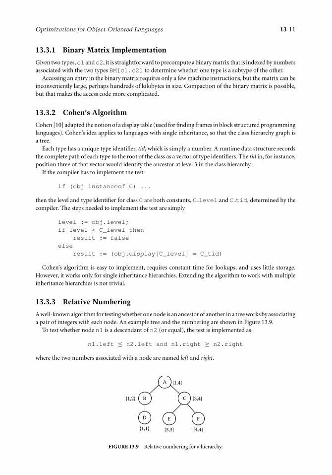
Optimizations for Object-Oriented Languages 13-11
13.3.1 Binary Matrix Implementation
Given two types,c1 andc2, it is straightforward to precompute a binary matrix that is indexed by numbersassociated with the two types BM[c1,c2] to determine whether one type is a subtype of the other.
Accessing an entry in the binary matrix requires only a few machine instructions, but the matrix can beinconveniently large, perhaps hundreds of kilobytes in size. Compaction of the binary matrix is possible,but that makes the access code more complicated.
13.3.2 Cohen’s Algorithm
Cohen [10] adapted the notion of a display table (used for finding frames in block structured programminglanguages). Cohen’s idea applies to languages with single inheritance, so that the class hierarchy graph isa tree.
Each type has a unique type identifier, tid, which is simply a number. A runtime data structure recordsthe complete path of each type to the root of the class as a vector of type identifiers. The tid in, for instance,position three of that vector would identify the ancestor at level 3 in the class hierarchy.
If the compiler has to implement the test:
if (obj instanceof C) ...
then the level and type identifier for class C are both constants, C level and C tid, determined by thecompiler. The steps needed to implement the test are simply
level := obj.level;if level < C_level then
result := falseelse
result := (obj.display[C_level] = C_tid)
Cohen’s algorithm is easy to implement, requires constant time for lookups, and uses little storage.However, it works only for single inheritance hierarchies. Extending the algorithm to work with multipleinheritance hierarchies is not trivial.
13.3.3 Relative Numbering
A well-known algorithm for testing whether one node is an ancestor of another in a tree works by associatinga pair of integers with each node. An example tree and the numbering are shown in Figure 13.9.
To test whether node n1 is a descendant of n2 (or equal), the test is implemented as
n1.left ≤ n2.left and n1.right ≥ n2.right
where the two numbers associated with a node are named left and right.
{1,4}
{3,4}
{4,4}{3,3}{1,1}
{1,2}
E
A
D
B C
F
FIGURE 13.9 Relative numbering for a hierarchy.

13-12 The Compiler Design Handbook: Optimizations and Machine Code Generation
The scheme is simple and efficient. It is probably the method of choice for implementing the subtypetest for single inheritance hierarchies. Extension of the idea to multiple inheritance hierarchies was a longtime coming, but has now been achieved by Gil and Zibin. Their scheme is known as PQ-encoding [14]and is explained in a following section.
13.3.4 Hierarchical Encoding
With hierarchical encoding, a bit vector is associated with each type. Each bit vector implements a compactset of integers. The test of whether typet1 is a subclass oft2 is implemented as the subset testt2.vector⊆ t1.vector. The approach works with multiple inheritance hierarchies.
A simple way to implement the bit vectors is to number all the nodes in the class hierarchy graph. Thebit vector for node n represents the set of all the integers associated with n and the ancestors of n. Thatyields correct but unnecessarily large vectors.
Caseau [8], Aıt-Kaci et al. [3], and Krall et al. [20] provide algorithms for constructing much smaller bitvectors. The algorithms are, however, computationally expensive and would need to be reexecuted aftereven a small change to the class hierarchy.
13.3.5 More Algorithms
Vitek et al. [32] describe three more type test algorithms that they call packed encoding, bit-packed encoding,and compact encoding. All three perform worse than hierarchical encoding if the total size of the data tablesis used as the only criterion. However, these algorithms are much faster and are therefore more suitablefor an environment where the class hierarchy may be dynamically updated, as with Java or Smalltalk, forexample.
13.3.6 Partitioning the Class Hierarchy
Because type tests for trees are more (space) efficient than type tests for direct acyclic graphs (DAGs), apossible solution is to split a DAG into a tree part and the remaining graph. For languages with singleinheritance and multiple subtyping, this partitioning of the class hierarchy is already done in the languageitself.
CACAO uses a subtype test based on relative numbering for classes and a kind of matrix implementationfor interfaces. Two numbers low and high are stored for each class in the class hierarchy. A depth-firsttraversal of the hierarchy increments a counter for each class and assigns the counter to the low field whenthe class is first encountered and assigns the counter to the high field when the traversal leaves the class. Inlanguages with dynamic class loading, a renumbering of the hierarchy is needed whenever a class is added.A class sub is a subtype of another class super if super.low ≤ sub.low ≤ super.high. Because a range check isimplemented more efficiently by an unsigned comparison, CACAO stores the difference between the lowand high values and compares it against the difference between the low values of both classes. The codefor instanceof looks similar to:
return(unsigned)(sub->vftbl->baseval - super->vftbl->baseval)<= (unsigned)(super->vftbl->diffval);
Figure 13.10 shows an example hierarchy using baseval and diffval pairs. For leaf nodes in theclass hierarchy the diffval is 0, which results in a faster test (a simple comparison of the basevalfields of the sub- and superclass). In general, a just-in-time (JIT) compiler can generate the faster test onlyfor final classes. An ahead-of-time (AOT) compiler or a JIT compiler that does patching of the alreadygenerated machine code may also replace both the baseval and the diffval of the superclass by aconstant. Currently, CACAO uses constants only when dynamic class loading is not used.
CACAO stores an interface table at negative offsets from the virtual method table (as seen inFigure 13.7). This table is needed for the invocation of interface methods. The same table is also used

Optimizations for Object-Oriented Languages 13-13
{1,5}
{5,1}
{6,0}{4,0}{3,0}
{2,2}
E
A
D
B C
F
FIGURE 13.10 Relative numbering with baseval and diffval pairs.
by the subtype test for interfaces. If the table is empty for the index of the superclass, the subtype test fails.The code for instanceof looks similar to
return (sub->vftbl->interfacetable[-super->index] != NULL);
Both subtype tests can be implemented by just a few machine code instructions without using branchesthat are expensive on modern processors.
13.3.7 PQ-Encoding
An observation made by Gil and Zibin [14] is that a minor generalization to the relative numbering schemeenables it to handle many multiple inheritance hierarchies. The example from their paper is shown inFigure 13.11. In this hierarchy, class C has two parents, A and B, and so on.
Each class in the hierarchy has three associated integers: L, R, and id. The L and R numbers represent arange [L, R], analogous to the relative numbering scheme. If we wish to test whether class C1 is a subtypeof class C2, we would perform the following test:
C1.id ≥ C2.L and C1.id ≤ C2.R
Like the relative numbering scheme, this test requires a small fixed number of instructions.Unfortunately, it is not always possible to find L, R, and id numbers that work for an arbitrary multiple
inheritance hierarchy. However, Gil and Zibin recognized that the PQ-encoding scheme could be used formost nodes in the hierarchy and that the exceptional cases would be relatively uncommon. Their solutionsolves the problem as a number of slices. The first slice is a PQ-encoding solution, like that shown inFigure 13.11, where as many nodes as possible in the hierarchy are handled. The second slice is anotherPQ-encoding solution that handles as many nodes as possible of those that were not handled by thefirst slice, and so on. The number of slices needed for even the most complicated multiple inheritancehierarchies found in practice is small.
1[1,6]
A9
[2,9]
B
2[2,4]
C5
[4,6]
D7
[6,8]
E
3[3,3]
F4
[4,4]
G6
[6,6]
H8
[8,8]
I
id[L,R]
Legend
FIGURE 13.11 PQ-encoding for a multiple inheritance hierarchy.

13-14 The Compiler Design Handbook: Optimizations and Machine Code Generation
1,1[1,6]
1A
9,2[2,9]
1B
2,3[2,4]
1C
5,4[4,6]
1D
7,8[6,8]
1E
3,5[3,3]
1F
4,6[4,4]
1G
6,9[6,6]
1H
8,10[8,8]
1I
10,7[7,10]
2N
ids
[L,R]
S
Legend
FIGURE 13.12 A two-slice PQ-encoding for a multiple inheritance hierarchy.
Figure 13.12 shows a one-node addition to the previous hierarchy, which makes it impossible to find acorrect PQ-encoding.
The PQ-encoding solution for this hierarchy requires two slices. Each class in the hierarchy now hasthree integers plus a list of integers associated with it. The first two integers, L and R, represent a range asbefore. The third integer, S, represents the slice to which that class belongs. Finally, ids is a list of integers,providing an id number for each slice. The test to determine whether class C1 is a subclass of C2 can nowbe implemented as follows:
C1.ids[C2.S] ≥ C2.L and C1.ids[C2.S] ≤ C2.R
In this code, C2.S specifies the slice to which node C2 belongs; then the expression C1.ids[C2.S]gives the id number for node C1 in that slice.
As Gil and Zibin admit, their algorithm for constructing the slices and determining the L, R, and idnumbers in each slice is not incremental. If the hierarchy changes because of dynamic class loading, it isnecessary to rerun the algorithm from scratch. However, the same is true of most of the type inclusion testimplementations described in this chapter. The major advantage of the multislice PQ-encoding scheme isthat it requires the least amount of data compared to all the other approaches, while being a (very fast)constant-time test.
13.4 Devirtualization
Devirtualization is a technique to reduce the overhead of virtual method invocation in object-orientedlanguages. The aim of this technique is to statically determine which methods can be invoked by virtualmethod calls. If exactly one method is resolved for a method call, the method can be inlined or the virtualmethod call can be replaced by a static method call. The analyses necessary for devirtualization also improvethe accuracy of the call graph and the accuracy of subsequent interprocedural analyses. We first discussdifferent type analysis algorithms, comparing their precision and complexity. Then different solutions fordevirtualization of extensible class hierarchies and similar problems are presented.
13.4.1 Class Hierarchy Analysis
The simplest devirtualization technique is class hierarchy analysis (CHA), which determines the classhierarchy used in a program. A Java class file contains information about all referenced classes. Thisinformation can be used to create a conservative approximation of the class hierarchy. The approximationis formed by computing the transitive closure of all classes referenced by the class containing the mainmethod. A more accurate hierarchy can be constructed by computing the call graph [11]. CHA uses thedeclared types for the receiver of a virtual method call for determining all possible receivers.

Optimizations for Object-Oriented Languages 13-15
Am1()m2 ()
Cm1 ()
Bm1 ()
C.main
a.m1 () b.m1 () b.m2 ()
A.m1 B.m1 C.m1 A.m2
object
FIGURE 13.13 Class hierarchy and call graph.
As an example, Figure 13.13 shows the class hierarchy and call graph that correspond to the followingfragment of Java code:
class A extends Object {void m1() {...}void m2() {...}}
class B extends A {void m1() {...}}
class C extends A {void m1() {...}public static void main(...) {
A a = new A();B b = new B();
a.m1(); b.m1(); b.m2();}
}
Informally, CHA collects all methods in the call graph in a work list of methods. This work list is initializedwith the main method. To this work list is added every method that is inherited by a subtype of thedeclared type of a virtual method call in the body of each method in the work list. The algorithm given inFigure 13.14 gives the computation of the class hierarchy and call graph in more detail.
13.4.2 Rapid Type Analysis
A more accurate class hierarchy and call graph can be computed if the type of the receiver can be determinedmore precisely than the declared type specifies. Rapid type analysis (RTA) uses the fact that a method mof a class c can be invoked only if an object of type c is created during the execution of a program [5, 6].RTA refines the class hierarchy by only including classes for which objects can be created at runtime. Thepessimistic algorithm includes all classes in the class hierarchy for which instantiations occur in methodsof the call graph from CHA.
The optimistic algorithm initially assumes that no methods besides main are called and that no objectsare instantiated. It traverses the call graph, initially ignoring virtual calls (only marking them in a class

13-16 The Compiler Design Handbook: Optimizations and Machine Code Generation
/* Notation:main -- the main method in a programx ( ) -- call of static method xtype (x) -- the declared type of the expression xx. y () -- call of virtual method y in expression xsubtype (x) -- x and all classes which are subtypes of xmethod (x, y) -- the method y which is defined for class x
*/callgraph := mainhierarchy := { }for each m in callgraph do
for each ms tat ( ) occurring in m doif ms tat not in callgraph then
add ms tat to callgraphfor each e.mvir ( ) occurring in m dofor each c in subtype (type (e)) do
mde f := method (c , mvir )if mde f not in callgraph then
add mde f to callgraphadd c to hierarchy
FIGURE 13.14 Class hierarchy analysis.
mapping as a potential call) and following static calls only. When the instantiation of an object is foundduring the analysis, all virtual methods of the corresponding class that were left out previously are thentraversed as well. The live part of the call graph and the set of instantiated classes grow interleaved as thealgorithm proceeds.
Figure 13.15 shows the rapid type analysis algorithm.
13.4.3 Other Fast Precise-Type Analysis Algorithms
Tip and Palsberg [30] evaluated different algorithms that are more precise but are on average only a factorof five slower than RTA. The different type analysis algorithms differ primarily in the number of sets oftypes used. RTA uses one set for the whole program. 0-Control flow analysis (CFA) [15, 26] uses one set perexpression. k–l-CFA makes separate analyses for k levels of method invocations and uses more than one setper expression. These algorithms have high computational complexity and only work for small programs.Therefore, Tip and Palsberg evaluated the design space between RTA and 0-CFA [30] by proposing andcomparing three analysis algorithms which they name XTA, MTA, and FTA.
XTA uses a distinct set for each field and method of a class, fast type analysis (FTA) uses one set for allfields and a distinct set for every method of a class, and MTA uses one set for all methods and a distinct setfor every field of a class. Arrays are modeled as classes with one instance field. All algorithms use iterativepropagation-based flow analysis to compute the results. Three work lists are associated with each methodor field that keeps track of processed types. New types are propagated to the method or field in the currentiteration and can be propagated onward in the next iteration. Current types can be propagated onward inthe current iteration. Processed types have been propagated onward in previous iterations.
Tip and Palsberg efficiently implemented the type sets using a combination of array-based and hash-based data structures to allow efficient membership tests, element additions, and iterations over all elements[30]. Type inclusion is implemented by relative numbering. These techniques are necessary because thetype sets are filtered by the types of fields, method parameters, and method return types. Additionally,type casts restricting return types are used for filtering.

Optimizations for Object-Oriented Languages 13-17
/* Notation:main -- the main method in a programnew x -- instantiation of an object of class xmarked (x) -- marked methods of class xx ( ) -- call of static method xtype (x) -- the declared type of the expression xx.y ( ) -- call of virtual method y in expression xsubtype (x) -- x and all classes which are subtypes of xmethod (x, y) -- the method y which is defined for class xmark (m, x) -- mark method m in class x
*/callgraph := mainhierarchy := { }for each m in callgraph do
for each new c occurring in m doif c not in hierarchy then
add c to hierarchyfor each mmar k in marked (c) do
add mmar k to callgraphfor each ms tat () occurring in m do
if ms tat not in callgraph thenadd ms tat to callgraph
for each e.mvir ( ) occurring in body (m) dofor each c in subtype (type (e)) do
mde f : = method c, mvir )if mde f not in callgraph then
if c not in hierarchy thenmark (mde f , c)
elseadd mdef do callgraph
FIGURE 13.15 Rapid type analysis.
All these algorithms are more precise than RTA. On the range of Java benchmark programs (benchmarkcode only), MTA computes call graphs with 0.6% fewer methods and 1.6% fewer edges than RTA. FTAcomputes call graphs with 1.4% fewer methods and 6.6% fewer edges than RTA. XTA computes callgraphs with 1.6% fewer methods and 7.2% fewer edges than RTA. All algorithms are about five times asslow as RTA. Therefore, XTA has the best precision and performance trade-off of the three algorithmscompared.
13.4.4 Variable Type Analysis
RTA is imprecise because every type that is instantiated somewhere in the program and is a subtype ofthe declared type can be the receiver of a method invocation. Variable type analysis (VTA) is more precisebecause it computes reaching type information, taking into consideration chains of assignments betweeninstantiations and method invocations [27], but it does ignore type casts. It is a flow-insensitive algorithmthat avoids iterations over the program. The analysis works by constructing a directed type propagationgraph where nodes represent variables and edges represent assignments. Reaching type information isinitialized by object instantiations and propagated along the edges of the type propagation graph.

13-18 The Compiler Design Handbook: Optimizations and Machine Code Generation
The type propagation graph is constructed from the classes and methods contained in the conservativecall graph. For every class c and for every field f of c that has a reference type, a node c.f is created.Additionally for every method c .m and:� For every formal parameter p (including this) of c.m that has a reference type, create a node c.m.p.� For every local variable l of c.m that has a reference type, create a node c.m.l.� If c.m returns a reference type, create a node c.m.ret.
After the nodes are created, for every assignment of reference types an edge is added to the graph. As-signments are either explicit assignments of local variables or object fields or assignments resulting frompassing of parameters or returning a reference value. Native methods are handled by summarizing theireffects on the analysis.
To avoid alias analysis, all variable references and all their aliases are represented by exactly one node.In Java, locals and parameters cannot be aliased. All instances of a field of a class are represented by onenode. Arrays can introduce aliasing. Different variables can point to the same array. Therefore, if bothsides of an assignment are of type Object or if at least one side is an array type, edges in both directionsare added.
Type propagation is accomplished in two phases. The first phase detects strongly connected componentsin the type propagation graph. All nodes of a strongly connected component are collapsed into onesupernode. The type of this supernode is the union of the types of all its subnodes. The remaining graph isa DAG. Types are propagated in a topological order where a node is processed after all its predecessors havebeen processed. The complexity of both strongly connected component detection and type propagationis linear in the maximum of the number of edges and nodes. The most expensive operation is the unionof type sets.
The algorithm does no killing of types on casts or declared types. An algorithm using declared typeinformation would be more precise, but collapsing of strongly connected components would not be pos-sible anymore. Impossible types are filtered after type propagation has been finished. Over the set ofJava benchmarks (the benchmark code only), VTA computes call graphs with 0.1 to 6.6% fewer meth-ods and 1.1 to 18% fewer edges than RTA. For the set of Java applications (including the libraries),VTA computes call graphs with 2.1 to 20% fewer methods and 7.7 to 27% fewer edges than RTA.The implementation is untuned and written in Java. The performance numbers indicate that the al-gorithm scales linearly with the size of the program (54 sec for 27,570 instructions, 102 sec for 55,468instructions).
13.4.5 Cartesian Product Algorithm
Agesen [2] developed a type analysis algorithm called the Cartesian product algorithm (CPA), in which amethod is analyzed separately for every combination of argument types (Cartesian product of the argumenttypes). For example, a method with two arguments, where the first argument can be of typeInt andLongand the second argument can be of type Float and Double, can result in four different analyses withargument types (Int, Float), (Long, Float), (Int, Double), and (Long, Double).For better precision, CPA computes the needed analyses lazily. Only argument type combinations thatoccur during program analysis are analyzed. The return type of a method is the union of the return typesof the different analyses for a specific method invocation.
CPA is precise in the sense that it can analyze arbitrary deep call chains without loss of precision. CPAis efficient, because redundant analysis is avoided. However, megamorphic call sites, where the methodhas many arguments and an argument has a high number of different types, can lead to long analysistimes. Therefore, Agesen restricted the number of different types for an argument and combined theanalyses if the number exceeded a small constant. The bounded CPA scales well for bigger programstoo.

Optimizations for Object-Oriented Languages 13-19
13.4.6 Comparisons and Related Work
Grove et al. investigated the precision and complexity of a set of type analysis algorithms [15]. Theyimplemented a framework where different algorithms can be evaluated. They evaluated RTA, the boundedCPA, and different levels of k–l-CFA. CPA gives more accuracy than 0-CFA with reasonable computationtimes. The higher levels of k–l-CFA cannot be used for large applications.
CHA and RTA have the same time complexity, but RTA always produces more accurate results. Theresults for XTA and VTA cannot be compared directly, since different programs are used for benchmarking,and the implementation of VTA was not done for performance. It can be estimated that the running timefor the algorithms will be similar, but VTA may produce more accurate results. 0-CFA is more accuratethan the other algorithms at slightly higher analysis costs.
Qian and Hendren [24] did a limit study and compared dynamic CHA and VTA with an ideal typeanalysis based on efficient call graph profiling using the Jikes Research Virtual Machine (JikesRVM) as atestbed. The ideal type analysis logs the call targets of each virtual method call during the first benchmarkrun and determines all monomorphic method invocations. The logged information is used in subsequentbenchmark runs to compare the inlining results of other analyses against the ideal one.
Qian and Hendren developed a common dynamic type analysis framework for method inlining in theJikesRVM. The framework supports speculative inlining with invalidations. Since the framework is writtenin Java, the data structures impose more work on the garbage collector. VTA analysis increases the livedata by 60% for the javac benchmark program.
Already the simple CHA comes close to the ideal type analysis for virtual method calls but misses someinlining opportunities for interface calls. Dynamic VTA is as effective as the ideal type analysis for interfacecalls, leading to speedups between 0.6 and 2.1% over CHA.
13.4.7 Inlining and Devirtualization Techniques
Ishizaki et al. [17] point out that straightforward devirtualization may have little effect on the perfor-mance of Java programs. Because Java is strongly typed, a vtbl can be used for dispatching. Devirtual-izing simply removes the lookup in the vtbl, and that is not significant compared with the other costsof calling a method. Significant performance gains only arise if the devirtualized method is inlined atthe call site; many opportunities for devirtualization are lost in any case because Java has dynamic classloading.
Ishizaki et al. [17] propose a technique based on code patching that allows methods to be inlined andinlining to be removed if dynamic class loading subsequently requires the method call to be implementedby the normal vtbl dispatching again. Their code patching technique avoids any need to recompile the codeof the caller.
An example can make the idea clear. Suppose that the program to be compiled contains the followingJava statements:
i = i + 1;obj.meth(i,j);j = j-1;
The compiler would normally generate the following pattern of code for those statements:
// code for i = i + 1// code to load arguments i and j// dispatch code to lookup address of method meth// ... and pass obj and arguments to that method// code for j = j-1

13-20 The Compiler Design Handbook: Optimizations and Machine Code Generation
Now suppose analysis of the program shows that only one possible implementation of method meth canbe invoked at this call site. If the body of that method is reasonably small, it can be inlined. The generatedcode corresponds to the following pattern:
// code for i = i + 1// inlined code for method meth parameterized// ... by the arguments obj, i, and j
L2: // code for j = j - 1
... // much omitted code
L1: // code to load arguments i and j// dispatch code to lookup address of method meth// ... and pass arguments and obj to that methodgoto L2;
Label L1 is not reached with this version of the code.Now suppose dynamic class loading causes an alternative implementation of method meth to be loaded.
The runtime environment now uninlines the method call by patching the code. It overwrites the first wordof the inlined method with a branch instruction, so that the patched code corresponds to the followingpattern:
// code for i = i + 1goto L1// remainder of code of inlined method, which// is now unreachable.
L2: // code for j = j - 1
... // much omitted code
L1: // code to load arguments i and j// dispatch code to lookup address of method meth// ... and pass arguments and obj to that methodgoto L2;
This patched code contains two more branches than the original unoptimized program and wouldtherefore run more slowly; it also contains unreachable code that incurs a modest space penalty. Theassumption is that dynamic class loading is rare and that methods rarely need to be uninlined.
Experiments with a JIT compiler showed that the number of dynamic method calls is reduced by 9 to97% on their test suite. The effect on execution speed ranged from a small 1% worsening of performanceto an impressive 133% improvement in performance, with a geometric mean speedup of 16%.
Ishizaki et al. [17] also point out that a similar technique is applicable to a method invoked via aninterface. If only one class implements an interface class, we can generate code that assumes this class isactually used and we can inline methods of that class that are not overridden by any of its subclasses. If theassumption is later broken by dynamically loading a new class that also implements the interface or thatoverrides the method, we can patch the code to revert to the original full scheme of looking up the classand looking up the method.
13.5 Escape Analysis
In general, instances of classes are dynamically allocated. Storage for these instances is normally allocated onthe heap. In a language such as C++, where the programmer is responsible for allocating and deallocating
Optimizations for Object-Oriented Languages 13-21
memory for objects on the heap, the program should free the memory for a class instance when it is nolonger needed. Other languages, such as Java, provide automatic garbage collection. At periodic intervals,the garbage collector is invoked to perform the computationally intensive task of tracing through thereferences between objects and determining which objects can no longer be referenced. The storage forthese objects is reclaimed.
The goal of escape analysis is to determine which objects have lifetimes that do not stretch outside thelifetime of their immediately enclosing scopes. The storage for such objects can be safely allocated as partof the current stack frame; that is, their storage can be allocated on the runtime stack. (For C programmerswho use the gcc C compiler, the transformation is equivalent to replacing a use of the malloc functionwith the alloca function.) This optimization is valuable for Java programs. The transformation alsoimproves the data locality of the program and, depending on the computer cache, can significantly reduceexecution time.
Another benefit of escape analysis is that objects with lifetimes that are confined to within a single scopecannot be shared between two threads. Therefore, any synchronization actions for these objects can beeliminated. Escape analysis does not capture all possibilities for synchronization removal, however. If thisis deemed to be an important optimization, a separate analysis to uncover unnecessary synchronizationoperations should be performed.
Algorithms for escape analysis are based on abstract interpretation techniques [1]. Different algorithmsmake different trade-offs between the precision of the analysis and the length of time the analysis takes.The better the precision, the more opportunities for optimization that should be found.
The reported speedup of Java programs can range up to 44% [7], but that figure includes savings due tosynchronization removal and due to inlining of small methods. (Blanchet [7] reports an average speedupof 21% in his experiments.) Inlining significantly increases the number of opportunities for finding objectsthat do not escape from their enclosing scope, especially because many methods allocate a new object thatis returned as the result of the method call.
13.5.1 Escape Analysis by Abstract Interpretation
A prototype implementation of escape analysis was included in the IBM High Performance Compiler forJava. This implementation is based on straightforward abstract interpretation techniques and has beenselected for presentation in this text because it is relatively easy to understand. Further details of thealgorithm may be found in the paper published by Choi et al. [9].
The approach of Choi et al. [9] attempts to determine two properties for each allocated object—whetherthe object escapes from a method (i.e., from the scope where it is allocated), and whether the object escapesfrom the thread that created it. It is possible that an object escapes the method but does not escape fromthe thread, and thus synchronization code may be removed. The converse is not possible; if an object doesnot escape a method, then it cannot escape its thread. The analysis therefore uses the very simple latticeof three values shown in Figure 13.16. If analysis determines that an object status is NoEscape, the objectdefinitely does not escape from its method or from its thread; if the status is ArgScape, the object mayescape from a method via its arguments but definitely does not escape the thread; finally, GlobalEscapemeans the object may escape from both the method and the thread.
The two versions of the analysis are a fast flow-insensitive version that yields imprecise results and a slowerflow-sensitive version that gives better results. Imprecise means the analysis can be overly conservative,reporting many objects as having GlobalEscape status when a more accurate analysis might have shownthe status as one of the other two possibilities, or reporting ArgEscape instead of NoEscape. Imprecision inthis manner does not cause incorrect optimizations to be made; some opportunities for optimization cansimply be missed. We give only the more precise flow-sensitive version of the analysis in this chapter.
13.5.1.1 Connection Graphs
As its name suggests, abstract interpretation involves interpretive execution of the program. With thisform of execution, the contents of variables (or fields of classes when analyzing a Java program) are

13-22 The Compiler Design Handbook: Optimizations and Machine Code Generation
ArgEscape
GlobalEscape ( )
NoEscape (T)
FIGURE 13.16 Lattice elements for escape analysis.
tracked. However, we do not attempt to determine the contents of the variables for normal execution ofthe program—we would of course simply execute the program to do that. To perform escape analysis,we are interested only in following an object O from its point of allocation, knowing which variablesreference O and which other objects are referenced by O fields. The abstraction implied in the nameabstract interpretation is to abstract out just the referencing information, using a graph structure wherenodes represent variables and objects and directed edges represent object references and containment offields inside objects. Choi et al. [9] call this graph a connection graph.
A sample connection graph is shown in Figure 13.17; it shows the program state after executing thecode:
A a = new A(); // line L1a.b1 = new B(); // line L2a.b2 = a.b1;
where we assume that the only fields of AC are b1 and b2, and BC has only fields with intrinsic types (i.e.,the types int and char).
The notational conventions used in the connection graph are as follows. A circle node represents avariable (i.e., a field of a class or a formal parameter of a method); a square node represents an objectinstance. An edge from a circle to a square represents a reference; an edge from a square to a circlerepresents ownership of fields.
The graph shown in Figure 13.17 on the left is a simplification of that used by Choi et al. [9]. Their morecomplicated graph structure has two kinds of edges. An edge drawn as a dotted arrow is called a deferrededge. When there is an assignment from copies of one object reference to another, which copies an objectreference from one variable to another, such as
p = q; // p and q have class types
then the effect of the assignment is shown as a deferred edge from the node for p to the node for q. InFigure 13.17, the graph on the right uses a deferred edge to show the effect of an assignment from onevariable to another.
a
Simple Version
b1 b2
L1
L2
a
Using Deferred Edges
b1 b2
L1
L2
FIGURE 13.17 Sample connection graph.

Optimizations for Object-Oriented Languages 13-23
Before After
a
c
L1
cb
p
a L1
b
p
FIGURE 13.18 Effect of bypass operation.
Each node in a connection graph has an associated escape state, chosen from the three possibilities givenin Figure 13.16. If a connection graph has been constructed for a method M and if O is an object node inM, then if O can be reached from any node in the graph whose escape state is other than NoEscape, thenO may escape from M. A similar property holds for objects escaping from a thread.
13.5.1.2 Intraprocedural Abstract Interpretation
The abstract interpretation is performed on a low-level version of the code where only one action at a timeis performed. The Java bytecode is adequate for this purpose, as are other intermediate representationformats used in a typical compiler. Assuming that the code has been suitably simplified, abstract inter-pretation of the code within a method steps through the code and performs an action appropriate foreach low-level operation. This interpretive execution involves following control flow edges, as explainedin more detail later.
The actions for assignment statements and instantiations of new object instances are shown next. Eachaction involves an update to the connection graph. An assignment to a variable p kills any value that thevariable previously had. The kill part of an assignment to p is implemented by an update to the connectiongraph that is called ByPass(p). The ByPass(p) operation redirects or removes deferred edges as illustrated inFigure 13.18. Note also that compound operations, such asp.a.b.c, are assumed to be decomposed intosimpler steps that dereference only one level at a time. The bytecode form of the program automaticallypossesses this property:
p = new C(); // line L
If the connection graph does not already contain an object node labeled L, one is created and added tothe graph. If the node needs to be created, then nodes for the fields of C that have nonintrinsic types arealso created and are connected by edges pointing from the object node. Any outgoing edges from the nodefor p are deleted by applying the ByPass(p) operation, and then a new edge from p to the object node forL is added:
p=q;
The ByPass(p) operation is applied to the graph. Then a new deferred edge from p to q is created:
p.f=q;
Ifp does not point to any object nodes in the connection graph, a new object node (with the appropriatefields for the datatype of p) is created and an edge from p to the new object node is added to the graph.(Choi et al. [9] call this new object node a phantom node. Two reasons phantom nodes may arise are (a)the original program may contain an error and p would actually be null, referencing no object, when thisstatement is reached and (b) p may reference an object outside the current method—and that situationcan be covered by the interprocedural analysis.) Then, for each object node that is connected to p by anedge, an assignment to the f field of that object is performed. That assignment is implemented by addinga deferred edge from the f node to the q node. Note that no ByPass operation is performed (to kill the

13-24 The Compiler Design Handbook: Optimizations and Machine Code Generation
previous value of f) because there is not necessarily a unique object that p references, and we cannottherefore be sure that the assignment kills all previous values for f:
p = q.f;
As before, if q does not point at any object nodes, a phantom node is created, and an edge from q tothe new node is added to the graph. Then ByPass(p) is applied, and deferred edges are added from p to allthe f nodes that q is connected to by field edges.
In principle, a different connection graph represents the state of the program at each statement inthe method. Thus, when the abstract interpretation action modifies the graph, it is modifying a copy ofthe graph. When analyzing a sequence of statements in a basic block, the analysis proceeds sequentiallythrough the statements in order. At a point where control flow diverges, such as at a conditional statement,each successor statement of the conditional is analyzed using a separate copy of the connection graph. At apoint where two or more control paths converge, the connection graphs from each predecessor statementare merged.
A small example is given to make the process clearer. Suppose the code inside some method is as follows,with the declarations of classes A, B1, and B2 omitted:
A a = new A(); // line L1if (i > 0)
a.f1 = new B1(); // line L3else
a.f1 = new B2(); // line L5a.f2 = a.f1; // line L6
The connection graphs that are constructed by the abstract interpretation actions are shown inFigure 13.19. Diagram 1 in the figure shows the state after executing line L1; diagrams 2 and 3 show
a
f1 f 2
L1 a
f1 f2
L1
L3
1. 2.
4. a
f1 f 2
L1
L3 L5
3. a
f1 f2
L1
L5
5. a
f1 f2
L1
L3 L5
FIGURE 13.19 Sequence of connection graphs.

Optimizations for Object-Oriented Languages 13-25
L3head
nextn
After One Iteration After Two or More
Iterations
L3head
nextn
FIGURE 13.20 Connection graph for a loop.
the states after lines L3 and L5, respectively. Note that diagrams 2 and 3 are obtained by applying theeffects of lines L3 and L5 to the state in diagram 1. After the if statement, the two control flow paths merge;the graph in diagram 4 is the result of merging diagrams 2 and 3. Finally, diagram 5 shows the effect ofapplying line L6.
If the program contains a loop, abstract interpretation is performed repeatedly until the connectiongraphs converge. Convergence is guaranteed because the maximum number of nodes in the graph is a finitenumber that is proportional to the number of occurrences of new in the source code, and the number ofedges that can be added between the nodes is also finite. If, for example, the source code to be analyzed is
Node head = null;for( int cnt = 0; cnt < 1000; cnt++ ) {
Node n = new Node(); // Line L3n.next = head;n.data = cnt;head = n;
}
then analysis gives the connection graphs shown in Figure 13.20. After analyzing the loop body once, thegraph has the structure shown on the left; after analyzing a second time, the graph has converged to thediagram on the right. Even though the actual program allocates 1,000 instances of the Node class, onlyone new operation is in the code, and therefore only one object node is in the graph. The fact that onegraph node represents 1,000 objects in the program is one of the approximations inherent in the graphstructure invented by Choi et al. [9].
13.5.1.3 Interprocedural Abstract Interpretation
A call to a method M is equivalent to copying the actual parameters (i.e., the arguments are passed inthe method call) to the formal parameters, then executing the body of M, and finally copying any valuereturned by M as its result back to the caller. If M has already been analyzed intraprocedurally following theapproach described earlier, the effect of M can be summarized with a connection graph. That summaryinformation eliminates the need to reanalyze M for each call site in the program.
It is necessary to analyze each method in the reverse of the order implied by the call graph. If method Amay call methods B and C, then B and C should be analyzed before A. Recursive edges in the call graphare ignored when determining the order. Java has virtual method calls. At a method call site where itis not known which method implementation is invoked, the analysis must assume that all the possibleimplementations are called, combining the effects from all the possibilities. The interprocedural analysisiterates over all the methods in the call graph until the results converge. The extra actions needed to createthe summary information for a method M follow:
Entry to a methodM: If Mhas n−1 formal parameters, fi, . . . fn, then n object nodes a1 . . . an are created.These correspond to the actual parameters (or arguments). The extra parameter corresponds to theimplicit this parameter. Because Java has call-by-value semantics, an implicit assignment exists

13-26 The Compiler Design Handbook: Optimizations and Machine Code Generation
from each actual parameter to the corresponding formal parameter at method invocation. Theseassignments are modeled by creating a deferred edge from fi to ai for each parameter. The escapestate initially associated with an fi node is NoEscape, and the state initially associated with an ai nodeis ArgEscape. By having created the first object nodes for the parameters, the body of the method isanalyzed using the approach described for intraprocedural analysis.
Exit from method M: A return statement is processed by creating a dummy variable named return,to which the returned result is assigned. If there are multiple return statements in the method,the different result values are merged into the connection graph by adding deferred edges from thereturn node to the different results.
When the whole method body has been processed, the connection graph that was created after thereturn statement represents the summary information for the method. In particular, after the ByPassfunction has been used to eliminate all deferred edges, the connection graph can be partitioned into threesubgraphs:
Global escape nodes: All nodes that are reachable from a node whose associated state is GlobalEscapeare themselves nodes that are considered to be global escape nodes and form the first subgraph.The nodes initially marked as GlobalEscape are the static fields of any classes and instances of anyclass that implements the Runnable interface.
Argument escape nodes: All nodes reachable from a mode whose associated state is ArgEscape, but arenot reachable from a Global Escape node, are in the second subgraph. The nodes initially markedas ArgEscape are the argument nodes a1 . . . an.
No escape nodes: All other nodes in the connection graph form the third subgraph and have NoEscapestatus.
All objects created within a method M and that have the NoEscape status after the three subgraphs aredetermined can be safely allocated on the stack. The third subgraph represents the summary informationfor the method because it shows which objects can be reached via the arguments passed to the method.The part that remains to be covered is how to process a method call when it is encountered in the body ofthe method analyzed.
Suppose that while analyzing some method m1, we reach a method call:
result = obj.m2(p1,p2);
and that we have previously analyzed methodm2 in the class to whichobj belongs. The analysis algorithmcreates three formal parameter nodes a1, a2, and a3 and processes three assignments:
a1 = obj; a2 = p1; a3 = p2;
The nodes a1 . . . correspond to the argument nodes a1 . . . in the connection graph that summarizesmethod m2, whereas the values obj, p1, and p2 are nodes within the connection graph constructed formethod m1.
The summary connection graph for m2 is used like a macro. Connections from a1 . . . are copied,becoming edge connections fromobj. Field nodes that are children of object values thatai nodes referenceare matched against field nodes that are children of the obj, p1, and p2 nodes and so on recursively.During this process, many of the phantom nodes that were introduced into the connection graph of m2can be matched against nodes of m1. The algorithm for matching and duplicating the nodes and edges isomitted for space reasons.
One more issue needs to be covered. If the method call graph contains cycles, as occurs in the presenceof direct or indirect recursion, then it appears to be necessary to use a method summary connection graphbefore it has been created. For this situation, a special bottom graph is used in place of the connectiongraph for the unanalyzed method. The bottom graph represents a worst-case (or conservative) scenariofor escape of objects from any method in the program. The bottom graph has one node for every class. Apoints-to edge is from the node for class C1 to the node for class C2 if C1 contains a field of type C2; a

Optimizations for Object-Oriented Languages 13-27
deferred edge is from the node for C1 to the node for C2 if C2 is a subtype of C1. This graph can be usedto make a conservative estimate for the escape of objects passed to a method by matching the argumenttypes against the nodes in the bottom graph.
13.5.2 Other Approaches
Blanchet [7] developed a different analysis technique. His approach also uses abstract interpretation, butthree significant differences exist.
First, the Java bytecode is directly interpreted so that an abstract representation of the values on the Javaruntime stack is managed. During abstract interpretation, each bytecode operation has an effect on thatrepresentation of the stack.
Second, information is propagated both forward and backward. Forward propagation occurs wheninstructions are analyzed following the normal flow of control — as in the approach of Choi et al. [9].Backward propagation is performed by interpretively executing the bytecode instructions along the reverseof control flow paths. The reverse execution mode has, of course, different semantics for the abstractmeaning of each instruction (e.g., an instruction that pushes a value when interpreted forward becomesone that pops a value when analyzed backward). The combination of forward and backward analysis passesenables much more precise results to be obtained, especially when used in conjunction with the programanalyzed containing no errors. (This is a common assumption for code optimization.)
Third, Blanchet [7] uses a quite different domain of values to represent escape of objects. He representseach class type by an integer, which is the context for what may escape from an instance of that class. Hisabstract values are equations (or context transformers) that map from the contexts of the arguments andresult of a method to the escape contexts of concrete values. Instead of manipulating a collection of graphs,like Choi et al. [9], Blanchet [7] manipulates sets of equations.
No comparison has been made between the approaches of Choi et al. and Blanchet. Blanchet statesthat the Choi et al. analysis is more time consuming, and that is almost certainly true. Blanchet also claimsbigger speedups for his set of sample programs, but Blanchet also performs extensive inlining of smallmethods.
13.6 Conclusion
We presented the most important optimizations for object-oriented programming languages that shouldgive language implementors good choices for their work. Method invocation can be efficiently solved bydifferent kinds of dispatch tables and inlining. Inlining and specialization greatly improve the performancebut need precise and efficient type analysis algorithms. Escape analysis computes the information necessaryto allocate objects on the runtime stack.
References
1. S. Abramsky and C. Hankin. 1987. Abstract interpretation of declarative languages. New York: EllisHorwood.
2. O. Agesen. 1995. The Cartesian product algorithm: Simple and precise type inference of parametricpolymorphism. In ECOOP ’95 — Object-Oriented Programming, 9th European Conference, ed. W. G.Olthoff, 2–26. Lecture Notes in Computer Science, Vol. 952. New York: Springer-Verlag.
3. H. Aıt-Kaci, R. Boyer, P. Lincoln, and R. Nasr. 1989. Efficient implementation of lattice operations.ACM Trans. Program. Lang. Syst. 11(1):115–46.
4. B. Alpern, A. Cocchi, D. Grove, and D. Lieber. 2001. Efficient dispatch of Java interface methods.In HPCN ’01: Java in High Performance Computing, ed. V. Getov and G. K. Thiruvathukal, 621–28.Lecture Notes in Computer Science, Vol. 2110. New York: Springer-Verlag.
5. D. F. Bacon. 1997. Fast and effective optimization of statically typed object-oriented languages.Ph.D. thesis, University of California, Berkeley.

13-28 The Compiler Design Handbook: Optimizations and Machine Code Generation
6. D. F. Bacon and P. F. Sweeney. 1996. Fast static analysis of C++ virtual function calls. In Conferenceon Object-Oriented Programming Systems, Languages & Applications (OOPSLA ’96), 324–41. NewYork: ACM Press.
7. B. Blanchet. 2000. Escape analysis for object oriented languages: Application to java. In Proceedingsof OOPSLA ’99, 20–34. New York: ACM Press.
8. Y. Caseau. 1993. Efficient handling of multiple inheritance hierarchies. In Proceedings of OOPSLA’93, 271–87. New York: ACM Press.
9. J.-D. Choi, M. Gupta, M. J. Serrano, V. C. Sreedhar, and S. P. Midkiff. 2003. Stack allocation andsynchronization optimizations for Java using escape analysis. ACM Trans. Program. Lang. Syst.25(6):876–910.
10. N. J. Cohen. 1991. Type-extension type tests can be performed in constant time. ACM Trans. Program.Lang. Syst. 13(4):626–29.
11. J. Dean, D. Grove, and C. Chambers. 1995. Optimization of object-oriented programs using staticclass hierarchy analysis. In Proceedings of the 9th European Conference on Object-Oriented Program-ming (ECOOP ’95), 77–101. Lecture Notes in Computer Science, Vol. 952. New York: Springer-Verlag.
12. P. Dencker, K. Durre, and J. Heuft. 1984. Optimization of parser tables for portable compilers. ACMTrans. Program. Lang. Syst. 6(4):546–72.
13. S. Gehmawat, K. H. Randall, and D. J. Scales. 2000. Field analysis: getting useful and low-costinter-procedural information. In Conference on Programming Language Design and Implementation,334–44. New York: ACM Press.
14. J. Gil and Y. Zibin. 2005. Efficient subtyping tests with PQ-encoding. ACM Trans. Program. Lang.Syst. 27(5):819–56.
15. D. Grove, G. DeFouw, J. Dean, and C. Chambers. 1997. Call graph construction in object-orientedlanguages. In Proceedings of the ACM SIGPLAN Conference on Object-Oriented Programming Systems,Languages and Applications (OOPSLA-97), 108–24. New York: ACM Press.
16. U. Holzle, C. Chambers, and D. Ungar. 1991. Optimizing dynamically-typed object-oriented pro-gramming languages with polymorphic inline caches. In Proceedings of the European Conference onObject-Oriented Programming (ECOOP ’91), 21–38. Lecture Notes in Computer Science, Vol. 512.New York: Springer-Verlag.
17. K. Ishizaki, M. Kawahito, T. Yasue, H. Komatsu, and T. Nakatani. 2000. A study of devirtualizationtechniques for a JavaTM just-in-time compiler. In Proceedings of the Conference on Object-OrientedProgramming, Systems, Languages and Application (OOPSLA-00), 294–310. New York: ACM Press.
18. R. Jones and R. Lins. 1996. Garbage collection. New York: John Wiley & Sons.19. A. Krall and R. Grafi. 1997. CACAO — A 64 bit JavaVM just-in-time compiler. Concurrency Practice
Exper. 9(11):1017–30.20. A. Krall, J. Vitek, and N. Horspool. 1997. Near optimal hierarchical encoding of types. In 11th
European Conference on Object Oriented Programming (ECOOP ’97), ed. M. Aksit and S. Matsuoka,128–45. Lecture Notes in Computer Science, Vol. 1241. New York: Springer-Verlag.
21. B. Liskov, D. Curtis, M. Day, S. Ghemawat, R. Gruber, P. Johnson, and A. C. Myers. 1995. Thetareference manual. In Technical Report Programming Methodology Group Memo 88. Laboratory forComputer Science, Massachusetts Institute of Technology, Cambridge, MA.
22. A. C. Myers. 1995. Bidirectional object layout for separate compilation. In OOPSLA ’95 ConferenceProceedings: Object-Oriented Programming Systems, Languages, and Applications, 124–39. New York:ACM Press.
23. W. Pugh and G. Weddell. 1990. Two-directional record layout for multiple inheritance. In Proceedingsof the ACM SIGPLAN ’90 Conference on Programming Language Design and Implementation (PLDI’90), 85–91. New York: ACM Press.
24. F. Qian and L. J. Hendren. 2005. A study in type analysis for speculative method inlining in aJIT environment. In Proceedings of International Conference on Compiler Construction (CC 2005),255–70, Lecture Notes in Computer Science, Vol. 3443. New York: Springer-Verlag.
Optimizations for Object-Oriented Languages 13-29
25. J. R. Rose. 1991. Fast dispatch mechanisms for stock hardware. In OOPSLA ’88: Object-OrientedProgramming Systems, Languages and Applications: Conference Proceedings, ed. N. Meyrowitz, 27–35.New York: ACM Press.
26. O. Shivers. 1991. Control-flow analysis of higher-order languages. Ph.D. thesis, Carnegie-MellonUniversity, Pittsburgh, PA.
27. V. Sundaresan, L. J. Hendren, C. Razafimahefa, R. Vallee-Rai, P. Lam, E. Gagnon, and C. Godin. 2000.Practical virtual method call resolution for Java. In Proceedings of the Conference on Object-OrientedProgramming, Systems, Languages and Application (OOPSLA-00), 264–80. New York: ACM Press.
28. T. Suganuma, T. Ogasawara, M. T. Yasuekeuchi, M. Kawahito, K. Ishizaki, and H. Komatsuatani.2000. Overview of the IBM Java just-in-time compiler. IBM Syst. J. 39(1):175–93.
29. B. Stroustrup. 1989. Multiple inheritance for C++. Comput. Syst. 2(4):367–95.30. F. Tip and J. Palsberg. 2000. Scalable propagation-based call graph construction algorithms. In
Proceedings of the Conference on Object-Oriented Programming Systems, Languages and Application(OOPSLA-00), 281–93. New York: ACM Press.
31. J. Vitek and R. N. Horspool. 1996. Compact dispatch tables for dynamically typed object orientedlanguages. In Proceedings of International Conference on Compiler Construction (CC ’96), 307–25,Lecture Notes in Computer Science, Vol. 1060. New York: Springer-Verlag.
32. J. Vitek, N. Horspool, and A. Krall. 1997. Efficient type inclusion tests. In Conference on Object-Oriented Programming Systems, Languages and Applications (OOPSLA ’97), ed. T. Bloom, 142–57.New York: ACM Press.
33. O. Zendra, D. Colnet, and S. Collin. 1997. Efficient dynamic dispatch without virtual functiontables: The Small Eiffel compiler. In Proceedings of the ACM SIGPLAN Conference on Object-OrientedProgramming Systems, Languages and Applications (OOPSLA-97), 125–41. New York: ACM Press.
34. Y. Zibin and J. Gil. 2002. Fast algorithm for creating space efficient dispatching tables withapplication to multi-dispatching. In Proceedings of the 17th ACM SIGPLAN Conference onObject-Oriented Programming, Systems, Languages and Applications (OOPSLA-02), 142–60.New York: ACM Press.


14Program Slicing
G. B. MundDepartment of Computer Science andEngineering,Kalinga Institute of IndustrialTechnology, Bhubaneswar, India,[email protected]
Rajib MallDepartment of Computer Science andEngineering,Indian Institute of Technology,Kharagpur, India,[email protected]
14.1 Introduction . . . . . . . . . . . . . . . . . . . . . . . . . . . . . . . . . . . . . . . . . .14-1Static and Dynamic Slicing • Backward and Forward Slicing• Organization of the Chapter
14.2 Applications of Program Slicing . . . . . . . . . . . . . . . . . . . . . . .14-3Debugging • Software Maintenance and Testing • ProgramIntegration • Functional Cohesion-Metric Computation• Parallelization • Other Applications of Program Slicing
14.3 Some Basic Concepts and Definitions . . . . . . . . . . . . . . . . . .14-5Intermediate Program Representation • Precision andCorrectness of Slices
14.4 Basic Slicing Algorithms: An Overview . . . . . . . . . . . . . . . . .14-11Slicing Using Data Flow Analysis • Slicing UsingGraph-Reachability Analysis • Slicing in the Presence ofComposite Data Types and Pointers • Slicing of UnstructuredPrograms
14.5 Slicing of Concurrent and Distributed Programs: AnOverview . . . . . . . . . . . . . . . . . . . . . . . . . . . . . . . . . . . . . . . . . . . . .14-18Nondeterminism • Process Interaction • A Coding View• Interaction via Shared Variables • Interaction by MessagePassing • Concurrency at the Operating System Level • SlicingConcurrent and Distributed Programs
14.6 Parallelization of Slicing . . . . . . . . . . . . . . . . . . . . . . . . . . . . . . .14-23Parallel Slicing of Sequential Programs • Parallel Slicing ofConcurrent Programs
14.7 Slicing of Object-Oriented Programs . . . . . . . . . . . . . . . . . .14-25Static Slicing of Object-Oriented Programs • Dynamic Slicingof Object-Oriented Programs
14.8 Slicing of Concurrent and Distributed Object-OrientedPrograms . . . . . . . . . . . . . . . . . . . . . . . . . . . . . . . . . . . . . . . . . . . . .14-27Static Slicing • Dynamic Slicing
14.9 Conclusions . . . . . . . . . . . . . . . . . . . . . . . . . . . . . . . . . . . . . . . . . .14-28References . . . . . . . . . . . . . . . . . . . . . . . . . . . . . . . . . . . . . . . . . . . . . . . . . .14-28
14.1 Introduction
Program slicing is a program analysis technique. It can be used to extract the statements of a program thatare relevant to a given computation. The concept of program slicing was introduced by Weiser [1–3]. Aprogram can be sliced with respect to a slicing criterion. A slicing criterion is a pair <p, V>, where p is aprogram point of interest and V is a subset of the program’s variables. If we attach integer labels to all thestatements of a program, a program point of interest could be an integer i representing the label associatedwith a statement of the program. A slice of a program P with respect to a slicing criterion <s , V > is the
14-1

14-2 The Compiler Design Handbook: Optimizations and Machine Code Generation
int i, sum, prd;1. read(i);2. prd = 1;3. sum = 0;4. while(i<10);5. sum=sum+i;6. prd = prd * i;7. i = i + 1;8. write(sum);9. write(prd);
FIGURE 14.1 An example program.
set of all the statements of the program P that might affect the slicing criterion for every possible input to theprogram. The program slicing technique introduced by Weiser [1–3] is now called static backward slicing.It is static in the sense that the slice is independent of the input values to the program. It is backwardbecause the control flow of the program is considered in reverse while constructing the slice.
14.1.1 Static and Dynamic Slicing
Static slicing techniques perform analysis of a static intermediate representation of the source code toderive slices. The source code of the program is analyzed and slices are computed that hold well for allpossible input values [3]. A static slice contains all the statements that may affect the value of a variableat a program point for every possible input. Therefore, we need to make conservative assumptions thatoften lead to relatively larger slices. That is, a static slice may contain some statements that might not beexecuted during an actual run of the program.
Korel and Laski [4] introduced the concept of dynamic program slicing. Dynamic slicing makes use ofthe information about a particular execution of a program. A dynamic slice with respect to a slicing criterion<p, V>, for a particular execution, contains statements that affect the slicing criterion in the particularexecution. Therefore, dynamic slices are usually smaller than static slices and are more useful in interactiveapplications such as program debugging and testing. A comprehensive survey on the existing dynamicprogram slicing algorithms is reported in Korel and Rilling [5].
Consider the example program given in Figure 14.1. The static slice with respect to the slicing criterion<8, sum> is {1, 3, 4, 5, 7}. Consider a particular execution of the program with the input value i = 15.The dynamic slice with respect to the slicing criterion <8, sum> for the particular execution of the programis {3}.
14.1.2 Backward and Forward Slicing
A backward slice contains all parts of the program that might directly or indirectly affect the slicingcriterion. Thus, a static backward slice provides the answer to the question: Which statements affect theslicing criterion?
A forward slice with respect to a slicing criterion <p, V> contains all parts of the program that mightbe affected by the variables in V used or defined at the program point p [6]. A forward slice providesthe answer to the question: Which statements will be affected by the slicing criterion? Unless otherwisespecified, we consider backward slices throughout the discussion in this chapter.
14.1.3 Organization of the Chapter
The remainder of this chapter is organized as follows. In Section 14.2, we discuss the applications of pro-gram slicing. In Section 14.3, we discuss some basic concepts, notations, and terminologies associated withintermediate representations of sequential programs. Section 14.4 presents some basic slicing algorithmsfor sequential programs. Section 14.5 deals with intermediate representations and slicing of concurrent

Program Slicing 14-3
and distributed programs. In Section 14.6, we discuss parallel slicing of sequential and concurrent pro-grams. In Section 14.7, we discuss intermediate representations and slicing of object-oriented programs. InSection 14.8, we discuss slicing of concurrent and distributed object-oriented programs. We present ourconclusions in Section 14.9.
14.2 Applications of Program Slicing
The program slicing technique was originally developed to realize automated static code decomposi-tion tools. The primary objective of those tools was to aid program debugging [1–3]. From this modestbeginning, program slicing techniques have now ramified into a powerful set of tools for use in suchdiverse applications as program understanding, program verification, debugging, software maintenanceand testing, functional cohesion metric computation, dead code elimination, reverse engineering, paral-lelization of sequential programs, software portability analysis, reusable component generation, programintegration, tuning of compilers, compiler optimization, determining uninitialized variables, Y2K prob-lems, and so on [7–65]. Excellent surveys of existing slicing algorithms and their applications are reportedin [5, 41, 44, 63, 64, 66, 67]. In the following, we briefly discuss some of these applications of programslicing.
14.2.1 Debugging
Realization of automated tools to help effective program debugging was the original motivation for thedevelopment of the static slicing technique. In his doctoral thesis, Weiser provided experimental evidencethat programmers unconsciously use a mental form of slicing during program debugging [1]. Locating abug can be a difficult task when one is confronted with a large program. In such cases, program slicingis useful because it can enable one to ignore many statements while attempting to localize the bug. If aprogram computes an erroneous value for a variable x , only those statements in its slice would containthe bug; all statements not in the slice can safely be ignored.
The control and data dependences existing in a program are determined during slice computation. Aprogram slicer integrated into a symbolic debugger can help in visualizing control and data dependences.Variants of the basic program slicing technique have been developed to further assist the programmerduring debugging; program dicing [10] identifies statements that are likely to contain bugs by usinginformation that some variables fail some tests while others pass all tests at some program point. Considera slice with respect to an incorrectly computed variable at a particular statement. Now consider a correctlycomputed variable at some program point. The bug is likely to be associated with the slice on the incorrectlycomputed variable minus the slice on the correctly computed variable. This dicing heuristic can be usediteratively to locate a program bug. Several slices may be combined with each other in different ways. Theintersection of two slices contains all statements that lead to an error in both test cases. The union of twoslices contains all statements that lead to an error in at least one of the test cases. The symmetric differenceof two slices contains all statements that lead to an error in exactly one of the test cases.
Another variant of program slicing is program chopping [68, 69]. It identifies statements that lie betweentwo points a and b in the program and are affected by a change at a . Debugging in such a situation shouldbe focused only on statements between a and b that transmit the change of a to b.
14.2.2 Software Maintenance and Testing
Software maintainers often have to perform regression testing, that is, retesting a software product afterany modifications are carried out to ensure that no new bugs have been introduced [59]. Even after asmall change, extensive tests may be necessary, requiring running of many test cases. Suppose a programmodification requires only changing a statement that defines a variable x at a program point p. If theforward slice with respect to the slicing criterion <p, x> is disjoint from the coverage of a regression test

14-4 The Compiler Design Handbook: Optimizations and Machine Code Generation
t, then it is not necessary to rerun the test t. Let us consider another situation. Suppose a coverage toolreveals that a use of variable x at some program point p has not been tested. What input data is requiredto cover p? The answer to this question can be provided by examining the backward slice with respect tothe slicing criterion <p, x>. Work has also been reported concerning testing incrementally through anapplication of program slicing [27]. These applications are discussed in detail in [47, 70].
Software testers have to locate the parts of code that might affect a safety-critical computation and toascertain its proper functioning throughout the system. Program slicing techniques can be used to locateall the code parts that influence the values of variables that might be part of a safety-critical computation,but these variables that are part of the safety-critical computation have to be determined beforehand bydomain experts.
One way to assure high quality is to incorporate redundancy into the system. If some output values arecritical, they should be computed independently. For doing this, one has to ensure that the computationof these values should not depend on the same internal functions, since an error might manifest in bothoutput values in the same way, thereby causing both parts to fail. An example of such a technique isfunctional diversity [43]. In this technique, multiple algorithms are used for the same purpose. Thus, thesame critical output values are computed using different internal functions. Program slicing can be usedto determine the logical independence of the slices with respect to the output values computing the sameresult.
14.2.3 Program Integration
Programmers often face the problem of integrating several variants of a base program. To achieve integra-tion, the first step may be to look for textual differences between the variants. Semantics-based programintegration is a technique that attempts to create an integrated program that incorporates the changedcomputations of the variants as well as the computations of the base program that are preserved in allvariants [13].
Consider a program Base. Let A and B be two variants of Base created by modifying separate copies ofBase. The set of preserved components consists of those components of Base that are affected in neitherA nor B . This set precisely consists of the components having the same slices in Base, A, and B . Horwitzet al. presented an algorithm for semantics-based program integration that creates the integrated programby merging the program Base and its variants A and B [13]. The integrated program is produced throughthe following steps: (a) building dependence graphs D1, D2, and D3, which represent Base, A, andB , respectively; (b) obtaining a dependence graph of the merged program by taking the graph unionof the symmetric difference of D1 and D2, the symmetric difference of D1 and D3, and the inducedgraph on the preserved components; (c) testing the merged graph for certain interference criteria; and(d) reconstructing a program from the merged graph.
14.2.4 Functional Cohesion-Metric Computation
The cohesion metric measures the relatedness of the different parts of some component. A highly cohesivesoftware module is a module that has one function and is indivisible. For developing an effective functionalcohesion metric, Beiman and Ott define data slices that consist of data tokens (instead of statements) [36].Data tokens may be variables and constant definitions and references. Data slices are computed for eachoutput of a procedure (e.g., output to a file, output parameter, assignment to a global variable). Thetokens that are common to more than one data slice are the connections between the slices; they are theglue that binds the slices together. The tokens that are present in every data slice of a function are calledsuper-glue. Strong functional cohesion can be expressed as the ratio of super-glue tokens to the total numberof tokens in the slice, whereas weak functional cohesion is the ratio of glue tokens to the total number oftokens. The adhesiveness of a token is another measure expressing how many slices are glued together bythat token.

Program Slicing 14-5
14.2.5 Parallelization
Program slicing can be used to decompose a conventional program into substantially independent slicesfor assignment to separate processors as a way to parallelize the program. A goal of such parallelization isto determine slices with almost no overlap. Assuming that a combination slicer–compiler could producea sliced executable code suitable for a parallel machine, an issue of some complexity is the problem ofreconstructing the original behavior by “splicing” the results of the separate outputs of different slices.Such a technique is investigated in [7].
14.2.6 Other Applications of Program Slicing
Program slicing methods have been used in several other applications such as tuning of compilers, compileroptimizations, detecting dead code, determining uninitialized variables, software portability analysis,program understanding, reverse engineering, program specialization and reuse, program verification, andso on. These applications are discussed in some detail in [41, 44, 63–67, 71].
14.3 Some Basic Concepts and Definitions
In this section we present a few basic concepts, notations, and terminologies that are used later in thischapter. The existing program slicing literature shows a wide variation in and disagreement about thenotations used in program slicing. We explain our usage here because of this lack of consensus. The usagepresented here does not come from any single source but rather is a personal blending of ideas from manysources.
Definition 14.1 Directed graph or graph: A directed graph (or graph) G is a pair (N, E ), where N isa finite non-empty set of nodes, and E ⊆ N × N is a set of directed edges between the nodes.
Let G = (N, E ) be a graph. If (x , y) is an edge of G , then x is called a predecessor of y, and y is calleda successor of x . The number of predecessors of a node is its in-degree, and the number of successors ofthe node is its out-degree. A directed path (or path) from a node x1 to a node xk in a graph G = (N, E ) is asequence of nodes (x1, x2, ..., xk) such that (xi , xi+1) ∈ E for every i , 1 ≤ i ≤ k − 1.
Definition 14.2 Flow graph: A flow graph is a quadruple (N, E, Start, Stop), where (N, E) is a graph,Start ∈ N is a distinguished node of in-degree 0 called the start node, Stop ∈ N is a distinguished node ofout-degree 0 called the stop node, there is a path from Start to every other node in the graph, and there is apath from every other node in the graph to Stop.
Definition 14.3 Dominance: If x and y are two nodes in a flow graph, then x dominates y iff every pathfrom Start to y passes through x. y post-dominates x iff every path from x to Stop passes through y.
Let x and y be nodes in a flow graph G . Node x is said to be the immediate post-dominator of nodey iff x is a post-dominator of y, x �= y, and each post-dominator z �= x of y post-dominates x . Thepost-dominator tree of a flow graph G is the tree that consists of the nodes of G , has the root Stop, and hasan edge (x , y) iff x is the immediate post-dominator of y.
Consider the flow graph shown in Figure 14.3. In the flow graph, each of the nodes 1, 2, and 3 dominatesthe node 4. Node 5 does not dominate node 7. Node 7 post-dominates nodes 1, 2, 3, 4, 5, and 6. Node6 post-dominates node 5. Node 6 post-dominates none of the nodes 1, 2, 3, 4, 7, 8, and 9. Node 3 is theimmediate post-dominator of node 2. Node 7 is the immediate post-dominator of node 4.

14-6 The Compiler Design Handbook: Optimizations and Machine Code Generation
int a, b, sum;1. read(a);2. read(b);3. sum = 0;4. while(a < 8);5. sum = sum + b;6. a = a + 1;7. write(sum);8. sum = b;9. write(sum);
FIGURE 14.2 An example program.
14.3.1 Intermediate Program Representation
To compute a slice, it is first required to transform the program code into a suitable intermediate repre-sentation. In the following, we present a few basic concepts, notations, and terminologies associated withintermediate program representation that are used later in this chapter. A common cornerstone for mostof the slicing algorithms is that programs are represented by a directed graph, which captures the notionof data dependence and control dependence.
14.3.1.1 Control Flow Graph
The control flow graph (CFG) is an intermediate representation for imperative programs that is usefulfor data flow analysis and for many optimizing code transformations such as common subexpressionelimination, copy propagation, and loop-invariant code motion [11, 72].
Definition 14.4 Control flow graph: Let the set N represent the set of statements of a program P . Thecontrol flow graph of the program P is the flow graph G = (N1, E ), where N1 = N ∪ {Start, Stop}. Anedge (m, n) ∈ E indicates the possible flow of control from the node m to the node n.
Note that the existence of an edge (x , y) in the control flow graph does not mean control must transferfrom x to y during program execution. Figure 14.3 represents the CFG of the example program givenin Figure 14.2. The CFG of a program P models the branching structures of the program, and it can bebuilt while parsing the source code using algorithms that have linear time complexity in the size of theprogram [35].
Start 4
6
21 3
9
7
8Stop
5
FIGURE 14.3 The CFG of the example program shown in Figure 14.2.

Program Slicing 14-7
14.3.1.2 Data Dependence Graph
Several types of data dependences can be distinguished, such as flow dependence, output dependence, andanti-dependence [11]. However, for the purpose of slicing, only flow dependence is relevant [41].
The CFG of a program represents the flow of control through the program. However, the concept thatis often more useful in program analysis is the flow of data through a program. Data flow describes theflow of the values of variables from the points of their definitions to the points where their values are used.
Definition 14.5 Data dependence: Let G be the CFG of a program P . A node n is said to be data
dependent on a node m if there exists a variable var of the program P such that the following hold:� The node m defines var.� The node n uses var.� There exists a directed path from m to n along which there is no intervening definition of var.
Consider the example program given in Figure 14.2 and its CFG of Figure 14.3. The node 5 has datadependence on each of the nodes 2, 3, and 5. The node 8 has data dependence on node 2. Note that node8 is data dependent on none of the nodes 3 and 5.
Aho et al. [72] use the term reaching definition to mean that a value defined at a node may be used atanother node. That is, node x is a reaching definition for a node y iff y is data dependent on x . A datadependence from node x to node y indicates that a value computated at x may be used at y under somepath through the control flow graph. A dependence from x to y is a conservative approximation that saysthat under some conditions a value computed at x may be used at y.
Definition 14.6 Data dependence graph: The data dependence graph of a program P is the graphG = (N, E ), where each node n ∈ N represents a statement of the program P and (x , y) ∈ E iff x is datadependent on y.
14.3.1.3 Control Dependence Graph
Ferrante et al. [11] introduced the notion of control dependences to represent the relations between programentities arising because of control flow.
Definition 14.7 Control dependence: Let G be the control flow graph of a program P. Let x and y benodes in G. Node y is control dependent on node x if the following hold:� There exists a directed path Q from x to y.� y post-dominates every z in Q (excluding x and y).� y does not post-dominate x.
Let x and y be two nodes in the CFG G of a program P . If y is control dependent on x , then x musthave multiple successors in G . Conversely, if x has multiple successors, at least one of its successors mustbe control dependent on it.
Consider the example program of Figure 14.2 and its CFG given in Figure 14.3. Each of the nodes 5 and6 is control dependent on node 4. Note that node 4 has two successor nodes, 5 and 7, and node 5 is controldependent on node 4.
Definition 14.8 Control dependence graph (CDG): The control dependence graph of a program P isthe graph G = (N, E ), where each node n ∈ N represents a statement of the program P and (x , y) ∈ E iff xis control dependent on y.
14.3.1.4 Program Dependence Graph
Ferrante et al. [11] presented a new mechanism of program representation called a program dependencegraph (PDG). Unlike the flow graphs, an important feature of the PDG is that it explicitly represents

14-8 The Compiler Design Handbook: Optimizations and Machine Code Generation
32
6 9
8
4
1
5 7
Control Dependence Edge
Data Dependence Edge
FIGURE 14.4 PDG of the example program shown in Figure 14.2.
both control and data dependences in a single program representation. A PDG models a program as agraph in which the nodes represent the statements and the edges represent interstatement data or controldependences.
Definition 14.9 Program dependence graph (PDG): The program dependence graph G of a programP is the graph G = (N, E ), where each node n ∈ N represents a statement of the program P. The graphcontains two kinds of directed edges: control dependence edges and data dependence edges. A control (ordata) dependence edge (n, m) indicates that n is control (or data) dependent on m.
Note that the PDG of a program P is the union of a pair of graphs: the data dependence graph of Pand the control dependence graph of P . Consider the example program given in Figure 14.2. Its PDG isgiven in Figure 14.4. We consider the PDG representation with the direction of dependences inverse tothe traditional representation. In such a representation, graph traversal becomes more natural, as we cantraverse along the edges directly without reversing their directions.
The program dependence graph of a program P can be built from its control flow graph in O(n2) time,where n is the number of nodes in the control flow graph [11].
14.3.1.5 System Dependence Graph
The PDG of a program combines the control dependences and data dependences into a common frame-work. The PDG has been found to be suitable for intraprocedural slicing. However, it cannot handleprocedure calls. Horwitz et al. enhanced the PDG representation to facilitate interprocedural slicing [73].They introduced the system dependence graph (SDG) representation, which models the main programtogether with all nonnested procedures. The SDG, an extention of the PDG, models programs in a languagewith the following properties [73]:� A complete program consists of a main program and a collection of auxiliary procedures.� Procedures end with return statements. A return statement does not include a list of variables.� Parameters are passed by value-results.
The SDG is very similar to the PDG. Indeed, a PDG of the main program is a subgraph of the SDG. Inother words, for a program without procedure calls, the PDG and the SDG are identical. The techniquefor constructing an SDG consists of first constructing a PDG for every procedure, including the mainprocedure, and then adding auxiliary dependence edges that link the various subgraphs together. This

Program Slicing 14-9
main()int s, i;{
s = 0; void add(int a, int b) void inc(int z)i = 1; { {while (i < 10) do a = a + b; add(z, 1);
add(s, i); return; return;inc(i); } }
write(s);}
FIGURE 14.5 An example program consisting of a main program and two procedures.
results in a program representation that includes the information necessary for slicing across procedureboundaries.
An SDG includes several types of nodes to model procedure calls and parameter passing:� Call-site nodes represent the procedure call statements in a program.� Actual-in and actual-out nodes represent the input and output parameters at the call sites. They arecontrol dependent on the call-site nodes.� Formal-in and formal-out nodes represent the input and output parameters at the called procedure.They are control dependent on the procedure’s entry node.
Control dependence edges and data dependence edges are used to link the individual PDGs in an SDG.The additional edges used to link the PDGs together are as follows:� Call edges link the call-site nodes with the procedure entry nodes.� Parameter-in edges link the actual-in nodes with the formal-in nodes.� Parameter-out edges link the formal-out nodes with the actual-out nodes.
Finally, summary edges are used to represent the transitive dependences that arise from calls. A summaryedge is added from an actual-in node A to an actual-out node B , if there exists a path of control, data,and summary edges in the called procedure from the corresponding formal-in node A
′to the formal-out
node B ′. Figure 14.6 represents the SDG of the example program shown in Figure 14.5.
14.3.2 Precision and Correctness of Slices
Let P be a program and S be a static slice of P with respect to a slicing criterion C . In Weiser’s originaldefinition [3], the reduced program S is required to be an executable program, and its behavior withrespect to the slicing criterion C must be the same as the original program P . A slice S of P with respectto a slicing criterion C is statement-minimal if no other slice of P with respect to the slicing criterion hasfewer statements than S. Weiser [3] has shown that the problem of computing statement-minimal slicesis undecidable.
Another common definition of a static slice is the following: a slice S of a program P with respect to aslicing criterion C is a subset of the statements of the program that directly or indirectly affect the slicingcriterion [11, 73, 74]. Note that such a slice need not be executable. Unless specified otherwise, we followthis definition of a slice throughout the discussion in the chapter.
Let G C be the CFG of a program P . In all the existing program slicing frameworks, for each statement sin the program P , a set UseSet(s ) of variable names used at s and a set DefSet(s ) of variable names definedat s are maintained. The interstatement dependences in the program P are captured using the CFG G C
and the variable names in the sets UseSet(s ) and DefSet(s ) for each statement s [2, 3, 11, 73, 74].Note that statement 4 of the example program shown in Figure 14.7 uses the variable m. Though node
4 assigns the value 0 = (m − m) to the variable z, it has dependence on node 1 in the program slicingframeworks since node 1 is a reaching definition of the variable m for node 4.

14-10 The Compiler Design Handbook: Optimizations and Machine Code Generation
entry main
entry inc
entry add
s = 0 i = 1 while i<10 write(s)
add inc
a = ain aout = a
zout = z
z = aout
s = aout i = zout
a = a+b b = bin
bin = 1
bin = i
ain = z
ain = s
z = zin
zin = i
add
Call, Parameter-in, Parameter-out Edge
Control Dependence Edge
Data Dependence Edge
Summary Edge
FIGURE 14.6 The SDG of the example program shown in Figure 14.5. (An edge (x , y) in the SDG indicates that thenode y has dependence on the node x .)
integer m, i, x, z;1. read(m);2. i = 1;3. x = 4;4. z = m - m;5. write(z)
FIGURE 14.7 An example program.

Program Slicing 14-11
The precision of a dynamic slice in the existing program slicing frameworks is defined as follows. Adynamic slice is said to be precise if it contains only those statements that actually affect the slicing criterion inthe particular execution.
Note that a precise dynamic slice need not be a statement-minimal slice. Consider the example programin Figure 14.7. For any input value of the variable m, the statement-minimal slice with respect to the slicingcriterion <4, z> is {4}, as z is always assigned the value 0 (= m − m). In the existing program slicingframeworks, the precise slice for the slicing criterion is certainly {1, 4}, as node 1 is a reaching definitionof the variable m for the 4.
A slice is said to be correct if it contains all the nodes that affect the slicing criterion. A slice is said to beincorrect if it fails to contain at least one statement that affects the slicing criterion. Note that the wholeprogram is always a correct slice of any slicing criterion. A correct slice is imprecise if and only if it containsat least one statement that does not affect the slicing criterion.
14.4 Basic Slicing Algorithms: An Overview
This section presents an overview of the basic program slicing techniques and includes a brief history oftheir development. We do not aim to give a comprehensive review of the related work. Such an attemptwould be extremely difficult because of the numerous publications in this area and the diverse theory andtechniques used by researchers over the years. Instead, we briefly review the work relevant to our discussionin this chapter. We start with the original approach of Weiser [1], where slicing is considered as a data flowanalysis problem, and then examine the slicing techniques where slicing is seen as a graph-reachabilityproblem.
14.4.1 Slicing Using Data Flow Analysis
Weiser introduced the concept of program slicing in his doctoral dissertation [1]. His original motivationwas to develop the slicing technique as an aid to program debugging. His ideas were inspired by theabstraction mechanisms used by programmers while analyzing existing programs. In his slicing technique,the units of abstraction were called slices. The slices abstract a program based on the behavior of the programwith respect to a specified set of data components, for example, variables.
14.4.1.1 Static Slicing
The first slicing algorithm was presented by Weiser [1]. His static slicing method used a CFG as anintermediate representation of the program to be sliced and was based on iteratively solving data andcontrol flow equations representing interstatement influences. Let v be a variable and n be a statement(node) of a program P and S be the slice with respect to the slicing criterion <n, v>. Consider a nodem ∈ S. Weiser defined the set of relevant variables for the node m, relevant(m), as the set of variables ofthe program P whose values (transitively) affect the computation of the value of the variable v at the noden. Consider the example program shown in Figure 14.1a and the slice with respect to the slicing criterion<9, prd>. For this example, relevant(8) = {prd}, relevant(7) = {prd}, and relevant(6) = {prd, i}. InWeiser’s methodology, computing a slice from a CFG requires computation of the data flow informationabout the set of relevant variables at each node. That is, slices can be computed by solving a set of data andcontrol flow equations derived directly from the CFG of the program being sliced.
Weiser’s algorithms [1, 2] for computing static slices did not handle programs with multiple procedures.Later [3], Weiser presented algorithms for interprocedural slicing.
In Weiser’s approaches, every slice is computed from scratch. That is, no information obtained duringany previous computation of slices is used. This is a serious disadvantage of his algorithm. It has beenshown that computation of static slices using his algorithm requires O(n2e) time, where n is the numberof nodes and e is the number of edges in the CFG [1].

14-12 The Compiler Design Handbook: Optimizations and Machine Code Generation
int i, n, z, x, y;1. read(i);2. n = 3;3. z = 1;4. while (i < n) do5. read(x);6. if (x < 0) then7. y = x + 2;
else8. y = x + 8;9. z = y + 7;10. i = i +1;11. write(z)
FIGURE 14.8 An example program.
14.4.1.2 Dynamic Slicing
Korel and Laski [4] introduced a new form of slicing. This new form of slicing is dependent on inputdata and is generated during execution-time analysis as opposed to Weiser’s static-analysis slicing andis therefore called dynamic slicing. Similar to the major objective of static slicing, dynamic slicing wasspecifically designed as an aid to debugging and can be used to help in the search for offending statementsthat caused the program error.
Consider the example program in Figure 14.8. The static slice of the program with respect to the criterion<11, z> includes the whole program. Suppose the program is executed with the input value i = 3. Thedynamic slice with respect to the slicing criterion<11, z> for this execution of the program is {3}. If the valueof z computed at the end of the program is not as expected, we can infer that the program contains a bug.
The dynamic slice identifies statements that contribute to the value of the variable z when the inputi = 3 is supplied to the program. Locating the bug using the dynamic slice is thus easier than examining theoriginal program or the corresponding static slice, as the number of statements included in the dynamicslice is normally much less.
Korel and Laski extended Weiser’s CFG-based static slicing algorithm to compute dynamic slices [4].They computed dynamic slices by solving the associated data flow equations. Their method needs O(N)space to store the execution history and O(N2) space to store the dynamic flow data, where N is the numberof statements executed (length of execution) during the run of the program. To compute a dynamic sliceusing the stored execution history, their method requires O(N) time. Note that for programs containingloops, N may be unbounded. That is, N may not be bounded in the size of the program. This is a majorshortcoming of their method. Furthermore, the dynamic slices computed by the algorithm of Korel andLaski [4] may be imprecise [41, 75]. That is, the computed dynamic slice may contain some statementsthat do not affect the slicing criterion.
Other relevant dynamic slicing algorithms based on execution history are reported in [76–82]. Thesealgorithms use execution history along with other relevant information and compute dynamic slices. Notethat these dynamic slicing algorithms have essentially the same space complexity and time complexity asthe basic algorithm of Korel and Laski [4].
14.4.2 Slicing Using Graph-Reachability Analysis
Ottenstein and Ottenstein [74] defined slicing as a reachability problem in the dependence graph repre-sentation of a program. A directed graph is used as an intermediate representation of the program. Thisdirected graph models the control or data dependences among the program entities. Slices can be computedby traversing along the dependence edges of this intermediate representation. An important advantage ofthis approach is that data flow analysis has to be performed only once and that the information can beused for computing all slices.

Program Slicing 14-13
14.4.2.1 Static Slicing Using Dependence Graphs
Ottenstein and Ottenstein introduced the PDG as an intermediate program representation [74]. Theydemonstrated how the PDG could be used as the basis of a new slicing algorithm. Their algorithmproduced smaller slices than Weiser’s algorithm. This method differed from Weiser’s in an important way:it used a single reachability pass of a PDG compared to Weiser’s incremental flow analysis. Ottenstein andOttenstein presented a linear time solution for intraprocedural static slicing in terms of graph reachabilityin the PDG [74]. The construction of the PDG of a program requires O(n2) time, where n is the numberof statements in the program. Once the PDG is constructed, the slice with respect to a slicing criterioncan be computed in O(n + e) time, where n is the number of nodes and e is the number of edges in thePDG. The process of building the PDG of a program involves computation and storage of most of theinformation needed for generating slices of the program.
As described earlier, the notion of the PDG was extended by Horwitz et al. into a system dependencegraph (SDG) to represent multiprocedure programs [73]. Interprocedural slicing can be implemented as areachability problem over the SDG. Horwitz et al. developed a two-phase algorithm that computes preciseinterprocedural slices [73]. To compute a slice with respect to a node n in a procedure P requires twophases of computations that perform the following:
� In the first phase, all edges except the parameter-out edges are followed backward starting with noden in procedure P . All nodes that reach n and are either in P itself or in procedures that (transitively)call P are marked. That is, the traversal ascends from procedure P upward to the procedures thatcalled P . Since parameter-out edges are not followed, phase 1 does not “descend” into procedurescalled by P . The effects of such procedures are not ignored. Summary edges from actual-in nodesto actual-out nodes cause nodes to be included in the slice that would only be reached through theprocedure call, though the graph traversal does not actually descend into the called procedure. Themarked nodes represent all nodes that are part of the calling context of P and may influence n.� In the second phase, all edges except parameter-in and call edges are followed backward startingfrom all nodes that have been marked during phase 1. Because parameter-in edges and call edgesare not followed, the traversal does not “ascend” into calling procedures. Again, the summary edgessimulate the effects of the calling procedures. The marked nodes represent all nodes in the calledprocedures that induce summary edges.
14.4.2.2 Dynamic Slicing Using Dependence Graphs
Agrawal and Horgan [75] were the first to present algorithms for finding dynamic program slices using thePDG as the intermediate program representation. In [75] they proposed four intraprocedural dynamicslicing algorithms.
Their first approach to compute dynamic slices uses the PDG as the intermediate program representationand marks the nodes of this graph as the corresponding parts of the program are executed for a given setof input values. A dynamic slice is computed by applying the static slicing algorithm of Ottenstein andOttenstein [74] to the subgraph of the PDG induced by the marked nodes. This approach is imprecisebecause it does not consider situations where there exits an edge in the PDG from a marked node u to amarked node v but the definition at v is not used at u.
We illustrate this imprecision through an example. Consider the program of Figure 14.9 and its PDGin Figure 14.10. Let the input value of the variable m be 2 and the input values of x in the first and seconditerations of the while loop be 0 and 2, respectively. In the first iteration of the while loop, statement8 defines a value for y. In the second iteration of the loop, statement 9 defines a value for y withoutusing its previous value and destroys the previous definition of y. Therefore, the dynamic slice for theslicing criterion <10, w> in the second iteration of the while loop should contain the statement 9 andshould not contain the statement 8. Let us find the dynamic slice using the first approach of Agrawal andHorgan [75]. We mark node 8 in the first iteration of the loop and node 9 in the second iteration. As node10 has outgoing dependence edges to both the nodes 8 and 9 in the PDG, both statements 8 and 9 getincluded in the dynamic slice, which is clearly imprecise.

14-14 The Compiler Design Handbook: Optimizations and Machine Code Generation
int m, p, i, q, x, y, w1. read(m);2. p = 20;3. i = 1;4. q = 0;5. while (i <= m)6. read(x);7. if (x <= 0) then8. y = x + 5;
else9. y = x - 5;10. w = y + 4;11. if (w > 0) then12. p = p * w;
else13. q = p - 4;14. i = i + 1;15. write(p);16. write(q)
FIGURE 14.9 An example program.
The second approach of Agrawal and Horgan [75] marks the edges of the PDG as and when thecorresponding dependences arise during program execution. A dynamic slice is computed by applying thestatic slicing algorithm of Ottenstein and Ottenstein [74] and traversing the PDG only along the markededges. This approach finds precise dynamic slices of programs with no loops. In the presence of loops, theslices may sometimes include more statements than necessary because this approach does not consider
1 5 9
6 10 13
7 11
8 12
2
14
3
16
4
15
Data Dependence Edge
Control Dependence Edge
FIGURE 14.10 The PDG of the example program shown in Figure 14.9.

Program Slicing 14-15
that execution of the same statement during different iterations of a loop may be (transitively) dependenton different sets of statements.
To illustrate this point, consider the example program in Figure 14.9 and its PDG in Figure 14.10, withthe input values m = 2 and x = 0 in the first iteration of the while loop and x = 2 in the seconditeration. The dynamic slice for the slicing criterion <10, w> in the second iteration of the while loopshould contain the statement 9 and should not contain the statement 8. Using the second approach ofAgrawal and Horgan [75], we mark the outgoing dependence edge (10, 8) in the first iteration of thewhile loop. In the second iteration, we mark the outgoing dependence edge (10, 9). Traversing alongthe marked edges, we include both the statements 8 and 9 in the dynamic slice, which clearly results in animprecise slice.
Agrawal and Horgan [75] pointed out that their second approach to compute dynamic slices producesresults identical to those produced by the algorithm of Korel and Laski [4]. Note that the PDG of a programwith n statements requires only O(n2) space. Thus, the space requirement of Agrawal and Horgan’s secondalgorithm [75] is O(n2), but the algorithm of Korel and Laski [4] may use unbounded space in the worstcase.
The shortcomings of the second approach of Agrawal and Horgan [75] motivated their third approach:construct a dynamic dependence graph (DDG) creating a new node for each occurrence of a statement inthe execution history along with the associated dependence edges. A dynamic slicing criterion is identifiedwith a node in the DDG, and a dynamic slice is computed by determining all the nodes of the DDG thatcan be reached from the slicing criterion.
Clearly, the space complexity and time complexity of the DDG-based algorithm are linear in the numberof nodes in the DDG. The disadvantage of using the DDG is that the number of nodes in a DDG is equalto the number of executed statements (length of execution), which may be unbounded for programs withloops.
In their fourth approach, Agrawal and Horgan [75] proposed to reduce the number of nodes in theDDG by merging nodes whose transitive dependences map to the same set of statements. In other words,a new node is introduced only if it can create a new dynamic slice. This check incurs O(dun) runtimeoverhead, where n is the number of statements in the program under consideration and du is the numberof stored (different) dynamic slices corresponding to node u prior to its present execution in the particularexecution of the program. The resulting reduced graph is called the reduced dynamic dependence graph(RDDG). The size of the RDDG is proportional to the number of dynamic slices that can arise duringexecution of the program. Note that in the worst case, the number of dynamic slices of a program havingn statements is O(2n) [41].
Other relevant dependence graph–based dynamic slicing methods that use DDGs are reported in[83–86]. The interprocedural dynamic slicing algorithms of Agrawal et al. [83] and Kamkar et al. [84–86]use DDGs with distinct vertices for different occurrences of a statement in the execution history. Therefore,these algorithms have essentially the same space complexity and time complexity as the basic DDG-basedalgorithm of Agrawal and Horgan [75].
In [87] Mund et al. introduced the concepts of stable and unstable edges. They modified the PDG andused the modified program dependence graph (MPDG) as the intermediate program representation for theiralgorithm. Their algorithm [87] is based on marking and unmarking the unstable edges of the MPDGappropriately as and when the dependences arise and cease during execution of the program. The spacecomplexity of their algorithm [87] is quadratic in the number of statements in the program. The dynamicslicing algorithm requires at most O(n2) time to compute a dynamic slice after execution of a statementof interest.
Goswami and Mall [88] proposed a dynamic slicing algorithm based on a compact dynamic dependencegraph (CDDG). In their approach, they construct the CDDG at runtime. During execution of a loopcontaining conditionals (LCC), their method examines the path (sequence of the nodes executed) taken inevery iteration. If the path is not taken in any previous iterations of the LCC, then the path along withits iteration number is stored. If the path is already taken in some previous executions, then its associatediteration number is updated with the current iteration number. After execution of the LCC, the paths

14-16 The Compiler Design Handbook: Optimizations and Machine Code Generation
are arranged in ascending order of their associated iteration numbers, and control and data dependenceedges are added. The control and data dependences among nodes of the arranged paths are obtained bytraversing backward along the sequence of paths.
Mund et al. [89] have shown that the dynamic slicing algorithm of Goswami and Mall [88] may computeincorrect dynamic slices. That is, it may fail to include some statements that actually affect a slicing criterion.
The edge-marking and node-marking dynamic slicing algorithms of Mund et al. [89] use the PDG asthe intermediate program representation and compute precise dynamic slices. The space complexity ofeach of these algorithms is quadratic in the number of statements in the program. Each of the dynamicslicing algorithms reported in [89] requires at most O(n) time to compute and store a dynamic slice afterexecution of a statement of interest, where n is the number of statements in the program.
Zhang et al. [90] presented three precise dynamic slicing algorithms. The algorithms differ in thedegree of preprocessing they carry out prior to computation of dynamic slices. They have reported thattheir limited preprocessing (LP) algorithm is better than the other two algorithms. Their LP algorithmaugments the execution trace with summary information for faster traversal of the trace. During slicing itperforms demand-driven analysis to capture dynamic dependences from the compacted execution trace.The space complexity of the algorithm is proportional to the length of the execution trace. The timerequired to compute a dynamic slice after execution of a statement of interest is also proportional to thelength of the execution history.
Recently, Mund and Mall [91] presented two precise dynamic slicing algorithms named the IntraSlice al-gorithm and the InterSlice algorithm. The intraprocedural dynamic slicing algorithm (IntraSlice algorithm)uses a CDG as the intermediate program representation. The IntraSlice algorithm is based on computingand updating the data and control dependences at runtime. The interprocedural dynamic slicing algorithm(InterSlice algorithm) uses a collection of CDGs (one for each function of the program) as the intermediateprogram representation. The InterSlice algorithm is similar to the IntraSlice algorithm. However, it usesadditional data structures to handle the interprocedural dependences caused by the calling nodes, theparamater passing mechanisms, and the RETURN mechanisms.
Mund and Mall [91] have shown that the space complexity of each of their algorithms is quadratic inthe number of statements in the program. The time required to compute and store a dynamic slice afterexecution of a statement of interest is at most linear in the number of statements in the program.
14.4.3 Slicing in the Presence of Composite Data Types and Pointers
Lyle [8] proposed a conservative solution to the problem of static slicing in the presence of arrays. Essentially,any update to an element of an array is regarded as an update and a reference of the entire array. In thepresence of pointers, situations may occur where two or more variables refer to the same memory location;this phenomenon is commonly called aliasing.
Slicing in the presence of aliasing may require a generalization of the notion of data dependence totake potential aliases into account. Horwitz et al. [92] defined this notion of data dependence in terms ofpotential definitions and uses of abstract memory locations. The DDG-based slicing algorithm of Agrawalet al. [83] implements a similar idea to deal with both composite data types and pointers.
Jiang et al. [93] presented an algorithm for slicing C programs with pointers and arrays. Tip [41] hasshown that the algorithm of Jiang et al. [93] may compute incorrect slices. Other relevant methods tocompute static slices in the presence of pointer variables are reported in [94–98].
Korel and Laski [4, 76] considered dynamic slicing in the presence of arrays by regarding each elementof an array as a distinct variable. Dynamic data structures are treated as two distinct entities: the elementpointed to and the pointer itself [76]. Agrawal et al. [83] presented a DDG-based algorithm for dynamicslicing in the presence of arrays and pointers. To handle arrays and pointers, their algorithm uses the actualmemory location of the variables provided by the compiler. The space complexity and time complexity ofthese dynamic slicing algorithms remain essentially the same as the basic algorithm of Korel and Laski [4].
In [91] Mund and Mall considered dynamic slicing in the presence of arrays, structures, and pointers.They follow the approach of Korel and Laski [4, 76] and regard each element of an array as distinct. Let

Program Slicing 14-17
arr be an array of k elements in a program P . Consider each array element arr[1], . . . , arr[k] as distinct.Let a statement s use or define arr[i]. During an actual run of the program, the index value i is knownprior to execution of the statement s . As the sets of array elements used or defined at s correspondingto its different executions may be different, they consider computing and storing these sets dynamically.Let ptr be a pointer variable in the program P . Mund and Mall [91] consider ptr and ∗ptr as two distinctvariables. Following an approach similar to their approach of handling arrays, they have proposed efficienthandling of pointers and structures.
14.4.4 Slicing of Unstructured Programs
Computation of slices becomes complicated in the presence of unstructured constructs (e.g., goto). Itis difficult to capture the interstatement dependences caused by the goto statements or their restrictedforms such as return, exit, break, and continue in a program [41, 44].
Some methods to compute static and dynamic slices for unstructured programs have been reported[8, 16, 20, 35, 79–81, 93, 99–104]. Lyle [8] reported that the static slicing algorithms of Weiser [2, 3] maycompute incorrect slices in the presence of unstructured control flow. He proposed a solution to slicing inthe presence of unstructured control flows. Gallagher [16] and Gallagher and Lyle [20] used a variationof Weiser’s methods. They proposed including a goto statement in the slice if it can jump to a label of anincluded statement.
Jiang et al. [93] proposed extending Weiser’s static slicing algorithms to C programs by introducing anumber of rules to include the unstructured control flow statements in a slice. However, they have notgiven any formal justification for proper handling of the unstructured flow constructs.
Agrawal [99] presented an algorithm to compute static slices of unstructured programs and showedthat the algorithm of Gallagher and Lyle [20] may produce incorrect slices. Agrawal’s algorithm [99] usesthe standard PDG as the intermediate representation and computes slices as a graph-reachability problem.Finally, affecting jump statements are added to the slices.
Ball and Horwitz [100] and Choi and Ferrante [101] discovered independently that conventional PDG-based slicing algorithms may produce incorrect slices in the presence of unstructured control flow. Thealgorithms presented in Ball and Horwitz [100] and Choi and Ferrante [101] use an augmented CFG(ACFG) to build a dependence graph. Augmented PDGs (APDG) are constructed using the ACFG. Thecontrol dependence edges in the APDGs are different from those in the PDGs.
Harman and Daninic [102] presented an algorithm for static slicing of unstructured programs. Theiralgorithm is an extension of Agrawal [99], and it produces smaller slices by using a refined rule for addingjump statements.
Sinha et al. [103] proposed a system dependence graph–based static slicing algorithm to handle arbitraryinterprocedural control flow. Their algorithm handles interprocedural control flows in which a return maynot occur, and if it does, it may not be to the call site.
Kumar and Horwitz [104] presented a static slicing algorithm for programs with jumps and switches.Their algorithm uses ACFG to build a dependence graph called a pseudo-predicate PDG (PPDG) andcomputes slices as a restricted graph-reachability problem in the PPDG. Finally, a label L is included inthe static slice iff a goto L statement is already in the slice.
Korel [79] presented a dynamic slicing algorithm for an unstructured program. He employs the notionof removable blocks to find dynamic program slices. In his approach, data dependencies are used tocompute the parts of the program that affect the value of a variable of interest. The removable blocks areused to identify parts of the noncontributing computations.
Huynh and Song [80] presented a dynamic slicing algorithm for programs with structured jump state-ments. Their algorithm also employs the notion of removable blocks to find dynamic program slices. Itcan handle unstructured programs that have only structured jumps.
Beszedes et al. [81] presented a dynamic slicing algorithm. Their program representation records twolists of variable names for each statement of the program: a list of variables defined and a list of variablesused. During execution of the program they keep track of the last definitions of the variables and predicates

14-18 The Compiler Design Handbook: Optimizations and Machine Code Generation
in the execution history. Using the last definitions of variables and predicates, they compute and store thedynamic slices corresponding to each execution of a statement in the execution history.
Mund et al. [89] presented a node-marking algorithm to compute precise dynamic slices of unstructuredprograms. They introduced the concept of jump dependence. Based on the notion of jump dependence,they built an unstructured program dependence graph (UPDG) as an intermediate representation of theunstructured program to be sliced. Their algorithm is based on marking and unmarking the nodes of theUPDG as and when the corresponding dependences arise and cease during runtime.
14.5 Slicing of Concurrent and DistributedPrograms: An Overview
In this section, we first discuss some basic issues associated with concurrent programming. Later, we discusshow these issues have been addressed in computation of slices of concurrent and distributed programs.
The basic “unit” of concurrent programming is the process (also called task in the literature). A processis an execution of a program or a section of a program. Multiple processes can execute the same program(or a section of the program) simultaneously. A set of processes can execute on one or more processors.In the limiting case of a single processor, all processes are interleaved or time-shared on this processor.Concurrent program is a generic term that is used to describe any program involving potential parallelbehavior. Parallel and distributed programs are subclasses of concurrent programs that are designed forexecution in specific parallel processing environments.
14.5.1 Nondeterminism
A sequential program imposes a total ordering on the actions it performs. In a concurrent program, there isan uncertainty over the precise order of occurrence of some events. This property of a concurrent programis referred to as nondeterminism. A consequence of nondeterminism is that when a concurrent program isexecuted repeatedly, it may take different execution paths even when operating on the same input data.
14.5.2 Process Interaction
A concurrent program normally involves process interaction. This occurs for two main reasons:
� Processes compete for exclusive access to shared resources, such as physical devices or data, andtherefore need to coordinate access to the resource.� Processes communicate to exchange data.
In both the above cases, it is necessary for the processes concerned to synchronize their execution, eitherto avoid conflict, when acquiring resources, or to make contact, when exchanging data. Processes caninteract in one of two ways: through shared variables or by message passing. Process interaction may beexplicit within a program description or may occur implicitly when the program is executed.
A process needing to use a shared resource must first acquire the resource, that is, obtain permission toaccess it. When the resource is no longer required, it is released. If a process is unable to acquire a resource,its execution is usually suspended until that resource is available. Resources should be administered so thatno process is delayed unduly.
14.5.3 A Coding View
The main concerns in the representation of concurrent programs are:
� The representation of processes.� The representation of process interactions.

Program Slicing 14-19
Concurrent behavior may be expressed directly in a programming notation or implemented by systemcalls. In a programming notation, a process is usually described in a program block, and process instancesare created through declaration or invocation references to that block. Process interaction is achieved viashared variables or by message passing from one process to another.
14.5.4 Interaction via Shared Variables
A commonly used mechanism for enforcing mutual exclusion is the use of semaphores. Entry to and exitfrom a critical region are controlled by using P and V operations, respectively. This notation was proposedby Dijkstra [105], and the operations can be read as “wait if necessary” and “signal” (the letters actuallyrepresent Dutch words meaning “pass” and “release”). Some semaphores are defined to give access tocompeting processes based on their arrival order. The original definition, however, does not stipulate anorder. The less strict definition gives greater flexibility to the implementor but forces the program designerto find other means of managing queues of waiting processes.
14.5.5 Interaction by Message Passing
Process interaction through message passing is very popular. This model has been adopted by the majorconcurrent programming languages [106]. It is also a model amenable to implementation in a distributedenvironment. Within the general scheme of message passing, there are two alternatives:� Synchronous, in which the sending process is blocked until the receiving process has accepted the
message (implicitly or by some explicit operation).� Asynchronous, in which the sender does not wait for the message to be received but continuesimmediately. This is sometimes called a nonblocking or no-wait send.
Synchronous message passing, by definition, involves a synchronization as well as a communicationoperation. Since the sender process is blocked while awaiting receipt of the message, there can be at mostone pending message from a given sender to a given receiver, with no ordering relation assumed betweenmessages sent by different processes. The buffering problem is simple because the number of sendingmessages is bounded.
In asynchronous message passing, the pending messages are buffered transparently, leading to potentialunreliability in case of a full buffer. For most applications, synchronous message passing is thought tobe the easier method to understand and use and is more reliable as well. Asynchronous message passingallows a higher degree of concurrency.
14.5.6 Concurrency at the Operating System Level
In this section we confine our attention to a discussion of the Unix Operating System. Unix [107, 108]is not a single operating system but an entire family of operating systems. The discussion here is basedchiefly on the POSIX standard, which describes a common, portable, Unix programmer’s interface.
Unix uses a pair of system calls, fork and exec, for process creation and activation. The fork call createsa copy of the forking process with its own address space. The exec call is invoked by either the originalor a copied process to replace its own virtual memory space with the new program, which is loaded intomemory, destroying the memory image of the calling process. The parent process of a process terminatingby using the exit system call can wait on the termination event of its child process by using the wait systemcall. Process synchronization is implemented using semaphores. Interprocess communication is achievedthrough shared memory and message passing mechanisms [109]. A shared memory segment is createdusing the shmget function. It returns an identifier to the segment. The system call shmat is used to mapa segment to the address space of a particular process. Message queues are created by using the msggetfunction. Messages are sent by using the msgsnd function, and these messages get stored in the messagequeue. The msgrcv function is used by a process to receive a message addressed to it from the message queue.

14-20 The Compiler Design Handbook: Optimizations and Machine Code Generation
14.5.7 Slicing Concurrent and Distributed Programs
Research in slicing of concurrent programs is scarcely reported in the literature. In the following, we reviewthe reported work in static and dynamic slicing of concurrent and distributed programs.
14.5.7.1 Static Slicing
Cheng [110] generalized the notion of a CFG and a PDG to a nondeterministic parallel control flow netand a program dependence net (PDN), respectively. In addition to edges for data dependence and controldependence, a PDN may also contain edges for selection dependences, synchronization dependences, andcommunication dependences. Selection dependence is similar to control dependence but involves non-deterministic selection statements, such as the ALT statement of Occam-2. Synchronization dependencereflects the fact that the start or termination of the execution of a statement depends on the start or ter-mination of the execution of another statement. Communication dependence corresponds to a situationwhere a value computed at one point in the program influences the value computed at another pointthrough interprocess communication. Static slices are computed by solving for the reachability problemin a PDN. However, Cheng did not precisely define the semantics of synchronization and communicationdependences, nor did he state or prove any property of the slices computed by his algorithm [110].
Goswami et al. [111] presented an algorithm for computing static slices of concurrent programs in a Unixprocess environment. They introduced the concept of a concurrent program dependence graph (CPDG) andconstructed the graph representation of a concurrent program through three hierarchical levels: processgraph, concurrency graph, and CPDG. A process graph captures the basic process structure of a concurrentprogram and represents process creation, termination, and joining of processes. A process node consists ofa sequence of statements of a concurrent program that would be executed by a process.
Krinke [112] proposed a method for slicing threaded programs. Krinke’s work extends the structuresof the CFG and PDG for threaded programs with interference. She defines interference as data flow that isintroduced through the use of variables common to parallel executing statements. In [112] she proposeda slicing algorithm to compute slices from the new constructs for threaded programs called threaded-PDG and threaded-CFG. Nanda and Ramesh [113] later pointed out some inaccuracies in Krinke’s slicingalgorithm and proposed some improvements over it. Their algorithm has a worst-case complexity ofO(Nt ), where N is the number of nodes in the graph and t is the number of threads in the program. Theyalso proposed three optimizations to reduce this exponential complexity.
A process graph captures only the basic process structure of a program. This has been extended tocapture other Unix programming mechanisms such as interprocess communication and synchronization.A concurrency graph is a refinement of a process graph where the process nodes of the process graphcontaining message passing statements are split up into three different kinds of nodes: send node, receivenode, and statement node. The significance of these nodes and their construction procedure are explainedin the following:
� Send node: A send node consists of a sequence of statements that ends with a msgsend statement.� Receive node: A receive node consists of a sequence of statements that begins with a msgrecvstatement.� Statement node: A statement node consists of a sequence of statements without any message passingstatement.
Each node of the concurrency graph is called a concurrent component. A concurrency graph capturesthe dependencies among different components arising from message passing communications amongthem. However, components may also interact through other forms of communication such as sharedvariables. Access to shared variables may be either unsynchronized or synchronized using semaphores.Furthermore, to compute a slice, in addition to representing concurrency and interprocess communicationaspects, one needs to represent all traditional (sequential) program instructions. To achieve this, Goswamiand Mall [111] extended the concurrency graph to construct a third-level graph called a concurrent programdependence graph (CPDG). Consider the example program given in Figure 14.11a. Its process graph,

Program Slicing 14-21
Entry
P0
P1 P2
P3 P4
P5
End
End
main()
{ /* P0 */
int i, j, x, n;
x = shmat(...);
1. x = 0;
2. scanf(“%d”, &n);
3. i = 1;
4. j = 0;
5. if (fork() == 0)
{ /* P1 */
6. x = x + n;
7. j = i + x;
8. msgsend(m1, j);
9. for(i=1; i<n; i++)
10. j++;
}
else { /* P2 */
11. if (fork() == 0)
{ /* P3 */
12. i = i +1;
13. msgrecv(m1, j);
14. i = i +j;
15. x--;
}
else { /* P4 */
16. if (n>0)
17. x--;
else
18. x++;
19. n++;
20. wait(0);
}
/* P5 */
21. printf(“%d”, n);
}
}
Entry
End
P0
P2
P4
P5
P1
P1 P3
P3End
(a)
(b)
(c)
Communication Edge
Fork, Join, Control Edge
1
2 1
2
FIGURE 14.11 (a) An example program. (b) The process graph. (c) The concurrency graph.
concurrency graph, and CPDG are shown in Figure 14.11b, 14.11c, and Figure 14.12, respectively. Oncethe CPDG is constructed, slices can be computed through simple graph-reachability analysis.
Goswami et al. [111] implemented a static slicing tool that supports an option to view slices of programsat different levels, that is, process level, concurrent component level, or code level. They reported on the basisof implementation experience that their approach of hierarchical presentation of the slicing informationhelps users get a better understanding of the behaviors of concurrent programs.
Krinke [114] proposed a context-sensitive method to slice concurrent recursive programs. She usedextended CFG and extended PDG to represent concurrent programs with interference. Her techniquedoes not require serialization or inlining of called procedures.
14.5.7.2 Dynamic Slicing
Korel and Ferguson extended the dynamic slicing method of [4, 76] to distributed programs with Ada-type rendezvous communication [115]. For a distributed program, the execution history is formalized as

14-22 The Compiler Design Handbook: Optimizations and Machine Code Generation
if(n<0)
msgrecv(m1, j)
x = 0 scanf(“%d”, & n) i = 1 J = 0 if(fork()==0)
if(fork()==0)P1
start
P2start
P4start
P0start
P5start
P3start
x = x+n j = i+x msgsend(m1,j)
for(...)
j++n++
x++x--wait(0)
i = i+1 i = i+j x--
printf(“%d”, n)
To 6,15,17,18To 6,9,16,19
To 7,9,12
To 15
From 1
17,18
17,18
6,15 6,15
1 23 4 5
876
9
10
13 12 14 15
2017 18
19
21
16
To 21
11
Fork Edge, Data/Control Dependence Edge
Shared Dependence Edge
Communication Edge
FIGURE 14.12 The CPDG for the example program shown in Figure 14.11a.
a distributed program path that, for each task, comprises of: (a) the sequences of statements (trajectory)executed by it and (b) a sequence of triples (A, C, B) identifying each rendezvous in which the task isinvolved.
A dynamic slicing criterion of a distributed program specifies: (a) the inputs to each task, (b) a distributedprogram path P , (c) a task W, (d) a statement occurrence q in the trajectory of w , and (e) a variable v . Adynamic slice with respect to such a criterion is an executable projection of the program that is obtainedby deleting statements from it. However, the computed slice is only guaranteed to preserve the behaviorof the program if the rendezvous in the slice occurs in the same relative order as in the program.
Duesterwald et al. presented a dependence graph–based algorithm for computing dynamic slices ofdistributed programs [116]. They introduced a DDG for representing distributed programs. A DDGcontains a single vertex for each statement and predicate in a program. Control dependences betweenstatements are determined statically, prior to execution. Edges for data and communication dependencesare added to the graph at runtime. Slices are computed in the usual way by determining the set ofDDG vertices for which the vertices specified in the criterion can be reached. Both the construction ofthe DDG and the computation of slices are performed in a distributed manner. Thus, a separate DDGconstruction process and slicing process are assigned to each process Pi in the program. The differentprocesses communicate when a send or receive statement is encountered, but, because a single vertex isused for all occurrences of a statement in the execution history, inaccurate slices may be computed in thepresence of loops.
Cheng presented an alternative graph-based algorithm for computing dynamic slices of distributedand concurrent programs [110]. Cheng’s algorithm is basically a generalization of the initial approach

Program Slicing 14-23
proposed by Agrawal and Horgan in [75]; the PDN vertices corresponding to executed statements aremarked, and the static slicing algorithm is applied to the PDN subgraph induced by the marked vertices.This, however, yields inaccurate slices in the presence of loops.
In [117] Goswami and Mall extended their static slicing framework [111] to compute dynamic slicesof concurrent programs. They introduced the notion of the dynamic program dependence graph (DPDG)
to represent various intra- and inter-process dependences of concurrent programs. They constructed theDPDG of a concurrent program through three hierarchical stages. At compile time, a dynamic processgraph and a static program dependence graph (SPDG) are constructed. A dynamic process graph is the mostabstract representation of a concurrent program. It captures the basic information about processes that isobtained through a static analysis of the program code. The SPDG of a concurrent program represents thestatic part of data and control dependences of the program. Trace files are generated at runtime to recordthe information regarding the relevant events that occur during the execution of concurrent programs.Using the information stored in the trace files, the dynamic process graph is refined to realize a dynamicconcurrency graph. The SPDG, the information stored in the trace files, and the dynamic concurrencygraph are then used to construct the DPDG. The DPDG of a concurrent program represents dynamicinformation regarding fork/join, semaphore/shared dependences and communication dependences dueto message passing in addition to data and control dependences. After construction of the DPDG of aconcurrent program, dynamic slices can be computed using some simple graph-reachability algorithm.
The dynamic slicing algorithm of Goswami and Mall [117] can handle both shared memory and messagepassing constructs. They have shown that their dynamic slicing algorithm computes more precise dynamicslices than the dynamic slicing algorithms of Duesterwald et al. and Soffa [116] and Cheng [110].
Rilling et al. [118, 119] proposed predicate-based dynamic slicing algorithms for message passing pro-grams. They considered slicing criteria to focus on parts of the program that affect the predicates. Theirdynamic predicate slices capture all statements that are relevant to some global requirements or suspectederror properties of the distributed program.
14.6 Parallelization of Slicing
Parallel algorithms have the potential of being faster than their sequential counterparts since the com-putation work can be shared by many computing agents all executing at the same time. Also, for largeprograms, sequential algorithms become very slow. Slicing algorithms for concurrent programs are highlycompute-intensive, as the graphs required for intermediate representations of the programs often becomevery large for practical problems. Therefore, parallelization of slicing algorithms seems to be an attractiveoption to improve efficiency. In the following, we review the research results in parallelization of slicingalgorithms for sequential and concurrent programs.
14.6.1 Parallel Slicing of Sequential Programs
Harman et al. presented a parallel slicing algorithm to compute intraprocedural slices for sequential pro-grams. In their method, a process network is constructed from the program to be sliced. A process network isa network of concurrent processes. It is represented as a directed graph in which nodes represent processesand edges represent communication channels among processes.
The process network is constructed using the CFG of the program. The reverse control flow graph (RCFG)is constructed by reversing the direction of every edge in the CFG. The topology of the process networkis obtained from the RCFG, with one process for each of its nodes and with communication channelscorresponding to its edges. The edges entering a node i represent input to process i , and the edges leavingnode i represent outputs from process i .
To compute a slice for the slicing criterion <n, V>, where V is a set of variables of the program and n isa node of the CFG of the program, network communication is initiated by outputing the message V fromthe process n of the process network. Messages will then be generated and passed around the networkuntil it eventually stabilizes, that is, when no new message arrives from any node. The algorithm computes

14-24 The Compiler Design Handbook: Optimizations and Machine Code Generation
the slice of a program by including the set of nodes whose identifiers are input to the entry node of theprocess network. The parallel slicing algorithm has been shown to be correct and finitely terminating [120].Implementation details of the algorithm were not reported in [120].
14.6.2 Parallel Slicing of Concurrent Programs
Goswami et al. [121–123] extended the parallel static slicing algorithm of Harman et al. [120] for sequentialprograms to concurrent programs. They introduced the concept of the concurrent control flow graph(CCFG). The CCFG of a concurrent program consists of the CFGs of all the processes, with nodes andedges added to represent interprocess communications. Note that fork edges in a process graph representflow of control among processes in a concurrent program. When a process forks, it creates a child processand executes concurrently with the child, so a fork edge in a process can be used to represent parallel flowof control. Process graphs and concurrency graphs are constructed as already discussed in the contextof static slicing of concurrent programs. For every node x of the process graph, a CFG is constructedfrom the process represented by node x . The CCFG is then constructed by interconnecting the individualCFGs.
The algorithm of Goswami et al. [121, 122] first constructs the process network of a given concurrentprogram. The topology of the process network is given by the reverse concurrent control flow graph (RCCFG).The RCCFG is constructed from the CCFG by reversing the direction of all the edges. Every node of theRCCFG represents a process, and the edges represent communication channels among processes. Considera slicing criterion<P , s , V>of a concurrent program, where P is a process, s is a statement in the process P ,and V is a set of variables of the program. To compute a slice with respect to this criterion, the processnetwork is first initiated. Let n be the node in the CCFG corresponding to the statement s in the processP and m be the process in the process network corresponding to the CCFG node m. The process networkis initiated by transmitting the message {m, V} on all output channels of m. Each process in the processnetwork repeatedly sends and receives messages until the network stabilizes. The network stabilizes whenno messages are generated in the whole network. The set of all node identifiers that reach the Entry nodegives the required static slice. Goswami et al. [121, 122] proved that their algorithm is correct and finiteterminating. The steps for computation of slices are summarized below:
1. Construct the hierarchical CCFG for the concurrent program.2. Reverse the CCFG.3. Compile the RCCFG into a process network.4. Initiate network communication by outputting the message {s , v} from the process in the process
network representing statement s in the process P , where <P , s , v> is the slicing criterion.5. Continue the process of message generation until no new messages are generated in the network.6. Add to the slice all statements whose node identifiers have reached the entry node of the CCFG.
14.6.2.1 Implementation Results
Goswami et al. [121, 122] implemented their parallel algorithm for computing dynamic slices of concurrentprograms in a Digital–Unix environment. They considered a subset of C language with Unix primitivesfor process creation and interprocess communications. Standard Unix tools Lex and Yacc have been usedfor lexical analysis and parsing of the source code.
A major aim of Goswami et al.’s implementation was to investigate the achieved speed-up in computingslices. They examined their algorithm with several input concurrent programs. The lengths of the inputprograms were between 30 to 100 lines.
They reported the following encouraging results of the implementation. The speed-up achieved fordifferent programs in a two-processor environment is between 1.13 and 1.56; in a three-processor envi-ronment it is between 1.175 and 1.81; in a four-processor environment it is between 1.255 and 2.08. For thesame number of processors used, speed-up varies for different program samples. It is shown that speed-upis more for larger programs. This may be because the number of nodes in the process network for larger

Program Slicing 14-25
programs is higher compared to smaller programs, leading to higher utilization of processors. Goswamiet al.’s implemetation supported up to four-processor environment and considered small input programs(up to 100 lines).
14.7 Slicing of Object-Oriented Programs
Object-oriented programming languages have become very popular during the last decade. The conceptsof classes, inheritance, polymorphism, and dynamic binding are the basic strengths of object-orientedprogramming languages. However, these concepts raise new challenges for program slicing. Intermedi-ate representations for object-oriented programs need to model classes, objects, inheritance, scoping,persistence, polymorphism, and dynamic binding effectively. In the literature, research efforts to sliceobject-oriented programs are rarely reported. In the following, we briefly review the reported work onstatic and dynamic slicing of object-oriented programs.
14.7.1 Static Slicing of Object-Oriented Programs
Several researchers have extended the concepts of intermediate procedural program representation tointermediate object-oriented program representation. Kung et al. [124–126] presented a representationfor object-oriented software. Their model consists of an object relation diagram and a block branch diagram.The object relation diagram of an object-oriented program provides static structural information onthe relationships existing between objects. It models the relationship that exists between classes such asinheritance, aggregation, association, and so on. The block branch diagram of an object-oriented programcontains the CFG of each of the class methods and presents a static implementation view of the program.Harrold and Rothermel [127] presented the concept of the call graph. A call graph provides a static viewof the relationship between object classes. A call graph is an interprocedural program representation inwhich nodes represent individual methods and edges represent call sites. However, a call graph does notrepresent important object-oriented concepts such as inheritance, polymorphism, and dynamic binding.
Krishnaswamy [128] introduced the concept of the object-oriented program dependence graph (OPDG).The OPDG of an object-oriented program represents control flow, data dependences, and control de-pendences. The OPDG representation of an object-oriented program is constructed in three layers: classhierarchy subgrach (CHS), control dependence subgraph (CDS), and data dependence subgraph (DDS). TheCHS represents the inheritance relationship between classes and the composition of methods into a class.A CHS contains a single class header node and a method header node for each method that is defined in theclass. Inheritance relationships are represented by edges connecting class headers. Every method header isconnected to the class header by a membership edge. Subclass representations do not repeat representationsof methods that are already defined in the superclasses. Inheritance edges of a CHS connect the class headernode of a derived class to the class header nodes of its superclasses. Inherited membership edges connect theclass header node of the derived class to the method header nodes of the methods that it inherits. A CDSrepresents the static control dependence relationships that exist within and among the different methodsof a class. The DDS represents the data dependence relationship among the statements and predicates ofthe program. The OPDG of an object-oriented program is the union of the three subgraphs: CHS, CDS,and DDS. Slices can be computed using an OPDG as a graph-reachability problem.
The OPDG of an object-oriented program is constructed as the classes are compiled, and hence itcaptures the complete class representations. The main advantage of OPDG representation over otherrepresentations is that the representation has to be generated only once during the entire life of the class.It does not need to be changed as long as the class definition remains unchanged. Figure 14.13b representsthe CHS of the example program of Figure 14.13a.
Larsen and Harrold [129] extended the concept of the system dependence graph (SDG) to represent someof the features of object-oriented programs. They introduced the notions of the class dependence graph,class call graph, class control flow graph, and interclass dependence graph. A class dependence graph capturesthe control and data dependence among statements in a single class hierarchy. It connects individual PDGs

14-26 The Compiler Design Handbook: Optimizations and Machine Code Generation
Class A{
Public:A( );void ~A( );
Private:
}
Class B: Public A
{
B( );~B( );void D( );
}
Class-header A
Class-header B
Method A()
Method ~A()
Method C()
Method B()
Method ~B()
Method D()
void C( );
(a) (b)
Class Membership
Inherited Method
Inheritance
FIGURE 14.13 (a) An object-oriented program and (b) its CHS.
for methods that are members of the class. A class dependence graph uses a polymorphic choice nodeto represent the dynamic choice among the possible destinations. Such a node has all edges incident tosubgraphs representing calls to each possible destination. A class call graph captures calling relationshipsamong methods in a class hierarchy. Like the CHS, it contains class header nodes, method header nodes,virtual method header nodes, membership edges, inheritance edges, and inherited membership edges. Aclass call graph also includes edges that represent method calls. A class control flow graph captures the staticcontrol flow relationships that exist within and among methods of the class. It consists of a class call graphin which each method header node is replaced by the control flow graph for its associated method. Aninterclass dependence graph captures the control and data dependences for interacting classes that are notin the same hierarchy. In object-oriented programs, a composite class may instantiate its component classeither through a declaration or by using an operation, such as new. Larsen and Harrold [129] constructedSDGs for these individual classes, groups of interacting classes, and finally for the complete object-orientedprogram. Slices are computed using a graph-reachability algorithm.
14.7.2 Dynamic Slicing of Object-Oriented Programs
Zhao [130] presented an algorithm for dynamic slicing of object-oriented programs. He adopted thefollowing concepts for slicing of object-oriented programs:
� A slicing criterion for an object-oriented program is of the form (s , v , t, i), where s is a statementin the program, v is a variable used at s , and t is an execution trace of the program with input i .� A dynamic slice of an object-oriented program on a given slicing criterion (s , v , t, i) consists of allstatements in the program that affected the value of the variable v at the statement s .
Zhao [130] introduced the concept of the dynamic object-oriented dependence graph (DODG). Con-struction of DODG involves creating a new node for each occurrence of a statement in the execution

Program Slicing 14-27
history and creating all the dependence edges associated with the occurrence at runtime. Zhao’s methodof construction of the DODG of an object-oriented program is based on performing dynamic analysis ofdata and control flow of the program. This is similar to the methods of Agrawal and Horgan [75] andAgrawal et al. [83] for constructing DDGs of procedural programs. Computation of dynamic slices usingthe DODG is carried out as a graph-reachability problem. Other relevant dynamic slicing methods forobject-oriented programs have been reported in [131–136].
Mohapatra et al. [134–136] proposed dynamic slicing algorithms for object-oriented programs. Theyused the basic concepts of the edge-marking and node-marking algorithms of Mund et al. [65, 89]. Theiredge-marking dynamic slicing algorithm [135] and node-marking dynamic slicing algorithm [134] forobject-oriented programs use an extended system dependence graph as the intermediate program repre-sentation. Mohapatra et al. [134–136] have shown that each of their algorithms is more space and timeefficient than the existing dynamic slicing algorithms for object-oriented programs.
14.8 Slicing of Concurrent and DistributedObject-Oriented Programs
The nondeterministic nature of concurrent and distributed programs, unsynchronized interactions amongobjects, lack of global states, and dynamically varying numbers of objects make the understanding anddebugging of concurrent and distributed object-oriented programs difficult. An increasing amount ofresources are being spent in testing and maintaining these software products. Slicing techniques promise tocome in handy at this point. However, research reports dealing with intermediate representations and slicingof concurrent and distributed object-oriented programs are scarce in the literature [57, 67, 131, 137–148].
14.8.1 Static Slicing
Zhao et al. [57] introduced an intermediate program representation called system dependence net (SDN) tocapture various dependence relations in a concurrent object-oriented program. To represent interprocesscommunications between different methods in a class of a concurrent object-oriented program, theyintroduced a new type of dependence edge called an external communication dependence edge. An SDNcaptures the object-oriented features as well as the concurrency issues in a concurrent object-orientedprogram. Using SDN as the intermediate program representation, Zhao et al. [57] presented a static slicingalgorithm for concurrent object-oriented programs.
Zhao [138, 139] introduced the concept of a multithreaded dependence graph (MDG) as an intermediaterepresentation of a concurrent Java program. The MDG consists of a collection of thread dependence graphs(TDGs). A TDG represents a single thread of the program. Zhao’s algorithm [139] uses an MDG as theintermediate program representation to compute static slices of the concurrent Java program.
Chen and Xu [140] proposed a static slicing algorithm for concurrent Java programs. Their algorithmuses a CPDG as the intermediate program representation and computes more precise slices than Zhao’salgorithm [139].
14.8.2 Dynamic Slicing
Recently, Mohapatra et al. [136, 146, 147] presented algorithms for dynamic slicing of concurrent Javaprograms. They use a concurrent system dependence graph (CSDG) as the intermediate program repre-sentation. A CSDG contains control dependence, data dependence, synchronization dependence, andcommunication dependence edges. Their edge-marking algorithm is based on marking and unmark-ing the edges of the CSDG as and when the corresponding dependences arise and cease during an ac-tual run of the program. The space complexity of their algorithm is O(n2), and the time complexity isO(n2 S), where n is the number of statements in the program and S is the length of the execution trace ofthe program.

14-28 The Compiler Design Handbook: Optimizations and Machine Code Generation
Lallchandani and Mall [149] proposed a novel dynamic slicing technique for object-oriented concur-rent programs. They introduced the notion of the object-oriented concurrent program dependence graph(OOCPDG). Their dynamic slicing algorithm [149] uses an OOCPDG as the intermediate program rep-resentation and is based on marking and unmarking the dependence edges as and when the dependencesarise and cease at runtime. Their technique encompasses different aspects of an object-oriented program-ming paradigm, namely inheritance and polymorphism from the slicing arena. Their approch handlesdynamically created object-based processes and process interactions through shared memory and mes-sage passing. They have also reported a dynamic slicing tool called the concurrent dynamic slicer forobject-oriented concurrent programs, which implements their dynamic slicing technique.
Mohapatra et al. [145] were the first to present an algorithm for dynamic slicing of distributed object-oriented programs. They introduced the notion of the DPDG. Based on the DPDG, Mohapatra et al.[136, 145] presented an algorithm for dynamic slicing of distributed object-oriented programs. Theiralgorithm addresses the concurrency issues of the object-oriented program while computing the dynamicslices. The algorithm also handles the communication dependences arising because of objects sharedamong processes on the same machine and because of message passing among processes on differentmachines. The space complexity of their dynamic slicing algorithm is O(n2), and the time complexity isO(n2 S), where n is the total number of statements in the distributed object-oriented program and S is thetotal length of execution of the program. Mohapatra et al. [136, 148] also presented an efficient dynamicslicing algorithm for distributed Java programs.
14.9 Conclusions
We started with a discussion on the basic concepts and terminologies used in the area of program slicing.We also reviewed recent work in the area of program slicing, including slicing of sequential, concurrent,and object-oriented programs. Starting with the basic sequential program constructs, researchers havenow started to address various issues of slicing distributed object-oriented programs. Also, slicing algo-rithms are being extended to architectural slicing and slicing of low-level programs such as hardwaredescription languages. Since modern software products often require programs with millions of lines ofcode, development of parallel algorithms for slicing has assumed importance to reduce the slicing time.
References
1. M. Weiser. 1979. Program slices: Formal, psychological, and practical investigations of an automaticprogram abstraction method. PhD thesis, University of Michigan, Ann Arbor.
2. M. Weiser. 1982. Programmers use slices when debugging. Communications of the ACM 25(7):446–52.
3. M. Weiser. 1984. Program slicing. IEEE Transactions on Software Engineering 10(4):352–57.4. B. Korel and J. Laski. 1988. Dynamic program slicing. Information Processing Letters 29(3):155–63.5. B. Korel and J. Rilling. 1998. Dynamic program slicing methods. Information and Software Technology
40:647–49.6. J.-F. Bergeretti and B. Carre. 1985. Information-flow and data-flow analysis of while-programs.
ACM Transactions on Programming Languages and Systems 7(1):37–61.7. M. Weiser. 1983. Reconstructing sequential behavior from parallel behavior projections. Information
Processing Letters 17(10):129–35.8. J. Lyle. Evaluating variations on program slicing for debugging. PhD thesis, University of
Maryland, College Park.9. S. Rapps and E. J. Weyuker. 1985. Selecting software test data using data flow information. IEEE
Transactions on Software Engineering SE-11(4):367–75.10. J. R. Lyle and M. D. Weiser. 1987. Automatic program bug location by program slicing. In Proceedings
of the Second International Conference on Computers and Applications, Peking, China, 877–82.

Program Slicing 14-29
11. J. Ferrante, K. Ottenstein, and J. Warren. 1987. The program dependence graph and its use inoptimization. ACM Transactions on Programming Languages and Systems 9(3):319–49.
12. J.-D. Choi. 1989. Parallel program debugging with flowback analysis. PhD thesis, University ofWisconsin–Madison.
13. S. Horwitz, J. Prins, and T. Reps. 1989. Integrating non-interfering versions of programs. ACMTransactions on Programming Languages and Systems 11(3):345–87.
14. A. Podgurski and L. A. Clarke. 1990. A formal model of program dependences and its implicationsfor software testing, debugging, and maintenance. IEEE Transactions on Software Engineering 16(9):965–79.
15. N. Shahmehri. 1991. Generalized algorithmic debugging. PhD thesis, Linkoping University, Sweden.16. K. Gallagher. 1989. Using program slicing in software maintenance. PhD thesis, University of Mary-
land, Baltimore.17. K. B. Gallagher. 1990. Surgeon’s assistant limits side effects. IEEE Software 7:64.18. K. B. Gallagher. 1991. Using program slicing to eliminate the need for regression testing. In Eighth
International Conference on Testing Computer Software.19. S. Horwitz. 1990. Identifying the semantic and textual differences between two versions of a program.
SIGPLAN Notices 25(6):234–45.20. K. B. Gallagher and J. Lyle. 1991. Using program slicing in software maintenance. IEEE Transactions
on Software Engineering SE-17(8):751–61.21. J.-D. Choi, B. Miller, and R. Netzer. 1991. Techniques for debugging parallel programs with flowback
analysis. ACM Transactions on Programming Languages and Systems 13(4):491–530.22. H. Agrawal. 1992. Towards automatic debugging of computer programs. PhD thesis, Purdue Uni-
versity, West Lafayette, IN.23. T. Shimomura. 1992. The program slicing technique and its application to testing, debugging, and
maintenance. Journal of IPS of Japan 9(9):1078–86.24. J. Laski and W. Szermer. 1992. Identification of program modifications and its application in software
maintenance. In Proceedings of the IEEE Conference on Software Maintenance, 282–90. Washington,DC: IEEE Computer Society Press.
25. L. M. Ott and J. J. Thuss. 1992. Effects of software changes in module cohesion. In Proceedings of theIEEE Conference on Software Maintenance, 345–53. Washington, DC: IEEE Computer Society Press.
26. D. Binkley. 1992. Using semantic differencing to reduce the cost of regression testing. In Proceedingsof the IEEE Conference on Software Maintenance, 41–50. Washington, DC: IEEE Computer SocietyPress.
27. S. Bates and S. Horwitz. 1993. Incremental program testing using program dependence graphs.In Conference Record of the Twentieth ACM Symposium on Principles of Programming Languages,384–96. New York: ACM Press.
28. F. Lanubile and G. Visaggio. 1993. Function recovery based on program slicing. In Proceedings of theConference on Software Maintenance, 396–404. Los Alamitos, CA: IEEE Computer Society Press.
29. L. M. Ott and J. J. Thuss. 1993. Slice based metrics for estimating cohesion. In Proceedings ofthe IEEE-CS International Metrics Symposium, 71–81. Los Alamitos, CA: IEEE Computer SocietyPress.
30. H. Agrawal, R. A. DeMillo, and E. H. Spafford. 1993. Debugging with dynamic slicing and back-tracking. Software Practice and Experience 23(6):589–616.
31. M. Kamkar. 1993. Interprocedural dynamic slicing with applications to debugging and testing.PhD thesis, Linkoping University, Sweden.
32. J. A. Beck. 1993. Interface slicing: A static program analysis tool for software engineering. PhD thesis,West Virginia University, Morgantown.
33. J. Beck and D. Eichmann. 1993. Program and interface slicing for reverse engineering. In Proceedingsof the IEEE/ACM Fifteenth International Conference on Software Engineering, ICSE ’93, 509–18.
34. K. B. Gallagher and J. R. Lyle. 1993. Program slicing and software safety. In Proceedings of the 8thAnnual Conference on Computer Assurance, COMPASS ’93, 71–80.

14-30 The Compiler Design Handbook: Optimizations and Machine Code Generation
35. T. Ball. 1993. The use of control flow and control dependence in software tools. PhD thesis,Computer Science Department, University of Wisconsin–Madison.
36. J. M. Beiman and L. M. Ott. 1994. Measuring functional cohesion. IEEE Transactions on SoftwareEngineering 20(8):644–57.
37. G. Rothermel and M. J. Harrold 1994. Selecting tests and identifying test coverage requirementsfor modified software. In Proceedings of the ACM SIGSOFT International Symposium on SoftwareTesting and Analysis, 169–84. New York: ACM Press.
38. J. Q. Ning, A. Engberts, and W. Kozaczynski. 1994. Automated support for legacy code understand-ing. Communications of the ACM 37(5):50–57.
39. M. Harman and S. Daninic. 1995. Using program slicing to simplify testing. Journal of SoftwareTesting, Verification and Reliability 5(3):143–62.
40. M. Harman, S. Daninic, and Y. Sivagurunathan. 1995. Program comprehension assisted by slicingand transformation. In Proceedings of the First UK Workshop on Program Comprehension, ed. M.Munro.
41. F. Tip. 1995. A survey of program slicing techniques. Journal of Programming Languages 3(3):121–89.
42. D. Binkley, S. Horwitz, and T. Reps. 1995. Program integration for languages with procedure calls.ACM Transactions on Software Engineering and Methodology 4(1):3–31.
43. J. R. Lyle, D. R. Wallace, J. R. Graham, K. B. Gallagher, J. E. Poole, and D. W. Binkley. 1995. A casetool to evaluate funcational diversity in high integrity software. U.S. Department of Commerce,Technology Administration, National Institute of Standards and Technology, Computer SystemsLaboratory, Gaithersburg, MD.
44. D. Binkley and K. B. Gallagher. 1996. Program slicing. Advances in computers, vol. 43, ed. M.Zelkowitz, 1–50. San Diego, CA: Academic Press.
45. A. De Lucia, A. R. Fasolino, and M. Munro. 1996. Understanding function behaviors throughprogram slicing. In Proceedings of the Fourth IEEE Workshop on Program Comprehension, 9–18. LosAlamitos, CA: IEEE Computer Society Press.
46. A. Cimitile, A. De Lucia, and M. Munro. 1996. A specification driven slicing process for identifyingreusable functions. Software Maintenance: Research and Practice 8:145–78.
47. R. Gupta, M. J. Harrold, and M. L. Soffa. 1996. Program slicing-based regression testing techniques.Journal of Software Testing, Verification and Reliability 6(2).
48. F. Lanubile and G. Visaggio. 1997. Extracting reusable functions by flow graph-based programslicing. IEEE Transactions on Software Engineering 23(4):246–59.
49. J. Cheng. 1997. Dependence analysis of parallel and distributed programs and its applications.In Proceedings of the International Conference on Advances in Parallel and Distributed Computing,370–77, Los Alamitos, CA: IEEE Computer Society Press.
50. B. Korel and J. Rilling. 1997. Dynamic program slicing in understanding of program execution. InProceedings of the 5th International Workshop on Program Comprehension, 80–90, Los Alamitos, CA:IEEE Computer Society Press.
51. J. Krinke and G. Snelting. 1998. Validation of measurement software as an application of slicing andconstraint solving. Information and Software Technology 40:661–76.
52. M. Harman and K. B. Gallagher. 1998. Program slicing. Information and Software Technology 40:577–81.
53. D. Binkley. 1998. The application of program slicing to regression testing. Information and SoftwareTechnology 40:583–94.
54. M. Kamkar. 1998. Application of program slicing in algorithmic debugging. Information and SoftwareTechnology 40:637–45.
55. L. M. Ott and J. M. Bieman. 1998. Program slices as an abstraction for cohesion measurement.Information and Software Technology 40:691–99.
56. T. Reps. 1998. Program analysis via graph reachability. Information and Software Technology 40:701–26.

Program Slicing 14-31
57. J. Zhao, J. Cheng, and K. Ushijima. 1998. A dependence-based representation for concurrent object-oriented software maintenance. In Proceedings of the Second Euromicro Conference on Software Main-tenance and Re-engineering, 60–66. Los Alamitos, CA: IEEE Computer Society Press.
58. A. Lakhotia and J. C. Deprez. 1998. Restructuring programs by tucking statements into functions.Information and Software Technology 40:677–91.
59. R. Mall. 1999. Fundamentals of software engineering. New Delhi: Prentice Hall of India.60. R. M. Hierons, M. Harman, and S. Daninic. 1999. Using program slicing to assist in the detection
of equivalent mutants. Journal of Software Testing, Verification and Reliability 9(4):233–62.61. J. Zhao. 2000. A slicing based approach to extracting reusable software architectures. In Proceedings
of the 4th European Conference on Software Maintenance and Reengineering, 215–23.62. R. Mall and A. Chakraborty. An approach to prioritize test cases for object-oriented programs.
In Proceedings of the International Workshop on Software Design and Architecture (SoDA 2002),Chennai, India, 21–32.
63. A. De Lucia. 2001. Program slicing: Methods and applications. In IEEE Proceedings of Workshop onSource Code Analysis and Manipulation, 142–49. Washington, DC: IEEE Computer Society Press.
64. M. Harman and R. M. Hierons. 2001. An overview of program slicing. Software Focus 2(3):85–92.65. G. B. Mund. 2003. Efficient dynamic slicing of programs. PhD thesis, Department of Computer
Science and Engineering, Indian Institute of Technology, Kharagpur.66. B. Xu, J. Qian, X. Zhang, Z. Wu, and L. Chen. 2005. A brief survey of program slicing. ACM SIGSOFT
Software Engineering Notes 30(2):1–36.67. D. P. Mohapatra, R. Mall, and R. Kumar. 2006. An overview of slicing techniques for object-oriented
programs. Informatica 30(2):253–77.68. D. Jackson and E. J. Rollins. 1994. A new model of program dependences for reverse engineering.
In Proceedings of the Second ACM SIGSOFT Symposium on the Foundations of Software Engineering,2–10. New York: ACM Press.
69. T. Reps and G. Rosay. 1995. Precise interprocedural chopping. In Proceedings of the Third ACMSymposium on the Foundations of Software Engineering, 41–52. New York: ACM Press.
70. I. Forgacs and A. Bertolino. 1997. Feasible test path selection by principal slicing. In Proceedings of theSixth European Software Engineering Conference (ESEC/FSE97). LNCS 1301. Heidelberg, Germany:Springer-Verlag.
71. J. Larus and S. Chandra. 1993. Using tracing and dynamic slicing to tune compilers. ComputerSciences Technical Report 1174, University of Wisconsin–Madison.
72. A. V. Aho, R. Sethi, and J. D. Ullman. 1986. Compilers: Principles, techniques and tools. Reading, MA:Addison-Wesley.
73. S. Horwitz, T. Reps, and D. Binkley. 1990. Interprocedural slicing using dependence graphs. ACMTransactions on Programming Languages and Systems 12(1):26–61.
74. K. Ottenstein and L. Ottenstein. 1984. The program dependence graph in software developmentenvironment. SIGPLAN Notices 19(5):177–84.
75. H. Agrawal and J. Horgan. 1990. Dynamic program slicing. SIGPLAN Notices, Analysis and Verifi-cation 25(6):246–56.
76. B. Korel and J. Laski. 1990. Dynamic slicing of computer programs. Journal of Systems and Software13:187–95.
77. R. Gopal. 1991. Dynamic program slicing based on dependence relations. In Proceedings of the IEEEConference on Software Maintenance, 191–200. Washington, DC: IEEE Computer Society Press.
78. B. Korel and S. Yalamanchili. 1994. Forward computation of dynamic program slices. In Proceedings ofthe International Symposium on Software Testing and Analysis (ISSTA), 66–79. New York: ACM Press.
79. B. Korel. 1997. Computation of dynamic program slices for unstructured programs. IEEE Transac-tions on Software Engineering 23(1):17–34.
80. D. Huynh and Y. Song. 1997. Forward computation of dynamic slices in the presence of struc-tured jump statements. In Proceedings of International Symposium on Applied Corporate Computing(ISACC)’97, 73–81. Los Alamitos, CA: IEEE Computer Society Press.

14-32 The Compiler Design Handbook: Optimizations and Machine Code Generation
81. A. Beszedes, T. Gergely, Z. M. Szabo, J. Csirik, and T. Gyimothy. 2001. Dynamic slicing methodfor maintenance of large C programs. In Proceedings of the 5th European Conference on SoftwareMaintenance and Reengineering, 105–113. Los Alamitos, CA: IEEE Computer Society Press.
82. D. M. Dhamdhere, K. Gururaja, and P. G. Ganu. 2003. A compact execution history for dynamicslicing. Information Processing Letters 85(3):145–52.
83. H. Agrawal, R. A. Demillo, and E. H. Spafford. 1991. Dynamic slicing in the presence of unconstrainedpointers. In Proceedings of the ACM Fourth Symposium on Testing, Analysis, and Verification (TAV4),60–73. New York: ACM Press.
84. M. Kamkar, N. Shahmehri, and P. Fritzson. 1992. Interprocedural dynamic slicing. In Proceed-ing of the Fourth International Conference on Programming Language Implementation and LogicProgramming, ed. M. Bruynooghe and M. Wirsing, 370–84. LNCS 631. Heidelberg, Germany:Springer-Verlag.
85. M. Kamkar, N. Shahmehri, and P. Fritzson. 1993. Three approaches to interprocedural dynamicslicing. Microprocessing and Microprogramming 38:625–36.
86. M. Kamkar, P. Fritzson, and N. Shahmehri. 1993. Interprocedural dynamic slicing applied tointerprocedural data-flow testing. In Proceedings of the Conference on Software Maintenance,386–95. Los Alamitos, CA: IEEE Computer Society Press.
87. G. B. Mund, R. Mall, and S. Sarkar. 2002. An efficient dynamic program slicing technique. Informationand Software Technology 44(2):123–32.
88. D. Goswami and R. Mall. 2002. An efficient method for computing program slices. InformationProcessing Letters 81(2):111–17.
89. G. B. Mund, R. Mall, and S. Sarkar. 2003. Computation of intraprocedural dynamic program slices.Information and Software Technology 45(8):499–512.
90. X. Zhang, R. Gupta, and Y. Zhang. 2003. Precise dynamic slicing. In Proceedings of the 25th Interna-tional Conference on Software Engineering, 319–29. Los Alamitos, CA: IEEE Computer Society Press.
91. G. B. Mund and R. Mall. 2006. An efficient interprocedural dynamic slicing technique. Journal ofSystems and Software 79(6):791–806.
92. S. Horwitz, P. Pfiffer, and T. Reps. 1989. Dependence analysis for pointer variables. SIGPLAN Notices24(7):28–40.
93. J. Jiang, X. Zhou, and D. Robson. 1991. Program slicing for C — The problems in implementation. InProceedings of the Conference on Software Maintenance, 182–90. Los Alamitos, CA: IEEE ComputerSociety Press.
94. J. R. Lyle and D. Binkley. 1993. Program slicing in the presence of pointers. In Proceedings of the ThirdAnnual Software Engineering Research Forum. Los Alamitos, CA: IEEE Computer Society Press.
95. J.-D. Choi, B. Miller, and P. Carini. 1993. Efficient flow-sensitive interprocedural computation ofpointer induced aliases and side effects. In Conference Records of the Twentieth ACM Symposium onPrinciples of Programming Languages, 232–45. New York: ACM Press.
96. P. E. Livadas and A. Rosenstein. 1994. Slicing in the presence of pointer variables. Technical ReportSERC-TR-74-F, Computer Science and Information Services Department, University of Florida,Gainesville.
97. D. Liang and M. J. Harrold. 1999. Reuse-driven interprocedural slicing in the presence of pointersand recursion. In Proceedings of the International Conference on Software Maintenance, 421–32.Los Alamitos, CA: IEEE Computer Society Press.
98. A. Orso, S. Sinha, and M. J. Harrold. 2000. Effects of pointers on data dependences and programslicing. Technical Report GIT-CC-00-33, Georgia Institute of Technology.
99. H. Agrawal. 1994. On slicing programs with jump statements. SIGPLAN Notices 29(6):302–12.100. T. Ball and S. Horwitz. 1993. Slicing programs with arbitrary control flow. In Proceedings of the First
International Workshop on Automated and Algorithmic Debugging, ed. P. Fritzson, 206–22. LectureNotes in Computer Science, vol. 749. Heidelberg, Germany: Springer-Verlag.
101. J. D. Choi and J. Ferrante. 1994. Static slicing in the presence of goto statements. ACM Transactionson Programming Languages and Systems 16(4):1097–113.

Program Slicing 14-33
102. M. Harman and S. Daninic. 1998. A new algorithm for slicing unstructured programs. Journal ofSoftware Maintenance: Research and Practice 10(6):415–41.
103. S. Sinha, M. J. Harrold, and G. Rothermel. 1999. System dependence graph based slicing of programswith arbitrary interprocedural control flow. In Proceedings of the 21st International Conference onSoftware Engineering, 432–41. Los Alamitos, CA: IEEE Computer Society Press.
104. S. Kumar and S. Horwitz. 2002. Better slicing of programs with jump and switches. In Proceedingsof FASE 2002. Los Alamitos, CA: IEEE Computer Society Press.
105. E. W. Dijkstra. 1968. Cooperating sequential processes. In Programming languages, ed. F. Genuys,43–112. New York: Academic Press.
106. A. Burns. 1985. Concurrent programming in Ada. Cambridge, U.K.: Cambridge UniversityPress.
107. B. W. Kernighan and R. Pike. 1984. The UNIX programming environment. Englewood Cliffs, NJ:Prentice Hall.
108. M. Rochkind. 1985. Advanced UNIX programming. Englewood Cliffs, NJ: Prentice Hall.109. M. J. Bach. 1986. The design of the Unix operating system. New Delhi: Prentice Hall India.110. J. Cheng. 1993. Slicing concurrent programs — A graph theoretical approach. In Proceedings of
the First International Workshop on Automated and Algorithmic Debugging, ed. P. Fritzson, 223–40.Lecture Notes in Computer Science, vol. 749. Heidelberg, Germany: Springer-Verlag.
111. D. Goswami, R. Mall, and P. Chatterjee. 2000. Static slicing in Unix process environment. SoftwarePractice and Experience 30(1):17–36.
112. J. Krinke. 1998. Static slicing of threaded programs. In Program Analysis for Software Tools andEngineering (PASTE’98), ACMSOFT, 35–42. New York: ACM Press.
113. M. G. Nanda and S. Ramesh. 2000. Slicing concurrent programs. In Proceedings of the ACM Inter-national Symposium on Software Testing and Analysis, ISSTA-2000. New York: ACM Press.
114. J. Krinke. 2003. Context sensitive slicing of concurrent programs. ACM SIGSOFT Software Engi-neering Notes. New York: ACM Press.
115. B. Korel and R. Ferguson. 1992. Dynamic slicing of distributed programs. Applied Mathematics andComputer Science 2(2):199–215.
116. E. Duesterwald, R. Gupta, and M. L. Soffa. 1992. Distributed slicing and partial re-execution fordistributed programs. In Proceedings of the Fifth Workshop on Languages and Compilers for ParallelComputing, 329–37. LNCS 757. Heidelberg, Germany: Springer-Verlag.
117. D. Goswami and R. Mall. 2000. Dynamic slicing of concurrent programs. In Proceedings of SeventhInternational Conference on High Performance Computing, 15–26. LNCS 1970. Heidelberg, Germany:Springer-Verlag.
118. J. Rilling, H. F. Li, and D. Goswami. 2002. Predicate-based dynamic slicing of message passingprograms. In Proceedings of the Second IEEE International Workshop on Source Code Analysis andManipulation (SCAM2002), 133–42. Washington, DC: IEEE Computer Society Press.
119. H. F. Li, J. Rilling, and D. Goswami. 2004. Granularity-driven dynamic predicate slicing for messagepassing systems. Automated Software Engineering Journal 11(1): 63–89.
120. M. Harman, S. Daninic, and Y. Sivagurunathan. 1996. A parallel algorithm for static program slicing.Information Processing Letters 56(6):307–13.
121. M. Haldar, D. Goswami, and R. Mall. 1998. Static slicing of shared memory parallel programs. InProceedings of the Seventh International Conference on Advanced Computing. Los Alamitos, CA: IEEEComputer Society Press.
122. D. Goswami. 2001. Slicing of parallel and distributed programs. PhD thesis, Department of Com-puter Science and Engineering, Indian Institute of Technology, Kharagpur.
123. D. Goswami and R. Mall. 2004. A parallel algorithm for static slicing of concurrent programs.Concurrency Practice and Experience 16(8):751–69.
124. D. Kung, J. Gao, P. Hsia, Y. Toyoshima, and C. Chen. 1993. Design recovery for software testingof object-oriented programs. In Working Conference on Reverse Engineering, 202–11. Los Alamitos,CA: IEEE Computer Society Press.

14-34 The Compiler Design Handbook: Optimizations and Machine Code Generation
125. D. Kung, J. Gao, P. Hsia, Y. Toyoshima, F. Wen, and C. Chen. 1994. Change impact identificationin object-oriented software maintenance. In International Conference on Software Maintenance,202–11. Los Alamitos, CA: IEEE Computer Society Press.
126. D. Kung, J. Gao, P. Hsia, Y. Toyoshima, F. Wen, and C. Chen. 1994. Firewall regression testing andsoftware maintenance of object-oriented systems. Journal of Object-Oriented Programing.
127. M. J. Harrold and G. Rothermel. 1994. Performing data flow testing on classes. Second ACM SIGSOFTSymposium on the Foundation of Software Engineering, 154–63. New York: ACM Press.
128. A. Krishnaswamy. 1994. Program slicing: An application of object-oriented program dependencygraphs. Technical Report TR-94-108, Department of Computer Science, Clemson University, Clem-son, SC.
129. L. Larsen and M. J. Harrold. 1996. Slicing object-oriented software. In Proceedings of the 18th Inter-national Conference on Software Engineering, 495–505. Los Alamitos, CA: IEEE Computer SocietyPress.
130. J. Zhao. 1998. Dynamic slicing of object-oriented programs. Technical Report SE-98-119, Informa-tion Processing Society of Japan, 17–23.
131. Z. Chen and B. Xu. 2001. Slicing objected-oriented Java programs. ACM SIGPLAN Notices 36:33–40.132. F. Ohata, K. Hirose, M. Fuji, and K. Inoue. 2001. A slicing method for object-oriented programs
using dynamic light weight information. In Proceedings of the Eighth Asia Pacific Software EngineeringConference. Los Alamitos, CA: IEEE Computer Society Press.
133. T. Wang and A. Roychoudhury. 2004. Using compressed bytecode traces for slicing Java programs.In Proceedings of the IEEE International Conference on Software Engineering, 512–21. Washington,DC: IEEE Computer Society Press.
134. D. P. Mohapatra, R. Mall, and R. Kumar. 2004. A node marking dynamic slicing technique forobject-oriented programs. In Proceedings of the Workshop on Software Development and Architecture(SoDA), 1–15.
135. D. P. Mohapatra, R. Mall, and R. Kumar. 2004. An edge marking technique for dynamic slicing ofobject-oriented programs. In Proceedings of the COMPSAC 2004, 60–65.
136. D. P. Mohapatra. 2005. Dynamic slicing of object-oriented programs. PhD thesis, Department ofComputer Science and Engineering, Indian Institute of Technology, Kharagpur.
137. J. Zhao, J. Cheng, and K. Ushijima. 1996. Static slicing of concurrent object-oriented programs. InProceedings of the 20th IEEE Annual International Computer Software and Application Conference,312–20. Washington, DC: IEEE Computer Society Press.
138. J. Zhao. 1999. Multithreaded dependence graphs for concurrent Java programs. In Proceedingsof the 1999 International Symposium on Software Engineering for Parallel and Distributed Systems(PDSE’99), 13–23. Los Alamitos, CA: IEEE Computer Society Press.
139. J. Zhao. 1999. Slicing concurrent Java programs. In Proceedings of the IEEE International Workshopon Program Compression, 126–33. Washington, DC: IEEE Computer Society Press.
140. Z. Chen and B. Xu. 2001. Slicing concurrent Java programs. ACM SIGPLAN Notices 36:41–47.141. V. K. Garg and N. Mittal. 2001. On slicing distributed computation. In Proceedings of the 21st IEEE
International Conference on Distributed Computing Systems (ICDCS2001), 322–29. Washington, DC:IEEE Computer Society Press.
142. N. Mittal and V. K. Garg. 2001. Computation slicing: Techniques and theory. In Proceedings of the15th International Symposium on Distributed Computing (DISC2001), 78–92.
143. Z. Chen, B. Xu, and J. Zhao. 2002. An overview of methods for dependence analysis of concurrentprograms. ACM SIGPLAN Notices 37(8):45–52. New York: Springer-Verlag.
144. J. Zhao and B. Li. 2004. Dependence based representation for concurrent Java programs and itsapplication to slicing. In Proceedings of ISFST, 105–12.
145. D. P. Mohapatra, R. Mall, and R. Kumar. 2004. A novel approach for dynamic slicing of distributedobject-oriented programs. In Proceedings of the ICDCIT 2004, 304–309.
146. D. P. Mohapatra, R. Mall, and R. Kumar. 2004. An efficient technique for dynamic slicing of con-current Java programs. In Proceedings of the AACC 2004, 255–62.

Program Slicing 14-35
147. D. P. Mohapatra, R. Mall, and R. Kumar. 2005. Computing dynamic slices of concurrent object-oriented programs. Information and Software Technology 47(12):805–17.
148. D. P. Mohapatra, R. Kumar, R. Mall, D. S. Kumar, and M. Bhasin. 2007. Distributed dynamic slicingof Java programs. Journal of Systems and Software. (2006).
149. J. T. Lallchandani and R. Mall. 2005. Computation of dynamic slices for object-oriented concurrentprograms. In Proceedings of the Asia-Pacific Software Engineering Conference (APSEC 2005), 341–50.Los Alamitos, CA: IEEE Computer Society Press.


15Computations on
Iteration Spaces
Sanjay Rajopadhye,LakshminarayananRenganarayana,Gautam,andMichelle Mills StroutDepartment of Computer Science,Colorado State University,Fort Collins, [email protected]@[email protected]@cs.colostate.edu
15.1 Introduction . . . . . . . . . . . . . . . . . . . . . . . . . . . . . . . . . . . . . . . . .15-115.2 The Z-Polyhedral Model and Some Static Analyses . . . .15-1
Mathematical Background • The Z-Polyhedral Model• Equational Language • Simplification of Reductions• Scheduling • Backend • Bibliographic Notes
15.3 Iteration Space Tiling . . . . . . . . . . . . . . . . . . . . . . . . . . . . . . . .15-21Tiling for Dense Iteration Spaces • Tiling Irregular Applications• Bibliographic Notes
References . . . . . . . . . . . . . . . . . . . . . . . . . . . . . . . . . . . . . . . . . . . . . . . . . .15-46
15.1 Introduction
This chapter consists of two independent parts. The first deals with programs involving indexed data setssuch as dense arrays and indexed computations such as loops. Our position is that high-level mathematicalequations are the most natural way to express a large class of such computations, and furthermore, suchequations are amenable to powerful static analyses that would enable a compiler to derive very efficientcode, possibly significantly better than what a human would write. We illustrate this by describing asimple equational language and its semantic foundations and by illustrating the analyses we can perform,including one that allows the compiler to reduce the degree of the polynomial complexity of the algorithmembodied in the program.
The second part of this chapter deals with tiling, an important program reordering transformationapplicable to imperative loop programs. It can be used for many different purposes. On sequential machinestiling can improve the locality of programs by exploiting reuse, so that the caches are used more effectively.On parallel machines it can also be used to improve the granularity of programs so that the communicationand computation “units” are balanced.
We describe the tiling transformation, an optimization problem for selecting tile sizes, and how togenerate tiled code for codes with regular or affine dependences between loop iterations. We also discussapproaches for reordering iterations, parallelizing loops, and tiling sparse computations that have irregulardependences.
15.2 The Z-Polyhedral Model and Some Static Analyses
It has been widely accepted that the single most important attribute of a programming language isprogrammer productivity. Moreover, the shift to multi-core consumer systems, with the number ofcores expected to double every year, necessitates the shift to parallel programs. This emphasizes the needfor productivity even further, since parallel programming is substantially harder than writing unithreaded
15-1

15-2 The Compiler Design Handbook: Optimizations and Machine Code Generation
code. Even the field of high-end computing, typically focused exclusively on performance, is becomingconcerned with the unacceptably high cost per megaflop of current high-end systems resulting fromthe required programming expertise. The current initiative is to increase programmability, portability,and robustness. DARPA’s High Productivity Computing Systems (HPCSs) program aims to reevaluateand redesign the computing paradigms for high-performance applications from architectural models toprogramming abstractions.
We focus on compute- and data-intensive computations. Many data-parallel models and languageshave been developed for the analysis and transformation of such computations. These models essentiallyabstract programs through (a) variables representing collections of values, (b) pointwise operations onthe elements in the collections, and (c) collection-level operations. The parallelism may either be specifiedexplicitly or derived automatically by the compiler. Parallelism detection involves analyzing the dependencebetween computations. Computations that are independent may be executed in parallel.
We present high-level mathematical equations to describe data-parallel computations succinctly andprecisely. Equations describe the kernels of many applications. Moreover, most scientific and mathematicalcomputations, for example, matrix multiplication, LU-decomposition, Cholesky factorization, Kalmanfiltering, as well as many algorithms arising in RNA secondary structure prediction, dynamic programming,and so on, are naturally expressed as equations.
It is also widely known that high-level programming languages increase programmer productivity andsoftware life cycles. The cost of this convenience comes in the form of a performance penalty compared tolower-level implementations. With the subsequent improvement of compilation technology to accommo-date these higher-level constructs, this performance gap narrows. For example, most programmers neveruse assembly language today. As a compilation challenge, the advantages of programmability offered byequations need to be supplemented by performance. After our presentation of an equational language,we will present automatic analyses and transformations to reduce the asymptotic complexity and to par-allelize our specifications. Finally, we will present a brief description of the generation of imperative codefrom optimized equational specifications. The efficiency of the generated imperative code is comparableto hand-optimized implementations.
For an example of an equational specification and its automatic simplification, consider the following:
Yi =i∑
j=0
i∑k=0
Ai, j+k × Bk, j for 0 ≤ i ≤ n (15.1)
Here, the variable Y is defined over a line segment, and the variables A and B , over a triangle anda square, respectively. These are the previously mentioned collections of values and are also called thedomains of the respective variables. The dependence in the given computation is such that the value of Yat i requires the value of A at [i, j + k] and the value of B at [k, j ] for all valid values of j and k.
An imperative code segment that implements this equation is given in Figure 15.1. The triply nestedloop (with linear bounds) indicates a �(n3) asymptotic complexity for such an implementation. However,a �(n2) implementation of Equation 15.1 exists and can be derived automatically. The code for this“simplified” specification is provided as well in Figure 15.1. The required sequence of transformationsrequired to optimize the initial specification is given in Section 15.2.4. These transformations have beendeveloped at the level of equations.
The equations presented so far have been of a very special form. It is primarily this special form thatenables the development of sophisticated analyses and transformations. Analyses on general equations areoften impossible. The class of equations that we consider consist of (a) variables defined on Z-polyhedraldomains with (b) dependences in the form of affine functions. These restrictions enable us to use linearalgebraic theory and techniques. In Section 15.2.1, we present Z-polyhedra and associated mathematicalobjects in detail that abstract the iteration domains of loop nests. Then we show the advantages of manip-ulating Z-polyhedra over integer polyhedra. A language to express equations over Z-polyhedral domainsis presented in Section 15.2.3. The latter half of this section presents transformations to automaticallysimplify and parallelize equations. Finally, we provide a brief explanation of the transformations in thebackend and code generation.

Computations on Iteration Spaces 15-3
for i = 0 to n {Y [i] = 0;for j = 0 to i
for k = 0 to iY[i] += A[i, j + k] * B[k, j];
}
// Evaluation of temporary variable Xfor i = 1 to n {
l = i - 1;X[i, l] = 0;for k = 0 to 1
X[i, l] += B[k, l-k];for l = 0 to i -2
X[i, l] = X[i-1, l];}
// Evaluation of temporary variable Wfor i = 0 to n {
for l = 2i-1 to 2i { // Constant trip countW[i, l] = 0;for k = l-i to i
W[l, l] += B[k, l-k];}for l = i to 2i-2
W[i, l] = W[i-1, l] + B [l-i, i] + B[i, l-i];}
// Evaluation of temporary variable Zfor i = 0 to n {
for l = 0 to i-1Z [i, l] = X [i, l];
for 1 = i to 2iZ [i, l] =W [i, l];
}// Evaluation of Y
for i = 0 to n {Y[i] = 0;for l = 0 to 2i
Y[i] += A[i, l]*Z [i, l];}
FIGURE 15.1 A �(n3) loop nest for Equation 15.1 and an equivalent �(n2) loop nest.
15.2.1 Mathematical Background1
First, we review some mathematical background on matrices and decribe terminology. As a convention,we denote matrices with upper-case letters and vectors with lower-case. All our matrices and vectors haveinteger elements. We denote the identity matrix by I . Syntactically, the different elements of a vector v willbe written as a list.
We use the following concepts and properties of matrices:
� The kernel of a matrix T , written as ker(T), is the set of all vectors z such that T z = 0.� The column (respectively row) rank of a matrix T is the maximal number of linearly independentcolumns (respectively rows) of T .� A matrix is unimodular if it is square and its determinant is either 1 or −1.
1Parts of this section are adapted from [37], © 2007, Association for Computing Machinery, Inc., included by permission.

15-4 The Compiler Design Handbook: Optimizations and Machine Code Generation
� Two matrices L and L ′ are said to be column equivalent or right equivalent if there exists aunimodular matrix U such that L = L ′U .� A unique representative element in each set of matrices that are column equivalent is the one inHermite normal form (HNF).
Definition 15.1An n × m matrix H with column rank d is in HNF if:
1. For columns 2,. . ., d, the first nonzero element is positive and is belowthe first positive element for the previous column.
∃i1,. . ., id , 1 ≤ i1 < . . . < id ≤ n : Hi j , j > 0
2. In the first d columns, all elements above the first positive element arezero.
∀1 ≤ j ≤ d , 1 ≤ i < i j : Hi, j = 0
3. The first positive entry in columns 1,. . ., d is the maximal entry on itsrow. All elements are nonnegative in this row.
∀1 ≤ l < j ≤ d : 0 ≤ Hi j ,l < Hi j , j
4. Columns d + 1, . . . m are zero columns.
∀d + 1 ≤ j ≤ m, 1 ≤ i ≤ n : Hi, j = 0
⎛⎜⎜⎜⎜⎜⎜⎜⎜⎜⎜⎜⎜⎜⎜⎜⎜⎜⎜⎜⎜⎜⎝
� 0 0 0 0
� 0 0 0 0
� � 0 0 0
� � 0 0 0
� � � 0 0
� � � 0 0
� � � 0 0
� � � � 0
� � � � 0
� � � � 0
⎞⎟⎟⎟⎟⎟⎟⎟⎟⎟⎟⎟⎟⎟⎟⎟⎟⎟⎟⎟⎟⎟⎠
A template of a matrix in HNF is provided above. In the template, � denotes the maximum elementin the corresponding row, � denotes elements that are not the maximum element, and � denotes anyinteger. Both � and � are nonnegative elements.
For every matrix A, there exists a unique matrix H that is in HNF and column equivalent to A, thatis, there exists a unimodular matrix U such that A = HU . Note that the provided definition of the HNFdoes not require the matrix A to have full row rank.
15.2.1.1 Integer Polyhedra
An integer polyhedron, P , is a subset of Zn that can be defined by a finite number of affine inequalities (alsocalled affine constraints or just constraints when there is no ambiguity) with integer coefficients. We followthe convention that the affine constraint ci is given as (aT
i z + αi ≥ 0), where z, ai ∈ Zn, αi ∈ Z. The integerpolyhedron, P , satisfying the set of constraints C = {c1,. . ., cb}, is often written as {z ∈ Zn|Qz + q ≥ 0},where Q = (a1 . . . ab)T is an b × n matrix and q = (α1 . . . αb)T is a b-vector.
Example 15.1
Consider the equation
Yi =i∑
j=0
i∑k=0
Ai, j+k × Bk, j , 0 ≤ i ≤ 10
The domains of the variables Y , A, and B are, respectively, the sets {i |0 ≤ i ≤ 10}, {i, l |0 ≤ i ≤ 10, 0 ≤l ≤ 2i}, and {k, j |0 ≤ k ≤ 10, 0 ≤ j ≤ 10}. These sets are polyhedra, and deriving the aforementionedrepresentation simply requires us to obtain, through elementary algebra, all affine constraints of thecorrect form, yielding {i |i ≥ 0, −i + 10 ≥ 0}, {i, l |i ≥ 0, −i + 10 ≥ 0, l ≥ 0, 2i − l ≥ 0}, and{k, j |k ≥ 0, −k + 10 ≥ 0, j ≥ 0, − j + 10 ≥ 0}, respectively. Nevertheless, these are less intuitive, and inour presentation, we will not conform to the formalities of representation.

Computations on Iteration Spaces 15-5
A subtle point to note here is that elements of polyhedral sets are tuples of integers. The index variablesi , j , k, and l are simply place holders and can be substituted by other unused names. The domain of Bcan also be specified by the set {i, j |0 ≤ i ≤ 10, 0 ≤ j ≤ 2i}.
We shall use the following properties and notation of integer polyhedra and affine constraints:
� For any two coefficients β and β ′, where β, β ′ ≥ 0 and β + β ′ = 1, βz + β ′z′ is said to be a convexcombination of z and z′. If z and z′ are two iteration points in an integer polyhedron, P , then anyconvex combination of z and z′ that has all integer elements is also in P .� The constraint c ≡ (aT z + α ≥ 0) of P is said to be saturated iff (aT z + α = 0) ∩ P = P .� The lineality space of P is defined as the linear part of the largest affine subspace contained in P . Itis given by ker(Q).� The context of P is defined as the linear part of the smallest affine subspace that contains P . If thesaturated constraints in C are the rows of {Q0z + q0 ≥ 0}, then the context of P is ker(Q0).
15.2.1.1.1 Parameterized Integer PolyhedraRecall Equation 15.1. The domain of Y is given by the set {i |0 ≤ i ≤ n}. Intuitively, the variable n is seenas a size parameter that indicates the problem instance under consideration. If we associate every iterationpoint in the domain of Y with the appropriate problem instance, the domain of Y would be described bythe set {n, i |0 ≤ i ≤ n}. Thus, a parameterized integer polyhedron is an integer polyhedron where someindices are interpreted as size parameters.
An equivalence relation is defined on the set of iteration points in a parameterized polyhedron suchthat two iteration points are equivalent if they have identical values of size parameters. By this relation,a parameterized polyhedron is partitioned into a set of equivalence classes, each of which is identified bythe vector of size parameters. Equivalence classes correspond to program instances and are, thus, calledinstances of the parameterized polyhedron. We identify size parameters by omitting them from the indexlist in the set notation of a domain.
15.2.1.2 Affine Images of Integer Polyhedra
An (standard) affine function, f , is a function from iteration points to iteration points. It is of the form(z → T z + t), where T is an n × m matrix and t is an n-vector.
Consider the integer polyhedron P = {z ∈ Zm|Qz + q ≥ 0} and the standard affine function givenabove. The image of P under f is of the form {T z + t|Qz + q ≥ 0, z ∈ Zm}. These are the so-calledlinearly bound lattices (LBLs). The family of LBLs is a strict superset of the family of integer polyhedra.Clearly, every integer polyhedra is an LBL with T = I and t = 0. However, for an example of an LBL thatis not an integer polyhedron refer to Figure 15.2.
0
(0,0)
(0,1)
(0,2)
(0,3)
(1,2)
(1,1) (2,1)
(1,0) (2,0) (3,0)
1 2 3
{i + 3j|0 ≤ i, 0 ≤ j, i + j ≤ 3}
{i, j|0 ≤ i, 0 ≤ j, i + j ≤ 3}
4 5 6 7 8 9
FIGURE 15.2 The LBL corresponding to the image of the polyhedron {i, j |0 ≤ i, 0 ≤ j, i + j ≤ 3} by the affinefunction (i, j → i + 3 j ) does not contain the iteration point 8 but contains 7 and 9. Since 8 is a convex combinationof 7 and 9, the set is not an integer polyhedron. Adapted from [37], © 2007, Association for Computing Machinery,Inc., included by permission.
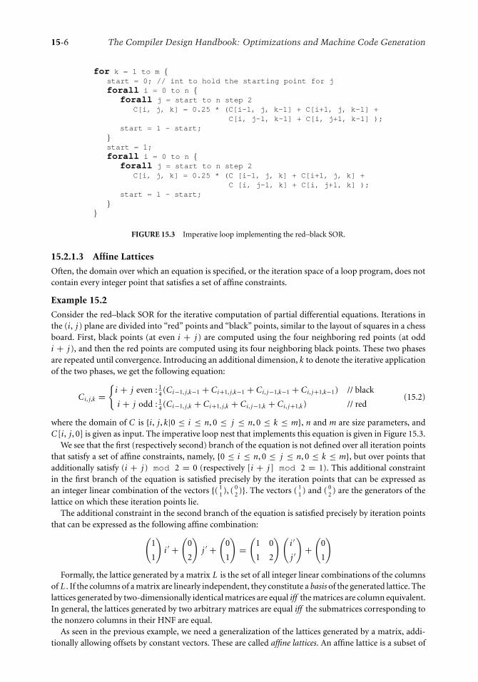
15-6 The Compiler Design Handbook: Optimizations and Machine Code Generation
for k = 1 to m {start = 0; // int to hold the starting point for jforall i = 0 to n {
forall j = start to n step 2C[i, j, k] = 0.25 * (C[i-1, j, k-1] + C[i+1, j, k-1] +
C[i, j-1, k-1] + C[i, j+1, k-1] );start = 1 - start;
}start = 1;forall i = 0 to n {
forall j = start to n step 2C[i, j, k] = 0.25 * (C [i-1, j, k] + C[i+1, j, k] +
C [i, j-1, k] + C[i, j+1, k] );start = 1 - start;
}}
FIGURE 15.3 Imperative loop implementing the red–black SOR.
15.2.1.3 Affine Lattices
Often, the domain over which an equation is specified, or the iteration space of a loop program, does notcontain every integer point that satisfies a set of affine constraints.
Example 15.2
Consider the red–black SOR for the iterative computation of partial differential equations. Iterations inthe (i, j ) plane are divided into “red” points and “black” points, similar to the layout of squares in a chessboard. First, black points (at even i + j ) are computed using the four neighboring red points (at oddi + j ), and then the red points are computed using its four neighboring black points. These two phasesare repeated until convergence. Introducing an additional dimension, k to denote the iterative applicationof the two phases, we get the following equation:
Ci, j,k ={
i + j even : 14 (Ci−1, j,k−1 + Ci+1, j,k−1 + Ci, j−1,k−1 + Ci, j+1,k−1) // black
i + j odd : 14 (Ci−1, j,k + Ci+1, j,k + Ci, j−1,k + Ci, j+1,k) // red
(15.2)
where the domain of C is {i, j, k|0 ≤ i ≤ n, 0 ≤ j ≤ n, 0 ≤ k ≤ m}, n and m are size parameters, andC[i, j, 0] is given as input. The imperative loop nest that implements this equation is given in Figure 15.3.
We see that the first (respectively second) branch of the equation is not defined over all iteration pointsthat satisfy a set of affine constraints, namely, {0 ≤ i ≤ n, 0 ≤ j ≤ n, 0 ≤ k ≤ m}, but over points thatadditionally satisfy (i + j ) mod 2 = 0 (respectively [i + j ] mod 2 = 1). This additional constraintin the first branch of the equation is satisfied precisely by the iteration points that can be expressed asan integer linear combination of the vectors {( 1
1 ), ( 02 )}. The vectors ( 1
1 ) and ( 02 ) are the generators of the
lattice on which these iteration points lie.The additional constraint in the second branch of the equation is satisfied precisely by iteration points
that can be expressed as the following affine combination:(1
1
)i ′ +
(0
2
)j ′ +
(0
1
)=
(1 0
1 2
) (i ′
j ′
)+
(0
1
)Formally, the lattice generated by a matrix L is the set of all integer linear combinations of the columns
of L . If the columns of a matrix are linearly independent, they constitute a basis of the generated lattice. Thelattices generated by two-dimensionally identical matrices are equal iff the matrices are column equivalent.In general, the lattices generated by two arbitrary matrices are equal iff the submatrices corresponding tothe nonzero columns in their HNF are equal.
As seen in the previous example, we need a generalization of the lattices generated by a matrix, addi-tionally allowing offsets by constant vectors. These are called affine lattices. An affine lattice is a subset of

Computations on Iteration Spaces 15-7
Zn of the form {L z + l |z ∈ Zm}, where L and l are an n × m matrix and n-vector, respectively. We call zthe coordinates of the affine lattice.
The affine lattices {L z + l |z ∈ Zm} and {L ′z′ + l ′|z′ ∈ Zm′ } are equal iff the lattices generated by L andL ′ are equal and l ′ = L z0 + l for some constant vector z0 ∈ Zm. The latter requirement basically enforcesthat the offset of one lattice lies on the other lattice.
15.2.1.4 Z-Polyhedra
A Z-polyhedron is the intersection of an integer polyhedron and an affine lattice. Recall the set of it-eration points defined by either branch of the equation for the red–black SOR. As we saw above, theseiteration points lie on an affine lattice in addition to satisfying a set of affine constraints. Thus, the set ofthese iteration points is precisely a Z-polyhedron. When the affine lattice is the canonical lattice, Zn, aZ-polyhedron is also an integer polyhedron. We adopt the following representation for Z-polyhedra:
{L z + l |Qz + q ≥ 0, z ∈ Zm} (15.3)
where L has full column rank, and the polyhedron P c = {z|Qz + q ≥ 0, z ∈ Zm} has a context that is theuniverse, Zm. P c is called the coordinate polyhedron of the Z-polyhedron. The Z-polyhedron for whichL has no columns has a coordinate polyhedron in Z0.
We see that every Z-polyhedron is an LBL simply by observing that the representation for aZ-polyhedron is in the form of an affine image of an integer polyhedron. However, the LBL in Figure15.2 is clearly not a Z-polyhedron. There does not exist any lattice with which we can intersect the integerpolyhedron {i |0 ≤ i ≤ 9} to get the set of iteration points of the LBL. Thus, the family of LBLs is a strictsuperset of the family of Z-polyhedra.
Our representation for Z-polyhedra as affine images of integer polyhedra is specialized through therestriction to L and P c . We may interpret the Z-polyhedral representation in Equation 15.3 as follows.It is said to be based on the affine lattice given by {L z + l |z ∈ Zm}. Iteration points of the Z-polyhedraldomain are points of the affine lattice corresponding to valid coordinates. The set of valid coordinates isgiven by the coordinate polyhedron.
15.2.1.4.1 Parameterized Z-PolyhedraA parameterized Z-polyhedron is a Z-polyhedron where some rows of its corresponding affine latticeare interpreted as size parameters. An equivalence relation is defined on the set of iteration points in aparameterized Z-polyhedron such that two iteration points are equivalent if they have identical value ofsize parameters. By this relation, a parameterized Z-polyhedron is partitioned into a set of equivalenceclasses, each of which is identified by the vector of size parameters. Equivalence classes correspond toprogram instances and are, thus, called instances of the parameterized Z-polyhedron.
For the sake of explanation, and without loss of generality, we may impose that the rows that denotesize parameters are before all non-parameter rows. The equivalent Z-polyhedron based on the HNF ofsuch a lattice has the important property that all points of the coordinate polyhedron with identical valuesof the first few indices belong to the same instance of the parameterized Z-polyhedron.
Example 15.3
Consider the Z-polyhedron given by the intersection of the polyhedron {p, i |0 ≤ i ≤ p} and the lattice{ j + k, j − k}.2 It may be written as
{ j + k, j − k|0 ≤ j − k ≤ j + k} = { j + k, j − k|0 ≤ k ≤ j }
Now, suppose the first index, p, in the polyhedron is the size parameter. As a result, the first row in thelattice { j + k, j − k} corresponding to the Z-polyhedron is the size parameter. The HNF of this lattice is
2For both the polyhedron and the affine lattice, the specification of the coordinate space Z2 is redundant. It can bederived from the number of indices and is therefore dropped for the sake of brevity.
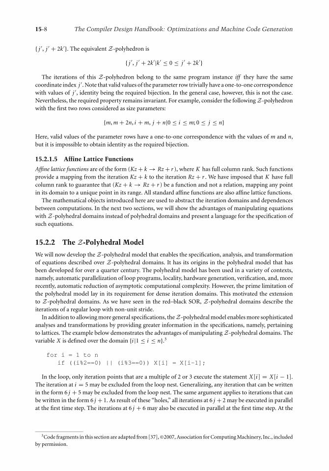
15-8 The Compiler Design Handbook: Optimizations and Machine Code Generation
{ j ′, j ′ + 2k′}. The equivalent Z-polyhedron is
{ j ′, j ′ + 2k′|k′ ≤ 0 ≤ j ′ + 2k′}
The iterations of this Z-polyhedron belong to the same program instance iff they have the samecoordinate index j ′. Note that valid values of the parameter row trivially have a one-to-one correspondencewith values of j ′, identity being the required bijection. In the general case, however, this is not the case.Nevertheless, the required property remains invariant. For example, consider the following Z-polyhedronwith the first two rows considered as size parameters:
{m, m + 2n, i + m, j + n|0 ≤ i ≤ m; 0 ≤ j ≤ n}
Here, valid values of the parameter rows have a one-to-one correspondence with the values of m and n,but it is impossible to obtain identity as the required bijection.
15.2.1.5 Affine Lattice Functions
Affine lattice functions are of the form (Kz + k → Rz + r ), where K has full column rank. Such functionsprovide a mapping from the iteration Kz + k to the iteration Rz + r . We have imposed that K have fullcolumn rank to guarantee that (Kz + k → Rz + r ) be a function and not a relation, mapping any pointin its domain to a unique point in its range. All standard affine functions are also affine lattice functions.
The mathematical objects introduced here are used to abstract the iteration domains and dependencesbetween computations. In the next two sections, we will show the advantages of manipulating equationswith Z-polyhedral domains instead of polyhedral domains and present a language for the specification ofsuch equations.
15.2.2 The Z-Polyhedral Model
We will now develop the Z-polyhedral model that enables the specification, analysis, and transformationof equations described over Z-polyhedral domains. It has its origins in the polyhedral model that hasbeen developed for over a quarter century. The polyhedral model has been used in a variety of contexts,namely, automatic parallelization of loop programs, locality, hardware generation, verification, and, morerecently, automatic reduction of asymptotic computational complexity. However, the prime limitation ofthe polyhedral model lay in its requirement for dense iteration domains. This motivated the extensionto Z-polyhedral domains. As we have seen in the red–black SOR, Z-polyhedral domains describe theiterations of a regular loop with non-unit stride.
In addition to allowing more general specifications, theZ-polyhedral model enables more sophisticatedanalyses and transformations by providing greater information in the specifications, namely, pertainingto lattices. The example below demonstrates the advantages of manipulating Z-polyhedral domains. Thevariable X is defined over the domain {i |1 ≤ i ≤ n}.3
for i = 1 to nif ((i%2==0) || (i%3==0)) X[i] = X[i-1];
In the loop, only iteration points that are a multiple of 2 or 3 execute the statement X[i] = X[i − 1].The iteration at i = 5 may be excluded from the loop nest. Generalizing, any iteration that can be writtenin the form 6 j + 5 may be excluded from the loop nest. The same argument applies to iterations that canbe written in the form 6 j + 1. As result of these “holes,” all iterations at 6 j + 2 may be executed in parallelat the first time step. The iterations at 6 j + 6 may also be executed in parallel at the first time step. At the
3Code fragments in this section are adapted from [37], ©2007, Association for Computing Machinery, Inc., includedby permission.

Computations on Iteration Spaces 15-9
next time step, we may execute iterations at 6 j +3 and finally at iterations 6 j +4. The length of the longestdependence chain is 3. Thus, the loop nest can be parallelized to execute in constant time as follows:
forall i = 2 to n step 6X[i] = X[i-1];
forall i = 6 to n step 6X[i] = X[i-1];
forall i = 3 to n step 6X[i] = X[i-1];
forall i = 4 to n step 6X[i] = X[i-1];
However, our derivation of parallel code requires to manipulate Z-polyhedral domains. A polyhedralapproximation of the problem would be unable to result in such a parallelization.
Finally, the Z-polyhedral model allows specifications with a more general dependence pattern than thespecifications in the polyhedral model. Consider the following equation that cannot be expressed in thepolyhedral model.
A[i] ={
i even : A[i/2]i odd : 0
(15.4)
where 1 ≤ i ≤ n and the corresponding loop is
for i = 1 to NA[i] = (i%2==0 ? A[i/2] : 0);
This program exhibits a dependence pattern that is richer than the affine dependences of the polyhedralmodel. In other words, it is impossible to write an equivalent program in the polyhedral model, that is,without the use of the mod operator or non-unit stride loops, that can perform the required computation.One may consider replacing the variable A with two variables X and Y corresponding to the even and oddpoints of A such that A[2i] = X[i] and A[2i − 1] = Y [i]. However, the definition of X now requires themod operator, because X[2i] = X[i] and X[2i − 1] = Y [i].
Thus, the Z-polyhedral model is a strict generalization of the polyhedral model and enables morepowerful optimizations.
15.2.3 Equational Language
In our presentation of the red–black SOR in Section 15.2.1.3, we studied the domains of the two branchesof Equation 15.2. More specifically, these are the branches of the case expression in the right-hand side (rhs)of the equation. In general, our techniques require the analysis and transformation of the subexpressionsthat constitute the rhs of equations, treating expressions as first-class objects.
For example, consider the simplification of Equation 15.1. As written, the simplification transforms theaccumulation expression in the rhs of the equation. However, one would expect the technique to be ableto decrease the asymptotic complexity of the following equation as well.
Yi = 5 +i∑
j=0
i∑k=0
Ai, j+k × Bk, j for 0 ≤ i ≤ n (15.5)
Generalizing, one would reasonably expect the existence of a technique to reduce the complexity ofevaluation of the accumulation subexpression (
∑ij=0
∑ik=0 Ai, j+k × Bk, j ), irrespective of its “level.” This
motivates a homogeneous treatment of the subexpression at any level. At the lowest level of specification,

15-10 The Compiler Design Handbook: Optimizations and Machine Code Generation
TABLE 15.1 Expressions: Syntax and Domains
Expression Syntax Domain
Constants Constant name or symbol DC
Variables V DV
Operators op(Expr1, . . .,ExprM)⋂M
i=1 DExpri
Case caseExpr1; . . .; ExprMesac⊎M
i=1 DExpri
Restriction D′ :Expr D′ ∩ DExpr
Dependence Expr. f f −1(DExpr)Reductions reduce (⊕, f, E xpr) f (DExpr)
The domain of an expression A is denoted by DA. The operator,op, may be written in infix notation if it is binary.
⊎denotes disjoint
union and f −1 denotes relational inverse. Adapted from [38], ©2006,Association for Computing Machinery, Inc., included by permission.
a subexpression is a variable (or a constant) associated with a domain. Generalizing, we associate domainsto arbitrary subexpressions.
The treatment of expressions as first-class objects leads to the design of a functional language whereprograms are a finite list of (mutually recursive) equations of the form Var = Expr, where both Varand Expr denote mappings from their respective domains to a set of values (similar to multidimensionalarrays). A variable is defined by at most one equation. Expressions are constructed by the rules givenin Table 15.1, column 2. The domains of all variables are declared, the domains of constants are eitherdeclared or defined over Z0 by default, and the domains of expressions are derived by the rules given inTable 15.1, column 3. The function specified in a dependence expression is called the dependence function(or simply a dependence), and the function specified in a reduction is called the projection function (orsimply a projection).
In this language, Equation 15.5 would be a syntactically sugared version of the following concreteproblem.
Y=5.(i->) + reduce(+,(i,j,k->i),A.(i,j,k->i,j+k)*B.(i,j,k->k,j))
In the equation above,5 is a constant expression defined over {i |0 ≤ i ≤ n} andY, A, andB are variables.In addition to the equation, the domains of Y, A, and B would be declared as the sets {i |0 ≤ i ≤ n},{i, l |0 ≤ i ≤ n, 0 ≤ l ≤ 2i}, and {k, j |0 ≤ k ≤ n, 0 ≤ j ≤ n}, respectively. The reduction expression isthe accumulation in Equation 15.5. Summation is expressed by the reduction operator + (other possiblereduction operators are ∗, max, min, or, and, etc.). The projection function (i,j,k->i) specifiesthat the accumulation is over the space spanned by j and k resulting in values in the one-dimensionalspace spanned by i . A subtle and important detail is that the expression that is accumulated is definedover a domain in three-dimensional space spanned by i , j , and k (this information is implicit in standardmathematical specifications as in Equation 15.5). This is an operator expression equal to the product of thevalue of A at [i, j + k] and B at [k, j ]. In the space spanned by i , j , and k, the required dependences on Aand B are expressed through dependence expressions A.(i,j,k->i,j+k) and B.(i,j,k->k,j),respectively. The equation does not contain any case or restrict constructs. For an example of these twoconstructs, refer back to Equation 15.4. In our equational specification, the equation would be written as
A = case
{2 j |1 ≤ 2 j ≤ n}:A.(2j->j){2 j − 1|1 ≤ 2 j − 1 ≤ n}:0esac
where the domains of A and the constant 0 are {i |1 ≤ i ≤ n} and {2i − 1|1 ≤ 2i − 1 ≤ n}, respectively.There are two branches of the case expression, each of which is a restriction expression. We have notprovided domains of any of the subexpressions mentioned above for the sake of brevity. These can becomputed using the rules given in Table 15.1, column 3.

Computations on Iteration Spaces 15-11
15.2.3.1 Semantics4
At this point, we intuitively understand the semantics of expressions. Here, we provide the formal semanticsof expressions over their domains of definition. At the iteration point z in its domain, the value of:
� A constant expression is the associated constant.� A variable is either provided as input or given by an equation; in the latter case, it is the value, at z,of the expression on its rhs.� An operator expression is the result of applying op on the values, at z, of its expression arguments.op is an arbitrary, iteration-wise, single valued function.� A case expression is the value at z of that alternative, to whose domain z belongs. Alternatives of acase expression are defined over disjoint domains to ensure that the case expression is not under-or overdefined.� A restriction over E is the value of E at z.� The dependence expression E. f is the value of E at f (z). For the affine lattice function (L z + l →Rz + r ), the value of the (sub)expression E.(L z + l → Rz + r ) at L z + l equals the value of E atRz + r .� reduce(⊕, f,E) is the application of ⊕ on the values of E at all iteration points in DE that mapto z by f . Since ⊕ is an associative and commutative binary operator, we may choose any order ofits application.
It is often convenient to have a variable defined either entirely as input or only by an equation. The formeris called an input variable and the latter is a computed variable. So far, all our variables have been of thesetwo kinds only. Computed variables are just names for valid expressions.
15.2.3.2 The Family of Domains
Variables (and expressions) are defined over Z-polyhedral domains. Let us study the compositional con-structs in Table 15.1 to get a more precise understanding of the family of Z-polyhedral domains.
For compound expressions to be defined over the same family of domains as their subexpressions, thefamily should be closed under intersection (operator expressions, restrictions), union (case expression),and preimage (dependence expressions) and image (reduction expressions) by the family of functions.With closure, we mean that a (valid) domain operation on two elements of the family of domains shouldresult in an element that also belongs to the family. For example, the family of integer polyhedra is closedunder intersection but not under images, as demonstrated by the LBL in Figure 15.2. The family of integerpolyhedra is closed under intersection since the intersection of two integer polyhedra that lie in the same di-mensional space results in an integer polyhedron that satisfies the constraints of both the integer polyhedra.
In addition to intersection, union, and preimage and image by the family of functions, most analysesand transformations (e.g., simplification, code generation, etc.) require closure under the difference oftwo domains. With closure under the difference of domains, we may always transform any specificationto have only input and computed variables.
The family of Z-polyhedral domains should be closed under the domain operations mentioned above.This constraint is unsatisfied if the elements of this family are Z-polyhedra. For example, the union of twoZ-polyhedra is not a Z-polyhedron. Also, the LBL in Figure 15.2 shows that the image of a Z-polyhedronis not a Z-polyhedron. However, if the elements of the family of Z-polyhedral domains are unions ofZ-polyhedra, then all the domain operations mentioned above maintain closure.
15.2.3.3 Parameterized Specifications
Extending the concept of parameterizedZ-polyhedra, it is possible to parameterize the domains of variablesand expressions with size parameters. This leads to parameterized equational specifications. Instances ofthe parameterized Z-polyhedra correspond to program instances.
4Parts of this section are adapted from [38], © 2006, Association for Computing Machinery, Inc., included by permission.

15-12 The Compiler Design Handbook: Optimizations and Machine Code Generation
TABLE 15.2 Normalization Rules
# Input Output
1 case E 1, . . ., E k−1, case, E ′1, . . ., E ′
m esac, case E 1, . . ., E k−1, E ′1, . . ., E ′
m,E k+1, . . ., E n esac E k+1, . . . ,E n esac
2 D′:case E 1, . . ., E n esac case D′ : E 1, . . . , D′ : E n esac3 op(E 1, . . ., E k−1, case E ′
1, . . ., E ′m esac, case op(E 1, . . ., E k−1, E ′
1, E k+1, . . ., E n), . . .,E k+1, . . ., E n) op(E 1, . . ., E k−1, E ′
m, E k+1, . . ., E n) esac4 (case E 1, . . ., E n esac). f case E 1. f, . . ., E n. f esac5 D1 : D2 : E (D1 ∩ D2) : E6 op(E 1, . . ., E k−1,D′ : E , E k+1, . . ., E n) D′ :op(E 1, . . ., E k−1, E , E k+1, . . ., E n)7 (D′ : E ). f f −1(D′) : E8 (op(E 1, . . ., E n)). f op(E 1. f, . . ., E n. f )9 (E . f1). f2 E .( f1 ◦ f2)
Every program instance in a parameterized specification is independent, so all functions should mapconsumer iterations to producer iterations within the same program instance.
15.2.3.4 Normalization
For most analyses and transformations (e.g., the simplification of reductions, scheduling, etc.), we needequations in a special normal form. Normalization is a transformation of an equational specificationto obtain an equivalent specification containing only equations of the canonic forms V = E or V =reduce(⊕, f p ,E), where the expression E is of the form
case . . .,DV,i : op(. . .,U. f, . . . ), . . . esac (15.6)
and U is a variable or a constant.Such a normalization transformation5 first introduces an equation for every reduce expression,
replacing its occurrence with the corresponding local variable. As a result, we get equations of the formsV = E or V = reduce(⊕, f p ,E), where the expression E does not contain any reduce subexpressions.Subsequently, these expressions are processed by a rewrite engine to obtain equivalent expressions of theform specified in Equation 15.6. The rules for the rewrite engine are given in Table 15.2. Rules 1 to 4 “bubble”a single case expression to the outermost level, rules 5 to 7 then “bubble” a single restrict subexpressionto the second level, rule 8 gets the operator to the penultimate level, and rule 9 is a dependence compositionto obtain a single dependence at the innermost level.
The validity of these rules, in the context of obtaining a valid specification of the language, relies on theclosure properties of the family of unions of Z-polyhedra.
15.2.4 Simplification of Reductions6
We now provide a deeper study of reductions. Reductions, commonly called accumulations, are theapplication of an associative and commutative operator to a collection of values to produce a collection ofresults.
Our use of equations was motivated by the simplification of asymptotic complexity of an equationinvolving reductions. We first present the required steps for the simplification. Then we will provide anintuitive explanation of the algorithm for simplification. For the sake of intuition, we use the standardmathematical notation for accumualations rather than the reduce expression.
5More sophisticated normalization rules may be applied, expressing the interaction of reduce expressions withother subexpressions. However, these are unnecessary in the scope of this chapter.
6Parts of this section are adapted from [38], © 2006, Association for Computing Machinery, Inc., included by permission.

Computations on Iteration Spaces 15-13
Our initial specification was
Yi =i∑
j=0
i∑k=0
Ai, j+k × Bk, j for 0 ≤ i ≤ n (15.7)
The loop nest corresponding to this equation has a �(n3) complexity. The cubic complexity for thisequation can also be directly deduced from the equational specification. Parameterized by n, there arethree independent7 indices within the summation. The following steps are involved in the derivation ofthe �(n2) equivalent specification.
1. Introduce the index variable l = j + k and replace every occurrence of j with l . This is a changeof basis of the three-dimensional space containing the domain of the expression that is reduced.
Yi =2i∑
l=0
min(i,l)∑k=max(0,l−i)
Ai,l × Bk,l−k for 0 ≤ i ≤ n
The change in the order of summation is legal under our assumption that the reduction operatoris associative and commutative.
2. Distribute multiplication over the summation since Ai,l is independent of k, the index of the innersummation.
Yi =2i∑
l=0
⎛⎝Ai,l ×min(i,l)∑
k=max(0,l−i)
Bk,l−k
⎞⎠ for 0 ≤ i ≤ n
3. Introduce variable Zi,l to hold the result of the inner summation∑min(i,l)
k=max(0,l−i) Bk,l−k .
Yi =2i∑
l=0
Ai,l × Zi,l for 0 ≤ i ≤ n
Zi,l =min(i,l)∑
k=max(0,l−i)
Bk,l−k for 0 ≤ i ≤ n, 0 ≤ l ≤ 2i
Note that the complexity of evaluating Y is now quadratic. However, we still have an equationalspecification that has cubic complexity (for the evaluation of Z).
4. Separate the summation over k to remove min and max operators in the equation for Zi,l .
Zi,l ={
0 ≤ l < i :∑l
k=0 Bk,l−k
i ≤ l ≤ 2i :∑i
k=l−i Bk,l−kfor 0 ≤ i ≤ n
5. Introduce variables Xi,l and Wi,l for each branch of the equation defining Zi,l .
Xi,l =l∑
k=0
Bk,l−k for 1 ≤ i ≤ n, 0 ≤ l < i
Wi,l =i∑
k=l−i
Bk,l−k for 0 ≤ i ≤ n, i ≤ l ≤ 2i
Both the equations given above have cubic complexity.
7With independent, we mean that there are no equalities between indices.
15-14 The Compiler Design Handbook: Optimizations and Machine Code Generation
6. Reuse. The complexity for the evaluation of X can be decreased by identifying that the expressionon the rhs is independent of i . We may evaluate each result once (for instance, at a boundary) andthen pipeline along i as follows.
Xi,l ={
1 ≤ i ≤ n, l = i − 1 :∑l
k=0 Bk,l−k
1 ≤ i ≤ n, 0 ≤ l < i − 1 : Xi−1,l
The initialization takes quadratic time since there are a linear number of results to evaluate andeach evaluation takes linear time. Then the pipelining of results over an area requires quadratictime. This decreases the overall complexity of evaluating X to quadratic time.
7. Scan detection. The simplification of Wi,l occurs when we identify
Wi,l = Bl−i,i + Bi,l−i +i−1∑
k=l−i+1
Bk,l−k for 0 ≤ i ≤ n, i ≤ l ≤ 2i − 2
= Bl−i,i + Bi,l−i + Wi−1,l for 0 ≤ i ≤ n, i ≤ l ≤ 2i − 2
The values are, once again, initialized in quadratic time at a boundary (here, 0 ≤ i ≤ n, 2i − 1 ≤l ≤ 2i). The scan takes constant time per iteration over an area and can be performed in quadratictime as well, thereby decreasing the complexity for the evaluation of W to quadratic time.
8. Summarizing, we have the following system of equations:
Yi =2i∑
l=0
Ai,l × Zi,l , 0 ≤ i ≤ n
Zi,l ={
0 ≤ i ≤ n, 0 ≤ l < i : Xi,l
0 ≤ i ≤ n, i ≤ l ≤ 2i : Wi,l
Xi,l ={
1 ≤ i ≤ n, l = i − 1 :∑l
k=0 Bk,l−k
1 ≤ i ≤ n, 0 ≤ l < i − 1 : Xi−1,l
Wi,l ={
0 ≤ i ≤ n, 2i − 1 ≤ l ≤ 2i :∑i
k=l−i Bk,l−k
0 ≤ i ≤ n, i ≤ l ≤ 2i − 2 : Bl−i,i + Bi,l−i + Wi−1,l
These equations directly correspond to the optimized loop nest given in Figure 15.1. We have not optimizedthese equations or the loop nest any further for the sake for clarity, and moreso, because we only wantto show an asymptotic decrease in complexity. However, a constant-fold improvement in the asymptoticcomplexity (as well as the memory requirement) can be obtained by eliminating the variable Z (or,alternatively, the two variables X and W).
We now provide an intuitive explanation of the algorithm for simplification. Consider the reduction
Y = reduce(⊕, f p , E )
where E is defined over the domain DE . The accumulation space of the above equation is characterized byker( f p). Any two points z and z′ that contribute to the same element of the result, Y , satisfy z−z′ ∈ ker( f p).To aid intuition, we may also write this reduction as
Y [ f p(z)] = ⊕E [z] (15.8)
Y [ f p(z)] is the “accumulation,” using the ⊕ operator, of the values of E at all points z ∈ DE that havethe same image f p(z). Now, if E has a distinct value at all points in its domain, they must all be computed,and no optimization is possible. However, consider the case where the expression E exhibits reuse: its valueis the same at many points in DE . Reuse is characterized by ker( fr ), the kernel of a many-to-one affine

Computations on Iteration Spaces 15-15
The reuse space is spanned by {(1, 0, 0)T} and the accumulation
space is spanned by {(0, 0, 1)T}. Translating D by (1, 0, 0)T
exposes the left and top diagonal boundaries (light), and exceedsthe right and bottom diagonal boundaries (dark). Moreover,
left and right boundaries contain the accumulation space. Each
boundary is thus treated differently
The left boundary is the initialization domain.
The top diagonal boundary is the addition domain.
The bottom diagonal boundary is the subtraction domain.
The right boundary is ignored (the projection along the
accumulation space is outside the domain of the answer).
The front, back, and top horizontal boundaries are also
ignored since translation is along these boundaries.
k j
i
FIGURE 15.4 Illustration of the core algorithm for Yi, j = ∑min(i+n,3n/2)k=i+1 X j,k for 1 ≤ i, j ≤ n. Adapted from
[38], © 2006, Association for Computing Machinery, Inc., included by permission.
function, fr ; the value of E at any two points inDE is the same if their difference belongs to ker( fr ). We candenote this reuse by E [z] = X[ fr (z)], where X is a variable with domain DX . In our language, this wouldbe expressed by the dependence expression X.(z → fr [z]). The canonical equation that we analyze is
Y [ f p(z)] = ⊕X[ fr (z)] (15.9)
Its nominal complexity is the cardinality of the domain DE of E . The main idea behind our method isbased on analyzing (a) DE , the domain of the expression E inside the reduction, (b) its reuse space, and(c) the accumulation space.
15.2.4.1 Core Algorithm
Consider two adjacent instances of the answer variable, Yz and Yz−rY along rY = f p(r E ), where r E is avector in the reuse space of E . The set of values that contribute to Yz and Yz−rY overlap. This would enableus to express Yz in terms of Yz−rY . Of course, there would be residual accumulations on values outsidethe intersection that must be “added” or “subtracted” accordingly. We may repeat this for other values ofY along rY . The simplification results from replacing the original accumulation by a recurrence on Yz−rY
and residual accumulations. For example, in the simple scan, Yi = ∑ij=1 X j , the expression inside the
summation Fi, j = X j has reuse along (1, 0)T . Taking rY = (1), we get Yi = Yi−1 + Fi,i = Yi−1 + Xi .The geometric interpretation of the above reasoning is that we translateDE by a vector in the reuse space
of E . Let us call the translated domainDE ′ . The intersection ofDE andDE ′ is precisely the domain of values,the accumulation over which can be avoided. Their differences account for the residual accumulations. Inthe simple scan explained above, the residual domain to be added is {i, j |1 ≤ i = j ≤ n}, and the domainto be subtracted is empty. The residual accumulations to be added or subtracted are determined only byDE and r E .
This leads to Algorithm 15.1 (also see Figure 15.4).
Algorithm 15.1 Intuition of the Core Algorithm8
1. Choose r E , a vector in ker( fr ), along which the reuse of E is to be exploited. In general, ker( fr ) ismultidimensional and therefore there may be infinitely many choices.
2. Determine the domains D0, D−, and D+ corresponding to the domain of initialization, andthe residual domains to subtract and to add, respectively. The choice of r E is made such thatthe cardinalities of these three domains are polynomials whose degree is strictly less than that forthe original accumulation. This leads to simplification of the complexity.
8Adapted from [38], © 2006, Association for Computing Machinery, Inc., included by permission.

15-16 The Compiler Design Handbook: Optimizations and Machine Code Generation
3. For these three domains, D0, D−, and D+, define the three expressions, E 0, E −, and E +, consistingof the original expression E , restricted to the appropriate subdomain.
4. Replace the original equation by the following recurrence:
Y [ f p(z)] =
⎧⎪⎨⎪⎩f p(D0) : ⊕E 0
DY − f p(D0) : Y [z − r E ]⊕(⊕E +) � (⊕E −)
5. Apply steps 1 to 4 recursively on the residual reductions over E 0, E −, or E + if they exhibit furtherreuse.
Note that Algorithm 15.1 assumes that the reduction operation admits an inverse; that is, “subtraction”is defined. If this is not the case, we need to impose constraints on the direction of reuse to exploit:essentially, we require that the domain D− is empty. This leads to a feasible space of exploitable reuse.
15.2.4.2 Multidimensional Reuse
When the reuse space as well as the accumulation space are multidimensional, there are some interestinginteractions. Consider the equation Yi = ∑i−1
j=1
∑i− jk=1 X j for i ≥ 2. It has two-dimensional reuse (in
the {i, k} plane), and the accumulation is also two-dimensional (in the { j, k} plane). Note that the twosubspaces intersect, and this means that in the k direction, not only do all points have identical values, butthey also all contribute to the same answer. From the bounds on the k summation we see that there areexactly i − j such values, so the inner summation is just (i − j ) × X j , because multiplication is a higher-order operator for repeated addition of identical values (similar situations arise with other operators, e.g.,power for multiplication, identity for the idempotent operator max, etc.). We have thus optimized the�(n3) computation to �(n2). However, our original equation had two dimensions of reuse, and we maywonder whether further optimization is possible. In the new equation Yi = ∑i−1
j=1(i − j )× X j , the body isthe product of two subexpressions, (i − j ) and X j . They both have one dimension of reuse, in the (1, 1)T
and (1, 0)T directions, respectively, but their product does not. No further optimization is possible for thisequation.
However, if we had first exploited reuse along i , we would have obtained the simplified equationYi = Yi−1 + ∑i−1
j=1 X j , initialized with Y2 = X1. The residual reduction here is itself a scan, and we mayrecurse the algorithm to obtain Yi = Yi−1 + Zi and Zi = Zi−1 + Xi−1 initialized with Z2 = X1. Thus,our equation can be computed in linear time. This shows how the choice of reuse vectors to exploit, andtheir order, affects the final simplification.
15.2.4.3 Decomposition of Accumulation
Consider the equation Yi = ⊕n−ik=1
⊕ij=1 X j,k for 1 ≤ i ≤ n − 1. The one-dimensional reuse space is
along {i}, and { j, k} is the two-dimensional accumulation space. The set of points that contribute to thei th result lie in an i × (n − i) rectangle of the two-dimensional input array X . Comparing successiverectangles, we see that as the width decreases from one to the other, the height increases (Figure 15.5). Ifthe operator ⊕ does not have an inverse, it seems that we may not be able to simplify this equation. This isnot true: we can see that for each k we have an independent scan. The inner reduction Zi,k = ⊕i
j=1 X j,k
is just a family of scans, which can be done in quadratic time with Zi,k = Zi−1,k + Xi,k initialized withZ1,k = X1,k . The outer reduction just accumulates columns of Zi,k , which is also quadratic.
What we did in this example was to decompose the original reduction that was along the { j, k} space intotwo reductions, the inner along the { j } space yielding partial answers along the {i, k}plane and the outer thatcombined these partial answers along the {k} space. Although the default choice of the decomposition —the innermost accumulation direction — of the {k, j } space worked for this example, in general this is notthe case. It is possible that the optimal solution may require a nonobvious decomposition, for instance,

Computations on Iteration Spaces 15-17
Additional Values
j
ik
Absent ValuesScans
FIGURE 15.5 Geometric interpretation for Yi = ⊕n−ik=1 ⊕i
j=1 X j,k . Adapted from [38], © 2006, Association forComputing Machinery, Inc., included by permission.
along some diagonal. We encourage the reader to simplify9 the following equation:
Yi =n+i⊕j=i
n+2i− j⊕k=i
X j,k
15.2.4.4 Distributivity and Accumulation Decomposition
Returning to the simplification of Equation 15.7, we see that the methods presented so far do not apply,since the body of the summation, Ai, j+k × Bk, j , has no reuse. The expression has a distinct value at eachpoint in the three-dimensional space spanned by i , j , and k. However, the expression is composed of twosubexpressions, which individually have reuse and are combined with the multiplication operator thatdistributes over the reduction operator, addition.
We may be able to distribute a subexpression outside a reduction if it has a constant value at all thepoints that map to the same answer. This was ensured by a change in basis of the three-dimensional spaceto i , l , and k, followed by a decomposition to summations over k and then l . Values of A were constantfor different iterations of the accumulation over k. After distribution, the body of the inner summationexhibited reuse that was exploited for the simplification of complexity.
15.2.5 Scheduling10
Scheduling is assigning an execution time to each computation so that precedence constraints are satisfied.It is one of the most important and widely studied problems. We present the scheduling analysis forprograms in the Z-polyhedral model. The resultant schedule can be subsequently used to construct aspace–time transformation leading to the generation of sequential or parallel code. The application of thisschedule is made possible as a result of closure of the family of Z-polyhedral domains under image bythe constructed transformation. We showed the advantages of scheduling programs in the Z-polyhedralmodel in Section 15.2.2. The general problem of scheduling programs with reductions is beyond the scopeof this chapter. We will restrict our analysis to Z-polyhedral programs without reductions.
The steps involved in the scheduling analysis are (a) deriving precedence (causality) constraints forprograms written in the Z-polyhedral model and (b) formulation of an integer linear program to obtainthe schedule.
9Solution: The inner reduction would map all points for which j + k = c , for a given constant c , to the same partialanswer.
10Adapted from [36] © 2007 IEEE, included by permission.

15-18 The Compiler Design Handbook: Optimizations and Machine Code Generation
(a) Basic RDG
{2i|1 ≤ 2i ≤ n}
{2i i}
{2i − 1|1 ≤ 2i − 1 ≤ n}X
(b) Refined RDG
XY{2i − 1|1 ≤ 2i − 1 ≤ n} {2i|1 ≤ 2i ≤ n}
{4i 2i}{4i − 2 2i − 1}
Y
{2i i}
FIGURE 15.6 Basic and refined reduced dependence graphs for Example 15.4. Adapted from [36], © 2007 IEEE,included by permission.
The precedence constraints between variables are derived from the reduced dependence graph (RDG).We will now provide some refinements of the RDG.
15.2.5.1 Basic and Refined RDG
Equations in the Z-polyhedral model can be defined over an infinite iteration domain. For any depen-dence analysis on an infinite graph, we need a compact representation. A directed multi-graph, the RDGprecisely describes the dependences between iterations of variables. It is based on the normalized form ofa specification and defined as follows:
� For every variable in the normalized specification, there is a vertex in the RDG labeled by thevariable name and annotated by its domain. We will refer to vertices and variables interchangeably.� For every dependence of the variable V on U, there is an edge from V to U, annotated by thecorresponding dependence function. We will refer to edges and dependences interchangeably.
At a finer granularity, every branch of an equation in a normalized specification dictates the dependencesbetween computations. A precise analysis requires that dependences be expressed separately for everybranch. Again, for reasons of precision, we may express dependences of a variable separately for everyZ-polyhedron in the Z-polyhedral domain of the corresponding branch of its equation. To enable these,we replace a variable by a set of new variables as elaborated below. Remember, our equations are of theform
case. . .,DV,i : op(. . .,U. f, . . . ), . . . esac (15.10)
Let DV,i be written as a disjoint union of Z-polyhedra given by⊎
j Z j . The variable V in the domainZ j is replaced by a new variable, for instance, X j . Similarly, let U be replaced by new variables given asYk . The dependence of V in DV,i on U is replaced by dependences from all X j on all Yk . An edge fromX j to Yk may be omitted if there are no iterations in X j that map to Yk (mathematically, if the preimageof Yk by the dependence function does not intersect with X j ). A naive construction following these rulesresults in the basic reduced dependence graph.
Figure 15.6a gives the basic RDG for Equation 15.4, which is repeated here for convenience.
A ={
{2i |1 ≤ 2i ≤ n} : A.(2i → i) (denoted by X){2i − 1|1 ≤ 2i − 1 ≤ n} : 0 (denoted by Y )
The domains of A and the constant 0 are {i |1 ≤ i ≤ n} and {2i − 1|1 ≤ 2i − 1 ≤ n}, respectively. Next,we will study a refinement on this RDG.
In the RDG for the generic equation given in Equation 15.10, let X be a variable derived from V anddefined on ZX ∈ DV,i , and let Y be a variable derived from U defined on ZY ∈ DU , where ZX and ZY
are given as follows:
ZX = {L X zX + l X |zX ∈ P cX}
ZY = {L Y zY + lY |zY ∈ P cY }

Computations on Iteration Spaces 15-19
A dependence of the form (L z + l → Rz + r ) is directed from X to Y . X at (L z + l) ∈ ZX cannot beevaluated before Y at (Rz + r ) ∈ ZY . The affine lattice {L z + l |z ∈ Zn} may contain points that do not liein the affine lattice {L X zX + l X |zX ∈ ZnX }. Similarly, the affine lattice {Rz + r |z ∈ Zn} may contain pointsthat do not lie in the affine lattice {L Y zY + lY |zY ∈ ZnY }. As a result, the dependence may be specified on afiner lattice than necessary and may safely be replaced by a dependence of the form (L ′z′ + l ′ → R′z′ +r ′),where
L ′ = L X S, l ′ = L X s + l X
R′ = L Y S ′, r ′ = L Y s ′ + lY(15.11)
where S and S ′ are matrices and s and s ′ are integer vectors. The refined RDG is a refinement of the basicRDG where every dependence has been replaced by a dependence satisfying Equation 15.11. Figure 15.6bgives the refined RDG for Equation 15.4.
15.2.5.2 Causality Constraints
Dependences between the different iterations of variables impose an ordering on their evaluation. A validschedule of the evaluation of these iterations is the assignment of an execution time to each computationso that precedence (causality) constraints are satisfied.
Let X and Y be two variables in the refined RDG defined on {L X zX + l X |zX ∈ P cX} and {L Y zY + lY |zY ∈
P cY }, respectively. We seek to find schedules on X and Y of the following form:
λ′X (zX ) = (L X zX + l X → λX (zX ))
λ′Y (zY ) = (L Y zY + lY → λY (zY )) (15.12)
where λX and λY are affine functions on zX and zY , respectively. Our motivation for such schedules is thatall vectors and matrices are composed of integer scalars. If we seek schedules of the form λ′(z′), whereλ′ is an affine function and z′ is an iteration in the domain of a variable, then we may potentially assignexecution times to “holes,” or computations that do not exist.
We will now formulate causality constraints using the refined RDG. Consider dependences from X toY . All such dependences can be written as
(L X (Sz + s ) + l X → L Y (S ′z + s ′) + lY )
where S and S ′ are matrices and s and s ′ are vectors. The execution time for Y at L Y (S ′z + s ′) + lY
should precede the execution time for X at L X (Sz + s ) + l X . With the nature of the schedules presentedin Equation 15.12, our causality constraint becomes
λX (Sz + s ) − λY (S ′z + s ′) ≥ 1 (15.13)
with the assumption that op is atomic and takes a single time step to evaluate.From these constraints, we may derive an integer linear program to obtain schedules of the form
λ′(z) = (L z + l → λ[z]), where {L z + l |z ∈ Zn} is the lattice corresponding to the Z-polyhedron andλ(z) is the affine function (composed of integer scalars) on the coordinates of this lattice. An importantfeature of this formulation is that the resultant schedule can then be used to construct a space–timetransformation.
15.2.6 Backend
After optimization of the equational specification and obtaining a schedule, the following steps are per-formed to generate (parallel) imperative code.
Analogous to the schedule that assigns a date to every operation, a second key aspect of the parallelizationis to assign a processor to each operation. This is done by means of a processor allocation function. As withschedules, we confine ourselves to affine lattice functions. Since there are no causality constraints for

15-20 The Compiler Design Handbook: Optimizations and Machine Code Generation
choosing an allocation function, there is considerable freedom in choosing it. However, in the search forprocessor allocation functions, we need to ensure that two iteration points that are scheduled at the sametime are not mapped to the same processing element.
The final key aspect in the static analysis of our equations is the allocation of operations to memorylocations. As with the schedule and processor allocation function, the memory allocation is also an affinelattice function. The memory allocation function is, in general, a many-to-one mapping with most valuesoverwritten as the computation proceeds. The validity condition for memory allocation functions is thatno value is overwritten before all the computations that depend on it are themselves executed.
Once we have the three sets of functions, namely, schedule, processor allocation, and memory allocation,we are left with the problem of code generation. Given the above three functions, how do we produce parallelcode that “implements” these choices? Code generation may produce either sequential or parallel code forprogrammable processors, or even descriptions of application-specific or nonprogrammable hardware (inappropriate hardware description language) that implements the computation specified by the equation.
Current techniques in code generation produce extremely efficient implementations comparable tohand-optimized imperative programs. With this knowledge, we return to our motivation for the use ofequations to specify computations. An imperative loop nest that corresponds to an equation contains moreinformation than required to specify the computation. There is an order (corresponding to the schedule)in the evaluation of values of a variable at different iteration points, namely, the lexicographic order of theloop indices. A loop nest also specifies the order of evaluation of the partial results of accumulations. Amemory mapping has been chosen to associate values to memory locations. Finally, in the case of parallelcode, a loop nest also specifies a processor allocation. Any analysis or transformation of loop nests thatis equivalent to analysis or transformations on equations has to deconstruct these attributes and, thus,becomes unnecessarily complex.
15.2.7 Bibliographic Notes11
Our presentation of the equational language and the various analyses and transformations is based on thethe ALPHA language [59, 69] and the MMALPHA framework for manipulating ALPHA programs, whichrelies on a library for manipulating polyhedra [107].
Although the presentation in this section has focused on equational specifications, the impact of thepresented work is equally directed toward loop optimizations. In fact, many advances in the developmentof the polyhedral model were motivated by the loop parallelization and hardware synthesis communities.
To overcome the limitations of the polyhedral model in its requirement of dense iteration spaces, Teichand Thiele proposed LBLs [104]. Z-polyhedra were originally proposed by Ancourt [6]. Le Verge [60]argued for the extension of the polyhedral model to Z-polyhedral domains. Le Verge also developednormalization rules for programs with reductions [59].
The first work that proposed the extension to a language based on unions ofZ-polyhedra was by Quintonand Van Dongen [81]. However, they did not have a unique canonic representation. Also, they could notestablish the equivalence between identical Z-polyhedra nor provide the difference of two Z-polyhedraor their image under affine functions. Closure of unions of Z-polyhedra under all the required domainoperations was proved in [37] as a result of a novel representation for Z-polyhedra and the associatedfamily of dependences. One of the consequences of their results on closure was the equivalence of thefamily of Z-polyhedral domains and unions of LBLs.
Liu et al. [67] described how incrementalization can be used to optimize polyhedral loop computationsinvolving reductions, possibly improving asymptotic complexity. However, they did not have a cost modeland, therefore, could not claim optimality. They exploited reuse only along the indices of the accumulationloops and would not be able to simplify an equation like Yi, j = ∑
k Xi− j,k . Other limitations were therequirement of an inverse operator. Also, they did not consider reduction decompositions and algebraic
11Parts of this section are adapted from [36] ©2007 IEEE and [37, 38], ©2007, 2006 Association for Computing Machinery,Inc., included by permission.

Computations on Iteration Spaces 15-21
transformations and do not handle the case when there is reuse of values that contribute to the same answer.These limitations were resolved in [38], which presented a precise characterization of the complexity ofequations in the polyhedral model and an algorithm for the automatic and optimal application of programsimplifications.
The scheduling problem on recurrence equations with uniform (constant-sized) dependences wasoriginally presented by Karp et al. [52]. A similar problem was posed by Lamport [56] for programswith uniform dependences. Shang and Fortes [97] and Lisper [66] presented optimal linear schedulesfor uniform dependence algorithms. Rao [87] first presented affine by variable schedules for uniformdependences (Darte et al. [21] showed that these results could have been interpreted from [52]). Thefirst result of scheduling programs with affine dependences was solved by Rajopadhye et al. [83] andindependently by Quinton and Van Dongen [82]. These results were generalized to variable dependentschedules by Mauras et al. [70]. Feautrier [31] and Darte and Robert [23] independently presented theoptimal solution to the affine scheduling problem (by variable). Feautrier also provided the extension tomultidimensional time [32]. The extension of these techniques to programs in the Z-polyhedral modelwas presented in [36]. Their problem formulation searched for schedules that could directly be used toperform appropriate program transformations. The problem of scheduling reductions was initially solvedby Redon and Feautrier [90]. They had assumed a Concurrent Read, Concurrent Write Parallel RandomAccess Machine (CRCW PRAM) such that each reduction took constant time. The problem of schedulingreductions on a Concurrent Read, Exclusive Write (CREW) PRAM was presented in [39]. The schedulingproblem was studied along with the objective for minimizing communication by Lim et al. [63]. Theproblem of memory optimization, too, has been studied extensively [22, 26, 57, 64, 79, 105].
The generation of efficient imperative code for programs in the polyhedral model was presented byQuillere et al. [80] and later extended by Bastoul [9]. Algorithms to generate code, both sequential andparallel, after applying nonunimodular transformations to nested loop programs has been studied exten-sively [33, 62, 85, 111]. However, these results were all restricted to single, perfectly nested loop nests, withthe same transformation applied to all the statements in the loop body. The code generation problemthus reduced to scanning the image, by a nonunimodular function, of a single polyhedron. The generalproblem of generating loop nests for a union of Z-polyhedra was solved by Bastoul in [11].
Lenders and Rajopadhye [58] proposed a technique for designing multirate VLSI arrays, which areregular arrays of processing elements, but where different registers are clocked at different rates. Theirformulation was based on equations defined over Z-polyhedral domains.
Feautrier [30] showed that an important class of conventional imperative loop programs called affine con-trol loops (ACLs) can be transformed to programs in the polyhedral model. Pugh [78] extended Feautrier’sresults. The detection of scans in imperative loop programs was presented by Redon and Feautrier in [89].Bastoul et al. [10] showed that significant parts of the SpecFP and PerfectClub benchmarks are ACLs.
15.3 Iteration Space Tiling
This section describes an important class of reordering transformations called tiling. Tiling is crucial toexploit locality on a single proccessor, as well as for adapting the granularity of a parallel program. We firstdescribe tiling for dense iteration spaces and data sets and then consider irregular iteration spaces and sparsedata sets. Next, we briefly summarize the steps involved in tiling and conclude with bibliographic notes.
15.3.1 Tiling for Dense Iteration Spaces
Tiling is a loop transformation used for adjusting the granularity of the computation so that its character-istics match those of the execution environment. Intuitively, tiling partitions the iterations of a loop intogroups called tiles. The tile sizes determine the granularity.
In this section, we will study three aspects related to tiling. First, we will introduce tiling as a looptransformation and derive conditions under which it can be applied. Second, we present a constrainedoptimization approach for formulating and finding the optimal tile sizes. We then discuss techniques forgenerating tiled code.

15-22 The Compiler Design Handbook: Optimizations and Machine Code Generation
15.3.1.1 Tiling as a Loop Transformation
Stencil computations occur frequently in many numerical solvers, and we use them to illustrate theconcepts and techniques related to tiling. Consider the typical Gauss–Seidel style stencil computationshown in Figure 15.7 as a running example. The loop specifies a particular order in which the values arecomputed. An iteration reordering transformation specifies a new order for computation. Obviously notevery reordering of the iterations is legal, that is, semantics preserving. The notion of semantics preservingcan be formalized using the concept of dependence. A dependence is a relation between a producer andconsumer of a value. A dependence is said to be preserved after the reordering transformation if theiteration that produces a value is computed before the consumer iteration. Legal iteration reorderings arethose that preserve all the dependences in a given computation.
Array data dependence analyses determine data dependences between values stored in arrays. Therelationship can be either memory-based or value-based. Memory-based dependencies are induced by writeto and read from the same memory location. Value-based dependencies are induced by production andconsumption of values. Once can view memory-based dependences as a relation between memory locationsand valued-based dependences as a relation between values produced and consumed. For computationsrepresented by loop nests, the values produced and consumed can be uniquely associated with an iteration.Hence, dependences can be viewed as a relation between iterations.
Dependence analyses summarize these dependence relationships with a suitable representation. Dif-ferent dependence representations can be used. Here, we introduce and use distance vectors that canrepresent a particular kind of dependence and discuss legality of tiling with respect to them. More gen-eral representations such as direction vectors, dependence polyhedra, and cones can be used to capturegeneral dependence relationships. Legality of tiling transformations can be naturally extended to theserepresentations, and a discussion of them is beyond the scope of this article.
We consider perfect loop nests. Since, through array expansion, memory-based dependences can beautomatically transformed to value-based dependences, we consider only the later. For an n-deep perfect
for i = 1 . . . M
for j = 2 . . . N–1
A [j] = (A [j] + A [j – 1] + A [j + 1])/3;
6
j
5
4
3
2
1
1 2 3 4 5 6 i
6
Cyclic
dependences
between tiles
j
5
4
3
2
1
1 2 3 4 5 6 i
FIGURE 15.7 A stencil computation is shown on the bottom-left and a geometric view of its data flow is shownabove it. Shown on the right is an illegal rectangular tiling of the iteration space with 2 × 2 tiles. This is due to the cyclicdependences between the tiles. An instance of this is highlighted.

Computations on Iteration Spaces 15-23
loop nest, the iterations can be represented as integer n-vectors. A dependence vector for an n-dimensionalperfect loop nest is an n-vector d = (d1,. . ., dn), where the kth component corresponds to the kth loop(counted from outermost to innermost). A distance vector is a dependence vector d ∈ Zn, that is, everycomponent dk is an integer. A dependence distance is the distance between the iteration that produces avalue and the iteration that consumes a value. Distance vectors represent this information. The dependencedistance vector for a value produced at iteration p = (p1,. . ., pn) and consumed at a later iterationc = (c1,. . ., cn) is d = (c − p) = (c1 − p1,. . ., cn − pn). The stencil computation given in Figure 15.7has three dependences. The values consumed at an iteration (i, j ) are produced at iterations (i, j − 1),(i − 1, j ), and (i − 1, j + 1). The corresponding three dependence vectors are ( 0
1 ), ( 10 ), and ( 1
−1 ).Tiling is an iteration reordering transformation. Tiling reorders the iterations to be executed in a block-
by-block or tile-by-tile fashion. Consider the tiled iteration space shown in Figure 15.7 and the followingexecution order. Both the tiles and the points within a tile are executed in the lexicographic order. The tilesare also executed in an atomic fashion, that is, all the iterations in a tile are executed before any iterationof another tile. It is very instructive to pause for a moment and ask whether this tiled execution orderpreserves all the dependences of the original computation. One can observe that the dependence ( 1
−1 ) isnot preserved, and hence the tiling is illegal. There exists a nice geometric way of checking the legality ofa tiling. A given tiling is illegal if there exist cyclic dependences between tiles. An instance of this cyclicdependence is highlighted in Figure 15.7.
The legality of tiling is determined not by the dependences alone, but also by the shape of the tiles.12
We saw (Figure 15.7) that tiling the stencil computation with rectangles is illegal. However, one mightwonder whether there are other tile shapes for which tiling is legal. Yes, tiling with parallelograms is legal asshown in Figure 15.8. Note how the change in the tile shape has avoided the cyclic dependences that werepresent in the rectangular tiling. Instead of considering nonrectangular shapes that make tiling legal, onecould also consider transforming the data dependences so that rectangular tiling becomes legal. Often, onecan easily find such transformations. A commonly used transformation is skewing. The skewed iterationspace is shown in Figure 15.8 together with a rectangular tiling. Compare the dependences between tilesin this tiling with those in the illegal rectangular tiling shown in Figure 15.7. One could also think of morecomplicated tile shapes, such as hexagons or octagons. Because of complexity of tiled code generation suchtile shapes are not used.
A given tiling can be characterized by the shape and size of the tiles, both of which can be conciselyspecified with a matrix. Two matrices, clustering and tiling, are used to characterize a given tiling. Theclustering matrix has a straightforward geometric interpretation, and the tiling matrix is its inverse andis useful in defining legality conditions. A parallelogram (or a rectangle) has four vertices and four edges.Let us pick one of the vertices to be the origin. Now we have two edges or two vertices adjoining theorigin. The shape and size of the tiles can be specified by characterizing these edges or vertices. We caneasily generalize these concepts to higher dimensions. In general, an n-dimensional parallelepiped has 2n
vertices and 2n facets (higher-dimensional edges), out of which n facets and n vertices adjoin the origin.A clustering matrix is an n × n square matrix whose columns correspond to the facets that determine atile. The clustering matrix has the property that the absolute value of its determinant is equal to the tilevolume.
The clustering matrices of the parallelogram and rectangular tilings shown in Figure 15.8 are
G ppd =(
0 22 −2
)and G rect =
(2 00 2
)
12Legality of tiling also depends on the shape of the iteration space. However, for practical applications, we cancheck the legality with the shape of the tiles and dependence information alone.

15-24 The Compiler Design Handbook: Optimizations and Machine Code Generation
8
6
7
8
j
j
5
4
3
2
1
6
7
8
9
10
11
12
13
5
4
3
2
1
0
–1
10 2 3 4 5 6i
1 2 3 4 5 6 i
FIGURE 15.8 Shown on the left is a parallelogram tiling. A rectangular tiling of the transformed iteration space isshown on the right. A skewing transformation is required to make the rectangular tiling valid.
In G ppd, the first column represents the horizontal edge, and the second represents the oblique edge. InG rect , the first column represents the horizontal edge, and the second represents the vertical edge.
The tiling matrix is the inverse of the clustering matrix. The tiling matrices of the parallelogram and therectangular tilings shown in Figure 15.8 are
Hppd = G−1ppd =
(12
12
12 0
)and Hrect = G−1
rect =(
12 0
0 12
)
For rectangular tiling the edges are always along the canonical axes, and hence, there is no loss of generalityin assuming that the tiling and clustering matrices are diagonal. The tiling is completely described by justthe so-called tile size vector, s = (s1,. . ., sn), where each si denotes the tile size along the i th dimension.The clustering and tiling matrices are simply G rect = diag(s1,. . ., sn) and Hrect = diag( 1
s1,. . ., 1
sn), where
diag(x1,. . ., xn) denotes the n × n diagonal matrix with x1,. . ., xn as the diagonal entries.A geometric way of checking the legality of a given tiling was discussed earlier. One can derive formal
legality conditions based on the shape and size of the tiles and the dependences. Let D be the set ofdependence distance vectors. A vector x = (x1,. . ., xn) is lexicographically nonnegative if the leadingnonzero component of the x is positive, that is, x1 > 0 or both x1 = 0 and (x2,. . ., xn) � 0. The flooroperator �.� when used on vectors is applied component-wise, that is, �x� = (�x1�,. . ., �xn�). The legalitycondition for a given (rectangular or parallelepiped) tiling specified by the tiling matrix H and dependenceset D is
∀d ∈ D : �Hd� � 0
The above condition formally captures the presence or absence of cycles between tiles.

Computations on Iteration Spaces 15-25
We can now apply this legality condition to the stencil computation example. Let Dorig = {( 01 ), ( 1
0 ), ( 1−1 )},
the set of dependence vectors from the original or given stencil computation, and Dskew = {( 01 ), ( 1
1 ), ( 10 )},
the dependence vectors obtained after applying the skewing transformation ( 1 01 1 ) to the original depen-
dences. Earlier we showed that rectangular tiling of the original iteration space is not legal based on theexistence of cycles between tiles (cf. Figure 15.7). This can also be verified by observing that the condition forvalidity, ∀d ∈ Dorig : �Hrectd� � 0, is not satisfied, since, for the dependence vector ( 1
−1 ) in Dorig , we have
�Hrect(1
−1 )� = ( 0−1 ). However, for the same dependences, Dorig , as shown in Figure 15.8, a parallelogram
tiling is valid. This validity is confirmed by the satisfaction of the constraint ∀d ∈ Dorig : �Hppdd� � 0. Wealso showed that a skewing transformation of the iteration space can make rectangular tiling valid. Thiscan also be verified by observing the satisfaction of ∀d ∈ Dskew : �Hrectd� � 0. In the case of rectangulartiling the legality condition can be simplified by using the fact that the tiling can be completely specifiedby the tile size vector s = (s1,. . ., sn). The legality condition for rectangular tiling specified by the tile sizevector s for a loop nest with a set of dependences D is
∀d ∈ D :
⎛⎜⎜⎜⎝⌊
d1
s1
⌋...⌊
dn
sn
⌋⎞⎟⎟⎟⎠ � 0
A rectangular tiling can also be viewed as a sequence of two transformations: strip mining and loopinterchange. This view is presented by Raman and August in this text [84].
15.3.1.2 Optimal Tiling
Selecting the tile shape and selecting the sizes are two important tasks in using loop tiling. If rectangulartiling is valid or could be made valid by appropriate loop transformation, then it should be preferred overparallelepipeds. This preference is motivated by the simplicity and efficiency in tiled code generation as wellas tile size selection methods. For many practical applications we can transform the loop so that rectangulartiling is valid. We discuss rectangular tiling only. Having fixed the shape of tiles to (hyper-)rectangles, weaddress the problem of choosing the “best” tile sizes.
Tile size selection methods vary widely depending on the purpose of tiling. For example, when tilingfor multi-processor parallelism, analytical models are often used to pick the best tile sizes. However, whentiling for caches or registers, empirical search is often the best choice. Though the methods vary widely,they can be treated in the single unifying formulation of constrained optimization problems. This approachis used in the next section to formulate the optimal tile size selection problem.
15.3.1.2.1 Optimal Tile Size Selection ProblemThe optimal tile size selection problem involves selecting the best tile sizes from a set of valid tile sizes.What makes a tile size valid and what makes it the best can be specified in a number of ways. Constrainedoptimization provides this unified approach. Validity is specified with a set of constraints, and an objectivefunction is used to pick the best tile sizes. A constrained optimization problem has the following form:
minimize f (s )
subject to gi (s ) ≤ 0 for i = 1 . . . m (15.14)
where s is the variable, f (s ) is the objective function, and gi (s ) ≤ 0 are constraints on s . The solution tosuch an optimization problem has two components: (a) the minimum value of f over all valid s and (b) aminimizer s ∗, which is a value of s at which f attains the minimum value.
All the optimal tile size selection problems can be formulated as a constrained optimization problemwith appropriate choice of the f and gi s. Furthermore, the structure of f and gi s determines the techniquesthat can be used to solve the optimization problem. For example, consider the problem of tiling for datalocality, where we seek to pick a tile size that minimizes the number of cache misses. This can be cast intoan optimization problem, where the objective function is the number of misses, and the constraints are
15-26 The Compiler Design Handbook: Optimizations and Machine Code Generation
the positivity constraints on the tile sizes and possibly upper bounds on the tile sizes based on programsize parameters as well as cache capacity. In the next two sections, we will present an optimization-basedapproach to optimal tile size selection in the context of two problems: (a) tiling for data locality and(b) tiling for parallelism. The optimization problems resulting from optimal tiling formulations can becast into a particular form of numerical convex optimization problems called geometric programs, forwhich powerful and efficient tools are widely available. We first introduce this class of convex optimizationproblems in the next section and use them in the later sections.
15.3.1.2.2 Geometric ProgramsIn this section we introduce the class of numerical optimization problems called geometric programs,which will be used in later sections to formulate optimal tile size selection problems.
Let x denote the vector (x1, x2,. . ., xn) of n real, positive variables. A function f is called a posynomialfunction of x if it has the form
f (x1, x2,. . ., xn) =t∑
k=1
ck xα1k1 xα2k
2 · · · xαnkn
where c j ≥ 0 and αi j ∈ R. Note that the coefficients ck must be nonnegative, but the exponents αi j can bearbitrary real numbers, including negative or fractional. When there is exactly one nonzero term in the sum,that is, t = 1 and c1 > 0, we call f a monomial function. For example, 0.7 + 2x1/x2
3 + x0.32 is a posynomial
(but not monomial), 2.3(x1/x2)1.5 is a monomial (and, hence, a posynomial), while 2x1/x23 −x0.3
2 is neither.Note that posynomials are closed under addition, multiplication, and nonnegative scaling. Monomials areclosed under multiplication and division.
A geometric program (GP) is an optimization problem of the form
mimimize f0(x)
subject to fi (x) ≤ 1, i = 1, . . ., m
gi (x) = 1, i = 1, . . ., p (15.15)
xi > 0, i = 1, . . ., n
where f0,. . ., fm are posynomial functions and g1,. . ., g p are monomial functions. If ∀i = 1 . . . n : xi ∈ Z,we call the GP an integer geometric program (IGP).
15.3.1.2.2.1 Solving IGPsGPs can be transformed into convex optimization problems using a variable substitution and solvedefficiently using polynomial time interior point methods. Integer solutions can be found by using a branch-and-bound algorithm. Tools such as YALMIP provide a high-level symbolic interface (in MATLAB) thatcan be used to define and solve IGPs. The number of (tile) variables of our IGPs are related to numberof dimensions tiled and hence are often small. In our experience with solving IGPs related to tiling, theinteger solutions were found in a few (fewer than 10) iterations of the branch-and-bound algorithm.The (wall clock) running time of this algorithm was just a few seconds, even with the overhead of usingthe symbolic MATLAB interface.
15.3.1.2.3 Tiling for ParallelismWe consider a distributed memory parallel machine as the execution target. Message passing is a widelyused interprocess communication mechanism for such parallel machines. The cost of communication insuch systems is significant. Programs with fine-grained parallelism require frequent communications andare not suited for message-passing-style parallel execution. We need to increase the granularity of parallelcomputation and make the communications less frequent. Tiling can be used to increase the granularityof parallelism from fine to coarse. Instead of executing individual iterations in parallel, we can executetiles in parallel, and instead of communicating after every iteration, we communicate between tiles. Thetile sizes determine how much computation is done between communications.

Computations on Iteration Spaces 15-27
Tile graph for a tiling with si = sj(square tiles) is shown. Each column
of tiles is mapped to a single proces-
sor resulting in a set of virtual pro-
cessors. The virtual processors exe-
cute the tiles in a parallel wavefront
style schedule. Often the number
of physical processors available is far
less than the virtual processors. The
physical processors simulate the vir-
tual processors by executing them in
multiple passes. Three physical pro-
cessors, simulating the execution of
six virtual processors in two passes,
are shown.
Parallel
Wavefront
Schedule
Pass Boundary
j
Physical Processors
P0 P1 P2 P0 P1 P2
i
FIGURE 15.9 Tile graph and a parallelization of it.
Consider the 2 × 2 rectangular tiling shown in Figure 15.8. We seek to execute the tiles in parallel.To do this we need (a) a processor mapping that maps tiles to processors and (b) a schedule that specifiesa (parallel) time stamp for each tile. A parallelization of a tiled iteration space involves derivation of aprocessor mapping and a schedule. A better abstraction of the tiled iteration space useful in comparingand analyzing different parallelizations is the tile graph. A tile graph consists of nodes that are tiles andedges representing dependences between them. Figure 15.9 shows the tile graph of the 2 × 2 tiling shownin Figure 15.8. The dependences between tiles are induced by the dependences between the iterations andthe tiles they are grouped into. The shape of the tile graph is determined by the shape of the tiled iterationspace as well as the tile sizes. The shapes of the tile graph (Figure 15.9) and the rectangular tiled iterationspace (Figure 15.8) are the same because the tile sizes si = s j = 2 are the same. It is useful to pause for amoment and think of the tile graph shape when si = 2 and s j = 4.
To parallelize the tile graph we need to find a parallel schedule and a processor mapping. As shown inFigure 15.9, the wavefronts corresponding to the i + j = c lines define a parallel schedule — all the tiles ona wavefront can be executed in parallel. We can verify that this schedule is valid by observing that any giventile is scheduled after all the tiles it depends on are executed. A processor mapping is valid if it does notmap two tiles scheduled to execute at the same time to the same processor. There are many valid processormappings possible for this schedule. For example, one can easily verify that the following three mappingsare valid: (a) map each column of tiles to a processor, (b) map each row of tiles to a processor, and (c) mapall the tiles along the i = j diagonal line to a single processor. Though all of them are valid, they havevery different properties: the first (column-wise) and the last (diagonal) map the same number of tiles toeach processor, whereas the second (row-wise) maps a different number of tiles to different processors.For a load-balanced allocation one would prefer the column-wise or the diagonal mappings. However, forsimplicity of the resulting parallel program, one would prefer the column-wise over the diagonal mapping.
Typically the number of processors that results from a processor mapping is far greater than the numberof available processors. We call the former the virtual processors and the latter the physical processors. Fewerphysical processors simulate the execution of the virtual processors in multiple passes. For example, thecolumn-wise mapping in Figure 15.9 results in six virtual processors, and they are simulated by three
15-28 The Compiler Design Handbook: Optimizations and Machine Code Generation
foreach tile t ∈ tiles (p)Receive tile-inputs for t from neighboring processorscompute tSend tile-outputs for t to neighboring processors
FIGURE 15.10 Steps performed by each processor p for computing the tiles allocated to it. tiles(p) gives thetiles allocated to a processor p.
physical processors in two passes. Tiles are executed in an atomic fashion; all the iterations in a tile areexecuted before any iteration of another tile. The parallel execution proceeds in a wavefront style.
We call a parallelization idle-free if it has the property that once a processor starts execution it will neverbe idle until it finishes all the computations assigned to it. We call a parallelization load-balanced if it has theproperty that all the processors are assigned an (almost) equal amount of work. For example, the column-wise and diagonal mappings are load-balanced, whereas the row-wise mapping is not. Furthermore, withina given pass, the wavefront schedule is idle-free. Across multiple passes, it will be idle-free if by the timethe first processor finishes its first column of tiles the last processor finishes at least one tile. This will betrue whenever the number of tiles in a column is more than the number of physical processors.
15.3.1.2.4 An Execution Time ModelAfter selecting a schedule and a processor mapping, the next step is to pick the tile size. We want to pick thetile size that minimizes the execution time. We will develop an analytical model for the total running timeof the parallel program and then use it to formulate a constrained optimization problem, whose solutionwill yield the optimal tile sizes.
We choose the wave front schedule and the column-wise processor mapping discussed earlier. Recallthat the column-wise mapping is load-balanced, and within a pass the wave front schedule is idle-free.To ensure that the schedule is also idle-free across passes, we will characterize and enforce the constraintthat the number of tiles in a column is greater than the number of physical processors. Furthermore, weconsider the following receive–compute–send execution pattern (shown in Figure 15.10): every processorfirst receives all the inputs it needs to execute a tile and then executes the tiles and then sends the tileoutputs to other processors. The total execution time is the time elapsed between the start of the first tileand the completion of the last tile. Let us assume that all the passes are full, that is, in each pass all theprocessors have a column of tiles to execute. Now, the last tile will be executed by the last processor, andits completion time will give the total execution time. Given that the parallelization is idle-free, the totaltime taken by any processor is equal to the initial latency (time it waits to get started) and the time it takesto compute all the tiles allocated to it. Hence, the sum of the latency and the computation time of the lastprocessor is equal to the total execution time. Based on this reasoning, the total execution time is
T = L + (TPP × TET)
where L denotes the latency last processor to start, TPP denotes the number of tiles allocated per processor,and TET is the time to execute a tile (sequentially) by a single processor. Here, the term TPP×TET denotesthe time any processor takes to execute all the tiles allocated to it. Given that we have a load-balancedprocessor mapping, this term is same for all processors. In the following derivations, P is the number ofphysical processors, Ni and Nj denote the size of the iteration space along i and j, respectively, and si ands j are the tile sizes along i and j , respectively.
Let us now derive closed-form expressions for the terms discussed above. The time to execute a tile,TET, is the sum of the computation and communication time. The computation time is proportionalto the area of the rectangular tile and is given by si × s j × α. The constant α denotes the average timeto execute one iteration. The communication time is modeled as an affine function of the message size.Every processor receives the left edge of the tile from its left neighbor and sends its right edge to the rightneighbor. This results in two communications with messages of size s j , the length of the vertical edge of

Computations on Iteration Spaces 15-29
a tile. The cost of sending a message of size x is modeled by τ x + β, where τ and β are constants thatdenote the transmission cost per byte and the start-up cost of a communication call, respectively. The costof the two communications performed for each tile is 2(τ s j + β). The total time to execute a tile is nowTET = si s j α + 2(τ s j + β).
The number of tiles allocated to a processor is equal to the number of columns allocated to a processortimes the number of tiles per column. The number of columns is equal to the number of passes, which isNi
si P . The tiles per column is equal to Nj +si
s j, which makes TPP = Ni
si P × Nj +si
s j.
The dependences in the tile graph induce the delay between the start of the processors. The slope σ = s j
si,
known as the rise, plays a fundamental role in determining the latency. The last processor can start as soonas the processor before it completes the execution of its first two tiles. Formally, the last processor can startits first tile only after (P − 1) × (σ + 1). For example, in Figure 15.9 the last processor can start only afterfour time steps since σ = 2
2 = 1 and P = 3, yielding (3 − 1) × (1 + 1) = 4. Since at each time step aprocessor computes a tile, (P − 1) × (σ + 1) ×TET gives the time after which the last processor can start,that is, L = (P − 1) × (σ + 1) × TET.
To ensure that there is no idle time between passes, we need to constrain the tile sizes such that by thetime the first processor finishes its column of tiles, the last processor must have finished its first tile. Thetime the first processor takes to complete a column of tiles is equal to Nj +si
s j×TET, and the time by which
the last processor would finish its first tile is [(P − 1 + 1) × (σ + 1)] × TET. The no idle time betweenpasses constraint is Nj +si
s j× TET ≥ [P × (σ + 1)] × TET.
Using the terms derived above we can now formulate an optimization problem to pick the optimaltile size.
minimize T =[
((P − 1)(σ + 1)) +(
Ni
si P× Nj + si
s j
)]× (αsi s j + 2(τ s j + β)) (15.16)
subject toNj + si
s j≥ P (σ + 1)
The solution to the above optimization problem yields the optimal tile sizes, that is, the tile sizes thatminimize the total execution time of the parallel program, subject to the constraint that there is no idletime between passes.
The optimization problem in Equation 15.16 can be transformed into a GP. The objective function Tis directly a posynomial. With the approximation of Nj + si ≈ Nj , the constraint transforms into
P (σ + 1)s j
Nj≤ 1
which is the required form for a GP constraint. Adding to it the obvious constraints that tile sizes areintegers and positive, that is, si , s j ∈ Z, si ≥ 1, and s j ≥ 1, we get an IGP that can be solved efficiently asdiscussed above. The solution to this IGP will yield the optimal tile sizes.
15.3.1.2.4.1 Generality of ApproachThe analysis techniques presented above can be directly extended to higher-dimensional rectangularor parallelepiped iteration spaces. For example, stencil computations with two-dimensional or three-dimensional data grids, after skewing to make rectangular tiling valid, have parallelepiped iteration spaces,and the techniques described above can be directly applied to them. The GP-based modeling approachis quite general. Because of the fundamental positivity property of tile sizes, often the functions usedin modeling parallel execution time or communication or computation volumes are posynomials. Thisnaturally leads to optimization problems that are GPs.
15.3.1.2.5 Tiling for Data LocalityConsider the stencil computation shown in Figure 15.7. Every value, A[j], computed at an iteration (i, j )is used by three other computations as illustrated in the geometric view shown in Figure 15.7 (left). The

15-30 The Compiler Design Handbook: Optimizations and Machine Code Generation
for (iT = 1; iT < = N; iT += Si)for (jT = 2; jT < = N+M; jT += Sj)for (i= max(iT,1); i<=min(iT+Si-1, N); i++)for (j= max(jT, i+1); i<=min(jT+Sj-1, i+N); j++)
/* Loop Body */
FIGURE 15.11 Tiled loop nest with tile sizes as parameters.
three uses are in iterations (i, j + 1), (i + 1, j ), and (i + 1, j − 1). Consider the case when the size of A ismuch larger than the cache size. On the first use at iteration (i, j + 1), the value will be cache. However,for the other two uses, (i + 1, j ) and (i + 1, j − 1), the value may not be in cache, resulting in a cache miss.This cache miss can be avoided if we can keep the computed values in the cache until their last use. Oneway to achieve this is by changing the order of the computations such that the iterations that use a valueare computed “as soon as” the value itself is computed. Tiling is widely used to achieve such reorderingsthat improve data locality. Furthermore, the question of how soon the iterations that use a value shouldbe computed is dependent on the size of the cache and processor architecture. This aspect can be capturedby appropriately picking the tile sizes.
Consider the rectangular tiling of the skewed iteration space shown in Figure 15.8 (right). Figure 15.11shows the tiled loop nest of the skewed iteration space, with tile sizes as parameters. The new executionorder after tiling is as follows: both the tiles and the points within a tile are executed in column-majororder. Observe how the new execution order brings the consumers of a value closer to the producer, therebydecreasing the chances of a cache miss. Figure 15.8 (right) shows a tiling with tiles of sizes 2×2. In general,the sizes are picked so that the volume data touched by a tile, known as its footprint, fits in the cache, andsome metric such as number of misses or total execution time is minimized. A discussion of other looptransformations (e.g., loop fusion, fission, etc.) aimed at memory hierarchy optimization can be found inthe chapter by Raman and August [84] in the same text.
15.3.1.2.5.1 Tile Size Selection ApproachesA straightforward approach for picking the best tile size is empirical search. The tiled loop nest is executedfor a range of tile sizes, and the one that has the minimum execution time is selected. This search methodhas the advantage of being accurate, that is, the minimum execution time tile is the best for the machineon which it is obtained. However, such a search may not be feasible because of the huge space of tilesizes that needs to be explored. Often, some heuristic model is used to narrow down this space. In spiteof the disadvantages, such an empirical search is the popular and widely used approach for pickingthe best tile sizes. For the obvious reason of huge search time, such an approach is not suitable for acompiler.
Compilers trade off accuracy for search time required to find the best tile size. They use approximatecache behavior models and high-level execution time models. Efficiency is achieved by specializing thetile size search algorithm to the chosen cache and execution time models. However, such specialization ofsearch algorithms makes it difficult to change or refine the models.
Designing a good model for the cache behavior of loop programs is hard, but even harder is the task ofdesigning a model that would keep up with the advancements in processor and cache architectures. Thus,cache models used by compilers are often outdated and inaccurate. In fact, the performance of a tiledloop nest generated by a state-of-the-art optimizing compiler could be a few factors poorer than the onehand-tuned with an empirical search for best tile sizes. This has led to the development of the so-calledauto-tuners, which automatically generate loop kernels that are highly tuned to a given architecture. Tilesizes are an important parameter tuned by auto-tuners. They use a model-driven empirical search to pickthe tile sizes. Essentially they do an empirical search for the best tile size over a space of tile sizes and usean approximate model to prune the search space.

Computations on Iteration Spaces 15-31
15.3.1.2.5.2 Constrained Optimization ApproachInstead of discussing specialized algorithms, we present a GP-based framework that can be used to developmodels, formulate optimal tile size selection problems, and obtain the best tile sizes by using the efficientnumerical solvers. We illustrate the use of the GP framework by developing an execution time model forthe tiled stencil computation and formulating a GP whose solution will yield the optimal tile sizes. Thoughwe restrict our discussion to this illustration-based presentation, the GP framework is quite general andcan be used with several other models. For example, the models used in the IBM production compiler orthe one used by the auto-tuner ATLAS can be transformed into the GP framework.
The generality and wide applicability of the GP framework stems from a fundamental property of themodels used for optimal tile size selection. The key property is based on the following: tile sizes are alwayspositive and all these models use metrics and constraints that are functions of the tile sizes. These functions oftile size variables often turn out to be posynomials. Furthermore, the closure properties of posynomialsprovide the ability to compose models. We illustrate these in the following sections.
15.3.1.2.5.3 An Analytical ModelWe will first derive closed-form characterizations of several basic components related to the execution ofa tiled loop and then use them to develop an analytical model for the total execution time. We will usethe following parameters in the modeling. Some of them are features of processor memory hierarchy andothers are a combination of processor and loop body features:
� α: The average cost (in cycles) of computing an iteration assuming that the accessed data valuesare in the lowest level of cache. This can be determined by executing the loop for a small numberof iterations, such that the data arrays fit in the cache, and taking the average.� μ: The cost (in cycles) for moving a word from main memory to the lowest level of cache. Thiscan be determined by the miss penalties associated with caches, translation look aside buffers,and so on.� λ: The average cost (in cycles) to compute and check loop bounds. This can be determined byexecuting the loops without any body and taking the average.� C and L : The capacity and line size, in words, of the lowest level of cache. These two can be directlydetermined from the architecture manual.
15.3.1.2.5.4 Computation CostThe number of iterations computed by a tile is given by the tile area si × s j . If the data values are presentin the lowest level of cache, then the cost of computing the iterations of a tile, denoted by �(s ), is αsi s j ,where α is the average cost to compute an iteration.
15.3.1.2.5.5 Loop Overhead CostTiling (all the loops of) a loop nest of depth d results in 2d loops of which the outer d loops enumeratethe tiles and the inner d loops enumerate points in a tile. We refer to the cost for computing and testingloop bounds as the loop overhead cost. In general, the loop overhead is significant for tiled loops and needsto be accounted for in modeling the execution time. The loop overhead cost of a given loop is proportionalto the number of iterations it enumerates. In general, λ, the loops bounds check cost, is dependent on thecomplexity of the loop bounds of a given loop. However, for notational and modeling simplicity we willuse the same λ for all the loops. Now the product of λ with the number iterations of a loop gives the loopoverhead of that loop.
Consider the tiled loop nest of the skewed iteration space shown in Figure 15.11. The total number ofiterations enumerated by the tile-loops (iT and jT loops) is N×(N+M)
s j+ N
si. The loop overhead of the
tile-loops is λ N×(N+M)s j
+ Nsi
. With the small overapproximation of partial tiles by full tiles, the number of
iterations enumerated by the point-loops (i and j loops), for any given iteration of the outer tile-loops,

15-32 The Compiler Design Handbook: Optimizations and Machine Code Generation
is si × (si × s j ). The loop overhead of the point-loops is λ(s 2i s j ). The total loop overhead of the tiled loop
nest is denoted by �(s ) = λs 2i s j
N×(N+M)s j
+ Nsi
.
15.3.1.2.5.6 Footprint of a TileThe footprint of a tile is the number of distinct array elements touched by a tile. Let us denote the footprintof a tile of size s by F(s ). Deriving closed-form descriptions of F(s ) for loop nests with an arbitrary loopbody is hard. However, for the case when the loop body consists of references to arrays and the dependencesare distance vectors, we can derive closed-form descriptions of F(s ). However, for the case when the loopbody contains affine references, deriving closed-form expressions for F(s ) is complicated. We illustrate thesteps involved in deriving F(s ) for dependence distance vectors with our stencil computation example.
Consider the tiled stencil computation. Let s = (si , s j ) be the tile size vector, where si represents the tilesize along i and s j along j. Each (nonboundary, full) tile executes si × s j iterations updating the values ofthe one-dimensional array A. The number of distinct values of A touched by a tile is proportional to oneof its edges, namely, s j . One might have to store some intermediate values during the tiled execution, andthese require an additional array of size si . Adding these two together, we get F(s ) = si + s j . Note thatF(s ) takes into account the reuse of values. Loops with good data locality (i.e., with at least one dimensionof reuse) have the following property: the footprint is proportional to the (weighted) sum of the facets ofthe tile. Note that our stencil computation has this property, and hence F(s ) is the sum of the facets (herejust edges) si and s j . To maximize the benefits of data locality, we should make sure that the footprint F(s )fits in the cache.
15.3.1.2.5.7 Load Store Cost of a TileEarlier during the calculation of the computation cost, we assumed that the values are available in thelowest level of the cache. Now we will model the cost of moving the values between main memory and thelowest level of cache. To derive this cost we need a model of the cache. We will assume a fully associativecache of capacity C words with cache lines of size L words. μ is the cost of getting a word from the mainmemory to the cache. Ignoring the reuse of cache lines across tiles, F(s ) provides a good estimated numberof values accessed by a tile during its execution. Let FL(s ) be the number of cache lines needed for F(s ).We have FL(s ) = � F(s )
L �, where L is the cache line size. Then the load store cost of a tile, denoted by (s ),is FL(s ) × μ.
15.3.1.2.5.8 Total Execution Time of a Tiled Loop NestThe total execution time of the tiled loop nest is the sum of the time it takes to execute the tiles and theloop overhead. The time to execute the tiles can be modeled as the product of time to execute a tile timesthe number of tiles. For our stencil computation the iteration space is a parallelogram, and calculatingthe number of si × s j rectangles that cover it is a hard problem. However, we can use the reasonableapproximation of N×M
si ×s jto model the number of tiles, denoted by ntiles(s ). The total execution time T is
given by
T = ntiles × [�(s ) + (s )] + �(s ) (15.17)
where ntiles(s ) is the number of tiles, �(s ) is the cost of executing a tile, (s ) is the load store cost, and�(s ) is the loop overhead.
15.3.1.2.5.9 Optimal Tile Size Selection Problem FormulationUsing the quantities derived above, we can now formulate an optimization problem whose solution willyield the optimal tile size — one that minimizes the total execution time. Recall that the function T(Equation 15.17) derived above models the execution time under the assumption that the data accessedby a tile fits in the cache. We model this assumption by translating it into a constraint in the optimizationproblem. Recall that F(s ) measures the data accessed by a tile, and FL(s ) gives the number of cache linesneeded for F(s ). The constraint FL(s ) ≤ C , where C is the cache capacity, ensures that all the data touched

Computations on Iteration Spaces 15-33
by a tile fits in the cache. Now we can formulate the optimization problem to find the tile size that minimizesTbase as follows:
minimize Tbase = ntiles × [�(s ) + (s )] + �(s ) (15.18)
subject to FL(s ) ≤ C
si , s j ≥ 1
si , s j ∈ Z
where the last two constraints ensure that si and s j are positive and are integers.
15.3.1.2.5.10 Optimal Tiling Problem Is an IGPThe constrained optimization problem formulated above (Equation 15.18) can be directly cast into an IGP(integer geometric program) of the form of Equation 15.15. The constraints are already in the requiredform. The objective function T is a posynomial. This can be easily verified by observing that the terms usedin the construction of Tbase, namely, ntiles, �(s ), (s ), and �(s ), are all posynomials, and posynomialsare closed under addition — the sum of posynomials is a posynomial. Based on the above reasoning, theoptimization problem Equation 15.18 is an IGP.
15.3.1.2.5.11 A Sophisticated Execution Time ModelOne can also consider a sophisticated execution time model that captures several hardware and compileroptimizations. For example, modern processor architectures support nonblocking caches, out-of-orderissue, hardware prefetching, and so on, and compilers can also do latency hiding optimizations such assoftware prefetching and instruction reordering. As a result of these hardware and compiler optimizations,one can almost completely hide the load–store cost. In such a case, the cost of a tile is not the sum of thecomputation and communication cost, but the maximum of them. We model this sophisticated executiontime with the function Topt as follows:
Topt = ntiles × max (�(s ), (s )) + �(s )
Thanks to our unified view of the optimization problem approach, we can substitute Tbase with Topt inthe optimization problem Equation 15.18 and solve for the optimal tile sizes. However, Topt must be aposynomial for this substitution to yield a GP. We can easily transform Topt to a posynomial by introducingnew variables to eliminate the max (.) operator.
15.3.1.3 Tiled Code Generation
An important step in applying the tiling transformation is the generation of the tiled code. This stepinvolves generation of tiled loops and the transformed loop body. Since tiling can be used for a varietyof purposes, depending on the purpose, the loop body generation can be simple and straightforwardto complicated. For example, loop body generation is simple when tiling is used to improve data cachelocality, whereas, in the context of register tiling, loop body generation involves loop unrolling followed byscalar replacement, and in the context of tiling for parallelism, loop body generation involves generationof communication and synchronization. There exist a variety of techniques for loop body generation, anda discussion of them is beyond the scope of this article. We will present techniques that can be used fortiled loop generation both when the tile sizes are fixed and when they are left as symbolic parameters.
15.3.1.3.1 Tiled Loop GenerationWe will first introduce the structure of tiled loops and develop an intuition for the concepts involved ingenerating them. Consider the iteration space of a two-dimensional parallelogram such as the one shownin Figure 15.12, which is the skewed version of the stencil computation. Figure 15.13 shows a geometricview of the iteration space superimposed with a 2 × 2 rectangular tiling. There are three types of tiles: full(which are completely contained in the iteration space), partial (which are not completely contained buthave a nonempty intersection with the iteration space), and empty (which do not intersect the iteration

15-34 The Compiler Design Handbook: Optimizations and Machine Code Generation
for (i=1; i<=M; i++)for (j=i+1; j<=N+i-1; j++)
A[j-1]=(A[j-1]+A[j-i-1]+A[j-i+1])/3;
FIGURE 15.12 Skewed iteration space of the stencil computation.
space). The lexicographically earliest point in a tile is called its origin. The goal is to generate a set of loopsthat scans (i.e., visits) each integer point in the original iteration space based on the tiling transformation,where the tiles are visited lexicographically and then the points within each tile are visited lexicographically.We can view the four loops that scan the tiled iteration space as two sets of two loops each, where the firstset of two loops enumerate the tile origins and the next set of two loops visit every point within a tile. Wecall the loops that enumerate the tile origins the tile-loops and those that enumerate the points within atile the point-loops.
15.3.1.3.2 Bounding Box MethodOne solution for generating the tile-loops is to have them enumerate every tile origin in the bounding boxof the iteration space and push the responsibility of checking whether a tile contains a valid iteration to thepoint-loops. The tiled loop nest generated with this bounding box scheme is shown in Figure 15.11. Thefirst two loops (iT and jT) enumerate all the tile origins in the bounding box of size N × (N + M), andthe two inner loops (i and j) scan the points within a tile. A closer look at the point-loop bounds revealsits simple structure. One set of bounds is from what we refer to as the tile box bounds, which restrict theloop variable to points within a tile. The other set of bounds restricts the loop variable to points within
13
Bounding Box Original
Iteration
Space
Full Tile
Partial Tile
Empty Tile
Full Tile Origins Partial Tile Origins
12
11
10
9
8
7
6
5
4
3
2
1
1 2 3 4 5 6 7i
j
FIGURE 15.13 A 2×2 rectangular tiling of the 2D stencil iteration space is shown. The bounding box of the iterationspace together with full, partial, and empty tiles and their origins are also shown. Adapted from [92], ©2007 Associationfor Computing Machinery, Inc., included by permission.

Computations on Iteration Spaces 15-35
for (iT = 0; iT < = �(N/2)�; iT++)for (jT = max (1, iT); jT <=min (� (2*iT+M+1)/2�, (�N+M/2�); jT++)for (i = max (max (1,2*iT), 2*jT-M); i <=min (min (2*iT+1, 2*jT), N); i++)for (j = max (2*jT, i+1); j <=min (2* jT+1, i+M); j++)
/* Loop Body */
FIGURE 15.14 Tiled loops generated for fixed tile sizes using the classic scheme.
the iteration space. Combining these two sets of bounds, we get the point-loops that scan points withinthe iteration space and tiles. Geometrically, the point-loop bounds correspond to the intersection of thetile box (or rectangle) and the iteration space, here the parallelogram in Figure 15.13.
The bounding box scheme provides a couple of important insights into the tiled-loop generationproblem. First, the problem can be decomposed into the generation of tile-loops and the generation ofpoint-loops. Such a decomposition leads to efficient loop generation, since the time and space complexity ofloop generation techniques is a doubly exponential function of the number of bounds. The second insightis the scheme of combining the tile box bounds and iteration space bounds to generate point-loops. Animportant feature of the bounding box scheme is that tile sizes need not be fixed at loop generation time,but can be left as symbolic parameters. This feature enables generation of parameterized tiled loops, whichis useful in iterative compilation, auto-tuners, and runtime tile size adaptation. However, the empty tilesenumerated by tile-loops can become a source of inefficiency, particularly for small tile sizes.
15.3.1.3.3 When Tile Sizes Are FixedWhen the tile sizes can be fixed at the loop generation time, an exact tiled loop nest can be generated. Thetile-loops are exact in the sense that they do not enumerate any empty tile origins. When the tile sizes arefixed, the tiled iteration space can be described as a set of linear constraints. Tools such as OMEGA andCLOOG provide standard techniques to generate loops that scan the integer points in sets described bylinear constraints. These tools can be used to generate the tiled loop nest. The exact tiled loop nest for thetwo-dimensional stencil example is shown in Figure 15.14. Note that the efficiency due to the exactness of thetile-loops has come at the cost of fixing the tile sizes at generation time. Such loops are called fixed tiled loops.
The classic schemes for tiled loop generation take as input all the constraints that describe the boundsof the 2d loops of the tiled iteration space, where d is the depth of the original loop nest. Since the time–space complexity of the method is doubly exponential on the number of constraints, an increase in thenumber (from d to 2d) of constraints might lead to situations where the loop generation time becomesprohibitively expensive. Similar to the bounding box technique, tiled loop generation for fixed tile sizescan also be decomposed into generating tile-loops and point-loops separately. Such a decomposition willreduce the number of constraints considered into each step by half and will improve the scalability of thetiled loop generation method.
15.3.2 Tiling Irregular Applications
Applications that make heavy use of sparse data structures are difficult to parallelize and reschedule forimproved data locality. Examples of such applications include mesh-quality optimization, nonlinear equa-tion solvers, linear equation solvers, finite element analysis, N-body problems, and molecular dynamicssimulations. Sparse data structures introduce irregular memory references in the form of indirect arrayaccesses (e.g., A[B[i]]), which inhibit compile-time, performance-improving transformations such astiling. For example, in Figure 15.15, the array A is referenced with two different indirect array accesses,p[i] and q[i].
The flow, memory-based data dependences within the loop in Figure 15.15 can be described with thedependence relation (i ′ → i), where iteration i ′ depends on the value generated in iteration i .
{(i ′ → i) | q(i ′) = p(i) and (1 ≤ i, i ′ ≤ N) and i ′ > i}

15-36 The Compiler Design Handbook: Optimizations and Machine Code Generation
for i = 1 .. NA[p[i]]=...
...=A[q[i]]
FIGURE 15.15 Example loop with irregular memory references.
The uninterpreted functions p() and q() are static place holders for quantities that are unknown untilruntime. It is not possible to parallelize or tile the loop in Figure 15.15 without moving some of the requiredanalysis to the runtime.
To address this problem, inspector and executor strategies have been developed where the inspectordynamically analyzes memory reference patterns and reorganizes computation and data, and the executorexecutes the irregular computation in a different order to improve data locality or exploit parallelism. Theideal role for the compiler in applying inspector and executor strategies is performing program analysisto determine where such techniques are applicable and inserting inspector code and transforming theoriginal code to form the executor. This section summarizes how inspector and executor strategies arecurrently applied to various loop patterns. The section culminates with the description of a techniquecalled full sparse tiling being applied to irregular Gauss–Seidel.
15.3.2.1 Terminology
Irregular memory references are those that cannot be described with a closed-form, static function. Irregulararray references often occur as a result of indirect array references where an access to an index array is usedto reference a data array (e.g., A[p[i]] and A[q[i]] in Figure 15.15). A data array is an array thatholds data for the computation. An index array is an array of integers, where the integers indicate indicesinto a data array or another index array.
This section assumes that data dependence analysis has been performed on the loops under consid-eration. The dependences are represented as relations between integer tuples with contraints specifiedusing Presburger arithmetic including uninterpreted function symbols. Presburger arithmetic includes theuniversal operator ∀, existential operator ∃, conjunction ∧, disjunction ∨, negation ¬, integer addition +,and multiplication by a constant.
The dependence relations are divided into flow dependences, anti dependences, and output dependences.Flow dependence relations are specified as a set of iteration pairs where the iteration in which a read occursdepends on the iteration where a write occurs. The flow dependence relation for Figure 15.15 is as follows:
{(i ′ → i) | q(i ′) = p(i) ∧ (1 ≤ i, i ′ ≤ N) ∧ i ′ > i}
An anti dependence is when a write must happen after a read because of variable reuse. The anti dependencerelation for the example in Figure 15.15 is
{(i ′ → i) | p(i ′) = q(i) ∧ (1 ≤ i, i ′ ≤ N) ∧ i ′ > i}
An output dependence is a dependence between two writes to the same memory location. The outputdependence relation for the example in Figure 15.15 is
{(i ′ → i) | p(i ′) = p(i) ∧ (1 ≤ i, i ′ ≤ N) ∧ i ′ > i}
A reduction loop has no loop-carried dependences except for statements of the form
X = X op expression
where X is a reference to a scalar or an array that is the same on the left- and right-hand side of theassignment, there are no references to the variable being referenced by X in the expression on theright-hand side, and op is an associative operator (e.g., addition, max, min). Since associative statements

Computations on Iteration Spaces 15-37
for i = 1 .. nfor j = 1 .. m
x[j] = ...for k = 1 .. p
y[i][k] = x[pos[k]]
FIGURE 15.16 Compile-time analysis can determine that the x array is privatizable.
may be executed in any order, the loop may be parallelized as long as accesses to X are surrounded with alock.
15.3.2.2 Detecting Parallelism
In some situations, static analysis algorithms are capable of detecting when array privatization and loopparallelization are possible in loops involving indirect array accesses. Figure 15.16 shows an example wherecompile-time program analysis can determine that the array x can be privatized, and therefore the i loopcan be parallelized. The approach is to analyze the possible range of values that pos[k] might have andverify that it is a subset of the range [1..m], which is the portion of x being defined in the j loop.
If compile-time parallelism detection is not possible, then it is sometimes possible to detect parallelismat runtime. Figures 15.17 and 15.19 show loops where runtime tests might prove that the loop is infact parallelizable. For the example in Figure 15.17, there are possible sets of flow and anti dependencesbetween the write to A[p[i]] and the read of A[i]. If a runtime inspector determines that for all i ,p(i) is greater than N, then the loop is parallelizable. Figure 15.18 shows an inspector that implements theruntime check and an executor that selects between the original loop and a parallel version of the loop.
To show an overall performance improvement, the overhead of the runtime inspector must be amortizedover multiple executions of the loop. Therefore, one underlying assumption is that an outer loop enclosesthe loop to be parallelized. Another assumption needed for correctness is that the indirection arrays p andq are not modified within the loops. Figure 15.19 has an example where the inspection required might beoverly cumbersome. In Figure 15.19, there are possible sets of flow and anti dependences between the writeto A[p[i]] and the read of A[q[i]]. If it can be shown that for all i and j such that 1 ≤ i, j ≤ N,p(i) is not equal to q( j ), then there are no dependences in the loop. Notice in Figure 15.20 that for thisexample, the inspector that determines whether there is a dependence requires O(N2) time, thus makingit quite difficult to amortize such parallelization detection for this example.
15.3.2.3 Runtime Reordering for Data Locality and Parallelism
Many runtime data reordering and iteration reordering heuristics for loops with no dependences oronly reduction dependences have been developed. Such runtime reordering transformations inspect datamappings (the mapping of iterations to data) to determine the best data and iteration reordering withina parallelizable loop.
In molecular dynamics simulations there is typically a list of interactions between molecules, and eachinteraction is visited to modify the position, velocity, and acceleration of each molecule. Figure 15.21outlines the main loop within the molecular dynamics benchmark moldyn. An outer time-stepping loopmakes amortization of inspector overhead possible. The j loop calculates the forces on the moleculesusing the left and right index arrays, which indicate interaction pairs. In the j loop are two reduction
for i = 1 .. NA[p[i]] = ... A[i] ...
FIGURE 15.17 A runtime inspector can determine this loop is parallelizable if for i = 1 to N, p[i] is greaterthan N.

15-38 The Compiler Design Handbook: Optimizations and Machine Code Generation
// inspectordep = falsefor i = 1 . . N
if p [i] <=N thendep = true
for s = . . .
// executorif dep then // serial version
for i = 1 to NA[p[i]] = . . . A[i] . . .
else // parallel versionfor all i = 1 to N
A [p[i]]= . . . A [i] . . .
FIGURE 15.18 An inspector checks if any of the writes to array A will occur in the same range as the reads. If not, itis possible to execute the loop from Figure 15.17 in parallel.
for i=1 .. NA[p[i]] = ... A[q[i]]
FIGURE 15.19 To disprove loop-carried dependence in this loop, a runtime inspector would need to show that forall i and j such that 1 ≤ i, j ≤ N, p(i) is not equal to q( j ).
// inspectordep = falsefor i = 1 . . N
for j = 1 . . Nif p [i] = = p[j] then
dep = true
for s = . . .
// executorif dep then // serial version
for i = 1 to NA[p[i]] = . . . A[q[i]]
else // parallel versionfor all i = 1 to N
A [p[i]]= . . . A[q[i]]
FIGURE 15.20 An inspector checks if there are any possible conflicts between the reads and writes for the loop inFigure 15.19.
for s = 1 .. num stepsfor i = 1 .. num nodes
S1 x [i] = x[i] + vx[i] + fx[i]
for j = 1 .. num interS2 fx[left [j]] += g( x [left [j]], x [right [j]] )S3 fx[right [j]] -= g( x [left [j]], x [right [j]] )
for k = 1 .. num nodesS4 vx [k] += fx [k]
FIGURE 15.21 Simplified moldyn example. Adapted from [102], © 2003 ACM, Inc., included with permission.

Computations on Iteration Spaces 15-39
for s = 1 .. Mforall i in wavefront(s)
A[p[i]] = ...... = A[q[i]]
FIGURE 15.22 Executor for a loop that has been dynamically scheduled into parallel wavefronts of iterations.
statements where the x-coordinate of the force fx for a molecule is updated as a function of the originalx position for that molecule and the x position of some neighboring molecule right[i]. The j loopindirectly accesses the data arrays x and fx with the index arrays left and right.
Runtime data and iteration reorderings are legal for the j loop, because it only involves loop-carrieddependences due to reductions. The data and iteration reordering inspectors can be inserted before the sloop, because the index arrays left and right are not modified within s (in some implementationsof moldyn the index arrays are modified every 10 to 20 iterations, at which point the reorderings wouldneed to be updated as well). The inspector can use various heuristics to inspect the index arrays andreorder the data arrays x and fx including: packing data items in the order they will be accessed in theloop, ordering data items based on graph partitioning, and sorting iterations based on the indices ofthe data items accessed. As part of the data reordering, the index arrays should be updated using atechnique called pointer update. Iteration reordering is implemented through a reordering of the entriesin the index array. Of course in this example, the left and right arrays must be reordered identicallysince entries left[i] and right[i] indicate an interacting pair of molecules. The executor is theoriginal computation, which uses the reordered data and index arrays.
A significant amount of work has been done to parallelize irregular reduction loops on distributedmemory machines. The data and computations are distributed among the processors in some fashion.Often the data is distributed using graph partitioning, where the graph arises from a physical mesh or list ofinteractions between entities. A common way to distribute the computations is called “owner computes,”where all updates to a data element are performed by the processor where the data is allocated. Inspector andexecutor strategies were originally developed to determine a communication schedule for each processorso that data that is read in the loop is gathered before executing the loop, and at the end of the loopresults that other processors will need in the next iteration are scattered. In iterative computations, anowner-computes approach typically involves communication between processors with neighboring dataat each outermost iteration of the computation. The inspector must be inserted into the code after theindex arrays have been initialized, but preferably outside of a loop enclosing the target loop. The executoris the original loop with gather and scatter sections inserted before and after.
For irregular loops with loop-carried dependences, an inspector must determine the dependences atruntime before rescheduling the loop. The goal is to dynamically schedule iterations into wavefronts suchthat all of the iterations within one wavefront may be executed in parallel. As an example, consider the loop inFigure 15.15. The flow, anti, and output dependences for the loop are given in Section 15.3.2.1. An inspectorfor detecting partial parallelism inspects all the dependences for a loop and places iterations into wavefronts.The original loop is transformed into an executor similar to the one in Figure 15.22, where the newly inserteds loop iterates over wavefronts, and all iterations within a wavefront can be executed in parallel.
15.3.2.4 Tiling Irregular Loops with Dependences13
The partial parallelism techniques described in Section 15.3.2.3 dynamically discover fine-grained paral-lelism within a loop. Sparse tiling techniques can dynamically schedule between loops or across outermostloops and can create course-grain parallel schedules. Two application domains where sparse tiling tech-niques have been found useful are iterative computations over interaction lists (e.g., molecular dynamicssimulations) and iterative computations over sparse matrices. This section describes full sparse tiling, which
13Parts of this section are adapted from [102], ©ACM, Inc., included with permission, and from [101], with kind permissionof Springer Science and Business Media © 2002.
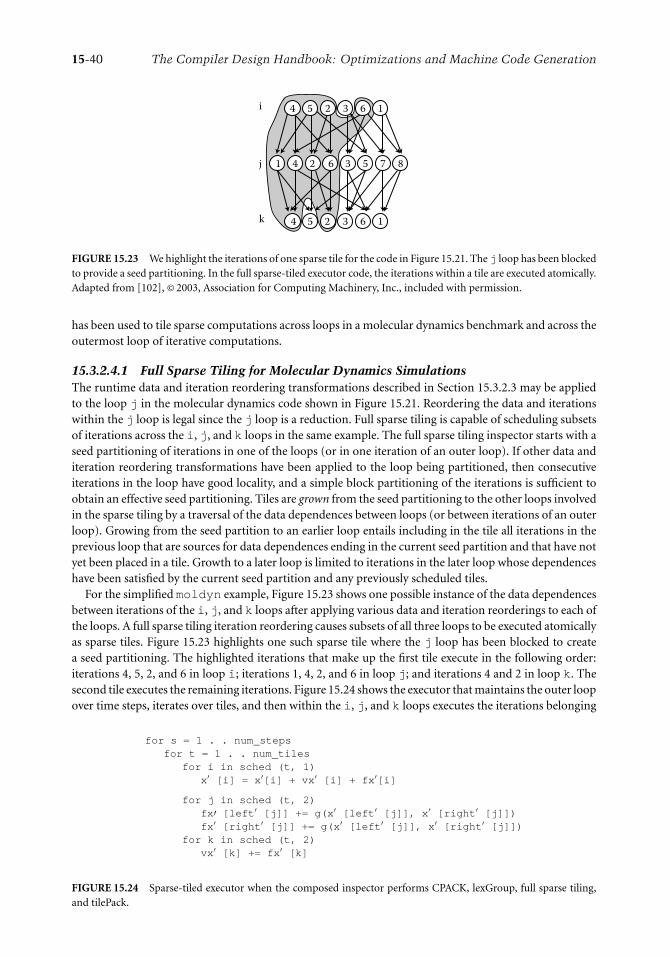
15-40 The Compiler Design Handbook: Optimizations and Machine Code Generation
341 2 6 5 7 8j
65 1324k
i 4 25 3 6 1
6
FIGURE 15.23 We highlight the iterations of one sparse tile for the code in Figure 15.21. The j loop has been blockedto provide a seed partitioning. In the full sparse-tiled executor code, the iterations within a tile are executed atomically.Adapted from [102], © 2003, Association for Computing Machinery, Inc., included with permission.
has been used to tile sparse computations across loops in a molecular dynamics benchmark and across theoutermost loop of iterative computations.
15.3.2.4.1 Full Sparse Tiling for Molecular Dynamics SimulationsThe runtime data and iteration reordering transformations described in Section 15.3.2.3 may be appliedto the loop j in the molecular dynamics code shown in Figure 15.21. Reordering the data and iterationswithin the j loop is legal since the j loop is a reduction. Full sparse tiling is capable of scheduling subsetsof iterations across the i, j, and k loops in the same example. The full sparse tiling inspector starts with aseed partitioning of iterations in one of the loops (or in one iteration of an outer loop). If other data anditeration reordering transformations have been applied to the loop being partitioned, then consecutiveiterations in the loop have good locality, and a simple block partitioning of the iterations is sufficient toobtain an effective seed partitioning. Tiles are grown from the seed partitioning to the other loops involvedin the sparse tiling by a traversal of the data dependences between loops (or between iterations of an outerloop). Growing from the seed partition to an earlier loop entails including in the tile all iterations in theprevious loop that are sources for data dependences ending in the current seed partition and that have notyet been placed in a tile. Growth to a later loop is limited to iterations in the later loop whose dependenceshave been satisfied by the current seed partition and any previously scheduled tiles.
For the simplified moldyn example, Figure 15.23 shows one possible instance of the data dependencesbetween iterations of the i, j, and k loops after applying various data and iteration reorderings to each ofthe loops. A full sparse tiling iteration reordering causes subsets of all three loops to be executed atomicallyas sparse tiles. Figure 15.23 highlights one such sparse tile where the j loop has been blocked to createa seed partitioning. The highlighted iterations that make up the first tile execute in the following order:iterations 4, 5, 2, and 6 in loop i; iterations 1, 4, 2, and 6 in loop j; and iterations 4 and 2 in loop k. Thesecond tile executes the remaining iterations. Figure 15.24 shows the executor that maintains the outer loopover time steps, iterates over tiles, and then within the i, j, and k loops executes the iterations belonging
for s = 1 . . num stepsfor t = 1 . . num tiles
for i in sched (t, 1)x′ [i] = x′[i] + vx′ [i] + fx′[i]
for j in sched (t, 2)fx′ [left′ [j]] += g(x′ [left′ [j]], x′ [right′ [j]])fx′ [right′ [j]] += g(x′ [left′ [j]], x′ [right′ [j]])
for k in sched (t, 2)vx′ [k] += fx′ [k]
FIGURE 15.24 Sparse-tiled executor when the composed inspector performs CPACK, lexGroup, full sparse tiling,and tilePack.

Computations on Iteration Spaces 15-41
for iter =1 .. Tfor i = 0 . . (R-1)
S1 u [i] = f[i]for p = ia[i] . . ia [i+1]-1if (ja[p] ! = i)
S2 u[i] = u[i] - a [p] * u [ja[p]]else
S3 diag[i] = a[p]S4 u[i] = u[i] / diag[i]
FIGURE 15.25 Typical Gauss–Seidel for CSR assuming an initial reordering of sparse matrix rows and columns andentries in vectors u and f.
to each tile as specified by the schedule data structure. Since iterations within all three loops touch thesame or adjacent data locations, locality between the loops is improved in the new schedule.
Full sparse tiling can dynamically parallelize irregular loops by executing the directed, acyclic dependencegraph between the sparse tiles in parallel using a master–worker strategy. The small example shown inFigure 15.23 only contains two tiles, where one tile must be executed before the other to satisfy dependencesbetween the i, j, and k loops. In a typical computation where the seed partitions are ordered via a graphcoloring, more parallelism between tiles is possible.
15.3.2.4.2 Full Sparse Tiling for Iterative Computations Over Sparse MatricesFull sparse tiling can also be used to improve the temporal locality and parallelize the Gauss–Seidelcomputation. Gauss–Seidel is an iterative computation commonly used alone or as a smoother withinmultigrid methods for solving systems of linear equations of the form Au = f , where A is a matrix, uis a vector of unknowns, and f is a known right-hand side. Figure 15.25 contains a linear Gauss–Seidelcomputation written for the compressed sparse row (CSR) sparse matrix format. We refer to iterationsof the outer loop as convergence iterations. The iteration space graph in Figure 15.26 visually representsan instance of the linear Gauss–Seidel computation. Each iteration point 〈iter, i〉 in the iteration spacerepresents all the computation for the unknown ui at convergence iteration iter (one instance of S1 and S4and multiple instances of S2 and S3). The iter axis shows three convergence iterations. The dark arrows showthe data dependences between iteration points for one unknown ui in the three convergence iterations. Theunknowns are indexed by a single variable i , but the computations are displayed in a two-dimensional planeparallel to the x and y axes to exhibit the relationships between iterations. At each convergence iterationiter the relationships between the unknowns are shown by the lightly shaded matrix graph. Specifically,for each nonzero in the sparse matrix A, ai j �= 0, there is an edge 〈i, j 〉 in the matrix graph. The original
Iter
x
y
FIGURE 15.26 The arrows show the data dependences for one unknown ui . The relationships between the iterationpoints are shown with a matrix graph.

15-42 The Compiler Design Handbook: Optimizations and Machine Code Generation
Iter
y
x
FIGURE 15.27 Full sparse-tiled Gauss–Seidel iteration space. Adapted from [101], with kind permission of SpringerScience and Business Media, © 2002.
order, v = 0, 1, . . ., (R − 1), given to the unknowns and corresponding matrix rows and columns is oftenarbitrary and can be changed without affecting the convergence properties of Gauss–Seidel. Therefore, ifthe unknowns are mapped to another order before performing Gauss–Seidel, the final numerical resultwill vary somewhat, but the convergence properties still hold.
In linear Gauss–Seidel, the data dependences arise from the nonzero structure of the sparse matrix A.Each iteration point 〈iter, i〉 depends on the iteration points of its neighbors in the matrix graph from eitherthe current or the previous convergence iteration, depending on whether the neighbor’s index j is orderedbefore or after i . The dependences between iteration points within the same convergence iteration makeparallelization of Gauss–Seidel especially difficult. Approaches to parallelizing Gauss–Seidel that maintainthe same pattern of Gauss–Seidel data dependences use the fact that it is possible to apply an a priorireordering to the unknowns and the corresponding rows of the sparse matrix A. This domain-specificknowledge is impossible to analyze with a compiler, so while automating full sparse tiling, it is necessary toprovide some mechanism for a domain expert to communicate such information to the program analysistool.
Figure 15.27 illustrates how the full sparse tiling inspector divides the Gauss–Seidel iteration spaceinto tiles. The process starts by performing a seed partitioning on the matrix graph. In Figure 15.27, theseed-partitioned matrix graph logically sits at the second convergence iteration, and tiles are grown to thefirst and third convergence iterations.14 The tile growth must satisfy the dependences. For Gauss–Seidel,that involves creating and maintaining a new data order during tile growth. The full sparse tiling executoris a transformed version of the original Gauss–Seidel computation that executes each tile atomically (seeFigure 15.28).
At runtime, the full sparse tiling inspector generates a data reordering function for reordering the rowsand columns in the matrix, σ (v) : V → {0, . . ., (R − 1)}, and a tiling function, θ(iter, v) : {1, .., T} xV → {0,. . ., (k − 1)}. The tiling function maps iteration points 〈iter, v〉 to tiles. From this tiling function,the inspector creates a schedule function, sched(tileID, iter) : {0,. . ., (k −1)} x {1,. . ., T} → 2{0,... ,(R−1)}. Theschedule function specifies for each tile and convergence iteration the subset of the reordered unknownsthat must be updated. The transformed code shown in Figure 15.28 performs a tile-by-tile execution ofthe iteration points using the schedule function, which is created by the inspector to satisfy the following:
sched(tileID, iter) = {σ (v) | θ(iter, v) = tileID}
14The number of iterations for tile growth is usually small (i.e., two to five), and the full sparse tiling pattern can berepeated multiple times if necessary. The tile growth is started from a middle iteration to keep the size of the tiles assmall as possible.

Computations on Iteration Spaces 15-43
for tileID = 0 .. (k-1)for iter = 1 .. T
for i in sched (tileID, iter)S1 u′ [i] = f′ [i]
for p = ia [i] .. ia[i+1]-1if (ja [p] ! = i)
S2 u′ [i] = u′ [i] - a [p] * u′[ja[p]]else
S3 diag [i] = a[p]S4 u′[i] = u′[i] / diag [i]
FIGURE 15.28 Code that performs a serial execution of sparse-tiled Gauss–Seidel for compressed sparse row (CSR).
A matrix graph partitioning serves as a seed partitioning from which tiles can be grown. The seedpartitioning determines the tiling at a particular convergence iteration, iters . Specifically at iters , where1 ≤ iters ≤ T , the tiling function is set to the partition function, θ(iters , v) = part(v). To determinethe tiling at other convergence iterations, the tile growth algorithm adds or deletes nodes from the seedpartition as needed to ensure that atomic execution of each tile does not violate any data dependences.
The FULLSPARSENAIVE GSCSR algorithm, shown in Figure 15.29, generates the tiling function θ forthe Gauss–Seidel computation in Figure 15.25. While generating the tiling function, ordering constraintsbetween nodes in the matrix graph are maintained in the relation NodeOrd. The first two statements in
ALGORITHM FULLSPARSENAIVE GSCSR (G(V, E ), part( ), T, iters )
1: foreach vertex v ∈ V , θ (iters , v) ← part (v)2: NodeOrd ← {〈v , w〉| θ (iters , v) < θ (iters , w)
and (〈v , w〉 ∈ E or 〈w , v〉 ∈ E )}Downward tile growth3: for iter = (iters – 1) downto 14: foreach vertex v ∈ V , θ (iter, v) ← θ (iter + 1, v)5: do while θ changes6: foreach 〈v , w〉 ∈ NodeOrd7: θ(iter, w) ← min(θ(iter, w), θ(iter + 1, v))8: θ (iter, v) ← min(θ(iter, v), θ (iter, w))9: end foreach10: end do while11: NodeOrd ← NodeOrd
⋃{〈v , w〉|θ (iter, v) < θ (iter, w)
and (〈v , w〉 ∈ E or 〈w , v〉 ∈ E )}12: end for
Upward tile growth13: for iter = (iters +1) to T14: foreach vertex v ∈ V , θ (iter, v) ← θ(iter – 1, v)15: do while θ changes16: foreach 〈v , w〉 ∈ NodeOrd17: θ (iter, v) ← max (θ (iter, v), θ (iter,– 1, w))18: θ (iter, w) ← max (θ (iter,, w), θ (iter, v))19: end foreach20: end do while21: NodeOrd ← NodeOrd
⋃{〈v , w〉| θ (iter, v) < θ (iter, w)
and (〈v , w〉 ∈ E or 〈w , v〉 ∈ E )}22: end for
FIGURE 15.29 FullSparseNaive GSCSR algorithm.

15-44 The Compiler Design Handbook: Optimizations and Machine Code Generation
the algorithm initialize the NodeOrd relation and all of the tiling function values for the convergenceiteration iters . The algorithm then loops through the convergence iterations iter such that iter < iters ,setting θ at each iteration point 〈iter, v〉 to 〈iter+1, v〉. Finally, it visits the edges that have endpoints in twodifferent partition cells, adjusting the tiling function θ to ensure that the data dependences are satisfied.The process is repeated for the convergence iterations between iters and T in the upward tile growth.Once neighboring nodes, 〈v , w〉 ∈ E , are put into two different tiles at any iteration iter, the relative orderbetween these two nodes must be maintained. The NodeOrd relation maintains that relative order. Forexample, if θ(iter, v) < θ(iter, w), then 〈v , w〉 ∈ NodeOrd.
The running time of this algorithm is O(Tk|V ||E |), where T is the number of convergence iterations,k is the number of tiles, |V | is the number of nodes in the matrix graph, and |E | is the number ofedges in the matrix graph. The k|V ||E | term is due to the while loops that begin at lines 5 and 15.In the worst case, the while loop will execute k|V | times, with only one θ(iter, v) value decreasing (orincreasing in the forward tile growth) each time through the while loop. Each θ(iter, v) can take on valuesbetween 1 and k, where k is the number of tiles. In practice, the algorithm runs much faster than thisbound.
To exploit parallelism, the inspector creates a tile dependence graph, and the executor for the full sparse-tiled computation executes sets of independent tiles in parallel. The tile dependence graph is used by amaster–worker implementation that is part of the executor. The master puts tiles whose data dependencesare satisfied on a ready queue. The workers execute tiles from the ready queue and notify the master uponcompletion. The following is an outline of the full sparse tiling process for parallelism:
� Partition the matrix graph to create the seed partitioning.� Choose a numbering on the cells of the seed partition. The numbering dictates the order inwhich tiles are grown and affects the resulting parallelism in the tile dependence graph (TDG). Anumbering that is based on a coloring of a partition interaction graph results in much improvedTDG parallelism.� Grow tiles from each cell of the seed partitioning in turn, based on the numbering, to create thetiling function θ that assigns each iteration point to a tile. The tile growth algorithm will alsogenerate constraints on the data reordering function.� Reorder the data using a reordering function that satisfies the constraints generated during tilegrowth.� Reschedule by creating a schedule function based on the tiling function θ . The schedule functionprovides a list of iteration points to execute for each tile at each convergence iteration.� Generate a TDG identifying which tiles may be executed in parallel.
15.3.3 Bibliographic Notes
As early as 1969, McKellar and Coffman [71] studied how to match the organization of matrices and theiroperations to paged memory systems. Early studies of such matching, in the context of program transfor-mation, were done by Abu-Sufah et al. [2] and Wolfe and coworkers [55, 109]. Irigoin and Triolet [49]in their seminal work give validity conditions for arbitrary parallelepiped tiling. These conditions werefurther refined by Xue [113].
Tiling for memory hierarchy is a well-studied problem, and so is the problem of modeling the cachebehavior of a loop nest. Several analytical models measure the number of cache misses for a given classof loop nests. These models can be classified into precise models that use sophisticated (computationallycostly) methods and approximate models that provide a closed form with simple analysis. In the precisecategory, we have the cache miss equations [40] and the refinement by Chatterjee et al. [17], whichuse Ehrhart polynomials [18] and Presburger formulae to describe the number of cache misses. Harperet al. [44] propose an analytical model of set-associative caches and Cascaval and Padua [15] give a compile-time technique to estimate cache misses using stack distances. In the approximate category, Ferranteet al. [34] present techniques to estimate the number of distinct cache lines touched by a given loop nest.

Computations on Iteration Spaces 15-45
Sarkar [94] presents a refinement of this model. Although the precise models can be used for selecting theoptimal tile sizes, only Abella et al. [1] have proposed a near-optimal loop tiling using cache miss equationsand genetic algorithms. Sarkar and Megiddo [95] have proposed an algorithm that uses an approximatemodel [34] and finds the optimal tile sizes for loops of depth up to three.
Several algorithms [16, 19, 47, 54] have been proposed for single-level tile size selection (see Hsu andKremer [47] for a good comparison). The majority of them use an indirect cost function such as thenumber of capacity misses or conflict misses, and not a direct metric such as overall execution time.Mitchell et al. [74] illustrate how such local cost functions may not lead to globally optimal performance.
Mitchell et al. [74] were the first to quantify the multilevel interactions of tiling. They clearly point outthe importance of using a global metric such as execution time rather than local metrics such as number ofmisses. Furthermore, they also show, through examples, the interactions between different levels of tilingand hence the need for a framework in which the tile sizes at all the levels are chosen simultaneously withrespect to a global cost function. Other results that show the application and importance of multilevel tilinginclude [14, 50, 75]. Auto-tuners such as PHiPHAC [12] and ATLAS [106] use a model-driven empiricalapproach to choose the optimal tile sizes.
The description of optimal tiling literature presented above and the GP-based approach presented in thischapter is based on the work of Renganarayanan and Rajopadhye [91]15, who present a general techniquefor optimal multilevel tiling of rectangular iteration spaces with uniform dependences. YALMIP [68] is atool that provides a symbolic interface to many optimization solvers. In particular, it provides an interfacefor defining and solving IGPs.
15.3.3.1 Tiled Loop Generation16
Ancourt and Irigoin proposed a technique [6] for scanning a single polyhedron, based on Fourier–Motzkinelimination over inequality constraints. Le Verge et al. [61] proposed an algorithm that exploits the dualrepresentation of polyhedra with vertices and rays in addition to constraints. The general code generationproblem for affine control loops requires scanning unions of polyhedra. Kelley et al. [53] solved thisby extending the Ancourt–Irigoin technique, and together with a number of sophisticated optimizations,developed the widely distributed Omega library [78]. The SUIF [108] tool has a similar algorithm. Quillereet al. proposed a dual-representation algorithm [80] for scanning the union of polyhedra, and this algorithmis implemented in the CLooG code generator [11] and its derivative Wloog used in the WRaP-IT project.
Code generation for fixed tile sizes can also benefit from the above techniques, thanks to Irigoin andTriolet’s proof that the tiled iteration space is a polyhedron if the tile sizes are constants [49]. Either of theabove tools may be used (in fact, most of them can generate such tiled code). However, it is well known thatsince the worst-case complexity of Fourier–Motzkin elimination is doubly exponential in the number ofdimensions, this may be inefficient. Goumas et al. [41] decompose the generation into two subproblems,one to scan the tile origins, and the other to scan points within a tile, thus obtaining significant reductionof the worst-case complexity. They propose a technique to generate code for fixed-sized, parallelogram tiles.
There has been relatively little work for the case when tile sizes are symbolic parameters, except for thevery simple case of orthogonal tiling: either rectangular loops tiled with rectangular tiles or loops that can beeasily transformed to this. For the more general case, the standard solution, as described in Xue’s text [114],has been to simply extend the iteration space to a rectangular one (i.e., to consider its bounding box)and apply the orthogonal technique with appropriate guards to avoid computations outside the originaliteration space.
Amarasinghe and Lam [4, 5] implemented, in the SUIF tool set, a version of Fourier-Motzkin Elimina-tion (FME) that can deal with a limited class of symbolic coefficients (parameters and block sizes), but thefull details have not been made available. Großlinger et al. [42] have proposed an extension to the polyhe-dral model, in which they allow arbitrary rational polynomials as coefficients in the linear constraints thatdefine the iteration space. Their generosity comes at the price of requiring computationally very expensive
15Portions reprinted, with permission, from [91], © 2004 IEEE.16Parts of this section are based on [92], © 2007, Association for Computing Machinery, Inc., included with permission.

15-46 The Compiler Design Handbook: Optimizations and Machine Code Generation
machinery such as quantifier elimination in polynomials over the real algebra to simplify constraints thatarise during loop generations. Because of this their method does not scale with the number of dimensionsand the number of nonlinear parameters.
Jimenez et al. [51] develop code generation techniques for register tiling of nonrectangular iterationspaces. They generate code that traverses the bounding box of the tile iteration space to enable parameterizedtile sizes. They apply index-set splitting to tiled code to traverse parts of the tile space that include only fulltiles. Their approach involves less overhead in the loop nest that visits the full tiles; however, the resultingcode experiences significant code expansion.
15.3.3.2 Tiling for Parallelism
Communication-minimal tiling refers to the problem of choosing the tile sizes such that the communicationvolume is minimized. Schriber and Dongarra [96] are perhaps the first to study communication-minimaltilings. Boulet et al. [13] are the first to solve the communication-minimal tiling optimally. Xue [112] givesa detailed comparison of various communication-minimal tilings.
Hogstedt et al. [45] studied the idle time associated with parallelepiped tiling. They characterize thetime processor’s wait for data from other processors. Desprez et al. [27] present simpler proofs to thesolution presented by Hogstedt et al.
Several researchers [46, 76, 86, 115] have studied the problem of picking the tile sizes that minimizethe parallel execution time. Andonov et al. [7, 8] have proposed optimal tile size selection algorithms forn-dimensional rectangular and two-dimensional parallelogram iteration spaces. Our formulation of theoptimal tiling problem for parallelism is very similar to theirs. They derive closed-form optimal solutionsfor both cases. We presented a GP-based framework that can be used to solve their formulation directly.Xue [114] gives a good overview of loop tiling for parallelism.
15.3.3.3 Tiling for Sparse Computations
Irregular memory references are also prevalent in popular games such as Unreal, which was analyzed ashaving 90% of its integer variables within index arrays such as B [103].
In Section 15.3.2.2, the static analysis techniques described were developed by Lin and Padua [65]. Pughand Wonnacott [77] and Rus et al. [92] have developed techniques for extending static data dependenceanalysis with runtime checks, as discussed in Section 15.3.2.2. In [77] constraints for disproving depen-dences are generated at compile time, with the possibility of evaluating such constraints at runtime. Ruset al. [92] developed an interprocedural hybrid (static and dynamic) analysis framework, where it is possibleto disprove all data dependences at runtime, if necessary.
Examples of runtime reordering transformation for data locality include [3, 20, 24, 28, 35, 43, 48,72, 73, 99]. The pointer update optimization was presented by Ding and Kennedy [28].
Saltz et al. [93] originally developed inspector–executor strategies for the parallelization of irregularprograms. Initially such transformations were incorporated into applications manually for parallelism [24].Next, libraries with runtime transformation primitives were developed so that a programmer or compilercould insert calls to such primitives [25, 98].
Rauchwerger [88] surveys various techniques for dynamically scheduling iterations into wavefrontssuch that all of the iterations within one wavefront may be executed in parallel. Rauchwerger also discussesmany issues such as load balancing, parallelizing the inspector, finding the optimal schedule, and removinganti and output dependences.
Strout et al. developed full sparse tiling [100–102]. Cache blocking of unstructured grids is anothersparse tiling transformation, which was developed by Douglas et al. [29]. Wu [110] shows that reorderingthe unknowns in Gauss–Seidel does not affect the convergence properties.
References
1. J. Abella, A. Gonzalez, J. Llosa, and X. Vera. 2002. Near-optimal loop tiling by mean of cache missequations and genetic algorithms. In Proceedings of International Conference on Parallel ProcessingWorkshops.

Computations on Iteration Spaces 15-47
2. W. Abu-Sufah, D. Kuck, and D. Lawrie. 1981. On the performance enhancememt of paging systemsthrough program analysis and transformations. IEEE Trans. Comput. 30(5):341–56.
3. I. Al-Furaih and S. Ranka. 1998. Memory hierarchy management for iterative graph structures. InProceedings of the 1st Merged International Parallel Processing Symposium and Symposium on Paralleland Distributed Processing, 298–302.
4. S. P. Amarasinghe. 1997. Parallelizing compiler techniques based on linear inequalities. PhD thesis,Computer Science Department, Stanford University, Stanford, CA.
5. Saman P. Amarasinghe and Monica S. Lam. 1993. Communication optimization and code gen-eration for distributed memory machines. In PLDI ’93: Proceedings of the ACM SIGPLAN 1993Conference on Programming Language Design and Implementation, 126–38. New York: ACMPress.
6. C. Ancourt. 1991. Generation automatique de codes de transfert pour multiprocesseurs a memoireslocales. PhD thesis, Universite de Paris VI.
7. Rumen Andonov, Stephan Balev, Sanjay V. Rajopadhye, and Nicola Yanev. 2003. Optimal semi-oblique tiling. IEEE Trans. Parallel Distrib. Syst. 14(9):944–60.
8. Rumen Andonov, Sanjay V. Rajopadhye, and Nicola Yanev. 1998. Optimal orthogonal tiling. InEuro-Par, 480–90.
9. C. Bastoul. 2002. Generating loops for scanning polyhedra. Technical Report 2002/23, PRiSM,Versailles University.
10. C. Bastoul, A. Cohen, A. Girbal, S. Sharma, and O. Temam. 2000. Putting polyhedral loop transfor-mations to work. In Languages and compilers for parallel computers, 209–25.
11. Cedric Bastoul. 2004. Code generation in the polyhedral model is easier than you think. In IEEEPACT, 7–16.
12. Jeff Bilmes, Krste Asanovic, Chee-Whye Chin, and Jim Demmel. 1997. Optimizing matrix multiplyusing phipac: A portable, high-performance, ANSI C coding methodology. In Proceedings of the11th International Conference on Supercomputing, 340–47. New York: ACM Press.
13. Pierre Boulet, Alain Darte, Tanguy Risset, and Yves Robert. (Pen)-ultimate tiling? Integr. VLSI J.17(1):33–51.
14. L. Carter, J. Ferrante, F. Hummel, B. Alpern, and K. S. Gatlin. 1996. Hierarchical tiling: A methodologyfor high performance. Technical Report CS96-508, University of California at San Diego.
15. Calin Cascaval and David A. Padua. 2003. Estimating cache misses and locality using stack distances.In Proceedings of the 17th Annual International Conference on Supercomputing, 150–59. New York:ACM Press.
16. Jacqueline Chame and Sungdo Moon. 1999. A tile selection algorithm for data locality and cacheinterference. In Proceedings of the 13th International Conference on Supercomputing, 492–99. NewYork: ACM Press.
17. Siddhartha Chatterjee, Erin Parker, Philip J. Hanlon, and Alvin R. Lebeck. 2001. Exact analysisof the cache behavior of nested loops. In Proceedings of the ACM SIGPLAN 2001 Conference onProgramming Language Design and Implementation, 286–97. New York: ACM Press.
18. Philippe Clauss. 1996. Counting solutions to linear and nonlinear constraints through Ehrhartpolynomials: Applications to analyze and transform scientific programs. In Proceedings of the 10thInternational Conference on Supercomputing, 278–85. New York: ACM Press.
19. Stephanie Coleman and Kathryn S. McKinley. 1995. Tile size selection using cache organizationand data layout. In Proceedings of the ACM SIGPLAN 1995 Conference on Programming LanguageDesign and Implementation, 279–90. New York: ACM Press.
20. E. Cuthill and J. McKee. 1969. Reducing the bandwidth of sparse symmetric matrices. In Proceedingsof the 24th National Conference ACM, 157–72.
21. A. Darte, Y. Robert, and F. Vivien. 2000. Scheduling and automatic parallelization. Basel, Switzerland:Birkhauser.
22. A. Darte, R. Schreiber, and G. Villard. 2005. Lattice-based memory allocation. IEEE Trans. Comput.54(10):1242–57.

15-48 The Compiler Design Handbook: Optimizations and Machine Code Generation
23. Alain Darte and Yves Robert. 1995. Affine-by-statement scheduling of uniform and affine loop nestsover parametric. J. Parallel Distrib. Comput. 29(1):43–59.
24. R. Das, D. Mavriplis, J. Saltz, S. Gupta, and R. Ponnusamy. 1992. The design and implementationof a parallel unstructured Euler solver using software primitives. AIAA J. 32:489–96.
25. R. Das, M. Uysal, J. Saltz, and Yuan-Shin S. Hwang. 1994. Communication optimizations forirregular scientific computations on distributed memory architectures. J. Parallel Distrib. Comput.22(3):462–78.
26. E. De Greef, F. Catthoor, and H. De Man. 1997. Memory size reduction through storage orderoptimization for embedded parallel multimedia applications. In Parallel processing and multimedia.Geneva, Switzerland. Amsterdam, Netherlands: Elsevier Science.
27. Frederic Desprez, Jack Dongarra, Fabrice Rastello, and Yves Robert. 1997. Determining the idletime of a tiling: New results. In PACT ’97: Proceedings of the 1997 International Conference on ParallelArchitectures and Compilation Techniques, 307. Washington, DC: IEEE Computer Society.
28. C. Ding and K. Kennedy. 1999. Improving cache performance in dynamic applications through dataand computation reorganization at run time. In Proceedings of the 1999 ACM SIGPLAN Conferenceon Programming Language Design and Implementation (PLDI), 229–41. New York: ACM Press.
29. C. C. Douglas, J. Hu, M. Kowarschik, U. Rude, and C. Weiss. 2000. Cache optimization for structuredand unstructured grid multigrid. Electron. Trans. Numerical Anal. 10:21–40.
30. P. Feautrier. 1991. Dataflow analysis of array and scalar references. Int. J. Parallel Program.20(1):23–53.
31. P. Feautrier. 1992. Some efficient solutions to the affine scheduling problem. Part I. One-dimensionaltime. Int. J. Parallel Program. 21(5):313–48.
32. P. Feautrier. 1992. Some efficient solutions to the affine scheduling problem. Part II. Multi-dimensional time. Int. J. Parallel Program. 21(6):389–420.
33. Agustin Fernandez, Jose M. Llaberıa, and Miguel Valero-Garcıa. 1995. Loop transformation usingnonunimodular matrices. IEEE Trans. Parallel Distrib. Syst. 6(8):832–40.
34. J. Ferrante, V. Sarkar, and W. Thrash. 1991. On estimating and enhancing cache effectiveness. InFourth International Workshop on Languages and Compilers for Parallel Computing, ed. U. Banerjee,D. Gelernter, A. Nicolau, and D. Padua, 328–43. Vol. 589 of Lecture Notes on Computer Science.Heidelberg, Germany: Springer-Verlag.
35. Jinghua Fu, Alex Pothen, Dimitri Mavriplis, and Shengnian Ye. 2001. On the memory systemperformance of sparse algorithms. In Eighth International Workshop on Solving Irregularly StructuredProblems in Parallel.
36. Gautam, DaeGon Kim, and S. Rajopadhye. Scheduling in the Z-polyhedral model. In Proceedingsof the IEEE International Symposium on Parallel and Distributed Systems (Long Beach, CA, USA,March 26–30, 2007). IPDPS ’07. IEEE Press, 1–10.
37. Gautam and S. Rajopadhye. 2007. The Z-polyhedral model. PPoPP 2007: ACM Symposium on Prin-ciples and Practice of Parallel Programming. In Proceedings of the 12th ACM SIGPLAN Symposium onPrinciples and Practice of Parallel Programming (San Jose, CA, USA, March 14–17, 2007). PPoPP ’07.New York, NY: ACM Press, 237–248.
38. Gautam and S. Rajopadhye. 2006. Simplifying reductions. In POPL ’06: Symposium on Principles ofProgramming Languages, 30–41. New York: ACM Press.
39. Gautam, S. Rajopadhye, and P. Quinton. 2002. Scheduling reductions on realistic machines. In SPAA’02: Symposium on Parallel Algorithms and Architectures, 117–26.
40. Somnath Ghosh, Margaret Martonosi, and Sharad Malik. 1999. Cache miss equations: A com-piler framework for analyzing and tuning memory behavior. ACM Trans. Program. Lang. Syst.21(4):703–46.
41. Georgios Goumas, Maria Athanasaki, and Nectarios Koziris. 2003. An efficient code generationtechnique for tiled iteration spaces. IEEE Trans. Parallel Distrib. Syst. 14(10):1021–34.
42. Armin Großlinger, Martin Griebl, and Christian Lengauer. 2004. Introducing non-linear parametersto the polyhedron model. In Proceedings of the 11th Workshop on Compilers for Parallel Computers

Computations on Iteration Spaces 15-49
(CPC 2004), ed. Michael Gerndt and Edmond Kereku, 1–12. Research Report Series. LRR-TUM,Technische Universitat Munchen.
43. H. Han and C. Tseng. 2000. A comparison of locality transformations for irregular codes. In Proceed-ings of the 5th International Workshop on Languages, Compilers, and Run-time Systems for ScalableComputers. Vol. 1915 of Lecture Notes in Computer Science. Heidelberg, Germany: Springer.
44. John S. Harper, Darren J. Kerbyson, and Graham R. Nudd. 1999. Analytical modeling of set-associative cache behavior. IEEE Trans. Comput. 48(10):1009–24.
45. Karin Hogstedt, Larry Carter, and Jeanne Ferrante. 1997. Determining the idle time of a tiling. InPOPL ’97: Proceedings of the 24th ACM SIGPLAN-SIGACT Symposium on Principles of ProgrammingLanguages, 160–73. New York: ACM Press.
46. Karin Hogstedt, Larry Carter, and Jeanne Ferrante. 2003. On the parallel execution time of tiledloops. IEEE Trans. Parallel Distrib. Syst. 14(3):307–21.
47. C. Hsu and U. Kremer. 1999. Tile selection algorithms and their performance models. TechnicalReport DCS-TR-401, Computer Science Department, Rutgers University, New Brunswick, NJ.
48. E. Im and K. Yelick. 2001. Optimizing sparse matrix computations for register reuse in sparsity. InComputational Science — ICCS 2001, ed. V. N. Alexandrov, J. J. Dongarra, B. A. Juliano, R. S. Renner,and C. J. K. Tan, 127–36. Vol. 2073 of Lecture Notes in Computer Science. Heidelberg, Germany:Springer-Verlag.
49. F. Irigoin and R. Triolet. 1988. Supernode partitioning. In 15th ACM Symposium on Principles ofProgramming Languages, 319–28. New York: ACM Press.
50. M. Jimenez, J. M. Llaberia, and A. Fernandez. 2003. A cost-effective implementation of multileveltiling. IEEE Trans. Parallel Distrib. Comput. 14(10):1006–20.
51. Marta Jimenez, Jose M. Llaberia, and Agustin Fernandez. 2002. Register tiling in nonrectangulariteration spaces. ACM Trans. Program. Lang. Syst. 24(4):409–53.
52. R. M. Karp, R. E. Miller, and S. V. Winograd. 1967. The organization of computations for uniformrecurrence equations. J. ACM 14(3):563–90.
53. W. Kelly, W. Pugh, and E. Rosser. 1995. Code generation for multiple mappings. In Frontiers ’95:The 5th Symposium on the Frontiers of Massively Parallel Computation.
54. Monica D. Lam, Edward E. Rothberg, and Michael E. Wolf. 1991. The cache performance andoptimizations of blocked algorithms. In Proceedings of the Fourth International Conference on Archi-tectural Support for Programming Languages and Operating Systems, 63–74. New York: ACM Press.
55. Monica S. Lam and Michael E. Wolf. 1991. A data locality optimizing algorithm (with retrospective).In Best of PLDI, 442–59.
56. Leslie Lamport. 1974. The parallel execution of DO loops. Commun. ACM 17(2) 83–93.57. V. Lefebvre and P. Feautrier. 1997. Optimizing storage size for static control programs in automatic
parallelizers. In Euro-Par’97, ed. C. Lengauer, M. Griebl, and S. Gorlatch. Vol. 1300 of Lecture Notesin Computer Science. Heidelberg, Germany: Springer-Verlag.
58. P. Lenders and S. V. Rajopadhye. 1994. Multirate VLSI arrays and their synthesis. Technical Report94-70-01, Oregon State University.
59. H. Le Verge. 1992. Un environnement de transformations de programmmes pour la synthesed’architectures regulieres. PhD thesis, L’Universite de Rennes I, IRISA, Campus de Beaulieu, Rennes,France.
60. H. Le Verge. 1995. Recurrences on lattice polyhedra and their applications. Based on a manuscriptwritten by H. Le Verge just before his untimely death.
61. H. Le Verge, V. Van Dongen, and D. Wilde. 1994. Loop nest synthesis using the polyhedral library.Technical Report PI 830, IRISA, Rennes, France. Also published as INRIA Research Report 2288.
62. Wei Li and Keshav Pingali. 1994. A singular loop transformation framework based on non-singularmatrices. Int. J. Parallel Program. 22(2):183–205.
63. Amy W. Lim, Gerald I. Cheong, and Monica S. Lam. 1999. An affine partitioning algorithm to max-imize parallelism and minimize communication. In International Conference on Supercomputing,228–37.

15-50 The Compiler Design Handbook: Optimizations and Machine Code Generation
64. Amy W. Lim, Shih-Wei Liao, and Monica S. Lam. 2001. Blocking and array contraction acrossarbitrarily nested loops using affine partitioning. In PPoPP ’01: Proceedings of the Eighth ACMSIGPLAN Symposium on Principles and Practices of Parallel Programming, 103–12. New York: ACMPress.
65. Yuan Lin and David Padua. 2000. Compiler analysis of irregular memory accesses. In Proceedingsof the ACM SIGPLAN Conference on Programming Language Design and Implementation, 157–68.Vol. 35.
66. B. Lisper. 1990. Linear programming methods for minimizing execution time of indexed computa-tions. In International Workshop on Compilers for Parallel Computers.
67. Yanhong A. Liu, Scott D. Stoller, Ning Li, and Tom Rothamel. 2005. Optimizing aggregate arraycomputations in loops. ACM Trans. Program. Lang. Syst. 27(1):91–125.
68. J. Lofberg. 2004. YALMIP: A toolbox for modeling and optimization in MATLAB. In Proceedings ofthe CACSD Conference. http://control.ee.ethz.ch/˜joloef/yalmip.php.
69. C. Mauras. 1989. ALPHA: Un langage equationnel pour la conception et la programmationd’architectures paralleles synchrones. PhD thesis, L’Universite de Rennes I, Rennes, France.
70. C. Mauras, P. Quinton, S. Rajopadhye, and Y. Saouter. 1990. Scheduling affine parametrized recur-rences by means of variable dependent timing functions. In International Conference on ApplicationSpecific Array Processing, 100–10.
71. A. C. McKellar and E. G. Coffman, Jr. 1969. Organizing matrices and matrix operations for pagedmemory systems. Commun. ACM 12(3):153–65.
72. J. Mellor-Crummey, D. Whalley, and K. Kennedy. 1999. Improving memory hierarchy performancefor irregular applications. In Proceedings of the 1999 ACM SIGARCH International Conference onSupercomputing (ICS), 425–33.
73. N. Mitchell, L. Carter, and J. Ferrante. 1999. Localizing non-affine array references. In Proceed-ings of the 1999 International Conference on Parallel Architectures and Compilation Techniques,192–202.
74. N. Mitchell, N. Hogstedt, L. Carter, and J. Ferrante. 1998. Quantifying the multi-level nature oftiling interactions. Int. J. Parallel Program. 26(6):641–70.
75. Juan J. Navarro, Toni Juan, and Toms Lang. 1994. Mob forms: A class of multilevel block algo-rithms for dense linear algebra operations. In Proceedings of the 8th International Conference onSupercomputing, 354–63. New York: ACM Press.
76. Hiroshi Ohta, Yasuhiko Saito, Masahiro Kainaga, and Hiroyuki Ono. 1995. Optimal tile size ad-justment in compiling general doacross loop nests. In ICS ’95: Proceedings of the 9th InternationalConference on Supercomputing, 270–79. New York: ACM Press.
77. B. Pugh and D. Wonnacott. 1994. Nonlinear array dependence analysis. Technical Report CS-TR-3372, Department of Computer Science, University of Maryland, College Park.
78. W. Pugh. 1992. A practical algorithm for exact array dependence analysis. Commun. ACM35(8):102–14.
79. Fabien Quillere and Sanjay Rajopadhye. 2000. Optimizing memory usage in the polyhedral model.ACM Trans. Program. Lang. Syst. 22(5):773–815.
80. Fabien Quillere, Sanjay Rajopadhye, and Doran Wilde. 2000. Generation of efficient nested loopsfrom polyhedra. Int. J. Parallel Program. 28(5):469–98.
81. P. Quinton, S. Rajopadhye, and T. Risset. 1996. Extension of the alpha language to recurrences onsparse periodic domains. In ASAP ’96, 391.
82. Patrice Quinton and Vincent Van Dongen. 1989. The mapping of linear recurrence equations onregular arrays. J. VLSI Signal Process. 1(2):95–113.
83. S. V. Rajopadhye, S. Purushothaman, and R. M. Fujimoto. 1986. On synthesizing systolic arrays fromrecurrence equations with linear dependencies. In Foundations of software technology and theoreticalcomputer science, 488–503.
84. Easwaran Raman and David August. 2007. Optimizations for memory hierarchy. In The compilerdesign handbook: Optimization and machine code generation. Boca Raton, FL: CRC Press.

Computations on Iteration Spaces 15-51
85. J. Ramanujam. 1995. Beyond unimodular transformations. J. Supercomput. 9(4):365–89.86. J. Ramanujam and P. Sadayappan. 1991. Tiling multidimensional iteration spaces for nonshared
memory machines. In Supercomputing ’91: Proceedings of the 1991 ACM/IEEE Conference on Super-computing, 111–20. New York: ACM Press.
87. S. K. Rao. 1985. Regular iterative algorithms and their implementations on processor arrays. PhDthesis, Information Systems Laboratory, Stanford University, Stanford, CA.
88. Lawrence Rauchwerger. 1998. Run-time parallelization: Its time has come. Parallel Comput.24(3–4):527–56.
89. Xavier Redon and Paul Feautrier. 1993. Detection of recurrences in sequential programs with loops.In PARLE ’93: Parallel Architectures and Languages Europe, 132–45.
90. Xavier Redon and Paul Feautrier. 1994. Scheduling reductions. In International Conference onSupercomputing, 117–25.
91. Lakshminarayanan Renganarayana and Sanjay Rajopadhye. 2004. A geometric programmingframework for optimal multi-level tiling. In SC ’04: Proceedings of the 2004 ACM/IEEE Conferenceon Supercomputing, 18. Washington, DC: IEEE Computer Society.
92. S. Rus, L. Rauchwerger, and J. Hoeflinger. 2002. Hybrid analysis: Static & dynamic memory referenceanalysis. In Proceedings of the 16th Annual ACM International Conference on Supercomputing (ICS).
93. Joel H. Salz, Ravi Mirchandaney, and Kay Crowley. 1991. Run-time parallelization and schedulingof loops. IEEE Trans. Comput. 40(5):603–12.
94. V. Sarkar. 1997. Automatic selection of high-order transformations in the IBM XL Fortran compilers.IBM J. Res. Dev. 41(3):233–64.
95. V. Sarkar and N. Megiddo. 2000. An analytical model for loop tiling and its solution. In Proceedingsof ISPASS.
96. R. Schreiber and J. Dongarra. 1990. Automatic blocking of nested loops. Technical Report 90.38,RIACS, NASA Ames Research Center, Moffett Field, CA.
97. W. Shang and J. Fortes. 1991. Time optimal linear schedules for algorithms with uniform depen-dencies. IEEE Trans. Comput. 40(6):723–42.
98. Shamik D. Sharma, Ravi Ponnusamy, Bongki Moon, Yuan-Shin Hwang, Raja Das, and Joel Saltz.1994. Run-time and compile-time support for adaptive irregular problems. In Supercomputing ’94.Washington, DC: IEEE Computer Society.
99. J. P. Singh, C. Holt, T. Totsuka, A. Gupta, and J. Hennessy. 1995. Load balancing and data locality inadaptive hierarchical N-body methods: Barnes-Hut, fast multipole, and radiosity. J. Parallel Distrib.Comput. 27(2):118–41.
100. M. M. Strout, L. Carter, and J. Ferrante. 2001. Rescheduling for locality in sparse matrix computa-tions. In Computational Science — ICCS 2001, ed. V. N. Alexandrov, J. J. Dongarra, B. A. Juliano, R. S.Renner, and C. J. K. Tan. Vol. 2073 of Lecture Notes in Computer Science. Heidelberg, Germany:Springer-Verlag.
101. M. M. Strout, L. Carter, J. Ferrante, J. Freeman, and B. Kreaseck. 2002. Combining performanceaspects of irregular Gauss-Seidel via sparse tiling. In Proceedings of the 15th Workshop on Languagesand Compilers for Parallel Computing (LCPC).
102. Michelle Mills Strout, Larry Carter, and Jeanne Ferrante. 2003. Compile-time composition of run-time data and iteration reorderings. In Proceedings of the 2003 ACM SIGPLAN Conference on Pro-gramming Language Design and Implementation (PLDI).
103. Tim Sweeney. 2006. The next mainstream programming language: A game developer’s perspec-tive. Invited talk at ACM SIGPLAN Conference on Principles of Programming Languages (POPL).Charleston, SC, USA.
104. J. Teich and L. Thiele. 1993. Partitioning of processor arrays: A piecewise regular approach. INTE-GRATION: VLSI J. 14(3):297–332.
105. William Thies, Frederic Vivien, Jeffrey Sheldon, and Saman P. Amarasinghe. 2001. A unified frame-work for schedule and storage optimization. In Proceedings of the 2001 ACM SIGPLAN Conferenceon Programming Language Design and Implementation, 232–42, Snowbird, Utah, USA.

15-52 The Compiler Design Handbook: Optimizations and Machine Code Generation
106. R. Clint Whaley and Jack J. Dongarra. 1998. Automatically tuned linear algebra software. In Pro-ceedings of the 1998 ACM/IEEE Conference on Supercomputing (CDROM), 1–27. Washington, DC:IEEE Computer Society.
107. D. Wilde. 1993. A library for doing polyhedral operations. Technical Report PI 785, IRISA, Rennes,France.
108. R. P. Wilson, Robert S. French, Christopher S. Wilson, S. P. Amarasinghe, J. M. Anderson, S. W. K.Tjiang, S.-W. Liao, C.-W. Tseng, M. W. Hall, M. S. Lam, and J. L. Hennessy. 1994. SUIF: An infra-structure for research on parallelizing and optimizing compilers. SIGPLAN Notices 29(12):31–37.
109. Michael Wolfe. 1989. Iteration space tiling for memory hierarchies. In Proceedings of the ThirdSIAM Conference on Parallel Processing for Scientific Computing, 357–61, Philadelphia, PA: Societyfor Industrial and Applied Mathematics.
110. C. H. Wu. 1990. A multicolour SOR method for the finite-element method. J. Comput. AppliedMath. 30(3):283–94.
111. Jingling Xue. 1994. Automating non-unimodular loop transformations for massive parallelism.Parallel Comput. 20(5):711–28.
112. Jingling Xue. 1997. Communication-minimal tiling of uniform dependence loops. J. Parallel Distrib.Comput. 42(1):42–59.
113. Jingling Xue. 1997. On tiling as a loop transformation. Parallel Process. Lett. 7(4):409–24.114. Jingling Xue. 2000. Loop tiling for parallelism. Dordrecht, The Netherlands: Kluwer Academic
Publishers.115. Jingling Xue and Wentong Cai. 2002. Time-minimal tiling when rise is larger than zero. Parallel
Comput. 28(6):915–39.

16Architecture
Description Languagesfor Retargetable
Compilation
Wei QinDepartment of Electrical & ComputerEngineering,Boston University, Boston, [email protected]
Sharad MalikDepartment of Electrical Engineering,Princeton University, Princeton, [email protected]
16.1 Introduction . . . . . . . . . . . . . . . . . . . . . . . . . . . . . . . . . . . . . . . . . .16-116.2 Architecture Description Languages . . . . . . . . . . . . . . . . . . .16-3
Structural Languages • Behavioral Languages • MixedLanguages
16.3 Discussions . . . . . . . . . . . . . . . . . . . . . . . . . . . . . . . . . . . . . . . . . . .16-16Summary of ADLs • Essential Elements of an ADL •
Organization of an ADL • Challenges • Future Directions
16.4 Conclusion . . . . . . . . . . . . . . . . . . . . . . . . . . . . . . . . . . . . . . . . . . .16-24References . . . . . . . . . . . . . . . . . . . . . . . . . . . . . . . . . . . . . . . . . . . . . . . . . .16-25
16.1 Introduction
Retargetable compilation has posed many challenges to researchers. The ultimate goal of the field is todevelop a universal compiler that generates high-quality code for all known architectures. Among allexisting compilers, GNU Compiler Collection (GCC) comes closest to this goal by using a myriad offormal algorithms and engineering hacks. Currently, GCC officially supports more than 30 architecturescommonly used around the world [12]. Still, for many less known architectures, there is no GCC support.Many recent application-specific instruction set processors (ASIPs) are designed with such specializedarchitectural features that it is not a straightforward task to create customized compilers for them, letalone retarget GCC. Despite the difficulties, good retargetable compilers are highly desirable for thesearchitectures, especially during their development stages in which many candidate domain-specific featuresneed to be evaluated. If a retargetable compiler is capable of utilizing these candidate features and generatingoptimized code accordingly, their effectiveness can be quickly evaluated by running the resulting code onan equally retargetable simulator. In this regard, retargetable compilation and retargetable simulation areclosely related problems, but retargetable compilation is a much harder one.
The need for retargetability largely comes from the back-ends of compilers. Compiler back-ends may beclassified into the following three types: customized, semi-retargetable, and retargetable. Customized back-ends have little retargetability. They are usually written for high-quality proprietary compilers or developedfor special architectures requiring nonstandard code generation flow. In contrast, semi-retargetable andretargetable compilers reuse at least part of the compiler back-end by factoring out target-dependentinformation into machine description systems. The difference of customization and retargetability isillustrated in Figure 16.1.
16-1

16-2 The Compiler Design Handbook: Optimizations and Machine Code Generation
Backend 1
Frontend
Backend 2 Backend N
Asm 1 Asm 2 Asm N
Application
Application
Frontend
Retargetable
Backend
Asm 1 Asm 2 Asm N
Description 2
Machine
Description 1
Machine
Description N
FIGURE 16.1 Different compilation flows.
Semi-retargetable compilers, for example, lcc [11] and GCC [12], share a significant amount of codeacross the back-ends for different targets. The sharing reduces the time to retarget the compilers to a newprocessor. Nevertheless, the retargeting effort is still substantial because of target-specific architecturalfeatures or function calling conventions. In a semi-retargetable compiler implementation, the instructionset of the target is usually described in tree patterns as is required by popular code generation algorithms [3].General-purpose register files and usage of the registers are either described as some data structures orsimply hard-coded in algorithms. This type of description system serves as the interface between themachine-independent part and the machine-dependent part of the compiler. It typically involves a mixtureof the pattern descriptions and C interface functions or macros. It is the primitive form of architecturedescription languages.
A fully retargetable compiler minimizes coding effort for various target architectures by providing amore friendly machine description interface. Retargetable compilers are important for the development ofASIPs (including digital signal processors [DSPs]). These cost-sensitive processors are usually designed forspecialized application domains and have a narrow market window. During their development process,numerous design choices need to be evaluated with benchmarks. It is impractical for designers to manuallytune a general-purpose semi-retargetable compiler for each design choice to quantitatively verify its efficacy.A fully retargetable compiler, which can be configured through an architecture description language (ADL),is desirable in such situations.
An ideal ASIP design flow involving an ADL is illustrated as the Y-chart [30] in Figure 16.2. In such a flow,a designer or possibly an automated tool tunes the architecture description. The retargetable compiler readsthe description, configures itself, and compiles the applications (usually a set of benchmark programs)

Architecture Description Languages for Retargetable Compilation 16-3
Applications
Retargetable
Compiler
Retargetable
Simulator
Architecture
Description
Performance/Cost
Evaluation
FIGURE 16.2 Design space exploration of ASIP.
into target binary code. The retargetable simulator also reads the description, configures itself, executes thecompiled code, and produces performance metrics such as cycle count and power consumption. Based onthese metrics, the designer can then tune the architecture and the corresponding architecture description.The updated description will initiate another round of compilation and simulation. The process iteratesuntil a satisfactory trade-off is found. Since the process may iterate for dozens of times, fully retargetabletools driven by a common ADL description are indispensable.
In the past three decades, many interesting ADLs have been introduced together with their related retar-getable tools. These ADLs include MIMOLA [33], UDL/I [4], nML [9], ISDL [15], CSDL [48], Maril [7],HMDES [14], TDL [28], LISA [39, 40], RADL [50], EXPRESSION [17], PRMDL [52], and MADL [44].The common retargetable tools driven by an ADL include a retargetable compiler, an assembler, a dis-assembler, and a functional simulator. In some rare cases, a cycle-accurate simulator and even hardwaresynthesis tools are included. This chapter starts with a survey of the existing ADLs. It will then analyze andcompare the ADLs and highlight their relative strengths and weaknesses. This will be followed by a studyof the necessary elements and the organization of ADLs. The chapter then discusses the major challengesfaced by ADL designers and ADL users. In the end, this chapter points out the future architecture trendsof ASIPs and their implications for future ADLs.
16.2 Architecture Description Languages
Traditionally, ADLs are classified into three categories: structural, behavioral, and mixed. This classifica-tion is based on the nature of the information provided by the language. Structural ADLs describe themicroarchitecture organization of the processor. Behavioral ADLs focus on the instruction set architecture(ISA) of the processor, and mixed ADLs contain both microarchitecture and architecture information.
16.2.1 Structural Languages
Structural ADLs are similar to hardware description languages (HDLs). They describe the actual structuralorganization of microprocessors at the register-transfer level (RT-level). At the RT-level, structural ADLsspecify data transformation and transfer among storage units at each clock cycle. It is sufficiently generalto model the behavior of arbitrary digital logic, but without the tedious details of gates or transistors. Thestructural ADLs include MIMOLA [33] and UDL/I [4].
It is worth noting that the RT-level abstraction is not the same as the notion of register-transfer lists(RT-lists) used by computer scientists, though both are often abbreviated as RTL. The latter is a higherabstraction level used for specifying instruction semantics. The major difference between the two is thenotion of time. Cycle time is an essential element in an RT-level description. All RT-level events areassociated with a specific time stamp and are fully ordered. In contrast, for RT-lists time is not a concern.Only causality is of interest, and events are only partially ordered based on data dependency.

16-4 The Compiler Design Handbook: Optimizations and Machine Code Generation
16.2.1.1 MIMOLA
MIMOLA [33] is an interesting combination of a computer hardware description language and a high-levelprogramming language developed at the University of Dortmund, Germany. It was originally proposedfor microarchitecture implementation. Over the years, MIMOLA has undergone many revisions, anda number of tools have been developed based on it. These tools cover the areas of hardware synthesis,simulation, test generation, and code generation. They include the MSSH hardware synthesizer, the MSSQcode generator, the MSST self-test program compiler, the MSSB functional simulator, and the MSSURT-level simulator. MIMOLA was also used by the RECORD compiler as its ADL [32].
MIMOLA contains two parts: the hardware part in which microarchitectures are specified in the form ofa component netlist and the software part in which application programs are written using a PASCAL-likesyntax. Hardware structures in MIMOLA are described as a network of modules at the RT-level. A simplearithmetic unit module, slightly modified from an example in [33], is shown below.
MODULE Alu(IN i1, i2: (15:0); OUT outp: (15:0);IN ctr: (1:0));
CONBEGINoutp <- CASE ctr OF
0: i1 + i2 ;1: i1 - i2 ;2: i1 AND i2 ;3: i1 ;END AFTER 1;
CONEND;
The syntax of the hardware part of MIMOLA is similar to the Verilog Hardware Description Lan-guage [21]. The first line of the above example declares the module named “Alu.” The following two linesdescribe the names, directions, and bit-widths of the module’s ports. The name of the ports can be referredin the rest part of the description, for example, the behavior statements, for their signal values. If multiplestatements exist between “CONBEGIN” and “CONEND,” they are evaluated concurrently. The “AFTER”statement in the above example describes timing information. It means that the output is produced onecycle after the input is received. For a network of module instances, connections need to be declared toconnect the ports of module instances. Below is an example connection statement from [33].
CONNECTIONS Alu.outp -> Accu.inpAccu.outp -> alu.i1
The MSSQ code generator extracts instruction set information from the network of modules. It trans-forms the RT-level hardware structure into a connection operation graph (COG). The nodes in a COGrepresent hardware operators or module ports, while the edges represent data flow through the nodes. Aninstruction tree (I-tree) is also derived from the netlist and the decoder module. It records the encodinginformation of instructions. During code generation, a MIMOLA application program is translated toan intermediate representation. Then pattern matching is performed to map the intermediate code toCOGs. After that, register allocation is performed on the COGs, and binary code is emitted. For the MSSQcompiler to identify important hardware modules such as the register file, the instruction memory, andthe program counter, linkage information is provided in MIMOLA as hints. For example, the programcounter and instruction memory location can be specified as in the example below [33].
LOCATION_FOR_PROGRAMCOUNTER PCReg;LOCATION_FOR_INSTRUCTIONS IM[0..1023];

Architecture Description Languages for Retargetable Compilation 16-5
The above statements point out that the “PCReg” is the program counter and the “IM” is the instructionmemory. Despite the linkage information, it is a very difficult task to extract the COG and I-trees fromthe MIMOLA description in general. Extra constraints are imposed for the MSSQ code generator to workproperly. The constraints limit the architecture scope of MSSQ to micro-programmable controllers, inwhich all control signals must originate directly from the instruction word [33].
MIMOLA’s software programming part is an extension of PASCAL. It is different from other high-levelprogramming languages in that it allows programmers to designate variables to physical registers and torefer to hardware as procedures calls. For example, to use an operation performed by a module called“Simd,” programmers can write the following:
x: = Simd(y,z);
This special feature helps programmers control code generation and map intrinsics effectively. Compilerintrinsics are assembly instructions disguised as library functions. They help programmers utilize complexmachine instructions while avoiding writing inline assembly.
16.2.1.2 UDL/I
A second RT-level ADL used for compiler generation is UDL/I developed at Kyushu University in Japan [4].ADL descriptions in UDL/I serve as the input to an automated ASIP design system named COACH. Fromthe structural description of a processor, the COACH system will extract the instruction set following thehints given by the designer. Similar to MIMOLA, restrictions must be imposed on the type of processors forsuccessful extraction. According to [4], superscalar and very long instruction word (VLIW) architecturesare not supported because of their complicated structure.
In general, RT-level ADLs enable flexible and precise microarchitecture descriptions. An RT-level ADLdescription can be used by a range of electronic design automation (EDA) tools including logic syn-thesizers and automatic test generators as well as software tools such as retargetable compilers and sim-ulators. However, for users only interested in retargetable compilers, describing a processor at the RT-level is an overly arduous process. The resulting instruction set information is buried under enormousmicroarchitecture details that only hardware designers care about. Additionally, the extraction of instruc-tion set information is very difficult in general. Restrictions on the processor microarchitecture must beimposed. Consequently, the generality provided by the RT-level abstraction is lost in the support for codegeneration.
16.2.2 Behavioral Languages
Behavioral ADLs directly specify the ISAs, avoiding the difficulty of extracting the instruction set. Inbehavioral ADLs, instruction semantics are directly specified in the form of RT-lists, while detailed hardwarestructures are ignored. A typical behavioral ADL description is close in its form to an instruction setreference manual. ADLs in this category include nML [9], ISDL [15], and CSDL [48].
16.2.2.1 nML
nML is a simple and elegant formalism for instruction set modeling. It was proposed at the TechnicalUniversity of Berlin, Germany. nML was used by the retargetable code generator CBC [8] and the instructionset simulator Sigh/Sim [34]. It has also been used by the CHESS [31] code generator and the CHECKERSinstruction set simulator at IMEC. CHESS and CHECKERS were later commercialized [51].
Designers of nML observed that in any real-world processor, many instructions share common prop-erties. Factorization based on these common properties can yield a simple and compact representation.Consequently, nML uses a hierarchical scheme to factorize instructions. The root elements of the hierarchyare instructions, and the intermediate elements are partial instructions (PIs). Two composition rules canbe used to specify the relationships between the elements: the AND-rule groups several PIs into a larger

16-6 The Compiler Design Handbook: Optimizations and Machine Code Generation
PI, and the OR-rule enumerates a set of alternatives for one PI. Thus, instruction definitions in nMLcan be in the form of an AND–OR tree. Each possible derivation of the tree corresponds to an actualinstruction.
nML utilizes attribute grammars [38] to simplify the description of instruction properties. Each elementin nML defines a few attributes such as semantic behavior and instruction encoding. The attribute valuesof a non-leaf element can be derived based on the attribute values of its children. Attribute grammar waslater adopted by Instruction Set Description Language (ISDL) and several other ADLs.
An example nML instruction semantics specification is provided below:
op num_instruction(a:num_action, src:SRC, dst:DST)action {
temp_src = src;temp_dst = dst;a.action;dst = temp_dst;
}op num_action = add | sub | mul | divop add()action = {
temp_dst = temp_dst + temp_src}
The “num instruction” definition above combines three PIs using the AND-rule. The first PI,“num action,” is formed through an OR-rule. Any of “add,” “sub,” “mul,” and “div” is a valid optionfor “num action.” The set of instructions covered by the “num instruction” is the Cartesian product of thesets of “num action,” “SRC,” and “DST.” The common behavior of all these instructions is defined in theaction attribute of “num instruction.” Each option of “num action” should have its own action attributedefined as its functional behavior, which is referred to via the “a.action” statement in the “num instruction”module. Besides the action attribute shown in the example, two additional attributes, image and syntax,can be specified in the same hierarchical manner. Image represents the binary encoding of instructions,and syntax is their assembly mnemonic.
Although generally classified as a behavioral language, nML is not completely free of structural in-formation. In addition to instruction properties, nML also specifies the storage units including RAM,register, and transitory storage. Transitory storage refers to machine states that are retained only for alimited number of cycles, for instance, values on busses and latches. nML assumes a simple timing model:computation has no delay; only storage units have delay. Instruction delay slots can be modeled by usingstorage units as pipeline registers and by propagating the result through the registers in the behaviorspecification [9].
nML models constraints between operations by enumerating all valid combinations. For instance,consider a VLIW architecture with three issue slots and two operation types: A and B. If because of someresource contention at most one type A operation can be issued at each cycle, then the user needs toenumerate all the possible issue combinations including ABB, BAB, BBA, and BBB. The enumeration ofvalid cases can make nML descriptions lengthy. More complicated constraints, which often appear in DSPswith irregular instruction level parallelism (ILP) constraints or VLIW processors with many issue slots,are hard to model with nML. For example, nML cannot model the temporal constraint that operation Xcannot directly follow operation Y.
16.2.2.2 ISDL
ISDL tackles the problem of constraint modeling with its explicit constraint specification. ISDL wasdeveloped at MIT and used by the Aviv compiler [19]. It was also used by the retargetable simulatorgeneration system GENSIM [16]. ISDL was designed to assist hardware-software codesign for embeddedsystems. Its target scope is VLIW ASIPs.

Architecture Description Languages for Retargetable Compilation 16-7
ISDL mainly contains five sections:� Storage resources� Instruction word format� Global definition� Instruction set� Constraints
Similar to nML, ISDL also contains storage resources. In ISDL, the register files, the program counter,and the instruction memory must be defined for each architecture. An instruction word format sectiondescribes the composing fields of the instruction word. ISDL assumes a simple tree-like VLIW instructionmodel; an instruction word contains a list of fields, and each field contains a list of subfields. Each fieldcorresponds to one operation. For VLIW architectures, an ISDL operation is equivalent to an nML PI, andan ISDL instruction is equivalent to an nML instruction.
The global definition section describes the addressing modes of operations. Production rules for tokensand non-terminals can be defined in this section. Tokens are the primitive operands of instructions.For each token, assembly format and binary encoding information must be defined. An example tokendefinition of a register operand is
Token "RA"[0..15] RA {[0..15];}
In this example, following the keyword “Token” is the assembly format of the operand. Here any one of“RA0” to “RA15” is a valid choice. Next, “RA” defines the name of the token. The second “[0..15]” definesthe range of its value. The value will be used during the definition of behavioral action, binary encoding, andassembly format. The non-terminal is a mechanism provided to exploit commonalities among operations.It is often used to describe complex addressing modes. A non-terminal typically groups a few tokensor other child non-terminals as its arguments, whose assembly formats and return values are referred towhen defining the properties of the non-terminal itself. An example non-terminal specification is providedbelow.
Non_Terminal SRC:RA {$$ = 0x00000 | RA;} {RFA[RA]} {} {} {} |RB {$$ = 0x10000 | RB;} {RFB[RB]} {} {} {};
The above example shows a non-terminal named “SRC.” It defines an addressing mode with two options:“RA” and “RB.” The first pair of braces in each line defines the binary encoding of the operand. In this caseit is the result of a bitwise-OR expression. The “$$” symbol indicates the return value of the non-terminal,a usage likely borrowed from Yacc [25]. The second pair of braces contains the semantic action. Here the“SRC” operand refers to the data value in the register indexed by the return value of token “RA” as its action.The following three empty pairs of braces specify side effects, cost, and time, which are all nonexistent forthis simple operand. These three fields exist in the instruction set section as well.
The instruction set section of an ISDL describes the instruction set in terms of its fields. For each field,a list of alternative operations can be described. Similar to non-terminals, an operation contains a name,a list of tokens or non-terminals as arguments, a binary encoding definition, an action definition, sideeffects, and costs. Side effects refer to behaviors such as the setting or clearing of a machine flag. Threetypes of cost can be specified: execution cycles, encoding size, and stall. Stall models the cycle numberof pipeline stalls if the next instruction uses the result of the current instruction. The timing model ofISDL contains two parameters: latency and usage. Latency is the number of fetch cycles before the result ofthe current operation becomes available. Usage is the cycle count that the operation spends in its slot. Thedifference between the latency and the stall cost is not clear from the available publications of ISDL. Themost interesting part of ISDL is its explicit constraint specification. In contrast to nML, which enumeratesall valid combinations, ISDL defines invalid combinations in the form of Boolean expressions. This oftenresults in a much simpler constraint specification. It also enables ISDL to capture more irregular ILPconstraints. Recall the temporal constraint that instruction X cannot directly follow Y, which cannot be

16-8 The Compiler Design Handbook: Optimizations and Machine Code Generation
modeled by nML. ISDL can describe the constraint as follows [15]:
~(Y *) & ([1] X *, *)
The above “[1]” indicates a one-cycle delay between the fetch bundle (instruction) containing Y andthe one containing X. The “ ” is an operator for logic complement and “&” for logical and. The detailedgrammar of the Boolean constraints syntax is available in [19]. The way ISDL models constraints affectsthe code generation process; a constraint checker is needed to check if the selected instructions meet theconstraint. In case of a checking failure, alternative code must be generated.
Overall, ISDL provides the means for compact, hierarchical specification of instruction sets. Its Booleanconstraint specification models irregular ILP constraints effectively. A shortcoming of ISDL is that its simpletree-like instruction format forbids the description of instruction sets with multiple encoding formats.
16.2.2.3 CSDL
CSDL (Computer System Description Languages) [48] is a family of machine description languages usedby the Zephyr compiler infrastructure. The CSDL family currently includes CCL [5], a function-callingconvention-specification language; SLED [49], a formalism describing instruction assembly format anda specification language for functions calling conventions, binary encoding, and λ-RTL [47], an RT-listdescription language for instruction semantics.
SLED (Specification Language for Encoding and Decoding) was developed as part of the New Jer-sey Machine-Code Toolkit, which helps programmers build binary editing tools. The retargetable linkermld [10] and the retargetable debugger ldb [46] were developed based on the toolkit. Similar to ISDL,SLED uses a hierarchical model for machine instructions. A SLED instruction is composed of one or moretokens, each of which is composed of one or more fields. The pattern construct groups the fields togetherand binds them to binary encoding values. The directive construct concatenates the fields to form instruc-tion words. A detailed description of the syntax can be found in [49]. SLED does not assume a single formatof the instruction set. Therefore, it is sufficiently flexible to describe the encoding and the assembly formatof both reduced instruction set computers (RISCs) and complex instruction set computers (CISCs). LikenML, SLED enumerates valid combinations of fields. There is neither a notion of hardware resources norexplicit constraint descriptions. Therefore, in its current form, SLED is not suitable for describing VLIWinstruction sets.
The vpo (very portable optimizer) in the Zephyr system is capable of instruction selection, instructionscheduling, and global optimization. Instruction sets are represented as RT-lists in vpo. Since the rawRT-list form is verbose, λ-RTL was developed to improve description efficiency. A λ-RTL description istranslated into RT-lists for the use of vpo. According to its developers [47], λ-RTL is “a high order, stronglytyped, polymorphic, and pure functional language” based on Standard ML [35]. It has many high-levellanguage features such as name space (through the module and import directives) and function. Users caneven overload basic operators to introduce new semantics and precedence.
The CSDL family of languages does not specify any timing information. Therefore, CSDL does notcontain enough information for supporting code generation and scheduling of VLIW processors. It ismore suitable for modeling conventional general-purpose processors.
In summary, the behavioral languages share one common feature: hierarchical description of the in-struction set based on attribute grammars [38]. This feature greatly simplifies the description of instructionsets by sharing common parts among operations. However, the lack of solid pipeline and timing infor-mation prevents these languages from being useful to modern optimizing schedulers. Also, the behavioralADLs cannot be used to generate a cycle-accurate simulator without assumptions on the control behaviorof the architecture. In other words, underlying architecture templates must be used to interpret the fullbehavior of the ADL descriptions.
16.2.3 Mixed Languages
Similar to behavioral languages, mixed ADLs often use RT-lists for specifying instruction semantics. Theyalso include abstract hardware resources and temporal behavior of the instructions.

Architecture Description Languages for Retargetable Compilation 16-9
16.2.3.1 Maril
Maril is a mixed ADL used by the retargetable compiler Marion [7], which targets RISC-style processors.Maril contains both instruction set information and coarse-grained structural information. Its structuralinformation contains storage units as well as highly abstracted pipeline units. Compiler back-ends for theMotorola 88000 [36], the MIPS R2000 [26], and the Intel i860 [22] architectures were developed based onMaril descriptions.
Maril contains the following three sections:
� Declaration: The declaration section describes structural information, such as register files, mem-ory, and abstract hardware resources. Abstract hardware resources include pipeline stages anddata buses. They are useful for specifying reservation tables, which are essentially temporal map-ping relationships between instructions and architecture resources. A reservation table capturesthe resource usage of an instruction at every cycle starting with the fetch. It is often a one-to-manymapping since there may be multiple alternative paths for an instruction. Besides hardware struc-tures, the declaration section also contains information such as the range of immediate operandsor relative branch offset. This is necessary for the correctness of generated code.� Runtime model: The runtime model section specifies the conventions of the architecture, mostly thefunction calling conventions. However, it is not intended to be a general framework for specifyingthese, but instead, is a parameter system for configuring the Marion compiler. Specifying thefunction calling conventions is a complicated subject and falls beyond the scope of this chapter.Interested readers can refer to [5] for more information.� Instruction: The instruction section describes the instruction set. Each instruction is specified in fiveparts. The first part is the instruction mnemonics and operands, which specify the assembly formatof instructions. The optional second part declares data type constraints of the operation for codeselection use. The third part describes an expression that can be used by the Marion code generatoras the tree-pattern of the instruction. Only one assignment can occur in the expression since the tree-pattern can have only one root node (and an assignment operator is always a root). As a result, thispart cannot specify instruction behaviors such as side effects on machine flags and post-incrementmemory addressing modes because they all involve additional assignments. This limitation can beworked around for code generation purposes since code generators require simplified semanticsspecification anyway. But for simulators, the Maril description seems insufficient. The fourth partof the instruction description is the reservation table of the instruction. The abstract resources usedin each cycle can be described here, starting from the instruction fetching cycle. The fifth and lastpart of the instruction description is a triple of (cost, latency, slot). The cost is used to distinguishactual instructions from the so-called dummy instructions, which are used for type conversion. Thelatency is the number of cycles before the result of the instruction can be used by other operations.The slot specifies the delay slot count. Instruction encoding information is not provided in Maril.An example definition integer “Add” instruction is given below [7].
%instr Add r, r, r (int){$3 = $1+$2;}{IF; ID; EX; MEM; WB} (1,1,0)
The operands of the “Add” instruction are all general-purpose registers, as denoted by the “r”s in the firstline. The “;” in the reservation table specification delimits cycle boundaries. The “Add” instruction will gothrough five pipeline stages in five cycles. It has a cost of one, takes one cycle, and has no delay slot.
In general, Maril is designed for code generation and scheduling of RISC architectures. Maril does notdescribe VLIW instruction sets, nor does it provide enough information for cycle-accurate simulation.Some information in Maril is not part of the target architecture, but hints to Marion. Maril does notutilize a hierarchical instruction set description scheme, as do most behavioral languages. Nonetheless,compared with the behavioral languages, it carries more structural information than just storage units. Its

16-10 The Compiler Design Handbook: Optimizations and Machine Code Generation
Reservation
Table
Table Option
Resource Unit
Resource Usage
FIGURE 16.3 HMDES reservation table hierarchy.
description of reservation tables enables resource-based instruction scheduling, which can bring notableperformance improvement for deeply pipelined processors.
16.2.3.2 HMDES
HMDES is an ADL emphasizing scheduling support [14]. It was developed at the University of Illinois atUrbana-Champaign for the IMPACT research compiler. Because IMPACT focuses on exploring ILP, thereservation tables of instructions become the major content of HMDES. There is no explicit notion ofinstruction or operation bundle in HMDES. Instead, it represents VLIW issue slots as artificial resourcesthat are consumed by operations. IMPACT is interested in wide-issue architectures in which a singleinstruction can have numerous scheduling alternatives. For example, if in an eight-issue processor an“Add” instruction can go from any of the eight decoding slots to any of the eight function units, there arein total 64 scheduling alternatives. To avoid laboriously enumerating the alternatives, an AND–OR treestructure is used in HMDES to compress reservation tables. Figure 16.3 shows the description hierarchyused in HMDES. The leaf nodes are called resource usages, which are tuples of (resource, time).
A special feature of HMDES is its preprocessing constructs. It performs C-like preprocessing taskssuch as conditional file inclusion and macro expansion. More complex preprocessing constructs such asloops are also supported. The preprocessing does not provide extra description power, but helps keepthe description compact and readable. Instruction semantics, assembly format, and binary encodinginformation are not part of HMDES since IMPACT is not designed to be a fully retargetable compiler.Instead, it uses manually written code generation back-ends. After generating machine code, the back-endsquery the machine database based on HMDES to do ILP scheduling. A detailed description of the interfacebetween the machine description system and the compiler back-end can be found in the documentationof Elcor [1].
16.2.3.3 TDL
TDL (Target Description Language) was developed at Saarland University in Germany. The language is usedin a retargetable post-pass assembly-based code optimization system called PROPAN [27]. In PROPAN, aTDL description is transformed into a parser for target assembly code and a set of ANSI C files containingdata structures and functions. The C files are included in the application as a means of generic access toarchitecture information. A TDL description consists of four parts:� Resource section: Storage units such as register files and memory have built-in syntax support in
this section. Moreover, TDL allows the description of the cache memory, which partially exposes thememory hierarchy to the compiler and allows for more optimization opportunities. Function units

Architecture Description Languages for Retargetable Compilation 16-11
are also described in this section. TDL also provides flexible syntax support for the user to definegeneric function units that do not belong to any predefined category.� Instruction set section: Similar to the behavioral languages, TDL utilizes the attribute gram-mar [38]. TDL supports VLIW architectures explicitly, so it distinguishes the notions of operationand instruction. However, no binary encoding information is provided by TDL. An adapted exam-ple description from [28] for an integer add operation is shown below.
DefineOp IAdd "%s=%s+%s"{dst1="$1" in {gpr}, src1="$2" in {gpr}, src2="$3" in {gpr}},{ALU1(latency=1, slots=0, exectime=1) |ALU2(latency=1, slots=0, exectime=2);WbBus(latency=1)},
{dst1 := src1+src2;}.
The above operation definition contains a name, an assembly format, a list of predefined attributessuch as the locations and the types of the source and destination operands, the reservation table,and the semantics in RT-lists form. In this example, the destination operand “$1” corresponds tothe first “%s” in the assembly format and is from the register file named “gpr.” The operation can bescheduled on either function unit “ALU1” or “ALU2.” It will also occupy the result write back bus(“WbBus”) resource. The operation performs addition. The detailed TDL syntax rules for describingoperation semantics can be found in [28]. This section also contains an operation class definitionthat groups operations into groups for ease of reference. The format of an instruction word canbe defined based on the operation classes. For instance, a declaration “InstructionFormat ifo2[opclass3, opclass4];” means the instruction format “ifo2” contains one operation from opclass3and one from opclass4. Similar to ISDL, TDL also provides a non-terminal syntax construct tocapture common components between operations.� Constraints section: The Boolean expression used in ISDL is based on lexical elements in theassembly instruction. TDL also uses Boolean expressions for constraint modeling, but its expressionsare based on explicitly declared operation attributes defined in the other sections. A constraintdefinition includes a premise part followed by a rule part, separated by a colon. An exampledefinition from [28] is given below.
op1 in {MultiAluFixed} & op2 {MultiMulFixed} :!(op1 && op2) | op1.src1 in {iregC} & op1.src2 in {iregD}
& op2.src1 in {iregA} & op2.src2 in {iregB}
The example specifies the constraint for two operations from the “MultiAluFixed” class and the“MultiMulFixed” class, respectively. Either they do not coexist in one instruction word or theiroperands have to be in the designated register files. The constraint specification is equally powerfulto that of ISDL, but in a cleaner syntax. The Boolean expression will be transformed to integerlinear programming constraints to be used in the PROPAN system.� Assembly section: This section describes the lexical elements in assembly code including commentsyntax, operation and instruction delimiters, and assembly directives.
Overall, TDL provides a well-organized formalism for describing the assembly code of VLIW DSPs. Itsupports preprocessing and description of hardware resources such as caches. It also meticulously definesthe rules for describing RT-lists. It uses a hierarchical scheme to exploit the commonality among opera-tions and provides both resource-based (function units) and explicit Boolean constraints for constraintmodeling. However, its timing model and reservation table model seem to be restricted by the syntax.There is no way for users to flexibly specify operand latency — the cycle time when operands are read andwritten. These restrictions prevent the use of TDL for accurate RISC architecture modeling. Furthermore,register ports and data transfer paths are not explicitly modeled in the resource section. Both are oftenresource bottlenecks in VLIW DSPs.

16-12 The Compiler Design Handbook: Optimizations and Machine Code Generation
A related but more restrictive machine description formalism for assembly code analysis andtransformation applications can be found in the SALTO framework [6]. Its organization is similar tothat of TDL.
16.2.3.4 EXPRESSION
The explicit reservation table description in HMDES is not natural and intuitive. Users have to manuallytranslate pipeline structures to abstract resources, which is an annoying task during design space explo-ration. The EXPRESSION [17] ADL eliminates such manual effort. In EXPRESSION, one can describe agraph of pipeline stages and storage units. The EXPRESSION compiler can automatically generate reser-vation tables based on the graph. In contrast to MIMOLA’s fine-grained netlist, EXPRESSION uses a muchcoarser representation. Its graph style specification is more friendly to computer architects.
EXPRESSION was developed at the University of California at Irvine. It was used by the researchcompiler EXPRESS [18] and the research simulator SIMPRESS [29], developed at the same university. Agraphical user interface (GUI) front-end for EXPRESSION was also reported [29]. EXPRESSION takes abalanced view of behavioral and structural descriptions. It contains a behavioral section and a structuralsection. The behavioral section is similar to that of ISDL in that it distinguishes instructions and operations,but it does not cover assembly format and binary encoding. Nor does it use any hierarchical structure fordescribing operation properties.
The behavioral section contains three subsections: operation, instruction, and operation mapping. Theoperation subsection is in the form of RT-lists, but detailed rules for semantics description are not publiclyavailable. Similar to TDL, EXPRESSION groups similar operations together for ease of reference. Operationaddressing modes are also defined in the operation subsection. The instruction subsection describes thebundling of operations that can be issued in parallel. Instruction width, issuing widths, and the functionunits bound to the issuing slots are in this section. Such information is essential for VLIW modeling.The operation mapping subsection specifies the translation rules when generating code. Two types ofmapping can be specified: mapping from a compiler’s intermediate generic operations to target operationsand mapping from some target operations to other target-specific operations. The first type of mappingis used for code generation. The second type is required for code optimization purposes. Predicates canbe specified for conditional mappings. The mapping subsection in EXPRESSION makes code generationmuch easier, but it also makes the EXPRESSION language dependent on the code generation algorithm,which is based on direct mapping.
The most interesting part of EXPRESSION is its structural specification in a graph. This part containsthree subsections: component declaration, path declaration, and memory subsystem declaration. In thecomponent subsection, coarse-grained structural units such as pipeline stages, memory controllers, mem-ory banks, register files, and latches are specified. Linkage resources such as ports and connections can alsobe declared in this part. A pipeline stage declaration for the example architecture in Figure 16.4 is shownbelow.
FE ID
F2
F1
ME
M
EX
F4F3
WB
RFIMEMDMEM
FIGURE 16.4 Example DLX pipeline.

Architecture Description Languages for Retargetable Compilation 16-13
(DECODEUnit ID(LATCHES decodeLatch)(PORTS ID_srcport1 ID_srcport2)(CAPACITY 1)(OPCODES all)(TIMING all 1)
)
The above example describes an instruction decoding stage. The “LATCHES” statement refers to the outputpipeline register of the unit. The “PORTS” statement refers to the abstract data ports of the unit. Here the“ID” unit has two register read ports. “CAPACITY” describes the number of instructions that the pipelinestage can hold at the same time. Normal function units have a capacity of one, while the fetching anddecoding stages of VLIW or superscalar processors can have a capacity as large as the issue width of theprocessor. “OPCODES” describes the operations that can go through this stage. The “all” refers to a prede-fined operation group containing all operations. “TIMING” is the cycle count that operations spend in theunit. In this example, each operation takes one cycle. Timing can also be specified on a per-operation basis.
In the path subsection of the structural description, the pipeline paths and the data paths betweenpipeline stages and storage units are specified. This subsection connects the components into a graph. Thepipeline path declaration stitches together the pipeline stages to form a directed acyclic pipeline graph. Anexample path declaration for the simple DLX architecture [20] in Figure 16.4 is shown below.
(PIPELINE FE ID EX MEM WB)(PIPELINE FE ID F1 F2 F3 F4 WB)
Recall that the “OPCODES” attribute of pipeline stages declares the operations that can go through eachstage, so the paths that an operation may traverse are those whose pipeline stages can all accommodate theoperation. Since the time spent by each operation in each stage is specified in the “TIMING” declaration inthe component subsection, a reservation table can be generated for the operation. In addition to pipelinestage resources, the usage of register ports and data transfer paths by an operation can also be inferred fromits operands and the connections between the pipeline stages and the storage units. The ports and datatransfer paths are modeled as resources in the reservation tables too. Compared to the explicit descriptionstyle of reservation tables in HMDES and Maril, EXPRESSION’s graph style is more convenient andintuitive. However, the expressiveness of EXPRESSION in this regard is limited for the same reason. Forexample, it cannot describe the situation in which an operation should occupy two pipeline stages at thesame cycle, which often occurs in floating point pipelines or when artificial resources [45] need to beintroduced for irregular ILP constraint modeling.
The last structural subsection is the memory model. EXPRESSION adopts a parameterized memoryhierarchy model. Description of memory hierarchy is useful for optimizing compilers to improve the cachebehavior of the generated code. EXPRESSION and TDL are the only ADLs that address memory hierarchy.
In general, EXPRESSION captures the data path information in the processor. As with all the afore-mentioned mixed languages, the control path is not explicitly modeled. Thus, it does not contain completeinformation for cycle-accurate simulation. An underlying architecture template is necessary to provide themissing information of the control path for simulation purposes. The behavioral model of EXPRESSIONdoes not utilize hierarchical techniques such as the AND–OR tree. This makes it tedious to specify a com-plete instruction set. The VLIW instruction composition model is simple. It is not clear if interoperationconstraints such as sharing of common fields can be modeled. Such constraints can be modeled in ISDLthrough cross-field encoding assignment.
16.2.3.5 LISA
The emphasis of the behavioral languages is on instruction set specification. Mixed languages look beyondthat and provide coarse-grained data path information. However, the description of control paths islargely ignored by the aforementioned mixed languages. This is probably due to the lack of convenient

16-14 The Compiler Design Handbook: Optimizations and Machine Code Generation
formalism for modeling control paths. Complex control-related behaviors such as speculation and zero-overhead loops are very difficult to model cleanly. Nevertheless, modeling of control behaviors is valuablefor code generation and simulation. As the pipeline structures of high-end processors become increasinglycomplicated, control behaviors such as branching and speculation can have a significant effect on theperformance of a processor.
The LISA (Language of Instruction Set Architecture) [40] ADL is capable of accurately specifying thecontrol-related behaviors of a processor. It was developed at Aachen University of Technology in Germany.LISA’s development accompanies that of a production-quality cycle-accurate simulator [39]. LISA hasmany features of an imperative programming language. Using a C-like syntax, it can specify control-related behaviors such as pipeline flush or stall. The flexibility of the imperative-style description allowsLISA to specify a wide range of processors.
LISA contains mainly two types of top-level declarations: resource and operation. Resource declara-tions cover hardware resources including register files, memories, program counters, and pipeline stages.A pipeline definition in LISA enumerates all possible pipeline paths that the operations can go through.A pipeline description corresponding to the same example in Figure 16.4 is as follows:
PIPELINE pipe = {FE; ID; EX; MEM; WB}PIPELINE pipe_fp = {FE; ID; F1; F2; F3; F4; WB}
Similar to Maril, the “;”s above are used to delimit the cycle boundary. Machine operations are describedwith respect to the pipeline stages in LISA. Its basic description unit is an OPERATION, which specifiesthe behavior, the encoding, and the assembly format of similar instructions at one pipeline stage. TheOPERATIONs form an AND–OR tree structure in LISA, greatly reducing the amount of code for aprocessor. In a slightly modified example from [39], the decoding behavior for arithmetic operations inthe DLX ID stage can be described as below.
OPERATION arithmetic IN pipe.ID {DECLARE {
GROUP opcode={ADD || ADDU || SUB || SUBU}GROUP rs1, rs2, rd = {fix_register};
}CODING {opcode rs1 rs2 rd}SYNTAX {opcode rd "," rs1 "," rs2}BEHAVIOR {
reg_a = rs1;reg_b = rs2;cond = 0;
}ACTIVATION {opcode, writeback}
}
The above example captures the common behavior of the arithmetic instructions “ADD,” “ADDU,” “SUB,”and “SUBU” in the decoding stage, as well as their assembly format and binary encoding. In general, an“OPERATION” declaration can contain several parts:� DECLARE, where local identifiers are specified.� CODING, where the binary encoding of the operation is described.� SYNTAX, where the assembly format of the operation is declared.� BEHAVIOR, where the exact instruction semantics including side effects are specified in a C-like
syntax.� ACTIVATION, where the follow-up operations are activated.
In LISA, one OPERATION can activate another OPERATION. The firing time of the activated OP-ERATION is dependent on the distance between the two OPERATIONs in the pipeline path. The above

Architecture Description Languages for Retargetable Compilation 16-15
LISA example activates one of the opcodes, which are OPERATIONs declared with respect to the “EX”stage. Since “EX” directly follows “ID,” the activated opcode will execute in the following cycle. In the sameexample [39], an opcode “ADD” is declared as follows:
OPERATION ADD IN pipe.EX {CODING {0b001000}SYNTAX {"ADD"}BEHAVIOR {alu = reg_a + reg_b;}
}
Each LISA description contains a special main OPERATION, which will be activated at every cycle.It serves as a kernel loop in simulation. Built-in pipeline control functions such as “shift,” “stall,” and“flush” can be invoked in the main loop. One advantage of LISA is that the user can describe detailedcontrol path information with the activation model. Control path description is important in generatinga real cycle-accurate simulator. A fast and accurate simulator for Texas Instrument’s TMS320C6201 VLIWDSP [53] based on LISA was reported [39].
To use a LISA description for code generation, the instruction set needs to be extracted. First, theAND–OR tree formed by the OPERATIONs can be analyzed and expanded. Each derivation representsone instruction. It contains architecture information such as the semantics of the instruction, as wellas microarchitecture information such as timing and bypassing. Second, semantics information can beextracted in the form of RT-lists. However, for complicated processors, the extraction task is not straight-forward. Consequently, LISA supports an optional SEMANTICS subsection for users to specify simplifiedinstruction semantics directly. The use of the SEMANTICS subsection introduces redundancy into theLISA description since its content overlaps with the BEHAVIOR subsection. Similar redundancy can also befound in EXPRESSION, whose operation subsection and mapping subsection are related to the semanticsspecification.
16.2.3.6 MADL
The MESCAL Architecture Description Language (MADL) was developed at Princeton University as partof the MESCAL project [44]. It provides support to tools including the cycle-accurate simulator, thefunctional simulator, the compiler, the assembler, and the disassembler. MADL is an open-source ADL.Its reference manual and the MADL compiler are available for download from [41].
MADL is based on a flexible computation model called the Operation State Machine (OSM) [43].The OSM model adopts a two-layer view of microprocessors: an operation layer that defines instructionsemantics and resource consumption and an abstract hardware layer that controls the resource tokens.The operation layer contains a set of finite state machines (FSMs), each representing an instruction in thepipeline. The hardware layer contains a set of token managers, each of which controls a set of resourcetokens. The FSMs communicate with the token managers through token transactions. The model is veryflexible in modeling all types of processor architectures, including superscalar and VLIW.
MADL recognizes that there may be both tool-independent and tool-dependent information in de-scriptions. The former represents the architecture and can be shared among different tools, while the latterserve only individual tools using the ADL. To separate these two types of information, MADL is designedwith a two-level structure, the core level and the annotation level. The core level of MADL is a descriptionlanguage for the operation layer of the OSM model. This level defines the FSMs and their interactionwith the token managers. Based on the well-defined semantics of the OSM model, the core description isexecutable. The annotation level of MADL is a generic description language for specifying tool-dependentinformation. For example, hints for the compiler can be placed in this level. The hints help the compilerextract useful information for its optimizers.
Overall, MADL is designed for balanced support of simulation and compilation. The fast cycle-accuratesimulator in the popular SimIt-ARM [42] package was generated from an MADL description of theStrongARM processor. An MADL description is also highly analyzable. For retargetable compilation, it isconvenient to extract reservation tables from MADL descriptions owing to the resource-based abstraction

16-16 The Compiler Design Handbook: Optimizations and Machine Code Generation
used in OSM. MADL also allows users to embed instruction properties into FSMs, such as semanticsand assembly encoding. It supports the AND–OR tree description style for both FSMs and instructionproperties, allowing the descriptions to be very compact. In theory, it is possible to extract instructionsemantics information from MADL for code generation purposes. However, because of the complexity ofimplementing a retargetable code generator, it remains a work in progress.
16.2.3.7 Other ADLs
An ADL similar to LISA is RADL (Rockwell Architecture Description Language) [50]. It was developedas a follow-up of some earlier work on LISA. The only purpose of RADL is to support cycle-accuratesimulation. Control-related library functions such as “stall” and “kill” may be used in RADL descriptionsto control the pipeline. There is no available information on the simulator utilizing RADL. Besides RADL,another Architecture Description Language developed in the industry is PRMDL (Philips ResearchMachine Description Language) [52]. Its goal is to cover a range of VLIW architectures, mostly clus-tered VLIW architectures with incomplete bypassing networks and shared function units among differentissuing slots. A PRMDL description separates the software view (the virtual machine) and the hardwareview (the physical machine) of the processor. The separation ensures code portability by keeping applica-tion programs independent of changes in hardware. However, no information is available on the mappingfrom the virtual machine to the physical machine.
16.3 Discussions
16.3.1 Summary of ADLs
ADL as a research area is far from being mature. In contrast to other computer languages such as pro-gramming languages and HDLs, there is no common or de facto standard in the ADL field. New ADLscontinue to show up and there seems no sign of convergence.
An obvious reason for this situation is the lack of mathematical formalism for general modeling ofcomputer architecture. Modern computer architectures range from simple DSP/ASIPs with small registerfiles and little control logic to complex out-of-order superscalar machines [20] with deep memory hierarchyand heavy control and data speculation. As semiconductor processes evolve, more and more transistors arebeing squeezed into a single chip. The growing thirst for higher performance and lower power led to thebirth of even more sophisticated architectures such as multithreaded and multicore processors. Without asolid underlying mathematical model, it is extremely hard for an ADL to simply use description techniquesto cover the vast range of computer architectures.
A second reason for the absence of convergence is the diverging purposes of ADLs. Some ADLs wereoriginally designed as hardware description languages, for example, MIMOLA and UDL/I. The main goalof those languages is accurate hardware modeling. Cycle-accurate simulators and hardware synthesizersare natural products of such languages. However, it is nontrivial to extract the ISA from them for useby a compiler. Some other ADLs were initially developed to be high-level processor modeling languages,such as nML, LISA, EXPRESSION, and MADL. The main goals of these ADLs are general coverage overa wide architecture range and general support for both compilers and simulators. However, because ofthe diverging needs of compilers and simulators, these ADLs tend to have notable limitations for theirsupport for one type of tools. Furthermore, many ADLs were developed as configuration systems for theirassociated tools, such as Maril, HMDES, TDL, and PRMDL. In some sense those languages can be viewedas a by-product of the software tools. They are valuable only in the context of their associated tools.
In summary, ADLs are designed for different purposes, at different abstraction levels, with emphasis ondifferent architectures of interest, and with support for different tools. Table 16.1 compares the importantfeatures of various ADLs. A few entries in the table were left empty, because information is either notavailable (no related publication) or not applicable. The parentheses in some entries indicate support withsignificant limitation. Without a flexible and solid mathematical model for processors, it is hard to unify

Architecture Description Languages for Retargetable Compilation 16-17
TAB
LE
16.1
Com
pari
son
betw
een
AD
Ls
MIM
OLA
UD
L/I
nM
LIS
DL
SLE
D/λ
-RT
LM
aril
HM
DE
ST
DL
EX
PR
ESS
ION
LISA
MA
DL
cate
gory
HD
LH
DL
beh
avio
ral
beh
avio
ral
beh
avio
ral
mix
edm
ixed
mix
edm
ixed
mix
edm
ixed
com
pile
rM
SSQ
,C
OA
CH
CB
C,
Avi
vZ
ephy
rM
ario
nIM
PAC
TP
RO
PAN
EX
PR
ESS
Rec
ord
CH
ESS
sim
ula
tor
MSS
B,
CO
AC
HSi
gn/S
imG
EN
SIM
SIM
PR
ESS
LISA
Sim
ItM
SSU
Ch
ecke
rs
beh
avio
ral
RT
-lev
elR
T-l
evel
RT
-lis
tsR
T-l
ists
RT
-lis
tsR
T-l
ists
RT
-lis
tsR
T-l
ists
,R
T-l
ists
RT
-lis
tsre
pres
enta
tion
map
pin
g
hie
rarc
hic
alye
sye
sye
sn
oye
sye
sn
oye
sye
sbe
hav
ior
stru
ctu
ral
net
list
net
list
reso
urc
ere
sou
rce
reso
urc
en
etlis
tpi
pelin
eto
ken
repr
esen
tati
onm
anag
er
ILP
com
pile
rye
sye
sye
sye
sye
sye
sye
sye
ssu
ppor
t
cycl
esi
mu
lati
onye
sye
s(y
es)
(yes
)n
on
o(y
es)
no
yes
yes
yes
supp
ort
con
trol
path
yes
yes
no
no
no
no
no
no
no
yes
yes
con
stra
int
Boo
lean
reso
urc
ere
sou
rce
reso
urc
e,re
sou
rce
reso
urc
em
odel
Boo
lean
oth
erfe
atu
res
prep
roce
ssin
gpr
epro
cess
ing
mem
ory
inte
rru
ptan
not
atio
n

16-18 The Compiler Design Handbook: Optimizations and Machine Code Generation
all the ADL efforts. However, this situation may change in the near future. As programmable processorsplay an increasingly important role in the development of systems, the ADL field is attracting the attentionof more researchers and engineers. Some excellent ADLs will eventually stand out.
16.3.2 Essential Elements of an ADL
Modern retargetable compiler back-ends normally consist of three phases: code selection, register allo-cation, and operation scheduling. Although the phases and the additional optimization steps [37] maysometimes be performed in a different order and in different combinations, the first two phases are indis-pensable to generating working code. They require operation semantics and addressing mode information.The last phase, operation scheduling, is traditionally viewed as an optimization phase. It minimizes po-tential pipeline hazards during the execution of the resulting code. Scheduling also packs operations intoinstruction words for VLIW processors and minimizes the number of wasted slots. As deeper pipelinesand wider instruction words are gaining popularity in processors, scheduling is increasingly important tothe quality of generated code. A good ILP scheduler can improve performance as well as reduce code sizenotably. Therefore, we assume in this chapter that it is also an essential part of the compiler back-end.
The data model of a typical operation scheduler contains two basic elements: operand latency andreservation table [14]. The first element models data hazards and is used to build a directed acyclicdependency graph of the operations in a program. The second element models structural hazards betweenoperations. For VLIW architectures, the instruction word packing constraints can also be modeled asreservation tables. The key idea is to convert the packing constraints into artificial resources [45]. Forexample, if two types of operation cannot be scheduled in the same instruction, an artificial resource iscreated. Each type of operation is required to obtain the artificial resource to be issued. Therefore, only oneoperation can be packed into the instruction at the same time. By augmenting the reservation table withartificial resources, the scheduler unifies the operation scheduling problem and the instruction packingproblem.
Each machine operation performs some state transition in the processor. A precise description of the statetransition should include three elements: what, where, and when. Correspondingly, information requiredby a compiler back-end contains three basic elements: behavior, resource, and time. Here, behavior meanssemantic actions including reading of source operands, calculation, and writing of destination operands.Resource refers to abstracted hardware resources used to model structural hazards or artificial resourcesused to model instruction packing. Common hardware resources include pipeline stages, register file ports,memory ports, and data transfer paths. The last element, time, is the cycle number when the behavioroccurs and when resources are occupied. It is usually relative to the operation fetching time or issuingtime. In some cases, phase (subcycle) number can be used for even more accurate modeling. With thethree basic elements, we can easily represent each machine operation in a list of triples. Each triple is inthe form of (behavior, resource, time). For example, an integer “Add” operation in the pipeline depictedby Figure 16.4 can be described as
(read operand reg[src1], through register file port a,at the 2nd cycle since fetch);
(read operand reg[src2], through register file port b,at the 2nd cycle since fetch);
(perform addition, in alu, at the 3rd cycle since fetch);(write operand reg[dst], through register file write port,
at the 5th cycle since fetch).
From the triple list, a compiler can extract the operation semantics and addressing mode by combiningthe first elements in the description order. It can also extract operand latency and reservation tableinformation for the scheduler. Operand latency is used to avoid data hazards, while reservation table canbe used to avoid structural hazards. The triple list is a simple and general way of operation description. Inpractice, some triples may sometimes be simplified into tuples. For instance, most architectures contain

Architecture Description Languages for Retargetable Compilation 16-19
sufficient register ports so that no resource hazard can ever occur because of those. As a result, the schedulerdoes not need to take the ports into consideration. In the above example, one can simplify the first twotriples by omitting the resource elements. However, when there are resources that may cause contention,but there is no visible behavior associated with the resources, the behavior can be omitted from the triple.In the same integer “Add” example, if the MEM stage becomes a source of conflict, one may model it as atuple of (MEM stage, at the 4th cycle since fetch).
The triple/tuple list can be found in all mixed languages in some form. For instance, the HMDESlanguage is composed of these two types of tuples: the (behavior, time) tuple for operand latency and the(resource, time) tuple for reservation table. In LISA, operations were described in terms of pipeline stages.Each pipeline stage has an associated time stamp according to its position in the path. Therefore, a LISAdescription contains the triple list. The pieces of architectural information left out by the triple list are theassembly format and the binary encoding. These two can be viewed as attributes attached to the operationbehavior. It is a relatively straightforward task to describe them.
16.3.3 Organization of an ADL
It is possible to directly use the triple list form as an ADL. However, describing a processor based onsuch an ADL can be a tedious task for a human. A typical RISC processor contains 50 to 100 operations.Each operation has multiple issuing alternatives, proportional to the issuing width of the processor. Eachissuing alternative corresponds to one triple list, whose length is approximately the depth of the pipeline.Consequently, the total number of tuples is the product of the operation count, the issuing width, andthe depth of the pipeline, which is typically at the order of thousands. Moreover, artificial resources canbe used to model instruction packing constraints. A raw triple list representation requires that the usermanually perform the artificial resource formation prior to the description. This process can be laboriousand error-prone for a human.
The task of an ADL design is to find a simple, concise, and intuitive organization to capture the requiredinformation. Conceptually, to capture all relevant architecture and microarchitecture information, an ADLshould contain three parts:� Behavioral part: This part contains operation addressing modes, operation semantics, assembly
mnemonics, and binary encoding. These correspond to the first element in the triple. Behaviorinformation can be found directly in architecture reference manuals. For typical processors, op-erations in the same category share common properties. For instance, usually all three-operandarithmetic operations and logic operations share the same addressing modes and binary encodingformats. They differ only in their opcode encoding and semantics. Exploiting the commonalitiesamong them can make the description compact, as has been demonstrated by at least nML andISDL. Both ADLs adopt hierarchical description schemes, under which common behaviors aredescribed at the roots of the hierarchy while specifics are kept in the leaves. Besides the sharingof common properties, another powerful description scheme is factorization. A single machineoperation can be viewed as the combination of several suboperations, each of which has a fewalternatives. Take, for example, the “Load” operation of the TMS320C6200 DSP family [53]. Theoperation contains two suboperations: the load action and the addressing mode. Five versions ofload action exist: load byte, load unsigned byte, load half word, load unsigned half word, and loadword. The addressing mode can further be decomposed into two parts: the offset mode and theaddress calculation mode. Two offset modes exist: register offset and constant offset. In the ad-dress calculation mode, six options exist: plus-offset, minus-offset, pre-increment, pre-decrement,post-increment, and post-decrement. Overall, the single “Load” operation contains 5 ∗ 2 ∗ 6 = 60versions. Under a flat description scheme, it would be a laborious task to enumerate all 60 versions.To reduce the description effort, a hierarchical description scheme can factorize suboperations. Itfirst describes the set of load actions and the set of addressing modes separately and then combinesthem into a set of operations through the Cartesian product of the suboperation sets. The resultingcompact description is much easier to verify and modify.

16-20 The Compiler Design Handbook: Optimizations and Machine Code Generation
� Structural part: This part describes the hardware resources corresponding to the second element inthe triple. Artificial resources may also be included in this part. The level of abstraction in this partcan vary from fine-grained RT-level to coarse-grained pipeline level. Two schemes exist for coarse-grained structural descriptions: resource based and netlist based. Maril, TDL, and HMDES utilizethe resource-based description scheme. The main advantage of using resources is flexibility. Whencreating a resource, the description writer does not need to be concerned about its correspondingphysical entity and its interconnection with other entities. It may be just an artificial resourceused for constraint modeling. In contrast, EXPRESSION and PRMDL utilize the netlist-basedscheme. The advantage of a netlist-based description is its intuitiveness. Netlists are more familiarto computer architects. The netlist description scheme also enables the use of friendly GUIs. Areservation table can be extracted from the netlist through some simple automated translation.The disadvantage of netlist is its limited modeling capability. Architectures with complex dynamicpipeline behaviors are hard to model as a simple coarse-grained netlist. Also, netlists of commercialsuperscalar architectures may not be available to researchers. In summary, the resource-basedscheme seems more suitable for complex high-end architectures, while the netlist-based scheme isbetter suited as an accurate model for simple ASIP/DSP designs whose netlists are available andwhose control logic is minimal.� Linkage part: This part completes the triple. The linkage information maps operation behavior toresources and time. It is usually an implicit part of ADLs. In Maril, TDL, and HMDES, linkage isdescribed in the form of an explicit reservation table. For each operation, the resources that it usesand the time of each use are enumerated. HMDES further exploits the commonality of resourceusages through a hierarchical description scheme. In EXPRESSION, the linkage information isexpressed in multiple ways: operations are mapped to pipeline stages by the OPCODES attributeassociated with the pipeline stages and are mapped to data transfer resources according to theinterconnection of the pipeline stages and the storage units. Grouping of operations helps simplifythe mapping in EXPRESSION.
In summary, the desirable features of an ADL include simplicity, conciseness, and generality. Thesefeatures may be contradictory to each other. A major task of the ADL design process is to find a goodtrade-off among the three for the architecture family of interest. A good ADL design should alsodistinguish true architecture information and artificial information useful only for individual toolimplementations.
16.3.4 Challenges
ADL designers are constantly coping with the trade-off of generality and efficiency. A low abstractionlevel brings more generality but at the cost of efficiency. A high abstraction level makes ADL descriptionsmore concise but less general in supporting different architectures. Regarding the retargetable tools utilizingADLs, compilers prefer simplified high-level abstraction, while simulators prefer concrete low-level mod-els. It is very difficult to find a clean and elegant representation to satisfy both. In addition, idiosyncrasiesof various architectures make the design of a general ADL an agonizing process. When a new processorneeds to be described, designers need to first reevaluate the generality of the ADL. If the ADL is not generalenough to cover the new processor, they need to extend the ADL but without seriously disrupting all theexisting descriptions based on the ADL. If this is not possible, the entire language must be revised, theparser should be rewritten, and all existing architecture descriptions need to be updated. The constantemergence of new “weird” architectural features keeps designers struggling with such reevaluations, revis-ing and rewriting tasks. Consequently, most ADLs give up generality to some degree but focus on a fixedrange of architectures that are interesting to the associated tools.
Below we enumerate a few common challenges faced by ADL designers and users. There seems to beno clean solution for most of the challenges. Trade-offs have to be made depending on the specific needsof each case.

Architecture Description Languages for Retargetable Compilation 16-21
16.3.4.1 Ambiguity
The most common challenge when designing an ADL is to control its ambiguity, or the inability toprecisely describe architectural features. Ambiguity is a by-product of abstraction. It exists in most ADLsand especially manifests itself in the description of control-related behaviors. Take, for example, thecommon behavior of pipeline interlocking. RISC architectures have the capability to detect data and controlhazards and stall the pipeline when a hazard exists. Many VLIW architectures, however, do not have theinterlocking mechanism. The difference between the two will obviously result in different requirementsfor the operation scheduler. For RISC processors, the scheduler needs to remove as many read-after-write(RAW) data hazards as possible, while for VLIWs, the scheduler must ensure the correctness of the codeby completely removing all data hazards. For these two very different architecture types, it is expected thatthey result in very different ADL descriptions. However, in most ADLs, there is no difference between thetwo because of their inability to precisely specify control paths. Among the mixed ADLs, only LISA andRADL can model the interlocking mechanism since they focus on accurate simulator generation.
Another example is the instruction packing of VLIW processors. Some architectures allow only oneissue bundle in an instruction word; that is, only operations scheduled to issue at the same cycle can appearin the same instruction word, while other architectures allow multiple issue bundles in one instructionword. The latter architectures will dispatch the issue bundles at different cycles according to the stop bitsencoded in the instruction words [24] or according to the instruction templates. Among the mixed ADLs,few can capture such instruction packing details. The code compression [2, 54] feature in some processorsis more difficult than simple bundling and is not addressed by ADLs at all.
The amount of ambiguity in an ADL is directly affected by its abstraction level. RT-level languageshave the least amount of ambiguity, while behavioral-level ADLs have the most. Among mixed ADLs,executable simulator-oriented ADLs are less ambiguous than descriptive compiler-oriented ADLs. A goodADL involves clever abstraction with minimal ambiguity. In practice, ambiguity can be resolved by usingan underlying architecture template; that is, the compiler or simulator presumes some basic architectureinformation that is not explicitly described by the ADL. This strategy has been adopted by the tool-specificADLs. A more general ADL may resolve the ambiguity while preserving generality by using multiplearchitecture templates.
16.3.4.2 Variable Latency
In many processors, operations or their operands may have variable latency. Many compiler-oriented ADLscan only describe a fixed latency rather than the accurate variable latency. Consider again the exampleof the integer “Add” in Figure 16.4. By default, the source operands will be read at the “ID” stage andthe destination written at the “WB” stage. Therefore, the source operand has a latency of one, while thedestination operand’s latency is four, both relative to the fetching time. However, if there exists a forwardingpath, which allows the processor to forward computation results from the “MEM” stage to “EX,” thenits destination operand latency is equivalent to three. It is sufficient for the compiler if we provide theequivalent latency. Now consider a multi-issue version of the same architecture in which interpipelineforwarding is forbidden, shown in Figure 16.5. Inside each pipeline, forwarding can occur, resulting inan equivalent latency of three. Between pipelines, no forwarding is allowed, so the equivalent latency isfour. Here we see a variable latency for the same operand. It may be three or four, depending on whetherthe forwarding occurs within the same pipeline and between pipelines. Such a type of variable latency ishard to describe explicitly in the triple list, unless the forwarding path and its implication become partof the ADL. ADLs based on reservation tables normally do not capture forwarding paths. The commonpractice is to inform the scheduler about the worst-case latency, which means there is no distinctionto the compiler between the above intrapipeline and interpipeline forwarding case. Consequently, someoptimization opportunities are lost.
Another type of variable latency resides in the operations themselves. Operations such as floating pointdivision or square root can take a variable number of execution cycles depending on the value of thesource operands. In the triple list model, a variable latency means the time element should be a function,which would complicate the ADL greatly. To save the complexity, usually a worst-case latency is used in the

16-22 The Compiler Design Handbook: Optimizations and Machine Code Generation
FE ID
ME
M
EX
WB
ME
M
EX
from RF
FIGURE 16.5 Two-issue integer pipeline with forwarding.
description. Memory operations can also introduce variable latencies due to the presence of probabilisticcomponents such as TLBs and caches. Most ADLs ignore the memory hierarchy by specifying an optimisticlatency for load and store operations since their emphasis is only on the processors. Memory hierarchymodeling is nontrivial because of different types of memory technologies, different hierarchical structures,and different memory management policies. Research has indicated that memory-aware code optimizationmay yield an average performance gain of 24% [13]. As the speed gap between digital logic and memorycontinues to enlarge, it is increasingly important that the compiler be aware of the memory hierarchy. Sofar only EXPRESSION and TDL support a simple parameterized memory hierarchy model.
16.3.4.3 Irregular Constraints
Constraints exist in computer architectures because of the limitation of resources, such as the functionunits in a pipeline and the bit fields in an instruction word. Common constraints include the range ofconstant operands and the number of issue slots. These constraints are familiar to compiler developers andcan be handled with standard code generation and scheduling techniques. The recent trend of ASIP bringsabout many extra-irregular constraints. Most ASIP processors are extremely optimized for cost and powerconsumption. They often use features such as clustered register files, incomplete data transfer paths,and irregular instruction encoding. Irregular instruction encoding helps reduce the size of individualinstruction words and therefore the size of the instruction memory. Instruction encoding constraintsinclude intraoperation constraints and interoperation constraints. An intraoperation constraint examplefrom a real proprietary DSP design is that if in operation “ADD D1, S0, S1,” “D1” is “AX,” then “S0” and“S1” must be chosen from “B0” and “B1.” If “D1” is not “AX,” there is no constraint on “S0” and “S1.”Interoperation constraints may involve operands in different operations. These operand-related constraintsare difficult to convert to artificial resource-based constraints. Special compiler techniques are necessaryto handle them. For example, the Aviv compiler uses an extra constraint-checking phase [19], and thePropane system uses integer linear programming to solve the constraints [27]. The irregular constraintscreate new challenges for ADLs as well as compilers. Most existing ADLs cannot model irregular constraints.The exceptions are ISDL and TDL. Both utilize Boolean expressions for constraint modeling, which areeffective supplements to the triple list.
16.3.4.4 Operation Semantics
Both the code generator and the instruction set simulator need operation semantics information. For codegeneration, simple tree-like semantics is most desirable because of the popularity of tree-pattern-basedcode-generation algorithms [3]. Side effects such as the setting of machine flags cannot be expressed directlyas a part of the tree-patterns and are often omitted. Similarly, operations unused for code generation areoften omitted too. In contrast, for simulation, precise operation semantics of all operations should beprovided. It is not a straightforward task to unify the two types of semantic specification into one, whileat the same time making it convenient to access by both the compiler and simulator. Consequently, ADLslike LISA and EXPRESSION separate the two types of semantic specification at the cost of redundancy.Redundancy leads to additional verification challenges to verify the consistency between the two parts ofthe description.

Architecture Description Languages for Retargetable Compilation 16-23
For compilers, two description schemes for operation semantics have been used in ADLs. The first is asimple mapping from machine-independent intermediate operations to machine-dependent operations.Both EXPRESSION and PRMDL use this scheme. The mapping scheme makes code generation a simpletable lookup. The disadvantage of this practical scheme is that the description cannot be reused forsimulation purposes, and the description is dependent on the implementation of the compiler. A differentcompiler may not be able to use the mapping if it uses a different set of intermediate operations. Thesecond description scheme defines for each operation one or more statements based on a predefined setof primitive operators. nML, ISDL, and Maril use this approach. The statements can be directly used forsimulation. For most operations, the compiler can derive tree-patterns for its use. It will then be ableto apply the pattern matching algorithm for code generation [3]. However, occasionally the compiler’sintermediate representations (IR) may fail to match any single operation. For example, in lcc’s IR, acomparison operation and a branch operation are unified in the same tree node. Its operator “EQ”compares its two operands and jumps to the associated label if they are equal. But many processors do nothave a single operation performing this task. Take the IA32 family, for example [23]. A comparison followedby a conditional branch is used to perform this task. The former sets machine flags. The latter reads theflags and updates the program counter conditionally. The IA32 floating point comparison and branch iseven more complicated; the flags set by the comparison need to be moved through an integer register to themachine flags before the branch operation can read them. As a result, a total of four operations is neededto map the single “EQ” node. It is a complicated task for the compiler to understand the meanings of theoperations and the flags. Some hints to the compiler should be provided in such cases. Because of these,Maril [7] contains the “glue” and “∗func” mechanisms. “Glue” allows users to transform the IR tree foreasier pattern matching, and “∗func” maps an IR node to multiple operations. However, such mechanismsexpose the internals of the compiler to the ADL and make ADL descriptions dependent on the compiler.
16.3.4.5 Debugging of ADL Descriptions
Debugging support is an important feature for any programming language since code written by humansinvariably contains bugs. Retargetable compilers and simulators are difficult to write and debug themselves.The bugs inside an ADL description simply make the development process harder. An initial ADL descrip-tion may contain thousands of lines of code and may have hundreds of errors. Among the errors, syntaxones can be easily detected by the ADL compiler. Some others can be detected by careful semantic analysisin the ADL compiler. However, many functional errors can pass both tests and remain in the software fora long time. The experience of LISA developers shows that it takes longer to debug a machine descriptionthan to write the description itself [39]. So far there is no formal methodology for ADL debugging. AnADL description itself does not execute on the host machine. It is usually interpreted or transformed intoexecutable C code. In the former case, debugging the ADL description is intertwined with the task ofdebugging the tool that utilizes the description. In the latter case, debugging can be performed on thegenerated C code, which probably looks familiar only to the developers of the tool.
The task of debugging may be easier if there exists a golden reference compiler and simulator for thearchitecture to be described. Comparison of emitted assembly code or simulation traces helps detect errors.Unfortunately, this is impossible for the descriptions of new architectures. The ADL users invariably spendmonths to go through a trial-and-error process before getting a working description. Though it takes longto get the right description, it is still worthwhile since it would take even longer to customize a compiler.
16.3.4.6 Miscellaneous
Other challenges in designing an ADL include the handling of register overlapping and the mapping ofintrinsics. These challenges have been addressed by several existing ADLs, but they are still well worth theattention of ADL designers. Register overlapping, or alias, is common to many architectures. For example,in the IA32 architecture, the lower 16 bits of the 32-bit register “EAX” can be used independently as “AX.”The lower and upper half of “AX” can also be used as 8-bit registers “AL” and “AH.” Register overlappingalso commonly exists in floating point register files in which a single-precision register occupies half of adouble-precision register. An ADL must provide proper syntax constructs to handle such cases.

16-24 The Compiler Design Handbook: Optimizations and Machine Code Generation
Most architectures contain a few operations that cannot be expressed by predefined RT-list operators.For example, the TI’s TMS320C6200 family implements some bit manipulation operations such as thebit-reverse “BITR.” Such operations are useful to special application families, but no high-level languageoperators resemble such operations. To utilize them, the programmers may either write assembly code orresort to intrinsics, which are essentially assembly-level code in C syntax.
16.3.5 Future Directions
As both chip density and size increase, traditional board-level functionality can now be performed on asingle chip. Processors are no longer privileged central components in electronic systems. Sophisticatedmodern chips contain multiple processors, busses, memories, and peripheral circuits. As EDA tools startto address system-on-chip (SoC) design issues, system-level modeling becomes a very active research area.It is desirable that an ADL that models processors can be extended to model a complete system. RT-levelADLs such as MIMOLA may naturally be used for this purpose. However, because of the large size ofa typical SoC, describing the entire system at the RT-level inevitably suffers from poor efficiency. Usingmixed abstraction levels seems a more practical approach.
To reuse the existing tools and ADLs for system-level description, a convenient approach is to equipthe ADLs with the capability to model communication interfaces, which include bus drivers, memorycontrollers, interrupt interfaces, and so on. The communication interfaces are useful for the processorsimulators to interact with other components in the system-level simulator. They are also important foradvanced optimizing compilers. For instance, a system-level compiler may partition tasks and assign themto multiple processors according to their computation power and their communication latency. It can alsoschedule individual communication transactions to avoid congestion. Among the existing mixed ADLs,LISA is capable of modeling interrupts, and EXPRESSION has a parameterized memory hierarchy model.Both have made important first steps toward the specification of system-level communication interfaces,but overall, the systematic modeling of communication interfaces still faces a lot of challenges.
16.4 Conclusion
Architecture Description Languages provide machine models for retargetable software tools includingcompilers and simulators. They are crucial to the design space exploration of ASIPs. To effectively supportan optimizing compiler, an ADL should contain several pieces of information:� Behavioral information in the form of RT-lists. Hierarchical behavioral models based on attribute
grammars are common and effective means. For VLIW architectures, instruction formats shouldbe also modeled.� Structural information in the form of a reservation table or coarse-grained netlists. Essential in-formation provided by this part includes abstracted resources such as pipeline stages and datatransfer paths.� Mapping between behavioral and structural information. Information in this part includes thetime when semantic actions take place and the resources used by the actions.
In addition, modeling of irregular ILP constraints is useful for ADLs targeting ASIPs. In summary, thedesirable features of an ADL include simplicity for comprehending, conciseness for efficiency, generalityfor supporting wide architecture range, flexibility for supporting wide tool range, minimal ambiguity, andminimal redundancy. It is also helpful to separate the description of true architecture information andartificial information used only for individual tool implementations. It is extremely difficult to design anADL with these features. In practice, trade-offs are always necessary and helpful. As ASIPs gain popularityin the SoC era, ADLs as well as retargetable compilers will become important additions to electronicdesign automation tools. Eventually, they should encompass not just single processors, but completesystems.

Architecture Description Languages for Retargetable Compilation 16-25
References
1. S. Aditya, V. Kathail, and B. Rau. 1993. Elcors machine description system: Version 3.0. Technicalreport, Hewlett-Packard.
2. S. Aditya, S. A. Mahlke, and B. R. Rau. 2000. Code size minimization and retargetable assembly forcustom EPIC and VLIW instruction formats. ACM Transactions on Design Automation of ElectronicSystems 5(4):752–73.
3. A. V. Aho, M. Ganapathi, and S. W. K. Tjiang. 1989. Code generation using tree matching anddynamic programming. ACM Transactions on Programming Languages and Systems 11(4):491–516.
4. H. Akaboshi. 1996. A study on design support for computer architecture design. PhD thesis,Department of Information Systems, Kyushu University, Japan.
5. M. W. Bailey and J. W. Davidson. 1995. A formal model and specification language for procedurecalling conventions. In Proceedings of the 22nd ACM SIGPLAN-SIGACT Symposium on Principles ofProgramming Languages (POPL 95), San Francisco, CA, 298–310. New York: ACM Press.
6. F. Bodin, E. Rohou, and A. Seznec. 1996. SALTO: System for assembly-language transformation andoptimization. In Proceedings of the 6th Workshop on Compilers for Parallel Computers.
7. D. G. Bradlee, R. R. Henry, and S. J. Eggers. 1991. The Marion system for retargetable instructionscheduling. In Proceedings of the Conference on Programming Language Design and Implementation,Toronto, Ontario, Canada. New York: ACM Press.
8. A. Fauth and A. Knoll. 1993. Automatic generation of DSP program development tools using amachine description formalism. In Proceedings of International Conference on Acoustics, Speech andSignal Processing (ICASSP), Minneapolis, MN, 457–60. New York: IEEE Press.
9. A. Fauth, J. V. Praet, and M. Freericks. 1995. Describing instructions set processors using nML.In Proceedings of the 1995 European Conference on Design and Test, 503–7. Washington, DC: IEEEComputer Society.
10. M. F. Fernandez. 1995. Simple and effective link-time optimization of modula-3 programs. InProceedings of the Conference on Programming Language Design and Implementation, La Jolla, CA,103–15. New York: ACM Press.
11. C. Fraser and D. Hanson. 1995. A retargetable C compiler: Design and implementation. Reading, MA:Addison-Wesley.
12. Free Software Foundation. Using the GNU compiler collection (GCC). http://gcc.gnu.org/onlinedocs/gcc.
13. P. Grun, N. Dutt, and A. Nicolau. 2000. Memory aware compilation through accurate timing ex-traction. In Proceedings of Design Automation Conference, Los Angeles, CA, 316–21. New York: ACMPress.
14. J. C. Gyllenhaal, W. Hwu, and B. R. Rao. 1996. HMDES version 2.0 specification. Technical ReportIMPACT-96-3, University of Illinois at Urbana-Champaign.
15. G. Hadjiyiannis, S. Hanono, and S. Devadas. 1997. ISDL: An instruction set description languagefor retargetability. In Proceedings of Design Automation Conference, Anaheim, CA, 299–302. NewYork: ACM Press.
16. G. Hadjiyiannis, P. Russo, and S. Devadas. 1999. A methodology for accurate performance evaluationin architecture exploration. In Proceedings of Design Automation Conference, New Orleans, LA,927–32. New York: ACM Press.
17. A. Halambi, P. Grun, V. Ganesh, A. Khare, N. Dutt, and A. Nicolau. 1999. EXPRESSION: A lan-guage for architecture exploration through compiler/simulator retargetability. In Proceedings ofConference on Design Automation and Test in Europe, Munich, Germany, 485–90. New York: ACMPress.
18. A. Halambi, A. Shrivastava, N. Dutt, and A. Nicolau. 2001. A customizable compiler framework forembedded systems. In 5th International Workshop on Software and Compilers for Embedded Systems(SCOPES), Schloss Rheinfels, St. Goar, Germany.
19. S. Z. Hanono. 1999. Aviv: A retargetable code generator for embedded processors. PhD thesis,Massachusetts Institute of Technology, Cambridge, MA.

16-26 The Compiler Design Handbook: Optimizations and Machine Code Generation
20. J. Hennessy and D. Patterson. 2006. Computer architecture: A quantitative approach, 4th ed. SanFrancisco: Morgan Kaufmann.
21. IEEE. 2001. IEEE Standard Hardware Description Language based on the Verilog Hardware DescriptionLanguage (1364-2001). New York: IEEE.
22. Intel Corporation. 1989. i860 64-bit microprocessor programmers reference manual.23. Intel Corporation. 1997. Intel architecture software developer’s manual. Vol. 2. Instruction set reference
manual.24. Intel Corporation. 2000. Intel IA-64 software developers manual. Vol. 3. Instruction set reference.25. S. C. Johnson. Yacc: Yet another compiler-compiler. http://dinosaur.compilertools.net/yacc/
index.html.26. G. Kane. 1988. MIPS R2000 RISC Architecture. Chicago: Longman Higher Education.27. D. Kastner. 2000. Retargetable postpass optimization by integer linear programming. PhD thesis,
Saarland University, Germany.28. D. Kastner. 2000. TDL: A hardware and assembly description languages. Technical report, Saarland
University, Germany.29. A. Khare, N. Savoiu, A. Halambi, P. Grun, N. Dutt, and A. Nicolau. 1999. V-SAT: A visual specifica-
tion and analysis tool for system-on-chip exploration. In Proceedings of EUROMICRO. New York:Elsevier North-Holland, Inc.
30. B. Kienhuis. 1999. Design space exploration of stream-based dataflow architecture. PhD thesis, DelftUniversity of Technology, The Netherlands.
31. D. Lanneer. 1995. Chess: Retargetable code generation for embedded DSP processors. In Codegeneration for embedded processors. Dordrecht, The Netherlands: Kluwer Academic.
32. R. Leupers and P. Marwedel. 1997. Retargetable generation of code selectors from HDL processormodels. In Proceedings of Conference on Design Automation and Test in Europe, 140–44. Washington,DC: IEEE Computer Society.
33. R. Leupers and P. Marwedel. 1998. Retargetable code generation based on structural processordescriptions. Design Automation for Embedded Systems 3(1):1–36.
34. F. Lohr, A. Fauth, and M. Freericks. 1993. SIGH/SIM: An environment for retargetable instructionset simulation. Technical Report 43, Technical University of Berlin, Germany.
35. R. Milner, M. Tofte, and D. Macqueen. 1997. The definition of Standard ML. Cambridge, MA: MITPress.
36. Motorola, Inc. 1988. MC88100 RISC microprocessor user’s manual.37. S. S. Muchnick. 1997. Advanced compiler design and implementation. San Francisco: Morgan
Kaufmann.38. J. Paakki. 1995. Attribute grammar paradigms — A high-level methodology in language implemen-
tation. ACM Computing Surveys 27(2):196–255.39. S. Pees, A. Hoffmann, and H. Meyr. 2000. Retargetable compiled simulation of embedded processors
using a machine description language. ACM Transactions on Design Automation of Electronic Systems5(4):815–34.
40. S. Pees, A. Hoffmann, V. Zivojnovic, and H. Meyr. 1999. LISA — Machine description languagefor cycle-accurate models of programmable DSP architectures. In Proceedings of Design AutomationConference, New Orleans, LA, 933–38. New York: ACM Press.
41. W. Qin. http://people.bu.edu/wqin/pub/madl-1.0.tar.gz.42. W. Qin. http://sourceforge.net/projects/simit-arm/.43. W. Qin and S. Malik. 2003. Flexible and formal modeling of microprocessors with application
to retargetable simulation. In Proceedings of Conference on Design Automation and Test in Europe,556–61. Washington, DC: IEEE Computer Society.
44. W. Qin, S. Rajagopalan, and S. Malik. 2004. A formal concurrency model based architecturedescription language for synthesis of software development tools. In Proceedings of the ACMSIGPLAN/SIGBED 2004 Conference on Languages, Compilers, and Tools for Embedded Systems(LCTES’04). New York: ACM Press.

Architecture Description Languages for Retargetable Compilation 16-27
45. S. Rajagopalan, M. Vachharajani, and S. Malik. 2000. Handling irregular ILP within conventionalVLIW schedulers using artificial resource constraints. In Proceedings of the International Conferenceon Compilers, Architecture, and Synthesis for Embedded Systems, San Jose, CA, 157–64. New York:ACM Press.
46. N. Ramsey. 1992. A retargetable debugger. PhD thesis, Princeton University, Princeton, NJ.47. N. Ramsey and J. Davidson. 1999. Specifying instructions semantics using λ-RTL. Technical report,
University of Virginia.48. N. Ramsey and J. W. Davidson. 1998. Machine descriptions to build tools for embedded systems.
In Proceedings of the ACM SIGPLAN Workshop on Languages, Compilers, and Tools for EmbeddedSystems, 176–92. London: Springer-Verlag.
49. N. Ramsey and M. F. Fernandez. 1997. Specifying representations of machine instructions. ACMTransactions on Programming Languages and Systems 19(3):492–524.
50. C. Siska. 1998. A processor description language supporting retargetable multi-pipeline DSP pro-gram development tools. In Proceedings of the International Symposium on System Synthesis, Hsinchu,Taiwan, 31–36. Washington, DC: IEEE Computer Society.
51. Target Compiler Technologies N.V. http://www.retarget.com.52. A. Terechko, E. Pol, and J. van Eijndhoven. 2001. PRMDL: A machine description language
for clustered VLIW architectures. In Proceedings of Conference on Design Automation and Test inEurope, Munich, Germany, 821. Piscataway, NJ: IEEE Press.
53. Texas Instruments Inc. TMS320C6000 CPU and instructions, set reference guide.54. A. Wolfe and A. Chanin. 1992. Executing compressed programs on an embedded RISC architec-
ture. In Proceedings of International Symposium on Microarchitecture, Portland, Oregon, 81–91. LosAlamitos, CA: IEEE Computer Society Press.


17Instruction Selection
Using Tree Parsing
Priti ShankarDepartment of Computer Scienceand Automation,Indian Institute of Science,Bangalore, [email protected]
17.1 Introduction and Background . . . . . . . . . . . . . . . . . . . . . . . 17-1Introduction • Dynamic Programming
17.2 Regular Tree Grammars and Tree Parsing . . . . . . . . . . . . 17-517.3 A Top-Down Tree-Parsing Approach . . . . . . . . . . . . . . . . . 17-917.4 Bottom-Up Tree-Parsing Approaches . . . . . . . . . . . . . . . . 17-14
The Iterative Bottom-Up Preprocessing Algorithm • AWorklist-Based Approach to Bottom-Up Code-GeneratorGenerators • Hard Coded Bottom-Up Code-GeneratorGenerators • The Code Generation Pass
17.5 Techniques Extending LR-Parsers . . . . . . . . . . . . . . . . . . . . 17-24Extension of the LR(0) Parsing Algorithm • Precomputation ofTables
17.6 Related Issues . . . . . . . . . . . . . . . . . . . . . . . . . . . . . . . . . . . . . . . 17-3217.7 Conclusion and Future Work . . . . . . . . . . . . . . . . . . . . . . . . 17-33Acknowledgments . . . . . . . . . . . . . . . . . . . . . . . . . . . . . . . . . . . . . . . . 17-34References . . . . . . . . . . . . . . . . . . . . . . . . . . . . . . . . . . . . . . . . . . . . . . . . 17-34
17.1 Introduction and Background
17.1.1 Introduction
One of the final phases in a typical compiler is the instruction selection phase. This traverses an intermediaterepresentation of the source code and selects a sequence of target machine instructions that implement thecode. There are two aspects to this task. The first has to do with finding efficient algorithms for generatingan optimal instruction sequence with reference to some measure of optimality. The second has to dowith the automatic generation of instruction selection programs from precise specifications of machineinstructions. Achieving the second aim is a first step toward retargetabiltiy of code generators. We confineour attention to instruction selection for basic blocks. An optimal sequence of instructions for a basicblock is called locally optimal code.
Early techniques in code generation centered around interpretive approaches where code is producedfor a virtual machine and then expanded into real machine instructions. The interpretive approach suffersfrom the drawback of having to change the code generator for each machine. The idea of code generationby tree parsing replaced the strategy of virtual machine interpretation. The intermediate representation(IR) of the source program is in the form of a tree, and the target machine instructions are representedas productions of a regular tree grammar augmented with semantic actions and costs. The code generatorparses the input subject tree, and on each reduction, outputs target code. This is illustrated in Figure 17.1for a subject tree generated by the grammar of Example 17.1.
17-1

17-2 The Compiler Design Handbook: Optimizations and Machine Code Generation
Example 17.1
Consider the tree grammar below where the right-hand sides of productions represent trees using theusual list notation. Each production is associated with a cost and a semantic action enclosed in braces. Theoperator := is the assignment operator; deref is the deferencing operator that dereferences an address torefer to its contents. Subscripts on nonterminals are used to indicate attributes. For example, c j indicatesa constant with value j . Costs are assumed to be additive.
S →:= (+(cj, Gk), Ri) [3] {emit(“store R%s, %s[%s] ′′), i, j, k)}R → +(deref(+(cj, Gk), Ri) [3] {emit(“add %s[%s], R%s ′′), j, k, i}Ri → cj [2] {i = allocreg(); emit(“mov #%s, R%s′′), j, i}Gi → sp [0] {i = sp}
Consider the source level statement b := b + 1, where b is a local variable stored in the current framepointed at by the stack pointer sp. The IR tree is shown as the first tree in Figure 17.1, with nodes numberedfrom 1 to 10. The IR tree is processed using the replacements shown in Figure 17.1. Each nonterminalreplacing a subtree has its cost shown alongside.
The tree is said to have been reduced to S by a tree-parsing process, which implicitly constructs thederivation tree shown in Figure 17.2 for the subject tree. The set of productions used is a cover for the tree.In general, there are several covers, given a set of productions, and we aim to obtain the best one accordingto some measure of optimality. The semantic actions also include a call to a routine to allocate a register.This can go hand in hand with the tree parsing, and the selection of the register is independent of theparsing process. For the sequence of replacements shown, the code emitted is
move #1, R0
add b[sp], R0
store R0, b[sp]
Fraser [19] and Cattell [12] employed tree-pattern matching along with heuristic search for codegeneration. Fraser used knowledge-based rules to direct pattern matching, whereas Cattell suggested agoal-directed heuristic search. In 1978, Graham and Glanville [23] opened up new directions in thearea of retargetable code generation. They showed that if the intermediate code tree is linearized and thetarget machine instructions are represented as context-free grammar productions, then bottom-up parsingtechniques could be used to generate parsers that parse the linearized intermediate code tree and emitmachine instructions while performing reductions. This was a purely syntactic approach to the problemof instruction selection and suffered from the drawback that the effective derivation has a left bias, inthat the code for the subtree corresponding to the left operand is selected without considering the rightoperand. As a result, the code generated is suboptimal in many instances. A second problem with theGraham–Glanville approach is that many architectural restrictions have to be taken into account whengenerating code, such as register restrictions on addressing modes and so on. A purely syntactic approachto such semantics yields a very large number of productions in the specifications. Several implementationsof the Graham–Glanville technique have been described, and the technique has been applied to practicalcompilers [24, 30]. Ganapathi and Fischer [21] suggested using attribute grammars instead of context-freegrammars to handle the problem of semantics. Attributes are used to track multiple instruction results,for example, the setting of condition codes. Furthermore, predicates are used to specify architecturalrestrictions on the programming model. Instruction selection is therefore performed by attributed parsing.While this solves the problem of handling of semantic attributes, it is still not able to overcome the problemof left bias in the mode of instruction selection. A good survey of early work in this area is [22].
The seminal work of Hoffman and O’Donnell (HOD) [28] provided new approaches that could beadopted for retargetable code generation. They considered the general problem of pattern matching intrees with operators of fixed arity and presented algorithms for both top-down and bottom-up tree

Instruction Selection Using Tree Parsing 17-3
cb(1) sp(2) c1(8)
+(6)
cb(4)
c1
cb
cb
cb
cb
cb
cb
+
:=
R[5]
G[0]
S
rule G spapplied at leaf 5
+(3) +(9)
:= (10)
deref(7)
sp(5)
:=
+
cb G[0]
+
deref
+
sp
:=
+ +
deref
G[0]
R[2]
:=
+
G[0]
+
c1deref
++
G[0]
Step 1
Step 5
rule :=(+(c,G),R)
R +(deref(+(c,G),R)rule
Step 3
rule R c
applied at node 9
rule G spapplied at leaf 2
applied at leaf 8
Step 4
Step 2
applied at the root
G[0]
S[8]
FIGURE 17.1 A sequence of tree replacements for an IR tree for the grammar of Example 17.1.
pattern matching. The fact that choices for patterns that are available can be stored, and decisions canbe deferred until an optimal choice can be made, overcomes the problem of left bias in the Graham–Glanville approach. The basic idea here is that a tree automaton can be constructed from a specificationof the machine instructions in terms of tree patterns during a “preprocessing” phase, and this can beused to traverse an intermediate code tree during a “matching” phase to find all matches and finallygenerate object code. Hoffmann and O’Donnell showed that if tables encoding the automaton could beprecomputed, matching could be achieved in linear time. The size of the tables precomputed for bottom-uptree-pattern-matching automata can be exponential in the product of the arity and the number of sub-patterns. Chase [13] showed that table compression techniques that could be applied as the tables werebeing constructed could greatly reduce auxiliary space requirements while performing pattern matching.This important observation made the HOD technique practically useful. Several bottom-up tools for

17-4 The Compiler Design Handbook: Optimizations and Machine Code Generation
c
c
R
S
:=
+ R
G +
deref
+
G
sp
sp
c
FIGURE 17.2 Derivation tree for the IR tree of Figure 17.1.
generating retargetable code generators were designed. Some of these are “hard coded” in that their controlstructure mirrors the underlying regular tree grammar [17, 20]. Such techniques have been employed in thetools BEG [17] and iburg [20], where the dynamic programming strategy first proposed by Aho andJohnson [4] is used in conjunction with tree parsing to obtain locally optimal code.
Aho and Ganapathi [2] showed that top-down tree parsing combined with dynamic programming canbe used for generating locally optimal code. Their technique is implemented in the code-generator gener-ators twig [41] and olive [42]. The advantage of a top-down technique is that the tables describing thetree-parsing automaton are small. The disadvantage stems from the fact that cost computations associatedwith dynamic programming are performed at code generation time, thus slowing down the code generator.Dynamic programming using a top-down traversal was also used by Christopher et al. [14]. Appel [7] hasgenerated code generators for the VAX and Motorola 68020 using twig. Weisgerber and Wilhelm [44]describe top-down and bottom-up techniques to generate code. Henry and Damron [27] carried out anextensive comparison of Graham–Glanville style code generators and those based on tree parsing. Hatcherand Christopher [26] showed that costs could be included in the states of the finite-state tree-pattern-matching automaton so that optimal instruction selection could be performed without incurring the extraoverhead of the cost computations on-line. Static cost analysis exemplified in the approach of Hatcherand Christopher makes the code-generator generator more complex and involves large space overheads.However, the resultant code generator is simple and fast, which implies faster compilation. The techniqueof Hatcher and Christopher does not guarantee that the statically selected code will always be optimal andrequires interaction from the user.
Pelegri-Llopart and Graham [37] combined static cost analysis with table compression techniques fromChase [13] and used term rewrite systems rather than tree patterns to develop a bottom-up rewrite system(BURS). A BURS is more powerful than a bottom-up pattern-matching system, as it can incorporatealgebraic properties of terms into the code generation system. However, systems based on BURS aregenerally more complex than those based on tree parsing. Balachandran et al. [9] used an extension ofthe work of Chase [13] to perform static cost analysis and produce optimal code. Proebsting [38] used asimple and efficient algorithm for generating tables with static costs, in which new techniques called triangletrimming and chain rule trimming are used for state reduction. This technique is used in the bottom-up tool burg. Ferdinand et al. [18] reformulated the static bottom-up tree-parsing algorithm based onfinite tree automata. This generalized the work of Chase to work for regular tree grammars and includedtable compression techniques. More recently, Nymeyer and Katoen [36] described an implementation ofan algorithm based on BURS theory, which computes all pattern matches and does a search that results

Instruction Selection Using Tree Parsing 17-5
in optimal code. Heuristics are used to cut down the search space. Shankar et al. [40] constructed anLR-like parsing algorithm for regular tree parsing, which can be used for code generation with dynamiccost computation. The static cost computation technique of Balachandran et al. and the LR-like parsingapproach of Shankar et al. have been combined into a technique for locally optimal code generation in[34]. A treatment of tree parsing for instruction selection is given in [45].
The bottom-up techniques mentioned above all require at least two passes over the intermediate codetree, one for labeling the tree with matched patterns and costs and the next for selecting the least-costparse based on the information collected during the first pass. Thus, an explicit IR tree needs to be built.A technique that avoids the building of an explicit IR tree is proposed by Proebsting and Whaley [39].The tool wburg generates parsers that can find an optimal parse in a single pass. An IR tree is not builtexplicitly, as the tree structure is mirrored in the sequence of procedure invocations necessary to buildthe tree in a bottom-up fashion. The class of grammars handled by this technique is a proper subset ofthe grammars that the two pass systems can handle. However, Proebsting and Whaley have claimed thatoptimal code can be generated for most major instruction sets including the SPARC, the MIPS R3000, andthe x86.
We restrict our attention in this chapter to instruction selection techniques based on tree parsing. Thetechniques based on term rewriting systems [15, 36, 37] are more powerful but not as practical.
17.1.2 Dynamic Programming
Aho and Johnnson [4] used dynamic programming to generate code for expression trees. The algorithmthey presented generates optimal code for a machine with r interchangeable registers and instructionsof the form Ri := E . Ri is one of the registers, and E is any expression involving operators, registers,and memory locations. The dynamic programming algorithm generates optimal code for evaluation ofan expression “contiguously.” If T is an expression tree with op at its root and T1 and T2 as its subtrees,then a program is said to evaluate the tree contiguously if it first evaluates the subtrees of T that need tobe computed into memory and then evaluates the remainder of the tree either in the order T1, T2, andthen the root, or T2, T1, and then the root. Aho and Johnson proved that for a uniform register machine,optimal code would always be generated by their algorithm. The implication of the property is that for anyexpression tree there is always an optimal program that consists of optimal programs for subtrees of theroot followed by an instruction to evaluate the root. The original dynamic programming algorithm usesthree phases. In the first bottom-up phase it computes a vector of costs for each node n of the expressiontree, in which the i th component of the vector is the cost of computing the subtree at that node intoa register, assuming i registers are available for the computation 0 ≤ i ≤ r . The zeroth component ofthe vector is the minimal cost of computing the subtree into memory. In the second phase the algorithmtraverses the tree top-down to determine which subtrees should be computed into memory. In the thirdphase the algorithm traverses each tree using the cost vectors to generate the optimal code.
A simplified form of the dynamic programming algorithm is used in most code generator tools wherewhat is computed at each node is a set of (rule, scalar cost) pairs. Register allocation is not part ofthe instruction selection algorithm, though it can be carried out concurrently. The cost associated with asubtree is computed either at compile time (i.e., dynamically), by using cost rules provided in the grammarspecification, or by simply adding the costs of the children to the cost of the operation at the root or atcompiler generation time (i.e., statically) by precomputing differential costs and storing them along withthe instructions that match, as part of the state information of a tree-pattern-matching automaton. Howexactly this is done will become clear in the following sections.
17.2 Regular Tree Grammars and Tree Parsing
Let A be a finite alphabet consisting of a set of operators OP and a set of terminals T . Each operator opin OP is associated with an arity, arity(op). Elements of T have arity 0. The set TREES(A) consists of alltrees with internal nodes labeled with elements of OP and leaves with labels from T . Such trees are called

17-6 The Compiler Design Handbook: Optimizations and Machine Code Generation
subject trees in this chapter. The number of children of a node labeled op is arity(op). Special symbols calledwildcards are assumed to have arity 0. If N is a set of wildcards, the set TREES(A ∪ N) is the set of all treeswith wildcards also allowed as labels of leaves.
We begin with a few definitions drawn from [9] and [18].
Definition 17.1 A regular cost-augmented tree grammar G is a four tuple (N, A, P , S) where:
1. N is a finite set of nonterminal symbols.2. A = T ∪ OP is a ranked alphabet, with the ranking function denoted by arity. T is the set of terminal
symbols, and OP is the set of operators.3. P is a finite set of production rules of the form X → t [c], where X ∈ N and t is an encoding of a
tree in TREES(A ∪ N), and c is a cost, which is a nonnegative integer.4. S is the start symbol of the grammar.
A tree pattern is thus represented by the right-hand side of a production of P in the grammar above. Aproduction of P is called a chain rule if it is of the form A → B , where both A and B are nonterminals.
Definition 17.2 A production is said to be in normal form if it is in one of the three forms below.
1. A → op(B1, B2 . . . , Bk)[c], where A, Bi , i = 1, 2, . . . k are all nonterminals, and op has arity k.2. A → B [c], where A and B are nonterminals. Such a production is called a chain rule.3. B → b [c], where b is a terminal.
A grammar is in normal form if all its productions are in normal form.Any regular tree grammar can be put into normal form by the introduction of extra nonterminals and
zero-cost rules.Below is an example of a cost-augmented regular tree grammar in normal form. Arities of symbols in
the alphabet are shown in parentheses next to the symbol.
Example 17.2
G = ({V, B, G}, {a(2), b(0)}, P, V)
P :V →a(V, B)[0]V →a(G, V)[1]V →G [1]G →B [1]V →b [7]B →b [4]
Definition 17.3 For t, t ′ ∈ TREES(A ∪ N), t directly derives t ′, written as t ⇒ t ′, if t ′ can be obtainedfrom t by replacement of a leaf of t labeled X by a tree p where X → p ∈ P . We write ⇒r if we wantto specify that rule r is used in a derivation step. The relations ⇒+ and ⇒∗ are the transitive closure andreflexive-transitive closure, respectively, of ⇒.
An X-derivation tree, DX , for G has the following properties:� The root of the tree has label X .� If X is an internal node, then the subtree rooted at X is one of the following three types (fordescribing trees we use the usual list notation).

Instruction Selection Using Tree Parsing 17-7
a
<V,17>
<V,13> <B,4>
ba
<V,7><G,5>
<B,4> b
b
a
<V,11> <B,4>
ba
<V,7> <B,4>
b b
<V,15> <V,14>
a
<V,10> <B,4>
ba
<V,6> <B,4>
b<G,5>
<B,4>
b
<B,4>
<G,5>
<V,6><G,5>
<B,4>
b
b
a b
<B,4><V,12>
a
<V,16>
FIGURE 17.3 Four cost-augmented derivation trees for the subject tree a(a(b, b), b) in the grammar ofExample 17.2.
• X(DY ) if X → Y is a chain rule and DY is a derivation tree rooted at Y .
• X(a) if X → a , a ∈ T is a production of P .
• X(op(DX1 , DX2 , . . . DXk )) if X → op(X1, X2 . . . Xk) is an element of P .
The language defined by the grammar is the set
L (G) = {t | t ∈ TREES(A), and S =⇒∗ t}
With each derivation tree is an associated cost, namely, the sum of the costs of all the productions usedin constructing the derivation tree. We label each nonterminal in the derivation tree with the cost of thesubtree below it. Four cost-augmented derivation trees for the subject tree a(a(b, b), b) in the languagegenerated by the regular tree grammar of Example 17.2 above are displayed in Figure 17.3.
Definition 17.4 A rule r : X → p matches a tree t if there exists a derivation X ⇒r p ⇒∗ t.
Definition 17.5 A nonterminal X matches a tree t if there exists a rule of the form X → p thatmatches t.
Definition 17.6 A rule or nonterminal matches a tree t at node n if the rule or nonterminal matches thesubtree rooted at the node n.
Each derivation tree for a subject tree thus defines a set of matching rules at each node in the subjecttree (a set because there may be chain rules that also match at the node).
Example 17.3
For all the derivation trees of Figure 17.3 the rule V → a(V, B) matches at the root.

17-8 The Compiler Design Handbook: Optimizations and Machine Code Generation
a(V,B), 0>}a{<V
b{<V
<B b, 0>}
<G B, 1>,G, 2>,b{<V
<B b, 0>}<G B, 1>,
G, 2>,
b{<V
<B b, 0>} <G B, 1>,
G, 2>,<V
{<V a(V,B), 0>,
a(G,V), 2>} a
FIGURE 17.4 Subject tree of Figure 17.3 shown with <matching rule, relative cost> pairs.
For a rule r : X → p matching a tree t at node n, where t1 is the subtree rooted at node n, we define:
� The cost of rule r matching t at node n. It is the minimum of the cost of all possible derivations ofthe form X ⇒r p ⇒∗ t1.� The cost of nonterminal X matching t at node n is the minimum of the cost of all rules r of theform X → p that match t1.
Typically, any algorithm that does dynamic cost computations compares the costs of all possible deriva-tion trees and selects one with minimal costs while computing matches. To do this it has to compute foreach nonterminal that matches at a node the minimal cost of reducing to that nonterminal (or equiva-lently, deriving the portion of the subject tree rooted at that node from the nonterminal.) In contrast,algorithms that perform static cost computations precompute relative costs, and store differential costs fornonterminals. Thus, the cost associated with a rule r at a particular node in a subject tree is the differencebetween the minimum cost of deriving the subtree of the subject tree rooted at that node using rule r at thefirst step and the minimum cost of deriving it using any other rule at the first step. Figure 17.4 shows thematching rules with relative costs at the nodes of the subject tree for which derivation trees are displayedin Figure 17.3. Assuming such differences are bounded for all possible derivation trees of the grammar,they can be stored as part of the information in the states of a finite-state tree-parsing automaton. Thus,no cost analysis need be done at matching time. Clearly, tables encoding the tree automaton with staticcosts tend to be larger than those without cost information in the states.
The tree-parsing problem we will address in this chapter is:
Given a regular tree grammar G = (N, T, P , S), and a subject tree t in TREES(A), find (a representationof) all S-derivation trees for t.
The problem of computing an optimal derivation tree has to take into account costs as well. We will bediscussing top-down as well as bottom-up strategies for solving this problem. All the algorithms we willpresent will solve the following problem, which we will call the optimal tree-parsing problem:
Given a cost-augmented regular tree grammar G and a subject tree t in TREES(A), find a representationof a cheapest derivation tree for t in G.
Given a specification of the target machine by a regular tree grammar at the semantic level of a targetmachine and an IR tree, we distinguish between the following two times when we solve the optimaltree-parsing problem for the IR tree:
� Preprocessing time: This is the time required to process the input grammar, independent of theIR tree. It typically includes the time taken to build the matching automaton or the tables.� Matching time: This involves all IR tree–dependent operations and captures the time taken by thedriver to match a given IR tree using the tables created during the preprocessing phase.

Instruction Selection Using Tree Parsing 17-9
For the application of code generation, minimizing matching time is important since it adds to compiletime, whereas preprocessing is done only once at compiler generation time.
17.3 A Top-Down Tree-Parsing Approach
The key idea here is to reduce tree-pattern matching to string-pattern matching. Each root-to-leaf path ina tree is regarded as a string in which the symbols in the alphabet are interleaved with numbers indicatingwhich branch from father to son has been followed. This effectively generates a set of strings. The well-known Aho–Corasick multiple-keyword pattern-matching algorithm [1] is then adapted to generate atop-down tree-pattern-matching algorithm. The Aho–Corasick algorithm converts the set of keywordsinto a trie; the trie is then converted into a string-pattern-matching automaton that performs a parallelsearch for keywords in the input string. If K is the set of keywords, then each keyword has a root leaf pathin the trie, whose branch labels spell out the keyword. This trie is then converted into a string-pattern-matching automaton as follows. The states of the automaton are the nodes of the trie, with the root beingthe start state. All states that correspond to complete keywords are final states. The transitions are justthe branches of the trie with the labels representing the input symbols on which the transition is made.There is a transition from the start state to itself on every symbol that does not begin a keyword. Thepattern-matching automaton has a failure function for every state other than the start state. For a statereached on input w , this is a pointer to the state reached on the longest prefix of a keyword that is aproper suffix of w . The construction of the trie as well as the pattern-matching automaton has complexitylinear in the sum of the sizes of the keywords. Moreover, matches of the keywords in an input string w arefound in time linearly proportional to the length of w . Thus, the string-pattern-matching problem can besolved in time O(|K | + |w |), where K is the sum of the lengths of the keywords and w is the length ofthe input string [1].
Hoffman and O’Donnell generalized this algorithm for tree-pattern matching by noting that a treecan be defined by its root-to-leaf paths. A root-to-leaf path contains, alternately, root labels and branchnumbers according to a left-to-right ordering. Consider the tree patterns on the right-hand sides of theregular tree grammar in Example 17.4. Arities of various terminals and operators are given in parenthesesnext to the operators and terminals and rules for computing costs shown along with the productions.Actions to be carried out at each reduction are omitted.
Example 17.4
G = ({S, R}, {:= (2), +(2), deref (1), sp(0), c(0)}, P , S), where P consists of the following productions:
� S → := (deref (sp), R) cost = 3 + cost(R)� R → deref (sp) cost = 2� R → +(R, c) cost = 1 + cost(R)� R → +(c , R) cost = 1 + cost(R)� R → c cost = 1
Thus, the patterns on the right-hand sides of productions in Example 17.4 are associated with thefollowing set of path strings:
1. := 1 deref 1 sp2. := 2 R3. deref 1 sp4. + 1 R5. + 2 c6. + 1 c7. + 2 R8. c

17-10 The Compiler Design Handbook: Optimizations and Machine Code Generation
t1, t2
t5
t2
t3
t4
t1
t4, t5
16
3sp1
:=
deref
deref
6R
0
c
7
R
8
11
15
9c
14 5
+
2
12
14
21
10 t3, t5R
13
1
18
c
2
17
sp
1
1
other
2
FIGURE 17.5 The tree-pattern-matching automaton for the tree grammar of Example 17.2.
Using the Aho–Corasick algorithm, we can construct the pattern-matching automaton shown in Fig-ure 17.5. The final states are enclosed in double circles, and the failure function pointers that do not pointto state 0 are shown as dashed lines. Path strings that match at final states are indicated by specifying thetrees they belong to next to the state, ti , indicating the right-hand side of rule i . Once the pattern-matchingautomaton is constructed, the subject tree is traversed in preorder, computing automaton states as we visitnodes and traverse edges.
The top-down tree-pattern-matching algorithm was adapted to the problem of tree parsing by Aho andGanapathi, and the presentation that follows is based on [3]. First, the subject tree is traversed in depth-firstorder using the routine MarkStates(n), and the automaton state reached at each node is kept track of. Thisis displayed in Figure 17.6, where δ is the transition function of the underlying string-pattern-matchingautomaton. The routine also determines the matching-string patterns. The scheme described by Hoffmanand O’Donnell [28] using bit vectors to decide whether there is a match at a node is used here. With eachnode of the subject tree, a bit string bi is associated with every right-hand side pattern ti , 1 ≤ i ≤ m,where m is the total number of patterns. At any node n of the subject tree, bit j of the bit string bi is 1iff every path from the ancestor of n at distance j through n to every descendant of n has a prefix thatis a path string of the pattern we want to match. The bit string need not be longer than the height ofthe corresponding pattern. To find a cover of the intermediate code tree, it is necessary to keep track ofreductions that are applicable at a node. The routine Reduce shown in Figure 17.7 does this. Since we are

Instruction Selection Using Tree Parsing 17-11
procedure MarkStates(n)if n is the root then
n.state = δ (0, n.symbol)else
n.state = δ(δ(n.parent.state, k), n.symbol)where n is the kth child of n.parent
end iffor every child c of n do
MarkStates(c)end forn.bi = 0if n.state is accepting then
for each path string of ti of length 2 j + 1 recognized at n.state don.bi = n.bi or 2 j
end forend iffor every righthandside tree pattern ti do do
n.bi = n.bi or∏
c∈C(n) right shifit (c .bi )where C(n) is the set of all children of node n
end forReduce(n)end procedure
FIGURE 17.6 The procedure for visiting nodes and computing states.
looking for an optimal cover, there is the need to maintain a cost for each tree ti that matches at a noden. The implementation in [3] allows general cost computation rules to be used in place of simple additivecosts. The function cost(ti , n) computes this cost for each node n. For each node n, there is an array n.costof dimension equal to the number of nonterminals. The entry corresponding to a nonterminal is the costof the cheapest match of a rule with that nonterminal on the left-hand side. The index of that rule is
procedure Reduce(n)list = set of productions li → ti such that the zeroth bit of n.bi is 1while list = /0 do
choose and remove next element li → ti from listif cost (ti , n) < n.cost [li ] then
n.cost [li ] = cost (ti , n)n.match [li ]= iif n is the root then
q = δ (0, li )else
q = δ(δ (n.parent.state, k), li )where n is the kth child or n.parent
end ifif q is an accepting state then
for each path string of tk of length 2 j + 1 recognized at q don.bk = n.bk or 2 j
if the zeroth bit of n.bk is a 1 thenadd lk → tk to list
end ifend for
end ifend if
end whileend procedure
FIGURE 17.7 Procedure for reducing IR trees.

17-12 The Compiler Design Handbook: Optimizations and Machine Code Generation
deref(2)
sp(3)
+(7)
c(6)deref(5)
sp(4)
:=(1)
FIGURE 17.8 A subject tree generated by the tree grammar of Example 17.2.
stored in the array n.match, which also has dimension equal to the number of nonterminals. Thus, afterthe parsing is over, the least-cost covers at each node along with their associated costs are available. Theresult of applying MarkStates to the root of the subject tree shown in Figure 17.8 is shown in Figure 17.9.We trace through the first few steps of this computation.
Example 17.5
We use the subject tree of Figure 17.8 with the nodes numbered as shown and the automaton of Figure 17.5whose transition function is denoted by δ.
1. The start state is 0.2. node(1).state = δ(0, :=) = 11.3. node(2).state = δ(δ(11, 1), deref ) = 13.4. node(3).state = δ(δ(13, 1), sp) = 15.5. Path strings corresponding to patterns t1 and t3 are matched at node(3). Bit strings node(3).b1 = 100,
node(3).b2 = 10, and all the other bit strings are 0.6. The routine Reduce(node(3)) does nothing, as no reductions are called for.7. We now return to node(2) and update the bit string node(2).b1 = 10 and node(2).b2 = 1 to reflect
the fact that we have moved one level up in the tree.8. The call to Reduce(node(2)) notes that the zeroth bit of node(2).b2 = 1. Thus, a reduction by the
rule R → deref (sp) is called for. The cost of this rule is 2 and the rule number is 2; thus, Cost(R) = 2and Match(R) = 2 at node(2).
9. We return to node(1) and call MarkState(node(7)); node(7) is the second child of its parent, thefailure function is invoked at state 16 on which a transition is made to state 0 and then from state0 to state 4 on the symbol +. Thus, node(7).state = 4.
10. node(5).state = δ(δ(4, 1), deref ) = 1. (Note: The failure function is invoked here again at state 5.)11. node(4).state = δ(δ(1, 1), sp) = 3.12. A path string corresponding to pattern t2 is matched at node(4). The bit string node(4).b2 = 10,
and all other bit strings are 0.13. The routine Reduce(node(4)) does nothing, as no reductions are called for.14. We return to node(5); the bit string node(5).b2 = 1 to reflect that we have moved one level up in
the tree.15. The call to Reduce(node(5)) notes that the zeroth bit of node(5).b2 is a 1. Thus, a reduction by the
rule R → deref (sp) is called for. The cost of this rule is 2, and the number of the rule is 2. ThusCost(R) = 2 and Match(R) = 2 at node(5).
16. The variable q at node(5) is updated to reflect the state after reduction. Thus, q = δ(δ(4, 1), R) = 6.The state 6 is an accepting state, which matches a string pattern of t3. Therefore, node(5).b3 = 10.
17. Continuing in this manner, we obtain the labels in Figure 17.9.

Instruction Selection Using Tree Parsing 17-13
Cost(R) = 6
Match(R) = 1
State = 11
Symbol = :=
b1 = 1 b2 = 0
b3 = 0 b4 = 0
b5 = 0
Cost(R) = 2
Match(R) = 2
State = 13
Symbol = deref
b1 = 10 b2 = 1
b3 = 0 b4 = 0
b5 = 0
Cost(R) = 2
Match(R) = 2
State = 1
Symbol = deref
b1 = 0 b2 = 1
b3 = 10 b4 = 0
b5 = 0
Cost(R) = 1
Match(R) = 5
State = 10
Symbol = c
Cost(R) = ∞
Match(R) = 0
State = 15
Symbol = sp
b1 = 100 b2 = 10
b3 = 0 b4 = 0
b5 = 0
Cost(R) = 3
Match(R) = 3
State = 4
Symbol = +
b1 = 10 b2 = 0
b3 = 1 b4 = 0
b5 = 0
b1 = 0 b2 = 0 b3 = 10 b4 = 10
b5 = 1
Cost(R) = ∞
Match(R) = 0
State = 3
Symbol = sp
b1 = 0 b2 = 10b3 = 0 b4 = 0
b5 = 0
FIGURE 17.9 The information at each node after MarkStates is applied to the subject tree of Figure 17.8.
Once a cover has been found, the reductions are performed, during which time the action parts of theproductions constituting the cover are executed. As we observed earlier, a reduction may be viewed asreplacing a subtree corresponding to the right-hand side of a production with the left-hand side nonter-minal. In addition, the action part of the rule is also executed. Usually actions associated with reductionsare carried out in depth-first order.

17-14 The Compiler Design Handbook: Optimizations and Machine Code Generation
17.4 Bottom-Up Tree-Parsing Approaches
We begin with cost-augmented regular tree grammars in normal form. We first describe a strategy for thegeneration of tables representing a tree automaton whose states do not encode cost information. Usingsuch an automaton, cost computations for generating locally optimal code will have to be performed atcode generation time, that is, dynamically.
Our aim is to find at each node n in the subject tree, minimal cost rules for each nonterminal that matchesat the node. We call such a set of nonterminals matching nonterminals at node n. If the intermediate codetree is in the language generated by the tree grammar, we expect one of the nonterminals that matches atthe root to be the start symbol of the regular tree grammar. The information about rules and nonterminalsthat match as we go up the tree can be computed with the help of a bottom-up tree-pattern-matchingautomaton built from the specifications. Thus, during the matching or code generation phase, we traversethe intermediate code tree bottom-up, computing states and costs as we go along. For a given nonterminalin a set, we retain only the minimal cost rule associated with that nonterminal. Finally, when we reach theroot of the tree, we have associated with the start symbol the minimal cost of deriving the tree from thestart nonterminal. Next, in a top-down pass we select the nonterminals that yield the minimal-cost treeand generate code as specified in the translation scheme.
We present an iterative algorithm as well as a worklist-based algorithm drawing from the work ofBalachandran et al. [9] and Proebsting [38].
17.4.1 The Iterative Bottom-Up Preprocessing Algorithm
Let G = (N, A, P , S) be a regular tree grammar in normal form. Before describing the algorithm, wedescribe some functions that we will be using in the computation. Let maxarity be the maximum arity ofan operator in A. Let Il be the set of positive integers of magnitude at most maxarity.
rules : T ∪ OP → 2P
Fora ∈ Trules(a) = {r |r : n → a ∈ P }Forop ∈ OPrules(op) = {r : |r : n → op(n1, n2, . . . , nk) ∈ P }
The set rules(a) contains all production rules of the grammar whose right-hand side tree patterns arerooted at a .
child rules : N × Il → 2P
child rules(n, i) = {r |r : nl → op(n1, n2, . . . , nk) and ni = n}
The set child rules(n, i) contains all those productions such that the i th nonterminal on the right-handside is n. The function can be extended to a set of nonterminals N1 as follows:
child rules(N1, i) = ∪n∈N1 child rules(n, i)
child NT : OP × Il → 2N
child NT(op, j ) = {n j |r : nl → op n1, n2, . . . , n j , . . . , nk ∈ P }
In other words, child NT(op, j ) is the set of all nonterminals that can appear in the j th position in thesequence of nonterminals on the right-hand side of a production for operator op. (If j exceeds arity[op],the function is not defined.)
nt : P → 2N
nt(r ) = {n|r : n → α ∈ P }

Instruction Selection Using Tree Parsing 17-15
function Match(t)beginif t = a ∈ T then
match rules = rules(a);match NT = nt(match rules);Match = match rules ∪ chain rule closure (match NT);
elselet t = op(t1, t2, . . . tk ) where arity (op) = kfor i = 1 to k do
mri = Match(ti )nti = nt(mri )
end formatch rules = rules(op) ∩ child rules (nt1, 1) ∩ child rules (nt2, 2) . . . ∩child rules (ntk , k)match NT = nt(match rules);Match = match rules ∪ chain rule closure (match NT)
end ifend function
FIGURE 17.10 Function that computes matching rules and nonterminals.
The set nt(r ) contains the left-hand side nonterminal of the production. The function can be extendedto a set R of rules as follows:
nt(R) = ∪r∈Rnt(r )
chain rule closure : N → 2P
chain rule closure(n) = {r |r ∈ P , r : n1 → n2, n1 ⇒ n2 ⇒∗ n}
The set chain rule closure of a nonterminal is the set of all rules that begin derivation sequences that derivethat nonterminal and contain only chain rules. The function can be extended to a set of nonterminals asfollows:
chain rule closure(N1) = ∪n∈N1 chain rule closure(n)
Given a regular tree grammar in normal form and a subject tree, function Match in Figure 17.10computes the rules that match at the root. For the time being, we ignore the costs of the rules.
The function computes the matching rules at the root of the subject tree by recursively computingmatching rules and hence matching nonterminals at the children. This suggests a bottom-up strategy thatcomputes matching rules and nonterminal sets at the children of a node before computing the sets atthe node. Each such set can be thought of as a state. The computation that finds the matching rules at anode from the nonterminals that match at its children need not be performed at matching time, as all thesets under consideration are finite and can be precomputed and stored in the form of tables — one foreach operator and terminal. This set of tables is actually an encoding of the transition function of a finite-state bottom-up tree-pattern-matching automaton, which computes the state at a node corresponding toan operator from the states of its children. For a terminal symbol a ∈ T , the table τa will contain justone set of rules. For an operator op ∈ OP, of arity k, the table τop will be a k-dimensional table. Eachdimension is indexed with indices corresponding to the states described above. Assume that such tables areprecomputed and stored as auxiliary information to be used during matching. The function TableMatchshown in Figure 17.11 will find the matching rules at the root of a subject tree.

17-16 The Compiler Design Handbook: Optimizations and Machine Code Generation
function Table Match(t)beginif t = a ∈ T then
Table Match = τa
elselet t = op(t1, t2, . . . tk ) where arity (op) = kTable Match = τop(TableMatch)(t1), TableMatch(t2) . . . TableMatch(tk ))
end ifend function
FIGURE 17.11 Function that computes matches using precomputed tables.
The function TableMatch computes transitions in a bottom-up fashion, performing a constant amountof computation per node. Thus, matching time with precomputed tables is linear in the size of the subjecttree. The size of the table for an operator of arity k is O(2|N|×maxarity). The table sizes computed in thismanner are huge and can be reduced in the following way.
Assume that States is the set of states that is precomputed and indexed by integers from the set I . Let uscall each element of States an itemset. Each such set consists of a set of rules, satisfying the property that thereis some subject tree matched by exactly this set of rules. Let itemset(i) denote the set indexed by i . We definefor each operator op and each dimension j , 1 ≤ j ≤ arity(op), an equivalence relation R j
op as follows:
for i p and iq ∈ I , i p R jop iq , if nt(itemset[i p]) ∩ child NT(op, j ) = nt(itemset[iq ]) ∩ child NT(op, j ). In
other words, two indices are put into the same equivalence class of operator op in dimension j if theircorresponding nonterminal sets project onto the same sets in the j th dimension of operator op. If i p
and iq are in the same equivalence class of R jop, then it follows that for all (i1, i2, . . . , i j−1, i j+1, . . . , ik),
τop(i1, i2, . . . , i j−1, i p , i j+1, . . . , ik) = τop(i1, i2, . . . , i j−1, iq , i j+1, . . . , ik). For the case k = 2 this meansthat i p and iq correspond to the indices of identical rows or columns. This duplication can be avoidedby storing just one copy. We therefore use index maps as follows. The mapping from the set of indicesin I to the set of indices of equivalence classes of R j
op denoted by I jop is denoted by μ
jop. Thus, we have
the mapping
μ jop : I → I j
op, 1 ≤ j ≤ k, arity(op) = k
The table τop is now indexed by elements of I jop in dimension j instead of those of I . At matching time
one extra index table lookup is necessary in each dimension to obtain the resulting element of States. Thisis expressed by the following relation that will replace the table lookup statement of function TableMatch.τop(i1, i2, . . . , ik) = θop(μ1
op(i1), μ2op(i2), . . . , μk
op(ik)), where θop is the compressed table.The next step is the direct generation of compressed tables. Informally, the algorithm works as follows.
It begins by finding elements of States for all symbols of arity 0. It then finds elements of States thatresult from derivation trees of height increasing by one at each iteration until there is no change to theset States. At each iteration, elements of States corresponding to all operators that contribute to derivationtrees of that height are computed. For each operator op and each dimension j of that operator, onlynonterminals in child NT(op, j ) that are also members of a set in States computed so far will contribute tonew sets associated with op. Such a collection of subsets for op in the j th dimension at iteration i is calledrepset(op, j, i). Thus, choices for a sequence of children of op are confined to elements drawn from a tupleof sets in the Cartesian product of collections at each iteration. Each such tuple is called a repset tuple.Iteration is confined only to elements drawn from new tuples formed at the end of every iteration. At theend of each iteration, the new values of repset(op, j, i) are computed for the next iteration. The computationis complete when there is no change to repset(op, j, i) for all operators in all dimensions, for then no newtuples are generated. The procedure for precomputing compressed tables is given in Figure 17.12. Weillustrate with the help of an example (adapted from [20]).

Instruction Selection Using Tree Parsing 17-17
procedure MainNoCost( )States = /0itemset = /0for each a ∈ T do
mrules = mrules (a)mnonterminals = nt(mrules(a))match rules = mrules ∪ chain rule closure(mnonterminals)itemset = match rulesStates = States ∪ {itemset}
end forgenerate child NT (op, j) for each op ∈ OP and j , 1 ≤ j ≤ arity (op);generate repset (op, j, 1) for each op ∈ OP and j, 1 ≤ j ≤ arity (op) andupdate index maps;i = 1; repset product0 = /0repeat
for each op ∈ OP dolet repset producti = ∏
j=1...arity(op) repset (op, j, i)
for each repset tuple = (S1, S2, . . . Sk ) ∈ repset producti –repset producti−1
doitemset = /0for each (n1, n2 . . . nk ) with ni ∈ Si , 1 ≤ i ≤ k do
mrules = {r : n → op (n1, n2 . . . nk ) ∈ P}mnonterminals = nt(mrules)match rules = mrules ∪ chain rule closure(mrules)itemset = itemset ∪ match rules
end forθop (S1, S2 . . . Sk ) = itemsetStates = States ∪ {itemset}
end forend fori = i+ 1generate repset(op, j, i) for each op ∈ OP and j , 1 ≤ arity(op) and update index maps
until repset (op, j, i) = repset (op, j, i –1) ∀op∀ j , 1 ≤ j ≤ arity(op)end
FIGURE 17.12 Algorithm to precompute compressed tables without costs.
Example 17.6
Let the following be the rules of a regular tree gramar. The rules and nonterminals are numbered forconvenience:� stmt →:= (addr, reg) [1]� addr → +(reg, con) [0]� addr → reg [0]� reg → +(reg, con) [1]� reg → con [1]� con → CONST [0]
The nonterminals are numbered as follows: stmt = 1, addr = 2, reg = 3, and con = 4.
The operators are := and + both of arity 2, and there is a single terminal CONST of arity 0.Below are the results of the first iteration of the algorithm:� There is only one symbol of arity 0, namely CONST.
mrules = {con → CONST}mnonterminals = {con}match rules = {con → CONST, reg → con, addr → reg}

17-18 The Compiler Design Handbook: Optimizations and Machine Code Generation
Thus, after processing symbols of arity 0 States = {con → CONST, reg → con, addr → reg}.Assume this set has index 1. Thus, I = {1}.Referring to the state by its index, nt(1) = {con, reg, addr}.� Consider the operator +.The set child NT(+, 1) = {reg} and child NT(+, 2) = {con}.Thus, repset(+, 1, 1) = child NT(+, 1) ∩ nt(1) = {{reg}}, μ1
+(1) = 1, I 1+ = {1}. Here the pro-
jection onto the first dimension of operator + gives the set containing a single set {reg} assignedindex 1. For ease of understanding, we will use the indices and the actual sets they representinterchangeably. repset(+, 2, 1) = child NT(+, 2) ∩ nt(1) = {{con}}, μ2
+ = 1, I 2+ = {1}.
Thus, for i = 1 repset product for + = {{{reg}}, {{con}}}.For repset tuple = ({reg}, {con}), i = 1,mrules = {reg → +(reg, con), addr → +(reg, con)}mnonterminals = {reg, addr}match rules = {reg → +(reg, con), addr → +(reg, con), addr → reg}This set match rules is added as a new element of States with index 2.Thus, θ+(1, 1) = 2.There are no more states added due to operator + at iteration 1.� Consider the operator :=.The set child NT(1, :=) = {addr} and child NT(2, :=) = {reg}.Thus, repset(:=, 1, 1) = {{addr}} and μ1
:= = 1, I 1:= = {1}.
repset(:=, 2, 1) = {{reg}} and μ2:= = 1, I 1
:= = {1}.Thus, for i = 1 repset product for operator := ={ {{addr}},{{reg}}}.For repset tuple = ({addr}, {reg}) and i = 1,mrules = {stmt → := (addr, reg)}, mnonterminals = {stmt}match rules = {stmt → := (addr, reg)}A new state corresponding to match rules is added to States with index 3. Thus θ:=(1, 1) = 3. Thereare no more states added due to operator := at iteration 1.� At the end of the iteration for i = 1, States= {1, 2, 3}.� It turns out that no more states can be added to States.
We next show how costs can be included in the states of the bottom-up tree-pattern-matching automaton.We want to capture the following information. Supposing we had a subject tree t and we computed allmatching rules and nonterminals as well as minimal costs for each rule and each nonterminal that matchedat a node. If we now compute the difference between the cost of each rule and that of the cheapest rulematching at the same node in the tree, we obtain the differential cost. If these differential costs are bounded,they can be precomputed and stored as part of the item in the itemset. Likewise, we can store differentialcosts with each nonterminal.
As before, let match rules(t) be the set of rules matching at the root of a subject tree t. We now definethe set of (rule, cost) pairs, itemset matching the root of t.
itemset = {(r, �r )|r ∈ match rules(t), �r = cost(r ) − min{cost(r ′)|r ′ ∈ match rules(t)}}
If the costs are bounded for all such pairs, we can precompute them by augmenting the procedure inFigure 17.12. The function that performs the computation for arity 0 symbols is given in Figure 17.13.
Given this procedure, we present the algorithm for precomputing tables with costs. We note thatrepset(op, i, j ) is a collection of sets whose elements are <nonterminal, cost > pairs. The iterative procedureIterativeMain in Figure 17.14, for precomputation of itemsets, first calls IterativeArityZeroTables to createthe tables for symbols of arity 0. It then iterates over patterns of increasing height until no further itemsare generated. The procedure IterativeComputeTransitions in Figure 17.15 creates the new states for eachoperator at each iteration and updates States.
We illustrate the procedure for the grammar of Example 17.6.

Instruction Selection Using Tree Parsing 17-19
procedure Iterative Arity Zero TablesStates = /0for each a ∈ T do
itemset = /0mrules = rules(a)mnonterminals = nt(rules(a))match rules = mrules ∪ chain rule closure (mnonterminals)match NT = nt(match rules)�r = ∞, τ ∈ match rulesDn = ∞, n ∈ match NTCOSTmin = min{rule cost(r )|r ∈ mrules}for each r in mrules do
�r = COSTτ – COSTmin
end forfor each n in mnonterminals do
Dn = min {�r |∃r ∈ mrules, n ∈ nt(r )}end forrepeat
for each r : n → n1 such that r ∈ chain rule closure(mnonterminals))do
Dn = min {Dn , Dn1 + rule cost(ir)}�r = min {�r , Dn1 + rule cost(r )}
end foruntil no change to any Dn or �r
itemset = {(r , �r )}|r ∈ match rules}τa = itemsetStates = States ∪ {itemset}
end forend procedure
FIGURE 17.13 Computation of arity 0 tables with static costs.
Example 17.7
The following steps are carried out for the only symbol CONST of arity 0:� mrules = {6 : con → CONST}, mnonterminals = {con}.� match rules = {6 : con → CONST, 5 : reg → con, 3 : addr → con}, match NT = {con, reg, addr}.� �6 = ∞, �5 = ∞, �3 = ∞.� D4 = ∞, D3 = ∞, D2 = ∞.� COSTmin = min{rule cost(con → CONST)} = 0.
procedure IterativeMain( )Iterative Arity Zero Tablesgenerate repset(op, j , 1) for each op ∈ OP and j , 1 ≤ j ≤ arity (op)i = 1; repset product0 = /0repeat
for each op ∈ OP doIterativeComputeTransition (op, i)
end fori = i+ 1generate repset (op, j, i) for each op ∈ OP and j , 1 ≤ j ≤ arity(op) andupdate index maps
until repset (op, j, i) = repset(op, j, i –1)∀op∀ j , 1 ≤ j ≤ arity (op)end
FIGURE 17.14 Procedure to precompute reduced tables with static costs.

17-20 The Compiler Design Handbook: Optimizations and Machine Code Generation
procedure IterativeComputeTransition (op, i)let repset producti = ∏
j=1...arity(op) repset (op, j , i)for each repset tuple = (S1, S2, . . . Sk ) ∈ repset producti -repset producti−−1
doitemset = /0; mrules = /0;for each (< n1 Dn1 >, < n2, Dn2 > . . . < nk , Dnk >), < ni Di > ∈ Si
doif r : n → op (n1, n2, . . . nk ) ∈ P then
Crhs,r = Dn1 + Dn2 + · · · Dnk
mrules = mrules ∪ {r}end if
end formnonterminals = nt(mrules)match rules = mrules ∪ chain rule closure(mrules)match NT = nt(match rules)�r = ∞, r ∈ match rules; Dn = ∞, n ∈ match NTfor each r in mrules do
COSTr = Crhs,r + rule cost(r )end forCOSTmin = min {COSTr |r ∈ mrules}for each r in mrules do
�r = COSTr – COSTmin
end forfor each n in mnonterminals do
Dn= min {�r |n ∈ nt(r )}end forrepeat
for each r : n → n1 such that r ∈ chain rule closure (match NT))do
Dn = min {Dn , Dn1 + rule cost(r )}�r = min {�r , Dn1 + rule.cost(r )}
end foruntil no change to any Dn or �n
itemset = itemset ∪ {(r , �r )}|r ∈ match rules, �r ≤ �r ′ if nt(r ) = nt(r ′)}θop (S1, S2. . . Sk ) = itemsetStates = States ∪ {itemset}
end forend procedure
FIGURE 17.15 Procedure for computing transitions on operators.
� �6 = rule cost(con → CONST) − COSTmin = 0.� D4 = 0.� After the first iteration of the repeat-until loop D4 = 0, D3 = 1, D2 = ∞, �6 = 0, �5 = 1, �3 =∞.� After the second iteration of the repeat-until loop D4 = 0, D3 = 1, D2 = 1, �6 = 0, �5 = 1, �3 =1.� There is no change at the next iteration, so States = {{< con → CONST, 0 >, < reg → con, 1 >,<addr → reg, 1>}}.
We next consider the operator + of arity 2. child NT(+, 1) = {reg}, child NT(+, 2) = {con}. repset(+, 1, 1) = {{< reg, 0>}}, repset(+, 2, 1) = {{< con, 0>}}. The following steps are then carried out for theoperator + at the first iteration:� repset pr oduct1 = {{< reg, 0>}} × {{< con, 0>}}.� repset tuple = ({< reg, 0>}, {< con, 0>}).� mrules = {2 : addr → + (reg con), 4 : reg → + (reg con)}.

Instruction Selection Using Tree Parsing 17-21
� Crhs,2 = 0, Crhs,4 = 0.� mnonterminals = {addr, reg}.� match rules = {2 : addr → + (reg con), 4 : reg → + (reg con), 3 : addr → reg}.� match NT = {addr, reg}.� �2 = �4 = �3 = ∞.� D3 = D2 = ∞.� COST2 = 0 + 0 = 0, COST4 = 0 + 1 = 1, COSTmin = 0.� �2 = 0, �4 = 1, D2 = 0, D3 = 1.� There is no change to these sets during the first iteration of the while loop, so the value of itemsetafter discarding more expensive rules for the same nonterminal is itemset = {<addr → + (reg con),0>, < reg → + (reg con), 1>}.� Thus, States = {{< con → CONST, 0>, < reg → con, 1>, <addr → reg, 1>}} ∪ {{<addr → +(reg con), 0>, < reg → + (reg con), 1>}}.
After processing the operator := in a similar manner, we get the following three itemsets in States:� {< con → CONST, 0>, < reg → con, 1>, <addr → reg, 1>}� {<addr → + (reg con), 0>, < reg → + (reg con), 1>}� {< stmt →:= (addr, reg), 0>}
17.4.2 A Worklist-Based Approach to Bottom-Up Code-Generator Generators
Proebsting [38] employs a worklist approach to the computation of itemsets; the presentation that followsis based on [38]. A state is implemented as a set of tuples, each tuple containing:� A nonterminal that matches a node� The normalized cost of this nonterminal� The rule that generated this nonterminal at minimal cost
A tuple structured as above is called an item; a collection of such items is termed an itemset. Eachitemset represents a state of the underlying cost-augmented tree-pattern-matching automaton whose setof states is States. Each itemset is represented as an array of (rule, cost) pairs indexed by nonterminals.Thus, itemset[n].cost refers to the normalized cost of nonterminal n of the itemset, and itemset[n].rulegives a rule that generates that nonterminal at minimal cost. A cost of ∞ in any position indicates that norule derives the given nonterminal. The empty state (∅) has all costs equal to infinity.
The procedure WorklistMain() in Figure 17.16 manipulates a worklist that processes itemsets. Assumethat States is a table that maintains a one-to-one mapping from itemsets to nonnegative integers. Theroutine WorklistArityZeroTables in Figure 17.17 computes the tables for all terminals in T .
The routine WorklistComputeTransition shown in Figure 17.18 augments the operator tables with a newtransition computed from an itemset in the worklist. The itemset is projected in each dimension of eachoperator and combined with other representer sets for that operator to check if the combination leads toa new state. The closure is computed only if this is a new state. Finally, the itemset is added to the worklistand the set of states, and the appropriate transition table is updated.
Proebsting has shown that an optimization that he calls state trimming considerably reduces table sizes.We briefly explain one of the optimizations, called triangle trimming. Consider the two derivation treesshown in Figure 17.19. Both these have the same root and leaves except for a single leaf nonterminal. Bothtrees use different rules for the operator op to reduce to A. Let r1 : A → op(X, Q) and r2 : B → op(Y, R),with A → B , R → Q, and Y → Z being chain rules. Triangle trimming notes that both reductions to Ainvolve different nonterminals for a left child state related to operator op that occur in the same state. Let thatstate be state. If state[X].cost exceeds or equals state[Z].cost in all contexts, we can eliminate nonterminalX from all such states. Considerable savings in storage have been reported using this optimization.

17-22 The Compiler Design Handbook: Optimizations and Machine Code Generation
procedure WorklistMain( )States = /0WorkList = /0Worklist Arity Zero Tableswhile WorkList = /0 do
itemset = next itemset from WorkListfor op ∈ OP do
WorklistComputeTransition (op, itemset)end for
end whileend procedure
FIGURE 17.16 Worklist processing routine.
17.4.3 Hard Coded Bottom-Up Code-Generator Generators
Hard coded code-generator generators are exemplified in the work of Fraser et al. [20] and Emmelmannet al. [17]. They mirror their input specifications in the same way that recursive descent parsers mirror thestructure of the underlying LL(1) grammar. Examples of such tools are BEG [17] and iburg [20]. Codegenerators generated by such tools are easy to understand and debug, as the underlying logic is simple.The code generator that is output typically works in two passes on the subject tree. In a first bottom-up,left-to-right pass it labels each node with the set of nonterminals that match at the node. Then in a secondtop-down pass, it visits each node, performing appropriate semantic actions, such as generating code. Thetransition tables used in the techniques described earlier in this section are thus encoded in the flow ofcontrol of the code generator, with cost computations being performed dynamically.
17.4.4 The Code Generation Pass
Following the first pass, where all the nodes of the IR tree are labeled with a state, a second pass over the treegenerates the optimal code. Each rule has associated with it a case number that specifies a set of actions to
procedure WorklistArityZeroTablesfor a ∈ T do
itemset = /0for each r ∈ rules (a) do
itemset[nt(r )] = (r , rule cost(r ))end for// normalize costsfor all n ∈ N do
itemset[n].cost = itemset[n].cost – mini {itemset[i].cost}end for// compute chain rule closurerepeat
for all r such that r : n → m is a chain rule docost = rule cost(r ) + itemset[m].costif cost < itemset[n].cost then
itemset[n] = (r , cost)end if
end foruntil no changes to itemsetAppend itemset to WorkListStates = States ∪ {itemset}τ a = itemset
end forend procedure
FIGURE 17.17 The computation of tables of arity 0.

Instruction Selection Using Tree Parsing 17-23
procedure WorklistComputeTransition (op, itemset)for i = 1 to arity(op) do
repstate = /0for n ∈ N do
if child rules(n, i) ∪ rules (op) = /0 thenrepstate[n].cost = itemset[n].cost
end ifend forfor all n ∈ N do
repstate[n].cost = repstate[n].cost – mini {repstate [i].cost}end forμi
op (itemset) = repstateif repstate ∈ I i
op thenI iop = I i
op ∪ {repstate}for each repset tuple = (S1, S2, . . . Si−1, repstate Si+1, . . . Sk ) where S j ∈I iop , j = i do
newitemset = /0for each rule r of the form n → op n1n2 . . . narity(op) in rules (op) do
cost = rule cost(r ) + repstate[ni ].cost + � j =i S j [n j ].costif cost < newitemset[n].cost then
newitemset[n] = (r , cost)end if
end forfor all n ∈ N do
newitemset[n].cost = newitemset[n].cost–mini {newitemset[i].cost}end forif newitemset /∈ States then
repeatfor all r such that r : n → m is a chain rule do
cost = rule cost(r ) + newitemset[m].costif cost < newitemset[n].cost then
newitemset[n] = (r , cost)end if
end foruntil no changes to newitemsetappend newitemset to WorkListStates = States ∪ {newitemset}
end ifθop (S1, S2, . . ., Si−1, repset, Si+1, . . . Sk ) = newitemset
end forend if
end forend procedure
FIGURE 17.18 Procedure to compute transitions on operators.
A
B
op
RY
OZ
r2:A
op
QX
r1:
FIGURE 17.19 Two derivation trees to illustrate triangle trimming.

17-24 The Compiler Design Handbook: Optimizations and Machine Code Generation
procedure GenerateCodetop down traverse(root, S)execute actions in root.caselist in reverse order of the listend procedure
FIGURE 17.20 Code generation routine.
be executed when the rule is matched. The actions could include allocation of a register, emission of code,or computation of some attribute. During this phase each node n will be assigned a list of case numbersstored in n.caselist in the reverse order of execution. This is described in the procedures GenerateCode andTopDownTraverse in Figures 17.20 and 17.21, respectively.
17.5 Techniques Extending LR-Parsers
The idea of LR-based techniques for table-driven code generation had been proposed earlier by Grahamand Glanville [23]. However, their approach cannot be applied in general to the problem of regular treeparsing for ambiguous tree grammars, as it does not carry forward all possible choices in order to be able toreport all matches. The technique described here can be viewed as an extension of the LR(0) parsing strategyand is based on the work reported in Shankar et al. [40] and Madhavan et al. [34]. Let G ′ be the context-free grammar obtained by replacing all right-hand sides of productions of G by postorder listings of thecorresponding trees in TREES(A ∪ N). Note that G is a regular tree grammar whose associated languagecontains trees, whereas G ′ is a context-free grammar whose language contains strings with symbols fromA. Of course, these strings are just the linear encodings of trees.
Let post(t) denote the postorder listing of the nodes of a tree t. The following (rather obvious) claimunderlies the algorithm:
procedure TopDownTraverse (node, nonterminal)if node is a leaf then
if node.state[nonterminal].rule is r : X → Y , Y ∈ N thenappend case number of r to node.caselistTopDownTravese(node, Y)
elseif node.state[nonterminal].rule is r : X → a , a ∈ T then
append case number of r to node.caselistexecute actions in node.caselist in reverse order
end ifend if
elseif node.state [nonterminal].rule is r : X → Y, Y ∈ N then
append case number of r to node.caselistTopDownTraverse (node, Y)
elseif node.state[nonterminal].rule is r : X → op (X1, X2, . . . Xk ) then
append case number of r to node.caselistfor i = 1 to k do
TopDownTraverse (child (i, node), Xi )end for
end ifexecute actions in node.caselist in reverse order
end ifend ifend procedure
FIGURE 17.21 Top-down traversal for code generation.

Instruction Selection Using Tree Parsing 17-25
A tree t is in L (G) if and only if post(t) is in L (G ′). Also, any tree α in TREES(A∪ N) that has anassociated S-derivation tree in G has a unique sentential form pos t(α) of G ′ associated with it.
The problem of finding matches at any node of a subject tree t is equivalent to that of parsing the stringcorresponding to the postorder listing of the nodes of t. Assuming that a bottom-up parsing strategy isused, parsing corresponds to reducing the string to the start symbol, by a sequence of shift and reduce moveson the parsing stack, with a match of rule r being reported at node j whenever r is used for the reductionat the corresponding position in the string. Thus, in contrast with earlier methods that seek to construct atree automaton to solve the problem, a deterministic pushdown automaton is constructed for the purpose.
17.5.1 Extension of the LR(0) Parsing Algorithm
We assume that the reader is familiar with the notions of rightmost derivation sequences, handles, viableprefixes of right sentential forms, and items being valid for viable prefixes. Definitions can be found in[29]. The meaning of an item in this section corresponds to that understood in LR parsing theory. By aviable prefix induced by an input string is the stack contents that result from processing the input stringduring an LR parsing sequence. If the grammar is ambiguous, there may be several viable prefixes inducedby an input string.
The key idea used in the algorithm is contained in the theorem below [40].
Theorem 17.1 Let G ′ be a normal form context-free grammar derived from a regular tree grammar. Thenall viable prefixes induced by an input string are of the same length.
To apply the algorithm to the problem of tree-pattern matching, the notion of matching is refined to oneof matching in a left context.
Definition 17.7 Let n be any node in a tree t. A subtree ti is said to be to the left of node n in the tree ifthe node m at which the subtree ti is rooted occurs before n in a postorder listing of t. ti is said to be a maximalsubtree to the left of n if it is not a proper subtree of any subtree that is also to the left of n.
Definition 17.8 Let G = (N, T, P , S) be a regular tree grammar in normal form and t be a subject tree.Then rule X → β matches at node j in left context α, α ∈ N∗ if:� X → β matches at node j or equivalently, X ⇒ β ⇒∗ t ′, where t ′ is the subtree rooted at j .� If α is not ε, then the sequence of maximal complete subtrees of t to the left of j , listed from left to right,
is t1, t2, . . . , tk , with ti having an Xi -derivation tree, 1 ≤ i ≤ k, where α = X1 X2 . . . Xk.� The string X1 X2 . . . Xk X is a prefix of the postorder listing of some tree in TREES(A ∪ N) with anS-derivation.
Example 17.8
We reproduce the tree grammar of Example 17.6 as a context-free grammar below:
1. stmt → addr reg := [1]2. addr → reg con + [0]3. addr → reg [0]4. reg → reg con+ [1]5. reg → con [1]6. con → CONST [0]
Consider the subject tree of Figure 17.22 and the derivation tree alongside. The rule con → CONSTmatches at node 2 in left context ε. The rule con → CONST matches at node 3 in left context addr. Therule reg → reg con + matches at node 5 in left context addr.

17-26 The Compiler Design Handbook: Optimizations and Machine Code Generation
:=
stmt
addr
reg
con
reg
reg
+
con
CONST(2)
CONST(3)
(1)
+(5)
CONST(4)
:=
con CONSTCONST
CONST
FIGURE 17.22 A derivation tree for a subject tree derived by the grammar of Example 17.8.
The following property forms the basis of the algorithm. Let t be a subject tree with postorder listinga1 . . . a j w , ai ∈ A, w ∈ A∗. Then rule X → β matches at node j in the left context α if and only if thereis a rightmost derivation in the grammar G ′ of the form
S ⇒∗ αXz ⇒∗ α post(β)z ⇒∗ αah . . . a j z ⇒∗ a1 . . . a j z, z ∈ A∗
where ah . . . a j is the subtree rooted at node j .Since there is a direct correspondence between obtaining rightmost derivation sequences in G ′ and findingmatches of rules in G , the possibility of using an LR-like parsing strategy for tree parsing is obvious. Sinceall viable prefixes are of the same length, a deterministic finite automaton (DFA) can be constructed thatrecognizes sets of viable prefixes. We call this device the auxiliary automaton. The grammar is first aug-mented with the production Z → S$ to make it prefix free. Next, the auxiliary automaton is constructed;this plays the role that a DFA for a canonical set of LR items does in an LR parsing process. We first explainhow this automaton is constructed without costs. The automaton M is defined as follows:
M = (Q, �, δ, q0, F )
where each state of Q contains a set of items of the grammar:� � = A ∪ 2N .� q0 ∈ Q is the start state.� F is the state containing the item Z −→ S$.� δ : Q × (A ∪ 2N) → Q.
Transitions of the automaton are thus either on terminals or on sets of nonterminals. A set of nonterminalswill label an edge iff all the nonterminals in the set match some subtree of a tree in the language generated bythe regular tree grammar in the same left context. The precomputation of M is similar to the precomputationof the states of the DFA for canonical sets of LR(0) items for a context-free grammar. However, there isone important difference. In the DFA for LR(0) items, transitions on nonterminals are determined just bylooking at the sets of items in any state. Here we have transitions on sets of nonterminals. These cannotbe determined in advance, as we do not know a priori which rules are matched simultaneously whenmatching is begun from a given state. Therefore, transitions on sets of nonterminals are added as andwhen these sets are determined. Informally, at each step, we compute the set of items generated by makinga transition on some element of A. Because the grammar is in normal form, each such transition leads

Instruction Selection Using Tree Parsing 17-27
procedure TreeParser (a, M, matchpairs)// The input string of length n + 1 including the end marker is in array a// M is the DFA (constructed from the context free grammar) whichcontrols the parsing process with transition functions δA and δLC .
// matchpairs is a set of pairs (i, m) such that the set of rules in m matchesat node i in a left context induced by the sequence of complete subtrees to the left of i .stack = q0; matchpairs = /0current state = q0
for i = 1 to n docurrent state: = δA (current state, a[i]);match rules = current state.match rules// The entry in the table δA directly gives the set of rules matched.pop(stack) arity (a|[i] + 1 times;current state: = δLC (topstack, Sm);// Sm is the set of nonterminals matched after chain rule applicationmatch rules = match rules ∪ current state.match rules// add matching rules corresponding to chain rules that are matchedmatchpairs = matchpairs ∪ {(i, match rules)}push(current state)
end forend procedure
FIGURE 17.23 Procedure for tree parsing using bottom-up context-free parsing approach.
to a state, termed a matchset, that calls for a reduction by one or more productions called match rules.Since all productions corresponding to a given operator are of the same length (because operator aritiesare fixed and the grammar is in normal form), a reduction involves popping off a set of right-hand sidesfrom the parsing stack and making a transition on a set of nonterminals corresponding to the left-handsides of all productions by which we have performed reductions, from each state (called an LCset) that canbe exposed on the stack after popping off the set of handles. This gives us, perhaps, a new state, which isthen added to the collection if it is not present. Two tables encode the automaton. The first, δA, encodes thetransitions on elements of A. Thus, it has as row indices, the indices of the LCsets and as columns, elementsof A. The second, δLC , encodes the transitions of the automaton on sets of nonterminals. The rows areindexed by LCsets and the columns by indices of sets of nonterminals. The operation of the matcher, whichis effectively a tree parser, is defined in Figure 17.23. Clearly, the algorithm is linear in the size of the subjecttree. It remains to describe the precomputation of the auxiliary automaton coded by the tables δA and δLC .
17.5.2 Precomputation of Tables
The start state of the auxiliary automaton contains the same set of items as would the start state of the DFAfor sets of LR(0) items. From each state, for instance, q , identified to be a state of the auxiliary automaton,we find the state entered on a symbol of A, for instance, a . (This depends only on the set of items in thefirst state.) The second state, for instance, m (which we will refer to as a matchstate) will contain onlycomplete items. We then set δA(q , a) to the pair (match rules(m), Sm), where match rules(m) is the set ofrules that match at this point and Sm is the set of left-hand side nonterminals of the associated productionsof the context-free grammar. Next we determine all states that have paths of length arity(a) + 1 to q . Werefer to such states as valid left context states for q . These are the states that can be exposed on the stackwhile performing a reduction after the handle is popped off the stack. If p is such a state, we computethe state r corresponding to the itemset obtained by making transitions on elements of Sm augmented byall nonterminals that can be reduced to because of chain rules. These new itemsets are computed usingthe usual rules that are used for computing sets of LR(0) items. Finally, the closure operation on resultingitems completes the new itemset associated with r . The closure operation here is the conventional oneused for constructing canonical sets of LR items [6].
17-28 The Compiler Design Handbook: Optimizations and Machine Code Generation
function Validlc(p, m)if NTSET (p, rhs(m)) = Sm then
Validlc := trueelse
Validlc := falseend ifend function
FIGURE 17.24 Function to compute valid left contexts.
Computing states that have paths of the appropriate length to a given state is expensive. A very goodapproximation is computed by the function Validlc in Figure 17.24. This function just examines the setsof items in a matchstate and a candidate left context state and decides whether the candidate is a valid leftcontext state. For a matchstate m let rhs(m) be the set of right-hand sides of productions correspondingto complete items in m.
For a matchstate m and a candidate left context state p, define
NTSET(p, rhs(m)) = {B | B → .α ∈ itemset( p), α ∈ rhs(m)}Then a necessary, but not a sufficient, condition for p to be a valid left context state for a matchstatecorresponding to a matchset m is NTSET( p, rhs[m]) = Sm. (The condition is only necessary becausethere may be another production that always matches in this left context when the others do but that isnot in the matchset.)
Before we describe the preprocessing algorithm, we have to define the costs that we will associate withitems. The definitions are extensions of those used in Section 17.4 and involve keeping track of costsassociated with rules partially matched (as that is what an item encodes) in addition to costs associatedwith rules fully matched.
Definition 17.9 The absolute cost of a nonterminal X matching an input symbol a in left context ε isrepresented by abscost(ε, X, a). For a derivation sequence d represented by X ⇒ X1 ⇒ X2 . . . ⇒ Xn ⇒ a,let Cd = rulecost(Xn → a) + ∑n−1
i=1 rulecost(Xi → Xi+1) + rulecost(X → X1); then abscost(ε, X, a) =mind (Cd ).
Definition 17.10 The absolute cost of a nonterminal X matching a symbol a in left context α is definedas follows:
abscost(α, X, a) = abscost(ε, X, a) if X matches in left context α
abscost(α, X, a) = ∞ otherwise
Definition 17.11 The relative cost of a nonterminal X matching a symbol a in left context α iscost(α, X, a) = abscost(α, X, a) − miny∈N{abscost(α, Y, a)}.
Having defined costs for trees of height 1, we next look at trees of height greater than 1. Let t be a treeof height greater than 1.
Definition 17.12 The cost abscost(α, X, t) = ∞ if X does not match t in left context α. If X matchest in left context α, let t = a(t1, t2, . . . , tq ) and X −→ Y1Y2 . . . Yq a where Yi matches ti , 1 ≤ i ≤ q. Letabscost(α, X → Y1Y2 . . . Yq a , t) = rulecost(X → Y1 . . . Yq a) + cost(α, Y1, t1) + cost(αY1, Y2, t2) + . . . +cost(αY1Y2 . . . Yq−1, Yq , tq ). Hence, define
abscost(α, X, t) = minX⇒β⇒∗t{abscost(α, X ⇒ β, t)}
Definition 17.13 The relative cost of a nonterminal X matching a tree t in left context α is cost(α, X, t) =abscost(α, X, t) − minY⇒∗t{abscost(α, Y, t)}.

Instruction Selection Using Tree Parsing 17-29
function Goto(itemset, a)Goto = {[A → αa., c]|[A → α.a , c ′] ∈ intemset andc = c ′ + rule cost(A → αa)−min{c ′′ + rule cost(B → βa)|[B → β.a , c ′′] ∈ itemset}}end function
FIGURE 17.25 The function to compute transitions on elements of A.
We now proceed to define a few functions that will be used by the algorithm. The function Goto inFigure 17.25 makes a transition from a state on a terminal symbol in A and computes normalized costs.Each such transition always reaches a matchstate, as the grammar is in normal form.
The reduction operation on a set of complete augmented items itemset1 with respect to another set ofaugmented items, itemset2, is encoded in the function Reduction in Figure 17.26. The function Closureis displayed in Figure 17.27 and encodes the usual closure operation on sets of items. The functionClosureReduction is shown in Figure 17.28. Having defined these functions, we present the routine forprecomputation in Figure 17.29.
The procedure LRMain will produce the auxiliary automaton for states with cost information includedin the items. Equivalence relations that can be used to compress tables are described in [34]. We nowlook at an example with cost precomputation. The context-free grammar obtained by transforming thegrammar of Example 17.2 is displayed in Example 17.9.
Example 17.9
G = (V, B , G , a(2), b(0), P , V)P :V →V Ba [0]V →G Va[1]V →G [1]G →B [1]V →b [7]B →b [4]
The automaton is shown in Figure 17.30.
function Reduction(itemset2, itemset1)// First compute costs of nonterminals in matchsetsS − Sitemset1
cost (X) = min {ci | [X → αi.,ci ] ∈ itemset1} if X ∈ S∞ otherwise// process chain rules and obtain updated costs of nonterminalstemp = ∪{[A → B ., c] |∃ [A → .B ,0] ∈ itemset2∧ [B → γ ., c1] ∈itemset1 ∧ c = c1 + rule cost (A → B)}repeat
S = S ∪ {X| [X → Y ., c] ∈ temp}for X ∈ S do
cost(X) = min(cost (X), min {ci |∃ [X → Y i., ci ] ∈ temp})temp = {(A → B ., c]|∃ [A → .B , 0] ∈ itemset2∧ [B → Y ., c1] ∈temp ∧c = c1 + rule cost (A → B)}
end foruntil no change to cost array or temp = φ
// Compute reductionReduction = ∪ {[A → α B .β, c]| [A → α, B β, c1] ∈ itemset2 ∧ B∈ S ∧ c = cost (B) + c1 if β = ε else//This is a complete item corresponding to a chain rulec = rule cost(A → B) – min {ci |∃ [X → .Y , 0] ∈ itemset2, ∧ci = rule cost (X → Y)}end function
FIGURE 17.26 Function that performs reduction by a set of rules given the LCstate and the matchstate.

17-30 The Compiler Design Handbook: Optimizations and Machine Code Generation
function Closure (itemset)repeat
itemset = itemset ∪ {[A → .α, 0]|[B → .Aβ, c] ∈ itemsetuntil no change to itemsetClosure = itemsetend function
FIGURE 17.27 Function to compute the closure of a set of items.
function Closure Reduction(itemset)Closure Reduction = Closure(Reduction(itemset))end function
FIGURE 17.28 Function to compute ClosureReduction of a set of items.
procedure LRMain( )lcsets : = /0matchsets : = /0list: = Closure ({[S → .α, 0] |S → α ∈ P})while list is not empty do
delete next element q from list and add it to lcsetsfor each a ∈ A such there is a transition on a from q do
m: Goto(q , a)δA(q , a): = (match (m), Sm)if m is not in matchsets then
matchsets: = matchsets ∪ {m}for each state r in lcsets do
if Validle(r, m) thenp: = ClosureReduction (r, m)δLC (r , Sm):= (match (p), p)if p is not in list or lcsets then
append p to listend if
end ifend for
end ifend forfor each state t in matchsets do
if Validlc(q , t) thens : = ClosureReduction (q , t)δLC (q , St ): = (match (s ), s )if s is not in list or lcsets then
append s to listend if
end ifend for
end whileend procedure
FIGURE 17.29 Algorithm to construct the auxiliary automaton.
Example 17.10
Let us look at a typical step in the preprocessing algorithm. Let the starting state be q0, that is, the firstLCset.
q0 = {[S → .V$, 0], [V → . V B a , 0], [V → . G V a , 0], [V → . G , 0], [G → . B , 0],
[V → . b, 0], [B → . b, 0] }

Instruction Selection Using Tree Parsing 17-31
0
23
V V B a . , 0
G V a . , 2V
4
V b . , 3
B b . , 0
1
V V . B a, 0
V G V . a, 1
5
V V B . a, 0
V V B a . , 0
8
10
V V . B a, 0
B . b, 0
6
V G V a . , 0
9
B b . , 0
7
b
{(V,2),(B,0),(G,1)}
{(V,0)}
b
bb
a
a
a
b
{(V,2),(B,0),(G,1)}
{(V,0)}
{(V,0)}
{(V,2),(B,0),(G,1)}
{(B,0)}
{(B,0)}
B . b, 0
V . V B a, 0
V
V
V
V
V
V
V
G
G
V
B
V B . a, 2
. G V a, 0
G . V a, 1
G V . a, 3
. G, 0
G . , 1
. B, 0
B . , 0
. b, 0
. b, 0
V . B a, 2
V . V B a, 0
V . G V a, 0
V . b, 0
B . b, 0
G . B, 0
V . G, 0
S . V$, 0
V . V B a, 0
V V . B a, 2
V . G V a, 0
V G . V a, 1
V . b , 0
B . b, 0
G B . , 0
V G . , 1
V . G, 0
G . B, 0
S V . $, 2
S V$ . , 0
11
$S V . $, 0 $
FIGURE 17.30 Auxiliary automaton for grammar of Example 17.9.
Using the definition of the goto operation, we can compute the matchset q1 as
q1 = Goto(q0, b) = { [V → b ., 3], [B → b ., 0] }In the matchset, the set of matching nonterminals Sq1 is
Sq1 = {V, B}with costs 3 and 0, respectively.
Now we can compute the set ClosureReduction(q0, q1). First we compute Reduction(q0, q1).Initialization:
S = Sq1 = {V, B}cost(V) = 3
cost(B) = 0
cost(G) = ∞temp = {[G → B ., 1]}
Processing chain rules:Iteration 1:
S = S ∪ {G} = {V, B , G}cost(V) = 3
cost(B) = 0
cost(G) = 1
temp = {[V → G ., 2]}

17-32 The Compiler Design Handbook: Optimizations and Machine Code Generation
Iteration 2:
S = S ∪ {V} = {V, B , G}cost(V) = 2
cost(B) = 0
cost(G) = 1
temp = φ
Computing reduction:
Reduction = {[S → V.$, 2], [V → V . B a , 2], [V → G . V a , 1], [V → G ., 1], [G → B ., 0]}Once we have Reduction(q0, q1), we can use the function Closure and compute ClosureReduction. Therefore,
q2 = ClosureReduction(q0, q1)
= Closure(Reduction(q0, q1))
= Closure({[S → V.$, 2], [V → V . B a , 2], [V → G . V a , 1], [V → G ., 1], [G → B ., 0], })= {[S → V.$, 2], [V → . V B a , 0], {[V → V . B a , 2], [V → . G V a , 0], [V → G . V a , 1],
[V → . G , 0], [V → G ., 1], [G → . B , 0],
[G → B ., 0], [V → . b, 0], [B → . b, 0]}
The auxiliary automaton for the grammar of Example 17.6 is shown in Figure 17.31. Though the numberof states for this example exceeds that for the conventional bottom-up tree-pattern-matching automaton,it has been observed that for real machines, the tables tend to be smaller than those for conventionalbottom-up tree-pattern-matching automata [34]. This is perhaps because separate tables need not bemaintained for each operator. An advantage of this scheme is that it allows the machinery of attributegrammars to be used along with the parsing.
17.6 Related Issues
A question that arises when generating a specification for a particular target architecture is the following:Can a specification for a target machine produce code for every possible intermediate code tree producedby the front-end? (We assume here, of course, that the front-end generates a correct intermediate codetree.) This question has been addressed by Emmelmann [16], who refers to the property that is desired ofthe specification as the completeness property. The problem reduces to one of containment of the languageL (T) of all possible intermediate code trees in L (G), the language of all possible trees generated by theregular tree grammar constituting the specification. Thus, the completeness test is the problem of testingthe subset property of two regular tree grammars, which is decidable. An algorithm is given in [16].
A second question has to do with whether a code-generator generator designed to compute normalizedcosts statically terminates on a given input. If the grammar is such that relative costs diverge, the code-generator generator will not halt. A sufficient condition for ensuring that code-generator generators basedon extensions of LR parsing techniques halt on an input specification is given in [34]. However, it is shownthat there are specifications that can be handled by the tool but that fail the test.
An important issue is the generation of code for a directed acyclic graph (DAG) where shared nodesrepresent common subexpressions. The selection of optimal code for DAGs has been shown to be intractable[5], but there are heuristics that can be employed to generate code [6]. The labeling phase of a bottom-up tree parser can be modified to work with DAGs. One possibility is that the code generator could, inthe top-down phase, perform code generation in the normal way but count visits for each node. For thefirst visit it could evaluate the shared subtree into a register and keep track of the register assigned. On

Instruction Selection Using Tree Parsing 17-33
Z
.CONST[0]
.reg con+[0]
.con[0]
.CONST
+
{<reg,1>,<con,0>}
{<reg,0>}
.CONST[0]
:=
:=
{<reg,1>,<con,0>}
{<con,0>}
:=
{<stmt,0>}$
CONST
+
CONST
CO
NST
{<addr,1>,<reg,1>,<con,0>}
{<ad
dr,0>,<
con,0
>}
+
CO
NST
Z stmt .$[0]
stmt $ .[0]
{<con,0>}
{<con,0>}
8
12 0Z .stmt $[0]
.addr reg:=[0]
.reg[0]
.reg con+[0]
.CONST[0]
.con[0]
.reg con+[0]
stmt
addr
addr
reg
reg
con
9
32
6addr
reg4
reg
7reg
5
10
stmt
addr
addr
reg
reg
reg
con
addr
reg
con
con1
CONST.[0]
reg con.+[1]
reg.con+[0]
reg.[0]
reg.con+[0]
reg con.+[0]
reg
stmt
regstmt
reg
con
stmt addr reg:=.[0]
addr.reg:=[0]
reg con+.[0]
addr reg.:=[1]
reg.con+[1]addr reg.:=[0]
reg.con+[0]
To 1
To 5
11
reg con.+[0]
reg con+.[0]
reg con+.[0]
.CONST[0]
stmt
addr
reg
reg
reg
con
reg con.+[1]
addr reg.:=[2]
reg.con +[1]
reg con.+[1]
con.[0]
CONSTTo 1
con.+[0]To 1
CONST
reg
reg
reg
reg
con
stmt
addr
addr reg.[1]
addr.reg:=[1]
.CONST[0]
reg.con+[1]
con.[0]
.reg con[0]
.con[0]
reg.con+[1]
FIGURE 17.31 Auxiliary automaton for the grammar of Example 17.6.
subsequent visits to the node it could reuse the value stored in the register. However, assigning commonsubexpressions to registers is not always a good solution, especially when addressing modes in registersprovide free computations associated with offsets and immediate operands. One solution to this probleminvolves adding a DAG operator to the intermediate language [10].
17.7 Conclusion and Future Work
We have described various techniques for the generation of instruction selectors from specifications inthe form of tree grammars. Top-down, bottom-up, and LR-parser-based techniques have been describedin detail. Instruction selection using the techniques described in this chapter is useful and practical, but

17-34 The Compiler Design Handbook: Optimizations and Machine Code Generation
the formalism is not powerful enough to capture features such as pipelines, clustered architectures, andso on. While it would be useful to have a single formalism for specification from which a complete codegenerator can be derived, no commonly accepted framework exists as yet. Instruction selection is impor-tant for complex instruction set computer architectures, but for reduced instruction set architectures thereis a shift in the functional emphasis from code selection to instruction scheduling. In addition, becausecomputation must be done in registers and because the ratio of memory access time to cycle time is high,some form of global register allocation is necessary. The interaction between instruction scheduling andregister allocation is also important. Bradlee [11] has implemented a system that integrates instructionscheduling and global register allocation into a single tool. The advent of embedded processors withclustered architectures and VLIW instruction formats has added an extra dimension to the complexityof code-generator generators. The impact of compiler techniques on power consumption has been thesubject of research only recently. Considerable work on retargetable compilers for embedded processorsis already available, including MSSQ [35], RECORD [32], SPAM [8], CHESS [31, 43], CodeSyn [33], andAVIV [25]. Much more work is needed to address related problems on a sound theoretical basis.
Acknowledgments
The author gratefully acknowledges the assistance of J. Surya Kumari, Balvinder Singh, and V. Suresh inthe preparation of the figures.
References
1. A. V. Aho and M. J. Corasick. 1975. Efficient string matching: An aid to bibliographic search.Communications of the ACM 18(6):333–40.
2. A. V. Aho and M. Ganapathi. 1985. Efficient tree pattern matching: An aid to code generation. InProceedings of the 12th ACM Symposium on Principles of Programming Languages, 334–40. New York:ACM Press.
3. A. V. Aho, M. Ganapathi, and S. W. Tjiang. 1989. Code generation using tree matching and dynamicprogramming. ACM Transactions on Programming Languages and Systems 11(4):491–516.
4. A. V. Aho and S. C. Johnson. 1976. Optimal code generation for expression trees. Journal of the ACM23(3):146–60.
5. A. V. Aho, S. C. Johnson, and J. D. Ullman. 1977. Code generation for expressions with commonsubexpressions. Journal of the ACM 24(1):21–28.
6. A. V. Aho, R. Sethi, and J. D. Ullman. 1986. Compilers: Principles, techniques, and tools. Reading MA:Addison Wesley.
7. A. W. Appel. 1987. Concise specifications of locally optimal code generators. Technical ReportCS-TR-080-87, Department of Computer Science, Princeton University, Princeton, NJ.
8. G. Araujo, S. Malik, and M. Lee. 1996. Using register transfer paths in code generation for het-erogenous memory-register architectures. In Proceedings of the 33rd Design Automation Conference(DAC): IEEE CS Press.
9. A. Balachandran, D. M. Dhamdhere, and S. Biswas. 1990. Efficient retargetable code generationusing bottom up tree pattern matching. Computer Languages 3(15):127–40.
10. John Boyland and H. Emmelmann. 1991. Discussion: Code generator specification techniques. InCode-generation—Concepts, tools, techniques. Workshops in computing series, ed. R. Giegerich andS. L. Graham, 66–69. Heidelberg, Germany: Springer-Verlag.
11. D. G. Bradlee. 1991. Retargetable instruction scheduling for pipelined processors. PhD thesis, Uni-versity of Washington, Seattle, WA.
12. R. G. G. Cattell. 1980. Automatic derivation of code generators from machine descriptions. ACMTransactions on Programming Languages and Systems 2(2):173–90.

Instruction Selection Using Tree Parsing 17-35
13. D. Chase. 1987. An improvement to bottom up tree pattern matching. In Proceedings of the 14thACM Symposium on Principles of Programming Languages, 168–77. New York: ACM Press.
14. T. W. Christopher, P. J. Hatcher, and R. C. Kukuk. 1984. Using dynamic programming to generateoptimised code in a Graham-Glanville style code generator. In Proceedings of the ACM SIGPLAN1984 Symposium on Compiler Construction, 25–36. New York: ACM Press.
15. H. Emmelmann. 1991. Code selection by regularly controlled term rewriting. In Code-generation —Concepts, tools, techniques. Workshops in computing series, ed. R. Giegerich and S. L. Graham, 3–29.Heidelberg, Germany: Springer-Verlag.
16. H. Emmelmann. Testing completeness of code selector specifications. In Proceedings of the 4thInternational Conference on Compiler Construction, CC ’92. Vol. 641 of Lecture Notes in ComputerScience, 163–75. New York: Springer.
17. H. Emmelmann, F. Schroer, and R. Landwehr. 1987. BEG — A generator for efficient back ends. InProceedings of the SIGPLAN ’89 Conference on Programming Language Design and Implementation,227–37. New York: ACM Press.
18. C. Ferdinand, H. Seidl, and R. Wilhelm. 1994. Tree automata for code selection. Acta Informatica31:741–60.
19. C. Fraser. 1977. Automatic generation of code generators. PhD thesis, Yale University, New Haven,CT.
20. C. W. Fraser, D. R. Hanson, and T. A. Proebsting. 1992. Engineering a simple, efficient code-generatorgenerator. ACM Letters on Programming Languages and Systems 1(3):213–26.
21. M. Ganapathi and C. W. Fischer. 1985. Affix grammar driven code generation. ACM Transactionson Programming Languages and Systems 7(4):560–99.
22. M. Ganapathi, C. N. Fischer, and J. L. Hennessy. 1982. Retargetable compiler code generation.Computing Surveys 14(4).
23. S. L. Graham, and R. S. Glanville. 1978. A new method for compiler code generation. In Pro-ceedings of the 5th ACM Symposium on Principles of Programming Languages, 231–40. New York:ACM Press.
24. S. L. Graham, R. Henry, and R. A. Schulman. 1982. An experiment in table driven code generation.In Proceedings of the SIGPLAN ’82 Symposium on Compiler Construction. New York: ACM Press.
25. S. Hanono and S. Devadas. 1998. Instruction selection, resource allocation and scheduling in theAVIV retargetable code generator. In Proceedings of the 35th Design Automation Conference (DAC):IEEE CS Press.
26. P. Hatcher and T. Christopher. 1986. High-quality code generation via bottom-up tree patternmatching. In Proceedings of the 13th ACM Symposium on Principles of Programming Languages,119–30. New York: ACM Press.
27. R. R. Henry and P. C. Damron. 1989. Performance of table driven generators using tree patternmatching. Technical Report 89-02-02, Computer Science Department, University of Washington,Seattle.
28. C. Hoffman and M. J. O’Donnell. 1982. Pattern matching in trees. Journal of the ACM 29(1):68–95.29. J. E. Hopcroft and J. D. Ullman. 1979. An introduction to automata theory, languages and computation.
Reading, MA: Addison Wesley.30. R. Landwehr, H. St. Jansohn, and G. Goos. 1982. Experience with an automatic code generator
generator. In Proceedings of the SIGPLAN ’82 Symposium on Compiler Construction. New York: ACMPress.
31. D. Lanneer, J. Van Praet, A. Kifli, K. Schoofs, W. Geurts, F. Thoen, and G. Goossens. 1995. CHESS:Retargetable code generation for embedded DSP processors. In Code generation for embedded pro-cessors, ed. P. Marwedel, G. Goosens, Chapter 5.
32. R. Leupers and P. Marwedel. 1997. Retargetable generation of code selectors from HDL processormodels. In Proceedings of the European Design and Test Conference (ED & TC): IEEE CS Press.
33. C. Liem. 1997. Retargetable compilers for embedded core processors. Dordrecht, The Netherlands:Kluwer Academic.

17-36 The Compiler Design Handbook: Optimizations and Machine Code Generation
34. Maya Madhavan, Priti Shankar, S. Rai, and U. Ramakrishna. 2000. Extending Graham-Glanvilletechniques for optimal code generation. ACM Transactions on Programming Languages and Systems22(6):973–1001.
35. P. Marwedel. 1993. Tree-based mapping of algorithms to predefined structures. In Proceedings of theInternational Conference on Computer-Aided Design (ICCAD). New York: ACM Press.
36. A. Nymeyer and J. P. Katoen. 1997. Code generation based on formal BURS theory and heuristicsearch. Acta Informatica 34(8):597–636.
37. E. Pelegri-Llopart and S. L. Graham. 1988. Optimal code generation for expression trees. In Pro-ceedings of the 15th ACM Symposium on Principles of Programming Languages, 119–29. New York:ACM Press.
38. T. A. Proebsting. 1995. BURS automata generation. ACM Transactions on Programming Languagesand Systems 17(3):461–86.
39. T. A. Proebsting and B. R. Whaley. 1996. One-pass optimal tree parsing — with or without trees. InInternational Conference on Compiler Construction, LNCS 1060, 294–308: Springer.
40. P. Shankar, A. Gantait, A. R. Yuvaraj, and M. Madhavan. 2000. A new algorithm for linear regulartree pattern matching. Theoretical Computer Science 242:125–42.
41. S. W. K. Tjiang. 1985. Twig reference manual. Computing Science Technical Report 120, AT&T BellLabs, Murray Hills, NJ.
42. S. W. K. Tjiang. 1993. An olive twig. Technical report, Synopsys, Inc.43. J. Van Praet, D. Lanneer, W. Geurts, and G. Goossens. 2001. Processor modeling and code selection
for retargetable compilation. ACM Transactions on Design Automation of Digital Systems 6(3):277–307.
44. B. Weisgerber and R. Willhelm. 1988. Two tree pattern matchers for code selection. In Compilercompilers and high speed compilation. Vol. 371 of Lecture Notes in Computer Science, 215–29:Springer.
45. R. Wilhelm and D. Maurer. 1995. Compiler design. International Computer Science Series. Reading,MA: Addison Wesley.

18A Retargetable Very
Long Instruction WordCompiler Framework
for Digital SignalProcessors
Subramanian RajagopalanSynopsis (India) EDA Software Pvt. Ltd.,Bangalore, [email protected]
Sharad MalikDepartment of Electrical Engineering,Princeton University, Princeton, [email protected]
18.1 Introduction . . . . . . . . . . . . . . . . . . . . . . . . . . . . . . . . . . . . . . . . 18-118.2 Digital Signal Processor Architectures . . . . . . . . . . . . . . . . 18-2
Fixed Operation Width Digital Signal Processor Architectures •
Variable Operation Width Digital Signal Processor Architectures
18.3 Compilation for Digital Signal Processors . . . . . . . . . . . . 18-5Operation Instruction Level Parallelism Constraints• Operand Instruction Level Parallelism Constraints
18.4 Retargetable Compilation . . . . . . . . . . . . . . . . . . . . . . . . . . . 18-7Automatic Retargetability • User Retargetability • DeveloperRetargetability
18.5 Retargetable Digital Signal Processor CompilerFramework . . . . . . . . . . . . . . . . . . . . . . . . . . . . . . . . . . . . . . . . . 18-10Instruction Selection • Offset Assignment Problem• Reference Allocation • Register Allocation forIrregular Operand Constraints • Irregular ILPConstraints • Array Reference Allocation • Addressing Modes
18.6 Summary . . . . . . . . . . . . . . . . . . . . . . . . . . . . . . . . . . . . . . . . . . . 18-25References . . . . . . . . . . . . . . . . . . . . . . . . . . . . . . . . . . . . . . . . . . . . . . . . 18-25
18.1 Introduction
Digital signal processors (DSPs) are used in a wide variety of embedded systems ranging from safety-criticalflight navigation systems to common electronic items such as cameras, printers, and cellular phones. DSPsare also some of the more popular processing element cores available in the market today for use insystem-on-a-chip (SOC)-based design for embedded processors. These systems not only have to meet thereal-time constraints and power consumption requirements of the application domain, but also need toadapt to the fast-changing applications for which they are used. Thus, it is very important that the targetprocessor be well matched to the particular application to meet the design goals. This in turn requiresthat DSP compilers produce good-quality code and be highly retargetable to enable a system designer toquickly evaluate different architectures for the application on hand.
18-1

18-2 The Compiler Design Handbook: Optimizations and Machine Code Generation
Unlike their general-purpose counterparts, an important requirement for embedded system softwareis that it has to be sufficiently dense to fit within the limited quantity of silicon area, either random-access memory (RAM) or read-only memory (ROM), dedicated to program memory on the chip. Thisrequirement arises because of the limited and expensive on-chip program memory. To achieve this goal,and at the same time not sacrifice dynamic performance, DSPs have often been designed with specialarchitectural features such as address generation units, special addressing modes for better memory access,computation units optimized for digital signal processing, accumulator-based data-paths, and multiplememory banks. Hence, to produce good-quality code, it is necessary for DSP compilers to incorporate alarge set of optimizations to support and exploit these special architectural features.
This chapter is organized as follows. DSP architectures are first presented and classified from a compilerdeveloper’s view in Section 18.2. An overview of the constraints imposed by DSP architectures is thenprovided in Section 18.3, using an illustrative example. The need for retargetable methodologies andprevious efforts on this are discussed in Section 18.4. Some of the retargetable code generation andoptimization techniques that have been developed to exploit the special DSP features are then presentedin Section 18.5, followed by the summary in Section 18.6.
18.2 Digital Signal Processor Architectures
A close examination of DSP architectures and the requirements for a DSP compiler suggests that DSPscan be modeled as very long instruction word (VLIW) processors. A VLIW processor is a fully staticallyscheduled processor capable of issuing multiple operations per cycle. Figure 18.1 shows a simplifiedoverview of the organization of instruction set architectures (ISAs) of VLIW processors.
The ISA of a VLIW processor is composed of multiple instruction templates that define the sets ofoperations that can be issued in parallel. Each slot in an instruction can be filled with one operation froma set of possible operations. Each operation consists of an opcode and a set of operands. The opcode of anoperation defines the operation’s resource usage when it executes. An operand in an operation can be aregister, a memory address, or an immediate operand. The register operand in an operation can be a singlemachine word register, a part of a machine word register, or a set of registers. Although the memory addressis shown as a single operand in Figure 18.1, in general, the address itself can be composed of multipleoperands depending on the addressing mode used in the operation. DSPs have statically determined ILPand thus are specific instances of VLIW compilers, albeit with special constraints.
As compilers for VLIW processors are well studied, they serve as useful starting points for developingcompilers for DSP processors. There is one major point of difference, though. Compilers for VLIWarchitectures need optimizations to exploit the application’s instruction level parallelism (ILP) to primarily
ISA
VLIW Inst. Template VLIW Inst. Template VLIW Inst. Template
OperationOperationOperation
Opcode OpcodeOperands Operands
Immediate
Register
Register Register Set Sub-register
AddressRes-table
FIGURE 18.1 VLIW instruction set architecture.

A Retargetable Very Long Instruction Word Compiler Framework 18-3
obtain good dynamic performance, and this is often achieved at the expense of increased static code size.For DSPs, however, static code size is equally or even more important than the dynamic performance.
This section gives an overview of the features of different classes of DSP architectures from a compilerperspective. The basic architecture of DSPs is a Harvard architecture with separate data and programmemories. Some of the architectural features of DSPs are motivated by the applications:� Because DSP applications often work with multiple arrays of data, DSPs feature multiple data
memory banks to extract ILP from memory operations.� Because vector products and convolutions are common computations in signal processing, a fastsingle cycle multiply and multiply-accumulate-based data-paths are common.� Multiple addressing modes, including special modes such as circular addressing, are used to optimizevariable access.� Fixed or floating point architectures are used depending on the application’s requirements such asprecision, cost, and scope.� Hardware to support zero overhead loops is present for efficient stream-based iterative computation.
For the discussion in the rest of this chapter, a VLIW instruction in an ISA is defined as a set of operationsallowed by the ISA to be issued in parallel in a single cycle. ISAs of DSPs can be classified based on thefollowing attributes:� Fixed operation width (FOW) ISA or variable operation width (VOW) ISA. A fixed operation
width ISA is an ISA in which all the operations are encoded using a constant number of bits. Avariable operation width ISA is any ISA that does not use a fixed operation width for all operations.� Fixed operation issue ISA or variable operation issue ISA. A fixed operation issue ISA is an ISA inwhich the number of operations issued in each cycle remains a constant. A variable operation issueISA can issue a varying number of operations in each cycle.� Fixed instruction width ISA or variable instruction width ISA. A fixed instruction width ISA is anISA in which the number of bits used to encode all the VLIW instructions is a constant. A variableinstruction width ISA is any ISA whose instruction-encoding size is not a constant.
Of these three attributes, operation width and instruction width are more important because the issuewidth of a DSP is usually dependent on these two attributes. Hence, programmable DSP architectures canbe broadly classified into four categories as shown in Figure 18.2:� ISAs with FOW and fixed instruction width (Figure 18.2a).� ISAs with FOW and variable instruction width (Figure 18.2b).
W W WW
Inst 1:
Inst 2:
Inst 3:
Oper
W W WW
Inst 1:
Inst 2:
Inst 3:
Oper
W1 W3 W4W2
Inst 1:
Inst 2:
Inst 3:
Oper
(a)
(c)
W1 W3 W4W2
Inst 1:
Inst 2:
Inst 3:
Oper
(d)
(b)
FIGURE 18.2 Different classes of DSP architectures: (a) Fixed operation width and fixed instruction width;(b) fixed operation width and variable instruction width; (c) variable operation width and fixed instruction width;(d) variable operation width and variable instruction width.

18-4 The Compiler Design Handbook: Optimizations and Machine Code Generation
� ISAs with VOW and fixed instruction width (Figure 18.2c).� ISAs with VOW and variable instruction width (Figure 18.2d).
Because the architectural features of the first two categories of DSPs are more due to the FOW attribute,the two categories can be combined into a single FOW category. Similarly, because compiling for archi-tectures in the last category is similar to VOW and fixed instruction width architectures, they can also becombined into a single VOW architecture category.
18.2.1 Fixed Operation Width Digital Signal Processor Architectures
The ISA of an FOW architecture consists of reduced instruction set computer (RISC)-style operations, allof which are encoded using a constant number of bits. From Figure 18.2a and 18.2b, it can be seen that theissue width and instruction width of these processors are tied to one another. As the issue width is increasedto get more ILP, the instruction width to be decoded also increases proportionally. Examples in this categoryinclude the Texas Instruments (TI) TIC6X series DSPs. Many high-end DSPs and, in particular, floatingpoint DSP architectures fall into this category. Some of the features of these architectures are:� These architectures are regular with fewer instruction level constraints on operands and opera-
tions when compared with the other categories of DSPs. The primary reason for this regularityis the encoding of the instructions. Not only is the encoding of each operation in an instructionindependent, but the encoding of opcode and operands within an operation is also separate.� A large general-purpose register set, which is a key to exploiting ILP, is an important feature ofthese architectures. This set may even be organized into multiple register files.� The regularity and the large register set together make these DSPs more compiler friendly andeasier to program than their VOW counterparts. This also stems from the fact that these architecturestend to have an orthogonal set of operands, operations, and instructions.� Because of the general nature of operations and increased ILP, these processors are capable ofhandling a wider variety of applications, and the applications themselves can be large. Specializedfunctional units are sometimes used to improve a group of applications.� To extract more ILP, there is a trend in these architectures to support speculation and predica-tion, which are features in general-purpose processors. Because a discussion of speculation andpredication is beyond the scope of this chapter, readers are referred to [7, 11].� One of the drawbacks of fixed instruction width FOW DSPs is code size. For every VLIW slot in aninstruction that the compiler is not able to fill with a useful operation, no-operations (NO-OPs)need to be filled in. This often leads to an increase in code size because the instruction widthremains constant. To overcome this problem, some processors allow a compiler to signal the endof an instruction in each operation by turning on a flag in the last operation of an instruction. Thisprevents any unnecessary NO-OPs from being inserted, and it is the responsibility of the hardwareto separate the instructions before or during issue. With this feature enabled, fixed instructionwidth FOW processors appear similar to variable instruction width FOW processors.
Because the features of these processors are very similar to VLIW processors, their compilers can leveragethe work done in VLIW compilation. Thus, the DSP compiler techniques and optimizations described inthis chapter may not be applicable or useful to most processors in this category.
18.2.2 Variable Operation Width Digital Signal Processor Architectures
The features of VOW architectures shown in Figures 18.2c and 18.2d are in sharp contrast to those of FOW-style architectures. These DSPs are used in applications such as cellular telephones. Hence, the binary codesize of applications running on these processors needs to be extremely dense because of the limited andexpensive on-chip program memory. Also, a conflicting requirement of good dynamic performance existsbecause these applications usually run on battery. Examples in this category include Fujitsu Hiperion, TI

A Retargetable Very Long Instruction Word Compiler Framework 18-5
TMS320C25, Motorola DSP56000, and so on. Most of the features of VOW DSPs described in this chapterreflect the decisions made by hardware architects to meet these conflicting requirements:� To contain the code size of applications, but still exploit ILP, VOW DSP instructions are encoded
such that the instruction width does not change with issue width. This leads to a situation where allthe operations in an instruction are encoded together and operands within an operation are alsotied together in an encoding that leads to irregular architectures with restricted ILP support.� These DSPs feature only a small number of registers with many constraints on how each registercan and cannot be used.� The irregular architecture and the heterogeneous register set pose a challenge to DSP compilersthat have to tackle the numerous constraints and yet meet the conflicting requirements. This isprimarily due to the irregular operation and instruction encoding in VOW DSPs. This leads tononorthogonal operands within operations, nonorthogonal operations within instructions, and anonorthogonal instruction set.� The DSPs in this class have traditionally been programmed in assembly. This drastically restrictsthe domain of applications to small programs that are usually kernels of larger applications thatcan be accelerated using DSPs.� To compensate for the lack of a rich register set and to utilize the data memory banks effectively, theseDSPs have an address register set and an address generation unit that enable address computationsto be performed in parallel with other operations.
Section 18.3 discusses how some of these features affect the development of compilers for DSPs. For amore detailed discussion on DSP architectures, the readers are referred to [26].
18.3 Compilation for Digital Signal Processors
In this section, some of the constraints posed by VOW DSP architectures to compilers are describedusing an example from [49]. Some common DSP ISA constraints are shown in Figure 18.3, where theconstraints between the different entries are represented in dotted lines. Figure 18.3a shows operation ILPconstraints in the instruction template that restrict the set of operations that can be performed in parallel.
Operation
OperationOperationOperation
Opcode
Opcode Opcode
Operands
Operands Operands
RegisterAddressRegister
VLIW Instruction
OperationOperation
Register RegisterAddress Address
VLIW Inst. Template
(a) (b)
(c)
FIGURE 18.3 DSP constraints.

18-6 The Compiler Design Handbook: Optimizations and Machine Code Generation
A-RAM B-RAM
Register set
AX, BX - 32 bit
A0,A1;B0,B1 - 16 bit
CX,DX - 40 bit
C0,C1;D0,D1 - 16 bit
ALU, MAC
Restricted ILP
ALU & 1 MEMop
SFT & 1 MEMop
MAC & 1 MEMop
MAC & 2 LOADs
2 LOADs
1 LOAD & 1 STORE
MEMops & AGU
AGU
address regs
X0, X1, .., X8
Address bus
Data bus
(a) (b)
FIGURE 18.4 (a) Hiperion DSP data-path; (b) some operation ILP constraints [49].
Figure 18.3b shows operand constraints that exist between operands within an operation. This can be ofdifferent types such as register–register constraints, register-addressing mode or register–immediate sizeconstraints, and so on. Finally, Figure 18.3c extends the operand constraints across operations within aninstruction.
Figure 18.4, taken from [49], shows the data-path of Hiperion, a fixed-point DSP core. It is a fixedinstruction width VOW DSP. Its data-path consists of dual memory banks, an arithmetic and logic unit(ALU) comprising a shift unit, an add unit, a multiply unit, and an address generation unit. There areeight address registers (ARs) and four accumulators, each with 32b and each of which can also be accessedas two general-purpose registers, each with 16b. In addition to instructions with parallel memory accessoperations, restricted ILP also exists between arithmetic and memory operations. Some of these constraintsare now briefly described and explained with examples:
� Because addressing modes occupy more instruction bits, many restrictions exist on the addressingmode that a memory operation can use in different instructions. This includes the set of ARs thatcan be used by a particular addressing mode in a particular instruction.� The fixed instruction width and the VOW together enforce several constraints on what set ofoperations can be performed in parallel.� Operations in a single instruction share operands because of a lack of bits to encode the operationsindependently. This may or may not affect data flow.� Operations in a single instruction have to split an already small number of instruction bits to encodetheir operands, leading to register allocation constraints that arise not from a lack of registers, butfrom a lack of bits to encode more registers.� Large immediate operands require multiple instruction words to encode them, leading to largercode size and a potentially extra operation execution time.
The constraints described in this section are representative of constraints found in many commercialDSPs and are difficult to capture in both behavior description-based machine descriptions (MDs) (MDsbased on ISA descriptions) and structural description-based MDs (MDs that extract ISA informationfrom description of a processor data-path). It is also important to note that the internal data-paths of aprocessor are seldom transparent to the application developer; thus, the latter may not even be an option.

A Retargetable Very Long Instruction Word Compiler Framework 18-7
18.3.1 Operation Instruction Level Parallelism Constraints
These constraints describe what set of operations can and cannot be issued in parallel. Figure 18.4b showsan example set of ILP constraints. MEMop stands for either a LOAD or a STORE operation; ALU stands foroperations that use the ALU such as ADD, SUB, and Shift operations; and MAC stands for all operationsassociated with the MAC unit such as Multiply and Multiply-Accumulate. Although two LOAD operationscan be issued in parallel with a MAC operation, only one LOAD can be issued in parallel with an ALUoperation. Hence, these constraints do not need to be limited by physical resources alone.
18.3.2 Operand Instruction Level Parallelism Constraints
These constraints describe how registers should be assigned to operands of operations issued in parallel.These constraints may or may not affect data flow.
Example 18.1
Constraint Affecting Data Flow: MUL dest, source1, source2; LOAD dest1, [M1] ; LOAD dest2, [M2] is avalid single-cycle schedule only if dest1 and dest2 are assigned the same registers as source1 and source2. Itis the responsibility of the compiler to ensure that the two sources of the multiply operation are not usedafter this instruction. Hence, these constraints are data-flow-affecting constraints. In addition, there canalso be restrictions on what registers can be assigned to each operand in an operation or instruction.
Example 18.2
Constraint Not Affecting Data Flow: ADD dest1, source1, source2; LOAD dest2, [M] is a valid single-cycleschedule only if the following conditions are satisfied. If dest1 is assigned the register CX, then:
1. Condition: dest2 can be assigned a register only from the following set of registers {A0,A1,B0,B1,D0,D1,CX,DX}.
2. Condition: source1 can be assigned only one of {CX, A0}.3. Condition: source2 must be assigned register A1.
The first constraint is an example of operand constraints across operations, and the other two areexamples of operand constraints within an operation.
Most of these constraints can be attributed to the nonorthogonality property of VOW DSP architec-tures. Apart from the lack of orthogonality in operand, operation, and instruction encodings, this alsoincludes difficulty in classifying arithmetic operations into similar classes, for example, an ADD and SUBmay have completely different sets of constraints.
18.4 Retargetable Compilation
Section 18.2 described the architectural features of DSPs that were designed by hardware architects withthe intent of meeting application demands, and Section 18.3 described the constraints posed by thearchitectures for compiler developers that are in addition to traditional compiler issues. While the compilerdevelopers need a clean abstraction of the architecture that allows them to develop reusable or synthesizablecompilers that do not need to know the actual architecture they are compiling for, the hardware architectsneed a configurable abstraction of the compiler that allows them to quickly evaluate the architecturalfeature that they have designed without much knowledge of how the feature is supported by the compiler.Traditionally, the compiler has been split into two phases, namely, the front end that converts the applicationprogram into a semantically equivalent common intermediate representation and the back end that takesthe intermediate representation as input and emits the assembly code for the given target. This partiallyeases the job of the compiler developer and the hardware designer of having to match the application tothe target.

18-8 The Compiler Design Handbook: Optimizations and Machine Code Generation
I n s t r u c t i o n
S e l
O p t i
m i z a t i o n
S
c
h
e
d
u
l
i
n
g
Register
Alloc
Assembly
Emit
Architecture
Compiler/Application
FU FU FU
MEM REG
Architecture Abstraction
Retargetable Layer
Compiler Abstraction
Hardware
Designer
Compiler
Developer F
r
o
n
t
E
n
d
FIGURE 18.5 Retargetable interface.
However, this coarse-grain reusability is not sufficient, because the growing number of applications andthe increasing number of processor designs both require an efficient fine-grain reusability of componentsthat is often referred to as retargetability. This is shown in Figure 18.5, where a retargetable interface capturesthe hardware artifacts, exports them to the compiler developer, captures the ability to parameterize thecompiler (masking the algorithms, complexity, etc.), and exports it to the architecture designer. In thisdesign, each phase of the compiler may be individually configurable, or each phase itself may be dividedinto configurable components as shown by dotted lines within each phase in Figure 18.5. An interestingside effect of such a retargetable design is that the abstraction does not require the user to be an expert inboth architectures and compilers.
For an SOC design, an architect may be faced with many options for the cores that meet the demandsof the application on hand. The designer then needs a software tool-set such as a compiler and a simulatorto quickly evaluate the set of DSP cores available, pick the best core, and reduce the time to market thedesign. This set of DSP cores includes programmable cores that may still have to be developed for aset of applications, therefore also requiring the development of the necessary tool-set, and off-the-shelfprocessor cores that are readily available with the tool-set. Although in the second case, the architectures arepredefined and the necessary compilers for the specific processors may be readily available, in the former,the architecture itself is not defined and it is not practically possible to develop an architecture-specificcompiler for every potential architecture solution. Hence, clearly, a need exists to design the compilerframework so that it is easy either to synthesize a new compiler for every potential architecture or to reuseparts of the compiler to the maximum extent possible by minimizing the amount of architecture-specificcomponents. Based on this need for retargetability, different types of retargetability have been defined withrespect to the extent of reuse [56].

A Retargetable Very Long Instruction Word Compiler Framework 18-9
18.4.1 Automatic Retargetability
An automatically retargetable compiler framework has built-in support for all potential architectures thatmeet the demands of the applications on hand. Compilers for specific architectures can then be generated byconfiguring a set of parameters in the framework. Although this is an attractive solution for retargetability,it is limited in scope to a regular set of parameterizable architectures and is not capable of supporting awide variety of specialized architectural features found in DSPs.
18.4.2 User Retargetability
A user retargetable compiler framework relies on an architectural description to synthesize a compiler fora specific architecture. Although support exists for a wide variety of machine-independent optimizations,this type of framework also suffers from the drawback of not having the ability to automatically generatemachine-dependent optimizations. This level of retargetability has been achieved only in the instructionselection phase of the back ends. Some examples in this category include Twig [1] and Iburg [16], both ofwhich automatically generate instruction selectors from a given specification.
18.4.3 Developer Retargetability
A developer is an experienced compiler designer, and a developer retargetable framework is based on alibrary of parameterized optimizations for architectural features. A compiler for a specific architecture canbe synthesized in this framework by stringing together the set of relevant optimizations from the developer’slibrary with the correct set of parameters. If the library lacks an optimization that can be applied to a certainnew architectural feature, then the developer is responsible for developing a parameterized optimizationmodule, the associated procedure interface, and its insertion into the library. The new optimizationmodule can then be used for designs in the future that have the new architectural feature. The successof this framework lies in the extent of code reuse or optimization module reuse. Hence, this type ofretargetability is best suited for evaluation of architectures in a single family.
Figure 18.6 shows a potential retargetable compiler development methodology that can be used to designDSP compilers. The methodology starts either by hand-coding DSP kernels in assembly, or, if possible, byusing a simple machine-specific compiler that produces correct code with no optimizations. For example,this compiler can be obtained from a simple modification of a compiler developed for a closely relatedprocessor, or it can be a first cut of the compiler or one of the publicly available retargetable researchcompilers that fits the domain of the applications. The developer then examines the assembly code forinefficiencies and suggests optimizations for the various regular and irregular parts of the DSP architecture.This includes efficient capture of the processor ISA and micro-architecture using machine descriptions andgeneral-purpose performance optimizations for the regular parts. For the special architectural features, aparameterized optimization library is developed, and the optimizations are added to this library as andwhen they are developed. An optimizing compiler is then assembled using the different components,and the cycle is repeated until satisfactory code quality is achieved. Conventionally, retargetability hasalways been achieved with some kind of MD that describes the processor ISA and/or structure. Thisdatabase is then queried by the different phases of compilation to generate code specific to the targetprocessor.
The success of a retargetable methodology can be evaluated or measured based on several qualities suchas nature (parameterizable or synthesizable components), modularity (fine- or coarse-grain capture ofhardware artifacts), efficiency (quality of code generated for a set of processors and time taken to producethe code in the first place), and extensibility (ability to add new modules or optimizations and abilityto extend the framework to other domains). These are not all independent or arranged in any order ofpreference.

18-10 The Compiler Design Handbook: Optimizations and Machine Code Generation
Examine Assembly for
Inefficiencies/Improvements
Assembly
Exploit Regular Structures Develop machine descriptions
Code size aware opti.
(e.g., ILP)
Code-generator generators
Exploit Irregular Structures Special purpose opti–
potentially parametric
Add to library of opti
Optimizing Compiler
Assembly Programmer Simple/Primitive Compiler
Machine-Independent Opti.Apply machine-independent
opti. that apply
Develop opti. not in library
Add new opti. to library
Satisfactory Code
FIGURE 18.6 Retargetable compiler methodology.
18.5 Retargetable Digital Signal Processor Compiler Framework
In this section, the flow of a retargetable DSP compiler for an architecture with various constraintsmentioned in Section 18.3 is described. The DSP code generator flow is shown in Figure 18.7. Because thecompiler flow shown in Figure 18.7 is very similar to a general-purpose compiler flow, only the issue of
Front End
C
IR
Operation Selection
Assembly
Reference Allocation
Compaction
Register Allocation
DSP Optimization
Machine-Independent
Optimizations
Assembly Emission Back End
FIGURE 18.7 DSP code generator flow.

A Retargetable Very Long Instruction Word Compiler Framework 18-11
DSP-specific optimizations is addressed in this section. In general, the wide variety of machine-independentcompiler optimizations used in compilers for general-purpose processors can also be applied to DSPcompilers [2]. However, certain precautions need to be taken before directly applying an optimizationbecause of the nature of the DSP architectures. For example, in most VOW-style DSPs, an extra instructionword is needed to store large constants if the operation uses one. Because this may also cause a one-cyclefetch penalty, constant propagation1 must be applied selectively. Other examples that can have a negativeeffect include common subexpression elimination2 and copy propagation.3 These sets of optimizationstend to increase the register pressure by extending live ranges that can lead to negative results in architectureswith small register sets. Some of the most beneficial optimizations for DSPs are the loop optimizationssuch as loop invariant code motion,4 induction variable elimination,5 strength reduction,6 and so on.Optimizations such as loop unrolling,7 however, increase static code size, and some loop optimizationsalso tend to increase register pressure. The trade-off in either case is the gain in reduction of executiontime. Most DSP applications involve some kind of kernel loops that account for the majority of theirexecution time. Hence, optimizing loops is an important task in a successful DSP compiler framework.However, optimizations such as loop induction variable elimination can prevent efficient utilization ofzero overhead looping features in DSPs.
In general, aggressive machine-independent optimizations can also destroy information needed byDSP optimizations such as array reference allocation and offset assignment. Similar to general-purposecompilation, DSP compilation also suffers from the interplay between the various optimizations that iscommonly known as the phase-ordering problem. For example, the most commonly used example of thephase-ordering problem is that between scheduling and register allocation. If scheduling is done priorto register allocation, the variable live ranges can be long, which can increase register pressure and causeexcessive spills (save/restore registers to/from memory). This may require another scheduling phase to beintroduced after the allocation to take care of the spill code. However, if register allocation is performedfirst, several false dependencies are introduced that can lead to extended static schedules. The situationis no different in the case of DSP compilation. In the examples given in Sections 18.3.1 and 18.3.2, theconstraints can be viewed as the problems of the scheduler, thereby creating unnecessary constraints forthe register allocator, or they can be viewed as constraints for the register allocator, leading to bad schedulesthat do not exploit the ILP features of DSPs. Although the different phases in DSP compilation are listedin Figure 18.7, they may not necessarily be performed in the order shown.
Another concern about optimizations is in terms of the compilation time. Most optimizations describedin this section have been shown to be in NP [17]. Given this, only a few options are available to a user, suchas sacrificing optimality and converting the problem to one that can be solved in polynomial (preferablylinear) time or attempting to solve smaller versions of the problem optimally or use good heuristics.Hence, the user often needs to make a time versus performance trade-off. This is an important issue ina retargetable design space exploration environment where faster techniques can be used to eliminatelarge portions of the search space and longer near-optimal solutions can be applied to arrive at the finalchoice. Because of the many constraints in DSP compilation, some of the techniques use methods suchas simulated annealing and linear programming to solve the problems and more often attempt to solvemultiple problems or phases at a time. This leads to an increase in complexity and a potential increase
1If there is an operation that moves a constant c to a virtual register u, then the uses of u may be replaced by c .2If a program computes an expression more than once with exactly the same sources, it may be possible to remove
redundant expressions.3If there is an MOV operation that moves one virtual register v to another virtual register u, then the uses of u may
be replaced by use of v .4Moving loop invariant computations outside the loop.5Removing the loop induction variable from inside the loop.6Replacing expensive computations such as multiply and divide with simple operations such as shift, add, etc.7Placing two or more copies of the loop body in a row to improve efficiency.

18-12 The Compiler Design Handbook: Optimizations and Machine Code Generation
in compilation time. In such cases, the trade-off is between optimality with some generality within anarchitecture class and compilation time, complexity, and scalability. Heuristics can result in completelydifferent behavior even for small changes in the constraints, whereas an exact method can produce robustsolutions. This is another reason why a compiler framework and an MD need to be tied to one another.
This section briefly describes some of the common DSP optimizations performed to either exploitspecialized architectural features or merely satisfy data-path constraints such as those mentioned in Sec-tion 18.3. For details on the conventional phases of general-purpose compilation such as scheduling andregister allocation, the readers are referred to the corresponding chapters in this book.
18.5.1 Instruction Selection
Instruction selection corresponds to the task of selecting the sequence of appropriate target architectureopcodes from the intermediate representation of the application program. The output of most front endsof compilers is a forest of directed acyclic graphs (DAGs) semantically equivalent to the input program.It has been shown that the problem of covering the DAG with target opcodes is an NP-complete problemeven for a single register machine [10, 17, 54]. However, optimal solutions exist when the intermediaterepresentation is in the form of a sequence of expression trees (e.g., Iburg [16] and Twig [1]). Some ofthe DSP compilers use heuristics that convert a forest of DAGs to expression trees, potentially losingoverall optimality, followed by locally (per tree) optimal pattern-matching algorithms to do instructionselection. Araujo proposed a heuristic to transform a DAG into a series of expression trees for acyclicarchitectures, classifying the ISA of DSPs as either cyclic or acyclic based on a register transfer graph (RTG)model [4].
The RTG model of an ISA describes how the different instructions utilize the transfer paths between thevarious storage locations to perform computations. The registers transparent to the developer through theprocessor ISA are divided into register classes, where each class has a specific function in the data-path.For example, a typical DSP data-path consists of an address register class, an accumulator class, and ageneral-purpose register class.
18.5.1.1 Register Transfer Graph
An RTG is a directed acyclic multi-graph where each node represents a register class, and an edge betweennodes ri and r j is labeled with instructions in the ISA that take operands from location ri and store theresult in location r j . Memory is assumed to be infinitely large and not represented in the RTG. However,an arrowhead is added to the register class nodes for memory transfer operations to indicate the directionof memory transfer.
Figure 18.8a shows a simple processor data-path; the corresponding RTG for this data-path is shownin Figure 18.8b. For clarity, the operations are not shown in the RTG. The accumulator (ACC), registerset Ri , and register set R j are the three register classes in the data-path and hence have a vertex each inthe RTG. Because the data-path allows the accumulator to be both a source operand and a destinationoperand of some ALU operations, a self-edge exists around ACC in Figure 18.8b. Because some ALUoperations have Ri and R j as sources and ACC as the destination, a directed edge exists from both Ri andR j to ACC. The remaining arrowheads in the RTG represent memory operations. Load operations canbe performed only with Ri or R j as destinations, and store operations can be performed using only theaccumulator.
An architecture is said to be cyclic (acyclic) if its RTG has (no) cycles where a cycle is composed of atleast two distinct vertices in the RTG. Acyclic ISAs have the property that any data-path cycle, which isnot a self-loop, including a path between two nodes ri and r j in the RTG, goes through memory. Hence,the data-path shown in Figure 18.8a is acyclic because the RTG in Figure 18.8b does not have a cycle withtwo distinct vertices. Araujo and Malik show that spill-free code can be generated from expression treesfor architectures with acyclic RTGs and provide a linear time algorithm for optimal scheduling for sucharchitectures [5].

A Retargetable Very Long Instruction Word Compiler Framework 18-13
MEM1 MEM2
Ri Rj
ALU
ACC
ACC
Ri
Rj
(a) (b)
MUX
FIGURE 18.8 (a) Processor data-path; (b) RTG for the data-path.
To transform the DAG into a series of expression trees, a four-phase heuristic is used:� Partial register allocation is done for operands of operations for which the ISA itself clearly specifiesthe allocation. For example, for the data-path in Figure 18.8a, the results of all the ALU operationsare always written to the accumulator.� The architectural information and the set of constraints imposed by the ISA are used to determinethe set of edges in the DAG that can be broken without loss of optimality in the subsequent phases.For example, for the data-path in Figure 18.8a, the result of an ALU operation cannot be used as theleft operand of a dependent operation. Such dependencies have to go through memory, and thusthe corresponding DAG edge, called the natural edge, can be broken without any loss. Similarly,if an ALU operation is dependent on the results of two other ALU operations, at least one of thedependencies has to go through memory. Such edges are called pseudo-natural edges, and breakingsuch an edge does not guarantee optimality, but there is a reasonable probability that this is the case.� Selective edges of the DAG are then marked and disconnected from the DAG to generate a forestof trees, while preserving the data flow constraints of the DAG.� Optimal code is finally generated and scheduled for each expression tree.
Because the conversion of a DAG to expression trees potentially sacrifices optimality, Liao et al. proposeda technique using a combinatorial optimization algorithm called binate covering for instruction selectionof DAGs. This can be solved either exactly or heuristically using branch and bound techniques [34]. Thismethod, briefly summarized here, primarily involves the following steps for each basic block:� All patterns that match each node in the subject program graph and their corresponding costs are
first obtained. This phase does not take into account the data-path constraints and assumes thatthe associated data transfers necessary are for free.� The covering matrix is then constructed, with a Boolean variable for each of the matched patternsas columns and the clauses and conditions that need to be satisfied for a legal cover of the programgraph using the patterns as rows. This set of conditions is two-fold:
• Each node must be covered by at least one pattern. This is represented as a set of clauses, one foreach node in the program DAG, each of which is the inclusive OR of the Boolean variables thatcover the node. For each row, or clause, an entry of 1 is made in the columns of Boolean variablesincluded in the clause.
• For each match, all the non-leaf inputs to the match must be outputs of other matches. Thisis represented by a set of implication clauses. For each non-leaf input, I, of each match, M, theset of all matches, MI , that can generate I are determined. If M is chosen to cover a node or a

18-14 The Compiler Design Handbook: Optimizations and Machine Code Generation
set of nodes in the program DAG, at least one of the matches from the set MI must be chosento obtain the input, I, to M. This needs to be true for each of the inputs of M and for all suchmatches chosen to cover the program graph. In the covering matrix, this is captured by enteringa 0 in the column corresponding to M for all the implication clauses generated by M, and in eachrow corresponding to an implication clause of M, a 1 is entered in the columns of the variablesincluded in the clause apart from M.� A binate covering of the covering matrix that minimizes the cost and satisfies all the covering
constraints — every row has either a 1 in the entry corresponding to a selected column or a 0 inthe corresponding unselected column. The cost of a cover is the total cost of the selected columns.The main purpose of this covering is to generate complex instructions in the ISA from the programDAG that may not be possible by transforming to expression trees.� The program graph is then modified into a new graph based on the obtained covering to reflectthe complex instructions that have been generated.� Additional clauses and costs corresponding to the irregular data-path constraints, such as registerclass constraints of the selected instructions, and the consequent data transfer constraints and costsare added.� A new binate covering of the modified graph using the new set of clauses is then obtained. Thetwo-phase approach is used to contain the size of the code generation problem by solving for asmaller number of clauses.
Leupers and Marwedel developed a two-phase linear programming–based method for DSPs with com-plex instructions [30, 32]. In the first phase, a tree-pattern matcher is used to obtain a cover on expressiontrees. In the second phase, complex instructions, which include a set of operations that can be issued in par-allel, are generated from the cover (i.e., code scheduling is performed using linear programming). Leupersand Bashford developed a constraint logic programming–based code selection technique for DSPs andmedia processors [27]. This technique addresses two potential drawbacks of tree-based methods. The firstis that splitting DAGs into trees can prevent generation of chained operations. For example, a multiply–accumulate operation cannot be generated if the result of the multiply is used by multiple operations, andcovering expression trees with operation patterns does not take into account the available ILP in the ISA.Hence, the instruction selection algorithm takes the data flow graphs as input, keeps track of the set ofall alternatives (both operation and instruction patterns that are possible), and then uses constraint logicprogramming to arrive at a cover. In addition, the authors incorporate support for single instruction mul-tiple data (SIMD)-style operations where an SIMD operation is a set of independent identical operationsoperating on separate virtual subregisters of a register.
In CodeSyn, Paulin et al. use a hierarchical tree-like representation of the operations in the ISA to covera control and data flow graph (CDFG) [43, 44]. If an operation in the tree does not match, the search spacefor the matching patterns is reduced by pruning the hierarchical tree at the operation node. Once all thematching tree patterns are found, dynamic programming is used to select the cover of the CDFG.
Van Praet et al. use their instruction set graph (ISG) model of the target architecture, along with thecontrol and data flow graph representation of the program, in a branch-and-bound–based instructionselection algorithm in the CHESS compiler [25, 47]. The ISG is a mixed model of structural and behavioralmodels that captures the connectivity, ILP, and constraints of the target processor. CHESS also performsinstruction selection on the program DAG by covering the DAG with patterns called bundles. Bundles arepartial instructions in the target processor that are generated dynamically for a DAG from the ISG whenrequired. This is a key difference between other techniques that statically determine all possible bundles.Initially nodes in the DAG may be covered by more than one bundle that is then reduced to the minimumnumber of bundles required to cover the DAG by a branch-and-bound strategy.
In addition, there are systems that solve multiple code generation problems in a combined manner.Hanono and Devadas provide a branch-and-bound–based solution for performing instruction selectionand partial register allocation in a parallelism-aware manner on DAGs [21]. At the core of this methodis the split-node DAG representation of the program DAG. The split-node DAG is used to represent the

A Retargetable Very Long Instruction Word Compiler Framework 18-15
program DAG with the set of all alternatives available for the nodes in the program DAG along withthe corresponding data transfers. The algorithm then searches for a low-cost solution with the maximalparallelism among nodes in the split-node DAG while looking for the minimal number of instructions thatcover the program DAG, on which graph-coloring-based register allocation is then performed. The validoperations, instructions, and various constraints of the ISA are represented using the “ISDL” description.
Novack et al. developed the mutation scheduling framework, which is a unified method to performinstruction selection, register allocation, and scheduling [40, 41]. This is achieved by defining a mutationset for each expression generating a value. The mutation set keeps track of all the possible machine-dependent methods of implementing an expression, and this set is dynamically updated as scheduling isperformed. For example, the references to a value depend on the register or memory assigned to it, and theexpression that records this information is added into the corresponding mutation set. During scheduling,an expression used to implement the corresponding value may be changed to better adapt to the processorresource constraints by replacing it with another expression in the mutation set.
Wilson et al. provide a linear programming–based integrated solution that performs instruction se-lection, register allocation, and code scheduling on a DFG [65]. Wess provides another code generationtechnique based on trellis diagrams, an alternate form of representing instructions [63]. For more workin code generation, readers are referred to [9, 22, 24, 33, 36, 39, 46, 48, 51, 55].
18.5.2 Offset Assignment Problem
As stated in Section 18.2, DSPs provide special ARs, various addressing modes, and address generationunits. The address generation units are used by auto-increment or auto-decrement arithmetic operations,which operate on ARs used in memory accesses. The offset assignment (OA) problem addresses the issue offinding an ordering of variables within a memory bank that can reduce the amount of address computationcode to a minimum by optimally utilizing the auto-increment and auto-decrement feature. This is shownin the example in Figure 18.9 taken from [35, 58]. Figures 18.10b and 18.10d show the simple OA (SOA)optimized code sequence and the SOA unoptimized code sequence, respectively, for the piece of codein Figure 18.9a. Five additional address modification operations are needed by the unoptimized versionthat places variables in the order in which they are accessed in the code. Whereas SOA addresses the offsetassignment problem with one AR and increments and decrements by 1, the multiple AR and the l incrementand decrement variant are addressed by general offset assignment (GOA) and l-SOA, respectively.
The following sequence of steps summarizes the work done by Liao et al. to solve the SOA problem atthe basic block level [35]:� For the sequence of arithmetic computations shown in Figure 18.9a, the first step in SOA is to
construct the access sequence shown in Figure 18.9b. This is done by adding the source variablesin each operation, from left to right, to the access sequence followed by the destination operand tothe access.� The next step is the construction of the access graph shown in Figure 18.9c. Each vertex in thisgraph corresponds to a variable in the access sequence. An edge with weight w exists between two
c = a + b;
f = d + e;
a = a + d;
c = d + a;
d = d + f + a;
(a)
abcdefadadacdfad
(b)
1
1
1
1
1
15
2
2
a f
b e
c d
(c)
FIGURE 18.9 (a) Code sequence; (b) access sequence; (c) access graph [35].

18-16 The Compiler Design Handbook: Optimizations and Machine Code Generation
MOV AR, &a
LD [AR] ; (a)
AR -= 3
LD [AR]++ ; (b)
c = a + bST [AR]++ ; (c)
LD [AR] ; (d)
AR += 3
LD [AR]-- ; (e)
f = d + e
ST [AR]-- ; (f)
LD [AR]-- ; (a)
LD [AR]++ ; (d)a = a + d
ST [AR]-- ; (a)
LD [AR]++ ; (d)
LD [AR] ; (a)
c = d + a
AR -= 2
ST [AR]++ ; (c)LD [AR] ; (d)
AR += 2
LD [AR]-- ; (f)
d = d + f
LD [AR]-- ; (a)
d = d + a
ST [AR] ; (d)
b (0)
c (1)
d (2)
a (3) - AR
f (4)
e (5)
a (0) - AR
b (1)
c (2)
d (3)
e (4)
f (5)
MOV AR, &a
LD [AR]++ ; (a)
LD [AR]++ ; (b)
c = a + b
ST [AR]++ ; (c)
LD [AR]++ ; (d)
LD [AR]++ ; (e)f = d + e
ST [AR] ; (f)
AR -= 5
LD [AR] ; (a)
AR += 3
LD [AR] ; (d)
a = a + dAR -= 3
ST [AR] ; (a)AR += 3
LD [AR] ; (d)
AR -= 3
LD [AR] ; (a)
c = d + a
AR += 2
ST [AR]++ ; (c)LD [AR] ; (d)
AR += 2
LD [AR] ; (f)
d = d + f
AR -= 5
LD [AR] ; (a)
d = d + aAR += 3
ST [AR] ; (d)
(a)
(b)
(c)
(d)
FIGURE 18.10 (a) Optimized memory placement; (b) optimized code sequence; (c) unoptimized memory place-ment; (d) unoptimized code sequence.
vertices if and only if the corresponding two variables are adjacent to each other w times in theaccess sequence.� From the access graph, the cost of an assignment is equal to the sum of the weights of all edgesconnecting pairs of vertices that are not assigned adjacent locations in memory. Hence, the variablesshould be assigned memory locations in such a way that the sum of the weights of all edges connect-ing variables not assigned contiguous locations in memory is minimized. Liao et al. have shownthat this problem is equivalent to finding the maximum-weighted path covering (MWPC) of theaccess graph [35]. Because MWPC is NP-hard, heuristics are used to find a good assignment ofvariables to memory locations. In Figure 18.9c, the dark edges form an MWPC of the access graphwith a cost of 4. Figure 18.10a shows the memory placement using the SOA path cover shown inFigure 18.9c and the consequent pseudo-assembly for a data-path like the one shown in Figure 18.8a.Additional optimizations such as memory propagation can be applied to the pseudo-assembly toprevent some unnecessary loads and stores. The heuristic given by Liao et al. to find the MWPCis a greedy approach that looks at the edges in the access graph in decreasing order of weight andadds an edge to the cover if it does not form a cycle with the edges already in the cover and if it doesnot increase the degree of a node in the cover to more than 2.� A heuristic to solve the GOA problem with k address registers based on the SOA problem was alsoprovided by Liao. This heuristic recursively partitions the accessed variables into two partitions,solves the simple assignment problem on each partition, and then decides to either partition furtheror return the current partition based on the costs of each assignment. The total number of partitionsgenerated is dependent on the number of address registers k in the architecture.
In the presence of control flow, the exact access sequence in a procedure can be known only duringexecution time. To perform offset assignment optimization at the procedure level instead of at the basicblock level, the access graphs of the basic blocks are merged with equal weighting and the variables
A Retargetable Very Long Instruction Word Compiler Framework 18-17
connected by control flow edges. After including the increments and decrements for each basic block, aseparate phase decides whether to include an increment or a decrement across basic blocks.
Bartley was the first to address the SOA problem [8]. Leupers and Marwedel have also addressed the SOAproblem [31]. Their work includes an improvement to the MWPC heuristic by introducing a tie-breakingfunction when the MWPC heuristic is faced with edges of equal weights and another heuristic to partitionthe vertices of the access graph for the GOA problem.
Sudarsanam et al. address the issue of an l-SOA problem that corresponds to the case with one AR andan offset of +/- l and the l, k-GOA problem with k address registers and a maximum offset of l [57]. In thiswork, the authors note that with an offset of more than 1, some of the edges in the access graph but not inthe MWPC cover do not contribute to the cost of the cover. To identify these edges, called induced edges,they define an induced (l + 1) clique of a cover C of the access graph G . Intuitively, if there is a path Pof length l in G , then using the free 1-l auto-increment and auto-decrement feature, it is possible to coverevery edge that is a part of the complete subgraph induced by the (l + 1) vertices of the path P in cover Con G . Hence, edges in G that are induced by a cover C are called induced edges; the sum of the weightsof all edges in C and the edges induced by C is defined as the induced weight; the sum of the weightsof all edges that are in G but are neither in C nor in the induced edges of C is defined as the l-inducedcost of C . The l-SOA problem now reduces to finding a cover of an access graph G with the minimuml-induced cost. They define the (k, l)-GOA problem as given an access sequence L for a set of variables Vand partition V into at most k partitions so that the total sum of the induced cost of each l-SOA and theassociated setup costs is minimized. Other work in OA includes [29, 60, 64].
18.5.3 Reference Allocation
The DSP compiler phases of memory bank allocation and register allocation together constitute referenceallocation. Memory bank allocation is performed to exploit the ILP between arithmetic operations andmemory operations and between memory operations themselves. The register allocator is similar to thegeneral-purpose register allocator that decides which variables should be assigned to registers and towhich register each variable should be assigned. As described in Section 18.3, DSPs can have numerousoperand and operation constraints that directly affect reference allocation. A general technique developedby Sudarsanam and Malik for reference allocation is presented here [58]. This is a simulated annealing-based technique that simultaneously performs memory bank allocation and register allocation phaseswhile taking into account various constraints similar to those described in Section 18.3. The assumptionsmade by this technique include statically allocating all static and global variables to one memory bankand only compiling applications that are nonrecursive in nature. Also, the reference allocation techniquedescribed is performed after code compaction or scheduling.
The first step of the algorithm is to generate the constraint graph. The constraint graph has a vertex foreach symbolic register and variable. The problem of reference allocation is then transformed to a graph-labeling problem where every vertex representing a symbolic register must be labeled with a physicalregister and every vertex representing a variable must be labeled with a memory bank. The differenttypes of constraint-weighted edges, where the weight corresponds to the penalty of not satisfying theconstraint, are:� A red edge is added between two symbolic registers if and only if they are simultaneously live [2].
The only exception to adding this edge is between two symbolic registers that are accessed in thesame instruction by two memory operations. In this case, another type of edge ensures correctness.This edge ensures that the two symbolic registers connected by the edge are not assigned the samephysical register. The cost of this edge is the amount of spill code that needs to be inserted if thisconstraint is violated. In the algorithm, this cost is assumed to be a large constant that significantlyreduces the chances of assigning two symbolic registers the same architectural register. Hence, thealgorithm does not compute the spill cost for each symbolic register.� A green edge is added between two symbolic registers accessed by parallel memory operations totake into account any constraints that may exist between them. For example, for the instruction

18-18 The Compiler Design Handbook: Optimizations and Machine Code Generation
“MOV vari , reg j MOV vark regl ,” a green edge would be added in the constraint graph betweenthe vertices corresponding to reg j and regl to take care of any register constraints between thetwo symbolic registers. If a restriction exists on the two variables vari and vark concerning thememory banks to which they can be allocated, this is captured by a pointer to vari and vark fromreg j and regl , respectively. The cost of this edge is the statically estimated instruction executioncount because the two operations have to be issued in separate instructions if this constraint is notsatisfied.� Similar to green edges, blue, brown, and yellow edges are added to the constraint graph with appro-priate costs to represent constraints between parallel memory and register transfer operations. Blueedges are added for instructions involving a register transfer and a load operation. Brown edges areadded for instructions involving an immediate load and a register transfer. Yellow edges are addedfor instructions involving a register transfer and a store operation.� A black edge is added to represent operand constraints within an operation. These edges are addedbetween symbolic registers and global vertices, which correspond to the register set of the DSParchitecture. A black edge prevents the assignment of a symbolic register to the architectural registerthat it connects, because of the encodings of the ISA. Each black edge has an infinite cost because anunsatisfied black edge constraint is not supported by the hardware. For example, the accumulatorcannot be a destination operand of load operations in the processor data-path shown in Figure 18.9a,so black edges would be added between symbolic registers representing the destination operandsof load operations and the global vertex representing the accumulator.
Once the constraint graph has been constructed, the reference allocation algorithm uses simulatedannealing to arrive at a low-cost labeling of the constraint graph. The authors reported that a greedysolution implemented to solve the constraint graph produced results very close to those produced by thesimulated annealing algorithm [58]. The problem, however, with this approach is that for more varieties ofconstraints between operands, more complex formulations and additional colored edges would be needed.
Saghir et al. developed an algorithm to exploit the dual memory banks in DSPs using compaction-basedpartitioning and partial data duplication [52, 53]. In this method, an interference graph is constructedfor each basic block, with the variables accessed in the program as vertices, and an edge is added betweenevery pair of memory operations that can be legally performed, based on both the ISA and the dataflow in the program. The edges are labeled with a cost that signifies the performance penalty if thecorresponding two variables are not accessed simultaneously. The interference graph is then partitionedinto two sets corresponding to the two memory banks such that the overall cost is minimum. During theinterference graph construction, memory operations accessing the same variables and locations may bemarked for duplication; these are placed in both memory banks, and operations to preserve data integrityare inserted.
For more work on reference allocation, readers are referred to [23, 45, 62].
18.5.4 Register Allocation for Irregular Operand Constraints
Register allocation is an important phase in compilation for DSPs. Most compiler optimizations that workon the IR generate new temporaries assuming that they can be assigned to machine registers without anypenalty. A poor register allocator can undo the effects of the prior optimization phases and weaken theperformance of the compiled code, as register allocation can affect both code size and performance. Someof the challenges posed by nonorthogonal instruction sets were presented in Section 18.3. This sectionpresents an adaptation of the integer linear programming–based register allocation technique developedby Appel and George to handle such irregular constraints [3].
While integer linear program is NP-complete, this technique has several advantages compared tothe technique presented in Section 18.5.3. The integer linear programming–based works by Appel andGeorge [3] and by George and Matthias [19] have been shown to work well under various constraints.The model provides for flexibility, that is, the integer linear programming part of the allocator can be used

A Retargetable Very Long Instruction Word Compiler Framework 18-19
ADD v1 <– v2 + v3
…
SUB v5 <– v5 – 1
BEQ v5, 0
SUB v4 <– v2–v1
…
p1
p2
p3
p4
p5
p6
p7
p8
Set examples
Exists : (p2,v1), (p4,v5), (p6,v1) …
Copy : (p5,p6,v1) …
Define : (p3,p4,v5), (p1,p2,v1) …
Use : (p6,p7,v1), (p3,p4,v5) …
Branch : p5 …
FIGURE 18.11 An integer linear program–based modeling example.
only to decide if a temporary should be in a register or memory at a program location, and it can decidewhich register the temporary should reside in. AMPL [15] is used to develop the integer linear program.AMPL provides a clean separation between the allocation model, which is highly architecture dependent,and the program data, which are dependent on the application program. This is a huge bonus in ease ofimplementation and reuse of models. The AMPL representation is compact and easy to read, debug, andretarget. The flexibility provided by “AMPL” to choose solvers is also an important feature.
The original allocator works in two parts, using integer linear programming to decide which temporariesare to reside in registers and which ones in memory at each program point, followed by a graph-coloring-based assignment. The integer linear program model primarily works out of two sets of data, namely, the setof all program points P and the set of all temporaries V . Figure 18.11 shows a code-snippet with basic blocks,the set of program points p1, p2, . . . , p8, and some temporaries v1, v2, . . . , v5. The set of register allocationconstraints are captured as tuples in the model. In the set of Exists of tuples ( p j , vi ), p j ∈ P , vi ∈ V , eachtuple (p j , vi ) represents the fact that temporary v j either is live at program point pi or was defined in anoperation just prior to program point p j . Copy, a set of tuples of the form ( p j , pk , vi ), vi ∈ V ; p j , pk ∈ P ,where p j and pk are adjacent program points, specifies that vi is unchanged from p j to pk . Branch is aset of all the program points pi ∈ P that are immediately after a branch operation. In addition, there areseveral sets of tuples of the form ( p j , pk , v1, v2, . . . , vn), v1, v2, . . . , vn ∈ V ; p j , pk ∈ P . For example, theset of all tuples (p j , pk , vi ) denotes that vi is used (similarly for defined) at an operation between pointsp j and pk .
A key point about this model is that at each program point a temporary can be live only in a register ormemory, but not both. To capture this information, a set of four integer linear program variables is usedfor each v that exists at each p with the following interpretation, shown pictorially in Figure 18.12.
� r( p,v) = 1 implies v is live in a register before and after p.� s( p,v) = 1 implies v is live in a register before p and spilled to memory between the operation beforep and p.� l( p,v) = 1 implies v is live in memory before p and loaded into a machine register after p.� m( p,v) = 1 implies v is live in memory before and after p.

18-20 The Compiler Design Handbook: Optimizations and Machine Code Generation
reg
reg
r(pj, vi)
reg
mem
s(pj, vi)
mem
reg
l(pj, vi)
mem
mem
m(pj, vi)
pj pj pj pj
FIGURE 18.12 Storage assignment possibilities for vi at program point p j where it is live.
Given the definition of the variables and using the constraint sets, the set of equations can be writtenfor register allocation as follows:
� ∀(p, v) ∈ Exists,l( p,v) + s( p,v) + r(p,v) + m( p,v) = 1� ∀(pi , p j , vi ) ∈ Copy,l( p j ,vi ) + r( p j ,vi ) = r(pk ,vi ) + s( pk ,vi )
∀(p j , pk , vi ) ∈ Copy,s( p j ,vi ) + m( p j ,vi ) = m(pk ,vi ) + l( pk ,vi )� ∀(p j , pk , vi ) ∈ Defined,s( pk ,vi ) + r( pk ,vi ) = 1Similar equations can be written for temporaries that are used, and so on. It must be noted thatthere can be no spill code immediately after branch operations, and hence there are equationsenforcing that condition.� Equations governing the number of machine registers at each program point. This can vary, forexample, because of parameter passing registers or caller/callee save registers being used up atcertain points in the program.
A simple objective that can be used for the integer linear program would be to minimize the number ofloads and stores, but more complex functions can be easily incorporated. The solution of the integer linearprogram does not guarantee a valid coloring in the graph coloring phase since a temporary can interferewith more temporaries than the number of registers in the overall interference graph (though not at aprogram point). Appel and George use a combination of splitting live ranges, optimistic coalescing, andspecial x86 instructions to address this issue [3].
In the presence of irregular constraints, integer linear programming can also be used to assign theregisters to temporaries by identifying the set of valid register assignments at each program point. Notethat the set of valid registers can be different for a given temporary at different program points dependingupon the context due to the nature of irregular operand constraints mentioned in Section 18.3.2. Otherconstraints such as register-pairs (for example, overlapping double and float registers) and temporary-pairs (constraints relating pairs of temporaries) can be incorporated into the model via simple extensions.The equations can be augmented to reflect the fact that a machine register can be assigned to only onetemporary at each program point, and each temporary inturn can be assigned to only one machine registerat each program point.
The primary restriction of the integer linear program model presented here is that a temporary can bein either register or memory at a program point, but not in both. This can be relaxed by including morevariables at each program point. For example, by using six variables instead of four with the followinginterpretation, the quality of allocation can possibly be improved upon:

A Retargetable Very Long Instruction Word Compiler Framework 18-21
� r( p,v) = 1 implies v is live only in a register before and after p.� s( p,v) = 1 implies v is live only in a register before p and only in memory after p.� l( p,v) = 1 implies v is live only in memory before p and live in both register and memory after p.� m( p,v) = 1 implies v is live only in memory before and after p.� k( p,v) = 1 implies v is live in register and memory before p and only in memory after p.� b( p,v) = 1 implies v is live in register and memory before and after p.
Similarly, more variables can be meaningfully incorporated into this model to potentially improve thequality of results, but at the cost of increased total number of variables for a program.
For more work on register allocation, readers are referred to Chapter 21.
18.5.5 Irregular ILP Constraints
Pressures to reduce code size and yet meet the power and execution time constraints of embedded ap-plications often force designers to design processors, such as DSPs, with irregular architectures. As aconsequence, DSPs are designed with small instruction widths and nonorthogonal opcode and operandencodings. This poses several problems to a compiler as illustrated in Section 18.3. In this section, theartificial resource allocation (ARA) algorithm for the operation ILP problem developed by Rajagopalanet al. is described [49, 50]. Conventional VLIW compilers use a reservation table–based scheduler thatkeeps track of the processor’s resource usage as operations are scheduled. One of the highlights of the ARAalgorithm is to allow compilers for irregular DSP architectures to use processor-independent table-basedschedulers instead of writing processor-specific schedulers. This is achieved by transforming the set ofirregular operation ILP constraints to a set of artificial regular constraints that can subsequently be usedby conventional VLIW schedulers.
The ARA algorithm takes as input the set of all possible combinations of operations that can be issued inparallel and produces as output an augmented resource usage of the MD such that the following constraintsare satisfied:
Constraint 1: Every pair of operations that cannot be issued in parallel must share an artificial resource.Constraint 2: Every pair of operations that can be issued in parallel must not share a resource.Constraint 3: The total number of artificial resources generated must be minimum. This condition is
used to reduce the size of the reservation table and potentially the scheduler time.
The ARA algorithm is explained next with an example from the Fujitsu Hiperion DSP ISA, as shown inFigure 18.13 taken from [49]:� The first step of the ARA algorithm is construction of a compatibility graph G . A vertex in the
compatibility graph corresponds to an operation in the ISA. An edge exists between two verticesonly if the two corresponding operations can be performed in parallel. For example, in Figure 18.13there are five vertices in the compatibility graph, one each for Add, Shift, Multiply, and two Loads.
v3: MPY(C1)
v4: LOAD2
(C2)
v5: SFT
(C1,C2)
v1: ADD
(C1,C2)
v2: LOAD1
(C3)
Ops that can be issuedin parallel in thisexampleSFT LOADADD LOADMPY LOAD LOAD
FIGURE 18.13 ARA algorithm applied to a subset of Hiperion ISA [49].

18-22 The Compiler Design Handbook: Optimizations and Machine Code Generation
The parallel combinations shown in the right of Figure 18.13 are captured by the straight-line edgesin the compatibility graph.� The complement G ′ of the compatibility graph shown in dotted lines in Figure 18.13 is then con-structed. An edge between two vertices in G ′ implies that the two operations cannot be performedin parallel. An immediate solution that follows is to assign an artificial resource to each edge inG ′. Because this solution can cause the size of the reservation table to grow significantly, a bettersolution is obtained in the next step.� The minimum number of artificial resources needed to satisfy the operation ILP constraints isobtained by performing the minimum edge clique cover on G ′ [50]. The problem of findingthe minimum edge clique cover on G ′ is first converted to an equivalent problem of finding theminimum vertex clique cover on graph G 1. G 1 is obtained from G ′ as follows. A vertex in G 1
corresponds to an edge in G ′, and an edge exists between two vertices in G 1 if and only if thevertices connected by the corresponding edges in G ′ form a clique. Hence, a vertex clique cover ofG 1 identifies larger cliques in G . This problem in turn is transformed to graph coloring [17] onthe complement of G 1. In the Figure 18.13 example, three cliques, C1, C2, and C3, are required toobtain the minimum edge clique cover.� The final step in the ARA algorithm translates the result of the minimum edge clique cover algorithminto the resource usage section of the processor machine description.
The advantages of using this algorithm are that it is a highly retargetable solution to the operation ILPproblem and it helps avoid processor-specific schedulers when such irregular constraints exist. Eichenbergerand Davidson have provided techniques to compact the size of machine descriptions of general-purposeprocessors [14]. Gyllenhaal and Hwu provided methods to optimize not only the size of the MDs but alsothe improvement of the efficiency of queries [20]. For more work on MDs, readers are referred to thechapter 16 of this handbook.
18.5.6 Array Reference Allocation
The ISA of DSPs provides special address-modifying instructions that update address registers used bymemory operations. Because many signal processing applications contain kernels that operate on arrays,one of the most important DSP optimizations is to assign ARs to array references so that a majority of theaddress computation operations can be replaced by auto-increment and auto-decrement address modifyingoperations that are free. This can significantly affect the static code size and the dynamic performance ofthe assembly code because address computation for successive memory operations is performed in parallelwith current memory operations. In this section, the array reference allocation algorithm developed byAraujo and others is described [12, 42, 49].
Global reference allocation (GRA) is the problem of allocating ARs to array references such that thenumber of simultaneously live ARs is kept below the maximum number of such registers available in theprocessor, and the number of instructions required to update them is minimized. The local version ofthis problem, called local reference allocation (LRA), has all references restricted to basic block boundaries.There are known efficient graph-based solutions for LRA [18, 28]. Araujo et al. proposed a solution foroptimizing array references within loops based on an index graph structure [6]. The index graph isconstructed as follows. A vertex exists for each array access in the loop. An edge exists between two accessesonly if the indexing distance between the two accesses is less than the limit of the auto-increment and auto-decrement limit in hardware. The array reference allocation problem then deals with finding the disjointpath cycle cover that minimizes the number of paths and cycles. This is similar to the offset assignmentalgorithm explained in Section 18.5.2.
Whereas general-purpose register allocation concerns itself with allocating a fixed set of general-purposeregisters to a potentially much larger set of virtual registers in the program, reference allocation pertainsto assigning a fixed set of address registers to the various memory access references in the program. Whentwo virtual registers are assigned the same general register, it is the allocator’s responsibility to insert the

A Retargetable Very Long Instruction Word Compiler Framework 18-23
appropriate spill code (store to memory and load from memory). Similarly, when reference allocationcombines two references using a single address register, it is the reference allocator’s responsibility to insertappropriate update operations.
In the GRA algorithm developed by Cintra and Araujo called live range growth (LRG), to assign ARsto array references [12], the set of array reference ranges is first initialized to all the independent arrayreferences in the program. The next step involves reducing the number of array reference ranges in theprogram to the number of ARs in the processor. This involves combining array reference ranges and atthe same time minimizing the number of reference update operations. To quantify the cost of combiningreference ranges, the notion of an indexing distance is defined as follows:
Definition 18.1 Let a and b be array references and s be the increment of the loop containing thesereferences. Let index(a) be a function that returns the subscript expression of reference a. The indexingdistance between a and b is the positive integer:
d(a , b) ={|index(b) − index(a)| if a < b
|index(b) − index(a) + s | if a > b
where a < b (a > b) if a (b) precedes b (a) in the schedule order.
An update operation is required when combining two reference ranges whenever the indexing distanceis greater (less) than the maximum (minimum) allowed automatic increment (decrement) value. Hence,the cost of combining two ranges is the number of update instructions that need to be inserted. This isshown in the example in Figure 18.14b taken from [49], where the two live ranges R and S in Figure 18.14a,with an indexing distance of 1, have been merged into a single live range. To maintain correctness, necessaryaddress register update operations have been inserted both within basic blocks and along the appropriatecontrol flow edges.
To facilitate the computation of the indexing distances, an important requirement is that the referencesin the control flow graph are in single reference form [12], a variation of static single assignment (SSA)form [13].
Although GRA is a typical DSP optimization, it is implemented along with machine-independentoptimizations. It is performed before most of the classical optimizations because techniques such ascommon subexpression elimination may destroy some opportunities for applying GRA.
A[i]++
A[i-1]
A[i+1]--
A[i]++
A[i+1]
A[i-1]++
A[i]--
A[i+1]
A[i-1]
R S
A[i]--
A[i-1]
A[i+1]--
A[i]++
A[i+1]
A[i-1]++
A[i]++
A[i+1]
A[i-1]
AR+=2
AR+=2
AR–=1
(a) (b)
FIGURE 18.14 (a) Two array reference live ranges, R, S; (b) after merging live ranges R and S into a single liverange [49].

18-24 The Compiler Design Handbook: Optimizations and Machine Code Generation
Leupers, Basu, and Marwedel have proposed an optimal algorithm for AR allocation to array referencesin loops [28]. Liem, Paulin, and Jerraya have developed an array reference analysis tool that takes, as input,the C program with array references and the address resources of the hardware and produces an equivalentC program output in which the array references have been converted to optimized pointer references forthe given hardware [37].
18.5.7 Addressing Modes
18.5.7.1 Paged Absolute Addressing
A consequence of reducing instruction width to reduce static code size, as noted in Section 18.2, is thatmemory operations using absolute addressing mode (i.e., using a physical address of memory location)to access data have to be encoded in more than one instruction word. To overcome this extra wordpenalty and potentially an extra cycle penalty, architectures such as the TI TMS320C25 [61] feature apaged absolute addressing mode. In these architectures, a single data memory space is partitioned intoN nonoverlapping pages numbered 0 through N − 1, and a special page pointer register is dedicatedto storing the ordinal of the page that is currently accessed. The absolute address can then be specifiedby loading the page pointer register with the appropriate page number and specifying the offset withinthe page in the memory operation. This can save instruction memory words and reduce execution timefor a sequence of memory operations accessing the same page. In addition, because a machine register isused instead of ARs or general-purpose registers, a better register assignment of the program code is alsopossible. Because DSP programs are nonrecursive in nature, the automatic variables are statically allocatedin memory to exploit absolute addressing and relieve address registers. In this section, some optimizationsdeveloped by Sudarsanam et al. to exploit absolute paged addressing modes are described [59].
The LDPK operation is used in the TI TMS320C25 DSP to load the page pointer register. To justify theuse of absolute addressing for automatic variables, the LDPK operation overhead should be minimum.Hence, this algorithm tries to reduce the number of LDPK operations using data flow analysis [2]. Themain steps in this algorithm are as follows:
� Assuming that code is generated on a per basic block basis, the algorithm conservatively assumesthat the first operation to use absolute addressing in each basic block should be preceded by anLDPK operation.� Another conservative assumption is that the value of the page pointer register is not preservedacross procedure calls and hence must be restored after each procedure call.� An LDPK operation can be suppressed before an operation using absolute addressing if the newvalue of the page pointer register is the same as the current value of the page pointer register.� By using data flow analysis [2] on the assembly code, the set of unnecessary LDPK operations aredetermined across basic blocks. For each basic block B and page pointer register DP, three variablesare used: IN(B), which holds the value of DP at the entry of B; OUT(B), which holds the value ofDP at the exit of B; and LAST(B), which holds the ordinal of the last referenced page in B.� A global data flow analysis described here is then performed to identify the redundant LDPKoperations. While traversing B in reverse order, LAST(B) is assigned the value UNKNOWN after aprocedure call and prior to an LDPK operation. LAST(B) is assigned the ordinal of the last LDPKoperation prior to a procedure call while traversing B. Finally, LAST(B) is assigned PROPAGATE ifneither an LDPK operation nor a procedure call is encountered after the traversal of B.� For each basic block, B, IN(B) is computed as the intersection of all OUT sets of its predecessors.If the intersection is empty, IN(B) is assigned UNKNOWN. If LAST(B) is PROPAGATE, OUT(B)is set as IN(B); otherwise OUT(B) is set as LAST(B).� The previous step is repeated when there is a change in OUT sets.� After computing the data flow variables for each basic block, if the first LDPK operation of a basicblock B is not preceded by a procedure call, then it can be removed if the ordinal of the LDPKoperation is the same as IN(B).

A Retargetable Very Long Instruction Word Compiler Framework 18-25
An extension of this algorithm for interprocedural optimization was also provided by Sudarsanam et al.[59]. Lin provides a simple postpass algorithm that removes redundant LDPK instructions within basicblocks, assuming that an LDPK is generated for each access of a statically allocated variable [38].
18.6 Summary
DSPs are a significant fraction of the processor market and, in particular, low-cost embedded DSPs arein a wide variety of products and applications of daily use. Hence, it is important not only to designthe necessary tools to program these processors but also to develop tools that can help in an automaticcooperative synthesis of both the architecture and the associated software tool-set for a given set ofapplications. A first step in this direction is the design of a highly reusable and retargetable compiler forDSPs. In this chapter, DSP architectures were first classified into two classes: FOW DSPs and VOW DSPs.Although DSPs in the former category are more regular with orthogonal instruction sets, the ones inthe latter category are the low-end processors with highly optimized irregular architectures. VOW DSPsare also more cost sensitive and require special algorithms to exploit their hardware features and thusare the focus of this chapter. Sections 18.2 and 18.3 explain the consequences of a VOW-based designand point out the nature of constraints that a DSP compiler must solve. In Section 18.4, retargetablecompilation is classified into three categories: automatic retargetability, user retargetability, and developerretargetability, depending on the level of automation, the level of user interaction in retargeting, and thelevel of architecture coverage provided by the compiler framework. Retargetability is a key factor in designautomation and reduction of time to market. A potential approach for retargetable compiler developmentis also presented along with some qualitative measures.
Finally, in Section 18.5, some DSP architecture–specific issues that a compiler framework developermust solve to achieve a high level of retargetability and good efficiency were discussed. Some of thecommon DSP optimizations that have been developed were presented. In addition to the architectureconstraints described, new features are available such as media operations that usually pack multipleidentical operations into a single operation operating on smaller bit-width operands. Hence, DSP compilerframeworks also need to be extensible in that it should be easy to add new architectural features and newalgorithms to exploit such features to the framework.
References
1. A. Aho, M. Ganapathi, and S. Tjiang. 1989. Code generation using tree matching and dynamicprogramming. ACM Transactions on Programming Languages and Systems 11(4):491–516.
2. A. V. Aho, R. Sethi, and J. D. Ullman. 1988. Compilers: Principles, techniques, and tools. Reading,MA: Addison-Wesley.
3. A. W. Appel and L. George. 2001. Optimal spilling for CISC machines with few registers. In Pro-ceedings of the ACM SIGPLAN Conference on Programming Language Design and Implementation,243–53.
4. G. Araujo. 1997. Code generation algorithms for digital signal processors. PhD thesis, PrincetonUniversity, Princeton, NJ.
5. G. Araujo and S. Malik. 1970. Code generation for fixed-point DSPs. ACM Transactions on DesignAutomation of Electronic Systems 3(2):136–61.
6. G. Araujo, A. Sudarsanam, and S. Malik. 1996. Instruction set design and optimizations for ad-dress computation in DSP processors. In 9th International Symposium on Systems Synthesis, 31–37.Washington, DC: IEEE Computer Society Press.
7. D. I. August, D. A. Connors, S. A. Mahlke, J. W. Sias, K. M. Crozier, B.-C. Cheng, P. R. Eaton,Q. B. Olaniran, and W. W. Hwu. 1998. Integrated predicated and speculative execution in theIMPACT EPIC architecture. In Proceedings of the 25th International Symposium on ComputerArchitecture. Washington, DC: IEEE Computer Society Press.

18-26 The Compiler Design Handbook: Optimizations and Machine Code Generation
8. D. H. Bartley. 1992. Optimizing stack frame accesses for processors with restricted addressing modes.Software — Practice and Experience 22(2), 101–110, John Wiley & Sons, Inc.
9. S. Bashford and R. Leupers. 1999. Phase-coupled mapping of data flow graphs to irregular datapaths. Design Automation for Embedded Systems 4(2/3):119–65.
10. J. L. Bruno and R. Sethi. 1976. Code generation for one-register machine. Journal of the ACM23(3):502–10.
11. P. P. Chang, S. A. Mahlke, W. Y. Chen, N. J. Warter, and W. W. Hwu. 1991. IMPACT: An architec-tural framework for multiple-instruction-issue processors. In Proceedings of the 18th InternationalSymposium on Computer Architecture, 266–75. http://www.crhc.uiuc.edu/IMPACT.
12. M. Cintra and G. Araujo. 2000. Array reference allocation using SSA-Form and live range growth.In Proceedings of the ACM SIGPLAN LCTES 2000, 26–33.
13. R. Cytron, J. Ferrante, B. Rosen, M. Wegman, and F. Zadeck. 1989. An efficient method of computingstatic single assignment form. In Proceedings of the ACM POPL’89, 23–25. New York: ACM Press.
14. A. E. Eichenberger and E. S. Davidson. 1996. A reduced multipipeline machine description thatpreserves scheduling constraints. In Proceedings of the ACM SIGPLAN Conference on ProgrammingLanguage Design and Implementation. New York: ACM Press.
15. Robert Fourer, David M. Gay, and Brian W. Kernighan. 1995. AMPL: A mathematical language formathematical programming. Danvers, MA: Boyd and Fraser.
16. C. Fraser, D. Hanson, and T. Proebsting. 1992. Engineering a simple, efficient code-generatorgenerator. ACM Letters of Programming Languages and Systems 1(3):213–26.
17. M. R. Garey and D. S. Johnson. 1979. Computers and intractability: A guide to the theory ofNP-completeness. W.H. Freeman.
18. C. Gebotys. 1997. DSP address optimization using a minimum cost circulation technique. In Pro-ceedings of the International Conference on Computer-Aided Design, 100–103. Washington, DC: IEEEComputer Society Press.
19. Lal George and Matthias Blume. 2003. Taming the IXP network processor. In Proceedings of the ACMSIGPLAN’03 Conference on Programming Language Design and Implementation, 26–37. New York:ACM Press.
20. J. C. Gyllenhaal and W. W. Hwu. 1996. Optimization of machine descriptions for efficientuse. In Proceedings of the 29th Annual ACM/IEEE International Symposium on Microarchitecture,pp. 349–358.
21. S. Hanono and S. Devadas. 1998. Instruction selection, resource allocation, and scheduling inthe AVIV retargetable code generator. In Proceedings of the 35th Design Automation Conference,510–15. ACM/IEEE.
22. R. Hartmann. 1992. Combined scheduling and data routing for programmable ASIC systems. InEuropean Conference on Design Automation (EDAC), 486–90.
23. D. J. Kolson, A. Nicolau, N. Dutt, and K. Kennedy. 1995. Optimal register assignment to loops forembedded code generation. In Proceedings of 8th International Symposium on System Synthesis.
24. D. Lanneer, M. Cornero, G. Goossens, and H. D. Man. 1994. Data routing: A paradigm for efficientdata-path synthesis and code generation. In Proceedings of 7th IEEE/ACM International Symposiumon High Level Synthesis, 17–21.
25. D. Lanneer, J. V. Praet, A. Kifli, K. Schoofs, W. Geurts, F. Thoen, and G. Goossens. 1995. CHESS:Retargetable code generation for embedded DSP processors. In Code generation for embeddedprocessors, chapter 5, 85–102. Dordrecht, Netherlands: Kluwer Academic Publishers.
26. P. Lapsley, J. Bier, A. Shoham, and E. A. Lee. 1997. DSP processor fundamentals. Washington, DC:IEEE Press.
27. R. Leupers and S. Bashford. 2000. Graph based code selection techniques for embedded processors.ACM Transactions on Design Automation of Electronic Systems 5(4), 794–814.
28. R. Leupers, A. Basu, and P. Marwedel. 1998. Optimized array index computation in DSP programs.In Proceedings of the Asia and South Pacific Design Automation Conference, pp. 87–92.