The Changing Role of Nominal Government Bondsin Asset Allocation

John Y. Campbell1

First draft: July 2009This version: October 2009

1Department of Economics, Littauer Center, Harvard University, Cambridge MA 02138, USA,and NBER. Email john_campbell@harvard.edu. This paper is based on the Geneva Lecture deliv-ered in Toulouse, France to the European Group of Risk and Insurance Economists on September16, 2008. I acknowledge the support of the US Social Security Administration (SSA) through grant#10-M-98363-1-01 to the National Bureau of Economic Research (NBER) as part of the SSA Retire-ment Research Consortium. The �ndings and conclusions expressed are solely those of the authorand do not represent the views of SSA, any agency of the federal government, or the NBER. I amgrateful to an anonymous referee for comments, to Carolin P�ueger for able research assistance andto Robert Shiller, Adi Sunderam, and especially Luis Viceira for their collaboration on researchunderlying this paper.

Abstract

The covariance between nominal bonds and stocks has varied considerably overrecent decades and has even switched sign. It has been predominantly positive inperiods such as the late 1970�s and early 1980�s when the economy has experiencedsupply shocks and the central bank has lacked credibility. It has been predominantlynegative in periods such as the 2000�s when investors have feared weak aggregatedemand and de�ation. Nominal bonds are attractive to short-term equity investorswhen these bonds are negatively correlated with stocks, as has been the case duringthe 2000�s and especially during the downturn of 2007-08. They are attractive toconservative long-term investors when long-term in�ationary expectations are stable,for then these bonds are close substitutes for in�ation-indexed bonds which are risklessin the long term.

1 Introduction

How should households saving for retirement allocate their portfolios across di¤erentasset classes such as stocks, nominal government bonds, in�ation-indexed governmentbonds, and money market instruments or �cash�? Conventional analysis of this ques-tion assumes that broad asset classes have stable risks, which can be measured bylooking at the covariances of asset classes over long periods of history. Even researchthat emphasizes the distinction between the risks faced by short-term investors andthose faced by long-term investors (Campbell and Viceira�s (2005) �term structure ofthe risk-return tradeo¤�) tends to assume that this term structure is constant overtime.

In recent years it has become clear that the relative risks of nominal governmentbonds and stocks are not constant over time. I will illustrate the point using USdata, but similar patterns are evident in other countries as well. Figure 1, takenfrom Viceira (2007), shows one measure of the risk of bonds relative to stocks, thebeta or regression coe¢ cient of daily nominal 10-year zero-coupon Treasury bondreturns on stock returns, measured within a rolling three-month window from July1962 to December 2003. The �gure shows high-frequency variation from one quarterto the next in the realized beta of bonds on stocks, much of which is unpredictablenoise. It also shows low-frequency movements in the beta, which was close to zerobut slightly positive on average in the 1960�s and early 1970�s, was considerably higherwith an average of about 0.2 in the 1980�s and again in the mid-1990�s, and turnednegative in the late 1990�s.

The negative average beta of nominal Treasury bonds has persisted throughoutthe current decade. Figure 2 plots the same beta coe¢ cient over the period fromJune 2002 through April 2008. The average is clearly negative, and particularly soin the downturns of the early 2000�s and 2007-08. Campbell, Shiller, and Viceira(2009) and Donovon, Gonçalves, and Meddahi (2008) report similar results usingrecent data from both the US and the UK. The latter paper uses both asymptotictheory of Barndor¤-Nielsen and Shephard (2004) and bootstrap simulations to showthat the sign switches in realized betas are statistically signi�cant.

The beta of nominal bonds with stocks measures the risk that a small bond in-vestment, �nanced by short-term borrowing, adds to a portfolio initially invested inequities. When this beta is positive, bonds are incrementally risky and will only beattractive to equity investors if they o¤er a positive term premium (that is, a positive

1

expected excess return over cash). When the beta is negative, however, bonds act asa hedge against equity risk and may be held for this reason even if the term premiumis zero or negative. Thus time-variation in the beta of bonds with stocks can haveprofound implications for asset allocation.

Both academics and investment practitioners have changed their attitudes towardsnominal bonds over the decades, mirroring the low-frequency movements in bond risksillustrated in Figures 1 and 2. In the late 1970�s and early 1980�s, the Wall Streeteconomist Henry Kaufman rose to prominence by emphasizing the risk that in�ationposed to bond investors, while academic research emphasized that bonds should o¤era large term premium to compensate for this in�ation risk exposure. This viewin�uenced the decision of the UK government to issue in�ation-indexed bonds in theearly 1980�s, followed much later by the US government in 1997. By the 2000�s, incontrast, nominal bonds were seen as relatively safe investments, and even hedgesagainst slow growth accompanied by de�ation of the sort that Japan experienced inthe 1990�s.

In this paper I argue that investors need to understand and respond to variationover time in the relative risks of nominal government bonds and stocks. I begin insection 2 by surveying recent work that models this variation. I indicate fruitfuldirections for future research on this topic. In section 3, I explore implications foroptimal asset allocation. Section 4 concludes.

2 Modelling Time-Varying Bond Risk

2.1 The importance of in�ation

In�ation is relevant for investors in nominal government bonds because these investorsare promised �xed nominal payments, not �xed real payments. The greater is real-ized in�ation over the life of the bond, the lower the real return on the investment.Therefore nominal bond prices fall when expected in�ation increases, and movementsin expected in�ation are a major source of short-term volatility in bond returns.

Figure 3 shows that there have been changes in the covariance between realizedin�ation and stock returns, mirroring the changes in the covariance between nominalbond and stock returns shown in Figure 1. The �gure works with de�ation, the

2

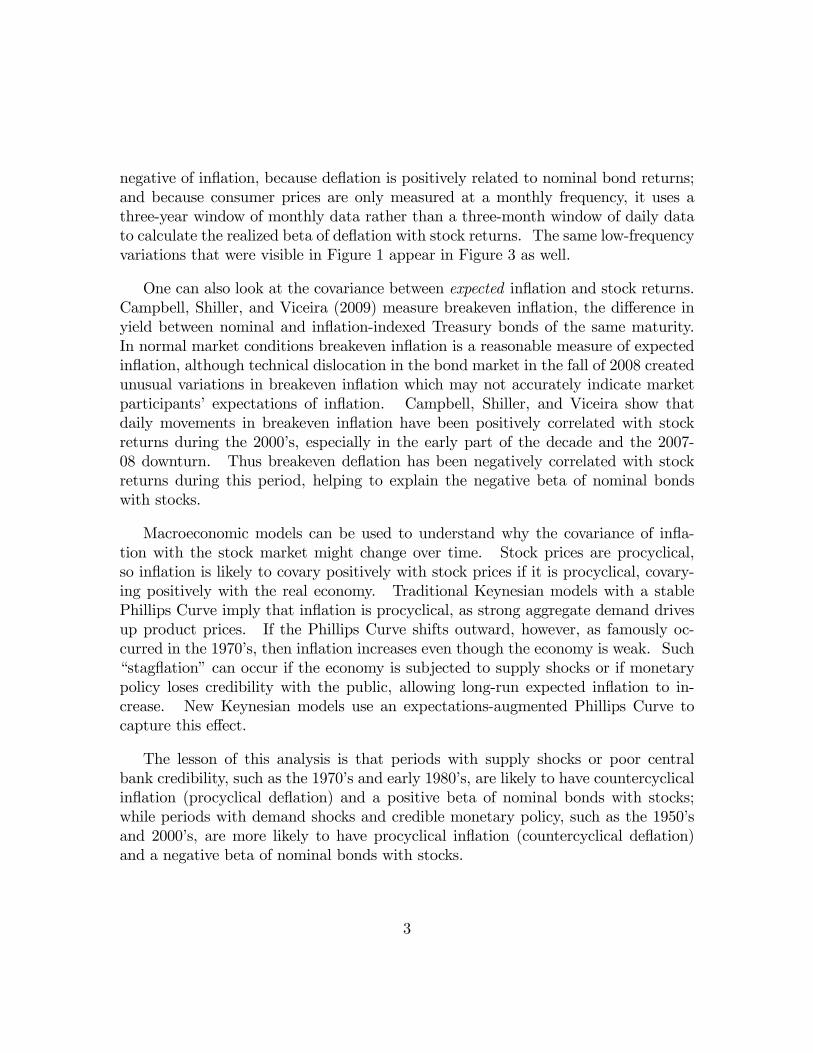
negative of in�ation, because de�ation is positively related to nominal bond returns;and because consumer prices are only measured at a monthly frequency, it uses athree-year window of monthly data rather than a three-month window of daily datato calculate the realized beta of de�ation with stock returns. The same low-frequencyvariations that were visible in Figure 1 appear in Figure 3 as well.

One can also look at the covariance between expected in�ation and stock returns.Campbell, Shiller, and Viceira (2009) measure breakeven in�ation, the di¤erence inyield between nominal and in�ation-indexed Treasury bonds of the same maturity.In normal market conditions breakeven in�ation is a reasonable measure of expectedin�ation, although technical dislocation in the bond market in the fall of 2008 createdunusual variations in breakeven in�ation which may not accurately indicate marketparticipants� expectations of in�ation. Campbell, Shiller, and Viceira show thatdaily movements in breakeven in�ation have been positively correlated with stockreturns during the 2000�s, especially in the early part of the decade and the 2007-08 downturn. Thus breakeven de�ation has been negatively correlated with stockreturns during this period, helping to explain the negative beta of nominal bondswith stocks.

Macroeconomic models can be used to understand why the covariance of in�a-tion with the stock market might change over time. Stock prices are procyclical,so in�ation is likely to covary positively with stock prices if it is procyclical, covary-ing positively with the real economy. Traditional Keynesian models with a stablePhillips Curve imply that in�ation is procyclical, as strong aggregate demand drivesup product prices. If the Phillips Curve shifts outward, however, as famously oc-curred in the 1970�s, then in�ation increases even though the economy is weak. Such�stag�ation�can occur if the economy is subjected to supply shocks or if monetarypolicy loses credibility with the public, allowing long-run expected in�ation to in-crease. New Keynesian models use an expectations-augmented Phillips Curve tocapture this e¤ect.

The lesson of this analysis is that periods with supply shocks or poor centralbank credibility, such as the 1970�s and early 1980�s, are likely to have countercyclicalin�ation (procyclical de�ation) and a positive beta of nominal bonds with stocks;while periods with demand shocks and credible monetary policy, such as the 1950�sand 2000�s, are more likely to have procyclical in�ation (countercyclical de�ation)and a negative beta of nominal bonds with stocks.

3

2.2 A formal model

The evidence I have presented implies that a satisfactory model of nominal bondpricing must have three properties. First, it must allow for changes over time inthe risks of nominal bonds. Second, it must allow the covariance between bond andstock returns to switch sign. Third, the changing risks of nominal bonds should belinked to the behavior of in�ation.

It is not straightforward to build a model with all three of these properties. Manysimple models of changing bond risk premia are driven by a single time-varying volatil-ity process, either for the real interest rate (Cox, Ingersoll, and Ross (1985)) or forthe stochastic discount factor. Models of this sort scale covariances up and downbut do not allow them to switch sign. More generally, it is di¢ cult to allow for signswitches in covariances while remaining within the tractable a¢ ne class of models inwhich log bond yields are linear in state variables (Dai and Singleton 2002, Du¤ee2002). Also, many bond pricing models are not fully explicit about the distinctionbetween real and nominal quantities.

Campbell, Sunderam, and Viceira (CSV, 2009) write down a simple model thatdoes meet these three criteria. Their model is a traditional a¢ ne model of thereal yield curve, augmented with a time-varying covariance between in�ation and thereal economy. The resulting nominal term structure model is linear-quadratic inmacroeconomic state variables.2

The real economy, real interest rates, and the stock market

CSV begin by assuming that the log of the real stochastic discount factor (SDF)mt+1 = log (Mt+1) follows a linear-quadratic, conditionally heteroskedastic process:

�mt+1 = xt +�2m2z2t + zt"m;t+1; (1)

where both xt and zt follow standard AR(1) processes. Given homoskedasticity ofunderlying shocks ", the log real SDF is conditionally heteroskedastic, with

Vart (mt+1) = z2t :

2Other linear-quadratic term structure models include Beaglehole and Tenney (1991), Constan-tinides (1992), and Ahn, Dittmar and Gallant (2002). Du¢ e and Kan (1996) point out thatlinear-quadratic models can often be rewritten as a¢ ne models if we allow the state variables to bebond yields rather than macroeconomic fundamentals. Buraschi, Cieslak, and Trojani (2008) alsoexpand the state space to obtain an a¢ ne model in which correlations can switch sign.

4

The state variable zt drives the time-varying volatility of the SDF or, equivalently,the price of aggregate market risk or maximum Sharpe ratio in the economy. It canbe understood as a measure either of changing risk aversion (Campbell and Cochrane1999, Bekaert, Engstrom, and Grenadier 2005), or of changing volatility in the realeconomy (Bansal and Yaron 2004).

It is straightforward to show that the one-period real interest rate equals thestate variable xt, and the whole term structure of real interest rates is linear in thetwo real state variables xt and zt. To bring stock returns into the model, CSVwrite down a reduced form equation expressing shocks to realized stock returns as alinear combination of shocks to the real interest rate and shocks to the log stochasticdiscount factor. This implies that the equity premium, like all other risk premiain the model, is proportional to risk aversion zt. It depends not only on the directsensitivity of stock returns to the SDF, but also on the sensitivity of stock returns tothe real interest rate and the covariance of the real interest rate with the SDF.

In�ation and nominal interest rates

To price nominal bonds, CSV specify a model for in�ation. They assume that login�ation �t = log (�t) follows a linear-quadratic conditionally heteroskedastic process:

�t+1 = �t + �t +�2�2 2t + t"�;t+1; (2)

where expected log in�ation is the sum of two components, a permanent component�t and a transitory component �t, both driven by underlying shocks that are alsoscaled by the state variable t.

The inclusion of two components of expected in�ation gives the model the �exi-bility it needs to �t simultaneously persistent shocks to both real interest rates andexpected in�ation. This �exibility is necessary because both realized in�ation and theyields of long-dated in�ation-indexed bonds move persistently, which suggests thatboth expected in�ation and the real interest rate follow highly persistent processes.At the same time, short-term nominal interest rates exhibit more variability thanlong-term nominal interest rates, which suggests that a rapidly mean-reverting statevariable must also drive the dynamics of nominal interest rates.

The state variable t, which multiplies the underlying shocks that drive realizedand expected in�ation, is assumed to follow a homoskedastic AR(1) process with anonzero mean. This speci�cation implies that the conditional volatility of in�ation

5

is time varying, as in the original ARCH model of Engle (1982). The novel featureof the speci�cation is that t can change sign. The sign of t does not a¤ect thevariances of expected or realized in�ation or the covariance between them, becausethese moments depend on the square 2t . However the sign of t does determinethe sign of the covariance between expected and realized in�ation, on the one hand,and real economic variables, on the other hand. Thus it can track the changes incovariances illustrated in Figures 1 and 2.

CSV show that under these assumptions the log nominal short rate is a linear-quadratic function of the state variables, and this property carries over to the entirezero-coupon nominal term structure. The log price of a n-period zero-coupon nominalbond can be written as a linear function of the state variables xt, zt, �t, �t, and t,and the squares and cross-product z2t ,

2t , and zt t.

CSV estimate the model using a nonlinear �unscented�Kalman �lter (Wan andvan der Merwe 2001) to construct the likelihood function. They �nd that the termstructure is driven by shocks to the permanent component of expected in�ation �t,which move the entire yield curve up and down (�level�shocks in the terminology of�xed-income practitioners), shocks to real interest rates xt and the temporary com-ponent of expected in�ation �t, which move short rates more than long rates (�slope�shocks), and shocks to risk aversion zt and the covariance of real and nominal mag-nitudes t, which alter risk premia and the concavity of the yield curve (�curvature�shocks). The last two shocks drive risk premia on nominal bonds, which are approx-imately proportional to the product zt t. In this way the model helps to explain theempirical association between concavity of the yield curve and excess bond returns,noted by Cochrane and Piazzesi (2005) among others.

Extending the model

The work of CSV can be extended in several directions. One limitation is that thea¢ ne structure of the real side of the model implies a constant covariance betweenin�ation-indexed bonds and stocks. Campbell, Shiller, and Viceira (2009) showthat both TIPS in the US and in�ation-indexed gilts in the UK have moved morenegatively with stocks during the downturns of the early 2000�s and 2007�08 thanthey did in the mid-2000�s or (in the UK) the 1990�s. To capture this they introducea state variable that moves the covariance of real interest rates with the stochasticdiscount factor, a real-side analog to the nominal variable t.

Ultimately, one would like to have a deeper structural understanding of the origin

6

of these �uctuations in covariances. It should be possible to achieve this by writingdown a New Keynesian macroeconomic model and allowing some of the parameters,including perhaps the volatilities of shocks and the parameters describing monetarypolicy, to vary over time as in Clarida, Gali, and Gertler (2000). This raises theexciting possibility that one can use the changing covariances between stocks andreal and nominal government bonds to learn about the nature of the underlyingmacroeconomic regime.

3 Asset Allocation with Time-Varying Bond Risk

How should investors respond to changes over time in the covariance between nominalbonds and stocks? It is important at the outset to distinguish between short-terminvestors, who are concerned with the distribution of invested wealth a quarter or ayear ahead, and long-term investors, who measure risk by the distribution of wealthmany years ahead or even by the sustainable consumption stream that wealth cansupport.

3.1 The changing role of bonds for short-term investors

Short-term investors have an almost entirely safe asset available in the form of Trea-sury bills, whose nominal return is guaranteed and whose real return has minimalvariability given that in�ation is highly predictable over a quarter and even over ayear. It follows that short-term investors hold long-term bonds not for safety, buteither for their expected excess return (the �speculative motive�) or for their abilityto hedge the risks of other assets such as equities (the �hedging motive�).

The standard mean-variance analysis of Markowitz (1952) can be used to evaluatethe role of bonds in risky portfolios for short-term investors. Short-term mean-variance investors invest in a unique tangency portfolio of risky assets, combining thiswith Treasury bills in proportions that depend on the risk aversion of each investor. Ifthe two available risky assets are nominal Treasury bonds and the aggregate US stockmarket, the weight of bonds in the tangency portfolio depends on the mean excessreturns of bonds and stocks, their variances, and the covariance between them.

If in addition mean excess returns and the variance of stock returns are reasonably

7

stable over time, then the role of nominal bonds in the tangency portfolio dependsprimarily on their volatility and their covariance with the stock market. Whenbonds are positively correlated with stocks, they have a relatively small weight in thetangency portfolio and that portfolio is quite volatile. When bonds are negativelycorrelated with stocks, they have a larger weight in the tangency portfolio because oftheir ability to hedge stock market risk. The tangency portfolio is also more stableand has a higher Sharpe ratio (return per unit of risk).

These properties are illustrated in Figure 4, which shows the ratio of stocks tobonds in the tangency portfolio implied by Campbell, Sunderam, and Viceira�s (2009)�ltered estimates of their term structure model. Although expected returns do varyin the CSV model, they do not move enough to o¤set the e¤ects of changing risks onthe composition of the tangency portfolio. In the early 1980�s the tangency portfoliois dominated by stocks and is correspondingly volatile, whereas in the 1950�s, 1960�s,and 2000�s, bonds play a dominant role with a stock-bond ratio less than one. Atsuch times the stability of the tangency portfolio encourages aggressive investors touse leverage. This suggests that the negative correlation between nominal bonds andstocks in the 2000�s may have contributed to the increased use of leverage during thecredit boom of the mid-2000�s.

3.2 The changing role of bonds for long-term investors

Campbell and Viceira (2001, 2002) have emphasized that long-term bonds play amore important role for long-term investors. For these investors, Treasury bills arenot safe because they must be rolled over at uncertain future interest rates. Aninvestor who seeks safety at a �xed long horizon can achieve it by buying a zero-coupon in�ation-indexed bond of the given maturity, and an investor who seeks asafe consumption stream that is inde�nitely sustainable can achieve it by buying anin�ation-indexed perpetuity. If in�ation-indexed bonds are not available, long-terminvestors must combine other assets, including Treasury bills, nominal bonds, andstocks, to minimize their risk.

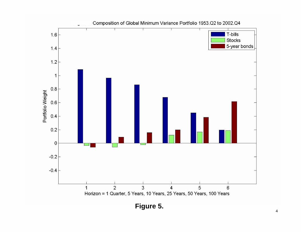
Campbell and Viceira (2005) speci�cally show how to calculate a global minimum-variance (GMV) portfolio at any investment horizon, using a vector autoregressive(VAR) model to capture changes over time in real interest rates and expected bondand stock returns. Their analysis assumes that the covariance matrix of shocks to theVAR is constant over time; thus they do not consider the phenomenon of changing

8

covariances discussed in this paper. Figure 5, taken from their paper, shows how theGMV portfolio weights of Treasury bills, 5-year nominal Treasury bonds, and stockschange with the investment horizon. The �gure is based on a covariance matrix ofshocks that is estimated over Campbell and Viceira�s full sample period 1953�2002.At short horizons, the GMV portfolio is dominated by Treasury bills, with modestshort positions in stocks and bonds to hedge against in�ation shocks that lower realbill returns and also lower the prices of stocks and bonds. At longer horizons, therollover risk of Treasury bills becomes more important, so nominal Treasury bondsbecome the dominant asset in the GMV portfolio.

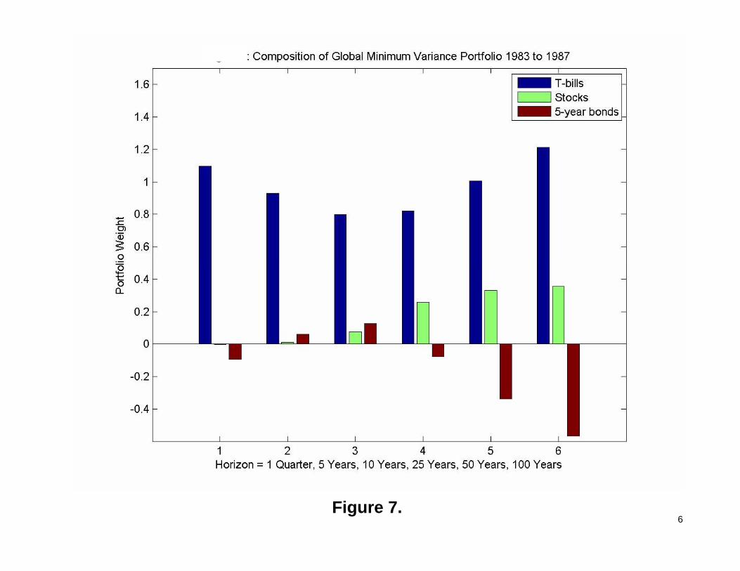
Figures 6, 7, and 8 show how these conclusions are altered by estimating the VARcovariance matrix over three di¤erent �ve-year periods, chosen to illustrate threedi¤erent regimes in asset markets. In the mid-1950�s (1953�1957), real interest rateswere extremely stable so there was little rollover risk in Treasury bills, which remainthe dominant asset in the GMV portfolio out to a 100-year investment horizon (Figure6).

In the mid-1980�s (1983�1987), real interest rates were volatile implying that Trea-sury bills were not safe long-term assets. At the same time, there was great uncer-tainty about in�ationary conditions so nominal Treasury bonds were not similar toin�ation-indexed bonds and did not o¤er safe long-term returns. In this period, equi-ties play a major role in the long-term GMV portfolio and short positions in nominalbonds, which were positively correlated with stocks at this time, are used to hedgeequity risk (Figure 7.)

Finally, around the turn of the millennium (1998�2002), real interest rates werevolatile but long-term expectations of in�ation were stable. This implies that nominalTreasury bonds are extremely similar to in�ation-indexed bonds and play a dominantrole in the long-term GMV portfolio (Figure 8.) Campbell, Shiller, and Viceira (2009)show that Treasury in�ation-protected securities (TIPS) have had a correlation withnominal Treasuries close to one for much of this decade, supporting the plausibilityof this �nding.

One caveat about the long-term GMV analysis should be mentioned here. Camp-bell and Viceira�s (2005) methodology assumes that a portfolio must be chosen onceand for all at the start of the investment horizon, without allowing rebalancing to re-spond to changing investment opportunities. However, a full intertemporal analysisalong the lines of Merton (1973) delivers similar results in the empirical implementa-tion of Campbell, Chan, and Viceira (2003).

9

4 Conclusion

Traditional asset allocation analysis assumes that asset classes have stable risks thatcan be estimated from long-term historical data. Even sophisticated approaches thatrecognize changes over time in expected returns, and the resulting di¤erences in therisks perceived by short-term and long-term investors, typically ignore the fact thatrisks may also change over time.

When nominal bonds are included in an asset allocation exercise, as is almostalways the case, the assumption of constant risks is dangerously misleading. Thecovariance between nominal bonds and stocks has varied considerably over recentdecades and has even switched sign. It has been predominantly positive in periodssuch as the late 1970�s and early 1980�s when the economy has experienced supplyshocks and the central bank has lacked credibility. It has been predominantly negativein periods such as the 2000�s when investors have feared weak aggregate demand andde�ation.

Nominal bonds are attractive to short-term equity investors when these bondsare negatively correlated with stocks, as has been the case during the 2000�s andespecially during the downturn of 2007�08. They are attractive to conservative long-term investors when long-term in�ationary expectations are stable, for then thesebonds are close substitutes for in�ation-indexed bonds which are riskless in the longterm. At present, nominal bonds therefore play an important role in asset allocationeven if they o¤er a small or negative term premium over Treasury bills.

The demand for nominal bonds in asset allocation can however change rapidly ifthe regime changes. If investors come to fear stag�ation, bonds�ability to hedgeagainst de�ation will no longer be so attractive, and the correlation between bondsand stocks may switch sign once again. If in�ationary expectations destabilize,nominal bonds are no longer close substitutes for in�ation-indexed bonds and areless appealing for conservative long-term portfolios. Both investors and �scal andmonetary authorities should pay close attention to changing covariances among nom-inal bonds, in�ation-indexed bonds, and stocks as a guide to asset allocation and anindicator of the state of the economy.

The importance of the macroeconomic regime for asset allocation applies beyondthe speci�c example discussed in this paper. Many other asset classes, includingforeign currencies (Campbell, Serfaty-de Medeiros, and Viceira 2009), real estate, and

10

commodities, also have risks that are likely to vary with the economic environment.Much as investors might wish to choose portfolios based on mechanical processing ofhistorical data, asset allocation cannot be conducted without forming a view aboutthe structure of the economy and the relative magnitudes of the shocks that impingeupon it.

11

References

Ahn, Dong-Hyun, Robert F. Dittmar, and A. Ronald Gallant, 2002, �QuadraticTerm Structure Models: Theory and Evidence�, Review of Financial Studies15, 243�288.

Bansal, Ravi, and Amir Yaron, 2004, �Risks for the Long Run: A Potential Resolu-tion of Asset Pricing Puzzles,�Journal of Finance 59, 1481-1509.

Barndor¤-Nielsen, Ole, and Neil Shephard, 2004, �Econometric Analysis of RealizedCovariation: High Frequency Based Covariance, Regression, and Correlation inFinancial Econometrics�, Econometrica 72, 885�925.

Beaglehole, David R. and Mark S. Tenney, 1991, �General Solutions of Some In-terest Rate-Contingent Claim Pricing Equations�, Journal of Fixed Income,September, 69�83.

Bekaert, Geert, Eric Engstrom, and Steve Grenadier, 2005, �Stock and Bond Returnswith Moody Investors�, unpublished paper, Columbia University, University ofMichigan, and Stanford University.

Buraschi, Andrea, Anna Cieslak, and Fabio Trojani, 2008, �Correlation Risk and theTerm Structure of Interest Rates�, unpublished paper, Imperial College Londonand University of St. Gallen.

Campbell, John Y., Y. Lewis Chan, and Luis M. Viceira, 2003, �A MultivariateModel of Strategic Asset Allocation�, Journal of Financial Economics 67, 41�80.

Campbell, John Y. and John H. Cochrane, 1999, �By Force of Habit: A Consumption-Based Explanation of Aggregate Stock Market Behavior�, Journal of PoliticalEconomy 107, 205�251.

Campbell, John Y., Karine Serfaty-de Medeiros, and Luis M. Viceira, 2009, �GlobalCurrency Hedging�, NBER Working Paper No. 13088, forthcoming Journal ofFinance.

Campbell, John Y., Robert J. Shiller, and Luis M. Viceira, 2009, �UnderstandingIn�ation-Indexed Bond Markets�, NBER Working Paper No. 15014, forthcom-ing Brookings Papers on Economic Activity.

12

Campbell, John Y., Adi Sunderam, and Luis M. Viceira, 2009, �In�ation Bets orDe�ation Hedges? The Changing Risks of Nominal Bonds�, NBER WorkingPaper No. 14701.

Campbell, John Y. and Luis M. Viceira, 2001, �Who Should Buy Long-TermBonds?�,American Economic Review 91, 99�127.

Campbell, John Y. and Luis M. Viceira, 2002, Strategic Asset Allocation: PortfolioChoice for Long-Term Investors, Oxford University Press, New York, NY.

Campbell, John Y. and Luis M. Viceira, 2005, �The Term Structure of the Risk-Return Tradeo¤�, Financial Analysts Journal 61 (January/February), 34�44.

Clarida, Richard, Jordi Gali, and Mark Gertler, 2000, �Monetary Policy Rules andMacroeconomic Stability: Evidence and Some Theory�, Quarterly Journal ofEconomics 115, 147�180.

Cochrane, John H. and Monika Piazzesi, 2005, �Bond Risk Premia�, AmericanEconomic Review 95, 138�160.

Constantinides, George M., 1992, �A Theory of the Nominal Term Structure ofInterest Rates�, Review of Financial Studies 5, 531�552.

Cox, John C., Jonathan E. Ingersoll, and Stephen A. Ross, 1985, �An IntertemporalGeneral Equilibrium Model of Asset Prices�, Econometrica 53, 363�384.

Dai, Qiang and Kenneth Singleton, 2002, �Expectations Puzzles, Time-Varying RiskPremia, and A¢ ne Models of the Term Structure�, Journal of Financial Eco-nomics 63, 415�442.

Donovon, Prosper, Sílvia Gonçalves, and Nour Meddahi, 2008, �Bootstrapping Real-ized Multivariate Volatility Measures�, unpublished paper, Université de Mon-tréal.

Du¤ee, Greg, 2002, �Term Premia and Interest Rate Forecasts in A¢ ne Models�,Journal of Finance 57, 405�443.

Du¢ e, Darrell and Rui Kan, 1996, �A Yield-Factor Model of Interest Rates�, Math-ematical Finance 6, 379�406.

Engle, Robert F., 1982, �Autoregressive Conditional Heteroskedasticity with Esti-mates of the Variance of UK In�ation�, Econometrica 50, 987�1008.

13

Markowitz, Harry, 1952, �Portfolio Selection�, Journal of Finance 7, 77�91.

Merton, Robert C., 1973, �An Intertemporal Capital Asset Pricing Model�, Econo-metrica 41, 867�87.

Viceira, Luis M., 2007, �Bond Risk, Bond Return Volatility, and the Term Structureof Interest Rates�, unpublished paper, Harvard Business School.

Wan, Eric A. and Rudolph van der Merwe, 2001, �The Unscented Kalman Filter�,Chapter 7 in Simon Haykin ed., Kalman Filtering and Neural Networks, Wiley,New York, NY.

14

0

Figure 1. Source: Luis Viceira, “Bond Risk, Bond Return Volatility, and the Term Structure of Interest Rates”, 2007

1

CAPM beta of bonds (2002.06-2008.04)

-0.4

-0.3

-0.2

-0.1

0

0.1

0.2

0.3

06/20

/2002

09/20

/2002

12/23

/2002

03/25

/2003

06/25

/2003

09/25

/2003

12/26

/2003

03/29

/2004

06/29

/2004

09/29

/2004

12/30

/2004

04/01

/2005

07/04

/2005

10/04

/2005

01/04

/2006

04/06

/2006

07/07

/2006

10/09

/2006

01/09

/2007

04/11

/2007

07/12

/2007

10/12

/2007

01/14

/2008

04/15

/2008

Date

CA

PM b

eta

3-month centered beta, 10-year Treasury on S&P500

Figure 2.

2

CAPM Beta of Deflation(3-yr rolling window of Shocks to -Log(Inflation) and Stock Returns)

-0.06

-0.04

-0.02

0

0.02

0.04

0.06

0.08

1955 1960 1965 1970 1975 1980 1985 1990 1995 2000 2005

Figure 3.

3

Figure 4. Stock/Bond Ratio in the Tangency Portfolio

4Figure 5.

5Figure 6.

6Figure 7.

7Figure 8.