inflation risk and inflation-protected and nominal treasury...
TRANSCRIPT

Inflation Risk and Inflation-Protected and
Nominal Treasury Bonds
Philipp Karl ILLEDITSCH∗
November 5, 2008
Abstract
I decompose inflation risk into (i) a component that is correlated with real returns on
positive-net-supply securities (stocks, inflation-protected and nominal corporate bonds,
real estate, etc.) and factors that determine investor’s preferences and investment op-
portunities and (ii) a residual component. In equilibrium, only the first component earns
a risk premium. Therefore investors should avoid exposure to the residual component.
All nominal Treasury bonds, including the nominal money-market account, are equally
exposed to the residual component except inflation-protected Treasury bonds, which
provide a means to hedge it. Every investor should put 100% of his wealth in positive-
net-supply securities and inflation-protected Treasury bonds and should finance every
long/short position in nominal Treasury bonds with an equal amount of other nominal
Treasury bonds or by borrowong/lending in the nominal money market account; i.e.
investors should hold a zero-investment portfolio of nominal Treasury bonds and the
nominal money market account.
∗The Wharton School, University of Pennsylvania, 3620 Locust Walk, 2300 SH-DH, Philadelphia, PA19104−6367, phone: 215−898−3477, e-mail: [email protected]. I would like to thank Kerry Back,Ekkehart Boehmer, Michael Gallmeyer, Shane Johnson, Dmitry Livdan, and seminar participants at TexasA&M University for their comments. I am also very grateful for the generous support of Mays BusinessSchool. This paper is based on Chapter 1 of my dissertation at Texas A&M University.

Inflation can affect real security prices through two channels. First, inflation may
affect the real economy, meaning the real stochastic discount factor and the real cash flows
of positive-net-supply securities. Second, inflation will affect the real cash flows of zero-
net-supply securities such as nominal Treasury bonds. I decompose inflation risk into (i)
a component that is correlated with real returns on positive-net-supply securities (stocks,
inflation-protected and nominal corporate bonds, real estate, etc) and factors that determine
investor’s preferences and investment opportunities and (ii) a residual component. The first
component affects security prices through both channels; however, the residual component,
by definition, operates only through the second. In equilibrium, only the first component
earns a risk premium, and investors should avoid exposure to the residual component.
Inflation-protected Treasury bonds (TIPS) provide a means to hedge exposure to resid-
ual inflation risk. This role for TIPS has not been emphasized in previous literature, but it
has dramatic consequences for optimal portfolios. This paper demonstrates the following:
(i) there is a real instantaneously risk-free asset consisting of a long position in inflation-
protected Treasury bonds and a zero-investment portfolio of nominal Treasury bonds and
the nominal money market account, (ii) the portfolios on the instantaneous mean-variance
frontier of risky assets consist of long or short positions in positive-net-supply securities
and inflation-protected Treasury bonds and zero-investment portfolios of nominal Treasury
bonds and the nominal money market account, and (iii) the portfolios that hedge changes
in the investment opportunity set consist of long or short positions in positive-net-supply
securities and inflation-protected Treasury bonds and zero-investment portfolios of nominal
Treasury bonds and the nominal money market account. These facts imply directly that (iv)
every investor should put 100% of his wealth in positive-net-supply securities and inflation-
protected Treasury bonds and hold a zero-investment portfolio of nominal Treasury bonds
and the nominal money-market account.
Results (i)-(iv) follow from the equal exposure of nominal bonds and the nominal money
market account to residual inflation risk. This risk cannot be present in the real locally
risk-free asset; thus (i) holds. This risk is not priced; thus, the variance-minimizing portfolio
producing a given expected return has no residual inflation risk, producing result (ii). The
hedging portfolios are the portfolios maximally correlated with the latent state variables
and therefore cannot include residual inflation risk; thus, (iii) holds.
1

The conclusion that investors in aggregate should hold zero-investment portfolios in
nominal Treasury bonds and the nominal money market account follows from equilibrium
considerations — market clearing for zero-net-supply securities. However, the conclusion
here is much stronger: every investor, not just the representative investor, should hold
a zero-investment portfolio in nominal Treasury bonds and the nominal money market
account.1
It is well known since Merton (1971) that the optimal dynamic investment strategy
is to hold a linear combination of k + 2 mutual funds: two funds to form the optimal
portfolio on the mean-variance frontier and k funds to hedge changes in investor’s preferences
and investment opportunities. I show for a broad class of preferences and asset return
distributions that the optimal amount of nominal Treasury bonds and the nominal money
market account invested in each mutual fund is always zero without explicitly solving for
the value function.
Fischer (1975), Bodie, Kane, and McDonald (1983), and Viard (1993), assuming a
constant investment opportunity set, show that (i) only the part of inflation risk that is
correlated with real stock returns should earn a risk premium if the CAPM for real asset
returns holds (residual inflation risk is not priced) and (ii) investors should shun nominal
bonds when inflation-protected bonds are available. I show that part (ii) is no longer true
when the real and nominal short rate is stochastic (the nominal money market account and
nominal bonds, as well as, the real risk-free asset and inflation-protected bonds aren’t perfect
substitutes) because in this case investors hold long/short positions in nominal bonds that
are financed by an equal amount of other nominal bonds and the nominal money market
account when inflation-protected bonds are available. However, I derive the ICAPM for
heterogeneous investors with state dependent preferences and investment opportunities and
confirm the first result when residual inflation risk is defined as the part of inflation risk that
is not only uncorrelated with real stock returns but with real returns on positive-net-supply
securities and factors that determine investor’s preferences and investment opportunities.
Moreover, I show that inflation-protected bonds are used to hedge residual inflation risk
(allow investors to create a real risk-free asset) without assuming that the real short rate is
1The zero-investment portfolio in nominal Treasury bonds should be interpreted as inclusive of the in-vestor’s short position in nominal Treasury bonds that corresponds to his position as a taxpayer. In otherwords, an investor should hold enough Treasury bonds to immunize his tax liability. See Section III.
2

constant.
Recent studies on optimal portfolio choice with inflation-protected bonds include Camp-
bell and Viceira (2001) and Campbell, Chan, and Viceira (2003). Campbell and Viceira
(2001) and Campbell, Chan, and Viceira (2003) solve the discrete-time dynamic portfolio
choice problem of an infinitely-lived investor with Epstein-Zin preferences, who can invest
in equity, nominal bonds, and inflation-protected bonds, using a log linear approximation
and a Gaussian investment opportunity set. While this paper employs different assumptions
and a different solution method, the principal difference is that the main portfolio choice
results are derived when residual inflation risk is unpriced.
This paper is also related to recent papers of Brennan and Xia (2002) and Sangvinatsos
and Wachter (2005), who discuss dynamic asset allocation decision with inflation risk and
provide closed form solutions. Brennan and Xia (2002) analyze the portfolio problem of a
finite-lived investor with power utility who can invest in the stock market, cash, and nomi-
nal bonds when the conditional distribution of all asset returns is Gaussian. Sangvinatsos
and Wachter (2005) extend their work by adding another state variable to account for time-
varying risk premia and explore the resulting predictability of nominal bond returns for
portfolio choice. My paper differs from these papers in that I add inflation-protected bonds
to the analysis and consider a broader class of preferences and asset return distributions.
Importantly, the fact that residual inflation risk is not priced allows me to determine the
optimal investment in nominal bonds and the nominal money market account in each mu-
tual fund without explicitly solving for the value function of the dynamic portfolio choice
problem.
My paper is also related to recent studies of inflation-protected bonds by Bodie (1990),
Gapen and Holden (2005), Hunter and Simon (2005), Kothari and Shanken (2004), Roll
(2004), Brynjolfsson and Fabozzi (1999), Deacon, Derry, and Mirfendereski (2004), and
Benaben (2005). These studies analyze the mean, variance, and correlation of returns
on nominal bonds, inflation-protected bonds, and stocks and discuss the welfare gains of
adding inflation-protected bonds to standard investment portfolios consisting of nominal
bonds and stocks in a static mean-variance framework. The main conclusion is that adding
inflation-protected bonds increases the welfare of investors because of the low standard
deviation of real returns of inflation-protected bonds and their diversification benefits (the
3

low correlation between inflation-protected bonds and both nominal bonds and stocks).
However, the gains are usually found to be quite small for U.S. investors because of the low
volatility of inflation risk in the United States.
I Asset Prices
Let X denote a k-dimensional vector of state variables (factors) that describe investor’s
preferences and investment opportunity sets and Z a d-dimensional vector of independent
Brownian motions. The dynamics of the state vector are
dX = µX(X) dt + σX(X)′ dZ, (1)
in which µX(X) is k-dimensional and σX(X) is d × k-dimensional.2
Prices in the economy are measured in terms of a basket of real goods. Let π denote
the price level, µπ(X) the expected inflation rate, and σπ(X) the d-dimensional volatility
vector of π. The dynamics of the price level are
dπ
π= µπ(X) dt + σπ(X)′ dZ. (2)
Assume there is no arbitrage and therefore there exists a strictly positive stochastic
discount factor M that determines real prices of all assets in the economy. Let r(X) denote
the (shadow) risk-free rate or real short rate and Λ(X) the d-dimensional vector of market
prices of risk. The dynamics of the real stochastic discount factor are
dM
M= −r(X) dt − Λ(X)′ dZ. (3)
The real stochastic discount factor M and the price level π are sufficient to price all assets
in the economy. Let M∗ denote the the nominal stochastic discount factor that is given by
M∗ = M/π. The dynamics of M∗ are
dM∗(π)
M∗(π)= −r∗(X) dt − (Λ(X) + σπ(X))′ dZ, (4)
2The covariance matrix of X is not necessarily invertible, e.g. time could be a state variable. Anapostrophe denotes the transpose of a vector or matrix.
4

in which
r∗(X) = r(X) + µπ(X) − Λ(X)′σπ(X) − σπ(X)′σπ(X). (5)
The nominal short rate r∗(X) is equal to the sum of the real short rate, the expected inflation
rate, an inflation risk premium, and a Jensen inequality term. The Fisher equation for the
nominal short rate does not hold unless the term −Λ(X)′σπ(X) is zero in which case the
expected real return of the nominal money market account is equal to the real short rate
(see equation (11) below).3
Suppose there are N non-redundant positive-net-supply securities outstanding. For
n = 1, . . . , N , let Sn denote the real, dividend-reinvested price of security n and dS/S the
column vector with dSn/Sn as its n-th component. Assume
dS
S= µS(X) dt + σS(X)′ dZ, (6)
in which µS(X) = r(X)1 + σS(X)′Λ(X) and σS(X) is d × N -dimensional.4 Positive-
net-supply securities include stocks, inflation-protected and nominal corporate bonds, real
estate, etc. but exclude the nominal money market account, nominal Treasury bonds, and
inflation-protected Treasury bonds.5
The state vector X, the positive-net-supply securities S1, . . ., SN , and the consumer
price index π form a Markov system with dynamics
dX
dS/S
dπ/π
=
µX(X)
µS(X)
µπ(X)
dt + σ(X)′ dZ. (7)
Without loss of generality, one can take X1 to depend only on the Brownian motion Z1, X2
3A zero inflation risk premium for the nominal money market account does not imply that the inflationrisk premium for longer holding periods is zero. Specifically, the τ -year inflation risk premium (the expectedreal return difference of holding a τ -year nominal zero-coupon bond until maturity and of holding a τ -yearreal zero-coupon bond until maturity) is in general not zero if Λ(X)′σπ(X) = 0. It is in general not zeroeven if σπ(X) = 0.
41 denotes a column vector of ones.
5The cash flows of Treasury bonds are offset by corresponding tax liabilities, rendering the net supply ofthese cash flows zero. A simple model in which investor’s are subject to lump-sum tax payments is providedin Section III. Inflation-protected and nominal corporate bonds are claims on a firm’s cash flow and thus inpositive-net-supply.
5

to depend only on Z1 and Z2, etc. This means that we can assume d = k + N + 1 and that
the (d × d)-dimensional, volatility matrix
σ(X) = (σX(X), σS(X), σπ(X)) (8)
is upper diagonal. Define Zd which is the additional shock in dπ/π that is uncorrelated
with changes in the state variables and real returns on all positive-net-supply securities as
residual inflation risk. The Markov system in equation (7) is very general. It allows for
perfect or imperfect correlations of any variables, and it does not impose an affine or any
other structure on the drifts and volatilities.
All bonds considered in this paper are default-free zero-coupon Treasury bonds if not
explicitly stated otherwise. An inflation-protected bond pays one unit of a basket of real
goods at its maturity date T . A nominal bond pays one unit of currency at its maturity
date. Denote real prices of real (inflation-protected) bonds by P , real prices of nominal
bonds by B, and the real value of the nominal money market account by R. Asterisks
indicate nominal prices (S∗1 = S1π, . . ., S∗
N = SNπ, P ∗ = Pπ, B∗ = Bπ, and R∗ = Rπ).
Suppose real prices of inflation-protected bonds are sufficiently smooth (see Definition
1 in Appendix A). Then the real price of an inflation-protected bond and its dynamics are
given in the next proposition.
Proposition 1 (Inflation-protected bonds). The real price of an inflation-protected bond
maturing at T is only a function of the state vector X and time to maturity T − t; i.e.
P = P (T − t,X).6 The real return of an inflation-protected bond maturing at T is
dP (T − t,X)
P (T − t,X)=(
r(X) + σP (T − t,X)′Λ(X))
dt + σP (T − t,X)′ dZ, (9)
in which the d-dimensional local real return volatility vector is
σP (T − t,X) = σX(X)∇XP (T − t,X)/P (T − t,X) (10)
and ∇XP (T − t,X) denotes the gradient of P (T − t,X). Moreover, σPd(T − t,X) = 0.7
6When time t is a state variable (and thus part of the state vector X), then P depends on t and T − t.7I denote with vi the i-th component of the vector v.
6

Proof. See Appendix A.
Real cash flows of inflation-protected bonds are constant, and hence the real return of
inflation-protected bonds may be affected by inflation only through the first channel: the
real stochastic discount factor. Specifically, real returns of inflation-protected bonds are
only exposed to factor risk. This is in stark contrast to assets such as nominal bonds and
the nominal money market account whose real cash flows are affected by inflation risk as
the next proposition shows.
Suppose nominal prices of nominal bonds are sufficiently smooth (see Definition 1 in
Appendix A). The nominal value of a unit of currency invested in the nominal money
market account and the nominal price of a nominal bond and their dynamics are given in
the next proposition.
Proposition 2 (Nominal bonds and the nominal money market account). The nominal
value at time t of one unit of currency invested in the nominal money market account at time
0 depends on the path of the state vector X and time t, i.e. R∗ = R∗(t, X(a), 0 ≤ a ≤ t).
The real return of the nominal cash or money market account is
dR(R∗, π)
R(R∗, π)=(
r(X) − σπ(X)′Λ(X))
dt − σπ(X)′ dZ. (11)
The nominal price of a nominal bond maturing at T is only a function of the state
vector X and time to maturity T − t; i.e. B∗ = B∗(T − t,X).8 The real return of a nominal
bond maturing at T is
dB(T − t,X, π)
B(T − t,X, π)=(
r(X) + σB(T − t,X)′Λ(X))
dt + σB(T − t,X)′ dZ, (12)
in which the d-dimensional local real return volatility vector is
σB(T − t,X) = σX(X)∇XB∗(T − t,X)/B∗(T − t,X) − σπ(X) (13)
and ∇XB∗(T − t,X) denotes the gradient of B∗(T − t,X).9 Moreover, σBd(T − t,X) =
−σπd(X) for all maturities T .
8When time t is a state variable (and thus part of the state vector X), then B∗ depends on t and T − t.9The nominal return of a nominal bond is given in equation (23) in Appendix A.
7

Proof. See Appendix A.
Nominal bonds are claims on a unit of currency at maturity and their real returns are
therefore affected by inflation through the second channel (the price level) and may also be
affected by inflation through the first channel (the real stochastic discount factor). Specifi-
cally, real returns of nominal bonds and the nominal money market account are exposed to
factor and residual inflation risk. Moreover, equation (11) implies that real returns of the
nominal money market account are perfectly negatively correlated with inflation.
If unanticipated inflation risk is not perfectly correlated with changes in the factors and
real returns on all positive-net-supply securities (i.e. σπd(X) 6= 0), then the effects of infla-
tion risk (i) on the real cash flows of all positive-net-supply securities can be distinguished
from the effects (ii) on the real cash flows of zero-net-supply securities such as nominal
bonds and the nominal money market account. All assets may be affected by inflation risk
through the part of unanticipated inflation risk that is correlated with changes in the factors
and real returns on positive-net-supply securities but only nominal bonds and the nominal
money market account are affected by residual inflation risk. Specifically, all nominal bonds
and the nominal money market account have exactly the same exposure to this risk source
which is −σπd(X), as shown in Proposition 2. Hence, it is impossible to have a long or short
position in a portfolio consisting solely of nominal bonds and the nominal money market
account without having exposure to residual inflation risk. This risk is not priced as the
next theorem shows and investors should avoid it, as the next section shows.10
Theorem 1 (ICAPM). Assume that the nominal money market account, nominal Treasury
bonds, and inflation-protected Treasury bonds are in zero-net-supply and investors have
homogeneous beliefs, their endowments are spanned by real asset returns, and their initial
wealth (including the present value of future labor income) is strictly positive. Then the
market price of residual inflation risk is zero; i.e. Λd(X) = 0.
Proof. See Appendix B.
Intuitively, the value function of the representative investor depends on aggregate wealth
which is equal to the market portfolio and on the state vector that describes changes in in-
10Preferences of every investor and the security market are described in Appendix A.
8

vestors’s preferences and investment opportunities. The market portfolio is a value weighted
sum of all positive-net-supply securities and hence excludes assets such as inflation-protected
Treasury bonds, nominal Treasury bonds, and the nominal money market account. Resid-
ual inflation risk is neither correlated with the state vector nor with real returns on the
market portfolio and therefore it is not priced. The conclusion that residual inflation risk
is not priced does not require complete markets and homogeneous investors. Specifically,
investors can differ with respect to endowments, preferences, and investment horizons.11
In the remainder of this paper I make the following assumption.
Assumption 1 (Residual inflation risk). Inflation rate is not spanned by the factors and
real returns on positive-net-supply securities, i.e. σπd(X) 6= 0 (residual inflation risk is not
zero). Moreover, the real market price of residual inflation risk is zero, i.e. Λd(X) = 0.
Assumption 1 implies that neither the price level nor functions of the price level can
be part of the state vector, but it doesn’t rule out the expected inflation rate and/or the
volatility of inflation as state variables. Moreover, it is possible that the price level and
functions of it can be correlated with the state variables. It is only being assumed that they
are not perfectly correlated with state variables.
Optimal portfolios when the market price of residual inflation risk is zero are determined
in the next section.
II Dynamic Portfolio Choice
Consider investors who can continuously trade in a frictionless security market and maximize
E
[∫ T
0e−
∫
t
0β(X(a)) da u(c(t),X(t)) dt + e−
∫
T
0β(X(a)) da U(W (T ),X(T ))
]
(14)
for some investment horizon T , subjective discount factor β, utility function u, and bequest
U .12 The horizon T could be infinite in which case U = 0 or it could be random in which
case it is assumed to be independent of asset returns. All investors have strictly positive
11I show in Section III that residual inflation risk is still zero when investors are subject to differentnominal lump-sum tax payments.
12The expectation in equation (14) is assumed to be finite and u and U are assumed to fulfill the standardconditions for utility functions (see Karatzas and Shreve (1998)).
9

initial wealth and receive either no labor income or labor income that is spanned by real
asset returns in which case the present value of future labor income is taken to be part of
the initial wealth.
The following spanning condition is imposed:
Assumption 2 (Spanning condition). Let X=(U, V ) in which U is spanned by real returns
of inflation-protected Treasury bonds and nominal returns of nominal Treasury bonds. Ei-
ther (i) the market is complete, or (ii) the part of inflation risk that is not spanned by U is
orthogonal to V and to real returns on positive-net-supply securities.
Neither condition (i) nor (ii) of Assumption 2 implies the other.13 Assumption 2 implies
that there is a mimicking portfolio for the real risk-free asset.14 Intuitively, a long position
in inflation-protected bonds avoids exposure to residual inflation risk, which is not possible
with a long or short position in nominal bonds and the nominal money market account
because of their equal exposure to residual inflation risk. On the other hand, the exposure
of the long position in inflation-protected bonds to factor risk (components of U) can be
hedged, because U is spanned by real returns of inflation protected bonds and real returns
of zero investment portfolios of nominal bonds and the nominal money market account.
Moreover, every claim that solely depends on the state vector U can be perfectly replicated
with a portfolio consisting of inflation-protected bonds and zero-investment portfolios of
nominal bonds and the nominal money market account. Hence, Assumption 2 implies that
the nominal and inflation-protected bond market is complete.
The optimal portfolio of an investor who seeks to maximize the utility function in equa-
tion (14) and who can trade continuously in the nominal money market account, positive-
net-supply securities such as stocks, inflation-protected and nominal corporate bonds, real
estate, etc., and nominal and inflation-protected Treasury bonds is given in the next theo-
rem.15
13It is equivalent to say in Assumption 2 that U is spanned by real returns of inflation-protected Treasurybonds and real returns of zero-investment portfolios of nominal Treasury bonds and the nominal moneymarket account because the additional exposure of real returns of nominal Treasury bonds to (i) residualinflation risk and (ii) to factor risk (if the factor is correlated with inflation) is offset by borrowing/lending inthe nominal money market account. A formal discussion of the spanning condition is provided in Proposition3 in Appendix C.
14The proof is given in Theorem 1.15The value function J(·) is defined in equation (62) in Appendix C.
10

Theorem 2. Adopt Assumptions 1 and 2. Every investor should hold a linear combination
of the real risk-free asset, the tangency portfolio, and hedging portfolios. Moreover,
1. The mimicking portfolio for the real risk-free asset consists of a long position in
inflation-protected Treasury bonds and a zero-investment portfolio of nominal Treasury
bonds and the nominal money market account.
2. The tangency portfolio consists of long or short positions in positive-net-supply securi-
ties and inflation-protected Treasury bonds, and a zero-investment portfolio of nominal
Treasury bonds and the nominal money market account.
3. The portfolios that hedge changes in the investment opportunity set consist of long
or short positions in positive-net-supply securities and inflation-protected Treasury
bonds, and zero-investment portfolios of nominal Treasury bonds and the nominal
money market account.
4. Investors should put 100% of their wealth in positive-net-supply securities and inflation-
protected Treasury bonds and hold a zero-investment portfolio of nominal Treasury
bonds and the nominal money market account.
Proof. See Appendix C.
A brief description of the proof is as follows. Assumption 2 implies that there exists
a real risk-free asset and hence by the (k + 2)-fund separation theorem of Merton (1971)
the optimal portfolio is a linear combination of the mimicking portfolio for the real risk-free
asset, the tangency portfolio, and k portfolios that hedge changes in investor’s preferences
and investment opportunities. The tangency portfolio is by definition the portfolio with
maximal local Sharpe ratio and hence the local volatility vector of this portfolio is propor-
tional to the projection of the market price of risk vector onto the asset space. The hedging
portfolios are maximally correlated with the factors and hence determined by projecting
the state vector onto the asset space. The mimicking portfolio of the real-risk free asset is
locally riskless, the market price of residual inflation risk and its projection onto the asset
space is zero, and the projection of all factors onto the asset space is orthogonal to residual
inflation risk, and hence the total investments in nominal Treasury bonds and the nominal
11

money market account in the mimicking portfolio for the real risk-free asset, the tangency
portfolio, and all hedging portfolios are zero.16
The composition of the mimicking portfolios for the real risk-free asset, the tangency
portfolio, and the hedging portfolios do not depend on the value function. But to obtain
the optimal portfolio (to choose the optimal linear combination of the (k + 2) funds) it is
necessary to determine the marginal value of wealth, the sensitivity of the marginal value of
wealth to changes in wealth and to changes in the state variables. Specifically, the optimal
point on the local mean-variance frontier depends on investor’s attitude towards risk as
measured by the relative risk aversion coefficient γ ≡ −wJww/Jw, whereas the hedging
demands depend on the sensitivity of the investor’s marginal value of wealth to changes in
the factors measured by Θ ≡ −JwX/(wJww).17
III Taxes
I show in this section that the market price of residual inflation risk is still zero when
investors are subject to nominal lump-sum tax payments and Treasury bonds are in positive
supply. Suppose that there are I individuals in the economy that share the same beliefs and
can continuously trade in the frictionless security market specified below. Each individual
makes investment decisions and consumption choices to maximize
E
[∫ ∞
0ui(t, ci(t),X(t)) dt | X(0) = x
]
(15)
for some utility function ui.18
It is assumed that the labor income of every investor is spanned by real asset returns and
hence it can be taken as part of an investor’s initial wealth wi. Moreover, each individual
has to continuously pay the nominal lump-sum tax τ∗i(t). Real tax payments are denoted
16The projector onto the asset space is provided in Lemma 2 in Appendix C.17Illeditsch (2007) provides closed form solutions for the value function and optimal portfolios (consisting
the nominal money market account, the stock market, and nominal and inflation-protected Treasury bonds)when investors have constant relative risk aversion preferences and asset drifts are quadratic and assetvolatilities are affine functions of the expected inflation rate that follows a mean reverting Ornstein-Uhlenbeckprocess. More generally, Liu (2007) solves the dynamic portfolio choice problem of constant relative riskaverse investors (up to the solution of a system of ordinary differential equations) when asset returns arequadratic.
18The expectation in equation (15) is assumed to be finite and ui is assumed to fulfill the standardconditions for utility functions (see Karatzas and Shreve (1998)).
12

without asterisks (τ∗i(t) = τ i(t)π(t)).
Suppose that for any i there exist a stochastic discount factor process M i(t) such that
investor i’s static budget constraint can be written as
wi − E
[∫ ∞
0M i(t)τ i(t) dt
]
≥ E
[∫ ∞
0M i(t)ci(t) dt
]
(16)
and each investor’s initial wealth exceeds his tax liability (the left hand side of equation
(16) is positive).
Each individual can invest in a well diversified asset portfolio (consisting of stocks,
inflation-protected and nominal corporate bonds, real estate, etc., but excluding nominal
and inflation-protected Treasury bonds) and two Treasury bonds (a real consol that con-
tinuously pays the real constant coupon ν and a nominal consol that continuously pays
the nominal constant coupon κ∗). Let Y (t) denote the real ex-dividend price per share
of the asset portfolio, δ∗(t) the continuous nominal dividend payment per unit of time dt,
and S(t) the real dividend-reinvested price per share of the asset portfolio. The total num-
ber of shares with price Y (t) outstanding is normalized to one. Moreover, denote the real
price of the real consol by Pν(t) and the real price of the nominal consol by Bκ(t). The
total real return of S(t) is (dY (t) + δ(t) dt)/Y (t), the total real return of the inflation-
protected consol is (dPν(t) + ν dt)/Pν(t), and the total real return of the nominal con-
sol is (dBκ(t) + κ(t) dt)/Bκ(t). Asterisks indicate nominal dividend or coupon payments
(δ∗(t) = δ(t)π(t), ν∗(t) = νπ(t), and κ∗ = κ(t)π(t)).
At any time t the government has one inflation-protected and one nominal consol out-
standing and it collects continuously the nominal lump-sum tax τ∗i(t) = f i ·τ∗(t) from each
investor. The constant f i captures the heterogeneity in tax liabilities across investors and
satisfies∑I
i=1 f i = 1. Assume that aggregate tax payments are used to pay the interest on
both consols; i.e. τ∗(t) = νπ(t) + κ∗.
The tax liability of an investor is the present value of his future tax payments. It is
determined in the next lemma.
Lemma 1 (Individual tax liabilities). The real value of investor i’s tax liability is
Liτ (t) = f i(Pν(t) + Bκ(t)), ∀ 0 ≤ t < ∞. (17)
13

Proof. See Appendix B.
Lemma 1 implies that every investor can immunize his tax liability by holding a constant
share of Treasury consols. Hence, the initial wealth of every investor has to exceed the cost
of this strategy; i.e. wi > f i(Pν(0) + Bκ(0)). I show in the next theorem that the market
price of residual inflation risk is zero.
Theorem 3 (ICAPM with taxes). Assume that investors have homogeneous beliefs and
their endowments are spanned by real asset returns. Each investor is subject to continuous
lump-sum tax payments f iτ∗(t) and is initially endowed (including the present value of
future labor income) with αiS0 > 0 shares of the asset portfolio and f i shares of both the
inflation-protected and nominal consol. Moreover, the aggregate tax payment τ∗(t) is used by
the government to pay the interest on their two Treasury consols outstanding (one inflation-
protected and one nominal). Then the market price of residual inflation risk is zero.
Proof. See Appendix B.
The two consols outstanding do not appear in the market portfolio because their positive
cash flows are offset by the negative cash flows of investor’s tax liabilities. Residual inflation
risk is by definition not correlated with real returns on the market portfolio and changes in
factors and hence it is not priced.
The conclusion that every investor, not just the representative investor, should hold
exactly enough Treasury bonds to cover his tax liability does not require complete markets
or homogeneous investors. In particular, investors can be subject to different tax payments.
IV Conclusion
I decompose inflation risk into (i) a component that is correlated with real returns on
positive-net-supply securities such as stocks, inflation-protected and nominal corporate
bonds, real estate, etc. and factors that determine investor’s preferences and investment op-
portunities and (ii) a residual component. I derive the ICAPM for investors that can differ
with respect to preferences, investment horizons, and endowments (which are assumed to be
spanned by real asset returns) and show that the residual inflation component is not priced.
14

All nominal Treasury bonds, including the nominal money-market account, are equally ex-
posed to residual inflation risk except inflation-protected Treasury bonds, which provide
a means to hedge it. Hence, every investor should put 100% of his wealth in positive-
net-supply securities and inflation-protected Treasury bonds and hold a zero-investment
portfolio of nominal Treasury bonds and the nominal money market account.
References
Benaben, Brice, 2005, Inflation-Linked Products: A Guide for Investors and Asset and
Liability Management (Risk books) 1 edn.
Bertsekas, Dimitri P., Angelia Nedic, and Asuman E. Ozdaglar, 2003, Convex Analysis and
Optimization (Athena Scientific) 1 edn.
Bodie, Zvi, 1990, Inflation, index-linked bonds, and asset allocation, Journal of Portfolio
Management 16, 48–53.
, Alex Kane, and Robert McDonald, 1983, Inflation and the role of bonds in investor
portfolios, NBER Working Paper Series; Working Paper No 1091.
Brennan, Michael J., and Yihong Xia, 2002, Dynamic asset allocation under inflation,
Journal of Finance 57, 1201–1201.
Brockwell, Peter J., and Richard A. Davis, 2006, Time Series: Theory and Methods
(Springer) 2 edn.
Brynjolfsson, John, and Frank J. Fabozzi, 1999, Handbook of Inflation Indexed Bonds (FJF)
1 edn.
Campbell, John Y., Yeung. L. Chan, and Luis M. Viceira, 2003, A multivariate model of
strategic asset allocation, Journal of Financial Economics 67, 41–80.
Campbell, John Y., and Luis M. Viceira, 2001, Who should buy long term bonds?, American
Economic Review 91, 99–125.
Deacon, Mark, Andrew Derry, and Dariush Mirfendereski, 2004, Inflation-Indexed Securi-
ties: Bonds, Swaps, and Other Derivatives (Wiley) 2 edn.
15

Fischer, Stanley, 1975, The demand for index bonds, Journal of Political Economy 83,
509–534.
Gapen, Michael T., and Craig W. Holden, 2005, An international welfare analysis of
inflation-indexed government bonds, Working Paper.
Hunter, Delroy M., and David P. Simon, 2005, Are TIPS the “real” deal?: A conditional
assessment of their role in a nominal portfolio, Journal of Banking and Finance 29,
347–368.
Illeditsch, Philipp Karl, 2007, Asset allocation and inflation, Working Paper.
Karatzas, I., and S. E. Shreve, 1998, Methods of Mathematical Finance (Springer) 1 edn.
Kothari, S.P., and Jay Shanken, 2004, Asset allocation with inflation protected bonds,
Financial Analysts Journal 60, 54–70.
Kreyszig, Erwin, 1989, Introductory Functional Analysis with Application (Wiley) 1 edn.
Liu, Jun, 2007, Portfolio selection in stochastic environments, Review of Financial Studies
20, 1–39.
Merton, R., 1971, Optimum consumption and portfolio rules in a continuous time model,
Journal of Economic Theory 3, p. 373–413.
Roll, Richard, 2004, Empirical TIPS, Financial Analysts Journal 60, 31–53.
Sangvinatsos, Antonios, and Jessica A. Wachter, 2005, Does the failure of the expectations
hypothesis matter for long-term investors?, Journal of Finance 60, 179–179.
Viard, Alan D., 1993, The welfare gain from the introduction of indexed bonds, Journal of
Money, Credit, and Banking 25, 613–628.
A Asset Prices
Definition 1 (D: Sufficiently smooth). A function f(t,X, S, π) is sufficiently smooth if it
is continuously differentiable with respect to time t and all second partial derivatives with
respect to X, S, and π exist and are continuous.
16

Proof of Proposition 1 (Inflation-protected bonds). The solution of the stochastic differen-
tial equation (3) is
M(T ) = M(t)e−∫
T
t(r(X(a))+ 1
2Λ(X(a))′Λ(X(a))) da−
∫
T
tΛ(X(a))′ dZ(a). (18)
The state vector X is Markov and therefore the conditional distribution of M(T )/M(t) at
time t only depends on the value of X at time t and time to maturity T − t. Hence, the
real price of an inflation-protected bond at time t given by
P = Et
[
M(T )
M(t)
]
(19)
depends only on X and T − t, i.e. P = P (T − t,X).
P (T − t,X) is sufficiently smooth and hence applying Ito’s Lemma to P (T − t,X) and
using the continuous time pricing equation E[dP/P ]− r dt = −dP/P dM/M for real assets
leads to the local return dynamics in equation (9) with σP (T − t,X) given in equation
(10).19
Moreover, the upper diagonal form of the volatility matrix σX(X) (see equation (8))
implies that the last column of σX(X) is zero and hence σPd(T − t,X) = 0.
Proof of Proposition 2 (Nominal bonds and the nominal money market account). The nom-
inal value of a unit of currency invested in the nominal money market account at time t
is
R∗ = e∫
t
0r∗(X(a)) da (20)
and hence depends on the whole path of the nominal short rate. Specifically, R∗ =
R∗(t, X(a), 0 ≤ a ≤ t).
Applying Ito’s Lemma to R(t, X(a) | 0 ≤ a ≤ t, π) = R∗(t, X(a) | 0 ≤ a ≤ t)/π
and using equation (5) for the nominal short rate leads to the real return dynamics of R
given in equation (11).
19In the remainder of this section I abuse notation and denote with E[dY ] the drift of the stochasticprocess Y ’s dynamics.
17

The solution of the stochastic differential equation (4) is
M∗(T ) = M∗(t)e−∫
T
t (r∗(X(a))+ 1
2Λ∗(X(a))′Λ∗(X(a))) da−
∫
T
tΛ∗(X(a))′ dZ(a), (21)
in which Λ∗(X) = Λ(X) + σπ(X) denotes the nominal market price of risk. The state
vector X is Markov and therefore the conditional distribution of M∗(T )/M∗(t) at time t
only depends on the value of X at time t and time to maturity T − t. Hence, the nominal
price of a nominal bond at time t is given by
B∗ = Et
[
M∗(T )
M∗(t)
]
(22)
depends only on X and T − t, i.e. B∗ = B∗(T − t,X).
B∗(T − t,X) is sufficiently smooth and hence applying Ito’s Lemma to B∗(T − t,X)
and using the continuous time pricing equation E[dB∗/B∗] − r∗ dt = −dB∗/B∗ dM∗/M∗
for nominal assets leads to the nominal return dynamics of nominal bonds. Specifically,
dB∗(T − t,X, π)
B∗(T − t,X, π)=(
r∗(X) + σ∗B(T − t,X)′(Λ(X) + σπ(X))
)
dt + σ∗B(T − t,X)′ dZ (23)
with
σ∗B(T − t,X) =
σX(X)∇XB∗(T − t,X)
B∗(T − t,X).
Applying Ito’s Lemma to B(T − t,X, π) = B∗(T − t,X)/π and using the continuous
time pricing equation E[dB/B] − r dt = −dB/B dM/M for real assets leads to the real
return dynamics of nominal bonds given in equation (12).
Moreover, the upper diagonal form of the volatility matrix σX(X) (see equation (8))
implies that the last column of σX(X) is zero and hence σBd(T − t,X) = −σπd(X).
B Equilibrium
I show in this section that the market price of residual inflation risk is zero in equilibrium.
Specifically, I prove Theorem 1 and Theorem 3.
18

Suppose that there are I individuals in the economy that share the same beliefs and
can continuously trade in a frictionless security market. The security market may consist
of stocks, inflation-protected and nominal corporate bonds, real estate, inflation-protected
Treasury bonds, nominal Treasury bonds, a nominal money market account, etc. Each
individual makes investment decisions and consumption choices to maximize
E
[
∫ T i
0ui(t, ci(t),X(t)) dt + U i(T i,W i(T ),X(T )) | X(0) = x
]
(24)
for some horizon T i, utility function ui, and bequest function U i.20 The horizon T i could
be infinite in which case U = 0 or it could be random in which case it is assumed to be
independent of asset returns.
It is assumed that the labor income of every investor is spanned by real asset returns and
hence it can be taken as part of an investor’s initial wealth wi. Moreover, each individual
has to continuously pay the nominal lump-sum tax τ∗i(t) until T i. Real tax payments are
denoted without asterisks (τ∗i(t) = τ i(t)π(t)).
Suppose that for any i there exist a stochastic discount factor process M i(t) such that
investor i’s static budget constraint can be written as
wi − E
[
∫ T i
0M i(t)τ i(t) dt
]
≥ E
[
∫ T i
0M i(t)ci(t) dt
]
+ E[
M i(T i)W i(T i)]
(25)
and each investor’s initial wealth exceeds his tax liability (the left hand side of equation
(25) is positive).
For i = 1, . . . , I. Optimal consumption of investor i who maximizes (24) subject to the
static budget constraint (25) has to satisfy the first order condition
uic(t, c
i(t),X(t)) = λiM i(t), (26)
in which uic denotes the partial derivative of ui with respect to consumption and λi denotes
the Lagrange multiplier for the budget constraint (25). Let U iW denote the partial derivative
of U i with respect to wealth. If the investment horizon is finite, then M i(t) has to satisfy
20The expectation in equation (24) is assumed to be finite and u and U are assumed to fulfill the standardconditions for utility functions (see Karatzas and Shreve (1998)).
19

the FOC, U iW (T,W i(T i),X(T i)) = λiM i(T i), and if the investment horizon is infinite, then
it has to satisfy, limT i→∞
M i(T i) = 0.
Proof of Theorem 1 (ICAPM). Consider a frictionless security market consisting of N + 1
risky assets, such as stocks, inflation-protected and nominal corporate bonds, real estate,
inflation-protected Treasury bonds, nominal Treasury bonds, a nominal money market ac-
count, etc. There are no tax liabilities and the nominal money market account and all
Treasury bonds are in zero-net-supply. Moreover, assume w.l.o.g. that the number of
shares of each positive-net-supply security outstanding is normalized to one.
For n = 0, 1, ..., N + 1, let S0(t) denote the real price of the nominal money market
account, Yn(t) the real ex-dividend price of risky asset n, δn(t) the real dividend payed by
asset n, and Sn(t) the dividend reinvested price of risky asset n. If asset n doesn’t pay
dividends (e.g. a nominal zero-coupon bond), then δn(t) ≡ 0. The price of the market
portfolio is
Y =∑
n∈positive-net-supply securities
Yn.
Moreover, let dS(t)/S(t) denote the N -dimensional column vector with (dYn(t) +
δn(t) dt)/Yn(t) as its n-th component. The dynamics of all assets are
dY (t)
Y (t)= µ(t) dt + σ(t)′dZ(t)
dS0(t)
S0(t)= µ0(t) dt + σ0(t)
′dZ(t),
(27)
in which µ0 is one-dimensional, µ is N -dimensional, σ0 is d-dimensional, and σ is (d × N)-
dimensional.
Let αin(t) the fraction of wealth investor i holds in the n-th risky asset at time t, and
αi(t) denote the column vector with n-th component equal to αin(t). The remaining wealth
of investor i is put in the nominal money market account; i.e. αi0(t) = 1 − 1′αi(t).21
The intertemporal budget constraint of each investor is
dW i + ci dt = W i(
(
µ0 + (µ − µ01)′ αi)
dt +(
σ0 +(
σ(t) − σ01′)
αi)′
dZ(t))
. (28)
211 denotes the N-dimensional vector of ones.
20

The value function of each investor is
J i(t, wi, x) = supαi(a),ci(a)|t≤a≤T i
(
E
[
∫ T i
t
ui(a, ci(a),X(a)) da
+ U i(T i,W i(T i),X(T i)) | W i(t) = wi,X(t) = x])
.
(29)
The envelope condition and the boundary condition of the HJB-equation together with
the FOC of the static optimization problem in equation (26) imply that
λiM i(t) = J iw(t, wi(t),X(t)) ∀ 0 ≤ t ≤ T i, ∀ i = 1, . . . , I, (30)
in which J iw(·) denotes the partial derivative of investor i’s value function w.r.t. his wealth.
Applying Ito’s Lemma to equation (30) leads to22
dM i
M i− E
[
dM i
M i
]
= −Ai(
dW i − E[
dW i])
−
k∑
l=1
Ψil (dXl − E [dXl]) ∀ i, (31)
in which Ai = −J iww/J i
w denotes individual i’s coefficient of absolute risk aversion and
Ψil = −J i
wXl/J i
w denotes the sensitivity of individual i’s marginal value of wealth with
respect to changes in the state vector.
For i = 1, . . . , I and n = 1, . . . , N . The following pricing equation for asset n has to
hold at an optimum for investor i:
(µn(t) − µ0(t)) dt = −
(
dSn
Sn
−dS0
S0
)
dM i
M i
=
(
dSn
Sn−
dS0
S0
)
(
AidW i +
k∑
l=1
ΨildXl
) (32)
Rearranging terms and summing over all investors leads to
(µn(t) − µ0(t)) dt =
(
dSn
Sn
−dS0
S0
)
(
AdW +k∑
l=1
ΨldXl
)
(33)
in which W =∑I
i=1 W i denotes aggregate wealth, A = 1/(∑I
i=1 1/Ai), and Ψ =∑I
i=1(A/Ai)Ψi.
22In the remainder of this section I abuse notation and denote with E[dY ] the drift of the stochasticprocess Y ’s dynamics.
21

Market clearing implies that Y = W . Residual inflation risk is by definition not cor-
related with factors and positive-net-supply securities (and thus with the market portfolio)
and hence it is not priced.
Taxes
Proof of Lemma 1. For i = 1, . . . , I. The individual real tax liability of investor i at time t
is
Liτ (t) = Et
[∫ ∞
t
M i(a)
M i(t)τ i(a) da
]
= Et
[∫ ∞
t
M i(a)
M i(t)f i(ν + κ∗/π(a)) da
]
= f iEt
[∫ ∞
t
M i(a)
M i(t)ν da
]
+f i
π(t)Et
[∫ ∞
t
M∗i(a)
M∗i(t)κ∗ da
]
= f i(Pν(t) + Bκ(t)) ∀ 0 ≤ t ≤ ∞,
(34)
in which M∗i(t) = M i(t)/π(t) is investor i’s nominal stochastic discount factor.
Proof of Theorem 3 (ICAPM with taxes). For each individual i = 1, . . . , I. Let αiS(t) de-
note the number of shares invested in the asset portfolio at time t, αiP (t) the number of
shares invested in the inflation-protected consol at time t, αiB(t) the number of shares in-
vested in the nominal consol at time t, W i(t) the real wealth at time t, ci(t) real consumption
at time t, and Liτ (t) the real tax liability at time t. Moreover, let W (t) =
∑Ii=1 W i(t) de-
note aggregate wealth, c(t) =∑I
i=1 ci(t) aggregate consumption, and Lτ (t) =∑I
i=1 Liτ (t)
the aggregate real tax liability.
Each investor is initially endowed with αiS(0) = αi
S0 > 0 shares of the asset portfolio
and f i shares of the inflation-protected and nominal consol; i.e. αiP (0) = αi
B(0) = f i.
Hence, investor i’s initial wealth is equal to
wi = αiS0S(0) + f i(Pν(0) + Bκ(0)). (35)
Lemma 1 implies that every investor can always immunize his tax liability by holding the
constant share f i in the inflation-protected and nominal consol. This strategy is affordable
for every investor because wi − Liτ (0) = αi
S0S(0) > 0.
22

Moreover, Lemma 1 implies that
Lτ (t) = Pν(t) + Bκ(t) ∀0 ≤ t ≤ ∞. (36)
because∑I
i=1 f i = 1.
The intertemporal budget constraint of each investor is
dW i + ci dt + (dLiτ + τ i dt) = αi
S(dY + δ dt) + αiP (dPν + ν dt) + αi
B(dBκ + κ dt) (37)
W i(0) + Liτ (0) = wi (38)
In equilibrium markets clear. Specifically,
I∑
i=1
αiS(t) = 1,
I∑
i=1
αiP (t) = 1,
I∑
i=1
αiB(t) = 1, c(t) = δ(t). (39)
Summing over all individuals in equations (37) and (38), and using equations (36) and (39)
leads to
dW = dY with W (0) = S(0). (40)
Hence, aggregate wealth equals the market portfolio; i.e. W (t) = Y (t).
The two consols outstanding do not appear in the market portfolio because their positive
cash flows are offset by the negative cash flows of investor’s tax liabilities. Only the part of
inflation risk that is correlated with factors and real stock returns is priced and hence the
market price of residual inflation risk is zero.23
C Dynamic Portfolio Choice
We know that the expected rate of return of every traded asset in a frictionless economy
that allows for continuous trading is equal to the real risk-free rate plus the local volatility
of the asset times the market price of risk and hence every continuously traded asset is
23The derivation of the pricing equation (33) is similar to the derivation in the proof of Theorem 3 andthus omitted.
23

uniquely defined by its local volatility vector.24
Define local excess returns of all real assets introduced in Section I as the difference
between the real local return of an asset minus the real local return of the nominal money
market account.25 Specifically, the real local excess return of a nominal zero-coupon bond
maturing at T is26
dBT
BT
−dR
R= σ′
BTΛ dt + σ′
BTdZ. (41)
The real local excess return of an inflation-protected zero-coupon bond maturing at T is
dPT
PT−
dR
R= (σPT
+ σπ)′ Λ dt + (σPT+ σπ)′ dZ. (42)
The real local excess return of positive-net-supply security n is
dSn
Sn−
dR
R= (σSn
+ σπ)′ Λ dt + (σSn+ σπ)′ dZ. (43)
Let Ω(X) denote the (d × l)-dimensional local real excess return volatility matrix with
l = hB + hP + N + 1. Specifically, the first hB columns of Ω(X) are the volatility vectors
of (dB1/B1 − dR/R), . . ., (dBhB/BhB
− dR/R), the next hP + 1 columns are the volatility
vectors of (dP1/P1 − dR/R), . . ., (dPhP +1/PhP +1 − dR/R), and the last N columns are the
volatility vectors of (dS1/S1 − dR/R), . . ., (dSN/SN − dR/R).
Let M(X) denote the asset return or asset space that consists of l+1 assets: hB nominal
bonds, hP + 1 inflation-protected bonds, N positive-net-supply securities, and the nominal
money market account. Moreover, let E(X) denote the excess return space consisting of
the same assets. Geometrically, E(X) is a l-dimensional vector space that is spanned by
the columns of Ω(X) and M(X) = (−σP (X), E(X)) is a l-dimensional affine space.27 The
dimension of E(X) and hence M(X) is equal to the number of non redundant assets (linearly
independent columns of Ω(X)).
I show in Claim III of Proposition 3 below that if Assumption 1 and Assumption 2 are
24See equation (6), Proposition 1, and Proposition 2 in Section I.25There is no loss in generality to choose the nominal money market account as reference asset. The
nominal money market (the nominal risk-free rate) is usually chosen as reference asset in the literature.However, I consider real returns in which case the nominal money market account is in general not risk-freebecause of its exposure to inflation risk.
26I sometimes suppress arguments of functions for notional simplicity.27If the nominal money market account is locally riskless, then E(X) and M(X) coincide.
24

true and if returns on each positive-net-supply securities (it is assumed that all N positive-
net-supply securities are non-redundant) are not spanned by returns of the nominal money
market account, nominal bonds, and inflation-protected bonds, then the number of linearly
independent nominal and inflation-protected bonds is equal to the dimension of U and
l = k1 + N + 1, in which k1 denotes the dimension of U .28
Let W denote the real value of a self financing investment portfolio α ∈ Rl. Specifically,
the first hB elements of α denote the fraction of W invested in the hB nominal bonds, the
second hP + 1 elements denote the fraction of W invested in the hP + 1 inflation-protected
bonds, the last N element denote the fraction of W invested in the N positive-net-supply
securities, and 1 − 1′lα denotes the fraction of W invested in the nominal money market
account.29 The real local return of the portfolio α is uniquely defined by the local return
volatility
σW (X) = −σπ(X) + Ω(X)α. (44)
Hence, the real local return of W is
dW
W= (r(X) + σW (X)′Λ(X)) dt + σW (X)′ dZ (45)
and the volatility σW (X) is an element of the affine space M(X).
We will see below that the geometric interpretation of any self financing portfolio with
dynamics given in (45) as an element of M(X) is very useful in determining the optimal
investment portfolio. Specifically, I show in the proof of Theorem 2 that the mimicking
portfolio for the real risk-free asset, the tangency portfolio, and the hedging portfolios are
uniquely determined by the projection of the null vector, the market price of risk Λ(X),
and the local covariance matrix of the state vector σX(X) onto the asset space M(X).
Recall that X = (U, V ) with σX(X) = (σU (X), σV (X)) and let U be k1- and V be
k2-dimensional. If time t is a state variable, then redefine the state vector X as (t,X).
Moreover, exclude any state variable that can be written as a linear combination of other
state variables from the definition of the state vector X. Finally, if some positive-net-
28If the real returns of n positive-net-supply securities are spanned by returns of the nominal moneymarket account and nominal and inflation-protected bonds, then all n assets are excluded and the wholeanalysis that follows holds true with l = k1 + N − n + 1.
291l denotes the l-dimensional vector of ones.
25

supply securities are state variables or can be written as a linear combination of some
state variables, then the state vector is redefined. Specifically, let S1, . . . , Sn with n ≤
N denote the set (which is empty if no positive-net-supply security can be written as
a linear combination of the state vectors) of all positive-net-supply securities which can
be written as a linear combination of the state variables. Then the state vector can be
defined by Y = (X,S1, . . . , Sn). Hence, we can without loss of generality assume that the
local covariance matrix of X and S1, . . . , SN which is (σX(X), σS(X))′(σX(X), σS(X)) has
full rank.30 Implications of the spanning condition of the economy – Assumption 2 – are
provided in the next proposition.
Proposition 3. Let σ⊥π denote the part of inflation risk that is not spanned by U . Then,
σ⊥π (X) = (0, . . . , 0, σπk1+1(X), . . . , σπk+N+1(X))′ . (46)
Adopt Assumption 2. Then the following six claims are true.
Claim I: The part of inflation risk that is not spanned by U is orthogonal to V and real
returns on all positive-net-supply securities if and only if
σV (X)′σ⊥π (X) = 0 (47)
σS(X)′σ⊥π (X) = 0. (48)
Claim II: The part of inflation risk that is not spanned by U is orthogonal to V if and
only if it is orthogonal to X.
Claim III: The part of inflation risk that is not spanned by U is orthogonal to X and
real returns on all positive-net-supply securities if and only if
σπi = 0 ∀i = k1 + 1, . . . , k + N. (49)
Claim IV: U is spanned by real returns of inflation protected bonds and nominal returns
of nominal bonds if and only if U is spanned by real returns of inflation protected bonds and
real returns of zero-investment portfolios of nominal bonds and the nominal money market
30If Assumption 1 holds, then the local covariance matrix of the Markov system given in equation (8) hasfull rank.
26
account.
Claim V: If residual inflation risk is not zero, then real returns of inflation-protected
bonds and zero investment portfolios of nominal bonds and the nominal money market
account span U if hB + hP ≥ k1. Moreover, the dimension of the asset space is equal
to l = k1 + N + 1.
Claim VI: Neither Condition (i) nor (ii) of Assumption 2 implies the other.
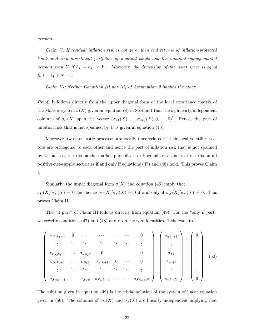
Proof. It follows directly from the upper diagonal form of the local covariance matrix of
the Markov system σ(X) given in equation (8) in Section I that the k1 linearly independent
columns of σU(X) span the vector (σπ1(X), . . . , σπk1(X), 0, . . . , 0)′. Hence, the part of
inflation risk that is not spanned by U is given in equation (46).
Moreover, two stochastic processes are locally uncorrelated if their local volatility vec-
tors are orthogonal to each other and hence the part of inflation risk that is not spanned
by V and real returns on the market portfolio is orthogonal to V and real returns on all
positive-net-supply securities if and only if equations (47) and (48) hold. This proves Claim
I.
Similarly, the upper diagonal form σ(X) and equation (46) imply that
σU (X)′σ⊥π (X) = 0 and hence σV (X)′σ⊥
π (X) = 0 if and only if σX(X)′σ⊥π (X) = 0. This
proves Claim II.
The “if part” of Claim III follows directly from equation (49). For the “only if part”
we rewrite conditions (47) and (48) and drop the zero identities. This leads to
σV 1k1+1 0 · · · · · · · · · · · · 0...
. . .. . .
. . .. . .
. . ....
σV k2k1+1. . . σV k2k 0 · · · · · · 0
σS1k1+1 . . . σS1k σS1k+1 0 · · · 0...
. . .. . .
. . .. . .
. . ....
σSN k1+1 . . . σSN k σSN k+1 · · · · · · σSNk+N
·
σπk1+1
...
σπk
σπk+1
...
σπk+N
=
0............
0
(50)
The solution given in equation (49) is the trivial solution of the system of linear equation
given in (50). The columns of σV (X) and σS(X) are linearly independent implying that
27

the coefficient matrix of the system of linear equations in (50) is non-singular and hence
the trivial solution is the unique solution. This proves the “only if part“ of Claim III.
The span of nominal returns of nominal bonds (see equation (23)) coincides with real
returns of zero investment portfolios of nominal bonds (see equation (12)) and the nominal
money market account (see equation (11)) because the difference between the local volatility
vector of nominal and real returns of every nominal bond and the nominal money market
account is equal to the volatility vector σπ and hence this difference vanishes if the total
investment in nominal bonds and the nominal money market account is zero. This proves
Claim IV.
Let Ebonds(X) denote the space spanned by real excess returns of hP + 1 inflation-
protected and hB nominal bonds. The hB + hP + 1 bonds are linearly independent.
Moreover, elementary column transformations lead to a set of hB + hP + 1 unit vectors
e1, . . . , ehB+hP, ed which span Ebonds(X).31 From the upper diagonal form of the local
covariance matrix of the Markov system given in equation (7) in Section I follows that the
local volatility matrix of U only loads on the first k1 components and hence it is spanned if
hB + hP = k1. If hB + hP > k1, then U is still spanned but in this case hB + hP − k1 bonds
are redundant.
Moreover, if real returns on all positive-net-supply securities are not spanned by real
returns of the nominal money market account and inflation-protected and nominal bonds,
then the dimension of the asset space is l = k1 + N + 1. If 0 ≤ n ≤ N positive-net-supply
securities are spanned, then there is no need to add them to the investment opportunity set
and hence we drop their excess return volatility vectors from Ω(X) and let l = k1+N−n+1.
This proves Claim V.
I provide two counter examples to prove Claim VI. Let k = 0, N = 1, σπ1 6= 0, σπ2 6= 0,
and σS1 6= 0. Then, the nominal money market account, the market portfolio (there is only
one positive-net-supply security), and an inflation-protected bond (which is in this case the
real risk-free asset) complete the market. But σπ1 6= 0 and hence part (i) of Assumption 2
is satisfied but part (ii) is violated.
Assume that part (ii) of Assumption 2 is satisfied and consider a state variable that
31ei denotes a d-dimensional vector with i-th component equal to one and remaining components zero.See Lemma 2 for details on the basis change.
28

is locally not perfectly correlated with real returns on all positive-net-supply securities
and is not spanned by real returns of inflation protected bonds and nominal returns of
nominal bonds – e.g. stochastic volatility of the market portfolio. In this case the market
is incomplete and hence part (ii) of Assumption 2 is satisfied but part (i) is violated.
Let PM denote the projector onto the asset space M and PE the projector onto the
excess return space E .32 Both projectors are given in the next lemma.
Lemma 2. [Projector onto the asset space]
The projector onto the asset space M is
PM(X) = −PE⊥(X)σπ(X) + PE(X) (51)
with projector on the excess return space E and the orthogonal complement of the excess
return space E⊥ given by33
PE (X) = Ω(X)(
Ω(X)′Ω(X))−1
Ω(X)′,
PE⊥(X) = Id −PE (X),(52)
respectively. Specifically, the projection of the d-dimensional vector v onto M is
PM(X)v = −PE⊥(X)σπ(X) + PE (X)v. (53)
Adopt Assumption 1 and 2. If the market is complete, then the projector onto E sim-
plifies to
PE(X) = Id. (54)
If the market is incomplete, then the projector simplifies to
PE(X) = PEbonds(X) + PES
(X), (55)
in which PEbondsdenotes the projector onto the space spanned by the real excess returns of
the hB nominal bonds and the hP + 1 inflation-protected bonds and PES(X) denotes the
32See Kreyszig (1989) Chapter 3 and Brockwell and Davis (2006) Chapter 2 for properties of Hilbertspaces and projectors.
33Let Ik denote the k-dimensional unit matrix.
29

projector onto the space spanned by the part of real excess returns on all positive-net-supply
securities that is uncorrelated with real excess returns of nominal and inflation-protected
bonds.34 Specifically,
PEbonds(X) =
Ik10 0
0 0 0
0 0 1
. (56)
and
PES(X) = σS(X)
(
σS(X)′σS(X))−1
σS(X)′
=
0 0 0
0 ∗ 0
0 0 0
(57)
in which σS(X) equals σS(X) except for the first k1 rows which are equal to zero.
Proof. If the market is complete, then Rd = E and hence PE(X) = Id.
If the market is incomplete, then Claim III of Proposition 3 implies that the volatility
of inflations is
σπ = (σπ1, . . . , σπk1, 0, . . . , 0, σπd)
′ . (58)
Hence, Ω(X) =
34In the special case when real returns of all positive-net-supply securities are uncorrelated with realreturns of nominal and inflation protected bond, then ES is spanned by real returns of all positive-net-supply securities.
30

σ1B1 . . . σh
B1 σ1P1 + σπ1 . . . σl+1
P1 + σπ1 σS11 + σπ1 · · · σSN1 + σπ1
.... . .
......
. . ....
.... . .
...
σ1Bk1
. . . σhBk1
σ1Pk1
+ σπk1. . . σl+1
Pk1+ σπk1
σS1k1+ σπk1
... σSN k1+ σπk1
0 . . . 0 0 . . . 0 σS1k1+1 . . . σSN k1+1
.... . .
......
. . ....
.... . .
...
0 . . . 0 0 . . . 0 σS1k . . . σSNk
0 . . . 0 0 . . . 0 σS1k+1 . . . σSN k+1
.... . .
...... . . .
... 0. . .
...
0 . . . 0 0 . . . 0 0 0 σSNk+N
0 . . . 0 σπd . . . σπd σπd . . . σπd
,
in which the first block of columns denotes the excess return volatility vectors of the hB
nominal bonds, the second block denotes the excess return volatility vectors of the hP + 1
inflation-protected bonds, and the last column denotes the excess return volatility vectors of
the N positive-net-supply securities. The first block of rows denotes excess return exposure
to the first k1 components of Z, the second block of rows denotes excess return exposure
to the next k2 components of Z, the third block denotes excess return exposure to next N
components of Z, and the last row denotes excess return exposure to residual inflation risk
Zk+N+1.
The first hb + hP + 1 columns span Ebonds by definition. Moreover, the hB nominal
bonds and the hP + 1 inflation-protected bonds are non-redundant and hence elementary
column transformations lead to
Ik10 0 . . . 0
0... σS1k1+1 . . . σSN k1+1
......
.... . .
......
... σS1k+1 . . . σSNk+1
...... 0
. . ....
......
.... . . σSNk+N
0 1 0 . . . 0
. (59)
31

The second block which I define as σS(X) is the part of real returns on all positive-net-supply
securities that is not spanned by real returns of inflation-protected bonds and real returns
of zero investment portfolios of nominal bonds and the nominal money market account and
hence N columns of the matrix σS(X) span ES . It is clear from equation (59) that Ebonds
and ES are orthogonal and hence E can be written as direct sum of the two spaces. Hence,
the projector onto E is equal to the projector onto Ebonds plus the projector onto ES .
Moreover, the space Ebonds(X) is spanned by the k1 + 1 unit vectors e1, . . . , ek1, ed
and thus PEbonds(X) is given in equation (56). The projector onto the space ES(X) that is
spanned by the column vectors of the matrix σS(X) is
PES(X) = σS(X)
(
σS(X)′σS(X))−1
σS(X)′. (60)
Ebonds(X) and ES(X) are orthogonal and hence
PES(X) =
0k1×k10k1×(N+k2) 0k1×1
0(N+k2)×k1∗ 0(N+k2)×1
01×k101×(N+k2) 0
, (61)
in which 0i×j denotes the i × j-dimensional null matrix.
Proof of Theorem 2. The value function of investors who can continuously trade in the
nominal money market account, hB nominal zero-coupon bonds, hP + 1 inflation-protected
zero-coupon bonds, and N positive-net-supply securities and who seek to maximize the
utility function in equation (14) is
J(t,W,X) = supc(a),α(a)|t≤a≤T
E
[∫ T
t
e−∫
b
tβ(X(a)) da u(c(b),X(b)) db
+ e−∫
T
tβ(X(a)) da U(W (T ),X(T )) | W (t) = W,X(t) = X
]
.
(62)
Assume that the value function satisfies all regularity condition. Hence, the value function
J(t,W,X) solves the HJB equation
supc>0,α∈Rl
(AαJ(t,W,X)) = 0, J(T,W (T ),X(T )) = U(W (T ),X(T )), (63)
32

in which the characteristic operator is given by35
AαJ = Jt + J ′XµX +
(
rW + WσW (α)′Λ − c)
JW +1
2trace
(
JXXσ′XσX
)
+ σW (α)′σXWJWX +1
2σW (α)′σW (α)W 2JWW + u − βJ.
(64)
If the investment horizon is infinite, then the value function does not depend on time t and
hence Jt = 0.
Investors prefer more to less and are strictly risk averse which implies that JW > 0 and
JWW < 0. Hence, the characteristic operator given in equation (64) can be rewritten as
AαJ = W 2JWW ·1
2
∥
∥
∥
∥
σW (α) −
(
1
γΛ + σXΘ
)∥
∥
∥
∥
2
+ K, (65)
in which γ = −WJWW /JW denotes the relative risk aversion coefficient, Θ = −JWX/(WJWW )
denotes the sensitivity of the marginal value of real wealth with respect to changes in the
state vector, ‖ · ‖ denotes the Euclidian norm, and K is given by
K = Jt + J ′XµX + (rW − c)JW +
1
2trace
(
JXXσ′XσX
)
−1
2W 2JWW
∥
∥
∥
∥
1
γΛ + σXΘ
∥
∥
∥
∥
2
+ u− βJ
(66)
and hence does not depend on the portfolio weight α.
The local volatility of the real wealth portfolio is σW (α) = −σπ +Ωα and W 2JWW < 0
and hence the optimal portfolio demand α∗ of the maximization problem given in equation
(63) is
α∗ = argminα∈Rl
(
1
2
∥
∥
∥
∥
σW (α) −
(
0 +1
γΛ + σXΘ
)∥
∥
∥
∥
2)
. (67)
Hence, the solution of the quadratic optimization problem in equation (67) is given by the
projection of(
0 + 1γΛ + σXΘ
)
onto the asset space M.36 Specifically, (i) the projection of
0 onto M is the portfolio with minimum distance to the origin – i.e. the minimum variance
portfolio which in this case is equal to the mimicking portfolio of the real risk-free asset
because 0 is spanned by real asset returns (0 ∈ M), (ii) the projection of Λ(X) onto M is
the portfolio with maximum local Sharpe ratio – i.e. the tangency portfolio, and (iii) the
35I sometimes suppress arguments for notional convenience.36See Bertsekas, Nedic, and Ozdaglar (2003) chapter 2.2 for applications of the projection theorem to
quadratic optimization problems.
33

projection of σX(X) onto M are the portfolios that are maximally correlated with the state
variables – i.e. the hedging portfolios.
Let Λ(X) ≡ PM(X)Λ(X) and σX(X) ≡ PM(X)σX (X). The market price of residual
inflation risk is zero – i.e. Λd(X) = 0 – and the state variables are uncorrelated with residual
inflation risk – i.e. σXd·(X) = 0 – and hence it follows from Lemma 2 that Λd(X) = 0 and
σXd·(X) = 0.37 Moreover, real returns of inflation-protected bonds and all positive-net-
supply securities are not exposed to residual inflation risk and real returns of nominal
bonds and the nominal money market account have exactly the same exposure to this risk
source and hence the total investment in nominal bonds and the nominal money market
account in (i) the mimicking portfolio for the real risk-free asset, (ii) the tangency portfolio,
and (iii) the hedging portfolio is zero.38
37vi denotes the i-th element of the vector v and Md· denotes the i-th row of the matrix M .38The optimal demand α∗ given in equation (67) is the solution of the system of linear equations
Ω(X)α∗ = σπ(X) +PE(X)Λ(X)
γ(W,X)+ PE(X)σX(X)Θ(W,X), (68)
with PE(X) given in Lemma 2. One could get α∗ directly from the first order condition of the HJB equation.Specifically,
α∗ =
(
Ω(X)′Ω(X))−1
Ω(X)′(
σπ(X) +Λ(X)
γ(W,X)+ σX(X)Θ(W,X)
)
. (69)
It is straightforward to verify that the solution for equation (68) and (69) are the same by multiplying bothsides of equation (68) with (Ω(X)′Ω(X))
−1Ω(X)′ and using the general formula for PE(X) given in equation
(52).
34