the benefits of positive passenger profiling on baggage … · 2004-09-28 · baggage screening...

This PDF document was made available from www.rand.org as a public

service of the RAND Corporation.

6Jump down to document

Visit RAND at www.rand.org

Explore RAND-Initiated Research

View document details

This document and trademark(s) contained herein are protected by law as indicated in a notice appearing later in this work. This electronic representation of RAND intellectual property is provided for non-commercial use only. Permission is required from RAND to reproduce, or reuse in another form, any of our research documents for commercial use.

Limited Electronic Distribution Rights

For More Information

CHILD POLICY

CIVIL JUSTICE

EDUCATION

ENERGY AND ENVIRONMENT

HEALTH AND HEALTH CARE

INTERNATIONAL AFFAIRS

NATIONAL SECURITY

POPULATION AND AGING

PUBLIC SAFETY

SCIENCE AND TECHNOLOGY

SUBSTANCE ABUSE

TERRORISM AND HOMELAND SECURITY

TRANSPORTATION ANDINFRASTRUCTURE

The RAND Corporation is a nonprofit research organization providing objective analysis and effective solutions that address the challenges facing the public and private sectors around the world.

Purchase this document

Browse Books & Publications

Make a charitable contribution

Support RAND

RAND-INITIATED RESEARCH

http://www.rand.org/pdfrd/

http://www.rand.org/pdfrd/

http://www.rand.org/pdfrd/feature/independent/findings.html

http://www.rand.org/pdfrd/publications/DB/DB411/

http://www.rand.org/pdfrd/research_areas/children/

http://www.rand.org/pdfrd/research_areas/children/

http://www.rand.org/pdfrd/research_areas/civil_justice/

http://www.rand.org/pdfrd/research_areas/education/

http://www.rand.org/pdfrd/research_areas/energy_environment/

http://www.rand.org/pdfrd/research_areas/health/

http://www.rand.org/pdfrd/research_areas/international_affairs/

http://www.rand.org/pdfrd/research_areas/national_security/

http://www.rand.org/pdfrd/research_areas/population/

http://www.rand.org/pdfrd/research_areas/public_safety/

http://www.rand.org/pdfrd/research_areas/science_technology/

http://www.rand.org/pdfrd/research_areas/science_technology/

http://www.rand.org/pdfrd/research_areas/substance_abuse/

http://www.rand.org/pdfrd/research_areas/substance_abuse/

http://www.rand.org/pdfrd/research_areas/terrorism/

http://www.rand.org/pdfrd/research_areas/terrorism/

http://www.rand.org/pdfrd/research_areas/infrastructure/

http://www.rand.org/pdfrd/research_areas/infrastructure/

http://www.rand.org/pdfrd/cgi-bin/Abstracts/e-getabbydoc.pl?DB-411

http://www.rand.org/pdfrd/publications/electronic/

http://www.rand.org/pdfrd/publications/electronic/

http://www.rand.org/pdfrd/giving/contribute.html

http://www.rand.org/pdfrd/feature/independent/findings.html

This product is part of the RAND Corporation documented briefing series. RAND

documented briefings are based on research briefed to a client, sponsor, or targeted au-

dience and provide additional information on a specific topic. Although documented

briefings have been peer reviewed, they are not expected to be comprehensive and may

present preliminary findings.

The Benefits of Positive Passenger Profiling on Baggage Screening Requirements

Russell Shaver, Michael Kennedy

DB-411-RC

September 2004

Approved for public release; distribution unlimited

The RAND Corporation is a nonprofit research organization providing objective analysis and effective solutions that address the challenges facing the public and private sectors around the world. RAND’s publications do not necessarily reflect the opinions of its research clients and sponsors.

R® is a registered trademark.

© Copyright 2004 RAND Corporation

All rights reserved. No part of this book may be reproduced in any form by any electronic or mechanical means (including photocopying, recording, or information storage and retrieval) without permission in writing from RAND.

Published 2004 by the RAND Corporation1700 Main Street, P.O. Box 2138, Santa Monica, CA 90407-2138

1200 South Hayes Street, Arlington, VA 22202-5050201 North Craig Street, Suite 202, Pittsburgh, PA 15213-1516

RAND URL: http://www.rand.org/To order RAND documents or to obtain additional information, contact

Distribution Services: Telephone: (310) 451-7002; Fax: (310) 451-6915; Email: [email protected]

ISBN: 0-8330-3629-7

This research in the public interest was supported by RAND, using discretionary funds made possible by the generosity of RAND’s donors, the fees earned on client-funded research, and independent research and development (IR&D) funds provided by the Department of Defense.

1

PREFACE

Shortly after the September 11, 200 terrorist attacks on the World Trade Center and the Pentagon, Congress passed a new law that mandated the screening of all baggage carried on all commercial aircraft by the end of calendar year (CY) 2002. The Transportation Security Agency (TSA), a newly formed organization that is part of the Department of Homeland Security, was given the responsibility for enssuring the rapid implementation of this mandate. To TSA’s credit, sufficient equipment was acquired and installed at all U.S. commercial airports.

This research addresses airport security needs over the longer term; namely, how best to balance in the future the two principal criteria that are commonly put forward for sizing the machine deployments at individual airports. These two criteria—keeping the cost to the government of acquiring, installing, and operating the baggage scanning equipment as low as possible and not seriously disrupting the passenger flow through the airport—are in conflict because lowering passenger disruption requires more machines and thus more program cost. In this research, we present a methodology for balancing the two criteria and thus for answering the question, How much (baggage scanning equipment) is enough?

Determining how much is enough is important for keeping the overall cost to the flying public at a minimum while still providing the mandated level of security. Failure to have deployments that minimize the overall cost to the public will unnecessarily impose a drag on the nation’s economic well-being.

This documented briefing is part of a larger study by the RAND Corporation of the implications of airport security measures for airports, airlines, and, more broadly, the nation’s economic well-being. RAND funded this study as a component of an even broader effort to expand our nation’s understanding of the implications of terrorist threats against the United States and its allies.

The results of this study should be of interest to policymakers who are responsible for implementing the most cost-effective approach to ensuring U.S. national security, especially those concerned with air transportation. It should also be of interest to organizations and individuals concerned with the same issues. The commerce associated with air travel is an important part of the U.S. economy. Ensuring its safety at minimum total cost to the economy is a critical policy challenge.

The breadth and depth of this study were inherently limited by time and cost, and more work in this area is warranted. Nonetheless, we believe these results provide very important insights into the best directions for policy.

2

This documented briefing is a product of RAND’s continuing program of self-sponsored independent research. Support for such research is provided, in part, by donors and by the independent research and development provisions of RAND’s contracts for the operation of its U.S. Department of Defense federally funded research and development centers.

Other documents produced as part of this study are

• DB-410-RC—How Much Is Enough? Sizing the Deployment of Baggage Screening Equipment to Minimize the Cost of Flying [Main Report]. Russell Shaver, Michael Kennedy, Chad Shirley, and Paul Dreyer.

• DB-412-RC—How Much Is Enough? Sizing the Deployment of Baggage Screening Equipment to Minimize the Cost of Flying [Executive Summary]. Russell Shaver and Michael Kennedy.

3

THE RAND CORPORATION QUALITY ASSURANCE PROCESS

Peer review is an integral part of all RAND research projects. Prior to publication, this document, as with all documents in the RAND documented briefing series, was subject to a quality assurance process to ensure that the research meets several standards, including the following: The problem is well formulated; the research approach is well designed and well executed; the data and assumptions are sound; the findings are useful and advance knowledge; the implications and recommendations follow logically from the findings and are explained thoroughly; the documentation is accurate, understandable, cogent, and temperate in tone; the research demonstrates understanding of related previous studies; and the research is relevant, objective, independent, and balanced. Peer review is conducted by research professionals who were not members of the project team.

RAND routinely reviews and refines its quality assurance process and also conducts periodic external and internal reviews of the quality of its body of work. For additional details regarding the RAND quality assurance process, visit http://www.rand.org/standards/.

4

ACKNOWLEDGEMENTS

The authors acknowledge the invaluable help they received from individuals both within and outside of RAND. We are grateful for the inputs and advice we received from JameCrites (Dallas-Fort Worth International Airport), Richard Marchi (Airports Council, International/North America), Amr Elsawy (MITRE), and Dr. David Sweringa (Air Transport Association). Their willingness to share their expertise and data with us played an essential role in our ability to do the research. We thank Jim Crites and Dick Marchifor being willing to review an early draft of the final report. We are also grateful for the informal review of the final report by Dr. Robert Raviera (MITRE, retired). These early reviews helped us formulate the final report.

Charles Kelley, Joe Guzman, Frank Camm, and Mayhar Amouzegar, all from RAND, critically reviewed both the drafts of the final document and the methodology that supported it. Without exception, we obtained valuable feedback from all the reviewers; their efforts substantially improved the quality of the document. We also thank RichardHillestad, our project leader and friend, who helped get us sufficient funding to complete the work.

Of course, the authors take full responsibility for what is in the report.

5

INTRODUCTION

This briefing describes work undertaken as part of a RAND internal study of the nation’s air transportation system and the impacts of proposed security measures on its long-term vitality. It extends work found in a recent RAND white paper, Safer Skies: Baggage Screening and Beyond, WP-131/1-RC/NSRD (Reference 1), and is a companion to How Much Is Enough? Sizing the Deployment of Baggage Screening Equipment by Considering the Economic Cost of Passenger Delays [Main Report], DB-410-RC (Reference 2), and How Much Is Enough? Sizing the Deployment of Baggage Screening Equipment to Minimize the Cost of Flying [Executive Summary],DB-412-RC (Reference 3).

It is an unfortunate fact that measures to make air travel secure from future terrorist attacks also make it less convenient and potentially substantially more expensive for most passengers. This unavoidable tension between the benefits of being more secure and the costs that come with it is currently neither well understood nor satisfactorily factored into existing plans for enhanced airport security measures. One important motivation for the study is to increase public awareness of this tension and encourage the U.S. government to take it more fully into account in its planning.

It is understandable and appropriate that the U.S. government should seek to provide the nation with the highest level of security possible at a time when we anticipate repeated terrorist attacks on this country’s infrastructure and population. But in the long term, it would be counter to the nation’s interest if we did not take into account the negative impacts of some of these security measures and strive to develop alternatives that would be more compatible with the normal travel interests of the public. These alternatives may be technical in character, may involve procedural changes, or may simply call for greater government investment in equipment and manpower. This briefing focuses on one such change, the employment of a “registered traveler” program, wherein passengers known to be non-terrorists are given preferential treatment when appropriate at U.S. airports.

One of the often-mentioned options is to use personnel databases on future airline travelers to identify passengers who might pose a threat to airport and aviation security. The Computer Assisted Passenger Pre-Screening System (CAPPS) is an early example. However, many believe that identifying potential terrorists with any degree of certainty is too difficult to accomplish. We would be inclined to agree with this view, although it certainly would be useful to know whether a passenger had already been identified by the various intelligence agencies as a terrorist. Some people, including the authors, believe that there is a much better chance that we can identify people who are most certainly not terrorists or terrorist sympathizers. These would be people whose backgrounds have been well vetted (usually because of their occupation). The “positive profiling” of these “registered travelers” and the benefits of so doing are the focus of this briefing. Most important, we will derive estimates of overall cost savings to the country of implementing a registered traveler program.

6

6

Briefing Outline

• Motivation for Considering Positive Passenger Profiling– Why are we interested in positive passenger profiling?– Arguments (Pro and Con) about its merits

• Basic Baggage Queuing Delay Calculus

• Adaptive Concepts for Enhancing Profiling

• “How Much Is Enough?” Balancing the Costs of Delay and Machine Acquisition, Installation, and Operations

• Conclusions and Observations

We will cover the following topics.

First, we will give a brief justification for our interest in passenger profiling. This introduction is not intended to be a full justification—that would require far more time and space than we can spare in this briefing. We will cover the main points, setting up the rationale for the subsequent calculations.

Next, we will give a short review of the delay calculations (with and without profiling). Reference 2, which we encourage the reader to obtain, has a significantly more complete discussion of these calculations.

Third, we will go into some detail on adaptive profiling concepts and their potential for balancing the two primary priorities that we have for baggage scanning: (1) keeping the probability of finding any bomb buried in a bag at a very high level by focusing on those bags that are most likely to pose a threat and spending less time on those that are not likely to pose a threat, and (2) keeping the baggage scanning delays short enough that they will not noticeably affect the passenger’s perception of convenience.

7

We will add some additional calculations that show some of the tradeoffs that we might make in reaching a good design point. We will specifically derive a “best” EDS* machine deployment, where the cumulative costs of machine deployments are balanced against the costs associated with delays imposed on the passengers because of inadequate baggage scanning equipment.

We will then conclude with a few observations.

------------------------------------* Electronic Detection System (EDS). The EDS name is usually associated with magnetic imaging machines that can scan bags and identify items within the bag that match various characteristics of forbidden objects. The characteristics include shape and density.

8

8

The Purposes of Positive Profiling

• Focus greater attention on passengers most likely to pose a threat

• Lower the overall costs of airport security

• Minimize the inconvenience to the flying public– Important for the continued economic growth of the nation

• Retain airport security at a high level– Deterring terrorists by assuring that no passenger can be certain that

his bag won’t be inspected and an implanted bomb discovered– Reducing terrorist opportunities by lowering volumes in terminals

• However, it is debatable whether positive profiling will increase or reduce overall airport security– Allowing some bags to pass security without being inspected is an

invitation to terrorists to find a way to exploit it

This chart points out the primary benefits of positive profiling: (1) higher attention to passengers whose backgrounds are not known; (2) reduced costs for acquiring, operating, and maintaining the security equipment at airports; (3) reduced inconvenience of travel associated with security measures for the flying public, leading to economic benefits for the nation; while (4) retaining high airport security. Overall, a successful positive profiling system could enhance airport throughput and increase the efficiency of the security system without harming airport security.

The chart also includes the important qualifier that not scanning some bags opens opportunities for terrorists to find ways past the security. This alone is sufficient for many people to reject positive profiling as a good idea.

Positive profiling of passengers means that a percentage of passengers checking baggage at the check-in counter are identified as “trustworthy.” On a random basis, the bags of these registered travelers are exempted from passing through the scanning machines. This exemption lowers the overall number of bags that must be scanned, which in turn increases the attention that the government scanners can apply to bags belonging to non-registered travelers. The increased scanning time per bag would logically translate into a higher likelihood of detection of whatever threatening objects exist in the bag.

Alternatively, if the amount of scanning time per bag were not a function of the overall demand, then the reduction in demand would result directly in a reduction in the time

9

needed to scan all the bags in the queue. Whether this is an important benefit or not depends on the length of the queue that would exist without profiling. The baggage scanning queue is, to first order, sensitive to only a few parameters: the number of bags per unit time entering the queue, the time needed to satisfactorily scan the bag for threatening objects, and the false alarm rate (also known as the false positive detection rate) that would call for additional machine scanning or (perhaps) even human intervention to open the bag. We will show some calculations later in this briefing to quantify this observation.

Regrettably, no profiling system can ensure 100 percent reliability of correct identification. So, deterrence is also important. By randomly selecting and scanning bags from “trusted travelers,” we reinforce deterrence by assuring that nobody, trusted or otherwise, can be confident of not having their baggage inspected. By maintaining assurance that nobody can confidently pass through the airport without also passing through the security scanning system, we deter terrorists from trying. In response, they may seek alternative targets and methods of attack where they would not have to face the same risks of discovery.

10

10

One Concept for Profiling Selectionand Implementation

• Some pre-arrival ticketed airline passengers are deemed trustworthy and are “registered” as such, based on various background data (e.g., CAPPs)

– Level of “trustworthiness” can be viewed as a variable

• Passenger is verified as “registered” when arriving at baggage check-in counter

– Non-forgeable ID card required to ensure passenger is the same person as the registered traveler in the data base

• A fraction of the baggage of verified registered passengers would be “marked” so as to avoid further inspection

– Fraction electronically determined as function of• Length of current baggage queue• Anticipated status of operating system• Current and anticipated baggage check-in demand• Desire to scan as many bags as possible without disrupting throughput

– No passenger knows whether his bag has been marked

This chart offers one view of how profiling might be implemented. For purposes of this briefing, it assumes that passengers are profiled and judged trustworthy at the ticket counter. It assumes the conservative approach of requiring the passenger to already have a reservation (to ensure time to search the database and identify the person’s trustworthiness) and to possess a suitable ID card for secure personal identification. The checked baggage would then be randomly selected for scanning (yes or no), where that randomness would be varied as a function of several parameters (e.g., the current length of the baggage scanning queues). If there is no “cost” to the passenger (in terms of inconvenience) because the queues are short, then his bags will be scanned regardless of his trustworthiness. And even if the queues are long, there will be a positive likelihood that the bag will be scanned anyway. When and where it is reasonable, knowledge of whether the bags have been scanned will be hidden from the passenger. This, of course, may not always be possible, especially under circumstances where the scanning occurs in the main concourse of the airport (as is currently envisioned at many large airports because of the lack of space in the baggage assembly areas). But the passenger will never know prior to checking his bag whether the bag is actually going to be scanned.

This concept would require a secure passenger ID system at the check-in counter. Other schemes exist (e.g., secure passenger ID at the passenger scanning portals) and can be

11

integrated with the baggage scanning system to ensure that every non-scanned bag placed on the airplane has an equivalent registered owner also on the airplane (a simple extrapolation of the already-in-existence baggage-passenger match procedures).

12

12

Three Ways That Profiling Can Help Overall Airport Throughput and Airline Economics

• Way One: Lower the demand for baggage scanning and, as a consequence, the maximum baggage scanning delays.

• Way Two: Lower the requirements for EDS/ETD* machine acquisition and installation, lowering the overall airport security costs while speeding up completion of deployment.

• Way Three: Provide adaptive options for baggage scanning that preserve airport throughput under unanticipated circumstances, e.g.,

– Loss of equipment due to reliability, sabotage, etc.– Greater-than-average demand due to special events, holidays, etc.– Increased threat levels– Longer-term growth that exceeds expectations

-----------------* Electronic Trace Detection

This chart extends the comments about the benefits of positive profiling.

We have already mentioned the first—lowering the demand on the baggage scanning system—but did not state the benefits to the airlines and the passengers. The airlines go to great trouble to ensure that the checked baggage gets onto the same plane as the passenger. Lost or misrouted baggage leads to dissatisfied passengers and discourages them from booking future flights with that airline. Loss of customer loyalty is very important to airlines and leads to a strong incentive on their part to have an efficient and timely baggage handling system. Obviously, inserting baggage scanning equipment into that system is cause for great concern, especially if the equipment isn’t sufficient to have the bags scanned in time for them to make it onto the plane. The obvious alternative—telling passengers to come early to the airport—also risks future business, given that many travelers view time spent at the airport as wasted time and a substantial inconvenience.

Another solution is to provide enough machines to keep the delays short. While this would satisfy the first concern, it potentially raises a second—namely, who pays for the extra equipment. At present, it appears that the government will “tax” the flying public for at least some of these costs. This cost will be added to the price of the tickets. The airlines are very price sensitive and have excellent reason to believe that this added cost will reduce the demand for air travel. Reduced air travel demand means lower revenues.

13

Obviously, if profiling can lower the baggage scanning demand, this added security cost could also be lowered because the government would not have to buy as many machines to satisfy the need.

Last, a number of uncertainties are associated with both future demand for air travel and the actual operational performance of the baggage scanning equipment once it has been installed and is in operation. Given the magnitude of the installations, flexibility to adapt to these uncertainties is almost certainly going to be small. Profiling appears to be an efficient and cost-effective way to deal with unplanned circumstances, including the potential of periodic increases in perceived threat levels.

14

14

Arguments Against Positive Passenger Profiling

• Scale of program is extremely large, perhaps costly– 2 billion travelers pass though U.S. airports each year; to be

successful system must have profiles on a good fraction

• There is no margin for error– Dedicated terrorists will have strong incentives to defeat

system, including coercing “Registered” passengers to do their dirty work

• Public interest groups are strongly opposed because of invasion of individual privacy and uncertain success– ACLU ridiculed concept as “get out of security free” card

• In the end, whether the benefits of positive profiling exceed the downsides rests on perceptions of the magnitude and character of the threat

There are a number of important objections to positive profiling. We have listed three major objections here.

First, the profiling job is extremely large. The total number of entrants in the profiling database will obviously be based on the number of passengers who enroll in the program, but several million or more should be anticipated. Procedures must be implemented and equipment deployed at the airports to ensure that registered travelers are not significantly slowed in transit because of their profiled status. To achieve this, the airport’s check-in counters must have rapid access to the database.

Terrorists will obviously have strong incentives either to masquerade as registered travelers or, failing that, to coerce a registered traveler into becoming an accomplice. It would take only one or two “successes” for terrorists to prevail. This implies that passenger IDs must be virtually foolproof. Moreover, it implies that the conditions for acceptance into the registered traveler program must be sufficiently stringent to weed out all would-be terrorists at the start. And it means either that only those who cannot be coerced become registered travelers or that there is a means to identify people who are acting under extreme duress. In all cases, these are difficult challenges.

Opposition also comes from civil libertarians, who view the idea of the government maintaining comprehensive databases on the general population of the United States as contradictory to the rights of individuals for privacy. They take seriously the potential for

15

misuse of those databases for purposes unrelated to security. Moreover, they are skeptical about whether they will really be secure.While the American Civil Liberties Union’s “get out of security free card” description may be an unfair characterization of a well-structured positive profiling system, the message is clear. If some bags aren’t checked, terrorists will find a way to exploit this fact.

This briefing will avoid debating the merits or demerits of passenger profiling. Ultimately, judgments about whether positive profiling is a good or bad idea will rest on perceptions of the threat and our ability to find bombs and other banned objects in bags. Is it too dangerous to allow any bag to go unchecked? And what do we do if the probability of detecting a real bomb is significantly less than 100 percent?

16

16

Briefing Outline–II

• Motivation for Considering Positive Passenger Profiling

• Basic Baggage Queuing Delay Calculus– Criteria for selecting maximum delays– Baggage scanning delays vs. maximum profiling permitted




The next set of charts will describe how we assess different baggage scanning deployments. We will start with a calculation that assumes no profiling. We will show outcomes related to the following:

• expected maximum delays as a function of the number of machines deployed and their reliability

• the distribution of delays as a function of cumulative probability

• the average delays over the day as a function of number of machines, reliability, and the degree of “hedging” assumed by the passenger behavior.

We will then consider reducing the baggage scanning requirement through profiling. If, for example, we had data that allowed us to judge that (on the average) 60 percent of the arriving passengers with bags were “good risks” and we decided to impose random scanning on one bag out of six, we could reduce the total baggage demand by 50 percent. We will show several charts that demonstrate the advantage of this “profiling” reduction. We will label this calculation the 50 percent profiling case, where it is understood that the amount of profiling is limited to 50 percent of the passengers arriving with bags.

The degree of random scanning of trustworthy passengers is, of course, subject to change. For the purposes of this briefing, we will assume that all maximum profiling percentages are a lower bound on what would be feasible, recognizing the need for occasional random testing.

17

17

Maximum Expected Delays for Various EDS Machine Deployments as Function of Reliability

0

10

20

30

40

50

60

70

80

90

100

110

120

30 35 40 45 50 55 60 65 70 75 80

Number of Machines Deployed

Max

Exp

ecte

d Q

ueu

ing

Del

ays

(min

)

Machine Rel. = 1.0

Machine Rel. = 0.9

Machine Rel. = 0.8

No Profiling Allowed DFW, 2010

This is our basic maximum delay calculation. It shows the expectation of the maximum baggage scanning delay that occurs over the day as a function of the number of machines deployed at the airport. The following assumptions underlie this chart:

• The data are from a single airport, Dallas–Fort Worth International (DFW), and represent forecasts of passenger demand at that airport for the year 2010.

• Passenger demand is tied to projected airport departures over a normal working day. It is a function of departure time, aircraft seating capacity, assumed load factor, and the likelihood that the passenger will wish to check one or more bags. The passenger arrival time prior to his scheduled departure is a variable and depends on the passenger’s perceived risk of not having his bag make the plane on time.

• The machines are deployed in two tiers. The first tier of machines performs a rapid scan (350 bags per hour) to see whether a more detailed scan is required. Seventy-five percent of these bags are found “safe” and are sent directly to the baggage assembly area. Twenty-five percent are tagged for a more detailed inspection in tier 2. The scan rate in tier 2 is 60 bags per minute. The machine deployments are “balanced” between the two tiers so that the delays at one tier do not dominate.

18

The maximum queuing delay that occurs during the day is one measure of merit. It represents the worst delay situation, and, if it can be kept small, there would be little cause for concern.

The three curves in the chart reflect different assumptions about the scanning equipment’s reliability. Historically, the baggage scanning equipment deployed at some airports have had poor reliability records. These are expected to improve as experience with these machines leads to fault identification and machine modification. We estimate that the machine’s future operational reliability will be better than 0.8 but (obviously) not as good as 1.0. We have carried all three of these reliabilities (1.0, 0.9, and 0.8) throughout the briefing.

The point to take from this calculation is that machine deployments in the vicinity of 50–65 machines will be needed to keep the overall maximum delays at DFW to within 10 minutes. If we can tolerate 30-minute delays, these number would drop to around 35–45 machines.

19

19

Results for EDS Deployment Options ConsideredAll Commercial Flights at DFW, CY2000 and 2010

DFW 2000 Number of Machines Criteria (% less than) Days over criteria

Total Bags = 40,714 Tier 1 Tier 2 Total Point Exp Value 10 min 30 min 60 min 10 min 30 min 60 min

No queue > 60 min 8 11 19 46.76 155.92 0.0% 0.0% 13.5% 365.0 365.0 315.7

No queue > 30 min 10 14 24 28.63 45.58 0.0% 8.0% 88.9% 365.0 335.9 40.5

No queue > 15 min 13 19 32 13.66 20.45 0.0% 95.8% 99.9% 365.0 15.4 0.4

No queue > 10 min 15 22 37 8.89 13.82 2.0% 99.8% 100.0% 357.6 0.9 0.0

No queue > 7 min 16 24 40 6.75 10.98 29.1% 100.0% 100.0% 259.0 0.2 0.0

No queue > 5 min 18 27 45 4.73 7.52 85.9% 100.0% 100.0% 51.5 0.0 0.0

DFW 2010 Number of Machines Criteria (% less than) Days over criteria

Total Bags = 63,068 Tier 1 Tier 2 Total Point Exp Value 10 min 30 min 60 min 10 min 30 min 60 min

No queue > 60 min 11 16 27 43.43 151.38 0.0% 0.0% 5.8% 365 365 344

No queue > 30 min 13 19 32 28.66 54.12 0.0% 3.4% 76.7% 365 352 85

No queue > 15 min 17 25 42 14.49 21.47 0.0% 96.9% 99.9% 365 11 0

No queue > 10 min 19 29 48 9.89 15.15 0.6% 99.8% 100.0% 363 1 0

No queue > 7 min 22 33 55 6.47 10.06 63.7% 100.0% 100.0% 132 0 0

No queue > 5 min 24 37 61 4.68 7.32 96.4% 100.0% 100.0% 13 0 0

Max Delay (min)

Max Delay (min)

The assumed reliability of the EDS machines is 90%, except for “max point delays,” where it is set at 100%.

This “results” chart is built from curves similar to those in the prior chart. For purposes of comparison, we have included results at DFW for passenger baggage demands in two calendar years, 2000 and 2010. The demand in 2000 is based on actual flight schedules. The demand in 2010 is based on a forecast that predates the events of 9/11 and probably overstates the future demand level. Nevertheless, the recent rise in airline travel suggests that this projected demand is likely to be reached no later than CY 2012.

The rows reflect different machine deployments, each selected to meet the specific criteria of being the lowest number of total machines consistent with a maximum queuing delay not greater than the specified amount. For example, in 2010, at least 27 machines (optimally balanced between the two tiers) are needed if the maximum delay is to be less than 60 minutes.

On each row are potential measures of performance. The maximum point delay (we define point delay as the specific delay that would occur if the EDS machines were 100 percent reliable) for the 27 machine case is 43.43 minutes. The expected maximum delay is 151 minutes, where we have assumed that the machines were only 90 percent reliable. The middle columns on the right-hand side of the chart show the probability that a passenger would incur a delay no greater than the criteria listed at the top (10 minutes, 30 minutes, or 60 minutes). The three columns on the far right translate the percentages

20

in the prior three columns into days of the year that the criteria would fail. The assumed EDS reliability in these six columns is 90 percent.

Obviously, adding more machines makes the outcomes better. However, more machines means higher costs to the airport and airlines in acquiring and deploying the equipment, costs that will eventually be reflected in higher ticket prices. Toward the end of this briefing, we will provide a calculation that balances the implied costs of delays at the airport against the anticipated costs associated with machine deployments, showing where the minimum occurs. The comparison of this minimum with and without positive profiling is one of the primary results of this briefing.

21

21

Cumulative Probability Distributions of Outcomes vs. EDS Deployment

0%

10%

20%

30%

40%

50%

60%

70%

80%

90%

100%

0 5 10 15 20 25 30 35 40 45 50 55 60

X = Maximum Bag Queuing Delays Encountered (minutes)

Pro

bab

ility

Max

Del

ays

< X

[24:37], Exp Del = 7.32 [22:33], Exp del = 10.06 [19:29]. Exp del = 15.15 [17:25]. Exp del = 21.47 [13:19], Exp del = 54.12 [11:16], Exp del = 151.38

DFW; 2010 Demand

EDS Machine Reliability = 90%

There are obviously several variables in the calculations that are inherently stochastic. Probably the most important is the number of machines that are actually in operation at any given time of the day. This chart assumes a machine reliability of 90 percent and plots, for specific machine deployments, the cumulative probability distribution as a function of the maximum point delay encountered. The machine deployments shown here are the same as those shown earlier in the results chart.

From either the airline’s or passengers’ perspective, small probabilities of large delays are important. The airlines are eager to make certain that all the bags are on the plane. Even a small fraction of bags missing the plane means a large number of complaints, unhappy passengers, and a potential loss of revenue. It has become common airline practice to warn passengers to arrive early to make flights during the busier parts of the day. Post-9/11, recommended early arrival times have often exceeded one hour, and in some cases more than 90 minutes.

Some passengers may be less risk adverse than the airlines, but most will deliberately set their arrival time sufficiently early to reduce to nil the likelihood of not having their bags on the plane. The use of expected maximum delays does not adequately capture these concerns. Point values—the measure of merit initially used by the Federal Aviation Administration (FAA) (and TSA) to size deployments at individual airports—are significantly deficient, given their failure to account for machine outages.

22

From the numbers, it is obvious that the 95 percent likelihood outcomes show maximum delays approximately twice those that would have occurred if the machines’ reliability were 100 percent (the intersection of the curve with the bottom axis).

23

23

Expected Delays vs. Machines Deployed(No Passenger Profiling; Reliability = 1.0)

0

10

20

30

40

50

60

70

80

90

605550454035302520

Total EDS Machines Deployed

Bag

gag

e Q

ueu

e D

elay

s (m

in)

Max Point Delays

Ave Delays, 30 min buffer

Ave Delays, 22.5 min buffer


Ave Delays, no buffer

DFW, 2010 Demand

EDS Reliability Assumed = 1.0

Fraction Passengers Profiled = 0.0

Looking only at the maximum delay over the entire day does not adequately capture the full spectrum of passenger experience. It is also important to consider the size of the delays when the passengers arrive at the airport. Our measure for this is “average delays,” defined as the weighted average of the product of passengers arriving at the airport at a specified time and the delay that exists at that time. This chart shows the average delays encountered over the entire day as a function of the number of machines deployed. Machine reliability has been set to 1.0, and no profiling is assumed. The upper curve is the maximum “point” delay. The lower four curves are all average delays, differentiated by the degree of risk that a passenger might wish to take. The buffer size accounts for the passenger’s recognition that delays are unpredictable.

The lowest of the average curves assumes that the passenger does not hedge against the uncertain peaks and valleys of the baggage queuing delays. Instead, it assumes that all such delays are “known” and the passenger can react accordingly. The other three average curves assume that the passenger wishes to hedge. We assume that he takes into account the maximum delays that would likely occur within a reasonable period of time around his planned arrival. The 15-, 22.5-, and 30-minute hedges shown in the chart reflect our assumption that the passenger would look at delays both earlier and later than his planned arrival and use the maximum over that span as his planning factor. The larger the hedge, the more likely that the passenger will include larger delays.

24

It is noteworthy that the three hedging curves are very close throughout the chart, suggesting that the degree of hedging does not significantly affect the answer.

Even allowing for hedging, the average delays are significantly less than the maximum. Average delays are good measures for the delays that the passenger will incur when planning to check baggage at the airport. Maximum delays, on the other hand, are good estimates of airline and airport concerns because both are sensitive to the “tails” of the distribution of outcomes. Later, we will introduce another calculation that relates passenger planned arrival time to the likelihood that his checked baggage actually gets onto the intended flight. We will use this latter calculation to form economic estimates of the overall cost to the passenger (and the nation) of failing to properly balance the costs of passenger delay and inconvenience against the cost of adding more machines.

25

25

Expected Delays vs. Machines Deployed(No Passenger Profiling; Reliability = 0.9)

0

10

20

30

40

50

60

70

80

90

605550454035302520

Total EDS Machines Deployed

Bag

gag

e Q

ueu

e D

elay

s (m

in)

Max Expected Delays


Ave Delays, 22.5 min buffer


Ave Delays, no buffer

Max Point Delays (rel. = 1.0)

DFW, 2010 Demand

EDS Reliability Assumed = 0.9


This chart is essentially a repeat of the prior one, with machine reliability lowered to 90 percent and a new curve—the expected maximum delay—added. A quick comparison of this chart and the one before it shows that the average expected delays are substantially higher than those for the average point delays on the prior chart. The expected maximum delay is also substantially higher than the point delay. For purposes of comparison, we have copied the point delay curve and pasted it onto this chart. At lower machine buy sizes, even the average delays exceed the maximum point estimate.

As before, the three average hedged curves are very close to each other.

26

26

Reducing Delays Through Profiling(A First Look)

0

10

20

30

40

50

60

70

80

90

100

50454035302520

Number of EDS Machines Deployed

Max

Exp

ecte

d D

elay

s (m

in)

Profile Fraction = 0.0 Profile Fraction = 0.1 Profile Fraction = 0.2 Profile Fraction = 0.3

Profile Fraction = 0.4

Profile Fraction = 0.5 DFW, 2010

No Delay in InitiatingPassenger Profiling

Machine Rel. = 1.0

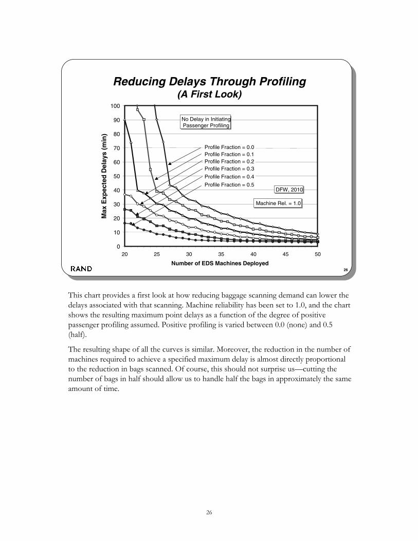
This chart provides a first look at how reducing baggage scanning demand can lower the delays associated with that scanning. Machine reliability has been set to 1.0, and the chart shows the resulting maximum point delays as a function of the degree of positive passenger profiling assumed. Positive profiling is varied between 0.0 (none) and 0.5 (half).

The resulting shape of all the curves is similar. Moreover, the reduction in the number of machines required to achieve a specified maximum delay is almost directly proportional to the reduction in bags scanned. Of course, this should not surprise us—cutting the number of bags in half should allow us to handle half the bags in approximately the same amount of time.

27

27

Benefits of Profiling for Specific EDS Deployments; EDS Reliability = 1.0

1

10

100

24::3722::3319::2917::2515::2213::1911::16

Tier 1 :: Tier 2 Deployment

Max

imu

m B

ag Q

ueu

ing

Del

ays

(min

) No Profiling

Max 10% Profiled

Max 20% Profiled

Max 30% Profiled

Max 40% Profiled

Max 50% Profiled

DFW; 2010 Demand

This is another way to display these results. Here we have selected a specific set of machine deployments (patterned after those on the results chart) and show how maximum delays are reduced with profiling. Machine reliability was assumed to be 1.0. We used a log scale to capture the dynamic range of the change in maximum delays. Note that the maximum delays drop rapidly for a fixed machine deployment, especially where relatively few machines are deployed.

28

28

Reducing Delays Through Profiling(Comparing Results for Different Reliabilities)

0

10

20

30

40

50

60

70

80

90

100

50454035302520


Max

imu

m E

xpec

ted

Del

ays

(min

)Profile Fraction = 0.0




DFW, 2010

No Delay in InitiatingPassenger Profiling

Machine Reliability:Solid Line = 1.0

Dashed Line = 0.9

This chart repeats some of the curves from page 26 (solid lines, with machine reliability equal to 100 percent) and overlays a similar set of curves (dashed lines) where the reliability has been reduced to 90 percent. Not surprisingly, the maximum expected delays increase with a reduction in reliability. The chart gives the reader a sense as to the size of the increase.

29

29

Maximum Expected Delays as Function of Reliability; Passenger Profiling Fraction = 0.5

0

25

50

75

100

125

150

175

200

605550454035302520

Number of Machines Deployed

Max

imu

m E

xpec

ted

Qu

eue

Del

ays

(min

) Reliability = 1.0, with Prof

Reliability = 0.9, with Prof

Reliability = 0.8, with Prof

Reliability = 0.8, w/o Prof



DFW 2010

Eligible for Positive Profiling = 50%

This chart replicates an earlier no-profiling chart (page 17) but assumes a maximum passenger profiling fraction of 0.5 (for comparison purposes, we have duplicated the no-profiling curves and shown them as dashed curves). It shows the maximum expected delays for machine reliabilities of 100 percent, 90 percent, and 80 percent. The shape of the curves is similar to that in the no-profiling chart, but the delays are reduced accordingly. For example, a total deployment of 30 machines in this case would yield maximum expected delays of no greater than 15 minutes (in the reliability = 0.8 case), with a maximum point delay of about five minutes. Without profiling, these numbers would have been more than 200 minutes and 31 minutes, respectively.

30

30

Expected Delays vs. Machines Deployed(50% Passenger Profiling; Reliability = 0.9)

0

10

20

30

40

50

60

70

80

90

40353025201510

Number of EDS Machines

Bag

gag

e Q

ueu

e D

elay

s (m

in)

Exp Max Point Delay

Exp Ave Delay, zero hedge

Exp Ave Delay, 15 min hedge

Exp Ave Delay, 22.5 min hedge

Exp Ave Delay, 30 min hedge

Max Point Delay, P(rel) = 1.0

Machine Reliability = 0.9

DFW, 2010


This is also a repeat of an earlier no-profiling chart (page 25), showing how average delays are similarly reduced at given machine deployments when 50 percent positive passenger profiling is assumed.

In this and the preceding chart, the number of machines required to reproduce comparable delays is approximately 50 percent of the number in the earlier charts, reconfirming what we expected (i.e., half the demand requires half the machines to achieve comparable delays).

31

31

Briefing Outline–III

• Motivation for Positive Profiling


• Adaptive Concepts for Enhancing Profiling– Delaying the employment of profiling until delays build past a

specified criterion– Tradeoffs among some of the variables– The ultimate profiling outcome



Heretofore, we have assumed that, with profiling, every passenger who qualifies for positive profiling (and is not randomly selected for inspection) will have his bag suitably marked so that it will not be scanned. This assumption suggests that a fairly large number of bags could avoid scanning even though the baggage scanning queues were minimal. We noted earlier that a reasonable strategy would be to scan all bags unless baggage scanning queues were substantial. In this section of the briefing, we will look at responsive profiling strategies that lead to a larger number of bags being scanned.

Scanning more bags is obviously better than scanning fewer bags, assuming no increase in delays. As we will show, there is a tradeoff between the number of bags that are scanned and the delays. We will offer one view of that tradeoff.

We will examine only one strategy—our so-called reactive strategy—which initiates profiling only after the baggage queues have grown sufficiently long to cause delays in processing by a specified amount. We have varied this amount—we call it the threshold—between zero and ten minutes.

A number of variables are involved in the calculation. Those considered here are

• the number of machines

• the maximum extent of profiling permitted

• the threshold value where profiling is started.

32

32

Adaptive Profiling Strategies

• Purpose of adaptive strategies is to balance three competing objectives

– Scan all or most bags that are placed onto commercial aircraft– Keep passenger delays to a minimum– Keep the costs of providing security at airports low

• Candidate concepts for analysis– Profile maximum number at all times

• Highest fraction limited by need for random checks

– Implement profiling only when delays reach a predetermined level• Allows maximum bag scanning whenever delays are not a problem• Can be adjusted when circumstances mandate

– Adjust implementation of profiling in anticipation of growing delays• Optimize to achieve maximum bags scanned per scanning delay• Requires a means to estimate future bag scanning delays

Adaptive profiling can help balance the competing objectives of scanning most if not all bags, keeping delays low, and deploying a relatively small number of baggage scanning machines at major airports.

For the reasons already mentioned, many people within and outside the government oppose any strategy that allows anyone (registered traveler or not) to avoid having his or her bags inspected. Others perceive the benefits of profiling as attractive despite the risks. In an attempt to balance the pros and cons of profiling, we sought to find a way to scan as many bags as possible without abandoning the benefits of profiling. Buying our way out of the problem is an option, but it would probably impose additional costs on the passengers. As we will show shortly, simply enduring substantial delays at the airports is also costly, yielding substantial negative impacts on the nation’s economy. If possible, we would like to find an acceptable compromise.

The first of the profiling candidates shown on the chart is the one used in the calculations shown earlier. It is neither adaptive nor responsive to the above concerns.

We will show some calculations that exploit the second profiling strategy. This strategy is reactive in that it reacts to the observed growth in delays. All bags are scanned when delays are below a specified threshold, with profiling kicking in (either in part or in toto) when the threshold is exceeded. Once delays fall below the threshold, profiling is set aside and the checking of all bags resumes.

33

Profiling strategies that are more proactive can also be imagined. For instance, if personnel know approximately how many travelers with to-be-checked bags are likely to show up at the airport at any given time of day, they can anticipate the growth in baggage queues and start the profiling early. A more complete examination of profiling options should thoroughly examine such strategies. But for the purpose of this briefing, our calculations will confirm that adaptive strategies have real merit.

34

34

The Impact of Simple Reactive Profiling Strategies on Increasing the Fraction of Bags Scanned

0

5

10

15

20

25

0.50 0.55 0.60 0.65 0.70 0.75 0.80 0.85 0.90 0.95 1.00

Fraction of Bags Scanned

Max

imu

m E

xpec

ted

Del

ays

0 min

2 min

3 min 4 min 5 min

7 min

10 min L = Minimum

Baggage DelayQueue Size

When ProfilingIn Operation

DFW, 2010Machine Rel. = 1.0

Deployment SizeTier 1 = 15Tier 2 = 22

To show the tradeoffs, we selected a specific deployment of machines. This chart shows a balanced deployment of 15 machines in tier 1 and 22 in tier 2. The overall maximum delay calculation for scanning 100 percent of all bags is just over 20 minutes (see the top right hand-part of the chart).

The top curve assumes that profiling of bags is implemented regardless of the size of the baggage scanning queue. The maximum delays fall steadily as the fraction of bags scanned falls. The data points on the top curve reflect positive profiling fractions, varying from 0.0 to 0.5 in increments of 0.05. In this case, the data points also match the tics along the X-axis. The remaining curves assume that no profiling is permitted unless the queue has reached a specified size. L is the variable representing this size. That is, profiling will start only when the length of the current scanning queue exceeds L minutes. As above, the data points on each curve represent the profiling fractions assumed for that curve—again varying from 0.0 to 0.5 in increments of 0.05. As we increase the delay threshold, L, the fraction of bags scanned for any maximum delay is increased. We do not drop bags from the scanning pool when the queuing delays do not warrant it.

These curves are sensitive to the level of demand and the machine buy size, so quantitative generalizations would not be appropriate. Qualitatively, it should be clear that delaying profiling until thresholds of five minutes or more has the potential of sharply increasing the total fraction of bags scanned while keeping delays near the level achieved if the profiling strategy were nonresponsive.

35

35

Expected Delays vs. Bags Checked(Tradeoffs for Different Delay Criteria)

0

5

10

15

20

25

30

35

40

0.50 0.55 0.60 0.65 0.70 0.75 0.80 0.85 0.90 0.95 1.00

Fraction of Total Checked Bags Inspected

Max

imu

m E

xpec

ted

Del

ays

(min

)

Delay Criteria = 10 min Delay Criteria = 5 min Delay Criteria = 3 min Delay Criteria = 2 min Delay Criteria = 0 min

Machine Rel. = 0.9

DFW, 2010

Eligible For Profiling = 50%

Machine Totals VaryFrom 20 to 50

Machine totals = 20

Machine totals = 50

This chart shows the results of adaptive profiling in a different and perhaps more informative format. We show the tradeoff between the two principal variables—delays and bags checked—with the number of machines deployed captured as a variable (shown as data points along the curves).

The chart assumes that the maximum profiling permitted is 50 percent. The number of deployed scanning machines runs from 20 to 50, optimally balanced between the two tiers. And the machine reliability is assumed to be 0.9.

Five curves are shown, each representing a given assumption about the threshold levels where profiling starts. Zero is the “implement profiling at all times” case. Obviously, in all cases only 50 percent of the bags are scanned. The two-, three-, five-, and ten-minute curves assume that profiling starts when delays exceed two, three, five, and ten minutes, respectively. Also obvious is that increasing the threshold increases the fraction of bags scanned. In addition, increasing the threshold adds to the overall delays. The shape of these curves gives some insight into which of these increases dominate.

The three-, five-, and ten-minute curves show significant increases in the fraction of bagsscanned but only a modest increase in maximum expected delays. This validates our interest in responsive profiling strategies and may offer a reasonable position for finding a balance among the priorities that everyone can accept.

36

36

Number of Machines vs. Profiling Eligibility:A Carpet Plot

0

5

10

15

20

25

30

35

40

45

50

55

60

0.75 0.80 0.85 0.90 0.95 1.00

Fraction of Bags Scanned

Max

imu

m E

xpec

ted

Del

ays

(min

)

0%

10%

20%

30%

40%

Eligible for Profiling = 50%

45

29

32

35

40

Number ofMachinesDeployed

50

Machine Rel. = 0.9

DFW, 2010

26

55Start Profiling at 5 min

This chart holds the starting profiling threshold fixed at five minutes and shows the tradeoff between the number of scanning machines deployed and the extent of profiling permitted. The thin lines marked with numbers are the constant machine deployment curves; those with marks are the fractions of passenger bags eligible for profiling (note that we are ignoring the need to randomly scan some fraction of the bags).

As above, generalizations from a single chart would be dangerous. However, this carpet plot shows the added tradeoffs among machine buy size, profile eligibility, and fraction of bags scanned.

37

37

Bags Scanned vs. Delays Imposed

0.50

0.55

0.60

0.65

0.70

0.75

0.80

0.85

0.90

0.95

1.00

0 2 4 6 8 10 12 14 16 18 20

Maximum Baggage Queuing Delay over Day (min)

Fra

ctio

n o

f B

ags

Sca

nn

ed o

ver

Day

Max Fraction Profiled = 0.5





Zero Profiling

Number of Machines = 45Machine Reliability = 0.9

DFW, 2010

CriteriaSteps:

(Bottomto Top)---------0 min2 min5 min10 min

This chart shows, for a given machine deployment size, the fraction of total bags that must be “deleted” in order to achieve a minimum delay. The fractions become quite small as the number of machines deployed reaches a level consistent with the optimum deployment levels discussed in Reference 2. Regrettably, the fraction of bags that must be profiled is still substantial, albeit over a short period during the day.

38

38

Briefing Outline—IV




• “How Much Is Enough?” Balancing the Costs of Delay and Machine Acquisition, Installation, and Operations– Calculating Passenger Predeparture Arrival Times– Minimizing the overall economic costs of security measures at

commercial airports in the United States


We now turn to our estimates of the overall costs of the EDS deployments and compare those costs with the costs borne by the passengers, the airline industry, and the country as a whole associated with congested and restricted throughputs at the major U.S. airports.

We will introduce an additional calculation to better characterize passenger response to anticipated baggage scanning delays. This calculation will focus on the passenger predeparture planned arrival time, a time selected to achieve a specified level of confidence that the passenger’s checked baggage will reach the airplane in time. The predeparture arrival times will be calculated against the number of EDS machines deployed and as a function of the machine reliability. Earlier arrival times translate into less risk to the passenger of having his baggage miss the plane.

This earlier arrival time also translates into additional time spent at the airport, time that we judge to be “wasted.” For purposes of our economic calculations, we will simply add this additional time to the total expected transportation time. The transportation time includes the flight time as well as time in the airport and average time going to and coming from the airport.

We will then calculate the cost of this additional wasted time against the cost of reducing that wasted time by deploying more EDS machines. Both cost curves are monotonic, the

39

first starting at infinite (zero machines) and going to zero at infinite machines; the latter does the reverse. Suitably adding these curves yields a minimum. It is this minimum that we are seeking.*

Although not mentioned until now, we have performed similar calculations for a second airport, Chicago O’Hare International Airport (ORD). The addition of a second airport is intended to reduce the likelihood that our small sample of airports is biasing our results. The cost calculations will use the data from both airports.

Our calculations will not include any reactive or proactive profiling strategies.---------------------------------------* We will also show an additional, more complex calculation for the impact on the nation’s economy that is not a linear sum of these two curves.

40

40

Passenger Arrival Time for 99% Assurance That Bag Makes Plane: Combined ORD & DFW

30

40

50

60

70

80

90

100

110

120

20 25 30 35 40 45 50 55 60 65 70


Pas

sen

ger

Pla

nn

ed A

rriv

al T

ime

(min

ute

s b

efo

re s

ched

ule

d d

epar

ture

) Rel. = 0.8

Rel. = 0.9

Rel. = 1.0

Probability ofBag MissingPlane = 1%

Max PassengerProfiling = 50%

The calculations shown on this chart make the following assumptions:

• There is an irreducible checking-in-the-baggage-to-loading-the-baggage-onto-the-airplanetimeline that we assume to be 30 minutes. That 30 minutes includes wait times to reach the check-in counter as well as time for the bags to be put through the baggage scanning system, conveyed into the baggage assembly area, loaded onto the baggage cart, and moved to the aircraft.

• The passenger plans his arrival time knowing that his actual arrival time will be scattered around that time by plus-or-minus 15 minutes. This “spread” of a total of 30 minutes is also included in the demand arrival times and directly influences the demand spread. A risk-adverse passenger, assured of no baggage queuing delays, will plan on arriving 45 minutes before plane departure, thereby eliminating the likelihood that a delayed arrival of 15 minutes would cause his bag to miss the plane.

• Assuming some delays, and recognizing that the magnitude of these delays cannot be predicted because of EDS machine reliability, the passenger estimates the likelihood of the bag not making the plane and sets his predeparture arrival time according to how risk adverse he wants to be. For this chart, the passenger has decided to plan on a predeparture arrival times that makes it probable that his bag will make the plane 99 percent of the time.

41

In this calculation, we assume that 50 percent of the arriving baggage will be exempt from scanning. Moreover, every bag that is exempt bypasses the scanning system (i.e., no reactive profiling is assumed). The demand is for both DFW and ORD, circa 2010.

As to the shape of the curves themselves, it is worth noting that they are relatively flat on the right-hand side of the chart, but as the number of machines drops they rise steeply once they pass a threshold.

42

42

Passenger Arrival Time for 99% Assurance That Bag Makes Plane: All Airports

30

40

50

60

70

80

90

100

110

120

1000 1500 2000 2500 3000 3500 4000 4500 5000

Total Number of EDS Machines Deployed

Pas

sen

ger

Pla

nn

ed A

rriv

al T

ime

(min

ute

s b

efo

re s

ched

ule

d d

epar

ture

)

Rel. = 0.8

Rel. = 0.9

Rel. = 1.0

Probability ofBag MissingPlane = 1%

Max PassengerProfiling = 50%

The calculation extends the results of the prior chart to EDS machine demand levels appropriate for supporting baggage scanning requirements at all U.S. commercial airports.

To scale up from the combined number of EDS machines at DFW and ORD, we took into account the following factors.

1. Airport baggage scanning inefficiencies: Until now, we have assumed that baggage scanning at DFW and ORD is done in a central facility. This maximizes the use of the machines but overstates what is possible at most airports. The airlines prefer to keep all checked bags under their control. Combining this fact with airport layout—which tends to segregate the larger airlines into individual terminals—we developed the following scale factors to take this into account:

• 25 percent increase in number of machines for reliability of 1.0

• 33 percent increase for reliability of 0.9

• 40 percent increase for reliability of 0.8.

2. Extrapolating machine demand at DFW and ORD to all commercial airports in the United States.: Past studies by the FAA on nationwide needs for baggage scanning equipment broke the needs into individual airports. Although the estimates for

43

machine needs in those earlier studies were significantly smaller than those derived in this study (mostly because the criteria for sizing these deployments were less demanding), the relative needs among airports is, in our judgment, satisfactory for our needs. The resulting scaling factor is 43.75.

We will use the demands shown on this chart as inputs to the cost tradeoffs that we will now discuss.

44

44

Costing Assumptions

• Factors included in total machine cost– Acquisition costs, based on estimated costs for EDS machines– Personnel costs for operating and maintaining the equipment– Facility modification costs for machine installation

• First-order estimates only, scaled for annual life cycle costs assuming a 10 year machine life

• Value of time from Department of Transportation guidelines

We calculated the annualized cost of any overall EDS machine buy using the following assumptions (all costs are in dollars of 2002 purchasing power). Procurement cost is $1 million per machine, and machines must be replaced every ten years. There is an installation cost of $4 million per machine, which is not again incurred when the machines are replaced. Machines operate two-thirds of the time and are attended by one operator when operating. The fully burdened cost of an operator is $80,000 per year, and five operators are required to provide full-time coverage for one machine. We derive the figure of five in the following way. From 52 weeks per year, we deduct two weeks for holidays, two weeks for vacation, and two weeks for sick leave. The remaining 46 weeks per year, at 40 hours of machine operation per week, would lead to a staffing ratio of 4.75. We judgmentally increase this to five people to account for such miscellaneous activities as continuing and refresher training. An additional $50,000 per year maintenance cost per machine is assumed. The present-value cost of buying, installing, and operating a machine for 30 years (at a 3 percent real discount rate, which we use) is $9.5 million, which translates into an annual charge of $630,000 per machine. Since our calculations are done in dollars of 2003 purchasing power, this is estimated at $640,000 per year to account for inflation.

As an illustration, we see from page 41 that about 2,750 machines would be needed nationwide to achieve a five-minute average delay per passenger checking baggage (at 90 percent machine reliability). Our machine sizing calculations are based on a level of air

45

travel in 2010 of 967 billion revenue passenger miles (RPM), so the total cost is 0.37 cents per RPM. This can be contrasted to the average cost (including taxes) of an RPM in 2002 of about 15 cents, so it represents about 2.5 percent of that amount.

We value delay time at $31.67 per hour, based on the Department of Transportation recommended value (found at api.hq.faa.gov/economic/742SECT1.PDF) of $28.60 per hour in dollars of 2000 purchasing power, adjusted upward by the change in nominal gross domestic product (GDP) per employed person between 2000 and 2003. Our machine sizing calculations are based on 600 million trips in 2010 (900 million enplanements from the U.S. Department of Transportation [2002] forecast and our assumption that the ratio of trips to enplanements is 2/3—i.e., 1/3 of enplanements are persons changing planes on the same trip). We assume that 70 percent of passengers check bags. Thus, the time cost of a five-minute delay in 2010 is $1.1 billion [5 × 600 million 5 × ($31.67/60) x 0.7].

46

46

How Much Equipment Is Enough?Minimizing Total Costs

$0

$1

$2

$3

$4

$5

$6

$7

2,400 2,600 2,800 3,000 3,200 3,400 3,600 3,800 4,000 4,200

Number of EDS Machines Deployed at US Airports

An

nu

al C

ost

of

Bag

gag

e S

cree

nin

g

Pro

gra

m in

201

0 ($

B)

Total cost--simplecalculation

Cost ofbaggagescanningequipmentat Airports

Cost ofexcesspassengertime atairports

Passenger Criteria: BaggageMakes Plane 99% of Trials

Max Positive Profiling = 50%EDS rel. = 90%

This chart shows, as a function of the total number of machines acquired, (1) the annualized costs of acquiring, installing, operating, and maintaining the EDS equipment; (2) the annual passenger delay costs; and (3) the arithmetic sum of these two costs. The reliability of the equipment is assumed to be 90 percent, and the passenger demand is assumed to be the forecast for 2010 (967 billion RPM and 600 million trips).

The equipment costs are a simple linear function of the size of the total buy. As seen in earlier charts, the amount of wasted time imposed on the passenger in order to avoid having his bag not reach the aircraft on time is a function of the number of machines. The wasted time decreases rapidly from the point where the equipment is barely able to keep up with the average demand during the day to a point where even the peaks of the day can be handled. Note that, for a total buy of 3,090 machines, machine cost is $1.98 billion and delay cost is $0.44 billion.

Adding these two curves together gives our estimate of the total cost that the traveling public will pay over the course of one year (the word “cost” is in italics because the wasted time isn’t monetary in character). Note that delays dominate the cost near the left-hand side of the chart, and machine costs dominate toward the right-hand side. The total cost reaches a minimum at around 3,100 machines. Buy sizes that are smaller than this amount incur greater overall economic costs because the passengers will be forced to arrive at the airport earlier than is economically efficient. Buy sizes greater than this

47

amount add costs that are not justified by the decrease in passenger time they produce. Given the slopes of the curves, it is clearly better to overbuy EDS machines than to underbuy them.

Note that the annual minimum cost to the flying public is around $2.45 billion.

Henceforth, we will call this calculation the simple calculation. A more complex calculation that takes into account a wider set of economic considerations will be discussed shortly. When applied to buy size calculations, we label it the complex calculation.

48

48

Sensitivity of Total Costs to EDS Reliability

$0

$1

$2

$3

$4

$5

$6

$7

$8

1,000 1,500 2,000 2,500 3,000 3,500 4,000 4,500 5,000


An

nu

al C

ost

of

Bag

gag

e S

cree

nin

g

Pro

gra

m in

201

0 ($

B)

EDS rel. = 80% EDS rel.

= 90% EDS re. = 100%


50% Positive Profiling

Simple Calculation

This chart shows the annual cost curves as a function of reliability, assuming that 50 percent of the bags are profiled and not scanned. Some observations are appropriate:

• Assuming 90 percent machine reliability, the minimum annual cost to the flying public is about $2.5 billion and the optimum buy size is in the neighborhood of 3,100 machines.

• Assuming perfect machine reliability, the minimum total annual cost of the security equipment is lowered to approximately $2.1 billion, with an optimum buy size around 2,500 machines. If the reliability were only 80 percent, the optimum buy size would increase to around 3,800 machines and the total annual cost to the flying public would be about $2.9 billion.

• In every case, the costs grow more rapidly with a less-than-optimum deployment size than with a greater-than-optimum size. Any strategy that takes uncertainties into account would hedge the buy toward deployment numbers higher than the calculated optimum.

49

49

Cost to the Flying Public vs. Machines Acquired (With and Without Profiling)

$0

$1

$2

$3

$4

$5

$6

$7

$8

$9

1,000 2,000 3,000 4,000 5,000 6,000 7,000 8,000


An

nu

al C

ost

of

Bag

gag

e S

cree

nin

g

Pro

gra

m in

201

0 ($

B)

No positive profiling

Max positive profiling = 50%


EDS machine rel. = 0.9 Simple Calculation

This chart compares the total costs with and without profiling. It adds to the 90 percentreliability curve on the prior chart the equivalent curve where no profiling is permitted. The minimum economic impact in the no-profiling case is about an 80 percent reduction in cost when compared with the 50 percent profiling outcome, dropping costs to $2.45 billion per year from around $4.6 billion per year. Moreover, the optimum number of machines is reduced by nearly half from that needed if no positive profiling is assumed.

The obvious conclusion from this chart is that profiling can do the following:

• Significantly lower the overall cost to the flying public by considerably reducing the number of scanning machines required to achieve an optimum outcome at each level of profiling.

• Reduce the total number of scanning machines needed at the airports by a fraction that is close to the fraction of reduced baggage that needs to be scanned (note that it would still cost nothing to scan all bags during times of the day when the machines would otherwise be underutilized).

• Reduce by an amount that is airport-specific the extent of airport facility modification and/or new construction needed to house all the new equipment.

50

50

Total Cost as a Function of Delay Time

0

1

2

3

4

5

6

7

1 3 5 7 9 11 13 15 17 19 21 23

Excess Time Spent at Airports (min)

An

nu

al C

ost

of

Bag

gag

e S

cree

nin

g

Pro

gra

m in

201

0 ($

B)

Costs ofbaggagescanningequipmentat Airports

Cost ofpassengersdelay time atairports

Total cost--simplecalculation


EDS Machine Rel. = 90%Max Positive Profiling = 50%

An important point can be made by viewing costs as a function of delay time rather than number of machines. This chart does that. The cost-of-delay curve is now a linear function of the delay time, given the cost of delay ($31.67 per hour) and our other assumptions noted above—that 70 percent of passengers check baggage and that there are 600 million trips in 2010. The cost of machines drops as average delays are allowed to grow. The sum of these two curves again yields the total cost to passengers. Note that for a delay time of five minutes, machine cost is $1.8 billion and delay cost is $1.1 billion.

Note that the minimum cost occurs at average delays that are in the vicinity of two minutes. This remarkable result is surprising at first glance, but a simple explanation illustrates why it is valid. Machines, their manning, and their maintenance are expensive items. But their numbers are small when compared with the number of passengers that flow through U.S. airports every year. That number, estimated in this research to be 600 million in 2010, is sufficiently large that the costs associated with delays of a few minutes can add up to a hefty sum.

The minimum cost point, of course, is the same as before—$2.45 billion.

An additional point is worth noting. The delays discussed here are related to hedging against baggage scanning delays and pertain only to a portion of the total number of passengers (70 percent was used in this analysis). As anyone who has flown in the pasttwo years knows, the most obvious delays—those at the passenger screening stations—

51

have nothing to do with checked baggage. The greater of these two delays will dominate and drive the passenger costs. In other words, the costs estimated here are the least that the passenger is likely to incur. The authors are not aware of a similar study pertaining to delays associated with the passenger screening stations but believe that matching an average delay of three minutes at these screening stations may also require additional investment on the part of the government and the airports.

52

52


0

1

2

3

4

5

6

7

1 2 3 4 5 6 7 8 9 10 11 12 13 14 15 16 17 18 19 20


An

nu

al C

ost

of

Bag

gag

e S

cree

nin

g

Pro

gra

m in

201

0 ($

B)

EDS rel. = 80% EDS rel. = 90% EDS rel. = 100%



Simple Calculation

This chart expands the prior calculations to include other reliability assumptions. It is noteworthy that the minimum costs all occur for average delays in the vicinity of three minutes. As a policy observation, this gives the government a good criterion for judging “how much is enough.” The total costs vary, as would be expected, because of the markedly different machine buy sizes for different reliabilities at these levels of delay.

As mentioned above, we also performed a more detailed calculation of the overall economic cost of any machine deployment policy, using a model of the entire U.S. economy and the role of air transportation in it. We did this because the simple calculation ignores many important phenomena that may affect best machine deployment policy. Among these are the effect of price and delay time on the amount of personal and business flying; the effect of price and delay time on business productivity; and the temporal effects of changes in economic activity on future GDP levels (through changes in investment flows) in any given year, due to the price and delay time of air travel. We took this second, more complex approach to calculating economic cost to capture such phenomena.

53

53

How the Cost of Air Transportation Affects Overall Economic Performance of the Nation

Resource costof air

transportation

Time costof air

transportation

Business useof air

transportation

Consumer useof air

transportation

Otherconsumergoods andservices

Investmentgoods andservices

Total output of goodsand services (GDP)

Overall economic well-being(“willingness to pay”)

(next year)

This flow chart illustrates the second methodology by which we calculated the overall economic cost of any level of baggage scanning equipment and its associated delay. The methodology is a model of the entire U.S. economy and the role of air transportation in determining overall GDP and consumer well-being. (A complete mathematical statement of the methodology is given in Reference 2.) For this calculation, we include consideration of how the level air travel depends on both its dollar or resource cost and the time it takes. For each level of delay, we calculate the average cost per RPM, and in the economic model we add this to the cost of air travel, in effect assuming that the cost will be passed on to air passengers in proportion to their RPM flown. We also assume that the level of machines required to achieve the given level of delay is proportional to the volume of air travel, as measured by RPM.

Thus, as the flow chart shows, we begin each calculation with the delay level (“time cost of air transportation”) and the increase in the cost of air travel (“resource cost of air transportation”). Changes in these variables have two primary effects. First, air travel is an input to the production process in the economy as a whole. Increases in either its resource cost or time cost will lower the overall level of output, or GDP, and will result in a decrease in air travel for business. GDP determines consumer income. Decreases in GDP, and increases in either the resource or time cost of air transportation, will lower consumer economic well-being, as well as decrease consumer use of air transportation. It is the decrease in the economic well-being of consumers that we use as the measure of

54

economic cost in these calculations. It is precisely defined as the amount consumers would be willing to pay to avoid the changes in resource and time cost, called consumer willingness to pay.

A further effect captured in the model is that investment in any year depends on GDP, and a decrease in GDP will lead to a decrease in investment, which will in turn lead to a decrease in GDP in future years from what it would have been. This thus affects consumer well-being in future years as well, and our calculations capture this effect on consumer well-being over time.

55

55

Willingness-To-Pay Illustration

A

B

C

P1

P0

Q1 Q0

Level of Consumer Air Transportation

Pri

ce o

f C

on

sum

erA

ir T

ran

spo

rtat

ion

O

We illustrate here the willingness-to-pay measure of consumer well-being, for the case of an increase in the dollar cost of air transportation. A standard demand curve is shown on this chart, with the level of consumer air transportation purchased on the horizontal axis and the price of air transportation on the vertical. This shows the standard downward-sloping demand relationship, in which the quantity purchased decreases with price.

The interpretation of the demand curve is that the height of the curve at any level of air travel represents the amount consumers are willing to pay for that increment of air travel. Thus, at a zero level of purchases, the height of the demand curve is A, implying that no unit of air travel has a value greater than A, because otherwise some units would be purchased at that price. The most that consumers are willing to pay for any unit of travel is in fact A, and at that price units of air travel begin to be purchased. The value of unit Q0 of travel is P0, since the Q0th unit is purchased only when the price falls to that level. By an extension of this logic, the height of any point on the demand curve is the value of that associated unit of consumption to the consumer and thus the consumer’s willingness to pay for that unit. The total value, or willingness to pay, to consumers of any quantity of output is the area under the demand curve up to that quantity, because this is the summation of the value of all the units of output. Thus, the total value to consumers of consuming quantity Q0 would be the area ACQ0O. If the market price to consumers is P0, the consumers will purchase an amount Q0, for which they would be willing to pay, as

56

Just discussed, ACQ0O. However, they only pay P0CQ0O, so the difference between what they would be willing to pay for this output and what they do pay is the area ACP0, which we refer to as consumer surplus. It is the amount consumers would be willing to pay to participate in this market.

The impact of a price increase on consumer well-being is measured by the change in consumer surplus that results. For example, if the price were to rise from P0 to P1, the consumer surplus would fall from ACP0 to ABP1. The difference, P1BCP0 , is the measure we use for the economic impact of a price increase on consumers. It is the amount consumers would be willing to pay to avoid the price increase.

In our overall analysis, we also include the impact of price increases on GDP production levels and the impact of changes in the time required for air transportation. The overall impact of these changes is measured by the willingness of consumers to pay to avoid them, and this is the measure of economic impact. The mathematical details of how we do the overall calculation can be found in Reference 2.

57

57

Results of More Complex Approach to Total Cost as a Function of Delay Time

0

1

2

3

4

5

6

7

1 3 5 7 9 11 13 15 17 19 21 23


An

nu

al C

ost

of

Bag

gag

e S

cree

nin

g

Pro

gra

m in

201

0 ($

B)

Costs ofbaggagescanningequipmentat Airports

Cost ofpassengersdelay time atairports

Total cost --simplecalculation

Total cost --complexcalculation


EDS Machine Rel. = 90%Max Positive Profiling = 50%

This chart overlays the results of the more complex approach on the results of the simple approach as shown in the chart on page 50. The results are very close. Thus, we conclude that including consideration of the impact of price and delay time on the level of air travel and on the level of business productivity and the resulting rate of economic growth does not change the basic finding of the simple approach: Sufficient machines should be procured to reduce delay times to very low levels.

Since the more complex approach includes the interaction of changes in resource costs and time costs, the separate contribution of the two cannot be disentangled in this approach. And because the results of the more complex approach are mediated through the various elasticity parameters, no direct comparison with the simple approach is possible. For example, because in the more complex approach air travel falls with price and delay increases, the size of the economic cost might be mitigated to some degree. On the other hand, because in the more complex approach any change in costs leads to lower GDP—which, through its effect on investment, also lowers future years’ GDP—the effect might be magnified. This chart shows that on balance the magnifying effects are calculated to be higher. We offer one explanation of why this magnification falls as delay levels increase. It may be due to economic growth effects—all the machine usage costs feed into investment and lower future GDP, while some of the time cost is borne every year but does not compound.

58

58


0

1

2

3

4

5

6

7

1 2 3 4 5 6 7 8 9 10 11 12 13 14 15 16 17 18 19 20


An

nu

al C

ost

of

Bag

gag

e S

cree

nin

g

Pro

gra

m in

201

0 ($

B)

EDS rel. = 80% EDS rel. = 90% EDS rel. = 100%



Complex Calculation

This chart shows the results of the more complex model at different machine reliabilities. Again, the results are very similar to the simple calculation results.

59

59

Briefing Outline–V






We will complete this briefing with a few conclusions and observations.

60

60

Observations and Conclusions

• Passenger profiling can benefit airline passengers, the airlines, and the nation’s economy in several ways

– Shorter delays for passengers– Higher assurance of baggage delivery to intended planes– Lower ticket prices if security costs taxed against passengers– Lower overall cost to nation of approximately 45% if 50% of travelers

can be positively profiled

• Adaptive strategies can play an important role – Can moderate baggage queuing delays in a manner that still ensures

that most bags get scanned– Variable levels of “trustworthy” are possible, yielding more adaptive

options, but data for assessments are not available

• But valid concerns about positive profiling remain and need to be resolved

– Primary concern appears to be potential for terrorists to exploit non-inspected baggage by coercing registered travelers

The first two observations are repeats of point made earlier in the briefing. We will not comment further. The third point is new and needs comment.

A wide set of criteria can be applied to identifying whether an individual deserves to be considered “trustworthy.” We could obviously start with the President, expand that set to include his family, add in the members of the his cabinet, add various congressional leaders, etc. We could further add individuals who have been extensively vetted by the government, usually involving the granting of access to highly sensitive information associated with intelligence sources and methods. We could expand that to include people who have top secret security clearances. And so forth.

Each of these classes of individuals can be judged to have different levels of trustworthiness. It is obvious that some people with access to highly classified information have nevertheless proved untrustworthy because they chose to sell that information to foreign governments, often leading to serious loss in information collection capabilities and, occasionally, directly to loss of life. But as a whole, few if any of the people in these classes are likely to join the Taliban or become terrorists.

The extent of profiling permitted can vary by category as well as by circumstance. This added flexibility offers even greater opportunity to ensure that our scanning assets are focused on the most probable targets and that our future airport security measures do

61

not impose so much inconvenience or cost on flying that passengers forgo their normal economic activities.

There is still a lot that we do not fully know about the pros and cons of passenger profiling. More research is needed.

62

REFERENCES

1. Kauvar, Gary, Bernard Rostker, and Russell Shaver. Safer Skies: Baggage Screening and Beyond—with Supporting Analyses. Santa Monica, CA: RAND Corporation, WP-131/1-RC/NSRD, 2002.

2. Shaver, Russell, Michael Kennedy, Chad Shirley, and Paul Dreyer. How Much Is Enough? Sizing the Deployment of Baggage Screening Equipment by Considering the Economic Cost of Passenger Delays [Main Report]. Santa Monica, CA: RAND Corporation, DB-410-RC, 2004.

3. Shaver, Russell, and Michael Kennedy. How Much Is Enough? Sizing the Deployment of Baggage Screening Equipment to Minimize the Cost of Flying [Executive Summary]. Santa Monica, CA: RAND Corporation, DB-412-RC, 2004.

the benefits of positive passenger profiling on baggage … · 2004-09-28 · baggage screening...

Documents