the analysis of microstrip wire-grid antenna arrays
TRANSCRIPT

Submitted in partial fulfilment of
the requirements for the degree
MEng
in the Faculty of Engineering
University of Pretoria
©© UUnniivveerrssiittyy ooff PPrreettoorriiaa

DIE ANALISE VAN MIKROSTROOK DRAADROOSTER·
ANTENNESAMESTELLINGS
VoorgeIe ter gedeeltelike vervulling
van die vereistes vir die graad
Mlng
in die Fakulteit Ingenieurswese
Universiteit van Pretoria

The analysis of microstrip wire-grid antenna arrays
by: Louis Trichardt Hildebrand
Supervisor: Prof. D.A McNamara
Department: Electrical and Electronic Engineering
Degree: MEng
The design of antenna arrays involves, amongst others, the selection of the array
elements and geometry, as well as the element excitations. The feeding network to obtain
the desired excitations can become quite complex, and hence expensive. One possible
alternative would be to make use of micros trip wire-grid antenna arrays. These arrays
are composed of staggered interconnected rectangular loops of dimensions a half-
wavelength by a wavelength (in the presence of the dielectric). It is because the short
sides are considered to be discrete elements fed via micros trip transmission lines, that
these antennas are viewed as arrays. While considerable success has been achieved in the
design of these antennas, published work has been either of an entirely experimental
nature or based on approximate (albeit clever) network models which do not allow for
fine control of the array element excitations or off-centre-frequency computations
generally. It is the purpose of this thesis to perform an almost rigorous numerical analysis
of these arrays in order to accurately predict their element excitations.
Models used to study microstrip antennas range from simplified ones, such as
transmission-line models up to more sophisticated and accurate integral-equation models.
The mixed-potential integral equation formulation is one of these accurate models which
allows for the analysis of arbitrarily shaped microstrip antennas with any combination of
frequency and dielectric thickness. The model treats the antenna as a single entity so that

physical effects such as radiation, surface waves, mutual coupling and losses are
automatically included. According to this formulation, the microstrip antenna is modelled
by an integral equation which is solved using the method of moments. By far the most
demanding part of the integral equation analysis is its actual numerical implementation.
For this reason a complete description of the numerical implementation of the
formulation is given in this thesis. To verify the accuracy of the implementation,
rectangular micros trip patch antennas were analysed and surface current distributions
were shown to compare favourably with published results. The formulation is then
applied to the analysis of micros trip wire-grid antenna arrays which makes it possible to
accurately predict surface current distributions on these arrays. Radiation patterns are
determined directly from computed current distributions in the presence of the dielectric
substrate and groundplane, and are essentially exact except for finite groundplane effects.
To verify theoretically predicted results for wire-grid antenna arrays, several arrays were
fabricated and actual radiation patterns were measured. Good correspondence between
measured and predicted co-polar radiation patterns was found, while the overall cross-
polarization behaviour in cases with large groundplanes could also be predicted.
The fact that numerical experimentation can be performed on wire-grid antenna arrays
to examine element excitations, means that it is now possible to carefully design for some
desired aperture distribution.

Die analise van mikrostrook draadrooster-antennesamestellings
deur: Louis Trichardt Hildebrand
Studieleier: Prof. D.A. McNamara
Departement Elektriese en Elektroniese Ingenieurswese
Graad: MIng
Die ontwerp van antennesamestellings behels, onder andere, die keuse van
stralingselemente, die geometrie van die antennestruktuur, asook die onderskeie
elementaandrywings. In sommige gevalle is die voemetwerk om die verlangde
aandrywings te verkry, egter ingewikkeld en daarom duur. 'n Antennestruktuur met 'n
relatief eenvoudige voemetwerk is die sogenaamde draadrooster-antennesamestelling.
Hierdie samestellings bestaan uit dun geetste interverbinde reghoekige draadlusse
waarvan die sye afmetings van 'n halwe golflengte en 'n golflengte in die teenwoordigheid
van die dielektrikum het. Omdat die afsonderlike kort sye van elke draadlus beskou word
as diskrete stralers wat gevoer word deur mikrostrooklyne, word die antennes beskou as
samestellings. Alhoewel heelwat sukses in die verlede behaal is in die ontwerp van die
antennes, is gepubliseerde result ate of eksperimenteel van aard of gebaseer op
benaderde analise-metodes. Dit is die doel van hierdie verhandeling om draadrooster-
antennesamestellings akkuraat en nougeset te analiseer met die doel om
elementaandrywings akkuraat te kan voorspel.
Metodes wat gebruik word om mikrostrookantennes te analiseer strek van eenvoudige
transmissielynmodelle tot meer ingewikkelde en akkurate integraalvergelyking-metodes.
Die gemengde-potensiaal integraalvergelyking-formulering is een van hierdie akkurate
metodes wat dit moontlik maak om arbitrere vorme van mikrostrookantennes te

analiseer, met enige kombinasie van frekwensie en dielektriese substraatdikte. Die
metode neem ook die effekte van verliese, oppervlakstrome en wedersydse koppeling
tussen verskillende elemente van 'n samestelling in agoVolgens die formulering word die
mikrostrookantenne met 'n integraalvergelyking gemodelleer wat dan met die momente-
metode opgelos word. Die mees veeleisende deel van die integraalvergelyking-metode
is die numeriese implementering van die metode self en daarom word baie aandag in
hierdie verhandeling daaraan geskenk. Om die akkuraatheid van die implementering te
bevestig, is oppervlakstroomverspreidings op reghoekige geetste stralingsvlakantennes
bereken, en met reeds-gepubliseerde berekende resultate vergelyk. Goeie ooreenkoms
is verkry. Die akkurate integraalvergelyking-metode is hiema gebruik om draadrooster-
antennesamestellings te analiseer. Die metode maak dit moontlik om die
stroomverpreidings (in effek die elementaandrywings) op die strukture akkuraat te
bereken. Stralingspatrone word direk van hierdie strome, in die teenwoordigheid van die
dielektrikum en grondvlak, bereken, en is in effek eksak behalwe vir eindige-grondvlak
effekte. Om teoretiese resultate wat met behulp van die analise-metode verkry is, te
verifieer, is draadrooster-antennesamestellings vervaardig en gemete en berekende
stralingspatrone vergelyk. Goeie ooreenkoms tussen die berekende en voorspelde ko-
polere stralingspatrone is gevind, terwyl selfs die kruis-polarisasie gedrag in gevalle met
groot grondvlakke, redelik goed voorspel kan word.
Die feit dat "numeriese eksperimentering" nou op mikrostrook draadrooster-
antennesamestellings uitgevoer kan word om elementaandrywings te bereken, bring mee
dat daar nou doelgerig ontwerp kan word vir verlangde stralingseienskappe van sodanige
antennes.

" Nie met mag en krag sal jy slaag nie,
maar deur my Gees,
se die Here die Almagtige. "

ACKNOWLEDGEMENTS
Prof. J.R. Mosig of the Ecole Polytechnique Federale de Lausanne, Switzerland,
for valuable advice given throughout the duration of this work.
To my family: thank you for giving me this opportunity and the moral support
throughout my studies.
Finally, a special word of appreciation to Karen for her understanding
encouragement and support.

TABLE OF CONTENTS
2 REVIEW OF EXISTING ANALYSIS TECHNIQUES FOR.MICROSTRIP ANTENNAS •••••••••••••••••••••• 5
2.1 INTRODUCTION. . . . . . . . . . . . . . . . . . . . . . . . . . . . . . . . . . . . . 5
2.2 CLASSIFICATION OF EXISTING TECHNIQUES FOR THE
ANALYSIS OF MICROSTRIP ANTENNAS . . . . . . . . . . . . . . . . . . 5
2.3 DETAILED EXPOSITION OF THE FORMULATION USED IN
THIS THESIS . . . . . . . . . . . . . . . . . . . . . . . . . . . . . . . . . . . . . . . . 8
2.3.1 The mixed-potential integral equation . . . . . . . . . 9
2.3.2 Green's functions 11
2.3.3 Basis and testing functions . . . . . . . . . . . . . . . . . . . . . . . . . 16
2.3.4 Discrete Green's functions. . . . . . . . . . . . . . . . . . . . . . . . . 19
2.3.5 The matrix equation 20
2.4 SUMMARY . . . . . . . . . . . . . . . . . . . . . . . . . . . . . . . . . . . . . . . . . 25
3 COMPUTATIONAL ASPECTS OF THE SPATIAL DOMAIN
FORMULATION IMPLEMENTED. . • • • • . • • • • • • • • • 273.1 INTRODUCTION. . . . . . . . . . . . . . . . . . . . . . . . . . . . . . . . . . . . 27
3.2 CONSTRUCTION OF THE REQUIRED GREEN'S
FUNCTIONS 28
3.2.1 Interval [0 , ko] 31
3.2.2 Interval [ko , ko( € r ' )1/2] ..................•........ 32
3.2.3 Method of averages in the interval [ko( €r' )1/2 , co] ••••••• 38
3.3 DISCRETE GREEN'S FUNCTIONS 49
3.3.1 Scalar potential discrete Green's function 49
3.3.2 Vector potential discrete Green's functions 59
3.4 MOMENT METHOD MATRIX EQUATION . . . . . . . . . . . . . . . . 69

3.5 INTEGRATION. . . . . . . . . . . . . . . . . . . . . . . . . . . . . . . . . . . . . 72
3.5.1 Single integration 72
3.5.2 Double integration 72
3.6 INTERPOIATION. . . . . . . . . . . . . . . . . . . . . . . . . . . . . . . . . . . 73
3.7 NUMERICAL ASPECTS IN THE COMPUTATION OF FAR-
FIELD RADIATION 76
3.8 CONCLUDING REMARKS 87
4 THE ANALYSISOF WIRE-GRID ANTENNAARRAyS..... 894.1 INTRODUCTION. . . . . . . . . . . . . . . . . . . . . . . . . . . . . . . . . . . . 89
4.2 VERIFICATION OF THE PRESENT ANALYSIS THROUGH
COMPARISON WITH KNOWN RESULTS. . . . . . . . . . . . . . . . . 89
4.3 THEORETICAL RESULTS FOR ETCHED WIRE-GRID
ARRAYS . . . . . . . . . . . . . . . . . . . . . . . . . . . . . . . . . . . . . . . . . . . 96
4.3.1 A 5-element uniformly excited linear array 98
4.3.2 A 7-element uniformly excited linear array 108
4.3.3 A 5-element linear tapered brick-wall array . . . . . . . . . . .. 113
4.3.4 A 4-level brick-wall array 119
4.3.5 A 3-level brick-wall array 124
4.3.6 A 5-level brick-wall array 130
4.4 MEASURED RESULTS FOR ETCHED WIRE-GRID ARRAYS .. 133
4.4.1 A 5-element linear tapered etched brick-wall array with
.e. •• Acff • • • • • • • • • • • • • • • • • • • • • • • • • • • • • • • • • • • • • •• 135
4.4.2 A 5-element linear tapered etched brick-wall array with
.e. = Acff •••••••••••••••••••••••••••••••••••••• 140
4.4.3 A 3-level brick-wall array 145
4.4.4 A 5-level brick-wall array 147
4.5 CONCLUDING REMARKS 150

Analytical integration of the singular part in vector
potential discrete Green's function seltlerm evaluations • • • Cl
Determination of the radiated electric fields of a microstrip
antenna given the surface current distribution. • • • • • • • •• Dl
The relationship between the coefficients Ixi and Iyi and
electrical current flowing on the elements of wire-grid

The purpose of this preface is not to replace the introductory chapter, but rather
intended briefly to point out to the reader the structure of the thesis. The principal
contributions contained in the thesis are stated in Section 3.8, Section 4.5 and Chapter 5.
Chapter 1 introduces the topic of the thesis and outlines its aims. Detail on the contents
of any chapter is given in the introductory section of that chapter. Chapter 2 can be
considered background information, with details of the author's contributions contained
in Chapters 3 and 4.

An antenna is a device that (depending on one's viewpoint) uses currents and voltages
from a transmission line, or the E and H fields from a waveguide, to launch an
electromagnetic wavefront into free space or into the local environment. The antenna
acts as a transducer to match the transmission line or waveguide to the medium
surrounding the antenna. The launching process is known as radiation, and the
transmitting antenna is the launcher. If a wavefront is intercepted by an antenna, some
power is absorbed from the wavefront, and the antenna acts as a receiving antenna. To
obtain certain radiation characteristics (for example, high directivity, narrow beamwidths,
low side lobes or steerable beams), several antennas can be arranged in space and
interconnected by a feeding network. Such a configuration of multiple radiating elements
is referred to as an antenna array. The design of an array involves the selection of the
array elements and geometry, as well as the element excitations. The feeding network
to obtain the desired excitations can become quite complex, and hence expensive. One
possible alternative is to make use of microstrip antenna arrays. Microstrip antennas are
thin and lightweight radiating elements, formed by a substrate which is backed by a
metallic sheet, referred to as the groundplane. Thin metallic conductors are then
deposited on the substrate by printed circuit techniques.
Microstrip patch arrays, however, have restricted bandwidth and can sometimes

Chapter 1
exhibit undesirable polarization characteristics. Microstrip wire-gridl antenna arrays, on
the other hand, combine all the usual benefits of patch-type radiators with adequate
cross-polarization control and good bandwidth. Wire-grid arrays, examples of which are
shown in Figures 1.1 and 1.2, are composed of staggered interconnected rectangular
loops of dimensions a half-wavelength by a wavelength (in the presence of the dielectric).
It is because of its appearance that these arrays are often referred to as brick-wall arrays.
It is argued that the excitation is such that the radiation due to currents on the short
segments (the vertical segments in Figure 1.1) combine constructively, while that due to
currents on the longer segments cancel. The wavelength-long segments are considered
to act as transmission lines. It is because of this that the short sides are regarded as
discrete elements of an array, fed via microstrip transmission lines. Element excitations
may be controlled by varying the widths of the short elements, thereby obtaining a
desired aperture distribution. While considerable success has been achieved in the design
of these antennas, published work has been either of an entirely experimental nature or
based on approximate network models. It is the purpose of this thesis to perform an
almost rigorous numerical analysis of these micros trip wire-grid antenna arrays. The
analysis will be done using a moment method solution of an integral equation
formulation of the problem, due to Mosig and Gardiol [2,3,4]. A detailed exposition of
this method is given in Section 2.3. By far the most demanding part of the integral
equation analysis is its actual numerical implementation. Published information on the
latter, in order to satisfy the space restrictions associated with journal articles, essentially
takes the form of suggestions on how to overcome numerical difficulties. There are
1 The wire-grid antenna array principle was derived some years ago by Kraus [1].

feedpoint~
: :
~ ;1.eff~ I' ..Y ....
"-eff2-l---
Figure 1.1 Example of a microstrip wire-grid antenna array. A.eJ! is the wavelength in the presence of thedielectric.


REVIEW OF EXISTING ANALYSIS TECHNIQUES FOR MICROSTRIP
ANTENNAS
In this chapter we will give a review of existing analysis techniques for
microstrip antennas. Widely used approximate models and some of their
shortcomings are discussed in Section 2.2, leading to a review of the more
accurate integral equation methods. A discussion of the formulation used in this
thesis will then be given in Section 2.3. However, details of numerical algorithms
and other computational aspects are deferred to Chapter 3. The present chapter
describes existing formulations and can be considered the technical background
to the thesis work.
2.2 CLASSIFICATION OF EXISTING TECHNIQUES FOR THE ANALYSIS OF
MICROSTRIP ANTENNAS
To date, several models for the analysis of microstrip antennas have been
developed. Some of these models are restricted to geometries such as rectangular
or circular patches, while others are restricted in terms of structure size or
attainable accuracy. These models range from simplified ones, such as
transmission-line network models [5]where the antenna is divided into components
(eg. T-junctions, hybrid junctions) and the effects of their individual network

2.2 Classification of existing techniques
models are combined using conventional scattering matrix theory. This method
can provide reasonable radiation pattern predictions for simplified structures,
however, network models for the individual components can be rather difficult to
compute and therefore this method is not easily extendable to complicated
geometries. Furthermore, a detailed analysis is needed in any case to include
phenomena such as radiation and surface waves into these individual network
models.
Widespread use is also made of the cavity model [6]. Hereby, the model used
in the study of resonators is extended to study radiation, the antenna radiating at
the resonant frequency of the equivalent cavity. This model may be expanded to
include the complete set of cavity modes (multimode cavity theory) and dielectric
losses by placing a lossy equivalent dielectric in the cavity. The effects of surface
waves may also be included, albeit approximately. The cavity model provides a
means of predicting, with reasonable accuracy, impedances and radiation
characteristics of thin separable structures. This model however, cannot be used
to consider the effects of external mutual coupling between different elements of
an array of such antennas and falls short of accurately predicting behaviour in the
case of electrically thick substrates.
In the more accurate and sophisticated approaches, the micros trip antenna is
modelled by an integral equation which is derived using appropriate Green's
functions and the boundary conditions on the electromagnetic fields. The method
of moments [7] is then used in solving for the unknowns (surface current and/or
associated surface charge densities) in these integral equations. In the moment

2.2 Classification of existing techniques
method application to these integral equations one arrives at expressions for the
determination of the impedance matrix elements. As pointed out by Pozar [8], it
is here that one has the choice of two approaches. The associated Green's
functions (Le. those for an electric current element radiating in the presence of
a dielectric slab backed by a groundplane) are usually derived in the Fourier
transform domain. The spectral domain approach uses the Green's functions in
this transform domain directly. The spatial domain approach uses the Green's
functions after these have been transformed to the spatial domain. In either case
the moment method solution yields the coefficients of the spatially distributed
current/ charge densities. A very clear comparison of the two approaches can be
found in [8,SectJV.B]. From the solutions of these integral equations, the radiated
fields can be determined using radiation integrals (in terms of the same Green's
functions used to formulate the integral equations). There are many different
forms of integral equations; the most common being the electric field integral
equation (EFIE) and magnetic field integral equation (MFIE). The EFIE
enforces the boundary conditions on the tangential electric field, while the MFIE
enforces the boundary conditions on the tangential magnetic field. When both
vector and scalar potentials are used in the formulation of especially the EFIE,
it has become customary to refer to it as the mixed-potential integral equation
(MPIE).

2.3 DETAILED EXPOSITION OF THE FORMULATION USED IN THIS THESIS
There has been little information published on the relative
advantages/disadvantages of the spectral-domain approach over the spatial-
domain approach, and vice versa. Numerical difficulties associated with one
approach are not entirely avoided through use of the other, but simply manifest
themselves in another form [8]. It is true, however, that the spectral-domain
approach applications have been limited to a few simple shapes. Especially for
more general shapes, it has recently been concluded that [9] "unless a
breakthrough is achieved in the acceleration of the slowly converging double
spectral integrals that arise - the spectral domain approach is not competitive in
terms of efficiency with the state-of-the-art space domain methods". This view is

2.3 Detailed exposition of the formulation used in this thesis
perhaps further strengthened by the improvements in the "analytical forms" of the
spatial domain approach [10]. At any rate, the spatial domain formulation of
Mosig and Gardiol [5] has been used in this thesis. The method allows for the
analysis of arbitrarily shaped patches (Figure 2.1) with no intrinsic limitations on
frequency and dielectric thickness. Mutual coupling between different elements
of an array is automatically taken into account, while the effects of surface waves
as well as dielectric and ohmic losses are included. The groundplane and
dielectric slab, however, are assumed to extend to infinity in the transverse
directions, and the formulation expects the substrate to be non-magnetic, isotropic
and homogeneous. The microstrip antenna is modelled by an integral equation,
where the unknown is the electric surface current distribution. The Green's
functions forming the kernel of this equation are that for an electric current
element radiating in the presence of a dielectric slab backed by a conducting
groundplane, the element being located at the surface of the slab.
2.3.1 The mixed-potential integral equation
The integral equation is formulated in the spatial domain using vector and
scalar potentials, hence the term mixed-potential integral equation (MPIE).
Introducing expressions for the potentials in an equation relating the total
tangential electric field to the electric surface current, yields the following
expression for the MPIE [3]:

i x (jCi) f GA' J,dS' + Vf Gy qsdS' + Zs J, ) = i x E- (2.1)So So
where the patch extends over the part of the z=0 plane denoted by So' EC denotes
the excitation electric field, while GAl and Gv represent the Green's functions
still offers a good approximation. (J. is an effective conductivity that includes
tables (typically one fourth); 6 represents skin depth and is approximated by
[2/( Ci)J.1.(J ·)]1/2 where Ca) is the working frequency and J.1. the permeability.
1 In this thesis bold overlined characters denote dyadics while vectors will be represented by boldcharacters.

GO
G:(r/r') = l10 f Jo(i..R)~e -Uozdi..21t 0 DTE
Gr;(r/r')
where J,Lo = 411" • 10-7 is the permeability of free space, In is the Bessel function

Uo = (A2_~)1/2, U = (A2_€~)1/2, ko is the free space wavenumber, h the substrate
r = ~ + yY and thus ¢ = tan-t{(y - y')/(x - x')}. For the case of a lossy
dielectric, €r = €/ (1 - jtancS) where2 tan cSis the loss tangent. Likewise, since a
GYJ(r/r/) = G:(r/r/)
G::(r/r/) = 0
Gf(r/r/)
Since only horizontal currents are considered, components G~z,Gr and G~zneed
••Gy(r/r/) = -1-f Jo(AR) A N e -"o%dA
21t€o 0 DTEDTM
2 a in this expression should not be mistaken with skin depth also denoted by a.

Closer inspection3 of the Green's function integrands, reveals the existence of
10 koPr= J F(A)dA + J F(A)dA + f F(A)dA
o 10 loP,J F(A)dAo
it is possible to address these problems separately. Firstly, in the interval [0, kol
the square root, (A2 - ~) 1/2, appearing in the denominator of the integrands,
introduces a discontinuity in the derivative at A= ko. This corresponds to a branch
point4 on the complex plane kp where kp =A + ju. Numerical difficulties
3 Section 3.2 gives graphical illustrations.
4 Section 32.1 discusses branch points.

DTE has no zeros and Drn has only one (corresponding to the zero-cutoff TMo
surface wave) if f[GHz] :S 75/{h[mm]( €/ _1)1/2}. In this thesis it will be assumed
is the case for Gv, G;'x, and G;'Y), it can be shown [4] that the singularity is
bounded to the interval [ko , ko(€r' )1/2] which justifies the subdivision proposed
plane kp; in the lossless case this singularity lies on the A-axis itself. Two
a singularity in the Green's function integrand at Ap + jvp can be extracted by
writing the integral as
loR loR loRJ F(J..) dJ.. = J [F(J..) - Fsing(J..)] dJ.. + J F mag(J..)dJ..10 10 10

Numerical root-finding techniques yield lp + jvp while Res is the residue of Fat
this pole. The function Fsingcan be integrated analytically, Le.
while [F(l) - Fsing(l)], being a well-behaved function (call it the difference term),
intervals [0 , ko] and [ko , ko( € r' )1/2]. Finally, in the interval [ko( € r' )1/2 , 00] the

2.3 Detailed exposition of the formulation used in this thesis
averages [14], can be used to numerically evaluate these integrals. This method
will be the subject of Section 3.2.3.
The development of accurate numerical techniques for the evaluation of the
Green's functions is an essential (and by far the most demanding) part of the
overall process.
2.3.3 Basis and testing functions
By expanding the unknown surface current distribution over a set of basis
functions and testing the integral equation against a set of testing functions, the
MPIE may be solved with the method of moments [7]. Careful consideration
should be given when choosing these basis and testing functions since correct
choices are essential to the accuracy of final results. When no a priori assumptions
about the surface current distribution on the microstrip antenna can be made,
subsectional basis functions (as opposed to entire-domain basis functions) have
been found to offer best results; in particular, rooftop basis functions have been
used successfully (15]. The surface of the arbitrarily shaped microstrip antenna is
divided into elementary cells called charge cells (Figure 2.2); two adjacent charge
cells forming a current cell on which one rooftop basis function (Figure 2.3) is
supported. Although equal cell size is not a condition, computation time increases
for cases of unequal cell size. The components of the surface current are then
expanded over basis functions Tx and Ty as follows:

{I - lxi/a
TJ;{r) = oIx I < a , Iy I < b/2
; elsewhere
and a similar expression holds for Ty(r). Ixj and Iy; are the unknown surface
1 { M
Ps = jCiJab E Ixj[II{r - r;) - II{r - r~)]i-I
(2.18)N }+ E IYi [II(r - r,;) - II(r - r,j)]
j=l

/ approximated contour
/T (r - rJ)x x
,
(/ ~
IT(r - r+.) - IT(r - rO.)XJ XJ/
I
Figure 2.3 X-directed rooftop basis function and the razor testing function. The associated charge distributionover the x-directed cUn'ent cell is also shown.

as shown in Figure 2.3. The centre of test segment Cxj associated with the j'th x-
directed current cell will be denoted by r~ with its ends at r~- and rxj+.
elementary point sources. r;. X(r / rj) is then the x-component of the vector potential
at r created by an x-directed rooftop distribution of surface current at rj, whereas
rv(r/roj) is the scalar potential at the same observation point resulting from a
rectangular distribution of unit surface charge at roj. The discrete Green's
A similar expression holds for rJ/. Sxj represents the surface of the current source
cell centred at rxj while the charge source cell centred at roj extends over Soj.


c5ij is the Kronecker delta, v<e) the excitation vector and Zo the free space
characteristic impedance. An expression for err is obtained by interchanging
couples (x,y), (a,b) and (M,N) within the expression for Cfj; reciprocity,
furthermore requires that for cells of equal size, Cn = Crr. We therefore have a
Mosig and Gardiol have shown [2] that for distances I rxi - rxj I much greater
than the dimensions of a charge cell, the following approximation for the integral
10ct 3094-('=:,Q3cJbt-

f r:(r/ rZj) "0 dx - "0 ar:(rzi rZj)
Cz/
diagonal terms [16]. Secondly, for large source-observer distances, the discrete
Green's functions may be approximated by the following analytical expressions5:
functions appearing in the integrands of expressions (2.19) and (2.20) are only
dependent on the distance between source and observer6• It is therefore possible
maximum linear dimension of the etched radiator, and to interpolate between the
5 Sections 3.3.1 and 3.3.2 illustrate the validity of these approximations.
6 On the other hand, discrete Green's functions are also dependent on source-observer orientation.

accurate for thin substrates 7; more complex feed models valid for thick substrates
J. = i ..!-Sgn(X)( 1 - ~ ) + j ..!-sgn(y)( 1 - ~ )4b a 4a b
current (as opposed to the charge) to v<e) can usually be neglected, otherwise it
7 Up to about A/IO thick. This model is used in this thesis since we are primarily interested incomputing the relative distribution of current on the structure (and hence array aperture distribution) ratherthan accurate input impedance computations which require considerably more computational intensiveexcitation models.

must be computed from the expression for r~x (rAY) with Jex (Jey) replacing
Tx (Ty). This model was developed to be compatible with the basis functions, and
thus, the elements of the excitation vector may be obtained from the matrix
current to v<e) cannot be neglected) computation mentioned above [2]. If we
that the contribution of the excitation current to v<e) is negligible. The matrix
~ appearing in expressions (2.15) and (2.16). Matrix C is ill-conditioned, so that

b/_ Cxj7
,7
. /i/I

2.4 Summary
of the spatial domain mixed-potential integral equation formulation of Mosig and
Gardiol [4] was then given. This formulation enables us to do an almost (except
for finite groundplane effects) rigorous analysis of microstrip antennas. It permits
for the analysis of complex-shaped microstrip radiators with any combination of
dielectric thickness and permittivity; dielectric and ohmic losses as well as surface
wave effects are also automatically included. There are in principle no limitations
on frequency and the analysis remains accurate at frequencies other than some
centre-frequency at which a particular design is done. However, to obtain
quantitative results this formulation has to be implemented numerically; such
numerical aspects form the subject of Chapter 3.
COMPUTATIONAL ASPECTS OF THE SPATIAL DOMAIN
FORMULATION IMPLEMENTED
3.1 INTRODUCTION
It was pointed out in Chapter 1 that the actual numerical implementation of
the integral equation analysis of micros trip radiators requires substantial effort.
Since relatively few details are available elsewhere, the present chapter is devoted
to this aspect.
Numerical techniques needed in the construction of the Green's functions will
receive close attention in Section 3.2, while discrete Green's functions defined in
Chapter 2 will be discussed in Section 3.3 regarding selfterm evaluation and the
possible use of approximations. The construction and solution of the moment
method matrix equation will be the subject of Section 3.4, while Section 3.5 is
concerned with routines used in numerical integration. Interpolation, used in the
evaluation of the discrete Green's functions in order to reduce computation time,
is discussed in Section 3.6. In particular, the tabulation scheme and interpolation
itself will receive attention. Integrals in far-field radiation computation are not
suited to standard numerical integration routines, necessitating the use of the
asymptotic techniques discussed in Section 3.7.
An effort has been made in this chapter to graphically illustrate why numerical
difficulties arise and how these are remedied. All computations performed for
such illustrative purposes in this chapter were done at 1.206 GHz for

€ r= (4.34, - 0.0868). The effective conductivity (a*) was taken as acui4 where
acu=5.76xl07 mhos/rn.
..G:(r/r') = Gf(r/r') = ~o f JoCAR)..J:.-d'A
2'Jt 0 DTE
..Gy(r/r') = -1-f Jo('AR) 'A N d'A
2'Jt€o 0 DTEDTM

Figure 3.11 shows the integrand of 21f/J1.o G~x as a function of i../ko at 1.206 GHz
in kp = i.. + ju. The scalar potential counterpart, i.e. the integrand of 21f€o Gy as
to
= f F(A)dA +o
koPr
f F(A) dA + f F(A) dAko koPr
f F(A)dAo
In the remainder of this section the problematic behaviour of the Green's
function integrands in each of these sub-intervals will be illustrated, and proposed
1 All figures in this chapter were generated by the author and are original.

0.2
0.15
-- 0.1-<~.......<t,:,tel 0 0.05('l=-
~ 0
J -0.05
-0.1
-0.15
-0.20 2 3 4
real part A I kO
-&- imaJinary part
Figure 3.1 The vector potential Green's function integrand, i.e. the integrand of 2tr/lJoG:t fore,.= (4.34,-0.0868), h/A.o=0.07 and R/A.o=0.5.
0.3
0.2
---<0>
0.1~'111
0
te('l
~ 0
J -0.1
-0.2
-0.30 2 3
A I ko4
real part
--...- imaginary part
Figure 3.2 The scalar potential Green's function integrand, i.e. the integrand of 2tr€oGv fore,.=(4.34,-0.0868), h/A.o=0.07 and R/A.o=0.5 atf = 1.206 GHz.

3.2.1 Interval [0 , 1\0]
The term Uo = (A2 - ~)1/2 appearing in the expressions for DlE, DTM and N
introduces a branch point at A= ko. To define the term "branch point", let us
consider a complex plane kp where kp = A + jv. From Appendix B we recall
that integration along the A-axis (as in (3.1) and (3.2), for instance) is a special
case of the complex integral along a path C on the kp -plane. Therefore, Uo
transforms to
on this plane. We will now attempt to illustrate that the square root of a complex
number is a multi-valued function. Consider for the moment a general complex
number kp' Now let us take the square root of kp: k//2=1 kp I 1/2 ei4J, where
(/)=(6t12 + m7T)=6/2 and 6=arg(kp); 61 being one possible value of 6. Examine
the behaviour of kp 1/2 as kp attains values moving around the origin on a circle
of unit radius. For 6 = 0 we have kp 1/2 = 1, since I kp 11/2 = 1. Now if 6
increases along the unit circle, we arrive back at the starting point after one
revolution, where 61 = 0, m = 1 and kp 1/2 = -1 !. Therefore k//2 has two possible
values (+ 1 and -1) for kp =(1,0), illustrating the multi-valuedness of the square
root2 of a complex number. The origin whose encirclement produces the multi-
valuedness is defined as the branch point. Hence, kp = 0 represents the branch point
for k//2 whereas application of this theory to (3.7) leads to the conclusion that
2 In similar fashion it may be shown that multi-valuedness occurs for general fractional powers.

kp = ± ko represents it's branch points. Since this root appeared in both Green's
derivatives seen at I.. = ko. Standard numerical integration routines may be
10
JF(A)dA =o
2nJ F(kocost) ( -kosint)dt1.5n
Since the integrand of Gv contains DTM in the denominator (3.2), a singularity
due to the existence of the dominant TMo surface wave mode, appears in the
interval (ko , ko(€r' )1/2], as discussed in Section 2.3.2 and seen from Figure 3.2

real i..-axis on the complex plane kp for cases of moderate dielectric loss, while
follows: Jo(i..R)i..N/(DrnDlM) = F(i..) = [F(i..) - Fsing(i..)]+ Fsing(i..) where
This leaves kpp and Res to be determined. The present author has used Muller's
method [19] with deflation to determine kpp - a root of the univariate complex
function DlM(kp); this method is numerically implemented in the IMSL routine
where C is any closed path around the pole at kpp• A condition, however, is that
function F(kp) must be analytic inside C except at kpp [21]; a function F(kp) is
said to be analytic in a domain D if F(kp) is defined and differentiable at all
points of D [21]. The residue in (3.9) is written in the form of a complex line

-21.,1r 4.9 '.1
real part
---..- Jmasinary part
21.81.6
1.4
1.2
1
0.8
0.6
0.40.2o
-0.2
-0.4
-0.6
-0.8
-11., 1r 4.9 '.1
real part
imaginary part

b dk (t)Res = Res {F(k
p) ,k
pp} = _1_. fF(k
p(t» p dt (3.10)
21tJ dta
where kp(t) = A(t) + jv(t), t f [a,b]. Since C may be represented by any closed
path around kpp, it is convenient to choose a circle. Then we have A(t) = r cos t
and v(t) = r sin t as the parametric equations; t f [0,21/'"}and r is the radius of
borders of the circle except at kpp' Figure 3.5 now shows the normalised distance
Ikpp/ko - 11between pole kpp and the branch point at A=ko (discussed in the
previous section) as a function of dielectric thickness (hiAo).It can be seen that
violating the analyticity of F(kp). With the use of (3.10) and careful selection of
1.206 GHz (ko=25.2753) for h/Ao=0.07, R/Ao=0.5 and fr=(4.34,-0.0868), we
have (for r=1.0153 m-1) Res = (0.47323,-0.01815) where
kpp= (27.3059, -0.052039).

Once kpp and the residue are known, the pole in the Gv integrand may be
extracted according to the technique described above; Le.:
loP, leap' loP,J F(l)dl = J [F(l) -Fsing(l)]dl + f Fsing(l)dl10 10 10
Fsing is analytically integrable as shown in (2.14), while the difference term, which
is a well-behaved function, may be integrated numerically. Although the
difference term itself is well-behaved, the terms F(A) and Fsing(A) become singular
at kpp• In the lossless case, to numerically evaluate the respective terms at kpp
before subtraction, a small increment is added to the argument A at the
singularity. In this way the difference term is evaluated at kpp + 0 where 0 -+ o. An
infinite derivative in the difference term integrand at A =ko may be eliminated by
At this point, we are able to accurately determine the integrals in (3.1) and
(3.2) for 0 S A S ko(€r' )1/2. This leaves the interval A > ko(€r' )1/2 which is the

x 10-4
11.06
- 9.48I•...~Ic•••••••• 7.90
j 6.31
I 4.74
3.16Z
1.'8
00 0.002
Figure 3.5 Nonnalised distance between the pole (due to DTM) and the branch point (due to uoJ as afunction of dielectric thickness, i.e. Ikp/ko - 1I (hi 10),
0.60.50.40.30.20.11 -o~1
.J'> -0.2•••• -0.3'=" ..Q.4;: .•. -0.'
I -0.6'0 -0.7"" ..().8
-0.9-1
-1.1-1.2-1.3-1.4
o 0.2real putimagiDary pan
Figure 3.6 27reoGv difference tenn integrand after substitution 1 =koeosh t. F( 1) and FsingC1) are definedin Section 3.2.2.

7
6
5
S 4~O< 3~I=-o 2
~ 1
J 0
-1
-2
-3
-4
-50 0.2 0.4 0.6 0.8
rat part-.;>- imaaiJwy part
Figure 3.7 Integrand of 2Tr/JJo G:t, shown in Figure 3.1, after substitution ;'=k~osh t in the interval). €[k()kO ve;'J.
3.2.3 Method of averages in the interval [ko(€r,)lj2 ,00]
..f g(~R)f(~)d~ = La n-O
a+(1I+1}p/2f g(~R)f(~)d~a+llp/2

Gardiol [14] suggested the use of the large-argument approximation
In(i..R) ~ [2/(7ri..R)]1/2cos(i..R-1l"/4-mr/2) to estimate the zero's of the Bessel
~ •.•[<m-l) +0.75 + n l~m 2 R

0.16
0.14
0.12
0.1.-....c 0.08~......•<0 0.06
~I:s.° 0.04
~ 0.02
J 0-0.
-0.04
-0.
-0.08
-0.1
-0.12
-0.142 4 6 8 10 12 14 16 18 20
real put A./kO--6-- lmaJinary put
Figure 3.8 Integrand of 2Tr/lJoG;'xfor A. € [koR, 20kol showing the oscillating integrand with the slowlyconverging envelope.
;<0> 0.02
WO~ 0.01
~ 0
} ~I
-0.02
-o.~246
real put
--- imagiDary put

m m'th ZERO OF JoO.) APPROXIMATION: ~m % ERROR
1 2.4048255576 2.3561944901 2.0222
2 5.5200781103 5.4977871437 0.4038
3 8.6537279129 8.6393797974 0.1658
4 11.791534439 11.780972450 0.08957
5 14.930917708 14.922565104 0.05594
6 18.071063968 18.064157758 0.03822
7 21.211636629 21.205750411 0.02775
8 24.352471531 24.347343065 0.02105
Table ,j.1: Zero's of J A determined with ZREAL 20 and 3.14 res ectivel .
for n > -1. This identity was confirmed for R values ranging from 2.0x10⁻⁶ to 2.0

rool(m)
m:-2
1100m
( integration)
kI(R):= 11
Figure 3.10 Flowchart for the method of averages. Integration is peifonned according to (3.17) while theweighted mean expression is given in (3.19).
0.500 . R=2,co 5.00 ; R = 0.2f J,,(AR)dA = (3.16)
5.00 X 10² 'R=2xl0-30 ,
5.00 X 10⁵ ; R = 2 X 10⁻⁶
step is to perform an integration over a half cycle to determine I~.

for m = 1
~m
I~_l + J g(~R)f(~)d~ for m > 1~m-l
I~ -1 is then determined through the use of a weighted mean
1 1 1 1wm-1lm-1 + Wm 1m
1 1Wm-1 + Wm
with both I~ and I~ -1 having been determined previously through integration and
with the weights given by w~ = (~tI~m)(cr+1-k).In general, (3.18) is given by
k-l Ik-1 k-l/k-lwm m + wm+1 m+l
k-l k-lwm + wm+1
simultaneously, leads to a value for I~, which will give an approximation of the
If the error criterion is not met, I~ (where m = k+ 1) may be determined through
integration, (3.17), and I~+1through repeated application of (3.19). In this way, an

oscillating function, Le. w~ = (~tI~m)(CZ+l-k).Now it is apparent that, for
~m > > ~1 and k a positive integer which may be large, the weight w~ could
1 1-1 1-1 1-1 1-1100g10(WIII ) 1010g1O(1111 ) + 1010g10(WIII+I) 1010810(111I+1)
1-1 1-11010g1O(W", ) + 1010g1O(w",+I)
a = (a+2-k)loglo(~tI~m)+loglO(I~-1);4
b = (a+2-k)loglO(~tI~m+l)+loglO(I~:D
c = (a+2-k)loglO(~tI~m) and
d = (a+2-k)loglO(~tI~m+l). Then it follows that
1~ = _l_oa_+_lO_b= _lO_a l_l_+_l_O_b-_aJ = loa-cl_l_+_l_O_b-_a JlOC + lOd lOc 1 + lOd-c 1 + lOd-c

{ ( ~I) (~I)}(<< +2 -k) loglo -- -loglo - 1-1 1-11+ 10 ~"'+I~.. 10loglo(l",+I) -loglo(l.. )
(<< +2 -k) {IOgIO(~) -lOglo(.5.!.)}1+ 10 ~•.+I~"
real number even though w~-I and/or w~~~ may be very large. Consider a
situation where ~1=200, ~50=8x1<r, ~51=8.1x1<r, k=50 and ex =0; then we have:
w~g=7.923x1076 and w~~=1.438xlO77 whilst f3 = 1.815 !. Therefore, to avoid
of (3.19), we propose (3.22) as a means to determine I~.
[ko(c/ )1/2, 20kol for R/Ao=0.5. As seen from this figure, the amplitude of the

3.2 Construction of the required Green's functions
the scalar potential integrand; the imaginary part of this integrand, on the other
hand, shows oscillations almost comparable in amplitude to that shown by the real
part. A comparison between the imaginary parts of the respective Green's
function integrands can be drawn from Figure 3.12 - note the strong oscillations
shown by the imaginary part of the Gv integrand compared to that shown by its
vector potential counterpart. This observation will be referred to again in
Section 3.3.2 on discrete Green's functions. The effect of dielectric substrate
thickness on the G;'x integrand is shown in Figure 3.13. For a very thin substrate
(h=O.001Ao), the integrand diverges over part of the interval; however,
convergence as the argument moves out to infinity can be seen on Figure 3.14,
which illustrates the G;'x integrand for h=O.01Ao5•
5 The same is observed for h=O.OOUo.

O.S
0.4
-- 0.30-110<
~I:s.° 0.2
'S 0.1
1 0j-0.1
-0.2
-0.32 4 6
RI Ao·O.S
-><- RI AO- O.OS
Figure 3.11 Nonna/ised integrand of G:Nr/r') for source-observer distances of R/lo=O.5 and R/lo=O.05.(h/lo=O.07 atf = 1.206 GHz)
0.00120.0011
::< 0.001:1'•.••.< 0.00090 0.0008lei 0N:s. 0.0007
0.0006
1 O.OOOS
::< 0.0004•...•.. 0.00030> 0.0002,»0 0.0001lC 0N'S -0.0001
J-0.0002-0.0003-0.0004-O.OOOS-0.0006-0.0007-0.0008
2 4 6 8 10 12 14 16 18 202ncO ).I koo v
-+-- k..oD.1'0 A
Figure 3.12 Imaginary parts of both nonna/ised Green's function integrands for kov'e;' ~l~ 20ko andR/lo=O.5.

0.16
0.14
0.12
0.1
0.08
0.06
0.04
0.02
o-0.
-0.04
-0.
-0.08
-0.1
-0.12
-0.142 4 6
hI AO
• 0.00
hI AO• 0.001
0.06
O.OS
0.04
o-0.01
-0.02

The scalar potential discrete Green's function rv(r/roj) is the scalar potential
due to the j'th source cell and is defined by the dimensionless expression [3]
where SOj is the surface occupied by the charge cell centred at roj' and II(r/-roj)
a two-dimensional unit pulse function defined over Soj. Expression (3.23) gives the
scalar potential at r created by a rectangular distribution of charge centred at roj

consider the integrand for ry(r/roj) in (3.23); with roj=O and r=O, this integrand
becomes €o/ko Gy(O/r') II(r'-O) ~which is a function ofr' =(x' ,y' ,0). The real
121t(€,+ 1) €o I r-r'l
Since the Green's function Gy becomes singular in both its real and imaginary
parts6, the static function behaves similarly in that €r is complex. Now by writing
6 This does not come as a surprise when considering the oscillations shown by the imaginary part(Figure 3.12) and keeping in mind the mechanism whereby these Green's functions become singular at thesource point.

from which it is clear that the singularity in the selfterm7 integrand has been
where ex =tan-1(b/a), with a and b the charge cell dimensions. Note that, as
ry{ToiToj) = €okof [Gy{To/T1) -GYs{ToiTI)] dSI + rvs{To/Toj) (3.26)SO}
7 Recall that by "selfterm" we mean those for which the observation point for a potential due to aspecific source cell lies within the source cell itself.

air-dielectric interface, where pR=xi + ~ and R= (r+r)1/2.
integrand is to be integrated) centred at r~=(O,O) and observation points at
rxi=(2a,O) and rxi=(8a,O), respectively.

: ."'~' -.
- ~ ...... -r ........;
: ········.:.f·······f··· ····1····.' ..~....
'".·f····
..~....
·t·······'" ...••~.-" ....
....:.
-y'/b
Figure 3.15 Real part of the integrand, before pole extraction, in the expression for the rv se/ftenns, as afunction of r' over the region over which it is to be integrated. (Maximum value is infinite) .
:........... :.-' ":"
\~
~80
70&0 ..50401dz0\0
o
.......~.'...:,-' .....~.,.
..' ...' ~..' ........ ~_... . ... '1""
....~,"'
..., ..... ' ~"....' .. ,_0":" ......~...- .......:- ......~.." . ;..' .' . .' •.•• ,_: •• ". ~ •• " 0"
.' .'.'~.'.'. .,..,:., . ,"...... ( ( -r,: .:...... . ;
..... or . . . .~....~.. , "
.:.....0- -0, .' ••
." '" '.~.'. ... .:" '. ' .. '~"" _0 . .....;... ~ _0. : ..• -"
..••)•.....}•...••.•!...••..•.....:"...•~..•.... '. '. ' ..~.:" '. .'.':" ..- '. - ~..........-J l. ;..
~ ...~.''.. ..'.:.' ...···· ... lro
" '. (0
o
-y'/b
Figure 3.16 Imaginary part of the rvintegrand co"esponding to Figure 3.15. Note that the maximum valueis infinite.

19
18.....• 17O="••••••0 16",,-S
151 14..•••>
139.0~- 12
11
10
9
8-9 -7
GreeD'a fuDcti_-3
log (RIA. )10 0
Figure 3.17 Real parts of the Green's (Gv) and static Green's functions (GvJ as the observer approachesthe source.
18
17---. 160>••••••0
£ 15
1 14
0>13
••••••012~-11
10
9
8-9 -7
Oreen'a fuDcti_
-3101 (RIA. )
10 0

-\50
-1lfd
-~-1lfd .'
-'f1A
-~ .'
-4'1d
-150
-200
-25e
-399
.... -359
.... -460.. _.. "!. -... ".
Figure 3.20 Imaginary part of the difference tenn integrand co"esponding to the real part shown inFigure 3.19.

3.2
32.82.62.4= 2.2
"=:: 2...., 1.8,--> 1.6~ 1.4
i 1.2
! 10.80.60.40.2
0-0.2
1 3 5aetlW disc:reto Orecm.'a fuDcticm (3.23)
approximation (3.27)
Figure 3.21 Real parts of the actual and approximated scalar potential discrete Green's functions, forh =0.8 mm and a =b =6.666 mm. (discrete Green's functions are dimensionless quantities)
2.62.52.42.32.2
= 2.1- 2"~ 1.9...., 1.8,--> 1.7
~ 1.6
i 1.51.4
1 1.31.2
! 1.11
0.90.80.70.6
1
--3 5
aetlW disc:reto Orecm.'a fuDcticm (3.23)
approximation (3.27)

i"~.'.':
.·····r····.. + .....
...; .
·r·..···· .....
'. -9.9tS
""9.82
-e.82S
Figure 3.23 Real part of the integrand of rv<rx/rxjJ as a junction of r' over the region over which it is tobe integrated, with rzi=(20,0) and rzj=(0,0).
0.030'5
0.030.029'5
029 .'0.0.02~
0.029
0.021'50.021
075/;0·0.026
0.0255
.. .•...•~ ... ..~........ .. I · ' " f· ..'" .
"'~""" 0.030:)..... ~ _" i· ......~ ····i···· ~....... 8.33
...... ~...... e.829S'o!,. . ..... !.....
...!........ .... e.e2S. -" ~ .. ~ ~..... e.828S
.... e.92S
'. e.8Z7S'" 9.827
........ 8.8265
'" 8.926
8.8<:is

-0.0005
-0.00\
~0.00t'5
~.eftl.
~0.00fJ
,\,.003
..·····t··..' .' : ..' .~..."
..... '~.'..' ....~... , . ....~..' .• ..- 0' "1"···-
0" .~ ••• -
;........:..... j .....
.... j ......"'~'"
',' .....' .• '.~.'''' .- ..\: .... -"": ro
"
-0.0015
-e.002
-e·ge25'. -e.~
'. -9·eeas
Figure 3.25 Real part of the integrand of ry(rx/rxjJ as a junction of r' over the region over which it is tobe integrated with rxi=(8a,0) and rxj=(0,0).
0.0\8&
0.0\84
0.0\82
0.11\8
0.9178 .'
0.'1\1&
0.81740.0\11
0.017
0.0168
0.0186•... j ....•.•..:.....
9.0184'. ·i······ -" -. '1'" .,.... +.... 0.3182"""'1-"" -' .... ;.... .. a.918........~.' .... -
0.9178...,(, a.9pr.....~.. '0
9.9174
.. 0.91729.en0.9168
-Y '/b

directly applicable to rAY' The vector potential discrete Green's function r;"'X(r/rxj)
Sxj is the surface occupied by the current cell centred at rxj while an x-directed
segment Cxi (as seen in (2.22». The singularity within current cell Sxj may thus
appear at any point along Cxi' Figure 3.27 gives an illustration of the real part of

Gxx
As =j.Lo
41t I r - r' I

to~(r /0) =-
nS X 21tili(X2---
(Xl 1t b 2 2(a -r )In·_J_+-) +-In
% \ 2 4 2 tan( :1) tan( (X2 1t)+ (a+r )In - +-X 2 4
2Irr (X- _"'O_x Intan(--.3. + ~ )
41ta 2 4
to ( 2In (Xl 1t--- a -r) tan(- +-) +41ta x 2 4

versus R (pR = xi + 'fl and R = (x2+f)1/2), in other words, the observer being
discrete Green's function integrands for source cells at rxj = (0,0) and observation

1-cfI/lIdff/fIIJ
7V113
f1IJlJ6
cjlflId
4'iifIJ .'iIfIId .'
ti'fd
\~
"
..' ..~.......... ;....... . .. -
.... :"
... ·i······.·.·.·.·.-r.·.· ··~·····....... 1'.' j -,r .
.....{.., ~ .
····.·.X······· ~ -( ..····t·· }.......~.. , .
.)-·········.r·····
.,~..
I~
3009
~7009
~~4~~~
'. Ieee9
. .. :....' ..~.."
····1.······ ... . ·1.·······.... ~.. .. j .......~....... ..( ~ .
······f······ ...... :.. . ._"!" roo'
". or"·"·".. . -" .~- ..."'~" -.·"··f -... ·····f·· -"
" .. : . '. -. "1" - .....:......... ·····f··· ... ...:........~.'. ...~..'. ..'. i· ..... '.
.' ..~..
Figure 3.27 Real integrand of 1":/(0/0), before pole extraction, as a function of r' over the cell over whichit is to be integrated.
_0.0\
--0.0\5 .'
_0.02 .'
,0.02'5--0.03
35 .'-0.0..0.04
..... :.: .........~
-13.305
-3.31
'. -e.31S
'. ~0.92
-9.925-e. 93
~9'B3S
.'.~ .
....: .......
.:.........~ .

-8.6
=-:.c -8.70
.§-8.8-'-"",~--8.9
-9
-9.1
-9.2-9 -7 -s -3 -1
log (RIA)10 0
Figure 3.29 Imaginary part of GAx as an observer approaches the source; the real part is shown inFigure 3.30.
11--0( -2e..S -3
~
-8
-9-9 -7
Green's function log (RIA)10 0
Figure 3.30 Real parts of the Green's (GAX
) and static Green's junctions (GA~) associated with the vectorpotential.

-fJ/b .'
~ttJA .'......\ .
...~.' .
."i'" 0.
..........······f····· ..... j .
• -0 'of -0 .• _ •........; .
···-f···· ..'.':~''''
.....;..
e
-~' . -~
.... -Gee
-~....
-I~
-12ee
~i o.!
3 5a<:UJa1discrete Oreea's function (3.28)
approximatiOll (3.31)
Figure 3.32 Real parts o[ the actual and approximated vector potential discrete Green's functions [ore,.=(4.34,-0.0868), h=0.8 mm and a=b=6.666mm at[=1.206 GHz.

-4.6
-4.7-4.8-4.9
-5-5.1-5.2-5.3-5.4-5.5-5.6-5.7-5.8-5.9
-6-6.1-6.2
-6.31 3 5
aetwI1 disaete GreeIl's function (3.28)
approxiDwicm (3.31)
9
Y/b

-13.002
-e.004
'. -e.~
'. -e. eea

o
-0.002 .'
~0.004
~0.00S
.-0.008
.-0.01
e
-e.002
il'~4
'. 'e.~
il.~

The moment method matrix (defined in Section 2.3.5) is ill-conditioned8 due
f r;; (r/ rx) ko dx '" ko a r;; (rx/ rXj)
ex;
8 A system of linear equations is said to be iII-eonditioned if small errors in the coefficients or in thesolving process have a large effect on the solution [21].

3.4 Moment method matrix equation
approximation, strictly speaking, does not apply for short distances between
current cells Sxi(rxi) and Sxj(rxj)' However, in these cases, the contribution of the
vector potential to the value of the matrix element is overshadowed by that of the
scalar potential, so that approximation (3.32) still applies. Consider, for example
the case: f=1.206 GHz, €r=(4.34,-0.0868), h=0.8 mm and a=b=6.666 mm for
which koar~x for an observer at r=(1.5a,0) and a source cell centred at (0,0) is
equal to (0.3018E - 04,0.1038E - 06), while the contribution of the scalar potential
to the matrix element is (-0.7777E-01,-0.1481E-02); keep in mind that
discrete Green's functions are dimensionless quantities. It can be seen that the
contribution of the scalar potential overshadows that of the vector potential in the
off-diagonal terms and the use of (3.32) will therefore not introduce a significant
error. In fact, for the same reason, (3.32) may even be considered for the diagonal
matrix elements, as has been confirmed by [16].
As outlined in Section 2.3.5 the moment method matrix is divided into four
submatrices. It has also been pointed out in the afore-mentioned section that for
charge cells of equal size Crr and Cn are equal. Under some circumstances
however, it may not be possible (or desirable) to discretize the upper conductor
with cells of equal size; in such cases Crr and Cn would not be equal.
The excitation vector is constructed according to (2.28) applying the same
approximation for r v as in the moment matrix case. Careful consideration should
finally be given to the solution process. In this case, since matrix C is ill-
conditioned, a conjugate gradient method [24] is used for the iterative solution of
the moment method system of linear algebraic equations.

Figure 3.38 Real parts of the actual integral and approximation (3.32) suggested by Mosig and Gardiol [2Jfor f=1.206 GHz, e,.=(4.34,-0.0868); h=O.8mm and a=b=6.666 mm.
(x 1(7)-0.76
-0.78
-0.8
1=~I-0.84
-0.86
-0.881
~-0.9
-0.92
1 -0.94
.~ -0.96.I -0.98
-1
.§ -1.02
-1.04-
-1.061 3 7 9
actual integralxla
-+- approxiDwiQll (3.32)
Figure 3.39 Imaginary parts of the actual integral and an approximation with the co"esponding real partshown in Figure 3.38.

3.5 INTEGRATION
Because numerical integration is such an important part of the analysis, it is
imperative that fast, accurate and reliable routines be used. The present author
has found that the IMSL integration routines [20] comply with these requirements.
3.5.1 Single integration
Single integrals are numerically evaluated through the use of the IMSL
routine QDAG [20] which is a general-purpose integrator that uses a
globally adaptive scheme in order to reduce the absolute error. It
subdivides the integration interval using a (2k+ I)-point Gauss-Kronrod
rule to estimate the integral over each sub-interval. The error for each
sub-interval is estimated by comparison with the k-point Gauss quadrature
rule. The sub-interval with the largest estimated error is then bisected and
the same procedure is applied to both halves. The bisection process is
continued until either the error criterion is satisfied, roundoff error is
detected, the sub-intervals become too small, or the maximum number of
sub-intervals allowed is reached. The subroutine QDAG is based on the
subroutine QAG by Piessens et al [25].
3.5.2 Double integration
Double integration is numerically performed by the IMSL integration
routine, TWODQ [20]. This routine approximates the two-dimensional
integral by iterated calls to QDAG. Therefore this algorithm will share

3.6 Interpolation
many of the characteristics of the QDAG-routine: the absolute and relative
error must be specified in addition to the Gauss- Kronrod pair which is
denoted by an integer between 1 and 6. The lower-numbered rules are
used for less smooth integrands, while the higher order rules are more
efficient for smooth oscillatory integrands.
For given material parameters and frequency, the Green's functions depend
only on the absolute distance from source to observer, R = I r - r' I. This fact
may be exploited through the use of an interpolation table to minimize
computation time. Values of the Green's functions are tabulated against a discrete
set of distances Rj (i = LN, where N is typically between 50 and 2509) varying
from the maximum linear dimension of the antenna (Rmax) to a minimum value
(Rmin). Interpolation may then be used to determine the Green's functions for any
source-observer distances ranging from Rmax to Rmin• Rmin may be chosen
arbitrarily provided it is several orders of magnitude smaller than the dimensions
of a charge cell. Tests performed by the author on discrete Green's function
selftenns for a =b =6.666 mm and Rmin values of LOE - 04 m and LOE - 11 m,
respectively, showed relative differences in the selfterm values on the order of
0.1%. Since the Green's functions become singular at R=I r-r' 1=0,evaluation
points (RJ for the interpolation table need to be concentrated around Rmin to
ensure accurate evaluation of the selfterrns in the moment method matrix.
9 Convergence tests may be performed to determine a value for N.

For Rmin = 1.0£-06 m, Rmax = 1.0£-02 m and N = 100, the first two entries in the
interpolation table, as shown in Table 3.2, will be at R1 = 1.0£-0610 and
R. = 10 (IOglO(~) + (i -1) [loglO(~~~~O~lO(~)])I
10 Throughout this section, R will be given in terms of meters [m].

dimension of a charge cell: Rjnter= (a2+ b2)1/2. Values of Rj for Rjnter= 1.0E-03 and
N1 =N2=50 are shown in Table 3.2. N1 and N2 are the total amount of evaluation

By means of proper interpolation, computation time may be reduced
1 LINEAR LOGARITHMIC PARABOLIC COMBINING
(3.33) (3.34) (3.35) (3.33)&(3.34)
1 1.00E-06 1.00E-06 1.00E-06 1.00E-06
2 1.02E-04 1.09E-06 4.00E-06 1.15E-06
3 2.03E-04 1.20E-06 9.00E-06 1.32E-06
----- -------------------- --------------------- ------------------ ------------------49 4.85E-03 8.69E-05 2.40E-03 8.69E-04
50 4.95E-03 9.54E-05 2.50E-03 1.00E-03
51 5.05E-03 1.04E-04 2.60E-03 1.18E-03
----- -------------------- --------------------- ~------------------ ------------------98 9.80E-03 8.30E-03 9.60E-03 9.64E-03
99 9.90E-03 9.llE-03 9.80E-03 9.82E-03
100 1.00E-02 1.00E-02 1.00E-02 1.00E-02
Table .2 R's determined accordin to the four tabulation schemes discussed in Section 3.6. All distances1 gare given in terms of meters [m].

= <o10\ co•••• :::L.
0.120.1
0.080.060.04
0.02o
-0.02
-0.04
-0.06-0.08-0.1
-0.12
-0.14-0.16-0.18-0.2
o
0.160.140.120.1
0.080.060.040.02
o
-o.02j-0.04-0.06-0.08-0.1
-0.12
-0.141-0.16-0.18
o
Figure 3.40: Normalised real integrands of G;'x ( i.e. Jo(AR)Aexp(-UoZ)/DTE for R/AO=O.5 andh/Ao=O.07 at f=1.206 GHz and €r=(4.34,-0.0868)) for z = 0.0 and 5.0 m.

3.7 Numerical aspects in the computation of far-field radiation
no longer be set to unity. Consider the following situation: an observer is placed
at (r, ep, e = 90°) with the radiating antenna centred at the origin. For fixed
values of rand ep, the observer is now rotated from e = 90° towards e = 0°. This
implies that z now becomes large for e < 90° if r is large (Figure 2.1), and the
following situation arises: since Uois purely imaginary in the interval 0 ~ A < ko,
and z a very large real number, exp(-j(~ - A2)Z) causes rapid sign changes in this
interval. Furthermore, since Uois real for A ~ kowe have exp( - uoZ) -+ 0 and thus
the integration interval in effect reduces to 0 ~ A < ko. An example of a Green's
function integrand for z = 5.0 m is shown in Figure 3.40(b). This figure illustrates
the rapid sign changes and reduced integration interval just spoken of. From this
we conclude that standard numerical integration routines are not capable of
yielding accurate estimates of the Green's function integrals with large z values.
We therefore resort to asymptotic techniques to obtain approximate analytic
solutions to these integrals. Mosig and Gardiol [3] have found the method of
steepest descent [28] to be particularly suited to integrals associated with microstrip
structures. This method is based on the concept of deforming the integration path,
within certain limits, without affecting the value of the integral, to such an extent
that the main contribution to the integral can be attributed to small segments on
the new path. The integrand can then be approximated by simpler functions over
the important parts of the path, whilst the contribution over the other segments
can be neglected. If in the deformation of the integration path, singularities are
encountered, we must add (a) the residue when crossing a pole and (b) the
integral when encountering a branch point [29]. The method of steepest descent

I = J F(w) e[Oq(w)) dwc
I = J J/'AR) 'An+1 g('A) e -"o(}.)2: d'Ao
Now if g(k,) is always an even function of kp the following identity holds [30]:
JIn
('AR) 'An+1 g( 'A)e -"0(>')2: d 'A
o
g(kp) = l/DTE(kp), for which 3-D plots of the real and imaginary parts are
this particular function over a part of the kp -plane. To draw conclusions on

Figure 3.41 Real part of l/DTE(kp) where kp = ..t + jv.
Figure 3.42 Imaginary part of l/DTE(k p) where kp

-3(X 10 )
1.0011.000
0.998
E 0.996
-IJ 0.994
'S 0.992
-8j 0.990
! 0.988
0.986
0.984-20 -10 0 10 20-e- ,,-0 A (0)
A-O v (+)
Figure 3.43 The real part of l/DTE(k,) shown in two planes: v = 0 and l = 0, where kp = l + jv.
(X 10-3)
0
-0.2
::ja-0.8
",
-IJ -1
-U~'S -1.4
j-'61t -1.8
-2
-2.2
-2.4-20 -10 0-e- ,,-0
~ A-O
A (0)
v (+)
Figure 3.44 The imaginary part of l/DTE(k,) shown in two planes: l = 0 and v = o.

concluded that l/DTE(kp) is an even function of kp. In similar fashion, the other
forms of function g (that is 1/ (DTEDTM) and N/ (DTEDTM» were confirmed to be
I = f H~2)(kpR)f(kp) e -uo(kp)1. dkpC
form of (3.36). In this regard, it is convenient to transform the complex kp-plane
into a new complex plane, w, by the relation: kp = kosin w [3]. Introducing
I = JH~2)(korsinesinw}f(kosinw} e -iAQrcoswcosokocoswdw (3.40)C·
where C· is the transformed integration path. Assuming that f(kp) has a pole at
Apon the kp-plane, then with the transformed path C·, the pole is now located
at wp= 11"/2 +jcosh -1( Ap/ko) [3] whilst the branch points at kp = ± ko disappear
the following first order asymptotic approximation for ~2) [29]:

.[~. . e . n~ ~]2 -J "'OTsmSIDW----------e 2 41t korsinesinw
approximation will yield correct results even for the broadside direction e = O.
Therefore, making use of (3.41) and noting that eUn"/2) = jn, &"/4 =Ul/2 and
2j f(k sinw) e -jOcos(w-6) k sinwdw1t nsine sinw 0 0
F(w) = jn 2'• J • f(kosinw) ko cosw1t Q smesmw
and n = kor. The path C· may now be transformed to a steepest descent path CSD
transformation. From the particularities of the steepest-descent path ll, it follows
11 It is not within the scope of this text to derive these particularities; more details are given in [3].

that CSD crosses the pole at wp only when 8 > 8p = sin-1(ko/Ap)[3]. The integral
f = f + u( a - ap) fC· CSD Cp
where U is the Heaviside unit step function12 and Cp a path surrounding the
pole at wp' A first-order analytical approximation for the integral along path CSD
-j/corI ""2jn+l cotanaf(ko sina) _e__
r
where Res is the residue of function f(kp) at Ap.It has been pointed out by Mosig
and Gardiol [3] that this asymptotic approximation is only valid if the pole is
located far enough from the saddle point, i.e. (kosin8 - Ap)r > > 1, otherwise a
modified saddle-point method must be used whereby the contributions of the pole
12 U(6) = 0 for 8 < 0 while U(6) = 1 for 8 ~ o.

coefficients lxi (i = L.M) and ~ (j= L.N). Mosig and Gardiol [3], applying (3.45),
M N
Ee = G:x (riD) La/xi eikogi+ G:Y (riD) L b/Yi e
ikogj
i=l i=l
M NE4> = G:x(rIO) La/xi eikogi
+ G:Y(rIO) L b/Yieikogji=l i=l
(z ) exp(-J·k r)
= -j ~ cos4>fa(6) 0AO r
13 Ee and Eep for a RED are given in [3]. From this, G~x and G~x follow directly, while G~Y and GVfollow from rotational symmetry about the z-axis.

= _j (Zo) sin <I> .t; (e) exp( -j kor)A e r°
= -j(Zo)coS<l>.f. (e) exp(-jkor)A ell r°
cose[cose - jTcotan(kohT)]

3.8 CONCLUDING REMARKS
The formal theoretical integral equation formulation of the micros trip antenna
problem as presented in Section 2.3 is but a relatively small first step in the
analysis problem. It is the numerical implementation of the analysis (and the
associated computer code development) that is the most cumbersome and time-
consuming part, and which requires substantial effort. Due to restrictions on their
length, journal articles contain a very limited amount of detail to aid in the latter
task. This chapter has provided such complete details required for direct
implementation of the formulation of [2,3,4], has illustrated graphically where and
why certain numerical difficulties arise, and how these may be handled. Such a
"pictorial guide" (for which all graphs were computed by the author), and the finer
points how to actually implement the numerical schemes, do not appear to be
available in the same detail elsewhere. The contents of the present chapter can
be summarized as follows: We saw that the required Green's functions, forming
the kernel of the integral equation, posed distinct numerical difficulties. These
were overcome by appropriate mathematical techniques, the applications of which
were discussed and illustrated in complete detail. In the solution of the integral
equation, it was mentioned that the introduction of discrete Green's functions
eased the computational task. A singularity problem in the selfterm evaluations
arose however, requiring the use of a pole extraction technique; the application
of this technique was illustrated. Since the construction of the moment method
matrix involves a large amount of computation, certain ways were described
whereby computation time could be reduced. This was achieved through

3.8 Concluding remarks
interpolation and the use of approximate expressions for the discrete Green's
functions. Illustrations were used to validate the use of these approximations.
Finally, far-field computational techniques were discussed and appropriate
expressions derived. Numerical techniques for the mixed-potential integral
equation method of microstrip analysis have therefore been developed and
implemented. This implementation is in the form of a computer code written in
FORTRAN.

4.1 INTRODUCTION
In Chapter 3 we discussed the numerical methods needed for the
implementation of the mixed-potential integral-equation formulation. This
implementation is now at our disposal for the analysis of arbitrarily shaped
microstrip antennas. Firstly, we will analyse rectangular microstrip patches and
give a comparison with known surface current distributions in order to verify the
present implementation. The method will then be applied to etched wire-grid
antenna arrays which have not yet been analysed rigorously. Theoretical results
will be given and discussed. A comparison with measured results will then be
given to verify the theoretical results.
4.2 VERIFICATION OF THE PRESENT ANALYSIS THROUGH COMPARISON
WITH KNOWN RESULTS
Rectangular microstrip patch antennas have been analysed rigorously and the
surface current distributions on these structures, at specific frequencies, are
known [2]. Consider a rectangular microstrip patch antenna with dimensions
60 x 40 mm on a dielectric substrate of thickness 0.8 mm and relative permittivity
€ r = (4.34, - 0.0868). An effective conductivity of a' = acui4 was assumed.
Rooftop subdomain basis functions will be used in the moment method expansion

4.2 Verification of the present analysis
and for this reason the patch is decomposed into 9 x 6 square cells referred to as
charge cells in Chapter 2 (Figures 2.2 and 2.3). In this case, these charge cells all
have equal size. A coaxial feed is used for the patch antenna and the coaxial
probe is located at the centre of the (2,2) charge cell, its position being indicated
by the bold dot in Figures 4.1 through 4.5. In [2], the surface current distributions
on this patch are shown at four resonances, as well as an off-resonance frequency.
According to numerical results given in [2], the first four resonance frequencies
are at 1.206 GHz (TMlO), 1.783 GHz (TMo1), 2.177 GHz (TMu) and 2.405 GHz
(TM20). Since microstrip patch computations were simply done in order to be able
to validate the computer code through comparison with the patch data given in
[2], the frequency was simply varied until the current distributions obtained
agreed with those in [2]. Such agreements were found at 1.210 GHz, 1.793 GHz,
2.1876 GHz and 2.398 GHz; all within 0.56% of the values given in [2]. This
discrepancy is often much less than what arises due to uncertainties in the
fabrication process and material parameters [3]. The code can thus be considered
validated. The real and imaginary parts of the surface current distributions on this
patch at these frequencies are shown in Figures 4.1 through 4.5. Feedpoints are
indicated and the numerical values given, correspond to the peak values of
current represented by the longest arrows. When compared, close correspondence
with published results [2] can be seen.

t 1


1 1 1
t 1 1 1 1 t~ 1 1 1 t
I I 1 1 1 1 1 1.J,
l l
(b) Imaginary component. Maximum value = 1.799 A


4.3 THEORETICAL RESULTS FOR ETCHED WIRE-GRID ARRAYS
The implemented integral equation formulation is, of course, not restricted to
the analysis of patch antennas and is applicable to larger and more complex
micros trip structures such as etched wire-grid arrays. The purpose of this section
is to examine the behaviour of these brick-wall arrays in order to come to a better
understanding of their operation. We will examine current distributions on these
structures (the relationship between the actual current distributions on the wire-
grid structures and the coefficients which are solved for in the moment method
matrix equation, is given in Appendix E) and show the effects on the far-field
radiation patterns. Radiation patterns are determined directly from computed
current distributions and are essentially exact, except for finite groundplane
effects.
For the purposes of the analysis, the brick-wall arrays will be assumed placed
on the xy-plane with x-directed horizontal segments (long segments) and y-
directed vertical segments (short segments). Since the vertical segments radiate
the dominant vertically polarized electric field, the zy-plane represents the E-
plane (¢ = 90° in Figure 4.6). The H-plane then coincides with the zx-plane
(¢ = 0°). Radiation patterns will be determined in these principal planes!, as a
function of the angle on either side of the z-axis in the appropriate plane.
Theoretical results for specific antenna geometries will now be discussed.
1 Weare not restricted to these planes, however.

A+ZI
I
Figure 4.6 The coordinate system which will be used in the analysis. The zx-plane (zy-plane) represents theH-plane (E-plane).
A
~. x, , Element n, ,~ .' /,
A B C D B
s ..-wn

4.3 Theoretical results for etched wire-grid arrays
4.3.1 AS-element unifonnly excited linear array
Consider the linear array shown in Figure 4.7 with t = 2s = Aeffand equal
vertical element widths wn = Aeff/20 (n= 1,2,..5). Aeffis the wavelength at some
centre-frequency fo in the presence of the dielectric substrate and groundplane.
The difficulty in determining Aeffis of course that it is not only a function of € l"
but also of the dielectric substrate thickness, frequency and specific line widths.
. Let us assume, for the moment, that we do not have access to a rigorous
numerical method such as this one. We would then have to consider an
approximation for Aeff (t), design and fabricate the antenna, measure the
performance and redesign until optimum performance is obtained. This trial-and-
error method may become time-consuming and expensive. To illustrate this,
suppose we were to design and fabricate a 5-element linear brick-wall array with
an approximate value for t obtained by assuming Aeff~ Ao/v"€;' (which assumes
the radiators are completely immersed in the dielectric). Use of the numerical
method to examine the current distributions along horizontal segments AE and
A' E', as well as along the vertical segments of this structure for a dielectric
substrate of thickness 0.8 mm and €r = (4.34, - 0.0005), at a frequency of 10 GHz,
reveals a distribution on the structure as shown in Figure 4.8. Note that this
approximation for Aeffdoes not give the desired 3600 phase shift along the
horizontal segments. The discontinuities in the current distributions occur at
points where the vertical segments are attached to the horizontal ones. For this
same case, the currents along the vertical segments are also shown in Figure 4.8.

f - 10 GHzo
e == ( 4.34,-0.0005)r
d§(,)
Q)
>.~ -0.5-~
Position on horizontal element--- A' - B' ----------------A - E
Figure 4.8 Current distributions on the 5-element equal-segment-width linear an-ay, with the approximationfor lerr'

€ - (4.34,-0.0005)r
f = fO= 10 GHz
h - 0.8 nun~I l~~~
FEED POINT
-50 -30 -10 10 30
ANGLE (DEGREES)
Figure 4.9 Nonna/ised H-plane radiation patterns for the 5-element array which was designed using theapproximation for I

4.3 Theoretical results for etched wire-grid arrays
Note that due to structural symmetry, the currents on A I A would be the same as
that on E I E; similarly for B'B and D'D. Despite the fact that the vertical
elements have equal widths, their current amplitudes differ. This is due to the
incorrect selection of t. For these currents, the normalised H-plane radiation
patterns are shown in Figure 4.9. It can be seen that this approximation for t
does not give a desired radiation pattern and another approximation has to be
considered. If we had in fact fabricated the antenna, it would probably not have
fulfilled our requirements. However, using an implementation of the rigorous
integral-equation formulation, we can examine the performance of this antenna
before fabrication. We therefore alter t p.'err) and use the computer code to
examine current distributions until they are as shown in Figure 4.10. This amounts
to a value for Aefr of 1.19 Ao/V€;'. (In this same way, values for Aerr related to
specific geometries will henceforth be determined.) We can now define a quantity,
€err, so that Aerr = Ao/../€;cr where Ao is the free space wavelength. €err is an
effective relative dielectric constant accounting for the fact that the radiators are
on the air-dielectric interface of the microstrip structure. € err = 1.552 for the
present case, for which € r I = 2.2. The horizontal currents now provide the
correct "phasing" to the vertical elements and the latter have essentially equal
amplitudes due to their equal widths. From Figure 4.10 we can also see that the
currents along horizontal segments AE and A I E I are equal in amplitude but 180
degrees out of phase. For this reason, radiation due to these currents interfere
destructively in the far-field over a sector broadside to the array, the effectiveness
thereof determining the cross-polarization levels over the main beam. The

4.3 Theoretical results for etched wire-grid arrays
associated normalised H-plane radiation patterns for the 5-element brick-wall are
shown in Figure 4.11, with a beamwidth between first nulls (BWFN) of some 40°
and a side lobe level of -13 dB, which is to be expected from a uniformly excited
linear array. The cross-polarization level is below -55 dB for much of the main
beam and below -40 dB throughout.
From Figure 4.10 we notice that (with the feedpoint at C') when the
horizontal currents provide the correct phasing to the vertical elements, there is
a current minimum at the feedpoint. This implies a relatively high input
impedance. We therefore next examine the effect on the radiation patterns of
moving the feedpoint to an existing current maximum. The radiation patterns for
this structure with a feedpoint moved J...efff 4 along a horizontal segment, are
shown in Figure 4.12. These radiation patterns, with rather high levels of cross-
polarization, are highly undesirable. It was found that by moving the feedpoint the
current distributions on the structure are disturbed to such an extent that the
structure can no longer be considered resonant. A manifestation thereof can be
seen in the radiation patterns shown in Figure 4.12.
One of the reasons for wanting to utilise these brick-wall arrays, is to obtain
relatively broadband behaviour. In this regard, we examine the behaviour of this
specific 5-element linear array over the frequency band 9 (fl) to 11 GHz (fu). H-
plane radiation patterns at different frequencies in this band were determined and
are shown in Figures 4.13 and 4.14. According to [34], an antenna is defined as
broadband if the impedance and radiation patterns do not change significantly
over about an octave (fuffl = 2) or more; clearly from a radiation pattern

1.0
] 0.8:=c..~ 0.6-=~u 0.4~>'':=«:I-~ 0.2
01
A. - 1.19eff f - 10 GHzo
€ - ( 4.34,-0.0005)r
1.0
0.80.60.40.2o-0.2-0.4
-0.6
-0.8
-1.0AI A'
Figure 4.10 Current distributions on the 5-element linear brick-wall array which was designed using thenumerical analysis method.

~-l>--------,-/
FEEDPOINT
€ •• (4.34,-0.0005)r
f - f = 10 GHzoh .• 0.8 mm
0
-10
-20dB /-30
-40
-50
-60
-70
-80-90 -70 -50 -30 -10 10 30 50 70 90

€ = (4.34,-0.0005)r
f = fO= 10 GHz
h = 0.8 nun~~.I~-I-7 ~ ~~effFEEDPOINT 4 ~ = 1.19 A 0
ve;-
~II
-60-90 -30 -10 10 30
ANGLE (DEGREES)
Figure 4.12 Radiation patterns for the 5-element linear brick-wall array, with the feedpoint moved to aposition where a feedpoint at C I yielded a cu"ent maximum.

e: - (4.34,-0.0005)r
f == 10 GHzoh = 0.8 rom~~l~--
~FEED POINT
-30 -10 10 30ANGLE (DEGREES)
Figure 4.13 Nonna/ised H-plane radiation pattems for the 5-element linear array at 9, 9.5 and 10 GHz. Thisarray was designed for a centre-frequency of 10 GHz.

-~I~-/
FEEDPOINT
€ - (4.34,-0.0005)r
f - 10 GHzo
Q - 1.19 A 0
~
-60
-70-90 -70 -50 -30 -10 10 30 50 70 90

<C,~
A B E F G
{A' B' C' /fY E' F G'
Coaxial feedpoint

4.3 Theoretical results for etched wire-grid arrays
Using numerical experimentation a resonant structure was designed for which the
current distributions are shown in Figure 4.16. In this case, Aerr = 1.195 Ao/.f€/
(in other words, the effective relative dielectric constant for this case is 1.541).
Once again, the horizontal currents provide the correct phasing to the vertical
elements, and the latter have essentially equal amplitudes, due to their equal
widths. Normalised radiation patterns for this structure in both principal planes
are shown in Figures 4.17 and 4.18. In the H-plane we now have a BWFN of
some 30° and an increased number of side lobes. The side lobe level is still at
-13 dB with predicted cross-polarized radiation below the -47 dB level (-60 dB
over the main beam). In the E-plane, radiation is strongly affected by the
groundplane and is similar to that for a rectangular microstrip patch antenna [2].
Up to this point we have only been able to attain side lobe levels of -13 dB.
This is the lowest that can be achieved from uniformly excited linear arrays. From
array theory [34], however, we know that the side lobe level of a linear antenna
array may be reduced by introducing amplitude tapering in the element
excitations. In some arrays, however, this requires a complex, and hence
expensive, feeding network. On the other hand, the element excitations of these
etched brick-wall arrays may be varied by simply varying the widths of the vertical
elements: the wider the element, the higher the relative current amplitude
therein. This is investigated next.

] o.s:.=~=lU 0
~~'.:::1 -o.s
~~
AQ _ ).. _ 1.195 _0_eff ~ r
€ - ( 4.34,-0.0005)r
Figure 4.16 Current distributions on the horizontal and vertical elements of the 7-element linear an-aydiscussed in Section 4.3.2.

e = (4.34,-0.0005)r
f = f = 10 GHzoh = 0.8 mmo==y=J~-
FEEDPOINT Q = Aeff = 1.195 AO
~
-30 -10 10 30
ANGLE (DEGREES)
Figure 4.17 Nonna/ised H-p/ane radiation patterns for the 7-e/ement linear brick-wall array with materialparameters as indicated.

€ = (4.34,-0.0005)r
f = f = 10 GHzoh = 0.8 mm
~FEED POINT Q =}.. = 1.195 }..eft ~o
0
-20
dB -40
-60
-80
-100
-120~
-140
. -160-90 -30 -10 10 30
ANGLE (DEGREES)
Figure 4.18 Nonnalised E-plane radiation patterns for the 7-element linear brick-wall array discussed inSection 4.3.2.

WEA D
wl w,
A' /C D' E'w
Coaxial feedpoint
w3/w = 5, with w once again equal to Aerr/20. For this structure the wider vertical
experimentation, it was found that i = Aerr = 1.12 Ao/./'€;' yields the expected

4.3 Theoretical results for etched wire-grid arrays
case. This illustrates the ease with which the side lobe levels of these etched
brick-wall arrays may be reduced.
To examine the effects of feedpoint placing on the radiation patterns of these
tapered brick-wall arrays, a similar 5-element linear array was analysed. An
existing array, which had not been designed with the help of the integral equation
method, was used for this experiment. Although this antenna was initially
designed for a centre-frequency of 10 GHz, measurements showed that the
antenna had a minimum in ISui at 10.37 GHz. For this reason, we also analyse
this antenna at 10.37 GHz. Firstly, for the feedpoint at C' (Figure 4.19), the H-
plane radiation patterns are shown in Figure 4.22 (these patterns remind of the
radiation patterns which were obtained for the array discussed in Section 4.3.1
using an incorrect value for Acrr (Figure 4.9». Now, by moving the feedpoint of
this same array a distance of Acrr/4 from C' towards B', the radiation patterns
are modified to that shown in Figure 4.23. Thus, we have moved from a situation
of a local maximum at e = 0° to that of a minimum. This seems to suggest that
by carefully selecting the feed position, some degree of radiation pattern synthesis
might be possible.

f = 10 GHz
0.36
0.27-8~
0.18
~ 0.09
1:1 0Q,)
~ -0.09Q,)
>.';:: -0.18~-Q,)
~ -0.27
-0.36A/A'
1.00.90
] 0.72:.=~ 0.54
=~
0.36(,)
~ 0.18•.:::l~
Q30et:
-0.181
Q = A = 1.12eff
f = 10 GHzo
E: =- ( 2.2,-0.001)r
Position on horizontal elementA' - E' _- A - E
A'-Ao
E' -EB'-B
+D'-D
Figure 4.20 Current distributions on the 5-e/ement tapered brick-wall an-ay discussed in Section 4.3.3 forleff = 1.12 lolve;'

_I~~II~I_-~
FEED POINT
€ - (2.2,-0.001)r
f - f - 10 GHzoh - 0.787 mm.
Q. - "" - 1.12 ""0eff ----
-/~e:~' -r
0I
-10 IdB-20 J
--30
-40 ~
-50 fill/ \1
-60 1 IJ
-70
-80-90 -70 -50 -30 -10 10 30
ANGLE (DEGREES)
Figure 4.21 Nonnalised H-plane cross- and co-polar radiation patterns for the 5-element linear brick-wallarray with a 1:3:5:3:1 vertical-element-width taper.

€ - (2.2,-0.001)r
fO
- 10 GHz
f - 10.37 GHz
~I~._I~-~FEED POINT
h - 0.787 nun
Q. - 1.30 "'0
.j e;NORMALISED H-PLANE RADIATION PATIERN
-60-90 -30 -10 10 30
ANGLE (DEGREES)
Figure 4.22 Radiation patterns for the tapered a"ay with an "inco"ect" value for i. Material and antennaparameters are also indicated. The feedpoint for this case is at C ~
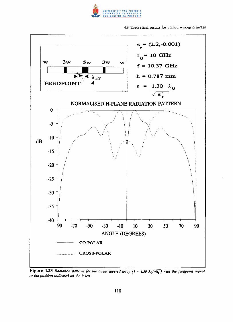
W' 3W' 5W' 3W'
1_1 11-1--.~ ~Aeff
FEEDPOINT 4
0
-5
-10dB
-15
-20
-25
-30
€ - (2.2,-0.001)r
fO-l00Hz
f - 10.370Hz
h - 0.787 mm.
Q. - 1.30 AO
.j e'r
-40-90 -30 -10 10 30
ANGLE (DEGREES)
Figure 4.23 Radiation patterns for the linear tapered tm'ay (I = 1.30 ..t<!ve;'J with the feedpoint movedto the position indicated on the insert.

l--~ I-I2 !
_!_-
Figure 4.24 Geometry of a brick-wall anay which has been extended in the transverse directions. All segmentwidths are equal at A.efr/20. We will refer to this as a "4-level brick-wall anay".

Q)
] o.s;.:=
id 0
~~..= -o.S
~~
"'0Q = '" - 1.20 f = 10 GHz
eff -/€" 0r
f = 10 GHz € = ( 4.34,-0.0005) h - 0.8 mmr
-1.0AlA'
A'-AE' - E
B'-B
D' -D
Figure 4.25 Current distributions on several elements of the 4-level brick-wall array represented in Figure 4.24.The current distributions on the remainder of the array elements are shown in Figure 4.26.

j~ O.S
j~~
'::1
~ 0
q-1.20~ e - ( 4.34,-0.00(5) h • 0.8 nunr
M·M
N"-N
Figure 4.26 Current distributions on several vertical elements of the 4-level brick-wall array shown inFigure 4.24

~FEEDPOINT
e - (4.34,-0.0005)r
f == f == 10 GHzoh == 0.8 rom
~ == 1 == 1.20 10eft ---~
i-10 -1
dB -20
-70-90 -30 -10 10 30
ANGLE (DEGREES)
Figure 4.27 Normalised H-plane radiation patterns for the cu"ent distributions shown in Figures 4.25 and4.26 on the 4-level etched brick-wall ~ay represented in Figure 4.24

0
-20
-40dB
-60
-80
-100
-120
-160-90
e: - (4.34,-0.0005)r
f = f = 10 GHzoh = 0.8 nun
~FEED POINTQ = A = 1.20 AOeft ---
~
-30 -10 10 30ANGLE (DEGREES)

A
)t:!
LLxj
~ L M
{

4.3 Theoretical results for etched wire-grid arrays
The current distribution on this structure, for a given set of material parameters,
is shown in Figures 4.30 and 4.31. From these figures, it can be seen that the
horizontal currents correctly feed the vertical elements and the latter have
essentially equal current amplitudes because of their equal widths. The E- and H- ,
plane far-field radiation patterns for these currents, on the structure represented
in Figure 4.29, are shown in Figures 4.32 and 4.33. From the H-plane radiation
patterns of this array, we notice that the cross-polarization characteristics have
improved from that shown by the 4-level array (Figure 4.27). We also note that
the side lobe level has increased from -23 dB to -13 dB, since the collapsed
distribution in the H-plane is now effectively uniform (because the array lattice
is completely filled). The increase in the sidelobe levels is accompanied by a
decrease in the BWFN (compared to the previous case) to some 30°. The BWFN
in the E-plane has become approximately 100°, and a sidelobe at -19 dB has
formed. The behaviour is different from that observed for the linear arrays simply
because for the present planar array case the array aperture transverse dimension
is larger. This observation leads naturally to consideration of the even larger
planar array in Section 4.3.6.

AQ - A - 1.145 _0_
eff --I€"r
f - 10 GHzo
€ - ( 2.2,-0.001)r
0.2
0 0""='.E.-- -0.2~-5 -0.4
~0 -0.6>.,::2
.!3~ -0.8
-11
A'-AB'- E
F-FI' - I
B'- B
D' - D
Figure 4.30 Cu"ent distributions on several elements of the 3-level brick-wall O"ay shown in Figure 4.29. Thecu"ent distributions on the remainder of the elements are shown in Figure 4.31.

..ga o.s:.=~
= 0~u~''::: -0.5~-~
~
A.Q _ A. - 1.145 _0_
eff -J€"r
f - 10 GHzo
e: - ( 2.2,-0.001)r

dB -20
e = (2.2,-0.001)r
6=~~
FEED POINT
f = f = 10 GHzoh = 0.787 mm
Q = A - 1.145 Aeff ~O
-V e'r

€ = (2.2,-0.001)r
M=6/FEEDPOINT
f = f - 10 GHzoh == 0.787 mm
Q = A = 1.145 AOeff ~-V € '
r
-20 f\!dB -40 ~
-140-90 -30 -10 10 30
ANGLE (DEGREES)

LL.x

€ - (2.2~-0.001)r
f - f - 10 GHzo
).. - 1.15 )..0eft ----
-100-90 -30 -10 10 30
ANGLE (DEGREES)

€ ••••(2.2,-0.001)r
f = f ...•10 GHzoh"" 0.787 nun
.A. •••• 1.15 .A. 0eff ---
~-€-, ~r
dB -60
-90
-120 ~
-180
-200-90

assumes the dielectric substrate and groundplane2 to extend to infinity in the
2 Unless stated otherwise, t~e dielectric substrate and metallic groundplane have the same transversedimensions

. - ...»:«:>,>::::: : : : : : : > :ax>: ..<»>. ».:::>:::>r<:.: . . . . . . . . . . .. . .. . . . ,.,. . :bi:> >:>:::: ::::
.......... .. .
...·.·:P#ipli#~(~()l1e:<·
~. x
Figure 4.37 An orientation by which the conductors of the etched antenna may be deposited on the dielectricsheet. This figure also seems to define what is meant by the tenn peripheral zone.
---T---------------------------------------?:~~---/'0 .
/ .. ::: ./ ....··»::::::>::::x:
:-:-::-:-:-:-:-:.:-:-:-:-:.:- .. , .. _ ............... ................ ............................... ..... - _ ................ .:-:-:-:-:-:.:-:-:.:-:-:-:-:-> .»:::::ax: .....
........................... .··::::::·:~iiPh¢6a··#l1"¥··/

4.4 Measured results for etched wire-grid arrays
4.4.1 A 5-element linear tapered etched brick-wall array with t ••Acff
The geometry of this array is shown in Figure 4.19 and theoretical results are
discussed in Section 4.3.3. An existing array which had been etched on RT / duroid
dielectric substrate backed by a metallic groundplane with transverse dimensions
(according to Figure 4.37) of X = 7.47 Aeff and Y = 3.18 Aeff was used for this
experiment. Since this 5-element array itself has transverse dimensions of
ax = 4.7 Aeff and ay = 0.64 Aeff (in other words, ax = 4.05 t and ay = 0.55 t
since t '* Aeff for this specific arraf), the structure has a peripheral zone with
widths wI = 1.27 Aeff and w2 = 1.385 Aeff• This is certainly an electrically small
groundplane. The H-plane co-polar radiation pattern of this structure was
measured at 10 GHz and a comparison between measured and predicted results
is shown in Figure 4.39. The comparison is surprisingly good when considering the
limited dimensions of the groundplane and dielectric substrate. In order to more
accurately predict the radiation patterns of this array, one would need to
considerably increase the transverse dimensions of the dielectric substrate and
groundplane. Although it would be difficult to enlarge both the dielectric substrate
and metallic groundplane of this "already-fabricated array", it is possible to
enlarge the groundplane portion only. This was accomplished by simply using
domestic tin foil to carefully cover a large non-conducting sheet, and securing the
micros trip antenna on the conducting tin foil. The important matter is that there
be electrical contact between the metallic groundplane of the original microstrip
structure and the tin foil. The groundplane now has dimensions of X = 24.21 Aeff
3 Also bx = 4.0 Aeff and by = 0.5 Aeffo

4.4 Measured results for etched wire-grid arrays
and Y = 19.13 Acer. One must of course, keep in mind that this is not the ideal
setup since the dielectric substrate still has not been enlarged. Nevertheless, the
H-plane co-polar radiation pattern of this antenna was measured and a
comparison with predicted results is given in Figure 4.40. It is interesting to note
that even for the array secured on this "home-made" groundplane, the
correspondence is much closer than that shown in Figure 4.39. This seems to
suggest that finite groundplane effects are primarily responsible for the deviation
between measured patterns for structures with electrically small groundplanes and
their computed patterns (which assume infinitely large groundplanes).
In general, the cross-polarized radiation pattern of a micros trip antenna is very
difficult to predict accurately and is sensitive in practice to the size of the
groundplane. Nevertheless, the H-plane cross-polarized radiation pattern of this
array on the large groundplane was measured and a comparison with predicted
results is shown in Figure 4.41. The overall angular behaviour of the cross-
polarization is correctly predicted, but not the details.
For this 5-element linear tapered etched brick-wall array, 5 megabytes of
memory was needed with approximately 22 hours of CPU execution time.

W' 3W' 5W' 3W'
~I_~II __ I_-~~*-A ff
FEEDPOINT) 4e
dB -10
e - (2.2,-0.001)r
f - f - 10 GHzoh - 0.787 nun
Q - 1.30 A 0
~ r
NORMALISED H-PLANE CO-POLAR RADIATIONo
20 40 60THETA (DEGREES)
Figure 4.39 Measured and predicted H-p/ane co-polar radiation pattems for the 5-e/ement linear brick-wallaJTay (I = 1.3 It/ve;'.) on the small groundp/ane (Section 4.4.1).

e: - (2.2,-0.001)r
f = f = 10 GHzo
_I~_~I-~~ *-A. ff
FEED POINT ) 4e
NORMALISED H-PLANE CO-POLAR RADIATIONo
20 40 60THETA (DEGREES)
Figure 4.40 Measured and predicted H-plane co-polar radiation patterns for the 5-element linear brick-walla"ay (i = 1.3 ,tt!ve;!) on an enlarged metallic ground plane.

€ = (2.2,-0.001)r
f - f - 10 GHzoh = 0.787 nun
~ = 1.30 "'0
-ve::r
I 1___ 1__~'\ ~"'eff
FEEDPOINT ) 4
NORMALISED H-PLANE CROSS-POLAR RADIATIONo
Figure 4.41 Measured and predicted cross-polar radiation patterns in the H-plane for the tapered an'ay onthe large ground plane.
-50 -30 -10 10 30 50ANGLE (DEGREES)

4.4 Measured results for etched wire-grid arrays
4.4.2 A 5-element linear tapered etched brick-wall array with t = Aell
This array which is described theoretically in Section 4.3.3 was etched
according to Figure 4.37 on a groundplane with dimensions of X = 13.47 Aerr and
Y = 9.85 A err, so that wI = 4.65 Aerr and w2 = 4.71 Aerr• Taconic [37] substrate
with €r' = 2.2 and h = 0.787 mm was used for this array. The H-plane co-polar
radiation pattern is shown in Figure 4.42. Close correspondence between
measured and predicted results is observed for this array, especially at smaller
angles: finite ground plane effects become greater at larger angles. The
encouraging fact about these results is that the first side lobe level at -23 dB is
closely predicted. Figure 4.43 shows the measured and predicted E-plane co-polar
radiation patterns. Since the E-plane pattern is broad, and there is "hard"
diffraction from the groundplane edge in this plane, one expects the groundplane
to have a strong effect on this pattern (as for the case of rectangular microstrip
patches [2]). This expectation is borne out in Figure 4.43.
The H-plane cross-polar radiation pattern of this tapered array was measured
and a comparison with computed results is given in Figure 4.44. Due to finite
groundplane effects, however, the correspondence between theoretical and
practical results is not entirely satisfactory.
Measured and predicted radiation patterns for this array at a frequency of
11 GHz are shown in Figure 4.45. Even though this is not the centre-frequency
good correspondence between measured and predicted results is observed. This
illustrates the fact that the numerical method is accurate at frequencies other than
the centre-frequency. This is important, considering that one is interested in
examining broadband behaviour of these brick-wall arrays.

E: - (2.2,-0.001)r
f - f - 10 GHzoh - 0.787 nun_I~i=l~-
~FEED POINT ~ - A - 1.12 AOeff ~
r
NORMALISED H-PLANE CO-POLAR RADIATIONo
20 40 60THETA (DEGREES)
Figure 4.42 Measured and predicted H-plane co-polar radiation pattems of the 5-element linear tapered brick-wall array with' = Jeff

e - (2.2,-0.001)r
f - f - 10 GHzo
_1-1-1_-~FEED POINT A - 1.12 A
eft --- 0~ r
NORMALISED E-PLANE CO-POLAR RADIATIONo
-24 ~
l-30
20 40 60
THETA (DEGREES)
Figure 4.43 Comparison between measured and predicted E-plane co-polar radiation patterns for the 5-element linear tapered array.
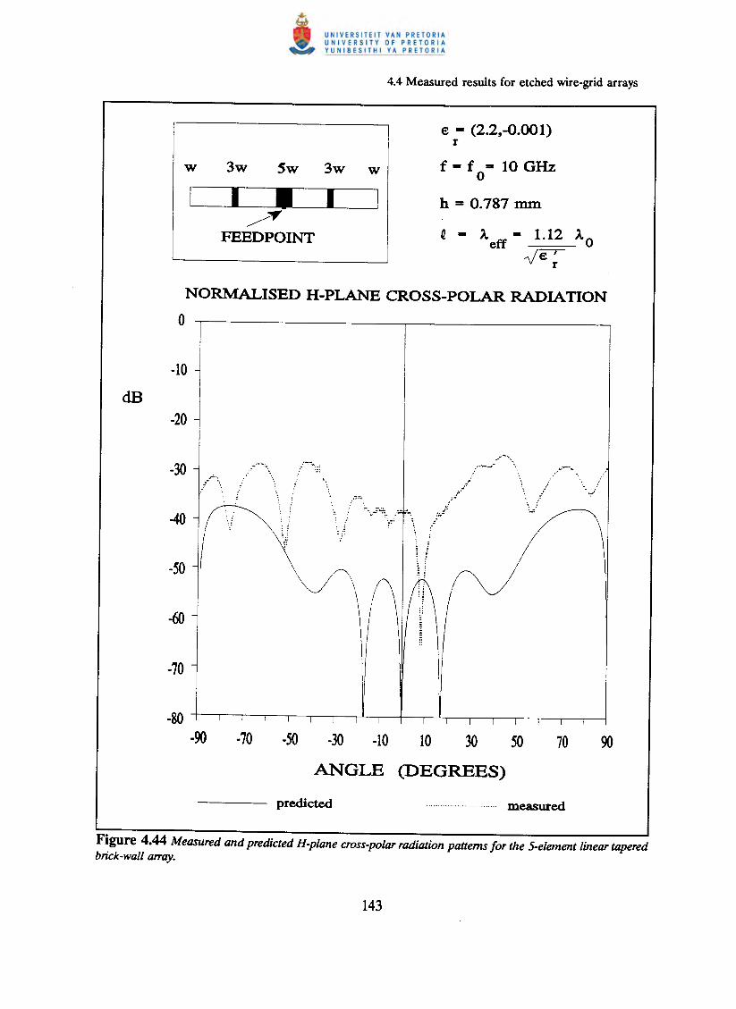
€ - (2.2,-0.001)r
~I~-=-~~~
FEEDPOINT
f - f = 10 GHzoh - 0.787 mm
~ - "'eff - 1.12 "'0vie:
r
-10
dB~-20
-30 ..•~.-,
-40
,./ .....•.'..•....•..._--
-so-90 -50 -30 -10 10 30 50
ANGLE (DEGREES)
Figure 4.44 Measured and predicted H-plane cross-polar radiation patterns for the 5-element linear taperedbrick-wall array.

e - (2.2,-0.001)r
fO" 10 GHz
f = 11 GHz
h = 0.787 nun
Q - 1.12 10~ r
_I_-=--~
FEEDPOINT
NORMALISED H-PLANE CO-POLAR RADIATIONo
Figure 4.45 Measured and predicted H-plane co-polar radiation pattems for the 5-element linear tapered arrayat 11 GHz. The centre-frequency for this an-ay is 10 GHz.

4.4.3 A 3-level brick-wall array
The geometry of this array is shown in Figure 4.29 and theoretical results are
given in Section 4.3.5. In that section we saw that for the given material
parameters and resonant behaviour at 10 GHz, that structure requires
t = Aeff = 1.145 Ao/..r€';'. However, in order to increase the variety of arrays for
which computations were performed, an array was etched with t = 1.072 AO/"/€;'
- this will be off-resonance at 10 GHz. This brick-wall array was etched on
RT /duroid [38] substrate (h = 0.787 mm and €r = (2.2,-0.001» with the
orientation shown in Figure 4.38. In other words, the array is deposited on the
diagonal of a rectangular groundplane of dimensions X = Y = 15 Aeff• This
implies that the widths of the peripheral zone are wI = 6.725 Aeff and
w2 = 5.475 Aeff. Measurements are now carried out in the two principal planes:
the H-plane (¢ = 0°) and the E-plane (¢ = 90°). Measured and predicted H-
plane co-polar radiation patterns for this 3-level brick-wall array are shown in
Figure 4.46. Close correspondence can be seen, even at large angles, and this
despite the fact that t '" Aeff and the structure therefore not resonant. This
supports the usefulness and generality of the numerical method.

€ • (2.2,-0.001)r
~/
FEEDPOINT
f - f - 10 GHzoh - 0.787 mm
Q - 1.072 A 0
~ r
NORMALISED H-PLANE CO-POLAR RADIATIONo
-roo 20 40 ro
THETA (DEGREES)
Figure 4.46 Measured and predicted H-plane co-polar radiation patterns for a 3-level brick-wall anay withI = 1.072 -ttl've;! at 10 GHz.

~[I J K
L' M'
E F G H
r J' K'
C N D
E' F G' H'
A B
C' w N' D'~w
A' B'

e = (2.2,-0.00 1)r
f = f = 10 GHzoh - 0.787 mm
~ - 1.084 AO
~ r
NORMALISED H-PLANE CO-POLAR RADIATIONo
-50 -30 -10 10 30 50ANGLE (DEGREES)

e - (2.2,-0.001)r
r-I~I~I~! "I
~jI~I-FEEDPOINT (.)
f - f - 10 GHzoh - 0.787 mm
Q - 1.084 A~O
r
NORMALISED H-PLANE CROSS-POLAR RADIATIONo
-60-90 -so -30 -10 10 30 50
ANGLE (DEGREES)

4.5 Concluding remarks
measured co-polarization pattern shown in Figure 4.48. The level of the measured
cross-polarization is some 20 dB above the value predicted.
4.5 CONCLUDING REMARKS
The general integral equation formulation of Section 2.3, implemented as
described in Chapter 3, was used in this chapter to examine the operation of
etched brick-wall antenna arrays. In order to validate the implementation
developed by the author, computed current distributions for a rectangular
micros trip patch were satisfactorily compared to previously published results. In
the design of wire-grid antenna arrays, dimensions are selected in terms of AeCC•
The difficulty in determining values for AeCC is that it is not only a function €r but
also of the dielectric substrate thickness, frequency and specific line widths. It was
also shown how the numerical method can be used to determine values for Aeff
related to specific geometries. Current distributions on several specific geometries
were examined, and the radiation patterns determined directly from these
computed current distributions (these are essentially exact, given a current
distribution, except for finite groundplane effects).
Several brick-wall arrays were fabricated and close correspondence between
measured and predicted co-polar radiation patterns was found. This essentially
validates the use of the present analysis for the design of brick-wall arrays. Cross-
polar radiation patterns are very difficult to predict accurately, and are dependent
on the actual size of the groundplane, an aspect not included in the numerical
model. Through a simple experiment, we showed that by increasing the transverse

4.5 Concluding remarks
dimensions of the metallic groundplane, closer correspondence between measured
and predicted radiation patterns could be observed. We also investigated,
theoretically, the effects on radiation patterns, of moving coaxial feedpoints.
These effects seemed to be very much case dependent. This numerical method
is equally valid at off-centre frequencies (important in determining the pattern
bandwidth of the antenna), and this was illustrated by the close correspondence
between measured and computed radiation patterns at 11 GHz for a 5-element
linear tapered array which had been designed for a centre-frequency of 10 GHz.
The fact that numerical experimentation can be performed on etched wire-grid
antenna arrays to examine current distributions, means that it is now possible to
carefully design for some desired aperture distribution and hence radiation
pattern.

The versatility of array antennas has been known for many years but their widespread
use was prevented by their relatively high cost compared to alternative antenna types.
More recently the realisation of arrays in microstrip has altered such considerations - not
only are microstrip antennas relatively in-expensive, but they can be directly integrated
with printed feed networks and active circuits. While many microstrip antenna
geometries have been proposed and investigated experimentally, only a few of these (and
the micros trip wire-grid array is not one of these) have enjoyed a rigorous theoretical
analysis. One reason for this is probably the very substantial and time-consuming effort
involved between the integral equation analysis formulation and its actual numerical
implementation in practice - the numerical analysis of layered structures is fraught with
difficulties, the finer details of whose solution is seldom readily available. The principal
contributions of this thesis therefore are:
(a) Chapter 3, which gives an illustrative guide to the numerical "pitfalls" encountered
in the application of the spatial domain integral equation analysis of microstrip
antennas (which guide shows such aspects in a form more easily understandable
than has heretofore been the case), and which provides information down to the
finest detail on the numerical implementation of the analysis. Such detail was
previously not readily available.

Chapter 5
(b) Chapter 4, which applies a rigorous full-wave integral equation analysis to
microstrip wire-grid arrays in order to achieve desired aperture distributions. This
does not appear to have been done previously, and the design of such arrays
through numerical experimentation is now possible.

DEFINITION OF THE SPATIAL FOURIER TRANSFORM;
THE SPECTRAL DOMAIN
+00 +IID
!(kx,ky) = 211t f f j(x,y) exp(-jkxx-jkyy)dxdy
-Olt -CIIJ
+00 +_
j(x,y) = 21
1t f f !(kx,ky) exp(jkxx +jkyy)dkXdky-. -00
where x and yare spacial domain variables; kx and ky representing their spectral domain

Appendix A
The application of the spectral domain method in electromagnetics was developed
and refined by Mittra [41] and numerous coworkers, beginning in the 1970's. Only
recently some examples of the application of this method to microstrip structures have
appeared in the technical literature. The first paper dealing with the full wave approach
to microstrip problems was presented in 1981 by Itoh [32]. Several authors have since
proposed spectral domain methods as viable alternatives to their spatial domain
counterparts [41,42,43,44,45,46,47,48].

DERIVATION OF THE GREEN'S FUNCTIONS FOR A GROUNDED
DIELECTRIC SLAB
(d2 2)---+u· A=O
dz2 I
where uj2 = ~ 2 + Js,2 - ~ 2 = kp
2 - ~ 2 and ~ is the wavenumber of medium i. Since (B.l)

where a and b are unknowns (they may be functions of the spectral variables ~ and ky)
A = i l!0 exp( -u 0 z )41t Uo
where uo2 = kp2 - ko2 and ko the wavenumber in free space. In the case of an x-directed

v: - 02 -
Hence, let A = iAx + :i~o Choosing now for ~ and ~ general expressions of the form
- !-LaA =-
x 21tsinhu (z + h)
(D TE sinhuh)
- !-LaA = -(e - 1)Jo k:: 21t T x
coshu (z + h)DTE DTM coshuh
where DTE = Uo + u coth uh, DTM = €rUO + U tanh uh, u2 = k/ _ €~2,

N sinhu (z + h)I
D 1'£ D TM sinhuh
potential of a single unit point charge (Vq) by the well-known expression [3]
- j kJ: -V= --Vj cu q
- 1V =--q 21tE: o Nsinhu(z + h)
D 1'£ D TM sinhuh
Appropriate expressions for the vector potential (.4.) due to a RED, and the scalar
potential (Vq) due to a single unit point charge, have now been determined in the

Since DTE and DTM depend on ~ and Js, only through the radial spectral variable
k/ = ~2 + Js,2, the inverse Fourier transform can be written as a Hankel transform [3]:
7-1[i( kp)] = f J 0 (kp R) kpj( kp) dkpo
7-1 [jkzi(kp)] = -cos4> f J1 (kpR)k~ j(kp)dkpo

with r = i x + y Y + i z, R = I r - r' I and ep = tan-1[(y-y')/(x-x')]. The integrals
above are line integrals on the complexkp -plane where kp = A + jv. Mosig and Gardiol
[3] have found that integration along the contour described by the real positive l-axis,
kp = A in the expressions above. Therefore
..Ax(rlr') = 1-10 f Jo(AR)~exP(-uoz)dA
21t 0 DTE
..Vq(rlr') = _1_ f Jo(AR) _A_N_exp( -UOZ)dA
21teo 0 DTE DTM
z ~ 0 follow directly: Gv=Vq\ G~x=" and Glx=~. The other terms of the dyadic
Green's function are either zero (G~Y= Gr = 0), not important for the purposes of this
1 The Green's function Gv is viewed as the scalar potential created by an isolated point charge on theair-dielectric interface. Since these charges do not exist in the real world, Gv is rather considered to be auseful mathematical device.

.•Ax(rlrl) = ~o J Jo(i..R)...!::-di..
21t 0 DTE
.•Vq(rlrl) = _1_ f Jo(i..R) i.. N di..
21t eo 0 DTE DTM
In conclusion, expressions for the vector potential (A) due to a RED, and the scalar
potential (Vq) due to a single unit point charge, have now been determined in the spatial
domain «B.16) through (B.18». These expressions are valid for z ~ 0; however, for
surface current computation the special case z = 0 is to be considered. Far-field

ANALYTICAL INTEGRATION OF THE SINGULAR PART IN VECTOR
POTENTIAL DISCRETE GREEN'S FUNCTION SELFTERM
EVALUATIONS
In the evaluation of the discrete Green's function selfterms the situation arises where
the observer and a source cell coincide. This leads to singularities in the discrete Green's
function integrands due to the presence of the Green's functions therein. It was then
suggested by Mosig and Gardiol [3] that the singular parts of the Green's functions be
extracted as follows: G = Gs + (G - Gs)' where G represents the Green's functions and
Gs the static values given by [3]
GAX;(r/r') = J10
41t I r - r' I
for the scalar potential; € r is the complex relative permittivity which takes into account
dielectric losses. The discrete Green's function integrands with the difference terms
(G-Gs) are well-behaved functions and can be integrated numerically, while the
integrands with the static parts, although being singular for r = r', are analytically
integrable. It is the purpose of this appendix to perform such an analytical surface

Since only an expression for rvs(r/r)l is given in [3], it is the purpose of this appendix
to derive analytically an expression for r;'~(r/rIj)' where r lies within the boundaries of
the x-directed current cell centred at rIj. In the construction of the Cij submatrix, r;.x
f r:(r/rXj) dxc.:1
point along the test segment Cxi placed within the source current cell at rIj. Surface
1 The subscript s indicates that the Green's function, appearing in the discrete Green's functionintegrand, has been replaced by it's static part.

p:(r/r xj) = f _1_ G:(r/r')[ 1 - Ix' ~ Xxj I] t;dS' (C.6)S lJ.oko .z,
Since r xi has no effect on the final expression (a correct choice does however simplify
mathematical manipulation), we may conveniently suppose that the source current cell
is centred at rxj = (0,0). Therefore
Sois now the surface occupied by the x-directed current cell centred at (0,0). Application
p:(r/O) = f-1-[GAX;(r/r')+(G:(r/r')-GAX;(r/r'») J[l-Jfl]t;dS' (C.8)slJ.~ a
o
P:s(r/O) = f ko G~:(r/r') [1 - 21] dS's lJ.o a
o
p:s(r/O) = ko f 1 dS' - ~ f Ix'i dS'411: So I r-r' I 411:a So I r-r'l

Appendix C
Since So is centred at the origin, the x-directed test segment therein extends along the
x-axis and therefore we know that the singularity is bound to this axis (Figure c.t). Also,
~(rIO) = ko f 1 dS' - ~ f ~dS'2 n I I r - r' I 2 na I I r - r' I
~ ~
centred at (0,0). Let us suppose that r = r~ where 0 ~ rx ~ a/2; we also have
r' = x'x + y'y. Thus I r - r,1 = [(rx-x,)2 + y,2]1/2. Analytical integration may be
simplified by application of the substitution x" = x' - rx and y" = y'. This implies that
accordingly. So" is now the area on the x"y"-plane described by -b/2 ~ y" ~ b/2 and
r" = [X,,2+y,,2]1/2and dS" = r"dr"d<t>".Then

k kr~;(.irxlO) = _0 f dr"dq," - _o-f I r"cosq," + rx I dr"dq,"21t 1/ 21ta 1/
SOt: SOt:
o ~ r" ~ b/2 cosec(¢")
a2 = tan-1[b/(2(a+rx»]; 'ff - a3 ~ ¢" ~ 'ff -a2;
Let us consider the two terms in (C.l3) separately. For the first term, integration may,
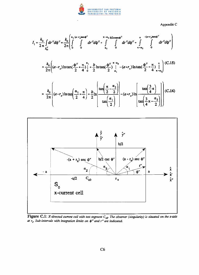
k ( <1>""1 b <1>" It-"2 <1>" 11: It] (C.tS)= ~ (a-rX)lntan(-+~) I +-lntan(-) I -(a+rX)lntan(-+-) I211: 2 4 0 2 2"1 2 4 It-"2
t~n(4311:)\ (C.t6)-----
w{~x-~2l
(t /2
/(a - Ix) see <1>"
Sox-current cell
Figure C.t: X-directed current cell with test segment exf) The observer (singularity) is situated on the x-axisat rx- Sub-intervals with integration limits on 4>'" and r'" are indicated.

We note from (C.16) that tan(31l"/4) = -1 appears in the argument of the natural
logarithm !. However, for 0 :s; rx :s; a/2 we have a2/2 < 'ff 14, and therefore
'ff12 < 3'ff 14 - azl2 < 'ff. This implies that the denominator will always be negative,
bringing about a positive argument for the logarithm. This argument may be rewritten
3tan( -1t)4
3 "2tan( -1t --)4 2
-tan(1t - ~1t)4
3 "2-tan(1t - -1t +-)4 2
in that expression. This integrand consists of I r" COS(/)" + rx I which transforms to
I x" + rx I in rectangular coordinates. This implies that
X" + rx for X" ~ -rx

x=x' =0 and secondly from there on to the edges of the current cell (Figure C.1).

"3r b tan("2) r; "2 1t r; "3 1t+ _x_InI· I - -Intan(- +-) + -Intan(- +-)
2 " 2 2 4 2 2 4tan(2)
2
Now 12 may be written as
kcP "2 1t kob2
12= - 41t Intan("2+"4)+161ta[cosec("3)-cosec("2)]
"3k 2 ko b tan(-)
r " r-~Intan(2 +~) +__x_ln 241ta 2 4 41ta "2
tan(-)2

Finally, r~~(irxlO) = 11 + 12, where 11 is given by (C.l8) and 12 by (C.26). Therefore
ili(X2---(X1 1t b 2 2 (X2 1t
(a -T ) In+_J_+-) +-In +(a +T )In+_J_+-)x .., 2 4 2 tan( :1) x'" 2 4
k ~b2oa (X2 1t "'0--lntan(- +-) + --[cosec«XJ -cosec«X2)]
41t 2 4 161ta
2~T (X
__ "'O_x Intan(~ + ~ )41ta 2 4
ko ( )2 In (Xl 1t--- a-r tan(- +-) +41ta x 2 4
kOTx (Xl 1t---(a-r )lntan(-+-)
21ta x 2 4
(X3~ b cotan(-)"'Orx 2--In· I41ta (Xtan(_l)
2
-a/2 ~ rx ~ 0 is a mirror-image of 0 ~ rx ~ a/2 and therefore r~(-irxlO) = r;':(irxlO).

DETERMINATION OF THE RADIATED ELECTRIC FIELDS OF A
MICROSTRIP ANTENNA GIVEN THE SURFACE CURRENT
DISTRIBUTION
In this appendix we will derive expressions for the radiated electric fields of a
micros trip antenna once the surface current distribution is known. Although final
expressions for the radiated fields of a HED on microstrip are given in [3], no derivation
is included and since the author is of the opinion that insight can be gained from such
an exercise, it is performed in this appendix.
A general expression 1 for the electric field in terms of vector and scalar potentials
A(r) = f GA (rlr'). J,(r') dS'So
-GA is the Green's function associated with A(r) while Js is the surface current
distribution. Since this is a mixed-potential formulation, the scalar potential due to the
surface current distribution (related to the charge distribution through the continuity
1 This is a general expression not unique to microstrip.

equation) has to be determined. Applying the Lorentz gauge [49] to A(r) and making use
-of the equality V.GA(r/r') = J1.€VGv(r/r') [3] leads to an expression for the scalar
= -~f VGy(r/r').J (r')dS'JCJ) •
So
E(r) = f GE(r/r') .J,(r')dS'So
-Green's function GE• This Green's function will now be expanded. The three-dimensional

Appendix D
-dyadic Green's function GA may be written as
i A iy
i GU 0 G:Ii
GA = j Gf"(D.7)
0 GJ!
i Grx G%Y G:Ii Ii
We also have
i A iy
i ~G a2 a2--G --G
ax2 v axay v axaz v
a2 a2 a2 (D.S)\l\lGv = j --G -G --G
ayax v ay2 v ayaz v
a2 a2 a2
£ --G --G -Gazax v azay v az2 V
-Therefore GE may be written as
i j £
1 & G . GU 1 a2 1 a2 G . GJCl.-- -Jw Ii ---G --- -Jw Ii
i jw ax2 v jwaxay v jwaxaz v
1 a2 1 a2 G . GY1 1 a2 G . GY% (D.9)
j ---G -.--- v-Jw Ii --- v-JW Ajwayax v Jway2 jwayaz
£ 1 a2 G . Grx 1 a2 G . G%Y 1 a2
G .GZ1.--- -JW --- -JW Ii -.---. v-Jw Iijw az ax v Ii jw az ay v Jwaz2

a set of discrete coefficients Ixi (i = L.M) and ~ (j = L.N) each related to a charge cell
of dimensions a and b. With this in mind, Mosig and Gardiol [3] have shown that in the
M N
Ee = G;xCr/O) L alxieil:ogj + G;YCr/O) L blyjeil:ogjj=l i=l
M NE4> = G:xCr/O)Lalxieil:ogj + G:Y(r/O)LbIYieil:ogj
j=l i=l
determine G~x, G~Y,G~x and G~Y.To illustrate such a transformation, consider for a
D = D(x) i + DCy) j + D(z) £

D(X) = Dxxx + DYXj + Dzx£
IP) = D xy X + D YY j + D r;y £
D(z) = Dxz.x + DYZj + DU£
Now with a rectangular-to-spherical coordinate transformation, D(x) becomes
D rx = D xx sine cos<l> + D yx sine sin<l>+ D Z% cose
D ex = D xx cose cos<l> + D'X cose sin<l> - D zx sine
D~ = - D xx sin<l> + D yxcos<l>
G;X(r/O) = G;(r/O) cose cos<l>+G~x(r/O) cose sin<l>-G:(r/O)sine (D.16)
Gr(r/O) = -G;(r/O)sin<l> + G:(r/O)cos<l> (D.17)
G~(r/O) = Gi(r/O) cose cos4> + Gr'(r/O)cosesin4> - Gi(r/O) sine (D.IS)
G:'(r/O) = -Gi(r/O)sin4> + Gr'(r/O)cos4> (D.19)
Let us now, for example, expand a:X(r/O). From (D.9) it follows that

G:X = (-!- LGv-jw G::)cosecos4> +(-!- &- Gv)cosesin4>JW aX2 JW ayax
(DolO)
-(-f-~G -jWG:)Sin6Jwazax v
..G::<r/r') = ~o J Jo(lR)-!:- e -"01. dl
2n 0 DTE
Gf (rlr') = G::(r/r')
..Gy(rlr') = _1_ J Jo(lR)-!:- e -"01. dl
2n€o 0 DTE
The partial derivatives in (D.9) (some of which appear in (D.20» may be obtained

Therefore we have for G~X(r/O), from (D.20):

[
• GO ]JW J.1 A-u- 0 f Jo(AR)-e otdA cos8cos4>
21t 0 DTE
By expanding GE 6y, GE~x and GE~Y in similar fashion and defining

[. I ] MJU> ~O X·--(E:,-1)coscPI3 +. 4 sine ) Lalxi~koKl +2it Ju>2itE:O R i",1

[. I 1 1E = ( J<U !-Lo1 + 1 _ 2 ( ~ i sin<l> +
4> 21t 0 j<U21t eoR j CJ>21teO R
Closer inspection2 of the integrands in (D.33) through (D.37) leads one to the
-jlcor
10 ...j cotan6/0(kosin6) _e_ ;r

x2uo(x)N(x)
DTE(x)DTM(x)
where Resj is the residue of function fj (i=2,3,4) at Ap• Since 11 only appears in terms
with "R" in the denominator (D.38 and D.39), and because these terms tend to zero in
M
[Ao(€, - 1)cos<j>/3 + A2 cos<j>/4] sine ) La/xi ej/.:og
, +i=l
N[Ao( €, -1 )sin<j>/3 + A2sin<j>/4 ] sine ) L b/
yjejJ.:ogj
j=l

AI
E. = ( [AoIo - A2cos24>I2]sin4> + [A2cos4>sin4>I2]cos4> ) E aI~i ejkog
, +i-I
N
( [ -AoIo +A2sin24>I2]cos4> - [A2cos4>sin4>I2]sin4> ) L blyjej~Jjal
where
Aoj CJ) fJ.o (D.46)=
21t
and
A21 (D.47)=
j CJ) 21t eo

THE RELATIONSHIP BElWEEN THE COEFFICIENTS IIi AND Iyi
AND ELECTRICAL CURRENT FLOWING ON THE ELEMENTS OF
WIRE-GRID ARRAYS
The solution to the moment matrix equation yields the coefficients lxi and lyi. The aim
of this appendix is to examine the relationship between these coefficients and the
1 MJ = - ~ I.T(r -r.)
$X bLJ XIX .ai,,1 (~)
1 NJ =-~I.T(r-r.)
sy a f::t. YI Y YI (~)
{I - Ix Ifa
Tx(r) = o; Ix I < a , Iy I < bf2
; elsewhere
and a similar expression holds for T/r). These expressions give the relationship between
coefficients lxi and ~, and the surface current density existing on the radiator. From these

expressions it also follows that coefficients Ixi and ~ have dimensions of current (A). To
relate these coefficients to the total current flowing on an element of an etched wire-grid
S
Itot(x) = .E Ii(x)i=1
(~)

m
ItoC<x2) = L Lni=4

Ix! I~ IX3 • Iv :~(x)-" f ,e.>, ··t·----, ----t---
", '. '1,;-"'.. . ,,:./ ><. : w; IX6
: ~(x)
(( ····1·········· ·······i········ ..··.-:·",·.-:······i··· : :.: _ ~ ~ ~ ~ ~ ~ofx)b 1I dy . --+ I (x) : • x7 :I (x)tl 4,,; 4({ - . - + .. .. '" _ ~ --.. -+--_ -:- .
~Xl~
Figure E.I: Decomposition of an x-directed segment on an etched radiator to calculate the total cu"entflowing along the segment. Rooftop basis functions are used in the moment method solution.

[1] J.D. Kraus, "A backward angle-fire array antenna", IEEE Trans., vol. AP-12, no. 1,
pp. 48-50, Jan. 1964.
[2] J.R. Mosig and F.E. Gardiol, "General integral equation formulation for
microstrip antennas and scatterers," lEE Proc., vol. 132, Pt.H, no. 7, Dec. 1985.
[3] J.R. Mosig and F.E. Gardiol, "Numerical analysis of microstrip patch antennas"
in: J.R. James and P.S. Hall (Edits.), Handbook of microstrip antennas (Peter
Peregrinus, vol. 1, Chapter 8, 1989).
[4] J.R. Mosig and F.E. Gardiol, "A dynamical radiation model for microstrip
structures," in P. Hawkes (Edit) Advances in electronics and electron physics
(Academic Press, 1982) pp. 139-237.
[5] L. Lier, "Improved formulas for input impedance of coax-fed microstrip patch
antennas," lEE Proc., Pt.H, 129, pp. 161-164, 1982.
[6] W.F. Richards, Y.T. 1.0 and D.D. Harrison, "An improved theory for microstrip
antennas and applications," IEEE Trans., vol. AP-29, pp. 38-46, 1981.
[7] R.F. Harrington, Field Computation by Moment Methods (MacMillan, 1968).
[8] D.M. Pozar, "Microstrip antennas", Proc.IEEE, vol. 80, no. 1, pp. 79-91, Jan. 1992.
[9] K.A. Michalski and D. Zheng, "Analysis of micros trip resonators of arbitrary
shape", IEEE Trans. Microwave Theory Tech., vol. MTT-40, no. 1, pp. 112-119, Jan.
1992.
[10] M. Marin, S. Barkeshli and P.H. Pathak, "Efficient analysis of planar microstrip
geometries using a closed-form asymptotic representation of the grounded
dielectric slab Green's function", IEEE Trans. Microwave Theory Tech., vol.
MTT-37, no. 4, pp. 669-678, April 1989.
[11] R.F. Harrington, Time Harmonic Electromagnetic Fields (McGraw-Hill, 1961).
[12] P.J. Davies and P. Rabinowitz, Methods of Numerical Integration (Academic Press,
1975).
[13] L.M. Delves, Comput.J., vol. 10, p.389, 1967.
[14] J.R. Mosig and F.E. Gardiol, "Analytic and numerical techniques in the Green's
function treatment of micros trip antennas and scatterers," lEE Proc., vol. 130,

Pt.H, no. 2, pp. 175-182, March 1983.
[15] A.W. Glisson and D.R. Wilton, "Simple and efficient numerical methods for
problems of electromagnetic radiation and scattering from surfaces," IEEE Trans.
Antennas Propagat., vol. AP-29, pp. 593-603, 1981.
[16] J.R. Mosig, Laboratoire d'Electromagnetisme et d'Acoustique, Ecole
Polytechnique Federale de Lausanne, Lausanne, Switzerland. Personal
communication.
[17] R.C. Hall, J.R. Mosig and F.E. Gardiol, "Analysis of microstrip antenna arrays
with thick subtrates", Proc. 17 th European Microwave Conf., Rome, 1987.
[18] J.T. Aberle, D.M. Pozar and e.R. Birtcher, "Evaluation of input impedance and
radar cross section of probe-fed microstrip patch elements using an accurate feed
model," IEEE Trans. Antennas Propagat., vol. 39, pp. 1691-1696, Dec. 1991.
[19] D.E. Muller, "A method for solving algebraic equations using an automatic
computer", Math. Tables Aids Comput., vol. 10, pp. 208-215, 1956.
[20] IMSL Inc., Houston, Texas, USA. library of Fortran Routines for Mathematical
Application, Version 1.0, April 1989.
[21] E. Kreyszig, Advanced Engineering Mathematics (John Wiley & Sons, 1988).
[22] H. Hurwitz and P.F. Zweifel, "Numerical quadrature of Fourier transform
integrals," Math. Tables Aids Comput., vol. 10, pp. 140-149, 1956.
[23] M.R. Spiegel, Mathematical handbook (McGraw-Hill, 1968).
[24] M. Hestenes and E. Stiefel, "Method of conjugate gradients for solving linear
systems," 1Res. NatL Bur. Stand., vol. 49, pp. 409-436, 1952.
[25] R.E. Piessens, de Doncker-Kapenga, e.W. Oberhuber and D.K. Kahaner,
QUADPAK (Springer-Verlag, 1983).
[26] e.G. Hsu, R.F. Harrington, J.R. Mautz and T.K. Sarkar, "On the location of leaky
wave poles for a grounded dielectric slab", IEEE Trans. Microwave Theory Tech.,
vol. 39, no. 2, pp. 346-349, Feb. 1991.
[27] W.H. Press et.al.,Numerical Recipes (Cambridge University Press, 1989).
[28] L.B. Felsen and N. Marcuvitz, Radiation Scattering of Waves (Prentice_Hall,
1973).
[29] e.A. Balanis, Advanced Engineering Electromagnetics (John Wiley & Sons, 1989).

[30] A Sommerfeld, Partial Differential Equations in Physics (Academic Press, 1949).
[31] A.C. Ludwig, "The definition of cross-polarization," IEEE Trans. Antennas
Propagat., vol. AP-21, pp. 116-119, Jan. 1973.
[32] T. Itoh and W. Menzel, "A full wave analysis method for open microstrip
structures," IEEE Trans. Antennas Propagat., vol. AP-29, pp. 63-68, Jan. 1981.
[33] J.R. Mosig and T.K. Sarkar, "Comparison of quasi-static and exact
electromagnetic fields from a horizontal electric dipole above a lossy dielctric
backed by an imperfect ground plane," IEEE Trans. Microwave Theory Tech., vol.
MTT-34, no. 4, April 1986.
[34] W.L. Stutzman and G.A Thiele, Antenna Theory and Design (John Wiley & Sons,
1981).
[35] R. Conti, J. Toth, T. Dowling and J. Weiss, "The wire-grid microstrip antenna",
IEEE Trans. Antennas Propagat., vol. AP-29, no. 1, pp. 157-166, Jan. 1981.
[36] M.D. Deshpande and M.C. Bailey, "Input impedance of microstrip antennas",
IEEE Trans. Antennas. Propagat., vol. AP-30, no. 4, July 1982.
[37] Taconic is marketed by Taconic Plastics Ltd, Petersburg, NA, 1213, USA
[38] RT /duroid is a registered trademark of Rogers Corporation, and marketed by
Rogers Corporation Microwave Materials Division, 100 S.Roosevelt Avenue,
Chandler, AZ 85226, USA.
[39] N. Fache and D. de Zutter, "Rigorous full-wave space-domain solution for
dispersive microstrip lines," IEEE Trans. Microwave Theory Tech., vol. MTT-36,
no. 4, April 1988.
[40] L. Beyne and D. de Zutter, "Green's function for layered lossy media with special
application to micros trip antennas," IEEE Trans. Microwave Theory Tech., vol.
MTT-36, no. 5, May 1988.
[41] R. Mittra, "Spectral domain methods for analyzing frequency selective surfaces
(FSS)" in: Lectures on Computational Methods in Electromagnetics (SCEEE Press,
St. Cloud, Florida, 1981)
[42] C.H. Tsao and R. Mittra, "A spectral-iteration approach for analyzing scattering
from frequency selective surfaces," IEEE Trans. Antennas Propagat., vol. AP-30,
no. 2, pp. 303-308, March 1982.

[43] C.H. Tsao and R. Mittra, "Spectral domain analysis of frequency selective surfaces
comprised of periodic arrays of cross dipoles and Jerusalem crosses," IEEE Trans.
Antennas Propagat., vol. AP-32, no. 5, May 1984.
[44] T.A Cwik and R. Mittra, "Scattering from a periodic array of free-standing
arbitrarily shaped perfectly conducting or resistive patches," IEEE Trans.Antennas
Propagat., vol. AP-35, no. 11, pp. 1226-1234, Nov. 1987.
[45] D.M. Pozar, "Input impedance and mutual coupling of rectangular microstrip
antennas", IEEE Trans. Antennas Propagat., vol. AP-30, no. 6, Nov. 1982.
[46] C. Scott, The Spectral Domain Method in Electromagnetics (Artech House, 1989).
[47] L. Vegni, R. Cicchetti and P. Capece, "Spectral dyadic Green's function
formulation for planar integrated structures," IEEE Trans.Antennas Propagat., vol.
36, no. 8, Aug. 1988.
[48] D.M. Pozar, "Radiation and scattering from a microstrip patch on a uniaxial
substrate," IEEE Trans. Antennas Propagat., vol. AP-35, no. 6, June 1987.
[49] R.E. Collin, Foundations for Microwave Engineering (McGraw-Hill, 1966).