tests for parameter instability and structural change with ... · (1992), zivot and andrews (1992),...
TRANSCRIPT

Tests for Parameter Instability and Structural Change With Unknown ChangePoint
Donald W K Andrews
Econometrica Vol 61 No 4 (Jul 1993) pp 821-856
Stable URL
httplinksjstororgsicisici=0012-96822819930729613A43C8213ATFPIAS3E20CO3B2-I
Econometrica is currently published by The Econometric Society
Your use of the JSTOR archive indicates your acceptance of JSTORs Terms and Conditions of Use available athttpwwwjstororgabouttermshtml JSTORs Terms and Conditions of Use provides in part that unless you have obtainedprior permission you may not download an entire issue of a journal or multiple copies of articles and you may use content inthe JSTOR archive only for your personal non-commercial use
Please contact the publisher regarding any further use of this work Publisher contact information may be obtained athttpwwwjstororgjournalseconosochtml
Each copy of any part of a JSTOR transmission must contain the same copyright notice that appears on the screen or printedpage of such transmission
The JSTOR Archive is a trusted digital repository providing for long-term preservation and access to leading academicjournals and scholarly literature from around the world The Archive is supported by libraries scholarly societies publishersand foundations It is an initiative of JSTOR a not-for-profit organization with a mission to help the scholarly community takeadvantage of advances in technology For more information regarding JSTOR please contact supportjstororg
httpwwwjstororgThu Mar 27 112808 2008
Econornetrica Vol 61 No 4 (July 19931 821-856
TESTS FOR PARAMETER INSTABILITY AND STRUCTURAL CHANGE WITH UNKNOWN CHANGE POINT
This paper considers tests for parameter instability and structural change with un-known change point The results apply to a wide class of parametric models that are suitable for estimation by generalized method of moments procedures The paper considers Wald Lagrange multiplier and likelihood ratio-like tests Each test implicitly uses an estimate of a change point The change point may be completely unknown or it may be known to lie in a restricted interval Tests of both pure and partial structural change are discussed
The asymptotic distributions of the test statistics considered here are nonstandard because the change point parameter only appears under the alternative hypothesis and not under the null The asymptotic null distributions are found to be given by the supremum of the square of a standardized tied-down Bessel process of order p gt 1 as in D L Hawkins (1987) Tables of critical values are provided based on this asymptotic null distribution
As tests of parameter instability the tests considered here are shown to have nontrivial asymptotic local power against all alternatives for which the parameters are nonconstant As tests of one-time structural change the tests are shown to have some weak asymptotic local power optimality properties for large sample size and small significance level The tests are found to perform quite well in a Monte Carlo experiment reported elsewhere
KEYWORDSAsymptotic distribution change point Bessel process Brownian bridge Brownian motion generalized method of moments estimator Lagrange multiplier test likelihood ratio test parameter instability structural change Wald test weak conver-gence
1 INTRODUCTION
THIS PAPER CONSIDERS TESTS for parameter instability and structural change with unknown change point in nonlinear parametric models The proposed tests are designed for a one-time change in the value of a parameter vector but are shown to have power against more general forms of parameter instability Tests are considered both for the case where the change point can be specified to lie in a particular interval and for the case where the change point is completely unknown Tests are considered for the case of pure structural change in which the entire parameter vector is subject to change under the alternative and for the case of partial structural change in which only a component of the parameter vector is subject to change under the alternative
The results given here cover Wald Lagrange multiplier (LM) and likelihood-ratio (LR)-like tests based on generalized method of moments (GMM) estimators Included in this class are tests based on various least squares nonlinear instrumental variables maximum likelihood (ML) and pseudo-ML
I thank Inpyo Li for computing the critical values reported in Section 5 I also thank two referees a co-editor Jean-Marie Dufour Bruce Hansen Werner Ploberger and the participants of the Princeton econometrics workshop for helpful comments I gratefully acknowledge research support from the National Science Foundation through Grant Numbers SES-8821021 and SES- 9121914 The first version of this paper appeared as the discussion paper Andrews (1989~)
822 DONALD WK ANDREWS
estimators among others See L P Hansen (1982) for further discussion of GMM estimators The data may be stationary or nonstationary under the null hypothesis of parameter stability provided they do not exhibit deterministic or stochastic time trends For results based on a more general class of extremum estimators see Andrews (1989~)
The statistical literature on change point problems is extensive (See the review papers by Zacks (1983) and Krishnaiah and Miao (19881) The economet- ric literature on the other hand is relatively small but growing rapidly Most of the results in the statistical literature concern models that are too simple for economic applications Most but not all cover scalar parameter models andor models with independent observations For example the recent papers by James James and Siegmund (1987) D L Hawkins (19871 and Kim and Siegmund (1989) fall into this category Few econometric models are covered by such results In addition results in the econometric literature focus entirely on linear regression models eg see Chu (1989) Banerjee Lumsdaine and Stock (1992) Zivot and Andrews (1992) and B E Hansen (19921~
The contribution of this paper is to provide results for a wide variety of nonlinear models that arise in econometric applications and to provide tests that can accommodate different restrictions on the change point The results allow for multiple parameters temporally dependent data and nonlinear mod- els estimated by a variety of different methods
The closest results in the literature to those given here are those of D L Hawkins (1987) Hawkins considers Wald tests of pure structural change based on ML estimators for independent identically distributed (iid) data when no information is available regarding the change point When specialized to this case the Wald test statistic considered here is identical to Hawkins statistic The method used here to obtain the asymptotic distributional results is essen- tially the same as that used by Hawkins (1987) (The proofs are different however because the present paper applies in a more general context)
The remainder of this paper is organized as follows Section 2 describes the null hypothesis and various alternative hypotheses that are of interest Section 3 introduces a class of partial-sample GMM (PS-GMM) estimators and estab- lishes their asymptotic distributions Section 4 defines the Wald LM and LR-like test statistics which are based on the PS-GMM estimators Section 5 determines the asymptotic null distributions of the Wald LM and LR-like test statistics and provides tables of critical values for them Section 5 also estab- lishes the asymptotic distributiops of these test statistics under local alternatives and obtains two local power optimality results Section 6 contains some conclud- ing comments An Appendix provides proofs of the results given in the paper
Lastly we mention notational conventions that are used throughout the paper Unless specified otherwise all limits are taken as T -+ m where T is the sample size The symbol = denotes weak convergence as defined by Pollard
One paper in the econometrics literature that does consider nonlinear models is B E Hansen (1990) This paper was written subsequent to the first version of the present paper
TESTS FOR PARAMETER INSTABILITY 823
(1984 pp 64-66) for sequences of (measurable) random elements of a space of bounded Euclidean-valued cadlag functions on [O 11 or on Lc(0 l ) equipped with the uniform metric and the a-field generated by the closed balls under this metric 4 denotes convergence in distribution 4 denotes convergence in probability C abbreviates C= 1111 denotes the Euclidean norm of a vector or matrix I I 112 denotes the L~norm of a random vector (ie llXl12 = ( E ~ ~ x I I ~ ) ~ ) and for simplicity TT denotes [TT] where [I is the integer part operator L denotes a set whose closure lies in (0l) Throughout it is implicitly assumed that any sequence of random variables or vectors that converges in probability or almost surely to zero is Bore1 measurable
2 HYPOTHESES OF INTEREST
In this section we discuss the null and alternative hypotheses of interest and provide a general discussion of the choice and use of the test statistics that are considered in the paper
We consider a parametric model indexed by parameters (P 6) for t =
12 The null hypothesis of interest here is one of parameter stability
In the case of tests of pure structural change no parameter 6 appears and the whole parameter vector is subject to change under the alternative hypothesis In the case of tests of partial structural change the parameter 6 appears and is taken to be constant under the null hypothesis and the alternative
The alternative hypothesis of interest may be of several forms First consider a one-time structural change alternative with change point T E (0l) Here T is the sample size TT is the time of change and for simplicity T rather than TT is referred to as the change point or point of structural change The one-time change alternative with change point T is given by
(22) HT(T) P = P(T) for t = 1 TT
P 2 ( r ) for t = TT + 1
for some constants P(T) P 2 ( r ) E B c R P
For the case where T is known one can form a Wald LM or LR-like test for testing H versus H(T) (eg see Andrews and Fair (1988) for such tests in nonlinear models) For specificity let WT(r) LMT(r) and LR(T) respec-tively denote the test statistics that correspond to these tests For a normal linear regression model (with P equal to the regression parameter) these tests are equivalent F tests and are often referred to in the literature as Chow tests
In the present paper we are interested in cases where the change point T is unknown In such cases one has to construct test statistics that do not take T as given Doing so is complicated by the fact that the problem of testing for structural change with an unknown change point does not fit into the standard regular testing framework see Davies (1977 1987) The reason is that the
824 DONALD WK ANDREWS
parameter r only appears under the alternative hypothesis and not under the null In consequence Wald LM and LR-like tests constructed with rr treated as a parameter do not possess their standard large sample asymptotic distribu- tions
Here we adopt a common method used in this scenario and consider test statistics of the form
(23) sup WT(rr) sup L M T ( r ) and sup L R T ( r ) euroII euroII rr euroU
where 17 is some pre-specified subset of [0 11whose closure lies in (0l) (The specification of 17 is discussed below) Other papers that consider tests of this form include Davies (1977 1987) and D L Hawkins (1987) among many others in the statistical literature Tests of this form can be motivated or justified on several grounds First sup LRT( r ) is the LR (or LR-like) test statistic for the case of an unspecified parameter r with parameter space 17 In addition the test statistics sup WT(r) and sup LMT(r ) are asymptotically equiv- alent to sup LRT(rr) under the null and local alternatives under suitable assumptions Second the test statistics sup WT(r) sup L R T ( r ) correspond to the tests derived from Roys type I (or union-intersection) principle see Roy (1953) and Roy Gnanadesikan and Srivastava (1971 pp 36-46) Third the above test statistics can be shown to possess certain (weak) asymptotic optimality properties against local alternatives for large sample size and small significance level These results are due to Davies (1977 Thm 42) for scalar parameter one-sided tests and are extended below to multi-parameter two-sided tests
We note that although the paper concentrates on statistics of the form (231 the results of the paper apply more generally to statistics of the form g(WT(r) rr euro171) for arbitrary continuous function g (and likewise for LMT() and LRT()) Depending upon the alternatives of interest one may want to use a function g that differs from the sup function For example in the maximum likelihood case analyzed recently by Andrews and Ploberger (1992) test statis- tics of the form h(WT(r) rr) dA(rr) are considered Test statistics of this form are found to have some advantages in terms of weighted average power for a certain weight function over test statistics of the sup form
We now return to the discussion of the alternative hypotheses of interest Two distinct cases arise The first is the case where interest centers on change points in a known restricted interval say 17c(0l) The second is the case where no information is available regarding the time of possible structural change and hence all change points in (0 l ) are of some interest
The case of a known restricted interval 17 arises when one wants to test for structural change that is initiated by some political or institutional change that has occurred in a known time period For example in a model estimated using annual data from 1920 to 1989 say one might want to test for structural change occurring sometime in the war period 1939-1949 In this case one would specify 17= [2070 3170] Analogously for some models of post-World War
825 TESTS FOR PARAMETER INSTABILITY
I1 US economic behavior the Viet Nam war period might be of interest as a potential time of structural change Alternatively one could test for a presiden- tial administration effect (or a chairman of the Fed effect) on certain parame- ters by letting Il correspond to a presidents (chairmans) term of office
A second set of cases where one can specify a restricted but nondegenerate interval Il includes those in which a specific exogenous event is the potential cause of structural change but change occurs only after a lag of unknown length or before the event due to anticipation of the event For example in a model of aggregate or disaggregate productivity one might want to test for structural change that occurs some time around the 1973 oil price shock Or in a model of the communications industry one might want to test for structural change that occurs some time close to the court decision to break up ATampT Or in a small open economy one might want to test for structural change that occurs some time close to a significant change in tariff or exchange rate policy As a last example in an industry study one might want to test for structural change that occurs some time close to the introduction of a new product or technological process (which may take some time to diffuse) such as a new drug a new chemical or new computer equipment
For any of the above examples the tests considered in this paper can be applied using the critical values provided below for a very broad range of different Il intervals The only requirement is that Il be bounded away from zero and one for reasons discussed below
Note that the structural changes associated with the above events may be more complicated than an abrupt change For example there may be a movement from one regime to another with a transition period in between It is shown below that the tests considered here have power against alternatives of this sort even though they are not the alternatives for which the tests are designed
Next we consider the case where no information is available regarding the time of structural change This case arises for example when one wants to apply a test of structural change as a general diagnostic test of model adequacy The usefulness of such tests is well recognized in the literature as shown by the widespread use of the CUSUM test of Brown Durbin and Evans (1975) for linear regression models and by the inclusion of rolling change point tests (even without accompanying distributional theory) in popular econometric packages such as PC-GIVE and Datafit see Hendry (1989 pp 44 49)
When a structural change test is employed as a general diagnostic test of model adequacy the range of alternatives of interest is usually broader than U HIT(rr) for some Ilc (0l) In such cases the alternative hypothesis may be
(24) HIp p for some s t gt 1
Although the tests sup WT(rr) sup LRT(rr) are constructed with the more restricted alternatives U HIT(rr) in mind we show below that they have power against more general alternatives in HI In particular we
826 DONALD WK ANDREWS
consider local alternatives of the form p = p + q(tT) 0for some bounded function q ( ) on [O 11 (as do Ploberger Kramer and Kontrus (1989)) and show that the tests of (23) have power against all alternatives for which q( ) is not almost everywhere on 17 equal to a constant In addition these tests even have power against many alternatives for which v() is constant on 17 and noncon- stant elsewhere Thus as tests of parameter instability the tests of (23) have some desirable properties
On the other hand if the model is stationary under the null and parameter instability can be characterized by the omission of some relevant but unob- served stationary variables (which can be viewed as causing structural change with an infinite number of regime changes as T -+ m) then tests of the form (23) will not detect it asymptotically The reason is that the model is stationary under the alternative and so the nonrandom parameters p (however defined) are constant across all t 1
A natural choice of the set of change points 17 for use with the statistics of (23) is (0l) when one has no information regarding the change point This choice however is not desirable When 17= (0 I) the statistics SUP WT(r) SUP LRT(r) are shown below to diverge to infinity in probability whereas when 17 is bounded away from zero and one the statistics converge in distribution In consequence the use of the full interval (0 l ) results in a test whose concern for power against alternatives with a change point near zero or one leads to much reduced power against alternatives with change points anywhere else in (0l) Thus when no knowledge of the change point is available we suggest using a restricted interval 17 such as 17= [1585]
As tests of general parameter instability the tests of (23) can be compared with several other tests in the literature such as the CUSUM test of Brown Durbin and Evans (1975) and the fluctuation test of Sen (1980) and Ploberger Kramer and Kontrus (1989) These tests are all designed for the linear regres- sion model whereas the tests of (23) apply more generally A drawback of the CUSUM test is that it exhibits only trivial power against alternatives in certain directions as shown by Kramer Ploberger and Alt (1988) using asymptotic local power and by Garbade (1977) and others using simulations The tests of (23) do not exhibit these local power problems The fluctuation test is similar to the sup WT(r) test considered here but the latter possesses large sample optimality properties for each fixed r whereas the former does not
Monte Carlo comparisons of the CUSUM fluctuation and sup WT(r) tests reported in Andrews (1989~) show that sup WT(r) is superior to the CUSUM test in terms of closeness of true and nominal size and very much superior in terms of power (both size-corrected and uncorrected) for almost all scenarios considered In addition sup WT(r) is clearly preferable to the fluctuation test in terms of the difference between true and nominal size and in terms of uncorrected power and more marginally preferable in terms of size- corrected power
Several additional tests in the literature for testing for parameter instability are the tests of Leybourne and McCabe (19891 Nyblom (19891 and B E
827 TESTS FOR PARAMETER INSTABILITY
Hansen (1992) (Also see the references in Kramer and Sonnberger (1986 pp 56-59)) These tests are designed for alternatives with stochastic trends and hence have a different focus than the tests considered here On the other hand they also have a number of similarities
3 PARTIAL-SAMPLE GMM ESTIMATORS
In this section we analyze partial-sample GMM (PS-GMM) estimators PS-GMM estimators are GMM estimators that primarily use the pre-TT or the post-TT data in estimating a parameter P for variable values of T in 17 and use all the data in estimating an additional parameter 6 These estimators are the basic components of the sup Wald test Furthermore the properties of PS-GMM estimators are used to obtain the asymptotic distribution of the corresponding sup LM and LR-like statistics
The first subsection below defines the class of estimators to be considered The second subsection establishes the weak convergence of PS-GMM estima- tors to a function of a vector Brownian motion process on [0 11 restricted to 17 The third subsection considers the estimation of unknown matrices that arise in the limiting Brownian motion process Estimators of these matrices are needed to construct the Wald and LM statistics
31 Definition of Partial-Sample GMM Estimators
First we define the standard GMM estimator which we call the full-sample GMM estimator Under the null hypothesis of parameter stability the unknown parameter to be estimated is a p + q-vector (Pt St) Let B ( cRP) and A ( C Rq) denote the parameter spaces of p and 6 respectively We assume the data are given by a triangular array of rvs W 1 6 t 6 T T 2 I defined on a probabil- ity space (0FP)(By definition a rv is Borel measurable) Triangular arrays are considered because they are required for the local power results below
The observed sample is W1 6 t 6 TI where W is used here and elsewhere below to denote W for notational simplicity The population orthogonality conditions that are used by the GMM estimator to estimate the true parameter (Pb SLY are Po 6) 0 for specified( ~ T ) C T E ~ ( W = a RV-valued function m( I
DEFINITIONA sequence of full-sample GMM estimators (p 6) T gt I is any sequence of (Borel measurable) estimators that satisfies
with probability -+ 1 where (PI 6) EB X A cR P X Rq m( ) is a function
828 DONALD W K ANDREWS
from W x B x A to R W c R ~ and j is a random (Bore1 measurable) symmet- ric v x v matrix (which depends on T in general) As is well-known (eg see L P Hansen (1982)) the class of GMM estimators is quite broad Among others it includes least squares nonlinear instrumental variables ML and pseudo-ML estimators
Next consider the case where the sample is broken into two parts viz t = 1 TT and t = TT + 1 T the parameter p takes the value pl for the first part of the sample and another value P2 for the second part and the parameter 6 is constant across the whole sample In this case the unknown parameter of interest is 8 = (Pi 6) E O =B X B X A c RPX R PX Rq
Let 6 = (p p l g) We call 8 the full-sample GMM estimator of 8 It is a restricted estimator that is consistent only under the null hypothesis that P1= P2
We now define an unrestricted GMM estimator of 8 that allows the estimates of p and p2 to differ Suppose the true value of 8 is (pi Pi 6) For the observations t = 1 TT we have the population orthogonality conditions ( ~ T ) C T E ~ ( W PI 6) = 0 and for the observations t = TT + 1 T we have a second set of orthogonality conditions (lT)C~+Em(W P 6) = 0 For each potential change point T EZ l c (O1) we can define an estimator that is based on the sample analogues of these orthogonality conditions The collection of such estimators for T E D is called the partial-sample GMM estimator of 8
DEFINITIONA sequence of partial-sample GMM estimators i ( ) T amp I =
($(T) T E Zl) T gt 1) is any sequence of estimators that satisfies
for all T E Zl
with probability -+ 1 and $() is a random element where 8 = (pi P i 6) E
O = B x B x A c R P X R P X R 4
m( ) is a function from W X B X A to R wcR ~ is a random(T) symmetric 2 v X 2v matrix (which depends on T in general) and j() is a random element
Existence of partial-sample GMM estimators can be established under stan- dard conditions For example compactness of O and continuity of the criterion function above are sufficient
(By definition a random element is a measurable function from ( O F P) to a space of bounded Euclidean-valued cadlag functions on [Ol] or on Zl c (0 l ) equipped with the v-field A generated by the closed balls under the uniform
829 TESTS FOR PARAMETER INSTABILITY
metric Note that such a function say j is necessarily FA-measurable and hence is a random element if j ( ~ ) is FBorel-measurable for all T EIlsee Pollard (1984 Problems 2 and 4(b) pp 80-81) Thus measurability of 6() can be established under standard assumptions For brevity we do not give suffi- cient conditions here)
As the definition indicates $71) = ( f l1(~l amp(T) t(7~ll is a 2 p + q-vector comprised of an estimator (TI E R P that primarily uses the pre-TT data an estimator i 2 ( r ) E R P that primarily uses the post-TT data and an estimator $(TIE Rq that uses all of the data For a fixed value of T the PS-GMM estimators defined above are a special case of the extremum estimators of Andrews and Fair (1988)
32 Weak Convergence of Partial-Sample GMMEstimators
In this subsection we establish the asymptotic distribution of the PS-GMM estimator 6 ( ) for the case of no structural change To do so we need to intrpduce some additional notation and definitions The asymptotic distribution of O( ) depends on the following matrices
For simplicity let m or m denote m(WP So) Let the domain W of m( p 8) be chosen to include the support of W VtVT Let B and A denote some compact subsets of R P and Rq that contain neighborhoods of Po and 6 and are contained in the parameter spaces B and A respectively (where 8 = (pb pb 8) when no structural change occurs) Let pTtdenote the distri- bution of W and let jZT = ( l ~ ) C r p ~We say that p T a 1) is tight on W if limjsupTl (IT)C~P(W E C) = 0 for some sequence of compact sets C c W for j 2 1 (A sufficient condition for tightness of jZT T a 1) when W is closed is the weak moment condition l imT ( l ~)C~EII~ I I f lt for some s gt 0) For a sequence of nonrandom matrices A(A) T a 11 indexed by a parameter A EA we say that lirn A(A) exists uniformly over A EA if there exist matrices A(A) A E A such that lim sup A lA(A) -A(A)l = 0 Following McLeish (1975a) for a constant q gt 0 and a sequence of nonnegative constants v m 2 11 we say that v m 2 1) is of size - q if v converges to
830 DONALD W K ANDREWS
zero at a fast enough rate A sufficient condition is that v = O ( m - A )for some A gt q The precise definition of size is given in McLeish (1975a)
Next we define a type of asymptotically weak temporal dependence called near epoch dependence (NED) This concept has origins as far back (at least) as Ibragimov (1962) It has appeared in various forms in the work of Billingsley (1968) McLeish (1975a b) Bierens (1980 Gallant (1987) Gallant and White (1988) Andrews (1988) Wooldridge and White (19881 B E Hansen (1991) and Potscher and Prucha (1991) among others The NED condition is used to obtain laws of large numbers CLTs and invariance principles for triangular arrays of temporally dependent rvs It is one of the most general concepts of weak temporal dependence for nonlinear models that is available See Bierens (19811 Gallant (1987) Gallant and White (19881 and Potscher and Prucha (1991) for examples of its application to particular econometric models
DEFINITIONFor p a 0 a triangular array of rvs X t = 1 T T 2 1) is said to be LP-NED on the strong mixing base YTtt = 01 T 2 1) if Y t = 01 T 2 1) is a strong mixing (ie a-mixing) array of rvs and
as m -+co when p gt 0 or
as m-+w VsgtO when p = O For p gt O q gt 0 and rgtO X t = 1 T T a 1) is said to be LP-NED of size -q on a strong mixing base Y t = 01 T 2 I of size -r if v m a 1) is of size -9 where V = S U P ~ T IIXTt-E(XTIIYTI-mYTI+m)lIPm 2 11 is of size and a - r where a m 2 1) are the strong mixing numbers of YTt
The following assumption is sufficient to obtain the weak convergence under the null hypothesis of the PS-GMM estimator as a process indexed by T euro17
ASSUMPTION1 (a) W t lt T T 2 I is a triangular array of W-valued rvs that is Lo-NED on a strong mixing base YTtt = 01 T 2 I where W is a Bore1 subset of R ~ and P Tgt I is tight on W
(b) For some r gt 2 m t lt T T 2 1) is a triangular array of mean zero Rv-valued rvs that is L2-NED of size - 12 on a strong mixing base Y t = 01 T gt I of size - r ( r - 2) and sup gt E l l m T l l r lt ~
(c) Var((l f l )~Trn ) -TS QT E [O11 for some positive definite v X v matrix S
(dl supT l l 8 ( ~ ) eoll- 13 for some 8 = (Pb Pb SbY in the - 0 and 6 -+
interior of O =B X B X A
TESTS FOR PARAMETER INSTABILITY 831
(el sup llT(rr)- y(rr)ll -t 0 for some symmetric 2v X 2v matrices Y(T) for which sup Ily(~gtlllt m
(f) m(w p S) is partially differentiable in (P 6) V(P 6) E B x A Vw E W cW for a Borel measurable set W that satisfies P(WTt E W) = 1 Vt lt T T gt 1 m(w p 6) is Borel measurable in w V(P 6) E B x A dm(w p 6gtd(pf 6) is continuous in (w p 6) on W x B x A and
for some E gt 0
(g) lim w Po SO)d(pf 6) exists uniformly rr E IJ( ~ T ) C T E ~ ~ ( over and equals TM VT E 17
(h) M(T) ~ (T) M(T) is nonsingular VT E 17 and has eigenvalues bounded away from zero
We now discuss Assumption 1 Assumptions l(a) and (b) are typical of asymptotic weak dependence conditions found in the literature on nonlinear dynamic models see the references above They are closest to conditions given by Potscher and Prucha (1991) Assumptions l(c) and (g) are asymptotic covariance stationarity conditions that are used for the results of the present paper but are not needed for results in the literature that deal only with the estimation of nonlinear dynamic models Assumptions l(d) and (el are used to show that various remainder terms in the proof of weak convergence of 6() are negligible Sufficient conditions for Assumption l(d) are provided in the Ap- pendix The verification of Assumption l(e) depends of course on the choice of the weight matrix T(rr) Often T(rr) is of the form ~ia~S^~(T) r r S^(T) (1 - T ) where S^(rr) is an estimator of S for r = 12 The definition of motivation for and uniform consistency of the estimators $(TI are discussed in the Comment following Theorem 1 and in Section 33 below Assumption l(f) is a standard smoothness condition on the function m(w 36) It could be relaxed at the expense of greater complexity by using the approaches taken in Huber (1967) in Andrews (1989a b) or elsewhere in the literature Assumption l(h) ensures that the estimator 6 ( ~ ) has a well-defined asymptotic variance Vrr E IJ In the common case that y ( ~ ) is of the form Diag y rr y( l -T)) Assump- tion l(h) holds if y M and M are full rank v p and q respectively and IJ has closure in (0l) For the ML estimator for instance this requires that the information matrix for ( p 6) in the case of parameter constancy is nonsingular as usually occurs
Before stating the main result of this section we introduce some additional notation Let B(T) rr E [0 11) denote a v-vector of independent Brownian motions on [O 11Let
832 DONALD WK ANDREWS
THEOREM1 Under Assumption 1 every sequence of PS-GMM estimators I$) T 2 1) satisfies
( 9 - 0 Y ) ) - ~ M ( ~ ) Y ( ) G ( ~ )
as a process indexed by rr E 17 provided Il has closure in ( 0 l )
COMMENTFor any fixed value of n- an optimal choice of the asymptotic weight matrix Y(n-) is
This matrix is asymptotically optimal in the sense of minimizing the covariance matrix of the asymptotic normal distribution of the normalized estimator fi(i(rr) - o ) ~ For y(rr) as in (351 the limit process of fi(i(rr) - 8) evaluated at n- can be written as
33 C0rariance Matrix Estimation for Partial-Sample GMM Estimators
The Wald statistic defined in Section 4 below is based on the vector f i ( p ( ) - p()) Here we introduce estimators of the unknown matrices that appear in the limit distribution of f i ( p l ( ) - $()) These estimators are needed to construct the weight matrices of the Wald and LM test statistics For brevity we consider the standard case where the weight matrix f ( n - ) is chosen to be asymptotically optimal
ASSUMPTION Diag S 1 n - S p ( l n-) for2 Y(n-)= -
(as in Assumption 1)
Let
(3 7) H = [I - Io] tR P ~ ~ )
This result can be proved using standard arguments eg see the proof of Theorem 32 of L P Hansen (1982)
833 TESTS FOR PARAMETER INSTABILITY
By Theorem 1 J(amp(rr) - fi2(7-r))=~ f i ( $ ( r r )- 00)converges in distribution to H(M(~Yy(rr)M(rr))-~M(rrYy(rr)G(rr) ofBy (36) and Lemma A5 the Appendix the latter simplifies to
Consider the following estimators of V
(39) ( 7 ) = for = 12( ~ ~ r r S ^ ~ r r ~ ~ r r ) ~
The estimators M(T) and S^(rr) can be defined in two ways The first way uses only the data for t = 1 Trr for the case r = 1 and only the data for t = TT + 1 T for the case r = 2
(Corresponding estimators S^ (T) are defined below) The second way uses all of the data for r = 1and r = 2
where (6 8) are the full-sample GMM estimators of (p 6) The estimators defined in (310) and (311) have the same probability limits
under the null hypothesis and under sequences of local alternatives (see Section 5) They do not necessarily have the same probability limits however under sequences of fixed alternatives Typically unrestricted estimators such as those of (310) are used to construct weight matrices for Wald statistics whereas restricted estimators such as those of (3111 are used for LM statistics The weight matrix is taken to equal (Ti() + f2(rr)(1 - ))-I in either case but in the latter case amp(T) = f 2 ( r )= f AS with the choice of weight matrices for classical Wald and LM tests one cannot distinguish between the two methods based on local power
under the assumptions ( ~ ~ ( r ~ S ( r ) ~ ~ ( r ) ) - l -+ 1 Whenmay exist only with probability ( M ~ ( = Y S ~ ( ~ T T ) M ~ ( ~ ) ) - ~is singular a g-inverse can be used in place of the inverse Similar comments apply elsewhere below
834 DONALD WK ANDREWS
Next we consider the definition of the estimators S^(T) of S(= lim ~ a r ((l )CTm)gt If m t gt 1) consists of mean zero uncorrelated rvs then S = lim (lT)CTEmm and we define either
for r = 12
where z l T ( r ) = ( l T r ) C T p r n ( ~ pnl(rgt ampTI) zZT(77)= ( I (T -T T gt ) c ~ + ~ ( w fi2(r) ampT)) and E = (lT)CTm(W 3 8)
Alternatively if m t I consists of mean zero temporally dependent ITS then S = C=oTv + TElr where Tv = l i m ( l ~ ) ~ ~ + ~ ~ r n m ~ In this case the estimator S(T) corresponding to (311) can be taken to be
for r = 12 where k ( ) is a kernel and l ( T ) is a (possibly data-dependent) bandwidth parameter The estimator S is a kernel estimator of the spectral density matrix at frequency zero of the sequence of rvs m(W So Po) t lt T) eg see Hannan (1970) For a suitable choice of kernel S is necessarily positive semi-definite See Andrews (1991) regarding the choice of kernel and bandwidth parameter Unrestricted kernel estimators Shl(r) and S(r) that correspond to
An attractive alternative to the kernel estimator of (316) is a prewhitened kernel estimator described in Andrews and Monahan (1992) (and for brevity not defined here) This estimator has proved to work well in simulation studies in terms of minimizing the discrepancy between the nominal and true size of test statistics constructed using a nonparametric covariance matrix estimator
835 TESTS FOR PARAMETER INSTABILITY
(310) can be defined analogously to (314) using the data from the time periods 1Trr and Tn- + 1T respectively and using the estimators (pl(rr) 8(n-)) and (b2(rr) 8(rr)) respectively
Under Assumptions 1 and 2 and the following assumption the estimators t ( r ) defined above are consistent for V uniformly over rr E II
ASSUMPTION that satisfies 3 t ( r ) is con~tructed using an estimator S^(n-)
supT ll$(n-) - Sll -fp 0 and V() is a random element for r = 12
Assumption 3 holds for S^(n-) as defined in (313) under Assumption 1 plus
Assumption 3 holds for S^(n-) as defined in (312) under the same conditions provided II has closure in (0l) (using Lemmas A3 and A4 of the Appendix in the proof) Assumption 3 holds for $(TI as in (314) under the conditions given in Andrews (1991)
THEOREM2 Under Assumptions 1-3
sup I I ~ ( ~ - ) - v I + o f o r r = 1 2 T G l l
provided II has closure in (0l)
4 DEFINITIONS OF THE TEST STATISTICS
41 The Wald Statistic
The Wald statistic for testing H against HIT(n-) is given by
where P1(r) and P2(r) are as in (39) plus either (310) or (310 etc Based on WT(n-) the following statistic can be used for testing H versus UHIT(rr) or H versus HI
(42) wT(n-) -En
where II is a set with closure in (0l) One rejects H for large values of SUPT WT(7)
Note that the asymptotic variance of (B1(r) -b2(r) ) takes on the additive form Vrr + V(1 - rr) even though Assumption 1 allows for temporal depen- dence This occurs because of the assumption of asymptotically weak temporal dependence plus the fact that the fraction of observations that are close to the
836 DONALD W K ANDREWS
change point say within R time periods goes to zero as T +w and this holds for all R
The sup Wald test of (42) has been considered previously by others in less general contexts For example D L Hawkins (1987) considers it in the context of tests of pure structural change based on ML estimators for models with iid observations Hawkins takes 17= [E1-E] for small E gt 0 whereas we consider more flexible choices of 17
One can compute WT(rr) using a standard GMM computer routine as follows For given EII form the vector of orthogonality conditions E(f3 T) and the weight matrix -j(rr) = S^zl(rr)(l -7)) Let $T) and~ia~S^c(rr)rr d(rr) denote the parameter vector and its estimated covariance matrix that are produced by the GMM computer routine Then W(T) equals 6(a)H(Hd(rr)~)-H6(x)where H = [I -10]~
42 The LM Statistic
Next we define the LM(T) statistic It makes use of the full-sample GMM estimator 6 =(fit$ $ I ) For fixed change point 7 the LM statistic is a quadratic form based on the vector of first-order conditions from the minimiza- tion of the PS-GMM criterion function evaluated at the restricted estimator i (ie [aET(6 rr)ae]-j(rr)E(i T)) The weight matrix of the quadratic form is chosen such that the statistic has a Xidistribution under the null for each fixed T The LM statistic can be written as
(43) L M T ( r ) = C ( T ~ ( P ~ ( T ) T+ P ~ ( T ) ( I -n-))-lc(T) where
and Mr =Mr(rr) S = S^(rr) and t ( r r ) are as in Section 33 for r = 12 Typically one uses restricted estimators M~(T) S^(T) and t ( r r ) when
constructing the LM statistic In this case LMT(r) simplifies In particular suppose Mr(rr) =M is as in (311) and Shr(rr) = S is as in (313) or (314) Then
6 ~ sdefined the weight matrix ( H ~ ( T ) H ) - will not necessarily be identical to that specified in (411 but it will at least be asymptotically equivalent to it
TESTS FOR PARAMETER INSTABILITY
L M T ( r )simplifies to
where
and = denotes equality that holds with probability + The LM statistic is particularly easy to compute because the only estimate of 6 that is required is the full-sample GMM estimate
43 The LR-like Statistic
Lastly we define the LR-like test statistic For fixed change point T it is given by the difference between the PS-GMM objective function evaluated at the full sample GMM and the PS-GMM estimators
As in (42) for testing Ho versus U HIT(r) or Ho versus H based on LMT( )or LRT( ) we consider
(46) sup L M T ( r ) and sup L R T ( r ) 7 r G n G l l
The null hypothesis H is rejected for large values of these statistics
5 ASYMPTOTIC PROPERTIES OF THE TEST STATISTICS
51 Asymptotic Distributions under the Null Hypothesis
This subsection provides the asymptotic null distributions of the test statistics introduced in Section 4
7The simplification of LM(a) from (43) to $442 occurs because jh_e first-order condi-tions of the full-sample GMM estimator are [MM]S-(~T)CT~(W~S)a 0 where M =
( l ~)CTarn(W ji ) a s1 In consequence
838 DONALD W K ANDREWS
THEOREM3 Suppose Assumptions 1-3 hold Given any set 17 whose closure lies in (Ol) the following processes indexed by rr E 17 satisfy
(a) WT()-Qp() and sup W(r)-+ supQ(rr) where Q(T)= - rrBp(l))l(Bp(rr)- rBp(l))[rrTT(l- rrTT)I
(b) LM() -Qlt) and sup LM(rr) +sup amp(TI (c) LRT()-Qp() and sup LRT(r)+sup Q(rr)
where B() is a p-vector of independent Brownian motions on [0 11 restricted to 17 The convergence in (a)-(c) holds jointly
COMMENTS is referred to in the literature as the 1 The limit process amp(I square of a standardized tied-down Bessel process of order p see Sen (1981 p 46) For any fked rr E (0 I) Q(r)has a chi-square distribution with p degrees of freedom Under the assumptions the asymptotic null distribution of SUP W(r) SUP LR(rr) is free of nuisance parameters except for the dimension p of p Thus critical values for the test statistics can be tabulated see Section 53 below
2 The requirement that 17 is bounded away from zero and one is made to ensure that the estimators upon which the test statistics are based are uniformly consistent for rr E17 and to ensure that the function mapping B() into Q() is continuous For example if 17= [O 11 the functions 7 -+ 1r and r + I (1 - r ) are not continuous In fact if 17 = [O 11 the test statistics SUP W(T) SUP LRT(r) do not converge in distribution see Corol- lary 1below
3 Theorem 3 establishes the asymptotic distributions of test statistics of the form g(W(r) r E 17)) for arbitrary continuous functions g (using the uni- form metric on the space of bounded cadlag Euclidean-valued functions on 17) In particular g(WT(~) 7E 171) -g(Q(rr) 7E 17)) under the assumptions and likewise for LM( ) and LRT( )
52 Asymptotic Behavior of the Test Statistics When 17= [O11
Next we consider the limiting behavior under the null of the statistics sup WT(r) SUP LR(rr) when 17= [O 11 For the location model with iid N(0l) errors D M Hawkins (1977) has already investigated this behavior (heuristically) In the general model scenario considered here this behavior is determined using the results of Theorem 3 Note that Anderson and Darling (1952 Sec 5) have considered a similar problem
COROLLARY1 Suppose the conditions of Theorem 3 and the null hypothesis H hold Then
839 TESTS FOR PARAMETER INSTABILITY
COMMENTS1 The Corollary shows that the restriction in Theorem 3 to sets II whose closure is in (0l) is not made only for technical convenience Unless II is bounded away from zero and one critical values for the test statistics SUP WT(r) SUP lr LRT(r) must diverge to infinity as T + w to obtain a sequence of level a tests By bounding r away from zero and one however a fixed critical value suffices for all T large This suggests that the restriction of II to a set whose closure is in (0l) yields significant power gains if the change point is in II or is close to II Some Monte Carlo results of Talwar (1983) and James James and Siegmund (1987) for the location model substantiate this result Furthermore the Monte Carlo results of Talwar (1983) show that the test statistic sup WT(r) has much closer true and nominal sizes in the location model under nonnormal errors when II is restricted than when II = [O11
2 Suppose 7j maximizes W(rr) LM(r) or LR(rr) over [O 11 By Theorem - E l3 and Corollary 1 SUP WT(r)= Op(l) Y Egt 0 SUP WT(r) +p w
under the null hypothesis and analogous results hold for LMT(r) and LR(r) In consequence 7j4 Ol under the null hypothesis By symmetry presum- ably 7j-tdBern(l2) where Bern(l2) denotes a Bernoulli distribution with parameter 12 In contrast if II has closure in (0l) and Q() has a unique maximum on II with probability one then 7j-tdargmaxQ(r) r E II by the continuous mapping theorem The latter distribution has support equal to II
53 Asymptotic Critical Values
Critical values c for the test statistics sup W(r) sup LR(r) are provided in Table I based on their asymptotic null distribution sup Qp(r) By definition c satisfies P(sup Q(r) gt c) = a The table covers a = 01 05 and lo p = 12 20 and II = [ r 1- r ] for an array of rOvalues between 05 and S O
Table I covers a much wider range of intervals IT however than just the symmetric intervals [T 1-T] If 17= [ r l rr21 for 0 lt rllt r2lt 1 then it can be shown (see the proof of Corollary 1 in the Appendix) that
where BM() denotes a p-vector of independent Brownian motion processes on [0 w) In consequence critical values based on the distribution of
Qp(rr) depend on rl and rr2 only through the parameter A = r2 (1 - rrl)(adl - rr2)) Table I provides the value of A corresponding to each value of rOconsidered (viz A = (1 -~ ) ~ r ) This allows one to obtain critical values for all intervals II=[rlrr21 whose corresponding value of A = rr2(l- r l ) ( r l ( l - rr2)) either is tabulated or can be interpolated from the
DONALD W K ANDREWS
TABLE I ASYMPTOTICCRITICALVALUES
Tn A 10
p = 1
5 1 10
p = 2
5 1 10
p = 3
5 1 10
p = 4
5 1 10
p = 5
5 1
TESTS FOR PARAMETER INSTABILITY 841
table The table covers values of A between 1and 361 so almost any interval of interest can be considered
Note that IIBM()ll is a Bessel process of order p In consequence the probability given in (51) is the probability that a Bessel process exceeds a square root boundary somewhere in the given interval Such probabilities and corresponding critical values for given significance levels have been computed numerically for p G 4 for a variety of A values by DeLong (1981) In contrast the critical values given here have been computed by simulation They cover a considerably wider range of values of p and A than those considered by DeLong
The values reported in Table I are estimates of the critical values c obtained by (i) approximating the distribution of the supremum of amp(TI over rr E [T
1-T] by its maximum over a fine grid of points n ( N ) and (ii) simulating the ( distribution of max Q(T) by Monte Carlo The grid n ( N ) is defined by
The value of N was chosen to be 3600 based on a comparison of the approximations obtained here with the numerical results of DeLong (1980 which are available for p G 4 A single realization from the distribution of max( Qp(r) was obtained by simulating a p-vector Bp() of independent Brownian motions at the discrete points in n ( N ) and computing max ( B(Tgt - TB(I))(B(T) - TB(I))[T(~ - T)] The number of repetitions R used was 10000 The accuracy of the simulated critical values for approximating the critical values based on the statistic max (
determined by noting that the rejection probability of the statistic Q(T) can be
( max Q(T) using the simulated critical value has mean a and standard error approximately equal to (a(1 - a) ~) For a = 01 05 and lo the standard errors due to simulation are 001 002 and 003 respectively
54 Asymptotic Local Power
In this section we consider the behavior of amp) WT() etc under sequences of local alternatives We introduce the following assumption
ASSUMPTION LP Assumption 1 holds but with the assumption in part (b) 1-that Em = 0 Vt lt T T 2 ( l f i ~ ~ ( ~ p ( ~ ) l l =op(l)1 replaced by sup T) -for some nonrandom bounded R-valued function p on 17
We write p ( ~ ) = (pl(rTT)I p2(~TT)IY for p l ( r ) p2(7) E R In many cases p ( ~ ) can be expressed in more primitive terms For example
suppose (i) Assumption 1-LP holds (ii) W t lt T T 2 1) is such that Em(W Po + r( t T) fi6) = 0 Vt lt T T gt 1 for some bounded RP-valued function r ( ) on [O 11 that is Riemann integrable on [OT] uniformly over
842 DONALD WK ANDREWS
T E E uU18 and (iii) max supg IIP-Pol l K f iIIE(aapt)m(WTt p 6) - M I I +0 as T +w where K = sup Ilq(~)ll In this case
THEOREM4 Suppose Assumption 1-L P holds Assumption 2 holds except in part (a) below and Assumption 3 holds except in parts (a) and (e) below Given any set E whose closure lies in (0 I) the following processes indexed by T E E satisfy
(a) fi(amp)3(M(Y~()M())-~M(YY(+)(G()p())-I -(b) SUP IIT(T)- VII +0 for r = 12 (c) WT()Q()=J(YJ() and SUPEnWT(~)+d SUP~Q(T)
where
J(Tr) = B p ( 4 - rBp(1)
[ T ( l -T ) ]
(d) LMT()Qlt) and sup L M T ( ~ )+sup Q(T) (e) LRT()3 Q() and s u ~ ~ L R ( r r ) + ~ sup Q(T)
where Bp() is a p-vector of independent Brownian motions on [O1] restricted to ( C C ) - ~ ~ C ( M s - ~ M ) - ~ M S - ~ ~E A = E RpxY and C = E RPXYIf p = ZJ
one can take A =I The convergence in (b)-(e) holds jointly
COMMENTS1 The local power results of Theorem 4 are similar to those obtained by D L Hawkins (1987) but are more general Hawkins results cover the particular case of one-time structural change in which p( ) is as in (53) with 7( ) of the form 7 ( ~ ) = b l ( ~lt 7) for some fixed T E (0l) and some con- stant b His results apply to ML estimators in iid contexts
2 When p( ) satisfies (53) Q() depends on T() in the following way Q(T) =J(TYJ(T) and
1- 12
(54) J (T) = p T p 1 + A s - M ( ( ) iT7( s ) ds [T(1 -T ) ]
By definition this means that 7 is Riemann integrable on [0a] V a E llU (1) and ( 1 T ) C T T 7 ( t ~ )- jq(s) ds uniformly over a E llu (1)as T -m
843 TESTS FOR PARAMETER INSTABILITY
3 For fixed r E (0 I) Q(r) has a noncentral chi-square distribution with p degrees of freedom and noncentrality parameter given by the squared length of the second summand in the definition of J(r)
4 By simulating the distribution of sup Q(r) the sensitivity of the power of the test considered here to the form of the alternative as specified by p ( ) or q() can be determined and the results hold asymptotically for a wide variety of models and estimators For example one can determine the effect of the location of the change point on the tests power by simulating sup Q z ( r ) with q ( r ) = 1 ( r TT 7) for a variety of values of r The results of Theorem 4 also can be used to compare the asymptotic power of the tests considered here for a wide variety of models with that of other tests in the literature again by simulation
5 The local power of the tests considered in Theorem 4 is the same whether 6 is estimated or is known
The local power results of Theorem 4 can be used to show that the tests based on sup WT(r) supT LRT(r) each have nontrivial power against alternatives for which the parameter P is nonconstant on Ll These results are analogous to results obtained by Ploberger et al (1989 Cor 1) for the fluctuation test in the more restrictive context of testing for pure structural change in an iid linear regression model
COROLLARY2 Suppose the assumptions of Theorem 4(c) (resp 4(d) 4(e)) hold with p ( ) as in (53) but with q( ) replaced by (q() Suppose Ll is an interval whose closure lies in (0l) If q is not almost everywhere (Lebesgue) equal to a constant vector on II then
WT(r) gt c ) = 1 [ - m T - m
(resp
sup L M T ( r ) gt c ) = 1
sup L R T ( r ) gt c ) = I )
where c is as defined above and a E (0l)
Next using Theorem 4 we can establish a weak optimality result for the test statistics sup WT(r)sup LRT(r) for testing against the alternatives in U H(r) This result is a generalization to multiparameter two-sided tests of a result of Davies (1977 Thm 42) for scalar parameter one-sided tests The result shows that as the significance level a goes to zero the power against all local alternatives of the level a test based on sup WT(r) is at least as large as that of the level a test based on WT(ii) for any fixed ii ELl Thus if WT(ii) possesses asymptotic local power optimality properties against certain
844 DONALD W K ANDREWS
alternatives eg as it does in the ML case against one-time structural changes (ie for q(s) = 0 for s lt + q(s) = 8 for s a +I then sup WT(r) inherits these properties as a + 0 The same also holds for sup LMT(r ) and SUP LRT(r)
THEOREM5 Let q denote a bounded RP-valued function on [O 11 that is Riemann integrable on [O TI uniformly over T E I7 U I Let 1 denote the set of all such functions q for which there exists a distribution P of the triangular array W t lt T T a 1) such that 1-LP 2 and 3 hold with p( 9 ) as in (53) Then
(55) lim inf inf lim W T ( r ) gt c) -P(WT(+) gt C)I gt 0a -0 ~ E B7 i E I I T -m
where c and E are such that the tests based on sup WT(r) and WT(+) have asymptotic level a E (0l) The result (55) also holds with WT() replaced by LMT() or LRT()
COMMENTThe optimality result (55) is referred to above as a weak result because it appears that a must be quite small before the result is illustrative of finite sample behavior of the test statistics sup WT(r) and WT(+) Nevertheless the result does serve to indicate that as a decreases the dif- ference decreases between the power function of the level a test based on sup WT(r) and the envelope of the power functions of the level a tests based on WT(+) for fixed + ELI
6 CONCLUDING COMMENTS
1 The tests discussed in this paper are asymptotic in general Nevertheless exact versions of them can be obtained in some cases In particular consider a linear regression model with fixed regressors and iid normal errors In this case the sup Wald test statistic based on the least squares estimator has null distribution that is invariant with respect to the regression and variance parame- ter values In consequence one can set the regression parameters equal to zero and the error variance equal to one and generate exact critical values by simulating the resultant model Since least squares regressions are very quick to compute this procedure is not very burdensome computationally See Andrews Lee and Ploberger (1992) for further details
2 The basic Assumption 1employed above utilizes the concept of near epoch dependence This assumption can be simplified if the underlying random variables W t = 01 are stationary and ergodic In particular it can be shown that Assumption 1 can be replaced by the following assumption and Theorems 1-5 still hold9 Let 3 denote the u-field generated by W- w lt t G s Let m B and A be as in Section 32
The invariance principle used to show this is given by Hall and Heyde (1980 Cor 54 p 145)
845 TESTS FOR PARAMETER INSTABILITY
ASSUMPTION1 (a) W t = 01 ) is stationary and ergodic (b) Em = 0 Emm lt m C= (EII ~ ( m ~-)112)12lt w1 and S is positive
definite (c) m( w p 8) is continuously partially differentiable in (P 8) V(P 8) E B X A
Vw E W c W for a Borel measurable set W that satisfies P(W E W) = 1 m(w P 6) and am(w p S)a(pr 8) are Borel measurable functions of w for each (P 6) E Bo X A and E s u ~ ( ~ ~ ) BoxdoIlam(W p 8)a(Pr 8)ll lt m
(d) Assumptions l(d) (e) and (h) hold
3 In the event that a test for structural change rejects the null hypothesis it may be of interest to estimate the parametric model defined by the restricted alternative IJ n H l r ( ~ ) This involves estimating the time of change parame- ter T Properties of the maximum likelihood (ML) estimator of T have been considered by Hinkley (1970) Picard (1983 1985) Deshayes (1983) Bai (1990 and Bai Lumsdaine and Stock (1991) for a variety of models No optimality properties are known for the ML estimator of 7
Cowles Foundation for Research in Economics Yale University PO Box 2125 Yale Station New Haven CT 06520 USA
Manuscript received June 1991 final revision received November 1992
APPENDIX
For notational simplicity we say X T ( a )= op(l) i f sup llX(a)ll = o(l) and we say X(T) = 0(1) i f sup llXT(a)ll= OP(1)
First we provide conditions under which the PS-GMM estimator is consistent for 0 uniformly over T E II under the null hypothesis
ASSUMPTIONA (a) Assumption l (a) holds (b ) sup l l ( ~ )- y(a)ll +0 for some symmetric 2 v X 2 v matrices y ( a ) for which
S U P ~n IIY(T)II lt m (c) B and A are bounded subsets of R P and Rq respectively (d) m(wp 6 ) is continuous in w for all ( p 6 ) E B X A and is continuous in ( p 6 ) uniformly over
( p 6 W ) E B X A X C for all compact sets C c W (e )~ ( l ~ ) ~ T ~ s u p ~ ~ ~ ) ~ ~ ~lm(WTtP8)11CElt m for some e gt 0 ( f ) lim ( l T)CTEm(WTffp 6 ) exists unijormly over T ) E B X A X II and equals lim(1T)ETEm(wTfp6) (8) amp(Po 6) = 0 where h ( P 6 )= lim ( I T ) ~ T E ~ ( W p 6) and for every neighborhood
0 ( C 0 ) of 0 inf info m(OaYy(a )m(0 a )gt 0 where m(0 a )= ( n - h ( p l 6Y(1 -T)h(P26YY
When Assumptions 2 and 3 hold Assumption A(b) automatically holds and A(g) simpli- fies to h (p0 6 ) = 0 and for all neighborhoods B and A o f Po and A respectively i n f ( p S ) E B X A B O ~ ~ oh ( P gt 6 Y S - h ( P 6 ) gt 0
THEOREMA l Under Assumption A the PS-GMM estimator satisfies sup l ( ( ~ )- 0ll -+
0 for any set II whose closure lies in (0 l )
846 DONALD W K ANDREWS
COMMENT estimator iAssumption A onlyTO obtain consistency o f the full-sample GMM needs to be altered slightly Consider the condition A(b) q + y for some nonsingular symmetric v x v matrix y where is the weight matrix o f the full-sample GMM estimator W e have 6 + O o i f Assumption A holds with A(b) replaced by A(bl) and with A(g) replaced by the simplified version o f A(g) given above except with y in place of S-
The proof o f Theorem A1 uses the following three lemmas (the latter two of which are also used in the proofs o f other results below)
LEMMA A l Suppose (a ) minimizes a random real function QT(Oa) over 0 E O c for each rr E Il with probability + 1 If (a) sup n 1 QT(e a ) - Q(Oa )1 -0 for some real function Q o n O x I l a n d (b)iorevely neighborhood O O ( c O ) of 00 inf(infooQ(O~)- Q(OP)) gt 0 then sup IlO(rr)- Ooll -0
LEMMAA2 Suppose ( X T t t lt T T gt 1) is a triangular array of mean zero real-valued rus that is LO-NED with respect to a strong mixing base YTt t = 01 T 1) and ~ T ( l ~ ) ~ T ~ ~ ~ T l i E mlt m for some E gt 0 Then E supsGT I( l T)CfxTI -0 as T-
LEMMAA3 Suppose (a) Assumption l (a) holds (b) A is a bounded subset of RS (c) f(w A) is an Rc-valued function on W x A that is continuous in w for -1 A E A and is continuous in A uniformly over (A w ) E A X C for all compact sets C cW and (d ) l imT(l ~)CTE sup ( f(WTtA)I +Elt m for some E gt 0 Then
PROOFOF THEOREMA l W e apply Lemma A1 with QT(O P ) = K T ( a) 9(rr)ZT(e P) and Q(O P ) =m(O ayy(n-)m(O T ) Condition (b) o f Lemma A1 holds by (Assumption) A(g) Given A(b) condition (a) o f Lemma A1 holds i f
( A J ) sup sup I I Z ( O T ) -m ( O a ) ( ( + 0 EL B E
Using C = CT - CT the latter holds i f
where al = infn-P euro171 gt 0 (A2) holds by Lemma A3 under A(a)-(e) (A3) holds by A( f ) QED
PROOFOF LEMMAA l By Assumption (b) given any neighborhood O0 o f O o there exists a constant E gt 0 such that in f [inf Q(O+) - Q(Oo+)I gt E gt 0 Thus
(A4) P ( ~ ( T )E OOo for some a E fl)
G P ( TGLjnf [ Q ( ( P ) ~ )- Q ( O ~ + ) ]gt E for some E fl1 g p(~( ( r r ) r r )-Q(Ooa )gt E for some a E IT) + 0
where +0 holds provided sup ( Q ( ~ ( P ) Q(Oorr) ( + 0 Using Assumptions (a) and rr) -
TESTS FOR PARAMETER INSTABILITY
(b) the latter follows from
(A5) 0 lt inf [ Q ( i ( a ) a ) -Q ( O ~ P ) ]lt sup [ Q ( ~ ( P ) P ) - ~ ( e o ~ ) ]T E I I T E ~
lt sup [ Q ( ~ ( P ) T ) - Q ~ ( ~ ( T ) T ) ]+ sup [ Q T ( ~ ( T ) ~ )- Q ( ~ o $ P ) ] ~ r e n Tr E I Z
lt Sup [ Q ( ~ ( P ) v ) - Q T ( ~ ( T ) T ) ] + sup [ Q T ( ~ O T ) - Q ( ~ O ~ ~ ) ] T E ~
QED
PROOFOF LEMMAA2 Under the moment conditions (X) is L1-NED by Theorem 61 of Potseer and Prucha (1991) This property and inequalities (2) and (3) of Andrews (1988) show that 6 ) ~imT+m(lT)~~~E(xTl~YTl YTr-m)l+ 0 as and (ii) l i m T + m ( l ~ ) ~ T l ~ T r i77 +m -E(XTrI YTr+m YTT)I +0 as m +m Conditions (i) and (ii) are a slightly weaker version of the L1-mixingale condition of Andrews (1988) with constants c = 1 and r-fields FTgiven by those generated by Y) Theorem 1 of Andrews (1988) holds with the L1-mixingale condition replaced by (i) and (ii) In fact the conclusion of Theorem 1 can be strengthened from E I(~T)CTX~I + 0 to E supsGT I ( ~ T ) C ~ X ~ +0 as T - with some alterations in its proof This gives the result of Lemma A2 The alteration in the proof of_ Theorem 1 include changing (ln)C=l to supjG I(ln)Cj= I and E I YmnI to E_sup I YmI in equation (7) and strengthening the result of the Lemma in Andrews (1988) from IIYnllp +0 as n +m to IlsupjG I (jn)I 1 11 -0 as n +aTo achieve the latter the proof of the Lemma needs to be changed by replacing (ln)C-l by SUP I (ln)Ci I throughout and by using the martingale inequality Ilsup 1 (ln)E= l ( v -E(UI q- ) ) I 11 2 lt 2ll(ln)C= (w -E ( K I q-))112 due to Doob (see Theorem 22 of Hall and Heyde (1980 p 15)) in equation (4) Q E D
PROOFOF LEMMAA3 The desired result follows from Theorem 1 of Andrews (1992) with Gn(0) set equal to supsGT l ( l ~ ) E f [ f ( W ~ A) -Ef(WTrA l l Hence it suffices to verify the conditions BD P-WCON and SE of Theorem 1 BD holds by Assumption (b) For Gn(0) as above the proof of Lemma 3 of Andrews (1992) shows that DM and TSE imply SE DM holds by Assumption (d) By Lemma 4(b) of Andrews (19921 TSE-2 implies TSE TSE-2 holds by Assumptions (a) and (c) It remains to show P-WCON Under Assumptions (a) (c) and (d) Theorem 65 of Potcher and Prucha (1991) implies that (f(W A) t lt T T gt 1) is Lo-approximable by the base (YTl) for all A E A By Assumption (d) and Theorem 61 of Potscher and Prucha (1991) the approximators can be taken to be the conditional means E(f(WT A)I YT- Y) t lt T T 3 1 m 1) In consequence f(WTr A) t lt T T gt 1) is Lo-NED on the strong mixing base (Y) for all A E A We now apply Lemma A2 with X equal to an element of the c-vector f(WTl A) -Ef(WTt A) to obtain P-WCON Q E D
The following lemma is used in the proof of Theorem 1
LEMMA A4 Let 77() T gt 0) be a sequence of random elements of the space of bounded R-ualued cadlag functions on a set A c [Ol] If (i) (YT() (Y T~(Va ER and (ii) ( T ~ ( ) T gt 1) has asymptotically independent increments (as defined eg by Billingsley (1968 p 157)) then TI() =770()
(Note that Prop 41 of Wooldridge and White (19881 which claims that condition (i) alone is sufficient for a multivariate invariance principle is not correct Their proposition cannot be derived in the manner they suggest)
PROOFOF THEOREM1 Since $P) minimizes ET(O a)f(a)RT(O T) and $(P) is in the interior of O VP El7 with probability + 1 by (Assumption) l(d) we have
848 DONALD W K ANDREWS
Let mTj(0r) denote the jth element of TiiT(0r) A mean value expansion of fiEiTj(i(r)r) about Bo gives Vj = 1 2v
where 8(= O(r)) is a rv on the line segment joining (a) and 8 (see Jennrich (1969 Lemma 3) for the mean value theorem for random functions) The latter property and l(d) imply that e = 0 + op(l)
Below we show that
am e (A8) sup T( -M(a)ll -rP011
TrEII
whenever O(r) satisfies sup llO(r) - eoll-0 We also show that
as a process indexed by a E I7 Equations (A614A91 l(e) and (h) and the continuous mapping theorem (see Pollard (1984 Thm IV12 p 70)) combine to give the desired result
- -(~(yy()~())-~(yy()~()
To establish (A81 we write
The third summand on the right-hand side of (All) -r 0 by l(g) The first summand -r 0 because Assumption 1 and Lemma A4 yield
Finally the second summand on the right-hand side of (All) + 0 because (i) by the tightness of (pT T 11 supTgt (~T)EP(W~~ E C) -0 as j -r for some sequence of compact sets Cjj gt 1) in W (ii) for all j gt 1 we have
am(wP 8) -
am(wPo 60) -tJY I1 a(pl 6) J(P 8)
as (p 6) - (Po aO) using l(f) and (iii) results (i) and (ii) combine to give
1 T a m ( w ~ p a )- a m ( w ~ l P o 6 0 ) +(A14) sup sup 1IIr gt l En 117F E [ a (p l a r ) a(pl 8)
as (p 6) -(Po 60) Thus the right-hand side of (A11) -rp0 and (A8) is established
849 TESTS FOR PARAMETER INSTABILITY
Next to show (A91 let v(T) = (I f i)cTrm Since f imT(eo a ) = (v(a) -~ ~ ( 1 ) vT(aYY (A9) follows from vT() = s~B() To obtain the latter we apply Lemma A4 Under l(a)-(c) we obtain condition (i) of Lemma A4 by Cor 31 of Wooldridge and White (1988) which utilizes results of McLeish (1977) (Note that Cor 31 yields weak convergence of the standard partial sum process in D[O 11 with the Skorokhod metric and the Borel u-field generated by it This can be converted into weak convergence in D[O 11 with the uniform metric and the u-field generated by the closed balls under the uniform metric as follows The result of Cor 31 implies weak convergence of the smoothed partial sum process (ie a l v T ( r ) + (TT - [~a])a m[ ~+ fi) using the Skorokhod metric on D[01] because the difference between the standard and the smoothed partial sum processes is G sup I am 1 fi and the latter is op(l) by the Lindeberg condition see Hall and Hyde (1980 p 53) Since the smoothed process is in C[O 11 the Skorokhod and uniform metrics are equivalent for C[O 11 and the Borel u-field and the a-field generated by the closed balls under the uniform metric are equivalent for C[O 11 the smoothed partial sum process converges weakly as a sequence of random elements of C[O 11 with the uniform metric and its Borel u-field This yields the desired univariate invariance principle for the standard partial sum process av(a) in D[O 11 with the uniform metric and the a-field generated by the closed balls under the uniform metric because the difference between these two processes is less than or equal to sup laml fi=
op(l) To obtain condition (ii) of Lemma A4 it suffices to show that
By the Cramamp-Wold device the latter holds if
(Note that this result is not implied by a lvT( ) = a1v() Va ER) TO obtain (A161 the same central limit theorem as used above viz Cor 31 of Wooldridge and White (19881 can be employed
QED
PROOFOF LEMMAA4 Conditions (i) and (ii) are sufficient because (a) tightness of (atvT() T gt 1) Va ERY implies tightness of (vT() T gt 1) on the v-dimensional product space (b) asymptot- ically independent increments plus weak convergence of vT(a2)- v T ( r l ) VO 6 al lt r2lt 1 is sufficient for joint convergence of all the finite dimensional distributions of (vT() T gt 11 and (c) weak convergence of a tvT( ) to a lvO( ) Va E R implies weak convergence of ( Y ( ~ ~ ( T ~ ) - TJ(T~)) to ~ ( V ~ ( T ~ ) - vO(al)) VO Q allt a2Q 1 which in turn implies weak convergence of vT(T2) -v ( ~ ) to v 0 ( r 2 ) - 7 ) 0 ( ~ 1 ) QEDusing the Cramamp-Wold device
PROOFOF THEOREM2 Assumptions l(h) and 2 imply that MS-M is nonsingular and hence that V is well defined By the argument of (A11)-(A14) and Assumption l(d) sup l lM(~)-MI1 +0 By Assumption 3 sup l lS (~)- SII -r 0 Using Assumption 2 this gives the desired result QED
The following Lemma is used in the proof of Theorem 3
LEMMAA5 Let J(T) be a nonsingular (2p + q) X (2p + q) matrk of the form
where al and a2are nonzero scalar constants J ER ~ J2E R pXq ~ J3 E R ~ Jq ~ ~ ~ E RqXP and
850 DONALD W K ANDREWS
J ERqXqLet g = (g g g) be any vector in R~~~~ and let H = [ I - IpO]E R P ~ ( P + ~ ) Letp
and H = [I - I] Then HJ- (T)~ = H J (T)~
PROOF OF LEMMA A5 Let v = (v v v) =J - ( T ) ~ and v = (ivkY =J (T)~ Since J(a)v =g we have
W - ( T ) ~= v1 - v2= - fi2 =H ~ - ( a ) ~ QEDi1
PROOFOF THEOREM3 Let the subscript be a deletion operator that deletes the last q rows and columns of (2p + q) x (2p + q) matrices the last q rows of 2p +q-vectors and (2p + q) Xp matrices and the last q columns of p x (2p + q) matrices Let
where the second equali holds by Assumption 2 By Lemma A5 we have H J - ( T ) ~ = H J(n)g for all ERYPq (where I(=) = [J(T)]-)
First we establish part (a) of Theorem 3 Let C = (Ms-M)-Ms-~ By Theorem 1 and Lemma AS we have
(419) f i ( b l ( 9 - b 2 ( 9 )
= C[B()L() - (B(1) -B( ) ) ( l -amp( ) ) I
where L(T) =T By Theorem 2
(A19) and (A20) and the continuous mapping theorem (see Pollard (1984 Thm IV12 p 70)) give
(421) W T ( )= (B() -L()B(~))(B() -L ( ) B ( ~ ) ) [ L ( ) ( ~- ~ ( ) ) 1
where B() = ( C C ) - 1 2 ~ ~ ( ) B() is a p-vector of independent Brownian motions because (CC)-~C[(CC)-~~C]= I This establishes the first result of part (a) The second and third results of part (a) follow from the first using the continuous mapping theorem The same is true for parts (b) and (c) so it suffices to establish the first result in parts (b) and (c)
TESTS FOR PARAMETER INSTABILITY 851
Next we establish part (b) By Theorem 2 c ( a ) = V+ o(l) In addition we show below that
Hence it suffices to show that LM$() -en()where
(A23) LM(P) = c(a)(vr + V( l - r))- c(a) and
0 c(r) = [I -I] 1
0 - (M~S-~M)- MJS-~1 - a 1
Using Lemma AS we obtain
Equations (A714A9) with i ( ) replaced by 6 ( )yield
This result and (A24) give
using the last three equalities of (A19) and the fact that H ~ ( v ) =Heo = 0 Equations (A23) and (A26) combine to give the desired result LM() = Q()in the same way that (A19) and (A20) yield (A21)
For part (b) it remains to show (A22) This follows from (A251 since (i) sup IIfiAT(Oo a)ll jdsupTEn IIG(r)ll (lt m as) by (A9) ad the continuous mappig theorem
(ii) sup M(r)lllt m and (iii) f i ( 0 - 8) = 0(1) because 0 is consistent by l(d) and given consistency is asymptotically normal by standard arguments given the remainder of Assumption 1
Next we consider part (c) For brevity we only give a sketch of its proof First by element by element mean value expansions one obtains
dAT(i a)fi( i - i)(A27) f i A ( i r ) = f i m T ( i r ) + +o(l) and aor
where the second equality uses (A6) Let 6 ( r ) be the restricted PS-GMM estimator that minimizes FE(e r)+(a)mT(e a ) over 0 = (6 E O e = (p p 8)) The first-order conditions for-O(a)-yield [am(O(a) ~ ) a e ] ~ ( ~ ) m ( O ( a ) HA for some p-vector of Lagrange multipliers A (= A(r))a ) = Under Assumption 2 the full sample GMM estimator 0 can be shown to satisfy the ame first-order conditions up to o(lfi) This result premultiplication of (A27) by [aR(Oa)aO]~(a)
852 DONALD W K ANDREWS
rearrangement of (A27) and application of (A6) give
= f i J - ( r ) H 1 i + o(l) and
( A ~ o ) LR(T) ~ ~ J H J - ~ ( ~ T ) H ~ ( W - ~ ( ~ ) H ~ ) - ~ ~ ~ H J - ~ ( T ) H ~ ~= + o p V ( i )
By Lemma A5 and the definitions of i and c$ (a ) we have
Combining (A30)-(A32) gives L R T ( a )= LM(P) + o(l) and the desired result follows from the proof above that LM$ ) =Q() QED
PROOFOF COROLLARY = - L()B()which appears in the definition 1 The process BE( ) B() of Q() is a p-vector of independent Brownian bridge processes on [Ol]An alternative method of defining such a process is via a p-vector EM( ) of independent Brownian motion processes on [0 m) In particular we have
(A33) B B ( a ) 7~ E [ O I ] = ( ( 1- r ) B M ( a ( l -T ) ) T E [oI ]
where = denotes equality in distribution Hence we have
sup B M ( L ) B M ( ~ ) ( ~ ) lt c )= P ( T E [ T ~ T Z ] 1 - 7 ~ 1 - 7 ~ 1 - 7 ~
=p ( sup BM()BM()() lt)s euro [ l T 2 1 - T l T l - T l l - T l 1 - P I 1-7T1
= P ( SUP B M ( s ) r n ( s ) s lt c ~ euro [ l T 2 ( 1 - T 1 ) ( T 1 ( 1 - T 2 ) ) 1
for all 0 lt P d rr2 lt 1 and c gt 0 where the second equality holds by change of variables with
by definition and BAT() is also a Brownian motion on [Om)(by direct verification) The result of Corollary 1 is now obtained as follows
(A35) lim P( sup WT(=) lt c ) d lim P ( SUP W T ( T ) lt c ) T + m ~ ~ [ 0 1 1 amp+o Tm V E [ E ~ - E I
-= lim P( sup Q(T) lt c )
E + O T E [ E ~ - E I
=P ( sup lt c ) =B M ( S ~ B M ( S ) S O s e [ l m )
where the first equality holds by Theorem 3 the second by (A34) and the last by well known
TESTS FOR PARAMETER INSTABILITY 853
properties of Brownian motion (ie the law of the iterated logarithm) The proof is identical for LMT(r) and LRT(r) Q E D
PROOFOF THEOREM4 Part (a) holds by the proof of Theorem 1 noting that (A9) holds with G() replaced by G() + p() since f i ~ ~ ( 0 ~ - + f i ~ ~ i i ( e = fi(ET(6 EET(Oo = G() + p ( ) under Assumption 1-LP Part (b) holds by the proof of Theorem 2
Parts (c)-(e) hold using the proof of Theorem 3 with references to Theorems 1and 2 replaced by references to Theorem 4(a) and (b) respectively with G( ) replaced by G() + p() with the right-hand side of (A19) replaced by
and with the right-hand side of (A21) and (A26) changed accordingly Q E D
PROOFOF COROLLARY in (54) it 2 By Theorem 4(c)-(e) and the nonsingularity of AS-M suffices for Corollary 2 to show that
does not hold Note that (A37) holds if and only if
where ~ ( a ) = TJ~(~)) ( ~ ( r ) Thus it suffices to show that (A38) does not hold Suppose (A38) holds Then since aldV(s)ds is twice differentiable in r V a E int(II) Vj =
1 p so must be j~(s) ds where int(II) denotes the interior of II In particular we must have
V a E int ( I I ) Vj = 1 p
This implies that 7 = c almost everywhere (Lebesgue) on II for some constant cj V j = 1 p which is a contradiction QED
PROOFOF THEOREM5 Let u = c and t =FA We will show that
(A40) u - t - + O as a -+ 0
Then using Theorem 4 we have
lim inf inf lim 1a-0 R E Z +En T+m
= lim inf sup [P( sup ~ ( r ) ~ gt u) -P~(Q(+) gt t)] a-0 R E E7 i ~ n ELI
lim inf sup [P(Q(+)~ gt u) -P(Q~ (+) gt t)] a-tO T E E+en
where the last equality uses (A40) and the fact that Q(+) is a noncentral chi-square rv and the density of the square root of a noncentral chi-square rv is bounded above uniformly over all possible values of its noncentrality parameter
To show (A40) we use an argument similar to that of van Zwet and Oosterhoff (1967 p 675) Let a = inf ( a E n ) gt 0 let r2= sup ( a E I I ) lt 1 and let v be such that P(supVE[T I T I 2 I Q(T)~ gt v) = a Since t d u g v to establish (A40) it suffices to show that v - t -+ 0 as a -+ 0
854 DONALD W K ANDREWS
By a result of James James and Siegmund (1987 eqn (261 p 78) we have
(A42) P ( sup Q(r)gt v) = ~ v ~ - ~ e x p ( - $ 2 ) ( ( $ - p ) I O ~ A+ 4 + o(1)) T r ~ [ T r ~ 2 1
as a + 0 where Q() is as in Theorem 3 K is a constant that depends only on the dimension p of the Brownian bridge vector that underlies Q() and A = r 2 ( l - r1 ) [ r l ( l - r 2 ) ] Taking r l= r2= 7j in (A42) yields log A = 0 and
(A43) ~ ( ~ ( 7 j ) ~gt t) = K ~ P - ~ exp ( -t22)4 + o(l) as a -0
The left-hand side of (A42) and (A43) each equal a Thus the logs of the right-hand side of (A42) and (A43) can be equated to yield
(A44) ( p - 2) log v - v22 + log (v - p ) log h + 4 + o(1))
= ( p - 2) log t - t22 + log (4 + o(l) and
as a -0 using the fact that t + m as a + 0 and t d v Since I v - t 1 lt v - tv (A45) implies that v - t -0 as a -0 QED
REFERENCES
ANDERSONT W AND D A DARLING (1952) Asymptotic Theory of Certain Goodness of Fit Criteria Based on Stochastic Processes Annals of Mathematical Statistics 23 193-212
ANDREWSD W K (1988) Laws of Large Numbers for Dependent Non-identically Distributed Random Variables Econometric Theory 4 458-467 -(1989a) Asymptotics for Semiparametric Econometric Models I Estimation and Testing
Cowles Foundation Discussion Paper No 908R Yale University -(1989b) Asymptotics for Semiparametric Econometric Models 11 Stochastic Equicontinu-
ity and Nonparametric Kernel Estimation Cowles Foundation Discussion Paper No 909R Yale University -(1989~) Tests for Parameter Instability and Structural Change with Unknown Change
Point Cowles Foundation Discussion Paper No 943 Yale University ---- (1991) Heteroskedasticity and Autocorrelation Consistent Covariance Matrix Estimation
Econometrica 59 817-858 ---- (1992) Generic Uniform Convergence Econometric Theory 8 241-257 ANDREWSD W K AND R C FAIR (1988) Inference in Nonlinear Econometric Models with
Structural Change Review of Economic Studies 55 615-640 ANDREWSD W K I LEE AND W PLOBERGER (1992) Optimal Changepoint Tests for Linear
Regression Cowles Foundation Discussion Paper No 1016 Yale University ANDREWSD W K AND J C MONAHAN (1992) An Improved Heteroskedasticity and Autocorre-
lation Consistent Covariance Matrix Estimator Econometrica 60 953-966 ANDREWSD W K AND W PLOBERGER (1992) Optimal Tests When a Nuisance Parameter Is
Present Only under the Alternative Cowles Foundation Discussion Paper No 1015 Yale University
BAI J (1991) Estimation of Structural Change in Econometric Models unpublished manuscript Department of Economics University of California Berkeley
BAI J R LUMSDAINE (1991) Testing for and Dating Breaks in Integrated and AND J H STOCK Cointegrated Time Series unpublished manuscript Kennedy School of Government Harvard University
855 TESTS FOR PARAMETER INSTABILITY
BANERJEEA R L LUMSDAINE AND J H STOCK (1992) Recursive and Sequential Tests for a Unit Root Theory and International Evidence Journal of Business and Economic Statistics 10 271-287
BIERENSH J (1981) Robust Methods and Asymptotic Theory Lecture Notes in Economics and Mathematical Systems No 192 Berlin Springer Verlag
BILLINGSLEYP (1968) Convergence of Probability Measures New York Wiley BROWN R L J DURBIN AND J M EVANS (1975) Techniques for Testing the Constancy of
Regression Relationships over Time Journal of the Royal Statistical Society Series B 37 149-192
CHOW Y S AND H TEICHER (1978) Probability Theory Independence Interchangeability Martin- gales New York Springer-Verlag
CHU C-S J (1989) New Tests for Parameter Constancy in Stationary and Nonstationary Regression Models unpublished manuscript Department of Economics University of Califor- nia-San Diego
DAVIES R B (1977) Hypothesis Testing When a Nuisance Parameter Is Present Only under the Alternative Biometrika 64 247-254 -(1987) Hypothesis Testing When a Nuisance Parameter Is Present Only under the
Alternative Biometrika 74 33-43 DELONG D M (1981) Crossing Probabilities for a Square Root Boundary by a Bessel Process
Communications in Statistics-Theory and Methods A10 (211 2197-2213 DESHAYESJ (1983) Rupture de ModZles en Statistique PhD Thesis Department of Mathematics
University of Paris Orsay GALLANTA R (1987) Nonlinear Statistical Models New York Wiley GALLANTA R AND H WHITE (1988) A Unified Theory of Estimation and Inference for Nonlinear
Dynamic Models Oxford Basil Blackwell GARBADEK (1977) Two Methods of Examining the Stability of Regression Coefficients Journal
of the American Statistical Association 72 54-63 GORDINM I (1969) The Central Limit Theorem for Stationary Processes Soviet Mathematics-
Doklady 10 1174-1176 HALL P AND C C HEYDE (1980) Martingale Limit Theory and Its Applications New York
Academic Press HANNANE J (1970) Multiple Time Series New York Wiley -(1973) Central Limit Theorems for Time Series Regressions Zeitschrift fur Wahrschein-
lichkeitstheorie und venvandte Gebeite 26 157-170 HANSEN B E (1990) Lagrange Multiplier Tests for Parameter Instability in Nonlinear Models
unpublished manuscript Department of Economics University of Rochester ---- (1991) Strong Laws for Dependent Heterogeneous Processes Econometric Theory 7
213-221 -(1992) Tests for Parameter Instability in Regressions with I(1) Processes Journal of
Business and Economic Statistics 10 321-335 HANSENL P (1982) Large Sample Properties of Generalized Method of Moments Estimators
Econometrica 50 1029-1054 HAWKINSD L (1987) A Test for a Change Point in a Parametric Model Based on a Maximal
Wald-type Statistic Sankhya 49 368-376 HAWKINSD M (1977) Testing a Sequence of Observations for a Shift in Location Journal of
the American Statistical Association 72 180-186 HENDRYD F (1989) PC-GIW An Interactive Econometric Modelling System Version 60 Oxford
Oxford University Press HINKLEYD V (1970) Inference about the Change-point in a Sequence of Random Variables
Biometrika 57 1-17 HUBER P J (1967) The Behaviour of Maximum Likelihood Estimates under Nonstandard
Conditions in Proceedings of the Fifth Berkeley Symposium in Mathematical Statistics and Probability Vol 1 221-233 Berkeley University of California
IBRAGIMOVI A (1962) Some Limit Theorems for Stationary Processes Theory of Probability and its Applications 7 349-382
JAMES B K L JAMES AND D SIEGMUND (1987) Tests for a Change-point Biometrika 74 71-83
JENNRICHR I (1969) Asymptotic Properties of Nonlinear Least Squares Estimators Annals of Mathematical Statistics 40 633-643
856 DONALD W K ANDREWS
KIM H J AND D SIEGMUND (1989) The Likelihood Ratio Test for a Change-point in Simple Linear Regression Biometrika 76 409-423
KRAMER W W PLOBERGER R ALT(1988) Testing for Structural Change in Dynamic AND
Models Econometrica 56 1355-1369 KRLMER W AND H SONNBERGER (1986) The Linear Regression Model under Test Heidelberg
Physica-Verlag KRISHNAIAHP R AND B Q MIAO (1988) Review about Estimation of Change Points in
Handbook of Statistics Vol 7 ed by P R Krishnaiah and C R Rao New York Elsevier LEYBOURNES J AND B P M MCCABE (1989) On the Distribution of Some Test Statistics for
Coefficient Constancy Biometrika 76 169-177 MCLEISHD L (1975a) A Maximal Inequality and Dependent Strong Laws Annals of Probabil-
ity 3 829-839 -(1975b) Invariance Principles for Dependent Variables Zeitschrift fur Wahrschein-
lichkeitstheorie und venvandte Gebeite 32 165-178 ---- (1977) On the Invariance Principle for Nonstationary Mixingales Annals of Probability 5
616-621 NYBLOMJ (1989) Testing for the Constancy of Parameters over Time Journal of the American
Statistical Association 84 223-230 PICARD D (1983) Rupture de Mod2les en Statistique PhD Thesis Department of Mathematics
University of Paris Orsay -(1985) Testing and Estimating Change-points in Time Series Advances in Applied
Probability 17 841 -867 PLOBERGERW W KRAMER AND K KONTRUS (1989) A New Test for Structural Stability in the
Linear Regression Model Journal of Econometrics 40 307-318 POLLARDD (1984) Convergence of Stochastic Processes New York Springer-Verlag POTSCHERP M AND I R PRUCHA (1991) Basic Structure of the Asymptotic Theory in Dynamic
Nonlinear Econometric Models Part I Consistency and Approximation Concepts Econometric Reviews 10 125-216
ROY S N (1953) On a Heuristic Method of Test Construction and Its Use in Multivariate Analysis Annals of Mathematical Statistics 24 220-238
ROY S N R GNANADESIKAN J N SRIVASTAVA CertainAND (1971) Analysis and Design of Quantitative Multiresponse Experiments Oxford Pergamon Press
SEN P K (1980) Asymptotic Theory of Some Tests for a Possible Change in Regression Slope Occurring at an Unknown Time Point Zeitschrift fur Wahrscheinlichkeitstheorie und venvandte Gebeite 52 203-218 -(1981) Sequential Nonparametrics Invariance Principles and Statistical Inference New York
Wiley TALWARP P (1983) Detecting a Shift in Location Journal of Econometrics 23 353-367 VAN ZWETW R AND J OOSTERHOFF(1967) On the Combination of Independent Test
Statistics Annals of Mathematical Statistics 38 659-680 WOOLDRIDGEJ M AND H WHITE (1988) Some Invariance Principles and Central Limit
Theorems for Dependent Heterogeneous Processes Econometric Theory 4 210-230 ZACKS S (1983) Survey of Classical and Bayesian Approaches to the Change-point Problem
Fixed Sample and Sequential Procedures of Testing and Estimation in Recent Advances in Statistics ed by M H Rivzi J S Rustagi and D Siegmund New York Academic Press
ZIVOT E AND D W K ANDREWS(1992) Further Evidence on the Great Crash the Oil Price Shock and the Unit Root Hypothesis Journal of Business and Economic Statistics 10 251-270
You have printed the following article
Tests for Parameter Instability and Structural Change With Unknown Change PointDonald W K AndrewsEconometrica Vol 61 No 4 (Jul 1993) pp 821-856Stable URL
httplinksjstororgsicisici=0012-96822819930729613A43C8213ATFPIAS3E20CO3B2-I
This article references the following linked citations If you are trying to access articles from anoff-campus location you may be required to first logon via your library web site to access JSTOR Pleasevisit your librarys website or contact a librarian to learn about options for remote access to JSTOR
[Footnotes]
3 Large Sample Properties of Generalized Method of Moments EstimatorsLars Peter HansenEconometrica Vol 50 No 4 (Jul 1982) pp 1029-1054Stable URL
httplinksjstororgsicisici=0012-96822819820729503A43C10293ALSPOGM3E20CO3B2-O
5 An Improved Heteroskedasticity and Autocorrelation Consistent Covariance MatrixEstimatorDonald W K Andrews J Christopher MonahanEconometrica Vol 60 No 4 (Jul 1992) pp 953-966Stable URL
httplinksjstororgsicisici=0012-96822819920729603A43C9533AAIHAAC3E20CO3B2-Q
References
Asymptotic Theory of Certain Goodness of Fit Criteria Based on Stochastic ProcessesT W Anderson D A DarlingThe Annals of Mathematical Statistics Vol 23 No 2 (Jun 1952) pp 193-212Stable URL
httplinksjstororgsicisici=0003-48512819520629233A23C1933AATOC22O3E20CO3B2-R
httpwwwjstororg
LINKED CITATIONS- Page 1 of 5 -
NOTE The reference numbering from the original has been maintained in this citation list
Heteroskedasticity and Autocorrelation Consistent Covariance Matrix EstimationDonald W K AndrewsEconometrica Vol 59 No 3 (May 1991) pp 817-858Stable URL
httplinksjstororgsicisici=0012-96822819910529593A33C8173AHAACCM3E20CO3B2-P
Inference in Nonlinear Econometric Models with Structural ChangeDonald W K Andrews Ray C FairThe Review of Economic Studies Vol 55 No 4 (Oct 1988) pp 615-639Stable URL
httplinksjstororgsicisici=0034-65272819881029553A43C6153AIINEMW3E20CO3B2-V
An Improved Heteroskedasticity and Autocorrelation Consistent Covariance MatrixEstimatorDonald W K Andrews J Christopher MonahanEconometrica Vol 60 No 4 (Jul 1992) pp 953-966Stable URL
httplinksjstororgsicisici=0012-96822819920729603A43C9533AAIHAAC3E20CO3B2-Q
Recursive and Sequential Tests of the Unit-Root and Trend-Break Hypotheses Theory andInternational EvidenceAnindya Banerjee Robin L Lumsdaine James H StockJournal of Business amp Economic Statistics Vol 10 No 3 (Jul 1992) pp 271-287Stable URL
httplinksjstororgsicisici=0735-00152819920729103A33C2713ARASTOT3E20CO3B2-C
Hypothesis Testing When a Nuisance Parameter is Present Only Under the AlternativeR B DaviesBiometrika Vol 64 No 2 (Aug 1977) pp 247-254Stable URL
httplinksjstororgsicisici=0006-34442819770829643A23C2473AHTWANP3E20CO3B2-0
Hypothesis Testing when a Nuisance Parameter is Present Only Under the AlternativesRobert B DaviesBiometrika Vol 74 No 1 (Mar 1987) pp 33-43Stable URL
httplinksjstororgsicisici=0006-34442819870329743A13C333AHTWANP3E20CO3B2-G
httpwwwjstororg
LINKED CITATIONS- Page 2 of 5 -
NOTE The reference numbering from the original has been maintained in this citation list
Two Methods for Examining the Stability of Regression CoefficientsKenneth GarbadeJournal of the American Statistical Association Vol 72 No 357 (Mar 1977) pp 54-63Stable URL
httplinksjstororgsicisici=0162-14592819770329723A3573C543ATMFETS3E20CO3B2-U
Large Sample Properties of Generalized Method of Moments EstimatorsLars Peter HansenEconometrica Vol 50 No 4 (Jul 1982) pp 1029-1054Stable URL
httplinksjstororgsicisici=0012-96822819820729503A43C10293ALSPOGM3E20CO3B2-O
Testing a Sequence of Observations for a Shift in LocationDouglas M HawkinsJournal of the American Statistical Association Vol 72 No 357 (Mar 1977) pp 180-186Stable URL
httplinksjstororgsicisici=0162-14592819770329723A3573C1803ATASOOF3E20CO3B2-O
Inference About the Change-Point in a Sequence of Random VariablesDavid V HinkleyBiometrika Vol 57 No 1 (Apr 1970) pp 1-17Stable URL
httplinksjstororgsicisici=0006-34442819700429573A13C13AIATCIA3E20CO3B2-9
Tests for a Change-PointBarry James Kang Ling James David SiegmundBiometrika Vol 74 No 1 (Mar 1987) pp 71-83Stable URL
httplinksjstororgsicisici=0006-34442819870329743A13C713ATFAC3E20CO3B2-2
Asymptotic Properties of Non-Linear Least Squares EstimatorsRobert I JennrichThe Annals of Mathematical Statistics Vol 40 No 2 (Apr 1969) pp 633-643Stable URL
httplinksjstororgsicisici=0003-48512819690429403A23C6333AAPONLS3E20CO3B2-3
httpwwwjstororg
LINKED CITATIONS- Page 3 of 5 -
NOTE The reference numbering from the original has been maintained in this citation list
The Likelihood Ratio Test for a Change-Point in Simple Linear RegressionHyune-Ju Kim David SiegmundBiometrika Vol 76 No 3 (Sep 1989) pp 409-423Stable URL
httplinksjstororgsicisici=0006-34442819890929763A33C4093ATLRTFA3E20CO3B2-5
Testing for Structural Change in Dynamic ModelsWalter Kraumlmer Werner Ploberger Raimund AltEconometrica Vol 56 No 6 (Nov 1988) pp 1355-1369Stable URL
httplinksjstororgsicisici=0012-96822819881129563A63C13553ATFSCID3E20CO3B2-4
On the Distribution of Some Test Statistics for Coefficient ConstancyS J Leybourne B P M McCabeBiometrika Vol 76 No 1 (Mar 1989) pp 169-177Stable URL
httplinksjstororgsicisici=0006-34442819890329763A13C1693AOTDOST3E20CO3B2-O
A Maximal Inequality and Dependent Strong LawsD L McLeishThe Annals of Probability Vol 3 No 5 (Oct 1975) pp 829-839Stable URL
httplinksjstororgsicisici=0091-1798281975102933A53C8293AAMIADS3E20CO3B2-P
On the Invariance Principle for Nonstationary MixingalesD L McLeishThe Annals of Probability Vol 5 No 4 (Aug 1977) pp 616-621Stable URL
httplinksjstororgsicisici=0091-1798281977082953A43C6163AOTIPFN3E20CO3B2-W
Testing for the Constancy of Parameters Over TimeJukka NyblomJournal of the American Statistical Association Vol 84 No 405 (Mar 1989) pp 223-230Stable URL
httplinksjstororgsicisici=0162-14592819890329843A4053C2233ATFTCOP3E20CO3B2-W
httpwwwjstororg
LINKED CITATIONS- Page 4 of 5 -
NOTE The reference numbering from the original has been maintained in this citation list
On a Heuristic Method of Test Construction and its use in Multivariate AnalysisS N RoyThe Annals of Mathematical Statistics Vol 24 No 2 (Jun 1953) pp 220-238Stable URL
httplinksjstororgsicisici=0003-48512819530629243A23C2203AOAHMOT3E20CO3B2-Q
On the Combination of Independent Test StatisticsW R van Zwet J OosterhoffThe Annals of Mathematical Statistics Vol 38 No 3 (Jun 1967) pp 659-680Stable URL
httplinksjstororgsicisici=0003-48512819670629383A33C6593AOTCOIT3E20CO3B2-5
Further Evidence on the Great Crash the Oil-Price Shock and the Unit-Root HypothesisEric Zivot Donald W K AndrewsJournal of Business amp Economic Statistics Vol 10 No 3 (Jul 1992) pp 251-270Stable URL
httplinksjstororgsicisici=0735-00152819920729103A33C2513AFEOTGC3E20CO3B2-7
httpwwwjstororg
LINKED CITATIONS- Page 5 of 5 -
NOTE The reference numbering from the original has been maintained in this citation list
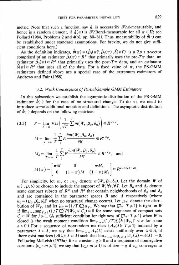
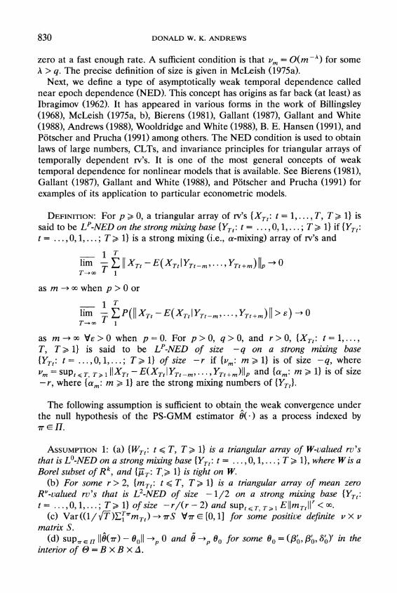
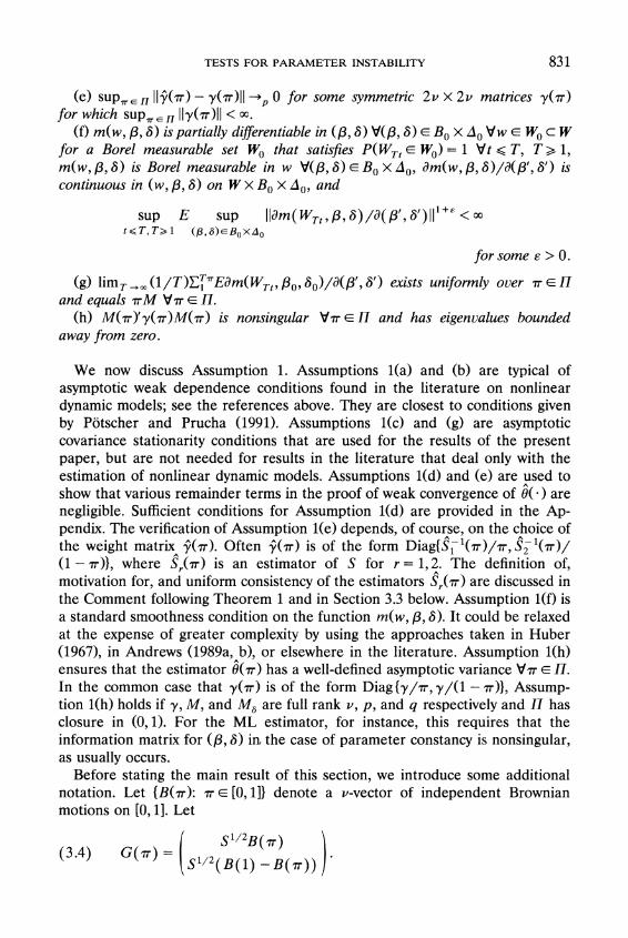
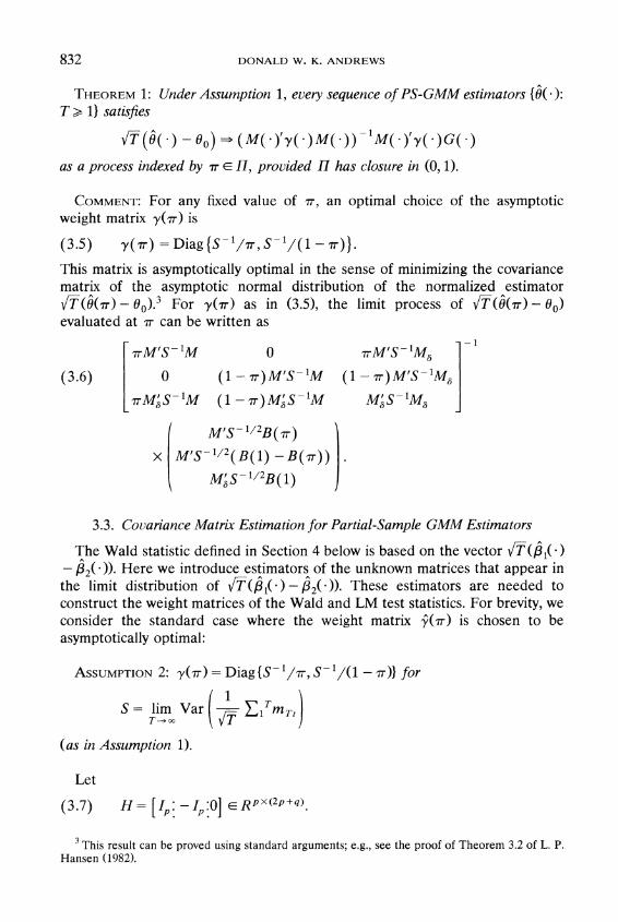
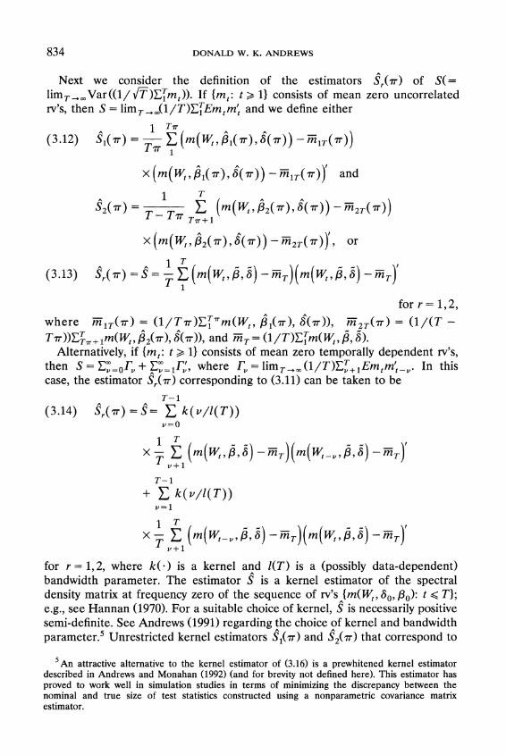
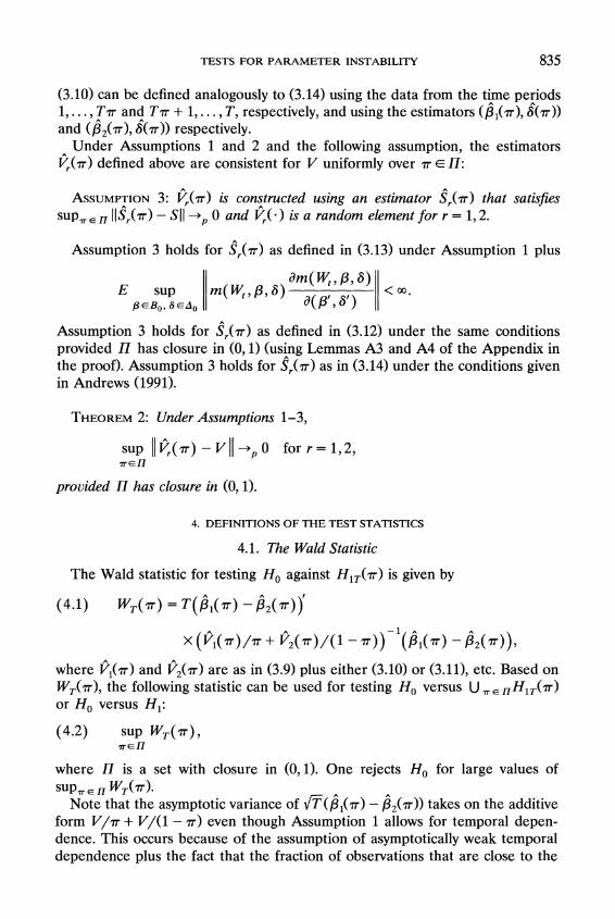
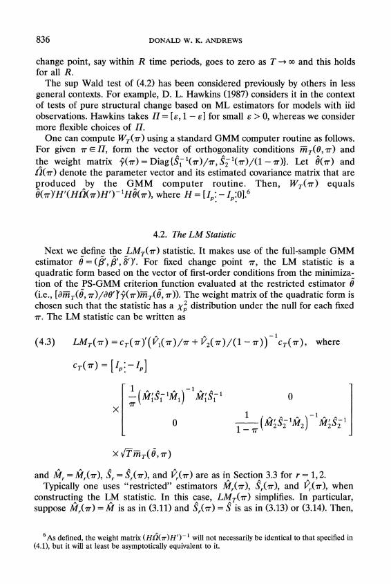
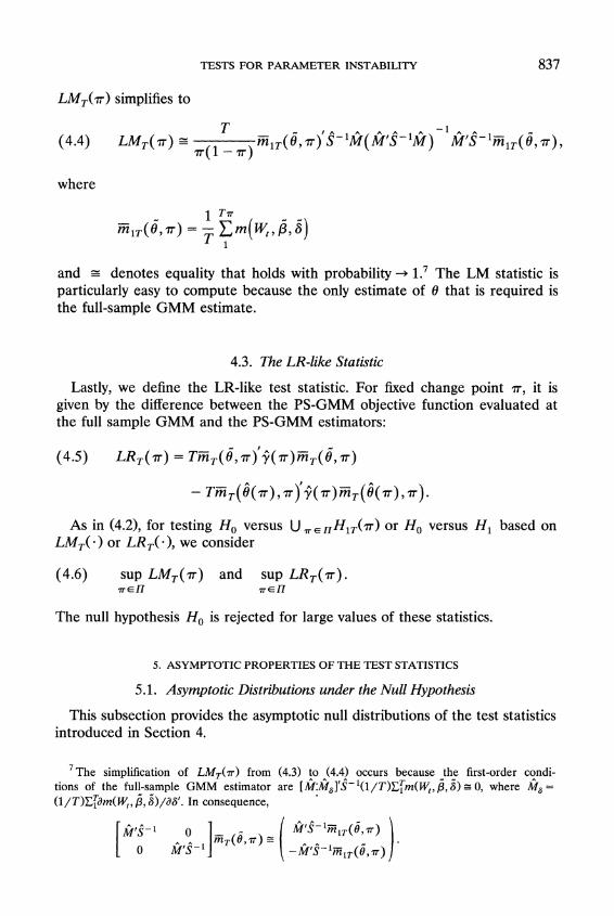
TESTS FOR PARAMETER INSTABILITY
L M T ( r )simplifies to
where
and = denotes equality that holds with probability + The LM statistic is particularly easy to compute because the only estimate of 6 that is required is the full-sample GMM estimate
43 The LR-like Statistic
Lastly we define the LR-like test statistic For fixed change point T it is given by the difference between the PS-GMM objective function evaluated at the full sample GMM and the PS-GMM estimators
As in (42) for testing Ho versus U HIT(r) or Ho versus H based on LMT( )or LRT( ) we consider
(46) sup L M T ( r ) and sup L R T ( r ) 7 r G n G l l
The null hypothesis H is rejected for large values of these statistics
5 ASYMPTOTIC PROPERTIES OF THE TEST STATISTICS
51 Asymptotic Distributions under the Null Hypothesis
This subsection provides the asymptotic null distributions of the test statistics introduced in Section 4
7The simplification of LM(a) from (43) to $442 occurs because jh_e first-order condi-tions of the full-sample GMM estimator are [MM]S-(~T)CT~(W~S)a 0 where M =
( l ~)CTarn(W ji ) a s1 In consequence
838 DONALD W K ANDREWS
THEOREM3 Suppose Assumptions 1-3 hold Given any set 17 whose closure lies in (Ol) the following processes indexed by rr E 17 satisfy
(a) WT()-Qp() and sup W(r)-+ supQ(rr) where Q(T)= - rrBp(l))l(Bp(rr)- rBp(l))[rrTT(l- rrTT)I
(b) LM() -Qlt) and sup LM(rr) +sup amp(TI (c) LRT()-Qp() and sup LRT(r)+sup Q(rr)
where B() is a p-vector of independent Brownian motions on [0 11 restricted to 17 The convergence in (a)-(c) holds jointly
COMMENTS is referred to in the literature as the 1 The limit process amp(I square of a standardized tied-down Bessel process of order p see Sen (1981 p 46) For any fked rr E (0 I) Q(r)has a chi-square distribution with p degrees of freedom Under the assumptions the asymptotic null distribution of SUP W(r) SUP LR(rr) is free of nuisance parameters except for the dimension p of p Thus critical values for the test statistics can be tabulated see Section 53 below
2 The requirement that 17 is bounded away from zero and one is made to ensure that the estimators upon which the test statistics are based are uniformly consistent for rr E17 and to ensure that the function mapping B() into Q() is continuous For example if 17= [O 11 the functions 7 -+ 1r and r + I (1 - r ) are not continuous In fact if 17 = [O 11 the test statistics SUP W(T) SUP LRT(r) do not converge in distribution see Corol- lary 1below
3 Theorem 3 establishes the asymptotic distributions of test statistics of the form g(W(r) r E 17)) for arbitrary continuous functions g (using the uni- form metric on the space of bounded cadlag Euclidean-valued functions on 17) In particular g(WT(~) 7E 171) -g(Q(rr) 7E 17)) under the assumptions and likewise for LM( ) and LRT( )
52 Asymptotic Behavior of the Test Statistics When 17= [O11
Next we consider the limiting behavior under the null of the statistics sup WT(r) SUP LR(rr) when 17= [O 11 For the location model with iid N(0l) errors D M Hawkins (1977) has already investigated this behavior (heuristically) In the general model scenario considered here this behavior is determined using the results of Theorem 3 Note that Anderson and Darling (1952 Sec 5) have considered a similar problem
COROLLARY1 Suppose the conditions of Theorem 3 and the null hypothesis H hold Then
839 TESTS FOR PARAMETER INSTABILITY
COMMENTS1 The Corollary shows that the restriction in Theorem 3 to sets II whose closure is in (0l) is not made only for technical convenience Unless II is bounded away from zero and one critical values for the test statistics SUP WT(r) SUP lr LRT(r) must diverge to infinity as T + w to obtain a sequence of level a tests By bounding r away from zero and one however a fixed critical value suffices for all T large This suggests that the restriction of II to a set whose closure is in (0l) yields significant power gains if the change point is in II or is close to II Some Monte Carlo results of Talwar (1983) and James James and Siegmund (1987) for the location model substantiate this result Furthermore the Monte Carlo results of Talwar (1983) show that the test statistic sup WT(r) has much closer true and nominal sizes in the location model under nonnormal errors when II is restricted than when II = [O11
2 Suppose 7j maximizes W(rr) LM(r) or LR(rr) over [O 11 By Theorem - E l3 and Corollary 1 SUP WT(r)= Op(l) Y Egt 0 SUP WT(r) +p w
under the null hypothesis and analogous results hold for LMT(r) and LR(r) In consequence 7j4 Ol under the null hypothesis By symmetry presum- ably 7j-tdBern(l2) where Bern(l2) denotes a Bernoulli distribution with parameter 12 In contrast if II has closure in (0l) and Q() has a unique maximum on II with probability one then 7j-tdargmaxQ(r) r E II by the continuous mapping theorem The latter distribution has support equal to II
53 Asymptotic Critical Values
Critical values c for the test statistics sup W(r) sup LR(r) are provided in Table I based on their asymptotic null distribution sup Qp(r) By definition c satisfies P(sup Q(r) gt c) = a The table covers a = 01 05 and lo p = 12 20 and II = [ r 1- r ] for an array of rOvalues between 05 and S O
Table I covers a much wider range of intervals IT however than just the symmetric intervals [T 1-T] If 17= [ r l rr21 for 0 lt rllt r2lt 1 then it can be shown (see the proof of Corollary 1 in the Appendix) that
where BM() denotes a p-vector of independent Brownian motion processes on [0 w) In consequence critical values based on the distribution of
Qp(rr) depend on rl and rr2 only through the parameter A = r2 (1 - rrl)(adl - rr2)) Table I provides the value of A corresponding to each value of rOconsidered (viz A = (1 -~ ) ~ r ) This allows one to obtain critical values for all intervals II=[rlrr21 whose corresponding value of A = rr2(l- r l ) ( r l ( l - rr2)) either is tabulated or can be interpolated from the
DONALD W K ANDREWS
TABLE I ASYMPTOTICCRITICALVALUES
Tn A 10
p = 1
5 1 10
p = 2
5 1 10
p = 3
5 1 10
p = 4
5 1 10
p = 5
5 1
TESTS FOR PARAMETER INSTABILITY 841
table The table covers values of A between 1and 361 so almost any interval of interest can be considered
Note that IIBM()ll is a Bessel process of order p In consequence the probability given in (51) is the probability that a Bessel process exceeds a square root boundary somewhere in the given interval Such probabilities and corresponding critical values for given significance levels have been computed numerically for p G 4 for a variety of A values by DeLong (1981) In contrast the critical values given here have been computed by simulation They cover a considerably wider range of values of p and A than those considered by DeLong
The values reported in Table I are estimates of the critical values c obtained by (i) approximating the distribution of the supremum of amp(TI over rr E [T
1-T] by its maximum over a fine grid of points n ( N ) and (ii) simulating the ( distribution of max Q(T) by Monte Carlo The grid n ( N ) is defined by
The value of N was chosen to be 3600 based on a comparison of the approximations obtained here with the numerical results of DeLong (1980 which are available for p G 4 A single realization from the distribution of max( Qp(r) was obtained by simulating a p-vector Bp() of independent Brownian motions at the discrete points in n ( N ) and computing max ( B(Tgt - TB(I))(B(T) - TB(I))[T(~ - T)] The number of repetitions R used was 10000 The accuracy of the simulated critical values for approximating the critical values based on the statistic max (
determined by noting that the rejection probability of the statistic Q(T) can be
( max Q(T) using the simulated critical value has mean a and standard error approximately equal to (a(1 - a) ~) For a = 01 05 and lo the standard errors due to simulation are 001 002 and 003 respectively
54 Asymptotic Local Power
In this section we consider the behavior of amp) WT() etc under sequences of local alternatives We introduce the following assumption
ASSUMPTION LP Assumption 1 holds but with the assumption in part (b) 1-that Em = 0 Vt lt T T 2 ( l f i ~ ~ ( ~ p ( ~ ) l l =op(l)1 replaced by sup T) -for some nonrandom bounded R-valued function p on 17
We write p ( ~ ) = (pl(rTT)I p2(~TT)IY for p l ( r ) p2(7) E R In many cases p ( ~ ) can be expressed in more primitive terms For example
suppose (i) Assumption 1-LP holds (ii) W t lt T T 2 1) is such that Em(W Po + r( t T) fi6) = 0 Vt lt T T gt 1 for some bounded RP-valued function r ( ) on [O 11 that is Riemann integrable on [OT] uniformly over
842 DONALD WK ANDREWS
T E E uU18 and (iii) max supg IIP-Pol l K f iIIE(aapt)m(WTt p 6) - M I I +0 as T +w where K = sup Ilq(~)ll In this case
THEOREM4 Suppose Assumption 1-L P holds Assumption 2 holds except in part (a) below and Assumption 3 holds except in parts (a) and (e) below Given any set E whose closure lies in (0 I) the following processes indexed by T E E satisfy
(a) fi(amp)3(M(Y~()M())-~M(YY(+)(G()p())-I -(b) SUP IIT(T)- VII +0 for r = 12 (c) WT()Q()=J(YJ() and SUPEnWT(~)+d SUP~Q(T)
where
J(Tr) = B p ( 4 - rBp(1)
[ T ( l -T ) ]
(d) LMT()Qlt) and sup L M T ( ~ )+sup Q(T) (e) LRT()3 Q() and s u ~ ~ L R ( r r ) + ~ sup Q(T)
where Bp() is a p-vector of independent Brownian motions on [O1] restricted to ( C C ) - ~ ~ C ( M s - ~ M ) - ~ M S - ~ ~E A = E RpxY and C = E RPXYIf p = ZJ
one can take A =I The convergence in (b)-(e) holds jointly
COMMENTS1 The local power results of Theorem 4 are similar to those obtained by D L Hawkins (1987) but are more general Hawkins results cover the particular case of one-time structural change in which p( ) is as in (53) with 7( ) of the form 7 ( ~ ) = b l ( ~lt 7) for some fixed T E (0l) and some con- stant b His results apply to ML estimators in iid contexts
2 When p( ) satisfies (53) Q() depends on T() in the following way Q(T) =J(TYJ(T) and
1- 12
(54) J (T) = p T p 1 + A s - M ( ( ) iT7( s ) ds [T(1 -T ) ]
By definition this means that 7 is Riemann integrable on [0a] V a E llU (1) and ( 1 T ) C T T 7 ( t ~ )- jq(s) ds uniformly over a E llu (1)as T -m
843 TESTS FOR PARAMETER INSTABILITY
3 For fixed r E (0 I) Q(r) has a noncentral chi-square distribution with p degrees of freedom and noncentrality parameter given by the squared length of the second summand in the definition of J(r)
4 By simulating the distribution of sup Q(r) the sensitivity of the power of the test considered here to the form of the alternative as specified by p ( ) or q() can be determined and the results hold asymptotically for a wide variety of models and estimators For example one can determine the effect of the location of the change point on the tests power by simulating sup Q z ( r ) with q ( r ) = 1 ( r TT 7) for a variety of values of r The results of Theorem 4 also can be used to compare the asymptotic power of the tests considered here for a wide variety of models with that of other tests in the literature again by simulation
5 The local power of the tests considered in Theorem 4 is the same whether 6 is estimated or is known
The local power results of Theorem 4 can be used to show that the tests based on sup WT(r) supT LRT(r) each have nontrivial power against alternatives for which the parameter P is nonconstant on Ll These results are analogous to results obtained by Ploberger et al (1989 Cor 1) for the fluctuation test in the more restrictive context of testing for pure structural change in an iid linear regression model
COROLLARY2 Suppose the assumptions of Theorem 4(c) (resp 4(d) 4(e)) hold with p ( ) as in (53) but with q( ) replaced by (q() Suppose Ll is an interval whose closure lies in (0l) If q is not almost everywhere (Lebesgue) equal to a constant vector on II then
WT(r) gt c ) = 1 [ - m T - m
(resp
sup L M T ( r ) gt c ) = 1
sup L R T ( r ) gt c ) = I )
where c is as defined above and a E (0l)
Next using Theorem 4 we can establish a weak optimality result for the test statistics sup WT(r)sup LRT(r) for testing against the alternatives in U H(r) This result is a generalization to multiparameter two-sided tests of a result of Davies (1977 Thm 42) for scalar parameter one-sided tests The result shows that as the significance level a goes to zero the power against all local alternatives of the level a test based on sup WT(r) is at least as large as that of the level a test based on WT(ii) for any fixed ii ELl Thus if WT(ii) possesses asymptotic local power optimality properties against certain
844 DONALD W K ANDREWS
alternatives eg as it does in the ML case against one-time structural changes (ie for q(s) = 0 for s lt + q(s) = 8 for s a +I then sup WT(r) inherits these properties as a + 0 The same also holds for sup LMT(r ) and SUP LRT(r)
THEOREM5 Let q denote a bounded RP-valued function on [O 11 that is Riemann integrable on [O TI uniformly over T E I7 U I Let 1 denote the set of all such functions q for which there exists a distribution P of the triangular array W t lt T T a 1) such that 1-LP 2 and 3 hold with p( 9 ) as in (53) Then
(55) lim inf inf lim W T ( r ) gt c) -P(WT(+) gt C)I gt 0a -0 ~ E B7 i E I I T -m
where c and E are such that the tests based on sup WT(r) and WT(+) have asymptotic level a E (0l) The result (55) also holds with WT() replaced by LMT() or LRT()
COMMENTThe optimality result (55) is referred to above as a weak result because it appears that a must be quite small before the result is illustrative of finite sample behavior of the test statistics sup WT(r) and WT(+) Nevertheless the result does serve to indicate that as a decreases the dif- ference decreases between the power function of the level a test based on sup WT(r) and the envelope of the power functions of the level a tests based on WT(+) for fixed + ELI
6 CONCLUDING COMMENTS
1 The tests discussed in this paper are asymptotic in general Nevertheless exact versions of them can be obtained in some cases In particular consider a linear regression model with fixed regressors and iid normal errors In this case the sup Wald test statistic based on the least squares estimator has null distribution that is invariant with respect to the regression and variance parame- ter values In consequence one can set the regression parameters equal to zero and the error variance equal to one and generate exact critical values by simulating the resultant model Since least squares regressions are very quick to compute this procedure is not very burdensome computationally See Andrews Lee and Ploberger (1992) for further details
2 The basic Assumption 1employed above utilizes the concept of near epoch dependence This assumption can be simplified if the underlying random variables W t = 01 are stationary and ergodic In particular it can be shown that Assumption 1 can be replaced by the following assumption and Theorems 1-5 still hold9 Let 3 denote the u-field generated by W- w lt t G s Let m B and A be as in Section 32
The invariance principle used to show this is given by Hall and Heyde (1980 Cor 54 p 145)
845 TESTS FOR PARAMETER INSTABILITY
ASSUMPTION1 (a) W t = 01 ) is stationary and ergodic (b) Em = 0 Emm lt m C= (EII ~ ( m ~-)112)12lt w1 and S is positive
definite (c) m( w p 8) is continuously partially differentiable in (P 8) V(P 8) E B X A
Vw E W c W for a Borel measurable set W that satisfies P(W E W) = 1 m(w P 6) and am(w p S)a(pr 8) are Borel measurable functions of w for each (P 6) E Bo X A and E s u ~ ( ~ ~ ) BoxdoIlam(W p 8)a(Pr 8)ll lt m
(d) Assumptions l(d) (e) and (h) hold
3 In the event that a test for structural change rejects the null hypothesis it may be of interest to estimate the parametric model defined by the restricted alternative IJ n H l r ( ~ ) This involves estimating the time of change parame- ter T Properties of the maximum likelihood (ML) estimator of T have been considered by Hinkley (1970) Picard (1983 1985) Deshayes (1983) Bai (1990 and Bai Lumsdaine and Stock (1991) for a variety of models No optimality properties are known for the ML estimator of 7
Cowles Foundation for Research in Economics Yale University PO Box 2125 Yale Station New Haven CT 06520 USA
Manuscript received June 1991 final revision received November 1992
APPENDIX
For notational simplicity we say X T ( a )= op(l) i f sup llX(a)ll = o(l) and we say X(T) = 0(1) i f sup llXT(a)ll= OP(1)
First we provide conditions under which the PS-GMM estimator is consistent for 0 uniformly over T E II under the null hypothesis
ASSUMPTIONA (a) Assumption l (a) holds (b ) sup l l ( ~ )- y(a)ll +0 for some symmetric 2 v X 2 v matrices y ( a ) for which
S U P ~n IIY(T)II lt m (c) B and A are bounded subsets of R P and Rq respectively (d) m(wp 6 ) is continuous in w for all ( p 6 ) E B X A and is continuous in ( p 6 ) uniformly over
( p 6 W ) E B X A X C for all compact sets C c W (e )~ ( l ~ ) ~ T ~ s u p ~ ~ ~ ) ~ ~ ~lm(WTtP8)11CElt m for some e gt 0 ( f ) lim ( l T)CTEm(WTffp 6 ) exists unijormly over T ) E B X A X II and equals lim(1T)ETEm(wTfp6) (8) amp(Po 6) = 0 where h ( P 6 )= lim ( I T ) ~ T E ~ ( W p 6) and for every neighborhood
0 ( C 0 ) of 0 inf info m(OaYy(a )m(0 a )gt 0 where m(0 a )= ( n - h ( p l 6Y(1 -T)h(P26YY
When Assumptions 2 and 3 hold Assumption A(b) automatically holds and A(g) simpli- fies to h (p0 6 ) = 0 and for all neighborhoods B and A o f Po and A respectively i n f ( p S ) E B X A B O ~ ~ oh ( P gt 6 Y S - h ( P 6 ) gt 0
THEOREMA l Under Assumption A the PS-GMM estimator satisfies sup l ( ( ~ )- 0ll -+
0 for any set II whose closure lies in (0 l )
846 DONALD W K ANDREWS
COMMENT estimator iAssumption A onlyTO obtain consistency o f the full-sample GMM needs to be altered slightly Consider the condition A(b) q + y for some nonsingular symmetric v x v matrix y where is the weight matrix o f the full-sample GMM estimator W e have 6 + O o i f Assumption A holds with A(b) replaced by A(bl) and with A(g) replaced by the simplified version o f A(g) given above except with y in place of S-
The proof o f Theorem A1 uses the following three lemmas (the latter two of which are also used in the proofs o f other results below)
LEMMA A l Suppose (a ) minimizes a random real function QT(Oa) over 0 E O c for each rr E Il with probability + 1 If (a) sup n 1 QT(e a ) - Q(Oa )1 -0 for some real function Q o n O x I l a n d (b)iorevely neighborhood O O ( c O ) of 00 inf(infooQ(O~)- Q(OP)) gt 0 then sup IlO(rr)- Ooll -0
LEMMAA2 Suppose ( X T t t lt T T gt 1) is a triangular array of mean zero real-valued rus that is LO-NED with respect to a strong mixing base YTt t = 01 T 1) and ~ T ( l ~ ) ~ T ~ ~ ~ T l i E mlt m for some E gt 0 Then E supsGT I( l T)CfxTI -0 as T-
LEMMAA3 Suppose (a) Assumption l (a) holds (b) A is a bounded subset of RS (c) f(w A) is an Rc-valued function on W x A that is continuous in w for -1 A E A and is continuous in A uniformly over (A w ) E A X C for all compact sets C cW and (d ) l imT(l ~)CTE sup ( f(WTtA)I +Elt m for some E gt 0 Then
PROOFOF THEOREMA l W e apply Lemma A1 with QT(O P ) = K T ( a) 9(rr)ZT(e P) and Q(O P ) =m(O ayy(n-)m(O T ) Condition (b) o f Lemma A1 holds by (Assumption) A(g) Given A(b) condition (a) o f Lemma A1 holds i f
( A J ) sup sup I I Z ( O T ) -m ( O a ) ( ( + 0 EL B E
Using C = CT - CT the latter holds i f
where al = infn-P euro171 gt 0 (A2) holds by Lemma A3 under A(a)-(e) (A3) holds by A( f ) QED
PROOFOF LEMMAA l By Assumption (b) given any neighborhood O0 o f O o there exists a constant E gt 0 such that in f [inf Q(O+) - Q(Oo+)I gt E gt 0 Thus
(A4) P ( ~ ( T )E OOo for some a E fl)
G P ( TGLjnf [ Q ( ( P ) ~ )- Q ( O ~ + ) ]gt E for some E fl1 g p(~( ( r r ) r r )-Q(Ooa )gt E for some a E IT) + 0
where +0 holds provided sup ( Q ( ~ ( P ) Q(Oorr) ( + 0 Using Assumptions (a) and rr) -
TESTS FOR PARAMETER INSTABILITY
(b) the latter follows from
(A5) 0 lt inf [ Q ( i ( a ) a ) -Q ( O ~ P ) ]lt sup [ Q ( ~ ( P ) P ) - ~ ( e o ~ ) ]T E I I T E ~
lt sup [ Q ( ~ ( P ) T ) - Q ~ ( ~ ( T ) T ) ]+ sup [ Q T ( ~ ( T ) ~ )- Q ( ~ o $ P ) ] ~ r e n Tr E I Z
lt Sup [ Q ( ~ ( P ) v ) - Q T ( ~ ( T ) T ) ] + sup [ Q T ( ~ O T ) - Q ( ~ O ~ ~ ) ] T E ~
QED
PROOFOF LEMMAA2 Under the moment conditions (X) is L1-NED by Theorem 61 of Potseer and Prucha (1991) This property and inequalities (2) and (3) of Andrews (1988) show that 6 ) ~imT+m(lT)~~~E(xTl~YTl YTr-m)l+ 0 as and (ii) l i m T + m ( l ~ ) ~ T l ~ T r i77 +m -E(XTrI YTr+m YTT)I +0 as m +m Conditions (i) and (ii) are a slightly weaker version of the L1-mixingale condition of Andrews (1988) with constants c = 1 and r-fields FTgiven by those generated by Y) Theorem 1 of Andrews (1988) holds with the L1-mixingale condition replaced by (i) and (ii) In fact the conclusion of Theorem 1 can be strengthened from E I(~T)CTX~I + 0 to E supsGT I ( ~ T ) C ~ X ~ +0 as T - with some alterations in its proof This gives the result of Lemma A2 The alteration in the proof of_ Theorem 1 include changing (ln)C=l to supjG I(ln)Cj= I and E I YmnI to E_sup I YmI in equation (7) and strengthening the result of the Lemma in Andrews (1988) from IIYnllp +0 as n +m to IlsupjG I (jn)I 1 11 -0 as n +aTo achieve the latter the proof of the Lemma needs to be changed by replacing (ln)C-l by SUP I (ln)Ci I throughout and by using the martingale inequality Ilsup 1 (ln)E= l ( v -E(UI q- ) ) I 11 2 lt 2ll(ln)C= (w -E ( K I q-))112 due to Doob (see Theorem 22 of Hall and Heyde (1980 p 15)) in equation (4) Q E D
PROOFOF LEMMAA3 The desired result follows from Theorem 1 of Andrews (1992) with Gn(0) set equal to supsGT l ( l ~ ) E f [ f ( W ~ A) -Ef(WTrA l l Hence it suffices to verify the conditions BD P-WCON and SE of Theorem 1 BD holds by Assumption (b) For Gn(0) as above the proof of Lemma 3 of Andrews (1992) shows that DM and TSE imply SE DM holds by Assumption (d) By Lemma 4(b) of Andrews (19921 TSE-2 implies TSE TSE-2 holds by Assumptions (a) and (c) It remains to show P-WCON Under Assumptions (a) (c) and (d) Theorem 65 of Potcher and Prucha (1991) implies that (f(W A) t lt T T gt 1) is Lo-approximable by the base (YTl) for all A E A By Assumption (d) and Theorem 61 of Potscher and Prucha (1991) the approximators can be taken to be the conditional means E(f(WT A)I YT- Y) t lt T T 3 1 m 1) In consequence f(WTr A) t lt T T gt 1) is Lo-NED on the strong mixing base (Y) for all A E A We now apply Lemma A2 with X equal to an element of the c-vector f(WTl A) -Ef(WTt A) to obtain P-WCON Q E D
The following lemma is used in the proof of Theorem 1
LEMMA A4 Let 77() T gt 0) be a sequence of random elements of the space of bounded R-ualued cadlag functions on a set A c [Ol] If (i) (YT() (Y T~(Va ER and (ii) ( T ~ ( ) T gt 1) has asymptotically independent increments (as defined eg by Billingsley (1968 p 157)) then TI() =770()
(Note that Prop 41 of Wooldridge and White (19881 which claims that condition (i) alone is sufficient for a multivariate invariance principle is not correct Their proposition cannot be derived in the manner they suggest)
PROOFOF THEOREM1 Since $P) minimizes ET(O a)f(a)RT(O T) and $(P) is in the interior of O VP El7 with probability + 1 by (Assumption) l(d) we have
848 DONALD W K ANDREWS
Let mTj(0r) denote the jth element of TiiT(0r) A mean value expansion of fiEiTj(i(r)r) about Bo gives Vj = 1 2v
where 8(= O(r)) is a rv on the line segment joining (a) and 8 (see Jennrich (1969 Lemma 3) for the mean value theorem for random functions) The latter property and l(d) imply that e = 0 + op(l)
Below we show that
am e (A8) sup T( -M(a)ll -rP011
TrEII
whenever O(r) satisfies sup llO(r) - eoll-0 We also show that
as a process indexed by a E I7 Equations (A614A91 l(e) and (h) and the continuous mapping theorem (see Pollard (1984 Thm IV12 p 70)) combine to give the desired result
- -(~(yy()~())-~(yy()~()
To establish (A81 we write
The third summand on the right-hand side of (All) -r 0 by l(g) The first summand -r 0 because Assumption 1 and Lemma A4 yield
Finally the second summand on the right-hand side of (All) + 0 because (i) by the tightness of (pT T 11 supTgt (~T)EP(W~~ E C) -0 as j -r for some sequence of compact sets Cjj gt 1) in W (ii) for all j gt 1 we have
am(wP 8) -
am(wPo 60) -tJY I1 a(pl 6) J(P 8)
as (p 6) - (Po aO) using l(f) and (iii) results (i) and (ii) combine to give
1 T a m ( w ~ p a )- a m ( w ~ l P o 6 0 ) +(A14) sup sup 1IIr gt l En 117F E [ a (p l a r ) a(pl 8)
as (p 6) -(Po 60) Thus the right-hand side of (A11) -rp0 and (A8) is established
849 TESTS FOR PARAMETER INSTABILITY
Next to show (A91 let v(T) = (I f i)cTrm Since f imT(eo a ) = (v(a) -~ ~ ( 1 ) vT(aYY (A9) follows from vT() = s~B() To obtain the latter we apply Lemma A4 Under l(a)-(c) we obtain condition (i) of Lemma A4 by Cor 31 of Wooldridge and White (1988) which utilizes results of McLeish (1977) (Note that Cor 31 yields weak convergence of the standard partial sum process in D[O 11 with the Skorokhod metric and the Borel u-field generated by it This can be converted into weak convergence in D[O 11 with the uniform metric and the u-field generated by the closed balls under the uniform metric as follows The result of Cor 31 implies weak convergence of the smoothed partial sum process (ie a l v T ( r ) + (TT - [~a])a m[ ~+ fi) using the Skorokhod metric on D[01] because the difference between the standard and the smoothed partial sum processes is G sup I am 1 fi and the latter is op(l) by the Lindeberg condition see Hall and Hyde (1980 p 53) Since the smoothed process is in C[O 11 the Skorokhod and uniform metrics are equivalent for C[O 11 and the Borel u-field and the a-field generated by the closed balls under the uniform metric are equivalent for C[O 11 the smoothed partial sum process converges weakly as a sequence of random elements of C[O 11 with the uniform metric and its Borel u-field This yields the desired univariate invariance principle for the standard partial sum process av(a) in D[O 11 with the uniform metric and the a-field generated by the closed balls under the uniform metric because the difference between these two processes is less than or equal to sup laml fi=
op(l) To obtain condition (ii) of Lemma A4 it suffices to show that
By the Cramamp-Wold device the latter holds if
(Note that this result is not implied by a lvT( ) = a1v() Va ER) TO obtain (A161 the same central limit theorem as used above viz Cor 31 of Wooldridge and White (19881 can be employed
QED
PROOFOF LEMMAA4 Conditions (i) and (ii) are sufficient because (a) tightness of (atvT() T gt 1) Va ERY implies tightness of (vT() T gt 1) on the v-dimensional product space (b) asymptot- ically independent increments plus weak convergence of vT(a2)- v T ( r l ) VO 6 al lt r2lt 1 is sufficient for joint convergence of all the finite dimensional distributions of (vT() T gt 11 and (c) weak convergence of a tvT( ) to a lvO( ) Va E R implies weak convergence of ( Y ( ~ ~ ( T ~ ) - TJ(T~)) to ~ ( V ~ ( T ~ ) - vO(al)) VO Q allt a2Q 1 which in turn implies weak convergence of vT(T2) -v ( ~ ) to v 0 ( r 2 ) - 7 ) 0 ( ~ 1 ) QEDusing the Cramamp-Wold device
PROOFOF THEOREM2 Assumptions l(h) and 2 imply that MS-M is nonsingular and hence that V is well defined By the argument of (A11)-(A14) and Assumption l(d) sup l lM(~)-MI1 +0 By Assumption 3 sup l lS (~)- SII -r 0 Using Assumption 2 this gives the desired result QED
The following Lemma is used in the proof of Theorem 3
LEMMAA5 Let J(T) be a nonsingular (2p + q) X (2p + q) matrk of the form
where al and a2are nonzero scalar constants J ER ~ J2E R pXq ~ J3 E R ~ Jq ~ ~ ~ E RqXP and
850 DONALD W K ANDREWS
J ERqXqLet g = (g g g) be any vector in R~~~~ and let H = [ I - IpO]E R P ~ ( P + ~ ) Letp
and H = [I - I] Then HJ- (T)~ = H J (T)~
PROOF OF LEMMA A5 Let v = (v v v) =J - ( T ) ~ and v = (ivkY =J (T)~ Since J(a)v =g we have
W - ( T ) ~= v1 - v2= - fi2 =H ~ - ( a ) ~ QEDi1
PROOFOF THEOREM3 Let the subscript be a deletion operator that deletes the last q rows and columns of (2p + q) x (2p + q) matrices the last q rows of 2p +q-vectors and (2p + q) Xp matrices and the last q columns of p x (2p + q) matrices Let
where the second equali holds by Assumption 2 By Lemma A5 we have H J - ( T ) ~ = H J(n)g for all ERYPq (where I(=) = [J(T)]-)
First we establish part (a) of Theorem 3 Let C = (Ms-M)-Ms-~ By Theorem 1 and Lemma AS we have
(419) f i ( b l ( 9 - b 2 ( 9 )
= C[B()L() - (B(1) -B( ) ) ( l -amp( ) ) I
where L(T) =T By Theorem 2
(A19) and (A20) and the continuous mapping theorem (see Pollard (1984 Thm IV12 p 70)) give
(421) W T ( )= (B() -L()B(~))(B() -L ( ) B ( ~ ) ) [ L ( ) ( ~- ~ ( ) ) 1
where B() = ( C C ) - 1 2 ~ ~ ( ) B() is a p-vector of independent Brownian motions because (CC)-~C[(CC)-~~C]= I This establishes the first result of part (a) The second and third results of part (a) follow from the first using the continuous mapping theorem The same is true for parts (b) and (c) so it suffices to establish the first result in parts (b) and (c)
TESTS FOR PARAMETER INSTABILITY 851
Next we establish part (b) By Theorem 2 c ( a ) = V+ o(l) In addition we show below that
Hence it suffices to show that LM$() -en()where
(A23) LM(P) = c(a)(vr + V( l - r))- c(a) and
0 c(r) = [I -I] 1
0 - (M~S-~M)- MJS-~1 - a 1
Using Lemma AS we obtain
Equations (A714A9) with i ( ) replaced by 6 ( )yield
This result and (A24) give
using the last three equalities of (A19) and the fact that H ~ ( v ) =Heo = 0 Equations (A23) and (A26) combine to give the desired result LM() = Q()in the same way that (A19) and (A20) yield (A21)
For part (b) it remains to show (A22) This follows from (A251 since (i) sup IIfiAT(Oo a)ll jdsupTEn IIG(r)ll (lt m as) by (A9) ad the continuous mappig theorem
(ii) sup M(r)lllt m and (iii) f i ( 0 - 8) = 0(1) because 0 is consistent by l(d) and given consistency is asymptotically normal by standard arguments given the remainder of Assumption 1
Next we consider part (c) For brevity we only give a sketch of its proof First by element by element mean value expansions one obtains
dAT(i a)fi( i - i)(A27) f i A ( i r ) = f i m T ( i r ) + +o(l) and aor
where the second equality uses (A6) Let 6 ( r ) be the restricted PS-GMM estimator that minimizes FE(e r)+(a)mT(e a ) over 0 = (6 E O e = (p p 8)) The first-order conditions for-O(a)-yield [am(O(a) ~ ) a e ] ~ ( ~ ) m ( O ( a ) HA for some p-vector of Lagrange multipliers A (= A(r))a ) = Under Assumption 2 the full sample GMM estimator 0 can be shown to satisfy the ame first-order conditions up to o(lfi) This result premultiplication of (A27) by [aR(Oa)aO]~(a)
852 DONALD W K ANDREWS
rearrangement of (A27) and application of (A6) give
= f i J - ( r ) H 1 i + o(l) and
( A ~ o ) LR(T) ~ ~ J H J - ~ ( ~ T ) H ~ ( W - ~ ( ~ ) H ~ ) - ~ ~ ~ H J - ~ ( T ) H ~ ~= + o p V ( i )
By Lemma A5 and the definitions of i and c$ (a ) we have
Combining (A30)-(A32) gives L R T ( a )= LM(P) + o(l) and the desired result follows from the proof above that LM$ ) =Q() QED
PROOFOF COROLLARY = - L()B()which appears in the definition 1 The process BE( ) B() of Q() is a p-vector of independent Brownian bridge processes on [Ol]An alternative method of defining such a process is via a p-vector EM( ) of independent Brownian motion processes on [0 m) In particular we have
(A33) B B ( a ) 7~ E [ O I ] = ( ( 1- r ) B M ( a ( l -T ) ) T E [oI ]
where = denotes equality in distribution Hence we have
sup B M ( L ) B M ( ~ ) ( ~ ) lt c )= P ( T E [ T ~ T Z ] 1 - 7 ~ 1 - 7 ~ 1 - 7 ~
=p ( sup BM()BM()() lt)s euro [ l T 2 1 - T l T l - T l l - T l 1 - P I 1-7T1
= P ( SUP B M ( s ) r n ( s ) s lt c ~ euro [ l T 2 ( 1 - T 1 ) ( T 1 ( 1 - T 2 ) ) 1
for all 0 lt P d rr2 lt 1 and c gt 0 where the second equality holds by change of variables with
by definition and BAT() is also a Brownian motion on [Om)(by direct verification) The result of Corollary 1 is now obtained as follows
(A35) lim P( sup WT(=) lt c ) d lim P ( SUP W T ( T ) lt c ) T + m ~ ~ [ 0 1 1 amp+o Tm V E [ E ~ - E I
-= lim P( sup Q(T) lt c )
E + O T E [ E ~ - E I
=P ( sup lt c ) =B M ( S ~ B M ( S ) S O s e [ l m )
where the first equality holds by Theorem 3 the second by (A34) and the last by well known
TESTS FOR PARAMETER INSTABILITY 853
properties of Brownian motion (ie the law of the iterated logarithm) The proof is identical for LMT(r) and LRT(r) Q E D
PROOFOF THEOREM4 Part (a) holds by the proof of Theorem 1 noting that (A9) holds with G() replaced by G() + p() since f i ~ ~ ( 0 ~ - + f i ~ ~ i i ( e = fi(ET(6 EET(Oo = G() + p ( ) under Assumption 1-LP Part (b) holds by the proof of Theorem 2
Parts (c)-(e) hold using the proof of Theorem 3 with references to Theorems 1and 2 replaced by references to Theorem 4(a) and (b) respectively with G( ) replaced by G() + p() with the right-hand side of (A19) replaced by
and with the right-hand side of (A21) and (A26) changed accordingly Q E D
PROOFOF COROLLARY in (54) it 2 By Theorem 4(c)-(e) and the nonsingularity of AS-M suffices for Corollary 2 to show that
does not hold Note that (A37) holds if and only if
where ~ ( a ) = TJ~(~)) ( ~ ( r ) Thus it suffices to show that (A38) does not hold Suppose (A38) holds Then since aldV(s)ds is twice differentiable in r V a E int(II) Vj =
1 p so must be j~(s) ds where int(II) denotes the interior of II In particular we must have
V a E int ( I I ) Vj = 1 p
This implies that 7 = c almost everywhere (Lebesgue) on II for some constant cj V j = 1 p which is a contradiction QED
PROOFOF THEOREM5 Let u = c and t =FA We will show that
(A40) u - t - + O as a -+ 0
Then using Theorem 4 we have
lim inf inf lim 1a-0 R E Z +En T+m
= lim inf sup [P( sup ~ ( r ) ~ gt u) -P~(Q(+) gt t)] a-0 R E E7 i ~ n ELI
lim inf sup [P(Q(+)~ gt u) -P(Q~ (+) gt t)] a-tO T E E+en
where the last equality uses (A40) and the fact that Q(+) is a noncentral chi-square rv and the density of the square root of a noncentral chi-square rv is bounded above uniformly over all possible values of its noncentrality parameter
To show (A40) we use an argument similar to that of van Zwet and Oosterhoff (1967 p 675) Let a = inf ( a E n ) gt 0 let r2= sup ( a E I I ) lt 1 and let v be such that P(supVE[T I T I 2 I Q(T)~ gt v) = a Since t d u g v to establish (A40) it suffices to show that v - t -+ 0 as a -+ 0
854 DONALD W K ANDREWS
By a result of James James and Siegmund (1987 eqn (261 p 78) we have
(A42) P ( sup Q(r)gt v) = ~ v ~ - ~ e x p ( - $ 2 ) ( ( $ - p ) I O ~ A+ 4 + o(1)) T r ~ [ T r ~ 2 1
as a + 0 where Q() is as in Theorem 3 K is a constant that depends only on the dimension p of the Brownian bridge vector that underlies Q() and A = r 2 ( l - r1 ) [ r l ( l - r 2 ) ] Taking r l= r2= 7j in (A42) yields log A = 0 and
(A43) ~ ( ~ ( 7 j ) ~gt t) = K ~ P - ~ exp ( -t22)4 + o(l) as a -0
The left-hand side of (A42) and (A43) each equal a Thus the logs of the right-hand side of (A42) and (A43) can be equated to yield
(A44) ( p - 2) log v - v22 + log (v - p ) log h + 4 + o(1))
= ( p - 2) log t - t22 + log (4 + o(l) and
as a -0 using the fact that t + m as a + 0 and t d v Since I v - t 1 lt v - tv (A45) implies that v - t -0 as a -0 QED
REFERENCES
ANDERSONT W AND D A DARLING (1952) Asymptotic Theory of Certain Goodness of Fit Criteria Based on Stochastic Processes Annals of Mathematical Statistics 23 193-212
ANDREWSD W K (1988) Laws of Large Numbers for Dependent Non-identically Distributed Random Variables Econometric Theory 4 458-467 -(1989a) Asymptotics for Semiparametric Econometric Models I Estimation and Testing
Cowles Foundation Discussion Paper No 908R Yale University -(1989b) Asymptotics for Semiparametric Econometric Models 11 Stochastic Equicontinu-
ity and Nonparametric Kernel Estimation Cowles Foundation Discussion Paper No 909R Yale University -(1989~) Tests for Parameter Instability and Structural Change with Unknown Change
Point Cowles Foundation Discussion Paper No 943 Yale University ---- (1991) Heteroskedasticity and Autocorrelation Consistent Covariance Matrix Estimation
Econometrica 59 817-858 ---- (1992) Generic Uniform Convergence Econometric Theory 8 241-257 ANDREWSD W K AND R C FAIR (1988) Inference in Nonlinear Econometric Models with
Structural Change Review of Economic Studies 55 615-640 ANDREWSD W K I LEE AND W PLOBERGER (1992) Optimal Changepoint Tests for Linear
Regression Cowles Foundation Discussion Paper No 1016 Yale University ANDREWSD W K AND J C MONAHAN (1992) An Improved Heteroskedasticity and Autocorre-
lation Consistent Covariance Matrix Estimator Econometrica 60 953-966 ANDREWSD W K AND W PLOBERGER (1992) Optimal Tests When a Nuisance Parameter Is
Present Only under the Alternative Cowles Foundation Discussion Paper No 1015 Yale University
BAI J (1991) Estimation of Structural Change in Econometric Models unpublished manuscript Department of Economics University of California Berkeley
BAI J R LUMSDAINE (1991) Testing for and Dating Breaks in Integrated and AND J H STOCK Cointegrated Time Series unpublished manuscript Kennedy School of Government Harvard University
855 TESTS FOR PARAMETER INSTABILITY
BANERJEEA R L LUMSDAINE AND J H STOCK (1992) Recursive and Sequential Tests for a Unit Root Theory and International Evidence Journal of Business and Economic Statistics 10 271-287
BIERENSH J (1981) Robust Methods and Asymptotic Theory Lecture Notes in Economics and Mathematical Systems No 192 Berlin Springer Verlag
BILLINGSLEYP (1968) Convergence of Probability Measures New York Wiley BROWN R L J DURBIN AND J M EVANS (1975) Techniques for Testing the Constancy of
Regression Relationships over Time Journal of the Royal Statistical Society Series B 37 149-192
CHOW Y S AND H TEICHER (1978) Probability Theory Independence Interchangeability Martin- gales New York Springer-Verlag
CHU C-S J (1989) New Tests for Parameter Constancy in Stationary and Nonstationary Regression Models unpublished manuscript Department of Economics University of Califor- nia-San Diego
DAVIES R B (1977) Hypothesis Testing When a Nuisance Parameter Is Present Only under the Alternative Biometrika 64 247-254 -(1987) Hypothesis Testing When a Nuisance Parameter Is Present Only under the
Alternative Biometrika 74 33-43 DELONG D M (1981) Crossing Probabilities for a Square Root Boundary by a Bessel Process
Communications in Statistics-Theory and Methods A10 (211 2197-2213 DESHAYESJ (1983) Rupture de ModZles en Statistique PhD Thesis Department of Mathematics
University of Paris Orsay GALLANTA R (1987) Nonlinear Statistical Models New York Wiley GALLANTA R AND H WHITE (1988) A Unified Theory of Estimation and Inference for Nonlinear
Dynamic Models Oxford Basil Blackwell GARBADEK (1977) Two Methods of Examining the Stability of Regression Coefficients Journal
of the American Statistical Association 72 54-63 GORDINM I (1969) The Central Limit Theorem for Stationary Processes Soviet Mathematics-
Doklady 10 1174-1176 HALL P AND C C HEYDE (1980) Martingale Limit Theory and Its Applications New York
Academic Press HANNANE J (1970) Multiple Time Series New York Wiley -(1973) Central Limit Theorems for Time Series Regressions Zeitschrift fur Wahrschein-
lichkeitstheorie und venvandte Gebeite 26 157-170 HANSEN B E (1990) Lagrange Multiplier Tests for Parameter Instability in Nonlinear Models
unpublished manuscript Department of Economics University of Rochester ---- (1991) Strong Laws for Dependent Heterogeneous Processes Econometric Theory 7
213-221 -(1992) Tests for Parameter Instability in Regressions with I(1) Processes Journal of
Business and Economic Statistics 10 321-335 HANSENL P (1982) Large Sample Properties of Generalized Method of Moments Estimators
Econometrica 50 1029-1054 HAWKINSD L (1987) A Test for a Change Point in a Parametric Model Based on a Maximal
Wald-type Statistic Sankhya 49 368-376 HAWKINSD M (1977) Testing a Sequence of Observations for a Shift in Location Journal of
the American Statistical Association 72 180-186 HENDRYD F (1989) PC-GIW An Interactive Econometric Modelling System Version 60 Oxford
Oxford University Press HINKLEYD V (1970) Inference about the Change-point in a Sequence of Random Variables
Biometrika 57 1-17 HUBER P J (1967) The Behaviour of Maximum Likelihood Estimates under Nonstandard
Conditions in Proceedings of the Fifth Berkeley Symposium in Mathematical Statistics and Probability Vol 1 221-233 Berkeley University of California
IBRAGIMOVI A (1962) Some Limit Theorems for Stationary Processes Theory of Probability and its Applications 7 349-382
JAMES B K L JAMES AND D SIEGMUND (1987) Tests for a Change-point Biometrika 74 71-83
JENNRICHR I (1969) Asymptotic Properties of Nonlinear Least Squares Estimators Annals of Mathematical Statistics 40 633-643
856 DONALD W K ANDREWS
KIM H J AND D SIEGMUND (1989) The Likelihood Ratio Test for a Change-point in Simple Linear Regression Biometrika 76 409-423
KRAMER W W PLOBERGER R ALT(1988) Testing for Structural Change in Dynamic AND
Models Econometrica 56 1355-1369 KRLMER W AND H SONNBERGER (1986) The Linear Regression Model under Test Heidelberg
Physica-Verlag KRISHNAIAHP R AND B Q MIAO (1988) Review about Estimation of Change Points in
Handbook of Statistics Vol 7 ed by P R Krishnaiah and C R Rao New York Elsevier LEYBOURNES J AND B P M MCCABE (1989) On the Distribution of Some Test Statistics for
Coefficient Constancy Biometrika 76 169-177 MCLEISHD L (1975a) A Maximal Inequality and Dependent Strong Laws Annals of Probabil-
ity 3 829-839 -(1975b) Invariance Principles for Dependent Variables Zeitschrift fur Wahrschein-
lichkeitstheorie und venvandte Gebeite 32 165-178 ---- (1977) On the Invariance Principle for Nonstationary Mixingales Annals of Probability 5
616-621 NYBLOMJ (1989) Testing for the Constancy of Parameters over Time Journal of the American
Statistical Association 84 223-230 PICARD D (1983) Rupture de Mod2les en Statistique PhD Thesis Department of Mathematics
University of Paris Orsay -(1985) Testing and Estimating Change-points in Time Series Advances in Applied
Probability 17 841 -867 PLOBERGERW W KRAMER AND K KONTRUS (1989) A New Test for Structural Stability in the
Linear Regression Model Journal of Econometrics 40 307-318 POLLARDD (1984) Convergence of Stochastic Processes New York Springer-Verlag POTSCHERP M AND I R PRUCHA (1991) Basic Structure of the Asymptotic Theory in Dynamic
Nonlinear Econometric Models Part I Consistency and Approximation Concepts Econometric Reviews 10 125-216
ROY S N (1953) On a Heuristic Method of Test Construction and Its Use in Multivariate Analysis Annals of Mathematical Statistics 24 220-238
ROY S N R GNANADESIKAN J N SRIVASTAVA CertainAND (1971) Analysis and Design of Quantitative Multiresponse Experiments Oxford Pergamon Press
SEN P K (1980) Asymptotic Theory of Some Tests for a Possible Change in Regression Slope Occurring at an Unknown Time Point Zeitschrift fur Wahrscheinlichkeitstheorie und venvandte Gebeite 52 203-218 -(1981) Sequential Nonparametrics Invariance Principles and Statistical Inference New York
Wiley TALWARP P (1983) Detecting a Shift in Location Journal of Econometrics 23 353-367 VAN ZWETW R AND J OOSTERHOFF(1967) On the Combination of Independent Test
Statistics Annals of Mathematical Statistics 38 659-680 WOOLDRIDGEJ M AND H WHITE (1988) Some Invariance Principles and Central Limit
Theorems for Dependent Heterogeneous Processes Econometric Theory 4 210-230 ZACKS S (1983) Survey of Classical and Bayesian Approaches to the Change-point Problem
Fixed Sample and Sequential Procedures of Testing and Estimation in Recent Advances in Statistics ed by M H Rivzi J S Rustagi and D Siegmund New York Academic Press
ZIVOT E AND D W K ANDREWS(1992) Further Evidence on the Great Crash the Oil Price Shock and the Unit Root Hypothesis Journal of Business and Economic Statistics 10 251-270
You have printed the following article
Tests for Parameter Instability and Structural Change With Unknown Change PointDonald W K AndrewsEconometrica Vol 61 No 4 (Jul 1993) pp 821-856Stable URL
httplinksjstororgsicisici=0012-96822819930729613A43C8213ATFPIAS3E20CO3B2-I
This article references the following linked citations If you are trying to access articles from anoff-campus location you may be required to first logon via your library web site to access JSTOR Pleasevisit your librarys website or contact a librarian to learn about options for remote access to JSTOR
[Footnotes]
3 Large Sample Properties of Generalized Method of Moments EstimatorsLars Peter HansenEconometrica Vol 50 No 4 (Jul 1982) pp 1029-1054Stable URL
httplinksjstororgsicisici=0012-96822819820729503A43C10293ALSPOGM3E20CO3B2-O
5 An Improved Heteroskedasticity and Autocorrelation Consistent Covariance MatrixEstimatorDonald W K Andrews J Christopher MonahanEconometrica Vol 60 No 4 (Jul 1992) pp 953-966Stable URL
httplinksjstororgsicisici=0012-96822819920729603A43C9533AAIHAAC3E20CO3B2-Q
References
Asymptotic Theory of Certain Goodness of Fit Criteria Based on Stochastic ProcessesT W Anderson D A DarlingThe Annals of Mathematical Statistics Vol 23 No 2 (Jun 1952) pp 193-212Stable URL
httplinksjstororgsicisici=0003-48512819520629233A23C1933AATOC22O3E20CO3B2-R
httpwwwjstororg
LINKED CITATIONS- Page 1 of 5 -
NOTE The reference numbering from the original has been maintained in this citation list
Heteroskedasticity and Autocorrelation Consistent Covariance Matrix EstimationDonald W K AndrewsEconometrica Vol 59 No 3 (May 1991) pp 817-858Stable URL
httplinksjstororgsicisici=0012-96822819910529593A33C8173AHAACCM3E20CO3B2-P
Inference in Nonlinear Econometric Models with Structural ChangeDonald W K Andrews Ray C FairThe Review of Economic Studies Vol 55 No 4 (Oct 1988) pp 615-639Stable URL
httplinksjstororgsicisici=0034-65272819881029553A43C6153AIINEMW3E20CO3B2-V
An Improved Heteroskedasticity and Autocorrelation Consistent Covariance MatrixEstimatorDonald W K Andrews J Christopher MonahanEconometrica Vol 60 No 4 (Jul 1992) pp 953-966Stable URL
httplinksjstororgsicisici=0012-96822819920729603A43C9533AAIHAAC3E20CO3B2-Q
Recursive and Sequential Tests of the Unit-Root and Trend-Break Hypotheses Theory andInternational EvidenceAnindya Banerjee Robin L Lumsdaine James H StockJournal of Business amp Economic Statistics Vol 10 No 3 (Jul 1992) pp 271-287Stable URL
httplinksjstororgsicisici=0735-00152819920729103A33C2713ARASTOT3E20CO3B2-C
Hypothesis Testing When a Nuisance Parameter is Present Only Under the AlternativeR B DaviesBiometrika Vol 64 No 2 (Aug 1977) pp 247-254Stable URL
httplinksjstororgsicisici=0006-34442819770829643A23C2473AHTWANP3E20CO3B2-0
Hypothesis Testing when a Nuisance Parameter is Present Only Under the AlternativesRobert B DaviesBiometrika Vol 74 No 1 (Mar 1987) pp 33-43Stable URL
httplinksjstororgsicisici=0006-34442819870329743A13C333AHTWANP3E20CO3B2-G
httpwwwjstororg
LINKED CITATIONS- Page 2 of 5 -
NOTE The reference numbering from the original has been maintained in this citation list
Two Methods for Examining the Stability of Regression CoefficientsKenneth GarbadeJournal of the American Statistical Association Vol 72 No 357 (Mar 1977) pp 54-63Stable URL
httplinksjstororgsicisici=0162-14592819770329723A3573C543ATMFETS3E20CO3B2-U
Large Sample Properties of Generalized Method of Moments EstimatorsLars Peter HansenEconometrica Vol 50 No 4 (Jul 1982) pp 1029-1054Stable URL
httplinksjstororgsicisici=0012-96822819820729503A43C10293ALSPOGM3E20CO3B2-O
Testing a Sequence of Observations for a Shift in LocationDouglas M HawkinsJournal of the American Statistical Association Vol 72 No 357 (Mar 1977) pp 180-186Stable URL
httplinksjstororgsicisici=0162-14592819770329723A3573C1803ATASOOF3E20CO3B2-O
Inference About the Change-Point in a Sequence of Random VariablesDavid V HinkleyBiometrika Vol 57 No 1 (Apr 1970) pp 1-17Stable URL
httplinksjstororgsicisici=0006-34442819700429573A13C13AIATCIA3E20CO3B2-9
Tests for a Change-PointBarry James Kang Ling James David SiegmundBiometrika Vol 74 No 1 (Mar 1987) pp 71-83Stable URL
httplinksjstororgsicisici=0006-34442819870329743A13C713ATFAC3E20CO3B2-2
Asymptotic Properties of Non-Linear Least Squares EstimatorsRobert I JennrichThe Annals of Mathematical Statistics Vol 40 No 2 (Apr 1969) pp 633-643Stable URL
httplinksjstororgsicisici=0003-48512819690429403A23C6333AAPONLS3E20CO3B2-3
httpwwwjstororg
LINKED CITATIONS- Page 3 of 5 -
NOTE The reference numbering from the original has been maintained in this citation list
The Likelihood Ratio Test for a Change-Point in Simple Linear RegressionHyune-Ju Kim David SiegmundBiometrika Vol 76 No 3 (Sep 1989) pp 409-423Stable URL
httplinksjstororgsicisici=0006-34442819890929763A33C4093ATLRTFA3E20CO3B2-5
Testing for Structural Change in Dynamic ModelsWalter Kraumlmer Werner Ploberger Raimund AltEconometrica Vol 56 No 6 (Nov 1988) pp 1355-1369Stable URL
httplinksjstororgsicisici=0012-96822819881129563A63C13553ATFSCID3E20CO3B2-4
On the Distribution of Some Test Statistics for Coefficient ConstancyS J Leybourne B P M McCabeBiometrika Vol 76 No 1 (Mar 1989) pp 169-177Stable URL
httplinksjstororgsicisici=0006-34442819890329763A13C1693AOTDOST3E20CO3B2-O
A Maximal Inequality and Dependent Strong LawsD L McLeishThe Annals of Probability Vol 3 No 5 (Oct 1975) pp 829-839Stable URL
httplinksjstororgsicisici=0091-1798281975102933A53C8293AAMIADS3E20CO3B2-P
On the Invariance Principle for Nonstationary MixingalesD L McLeishThe Annals of Probability Vol 5 No 4 (Aug 1977) pp 616-621Stable URL
httplinksjstororgsicisici=0091-1798281977082953A43C6163AOTIPFN3E20CO3B2-W
Testing for the Constancy of Parameters Over TimeJukka NyblomJournal of the American Statistical Association Vol 84 No 405 (Mar 1989) pp 223-230Stable URL
httplinksjstororgsicisici=0162-14592819890329843A4053C2233ATFTCOP3E20CO3B2-W
httpwwwjstororg
LINKED CITATIONS- Page 4 of 5 -
NOTE The reference numbering from the original has been maintained in this citation list
On a Heuristic Method of Test Construction and its use in Multivariate AnalysisS N RoyThe Annals of Mathematical Statistics Vol 24 No 2 (Jun 1953) pp 220-238Stable URL
httplinksjstororgsicisici=0003-48512819530629243A23C2203AOAHMOT3E20CO3B2-Q
On the Combination of Independent Test StatisticsW R van Zwet J OosterhoffThe Annals of Mathematical Statistics Vol 38 No 3 (Jun 1967) pp 659-680Stable URL
httplinksjstororgsicisici=0003-48512819670629383A33C6593AOTCOIT3E20CO3B2-5
Further Evidence on the Great Crash the Oil-Price Shock and the Unit-Root HypothesisEric Zivot Donald W K AndrewsJournal of Business amp Economic Statistics Vol 10 No 3 (Jul 1992) pp 251-270Stable URL
httplinksjstororgsicisici=0735-00152819920729103A33C2513AFEOTGC3E20CO3B2-7
httpwwwjstororg
LINKED CITATIONS- Page 5 of 5 -
NOTE The reference numbering from the original has been maintained in this citation list
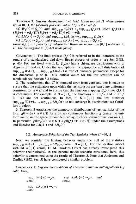
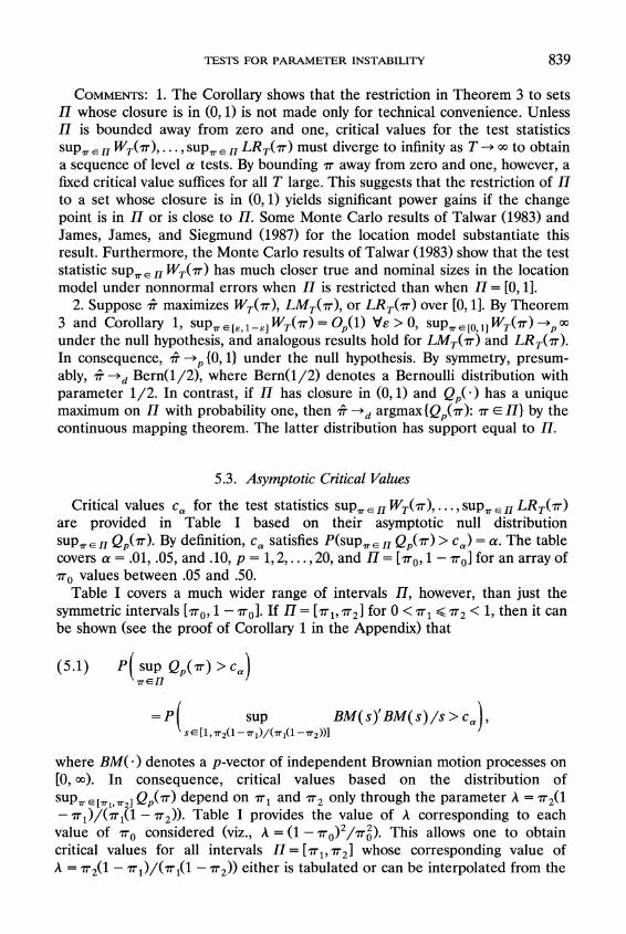
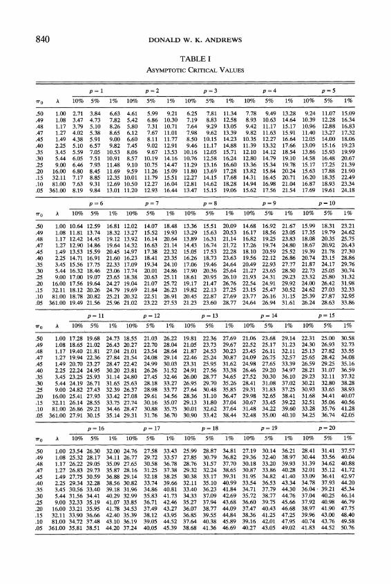
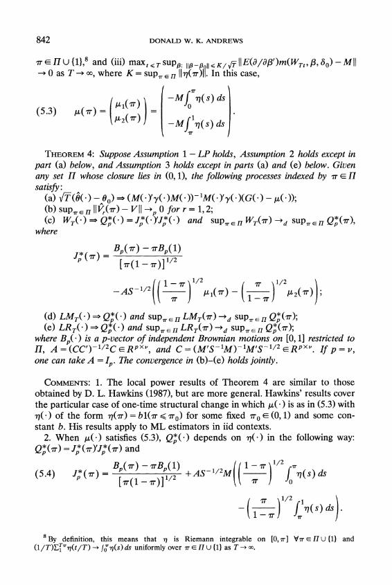
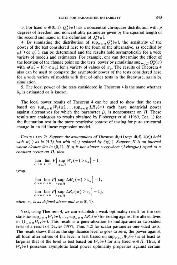
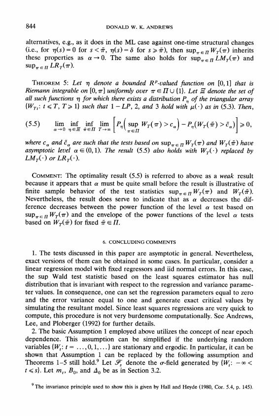
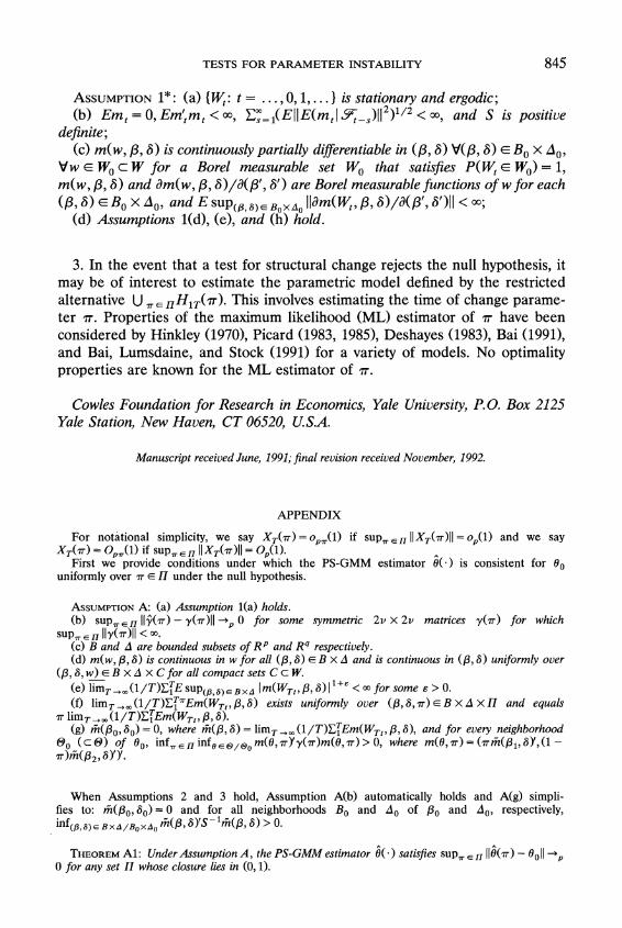
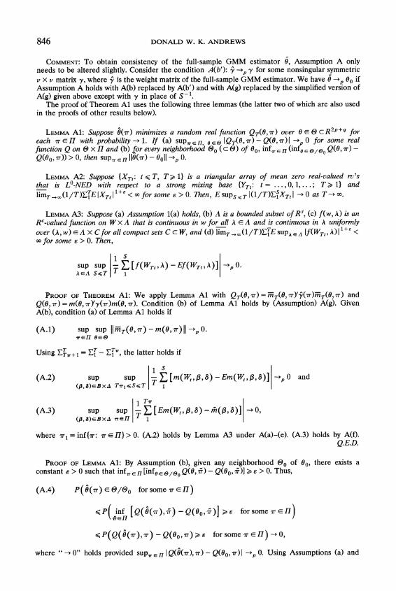
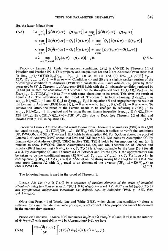
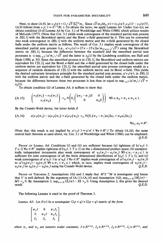
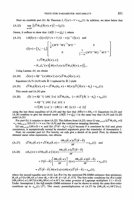