testing the marshall-lerner condition in kenya · increasingly empirical investigations have been...

Department of Economics and Finance

Working Paper No. 12-22

http://www.brunel.ac.uk/economics

Econ

omic

s an

d Fi

nanc

e W

orki

ng P

aper

Ser

ies

Guglielmo Maria Caporale, Luis A. Gil-Alana and Robert Mudida

Testing the Marshall-Lerner Condition in Kenya

September 2012

TESTING THE MARSHALL-LERNER CONDITION IN KENYA

Guglielmo Maria Caporale Centre for Empirical Finance, Brunel University, London, UK

Luis A. Gil-Alana*

Navarra Center for International Development, University of Navarra, Pamplona, Spain

and

Robert Mudida

Strathmore University, Nairobi, Kenya

September 2012

Abstract In this paper we examine the Marshall-Lerner (ML) condition for the Kenyan economy. In particular, we use quarterly data on the log of real exchange rates, export-import ratio and relative (US) income for the time period 1996q1 – 2011q4, and employ techniques based on the concept of long memory or long-range dependence. Specifically, we use fractional integration and cointegration methods, which are more general than standard approaches based exclusively on integer degrees of differentiation. The results indicate that there exists a well-defined cointegrating relationship linking the balance of payments to the real exchange rate and relative income, and that the ML condition is satisfied in the long run although the convergence process is relatively slow. They also imply that a moderate depreciation of the Kenyan shilling may have a stabilizing influence on the balance of payments through the current account without the need for high interest rates. Keywords: Marshall-Lerner condition, fractional integration, fractional cointegration JEL Classification: C22, C32, F32

Corresponding author: Professor Guglielmo Maria Caporale, Centre for Empirical Finance, Brunel University, West London, UB8 3PH, UK. Tel.: +44 (0)1895 266713. Fax: +44 (0)1895 269770. Email: [email protected] * Luis A. Gil-Alana gratefully acknowledges financial support from the Ministry of Education of Spain (ECO2011-2014 ECON Y FINANZAS, Spain) and from a Jeronimo de Ayanz project of the Government of Navarra.

1

1. Introduction

A lot of the literature on the balance of trade is based on the so-called "elasticity

approach", namely on testing the extent to which trade flows are responsive to relative

price changes, more specifically whether a devaluation improves the trade balance, which

implies that the well-known Marshall-Lerner (ML) condition holds. The seminal

empirical paper by Houthakker and Magee (1969) found inconclusive evidence. Several

subsequent studies using least-squares methods to estimate price elasticities in import and

export equations also produced mixed results (see, e.g., Khan 1974, Goldstein and Khan

1985, Wilson and Takacs 1979, Warner and Kreinin 1983, Bahmani-Oskooee 1986,

Krugman and Baldwin 1987). More recently, the evidence obtained with more advanced

econometric techniques taking into account non-stationarities in the data has been more

supportive of the ML condition (see, e.g., Bahmani-Oskooee 1998, Bahmani-Oskooee

and Niroomand 1998, Caporale and Chui 1999, Boyd, Caporale and Smith, 2001). Also,

increasingly empirical investigations have been based on a reduced-form equation for the

balance of trade, a method which allows to test directly for the response of trade flows to

relative price movements using the real exchange rate (as opposed to the terms of trade)

(see, e.g., Rose 1991, and Lee and Chinn 1998).

It is normally thought that a nominal devaluation or depreciation can only reduce

trade imbalances if it translates into a real one and if trade flows respond to relative prices

in a significant and predictable manner (Reinhart, 1995). A depreciation (or devaluation)

of the domestic currency may stimulate economic activity through an initial increase in

the price of foreign goods relative to home goods: by increasing the global

competitiveness of domestic industries it diverts spending from the former to the latter

(Kandil and Mirazaie, 2005).

2

Dornbusch (1988) shows that the effectiveness of a depreciation in improving the

balance of payments depends on redirecting demand in the right direction and by the

correct amount and also on the capacity of the domestic economy to meet the additional

demand through increased supply. Bird (2001) argues that there is no mechanism for

keeping the real exchange rate at an equilibrium level if inflation is rising quickly or for

changing equilibrium rates in the case of permanent real shocks. In his opinion, this is the

reason why many developing countries have chosen flexible exchange rates, although this

is not an ideal solution since demand and supply elasticities may be relatively low: even

when they satisfy the Marshall-Lerner conditions, their response to exchange rate

changes may not be as big as in developed economies. Moreover, with thin foreign

exchange markets floating exchange rates may be unstable and vulnerable to speculative

attacks as the Kenyan exchange rate crisis of 2011 illustrated (Mudida, 2012): if the

exchange rate is driven down sufficiently, it can generate additional inflation which may

offset the extra competitiveness associated with a depreciation.

A related issue is whether there exist J-curve effects, i.e. whether following a

currency depreciation or devaluation the balance of trade will worsen in the short run, but

then, as elasticities increase over time, it will begin to improve (Kulkarni and Clarke,

2009). Case studies on several African countries such as Zambia and Nigeria seem to

support empirically the existence of a J-curve. However, no studies have been carried out

yet to test the Marshall-Lerner condition in Kenya, which represents an interesting case

since its exports are relatively more diversified than those of the sub-Saharan African

economies. The present paper is the first to provide evidence for this country; moreover,

it uses advanced techniques in time series analysis, based on the concepts of fractional

integration and cointegration, which are more general than the standard methods based

3

exclusively on integer degrees of differentiation and have not been previously used to

analyse the Marshall-Lerner condition in an African context.

The layout of the paper is as follows. Section 2 discusses the importance of the

Marshall-Lerner condition in the Kenyan case. Section 3 briefly describes the theoretical

framework, whilst Section 4 presents the econometric analysis. Finally, Section 5

summarises the main findings and offers some concluding remarks.

2. The Marshall-Lerner condition and the Kenyan economy

The International Monetary Fund (IMF) classifies Kenya as having operated an

independent float between 1992 and 1997 and a managed float since 1998. Prior to that,

the Kenyan shilling was pegged first to the British pound, then to the US dollar, and

finally to the IMF’s Special Drawing Rights (SDRs) before a crawling peg based on a

trade-weighted basket was introduced. The Marshall-Lerner condition should therefore be

analysed in Kenya in the context of the current exchange rate system, which is a managed

float system, and indeed the data set used in this study covers the floating period.

Consequently, we consider a depreciation rather than a devaluation of the Kenyan shilling

since this is what is relevant for the period under investigation. The existing empirical

evidence on the operation of Kenya’s managed float system suggests that at times of

relative tranquillity in foreign exchange markets the Central Bank of Kenya can smooth

out exchange rate volatility with relatively modest interventions; by contrast, more active

policies are required in the presence of more volatile exchange rates (O’Connell et. al,

2010).

Testing the Marshall-Lerner condition is particularly important in the Kenyan case

because, as in many other developing countries, the current account of the Kenyan

balance of payments is persistently in deficit. The issue of whether a depreciation of the

4

exchange rate can reduce this deficit therefore becomes critical. A large share of Kenyan

exports is represented by agricultural products with low price elasticities of demand.

However, horticultural products and manufactured goods are also exported. Indeed,

Kenya’s largest trading partner is Uganda which imports primarily manufactured goods

from Kenya. On the other hand, Kenyan imports are primarily made up of agricultural

machinery, petroleum and manufactured goods which one would expect to have a low

price elasticity of demand for imports owing to their critical role in the development

process. This raises the interesting question of the size of real exchange depreciation

required to eliminate Kenya’s balance of payments current account deficit.

The broader issue related to the Marshall-Lerner condition in Kenya is that of real

exchange targets for the Central Bank of Kenya, namely is there an optimal real exchange

rate that should be targeted? A real exchange rate appreciation redirects resources from

the export-producing sector penalizing it and causing potentially severe welfare losses

(Rodrik, 2008). Pollin and Heintz (2007) have advocated the adoption of a new monetary

policy framework in Kenya in order to achieve a more sizeable depreciation of the

shilling in real terms. They stress that the contribution of the export sector, which is

favoured by a real exchange depreciation, is unique from a development perspective

owing to the number and quality of jobs created and also to the productivity spillovers to

other sectors of the economy. The challenge of an excessively weak Kenya shilling,

however, was illustrated in 2011 when a vicious cycle was created between inflation and

depreciation (Mudida, 2012). This paper therefore also aims to contribute to the debate on

the target for the real exchange rate of the Kenya shilling, which is a particularly

interesting one because the primary task of the Central Bank of Kenya is price stability, at

present being pursued through inflation targeting, with expected inflation as the nominal

anchor. It is well known that inflation targeting may be counterproductive in the presence

5

of supply-side shocks, which are prevalent in the Kenyan economy (Adam et. al, 2010).

Therefore analysing the Marshall-Lerner condition in Kenya is also important in view of

the concerns facing the Kenyan monetary authorities.

3. Theoretical Framework

The balance of trade can be expressed as the ratio of nominal exports to nominal imports,

B, which is equal to the ratio of the volume of exports, X, multiplied by domestic prices,

P, to the volume of imports M, multiplied by foreign prices, P*, and the nominal spot

exchange rate S:

,MSP

XPBtt

*t

ttt =

or using lower case letters for logarithms:

( ) ,emxppsmxb ttt*tttttt −−=+−−−= (1)

where *tttt ppse +−= is the real exchange rate. Long-run import and export demand

are given by:

teyx xtx*t

*xt γ+η+β+α= , (2)

teym mtmtmt γ+η−β+α= . (3)

where yt and yt* stand for domestic and foreign real income respectively, the trends

capture terms of trade effects, and ηx and ηm represent the export and income elasticities

respectively.

The long-run balance of trade is

t)(e)1(yy)(b mxtmxt*t

*yxt γ−γ+−η+η+β−β+α−α=

. (4)

The coefficient on et gives the familiar Marshall-Lerner condition for a

devaluation (increase in et) to improve the balance of payments (i.e., this coefficient

6

needs to be statistically significant and positive for the ML condition to be satisfied,

which means that the sum of the demand elasticity for imports and the foreign demand

elasticity for the nation’s export exceeds unity). Solvency requires bt = 0 in the long run,

whilst Purchasing Power Parity (PPP) requires et = e, for all t.

The long-run relationship (4) can be written as

,teyyb tt*t

*t γ+η+β−β+α= (5)

where α = (αx - αm); η = (ηx – ηm - 1), and γ = (γx – γm), and the deviations from the long-

run equilibrium can be defined as

.bteyyz ttt*t

*t −γ+η+β−β+α= (6)

4. Econometric Analysis

We use quarterly data on the log of real exchange rates, export-import ratio and relative

(US) income for the time period 1996q1 – 2011q4. All series were obtained from the

Central Bank of Kenya. The base period for the real effective exchange rate is January

2003. The real effective exchange rate is constructed using a basket including the eight

countries which are Kenya’s most important trading partners, and is defined in such a

way that an increase represents a depreciation, i.e. a direct quote is used as common in

developing countries.

Figure 1 displays the three series (in logs) in both levels and first differences. The

export/import ratio and the real exchange rate decline over the sample period, whilst

relative income increases. The first differenced series data show that seasonality is an

important feature of these data, especially for the export/import ratio and relative income.

[Insert Figures 1 – 3 about here]

Figure 2 displays the first thirty sample autocorrelations for the original series and

their first differences. The slow decay for the series in levels indicates that they may be

7

nonstationary, while the sample autocorrelations for the first differences suggest once

more the presence of seasonality, especially in the case of relative income. Finally, Figure

3 displays the periodograms. For the series in levels the highest value corresponds to the

smallest frequency, which indicates that they may require differencing. However, the

periodogram of the first differenced export/import ratio series has a value close to zero at

the smallest frequency, suggesting that this series may now be overdifferenced.

As a first step we check the order of integration of the three series by means of

standard methods such as ADF (Dickey and Fuller, 1979), Phillips and Perrron (PP,

1988), Kwiatkowski et al. (KPSS, 1992), Elliot et al. (ERS, 1996) and Ng and Perron

(NG, 2001) tests. The results (not reported) are conclusively in favour of unit roots for the

real exchange rate and relative income, whilst mixed evidence is found in the case of the

export/import ratio. However, they should be taken with caution, since the above methods

have limitations such as very low power if the true Data Generating Process (DGP) is

fractionally integrated (see, e.g., Diebold and Rudebusch, 1991; Hassler and Wolters,

1994; Lee and Schmidt, 1996 among others). Thus, in what follows we consider models

that allow for both integer and fractional orders of differentiation.

We estimate d (the differencing parameter) using the Whittle function in the

frequency domain (Dahlhaus, 1989) and also employ a testing procedure developed by

Robinson (1994) which has been shown to be the most efficient in the context of I(d)

models. The latter method is parametric, so a parametric model for the disturbances term

has to be specified. A semiparametric method, also based on the Whittle function

(Robinson, 1995, Abadir et al., 2007) will also be employed.

We report in Table 1 the estimated values of d in a model given by

,)1(; ttd

tt uxLxty =−++= βα (7)

8

where yt is the observed (univariate) time series; α and β are the coefficients on the

intercept and a linear trend respectively, and xt is assumed to be an I(d) process. Thus, ut

is I(0) and given the parametric nature of this method its functional form must be

specified. We assume that ut is a white noise, autocorrelated and seasonally

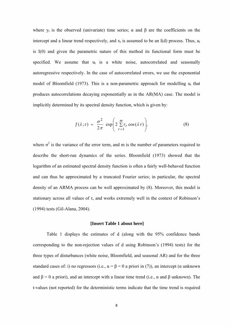
autoregressive respectively. In the case of autocorrelated errors, we use the exponential

model of Bloomfield (1973). This is a non-parametric approach for modelling ut that

produces autocorrelations decaying exponentially as in the AR(MA) case. The model is

implicitly determined by its spectral density function, which is given by:

,)(cos2exp2

);(1

2

⎟⎟⎠

⎞⎜⎜⎝

⎛∑==

m

rr rf λτ

πστλ (8)

where σ2 is the variance of the error term, and m is the number of parameters required to

describe the short-run dynamics of the series. Bloomfield (1973) showed that the

logarithm of an estimated spectral density function is often a fairly well-behaved function

and can thus be approximated by a truncated Fourier series; in particular, the spectral

density of an ARMA process can be well approximated by (8). Moreover, this model is

stationary across all values of τ, and works extremely well in the context of Robinson’s

(1994) tests (Gil-Alana, 2004).

[Insert Table 1 about here]

Table 1 displays the estimates of d (along with the 95% confidence bands

corresponding to the non-rejection values of d using Robinson’s (1994) tests) for the

three types of disturbances (white noise, Bloomfield, and seasonal AR) and for the three

standard cases of: i) no regressors (i.e., α = β = 0 a priori in (7)), an intercept (α unknown

and β = 0 a priori), and an intercept with a linear time trend (i.e., α and β unknown). The

t-values (not reported) for the deterministic terms indicate that the time trend is required

9

in all cases. The upper part of the table refers to the case of white noise disturbances.

Focusing on the case of a linear trend, we see that the estimated value of d for the

log(export/import) ratio is 0.373, and the confidence interval excludes the cases of

stationarity I(0) (d = 0) and nonstationary unit roots (d =1). For the real exchange rate, the

estimated d is 0.888 and the unit root null hypothesis cannot be rejected at the 5% level.

Finally, for relative income, the estimated value of d is 0.664 and the I(1) case is rejected

in favour of mean reversion (d < 1). The results based on the assumption of

autocorrelation as in the model of Bloomfield (1973) (with m = 1)1 are displayed in Table

1(ii). The estimated values of d (for the case of a linear trend) are 0.574, 0.728 and 0.865

respectively for the export/import ratio, real exchange rates and relative income, and the

unit root null cannot be rejected in the last two cases. Finally, when imposing seasonal

(quarterly) autoregressions, these values are 0.376, 0.899 and 0.963 and similarly to the

previous case the I(1) hypothesis cannot be rejected for real exchange rates and relative

income, while it is rejected in favour of mean reversion for the export/import ratio.

The above results are corroborated by those based on the semiparametric method

of Robinson (1995). This is essentially a local ‘Whittle estimator’ in the frequency

domain, which uses a band of frequencies degenerating to zero. The estimator is

implicitly defined by:

,log12)(logminargˆ1

⎟⎟⎠

⎞⎜⎜⎝

⎛−= ∑

=

m

ssd m

ddCd λ (9)

,01,2,)(1)(1

2 →+=∑== T

mmT

sIm

dC sm

s

dss

πλλλ

where I(λs) is the periodogram of the raw time series, and d ∈ (-0.5, 0.5). Under

finiteness of the fourth moment and other mild conditions, Robinson (1995) proved that:

1 Other values of m produced essentially the same results.

10

,)4/1,0()ˆ( * ∞→→− TasNddm dtb

where d* is the true value of d. This estimator is robust to a certain degree of conditional

heteroscedasticity (Robinson and Henry 1999) and is more efficient than other semi-

parametric competitors.2

[Insert Figure 4 about here]

Figure 4 display the estimates of d in (9) along with the 95% confidence interval

corresponding to the I(0) and I(1) cases. The horizontal axis reports the bandwidth

parameter while the vertical one the estimates of d. For the export/import ratio some of

the estimates are within the I(1) interval but most are below it although above the I(0)

one. For the real exchange rate, most of the estimates of d are within the I(1) interval.

Finally, for relative income, they are above the I(1) interval if the bandwidth parameter is

low, whilst are within it if it is large. This may be a consequence of the strong seasonal

pattern observed in this series.3 It is also consistent with the results reported for the

parametric case above where the unit root cannot be rejected in case of the exchange rate

(and in some cases for relative income) and is rejected in favour of mean reversion for the

export/import ratio.

Considering again the results presented in Table 1, we next select the best model

specification for each series. We conducted several diagnostic tests on the residuals of the

estimated models, and, in particular, we used Box-Pierce and Ljung-Box-Pierce statistics

(Box and Pierce, 1970; Ljung and Box, 1978) to test for no serial correlation, as well as

LR tests and other likelihood criteria.4 The selected models for each variable are the

following:

2 This method has been further refined by Velasco (1999), Velasco and Robinson (2000), Phillips and Shimotsu (2004, 2005), Abadir et al. (2007) and others. When using these approaches the results were practically identical to those reported in the paper. 3 The bandwidth determines the trade-off between the bias and the variance in the estimation of d. 4 Specifically, the AIC and the SIC. Note, however, that these criteria might not necessarily be the best ones in applications involving fractional differences, as they focus on the short-term forecasting ability of the

11

)291.0(Bloomfieldu)00.3()09.5(

,ux)L1(,xt0081.04073.0y

t

tt573.0

tt

−=τ≈−−

=−+−−=

for the export/import ratio. (t-values in parenthesis).

For the real exchange rate, the selected model is

)208.0(Bloomfieldu)71.3()12.135(

,ux)L1(,xt0064.06981.4y

t

tt728.0

tt

=τ≈−

=−+−=

Finally, for relative income,

t4tt

tt963.0

tt

u893.0u)19.5()33.204(

,ux)L1(,xt0106.08257.3y

ε+=−−

=−+−−=

− .

The fact that the confidence intervals for the fractional differencing parameters in

the selected models overlap for the three series5 implies that the null of equal orders of

integration cannot be rejected. This is important since it makes it legitimate to run an

OLS regression with the three variables to check if the estimated errors are I(0) or at least

mean-reverting with a smaller order of integration than the three parent series.6

We follow a two-step procedure, similar to that of Engle and Granger (1987), but

specifically designed to allow for fractional integration. In the first step, we compute the

following regression,

,xzzy tt22t11t +β+β+α= (10)

fitted model and may not give sufficient attention to their long-run properties (see, e.g. Hosking, 1981, 1984). 5 These intervals are (0.267, 0.975) for the export/import ratio, (0.441, 1.124) for the real exchange rate, and (0.763, 1.247) for relative income (see Table 1). 6 We also compute an adaptation of the Robinson and Yajima (2002) statistic xyT̂ for log-periodogram

estimation in pairwise comparisons of the three series; the results support the hypothesis of homogeneity in the orders of integration.

12

where yt stands for the balance of trade, z1t for the real exchange rate and z2t for relative

income. Then, in the second step, we estimate the order of integration of the residuals

from (10) using the methods employed above for the univariate analysis.

Performing the OLS regression in (10) we obtain

)89.4()77.1()84.6(

.x̂z6643.0z0942.04087.3y tt2t1t

−−

+−+−= (11)

The estimated residuals are plotted in Figure 4. The positive (and statistically significant)

coefficient on the real exchange rate indicates that the ML condition is satisfied in Kenya.

[Insert Figure 4 and Table 2 about here]

Table 2 displays the estimated values of d for the OLS residuals. We consider

again the three standard cases of no regressors, an intercept and a linear trend, for white

noise, Bloomfield, and seasonal AR disturbances. The estimates are all in the range (0.23,

0.25) being substantially smaller than those for the individual series and thus supporting

the existence of mean reversion in the long-run equilibrium relationship. If we focus now

on the confidence intervals we see that the null hypothesis of I(0) errors is rejected for the

cases of white noise and seasonal AR disturbances in favour of positive orders of

integration, while this hypothesis cannot be rejected with autocorrelated (Bloomfield)

disturbances.

The most adequate specification for the estimated residuals in the cointegrating

regression (10) appears in bold in Table 2. This model includes an intercept and seasonal

AR disturbances. We also perform the Hausman-type test of no cointegration against the

alternative of fractional cointegration proposed by Marinucci and Robinson (2001); the

results (not reported) strongly reject the null for different bandwidth parameters given

further support to the hypothesis of cointegration among the variables examined.

13

5. Conclusions and Policy Recommendations

Our findings support the existence of a well-defined cointegrating relationship between

the balance of payments, the real exchange rate and relative income and indicate that the

Marshall-Lerner condition holds in Kenya. Our analysis is based on fractional integration

and cointegration methods, which are more general than the standard methods allowing

only for integer degrees of differentiation. Studies using the latter to test the Marshall-

Lerner condition in many African countries are either inconclusive or tend to suggest that

it does not hold in the short run although it may hold in the long run. The evidence (based

on more general methods) that it holds in Kenya has important policy implications for

this country. It implies that the exchange rate is an important tool for attempting to

address persistent balance of payments current account deficits in Kenya and can

therefore contribute to achieving an external balance.

The fact that the Marshall-Lerner condition holds means that a depreciation of the

exchange rate leads to a reduction in import expenditure and an increase in export sales.

This reflects an important transition made in Kenya in terms of the composition of

exports: from traditional agricultural exports exhibiting low export elasticities of demand

to more diversified non-traditional exports such as horticulture and manufactured goods

that exhibit a higher elasticity of demand. Our results indicate that a depreciation in the

Kenya shilling can therefore have potentially beneficial effects on Kenya’s current

account deficit. These, however, have to be weighed against the higher inflation rate

associated with such an exchange rate movement. Inflationary effects were evident

during the 2011 foreign exchange crisis in Kenya when a depreciation of 30% of the

Kenya shilling against the US dollar led to month-on-month inflation of 19% by the end

of 2011 (Mudida, 2012).

14

Given that at present the primary objective of the Central Bank of Kenya is price

stability, the focus recently has been on maintaining high interest rates so as to reduce the

inflation rate and also to avoid a significant depreciation of the Kenya shilling. This tight

monetary policy stance is thought to reduce inflationary pressure and also to promote

portfolio investment inflows into Kenya, thus improving the capital account. High

interest rates tend to have a detrimental effect on economic growth. Our findings,

however, suggest that a moderate depreciation of the Kenyan shilling may in fact have a

stabilizing influence on the balance of payments through the current account without the

need for high interest rates. Thus a less contractionary monetary policy by the Central

Bank of Kenya could in fact be combined with an appropriate exchange rate policy to

achieve more effectively the objectives of internal and external balance in Kenya. This

would be a better option than the current high interest rate policy being pursued by the

Central Bank that achieves external balance but only at the high cost of stifling economic

growth.

Other recently developed bivariate or multivariate fractional cointegration testing

methods (e.g. Johansen, 2010; Nielsen, 2010; Nielsen and Frederiksen, 2011) could also

be applied. This could be very useful to investigate possible J-curve effects in the context

of a much richer structure including other underlying dynamics and short-run

components. Structural breaks and non-linearities could also be examined in the context

of fractional integration. These issues will be investigated in future papers.

15

References Abadir, K.M., W. Distaso and L. Giraitis. 2007. Nonstationarity-extended local Whittle estimation. Journal of Econometrics 141: 1353-84. Adam, C.S., B.O. Maturu, N.S. Ndung’u and S.A. O’Connell (2010), ‘Building a Kenyan Monetary Policy Regime for the Twenty-first Century’ in C.S. Adam, P. Collier and N.S. Ndung’u (eds) Kenya: Policies for Prosperity Oxford: Oxford University Press. Bahmani-Oskooee, M. (1986), "Determinants of international trade flows: the case of developing countries", Journal of Development Economics, 20, 107-123. Bahmani-Oskooee, M. (1998), "Cointegration approach to estimate the long-run trade elasticities in LDCs", International Economic Journal, 12, 3, 89-96. Bahmani-Oskooee, M. and F. Niroomand (1998), "Long-run price elasticities and the Marshall-Lerner condition revisited", Economics Letters, 61, 101-109. Bird, G. (2001) “Conducting macroeconomic policy in developing countries: piece of cake or mission impossible?” Third World Quarterly, Vol. 22, No. 1, pp. 37-49. Bloomfield, P., 1973, An exponential model in the spectrum of a scalar time series, Biometrika 60, 217-226. Box, G.E.P. and D.A. Pierce, 1970, Distribution of residual autocorrelations in autoregressive integrated moving average time series models, Journal of the American Statistical Association 65, 1509-1526. Boyd, D., Caporale, G.M. and R. Smith (2001), "Real exchange rate effects on the balance of payments: cointegration and the Marshall-Lerner condition", International Journal of Finance and Economics, 6, 3, 187-200. Caporale, G.M., and M.K.F. Chui (1999), "Estimating income and price elasticities of trade in a cointegration framework", Review of International Economics, 7, 2, 192-202. Dahlhaus. R., (1989), “Efficient parameter estimation for self-similar processes”, Annals of Statistics 17, 1749-1766. Dickey, D.A. and W.A. Fuller, 1979, Distribution of the estimators for autoregressive time series with a unit root, Journal of the American Statistical Association 74, 355-367. Diebold, F.X., and G.D. Rudebusch (1991). “On the power of Dickey-Fuller test against fractional alternatives”. Economics Letters, 35: 155-160. Dornbusch R (1988) Open Economy Macroeconomics, Second Edition, New York, 1988. Elliot, G., Rothenberg, T. & Stock, J. (1996). Efficient tests for an autoregressive unit root. Econometrica, 64, 813-36.

16

Gil-Alana, L.A, 2004, The use of the model of Bloomfield as an approximation to ARMA processes in the context of fractional integration, Mathematical and Computer Modelling 39, 429-436. Goldstein, M. and M.S. Khan (1985), "Income and price effects in foreign trade", in R.W. Jones and P.B. Kenen (eds.), Handbook of International Economics, North-Holland, Amsterdam, 1041-1105. Hasslers, U., and J. Wolters (1994). “On the power of unit root tests against fractional alternatives”. Economics Letters, 45: 1-5. Hosking, J.R.M., 1981, Fractional differencing, Biometrika 68, 165-176. Hosking, J.R.M., 1984, Modelling persistence in hydrological time series using fractional differencing, Water Resources Research 20, 1898-1908. Houthakker, H. and S. Magee (1969), "Income and price elasticites in world trade", Review of Economics and Statistics, 51, 11-125. Kandil M. and I. Mirazaie (2005) “The Effects of Exchange Rate Fluctuations on Output and Prices: Evidence from Developing Countries” The Journal of Developing Areas, Vol. 38, No.2, Spring. Khan, M. (1974), "Import and export demand in developing countries", IMF Staff Papers, 21, 678-693. Krugman, P.R. and R.E. Baldwin (1987), "The persistence of the US trade deficit", Brookings Papers on Economic Activity, 1, 1-43. Kulkarni and Clarke (2009) “Testing the J-curve Hypothesis: Case Studies from Around the World” International Economics Practicum, Final Paper. Kwiatkowski, D., Phillips, P.C.B., Schmidt, P., Shin, Y. (1992). Testing the null hypothesis of stationarity against the alternative of a unit root. Journal of Econometrics, 54, 159-178. Lee, J. and M.D. Chinn (1998), "The current account and the real exchange rate: a structural VAR analysis of major currencies", NBER W.P. no. 6495. Lee, D., and Schmidt, P (1996). “On the power of the KPSS test of stationarity against fractionally integrated alternatives”. Journal of Econometrics, 73: 285-302. Ljung, G.M. and G.E.P. Box, 1978, On a measure of lack of fit in time series models, Biometrika 65, 297-303. Marinucci, D. and P.M. Robinson (2001) Semiparametric fractional cointegration analysis, Journal of Econometrics 105, 225-247.

17

Mudida R (2012), “The Evolution and Management of Kenya’s 2011 Exchange Rate Crisis” Working Paper presented at the Navarre Development Week, University of Navarra, 4-8th June 2012. Ng, S. & Perron, P. (2001). Lag length selection and the construction of unit root tests with good size and power. Econometrica, 69, 1519-54. O’Connell, S.A., B.O. Maturu, f.m. Mwega, N. Ndung’u and R.W. Ngugi (2010) “Capital Mobility, Monetary Policy and Exchange Rate Management in Kenya” in C.S. Adam, P. Collier and N.S. Ndung’u (eds) Kenya: Policies for Prosperity Oxford: Oxford University Press. Phillips, P.C.B. and K. Shimotsu, 2004. Local Whittle estimation in nonstationary and unit root cases. Annals of Statistics 32, 656-692. Phillips, P.C.B. and K. Shimotsu, 2005. Exact local Whittle estimation of fractional integration. Annals of Statistics 33, 1890-1933. Pollin R. and J. Heintz (2007), ‘Expanding Decent Employment in Kenya: The Role of Monetary Policy, Inflation Control and the Exchange Rate.’ International Poverty Country Study No. 6, March. Phillips, P.C.B. & Perron, P. (1988). Testing for a unit root in time series regression. Biometrika, 75, 335-346. Reinhart, C.M., 1995, Devaluation, relative prices and international trade: evidence from developing countries. IMF Staff papers, 42, 2, 290-312. Robinson, P.M., 1994, Efficient tests of nonstationary hypotheses. Journal of the American Statistical Association 89, 1420-1437. Robinson, P.M., 1995. Gaussian semiparametric estimation of long range dependence. Annals of Statistics 23, 1630-1661. Robinson, P.M. and M. Henry. 1999. Long and short memory conditional heteroskedasticity in estimating the memory in levels. Econometric Theory 15: 299-336. Robinson, P.M. and Y. Yajima (2002), Determination of cointegrating rank in fractional systems, Journal of Econometrics 106, 217-241. Rodrick D. (2008), The Real Exchange and Economic Growth. Cambridge: John F. Kennedy School of Government, Harvard University. Rose, A.K. (1991), "The role of exchange rates in a popular model of international trade: Does the `Marshall-Lerner' condition hold?", Journal of International Economics, 30, 301-316. Velasco, C., 1999b. Gaussian semiparametric estimation of nonstationary time series. Journal of Time Series Analysis 20, 87-127.

18

Velasco, C. and P.M. Robinson (2000) Whitle pseudo maximum likelihood estimation for nonstationary time series. Journal of the American Statistical Association 95, 1229-1243. Warner, D. and M.E. Kreinin (1983), "Determinants of international trade flows", Review of Economics and Statistics, 65, 96-104. Wilson, J.F. and W.E. Takacs (1979), "Differential responses to price and exchange rate influences in the foreign trade of selected industrial countries", Review of Economics and Statistics, 61, 267-279.

19

Figure 1: Original series and first differences

LOG(EXP/IMP) = x1t (1 – L)x1t

-1,2

-1

-0,8

-0,6

-0,4

-0,2

0

1996q1 2011q4-0,4

-0,2

0

0,2

0,4

1996q2 2011q4

LOG(REER) = x2t (1 – L)x2t

3,8

4

4,2

4,4

4,6

4,8

1996q1 2011q4-0,15

-0,05

0,05

0,15

1996q2 2011q4

LOG(NOMGNP/USGNP) = x3t (1 – L)x3t

-4

-3,8

-3,6

-3,4

-3,2

-3

1996q1 2011q4-0,15

-0,05

0,05

0,15

1996q2 2011q4

EXP/IMP = Export/Import ratio; REER = Real Effective Exchange Rate; NOMGNP = Nominal GNP and USGNP= US GNP.

20

Figure 2: Correlograms of the original series and first differences


-0,4

0

0,4

0,8

1,2

1 4 7 10 13 16 19 22 25 28 31-0,8

-0,4

0

0,4

0,8

1 3 5 7 9 11 13 15 17 19 21 23 25 27 29


-0,4

0

0,4

0,8

1,2

1 4 7 10 13 16 19 22 25 28 31-0,3

-0,1

0,1

0,3

1 3 5 7 9 11 13 15 17 19 21 23 25 27 29


-0,4

0

0,4

0,8

1,2

1 4 7 10 13 16 19 22 25 28 31

-0,5

-0,1

0,3

0,7

1 3 5 7 9 11 13 15 17 19 21 23 25 27 29

The thick lines give the 95% confidence band for the null hypothesis of no autocorrelation.

21

Figure 3: Periodograms of the original series and first differences


0

0,02

0,04

0,06

0,08

1 4 7 10 13 16 19 22 25 28 310

0,004

0,008

0,012

0,016

1 3 5 7 9 11 13 15 17 19 21 23 25 27 29 31


0

0,02

0,04

0,06

0,08

0,1

1 4 7 10 13 16 19 22 25 28 310

0,0005

0,001

0,0015

0,002

1 3 5 7 9 11 13 15 17 19 21 23 25 27 29 31


0

0,05

0,1

0,15

0,2

1 4 7 10 13 16 19 22 25 28 310

0,001

0,002

0,003

0,004

1 3 5 7 9 11 13 15 17 19 21 23 25 27 29 31

The horizontal axis refers to the discrete Fourier frequencies λj = 2πj/T, j = 1, …, T/2.

22

Table 1: Estimates of d and 95% confidence bands for the three individual series i) White noise disturbances

No regressors An intercept A linear time trend

LOG(EXP/IMP) 0.511 (0.372, 0.714)

0.493 (0.413, 0.605)

0.373 (0.258, 0.536)

LOG(REER) 0.934 (0.787, 1.148)

0.883 (0.742, 1.129)

0.888 (0.740, 1.129)

LOG(NOM/USGNP) 0.949 (0.792, 1.174)

0.755 (0.691, 0.856)

0.664 (0.569, 0.802)

ii) Bloomfield‐type disturbances


LOG(EXP/IMP) 0.728 (0.394, 1.144)

0.643 (0.422, 0.971)

0.574 (0.267, 0.975)

LOG(REER) 0.842 (0.552, 1.234)

0.803 (0.637, 1.117)

0.728 (0.441, 1.124)

LOG(NOM/USGNP) 0.824 (0.543, 1.173)

0.892 (0.741, 1.074)

0.865 (0.673, 1.093)

iii) Seasonal (quarterly) AR disturbances


LOG(EXP/IMP) 0.495 (0.321, 0.734)

0.495 (0.361, 0.626)

0.376 (0.223, 0.569)

LOG(REER) 0.857 (0.546, 1.155)

0.896 (0.745, 1.134)

0.899 (0.723, 1.137)

LOG(NOM/USGNP) 0.885 (0.574, 1.173)

0.969 (0.802, 1.262)

0.963 (0.763, 1.247)

23

Figure 4: Estimates of d and 95% confidence bands for the three individual series i) LOG(EXP/IMP)

-1-0,5

00,5

11,5

2

1 4 7 10 13 16 19 22 25 28 31

ii) LOG(REEF)

-1-0,5

00,5

11,5

2

1 4 7 10 13 16 19 22 25 28 31

iii) Log(NOM/USGNP)

-1-0,5

00,5

11,5

2

1 4 7 10 13 16 19 22 25 28 31

The horizontal axis concerns the bandwidth parameter while the vertical one refers to the estimated value of d. The thick lines give the 95% confidence bands for the I(0) and I(1) hypotheses.

24

Figure 4: Estimated residuals from the cointegrating regression

-0,4

-0,2

0

0,2

0,4

1966q1 2011q4

Table 2: Estimates of d and 95% confidence bands for the three individual series i) White noise disturbances


White noise 0.239 (0.089, 0.435)

0.239 (0.089, 0.434)

0.241 (0.091, 0.436)

Bloomfield 0.255 (‐0.046, 0.575)

0.258 (‐0.050, 0.579)

0.259 (‐0.048, 0.579)

Seasonal AR 0.244 (0.072, 0.453)

0.244 (0.071, 0.452)

0.246 (0.072, 0.455)

testing the marshall-lerner condition in kenya · increasingly empirical investigations have been...

Documents