testing the fractionally integrated hypothesis using m
TRANSCRIPT


Lisbon, 2018 • www.bportugal.pt
Working Papers 2018
JULY 2018 The analyses, opinions and findings of these papers representthe views of the authors, they are not necessarily those of the
Banco de Portugal or the Eurosystem
Please address correspondence toBanco de Portugal, Economics and Research Department
Av. Almirante Reis, 71, 1150-012 Lisboa, PortugalTel.: +351 213 130 000, email: [email protected]
17Testing the fractionally
integrated hypothesis using M estimation: With an application
to stock market volatility
Matei Demetrescu | Paulo M. M. Rodrigues | Antonio Rubia

Working Papers | Lisbon 2018 • Banco de Portugal Av. Almirante Reis, 71 | 1150-012 Lisboa • www.bportugal.pt •
Edition Economics and Research Department • ISBN (online) 978-989-678-595-6 • ISSN (online) 2182-0422

Testing the fractionally integrated hypothesisusing M estimation: With an application to stock
market volatility
Matei DemetrescuChristian-Albrechts-University of Kiel
Paulo M. M. RodriguesBanco de Portugal
NovaSBE, Universidade Nova deLisboa
Antonio RubiaUniversity of Alicante
July 2018
AbstractA new class of tests for fractional integration in the time domain based on M estimation isdeveloped. This approach offers more robust properties against non-Gaussian errors thanleast squares or other estimation principles. The asymptotic properties of the tests arediscussed under fairly general assumptions, and for different estimation approaches basedon direct optimization of the M loss-function and on iterated k-step and reweighted LSnumeric algorithms. Monte Carlo simulations illustrate the good finite sample performanceof the new tests and an application to daily volatility of several stock market indices showsthe empirical relevance of the new tests.
JEL: C12, C22
Correspondence to: Paulo M. M. Rodrigues, Economics and Research Department, Banco dePortugal, Av. Almirante Reis, 71-6th floor, 1150-012 Lisbon, Portugal. Tel. (351) 213130831.The opinions expressed in the paper are those of the authors and do not necessarily coincidewith those of Banco de Portugal or the Eurosystem. Any errors and omissions are the soleresponsibility of the authors.E-mail: ; [email protected];
Working Papers 2
1. Introduction
Most unit root and cointegration tests build on least squares (LS) estimation.This principle ensures efficiency under Gaussian conditions. In practice,however, macroeconomic and financial variables are usually driven by heavy-tailed distributions. In this context, LS-based tests remain asymptotically validunder appropriate conditions, but are no longer efficient. Suitable alternatives,which either accommodate the true likelihood of the data or ensure more robustproperties against deviations from normality, can exhibit improved power. Thisconsideration becomes particularly relevant in stochastic-trend detection andpersistence analysis because the relative losses in power from using inefficienttests tend to be greater under nonstationarity; see, among others, Rothenbergand Stock (1997) and Georgiev, Rodrigues and Taylor (2017).
This concern is extensible to fractionally integrated models (Beran, 1994;Haldrup and Nielsen, 2003; Tolvi, 2003), which generalize the unit root settingand provide a convenient form to describe long-range dependence; see Baillie(1996) and Robinson (2003) for reviews. While the unit root literature hassuggested alternative procedures to deal with non-Gaussian errors (see, amongothers, Lucas, 1993; Campbell and Dufour, 1995; Phillips, 1995; Herce, 1996;Breitung and Gourieroux, 1997; Rothenberg and Stock, 1997; Hasan andKoenker, 1997; Wright 2000; Ling and McAleer, 2004; Koenker and Xiao 2004;and Galvao, 2009), there have been little attempts to develop robust tests forfractional integration. To the best of our knowledge, only the tests in Delgadoand Velasco (2005), based on signed residuals, and Hassler, Rodrigues andRubia (2016), based on quantile regression (QR), ensure a form of robustnessin the estimation of the fractional parameter in a general context characterizedby either stationary or nonstationary dynamics with errors drawn from a heavy-tailed distribution.1
In this paper, we propose a class of tests for fractional integration in thetime domain under M estimation; see Huber (1981) and Amemiya (1985)for a review of this topic. This framework is fairly general and encompassesdifferent estimation techniques including, among others, LS, QR and maximumlikelihood (ML) estimation. The main interest is on the class of weightingfunctions that reduce the influence of large observations and, therefore, lead torobust properties against heavy-tailed distributions. This analysis extends thetests for fractional integration in Breitung and Hassler (2002), Demetrescu,Kuzin and Hassler (2008) and Hassler et al. (2009) to a non-Gaussianframework. We discuss the asymptotic properties of the new tests under fairly
1. Beran (1994) proposes an approximated maximum likelihood estimator based on theautoregressive representation of a stationary ARFIMA model which belongs to a class of M-estimators; see also Agostinelli and Bisaglia (2010). Li and Li (2008) discuss the asymptoticproperties of LAD estimators of stationary ARFIMA models in a Laplace quasi-maximumlikelihood estimation setting.

3 Testing the fractionally integrated hypothesis using M estimation
general conditions on the data generating process, and for different estimationstrategies based on direct optimization of the M loss-function and on iteratedk-step and reweighted LS numeric algorithms. As in the LS context, the nullasymptotic distribution of these tests is shown to be standard normal andindependent of the value of the fractional integration parameter. Monte Carloexperimentation shows that M tests for fractional integration exhibit empiricalsize close to the nominal level in finite samples and enhanced power in relationto alternative procedures, such as LS and even QR, when innovations are drawnfrom heavy-tailed distributions.
The empirical section addresses the long-run dynamics of different volatilitymeasures of stock market indices in developed and emerging markets. Inparticular, we consider daily observations for the period 2000-2016 of logabsolute returns and log price range estimates (the log-transform of thespread between the highest and lowest log-asset prices over the day). Absolutereturns and related transformations are well-known proxies of the conditionalvariability of financial returns. Similarly, the high-low range is a highlyefficient proxy of conditional volatility, as it builds on the entire intraday pricepath rather than on closing prices; see, among others, Alizadeh, Brandt andDiebold (2002) and references therein. Both volatility measures exhibit thedistinctive pattern of long-range persistence in the autocorrelation functionthat characterizes fractional integration, but they are drawn from statisticaldistributions with completely different properties. Whereas log absolute returnsare highly non-normal, the distribution of log-range estimates can be reasonablywell approximated by a normal distribution; see Alizadeh et al. (2002).Consequently, the use of different estimation techniques with complementaryproperties in terms of efficiency/robustness given the distribution of the datais naturally motivated in this context.
We provide formal insight on the long-term dynamics of volatility byconstructing confidence intervals of the fractional parameter using a largebattery of alternative estimation principles. Our analysis includes regression-based tests for long-memory based on LS, QR and M estimation, the signtest in Delgado and Velasco (2005), and the frequency-domain local Whittleestimator in Shimotsu and Phillips (2005). Consistent with previous evidence,the overall results from this analysis pinpoint that market return volatility isdriven by fractional integration. The analysis of log-range volatility estimatessystematically indicates a stronger degree of persistence than that based on logabsolute returns. Because the former is widely considered as a more efficientvolatility proxy (see, e.g., Andersen and Bollerslev 1998; Alizadeh et al. 2002;Brandt and Diebold 2006), the related evidence is more reliable. In this analysis,M estimation produces estimates which are not markedly different from thosebased on LS, but which nevertheless tend to exhibit smaller amplitude (i.e.,smaller parameter uncertainty). This evidence, which completely agrees withthe experimental results reported in the Monte Carlo section, suggests thatM-based testing can improve the empirical efficiency of LS-based inference,
Working Papers 4
with relative gains that depend on the extent of non-normality of the data. Inpractice, these gains come at the expense of little incremental computationalcost because iterated algorithms used in M estimation do not require numericoptimization or complex operations. M-based inference, therefore, represents avaluable alternative (or complement) since it provides significant refinementsover LS even in a quasi-Gaussian context.
The remainder of the paper is organized as follows. Section 2 outlinesthe general fractional integration context analyzed in the paper. Section3 details the asymptotic behavior of the test statistics. Section 4 reportsMonte Carlo simulation results on the small-sample performance of the tests.Section 5 discusses the empirical application. Finally, Section 6 summarizesand concludes. All proofs of the main theoretical statements are collected in atechnical appendix.
In what follows, ‘⇒’ and ‘ p→’ denote weak convergence and convergence inprobability, respectively, of a sequence of random elements when the samplelength is allowed to diverge. The terms op (1) and Op (1) represent a sequence ofrandom numbers converging to zero in probability and bounded in probability,respectively.
2. Testing for fractional integration
2.1. The data generating process
Assume that the observable time series, ytTt=1 , is generated as,
(1− L)d+θ yt = εtI(t > 1) (1)
where L denotes the lag operator, d+ θ is a real value, usually referred to asthe long-memory or fractional integration parameter, I(·) denotes the indicatorfunction, and εt is a covariance stationary and invertible noise process.
According to this specification, yt in (1) is generally said to be a (Type-II) fractionally integrated process of order d + θ, which shall be referred toas FI(d+ θ) in the sequel. The yt variable is driven by a unit root processwhen d + θ = 1, and by a weakly-stationary process when d + θ = 0. Non-integer values in (0, 1) give rise to long-range dependence characterized byhyperbolically-decaying impulse response functions (Hassler and Kokoszka,2010), offering an intermediate case between the characteristic exponentialdecay of short memory and the infinite persistence of unit root processes.In contrast to most of the existing tests, model (1) does not require thatd+ θ lies in the (−0, 5, 0.5) interval in which yt is stationary and invertible.This outstanding property provides a considerable degree of generality in ouranalysis.
For a real-valued d, our main purpose is to address whether yt is FI (d)or, equivalently, to test the null hypothesis H0 : θ = 0. This hypothesis is tested
5 Testing the fractionally integrated hypothesis using M estimation
against the two-sided alternative H1 : θ 6= 0, noting that one-sided alternativesare also a straightforward possibility in this context. The following assumptionlays out the properties of εt in (1) and completes the characterization of theDGP considered in this paper.
Assumption 1. The error process εt in (1) is characterized as A (L) εt = et,with A (L) = 1−
∑pj=1 ajL
j having all roots outside the unit root circle, andet,Ft is a strictly stationary and ergodic Martingale Difference Sequence(MDS) with E(et|Ft−1) = 0, E
(e2t |Ft−1
)= σ2, and E
(|et|2+ε
)<∞ for some
ε ≥ 2/3, where Ft = es : s ≤ t denotes the σ-field generated by es, s ≤ t .
Remark 1. Assumption 1 allows for AR(p) short-run dynamics. When theinnovations et are i.i.d., (1) is often referred to as an ARFIMA(p, d+ θ, 0)process. For large values of p, this can be seen as a truncated approximation ofan ARFIMA(p∗, d+ θ, q∗) model with finite p∗ ≥ 0 and q∗ > 0. Assumption 1allows et to be a conditionally homoskedastic MDS, a generalization of thei.i.d. setting usually considered in the fractional integration literature; see, e.g.,Hualde and Robinson (2007). In this literature it is also customary to assumeL4-bounded innovations, but a natural motivation for M estimators is thatthey can downweigh the influence of innovations drawn from a heavy-taileddistribution for which lower-order moments may not exist. Assumption 1 onlyrequires innovations to be L2+2/3-bounded.
2.2. Regression-based tests for fractional integration
Given the yt series and the real value d, define the stochastic processes
εt,d := (1− L)d+ yt =t−1∑j=0
λj (d) yt−j , (2)
and
x∗t−1,d :=t−1∑j=1
j−1εt−j,d, t = 2, ..., T (3)
with λj (d)t−1j=0 characterized by the truncated series of polynomial coefficients
in the binomial expansion (1− L)d :=∑∞j=0 λj (d)Lj , namely,
λ0 (d) := 1, and λj (d) :=j − 1− d
jλj−1 (d) , j ≥ 1. (4)
As discussed in Breitung and Hassler (2002) and Demetrescu et al. (2008),testing the null hypothesis that d is the order of integration of yt in (1), orH0 : θ = 0, is equivalent to testing H0 : ϕ = 0 in the LS auxiliary regression
εt,d = ϕx∗t−1,d +
p∑j=1
πjεt−j,d + vt, (5)
Working Papers 6
because this characterization holds exactly with ϕ := 0, πj := aj , and vt := etunder H0 : θ = 0 and Assumption 1. This is the result of the applicationof the Lagrange Multiplier (LM) principle; see also Tanaka (1999). Underlocal alternatives of the form H1 : θ = c/
√T with a fixed c 6= 0, it can be
shown that ϕ = c/√T + O
(T−1
)and that the regression disturbances vt
have a fractionally integrated noise component. As a result, the heterogenousbehavior of ϕ and the different stochastic properties of the random disturbanceprovide a sound statistical basis to identify the order of fractional integrationin yt. Despite the apparent theoretical simplicity of this framework, thefact that x∗t−1,d converges in mean square sense to x∗∗t−1,d :=
∑∞j=1 j
−1εt−j,d
under the null hypothesis and Assumption 1, withx∗∗t−1,d
being a stationary
linear process with non-absolutely summable coefficients, is a source of majortechnical difficulties for the asymptotic analysis in this context.
Demetrescu et al. (2008) and Hassler et al. (2009) derive the asymptotictheory of the fractional integration tests under LS estimation of the setof parameters κ := (ϕ,π1, ..., πp)
′, showing√T -consistency and asymptotic
normality under fairly general conditions. As a result, H0 : ϕ = 0 can betested by means of a standard t-ratio, or measurable transformations suchas its squares. If Assumption 1 is strengthened to require εt ∼ iidN
(0, σ2
), the
specific harmonic weighting upon whichx∗t−1,d
is constructed in (3) ensures
efficient testing, and the squared t-statistic for H0 : ϕ = 0 is asymptoticallyequivalent to the LM test for H0 : θ = 0 under ML; see also Robinson (1994)and Tanaka (1999).
If Assumption 1 holds with non-Gaussian innovations, the regression-basedapproach still ensures asymptotically correct nominal size, independently ofthe underlying distribution of et , and consistency to detect departuresfrom the null. However, LS estimation is no longer efficient, and alternativeprocedures may render more powerful tests. Hassler et al. (2016) discuss theasymptotic theory for QR estimators, showing that median-based tests canlargely outperform LS-based inference when innovations are driven by heavy-tailed distributions. Similarly, LS is known to be highly sensitive to extremevalues, which may lead to parameter bias and wrong inference even in largesamples. These considerations provide a natural motivation for developingrobust tests based on alternative estimation principles, such as M estimation.
7 Testing the fractionally integrated hypothesis using M estimation
3. M estimation
3.1. Theoretical setup
We now proceed to the asymptotic analysis of M-based tests for fractionalintegration. To this end, consider the following auxiliary regression:
εt,d = α+ ϕx∗t−1,d +
p∑j=1
πjεt−j,d + ut, t = p+ 1, ..., T, (6)
or, in vector notation,εt,d = β′x∗t−1,d + ut (7)
with β := (α,ϕ, π1, ..., πp)′, x∗t−1,d := (1, x∗t−1,d, εt−1,d, ..., εt−p,d)
′ and utdenoting a random disturbance. Although the similitudes with (5) arestraightforward, there are meaningful differences. In the LS context, therestriction α = 0 follows directly from model (1) and, hence, there is noneed for an intercept. In contrast, in our generalized context it is necessaryto include this term because it can generally differ from zero. Specifically, thetheoretical value of the intercept in this framework, denoted αρ, is determinedby sample-dependent features of the data and the choice of the ρ (·) functionthat characterizes M optimization.2 Consequently, under the null hypothesis,it follows readily that ut := et − αρ, and hence Var(ut) = σ2.
The M estimator of β in (6), denoted βM , can generally be defined as thesolution of the optimization problem:
minβ∈Θ
Q∗T (β) := minβ∈Θ
T−1T∑
t=p+1
ρ
(εt,d − β′x∗t−1,d
σ
)(8)
where ρ (·) is a measurable function, σ is a preliminary consistent estimateof the scale of the residuals, and Θ ∈ Rp+2 denotes the parameter space.When θ = 0, then ϕ = 0 holds true in (6) , independently of the choice ofthe ρ (·) function, and therefore the null hypothesis that yt is FI (d) can beaddressed by testing the restriction H0 : ϕ = 0 on the solution of (8) , with thevalidity of this procedure relying once more on the LM principle under quasi-ML estimation; see Appendix A for a discussion. The particular choice of theρ (·) function is in general driven by efficiency, robustness, or computationalissues and characterizes the properties of the resultant M estimator. Forinstance, ρ (r/σ) = r2 leads to the LS estimator in Demetrescu et al. (2008);ρ (r/σ) = r(τ − I(r < 0)), with τ ∈ (0, 1) , leads to the QR estimator in
2. For instance, the QR setting in Hassler et al. (2016) arises as a particular case under suitableconditions. In this setting, the theoretical value of α corresponds to the τ -th conditional quantileof et, which is dictated by the distribution of innovations and the (arbitrary) choice of thequantile in the estimation.

Working Papers 8
Hassler et al. (2016); and finally, ρ (r/σ) = − ln fε (r) , with fε (r) denotinga differentiable density function, leads to the ML estimator.
3.2. Asymptotic distribution of the M estimator
In this section, we characterize the existence, consistency, and first-orderasymptotic distribution of the solution of minβ∈ΘQ
∗T (β) for a class of ρ (·)
functions. This is the basis to construct tests for fractional integration. Tothis end, we first introduce further notation and additional conditions that,together with Assumption 1, conform the set of sufficient conditions in ouranalysis. Thus, define the variables,
u∗t,s (β) :=εt,d − β′x∗t−1,d
s; and u∗∗t,s (β) :=
εt,d − β′x∗∗t−1,d
s(9)
for all β ∈ Θ, where s > 0 is a generic scale factor and x∗∗t−1,d :=(1, x∗∗t−1,d, εt−1,d, ..., εt−p,d
)′, with x∗∗t−1,d :=
∑∞j=1 j
−1εt−j,d. Similarly, giventhe theoretical value αρ, formally defined in Assumption 2 below, defineet,s := (et − αρ) /s, and note that under H0 : ϕ = 0, u∗∗t,s (β) := et,s.
Assumption 2. ρ : R → R is a measurable function satisfying the followingconditions:i) ρ (r) is twice differentiable;ii) ψ (r) := ∂ρ (r) /∂r is bounded;iii) ψ′ (r) := ∂ψ (r) /∂r is first-order Lipschitz continuous;iv) E (ψ (et,σ) |Ft−1) = 0, E(ψ′ (et,σ) |Ft−1) > 0 almost surely, where αρ is theunique, real-valued solution of min
c∈ΘαE(ρ(et−cσ
)|Ft−1
);
v) E (ψ′ (et,σ) et|Ft−1) and E (ψ′ (et,σ) |Ft−1) are constant.
Assumption 3. There exists an estimator σ such that σ − σ = op(T−1/4
).
Assumption 4. β0 ∈ Θ, where Θ = Θα × Θκ is a compact subset of Rp+2,with β0 := (αρ, κ
′0)′ and κ0 := (0, a1, ..., ap)
′ denoting the true value of β whenH0 : θ = 0 and the previous assumptions hold true.
Remark 2. Assumption 2 is slightly more general than related conditions inthe extant literature; see, for instance, Lucas (1995). In this literature, it isoften assumed that ρ (r) is bounded, but this restriction is not essential andcan be dispensed since E
(|ρ(u∗∗t,σ (β)
)|)<∞, here implied under Assumption
1. Condition i) requires twice differentiability, which can be weakened by simplyrequiring Lipschitz-continuity without affecting consistency, but i) plays arole in deriving the limiting distributions; see Appendix B for details. Theboundedness and smoothness conditions in ii) and iii) aim to reduce theinfluence of large observations. Condition iv) ensures that β0 is the unique

9 Testing the fractionally integrated hypothesis using M estimation
solution of minβ∈ΘE(ρ(u∗∗t,σ (β)
))under the null hypothesis. Condition v)
is a technical restriction that ensures the asymptotic negligibility of certainremaining terms. It holds true, for instance, when et is an i.i.d. process, butit may hold under more general conditions as well. Assumption 3 requires σ tobe consistent at a rate greater than T 1/4, which could be obtained from theresiduals of any preliminary
√T -consistent estimate of β; see Theorem 3 below.
Finally, Assumption 4 is standard in this framework.
The following Theorems characterize the existence, consistency, andasymptotic null distribution of βM under H0 : θ = 0 and Assumptions 1 to4. Detailed proofs of all these theoretical statements are provided in AppendixB.
Theorem 1. Let ytTt=1 be a sample generated according to (1). Considerthe optimization problem min
β∈ΘQ∗T (β) as characterized in (8) , with εt,d and
x∗t−1,d
generated as in (2) and (3), respectively. Under the null hypothesis,
H 0 : θ = 0, and Assumptions 1 to 4, there exists a random vector βM whichsolves min
β∈ΘQ∗T (β) such that,
βMp→ β0 (10)
with β0 := (αρ, 0, a1, ..., ap)′ denoting the vector of true parameters.
Theorem 2. For constants K and ζ such that K > 0 and 3/8< ζ < 1/2, defineΦT := β ∈Θ : T ζ ||β − β0|| ≤ K and let βM be the solution of min
β∈ΦTQ∗T (β) .
Then, under the null hypothesis, H 0 : θ = 0, and Assumptions 1-4, it followsthat:
√T(βM − β0
)⇒N (0,Ωβ) (11)
where Ωβ := σ2A−1β BβA−1
β , Aβ := E(ψ′ (et,σ) x∗∗t−1,dx
′∗∗t−1,d
), Bβ :=
E(ψ2 (et,σ) x∗∗t−1,dx
′∗∗t−1,d
).
Working Papers 10
Remark 3. When the ρ function is strictly convex such that ψ is monotonicallyincreasing, Q∗T (β) is a strictly convex function with a unique minimumattainable in Θ, so βM exists and is unique. Unfortunately, strict convexityis not compatible with the class of ρ-functions typically used in relatedliterature and, hence, we do not impose this restriction. As a result, min
β∈ΘQ∗T (β)
may present multiple solutions corresponding to local minima, a well-knownpractical concern in M estimation; see Amemiya (1985). Theorem 1 ensuresthe existence of a ‘correct’ solution which converges in probability to the trueparameter vector. In order to characterize the asymptotic distribution of thissolution, Theorem 2 considers the compact ball ΦT ⊂Θ in a local neighborhoodof β0. The bounds on ζ are chosen to ensure that any
√T -consistent preliminary
estimator of β belongs to ΦT with probability one. Since Q∗T (β) is continuouson Θ and ΦT is compact, the objective function takes its minimum value in ΦT ,which ensures the existence of a local solution, denoted βM , which necessarilycorresponds to the global minimum in large samples. Consequently, Theorem 2characterizes the asymptotic behavior of the consistent solution in Theorem 1,showing that βM is
√T -consistent and asymptotically normal distributed with
zero mean and covariance matrix σ2A−1β BβA−1
β .
Remark 4. Consistency holds if twice differentiability in Assumption 2i) isreplaced by Lipschitz continuity, a more general condition; see Lemma A1in Appendix B. This allows us to extend consistency to the QR contextas a corollary of Theorem 2. QR is characterized by ρ(r/σ) = r(τ − I(r <0)), τ ∈ (0, 1) , i.e., a Lipschitz-continuous function not differentiable atthe origin. Hence, the QR test in Hassler et al. (2016) –derived underi.i.d. innovations– is shown to generate consistent estimates under the moregeneral conditions considered here. Since Hassler et al. (2016) require L2+ε-bounded innovations for some ε > 0, and Assumption 1 requires ε ≥ 2/3,this property may seem to come at the cost of a slight strengthening of themoment condition. Nevertheless, this requirement is due to scaling the residualsunder ρ in Assumption 2 which, unlike the check function used for QR, is nothomogenous. Consequently, for the specific purpose of showing consistency inQR, Assumption 1 could be weakened to simply require ε > 0 as in Hassler etal. (2016); see Appendix B.
3.3. Asymptotic distribution of iterated estimators
Alternatively to the direct optimization ofQ∗T (β), a consistent M estimator of βcan be obtained using iterated numerical methods. These build on a preliminary√T -consistent estimate, say β(0), which can be obtained from the optimization
of a strictly convex function. This preliminary estimate is then iterated ina numeric algorithm without engaging in further optimization, obtaining anestimator which can be shown to be asymptotically distributed as βM ; see, forexample, Kreiss (1985), Welsh and Ronchetti (2002), and Ling and Li (2003).
11 Testing the fractionally integrated hypothesis using M estimation
In this section, we first propose a suitable methodology to determineβ(0), and then characterize the asymptotic null distribution of two alternativeestimators building on iterated algorithms, namely, the k-iterated Newton-Raphson and the Iterated Reweighted Least Squares (IRLS) algorithms.
Theorem 3. Let κ(0) be a√T -consistent estimate of κ : = (ϕ,π1, ..., πp)
′
under Assumption 1. Denote e(0)t := εt,d− κ′(0)z∗t−1,d and let σ2
(0) be the samplevariance of e(0)t. Furthermore, let α(0) := arg minc∈Θα
∑∞t=p+1 ρ
(e(0)t−cσ(0)
)and
β(0) :=(α(0), κ
′(0)
)′. Under Assumptions 1 to 4 and H0 : θ = 0, it then follows
that β(0) = β0 +Op(T−1/2
)and σ(0) − σ = op
(T−1/4
).
Remark 5. The simplest method to construct a√T -consistent estimate
of κ under Assumption 1 is LS, but other methods are possible as well.Given the resulting residuals, it is straightforward to construct a consistentestimate of σ satisfying Assumption 3. The simplest alternative is the standarddeviation of residuals. Other alternatives building on absolute residuals, suchas transformation of the mean absolute deviation, may render this property aswell. Finally, given the regression residuals
e(0)t
, a preliminary estimate of
αρ arises by solving the M equation. Optimization at this stage only involvesa single parameter and, hence, grid-search methods are highly effective inensuring convergence to the global minimum. As a result, β(0) :=
(α(0), κ
′(0)
)′can be seen as a two-stage consistent preliminary estimator of β0.
3.3.1. Iterated Newton-Raphson estimators. Given β(0) and σ(0), the one-stepM estimator of β based on the Newton-Raphson algorithm, denoted βNR, isdetermined as
βNR = β(0) −
1
σ(0)
T∑t=p+1
ψ′(u∗t,σ(0)
(β))
x∗t−1,dx∗′t−1,d
−1
β=β(0)
×
T∑t=p+1
ψ(u∗t,σ(0)
(β))
x∗t−1,d
β=β(0)
(12)
see Lehmann (1983, Theorems 3.1 and 4.2 of Chapter 6). This procedure canbe iterated a finite k number of times, leading to the k-step Newton-RaphsonM estimator of β. In practice, the most common choice is k = 1, since asingle iteration starting from a
√T -consistent pre-estimate suffices to ensure
the asymptotic properties of M estimators. The following result formally provesthis statement in our context and characterizes the asymptotic distribution ofβNR under the set of assumptions considered.

Working Papers 12
Theorem 4. Let β(0) be a preliminary estimator of β such that√T(β(0) − β0
)= Op (1) and σ(0) − σ = op
(T−1/4
)under H 0 : θ = 0 and
Assumptions 1 to 4. Denote βNR as the M estimator of β based on a one-stepiteration of the Newton-Raphson algorithm as defined in (12). Then, under theset of conditions considered:
√T(βNR − β0
)⇒N (0,Ωβ) . (13)
Remark 6. Theorem 4 shows that iterated estimators from the Newton-Raphson algorithm, based on a preliminary
√T -consistent estimate, have
the same asymptotic null distribution as the consistent solution fromminβ∈ΘQ
∗T (β) . The null asymptotic distribution of βNR is not affected by
the distribution of the preliminary estimate β(0) and, remarkably, even a singleiteration suffices to produce an estimator which is asymptotically equivalent tothat obtained from the direct numerical optimization of Q∗T (β) . Furthermore,because a single iteration produces a
√T -consistent estimator of β, Theorem
4 applies trivially to any of the subsequent iterations, thereby characterizingthe distribution of k-iterated Newton-Raphson estimators for any k ≥ 1 whenbuilding on the estimates of the previous iteration.
3.3.2. Iterated Reweighted Least Squares (IRLS). The k-step Newton-Raphson algorithm involves the computation of the Hessian. Alternativemethods which do not rely upon this estimation may result more attractive.Among these alternatives, the IRLS estimator is probably the mostcommon numerical technique implemented in practice. This procedureexploits the analogy between the first-order condition of the optimizationproblem and the equation vector that characterizes a simple WeightedLeast Squares (WLS) problem. In particular, if we denote ω (rt) :=ψ (rt) /rt, setting ω (0) := 0, the first-order condition equation system∑Tt=p+1 ψ
(u∗t,σ (β)
)x∗t−1,d = 0 that characterizes M estimators can be
rewritten as∑Tt=p+1 ω
(u∗t,σ (β)
)u∗t,σ (β) x∗t−1,d = 0. As a result, βM :=
minβ∈Θ
Q∗T (β) admits an implicit WLS-type representation of the form:
T∑t=p+1
ω(u∗t,σ (β)
)x∗t−1,dx
′∗t−1,d
−1T∑
t=p+1
ω(u∗t,σ (β)
)x∗t−1,dεt,d. (14)
This property suggests an iterated algorithm to approximate the solution in theoptimization problem by recursive methods using (14). In particular, startingfrom a preliminary estimate β(0), one obtains the scaled residuals u∗t,σ
(β(0)
)
13 Testing the fractionally integrated hypothesis using M estimation
and the corresponding weights ωt(u∗t,σ
(β(0)
))and, hence, a new estimator,
say βIRLS,(1), by direct computation of (14). This procedure is then repeateda number of times until convergence, leading to the IRLS M estimator of β,which we shall denote as βIRLS . Theorem 5 below characterizes the asymptoticdistribution of this estimator upon additional regularity conditions.
Theorem 5. Let β(0) be a preliminary estimate of β satisfying Theorem 3,and denote βIRLS as the M estimator of β based on k iterations of the IRLSalgorithm. Under the null hypothesis, Assumptions 1 to 4, and when i) ψ (r)is odd such that ψ(0) = 0 and ψ′′(0) is finite, ii) ω (r) is Lipschitz continuous,and iii) the eigenvalues of Dβ := I − C−1
β Aβ are smaller than unity, withCβ := plimT→∞T
−1∑Tt=p+1 ωt (et,σ) x∗∗t−1,dx
′∗∗t−1,d, it follows that:
√T(βIRLS − β0
)⇒N (0,Ωβ)
when k is allowed to diverge.
Remark 7. The condition that ψ is odd is standard in this literature; e.g.,Welsh and Ronchetti (2002). In contrast to the Newton-Raphson algorithm,the IRLS method generally yields a numerical approximation of the true globalsolution. When Cβ = Aβ , the term Dβ = 0 and the approximation of theasymptotic distribution of the test is exact for any finite iteration. This maybe the case, for instance, if ρ has a constant, non-trivial third derivative. Moregenerally, Cβ may differ from Aβ , but if the difference is small enough becausethe eigenvalues of Dβ are smaller than unity, the asymptotic null distributionof βIRLS is the same as βM when the number of iterations is allowed to diverge.It can be seen from the proof (see Appendix B) that the k-step IRLS estimator,as T diverges, has a different limiting distribution for each k. In this context,condition iii) in Theorem 5 guarantees numerical convergence of this sequenceof approximations for a finite, large enough value of k. This is the case, forinstance, when using Huber’s function.
3.4. Testing for fractional integration
Building on any of the previous estimates of β and on a consistent estimate ofthe asymptotic covariance matrix, a test for the order of fractional integration ofyt can readily be implemented through a standard t-statistic. The asymptoticdistribution of this test is formally stated in the following Theorem.
Theorem 6. Let βM ∈ S, S :=βM , βNR, βIRLS,
, be the M estima-
tor of β such that√T(βM − β0
)= Op (1) holds true under the respec-
tive conditions outlined in Theorems 2, 4 and 5. Given ut := εt,d −

Working Papers 14
β′Mx∗t−1,d, define σ2
M := T−1∑Tt=p+1 (ut − u)2, and the matrices AβT :=
T−1∑Tt=p+1 ψ
′(utσM
)x∗t−1,dx
′∗t−1,d, BβT := T−1
∑Tt=p+1 ψ
2(utσM
)x∗t−1,dx
′∗t−1,d,
and ΩβT := σ2M A−1
βT BβT A−1βT , it then follows that σ2
Mp→ σ2, AβT
p→ Aβ ,
BβTp→ Bβ , and, consequently,
ΩβTp→ Ωβ .
Hence, under the null hypothesis, H 0 : θ = 0, and the remaining assumptionsconsidered,
tM :=ϕM√ω22/T
⇒N (0, 1)
where ϕM and ω22 denote the second element in βM and in the diagonal ofΩβT , respectively.
Remark 8. Theorem 6 gives a theoretical basis for the construction ofconfidence intervals that include the true value of the fractional parameterwith 100 (1− λ) % asymptotic coverage by inverting the non-rejection region oftM; see Hassler et al. (2016). More specifically, let tM(l) denote the value oftM when testing H0 : yt ∼ FI (l) for an arbitrary l. For a closed interval Ψ inR, define Dλ = s ∈ Ψ : Pr [Z ≤ |tM(s)|] ≤ 1− λ with λ ∈ (0, 1) , and Z thestandard normal variate, i.e., the subset of Ψ for which the null hypothesiscannot be rejected at the λ significance level. From Theorem 6, it followsthat if Dλ is in the interior of Θ, then the probability of the true order ofintegration being within Dλ is at least (1− λ). Thus, a confidence interval canbe constructed through a grid-search process in Ψ, which is computationallyfeasible because the fractional parameter typically lies in the interval (0, 1).
Finally, the following theorem characterizes the asymptotic distributionof tM under sequences of local alternatives in a
√T neighbourhood of the
null hypothesis and, hence, completes the theoretical discussion. It is shownthat M-based tests for fractional integration exhibit non-trivial power againstsuch alternatives, so departures from the null hypothesis will be detected withincreasing probability.
Theorem 7. Consider a sequence of local alternatives of the form H1 : θ =c/√T for some finite c 6= 0. Under the assumptions of Theorem 6, it then
follows under the alternative hypothesis that:
tM ⇒N(
c√ω22
, 1
)where ω22 is the second element in the diagonal of Ωβ . Consequently,Pr(|tM| > z1−λ/2
)is an increasing sequence on c, with z1−λ/2 denoting the
two-sided critical value of the standard normal distribution for theλ% nominalsize level.
15 Testing the fractionally integrated hypothesis using M estimation
4. Monte Carlo analysis
In this section, we analyze the finite-sample properties of the M tests forfractional integration by means of Monte Carlo simulation. We considertwo alternative ρ-functions widely used in related literature, namely, the so-called Huber and Bisquare (or Biweight) ρ-functions defined, respectively, asρ (r) = 0.5r2I (|r| ≤ cH) +
[cH |r| − k2
2
]I (|r| > k) with cH = 1.345, and ρ (r) =[
c2B6
1−
[1−
(rk
)2]3]I (|r| ≤ cB) +
c2B6 I (|r| > cB) with cB = 4.685. Since
IRLS is the most common approach used in practice, we report results basedon this algorithm, noting that results based on Newton-Raphson estimation aresimilar. In the empirical implementation of the IRLS algorithm, we first useLS to estimate a preliminary value of the slope parameters in the augmentedregression, and then infer the scatter of the residuals using the Mean AbsoluteDeviation, as usual in this literature. We iterate until convergence setting maxk = 100.
The t-statistics from the Huber and Bisquare ρ-functions are denoted as tHMand tBM, respectively. For benchmarking purposes, we consider the LS-basedtest statistics with standard errors computed either for i.i.d. innovations as inBreitung and Hassler (2000), denoted tLS , or using Eicker-White’s correctionagainst heteroskedasticity as in Demetrescu et al. (2008), denoted tHCLS . Inaddition, we compute the QR t-test in Hassler et al. (2016), estimating equation(6) with QR at the 50th quantile, and using Powell’s robust standard errorswith a Gaussian kernel and bandwidth parameter hT = 0.3×min σu, IQRu×T−1/5, where σu and IQRu denote the sample standard deviation and thesample interquartile range of the residuals of the regression, respectively.We shall denote the resultant test as tQR. As discussed previously, both LSand QR can be seen as particular cases of the generalized M estimationframework, exhibiting different properties because of the different choices ofthe weighting function implemented. LS-based inference is expected to providemore powerful results under normality, whereas QR-based inference can leadto enhanced power in relation to LS under departures from normality, asshown experimentally in Hassler et al. (2016). Finally, we also consider thesign test in Delgado and Velasco (2005), denoted DV . This test is based onthe same harmonic weighting structure that characterizes the regression-basedtests discussed in this paper, but has the outstanding property of being formallyvalid even if E
(e2t
)=∞. On the other hand, it requires the median of et to be
zero, i.e., requires symmetric errors, which in practice may result excessivelyrestrictive, but which holds true in our experimental analysis. The DV teststatistic is asymptotically distributed as a standard normal distribution underthe null hypothesis and, given St,d := sign (εt,d) , can be computed as
DV =
√6
π2T
T−1∑j=1
1
j
T∑t=j+1
St,dSt−j,d. (15)

Working Papers 16
4.1. Finite-sample rejection frequencies
In this experiment, we consider a DGP characterized by (1 − a1L)(1 −L)1+θyt = et, t = 1, ..., T, where a1 ∈ 0, 0.5 , et are i.i.d. innovationsdrawn from a Student-t distribution with v ∈ 2, 3, 1000 degrees of freedom,and T ∈ 250, 500. The case v = 1000 corresponds close to the Gaussiandistribution, whereas v ∈ 2, 3 are characterized by heavy-tailed distributions,having infinite variance when v = 2. As in Breitung and Hassler (2002) andHassler et al. (2016), under the null hypothesis we test for a unit root, namely,H0 : yt ∼ FI(1), noting that the true order of integration is given by d0 = 1 + θwith θ ∈ −0.3, ...,−0.1, 0, 0.1, ..., 0.3. We then compute the different teststatistics against a two-sided alternative at the 5% significance level and analyzethe average rejection frequencies given 5, 000 replications of the experiments.The case θ = 0 determines the empirical size of the tests in this context,while values θ 6= 0 characterize the finite-sample power behaviour. Finally,the autoregressive coefficients a1 = 0 and a1 = 0.5 allow us to analyze theperformance of the tests under errors driven by i.i.d. innovations and short-run dependence, respectively. In the latter case, LS- and M-based tests arecomputed from auxiliary regressions augmented with one lag of the dependentvariable, while the DV test is computed on the residuals of a first-orderautoregression.
[Insert Table 1 around here]Table 1 reports the rejection frequencies in the i.i.d. experiment (a1 = 0).
Under the null hypothesis, all regression-based tests exhibit approximatelycorrect empirical size with rejection frequencies close to 5%. LS-basedestimation tends to yield more stable results than QR in small samples,since the latter requires numerical optimization, but these differences tend todisappear quickly as the sample size increases. For v = 2 and T = 500, tLS andtQR suffer size departures in this experiment, which is not surprising becauseerrors have infinite variance and this possibility is ruled out in their theoreticalderivations. In contrast, the remaining tests, including tHCLS , exhibit good sizeperformance in this context, even though only DV is theoretically ensured toexhibit correct nominal size (asymptotically) when errors have infinite variance.
Under the alternative hypotheses, the Gaussian environment v = 1000provides the conditions for the optimality of tLS , which generally outperformsthe alternative tests. The differences are fairly small under M estimation andtend to be more substantial for the QR and DV tests. When v = 2 or v = 3,LS-based tests tend to become conservative in relation to QR- and M-basedtests. In this context, tLS is no longer efficient, and the Monte Carlo analysisconfirms that M-estimation leads to large gains in relative power. For instance,for T = 250, v = 3 and θ = −0.1, the power of tLS and tHCLS is 54.00%and 61.22%, respectively, whereas that of tHM and tBM is 73.62% and 72.96%,respectively. The differences in power between tHM and tBM are small and tend
17 Testing the fractionally integrated hypothesis using M estimation
to disappear as the sample length increases. The QR test exhibits enhancedproperties under heavy-tailed distributions, as reported in Hassler et al. (2016),but the power of this test tends to be dominated by M testing. For instance,for T = 250, v = 3 and θ = −0.1, tQR has power of 64.10%. The DV testdisplays considerably smaller power in comparison to the other tests, which isnot surprising because sign tests are fairly robust, but known to exhibit reducedpower in small samples.
The ability to reject the false null increases with the sample length. Inthe case of M-based tests, this is formally expected from Theorem 7. Forinstance, for T = 500, v = 3 and θ = −0.1, the power of tLS and tHCLS is82.24% and 83.64%, showing sizeable increments. Similarly, the power of theM-based tests, tHM and tBM, is 96.04% and 95.74%, respectively, while the powerof tQR is 90.98%. All these tests exhibit good power, and the differences tendto disappear in large samples, but M-based tests clearly outperform the otheralternatives under heavy-tailed innovations. Interestingly, power exhibits anasymmetric pattern such that the relative gains tend to be much larger whenθ < 0, a feature noted in previous literature (see e.g. Hassler et al., 2016). Thispattern is data-dependent and, for instance, tends to disappear as v approaches2, for which power exhibits a more symmetric behavior.
[Insert Table 2 around here]
Table 2 reports the rejection frequencies when the DGP is driven by weakly-dependent errors with a1 = 0.5. Under the null hypothesis all tests, andparticularly the DV test, display finite sample size departures as a consequenceof augmentation. These departures are more evident for T = 250, and withGaussian errors. The size distortion caused by augmentation is a small-samplefeature and, it is almost completely eliminated when the sample length increasesto T = 500. For the DV test, the overall distortion still remains sizeable withT = 500. Finally, under the alternative hypotheses, all tests display significantpower reductions in relation to the i.i.d. context, a well-known feature causedby augmentation. Nevertheless, power increases as θ| and/or the sample sizeincreases, showing that these distortions are a finite-sample result. In thiscontext, the power of all tests is characterized by a strong asymmetric patternsuch that when θ < 0 alternatives are easier detected. As in the i.i.d. case,the power of the M- and QR-based tests largely improves in relation to theLS-based alternatives as the degree of excess kurtosis increases, particularly.when θ < 0.
In summary, the overall picture that emerges from this experiment supportsthe asymptotic theory discussed in Theorems 6 and 7, showing that M-based tests are well-suited in finite-samples and exhibit approximately correctempirical size. Short-run dependence can be handled successfully throughaugmentation, particularly in large samples, and M estimation can provideimproved performance over LS- and even QR-based alternatives when the datais driven by non-Gaussian distributions.
Working Papers 18
4.2. MDS with time-varying volatility
The second experiment addresses the empirical power when errors exhibitdependence in volatility. Assumption 1 does not formally allow for thispossibility, but our interest is motivated by the empirical relevance of thispattern in financial variables. As in the previous experiment, data are generatedfrom (1 − L)1+θyt = εt, where εt := σtηt, σ
2t characterizes the GARCH
dynamics and ηt are i.i.d. innovations drawn from a Student-t distribution withv ∈ 2, 3, 1000 degrees of freedom. For σ2
t we consider two GARCH processes,namely, a GARCH A which is characterized by σ2
t = 0.01 + 0.10ε2t−1 + 0.60σ2
t−1,and a GARCH B characterized by a more persistent volatility process such asσ2t = 0.01 + 0.05ε2
t−1 + 0.90σ2t−1. Time-varying volatility is a distinctive feature
of high-frequency data, so the number of available observations in samples of thevariables involved is fairly large and typically spans thousands of observations(see, for instance, the empirical analysis in Section 5). In order to make resultscomparable to those reported previously, we set T = 1000 in this experiment.As in the previous experiment, LS- and M-based tests are computed fromaugmented regressions with one lag of the dependent variable.
[Insert Table 3 around here]Table 3 presents the rejection frequencies when the volatility dynamics
is generated by the GARCH A and GARCH B processes. Although we stillobserve some small size distortions, these are in general acceptable from anempirical point of view. In general, under the alternative, the empirical rejectionfrequencies of all tests are very similar regardless of whether GARCH Aor GARCH B is considered. Moreover, as also observed in Tables 1 and 2,departures from normality lead the M-tests (tHM and tBM) to display improvedpower performance, even in relation to QR-based tests.
Thus, the overall picture that emerges from these experiments confirms thatM-based tests exhibit improved performance in relation to LS and even QRalternatives when the data are driven by heavy-tailed distributions. While theempirical implementation of these tests may seem more involved than simpleLS, it can produce inference with more reliable results against a backdrop ofnon-Gaussianity.
5. Empirical analysis: volatility of financial assets
Volatility modeling has taken a predominant position in financial econometricsbecause of the empirical relevance of this topic in asset pricing, asset allocation,and risk management. In this section, we analyze the long-term dynamics oftwo alternative daily volatility measures which are characterized by differentstatistical properties. On the one hand, we consider log absolute returns.Functions of absolute returns, such as log-power transformations, are the

19 Testing the fractionally integrated hypothesis using M estimation
most common proxy of the conditional variability of financial assets. Theseproxies typically exhibit autocorrelations with hyperbolic rates of decay (e.g.,Bollerslev and Wright 2000) and a considerable degree of non-normality owingto the influence of extreme observations; see, e.g., Brand and Jones (2006) andreferences therein. In addition, we consider the log transform of the high-lowrange price range, a simple, yet highly effective empirical proxy of volatility.This is defined as the logarithm of the spread between the highest and lowestlog-asset prices in a day. This measure displays the characteristic pattern ofstrong persistence of volatility measures, but in contrast to log absolute returns,its distribution is close to be normal. This framework poses an interestingscenario to empirically compare the performance of M tests in relation to LS.
We compute both volatility measures on daily prices of stock marketindices in both developed and emerging markets over the period 01/01/2000to 31/12/2016. These include indices for the U.S. (SP500 and NASDAQComposite), France (CAC40), Germany (DAX30), Japan (NIKKEI250), Spain(IBEX35), U.K. (FTSE100), Brazil (BOVESPA), Hong Kong (HANG SENG),Argentina (MERVAL), and Mexico (MXX).3 For both volatility measures,Table 3 reports standard descriptive statistics (mean, standard deviation,skewness, and kurtosis) as well as the Ljung-Box Q-test statistic for absence ofserial correlation up to the first 100 lags, and the Jarque-Bera test statistic fornormality based on sample deviations from the theoretical values of kurtosisand skewness under Gaussianity. The main features of this analysis shall becommented in greater detail below.
Given these series,we construct 95% confidence intervals for the fractionalparameter by inverting the non-rejection regions of the following test statistics:the LS-based test in Demetrescu et al. (2008) computed with robust standarderrors to (conditional) heteroskedasticity, denoted tHCLS ; the QR test in Hassleret al. (2016) computed at the median with robust standard errors, as describedin the Monte Carlo section, denoted tQR; the Kolmogorov-Smirnov joint QRtest to simultaneously address the null hypothesis at the quantiles [0.1, 0.9],as described in Hassler et al. (2016), denoted KS; and, finally, the M-basedtests computed from IRLS and one-step Newton-Raphson algorithms, denotedIRLS (tIRLS) and NR (tNR), respectively, with Huber and Bisquare weightingρ-functions, denoted with superscripts H and B, respectively (e.g., tHIRLS andtBIRLS). These algorithms are iterated starting from the LS estimation, settingthe initial value of the intercept equal to zero and allowing the iterativeprocedure to freely determine all the parameters involved.
In the implementation of these tests, we follow two common methodologicalapproaches. First, in order to account for a likely non-zero deterministic meanin the level of the volatility measures, we use the demeaning process described in
3. The data used to compute these measures (maximum, minimum and closing prices) areavailable from commercial data providers and can be obtained freely from Yahoo Finance.

Working Papers 20
Robinson (1994); see also Demetrescu et al. (2008) and Hassler et al. (2016). Inparticular, model (1) can be generalized by setting yt = µ+ (1− L)−d−θ εtI(t >
1) with µ 6= 0. Under H0 : θ = 0, (1− L)d+ yt = µ (1− L)d+ + εtI(t > 1), soµ can be estimated consistently under Assumption 1 from the regression of∆d
+yt :=∑t−1j=0 λj (d) yt−j on bt,d :=
∑t−1j=0 λj (d) , t = 2, ..., T, with λj (d) as
defined in (4) . The residuals of this regression correspond to εt and, therefore,it suffices to redefine (2) as εt,d := ∆d
+yt − µbt,d, with µ denoting the estimateof µ, to remove the effects of the deterministic mean. We determine µ from aLS regression in all cases, noting that alternative estimation methods (e.g., Mor QR estimation) may be valid as well. Secondly, the auxiliary regressions areaugmented based on Schwert’s rule, i.e., p :=
[4 (T/100)1/4
]; see Demetrescu
et al. (2008) for a discussion on the convenience of this procedure.Finally, together with these tests, we implement the DV sign test and
the Exact Local Whittle (ELW) estimator in Shimotsu and Phillips (2005).In order to account for short-run dependence in the DV test, this test iscomputed on the residuals of an AR(p). The 95% confidence intervals are thenconstructed by inverting the empirical non-rejection regions of this test. Theconfidence intervals from the ELW are constructed from point-estimates basedon estimation with bandwidth parameter
[T 0.6
], using asymptotic standard
errors, and building on the asymptotic normality of this estimator.
[Insert Table 4 around here]
5.1. Log absolute returns
For illustrative purposes, Figure 1 displays the time-series dynamics, the samplehistogram (confronted with the theoretical normal distribution), and the sampleautocorrelation function (with asymptotic 95% confidence bands) of the logabsolute-valued returns of the SP500 index. As expected, log absolute returnsexhibit a pattern of slow-decaying autocorrelations that suggests long-rangepersistence. Furthermore, as discussed previously, these series are highly non-normal owing to the occurrence of extreme returns that cause excess kurtosisand skewness, even after applying the log-transform. For instance, the logabsolute return of the SP500 index has sample skewness and kurtosis of −1.09and 5.27, respectively, so normality is strongly rejected according to the Jarque-Bera test owing to extreme observations in the left tail of the distribution. Theremaining series are characterized by similar characteristics; see Table 4, PanelA.
[Insert Figure 1 around here]
Table 5 reports the 95% confidence interval estimates for the fractionalparameter from the different testing procedures. In this analysis, the DV testalways rejects the null hypothesis, failing to provide reasonable estimates, so we
21 Testing the fractionally integrated hypothesis using M estimation
do not report results for this statistic. This evidence should not be surprisingin view that log absolute returns are strongly left-skewed and that the DV testbuilds on the critical assumption that the underlying distribution is symmetric.As a result, the test is largely biased towards overrejection, with rejectionsignalling that (at least) one of the key assumptions that define the DGP underthe null is not supported by the data.
[Insert Table 5 around here]
In contrast, the results from the alternative time- and frequency-domaintests suggest strong evidence of fractional integration, with the hypothesesof FI(0) or FI(1) dynamics being largely rejected in all cases. ExcludingMERVAL, all confidence intervals include d = 0.4, considered as the“characteristic” value of the long-memory parameter in empirical studiesinvolving daily transformations of squared returns or realized volatility; see,for instance, Bollerslev and Wright (2000) and Andersen et al. (2001, 2003).For summarizing purposes, the column labelled Intersection in Table 5 showsthe set of values for which the null hypothesis cannot be rejected by anyof the regression-based tests, i.e., a “core” set of values for which there ismethodological agreement. This region is essentially formed by values smallerthan the cut-off level d < 0.5, essentially suggesting that log absolute returnsare driven by a stationary long-memory process. The results from local Whittleestimation agree with this evidence.
Particularizing on M estimates, there are minor differences attending tothe choice of the weighting function or the iterative algorithm. Confidenceintervals are not markedly different from those based on LS estimation, whichis not surprising since the empirical analysis involves a fairly large sample andLS-based inference is consistent and should not be affected critically by thedistribution of the data provided regularity conditions. As discussed previously,however, LS is not efficient in a non-Gaussian context, and it is worth notingthat the amplitudes of the M confidence intervals tend to be smaller than theirLS counterparts in all cases. As shown in the Monte Carlo section, this evidenceis consistent with relative gains in power performance. Similarly, M confidenceintervals are smaller than their QR counterpart, which, again, agrees with thefinite-sample performance exhibited by M and QR tests under heavy-tailedinnovations in the Monte Carlo analysis.
In order to give a sense of the relative size of these reductions, the lasttwo columns in Table 5 report the average relative change in the amplitudeof the confidence intervals when moving from LS to M estimation withIRLS and NR algorithms, respectively.4 Relative changes are determined as
4. Note that this is an intuitive way to appraise the differences in the estimation. We do notpursue a formal, statistical analysis to determine if, for instance, reductions are statisticallysignificant.

Working Papers 22
RC := (AM −ALS) /ALS , with AM and ALS denoting the amplitude of theM- and LS-based confidence interval, respectively. For ease of presentation, wereport the average values of RC based on the estimates from the two differentweighting functions. For instance, for the log absolute return of the SP500,the LS confidence interval is [0.37, 0.53], whereas the tHIRLS and tBIRLS yieldconfidence intervals of [0.38, 0.49] and [0.37, 0.49], respectively. Hence, IRLSestimation leads to an average relative change (ARC) in the amplitude of theLS interval of -28.13%. Table 5 shows that the ARC tend to be larger for IRLSand somewhat more conservative for NR, with values ranging, respectively, from-25.00% and -15.63% (MERVAL) to -50.00% and -38.24% (NASDAQ). Theoverall cross-sectionally averaged values are -37.66% and -24.16%, respectively.
5.2. Log-price range volatility
Under the assumptions that the asset price Ps follows a driftless geometricBrownian motion, Parkinson (1980) shows that the variance estimator σ2
t :=
κ1 (Ht − Lt)2 is about five times more efficient than the squared return overthe same interval, with κ1 := 1
4 ln 2 and Ht := maxs∈[t−∆,t] lnPs and Lt :=mins∈[t−∆,t] lnPs denoting the log-transform of the high and low prices overthe interval [t−∆, t]; see also Andersen and Bollerslev (1998). This propertyholds independently of the discrete amplitude ∆ (Martens and van Dijk, 2007),but the typical interval considered in the literature is the trading day. Alizadehet al. (2002) discuss the statistical properties of the daily log-range volatilityestimator Lt := ln (Ht − Lt), arguing that this is approximately distributed as anormal distribution. Since ln σt = 0.5 lnκ1 +Lt, Lt is a noisy linear proxy of thelog-volatility process of returns; see also Brand and Jones (2006). Consequently,the evidence based on this variable can be compared directly to that obtainedfor the log absolute-valued returns.
[Insert Figure 2 around here]Paralleling the analysis on log absolute returns, Figure 2 shows the dynamics
of the log-range volatility of the SP500 index and the related histogramand sample autocorrelation function. The most striking differences are thatpersistence is now much more evident, with autocorrelations exhibiting astronger pattern of dependence (i.e., a greater degree of fractional integration),and that the distribution of the log-range volatility estimator is close to benormal in most cases; see Table 4, Panel B. For instance, the Jarque-Bera testis unable to reject normality for the variability of the IBEX index. Nevertheless,Panel B in Table 4 still shows significant departures in terms of skewness andexcess kurtosis, leading to rejections of normality in most cases. For instance,kurtosis in the log-range of NIKKEI is nearly 5.2, not very different fromthe value reported for the log absolute return. In a context characterized bynearly-Gaussianity and large sample sizes, the performance of LS- and M-basedtests is expected to be similar. Nevertheless, M tests may still produce more
23 Testing the fractionally integrated hypothesis using M estimation
efficient results, reflected in narrower confidence intervals, when departuresfrom normality are larger.
[Insert Table 6 around here]
Table 6 reports the confidence interval estimates for the log-range series.Consistent with the results reported for log absolute returns, all regression-based tests and the ELW estimator strongly reject FI(0) or FI(1) dynamics.On the other hand, the DV test fails to reject FI(0) dynamics in most casesbecause the confidence intervals are so wide that they include the origin. Forsimilar reasons, the DV cannot reject that the volatility of the HANG SENGindex is driven by a unit root process. As shown in the Monte Carlo section,the DV test may suffer important finite-sample undersizing effects when dealingwith short-run dependence and, like other sign-based tests, tends to exhibit lowpower. Finite-sample underrejections, therefore, seem a likely explanation tounderstand the unusual performance of this test in relation to the alternativeapproaches.
The conclusions drawn from the results of the other tests lead to a consistentpicture. In contrast to the results reported in the previous section, confidenceintervals now tend to include values above and below the cut-off limit of 0.5.Consequently, there is more uncertainty about the non-stationarity of manyof these series and, in some cases, such as DAX, stationarity is rejected by alltests. In our view, this evidence is reasonable because the total sample analyzedcomprises the 2007-2009 financial crisis, a period of considerable distress infinancial markets in which market volatility increased to unprecedented levels.This is a form of nonstationarity which could be accommodated by a fractionalintegrated model with a long-memory coefficient close to or larger than 0.5, asreflected in the estimates.
Particularizing on the outcomes from M estimation, once again the resultsare not critically affected by the choices of the weighting ρ-function nor theiterative algorithm implemented. For instance, for the volatility of SP500,tHIRLS and tBIRLS yield 95% confidence intervals of [0.49, 0.66] and [0.48, 0.66],respectively, while tHNR and tBNR yield [0.47, 0.68] and [0.47.0.67]. As expectedin view of the quasi-Gaussian nature of log-ranges, M estimates are not verydifferent from LS estimates; e.g., the LS confidence interval in the SP500 caseis [0.50, 0.69]. The ARC, shown in the last columns of Table 6, suggest moremoderate changes which tend to be larger for the IRLS algorithm, rangingfrom -3.57% (NASDAQ) to -31.03% (BOVESPA). The overall cross-sectionalmean value of ARC for IRLS is -18.09%, which is about 50% smaller thanthe corresponding value in log absolute returns. The difficulties to improve LSestimates in this context are more evident under the NR algorithm. The ARCexhibits noisier behavior around zero, ranging from -15.52% (BOVESPA) to14.29% (NASDAQ). The overall cross-sectional value is 0.1%, suggesting that,on average, the parameter uncertainty embedded in this procedure is similarto that in LS.

Working Papers 24
Nevertheless, this analysis shows that M estimation may yield sizeablereductions in the amplitude of the confidence intervals. In particular, the largestvalues of the ARC when implementing the IRLS and NR algorithms correspondto BOVESPA, with relative changes of -31.03% and -15.52%, respectively, andNIKKEI, with relative gains of -28.57% and -14.29%, respectively. In fact, forthese series, M estimation leads to smaller confidence interval estimation thanany of the other procedures considered. As reported in Table 4, Panel B, itis precisely these series that present the largest combined skewness-kurtosisdepartures of normality, leading to the largest values of the Jarque-Bera teststatistics in the sample. This evidence, therefore, suggests that M estimatorscan still take advantage of non-normality and successfully refine the outcomesfrom LS estimation.
5.3. Discussion
Whereas the results based on both volatility measures essentially agree that thedynamics of this latent process is driven by fractional integration, the estimatesfor the log absolute returns tend to be significantly smaller than those basedon the log-range series, suggesting smaller persistence. These differences maypartially be related to differences in the distribution of the data, but they morelikely stem from the negative influence of measurement errors on log absolutereturns, causing a well-known problem of attenuation bias when inferring theorder of fractional integration.
To see this, note that discrete returns can generally be written as rt = µt +σtηt, where µt and σt denote the conditional mean and volatility of the process,and ηt is a short-run innovation component, typically assumed to be i.i.d. intheoretical models. At the daily frequency, µt is typically small, so rt ' σtηt andhence ln |rt| ' lnσt + ln |ηt|. As a result, innovation to returns introduce randommeasurement errors in log absolute returns. Intuitively, this term weakens thepattern of correlation in ln |rt| because the short-run component ln |ηt| makesthis series noisier. This causes seemingly smaller persistence (an effect that isevident through the differences in the autocorrelation functions shown in Figure3 and 4) and downward-biased estimates of the long-memory coefficient; see, forinstance, Haldrup and Nielsen (2007).5 As discussed by Bollerslev and Wright(2000), the problem can be related to temporal aggregation. Even at a relativelyhigh sampling frequency such as daily, aggregation induces downward biasesin the estimates based on the squared, log-squared or absolute returns becausethe variability of the term ln |ηt| largely increases with temporal aggregation.
5. This effect has been documented for log-periodogram based estimators, but is extensibleto regression-based tests because the properties of the tests are critically determined by thestochastic properties of the regressor. Since measurement errors would feed into the right-handside variables, the pattern of correlation that serves as a basis to identify long-memory isdistorted, leading to similar biases as in the case of log-periodogram estimation.
25 Testing the fractionally integrated hypothesis using M estimation
The log-range volatility estimator relies on a different form of aggregation,as it essentially builds on the spread of the high and low log-prices over thesession. Whereas this difference may still be contaminated with measurementerrors, the variability of the long-range volatility estimate is much smaller thanthat of log absolute returns, which implies that the log-volatility process ismore accurately captured, or, in other words, that measurement errors have amuch weaker influence.6 Andersen and Bollerslev (1998) argue that the dailyrange has approximately the same informational content as sampling intradailyreturns every 4 hours; see also Brandt and Diebold (2006). Higher efficiency,comparable to realized variance estimates over such intraday intervals, mustnecessarily reduce the downward bias in long-memory estimation caused byaggregation, following the arguments in Andersen and Bollerslev (1998). Theevidence reported in Table 5 seems entirely consistent with this statement.Consequently, the results from the range-based estimation are, in our view,more reliable and likely to capture the long-term behavior of the volatilityprocess.
6. Conclusion
This paper has discussed the theory under M estimation for the class ofregression-based tests for fractional integration put forward in Breitung andHassler (2002), Demetrescu et al. (2008) and Hassler et al. (2009). Thesetests are derived under the Lagrange Multiplier principle of a Gaussian scorefunction, which ensures efficiency in the appropriate context of normality.Because normality is not a crucial assumption in order to characterize theasymptotic distribution of these tests, they still are valid when the series ofinterest display non-normal features. In the empirically relevant context inwhich variables are not normally distributed, however, alternative estimationprocedures, such as M estimation, may exhibit better properties. This paper hasdiscussed the asymptotic null distribution for M tests for fractional integration,showing that they retain the most appealing properties of LS tests, namely,asymptotic normality, which holds independently of the degree of fractionalintegration, and power to detect (local) departures from the null hypothesis.Monte Carlo analysis confirms that these tests can be more appropriate undernon-Gaussian innovations, largely improving the power exhibited by LS tests.
6. Under the assumption that log stock price follows a martingale process with constantvariance, Alizadeh et al. (2002) showed that the log range obeys approximately a normaldistribution with mean of 0.43+ lnσt and a variance of 0.292, whereas the log absolute returnhas a mean of −0.64+ lnσt, and a variance of 1.112. As remarked by Brand and Jones (2006),both measures are linear proxies of the log-volatility process (with the same loading of one), butthe variability of the latter is about four times larger. Measurement errors, consequently, havea smaller impact on the variability of the variable and the range is a much more informativeproxy of the true log-volatility process.

Working Papers 26
The empirical analysis has addressed the existence of long-memorydynamics in some well-known proxies of volatility, characterized by strongpersistence in their autocorrelation function, but with very differentdistributional properties. Log absolute returns is a highly non-normal proxyof volatility, whereas log-range volatility is very well approximated by a normaldistribution. The evidence put forward for the latter is more reliable, becauselog-range is a more efficient proxy of volatililty. In a nearly-Gaussian context,LS-based estimation is expected to produce reliable and (approximately)efficient results, and the evidence obtained from alternative methods essentiallymatches that of LS estimation. Interestingly, the empirical evidence in ourpaper suggests that M-based estimators may still be able to introduce finite-sample refinements, leading to more accurate estimates of the long-memoryparameter in the form of confidence intervals with smaller amplitude. Whilethese refinements may generally be conservative in a quasi-Gaussian context,in practice they do not imply an incremental computational burden, sinceiterative methods used in M estimation essentially refine the preliminary LS-based estimation without involving further optimization or complex operations.Consequently, M estimation seems to provide a valuable complementaryalternative to LS.
References
Agostinelli, C. and L. Bisaglia. 2010.ARFIMA Processes and Outliers: aWeighted Likelihood Approach. Journal of Applied Statistics 37: 1569-1584.
Alizadeh, S., Brandt, M.W., and F.X. Diebold. 2002. Range-Based Estimationof Stochastic Volatility Models. Journal of Finance 57: 1047-1091.
Andersen, T.G. and T. Bollerslev. 1998. Answering the Skeptics: Yes,Standard Volatility Models Do Provide Accurate Forecasts. InternationalEconomic Review 39: 885-905.
Andersen, T.G.; Bollerslev, T.; Diebold, F.X. and P. Labys. 2001. TheDistribution of Realized Exchange Rate Volatility. Journal of the AmericanStatistical Association 96: 42-55.
Andersen, T.G.; Bollerslev, T.; Diebold, F.X. and P. Labys. 2003. Modelingand Forecasting Realized Volatility. Econometrica 71: 529-626.
Baillie, R.T. 1996. Long Memory Processes and Fractional Integration inEconometrics. Journal of Econometrics 73: 6-59.

27 Testing the fractionally integrated hypothesis using M estimation
Beran, J. 1994. On a class of M-estimators for Gaussian Long-MemoryModels. Biometrika 81: 755-766.
Bollerslev, T. and J. Wright. 2000. Semiparametric Estimation of Long-Memory Volatility Dependencies: The role of High-Frequency Data.Journal of Econometrics 98: 81-106.
Brandt, M.W., and F.X. Diebold. 2006. A No-Arbitrage Approach to Range-based Estimation of Return Covariances and Correlations. Journal ofBusiness 79: 61–74.
Brandt, M.W., and C.S. Jones. 2006. Forecasting With Range-BasedEGARCH Models. Journal of Business and Economic Statistics 24:470-486.
Breitung, J., and U. Hassler. 2002. Inference on the Cointegration Rank inFractionally Integrated Processes. Journal of Econometrics 110: 167-185.
Delgado, M.A., and C. Velasco. 2005. Sign Tests for Long-Memory TimeSeries. Journal of Econometrics 128: 215-251.
Demetrescu, M., U. Hassler, and V. Kuzin. 2011. Pitfalls of Post-Model-Selection Testing: Experimental Quantification. Empirical Economics 40:359-372.
Demetrescu, M., V. Kuzin, and U. Hassler. 2008. Long Memory Testing inthe Time Domain. Econometric Theory 24: 176-215.
Georgiev, I.; P.M.M. Rodrigues and A.M.R. Taylor. 2017. Unit Root Testsand Heavy-Tailed Innovations. Journal of Time Series Analysis, in press.
Haldrup, N., and M.Ø. Nielsen. 2007. Estimation of Fractional Integration inthe Presence of Data Noise. Computational Statistics & Data Analysis 51:3100-3114.
Hampel, F.R., E.M. Ronchetti, P.J. Rousseeuw andW.A. Stahel. 1986. RobustStatistics: the Approach based on Influence Functions. (Wiley, New York).
Hassler, U., and P. Kokoszka. 2010. Impulse Responses of FractionallyIntegrated Processes with Long Memory. Econometric Theory 26: 1855-1861.
Hassler, U., P.M.M. Rodrigues, and A. Rubia. 2009. Testing for the GeneralUnit Root Hypothesis in the Time Domain. Econometric Theory 25: 1793-1828.
Hassler, U., P.M.M. Rodrigues, and A. Rubia. 2016. Quantile regression forlong memory testing: a case of realized volatility. Journal of Financial

Working Papers 28
Econometrics 14(4), 693-724. Journal of Financial Econometrics 14(4),693-724.
Huber, P.J. 1981. Robust Statistics. (Wiley, New York).Koul, H.L. and D. Surgailis. 1997. Asymptotic Expansion of M-Estimators
with Long-Memory Errors. The Annals of Statistics 25: 818-850.Kew, H., and D. Harris. 2009. Heteroskedasticity-Robust Testing for a
Fractional Unit Root. Econometric Theory 25: 1734-1753.Kreiss, J.P. 1985. A note on M-estimation in stationary ARMA processes.
Statistical Decision 3, 317-336.Lehmann, E.L. 1983. Theory of Point Estimation. (Wiley, New York).Li, G. and W.K. Li. 2008. Least Absolute Deviation Estimation for
Fractionally Integrated Autoregressive Moving Average Time SeriesModels with Conditional Heteroscedasticity. Biometrika 95: 399-414.
Parkinson, M. 1980. The Extreme Value Method for Estimating the Varianceof the Rate of Return. Journal of Business 53: 61-65.
Robinson, P.M. 2003. Long-Memory Time Series. In: Robinson, P.M. (Ed.),Time Series With Long Memory. Oxford University Press, Oxford, pp.4-32.
Robinson, P.M. 1994. Efficient Tests of Nonstationary Hypotheses. Journalof the American Statistical Association 89: 1420-1437.
Rothenberg, T.J., and J.H. Stock. 1997. Inference in a NearlyIntegrated Autoregressive Model With Nonnormal Innovations. Journalof Econometrics 80: 269-286.
Shimotsu, K., and P.C.B. Phillips. 2005. Exact Local Whittle Estimation ofFractional Integration. Annals of Statistics 33: 1890-1933.
Tanaka, K. 1999. The Nonstationary Fractional Unit Root. EconometricTheory 15: 549-582.
Tolvi, J. 2003. Long Memory and Outliers in Stock Market Returns. AppliedFinancial Economics:13: 495-502.
Welsh A.H., and E. Ronchetti. 2002. A journey in single steps: robust one-step M-estimation in linear regression. Journal of Statistical Planning andInference, 103, 287–310.
Wooldridge, J.M. 1994. Estimation and inference for dependent processes, inR.F. Engle and D.L. McFadden (eds.), Handbook of Econometrics vol. IV,(North-Holland, Amsterdam). P. 2639-2738.

29 Testing the fractionally integrated hypothesis using M estimation
Appendix A: M estimation and the LM principle
For ease of exposition, consider that Assumption 1 holds with εt ∼ iid(0, σ2
),
having a differentiable, continuous probability density function fε (r) . Let∆θ
+ := (1− L)θ+ , noting that εt = ∆θ+εt,d. Then, for a parameter αρ and a
constant s > 0, define εt,d,s := (εt,d − αρ) /s such that
εt,d,s = ∆θ+
εt,ds− αρ
s.
The log-likelihood considered for the estimation of λ := (αρ, θ)′ conditional on
εt,d; s can be written as ` (λ) :=∑Tt=1 ln fε (εt,d,s) . The score vector is given
by: `(λ)∂αρ
= −1s
∑Tt=1
(∂ ln fε(r)
∂r
)∣∣∣r=εt,d,s
`(λ)∂θ =
∑Tt=1
(∂ ln fε(r)
∂r
)∣∣∣r=εt,d,s
∆θ+ ln (1− L)
εt,ds
.Using the series expansion of the logarithm
− ln (1− L) = L+L2
2+L3
3+ . . . ,
and setting ψML(r) := −∂ ln fε(r)/∂r, the score vector can equivalently bewritten as:
1
s
(−
T∑t=1
ψML(εt,d,s),T∑t=1
ψML (εt,d,s)x∗t−1,d
)′.
Under H0 : θ = 0, we have εt,d := εt and εt,d,σ = εt,σ + op (1) under Assumption3, with εt,σ := (εt − αρ) /σ. Then, the ML first-order condition ` (λ) /∂λ′ = 0
with s = σ leads to the vector equation system:
T∑t=1
ψML
(εt − αρσ
)x∗t−1,d = 0; x∗t−1,d :=
(1, x∗t−1,d
)′; (16)
which, as discussed in Section 3.3.1, would characterize M estimation in theregression of εt,d on x∗t−1,d and a constant. More generally, consider an arbitraryψ-function in (16), and let βM be the solution of
∑Tt=1 ψ
(u∗t,σ (β)
)x∗t−1,d = 0,
with u∗t,σ (β) =(εt,d − β′x∗t−1,d
)/σ. When ψ = ψML, βM matches the ML
solution under H0 : θ = 0 and subsequent inference has optimal asymptoticproperties under regularity conditions, but this typically requires knowledgeof fε. On the other hand, under suitable conditions that do not impose a

Working Papers 30
parametric assumption on fε, we typically have ψ 6= ψML, but βM will stillretain consistency and asymptotic normality, so it is possible to design tests forH0 : θ = 0 with non-trivial power, as formally proven in Appendix B. The caseof dependent errors can be handled similarly, using p-th order augmentationsuch that x∗t−1,d :=
(1, x∗t−1,d, εt−1,d, ..., εt−p,d
)′.
Appendix B: Technical Proofs
In what follows, recall that x∗∗t−1,d :=∑∞j=0 j
−1εt−j,d, x∗∗t−1,d
=(
1, x∗∗t−1,d, εt−1,d, ..., εt−p,d
)′, u∗∗t,s (β) :=
(εt,d − β′x∗∗t−1,d
)/s, u∗t,s (β) :=(
εt,d − β′x∗t−1,d
)/s for any β ∈ Θ and for any finite s > 0, and that et,s :=
(et − αρ) /s.
Lemma A1. Under the null hypothesis, H 0 : θ = 0, Assumptions 1, 3and 4, and a first-order Lipschitz continuous ρ-function, it follows thatarg minβ∈Θ
Q∗∗T (β)p→ β0, where Q∗∗T (β) := T−1
∑Tt=p+1 ρ
(u∗∗t,σ (β)
), β0 :=
(αρ, 0, a1, ..., ap)′, and αρ := arg minc∈Θα E
(ρ(et−cσ
)).
Proof of Lemma A.1.The proof takes two steps. In the first step (Step 1) we show, under H0 : θ = 0
and the assumptions considered, that the random function Q∗∗T (β) convergesuniformly in probability to E
(ρ(u∗∗t,σ (β)
))on Θ. In the second step (Step
2), we show that E(ρ(u∗∗t,σ (β)
))is uniquely minimized at β0 on Θ under
these restrictions. Because Θ is compact and the continuity of ρ ensures thatthe measurable functions Q∗∗T (β) and E
(ρ(u∗∗t,σ (β)
))are continuous in β,
conditions (A) to (C) in Thm. 4.1.1 in Amemiya (1985) are verified and, hence,arg minβ∈ΘQ∗∗T (β)
p→ arg minβ∈ΘE(ρ(u∗∗t,σ (β)
)).
Proof of Step 1.Under H0 : θ = 0 and Assumption 1,
(εt,d,x
′∗∗t−1,d
)′is a strictly stationary
and ergodic vector, and so are the measurable transformations u∗∗t,σ (β) andρ(u∗∗t,σ (β)
)for all β ∈Θ and σ > 0. Since E|ρ
(u∗∗t,σ (β)
)| < ∞, the Ergodic
Theorem ensures that Q∗∗T (β)a.s→ E
(ρ(u∗∗t,σ (β)
))for any fixed β ∈Θ, and
hence Q∗∗T (β) converges point-wise to E(ρ(u∗∗t,σ (β)
))in Θ. A sufficient

31 Testing the fractionally integrated hypothesis using M estimation
condition for uniform convergence in probability (Newey 1989; Andrews 1989;and Pötscher and Prucha 1994) is thatQ∗∗T (β) be stochastically equicontinuous,i.e., if for any ε > 0,
limδ→0
limT→∞
supβ1,β2:‖β1−β2‖<δ
Pr (|Q∗∗T (β1)−Q∗∗T (β2)| > ε) = 0
which follows if
limδ→0
limT→∞
supβ1,β2:‖β1−β2‖<δ
|Q∗∗T (β1)−Q∗∗T (β2)| p→ 0. (17)
Recall that a function f (x) : R→R is said to be first-order Lipschitz continuousif |f (c1)− f (c2) | ≤C|c1− c2| for some finite C > 0 and all c1, c2 ∈ R. Therefore,
supβ1,β2:‖β1−β2‖<δ
|Q∗∗T (β1)−Q∗∗T (β2) | ≤ T−1T∑
t=p+1
|ρ(u∗∗t,σ (β1)
)− ρ
(u∗∗t,σ (β2)
)|
≤ Cδ
σ
T−1T∑
t=p+1
∥∥x∗∗t−1,d
∥∥ = op (1)
as T → ∞ and δ → 0, irrespectively of β1 or β2, noting thatT−1
∑Tt=p+1
∥∥∥x∗∗t−1,d
∥∥∥=Op (1) from Chebyshev’s inequality becauseE||x∗t−1,d||2 <∞ under Assumption 1. Consequently, supβ∈Θ
∣∣Q∗∗T (β)−E[ρ(u∗∗t,σ (β)
)]∣∣ =
op (1) as required.
Proof of Step 2.Consider the partitions β = (α,κ′)
′, β0 = (αp, κ′0)′, and x∗∗t−1,d =(
1,z′∗∗t−1,d
)′, with these terms defined implicitly. Under the null hypothesis
and Assumptions 1 to 3, the characterization εt,d = κ′0z∗∗t−1,d + et holds true
and we have
arg minβ∈Θ
E
(ρ
(εt,d − β′x∗∗t−1,d
σ
))
= arg minβ∈Θ
E
(ρ
(etσ− (κ− κ0)′
z∗∗t−1,d
σ− α
σ
))
= arg minβ∈Θ
E
(ρ
(et − αpσ
−[(κ− κ0)′
z∗∗t−1,d
σ+
(α− αp)σ
]))
= arg minβ∈Θ
E
(ρ
(et − αpσ
− (β − β0)′x∗∗t−1,d
σ
)). (18)

Working Papers 32
The orthogonality restriction E(ψ(et−αρσ
)∣∣∣Ft−1
)= 0 and the con-
dition E(ψ′(et−αρσ
)∣∣∣Ft−1
)> 0 in Assumption 2 iv) imply that
minλE(ρ(et−αpσ − λ
)∣∣∣λ) for adapted λ is uniquely solved at λ = 0. Hence,the Law of Iterated Expectations (LIE) indicates that E
[ρ(u∗∗t,σ (β)
)]attains
its global minimum at β = β0.
Lemma A2. Let RT (β) := T−1∑Tt=p+1 ψ (ξt)
(u∗t,σ (β)− u∗∗t,σ (β)
), with ξt
lying between u∗∗t,σ (β) and u∗t,σ (β) for each t. Under the null hypothesisH0 : θ = 0, and Assumptions 1 to 4 holding true, RT (β)
p→ 0 uniformly onΘ.
Proof of Lemma A2.For any arbitrary, finite constant K > 0,
sup||β||≤K
|RT (β)| ≤ sup||β||≤K
∣∣∣∣∣∣ 1
T
T∑t=p+1
ψ (ξt) εt,d bσ
∣∣∣∣∣∣+ sup||β||≤K
∣∣∣∣∣∣ 1
T
T∑t=p+1
ψ (ξt) β′x∗t−1,d bσ
∣∣∣∣∣∣+ sup||β||≤K
∣∣∣∣∣∣ 1
σT
T∑t=p+1
ψ (ξt)β′ (x∗∗t−1,d − x∗t−1,d
)∣∣∣∣∣∣ (19)
where RT (β) := T−1∑Tt=p+1 ψ (ξt)
(u∗t,σ (β)− u∗∗t,σ (β)
)and bσ := σ−1 − σ−1.
Hence, we prove the required result by showing that all terms on the right-hand side of (19) are op (1) . For the first term, note that ψ (r) is boundedand |bσ| = op (1) under Assumptions 2 and 3, respectively, so there exists someC > 0 such that sup |ψ (r) | ≤ C. SettingM := max [C,K], it follows that underH0 : θ = 0 and Assumptions 1 to 3,
sup||β||≤K
∣∣∣∣∣∣ 1
T
T∑t=p+1
ψ (ξt) εt,d bσ
∣∣∣∣∣∣ ≤M |bσ|
T−1T∑
t=p+1
|εt,d|
= op (1) .
For the second term, it follows similarly that
sup||β||≤K
∣∣∣∣∣∣ 1
T
T∑t=p+1
ψ (ξt) β′x∗t−1,d bσ
∣∣∣∣∣∣ ≤ M2 |bσ|
1
T
T∑t=p+1
∥∥x∗t−1,d
∥∥ = op (1)

33 Testing the fractionally integrated hypothesis using M estimation
because E(ε2t,d
)< ∞ and E||x∗t−1,d||2 < ∞ for all β ∈ Θ, so
T−1∑Tt=p+1
∥∥∥x∗t−1,d
∥∥∥ = Op (1) from Chebyshev’s inequality. Finally,
sup||β||≤K
∣∣∣∣∣∣ 1
σT
T∑t=p+1
ψ (ξt)β′ (x∗∗t−1,d − x∗t−1,d
)∣∣∣∣∣∣ ≤ M2
T
T∑t=p+1
∥∥x∗∗t−1,d − x∗t−1,d
∥∥ ,since under H0 : θ = 0 and Assumption 1 (see e.g. Demetrescu et al.,2008) E
∥∥∥x∗∗t−1,d − x∗t−1,d
∥∥∥ =∥∥∥∑∞j=t j−1εt−j,d
∥∥∥ = O(1/√t), this implies that
T−1∑Tt=p+1
∥∥∥x∗∗t−1,d − x∗t−1,d
∥∥∥ = Op(T−1/2
). Consequently, for any finite,
arbitrary K > 0, we have that sup||β||≤K |RT (β)| = op (1) , and thussupβ∈Θ |RT (β)| = op (1) under Assumption 4.
Lemma A3. Let Aβ :=E(ψ′ (et,σ)x∗∗t−1,dx
′∗∗t−1,d
)and Bβ :=E
(ψ2 (et,σ)x∗∗t−1,dx
′∗∗t−1,d
).
Then, under the null hypothesis H 0 : θ = 0 and Assumptions 1-4, the followingresults hold:i) ||Aβ|| is bounded, bounded away from zero, and det(Aβ) > 0;
ii) T−1∑Tt=p+1 ψ
′ (et,σ) x∗∗t−1,dx′∗∗t−1,d
p→ Aβ;
iii) T−1/2∑Tt=p+1 ψ (et,σ) x∗∗t−1,d ⇒N (0,Bβ) .
Proof of Lemma A3.To prove i) we need an upper bound on the expectation, which follows from
the finite variance of x∗∗t−1,d and the fact that ψ′ can only be bounded underthe conditions in Assumption 1 ii) and iii). Now, let a ∈ R
p+2 6= 0 and notethat
a′E(ψ′ (et,σ) x∗∗t−1,dx
′∗∗t−1,d
)a = E
((a′x∗∗t−1,d
)2E(ψ′ (et,σ)
∣∣Ft−1
)).
Since E (ψ′ (et,σ)| Ft−1) > 0 a.s., the expectation on the right-hand side ispositive as long as a′x∗∗t−1,d is nondegenerate; this is obviously the case andtherefore Aβ is positive definite. Part ii) follows from the Ergodic Theorembecause
ψ′ (et,σ) ,x′∗∗t−1,d
is strictly stationary and ergodic with finite
expectation. For iii), consider ςt:=ψ (et,σ) x∗∗t−1,d and note that E (ςt|Ft−1) = 0
and E (|ςt|) < ∞ under H0 : θ = 0 and Assumptions 1 and 2, so that ςt,Ftis a strictly stationary, ergodic L2-bounded MDS vector with E (ςtς
′t) = Bβ,
where it can be shown that Bβ is bounded and bounded away from zero usingsimilar arguments as in i) above. The required result then follows from the
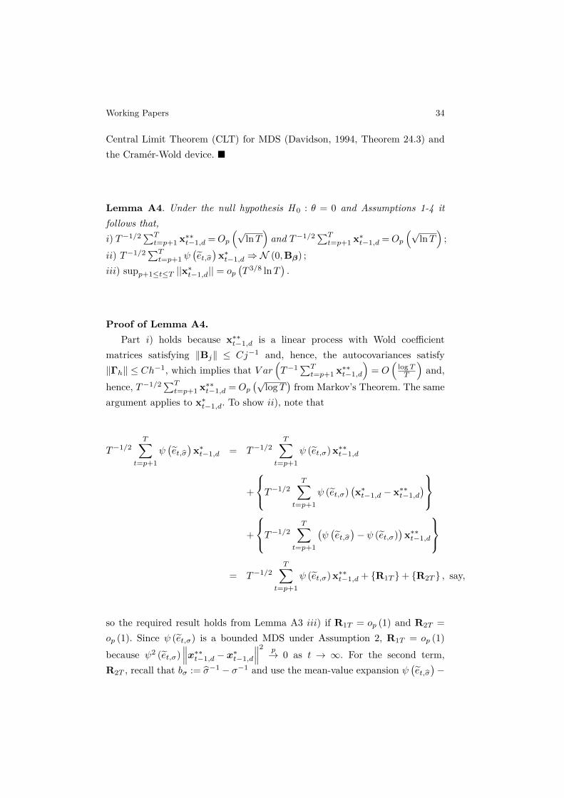
Working Papers 34
Central Limit Theorem (CLT) for MDS (Davidson, 1994, Theorem 24.3) andthe Cramér-Wold device.
Lemma A4. Under the null hypothesis H 0 : θ = 0 and Assumptions 1-4 itfollows that,i) T−1/2
∑Tt=p+1 x∗∗t−1,d =Op
(√lnT
)and T−1/2
∑Tt=p+1 x∗t−1,d =Op
(√lnT
);
ii) T−1/2∑Tt=p+1 ψ
(et,σ)x∗t−1,d ⇒N (0,Bβ) ;
iii) supp+1≤t≤T ||x∗t−1,d|| = op(T 3/8 lnT
).
Proof of Lemma A4.Part i) holds because x∗∗t−1,d is a linear process with Wold coefficient
matrices satisfying ‖Bj‖ ≤ Cj−1 and, hence, the autocovariances satisfy‖Γh‖ ≤ Ch−1, which implies that V ar
(T−1
∑Tt=p+1 x∗∗t−1,d
)= O
(logTT
)and,
hence, T−1/2∑Tt=p+1 x∗∗t−1,d = Op
(√logT
)from Markov’s Theorem. The same
argument applies to x∗t−1,d. To show ii), note that
T−1/2T∑
t=p+1
ψ(et,σ)x∗t−1,d = T−1/2
T∑t=p+1
ψ (et,σ) x∗∗t−1,d
+
T−1/2T∑
t=p+1
ψ (et,σ)(x∗t−1,d − x∗∗t−1,d
)+
T−1/2T∑
t=p+1
(ψ(et,σ)− ψ (et,σ)
)x∗∗t−1,d
= T−1/2
T∑t=p+1
ψ (et,σ) x∗∗t−1,d + R1T + R2T , say,
so the required result holds from Lemma A3 iii) if R1T = op (1) and R2T =
op (1). Since ψ (et,σ) is a bounded MDS under Assumption 2, R1T = op (1)
because ψ2 (et,σ)∥∥∥x∗∗t−1,d − x∗t−1,d
∥∥∥2 p→ 0 as t → ∞. For the second term,R2T , recall that bσ := σ−1 − σ−1 and use the mean-value expansion ψ
(et,σ)−
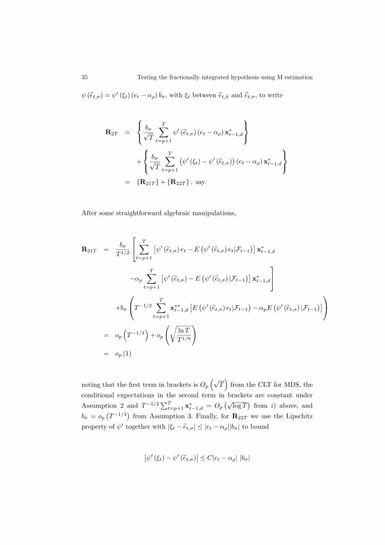
35 Testing the fractionally integrated hypothesis using M estimation
ψ (et,σ) = ψ′ (ξt) (et − αρ) bσ, with ξt between et,σ and et,σ, to write
R2T =
bσ√T
T∑t=p+1
ψ′ (et,σ) (et − αρ) x∗t−1,d
+
bσ√T
T∑t=p+1
(ψ′ (ξt)− ψ′ (et,σ)
)(et − αρ) x∗t−1,d
= R21T + R22T , say.
After some straightforward algebraic manipulations,
R21T =bσT 1/2
T∑t=p+1
[ψ′ (et,σ) et −E
(ψ′ (et,σ) et|Ft−1
)]x∗t−1,d
−αρT∑
t=p+1
[ψ′ (et,σ)−E
(ψ′ (et,σ) |Ft−1
)]x∗t−1,d
+bσ
T−1/2T∑
t=p+1
x∗∗t−1,d
[E(ψ′ (et,σ) et|Ft−1
)− αpE
(ψ′ (et,σ) |Ft−1
)]= op
(T−1/4
)+ op
(√lnT
T 1/8
)= op (1)
noting that the first term in brackets is Op(√
T)from the CLT for MDS, the
conditional expectations in the second term in brackets are constant underAssumption 2 and T−1/2
∑Tt=p+1 x∗t−1,d = Op
(√logT
)from i) above, and
bσ = op(T−1/4
)from Assumption 3. Finally, for R22T we use the Lipschitz
property of ψ′ together with |ξt − et,σ| ≤ |et − αρ||bσ| to bound
∣∣ψ′ (ξt)− ψ′ (et,σ)∣∣ ≤ C|et − αρ| |bσ|

Working Papers 36
for some C > 0 such that
||R22T || ≤C|bσ|2√
T
T∑t=p+1
|et − αρ|2 ||x∗t−1,d||
≤ C|bσ|2√T
T∑t=p+1
e2t ||x∗t−1,d||+
C|bσ|2α2ρ√
T
T∑t=p+1
||x∗∗t−1,d||
+2C|bσ|2|αρ|√
T
T∑t=p+1
|et| ||x∗t−1,d||
= op (1)
from Assumption 3, noting that E(∣∣∣ 1√
T
∑Tt=p+1 e
2t
∥∥∥x∗∗t−1,d
∥∥∥∣∣∣)≤√TE (e2t
)E(∥∥∥x∗∗t−1,d
∥∥∥)under conditional homoskedasticity from Assumption 1, so consistency of σ atany rate higher than T 1/4 collapses the first term. Clearly, the same conditioncarries over to the other two components as well.Moving on to iii), we use Minkowski’s norm inequality and the linearrepresentation of x∗t,d to conclude that
∥∥x∗t,d∥∥8/3≤
t−1∑j=0
‖Bj‖ ‖et‖8/3 = O (lnT )
since the Wold coefficient matrices satisfy ‖Bj‖ = O(j−1). Hence,
E
(∥∥∥ 1lnT x∗t,d
∥∥∥8/3)
is uniformly bounded, and thus
supp+1≤t≤T
∥∥∥∥ 1
lnTx∗t,d
∥∥∥∥ = Op
(T 3/8
)as required for the result.
Lemma A5. Assume that ξt lies on the line segment between u∗t,σ (β1) andu∗t,σ (β0) , with β1 ∈ ΦT , ΦT := β ∈Θ : T ζ ||β − β0|| ≤ K, for any finite,arbitrary K > 0 and 3/8 < ζ < 1/2. Under H0 : θ = 0 and Assumptions 1 to 4,
supβ1∈ΦT
∥∥∥∥∥∥T−1T∑
t=p+1
ψ′ (ξt) x∗t−1,dx′∗t−1,d −Aβ
∥∥∥∥∥∥ = op (1) .

37 Testing the fractionally integrated hypothesis using M estimation
Proof of Lemma A5. Recall that et,σ := σ−1 (et − αρ) . Then,
1
T
T∑t=p+1
ψ′ (ξt) x∗t−1,dx′∗t−1,d =
1
T
T∑t=p+1
ψ′ (et,σ) x∗∗t−1,dx′∗∗t−1,d
+
1
T
T∑t=p+1
ψ′ (et,σ)(x∗t−1,dx
′∗t−1,d − x∗∗t−1,dx
′∗∗t−1,d
)+
1
T
T∑t=p+1
(ψ′ (ξt)− ψ′ (et,σ)
)x∗t−1,dx
′∗t−1,d
=
A∗∗βT
+ R1T + R2T (ξt) , say.
Neither A∗∗βT nor R1T depend on β1, so
supβ1∈ΦT
∥∥∥∥∥∥T−1T∑
t=p+1
ψ′ (ξt) x∗t−1,dx′∗t−1,d −Aβ
∥∥∥∥∥∥≤ ∥∥A∗∗βT −Aβ
∥∥+ ‖R1T ‖+ supβ1∈ΦT
‖R2T (ξt)‖
and the required result holds by showing the asymptotic negligibility of thethree terms on the right-hand side. Lemma A3ii) ensures that A∗∗βT
p→ Aβ, so∥∥∥A∗∗βT −Aβ
∥∥∥ = op (1) . For the second term, note that
‖R1T ‖ ≤ sup1≤t≤T
∣∣ψ′ (et,σ)∣∣ 1
T
T∑t=p+1
∥∥x∗t−1,dx′∗t−1,d − x∗∗t−1,dx
′∗∗t−1,d
∥∥ = op
(T−1/8
)= op (1)
because sup≤t≤T |ψ′ (et,σ)| = op(T 3/8
)since ψ′, being Lipschitz, has at most
linear tails at infinity so ψ′ (et,σ) is uniformly L8/3-bounded, and, as discussedin the proof of Lemma A2, T−1
∑Tt=p+1
∥∥∥x∗t−1,dx′∗t−1,d − x∗∗t−1,dx
′∗∗t−1,d
∥∥∥ =
Op(T−1/2
). For the last term, note that
‖R2T (ξt)‖ ≤1
T
T∑t=p+1
∣∣ψ′ (ξt)− ψ′ (et,σ)∣∣ ∥∥x∗t−1,d
∥∥2.
The Lipschitz condition on ψ′ indicates that |ψ′ (ξt)− ψ′ (et,σ)| ≤ C |ξt − et,σ|,where, for each t, we may represent ξt as ξt = λt
σ
(εt,d − β′1x∗t−1,d
)+
(1−λt)σ
(εt,d − β′0x∗t−1,d
)for some λt ∈ [0, 1] , and 1 ≤ t ≤ T . Since εt,d =

Working Papers 38
β′0x∗t−1,d + (et − αρ), and recalling that bσ := σ−1 − σ−1, it follows that
|ξt − et,σ| =
∣∣∣∣εt,dσ − λtσβ′1x∗t−1,d −
(1− λt)σ
β′0x∗t−1,d − et,σ
∣∣∣∣=
∣∣∣∣−λtσ (β1 − β0) x∗t−1,d + (et − αρ) bσ∣∣∣∣
≤ 1
σ‖β1 − β0‖
∥∥x∗t−1,d
∥∥+ |bσ| (|et|+ |αρ|)
so setting M = max [C,K] leads to
supβ1∈ΦT
‖R2T (ξt)‖ ≤M2
σ
1
T 1+ζ
T∑t=p+1
∥∥x∗t−1,d
∥∥3
+ |bσ|M
T
T∑t=p+1
(|et|+ |αρ|)∥∥x∗t−1,d
∥∥2.
The first term on the right-hand side of this expression vanishes because σ p→ σ
and
1
T 1+ζ
T∑t=p+1
∥∥x∗t−1,d
∥∥3 ≤ 1
T ζsup
1≤t≤T
∥∥x∗t−1,d
∥∥T−1T∑
t=p+1
∥∥x∗t−1,d
∥∥2
= op (1)
given that sup1≤t≤T
∥∥∥x∗t−1,d
∥∥∥ = op(T ζ)which follows from Lemma A4iii) and
ζ > 3/8, and T−1∑Tt=p+1
∥∥∥x∗t−1,d
∥∥∥2
= Op (1).For the second term,
T−1T∑
t=p+1
|et|∥∥x∗t−1,d
∥∥2 ≤ sup1≤t≤T
|et|1/31
T
T∑t=p+1
|et|2/3∥∥x∗t−1,d
∥∥2
where sup1≤t≤T |et|1/3 = Op
(3√T 3/8
)given the uniform L8/3-boundedness,
while Hölder’s inequality gives that
E(|et|2/3
∥∥x∗t−1,d
∥∥2)≤ 4
√E(|et|8/3
)4/3
√E
(∥∥∥x∗t−1,d
∥∥∥8/3).
Thus, since αρ = O (1) under Assumption 4, it follows that
|bσ| sup1≤t≤T
|et|1/3 1
T
T∑t=p+1
|et|2/3∥∥x∗t−1,d
∥∥2
= op (1)
and
|bσ|
1
T
T∑t=p+1
∥∥x∗t−1,d
∥∥2
|αρ| = op (1)

39 Testing the fractionally integrated hypothesis using M estimation
for any σ fulfilling σ − σ = op(T−1/4
), as required in Assumption 3, so
supβ1∈ΦT‖R3T (ξt)‖ = op (1).
Lemma A6. For any β1, β2 ∈ Θ, let
πT (β1β2) :=1√T
T∑t=p+1
[ψ(u∗t,σ (β1)
)− ψ
(u∗t,σ (β2)
)]x∗t−1,d.
Then,
πT (β1, β2) =√T (β1−β2)
[1
σT
T∑t=2
ψ′ (ξt) x∗t−1,dx′∗t−1,d
]with ξt between u∗t,σ (β) and u∗t,σ (β0) for each t.
Proof of Lemma A6.Since
πT (β1, β2) =1√T
T∑t=p+1
[ψ(u∗t,σ (β1)
)− ψ
(u∗t,σ (β2)
)]x∗t−1,d
and mean-value expanding ψ(u∗t,σ (β1)
)about u∗t,σ (β2) yields
√T (β1−β0)
1
σT
T∑t=p+1
ψ′ (ξt) x∗t−1,dx′∗t−1,d
with ξt between u∗t,σ (β1) and u∗t,σ (β2) .

Working Papers 40
Proof of Theorem 1.Noting that conditions i) and ii) in Assumption 2 imply that the ρ-function
is Lipschitz, the proof follows directly from Lemmas A1, A2 and the AsymptoticEquivalence Lemma (AEL). Using the Mean Value Theorem (MVT), we canwrite Q∗T (β) = Q∗∗T (β) + RT (β) , with Q∗∗T (β) from Lemma A1 and RT (β)
from Lemma A2. Consequently, under H0 : θ = 0 and the set of assumptionsconsidered, Lemma A2 ensures that
supβ∈Θ||Q∗T (β)−Q∗∗T (β) || = op (1)
so that Q∗T (β) = Q∗∗T (β) + op (1) uniformly on Θ. The required result thenfollows from Lemma A1 and the AEL.
Proof of Theorem 2.Let ∇Q∗T (β) be the gradient of Q∗T (β) with respect to β, i.e.,
∇Q∗T (β) := −T−1T∑
t=p+1
ψ(u∗t,σ (β)
) x∗t−1,d
σ(20)
and note that, since the ρ-function is twice continuous differentiable, the mean-value expansion of ψ
(u∗t,σ (β0)
)about u∗t,σ
(βM
)yields,
∇Q∗T (β0) = ∇Q∗T(βM
)−
T−1T∑
t=p+1
ψ′ (ξt)x∗t−1,dx
′∗t−1,d
σ2
(βM − β0
),
with ξt lying between u∗t,σ (β0) and u∗t,σ(βM
)for each t. From the continuity
of the objective function and compactness of ΦT , then βM ∈ ΦT , and sinceLemma A5 makes clear that for any β ∈ ΦT
supβ∈ΦT
∥∥∥∥∥∥T−1T∑
t=p+1
ψ′ (ξt)x∗t−1,dx
′∗t−1,d −Aβ
∥∥∥∥∥∥ = op (1)
where Aβ is invertible by Lemma A3 i), the following representation holds:
√T(βM − β0
)= −σA−1
β
1√T
T∑t=p+1
ψ
(et − αρσ
)x∗t−1,d
+ op (1)
noting that ∇QT(βM
)= 0 and σ
p→ σ. Then, from Lemma A4ii) it followsthat,

41 Testing the fractionally integrated hypothesis using M estimation
1√T
T∑t=p+1
ψ
(et − αρσ
)x∗t−1,d ⇒N (0,Bβ)
and, consequently,
√T(βM − β0
)⇒N
(0;σ2A−1
β BβA−1β
),
as required.
Proof of Theorem 3.Note that, given the differentiability of the ρ-function with bounded
derivative, supα∈Θa E(|ρ(et−ασ
)|)< ∞, with Θa being a closed interval in
R. Define now et,σ := et−ασ , PT (α) := T−1
∑Tt=p+1 ρ
(et−ασ
), and PT (α) :=
T−1∑Tt=p+1 ρ
(e(0)t−ασ(0)
). Using the MVT, we may characterize
PT (α) = PT (α) +
1
σ(0)T
T∑t=p+1
ψ (ξt,1)(et − e(0)t
)+bσT
T∑t=p+1
ψ (ξt,2) (et − α)
for all α ∈Θa, with bσ := σ−1
(0) −σ−1 and ξt,1 and ξt,2 lying in the line connecting
e(0)t and e(0)t, and σ(0) and σ, respectively. Then, for any K > 0 and finiteC > 0, consistency of κ(0) and σ(0) together with Assumptions 1 and A2ii)
imply that,
sup|α|≤K
∣∣∣PT (α)− PT (α)∣∣∣ ≤ C
σ(0)||κ(0) − κ||
T−1T∑
t=p+1
||x∗t−1,d||
+C|bσ|
K + T−1T∑
t=p+1
|et|
= op (1)
and, hence, supα∈Θa
∣∣∣PT (α)− PT (α)∣∣∣ = op (1) for a bounded Θa. Paralleling
the proof of Lemma A1, it can be shown that PT (α) is stochasticallyequicontinuous under Assumption 1 because the ρ-function is Lipschitzunder Assumption 2i) and ii) and, therefore, PT (α) converges uniformly inprobability to E (ρ (et,σ)) in Θa by the AEL. Since conditions (A) to (C) inThm. 4.1.1 in Amemiya (1985) are verified, there exists a solution to α(0) :=
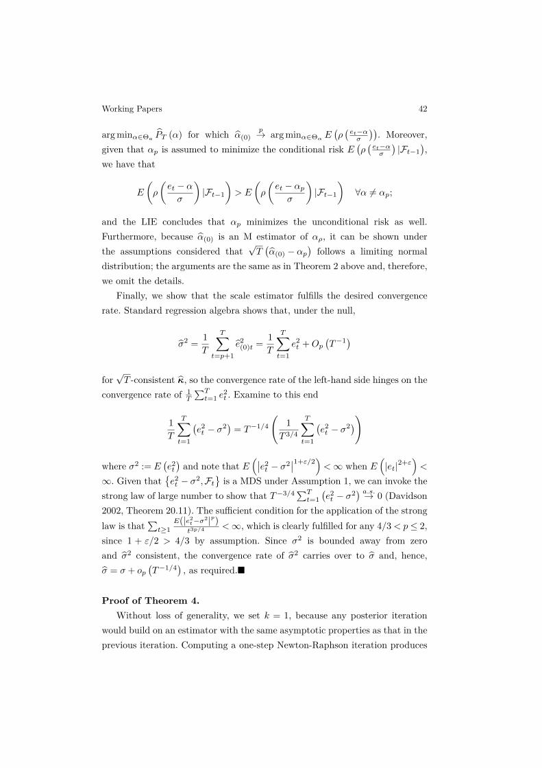
Working Papers 42
arg minα∈Θa PT (α) for which α(0)p→ arg minα∈Θα E
(ρ(et−ασ
)). Moreover,
given that αp is assumed to minimize the conditional risk E(ρ(et−ασ
)|Ft−1
),
we have that
E
(ρ
(et − ασ
)|Ft−1
)> E
(ρ
(et − αpσ
)|Ft−1
)∀α 6= αp;
and the LIE concludes that αp minimizes the unconditional risk as well.Furthermore, because α(0) is an M estimator of αρ, it can be shown underthe assumptions considered that
√T(α(0) − αp
)follows a limiting normal
distribution; the arguments are the same as in Theorem 2 above and, therefore,we omit the details.
Finally, we show that the scale estimator fulfills the desired convergencerate. Standard regression algebra shows that, under the null,
σ2 =1
T
T∑t=p+1
e2(0)t =
1
T
T∑t=1
e2t +Op
(T−1
)for√T -consistent κ, so the convergence rate of the left-hand side hinges on the
convergence rate of 1T
∑Tt=1 e
2t . Examine to this end
1
T
T∑t=1
(e2t − σ2
)= T−1/4
(1
T 3/4
T∑t=1
(e2t − σ2
))
where σ2 := E(e2t
)and note that E
(∣∣e2t − σ2
∣∣1+ε/2)<∞ when E
(|et|2+ε
)<
∞. Given thate2t − σ2,Ft
is a MDS under Assumption 1, we can invoke the
strong law of large number to show that T−3/4∑Tt=1
(e2t − σ2
) a.s.→ 0 (Davidson2002, Theorem 20.11). The sufficient condition for the application of the stronglaw is that
∑t≥1
E(|e2t−σ2|p)t3p/4
<∞, which is clearly fulfilled for any 4/3 < p ≤ 2,since 1 + ε/2 > 4/3 by assumption. Since σ2 is bounded away from zeroand σ2 consistent, the convergence rate of σ2 carries over to σ and, hence,σ = σ + op
(T−1/4
), as required.
Proof of Theorem 4.Without loss of generality, we set k = 1, because any posterior iteration
would build on an estimator with the same asymptotic properties as that in theprevious iteration. Computing a one-step Newton-Raphson iteration produces

43 Testing the fractionally integrated hypothesis using M estimation
βNR,(1) = β(0) − sT
(β(0)
)with
sT
(β(0)
):=
1
σT
T∑t=p+1
ψ′(u∗t,σ (β)
)x∗t−1,dx
′∗t−1,d
−1
β=β(0)
×
1
T
T∑t=p+1
ψ(u∗t,σ (β)
)x∗t−1,d
β=β(0)
and, therefore,
√T(βM,(1) − β0
)=√T(β(0) − β0
)−√T sT
(β(0)
).
Since√T(β(0) − β0
)= Op (1), we may use Lemma A5 to write
√T sT
(β(0)
)= σA−1
β
1√T
T∑t=p+1
ψ(u∗t,σ
(β(0)
))x∗t−1,d
+ op (1)
= σA−1β
1√T
T∑t=p+1
ψ(u∗t,σ (β0)
)x∗t−1,d + πT
(β(0), β0
)+ op (1)
for
πT
(β(0), β0
):=
1√T
T∑t=p+1
ψ(u∗t,σ
(β(0)
))x∗t−1,d−
1√T
T∑t=p+1
ψ(u∗t,σ (β0)
)x∗t−1,d
but since
πT
(β(0), β0
)=√T(β(0)−β0
)[ 1
σT
T∑t=2
ψ′ (ξt) x∗t−1,dx′∗t−1,d
]
we have from Lemma A6
√T sT
(β(0)
)= σA−1
β
1√T
T∑t=p+1
ψ(u∗t,σ (β0)
)x∗t−1,d
+√T(β(0)−β0
)+ op (1)
and hence
√T(βM,(1) − β0
)= σA−1
β
1√T
T∑t=p+1
ψ(u∗t,σ (β0)
)x∗t−1,d
+ op (1)

Working Papers 44
from which we can conclude that,√T(βM,(1) − β0
)⇒N
(0, σ2A−1
β BβA−1β
).
from Lemma A4ii).
Proof of Theorem 5.First, extend ψ(r)
r continuously on R by setting it to equal ψ′(0) at r = 0.Note then that ψ(r)
r is Lipschitz since its derivative ψ′
r −ψr2 is bounded on
R with ψ′ being itself Lipschitz, and thus having at most linear behavior atr→±∞, and ψ being bounded, and also noting that ψ
′
r −ψr2 → ψ′′(0) as r→ 0.
With ψ(r)r Lipschitz, like ψ′, we may use the arguments from the proof of
Lemma A5 to conclude that
1
T
T∑t=p+1
ψ(u∗t,σ
(β(0)
))u∗t,σ
(β(0)
)x∗t−1,dx
′∗t−1,d
p→E
([ψ (et,σ)
et,σ
]x∗t−1,dx
′∗t−1,d
):= Cβ > 0.
(21)Let us now examine the first iteration, k = 1. Given the convergence in (21), itis easily shown that√T(βIRLS,(1) − β0
)=√T(β(0) − β0
)−σC−1
β
1√T
T∑t=p+1
ψ(u∗t,σ
(β(0)
))x∗t−1,d
+ op (1)
=√T(β(0) − β0
)−σC−1
β
1√T
T∑t=p+1
ψ(u∗t,σ (β0)
)x∗t−1,d + πT
+ op (1) .
But
πT =
1
σT
T∑t=p+1
ψ′ (ξt)x∗t−1,dx
′∗t−1,d
√T (β(0) − β0
)such that for Dβ := I−C−1
β Aβ, we have√T(βIRLS,(1) − β0
)= Dβ
√T(β(0) − β0
)−σC−1
β
1√T
T∑t=p+1
ψ(u∗t,σ (β0)
)x∗t−1,d
+ op (1) .

45 Testing the fractionally integrated hypothesis using M estimation
For k = 2, we obtain analogously that
√T(βIRLS,(2) − β0
)= Dβ
√T(βIRLS,(1) − β0
)−σC−1
β
1√T
T∑t=p+1
ψ(u∗t,σ (β0)
)x∗t−1,d
+ op (1)
= D2β
√T(β(0) − β0
)−σDβC−1
β
1√T
T∑t=p+1
ψ(u∗t,σ (β0)
)x∗t−1,d
−σC−1
β
1√T
T∑t=p+1
ψ(u∗t,σ (β0)
)x∗t−1,d
;
and iterating k times leads to
√T(βIRLS,(k) − β0
)= Dk
β
√T(β(0) − β0
)−
k∑j=0
Djβ
σC−1β
1√T
T∑t=p+1
ψ(u∗t,σ (β0)
)x∗t−1,d
+ op (1) .
Since I−C−1β Aβ has eigenvalues smaller than unity, we have that (Dβ)k → 0
and∑kj=0 (Dβ)j →
(C−1β Aβ
)−1
as k→∞, such that
√T(βIRLS,(k) − β0
)→k→∞ −σA−1
β
1√T
T∑t=p+1
ψ(u∗t,σ (β0)
)x∗t−1,d
+ op (1)
which possesses the required weak limit as T →∞.
Proof of Theorem 6.Note that Theorem 2 and Lemma A5 ensure that AβT
p→Aβ , and that thesame arguments may be employed to show that BβT
p→Bβ since ψ2(r) is easilyshown to be Lipschitz. The result then follows from Theorems 2, 4 and 5.

Working Papers 46
Proof of Theorem 7.We give the details for the test based on βM ; the arguments are essentially
the same for the iterated estimators. First, since θ = c/√T , the fractional
difference ∆θ := (1− L)θ may be linearized (cf. Tanaka, 1999),
∆θ − 1 ≈ θ(L+
L2
2+L3
3+ . . .
)+O(θ2)
leading to
εt,d = ∆−θεt,d+θ = εt,d+θ +c√Tx∗t−1,d+θ +Op
(T−1
)with x∗t−1,d+θ =
∑t−1j=1 j
−1εt−j,d+θ =∑t−1j=1 j
−1εt−j . At the same time,
εt,d+θ = εt = et +
p∑j=1
πjεt−j = et + β′0x∗t−1,d+θ,
hence
εt,d = et +
p∑j=1
πjεt−j,d+θ +c√Tx∗t−1,d+θ
= 0x∗t−1,d +
p∑j=1
πjεt,d +
et +c√Tx∗t−1,d+θ −
c√T
p∑j=1
πjx∗t−j,d+θ
;
the DGP under the local alternative is
εt,d = β′0x∗t−1,d + et,θ
where
et,θ = et +c√Tx∗t−1,d+θ −
c√T
p∑j=1
πjx∗t−j,d+θ +Op
(1
T
)(22)
and
x∗t−1,d = ∆−θx∗t−1,d+θ = x∗t−1,d+θ +c√T
t−2∑j=0
j−1x∗t−1−j,d+θ
has analogous properties to x∗t−1,d+θ; in particular, E(∥∥∥x∗t−1,d
∥∥∥2)<C ∀t (this
is because x∗t−1−j,d+θ is uniformly L2-bounded and T−1/2 lnT → 0).Now, since θ = c/
√T is a deviation in a 1/
√T neighbourhood of the
null which is of the same order of magnitude as the estimation error, it is

47 Testing the fractionally integrated hypothesis using M estimation
straightforward to show that σ2 p→ σ2, AβTp→ Aβ and BβT
p→ Bβ like in theproof of Theorem 6. To discuss the limiting behavior of the estimator ϕM , weadapt the proof of Theorem 2 accordingly. The key step is to establish thelimiting behavior of
1√T
T∑t=p+1
ψ
(εt,d − β′0x∗t−1,d
σ
)x∗t−1,d
σ.
Unlike the case θ = 0, the limiting distribution of this normalized (pseudo-)score is not centered at zero. We resort to the mean value theorem for ψ withξt between
εt,d−β′0x∗t−1,d
σ and the expansion points et−αρσ to obtain
1√T
T∑t=p+1
ψ
(εt,d − β′0x∗t−1,d
σ
)x∗t−1,d
σ
=1√T
T∑t=p+1
ψ
(et − αρσ
)x∗t−1,d
σ+
1√T
T∑t=p+1
ψ′ (ξt)
(εt,d − β′0x∗t−1,d
σ− et − αρ
σ
)x∗t−1,d
σ
=1√T
T∑t=p+1
ψ
(et − αρσ
)x∗t−1,d+θ
σ
+1√T
T∑t=p+1
ψ
(et − αρσ
)(x∗t−1,d
σ−x∗t−1,d+θ
σ
)
+1
σ2√T
T∑t=p+1
ψ′ (ξt) (et,θ − et)x∗t−1,d (23)
with et,θ = et + c√Tx∗t−1,d+θ −
c√T
∑pj=1 πjx
∗t−j,d+θ. Using the same arguments
as under the null hypothesis and exploiting the fact that now θ = c/√T , it
follows that
1
σ
1√T
T∑t=p+1
ψ
(et − αρσ
)x∗t−1,d+θ
⇒N (0;1
σ2Bβ
);
we also notice that
1√T
T∑t=p+1
ψ
(et − αρσ
)(x∗t−1,d
σ−x∗t−1,d+θ
σ
)p→ 0

Working Papers 48
(see the discussion in the proof of Lemma A4ii)). By replacing et,θ − et byc√Tx∗t−1,d+θ −
c√T
∑pj=1 πjx
∗t−j,d+θ, we obtain for the third summand in (23)
that,
∆T =1
σ2√T
T∑t=p+1
ψ′ (ξt)
c√Tx∗t−1,d+θ −
c√T
p∑j=1
πjx∗t−j,d+θ
x∗t−1,d.
Denote now δc := c (0, 1,−π1, . . . ,−πp)′ and recall that x∗t−1,d+θ = x∗t−1,d −c√T
∑t−2j=0 j
−1x∗t−1−j,d+θ so
1
σ2√T
T∑t=p+1
ψ′ (ξt)
c√Tx∗t−1,d+θ −
c√T
p∑j=1
πjx∗t−j,d+θ
x∗t−1,d
=1
σ2T
T∑t=p+1
ψ′ (ξt)x∗t−1,d
x′∗t−1,dδc −c2√T
t−2∑j=0
j−1x∗t−1−j,d+θ
=
1
σ2T
T∑t=p+1
ψ′ (ξt)x∗t−1,dx
′∗t−1,dδc + op (1)
since
E
∣∣∣∣∣∣ψ′ (ξt)x∗t−1,d
t−2∑j=0
j−1x∗t−1−j,d+θ
∣∣∣∣∣∣ ≤ C
t−2∑j=0
j−1
√E
(∥∥∥x∗t−1,d
∥∥∥2)E
(∣∣∣x∗t−1−j,d+θ
∣∣∣2)= O (lnT )
and thus
c2
σ2T 3/2
T∑t=p+1
ψ′ (ξt)x∗t−1,d
t−2∑j=0
j−1x∗t−1−j,d+θ
= Op
(lnT√T
).
Hence, using Lemma A5 again,
∆Tp→ 1
σ2Aβδc
Consequently, under the conditions considered,
√T(βM − β0
)⇒N (δc; Ωβ)
from which the required result follows directly.

49Testing
thefractionally
integratedhypothesis
usingM
estimation
Table 1: Rejection frequencies of fractional integration tests (DGP with iid errors drawn from a student-t with v degrees of freedom)
θ tLS
tHCLS
tHM tBM DV tQR
θ tLS
tHCLS
tHM tBM DV tQR
v = 1000, T = 250 v = 1000, T = 500
-0.3 100.00 100.00 99.98 99.98 71.78 98.72 -0.3 100.00 100.00 100.00 100.00 97.96 100.00-0.2 97.58 97.64 96.84 96.80 41.14 84.62 -0.2 99.98 99.98 99.96 99.94 78.96 98.50-0.1 53.88 54.06 50.62 50.48 11.80 37.76 -0.1 81.12 81.58 79.04 79.14 28.68 60.240.0 5.20 5.70 5.24 5.22 4.56 5.98 0 5.38 5.64 5.46 5.40 4.80 5.900.1 36.18 37.04 34.50 34.52 35.70 27.34 0.1 70.76 71.06 68.82 68.96 56.68 53.480.2 91.60 91.92 90.44 90.40 85.72 80.62 0.2 99.92 99.94 99.88 99.84 98.32 98.520.3 99.88 99.92 99.80 99.78 98.96 98.38 0.3 100.00 100.00 100.00 100.00 100.00 100.00
v = 3, T = 250 v = 3, T = 500
-0.3 99.96 99.60 100.00 100.00 68.20 100.00 -0.3 100.00 99.94 100.00 100.00 96.48 100.00-0.2 97.54 96.72 99.66 99.54 43.72 98.86 -0.2 99.96 99.68 100.00 100.00 81.72 100.00-0.1 54.00 61.22 73.62 72.96 15.36 64.10 -0.1 82.24 83.64 96.04 95.74 37.20 90.980.0 5.16 5.82 5.26 5.42 4.40 4.86 0 4.92 5.68 5.30 5.36 4.84 4.540.1 37.12 42.20 59.92 62.86 51.38 54.68 0.1 71.58 73.04 91.50 92.00 76.80 88.240.2 91.72 90.82 98.36 98.62 95.12 97.70 0.2 99.88 99.58 100.00 100.00 99.82 100.000.3 99.76 99.50 99.98 99.98 99.82 99.98 0.3 100.00 99.98 100.00 100.00 100.00 100.00
v = 2, T = 250 v = 2, T = 500
-0.3 99.8 98.84 99.98 99.98 50.66 99.98 -0.3 99.98 99.60 100.00 99.98 80.46 100.00-0.2 97.06 95.62 99.94 99.96 33.70 99.82 -0.2 99.82 99.10 100.00 100.00 62.72 100.00-0.1 53.22 69.42 91.16 91.22 15.18 85.34 -0.1 85.72 89.32 99.68 99.64 32.92 99.060.0 4.26 5.48 5.38 5.44 4.26 3.92 0 3.76 4.64 5.36 5.44 4.70 3.660.1 35.92 50.16 83.32 86.30 68.26 81.68 0.1 74.24 78.20 98.90 99.16 91.46 98.560.2 93.40 91.48 99.76 99.84 98.50 99.70 0.2 99.80 99.22 100.00 100.00 99.98 100.000.3 99.70 99.06 100.00 100.00 99.96 100.00 0.3 100.00 99.94 100.00 100.00 100.00 100.00
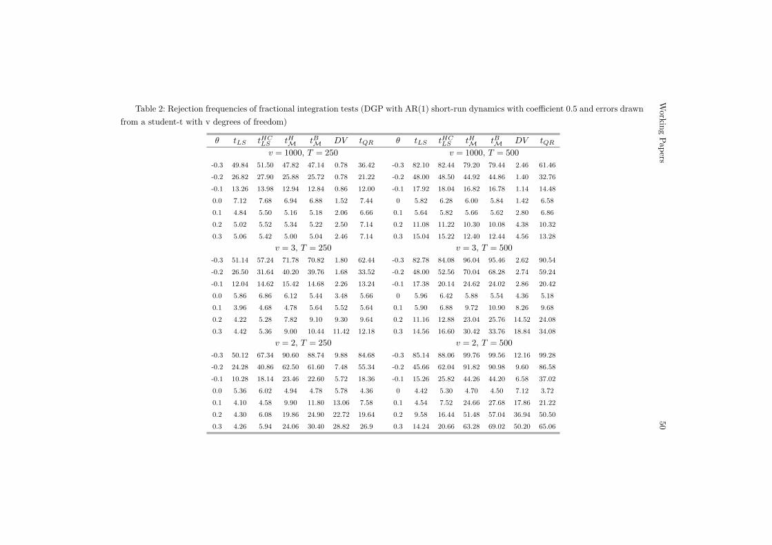
Working
Papers50
Table 2: Rejection frequencies of fractional integration tests (DGP with AR(1) short-run dynamics with coefficient 0.5 and errors drawnfrom a student-t with v degrees of freedom)
θ tLS tHCLS tHM tBM DV tQR θ tLS tHCLS tHM tBM DV tQR
v = 1000, T = 250 v = 1000, T = 500
-0.3 49.84 51.50 47.82 47.14 0.78 36.42 -0.3 82.10 82.44 79.20 79.44 2.46 61.46-0.2 26.82 27.90 25.88 25.72 0.78 21.22 -0.2 48.00 48.50 44.92 44.86 1.40 32.76-0.1 13.26 13.98 12.94 12.84 0.86 12.00 -0.1 17.92 18.04 16.82 16.78 1.14 14.480.0 7.12 7.68 6.94 6.88 1.52 7.44 0 5.82 6.28 6.00 5.84 1.42 6.580.1 4.84 5.50 5.16 5.18 2.06 6.66 0.1 5.64 5.82 5.66 5.62 2.80 6.860.2 5.02 5.52 5.34 5.22 2.50 7.14 0.2 11.08 11.22 10.30 10.08 4.38 10.320.3 5.06 5.42 5.00 5.04 2.46 7.14 0.3 15.04 15.22 12.40 12.44 4.56 13.28
v = 3, T = 250 v = 3, T = 500
-0.3 51.14 57.24 71.78 70.82 1.80 62.44 -0.3 82.78 84.08 96.04 95.46 2.62 90.54-0.2 26.50 31.64 40.20 39.76 1.68 33.52 -0.2 48.00 52.56 70.04 68.28 2.74 59.24-0.1 12.04 14.62 15.42 14.68 2.26 13.24 -0.1 17.38 20.14 24.62 24.02 2.86 20.420.0 5.86 6.86 6.12 5.44 3.48 5.66 0 5.96 6.42 5.88 5.54 4.36 5.180.1 3.96 4.68 4.78 5.64 5.52 5.64 0.1 5.90 6.88 9.72 10.90 8.26 9.680.2 4.22 5.28 7.82 9.10 9.30 9.64 0.2 11.16 12.88 23.04 25.76 14.52 24.080.3 4.42 5.36 9.00 10.44 11.42 12.18 0.3 14.56 16.60 30.42 33.76 18.84 34.08
v = 2, T = 250 v = 2, T = 500
-0.3 50.12 67.34 90.60 88.74 9.88 84.68 -0.3 85.14 88.06 99.76 99.56 12.16 99.28-0.2 24.28 40.86 62.50 61.60 7.48 55.34 -0.2 45.66 62.04 91.82 90.98 9.60 86.58-0.1 10.28 18.14 23.46 22.60 5.72 18.36 -0.1 15.26 25.82 44.26 44.20 6.58 37.020.0 5.36 6.02 4.94 4.78 5.78 4.36 0 4.42 5.30 4.70 4.50 7.12 3.720.1 4.10 4.58 9.90 11.80 13.06 7.58 0.1 4.54 7.52 24.66 27.68 17.86 21.220.2 4.30 6.08 19.86 24.90 22.72 19.64 0.2 9.58 16.44 51.48 57.04 36.94 50.500.3 4.26 5.94 24.06 30.40 28.82 26.9 0.3 14.24 20.66 63.28 69.02 50.20 65.06

51Testing
thefractionally
integratedhypothesis
usingM
estimation
Table 3: Rejection frequencies of fractional integration tests (DGP with dependence in volatility and iid innovations drawn fom astudent-t distribution with v degrees of freedom)
CASE A CASE Bθ tLS tHCLS tHM tBM tQR tLS tHCLS tHM tBM tQR
v = 1000 v = 1000-0.3 100.00 100.00 100.00 100.00 100.00 -0.3 100.00 100.00 100.00 100.00 100.00-0.2 99.96 99.96 99.94 99.94 98.22 -0.2 99.92 99.90 99.92 99.92 98.20-0.1 73.16 72.70 75.24 75.08 57.26 -0.1 73.10 71.68 74.96 74.62 57.900 5.38 5.18 6.06 6.02 5.90 0 5.18 4.80 6.26 6.16 6.000.1 65.76 65.82 50.34 50.36 38.78 0.1 65.46 65.06 50.58 50.52 39.000.2 98.96 98.98 97.02 96.86 90.02 0.2 98.92 98.96 96.92 96.76 89.900.3 99.98 99.98 99.88 99.86 99.38 0.3 100.00 100.00 99.86 99.86 99.34
v = 3 v = 3-0.3 100.00 99.90 100.00 100.00 100.00 -0.3 100 99.90 100.00 100.00 100.00-0.2 99.88 99.60 100.00 100.00 100.00 -0.2 99.88 99.50 100.00 100.00 100.00-0.1 71.28 73.48 93.52 93.12 88.24 -0.1 71.02 72.24 93.66 92.78 88.200 5.10 5.62 5.48 5.26 5.44 0 5.54 5.50 6.00 5.66 5.600.1 67.98 69.70 80.36 83.06 76.38 0.1 68.2 69.02 80.48 83.02 76.240.2 99.08 98.78 99.88 99.92 99.76 0.2 99.1 98.70 99.90 99.92 99.800.3 99.98 99.98 100.00 100.00 100.00 0.3 99.98 99.96 100.00 100.00 100.00
v = 2 v = 2-0.3 99.98 99.70 100.00 100.00 100.00 -0.3 99.98 99.68 100.00 100.00 100.00-0.2 99.78 99.04 100.00 100.00 100.00 -0.2 99.76 98.88 100.00 100.00 100.00-0.1 75.44 81.02 99.66 99.52 99.32 -0.1 75.30 80.48 99.64 99.54 99.320 4.06 4.32 5.28 5.26 3.42 0 4.44 4.40 5.62 5.38 3.920.1 68.30 73.64 97.04 98.08 96.74 0.1 68.46 73.38 96.90 97.98 96.740.2 98.98 97.92 100.00 100.00 100.00 0.2 98.96 97.80 100.00 100.00 100.000.3 99.96 99.82 100.00 100.00 100.00 0.3 99.96 99.82 100.00 100.00 100.00
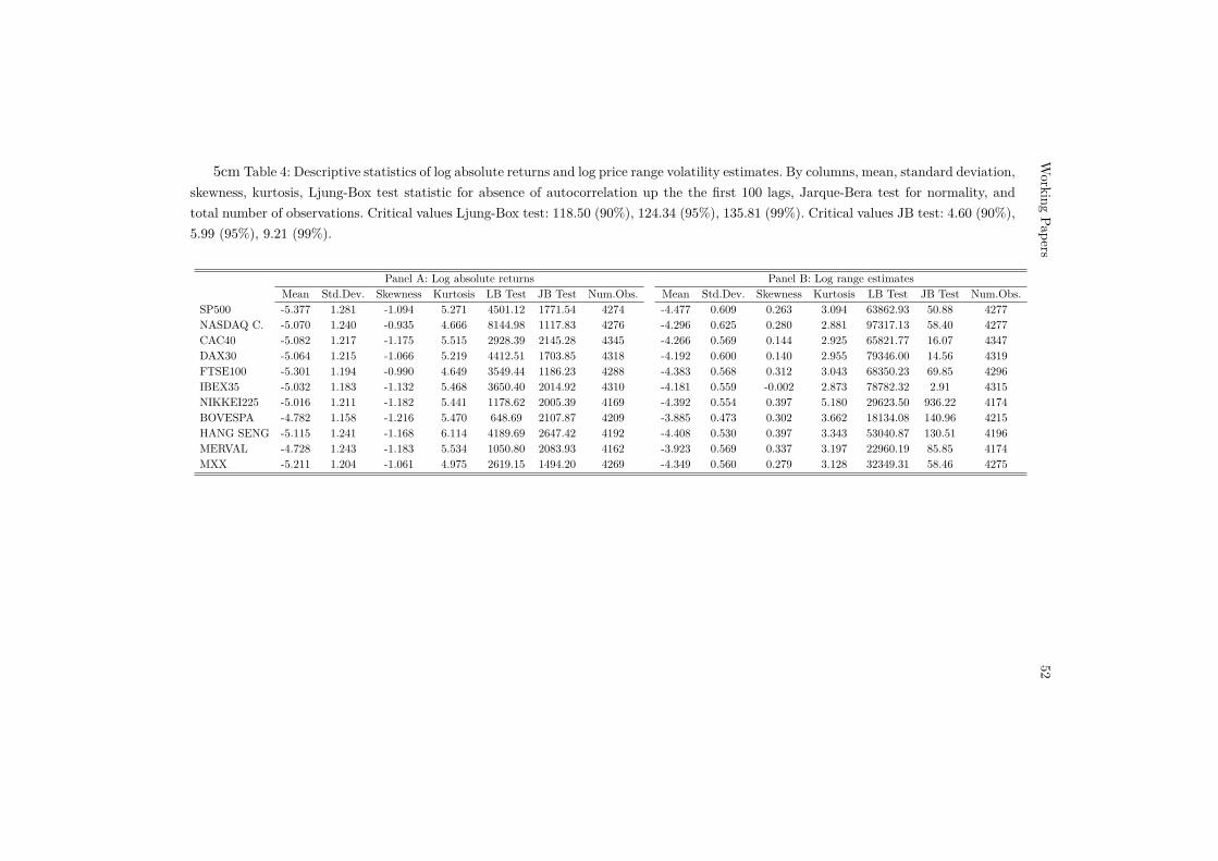
Working
Papers52
5cm Table 4: Descriptive statistics of log absolute returns and log price range volatility estimates. By columns, mean, standard deviation,skewness, kurtosis, Ljung-Box test statistic for absence of autocorrelation up the the first 100 lags, Jarque-Bera test for normality, andtotal number of observations. Critical values Ljung-Box test: 118.50 (90%), 124.34 (95%), 135.81 (99%). Critical values JB test: 4.60 (90%),5.99 (95%), 9.21 (99%).
Panel A: Log absolute returns Panel B: Log range estimatesMean Std.Dev. Skewness Kurtosis LB Test JB Test Num.Obs. Mean Std.Dev. Skewness Kurtosis LB Test JB Test Num.Obs.
SP500 -5.377 1.281 -1.094 5.271 4501.12 1771.54 4274 -4.477 0.609 0.263 3.094 63862.93 50.88 4277NASDAQ C. -5.070 1.240 -0.935 4.666 8144.98 1117.83 4276 -4.296 0.625 0.280 2.881 97317.13 58.40 4277CAC40 -5.082 1.217 -1.175 5.515 2928.39 2145.28 4345 -4.266 0.569 0.144 2.925 65821.77 16.07 4347DAX30 -5.064 1.215 -1.066 5.219 4412.51 1703.85 4318 -4.192 0.600 0.140 2.955 79346.00 14.56 4319FTSE100 -5.301 1.194 -0.990 4.649 3549.44 1186.23 4288 -4.383 0.568 0.312 3.043 68350.23 69.85 4296IBEX35 -5.032 1.183 -1.132 5.468 3650.40 2014.92 4310 -4.181 0.559 -0.002 2.873 78782.32 2.91 4315NIKKEI225 -5.016 1.211 -1.182 5.441 1178.62 2005.39 4169 -4.392 0.554 0.397 5.180 29623.50 936.22 4174BOVESPA -4.782 1.158 -1.216 5.470 648.69 2107.87 4209 -3.885 0.473 0.302 3.662 18134.08 140.96 4215HANG SENG -5.115 1.241 -1.168 6.114 4189.69 2647.42 4192 -4.408 0.530 0.397 3.343 53040.87 130.51 4196MERVAL -4.728 1.243 -1.183 5.534 1050.80 2083.93 4162 -3.923 0.569 0.337 3.197 22960.19 85.85 4174MXX -5.211 1.204 -1.061 4.975 2619.15 1494.20 4269 -4.349 0.560 0.279 3.128 32349.31 58.46 4275

53Testing
thefractionally
integratedhypothesis
usingM
estimation
Table 5: 95% confidence interval estimates for the fractional parameter on log absolute returns according to different testing methodologies.By columns, LS-based estimates with robust standard errors to hetoroskedasticity, tHCLS ; QR-based estimates at the median with robuststandard errors, tQR; Kolmogorov-Smirnov joint QR test-based estimates at quantiles in [0.1,0.9], KS; IRLS-based estimates with Huber,tHIRLS , and Biweight, tBIRLS , weighting functions; one-step Newton-Raphson test-based estimates with Huber, tHNR, and Biweight, tBNR,weigthing functions. The column labelled Intersection shows the values for which none of these tests can reject the null hypothesis offractional integration, i.e., the intersection of the confidence intervals. ELW reports 95% confidence intervals based on exact local Whittleestimation. Finally, the last two columns show the average relative change in the amplitude of the estimated confidence intervals when LS isreplaced by IRLS and NR estimation, respectively, with average values computed over the estimates from Huber and Bisquare weighthingfunctions.
tHCLS tQR KS tHIRLS tBIRLS tHNR tBNR Intersection ELW ARC IRLS ARC NR
SP500 [0.37,0.53] [0.35,0.52] [0.34,0.54] [0.38,0.49] [0.37,0.49] [0.37,0.50] [0.36,0.50] [0.38,0.49] [0.39.0.45] -28.13% -15.63%NASDAQ C. [0.37,0.54] [0.37,0.48] [0.35,0.48] [0.37,0.45] [0.38,0.47] [0.36,0.46] [0.36,0.46] [0.38,0.45] [0.39,0.46] -50.00% -38.24%CAC40 [0.30,0.48] [0.25,0.42] [0.31,0.44] [0.31,0.41] [0.31,0.41] [0.30.0.43] [0.30,0.42] [0.31,0.41] [0.33,0.39] -44.44% -33.33%DAX30 [0.36,0.52] [0.33,0.46] [0.32,0.48] [0.36,0.46] [0.35,0.45] [0.35,0.47] [0.34,0.46] [0.36,0.45] [0.37,0.44] -37.50% -25.00%FTSE100 [0.32,0.48] [0.35,0.47] [0.33,0.49] [0.36,0.46] [0.36,0.47] [0.34,0.48] [0.35,0.48] [0.36,0.46] [0.33,0.39] -34.38% -15.63%IBEX35 [0.37,0.53] [0.34,0.48] [0.35,0.51] [0.37,0.47] [0.37,0.47] [0.36,0.48] [0.36,0.48] [0.37,0.47] [0.37,0.44] -37.50% -25.00%NIKKEI225 [0.27,0.44] [0.23,0.39] [0.26,0.43] [0.28,0.40] [0.28,0.40] [0.27,0.41] [0.27,0.41] [0.28,0.39] [0.30,0.37] -29.41% -17.65%BOVESPA [0.20,0.39] [0.23,0.39] [0.24,0.40] [0.26,0.36] [0.26,0.36] [0.24,0.37] [0.25,0.37] [0.26,0.40] [0.24,0.30] -47.37% -34.21%HANG SENG [0.36,0.50] [0.37,0.51] [0.35,0.48] [0.37,0.46] [0.37,0.46] [0.36,0.47] [0.36,0.47] [0.37,0.46] [0.36,0.43] -35.71% -21.43%MERVAL [0.19,0.35] [0.18,0.36] [0.23,0.36] [0.23,0.33] [0.23,0.34] [0.21,0.35] [0.22,0.35] [0.23,0.33] [0.23,0.29] -25.00% -3.57%MXX [0.32,0.50] [0.27,0.41] [0.28,0.43] [0.32,0.41] [0.32,0.41] [0.31,0.43] [0.31,0.42] [0.32,0.41] [0.32,0.38] -44.44% -36.11%
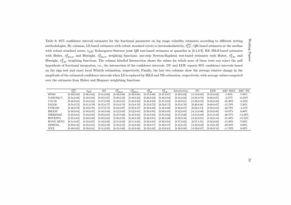
Working
Papers54
Table 6: 95% confidence interval estimates for the fractional parameter on log range volatility estimates according to different testingmethodologies. By columns, LS-based estimates with robust standard errors to hetoroskedasticity, tHCLS ; QR-based estimates at the medianwith robust standard errors, tQR; Kolmogorov-Smirnov joint QR test-based estimates at quantiles in [0.1,0.9], KS; IRLS-based estimateswith Huber, tHIRLS , and Biweight, tBIRLS , weighting functions; one-step Newton-Raphson test-based estimates with Huber, tHNR, andBiweight, tBNR, weigthing functions. The column labelled Intersection shows the values for which none of these tests can reject the nullhypothesis of fractional integration, i.e., the intersection of the confidence intervals. DV and ELW reports 95% confidence intervals basedon the sign test and exact local Whittle estimation, respectively. Finally, the last two columns show the average relative change in theamplitude of the estimated confidence intervals when LS is replaced by IRLS and NR estimation, respectively, with average values computedover the estimates from Huber and Bisquare weighthing functions.
tHCLS tQR KS tHIRLS tBIRLS tHNR tBNR Intersection DV ELW ARC IRLS ARC NR
SP500 [0.50,0.69] [0.36,0.62] [0.41,0.68] [0.49,0.66] [0.48,0.66] [0.47,0.68] [0.47.0.67] [0.49,0.62] [-0.10,0.65] [0.55,0.62] -7.89% 7.89%NASDAQ C. [0.54,0.68] [0.49,0.68] [0.45,0.67] [0.49,0.62] [0.49,0.63] [0.48,0.64] [0.48,0.64] [0.54,0.62] [-0.05,0.78] [0.60,0.67] -3.57% 14.29%CAC40 [0.46,0.64] [0.44,0.64] [0.47,0.68] [0.48,0.61] [0.48,0.62] [0.46,0.63] [0.47,0.63] [0.48,0.61] [-0.28,0.85] [0.56,0.63] -25.00% -8.33%DAX30 [0.54,0.73] [0.51,0.78] [0.55,0.77] [0.54,0.70] [0.54,0.70] [0.52,0.72] [0.52,0.72] [0.55,0.70] [0.26,0.66] [0.60,0.67] -15.79% 5.26%FTSE100 [0.48,0.70] [0.43,0.76] [0.47,0.73] [0.50,0.67] [0.50,0.67] [0.48,0.69] [0.48,0.69] [0.50,0.67] [0.02,0.74] [0.58,0.64] -22.73% -4.55%IBEX35 [0.49,0.64] [0.40,0.67] [0.46,0.68] [0.52,0.63] [0.52,0.64] [0.50,0.65] [0.50,0.65] [0.52,0.63] [-0.14,0.86] [0.53,0.60] -16.67% 0.00%NIKKEI225 [0.43,0.64] [0.43,0.62] [0.39,0.65] [0.47,0.60] [0.45,0.62] [0.44,0.63] [0.45,0.62] [0.47,0.60] [-0.13,0.69] [0.51,0.58] -28.57% -14.29%BOVESPA [0.35,0.64] [0.32,0.60] [0.30,0.64] [0.38,0.58] [0.38,0.58] [0.36,0.61] [0.36,0.60] [0.38,0.58] [-0.24,0.81] [0.48,0.54] -31.03% -15.52%HANG SENG [0.54,0.67] [0.52,0.67] [0.49,0.62] [0.51,0.62] [0.51,0.62] [0.50,0.64] [0.50,0.64] [0.57,0.62] [0.57,1.05] [0.56,0.62] -15.38% 7.69%MERVAL [0.39,0.56] [0.45,0.65] [0.40,0.59] [0.42,0.55] [0.42,0.56] [0.40,0.57] [0.40,0.57] [0.45,0.55] [-0.29,0.60] [0.43,0.49] -20.59% 0.00%MXX [0.48,0.65] [0.39,0.61] [0.41,0.65] [0.45,0.60] [0.45,0.60] [0.43,0.62] [0.43,0.61] [0.48,0.60] [-0.30,0.87] [0.48,0.54] -11.76% 8.82%

55 Testing the fractionally integrated hypothesis using M estimation
Figures
Figure 1: Time-series dynamics, sample histogram (confronted with thetheoretical normal distribution), and sample autocorrelation function (withasymptotic 95% confidence bands) of the log absolute-valued returns of theSP500 index.
01/00 12/01 12/03 12/05 12/07 12/09 12/11 12/13 12/15−15
−10
−5
0Log absolute−valued returns
−14 −12 −10 −8 −6 −4 −2 00
100
200
300Histogram
0 10 20 30 40 50 60 70 80 90 1000
0.05
0.1
0.15
0.2Sample Autocorrelation Function
Figure 2: Time-series dynamics, sample histogram (confronted with thetheoretical normal distribution), and sample autocorrelation function (withasymptotic 95% confidence bands) of the log high-low range estimator of theSP500 index.
01/00 12/01 12/03 12/05 12/07 12/09 12/11 12/13 12/15−8
−6
−4
−2Log High−Low range estimator
−6.5 −6 −5.5 −5 −4.5 −4 −3.5 −3 −2.5 −20
50
100
150
200Histogram
0 10 20 30 40 50 60 70 80 90 1000
0.2
0.4
0.6
0.8Sample Autocorrelation Function

Working Papers
20161|16 A mixed frequency approach to forecast
private consumption with ATM/POS data
Cláudia Duarte | Paulo M. M. Rodrigues | António Rua
2|16 Monetary developments and expansionary fiscal consolidations: evidence from the EMU
António Afonso | Luís Martins
3|16 Output and unemployment, Portugal, 2008–2012
José R. Maria
4|16 Productivity and organization in portuguese firms
Lorenzo Caliendo | Luca David Opromolla | Giordano Mion | Esteban Rossi-Hansberg
5|16 Residual-augmented IVX predictive regression
Matei Demetrescu | Paulo M. M. Rodrigues
6|16 Understanding the public sector pay gap
Maria M. Campos | Evangelia Papapetrou | Domenico Depalo Javier J. Pérez | Roberto Ramos
7|16 Sorry, we’re closed: loan conditions when bank branches close and firms transfer to another bank
Diana Bonfim | Gil Nogueira | Steven Ongena
8|16 The effect of quantitative easing on lending conditions
Laura Blattner | Luísa Farinha | Gil Nogueira
9|16 Market integration and the persistence of electricity prices
João Pedro Pereira | Vasco Pesquita | Paulo M. M. Rodrigues | António Rua
10|16 EAGLE-FLI | A macroeconomic model of banking and financial interdependence in the euro area
N. Bokan | A. Gerali | S. Gomes | P. Jacquinot | M. Pisani
11|16 Temporary contracts’ transitions: the role of training and institutions
Sara Serra
12|16 A wavelet-based multivariate multiscale approach for forecasting
António Rua
13|16 Forecasting banking crises with dynamic panel probit models
António Antunes | Diana Bonfim | Nuno Monteiro | Paulo M. M. Rodrigues
14|16 A tale of two sectors: why is misallocation higher in services than in manufacturing?
Daniel A. Dias | Carlos Robalo Marques | Christine Richmond
15|16 The unsecured interbank money market: a description of the Portuguese case
SofiaSaldanha
16|16 Leverage and r isk weighted capital requirements
Leonardo Gambacorta | Sudipto Karmakar
17|16 Surviving the perfect storm: the role of the lender of last resort
NunoAlves|DianaBonfim|CarlaSoares
18|16 Public debt expansions and the dy-namics of the household borrowing constraint
António Antunes | Valerio Ercolani

20171|17 The diffusion of knowledge via managers’
mobility
Giordano Mion | Luca David Opromolla | Alessandro Sforza
2|17 Upward nominal wage rigidity
Paulo Guimarães | Fernando Martins | Pedro Portugal
3|17 Zooming the ins and outs of the U.S. unemployment
Pedro Portugal | António Rua
4|17 Labor market imperfections and the firm’s wage setting policy
Sónia Félix | Pedro Portugal
5|17 International banking and cross-border effects of regulation: lessons from Portugal
DianaBonfim|SóniaCosta
6|17 Disentangling the channels from birthdate to educational attainment
Luís Martins | Manuel Coutinho Pereira
7|17 Who’s who in global value chains? A weight-ed network approach
João Amador | Sónia Cabral | Rossana Mastrandrea | Franco Ruzzenenti
8|17 Lending relationships and the real economy: evidence in the context of the euro area sovereign debt crisis
Luciana Barbosa
9|17 Impact of uncertainty measures on the Portuguese economy
Cristina Manteu | Sara Serra
10|17 Modelling currency demand in a small open economy within a monetary union
António Rua
11|17 Boom, slump, sudden stops, recovery, and policy options. Portugal and the Euro
Olivier Blanchard | Pedro Portugal
12|17 Inefficiency distribution of the European Banking System
João Oliveira
13|17 Banks’ liquidity management and systemic risk
Luca G. Deidda | Ettore Panetti
14|17 Entrepreneurial risk and diversification through trade
Federico Esposito
15|17 The portuguese post-2008 period: a narra-tive from an estimated DSGE model
Paulo Júlio | José R. Maria
16|17 A theory of government bailouts in a het-erogeneous banking system
Filomena Garcia | Ettore Panetti
17|17 Goods and factor market integration: a quan-titative assessment of the EU enlargement
FLorenzo Caliendo | Luca David Opromolla | Fernando Parro | Alessandro Sforza

20181|18 Calibration and the estimation of macro-
economic models
Nikolay Iskrev
2|18 Are asset price data informative about news shocks? A DSGE perspective
Nikolay Iskrev
3|18 Sub-optimality of the friedman rule with distorting taxes
Bernardino Adão | André C. Silva
4|18 The effect of firm cash holdings on monetary policy
Bernardino Adão | André C. Silva
5|18 The returns to schooling unveiled
Ana Rute Cardoso | Paulo Guimarães | Pedro Portugal | Hugo Reis
6|18 Real effects of financial distress: the role of heterogeneity
Francisco Buera | Sudipto Karmakar
7|18 Did recent reforms facilitate EU labour mar-ket adjustment? Firm level evidence
Mario Izquierdo | Theodora Kosma | Ana Lamo | Fernando Martins | Simon Savsek
8|18 Flexible wage components as a source of wage adaptability to shocks: evidence from European firms, 2010–2013
Jan Babecký | Clémence Berson | Ludmila Fadejeva | Ana Lamo | Petra Marotzke | Fernando Martins | Pawel Strzelecki
9|18 The effects of official and unofficial informa-tion on tax compliance
Filomena Garcia | Luca David Opromolla Andrea Vezulli | Rafael Marques
10|18 International trade in services: evidence for portuguese firms
João Amador | Sónia Cabral | Birgitte Ringstad
11|18 Fear the walking dead: zombie firms, spillovers and exit barriers
Ana Fontoura Gouveia | Christian Osterhold
12|18 Collateral Damage? Labour Market Effects of Competing with China – at Home and Abroad
Sónia Cabral | Pedro S. Martins | João Pereira dos Santos | Mariana Tavares
13|18 An integrated financial amplifier: The role of defaulted loans and occasionally binding constraints in output fluctuations
Paulo Júlio | José R. Maria
14|18 Structural Changes in the Duration of Bull Markets and Business Cycle Dynamics
João Cruz | João Nicolau | Paulo M.M. Rodrigues
15|18 Cross-border spillovers of monetary policy: what changes during a financial crisis?
Luciana Barbosa | Diana Bonfim | Sónia Costa | Mary Everett
16|18 When losses turn into loans: the cost of undercapitalized banks
Laura Blattner | Luísa Farinha | Francisca Rebelo
17|18 Testing the fractionally integrated hypothesis using M estimation: With an application to stock market volatility
Matei Demetrescu | Paulo M. M. Rodrigues | Antonio Rubia

www.bportugal.pt