testing for level shifts in fractionally integrated...

Department of Economics and Business Economics

Aarhus University

Fuglesangs Allé 4

DK-8210 Aarhus V

Denmark

Email: [email protected]

Tel: +45 8716 5515

Testing for Level Shifts in Fractionally Integrated Processes:

a State Space Approach

Davide Delle Monache, Stefano Grassi

and Paolo Santucci de Magistris

CREATES Research Paper 2015-30

mailto:[email protected]

Testing for Level Shifts in Fractionally Integrated Processes: a

State Space Approach∗

Davide Delle Monache† Stefano Grassi ‡ Paolo Santucci de Magistris §

June 17, 2015

Abstract

Short memory models contaminated by level shifts have similar long-memory featuresas fractionally integrated processes. This makes hard to verify whether the true datagenerating process is a pure fractionally integrated process when employing standardestimation methods based on the autocorrelation function or the periodogram. In thispaper, we propose a robust testing procedure, based on an encompassing parametricspecification that allows to disentangle the level shifts from the fractionally integratedcomponent. The estimation is carried out on the basis of a state-space methodology andit leads to a robust estimate of the fractional integration parameter also in presence oflevel shifts. Once the memory parameter is correctly estimated, we use the KPSS test forpresence of level shift. The Monte Carlo simulations show how this approach producesunbiased estimates of the memory parameter when shifts in the mean, or other slowlyvarying trends, are present in the data. Therefore, the subsequent robust version of theKPSS test for the presence of level shifts has proper size and by far the highest powercompared to other existing tests. Finally, we illustrate the usefulness of the proposedapproach on financial data, such as daily bipower variation and turnover.

Keywords: Long Memory, ARFIMA Processes, Level Shifts, State-Space methods,KPSS test.

JEL Classification: C10, C11, C22, C80.

∗We are grateful to Domenico Giannone, Liudas Giraitis, Emmanuel Guerre, Niels Haldrup, GeorgeKapetanios and David Veredas for useful comments and discussions. We would also like to thank the par-ticipants at the 7th CSDA International Conference on Computational and Financial Econometrics 2013(London), the 3rd Long Memory Symposium 2013 (Aarhus), and at the seminars held at the Erasmus Uni-versity of Rotterdam, at the School of Economics and Finance of Queen Mary University, at ECARES and atCREATES. Furthermore, Stefano Grassi and Paolo Santucci de Magistris acknowledge support from CRE-ATES, Center for Research in Econometric Analysis of Time Series (DNRF78), funded by the Danish NationalResearch Foundation.

†Banca d’Italia. Via Nazionale 91, 00184, Rome - Italy. [email protected]‡School of Economics, University of Kent, United Kingdom. [email protected]§CREATES, Department of Economics and Business Economics, Aarhus University, Denmark. psan-

[email protected]

1

1 Introduction

The phenomenon of long memory has been known for years in fields like hydrology and

physics. The hydrologist Hurst (1951) was the first to formally study that long periods of

dryness of the Nile river were followed by long periods of floods. A formal theory on long

memory processes was subsequently formulated by Mandelbrot (1975), who introduced the

fractional Brownian motion and studied the so called self-similarity property. The introduc-

tion of fractional integration in economics and econometrics dates back to Granger (1980)

and Granger and Joyeux (1980) who defined the autoregressive fractionally integrated mov-

ing average (ARFIMA henceforth) model. Similarly to hydrological and climatological time

series, many economic and financial time series show evidence of being neither integrated

of order zero (I(0) henceforth) nor integrated of order one (I(1) henceforth). In these cir-

cumstances the use of ARFIMA models becomes necessary. Nowadays, a broad range of

applications in finance and macroeconomics shows that long-memory models are relevant -

see among others Diebold et al. (1991) for exchange rate data, Andersen et al. (2001a) and

Andersen et al. (2001b) for financial volatility series, and Baillie et al. (1996) for inflation

data. Early papers on the estimation of long-memory models are due to Fox and Taqqu

(1986), Dahlhaus (1989), Sowell (1992) and Robinson (1995).

In order to carry out inference on the degree of long memory of a given time series,

it is standard practice to look at the decay rate of its autocorrelation function or at its

periodogram close to the origin. However, it is well known that the long memory feature can

be generated by an I(0) process contaminated by levels shifts in the mean, see Diebold and

Inoue (2001) and Granger and Hyung (2004). The so called spurious long-memory can arise

from a short-memory process contaminated with level shifts, or by slowly varying trends.

Mikosch and Starica (2004) stress that when a short memory process is contaminated by level

shifts, its autocorrelation function mimics that of an ARFIMA process. Similarly, Dolado

et al. (2008) show that the slow hyperbolic decay of the autocorrelation function, typical of

the ARFIMA processes, could be confused with that generated by short memory processes

whose mean is subject to breaks.

The literature of testing for fractional integration (true long-memory) versus spurious

long-memory has grown in recent years. Mikosch and Starica (2004) test long-memory versus

short-memory plus level shifts (or breaks) and propose a modified Dickey-Fuller test with

shifts. Ohanissian et al. (2008) develop a test, based on temporal aggregation of the fractional

process, that exploits the invariance of the fractional parameter to temporal aggregation.

Shimotsu (2006) proposes two different strategies: the first one is based on sample splitting

and subsequent comparison among different estimates of the memory parameter; the second

one is based on a stationary test, such as KPSS and PP tests, performed on the dth-differenced

data. Perron and Qu (2010) propose a test based on log-periodogram regression with different

bandwidths. Alternatively, Qu (2011) compares the spectral domain properties of long-

memory and short-memory processes with level shifts at the critical frequency range. This

score-type test is based on the derivatives of the profile local Whittle function and it does

not require the specification of the shifting process. Xiaofeng and Xianyang (2010) propose a

2

test to detect a mean shift with unknown dates in the time domain, which can be considered

as a parametric version of Qu (2011). Recently, Leccadito et al. (2015) perform an extensive

Monte Carlo exercise concluding that overall the test proposed by Qu (2011) has the best

finite sample performance.

This paper proposes a new strategy to test whether an ARFIMA process is contaminated

by random level shifts. With respect to the previous literature, our testing strategy is not

based on the evaluation of the properties of a fractional process, but it is based on an

encompassing specification in which both components, the ARFIMA and the random level

shifts, are potentially present. In particular, we rely on a fully parametric approach, based

on the state-space representation of the process, which allows obtaining robust estimates

of the ARFIMA parameters as well as of the probability and the size of the random level

shifts. Given the correct estimates of the model parameters, we can test for the absence

of the shifting component. Thus, our approach can be considered as a robust version of

the test proposed by Shimotsu (2006). Specifically, we use a two-step procedure: first,

a modified Kalman filter routine, as proposed by Kim (1994), is adopted to estimate the

model parameters by maximum likelihood; second, the null hypothesis of absence of the

shift is tested by a KPSS statistic applied to the ’filtered’ series (i.e. where the fractional

component has been removed by dth-difference).

The contributions of the paper can be summarized as follows: (i) we propose a state-

space model to deal with the presence of both ARFIMA and random level shift processes;

(ii) the corrected estimates of the ARFIMA parameters entail the possibility to compute a

feasible and robust version of the KPSS test for the null hypothesis of absence of the level

shifts; (iii) a Monte Carlo study shows that the test has the correct size and, in most cases,

the highest power compared to the existing testing strategies; (iv) the testing procedure

is robust to misspecifications of the shifting process and the empirical power is generally

very high also when the ARFIMA is contaminated by a slowly moving trend; (v) the new

testing method is carried out on a number of financial time series, such as daily bipower

variation and turnover and the results are different from those obtained through other tests.

In most cases, the results suggest that both ARFIMA and random changes in the mean are

responsible for the long-run dependence in the data.

The paper is organized as follows. In Section 2, we specify the model as the sum of

two unobserved components: an ARFIMA term and a level-shift process. Hence, we discuss

the properties of the model, the corresponding state-space representation, the estimation

methodology and the KPSS testing statistic. Section 3 reports the results of the Monte

Carlo simulations, while Section 4 provides an empirical application and Section 5 concludes

the paper.

3

2 ARFIMA model with level shifts

2.1 Model specification

Various semi-parametric approaches to test for true long memory, see among others Ohanis-

sian et al. (2008), Perron and Qu (2010) and Qu (2011), focus on the properties that the

series at hands must fulfill to be generated by a fractionally integrated process while the

alternative hypothesis is not necessarily specified in a parametric form. In other words, a

rejection of the null hypothesis of fractional integration is not informative on the properties

of the data generating process (DGP henceforth) under the alternative.

Contrary to existing approaches, the methodology presented in this paper is based on

the idea that the observed series may contain both the fractional and the level shift compo-

nents. By doing so, we focus on whether the series is characterized by a level shift process

- rather than looking at the properties that it must fulfill under the hypothesis of fractional

integration. Using a fully parametric specification of the model, we obtain a robust estimate

of the ARFIMA parameters both in presence and in absence of the contaminating term.

Subsequently, we test for the presence of level shifts on the fractionally differenced series.

This approach presents two advantages. First, the null and the alternative hypothesis are

well defined in terms of the model parameters. Second, the presence of level shifts (or other

slowly moving trends) does not automatically exclude the presence of a fractional component,

but the two terms can co-exist.

We assume that the observed series is given by the sum of two unobserved components

yt = µt + xt, t = 1, . . . , T, (1)

where xt follows an ARFIMA(p, d, q) process and µt is the random shift component modeled

as follows,

µt = µt−1 + δt, δt = γtδ1t + (1− γt)δ2t, (2)

where δt is a mixture of Gaussian random variables. In particular, δjt ∼ N(0, σ2jδ) for j = 1, 2,

with σ21δ = σ2δ and σ22δ = 0, and the mixture is regulated by a Bernoulli random variable

γt ∼ Bern(π). The ARFIMA(p, d, q) process xt is defined as:

Φ(L)(1− L)dxt = Θ(L)ξt, t = 1, . . . , T, (3)

where ξt is a sequence of independent Gaussian random variables with zero mean and

constant variance σ2ξ , the lag operator L is such that Lyt = yt−1; Φ(L) = 1−φ1L− . . .−φpLp

is the autoregressive polynomial, while Θ(L) = 1 + θ1L+ . . .+ θqLq, is the moving average

operator, such that Φ(L) and Θ(L) have all their roots outside the unit circle, with no

common factors. The long memory property is induced by the term (1 − L)d, which is the

fractional difference operator. The parameter d determines the fractional integration degree

of the process, also known as memory parameter. If d > −1/2, xt is invertible and has a

linear representation. If d < 1/2, the process is covariance stationary. Furthermore, for d > 0

the process is said to have long memory and its autocorrelations die out at an hyperbolic rate

4

(and indeed are no longer absolutely summable) in contrast to the (much faster) exponential

rate for the weak dependence process. If d = 0 the process is an ARMA, also known as

short memory process. The full vector of parameters of model (1) contains the ARFIMA

parameters plus two extra parameters regulating the random level shift component, namely

ψ = (d, φ1, . . . , φp, θ1, . . . , θq, σ2ξ , σ

2δ , π).

This formulation nests three different models: (i) when π = 0, yt is a pure stationary

ARFIMA process; (ii) for π = 1, µt is a random walk; (iii) if π > 0 then yt is an ARFIMA

process with random level shifts and the process yt is non-stationary. Moreover, the non-

stationarity degree of the process µt can be characterized in terms of summability order, see

Berenguer-Rico and Gonzalo (2014).

Proposition 1. Let the process µt be generated by model (2), with δjt ∼ N(0, σ2jδ) for

j = 1, 2, with σ21δ = σ2δ and σ22δ = 0, and the mixture is regulated by a Bernoulli random

variable γt ∼ Bern(π). It follows that

1

T 3/2

1

σδ√π

[Tr]∑

t=1

µtd→∫ r

0W (r)dr, (4)

so that µt is summable of order 1, i.e. µt ∼ I(1) process.

Proof in Appendix A.1.

The slowly varying function L(T ) = 1σδ

√π

does not depend on time in this case and

the convergence rate of µt is proportional to πσ2δ . Hence, for a given σ2δ , the smaller π,

the slower the convergence rate. When π = 1, we obtain the usual convergence rate of the

random walk with i.i.d. innovations, i.e. 1T 3/2σδ

, with L(T ) = 1σδ. These results imply that

yt in (1) is I(1) when π · σ2δ > 0, i.e. when the variance of the innovation of the shifting

process µt and π are both non-zero. On the other hand, when π · σ2δ = 0 then yt is I(d).

Indeed, the summability/integration order of xt is given by 1T (d+0.5) , so that xt is summable

of order d so that xt ∼ I(d). Since the ARFIMA encompasses the class of ARMA processes,

the specification in (1) nests also the case of a short memory ARMA process with d = 0 plus

level shifts.

2.2 The testing procedure

We now outline a testing procedure for the absence of level shifts in model (1). Suppose

that the true value of the fractional integration parameter, 0 ≤ d0 ≤ 1/2, is available, the

observed series (1) can therefore be filtered as follows

yt := (1− L)d0yt = µt + xt,

where

∆µt = (1− L)d0δt, Φ(L)xt = Θ(L)ξt.

5

Under the null hypothesis H0 : πσ2δ = 0, i.e. µt = 0 ∀t, the filtered series is a stationary

process, i.e. yt = xt ∼ I(0). Then we conclude that yt ∼ I(d0) process. Under the alternative

hypothesis, H1 : πσ2δ > 0, then yt contains a level shift term, (i.e. µt 6= 0), and the filtered

series yt is non-stationary given that µt ∼ I(1− d0).

A KPSS test statistic can be then computed as follows

Ψ =1

T 2

∑Tt=1(

∑ti=1 yi)

2

σ2y, (5)

where σ2y is an estimate of the long-run variance of the filtered process yt. Under the null hy-

pothesis, the test has a Cramer-Von-Mises distribution, see Nyblom and Makelainen (1983),

Leybourne and McCabe (1994) and Harvey (1997). Unfortunately, the test statistic in (5)

is unfeasible since d0 is unknown. In order to compute a feasible version of the KPSS test

statistic, it is therefore necessary to obtain an unbiased estimate of the long memory pa-

rameter, d, under both the null and the alternative hypothesis. This cannot be achieved

with the traditional parametric and semiparametric estimators of the long memory param-

eter. Indeed, while those estimators are reliable and efficient under the null hypothesis, i.e.

in absence of shifts, they are severely biased under the alternative. In the Section 2.3, we

describe how to obtain reliable estimates of the long memory parameter that can be used to

compute the feasible KPSS test statistic. Henceforth, the feasible test statistic, denoted by

SSFk, is

Ψ∗ =1

T 2

∑Tt=1(

∑ti=1 y

∗i )

2

σ2y∗, (6)

where y∗t = (1 − L)dyt and σ2y∗ is its long run variance. The relevant quantiles of the

asymptotic distribution of Ψ∗ are tabulated in Shimotsu (2006). Interestingly, the quantiles

of Ψ∗ are very close to those of the standard Cramer-Von-Mises distribution when 0 < d0 <

0.5. The estimation method outlined below allows to correctly estimate d under the null

and, more importantly, also under the alternative hypothesis. In other words, the proposed

test methodology can be thought of as a robust version of the KPSS test of Shimotsu (2006),

where the estimate of the memory parameter d is correct under both the null and the

alternative hypothesis.

2.3 Estimation

We propose a robust estimation method of model (1) that relies on a modified Kalman filter

routine as in Kim (1994). First, model (1) is cast in a state-space form

yt = Zαt, t = 1, . . . , T,

αt = Fαt−1 +Rηt, ηt ∼ N(0,Q(j)), j = 1, 2,(7)

6

where the state vector and the system matrices are defined as following

αt = (µt, xt, . . . , xt−m+1)′, Z = (1, 1, 0, . . . , 0), ηt = (δt, ξt)

′,

F =

[

1 01×m

0m×1 F22

]

, R =

[

1 0

0m×1 R22

]

, Q(j) =

[

σ2jδ 0

0 σ2ξ

]

,

F22 =

[

ϕ1 . . . . . . ϕm

Im−1 0(m−1)×1

]

, R22 = (1, 0, . . . , 0)′.

Note that the coefficients ϕ1, . . . , ϕm are determined by the ARFIMA parameters, andm > 0

is the truncation order. Hosking (1981) shows that a stationary ARFIMA(p, d, q) admits in-

finite AR (and MA) expansions and provides a formula to compute the coefficients of such

representations as an infinite convolution of the AR (and MA) filter with the fractional dif-

ference operator. Although a long memory process has infinite AR and MA representations,

Chan and Palma (1998) propose an approximation based on the truncation up to the m-th

lag and provide the asymptotic properties of the truncated ML estimator. The small sample

properties of state space approach has been recently investigated by Grassi and Santucci de

Magistris (2014), who have shown the reliability of the methodology. In particular, they

show that the ML estimator based on the truncated model is consistent, asymptotically

Gaussian and efficient. For details on the state-space method for long-memory process see

Appendix A.2.

Define St−1 = i as the state at time t − 1 and St = j as the state at time t, with

i, j = 1, 2. Using the pair i, j the first element denotes the past regime and the second

one refers to the present regime. We define with Yt = yt, . . . , y1, the information set up

to time t, with π(i,j)t|t := Pr(St−1 = i, St = j|Yt) the real-time filter probability to switch

from i to j, and the real-time filter probability to be in j is then equal to π(j)t|t := Pr(St =

j|Yt) =∑2

i=1 π(i,j)t|t . Similarly, the predictive filter probability to switch from i to j, is

π(i,j)t|t−1 := Pr(St−1 = i, St = j|Yt−1), and the predictive filter probability to be in state j’

is π(j)t|t−1 := Pr(St = j|Yt−1) =

∑2i=1 π

(i,j)t|t−1. While the constant transition probability is

λij := Pr(St = j|St−1 = i) = Pr(St = j) = λj , with λ1 = π and λ2 = (1− π), and it will one

of the static parameter to be estimated.

The representation (7) differs from the standard state-space representation of an ARFIMA

model because the matrix Q(j) is subject to stochastic changes driven by the shift parameters

π and σ2δ . Therefore, the Kalman filter routine required to compute the log-likelihood func-

tion of the model needs to be modified according to Kim (1994) and Kim and Nelson (1999).

Differently from the specification adopted in Grassi and Santucci de Magistris (2014), the

measurement equation links the levels of the observed variable yt to the unobserved states.

When working with the first difference of yt as in Grassi and Santucci de Magistris (2014),

the innovation to the shift term, δt, enters directly in the measurement equation and it is

treated as a measurement error. Instead, in the above representation both the ARFIMA

term and the level shift are modeled as unobserved state variables and the variances of their

innovations enter in the matrix Q(j). In this way, the measurement equation can be extended

with the inclusion of other unobserved components, if necessary.

7

The predictive filter for the state vector and its mean squared error (MSE) are

α(i,j)t|t−1 = Fα

(i)t−1|t−1, P

(i,j)t|t−1 = FP

(i)t−1|t−1F

′ +RQ(j)R′, (8)

where α(i,j)t|t−1 = E(αt|Yt−1, St−1 = i, St = j) and P

(i,j)t|t−1 = Var(αt|Yt−1, St−1 = i, St = j). The

corresponding prediction error and its MSE are

v(i,j)t = yt − Zα

(i,j)t|t−1, G

(i,j)t = ZP

(i,j)t|t−1Z

′. (9)

The real-time filter and its MSE for the transition state are

α(i,j)t|t = α

(i,j)t|t−1 + [P

(i,j)t|t−1Z

′/G(i,j)t ]v

(i,j)t , P

(i,j)t|t = P

(i,j)t|t−1 − P

(i,j)t|t−1Z

′ZP(i,j)t|t−1/G

(i,j)t . (10)

where α(i,j)t|t = E(αt|Yt, St−1 = i, St = j) and P

(i,j)t|t = Var(αt|Yt, St−1 = i, St = j). Given

real-time filter probability to be in state “i” at time t− 1, that is π(i)t−1|t−1, we can compute

the predictive filter transition probability

π(i,j)t|t−1 = λjπ

(i)t−1|t−1, (11)

and the predictive filter probability to be in state “j”, is obtained as follows π(j)t|t−1 =

∑2i=1 π

(i,j)t|t−1. The conditional probability of the observation is obtained as a weighted av-

erage of the single conditional Gaussian probabilities

Pr(yt|Yt−1) =2

∑

i=1

2∑

j=1

Pr(y(i,j)t |Yt−1)π

(i,j)t|t−1, (12)

where the observations are conditionally Gaussian

Pr(y(i,j)t |Yt−1) =

[

2πG(i,j)t

]−1/2exp

[

− v(i,j)2t

2G(i,j)t

]

. (13)

Given the predictive filter transition probabilities, we can now update the real-time filter

transition probabilities

π(i,j)t|t =

Pr(y(i,j)t |Yt−1)π

(i,j)t|t−1

Pr(yt|Yt−1), (14)

and we can aggregate them to obtain the real-time filter probability to be in state “j” which

is π(j)t|t =

∑2i=1 π

(i,j)t|t . Using (11)-(14) we can then construct the full log-likelihood function

ℓ(YT |ψ) =T∑

t=1

log [Pr(yt|Yt−1)] , (15)

where ψ is the set of unknown parameters. Finally, the real-time filter for the state vector

8

to be in state “j” and its MSE are

α(j)t|t =

[

∑2i=1 π

(i,j)t|t α

(i,j)t|t

]

/π(j)t|t ,

P(j)t|t =

[

∑2i=1 π

(i,j)t|t P(i,j)

t|t + [α(j)t|t − α

(i,j)t|t ][α

(j)t|t − α

(i,j)t|t ]′

]

/π(j)t|t ,

(16)

and the final filter estimate is

αt|t =2

∑

j=1

π(j)t|t α

(j)t|t .

To summarize, for t = 1, . . . , T , we compute the set of Kalman filter recursions (8)-(10) and

(16). In parallel, using (11)-(15) we compute the probabilities and the log-likelihood function

which is then maximize with respect to the vector of parameters ψ. For more details and

derivations see Appendix A.3.

The recursions in (8) are initialized as follows: the first element of the state vector with

“diffuse prior” for i = 1 (see Harvey (1989), sec. 3.3.4), and with a constant for i = 2.

The remaining m elements are initialized with the unconditional mean and variance of the

stationary long-memory process. Namely,

α(i)0|0 =

[

0

0

]

, P(i)0|0 =

[

P(i)µ 0

0 P(i)x

]

, i = 1, 2,

with P(1)µ = κ, with κ → ∞, and P

(2)µ = 0, while P

(1)x = P

(2)x is initialized as described

in Appendix A.2. Similarly, the recursion in (11) is initialized as follows: π(1)0|0 = π and

π(2)0|0 = 1− π.

3 Monte Carlo analysis

We perform a set of Monte Carlo simulations to evaluate the finite-samples ability of the

proposed testing methodology. We study the empirical size and power of the test based on

alternative choices of the parameters governing the ARFIMA process xt and the shifting

process µt. The proposed method presents the potential pitfall of being fully parametric,

meaning that model misspecification may induce severe size distortions and power losses.

Hence, the Monte Carlo simulations are carried out to evaluate the robustness of the esti-

mation method to misspecification in µt, for which we follow the DGPs used in Qu (2011,

p.430).

The performance of the proposed procedure is assessed relatively to several existing tests.

In particular, we consider Ohanissian et al. (2008) (ORT, henceforth), Perron and Qu (2010)

(PQ, henceforth), Qu (2011) (QU, henceforth), and the three tests of Shimotsu (2006): SHk

and SHp based on KPSS and PP test statistic respectively, and the SHs based on the sample

splitting.1 Since the ARMA dynamics worsen the finite sample properties of the Qu (2011)

test, this is performed using the pre-whitening procedure outlined in Qu (2011) to remove

1Due to space constraints, we don’t provide a detailed discussion of these tests. A formal presentation ofall these tests can be found in Leccadito et al. (2015).

9

the ARMA terms and keep the empirical size of the test under control. As described in Qu

(2011, p.429), a low-order ARFIMA(p,d,q) with p, q ≤ 1 is fitted on the observed series, yt,

and the optimal ARMA lag-order is determined with the Akaike information criterion (AIC).

Subsequently, the series y∗t , i.e. yt filtered from the ARMA terms, is used to construct the

test statistics. Notice that our approach does not need this prewhitening procedure, since

all the parameters are jointly estimated as outlined above. In the next section, we present

the results for the empirical size, the empirical power and the case in which both ARFIMA

and shifts components are present in the data.

3.1 Empirical size

The empirical size of the test is assessed when yt does not contain any level shifts, i.e. π ·σ2δ =

0, which in turns implies that µt = 0 ∀t ∈ [0, T ]. In this case, yt is a stationary ARFIMA

process, (1 − φL)dyt = (1 − θL)ξt, ξt ∼ iiN(0, σ2ξ ), with d = 0.4 and different combinations

of the ARMA terms, as in Qu (2011). The sample sizes are T = 500, 1000, 2000. Table 1

reports the empirical rejection frequencies at 5% nominal level of the various test statistics

considered. The last column reports the Monte Carlo average, based onM = 1000 replicates,

of the estimates of the fractional parameter, d, based on the state-space representation. It

emerges that the estimates of the long memory parameter are very close to the true value in

all cases.2 In other words, the modified Kalman filter routine is able to provide the proper

estimates of the ARFIMA parameters also when the level shift process is absent. Indeed, the

estimates of π and σ2δ are such that their product is very small, meaning that the estimated

shift component is negligible if compared to the ARFIMA component. This makes the

empirical size of the SSFk test very close to the nominal value, with a slight over-rejection

rate for small sample. The other reported tests have also good size properties. In general,

the Qu (2011) test is slightly conservative in small samples as well in large samples. Overall,

the empirical size of the proposed testing strategy is in line with that of the other tests and

in line with the findings in Qu (2011) and Leccadito et al. (2015).

3.2 Empirical power

The major advantage of the proposed procedure arises when looking at the empirical power

of the test, i.e. µt 6= 0. In line with Qu (2011, p.430), we consider a signal, xt, contaminated

by a trend process, µt, i.e. yt = xt+µt. In order to assess the robustness of the SSFk test to

different trend processes, the estimation/testing procedure is carried out under the following

DGPs for µt:

1. Non-stationary random level shifts: µt = µt−1 + γtδt, with δt ∼ N(0, 1), γt ∼Bern(6/T );

2. Stationary random level shifts: µt = (1 − γt)µt−1 + γtδt, with δt ∼ N(0, 1), γt ∼Bern(0.003);

2We do not report the Monte Carlo average of the estimates of the other model parameters but they areavailable upon request to the authors.

10

3. Monotonic trend: µt = 3t−0.1;

4. Non-monotonic trend: µt = sin(4πt/T );

5. Markov-switching: µt ∼ N(1, 1) if st = 0 and µt ∼ N(−1, 1) if st = 1, with state

transition probabilities π10 = π01 = 0.001;

6. Markow-switching with GARCH regimes: µt = log(r2t ) with rt =√htzt with

ht = 1 + 2st + 0.4r2t−1 + 0.3ht−1, and zt ∼ N(0, 1) with π10 = π01 = 0.001.

Note that the first specification for µt matches the DGP in equation (2). However, the

finite sample properties of the SSFk test are also investigated for other types of trends that

can characterize the observed series. In addition to the setup in Qu (2011), where an i.i.d.

Gaussian random variable, xt, is added to the shifting process, µt, we also consider the

possibility that xt follows an ARFIMA process. In our setup, the two sources of persistence

can co-exist and the state space approach is designed to disentangle them, thus providing

reliable parameter estimates in both cases.

3.2.1 Non-stationary random level shifts

The main result that emerges from Table 2 is that the proposed testing procedure has very

high power for all the cases considered and for all sample sizes, as opposed to most existing

tests. This result is mainly due to the ability of our method to provide good estimates of the

model parameters when the observed data, yt, is given by the sum of a non-stationary random

level shift process, µt, and an ARFIMA process, xt, with different parameter combinations.

The highest empirical power is obtained when a white noise process is added to µt, which is

the case considered in Qu (2011). In particular, when T = 2000, the empirical rejection rate

of the null hypothesis obtained by the SSFk is almost 100% and the estimates of d are centered

around 0, as expected. The highest power obtained by the other tests is that of the KPSS

statistic of Shimotsu (2006) which in any case falls well below 100%. The empirical power

of the SSFk remains high also when ARFIMA processes with d = 0.2 are considered for xt.

In all cases, the estimates of d are centered around the true value, confirming the validity of

the state space approach when both the long memory component and the shifts are present.

The power is drastically reduced when we consider a highly persistent ARFIMA process with

φ = 0.8. Indeed, as indicated by the variance ratio (VR, henceforth) reported in the last

column of the table, the variability of the shift process relative to the total variability of yt is

only one third of that of the white-noise case. It follows that it is relatively more difficult to

conduct precise inference on the shift process when the ARFIMA series is more persistent,

and this impacts on the empirical power of the SSFk test. Moreover, as noted by Grassi and

Santucci de Magistris (2014), the estimates of the parameter d become more imprecise as

the AR parameter gets closer to 1. It should be noted that this parameter configuration is

rather extreme and not often found in the real data. Interestingly, the power of the SSFk

remains the highest also in this case, while the power of the other semi-parametric tests is

almost null for all sample sizes.

11

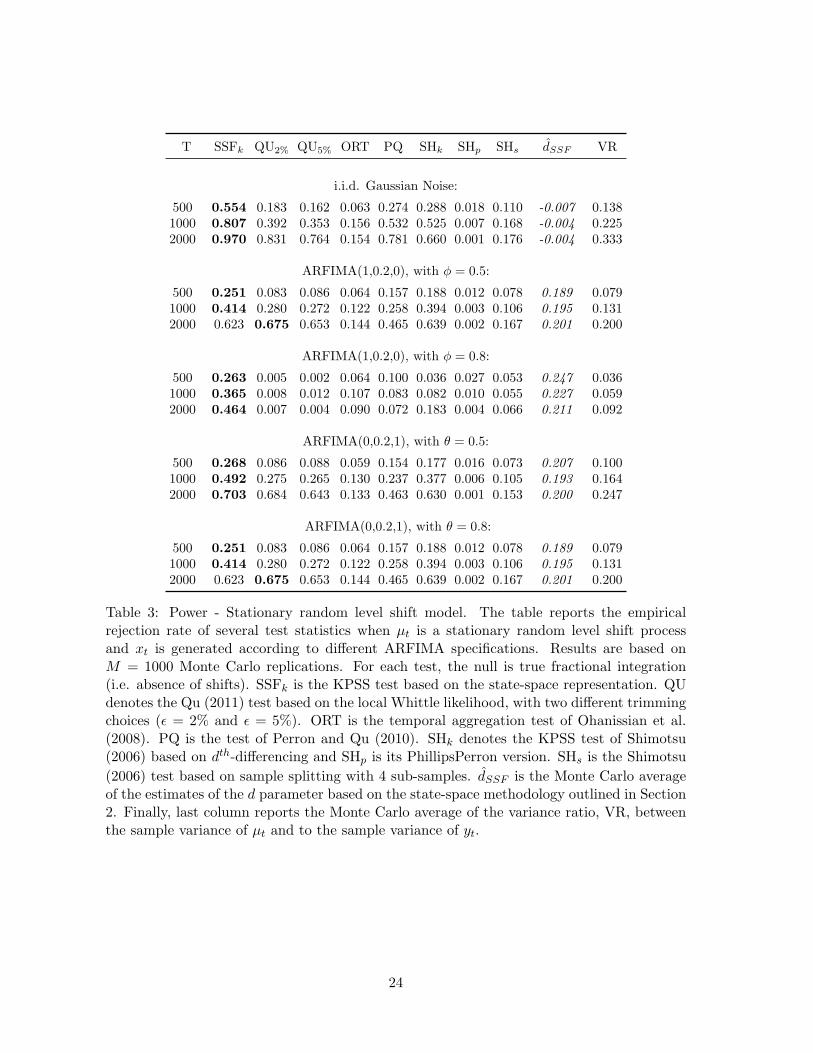
3.2.2 Stationary random level shifts

The good performance of the SSFk test is confirmed also when an ARFIMA process is

contaminated by a stationary random level shift process, see Table 3. The power of the SSFk

test in detecting the presence of the shift process is the highest in almost all cases considered.

This is again due to our approachs ability to provide accurate parameter estimates in all

cases. Indeed, the estimates of the long memory parameter d, reported in the last column of

the table, are always centred around the true value. Also in this case, we note a relatively

low empirical power for the ARFIMA with φ = 0.8 as a consequence of the low VR and the

biased estimates of the long memory parameter. However, the empirical power of the SSFk

remains the highest compared to the semi-parametric alternatives.

3.2.3 Monotonic and non-monotonic trends

The SSFk test performs surprisingly well also when non-stochastic trends are present in the

data, see Tables 4 and 5. Although the model specification is not designed to account for

those DGPs, our method provides a good tracking of the deterministic trends when they

are present in the data. Thus, the empirical power of the SSFk test is almost 1 in many

cases and it drops only when a highly persistent ARFIMA process is present in the data.

Relatively to the other semi-parametric tests, the power of our test is extremely high for

the monotonic trend. For the non-monotonic trend, we observe a good performance of the

Qu (2011) test, with the exclusion of the ARFIMA(1,0.2,0) with φ = 0.8. Interestingly, the

power of the SSFk is high even though the VR is relatively low compared to the random

level-shift processes in the previous tables.

3.2.4 Markov-switching processes

Tables 6 and 7 report the results for a trend µt generated by a Markow-switching process.

Also in this case, the observed series is obtained by the sum of the Markov-switching process

and an ARFIMA term. The power of the SSFk test is generally the highest compared to

the methods and the estimates of d are well centred on the true values with the exception

of the case with φ = 0.8. In this case, the best performance is achieved by the KPSS test of

Shimotsu (2006), but the power is rather low for all T . On the contrary, the power of the

SSFk relative to the other tests is very high when the ARFIMA process contains MA terms

or when xt is an i.i.d. noise for moderate values of T .

When the Markov switching term is characterized by GARCH effects, the overall power

is rather low for all tests. Still, the SSFk has the overall best performance, but the power is

above 50% only in one case, when xt follows an ARFIMA with θ = 0.8 and T = 2000. In

fact, the estimates of the fractional parameter d are generally far from the true value and

this leads to lower power than that achieved under different DGPs for µt. This result is

mainly due to the fact that, although the VR is rather high in this case, the autocorrelation

function of µt is not characterized by very high persistence, so that it is hard for the modified

Kalman filter of Kim (1994) to disentangle µt and xt, with consequent power losses.

12

4 Empirical application

Let us now apply the SSFk test to a number of financial time series for which evidence of

fractional integration has been documented. In particular, we choose daily bipower-variation

and turnover, which is the trading volume divided by the number of outstanding shares. The

sample covers 15 stocks traded on NYSE for the period between January 2, 2003 and June

28, 2013, for a total of 2640 observations. As it has been widely shown in the past, the series

of realized volatility and bipower-variation are characterized by long-range dependence, or

long memory, see Andersen et al. (2001a), Andersen et al. (2001b), Andersen et al. (2003),

Andersen et al. (2009) and Martens et al. (2009). Analogously, it has been documented that

trading volume also displays long-range dependence features. For instance, Bollerslev and

Jubinski (1999) and Lobato and Velasco (2000) both report strong evidence that volume

exhibits long memory. More recently, Rossi and Santucci de Magistris (2013) study the

common dynamic dependence between volatility and volume and find evidence of fractional

cointegration only for the series belonging to the bank/financial sector, i.e. those that during

the financial crises have experienced a large upward level shift. It is therefore of interest to

be able to formally test, although in an univariate setup, if volatility and volume are subject

to level shifts or if their long-run dependence is more likely generated by a pure fractional

process.

The bipower-variation is constructed using log-returns at 1-minute frequencies as

BPVt =π

2

(

M

M − 1

) M∑

j=2

|rt,j−1| · |rt,j |, (17)

where rt,j is the j-th log-return on day t and M = 390 is the number of intra-daily ob-

servations associated to 1-minute frequencies. The BPVt estimator converges to the daily

integrated variance, i.e. the instantaneous variance cumulated over daily horizons, and it is

robust to price jumps. For what concerns the daily turnover, they are defined as

TRVt =VtSt, (18)

where Vt is the trading volume, i.e. number of shares that have been bought and sold within

day t and St is the number of shares available for sale by the general trading public at time t.

The turnover is by construction more robust than trading volume to effects like stock splits

and it does not display large upward trends as Vt. The empirical analysis is carried out on

the log-transformed series, log(BPVt) and log(TRVt) as the model (1) involves unobserved

components that are defined on the entire set of real numbers. Moreover, although the

distributions of bipower-variation and turnover are clearly right-skewed, the distributions of

their logarithms are approximately Gaussian.

Tables 8 and 9 report the values of the tests for the presence of fractional integration in

log(BPVt) and log(TRVt). For what concerns log(BPVt), the SSFk rejects the null hypothe-

sis of absence of shift for 8 out of 15 stocks at 5% significance level. Interestingly, the highest

values of the tests are associated with the companies operating in the financial sector, like

13

Bank of America (BAC), Citygroup (C), JP-Morgan (JPM) and Wells Fargo (WFC). These

companies have been subject to a major financial distress during the 2008-2009 financial

crisis, and the values of BPVt have been extremely high for many months in this period.

The test of Perron and Qu (2010) also seems to find significant evidence of shifts for three

out of four volatility series of the stocks in the bank sector. However, the tests based on

semi-parametric specifications are unable to reject the null hypothesis of fractional integra-

tion in most cases. This may be a consequence of their rather low power, as it emerged in

the Monte Carlo study. Indeed, looking at the semi-parametric estimates of d, obtained with

the Whittle estimator, they lie generally above the stationary threshold, i.e. d > 0.5. On the

other hand, the estimates obtained with the state-space methodology are still positive but

significantly smaller than 0.5 (with the exception of PG), meaning that a large portion of

the observed long-run dependence is attributed to the random level shifts (or possibly other

trend components).

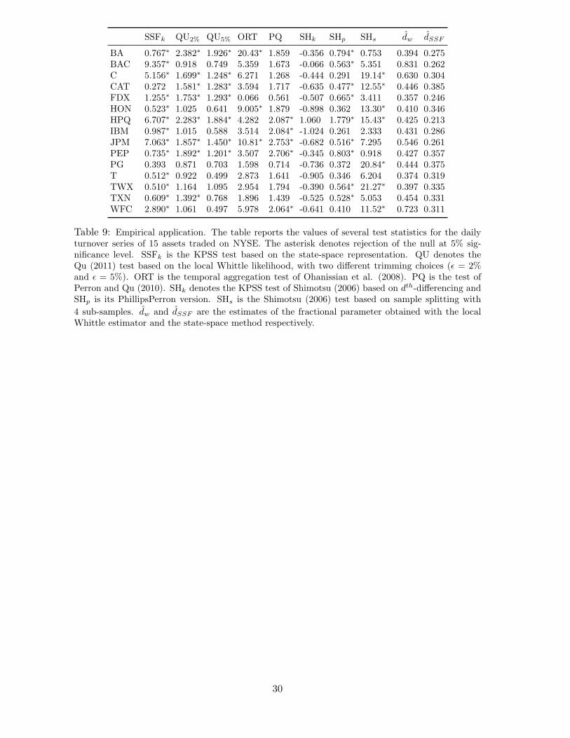
For what concerns log(TRVt), the SSFk rejects the null hypothesis of absence of shifts

for 13 out of 15 stocks at 5% significance level, and the estimated fractional parameter is

significantly larger than 0 in all cases. Interestingly, there is an almost unanimous agreement

across all tests that the turnover series of BA, HPQ, JPM and PEP present spurious long-

memory features, while the assumption of truly long-memory for the log(TRVt) of PG is

only rejected by the SHs test. Again, the highest values of the SSFk test are associated

with BAC, C, JPM and WFC. This seems to provide some evidence in favour of the long

run relationship between volatility and volume as possibly driven by the joint presence of

shifts and not only by a common fractional trend. Indeed, both log(BPVt) and log(TRVt)

may be generated by the combination of a fractional process and a shift (or a potentially

non-linear and smooth trend). Thus, the current univariate setup could be extended to the

multivariate case and, in particular, to the possibility of jointly model common fractional

trends and common shifts. This extension, coupled with the definition of an efficient method

to track the shifting process given the parameter estimates, is left to future research.

5 Conclusion

In this paper, we have proposed a robust testing strategy for a fractional process potentially

subject to structural breaks. Contrary to the other tests for true fractional integration

presented so far in the literature, the focus of our approach is on the level shift process. We

propose a flexible state-space parametrization that is able to account for the presence of both

an ARFIMA and a level-shift process. In particular, our parametric approach provides robust

estimates of the memory parameter for a given time series possibly subject to level shifts or

other smoothly varying trends. The testing procedure can be seen as a robust version of the

KPSS test for the presence of level shifts. A Monte Carlo study shows that the proposed

method performs much better than the other existing tests, especially under the alternative.

Interestingly, the modified Kalman filter routine adopted to estimate the model parameters

is robust to a variety of different contamination processes and it is reliable also when slowly

14

varying trends characterize the data. From the empirical analysis on a set of US stocks, it

emerges that volatility and trading volume are likely to be characterized by the combined

presence of both long-memory and level shifts. This result differs from that of other existing

tests, which usually over-estimate the long memory parameter and are characterized by low

power. The theoretical and empirical results outlined in this paper call for extensions in

several directions. For example, the tracking of the shift process, possibly using a smoothing

algorithm, would be very informative on the type of trend that characterizes the data and

could be exploited for forecasting purposes. Alternatively, a multivariate extension of model

(1) would allow to distinguish and test the hypothesis of fractional cointegration in a context

characterized by common and idiosyncratic level shifts.

References

Andersen, T. G., Bollerslev, T., and Diebold, F. X. (2009). Parametric and nonparamet-

ric volatility measurement. In Ait-Sahalia, Y. and Hansen, L. P., editors, Handbook of

Financial Econometrics, volume 1, chapter 2. Elsevier/North-Holland.

Andersen, T. G., Bollerslev, T., Diebold, F. X., and Ebens, H. (2001a). The distribution of

stock return volatility. Journal of Financial Economics, 61:43–76.

Andersen, T. G., Bollerslev, T., Diebold, F. X., and Labys, P. (2001b). The distribution of

exchange rate volatility. Journal of the American Statistical Association, 96:42–55.

Andersen, T. G., Bollerslev, T., Diebold, F. X., and Labys, P. (2003). Modeling and fore-

casting realized volatility. Econometrica, 71:579–625.

Baillie, R. T., Chung, C. F., and Tieslau, M. A. (1996). Analysing inflation by the fractionally

integrated ARFIMA-GARCH model. Journal of Applied Econometrics, 11:23–40.

Berenguer-Rico, V. and Gonzalo, J. (2014). Summability of stochastic processes: A gener-

alization of integration for non-linear processes. Journal of Econometrics, 178:331–341.

Bollerslev, T. and Jubinski, D. (1999). Equity trading volume and volatility: Latent in-

formation arrivals and common long-run dependencies. Journal of Business & Economic

Statistics, 17:9–21.

Chan, N. and Palma, W. (1998). State space modeling of long-memory processes. Annals of


Dahlhaus, R. (1989). Efficient parameter estimation for self-similar processes. Annals of


Diebold, F. X., Husted, S., and Rush, M. (1991). Real exchange rates under the gold

standard. Journal of Political Economy, 99:1252–1271.

Diebold, F. X. and Inoue, A. (2001). Long memory and regime switching. Journal of

Econometrics, 105:131–159.

15

Dolado, J., Gonzalo, J., and Mayoral, L. (2008). Wald tests of i(1) against i(d) alternatives:

Some new properties and an extension to processes with trending components. Studies in

Nonlinear Dynamics & Econometrics, 12:1562–1562.

Fox, R. and Taqqu, M. S. (1986). Large-sample properties of parameter estimates for strongly

dependent stationary gaussian series. Annals of Statistics, 14:517–532.

Granger, C. W. J. (1980). Long memory relationships and the aggregation of dynamic

models. Journal of Econometrics, 14:227–238.

Granger, C. W. J. and Hyung, N. (2004). Occasional structural breaks and long memory

with application to the S&P 500 absolute stock returns. Journal of Empirical Finance,

11:399–421.

Granger, C. W. J. and Joyeux, R. (1980). An introduction to long-memory time series

models and fractional differencing. Journal of Time Series Analysis, 4:221–238.

Grassi, S. and Santucci de Magistris, P. (2014). When long memory meets the kalman filter:

A comparative study. Computational Statistics and Data Analysis, 76:301–319.

Harvey, A. (1989). Forecasting, Structural Time Series and the Kalman Filter. Cambridge

University Press, Cambridge, UK.

Harvey, A. and Proietti, T. (2005). Readings in Unobserved Components Models. OUP

Catalogue. Oxford University Press.

Hosking, J. (1981). Fractional differencing. Biometrika, 68:165–76.

Hurst, H. (1951). Long term storage capacity of reservoirs. Transactions of The American

Society of Civil Engineers, 1:519–543.

Kim, C. J. (1994). Dynamic linear models with Markov-switching. Journal of Econometrics,

60:1–22.

Kim, C. J. and Nelson, C. R. (1999). State-Space Models with Regime Switching: Classical

and Gibbs-Sampling Approaches with Applications, volume 1 of MIT Press Books. The

MIT Press.

Leccadito, A., Rachedi, O., and Urga, G. (2015). True versus spurious long memory: Some

theoretical results and a monte carlo comparison. Econometric Reviews, 34:452–479.

Leybourne, S. J. and McCabe, B. P. M. (1994). A consistent test for a unit root. Journal of

Business and Economic Statistics, 12:157–166.

Lobato, I. N. and Velasco, C. (2000). Long memory in stock-market trading volume. Journal

of Business & Economic Statistics, 18:410–427.

Mandelbrot, B. (1975). Limit theorems of the self-normalized range for weakly and strongly

dependent processes. Z. Wahrscheinlichkeitstheorie verw. Gebiete, 31:271–285.

16

Martens, M., Van Dijk, D., and De Pooter, M. (2009). Forecasting s&p 500 volatility: Long

memory, level shifts, leverage effects, day-of-the-week seasonality, and macroeconomic an-

nouncements. International Journal of Forecasting, 25:282–303.

Mikosch, T. and Starica, C. (2004). Nonstationarities in financial time series, the long-range

dependence, and the igarch effects. The Review of Economics and Statistics, 86:378–390.

Nyblom, J. and Makelainen, T. (1983). Comparisons of tests for the presence of random

walk coefficients in a simple linear model. Journal of the American Statistical Association,

78:865–864.

Ohanissian, A., Russell, J. R., and Tsay, R. S. (2008). True or spurious long memory? a

new test. Journal of Business & Economic Statistics, 26:161–175.

Perron, P. and Qu, Z. (2010). Long-memory and level shifts in the volatility of stock market

return indices. Journal of Business & Economic Statistics, 28:275–290.

Qu, Z. (2011). A test against spurious long memory. Journal of Business & Economic


Robinson, P. M. (1995). Log-periodogram regression of time series with long range depen-

dence. The Annals of Statistics, 23:1048–1072.

Rossi, E. and Santucci de Magistris, P. (2013). Long memory and tail dependence in trading

volume and volatility. Journal of Empirical Finance, 22:94–112.

Shimotsu, K. (2006). Simple (but effective) tests of long memory versus structural breaks.

Technical report, Working paper, Queen’s University.

Sowell, F. (1992). Maximum likelihood estimation of stationary univariate fractionally inte-

grated time series models. Journal of Econometrics, 53:165–188.

Xiaofeng, S. and Xianyang, Z. (2010). Testing for change points in time series. Journal of

the American Statistical Association, 105:1228–1240.

17

A Appendix

A.1 Summability order of the level shift component µt

The summability condition of the process µt can be derived by looking at µt as a random

walk, where the innovation is zt = γtδt, where γt ∼ Bern(π) and δt ∼ N(0, σ2δ ), so that

E(zt) = E(γt) · E(δt) = π · 0 = 0, (19)

Var(zt) = Var(γt) ·Var(δt) + Var(δt) · E(γt)2 +Var(γt) · E(δt)2 (20)

= p(1− π)σ2δ + π2σ2δ + 0 = π · σ2δ .

Therefore the partial sum

1

T12

1

σδ√π

[Tr]∑

t=1

ztd→W (r), (21)

so that zt ∼ S(0) and zt ∼ I(0). Provided that µt =∑T

t=1 zt, then

1

T32

1

σδ√π

[Tr]∑

t=1

µtd→∫ r

0W (r)dr, (22)

so that µt ∼ S(1) and µt ∼ I(1), but with a slowly varying function equal to L(T ) = 1σδ

√π,

see Berenguer-Rico and Gonzalo (2014). When π = 1 we obtain the usual convergence rate

of the random walk, with i.i.d. innovations. It is clear that the convergence depends on π,

so that to smaller π corresponds a slower convergence rate.

A.2 Estimation of ARFIMA models by state-space methods

Here we recall how to estimate the ARFIMA model introduced in Section 1 using state-space

methods. Following Harvey (1989) and Harvey and Proietti (2005), the time invariant state

space representation consists of two equations. The first is the measurement equation, which

relates the univariate time series, yt, to the state vector:

yt = Zαt + εt, t = 1, ..., T, (23)

where Z is 1×m selection vector, αt ism×1 state vector with initial values α1 ∼ N(α1|0,P1|0)

and εt ∼ N(0, σ2ε) is the measurement error. The second is the transition equation, that

defines the evolution of the state vector αt as a first order vector autoregression:

αt = Fαt−1 +Rηt, ηt ∼ N(0,Q), (24)

where F is m×m matrix, R is m×g selection matrix, and ηt is a g×1 disturbance vector and

Q is a g×g variance-covariance matrix. The two disturbances are assumed to be uncorrelated

18

E(εtη′t−j) = 0 for j = 0, 1, ..., T .

Let define Yt = y1, . . . , yt as the information set up to time t, the state vector αt and

the observations yt, are conditional Gaussian, i.e. αt|Yt−1 ∼ N(αt|t−1,Pt|t−1) and yt|Yt−1 ∼N(Zαt|t−1,Ft), with mean and variance computed by the Kalman filter (KF) recursions

vt = yt − Zαt|t−1, t = 1, . . . , T,

Gt = ZPt|t−1Z′ + σ2ε ,

Kt = FPt|t−1Z′G−1

t ,

αt+1|t = Fαt|t−1 +Ktvt,

Pt+1|t = FPt|t−1F′ −KtGtK

′t +RQR′.

(25)

The algorithm is initialized with the unconditional mean α1|0 = 0 and the unconditional

variance vec(P1|0) = (I − F ⊗ F)−1vec(RQR′). The system matrices are deterministically

related with the vector of parameter ψ, thus we can construct the log-likelihood function:

ℓ(YT ;ψ) =T∑

t=1

log Pr(yt|Yt−1;ψ) = −T2log 2π − 1

2

T∑

t=1

logGt −1

2

T∑

t=1

v2tGt. (26)

In case we are interested in the “contemporaneous filter” or “real-time estimate” of the state

vector, we have that αt|Yt ∼ N(αt|t,Pt|t), where

αt|t = αt|t−1 + Pt|t−1Z′G−1

t vt,

Pt|t = Pt|t−1 − Pt|t−1Z′G−1

t ZPt|t−1.(27)

Looking at equations (25) and (27), we can notice that the filtering (25) can be obtained

from (27) as follows

αt+1|t = Fαt|t,

Pt+1|t = FPt|tF′ +RQR′.

(28)

Equations (27) together with the prediction error vt and its variance Gt are known as the

“updating step”, while the equations (28) are known as the “prediction step”. To derive

the set of recursions for the model with switching parameters we break down the filtering in

those two steps.

The ARFIMA model (3) has the following autoregressive (AR) representation ϕ(L)xt =

ξt, where

ϕ(L) = 1−∞∑

j=1

ϕjLj = (1− L)d

Φ(L)

Θ(L), (1− L)d =

∞∑

j=0

Γ(j − d)

Γ(j + 1)Γ(−d)Lj ,

Its moving average (MA) representation is xt = Ψ(L)ξt, where

ζ(L) = 1 +∞∑

j=1

ψjLj = (1− L)−dΘ(L)

Φ(L), (1− L)−d =

∞∑

j=0

Γ(j + d)

Γ(j + 1)Γ(d)Lj .

Chan and Palma (1998) show that the exact likelihood function is obtained using the AR

19

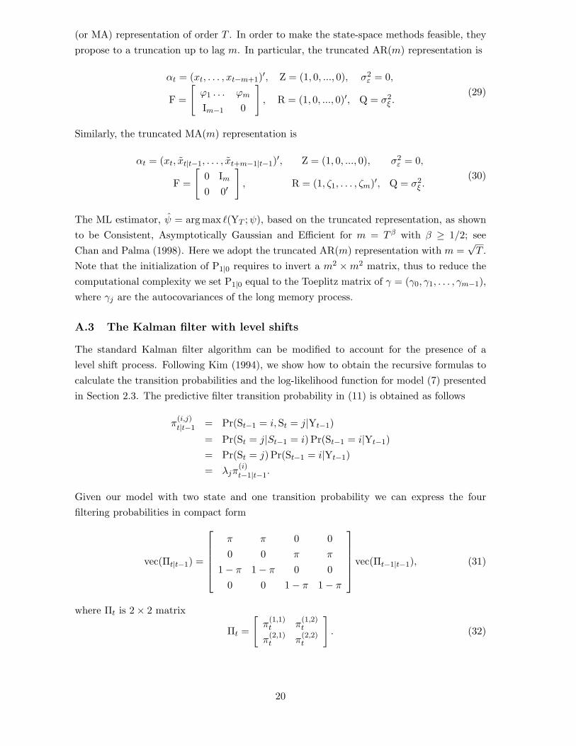
(or MA) representation of order T . In order to make the state-space methods feasible, they

propose to a truncation up to lag m. In particular, the truncated AR(m) representation is

αt = (xt, . . . , xt−m+1)′, Z = (1, 0, ..., 0), σ2ε = 0,

F =

[

ϕ1 . . . ϕm

Im−1 0

]

, R = (1, 0, ..., 0)′, Q = σ2ξ .(29)

Similarly, the truncated MA(m) representation is

αt = (xt, xt|t−1, . . . , xt+m−1|t−1)′, Z = (1, 0, ..., 0), σ2ε = 0,

F =

[

0 Im

0 0′

]

, R = (1, ζ1, . . . , ζm)′, Q = σ2ξ .(30)

The ML estimator, ψ = argmax ℓ(YT ;ψ), based on the truncated representation, as shown

to be Consistent, Asymptotically Gaussian and Efficient for m = T β with β ≥ 1/2; see

Chan and Palma (1998). Here we adopt the truncated AR(m) representation with m =√T .

Note that the initialization of P1|0 requires to invert a m2 ×m2 matrix, thus to reduce the

computational complexity we set P1|0 equal to the Toeplitz matrix of γ = (γ0, γ1, . . . , γm−1),

where γj are the autocovariances of the long memory process.

A.3 The Kalman filter with level shifts

The standard Kalman filter algorithm can be modified to account for the presence of a

level shift process. Following Kim (1994), we show how to obtain the recursive formulas to

calculate the transition probabilities and the log-likelihood function for model (7) presented

in Section 2.3. The predictive filter transition probability in (11) is obtained as follows

π(i,j)t|t−1 = Pr(St−1 = i, St = j|Yt−1)

= Pr(St = j|St−1 = i) Pr(St−1 = i|Yt−1)

= Pr(St = j) Pr(St−1 = i|Yt−1)

= λjπ(i)t−1|t−1.

Given our model with two state and one transition probability we can express the four

filtering probabilities in compact form

vec(Πt|t−1) =

π π 0 0

0 0 π π

1− π 1− π 0 0

0 0 1− π 1− π

vec(Πt−1|t−1), (31)

where Πt is 2× 2 matrix

Πt =

[

π(1,1)t π

(1,2)t

π(2,1)t π

(2,2)t

]

. (32)

20

B Tables

T SSFk QU2% QU5% ORT PQ SHk SHp SHs dSSF

ARFIMA(0,0.4,0):

500 0.078 0.013 0.016 0.054 0.077 0.021 0.033 0.080 0.384

1000 0.062 0.017 0.021 0.060 0.055 0.029 0.034 0.063 0.390

2000 0.060 0.019 0.024 0.061 0.045 0.033 0.036 0.064 0.392

ARFIMA(1,0.4,0), with φ = 0.5:

500 0.095 0.004 0.004 0.056 0.108 0.010 0.030 0.0760 0.375

1000 0.085 0.010 0.011 0.078 0.061 0.015 0.036 0.068 0.385

2000 0.067 0.017 0.024 0.064 0.044 0.022 0.046 0.063 0.394

ARFIMA(1,0.4,0), with φ = 0.8:

500 0.036 0.006 0.015 0.061 0.087 0.071 0.000 0.112 0.450

1000 0.046 0.010 0.016 0.059 0.058 0.084 0.000 0.130 0.447

2000 0.034 0.002 0.004 0.049 0.045 0.082 0.000 0.105 0.423

ARFIMA(0,0.4,1), with θ = 0.5:

500 0.065 0.014 0.014 0.060 0.071 0.025 0.034 0.087 0.370

1000 0.055 0.020 0.027 0.060 0.047 0.035 0.033 0.066 0.379

2000 0.053 0.023 0.032 0.057 0.045 0.034 0.033 0.065 0.381

ARFIMA(0,0.4,1), with θ = 0.8:

500 0.094 0.017 0.024 0.062 0.060 0.031 0.023 0.075 0.370

1000 0.060 0.017 0.026 0.061 0.056 0.033 0.030 0.066 0.381

2000 0.054 0.023 0.030 0.059 0.045 0.034 0.033 0.063 0.385

Table 1: Empirical Size. The table reports the empirical rejection rate of several test statisticswhen µt = 0 and xt is generated according to different ARFIMA specifications with d =0.4. Results are based on 1000 Monte Carlo replications. For each test, the null is truefractional integration (i.e. absence of shifts). SSFk is the KPSS test based on the state-space representation. QU denotes the Qu (2011) test based on the local Whittle likelihood,with two different trimming choices (ǫ = 2% and ǫ = 5%). ORT is the temporal aggregationtest of Ohanissian et al. (2008). PQ is the test of Perron and Qu (2010). SHk denotes theKPSS test of Shimotsu (2006) based on dth-differencing and SHp is its PhillipsPerron version.SHs is the Shimotsu (2006) test based on sample splitting with 4 sub-samples. Finally, lastcolumn reports the Monte Carlo average of the estimates of the d parameter based on thestate-space methodology outlined in Section 2.

22

T SSFk QU2% QU5% ORT PQ SHk SHp SHs dSSF VR

i.i.d. Gaussian Noise:

500 0.832 0.183 0.151 0.097 0.183 0.328 0.004 0.128 -0.028 0.4021000 0.904 0.264 0.212 0.183 0.297 0.454 0.002 0.184 0.002 0.3932000 0.967 0.571 0.374 0.223 0.422 0.669 0.001 0.284 -0.000 0.408

ARFIMA(1,0.2,0), with φ = 0.5:

500 0.586 0.082 0.067 0.067 0.144 0.239 0.005 0.089 0.174 0.2871000 0.638 0.193 0.151 0.122 0.169 0.350 0.003 0.110 0.165 0.2742000 0.739 0.423 0.274 0.128 0.170 0.550 0.002 0.132 0.171 0.283

ARFIMA(1,0.2,0), with φ = 0.8:

500 0.349 0.011 0.017 0.042 0.112 0.074 0.015 0.047 0.279 0.1411000 0.348 0.073 0.010 0.080 0.081 0.131 0.008 0.048 0.236 0.1282000 0.471 0.010 0.000 0.087 0.078 0.196 0.004 0.075 0.208 0.132

ARFIMA(0,0.2,1), with θ = 0.5:

500 0.628 0.212 0.206 0.068 0.258 0.269 0.001 0.095 0.193 0.3191000 0.702 0.449 0.433 0.141 0.329 0.451 0.003 0.124 0.194 0.3072000 0.814 0.692 0.667 0.118 0.495 0.624 0.002 0.135 0.195 0.319

ARFIMA(0,0.2,1), with θ = 0.8:

500 0.558 0.228 0.207 0.073 0.246 0.265 0.003 0.081 0.196 0.2671000 0.635 0.431 0.423 0.110 0.349 0.438 0.002 0.102 0.196 0.2552000 0.752 0.683 0.652 0.133 0.492 0.641 0.004 0.163 0.198 0.266

Table 2: Power. Non-stationary random level shift model. The table reports the empiricalrejection rate of several test statistics when µt is a random level shift process and xt isgenerated according to different ARFIMA specifications. Results are based on 1000 MonteCarlo replications. For each test, the null is true fractional integration (i.e. absence of shifts).SSFk is the KPSS test based on the state-space representation. QU denotes the Qu (2011)test based on the local Whittle likelihood, with two different trimming choices (ǫ = 2% andǫ = 5%). ORT is the temporal aggregation test of Ohanissian et al. (2008). PQ is thetest of Perron and Qu (2010). SHk denotes the KPSS test of Shimotsu (2006) based ondth-differencing and SHp is its PhillipsPerron version. SHs is the Shimotsu (2006) test based

on sample splitting with 4 sub-samples. dSSF is the Monte Carlo average of the estimatesof the d parameter based on the state-space methodology outlined in Section 2. Finally,last column reports the Monte Carlo average of the variance ratio, V R, between the samplevariance of µt and to the sample variance of yt.

23



500 0.554 0.183 0.162 0.063 0.274 0.288 0.018 0.110 -0.007 0.1381000 0.807 0.392 0.353 0.156 0.532 0.525 0.007 0.168 -0.004 0.2252000 0.970 0.831 0.764 0.154 0.781 0.660 0.001 0.176 -0.004 0.333

ARFIMA(1,0.2,0), with φ = 0.5:

500 0.251 0.083 0.086 0.064 0.157 0.188 0.012 0.078 0.189 0.0791000 0.414 0.280 0.272 0.122 0.258 0.394 0.003 0.106 0.195 0.1312000 0.623 0.675 0.653 0.144 0.465 0.639 0.002 0.167 0.201 0.200

ARFIMA(1,0.2,0), with φ = 0.8:

500 0.263 0.005 0.002 0.064 0.100 0.036 0.027 0.053 0.247 0.0361000 0.365 0.008 0.012 0.107 0.083 0.082 0.010 0.055 0.227 0.0592000 0.464 0.007 0.004 0.090 0.072 0.183 0.004 0.066 0.211 0.092

ARFIMA(0,0.2,1), with θ = 0.5:

500 0.268 0.086 0.088 0.059 0.154 0.177 0.016 0.073 0.207 0.1001000 0.492 0.275 0.265 0.130 0.237 0.377 0.006 0.105 0.193 0.1642000 0.703 0.684 0.643 0.133 0.463 0.630 0.001 0.153 0.200 0.247

ARFIMA(0,0.2,1), with θ = 0.8:

500 0.251 0.083 0.086 0.064 0.157 0.188 0.012 0.078 0.189 0.0791000 0.414 0.280 0.272 0.122 0.258 0.394 0.003 0.106 0.195 0.1312000 0.623 0.675 0.653 0.144 0.465 0.639 0.002 0.167 0.201 0.200

Table 3: Power - Stationary random level shift model. The table reports the empiricalrejection rate of several test statistics when µt is a stationary random level shift processand xt is generated according to different ARFIMA specifications. Results are based onM = 1000 Monte Carlo replications. For each test, the null is true fractional integration(i.e. absence of shifts). SSFk is the KPSS test based on the state-space representation. QUdenotes the Qu (2011) test based on the local Whittle likelihood, with two different trimmingchoices (ǫ = 2% and ǫ = 5%). ORT is the temporal aggregation test of Ohanissian et al.(2008). PQ is the test of Perron and Qu (2010). SHk denotes the KPSS test of Shimotsu(2006) based on dth-differencing and SHp is its PhillipsPerron version. SHs is the Shimotsu

(2006) test based on sample splitting with 4 sub-samples. dSSF is the Monte Carlo averageof the estimates of the d parameter based on the state-space methodology outlined in Section2. Finally, last column reports the Monte Carlo average of the variance ratio, VR, betweenthe sample variance of µt and to the sample variance of yt.

24



500 0.942 0.013 0.015 0.040 0.222 0.190 0.001 0.050 0.001 0.1131000 1.000 0.010 0.013 0.058 0.498 0.210 0.001 0.032 -0.004 0.1162000 1.000 0.020 0.016 0.072 0.729 0.515 0.001 0.050 -0.004 0.119

ARFIMA(1,0.2,0), with φ = 0.5:

500 0.757 0.006 0.012 0.069 0.101 0.089 0.006 0.067 0.200 0.0601000 0.929 0.020 0.026 0.078 0.093 0.146 0.005 0.058 0.174 0.0622000 0.987 0.046 0.042 0.072 0.074 0.258 0.002 0.047 0.159 0.065

ARFIMA(1,0.2,0), with φ = 0.8:

500 0.948 0.015 0.018 0.058 0.206 0.173 0.001 0.049 0.194 0.0631000 0.996 0.017 0.021 0.082 0.225 0.291 0.001 0.060 0.195 0.0652000 1.000 0.045 0.036 0.065 0.271 0.449 0.001 0.055 0.199 0.068

ARFIMA(0,0.2,1), with θ = 0.5:

500 0.989 0.013 0.016 0.055 0.187 0.172 0.001 0.043 0.193 0.0741000 1.000 0.013 0.015 0.090 0.197 0.257 0.001 0.049 0.198 0.0752000 1.000 0.050 0.038 0.098 0.275 0.448 0.001 0.066 0.199 0.077

ARFIMA(0,0.2,1), with θ = 0.8:

500 0.948 0.015 0.018 0.058 0.206 0.173 0.001 0.049 0.194 0.0631000 0.996 0.017 0.021 0.082 0.225 0.291 0.001 0.060 0.195 0.0652000 1.000 0.045 0.036 0.065 0.271 0.449 0.001 0.055 0.199 0.068

Table 4: Power - Monotonic trend model. The table reports the empirical rejection rateof several test statistics when µt is a monotonic trend and xt is generated according todifferent ARFIMA specifications. Results are based on 1000 Monte Carlo replications. Foreach test, the null is true fractional integration (i.e. absence of shifts). SSFk is the KPSStest based on the state-space representation. QU denotes the Qu (2011) test based on thelocal Whittle likelihood, with two different trimming choices (ǫ = 2% and ǫ = 5%). ORT isthe temporal aggregation test of Ohanissian et al. (2008). PQ is the test of Perron and Qu(2010). SHk denotes the KPSS test of Shimotsu (2006) based on dth-differencing and SHp isits PhillipsPerron version. SHs is the Shimotsu (2006) test based on sample splitting with 4sub-samples. dSSF is the Monte Carlo average of the estimates of the d parameter based onthe state-space methodology outlined in Section 2. Finally, last column reports the MonteCarlo average of the variance ratio, VR, between the sample variance of µt and to the samplevariance of yt.

25



500 0.993 0.839 0.491 0.079 0.085 0.003 0.001 0.099 -0.035 0.3341000 1.000 0.954 0.608 0.141 0.075 0.005 0.001 0.099 -0.025 0.3342000 1.000 1.000 0.722 0.162 0.095 0.015 0.001 0.124 -0.017 0.335

ARFIMA(1,0.2,0), with φ = 0.5:

500 0.070 0.126 0.072 0.079 0.106 0.016 0.003 0.066 0.319 0.2081000 0.235 0.286 0.162 0.109 0.096 0.030 0.001 0.081 0.267 0.2032000 0.661 0.602 0.337 0.103 0.064 0.082 0.001 0.099 0.157 0.202

ARFIMA(1,0.2,0), with φ = 0.8:

500 0.131 0.008 0.008 0.062 0.110 0.022 0.016 0.066 0.265 0.0831000 0.150 0.011 0.010 0.091 0.094 0.019 0.009 0.044 0.247 0.0792000 0.211 0.006 0.006 0.061 0.084 0.033 0.005 0.041 0.220 0.075

ARFIMA(0,0.2,1), with θ = 0.5:

500 0.243 0.449 0.286 0.075 0.074 0.002 0.001 0.067 0.257 0.2411000 0.501 0.660 0.589 0.115 0.079 0.020 0.001 0.107 0.210 0.2372000 0.887 0.962 0.921 0.131 0.040 0.186 0.001 0.133 0.205 0.237

ARFIMA(0,0.2,1), with θ = 0.8:

500 0.131 0.008 0.008 0.062 0.110 0.022 0.016 0.066 0.265 0.0831000 0.150 0.011 0.010 0.091 0.094 0.019 0.009 0.044 0.247 0.0792000 0.211 0.006 0.006 0.061 0.084 0.033 0.005 0.041 0.220 0.075

Table 5: Power - Nonmonotonic trend model. The table reports the empirical rejection rateof several test statistics when µt is a non-monotonic trend and xt is generated according todifferent ARFIMA specifications. Results are based on 1000 Monte Carlo replications. Foreach test, the null is true fractional integration (i.e. absence of shifts). SSFk is the KPSStest based on the state-space representation. QU denotes the Qu (2011) test based on thelocal Whittle likelihood, with two different trimming choices (ǫ = 2% and ǫ = 5%). ORT isthe temporal aggregation test of Ohanissian et al. (2008). PQ is the test of Perron and Qu(2010). SHk denotes the KPSS test of Shimotsu (2006) based on dth-differencing and SHp isits PhillipsPerron version. SHs is the Shimotsu (2006) test based on sample splitting with 4sub-samples. dSSF is the Monte Carlo average of the estimates of the d parameter based onthe state-space methodology outlined in Section 2. Finally, last column reports the MonteCarlo average of the variance ratio, VR, between the sample variance of µt and to the samplevariance of yt.

26



500 0.452 0.201 0.203 0.062 0.347 0.260 0.021 0.079 -0.008 0.5451000 0.669 0.415 0.392 0.108 0.573 0.341 0.017 0.110 -0.007 0.5782000 0.845 0.688 0.659 0.153 0.847 0.453 0.011 0.145 -0.007 0.613

ARFIMA(1,0.2,0), with φ = 0.5:

500 0.375 0.028 0.026 0.054 0.122 0.095 0.012 0.078 0.278 0.3881000 0.538 0.079 0.061 0.117 0.142 0.262 0.011 0.102 0.254 0.4142000 0.773 0.261 0.160 0.115 0.158 0.448 0.004 0.127 0.223 0.441

ARFIMA(1,0.2,0), with φ = 0.8:

500 0.029 0.004 0.005 0.057 0.104 0.040 0.024 0.053 0.437 0.1791000 0.027 0.006 0.007 0.076 0.076 0.104 0.006 0.057 0.452 0.1952000 0.010 0.009 0.008 0.072 0.068 0.215 0.002 0.054 0.460 0.212

ARFIMA(0,0.2,1), with θ = 0.5:

500 0.426 0.099 0.087 0.053 0.234 0.208 0.021 0.101 0.198 0.4291000 0.609 0.342 0.306 0.107 0.488 0.348 0.015 0.094 0.200 0.4642000 0.845 0.683 0.612 0.164 0.765 0.509 0.009 0.176 0.201 0.497

ARFIMA(0,0.2,1), with θ = 0.8:

500 0.408 0.123 0.107 0.062 0.300 0.187 0.020 0.070 0.191 0.3621000 0.593 0.364 0.346 0.112 0.571 0.346 0.015 0.092 0.198 0.3592000 0.819 0.715 0.692 0.149 0.847 0.506 0.007 0.157 0.205 0.416

Table 6: Power - Markov switching model. The table reports the empirical rejection rateof several test statistics when µt is a Markov-switching and xt is generated according todifferent ARFIMA specifications. Results are based on 1000 Monte Carlo replications. Foreach test, the null is true fractional integration (i.e. absence of shifts). SSFk is the KPSStest based on the state-space representation. QU denotes the Qu (2011) test based on thelocal Whittle likelihood, with two different trimming choices (ǫ = 2% and ǫ = 5%). ORT isthe temporal aggregation test of Ohanissian et al. (2008). PQ is the test of Perron and Qu(2010). SHk denotes the KPSS test of Shimotsu (2006) based on dth-differencing and SHp isits PhillipsPerron version. SHs is the Shimotsu (2006) test based on sample splitting with 4sub-samples. dSSF is the Monte Carlo average of the estimates of the d parameter based onthe state-space methodology outlined in Section 2. Finally, last column reports the MonteCarlo average of the variance ratio, VR, between the sample variance of µt and to the samplevariance of yt.

27



500 0.139 0.021 0.027 0.048 0.122 0.066 0.079 0.078 0.141 0.9001000 0.249 0.055 0.042 0.132 0.122 0.255 0.057 0.086 0.142 0.8572000 0.441 0.198 0.093 0.128 0.128 0.480 0.022 0.155 0.146 0.845

ARFIMA(1,0.2,0), with φ = 0.5:

500 0.111 0.005 0.013 0.043 0.112 0.026 0.034 0.068 0.102 0.7621000 0.233 0.015 0.016 0.087 0.071 0.114 0.018 0.062 0.122 0.0.7592000 0.368 0.036 0.022 0.098 0.080 0.244 0.010 0.072 0.138 0.742

ARFIMA(1,0.2,0), with φ = 0.8:

500 0.005 0.001 0.005 0.063 0.097 0.009 0.022 0.052 0.298 0.4731000 0.009 0.004 0.004 0.088 0.081 0.062 0.008 0.059 0.301 0.4852000 0.009 0.019 0.016 0.063 0.076 0.118 0.007 0.028 0.309 0.495

ARFIMA(0,0.2,1), with θ = 0.5:

500 0.112 0.002 0.004 0.052 0.119 0.073 0.064 0.071 0.094 0.8131000 0.307 0.055 0.058 0.114 0.106 0.258 0.057 0.085 0.096 0.8012000 0.484 0.189 0.109 0.135 0.123 0.486 0.027 0.134 0.104 0.781

ARFIMA(0,0.2,1), with θ = 0.8:

500 0.159 0.024 0.036 0.062 0.135 0.077 0.082 0.074 0.080 0.7311000 0.297 0.068 0.060 0.128 0.117 0.244 0.058 0.089 0.088 0.7302000 0.505 0.262 0.153 0.149 0.154 0.527 0.029 0.168 0.093 0.729

Table 7: Power - Markov switching model with GARCH errors. The table reports theempirical rejection rate of several test statistics when µt is a Markov-switching term withGARCH errors and xt is generated according to different ARFIMA specifications. Results arebased on 1000 Monte Carlo replications. For each test, the null is true fractional integration(i.e. absence of shifts). SSFk is the KPSS test based on the state-space representation. QUdenotes the Qu (2011) test based on the local Whittle likelihood, with two different trimmingchoices (ǫ = 2% and ǫ = 5%). ORT is the temporal aggregation test of Ohanissian et al.(2008). PQ is the test of Perron and Qu (2010). SHk denotes the KPSS test of Shimotsu(2006) based on dth-differencing and SHp is its PhillipsPerron version. SHs is the Shimotsu

(2006) test based on sample splitting with 4 sub-samples. dSSF is the Monte Carlo averageof the estimates of the d parameter based on the state-space methodology outlined in Section2. Finally, last column reports the Monte Carlo average of the variance ratio, VR, betweenthe sample variance of µt and to the sample variance of yt.

28

SSFk QU2% QU5% ORT PQ SHk SHp SHs dw dSSF

BA 0.638∗ 0.868 0.558 3.035 -0.298 -1.606 0.118 2.881 0.652 0.420BAC 1.735∗ 0.653 0.569 7.415 2.493∗ -0.802 0.226 3.169 0.711 0.412C 2.710∗ 0.421 0.685 7.224 2.589∗ -0.948 0.265 2.064 0.702 0.395CAT 0.318 1.080 0.721 1.286 0.191 -1.656 0.114 7.307 0.707 0.477FDX 0.732∗ 0.601 0.539 1.331 1.177 -1.166 0.195 4.251 0.617 0.373HON 0.355 0.771 0.460 1.099 -0.360 -1.195 0.097 9.070∗ 0.645 0.404HPQ 0.568∗ 0.425 0.540 0.681 -0.455 -2.203 0.078 3.474 0.668 0.339IBM 0.283 0.488 0.845 2.184 0.454 -2.334 0.058 6.114 0.705 0.447JPM 1.419∗ 0.517 0.633 7.361 1.810 -1.607 0.212 3.845 0.716 0.412PEP 0.426 0.365 0.468 4.374 -0.270 -1.664 0.084 6.159 0.699 0.436PG 0.166 0.565 0.670 4.548 0.749 -2.098 0.058 8.335∗ 0.673 0.499T 0.313 0.449 0.670 2.390 -0.410 -0.931 0.087 4.326 0.680 0.429TWX 0.584∗ 0.449 0.553 1.539 -0.079 -1.508 0.080 9.324∗ 0.702 0.450TXN 0.517∗ 0.755 0.314 1.072 -0.492 -1.382 0.123 5.775 0.695 0.442WFC 2.492∗ 0.594 0.368 4.773 2.029∗ -1.110 0.234 2.174 0.740 0.371

Table 8: Empirical application. The table reports the values of several test statistics for the bipower-variations series of 15 assets traded on NYSE. The asterisk denotes rejection of the null at 5%significance level. SSFk is the KPSS test based on the state-space representation. QU denotes theQu (2011) test based on the local Whittle likelihood, with two different trimming choices (ǫ = 2%and ǫ = 5%). ORT is the temporal aggregation test of Ohanissian et al. (2008). PQ is the test ofPerron and Qu (2010). SHk denotes the KPSS test of Shimotsu (2006) based on dth-differencing andSHp is its PhillipsPerron version. SHs is the Shimotsu (2006) test based on sample splitting with

4 sub-samples. dw and dSSF are the estimates of the fractional parameter obtained with the localWhittle estimator and the state-space method respectively.

29

SSFk QU2% QU5% ORT PQ SHk SHp SHs dw dSSF

BA 0.767∗ 2.382∗ 1.926∗ 20.43∗ 1.859 -0.356 0.794∗ 0.753 0.394 0.275BAC 9.357∗ 0.918 0.749 5.359 1.673 -0.066 0.563∗ 5.351 0.831 0.262C 5.156∗ 1.699∗ 1.248∗ 6.271 1.268 -0.444 0.291 19.14∗ 0.630 0.304CAT 0.272 1.581∗ 1.283∗ 3.594 1.717 -0.635 0.477∗ 12.55∗ 0.446 0.385FDX 1.255∗ 1.753∗ 1.293∗ 0.066 0.561 -0.507 0.665∗ 3.411 0.357 0.246HON 0.523∗ 1.025 0.641 9.005∗ 1.879 -0.898 0.362 13.30∗ 0.410 0.346HPQ 6.707∗ 2.283∗ 1.884∗ 4.282 2.087∗ 1.060 1.779∗ 15.43∗ 0.425 0.213IBM 0.987∗ 1.015 0.588 3.514 2.084∗ -1.024 0.261 2.333 0.431 0.286JPM 7.063∗ 1.857∗ 1.450∗ 10.81∗ 2.753∗ -0.682 0.516∗ 7.295 0.546 0.261PEP 0.735∗ 1.892∗ 1.201∗ 3.507 2.706∗ -0.345 0.803∗ 0.918 0.427 0.357PG 0.393 0.871 0.703 1.598 0.714 -0.736 0.372 20.84∗ 0.444 0.375T 0.512∗ 0.922 0.499 2.873 1.641 -0.905 0.346 6.204 0.374 0.319TWX 0.510∗ 1.164 1.095 2.954 1.794 -0.390 0.564∗ 21.27∗ 0.397 0.335TXN 0.609∗ 1.392∗ 0.768 1.896 1.439 -0.525 0.528∗ 5.053 0.454 0.331WFC 2.890∗ 1.061 0.497 5.978 2.064∗ -0.641 0.410 11.52∗ 0.723 0.311

Table 9: Empirical application. The table reports the values of several test statistics for the dailyturnover series of 15 assets traded on NYSE. The asterisk denotes rejection of the null at 5% sig-nificance level. SSFk is the KPSS test based on the state-space representation. QU denotes theQu (2011) test based on the local Whittle likelihood, with two different trimming choices (ǫ = 2%and ǫ = 5%). ORT is the temporal aggregation test of Ohanissian et al. (2008). PQ is the test ofPerron and Qu (2010). SHk denotes the KPSS test of Shimotsu (2006) based on dth-differencing andSHp is its PhillipsPerron version. SHs is the Shimotsu (2006) test based on sample splitting with

4 sub-samples. dw and dSSF are the estimates of the fractional parameter obtained with the localWhittle estimator and the state-space method respectively.

30

Research Papers 2013

2015-13: Michel van der Wel, Sait R. Ozturk and Dick van Dijk: Dynamic Factor Models for the Volatility Surface

2015-14: Tim Bollerslev, Andrew J. Patton and Rogier Quaedvlieg: Exploiting the Errors: A Simple Approach for Improved Volatility Forecasting

2015-15: Hossein Asgharian, Charlotte Christiansen and Ai Jun Hou: Effects of Macroeconomic Uncertainty upon the Stock and Bond Markets

2015-16: Markku Lanne, Mika Meitz and Pentti Saikkonen: Identification and estimation of non-Gaussian structural vector autoregressions

2015-17: Nicholas M. Kiefer and C. Erik Larson: Counting Processes for Retail Default Modeling

2015-18: Peter Reinhard Hansen: A Martingale Decomposition of Discrete Markov Chains

2015-19: Peter Reinhard Hansen, Guillaume Horel, Asger Lunde and Ilya Archakov: A Markov Chain Estimator of Multivariate Volatility from High Frequency Data

2015-20: Henri Nyberg and Harri Pönkä: International Sign Predictability of Stock Returns: The Role of the United States

2015-21: Ulrich Hounyo and Bezirgen Veliyev: Validity of Edgeworth expansions for realized volatility estimators

2015-22: Girum D. Abate and Niels Haldrup: Space-time modeling of electricity spot prices

2015-23: Eric Hillebrand, Søren Johansen and Torben Schmith: Data revisions and the statistical relation of global mean sea-level and temperature

2015-24: Tommaso Proietti and Alessandra Luati: Generalised partial autocorrelations and the mutual information between past and future

2015-25: Bent Jesper Christensen and Rasmus T. Varneskov: Medium Band Least Squares Estimation of Fractional Cointegration in the Presence of Low-Frequency Contamination

2015-26: Ulrich Hounyo and Rasmus T. Varneskov: A Local Stable Bootstrap for Power Variations of Pure-Jump Semimartingales and Activity Index Estimation

2015-27: Rasmus Søndergaard Pedersen and Anders Rahbek: Nonstationary ARCH and GARCH with t-distributed Innovations

2015-28: Tommaso Proietti and Eric Hillebrand: Seasonal Changes in Central England Temperatures

2015-29: Laurent Callot and Johannes Tang Kristensen: Regularized Estimation of Structural Instability in Factor Models: The US Macroeconomy and the Great Moderation

2015-30: Davide Delle Monache, Stefano Grassi and Paolo Santucci de Magistris: Testing for Level Shifts in Fractionally Integrated Processes: a State Space Approach

testing for level shifts in fractionally integrated...

Documents