1BAN

K O

F LI

THU

AN

IA.

WO

RKIN

G P

APE

R SE

RIES

No

1 / 2

008

S

HO

RT-T

ERM

FO

REC

AST

ING

OF

GD

P U

SIN

G L

ARG

E M

ON

THLY

DA

TASE

TS: A

PSE

UD

O R

EAL-

TIM

E FO

REC

AST

EVA

LUA

TIO

N E

XER

CIS

E

WORKING PAPER SERIES

No 50 / 2018

Term Premium and Quantitative Easing in aFractionally Cointegrated Yield Curve

By Mirko Abbritti, Hector Carcel, Luis Gil-Alana, Antonio Moreno

ISSN 2029-0446 (ONLINE) WORKING PAPER SERIES No 50 / 2018

TERM PREMIUM AND QUANTITATIVE EASING IN A FRACTIONALLY COINTEGRATED YIELD CURVE

Mirko Abbritti, Hector Carcel, Luis Gil-Alana, Antonio Moreno*

*Hector Carcel is economist at Bank of Lithuania, other authors from the University of Navarra, Spain. Antonio Moreno andMirko Abbritti gratefully acknowledge funding from the Spanish Ministry of Economy and Competitiveness Research Grant ECO2015-68815-P. Luis Gil-Alana acknowledges the financial support of the Spanish Ministry of Economy and Competitiveness Research Grants ECO2014-55236 and ECO2017-85503-R. Authors are grateful to comments from Michael Bauer, Aurelijus Dabušinskas, Hans Dewacther, Germán López-Espinosa, Asier Mariscal, Benoit Mojon, Morten Nielsen, Sigitas Šiaudinis and Tommaso Trani. They are also grateful to seminar participants in the Banque de France, Universidad Autónoma de Madrid, Bank of Lithuania, the IV Navarra-Basque Macro Workshop and the VIII Workshop in Time Series in Zaragoza.

July 30, 2018

© Lietuvos bankas, 2018Reproduction for educational and non-commercial purposes is permitted provided that the source is acknowledged.

Address Totorių g. 4 LT-01121 Vilnius Lithuania Telephone (8 5) 268 0103

Internet http://www.lb.lt

Working Papers describe research in progress by the author(s) and are published to stimulate discussion and critical comments.

The Series is managed by Applied Macroeconomic Research Division of Economics Department.

All Working Papers of the Series are refereed by internal and external experts.

The views expressed are those of the author(s) and do not necessarily represent those of the Bank of Lithuania.

ISSN 2029-0446 (ONLINE)

Abstract

The co-movement of US sovereign rates suggests a long-run common stochastic trend.

Traditional cointegrated systems need to assume that interest rates are unit roots and

thus imply non-stationary and non-mean-reverting dynamics. Based on recent economet-

ric developments, we postulate and estimate a fractional cointegrated model (FCVAR)

which allows for a mean-reverting stochastic trend. Our results point to the presence of

such mean-reverting fractional cointegration among sovereign rates. The implied term

premium is less volatile than the classic I(0) stationary and I(1) unit root models. Our

analysis highlights the role of real factors (but not inflation) in shaping term premium

dynamics. We further identify the dynamic effects of quantitative easing policies on our

identified term premium. In contrast to the stationary-implied term premium, we find a

significant term premium decline following these large-scale asset purchase programs.

JEL Classification: C2, C3, E4, G1

Keywords: U.S. yield curve; stochastic trend; fractional cointegration; term pre-

mium; quantitative easing

4

1 Introduction

Sovereign yield curve dynamics is of crucial concern to investors, bankers, policy makers

and researchers. As such, it has attracted a great deal of attention in these domains

and in the media. The joint co-movement of interest rates across maturities is a specific

source of term structure attention. US sovereign rates track each other quite closely

despite their different maturities (see Figure 1). Why is this the case? Many equilibrium

models, such as those based on no-arbitrage, propose that common factors (level, slope

and curvature) drive yield dynamics across all maturities. At the same time, researchers

and policy makers have long pointed to long-rates embedding expectations of short-rates.

Consequently, it is critical both to produce the accurate short-term forecasts and to

capture the common dependence of rates across maturities. Thus, empirical models aim

to improve both the characterization and estimation of joint bond yield dynamics. The

correct exploitation of this cross-sectional term structure co-movement has important

economic implications for both fiscal and monetary policy, term premium identification,

predictability of future macro variables and banking management.

[Insert Figure 1: US Sovereign Interest Rates]

Figure 1 also reveals a long-run dependence across the term structure of interest rates.

In the term structure literature, this long-run trend has been traditionally characterized

via cointegration techniques (see Campbell and Shiller (1987) for a seminal study). In

short, traditional cointegration requires that all interest rates are unit roots or I(1) pro-

cesses and that they cannot diverge from each other for long periods of time. While this

methodology has certain advantages, such as exploiting this long-term relation across

rates, the structure imposes an unappealing non-mean reversion in rates. As discussed

by Campbell, Lo and MacKinlay (1997) and Diebold and Rudebusch (2013), this im-

5

plies that shocks to interest rates have permanent effects, despite the fact that sovereign

interest rates, at least in most industrialized economies, do not exhibit such behavior.

Therefore, capturing this joint co-movement across maturities and at least allowing

for mean-reversion dynamics should be on the agenda of any natural term structure

model. This is what we explore and test in this paper, where we apply novel multivariate

fractional cointegration techniques which allow for a flexible stochastic trend in the term

structure of interest rates. This econometric model simultaneously identifies the order

of the integration of rates (one, zero or a fractional number) and the potential presence

of one (or several) cointegration relationships. Indeed, whether interest rates are coin-

tegrated, fractionally cointegrated or not cointegrated is an empirical question which we

tackle in this paper. To this end, we estimate a novel fractional cointegration vector

auto-regressive (FCVAR) model (Johansen and Nielsen, (2012)) with US sovereign rates

of different maturities.

We find that the U.S. term structure of interest rates exhibits a long-run mean-

reverting stochastic trend. Our estimation results show that the order of integration of

the interest rates is 0.756 with monthly data and statistically different from zero and one.

Our results thus reject modeling sovereign rates in a unit-root cointegration framework.

An implication of this result is that the common macro-finance shocks affecting the

yield curve stochastic trend turn out to have transitory (rather than permanent) though

long-lasting effects on the term structure. Our results also reject the joint modeling

of interest rates in standard stationary vector auto-regressive systems, given that we

estimate the order of integration to be well and significantly above zero and that we find

that a stochastic trend captures the long-run dependence across the term structure of

interest rates. We also show that the estimated long-run stochastic trend is consistent

with monetary policy being the driving force of this joint low-frequency co-movement.

6

Our analysis yields a natural estimate of the term premium on long-term bonds,

an important object of analysis for policy makers. Higher-term premiums reveal that

investors require higher returns for long-term bonds, which may indicate a number of

macro-financial or policy risks for the economy. The term premium associated with

our fractional cointegrated system displays a marked degree of persistence and is clearly

counter-cyclical. We analyze the sources of our term premium dynamics and show that

they diverge with respect to term premiums implied by stationary I(0) and unit-root

I(1) models. In particular, unemployment is key to understanding its counter-cyclical

dynamics, whereas inflation plays no role in this respect. Moreover, we demonstrate that

the term premium response to recent quantitative easing (QE) policies is significantly

different from that of stationary models. In particular, we identify a dynamic decline

of the term premium following these large expansions in asset purchases, whereas no

significant effect is found in the stationary model. QE shocks are also shown to increase

both economic activity and inflation. Our results thus pose relevant policy implications

in the current debate on the effects of monetary stimulus withdrawal (see Yellen, 2017).

The paper proceeds as follows. Section 2 summarizes the fractional cointegration

econometric framework and describes the economic implications of this modeling strategy

for the term structure of interest rates. Section 3 discusses the data, empirical strategy

and estimation procedure. Section 4 presents the empirical results of the paper. It

shows the nature of the stochastic trend present in the US yield curve, the implied term

premium and its economic sources (comparing to I(0) and I(1) alternatives), and the

effects of unconventional monetary actions across macro-finance variables. Section 5

concludes.

7

2 Fractional Cointegration

In this section, we first briefly outline the multivariate fractional cointegration framework

and lay out some of its general economic implications. Then, we go on to explain why

fractional cointegration can be an appropriate modeling technique for the term structure

of interest rates.

2.1 Econometric Setting

Our methodology to model term structure dynamics is based on the concept of long

memory behavior. Given a covariance stationary process xt, t = 0,±1, . . ., a series has

long memory if its spectral density function contains a pole or singularity at least at one

frequency in the spectrum. Alternatively, it can be defined in the time domain by saying

that xt displays the property of long memory if the infinite sum of the auto-covariances is

infinite. A typical model satisfying the above two properties is the fractionally integrated

or I(d) model, where d is a positive value and can be formulated as:

(1− L)dxt = ut, t = 1, 2, . . . , (1)

with xt = 0 for t ≤ 0, where L represents the lag-operator, i.e. Lxt = xt−1, and ut is

an I(0) or short-memory process defined in the frequency domain as a process with a

spectral density function that is positive and bounded at all frequencies. Note that in

this context, if d > 0, the spectral density function of xt is unbounded at the smallest

(zero) frequency, and the polynomial on the left hand side of equation (1) can be written

for all real d as:

8

(1−L)d =∞∑j=0

d

j

(−1)jLj =

(1− dL+

d(d− 1)

2!L2 − d(d− 1)(d− 2)

3!L3 . . .

), (2)

and thus:

(1− L)dxt = xt − dxt−1 +d(d− 1)

2xt−2 −

d(d− 1)(d− 2)

6xt−3 + . . . , (3)

so that equation (1) can be expressed as:

xt = dxt−1 −d(d− 1)

2xt−2 +

d(d− 1)(d− 2)

6xt−3 + . . .+ ut. (4)

Thus, the differencing parameter d plays a crucial role in describing the degree of

dependence (persistence) in the data: The higher the value of d, the higher the level

of dependence between observations. Three values of d are of particular interest. First,

the case of d = 0 that implies short memory behaviour as opposed to the case of long

memory with d > 0. Second, d = 0.5, since xt becomes non-stationary as long as d ≥ 0.5.1

Finally, if d < 1 xt is mean reverting with the effect of the shocks disappearing in the

long run, contrary to what happens if d ≥ 1 with shocks having permanent effects and

lasting forever.

The natural generalization of the concept of fractional integration to the multivariate

case is the idea of fractional cointegration. In this paper, we employ the Fractionally

Cointegrated Vector AutoRegressive (FCVAR) model recently introduced by Johansen

and Nielsen (2012). This method is used to determine the long-run equilibrium relation-

1It is non-stationary in the sense that the variance of the partial sums increases in magnitude with d.

9

ship between series. Given two real numbers d, b, the components of the vector zt are said

to be cointegrated of order d, b, denoted zt ∼ CI(d, b), if all the components of zt are I(d)

and there exists a vector α 6= 0 such that st = α′zt ∼ I(λ) = I(d− b), b > 0.2 The Frac-

tionally Cointegrated Vector AutoRegressive (FCVAR) model introduced by Johansen

(2008) and further expanded by Johansen and Nielsen (2010, 2012) is a generalization

of Johansen (1995) Cointegrated Vector AutoRegressive (CVAR) model which allows for

fractional processes of order d that cointegrate to order d − b. In order to introduce

the FCVAR model, we refer first to the well-known, non-fractional, CVAR model. Let

Yt, t = 1, ...T be a p-dimensional I(1) time series vector. The CVAR model is:

∆Yt = αβ′Yt−1 +k∑

i=1

Γi∆Yt−i + εt = αβ′LYt +k∑

i=1

Γi∆LiYt + εt, (5)

where ∆ refers to the first difference operator, i.e., ∆ = (1−L), α is the vector or matrix

of adjustment parameters, β is the vector or matrix of cointegrating vectors and the

sequence of matrices Γi governs the short-run I(0) VAR dynamics. The simplest way to

derive the FCVAR model is to replace the difference and lag operators ∆ and L in (5)

by their fractional counterparts, ∆b and Lb = 1−∆b, respectively. We then obtain:

∆bYt = αβ′LbYt +k∑

i=1

Γi∆bLi

bYt + εt, (6)

which is applied to Yt = ∆d−b(Xt−µ), where Xt is the p×1 vector of our series of interest

and µ is a level parameter which accommodates a non-zero starting point for the first

2 A more general definition of fractional cointegration permits different orders of integration for each

individual series. See, e.g., Robinson and Marinucci (2001), Robinson and Hualde (2003) and others.

10

observation on the process. We therefore have that:

∆d(Xt − µ) = αβ′Lb∆d−b(Xt − µ) +

k∑i=1

Γi∆dLi

b(Xt − µ) + εt, (7)

where εt is p-dimensional independent and identically distributed with mean zero and

covariance matrix Ω. The parameters have the usual interpretations known from the

CVAR model. In particular, α and β are p× r matrices, where 0 ≤ r ≤ p. The columns

of β are the cointegrating relationships in the system, that is, the long-run equilibria.

The parameters Γi govern the short-run behavior of the variables (with k being the lag

length of the VAR) and the coefficients in α represent the speed of adjustment towards

equilibrium for each of the variables. Thus, the FCVAR model permits simultaneous

modelling of the long-run equilibria, the adjustment responses to deviations from the

equilibria and the short-run dynamics of the system. In Johansen and Nielsen (2012)

and Nielsen and Popiel (2016) one can find estimation and inference explanations of

the model, and the latter provides Matlab computer programs for the calculation of

estimators and test statistics.

2.2 Fractionally Cointegrated Sovereign Rates

2.2.1 Why?

That the term structure of interest rates displays an empirical long-run trend is hard to

argue against (see Figure 1 and the Introduction). While no-arbitrage across maturities

in US bond markets seems a reasonable assumption, departures from it are surely small

enough to ensure that no-arbitrage forces lie behind the relation of the different yield

maturities. Indeed, most term structure models assume that a number of factors drive

11

the entire term structure of sovereign interest rates. This is true in models with absence of

arbitrage (Dai and Singleton (2000), Ang and Piazzesi (2003) or, more recently, Monfort,

Pegoraro, Renne and Roussellet, (2017)) and without this absence (see Nelson and Siegel

(1987) or Abbritti, Gil-Alana, Lovcha and Moreno (2017)). These factors are typically

characterized as the level, slope and curvature of the yield curve and shift all rates

across maturities. Some studies have even tried to develop an underlying macroeconomic

interpretation behind these factors, with expected inflation driving the level and economic

growth shaping the slope. In this context, several authors have proposed the presence of

long-run attractors (such as inflation target, the natural real rate or the natural level of

economic activity) to which both factors and the term structure converge (Dewachter and

Lyrio, (2006), Bekaert, Cho and Moreno (2010), Cieslak and Povala (2015) and Bauer

and Rudebusch (2017)).

There are additional reasons why long-rates may be related to short-rates. The expec-

tations hypothesis of interest rates, based on investors exploiting arbitrage opportunities,

is a case in point. If the long-rate is the sum of current and expected short-term rates,

then long-rates should naturally inherit dynamics of short-rates, often driven by mone-

tary policy actions. While the expectations hypothesis tends to be statistically rejected

in the data, most studies point to some economic truth in it (see, for instance, Campbell

and Shiller (1987) or Bekaert, Hodrick and Marshall, (2001)). As a result, a general

formulation of the relation between long-rates and short-rates typically includes an ex-

pectations hypothesis part and a time-varying term (risk) premium (the expectations

hypothesis assumes that this term premium is constant). Given the subsequent empiri-

cal analysis, we characterize here the relation between the 10-year rate (i(120)t ) and 1-year

12

rates (i(12)t ) with monthly data:

i(120)t =

1

10Et

9∑j=0

i(12)t+12j + tp

(120)t , (8)

where tp(120)t is the associated 10-year term premium and the remaining right-hand side

of the equation constitutes the risk-neutral rate. The term premium can be seen as

the compensation demanded by investors for bearing the interest rate risk associated

with a 10-year (longer-term) security. As is well known, the short-rate is affected by

macroeconomic variables through monetary policy setting. Take, for instance, credible

changes in the Central Bank inflation target. As shown in several economic models (see

Gurkaynak, Sack and Swanson (2005) or Bekaert, Cho and Moreno (2010)), this policy

change (which directly influences the monetary policy (short-term) rate) can be priced by

investors on bonds with different maturities and subsequently transmitted through the

entire yield curve. This has significant economic policy implications, as monetary policy

makers often resort to short-term interest rate policy to influence long-term expectations

and the overall economy (see Bernanke, 2006, and the policies applied by the Federal

Reserve after 2008, such as forward guidance).

At the same time, and from an empirical perspective, interest rates tend to dis-

play significant long-memory (fractional integration) dynamics, as found in Backus and

Zin (1993), Gil-Alana and Moreno (2011) and Abbritti, Gil-Alana, Lovcha and Moreno

(2016), among many others. There are several reasons for interest rates being fraction-

ally integrated. Inspired by the work of Robinson (1978) and Granger (1980), Altissimo,

Mojon and Zaffaroni (2009) show that aggregation of sub-indices can explain inflation

persistence. If aggregation explains fractional integration in inflation, then interest rates

can all inherit fractional integration due to standard inflation targeting strategies by

13

monetary policy makers.

Thus, if interest rates exhibit both stochastic long-run co-movement and fractional

integration, it makes sense to feature them jointly in order to capture the correct dynam-

ics. This is what we pursue in this paper. Of course, there are alternative techniques for

modeling interest rates. One of them is regime switching (see Ang and Bekaert (2002) and

Baele, Bekaert, Cho, Inghelbrecht and Moreno (2015), among others). Regime switching

has the appealing feature of allowing shifts in meaningful key reduced-form or policy

parameters, such as the reaction to inflation deviations from target or changes in interest

rate inertia induced by financial stability purposes. These shifts influence the whole term

structure, thus shaping joint yield dynamics. While the fractional cointegration approach

does not model these parameter shifts, it can be consistent with regime-switching dy-

namics. Indeed, as discussed by Diebold and Inoue (2001), the dynamics of fractional

integration and regime switching are easily confused because fractional integration can

capture some of the embedded autocorrelations derived from regime-switching processes.

2.2.2 What Differences Does It Make?

Long-run equilibrium relations stem from many economics and finance models (e.g.,

growth theory and asset pricing, among other areas). This is one of the reasons why

cointegration has attracted so much attention in empirical studies. But we are left with

the question: What are the new advantages that fractional cointegration brings to the

modeling of long-run relations, such as the yield curve? We cite here three relevant novel

features: First, letting the data choose the order of integration offers an important ad-

vantage, namely, avoiding the risk of over/under-differencing the variables (see Cochrane

and Piazzesi (2008) on this point). The fractional integration setting lets the data choose

what kind of long-run relationship there is among sovereign interest rates (sometimes al-

14

lowing for weaker or stronger, more realistic, autocorrelation in the model variables).

Second, and related to the first point, by assuming I(1) cointegration or an I(0) VAR

model, we may be mis-specifying the model estimates, parameters, test restrictions and

implied dynamics, such as the term premium. This is an especially important point

today, when scholars and policy makers alike strive to understand the effects of quantita-

tive easing policies (and subsequent tapering) on term premium dynamics (see D’Amico,

English, Lopez-Salido and Nelson (2012) and Yellen (2017), among others). Indeed, we

demonstrate below that both term premium interpretation and policy evaluation can

crucially differ, depending on term premium identification.

Third, by allowing for a stochastic trend of order lower than unity, we allow economic

shocks to have temporary mean-reverting effects on the variables of interest. This in-

troduces a higher degree of flexibility in modeling both theoretical and applied macro

dynamics, where the stochastic long-run term structure trend can be formed by shocks

having transitory effects on interest rates. In particular, this has implications for macro-

finance models elaborating on the relations between shocks and propagation. Impor-

tantly, neither theoretical nor applied modelers have to assume potentially I(1) behavior

for sovereign interest rates, given the widely accepted common trends or variables (such

as the standard term structure factors) affecting the yield curve.

3 Data and Estimation

In our empirical work, we employ monthly series corresponding to the U.S. Treasury Yield

Curve. The data was obtained online from the work of Gurkaynak, Sack and Wright

(2007). Their yield curve estimates are updated periodically and provide a benchmark

US sovereign zero-coupon yield curve. Our baseline specification includes four series,

15

namely, the one-, three-, five- and ten-year sovereign rates. In this way, our data vector

Xt includes information about the short, medium and long end of the yield curve. By

including different parts of the term structure, our model captures key macro-finance

information, including future economic and financial expectations. Our dataset covers

observations from August 1971 up to April 2018. Figure 1 shows the dynamics of the

four interest rates for our sample period.

In terms of estimation, we proceed as follows: We first assume that a sample of

length T + N is available on Xt, where N denotes the number of observations used for

conditioning. As shown in Johansen and Nielsen (2016), model (7) can be estimated

by conditional maximum likelihood, conditional on N initial values, by maximizing the

following function:

logLT (λ) =T

2(log (2π) + 1)− T

2log det

T−1

T+N∑t=N+1

εt (λ) εt (λ)′

. (9)

For model (7) the residuals are:

εt (λ) = ∆d (Xt − µ)− αβ ′∆d−bLb (Xt − µ)−

k∑i=1

Γi∆dLi

b (Xt − µ) , (10)

with λ = (d, b, µ, α, β,Γi)′. It is shown in Johansen and Nielsen (2012) and Dolatabadi,

Nielsen and Wu (2016) that, for fixed (d, b), the estimation of model (6) is carried out as

in Johansen (1995). In this way, the parameters (µ, α, β,Γi)′

can be concentrated out of

the likelihood function. Then, we only need to optimize the profile likelihood function

over the two fractional parameters, d and b. Through our analysis, we demonstrate the

results implied by estimation which allow for different estimates of d and b. We also

comment below on the estimates implied by a model where d is forced to be equal to

b. As explained by Johansen and Nielsen (2018), the likelihood ratio test of the usual

16

CVAR is asymptotically χ2(2) and the likelihood ratio test of the hypothesis that d = b

in the fractional model is asymptotically χ2(1). Hence, these tests are easy to implement

and can be calculated using Nielsen and Popiel’s (2016) software package.

4 Empirical Results

In this section, we present and discuss the empirical results of the paper. We first show

the empirical estimates of the FCVAR model and relate the implied model rates to

monetary policy management. We then extract the FCVAR-term premium, compare it

with alternative I(0) and I(1) counterparts and provide an interpretation of its underlying

economic sources. Finally, we examine the dynamic effects of the recent quantitative

easing policies on term premium dynamics.

4.1 Long-Run Trend and Monetary Policy Role

The dataset in Gurkaynak, Sack and Wright (2007) provides daily data of sovereign rates

from maturities 1-year to 30 years. To capture some relevant maturities at the short,

medium and long end of the yield curve, we work with the 1-year (i(12)t ), 3-year (i

(36)t ), 5-

year (i(60)t ) and 10-year (i

(120)t ) US sovereign rates. We work with the monthly frequency,

as results can then be related to key macro variables, such as unemployment, consumer

inflation and industrial production. We use end-of-the-month interest rate observations

over each month to construct the monthly dataset, which spans the August 1971-March

2017 sample period.

When we run the FCVAR system with the four interest rates, we obtain the following

estimated model:

17

∆0.756(Xt − µ) = αβ′L1.184∆0.756−1.184(Xt − µ) +

k∑i=1

Γi∆0.756Li

1.184(Xt − µ) + εt. (11)

Results are based on a VAR(1) for short-run dynamics (k = 1), as selected by the

Hannan-Quinn criterion. Table 1 reports the cointegrating rank test and identifies a single

stochastic trend for interest rates. In turn, the alternative of not having a cointegrating

relationship is clearly rejected. Hence the FCVAR model is validated. This stochastic

trend is of fractional nature, as the estimated common order of integration of the four

interest rates is 0.756, with a 95% confidence interval including the set (0.688, 0.824).

This value turns out to be statistically higher than 0.5 and different from 0 and 1. Table

2 also shows the results of an LR test and reveals that the CVAR is rejected in favor of

the FCVAR. The parameter b is estimated to be 1.184 (with standard deviation 0.087).

This implies that the error terms display anti-persistence, being therefore stationary and

with shocks reverting more often than those expected from a random series. In turn, the

level parameter is µ estimated at [5.264, 5.771, 5.993, 6.188]′.

[Insert Tables 1 and 2: Results of the Cointegrating Rank and LR Tests]

The estimated long-run fractional cointegration vector is:

β′= [1, −2.598, 2.347, −0.760]

′,

where the elements of this vector are associated with the 1-, 3-, 5- and 10-year bond

rates, respectively. Thus, loadings on the medium end of the yield curve are more than

twice higher than those in the short and long ends. In turn, the corresponding speed of

adjustment vector is estimated at:

18

α′= [0.016, 0.042, 0.053, 0.064]

′.

As a result, the implied speed of adjustment with respect to deviations from the long-run

relationship is fastest (and statistically significant, given that its standard deviation is

0.021) for the 10-year rate. In contrast, the 1-year rate adjustment to deviations from

this fractional cointegration is very sticky, almost null (and statistically insignificant,

given that its standard deviation is 0.020). The short-rate thus tends to be less driven by

the long-run relation among rates and more influenced by its own short-run dynamics,

at least at high frequencies. So, shocks affecting specifically the medium and long end

of the yield curve –and which generate deviations from the long-run relationship– are

transmitted to the short-rate very slowly, while specific shocks affecting the short and

medium ends of the yield curve –and, again, to the extent that they generate deviations

from the long-run relationship– are transmitted to the 10-year rate relatively fast.

To understand the impact of monetary policy in our fractionally cointegrated yield

curve, Figure 2 plots the monetary policy rate (Federal Funds Rate, FFR), together with

the 1-, 3-, 5- and 10-year bond rates implied by the long-run equilibrium relation vector

β′. Figure 2 shows that the FFR is very similar to the 1-year and 3-year rates implied

by the long-run relation. So our estimated fractional cointegration relation captures the

fact that monetary policy is the driving factor behind the short-end of the yield curve at

both high and low frequencies (see Moreno (2004)). When comparing the FFR with the

medium and long ends of the yield curve (5 and 10-year rates), some differences arise. In

particular, while the long-run trend of both rates is similar, the strong counter-cyclical

dynamics of the FFR are not replicated by the implied 10-year rate, which exhibits a less

volatile pattern and more nuanced changes. In the next subsection, we turn to further

scrutinize the dynamics of the 10-year rate by breaking it down into the risk-neutral rate

and the term premium.

19

[Insert Figure 2: Federal Funds Rate and FCVAR-implied Rates]

Finally, we note in this subsection that when we estimate the FCVAR imposing that

d = b, we also obtain a unique fractional cointegration relation with d=0.765 –very

similar to our benchmark 0.756– and a standard deviation of 0.050. Table 3 shows the

results of a likelihood ratio testing the benchmark model (d 6= b) versus the restricted

model (d = b). The table shows a statistical rejection of the restricted model. From an

economic perspective, subsequent results turn out quite similar under both specifications,

although the term premium implied by our more flexible benchmark (a topic to which

we now turn) is even more stable.

[Insert Table 3: LR Test, d = b v/s d 6= b]

4.2 Term Premium Analysis

Once we have determined that sovereign rates are fractionally cointegrated and assessed

their relation with monetary policy management, we can examine the implied term pre-

mium, which is obtained as the difference between the 10-year rate and the average of

current and expected future 1-year rates. Following our previously introduced relation

between long-rates and expected short-rates (see equation (8)) and based on the esti-

mates of our FCVAR model (equation (11)), we can identify the implied term premium

associated with the 10-year bond rate (tp(120)t ). This is plotted in Figure 3. As the fig-

ure shows, the implied term premium is markedly counter-cyclical and no clear trend

emerges. While the term premium is positive during most of the sample period, it also

displays low negative values at the end of the 70s and beginning of the 80s (reaching

values around -0.5%). During the recent 2008 financial crisis, the term premium also

20

increased to values close to 3%, but it has declined since then, with term premium levels

ranging between 0% and 1% by the end of the sample.

[Insert Figure 3: Term Premium Implied by the FCVAR System]

Table 4 shows the mean and standard deviation of the term premiums and risk-

neutral rates implied by the I(0)-VAR, I(1)-CVAR and FCVAR models, respectively.

The I(0)-VAR model generates the least variable risk neutral rate, due to the fast mean

reversion of forward-looking expectations. The opposite is the case for the CVAR model,

where expectations are the most volatile. The FCVAR model clearly delivers the most

stable term premium in terms of standard deviation (one-third lower than its CVAR

and I(0)-VAR counterparts). Its mean is also the lowest, 20 and 30 basis points lower

than the CVAR and I(0)-VAR models, respectively. Table 5 shows the correlation of the

term premiums and risk-neutral rates with four macro variables: Federal Funds Rate,

unemployment, industrial production growth and the term premium itself. While the

FCVAR and the CVAR term premiums display a negative correlation with the Federal

Funds Rate, this correlation is positive for the I(0)-VAR. Also, the risk-neutral rates

implied by the FCVAR and the CVAR have a negative correlation with their respective

term premiums, whereas the opposite is the case for the I(0)-VAR. All term premiums

have a positive correlation with unemployment, a theme we revisit below.

[Insert Tables 4 and 5: Term Premium Descriptive Statistics]

The top graph in Figure 4 plots the term premiums implied by the three models. It

shows how the I(0)-implied term premium was substantially higher during the early 80s

and has become increasingly negative since 2015. The bottom graph in Figure 4 shows

the differences between the term premium implied by both the I(0) and CVAR models,

21

respectively, and that implied by our FCVAR. The differences are quite sizable during

some periods. The I(0)-implied term premium is higher than the FCVAR-term premium

from 1976 to 1995 (reaching nearly 3% in the early 80s). This gap exhibits a downward

trend, revealing the downward trend in the I(0) implied term premium during the first

part of the sample. The downward trend in the I(0)-implied term premium thus reveals

the challenge that I(0) models face when describing the true counter-cyclical nature of

the term premium (see Bauer, Rudebusch and Wu (2012) small-sample analysis of I(0)-

type models). In contrast to the I(0)-implied model, the CVAR-implied term premium

is lower than the FCVAR-implied one during most of the first 15 years of the sample.

This difference reaches its maximum value in the last years of the 70s and the first years

of the 80s (nearly -3%), when sovereign rates were especially volatile due to monetary

policy tightening in an era of high inflation rates.

By the last years of the sample –when policy rates close to the zero lower bound–,

we see important remaining differences with different signs, depending on the model at

hand: around 0.5% higher in the CVAR and almost 2% lower in the I(0) VAR. The

first column of Figure 5 examines the patterns in the 1-year rate expectations for the

three models during the post-2006 period for three alternative horizons (1-year, 5-year

and 10-year). The differences are striking. While the I(0) model produces long-run (10-

year) expectations above 4% (close to the full sample average) –implying a negative term

premium by the end of the sample (see top graph in the second column of Figure 5)–,

the opposite is the case for the I(1)-CVAR, where implied expectations are very close to

zero (in fact, they are negative for almost three years!). The FCVAR-implied long-run

expectations are between 1 and 2%, showing a realistic slow mean reversion in the context

of a slow economic recovery. In sum, our FCVAR-identified term premium is less volatile

than its I(0) and CVAR counterparts. Our analysis demonstrates that this is due to the

22

fact that the I(0) model assumes too little volatility for the risk-neutral rate, whereas the

CVAR assumes too much volatility.

[Insert Figures 4 and 5: Term Premium and Risk-Neutral Differences:

FCVAR v/s CVAR and VAR]

Theoretical and empirical research identifies two main reasons for an increase in term

premiums: an increase in inflation uncertainty (see, e.g., Wright, 2011) and an increase

in economic risk (see e.g. Bauer, Rudebush and Wu, 2012). Thus, a correct identification

of the term premium is crucial for grasping the economic forces behind term premium

dynamics as well as for determining the appropriate policy response. In fact, these two

risk factors call for opposite monetary policy responses: Central banks should increase

interest rates if increasing risk premiums reflect inflation uncertainty, while they should

reduce them when a spike in term premiums reflects economic and financial risk (see

related comments in Bernanke, 2006). It is thus vital to identify the main forces that

drive term premium increases.

To shed some light on this issue, we follow, e.g, Backus and Wright (2007), Gagnon,

Raskin, Remache and Sack (2011), and Wright (2011), who introduce the following or-

dinary least squares regression model to explain historical time variation in the term

premium:

tpt = α + βxt + ηt, (12)

where tpt is a measure of the term premium –I(0)-VAR, FCVAR or CVAR–, xt denotes

a vector of regressors and ηt is the error term. In practice, we will consider two models.

In the first model, which is very similar to those in Backus and Wright (2007), Wright

(2011) and Bauer, Rudebusch and Wu (2012), we regress the term premium on measures

of inflation uncertainty and real economic activity. Specifically, we measure inflation

23

uncertainty with the long-run inflation disagreement series measured by the Michigan

Survey of Consumers, which captures the interquartile range of five-to-ten-year-ahead

inflation expectations. Business cycle uncertainty is captured with the unemployment

rate and an NBER recession dummy.

We compare in Table 6 the results obtained with the I(0)-VAR, the CVAR and the

FCVAR term premium. The dimension of the full sample, which starts in April 1990

and ends in April 2018, is constrained by the availability of the long-run inflation dis-

agreement series. We find that the correct identification of the persistence of the term

premium has a strong influence on its interpretation. All three term premiums react pos-

itively to the inflation dynamic, but while the stationary I(0) term premium is strongly

positively related to inflation uncertainty, the opposite is the case for the unit root-I(1)

term premium, as the conditional correlation with inflation uncertainty is negative. In

contrast, the results of the FCVAR model show no evidence of correlation with our mea-

sure of inflation uncertainty. Given that such results can be perceived as controversial,

we welcome further discussion on this issue, which we aim to address in future work.

[Insert Table 6: Term Premium Sources Regressions, Simple Model]

This first specification is admittedly very simple, probably too simple to derive defini-

tive conclusions on the relationship between term premiums and macroeconomic uncer-

tainty. To test for robustness of these findings to additional controls, we follow Gagnon,

Raskin, Remache and Sack (2011) and expand the set of variables considered by Wright

(2011) and Bauer, Rudebush and Wu (2012). In particular, we control for three addi-

tional variables:

• Core PCE inflation (year-on-year), which proxies for the long-run level of inflation

and is also correlated to inflation uncertainty.

24

• Six-month realized volatility of the ten-year Treasury yield, which proxies for in-

terest rate uncertainty.

• The Economic Policy Uncertainty index by Baker, Bloom and Davis (2016), which

proxies for policy-related economic risk.

The results for the I(0), I(1), I(d) term premiums, displayed in Table 7, confirm the

main message of the baseline regression: A correct term premium identification is crucial

for economic analysis. According to the I(0)-VAR model, the term premium is strongly

related to both inflation and inflation uncertainty. According to the I(1)-CVAR model,

term premiums are positively related to unemployment rates and recession dummies,

and negatively related to long-run inflation disagreement. The FCVAR model strikes a

balance between the two and allows us to conclude that the term premium does not grow

in line with inflation and inflation uncertainty.

[Insert Table 7: Term Premium Sources Regressions, Augmented Model]

4.3 Quantitative Easing and the Term Premium

In this final subsection, we provide a further illustration of the importance of correct

term premium identification for economic analysis and policy. The illustration is based

on a topic that has garnered a great deal of attention in recent years: The effects of large

assets purchase programs (also called “quantitative easing”)on macro-finance variables,

such as the term premium. To analyze this issue, we compute impulse responses to large

shocks to the Central Banks balance sheet by means of local projections (LPs). The

local projections methodology, developed by Jorda (2005), consists of running sequential

predictive regressions of the endogenous variables on a structural shock and a set of

25

controls for different prediction horizons. Specifically, we estimate local projections of

the following form:

yt+h = αh + β0(h)εt +

p∑i=1

γi(h)wi,t + u(h),t+h, (13)

where yt+h is the projection of the endogenous variable at the horizon h, εt is the shock of

interest and wi,t is a vector of control variables. We consider four endogenous variables:

The term premium, the risk neutral rate, core inflation and the year-on-year industrial

production growth. The vector of control variables include a constant, the term premium,

industrial production, inflation, the Gilchrist and Zakrajsek (2012) credit spread and the

nominal Federal Funds Rate. We also control for the lags 1 to 6, 9 and 12 of each of these

variables and of the endogenous variable of interest. The model is estimated by simple

OLS, and confidence intervals can be computed using Newey-West corrected standard

errors.

As discussed in Jorda (2005), LPs present several advantages with respect to a stan-

dard VAR. LPs do not require the specification and the estimation of an unknown data

generating process and are therefore more robust to specification, are less affected by

the curse of dimensionality and can easily accommodate non-linearities. He also shows

that, even though LPs estimates of impulse responses are less efficient than VAR-based

estimates, when the VAR is correctly specified and it is the true model, these efficiency

losses are usually not large.

We identify a “quantitative easing” (QE) shock with two different strategies:

• First, we identify the shock as the residual of the regression of the first differ-

ence of the St. Louis Adjusted Monetary Base, ∆mt, on a set of controls: εt =

∆mt − E(∆mt|w1,t, . . . , wp,t). The set of controls includes industrial production

26

growth, the inflation rate, the Gilchrist and Zakrajsek (2012) credit spread, the

term premium and the short-term interest rate. We also control for 12 lags of each

of these variables and for 12 lags of ∆mt.

• Second, we identify the QE shock using the actual timing of the FED announce-

ments. Specifically, we build a shock variable defined as the product of a dummy

D taking value 1 when a new round of quantitative easing is implemented, and

the growth rate in monetary base, ∆mt, which proxies for the importance of the

policy change: εt = D ·∆mt. D is a dummy that takes value 1 in the month of the

QE announcement and ∆mt is the monthly growth rate of the monetary base. In

particular, the variable D takes value 1 in the following dates:

1. December 2008 (QE1): The FOMC approves the purchase of agency mortgage-

based securities (MBS) and agency debt for up to 600 billion dollars.

2. March 2009: The FOMC expands its asset purchase program to a total of

1.25 trillion in purchases of agency MBS, 200 billion in government-sponsored

enterprises (GSE) obligations, and up to 300 billion of longer-term securities.

3. November 2011 (QE2). The FOMC announces the intention of purchasing 600

billion of longer-term securities. Since, in our data, the actual monetary base

started to increase the following month (in December 2012), the QE dummy

takes a value 1 in December. Note, however, that this timing assumption does

not affect the results.

4. September 2012 (QE3): The FOMC announces an open-ended commitment

to purchase 40 billion agency MBS per month. Since, in our data, the actual

monetary base started to increase the following month, the QE dummy takes

a value 1 in October 2012. Again, this timing assumption does not affect the

results.

27

The dummy variable is multiplied by the log change of monetary base, so that the

resulting coefficients in the impulse response functions correspond to the actual percent

change in the term premium when the change in QE episodes is 1%. Figure 6 shows the

impulse responses of the macro-finance variables (including the FCVAR implied term

premium and risk-neutral rate) to the QE shock following the second identification strat-

egy. Results from the first strategy are quite similar, and we do not report them for

brevity. The figure shows a protracted decline of the term premium together with an

increase in the risk-neutral rate. This increase in the risk-neutral rate seems to be driven

by the expansionary effects in inflation and economic activity which are shown in the

two bottom panels of the Figure. Thus, the QE shocks had a clear effective expansionary

effect in the real economy together with a considerable dynamic reduction in the risk

aversion of investors toward long-term bonds. Because of this expected increase in real

activity and inflation, investors (in a zero-lower bound environment) may have priced

a future increase in the future monetary policy (short-term) interest rate. While this

increase may have only materialized at a later date (see Bauer and Rudebusch (2016)),

the risk neutral rate clearly reflects these expectations. For these empirical applications,

we have not discriminated across different QE periods of time, which is something we

will take into account in future research.

As a final illustration of the differences among the term premiums identified through

the alternative modelling strategies, Figure 7 compares the impulse responses of three

term premiums and associated risk-neutral rates (I(0)-VAR, I(1)-CVAR and FCVAR)

to the same QE shock. Qualitatively, the responses of the FCVAR and the I(1)-VAR

are similar (decline of the term premium and increases in the risk-neutral rate), but the

responses of the I(1)-VAR are quantitatively larger. This is in contrast to the I(0)-VAR

model, where the term premium response to the QE shock is basically null and not even

28

statistically significant. Thus, policy analysis based on purely I(0) VAR models can be

especially misleading when focusing on the monetary policy effects on term premium

dynamics. This is particularly relevant now, at this point in time, when policy makers

are measuring the effects of future tapering of the monetary stimulus on term premium

dynamics. While the current withdrawal of monetary stimulus is asymmetric in timing

and size with respect to the QE injections (see Yellen (2017)), our results support the

view that term premiums will tend to increase over time.

[Insert Figures 6 and 7: Term Premium and Risk-Neutral Responses to QE Shock]

5 Conclusions

This paper presents a natural model of the yield curve, capturing both the joint co-

movement of U.S. sovereign rates and the existence of a common long-run trend present

in the data. Our estimates of the flexible FCVAR model confirmed the existence of

this trend and characterized it as a fractionally integrated mean-reverting process. Our

analysis also rejects some of the standard stationary and unit-root alternatives to joint

modelling of interest rates. The estimates implied by our general FCVAR model are thus

able to capture both the low-frequency movements in bond yields and the mean reversion

commonly assumed in many financial models.

As an important outcome of our exercise, this term structure model permits the

identification of a credible term premium which can be readily used by both scholars and

policy makers. We also shed light on the sources of the term premium, which are mainly

real, i.e. while economic growth lowers the term premium, economic slack and recessions

increase the risk priced by investors in long-term bonds. In a final exercise, we investigate

the role of quantitative easing policies on term premium dynamics. In contrast to the

29

I(0) stationary-implied term premium, our estimates of the FCVAR imply a significant

term premium decline following the quantitative easing episodes.

30

References

Abbritti, M., L.A. Gil-Alana, Y. Lovcha and A. Moreno (2016), Term Structure

Persistence, Journal of Financial Econometrics 14(2), 331-352.

Abbritti, M., S. Dell’Erba, A. Moreno and S. Sola (2017), Global Factors in the Term

Structure of Interest Rates, International Journal of Central Banking, Forthcoming.

Altissimo F, B. Mojon, P. Zaffaroni (2009), Can aggregation explain the persistence

of inflation?, Journal of Monetary Economics 56, 231-241.

Ang, A. and G. Bekaert (2002), Regime Switches in Interest Rates, Journal of Busi-

ness & Economic Statistics 20(2), 163-182.

Ang, A., and M. Piazzesi (2003), A No-Arbitrage Vector Autoregression of Term

Structure Dynamics with Macroeconomic and Latent Variables, Journal of Monetary

Economics, 50, 745-787.

Backus, D. K., and J. H. Wright (2007), Cracking the Conundrum, Brooking Papers

on Economic Activity 1, 293-316.

Backus, D. K., and S. E. Zin (1993), Long-Memory Inflation Uncertainty. Evidence

from the Term Structure of Interest Rates, Journal of Money, Credit and Banking 25,

681-700.

Baele, L., G. Bekaert, S. Cho, K. Inghelbrecht and A. Moreno (2015), Macroeconomic

Regimes, Journal of Monetary Economics 70, 51-71.

Baker, S. R., N. Bloom, and S. J. Davis (2016), Measuring Economic Policy Uncer-

tainty, The Quarterly Journal of Economics, 131(4), 1593-1636.

Bauer, M. D., and G. D. Rudebusch (2016), Monetary Policy Expectations at the

31

Zero Lower Bound, Journal of Money, Credit and Banking 48(7), 1439-1465.

Bauer, M. D., and G. D. Rudebusch (2017), Interest Rates under Falling Stars, Federal

Reserve Bank of San Francisco Working Paper 2017-16.

Bauer, M. D., G. D. Rudebusch, and J. (Cynthia) Wu. (2012), Correcting Estimation

Bias in Dynamic Term Structure Models, Journal of Business and Economic Statistics

30: 454-467.

Bekaert, G., S. Cho and A. Moreno (2010), New-Keynesian Macroeconomics and the

Term Structure, Journal of Money, Credit and Banking 42(1), 33-62.

Bekaert, G., R. J. Hodrick and D. A. Marshall (2001), Peso Problem Explanations

For Term Structure Anomalies, Journal of Monetary Economics, 48(2), 241-270.

Bernanke, B. S. (2006), Remarks before the Economic Club of New York, New York

March 20, 2006.

Campbell, J. Y, and R. J. Shiller (1987), Cointegration and Tests of Present Value

Models, Journal of Political Economy 95, 1062-1088.

Campbell, J. Y, A. W. Lo and C. MacKinlay (1997), The Econometrics of Financial

Markets, Princeton University Press, Princeton NJ.

Cieslak, A. and P. Povala (2015), Expected Returns in Treasury Bonds, Review of

Financial Studies, 28, 2859-2901.

Cochrane, J. H., and M. Piazzesi (2008), Decomposing the Yield Curve, Mimeo,

Stanford University.

Dai, Q., and K. J. Singleton. (2000), Specification Analysis of Affine Term Structure

Models. Journal of Finance, 55(5), 1943-1978.

32

D’Amico, S., W. English, D. Lopez-Salido and E. Nelson (2012), The Federal Reserve’s

Large-Scale Asset Purchase Programmes: Rationale And Effects, Economic Journal 122,

415-446.

Dewachter, H., and M. Lyrio (2006), Macro Factors and the Term Structure of Interest

Rates, Journal of Money, Credit, and Banking 38(1), 119-140.

Diebold, F. X., and A. Inoue (2001), Long Memory And Regime Switching, Journal

of Econometrics 105(1), 131-159.

Diebold, F. X., and G. Rudebusch (2013), Yield Curve Modeling and Forecasting,

Princeton University Press, Princeton NJ.

Dolatabadi, S., M.Ø. Nielsen and K. Xu (2016) A fractionally cointegrated VAR

model with deterministic trends and application to commodity futures markets, Journal

of Empirical Finance 38B, 623-639.

Gagnon, J., M. Raskin, J. Remache, and B. Sack (2011), The Financial Market

Effects of the Federal Reserves Large-Scale Asset Purchases, International Journal of

Central Banking 7(1), 3-43.

Gil-Alana, L.A., and A. Moreno (2011), Uncovering the US Term Premium: An

Alternative Route, Journal of Banking & Finance 36(4), 1181-1193.

Gilchrist, S., and E. Zakrajsek (2012), Credit Spreads and Business Cycle Fluctuation,

The American Economic Review, 102(4), 1692-1720.

Granger, C. W. J. (1980), Long Memory Relationships and the Aggregation of Dy-

namic Models, Journal of Econometrics 14, 227-238.

Gurkaynak, R.S., B. Sack, and E. Swanson (2005), The Sensitivity of Long-Term

Interest Rates to Economic News: Evidence and Implications for Macroeconomic Models,

33

American Economic Review 95, 425-436.

Gurkaynak, R.S., B. Sack and J. H. Wright (2007),The U.S. Treasury Yield Curve:

(1961) to the Present, Journal of Monetary Economics 54, 2291-2304.

Johansen, S. (1995), Likelihood based Inference in Cointegrated Vector Autoregressive

Models, Oxford University Press.

Johansen, S. (2008), A representation theory for a class of Vector Autoregressive

Models for fractional models, Econometric Theory 24(3), 651-676.

Johansen, S. and M.Ø. Nielsen (2010), Likelihood inference for a nonstationary frac-

tional autoregressive model, Journal of Econometrics 158, 51-66.

Johansen, S. and M.Ø. Nielsen (2012), Likelihood inference for a Fractionally Coin-

tegrated Vector Autoregressive Model, Econometrica 80(6), 2667-2732.

Johansen, S. and M.Ø. Nielsen (2016), The Role of initial Values in conditional

Sum-of-Squares Estimation of Nonstationary Fractional Time Series Models, Economet-

ric Theory 32(5), 1095-1139.

Johansen, S. and M.Ø. Nielsen (2018), Testing the CVAR in the Fractional CVAR

Model, Journal of Time Series Analysis, Special Issue, 1-14.

Jorda, O. (2005), Estimation and Inference of Impulse Responses by Local Projec-

tions, American Economic Review, 95(1), 161-182.

Monfort, A., F. Pegoraro, J-P. Renne and G. Roussellet (2017), Staying at Zero with

Affine Processes: An Application to Term Structure Modelling, Journal of Econometrics,

201(2), 348-366.

Moreno, A. (2004), Reaching Inflation Stability, Journal of Money, Credit, and Bank-

ing, 36(4), 801-825.

34

Nelson, C. and A. F. Siegel (1987), Parsimonious Modeling of Yield Curves, Journal

of Business 60(4), 473-489.

Nielsen, M.Ø. and M.K. Popiel (2016), A Matlab program and user’s guide for the

fractionally cointegrated VAR model, QED Working Paper 1330, Queens University.

Robinson, P. M. (1978), Statistical Inference for a Random Coefficient Autoregressive

Model, Scandinavian Journal of Statistics 5, 163-168.

Robinson, P. M., and J. Hualde (2003), Cointegration in Fractional Systems with

Unknown Integration Orders. Econometrica 71, 1727-1766.

Robinson, P.M. and D. Marinucci (2001), Semiparametric Fractional Cointegration

Analysis, Journal of Econometrics 105, 225-247.

Taylor, J. B. (1993), Discretion versus Policy Rules in Practice. Carnegie-Rochester

Conference Series on Public Policy 39, 195-214.

Yellen, J. (2017), A Challenging Decade And A Question For The Future,Speech at

the 2017 Herbert Stein Memorial Lecture, National Economists Club, Washington, D.C.

Wright, J. H. (2011), Term Premia and Inflation Uncertainty: Empirical Evidence

from an International Panel Dataset, American Economic Review 101, 1514-1534.

35

Table 1: Cointegrating Rank Test, Sovereign Yields

Rank Log-Likelihood LR statistic0 1343.603 60.1931 1751.443 25.1272 1371.076 5.2483 1372.619 2.1624 1373.700 —-

This table shows the results of the cointegrating rank test for the FCVAR model. In bold, the selected

cointegration rank.

Table 2: LR Test, Sovereign Yields, CVAR v/s FCVAR

Unrestricted log-like: 1361.136Restricted log-like: 1345.663LR statistic: 30.947p-value: 0.000

This table shows the results of the Likelihood Ratio (LR) Test, testing the likelihood of the FCVAR

model vis a vis the I(1) CVAR model.

Table 3: LR Test, Sovereign Yields, d = b v/s d 6= b

Unrestricted log-like: 1361.136Restricted log-like: 1357.200LR statistic: 7.873p-value: 0.014

This table shows the results of the Likelihood Ratio (LR) Test, testing the likelihood of the FCVAR

model with d different from b and the FCVAR model with the restricted model where d = b.

36

Table 4: Term Premium, Risk Neutral Rate: Descriptive Statistics

Variable Mean St.dev.I(0)-VAR Risk neutral rate 4.9527 2.1520

Term Premium 1.4666 1.3163I(1)-CVAR Risk neutral rate 5.0422 3.7325

Term Premium 1.3771 1.2590FCVAR Risk neutral rate 5.2297 3.1312

Term Premium 1.1897 0.8628

This table shows the first and second moments of the term premium and risk neutral rates implied by

the three alternative term structure models.

Table 5: Term Premium, Risk Neutral Rate: Descriptive Statistics

Variable Corr w/FFR Corr w/tp Corr w/unempl Corr w/∆ YI(0)-VAR Risk neutral rate 0.96 0.54 0.001 0.21

Term Premium 0.56 1 0.59 -0.08I(1)-CVAR Risk neutral rate 0.98 -0.66 0.009 0.15

Term Premium -0.68 1 0.35 -0.15FCVAR Risk neutral rate 0.98 -0.22 0.11 0.11

Term Premium -0.29 1 0.50 0.02

This table shows the correlations of the three alternative term premiums and risk neutral rates with

several macro-finance variables: Federal Funds Rate, term premium, unemployment and industrial pro-

duction growth, respectively.

37

Table 6: Term Premium Drivers: Simple Model

1990m4-2017m12 TP I(0) TP I(1) TP FCVAR

Constant -4.05*** -0.30 -0.62(0.75) (0.50) (0.42)

Long-run Inflation Disagreement 1.26*** -0.37*** -0.09(0.23) (0.18) (0.14)

Unemployment Rate 0.20*** 0.51*** 0.35***(0.05) (0.05) (0.05)

Recession dummy 0.30 0.54*** -0.10(0.24) (0.21) (0.14)

Adj. R2 0.41 0.52 0.38

This table shows the result of the simple OLS regressions of the alternative term premium on macro-

finance variables. Newey-West-corrected standard errors appear in parentheses.

Table 7: Term Premium Drivers: Augmented Model

1990m4-2017m12 TP I(0) TP I(1) TP FCVAR

Constant -3.54*** -0.26 -0.14(0.65) (0.51) (0.44)

Core inflation 0.50*** 0.02 0.13(0.13) (0.13) (0.11)

Long-run Inflation Disagreement 0.63*** -0.38** -0.34**(0.22) (0.18) (0.17)

Unemployment Rate 0.32*** 0.53*** 0.46***(0.05) (0.06) (0.05)

Recession dummy 0.45** 0.58*** 0.13(0.24) (0.24) (0.18)

Int. rate volatility 1.77*** 0.68 0.57(0.48) (0.56) (0.56)

Policy uncertainty -0.76** -0.25 -0.75(0.29) (0.28) (0.28)

Adj. R2 0.53 0.53 0.42

This table shows the result of the augmented OLS regressions of the alternative term premium on

macro-finance variables. Newey-West-corrected standard errors appear in parentheses.

38

Figure 1: US Sovereign Rates

1975 1980 1985 1990 1995 2000 2005 2010 20150

2

4

6

8

10

12

14

16

1-year3-year5-year10-year

This figure plots the historical monthly series of zero-coupon US sovereign rates (1-year, 3-year, 5-year

and 10-year).

39

Figure 2: Federal Funds Rate and FCVAR-implied Rates

1980 1990 2000 20100

5

10

15

20

implied 1-y ratePolicy rate (FFR)

1980 1990 2000 20100

5

10

15

20

implied 3-y ratePolicy rate (FFR)

1980 1990 2000 20100

5

10

15

20

implied 5-y ratePolicy rate (FFR)

1980 1990 2000 20100

5

10

15

20

implied 10-y ratePolicy rate (FFR)

This figure plots the historical monthly series of the Federal Funds Rate (FFR) together with the

FCVAR-long-run-implied US sovereign rates (1-year, 3-year, 5-year and 10-year).

40

Figure 3: Term Premium FCVAR

Term Premium

1980 1985 1990 1995 2000 2005 2010 2015-2

-1

0

1

2

3

4

This figure plots the monthly term premium implied by the FCVAR. Shaded areas reflect NBER

recession periods.

41

Figure 4: Differences in Term Premium: I(0) and CVAR v/s FCVAR

1980 1985 1990 1995 2000 2005 2010 2015

-2

0

2

4

FCVARI(0) VARCVAR

1980 1985 1990 1995 2000 2005 2010 2015-3

-2

-1

0

1

2

3I(0) VAR - FCVARCVAR - FCVAR

This figure plots the three monthly term premiums (CVAR, FCVAR and I(0)-VAR), as well as the

differences between the FCVAR-implied term premium and the other two.

42

Figure 5: Differences in Long-Term Expectations, Term Premium and Risk-NeutralRates: I(0) and CVAR v/s FCVAR

2006 2008 2010 2012 2014 2016

0

2

4

6I(0) model

2006 2008 2010 2012 2014 2016

0

2

4

6I(1) model

2006 2008 2010 2012 2014 2016

0

2

4

6I(d) model

Exp. 1-yExp. 1-y, 5 years aheadExp. 1-y rate, 10 years ahead

2006 2008 2010 2012 2014 2016

0

2

4

6I(0) model

2006 2008 2010 2012 2014 2016

0

2

4

6I(1) model

2006 2008 2010 2012 2014 2016

0

2

4

6I(d) model

10-y yieldsTPrisk neutral

The graphs in the left column show the long-term expectations of the 1-year rate implied by the three

models (I(0)-VAR, I(1)-CVAR and FCVAR (I(d))) for different horizons (1-year, 5-years and 10-years

ahead), whereas those in the right column plots the implied term premium and risk-neutral rates across

the three models together with the 10-year yields.

43

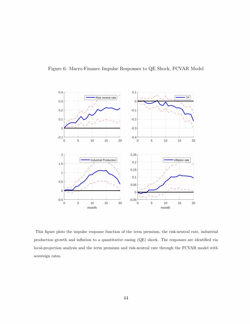
Figure 6: Macro-Finance Impulse Responses to QE Shock, FCVAR Model

0 5 10 15 20-0.1

0

0.1

0.2

0.3

0.4

Risk neutral rate

0 5 10 15 20-0.4

-0.3

-0.2

-0.1

0

0.1

TP

0 5 10 15 20

month

-0.5

0

0.5

1

1.5

2

Industrial Production

0 5 10 15 20

month

-0.05

0

0.05

0.1

0.15

0.2

0.25

Inflation rate

This figure plots the impulse response function of the term premium, the risk-neutral rate, industrial

production growth and inflation to a quantitative easing (QE) shock. The responses are identified via

local-projection analysis and the term premium and risk-neutral rate through the FCVAR model with

sovereign rates.

44

Figure 7: Term Premium and Risk-Neutral Rate Responses to QE Shock: I(0)-VAR, I(1)CVAR and FCVAR

0 5 10 15 20-0.5

-0.4

-0.3

-0.2

-0.1

0

0.1TP - I(0) model

0 5 10 15 20-0.5

-0.4

-0.3

-0.2

-0.1

0

0.1TP - I(1) model

0 5 10 15 20-0.5

-0.4

-0.3

-0.2

-0.1

0

0.1TP - I(d) model

0 5 10 15 20

0

0.2

0.4

0.6

0.8Neutral Rate - I(0) model

0 5 10 15 20

0

0.2

0.4

0.6

0.8Neutral Rate - I(1) model

0 5 10 15 20

0

0.2

0.4

0.6

0.8Neutral Rate - I(d) model

This figure compares the impulse response function of the term premium and the risk-neutral rate to a

quantitative easing (QE) shock (I(0)-VAR, I(1) CVAR and FCVAR (I(d) models)). The responses are

identified via local-projection analysis.

45