tensile properties of loblolly pine strands using …...tensile properties of loblolly pine strands...

Tensile Properties of Loblolly Pine Strands Using Digital Image Correlation and Stochastic Finite Element Method

Gi Young Jeong

Dissertation submitted to the faculty of Virginia Polytechnic Institute & State University in partial fulfillment of the requirements for the

degree of

Doctor of Philosophy In

Wood Science and Forest Products

Dr. Daniel P. Hindman, Chair Dr. Joseph R. Loferski Dr. Audrey Zink-Sharp

Dr. Layne T. Watson Dr. Surot Thangjitham

30 October, 2008 Blacksburg, VA

Keywords: earlywood, latewood, wood strands, digital image correlation (DIC), stochastic finite element method (SFEM)

Copyright © 2008 Gi Young Jeong

ii

Tensile Properties of Loblolly Pine Strands Using Digital Image Correlation and Stochastic Finite Element Method

Gi Young Jeong

ABSTRACT

Previous modeling of wood materials has included many assumptions of unknown

mechanical properties associated with the hierarchical structure of wood. The experimental

validation of previous models did not account for the variation of mechanical properties present

in wood materials. Little research has explored the uncertainties of mechanical properties in

earlywood and latewood samples as well as wood strands. The goal of this study was to evaluate

the effect of the intra-ring properties and grain angles on the modulus of elasticity (MOE) and

ultimate tensile strength (UTS) of different orientation wood strands and to analyze the

sensitivity of the MOE and UTS of wood strands with respect to these variables.

Tension testing incorporating digital image correlation (DIC) was employed to measure

the MOE and UTS of earlywood and latewood bands sampled from growth ring numbers 1-10

and growth ring numbers 11-20. A similar technique adjusted for strand size testing was also

applied to measure the MOE and UTS of different orientation wood strands from the two growth

ring numbers. The stochastic finite element method (SFEM) was used with the results from the

earlywood and latewood testing as inputs to model the mechanical property variation of loblolly

pine wood strands. A sensitivity analysis of the input parameters in the SFEM model was

performed to identify the most important parameters related to mechanical response.

Modulus of elasticity (MOE), Poisson ratio, and ultimate tensile strength (UTS) from

earlywood and latewood generally increased as the growth ring number increased except for the

UTS of latewood, which showed a slight decrease. MOE and UTS from radial, tangential, and

iii

angled grain orientation strands increased as the growth ring numbers increased while MOE and

UTS from cross-grain strands decreased as the growth ring number increased. Shear modulus of

wood strands increased as the growth ring number increased while shear strength decreased as

the growth ring number increased. Poisson ratio from radial and angled grain strands decreased

as the growth ring number increased while Poisson ratio from tangential and cross grain

orientation strands increased as the growth ring number increased.

The difference of average MOE from different grain strands between experimental results

and SFEM results ranged from 0.96% to 22.31%. The cumulative probability distribution curves

from experimental tests and SFEM results agreed well except for the radial grain models from

growth ring numbers 11-20. From sensitivity analysis, earlywood MOE was the most important

contributing factor to the predicted MOE from different grain orientation strand models. From

the sensitivity analysis, earlywood and latewood participated differently in the computation of

MOE of different grain orientation strand models. The predicted MOE was highly associated

with the strain distribution caused by different orientation strands and interaction of earlywood

and latewood properties. In general, earlywood MOE had a greater effect on the predicted MOE

of wood strands than other SFEM input parameters.

The difference in UTS between experimental and SFEM results ranged from 0.09% to

11.09%. Sensitivity analysis showed that grain orientation and growth ring number influenced

the UTS of strands. UTS of strands from growth ring numbers 1-10 showed strength indexes (Xt,

Yt, and S) to be the dominant factors while UTS of strands from growth ring numbers 11-20

showed both strength indexes and stress components (σ1, σ2, and τ12) to be the dominant factors.

Grain orientations of strands were a strong indicator of mechanical properties of wood strands.

iv

Acknowledgements

I am glad to have had this great opportunity provided during my Ph.D. time. I have met

many great scholars and had priceless courses. I have also met incredible people in Virginia,

especially Blacksburg, who have shown their hospitality and kindness. I feel a great jump that I

could pretend to be a modest researcher. The wonderful experiences I have cannot be assembled

into words and the piece of acknowledgement I am trying to make here.

Dr. Hindman, I do not know where I have to start. Your unstoppable guidance and

patience has changed my learning behavior and attitude as a scholar. I realized every comment

you have made turns out to improve my writing skills, logic, and generalizing problems that I

have often faced. Your kindness and patience has helped to improve my English skills. During

the over three years of my Ph.D. you have been a great mentor for me. I thank you for your

generality on flexible working time, which boosted my capacity so that I could adjust my mood

for taking classes, writing papers, testing specimens, organizing thoughts, and reading literature.

You have been friendly to me and I sometimes consider you a close buddy of mine, who helped

me share my thoughts freely. I believe your door has been open every day, which allowed me to

talk to you as I needed. I thank you for giving me inspiration in every way.

Dr. Zink-Sharp, I thank you for your guidance on the digital image correlation technique

and lending me your equipment which was an essential part of digital image correlation set-up.

You have spent a great deal of time to encourage me to finish testing. I probably bother you too

much. You have inspired me in the way how a scholar should be. Dr. Loferski, I would like to

thank you for sharing with me your great experiences on wood mechanics and engineering. Your

insight and wisdom impacted me greatly. I respect your kindness and care in personal

relationships. Dr. Watson, I must thank you for sharing with me your academic knowledge on

v

numerical analysis. I thank you for your participation in every committee meeting eventhough

you are busy and on sabbatical. I was impressed with your critical comments on my method and

writing. Dr. Thangjitham, I thank you for sharing your comments on my method. The unique

contribution from each committee member has helped me complete my Ph.D. work.

I must also thank the Brooks Center People, Angie, Will, Rick, and Kenny. You are kind

and my friends. I always wanted to have brothers and sisters. You are my American brothers and

sisters. Angie always greeted me with a smile and refreshed me with a cup of coffee. Will, you

are my younger brother. Rick, I probably bother you too much on testing set up. You have

always been kind to me and helped me to finish testing. Kenny Albert, you are such a gentle and

nice man. I feel you are my American father. Your free hugs lighten my spirit and refresh me

from tiredness.

I would like to thank my friends in Korea; Byung Hyn, Gwang Su, Ji Young, Ji Hoon,

and Jong Sik. You are my good old friends who have the same soul and dwell in other bodies.

You welcomed me whenever I would go back to Korea so that I would not feel remote.

Mom and Dad, you are my shadow that I always feel and the fact of your presence gives

me energy to be mature. As an only child, I should have contacted and spent time with you more.

I appreciate your patience and forgiveness.

I want to thank my wife, Yeonjeong. You have made our house feel like a real home so

that I could rest after work. Even though you are a Ph.D. student and busy with many things, you

have sacrificed your time to encourage me. Thank you for trusting in me and supporting me. I

love You, Yeonjeong in every moment I feel.

vi

Table of Contents

ABSTRACT .................................................................................................................................... ii

Acknowledgements ........................................................................................................................ iv

Table of Contents ........................................................................................................................... vi

List of Figures ................................................................................................................................ ix

List of Tables ................................................................................................................................. xi

List of Symbols ............................................................................................................................ xiii

Chapter 1. Introduction and Background ........................................................................................ 1

Chapter 2. Literature Review .......................................................................................................... 6

Use of strands in engineering wood products ............................................................................. 6

Hierarchical structure of wood .................................................................................................. 10

Nano-scale properties of wood ......................................................................................... 11

Micro-scale properties of wood ........................................................................................ 16

Macro-scale properties of wood ........................................................................................ 21

Mature wood and juvenile wood....................................................................................... 25

Previous mechanical models of wood ....................................................................................... 30

Previous modeling work on wood fibers .......................................................................... 31

Wood strand modeling ...................................................................................................... 37

Wood strand based board modeling .................................................................................. 37

Mechanical property evaluation methods of wood materials ................................................... 40

Mechanical properties measurement of earlywood and latewood fibers. ......................... 41

Axial elastic modulus of wood strands. ............................................................................ 44

Digital image correlation (DIC) ................................................................................................ 48

Principles of digital image correlation .............................................................................. 49

A defined representative window size for generalizing mechanical properties ............... 52

Application of DIC to wood and wood-based material .................................................... 52

Stochastic finite element method (SFEM) ................................................................................ 56

Comparison of conventional FEM and SFEM .................................................................. 57

Relevant SFEM applications to composite materials. ...................................................... 59

Summary and Conclusion ......................................................................................................... 62

References ................................................................................................................................. 64

vii

Chapter 3. Tensile Properties of Earlywood and Latewood from Loblolly Pine (Pinus taeda) Using Digital Image Correlation ................................................................................. 75

Introduction ............................................................................................................................... 76

Literature Review ...................................................................................................................... 77

Materials and Methods .............................................................................................................. 82

Results and Discussion ............................................................................................................. 86

Conclusions ............................................................................................................................... 95

References ................................................................................................................................. 96 Chapter 4. Comparison of Longitudinal Tensile Properties of Different Orientation Strands

from Loblolly Pine (Pinus taeda) ............................................................................... 99 Introduction ............................................................................................................................. 100

Literature Review.................................................................................................................... 101

Material and Methods ............................................................................................................. 103

Results and Discussion ........................................................................................................... 110

Conclusions ............................................................................................................................. 117

References ............................................................................................................................... 119 Chapter 5. Shear and Transverse Properties of Loblolly Pine (Pinus taeda) Strands Using

Tension Test Incorporating Digital Image Correlation (DIC) .................................. 121 Introduction ............................................................................................................................. 122

Literature Review .................................................................................................................... 123

Materials and Methods ............................................................................................................ 125


Conclusions ............................................................................................................................. 136

References ............................................................................................................................... 137 Chapter 6. Evaluation on Effective Modulus of Elasticity of Loblolly Pine Strands Using

Stochastic Finite Element Method (SFEM) .............................................................. 139 Introduction ............................................................................................................................. 140

Literature Review.................................................................................................................... 141

Methods................................................................................................................................... 144


viii

Conclusions ............................................................................................................................. 161

References ............................................................................................................................... 161 Chapter 7. Evaluation on Ultimate Tensile Strength of Loblolly Pine Strands Using

Stochastic Finite Element Method (SFEM) .............................................................. 163 Introduction ............................................................................................................................. 164

Literature Review .................................................................................................................... 165

Model Development ................................................................................................................ 168


Conclusions ............................................................................................................................. 186

References ............................................................................................................................... 187 Chapter 8. Summary and Conclusion ......................................................................................... 189

Limitations .............................................................................................................................. 196

Recommendations for Future Research .................................................................................. 196

Appendix 1. ................................................................................................................................. 198

Appendix 2. ................................................................................................................................. 213

ix

List of Figures

Figure 1.1 Hierarchical structure of wood showing wood characteristics ...................................... 2

Figure 2.1 Growth of engineered wood products (Adair 2005) ...................................................... 7

Figure 2.2 Ultrastructure of wood cell wall (S1, S2, and S3) ......................................................... 17

Figure 2.3 Three sections of southern pine spp. ........................................................................... 19

Figure 2.4 The global coordinate system and local coordinate system of wood . ........................ 22

Figure 2.5 Schematic description for the location of juvenile and mature wood in a tree ........... 25

Figure 2.6 The average properties of loblolly pine by age (Bentdsen and Senft 1986)................ 28

Figure 2.7 Schematic explanation of cross correlation techniques ............................................... 50

Figure 3.1 Cross correlation techniques for DIC .......................................................................... 81

Figure 3.2 Segmentation of earlywood and latewood specimens from a strand .......................... 83

Figure 3.3 Microtensile test set up ................................................................................................ 85

Figure 3.4 Earlywood and latewood MOE, and Ratio of latewood MOE to earlywood MOE .... 90

Figure 3.5 Strain distribution of earlywood and latewood from growth ring number 1-10 ......... 93

Figure 3.6 Strain distribution of earlywood and latewood from growth ring number 11-20 ........ 95

Figure 4.1 Strands generated from different cutting positions of the loblolly pine disk ............ 104

Figure 4.2 Experimental tensile testing set up showing camera for DIC ................................... 106

Figure 4.3 Generating a grid on the image from the surface of a strand .................................... 108

Figure 4.4 Relationship between specific gravity and tensile properties.................................... 116

Figure 4.5 Relationship between thickness and tensile properties ............................................. 117

(Unless otherwise noted, all images are property of the author)

x

Figure 5.1 Two different grain orientation strands used in testing. ............................................ 126

Figure 5.2 Tensile test set up for off-axis tension test ................................................................ 127

Figure 6.1 Structural analog of strand orientation models .......................................................... 145

Figure 6.2 Difference between experimental results and model results ..................................... 150

Figure 6.3 Strain y distribution from simulation models ............................................................ 152

Figure 6.4 Strain x distribution from simulation models ............................................................ 154

Figure 6.5 Shear strain xy from simulation models .................................................................... 155

Figure 6.6 Comparison between cumulative probability of MOE and predicted MOE ............ 158

Figure 7.1 Flowchart for the SFEM procedure ........................................................................... 169

Figure 7.2 Structural analog of strand orientation models .......................................................... 170

Figure 7.3 Stress x distribution from simulation models ............................................................ 178

Figure 7.4 Stress y distribution from simulation models ............................................................ 179

Figure 7.5 Shear stress distribution from simulation models ..................................................... 181

Figure 7.6 Comparison between cumulative probability of UTS and predicted UTS ................ 184

xi

List of Tables

Table 2.1 Elastic properties of cellulose, hemicellulose, and lignin at 12 % moisture content .... 14

Table 2.2 Composition of the S1, S2, and S3 layers ....................................................................... 18

Table 2.3 Radial tracheid diameter and cell wall thickness of loblolly pine ................................ 20

Table 2.4 Average earlywood and latewood fiber length, and specific gravity ............................ 23

Table 2.5 Variation of mechanical properties of earlywood and latewood of loblolly pine ......... 24

Table 2.6 Comparison of the average specific gravity, MOE, MOR. ........................................... 26

Table 2.7 Summarized previous studies on mechanical behavior of wood at the micro scale ..... 32

Table 2.8 Summary of previous research on wood-based composite modeling ........................... 38

Table 2.9 Previous works on wood fiber test showing test conditions and results ....................... 42

Table 2.10 Previous works on evaluation of mechanical properties of wood strands .................. 44

Table 2.11 Summary of objectives, main results from previous researches on DIC .................... 53

Table 2.12 Comparison of the FEM and SFEM procedures ......................................................... 59

Table 3.1 Previous works on intra-ring test showing test conditions and results ......................... 78

Table 3.2 Physical properties and mechanical properties of earlywood and latewood ................ 87

Table 3.3 Statistical comparison of the tensile properties for earlywood and latewood ............... 91

Table 3.4 Distribution fitting for tensile properties of earlywood and latewood .......................... 92

Table 4.1 Nomenclatures and sample sizes for different orientations of wood strands .............. 105

Table 4.2 Summary of physical properties and elastic properties of four strands ...................... 110

Table 4.3 Failure behavior of wood strands ................................................................................ 112

Table 4.4 Statistical comparison of MOE, UTS, and Poisson ratios .......................................... 114

Table 4.5 Distribution fitting for MOE, UTS, and Poisson ratios for wood strands .................. 115

Table 5.1 Nomenclatures and sample sizes for two different orientation wood strands. ............ 126

xii

Table 5.2 Physical properties of angled and cross-grain strands ................................................ 130

Table 5.3 Mechanical properties from angled grain and cross-grain strands.............................. 132

Table 5.4 Statistical distribution of shear strength, MOE, UTS, and Poisson ratios .................. 133

Table 5.5 Failure behavior of different grain orientation strands ............................................... 134

Table 5.6 The MOE, UTS, and shear strength of strands ........................................................... 136

Table 6.1 Distribution types and parameters for MOE of earlywood and latewood .................. 147

Table 6.2 Sensitivity analysis of input variables on MOE .......................................................... 159

Table 7.1 Distribution of strength indexes .................................................................................. 173

Table 7.2 Comparison of average strengths of wood strands. .................................................... 176

Table 7.3 Sensitivity analysis of input variables on UTS of different orientation strands ......... 185

xiii

List of Symbols

Acronyms

BVS = Broadband Viscoelastic Spectroscopy

CCM = Concentric Cylindrical Model

CML = Compound Middle Lamella

CLT = Classical Laminate Theory

COV = Coefficient of Variance

CPT = Classical Plate Theory

DIC = Digital Image Correlation

DMA = Dynamic Mechanical Analysis

DSP = Digital Speckle Photography

ESEM = Environmental Scanning Electron

Microscope

EW = Earlywood

EWP = Engineered Wood Products

FEM = Finite Element Method

FFT = Fast Fourier Transform

GMC = Generalized Methods of Cells

HM = Honeycomb Model

IB = Internal Bonding

LW = Latewood

LSL = Laminated Strand Lumber

LVL = Laminated Veneer Lumber

MC = Moisture Content

MCS = Monte-Carlo Simulation

MFA = Microfibril Angle

MOE = Modulus of Elasticity

MPM = Material Point Method

MOR = Modulus of Rupture

OSB = Oriented Strand Board

OSL = Oriented Strand Lumber

PSL = Parallel Strand Lumber

ROM = Rule of Mixture

SCL = Structural Composite Lumber

SFEM = Stochastic Finite Element Method

SG = Specific Gravity

TLT = Thick Laminate Theory

1

Chapter 1. Introduction and Background

Many natural and man-made materials exhibit different structure characteristics at

different magnifications. In hierarchical structure materials, smaller structural elements combine

to build larger structures. This structural hierarchy plays a major part in determining the bulk

material properties. Understanding the effects of hierarchical structures can guide the synthesis

of new materials with mechanical properties tailored for specific applications.

Fundamental characteristics of the structure of wood are arise from the existence of

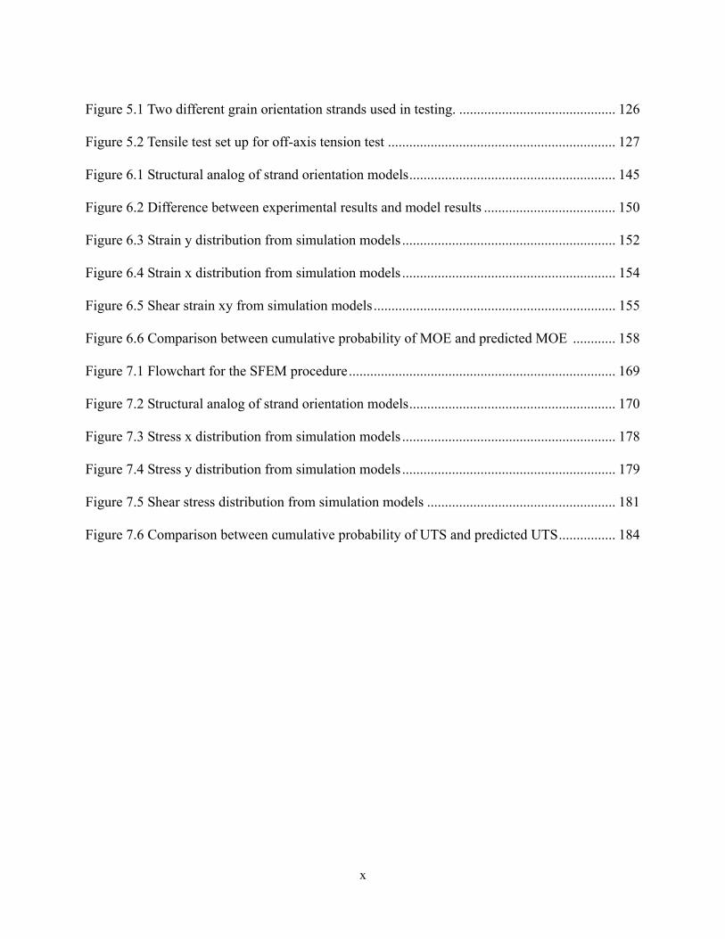
several hierarchical levels. The hierarchical structure of wood from nano to macro scale is

displayed in Figure 1.1. At the nano-scale, three main chemical components (cellulose,

hemicellulose, and lignin) build the fundamental structure of the wood cell wall. At the micro-

scale, the wood cell wall can be largely differentiated into microfibril and matrix. Microfibrils

are composed of cellulose and hemicelluloses, while the matrix is mainly composed of lignin.

The wood cell wall includes different layers having different orientations of a filament-wound

microfibril embedded in a matrix of hemicelluloses and lignin. Earlywood and latewood can be

distinguished at this level by the different thicknesses of cell walls. Earlywood is the layers

where wood grows during the early growing season, characterized by thiner cell walls and larger

lumens. Latewood is the layer where wood grows during the late growing season, characterized

by thicker cell walls and smaller lumens (Panshin and Zeeuw 1980). At the macro-scale, due to

the earlywood and latewood, or intra-ring characters, a distinctive ring pattern can be noticed.

Different cell wall characteristics are also found at different growth ring positions within a tree.

Juvenile wood located near the pith has a higher microfibril angle and a thinner cell wall while

2

mature wood located near the bark has a lower microfibril angle and a thicker cell wall (Larson

et al. 2001).

Figure 1.1 Hierarchical structure of wood showing wood characteristics at the macro,

micro, and nano scale.

The hierarchical structure of wood has a large effect upon the mechanical properties of

wood. Therefore, an understanding of wood structure characteristics at the different hierarchical

3

levels would help to use wood more efficiently. Detailed knowledge of these wood properties is

not fully available for expanding the modeling of the mechanical behavior of wood continuously

from the nano to the macroscale level at the current time. Many mechanical properties at the

micro and nano scale levels are assumed for the wood structure. Most existing wood fiber

models do not account for variation of chemical composition in the cell wall and different

geometries of the wood cell wall. Models to predict mechanical properties of wood at the macro

scale level could be improved by including the intra-ring characteristics.

In the U.S., the use of strands in oriented strand board (OSB) and structural composite

lumber (SCL) production has increased. The modeling of wood strands can produce a better

understanding of the mechanical properties of wood products. Properties of wood strands are

related to the hierarchical composition of wood. This hierarchical structure varies throughout the

different growth ring positions. Growth rings closer to the pith contain higher proportions of

juvenile wood than growth rings closer to the bark. Juvenile wood differs from mature wood in

that it has a higher microfibril angle, a greater percentage of compression wood, distorted grain

patterns, and a less percentage of latewood (Larson et al. 2001). The deleterious effect of

juvenile wood on the properties of wood strands is not well known. Understanding the wood

strand as a fiber composite can help scientists understand the effects of juvenile wood on the

mechanical behavior of wood strands.

Previous modeling of wood materials has included many assumptions of unknown

mechanical properties associated with the hierarchical structure of wood. Also, experimental

validation of those models did not account for the variation of mechanical properties. Little

research has explored the uncertainties of mechanical properties at the earlywood, the latewood

and at the strand sizes.

4

The goal of this study is to analyze the effect of the intra-ring properties and grain angles

on the MOE and UTS of different orientation wood strands and to analyze the sensitivity of the

MOE and UTS of wood strands with respect to these variables.

The objectives of this study include:

1) Evaluate the MOE and UTS of earlywood and latewood specimens from different growth

ring numbers within one loblolly pine (Pinus taeda)

2) Evaluate the MOE and UTS of loblolly pine strands with different grain orientations

(radial, tangential, and angled grain orientations)

3) Construct and validate stochastic finite element models (SFEM) of the wood strands

incorporating three different grain orientations

4) Evaluate the sensitivity of the input parameters on MOE and UTS from the SFEM

models

Digital image correlation (DIC) was employed to measure the MOE of earlywood and

latewood bands and wood strands sampled from different growth ring positions. MOE and UTS

of earlywood and latewood were measured by tension testing. A similar technique adjusted for

strand size testing was also applied to measure the MOE and UTS of different orientation wood

strands from the two growth ring numbers. Stochastic finite element method (SFEM) used the

results from the DIC testing as input values to account the mechanical property variation of

loblolly pine wood strands. A sensitivity analysis of the input parameters in the SFEM model was

performed to identify the most important parameters related to mechanical response.

This dissertation is composed of eight chapters. Chapter 1 includes the introduction for

5

the entire project. Chapter 2 includes a comprehensive literature review on wood structure and

mechanical properties of wood at different length scales. Chapter 3 evaluates the earlywood and

latewood properties from growth ring numbers 1-10 and growth ring numbers 11-20 using digital

image correlation (DIC). Chapter 4 reports on the longitudinal tensile properties of different

orientation of loblolly pine strands from different growth ring numbers. Chapter 5 reports on the

shear and transverse properties of loblolly pine strands from different growth ring numbers.

Chapter 6 discusses the effective elastic properties of different orientation wood strands (radial,

tangential, angled grain orientation strands) from different growth ring positions using stochastic

finite element method (SFEM). Chapter 7 discusses the ultimate tensile strength (UTS) of

different orientation wood strands from the different growth ring numbers using SFEM. Chapter

8 provides the conclusions of the disseration, including the summary, limitation of the study, and

recommendations for future research.

6

Chapter 2. Literature Review

Use of strands in engineering wood products

This section discusses market growth, wood species, strand sizes, manufacturing methods,

applications, and expected stresses under the service conditions for strand-based wood composite

products. The use of wood in construction has changed over the last 25 years due to the

development and production of engineered wood products (EWP). Specifically structural

composite lumber (SCL) and oriented strand board (OSB) utilize a greater portion of the wood

fiber in production compared to solid-sawn lumber. The OSB and SCL products are used as

building members such as sheathing, headers, rimboards, columns, floor joists, and beams.

According to the service conditions, strands are exposed to different stresses.

OSB is increasing in market share as a result of its lower cost compared to plywood.

Since OSB is a newer product than plywood, there has been a steady improvement in processing

methods, quality control, and performance (Smulski 1997). I-joist production in North America

has grown 160% from 2000 to 2004 (Adair 2005). Schuler and Adair (2000) proposed that the

main force driving the growth of these products in North America could be reasoned by

prevalence of wood frame construction. The growth of these products in North American

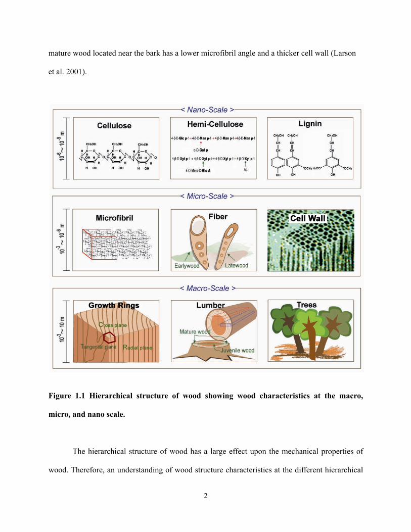
construction is very strong, and is expected to continue (Lam 2001). Figure 2.1 shows the growth

of OSB and I-joist in North America from 2000 to 2004. The market growth of 0.95 cm (3/8

inch) OSB (million square feet) shows an increase 45% while I-joist (million linear feet)

increases 160%. This tremendous growth shows the adaptability of these products for residential

construction.

7

Figure 2.1 Growth of engineered wood products (Adair 2005)

OSB is commercially produced from various species including aspen (Populus spp.),

Southern pine (Pinus spp.), and yellow-poplar (Liriodendron tulipifera). Strand sizes for OSB

range from 8 to 15 cm in length and less than 0.8 mm in thickness. OSB typically has 3 or 5

layers of oriented strands. In OSB production, strands are mechanically oriented in pre-specified

directions. Forming heads create distinct layers oriented perpendicularly with respect to each

other. The mat is trimmed and sent to either a multi-opening press or a continuous belt press.

Curing takes place at elevated temperatures. In some newly developed processes, boards are

cooled prior to trimming and packaging (Smulski 1997). OSB typically has a density variation

through the thickness direction. The density of face layer and core layer are 130% and 70%,

respectively, of the average board density (Lam 2001). Through-thickness shear strength is

approximately twice as high with OSB compared to that of plywood. OSB competes with

plywood in applications such as I-joist web material, single-layer flooring, sheathing, and

0%

20%

40%

60%

80%

100%

120%

140%

160%

180%In

crea

se (%

)

OSB I-Joist

Growth of EWPs from 2000 to 2004

OSB (Million square ft) 3/8’’ basis

I-Joist (Million linear ft.)

8

underlayment in light-frame structures.

Green (1998) reported that the impetus for the development of a variety of SCL products

has been the decreasing access to larger high quality logs, and industry commitments to better

utilization of harvests. The development of SCLs has many advantages, such as using smaller

trees, using waste wood from other processing, removal of defects, and creating more uniform

components. Most composites have improved some mechanical properties compared to solid

wood, and can be manufactured into different shapes. Compared to a 40% yield for solid sawn

lumber from a log with bark, SCLs have higher yield than solid lumber. PSL, LSL, and OSB

have 65%, 75%, and 80-90% yield, respectively (Schuler and Adair 2000 and Balatinecz and

Kretschmann 2001).

Three types of SCL products are laminated strand lumber (LSL), oriented strand lumber

(OSL), and parallel strand lumber (PSL). These products are produced using wood strands as the

primary constituent material. Stranding slices the entire log into 7.62 cm to 30.48 cm strands.

The strands are dried in a large rotary drum, where resin is applied. The strands are then dropped

into a forming bin and pressed together to form the individual products. These products can be

thin and flat sheets, like plywood, or long and wide, like lumber.

PSL is made from yellow-poplar (Liriodendron tulipifera) and Southern pine (Pinus spp.).

PSL is sold commercially under the product name Parallam. Strand size for PSL is 3 mm

thickness veneers cut to 100-300 mm long and 20 mm wide (Berglund and Rowell 2005). The

strands are generally taken from veneers peeled from the outermost section of the logs, where

stronger wood fibers are located. Veneers are dried to relative low moisture content and graded

for strength before chopping into strands. The veneers are then aligned parallel to one another,

coated with a waterproof adhesive, then pressed and cured using a radio frequency process to

9

form a rectangular billet up to 28 cm wide, 48 cm deep, and 20 m long. The varied profiles

accommodate several applications, which include 45 mm wide piles to serve as built-up headers

similar to LVL. Wider widths (65 mm, 133 mm and 178 mm) are well suited to longer span

beams and headers. The even distribution of small defects in the individual strands allows for a

considerably higher strength than is available from normally available solid timbers of the same

cross section. The main application of PSL is for columns and beams (Smulski 1997). Due to the

application of PSL, the significant portion of the stress exposed to strands is compression stress

parallel to grain and bending stress.

Laminate strand lumber (LSL) is similar to OSB; however, compared to OSB, longer and

slender strands (30 cm in length and 0.76~1.3 mm in thickness) are cut directly from whole logs

(Berglund and Rowell 2005). LSL is sold commercially under the product name Timber Strand.

LSL was produced from low grade logs (aspen, Populus spp. and yellow-poplar, Liriodendron

tulipifera) that would not normally be used for conventional wood products. Manufacturing

technique for LSL is similar to that used to produce OSB but using a polymeric diphenylmethane

diisocyanate. The billet could be up to 140 mm thick, 2.4 m wide and 14 m long, after sanding, a

large number of sizes are cut to suit applications such as headers, rimboard for floor systems,

columns, joists, and studs (Smulski 1997). When LSL is used for headers, strands are mainly

exposed to compression perpendicular to the grain and horizontal shear stress. However, LSL is

used for rimboards, columns, joists, and studs, strands are exposed to other stresses such as

crushing, compression parallel to grain, and bending stress.

Oriented strand lumber (OSL) is another type of strand composites whose strands are

oriented in the length direction of the lumber. The strand size for OSL is 15.24 cm in length and

less than 0.8 mm in thickness. OSL is mainly used for rimboards. The least dimension of the

10

board is less than 0.635 cm and the average length of OSL is between 75 and 150 times of the

least dimension (Adair 2005). Since the rimboards are required to carry vertical load and to be

able to transfer loads imposed by earthquake or winds, the board should be designed for

preventing from crushing.

Prefabricated I-Joists, also known wood composite I-joists, are manufactured to optimize

the bending stiffness of SCLs, similar to a steel I-beam. Wood I-joists are composed of a web

connecting two flanges. Flanges can be solid sawn lumber, LVL or LSL. Webs use OSB or

plywood. The length of the I-joist is limited by transportation restrictions which is about 20 m.

The depth of the I-joist for residential applications can range from 24.1 cm to 40.6 cm (Adair

2005). Wood I-joists are used for floor joists and roof joists in residential and commercial

constructions. The flanges are designed for bending stress and a good fastening surface for the

sheathing. The web is designed to transfer shear stress from the flange.

In summary, the size of strands used in SCL and OSB varies from 8 cm to 30 cm long

and from 0.8 mm to 3.2 mm thick. The strands used in SCL and OSB are exposed to different

stress conditions. Therefore, optimization of strand size and geometry for different material may

improve mechanical performance. In processing wood strands, understanding the effect of the

geometry on the mechanical properties is crucial to maximizing the properties for the end use.

Based on understanding, segregation into discrete categories can maximize the benefit of the

wood strands for specific applications. The knowledge of wood strand geometry can lead to

optimization in processing and utilization.

Hierarchical structure of wood

In contrast to most man-made composites, wood hierarchal structural levels span from

11

the nano-scale to the macro-scale. A wood fiber or tracheid shows a complex structure, which

can be described as different layers with specific orientations of a filament-wound microfibril

embedded in a matrix of amorphious or paracrystalline polymers-hemicellulose and lignin. From

the viewpoint of material science, wood can be considered as a natural fibrous and cellular

composite that is extremely heterogeneous and anisotropic. Navi et al. (1994) mentioned “the

physical and mechanical behavior of wood can be best understood by reference to its

microstructure and its chemical constituents”. The following sections discuss important

characteristics of wood at the different scales which affect the mechanical behavior of wood.

Nano-scale properties of wood

The nano-scale level is defined as the range of size from 1×10-6 to 1×10-9 m which includes

the chemical composition of wood cells. Cellulose, hemicellulose and lignin are the main

components of the composite cell wall layers. Even though their individual structure is well

known, there is still a lack of information regarding their arrangement (Salmen 2004).

Cellulose is the main constituent of wood. Cellulose is a homopolysaccharide composed of

β-D-glucopyranose units which are linked together by (1→4)-glycosidic bonds (Panshin and

Zeeuw 1980). Approximately 40-50% of the dry substance in most wood species is cellulose,

located predominantly in the secondary cell wall. The cellulose is highly crystallized and

hydrophobic. Cellulose is also the main component of the microfibrils, which provides stiffness

of wood in both the longitudinal and transverse directions.

Hemicelluloses are amorphous carbohydrates made of a group of heterogeneous polymers.

Hemicelluloses make up about 20-30% of the dry weight of wood. The hemicellulose is highly

hydrophilic. Hemicellulose may act as an adhesive between cellulose and lignin. In the cell wall,

12

hemicelluloses are closely associated with both cellulose and lignin. Hemicelluloses serve as the

matrix (or skeletal framework) in which the cellulose microfibrils are embedded. Hemicellulose

also provides support for the cell wall but to a much lesser degree than cellulose (Panshin and

Zeeuw 1980). Hemicelluloses influence significantly the moisture absorption behavior of wood

because of the high hydroxyl content and amorphous character. Without the presence of

hemicellulose, there would be no interaction between the lignin and cellulose in wood, making a

poor composite. The same is true for wood fiber plastic composites, where a coupling agent is

needed to improve the interface between the fiber and plastic, which otherwise would not

associate well with one another (Sjostrom 1993 and Fengel and Wegner 1983). The mechanical

function of hemicellulose is to act as a buffer to recover the elastic properties even beyond yield

point (Keckes et al. 2003).

Lignin is a heterogeneous three-dimensional polymer that constitutes approximately 30%

of the dry weight of wood. Lignin limits the penetration of water into the wood and makes the

wood compact. Lignin serves as a cementing material in the wood cell wall. It is primarily found

in the middle lamella and the secondary wall. In the secondary wall, lignin acts as a matrix

surrounding the cellulose fibers. Moreover, because of its high rigidity, lignin imparts strength

and stiffness in compression and in shear.

The mechanical properties of cellulose, hemicelluloses, lignin composed in wood cells are

tabulated in Table 2.1. Elastic properties of three main components were studied by different

researchers using various methods. Sakurada et al. (1962) and Matsuo et al. (1990) determined

longitudinal elastic modulus of ramie cellulose using x-ray diffraction. Mark (1967) estimated

longitudinal elastic modulus of cellulose using a cellulose chain model. Mark (1967) and Cave

(1978) estimated transverse elastic modulus of cellulose using cellulose model. Cousins (1976)

13

and Cousins (1978) determined the elastic modulus of hemicelluloses and lignin from extracted

radiata pine (Pinus radiate). Bergander and Salmen (2002) estimated the shear modulus of

hemicelluloses and transverse elastic modulus of lignin assuming the ratio of longitudinal elastic

modulus (EL) to transverse elastic modulus (ET) was 2.0 for hemicelluloses and lignin. As shown

in Table 2.1, cellulose and hemicellulose were treated as a transverse isotropic material while

lignin was treated as an isotropic material. Cellulose has a much higher stiffness than

hemicellulose and lignin. All three chemicals have a higher longitudinal modulus (EL) than

transverse modulus (ET) and shear modulus (GLT). The elastic ratio of cellulose is calculated to

be EL: ET: GLT = 25.2-30.6: 4.0-6.0: 1.0. The elastic ratio of hemicellulose is calculated to be EL:

ET: GLT=4.6: 0.8-2.0: 1.0. The elastic ratio of lignin is calculated to be EL: ET: GLT = 2.6-4.6: 1.3-

2.6: 1.0. Poisson ratio of three chemical components has similar trends with the elastic ratio. For

cellulose Poisson ratio, the ratio of υTR (tangential-radial) to υLR (longitudinal-radial) ranged

from 5.2 to 11.0. For hemicellulose Poisson ratio, the ratio of υLR to υTR ranged from 1.3 to 2.0.

For lignin Poisson ratio, the ratio of υLR to υTR was 1.0. Compared to the average elastic ratio

assumed for solid sawn lumber of EL: ET: GLT = 20.0: 0.875: 1.0 (Bodig and Jayne 1992), the

main chemical components elastic ratio was quite different because the different percentage of

these chemical components in the cell wall affected the elastic properties of the cell wall. Most

wood fiber modeling has used elastic properties of the chemical components and the percentage

of the chemicals in the cell wall to calculate the elastic properties of the wood cell wall.

14

Table 2.1 Elastic properties of cellulose, hemicellulose, and lignin at 12% moisture content

Constituent EL (Gpa) ET (Gpa) GLT (Gpa) LRν TRν

Cellulose 134a, 113.5b, 120-135c, 138d 27.2b, 18e 4.5b 0.1b, 0.047e 0.52e

Hemicellulose 8f 3.5e, 1.4-3.5g 1.75g

0.3e, 0.2g 0.4h

Lignin 2.0-3.5h, 2i 1g, 2i 0.76b 0.3h

0.3h

aSakurada et al. (1962), bMark (1967), cMatsuo et al. (1990), dNishino et al. (1995), eCave (1978), fCousins (1978), gBergander and Salmen (2002), hPersson (2000), iCousins (1976)

Wood can be thought of as a reinforced composite, similar to reinforced concrete. The

cellulose microfibrils act as rebar, lignin acts as the aggregate, and hemicellulose acts as the

portland cement binder. The microfibril (cellulose) provides the tensile strength parallel to its

length while the matrix provides the compression and shear resistance. The mechanical behavior

of wood is a combination of high elasticity of the cellulose under short-term loads and plastic

flow of the hemicellulose and lignin under long-term loads, which is different from most other

structural materials.

Since the mechanical behavior of wood is related to the arrangement of chemical

components in the wood cell, many researchers developed models to represent the arrangement

of cellulose, hemicelluloses, and lignin to understand physical and mechanical behavior of wood

better. Bonart et al. (1960) proposed the cable model of cellulose describing several crystallites

and the non-crystal monomers in one microfibril. Frey-Wyssling and Muhlethaler (1965)

suggested the microfibril concept describing perfectly crystalline elementary fibrils fastened to

make purely crystalline microfibrils. Hearle (1963) suggested a fringed model describing

microfibrils consist of extended chains, folded chains, fringed fibrils, or fringed micelles all

having different strength and elastic properties from one another.

15

Fengel (1984) described a unit cell model that the six of the crystalline polymer of

cellulose (β-D glucose) were located with or without some occasional substitutions of mannose

for glucose residues (hemicelluloses) in random or periodic form. The hemicellulose associated

with the microfibrils exhibits some degree of orientation and introduces crystal order defects in

cellulose. The rest of space is filled by mainly lignin. Any unit volume of wood cell wall on the

size order shown in the model can be described as a filament reinforced composite. Since the

fiber wall is built up of layers of such filament reinforced matter, it is also accurate to describe it

as a laminated composite.

Kerr and Goring (1975) have concluded on the basis of electron microscope studies that

the cell wall has an interrupted lamella structure where the dimension of a given lignin or

carbohydrate entity is greater in the tangential direction of the fiber wall than in the radial

direction. The hemicellulose not only exists as a matrix around the microfibrils but is present in

the lignin-containing entities. One of the most important aspects of the cell walls is the angle that

the cellulose microfibrils make with the long axis of the cells known as microfibril angle (MFA).

This is now generally acknowledged as one of the main determinants of stiffness in wood.

Salmen and Olsson (1998) used a dynamic mechanical analysis (DMA) to analyze the

effect of hemicelluose on softening wood pulp. The main conclusion was that hemicelluloses

were associated with both cellulose and lignin. Xylan was associated with lignin and

glucomannan was associated with cellulose. Akerholm and Salmen (2003) used polarized

infrared measurement to show the orientation of lignin. The conclusion was lignin had preferred

orientation with the other orientated cell wall components.

Xu et al. (2007) used dual-axis electron tomography to analyze the cellulose microfibrils

from the delignified cell wall of radiata pine (Pinus radiate) earlywood. Cellulose microfibrils in

16

the S2 layer were measured at 3.2 nm in diameter, which appears to be an unstained core 2.2 nm

and ~0.5 nm outer layer of residual hemicelluloses and lignin.

Many researchers have syudied the arrangement of three main chemical components of wood

cells using experiments and modeling at the nano-scale level. Although the exact arrangements

of three chemical components in wood cell have not been found yet, more sophisticated models

for the association of three components have developed. Bergander and Salmen (2002) used an

improved model for the chemical association as inputs to the analytical models for wood fibers.

These results proved that more realistic chemical arrangements for modeling of wood cells

provided more accurate predictions of mechanical properties. However, more information on the

modeling of wood at this scale is needed for more reliable results.

Micro-scale properties of wood

The micro-scale level is defined as the range of 1×10-3 to 1×10-6 m including the wood

cell wall and earlywood and latewood fibers. Cellulose microfibrils constitute the main structural

elements of tracheid cell walls. Microfibrils are arranged into organized layers within each cell

wall layer distinguished by different helical arrangements of their microfibrils. Microfibril angle

(MFA) was considered one of the main determinants of wood quality (Cave and Walker 1994).

MFA was also known to influence the fracturing properties of wood with small angles favoring

transwall as opposed to intrawall fracturing on tangential longitudinal surfaces under transverse

shear (Donaldson 1996). The MFA within individual tracheids showed little variability along the

length of the tracheid, with variation being less in latewood tracheid than in earlywood tracheids

(Susan et al. 2002).

Figure 2.2 shows the ultrastructure of a single wood cell wall with different layers. There

17

are five main layers consisting of the middle lamella, the primary layer, and three secondary

layers (S1, S2, and S3). The middle lamella is mainly composed of lignin and acts as a bond

between the fibers. The primary wall is thin and its components are not considered structurally

functional. Therefore these two layers are often combined and called compound middle lamella

(CML). The thickness of CML is from 0.5 to 1.6 micrometers thick. The secondary wall layers,

S1, S2, and S3 are all mechanically important. Each layer in secondary wall has different

microfibril angle adapted to environmental conditions.

The most obvious difference in the layers of the secondary wall is the angle of the

microfibrils. The S1 is only 0.1 to 0.35 micrometers thick and the average angle of 60 to 80

degrees. The S2 layer is 1 to 10 micrometers thick and the average angle about 5 to 30 degrees.

The S3 layer is only 0.5 to 1.1 micrometers thick and the average angle of 60 to 90 degrees

(Plomion et al. 2001).

Figure 2.2 Ultrastructure of wood cell wall showing middle lamella, primary wall and

secondary wall (S1, S2, and S3)

18

Since the S2 layer is much thicker than other cell wall layers, the physical and chemical

properties of the cell wall is dominated by S2 layer (Watson and Dadswell 1964, Cave 1968,

1969, Wood and Goring 1971, Siddiqui 1976, and Evans et al. 1996). In contrast, the S1 and S3

layers are very thin; nevertheless, the S1 and S3 layers are thought to have a crucial role in

strengthening the cell against deformation by water tension forces in the living tree, as well as

contributing to the hardness and crushing strength of timber (Booker 1993, Booker and Sell

1998). The MFA of the S2 layer in the tracheid cell wall is considered to be a significant factor

influencing the mechanical properties of wood, especially the modulus of elasticity (Harris and

Meylan 1965). The distribution of the main chemical compositions through the cell layers are

shown in Table 2.2. Many analytical models have used different chemical proportions in

different cell wall layers to calculate the modulus of individual cell wall layers.

Table 2.2 Composition of the S1, S2, and S3 layers expressed as weight fractions (%) of wood

constituents from Fengel and Wegener (1983)

Constituent S1 S2 S3 CML Lignin 30% 27% 27% 71%

Hemicellulose 35% 15% 15% 20% Cellulose 35% 58% 58% 9%

Figure 2.3 shows three sections of Southern pine (Pinus spp.). Two distinctive diameters

of wood cells, cell walls, and lumen sizes or interior cell areas can be seen in the cross section.

Thin cell walls and large lumens can be seen from the upper half in the cross section, normally

called earlywood. Thick cell walls and small lumens can be seen from the lower half in the cross

section, normally called latewood. Because of the anatomical structural differences, the

mechanical properties of these two are also different.

19

Tracheids with an oval shaped bundle of ray cells and resin canals can be seen from the

tangential section. The cross section of ray cells is shown in that tangential section since the ray

cells are aligned perpendicular to the tangential plane. In a radial section, one or more rows of

cells run cross tracheids. These cells are called ray cells. The rays are composed of parenchyma

cells storing food and conducting fluid radially, reinforcing the stiffness of the radial section.

Figure 2.3 Three sections of Southern pine (Pinus spp).

a) cross section showing earlywood and latewood b) tangential section showing tracheids with the cross section of ray cells c) radial section showing the earlywood and latewood layers

Taylor and Moore (1980) studied the growth effects of loblolly pine (Pinus taeda) on the radial

tracheid diameter and cell wall thickness from earlywood and latewood. These results are

Earlywood

Latewood

Ray cell

a) Cross section (50x)

b) Tangential section (50x) c) Radial section (50x)

Earlywood

Latewood

Ray cell

20

summarized in Table 2.3. Radial tracheid diameter of earlywood increased 4.7% as growh ring

numbers increased from 1-10 to 11-20. Radial tracheid diameter of earlywood increased 7 % as

growth ring numbers increased from 1-10 to 21-30. Radial tracheid diameter of latewood only

increased 2.4% as growh ring numbers increased from 1-10 to 11-20. Radial tracheid diameter of

latewood only increased 3% as growh ring numbers increased from 1-10 to 21-30. The cell wall

thickness of earlywood increased 4.4% as growth ring numbers increased from 1-10 to 21-30.

The cell wall thickness of latewood increased 6.3% as growth ring numbers increased from 1-10

to 21-30.

Table 2.3 Radial tracheid diameter and cell wall thickness of loblolly pine as a function of

growth ring (Taylor and Moore 1980)

Growth Ring Radial tracheid diameter (μm) Wall thickness (μm)

1-10 EW1 52.8 4.5 LW2 32.8 9.4

11-20 EW 55.3 4.6 LW 33.6 9.4

21-30 EW 56.7 4.6 LW 33.8 10.0

EW1: earlywood, LW2: latewood

Growth increments stand out in wood to varying degrees because of growth intensity, and

consequently the cell size, arrangement and density of the wood produced are not uniform

throughout the growing year. Earlywood has a density of about 280 kg/m3. Latewood has a

density of about 600 kg/m3 (Larson et al. 2001). The transition between the earlywood and

latewood may be gradual or abrupt, giving rise to differentiations between wood species. The

different density of earlywood and latewood are related to different cell wall diameters and cell

wall thickness. The elastic properties of earlywood and latewood were highly related to density

21

and MFA (Cramer et al. 2005). From the results of linear regression analysis by Cramer et al.

(2005), specific gravity and MFA explained 75% of the accuracy of the elastic modulus value for

latewood, but less than 50% of the accuracy for earlywood. The mechanical properties of the

wood cell wall, therefore, are highly dependent upon MFA, cell wall diameter, and wall thickness.

Macro-scale properties of wood

The macro-scale level is defined as the range of about 1×102 m to 1×10-3 m including the

intra-ring level composed of earlywood and latewood, strand level and full-size composites.

Because of the manner of the tree growth and the arrangement of wood cells within the stem,

wood has three orthogonal axes. These three axes are used to construct the radial (R), the

tangential (T), and the longitudinal axes (L) shown in Figure 2.4. The orthogonal axes form three

planes known as the cross section, radial section, and tangential section. The cross section is the

plane formed by R,T directions that is exposed when wood is cut or sawed at right angles to the

longitudinal axis of the tree stem. The radial section is exposed plane of L, R axes when the cut

follows a radius of the cross section of the lumber, and along the axis of the lumber. Lumber cut

so that the wide face of the board is principally radial is called quarter-sawn or edge-grained. The

tangential section of wood is exposed plane of L,T axes when the bark is peeled from a tree. In a

log this surface is curved. In sawn or sliced material, when the cut is made tangentially, the

exposed surface is flat, representing a chord of the curved surface under the bark. The section is

so aligned that the central part of the wide surface of the board is approximately tangent to the

growth rings. Lumber cut so that the wide face of the board is tangential is said to be plain or

flat-sawn. Rotary-cut veneers from the surface of the log are tangential at most points on their

faces.

22

Figure 2.4 The schematic illustration to define the global coordinate axis (X, Y, Z) and

material principal axis of wood (R, L, T).

The longitudinal direction is parallel to the direction of the fibers (tracheids) and has the

highest elastic stiffness and strength. The wood is somewhat stronger and stiffer in the radial

direction compared to the tangential direction. These strength differences are related to the

ultrastructure of wood (Bergander and Salmen 2002). However, the fibers are rarely aligned with

the main direction of the tree growth. Therefore it is important to define the material coordinate

system and global coordinate system (X, Y, Z) for the determination of mechanical properties of

wood in Cartesian coordinate system (Figure 2.4). Figure 2.4 shows grain orientations are

defined as material principal directions-R, L, T. Hermanson et al. (1997) transform the global

coordinates (X, Y, Z) to material principal axis (R, L, T) to analyze the effect of three surface

angles on the orthotropic properties of a cross grain lumber. From numerical analysis, the elastic

properties were significantly changed by change of the ring angles. The stresses were also

affected by different grain angles. The failure behavior of the material would expect to be

affected by the different grain angles.

Z

T

X

Y

L

R

23

As a material formed by nature, wood has a complex mechanical behavior. Natural

differences in properties are caused by genetics and dissimilar growth conditions such as climate,

type of soil and growth terrain. The density of the wood is affected by those same factors (Larson

et al. 2001). From the micro-scale section, the differences in cross-sectional cell wall thickness

between earlywood and latewood fiber also result in density variations affecting the mechanical

properties.

Table 2.4 shows the average earlywood and latewood fiber lengths according to growth

increments of loblolly pine from Taylor and Moore (1980). The growth increment of both

earlywood and latewood fiber lengths were 38.3% and 31.8% from the fifth growth increment to

fifteenth growth increment. Earlywood and latewood fiber lengths decreased from 4.6% to 0.2%,

respectively, as the growth ring position was from fifth to fifteenth. Table 2.4 shows differences

in fiber length not only between latewood and earlywood, but also between growth ring positions.

The mechanical properties could be varied across growth ring positions due to different fiber

lengths (Larson et al. (2001), Bentdsen and Senft (1986), Taylor and Moore (1980)).

Table 2.4 Average earlywood and latewood fiber length, and specific gravity in the fifth

growth and fifteenth increment of a loblolly pine (Taylor and Moore 1980)

Earlywood tracheid length (mm)

Latewood tracheid length (mm)

Difference of earlywood and latewood fiber length2 (%)

Specific gravity 0.28 0.6

Fifth growth increment 3 mm 3.14 mm 4.6%

Fifteenth growth increment 4.15 mm 4.14 mm 0.2%

Difference of fiber from different growth ring position1 (%)

38.3% 31.8%

24

1%Diff = (Fifteenth growth increment-fifth growth increment)/fifth growth increment×100% 2%Diff = (Earlywood fiber length-latewood fiber length)/earlywood fiber length×100% Cramer et al. (2005) proposed that specific gravity and MFA were strong indicators of

elastic properties of earlywood and latewood. The average EL and GLT of earlywood were 4.34

and 0.77 GPa, respectively. The average EL and GLT of latewood were 9.88 and 1.59 GPa,

respectively. The modulus of elasticity increased with the increment of ring number and height

while shear modulus increased with ring number but decreased with height. Table 2.5 shows the

average ratio of LW/EW in EL was 2.3 and the average ratio of LW/EW in GLT was 2.0. Within-

ring variation in EL was as large as within-bolt variation. The coefficient of variance (COV) of EL

of LW/EW from upper bolts (6m) and lower bolts (1m) were 52% and 47%, respectively. The

coefficient of variance (COV) of EL of LW/EW from ring 3 and ring 18 were 42% and 34%,

respectively.

Table 2.5 Variation of mechanical properties of earlywood and latewood of loblolly pine

from different growth ring number and height (Cramer et al. 2005)

EL (COV) GLT (COV) SG (COV) MFA (COV) LW/EW all specimen 2.3 (51%) 2.0 (38%) 1.9 (26%) 1.0 (29%)

LW/EW: upper bolts (6m) 2.7 (52%) 2.3 (35%) 2.1 (25%) 1.1 (37%)

LW/EW lower bolts (1m) 2.1 (47%) 1.8 (37%) 1.8 (25%) 1.0 (25%)

LW/EW ring 3 1.6 (42%) 1.6 (41%) 1.6 (34%) 1.1 (25%)

LW/EW ring 18 2.7 (34%) 2.0 (29%) 2.0 (11%) 1.0 (24%)

25

Mature wood and juvenile wood

Wood properties can vary widely from pith to bark. The first 10-20 growth rings from the

pith are termed juvenile wood, while the portion of wood near the bark is called mature wood

(Zobel and Sprague 1998). Large differences in the chemical content could be found in a single

tree. Juvenile wood had a high xylose content while mature wood had a high lignin content. The

content of extractives, lignin and pentosan decreased with increasing distance from pith while

cellulose content increased (Uprichard 1971). Sugar analyses showed that the xylan and mannan

content of the juvenile wood was higher, while mature wood contained more cellulose (Harwood

1971). The schematic location of juvenile wood and mature wood is described in Figure 2.5.

Many researchers have studied the effect of juvenile wood on mechanical properties of

wood and wood-based composites. Values for tensile strength, bending modulus of rupture

(MOR), and bending modulus of elasticity (MOE) of juvenile wood were less than mature wood

due to higher MFA, shorter tracheid length, and lower specific gravity (Bendtsen 1978, Panshin

and de Zeeuw 1980, Smith and Briggs 1986, Cave and Walker 1994). Moody (1970) found that

the tensile strength of juvenile wood from southern pines was 34% lower than mature wood.

MacDonald and Hubert (2002) found the elastic modulus of the fibers from juvenile wood was

Mature wood

Juvenile wood

Figure 2.5 Schematic description for the location of juvenile and mature wood in a tree

26

less than that of the fibers from mature wood. From the shape of the stress-strain curve, the fibers

from mature wood linearly increase until failure, while the fibers from juvenile wood showed a

nonlinear behavior (Rowland and Burdon 2004). Table 2.6 shows the SG, MOE, and MOR from

two different aged trees. As ring number increases, the modulus of rupture (MOR), modulus of

elasticity (MOE), and specific gravity (SG) increase. The differences of MOE and MOR of two

different age groups are as large as 37% and 24%, respectively, demonstrating that there is a

large effect of using wood fiber from different aged trees and from different ring positions.

Table 2.6 Comparison of the average specific gravity, MOE, and MOR from the average

number of rings of two different age trees (Pearson and Ross 1984).

Number of rings

from pith

Specific gravity MOE (GPa) MOR (MPa) 15 year old tree

25 year old tree

15 year old tree

25 year old tree

15 year old tree

25 year old tree

0 0.38 0.4 4.4 6.06 50.05 62.60 2 0.39 0.43 7.17 9.03 61.91 73.08 5 0.44 0.47 9.37 10.55 78.6 90.32 10 0.517 0.5 11.3 14.34 95.84 115.14

Bentdsen and Senft (1986) reported that the average MOE of mature wood (23 + years)

was five times higher than that of juvenile wood and the average MOR of mature wood was

three times higher than that of juvenile wood. Pearson (1988) found that MOE and crushing

strength of nominal 2 by 4 in. lumber from juvenile wood were 37% and 52% less, respectively,

compared to mature wood. McAlister et al. (1997) investigated bending and tensile properties of

different ages (22, 28, and 40 years) of loblolly pine lumber. The stiffness, strength, and specific

gravity of loblolly pine lumber increased with increasing age, but only the tension stiffness

values were statistically significant at an α of 0.05. Kretschmann (1997) studied the effect of ring

orientation and percentage of juvenile wood of loblolly pine on shear parallel to grain and

27

compression perpendicular to grain strength. The shear and compression strength decreased with

an increase in percentage of juvenile wood.

In mature loblolly pines, the MFA of the S2 layer is small, averaging about 5 to 10

degrees as measured by deviation from the vertical. In juvenile wood, the MFA is large,

averaging 25 to 35 degrees and often up to 50 degrees in rings next to the pith, then decreasing

outward in the juvenile core. Ying et al. (1994) found that MFA in tracheids of fast grown

loblolly pines decreased from 33 degrees at age 1, to 23 degrees at age 10, and to 17 degrees at

age 22. Bendtsen and Senft (1986) reported that loblolly pines had not yet attained stable MFA at

age 30. Figure 2.6 shows the change of MOR, MOE, and MFA by year. While the MOR and

MOE increased 1.6 and 4 times respectively from 1 year to 15 years, MFA was generally

decreased 40%. Therefore, there is an inverse relationship between mechanical properties and

MFA.

28

Year

0 2 4 6 8 10 12 14 16

MPa

0

20

40

60

80

100

120

140

MFA

(ang

le)

20

30

40

50

60MORMOE/100MFA

Figure 2.6 The average properties of loblolly pine by age (Bentdsen and Senft 1986)

Geimer and Crist (1980) studied mechanical properties of flake board manufactured from

short-rotation trees. The bending stiffness and strength of randomly distributed flakeboard was

3.1 GPa and 27.0 MPa, respectively. Alignment of face flakes increased MOE and MOR in the

direction of alignment to maximum values of 6.55 GPa and 48.0 MPa, respectively. Geimer et al.

(1997) studied the effect of juvenile wood on linear expansion, water adsorption, and thickness

swell of flakeboard. Boards made from juvenile wood had lower adsorption and thickness swell.

Geimer (1986) found boards made from seven years old wood material had higher internal bond

properties compared to boards made from six years old wood material. Wasnewski (1989)

identified a 10% increment of the bonding stiffness and strength as the age of wood increased

29

from 1 to 50 years. The effect of packing density and horizontal density grades was associated

with thicker flakes and lower density of the younger material. A 30 to 40% increase of stiffness

and strength was found with lumber as the wood age increased from 1 to 50 years. Pugel et al.

(1990) and Pugel et al. (1989) manufactured composite boards from loblolly pine of different

ages. Composite boards made from juvenile wood had similar mechanical properties (MOE,

MOR, and interal bond strength) to boards made from mature wood. Thickness swell and linear

expansion of boards made from fast-grown tree were significantly higher than those of boards

made from mature wood. However, the compaction ratio was higher in boards made from

juvenile wood compared to boards made from mature wood to achieve the same mechanical

properties. Board properties are determined by wood properties (age and anatomical properties)

and manufacturing properties (compaction ratio, density grade, and particle size). Reduction in

selected mechanical properties of parallel laminated veneer made from larch containing juvenile

wood was reported by Jo et al. (1981). Members fabricated with 100% juvenile wood had 90%

of the compression strength, 70% of the bending strength, and 70% to 80% of the block shear

strength of members made with 100% mature wood. Juvenile wood could have ten times higher

shrinkage compared to maturewood due to the higher MFA.

This section presented the hierarchical structure of wood, which varies between different

growth ring positions. The mechanical properties of wood and wood-based composites are

affected by the structure characteristics of wood. This research focused on the effect of the intra-

ring properties and grain orientations of strands on the mechanical properties of wood strands.

The following sections provide modeling work on wood at different hierarchical scales

considering some of the hierarchical structure of wood.

30

Previous mechanical models of wood

Many previous researchers have studied the mechanical behavior of wood at different

hierarchical scales using different methods. Micromechanics, laminate theories and finite

element methods (FEM) have been used to determine the mechanical properties of wood.

Failure theory has been incorporated to determine the strength of wood at the various scales.

Most modeling work has bridged the different scales of wood. For instance, Bergander and

Salmen (2000 and 2002) used chemical composition as an input for the models to predict the

elastic behavior of the wood cell. Based on the chemical composition in cell wall layers, the

stiffness of individual cell wall layers can be calculated using the rule of mixtures at the nano

scale of wood. The stiffness of individual cell walls can be transformed according to MFA in

each layer. The effective modulus, stress, and strain can be calculated using laminate theory at

the micro scale. Most previous analytical models followed these steps.

However, analytical models of wood fiber suffer from limited information on the

irregular shape of wood cells and approximations of both the chemical composition in cell walls

and the MFA in each cell wall. To overcome the irregular shape of wood fibers, numerical

methods were employed such as finite element method (FEM) and material point method (MPM)

at the macro scale. However, many assumptions are required to model wood at this scale. For

instance, transverse properties of cell wall stiffness must be assumed because of a lack of

measurement capability. Many previous researchers assumed boundary conditions of cell walls

in their laminate analogy model for predicting wood fiber properties. Previous finite element

models for wood fibers could not represent the elliptical shape of wood fibers and different

geometries of wood fibers.

Therefore, the results of these models were limited by the previously described

31

assumptions to predict mechanical properties of wood strands and strand-based composites. The

variability of mechanical properties of wood also must be considered in modeling. As previously

mentioned in the hierarchical structure of wood section, there can be a large variability in the

mechanical properties of wood. Model results accounting for mechanical property variability are

more reliable. The next section summarizes modeling efforts at different hierarchical scales of

wood.

Previous modeling work on wood fibers

Previous analytical modeling of wood fibers has included a flat plane laminate, tube like

composite, and honeycomb model with different angle layers. Muench (1938) emphasized the

helical winding of microfibrils in the cell wall, considered the cell wall to be composed of

several sets of helical springs embedded in a matrix of nanocrystalline material. One of the

earliest mechanical models for wood fiber was suggested by Mark (1967) and Schinewind

(1966). These models considered the different layers in the tracheid cell wall and developed a

cell-wall model based on the concept of a laminated structure. Adaptation of laminate theory to

predict the mechanical behavior of wood cell was done by Salmen and de-Ruvo (1985). The

effect of different wood polymers on the wood cell walls included the longitudinal and transverse

properties. Table 2.7 provides the summary of previous modeling on mechanical behavior of

wood at the micro scale.

32

Table 2.7 Summarized previous studies on mechanical behavior of wood at the micro scale

Researcher Theory Objective Result/Conclusion Mark (1967) CLT1

ROM2 Development of tracheid cell wall model.

Failure occured at S1 or S1-S2 layer due to high stress concentration.

Salmen and de-Ruvo (1985)

CLT Halpin-Tsai

The effect of different wood polymers on wood cell walls.

S1 and S3 layer played an important role in determining the elastic constants when microfibril angle of S2 layer was high.

Bergander and Salmen (2002)

CLT Halpin-Tsai

The effect of cellulose, hemicellulose and lignin on elastic modulus of cell wall properties.

This model considered the orthotropic properties of hemicelluloses and lignin and showed a better fit with the results from experimental tests. The thickness and fibril angles of the S1 and S3 layers were also found to be important parameters for the transverse properties of the fiber.

Gassan et al. (2006)

TLT5 Consideration of the elliptic geometry and hollow structure of the cross section of fiber to calculate elastic properties of natural fibers.

A more realistic cross section of fiber was taken into account and provided more accurate results.

Tang and Hsu (1973)

CCM3 The relationship between microstructure and elastic constants of cell walls to describe mechanical behavior of Virginia pine wood fiber.

If all the properties of MFA, ratio of filament, and matrix are similar between species, the spacing of microfibrils in each layer would affect the mechanical properties of wood fiber. Not only the MFA of the S2 layer, but also the MFA of the S3 layer affected the strength of wood fiber.

Neagu et al. (2006)

CCM Model incorporating ultrastructural morphology to analyze stiffness and stress distributions in the cell wall of spruce fiber.

Micromechanical modeling and analytical modeling were combined to predict the effect of the ultrastructure on the mechanical behavior of wood fibers.

33

Gibson and Ashby (1988)

HM4 Link the physical properties of cellular solids to their density and complex microstructure.

At low densities, experimental results indicated that the Young's modulus (E) of cellular solids is a function of their density (ρ) through the relation E=Cρn. However, the Poisson ratio was independent of density.

Watanabe (1999)

HM The determination of geometries for earlywood for seven species of softwood.

Bending and stretching of wood cells showed agreement between the prediction from the model and results from experimental test.

Persson (2000)

FEM7 A single fiber behavior under tension.

Twisting-extension coupling and coupling between in-plane shear and out-of-plane rotation were increased with higher MFA in S2 layer.

Perre (2005) FEM Development of a meshpore software.

Capability of generating image-based mesh for heterogeneous or porous media.

Wilhelmsson et al. (2006)

FEM Imported geometrical data of tracheids of Norway spruce into the finite element method.

The difference of mechanical behavior of models was highly dependent upon the irregularity of the cell wall structure. The difference of the results was mainly induced that analytical model doesn’t count the irregularity of the wood fiber and twisting-extension coupling by MFA.

Nairn (2005) MPM8 The effect of anatomy features on deformation and elastic-plastic properties of different wood species.

MPM had an advantage over foam theory because foam theory could not take into account the irregular geometry of wood cell.

1CLT: Classical laminate theory, 2ROM: Rule of mixture, 3CCM: Concentric cylinder model, 4HM: Honeycomb model, 5TLT: Thick laminate theory, 6TOE: Theory of elasticity, 7FEM: Finite element method, and 8MPM: Material point method

Tang and Hsu (1973) studied the relationship between microstructure and elastic

constants of the cell wall using composite theory. Wood cell walls were modeled as cylindrical

shapes with different layers to describe Virginia pine (Pinus virginiana) wood fibers. The ratio of

microfibril to matrix in each cell wall was assumed. If the properties of microfibril, ratio of

filament, and matrix were similar between species, the spacing of microfibrils in each layer was

34

the main factor in the mechanical properties of wood fiber. Tang and Hsu (1973) concluded that

not only the microfibril angle of the S2 layer but also the microfibril angle of the S3 layer affected

the strength of wood fiber. A larger extensibility was found for fibers with larger MFA. A

remarkable increase occurred in maximum strain and a decrease in the elastic moduli with

increasing MFA was found. (Reiterer, Lichtenegger, Tschegg, and Fratzl 1999).

Bergander and Salmen (2000) studied the transverse mechanical properties of wood. Ray

cells were found to have an important role in transverse mechanical properties of the cell wall.

The S1 and S3-layer and partly S2-layer affected the transverse modulus which was found to have

a large variation. Even in the transverse direction, the S2 layer plays an important role in

determining the elastic constant with high microfibril angle of the S2 layer (Mark 1972, Salmen

and de Ruvo 1985). Bergander and Salmen (2002) investigated the effect of cellulose,

hemicelluloses, and lignin on elastic modulus of cell wall properties using two different sets of

input data. One model assumed isotropic properties while the other model assumed orthotropic

properties. Comparison of results from these two models showed little difference in longitudinal

modulus evaluation, while the model including the orthotropic elastic constants of hemicellulose

and lignin gave a more accurate transverse modulus.

Gassan et al. (2006) suggested a thick laminate tube model to represent cell walls. The

thick laminate tube model considered the elliptic geometry and hollow structure of the cross

section of a wood fiber to calculate elastic properties. Elastic properties in the axial direction

decreased as the spiral angle increased. The stiffness of fiber linearly increased with the increase

of cellulose content. The results of this model were more accurate when a realistic cross section

of fiber was taken into account.

A honeycomb model was suggested by Gibson and Ashby (1988). The shape of the

35

model can be modified by changing the angle between the radial cell wall and tangential cell

wall, and radial cell wall length and tangential cell wall length. The model was used by Moden

(2006) to simulate transverse loading. Classical beam theory was used to describe in-plane

mechanical properties of the honeycomb model. However, this model was not able to provide

different properties of each layer of the wood cell wall (S1, S2, and S3). The honeycomb model

assumed that a uniform stress occurred through the transverse direction, which is not true for the

wood cell wall. The honeycomb model was modified by adjusting the angle according to

experimental data by Kahle and Woodhouse (1994). Determination of geometries for earlywood

for seven species of softwood was conducted by Watanabe (1999). The model presented the

behavior of bending and tension, and the agreement between the model predictions and results

from experimental testing was good.

Persson (2000) used the finite element method (FEM) to model a single fiber under

tension. Twisting-extension coupling and coupling between in-plane shear and out-of-plane

rotation increased with higher MFA in the S2 layer. A three-dimensional finite element model for

wood cell wall was developed by Magistris (2005). Perre (2005) developed a meshpore software

which has the capability of generating an image-based mesh for heterogeneous or porous media.

Wilhelmsson et al. (2006) imported geometrical data from Norway spruce (Picea abies)

tracheids into the finite element software and created a solid model and a shell model.

Comparing these models with analytical model results, Wilhelmsson et al. (2006) found that the

difference of mechanical behavior between the models was highly dependent upon the

irregularity of the cell wall structure. The analytical model does not account for the irregularity

of the wood fiber and twisting-extension coupling by MFA. Angeles et al. (2006) suggested a

theoretical model to predict the elastic properties of Urticaceae wood using its chemical

36

composition. ASTM D 143 bending for small clear samples was used to verify this model, with

good agreement. Neagu et al. (2006) used a composite cylinder assemblage model incorporating

ultrastructural morphology to analyze the stiffness and stress distribution in the cell wall of a

spruce fiber. This analytical model was compared to results from the FEM and stress function

approach based on the theory of Lekhnitskii (Lekhnitskii 1963). Combining micromechanical

modeling and analytical modeling to predict the effect of the ultrastructure on mechanical

properties of wood is fruitful if confident understanding of the mechanical behavior of wood

fiber is not achieved.

A two dimensional material point method (MPM) was applied to analyze transverse crack

propagation in wood (Nairn 2005). This numerical method falls into the category of meshless

methods. Algorithms were applied to digitized images of wood to separate earlywood and

latewood layers. After creating a fixed grid to track the deformation of the image, stress and

strain could be calculated based upon cellular movement. The disadvantages of this method were

that the hierarchical structure of wood was not considered and wood is not treated as an

orthotropic material. Nairn (2005) studied the transverse compression behavior of loblolly pine

(Pinus taeda), ponderosa pine (Pinus ponderosa) and yellow poplar (Liriodendron tulipifera)

using the material point method (MPM). The biggest advantage of MPM was the ability to

accurately describe the complex geometry of wood anatomy. Radial and tangential loading were

applied to evaluate the effect of deformation on anatomical features and the elastic-plastic

properties of different wood species. MPM results were compared with results from a foam

theory model. Overall, Nairn (2005) concluded that MPM had an advantage over the foam theory

model because foam theory cannot account for the irregular geometry of a wood cell.

37

Wood strand modeling

Although several models have bridged the nano-scale to micro-scale of wood, only one

article was found to link from the micro-scale to the macro-scale of wood. Hindman and Lee

(2007) studied the stiffness of three different geometries of strands from loblolly pine (Pinus

taeda) using the finite element method (FEM) and the rule of mixtures. Experimental

measurements of earlywood and latewood elastic stiffness were used to generate inputs for strand

models. Both a cellular model and a solid finite element model were used to represent wood

strands. Tension and bending loading were conducted to verify the models. The model

incorporating the intra-ring properties produced a better fit with the results from experimental

tests compared to the homogeneous model. A cellular model showed less stress concentration

occurs between intra-rings compared to the solid model. FEM models using earlywood and

latewood properties from experimental results increased the accuracy of the prediction of strand

properties compared to considering earlywood and latewood sections as homogeneous.

Wood strand based board modeling

Many previous models for wood strand-based composites were found. The main

approaches included the finite element method (FEM), the Monte Carlo simulation, and classical

laminate theory (CLT). Input variables for models included dimensions of strands, strand

orientation, and other manufacturing parameters such as drying simulation and hot-pressing

characteristics. The main results were effective modulus and strength of strand based composite

material. Previous research on strand-based composite models was summarized in Table 2.8.

However, no model was accounted for the effect of intra-ring properties on stiffness and strength

of the composite.

38

Table 2.8 Summary of previous research on wood-based composite modeling

Researchers Theories Variables Outputs Main Results Wang and Lam (1998)

FEM, Monte Carlo, Weibull weakest-link theory

Length of strands Probability of tensile strength of parallel aligned strand board

A strength modification factor and the number of layers of multiple ply veneer composite

Lu (1999) Monte Carlo Distribution of strands and void area

Mat formation Simulation of flake orientation, distribution and location of void sizes, number of strand crossings and horizontal density distribution

Clouston and Lam (2002)

FEM, Monte Carlo, Tsai-Wu failure criteria with flow rule

Strength and stiffness properties of material

Probability of effective elastic modulus and strength

Stochastic strength modeling of strand-based composites.

Lee and Wu (2003)

CLT, Von-Mises probability density function

Flake alignment distribution, flake weight ratio

Effective engineering constants

The effect of processing variables on mechanical properties of OSB.

Yadama et al. (2006)

Fiber undulation theory

In-plane and out-of-plane strand orientation

Elastic properties Strand undulation angles degrades the MOE of laminate in both tension and compression.

Shu et al. (2006)

CLT, Tsai-Wu failure criteria, probability distribution theory

Dimension of strands, drying parameters, pressing parameters

Mat formation, pressure distribution during pressing, stress and strain distribution through thickness

Integrated modeling on wood-based composite simulations.

39

Wang and Lam (1998) used a three dimensional nonlinear stochastic finite element

method to simulate strength distribution of parallel aligned strand board. The main variable for

the model was the length of the strands. The effects of resins, pressing, and other factors on the

strength of strand-based composites were defined using a non-linear least square fitting process

associated with the stochastic finite element method. From this nonlinear fitting process, a

strength modification factor was calibrated to adjust model results. Tensile strength from

experimental tests agreed well with the results from multilayer models.

Lu (1999) used a simulation program (Winmat) based on the Monte-Carlo simulation

technique to compute the mat formation of strands. In modeling the mat formation, the horizontal

distribution of overlap and density, free flake length, distribution of void sizes, and the degree of

orientation of flakes were considered. Computer simulations, robot mat formation, and X-ray

scanning techniques were used to verify the model. Similar works related to mat formation can

be found in Dai and Steiner (1994), Suginori and Lam (1999), Kruse et al. (2000), Zhang et al.

(2005).

Goel et al. (1999) invented a wood based composite simulation (WBCSIM) environment

to enhance the manufacturing process for wood-based composites based on strength. The

program includes rotary dryer simulation (RDS), radio-frequency pressing (RFP), oriented strand

board mat formation (MAT), hot compression, and composite material analysis (CMA). Since

then, other researchers have been involved in further development of WBCSIM. Shu et al. (2006)

described the improved WBCSIM and future work to create a better manufactured wood-based

composite.

Lee and Wu (2003) used the classical laminate theory combined with Von-Mises

probability functions to predict the mechanical properties of OSB. For both single and three-

40

layer OSB, the random orientation of flakes were simulated using transformation of certain

invariant components (Tsai and Pagano 1968) to evaluate laminate elastic modulus, Poisson ratio,

and linear expansion coefficients. Experimental tests were conducted to verify these results.

Clouston and Lam (2001, 2002) constructed a three dimensional stochastic finite element

model to predict the strength of strand based wood composites. Random stiffness and strength

were used as inputs for the finite element model that were incorporated with the orthotropic

plastic failure theory, the Tsai-Wu failure criteria, and plastic flow rule. The numerical results

agreed well with the results from experimental tests.

Yadama et al. (2006) studied the effect of undulation angle on the elastic properties of

wood-strand composites made of yellow-poplar. Undulation angle was represented using a

Fourier series. While compression test results were only 2-4% different from the result of the

compression models for maximum undulatory angles of 4 and 8 degrees, tension test results

showed 12 % greater than the result of the corresponding the tension model. In general, the

model results showed that as undulation angle increases, effective modulus of laminate decreases.

Mechanical property evaluation methods of wood materials

This section summarizes the experimental tests to measure the elastic properties of wood

fiber and wood strands. The study of mechanical properties of natural cellulosic fibers has

largely focused on testing of macromechanical properties of stress and strain. There is a need for

measurement of the strain within wood strands to improve the mechanical analysis of wood

composites. Also, the measurement of mechanical properties is used for validation of many

mechanical models from the previous section. Lee and Wu (2003) mentioned that “without full

understanding of the properties of strands with dimensions similar to those used in strand

41

composite manufacturing, there is no reliable prediction of mechanical and physical properties of

the strand composite”. Deomano and Zink-Sharp (2004) proposed that “quality of any wood

composite product depends heavily upon the quality of the raw materials used”. Cramer et al.

(2005) emphasized that the variation of mechanical properties of earlywood and latewood

ultimately affected the mechanical behavior of the wood product. The knowledge of mechanical

properties of the earlywood and latewood fibers and strands can lead to better strength and

performance of strand based wood composites.

Mechanical properties measurement of earlywood and latewood fibers.

Strength properties of single wood fibers have gained interest in recent years. Details of

sample preparation and test-set up can be found in the previous studies (Groom et al. 2002, Mott

et al. 2001, Mott et al. 2002). Table 2.9 lists previous research showing differences in mechanical

properties of earlywood and latewood from micro-tensile testing results. Although some previous

works on evaluation of mechanical properties of earlywood and latewood fiber from different

species were found, Table 2.9 is limited to pine and spruce species. While the present values

from Navi et al. (1994), Mott et al. (2002), Groom et al. (2002), and Burgert et al. (2003) are the

average longitudinal elastic modulus (EL) of earlywood and latewood fiber and the average

strength (σy) of earlywood and latewood fiber, the mechanical properties of a small specimen of

earlywood and latewood were presented from Cramer et al. (2005)

42

Table 2.9 Previous works on wood fiber test showing test conditions and results

Researchers Species Loading

speed [μm/min]

Average EL (earlywood)

[GPa]

Average σy(earlywood)

[MPa]

Average EL (latewood)

[GPa]

Average σy (latewood)

[Mpa] Navi et al. (1994)

Sitka spruce (Picea sitchensis) 10-4 1.2-1.9 4.23-6.65 3.3-4.1 8.44-11.03

Mott et al. (2002)

Lobolly pine (Pinus taeda) 80 14.8 604 N/A N/A

Groom et al. (2002)

Loblolly pine (Pinus taeda) 80 N/A N/A 6.55-27.5 410-1,422

Burgert et al. (2003)

Spruce fiber (Picea abies) 30-150 10 1 5301 N/A N/A

Cramer et al. (2005)

Loblolly pine (Pinus taeda) N/A 4.34 N/A 9.88 N/A

1Transition zone between earlywood and latewood in mature wood portion

Navi et al. (1994) performed microtensile testing with a cyclic loading to measure the

stiffness and strength of earlywood and latewood fibers of Sitka spruce (Picea sitchensis). The

loading speed was 4-10 μm/min. The load-extension curve showed three distinctive behaviors.

Linear elastic behavior was observed at first stage of loading. Beyond yield point, the specimen

became less stiff and underwent a large, irreversible deformation. Finally, as the load increased

further, the load-deformation curve exhibited the third stage shown by a significant change in

slope.

Mott et al. (2002) studied mechanical properties of earlywood fibers of loblolly pine

(Pinus taeda) using a 5N capacity load cell with a loading speed of 80 μm/min. Mature

earlywood fibers were much stiffer than juvenile earlywood fibers. The MOE and ultimate

strength of juvenile earlywood fibers were 11.7 GPa and 496 MPa while those of mature

earlywood fibers were 17.2 GPa and 648 MPa respectively. MFA for juvenile was from 25 to 30

degrees and MFA for mature wood was from 5 to 10 degrees. Based on the results, Mott et al.

(2002) concluded that MOE and strength were dependent upon MFA.

43

Groom et al. (2002) measured the stiffness and strength of latewood tracheids of loblolly

pine (Pinus taeda) in different growth ring position and height of the tree. The stiffness of

latewood fiber is increased with the ring number. The stiffness of latewood increased from 6.55

GPa to 27.5 GPa as the ring number increased from the pith to mature area. The strength of

latewood increased from 410 MPa to 1,422 MPa as the growth ring position switched from pith

to mature portion.

Burgert et al. (2002) combined a video extensometry with a micro tensile tester to

determine the stiffness and strength of mature spruce fiber (Picea abies) in transition zones.

Displacement was measured using a video extensometer instead of cross head deflection as

specimen displacement. This method provided a more reliable MOE value. The MOE and UTS

were 10 GPa and 530 MPa, respectively.

Cramer et al. (2005) used a broadband viscoelastic spectroscopy instrument (BVS) to

measure the MOE and shear modulus of earlywood and latewood of six loblolly pine (P. taeda)

trees. Samples with the size of 1 mm × 1 mm × 30 mm were obtained from different growth ring

numbers and heights (1.5 m and 6 m). The MOE of earlywood increased from 3.5 GPa to 5.1

GPa as the height of tree increased from 1.5 m to 6 m. The MOE of latewood increased from 8.1

GPa to 13.0 GPa as the height of tree increased from 1.5 m to 6 m. Shear modulus increased with

growth ring number, but decreased with height.

Eder et al. (2006) conducted micro-tensile testing using environmental scanning electron

microscopy (ESEM) to analyze the fracture behavior of latewood fibers of spruce (Picea abies).

A 500 mN load cell was used with test speed of 0.5 μm/s. The fiber had a tendency to twist even

though torsional deformation was restricted by fixation to the test device.

44

Axial elastic modulus of wood strands.

Previous studies showed different testing set-ups to evaluate the longitudinal elastic

modulus and strength of strands from different species. The dimension of specimen and loading

speed were also not identical. Since the test set-up and sample species were different, the

comparison of test results from different researchers is difficult. Table 2.10 shows the previous

research on strand testing with wood species, dimensions, loading speed, moisture content,

specific gravity, ultimate strength, and elastic modulus (EL). As can be seen from Table 2.10, the

loading speed and dimension of the specimens are different from previous studies.

Table 2.10 Previous research on the evaluation of mechanical properties of wood strands

from different species

Researcher Species Dimension (cm×cm×cm)

Loading speed

(cm/min)

Moisture content

(%)

Specific gravity

Ultimate strength (MPa)

Modulus of

elasticity (GPa)

Price (1975)

sweetgum (Liquidambar styraciflua L.)

7.62×0.95×0.038 0.0063-0.016 7 0.58 89.5 11.3

Geimer et al. (1985)

Douglas-fir (pseudotsuga menziesii)

5.71×1.27×0.038 0.0127 12 0.46 36.8 6.16

Hunt et al. (1989)

Yellow-poplar (Liriodendron tulipifera L.)

30.48×1.27×0.079 0.19 6.0-8.0 0.50 70.3 11.8

Deomano and Zink-Sharp (2004)

Southern Yellow Pine, sweetgum, and yellow- poplar

2.5×0.5×0.06 0.254 10.31

12.02 9.53

0.581

0.642 0.583

66.01 78.62 89.03

4.11 4.42 5.83

Wu et al. (2005)

Southern Pine (Pinus spp.) 15.24×2.54× 0.38 N/A 11 0.58 49.98 12.84

Zink-Sharp and Price (2006)

sweetgum (Liquidambar styraciflua L.), yellow-poplar,

0.4×0.1×0.1 0.002912.42 12.23 11.94

0.482 0.443 0.514

39.22 33.53 41.64

N/A

45

(Liriodendron tulipifera L.), soft maple (Acer rubrum)

Cai et al. (2007)

Yellow-poplar (Liriodendron tulipifera L.), loblolly pine (Pinus taeda), willow (Salix spp.), and red oak (Quercus spp.)

15.24×2.54×0.105 0.0127

6.973 5.66

5.955 5.836

0.463 0.54

0.395 0.596

48.53 58.7

22.75 40.76

8.713 8.60

5.045 7.896

Hindman and Lee (2007)

loblolly pine (Pinus taeda) 6.0×0.507×0.066 N/A N/A 0.55 43.3 4.91

Jeong et al. (2008)

Southern pine (Pinus spp.) 13.97×2.54×0.381 0.0254 7.8 0.55 37.3 11.4

1Southern Yellow Pine, 2sweet gum (Liquidambar styraciflua L.), 3yellow-poplar (Liriodendron

tulipifera L.), 4red maple (Acer rubrum), 5Willow (Salix spp.), and 6red oak (Quercus spp)

Price (1975) studied the effect of gage length on the modulus of elasticity (MOE) and

ultimate tensile strength (UTS) of sweetgum (Liquidambar styraciflua L.) flakes using a tensile

test with a strain rate of 0.005 cm/cm/min. Four different gage lengths (1.27, 1.90, 2.54 and 3.17

cm) were used in this study. UTS increased with increased gage length while the MOE decreased

with increased gage length. The MOE of flake was less than that of solid wood specimens.

Geimer et al. (1985) performed tensile testing to determine the MOE and UTS of two

different grades of strands from Douglas-fir (Pseudotsuga menziesii). The grade of strands was

determined by damage conditions. The test set-up had a 3.81 cm span and used cross head

movement to calculate strain in the flakes. The test speed was 0.019 cm/min. Boards made from

higher grade strands had 55% higher tensile strength compared to boards made from lower grade

strands. UTS and MOE of the strands were 28% and 50% of the reported value for northern

46

interior Douglas-fir (Pseudotsuga menziesii).

Hunt et al. (1989) conducted tensile testing to determine MOE and UTS of yellow-poplar

strands (Liriodendron tulipifera L.) with a 2224N load cell with a cross head speed of

0.190cm/min. The average MOE and UTS were 11.8 GPa and 70.3 MPa, respectively. Using

stress wave velocity and strand density, the MOE was also predicted. Simple linear regression

analysis showed the different MOE results had a R2 of 0.69.

Deomano and Zink-Sharp (2004) conducted the three point bending test to calculate

MOE and MOR of 25 mm by 5.0 mm by 0.6 mm flakes from three different species (southern

yellow pine (Pinus spp.), sweet gum (Liquidambar styraciflua L.), and yellow-poplar

(Liriodendron tulipifera L.)) with different test conditions including three different temperatures

and two cutting directions. The loading rate was 2.54 mm/min. Higher drying temperature

lowered mechanical properties of flakes. Tangentially cut specimens had higher mechanical

properties compared to radially cut specimens. The MOE of southern pine, sweet gum, and

yellow-poplar was 4,086.9, 4,430.6, and 5,829.4 N/mm2, respectively. The MOR of southern

pine, sweet gum, and yellow-poplar was 66.0, 78.6, and 89.0 N/mm2, respectively. The average

of MOE of radial and tangential cutting direction specimen was 4,308.0 and 5,256.6 N/mm2. The

MOR of radial and tangential cutting direction specimen was 69.1 and 86.7 N/mm2.

Wu et al. (2005) studied the mechanical and physical properties of strands from southern

pine. MOE and UTS of wood strand with thickness of more than 0.38 cm were similar to that of

solid wood while the linear expansion of wood strands was much larger than that of solid wood.

After pressing strands under 200 °C degree temperature for seven minutes, the MOE of the

strands located in face layer significantly increased by 23% while the MOE of strands in the core

layer remained same. The UTS of strands located in both layers increased about 26%. Cai et al.

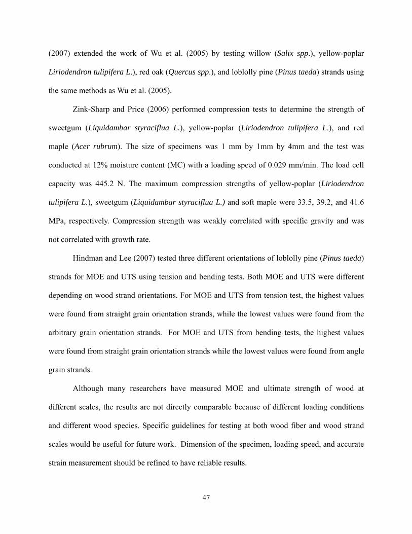
47

(2007) extended the work of Wu et al. (2005) by testing willow (Salix spp.), yellow-poplar

Liriodendron tulipifera L.), red oak (Quercus spp.), and loblolly pine (Pinus taeda) strands using

the same methods as Wu et al. (2005).

Zink-Sharp and Price (2006) performed compression tests to determine the strength of

sweetgum (Liquidambar styraciflua L.), yellow-poplar (Liriodendron tulipifera L.), and red

maple (Acer rubrum). The size of specimens was 1 mm by 1mm by 4mm and the test was

conducted at 12% moisture content (MC) with a loading speed of 0.029 mm/min. The load cell

capacity was 445.2 N. The maximum compression strengths of yellow-poplar (Liriodendron

tulipifera L.), sweetgum (Liquidambar styraciflua L.) and soft maple were 33.5, 39.2, and 41.6

MPa, respectively. Compression strength was weakly correlated with specific gravity and was

not correlated with growth rate.

Hindman and Lee (2007) tested three different orientations of loblolly pine (Pinus taeda)

strands for MOE and UTS using tension and bending tests. Both MOE and UTS were different

depending on wood strand orientations. For MOE and UTS from tension test, the highest values

were found from straight grain orientation strands, while the lowest values were found from the

arbitrary grain orientation strands. For MOE and UTS from bending tests, the highest values

were found from straight grain orientation strands while the lowest values were found from angle

grain strands.

Although many researchers have measured MOE and ultimate strength of wood at

different scales, the results are not directly comparable because of different loading conditions

and different wood species. Specific guidelines for testing at both wood fiber and wood strand

scales would be useful for future work. Dimension of the specimen, loading speed, and accurate

strain measurement should be refined to have reliable results.

48

Jeong et al. (2008) evaluated the effect of loading rate and thickness of strands on MOE

and UTS of southern pine (Pinus spp.) strands. Strand thickness varied 0.381 mm, 0.794 mm,

1.91 mm, and 3.81 mm. The different loading rates were 0.102 mm/min, 0.254 mm/min, and

0.406 mm/min. With a constant strand thickness of 0.794 mm, changes in the loading rate in the

range of 0.102 mm/min to 0.406 mm/min did not produce significantly different MOE and UTS

values at a level of α=0.05. Over the range of strand sizes tested, the MOE and UTS values were

significantly different. Using Tukey’s HSD comparisons, the MOE and UTS values were not

significantly different for strand thicknesses of 0.0794 cm and 0.191 cm. Based upon these

results, the authors recommend testing strands at 0.254 mm/min (0.005 cm/cm/min) and between

a thickness of 0.794 mm and 1.91 mm to reduce variability.

Digital image correlation (DIC)

Improved characterization of the constitutive behavior of wood strands with varying

microstructure would allow a more complete assessment of the resulting local stresses and make

a more precise characterization of the material properties. Previous work to characterize the

wood properties at the micro-scale level has used the constitutive properties of a representative

cell wall, relative volume fractions, and a generalization of the microstructure of wood fibers

(Bergander and Salmen 2000, Bergander and Salmen 2002, and Hindman and Lee 2007). These

assumptions, to some extent, are valid when examining average stress and strain for evaluating

the macro-scale behavior of wood. Failure of wood typically initiates from stress concentrations

induced by local variations due to inhomogeneities of the wood microstructure. Therefore, the

characterization of local material properties of wood is important to determine the mechanical

behavior of wood at various scales. One method for measuring the local material properties of

49

wood uses digital image correlation (DIC). DIC is a powerful method for analyzing small

specimens that cannot be attached to any extensometers or strain gauges to measure the strain.

The strain field can also be characterized since DIC is a non-contact method and only needs the

image of the surface of the specimens. However, DIC is sensitive to specimen characteristics and

requires a sophisticated testing set up to achieve reliable results. Currently, a guideline for

application of DIC to wood material is not well established. The fundamental knowledge of DIC

and previous research on application of DIC to wood material are summarized in the following

section. Details of the testing set-up and guidelines for the application of DIC to earlywood and

latewood bands, and wood strands are also mentioned.

Principles of digital image correlation

Digital image correlation (DIC), which has been used to process experimental stress

analysis results, began in the 1980s and has been broadly applied to different disciplines in

science and engineering (Jin and Bruck 2005). DIC was developed to resolve the displacement

on the surface of a specimen by correlating subimages of a sequence of images-one before

loading and several images during loading (Sun et al. 2005). Spatial domain image correlation is

the processing of digitizing images directly from the pixels of the image.

Deformation of the material can be achieved by tracking the displacement of markers on

the sample’s surface. The advantage of the DIC technique is the ability to track the change in

position of a point in the field under study. Figure 2.7 demonstrates the general scheme of

tracking the displacement of the window on the sequence of images. The first step is to locate the

point of interest, P, in the image of the reference configuration before loading by generating a

grid. The fixed grid on the image has information of the exact location of the point, P. After

50

loading, the change in the location of point P is tracked by image correlation using a pattern

matching technique. Eight subsets of pixels surrounding the point P in the reference image,

called a template or window, are matched with similar sized subsets of pixels within a search

window determined by the maximum expected inter-image displacement without marker.

The digital image correlation in the spatial domain is applied to obtain the displacements

of a point when a subimage with the point in the center on the reference image tracks another

subimage on the deformed image. The tracking of a subimage can be achieved by maximizing

the cross correlation coefficient between grey value patterns of two images. Equation 2.1 shows

the calculation of the cross correlation coefficient, C(p).

Cross Correlation Matching Technique

Reference grid Final grid

80 100

100

120

100

100 100 120

P 80 100

100

120

100

100 80 120

P

M

N

Figure 2.7 Schematic explanation of cross correlation techniques using DIC

51

C(p) =

∑ ∑ ∑ ∑

∑ ∑+

−=

+

−=

+

−=

+

−=

+

−=

+

−=

++

++

2/0

2/0

2/0

2/0

2/0

2/0

2/0

2/0

22

0

2/0

2/0

2/0

)),,(),,,((),(

)),,(),,,((),(

Ny

Nyy

Mx

Mxx

Ny

Nyy

Mx

Mxx

Ny

Nyy

Mx

Mxx

pyxypyxuxhyxg

pyxypyxuxhyxg

ν

ν (2. 1)

Where,

x0: the center point x of the subimage in the coordinate

y0: the center point y of the subimage in the coordinate

with the size of M by N pixels in the coordinate.

g(x,y): the pixel values at the point (x,y) in the reference image

h(x+u(x,y,p),y+v(x,y,p)): the grey values in the deformed image at the mapping position of the

point (x,y).

The pixel values at a sub-pixel position are obtained by using a cubic spline interpolation

scheme. The coefficients C(p), where p is the mapping point, are determined from the grey

values of pixel locations. The variables u(x,y,p) and v(x,y,p) are displacement functions which

define how each of the subimage points located in the reference image at (x,y) is mapped to that

in the deformed image.

In order to detect a small strain, the conventional DIC considered homogeneous

deformations on the surface of the specimens which were dependent upon sub-pixel accuracy. A

sub-set based correlation used the scheme of matching the sub-set of pixel intensity from the

undeformed image with the subset of pixel intensity after loading using interpolation. If the

material is not homogeneous, higher order interpolation is required while homogeneous materials

only require zero or first order interpolation to approximate the variation of the displacement

52

field (Jin and Bruck 2005). In this study, cubic spline interpolation scheme was employed to

represent the displacement field of wood.

A defined representative window size for generalizing mechanical properties of material

Baxter and Graham (2000) proposed a moving window generalized method of cells

(MW-GMC) to characterize material properties of composite materials based on digitized images

of local microstructure of the material. The statistical variability of material properties of

composite material is dependent upon the window size. Larger window sizes produced smaller

variance of material properties. However, if the window sizes become too large, the variability of

material properties approaches zero. A smaller window size produces noisier fields. Also, a

smaller window size required a higher computational effort which made it harder to analyze the

field statistically.

Baxter et al. (2001) extended MW-GMC to three dimensions to predict more accurate

material properties because of a three dimensional microstructure. The choice of window size

was emphasized to represent the local material properties. Therefore, the proper window size for

wood and wood-based materials should be calibrated to represent the local material properties.

Such a calibration can be done by checking the relationship between different window sizes and

calculated material properties at each window size. If the results converged from a certain

window size, the window size would be chosen for the test.

Application of DIC to wood and wood-based material

Many previous studies have applied DIC to wood and wood-based materials. The DIC

technique was introduced to measure the strain distribution of wood and paper material by Choi

53

et al (1991). The fundamental concept of DIC was well explained. The main objective of

application of DIC of wood material was to measure the strain distribution and quantify the

mechanical properties such as Poisson ratio and stress intensity factor. A summary of previous

work is presented in Table 2.11.

Table 2.11 Summary of objectives, main results and conclusions from previous researches

on DIC to wood and wood-based material

Researchers Objective Result/Conclusion

Choi et al. (1991)

Measured strain of wood and paper

The general concept of DIC and application of the method to wood mechanics were introduced.

Zink et al. (1995)

Measured the strain distribution of wood and wood-based composite

The stress concentration area can be captured and used to predict the eventual failure mode.

Zink et al. (1997)

Measured Poissons’s ratios for yellow-poplar

The magnitude of Poissons ratio (υLT) decreased by increasing load level because the tangential strains were fairly uniform but longitudinal strains increased with increasing load.

Mott et al. (1996)

Measured micro-strain distribution from wood pulp fiber

Non-uniform micro strain was observed. Poisson effect and failure mechanism were estimated.

Stelmokas et al. (1997)

Displacement beneath the bolts in multiple-bolted wood connections

DIC was an effective method for describing surface displacement fields and for detecting failure beneath a bolt

Muszynski et al. (2000)

Measured interlaminar shear strains in fiber reinforcement polymer composite

DIC was capable of characterizing interlaminar shear behavior of laminated composite.

Samarasinghe and Kulasiri

(2000)

Displacement fields of rubber and wood in parallel and perpendicular tension loading

While uniform stress distribution occured within the lignin matrix under tension loading perpendicular to the grain, parallel to the grain loading had a complex displacement pattern including internal shear and slippage.

Danvind (2002) Measured the strain of wood during drying

DIC was capable of calculating two dimensional shrinkage strain field.

Samarasinghe and Kulasiri

(2004)

Stress intensity factor of radiate pine (Pinus radiata) in tangential-longitudinal

A strong correlation between the critical stress intensity factor and the angle between the original crack plane and the radial-

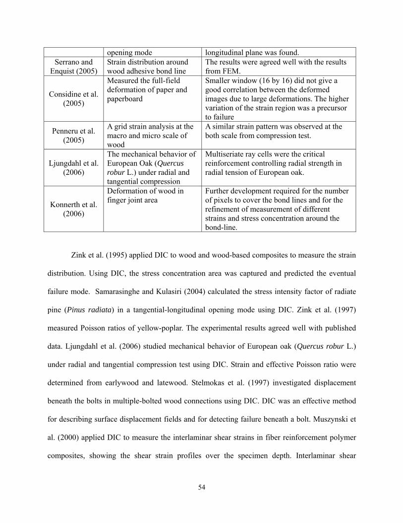
54

opening mode longitudinal plane was found. Serrano and

Enquist (2005) Strain distribution around wood adhesive bond line

The results were agreed well with the results from FEM.

Considine et al. (2005)

Measured the full-field deformation of paper and paperboard

Smaller window (16 by 16) did not give a good correlation between the deformed images due to large deformations. The higher variation of the strain region was a precursor to failure

Penneru et al. (2005)

A grid strain analysis at the macro and micro scale of wood

A similar strain pattern was observed at the both scale from compression test.

Ljungdahl et al. (2006)

The mechanical behavior of European Oak (Quercus robur L.) under radial and tangential compression

Multiseriate ray cells were the critical reinforcement controlling radial strength in radial tension of European oak.

Konnerth et al. (2006)

Deformation of wood in finger joint area

Further development required for the number of pixels to cover the bond lines and for the refinement of measurement of different strains and stress concentration around the bond-line.

Zink et al. (1995) applied DIC to wood and wood-based composites to measure the strain

distribution. Using DIC, the stress concentration area was captured and predicted the eventual

failure mode. Samarasinghe and Kulasiri (2004) calculated the stress intensity factor of radiate

pine (Pinus radiata) in a tangential-longitudinal opening mode using DIC. Zink et al. (1997)

measured Poisson ratios of yellow-poplar. The experimental results agreed well with published

data. Ljungdahl et al. (2006) studied mechanical behavior of European oak (Quercus robur L.)

under radial and tangential compression test using DIC. Strain and effective Poisson ratio were

determined from earlywood and latewood. Stelmokas et al. (1997) investigated displacement

beneath the bolts in multiple-bolted wood connections using DIC. DIC was an effective method

for describing surface displacement fields and for detecting failure beneath a bolt. Muszynski et

al. (2000) applied DIC to measure the interlaminar shear strains in fiber reinforcement polymer

composites, showing the shear strain profiles over the specimen depth. Interlaminar shear

55

behavior of laminated composite was successfully characterized.

Samarasinghe and Kulasiri (2000) measured displacement fields of rubber and wood in

parallel and perpendicular tension loading. Danvind (2002) used digital speckle photography

(DSP) and X-ray computerized tomography (CT) to measure the strain of wood during drying. A

method was presented for calculating the two dimensional shrinkage strain field.

Many authors emphasized precautions for the application of DIC to wood and wood

based materials. Zink et al. (1997) found a loading effect on strain behaviors of different sections

of wood. Considine et al. (2005) mentioned the window size for correlation of deformed images.

Four different window sizes (128 by 128, 64 by 64, 32 by 32, and 16 by 16 pixels) were used.

Smaller window sizes (16 pixels by 16 pixels) did not correlate well with large deformation.

Mott et al. (2002) applied cyclic loading every five seconds to prevent distortion of the surface

image of the specimen from suspended scanning. Lopez-Anido et al. (2004) applied 3-D DIC to

characterize mechanical behavior of composite materials. DIC with four different test set-ups

according to ASTM D3039 tension for composites, ASTM D638 tension for plastics, ASTM

D6641 compression for composites, and ASTM D695 compression for plastics were investigated.

Guidelines of the use of DIC for each test methods were presented.

DIC was also applied to measure the strain distribution of wood at the micro-scale level.

Mott et al. (1996) set up a MINIMAT tester inside an environmental scanning electron

microscopy (ESEM) to measure micro-strain distribution from wood pulp fiber. Murata and

Masuda (2001) used a confocal microscopy incorporated with DIC to measure the swelling

behavior of the cross section of cells from Douglas-fir (Pseudotsuga menziesii). Penneru et al.

(2005) introduced a grid strain analysis at the macro and micro scale of wood. A similar strain

pattern was observed at the both scale from compression test. Ljungdahl et al. (2006) studied the

56

mechanical behavior of European Oak (Quercus robur L.) under radial and tangential

compression using digital speckle photography (DSP). Multiseriate ray cells were the critical

reinforcement controlling radial strength in radial tension. The rays were the main

microstructural factor controlling transverse anisotropy in European oak.

Konnerth et al. (2006) investigated the deformation of wood in finger joint area using

electronic speckle-pattern interferometry (ESPI). Machine graded Norway spruce (Picea abies)

was used for the finger joint specimens and glued by two different types of adhesives; melamine-

urea-formaldehyde (MUF) and polyurethane (PUR). Further development was required for the

number of pixels to cover the bond lines and for the refinement of measurement of different

strains and stress concentrations around the bond-line. Serrano and Enquist (2005) investigated

the strain distribution around wood adhesive bond lines. The results agreed well with the results

from FEM.

Stochastic finite element method (SFEM)

The strength of wood strands originates from the intra-ring properties and grain angle.

However, the intra-ring properties and the orientation of grain are uncertain factors. The material

properties of wood are random in nature and the grain angle of strands can be random due to

indeterminate cutting. Therefore, it is desirable to investigate the effect of the uncertain variables

of intra-ring properties and grain angle on the mechanical behavior of wood strands under

various loading conditions.

Random properties and grain angles affect the strain and stress distributions of wood

strands because the mechanical behaviors are functions of the material properties. Under the

condition of the indeterminate properties of wood strands, the load-displacement relations of

57

wood strands are influenced by the variability of the intra-ring properties and grain angles.

Random properties of wood strands affect not only the stiffness of wood strands, but also the

evaluation of strains and stresses in the principal material directions, which are important for

failure estimation. These problems have not been elaborated in previous studies of wood science

area.

The SFEM can combine the existing finite element method (FEM) for deterministic

problems with uncertainty variables. The computation of the stochastic field of nodal

displacements (u) from the random stiffness matrix (K) is the main objective of the SFEM. There

are many representative methods to generate the stochastic finite element stiffness including

perturbation, Monte Carlo simulation, Neumann expansion, and Karhunen-Loeve decomposition.

The fundamental principle of the SFEM technique fits well with the uncertainty of wood

structure. The stiffness and grain variation in strands can be used as an input for SFEM.

Unfortunately, there are only a few SFEM applications specifically related to wood and wood

based materials in the research literature. Therefore, the literature review is limited to the

application of composite materials with similar structure to wood and fundamental knowledge of

SFEM.

Comparison of conventional FEM and SFEM

Conventional finite element methods (FEM) are widely used to solve many practical

problems in wood and wood-based composites (Mackerle 2005). The finite element solution is

an approximation of the actual continuous domain using a number of finite elements. FEM

results can achieve a high accuracy as the number of elements becomes large and converges to a

single solution. There are numerous practical problems in FEM due to many uncertainties that

58

can influence the results (Kleiber and Hien 1992). Conventional FEM assumes deterministic or

representative material properties and geometry of material. The nodal displacement {U} of the

system is deterministic corresponding to both the deterministic global stiffness [K] and loading

{F} (Equation 2.4).

.

Where

K: the global stiffness matrix

U: global displacement vector

F: the deterministic load vector

While the conventional FEM uses a deterministic stiffness matrix [K] and a deterministic

loading {F} to obtain a deterministic nodal displacement {U}, SFEM uses random stiffness

matrices [K] and random loadings {F} to solve the corresponding set of nodal displacement

vectors. Although the governing equation of SFEM is similar to the conventional FEM, SFEM

needs additional functions to generate random properties and corresponding response vectors.

As shown in Table 2.12, the general procedure of the SFEM is similar to that of FEM.

However, there are differences in each procedure. In pre-processing stage, SFEM generates

random material properties in each element. In the analysis part, SFEM deals with a set of

coefficients to generate responding displacements. In the post-processing part, SFEM produces

statistical stress and strain distribution. In this study, the random material properties (E(x,θ)) was

implemented using Monte-Carlo simulation (MCS) with known probabilities of material

59

properties and the corresponding nodal displacement was analyzed.

Table 2.12 Comparison of the FEM and SFEM procedures

Procedure FEM SFEM Difference1

Pre-processing

Discretize the element with determined element stiffness

Discretize the element with random element properties

Determined material properties/Random material properties

Analysis

Element stiffness matrices are computed, assembled to form global stiffness matrix for the system, applied boundary conditions.

The unknowns of this system are the set of nodal displacement vectors which describe the probabilistic nodal displacement of the system.

Mean displacemet/the set of nodal displacement vector

Post-processing

Mean displacement and stress distribution of the system can be calculated

Statistical analysis of stress distribution of the system based on the set of nodal displacement

Mean stress and strain distribution/ Statistical distribution of stress and strain

1FEM/SFEM

Relevant SFEM applications to composite materials.

SFEM has been applied to solve many different physical problems where uncertainty of

geometry, material property or boundary conditions exists. The accuracy and validity of SFEM

has been proven by previous work. However, since only a few SFEM applications have been

applied to wood based composite, similar applications to composite materials are also listed.

Wang and Lam (1998) applied a nonlinear SFEM to estimate the tensile strength of

parallel aligned wood strand composites. The input variables for the individual strands were

elastic properties and strength from the experimental test. Clouston and Lam (2002) extended the

study of Wang and Lam (1998) to predict the mechanical behavior of wood strand composites

with strands of different grain angles using Monte-Carlo simulation based SFEM. The simulation

results agreed well with the experimental test.

60

Chkraborty and Dey (2000) used the Neumann expansion technique based SFEM to

analyze uncertain structure parameters under seismic induced random ground motion. A direct

Monte Carlo simulation was performed to check the accuracy of the results from the SFEM. The

results showed that Neumann expansion solution could handle up to 20% coefficient of variation

of uncertain input parameters. Reliable results could be expected with less than 15 % coefficient

of variation of the random inputs.

Kaminski (2000) applied perturbation-based SFEM to simulate interface defects in fiber-

reinforced composites. The SFEM used real composite structures with various fictitious interface

percentages. A Monte Carlo simulation approach used homogenized elastic properties and three

different interface sizes to calculate the effective stiffness for a composite. The results from the

SFEM showed a greater horizontal displacement occurred at a larger percentage of interface

defects. Caution was emphasized using the perturbation-based SFEM in a larger percentage of

the interface defects due to the significant variation of the elastic characteristics of the interface.

The results from Monte-Carlo simulation showed a greater percentage interface defects had a

lower elastic constant. Among three different interface sizes, the largest interface had the highest

coefficient variation of the elastic constant.

Chung et al. (2005) used SFEM incorporated with a moving window generalized

methods of cells (GMC) to characterize the interface of fiber metal laminates. The results from

the GMC showed the variability of mean displacement was not influenced by different window

size while the variability of displacement was proportional to the window size. Based on the

results from the GMC, Karhunen-Loeve expansion was applied to generate the random material

properties. For the response displacement, Hermite polynomial expansion was applied. The

SFEM results showed the strain variability in the fiber-metal interface zone was in good

61

agreement with the experimental results. The largest strain variability in the interface zone was

likely to have the initiation of failure.

Eiermann et al. (2005) overviewed computational implementation of SFEM. K-L

expansion could produce a good random field with a large correlation length and a small number

of expansion terms. An efficient solution algorithm could be achieved from the Galerkin

discretization. The conclusion was an efficient implementation of SFEM and improvement of

generation of random field saved computational efficiency.

From this literature review, Most SFEMs were validated their accuracy by comparing the

results from the MCS based SFEM. Also Monte-Carlo simulation based SFEM has been applied

to wood material. Therefore, in this study Monte-Carlo simulation based SFEM was applied to

analyze the effect of the intra-ring properties and different grain angles on mechanical behavior

of wood strands.

62

Summary and Conclusion

SCL and OSB are manufactured from wood strands of various sizes. The use of SCL and

OSB products place strands in different stress conditions. Optimization of strand size and

geometry would improve the mechanical performance of SCL and OSB. In the processing of

wood strands, the effect of the wood strand geometry on the mechanical properties is crucial to

optimize the properties for end uses. The strength of wood strands originates from the intra-ring

properties and grain angles. However, the intra-ring properties and the orientation of grain are

uncertain factors. The material properties of wood are random in nature and the grain angle of

strands can be random due to indeterministic cutting. Therefore, it is desirable to investigate the

effect of the uncertain variables of intra-ring properties and grain angles on the mechanical

behavior of wood strands under various loading conditions.

Understanding the hierarchical structure of wood at different scales is important to

develop high strength materials. The nano-scale contains the mechanical functions of cellulose,

hemicelluloses, and lignin in wood cells. The micro-scale contains the different microfibril

angles and cell wall thickness in the cell wall layer. The macro-scale contains the different

characteristics of earlywood and latewood along with juvenile wood and mature wood. All of

these hierarchical structures affect the mechanical properties of wood and wood-based

composites.

The knowledge of mechanical properties of the earlywood and latewood bands and

strands can lead to better predictions of stiffness and strength of strand-based composites.

Improved characterization of the constitutive behavior of wood strands with random

microstructures would allow a more complete assessment of the resulting local stresses and make

63

a more precise characterization of the material properties. Failure of wood typically initiates

from stress concentrations induced by local variations due to inhomogeneities of the wood

microstructure. Therefore, the characterization of local material properties of wood is important

to determine the mechanical behavior of wood at various scales. The digital image correlation

(DIC) method is chosen to measure MOE of earlywood and latewood bands, and MOE of strands.

Many previous researchers have developed different models to predict the mechanical

behavior of wood at different scales using micromechanics, laminate theories and finite element

methods. Although many methods of modeling wood fiber and strand based composites were

found, there was a lack of research on modeling of wood strands. Analytical and numerical

models for wood fiber and strand based composites, however, suffer from limiting information

on input properties for the models. Most models used averaged material properties or assumed

material properties that may cause an error or a variable result. Therefore, prior to model wood

strands, the variation of input parameters that affect the mechanical properties of wood strands

should be included.

Random intra-ring properties and grain angles affect the strain and stress distributions of

wood strands because the mechanical behaviors are functions of the material properties. Under

the condition of the undetermined properties of wood strands, the stiffness-displacement

relations could be considered as random equations. The motivation of using stochastic analysis

stems from the variability of the intra-ring properties of the wood strands. Stochastic finite

element method (SFEM) can solve this variability as the known probabilities of material

properties. The SFEM can take advantage of the existing FEM for deterministic problems

combined with uncertainty variables. The fundamental principle of the SFEM technique fits well

with the high uncertainties of wood structure. The stiffness and grain variation in strands are

64

used as inputs for the SFEM.

Based on the understanding of the effect of the intra-ring properties and different grain

angles of the wood strands, segregation into discrete categories (earlywood, latewood, and

certain grain angle strands) can maximize the benefits of a certain geometry of wood strands for

specific uses. The knowledge of the effect of the intra-ring properties and grain angles of wood

strands can lead to optimization in processing and utilization. This process can begin with cutting

different angles of a wood block, experimentally determining intra-ring properties, and using the

properties to simulate models to analyze the mechanical behaviors of wood strands.

References

Adair, C. 2005. Structural panels and engineered wood yearbook, APA. The engineered wood association E171. Åkerholm, M. and L. Salmén 2003. The mechanical role of lignin in the cell wall of spruce tracheids. Holzforschung 57(5): 459–465. Angeles, G., R. Davalos-Sotelo, and R. Sanjuan-Duenas. 2006. Micromechanical analysis of Urticaceae wood. 5th Plant Biomechanics Conference-Stockholm, August 28-September 1. Anagnost, S. E., R. E. Mark, and R.B. Hanna. 2002. Variation of microfibril angle within individual fibers. Wood and Fiber Sci. 34: 337–349. Baxter, S. C., M. I. Hossain, and L. L. Graham. 2001. Micromechanics based random material property fields for particulate reinforced composites. Int. J. Solids Struct. 38: 9209–9220. Baxter S. C. and L. L. Graham. 2000. Characterization of random composites using a moving window technique. ASCE J. Eng. Mech. 126 (4):389–404. Bendtsen, B. A. and J. Senft. 1986. Mechanical and anatomical properties in individual growth rings of plantation-grown Eastern cottonwood and loblolly pine. Wood and Fiber Sci. 18: 23–38. Bergander A. and L. Salmén. 2002. Cell wall properties and their effects on the mechanical properties of fibers. J. Mater. Sci. 37 (1):151–156. Booker, R. E. 1993. The importance of the S3 cell wall layer incollapse prevention and wood hardness. 24th Forest Products Research Conference 15–18 November, CSIRODiv. of Forest

65

Products, Clayton, Victoria, Australia 3(17):1–13. Booker, R. E. and J. Sell. 1998. The nanostructure of the cell wallof soft woods and its function in a living tree. Holz Roh-Werkstoff 56:1-8. Balatinecz, J. J. and D. E. Kretschmann. 2001. Properties and utilization of poplar wood. In Poplar Culture in North America. Part A, Chapter 9. Edited by D.I. Dickmann, J.G. Isebrands, J.E. Eckenwalder, and J. Richardson. NRC Research Press, National Research Council of Canada, Ottawa, ON KIA OR6, Canada. 277-291 pp. Bendtsen, B.A. 1978. Properties of wood from improved and intensively managed stands. Forest Prod. J. 28(10):61-72. Bendtsen, B. A. and J. Senft. 1986. Mechanical and anatomicalproperties in individual growth rings of plantation grown eastern cottonwood and loblolly pine. Wood Fiber Sci. 18:23–38. Pearson, R. G. 1988. Compressive properties of clear and knotty loblolly pine juvenile wood. Forest Prod. J. 38(7/8):15-22. Bergander, A. and L. Salmén. 2000 Variations in transverse fibre wall properties: relations between elastic properties and structure. Holzforschung 54(6): 654-600 Bergander, A. and L. Salmén. 2002. Cell wall properties and their effects on the mechanical properties of fibers. J. Materials Sci. 37(1), 151–156. Burdon, R. D., R. P. Kibblewhite, J. C. F. Walker, R. A. Megraw, R. Evans, and D. J. Cown. 2004. Juvenile versus mature wood: a new concept, orthogonal to corewood versus outerwood, with special reference to Pinus radiata and P. taeda. Forest Sci. 50:399-415. Burgert, I. and J. Keckes. 2002. A comparison of two techniques for wood fibre isolation evaluation by tensile tests on single fibres with different microfibril angle. Plant Biology. 4(1): 9-12. Burgert, I. and K. Fruhmann. 2003. Microtensile testing of wood fibers combined with video extensometry for efficient strain detection. Holzforschung. 57(6): 661-664. Cave, I.D. 1968. The Anisotropic Elasticity of the Plant Cell Wall. Wood Science and Technology. 2(4): 268–278. Cave, I. D. 1969. The longitudinal Young’s modulus of Pinus radiata. Wood science and technology. 3(1): 40-48. Cave, I. D. 1978. Modeling Moisture-Related Mechanical-Properties of Wood .1. Properties of Wood Constituents. Wood Science and Technology 12(1): 75-86. Cave, I. D. and Walker, J. C. F., 1994. Stiffness of wood in fast grown plantation softwoods: the influence of microfibril angle. Forest Products J. 44(5): 43–48.

66

Chakraborty S. and S. S. Dey 2000. Stochastic finite element simulation of uncertain structures subjected to earthquake. Shock and Vibration. 7(5):309 -320. Choi, D., J. L. Thorpe, and R. B. Hanna. 1991. Image Analysis to Measure Strain in Wood and Paper. Wood Science and Technology 25(2): 251-262. Chung, D. B., M. A. Gutiérrez and R. D. Borst. 2005. Object-oriented stochastic finite element analysis of fibre metal laminates. Computer Methods in Applied Mechanics and Engineering 194(12-16):1427-1446. Clouston, P. and F. Lam. 2001. Computational Modeling of Strand-based Wood Composites. ASCE Journal of Engineering Mechanics, 127(8): 844-851. Clouston, P. and F. Lam. 2002. A Stochastic Plasticity Approach to Strength Modeling of Strand-based Wood Composites. Composites Science and Technology, 62:1381-1395. Cousins, W. J. 1976. Elastic modulus of lignin as related to moisture content. Wood Sci. and Technology. 10, 9–17. Cousins, W. J. 1978. Young's modulus of hemicellulose as related to moisture content. Wood Sci. and Technology. 12(3): 161-167. Cramer, S.M., D. E. Kretschmann, R. Lakes, and T. Schmidt. 2005. Earlywood and latewood elastic properties in loblolly pine. Holzforschung. 59(5):531-538. Dai C and P. R. Steiner. 1994. Spatial structure of wood composites in relation to processing and performance characteristics. Part III. Modeling the formation of multi-layered random flake mats. Wood Sci. Technol 28:229–239. Danvind, J. 2002. Methods for Collecting and Analysing Simultaneous Strain and Moisture Data During Wood Drying; Licenciate Thesis in the Division of Wood Physics, Skelleftea Campus: Skelleftea, Sweden, Lulea University of Technology, 2002. Deomano, E. C. and A. Zink-Sharp. 2004. Bending properties of wood flakes of three southern species. Wood and Fiber Sci. 36(4): 493-499. Deomano E. C. and A. Zink-Sharp. 2005. Effect of species, cutting direction, dimensions, and temperature on flake drying. Forest Prod. J. 55(9): 31-36 Donaldson, L. A. 1996. Effect of physiological age andsite on microfibril angle in Pinus radiata. IAWA Journal 17: 421–429. Eiermann M., O. G. Ernst, and E. Ullmann. 2005. Computational aspects of the stochastic finite element method. Proceeding of algoritmy. pp. 1-10.

67

Evans, R., S. Stuart, and J. Van der touw. 1996. Microfibrilangle scanning of increment cores by X-ray diffractometry. Appita Journal 49, 411–414. Fengel, D. and G. Wegener. 1983. Wood—Chemistry, Ultrastructure, Reactions (De Gruyter, Berlin). Frey-wyssling, A. and K. Muhlethaler. 1965. Ultrastructural Plant Cytology with an Introduction to Molecular Biology New York, Elsevier Publishing Co., First Edition. Gassan J., A. Chate and A. K. Bledzki. 2001. Calculation of elastic properties of natural fibers. Journal of Materials Sci. 36:3715-3720. Geimer R. L. and J. B. Crist. 1980. Structural flakeboard from short-rotation intensively curtured hybrid populous clones. Forest Prod. J. 30(6):42-48. Geimer, R. L. 1986. Properties of structural flakeboard manufactured from 7-year-old intensively cultured poplar, tamarack, and pine. Forest Prod. J. 36(4):42-26. Geimer, R. L., V. L. Herian, and D. Xu. 1997. Influence of juvenile wood on dimensional stability and tensile properties of flakeboard. Wood and Fiber Sci. 29(2): 103-120. Geimer, R. L., R. J. Mahoney, S. P. Loehnertz, and R. W. Meyer. 1985. Influence of processing-induced damage on the strength properties of oriented strand wood products. Forest Prod. J. 50(11/12):33-42. Ghanem R. G. and P. D. Spanos. 1991. Stochastic Finite Elements: A Spectral Approach, Springer-Verlag. Ghanem R. 1999. Higher order sensitivity of heat conduction problems to random data using the spectral stochastic finite element method, ASME Journal of Heat Transfer, 121:290–299. Goel A, C. Phanouriou, F. A. Kamke, C. J. Ribbens, C. A. Shaffer, and L. T. Watson. 1999. WBCSim: a prototype problem solving environment for wood-based composites simulations. EngComput 15:198–210. Groom, L. and L. Mott. 2002. Mechanical properties of individual southern pine fibers. Part I. Determination and variability of stress-strain curves with respect to tree height and juvenility. Wood and Fiber Sci. 34(1): 14-27. Groom, L., S. Shaler, and L. Mott. 2002. Mechanical properties of individual southern pine fibers. Part III. Global relationships between fiber properties and fiber location within an individual tree. Wood and Fiber Sci. 34(2): 238-250.

68

Gutierrez, M. A and S. Krenk 2004. Stochastic finite element methods. In E. Stein,R. de Borst, and T. J. R. Hughes (Eds.) Encyclopedia of Computational Mechanics. John Wiley & Sons, Ltd. in press. Harwood, V.D. 1971. Variation in carbohydrate analyses in relation to wood age in Pinus radiata. Holzforschung. 25 (3):73–77. Harris, J. M. and B. A. Meylan. 1965. The influence of microfibril angle on longitudinal and tangential shrinkage in Pinus radiata. Holzforschung. 19:144–153. Hearle, J. W. S. 1963. The fine structure of fibers and crystalline polymers. III. Interpretation of the mechanical properties of fibers Journal of Applied Polymer Science, 7:1207 – 1223. Hindman D. P. and J. N. Lee. 2007. Modeling wood strands as multi-layer composites: bending and tension loads. Wood and Fiber Sci. 39(4):516-526. Hunt, M. O., M. H. Triche, G. P. McCabe, and W. L. Hoover. 1989. Tensile properties of yellow-poplar veneer strands. Forest Prod. J. 39(9). Jeong, G. Y., D. P. Hindman, D. Finkenbinder, J. N. Lee, and Z. Lin. 2008. Effect of loading rate and thickness on the tensile properties of wood strands, Forest product J. 58(10):33-37. Jin, H. and H. A. Bruck. 2005. Theoretical development for pointwise digital image correlation. Optical Engineering, Volume 44, pp. Jo, J. M., B. J. Chung, Y. D. Lee, D. H. Kang, D. J. Chung, and S. G. Chung. 1981. Developing multiple utilization of larch wood. Forest Research Institute, No. 28. Seoul, Korea. Jones, R. M. 1975. Mechanics of composite materials. McGraw-Hill, New York. Kahle, E. and J. Woodhouse. 1994. The infuence of cell geometry on the elasticity of soft xylem tissue. Journal of Material Science 29:1250-1259. Kaminski, M. 2002. Stochastic problem of fiber-reinforced composite with interface defects. Engineering computations. 19 (7) :854-868 Keckes, J., I. Burgert, K. Fruhmann, M. Muller, K. Kolln, M. Hamilton, M. Burghammer, S. V. Roth, S. Stanzl-Tschegg and P. Fratzl. 2003. Cell-wall recovery after irreversible deformation of wood. Nature Materials 2(12): 810-814 Kerr, A.J.,and D.A.I. Goring. 1975. The ultrastructural arrangements of the wood cell wall, Cellul. Chem. Technol. 9: 536–573. Kleiber, M., T. Hien. 1992. The Stochastic Finite Element Method. Basic Perturbation Technique and Computer Implementation. John Willey & Sons.

69

Konnerth, J., W. Gindl, W., and U. Mueller. 2006a. Elastic properties ofadhesive polymers. Part I: Polymer films by means of electronic speckle pattern interferometry. J. Appl. Polym. Sci Vol. 103, 3936–3939. Konnerth, J., A.Valla , W. Gindl , and U. Muller. 2006b. Measurement of strain distribution in timber finger joints Wood Sci Technol 40:631–636. Kretschmann, D. E., H. A. Alden, and S. Verrill. 1997. Variations of microfibril angle in loblolly pine: comparison of iodine crystallization and X-ray diffraction techniques. In: Butterfield, B.G. (Ed.), Proceedings of the IAWA/IUFRO International Workshop on the Significance of Microfibril Angle to Wood Quality. Westport, New Zealand, pp. 157–176. Lam, F. 2001. Modern structural wood products. J. Progress in Structure Engineering Material 3:(3)238-245. Larson, P. R., D. E. Kretschmann, A. Clark III, and J. G. Isebrands. 2001. Juvenile Wood Formation and Properties in Southern Pine. General Technical Report FPL-GTR-129. Madison, Wisconsin: US Department of Agriculture, Forest Service, Forest Products Laboratory. Lee, J. N. and Q. Wu. 2003. Continuum modeling of engineering constants of oriented strand board. Wood and Fiber Sci. 35(1):24-40. Lekhnitskii, S. G. 1963. Theory of elasticity of an anisotropic elastic body, Holden-Day, San Francisco. Liu, J. Y. 2002. Analysis of off-axis tension test of wood specimens. Wood and Fiber Sci. 34(2):205-211. Ljungdahl, J. L. A. Berglund, and M. Burman. 2006. Transverse anisotropy of compressive failure in European oak-a digital speckle photography study. Holzforschung, 60: 190-195. Lopez-Anido, R., L. Muszyñski,H. J. Dagher. 2004. Composite Material Testing Using a 3-D Digital Image Correlation System COMPOSITES 2004 Convention and Trade Show American Composites Manufacturers Association October 6-8, 2004 Tampa, Florida USA. Lu C. 1999. Organization of wood elements in partially oriented flakeboard mats. PhD Dissertation. Dept. of Forestry, University of British Columbia, Vancouver, BC Macdonald E. and J. Hubert2002. A Review of the Effects of Silviculture on the Timber Quality of Sitka Spruce. Forestry, 75 (2). Mackerle, J. 2005. Finite element analyses in wood research: a bibliography. Wood Sci Technol 39: 579–600. Mark, R.E. 1967. Cell Wall Mechanics of Tracheids. Yale University Press, New Haven, USA, 2 edition.

70

Mark, R. E. and P. P. Gillis. 1973. The relationship between fiber modulus and S2 angle. Tappi 56:164-167. Matsuo M. and C. Sawatari, and Y. Iwai, and F. Ozaki. 1990. Effect of orientation distribution and crystallinity on the measurement by X-ray diffraction of the crystal lattice moduli of cellulose I and II Biomacromolecules, 23: 3266 - 3275. McAlister, R. H., A. Clark III, and J. R. Saucier. 1997. Effect of initial spacing on mechanical properties of lumber sawn from unthinned slash pine at age 40. Forest Prod. J. 47 (7/8):107–109. Moden, C. 2006. Transverse Anisotropy in Softwoods Licenciate Thesis Stockholm, Sweden 2006. Moody, R. C. 1970. Tensile strength of fingerjoints in pith-associated and non-pith associated Southern Pine lumber. Res. Pap. FPL-138. Madison, WI:U.S. Department of Agriculture, Forest Service, Forest Products Laboratory. 20pp. Mott, L., S. M. Shaler, and L. H. Groom 1996. A Novel Technique to Measure Strain Distributions in Single Wood Fibers. Wood and Fiber Sci. 28(4):429-437. Mott, L., L. Groom, and S. Shaler. 2002. Mechanical properties of individual southern pine fibers. Part II. Comparison of earlywood and latewood fibers with respect to tree height and juvenility. Wood and Fiber Sci. 34(2): 221-237 Munch, E. 1938. Investigations on the harmony of tree shape. Jahrbu¨cher fu¨r wissenschaftliche Botanik 86: 581–673. (Translated by M. H. Zimmermann, 1963). Murata, K. and Masuda M. 2001. Observation of microscopic swelling behavior of the cell wall. J. Wood Sci. 47:507-509. Muszynski, L., R. Lopez-Anido and S. M. Shaler. 2000. Image Correlation Analysis Applied to Measurement of Shear Strains in Laminated Composites. in: Proceedings of SEM IX InternationalCongress on Experimental Mechanics, Orando FL, June, 5-7, 2000. 163-166. Nairn, J. A. 2006. Numerical Simulations of Transverse Compression and Densification in Wood, Wood and Fiber Sci. 38(4):576 – 591. Navi, P., P. K. Rastogi, V. Gresse, and A. Tolou. 1994. Micromechanics of wood subjected to axial tension. Wood Science and Technology. 29(6):411-429. Neagu, R. C., E. K. Gamstedt and F. Berthold. 2006. Stiffness contribution of various wood fibers to composite materials, Journal of Composite Materials, 40:(8):663-699 Panshin, A. J., and C. D. Zeeuw. 1980. Textbook of wood technology. McGraw Hill Book Co., New York, NY.

71

Pearson, R. G. and B. E. Ross. 1984. Growth rate and bending properties of selected loblolly pines. Wood and Fiber Sci. 16:37-47. Penneru, A. P., K. Jayaramanand, D. Bhattacharyya 2005. Strain analysis in bulk forming of wood Holzforschung, 59:456–458. Perr´e, P. 2005. Meshpore: A software able to apply image-based meshing techniques to anisotropic and heterogeneous porous media. Dry Technol 239–11:1993–2006. Persson, K. 2000. Micromechanical Modelling of Wood and Fibre Properties, Doctoral Thesis, Department of Mechanics and Materials, Structural Mechanics, LTH, Lund University, Lund, Sweden. Price, E.W. 1975 Determining tensile properties of Sweetgum veneer flakes. Forest Prod. J. 26(10): 50-53 Pugel, A. D., E. W. Price, and C. Y. HSE. 1990a. Composites from southern pine juvenile wood. Part I. Panel fabrication and initial properties. Forest Prod. J. 40(1):29-33. Reiterer, A., H. Lichtenegger, S. Tschegg, and P. Fratzl. 1999. Experimental evidence for a mechanical function of the cellulose microfibril angle in wood cell walls. Philosophical Magazine A, 79(9): 2173-2184. Sakurada, I, A. Nukushina , T. Ito. 1962. Experimental determination of the elastic modulus of crystalline regions in oriented polymers. J Polymer Sci 57:651–660. Salmén, L. and de Ruvo, A. 1985. A model for prediction of fiber elasticity Wood and Fiber Science, 17, pp. 336 - 350. Salmén, L., and A. M. Olsson 1998. Interaction between hemicelluloses, lignin and cellulose: structure-property relationships, J. Pulp Pap. Sci. 24(3): 99–103. Salmén, L. 2004. Micromechanical understanding of the cell-wall structure. Comptes Rendus Biologies 327(9-10): 873-880. Samarasinghe, S. and G. D. Kulasiri, 2000. Displacement fields of wood in tension based on image processing: Part 1. Tension parallel- and perpendicular-to-grain and comparisons with isotropic behaviour. Silva Fennica 34(3): 251–259. Samarasinghe, S. and D. Kulasiri, 2004. Stress intensity factor of wood from crack-tip displacement fields obtained from digital image processing. Silva Fennica 38(3): 267–278. Saliklis, E. P. and R. H. Falk. 2000. Correlating off-axis tension tests to shear modulus of wood-based panels. J. Structural Engineering. 126(5):621-625.

72

Schuler, A. and C. Adair. 2000. Engineered Wood Products- Production, Trade, Consumption and Outlook. Forest Products Annual Market Review, Chapter 11, FAO/ECE Timber Section. United Nations, NY and Geneva. 131-146 pp. Serrano, E., and B. Enquist. 2005. Contact-free measurement and non-linear finite element analyses of strain distribution along wood adhesive bonds. Holzforschung 59:641–646. Shu, J., L. T. Watson, B. G. Zombori, and F. A. Kamke. 2006. WBCSim: an environment for modeling wood-based composites manufacture Engineering with Computers 21: 259–271. Siddiqui, K. M. 1976. Relationship between cell wall morphologyand chemical composition ofearlywood and latewood in two coniferous species. Pakistan J. For. 26:21–34. Sjöström, E. 1993. Wood Chemistry, Fundamentals and Applications, second ed. Academic Press, San Diego. Smith, R. W. and D. G. Briggs. 1986. Juvenile wood:Has it come of age? Pages 1-11 in proc., Juvenile wood: What does it mean to forest management and forest products? Forest Products Research Society, Madison, WI. Smulski, S. 1997. Engineered wood products, a guide for specifiers, designers and users. PFS Research Foundation. Madison, WI. 294 pp. Stelmokas, J. W., A. G. Zink, J. L. Loferski, and J.D. Dolan. 1997. Measurement of load distribution among multiple-bolted wood connections. Journal of Testing and Evaluation 25(5):510-515. Sugimori, M. and F. Lam. 1999. Measuring macro-void distribution in wood composites using computer tomography and image processing techniques. Mohuzai Gakkaishi (J. Japan Wood Res. Soc.) 45(3):254-257. Sun, Y., J. H. L. Pang, C. K. Wong, and F. Su. 2005. Finite element formulation for a digital image correlation method. Appl. Opt. 44, 7357-7363. Tang, R. C. and N. N. Hsu. 1973. Analysis of the relationship between microstructure and elastic properties of the cell wall. Wood and Fiber 5, 139–151. Taylor, F. W. and J. S. Moore, 1981. A comparison of earlywood and latewood tracheid lengths in loblolly pine. Wood and Fiber. 13:159-165. Uprichard, J. M. 1971. Cellulose and lignin content in Pinus radiataD. Don. Within-tree variation in chemical composition, density, and tracheid length. Holzforschung 25:97–105. Wang, Y. T. and F. Lam. 1998. Computational modeling of material failure for parallel-aligned strand-based wood composites. J. Computational Material Science 11:157-165.

73

Wasnewski, J. L. 1989. Evaluation of juvenile wood and its effect on Douglas fir structural composite panels. In proc. 23rd Particleboard and Composite Material Symposium, Washington State University, Pullman, WA. Watanabe, U, M. Norimoto M, T. Ohgama, and M. Fujita. 1999. Tangential Young's modulus of coniferous early wood investigated using cell models. Holzforschung 53:209-214. Watson, A. J. and H. E. Dadswell. 1964. Influence of fibre morphology on paper properties, 4. Micellar spiral angle. Appita 17,151–156. Wiener, N. 1938. The homogeneous chaos. Am. J. Math. 60, 897–936. Wilhelmsson, D., R. C., Neagu, S. L. Bardage, and E. K. Gamstedt. 2006. Finite element modelling of mechanical properties of geometrically characterized wood fibres. 5th Plant Biomechanics Conference, Vol 1, SalménL. (ed.), pp. 181–186. Stockholm: STFI-Packforsk. Wood, J. R. and D. A. I Goring. 1971. The distribution of lignin in stemand branch wood of Douglas fir. Pulp Pap. Mag. Can. 72:T95–T102. Wu, Q., and J. N. Lee. 2003. Continuum modeling of engineering constants of oriented strandboard. Wood and Fiber Sci. 35(1):24-40. Wu, Q., Z. Cai, and J. N. Lee. 2005. Tensile and dimensional properties of wood strands made from plantation southern pine lumber. Forest Prod. J. 52(2):1-6. Xu, P., A. Lloyd, A. Donaldson, R. Zachary, L. Gergely, and L. A. Staehelin. 2007. Dual-axis electron tomography: a new approachfor investigating the spatial organization of wood cellulose microfibrils Wood Sci Technol 41:101–116. Ying, L., D. E. Kretschmann, and B. A. Bendtsen. 1994. Longitudinal shrinkage in fast-growth loblolly pine plantation wood. Forest Prod. J. 44(1): 58-62. Yadama, V., M. P. Wolcott, and L.V. Smith. 2006. Elastic properties of wood-strand composites with undulating strands Composites: Part A 37: 385–392. Yoshihara, H. and M. Ohta. 2000. Estimation of the shear strength of wood by uniaxial-tension tests of off-axis specimens. J. Wood Sci. 46:159-163. Zhang, W. and A. Sliker. 1991. Measuring shear moduli in wood with small tension and compression samples. Wood and Fiber Sci. 21(1):58-68. Zhang, B., Q. Wu, L. Wang, and G Han. 2005. The Influence of In-Plane Density Variation On Engineering Properties of Oriented Strandboard: A Finite Element Simulation. In Proc. the McMat2005 – The 2005 joint ASME/ASCE/SES Conference on Mechanics and Materials. June 1-3, Baton Rouge, LA. Paper 257.

74

Zink, A. G, R. W. Davidson, and R. B. Hanna. 1995. Strain measurement in wood using a digital image correlation technique. Wood and Fiber Sci. 27(4): 346–359. Zink, A. G., R. B. Hanna, and J. W. Stelmokas. 1997. Measurement of Poisson’s ratios for yellow-poplar. Forest Prod. J. 47(3):78-80. Zink A. G. and C. Price. 2006. Compression strength parallel to the grain within growth rings of low density hardwoods. Maderas: Ciencia y Tecnologia 8(2):117-126.

75

Chapter 3. Tensile Properties of Earlywood and Latewood from Loblolly Pine (Pinus

taeda) Using Digital Image Correlation

The goal of this chapter was to measure the elastic properties and strength of earlywood

and latewood from growth ring numbers 1-10 and growth ring numbers 11-20. Because of the

small specimen size, a contactless strain measurement was applied using a microscope with an

appropriate field of view. The tensile properties of the earlywood and latewood were calculated

from load data from Minimat tester and coupled with elastic strain data from a digital image

correlation (DIC) technique. Incremental loading was applied until specimen failure occurred.

Elastic modulus, Poisson ratio, and strength generally increased as the growth ring number

increased except for the strength of Latewood showing slightly decreased. Elastic properties and

strength were significantly different for different growth ring positions and intra-ring layers. The

elastic modulus for earlywood and latewood were best fitted by Weibull distributions regardless

of growth ring positions while Poisson ratios were best fitted by Weibull distributions for

earlywood 1-10 and latewood 11-20 groups and Gamma distributions for earlywood 11-20 and

latewood 1-10 groups. Strain distribution analysis showed non-uniform strain distributions for

the four groups and also showed more resistance to load for earlywood and latewood from a

higher growth ring position.

76

Introduction

A large portion of the wood resources for strand-based composites are supplied from

plantation grown trees. These plantation grown trees are harvested on a short term rotation,

resulting in small diameter logs and a high proportion of juvenile wood (Larson et al. 2001). This

situation has placed pressure on the industry to use wood resources more efficiently for strand

based composite production. While there is more interest in the efficient utilization of wood

resources, there is lack of knowledge on the mechanical behavior of earlywood and latewood

layers of loblolly pine (Pinus taeda). Different morphological and chemical variations of wood

cells for earlywood and latewood produce different physical properties. Comprehensive

knowledge of certain physical properties of earlywood and latewood including cell length,

chemical composition, microfibril angle, and specific gravity are available from previous work

(Taylor and Moore 1980, Bentdsen and Senft 1986, and Larson et al. 2001, and Yeh et al. 2006)

Indeed, it is hardly surprising that previous researchers have measured different

mechanical properties between earlywood and latewood. However, there is little information

about the effect of the growth ring numbers on the mechanical properties of earlywood and

latewood. From pith to bark, there are many changes in anatomical structure including smaller

microfibril angles and larger cell diameters (Taylor and Moore 1981, Bentdsen and Senft 1986,

and Larson et al. 2001). These changes in earlywood and latewood properties may lead to

fundamental changes in wood materials which could affect wood composite production.

Therefore, measurement of earlywood and latewood from different growth ring positions can

help maximize resource use.

However, elastic properties are difficult to measure for earlywood and latewood bands

due to the small specimen size. Since it is difficult to use an extensometer or strain gauge

77

mounted to the surface of the earlywood and latewood without interference of strain

measurement, non-contact methods are required to measure the elastic strain to calculate the

elastic modulus. Digital image correlation (DIC) is one of the alternative options for this case

since this technique uses images of the surface of test specimens acquired during the testing.

Although the DIC is well developed and widely used to measure the strain distribution of

materials qualitatively, there is lack of research on measuring elastic strain for wood material

quantitatively using DIC. In order to apply DIC to measure the elastic strain, a complex testing

set up and many calibrations are needed to have accurate results. In this chapter, earlywood and

latewood properties from two different growth ring positions were measured using DIC.

Understanding of earlywood and latewood properties from different growth ring positions will

allow improved characterization of the constitutive behavior of wood strands and provide a more

detailed characterization of the mechanical behavior.

Literature Review

Previous measurement of intra-ring properties

Previous studies have used different test methods to measure elastic properties of

earlywood and latewood from different wood species. Table 3.1 provides previous work showing

differences in mechanical properties of earlywood and latewood from different species. While

Groom et al. (2002) and Mott et al. (2002) measured the properties of single fiber, Kretschmann

et al. (2006) and Hindman and Lee (2007) measured the properties of small specimen of

earlywood and latewood from loblolly pine (Pinus taeda).The presented values are the

longitudinal elastic modulus (EL) of earlywood and latewood and the longitudinal strength (σL)

78

of earlywood and latewood.

Table 3.1 Previous works on intra-ring test showing test conditions and results

Researchers Species Loading

speed [μm/min]

EarlywoodEL [GPa]

EarlywoodσL [MPa]

Latewood EL [GPa]

LatewoodσL [MPa]

Groom et al. (2002)

Loblolly pine (Pinus taeda) 80 N/A N/A 6.55-27.5 410-1,422

Mott et al. (2002)

Loblolly pine (Pinus taeda) 80 14.8 604 N/A N/A

Kretschmann et al. (2006)

Loblolly pine (Pinus taeda) N/A1 3.52

5.13 N/A 8.11

13.02 N/A


Loblolly pine (Pinus taeda) 127 2.71 27.5 6.38 48.8

1Not Applicable 2Earlywood and latewood at a height of approximately 1.5 m 3Earlywood and latewood at a height of approximately 6 m

Groom et al. (2002) measured the modulus of elasticity (MOE) and ultimate tensile

strength (UTS) of latewood tracheids of loblolly pine in different growth ring positions and tree

heights. The MOE of latewood increased from 6.55 GPa to 27.5 GPa as the ring number

increased from pith to mature area. The strength of latewood increased from 410 MPa to 1,422

MPa as the growth ring position moved from pith to mature portion.

Mott et al. (2002) studied mechanical properties of earlywood of loblolly pine using a

tensile tester with loading speed of 80 μm/min. The MOE and UTS of juvenile earlywood

tracheids were 11.7 GPa and 496 MPa while those of mature earlywood fibers were 17.2 GPa

and 648 MPa, respectively. Microfibril angle (MFA) for juvenile wood was 25 to 30 degrees and

MFA for mature wood was 5 to 10 degrees. Based on the results, Mott et al. (2002) concluded

that the MOE and UTS were dependent upon MFA.

Burgert et al. (2002) combined a video extensometry with a microtensile tester to

79

determine the MOE and strength of mature spruce fiber in a transition zone between earlywood

and latewood. The MOE and UTS were 10 GPa and 530 MPa. Displacement was measured

using the video extensometry instead of using cross head movement as specimen deformation.

This method provided a more reliable MOE value.

Kretschmann et al. (2006) used a broadband viscoelastic spectroscopy instrument (BVS)

to measure the modulus of elasticity and shear modulus of earlywood and latewood of six

loblolly pine trees. Samples with the size of 1 mm by 1 mm by 30 mm were obtained from

different growth ring numbers and different heights of trees. The MOE of earlywood increased

from 3.5 GPa to 5.1 GPa as the height of tree increased from 1.5 m to 6 m. The MOE of

latewood increased from 8.1 GPa to 13.0 GPa as the height of tree increased from 1.5 m to 6 m.

Hindman and Lee (2007) measured the MOE and strength of earlywood and latewood

bands from loblolly pine using a tensile tester with a loading rate of 127μm/min. Earlywood

samples with the size of 0.66 mm by 4.58 mm by 60 mm and latewood samples with the size of

0.66 mm by 3.3 mm by 60 mm were used. The MOE and UTS from earlywood showed 2.71 GPa

and 27.5 MPa while those from latewood showed 6.38 GPa and 48.8 MPa.

Previous work to characterize the wood properties of earlywood and latewood has used

the cross head movement as deformation of the specimen (Navi et al. 1994, Mott et al. 2002,

Groom et al. 2002, and Hindman and Lee 2007). These measurements assumed no slippage in

the grips. Also uniform elastic strain through entire span of specimen was assumed. From the

result of Burgert et al. (2003), refinement of measurement on displacement of specimen can be

found. Due to the size of the specimen used for testing, an accurate measurement of elastic strain

is a key component to calculate MOE. Therefore, the elastic strain of earlywood and latewood

should be determined from measurement of the center section apart from the edge to avoid edge

80

effect. One method for measuring elastic strain in the center of a specimen is the digital image

correlation (DIC) method. The advantage of the DIC technique is the ability to track the change

in position of a point in the field under study.

Digital Image Correlation (DIC) for Strain Measurement

DIC was developed to resolve the displacement on the surface of a specimen by

correlating sub-images of a sequence of images - one before loading and several images during

loading. Deformation of the material can be achieved by tracking the displacement of markers on

the sample’s surface. The advantage of DIC is that it can avoid overestimated strain due to the

slippage of the clamp and the effect of the low stiffness of the test specimen. Figure 3.1

demonstrates the general scheme of tracking the displacement of the window on the sequence of

images. The first step is to locate the interest point, P, in the image of the reference configuration

before loading by virtually generating a grid. The virtual fixed grid on the image has information

of the exact location of the point, P. After loading, the change in the location of point P is tracked

by image correlation using a pattern matching technique. Eight subsets of pixels surrounding the

point P in the reference image, called a template or window, are matched with similar sized

subsets of pixels within a search window determined by the maximum expected inter-image

displacement without marker. Tracking of a sub-image can be achieved by maximizing the cross

correlation coefficient between grey value patterns of two images (Sun et al. 2005).

81

Figure 3.1 Cross correlation techniques for DIC: a) a sequence of images showing the

change of grid positions, b) cross correlation matching technique

Many previous researchers have applied DIC to wood and wood-based materials. After

the DIC technique was introduced to measure the strain distribution of wood and paper material

by Choi et al. (1991), there was a body of DIC applications to wood material (Zink et al. 1995,

Mott et al. 1996, Zink et al. 1997, Stelmokas et al. 1997, Muszynski et al. 2000, Murata and

Masuda 2001, Danvind 2002, Samarasinghe and Kulasiri 2004, Penneru et al. 2005, Serrano and

Enquist 2005, Ljungdahl et al. 2006, and Keunecke and Niemz 2008). While the main

application of DIC to wood material was to measure the strain distribution, most DIC

applications were not applied to quantify the average strain. Although the strain distribution

showed qualitative information, the information could not validate and compare to quantitative

properties from other test methods. Therefore, a novel procedure was required to quantify tensile

properties of earlywood and latewood.

The objective of this chapter was to measure MOE, Poisson ratio, and UTS of loblolly

pine earlywood and latewood from different growth ring positions using DIC. A specific

Reference grid Final grid

25

Cross correlation matching technique

80 10

10

12

10

10 1012

P 80 10

10

12

10

10 80 12

P

25

(a) (b)

82

guideline for using DIC to measure elastic properties of earlywood and latewood from growth

ring numbers 1-10 and growth ring numbers 11-20 was developed. Elastic properties of the

earlywood and latewood were calculated from load data from Minimat tester coupled with elastic

strain data from a digital image correlation (DIC) technique. Strain distribution within the

earlywood and latewood samples was also observed.

Materials and Methods

Material Preparation

A twenty-five year old loblolly pine (Pinus taeda L.) from Reynolds Homestead

Research Center in Patrick County, Virginia was chosen for this study. Four wood disks were cut

approximately 0.6 m height from the ground. Wood blocks with a size of 13.9 cm by 13.3 cm by

5.08 cm were taken from growth ring numbers 1 to 10 and growth ring numbers 11 to 20 from

pith. Due to the method of strand generation, finer gradiations into discrete growth rings were

not obtained. All wood blocks were submerged in water and a vacuum applied to minimize

cutting damage. Strands were processed from a flaker located at Brooks Forest Products Center

at Virginia Polytechnic Institute and State University. Earlywood and latewood specimens were

prepared from aligned strands using a razor knife and a metal ruler. Aligned strands were cut to

the size of 55 mm by 10 mm by 0.5 mm of earlywood and latewood from growth ring number 1

to 10 from pith, and the same size of earlywood and latewood from growth ring number 11 to 20

from pith. Four specimen groups were obtained from the same disk. Sample size for each group

was 50. Figure 3.2 shows the segmented earlywood and latewood bands from a strand. After

extracting the earlywood and latewood separately, both earlywood and latewood bands were

83

carefully placed into re-closable bags. Strands were kept in an environmental chamber to

normalize the moisture content at 6 % for one month.

Figure 3.2 Segmentation of earlywood and latewood specimens from a strand

Test Set Up

Specimens were tested using a Minimat tester (Rheometric Scientific, 2000) and a Zeiss

microscope with a 10x ocular and 2.5x objective lens. Minimat test frame contained a 200 N load

cell and computer controlled displacement with cross head travel range of 100 mm and the

sensitivity of 0.15 microns. The Zeiss microscope has a DAGE MTI 72 CCD camera attached to

capture the surface of the test specimen. Resolution of the camera was 768 by 493 pixels. Spacial

size of the image pixel was calculated using a stage micrometer (100 units in 3 mm) correlated

with pixel size of the image in the field of view on the specimen. The spatial resolution of the

camera was 11 μm/pixel by 13 μm/pixel. Field of view was calculated to be 4.20 mm

(horizontal) by 3.22 mm (vertical). Resolution of the image was 632 by 480 pixels. Pixel size in

spatial area was determined to be 6.64 μm by 6.71 μm. However, subpixel was set to 1/1000

pixel to match the displacement of the sequence of images using cross-correlation and bi-cubic

A straight grain strand

Latewood specimen

Earlywood specimen

84

interpolation. Therefore, the pixel resolution can detect a minimum length change of 6.64 by 10-3

μm by 6.71 by 10-3 μm.

The Minimat test frame was mounted on a newly designed stage, which has a fine level

adjustment and two side bars with screws to hold the Minimat tightly (Figure 3.3). The designed

stage has two legs in the left side to minimize vibration during testing. Specimens were gripped

at both ends using metal jaws. Span length between the grips was 40 mm. Specimens were

loaded at a rate of 0.126 mm/min. A preload of 1N was applied to stabilize the specimen and to

adjust the focus of the lens. From preliminary testing, this preload represents less than 2% of the

failure load, and is well within the elastic range. After adjusting the focus distance, tensile testing

continued until the specimen failed. Incremental loading was applied to prevent the capture of

distorted images for strain determination. Capture of images during loading can cause strain

greater than true strain (Mott et al. 1996). Test was paused for 8 seconds while each image was

captured. To have clear contrast for image correlation, a speckle pattern was generated on the

surface of the specimen using carbon black particles and a paint brush. Images were taken every

20 seconds for up to 300 seconds. To minimize the influence of light other than a fiber optic

lamp, all testing was conducted at night with no room light. All input devices including mouse

and keyboard were placed on a different table to avoid creating vibrations while conducting the

testing. To analyze the effect of the pause time on relaxation of specimen, images were taken

every two seconds up to 120 seconds. The results showed only 1% change in strain compared to

the change of strain value for calculating elastic modulus. Therefore, the effect of the 8 second

pause time on the strain variation can be ignored.

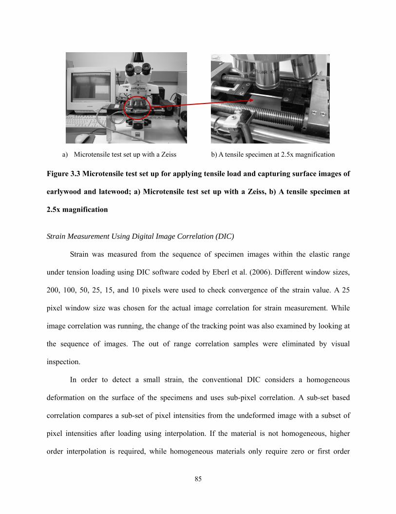
85

Figure 3.3 Microtensile test set up for applying tensile load and capturing surface images of

earlywood and latewood; a) Microtensile test set up with a Zeiss, b) A tensile specimen at

2.5x magnification

Strain Measurement Using Digital Image Correlation (DIC)

Strain was measured from the sequence of specimen images within the elastic range

under tension loading using DIC software coded by Eberl et al. (2006). Different window sizes,

200, 100, 50, 25, 15, and 10 pixels were used to check convergence of the strain value. A 25

pixel window size was chosen for the actual image correlation for strain measurement. While

image correlation was running, the change of the tracking point was also examined by looking at

the sequence of images. The out of range correlation samples were eliminated by visual

inspection.

In order to detect a small strain, the conventional DIC considers a homogeneous

deformation on the surface of the specimens and uses sub-pixel correlation. A sub-set based

correlation compares a sub-set of pixel intensities from the undeformed image with a subset of

pixel intensities after loading using interpolation. If the material is not homogeneous, higher

order interpolation is required, while homogeneous materials only require zero or first order

a) Microtensile test set up with a Zeiss b) A tensile specimen at 2.5x magnification

86

interpolation to approximate the variation of the displacement field (Jin and Bruck 2005). In this

study, a cubic spline interpolation scheme was employed to represent the inhomogeneous

displacement field of wood. Image acquisition and deflection rate were synchronized to evaluate

the elastic modulus. A virtual reference grid was generated on the first image before the load was

applied, the grid point was tracked by correlated grey scale of the region around the reference

point as the image goes from the first to last.

Specific Gravity Measurement

Specific gravity was measured according to ASTM D 2395 (ASTM 2004a). Samples for

specific gravity measurement were obtained from untested samples of the same population. To

minimize the influence of the environment of room humidity and temperature prior to testing, all

samples were kept in the closable bag and handled by forceps when the specimens were mounted

on the balance. The balance has a sensitivity of ± 0.00001g. Volume of specimens was measured

using micro caliper having a sensitivity of ± 0.001 mm. After measuring the specimen weight, all

samples were kept inside petri dishes and covered by a closable bag. To measure the oven-dry

weight, the petri dishes were taken out from the closable bag, and put in the oven for twenty-four

hours. Specific gravity was measured based on the oven-dry weight and volume at the same

condition as during mechanical testing.

Results and Discussion

Experimental Results

Table 3.2 provides a summary of the test results from the four sample groups. Specific

87

gravity increased as growth ring number increased. The latewood specific gravity from growth

ring number 1-10 and from growth ring number 11-20 had 74% and 26% higher than the

earlywood specific gravity from growth ring number 1-10 and growth number 11-20. However,

for Latewood 1-10 and Latewood 11-20 the specific gravity was slightly decreased from 0.54 to

0.53.

Table 3.2 Physical properties and mechanical properties of earlywood and latewood from

growth rings 1-10 and growth rings 11-20

Test groups SG MOE (GPa) UTS (MPa) Poisson ratio

AVE COV AVE COV AVE COV AVE COVEarlywood 1-10 0.31 13% 1.92 31% 18.69 35% 0.49 53% Latewood 1-10 0.54 8% 3.44 31% 34.21 37% 0.59 48%

Earlywood 11-20 0.42 7% 2.48 29% 25.01 29% 0.49 54% Latewood 11-20 0.53 7% 5.09 36% 33.47 27% 0.80 54%

Latewood 11-20 had the highest MOE of 5.09 GPa with coefficient of variance (COV) of

36% while Earlywood 1-10 had the lowest MOE of 1.92 GPa with COV of 31%. Compare to the

MOE of Earlywood 1-10 and Earlywood 11-20, the MOE of Latewood 1-10 and Latewood 11-20

showed 1.79 and 2.05 times higher, respectively. Compared to the MOE of Earlywood 1-10 and

Latewood 1-10, the MOE of Earlywood 11-20 and Latewood 11-20 showed 1.29 and 1.48 times

higher, respectively.

Latewood 1-10 had the highest UTS of 34.21 MPa with COV of 37% while Earlywood 1-

10 had the lowest UTS of 18.69 MPa with COV of 35%. Compared to the UTS of Earlywood 1-

10 and Earlywood 11-20, the UTS of Latewood 1-10 and Latewood 11-20 showed 1.83 and 1.33

times higher, respectively. Compared to the UTS of Earlywood 1-10 and Latewood 1-10, the

UTS of Earlywood 11-20 and Latewood 11-20 showed 1.33 times higher and 0.97 times lower,

respectively.

88

Latewood 11-20 had the highest Poisson ratio of 0.8 with COV of 54 % while the lowest

Poisson ratio found was 0.49 with COV of 53% and with COV of 54% from Earlywood 1-10 and

Earlywood 11-20. Compared to the Poisson ratio of Earlywood 1-10 and Earlywood 11-20, the

Poisson ratio of Latewood 1-10 and Latewood 11-20 showed 1.20 and 1.63 times higher,

respectively. Compared to the Poisson ratio of Earlywood 1-10 and Latewood 1-10, the Poisson

ratio of Earlywood 11-20 and Latewood 11-20 showed 1.0 times and 1.35 times higher,

respectively

Except for the cases of Latewood 1-10 and Latewood 11-20 UTS, the general trend was

as the growth ring number increased, the UTS, MOE, and Poisson ratios also increased. While

specific gravity was highly correlated with UTS from earlywood and latewood, specific gravity

was weakly correlated with MOE from latewood. Weak correlation between specific gravity and

MOE of earlywood and latewood was also found by Cramer et al. (2005) and Kretschmann et al.

(2006). Less variation of physical and mechanical properties of earlywood and latewood was

found from COV of SG, UTS, and MOE as the growth ring number switched from 1-10 to 11-20.

Greater mechanical properties and less variation of earlywood and latewood from a higher

growth ring number can be speculated that more mature earlywood and latewood have a more

oriented reinforcement to the longitudinal direction. The oriented reinforcement can be

associated with the MFA that are more oriented to the fiber axis for a higher growth ring number.

Previous results also found that as growth ring number increased, MFA decreased (Groom et al.

2002 and Kretschmann et al. 2006). The less reinforcement to the off-diagonal of the loading

direction due to the lower MFA in a higher growth ring position could have resulted in a higher

deflection in the transverse direction, which eventually induced a higher Poisson ratio.

Figure 3.4 shows the relationship between tree height and average MOE from earlywood

89

and latewood from the same species. The average MOE data at growth ring number 1 to 20 from

0.6 m tree height were used from current study. The average MOE data at growth ring number 3,

6, 12, and 18 from 1.5 m and 6 m tree height were obtained from a previous study (Kretschmann

et al. 2006). The correlation between MOE of earlywood and height, between MOE of latewood

and height, and between the MOE ratio of latewood to earlywood and height showed a strong

positive linear relation presenting R2 of 0.996, 0.995, and 0.931. From the MOE ratio of

latewood to earlywood as a function of height, the MOE of latewood increased more than that of

earlywood. It can be speculated that in the lower height of tree, earlywood and latewood fiber

structures are physiologically adapted to support compression by tree mass and gravity with

higher MFA, thicker cell wall diameter, larger cell dimension, and shorter fiber lengths, while in

the upper height of tree, earlywood and latewood fiber structures are adapted to support tension

by wind and growth stress with lower MFA, thinner cell wall diameter, smaller cell dimension,

and longer fiber length (Yeh et al. 2006, Xu et al. 2004, Groom et al. 2002, Mott et al. 2002,

Burdon et al. 2003, and Cramer et al. 2005, Kretschmann et al. 2006). These speculations on the

anatomical structure adaptations of earlywood and latewood are rather relative comparison for

the earlywood and latewood from the three heights of tree and away from bark than the

comparison for the individual growth rings at the same height

90

Figure 3.4 Earlywood MOE, latewood MOE, and Ratio of latewood MOE to earlywood

MOE as a function of tree heights from current test results including data at 0.6 m height

and a previous study by Kretschmann et al. 2006 including data at 1.5 and 6 m height

Table 3.3 shows the summary of the Two-Way ANOVA results considering factors of

growth ring and intra-ring position on the MOE, UTS and Poisson ratio from the sample groups.

The alpha of 0.05 was used as a significant difference. Although there were many other

interaction results between growth ring numbers and intra-ring layers, only the physically

meaningful comparisons are shown in Table 3.3. Overall comparison between growth ring

number 1-10 and growth ring number 11-20 shows significant differences in MOE, UTS, and

Poisson ratio. Overall, comparison between earlywood and latewood also showed significant

differences in MOE, UTS, and Poisson ratio. When looking at the detailed comparison of

interaction between growth ring numbers and intra-ring layers, all MOE comparisons showed

significant differences, which agreed with the results from Table 3.2. For the UTS, only

comparison between Latewood 1-10 and Latewood11-20 was not significantly different, which

y = 1.45x + 0.7R² = 0.996

y = 4.367x - 0.28R² = 0.995

y = 0.305x + 1.585R² = 0.931

1.5

1.7

1.9

2.1

2.3

2.5

2.7

02468

1012141618

0.6 1.5 6

Rat

io (L

W/E

W)

MO

E (G

Pa)

Height (m)

EarlywoodLatewoodLatewood/Earlywood

91

agreed with results from Table 3.2 showing that 34.21 MPa for Latewood 1-10 with COV of 31%

and 33.47 MPa for Latewood 11-20 with COV of 36%. The difference of specific gravity

between Latewood 1-10 and Latewood 11-20 was only 1.8%. For Poisson ratio, all comparisons

showed significant difference except for the case between Earlywood 1-10 and Earlywood 11-20,

which also agrees with the results from Table 3.2.

Table 3.3 Statistical comparison of the tensile properties for earlywood and latewood from

two different growth ring positions; growth ring number 1-10 and growth ring number 11-

20 (α=0.05)

Variable A Variable B p-value for MOE p-value for UTS p-value for Poisson ratio

Growth ring position 1-10

Growth ring position 11-20 <0.0001 0.006 0.030

Earlywood Latewood <0.0001 <0.0001 <0.0001 Earlywood 1-10 Earlywood 11-20 0.006 0.0003 0.440 Earlywood 1-10 Latewood 1-10 <0.0001 <0.0001 0.017 Earlywood 11-20 Latewood 11-20 <0.0001 <0.0001 <0.0001 Latewood 1-10 Latewood 11-20 <0.0001 0.831 0.028

Table 3.4 shows the distribution fitting for MOE, UTS, and Poisson’s ratio from four

groups. The alpha value of 0.05 was used to find the best fitting curve for the MOE, UTS, and

Poisson’s ratio from normal, lognormal, Weibull, and Gamma distribution using SAS 9.1 (SAS

Institute Inc. 2004). The distribution fitting was examined by Kolmogorov-Smimov (K-S) and

Chi-square test. Visual inspection also conducted for estimating the best fitting curve. Based on

the p-value from K-S and Chi-square test and visual inspection, the Weibull distributions were

decided to be the best fitting curve with the three estimated parameters. The best fitting curves

for UTS of Earlywood 1-10 and Latewood 1-10 were Weibull distribution while Earlywood 11-

20 and Latewood 11-20 group were lognormal. However, for Earlywood 11-20 group, Chi-

92

square test was below p-value of 0.05. For the Poisson ratio, Earlywood 1-10 and Latewood 11-

20 groups were fitted best with the Weibull distribution while the Latewood 1-10 and Earlywood

11-20 followed with the Gamma distribution. Analytical distribution of mechanical properties for

earlywood and latewood from different growth ring number could be used for numerical

modeling.

Table 3.4 Distribution fitting for tensile properties of earlywood and latewood from growth

ring numbers 1-10 and growth ring numbers 11-20 (α=0.05)

Test groups Normal Lognormal Weibull Gamma MOE K-S Chi-square K-S Chi-square K-S Chi-square K-S Chi-square

Earlywood 1-10 0.14 0.32 0.25 0.26 0.11 0.31 0.09 0.30 Latewood 1-10 0.15 0.29 0.25 0.26 0.25 0.51 0.25 0.36

Earlywood 11-20 0.15 0.15 0.50 0.05 0.5 0.08 0.02 0.08 Latewood 11-20 0.06 0.28 0.5 0.71 0.5 0.85 0.5 0.79

UTS K-S Chi-square K-S Chi-square K-S Chi-square K-S Chi-squareEarlywood 1-10 0.15 0.23 0.25 0.17 0.5 0.22 0.25 0.22 Latewood 1-10 0.13 0.14 0.23 0.75 0.14 0.40 0.25 0.67

Earlywood 11-20 0.08 0.001 0.25 0.01 NA 0.001 0.25 0.004 Latewood 11-20 0.15 0.07 0.23 0.05 0.25 0.04 N/A N/A

Poisson Ratio K-S Chi-square K-S Chi-square K-S Chi-square K-S Chi-squareEarlywood 1-10 0.15 0.03 0.04 N/A 0.5 0.50 0.25 0.59 Latewood 1-10 0.02 0.001 0.04 0.17 0.06 0.05 0.25 0.17

Earlywood 11-20 0.01 0.001 0.03 0.13 0.007 0.04 0.06 0.09 Latewood 11-20 0.01 0.001 0.25 0.11 0.25 0.25 0.13 0.04 Strain Distribution of Earlywood and Latewood from growth ring number 1-10 and 11-20

Representative strain distributions of one sample from each test group are shown in

Figure 3.5 and Figure 3.6. The strain distribution in x is the direction parallel to the load

direction, while strain distribution in y direction is the direction perpendicular to the loading

direction. To compare the strain distribution for earlywood and latewood from different growth

ring positions at a similar stress level, a sequence from images correlation is shown here; the

93

seventh image for Earlywood 1-10, the fourth image for Latewood 1-10, the sixth image for

Earlywood 11-20, and the second image for Latewood 11-20, which were under elastic range.

Normally failure of earlywood and latewood occurred at least after the tenth image was taken for

all groups.

Figure 3.5 shows the strain distribution of sample number 45 from Earlywood 1-10 and

sample number 50 from Latewood 1-10. The strain distributions in x and y directions for the

Latewood 1-10 showed more resistance under similar stress level, showing that approximately

one magnitude smaller strain occurred. The Latewood 1-10 strain distribution showed higher

proportions of negative strain distributions in the x-direction to the positive strain by applied load

and higher proportions of negative strain distributions in the y-direction to the negative strain by

applied load. Due to the strain distribution of earlywood and latewood, Latewood 1-10 had

higher MOE and Poisson ratio found from Table 3.2.

Figure 3.5 Strain distribution of earlywood and latewood from growth ring numbers 1-10

(Specimen number 45 under 19.6 MPa, Specimen number 50 under 21.9 MPa)

a) Strain x of Earlywood 1-10 b) Strain y of Earlywood 1-10

d) Strain y of Latewood 1-10 c) Strain x of Latewood 1-10

94

Figure 3.6 shows the strain distribution of specimen number 50 for the Earlywood 11-20

and specimen number 50 for the Latewood 11-20. The magnitude of the strain distributions was

much lower for earlywood and latewood from growth ring number 11-20, which can be

interpreted as more oriented structure to the load direction for growth ring number 11-20 group.

Compared to growth ring number 1-10, a higher MOE value for growth ring number 11-20 can

be seen from the strain distribution in x showing much lower magnitude in strain x of earlywood

11-20 and Latewood 11-20. Under the same stress level, Latewood 11-20 showed the most

distinctive pattern for negative strain in x and negative strain in y from growth ring number 11-

20 resulted in the highest Poisson ratio among the groups.

Regardless of intra-ring layer and growth ring positions, non-uniform strain distribution

occurred in both directions during the testing. The average strain value used for the calculation of

elastic modulus and Poisson ratio was in the 10-3 range; however, high oscillations of the strain

distributions were observed on the cross section. This is an interesting point that non-uniform

strains occur in the middle of the cross section away from the edge since uniform strain

distribution within the gauge length is one of the assumptions made for ASTM D143 (ASTM

2004b) for tension and compression tests. However, from the results, the earlywood and

latewood structure responds differently under a given load. Therefore, the elastic moduli of wood

defined from ASTM D143 are actually effective moduli of the average of a set of individual

fibers.

95

Figure 3.6 Strain distribution of earlywood and latewood from growth ring number 11-20

(Specimen number 50 under 19.4 MPa and Specimen number 50 under 19.8 MPa)

Conclusions

The physical and mechanical properties of earlywood and latewood from two different

growth ring positions showed different values. The general trend was that specific gravity, MOE,

UTS, and Poisson ratio generally increased with the increment of the growth ring positions

except for specific gravity and UTS from latewood. While the MOE for earlywood and latewood

was not dependent on the specific gravity, UTS for earlywood and latewood was highly

dependent on specific gravity. From comparison between current results and a previous study,

MOE from earlywood and latewood showed a positive relationship with the height of tree.

Statistical comparisons showed that the MOE and UTS had a significant difference by both

growth ring and intra-ring positions. Distribution fitting showed that MOE for four groups were

a) Strain x of Earlywood 11-20 b) Strain y of Earlywood 11-20

c) Strain x of Latewood 11-20 d) Strain y of Latewood 11-20

96

best fitted by Weibull distribution while Poisson’ ratio were best fitted by Weibull distribution for

Earlywood 1-10 and Latewood 11-20 groups and Gamma distribution for Earlywood 11-20 and

Latewood 1-10 groups. Strain distribution showed non-uniform distributions for four groups.

Compared to Earlywood 1-10 and Latewood 1-10, Earlywood 11-20 and Latewood 11-20

showed more resistance to the load.

Acknowledgements This work was funded by the USDA National Research Initiative Competitive Grants Program (2005-35504-16115). Their financial contribution to this work is greatly acknowledged.

References

ASTM. 2004a. Standard Test Methods for Specific Gravity of Wood and Wood-Based Materials. ASTM D 2395. Annual Book of ASTM Standard. Vol. 4.10 Wood. ASTM, West Conshohocken, PA. ASTM. 2004b. Standard Test Methods for Small Clear Specimens of Timber. ASTM D 143. Annual Book of ASTM Standards. Vol. 4.10 Wood. ASTM, West Conshohocken, PA. Bendtsen, B. A. and J. Senft. 1986. Mechanical and anatomical properties in individual growth rings of plantation-grown Eastern cottonwood and loblolly pine. Wood and Fiber Sci. 18:23–38. Burdon, R. D., R. P. Kibblewhite, J. C. F. Walker, R. A. Megraw, R. Evans, and D. J. Cown. 2004. Juvenile versus mature wood: a new concept, orthogonal to corewood versus outerwood, with special reference to Pinus radiata and P. taeda. Forest Sci. 50:399-415. Burgert I, Fruhmann K, Keckes J, Fratzl P, Stanzl-Tschegg SE (2003) Microtensile testing of wood fibers combined with video extensometry for efficient strain detection. Holzforschung. 57:661-664 Choi, D., J. L. Thorpe and R. B. Hanna. 1991. Image analysis to measure strain in wood and paper. Wood Science and Technology 25(2):251-262. Cramer, S. M., D. E. Kretschmann, R. Lakes, and T. Schmidt. 2005. Earlywood and latewood elastic properties in loblolly pine. Holzforschung. 59:531-538. Danvind, J. 2002. Methods for Collecting and analysing simultaneous strain and moisture data during wood drying; Licenciate Thesis in the Division of Wood Physics, Skelleftea Campus:

97

Skelleftea, Sweden, Lulea University of Technology Eberl C., R. Thompson, and D. Gianola. 2006. Digital image correlation and tracking with Matlab. Matlab Central. http://www.mathworks.com/matlabcentral/fileexchange/ loadFile.do?objectId=12413&objectType=FILE (27 September 2006). Groom, L., L. Mott., and S. Shaler. 2002. Mechanical properties of individual southern pine fibers. Part I. Determination and variability of stress-strain curves with respect to tree height and juvenility. Wood and Fiber Sci. 34(1):14-27. Hindman D. P. and J. N. Lee. 2007. Modeling wood strands as multi-layer composites: bending and tension loads. Wood and Fiber Sci. 39(4):515-526. Jin H. and H. A. Bruck. 2005. Theoretical development for pointwise digital image correlation. Optical Engineering, Volume 44, pp Keunecke D, Niemz P (2008) Axial stiffness and selected structural properties of yew and spruce microtensile specimens. Wood Research 53:1-14 Kretschmann, D. E., S. M. Cramer, R. Lakes, and T. Schmidt. 2006. Selected mesostructure properties in loblolly pine from Arkansas plantations. Characterization of the Cellulosic Cell Wall. Ames, Iowa : Blackwell Pub., 149-170 pp. Larson, P. R., D. E. Kretschmann, A. Clark III, and J. G. Isebrands. 2001. Juvenile wood formation and properties in southern pine. General Technical Report FPL-GTR-129. Madison, Wisconsin: US Department of Agriculture, Forest Service, Forest Products Laboratory Ljungdahl J. L. A. Berglund, and M. Burman. 2006. Transverse anisotropy of compressive failure in European oak-a digital speckle photography study. Holzforschung, 60:190-195 Mott, L., L. Groom, and S. Shaler. 2002. Mechanical properties of individual southern pine fibers. Part II. Comparison of earlywood and latewood fibers with respect to tree height and juvenility. Wood and Fiber Sci. 34(2): 221-237. Mott, L., S. M. Shaler, and L. H. Groom. 1996. A novel technique to measure strain distributions in single wood fibers. Wood and Fiber Sci. 28(4):429-437. Muszynski, L., R. Lopez-Anido, and S. M. Shaler. 2000. Image correlation analysis applied to measurement of shear strains in laminated composites. In: Proceedings of SEM IX International Congress on Experimental Mechanics, Orlando FL, June, 5-7, 2000. 163-166. Penneru A. P., K. Jayaramanand, and D. Bhattacharyya. 2005. Strain analysis in bulk forming of wood. Holzforschung, 59:456–458 Samarasinghe, S. and D. Kulasiri. 2004. Stress intensity factor of wood from crack-tip displacement fields obtained from digital image processing. Silva Fennica 38(3):267–278.

98

Serrano, E., and B. Enquist. 2005. Contact-free measurement and non-linear finite element analyses of strain distribution along wood adhesive bonds. Holzforschung 59:641–646. SAS Institute Inc. 2004. SAS/STAT® 9.1 User’s Guide. Cary, NC: SAS Institute Inc. Stelmokas, J. W., A. G. Zink, J. L. Loferski, and J. D. Dolan. 1997. Measurement of load distribution among multiple-bolted wood connections. Journal of Testing and Evaluation 25(5):510-515 Sun Y, Pang JHL, Wong CK, Su F (2005) Finite element formulation for a digital image correlation method. Appl. Opt. 44:7357-7363 Taylor, F. W. and J. S. Moore. 1981. A comparison of earlywood and latewood tracheid lengths in loblolly pine. Wood and Fiber. 13:159-165 Xu P., L. Donaldson, J. Walker, R. Evans, and G. Downes. 2004. Effects of density and microfibril orientation on the vertical variation of low-stiffness wood in radiate pine butt logs. Holzforschung. 58:673-677. Yeh T. F., J. L. Braun, B. Goldfarb, H. M. Chang, and J. F. Kadla. 2006. Morphological and chemical variations between juvenile wood, mature wood, and compression wood of loblolly pine (Pinus taeda L.). Holzforschung. 60:1-8. Zink, A. G, R. W. Davidson, and R. B. Hanna. 1995. Strain measurement in wood using a digital image correlation technique. Wood and Fiber Sci. 27(4):346–359. Zink, A. G., R. B. Hanna, and J. W. Stelmokas. 1997. Measurement of Poisson’s ratios for yellow-poplar. Forest Prod. J. 47(3):78-80.

99

Chapter 4. Comparison of Longitudinal Tensile Properties of Different Orientation

Strands from Loblolly Pine (Pinus taeda)

The goal of this chapter was to measure the tensile properties of different orientations of

loblolly pine strands from growth ring numbers 1-10 and growth ring numbers 11-20 using

digital image correlation (DIC). A series of images was captured for strain measurement and

synchronized with loading data for calculation of modulus of elasticity (MOE) and Poisson ratio.

Ultimate tensile strength (UTS) was also measured. The general trend for straight grain

orientation strands and tangential grain orientation strands was that MOE and UTS increased as

the growth ring numbers increased. Statistical comparison showed no significant difference of

MOE between the two different orientations of wood strands, and no significant difference of

Poisson ratio between the two growth ring numbers. The UTS comparison between straight grain

orientation strands from inner growth ring number 1-10 and straight grain orientation strands

from outer growth ring number 11-20 were significantly different. The UTS comparison between

straight and tangential grain orientation strands from outer growth ring number 11-20 showed a

significant difference. Strands from higher growth ring number showed more consistent tensile

failure behavior.

100

Introduction

In the U.S., the use of softwood strands has been growing as oriented strand board (OSB)

and structural composite lumber (SCL) production increases. The impetus for development of a

variety of SCL products has been decreasing access to large high quality logs, and industry

commitments to better utilization of harvests. Development of SCL has many advantages, which

are to use smaller trees, to use waste wood from other processing, to remove defects, to create

more uniform components, to develop composites that improve some mechanical properties

compared to solid wood, and to have higher yield from logs with bark compared to solid sawn

lumber (Schuler and Adair 2000, and Balatinecz and Kretschmann 2001).

Although SCLs and OSB have several advantages over solid lumber, there is little

research analyzing the material properties of wood strands. Wood has an orientation developed

by the arrangement of earlywood and latewood. Earlywood and latewood properties vary

throughout different growth ring numbers. Growth rings closer to pith contain higher proportions

of juvenile wood than growth rings closer to bark. Juvenile wood differs from mature wood in

that it has a higher microfibril orientation, a high percentage of compression wood, distorted

grain patterns, and a lower percentage of latewood (Larson et al. 2001). The effects of orientation

and growth ring numbers on mechanical properties of wood strands are not well known.

This chapter focuses on the effect of the growth ring number and orientation of wood

strands on tensile properties of wood strands. Tensile testing was conducted with digital image

correlation (DIC). Two-dimensional measurements were carried out to measure longitudinal

strain as well as transverse strain. A better understanding of the mechanical properties of wood

strands can lead better mechanical properties of wood products (Wu et al. 2005). This chapter

can serve as a tool for manufacturing engineers to develop better performing material. The

101

knowledge of wood strands properties can maximize the use of wood resources.

Literature Review

Previous studies used different test set-ups to evaluate the modulus of elasticity (MOE)

and strength of strands from different species. Comprehensive results from previous research can

be found in Jeong et al. (2008). Literature review from this study focuses on the effect of testing

arrangement on mechanical properties of wood strands from different wood species.

Price (1975) studied the effect of gage length on the MOE and UTS of sweetgum

(Liquidambar styraciflua L.) flakes using a tensile test with the strain rate of 0.0127 cm/cm/min.

Four different gage lengths (1.27 cm, 1.90 cm, 2.54 cm and 3.17 cm) were used in this study.

UTS increased with an increase of gage length while MOE decreased with an increase of gage

length. MOE of flake specimens was less than that of solid wood for the same species.

Geimer et al. (1985) measured the tensile stiffness and strength of two different grades of

Douglas-fir (Pseudotsuga menziesii) strands. The grade of strands was determined by damage

conditions. The test set-up was 3.81 cm gage length and used cross head movement to calculate

strain in the flakes. The test speed was 0.0127 cm/min. Boards made from higher grade strands

had 55% higher tensile strength compared to boards made from lower grade strands. MOE and

UTS of the strands were 50% and 28% of the reported value for northern interior Douglas-fir

(Pseudotsuga menziesii).

Deomano and Zink-Sharp (2004) conducted three point bending to calculate MOE and

modulus of rupture (MOR) of 25 mm by 5.0 mm by 0.6 mm flakes from three different species

including southern pine (Pinus spp.), sweetgum (Liquidambar styraciflua L.), and yellow-poplar

(Liriodendron tulipifera L.) with different test conditioning (three different temperatures, two

102

cutting directions). The loading rate was 2.54 mm/min. Higher drying temperature lowered

mechanical properties of flakes and tangentially cut specimens had higher mechanical properties

compared to radially cut specimens. The average MOE of radial and tangential cutting direction

specimen was 4.3 GPa and 5.2 GPa. The MOR of radial and tangential cutting direction

specimens was 69.1 MPa and 86.7 MPa.

Cai et al. (2007) extended the work of Wu et al. (2005) by adding more species - willow

(Salix spp.), yellow-poplar (Liriodendron tulipifera L.), red oak (Quercus spp.), and loblolly pine

(Pinus taeda). The tensile properties of wood strands were significantly lower than those of solid

wood. Compared to the tensile strength of solid woods (USDA 1999), that of wood strands from

the various species was lower 31.1%, 44.2%, 36.2% , 73.4 % for willow, yellow-poplar, red oak,

and loblolly pine, respectively.

Hindman and Lee (2007) tested different orientations (straight, angle, arbitrary) of wood

strands for MOE and UTS using tension and bending tests. The results showed that both MOE

and UTS were different from different orientations of wood strands. For MOE and UTS from

tension test, the highest values were found from straight grain orientation strands, while the

lowest values were found from the arbitrary grain orientation strands. For MOE and UTS from

bending tests, the highest values were found from straight grain orientation strands while the

lowest values were found from angle grain strands.

Jeong et al. (2008) noted that previous research on measurement of mechanical properties

from wood strands cannot be directly comparable due to different testing arrangements. To

investigate the effect of the testing arrangement on mechanical properties of wood strands, a

different loading rate and different thickness of wood strands were used. While there was no

significant difference of MOE and UTS by different loading rate, there was a significant

103

difference of MOE and UTS by different thickness. The trends showed that as thickness

increased, MOE and UTS increased. Appropriate loading rate and thickness of wood strands for

tensile testing were suggested.

From previous studies, two key issues for measurement of MOE and UTS of wood

strands are the mechanical testing set-up and material preparation. For testing set-up, the

importance of application of correct gage length and loading speed to measure MOE was noted

by Price (1975). For material preparation, different thickness, grade, and cutting direction are

important parameters for the determination of mechanical properties of wood strands (Geimer et

al. 1985, Deomano and Zink-Sharp 2004, Cai et al. 2007, Hindman and Lee 2007, and Jeong et

al. 2008).

In processing wood strands, understanding the effect of the orientation and growth ring

numbers on the mechanical properties is crucial to maximize the properties for the end use.

Segregation of different strands into discrete categories can maximize the benefits of use.

Understanding the effect of the growth ring numbers on mechanical properties of wood strands

can lead to better utilization of resources. The purpose of this chapter was to measure tensile

properties of different grain orientation strands from growth ring number 1-10 and growth ring

number 11-20. The MOE, UTS, and Poisson ratios from strands were obtained using tension

tests incorporated with DIC.

Material and Methods

Specimen preparation

Two representative grain orientation strands for radial and tangential surfaces from two

104

different growth ring numbers were prepared from a loblolly pine disk. Figure 4.1 shows the

schematic illustration of a wood disk with the coordinate of the disk, two different orientations of

wood blocks, and the final wood strand geometry with dimension. Wood blocks A and B of size

127 mm by 133.4 mm by 25.4 mm were wood sliced from the loblolly pine disk using a band

saw. After all wood blocks were marked to notify the growth ring number, the blocks were

soaked in water and placed under a vacuum overnight to minimize surface damage during

flaking. Radial grain orientation strands were flaked from wood blocks sliced from A samples.

Tangential grain orientation strands were obtained from wood blocks sliced from B samples.

Figure 4.1 Strands generated from different cutting positions of the loblolly pine disk. (A)

radial specimen and (B) tangential specimen

Strands were processed from a flaker located at Brook Forest Center laboratory at

Virginia Polytechnic Institute and State University. All strands were processed to a size of 127

mm by 25.4 mm by 0.5 mm from growth ring number 1 to 10 from pith, and the same size from

growth ring number 11 to 20 from pith. Table 4.1 shows sample size for each tension test. All

25.4 mm

127 mm

133.4 mm

(B)

(A)

0.5 mm 25.4 mm

R

T

L

127 mm

A

B

A

105

strands were conditioned to stabilize at 6% moisture content in the environment chamber for one

month before testing.

Table 4.1 Nomenclatures and sample sizes for different orientations of wood strands from

different growth ring numbers

Orientation Growth Ring number Nomenclatures Sample

sizes Radial Grain1 1-10 Radial 1-10 30

Radial Grain 11-20 Radial 11-20 30

Tangential Grain2 1-20 Tangential 1-10 30

Tangential Grain 11-20 Tangential 11-20 30 1 Radial grain from A 2 Tangential grain from B

Test Methods

Tension tests used an MTS machine incorporated with digital image correlation (DIC) to

calculate elastic properties of wood strands. The test set up for the strand test is shown in Figure

4.2. The MTS machine with 889 N load cell was used for tension test. Loading speed was 0.025

cm/min. Span for tension test was 10.16 cm. A 22.24 N preload was applied to prevent slippage

of the grip. Load was intermittently applied at 44.48 N increments and paused for 5 seconds for

image capture.

Optem Zoom 70 lens with the magnification of 0.75x attached to a camera was used in this

test. To give a light source for the lens and to minimize the influence by the light, a fiber optic

light was used during the test. Sequence images of the strands during the test were captured

using a CCD camera (Model PL-A662) from Pixel Link Megapixel Firewire Camera. The CCD

camera was mounted on a stage with a macro adjustable driver. The distance between lens and

object was adjusted for the test to have a clear image. Camera set up was placed on a desk which

106

was apart from the MTS machine to prevent the vibration while the images were taken.

Figure 4.2 Experimental tensile testing set up showing camera for DIC

Resolution of the camera was 1280 by 1024 pixels with an 8-bit grey level. Pixel size of

the image was 1280 by 1024. The pixel size was converted to spatial size for the determination

of displacement. Horizontal and vertical length of the image taken was 10 mm and 8 mm,

respectively. Spatial size of the pixel was calculated to be 9.765 μm/pixel by 6.25 μm/pixel. An

aluminum bar with the same dimensions as the strands was used to evaluate strain measurement

using DIC coded by Eberl et al. (2006). Tensile testing was performed for an aluminum bar with

an extensometer to calculate the longitudinal elastic property with the loading speed of 0.025

mm/min. Tensile testing was then performed under the same conditions using DIC. The window

size for image correlation was defined as 25 by 25 pixels since the results converged from this

window size. Experimental results were calculated using measured elastic strains and a

maximum load of 2.20 KN, which was a load within the elastic range. The difference between

strain from DIC and strain from the extensometer was only 1.1%. The results prove the accuracy

of the strain measurement using DIC.

To validate DIC for calculating MOE of wood strands, specimens were tested with

107

speckle pattern and without speckle pattern on the surface of the wood strands and compared to

the results from extensometer. The difference was 5% between results from DIC with no speckle

and results from extensometer. The difference was 4% between results from DIC with speckle

and results from extensometer. Therefore, in this study, a speckle pattern was generated on the

surface of wood strands with carbon black particles and a paint brush. To minimize the influence

of light other than from the fiber optic lamp, all testing was conducted at night with no direct

room light. Rubber pads were put under the stage to reduce the vibration. Different loading

increments (22.2 N, 44.4 N, and 66.7 N) and loading speeds (0.00254 cm/min and 0.0254

cm/min) were used to determine the testing conditions for measuring the elastic properties of

straight grain orientation of wood strands. Preliminary testing found that a 44.4 N loading

increment and 0.0254 cm/min load rate were best for the elastic property measurements of

strands.

Baxter and Graham (2000) and Baxter et al. (2001) proposed a moving window

generalized method of cells (MW-GMC) to characterize material properties of composite

materials based on digitized images of local microstructure of the material. The statistical

variability of material properties of composite material is dependent upon the window size.

Larger window sizes produced smaller variance of material properties. However, if window size

becomes too large, the variability of material properties approaches zero. A smaller window size

produces noisier fields. Also a smaller window size requires higher computational effort. The

choice of window size was emphasized to represent the local material properties. Therefore, the

proper window size for wood and wood based material should be used to represent the local

material properties. A 25 by 25 pixel size (0.244 mm by 0.156 mm) of window was chosen to

represent the local material properties of strands. The grid was generated on the digital image of

108

the surface of the wood strands before a load was applied. The position of the grid was recorded

as x, y coordinate of the pixel position on the image. Figure 4.3 describes the grid generated on

the reference digital image of a strand.

Figure 4.3 Generating a grid on the image from the surface of a strand

MOE (EL) for both radial grain and tangential grain specimens was obtained using

Equation 1. UTS (σLMAX) for both radial grain and tangential grain specimens was obtained using

Equation 2. From straight grain specimens, strain parallel (εL) to the direction of load and strain

perpendicular (εR) to the direction of load was calculated from the change of grid point on the

sequence of images during loading. Poisson ratio (υLR) was calculated from the ratio of the

compression strain perpendicular to the load to expansion strain parallel to the load (Equation

4.3). From tangential grain specimens, strain parallel (εL) to the direction of load and strain

perpendicular (εT) to the direction of load was calculated from the change of grid point on the

sequence of images during loading. Poisson ratio (υLT) was calculated from the ratio of the

compression strain perpendicular to the load to expansion strain parallel to the load (Equation

4.4).

(761.5,

804.5)

(761.5,

304.5)

(761.5,

354.5)

(811.5,

304.5)

(961.5,

304.5)

(961.5,

804.5)

X

Y

109

∆ .

. .

. 4

Where, εL: longitudinal strain in loading to the longitudinal direction of wood. L: span length in longitudinal direction of wood εR: radial strain in loading to the longitudinal direction of wood PLMAX: maximum load in loading to the longitudinal direction of wood. A: area of cross section of specimens

∆: slope of load-displacement curve under elastic range

Moisture content and specific gravity measurement

Moisture content and specific gravity were measured according to ASTM D 4442 (ASTM

2004a) and ASTM D 2395 (ASTM 2004b). Samples for both testing methods were obtained

from the same populations using untested strands. To minimize the influence of the environment

of the room humidity and temperature, all samples were kept in a closable bag and handled by a

forcep when the specimens were mounted on the balance. The balance has a sensitivity of

measurement up to five decimal points in grams. Specimen volume was measured using a micro

caliper having a sensitivity of three decimal points in millimeters. After measuring the specimen

weight and volume, all samples were kept in a closable bag. To measure the oven-dry weight,

samples were put in the oven for twenty four hours. The specific gravity was measured based on

the oven-dry weight and volume at the same condition with mechanical testing.

110


Physical and mechanical test results

Table 4.2 presents a summary of the physical and mechanical test results. Moisture

contents for four strands were quite similar with the Radial 1-10 having the lowest moisture

content of 7.37% with coefficient of variance (COV) of 4% while Radial 11-20 had the highest

moisture content of 7.69% with COV of 3%. COV for the moisture contents indicates the low

variability for both within the groups and between the groups. Specific gravity increased as the

growth ring number increased. However, specific gravity for the four groups was quite varied

and the lowest specific gravity of 0.33 occurred in the Radial 1-10 with COV of 12% while the

highest specific gravity of 0.43 was found in the Tangential 11-20 with COV of 15%.

Table 4.2 Summary of physical properties and elastic properties of four strands from

growth ring number 1-10 and growth ring number 11-20

Growth ring number

1-10

Radial 1-10 Tangential 1-10 MC (%) SG MOE

(GPa)UTS

(MPa) νLR MC (%) SG MOE

(GPa) UTS

(MPa) νLT

AVE 7.37% 0.33 2.41 20.5 0.66 7.49% 0.37 2.47 17.0 0.95 COV 4% 12% 27% 37% 77% 2% 8% 23% 25% 42%

Growth ring number 11-20

Radial 11-20 Tangential 11-20 MC (%) SG MOE

(GPa)UTS

(MPa) νLR MC (%) SG MOE

(GPa) UTS

(MPa) νLT

AVE 7.69% 0.41 2.75 29.0 0.60 7.41% 0.43 2.53 17.4 1.31 COV 3% 5% 14% 24% 36% 2% 15% 32% 31% 43%

The highest MOE of 2.75 GPa was obtained from Radial 11-20 with COV of 14% while

the lowest MOE of 2.41 GPa was obtained from Radial 1-10 with COV of 27%, which explains

the mechanical properties was more correlated with grain orientations than specific gravity. For

111

the growth ring number 1-10 the Radial 1-10 had a lower MOE than Tangential 1-10 while for

the growth ring number 11-20 the Radial 11-20 had a higher MOE than Tangential 11-20. While

the COV from MOE of Straight 1-10 showed 48% higher than that of SO, the COV from

Tangential 1-10 showed 39% lower than that of Tangential 11-20.

The highest UTS of 29.03 GPa was obtained from Radial 11-20 with COV of 24 % while

the lowest UTS of 17.04 GPa was obtained from Tangential 1-10 with COV of 25%. The COV of

UTS from Radial 1-10 had 35% higher than that of SO while the COV of UTS from Tangential

1-10 showed 24 % lower than Tangential 11-20. For the growth ring number 1-10 the Radial 1-

10 had a lower UTS than Tangential 1-10 while for the growth ring number 11-20 the Radial 11-

20 had a higher UTS than Tangential 11-20. This explains more mature wood strands had a more

oriented reinforcement to the longitudinal direction.

Poisson ratios (υLR) found from the Radial 1-10 and Radial 11-20 while Poisson ratios

(υLT) found from the Tangential 1-10 and Tangential 11-20. The lowest Poisson ratio of 0.60 was

obtained from Radial 11-20 with COV of 36% while the highest Poisson ratio of 1.31 was

obtained from Tangential 11-20 with COV of 43 %. Poisson ratio from Radial 1-10 had 53.7%

higher COV than that of Radial 11-20 while Poisson ratio from Tangential 1-10 was very slightly

different from that of Tangential 11-20. At the same growth ring number Poisson ratio from

Radial 1-10 had 43% lower than that of Tangential 1-10 and Poisson ratio from Radial 11-20 had

118% lower than that from Tangential 11-20. Under the elastic loading parallel to the

longitudinal direction, the negative radial strain perpendicular to the loading showed a higher

resistance than the tangential direction.

112

Failure Modes

Table 4.3 shows the failure behavior of the four different wood strand groups. All four

groups had a different percentage of three particular failure behaviors. Shear failure describes the

failure around at 45 degree orientations. Brittle failure describes the failure like tearing in the

middle with no distinctive orientation. Wedge failure describes the failure showing crack

propagation along the grain. No grip failure was recorded for any group. These failure modes

were adapted from ASTM D 143 (2005b) testing of compression specimens. For the Radial 1-10,

the wedge failure had 40% followed by 30% for Shear and 30% for Brittle failure. For the Radial

11-20, shear failure mode was dominant rating 70% while brittle failure had 26.67% and wedge

failure had only 3.33%. For Tangential 1-10, the highest failure mode occurred 56.25% in shear

followed by brittle 40.63%. The wedge failure had only 3.13%. For the Tangential 11-20, the

highest failure mode was found in Brittle 53.13% followed by shear 37.5%. The wedge failure

mode had 9.38%. A trend can be seen from the Radial 1-10 and Radial 11-20 failure mode

showing more uniform failure types that could indicate more oriented structure. However, for

Tangential 1-10 and Tangential 11-20 failure mode showed more susceptibility to the orientation

of grain.

Table 4.3 Failure behavior of wood strands

Sample Shear Brittle Wedge Radial 1-10 30.00% 30.00% 40.00% Radial 11-20 70.00% 26.67% 3.33%

Tangential 1-10 56.25% 40.63% 3.13% Tangential 11-20 37.50% 53.13% 9.38%

113

Statistical comparison

Table 4.4 shows the results from One-Way ANOVA to analyze the effect of the growth

ring numbers and two different geometries on MOE, UTS, and Poisson ratio. An alpha value of

0.05 was used. Strands from different growth ring numbers showed different mechanical

properties. While straight grain orientation strands showed a significant difference on MOE and

UTS between two growth ring numbers, tangential grain orientation wood strands did not have a

significant difference on MOE, UTS, and Poisson ratio between the growth ring numbers.

At the same growth ring numbers, a comparison between the two different orientations

showed different trends. While comparison between Radial 1-10 and Tangential 1-10 for MOE

and UTS was not significantly different, the Poisson ratio comparison between Radial 1-10 and

Tangential 1-10 was significantly different. The comparison of MOE between Radial 11-20 and

Tangential 11-20 showed no significant difference while the comparison of UTS and Poisson

ratio showed a significant difference.

The statistical comparison of MOE for four groups explained that there was not

significant difference between the different grain orientations. This implies that MOE for wood

strands doesn’t change by strand cutting direction at the same growth ring number. The statistical

comparison of UTS for four groups showed no consistent trend from growth ring number and

from orientation of strands. However, it can be speculated that UTS for straight grain was not

significantly different by growth ring numbers and that UTS for two different orientation strands

from growth ring number 11-20 was not significantly different. The statistical comparison of

Poisson ratio for four groups explained that there was not a significant difference between the

different growth ring numbers while there was a significant difference between the different

orientations. This is not surprising that as Poisson ratio is calculated from two different strain

114

direction, the geometry of strands are highly sensitive to the two strain distribution.

Table 4.4 Statistical comparison of MOE, UTS, and Poisson’s ratios for the radial grain

strands and tangential grain strands from two different growth ring numbers 1

Growth ring numbers effect MOE p-value

UTS p-value

Poisson ratio p-value

Radial 1-10 Radial 11-20 0.01 <.0001 1.00 Tangential 1-10 Tangential 11-20 0.75 0.57 0.40

Orientation effect MOE p-value

UTS p-value

Poisson ratio p-value

Radial 1-10 Tangential 1-10 0.69 0.96 0.02 Radial 11-20 Tangential 11-20 0.15 <.0001 <.0001

1(α = 0.05)

Distribution Fitting

Table 4.5 shows the statistical distribution fitting for MOE, UTS, and Poisson ratio.

Normal, lognormal, Weibull, and Gamma distributions were used to fit the experimental results

from the four test groups. Kolmogorov-Smirnov (K-S), Chi-square statistical tests and visual

inspection were used to verify a particular distribution fitting with alpha value of 0.05. For MOE,

except for Tangential 1-10 followed Gamma distribution, the rest of three strand groups were

best fitted with Weibull distribution. While UTS from Radial 1-10 and Tangential 1-10 group

followed Weibull and Gamma distribution, Radial 11-20 and Tangential 11-20 did not follow any

distributions. For Poisson ratio, Radial 11-20 did not match with any distribution curve. Radial 1-

10, Tangential 1-10, and Tangential 11-20 followed Lognormal, Gamma, and Weibull

distribution, respectively. This statistical distribution can be used as input data to simulate the

strand based composites.

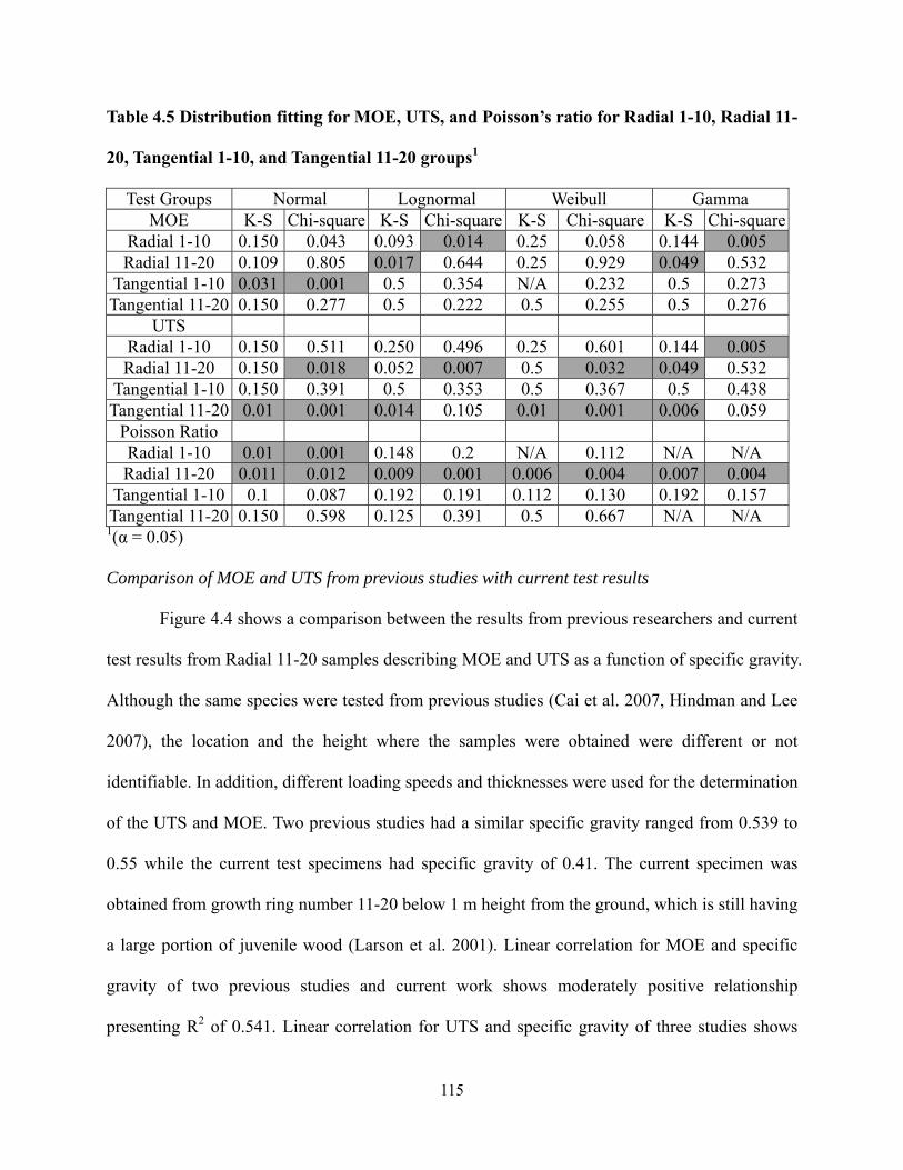
115

Table 4.5 Distribution fitting for MOE, UTS, and Poisson’s ratio for Radial 1-10, Radial 11-

20, Tangential 1-10, and Tangential 11-20 groups1

Test Groups Normal Lognormal Weibull Gamma MOE K-S Chi-square K-S Chi-square K-S Chi-square K-S Chi-square

Radial 1-10 0.150 0.043 0.093 0.014 0.25 0.058 0.144 0.005 Radial 11-20 0.109 0.805 0.017 0.644 0.25 0.929 0.049 0.532

Tangential 1-10 0.031 0.001 0.5 0.354 N/A 0.232 0.5 0.273 Tangential 11-20 0.150 0.277 0.5 0.222 0.5 0.255 0.5 0.276

UTS Radial 1-10 0.150 0.511 0.250 0.496 0.25 0.601 0.144 0.005 Radial 11-20 0.150 0.018 0.052 0.007 0.5 0.032 0.049 0.532

Tangential 1-10 0.150 0.391 0.5 0.353 0.5 0.367 0.5 0.438 Tangential 11-20 0.01 0.001 0.014 0.105 0.01 0.001 0.006 0.059

Poisson Ratio Radial 1-10 0.01 0.001 0.148 0.2 N/A 0.112 N/A N/A Radial 11-20 0.011 0.012 0.009 0.001 0.006 0.004 0.007 0.004

Tangential 1-10 0.1 0.087 0.192 0.191 0.112 0.130 0.192 0.157 Tangential 11-20 0.150 0.598 0.125 0.391 0.5 0.667 N/A N/A 1(α = 0.05) Comparison of MOE and UTS from previous studies with current test results

Figure 4.4 shows a comparison between the results from previous researchers and current

test results from Radial 11-20 samples describing MOE and UTS as a function of specific gravity.

Although the same species were tested from previous studies (Cai et al. 2007, Hindman and Lee

2007), the location and the height where the samples were obtained were different or not

identifiable. In addition, different loading speeds and thicknesses were used for the determination

of the UTS and MOE. Two previous studies had a similar specific gravity ranged from 0.539 to

0.55 while the current test specimens had specific gravity of 0.41. The current specimen was

obtained from growth ring number 11-20 below 1 m height from the ground, which is still having

a large portion of juvenile wood (Larson et al. 2001). Linear correlation for MOE and specific

gravity of two previous studies and current work shows moderately positive relationship

presenting R2 of 0.541. Linear correlation for UTS and specific gravity of three studies shows

116

that strong positive relationship presenting R2 of 0.798. A previous study also showed a poor

correlation found between specific gravity and MOE while a strong correlation was found

between specific gravity and strength (Zhang 1997).

Figure 4.4 Relationship between specific gravity and tensile properties of MOE and UTS of

current data and previous studies.

Figure 4.5 shows a comparison between the results from the previous studies and current

test results from Radial 11-20 samples describing MOE and UTS as a function of thickness.

Linear correlation for MOE and thickness of two previous studies and current work shows strong

positive relationship presenting R2 of 0.992. Linear correlation for UTS and thickness of three

studies shows that strong positive relationship presenting R2 of 0.954. A previous study also

showed the positive relationship between thickness and MOE, and between thickness and UTS,

respectively (Jeong et al. 2008). It can be speculated that the proportional surface damage on

thicker strands is relative lower than thinner strands, which resulted in higher MOE and UTS

values for thicker strands. This could be a reason for a higher MOE and strength of OSB

produced from proportionally less damaged strands by Geimer et al. (1985).

y = 27.95x - 8.547R² = 0.541

y = 155.6x - 34.08R² = 0.666

102030405060708090

0

2

4

6

8

10

0.4 0.45 0.5 0.55 0.6

UT

S (M

Pa)

MO

E (G

Pa)

Specific Gravity

MOE (GPa)

UTS (MPa)

(Current test )

(Cai et al. 2007)

(Hindman and Lee 2007)

117

Figure 4.5 Relationship between thickness and tensile properties of MOE and UTS of

current data and previous studies.

Conclusions

Tensile properties of two different grain orientations of wood strands from growth ring

number 1-10 and growth ring number 11-20 were examined using DIC. The following are

conclusions from this chapter:

As growth ring number increased, modulus of elasticity (MOE) and ultimate tensile

strength (UTS) from two different orientation strands increased. For the growth ring

number 1-10 the Radial 1-10 had a lower MOE and UTS than Tangential 1-10. For the

growth ring number 11-20 the Radial 11-20 had a higher MOE and UTS than Tangential

11-20. For Poisson ratios, tangential grain orientation strands had higher Poisson ratios

than straight grain orientation strands.

From the failure mode, although all four groups had a different percentage of three

particular failure behaviors, more mature wood had a more organized structure to show

y = 104.1x - 2.253R² = 0.992

y = 512.5x + 5.912R² = 0.954

10

20

30

40

50

60

70

0

2

4

6

8

10

0.02 0.04 0.06 0.08 0.1 0.12

UT

S(M

Pa)

MO

E (G

Pa)

Thickness (cm)

MOE (GPa)

UTS (MPa)

(Current test )

(Hindman and Lee 2007)

(Cai et al. 2007)

118

more consistent failure behavior.

Statistical comparisons of MOE and UTS from straight grain orientation strands were

significantly different between growth ring numbers, while MOE and UTS from

tangential grain orientation strands were not significantly different between growth ring

numbers.

Statistical comparisons also showed that there was no significant difference of MOE

between two different orientation wood strands. For UTS, the comparison between

Radial 1-10 and Radial 11-20 were significantly different as well as the comparison

between Radial 11-20 and Tangential 11-20.

For distribution fitting from MOE, except for Tangential 1-10, the rest of three strand

groups were best fitted with Weibull distribution. For UTS, while Radial 1-10 and Radial

11-20 group followed Weibull distribution, Gamma distribution for Tangential 1-10 and

Lognormal distribution for Tangential 11-20 were best fitted curve. For Poisson ratio,

Radial 11-20 did not match with any distribution curve. Radial 1-10, Tangential 1-10,

and Tangential 11-20 followed Lognormal, Gamma, and Weibull distribution,

respectively.

From comparison between previous studies and current test results, MOE and UTS of

wood strands were more linearly correlated with thickness than specific gravity.

Acknowledgements

This work was funded by the USDA National Research Initiative Competitive Grants

Program (2005-35504-16115). Their financial contribution to this work is greatly acknowledged.

119

Reference

American Society for Testing and Materials (ASTM). 2004a. ASTM D 4442. Standard Test Methods for Direct Moisture Content Measurement of Wood and Wood-Base Materials In: Annual Book of ASTM Standard, Section 4, Vol. 04.10 Wood. ASTM, West Conshohocken, PA. American Society for Testing and Materials (ASTM). 2004b. ASTM D 2395. Standard Test Methods for Specific Gravity of Wood and Wood-Based Materials. In: Annual Book of ASTM Standard, Section 4, Vol. 04.10 Wood. ASTM, West Conshohocken, PA. Balatinecz, J. J., and D. E. Kretschmann. 2001. Properties and utilization of poplar wood. In Poplar Culture in North America. Part A, Chapter 9. Edited by D.I. Dickmann, J.G. Isebrands, J.E. Eckenwalder, and J. Richardson. NRC Research Press, National Research Council of Canada, Ottawa, ON KIA OR6, Canada. 277-291 pp. Baxter S. C. and L. L. Graham. 2000. Characterization of random composites using a moving window technique, ASCE J. Eng. Mech. 126 (4):389–404 Baxter S. C., M. I. Hossain, and L. L. Graham. 2001. Micromechanics based random material property fields for particulate reinforced composites, Int. J. Solids Struct. 38: 9209–9220 Cai, Z., Q. Wu, G. Han, and J. N. Lee. 2007. Tensile and thickness swelling properties of strands from Southern hardwoods and Southern pine: Effect of hot-pressing and resin application. Forest Prod. J. 57(5):36-40. Deomano E. C., and A. Zink-Sharp 2005. Effect of species, cutting direction, dimensions, and temperature on flake drying. Forest Prod. J. 55(9):31-36 Geimer, R. L., R. J. Mahoney, S. P. Loehnertz, and R. W. Meyer. 1985. Influence of processing-induced damage on the strength properties of oriented strand wood products. Forest Prod. J. 50(11/12):33-42. Hindman D. P. and J. N. Lee. 2007. Modeling wood strands as multi-layer composites: bending and tension loads. Wood and Fiber Sci.39(4):515-526. Jeong, G. Y., D. P. Hindman, D. Finkenbinder, J. N. Lee, and Z. Lyne. 2008. Evaluation of loading rate and thickness effect on stiffness and strength of wood strands. Forest Prod. J. in process Larson, P. R., D. E. Kretschmann, A. Clark III, and J. G. Isebrands. 2001. Juvenile wood formation and properties in southern pine. General technical report FPL-GTR-129. Madison, Wisconsin: USDA, Forest Service, Forest Products Laboratory Price E.W. 1975. Determining tensile properties of sweetgum veneer flakes. Forest Prod. J. 26(10):50-53

120

Schuler, A. and C. Adair. 2000. Engineered wood products- production, trade, consumption and outlook. Forest products annual market review, Chapter 11, FAO/ECE Timber section. United Nations, NY and Geneva. 131-146 pp. United Stated Department of Agriculture. 1999. Wood Handbook: Wood as an engineering material. Forest Products Society. FPL-GTR-113. Madison, WI. 463 p. Wu, Q., Z. Cai, and J. N. Lee. 2005. Tensile and dimensional properties of wood strands made from plantation southern pine lumber. Forest Prod. J. 52(2):1-6 Zhang S. Y. 1997. Wood specific gravity-mechanical property relationship at species level. Wood Sci. and Technology. 31:181-191

121

Chapter 5. Shear and Transverse Properties of Loblolly Pine (Pinus taeda) Strands Using

Tension Test Incorporating Digital Image Correlation (DIC)

Shear and transverse properties of different orientation loblolly pine strands from growth

ring number 1-10 and growth ring number 11-20 were determined using tension tests

incorporating digital image correlation. From angled grain orientation strands, longitudinal

properties and shear properties for loblolly pine strands from different growth ring numbers were

evaluated. Transverse tension properties were evaluated from cross-grain strands. Modulus of

elasticity (MOE), shear modulus, and ultimate tensile strength (UTS) from angled grain strands

increased as the growth ring number increased. However, Poisson ratio and shear strength from

angled grain strands decreased as the growth ring number increased. MOE and UTS from cross-

grain strands decreased as the growth ring number increased, while Poisson ratio from cross

grain orientation strands increased as the growth ring number increased. The failure modes

indicated that the strands from growth ring number 11-20 showed more oriented structures to the

loading direction. From the results, grain orientations of strands were a strong indicator of

mechanical properties of wood strands.

122

Introduction

Efficient uses of wood resources are needed to maximize material production, lower costs,

and produce environmentally responsible products. These pressures have resulted in increased

use of oriented strand board (OSB) and structural composite lumber (SCL). However, the

fundamental study for measuring material properties of the main component of the products such

as wood strands has not been completed. If OSB and SCL can be designed based on known

material properties of the constituent, specific targeted properties could be achieved with

minimal time and resources.

A previous research (Jeong et al. 2008a) found differences of modulus of elasticity

(MOE), ultimate tensile strength (UTS), and Poisson ratio of different grain strands from growth

ring number 1-10 and growth ring number 11-20. Those different material properties were

reasoned to be structural differences of wood fibers between the two growth ring numbers.

However, off-axis properties of wood strands have not been evaluated yet.

Shear modulus of wood is an important property for analyzing elastic properties and

strength of strand based composites. However, shear properties are difficult to obtain for wood

materials especially for thin specimens. Due to the low stiffness and high aspect ratio of wood

strands, most shear modulus testing listed in ASTM and other literature cannot be applied. One

possible test method is the off-axis tension test. Due to the coupling between normal strain and

shear strain in the axis of loading, multi-axial deformation occurs. However, typical

extensometers or strain gauges cannot measure such a deformation.

Measurement of transverse elastic modulus is also hard due to the low stiffness of cross

grain wood strands. Cross-grain strands can be easily broken or damaged by an attempt to attach

an extensometer. The low strength cannot support the extensometer during cross-head movement.

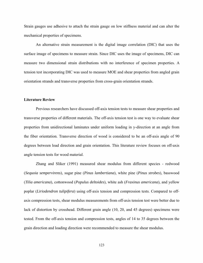
123

Strain gauges use adhesive to attach the strain gauge on low stiffness material and can alter the

mechanical properties of specimens.

An alternative strain measurement is the digital image correlation (DIC) that uses the

surface image of specimens to measure strain. Since DIC uses the image of specimens, DIC can

measure two dimensional strain distributions with no interference of specimen properties. A

tension test incorporating DIC was used to measure MOE and shear properties from angled grain

orientation strands and transverse properties from cross-grain orientation strands.

Literature Review

Previous researchers have discussed off-axis tension tests to measure shear properties and

transverse properties of different materials. The off-axis tension test is one way to evaluate shear

properties from unidirectional laminates under uniform loading in y-direction at an angle from

the fiber orientation. Transverse direction of wood is considered to be an off-axis angle of 90

degrees between load direction and grain orientation. This literature review focuses on off-axis

angle tension tests for wood material.

Zhang and Sliker (1991) measured shear modulus from different species - redwood

(Sequoia sempervirens), sugar pine (Pinus lambertiana), white pine (Pinus strobes), basswood

(Tilia americana), cottonwood (Populus deltoides), white ash (Fraxinus americana), and yellow

poplar (Liriodendron tulipifera) using off-axis tension and compression tests. Compared to off-

axis compression tests, shear modulus measurements from off-axis tension test were better due to

lack of distortion by crosshead. Different grain angle (10, 20, and 45 degrees) specimens were

tested. From the off-axis tension and compression tests, angles of 14 to 35 degrees between the

grain direction and loading direction were recommended to measure the shear modulus.

124

Yoshihara and Ohta (2000) measured the shear strength of Sitka spruce (Picea sitchensis

Carr.) and katsura (Cercidiphyllum japonicum Sieb. a Zucc.). Off-axis tension tests were

conducted with different grain orientation specimens from the two species. Shear properties

obtained from grain orientations between 15 and 30 degree specimens agreed well with results

from torsion tests. Yoshihara and Ohta (2000) noted that shear properties determined using off-

axis tension tests are highly influenced by other stresses due to the off-axis loading compared to

the torsion test.

Jernkvist and Thuvander (2001) measured elastic properties (ER, ET, GRT, νTR) of Norway

spruce (Picea abies) along growth ring positions from the radial tension test incorporated with

digital speckle photography (DSP). The strain values from earlywood had two times higher than

strains from latewood. The averaged elastic properties (ER and ET) found to be two times higher

than corresponding values from conventional experimental test with macro size, while the

average shear modulus was two time lower than shear modulus from conventional experimental

test.

Liu (2002) analyzed the effect of the Poisson ratio and shear coupling coefficient on

stress distribution by changing the grain angle of Sitka spruce (Picea sitchensis Carr.). The

principal stresses of grain direction at grain orientations ranged from 3 to 45 degree were more

influenced by shear coupling coefficient than Poisson ratio. For the principal stress of radial

direction at the grain orientation up to 67 degrees, shear coupling coefficient had a positive

influence, while Poisson ratio had a negative influence. Up to grain orientation of 30 degrees,

shear coupling coefficient dominantly controlled the shear stress compared to the Poisson ratio.

Galicki and Czech (2005) measured the ultimate tensile strength (UTS) of four different

grain angles (0, 30, 45, and 90 degrees) from scots pine (Pinus silvestris). The UTS from grain

125

angles up to 25 degree was dependent upon density showing a transverse rupture in latewood

band and earlywood band. However, the UTS of 30, 45, and 90 degree grain angle strands were

not related with density showing failure only within earlywood band.

From the previous study, the interaction between grain angle and stress distribution and

between grain angle and failure behavior of wood strands were recognized. Correct grain angle

and strain measurement were key components to have accurate the elastic properties and strength

of wood strands. The goal of this chapter was to measure shear and transverse properties of

different orientation loblolly pine strands from growth ring number 1-10 and growth ring number

11-20. Tension tests incorporated with DIC were used to measure strain in both parallel to the

loading direction and perpendicular to the loading direction. MOE and Poisson ratios at different

orientation strands were evaluated. Shear properties were obtained from angle grain orientation

strands while transverse properties were obtained from cross grain strands.


Specimen preparation

Figure 5.1 shows the two different orientations of wood blocks, and the final wood strand

orientation with dimensions. A size of 127 mm by 133.4 mm by 25.4 mm wood blocks were

sliced in portion of A and B from a wood disk using a band saw. After all wood blocks were

marked to notify the growth ring position, the blocks were submerged in water and a vacuum

applied overnight to minimize the surface damage during the flaking. For best results in

evaluation of shear modulus (Zhang and Sliker 1991), angle grain orientation strands were cut to

thirty degree grain angle (θ).

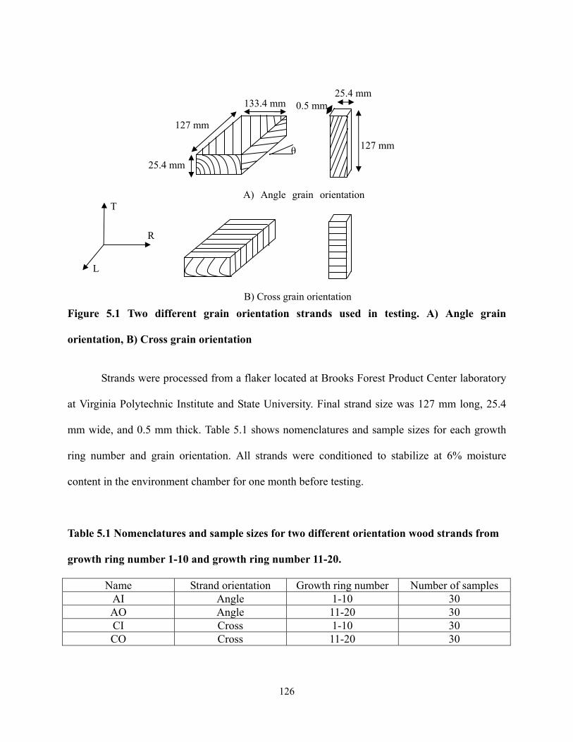
126

Figure 5.1 Two different grain orientation strands used in testing. A) Angle grain

orientation, B) Cross grain orientation

Strands were processed from a flaker located at Brooks Forest Product Center laboratory

at Virginia Polytechnic Institute and State University. Final strand size was 127 mm long, 25.4

mm wide, and 0.5 mm thick. Table 5.1 shows nomenclatures and sample sizes for each growth

ring number and grain orientation. All strands were conditioned to stabilize at 6% moisture

content in the environment chamber for one month before testing.

Table 5.1 Nomenclatures and sample sizes for two different orientation wood strands from

growth ring number 1-10 and growth ring number 11-20.

Name Strand orientation Growth ring number Number of samples AI Angle 1-10 30 AO Angle 11-20 30 CI Cross 1-10 30 CO Cross 11-20 30

θ

R

T

L

A) Angle grain orientation

B) Cross grain orientation

0.5 mm 25.4 mm

127 mm

127 mm

133.4 mm

25.4 mm

127

Test Methods

Figure 5.2 shows the testing arrangement for off-axis properties of strands from different

growth ring numbers. Tension testing used a MTS machine incorporating DIC. Loading data

were obtained from the MTS. The strain measurement was obtained from DIC using a program

developed by Eberl et al. (2006). The loading speed was 0.25 mm/min. Distance between grips

was 10.16 cm. For angled grain strands, a 22.24 N preload was applied to prevent slippage of the

grip. Load was intermittently applied at 22.24 N increments and paused for 5 seconds for image

capture. For cross-grain strands, a 4.44 N preload was applied to prevent slippage of the grip.

Load was intermittently applied at 4.44N increments and paused for 5 seconds for image capture.

Camera set up for DIC and synchronization for loading and strain used the same arrangement

from previous study (Jeong et al. 2008).

Figure 5.2 Tensile test set up for off-axis tension test showing the global axis (x and y), the

principal material axis (L and R), and angle (θ) between x and L

After all tests finished, elastic modulus at θ degree (Eθ) and UTS of angled grain strands

from growth ring number 1-10 and growth ring number 11-20 were calculated. Radial elastic

modulus (ER) and UTS of cross grain orientation strands from growth ring number 1-10 and

L

y

x

θ R

128

growth ring number 11-20 were also calculated. Poisson ratios for four groups were obtained

from the ratio of strain parallel to the loading direction to the strain perpendicular to the loading

direction. Shear modulus was calculated using Equation 5.1 (Jones 1975). Since wood strands

had a high slenderness ratio, the deformation of wood strands was assumed to show no distortion.

That is, St. Venant end effects can be ignored in the area away from the grips. The Eθ were

obtained from angled grain strands while ER was obtained from cross-grain strands. EL and

Poisson ratio (νLR) were obtained from the same population (Jeong et al. 2008). With the average

grain angle of 30 degree, the shear modulus for loblolly pine strands from growth ring number 1-

10 and growth ring number 11-20 were calculated. Shear strength was also measured from off-

axis tension test using Equation 5.2 (Jones 1975). UTS for the four groups were determined using

Equation 5.3.

1

1 1 1 1 2 5.1

5.2

5.3 Where, θ: angle between global axis and grain direction EL: Longitudinal elastic modulus from Jeong et al. (2008a) ER: Radial elastic modulus from cross grain strands A: area of cross section of specimen PLMAX: Peak load υLR: Poisson ratio from Jeong et al. (2008a)

129

After all elastic properties and strength from experimental test were determined, elastic

properties and strength were evaluated using orthotropic theory. Elastic modulus of strands was

calculated with respect to the grain angle using Equation 5.4 (Jones 1975). The UTS of strands

was also calculated using Tsai-Hill criterion to analyze the tensile strength as a function of grain

orientation using Equation 5.5 (Jones 1975).

1

1 1 2 1 5.4

1

1 1 5.5

Where, X: Longitudinal strength Y: Transverse strength S: Shear strength Moisture content and specific gravity measurement

Moisture content and specific gravity were measured according to ASTM D 4442 (ASTM

2004a) and ASTM D 2395 (ASTM 2004b). Samples for both testing methods were obtained

from the same populations using untested strands. To minimize the influence of the environment

of the room humidity and temperature, all samples were kept in a reclosable bag and handled by

forceps when the specimens were mounted on the balance. The balance has a sensitivity of

±0.00001 g. After measuring the specimen weight, all samples were kept in the reclosable bag.

To measure the oven-dry weight, samples were put in the oven for twenty four hours. The

specific gravity was measured based on the oven-dry weight and volume at the same condition as

during mechanical testing.

130


Table 5.2 shows the moisture content (MC) and specific gravity (SG) of angled grain

strands and cross-grain strands from growth ring number 1-10 and growth ring number 11-20. It

can be speculated that the average specific gravity is not dependent upon growth ring position

and cutting direction in this arrangement. However, the variation of specific gravity was

dependent upon growth ring position.

Table 5.2 Physical properties of angled and cross-grain strands from growth ring number

1-10 and growth ring number 11-20

Name MC (%), (COV)

SG, (COV)

AI 6.97% (1.75%)

0.44 (7.23%)

AO 6.74% (3.46%)

0.41 (8.08%)

CI 6.47% (7.67%)

0.39 (11.1%)

CO 6.50% (6.62%)

0.43 (15.1%)

Table 5.3 shows the mechanical properties of angled grain strands and cross-grain strands

from growth ring number 1-10 and growth ring number 11-20. While MOE from angled grain

strands (AI and AO) increased about 25% from growth ring number 1-10 to growth ring number

11-20, MOE from cross-grain strands (CI and CO) decreased 1% from growth ring number 1-10

to growth ring number 11-20. The distinctive difference of MOE between these two different

orientation strands showed that the fiber orientation of strands was a strong indicator on

mechanical properties of wood strands.

AO had the highest ultimate tensile strength (UTS) of 16.96 MPa with a COV of 19%

while CO had the lowest UTS of 2.52 MPa with a COV of 33%. The UTS from angle grain

131

orientation strands increased as the growth ring number increased. However, The UTS from

cross grain orientation strands decreased as the growth ring number increased, which could

indicate UTS from cross grain orientation strands is not dependent upon the growth ring

positions.

Shear moduli were calculated from Equation 5.1. The longitudinal elastic modulus and

Poisson ratio were obtained from previous research (Jeong et al. 2008a). The shear modulus

increased as the growth ring number increased. However, shear strength decreased as the growth

ring number increased. This counter-intuitive result can be speculated that shear strength is more

sensitive to the structure of earlywood and latewood bands. The higher ratio of latewood MOE to

earlywood MOE could result in lower shear strength as growth ring number increases (Jeong et

al. 2008b). The higher ratio of MOE could cause stress concentrations between the boundaries

resulting in a lower strength value. Shear modulus, however, was measured by average elastic

properties of earlywood and latewood band rather than elastic ratio of earlywood and latewood

band.

Poisson ratios from angled grain strands decreased as the growth ring number increased.

From the Poisson ratio (νRT) of 1.07 for CI and 1.10 for CO, the smaller radial strain over

tangential strain can be interpreted as a higher reinforcement in the radial direction compared to

that in the tangential direction. COV values of Poisson ratio from four groups decreased as

growth ring number increased.

Although specific gravity from AI shows a higher value than AO, AO had higher MOE

and UTS values than AI. AO showed lower COV values for MOE and UTS compared to AI.

Although specific gravity from CI was lower than CO, CI had higher MOE and UTS values than

CO. Compared to CI, CO showed lower COV values for MOE and UTS. With the lower COV

132

values, a less variation of strand structures in a higher growth ring number can be speculated.

The results showed that specific gravity was not a main control factor on mechanical properties

of angled grain strands from two different growth ring positions. The morphology of wood

structure from two strands group could be speculated as a main control factor including grain

orientation, microfibril angles, and anatomical structure.

Table 5.3 Mechanical properties from angled grain and cross-grain strands from growth

ring number 1-10 and growth ring number 11-20

Name Angle, θ

(COV)

MOE, GPa

(COV)

UTS, MPa

(COV)

Shear Modulus1, GPa

Shear Strength,

MPa (COV)

Poisson ratio (COV)

AI 33.46 (16.7%)

1.97 (27.2%)

13.58 (23.7%) 0.89 4.67

(27.2%) 1.04

(45.1%)

AO 23.53 (16.0%)

2.46 (22.9%)

16.96 (18.8%) 1.11 4.09

(26.2%) 0.72

(36.5%)

CI 90 0.89 (44.5%)

2.94 (42.1%) N/A2 N/A 1.07

(70.8%)

CO 90 0.88 (44.7%)

2.52 (33.1%) N/A N/A 1.10

(56.7%) 1 Calculated values of shear modulus based on average test values 2 Not applicable

Table 5.4 shows the statistical distribution fitting for shear strength, MOE, UTS, and

Poisson ratio. Normal, Lognormal, Weibull, and Gamma distribution were used to fit the

experimental results from four groups. Kolmogorov-Smirnov (K-S) and Chi-square were used to

verify a particular distribution fitting with alpha value of 0.05. Along with these two criteria,

visual inspection was also conducted to find the best fit. From two criteria and visual inspection,

the best fitting curves for mechanical properties of each group were estimated. Shaded values

indicated the best fitting curve for each mechanical value. Shear strength values from AI and AO

were best fitted with Gamma distribution. MOE values from AI, AO, and CO followed

133

Lognormal distribution, while MOE values from CI followed Weibull distribution. UTS values

from all four groups didn’t follow any specific distribution. Poisson ratio values from AI, CI, and

CO were best fitted with Normal distribution, while Poisson ratio values from AO followed

Lognormal distribution. This statistical distribution can be used as input data to simulate

mechanical properties of strand based composites.

Table 5.4 Statistical distribution of shear strength, MOE, UTS, and Poisson ratio from two

different orientation strands generated from two different growth ring positions

Normal Lognormal Weibull Gamma K-S Chi-square K-S Chi-square K-S Chi-square K-S Chi-square

Shear strength AI 0.08 0.037 0.250 0.075 0.244 0.063 0.232 0.081 AO 0.150 0.003 0.144 0.352 0.054 0.003 0.250 0.326

MOE AI <0.001 0.013 0.250 0.263 N/A 0.388 N/A N/A AO 0.150 0.701 0.150 0.777 0.250 0.636 0.250 0.759 CI 0.150 0.253 0.162 0.208 0.250 0.310 0.242 0.255 CO 0.019 0.006 0.250 0.359 0.140 0.143 0.137 0.222

UTS AI <0.001 0.054 <0.001 0.114 0.023 0.045 0.005 0.090 AO 0.018 0.035 0.079 0.038 0.02 0.033 0.045 0.031 CI 0.01 0.190 0.015 0.189 0.039 0.309 0.026 0.237 CO 0.01 0.069 0.01 0.026 0.01 0.07 0.02 0.056

Poisson ratio AI 0.150 0.225 <0.001 <0.001 0.049 0.042 0.011 0.005 AO <0.001 <0.001 0.150 0.157 <0.001 <0.001 0.126 <0.001 CI 0.150 0.183 0.067 0.015 0.054 0.157 0.110 0.143 CO 0.150 0.482 0.01 0.002 0.037 0.171 0.009 0.069

Table 5.5 shows the failure modes of strands from two different orientations and growth

ring positions. Three different failure modes were observed visually. Shear failure mode included

a crack propagating along the boundary between earlywood and latewood. Brittle failure mode

included failure with crack at no specific angles. Shear against grain angle failure mode

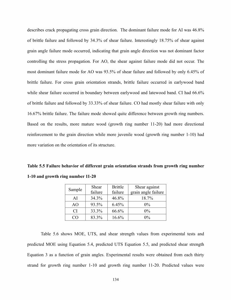
134

describes crack propagating cross grain direction. The dominant failure mode for AI was 46.8%

of brittle failure and followed by 34.3% of shear failure. Interestingly 18.75% of shear against

grain angle failure mode occurred, indicating that grain angle direction was not dominant factor

controlling the stress propagation. For AO, the shear against failure mode did not occur. The

most dominant failure mode for AO was 93.5% of shear failure and followed by only 6.45% of

brittle failure. For cross grain orientation strands, brittle failure occurred in earlywood band

while shear failure occurred in boundary between earlywood and latewood band. CI had 66.6%

of brittle failure and followed by 33.33% of shear failure. CO had mostly shear failure with only

16.67% brittle failure. The failure mode showed quite difference between growth ring numbers.

Based on the results, more mature wood (growth ring number 11-20) had more directional

reinforcement to the grain direction while more juvenile wood (growth ring number 1-10) had

more variation on the orientation of its structure.

Table 5.5 Failure behavior of different grain orientation strands from growth ring number

1-10 and growth ring number 11-20

Sample Shear failure

Brittle failure

Shear against grain angle failure

AI 34.3% 46.8% 18.7% AO 93.5% 6.45% 0% CI 33.3% 66.6% 0% CO 83.3% 16.6% 0%

Table 5.6 shows MOE, UTS, and shear strength values from experimental tests and

predicted MOE using Equation 5.4, predicted UTS Equation 5.5, and predicted shear strength

Equation 3 as a function of grain angles. Experimental results were obtained from each thirty

strand for growth ring number 1-10 and growth ring number 11-20. Predicted values were

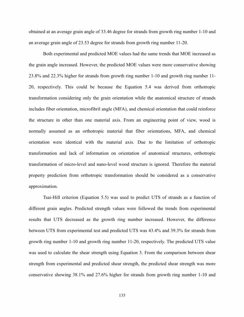
135

obtained at an average grain angle of 33.46 degree for strands from growth ring number 1-10 and

an average grain angle of 23.53 degree for strands from growth ring number 11-20.

Both experimental and predicted MOE values had the same trends that MOE increased as

the grain angle increased. However, the predicted MOE values were more conservative showing

23.8% and 22.3% higher for strands from growth ring number 1-10 and growth ring number 11-

20, respectively. This could be because the Equation 5.4 was derived from orthotropic

transformation considering only the grain orientation while the anatomical structure of strands

includes fiber orientation, microfibril angle (MFA), and chemical orientation that could reinforce

the structure in other than one material axis. From an engineering point of view, wood is

normally assumed as an orthotropic material that fiber orientations, MFA, and chemical

orientation were identical with the material axis. Due to the limitation of orthotropic

transformation and lack of information on orientation of anatomical structures, orthotropic

transformation of micro-level and nano-level wood structure is ignored. Therefore the material

property prediction from orthotropic transformation should be considered as a conservative

approximation.

Tsai-Hill criterion (Equation 5.5) was used to predict UTS of strands as a function of

different grain angles. Predicted strength values were followed the trends from experimental

results that UTS decreased as the growth ring number increased. However, the difference

between UTS from experimental test and predicted UTS was 43.4% and 39.3% for strands from

growth ring number 1-10 and growth ring number 11-20, respectively. The predicted UTS value

was used to calculate the shear strength using Equation 3. From the comparison between shear

strength from experimental and predicted shear strength, the predicted shear strength was more

conservative showing 38.1% and 27.6% higher for strands from growth ring number 1-10 and

136

growth ring number 11-20, respectively. These different values for UTS and shear strength from

the two different growth ring positions can be speculated that the anatomical structure may

influence the final strength value. Similar to the MOE prediction, strength predictions using

orthotropic transformation are sensitive to the direction of structure and structure variation

resulting in multi-axial stress distribution.

Table 5.6 The MOE, UTS, and shear strength of strands from growth ring number 1-10

and growth ring number 11-20

MOE (GPa) UTS (MPa) Shear strength (MPa) Ex1 Pr2 Diff3 Ex Pr Diff Ex Pr Diff

Growth ring number 1-10 1.97 1.50 23.8% 10.47 5.92 43.4% 4.66 2.88 38.1%

Growth ring number 11-20 2.46 1.91 22.3% 11.27 6.83 39.3% 4.09 2.96 27.6%1Experimental 2Predicted 3Diff= (experimental-predicted)/experimental*100%

Conclusions

Elastic and strength properties of loblolly pine strands from growth ring number 1-10 and

growth ring number 11-20 were measured using tension test incorporating DIC. The following

are conclusions from this study:

MOE of angled grain strands increased as the growth ring number increased while MOE

of cross-grain strands decreased 1% as the growth ring number increased. MOE was

more sensitive to the orientation compared to specific gravity.

UTS of angled grain strands increased as the growth ring number increased, while UTS

of cross-grain strands decreased as the growth ring number increased. The UTS was

dependent upon grain orientations of strands rather than specific gravity.

137

Shear modulus increased as the growth ring number increased, but shear strength

decreased as the growth ring number increased. Lower shear strength values can be

speculated as a higher elastic constant ratio of strands from growth ring number 11-20.

Poisson ratio from angled grain strands decreased with increasing growth ring numbers.

However, Poisson ratio from cross-grain strands slightly increased with the increment of

growth ring numbers.

COV values from MOE, UTS, Poisson ratio, and shear strength decreased as growth ring

number increased. From the results, a less variation in structure of strands from growth

ring number 11-20 can be speculated.

Statistical distribution fitting showed that shear strength values were best fitted with

Gamma distribution. MOE values from AI, AO, and CO followed Lognormal

distribution, while MOE values from CI followed Weibull distribution. UTS values from

four groups didn’t follow any specific distribution. Poisson ratio values from AI, CI, and

CO followed Normal distribution, while AO followed Lognormal distribution.

Although four groups of strands showed the mixed failure modes, strands from growth

ring number 11-20 showed a more consistent failure mode. The failure mode indicated

that strands from growth ring number 11-20 showed more oriented structures compared

to the strands from growth ring number 1-10.

From the comparison of MOE, UTS, shear strength from experimental and from

orthotropic transformation, conservative predicted values for all values were obtained.

References

American Society for Testing and Materials (ASTM). 2004a. ASTM D 4442. Standard Test Methods for Direct Moisture Content Measurement of Wood and Wood-Base Materials In: Annual Book of ASTM Standard, Section 4, Vol. 04.10 Wood. ASTM, West Conshohocken, PA.

138

American Society for Testing and Materials (ASTM). 2004b. ASTM D 2395. Standard Test Methods for Specific Gravity of Wood and Wood-Based Materials. In: Annual Book of ASTM Standard, Section 4, Vol. 04.10 Wood. ASTM, West Conshohocken, PA. American Society for Testing and Materials (ASTM). 2004c. Standard Test Methods for Shear Modulus of Wood-Based Structural Panels. Standard D 3044-94. In: Annual Book of ASTM Standard, Section 4, Vol. 04.10 Wood. ASTM, West Conshohocken, PA. Chang B. W., D. H. Huang, and D. G. Smith. 1984. A pinned-end fixture for off-axis testing. Experimental Tech. 28-30 (June) Eberl C., R. Thompson, and D. Gianola. 2006. Digital image correlation and tracking with matlab. Matlab Central. http://www.mathworks.com/matlabcentral/fileexchange/ loadFile.do?objectId=12413&objectType=FILE (27 September 2006). Galicki J. and M. Czech. 2005. Tensile strength of softwood in LR orthotropy plane. Mechanics of Materials. 37:677-686 Jernkvist L. O. and F. Thuvander. 2001. Experimental determination of stiffness variation across growth rings in Picea abies. Holzforschung. 55(3):309-317 Jeong G. Y., A. Zink-Sharp, and D. P. Hindman. 2008a. Comparison of longitudinal tensile properties of different grain orientation strands from loblolly pine (Pinus taeda). In review, Wood and Fiber Sci. Jeong G. Y., D. P. Hindman, and A. Zink-Sharp. 2008b. Tensile properties of earlywood and latewood from loblolly pine (Pinus taeda) using digital image correlation. In review, Wood and Fiber Sci. Jones R. M. 1975. Mechanics of Composite Materials. McGraw-Hill, New York. 55-79 pp. Liu J. Y. 2002. Analysis of off-axis tension test of wood specimens. Wood and Fiber Sci. 34(2):205-211. Yoshihara H. and M. Ohta. 2000. Estimation of the shear strength of wood by uniaxial-tension tests of off-axis specimens. J. Wood Sci. 46:159-163. Zhang W. and A. Sliker. 1991. Measuring shear moduli in wood with small tension and compression samples. Wood and Fiber Sci. 21(1):58-68.

139

Chapter 6. Evaluation on Effective Modulus of Elasticity of Loblolly Pine Strands

Using Stochastic Finite Element Method

Wood as a biological material has variations in structure leading to variations in material

properties. Previous modeling of wood and wood based composites has used average elastic

constants for estimating the mechanical behavior. The variation of wood material properties

should be accounted for to produce more reliable results. In this chapter, Monte-Carlo simulation

based stochastic finite element method (SFEM) was used to model the stiffness of wood strands

including intra-ring property variation and three different grain orientations (radial grain,

tangential grain, and angled grain). Homogenized models were used as a control to compare the

results from the deterministic layer finite element method (FEM) and SFEM models. The

homogeneous model predicted the average effective MOE well for radial and tangential grain

strands from growth ring number 1-10 but provided unrealistic physical strain distributions.

Except for the radial grain orientation models from growth ring number 11-20, the cumulative

probability curves from experimental tests and SFEM results agreed well. The difference of

average effective MOE between experimental results and SFEM results ranged from 0.96% to

22.31% for different grain orientation strands. From a sensitivity analysis, earlywood MOE was

the most important variable affecting the effective MOE.

140

Introduction

Although there are many models of mechanical behavior of wood at different length

scales, little research has explored the variations of mechanical properties in earlywood,

latewood, and wood strands. Earlywood is the layer of wood created by growth during the early

growing season, characterized by thin cell walls and large lumens. Latewood is the layer of wood

created by growth during the late growing season, characterized by thick cell walls and small

lumens. Due to the anatomical structural differences, the mechanical properties of these two

layers are also different. Previous studies have shown that latewood MOE was about two times

greater than earlywood MOE (Groom et al. 2002, Mott et al. 2002, Cramer et al. 2005, and Jeong

et al. 2008a). Growth rings closer to pith contain higher proportions of juvenile wood than

growth rings closer to bark. Juvenile wood differs from mature wood in that it has a higher

microfibril angles, a high percentage of compression wood, distorted grain patterns, and a lower

percentage of latewood (Larson et al. 2001). Variations of material properties of earlywood and

latewood were found in different growth ring positions (Cramer et al. 2005 and Jeong et al.

2008a). However, previous modeling work on strand based composites assumed wood as a

homogeneous material (Wang and Lam 1997, Clouston and Lam 2002, and Clouston 2007).

The mechanical properties of wood strands are different by the intra-ring properties and

grain orientations (Hindman and Lee 2007). However, the intra-ring properties and the

orientation of grain are uncertain factors. The material properties of wood are random in nature

and the grain orientation of strands may be varied due to indeterministic cutting (Jeong et al.

2008b and Jeong et al. 2008c). Therefore, it is desirable to investigate the effect of the uncertain

variables of intra-ring properties and grain angle on the mechanical behavior of wood strands.

Random properties of wood strands will affect not only modulus of elasticity (MOE) changes of

141

wood strands, but also the strain distribution, which is important for analyzing the effect of the

inputs on mechanical behavior of wood strands. These research topics have not been discussed in

the previous studies.

Stochastic finite element method (SFEM) is used to account for the uncertainties of

material properties from the earlywood and latewood as inputs to model the different grain

angles of loblolly pine wood strands. SFEM can solve for the variability associated with wood

strands as known probabilities of material properties. SFEM can take advantage of the existing

finite element method (FEM) for deterministic problems combined with uncertainty variables.

The fundamental principle of the SFEM technique fits well for the high uncertainties of wood

structure.

Literature Review

Although many previous researchers have studied the mechanical behavior of strand

based composites, only one article was found to be related to strand modeling (Hindman and Lee

2007). Among many strand based composite modeling studies, three representative studies were

present, which account for the randomness of material properties of wood as inputs for model.

Wang and Lam (1997) used SFEM to predict the tensile strength of parallel aligned multi

layer strand based wood composites. Based on the strength of multi layers from experimental test,

strength modification factors were evaluated using Weibull-weakest-link theory and size effect.

The results associated with strength modification factors from models were agreed with the

results from experimental test.

Clouston and Lam (2002) used SFEM to predict the strength of angle ply laminates

([±15]s and [±30]s). Tsai-Wu failure criteria associated with flow rule was used to calculate the

142

failure index. The failure index was modified by size effect and loading configuration effect

between tension and bending. The difference of strength between simulation and experimental

test results ranged from 3.8% to 9.8%. The difference of stiffness between simulation and

experimental test results ranged from 6.1% to 14.8%.

Clouston (2007) expanded the previous work to predict mechanical behavior of parallel

strand lumber made from Douglas fir (Pseudotsuga menziesii). Statistical variation of void area

and grain angle in PSL were counted as random variables for model to predict the strength from

tension, compression, and bending. The results were well agreed with the experimental tests

showing 5.5% difference for tension, 3.3% difference for compression, and 6.4% difference for

bending.

Hindman and Lee (2007) predicted the elastic properties of different orientation strands

from loblolly pine (Pinus taeda) using FEM that incorporated the elastic properties of earlywood

and latewood as inputs. Hindman and Lee (2007) used cellular FEM models and solid FEM

models to predict the modulus of elasticity (MOE) of different orientation strands under tension

and bending loading condition. Homogeneous models were also constructed to compare the

prediction of MOE from the layered models. The inputs for the models were average longitudinal

elastic moduli of earlywood and latewood from experimental test. The cellular models had a

better prediction of MOE from different orientation strands over solid models. The difference of

MOE between experimental results and layer cellular model results ranged from 1.7% to 20.4%.

While the three SFEM models (Wang and Lam 1997, Clouston and Lam 2002, and

Clouston 2007) were used for predicting the mechanical properties of strand based composite

using strand properties, the models did not consider the variability of mechanical properties of

earlywood and latewood. Although Hindman and Lee (2007) modeled different orientated

143

strands using earlywood and latewood properties, the results of the models were limited by the

deterministic inputs to predict the mechanical properties of wood strands. The variability of

mechanical properties of earlywood and latewood must be considered in modeling to represent

the true nature of wood as a biological composite material.

In order to have more rigorous data on earlywood and latewood properties, Jeong et al.

(2008a) measured the mechanical properties of earlywood and latewood from growth ring

number 1-10 and growth ring number 11-20 using tension testing incorporated with digital image

correlation (DIC). The results showed that MOE and Poisson ratio increased as the growth ring

number increased. Statistical comparisons showed that the MOE and UTS had a significant

difference by both growth ring positions and intra-ring. Based on testing results, probability

density functions for MOE, Poisson ratios, and UTS were examined using Kolmogorov-Smimov

(K-S), Chi-square test, and visual inspection. These results were used as inputs for the current

modeling work.

Jeong et al. (2008b) and Jeong et al. (2008c) measured the tensile properties of different

orientation loblolly pine (Pinus taeda) strands from growth ring number 1-10 and growth ring

number 11-20. Three different oriented strands (radial, tangential, and angled orientation strands)

showed MOE and UTS of wood strands increased as growth ring number increased. Statistical

comparison showed that the growth ring position and grain angle can impact the mechanical

properties of the wood strands. The MOE of three different oriented strands from the two

different growth ring positions were used as a validation of the current model.

The goal of this chapter was to analyze the effect of the intra-ring properties and grain

angles on the MOE of wood strands with respect to these variables. Monte Carlo simulation

based SFEM used the results from the earlywood and latewood testing as inputs to model the

144

mechanical property variation of loblolly pine wood strands. A sensitivity analysis of the input

parameters in the SFEM model was conducted to analyze the most important parameters related

to mechanical response.

Methods

SFEM models were constructed using ANSYS 11.0v program. Before the SFEM models

were constructed, the following assumptions were applied.

1. Wood strands behaved in a linear elastic manner.

2. No slippage occurred between earlywood and latewood under uniform loading.

3. Loading was assumed to be deterministic

4. MOE of earlywood and latewood were assumed to be random variables with known distribution.

5. Poisson ratio for earlywood and latewood were assumed to be random variables with known distribution.

Figure 6.1 shows four different wood strand models, dimensions of the model analogs,

and the loading conditions. While models A, B, and C consider variation of intra-ring properties

and grain angles, model D does not consider the intra-ring property variation and grain angle

effect. Model A shows radial grain orientation model. Model B shows tangential grain

orientation model. Model C shows angled grain orientation model. Model D shows a

homogenized model. The dimensions for all SFEM models were 10.0 cm in length, 2.54 cm in

width and 0.6 mm in thickness. The ratio of earlywood to latewood was defined to be 2.0:1.0.

Uniform tension pressure was applied at the top end of the strands and the bottom of the strands

was fixed in both x and y directions. To generate the random field for describing the properties of

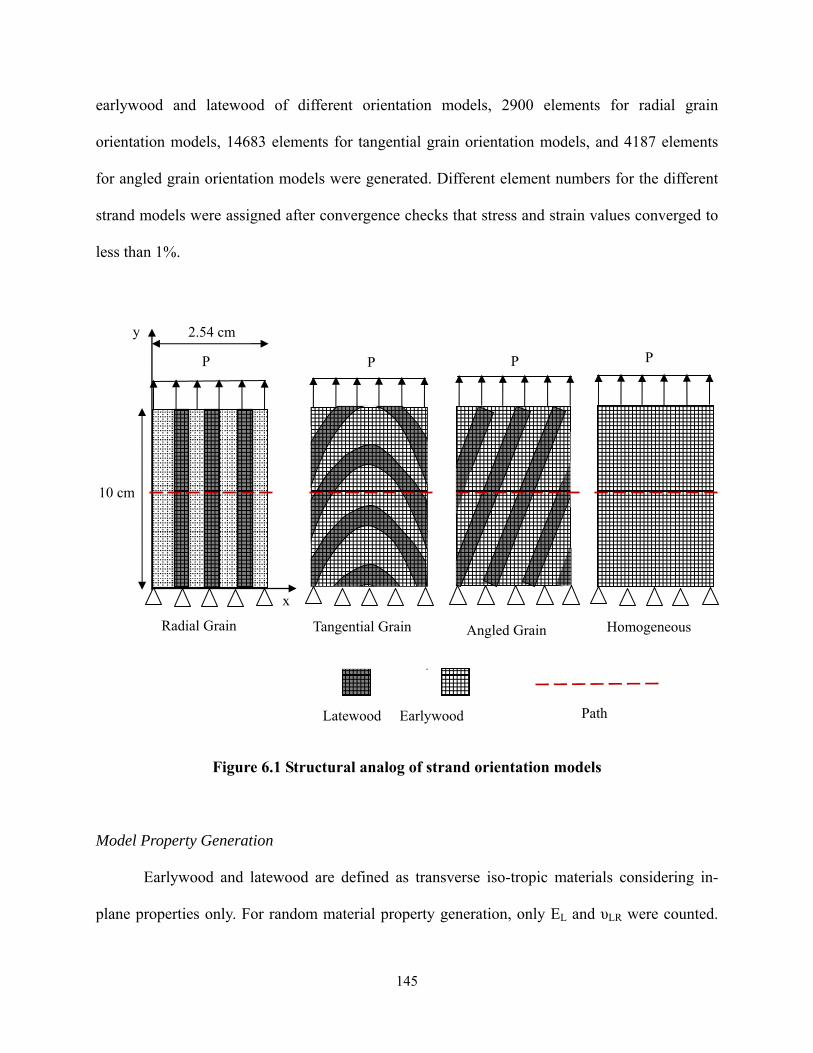
145

earlywood and latewood of different orientation models, 2900 elements for radial grain

orientation models, 14683 elements for tangential grain orientation models, and 4187 elements

for angled grain orientation models were generated. Different element numbers for the different

strand models were assigned after convergence checks that stress and strain values converged to

less than 1%.

Figure 6.1 Structural analog of strand orientation models

Model Property Generation

Earlywood and latewood are defined as transverse iso-tropic materials considering in-

plane properties only. For random material property generation, only EL and υLR were counted.

10 cm

Latewood Earlywood

P

Angled Grain

P

Radial Grain

2.54 cm y

Homogeneous

P P

x

Tangential Grain

Path

146

The elastic properties of EL, ER, and GLR were all expressed in terms of EL using reciprocal

relationships. This process was based on the assumption that longitudinal elastic modulus (EL),

transverse elastic modulus (ER), longitudinal elastic modulus (EL), and shear modulus (GLR) are

linearly correlated (Bodig and Goodman 1973). Kretschmann et al. (2006) found the ratio of

EL:GLR for latewood and for earlywood 3.5:1.0 regardless of growth ring position. This ratio was

used to calculate GLR for earlywood and latewood layers for the current model. Also the ratio of

EL:ER for earlywood and for latewood from the two different growth ring positions was

indirectly calculated from transverse tension testing of cross grain strands (Jeong et al. 2008c).

The EL:ER ratio of 2.72:1.0 was used to calculate the ER for earlywood and latewood from

growth ring number 1-10, and the EL: ER ratio of 3.12:1.0 was used to calculate the ER for

earlywood and latewood from growth ring number 11-20.

Table 6.1 shows the average EL and υLR from experimental test with the distribution type

and parameters (Jeong et al. 2008a). For homogeneous model, representative material properties

for EL and υLR for growth ring number 1-10 and growth ring number 11-20 were calculated by

combining average EL of earlywood and latewood based on experimental test using the Rule of

Mixtures and combining the average υLR of earlywood and latewood from experimental test

using the Rule of Mixtures. Based upon the EL and υLR, the rest of properties were generated

using the reciprocal relationships described above.

For deterministic layer FEM, material properties of earlywood and latewood from growth

ring number 1-10 and growth ring number 11-20 were calculated based on the reciprocal

relationship with the E/G ratio. For probabilistic SFEM, Monte Carlo simulation associated with

Latin Hypercube Sampling (LHS) technique used for generating random properties of earlywood

and latewood characterized by the distribution type and by the distribution parameters. Table 6.1

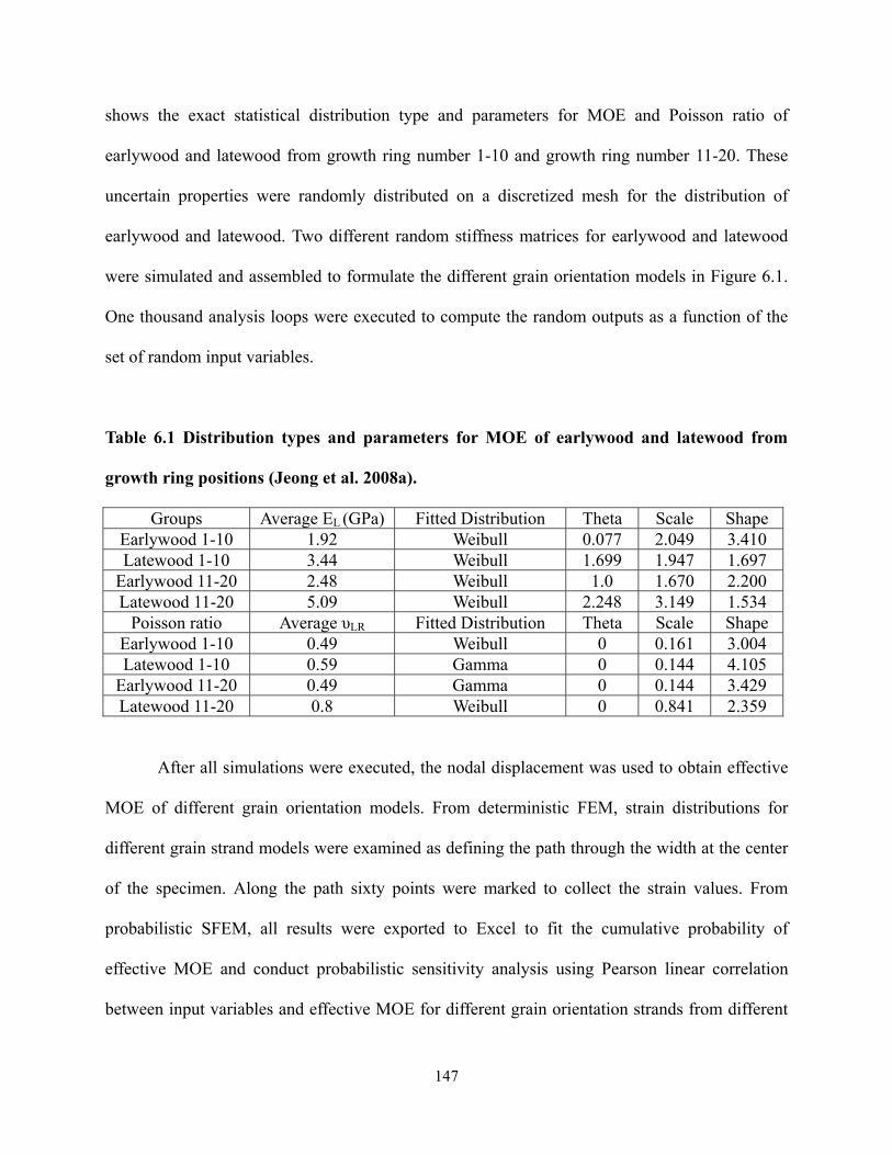
147

shows the exact statistical distribution type and parameters for MOE and Poisson ratio of

earlywood and latewood from growth ring number 1-10 and growth ring number 11-20. These

uncertain properties were randomly distributed on a discretized mesh for the distribution of

earlywood and latewood. Two different random stiffness matrices for earlywood and latewood

were simulated and assembled to formulate the different grain orientation models in Figure 6.1.

One thousand analysis loops were executed to compute the random outputs as a function of the

set of random input variables.

Table 6.1 Distribution types and parameters for MOE of earlywood and latewood from

growth ring positions (Jeong et al. 2008a).

Groups Average EL (GPa) Fitted Distribution Theta Scale Shape Earlywood 1-10 1.92 Weibull 0.077 2.049 3.410 Latewood 1-10 3.44 Weibull 1.699 1.947 1.697

Earlywood 11-20 2.48 Weibull 1.0 1.670 2.200 Latewood 11-20 5.09 Weibull 2.248 3.149 1.534

Poisson ratio Average υLR Fitted Distribution Theta Scale Shape Earlywood 1-10 0.49 Weibull 0 0.161 3.004 Latewood 1-10 0.59 Gamma 0 0.144 4.105

Earlywood 11-20 0.49 Gamma 0 0.144 3.429 Latewood 11-20 0.8 Weibull 0 0.841 2.359

After all simulations were executed, the nodal displacement was used to obtain effective

MOE of different grain orientation models. From deterministic FEM, strain distributions for

different grain strand models were examined as defining the path through the width at the center

of the specimen. Along the path sixty points were marked to collect the strain values. From

probabilistic SFEM, all results were exported to Excel to fit the cumulative probability of

effective MOE and conduct probabilistic sensitivity analysis using Pearson linear correlation

between input variables and effective MOE for different grain orientation strands from different

148

growth ring positions. The Pearson correlation coefficient was calculated using Equation 6.1.

∑ ∑ ∑

∑ ∑ ∑ ∑ 6.1

Where,

r: Pearson correlation coefficient

n: Number of samples

X: Random input variable

Y:MOE outputs

XY: Covariance between random input variable and MOE output.


Comparison of experimental results to model results

Figure 6.2 shows the comparison of the averaged effective MOE values from

experimental testing (Jeong et al. 2008b and Jeong et al. 2008c) and results from models. The

homogeneous models (H) for Radial 1-10 and Tangential 1-10 have differences of -0.64% and

8.57%, respectively from the experimental results. Predictions of effective MOE of Radial 11-20,

Tangential 11-20, Angled 1-10, and Angled 11-20 from the homogeneous models were not as

accurate as the Radial 1-10 and Tangential 1-10 ranging from -21.75% to -35.96%. The

deterministic layer FEM and probabilistic SFEM models were relatively good for all orientations

of wood strands tested, ranging from -0.8% to -22.31%. The highest three difference between

149

experimental results and model results were found in Radial 11-20, Tangential 11-20, and Angled

11-20. For growth ring number 11-20, a higher ratio of latewood MOE to earlywood MOE and a

higher ratio of latewood Poisson ratio to earlywood Poisson ratio may cause the slippage

between earlywood and latewood, which may result in lower MOE values than current model

results.

For the prediction of effective MOE for Radial 1-10 and Radial 11-20, homogeneous,

deterministic FEM, and probabilistic SFEM had little difference as shown in Figure 6.2. From

the analogy of laminate theory, radial grain orientation models were not influenced by the

different mechanical properties of earlywood and latewood due to the iso-strain movement along

the y-axis. Since input for homogeneous model was applied using the Rule of Mixtures based on

earlywood and latewood properties, the homogeneous models for radial grain orientation strands

should be the same strain value obtained from the corresponding deterministic FEM models.

However, effective MOE from tangential and angled grain orientation models were influenced

by different strain distributions caused by differences between the loading direction and the

orientation of earlywood and latewood. The homogeneous model cannot represent the different

orientation of earlywood and latewood other than loading direction, which resulted in a greater

effective MOE for the tangential and angled grain orientation models than the experimental

results.

150

Figure 6.2 Differences between the average MOE from experimental tests (Jeong et al.

2008a and Jeong et al. 2008b) and the average MOE from models ((Difference

(%)=Experimental-simulation/experimental)*100%)

Strain distribution from different orientation models from growth ring number 1-10 and growth

ring number 11-20

Figure 6.3, 6.4, and 6.5 show the normalized longitudinal strain y, transverse strain x, and

shear strain xy distribution through the center of the strand models (Figure 6.1), respectively.

Earlywood and latewood bands change position with the different orientations through the path.

For the radial, tangential, angled grain strand models, a smaller band plateau strain distribution

indicates the latewood band and a larger band plateau indicates the earlywood band.

Figure 6.3 shows the strain y distribution of different orientation models from different

growth ring positions. Homogeneous and radial grain orientation models showed a uniform

strain distribution through the width and overlapped each other. From iso-strain behavior from

homogeneous models and radial grain models, effective MOE from the two models was similar

-40.00%-35.00%-30.00%-25.00%-20.00%-15.00%-10.00%-5.00%0.00%5.00%

10.00%D

iffer

ence

(%)

EX VS H

EX VS FEM

EX VS SFEM

Radial 1-10

Tangential11-20

Angled1-10

Angled 11-20

Radial 11-20

Tangential1-10

151

(Figure 6.2). Tangential grain models and angled grain models showed non-uniform strain y

distribution because the orientation of grain was not parallel to the loading direction. For

tangential grain models, the strain y distribution showed a peak near the edge and generally

smoothed out to the middle width. For angled grain models, the strain y distribution in

earlywood was greater than latewood, since the latewood had a greater stiffness that produced

less strain at the same load level. All strand models from growth ring number 11-20 showed a

lower magnitude strain y distribution compared to strand models from growth ring number 1-10.

a) Growth ring number 1-10

22.5

33.5

44.5

55.5

0.00 0.85 1.69 2.54

Stra

in y

Width

Homogeneous ModelRadial Grain ModelTangential Grain ModelAngled Grain Model

152

b) Growth ring number 11-20

Figure 6.3 Strain y distribution from simulation models considering grain orientations and

growth ring positions. a) Growth ring number 1-10, b) Growth ring number 11-20

Figure 6.4 shows the strain x distributions of different strand models from different

growth ring positions. The homogenous models showed uniform strain x distribution through the

width of models, the radial, tangential, and angled grain orientation models showed non-uniform

strain distributions. The radial grain orientation models showed a greater compressive strain in

latewood band compared to the earlywood band because latewood MOE was greater than

earlywood MOE. The tangential grain models had the greatest negative strain, which occurred

near the edge of the model and generally decreased to the middle width due to the alignment

direction of earlywood and latewood. The angled grain models showed trends of both the radial

and tangential models, with a change in strain between earlywood bands and latewood bands,

and with a frequency similar to the radial grain orientation model but with a greater amplitude.

2

2.5

3

3.5

4

4.5

5

5.5

0.00 0.85 1.69 2.54

Stra

in y

Width


153

The off-axis angle of earlywood and latewood bands to the global x axis caused a greater strain x

distribution for earlywood and latewood bands from angled grain orientation models. Compared

to the strain distribution of different orientation models from growth ring numbers 1-10, the

strain distribution from growth ring numbers 11-20 showed a lower amplitude in general for all

strand simulations, which was reasonable to expect that a greater elastic properties of strands

from a higher growth ring numbers 11-20 had a greater resistance to the load.


-3.3

-2.8

-2.3

-1.8

-1.3

0.00 0.85 1.69 2.54

Stra

in x

Width


154


Figure 6.4 Strain x distribution from simulation models considering grain orientations and


Figure 6.5 shows the shear strain distribution of different models from different growth

ring positions. The homogeneous and radial grain orientation models showed a uniform shear

strain distribution through the width of models relative to the other grain orientation models. The

magnitude of shear strain distribution from the homogeneous and radial models was 100 times

lower than the shear strain from the tangential and angled grain orientation models. The shear

strain distributions from the homogeneous and radial grain orientation models appeared to be

overlapped. The tangential grain orientation models showed the maximum negative shear strain,

near the earlywood and latewood boundary at the left side, and continuously increased, crossing

zero at the center, and forming an anti-symmetric distribution in the other half. The angled grain

orientation models had shear strain distribution oscillated between earlywood and latewood

bands. A positive shear strain occurred from earlywood band while a negative shear strain

occurred from latewood band due to the higher MOE value in latewood and the lower value in

-3.3

-2.8

-2.3

-1.8

-1.3

0.00 0.85 1.69 2.54

Stra

in x

Width


155

earlywood. There was no noticeable shear strain distribution and magnitude difference between

different growth ring numbers.



Figure 6.5 Shear strain xy from simulation models considering grain orientations and


-1.0

-0.5

0.0

0.5

1.0

0.00 0.85 1.69 2.54

Shea

r st

rain

xy

Width


-1.0

-0.5

0.0

0.5

1.0

0.00 0.85 1.69 2.54

Shea

r st

rain

xy

Width


156

Statistical distribution of the effective MOE of different orientation of wood strands from different

growth ring positions.

Figure 6.6 shows the cumulative probability of the effective MOE of radial, tangential,

and angled grain orientation SFEM models and experimental testing from Jeong et al. (2008b

and 2008c). A minimum of thirty test results was fitted from the experimental MOE results while

one thousand simulation results were fitted for the SFEM results. Kolmogorov-Smimov (K-S)

tests with 95% confidence interval showed the comparison between experimental results and

SFEM results was not significantly different (p-value 0.999 for Radial 1-10, 0.973 for Tangential

1-10, 0.198 for Tangential 11-20, 0.855 for Angled 1-10, 0.275 for Angled 11-20 comparison)

except for the comparison for radial grain strands from growth ring number 11-20 (p-value 0.001

for Radial 11-20 comparison).

Although general agreement between experimental results and corresponding SFEM

results were made, some of the differences of MOE values between the experimental results and

the SFEM results are discussed. The highest effective MOE value of radial orientation strand

from growth ring numbers 11-20 obtained from experimental test was 3.48 GPa while the highest

values of 5.29 GPa was obtained from SFEM using the combination of input variables within the

distribution of experimental test data (Figure 6.6a). The lowest effective MOE value of tangential

orientation strands from growth ring number 11-20 from experimental was 1.35 GPa and from

SFEM model was 1.53 GPa (Figure 6.6b). The highest effective MOE value of the angled

orientation stands from growth ring number 11-20 from experimental was 3.42 GPa while the

corresponding SFEM model predicted 4.28 GPa (Figure 6.6c). The trends of the difference

showed that SFEM results were more conservative than experimental results. Possible

improvements in this modeling may provide for direct input of the volume fraction of earlywood

157

and latewood for each strand and also account for slippage between the earlywood and latewood

bands

a) Comparison for MOE of radial grain orientation strands from experimental and SFEM

b) Comparison for MOE of tangential grain orientation strands from experimental and SFEM

0

0.25

0.5

0.75

1

0.5 1 1.5 2 2.5 3 3.5 4 4.5 5 5.5 6 6.5 7

Cum

ulat

ive

Prob

abili

ty o

f MO

E

MOE (GPa)

Experimental SFEM

Experimental SFEM

Growth ring 1-10

Growth ring 11-20

0

0.25

0.5

0.75

1

0.5 1 1.5 2 2.5 3 3.5 4 4.5 5 5.5 6 6.5 7

Cum

ulat

ive

Prob

abili

ty o

f MO

E

MOE (GPa)

Experimental SFEM

Experimental SFEM

Growth ring 1-10

Growth ring 11-20

158

c) Comparison for MOE of angled grain orientation strands from experimental and SFEM

Figure 6.6 Comparison between cumulative probability of MOE from experimental and

that from SFEM; a) radial grain orientation strands comparison, b) tangential grain

orientation strands comparison, c) angled grain orientation strands comparison

Sensitivity of input variables for the effective MOE of different orientation strand models

Table 6.2 shows the sensitivity of input variables (MOE for earlywood and latewood

from growth ring numbers 1-10 and growth ring numbers 11-20, Poisson ratio for earlywood and

latewood from growth ring numbers 1-10 and growth ring numbers 11-20) on the effective MOE

from the SFEM models of growth ring numbers 1-10 and growth ring numbers 11-20. The

shaded cells represent a strong correlation of Pearson linear correlation coefficient, defined as

greater than 0.5, between an input variable and effective MOE of strand models (Equation 6.1).

For growth ring numbers 1-10, earlywood MOE and earlywood Poisson ratio were

strongly correlated with effective MOE from tangential and angled orientation strand models,

while only earlywood MOE was strongly correlated with effective MOE from radial orientation

0

0.25

0.5

0.75

1

0.5 1 1.5 2 2.5 3 3.5 4 4.5 5 5.5 6 6.5 7

Cum

ulat

ive

Prob

abili

ty o

f MO

E

MOE (GPa)

Experimenal SFEM

Experimental SFEM

Growth ring 1-10

Growth ring 11-20

159

strand models. Latewood MOE and latewood Poisson ratio were strongly correlated with

effective MOE of the radial orientation model. For growth ring numbers 11-20, earlywood MOE

and earlywood Poisson ratio had high correlations with the effective MOE of tangential and

angled orientation strand models, while earlywood MOE was strongly correlated with the

effective MOE of radial orientation strand models. Latewood MOE was strongly correlated with

the effective MOE of radial orientation model. Regardless of growth ring number, earlywood and

latewood MOE had greater correlations with the effective MOE of different orientation strand

models than the Poisson ratios.

Table 6.2 Sensitivity analysis of input variables on MOE of different grain orientation

strands from growth ring number 1-10 and growth ring number 11-20 showing the Pearson

linear correlation coefficient (r)

Growth ring Number 1-10 Variables Radial Tangential Angle

Earlywood MOE 0.734 0.916 0.952 Poisson ratio 0.410 0.551 0.598

Latewood MOE 0.662 0.259 0.255 Poisson ratio 0.571 0.168 0.194

Growth ring number 11-20 Variables Radial Tangential Angle

Earlywood MOE 0.603 0.899 0.936 Poisson ratio 0.400 0.563 0.543

Latewood MOE 0.809 0.385 0.269 Poisson ratio 0.452 0.256 0.192

The sensitivity of earlywood and latewood variables changed with varying orientation of

strands and growth ring number. While correlation between earlywood MOE and effective MOE

of different orientation strand models increased as orientation of strands switched from radial to

tangential to angle, the correlation between latewood MOE and effective MOE of different

160

orientation strand models decreased, which can be explained by the fact that the tangential and

angled orientation strand models had a different strain distribution through the width. In the

earlywood band, greater strains occurred while lower strains occurred in latewood band (Figure

6.3). With the same MOE value of latewood, increment of MOE of earlywood will significantly

increase the stiffness of the tangential and angled orientation strands.

As orientation of strands switched from radial to tangential to angle, correlation between

earlywood Poisson ratio and effective MOE of the different orientation strand models increased.

However, as orientation of strands switched from radial to tangential to angle, correlation

between latewood Poisson ratio and the effective MOE of the different orientation strand models

decreased. The correlation between Poisson ratio from earlywood and latewood and effective

MOE of different orientation wood strands can be explained by different strain x distribution

associated with strain y distribution (Figure 6.3 and Figure 6.4). From the superimposed strain x

and strain y distribution, radial strands had a greater magnitude of Poisson ratio in latewood

bands while tangential and angled strands had a greater magnitude of Poisson ratio in earlywood

bands. Poisson ratio can increase by increment of strain x and decrement of strain y. Therefore,

the effective MOE of radial strands had a positive correlation with Poisson ratio of latewood

while the effective MOE of tangential and angled strands had a positive correlation with Poisson

ratio of earlywood. The sensitivity of earlywood and latewood variables on effective MOE of

different orientation wood strands was changed by different strain distribution that was highly

related to growth ring number, orientation of strands, and interaction of variables. Regardless of

growth ring number and orientation, earlywood MOE was a dominant factor that controlled

effective MOE of different orientation wood strands.

161

Conclusions

Tensile properties of different orientation wood strands were evaluated using

deterministic finite element method (FEM) models and probabilistic stochastic finite element

method (SFEM) models. While the deterministic FEM models used average material properties

of earlywood and latewood, SFEM models used the distribution of material properties of

earlywood and latewood from growth ring number 1-10 and growth ring number 11-20. While

the homogeneous model predicted the average effective MOE well for radial and tangential

orientation strand from growth ring number 1-10, the physical strain distribution showed

unrealistic behavior. Compared to deterministic homogeneous model, deterministic layer FEM

and SFEM models predicted the average effective MOE of the rest orientation strands better.

From strain distribution analysis, different strain distribution for earlywood and latewood layers

occurred in different grain orientations. Homogeneous and radial orientation models, however,

showed iso-strain distribution in longitudinal y direction, which resulted in the same MOE values.

Comparison of cumulative probability curves from experimental test and SFEM was agreed well.

The difference of variation of MOE from different grain strands between experimental results

(Jeong et al. 2008b and Jeong et al. 2008c) and SFEM results ranged from 0.96% to 22.31%.

From sensitivity analysis, earlywood and latewood participated differently to effective MOE of

different grain orientation strand models, which was highly associated with the strain distribution

caused by different orientation strands and interaction of input parameters. In general, earlywood

MOE had a greater effect on effective MOE of wood strands than other input parameters.

References

Bodig, J. and J. R. Goodman. 1973. Prediction of elastic parameters for wood. Wood Sci. 5(4):

162

249-264. Clouston, P. and F. Lam, 2002. A stochastic plasticity approach to strength modeling of strand-based wood composites. Composites Science and Technology, 62:1381-1395. Clouston P. 2007. Characterization and strength modeling of parallel-strand lumber. Holzforschung, 61:394-399. Cramer, S. M., D. E. Kretschmann, R. Lakes, and T. Schmidt. 2005. Earlywood and latewood elastic properties in loblolly pine. Holzforschung. 59:531-538. Groom, L., L. Mott., and S. Shaler. 2002. Mechanical properties of individual southern pine fibers. Part I. Determination and variability of stress-strain curves with respect to tree height and juvenility. Wood and Fiber Sci. 34(1):14-27. Hindman D. P. and J. N. Lee. 2007. Modeling wood strands as multi-layer composites: bending and tension loads. Wood and Fiber Sci. 39(4):515-526. Jeong G. Y., D. P. Hindman, and A. Zink-Sharp. 2008a. Tensile properties of earlywood and latewood from loblolly pine (Pinus taeda) using digital image correlation. Jeong G. Y., A. Zink-Sharp, and D. P. Hindman. 2008b. Comparison of longitudinal tensile properties of different grain orientation strands from loblolly pine (Pinus taeda). Jeong G. Y., D. P. Hindman, and A. Zink-Sharp. 2008c. Shear and transverse properties of loblolly pine (Pinus taeda) strands using tension test incorporated with digital image correlation (DIC). Kretschmann, D. E., S. M. Cramer, R. Lakes, and T. Schmidt. 2006. Selected mesostructure properties in loblolly pine from Arkansas plantations Characterization of the cellulosic cell wall. Ames, Iowa : Blackwell Pub., 149-170 pp. Larson, P. R., D. E. Kretschmann, A. Clark III, and J. G. Isebrands. 2001. Juvenile wood formation and properties in southern pine. General Technical Report FPL-GTR-129. Madison, Wisconsin: US Department of Agriculture, Forest Service, Forest Products Laboratory Mott, L., L. Groom, and S. Shaler. 2002. Mechanical properties of individual southern pine fibers. Part II. Comparison of earlywood and latewood fibers with respect to tree height and juvenility. Wood and Fiber Sci. 34(2): 221-237.

Wang, Y. T. and F. Lam. 1998. Computational modeling of material failure for parallel-aligned strand-based wood composites. J. Computational Material Science 11:157-165.

163

Chapter 7. Evaluation on Ultimate Tensile Strength of Loblolly Pine Strands Using

Stochastic Finite Element Method

The purpose of the chapter was to predict the failure strength of different orientation of

wood strands from different growth ring positions under tension loading. Stochastic models were

constructed to account for the uncertainty of material properties. The Tsai-Hill criteria were used

to predict the ultimate tensile strength (UTS). The UTS results from experimental testing were

used to validate the results from models. The difference of UTS between experimental and

SFEM ranged from 0.09% to 11.09%. Stress distributions showed the different stress

distributions for the different orientation strand models while uniform stress distribution for

homogeneous models. The magnitude of the stress distribution was higher for strands from the

growth ring number 11-20. Sensitivity analysis showed that grain orientation and growth ring

number influenced the UTS of strands. UTS of strands from growth ring number 1-10 showed

strength indexes (Xt, Yt, and S) a dominant factor while UTS of strands from growth ring number

11-20 showed both strength indexes and stress components (σ1, σ2, and τ12) a dominant factor.

164

Introduction

The use of wood strand based composites in structural applications has been increasing.

Most wood strands have been prepared from plantation grown trees. Plantation grown trees have

a short-term rotation time, which results in high production of juvenile wood. Juvenile wood

located near the pith has a higher microfibril angle and a thinner cell wall while mature wood

located near the bark has a lower microfibril angle and a thicker cell wall (Larson et al. 2001).

Values for tensile strength, bending modulus of rupture (MOR), and bending modulus of

elasticity (MOE) of juvenile wood were less than mature wood due to higher fibril angle, shorter

tracheid length, and lower specific gravity (Bendtsen 1978, Panshin and de Zeeuw 1980, Smith

and Briggs 1986, Cave and Walker 1994). Prior to analyzing the effect of juvenile wood strands

on the mechanical properties of wood strand based composites, the rigorous analysis of

mechanical properties of wood strands from plantations is required maximizing wood resources.

Strength of wood materials shows large variation due to the complexity of structure,

interaction of failure modes, inherent inhomogenity, anisotropy, and orientation of grain (Jeong

et al. 2008a, Jeong et al 2008b, and Jeong et al. 2008c). A deterministic approach, however,

cannot predict the scatter range of the variables and the use of deterministic analysis can lead to

serious misinterpretation including overestimation of strength, underestimation of strength, and

inconclusive reliability level. A probability based failure prediction of wood is more appropriate

to overcome the limitation of deterministic approach. Random properties of wood strands will

affect not only stiffness changes of wood strands, but also the evaluation of stresses in principal

material directions, which are important for failure estimation of wood strands.

A great deal of failure criteria used in composite materials are empirical. Therefore, the

failure criteria for wood strands should be developed based on physical failure behavior of wood

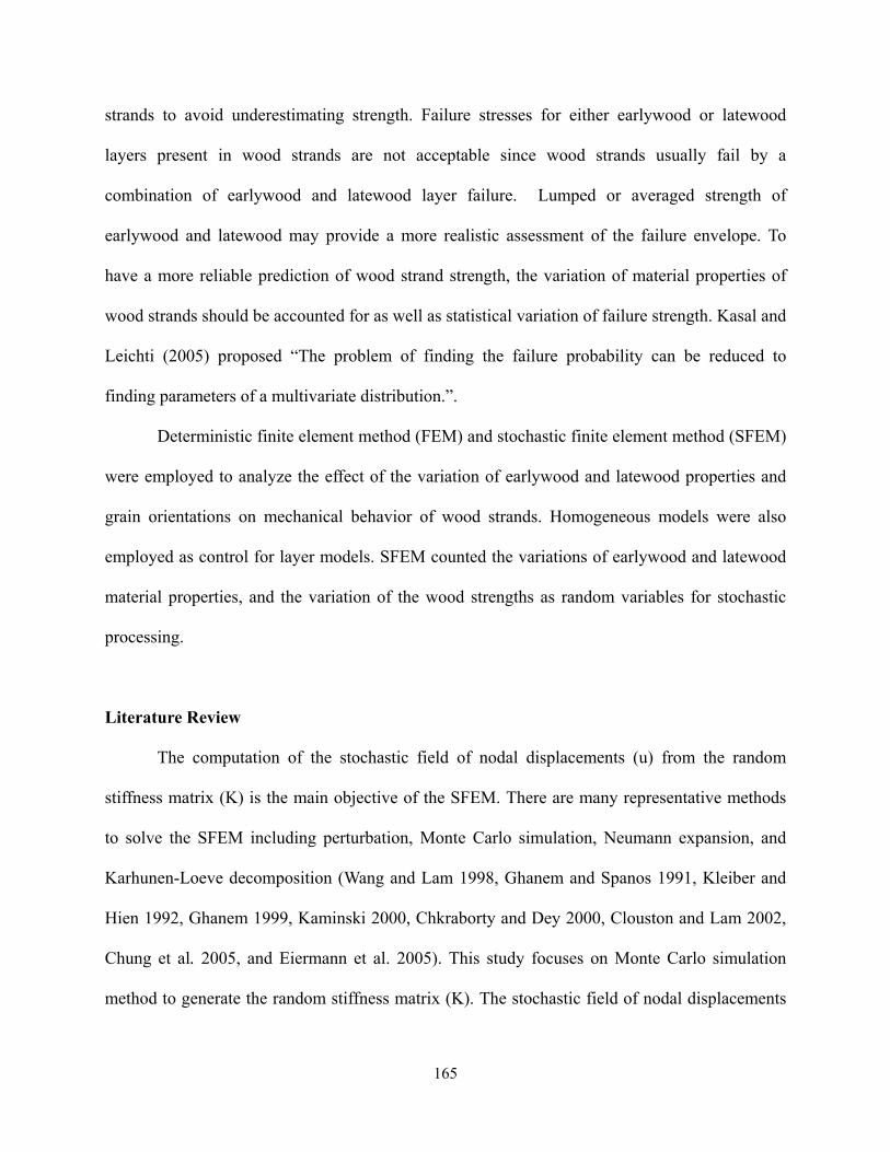
165

strands to avoid underestimating strength. Failure stresses for either earlywood or latewood

layers present in wood strands are not acceptable since wood strands usually fail by a

combination of earlywood and latewood layer failure. Lumped or averaged strength of

earlywood and latewood may provide a more realistic assessment of the failure envelope. To

have a more reliable prediction of wood strand strength, the variation of material properties of

wood strands should be accounted for as well as statistical variation of failure strength. Kasal and

Leichti (2005) proposed “The problem of finding the failure probability can be reduced to

finding parameters of a multivariate distribution.”.

Deterministic finite element method (FEM) and stochastic finite element method (SFEM)

were employed to analyze the effect of the variation of earlywood and latewood properties and

grain orientations on mechanical behavior of wood strands. Homogeneous models were also

employed as control for layer models. SFEM counted the variations of earlywood and latewood

material properties, and the variation of the wood strengths as random variables for stochastic

processing.

Literature Review

The computation of the stochastic field of nodal displacements (u) from the random

stiffness matrix (K) is the main objective of the SFEM. There are many representative methods

to solve the SFEM including perturbation, Monte Carlo simulation, Neumann expansion, and

Karhunen-Loeve decomposition (Wang and Lam 1998, Ghanem and Spanos 1991, Kleiber and

Hien 1992, Ghanem 1999, Kaminski 2000, Chkraborty and Dey 2000, Clouston and Lam 2002,

Chung et al. 2005, and Eiermann et al. 2005). This study focuses on Monte Carlo simulation

method to generate the random stiffness matrix (K). The stochastic field of nodal displacements

166

(u) can be expressed in response to the stiffness matrix. Although there was no previous research

on strength prediction of wood strands using SFEM, studies for prediction of strength of strand

based composite were available. Therefore, literature review was focused on the prediction of

strength of strand based composite.

Wang and Lam (1997) constructed a Monte Carlo simulation based SFEM to predict UTS

of parallel strand based wood composite. Strength modification factors for different layer models

were obtained using Weibull-weakest-link theory and size effect to fit the strength from

experimental results. The results associated with strength modification factors from models were

agreed with the results from experimental test.

Clouston and Lam (2002) used the SFEM to predict the strength of angle ply laminates

([±15]s and [±30]s). The SFEM had a capable of the prediction of failure indexes for the different

angle laminates using Tsai-Wu failure criteria associated with flow rule. The failure index was

modified by size effect and loading configuration effect between tension and bending. The

difference of strength between simulation and experimental test results ranged from 3.8% to

9.8%. Clouston (2007) expanded the model to count statistical variation of void area and grain

angle in parallel strand lumber (PSL) made from Douglas fir (Pseudotsuga menziesii). The

difference between model and experimental results for tension, compression, and bending

strength of the PSL was 5.5%, 3.3%, and 6.4%, respectively.

Kasal and Leichti (2005) summarized the previous studies on application of various

failure criteria on wood material. Most deterministic stress analysis assumed wood materials as a

homogeneous and isotropic material that violated the real physical structure of wood material.

Such simplifications were only acceptable for obtaining primitive results assuming uniaxial

stresses involved. Some stochastic analysis application on strength of wood material including

167

first order second moment method, Monte Carlo simulation method, and Binomial distribution

method were summarized.

Jeong et al. (2008d) constructed SFEM models to predict the MOE values for different

orientation wood strands from growth ring number 1-10 and growth ring number 11-20. The

inputs for the models were distribution of elastic properties of earlywood and latewood from the

two different growth ring position (Jeong et al. 2008a). The model results had a good agreement

with the experimental results ranging from 0.96% to 22.31%. The constructed models were used

in this current study.

Jeong et al. (2008b and 2008c) measured the strength of different orientation of wood

strands from the two different growth ring positions and found the specific distribution of

strength values including longitudinal strength, transverse strength, and shear strength. The

distribution of strength of wood strands was used to generate the random strength indexes to

predict the ultimate tensile strength (UTS) of different orientation wood strands. The average of

the strength values from experimental test were used to validate the predicted UTS from the

current models.

The goal of this chapter was to predict the UTS of different grain orientation strands from

growth ring number 1-10 and growth ring number 11-20 using SFEM considering the variability

of material properties. Uncertainties of strength indexes were implemented using Monte Carlo

simulation with known probabilities of UTS of different grain orientation strands from

experimental test result. The sensitivity analysis was conducted to analyze the effect of input

random variables on the UTS of different orientation wood strands.

168

Model Development

Figure 7.1 shows the flowchart describing the key steps to compute UTS and sensitivity

for the different orientation of wood strands. Jeong and Hindman (2008d) constructed eight

SFEM models for different orientation wood strands from growth ring number 1-10 and growth

ring number 11-20. The previous constructed models used random inputs (MOE, υLR of

earlywood and latewood) from Jeong et al. (2008a) to count the variability of mechanical

properties of earlywood and latewood band to analyze the mechanical behavior of different

orientation wood strands. Three strength components (Xt, Yt, S) were used to count the

variability of strength of wood strands (Jeong et al. 2008b and Jeong et al. 2008c). With the

assigned distributions of the random variables, stress components and strength indexes were

generated using Monte Carlo simulation method associated with Latin Hypercube Sampling. One

thousand loops were used to predict the UTS of different orientation strands. The UTS were

predicted from the strength and stress components using Tsai-Hill failure criteria. This method

can be applied due to the brittle failure behavior. From SFEM generated stress-displacement

relationships, UTS can be predicted associated with strength value from experimental test.

Newton-Raphson iteration method was used to find roots for the critical stress components to

calculate UTS.

169

Figure 7.1 Flowchart for the SFEM procedure

Figure 7.2 shows the four different orientation wood strand models, dimensions of the

model analogs, and the loading conditions. While models A, B, and C were considered variation

of intra-ring properties and grain angles, model D did not include intra-ring property variation

and grain angle effect. The dimension for all SFEM models was 10.0 cm in length, 2.54 cm in

width and 0.6 mm in thickness. The ratio of latewood and earlywood was defined to be 0.5.

Uniform tension displacement applied at the top end of the strands and at the bottom of the

strands was fixed in both x and y direction.

The following assumptions were made to predict UTS of different orientation strands.

Construct SFEM models based on random material

properties

Assign random input variables and Correlate random input variables

Generate random input variable based

on distributions

Random input sampling by MCS associated with LHS

(#1000)

Assign output corresponding the

random input variables

Compute Ultimate tensile Strength using Tsai-Hill criteria associated with

Newton-Raphson iteration method

Stochastic strength indexes

(Xt, Yt, S)

Stochastic stress components (σ1, σ2, τ12)

Sensitivity analysis

170

1. Strength indexes are random and independent

2. Stress components increase linearly with the increment of displacement.

3. Strength and stress components are not correlated

Figure 7.2 Structural analog of strand orientation models

The probabilistic failure stress was predicted using Equation 7.1 showing the Tsai-Hill

failure criteria. Based on analytical distribution of three parameters (Xt, Yt, S), random strength

indexes were generated using Monte Carlo simulation method. The distributions of stress

components (σ1, σ2, τ12) were obtained from the SFEM.

10 cm

Latewood Earlywood

P

Angled Grain

P

Radial Grain

2.54 cm y

Homogeneous

P P

x

Tangential Grain

Path

171

1 7.1

Where,

σ1: Principal stress in radial direction

σ2: Principal stress in longitudinal direction

τ12: Principal shear stress

Xt: Transverse strength

Yt: Longitudinal strength

S: Shear strength

Regardless of grain orientation and growth ring positions, most strands failed in a brittle

manner. From the stress-displacement, extrapolation of slope would meet the peak load, which

can be assumed from the experimental results (Jeong et al. 2008b and 2008c). The maximum

stress can be considered a function of deflection due to the lack of non-linear deformation. With

the slope, stress components were generated for model results. From the slope of stress and

displacement relationship, the three stresses components could be summarized as a function of

displacement and values of slope for the three stress components.

7.2

7.2

7.2

172

Where,

X : Given displacement (∆)

a: slope between σ1 and X

b: slope between σ2 and X

c: slope between τ 12 and X

Substitute Equations 7.2a, 7.2b, 7.2c into Equation 7.1, Equation 7.1 can be summarized as

1 0 7.3

From Equation 7.3, the strength of different grain orientation strands can be predicted as

a function of stochastic constants of a, b, and c, and stochastic constants of strength indexes. To

solve Equation 7.3, Newton-Raphson iteration method was used with an established tolerance of

1×10-7.

Deterministic FEM and Probabilistic SFEM Stress Components and Strength Indexes Generation

Table 7.1 shows the best fitted distribution for strength indexes (Xt, Yt, and S) from two

growth ring numbers with distribution parameters (Jeong et al. 2008b and Jeong et al. 2008c).

The average strength values and standard deviation from experimental and the distribution were

also shown. The Xt represented transverse strength, Yt represented longitudinal strength, and S

represented shear strength.

For deterministic layer FEM, stress components were generated using the average

material properties for earlywood and latewood from growth ring number 1-10 and growth ring

173

number 11-20. Average strength component for the deterministic models were used to predict the

UTS of different orientation strands. For homogeneous model, average stress components were

calculated using representative material properties for EL and υLR for growth ring number 1-10

and growth ring number 11-20 that were calculated combining average EL of earlywood and

latewood based on experimental test using rule of mixture and combining average υLR of

earlywood and latewood from experimental test using rule of mixture.

For probabilistic SFEM, Monte Carlo Simulation associated with Latin Hypercube

Sampling technique used for generating random stress components and strength indexes of

different orientation strands characterized by the distribution type and by the distribution

parameters. Table 7.1 shows the exact statistical distribution type and parameters for the three

strength indexes from growth ring number 1-10 and growth ring number 11-20. These uncertain

properties were randomly distributed on the discretized mesh for the distribution of earlywood

and latewood (Figure 7.1). One thousand analysis loops were executed to generate random stress

components and strength indexes for different orientation strands to predict UTS.

Table 7.1 Distribution of strength indexes from Jeong et al. (2008c) and Jeong et al. (2008d)

Growth ring

number 1-10

Estimated Average (MPa)

Estimated Standard deviation

(MPa)

PredictedAverage(MPa)

PredictedStandard deviation

(MPa)

Fitted Distribution Theta Scale Shape

Yt 20.52 7.56 20.50 7.48 Weibull 6.55 15.72 1.94 Xt 2.94 1.24 2.95 1.20 Weibull 0 3.32 2.64 S 4.66 1.26 4.73 1.24 Gamma 1.04 0.42 8.80

Growth ring

number 11-20

Estimated Average (MPa)

Estimated Standard deviation

(MPa)

PredictedAverage(MPa)

PredictedStandard deviation

(MPa)

Fitted Distribution Theta Scale Shape

Yt 29.03 6.85 29.06 6.45 Weibull 0 31.59 5.17 Xt 2.53 0.83 2.52 0.85 Weibull 0 2.81 3.25 S 4.09 1.07 4.09 1.01 Gamma 0 0.25 16.26

174

After all simulations executed, from deterministic FEM, stress distributions for different

grain strand models were examined as defining the path through the width at the center of the

specimen. Along the path sixty points were marked to collect the stress values. All results from

probabilistic SFEM were exported to Excel to fit the cumulative probability distribution of UTS

and conduct sensitivity analysis using the Spearman rank correlation coefficient (r) defined in

Equation 4 between input variables and UTS for different grain orientation strands from different

growth ring positions.

16 ∑

7.4

Where,

di: distance in ranks between an input variable and UTS

n: number of simulation (1000)


Table 7.2 shows the percent difference of model and experimental results from Jeong et al.

(2008b and 2008c). Homogeneous models for radial grain orientation strands from growth ring

number 1-10 (Radial 1-10), growth ring number 11-20 (Radial 11-20), and for tangential grain

orientation strands from growth ring number 1-10 (Tangential 1-10) agreed well with the

experimental results (0.15%, 0.20%, and 0.41% difference, respectively). However, the UTS

predictions of other oriented strands were not accurate with the homogeneous model ranging

from -23.24% to -157.06%. The homogeneous model predicted the strength of radial grain

175

orientation strands well due to the fact that the strength of strands was determined as a system

failure rather than either individual earlywood band or latewood band in different orientation

wood strands. Since input for the homogeneous model was applied using Rule of Mixture based

on earlywood and latewood properties, the homogeneous model for Radial 1-10 and Radial 11-

20 should be the same average stress value obtained from the corresponding layer FEM model.

The deterministic layer FEM models and SFEM models had the same average UTS

values for the different orientation strands. In general, both deterministic layer FEM and SFEM

models predicted well for the different grain orientation wood strands ranged from 0.09% to

11.09%. Radial grain orientation strands were influenced little by the orientation of earlywood

and latewood due to the prediction of system failure, where a failure of the strand would involve

multiple layers of both earlywood and latewood. The highest difference of 11.09% between UTS

and predicted UTS from FEM and SFEM for tangential grain orientation models was found.

Tangential grain orientation strand models were difficult to model since the geometry of

earlywood and latewood bands were created by cutting the tangent to the earlywood and

latewood boundary when the wood disk assumed a tapered cylinder (Figure 7.2). However, the

wood strands show variation in the actual earlywood and latewood bands present in the strands,

which may influence the volume fraction of earlywood and latewood as well as the specific

geometry associated with the mesh for the tangential grain orientation model in Figure 2.

The highest difference of 95.7% and 157.06% between UTS and predicted UTS from the

homogeneous models for angled grain orientation models of growth ring numbers 1-10 and 11-

20 was found, respectively. Since the geometry of the homogeneous models could not mimic the

complicated stress distributions induced by the combination of loading direction with orientation

of earlywood and latewood for angled grain orientation strands. However, the mimicked

176

geometry of layered FEM and SFEM for angled grain orientation strands could show the stress

distribution in earlywood and latewood bands that were important to predict the UTS. The

difference of UTS between experimental and model results was ranged from 0.34% for Angled

1-10 and 1.60% for Angled 11-20

Table 7.2 Comparison of average ultimate tensile strengths of wood strands from current

SFEM and previous experimental tests from Jeong et al. (2008b and 2008c).

Notation Ex (MPa)

H (MPa)

FEM (MPa)

SFEM (MPa)

Ex vs H (%)1

Ex vs FEM (%)

Ex vs SFEM (%)

Radial 1-10 20.52 20.51 20.50 20.50 0.15 0.09 0.09 Radial 11-20 29.03 29.07 29.06 29.06 0.20 -0.14 -0.14

Tangential 1-10 20.58 20.51 19.43 19.43 0.41 5.55 5.55 Tangential 11-20 23.51 29.07 26.11 26.11 -23.24 -11.09 -11.09

Angled 1-10 10.47 20.51 10.50 10.50 -95.70 -0.34 -0.34 Angled 11-20 11.27 29.07 11.08 11.08 -157.06 1.60 1.60

1Difference (%) = (experimental result-model results)/experimental results *100%

Stress distributions from different strands

Figure 7.3, 7.4, and 7.5 show the normalized longitudinal stress y, transverse stress x, and

shear stress xy distribution through the width of the center of the strand models (Figure 7.2),

respectively. Earlywood and latewood bands change position with the different orientation

through the path. Earlywood bands are two times wider than the latewood bands. For radial,

tangential, and angled grain strand models, a smaller band plateau stress distribution indicates

the latewood band and a larger band plateau indicates the earlywood band.

Figure 7.3 shows the longitudinal stress y distribution of different orientation models for

different growth ring positions. The stress distribution of the homogenous model was uniform

throughout the width of the strand regardless of growth ring positions. Radial grain orientation

models showed the distinctive stress y distribution showing lower stress in earlywood and

177

greater stress in latewood due to the lower longitudinal elastic modulus of earlywood and the

greater longitudinal elastic modulus of latewood. Tangential grain orientation models showed

greater stress in latewood at both edge and lower stress in earlywood. Although tangential grain

orientation model had a different stress distribution between earlywood and latewood, the

magnitude of difference between two bands were lowest compared to the radial and angled grain

orientation models. The angled grain orientation models showed lower stress in earlywood bands

than the latewood bands. The magnitude of the stress difference between earlywood and

latewood for angled grain model was lower than that of radial grain model. Compared to the

stress x distribution, the magnitude of stress y distribution was about twenty times greater for

growth ring numbers 1-10 and about fifteen times greater for growth ring numbers 11-20. The

general trend for stress distribution from different growth ring positions were similar but greater

magnitude stress in strands from a higher growth ring positions.


6

8

10

12

14

16

0.00 0.85 1.69 2.54

Stre

ss y

Width


178


Figure 7.3 Stress y distribution from simulation models considering grain orientations and

growth ring positions. a) Growth ring numbers 1-10, b) Growth ring numbers 11-20

Figure 7.4 shows the transverse stress x distribution from different orientation models for

different growth ring positions. Homogeneous models and radial grain orientation models

showed relatively uniform stress x distribution and overlapped each other while the tangential

and angled grain orientation models showed a distinctive non-uniform stress distribution through

the width of model. Strictly speaking, the homogeneous and radial grain orientation strands

showed the negative parabolic stress distributions. The magnitude of stress distribution from the

homogeneous and radial grain orientation strands was 1×10-2 times the stress x distribution from

the tangential and angled grain orientation strands. The stress distribution for tangential grain

models showed stress x generally increased to the middle width and decreased symmetrically.

The stress distribution for angled grain orientation strands showed oscillating stress distribution

through the width, with tension stress for latewood layers and compressive stress for earlywood

layers. The stress distributions for tangential and angled grain orientation models from growth

6

8

10

12

14

16

0.00 0.85 1.69 2.54

Stre

ss y

Width


179

ring numbers 11-20 had a greater magnitude than those from growth ring numbers 1-10.

a) Growth ring numbers 1-10

b) Growth ring numbers 11-20

Figure 7.4 Stress x distribution from simulation models considering grain orientations and

growth ring positions. a) Growth ring numbers 1-10, b) Growth ring numbers 11-20

Figure 7.5 shows shear stress distribution of different orientation models from different

growth ring positions. The homogeneous and radial grain orientation models showed the

-0.8 -0.6 -0.4 -0.2 0.0 0.2 0.4 0.6 0.8 1.0

0.00 0.85 1.69 2.54

Stre

ss x

Width


-0.8 -0.6 -0.4 -0.2 0.0 0.2 0.4 0.6 0.8 1.0

0.00 0.85 1.69 2.54

Stre

ss x

Width


180

relatively uniform shear stress distribution while tangential and angled grain orientation models

showed the non-uniform shear stress distribution. The magnitude of shear stress distributions

from homogeneous and radial grain orientation strands was 1×10-2 times the shear stress from the

tangential and angled grain orientation models. The shear stress distributions from homogeneous

and radial grain orientation models appeared to be overlapped. The material principal direction

of homogeneous and radial grain models was parallel to the loading direction that caused nearly

zero shear stress while tangential and angled grain orientation models had different directions

between grain orientation and loading direction that caused relative greater shear stress

distributions. The tangential grain orientation models had the greatest negative shear stress near

the left edge and showed the anti-symmetric distribution through the width of the strand, with

zero shear stress at the center and a maximum positive shear stress near the right edge. The

greatest shear stress near the right and left edge occurred due to the boundary between earlywood

and latewood. The shear stress of the angled grain orientation models showed a distinctive

pattern between earlywood and latewood band including the negative shear stress in latewood

band and positive shear stress in earlywood band. Greater MOE and shear modulus from

latewood induced negative and greater magnitude shear stress while lower MOE and shear

modulus from earlywood induced positive and lower magnitude shear stress. The general trend

for shear stress distribution from different growth ring positions was similar but greater

magnitude shear stress in strands from a higher growth ring positions.

181

a) Growth ring numbers 1-10

b) Growth ring numbers 11-20

Figure 7.5 Shear stress distribution from simulation models considering grain orientations

and growth ring positions. a) Growth ring numbers 1-10, b) Growth ring numbers 11-20

Statistical distribution of the UTS of different orientation of wood strands from different growth

ring positions.

Figure 7.6 shows the comparison between cumulative probability of UTS of radial grain

orientation models from experimental (Jeong et al. 2008b and Jeong et al. 2008c) and predicted

UTS from SFEM. A minimum of thirty test results were fitted for experimental cumulative

-1.6

-1.2

-0.8

-0.4

0.0

0.4

0.8

0.00 0.85 1.69 2.54

Shea

r st

ress

xy

Width


-1.6 -1.2 -0.8 -0.4 0.0 0.4 0.8

0.00 0.85 1.69 2.54

Shea

r st

ress

xy

Width


182

probability of UTS while one thousand simulation results were fitted for SFEM cumulative

probability of predicted UTS. Kolmogorov-Smimov (K-S) test with 95% confidence interval

showed that all comparisons between experimental and SFEM were not significantly different.

The two highest differences of 5.55% and 11.09% were found from the comparison for

tangential grain orientation strands from growth ring numbers 1-10 and growth ring numbers 11-

20, respectively (Figure 7.6b), which was also shown in Table 7.2. The difference for the rest of

models ranged from 0.09% to -1.39%. The two extreme differences were found from the

maximum UTS of angled grain orientation strands from growth ring numbers 1-10 and the

minimum predicted UTS of angled grain orientation strands from growth ring numbers 11-20

(Figure 7.6c). While experimental results had maximum UTS of 15.2 MPa from the angled grain

orientation strands from growth ring numbers 1-10, simulation results had maximum predicted

UTS of 21.5 MPa. The minimum UTS of angled grain orientation strands from growth ring

numbers 11-20 had 8.2 MPa while the simulation results had minimum predicted UTS of 2.2

MPa. SFEM models showed more conservative predicted UTS values that covered lowest and

highest UTS values from experimental tests.

Radial and tangential grain orientation models showed differences between the 1-10 and

11-20 growth ring numbers for the cumulative probability of predicted UTS while the angled

grain orientation models showed no significant difference. The differences of UTS from radial

grain orientation models between the 1-10 and 11-20 growth ring numbers and tangential grain

orientation models between the 1-10 and 11-20 growth ring numbers could be interpreted as the

differences of earlywood and latewood properties between the two growth ring numbers mainly

affected the cumulative probability of UTS. UTS values from the angled grain orientation model

were not much affected by the difference of earlywood and latewood properties between the two

183

growth ring numbers but grain orientation did affect the cumulative probability of UTS, which

explained grain orientation dominantly affecting the UTS of angled grain orientation while the

predicted UTS from radial and tangential grain orientation were mainly affected by earlywood

and latewood properties

a) Comparison for UTS of radial grain orientation strands from experimental and SFEM

b) Comparison for UTS of tangential grain orientation strands from experimental and SFEM

0

0.25

0.5

0.75

1

5 8 11 14 17 20 23 26 29 32 35 38 41

Cum

ulat

ive

Prob

abili

ty o

f UT

S

UTS (MPa)

SFEM Experimental

SFEM ExperimentalGrowth ring 11-20

Growth ring 1-10

0

0.25

0.5

0.75

1

5 8 11 14 17 20 23 26 29 32 35 38 41 44

Cum

ulat

ive

Prob

abili

ty o

f UT

S

UTS (MPa)

SFEM Experimental

SFEM Experimental

Growth ring 1-10

Growth ring 11-20

184

c) Comparison for UTS of angled grain orientation strands from experimental and SFEM Figure 7.6 Comparison between cumulative probability of UTS from experimental and that

from SFEM; a) radial grain orientation strands comparison, b) tangential grain orientation

strands comparison, c) angled grain orientation strands comparison

Sensitivity analysis for UTS of different grain orientation strands

Table 7.3 shows Spearman rank correlation coefficient (r) indicating the strength of linear

relationship between the random input variables and UTS (Equation 7.4). The shaded cells

indicate a correlation above 0.5 between the corresponding input variable and UTS. For growth

ring number 1-10, UTS from radial grain strands was highly correlated with the longitudinal

tension strength (Yt). UTS from the tangential grain strands was highly correlated with

earlywood MOE, latewood Poisson ratio, σy, Yt. UTS from angled grain strands was highly

correlated with transverse tension strength (Xt). For growth ring number 11-20, UTS from radial

grain strands was correlated with the latewood MOE, latewood Poisson ratio, σx, σy, τxy, and Yt.

UTS from tangential grain strands was correlated with the earlywood MOE, earlywood Poisson

ratio, σx, σy, τxy, and Yt. UTS from angled strands was correlated with latewood MOE, latewood

0

0.25

0.5

0.75

1

5 8 11 14 17 20 23 26

Cum

ulat

ive

Prob

abili

ty o

f UT

S

UTS (MPa)

SFEM Experimental

SFEM Experimental

Growth ring 1-10

Growth ring 11-20

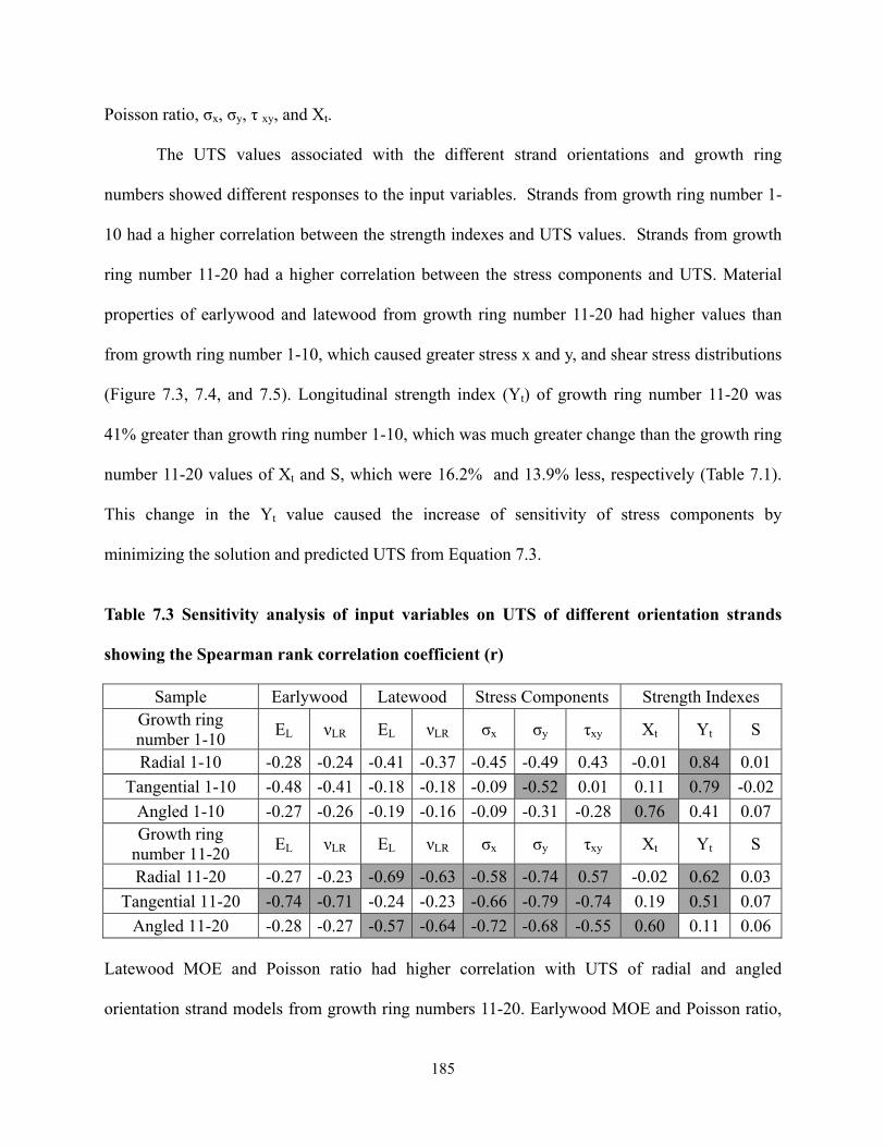
185

Poisson ratio, σx, σy, τ xy, and Xt.

The UTS values associated with the different strand orientations and growth ring

numbers showed different responses to the input variables. Strands from growth ring number 1-

10 had a higher correlation between the strength indexes and UTS values. Strands from growth

ring number 11-20 had a higher correlation between the stress components and UTS. Material

properties of earlywood and latewood from growth ring number 11-20 had higher values than

from growth ring number 1-10, which caused greater stress x and y, and shear stress distributions

(Figure 7.3, 7.4, and 7.5). Longitudinal strength index (Yt) of growth ring number 11-20 was

41% greater than growth ring number 1-10, which was much greater change than the growth ring

number 11-20 values of Xt and S, which were 16.2% and 13.9% less, respectively (Table 7.1).

This change in the Yt value caused the increase of sensitivity of stress components by

minimizing the solution and predicted UTS from Equation 7.3.

Table 7.3 Sensitivity analysis of input variables on UTS of different orientation strands

showing the Spearman rank correlation coefficient (r)

Sample Earlywood Latewood Stress Components Strength Indexes Growth ring number 1-10 EL νLR EL νLR σx σy τxy Xt Yt S

Radial 1-10 -0.28 -0.24 -0.41 -0.37 -0.45 -0.49 0.43 -0.01 0.84 0.01 Tangential 1-10 -0.48 -0.41 -0.18 -0.18 -0.09 -0.52 0.01 0.11 0.79 -0.02

Angled 1-10 -0.27 -0.26 -0.19 -0.16 -0.09 -0.31 -0.28 0.76 0.41 0.07 Growth ring

number 11-20 EL νLR EL νLR σx σy τxy Xt Yt S

Radial 11-20 -0.27 -0.23 -0.69 -0.63 -0.58 -0.74 0.57 -0.02 0.62 0.03 Tangential 11-20 -0.74 -0.71 -0.24 -0.23 -0.66 -0.79 -0.74 0.19 0.51 0.07

Angled 11-20 -0.28 -0.27 -0.57 -0.64 -0.72 -0.68 -0.55 0.60 0.11 0.06 Latewood MOE and Poisson ratio had higher correlation with UTS of radial and angled

orientation strand models from growth ring numbers 11-20. Earlywood MOE and Poisson ratio,

186

however, had higher correlation with the UTS of tangential orientation strand model. Compared

to the other orientation models, the physical geometry of tangential orientation strand models

showed that one individual latewood or earlywood band failure was more susceptible in similar

stress level to cause strand failure. The smallest longitudinal stress difference between earlywood

band and latewood band was shown in the tangential orientation models that evidenced the high

sensitivity of earlywood material properties on the UTS (Figure 7.3). Longitudinal strength index

(Yt) had a strong correlation with the UTS of radial and tangential orientation models because

the loading direction and fiber orientation were coincident. The transverse strength index (Xt)

had a strong correlation with the UTS of angled orientation models because the loading direction

and fiber orientation were not coincident.

Conclusions

Ultimate tensile strength (UTS) of different orientation wood strands was predicted from

homogeneous model, deterministic layer FEM models, and probabilistic SFEM models.

Comparison of average UTS from experimental and models indicated that homogeneous models

were not as accurate as layered FEM and SFEM models. Stress distributions associated with the

homogenous models were not representative for physical wood structures that composed of

earlywood and latewood bands. Tangential and angled grain orientation models showed greater

stress x distributions in earlywood bands and lower transverse stress distributions in latewood

bands. Radial, tangential, and angled grain orientation models showed lower longitudinal stress

distributions in earlywood bands and greater longitudinal stress distributions in latewood bands,

except for homogeneous models. The magnitude of shear stress from homogeneous and radial

grain orientation models showed 100 times lower than the shear stress from the tangential and

187

angled grain orientation models while tangential and angled grain orientation models showed

lower shear stress distributions in earlywood bands and greater stress distributions in latewood

bands. Comparison between cumulative probability of UTS from experimental test and that of

predicted UTS from SFEM found no significant difference. UTS of radial, tangential, and angled

orientation strands from the two different growth ring numbers showed a quite different

sensitivity on input variables showing that UTS from strands from growth ring number 1-10 had

a high sensitivity on strength indexes while UTS from strands from growth ring number 11-20

had a high sensitivity on stress components and strength indexes. Different grain orientation also

affected the sensitivity of UTS of different orientation strands. Longitudinal strength index (Yt)

had a strong correlation with UTS of radial and tangential orientation strands while transverse

strength index (Xt) had a strong correlation with UTS of angled orientation strand.

References

Bendtsen, B.A. 1978. Properties of wood from improved and intensively managed stands. Forest Prod. J. 28(10):61-72. Cave, I.D., J.C.F. Walker, 1994. Stiffness of wood in fast grownplantation softwoods: the influence of microfibril angle. Forest Prod. J. 44 (5): 43–48. Chakraborty S. and S. S. Dey 2000. Stochastic finite element simulation of uncertain structures subjected to earthquake. Shock and Vibration. 7(5):309 -320 Chung D. B., M. A. Gutiérrez and R. D. Borst. 2005. Object-oriented stochastic finite element analysis of fibre metal laminates. Computer Methods in Applied Mechanics and Engineering 194(12-16):1427-1446 Clouston, P. and F. Lam, 2002. A stochastic plasticity approach to strength modeling of strand-based wood composites. Composites Science and Technology, 62:1381-1395. Clouston P. 2007. Characterization and strength modeling of parallel-strand lumber. Holzforschung, 61:394-399. Eiermann M., O. G. Ernst and E. Ullmann. 2005. Computational aspects of the stochastic finite

188

element method. Proceeding of algoritmy. pp. 1-10. Ghanem R. G., P. D. Spanos. 1991. Stochastic Finite Elements: A Spectral Approach, Springer-Verlag. Ghanem R. G. 1999. Higher order sensitivity of heat conduction problems to random data using the spectral stochastic finite element method, ASME Journal of Heat Transfer, 121:290–299. Jeong G. Y., D. P. Hindman, and A. Zink-Sharp. 2008a. Tensile properties of earlywood and latewood from loblolly pine (Pinus taeda) using digital image correlation. Jeong G. Y., A. Zink-Sharp, and D. P. Hindman. 2008b. Comparison of longitudinal tensile properties of different grain orientation strands from loblolly pine (Pinus taeda). Jeong G. Y., D. P. Hindman, and A. Zink-Sharp. 2008c. Shear and transverse properties of loblolly pine (Pinus taeda) strands using tension test incorporated with digital image correlation (DIC). Jeong G. Y., D. P. Hindman. 2008d.Evaluation of effective elastic modulus of different orientation wood strands using stochastic finite element method. Jones R. M. 1975. Mechanics of composite materials. McGraw-Hill, New York Kasal B. and R. J. Leichti. 2005. State of the art in multiaxial phenomenological failure criteria for wood members. Progress in Structural Engineering and Materials 7(1):3-13 Kaminski M. 2002. Stochastic problem of fiber-reinforced composite with interface defects. Engineering computations. 19 (7) :854-868 Kleiber M., T. Hien, 1992. The Stochastic Finite Element Method. Basic Perturbation Technique and Computer Implementation. John Willey & Sons. Larson, P. R., D. E. Kretschmann, A. Clark III, and J. G. Isebrands. 2001. Juvenile wood formation and properties in southern pine. Gen Tech Rep FPL-GTR-129.: USDA Forest Prod Lab, Madison, WI Panshin, A. J., and C. D. Zeeuw. 1980. Textbook of wood technology. McGraw Hill Book Co., New York, NY. Smith, R. W., and D. G. Briggs. 1986. Juvenile wood:Has it come of age? Pages 1-11 in proc., Juvenile wood: What does it mean to forest management and forest products? Forest Products Research Society, Madison, WI. Wang, Y. T. and F. Lam. 1998. Computational modeling of material failure for parallel-aligned strand-based wood composites. J. Computational Material Science 11:157-165.

189

Chapter 8. Summary and Conclusion

The results from this study demonstrated the effect of intra-ring properties on the

mechanical behavior of wood strands incorporating strand cutting orientations and growth ring

positions. Each Chapter has a specific contribution to this dissertation. Chapter 1 shows the

background and goal of this project. A comprehensive literature from Chapter 2 serves as the

basis of the literature reviews in Chapters 3 through 7. Loblolly pine earlywood and latewood

properties from growth ring numbers 1-10 and growth ring numbers 11-20 were measured in

Chapter 3. Mechanical properties of radial, tangential, angled, and cross grain orientation strands

from the two growth ring numbers were measured in Chapter 4 and 5. The results from Chapter 3

are used as input variables for development of stochastic finite element method (SFEM) models

for different orientation strands (radial, tangential, and angled grain orientation) in Chapter 6 and

7. The results from Chapter 4 and 5 are used as validation of predictions from Chapter 6 and 7.

Effective elastic modulus of the different orientation strands and sensitivity of the input variables

are evaluated in Chapter 6. Ultimate tensile strength of the different orientation strands and

sensitivity of the input variables are evaluated in Chapter 7. The following conclusions have been

made based on the results from Chapter 3 to Chapter 7.

Tensile Properties of Earlywood and Latewood Using DIC (Chapter 3)

The physical and mechanical properties of earlywood and latewood from the two

different growth ring positions were measured using DIC.

In general, specific gravity, MOE, UTS, and Poisson ratio generally increased with the

increment of the growth ring positions except for specific gravity and UTS from

190

latewood.

While the MOE for earlywood and latewood was not dependent on specific gravity, UTS

for earlywood and latewood was highly dependent on specific gravity.

Combining current results and Kretschmann et al. (2006), MOE from earlywood and

latewood showed a positive relationship with the height of material in the tree.

Statistical comparisons showed that the MOE and UTS had a significant difference from

the factor of growth ring number and intra-ring position.

Distribution fitting of MOE for Earlywood 1-10, Latewood 1-10, Earlywood 11-20, and

Latewood 11-20 was best fitted by the Weibull distribution. Poisson ratios were best

fitted by Weibull distribution for Earlywood 1-10 and Latewood 11-20 groups and

Gamma distribution for Earlywood 11-20 and Latewood 1-10 groups.

Strain distribution showed non-uniform distributions for the four groups. Compared to

Earlywood 1-10 and Latewood 1-10, Earlywood 11-20 and Latewood 11-20 showed

more resistance to the load indicating more oriented structure and reinforcement to the

longitudinal direction.

Longitudinal Elastic Properties of Different Orientation Loblolly Pine Strands (Chapter 4)

Tensile properties of radial and tangential grain orientations of wood strands from growth

ring numbers 1-10 and growth ring numbers 11-20 were measured using DIC.

As growth ring number increased, MOE and UTS from radial and tangential grain

orientation strands increased.

Radial 1-10 strands had a lower MOE and UTS than Tangential 1-10 strands. Radial 11-

20 strands had a higher MOE and UTS than Tangential 11-20 strands.

191

Tangential grain orientation strands had higher Poisson ratios than radial grain orientation

strands.

Although Radial 1-10, Radial 11-20, Tangential 1-10, and Tangential 11-20 strands had a

different percentage of three particular failure behaviors, more mature wood had a more

organized structure to show more consistent failure behavior.

Statistical comparisons of MOE and UTS from radial grain orientation strands were

significantly different between growth ring numbers, while MOE and UTS from

tangential grain orientation strands were not significantly different between growth ring

numbers.

Statistical comparisons also showed that there was no significant difference of MOE

between the radial and tangential orientation strands. For UTS, the comparisons between

Radial 1-10 and Radial 11-20 strands and the comparison between Radial 11-20 and

Tangential 11-20 strands were significantly different.

For distribution fitting from MOE, Radial 1-10, Radial 11-20, and Tangential 11-20

strands were best fitted with Weibull distribution except for Tangential 1-10 fitted with

Lognormal distribution. For UTS, while Radial 1-10 and Radial 11-20 group followed

Weibull distribution, Gamma distribution for Tangential 1-10 and Lognormal

distribution for Tangential 11-20 were best fitted curve. For Poisson ratio, Radial 11-20

strands did not match with any distribution curve. Radial 1-10, Tangential 1-10, and

Tangential 11-20 strands followed Lognormal, Gamma, and Weibull distribution,

respectively.

Comparing current test results to Cai et al. (2007) and Hindman and Lee (2007), MOE

and UTS of wood strands had higher correlations with thickness than specific gravity.

192

Transverse and Shear Properties of Loblolly Pine Strands (Chapter 5)

Transverse elastic properties, shear properties, and UTS of loblolly pine strands from

growth ring numbers 1-10 and growth ring numbers 11-20 were measured using tension test

incorporating DIC.

MOE of angled grain strands increased as the growth ring number increased while MOE

of cross-grain strands decreased 1% as the growth ring number increased. MOE of cross

grain strands was more sensitive to the orientation of strands than specific gravity.

UTS of angled grain strands increased as the growth ring number increased, while UTS

of cross-grain strands decreased as the growth ring number increased. The UTS was

dependent upon grain orientations of strands rather than specific gravity.

Shear modulus increased as the growth ring number increased, but shear strength

decreased as the growth ring number increased. Lower shear strength values can be

speculated as a higher elastic constant ratio of strands from growth ring numbers 11-20.

Poisson ratio from angled grain strands decreased with increasing growth ring numbers.

However, Poisson ratio from cross-grain strands slightly increased with the increment of

growth ring numbers.

COV values from MOE, UTS, Poisson ratio, and shear strength decreased as growth ring

number increased. Based on the lower variation of mechanical properties, more uniform

structure of strands from growth ring numbers 11-20 can be speculated.

Statistical distribution fitting showed that shear strength values were best fitted with

Gamma distribution. MOE values from Angled 1-10, Angled 11-20, and Cross 11-20

followed Lognormal distributions, while MOE values from Cross 1-10 followed a

Weibull distribution. UTS values from four groups did not follow any specific

193

distribution. Poisson ratio values from Angled 1-10, Cross 1-10, and Cross 11-20

followed Normal distribution, while Angled 11-20 followed Lognormal distribution.

Although four groups of strands showed mixed failure modes, strands from growth ring

numbers 11-20 showed a more consistent failure mode. The consistency in failure mode

indicated that strands from growth ring numbers 11-20 showed less variations in

structures compared to the strands from growth ring numbers 1-10.

Comparing the MOE, UTS, and shear strength from both experimental and orthotropic

transformation, conservative predicted values from the orthotropic transformation were

obtained.

Effective Elastic Modulus of Different Orientation Strands Using SFEM (Chapter 6)

Tensile properties of different orientation wood strands were evaluated using

deterministic FEM and SFEM models. While the deterministic models used average material

properties of earlywood and latewood, SFEM models used the distribution of material properties

of earlywood and latewood from growth ring numbers 1-10 and growth ring numbers 11-20.

While the homogeneous model predicted the average MOE well for radial and tangential

grain orientation strand from growth ring numbers 1-10, the physical strain distribution

showed an unrealistic behavior.

In general, the predicted average MOE of strands from the deterministic layer FEM and

SFEM was better than the homogeneous models.

From strain distribution analysis, different strain distribution for earlywood and latewood

layers occurred by different grain orientations. Homogeneous and radial orientation

models, however, showed iso-strain distribution in y direction, which resulted in the

194

same MOE values.

Comparison of cumulative probability curves from experimental test and SFEM agreed

well. The difference of variation of MOE from different grain strands between

experimental results (Chapter 4 and Chapter 5) and SFEM results ranged from 0.96% to

22.31%.

From sensitivity analysis, earlywood and latewood participated differently to MOE of

different grain orientation strand models, which is highly associated with the strain

distribution caused by different orientation strands and interaction of input parameters.

In general, earlywood MOE had a greater effect on MOE of wood strands than other

input parameters.

Ultimate Tensile Strength (UTS) of Different Orientation Strands Using SFEM (Chapter 7)

Ultimate tensile strength (UTS) of different orientation wood strands was predicted from

homogeneous model, deterministic layer FEM models, and probabilistic SFEM models.

Comparison of average UTS from experimental and models indicated that homogeneous

models were not as accurate as layered FEM and SFEM models.

Stress distributions associated with the homogenous models were not representative for

physical wood structures that composed of earlywood and latewood bands.

Comparison between experimental and SFEM agreed well with the UTS from different

orientation strands ranging from 0.09% and 11.09%.

UTS of different orientation strands from the two different growth ring numbers showed

a quite different sensitivity on input variables showing that UTS from strands from

growth ring number 1-10 had a high sensitivity on strength indexes while UTS from

195

strands from growth ring number 11-20 had a high sensitivity on stress components and

strength indexes.

Different grain orientation also affected the sensitivity of UTS of different orientation

strands. Longitudinal strength index (Yt) had a strong correlation with UTS of radial and

tangential orientation strands while transverse strength index (Xt) had a strong

correlation with UTS of angled orientation strand.

Overall Conclusions of Research

Different elastic properties of earlywood and latewood from the two different growth ring

positions affected the mechanical properties of strands. Mechanical properties of strands were

influenced by different orientation wood strands and growth ring numbers. With the difference of

earlywood and latewood and the different orientation, stress and strain distributions of strands

showed a distinctive pattern. Homogeneous models could not represent the physical stress and

strain distributions while SFEM for different orientation strand models incorporating the

variation of the mechanical properties of earlywood and latewood could represent the physical

stress and strain behavior of wood strands. With the different stress and strain distribution

sensitivity of mechanical properties of wood strands was changed. Earlywood MOE was the

most important parameter to maximize the effective MOE of strands. Longitudinal strength index

(Yt) had a strong correlation with UTS of radial and tangential orientation strands while

transverse strength index (Xt) had a strong correlation with UTS of angled orientation strand.

This hierarchical approach showed if material properties of earlywood and latewood, and

orientation of wood strands can be manipulated, the final MOE and UTS of wood strands can be

controlled.

196

Limitations

The following limitations were found from the scope of this study.

DIC measured only longitudinal elastic properties and one major Poisson ratio from

earlywood and latewood while microfibril angle (MFA) and other physical structure of

earlywood and latewood were cited from previous studies.

Six elastic properties (EL, ER, GLR, υLR, υLT, and υRT) and three strengthes (σL, σR, and

τLR) were measured and three elastic properties (ET, GLT and GRT) and three strengthes

(σT, τLT, and τRT) were missed.

SFEM used analytical distributions from the experimental results rather the exact

distribution from the experimental tests.

SFEM used a plane stress assumption, which could be expanded to a three dimensional

orthotropic problem with measured material properties.

SFEM model used an average volume fraction and assumed no slippage between the

earlywood and latewood bands.

SFEM model for prediction of UTS assumed that the strength indexes were independent

each other, which could have some correlation between strength indexes.

Recommendations for Future Research

This study was originally initiated to establish the link between mechanical behavior of

loblolly pine strands and the mechanical properties of earlywood and latewood by developing

different orientation strand models and measuring earlywood and latewood properties. With the

developed models and newly designed testing methods, this research could be directly expanded

to evaluate the mechanical properties of other wood species and natural fiber sources. A novel

197

DIC testing set up could be expanded to examine a similar micro-scale analysis such as the

mechanical behavior of glue lines, micromechanical fracture testing, micromechanical shear

testing, and other micromechanical testings. Also this testing set-up has the capability of adding

other devices such as the Raman microscope which could examine the relationship between

major chemical components of wood (cellulose, hemicelluloses, and lignin) with mechanical

properties of wood. The developed DIC testing set-up for strands could measure nine elastic

properties including elastic modulus (EL, ER, and ET), Poisson ratio (νLR νRL and νRT), and shear

modulus (GLR, GLT, and GRT) of different wood species. The DIC testing set-up could expand for

fracture testing, connection testing, and other macro size testings. Although this research has

connected one length scale to other length scale, there are still many missing links between

different length scales. This research could be expanded to examine how properties of earlywood

and latewood affect the mechanical properties of strand based composites. This research could

also be expanded to understand how silvicultural activities affect earlywood and latewood, wood

strands, and strand based composite properties.

198

Appendix 1.

Comparison of Elastic Constants Generated from Plate Tests to Bending Tests

Gi Young Jeong Graduate Research Assistant

Department of Wood Science and Forest Products Virginia Polytechnic Institute and State University

Brooks Forest Products Center 1650 Ramble Road

Blacksburg, VA 24061-0503

Daniel P. Hindman Assistant Professor




Notice - Appendix 1 appears in the Forest Product Journal, 58(9):53-58.

199

Abstract

Many different test methods have been used to evaluate the elastic constants and elastic

constant ratios of solid sawn lumber and structural composite lumber (SCL). Previous work has

noted that the elastic constant ratios of solid sawn lumber and SCL are different. However, no

direct comparison of current bending test methods and previously used plate bending and

twisting methods has been performed. This study conducted plate bending and twisting tests to

determine the longitudinal modulus of elasticity and in-plane shear modulus of MSR and PSL

materials. Samples were taken from the same material previously tested by Hindman et al.

(2006) The E:G ratios from MSR plate testing were 40% less than values from ASTM D 198

Bending and the five point bending test (FPBT), while the E:G ratios from PSL plate testing

showed no consistent trend. Statistical comparisons of the E and G values found that the MSR E

values for all three tests and the PSL G values from plate testing and ASTM D 198 Bending were

not significantly different. The differences in elastic constant ratios and comparison of the

elastic constants indicate that the elastic behavior of MSR and PSL is different. Therefore,

elastic constant ratios derived from plate testing methods for MSR and PSL are not directly

comparable to elastic constant ratios derived from structural sized bending tests.

200

Previous researchers have found differences in the elastic constants and elastic constant

ratios of structural size solid-sawn lumber and SCL materials using a variety of bending and

torsion test methods. These test methods have been compared to elastic constant ratio of 16:1

found in the Wood Handbook (USDA 1999) and Bodig and Jayne (1982). This value is an

average of many different wood species tested using plate bending and twisting tests (Bodig and

Goodman 1973). Plate bending and twisting tests were performed on clear sections of wood

laminated together to achieve different directional orientations (Bodig and Goodman 1973).

Recent studies to evaluate the shear modulus of solid-sawn lumber and SCL materials have

focused on structural sized lumber only. The discrepancy between small sized samples from

plate bending and twisting compared to structural sized samples in bending has not been

previously explored.

Currently, there is no specific guideline to determine the material properties of SCL

products. ASTM D 5456 (ASTM 2005a) is the standard governing SCL products and gives no

guidance on the test methods to use for shear modulus evaluation. The only mention of test

methods is a reference to ASTM D 198 (ASTM 2005b), which is the test standard for structural

sized lumber. Previous findings (Janowiak et al. 2001, Hindman et al. 2006, Harrison and

Hindman 2007) have recommended that the shear modulus test method be similar to the intended

loading of the member. While these previous studies compared the shear modulus and elastic

constant ratios developed to solid wood results from Bodig and Goodman (1973), no testing of

equivalent materials using the plate bending and plate twisting test methods was performed.

Table 1 shows the modulus of elasticity and shear modulus values determined from

different studies for solid wood, solid-sawn lumber and parallel strand lumber (PSL). Bodig and

Goodman (1973) performed plate bending and plate twisting tests on an extensive number of

201

softwood and hardwood specimens. These test results are summarized by Bodig and Jayne

(1982) and in the Wood Handbook (USDA 1999).

Table 1. MSR and PSL Elastic and Shear Modulus Values from Previous Studies

Researcher Material Test Method Average E, GPa (106 psi)

Average G, GPa (106 psi)

Bodig and Goodman 1972

Loblolly pine (P. taeda)

Plate bending/twisting 11.1 (1.61) 0.903 (0.131)


Longleaf pine (P. palustris)



Slash pine (P. elliottii)


Hindman 2006 MSR lumber (Pinus spp.) FPBT 16.1 (2.35) 0.748 (0.109)

Hindman 2006 MSR lumber (Pinus spp.)

ASTM D 198 Bending 17.2 (2.51) 0.800 (0.16)

Harrison and Hindman 2007

MSR lumber (Pinus spp.)

ASTM D 198 Bending 17.4 (2.53) 0.903 (0.131)


MSR lumber (Pinus spp.)

ASTM D 198 Torsion N/A 1.16 (0.168)


MSR lumber (Pinus spp.) FPBT 17.5 (2.54) 0.789 (0.114)

Hindman et al. 2006 PSL (Pinus spp.) FPBT 13.4 (1.96) 0.727 (0.106)

Hindman et al. 2006 PSL (Pinus spp.) ASTM D 198

Bending 12.4 (1.81) 1.03 (0.149)

Recent research comparing the elastic modulus, shear modulus and elastic constant ratios

from different test methods has been performed by Hindman et al. (2006) and Harrison and

Hindman (2007). Hindman et al. (2006) compared results from ASTM D 198 Bending and five

point bending test (FPBT) to determine the elastic constants of SCLs and to compare the test

methods. The ASTM D 198 (2005b) bending test consists of testing three-point bending

specimens at different length to height aspect ratios to determine the elastic and shear modulus

simultaneously. The FPBT is a novel test method proposed by Bradtmueller et al. (1994) as an

202

alternative method for shear modulus measurement. Harrison and Hindman (2007) compared

the ASTM D 198 Bending, ASTM D 198 Torsion and the FPBT for MSR lumber and LVL.

ASTM D 198 Torsion is another ASTM D 198 (2005b) method to measure shear modulus that

uses a torsion loading and angle measurement. Trends from both of these papers demonstrated

that there is no consistent pattern of equivalency between the elastic constants and elastic

constant ratios measured using different test methods.

The results in Table 1 demonstrate some of the trends previously observed in the study of

solid wood, solid-sawn lumber and parallel strand lumber (PSL). While it is difficult to make a

direct comparison between the results of Bodig and Goodman (1973) and current species group

assignments used for solid-sawn lumber, three of the four species currently included in the

southern pine species group are given. From Bodig and Goodman (1973), the modulus of

elasticity values ranged from 11.1 GPa to 16.0 GPa (1.61x106 psi to 2.32 x 106 psi) and the shear

modulus values ranged from 903 MPa to 1.04 GPa (1.28 x 105 psi to 1.51 x 105 psi). Comparing

the range of Bodig and Goodman (1973) values to the ASTM D 198 Bending, the modulus of

elasticity values were greater than the range, while the shear modulus values were within the

range or slightly below it. Comparing the range of Bodig and Goodman (1973) values to the

FPBT results, the modulus of elasticity was within or greater than the range of values, while the

shear modulus was less than the range. The ASTM D 198 Torsion value was much higher than

the range of values from Bodig and Goodman (1973). Due to the differences in the loading

conditions, the different test methods may not produce the same results. This study measured

the elastic and shear modulus of MSR lumber and PSL materials using plate bending and ASTM

D 3044 plate twisting test for comparison to previous testing results of ASTM D 198 Bending

and FPBT from Hindman et al. (2006).

203


MSR and PSL materials used for this testing were taken from an untested subset of the

material used by Hindman et al. (2006). MSR lumber was southern pine (Pinus spp.) 2250f-1.9E

with a modulus of elasticity of 13.1 GPa (1.90 x 106 psi). PSL was 2.0E rated southern pine

(Pinus spp.) with a modulus of elasticity of 13.8 GPa (2.0 x 106 psi). Specimens were cut to

40.6 cm long by 20.3 cm wide by 8.89 mm high (16.0 in by 8.0 in by 0.35 in) for the plate

bending test. Ten specimens from each material were tested. After the plate bending test was

complete, the specimens were cut in half to a size of 20.3 cm long by 20.3 cm wide by 8.89 mm

high (8.0 in x 8.0 in x 0.35 in) for ASTM D 3044 plate twisting test (ASTM 2005c). All

specimens were labeled and stored in an environmental chamber at 20 degrees C and 65%

relative humidity. After plate twisting testing was completed, moisture content and specific

gravity samples were measured according to ASTM D 2395 (ASTM 2005d) and ASTM D 4442

(ASTM 2005e). Table 2 summarizes the rated modulus of elasticity as well as the resultant

moisture content and specific gravity. Materials tested by Hindman et al. (2006) have a specific

gravity of 0.56 for MSR and 0.66 for PSL, demonstrating that these materials are similar to those

previously tested.

Table 2. Summary of test materials

Test material Rated E, GPa (psi)

Moisture content (%), (COV)

Specific gravity, (COV)

2250f-1.9E Southern Pine MSR 13.1 (1.9ｘ106) 11.6 (3.10%) 0.62 (8.15 %)

2.0E Southern Pine PSL 13.8 (2.0ｘ106) 11.0 (3.05 %) 0.71 (5.12 %)

204

Plate Bending Test

The determination of orthotropic elastic constants using plate bending and plate twisting methods

was originally developed by Witt et al. (1953). The plate bending test uses a three point loading

on the top of the plate and a three point support on the bottom of the plate placed in an anti -

symmetric pattern. Figure 1 shows a schematic drawing of the plate bending samples indicating

the position of the loading, support and deflection measurement points. This configuration

allows the plate to have a constant bending moment in the center and no bending moment at the

three supports. Due to the large difference in stiffness between the parallel to grain direction and

perpendicular to grain direction, a correction factor must be applied using an alternative beam

theory (Gunnerson et al. 1972).

A B

Bottom

Top

= Load Point= Support Point= Deflection Reading29.20 cm (11.45 in)

14.6 cm (5.75 in)

7.30 cm(2.87 in)

14.6 cm(5.75 in)

14.6 cm (5.75 in)

P/2

P/4

P/4

7.30 cm(2.87 in)

Grain Dir.

Grain Dir.

Figure 1. Schematic Drawing of Plate Bending Sample

Figure 2 shows a plate bending specimen being tested. The loading speed was set to

0.0762 cm/min (0.03 in/min). Two Trans-Tek 351-0000 linear variable differential transformers

(LVDT)

measure

modulus

E

applied t

at A. Th

of the pla

where

P/∆= load

L = span

I = mome

(range of 5.

the displace

of plate.

Equation 1 sh

o the plate.

his is the corr

ate, or 29.20

d-deflection

length of pl

ent of inertia

.08 mm (0.2

ement at the

hows the cal

The deflect

rection facto

0 cm (11.45 i

n curve

late

a = width * h

Figure 2

20 in.) and s

point A and

culation of t

ion ∆ is equ

or discussed

in.).

⎜⎝⎛Δ

=PE

height3/12

. Plate Bend

205

sensitivity o

d B under el

the modulus

ual to the def

by Gunners

⎟⎟⎠

⎞⎜⎜⎝

⎛⎟⎠⎞

Δ ILP

76811 3

ding Sample

f 0.0091 mm

lastic range

of elasticity

fIection at B

son et al. (19

e During Te

m (0.0025 in

for the calc

y. The load P

minus one h

972). The len

esting

n.)) were us

culation of e

P is the total

half of defle

ngth L is the

(1)

sed to

lastic

l load

ection

span

)

206

ASTM D 3044 Plate twisting

Plate twisting test procedures are detailed in ASTM D 3044 (ASTM 2005c). Figure 3

shows the anticlastic plate twisting, where two diagonal corners of a square plate are supported

and the other two diagonal corners are loaded. To avoid edge damage from the concentrated

loads at each corner, small metal plates were clamped to the top and bottom of each corner. An

MTS test machine applied a displacement rate of 0.0762 cm/min (0.03 in/min) to the specimen.

Deflection was taken as the difference of the movement between the two diagonals as described

in ASTM D 3044 (ASTM 2005c). Deflection was measured using an LVDT (range of 5.08 mm

(0.20 in.) and sensitivity of 0.0091 mm (0.0025 in.)) attached to a metal jig to measure the

difference between the diagonal deflections. Equation 2 shows the calculation of the shear

modulus.

⎟⎟⎠

⎞⎜⎜⎝

⎛⎟⎠⎞

⎜⎝⎛Δ

= 3

25.1h

uPG (2)

where

P/∆ = load-deflection curve

u = distance from the center of plate to the point where the deflection was measured.

h= thickness of plate

L

both plat

Excel to

specimen

elastic ra

define th

crosshead

twisting

0.254cm

Plate ben

T

coefficien

modulus

Figu

Load and def

te bending a

plot the loa

n and the lo

ange of the

he maximum

d were limi

test, the ma

(0.1 in), res

nding and AS

Table 3 sum

nt of variati

of elasticity

ure 3. ASTM

flection infor

and plate tw

ad-deflection

oad-deflectio

specimens,

m loading. F

ited to 444.

aximum load

spectively.

STM D 3044

mmarizes the

ion from th

y of PSL wa

M D 3044 Pla

rmation were

wisting test m

n (P/∆) curv

on curves w

several plyw

For the plate

8N (100 lb)

d and deflect

Results

4 plate twisti

e modulus

e plate bend

as higher th

207

ate Twisting

e collected u

methods. A

ve. Three l

were average

wood specim

e bending te

) and 0.254

tion of cross

and Discus

ing results

of elasticity

ding and AS

an that of M

g Specimen

using the TE

All test data

oading repe

d. To ensu

mens of sim

est, the maxi

cm (0.1 in)

shead were

ssion

y and shear

STM D 304

MSR while t

Under Load

EST WORK

were expor

etitions were

ure all loads

milar stiffnes

imum load a

), respective

limited to 4

r modulus

44 plate twi

the shear mo

d

3.09 softwar

rted to Micr

e applied to

were withi

ss were test

and deflectio

ely. For the

4.4N (10 lb

values inclu

isting tests.

odulus of P

re for

rosoft

each

n the

ed to

on of

plate

) and

uding

The

SL is

208

much lower than that of MSR. The modulus of elasticity COV values of MSR and PSL were

18.8% and 11.48 %, respectively, while the shear modulus COV values for MSR and PSL were

11.34% and 7.58%, respectively. For both elastic constants, the COV of the MSR value was

greater than the PSL value. The E:G ratio for MSR was 12.9 while the E:G ratio for PSL was

17.8. The measured moduli of elasticity were greater than the rated E for both materials.

Table 3. Test results from plate bending and plate twisting test

Material Modulus of Elasticity1, GPa (106 psi) [COV]

Shear Modulus2, GPa (106 psi) [COV]

E:G ratio3

MSR 14.7 (2.15) [18.8]

1.13 (0.165) [11.3]

12.9:1

PSL 15.2 (2.22) [11. 5]

0.85 (0.124) [7.58]

17.8:1

1 Modulus of elasticity was measured using plate bending test methods. 2 Shear modulus was measured using plate twisting test methods. 3 E:G ratio refers to the E1:G12 ratio. Comparison of E:G Ratios with Previous Results

Table 4 shows the comparison of the E:G ratio of MSR and PSL from plate testing with

the results from Hindman et. al (2006). These results are directly comparable since the test

materials of both studies were sampled from the same population. For MSR, the E:G ratio from

plate testing was 40.1% less than the FPBT ratio and 40.4% less than the ASTM D 198 Bending

ratio. For PSL, the E:G ratio from plate testing was 3.83% less than the FPBT ratio and 46.8%

greater than the ASTM D 198 Bending ratio. The plate testing results shows a different elastic

relationship for MSR lumber and PSL material. The MSR E:G ratio from plate testing is

consistently 40% less than the other test method ratios from structural-sized bending tests, while

the PSL has a different relationship. Hindman et al. (2006) and Harrison and Hindman (2007)

reasoned that the change in E:G ratio was caused by differences in stress distribution combined

209

and the vertical density profile for wood composites. Gunnerson et al. (1972) demonstrated that

the stress distribution of the plate bending specimen is different from a simple beam due to the

high orthotropy of wood materials.

Table 4. Comparison of the measured E1:G12 ratios and Hindman et al. (2006)

Material

Plate Testing

E:G Ratio

Hindman et al. (2006) % Difference of Plate Testing and FPBT1

% Difference of Plate Testing and

ASTM D 198 Bending2

FPBT E:G

Ratio

ASTM D 198 Bending

E:G Ratio MSR 12.9:1 21.6:1 21.7:1 -40.1% -40.4% PSL 17.8:1 18.5:1 12.1:1 -3.83% 46.8%

1% Difference = (Plate test – FPBT)/FPBT * 100%

2% Difference = (Plate test – ASTM D 198 Bending)/ASTM D 198 Bending * 100%

Table 5 presents the statistical comparison of the elastic modulus and shear modulus

results comparing previous research to plate bending results. The analysis of variance (ANOVA)

statistical test used an alpha of 0.05 for comparing three different test methods with different

sample sizes. The null hypothesis was not rejected for the MSR E values from the three test

methods. The Plate Testing vs. ASTM Bending comparison for the PSL G value also did not

reject the null hypothesis. In general, the trend of the shear modulus values and modulus of

elasticity from PSL was to reject the null hypothesis, indicating that the elastic constant values

from the different test methods were significantly different. This statistical comparison

demonstrates that the elastic behavior of MSR lumber is different from PSL, which was

previously noted by Janowiak et al. (2001).

210

Table 5. Statistical comparison of E1 and G12 from three different test methods (α=0.05)

Tests for Comparison Material p-value for E p-value for G

Plate Tests vs. FPBT1 MSR 0.262 0.000 PSL 0.037 0.000

Plate Tests vs. ASTM Bending2 MSR 0.204 0.010 PSL 0.000 0.182

Plate Tests vs, FBPT vs. ASTM Bending MSR 0.369 0.000 PSL 0.001 0.004

1 Sixteen data points from Hindman et al. (2006)

2 Eight data points from Hindman et al. (2006)

Comparison of MSR Lumber with Previous Plate Testing Results

Table 6 shows the comparison of selected southern pine species test results from Bodig

and Goodman (1973) with the results from this study. The elastic constants of longleaf pine (P.

palustris) were the closest to the test results, with a modulus of elasticity 7.4% less than the

average MSR value and a shear modulus 8.7% less than the average MSR value. The E1:G12

ratio for three southern pine groups varied from 12.27 to 18.08. The E1:G12 ratio of MSR was in

the range of the ratios given by Bodig and Goodman (1973). .

Table 6 Comparison of the test results to Bodig and Goodman (1973)

Elastic Property

Current MSR Value

Loblolly Pine (P. taeda)

Longleaf Pine (P. palustris)

Slash Pine (P. elliottii)

Value1 % Diff.2 Value1 % Diff.2 Value1 % Diff.2

E1 14.7 GPa 11.1 GPa -24.8% 14.6 GPa -7.4% 16.0 GPa 8.2%

G12 1.13 GPa 903 MPa -20.6% 1.04 GPa -8.7% 883 MPa -22.3%

E1:G12 13.0:1.0 12.3:1.0 -5.3% 14.1:1.0 8.7% 18.1:1.0 39.5% 1 values from Bodig and Goodman (1973) 2 % Difference = (Previous Result-MSR)/MSR*100%

211

Conclusions

This research studied the elastic constants measured from plate testing methods versus

ASTM D 198 Bending and the five-point bending test for MSR lumber and PSL. The elastic

constant ratios of MSR lumber from the plate testing methods demonstrated a consistent

difference with both the ASTM D 198 Bending and FPBT test methods. PSL elastic constant

ratios from the plate testing methods did not show a consistent relationship between the two test

methods, indicating that the MSR lumber and PSL demonstrate different elastic behaviors

possibly due to the manufacture of PSL materials. Statistical comparisons of the modulus of

elasticity and shear modulus values indicated that the three test methods produce values that are

not significantly different for the MSR modulus of elasticity values and between the plate testing

and ASTM Bending for the PSL shear modulus. Except for the above comparisons, the three test

methods produced values that were significantly different for the MSR shear modulus and for the

PSL modulus of elasticity and shear modulus. Therefore, elastic constant ratios derived from

plate testing methods for MSR and PSL are not directly comparable to elastic constant ratios

derived from structural sized bending tests. Comparing the MSR lumber values to Bodig and

Goodman (1973), the MSR lumber elastic constants were similar to longleaf pine (P. palustris).

References

American Society for Testing and Materials (ASTM). 2005a. Standard Specification for Evaluation of Structural Composite Lumber Products. Standard D 5456-03. In: Annual Book of ASTM Standard, Section 4, Vol. 04.10 Wood. ASTM, West Conshohocken, PA. American Society for Testing and Materials (ASTM). 2005b. Standard Test Methods of Static Tests of Lumber in Structural Sizes. Standard D 198-02. In: Annual Book of ASTM Standard, Section 4, Vol. 04.10 Wood. ASTM, West Conshohocken, PA.

212

American Society for Testing and Materials (ASTM). 2005c. Standard Test Methods for Shear Modulus of Wood-Based Structural Panels. Standard D 3044-94. In: Annual Book of ASTM Standard, Section 4, Vol. 04.10 Wood. ASTM, West Conshohocken, PA. American Society for Testing and Materials (ASTM). 2005d. Standard Test Methods for Specific Gravity of Wood and Wood-Based Materials. Standard D 2395-02. In: Annual Book of ASTM Standard, Section 4, Vol. 04.10 Wood. ASTM, West Conshohocken, PA American Society for Testing and Materials (ASTM). 2005e. Standard Test Methods for Direct Moisture Content Measurement of Wood and Wood-Based Materials. Standard D 4442-92. In: Annual Book of ASTM Standard, Section 4, Vol. 04.10 Wood. ASTM, West Conshohocken, PA. Bodig, J. and , J. R. Goodman. 1973. Prediction of elastic parameters for wood. Wood Sci. 5(4): 249-264. Bodig, J. and B. A. Jayne. 1982. Mechanics of Wood and Wood Composites. Van Nostrand Reinhold Company, New York, NY. 714 pp. Bradtmueller, J. P., M. O. Hunt, K. J. Fridley and G. P. McCabe. 1994. Development of the five-point bending test to determine shear moduli of wood composites. Forest Prod. J. 44(5):17-26. Gunnerson, R. A., J. R. Goodman and J. Bodig. 1972. Plate Tests for Determination of Elastic Parameters of Wood. Wood Sci. 5(4): 241-248. Harrison, S. K. and D. P. Hindman. 2007. Test Method Comparison of Shear Modulus Evaluation of MSR and SCL Products. Forest Prod. J. 57 (7). In Press. Hindman, D. P., J. J.Janowiak and H. B. Manbeck. 2006. Comparison of ASTM D 198 and five-point bending for elastic constant ratio determination. Forest Prod. J. 56(7):85-90. Janowiak, J. J., D. P. Hindman, H. B. Manbeck. 2001. Orthotropic behavior of lumber composite materials. Wood and Fiber Sci. 33(4):580-594. USDA Forest Service, Forest Products Laboratory. 1999. Wood Handbook: Wood as an engineering material. Forest Prod. Soc., Madison, WI. 463 pp. Witt, R. K., W. H. Hoppmann, and R. S. Buxbaum. 1953. Determination of Elastic Constants of Orthotropic Materials with Special Reference to Laminates. ASTM Bulletin: 53-57

213

Appendix 2.

Effect of loading rate and thickness on the tensile properties of wood strands

Gi Young Jeong Graduate Research Assistant




Daniel P. Hindman* Assistant Professor




David Finkenbinder Graduate Research Assistant




Jong N. Lee Staff Engineer

APA-The Engineered Wood Association 7011 South 19th St. Tacoma, WA 98466

Zhiyuan Lin

Graduate Research Assistant Department of Wood Science and Forest Products Virginia Polytechnic Institute and State University



Notice –This appendix appears in the Forest Product Journal, 58(10):33-37.

214

Abstract

Previous studies evaluating the tensile properties of wood strands used different test

conditions and different wood species. Direct comparison of these results cannot be performed.

Guidelines for the standardized testing of wood strands are not currently available. Specifically,

there is no information on the effect of different loading rates and strand sizes for the tensile

properties of wood strands. The goal of this paper was to investigate the effect of loading rate

and strand thickness on tensile modulus of elasticity (MOE) and ultimate tensile strength (UTS)

of southern pine (Pinus spp.) strands. Tensile testing used three different loading rates (0.0102

cm/min, 0.0254 cm/min, and 0.0406 cm/min) and four different specimen thicknesses (0.0381

cm, 0.0794 cm, 0.191 cm, and 0.381 cm). Results showed the UTS and MOE of wood strands

generally increased as the thickness increased except for the 0.381 cm thick strands. All of the

0.381 cm strands showed slippage in the grip areas of the specimens, which caused lower

average MOE value for this group. Statistical analysis showed that the MOE and UTS from

different loading rates were not significantly different, while the MOE and UTS from different

strand thicknesses were significantly different. Results of Tukey’s HSD comparisons found that

MOE and UTS values from the 0.0794 cm and 0.191 cm thick strands were not significantly

different. To decrease variability of test results, the authors recommend testing strands at 0.0254

cm/min and a strand thickness between 0.0794 cm and 0.191 cm.

215

Wood strands are the main constituents of engineered wood products (EWP) including

laminated strand lumber (LSL), parallel strand lumber (PSL), oriented strand lumber (OSL) and

oriented strand board (OSB). Strand thickness for these EWPs can vary from 0.76 mm to 3.0

mm (Smulski 1997). Currently, there is no test protocol for measurement of the tensile

properties of wood strands. While previous studies have measured tensile properties of strands,

these results cannot be directly compared because of differences in specimen size, loading rate

and wood species. The strand geometry and test methods may affect the tensile properties of

wood strands. This study investigates the effect of loading rate and strand thickness on the

tensile properties of wood strands.

While there are no ASTM standards for the tensile testing of wood strands, several

previous researchers have measured the tensile properties. Table 1 lists previous tensile testing

results including the parent wood species, dimensions, loading rate, specific gravity, ultimate

tensile strength (UTS) and modulus of elasticity (MOE). As can be seen from Table 1, the

loading rate, dimension of the specimens, and parent wood species vary. The loading rate ranged

from 0.0127 cm/min to 0.19 cm/min and the thickness of wood strands ranged from 0.038 cm to

0.105 cm.

216

Table.1 Previous research on the tensile properties of wood strands from different species

Researcher Species Dimensions (cm×cm×cm)

Loading rate

(cm/min)

Specific gravity

UTS (MPa)

MOE(GPa)

Price (1975) Sweetgum

(Liquidambar styraciflua L.)

7.62×0.95× 0.038 0.0161 0.58 54.4 4.65

Geimer et al. (1985)

Douglas-fir (Pseudotsuga

menziesii)

5.71×1.27× 0.038 0.019 0.46 36.8 6.16

Hunt et al. (1989)


30.48×1.27× 0.079 0.19 0.50 70.3 11.8

Wu et al. (2005)

Southern pine (Pinus spp.)

15.24×2.54× 0.38 0.0127 0.58 49.98 12.84


Loblolly pine (Pinus taeda)

6.0×0.507× 0.066 0.0127 0.55 43.3 4.91

Cai et al. (2007)


15.24×2.54× 0.105 0.0127 0.459 48.5 8.71

Cai et al. (2007)

Loblolly pine (Pinus taeda)

15.24×2.54× 0.105 0.0127 0.539 58.7 8.60

1 Tension properties were measured at a gage length of 3.81 cm (1.25 in).

Price (1975) studied the effect of gage length on the stiffness and strength of sweetgum

flakes. The average UTS value increased as the gage length increased while the average MOE

value decreased as the gage length increased. Geimer et al (1985) measured the MOE and UTS

of two different grades of Douglas-fir strands. Hunt et al. (1989) measured the MOE and UTS as

well as a stress wave MOE for yellow poplar strands. Good correlation was found between the

tensile MOE and stress wave MOE. Wu et al. (2005) measured the MOE and UTS of southern

pine strands and found that these properties were similar to solid wood. Hindman and Lee

(2007) measured the MOE and UTS of loblolly pine strands. Cai et al. (2007) extended the work

of Wu et al. (2005) by testing willow, yellow-poplar, red oak, and southern pine strands using the

217

same methods as Wu et al. (2005).

Table 1 demonstrates the variability of test conditions and test results found by previous

researchers. For example, comparing the loblolly pine results of Hindman and Lee (2007) and

Cai et al. (2007), the MOE is 75% greater and UTS is 36% greater from Cai et al. (2007).

Similarly, the yellow-poplar results of Hunt et al. (1989) are 37% greater for MOE and 20%

greater for UTS than the results from Cai et al (2007). These comparisons are complicated by

different strand sizes and loading rates.

Although many researchers have measured the MOE and UTS of wood strands, the

results are not directly comparable because of different loading conditions and different wood

species. Specific guidelines for testing wood strands would allow comparison of different test

methods. The goal of this paper is to compare the MOE and UTS results of southern pine

strands (Pinus spp.) under different loading rates and strand thickness.


Clear, straight grained rectangular strand specimens were cut from a single piece of

southern pine (Pinus spp.) lumber using a disc flaker. The average strand dimensions were 13.97

cm long by 2.54 cm wide. Strand thickness varied between four different levels : 0.0381 cm,

0.0794 cm, 0.1905 cm, and 0.381 cm. All strands were conditioned in an environmental

chamber at 25.4 degrees C and 36% RH, resulting in an equilibrium moisture content of 7.0%.

The strands were stored for two weeks of conditioning in reclosable plastic bags which were

sealed during testing to prevent moisture loss when the samples were outside of the

environmental chamber.

Table 2 shows the experimental plan used for testing. Three different loading rates and

218

four different strand sizes were evaluated in a split-plot design. The different loading rates were

chosen so correspond to strain rates of 0.002 cm/cm/min, 0.005 cm/cm/min and 0.008

cm/cm/min. The different thicknesses of strands were chosen based upon the range of strand

thicknesses from the previous research in Table 1. A minimum of 30 specimens were tested for

each combination of specimen thickness and loading rate used, with Table 2 giving the exact

numbers for each test factor.

Table 2. Experimental Plan for Evaluating Tensile Properties

Loading Rate Strand Thickness 0.0381 cm 0.0794 cm 0.191 cm 0.381 cm

0.0102 cm/min 31 0.0254 cm/min 32 31 30 30 0.0406 cm/min 30

Strands were loaded in tension parallel to grain, in accordance with the provisions of

ASTM D 1037 (ASTM 2005a). Testing equipment included an MTS universal testing machine

with a 44.5 kN load cell, pressure-driven tension grips and a clip extensometer, as shown in

Figure 1. The test span was 10.2 cm from grip to grip. The clip extensometer was a DSST-II

(Measurement Technology Inc.) with a gage length of 5.08 cm that was centered between the

grips to limit end effects.

C

The MO

respectiv

occurred

F

These fai

with the

The shea

strand.

cracking.

contained

maximum

demonstr

Commercial d

E and UTS

vely, accordi

, the wood s

igure 2 show

ilure modes

removal of

ar failure mo

The wedge

. The grip

d in the gri

m load of th

rated no diff

Figur

data acquisit

were calcul

ng to proced

trands were

ws five diffe

were adapte

the crushing

ode has a c

e split failur

failure mo

ip. Grip fa

he specimen

ference in th

e 1. Tensile

tion softwar

lated from t

dures includ

visually insp

erent failure

ed from AST

g and broom

crack propag

re mode ha

de shows a

ailures are o

n is achieved

e strength an

219

Testing of W

re recorded t

the load-def

ded in ASTM

pected for th

modes asso

TM D 143 (2

ming failures

gating at a 4

as a transve

a fracture at

often thoug

d. Statistica

nd stiffness

Wood Stran

he load-defl

flection curv

M D 1037 (A

he failure mo

ociated with

2005b) testin

and the add

45 degree an

erse crack w

t the edge o

ht of as fai

al analysis o

of strands w

nds

lection curve

ve and maxim

ASTM 2005

ode.

wood strand

ng of compre

dition of grip

ngle across

with or with

of the area

ilures that o

of a subset

with and with

e for each sa

mum load v

5a). After fa

ds under ten

ession specim

p-related fail

the width o

hout longitu

of the spec

occur before

of strands t

hout grip fail

ample.

value,

ailure

nsion.

mens,

lures.

of the

udinal

cimen

e the

tested

lures.

220

The splitting failure mode shows splitting in the longitudinal direction. The slippage failure

mode shows a crosshatched pattern and a reduced thickness of the sections held within the grips,

which may occur along with one of the other failure modes.

Figure 2. Failure Modes of Wood Strands under Tensile Loading

Untested specimens were selected from the 0.381 cm thickness for moisture content and

specific gravity measurement. The largest size strand was chosen for ease of measurement.

Since all specimens were flaked from the same board and all strands were conditioned in the

same environmental chamber, the moisture content and specific gravity from this subset were

assumed to be equal for the set of strands tested. Measurement of moisture content followed

Method A of ASTM D 4442 (ASTM 2005c) and measurement of specific gravity followed

Method A in ASTM D 2395 (ASTM 2005d).

a) Shearing b) Wedge split c) Grip failure d) Splitting e) Slippage

Grip

A

221


Table 3 shows the moisture content and specific gravity values. The specific gravity

determined from these strands was identical to the specific gravity assumed in the National

Design Specification for Wood Construction (NDS) (AF&PA 2005) for the Southern Pine species

group.

Table 3. Moisture Content and Specific Gravity from Untested 0.381 cm Strands

Thickness of Strand Moisture Content, % (COV) Specific Gravity, (COV) 0.381 cm 7.8% (1.2%) 0.55 (3.4%)

Table 4 shows the average MOE and UTS measured from each strand group. The MOE

COV values ranged from 10.7% to 18.9%, and the UTS COV values ranged from 11.6% to

25.1%. The Wood Handbook (USDA 1999) predicts that the COV associated with the tensile

testing of solid wood is 25%. The average MOE and UTS values are similar for all strand

thickness sizes, except for the 0.381 cm thick specimens.

Table 4. Modulus of Elasticity and Tensile Strength Results from Strand Testing

Strand Thickness, cm Loading Rate, cm/min MOE, GPa (COV) UTS, MPa (COV) 0.0381 0.0254 11.4 (15.6%) 37.3 (21.3%) 0.0794 0.0102 12.1 (15.0%) 50.0 (24.3%) 0.0794 0.0254 12.9 (12.0%) 47.2 (18.2%) 0.0794 0.0406 13.2 (18.9%) 52.2 (25.1%) 0.191 0.0254 13.5 (13.4%) 46.0 (14.5%) 0.381 0.0254 0.22 (10.7%) 73.8 (11.6%)

Table 5 shows the strand failure modes from Figure 2 in terms of the percentage of

sample size for each loading rate and strand thickness. Comparing the 0.0794 cm results at

different loading rates, shear failures were 61.3-83.9% of the failures, wedge failures were 12.9-

222

29.0% of the failures, grip and splitting failures accounted for 10.0% or less of the failures, and

no slip failures were noted. Comparing the 0.0254 cm/min results at different strand thicknesses,

specimens with 0.191 cm or less thickness exhibited similar trends in failure mode percentages,

while the 0.381 cm specimens differed significantly. For 0.381 cm thick specimens, slip failures

occurred in all of the specimens, regardless of the presence of other failure types. The

differences in the 0.381 cm specimens from Table 5 correspond with an observed lower MOE

value in Table 4 for this group. The slippage observed indicates that this test arrangement may

not be suitable for testing strands with a thickness of 0.381 cm.

Table 5. Summary of Failure Mode Occurrences

Loading Rate Thickness Failure (% of set) cm/min cm Shear Wedge Grip Splitting Slip 0.0102 0.0794 83.9% 12.9% 0.0% 3.2% 0.0%

0.0254

0.0381 71.9% 21.9% 0.0% 6.3% 0.0% 0.0794 61.3% 29.0% 3.2% 6.5% 0.0% 0.191 83.3% 6.7% 0.0% 10.0% 0.0% 0.381 16.7% 6.7% 3.3% 20.0% 100.0%

0.0406 0.0794 76.7% 13.3% 10.0% 0.0% 0.0%

Figure 5 shows the average MOE and UTS values of wood strands with varying load rate

and a thickness of 0.0254 cm. The error bars in Figure 5 represent one standard deviation

positive and negative to the average value. The average MOE value increases slightly as loading

rate increases. The MOE error bars for different loading rates overlap. The average UTS value

for the 0.0254 cm/min loading rate is less than the average UTS of the other two loading rates.

The UTS error bars for different load rates overlap.

223

Figure 5. MOE and UTS of wood strands at different loading rates and constant

thickness (0.0254 cm)

Figure 6 shows the MOE and UTS values of wood strands with varying thickness at a

loading rate of 0.0254 cm/min. The error bars in Figure 6 represent one standard deviation

positive and negative to the average value. The average MOE value increases as thickness

increases, except for the 0.381 cm size. The lower average MOE value for the 0.381 cm

thickness corresponds to the slippage failures from Table 5. The error bars of the MOE values at

different thicknesses overlap, except for the 0.381 cm value. The average UTS value increases

Loading Rate (cm/min)

Mod

ulus

of E

last

icity

(GPa

)

0

5

10

15

20

Ulti

mat

e Te

nsile

Stre

ngth

(MPa

)

0

50

100

150

200MOE UTS

0.0102 0.0254 0.0406

224

Thickness (cm)

Mod

ulus

of E

last

icity

(GPa

)

0

5

10

15

20

Ulti

mat

e Te

nsile

Stre

ngth

(MPa

)

0

50

100

150

200

MOE UTS

0.0381 0.0794 0.0191 0.381

as thickness increases, except for the 0.191 cm thickness, which had a UTS value similar to the

0.0794 cm thickness. The UTS results from the varying thickness do not appear to be affected

by the slippage failures at the 0.381 cm thickness. The error bars for the three smaller

thicknesses overlap for the UTS values.

Figure 6. MOE and UTS of wood strands at different strand thicknesses and constant load

rate (0.0254 cm/min).

Table 6 shows the analysis of variance (ANOVA) results for the statistical comparison of

the MOE and UTS values considering different loading rates and strand thickness. Comparing

the different loading rates, both MOE and UTS had p-values greater than an alpha of 0.05,

indicating no statistical difference. Comparing the different strand thicknesses, both MOE and

UTS had p-values less than an alpha of 0.05, indicating a statistical difference. For these

225

different strand thicknesses, subsequent Tukey’s Honestly Significant Difference (HSD) multiple

comparison analysis was performed to determine the relationship of the statistical difference.

The MOE values from the 0.381 cm thick specimens were significantly less than all other tested

thicknesses due to the slippage in the grips. The UTS values from the 0.381 cm thick specimens

were significantly greater than all other tested thicknesses. The MOE values from the 0.0381 cm

thick specimens were significantly less than the 0.0794 cm and 0.191 cm thick specimens. The

UTS values from the 0.0381 cm thick specimens were significantly less than the other tested

thickness. No difference was detected between the MOE and UTS values at the 0.0794 cm and

0.191 cm thicknesses. These results correspond with the error bar trends noted in Figure 5 and

Figure 6.

Table 6 Analysis of variance (ANOVA) comparisons of MOE and UTS

Variable Property Comparison p-valuec

Loading Ratea Modulus of elasticity 0.0740

Loading Ratea Tensile strength 0.2380Specimen Thicknessb Modulus of elasticity 0.0000

Specimen Thicknessb Tensile strength 0.0000aConstant specimen thickness = 0.76 mmbConstant loading rate = 0.254 mm/mm/mincα = 0.05

The increase of MOE and UTS with increasing thickness seems counter-intuitive

compared to current solid-sawn lumber design. In the NDS, no modification of reference MOE

values is made for changes in cross-section, while there is a size factor (CF) applied to the

reference strength terms which increases the strength as the specimen width decreases (AWC

2005). The size factor for solid-sawn lumber accounts for the increased probability of knots and

226

other defects in larger cross-sections that could act as strength-reducing characteristics. All

samples for this testing were clear, straight grained, and free of defects, negating this kind of a

size factor. A survey of current strand testing literature has not found any results on the thickness

effect associated with the MOE and UTS of wood strands to support or contradict these findings.

The 0.381 cm thickness seems to be a limiting value for this testing arrangement for stiffness

measurement.

Based on the results of this testing, the authors recommend that the loading rate in the

range of 0.0102 cm/min to 0.0406 cm/min did not significantly affect the MOE and UTS values

found. However, the MOE and UTS showed a general increase in value with increasing strand

size. Caution should be exercised in using thick strands greater than 0.191 cm for MOE

measurement to prevent slippage of the specimens in the grips. Based upon the COV values of

the results in Table 4 and the results of the Tukey’s HSD, the 0.0254 cm/min with a strand

thickness between 0.0794 cm and 0.191 cm is recommended.

Conclusions

The effect of different loading rate and strand thickness upon the MOE and UTS of

southern pine (Pinus spp.) strands was studied. With a constant strand thickness of 0.0794 cm,

changes in the loading rate in the range of 0.0102 cm/min to 0.0406 cm/min did not produce

significantly different MOE and UTS values at a level of α=0.05. At the thickest strand size of

0.381 cm, all of the strands had slippage in the grips, which produced a lowered MOE value.

Over the range of strand sizes tested, the MOE and UTS values were significantly different.

Using Tukey’s HSD comparisons, the MOE and UTS values were not significantly different for

strand thicknesses of 0.0794 cm and 0.191 cm. Based upon these results, the authors recommend

227

testing strands at 0.0254 cm/min (0.005 cm/cm/min) and between a thickness of 0.0794 cm and

0.191 cm to reduce variability.

References

American Forest and Paper Association. 2005. National Design Specification for Wood Construction. American Forest and Paper Association. American Society for Testing and Materials (ASTM). 2005a. ASTM D 1037 Standard Test Methods for Evaluating Properties of Wood-Base Fiber and Particle Panel Materials. In: Annual Book of ASTM Standard, Section 4, Vol. 04.10 Wood. ASTM, West Conshohocken, PA. American Society for Testing and Materials (ASTM). 2005b. ASTM D 143 Standard Test Methods for Small Clear Specimens of Timber. In: Annual Book of ASTM Standard, Section 4, Vol. 04.10 Wood. ASTM, West Conshohocken, PA. American Society for Testing and Materials (ASTM). 2005c. ASTM D 4442. Standard Test Methods for Direct Moisture Content Measurement of Wood and Wood-Base Materials In: Annual Book of ASTM Standard, Section 4, Vol. 04.10 Wood. ASTM, West Conshohocken, PA. American Society for Testing and Materials (ASTM). 2005d. ASTM D 2395. Standard Test Methods for Specific Gravity of Wood and Wood-Based Materials. In: Annual Book of ASTM Standard, Section 4, Vol. 04.10 Wood. ASTM, West Conshohocken, PA. Cai, Z., Q. Wu, G. Han, and J. N. Lee. 2007. Tensile and thickness swelling properties of strands from Southern hardwoods and Southern pine: Effect of hot-pressing and resin application. Forest Prod. J. 57(5):36-40. Geimer, R. L., R. J. Mahoney, S. P. Loehnertz, and R. W. Meyer. 1985. Influence of processing induced damage on the strength properties of oriented strand wood products. Forest Prod. J. 50(11/12):33-42. Hindman, D. P. and J. N. Lee. 2007. Modeling wood strands as multi-layer composites: bending and tension loads. Wood and Fiber Sci. in Process. Hunt, M. O., M. H. Triche, G. P. McCabe, and W. L. Hoover. 1989. Tensile properties of yellow-poplar veneer strands. Forest Prod. J. 39(9). Price E. W. 1975 Determining tensile properties of Sweetgum veneer flakes. Forest Prod. J. 26(10): 50-53. Smulski, S. 1997. Engineered wood products, a guide for specifiers, designers and users. PFS Research Foundation. Madison, WI. 294 p.

228

United Stated Department of Agriculture. 1999. Wood Handbook: Wood as an engineering material. Forest Products Society. FPL-GTR-113. Madison, WI. 463 p. Wu, Q., Z. Cai, and J. N. Lee. 2005. Tensile and dimensional properties of wood strands made from plantation southern pine lumber. Forest Prod. J. 52(2):1-6

tensile properties of loblolly pine strands using …...tensile properties of loblolly pine strands...

Documents