temperature rise of mass concrete in...
TRANSCRIPT

TEMPERATURE RISE OF MASS CONCRETE
IN FLORIDA
By
ARASH PARHAM
A THESIS PRESENTED TO THE GRADUATE SCHOOL OF THE UNIVERSITY OF FLORIDA IN PARTIAL FULFILLMENT
OF THE REQUIREMENTS FOR THE DEGREE OF MASTER OF SCIENCE IN BUILDING CONSTRUCTION
UNIVERSITY OF FLORIDA
2004

Copyright 2004
by
Arash Parham

iii
ACKNOWLEDGMENTS
First, I would like to express my gratitude to Dr. Abdol R. Chini for his guidance
and assistance throughout this project. I also greatly appreciate the guidance of Dr. Larry
C. Muszynski and Dr. R. Raymond Issa as members of my research committee.
I would like to thank the Florida Department of Transportation for providing the
funding for this project.
I am grateful to Charles Ishee, Structural Materials Engineer, State Materials Office
in Gainesville, Florida, for his guidance. I owe a great deal of gratitude to Lucy Acquaye
for her help in getting this project underway. In addition, I would like to thank Richard
DeLorenzo for his guidance and help in sampling and testing concrete specimens. I also
have to thank Jeffrey Cole for his assistance in the field experiments.
Most importantly, I would like to thank my parents, Vahideh Eslami and Daryoush
Parham. I cannot give enough credit for their love and support. I also would like to thank
my sister, Mandana, other family members and my friends for their continuous support.

iv
TABLE OF CONTENTS page ACKNOWLEDGMENTS ................................................................................................. iii LIST OF TABLES............................................................................................................ vii LIST OF FIGURES ............................................................................................................ x
ABSTRACT..................................................................................................................... xiv CHAPTER 1 INTRODUCTION ..................................................................................................... 1
Objectives .................................................................................................................. 1 Background................................................................................................................ 1 Scope of Work ........................................................................................................... 3
Literature Review................................................................................................... 3 Mix Design Selection............................................................................................. 3 Survey of State Highway Agencies ....................................................................... 4 Concrete Testing .................................................................................................... 4 Data Analysis ......................................................................................................... 4
2 LITERATURE REVIEW .......................................................................................... 5
Introduction................................................................................................................ 5 Mass Concrete............................................................................................................ 5 Mass Concrete History............................................................................................... 6 Portland Cement Types.............................................................................................. 7 Composition and Hydration of Portland Cement....................................................... 8 Fly Ash and Blast Furnace Slag................................................................................. 9 Thermal Properties of Concrete ............................................................................... 10 Factors Affecting Heat Generation of Concrete ...................................................... 11 Methods to Predict Temperature Rise in Mass Concrete......................................... 19 Experimental Methods to Measure the Heat of Hydration of Concrete .................. 25
3 METHODOLOGY .................................................................................................. 27
Introduction.............................................................................................................. 27 Mix Design Selection............................................................................................... 27

v
Concrete Class ..................................................................................................... 28 Cement Type........................................................................................................ 28 Pozzolanic Materials Proportion.......................................................................... 29 Cement Source ..................................................................................................... 30 Fly Ash Source..................................................................................................... 32 Blast Furnace Slag Source ................................................................................... 33 Coarse Aggregate Source..................................................................................... 33 Fine Aggregate Source......................................................................................... 34 Total Cementitious Materials............................................................................... 34 Mix Temperature ................................................................................................. 34 Number of Mixes ................................................................................................. 34
Test Methods and Equipments................................................................................. 35 Adiabatic Temperature Rise ................................................................................ 35 Thermal Diffusivity of Concrete.......................................................................... 39
Scope................................................................................................................ 40 Apparatus ......................................................................................................... 40 Procedure ......................................................................................................... 42 Calculations...................................................................................................... 42
Compressive Strength .......................................................................................... 43 Heat of Hydration ................................................................................................ 44
Test Procedures........................................................................................................ 44 Tests Performed For Each Mix ............................................................................ 44 Size and Number of Specimens ........................................................................... 44 Adiabatic Temperature Rise ................................................................................ 45
Test procedure.................................................................................................. 45 Laboratory tests................................................................................................ 46 Field tests ......................................................................................................... 48
Thermal Diffusivity ............................................................................................. 50 Test Procedure ..................................................................................................... 50
Sample preparation .......................................................................................... 51 Heating............................................................................................................. 51 Cooling............................................................................................................. 51
Compressive Strength .......................................................................................... 52 Heat of Hydration ................................................................................................ 53
Test Series I...................................................................................................... 53 Test Series II .................................................................................................... 54
4 TEST RESULTS...................................................................................................... 55
Introduction.............................................................................................................. 55 Mixture Properties ................................................................................................... 55 Fresh Concrete Properties ........................................................................................ 57 Heat of Hydration .................................................................................................... 59 Adiabatic Temperature Rise .................................................................................... 60
Laboratory Tests .................................................................................................. 60 Cement A with 73ºF Placing Temperature ...................................................... 60

vi
Cement B with 73ºF Placing Temperature ...................................................... 65 Cement A with 95ºF Placing Temperature ...................................................... 68 Cement B with 95ºF Placing Temperature ...................................................... 70
Field Tests............................................................................................................ 72 Thermal Diffusivity ................................................................................................. 74 Compressive Strength .............................................................................................. 78
5 DISCUSSION OF RESULTS.................................................................................. 85
Introduction.............................................................................................................. 85 Adiabatic Temperature Rise Curves ........................................................................ 85
Comparison Between Temperature Rise Curves ................................................. 90 Effect of percentage of pozzolans.................................................................... 90 Effect of placing temperature........................................................................... 99
Comparison Between Field and Laboratory Test Results.................................. 103 Comparison Between the Test Results and ACI Curves ................................... 106
Heat of Hydration .................................................................................................. 107 Thermal Diffusivity ............................................................................................... 108 Compressive Strength ............................................................................................ 110
6 SUMMARY, CONCLUSIONS, AND RECOMMENDATIONS......................... 112
Summary ................................................................................................................ 112 Conclusion ............................................................................................................. 113 Recommendations.................................................................................................. 114
APPENDIX A SURVEY OF STATE HIGHWAY AGENCIES................................................... 115 B SURE CURE MICRO COMPUTER SYSTEM.................................................... 118 C CALCULATION EXAMPLES............................................................................. 134 LIST OF REFERENCES................................................................................................ 139 BIOGRAPHICAL SKETCH .......................................................................................... 142

vii
LIST OF TABLES
Table page 2-1 AASHTO M 85 Standard Requirements for Portland Cement ..................................7
2-2 Specific Heat of Hydration of Individual Compounds of Portland Cement ..............8
2-3 Class F Fly Ash Chemical Properties.........................................................................9
2-4 GGBFS Chemical Composition ...............................................................................10
2-5 Minimum Level of Replacement Percentage ...........................................................16
2-6 Compound Composition of Cements Represented in Figure 2-7 ............................20
3-1 Cement Type Distribution in FDOT Approved Mixes ............................................28
3-2 Results of Chemical and Physical Analysis for the Cement Samples......................31
3-3 Results of Heat of Hydration Tests ..........................................................................32
3-4 Percentage of Mixes With Fly Ash From Different Sources ...................................32
3-5 Percentage of Mixes With Slag From Different Sources .........................................33
3-6 Percentages of Coarse Aggregates From Different Sources ....................................33
3-7 Total Cementitious Materials In FDOT Approved Class IV Concrete Mixes .........34
3-8 Number of Test Mixes..............................................................................................35
4-1 Concrete Mixture Properties ....................................................................................56
4-2 Fresh Concrete Properties ........................................................................................58
4-3 Heat of Hydration Test Results for Cement .............................................................59
4-4 Heat of Hydration for Cement and Pozzolanic Material Blends..............................59
4-5 Adiabatic Temperature Rise Data for Concrete with Cement A and 73ºF Placing Temperature .............................................................................................................62

viii
4-1 Adiabatic Temperature Rise Data for Concrete With Cement B and 73ºF Placing Temperature .............................................................................................................65
4-2 Adiabatic Temperature Rise Data for Concrete with Cement A and 95ºF Placing Temperature .............................................................................................................68
4-3 Adiabatic Temperature Rise Data for Concrete with Cement B and 95ºF Placing Temperature .............................................................................................................70
4-4 Mix Proportions of Field Test Samples....................................................................72
4-5 Fresh Concrete Properties of Field Test Samples ....................................................73
4-6 Adiabatic Temperature Rise for Samples Taken from the Field..............................73
4-7 Thermal Diffusivity of Concrete Samples ...............................................................75
4-8 History of Temperature Difference Between Concrete Specimen Core and Water.77
4-9 Compressive Strength of High Temperature Cured Concrete Specimens ..............78
4-10 Compressive Strength of Room Temperature Cured Concrete Specimens ............79
4-11 Compressive Strength at 28 Days for Moisture Room Cured Concrete Specimens84
5-1 Adiabatic Temperature Rise Data for Concrete with Cement A and 73ºF Placing Temperature .............................................................................................................86
5-2 Adiabatic Temperature Rise Data for Concrete with Cement B and 73ºF Placing Temperature .............................................................................................................87
5-3 Adiabatic Temperature Rise Data for Concrete with Cement A and 95ºF Placing Temperature .............................................................................................................88
5-4 Adiabatic Temperature Rise Data for Concrete with Cement B and 95ºF Placing Temperature .............................................................................................................89
5-5 Effect of Pozzolans on the Peak Temperature of Concrete......................................93
5-6 Constant Factors of Prp Equation ..............................................................................96
5-7 Temperature Rise of the Core of the Bella Vista Bridge Footers ..........................103
5-8 Adiabatic Temperature Rise for Samples Taken from the Field............................105
5-9 Comparison Between ACI Curves and Test Results..............................................106
5-10 Effect of Pozzolans on Heat of Hydration .............................................................107

ix
5-11 Effect of Pozzolan Content on 28-day Compressive Strength...............................111

x
LIST OF FIGURES
Figure page 2-1 Adiabatic Temperature Rise in Different Types of Concrete ..................................13
2-2 Rate of Heat Generation as Affected by Fineness of Cement .................................13
2-3 Effect of Placing Temperature Adiabatic Temperature Rise of Mass Concrete .....14
2-4 Variation In Maximum Temperature as Reported by Bamforth .............................15
2-5 Adiabatic Temperature Rise Curves Developed by Atiş .........................................17
2-6 Effect of Admixtures on Heat Generation................................................................18
2-7 Typical Heat-Generation Curves .............................................................................21
3-1 Mix Design Breakdown By Concrete Class.............................................................28
3-2 Fly Ash Percentage In FDOT Approved Mixes With Fly Ash ................................29
3-3 Slag Percentage In FDOT Approved Mixes With Slag ...........................................30
3-4 Hydration Chamber ..................................................................................................37
3-5 Cylinder Mold ..........................................................................................................37
3-6 Sure Cure System.....................................................................................................38
3-7 Sure Cure System Setup...........................................................................................39
3-8 Heating Bath.............................................................................................................40
3-9 Diffusion Chamber ...................................................................................................41
3-10 Temperature Recorder and Timer ............................................................................41
3-11 Example Showing Calculation Of Thermal Diffusivity Of A Concrete Cylinder ...43
3-12 Materials Prepared For The Next Day Test .............................................................46
3-13 Hydration Chamber ..................................................................................................47
xi
3-14 Cure Chambers and Metal Molds Connected to the Computer ...............................47
3-15 Hydration Chambers, Controller and Computer in Minivan....................................49
3-16 Cure Chambers in the Minivan ................................................................................50
3-17 Specimens Transferred From Heating Bath to Diffusion Chamber .........................51
3-18 Specimens Connected To Temperature Recorder During Cooling Stage................52
4-1 Temperature Rise for Concrete Mixtures of Cement A With Different Percentages of Fly Ash (First Run) ..............................................................................................63
4-2 Temperature Rise for Concrete Mixtures of Cement A With Different Percentages of Slag (First Run)....................................................................................................63
4-3 Temperature Rise for Mixtures of Cement A With Different Percentages of Fly Ash (Second Run)............................................................................................................64
4-4 Temperature Rise for Concrete Mixtures of Cement A With Different Percentages of Slag (Second Run) ...............................................................................................64
4-5 Temperature Rise for Concrete Mixtures of Cement B With Different Percentages of Fly Ash.................................................................................................................66
4-6 Temperature Rise for Concrete Mixtures of Cement B With Different Percentages of Slag (First Run)....................................................................................................66
4-7 Temperature Rise for Concrete Mixtures of Cement B With Different Percentages of Slag (Second Run) ...............................................................................................67
4-8 Temperature Rise for Concrete Mixtures of Cement A With Different Percentages of Fly Ash.................................................................................................................67
4-9 Temperature Rise for Concrete Mixtures of Cement A With Different Percentages of Slag ......................................................................................................................69
4-10 Temperature Rise for Concrete Mixtures of Cement A With Different Percentages of Slag (First & Second Run) ...................................................................................69
4-11 Temperature Rise for Concrete Mixtures of Cement B With Different Percentages of Fly Ash.................................................................................................................71
4-12 Temperature Rise for Concrete Mixtures of Cement B With Different Percentages of Slag ......................................................................................................................71
4-13 Temperature Rise for Field Test Samples ................................................................74
xii
4-14 Thermal Diffusivity of Concrete Samples with Different Percentage of Pozzolanic Materials...................................................................................................................76
4-15 Small Diffusion Chamber.........................................................................................76
4-16 Large Diffusion Chamber.........................................................................................76
4-17 Compressive Strength for Concrete Specimens with Cement A and 73°F Placing Temperature at 15 Days Age....................................................................................80
4-18 Compressive Strength for Concrete Specimens with Cement B and 73°F Placing Temperature at 15 Days Age....................................................................................80
4-19 Compressive Strength for Concrete Specimens with Cement A and 95°F Placing Temperature at 15 Days Age....................................................................................81
4-20 Compressive Strength for Concrete Specimens with Cement B and 95° F Placing Temperature at 15 Days Age....................................................................................81
4-21 Compressive Strength for Concrete Specimens with Cement A and 73° F Placing Temperature at 28 Days Age....................................................................................82
4-22 Compressive Strength for Concrete Specimens with Cement B and 73° F Placing Temperature at 28 Days Age....................................................................................82
4-23 Compressive Strength for Concrete Specimens with Cement A and 95° F Placing Temperature at 28 Days Age....................................................................................83
4-24 Compressive Strength for Concrete Specimens with Cement B and 95° F Placing Temperature at 28 Days Age....................................................................................83
5-1 Effect of Replacing Cement With Fly Ash on Adiabatic Temperature Rise (73ºF Placing Temperature) ...............................................................................................91
5-2 Effect of Replacing Cement With Fly Ash on Adiabatic Temperature Rise (95ºF Placing Temperature) ...............................................................................................91
5-3 Effect of Replacing Cement With Slag on Adiabatic Temperature Rise (73ºF Placing Temperature) ...............................................................................................92
5-4 Effect of Replacing Cement With Slag on Adiabatic Temperature Rise (95ºF Placing Temperature) ...............................................................................................92
5-5 Pr for Mixes with 73ºF Placing Temperature ...........................................................94
5-6 Pr for Mixes with 95ºF Placing Temperature ...........................................................94
5-7 Average Pr for Mixes with 73ºF and 95ºF Placing Temperatures............................95

xiii
5-8 The Relationship Between Prp , Rp, and Different Placing Temperatures ................97
5-9 Relationship Between αp and Rp...............................................................................99
5-10 Effect of Placing Temperature on Adiabatic Temperature Rise for Mixes with Plain Cement ...................................................................................................................100
5-11 Effect of Placing Temperature on Adiabatic Temperature Rise for Mixes with 20% Fly Ash ...................................................................................................................101
5-12 Effect of Placing Temperature on Adiabatic Temperature Rise for Mixes with 35% Fly Ash ...................................................................................................................101
5-13 Effect of Placing Temperature on Adiabatic Temperature Rise for Mixes with 50% Slag.........................................................................................................................102
5-14 Effect of Placing Temperature on Adiabatic Temperature Rise for Mixes with 70% Slag.........................................................................................................................102
5-15 Temperature Rise For Footers A, B and C.............................................................104
5-16 Comparison of Temperature Rise Between Field and Laboratory Tests ...............105
5-17 Effect of Thermal Diffusivity on Maximum Temperature Rise.............................109
5-18 Effect of Thermal Diffusivity on Thermal Gradient ..............................................110
5-19 Effect of Placing Temperature and Pozzolan Content on 28-day Compressive Strength ..................................................................................................................111

xiv
Abstract of Thesis Presented to the Graduate School
of the University of Florida in Partial Fulfillment of the Requirements for the Degree of Master of Science in Building Construction
TEMPERATURE RISE OF MASS CONCRETE IN FLORIDA
By
Arash Parham
December 2004
Chair: Abdol R. Chini Cochair: Larry Muszynski Major Department: Building Construction
Mass concrete is used in many projects carried out by the Florida Department of
Transportation (FDOT) such as bridge foundations, bridge piers, and concrete abutments.
Cement hydration is an exothermic reaction, so the temperature rise within a large
concrete mass can be quite high. Significant tensile stresses and strains may develop from
the volume change associated with the increase and decrease of temperature within the
mass concrete. It is necessary to predict the temperature rise and take measures to prevent
cracking due to thermal behavior. Cracks caused by thermal gradient may cause loss of
structural integrity and monolithic action or shortening of the service life of the
structures.
The prediction of temperature rise is very important to control the heat of
hydration. The objective of this research is to develop the adiabatic temperature rise
curves of different types of mass concrete used in FDOT projects. These curves will be
used to predict the expected temperature rise in mass concrete structures used in FDOT

xv
projects. The following is a summary of steps undertaken to achieve the goals of the
project.
• A literature review was conducted to identify the factors affecting temperature rise in concrete and to study previous works in this field.
• A series of experiments to determine the temperature rise of mass concrete and the effects of high temperature cure on the properties of concrete was conducted. The first step in the experimental phase of the project was to determine concrete mix designs and materials which needed to be tested. A total of 20 mixes with cements from two different sources with two different placing temperatures and various percentages of pozzolanic materials contain were tested for adiabatic temperature rise, thermal diffusivity and compressive strength. The heat of hydration of cement samples and blends of cement and pozzolan was also determined.
• The results of the tests were analyzed. The effect of placing temperature, curing temperature and pozzolan content on temperature rise curves, thermal diffusivity, and compressive strength were studied.
Analysis of the test results indicates the following:
• Fly ash is more effective in reducing the peak temperature of the mass concrete.
• Replacement of less than 50% of cement with slag does not have a significant effect on the peak temperature.
• A higher placing temperature reduces the effectiveness of fly ash and slag in peak temperature reduction.
Finally the Pozzolan Modification Factor (αp) was calculated for Florida mass
concrete mixes. This factor can be used to modify ACI adiabatic temperature rise curves
and develop new curves to be used in FDOT projects to predict the peak temperature.

1
CHAPTER 1 INTRODUCTION
Objectives
Mass concrete is used in many projects related to the Florida Department of
Transportation (FDOT) such as bridge foundations, bridge piers, and concrete abutments.
Since cement hydration is an exothermic reaction, the temperature rise within a large
concrete mass can be quite high. As a result, significant tensile stresses and strains may
develop from the volume change associated with the increase and decrease of
temperature within the mass concrete. It is, therefore, necessary to predict the
temperature rise and take measures to prevent cracking due to thermal behavior. Cracks
caused by thermal gradient may cause loss of structural integrity and monolithic action or
shortening of service life of the structures.
The prediction of temperature rise is important in controlling the heat of hydration.
The objective of this research is to develop the adiabatic temperature rise curves of
different types of mass concrete used in FDOT projects. These curves will be used to
predict the expected temperature rise in mass concrete structures used in FDOT projects.
Background
FDOT Structures Design Guidelines defines mass concrete as “any large volume of
cast-in-place or precast concrete with dimensions large enough to require that measures
be taken to cope with generation of heat and attendant volume change so as to minimize

2
cracking” (FDOT, 2002). Thermal action, durability and economy are the main factors in
the design of mass concrete structures. The most important characteristic of mass
concrete is thermal behavior. Hydration of Portland cement is exothermic and a large
amount of heat is generated during the hydration process of mass concrete elements.
Since concrete has a low conductivity, a great portion of generated heat is trapped in the
center of mass concrete element and escapes very slowly. This situation leads to a
temperature difference between center and outer part of the mass concrete element.
Temperature difference is a cause for tensile stresses, which forms thermal cracks in
concrete structure. These cracks are called thermal cracks. Thermal cracks may cause loss
of structural integrity and shortening of the service life of the concrete element.
Predicting the maximum temperature of mass concrete has always been the main
concern of designers and builders of mass concrete structures. One of the earliest efforts
to predict the maximum temperature of the mass concrete were carried in late 20’s and
early 30’s during the design phase of Hoover Dam (Blanks, 1933). Later on various
studies were performed to develop methods to predict the maximum temperature in mass
concrete elements.
One of the most popular methods to predict the mass concrete peak temperature
rise is using adiabatic temperature rise curves. These curves have been developed for
concrete with different cement types and placing temperature. American Concrete
Institute (ACI) Committee 207 has published adiabatic temperature rise curves that are
widely used.
Currently FDOT mandates contractors to provide temperature rise predictions for
mass concrete pours using ACI adiabatic temperature rise curves. These curves were

3
developed a few decades ago by testing concrete mixes made with American Society for
Testing Materials (ASTM) approved cements (ACI 207.1 R-96, 1996). However, FDOT
specifies American Association of State Highway Officials (AASHTO) approved
cements, which have different chemical composition and fineness.
Research is needed to investigate if the temperature rise predictions using ACI
curves are accurate for mass concrete mixes used in Florida projects. The objective of
this research is to study adiabatic temperature rise in mass concrete for concrete mixes
which are used in Florida.
Scope of Work
Literature Review
A comprehensive review of the previously performed research on adiabatic
temperature rise of mass concrete was undertaken. In this review researches on thermal
diffusivity of concrete were also studied.
Mix Design Selection
A comprehensive list of concrete mix designs approved by the FDOT since 1990
was compiled. The list of mix designs was analyzed and different designs were
categorized based on cement type, aggregate type, type and ratio of pozzolanic materials,
cement suppliers, and pozzolanic materials suppliers.
More frequently used mixes were chosen as representative mixes in each category.
Representative mixes were tested to develop adiabatic temperature rise curves.

4
Survey of State Highway Agencies
A group of states were selected based on previous studies about mass concrete
regulations. A questioner was send via e-mail to Material Engineers in selected states
concerning each state’s regulation on temperature rise in mass concrete to see if they
have ever undertaken any research to develop adiabatic temperature raise curves for mass
concrete. The results of this survey are presented in Appendix A.
Concrete Testing
In this phase, concrete mixes were prepared based on different mix designs selected
earlier. Samples were tested for slump, air content, adiabatic temperature rise,
compressive strength, and thermal diffusivity.
Data Analysis
After collecting data from the tests, adiabatic temperature rise curves were
developed for each mix and the new curves were compared to ACI curves for similar
concrete mixes. Also a correction factor was determined to predict the adiabatic
temperature rise curves for the mixes with pozzolanic materials.
Concrete thermal diffusivity test results led to a lower diffusivity number for
concretes used in Florida compared to ACI suggested numbers.

5
CHAPTER 2 LITERATURE REVIEW
Introduction
Before focusing on the adiabatic temperature rise of mass concrete, it is necessary
to review the definition and characteristics of mass concrete and its components. Also,
methods to predict the temperature rise of mass concrete are reviewed.
Mass Concrete
As mentioned before, mass concrete is defined as “any volume of concrete with
dimensions large enough to require that measures be taken to cope with generation of
heat from hydration of the cement and attendant volume change to minimize cracking”
(ACI 116R, 2000 ). In the design of mass concrete structures thermal action, durability
and economy are the main factors that are taken into consideration, while strength is
often a secondary concern. Since water cement reaction is an exothermic reaction and
mass concrete structures have large dimensions, the most important characteristic of mass
concrete is thermal behavior. A large amount of heat is generated during the hydration
process of cementitious material in mass concrete elements. A great portion of generated
heat that is trapped in the center of mass concrete element escapes very slowly because
concrete has a low conductivity. This situation leads to a temperature difference between
center and outer part of the mass concrete element. Temperature difference is a cause for
tensile strains, which in turn is a source for tensile stress. Tensile stress forms cracks in
concrete structure. These cracks are called thermal cracks. Thermal cracks may cause loss
of structural integrity and shortening of the service life of the concrete element.

6
Thermal cracks were first observed in dam construction. Other thick section
concrete structures including mat foundations, pile caps, bridge piers, thick walls and
tunnel linings also experienced temperature related cracks (ACI 207.1 R-96, 1996).
Mass Concrete History
During years 1930 to 1970 mass concrete construction developed rapidly. Some
records are available from this period of using mass concrete in few dams. These records
show wide internal temperature variation due to cement hydration. The degree of
cracking was associated with temperature rise (ACI 207.1 R-96, 1996).
Hoover Dam was in the early stages of planning by the beginning of 1930. Since
there were no examples of such a large concrete structure before Hoover Dam, an
elaborate investigation was undertaken to determine the effects of composition and
fineness of cement, cement factor, temperature of curing and, maximum size of aggregate
on heat of hydration of cement, comprehensive strength, and other properties of concrete.
Blanks (1933) reported some of the findings of these investigations. The results of these
investigations led to the use of low heat cement and embedded pipe cooling system in
Hoover dam. Low heat cement was used for the first time in construction of Morris Dam,
near Pasadena, California, a year before Hoover Dam (ACI 207.1 R-96, 1996).
Chemical admixtures as materials that could benefit mass concrete were recognized
in the 1950s. Wallace and Ore (1960) published their report on the benefit of these
materials to lean mass concrete in 1960. Since then, chemical admixtures have come to
be used in most mass concrete (ACI 207.1 R-96, 1996).
Use of purposely-entrained air for concrete became a standard practice in about
1945. Since then, air-entraining admixtures were used in concrete dams and other
structures such as concrete pavements (ACI 207.1 R-96, 1996).

7
Placement of conventional mass concrete has not largely changed since the late
1940s. Roller-compacted concrete is the new major development in the field of mass
concrete (ACI 207.1 R-96, 1996).
Portland Cement Types
AASHTO standard specifications for Portland cement (M85-93) cover different
types of Portland cement.
Table 2-1 shows AASHTO requirements for Type I, Type II, Type III, Type IV and
Type V cements are shown.
Table 2-1 AASHTO M 85 Standard Requirements for Portland Cement
Type of Cement SiO2 min
Al2O3 max
Fe2O3 max
SO3 C3A<8
SO3 C3A>8
C3S max
C2S min
C3A max
Type I When Special properties specified for any other type are not required
- - - 3 3.5 - - -
Type II When moderate sulfate resistance or moderate hear of hydration is desired
20 6 6 3 - 58* - 8
Type III When high early strength is desired - - - 3.5 4.5 - - 15 Type IV When low heat of hydration is desired - - 6.5 2.3 - 35 40 7 Type V When high sulfate resistance is desired - - - 2.3 - - - 5
* Not required for ASTM C 150
• Type I Portland cement is commonly used in general construction. It is not recommended for use by itself in mass concrete without other measures that help to control temperature problems because of its substantially higher heat of hydration (ACI 207.1 R-96, 1996).
• Type II Portland cement is suitable for mass concrete construction because it has a moderate heat of hydration important to control cracking.
• Type IP Portland-pozzolan cement is a uniform blend of Portland cement or Portland blast-furnace slag cement and fine pozzolan.

8
Composition and Hydration of Portland Cement
Portland cement is a composition of several different chemicals: SiO2, Al2O3,
Fe2O3, MgO, SO3, C3A, C3S, C2S and C3AF are the main components of Portland
cement. The proportions of these components change in different types of cements.
The major compounds of Portland cement are C3S, C2S, C3A and C3AF. These
constituents have different contributions in heat of hydration of cement. Table 2-2 shows
heat of hydration of main components of Portland cement as reported by Cannon (1986).
These numbers have been originally determined by heat of solution method by Lerch and
Bogue (1934).
Table 2-2 Specific Heat of Hydration of Individual Compounds of Portland Cement
Compound Specific Heat of Hydration (cal/gr)
C3S 120
C2S 62
C3A + gypsum 320
C3AF 100
Heat of hydration of Portland cement can be calculated as the sum of specific heat
of each compound weighted by the mass percentage of the individual compound
(Swaddiwudhipong et al., 2002).
C3A reaction with gypsum to form ettringite releases about 150 cal/g. After the
depletion of gypsum, C3A reacts with ettringite forming a more stable monosulphate and
releases additional heat of hydration of 207 cal/g. Therefore the total heat of hydration of
C3A and gypsum is 357 cal/g (Swaddiwudhipong et al., 2002). However,
Swaddiwudhipong (2002) suggests the total heat of hydration of C3A and gypsum be

9
considered as 320 cal/g. This suggestion is based on a series of least square analyses
carried out by Detwiler (1996).
Fly Ash and Blast Furnace Slag
In most of the FDOT approved mix designs, fly ash or slag has been used. Fly ash
is the flue dust from burning ground or powdered coal. Suitable fly ash can be an
excellent pozzolan if it has a low carbon content, a fineness about the same as that of
Portland cement, and occurs in the form of very fine, glassy spheres. Because of its shape
and texture, the water requirement is usually reduced when fly ash is used in concrete.
Class F fly ash is designated in ASTM C 618 and originates from anthracite and
bituminous coals. It consists mainly of alumina and silica and has a higher loss on
ignition (LOI) than Class C fly ash. Class F fly ash also has a lower calcium content than
Class C fly ash. Additional chemical requirements are listed in Table 2-3.
Table 2-3 Class F Fly Ash Chemical Properties Property ASTM C618 Requirements, %
SiO2 plus Al2O3 plus Fe2O3, min 70 SO3, max 5
Moisture content, max 3 Loss on Ignition, max 6
Finely ground granulated iron blast-furnace slag may also be used as a separate
ingredient with Portland cement as cementitious material in mass concrete (ACI 207.1 R-
96, 1996).
Ground granulated blast furnace slag (GGBFS) is designated in ASTM C 989 and
consists mainly of silicates and aluminosilicates of calcium. GGBFS is divided into three
classifications based on its activity index. Grade 80 has a low activity index and is used
primarily in mass structures because it generates less heat than Portland cement. Grade

10
100 has a moderate activity index, is most similar to Portland cement with respect to
cementitious behavior, and is readily available. Grade 120 has a high activity index and is
more cementitious than Portland cement. To be used in cement, GGBFS must have the
chemical requirements listed in Table 2-4.
Table 2 4 GGBFS Chemical Composition
Chemical Maximum Requirements (ASTM 989), %
Sulfide sulfur (S) 2.5
Sulfate ion reported as SO3 4
Thermal Properties of Concrete
It is essential to know the thermal properties of concrete to deal with any problem
caused by temperature rise. These properties are specific heat, conductivity and
diffusivity. The main factor affecting the thermal properties of concrete is the
mineralogical composition of the aggregate (Rhodes, 1978).
The specific heat is defined as the amount of thermal energy required to change the
temperature per unit mass of material by one degree. Values for various types of concrete
are about the same and vary from 0.22 to 0.25 Btu’s/pound/°F. Lu (Lu et. al., 2001)
reported that changes in aggregate types, mixture proportions, and concrete age did not
have a great influence on the specific heat of ordinary concrete at normal temperature, as
concrete volume is mainly occupied by aggregates with thermal stability.
The thermal conductivity of a material is the rate at which it transmits heat and is
defined as the ratio of the flux of heat to the temperature gradient. Water content, density,
and temperature significantly influence the thermal conductivity of a specific concrete.
Typical values are 2.3, 1.7, and 1.2 British thermal units (Btu)/hour/foot/Fahrenheit

11
degree (°F) for concrete with quartzite, limestone, and basalt aggregates, respectively
(USACE, 1995).
Thermal Diffusivity is described as an index of the ease or difficulty with which
concrete undergoes temperature change and, numerically, is the thermal conductivity
divided by the product of specific heat and density (USACE, 1995). Aggregate type
largely affects concrete thermal diffusivity. In ACI 207.1R-96 typical diffusivity values
for concrete are from 0.77 ft2/day for basalt concrete to 1.39 ft2/day for quartzite
concrete. Other sources report slightly different numbers for concrete thermal diffusivity.
Vodak and associates (1997) report thermal diffusivity numbers between 0.73 to 1.16
ft2/day for various siliceous concretes.
Thermal diffusivity of cement paste and mortar (cement + sand) is lower than
concrete. Xu and Cheng (2000) measured cement paste and mortar thermal diffusivity
with laser flash method. In laser flash method, laser beam is flashed to one side of the
specimen (a disc with 13mm diameter and 2mm in thickness). Temperature of the other
side of the specimen is measured by a thermocouple and thermal diffusivity is calculated
from the temperature vs. time curve. Thermal diffusivity of cement paste without silica
fume and mortar without silica was determined to be 0.33 ft2/day and 0.41 ft2/day
respectively (Xu and Cheng, 2000).
Factors Affecting Heat Generation of Concrete
The total amount of heat generated during hydration of concrete, as well as the rate
of heat generation, is affected by different factors.
The first factor affecting heat generation and the total amount of heat generated is
the type of the used cement. As mentioned before, the ratio of chemical compounds is
different in each cement type. Heat of hydration is also different for each of the cement

12
chemical compounds. Therefore combination of these compounds with various portions
results in different heats of hydration for each cement type (See Figure 2-1). Tricalcium
Silicate (C3S) and Tricalcium Aluminate (C3A) generate more heat and at a faster rate
than other cement compounds (Copland et. al., 1960). Therefore concrete mixes
containing cement types with higher percentage of C3S and C3A generate more heat.
Cement content of concrete is the next factor in heat generation. As cement is the
main source of heat generation during the hydration process, larger portion of cement
leads to larger amount of heat generated.
Another factor that affects the thermal behavior of concrete is cement fineness. The
cement fineness affects the rate of heat generation more than the total generated heat
(Price, 1982). Greater fineness increases the surface available for hydration, causing more
rapid generation of heat (the fineness of Type III is higher than that of Type I cement)
(U.S. Dept. Trans. 1990). This causes an increase in rate of heat liberation at early ages,
but may not influence the total amount of heat generated in several weeks.
Figure 2-2 shows how cement fineness affects rat of heat generation in cement
paste. These curves were developed by Verbeck and Foster for cement paste specimen
cured at 75°F (ACI 207.2R, 1996).
Placing temperature of concrete is another effective element on the maximum
temperature of concrete. A higher initial temperature results in higher maximum
temperature. The inner part of a mass concrete element is in a semi-adiabatic condition,
which means heat exchange with the outer environment is very difficult. Therefore the
initial heat entraps and the heat of hydration adds to the initial temperature. Placing
temperature also affects the rate of adiabatic temperature rise of concrete.

13
Figure 2-1 Adiabatic Temperature Rise in Different Types of Concrete (ACI 207.1R-96,
1996)
Figure 2-2 Rate of Heat Generation as Affected by Fineness of Cement (ACI 207.2R-96,
1996)

14
Figure 2-3 Effect of Placing Temperature and Time on Adiabatic Temperature Rise of
Mass Concrete Containing 376 lb/yd3 of Type I Cement (ACI 207.2R-96, 1996)
As it is shown in Figure 2-3 concrete mixes with higher placing temperatures reach
the maximum temperature faster than concrete mixes with low placing temperature.
However the maximum temperature is not significantly different within the mixes with
different placing temperatures (ACI 207.2R-96, 1996).
Replacement of cement with pozzolanic materials in the concrete mix reduces
maximum temperature. One of the earliest indication of effects of fly ash on heat
generation was made by Davis et. al. (1937). The first use of fly ash in mass concrete was
reported by Philleo (1967).
Bamforth (1980) performed an extensive study on effects of using fly ash or
GGBFS (Slag) on the performance of mass concrete. He monitored temperature and

15
strain in three pours of mass concrete each 14.75 ft deep, which formed part of
foundation of a grinding mill in the United Kingdom. The total cementitious material in
each pour was 675 lb/yd3 In one of the pours, 30% of cement was replaced by fly ash. In
another pour, 75% of cement was replaced bay GGBFS. OPC (Ordinary Portland
Cement) was used in the mixes. As reported, the cement contained 13.6% of C3A so it
will be categorized as Type III cement in the AASHTO standard (See Table ).
Figure 2-4 Variation In Maximum Temperature as Reported by Bamforth (1980)
Temperature rise of concrete was measured by Copper/Constantan thermocouples
placed in foundations. Initial temperature of the concrete was measured immediately after
16
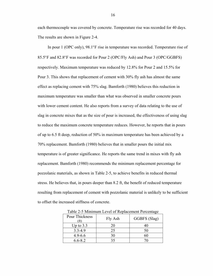
each thermocouple was covered by concrete. Temperature rise was recorded for 40 days.
The results are shown in Figure 2-4.
In pour 1 (OPC only), 98.1°F rise in temperature was recorded. Temperature rise of
85.5°F and 82.8°F was recorded for Pour 2 (OPC/Fly Ash) and Pour 3 (OPC/GGBFS)
respectively. Maximum temperature was reduced by 12.8% for Pour 2 and 15.5% for
Pour 3. This shows that replacement of cement with 30% fly ash has almost the same
effect as replacing cement with 75% slag. Bamforth (1980) believes this reduction in
maximum temperature was smaller than what was observed in smaller concrete pours
with lower cement content. He also reports from a survey of data relating to the use of
slag in concrete mixes that as the size of pour is increased, the effectiveness of using slag
to reduce the maximum concrete temperature reduces. However, he reports that in pours
of up to 6.5 ft deep, reduction of 50% in maximum temperature has been achieved by a
70% replacement. Bamforth (1980) believes that in smaller pours the initial mix
temperature is of greater significance. He reports the same trend in mixes with fly ash
replacement. Bamforth (1980) recommends the minimum replacement percentage for
pozzolanic materials, as shown in Table 2-5, to achieve benefits in reduced thermal
stress. He believes that, in pours deeper than 8.2 ft, the benefit of reduced temperature
resulting from replacement of cement with pozzolanic material is unlikely to be sufficient
to offset the increased stiffness of concrete.
Table 2-5 Minimum Level of Replacement Percentage Pour Thickness
(ft) Fly Ash GGBFS (Slag)
Up to 3.3 20 40 3.3-4.9 25 50 4.9-6.6 30 60 6.6-8.2 35 70

17
A study (Atiş, 2002) on high-volume fly ash concrete showed that using of 50% fly
ash causes a reduction of 23% in the peak temperature. The same study showed 70% fly
ash replacement leads to 45% reduction in the peak temperature (Figure 2-5). Atiş (2002)
believes that 20-30% of fly ash replacement may not cause significant reduction in the
maximum temperature of concrete. According to him, with 20-30% of fly ash
replacement a reduction of 10-15% in the maximum temperature is expected. He also
reports that changes in W/C ratio influence the temperature rise in concrete. A study on
concretes with 675 lb/yd3 OPC and W/C ratios of 0.35, 0.45, and 0.55 showed 104.4,
108.3 and 111.9 ºF of peak temperature in nonadiabatic conditions with no insulation
(Atiş, 2002).
Figure 2-5 Adiabatic Temperature Rise Curves Developed by Atiş (2002)
(M0: Control Mix 675lb/yd3 Cement, M1: 70% Fly Ash with Superplasticizer, M2: 70% Fly Ash without Superplasticizer, M3:50% Fly Ash with Superplasticizer, M4: 50% Fly Ash without Superplasticizer)
ACI 207.2R-96 recommends that the total quantity of heat generation is directly
proportional to an equivalent cement content (Ceq), which is the total quantity of cement
plus a percent to total pozzolan content. The contribution of pozzolans to heat generation

18
varies with age of concrete, type of pozzolan, the fineness of pozzolan compared to the
cement and pozzolans themselves. ACI 207.2R-96 suggests to test the cement and
pozzolan mixes to determine the fineness and heat of hydration of the blend. A rule of
thumb that has worked fairly well on preliminary computations has been to assume that
pozzolan produces only about 50 percent as much heat as the cement that it replaces (ACI
207.1 R-96, 1996).
Figure 2-6 Effect of Admixtures on Heat Generation
(Atiş, 2002)(M0: Control Mix 675lb/yd3 Cement, M1: 70% Fly Ash with Superplasticizer, M2: 70% Fly Ash without Superplasticizer, M3:50% Fly Ash with Superplasticizer, M4: 50% Fly Ash without Superplasticizer)
Using chemical admixtures as water-reducing, set-retarding agents affects the
concrete mix in the first 12 to 16 hours after mixing. These chemicals do not alter the
total heat generated in the concrete after the first 24 hours (ACI 207.2R-96, 1996).
However, for studies involving a large amount of mass concrete the proposed mix should
be tested for adiabatic temperature rise (ACI 207.1 R-96, 1996). Results from study
performed by Atiş (2002) on using high-volume fly ash concretes with low water cement
ratios and superplasticizers showed that concrete mixes with similar ingredients and
different amounts of superplasticizers have the same peak temperature. Mixes with

19
superplasticizers showed a delay in reaching the maximum temperature (Figure 2-6). This
fact is caused by the retarding effect of superplasticizers on cement hydration (Atiş,
2002).
The size of the element and ambient temperature are factors that affect the concrete
peak temperature in nonadiabatic conditions. However Bamforth (1980) showed that
mixes with high percentage of pozzolan in large concrete members may be affected by
cement replacement. As mentioned before, he believes pozzolan replacement in large
members increases concrete stiffness.
Methods to Predict Temperature Rise in Mass Concrete
One of the main problems of mass concrete construction is the necessity for
controlling the heat entrapped within it as the cement hydrates. Both the rate and the total
adiabatic temperature rise differ among the various types of cement (ACI 207.1 R-96,
1996).
Predicting the maximum temperature of mass concrete has always been the main
concern of designers and builders of mass concrete structures. As mentioned before,
planning phase for the construction of Hoover Dam was a turning point in mass concrete
studies. One of the earliest efforts to predict the maximum temperature of the mass
concrete is reported by Blanks (1933). He describes a series of tests on adiabatic
temperature rise of concretes with different cement types. Those test had been supported
by the U. S. Bureau of Reclamation. To develop the adiabatic temperature rise curves,
cylinders of full mass concrete with 188lb/yd3 cement content were cast in place in
accurately controlled adiabatic calorimeter rooms and immediately sealed by soldering a
cover on the light sheet metal mold. The temperature of the air in the room and the
temperature of the specimen were measured by resistance thermometers. These

20
thermometers were connected to control instruments. The control instruments operated to
maintain the temperature of the air in the calorimeter room the same as that of the
specimen. Blanks (1933) mentions that the special design of the room insured the
uniformity of temperature and the controls provide equality of temperature between the
air and the specimen within 0.10°F.
Figure 2-7 shows the results of tests reported by Blanks (1933). At that time the
final objective of the tests was to find the most proper commercial cement for the
construction of Hoover Dam. ASTM standard cements had not been defined therefore
different cements were designated by numbers (See Table 2-6).
Table 2-6 Compound Composition of Cements Represented in Figure 2-7 Cement
No. C3S C2S C3A C4AF MgO CaSO4 Free Lime
I-1 49.1 21.9 13.6 10.3 0.7 2.8 0.9 R-2252 57.8 17.4 6.7 10 2.6 3.6 1.2
Y-9 52.9 26.5 8.8 5.9 1.6 2.3 - U-2 23.2 50.1 12.9 6.2 3.5 2.9 0.3
S-310 Not a True Portland Cement R-2249 25.6 46.2 2.8 18.1 2.4 4.1 1.0
Figure 2-1 shows adiabatic temperature rise curves for mass concrete containing
376lb/yd3 of various types of cement. These curves are published in ACI 207.1R and are
widely used to predict the adiabatic temperature rise in mass concrete. ACI curves have
been traced to early 1960s.
As mentioned before, when a portion of the cement is replaced by pozzolan, the
temperature rise curves are greatly modified, particularly in the early ages. Depending on
the composition and fineness of the pozzolan and cement used in combination, the effect
of pozzolans differs greatly.

21
Figure 2-7 Typical Heat-Generation Curves (Blanks, 1933)
Specifications for mass concrete often require particular cement types, minimum
cement contents, and maximum supplementary cementitious material contents. Once this
information is available, the process of predicting maximum concrete temperatures and
temperature differences can begin. Several options are available to predict maximum
concrete temperatures.

22
Gajda (2002) reports a simplistic method, which is briefly described in a Portland
Cement Association document. This method is useful if the concrete contains between
500 and 1000 lbs of cement per cubic yard of concrete and the minimum dimension is
greater than 6 ft. For this approximation, every 100 lbs of cement increases the
temperature of the concrete by 12.8 F. Using this method, the maximum concrete
temperature of a concrete element that contains 900 lb of cement per cubic yard and is
cast at 60°F is approximately 175°F. This PCA method does not, however, consider
surface temperatures or supplementary cementitious materials (Gajda et al., 2002).
A more precise method is known as Schmidt’s method. This method is most
frequently used in connection with temperature studies for mass concrete structures in
which the temperature distribution is to be estimated. Determining the approximate date
for grouting a relatively thin arch dam after a winter’s exposure, the depth of freezing,
and temperature distributions after placement are typical applications of this step-by-step
method. Different exposure temperatures on the two faces of a theoretical slab and heat
of hydration of cement can be taken into consideration (Townsend, 1981).
In its simpler form, Schmidt’s Method assumes no heat flow normal to the slab and
is adapted to a slab of any thickness with any initial temperature distribution. Schmidt’s
Method states that the temperature, t2 , of an elemental volume at any subsequent time is
dependent not only upon its own temperature but also upon the temperatures, t1 and t3 , of
the adjacent elemental volumes. At time ∆t , this can be expressed as:
t2,∆t = [t1 + (M-2) t2 + t3] / M
Where M = [Cρ(∆x)2]/[K∆t] = (∆x)2/(h2∆t), since the diffusivity of concrete, h2
(ft2/hr), is given as K/Cρ.
23
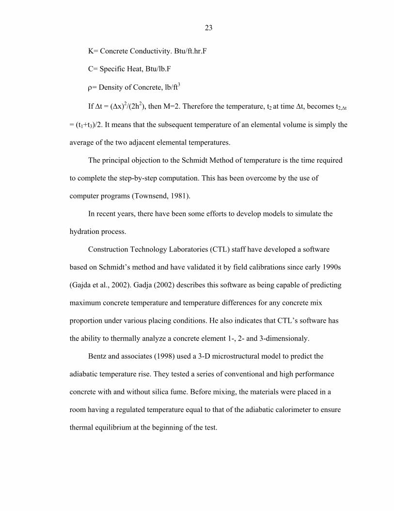
K= Concrete Conductivity. Btu/ft.hr.F
C= Specific Heat, Btu/lb.F
ρ= Density of Concrete, lb/ft3
If ∆t = (∆x)2/(2h2), then M=2. Therefore the temperature, t2 at time ∆t, becomes t2,∆t
= (t1+t3)/2. It means that the subsequent temperature of an elemental volume is simply the
average of the two adjacent elemental temperatures.
The principal objection to the Schmidt Method of temperature is the time required
to complete the step-by-step computation. This has been overcome by the use of
computer programs (Townsend, 1981).
In recent years, there have been some efforts to develop models to simulate the
hydration process.
Construction Technology Laboratories (CTL) staff have developed a software
based on Schmidt’s method and have validated it by field calibrations since early 1990s
(Gajda et al., 2002). Gadja (2002) describes this software as being capable of predicting
maximum concrete temperature and temperature differences for any concrete mix
proportion under various placing conditions. He also indicates that CTL’s software has
the ability to thermally analyze a concrete element 1-, 2- and 3-dimensionaly.
Bentz and associates (1998) used a 3-D microstructural model to predict the
adiabatic temperature rise. They tested a series of conventional and high performance
concrete with and without silica fume. Before mixing, the materials were placed in a
room having a regulated temperature equal to that of the adiabatic calorimeter to ensure
thermal equilibrium at the beginning of the test.

24
Cement was imaged using scanning electron microscope/X-ray analysis to obtain a
two-dimensional image. Each phase of the cement was uniquely identified in the image.
This image and measured particle size distribution for the cement were used to
reconstruct a three-dimensional representation of the cement (Bentz et al., 1998).
The cellular automatom-based 3-D cement hydration and microstructural model
operates as a sequence of cycles, each consisting of dissolution, diffusion, and reaction
steps.
Bentz and associates (1998) concluded that the 3-D microstructural model had
successfully predicted the adiabatic temperature rise and there have been a reasonable
relation between the developed model and experimental work. However, the accuracy of
the model’s prediction is restricted to correct computation of kinetic constants, activation
energies, and reaction product stoichiometries.
Swaddiwudhipong and associates proposed a numerical model to simulate the
exothermic hydration process of cement and temperature rise in mass concrete pours
(Swaddiwudhipong et al. 2002). In their model the hydration reaction of each major
mineral compound found in Portland cement, C3S, C2S, C3A and C4AF, is considered.
The hydration of each mineral compound is characterized by its thermal activity and the
reference rate of heat of hydration. Reference rate of heat of hydration is the rate of heat
of hydration per unit mass of mineral compound in cement under specified hydration
conditions.
In this model the influence of various factors on the exothermic hydration process
is taken into consideration. The applicability of the proposed model is verified by a series
of adiabatic temperature rise tests. Swaddiwudhipong and associates (2002) believe that

25
with the establishment of this approach, it is possible to simulate the exothermic
hydration process of Portland cement and the temperature rise directly on the basis of
intrinsic mechanism of hydration, chemical composition of cement, and mix proportion
of concrete mixture.
They concluded, “Compared with other empirical methods, the proposed model
serves as a more reasonable and effective tool to predict the evolution of heat of
hydration, the degree of hydration and the temperature rise in concrete mixtures”
(Swaddiwudhipong et al.,2002).
Ballim (2004) developed a finite difference heat model for predicting time-based
temperature profiles in mass concrete elements. In this study, a model representing a two-
dimensional solution to the Fourier heat flow equation was developed. This model runs
on a commercially available spreadsheet package. The model uses the results of a heat
rate determination using an adiabatic calorimeter together with Arrhenius maturity
function to indicate the rate and extent of hydration at any time and position within the
concrete element. Ballim (2004) reports that this model is able to predict the temperature
within 3.6ºF throughout temperature monitoring period.
Experimental Methods to Measure the Heat of Hydration of Concrete
There are normally four methods to measure the heat of hydration of concrete.
(Gibbon et al., 1997).
• Heat of Solution Test: This method determines the total heat produced by the binder content of the concrete over a 28-day period, but does not indicate the rate of heat production at any point in time.
• Conduction Calorimetry: In this method heat removed from a sample of hydrating cementitious paste is measured. Since the rate of hydration is dependent on temperature, this method does not allow the sample to attain temperatures that it would in a concrete structure and therefore does not simulate the true condition.

26
• Adiabatic Calorimetry: This method allows determination of both the total heat and the rate of heat generation. In this method, there is no heat transfer from or into the test sample.
• Isothermal Method: This method is similar to adiabatic calorimetry but uses a Dewar or thermos flask to prevent heat loss, instead of an adiabatic control system. The heat loss from the flask is difficult to determine and will affect the hydration process.

27
CHAPTER 3 METHODOLOGY
Introduction
In this chapter, the materials and the test methods to study the adiabatic
temperature rise of mass concrete are presented. In the first section of the chapter
procedures that were undertaken to choose sample concrete mixes’ materials and their
proportion are explained. Test methods and equipment used to measure the temperature
rise and other characteristics of concrete samples are presented in the second section. In
the third section, test procedures to determine adiabatic temperature rise, concrete
thermal diffusivity, compressive strength, and heat of hydration are described.
Mix Design Selection
The first step to prepare a concrete sample is to design the mix proportions and
choose the materials. There are many different mass concrete mix designs that have been
approved and used in various FDOT projects in the past. The goal was to choose a mix
design which is a representative of the majority of the mixes used in FDOT mass
concrete projects. To achieve this goal a comprehensive list of 87 FDOT approved mix
designs used for mass concrete elements in the time interval between 1990 and 2000 was
compiled. Based on the information gathered about these mix designs, concrete class,
cement type, proportion of pozzolanic material, and coarse and fine aggregates were
selected.

28
Concrete Class
The breakdown of concrete classes of the mixes used in mass concrete projects in
Florida is shown in Figure 3-1. The majority of the mixes were FDOT Class IV (5500
psi) concrete. It was therefore decided to use a Class IV concrete mix.
Class I2% Class II
15%Class III
6%
Class IV74%
Class V3%
Figure 3-1 Mix Design Breakdown By Concrete Class
Cement Type
The next step was to choose the cement type. Table 3-1 shows the distribution of
different types of cement used in 87 FDOT approved mass concrete mixes. Cements from
two different sources that satisfy the AASHTO criteria for type II cement were used.
Table 3-1 Cement Type Distribution in FDOT Approved Mixes Cement type Number Percentage Comment
Type IP 10 11 Type I 5 6 Type II 72 83 ← Selected Total 87 100

29
Pozzolanic Materials Proportion
Pozzolanic materials (Fly Ash or Slag) are generally used in mass concrete mixes.
The following approach was used to determine the percentage of pozzolanic materials to
be used in this project’s mix designs.
Figure 3-2 shows the percentage of mixes made with different ratios of fly ash in
FDOT approved mass concrete mixes. As one can readily observe, the ratio of fly ash to
total cementitious material varies from 18% to 40%. It was decided to make two mixes
with two different percentages of fly ash to have good representatives of the mixes.
Mixes were divided into two groups. First group included mixes with 18% to 22% of fly
ash. Based on weighted average and frequency of fly ash percentage, 20% was chosen for
this group. The second group consisted of mixes with 30% to 40% of fly ash. The
proportion of fly ash in this group was determined to be 35%.
0%
5%
10%
15%
20%
25%
30%
35%
40%
18% 19% 20% 21% 22% 30% 35% 39% 40%Fly Ash/Cementitious Material
Perc
ent o
f Mix
es W
ith F
ly A
sh
Figure 3-2 Fly Ash Percentage In FDOT Approved Mixes With Fly Ash

30
As shown in Figure 3-3, within the FDOT approved mass concrete mixes with slag,
slag to cementitious materials percentage was 50%, 60% or 70%. It was decided to test
two different mix designs with slag. For this purpose, 50% and 70% of slag in the mix
were chosen. These proportions are the most frequent ones.
0%
10%
20%
30%
40%
50%
60%
50% 60% 70%Slag/Cementitious Material
Perc
ent o
f Mix
es W
ith S
lag
Figure 3-3 Slag Percentage In FDOT Approved Mixes With Slag
Cement Source
Data from FDOT approved mass concrete mixes showed that cements used are
generally produced by the following cement manufacturers:
1. Rinker Materials (Miami)
2. Florida Rock Ind. (Newberry)
3. Florida Mining and Materials (Cemex in Brooksville)
4. Tarmac (Miami)

31
Samples from all four cements were tested for chemical analysis, physical analysis
and, heat of hydration. In Table 3-2 results of chemical and physical analysis tests are
presented. The final selection was based on the factors that are believed to affect the heat
generation in cement. As mentioned in Chapter 2, Tricalcium Silicate (C3S) and
Tricalcium Aluminate (C3S) have the largest contribution to the heat of hydration. Study
of the chemical analysis test results showed that the cement from source 2 has the
maximum C3S content. Chemical analysis test also showed that the cement from source 3
has the maximum C3A content while the other samples contain an equal percentage of
C3S. Based on the chemical analysis tests, cements from sources 2 and 3 were selected
preliminarily.
Table 3-2 Results of Chemical and Physical Analysis for the Cement Samples Source Number
1 2 3 4 Cement Source Rinker Materials
(Miami) Florida Rock Ind.
(Newberry) Florida Mining and
Materials (Cemex in Brooksville)
Tarmac (Miami)
Chemical Analysis Loss of Ignition 1.5% 1.7% 0.1% 1.5% Insoluble Residue 0.20% 0.21% 0.15% 0.16% Sulfur Trioxide 2.7% 2.9% 2.9% 2.8% Magnesium Oxide 0.9% 0.7% 0.9% 0.9% Tricalcium Aluminate (C3A) 6% 6% 7% 6% Total Alkali as Na2O 0.34% 0.36% 0.48% 0.44% Silicon Oxide 21.3% 20.1% 21.5% 21.2% Aluminum Oxide 4.6% 5.0% 5.1% 5.1% Ferric Oxide 3.8% 4.2% 3.8% 3.8% Tricalcium Silicate (CsS) 56% 58% 48% 50% Physical Analysis
3 3330 2740 2860 3050 Compressive strength (psi) 7 4360 3490 4110 4130 Fineness (m2/kg) 390 401 350 370
Initial 148 123 137 133 Setting time Gilmore (minutes) Final 208 183 235 216 Soundness - Autoclave 0.00 -0.02 0.00 0.00 Normal Consistency - - - - Comments Selected A Selected B

32
The results of heat of hydration test showed cement 2 has the minimum heat of
hydration at 7days and 28 days (see Table 3-3). Cement 3 did not have the maximum heat
of hydration but its heat of hydration at 7 an 28 days was only 2.3% and 0.7% smaller
than the heat of hydration of the cement 4 with the maximum heat of hydration. Thus
cements 2 (Florida Rock Ind.) and 3 (Florida Mining and Material) were selected as
cement A and cement B respectively.
Table 3-3 Results of Heat of Hydration Tests
No Cement Source Heat of Hydration @ 7 days (cal/g)
Heat of Hydration @ 28 days (cal/g)
1 Rinker (Miami) 77.6 88.2
2 Florida Rock Ind. (Newberry) 66.2 84.1
3 Florida mining and materials (Cemex in Brooksville) 78.2 94.4
4 Tarmac (Miami) 80.0 95.1
Fly Ash Source
Table 3-4 shows the percentage of mixes with fly ash from different sources.
Monex/Boral fly has the highest frequency of use in FDOT approved mass concrete
mixes and was selected to be used in this project.
Table 3-4 Percentage of Mixes With Fly Ash From Different Sources Source Percent
Monex/Boral 30% Ash Management (Carbo) 18% Florida Fly Ash 16% Ash Management 14% Florida Mining and Materials 10% Ash Management (St Johns Power) 6% Monier 2% JTM (Jacksonville) 2% Conversion System 2%

33
Blast Furnace Slag Source
Table 3-5 shows the percentage of mixes with blast furnace slag from different
sources. Although Blue Circle’s Newcem slag has the highest frequency of use, Lafarge
slag was used in this project because of the difficulty in obtaining Newcem.
Table 3-5 Percentage of Mixes With Slag From Different Sources Source Percent
Blue Circle (Newcem) 70%
Lafarge Florida inc 15%
Pencem Pennsuco 15%
Table 3-6 Percentages of Coarse Aggregates From Different Sources Coarse Aggregate Source S.G. Pit Number
Number of
Mixes Percentage
Rinker Materials 2.451 87-090 18 39% Vulcan/Ica 2.455 08-005 8 17% Florida Rock Ind. 2.493 08-004 4 9% Vulcan/Ica 2.738 AL-149 4 9% S & S Materials 2.620 AL-288 3 7% Cabbage Grove 2.480 38-268 2 4% Harper Brothers 2.500 12-260 2 4% Florida Rock Ind. 2.370 TM-478 1 2% Rinker Materials 2.420 87-035 1 2% Tarmac 2.430 87-145 1 2% Florida Rock Ind. 2.450 08-012 1 2% White Construction 2.630 38-036 1 2%
Type II Cem
ent
with Fly A
sh
Total 46 100% Rinker Materials 2.434 87-090 8 40% Tarmac 2.430 87-145 8 40% Florida Rock Ind. 2.375 87-049 2 10% Florida Rock Ind. 2.430 08-004 2 10%
Type II Cem
ent
with Slag
Total 20 100%
Coarse Aggregate Source
The other important component of a mix is coarse aggregate. Based on data
collected from FDOT approved mass concrete mixes, the most frequently used coarse
aggregate was produced by Rinker Materials (Pit Number 87).Table 3-6 shows source,

34
specific gravity, and pit number of coarse aggregates used in FDOT approved mass
concrete mixes with fly ash or slag. Coarse aggregate produced by Rinker Materials form
Pit Number 87-090 was therefore chosen for the test.
Fine Aggregate Source
Fine aggregate selected for this project was from the same source as the coarse
aggregate (Rinker Materials).
Total Cementitious Materials
The amount of cementitious material is one of the important factors in generating
heat of hydration in the concrete mix. Considering Table 3-7 and the fact that higher total
cementitious material generates more heat of hydration, 760 lbs/yd3 total cementitious
materials was used in this project.
Table 3-7 Total Cementitious Materials In FDOT Approved Class IV Concrete Mixes Total Cementitious
Materials (lbs) Number Percentage
650-709 27 47% 710-769 26 46% 770-869 4 7%
Mix Temperature
Concrete placing temperature also affects the heat of hydration. To demonstrate
how placing temperature affects maximum curing temperature, two placing temperatures,
73°F and 95°F, were used in this project.
Number of Mixes
The objective of this study was to develop adiabatic temperature rise for typical
mass concrete mixes made with Florida materials. To accomplish this objective 20
different mixes were made using two different cement sources, two placing temperatures,

35
and different percentages of pozzolanic materials. Table 3-8 exhibits the type and amount
of pozzolanic materials, cement source, and placing temperature for these 20 mixes.
Table 3-8 Number of Test Mixes
Binder Placing
Temp (°F)
Cement
Source
Mix
Designation
73 A 73A00P 73 B 73B00P 95 A 95A00P
Type II Cement 0% Pozzolanic Material
95 B 95B00P 73 A 73A20F 73 B 73B20F 95 A 95A20F
80% Type II Cement + 20% Fly Ash
95 B 95B20F 73 A 73A35F 73 B 73B35F 95 A 95A35F
65% Type II Cement + 35% Fly Ash
95 B 95B35F 73 A 73A50S 73 B 73B50S 95 A 95A50S
50% Type II Cement + 50% Slag
95 B 95B50S 73 A 73A70S 73 B 73B70S 95 A 95A70S
30% Type II Cement + 70% Slag
95 B 95B70S
Total Number of Mixes 20 Test Methods and Equipments
This research project involved development of adiabatic temperature rise curves for
FDOT approved concrete mixes, measuring concrete thermal diffusivity, and testing
compressive strength at different ages. In addition, the heat of hydration for plain and
blended cements used in different mixes was measured.
Adiabatic Temperature Rise
There is no standard method to measure the adiabatic temperature rise of mass
concrete. Literature review showed that the basis of all previous tests to monitor and
record the adiabatic temperature rise of mass concrete was to provide an adiabatic or semi
adiabatic condition for the concrete sample and at the same time record the temperature

36
rise by thermocouples placed in the core of the concrete samples. Different methods have
been used to provide an adiabatic condition for concrete samples. These methods range
from building an isolated room with controlled temperature to small chambers or
cylinders that are connected to heaters and thermocouples and are monitored by
computers.
Apparatus
For this study Sure Cure system was used. This system had been previously used
by FDOT in similar research projects. The system consists of a Hydration Chamber,
Cylinder Molds, I/O Controller Cabinet and Personal Computer.
Hydration Chamber
Hydration Chamber (Figure 3-4) is a caped cylinder that holds a fresh concrete
sample approximately equal to a 6"x12" cylinder. It has an insulated wall and cap which
prevents heat exchange between the concrete and the outside ambient. Two
thermocouples are mounted in the Hydration Chamber. The first one is called “Inner” and
is placed inside a cone in the middle of the cylinder (see Figure 3-6). This thermocouple
records the temperature of the core of the concrete sample placed in the Hydration
Chamber. The second thermocouple, called “Outer,” is placed in the wall of the cylinder
and monitors the temperature of the surface of the sample. These thermocouples are
connected to the I/O controller. Two heaters are placed in the wall and the cap of the
Hydration Chamber. Each heater is connected to the I/O Controller separately. Whenever
the temperature recorded by the Inner thermocouple is smaller than the one recorded by
the Outer, heaters will start heating the sample to eliminate the temperature gap between
the inside and the outside of the sample.

37
Figure 3-4 Hydration Chamber
Cylinder Molds
A cylinder mold holds a 4" by 8" concrete sample. A thermocouple is placed in
each mold and relays the temperature to the controller. The controller sends the data to
the computer and the control software compares the temperature of the mold to the
temperature recorded from the Inner thermocouple of the Hydration Chamber. If the
temperature of the cylinder mold is lower than the temperature of the Inner thermocouple,
the software orders the controller to turn on the heater inside the cylinder mold. Each
cylinder mold is insulated by flexible polyurethane insulation to protect the mold from
the environment (Figure 3-5). The specimens from the cylinder molds were used for
compressive strength test.
Figure 3-5 Cylinder Molds

38
I/O Controller Cabinet and Personal Computer
The I/O Controller can monitor and control up to 15 thermocouple channels and 8
heater channels. The computer provides complete time vs. temperature information. The
PC can control cylinder molds to follow the specimen in the Hydration Chamber or any
pre-programmed time/temperature curve. The thermocouple and 120V power circuits
from the Hydration Chambers and the cylinder molds can be plugged directly into the I/O
cabinet of the PC controller. As specified by the Sure Cure System Manufacturer, the
system controls the temperature of the cylinder molds within ±2ºF of the “master”
thermocouple. In these tests the Inner thermocouple of the Hydration Chamber was the
“master” thermocouple.
Concrete
I/O ControllerComputer
Outer Thermocouple
Heater Connection
Hydration Chamber
Inner Thermocouple
Figure 3-6 Sure Cure System
Concrete is placed in the Hydration Chamber. Immediately after the concrete
placement, the temperature data from Inner and Outer thermocouples is read every 6
seconds by I/O Controller. The software that monitors the I/O Controller compares the
core temperature and the outer surface temperature. As soon as the difference between
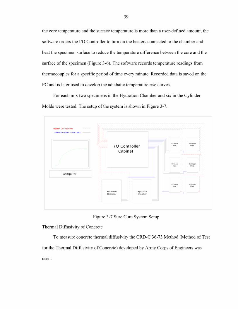
39
the core temperature and the surface temperature is more than a user-defined amount, the
software orders the I/O Controller to turn on the heaters connected to the chamber and
heat the specimen surface to reduce the temperature difference between the core and the
surface of the specimen (Figure 3-6). The software records temperature readings from
thermocouples for a specific period of time every minute. Recorded data is saved on the
PC and is later used to develop the adiabatic temperature rise curves.
For each mix two specimens in the Hydration Chamber and six in the Cylinder
Molds were tested. The setup of the system is shown in Figure 3-7.
I/O Controller Cabinet
Computer
Hydration Chamber
Hydration Chamber
Cylinder Mold
Cylinder Mold
Cylinder Mold
Cylinder Mold
Cylinder Mold
Cylinder Mold
Heater Connections
Thermocuople Connections
Figure 3-7 Sure Cure System Setup
Thermal Diffusivity of Concrete
To measure concrete thermal diffusivity the CRD-C 36-73 Method (Method of Test
for the Thermal Diffusivity of Concrete) developed by Army Corps of Engineers was
used.

40
Scope
This test is used to determine the thermal diffusivity of concrete. The thermal
diffusivity is equal to the thermal conductivity divided by the heat capacity per unit
volume and may be used as an index of the facility with which the material will undergo
temperature change.
Apparatus
The apparatus consists of Bath, Diffusion Chamber and Temperature Indicating and
recording instrument and Timer.
Bath.
A heating bath (Figure 3-8) in which concrete cylinders can be raised to uniform
high temperature (212 °F).
Diffusion chamber
A chamber containing running cold water (Figure 3-9).
Temperature indicating and recording instrument and timer
This device records time and temperature (Figure 3-10).
Figure 3-8 Heating Bath

41
Figure 3-9 Diffusion Chamber
Figure 3-10 Temperature Recorder and Timer

42
Procedure
Preparation of specimen
The test specimens were 6 by 12 in. cylinder. Molded specimens were moist-cured
for 28 days prior to testing.
Heating
Each specimen was heated to the same temperature by continuous immersion in
boiling water until the temperature of the center reached 212° F (100°C). The specimen
was then transferred to a bath of running cold water, and suspended in the bath so that the
entire surface of the specimen is in contact with the water. The temperature of the cold
water was determined by means of another thermocouple.
Cooling
The cooling history of the specimen was obtained from readings of the temperature
of the interior of the specimen at 1-min intervals from the time the temperature difference
between the center and the water reached 120 °F (67 °C) until the temperature difference
between the center and water reached 8 °F (4 °C). The data was recorded. Two such
cooling histories were obtained for each test specimen, and the diffusivities were
calculated within ± 0.002 f t2/ h.
Calculations
The temperature difference in ºF was plotted against the time in minutes on a semi
logarithmic scale. The best possible straight line was then drawn through the points so
obtained. A typical graph is shown in Figure 3-11. The time elapsed between the
temperature difference of 80 °F and 20 °F was read from the graph, and this value was
inserted in equation below from which the thermal diffusivity was calculated:

43
α = 0.812278/(t1 - t2) Equation 3.1
Where:
α = thermal diffusivity, ft2/ h r
And,
(t1 - t2) = elapsed time between temperature differences of 80 °F and 20 °F in
minutes, and
0.812278 = numerical factor applicable to 6- by 12-in cylinder.
Figure 3-11 Example Showing Calculation Of Thermal Diffusivity Of A Concrete
Cylinder
Compressive Strength
The compressive strengths of the samples were determined at ages of 14 and 28
days. The compressive strengths were determined according to ASTM C39-93a,

44
Standard Test Method for Compressive Strength of Cylindrical Concrete Specimens,
using FDOT physical laboratory equipment.
Heat of Hydration
The heat of hydration for cementitious materials was determined at 7 and 28 days.
The heat of hydration was determined according to ASTM C186, Standard Test Method
for the Determination of Heat of Hydration of Hydraulic Cement, by Construction
Technology Laboratories (CTL) in Skokie, Illinois.
Test Procedures
In this section test procedures to determine adiabatic temperature rise, thermal
diffusivity, and compressive strength for concrete and the heat of hydration for plain and
blended cement paste are described. Concrete tests were performed at the FDOT physical
laboratory, while Construction Technology Laboratories performed the heat of hydration
test for cement.
Tests Performed For Each Mix
The following tests were performed for each mix:
1-Fresh Concrete Properties
2-Adiabatic Temperature Rise
3-Compressive Strength at different ages
4- Concrete Thermal Diffusivity
5- Cementitious Materials Heat of Hydration
Procedures for each test will be described in the following sections.
Size and Number of Specimens
For each mix different sizes of specimen were prepared.

45
Hydration Chamber: 2 Hydration Chambers were used to monitor the adiabatic
temperature rise for each mix.
Cylinder molds: These molds are 4"x8" cylinder shaped and are connected to the
Sure Cure System I/O Controller. They are heated by electric heaters to follow
temperature rise of concrete in Hydration Chambers. Six cylinder molds were used for
each mix. Three of the specimens were tested for compressive strength at 14 days along
with three specimens cured at room temperature. The other three specimens were kept in
the moisture room for another 14 days. Three of the specimens cured at room temperature
were also kept in the moisture room for another 14 days. These specimens were tested for
compressive strength at 28 days.
Plastic molds:
6"x12" Cylinder: Six samples were prepared. Three were used for compressive
strength at 28 days and the other three were used for concrete diffusivity test.
4"x8" Cylinder: Six samples were prepared. All of them were kept in the molds in
room temperature and were covered to prevent moisture loss. At the age of 14 days molds
were stripped. Three specimens were broken for compressive strength test. The other
three specimens were transferred to moisture room and kept for 14 days. As explained
earlier, these specimens were tested for compressive strength at 28 days along with high
temperature cured specimens.
Adiabatic Temperature Rise
Test procedure
As explained earlier in this chapter, Sure Cure System was used to measure the
adiabatic temperature rise.

46
Laboratory tests
Preparation of mix materials
Concrete materials were prepared a day before the mix date with propitiations
determined in mix design calculations (Figure 3-12). For 73°F placing temperature tests,
materials were kept in the laboratory area with a controlled temperature of 72-75°F. For
the mixes with 95°F placing temperature, fine aggregates were placed in an oven with
200°F temperature for 24 hours.
Figure 3-12 Materials Prepared For The Next Day Test
Concrete mixing and placing stage
For each test a 3 Cubic Feet mix was prepared. As suggested by Hydration
Chamber manufacturer, there should not be a direct contact between concrete and the
chamber’s wall. Therefore concrete was placed in a plastic bag which was inside the
chamber (Figure 3-13)

47
Figure 3-13 Hydration Chamber
Immediately after concrete placing, Hydration Chambers were connected to the
controller and computer system and temperature recording started. At the same time
concrete was also placed in metal cylinder molds (Figure 3-5) and they were also
connected to the controller and computer. Hydration Chambers and cylinder molds were
placed on a table for the period of temperature rise monitoring (Figure 3-14).
Figure 3-14 Cure Chambers and Metal Molds Connected to the Computer

48
Temperature rise monitoring stage
Temperature monitoring started immediately after placing concrete in Hydration
Chambers. For first five mixes (73A00P, 73A20F, 73A35F, 73A50S and 73A70S)
temperature rise were monitored for 28 days. It was realized that there is not a significant
temperature gain after the second week, so for the following tests temperature rise was
monitored for 14 days.
At the end of the temperature rise monitoring stage, recorded temperature rise log
was saved for later analysis. Samples from Hydration Chambers were transferred to
moisture room and kept there for future use in microcrack test. Samples from metal
molds were used for compressive strength test.
Field tests
In addition to the laboratory tests, it was necessary to take samples from mass
concrete projects and monitor their temperature rise with hydration Chambers to evaluate
the correlation between the laboratory results and the field temperature readings.
The first step was to find FDOT mass concrete projects throughout the State of
Florida. Different regional offices of FDOT were contacted. Finally Interstate 4 project
was chosen. Test equipments were mounted in a minivan and were ready to be dispatched
to the project site at the notice from the project administrator (Figure 3-15).

49
Figure 3-15 Hydration Chambers, Controller and Computer in Minivan
On April 2nd 2004, the first group of samples were taken from Bella Vista Bridge (a
bridge over I-4 west of Memorial Blvd.) footing A in Lakeland. However because of
equipment malfunction temperature monitoring could not be started immediately after
sample placement so the results from this test was not considered reliable. On April 9th,
footing C of the same project was poured, so samples were taken again at this date.
Sample preparation
It was decided to take samples from the center of the concrete pour. This decision
was based on the fact that the middle core of a mass concrete element will most likely
reach the maximum curing temperature, in addition, temperature sensors to monitor
temperature rise of concrete are installed at the center of the pour.
Concrete was poured directly from the truck mixer to a wheel borrow. Immediately
concrete from the wheel borrow was placed in Hydration Chambers. Hydration Chambers
were transferred to the minivan and connected to the controller and the computer. Power
was supplied from minivan through a converter (Figure 3-16)
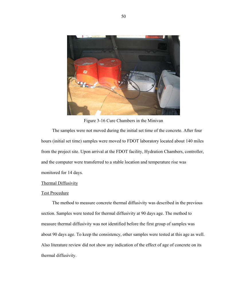
50
Figure 3-16 Cure Chambers in the Minivan
The samples were not moved during the initial set time of the concrete. After four
hours (initial set time) samples were moved to FDOT laboratory located about 140 miles
from the project site. Upon arrival at the FDOT facility, Hydration Chambers, controller,
and the computer were transferred to a stable location and temperature rise was
monitored for 14 days.
Thermal Diffusivity
Test Procedure
The method to measure concrete thermal diffusivity was described in the previous
section. Samples were tested for thermal diffusivity at 90 days age. The method to
measure thermal diffusivity was not identified before the first group of samples was
about 90 days age. To keep the consistency, other samples were tested at this age as well.
Also literature review did not show any indication of the effect of age of concrete on its
thermal diffusivity.

51
Sample preparation
For each mix three 6"x12" cylinders were cast. Within each cylinder a wire
thermocouple was placed. Specimens were kept in moisture room before they were tested
for thermal diffusivity.
Heating
Specimens were placed in a heating bath at the age of 90 days. Specimens remained
in the heating bath until their core temperature reached 212°F.
Figure 3-17 Specimens Transferred From Heating Bath to Diffusion Chamber
Cooling
Specimens were then transferred to a diffusion chamber. Diffusion chamber
contained a relatively large body of water and was connected to running water. These
factors kept water temperature constant during concrete cooling period.

52
Figure 3-18 Specimens Connected To Temperature Recorder During Cooling Stage
Core temperature of the specimen was recorded in one-minute intervals from the
time specimen was placed in the diffusion chamber until the temperature difference
between the specimen core and water was less than 8°F. Temperature drop history was
later used to calculate the thermal diffusivity.
Compressive Strength
Compressive strength test was performed for the specimens with different ages and
sizes as mentioned in previous sections according to ASTM C39.
Test Procedure
Sample preparation
In total, 18 samples were cast for compressive strength tests. All specimens were
placed in molds after placing concrete in Cure Chambers.
Testing of samples
Samples were tested at 2 different ages: 14 and 28 days.

53
14-Day tests
Two groups of specimens were tested at this age. Each group consisted of three
4″x8″ cylinders. The first group was cured in high temperature. The second group was
kept in molds in room temperature. Test results for two groups were compared to study
the effect of high curing temperature on compressive strength.
28-Day tests
Two series of tests were performed at this age. The first series of tests included two
groups of specimens. Each group consisted of three 4"x8" cylinders. The first group was
cured in high temperature for 14 days and was then cured in moisture room for another
14 days. The second group was kept in molds in room temperature and later was moved
to the moisture room and was kept there for additional 14 days. Test results for two
groups were compared to study the effect of high curing temperature on compressive
strength. For the second series, three 6"x12" samples were cured in moisture room and
were tested at 28 days age.
Heat of Hydration
Two series of Heat of Hydration tests were performed by CTL in August 2003 and
April 2004. ASTM C186 method was used to determine Heat of Hydration at 7 and 28
days.
Test Series I
In the first series four samples of plain cement (from four different sources) and
samples of fly ash and blast furnace slag were sent to CTL laboratory in Illinois to
perform the test. The results of Heat of Hydration tests were used to choose the two
cement sources to use for mix preparation. Also to study the correlation of Heat of

54
Hydration and maximum adiabatic temperature rise, blends of 80% cement A with 20%
fly ash and 50% cement A with 50% slag were tested for Heat of Hydration.
Test Series II
The first supply of cement A was finished during the test period due to the
repetition of some of the test mixes. It was necessary to measure Heat of Hydration for a
new supply of cement A. Therefore, sample of this cement was sent to CTL to perform
Heat of Hydration test. Along with the cement sample, fly ash and slag samples were also
sent to CTL. In this series, Heat of Hydration of cement A, 65% cement A with 35% fly
ash and 30% cement A with 70% slag was determined.

55
CHAPTER 4 TEST RESULTS
Introduction
This chapter provides the results of the various tests performed to measure the
properties of mass concrete mixes. Mixture properties can be found in the first section.
The second section provides fresh concrete properties measured for each mix. The heat of
hydration data, as reported by CTL is shown in the third section. In the forth section the
temperature of concrete samples recorded by Sure Cure system as well as adiabatic
temperature rise curves for different mixes are shown. In the fifth section results for the
thermal diffusivity tests are presented. In this section a sample calculation to determine
the thermal diffusivity of concrete is also shown. In the last section of the chapter,
compressive strength tests results are presented.
Mixture Properties
In Table 4-1 mixture properties of different test mixes are shown. The proportions
of cement, pozzolanic materials (fly ash or blast furnace slag), water, fine aggregate,
coarse aggregate, air entertainer and admixture for each mix can be found in this table.
Darex® air entertainer and WARDA® 56 water reducer were used in all of the mixes.

56
Table 4-1 Concrete Mixture Properties FDOT Class IV (5500 psi)
(Mix proportions per cubic yard)
No. Mix Designation
Cement (lb)
Fly Ash (lb)
Slag (lb)
Water (lb)
Fine Aggregate
(lb)
Coarse Aggregate
(lb)
Air Entertainer
(oz)
Admixture
(oz) 1 73A00P 760.00 0.00 0.00 279.00 1033.00 1736.00 2.30 68.202 73A20F 608.00 152.00 0.00 279.00 1033.00 1708.00 4.00 68.203 73A35F 494.00 266.00 0.00 279.00 980.00 1687.00 4.00 68.204 73A50S 380.00 0.00 380.00 279.00 1021.00 1724.00 2.30 68.205 73A70S 228.00 0.00 532.00 279.00 1021.00 1724.00 2.30 68.206 73B00P 760.00 0.00 0.00 279.00 1033.00 1736.00 2.30 45.657 73B20F 608.00 152.00 0.00 279.00 1033.00 1708.00 4.00 45.658 73B35F 494.00 266.00 0.00 279.00 980.00 1687.00 4.00 45.659 73B50S 380.00 0.00 380.00 279.00 1021.00 1724.00 2.30 68.20
10 73B70S 228.00 0.00 532.00 279.00 1021.00 1724.00 2.30 30.4011 95A00P 760.00 0.00 0.00 279.00 1033.00 1736.00 2.30 60.8612 95A20F 608.00 152.00 0.00 279.00 1033.00 1708.00 4.00 68.2013 95A35F 494.00 266.00 0.00 279.00 980.00 1687.00 4.00 60.8614 95A50S 380.00 0.00 380.00 279.00 1021.00 1724.00 2.30 25.8715 95A70S 228.00 0.00 532.00 279.00 1021.00 1724.00 2.30 68.2016 95B00P 760.00 0.00 0.00 279.00 1033.00 1736.00 2.30 60.8617 95B20F 608.00 152.00 0.00 279.00 1033.00 1708.00 4.00 30.4018 95B35F 494.00 266.00 0.00 279.00 980.00 1687.00 4.00 68.2019 95B50S 380.00 0.00 380.00 279.00 1021.00 1724.00 2.30 38.0620 95B70S 228.00 0.00 532.00 279.00 1021.00 1724.00 2.30 68.20

57
Fresh Concrete Properties
Table 4-2 shows the results of Slump and Air Content tests. The slump tests were
performed in accordance with ASTM C143. The objective was to maintain the slump in
3″±1 ½″. Air Content tests were run according to ASTM C231. Air temperature and mix
temperature were measured at the time of placing concrete in hydration Chambers. Water
to Cementitious Material Ratio was calculated using following equation:
WCr= Ww / Wc Equation 4-1
Where:
WCr= Water to Cementitious Material Ratio
Ww= Weight of Water in lbs from Table 4-1
Wc= Weight of Total Cementitious Materials (Cement + Fly Ash or Slag) in lbs
from Table 4-1
Weight of Total Cementitious Materials (Cement + Fly Ash or Slag) and water was
constant, therefore WCr equal to 0.37 in all mixes.
Unit weight was calculated by dividing the summation of all materials weights
from Table 4-1 by mix volume. For example unit weight of mix 73A00P was calculated
as follows:
Weight of Cement = 760 lbs
Weight of Water = 279 lbs
Weight of Fine Aggregate = 1033 lbs
Weight of Coarse Aggregate = 1736 lbs
Weight of Air Entertainer + Admixture = 2.3+68.20 = 70.50 oz = 4.41 lbs
Total of Weight of Mix Materials = 3812.41 lbs Mix Volume = 1 CY = 27 CF

58
⇒ Mix Density = 3812.41 lb/CY = 141.2 lb/CF
Table 4-2 Fresh Concrete Properties
No Mix Slump (in.)
Air Content
(%)
Mix Temp.
(ºF)
Air Temp.(ºF)
Water to Cementitious Material Ratio
Unit Weight (lb/CF)
1 73A00P 2.75 4.25 73 72 0.37 141.2 2 73A20F 2.00 2.75 73 72 0.37 140.2 3 73A35F 3.25 2.25 72 72 0.37 137.4 4 73A50S 3.50 3.75 81 80 0.37 140.3 5 73A70S 1.75 3.25 74 72 0.37 140.2 6 73B00P 7.25 3.25 73 72 0.37 141.1 7 73B20F 6.50 3.50 73 75 0.37 140.1 8 73B35F 6.00 2.00 75 72 0.37 137.4 9 73B50S 3.50 3.25 73 73 0.37 140.3
10 73B70S 3.75 3.00 73 72 0.37 140.2 11 95A00P 3.25 3.25 93 72 0.37 141.2 12 95A20F 2.75 2.25 95 72 0.37 140.2 13 95A35F 4.00 1.75 94 68 0.37 137.4 14 95A50S 3.50 2.25 96 70 0.37 140.3 15 95A70S 1.75 2.75 93 72 0.37 140.2 16 95B00P 4.25 5.50 99 73 0.37 141.1 17 95B20F 1.75 2.25 98 70 0.37 140.1 18 95B35F 0.50 2.00 101 70 0.37 137.4 19 95B50S 3.00 3.50 101 70 0.37 140.3 20 95B70S 2.75 2.50 101 72 0.37 140.2
Repeated Tests 21 73A00P-R 3.75 3.50 73 72 0.37 141.2 22 73A20F-R 3.75 2.00 74 73 0.37 140.2 23 73A35F-R 3.50 2.25 74 72 0.37 137.4 24 73A50S-R 3.75 2.75 68 68 0.37 140.3 25 73A70S-R 3.00 2.50 69 70 0.37 140.2 26 73B50S-R 3.00 3.50 73 73 0.37 140.3 27 73B70S-R 2.50 3.50 74 72 0.37 140.2 28 95A70S-R 3.25 2.50 97 72 0.37 140.2

59
Heat of Hydration
Heat of Hydration test results are shown in Tables 4-3 and 4-4 as reported by CTL.
Two samples of cement from Florida Rock Industries Newberry plant were submitted to
CTL. The heat of Hydration of the second sample was higher than the first sample. This
shows that heats of hydration of deferent batches of cements even from the same plant
varies.
Table 4-3 Heat of Hydration Test Results for Cement
No Cement Source Heat of Hydration @ 7 days (cal/g)
Heat of Hydration @ 28 days (cal/g)
1 Florida Rock Ind. (Sample 1) (Newberry) 66.2 84.1
2 Florida Rock Ind. (Sample 2) (Newberry) 76.7 91.3
3 Rinker (Miami) 77.6 88.2
4 Florida mining and materials (Cemex in Brooksville) 78.2 94.4
5 Tarmac (Miami) 80.0 95.1
Table 4-4 Heat of Hydration for Cement and Pozzolanic Material Blends
No Cement Source Heat of Hydration @ 7 days (cal/g)
Heat of Hydration @ 28 days (cal/g)
1 20% Fly ash + 80 % Florida Rock Ind. Sample 1 56.8 68.9
2 50% Slag + 50 % Florida Rock Ind. Sample 1 59.2 75.9
3 35% Fly ash + 65 % Florida Rock Ind. Sample 2 61.4 65.4
4 70% Slag + 30 % Florida Rock Ind. Sample 2 47.5 58.6
60
Adiabatic Temperature Rise
In this section test results for adiabatic temperature rise of different mixes are
presented. For each mix, temperature was monitored immediately after placing concrete
in Cure Chamber. To calculate temperature rise, initial temperature reading as recorded
by the computer was deducted from succeeding temperature readings. After calculating
the temperature rise for data from each Cure Chamber, numbers were averaged. Data was
recorded every six minutes for 14 days. In Tables 4-5 to 4-8 temperature rise data of the
different mixes are reported for every 12 hours. For the first five mixes, data was
recorded for 28 days. Tests were repeated for the following mixes: 73A00P, 73A20F,
73A35F, 73A50S, 73A70S, 73B50S, 73B70S and 95A705.
Laboratory Tests
Test results are divided into four groups based on cement source and placing
temperature. The results for each group are presented in a separate table.
Cement A with 73ºF Placing Temperature
Tests started with mixes 73A00P and 73A20F. The second group of mixes that
were tested consisted of mixes 73A35F and 73A50S. An Equipment malfunction
occurred during the second run of tests that halted the data recording for mix 73A35F . In
the third group of tests, mixes 73A35F and 73A70S were tested. These mixes were
monitored for 28 days, while the temperature rise was recorded. Continuous temperature
rise with a relatively high rate was noticed which was unexpected. The manufacturer of
the Sure Cure system was contacted for advice. The manufacturer suggested adjusting
one of the control parameters of the Sure Cure system in a way that always 1.5 to 2.0
degrees of Fahrenheit temperature difference between heaters and core temperature is
kept. The logic behind this provision is that there is a good possibility that if the heaters

61
are set to reach the exact same temperature as that of the sample core, due to small size of
the sample, extra heat is transferred to sample core. This extra heat, which is not
generated by cement hydration, causes core temperature to rise. A rise in core
temperature is relayed to the controller software and software in turn orders the heaters to
warm up to keep sample’s outer surface in a same temperature as the core. When heaters
start working again, extra heat is transferred to the core and the procedure repeats. These
events form a cycle of heating and thus a continuous temperature rise would be recorded.
The proceeding tests were run in accordance with this suggestion. To keep the
consistency in the results, it was decided to repeat the test for the first five mixes.
As it is shown in Figure 4-4, the second run of test for the mix 73A50S reached the
maximum temperature rise of 97.10 ºF, which is even higher than the maximum
temperature rise of the mix 73A00P without any pozzolanic material. The only
explanation for this unexpected result is the test equipment or controller software
malfunction. This set of data was not considered reliable.

62
Table 4-5 Adiabatic Temperature Rise Data for Concrete with Cement A and 73ºF Placing Temperature
Concrete with Cement A (73ºF Placing Temperature) Plain Cement 20% Fly Ash 35% Fly Ash 50% Slag 70% Slag
Temp. Rise (ºF)
Temp. Rise (ºF)
Temp. Rise (ºF)
Temp. Rise (ºF)
Temp. Rise (ºF)
Temp. Rise (ºF)
Temp. Rise (ºF)
Temp. Rise (ºF)
Temp. Rise (ºF)
Temp. Rise (ºF)
Time (Day)
1st Test 2nd Test 1st Test 2nd Test 1st Test 2nd Test 1st Test 2nd Test 1st Test 2nd Test
0.0 0.00 0.00 0.00 0.00 0.00 0.00 0.00 0.00 0.00 0.00 0.5 9.40 34.50 5.60 21.60 4.00 6.80 4.50 19.90 13.45 10.70 1.0 36.80 60.80 19.30 49.10 24.20 34.00 22.90 40.50 31.50 23.15 1.5 60.00 70.25 35.90 61.20 42.30 48.40 47.00 61.40 56.20 42.40 2.0 80.00 75.45 55.20 66.90 52.55 56.00 69.10 75.80 68.10 57.50 2.5 87.00 79.05 66.70 71.50 58.95 61.00 80.00 83.10 73.53 64.10 3.0 93.40 81.60 75.70 75.50 64.95 66.00 83.70 86.70 76.20 67.05 3.5 95.90 83.50 82.00 78.80 69.63 70.40 85.50 88.90 77.65 69.20 4.0 97.50 85.05 84.70 80.80 72.35 73.40 86.50 90.40 78.75 70.60 4.5 98.60 86.55 86.10 82.00 73.80 75.50 87.40 91.80 79.78 71.10 5.0 99.50 87.65 87.00 82.60 74.90 77.10 87.90 93.00 80.53 71.10 5.5 100.20 88.60 87.60 83.20 75.83 78.30 88.30 93.80 81.15 71.10 6.0 100.70 89.55 88.10 83.80 76.48 79.30 88.30 94.70 81.60 71.10 6.5 101.30 90.30 88.70 83.80 77.30 80.00 88.40 95.20 81.63 71.10 7.0 101.10 91.05 88.60 84.10 77.83 80.80 88.20 95.80 82.18 71.10 7.5 101.50 91.60 88.80 84.10 78.38 81.40 88.30 96.20 81.95 71.10 8.0 101.30 92.05 88.70 84.00 79.08 81.50 88.50 96.50 82.15 71.10 8.5 102.00 92.10 89.00 84.20 79.23 81.80 88.50 96.90 82.50 71.10 9.0 102.30 92.15 89.30 84.20 79.65 81.60 88.60 97.00 82.73 71.10 9.5 102.60 92.15 89.70 84.30 79.95 81.70 88.70 97.10 82.98 71.10
10.0 103.00 92.15 90.00 84.30 80.30 81.80 88.70 97.10 83.25 71.10 10.5 103.30 92.20 90.40 84.30 80.75 81.90 88.70 97.10 83.15 71.10 11.0 103.60 92.25 90.70 84.30 81.05 81.90 88.80 97.10 83.35 71.10 11.5 103.90 92.25 91.00 84.40 81.33 82.00 89.00 97.10 83.65 71.10 12.0 104.30 92.30 91.30 84.40 81.65 82.10 88.90 97.10 83.75 71.10 12.5 104.50 92.40 91.60 84.40 81.65 82.10 88.90 97.10 83.75 71.10 13.0 104.80 92.45 91.90 84.40 81.65 82.30 88.90 97.10 83.75 71.10 13.5 104.90 92.60 92.10 84.40 81.65 82.20 88.90 97.10 83.75 71.10 14.0 105.00 92.60 92.20 84.40 81.65 82.10 88.90 97.10 83.75 71.10

63
Cement AAdiabatic Temperature Rise (73ºF Placing Temperature)
0
20
40
60
80
100
120
0 2 4 6 8 10 12 14Time (Day)
Tem
pera
ture
Ris
e (º
F)
Plain Cement20% Fly Ash35% Fly Ash
º
Figure 4-1 Temperature Rise for Concrete Mixtures of Cement A With Different Percentages of Fly Ash (First Run)
Cement AAdiabatic Temperature Rise (73ºF Placing Temperature)
0
20
40
60
80
100
120
0 2 4 6 8 10 12 14Time (Day)
Tem
pera
ture
Ris
e (º
F)
Plain Cement50% Slag70% Slag
Figure 4-2 Temperature Rise for Concrete Mixtures of Cement A With Different Percentages of Slag (First Run)

64
Cement AAdiabatic Temperature Rise (73ºF Placing Temperature)
0
20
40
60
80
100
120
0 2 4 6 8 10 12 14
Time (Day)
Tem
pera
ture
Ris
e (ºF
)
Plain Cement20% Fly Ash35% Fly Ash
º
Figure 4-3 Temperature Rise for Mixtures of Cement A With Different Percentages of Fly Ash (Second Run)
Cement AAdiabatic Temperature Rise (73ºF Placing Temperature)
0
20
40
60
80
100
120
0 2 4 6 8 10 12 14Time (Day)
Tem
pera
ture
Ris
e (º
F)
Plain Cement50% Slag70% Slag
Figure 4-4 Temperature Rise for Concrete Mixtures of Cement A With Different
Percentages of Slag (Second Run)

65
Cement B with 73ºF Placing Temperature
In Table 4-1 temperature rise data for mixes with cement B and 73ºF placing
temperature is presented. Test for mixes 73B50S and 73B70S were repeated because the
first set of collected temperature rise records was stopped after 7.5 days due to equipment
malfunction.
Table 4-1 Adiabatic Temperature Rise Data for Concrete With Cement B and 73ºF Placing Temperature
Concrete with Cement B (73ºF Placing Temperature) Plain Cement 20% ºFly Ash 35% ºFly Ash 50% Slag 70% Slag
Temp. Rise (ºF) Temp. Rise (ºF) Temp. Rise (ºF) Temp. Rise (ºF)
Time (Day)
Temp. Rise (ºF) Temp. Rise (ºF Temp. Rise (ºF 1st Test 2nd Test 1st Test 2nd Test
0.0 0.00 0.00 0.00 0.00 0 0.00 0.00 0.5 28.90 15.50 25.10 23.85 20.07 13.85 15.65 1.0 69.85 61.10 45.40 47.30 49.95 32.30 40.00 1.5 80.10 74.75 54.20 68.15 67.51 57.00 61.22 2.0 84.40 82.70 60.00 78.15 72.48 67.80 66.52 2.5 87.65 87.35 64.10 83.65 75.48 73.40 69.39 3.0 90.60 88.25 67.60 87.05 77.91 76.55 71.57 3.5 92.70 90.00 70.00 87.95 79.89 77.95 73.48 4.0 94.50 91.35 71.80 88.55 81.47 79.25 74.96 4.5 95.85 92.35 73.00 88.75 82.85 80.20 76.35 5.0 97.15 93.20 74.00 88.75 83.86 81.55 77.22 5.5 98.10 93.75 74.50 88.75 84.47 82.05 77.65 6.0 99.05 94.35 75.10 88.75 85.05 82.25 78.05 6.5 99.95 94.70 75.40 88.75 85.35 82.80 78.05 7.0 100.80 95.30 75.80 88.75 85.63 82.80 78.05 7.5 101.60 95.75 76.00 88.75 85.90 82.80 78.05 8.0 102.45 96.05 76.20 - 86.18 - 78.05 8.5 102.85 96.05 76.50 - 86.32 - 78.05 9.0 103.30 96.15 76.60 - 86.47 - 78.05 9.5 103.65 96.10 76.80 - 86.58 - 78.05
10.0 104.20 96.25 77.00 - 86.77 - 78.05 10.5 104.35 96.30 77.10 - 86.82 - 78.05 11.0 104.55 96.30 77.30 - 86.88 - 78.05 11.5 104.70 96.45 77.40 - 86.93 - 78.05 12.0 104.90 96.45 77.50 - 87.00 - 78.05 12.5 105.20 96.60 77.60 - 87.10 - 78.05 13.0 105.45 96.65 77.50 - 87.18 - 78.05 13.5 105.60 96.80 77.70 - 87.23 - 78.05 14.0 105.95 96.95 78.30 - 87.35 - 78.05

66
Cement B(73ºF Placing Tem perature)
Adiabatic Temperature Rise
0
20
40
60
80
100
120
0 2 4 6 8 10 12 14T ime (Day)
Tem
pera
ture
Ris
e (º
F)
Plain Cement20% Fly Ash35% Fly Ash
Figure 4-5 Temperature Rise for Concrete Mixtures of Cement B With Different Percentages of Fly Ash
Cement B(73ºF Placing Temperature)
Adiabatic Temperature Rise
0
20
40
60
80
100
120
0 2 4 6 8 10 12 14Time (Day)
Tem
pera
ture
Ris
e (º
F)
Plain Cement50% Slag70% Slag
Figure 4-6 Temperature Rise for Concrete Mixtures of Cement B With Different Percentages of Slag (First Run)

67
C e m e n t B(7 3 º F P la c in g T e m p e r a tu r e )
A d ia b a t ic T e m p e r a tu r e R is e
0
2 0
4 0
6 0
8 0
1 0 0
1 2 0
0 2 4 6 8 1 0 1 2 1 4T im e (D a y )
Tem
pera
ture
Ris
e (º
F)
P la in C e m e n t5 0 % S la g7 0 % S la g
Figure 4-7 Temperature Rise for Concrete Mixtures of Cement B With Different Percentages of Slag (Second Run)
Cement A(95ºF Placing Temperature)
Adiabatic Temperature Rise
0
20
40
60
80
100
120
0 2 4 6 8 10 12 14Time (Day)
Tem
pera
ture
Ris
e (º
F)
Plain Cement20% Fly Ash35% Fly Ash
Figure 4-8 Temperature Rise for Concrete Mixtures of Cement A With Different
Percentages of Fly Ash

68
Cement A with 95ºF Placing Temperature
Five mixes were made with cement A with placing temperature ranging from 93ºF
to 96ºF (See Table 4-2). The first run of the test for the mix 95A70S showed unexpected
results. Temperature rise in the first 24 hours was only about 6ºF which is much lower
than similar mixes. It was decided to run this test again. The results of both tests are
presented in Table 4-2,Figures 4-9 and 4-10.
Table 4-2 Adiabatic Temperature Rise Data for Concrete with Cement A and 95ºF Placing Temperature
Concrete with Cement A (95ºF Placing Temperature) Plain Cement 20% Fly Ash 35% Fly Ash 50% Slag 70% Slag
Temp. Rise (ºF) Temp. Rise (ºF)
Time (Day) Temp. Rise (ºF) Temp. Rise (ºF) Temp. Rise (ºF) Temp. Rise (ºF)
1st Test 2nd Test
0.0 0.00 0.00 0.00 0.00 0.00 0.00 0.5 17.75 8.95 4.80 19.30 5.10 4.30 1.0 61.00 40.75 26.50 54.50 5.30 16.80 1.5 77.85 63.15 46.95 82.70 12.40 49.50 2.0 87.40 76.95 60.80 91.00 42.80 57.70 2.5 91.00 85.45 75.50 92.20 56.05 60.50 3.0 92.20 88.85 80.90 92.20 58.85 62.10 3.5 92.40 90.10 82.90 92.20 60.15 63.60 4.0 92.40 90.30 84.00 92.20 61.00 64.40 4.5 92.40 90.60 84.40 92.30 61.55 65.40 5.0 92.40 90.60 85.00 92.30 62.30 66.10 5.5 92.40 90.60 85.00 92.30 62.50 66.70 6.0 92.40 90.60 85.00 92.30 63.15 67.10 6.5 92.40 90.60 85.00 92.30 63.25 67.50 7.0 92.40 90.60 85.00 92.30 63.40 67.90 7.5 92.40 90.60 85.00 92.30 63.75 68.20 8.0 92.40 90.60 85.00 92.30 63.80 68.60 8.5 92.40 90.60 85.00 92.30 63.95 68.90 9.0 92.40 90.60 85.00 92.30 64.05 69.00 9.5 92.40 90.60 85.00 92.30 64.25 69.30
10.0 92.40 90.60 85.00 92.30 64.25 69.40 10.5 92.40 90.60 85.00 92.30 64.25 69.60 11.0 92.40 90.60 85.00 92.30 64.25 69.80 11.5 92.40 90.60 85.00 92.30 64.25 69.90 12.0 92.40 90.60 85.00 92.30 64.25 70.10 12.5 92.40 90.60 85.00 92.30 64.25 70.10 13.0 92.40 90.60 85.00 92.30 64.25 70.40 13.5 92.40 90.60 85.00 92.30 64.25 70.50 14.0 92.40 90.60 85.00 92.30 64.25 70.80

69
Cement A(95ºF Placing Temperature)
Adiabatic Temperature Rise
0
20
40
60
80
100
120
0 2 4 6 8 10 12 14Time (Day)
Tem
pera
ture
Ris
e (º
F)
Plain Cement50% Slag70% Slag
Figure 4-9 Temperature Rise for Concrete Mixtures of Cement A With Different Percentages of Slag
Cement A(95ºF Placing Temperature)
Adiabatic Temperature Rise
0
20
40
60
80
100
120
0 2 4 6 8 10 12 14Time (Day)
Tem
pera
ture
Ris
e (º
F)
Plain Cement70% Slag First Run70% Slag Second Run
Figure 4-10 Temperature Rise for Concrete Mixtures of Cement A With Different Percentages of Slag (First & Second Run)

70
Cement B with 95ºF Placing Temperature
In Table 4-3 temperature rise data for mixes with cement B and 95ºF placing
temperature is presented. A review of test results and Figures 4-11 and 4-12 shows that
temperature rise for the mix without pozzolanic material was very slow in the first 12
hours.
Table 4-3 Adiabatic Temperature Rise Data for Concrete with Cement B and 95ºF Placing Temperature
Concrete with Cement B (95ºF Placing Temperature) Plain Cement 20% Fly Ash 35% Fly Ash 50% Slag 70% Slag
Time (Day)
Temp. Rise (ºF) Temp. Rise (ºF) Temp. Rise (ºF) Temp. Rise (ºF) Temp. Rise (ºF)
0.0 0.00 0.00 0.00 0.00 0.00 0.5 2.60 56.80 50.35 58.60 45.00 1.0 72.15 72.90 61.90 76.70 69.40 1.5 84.20 77.40 67.85 80.70 73.90 2.0 85.60 77.60 68.90 81.80 76.30 2.5 85.65 77.60 69.20 82.00 77.90 3.0 85.95 77.60 69.30 82.00 78.90 3.5 85.95 77.60 69.60 82.00 79.50 4.0 85.95 77.60 69.90 82.00 79.90 4.5 85.95 77.60 69.95 82.00 79.90 5.0 85.95 77.60 69.95 82.00 79.90 5.5 85.95 77.60 69.95 82.00 79.90 6.0 85.95 77.60 69.95 82.00 79.90 6.5 85.95 77.60 69.95 82.00 79.90 7.0 85.95 77.60 69.95 82.00 79.90 7.5 85.95 77.60 69.95 82.00 79.90 8.0 85.95 77.60 69.95 82.00 79.90 8.5 85.95 77.60 69.95 82.00 79.90 9.0 85.95 77.60 69.95 82.00 79.90 9.5 85.95 77.60 69.95 82.00 79.90
10.0 85.95 77.60 69.95 82.00 79.90 10.5 85.95 77.60 69.95 82.00 79.90 11.0 85.95 77.60 69.95 82.00 79.90 11.5 85.95 77.60 69.95 82.00 79.90 12.0 85.95 77.60 69.95 82.00 79.90 12.5 85.95 77.60 69.95 82.00 79.90 13.0 85.95 77.60 69.95 82.00 79.90 13.5 85.95 77.60 69.95 82.00 79.90 14.0 85.95 77.60 69.95 82.00 79.90

71
Cement B(95ºF Placing Tem perature)
Adiabatic Temperature R ise
0
20
40
60
80
100
120
0 2 4 6 8 10 12 14T ime (Day)
Tem
pera
ture
Ris
e (º
F)
Plain C ement20% Fly Ash35% Fly Ash
Figure 4-11 Temperature Rise for Concrete Mixtures of Cement B With Different Percentages of Fly Ash
Cement B(95ºF Placing Temperature)
Adiabatic Temperature Rise
0
20
40
60
80
100
120
0 2 4 6 8 10 12 14Time (Day)
Tem
pera
ture
Ris
e (º
F)
Plain Cement50% Slag70% Slag
Figure 4-12 Temperature Rise for Concrete Mixtures of Cement B With Different
Percentages of Slag

72
Field Tests
In Table 4-6 the temperature rise readings for two series of tests run on samples
from a mass concrete pour are presented. The samples were taken from footings of Bella
Vista Bridge (a bridge over I-4 west of Memorial Blvd.) in Lakeland, Florida. Due to the
malfunction of computer system, it was not possible to monitor the temperature rise in
samples immediately after concrete placing. It was decided to bring back the samples
after placing in Cure Chambers to the FDOT laboratory in Gainesville. The samples were
moved while they were fresh and were not connected to the controller for about 2 hours.
These two factors may affect the heat generation, although it is not proven. However,
comparing the results from the first and the second tests do not show a significant
difference. For the first sample, temperature rise was 26.00°F in the first 12 hours, while
the second sample gained 25.65°F during the same period. Both samples continued to
generate heat with the same rate in the following days. The first sample was monitored
for 6 days. After six days, test equipment was needed for the second run of field tests,
therefore temperature rise monitoring was stopped.
Concrete for both samples was mixed according to FDOT approved mix design No.
01-0632 with 360 lb/yd3 of Type II cement from Florida Rock Newberry (Same source as
cement A used in laboratory tests) and 360 lb/yd3 slag (See Table 4-4). The sample
temperature was 70°F for the first test and 72°F for the second one.
Table 4-4 Mix Proportions of Field Test Samples
No. Mix Designation
Cement (lb/CY)
Fly Ash(lb/CY)
Slag (lb/CY)
Water (lb/CY)
Fine Aggregate (lb/CY)
Coarse Aggregate (lb/CY)
Air Entertainer (oz/CY)
Admixture(oz/CY)
1 Site50S-1 360.00 0.00 360.00 252.00 1168.00 1708.00 5.00 28.8 2 Site50S-2 360.00 0.00 360.00 260.00 1140.00 1696.00 5.00 28.8

73
Table 4-5 Fresh Concrete Properties of Field Test Samples
No Mix Slump (in.)
Air Content (%)
Mix Temp. (ºF)
Air Temp. (ºF)
Water to Cementitious
Material Ratio Unit Weight
(lb/CF)
1 Site50S-1 3.00 3.00 70 68 0.35 142.6 2 Site50S-2 3.25 3.00 72 71 0.38 141.4
Table 4-6 Adiabatic Temperature Rise for Samples Taken from the Field Temp. Rise (ºF) Temp. Rise (ºF) Time
(Day) 1st Test (Site50S-1) 2nd Test (Site50S-2)
0.0 0.00 0.00 0.5 26.00 24.65 1.0 43.80 41.95 1.5 62.60 59.50 2.0 74.03 69.75 2.5 79.66 75.20 3.0 82.54 78.60 3.5 84.32 81.10 4.0 85.58 83.00 4.5 86.65 84.55 5.0 87.56 85.95 5.5 88.29 87.25 6.0 88.92 88.26 6.5 - 89.15 7.0 - 89.94 7.5 - 90.75 8.0 - 91.23 8.5 - 91.65 9.0 - 91.98 9.5 - 92.10
10.0 - 92.15 10.5 - 92.17 11.0 - 92.18 11.5 - 92.18 12.0 - 92.18 12.5 - 92.18 13.0 - 92.18 13.5 - 92.18 14.0 - 92.18

74
0
1 0
2 0
3 0
4 0
5 0
6 0
7 0
8 0
9 0
1 0 0
0.0
1.0
2.0
3.0
4.0
5.0
6.0
7.0
8.0
9.0
10.
11.
12.
13.
14.
T im e (D a y )
Tem
pera
ture
Ris
e (°
F)
S ite 5 0 S -1
S ite 5 0 S -2
Figure 4-13 Temperature Rise for Field Test Samples
Thermal Diffusivity
In Table 4-7 thermal diffusivity values for different test mixes are shown. These
numbers were calculated based on method presented in Chapter 3.
In Figure 4-14 thermal diffusivity of cements A and B with different placing
temperatures and percentage of pozzolanic materials are drawn. As it is shown, three of
the curves follow the same pattern while one curve (Cement A 73°F placing temperature)
has a very different pattern. All of the diffusivity tests were run with the same apparatus
and under the same condition except the first three tests (73A00P, 73A20F and 73A50S;
shown in bold letters in Table 4-7). For the first three tests a smaller diffusing chamber
(Figure 4-15) was used compared to the diffusivity chamber used for other tests (Figure
4-16). The smaller body of water in the first diffusivity chamber has a lower capacity to
absorb heat from the concrete samples. It therefore takes longer for the samples to cool
down. A longer cool down time leads to a smaller diffusivity number. This fact explains
the different shape of curve for cement A with 73°F placing temperature. As mentioned

75
earlier, three of the points in this curve were results of the test with a different apparatus
while other two points (35% and 70%) were calculated based on data collected from a
test with the larger diffusion chamber. Because of this flaw in the test procedure,
diffusivity numbers for mixes 73A00P, 73A20F and 73A50S are not comparable to the
other results and are lower than the actual diffusivity numbers. In Figure 4-14, it can be
seen that mixes with higher percentage of pozzolanic material have a lower diffusivity
number.
Table 4-7 Thermal Diffusivity of Concrete Samples Mix
Designation Diffusivity
(ft2/day) Diffusivity
(ft2/hr) 73A00P 0.72 0.030 73A20F 0.70 0.029 73A35F 0.79 0.033 73A50S 0.69 0.029 73A70S 0.77 0.032 73B00P 0.82 0.034 73B20F 0.82 0.034 73B35F 0.80 0.033 73B50S 0.73 0.030 73B70S 0.71 0.030 95A00P 0.82 0.034 95A20F 0.81 0.034 95A35F 0.77 0.032 95A50S 0.76 0.031 95A70S 0.76 0.032 95B00P 0.79 0.033 95B20F 0.79 0.033 95B35F 0.79 0.033 95B50S 0.75 0.031 95B70S 0.73 0.031
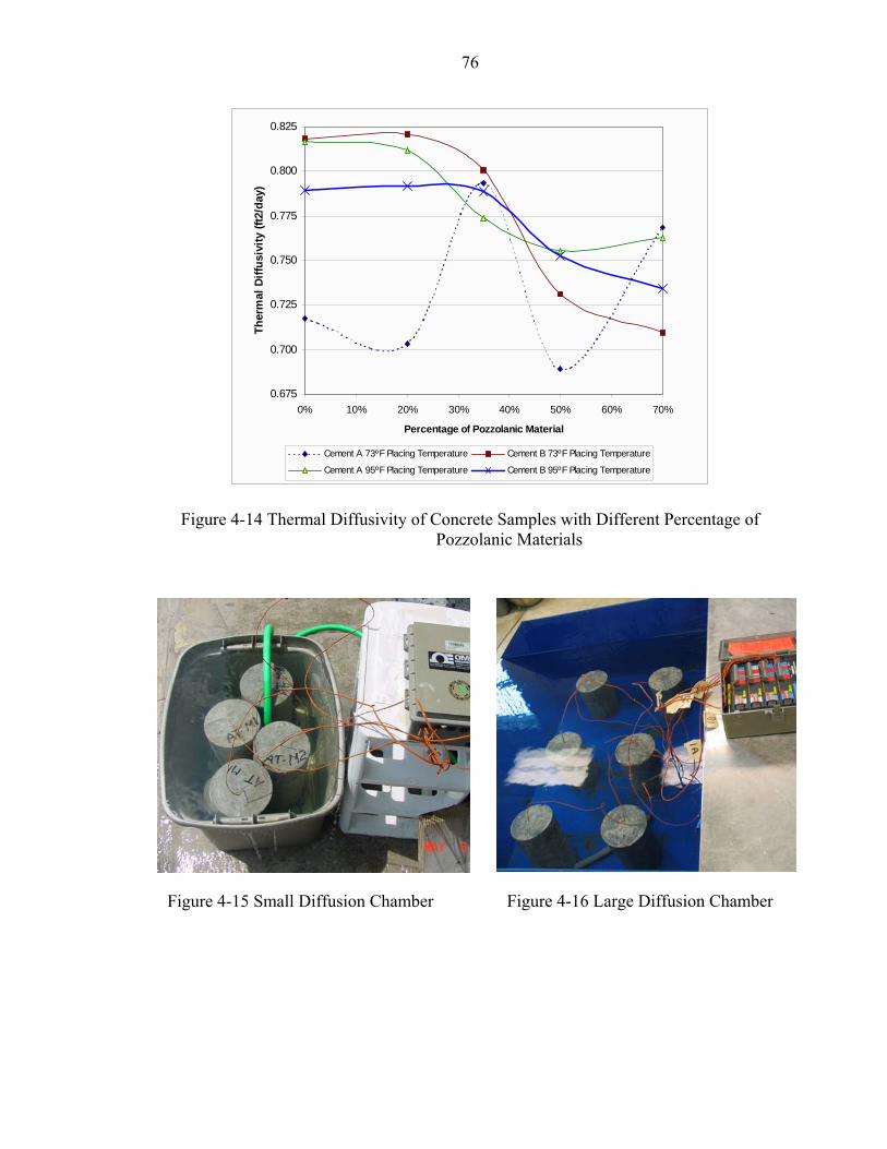
76
0.675
0.700
0.725
0.750
0.775
0.800
0.825
0% 10% 20% 30% 40% 50% 60% 70%
Percentage of Pozzolanic Material
Ther
mal
Diff
usiv
ity (f
t2/d
ay)
Cement A 73ºF Placing Temperature Cement B 73ºF Placing Temperature
Cement A 95ºF Placing Temperature Cement B 95ºF Placing Temperature
Figure 4-14 Thermal Diffusivity of Concrete Samples with Different Percentage of Pozzolanic Materials
Figure 4-15 Small Diffusion Chamber
Figure 4-16 Large Diffusion Chamber

77
Calculation Example for Concrete Thermal Diffusivity
In this section thermal diffusivity calculation method for mix 73B00P is presented.
Based on the data in Table 4-8 the elapsed time between the moment that temperature
difference is 80°F to the moment that it is 20°F equals to 23.98 minutes. Thermal
diffusivity for the mix is calculated as follows:
Thermal Diffusivity = α = 0.812278/(t1 - t2) and (t1 - t2)=23.98 minutes
⇒ α = 0.812278/23.98 = 0.034 ft2/hr = 0.81 ft2/day
Table 4-8 History of Temperature Difference Between Concrete Specimen Core and Water
Time (Minutes)
Temperature Difference Between Specimen and Water
(°F)
Time (Minutes)
Temperature Difference Between Specimen and Water
(°F)
1 84.0 14 40.3 2 79.8 15 38.0 3 75.4 16 35.7 4 71.3 17 33.7 5 67.4 18 31.7 6 63.7 19 30.0 7 60.4 20 28.3 8 57.0 21 26.8 9 53.9 22 25.4 10 51.1 23 23.8 11 48.0 24 22.3 12 45.6 25 21.0 13 42.9 26 19.7

78
Compressive Strength
Compressive strength tests were performed at different specimen ages and with
4″x8″ or 6″x12″ specimens. Compressive strength test results of 4″x8″ specimens are
modified to be comparable to results from tests with 6″x12″ specimens.
In Table 4-9 test results for high temperature cured specimens are presented. For
each mix 3 specimens were broken and the average number is reported. In Table 4-10 test
results for room temperature cured specimens are shown. These numbers are also the
average of results from three tests.
Table 4-9 Compressive Strength of High Temperature Cured Concrete Specimens
Mix Compressive
Strength
(psi)
Age (Day)
Max. Temp (ºF)
Compressive Strength
(psi)
Age (Day)
Max. Temp (ºF)
73A00P 7283 28 200.0 7417 28 190.0 73A20F 7930 28 180.0 7255 28 200.0 73A35F 7496 28 164.4 7428 28 154.1 73A50S 7846 28 170.0 7986 28 198.0 73A70S 8216 28 158.2 7055 28 150.8 73B00P 5679 15 181.9 5051 28 175.8 73B20F 6854 15 181.4 6508 28 171.5 73B35F 6702 15 151.9 6462 28 153.0 73B50S 7595 15 161.8 7433 28 164.4 73B70S 7431 15 155.8 7324 28 159.7 95A00P 7482 15 185.4 8623 28 190.2 95A20F 7671 15 185.6 7395 28 192.1 95A35F 6056 15 179.0 5182 28 189.8 95A50S 7334 15 186.2 6698 28 190.4 95A70S 8553 15 152.7 6378 28 161.8 95B00P 7369 15 184.6 6868 28 185.3 95B20F 8052 15 167.5 7114 28 183.7 95B35F 7287 15 170.8 6711 28 171.1 95B50S 7251 15 177.8 6843 28 188.2 95B70S 8332 15 173.9 7541 28 187.9
73A00P-R 7080 15 163.7 7391 28 167.5 73A20F-R 8675 15 157.2 8055 28 159.6 73A35F-R 8150 15 152 7980 28 160.2 73A50S-R 7946 15 163.2 7311 28 167.0 73A70S-R 8369 15 136.5 8485 28 143.7 73B50S-R 8862 15 150.1 9145 28 159.3 73B70S-R 8332 15 154 8710 28 150.1 95A70S-R 8716 15 164.5 9635 28 171.1

79
Table 4-10 Compressive Strength of Room Temperature Cured Concrete Specimens
Mix Compressive
Strength
(psi)
Age (Day)
Max. Temp (ºF)
Compressive Strength
(psi)
Age (Day)
Max. Temp (ºF)
73A00P 8985 28 80 8584 28 80 73A20F 8436 28 80 8854 28 80 73A35F 7441 28 80 - - - 73A50S 9308 28 75 - - - 73A70S 8036 28 75 - - - 73B00P 6705 15 75 6906 28 75 73B20F 7292 15 75 7372 28 75 73B35F 6174 15 74 7040 28 74 73B50S 7101 15 73 7960 28 73 73B70S 6997 15 75 7909 28 75 95A00P 8239 15 93 8394 28 93 95A20F 7065 15 95 8392 28 95 95A35F 4951 15 94 7565 28 94 95A50S 7252 15 96 8107 28 96 95A70S 7360 15 93 7213 28 93 95B00P 7306 15 99 9025 28 99 95B20F 7902 15 98 8172 28 98 95B35F 6754 15 101 8394 28 101 95B50S 8118 15 101 8392 28 101 95B70S 8028 15 101 7565 28 101
73A00P-R 7395 15 75 8180 28 75 73A20F-R 7108 15 75 8132 28 75 73A35F-R 6522 15 75 7654 28 75 73A50S-R 6435 15 75 7690 28 75 73A70S-R 7413 15 76 8181 28 76 73B50S-R 8107 15 75 9124 28 75 73B70S-R 7224 15 75 9131 28 75 95A70S-R 8871 15 97 7819 28 97
In Figures 4-17 through 4-24 changes in compressive strength for different mixes
with different curing temperatures are shown. First four figures show the data for
compressive strength at 15 days age, while the other figures show compressive strength
for specimens with 28 days age.

80
4500
5000
5500
6000
6500
7000
7500
8000
8500
9000
60 80 100 120 140 160 180 200
Curing Temperature (°F)
Com
pres
sive
Str
engt
h (p
si)
73A00P-R
73A20F-R
73A35F-R
73A50S-R
73A70S-R
Figure 4-17 Compressive Strength for Concrete Specimens with Cement A and 73°F Placing Temperature at 15 Days Age
4500
5000
5500
6000
6500
7000
7500
8000
8500
9000
9500
60 80 100 120 140 160 180 200
Curing Temperature (°F)
Com
pres
sive
Str
engt
h (p
si)
73B00P
73B20F
73B35F
73B50S
73B50S-R
73B70S
73B70S-R
Figure 4-18 Compressive Strength for Concrete Specimens with Cement B and 73°F
Placing Temperature at 15 Days Age

81
4500
5000
5500
6000
6500
7000
7500
8000
8500
9000
9500
60 80 100 120 140 160 180 200
Curing Temperature (°F)
Com
pres
sive
Str
engt
h (p
si)
95A00P
95A20F
95A35F
95A50S
95A70S
95A70S-R
Figure 4-19 Compressive Strength for Concrete Specimens with Cement A and 95°F Placing Temperature at 15 Days Age
4500
5000
5500
6000
6500
7000
7500
8000
8500
9000
60 80 100 120 140 160 180 200
Curing Temperature (°F)
Com
pres
sive
Str
engt
h (p
si)
95B00P
95B20F
95B35F
95B50S
95B70S
Figure 4-20 Compressive Strength for Concrete Specimens with Cement B and 95° F
Placing Temperature at 15 Days Age
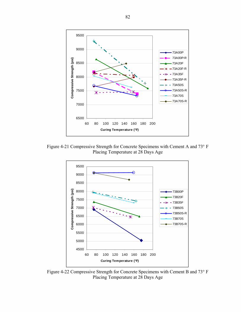
82
6500
7000
7500
8000
8500
9000
9500
60 80 100 120 140 160 180 200
Curing Temperature (°F)
Com
pres
sive
Str
engt
h (p
si)
73A00P
73A00P-R
73A20F
73A20F-R
73A35F
73A35F-R
73A50S
73A50S-R
73A70S
73A70S-R
Figure 4-21 Compressive Strength for Concrete Specimens with Cement A and 73° F Placing Temperature at 28 Days Age
4500
5000
5500
6000
6500
7000
7500
8000
8500
9000
9500
60 80 100 120 140 160 180 200
Curing Temperature (°F)
Com
pres
sive
Str
engt
h (p
si)
73B00P
73B20F
73B35F
73B50S
73B50S-R
73B70S
73B70S-R
Figure 4-22 Compressive Strength for Concrete Specimens with Cement B and 73° F
Placing Temperature at 28 Days Age

83
4500
5000
5500
6000
6500
7000
7500
8000
8500
9000
9500
60 80 100 120 140 160 180 200
Curing Temperature (°F)
Com
pres
sive
Str
engt
h (p
si)
95A00P
95A20F
95A35F
95A50S
95A70S
Figure 4-23 Compressive Strength for Concrete Specimens with Cement A and 95° F
Placing Temperature at 28 Days Age
4500
5000
5500
6000
6500
7000
7500
8000
8500
9000
9500
60 80 100 120 140 160 180 200
Curing Temperature (°F)
Com
pres
sive
Str
engt
h (p
si)
95B00P
95B20F
95B35F
95B50S
95B70S
Figure 4-24 Compressive Strength for Concrete Specimens with Cement B and 95° F
Placing Temperature at 28 Days Age

84
These figures show that at 15 days age, mixes with pozzolanic materials have
higher compressive strength if they are cured in high temperatures while at 28 days age
they show a lower strength compared to room temperature cured specimens.
In Table 4-11 the compressive strength of test mixes for moisture room cured
samples are shown. Each number is the average of three compressive strength test results
for 6″x12″ cylinder specimens that have been cured for 28 days.
Table 4-11 Compressive Strength at 28 Days for Moisture Room Cured Concrete Specimens
Mix Compressive Strength
(psi)
Age (Day) Mix
Compressive Strength
(psi)
Age (Day)
73A00P 8945 28 95A70S 8762 28 73A20F 7689 28 95B00P 7989 28 73A35F 7389 28 95B20F 8175 28 73A50S 8691 28 95B35F 7229 28 73A70S 8580 28 95B50S 8720 28 73B00P 7025 28 95B70S 8117 28 73B20F 7987 28 73A00P-R 8073 28 73B35F 6767 28 73A20F-R 7556 28 73B50S 7657 28 73A35F-R 9462 28 73B70S 7921 28 73A50S-R 8117 28 95A00P 8885 28 73A70S-R 7573 28 95A20F 8313 28 73B50S-R 8361 28 95A35F 6556 28 73B70S-R 9112 28 95A50S 7799 28 95A70S-R 7784 28

85
CHAPTER 5 DISCUSSION OF RESULTS
Introduction
In this chapter the results of the adiabatic temperature rise, the heat of hydration,
thermal diffusivity and compressive strength tests are summarized and compared for
different mixes. The effect of placing temperature and pozzolan content on properties of
concrete within the scope of this research project are studied. Also a group of equations
are introduced to calculate the modification factor for the replacement of pozzolans in
concrete mixes with different placing temperatures.
Adiabatic Temperature Rise Curves
In total, 20 adiabatic temperature rise tests were run. As explained in Chapter 4,
some of the tests were repeated. The main reason to repeat the tests was a change in the
test procedure to prevent the effect of heat from Hydration Chamber heaters on specimen
temperature rise. After reviewing the test results and taking into consideration the
suggestions made by Sure Cure system’s manufacturer, it can be said that heat from
heaters can affect temperature rise when the rate of temperature rise in concrete is less
than 5ºF/day. This stage normally occurs when concrete was three days old. Therefore it
would be reasonable to average the temperature rise data that have been repeated when
the temperature rise rate is more than 5ºF/day and use the data from that point through
day 14 from the second run of the test for a specific mix. Using this method the final
numbers for temperature rise data for each mix was determined.

86
In Tables 5-1 to 5-4, the adiabatic temperature rise data for test mixes are
presented. The temperature rise for repeated mixes are the average of two tests.
Table 5-1 Adiabatic Temperature Rise Data for Concrete with Cement A and 73ºF Placing Temperature
Concrete with Cement A (73ºF Placing Temperature) Plain Cement 20% Fly Ash 35% Fly Ash 50% Slag 70% Slag
Time (Day)
Temp. Rise (ºF) Temp. Rise (ºF) Temp. Rise (ºF) Temp. Rise (ºF) Temp. Rise (ºF)
0.0 0.0 0.0 0.0 0.0 0.0 0.5 22.0 13.6 5.4 12.2 12.1 1.0 48.8 34.2 29.1 31.7 27.3 1.5 65.1 48.6 45.4 54.2 49.3 2.0 77.7 61.1 54.3 72.5 62.8 2.5 83.0 69.1 60.0 81.6 68.8 3.0 87.5 75.6 65.5 85.2 71.6 3.5 89.4 80.4 70.0 87.0 73.4 4.0 91.0 82.4 72.9 88.0 74.7 4.5 92.5 83.6 75.0 88.9 75.4 5.0 93.6 84.2 76.6 89.4 75.8 5.5 94.5 84.8 77.8 89.8 76.1 6.0 95.5 85.4 78.8 89.8 76.4 6.5 96.2 85.4 79.5 89.9 76.4 7.0 97.0 85.7 80.3 89.7 76.5 7.5 97.5 85.7 80.9 89.8 76.6 8.0 98.0 85.6 81.0 90.0 76.7 8.5 98.0 85.8 81.3 90.0 76.9 9.0 98.1 85.8 81.1 90.1 77.0 9.5 98.1 85.9 81.2 90.2 77.1
10.0 98.1 85.9 81.3 90.2 77.3 10.5 98.1 85.9 81.4 90.2 77.4 11.0 98.2 85.9 81.4 90.3 77.5 11.5 98.2 86.0 81.5 90.5 77.6 12.0 98.2 86.0 81.6 90.4 77.6 12.5 98.3 86.0 81.6 90.4 77.6 13.0 98.4 86.0 81.8 90.4 77.6 13.5 98.5 86.0 81.7 90.4 77.6 14.0 98.5 86.0 81.6 90.4 77.6

87
Table 5-2 Adiabatic Temperature Rise Data for Concrete with Cement B and 73ºF Placing Temperature
Concrete with Cement B (73ºF Placing Temperature) Plain Cement 20% Fly Ash 35% Fly Ash 50% Slag 70% Slag
Time (Day)
Temp. Rise (ºF) Temp. Rise (ºF) Temp. Rise (ºF) Temp. Rise (ºF) Temp. Rise (ºF)
0.0 0.0 0.0 0.0 0.0 0.0 0.5 28.9 15.5 25.1 22.0 14.8 1.0 69.9 61.1 45.4 48.6 36.2 1.5 80.1 74.8 54.2 67.8 59.1 2.0 84.4 82.7 60.0 75.3 67.2 2.5 87.7 87.4 64.1 79.6 71.4 3.0 90.6 88.3 67.6 82.0 74.1 3.5 92.9 90.0 70.0 84.0 75.7 4.0 94.7 91.4 71.8 85.6 77.1 4.5 96.1 92.4 73.0 86.9 78.3 5.0 97.4 93.2 74.0 87.9 79.4 5.5 98.6 93.8 74.5 88.6 79.9 6.0 99.7 94.4 75.1 89.1 80.2 6.5 100.7 94.7 75.4 89.4 80.4 7.0 101.5 95.3 75.8 89.7 80.4 7.5 102.3 95.8 76.0 90.0 80.4 8.0 103.0 96.1 76.2 90.3 80.4 8.5 103.5 96.3 76.5 90.4 80.4 9.0 104.0 96.4 76.6 90.6 80.4 9.5 104.3 96.5 76.8 90.7 80.4
10.0 104.6 96.6 77.0 90.8 80.4 10.5 104.8 96.6 77.1 90.8 80.4 11.0 105.1 96.6 77.3 90.9 80.4 11.5 105.3 96.8 77.4 90.9 80.4 12.0 105.5 96.8 77.5 91.0 80.4 12.5 105.7 96.9 77.6 91.0 80.4 13.0 105.8 97.0 77.5 91.0 80.4 13.5 105.9 97.0 77.7 91.0 80.4 14.0 106.0 97.0 78.3 91.0 80.4

88
Table 5-3 Adiabatic Temperature Rise Data for Concrete with Cement A and 95ºF Placing Temperature
Concrete with Cement A (95ºF Placing Temperature) Plain Cement 20% Fly Ash 35% Fly Ash 50% Slag 70% Slag
Time (Day)
Temp. Rise (ºF) Temp. Rise (ºF) Temp. Rise (ºF) Temp. Rise (ºF) Temp. Rise (ºF)
0.0 0.0 0.0 0.0 0.0 0.0 0.5 17.8 9.0 4.8 19.3 4.3 1.0 61.0 40.8 26.5 54.5 16.8 1.5 77.9 63.2 47.0 82.7 49.5 2.0 87.4 77.0 60.8 91.0 57.7 2.5 91.0 85.5 75.5 92.2 60.5 3.0 92.2 88.9 80.9 92.2 62.1 3.5 92.4 90.1 82.9 92.2 63.6 4.0 92.4 90.3 84.0 92.2 64.4 4.5 92.4 90.6 84.4 92.3 65.4 5.0 92.4 90.6 85.0 92.3 66.1 5.5 92.4 90.6 85.0 92.3 66.7 6.0 92.4 90.6 85.0 92.3 67.1 6.5 92.4 90.6 85.0 92.3 67.5 7.0 92.4 90.6 85.0 92.3 67.9 7.5 92.4 90.6 85.0 92.3 68.2 8.0 92.4 90.6 85.0 92.3 68.6 8.5 92.4 90.6 85.0 92.3 68.9 9.0 92.4 90.6 85.0 92.3 69.0 9.5 92.4 90.6 85.0 92.3 69.3
10.0 92.4 90.6 85.0 92.3 69.4 10.5 92.4 90.6 85.0 92.3 69.6 11.0 92.4 90.6 85.0 92.3 69.8 11.5 92.4 90.6 85.0 92.3 69.9 12.0 92.4 90.6 85.0 92.3 70.1 12.5 92.4 90.6 85.0 92.3 70.1 13.0 92.4 90.6 85.0 92.3 70.4 13.5 92.4 90.6 85.0 92.3 70.5 14.0 92.4 90.6 85.0 92.3 70.8

89
Table 5-4 Adiabatic Temperature Rise Data for Concrete with Cement B and 95ºF Placing Temperature
Concrete Cement B (95ºF Placing Temperature) Plain Cement 20% Fly Ash 35% Fly Ash 50% Slag 70% Slag
Time (Day)
Temp. Rise (ºF) Temp. Rise (ºF) Temp. Rise (ºF) Temp. Rise (ºF) Temp. Rise (ºF)
0.0 0.0 0.0 0.0 0.0 0.0 0.5 2.6 56.8 50.4 58.6 45.0 1.0 72.2 72.9 61.9 76.7 69.4 1.5 84.2 77.4 67.9 80.7 73.9 2.0 85.6 77.6 68.9 81.8 76.3 2.5 85.7 77.6 69.2 82.0 77.9 3.0 86.0 77.6 69.3 82.0 78.9 3.5 86.0 77.6 69.6 82.0 79.5 4.0 86.0 77.6 69.9 82.0 79.9 4.5 86.0 77.6 70.0 82.0 79.9 5.0 86.0 77.6 70.0 82.0 79.9 5.5 86.0 77.6 70.0 82.0 79.9 6.0 86.0 77.6 70.0 82.0 79.9 6.5 86.0 77.6 70.0 82.0 79.9 7.0 86.0 77.6 70.0 82.0 79.9 7.5 86.0 77.6 70.0 82.0 79.9 8.0 86.0 77.6 70.0 82.0 79.9 8.5 86.0 77.6 70.0 82.0 79.9 9.0 86.0 77.6 70.0 82.0 79.9 9.5 86.0 77.6 70.0 82.0 79.9
10.0 86.0 77.6 70.0 82.0 79.9 10.5 86.0 77.6 70.0 82.0 79.9 11.0 86.0 77.6 70.0 82.0 79.9 11.5 86.0 77.6 70.0 82.0 79.9 12.0 86.0 77.6 70.0 82.0 79.9 12.5 86.0 77.6 70.0 82.0 79.9 13.0 86.0 77.6 70.0 82.0 79.9 13.5 86.0 77.6 70.0 82.0 79.9 14.0 86.0 77.6 70.0 82.0 79.9

90
Comparison Between Temperature Rise Curves
Effect of percentage of pozzolans
It is generally believed that replacing cement with pozzolan has a reducing effect
on the peak temperature of concrete. However, the amount of reduction has reported
differently in various sources. In the first part of this section, the adiabatic temperature
rise curves from this study are presented. In the second part, the percentage of reduction
in the temperature at 14 days is calculated and changes in the percentage of reduction in
the temperature are shown.
Adiabatic Temperature Rise Curves
In figures 5-1 and 5-2, the effect of replacing cement with fly ash is shown. As it
can be seen, adding pozzolan to the mix reduces the peak temperature. The amount of
reduction, however, has been different for the mixes with cements from the different
sources and also different placing temperatures. A comparison between Figure 5-1 and
Figure 5-2 shows that in mixes with lower placing temperature, the addition of pozzolan
have had a larger reducing effect on the peak temperature. In one case (cement A with
95ºF placing temperature) replacing cement with 20% fly ash did not have a significant
effect on the peak temperature. The other observation is that replacing more fly ash did
not result in the same amount of reduction in the peak temperature.
In Figures 5-3 and 5-4, the effect of replacing cement with slag is shown. The same
trend as replacement of fly ash can be seen in these figures. In Figure 5-4 it can be seen
that replacing 50% of cement with slag did not have a reducing effect on the peak
temperature, while using 70% slag reduced the peak temperature significantly. For this
cement and with 95ºF placing temperature, it could be said that replacing up to 50% of
cement with slag does not lead to a reduction in the peak temperature. The replacement of

91
cement with slag in the mixes with cement B did not show a significant reduction in the
peak temperature either. From these observations it could be said that slag in high
temperature placing conditions does not have a significant reducing effect on the peak
temperature.
Figure 5-1 Effect of Replacing Cement With Fly Ash on Adiabatic Temperature Rise
(73ºF Placing Temperature)
Figure 5-2 Effect of Replacing Cement With Fly Ash on Adiabatic Temperature Rise
(95ºF Placing Temperature)

92
Figure 5-3 Effect of Replacing Cement With Slag on Adiabatic Temperature Rise (73ºF
Placing Temperature)
Figure 5-4 Effect of Replacing Cement With Slag on Adiabatic Temperature Rise (95ºF
Placing Temperature)

93
Reduction in the peak temperature
The percentage of reduction in the peak temperature (Prp) for each mix with
pozzolan was calculated using the following equation.
Prp=(Tcm – Tpm)/ Tcm Equation 5-1
Where:
Prp : Percentage of reduction in the peak temperature,
Tcm : Peak temperature of the control mix (the mix with plain cement),
Tpm : Peak temperature of the mix with pozzolan (20% fly ash, 35% fly ash, 50%
slag, 70% slag)
Using Prp eliminates the possible errors in the peak temperatures recorded by the
Sure Cure system because all the mixes were made and tested in the same condition. The
ratio between peak temperatures should therefore be correct even if an error exists in the
peak temperature number. In 5-5, Prp for different mixes is shown. The numbers could be
averaged because both cements A and B are Type II AASHTO cement.
Table 5-5 Effect of Pozzolans on the Peak Temperature of Concrete % Reduction in Peak Temperature (at 14 days)
Cement Source Placing Temperature 20% Fly Ash 35% Fly Ash 50% Slag 70% Slag
A 73ºF 12.7 17.2 8.2 21.2 B 73ºF 8.5 26.1 14.1 24.1
Average for Cements A & B 10.6 21.7 11.2 22.7 A 95ºF 1.9 8.0 0.1 23.4 B 95ºF 9.7 18.6 4.6 7.0
Average for Cements A & B 5.8 13.3 2.4 15.2
In Figures 5-5 and 5-6, the effect of using pozzolans on temperature at different
ages of concrete is shown. The percent of reduction in temperature (Pr ) was calculated
as:
Pr=(Tc – Tp)/ Tc Equation 5-2

94
Where:
Pr : Percentage of reduction in the temperature,
Tc : Temperature of the control mix (the mix with plain cement),
Tp : Temperature of the mix with pozzolan (20% fly ash, 35% fly ash, 50% slag,
70% slag)
Figure 5-5 Pr for Mixes with 73ºF Placing Temperature
Figure 5-6 Pr for Mixes with 95ºF Placing Temperature

95
Figure 5-7 Average Pr for Mixes with 73ºF and 95ºF Placing Temperatures
Figure 5-7 shows the average Pr for mixes with different placing temperatures. The
first conclusion from this figure is that fly ash has a stronger effect on the temperature
reduction. In other words, a smaller percentage of fly ash replacement has the same effect
as that of a larger percentage of slag replacement. As it is shown, 20% fly ash
replacement has almost the same effect as 50% slag replacement and, in a similar fashion,
35% fly ash replacement reduces the temperature the same as does 70% slag replacement.
Also it can be said that placing temperature has an effect on the amount of reduction in
the temperature. A higher placing temperature weakens the reducing effect of pozzolans
on concrete temperature.
The data in Table 5-5 can be divided to four groups:
1. Average of cements A and B with fly ash and 73ºF placing temperature,
2. Average of cements A and B with fly ash and 95ºF placing temperature,
3. Average of cements A and B with slag and 73ºF placing temperature,
4. Average of cements A and B with slag and 95ºF placing temperature,

96
A second degree polynomial to calculate Prp for any given percentage of cement
replacement by pozzolan for each group can be determined if three points of the equation
are known. For each group, the data of the three points are known: two points in Table 5-
5 and the third point would be Prp= 0 in the mix with plain cement.
The general format of the equation is:
Prp = a(Rp)2 + b(Rp) + c Equation 5-3
Where:
Prp : Percentage of reduction in the pick temperature,
a, b and c: Constants,
Rp : Percentage of pozzolan in the mix.
a, b and c constants were determined by solving the equation for the known three
points. The amount of contents for each data group are shown in
Table 5-6 Constant Factors of Prp Equation Constants No. Data Group Description a b c
1 Cement + Fly Ash, 73ºF Placing Temperature 0.59 0.41 0.00 2 Cement + Fly Ash, 95ºF Placing Temperature 0.59 0.17 0.00 3 Cement + Slag, 73ºF Placing Temperature 0.50 -0.03 0.00 4 Cement + Slag, 95ºF Placing Temperature 0.85 -0.38 0.00
The relationship between Prp , Rp, and Different Placing Temperatures is shown in
Figure 5-8. As it can be seen, higher placing temperature has a smaller reducing effect on
the peak temperature.
As suggested by ACI committee 207, the adiabatic temperature rise curves must be
modified for mixes with pozzolans. One way is to calculate equivalent cement content

97
(Ceq ) and use it to determine a modification factor (kc) for the adiabatic temperature rise
curves published in the ACI 207.1R and ACI 207.2R reports.
Figure 5-8 The Relationship Between Prp , Rp, and Different Placing Temperatures
It is also possible to develop the adiabatic temperature rise curve for a mix with
only plain cement (base mix) and then apply kc to generate the adiabatic temperature rise
curve for any given mix with different pozzolan contents. Ceq is calculated as:
Ceq = Cc + αpCp Equation 5-4
Where:
Ceq : Equivalent Cement Content
Cc : Cement content of the mix (lb/yd3)
αp : Pozzolan modification factor
Cp : Pozzolan content of the mix (lb/yd3)
And
kc = Ceq / Cb Equation 5-5
Where:
kc : Adiabatic temperature rise curve modification factor

98
Cb : Cement content of the base mix (lb/yd3)
The relationship between αp and Prp is determined as follows:
Prp=(Tcm – Tpm)/ Tcm ⇒ Prp= 1 - Tpm/ Tbm Equation 5-6
According to ACI 207.1R-96, there is a linear relationship between the
cementitious material content and the peak temperature so:
Tpm/ Tcm = (Cc + αpCp )/ Ct Equation 5-7
Where:
Ct : Cement content of the control mix which is equal to the summation of the
amounts of Cc and Cp in lb/yd3 (Ct = Cc + Cp )
Therefore:
Tpm/ Tcm = (Cc + αpCp )/ (Cc + Cp ) Equation 5-8
Equations 5-7 and 5-8 ⇒ Prp = 1 - (Cc + αpCp )/ (Cc + Cp ) ⇒ Prp = Cp(1- αp)/( Cc +
Cp ) ⇒
(1- αp) = Prp( Cc + Cp )/ Cp ⇒ (1- αp) = Prp( Cc /Cp ) + Prp Equation 5-9
Rp = Cp / (Cc + Cp) ⇒ Cc/ Cp = 1/ Rp –1 Equation 5-10
Combining Equations 5-9 and 5-10 results:
(1- αp) = Prp (1/ Rp –1) + Prp ⇒ αp = 1- Prp/ Rp Equation 5-11
From Equations 5-3 and 5-11 it is concluded that:
αp = 1 - a(Rp) - b - c/ Rp Equation 5-12
Using the constant factors from Table 5-6 the equations to calculate αp would be as
follows:
For mixes with fly ash and 73ºF placing temperature: αp= 0.59 - 0.59Rp
For mixes with fly ash and 95ºF placing temperature: αp= 0.83 - 0.59Rp
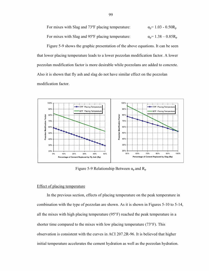
99
For mixes with Slag and 73ºF placing temperature: αp= 1.03 - 0.50Rp
For mixes with Slag and 95ºF placing temperature: αp= 1.38 – 0.85Rp
Figure 5-9 shows the graphic presentation of the above equations. It can be seen
that lower placing temperature leads to a lower pozzolan modification factor. A lower
pozzolan modification factor is more desirable while pozzolans are added to concrete.
Also it is shown that fly ash and slag do not have similar effect on the pozzolan
modification factor.
Figure 5-9 Relationship Between αp and Rp
Effect of placing temperature
In the previous section, effects of placing temperature on the peak temperature in
combination with the type of pozzolan are shown. As it is shown in Figures 5-10 to 5-14,
all the mixes with high placing temperature (95°F) reached the peak temperature in a
shorter time compared to the mixes with low placing temperature (73°F). This
observation is consistent with the curves in ACI 207.2R-96. It is believed that higher
initial temperature accelerates the cement hydration as well as the pozzolan hydration.

100
As it can be seen in Figures 5-10 to 5-14, it is not possible to conclude if a higher
placing temperature results in a higher peak temperature. Some mixes (95A20F, 95A35F
and 95A50S) showed a higher peak temperature compared to the similar mixes with low
placement temperature. The test results show a stop in temperature rise in all the mixes;
therefore the condition has not been fully adiabatic. This fact may affect the peak
temperature numbers and cause the different peak temperature in the mixes with different
placing temperature.
Figure 5-10 Effect of Placing Temperature on Adiabatic Temperature Rise for Mixes with Plain Cement

101
Figure 5-11 Effect of Placing Temperature on Adiabatic Temperature Rise for Mixes with 20% Fly Ash
Figure 5-12 Effect of Placing Temperature on Adiabatic Temperature Rise for Mixes with 35% Fly Ash

102
Figure 5-13 Effect of Placing Temperature on Adiabatic Temperature Rise for Mixes with 50% Slag
Figure 5-14 Effect of Placing Temperature on Adiabatic Temperature Rise for Mixes with 70% Slag

103
Comparison Between Field and Laboratory Test Results
It is necessary to compare the laboratory test results to the field temperature
recordings to determine how similar is the condition in the Hydration Chambers to the
real conditions of the core of a mass concrete element. Based on FDOT requirements,
contractors are required to record the temperature rise in any mass concrete element from
the time that the element is poured to the time it reaches the peak temperature. The data
for the temperature records of the core of the footers A, B, and C of the Bella Vista
Bridge was provided by the project administrator and is presented in Table 5-7. All
footers have a width and length of 17 feet and are 5 ½ feet in depth.
Table 5-7 Temperature Rise of the Core of the Bella Vista Bridge Footers Footer A Footer B Footer C
Time (hour)
Temperature Rise (°F)
Time (hour)
Temperature Rise (°F)
Time (hour)
Temperature Rise (°F)
0 0.0 0 0.0 0 0.0 13 34.2 9 26.1 8 27.1 19 45.1 15 35.1 14 36.9 25 50.1 21 39.4 20 51.4 31 64.3 27 54.0 26 66.0 37 75.4 33 58.2 32 80.1 43 76.7 39 65.7 38 85.1 49 78.6 45 71.6 44 86.8 55 79.6 51 74.9 50 83.0 61 80.3 57 76.1 56 80.1 67 80.2 63 77.3 62 85.1 73 79.1 69 75.1 68 86.8 79 76.2 75 70.5 74 84.3 85 78.5 81 73.1 80 86.4 91 77.3 87 75.2 86 85.6
The data from Table 5-7 is also presented graphically in Figure 5-15. As it is shown
all three footings reached the peak temperature approximately 64 hours after placing
concrete. The peak temperature for three footings is also close (average 81.5 °F).

104
Figure 5-15 Temperature Rise For Footers A, B and C
Footers A and B were placed on April 2nd, 2004, while footer C was placed on
April 7th the same year. The same mix with the same materials was used for all the three
footings. The mix contained 50% type II cement and 50% slag. As it can be seen in
Figure 5-15, some fluctuations have recorded in the temperature rise of footer C. This
unexpected behavior may be caused by a systemic error in the recording device.
Samples were taken from the same concrete that was used to pour the footers and
were tested by the Sure Cure system to determine the temperature rise curves. In Table 5-
8 the adiabatic temperature rise data for laboratory tests are shown. After 64 hours the
average sample temperature rise is 78.5°F, which is consistent with field recordings.
However, the temperature rises after this time in the laboratory, while it drops in the field.
The difference is due to the fact that in the field the condition is semi-adiabatic and
therefore concrete looses heat. Whenever the rate of heat loss is larger than the rate of
heat gain, the temperature drops.
0
10
20
30
40
50
60
70
80
90
100
0 20 40 60 80 100
Time (hour)
Tem
pera
ture
Ris
e (°
F)
Footer A Footer B Footer C

105
Table 5-8 Adiabatic Temperature Rise for Samples Taken from the Field Temp. Rise (ºF) Temp. Rise (ºF) Temp. Rise (ºF) Temp. Rise (ºF) Time
(hour) 1st Test (Site50S-1)∗ 2nd Test (Site50S-2)
Time (hour) 1st Test (Site50S-1) 2nd Test (Site50S-2)
0.0 0.00 0.00 168.0 - 89.94 12.0 26.00 24.65 180.0 - 90.75 24.0 43.80 41.95 192.0 - 91.23 36.0 62.60 59.50 204.0 - 91.65 48.0 74.03 69.75 216.0 - 91.98 60.0 79.66 75.20 228.0 - 92.10 64.0 80.62 76.33 240.0 - 92.15 72.0 82.54 78.60 252.0 - 92.17 84.0 84.32 81.10 264.0 - 92.18 96.0 85.58 83.00 276.0 - 92.18 108.0 86.65 84.55 288.0 - 92.18 120.0 87.56 85.95 300.0 - 92.18 132.0 88.29 87.25 312.0 - 92.18 144.0 88.92 88.26 324.0 - 92.18 156.0 - 89.15 336.0 - 92.18
0
10
20
30
40
50
60
70
80
90
100
0 20 40 60 80 100
Time (hour)
Tem
pera
ture
Ris
e (°
F)
Footer A Footer C Lab A Lab C
Figure 5-16 Comparison of Temperature Rise Between Field and Laboratory Tests
∗ As mentioned before, the data from this test may not be accurate because of the initial equipment malfunction. However, the results of the first and the second test are not significantly different.

106
The correlation between the field and the laboratory data for the first 96 hours after
placing concrete was 0.978 and 0.966 for footers A and C respectively. The high
correlation between the filed and the laboratory results shows that the results from the
Sure Cure system can be considered as an acceptable simulation of a mass concrete pour.
Comparison Between the Test Results and ACI Curves
In ACI 207.1R-96 (Same as Figure 2-1) the adiabatic temperature rise curves of
concrete for concrete samples with 376 lb/yd3 of cement from different types are shown.
The second column in Table 5-9 shows the data from the ACI curve for low placing
temperature. The third column presents the modified ACI data for the higher cement
content of the test mixes.
Table5-9 Comparison Between ACI Curves and Test Results Temperature Rise
(°F)
Cement A (73°F Placing Temperature)
Cement B (73°F Placing Temperature)
Time (day)
ACI Type II
376 lb/yd3
ACI Type II
760 lb/yd3
Temperature Rise
(°F)
Difference
Comparing to ACI
Curve
Temperature Rise
(°F)
Difference
Comparing to ACI
Curve
0 0.0 0.0 0.0 0.0% 0.0 0.0%
1 30.8 62.2 48.8 21.6% 69.9 -12.3%
2 40.2 81.3 77.7 4.4% 84.4 -3.8%
3 44.7 90.4 87.5 3.2% 90.6 -0.2%
4 47.1 95.2 91.0 4.4% 94.7 0.5%
5 49.5 100.0 93.6 6.4% 97.4 2.6%
6 50.3 101.6 95.5 6.0% 99.7 1.9%
7 51.6 104.3 97.0 7.0% 101.5 2.6%
8 52.6 106.4 98.0 7.9% 103.0 3.2%
9 53.2 107.5 98.1 8.7% 104.0 3.2%
10 53.7 108.5 98.1 9.6% 104.6 3.6%
11 54.2 109.6 98.2 10.4% 105.1 4.1%
12 55.0 111.2 98.2 11.7% 105.5 5.1%
13 55.3 111.7 98.4 11.9% 105.8 5.3%
14 55.8 112.8 98.5 12.7% 106.0 6.0%
Correlation With ACI Curve 0.991 0.994

107
Test results for concrete mixes containing plain cements A and B were compared to
ACI curve. Cement A showed a lower temperature rise during the test compared to the
ACI curve. Lower than average heat of hydration of the cement A may contribute to this
fact. Cement B showed a higher temperature rise in the first three days of the test. After
that, the temperature rise of cement B was lower than the ACI curve. The difference for
both cements was ascending during the test. This is due to the fact that the condition in
the Hydration Chambers is not completely adiabatic when the temperature gain of the
concrete is lower than 1.5 to 2.0 °F per day. Ever ascending ACI curves shows that these
curves were developed in a complete adiabatic condition.
Heat of Hydration
The results from the heat of hydration test are to a large extent consistent with the
concrete temperature rise tests. As it is shown in Table 5-10, fly ash has a stronger effect
on the reduction of the heat of hydration. The test results showed that replacing cement
with 20% fly ash reduces the heat of hydration at 7 days by 14.2%, while the replacement
of 50% reduces the heat of hydration by 10.2% at 7 days. However, 20% jump in the
amount of slag replacement significantly reduces the heat of hydration. (38.1% at 7 days
and 35.8% at 28 days).
Table 5-10 Effect of Pozzolans on Heat of Hydration % Reduction in Heat of Hydration
Cement Source Time 20% Fly Ash 35% Fly Ash 50% Slag 70% Slag
A-1 7 Days 14.2 - 10.2 - A-2 7 Days - 19.9 - 38.1 A-1 28 Days 18.1 - 9.1 - A-2 28 Days - 28.4 - 35.8

108
Thermal Diffusivity
The average thermal diffusivity number for the mixes was determined to be 0.80
ft2/day which is about 35% less than the amount suggested in ACI 207.1R-96 for
concrete mixes with lime stone aggregate (ACI suggested number is 1.22 ft2/day). ACI
207.1R-96 does not specify the maximum aggregate size of the samples that were used to
determine the concrete thermal diffusivity. Since the major application of mass concrete
is in dams, the numbers reported by ACI 207.1R-96 may be originated from the samples
with very large aggregate size. However, in FDOT approved mass concrete mix designs
coarse aggregate occupies about 45% of the mix volume. The rest is filled with cement,
fine aggregate, and water. The mixture of cement and sand has a thermal diffusivity of
about 0.40 ft2/day (Xu and Cheng, 2000). The thermal diffusivity of water is 0.13 ft2/day.
The thermal diffusivity of limestone has been reported between 1.00 to 1.40 ft2/day in
different sources with an average 1.20 ft2/day. Based on these diffusivity numbers it is
reasonable for a concrete containing about 45% limestone and the rest containing
materials with much lower thermal diffusivity to have a thermal diffusivity lower than
that of the limestone. Another observation of theses tests (as it was shown in Chapter 4)
was that concrete thermal diffusivity reduces with the replacement of higher percentage
of pozzolans.
The thermal diffusivity number affects the results of calculations to determine the
maximum temperature and temperature difference (thermal gradient) in a mass concrete
element. In Figure 5-17 the effect of thermal diffusivity on the maximum temperature rise
for mass concrete elements with thickness of 5.5, 6.5 and 7.5 feet is shown. The
maximum temperature rise was calculated using Schmidt method. Two different curing
conditions were assumed. At first it was assumed that no insulation is used during the

109
curing period. For the second time, the boundary conditions were modified to simulate
the use of insulation. As it is shown, higher diffusivity numbers result in lower maximum
temperature rise. Therefore, if the thermal diffusivity number of the concrete is assumed
higher than what it really is, the maximum temperature will be predicted lower than the
number that it will reach. In Figure 5-18 the effect of thermal diffusivity on thermal
gradient is shown. The model showed that if insulation is not used, changes in the
thermal diffusivity will affect the thermal gradient but if insulation is used, changes in the
thermal diffusivity do not affect the thermal gradient.
Figure 5-17 Effect of Thermal Diffusivity on Maximum Temperature Rise

110
Figure 5-18 Effect of Thermal Diffusivity on Thermal Gradient
Compressive Strength
In Chapter 4 it was shown that using pozzolans effects short term (15 day)
compressive strength of high temperature cured sampled positively. However, after 28
days, the compressive strength of high temperature cured samples is lower compared to
the room temperature cured samples.
Table 5-11 and Figure 5-19 show the summary of 28-day compressive strength
results for 6″x12″ specimens cured in moisture room. The numbers are average of
compressive strength tests for similar mixes. For specimens with 73°F a significant
difference in 28-day compressive strength was not resulted. It can also be seen that
replacing a portion of cement with slag helps the 28-day compressive strength of
concrete. The results for high temperature placed concrete showed that replacing cement
with pozzolans (slag or fly ash) reduces the 28-day compressive strength 2 to 3% in the

111
mixes with 20% fly ash, 50% and 70% slag. However, in the mixes with 35% fly ash a
significant (18%) loss of 28-day compressive strength was observed.
Table 5-11 Effect of Pozzolan Content on 28-day Compressive Strength
Placing Temperature Pozzolan Type
Pozzolan (%)
Compressive Strength (psi)
Compressive Strength Ratio (As a ratio of 0% pozzolan mix)
- 0 8014 1.00 20 7744 0.97 Fly Ash 35 7873 0.98 50 8207 1.02
73°F
Slag 70 8297 1.04 - 0 8437 1.00
20 8244 0.98 Fly Ash 35 6893 0.82 50 8260 0.98
95°F
Slag 70 8221 0.97
Figure 5-19 Effect of Placing Temperature and Pozzolan Content on 28-day Compressive Strength
0.80
0.90
1.00
1.10
0% 20% 40% 60% 80%
Percentage of Pozzolan
Com
pres
sive
Str
engh
t Rat
io
73°F Placing Temperature 95°F Placing Temperature

112
CHAPTER 6 SUMMARY, CONCLUSIONS, AND RECOMMENDATIONS
Summary
The main objective of this study was to develop the adiabatic temperature rise
curves for mass concrete made with Florida materials. In addition, the thermal diffusivity
of Florida concrete and the effect of high placing and curing temperature on compressive
strength of concrete were studied. The following is a summary of steps undertaken to
achieve the goals of the project.
A literature review was conducted to identify the factors affecting temperature rise
in concrete and to study previous works in this field. The literature review showed that
the temperature rise in concrete has been an issue of concern since early 1930’s when
mass concrete was first used in dam projects. Various methods have been developed to
predict the temperature rise in mass concrete. One of the most practical methods is to use
ACI curves in combination with the Schmidt method to predict the temperature rise in
mass concrete elements. The literature review also showed that in recent years with the
advances in computing devices some attempts have been made to develop numerical
methods and computer softwares to predict the temperature rise in a mass concrete
element.
The first step in the experimental phase of the project was to determine the concrete
mix designs and materials which needed to be tested. A total of 20 mixes with cements
from two different sources, with two different placing temperatures and various

113
percentages of pozzolanic materials contain were tested for adiabatic temperature rise,
thermal diffusivity and compressive strength. The Heat of hydration of cement samples
and blends of cement and pozzolan were also determined.
The results of the tests were analyzed. The effect of placing temperature, curing
temperature and pozzolan content on temperature rise curves, thermal diffusivity and
compressive strength were studied.
Conclusion
The following conclusions can be made after executing the aforementioned
activities for this study and analysing the results:
• Using fly ash and slag as a replacement for AASHTO Type II cement reduces the peak temperature in mass concrete pours.
• Fly ash is more effective in reducing the peak temperature of the mass concrete.
• Replacement of less than 50% of cement with slag does not have a significant effect on the peak temperature.
• Higher placing temperature reduces the effectiveness of fly ash and slag in peak temperature reduction.
• Higher placing temperature accelerates the hydration of cement; therefore the concrete reaches the peak temperature earlier.
• The calculated Pozzolan Modification Factor (αp) can be used to modify ACI curves for mixes with different cement and pozzolan contents.
• Thermal diffusivity of concrete reduces by replacing larger percentage of pozzolanic materials.
• Thermal diffusivity of mass concrete mixes used in Florida is approximately 33% lower than the number suggested by ACI.
• Concrete mixes with pozzolan have a higher short term compressive strength if cured in higher temperature. However, after 28 days the mixes with lower curing temperature show larger compressive strength.
• Placing temperature does not have a significant effect on 28-day compressive strength for mix with lower than 20% fly ash content as well as for mixes with slag.

114
• For mixes with more than 20% fly ash content it is likely that high placing temperature affect the 28-day compressive strength significantly but further investigation is necessary.
Recommendations
The results of this study lead to the following recommendations:
• To develop new adiabatic temperature rise curves, ACI adiabatic temperature rise curves should be modified by the Pozzolan Modification Factor (αp) calculated in this study.
• The calculated thermal diffusivity number ought to be used in peak temperature predictions calculations.
• Additional studies need to be performed on concrete thermal diffusivity.
• Additional studies should be performed on the effect of fly ash replacement for mixes with high placing temperature on the long term compressive strength.

115
APPENDIX A
SURVEY OF STATE HIGHWAY AGENCIES
A previous study1 on mass concrete showed that only nine states including Florida
have mass concrete specifications. The purpose of this survey was to figure out the other
states’ regulation on mass concrete pours and possible studies that have been done.
Following questions were sent to state Material Engineers of California, Idaho, Illinois,
Kentucky, North Carolina, South Carolina, Texas and Virginia via e-mail
1. Do you require contractors to provide you with calculations showing mass concrete temperature rise prediction?
2. If the answer to question number 1 is Yes, what method is used to predict the temperature rise? Do you use ACI curves?
3. Have you ever developed adiabatic temperature rise curves for concrete mixes that are usually used in mass concrete projects? If yes, can you provide us with your own curves?
4. If you have not developed adiabatic temperature rise curves, do you think it is necessary to develop curves for concrete mixes made of local materials or you think that ACI curves are accurate enough?
5. Do you have any suggestion regarding ACI curves or adiabatic temperature rise in mass concrete?
Four responses were received. Following is the description of responses.
1 Chini, Abdol R., Muszynski, Larry C., Acquaye, Lucy, Tarkhan, Sophia, 2003 “Determination of the Maximum Placement and Curing Temperatures in Mass Concrete to Avoid Durability Problems and DEF”, Final Report Submitted to The Florida Department of Transportation, Gainesville, Florida

116
California
Caltrans (California Department of Transportation) does very few projects where
mass concrete is involved. Of the ones that mass concrete was involved, Caltrans
typically leans to the side of performance specifications and requires the contractor to
deliver crack free concrete. Full responsibility of the mass pour is put on the contractor.
If the contractor does have a heat removal plan, it must be approved by the engineer
and the regional water quality control board (if they are in fact involved). Caltrans’s
approval does not imply that the plan will work, it is rather to check if it is reasonable,
follows "best management practices," and is workable.
One thing Caltrans does to help the contractor is to make sure to give mix
parameters that are conducive to low heat. For instance on the new San Francisco
Oakland Bay Bridge, California's "banner project," currently in construction, Caltrans
gives contractors a mix design which has 50% slag and/or 50% fly ash requirement.
Illinois
Illinois Department of Transportation does not require contractors to submit a mass
concrete plan. Contractors are required to monitor the temperatures, report the results,
and stay within the specification limitations for temperature difference.
Kentucky
Kentucky Department of Transportation does have a requirement for contractors to
submit a mass concrete. They use ACI 207 curves and do not think that they need to
develop their own curves because ACI are believed to be fairly accurate.
South Carolina
South Carolina Department of Transportation requires contractors to submit a mass
concrete plan. The requirements are as follows:

117
702.16 Mass Concrete Placement. Mass concrete placement shall be defined as any pour in which the concrete being cast has dimensions of 5 feet or greater in three different directions. For pours with a circular cross-section, a mass concrete placement shall be defined as any pour that has a diameter of 6 feet or greater and a length of 5 feet or greater. For all mass concrete pours, the mix temperature shall not exceed 80°F as measured at discharge into the forms. Further, the Contractor shall be required to maintain a temperature differential of 35°F or less between the interior and exterior of all mass pour elements during curing. Before placing mass concrete, the Contractor shall submit, to the Engineer for review and acceptance, a Mass Concrete Placement Plan containing, but not limited to, the following:
1. An analysis of the anticipated thermal developments within mass pour placements using the proposed materials and casting methods.
2. A plan outlining specific measures to be taken to control the temperature differential within the limits noted above.
3. Details of the Contractor's proposed monitoring system. If the Contractor is proposing a special concrete mix design as part of the temperature control plan, this mix design should also be submitted for review. The Contractor shall provide temperature monitoring devices to record temperature development between the interior and exterior of the element at points approved by the Engineer and shall monitor the mass pours to measure temperature differential. Temperature monitoring shall continue until the interior temperature is within 35°F of the lowest ambient temperature or a maximum of two (2) weeks. The Engineer shall be provided with a copy of each set of readings as they are taken and a temperature chart for each mass pour element showing temperature readings vs. time. If the monitoring indicates that the proposed measures are not controlling the concrete temperature differential within the 35°F specified, the Contractor shall make the necessary revisions to the plan and submit the revised plan for review. The Contractor shall assume all risks connected with placing a mass pour of concrete. Review of the Contractor's plan will in no way relieve the Contractor of the responsibility for obtaining satisfactory results. Should any mass concrete placed under this specification prove unsatisfactory, the Contractor will be required to make the necessary repairs or remove and replace the material at the Contractor's expense. All costs associated with special temperature controls for mass concrete placement shall be included in the unit cost of the concrete cast, and will be without additional specific compensation. The control of temperatures in mass concrete pours shall be in addition to any other requirements found on the plans and/or in the special provisions that may apply to the work in question.

118
APPENDIX B
SURE CURE MICRO COMPUTER SYSTEM
SURE CURE
BY
PRODUCTS ENGINEERING
3668 Heatherwood Way Evergreen, Colorado 80439
(303) 679-9635

119
CONTENTS INTRODUCTION 121 KEY WORDS AND CONCEPTS 122 INSTALLATION 125 APPLICATION LIST 127 RUNNING A SURE CURE PROGRAM 129 PROGRAMING A BED 130 PLOTTING TIME VS. TEMPERATURE 131 MAINTENANCE 132 TROUBLE SHOOTING 132

120
SURE CURE MICRO COMPUTER CONTROL SYSTEM
INTRODUCTION Congratulations on your purchase of the SURE CURE Micro
Temperature Controller (micro controller). The micro controller gives you some of the most important features of the SURE CURE Computer System. The micro controller is designed to be easy to use and install.
The micro controller consists of three major parts. The first is a
personal computer. The computer comes equipped with a floppy drive capable of holding 1.44 Mbytes of data and a hard drive capable of holding at least 2 Gbytes of data. Translating this into real terms, the hard disk is capable of storing more than 100 years of time-temperature data as well as the SURE CURE software, and other files necessary to make the system work.
The computer also comes with a parallel port. The port is used to
send data to the printer. A monitor is connected to the back of the computer. The computer
communicates to you by displaying information on the monitor (the computer assumes you can read, occasionally this assumption is incorrect).
You communicate to the computer using a keyboard and a mouse.
If possible, the computer asks you multiple choice questions, thus reducing the requirement on you to be able to spell.
The computer likes a nice environment (little dust and temperatures
between fifty and eighty degrees Fahrenheit). If the computer is located in a nice environment it should have a long trouble free life.
The second component, the printer, is Windows compatible. The
printer, as previously mentioned, connects to the computer through a parallel port. The printer produces permanent records of your curing activities.
The third and final component is the I/O cabinet. The cabinet
contains a multitude of connectors, cables, and plugs. The blue connectors are for thermocouples. The black connectors are for heating on-off devices such as cylinders, motorized valves, and

121
electric heaters. The multi-wire cable is to connect the I/O cabinet to the computer. The 120 volt inlet is to bring power to the I/O cabinet. You should be able to connect the entire system by simply plugging in devices (no hard wiring to terminal blocks).
Inside the I/O cabinet is an analog to digital converter. The
converter translates temperature signals from your plant into numbers. The computer in turn translates these numbers into temperatures which you can understand.
The micro controller is designed to operate twenty-four hours a day.
The controller functions in conjunction with a program named “Plnt”. “Plnt” must be running for the controller to be working. Warning: always unplug the I/O cabinet when ”Plnt” is not running. The controller communicates with you through the keyboard and monitor. The controller communicates with the plant through the analog to digital converter and the I/O cabinet. The controller can only look at one channel at a time. Therefore it may take up to twenty seconds for the controller to sample the temperature of a channel and determine whether to activate or deactivate it’s output relay. Once every six minutes the controller writes each channel's temperature on the disk. The controller does not operate if you turn the computer off. The controller does not operate if you deactivate the “Plnt” program.
In the event of a power failure, the controller automatically resumes
control when power is restored.
KEY WORDS AND CONCEPTS It is important to understand the terminology and devices used with
the system. The following is a list of items and terms which may not be familiar.
CHANNEL : A path through which the computer measures a
temperature of a point in the plant. CYLINDER : A way in which a SURE CURE programs a channel
on a bed. A cylinder follows the reference channels temperature until six hours after control of the reference ceases. A channel controlled as a cylinder is the same as a channel controlled as a slave with a temperature difference of zero and a finish time six hours after the references.
LEFT CLICK : Press the left button on the mouse. You select an
item from a menu by left clicking the mouse when the mouse

122
cursor is on top of the menu item. MASTER : A way in which a channel is controlled. A channel
programmed as a master is controlled to follow a time-temperature profile.
MATURITY : The area under a time-temperature curve. The units
of maturity are degree hours. The maturity of a concrete mix is proportional to it's strength (the higher the maturity, the higher the strength). The longer a mix cures the stronger it becomes. Likewise, the longer a mix cures the higher the maturity becomes. The warmer a mix cures (generally speaking) the stronger it becomes. Likewise the warmer a mix cures the higher the maturity becomes. The Micro controller uses zero degrees as a base temperature for calculating maturity. The Micro controller begins accumulating maturity for each channel after the channel's start time.
MOUSE CURSOR : Most often , an arrow which can be moved
about the screen using the mouse. The mouse cursor may take on many other forms besides the arrow (for example: an hour glass). The arrow is the most common form. You move the mouse cursor to locations on the screen to push buttons or enter time/temperature points.
RE-BOOT : To reset the computer. You can re-boot the computer
by left clicking the mouse on the Start button in the lower left corner (seems strange to press start in order to stop, but that is the way it works). Then left click on Shut down. Next left click on restart. Finally, press the OK button. Do not turn the power on and off to RE-BOOT.
REFERENCE : A channel, whose temperature or output is used to
control a cylinder, or slave. A reference channel provides the program temperature for either a cylinder or a slave.
SELECTION BAR : A highlighted rectangular area indicating the
present choice in a multiple choice area. The selection bar may be moved to another choice by using the arrow keys or the mouse.
SLAVE : A way in which a channel is controlled. A channel
programmed as a slave follows the temperature of a reference channel.

123
STATE : A variable which indicates whether a channel is be controlled by the Micro controller. The state can have one of three values. either ON, OFF, or SET. ON means the Micro controller is activating the channel's output relay to maintain a desired temperature. SET means you have programmed the channel to come ON but the start time has not been reached yet. Thus the Micro controller is not yet controlling the channel. Maturity and on time are zero when a channel is SET. OFF means the Micro controller is not controlling the channel's temperature. However, the Micro controller is accumulating maturity for the channel.
THERMOCOUPLE : A device which produces a small voltage
proportional to temperature. A thermocouple is produced by bring two dissimilar metals in contact. The Micro controller normally comes equipped to accept Type "T" thermocouples. The type "T" thermocouple consists of a copper wire encased in blue insulation and a constantan wire encased in red insulation. When the two wires are brought in contact they form a thermocouple. To make a thermocouple, you strip the insulation off the two wires and twists them together. Be sure the wires are twisted tightly. If the thermocouple is to be used for more than a couple of days, the wires should be soldered together. Always electrically isolate the thermocouple from the world (wrap the exposed metal end with electrical tape or shrink tubing). This helps protect the Micro controller from lightning and stray voltages. A thermocouple only produces millionths of a volt. Thus thermocouples are very sensitive to electrical noise. Avoid running thermocouple wire in parallel with AC voltage wires. Often a thermocouple cable will come with a third wire and a metallic foil to shield the thermocouple from electrical fields. The shield wire is connected to the I/O cabinet through the thermocouple plug. The shield should be electrically isolated from the world on the thermocouple end of the cable. Do not twist the shield wire with the thermocouple wires.
TEXT CURSOR : An vertical bar on the computer monitor which
indicates where the next character will appear. Often, but not always, the cursor blinks.
TIME/TMEPRATURE POINT : A description of the thermal state
with respect to time . A TIME/TEMPERATURE point describes the temperature at a given time.
TIME-ON : The duration the Micro controller activated the a

124
channel's output relay. Time-on is measured in hours and minutes. The Micro controller activates a channels output relay whenever the channel is cooler than it's program temperature. Thus, time-on is also the length of time the channel was too cool.
INSTALLATION
Carefully inspect the boxes the equipment was shipped in. Take
exception with the shipper if there appears to be any damage to the boxes. Next unpack the equipment from the boxes. Please call Products Engineering if there appears to be any damage.
Place the computer in a room with an office like environment.
Excessive dust or temperature can cause the computer's life to be significantly shortened. We recommend the temperature of the room be between fifty-five and eighty degrees Fahrenheit. Place the computer on top of a desk. Be sure you have access to the side with the serial port. Place the monitor near the computer. Plug the power cord from the monitor into a 120 VAC outlet (preferably on a surge suppresser). Plug the video cable into the monitor connector on the back of the computer. Place the keyboard in front of the monitor. Plug the keyboard cable into the keyboard connector on the back of the computer.
Mount the I/O cabinet on a wall. The I/O cabinet must be within ten
feet of the of the computer. Connect the serial cable from inside the I/O cabinet to the computer's serial port (the serial cable is shipped connected inside the I/O cabinet, run the serial cable though the chase nipple in the bottom of the I/O cabinet to the computer.
Connect 120 V.A.C. to the I/O cabinet. You can run approximately
12 amps of loads from a 15 amp breaker and 16 amps of load from a 20 amp breaker. A SURE CURE mould has a load of one amp. Check with the manufacturer for loads of motorized valves. If there is a problem with large loads, drive an interposing relay with the micro-system. Let the relay drive the large load.
Plug the thermocouples into the jacks on the side of the I/O cabinet.
You should have at least two thermocouples to test the system. Place the printer near the computer. Read the introductory
chapters of the printer manual. Connect the printer cable to the back of the printer. Connect the other end of the printer cable to the computer's parallel port. Load the paper into the printer. Plug the power cord from the printer into a 120 VAC outlet (preferably in a

125
surge suppresser). Plug the computer into a 120 VAC outlet (preferably in a surge
suppresser). Do not put a disk in the floppy drive (the system uses the hard drive).
You are now ready to test the system. Turn the computer on.
Within a minute you should see a list of the channels and their temperatures.
If you do not, turn the system off and check all connections. Turn
the system back on. If you still do not, call Products Engineering. Check the numbers under the Reading column on the monitor.
These should contain the temperatures of the thermocouples you connected. Be sure these readings appear realistic.
Next test the system’s outputs. Move the mouse cursor over the
Start button (the start button is in the monitor’s lower left corner) and left click the mouse. A menu pops up. Move the mouse cursor directly up to Programs. A menu appears to the right. Move the mouse cursor directly to the right onto the menu. Move the cursor up or down to SURE CURE micro. A menu appears to the right. Move the cursor directly to the right onto the menu. Left click the mouse on Relay Test. A dialog box appears. Enter a number between one and eight Press the Test button ( Press means move the mouse cursor over the portion of the screen that says Test and press the left mouse button). The computer turns on the relay for the given channel. Look inside the I/O cabinet. There are two circuit boards which hold black rectangular boxes. Next to the boxes are red pilot lights. The light associated with the channel you entered should be illuminated. Repeat the process for each of the eight controllable channels. If any of the lights fail to illuminate, check for loose wires. If the problem persists call Products Engineering.
Testing is now complete. The micro controller is ready for your
use. Products Engineering highly recommends the computer obtain 120
VAC power though a surge suppresser. If you do not already have one, most local computer retailers sell them.
You can configure your system to automatically resume after a
power failure by creating a shortcut to the “Plnt.exe” application. Then move the shortcut to your computer’s “Start Menu\Programs\Startup” folder. The SURE CURE system will then automatically launch

126
whenever the computer is booted. Products Engineering highly recommends that you have at least
two good backup copies of the floppy disk containing the SURE CURE software at all times. Blank floppy disk can be purchased from your local computer retailer and copies can be created using Windows Explorer.
APPLICATION LIST
The following is a list of applications which make up the SURE CURE Micro temperature controller system.
CURE The CURE application is used to enter a time/temperature program. You can enter a program for either a bed or a channel. You can also review a program or store programs using CURE.
PLANT The PLANT application manages all the input and output with the world. This application should be left running all the time. The application is automatically loaded when the computer starts. PLNT displays a summary for each of the physical channels which make up the system.
TimeVsTemp The TimeVsTemp application allows you to view the actual time/temperature profile for each channel. You can also superimpose a channels program over these profiles. You Use TimeVsTemp to evaluate the results of the curing process.
REVIEW The REVIEW application allows you to view cure data for a bed or channel. REVIEW also displays the programmed curve.
RELAY TEST The RELAY TEST application allows you to check one of the system’s outputs. The Micro controller turns on only the designated relay while turning all other relays off. This is a trouble shooting application.

127
SET BED CONFIG The SET BED CONFIG application allows you to define the channels which make up abed. You also tell micro controller how each channel is controlled when the bed is programmed.
SURE CURE CONFIG The SURE CURE CONFIG application allows you to define the channels which make up the micro control system. Using this application, you tell the micro controller a channel’s name, it’s physical channel, and it’s output. Note: You must restart “PLNT” after making changes to the channel configuration.
LIMITS The LIMITS application allows you to set thermal alarm limits as well as temperature dependent safe guards. Use this application to designate one of the system’s output relays as an alarm relay.
RELAY HISTORY The relay history application allows you to plot the history of when each relay was energized. Results are displayed as percentages of possible time energized. This application also allows you to view the amount of time a relay was energized during a given period.
DRIVR201 The drivr201 application allows you to configure the
computer’s serial port to work with the micro control system. This application should only be run when you are installing the SURE CURE system on a new computer with a different serial port. This is a DOS based application. To run the application, open Window Explorer, display the SURE CURE folder, and select the drivr201 application. This is the only application which has to be activated this way. You should call Products Engineering if it becomes necessary to run this application.
CURE, TimeVsTemp, and Review all have help files for addition
instructions on their use. Once any one of these applications is running, simply left click on the help menu for these instructions.
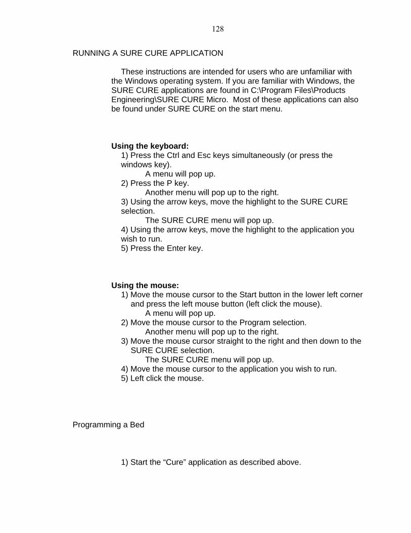
128
RUNNING A SURE CURE APPLICATION These instructions are intended for users who are unfamiliar with
the Windows operating system. If you are familiar with Windows, the SURE CURE applications are found in C:\Program Files\Products Engineering\SURE CURE Micro. Most of these applications can also be found under SURE CURE on the start menu.
Using the keyboard:
1) Press the Ctrl and Esc keys simultaneously (or press the windows key).
A menu will pop up. 2) Press the P key.
Another menu will pop up to the right. 3) Using the arrow keys, move the highlight to the SURE CURE selection.
The SURE CURE menu will pop up. 4) Using the arrow keys, move the highlight to the application you wish to run. 5) Press the Enter key.
Using the mouse: 1) Move the mouse cursor to the Start button in the lower left corner
and press the left mouse button (left click the mouse). A menu will pop up.
2) Move the mouse cursor to the Program selection. Another menu will pop up to the right.
3) Move the mouse cursor straight to the right and then down to the SURE CURE selection.
The SURE CURE menu will pop up. 4) Move the mouse cursor to the application you wish to run. 5) Left click the mouse.
Programming a Bed
1) Start the “Cure” application as described above.

129
2) Select “Bed” as the type of thing you are programming. You can either program a bed or channel. From the edit menu make sure Program a Bed is checked. If it is not, left click on Program a Channel. This changes the item you are programming from a channel to a bed. You can also left click on the button labeled Channel in the upper left corner (this button indicates the item being displayed). Left clicking the button toggles between programming a bed and programming a channel.
3) Select the bed you wish to program. Select “Select Which Bed” from the Edit menu. Cure allows you to select a bed. (Shortcut: left click on the second button from the upper left and select a bed.)
4) Select New Program. Select “New” from the File menu. Cure clears the old program from the computer's memory. Also, the program start time is reset to five minutes in the future. This step is not necessary if you wish to reuse the old program.
5) Enter time and temperature coordinates for your program. Left click on the “Start Temperature” button in the Time/Temperature Point Dialog Box located in the lower right corner. Enter time/temperature points as desired.
6) Start the Program. Select “Start Program” from the File menu. Cure saves the program and tells the computer to load the program for use.
There are many variations from the steps above which may be used to program a bed. These are given as a starting guide.
PLOTTING TIME VS. TEMPERATURE
The TimeVsTemp software is designed to enable the system operator to review the time-temperature data recorded over the course of a bed’s cure cycle. By reviewing this cure history, the system operator can either verify that the bed followed the programmed time-temperature curve or identify potential problems by comparing what was programmed with what actually happened.

130
1) Start the “TimeVsTemp” application as described above.
2) To check a bed's cure history, select one or more channels on the bed. (Channels are assigned to beds using Bed Setup, which is a separate SURE CURE program.) Click on the Edit menu and choose Plot Channels. This will bring up the Select Channels dialog box.
3) For a channel's time-temperature data to be plotted, the channel must appear in the Plot List. Specify the appropriate channel designation (either by typing it or selecting it from the list); then, click on the Add button. After adding a channel to the Plot List, you can change the plot color by highlighting the channel and clicking on the Color button. Once all the desired channels have been added to the Plot List, click the OK button.
4) After specifying the channels to be plotted, define the period of time over which the temperature data will be plotted. From the Edit menu, select Plot Times to bring up the Select Plot Times dialog box. This dialog box consists of two parts: Starting Time and Record Length. Under Starting Time, enter the appropriate hour, day, month, and year. For Record Length, enter the number of hours required to complete a cure cycle and click OK.
5) You should now see a time-temperature curve for the selected channel(s) on your bed. The curves should begin at the specified starting time and continue for the specified number of hours (i.e., record length). The two arrow buttons on the tool bar can be used to shift the graph forward or backward in one-hour increments.
5) Finally, TimeVsTemp provides a quick way to compare actual time-temperature data with the data that was programmed using Cure. To see the programmed time-temperature curve, click on the View menu and select Program .... The Select Program dialog box will come up. Enter a channel designation (generally the master channel for the bed in question) and assign it a color not already in use. Click OK, and the programmed curve will appear on the graph where it can be readily compared to the actual time-temperature data.
131
MAINTENANCE 1) Blow the dust out of the computer every six months.
Remove the computers cover. Using CLEAN, DRY compressed air, blow the dust off the components inside the computer.
2) Clean the floppy disk drive once every six months.
Purchase a floppy disk cleaning kit from a local computer retailer. Follow the instructions and clean the disk drive.
3) Clean or replace the thermocouple jacks and plugs.
Steel wool can be used to clean the thermocouple plugs. Systems where the plugs are always left in should seldom if ever need cleaning.
TROUBLESHOOTING The system should seldom have trouble. However, everything ever
created by man sooner or later breaks. The following is a list of potential problems which can occur with your system. If you cannot solve the problem with these suggestions, please try to gather as much data on the problem as possible and then call Products Engineering.
Thermocouples.
Thermocouples are by far the largest source of potential trouble.
The most common sign of trouble with a thermocouple is an "OPEN" reading on the menu or review a cycle screens. Thermocouple problems are also indicated by erratic time-temperature curves.
The cause of most thermocouple trouble is poor connections. The
copper side of the type "T" thermocouple is subject to oxidization. Thus connections must be checked periodically. The amount of oxidization is a function of the environment where the connection is located. Loose screws in plugs, jacks, and terminal blocks are another source of thermocouple troubles. Broken wires are yet another common problem. A thermocouple is created by twisting the two wires

132
in the thermocouple together. Therefore, a thermocouple may be checked independent of the Micro controller using an ohm meter. A good thermocouple should have a reading of less than one thousand ohms. A bad thermocouple has a very high reading.
A thermocouple which is not electrically isolated from the outside
world may give erratic readings. Therefore, be sure all thermocouples are either wrapped in electrical tape or shrink tubing. Isolating the thermocouple also provides protection against lightning.
A thermocouple which is not shielded from electrical noise can give
false readings. Remember, a thermocouple produces a signal which is in the millionths of a volt. Most thermocouples should be routed to the I/O cabinet through shielded cable. In some cases the shield may even have to enclose the thermocouple.
Occasionally a thermocouple will provide a good reading but not
the reading you expect. This is caused by the two conductors in the thermocouple cable coming in contact in between the I/O cabinet and the thermocouple you made. The controller sees the closest thermocouple.
Another thermocouple error is to terminate the wires backwards.
This error causes the temperature on the controller to decrease when the real temperature in the field increases. Be sure the copper wire is connected to the copper screw and the constantan wire is connected to the constantan screw.
Erratic thermocouple readings can be caused by poor electrical
ground. The system must have a good electrical ground. Measure the resistance between the ground terminals in the relay cabinet and a water pipe. The reading should be less than one ohm. Trace the ground connection back to your building’s electrical service. The ground should go to a grounding rod. Conduit does not provide a good path to ground. Run a wire from the outlet feeding your system to the grounding rod.
The computer.
The computer can have any one of a number of problems. Often
the problems can be corrected by turning the computer off, waiting five seconds, and then turning the computer back on.
One symptom which is not uncommon is a blank display. Most
often this is caused by having the brightness turned to low. Always check the brightness and contrast buttons when you cannot get a

133
picture on the display. Also don't forget about the screen off option. A loose cable between the monitor and the computer may cause a blank screen.
The computer may not re-boot if the keyboard or mouse are not
attached. Check to be sure both are correctly connected.
The I/O cabinet. The most common symptom associated with the I/O cabinet is no
120 VAC comes from the output relays. This is generally caused by one or more of the breakers which feed power to the I/O cabinet have tripped. You should know where these breakers are and be able to check them.
If you get bad readings for all temperatures on all channels and you
can not activate a red light with the Relay Test function, again the problem is the breakers feeding the I/O cabinet. Also check the cables which connect the I/O cabinet to the computer.

134
APPENDIX C
CALCULATION EXAMPLES
Developing Modified Adiabatic Temperature Rise Curves
As it is shown in Chapter 5, to develop the adiabatic temperature rise curves for
mass concrete mixes used in FDOT projects, ACI curves can be modified for total
cementitious materials, pozzolan content and placing temperature by using a modification
factor (kc). In this appendix, an example calculation to develop adiabatic temperature rise
curve for a given concrete mix is presented.
Mix Properties:
• Cement Content = Cc = 560 lb/yd3
• Fly Ash Content = Cp = 240 lb/yd3
• Placing Temperature = 73ºF
• Concrete Mix With Portland Cement Type II
The applicable formula to calculate αp would be: αp= 0.59 - 0.59Rp.
Rp (percentage of pozzolan in the mix) is calculated as:
Rp = 240 / (560 + 240) = 0.30
Therefore αp would be determined as follows:
αp = 0.59 – 0.59 (0.3) = 0.41
In Chapter 5 (Equation 5-4) Ceq was defined as:
Ceq = Cc + αpCp
Therefore Ceq for the given mix equals to:

135
Ceq = 560 + (0.41) (240) = 658 lb/yd3
The curve in ACI 207.1R can be used to develop the new adiabatic temperature rise
curve for the given mix. In this curve the cement content (Cb) is 376 lb/yd3.
Modification factor would be calculated as follows:
kc = Ceq / Cb = 658 / 376 = 1.75
In Table C-1 the calculated modification factor (kc = 1.75) is applied to the data for
ACI curve to develop the new adiabatic temperature rise curve for the given mix. Figure
C-1 shows the ACI curved and modified adiabatic temperature rise curve for the given
mix.
Table C-12 Calculated Adiabatic Temperature Rise Data for The Given Mix
Time (Days)
ACI Adiabatic Temperature Rise for Concrete With 376 lb/yd3 Type II
Portland Cement (°F)
Modified Adiabatic Temperature Rise for the Given Mix
(°F)
0.0 0.00 0.00 0.5 20.00 35.00 1.0 31.00 54.25 1.5 37.00 64.75 2.0 40.40 70.70 2.5 42.80 74.90 3.0 44.50 77.88 3.5 46.00 80.50 4.0 47.00 82.25 4.5 47.90 83.83 5.0 48.70 85.23 5.5 49.50 86.63 6.0 50.20 87.85 6.5 50.90 89.08 7.0 51.60 90.30

136
0
10
20
30
40
50
60
70
80
90
100
0 1 2 3 4 5 6 7
Time (day)
Adi
abat
ic T
empe
ratu
re R
ise
(°F)
ACI Curve Modif ied Curve
Figure C-8 ACI and Modified Adiabatic Temperature Rise Curves
Schmidt Method to Calculate the Maximum Temperature Rise in a Mass Concrete Pour
Schmidt Method (Chapter 2) can be used to calculate the maximum temperature
rise for a given mass concrete element. For Schmidt Method calculations adiabatic
temperature rise curve of the concrete mix, placing temperature of concrete, air
temperature and ground temperature need to be known. An example of the Schmidt
Method calculations is presented here.
For this example following assumptions have been made:
• Mass Concrete Element: A square concrete footing with 20 ft by 20
ft dimensions and 6 ft thickness,
• Concrete Mix: FDOT Class IV with Type II Portland Cement,
• Total Cementitious Material = 800 lb/yd3

137
• 30% Fly Ash replacement,
• Concrete Placing Temperature = 75°F
• Ground Temperature = 75°F
• Concrete Thermal Diffusivity = 0.80 sf/day
In Schmidt Method the concrete footing should be divided to layers. If simplified
Schmidt Method is used, the layer thickness should be in a way that ∆t = (∆x)2/(2h2).
However, in these calculations Schmidt Method’s formula in its complete format was
used. The footing was divided to five layers for calculations.
Table C-13 Schmidt Method Calculations Time (Day) 0.00 0.50 1.00 1.50 2.00 2.50 3.00
Temperature Rise (°F) 0.00 35.00 19.25 10.50 5.95 4.20 2.98
Temperature (°F) Air 75.00 75.00 75.00 75.00 75.00 75.00 75.00
6.0 ft 75.00 110.00 119.53 120.36 118.35 116.17 113.834.8 ft 75.00 110.00 129.25 137.05 138.74 138.19 136.453.6 ft 75.00 110.00 129.25 138.40 142.03 143.24 142.882.4 ft 75.00 110.00 124.39 131.41 134.57 136.29 136.81
Footing
1.2 ft 75.00 92.50 106.99 114.37 118.19 120.48 121.9075.00 92.50 97.26 100.38 102.51 104.42 105.9275.00 75.00 79.86 83.34 86.13 88.40 90.3875.00 75.00 75.00 76.35 77.92 79.49 80.9975.00 75.00 75.00 75.00 75.38 75.98 76.68
Layer
Ground
75.00 75.00 75.00 75.00 75.00 75.00 75.00
Time (Day) 3.50 4.00 4.50 5.00 5.50 6.00 6.50Temperature Rise (°F) 2.63 1.75 1.58 1.40 1.40 1.23 1.22
Temperature (°F) Air 75.00 75.00 75.00 75.00 75.00 75.00 75.00
6.0 ft 111.95 109.72 107.87 106.22 104.86 103.52 102.404.8 ft 134.58 132.11 129.74 127.49 125.51 123.59 121.873.6 ft 142.03 140.31 138.47 136.58 134.84 133.06 131.432.4 ft 136.98 136.23 135.36 134.34 133.37 132.25 131.20
Footing
1.2 ft 122.91 123.37 123.55 123.55 123.46 123.25 122.97107.35 108.31 109.21 109.93 110.58 111.04 111.44
92.09 93.64 94.95 96.12 97.15 98.06 98.8482.40 83.71 84.91 86.01 86.99 87.88 88.6877.41 78.13 78.81 79.45 80.03 80.57 81.05
Layer
Ground
75.00 75.00 75.00 75.00 75.00 75.00 75.00
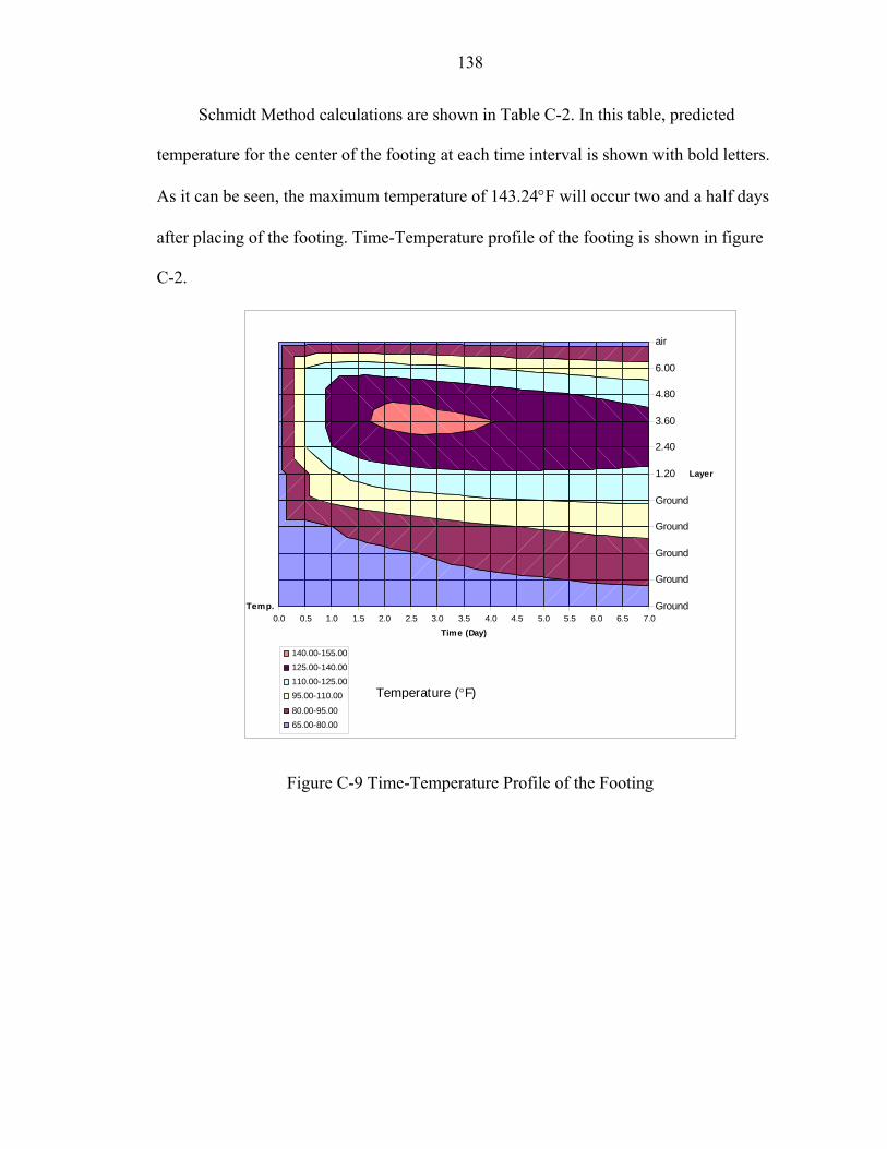
138
Schmidt Method calculations are shown in Table C-2. In this table, predicted
temperature for the center of the footing at each time interval is shown with bold letters.
As it can be seen, the maximum temperature of 143.24°F will occur two and a half days
after placing of the footing. Time-Temperature profile of the footing is shown in figure
C-2.
air
6.00
4.80
3.60
2.40
1.20
Ground
Ground
Ground
Ground
Ground0.0 0.5 1.0 1.5 2.0 2.5 3.0 3.5 4.0 4.5 5.0 5.5 6.0 6.5 7.0
Temp.
Layer
Time (Day)
140.00-155.00125.00-140.00110.00-125.0095.00-110.00
80.00-95.0065.00-80.00
Figure C-9
Temperature (°F)
Time-Temperature Profile of the Footing

139
LIST OF REFERENCES
American Concrete Institute (ACI) Committee 116, 2000, “Cement and Concrete Terminology,” (ACI 116R-00), American Concrete Institute, Farmington Hills, Mich., 73 pp.
American Concrete Institute (ACI) Committee 207, 1996, A, “Mass Concrete,” (ACI 207.1R-96), American Concrete Institute, Farmington Hills, Mich., 42 pp.
American Concrete Institute (ACI) Committee 207, 1996, B, “Cracking of Massive Concrete,” (ACI 207.2R-96), American Concrete Institute, Farmington Hills, Mich.,
American Society for Testing and Materials (ASTM), ASTM C618-94a, 1994, "Standard Specification for Coal Fly Ash and Raw or Calcined Natural Pozzolan for Use as a Mineral Admixture in Portland Cement Concrete," Annual Book of ASTM Standards, Vol. 04.02, Philadelphia, Pennsylvania.
Atiş, Cengiz Duran, 2002, “Heat Evolution of High-Volume Fly Ash Concrete,” Cement and Concrete Research, Vol.32, pp. 751-756.
Ballim, Yunus, 2004, “A Numerical Model and Associated Calorimeter for Predicting Temperature Profiles in Mass Concrete,” Cement and Concrete Composites, Vol.26, pp. 695-703.
Bamforth, P.B., 1980, “In Situ Measurement of the Effect of Partial Portland Cement Replacement Using Either Fly Ash or Ground Granulated Blast Furnace Slag on the Performance of Mass Concrete,” Proc. Inst. Civil Engrs. Part 2, Sept., pp. 777-800.
Bentz, D. P., Waller, V., and de Larrard, F., 1998, “Prediction of Adiabatic Temperature Rise in Conventional And High-Performance Concrete Using A 3-D Microstructural Model,” Cement and Concrete Research, Vol. 28, No.2, pp.285-297
Blanks, Robert F., 1933,”Cpmparison of Selected Portland Cements in Mass Concrete Tests,” Journal of the American Concrete Institute Proceedings, Vol. 30, Sept-Oct., pp. 9-20, Detroit, Michigan
Cannon, R. P., 1986, “Effects Of Changes In Cement Properties On The Temperature Of Concrete,” Concrete (London), v. 20 n. 2, Feb. pp. 26-28

140
Copland, L.E., Kantro, D.L., and Verbeck, George, 1966, Chemistry of Hydration of Portland Cement, RX153, Portland Cement Association, Skokie, Illinois
Davis, R.E., Carlson, R.W., Kelly, J.W., Dawis, H.E., 1937, “Properties of Cement and Concretes Containing Fly Ash”, ACI J.33, pp. 577-612.
Detwiler R. J., 1996, Supplementary Cementing Materials for Use in Blended Cements, Portland Cement Association, Chicago
Florida Department of Transportation (FDOT), 2002, Structures Design Guidelines for Load and Resistance Factor Design, Structures Design Office, Tallahassee, Florida, Jan., pp. 5-1
Gajda, John and VanGeem, Martha, 2002,”Controling Temperatures in Mass Concrete,” Concrete International, January, pp. 59-62
Gibbon, G. J., Ballim, Y., and Grieve, G. R. H., 1997 “A Low-Cost, Computer-Controlled Adiabatic Calorimeter for Determining the Heat of Hydration of Concrete,” Journal of Testing & Evaluation v 25 n 2 Mar. pp. 261-266
Lerch W. and Bogue R. H. 1934, “Heat of Hydration of Portland Cement Pastes,” Journal of Research of the National Bureau of Standards, 12, No. 5, pp. 645-664
Lu, H.R., Swaddiwudhipong, S. and Wee, T.H., 2001, “Evaluation of Thermal Crack by a Probabilistic Model Using The Tensile Strain Capacity,” Magazine of Concrete Research, Vol. 53, No.1, pp. 25-30.
Philleo, R.E., 1967, “Fly Ash in Mass Concrete,” Proceedings of 1st International Symposium on Fly Ash Utilization, Pittsburgh, PA, Bureau of Mines, Washington DC, pp. 69-79.
Price, W. H., 1982,“Control of Cracking in Mass Concrete Dams,” Concrete International, Vol. 4, No. 10, pp. 36-44
Rhodes, J. A., 1978,”Thermal Properties,” Significance of Tests and Properties of Concrete and Concrete Making Materials, STP-169B, ASTM, Philadelphia, pp. 242-266
Swaddiwudhipong, S., Chen, D., and Zhang, M.H., 2002, “Simulation of the Exothermic Hydration Process of Portland Cement,” Advances in Cement Research, Vol. 14, No.2, April, pp. 61-69
Townsend, C., L., 1981, Engineering Monograph No. 34, Control of Cracking in Mass Concrete Structures, Revised Reprint, United States Government Printing Office, Denver
U.S. Army Corps of Engineers, 1996, Engineering and Design-Gravity Dam Design, Publication Number: EM 1110-2-2200, Washington, DC

141
U.S. Department of Transportation, Federal Highway Administration,1990, Portland Cement Concrete Materials Manual, Report no.FHWA-Ed-89-006, August, Washington, FHWA.
Vodak, F., Cerny, R., Drchalova, J., Hoskova, S., Kapickova, O., Michalko, O., Semerak, P., Toman, J., 1997, “Thermophysical Properties of Concrete for Nuclear-Safety Related Structures,” Cement and Concrete Research, Vol. 27, No.3, pp. 415-426
Wallace, George B., and Ore, Elwood L., 1960, “Structural and Lean Mass Concrete as Affected by Water-Reducing, Set-Retarding Agents,” Symposium on Effect of Water of Water-Reducing Admixtures, American Society of Testing and Standards, Philadelphia, Pennsylvania
Xu, Yunsheng, Chung, D.D.L., 2000. “Effect Of Sand Addition On The Specific Heat And Thermal Conductivity Of Cement,” Cement and Concrete Research, Vol.30, No.1, pp. 59-61

142
BIOGRAPHICAL SKETCH
Arash Parham was born and raised in Shiraz, Iran, where he attended Shiraz
University and obtained his Bachelor of Science in civil engineering in 2000.
Arash entered the University of Florida’s M.E. Rinker Sr. School of Building
Construction graduate program in 2003. He will receive a Master of Science in Building
Construction in December 2004. He plans to obtain a job in the construction industry
after his graduation..