techno-economic assessment of voltage sag...
TRANSCRIPT

Techno-economic Assessment of Voltage Sag Performance and Mitigation
A Thesis submitted to The University of Manchester for the degree of
PhD
in the Faculty of Engineering and Physical Sciences
2008
Yan Zhang, B.Sc., M.Sc.
School of Electrical and Electronic Engineering

- 2 -
Contents
CONTENTS ................................................................................................. 2
LIST OF TABLES........................................................................................ 8
LIST OF FIGURES .................................................................................... 10
ABSTRACT ............................................................................................... 16
DECLARATION......................................................................................... 17
COPYRIGHT STATEMENT....................................................................... 18
ACKNOWLEDGEMENTS.......................................................................... 19
ABBREVIATION........................................................................................ 20
1 INTRODUCTION........................................................................... 21
1.1 Power quality ........................................................................................................................21
1.2 Voltage Sags ..........................................................................................................................23 1.2.1 Sag characteristics.........................................................................................................23 1.2.2 Sag causes.....................................................................................................................24 1.2.3 Sag consequences .........................................................................................................24
1.3 Voltage sag analysis..............................................................................................................26 1.3.1 Monitoring of power quality .........................................................................................26 1.3.2 Stochastic estimation methodology ..............................................................................27 1.3.3 Fault calculation............................................................................................................29
1.4 Voltage sag indices................................................................................................................31
1.5 Evaluation of voltage sag losses...........................................................................................33
1.6 Mitigation of voltage sags ....................................................................................................35 1.6.1 Conventional devices ....................................................................................................36 1.6.2 Modelling of FACTS devices .......................................................................................37 1.6.3 Cost of FACTS devices ................................................................................................38
1.7 Optimal placement of mitigation devices ...........................................................................41 1.7.1 Optimal technologies ....................................................................................................41

- 3 -
1.7.2 Optimization in placement of FACTS ..........................................................................42
1.8 Main objectives of the research...........................................................................................45
1.9 Main contributions of the thesis ..........................................................................................48
1.10 Outline of the thesis ..............................................................................................................49
2 ESTIMATION OF VOLTAGE SAG PERFORMANCE .................. 51
2.1 Introduction ..........................................................................................................................51
2.2 Sag Analysis ..........................................................................................................................51
2.3 Stochastic Sag Assessment ...................................................................................................52 2.3.1 Fault position method ...................................................................................................52 2.3.2 Fault calculation using system impedance matrix.........................................................53 2.3.3 Modelling of System Components................................................................................55 2.3.4 Impedance Matrix .........................................................................................................60 2.3.5 Fault calculation............................................................................................................62 2.3.6 Test System...................................................................................................................65 2.3.7 Statistical Sag Data .......................................................................................................67
2.4 Sag performance presentation.............................................................................................69 2.4.1 Number of sags .............................................................................................................69 2.4.2 Three dimensions bar chart ...........................................................................................70 2.4.3 Generalized Sag Table ..................................................................................................72
2.5 Uncertainties associated with fault positions assessment method ....................................73 2.5.1 Number of fault positions on lines................................................................................73 2.5.2 Fault resistance .............................................................................................................78 2.5.3 Transformer neutral impedance ....................................................................................85 2.5.4 Pre-fault voltage............................................................................................................88
2.6 Summary ...............................................................................................................................88
3 MODELLING OF FACTS DEVICES FOR SHORT-CIRCUIT STUDIES 90
3.1 Introduction ..........................................................................................................................90
3.2 Compensation devices based on power electronics............................................................91 3.2.1 Thyristor based devices -- SVC ....................................................................................92 3.2.2 VSC based devices ---- STATCOM, DVR...................................................................93

- 4 -
3.2.3 Voltage Compensation of STATCOM, SVC and DVR................................................94
3.3 Control Strategy ...................................................................................................................96
3.4 Mathematical Model of SVC, DVR and STATCOM ........................................................98 3.4.1 Models in fault calculation............................................................................................99 3.4.2 Calculation of injected current and voltage ................................................................100
3.5 Deciding the Rating of FACTS devices.............................................................................111 3.5.1 Rating of FACTS devices ...........................................................................................111 3.5.2 Mathematical derivation .............................................................................................111 3.5.3 Rating of devices ........................................................................................................114
3.6 Fault Calculation process with FACTS devices ...............................................................115
3.7 Simulation Results..............................................................................................................116 3.7.1 STATCOM as compensation device (reactive power only) .......................................116 3.7.2 SVC as compensation device......................................................................................120 3.7.3 STATCOM and SVC with calculated rated power.....................................................121 3.7.4 DVR as compensation device .....................................................................................123 3.7.5 Sag performance improvements with FACTS ............................................................124
3.8 Summary .............................................................................................................................127
4 ASSESSMENT OF FINANCIAL CONSEQUENCES OF VOLTAGE SAGS 129
4.1 Introduction ........................................................................................................................129
4.2 Assessment of financial losses due to voltage sags ...........................................................130 4.2.1 Sag losses evaluation ..................................................................................................130 4.2.2 Probabilistic analysis of sag losses .............................................................................131
4.3 Saving due to application of FACTS devices ...................................................................132 4.3.1 Advantages of application of FACTS devices ............................................................132 4.3.2 The cost of FACTSD ..................................................................................................133
4.4 Investment analysis ............................................................................................................134 4.4.1 Process of analysis ......................................................................................................134 4.4.2 Methods of analysis ....................................................................................................134 4.4.3 Examples.....................................................................................................................136
4.5 Uncertainties in sag loss analysis.......................................................................................141 4.5.1 Uncertainties due to fault position method .................................................................141

- 5 -
4.5.2 Various assigned user losses .......................................................................................143
4.6 Uncertainties in NPV analysis ...........................................................................................146 4.6.1 The NPV analysis .......................................................................................................146 4.6.2 Financial analysis with NPV.......................................................................................147 4.6.3 Uncertainties in NPV ..................................................................................................154
4.7 New approach to assessment of sag losses ........................................................................154 4.7.1 Equipment sensitivity..................................................................................................155 4.7.2 Proposed process sensitive curve................................................................................156 4.7.3 Sag cost factors ...........................................................................................................157 4.7.4 Evaluation of the losses at user site ............................................................................159 4.7.5 The losses in the network............................................................................................163
4.8 Summary .............................................................................................................................165
5 OPTIMAL PLACEMENT OF FACTS DEVICES.......................... 167
5.1 Introduction ........................................................................................................................167
5.2 Genetic Algorithm features ...............................................................................................168 5.2.1 Structure of simple GA (SGA)....................................................................................168 5.2.2 Genetic Algorithm operators.......................................................................................169 5.2.3 Genetic Algorithm parameters ....................................................................................170 5.2.4 Niching technique .......................................................................................................171
5.3 Objectives of placement of FACTS devices......................................................................173 5.3.1 Technical objective – to Reduce numbers of sags ......................................................173 5.3.2 Financial objective— to Reduce sag cost ...................................................................174
5.4 Application of GA for allocation of FACTS devices........................................................175 5.4.1 Implemented Simple GA ............................................................................................175 5.4.2 Niching in GA.............................................................................................................177
5.5 Simulation Results..............................................................................................................178 5.5.1 Results with simple GA ..............................................................................................179 5.5.2 Results with Niching GA............................................................................................190 5.5.3 Discussion about the location of FACTS devices.......................................................197
5.6 Summary .............................................................................................................................199
6 DESCRIPTION OF DEVELOPED SOFTWARE.......................... 201
6.1 Introduction ........................................................................................................................201

- 6 -
6.2 Software design...................................................................................................................201 6.2.1 Flow chart ...................................................................................................................202 6.2.2 System design modules...............................................................................................202 6.2.3 Description of main functions.....................................................................................204 6.2.4 Graphical User Interface (GUI) ..................................................................................208 6.2.5 File dictionary .............................................................................................................208
6.3 Abbreviated user manual...................................................................................................211 6.3.1 System development environment ..............................................................................211 6.3.2 Software command windows......................................................................................212
6.4 Areas for further software improvement .........................................................................223
6.5 Environmental set up .........................................................................................................223
6.6 Summary .............................................................................................................................224
7 PQ IN MARKET ENVIRONMENT ............................................... 225
7.1 Introduction ........................................................................................................................225
7.2 PQ in incentive regulation of electricity ...........................................................................226 7.2.1 Incentive regulation of electricity ...............................................................................226 7.2.2 Services quality incentives for electric distribution company.....................................227 7.2.3 Power quality incentives for electric distribution company........................................229 7.2.4 The emission characteristic of PQ ..............................................................................230
7.3 Power quality contract .......................................................................................................234 7.3.1 Basics of contract........................................................................................................234 7.3.2 Contract design ...........................................................................................................235 7.3.3 Existing PQ contracts..................................................................................................236 7.3.4 About PQ contract ......................................................................................................237
7.4 PQ market design ...............................................................................................................238 7.4.1 Objective of PQ market ..............................................................................................238 7.4.2 Design of PQ market...................................................................................................238 7.4.3 PQ market design practice ..........................................................................................239
7.5 Issues related to PQ in market environment....................................................................240 7.5.1 Accurate information ..................................................................................................240 7.5.2 Individual consideration..............................................................................................241 7.5.3 Setting the right target.................................................................................................242 7.5.4 Government policy and legislation .............................................................................243

- 7 -
7.5.5 The influence of PQ incentives in the power system markets ....................................244
7.6 Summary .............................................................................................................................245
8 CONCLUSION AND FUTURE WORK........................................ 247
8.1 Conclusion...........................................................................................................................247
8.2 Future Work .......................................................................................................................250
9 REFERENCES............................................................................ 252
10 APPENDIX .................................................................................. 261
10.1 Appendix A: Results of fault calculations ........................................................................261
10.2 Appendix B: Input data of test system..............................................................................268
10.3 Appendix C: Results of FACTS rating .............................................................................279
10.4 Appendix D: Author’s thesis based publications.............................................................282
Total words: 59,875

- 8 -
List of Tables
Table 1-1Fault Calculation ........................................................................................................................30
Table 1-2 FACTS and Custom Power [50] ...............................................................................................36
Table 1-3 Cost of FACTS (A) [61] ...........................................................................................................39
Table 1-4 Price of FACTS (B) [62]...........................................................................................................39
Table 2-1 Fault duration ............................................................................................................................68
Table 2-2 System fault statistics (fault rate/year) ......................................................................................68
Table 2-3 Fault positions on lines based on line impedance .....................................................................76
Table 3-1 Power Electronics based devices...............................................................................................91
Table 3-2 Injected power needed from FACTS devices (MW, MVar) ...................................................115
Table 3-3 Rating of STATCOM and SVC at different network buses....................................................121
Table 3-4 Voltage restoration of buses with FACTSDs ..........................................................................122
Table 3-5 Solution of sag mitigation .......................................................................................................124
Table 4-1 Assumed costs per voltage sag[39, 40] ...................................................................................130
Table 4-2 Solutions of sag mitigation......................................................................................................136
Table 4-3 Pay back years analysis ...........................................................................................................139
Table 4-4 Variations for 4 financial indicators........................................................................................148
Table 4-5 User group category(100MVW) [39, 40]................................................................................163
Table 4-6 Bus 111 possible sag losses.....................................................................................................163
Table 4-7 The test network loads and assigned cost................................................................................163
Table 5-1 Niching Methods [116] ...........................................................................................................173
Table 5-2 Bus map table..........................................................................................................................177
Table 5-3 Characteristics of implemented GA ........................................................................................179
Table 5-4 Sag performance without FACTS ...........................................................................................180
Table 5-5 Weightings used in different objective functions....................................................................180
Table 5-6 Optimized system sag performance ........................................................................................180
Table 5-7 Solutions with Simple GA ......................................................................................................182
Table 5-8 Sag number reduction with three phases considered...............................................................182
Table 5-9 Mitigation solution ..................................................................................................................187
- 9 -
Table 5-10 Optimized solution ................................................................................................................189
Table 5-11 Solutions from NGA and GA (five solutions with least objective value) .............................191
Table 5-12 Mitigation solutions P1 and P2 .............................................................................................192
Table 5-13 Financial analysis of solutions P1 and P2 (all costs are in (M£))..........................................194
Table 5-14 Mitigation solutions N1 and N2 ............................................................................................194
Table 6-1 System requirement.................................................................................................................211
Table 7-1 The price according to PQ emission and security level...........................................................232
Table 7-2 PQ contracts [131]...................................................................................................................236

- 10 -
List of Figures
Figure 1-1 Most prevalent PQ problems, measured at 1,400 sites in 8 countries [4] ................................22
Figure 1-2 Power quality disturbances [6].................................................................................................22
Figure 1-3 Voltage Sag..............................................................................................................................23
Figure 1-4 Sag Cost [17] ...........................................................................................................................25
Figure 1-5 Cost of FACTS devices [61]....................................................................................................39
Figure 1-6 Price of SVC and STATCOM [63]..........................................................................................40
Figure 2-1 A brief outline of Sag performance estimation process ...........................................................52
Figure 2-2 Fault position method ..............................................................................................................52
Figure 2-3 Equivalent circuit for lines and cables .....................................................................................55
Figure 2-4 Equivalent circuit for loads......................................................................................................56
Figure 2-5 Equivalent circuit for generators..............................................................................................56
Figure 2-6 Equivalent circuit for transformers ..........................................................................................57
Figure 2-7 Zero-sequence representation of transformers [93] .................................................................58
Figure 2-8 Equivalent circuit for tap changing transformer ......................................................................58
Figure 2-9 Network example (branch impedances are in per unit)............................................................61
Figure 2-10 Equivalent circuit for faulted system .....................................................................................64
Figure 2-11 Line fault................................................................................................................................64
Figure 2-12 Test system ............................................................................................................................66
Figure 2-13 3-D presentation of sag performance (sag number/year) .......................................................72
Figure 2-14 Generalized sag tables............................................................................................................73
Figure 2-15 Fault positions on line............................................................................................................74
Figure 2-16 Voltage at bus 111 for faults at 6 positions on all lines .........................................................74
Figure 2-17 Voltage on bus 111 when faults on 6 position of selected lines in the system.......................75
Figure 2-18 Three positions on line...........................................................................................................75
Figure 2-19 Generalized sag table of bus 111 with 3 positions on each line (sag number/year)...............76
Figure 2-20 Nine positions on line ............................................................................................................76
Figure 2-21 Generalized sag table of bus 111 with 9 position on each line (sag number/year) ................76
Figure 2-22 Generalized sag table of bus 111 when various points on each line (sag number/year) ........77

- 11 -
Figure 2-23 Sags at bus 111 for various points on line .............................................................................78
Figure 2-24 Sags at all buses for various points on line ............................................................................78
Figure 2-25 Voltage at bus 111for faults at all buses with various fault resistance...................................79
Figure 2-26 Generalized sag table of bus 111 for fault resistance 0Ω (sag number/year)........................79
Figure 2-27 Generalized sag table of bus 111 for fault resistance 15Ω (sag number/year).......................80
Figure 2-28 Sags at bus 111 for various fault resistances..........................................................................80
Figure 2-29 Generalized sag table of entire network for faults impedance 15ohm (sag number/year) .....81
Figure 2-30 Sags at all buses for various fault impedances.......................................................................81
Figure 2-31 Fault resistance distribution ...................................................................................................82
Figure 2-32 3-D presentation of sag performance on bus 111 (sag number/year).....................................82
Figure 2-33 3-D presentation of sag performance entire network (sag number/year) ...............................83
Figure 2-34 Generalized sag table of bus 111 ...........................................................................................84
Figure 2-35 Generalized sag table of with normally distributed fault resistances .....................................84
Figure 2-36 3D presentation of sag performance at bus 232 (sag number/year) .......................................85
Figure 2-37 3D presentation of sag performance of the entire network (sag number/year) ......................85
Figure 2-38 3D presentation of sag performance of bus 232 (phase A) (sag number /year) .....................86
Figure 2-39 Generalized sag tables for bus 232 ........................................................................................87
Figure 2-40 Generalized sag tables for entire network..............................................................................87
Figure 2-41 Voltage at bus 111 for LLLG faults at all buses ....................................................................88
Figure 3-1 SVC structure...........................................................................................................................92
Figure 3-2 Structure of (A) STATCOM and (B) DVR..............................................................................93
Figure 3-3 Model of FACTS (A-STATCOM B-SVC C-DVR) ................................................................95
Figure 3-4 V-I characteristic of SVC and STATCOM..............................................................................96
Figure 3-5 Restoration of bus voltage with reactive power injection ........................................................97
Figure 3-6 Real and reactive power injection..........................................................................................110
Figure 3-7 Single line diagram of STATCOM connected to a bus .........................................................111
Figure 3-8 Single line diagram of DVR connected to a bus ....................................................................113
Figure 3-9 Sag magnitudes at buses 130-200 ..........................................................................................116
Figure 3-10 Sag magnitudes in the whole system ...................................................................................116
Figure 3-11 Sag magnitudes at buses 130-200, phase A .........................................................................117

- 12 -
Figure 3-12 Sag magnitudes at buses 130-200, phase B .........................................................................117
Figure 3-13 Sag magnitudes at buses 130-200, phase C .........................................................................118
Figure 3-14 Sag magnitudes at buses 130-200, phase A .........................................................................118
Figure 3-15 Sag magnitudes at buses 130-200, phase B .........................................................................119
Figure 3-16 Sag magnitudes at buses 130-200, phase C .........................................................................119
Figure 3-17 Sag magnitudes at buses 130-200, phase A .........................................................................120
Figure 3-18 Sag magnitudes at buses 130-200, phase B .........................................................................120
Figure 3-19 Sag magnitudes at buses 130-200, phase C .........................................................................120
Figure 3-20 Voltage magnitudes with STATCOM and SVC at bus 226.................................................121
Figure 3-21 Sag magnitude of all buses when LLL fault on bus 76........................................................122
Figure 3-22 Sag phase angle of all buses when LLL fault on bus 76 ......................................................122
Figure 3-23 Bus 145 3-D sag numbers (sag number/year) ......................................................................124
Figure 3-24 Entire network 3-D sag number (sag number/year) .............................................................125
Figure 3-25 Generalized sag tables for bus 145 ......................................................................................126
Figure 3-26 Generalized sag tables for entire network (sag number/year) ..............................................127
Figure 4-1 Sag losses assessment ............................................................................................................131
Figure 4-2 Statistical analysis of sag losses.............................................................................................132
Figure 4-3 Process of investment analysis in FACTSD ..........................................................................134
Figure 4-4 Annual sag losses with solution 1 and solution 2 ..................................................................137
Figure 4-5 Solution1 sag losses ...............................................................................................................137
Figure 4-6 Solution2 sag losses ...............................................................................................................138
Figure 4-7 Comparing sag losses in solution 1 and solution 2 with base case ........................................138
Figure 4-8 Solution1 NPV analysis .........................................................................................................140
Figure 4-9 Solution2 NPV analysis .........................................................................................................140
Figure 4-10 Sag losses due to various fault impedances .........................................................................142
Figure 4-11 Statistical analysis of sag losses due to various fault impedances .......................................143
Figure 4-12 Sag losses with 10ohm fault resistance................................................................................143
Figure 4-13 Sag losses with 15ohm fault resistance................................................................................143
Figure 4-14 Sag loss variation assigned to different users ......................................................................144
Figure 4-15 Sag losses variation due to various assigned losses’ value ..................................................145

- 13 -
Figure 4-16 Statistical analysis of sag losses due to various assigned loss’ values .................................145
Figure 4-17 Mean sag losses variations due to various assigned losses’ values......................................145
Figure 4-18 Tornado diagram of 4 variables in financial analysis ..........................................................148
Figure 4-19 NPV analysis with constant n=12 ........................................................................................149
Figure 4-20 Monte Carlo analysis of NPV using variables’ combinations and distributions..................149
Figure 4-21 Statistical analysis of NPV...................................................................................................150
Figure 4-22 Discount rate Normal distribution withµ=0.1δ=0.025......................................................150
Figure 4-23Project life times Normal distribution withµ=10δ=2.5.......................................................150
Figure 4-24 Capital cost Normal distribution with µ=4.13δ=1.09 .......................................................151
Figure 4-25 Saving Weibull distribution with A=1, B=1.5 .....................................................................151
Figure 4-26 Statistical analysis of NPV...................................................................................................151
Figure 4-27 Monte Carlo NPV analysis with various project life times..................................................152
Figure 4-28 Decision tree analysis of NPV .............................................................................................153
Figure 4-29 NPV analysis using decision tree with different project life times considered ....................153
Figure 4-30 Voltage tolerance curve .......................................................................................................156
Figure 4-31 Process tolerant curve ..........................................................................................................157
Figure 4-32 Assigned losses ....................................................................................................................158
Figure 4-33 Percentage of losses due to various magnitudes of three phases .........................................159
Figure 4-34 Process sensitive curve and generalized sag table ...............................................................160
Figure 4-35 Number of sags (50- 70ms)..................................................................................................161
Figure 4-36 Number of sags (70-200ms).................................................................................................161
Figure 4-37 Number of sags (>200ms)....................................................................................................161
Figure 4-38 Number of sags which will trip the process .........................................................................162
Figure 4-39 Influential sags which will trip the process..........................................................................162
Figure 4-40 Generalized sag table with process tolerance curves for load group I .................................164
Figure 4-41 Generalized sag table with process tolerance curves for load group II ................................164
Figure 4-42 Generalized sag table with process tolerance curves for load group III...............................164
Figure 5-1 A Conventional GA Process ..................................................................................................168
Figure 5-2 Minimizing power quality improvement costs ......................................................................174
Figure 5-3 Population representation ......................................................................................................175

- 14 -
Figure 5-4 Problem specified crossover ..................................................................................................176
Figure 5-5 Distance between individuals ................................................................................................178
Figure 5-6 Optimization results...............................................................................................................181
Figure 5-7 Number of sags in percentage with different OFs .................................................................181
Figure 5-8 Number of sags in percentage with different OFs .................................................................183
Figure 5-9 Generalized Sag Tables..........................................................................................................184
Figure 5-10 Convergence of optimization with f1...................................................................................185
Figure 5-11 Convergence of optimization with f2...................................................................................185
Figure 5-12Convergence of optimization with f3....................................................................................186
Figure 5-13 Variation of sag losses due to solution.................................................................................186
Figure 5-14 sag losses .............................................................................................................................187
Figure 5-15 Pay back year analysis of the solution .................................................................................187
Figure 5-16 GA approach........................................................................................................................188
Figure 5-17 Sag losses.............................................................................................................................188
Figure 5-18 Sag cost with and without the solution ................................................................................189
Figure 5-19 NPV analysis of optimized results .......................................................................................189
Figure 5-20 GA approach........................................................................................................................190
Figure 5-21 Sag performance with different solutions f1........................................................................190
Figure 5-22 NGA f1 approach.................................................................................................................192
Figure 5-23 Sag losses.............................................................................................................................193
Figure 5-24 Probability of annual sag losses optimized by ‘pay-back year’ ...........................................193
Figure 5-25 Sag losses.............................................................................................................................195
Figure 5-26 Probability of annual sag losses optimized by NPV ............................................................195
Figure 5-27 NPV values (A) solution N1 (B) solution N2 ......................................................................196
Figure 5-28 Test network with optimal locations of FACTS devices indicated by signs........................198
Figure 5-29 Sag losses in 10 load-sites....................................................................................................198
Figure 6-1 Flow chart of whole analysis .................................................................................................202
Figure 6-2 System design module ..........................................................................................................203
Figure 6-3 Flow chart of fault calculation with FACTS..........................................................................204
Figure 6-4 Flow chart of sag performance estimation.............................................................................205

- 15 -
Figure 6-5 Flow chat of sag loss calculation ...........................................................................................206
Figure 6-6 Flow chart of investment analysis..........................................................................................207
Figure 6-7 Flow chart of Genetic Algorithm...........................................................................................207
Figure 6-8 GUI – calculation (with FACTS)...........................................................................................212
Figure 6-9 GUI – Calculation (FACTS)..................................................................................................213
Figure 6-10 GUIe – 3D sag profile..........................................................................................................214
Figure 6-11 GUI – 3D sag number ..........................................................................................................215
Figure 6-12 GUI – Transformer Motor Protection ..................................................................................216
Figure 6-13 GUI – Assessment of Sag Losses ........................................................................................217
Figure 6-14 GUI – Presentation of Sag losses.........................................................................................218
Figure 6-15 GUI – NPV&PayBackYear .................................................................................................219
Figure 6-16 GUI – NPV sensitivity analysis ...........................................................................................220
Figure 6-17 GUI – Optimization .............................................................................................................221
Figure 6-18 GUI – Monitoring Data analysis..........................................................................................222
Figure 7-1 The economic effects of incentive regulation [123]...............................................................227
Figure 7-2 Improvement effects of the incentive/penalty regime in Great Britain [123] ........................228
Figure 7-3 Outage cost in revenue [128] .................................................................................................229
Figure 7-4 Pricing of electricity with PQ levels ......................................................................................231
Figure 7-5 Classification of power quality characteristics [131].............................................................232
Figure 7-6 Classification of PQ emission and security level...................................................................232
Figure 7-7 Price with respect to different PQs and PQe..........................................................................233
Figure 7-8 Yearly saving or payment for PQ in tariff of electricity ........................................................233
Figure 7-9 Power quality contracts and regulator [123] ..........................................................................237
Figure 7-10 Market structure of PQ ........................................................................................................239
Figure 7-11 PQ market design [139] .......................................................................................................240
Figure 7-12 Monitoring and communication of continuity indicators [123] ...........................................241
Figure 7-13 The evolution pattern of regulation [118] ............................................................................242

- 16 -
Abstract
This thesis presented a comprehensive techno-economic analysis of voltage sag in distribution network. It has five main topics: sag performance estimation, FACTS modelling in fault calculation, investment analysis and optimal placement of FACTS for sag mitigation, overview of PQ in market environment.
The main task of the first topic was to employ the developed mathematical network models to perform sag analysis and produce results that can be presented in a form suitable for various research purposes and analysis objectives. First the process of sag assessment was introduced. Full discussion was then given of the fault position method stressing the fault calculation by system impedance matrix. At the end, several parameters such as fault impedance, number of fault positions on each line and pre-fault voltages were investigated to reveal their influences on sag performance results.
Then the developed models of three types of FACTS based devices, STATCOM, SVC and DVR using sequence network and system impedance are presented. This simplifies the process of sag performance analysis in large systems with FACTS devices and enables huge amount of sag data to be obtained in an efficient way. Detailed mathematical derivation of FACTS models was presented.
The third topic was devoted to assessment of financial consequences of voltage sag and techno-economic assessment of mitigating solutions (FACTS based devices). The discussion started with an introduction to the equipment sensitivities, based on which methodology of evaluating the losses due to voltage sag was developed. New method was also proposed that takes into account three-phase voltages and newly proposed process tolerance curve and generalized sag tables. Financial analysis tools in terms of ‘simply pay back year’, ‘Net Present value’ and ‘Net Present value index’ were then illustrated with examples and graphical presentations. The ‘uncertainties’ involved in the assessment and the ‘sensitivity’ of variables involved in the process of NPV analysis as well as their impact on final result were carefully examined.
Next, new methodology was proposed for placement of FACTS devices optimally in the network to improve system sag performance either by reducing sag number of reducing financial losses due to sag. Genetic algorithm was used to find the optimal solution with respect to number, size, type and location of devices. Niching technique in GA was also employed to explore its advantages of flexibility of solutions.
A comprehensive software which provided user-friendly environment to explore all the research achievements was also developed. Finally, a discussion about power quality in market environment offers a glimpse of many issues involved in power quality market at present and in the future.

- 17 -
Declaration
That no portion of the work referred to in the thesis has been submitted in support
of an application for another degree or qualification of this or any other university or
other institute of learning.

- 18 -
Copyright Statement
i. The author of this thesis owns any copyright in it (the “Copyright”) and s/he
has given The University of Manchester the right to use such Copyright for any administrative, promotional, educational and/or teaching purposes.
ii. Copies of this thesis, either in full or in extracts, may be made only in
accordance with the regulations of the John Rylands University Library of Manchester. Details of these regulations may be obtained from the Librarian. This page must form part of any such copies made.
iii. The ownership of any patents, designs, trade marks and any and all other
intellectual property rights except for the Copyright (the “Intellectual Property Rights”) and any reproductions of copyright works, for example graphs and tables (“Reproductions”), which may be described in this thesis, may not be owned by the author and may be owned by third parties. Such Intellectual Property Rights and Reproductions cannot and must not be made available for use without the prior written permission of the owner(s) of the relevant Intellectual Property Rights and/or Reproductions.
iv. Further information on the conditions under which disclosure, publication
and exploitation of this thesis, the Copyright and any Intellectual Property Rights and/or Reproductions described in it may take place is available from the Head of School of Electrical and Electronic Engineering.

- 19 -
Acknowledgements
I would like to thank my supervisor, Prof. J.V.Milanovic, for his support and hard
work to ensure that this research is completed finely and successfully.
I would like to express my gratitude to Joan Wallace for all of her time helping to
proofread this thesis.
I also wish to thank Mr. Jhan Yhee Chan for his advice and discussions.
I also wish to thank my friend Miss. Ningyan Wang for her encouragement and
support.

- 20 -
ABBREVIATION
FACTS Flexible AC Transmission devices GA Genetic Algorithm SVC Static Var Compensation STATCOM Static Synchronous Compensator DVR Dynamic Voltage Restoration ASD Adjustable Speed Drivers TCSC Thyristor Switched Series Capacitor UPFC Unified Power Flow Controllers SSSC Static Synchronous Series Compensator PE Power Electronics IGBT Insulated Gate Bipolar Transistors GTO Gate Turn off Thyristor SSB Solid State Breaker SSTS Solid State Transfer Switch ASVC Advanced SVC D-STATCOM Distributed STATCOM TCPS Thyristor Controlled Phase Shifter TCPAR Thyristor Controlled Phase-Angle Regulator TCPST Thyristor Controlled Phase Shifting Transformer SA Simulated Annealing TS Tabu Search ETO Emitter Turn-off Thyristor PQ Power Quality ASVC Advanced Static VAR Compensator NPV Net Present Value

Chapter 1 Introduction
- 21 -
1 INTRODUCTION
Equation Chapter 1 Section 1
1.1 Power quality
Reliability and power quality are two important issues in power systems. Reliability
refers to the continuity of power supply, while power quality relates to power
disturbances in terms of voltage, current and frequency variations. The power
electronics loads in modern industries are susceptible to disturbances such as short
interruptions, voltage sags, harmonics, etc., that historically were not cause of major
concern. Revitalizing of industry with more micro-electronic devices and more energy-
efficient equipment pushes power quality issues into even more prominent position. As
a result, there is an increasing interest in power quality and the problems of power
quality are challenging every participant in the chain of electricity supply.
Power quality is a collection of various subjects in terms of voltage quality, current
quality, supply quality and consumption quality [1]. It can be defined as: ‘Any power
problem manifested in voltage, current, or frequency deviations that result in failure or
malfunction of customer equipment’ [2]. Power quality is a customer-driven issue in
general. Poor power quality is often the main reason of unexplained equipment trips or
shutdowns; occasional equipment damage or component failure; erratic control of
process performance; random lockups and data errors, power system component
overheating, etc. [3]. Figure 1-1 illustrates the most common power quality problems
encountered at various sites in different power systems.
Problems of the quality of power delivered to the customers are an important issue
due to the associated significant financial losses. They have also become an increasing
concern for power suppliers because of the increasing demand of high quality of
electricity supply. For manufacturers of electrical equipment, the disturbance ride-
through capability of their devices is an important point to win potential buyers.

Chapter 1 Introduction
- 22 -
Figure 1-1 Most prevalent PQ problems, measured at 1,400 sites in 8 countries [4]
Though power quality is usually defined as any problem manifested in voltage,
current, or frequency deviations, voltage quality is ultimately of main concern [5]. The
most common types of voltage abnormalities are: harmonics, voltage sags, voltage
swells and short interruptions. Among these, voltage sags account for the highest
percentage of occurrences in equipment interruptions, as shown in Figure 1-2. The
figure indicates that voltage sags account for the highest percentage of equipment
interruptions, i.e., 31%. Voltage sags are also major power quality problem that
contributes to nuisance tripping and malfunction of sensitive equipment in industrial
processes.
Figure 1-2 Power quality disturbances [6]
The work presented in this thesis belongs to the general area of power quality. Only
one of the power quality disturbances however, voltage sags, is investigated in detail
here.

Chapter 1 Introduction
- 23 -
1.2 Voltage Sags
1.2.1 Sag characteristics
Generally, voltage sag can be characterized with the magnitude of the remaining
voltage at the bus, the duration of the low voltage event, its phase shift, point on wave
of sag initiation and recovery and asymmetry. Standards related to testing of electrical
equipment to voltage sags however, are almost exclusively concerned with only two
parameters: root mean square (rms) value of the retained voltage (i.e., voltage sag
magnitude) , and duration of this rms voltage reduction. This is because the magnitude
of voltage sag and its duration decide the severity and the impact of voltage sag on
end-user equipment. Other characteristics of voltage sag are usually not considered for
equipment compatibility evaluation. (E.g., standard IEEE 1346-1998 defines a voltage
sag as ‘a decrease in rms voltage at the power frequency for duration of 0.5 cycle to 1
minute’ [7].)
An example of voltage sag is shown in Figure 1-3 where it is represented as the
variation of the rms voltage over the sag duration. The sag is recorded as a logged event
with two parameters only: sag duration and sag magnitude.
ELECTRIC POWER ENGINEERING
0 1 2 3 4 5 60
0.2
0.4
0.6
0.8
1
Time in cycles
Vol
tage
in p
u
dip duration
dip magnitude
Figure 1-3 Voltage Sag
Monitoring is the most direct way to obtain relevant information about the sag.
Voltage sag magnitude is the rms value of the remaining voltage during the sag while
voltage drop or sag depth is the maximum deviation of the rms voltage from nominal
value. Sag duration is defined as the time during which the rms voltage remains below
the specified threshold (often chosen as 90% of the nominal voltage).The voltage sag

Chapter 1 Introduction
- 24 -
magnitude at any bus in the network can also be estimated using fault simulation tools
(and that’s how it is typically done in voltage sag studies). The sag duration in such
cases is typically determined by the setting of the protection fault-clearing times [8].
Usually, sags originating at higher voltage levels where protection defined fault clearing
times are shorter, can be considered to be rectangular in shape.
1.2.2 Sag causes
The most common causes of voltage sag are [9]:
• Faults or short circuits. Although the fault will be quickly removed by a fuse
or a circuit breaker, they will drag the voltage down until the protective device
operates, which can take anywhere from a few cycles to a few seconds.
• Starting a large load, such as a motor or resistive heater. Electric motors
typically draw 150% to 500% of their operating current as they come up to
speed. Resistive heaters typically draw 150% of their rated current until they
warm up.
• Transformer energizing.
• Loose or defective wiring, such as insufficiently tightened box screws on
power conductors. This effectively increases the system impedance, and
exaggerates the effect of current increases.
• Voltage regulator failures (far less common). Utilities have automated
systems to adjust voltage (typically using power factor correction capacitors, or
tap switching transformers), and these systems do occasionally fail.
1.2.3 Sag consequences
Voltage sag disturbances are considered to be the most prominent power quality
problem. This is largely due to the large number of occurrences throughout a typical
transmission and distribution network, the increasing sensitivity of customer equipment
to voltage sags, and the high costs of lost productivity and downtime [10].
The number of voltage sags that can occur at service entrance to a facility depends
on where the facility is located in the network, the characteristics of the utility's
distribution system (e.g., underground vs. overhead lines), lengths of the distribution
feeder circuits, the number of feeders, the lightning level/activity in the area, the

Chapter 1 Introduction
- 25 -
number of trees adjacent to the power lines, etc. Some studies found that nearly all
disruptive voltage sags were caused by current flowing to short circuits either within the
plant or on utility lines in the electrical neighbourhood [1]. Although the faults occur
relatively rarely, a large portion of the power system experiences voltage sags whenever
a fault occurs, so voltage sags are much more common than actual interruptions of
supply.
The sensitivity of individual equipment mainly determines how severely an
industrial process will be affected by the sags. The growth of demand side technologies
(most of these technologies utilize power electronics) is driven by the need for efficient
consumption of electricity. This implies that equipment has become less tolerant to
voltage disturbances. Some of the most sensitive devices, namely, AC adjustable speed
drives, AC coil contactors and personal computer have been thoroughly investigated
and detailed sensitivity curves have been developed and reported in [11-13].
The ultimate reason for the increased interest in power quality is economic value.
The reported financial losses resulting from process interruption due to sags are often
expressed in millions (or even billions) of pounds/dollars/euros per year [14-16]. The
reported losses vary widely depending on the type of industry. Figure 1-4 gives some
typical values. It is estimated that power quality problems cost industry and commerce
in the EU about € 10 billion per annum while the expenditure on preventative measures
is less than 5 % of this [17].
Figure 1-4 Sag Cost [17]
Financial loss due to voltage sags can show up in many aspect of industrial and
commercial operations, such as loss of revenue, lost opportunities, product damage,

Chapter 1 Introduction
- 26 -
wasted energy and decreased equipment life, field service warranty work,
manufacturing interruptions, loss of productivity, etc.
1.3 Voltage sag analysis
Voltage sag assessment has been recognized as a systematic and dynamic process of
evaluating specific power system network’s/site’s sag performance. The results of the
assessment can be used to investigate sag profile and to get better understanding of
potential mitigating options. A lot of research effort has been put in developing a level
of understanding of voltage sags based on a mixture of theoretical models, laboratory
experimentation and analysis of recorded data. The performance of voltage sags can be
assessed either by a long term monitoring of voltages at various buses in power system
or by a stochastic simulation approach.
1.3.1 Monitoring of power quality
Collecting power quality data is an important step in power quality analysis, and a
good knowledge of the real power quality situation in today’s system is a preliminary
step towards any kind of regulatory intervention [18]. A growing number of European
countries, i.e., power utilities have monitoring systems installed or plan to install them
in the near future [18].
For sag measurements, the monitoring duration must be sufficiently long to capture
all aspects of the network and individual site sag performance. As stated in [19], it is
required to collect voltage sag data for at least one year in order to get reliable
assessment of voltage sag phenomena at a site.
The methods for collecting, characterizing, storing and analyzing rms voltage
variation measurements were introduced in [20]. Voltage variations were collected
during power quality monitoring survey of 277 locations across the United States for a
period from June 1993 to September 1995. Histograms of monitor-limited-segmentation
system average RMS variation frequency index (MLS SARFI) were used to present the
data. It was noticed that among 107,834 recorded rms variations, 68% were related to
one phase variation, 19% to two phases and only 13% of them to all three phases’
voltage variations. Recorded results also indicated that 87% of these events involved
single operation of re-closer/breaker, 9% had two operations, 2% had three operations

Chapter 1 Introduction
- 27 -
and 2% had more than four operations which substantiate the belief that a vast majority
of power system faults were temporary in nature. A clear relationship between the
seasons and sag interruption rates was also observed from these voltage variations data.
An introduction to power quality categories, power quality monitoring devices and
methods for the analysis of recorded data was given in [1]. Power quality variations,
their main causes and examples of solutions were also briefly listed. Among all of these,
several variations in terms of steady-state voltage characteristics, harmonic distortion,
transients, short duration voltage variations were illustrated and defined in detail. The
main functions and usage of five types of data monitors for monitoring different power
quality disturbances were also introduced. An example data analysis system structure
was given in flow-chart format.
Monitoring is an effective tool to provide accurate and reliable sag data. It is
however an on-going process and can’t reveal the sag event which did not appear but
may happen in the future. Besides, it is impossible and impractical to monitor the entire
network for complete data collection. However, the monitoring data can establish the
basis on which realistic assumptions can be made to estimate the expected frequency
and duration of voltage sags.
1.3.2 Stochastic estimation methodology
Power quality monitoring has now become a rather common practice. However,
power quality measurements have their disadvantages, such as the long time needed for
adequate accuracy and the questions of how to extrapolate and correlate certain results
of measurements from one network to the other or to another time. One therefore,
depends on a subset of estimation data from sag analysis to predict sag performance.
Estimation methods can provide valuable information about the expected severity and
frequency of voltage disturbances and allow the utility to predict the power quality level
on their sites and guide in a realistic way the investment in devices for sag immunity or
mitigation.
The stochastic assessment of voltage sags is a process of mathematical numeration
based on computer simulations. The three most widely used methods for sag assessment,
namely, critical distances, fault positions and Monte Carlo, are investigated in [21].
Although it requires significant computational effort, the critical distances method can

Chapter 1 Introduction
- 28 -
give result with high accuracy, so it was used as the reference method in this paper. The
fault positions and Monte Carlo methods are very simple to employ but a large number
of fault positions are needed in order to reach the required accuracy. A small radial
network was used as test system in this paper. It was founded that for the method of
fault positions, 480 fault positions provide good accuracy of the results independent on
the observation node and the sag magnitude examined while almost 2000 iterations
were needed using Monte Carlo method to achieve similar accuracy.
These three methods were further compared in [22] for balanced and unbalanced
sags due to faults in meshed and radial power networks. Method of critical distances
was found to be a very simple prediction technique based on the voltage divider
equivalent circuit. Although the results obtained by this method were of high accuracy,
it was very difficult to select the appropriate root (or roots) to solve the inverse
equations and it required considerable programming effort. Both, the method of fault
positions and the Monte Carlo method were simpler and easier to implement than the
critical distances method but a sufficiently large number of fault positions and iterations,
respectively were required. It was found though that the method of fault positions with
appropriate number of pre-selected fault positions provided good accuracy of the results
independent on the network simulated and sag magnitude of interest.
The method of fault positions is a widely used method for voltage sag calculations
[21-24]. When applying the method of fault positions, a large number of faults are
generated throughout the power system and corresponding magnitude and duration of
sags are calculated. The expected number of sags can be calculated as a function of
magnitude and duration by taking the failure rate for each fault into account.
Whether the fault position method is the best approach for estimating sag
performance is of course controversial. Alternatives have also been explored by
researchers. The issue of accuracy of results obtained by the fault positions method was
raised in [25] since no research has been done about the influence of the number and
location of simulated faults. So the authors proposed a new analytical method, which
extended the critical distances approach typically limited to radial networks to meshed
networks for balanced and unbalanced fault conditions. To prove the efficiency of the
method, several case studies have been carried out using both, a small system (IEEE
RTS-24 system) and a real transmission system. The results obtained were compared
with fault positions method, showing the computational and accuracy advantage of the

Chapter 1 Introduction
- 29 -
former. There was still a problem however, how to determine the exact position along
the line in which the voltage magnitude has a specific value, especially in meshed
network. There may be several points on different lines that result in the same
magnitude of voltage reduction at a bus of interest.
The paper [24], second part of the serial paper, implemented a Monte Carlo
procedure to assess sag performance at end-user site, based on the ATP (alternative
transients program) models discussed in the first paper. This paper explored the
characteristics of voltage sags (sag magnitude, duration and phase shift) caused by
faults in distribution network. Different operations of protective devices (fuse, breaker)
regarding to faults with different duration are discussed. Based on that, the test system’s
sag performance for several scenarios with a different coordination between protective
devices has been investigated. The results showed that the protection system has a
significant influence on voltage sag characteristics and proper coordination between
protective devices can reduce voltage impact on end-user equipment.
Martinez and Martin described a complete sag analysis process in three joint papers
aimed at predicting the voltage sag performance of distribution networks by estimating
voltage sag indices [24, 26, 27]. The first paper discusses modelling guidelines for
representing power distribution components in voltage sag simulations and a Monte
Carlo procedure using a time-domain simulation tool followed. Two types of voltage-
sag indices (System average root mean square variation frequency index (SARFI) and
energy indices) were analyzed in the last paper illustrating sag performance of the
network.
1.3.3 Fault calculation
As mentioned before, voltage sag can be caused by starting of large motors and
energizing of transformers. But, the most common causes are faults in power system,
which could be initiated by lightning and failure of power system devices. In this thesis,
the focus is only on fault-caused sags. Short circuit analysis, which can calculate
currents and voltages in a power system during and after the fault, is the most important
tool to estimate voltage sag magnitude.
Short circuit analysis is a process of approximations. These approximations arise
from modelling of system and system devices. For different data needed, and different

Chapter 1 Introduction
- 30 -
modelling, the resulting accuracy and the time required to obtain the results would be
different.
There are three basic short circuit analysis approaches used [28]:
• Classical symmetrical components;
• Phase variable approaches;
• Complete time-domain simulations.
Table 1-1Fault Calculation
Fault calculation Modelling Symmetrical components 0 0 0
1 1 1
2 2 2
===
V [ Z ]IV [ Z ]IV [ Z ]I
Well balanced system;
Phase variable abc abc abcI =[Y ]V Unbalance system; Time-domain V(t)=Ri(t)
di(t)V(t)=L
dtdV(t)
i(t)=Cdt
Nonlinear elements are presented;
Error! Reference source not found. illustrates requirements of the three fault
calculation approaches. The suitability of the method depends on the type of the
problem dealt with, and on the required accuracy of the results.
Both time-domain and frequency-domain tools are capable of assessing voltage sag
through fault simulations. In [29], authors employed a time-domain tool for voltage sag
analysis in a medium size distribution network. The paper emphasized that high
accuracy of sag results can be obtained when a time-domain approach was used. Paper
[30] presented voltage sag study of a large transmission system by symmetrical
components and the impedance matrix. The voltage sag magnitudes were obtained
using these tools with simple network modelling. Compared with time-domain
simulation method, the application is much easier to implement and the results are of
appropriate accuracy.
Complete time-domain simulation requires detailed network models and it is very
time consuming, although complete and detailed instantaneous voltages during the fault
can be obtained. This is the most complex method, since it solves differential equations
that characterize the transient performance of the system. Simulations performed with

Chapter 1 Introduction
- 31 -
time-domain tools can capture all voltage sag characteristics (magnitude, duration,
phase angle jump, point of wave) with high accuracy.
The phase variable method works well in case of unbalanced network. The general
approach of this method is similar to classical symmetrical component algorithm
although system admittance matrix is used [31].
Classical symmetrical components method utilizes the well known positive,
negative and zero sequence impedance descriptions of power system components in
conjunction with classical network theory to develop mathematical system models in
the form of impedance matrices.
In this study, the interest is more in the residual voltage during the fault than in the
evolution of voltage as a function of time. Symmetrical-component-method is therefore
appropriate to offer the required results. Besides, it has an advantage of easy application
and simple network modelling. So, classical symmetrical components method is
employed to calculate voltage sags in this research.
The modelling of power system for voltage sag studies was detailed in [24, 26, 27].
System components such as lines and cables, transformer, monitoring and protective
devices were discussed in the papers with respect to modelling requirements and their
influence on voltage sag characteristics.
1.4 Voltage sag indices
PQ indices are key issue to indicate the different performance experienced at the
transmission, sub-transmission, substation and distribution circuit levels. There are
various ways of presenting voltage sag performance, such as SARFI (system average
rms variation frequency Index), SIARFI (System Instantaneous Average Rms Variation
Frequency Index) and SMARFI (System Momentary Average Rms Variation
Frequency Index) [32]. Paper [33] introduced SARFI to represent the voltage variation
performance of the whole system and of some local points of interest. SARFI is further
classified into: SIARFI, SMARFI, and STARFI. Using real measurement data and
assumed customer data, the authors demonstrated the application of SIARFI. They
proved that the indices can present system performance in a simplified manner to key
industrial customers. The application of a procedure for the stochastic prediction of
voltage sags in distribution networks for the calculation of voltage sag indices was

Chapter 1 Introduction
- 32 -
introduced in [27]. The sag indices employed here were SARFI and SAIDI. The impact
of protective devices, system topology (number of load buses and feeder length) and
equipment vulnerability on these sag indices were also investigated.
Besides sag indices described above, other presentation of sag profiles had also been
investigated by different researchers, e.g., voltage sag magnitude and duration table, sag
density table and voltage sag coordination contour chart [34]. A voltage sag density
table is a straightforward way for quantifying the number of voltage sag events. Once
the failure rates of the power components are known, the number of voltage sags can be
quantified as the function of sag magnitude and duration. The voltage sag density table
also had been used in paper [32] to evaluate the voltage sag performance of a
distribution network. It was also indicated that these estimates can be useful for
predicting potential impacts on the operation of sensitive loads and for planning
mitigating solutions to improve or maintain the power quality of the supply system. The
authors of [34] discussed a method which uses voltage sag contour chart as an
intermediate step. The transformation process was introduced with examples that
proved the efficiency and capability of the method.
Three categories to report voltage sag index in terms of site report, network report
and utility report were used in [35]. Authors used UACSI (Utility Average Customer
Sag Index) for assessing the impact of voltage sags on customers. The index took into
account the connected kVA.
The existing definition and classification of voltage sags and short interruptions
were critically reviewed in [36]. Based on very detailed discussion, authors came
forward to highlight that ‘current definitions and descriptions of voltage sags are
generally inadequate for assessment of both single-phase and three-phase equipment
sensitivity. Usual ways for presenting the site/system data about the voltage sags and
short interruptions may be useful as performance indicators for the overall supply
system, but they are not useful for the assessment of equipment sensitivity at any
specific location.’ They also indicated that classifying voltage sags is much more
complicated than that of short interruptions. Among all existing classification methods,
basic three-phase classification, classification related to number of sagged phases or to
complex phase voltage and minimum magnitude/total duration representation of sags
are most commonly used. Individual voltage sag usually can be represented either by its
rms values or instantaneous values. Site/system sag events are mostly represented by
Chapter 1 Introduction
- 33 -
minimum magnitude/total duration method in various manners, such as sag table, 2-D
bar chart, etc.
1.5 Evaluation of voltage sag losses
It is difficult to identify the exact financial cost of voltage sags although it has been
widely recognized that enormous losses can be caused by a single event. Survey and
data log are usually used to obtain detailed value of sag cost. In [17], the authors
reviewed the cost of poor power quality in terms of harmonic distortion, blackout,
voltage sags and voltage transients. They cited a study (ten-month period, 858
disturbances and 12 sites) with a financial loss totalling €600,000 due to voltage sags.
Another survey-based approach to estimate the direct costs of power disturbances to
U.S. businesses was carried out in [16], focusing on three industry sectors (digital
economy (DE); Continuous process manufacturing (CPM); Fabrication and essential
services (F&ES)). The frequency and duration of power outages at facilities and their
effect on the business operations were investigated. The costs investigated here
included idled labour, materials loss, equipment damage, and lost production or sales.
The outage costs were analyzed and compared as a function of duration of outage, by
sector and KWh consumption, and as function of business activities and equipment.
The cost of sags however was mainly decided by the frequency of sag events and
the losses due to each sag interruption in a survey from five Finish companies [37].
Instead of using constant data for fault occurrence frequency, the effect of distribution
system protection effects of relay and re-closer operation was taken into account, as
well as fault impedance. Only voltage sags below 50% were counted in this study. The
authors also highlighted high sag costs obtained with underestimated sag frequency data
which proved the importance of sag cost studies.
A weighting for economic analysis according the sag magnitude (Interruption: 1;
Sag below 70%: 0.8; Sag between 80% and 70%: 0.5; Sag between 80% and 90%: 0.2)
was employed in surveys of high-tech industry in the science-based industrial park in
Taiwan [38]. The results obtained are used to estimate the relevant damage functions
for different types of high-tech companies and it was stated that those can be used by
utility to determine the appropriate mitigating actions.

Chapter 1 Introduction
- 34 -
Despite of the evaluation of sag losses through survey, predictability based on
statistical averages is the foundation of sag losses estimation. A considerable variety of
such methods have been developed to assess losses due to voltage sags, with wide
differences in conceptual approach, computational effort required, and the power of
their results. There has been a number of discussions and comparisons of these
techniques in the literature. They seem however, to have come to dismayingly divergent
conclusions about the relative merits of those techniques. This can be at least partly
explained by differences in models and problems each study was concerned with.
Generally, the methodologies currently proposed by researchers focus on two important
aspects of the topic, namely technical assessment of equipment and process sensitivity,
and financial evaluation as a consequent of process disruption due to voltage sags.
A generalized methodology for probabilistic assessment of the annual financial
losses due to interruptions and voltage sags is presented in [39, 40]. This methodology
can be applied to assess both the individual customer losses and total network losses by
taking into account in a probabilistic manner all the uncertainties associated with the
voltage sag calculation, sensitivity of customer’s equipment to voltage sags, the
interconnection of the equipment within an industrial process, and customer types and
the location of the process in the network.
In sag evaluation based on statistical averages, a certain value of sag happening rate
is always used to represent the probability of number of faults that happen each year,
which is usually deduced from recorded monitoring data on the site. However such
number of faults is only most probable to happen and it is not true that every year that
many faults will actually occur. Therefore, the losses due to sags should also be
investigated in a probabilistic way rather than giving a definite losses value.
It is well known that power electronic devices are efficient solution to mitigate
power quality disturbances. Proper techno-economic assessment however, has to be
employed to evaluate their true contribution. Two business cases with analysis of the
value power electronics (PE) in transmission grid were reported in [41], targeting the
risk of investment in PE. The first case study provided a generalized economic analysis
for investments in power electronics for the transmission grid. The second case focused
on reliability of PE devices. The benefits in terms of avoided costs, security and
reliability, environmental effects are first individually stated and then summarized. A
Chapter 1 Introduction
- 35 -
discounted cash flow investment analysis process was demonstrated with estimated
price of FACTS devices.
Power quality enhancement and its economical advantages for facility managers and
customers are highlighted in [42]. A procedure of economic analysis, based on
improvement efficiency factor and a correction factor (Ki) (derived based on the
significance of the given load in relation to power quality) was proposed for correlation
between economic consideration and power quality parameters, and the cost of
improving performance for different solutions was compared.
1.6 Mitigation of voltage sags
There is a variety of engineering solutions available to eliminate or reduce the
effects of supply quality problems and it is a very active area of innovation and
development [43]:
• Reducing the number of faults;
• Improving the immunity of customer equipment to voltage sags;
• Installing mitigation equipment at the interface of customer equipment and the
power supply;
• Changing the network topology to reduce the severity of voltage sags
Reducing the number of faults certainly will reduce the number of voltage sags.
Tree trimming, insulator washing and additional re-closers placement will reduce the
probability of fault occurrence. However, this method is very costly as voltage sags also
happen due to faults that are hundreds of kilometres away.
Changing the network topology, such as installation of generators near the sensitive
loads, the replacement of overhead lines with underground cables and the reduction of
fault-clearing times, is an effective way of reducing the severity of voltage sags.
However the cost associated with the change is only justified for large industrial and
commercial customers.
Improving end-user equipment is another option to reduce the impact of voltage
sags on the industrial process. Even though manufacturers of end-use equipment will
not face the power quality problem and the consequent financial loss directly, the
market competition pressure is forcing them to constantly improve their products. The

Chapter 1 Introduction
- 36 -
cost effective improvement of the end-use equipment in certain circumstances though
may be limited.
It is indicated in [44] that the installation of mitigation devices at the system-
equipment interfaces may be the most attractive short-term solution for customers. The
mitigation devices solutions introduced in this paper are: A) Motor-generator sets; B)
Transformer-based solutions and C) Inverter-based solutions. Inverter based devices --
A UPS (Uninterruptible Power Supply), a serial voltage controller and a shunt-
connected voltage controller are discussed with energy storage.
DVR and STATCOM are the most commonly used devices to mitigate voltage sag
as illustrated in [45-47]. The differences between shunt and series compensators are
illustrated and discussed in these papers. Also, the simulation results showed that these
devices can contribute to system power factor correction and harmonics cancellation
even though they were originally designed for sag mitigation.
1.6.1 Conventional devices
The original aim behind the development of FACTS devices was to provide
electronics-based, real time control of transmission systems [48]. The power industry
term FACTS (Flexible AC Transmission Systems) covers a number of technologies that
enhance the security, capacity and flexibility of power transmission systems. Custom
Power is the application of power electronics to improve the quality of power
distribution for sensitive industrial plants [49].
Table 1-2 FACTS and Custom Power [50] Solution based on power electronics
Distribution systems Custom power devices
Transmission systems FACTS devices
As Error! Reference source not found. shows, the flexible ac transmission system
devices and Custom Power were envisioned as serving the transmission system and the
distribution system, respectively. Despite having a common technology base in power
electronics, they serve different purposes and have different economical justifications.
The Custom Power concept is one of two strategic, technological responses to the poor
power quality presently surfacing in factories, offices, and homes [51].

Chapter 1 Introduction
- 37 -
In both FACTS and Custom Power devices, voltage source converters are used as
the main component. The implementation and control of the converters however differs
considerably. To date, the main applications for power electronics in the distribution
system have been to improve two aspects of power quality: voltage sags and harmonic
distortion [48].
1.6.2 Modelling of FACTS devices
The paper [46] analyzed the new technologies in power quality and raised the
importance of the role of power electronics in the improvement of power quality. It
stated that the suitable technology to be used in the solution of quality problems is
marked by the continuous upgrade in the characteristics of the power semiconductor
devices, such as IGBTs, GTOs and thyristors. Three families of power-electronic based
devices were analyzed in detail: STATCOM, DVR and Solid State Breaker (SSB) and
Solid State Transfer Switch (SSTS).
In order to investigate the sag performance with the influences of FACTS device
(FACTSD), proper models of these devices are necessary. In [52, 53] the
electromagnetic transient models of DVR and STATCOM in PSCAD/EMTDC were
developed for mitigating power quality problems. The paper [53] addressed the timely
issue of analysis of these models, while [52] emphasized the importance of the control
system design (AC voltage control and reactive power control). A STATCOM
controller which can specifically handle unbalanced conditions was also introduced in
[54]. The new developed controller can control negative sequence current flow to
rebalance distribution system voltages without requiring any real power from the
compensator.
Research has also been done in the area of steady-state domain using FACTS
devices to mitigate voltage sags/swells. Control strategies used to mitigate voltage sags,
namely in-phase, pre-fault and energy-saving compensation, were introduced in [55]. A
generalized voltage compensation strategy for mitigating voltage sags/swells by DVR
was also proposed, which can be applied for balanced and unbalanced voltage
disturbances.
Haque [56], Ghosh [57] and Athanasiadis [58] explored respectively, the application
of DVR in distribution system for voltage sag mitigation. Haque developed a method to

Chapter 1 Introduction
- 38 -
determine the exact amount of voltage injection required to systematically correct a
specific voltage drop with minimum active power injection. Ghosh demonstrated the
behaviour of DVR during sag disturbances through steady-state analysis which is
extended to transient study. Athanasiadis focused on a modelling technique for the open
and closed loop control of DVR.
The paper [59] described the techniques of correcting the supply voltage sag by two
power electronics based devices: DVR and STATCOM in a distribution system. A
DVR injects a voltage in series with the system voltage and a D-STATCOM injects a
current into the system to correct the voltage sag. The mathematical model for steady
state performance of these two devices were derived to decide: 1) the maximum voltage
sag that can be corrected without injecting any active power; 2) the minimum apparent
power injection required to correct a given voltage sag by these devices. Simulation
results indicated that a DVR can correct a voltage-sag with much less injected apparent
power compared to that of a D-STATCOM.
It should be noted that FACTS devices can contribute to mitigation of other power
quality disturbances when applied primarily for the purpose of sag mitigation in [45-47].
At the same time, in [60] the authors investigated one typical example of Advanced
Static VAR Compensator (ASVC) that was installed for other purpose but offered extra
assistance in sag mitigation. The theoretical analysis showed that the voltage
improvement offered by an ASVC during voltage sags may significantly reduce the
number of trips of sensitive equipment which indicated that ASVC may be the cheapest
way to reduce the voltage sags since this sag mitigation function is just its ‘side-effect’.
1.6.3 Cost of FACTS devices
1.6.3.1 Cost Structure
The cost of a FACTS device has two components: initial installation costs and
operating expenses. The initial installation cost includes the purchase price of the
complete system plus delivery and installation charges, professional fees and sales tax.

Chapter 1 Introduction
- 39 -
Figure 1-5 Cost of FACTS devices [61]
The total installation cost can be expressed as a function of rated electrical capacity
of FACTS device. The other cost component, operating expenses, is incurred over the
lifetime of the system. Operating costs include maintenance and service, insurance and
any applicable taxes. A rule of thumb estimate for annual operating expenses is 5% to
10% of the initial system cost. A typical cost structure for FACTS could be laid out as
in Figure 5-1 [61].
1.6.3.2 Price guideline
The cost of a FACTS installation depends on many factors, such as power rating,
type of device, system voltage, system requirement, environmental conditions,
regulatory requirement etc. Due to the variety of options available for optimum design
renders, it is impossible to give a cost figure for a FACTS installation. However, in
some reports the approximate prices of these devices are given. In [61] the basic prices
of SVC and VSC based devices are shown in Error! Reference source not found..
Table 1-3 Cost of FACTS (A) [61] STATCOM $40/kVAR
SVC $35/kVAR UPFC $40/kVAR TCSC $50/kVAR PSS $70k per #of units
Rough guidelines are provided in [62] for the purchase and installation cost of a medium-size (between 100kVA and 500 KVA) devices. The price categories are defined as shown in Error! Reference source not found.:
Table 1-4 Price of FACTS (B) [62] Size Cost (euro per KVA)
> 500KVA <150 100-500KVA 150-250
<100KVA >250

Chapter 1 Introduction
- 40 -
In [63] the prices of SVC and STATCOM are given by two curves (one includes the
construction cost, the other does not).
Figure 1-6 Price of SVC and STATCOM [63]
Based on the above, it can be concluded that the price of FACTS devices varies
within a wide range. It is important to point out that the final solution to voltage sag
mitigation is not solely determined by the costs of FACTS devices. However, the price
of device will have significant influence on the final decision.
1.6.3.3 Future price estimation
FACTS technology began with silicon-based thyristor and then moved to voltage
source converter-based controllers. Components based around SVC are essentially
mature products. There is little room for major cost reduction in this technology [41].
However, it is clear that the cost of the turn-off semiconductor devices used in VSC
schemes must come down significantly for the overall cost to favour the STATCOM. In
other industries using high power semiconductors, like electrical traction and drives, the
main-stream transition to VSC technology is since long completed and it is reasonable
to believe that transmission applications, benefiting from traction and drive
developments, will follow. Although the semiconductor volumes in these fields are
relatively small, there is potential for the cost of STATCOM to come down [64]. Over
next 5 to 10 years, a total reduction in manufacturing price of 10-20% is expected.
Additionally, some newer technologies such Emitter Turn-off Thyristor (ETO) may
result in reducing the overall product cost furthermore.

Chapter 1 Introduction
- 41 -
1.7 Optimal placement of mitigation devices
1.7.1 Optimal technologies
Generally, any constrained optimization problem, which this is, can be expressed
mathematically as follows [65]:
min f(x) (1.1)
subject to g(x)=0 (1.2)
( ) 0h x ≥ (1.3)
f(x) is the objective function to be optimized, which guides the optimization process.
g(x) and h(x) represent the equality and inequality constraints, respectively [65].
The task of the optimization is to find the values of the variables that minimize or
maximize (in general case) the objective function while satisfying the constraints. Hill
climbing, fuzzy logic, linear programming etc. are widely used optimization techniques
in power system applications [65, 66] . For non-convex problems in engineering
applications, heuristic search, based on the evolutionary ideas of natural selection and
genetics, have been extensively studied as well [67]. Best known heuristic techniques
are SA (Simulated Annealing), TB (Taboo search) and GA (Genetic Algorithm) [68].
SA is a method to solve an optimization problem by simulating a physical fact that
liquid metal transmutes to crystal (which has the smallest internal thermal energy) if it
is cooled satisfactorily slowly from a high temperature state (with large internal thermal
energy) [65, 69]. The drawback of this method is the huge computation time it needs to
find the ‘best’ solution. It is also difficult to find proper “temperature decreasing
algorithm” that corresponds to the complexity of real problems. Generally it is used as
an approximation algorithm which can be applied to find starting/initial point for other
optimization algorithms.
The TABU search algorithm is generally applied to avoid entrainment in cycles by
forbidding or penalizing the moves which could take the solution in the next iteration to
the points in the solution space previously visited [65] . This method is strongly
problem dependant and there is rarely a methodology to guide the approach, e.g., [70]

Chapter 1 Introduction
- 42 -
employs a TABU search to find the optimal parameter settings of a widely used
conventional fixed-structure lead-lag Power System Stabiliser (PSS).
Genetic Algorithm is one type of the evolutionary search methods which takes their
inspiration from natural selection and survival of the fittest in the biological world.
Genetic algorithm is based on the principle of nature selection of the fittest in the
biological world. It starts its search from a population of solutions and employs a
competitive selection to weed out poor solutions [71]. More importantly, a genetic
algorithm can be applied to a problem space about which one knows very little. By
solving the problem one can potentially discover something about the problem space by
examining the solution.
The average performance of the solutions increases in the course of GA approach,
as “good” solutions are persevered and bred with one another and the less fit solutions
die out [72]. Many properties of GA such as encoding, the type of selection operator,
the type of fitness functions have been discussed and experimented with at large by
researchers to reach better results [66, 67, 72].
GA differs from traditional optimization algorithms in the following [65]: 1) GA
involves a search from a ‘population’ to ‘population’, not from a single point to single
point; 2) GA uses only objective function information, not derivatives; 3) GA works
with encoding of the control variables, rather than the variables themselves; 4) GA can
search in a discrete solution space instead of continuous values.
As a practical matter, the above methods may not be expected to find the exact
optimal solution. They sometimes find the best known solution which often may be
more than adequate for the task at hand. Furthermore, these methods tend to do best
when they can be tailored to particular characteristics of a problem that defy treatment
by more general approaches [67].
1.7.2 Optimization in placement of FACTS
Many power engineers, being aware of the growing concerns of providing solutions
with high techno-economic benefits to power system problems, have turned to
optimization techniques as means of decision making. In power system area, various
methods have been reported for finding the optimal locations of FACTS devices for
different purposes.

Chapter 1 Introduction
- 43 -
Verman and Singh [73] proposed an improved evolutionary programming (IEP) to
determine the optimal location of FACTS devices for maximizing the total transfer
capability of power. Four types of FACTS devices are included: TCSC, TCPS, UPFC,
and SVC. To solve the same problem of maximizing the total transfer capability, Feng
and Shrestha [74] used Genetic algorithm (GA) as the optimization tool to determine
the location and parameters of FACTS devices, but only TCSC was considered.
Yoshida and Kawata [75] presents a particle swarm optimization (PSO) for reactive
power and voltage control considering voltage security assessment. TS optimization
technique was used to design multi-machine power system stabilisers (PSSs) [70].
Malachi and Singer [76] presented an algorithm for the selection of corrective
control actions for bus voltage and generator reactive power. A genetic algorithm (GA)
and a heuristic selection were combined in a search method for the minimum number of
control actions. The GA was compared with an integer programming-based solution
method and showed a considerably reduced calculation time.
Gerbex [77] compares three heuristic methods (SA, TS and GA) applied to the
optimal location of FACTS devices in a power system. The objective was to enhance
the system security and the optimized parameters were: the location of the devices, their
types and their sizes. The simulation results showed that the three methods lead to
similar results, but generally TS and GA converge faster than SA to an optimal solution.
GA optimizations were widely applied in power system. GA was used to seek the
optimal location of multi-type FACTS devices as proposed in [77, 78] in order to
increase the load-ability of the system. Amany [79] used a GA based method to tackle
the optimal meter placement problem.
GA based hybrid technologies appeared to be attractive as well. Chung and Li [80]
presented a hybrid genetic algorithm (GA) integrated with conventional OPF to solve
optimal power flow in a power system in order to select the best control parameters to
minimize the total generation fuel cost and keep the power flows within the security
limits. Another hybrid method using GA and linear programming was proposed by EI-
Araby and Yorino [81] to find the optimal location of FACTS devices against voltage
collapse.
Li and D.Pilgrim [82] proposed an integer-coded, multi-objective GA applied to the
full reactive-power compensation planning problem considering both intact and

Chapter 1 Introduction
- 44 -
contingent operating states. Two objectives were planned: 1) optimization of the
installation of new devices; 2) optimization of preventive transformer taps and the
controller characteristics of dynamic compensation devices. To solve the reactive power
planning as well, Padhy and Kumar [83] also used genetic algorithms based
optimization. The optimized parameters were location of devices and their control
parameters. Furthermore, Yorino [84] solved the same problem of reactive power
planning by a new proposed formulation, which took into account the effects of
FACTSD on security in terms of the cost for power system operation.
In the method suggested by Singh [85] which is based on the sensitivity of the real
power flow performance index, maximizing social benefit while minimizing the cost of
FACTS was used as the objective function (OF). Results obtained showed that the new
sensitivity factors along with FACTS device cost could be effectively used for optimal
location of FACTS devices.
Cai and Erlich [86] used GA to find the optimal location, type and parameter of
FACTS devices in a multi-machine power system in order to achieve the power system
economic generation allocation and dispatch in deregulated electricity market. The
proposed method is proved to be an effective and practical method for the choice and
allocation of suitable FACTS devices in deregulated electricity market environment.
In GA based optimization to identify the optimal number and location of FACTS
devices in an assigned power-system network for maximizing system capabilities the
social surplus and to satisfy contractual requirements in an open power market [87], it
was suggested that a new device is installed only if its placement is cost-effective (only
TCPST was considered though).
The main drawback of GA is a premature convergence to a local optimum. However,
adequate representation and the choice of operators discussed above will improve the
performance of GA. Sometimes however, one deals with a fitness function which is
known to be multimodal, and therefore all the peaks need to be located. Unfortunately a
traditional GA can not do this; the whole population will eventually converge on a
single peak. This is due to genetic drift. The two basic techniques to solve this problem
are to maintain diversity, or to share the payoff associated with a niche [88].
Chapter 1 Introduction
- 45 -
1.8 Main objectives of the research
The main objective of this research is to give as complete as possible analysis of
voltage sags and their mitigation in distribution networks. This objective can be
achieved by addressing several tasks in a step by step approach.
• Stochastic assessment of voltage sags combines the results from short circuit
calculation and the probability of faults in the system. There are three major methods
that have been reported in the past: method of critical distances, method of fault
position and method of Monte Carlo simulations. The fault position method out of the
three provides good results with simple implementation. It, however, requires a huge
number of faults to be simulated in the network. So in order to obtain the result
efficiently and to be able to perform analysis with problem-specific features, a
computer program should be developed first to adequately estimate sag number and
parameters and to enable further assessment of sag performance in a reasonable size
network.
• As a matter of mathematical convenience, the fault position method usually includes
several assumptions such as bolted faults i.e., zero fault impedance and uniformly
distributed fault locations. Sag statistical data namely, fault rates, fault durations, fault
distributions are also one of the sources of uncertainties which can affect significantly
simulation results. All of these uncertainties could lead to either over- or under-
estimation of sag performance. Although inevitable, they need to be better understood
and modelled. Therefore, uncertainties involved with the fault position method should
be investigated.
• There are various mathematical models of FACTS devices developed to study
different functions that they can perform in a power system [89]. Quite a few studies in
the past dealt with placement and modelling of FACTS devices for voltage sag
mitigation purposes [59, 90]. They were mostly oriented towards the load where the
device is connected and simulations were focusing on the individual buses. This
approach tends to ignore the effect of FACTS devices on neighbouring buses or even
the whole network. So the analysis should be extended to the system level in order to
properly evaluate the contribution of FACTS devices to system sag performance. In
order to determine the effects of FACTS devices based on fault calculation by system
impedance matrix, the method of fault calculation by system impedance matrix has to

Chapter 1 Introduction
- 46 -
be upgraded to include appropriate models of FACTS devices. Adequate models of
FACTS devices are therefore needed.
• Sag performance has been a topic of academic study for several decades, and the
concept itself has been in use since the 1970s [35]. Although sag performance has been
used in various ways, the definition of sag performance is not entirely clear
(satisfactory). Conceptual developments have not been systematically integrated with
one another. They have usually been treated as free-standing, implicitly competing
ideas. How to present or measure the sag performance of a single site or a whole
network will mostly depend on the purpose of the research. As a result, proper
representation of sag performance should be defined by this research.
• Accurate predictions of financial losses due to voltage sags are very important for
investment decision in mitigation devices. For those who have suffered from one severe
sag event, the question would be how significant is the fact that there is a likelihood of
the occurrence of similar sag? So the sag losses need to be analysed by statistical
techniques.
The information needed in sag loss evaluation process includes:
− Fault happening rate and distribution
− Sag magnitude and duration for each fault in the network
− User’s equipment wiring details (single phase or three phase equipment)
− Equipment sensitivity characteristic (i.e., voltage tolerance curves)
− The losses associated with each trip at various load sites
There are always uncertainties in the required information. If the uncertainties are
substantial, one may not immediately be able to make a definitive recommendation
about which decision is ‘the best’. So, uncertainties involved with analysis of sag losses
also need to be considered carefully.
• Even though a variety of methods have been developed in the past to assess losses
due to voltage sags, with wide differences in conceptual approach, computational effort
required, and significance of results, there are still some unanswered questions. Most of
the past methods considered only one phase voltage magnitude, and they tend to focus
on equipment level. The connections of equipment were considered but far from

Chapter 1 Introduction
- 47 -
adequately because in reality the wirings of equipment are rather complicated.
Therefore, a new methodology is required to estimate sag losses which can take three
phase voltage into account with more consideration of system sensitivity rather than
individual equipment.
• The idea to comprehensively evaluate the benefits to the whole network, or at least
to more than one customer, arising from the installation of FACTS devices motivates
the research of optimal placement of FACTS for system sag performance improvement.
For the optimization technology, the appeal of GA comes from its simplicity as a
robust search algorithm. It is very powerful optimization tool when dealing with
complex nonlinear problems with a large search space and when it is difficult to reduce
the search space [91]. Consequently, GA will form here the base optimization method.
The optimization approach for FACTSD placement can be considered as multi-
objective problem because of co-existing problem and multi-functionality of FACTS
devices in the distribution network, e.g., mitigating harmonic as well as voltage sag
disturbances. While simple GA is capable of finding optimum for various functions, it
tends to converge to local optima when the search domain contains some local or global
maxima (i.e., multimodal problem). Niching method encourages GA to explore more
search space by maintaining genes’ diversity in the population and thereby converges to
the global optima [92]. GA that incorporates niching is capable of locating multiple,
optimal solutions within a single population. Therefore, Niching should be adopted in
the GA approach.
• In order to perform the above-mentioned studies and analysis effectively and
accurately on a realistic size power system, an automated comprehensive tool is
required for the assessment and visualization of the performance of voltage sags of
individual buses and the entire network.
• Finally, in order to complete the analysis and to paint a broader picture of future PQ
applications and developments, it is desirable to include an overview of power quality
in market environment and to indicate potential direction for future developments in
this area.

Chapter 1 Introduction
- 48 -
1.9 Main contributions of the thesis
The thesis aimed to develop a comprehensive methodology for voltage sag analysis,
performance and mitigation. The main achievement of the work can be summarized as
follows:
• Developed fault calculation computer program in MATLAB environment,
which employs symmetrical component method. The phase-shift and off-
nominal transformers are taken into account in the calculation. Complex
voltage sags are presented in the forms of matrices. (paper D.1, D.2, D.3 and
D.6)
• Three types of FACTS devices (DVR, SVC and STATCOM) are modelled for
the fault calculation method by system impedance matrix. Complete derivation
of models is given and the rating of FACTS device is determined based on the
bus fault level and the size of connected load. (paper D.2, D.6, D.10 and D.11)
• Stochastic sag analysis is performed by fault position method. Sag performance
with and without FACTS devices is assessed and the improvement resulting
from application of FACTS devices is clearly illustrated. (paper D.3, D.4, D.5,
D.7 and D.8)
• Genetic Algorithm based optimisation has been implemented to find the
location, type and rating of these three types of FACTS devices for the purpose
of improved voltage sag performance from the system point of view. Number
of sags, (with fault rate included) and sag cost, (with cost of investment in
FACTS devices included) are used as objective functions, respectively. (paper
D.3, D.4, D.5, D.7 and D.9)
• A niching technology is introduced into the developed GA to locate multiple
results. This approach gives more flexibility to investment decision-makers.
(paper D.3, D.4 and D.7)
• New methodology of sag assessment is proposed and illustrated with numerical
examples. The method introduced the sensitive curve with all three phase
voltages considered. (paper D.12)
• Uncertainties involved in sag performance assessment and losses analysis are
investigated and illustrated.

Chapter 1 Introduction
- 49 -
• A software, vSAS, is developed to perform all above described calculations in
a user-friendly manner, to incorporate some of previously developed modules
and to offer possibility for future use of monitoring data in sag performance
assessment.
• Review of PQ in market environment is presented. The incentive regulation,
PQ contract and the PQ market design have been introduced and briefly
discussed in order to establish solid base for future work in this emerging area.
1.10 Outline of the thesis
The thesis is organized in eight chapters.
Chapter 1: Introduction
This chapter provided the general background of the work as well as aims,
objectives and achievements of the research.
Chapter 2: Estimation of voltage sag performance
The chapter introduces the method of fault positions for stochastic assessment of
voltage sags. System components modelling employed in this assessment is illustrated
and the fault calculation method by system impedance matrix is also discussed in detail.
The sag performance mainly in the form of sag number is presented by 3D diagram and
generalized sag tables. Uncertainties, i.e., fault impedance, number of fault positions on
each line and pre-fault voltage, involved in the assessment approach are investigated.
Chapter 3: Modelling of FACTS devices for short circuit studies
In this chapter, the devices that can be used for voltage sag mitigation (DVR,
STATCOM and SVC) are introduced and compared based on their capability and
structure. The control strategies of these devices for sag mitigation are discussed. The
focus of this chapter is on the FACTS devices modelling for fault calculation. Complete
mathematical derivations of the models are given. The chapter also presents
mathematical derivation of the method used to decide the rating of FACTS devices
based on fault level and load size.
Chapter 4: Assessment of financial consequences of voltage sags
This chapter presents a comprehensive analysis of sag losses and mitigating solution.
Analysis of sag losses in a statistical manner is illustrated first. A new method of sag
Chapter 1 Introduction
- 50 -
losses evaluation based on three phase voltages and the system sensitivity curves is then
proposed. Uncertainties involved in assessment of sag losses are discussed. Second part
of this chapter discusses reduction of sag losses following the implementation of
FACTS devices. The NPV and pay back year are used to evaluate the viability of
investment in FACTS devices with considerations of sensitivity of NPV to parameters
of the analysis, such as the saving in sag losses, the capital cost of FACTS devices and
the life time of the project..
Chapter 5: Optimal placement of FACTS devices
This chapter presents a problem specific GA for placement of FACTS devices in
order to improve the whole system’s sag performance. The improvement is measured
either by reduction in numbers of sags combined with sag frequency or by the reduction
of financial losses due to sags (per year) of the whole system. The proposed methods
are thoroughly tested and the results and the applicability of simple GA and Niching
GA presented discussed.
Chapter 6: Description of developed software
This chapter describes developed software for voltage sag assessment. The main
functions and the structure of the software are briefly discussed.
Chapter 7: Overview of power quality in market
The brief review of PQ in market environment provides an overview of incentive
regulation methods currently in place for improving PQ. The review leads to discussion
about some of the market issues in terms of price cap incentive regulation, contract and
market design. Finally the chapter suggests possible direction for further work in this
emerging area.
Chapter 8: Conclusion
This chapter gives a summary of the research performed and the main conclusions
derived from it. It also indicates the areas where further research is needed and suggests
possible approaches.

Chapter 2 Estimation of Voltage Sag Performance
- 51 -
2 ESTIMATION OF VOLTAGE SAG
PERFORMANCE
2.1 Introduction
As the fundamental part of the entire thesis, this chapter deals with the basics of sag
performance estimation i.e., how sag data is calculated and presented so that sag
performance can be assessed as accurately as possible. The prime concern here is to
exam the sag performance of a network and end-user using primary steady-state
analysis tools. The main task of this chapter is therefore to describe methodology for
sag analysis and to produce and present comprehensive results in a way that suitable for
various research purposes and analysis objectives.
The method for sag performance estimation is illustrated with full attention given to
purpose of calculation, methodology used and its uncertainties involved. Fault position
method and fault calculation using system impedance matrix are discussed in details,
and illustrated using numerical examples.
2.2 Sag Analysis
The wider concept of sag analysis includes sag impact, sag causes, sag
benchmarking or sag losses etc. The analysis is narrowed here to: the process of
determining the severity of voltage sag and estimating single site or entire network sag
performances under fault condition. This kind of sag analysis can be very useful to
utilities in predicting the sag severity level at new industrial/commercial sites under
construction. Vital information can be obtained in advance, allowing customers to be
more proactive in specifying solutions as the facility is being built. It also allows
utilities to determine the effect of network changes and their impact on customer sag
levels. For example, adding generation can result in fewer (less severe) voltage sags to
nearby customers; Changing the configuration of tie switches, or adding transmission

Chapter 2 Estimation of Voltage Sag Performance
- 52 -
lines can also impact on performance. From the customers’ point of view, such analysis
can provide information regarding their exposure to voltage sags which can then
influence decisions regarding present operation and design of control and protection
schemes. When it comes to sag mitigation at an individual site or in the network, sag
analysis can help estimate effectiveness of alternative mitigating solutions in advance,
thus assisting decision-making.
Sag analysis process followed in this thesis is illustrated in Figure 2-1. The main sag
characteristic, sag magnitude, is determined by classical fault position calculation
method [21]. Stochastic assessment is then performed by including fault statistics,
distribution and duration in order to get expected number and characteristics of sags at
any given bus.
Figure 2-1 A brief outline of Sag performance estimation process
2.3 Stochastic Sag Assessment
2.3.1 Fault position method
The method of fault position has been developed as a stochastic tool to assist in
evaluating the sag performance due to faults in a power system network [23]. It is based
on classical steady state fault calculation, repeated for faults generated throughout the
network. Each fault is assigned corresponding duration and occurrence rate according to
its characteristics (e.g. three-phase-to-ground fault on line or single-phase-to-ground
phase on bus), and position in the network, as shown in Figure 2-2.
1 2 …….. N
Load
Load
Figure 2-2 Fault position method

Chapter 2 Estimation of Voltage Sag Performance
- 53 -
A large number of faults has to be simulated to obtain good representation of sag
performance either for a single-site or the entire network. The computation time
depends on the fault simulation method and the number of faults simulated.
Short-circuit simulation based on Thevenin’s theorem [93] and the network
impedance matrix is the method adopted for fault calculation in this study because of its
computational efficiency and simplicity in system modelling. Both, symmetrical and
asymmetrical faults i.e., three-phase-to-ground (LLLG), single-phase-to-ground (LG),
double-phase-to-ground (LLG) and double-phase (LL) are simulated throughout the
network – on lines and buses.
2.3.2 Fault calculation using system impedance matrix
In this study, the residual voltage at the bus during the fault is of interest, rather than
the fault evolution as function of time. The symmetrical-component-based-method is an
adequate approach to obtain the required results [28]. It is easy to apply, requires simple
network modelling and at the same time provides sufficiently accurate results.
The application of symmetrical component based method to fault analysis involves
several steps.
• First the components of the system, e.g., transmission lines, generators,
transformers and loads are modelled using three-sequence networks, namely,
positive, negative and zero sequence networks.
• Secondly these components are combined as dictated by network topology to
build, positive, negative and zero sequence impedance matrices to model the
fault.
• Faulted sequence network voltages and currents are then determined for
various fault types.
• Finally, those sequence network results are transformed back to obtain phase
values of voltages and currents in the network.
The method of symmetrical component utilizes the well-known positive, negative
and zero sequence impedance descriptions of power system components. The
mathematical expression for the balanced phase components is as follows:
0 1 2A A A A= + + (2.1) 0 1 2B B B B= + + (2.2)

Chapter 2 Estimation of Voltage Sag Performance
- 54 -
0 1 2C C C C= + + (2.3) The positive (1), negative (2), and zero (0) sequence vector components of any
phase have the angular relationship with respect to one another as described by complex
operator ‘ a ’, which causes a counter clockwise rotation through an angle of 1200 as: 01 120a = ∠ . The set of phasor equations(2.1), (2.2) and (2.3) can be therefore written as:
0 1 2A A A A= + + (2.4)
20 1 2B A a A aA= + + (2.5)
20 1 2C A aA a A= + + (2.6)
The symmetrical component analysis allows the response to any unbalanced
condition in a three-phase power system to be investigated and correctly synthesized by
the sum of the responses to as many as three separate balanced system conditions.
0 0 0V Z I= − (2.7) 1 1 1 1= −V E Z I (2.8) 2 2 2V Z I= − (2.9) where, 0V , 1V and 2V are zero, positive and negative sequence network voltages.
0Z , 1Z and 2Z are zero, positive and negative sequence matrix respectively. 1E is the
pre-fault voltage of the system.
For a n-bus system, the sequence method only needs to handle three n x n
impedance matrices. The positive-sequence impedance matrix ( 1Z ) is a full matrix for a
connected network. Zeros in 1Z only appear when the system is subdivided into
independent parts. These sub-networks arise in zero-sequence networks because of
transformer winding connections [94]. Normally, the negative-sequence impedance
matrix ( 2Z ) is the same as positive-sequence one. The zero-sequence impedance matrix
( 0Z ) is in general quite different from positive and negative sequences matrices due to
the effect of transformer winding connections which influence the flow of zero
sequence currents.
For balanced faults analysis, only positive sequence impedance matrix ( 1Z ) is
required. For unbalanced faults analysis, however all these matrices i.e., 1Z , 2Z and 0Z
are required. In case of resistance-grounded systems, the zero sequence impedance
matrix must include the value of grounding resistance.
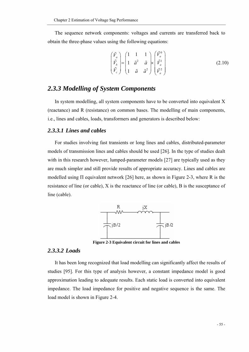
Chapter 2 Estimation of Voltage Sag Performance
- 55 -
The sequence network components: voltages and currents are transferred back to
obtain the three-phase values using the following equations:
0
2 1
2 2
1 1 1
1
1
aa
b a
c a
VVV a a VV a a V
⎛ ⎞⎛ ⎞⎛ ⎞⎜ ⎟⎜ ⎟⎜ ⎟
= ×⎜ ⎟⎜ ⎟⎜ ⎟⎜ ⎟⎜ ⎟⎜ ⎟ ⎜ ⎟⎝ ⎠ ⎝ ⎠ ⎝ ⎠
(2.10)
2.3.3 Modelling of System Components
In system modelling, all system components have to be converted into equivalent X
(reactance) and R (resistance) on common bases. The modelling of main components,
i.e., lines and cables, loads, transformers and generators is described below:
2.3.3.1 Lines and cables
For studies involving fast transients or long lines and cables, distributed-parameter
models of transmission lines and cables should be used [26]. In the type of studies dealt
with in this research however, lumped-parameter models [27] are typically used as they
are much simpler and still provide results of appropriate accuracy. Lines and cables are
modelled using Π equivalent network [26] here, as shown in Figure 2-3, where R is the
resistance of line (or cable), X is the reactance of line (or cable), B is the susceptance of
line (cable).
Figure 2-3 Equivalent circuit for lines and cables
2.3.3.2 Loads
It has been long recognized that load modelling can significantly affect the results of
studies [95]. For this type of analysis however, a constant impedance model is good
approximation leading to adequate results. Each static load is converted into equivalent
impedance. The load impedance for positive and negative sequence is the same. The
load model is shown in Figure 2-4.

Chapter 2 Estimation of Voltage Sag Performance
- 56 -
Figure 2-4 Equivalent circuit for loads
In Figure 2-4, R and X are the resistance and reactance of the load respectively,
which can be calculated as (2.11):
2
*( )VR jX
P jQ+ =
+ (2.11)
2.3.3.3 Generator
For the purposes of short-circuit current calculations, three values of reactance of
generator, namely sub-transient reactance (Xd’’), transient reactance (Xd
’) and
synchronous reactance (Xd) are used [96]. Sub-transient reactance determines the
current during the first few cycles after the fault occurs. The transient reactance
determines the current during the next few seconds and the synchronous reactance
determines the current after a steady state condition is reached [97].
Because most of short-circuit interrupting devices, such as circuit breakers and fuses,
operate well before steady-state conditions are reached, generator synchronous
reactance is seldom used in calculating fault currents [96] . Generators are modelled in
this study by corresponding sequence resistances and sub-transient reactance in series
with a constant driving voltage [96] as shown in Figure 2-5.
Figure 2-5 Equivalent circuit for generators
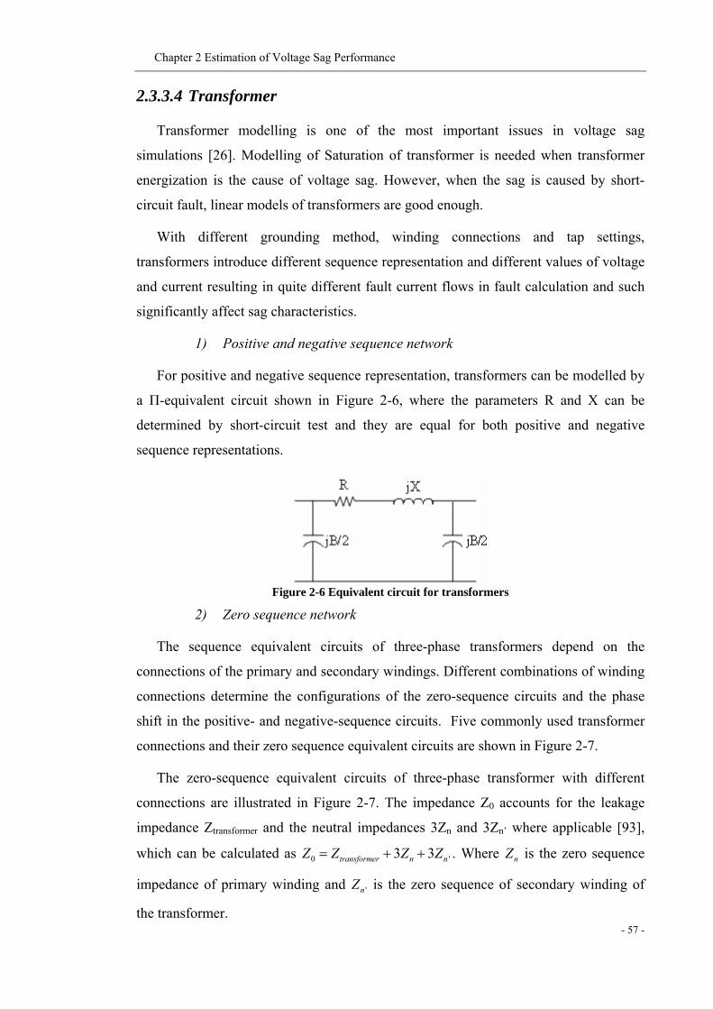
Chapter 2 Estimation of Voltage Sag Performance
- 57 -
2.3.3.4 Transformer
Transformer modelling is one of the most important issues in voltage sag
simulations [26]. Modelling of Saturation of transformer is needed when transformer
energization is the cause of voltage sag. However, when the sag is caused by short-
circuit fault, linear models of transformers are good enough.
With different grounding method, winding connections and tap settings,
transformers introduce different sequence representation and different values of voltage
and current resulting in quite different fault current flows in fault calculation and such
significantly affect sag characteristics.
1) Positive and negative sequence network
For positive and negative sequence representation, transformers can be modelled by
a Π-equivalent circuit shown in Figure 2-6, where the parameters R and X can be
determined by short-circuit test and they are equal for both positive and negative
sequence representations.
Figure 2-6 Equivalent circuit for transformers
2) Zero sequence network
The sequence equivalent circuits of three-phase transformers depend on the
connections of the primary and secondary windings. Different combinations of winding
connections determine the configurations of the zero-sequence circuits and the phase
shift in the positive- and negative-sequence circuits. Five commonly used transformer
connections and their zero sequence equivalent circuits are shown in Figure 2-7.
The zero-sequence equivalent circuits of three-phase transformer with different
connections are illustrated in Figure 2-7. The impedance Z0 accounts for the leakage
impedance Ztransformer and the neutral impedances 3Zn and 3Zn’ where applicable [93],
which can be calculated as 0 '3 3transformer n nZ Z Z Z= + + . Where nZ is the zero sequence
impedance of primary winding and 'nZ is the zero sequence of secondary winding of
the transformer.

Chapter 2 Estimation of Voltage Sag Performance
- 58 -
Figure 2-7 Zero-sequence representation of transformers [93]
3) Tap-change transformer
In the power system network, there are some transformers with an off-nominal tap
ratio, known as regulating transformers, which can be used to control the voltage and
the real and reactive power flows in the network. This type of transformers can be
presented by a Π equivalent circuit according to their real tap ratio [94]. Figure 2-8
shows a detailed representation of the regulating transformer with the ratio n:1 where n
is variable.
Figure 2-8 Equivalent circuit for tap changing transformer
4) Phase-shift in Wye-delta transformer
The phase shift of 030n× ( 1,5,11,n etc= ) resulting from different types of delta-
wye connections of transformer winding must be considered in models to account for

Chapter 2 Estimation of Voltage Sag Performance
- 59 -
their effect on sag propagation. The effect of these phase shifts only appears in the
positive and negative sequence network. The zero sequence network quantities are
unaffected.
In case of transformers manufactured according to the ANSI/IEEE
standard(ANSI/IEEE, 1988) [7], for either wye-delta or delta-wye connections, phases
shall be labelled in such a way that positive sequence quantities on the high voltage side
lead their corresponding positive sequence quantities on the low voltage side by 030n× .
The effect on negative sequence quantities is the reverse, that is, HV values lag LV
values by 030n× .
The method for including transformers phase shift in fault calculation using system
impedance matrix is developed in [98]. The process can be summarized as follows:
M(i): The phase adjusting parameter, one for bus i.
All M values are initially set to 99, to identify them as unknown. One value, M(1), is
set to zero arbitrarily. The algorithm then cycles over all the elements, locating all buses
(e.g., bus j connected to bus 1. If lines, wye-wye, or delta-delta connected
transformers are encountered, M(j) is set to be equal to M(1); if delta-wye connections
are encountered, M(j) is set to M(1)±n, (the ‘+’ or ‘-’ depending on lead or lag). Check
is then performed to see if all proper values have been determined. If not, the cycle is
repeated. After all M values are assigned. M is referenced to the faulted bus.
The sequence phase values are then corrected as follows:
1 1 1( ) 1 ( )j j jV new V newϕ= × ∠ (2.12)
2 2 2( ) 1 ( )j j jV new V newϕ= × ∠ (2.13)
Where 1jV , 2
jV are the original positive and negative sequence voltages of bus j
respectively, 1( )jV new , 2 ( )jV new are the positive and negative sequence voltages with the
influences of phase shifts. And
1 1( ) ( ) / 6j jnew M jϕ ϕ π= + × (2.14)
2 2( ) ( ) / 6j jnew M jϕ ϕ π= − × (2.15) Where, 1
jϕ , 2jϕ are the original positive and negative sequence voltage phase angles
of bus j respectively.

Chapter 2 Estimation of Voltage Sag Performance
- 60 -
2.3.4 Impedance Matrix
The use of the impedance matrix provides a convenient means for calculating fault
currents and voltages. Once the bus impedance matrix is formed the elements of this
matrix can be used directly to calculate the currents and voltages associated with
various types of faults. It is especially helpful for analyzing large and complex systems.
2.3.4.1 System Impedance Matrix
A general n-port passive linear network can be described in matrix notation as:
V=ZI (2.16) where, Z is the bus impedance matrix of the network, I is the currents entering into
the network and V is the voltages measured with respect to the reference node. It
should be noted that all the elements of the above matrices are complex values.
The bus impedance matrix is given by:
11 12 1 1
21 22 2 2
1 2
1 2
k n
k n
k k kk kn
n n nk nn
Z Z Z ZZ Z Z Z
Z Z Z Z
Z Z Z Z
⎛ ⎞⎜ ⎟⎜ ⎟⎜ ⎟
= ⎜ ⎟⎜ ⎟⎜ ⎟⎜ ⎟⎜ ⎟⎝ ⎠
Z (2.17)
The Z matrix elements on the principal diagonal, i.e., iiZ are called “driving-point
impedances” of the nodes, and they represent Thevenin’s equivalent impedance of the
network seen into the network from that corresponding node. Hence the diagonal
elements of the impedance matrix allow determining the short-circuit current of every
bus fault in the system. The off-diagonal elements, i.e., ijZ are called the transfer
impedances of the nodes. The transfer impedance allows finding the during-fault
voltage due to the fault current [93].
Usually, the impedance matrix is a full and symmetrical matrix. Any change in any
network impedance will in general affect every element of the impedance matrix.
Different elements of Z bus matrix are illustrated below using 4 bus network shown in
Figure 2-9.

Chapter 2 Estimation of Voltage Sag Performance
- 61 -
0.7166 0.6099 0.5330 0.58140.6089 0.7318 0.6400 0.69760.5334 0.6400 0.7166 0.66960.5803 0.6968 0.6695 0.7632
( ( ( (
j j j jj j j jj j j jj j j j
⎡ ⎤⎢ ⎥⎢ ⎥⎢ ⎥⎣ ⎦
(1)(2)Z = (3)(4)
1) 2) 3) 4)
Figure 2-9 Network example (branch impedances are in per unit)
2.3.4.2 Creating an Impedance Matrix
There are generally two methods for forming a Z matrix:
• Inverting the system admittance matrix Y s;
• Direct formation of Z .
In this study, the method of direct formation of a Z matrix is employed. The Z
matrix is assembled by starting with a single element connected to the reference bus and
by adding one element at a time and correspondingly modifying the matrix after each
addition. Each added element should be connected to at least one other bus of the
system.
This method is based on the principle of modification of a Z matrix, which can be
described as follows:
a) Adding a branch between existing buses;
b) Adding a branch from a new bus to the reference;
c) Adding a branch from a new bus to an existing bus;
d) Adding a branch from an existing bus to the reference.
A complete discussion of related techniques are provided in [93].The algorithm for
forming Zbus matrix step by step is simple providing that all the data required are
prepared before the process starts. The steps included are detailed below:

Chapter 2 Estimation of Voltage Sag Performance
- 62 -
• All bus numbers should be in a sequence. Generally, reference bus is denoted
as bus zero. Other bus numbers are assigned arbitrarily but in a sequence.
• The branch data are prepared in such a way that each element of the system is
described by the two buses at its ends and its impedance on a common per unit
base.
• The branch data are sequenced by an algorithm from a random ordering to a
sequence such that as each branch is selected from the data list for processing,
it can be connected to the system that has been assembled. The first branch in
this process must be the branch starting from the reference bus.
The branch ordering algorithm can be described as follows:
• The first branch that is found connected to the reference bus is transferred to
the recorded list.
• The branch data are examined till all the branches are in the recorded branch
list. Every line which has a node connected to the node being recorded is
assembled in the branch list.
The automated process of constructing Z matrix is implemented as follows:
• Data preparation: numbering bus, reordering branches
• Form Z using Step-by-Step method described above
• Adjust Z , the order of column should be in the same sequence as the real bus
number
2.3.5 Fault calculation
The electrical network under short-circuit conditions can be considered as a network
supplied by several sources (generators) with a single load connected to the system at
the bus subjected to the short circuit. The steady state customer load currents are
usually ignored, since they are small compared to the fault currents.
2.3.5.1 Bus faults
a) Three-phase fault (LLL)
In three-phase short-circuit analysis of the network, only the positive sequence
network is considered. The pre fault voltage is equal to the pre fault voltage at faulted
bus k obtained from previous load flow study. The impedance looking into the network

Chapter 2 Estimation of Voltage Sag Performance
- 63 -
from the faulted bus k is given by diagonal element kkZ of the positive-sequence
impedance matrix. Figure 2-10 (A) shows the sequence network connection. And the
short circuit current is:
2 0 0I I= = (2.18)
1k
fkk fault
VI IZ Z
= =+
(2.19)
where, faultZ is the fault impedance.
b) Single phase to ground fault (LG)
The fault is on Phase A as shown in Figure 2-10 (B):
The sequence currents and fault current are given by:
1 2 0 1 2 0 3
preak
kk kk kk fault
VI I IZ Z Z Z
= = =+ + + ×
(2.20)
13fI I= × (2.21)
c) Phase to phase to ground fault (LLG)
The positive and negative-sequence networks are connected in parallel to satisfy the
fault conditions as Figure 2-10 (C) shows.
The sequence current can be presented by the following equation:
1 2 01
0 2
( )( )
k
kk kk faultkk
kk fault kk
VIZ Z Z
ZZ Z Z
=+
++ +
(2.22)
0
2 1 2 0
( 3 )3
kk fault
kk kk fault
Z ZI I
Z Z Z+ ×
= −+ + ×
(2.23)
2
0 1 2 0 3kk
kk kk fault
ZI IZ Z Z
= −+ + ×
(2.24)
d) Phase to phase fault (LL)
Figure 2-10 (D) shows the sequence connection for phase to phase fault.
The voltage throughout the zero-sequence network must be zero since there are no
zero-sequence sources, and the current is not being injected into that network as there is
no path for zero-sequence current to flow, so:

Chapter 2 Estimation of Voltage Sag Performance
- 64 -
1 2 1 2k
kk kk fault
VI IZ Z Z
= − =+ +
(2.25)
0 0I = (2.26) All discussions so far considered solidly grounded ( 0faultZ = ) network, the
transformer neutral point is directly connected to earth. If this is not the case, the fault
current would be much less dependent on the impedance connected and the equivalent
circuit of LLL, LG, LLG and LL faults which are illustrated in Figure 2-10.
Figure 2-10 Equivalent circuit for faulted system
2.3.5.2 Line Faults
A fault occurring on transmission lines should be taken more seriously since the
number of fault occurrences each year is much higher than the bus faults.
In order to calculate faults on the transmission and distribution lines, additional
elements of the Zbus matrix should be introduced that correspond to line faults need to
be calculated [99]. The fault position on line k-j is represented by node p as shown in
Figure 2-11:
Figure 2-11 Line fault
where, Lkp is the distance between bus k and the additional node p.
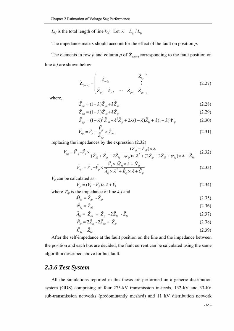
Chapter 2 Estimation of Voltage Sag Performance
- 65 -
Lkj is the total length of line k-j, Let /kp kjL Lλ =
The impedance matrix should account for the effect of the fault on position p.
The elements in row p and column p of ( )newZ corresponding to the fault position on
line k-j are shown below:
1
( )
1 2
porig
new
p p pn pp
ZZ
Z Z Z Z
⎛ ⎞⎜ ⎟
= ⎜ ⎟⎜ ⎟⎝ ⎠
Z (2.27)
where, (1 )np ni njZ Z Zλ λ= − + (2.28)
(1 )pn in jnZ Z Zλ λ= − + (2.29)
2 2(1 ) 2 (1 ) (1 )pp kk jj kj kjZ Z Z Zλ λ λ λ λ λ= − + + − + − Ψ (2.30)
pnp n np
pp
VV V Z
Z= − × (2.31)
replacing the impedances by the expression (2.32)
2
( )( 2 ) (2 2 )
nj nknp n p
kk jj kj kj kj kk kj kk
Z ZV V V
Z Z Z Z Z Zλ
ψ λ ψ λ− ×
= − ×+ − − × + − + × +
(2.32)
2p kj kj
np n pkj kj kj
V M NV V V
A B Cλ
λ λ× × +
= − ×× + × +
(2.33)
Vp can be calculated as: ( )p k j kV V V Vλ= − × + (2.34) where Ψkj is the impedance of line k-j and -kj nj nkM Z Z= (2.35)
kj nkN Z= (2.36)
- 2 - kj kk jj kj kjA Z Z Z Z= + (2.37)
2 - 2 kj kj kk kjB Z Z Z= + (2.38)
kj kkC Z= (2.39) After the self-impedance at the fault position on the line and the impedance between
the position and each bus are decided, the fault current can be calculated using the same
algorithm described above for bus fault.
2.3.6 Test System
All the simulations reported in this thesis are performed on a generic distribution
system (GDS) comprising of four 275-kV transmission in-feeds, 132-kV and 33-kV
sub-transmission networks (predominantly meshed) and 11 kV distribution network

Chapter 2 Estimation of Voltage Sag Performance
- 66 -
(predominantly radial). There are 295 buses, 276 lines (over-head lines and
underground cables) and 37 transformers with various winding connections. The single
line diagram of the network is shown in Figure 2-12 and the system parameters are
given in Appendix A.
Figure 2-12 Test system
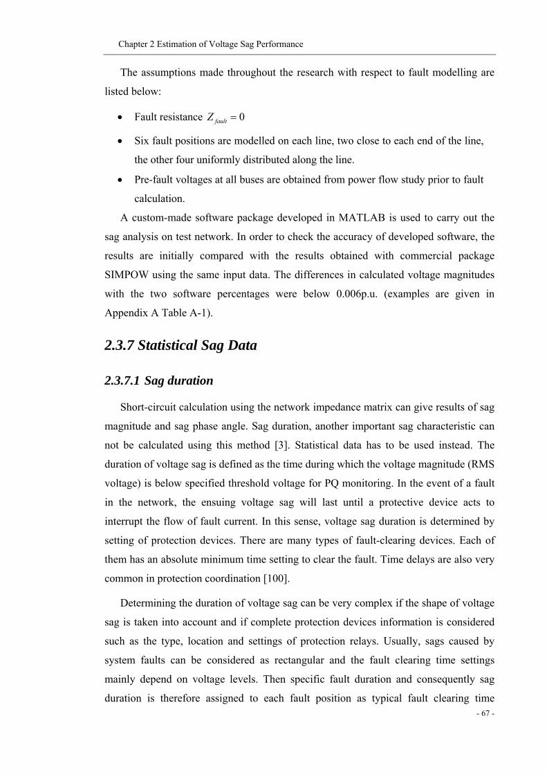
Chapter 2 Estimation of Voltage Sag Performance
- 67 -
The assumptions made throughout the research with respect to fault modelling are
listed below:
• Fault resistance 0faultZ =
• Six fault positions are modelled on each line, two close to each end of the line,
the other four uniformly distributed along the line.
• Pre-fault voltages at all buses are obtained from power flow study prior to fault
calculation.
A custom-made software package developed in MATLAB is used to carry out the
sag analysis on test network. In order to check the accuracy of developed software, the
results are initially compared with the results obtained with commercial package
SIMPOW using the same input data. The differences in calculated voltage magnitudes
with the two software percentages were below 0.006p.u. (examples are given in
Appendix A Table A-1).
2.3.7 Statistical Sag Data
2.3.7.1 Sag duration
Short-circuit calculation using the network impedance matrix can give results of sag
magnitude and sag phase angle. Sag duration, another important sag characteristic can
not be calculated using this method [3]. Statistical data has to be used instead. The
duration of voltage sag is defined as the time during which the voltage magnitude (RMS
voltage) is below specified threshold voltage for PQ monitoring. In the event of a fault
in the network, the ensuing voltage sag will last until a protective device acts to
interrupt the flow of fault current. In this sense, voltage sag duration is determined by
setting of protection devices. There are many types of fault-clearing devices. Each of
them has an absolute minimum time setting to clear the fault. Time delays are also very
common in protection coordination [100].
Determining the duration of voltage sag can be very complex if the shape of voltage
sag is taken into account and if complete protection devices information is considered
such as the type, location and settings of protection relays. Usually, sags caused by
system faults can be considered as rectangular and the fault clearing time settings
mainly depend on voltage levels. Then specific fault duration and consequently sag
duration is therefore assigned to each fault position as typical fault clearing time
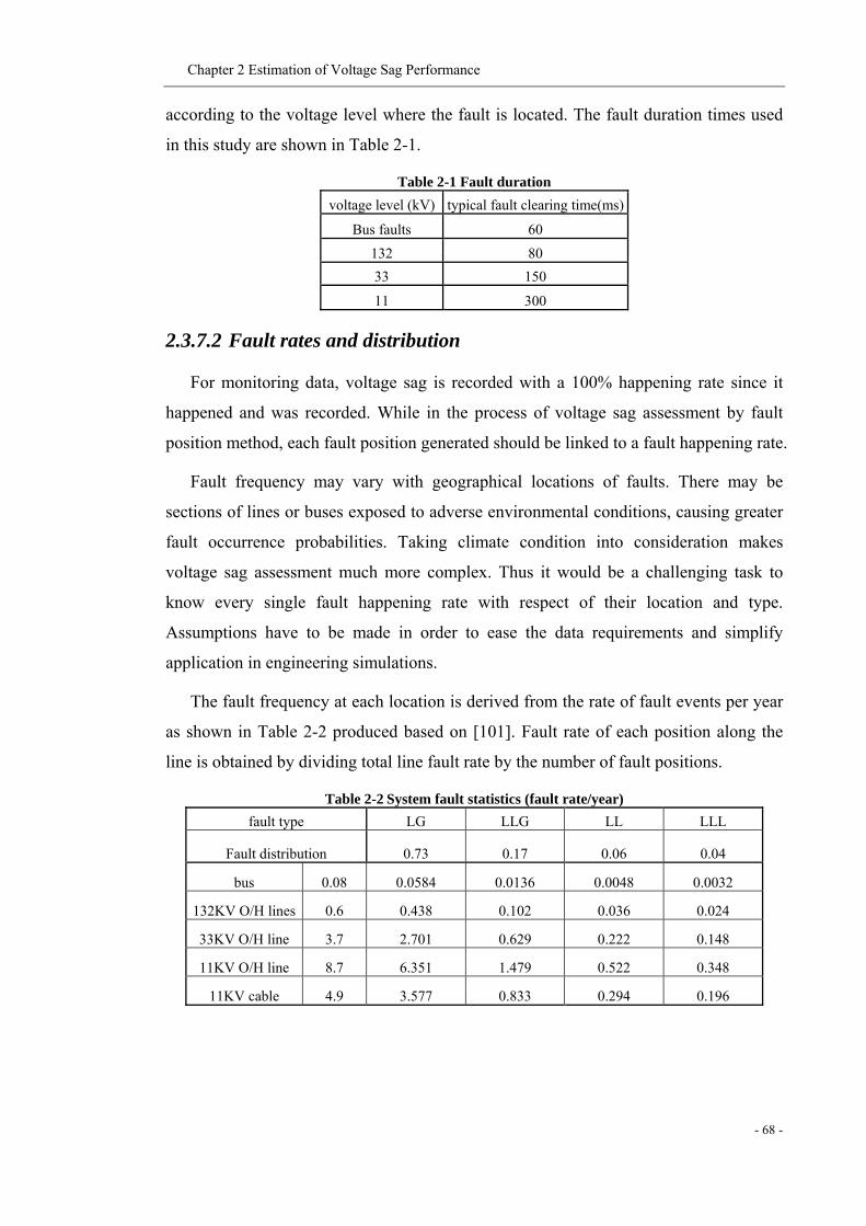
Chapter 2 Estimation of Voltage Sag Performance
- 68 -
according to the voltage level where the fault is located. The fault duration times used
in this study are shown in Table 2-1.
Table 2-1 Fault duration voltage level (kV) typical fault clearing time(ms)
Bus faults 60 132 80 33 150
11 300
2.3.7.2 Fault rates and distribution
For monitoring data, voltage sag is recorded with a 100% happening rate since it
happened and was recorded. While in the process of voltage sag assessment by fault
position method, each fault position generated should be linked to a fault happening rate.
Fault frequency may vary with geographical locations of faults. There may be
sections of lines or buses exposed to adverse environmental conditions, causing greater
fault occurrence probabilities. Taking climate condition into consideration makes
voltage sag assessment much more complex. Thus it would be a challenging task to
know every single fault happening rate with respect of their location and type.
Assumptions have to be made in order to ease the data requirements and simplify
application in engineering simulations.
The fault frequency at each location is derived from the rate of fault events per year
as shown in Table 2-2 produced based on [101]. Fault rate of each position along the
line is obtained by dividing total line fault rate by the number of fault positions.
Table 2-2 System fault statistics (fault rate/year)
fault type LG LLG LL LLL
Fault distribution 0.73 0.17 0.06 0.04
bus 0.08 0.0584 0.0136 0.0048 0.0032
132KV O/H lines 0.6 0.438 0.102 0.036 0.024
33KV O/H line 3.7 2.701 0.629 0.222 0.148
11KV O/H line 8.7 6.351 1.479 0.522 0.348
11KV cable 4.9 3.577 0.833 0.294 0.196

Chapter 2 Estimation of Voltage Sag Performance
- 69 -
2.4 Sag performance presentation
Sag performance has been a topic of academic study for several decades, and the
concept itself has been in use since the 1970s [35]. Although sag performance has been
used in various ways, the definition of sag performance is not entirely clear
(satisfactory). Conceptual developments have not been systematically integrated with
one another, but have usually been treated as free-standing, implicitly competing ideas.
How to present or measure the sag performance of a single site or a whole network will
mostly depend on the purpose of the research.
The network sag performance can be presented in various ways, though most of
them are based on sag magnitude and duration data. In this research representations of
sag performance is adopted from past literature [12].
2.4.1 Number of sags
Number of sags is often used to represent sag performance for a single site or the
entire network, and usually comprises the incidence of sag magnitude and sag duration:
, ,( , ) | ( , )n
k i ft L k L i ft Ui ft
N u t U U U t t tλ= < ≤ < Δ <∑∑ U (2.40)
where λi,ft is the fault frequency of fault type ft at fault position i, Uk is the voltage
sag experienced at node k, Δti,ft the sag duration for the fault place and fault type. UL and
UU are the low limit and upper limit of voltage magnitude range. tL and tU are the low
and upper limit of fault duration range.
A power system short-circuit fault may result in voltage disturbances on one, two or
all three phases of the network. The magnitude and duration of resulting RMS variation
on each phase may differ substantially. Voltage sag due to LLLG fault can be simply
counted and represented. In the case of unbalanced sag, decision must be made how to
report three-phase events. Unfortunately as with the characterization of non-rectangular
sags, characterization of these phase events has not been satisfactorily standardized and
is not very well defined yet. Unbalanced sag can be reported using only the lowest
voltage magnitude, average voltage magnitude, or sag in each phase can be reported
individually. If only the lowest voltage magnitude or average voltage magnitude is
concerned, then a single fault event will result in one voltage sag at each bus. If three

Chapter 2 Estimation of Voltage Sag Performance
- 70 -
phases are reported individually and considering equal probability of fault occurrence
on each phase, the fault frequency should be one third of the value described above [1].
For example, if there is a LLG bus fault resulting in voltage in
: 0.9 . ., : 0.5 . ., : 0.5 . .phase A p u phase B p u phase C p u , the fault rate of LLG bus fault
is 0.0136. The number of voltage sags should be calculated as follows:
Three phases considered individually:
0.0136(0.9) 0.00453
0.0136 0.0136(0.5) 0.0093 3
sag
sag
N per year
N per year
= =
= + =
Worst affected phase considered:
(0.5) 0.0136sagN = per year
The total number of faults simulated in the network is (276: number of lines in the
test network, 295 -- buses in the network, 4 -- types of faults, 6 -- fault positions along
each line):
295 4 276 6 4 7804× + × × =
When the actual fault rate is taken into account, it will be: 1,763 per year.
The total number of sags that all buses in the whole network will experience is:
295 (295 4 276 6 4) 2,302,180× × + × × =
When the fault rate is taken into account, it becomes: 520,150 per year. Vast
majority of these potential sags though will have magnitudes >0.9p.u. and therefore will
not be classed as sags at all.
2.4.2 Three dimensions bar chart
In the 3-D diagram representation one defines the sag number as a function of both
sag magnitude and sag duration as described in (2.40), where x and y axis present sag
duration and the sag magnitude range respectively and z axis the number of correspond
sags. Due to the different methodologies for calculating sag number, there is an issue of
how to report the three-phase sags. If only the worst affected phase is considered
(unbalanced sags are reported using lowest voltage magnitude), then a representation

Chapter 2 Estimation of Voltage Sag Performance
- 71 -
shown in Figure 2-13 can be obtained for arbitrary bus (154) in the test network and the
whole network, respectively.
Figure 2-13 (a) shows the sag performance of bus 154 (worst affected phase
considered). The number of voltage sags with magnitude between 0.7 – 0.9 p.u. and
duration of 300ms is the biggest. Figure 2-13 (b), (c) and (d) show the sag performance
of bus 154 A phase, B phase and C phase, respectively. It can be seen from these
figures that the number of sags is smaller when three phases are considered individually.
There are few (129.6) of swells with magnitude >1.1 on phase C (see Figure 2-13 (d)).
The sag performance of the entire network is the sum of corresponding sags of all buses
in the network, as shown in Figure 2-13 (e).
(a) Bus 154 worst affected phase considered (b) Bus 154 phase A
(c) Bus 154 phase B (d) Bus 154 phase C
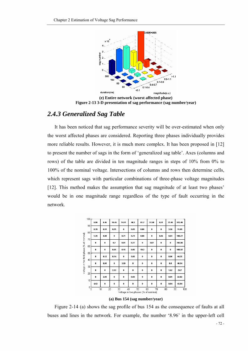
Chapter 2 Estimation of Voltage Sag Performance
- 72 -
(e) Entire network (worst affected phase)
Figure 2-13 3-D presentation of sag performance (sag number/year)
2.4.3 Generalized Sag Table
It has been noticed that sag performance severity will be over-estimated when only
the worst affected phases are considered. Reporting three phases individually provides
more reliable results. However, it is much more complex. It has been proposed in [12]
to present the number of sags in the form of ‘generalized sag table’. Axes (columns and
rows) of the table are divided in ten magnitude ranges in steps of 10% from 0% to
100% of the nominal voltage. Intersections of columns and rows then determine cells,
which represent sags with particular combinations of three-phase voltage magnitudes
[12]. This method makes the assumption that sag magnitude of at least two phases’
would be in one magnitude range regardless of the type of fault occurring in the
network.
(a) Bus 154 (sag number/year)
Figure 2-14 (a) shows the sag profile of bus 154 as the consequence of faults at all
buses and lines in the network. For example, the number ‘8.96’ in the upper-left cell

Chapter 2 Estimation of Voltage Sag Performance
- 73 -
indicates that there are 8.96 sags with two phases’ voltage magnitude below 10% and
the third phase voltage magnitude above 90%. Figure 2-14 (b) shows the sag profile in
the similar way of the entire network.
(b) Entire network (sag number/year)
Figure 2-14 Generalized sag tables
The generalized sag table of Figure 2-14 doesn’t take into account the duration of
sags. It was suggested in [12] though, how this can be easily included.
2.5 Uncertainties associated with fault positions
assessment method
The method of fault positions has been identified as an effective tool for evaluating
the system sag performance. The assumptions and uncertainties associated with this
method however, influence strongly conclusions based on the results of calculation.
They include aspects of modelling of the system, number and distribution of simulated
faults, system operating condition before and during the fault, etc.
This section illustrates the influence of some of them, namely number of fault
positions along the line, fault impedance and pre-fault voltage on sag performance
results.
2.5.1 Number of fault positions on lines
In the method of fault position, a number of faults is simulated in the network, on
buses and on transmission lines. Different location of fault positions on lines will result
in different voltage sag magnitudes. Base case assumption is that there are six fault

Chapter 2 Estimation of Voltage Sag Performance
- 74 -
positions along each line, two of them located close to line ends at 1% of the line length,
the other four uniformly distributed along the line, as illustrated in Figure 2-15. Sag
magnitudes at bus 111 for LLLG faults at all lines are shown in Figure 2-16.
Figure 2-15 Fault positions on line
Figure 2-16 Voltage at bus 111 for faults at 6 positions on all lines
As shown in Figure 2-16, when the faults occur on lines that are far away from bus
111, voltage magnitudes on bus 111 are almost undisturbed (close to 1p.u.). When the
faults are on lines close to bus 111, voltage drops significantly (e.g. when faults on lines
numbered from 100 – 160). It can also be seen from Figure 2-16 that faults on different
positions along one line result in different sag magnitudes. These differences vary with
line length and location: some are very obvious, and some are negligible.
To illustrate these differences more clearly, sag magnitudes of bus 111 for faults on
lines that are close to the bus are depicted in Figure 2-17 (a). It can be seen that in
some situations, the difference in sag magnitude could be over 10% depending on fault
positions along the same line (see Figure 2-17 (b)).
(a) Voltages for faults on all lines

Chapter 2 Estimation of Voltage Sag Performance
- 75 -
(b) Magnified voltage for faults on a few lines(1-20)
Figure 2-17 Voltage on bus 111 when faults on 6 position of selected lines in the system
Total number of sag at given bus is a function of sag voltage magnitude and
duration as shown by(2.40). Each fault event at particular location at given position
along the line is given by:
lineposition N
λλ = (2.41)
where N is the number of fault positions on the line and lineλ is the fault rate of the line.
The more fault positions are assumed on each line, the smaller will be fault rate
corresponding of each position. The calculation here is based on the assumption that the
faults are distributed uniformly along the line. The effect of different fault distributions
along the line on sag performance is described in [102]. The total number of sags
calculated using the approach described here will not be affected by the number of fault
positions along the line, however, the number of sags within different magnitude ranges
will depend on number of fault positions.
To illustrate this, simulations are performed assuming different number of fault
positions along each line. The number of fault positions considered was: 3, 4, 5, 6, 7, 8
and 9. In addition to this, fault position is assumed at each bus in the network. Results
obtained with 3 and 9 fault position along each line are shown in Figure 2-19 and
Figure 2-21 respectively. Corresponding distribution of fault positions is depicted in
Figure 2-18 and Figure 2-20 respectively. Results with 4, 5, 6, 7, 8 fault positions along
each line are shown in Figure A-1 – Figure A-10 in Appendix A.
Figure 2-18 Three positions on line

Chapter 2 Estimation of Voltage Sag Performance
- 76 -
Figure 2-19 Generalized sag table of bus 111 with 3 positions on each line (sag number/year)
1 3 4 5 62 87 9
Figure 2-20 Nine positions on line
Figure 2-21 Generalized sag table of bus 111 with 9 position on each line (sag number/year)
The next assumption is that the number of fault positions on each line would depend
on the length of line. The length of the line is decided by its impedance. The number of
fault positions is chosen based on the criteria shown in Table 2-3. The result of this
simulation is presented in Figure 2-22.
Table 2-3 Fault positions on lines based on line impedance line resistance(p.u.) number of fault position
<0.1 3 0.1-0.2 4 0.2-0.3 5 0.3-0.4 6 0.4-0.5 7
>0.5 8

Chapter 2 Estimation of Voltage Sag Performance
- 77 -
Figure 2-22 Generalized sag table of bus 111 when various points on each line (sag number/year)
From these sag tables (Figure 2-19, Figure 2-21 and Figure 2-22) one can see that
the results are very close in all three cases. For example, number of sags with
magnitudes of two phases between 60% to 70% and the third phase above 90% are:
15.6, 16.65 and 15.76, respectively (red circled in Figure 2-19, Figure 2-21 and Figure
2-22). The differences are almost negligible considering the size of the network, and the
total number of faults assumed in the network.
Taking the worst affected phase only, number of sags at bus 111 for simulations
with 3, 4, 5, 6, 7, 8, 9 and variable fault positions (fault positions on each line
depending on the impedance of line) is shown in Figure 2-23, while the number of sags
in the whole network is given in Figure 2-24.
Even though there are differences in the results shown in Figure 2-23 and Figure
2-24 they are very small. Bearing in mind that the total number of faults in the network
is high (there would be 1763 per year number of ‘sags’ for one bus, and 520,150 per
year for the entire network). These differences could be considered negligible.
Difference found (see Figure 2-23) was only 0.17% of 1211.41 sags in case of sags with
magnitudes >90% and 8.58% of 93.42 sags in case of sag with magnitude between 50%
and 60%. The differences are 0.11% and 4.32% in case of sags with magnitude >90%
and between 50% and 60%, respectively.
Previous results suggest that although different fault positions along the line result
in different sag magnitudes on buses close to the faulted line, the differences at the
system level are negligible and they do not warrant the use of excessive number of fault
positions along the line as long as overall system sag performance is concerned.

Chapter 2 Estimation of Voltage Sag Performance
- 78 -
0
20
40
60
80
100
120
0-0.1 0.1-0.2 0.2-0.3 0.3-0.4 0.4-0.5 0.5-0.6 0.6-0.7 0.7-0.8 0.8-0.9 >0.9
voltage magnitude
points 3 4 5 6 7 8 9 various
1208
1210
1212
Figure 2-23 Sags at bus 111 for various points on line
Figure 2-24 Sags at all buses for various points on line
2.5.2 Fault resistance
In fault calculations using system impedance matrix, fault impedances are usually
assumed to be zero. In reality, however fault resistance will always appear. Its value
depends on parameters such as the soil layer length, electric arc, amount of salt present
in the soil and also the time taken to discharge to the ground. The fault resistance can
reduce the fault current, and thus reduce the severity of sag, resulting in differences in
sag performance estimation.
In order to investigate the influences of fault resistance on sag performance
estimation, simulations are performed using zero fault resistance, 1Ω, 2Ω, 5Ω, 10Ω and
15Ω fault resistance respectively.

Chapter 2 Estimation of Voltage Sag Performance
- 79 -
Figure 2-25 shows voltage sag magnitudes in p.u. at bus 111 when LLLG faults
occurs on all buses (from 1 to 295) in the network with various fault impedances. It can
be clearly seen that higher fault resistance will result in higher sag magnitudes, i.e.,
more shallow sags.
Figure 2-25 Voltage at bus 111for faults at all buses with various fault resistance
Figure 2-26 and Figure 2-27 are generalized sag tables of bus 111 for simulations
with fault resistance 0Ω and 15Ω. Results with resistance values of 1Ω, 2Ω, 5Ω and
10Ω are shown in Figure A-11 – Figure A-14 in the Appendix. It can be seen that the
sags are shifting towards the upper right hand corner of these tables with increasing
fault resistance, which means that the number of sags with higher magnitudes increase
and number of sags with lower magnitude decreased, e.g. the number of sags with all
three phase voltages above 0.9 increased from 1210.31 (Figure 2-26) with 0Ω fault
impedance to 1479.74 with 15Ω fault impedance (Figure 2-27).
Figure 2-26 Generalized sag table of bus 111 for fault resistance 0Ω (sag number/year)
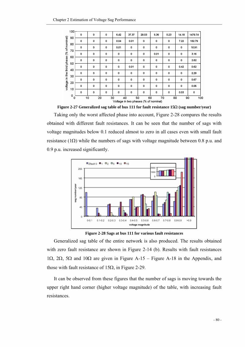
Chapter 2 Estimation of Voltage Sag Performance
- 80 -
Figure 2-27 Generalized sag table of bus 111 for fault resistance 15Ω (sag number/year)
Taking only the worst affected phase into account, Figure 2-28 compares the results
obtained with different fault resistances. It can be seen that the number of sags with
voltage magnitudes below 0.1 reduced almost to zero in all cases even with small fault
resistance (1Ω) while the numbers of sags with voltage magnitude between 0.8 p.u. and
0.9 p.u. increased significantly.
Figure 2-28 Sags at bus 111 for various fault resistances
Generalized sag table of the entire network is also produced. The results obtained
with zero fault resistance are shown in Figure 2-14 (b). Results with fault resistances
1Ω, 2Ω, 5Ω and 10Ω are given in Figure A-15 – Figure A-18 in the Appendix, and
those with fault resistance of 15Ω, in Figure 2-29.
It can be observed from these figures that the number of sags is moving towards the
upper right hand corner (higher voltage magnitude) of the table, with increasing fault
resistances.
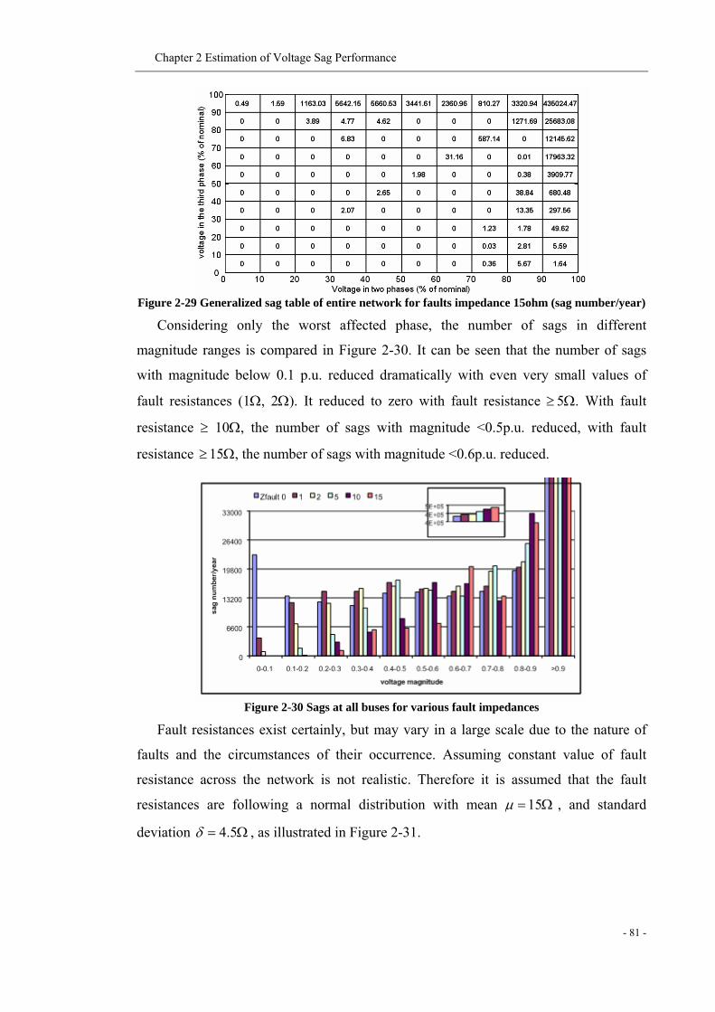
Chapter 2 Estimation of Voltage Sag Performance
- 81 -
Figure 2-29 Generalized sag table of entire network for faults impedance 15ohm (sag number/year)
Considering only the worst affected phase, the number of sags in different
magnitude ranges is compared in Figure 2-30. It can be seen that the number of sags
with magnitude below 0.1 p.u. reduced dramatically with even very small values of
fault resistances (1Ω, 2Ω). It reduced to zero with fault resistance ≥ 5Ω. With fault
resistance ≥ 10Ω, the number of sags with magnitude <0.5p.u. reduced, with fault
resistance ≥ 15Ω, the number of sags with magnitude <0.6p.u. reduced.
Figure 2-30 Sags at all buses for various fault impedances
Fault resistances exist certainly, but may vary in a large scale due to the nature of
faults and the circumstances of their occurrence. Assuming constant value of fault
resistance across the network is not realistic. Therefore it is assumed that the fault
resistances are following a normal distribution with mean 15μ = Ω , and standard
deviation 4.5δ = Ω , as illustrated in Figure 2-31.
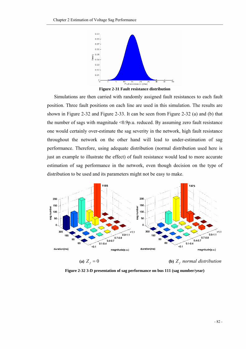
Chapter 2 Estimation of Voltage Sag Performance
- 82 -
Figure 2-31 Fault resistance distribution
Simulations are then carried with randomly assigned fault resistances to each fault
position. Three fault positions on each line are used in this simulation. The results are
shown in Figure 2-32 and Figure 2-33. It can be seen from Figure 2-32 (a) and (b) that
the number of sags with magnitude <0.9p.u. reduced. By assuming zero fault resistance
one would certainly over-estimate the sag severity in the network, high fault resistance
throughout the network on the other hand will lead to under-estimation of sag
performance. Therefore, using adequate distribution (normal distribution used here is
just an example to illustrate the effect) of fault resistance would lead to more accurate
estimation of sag performance in the network, even though decision on the type of
distribution to be used and its parameters might not be easy to make.
(a) 0fZ = (b) fZ normal distribution
Figure 2-32 3-D presentation of sag performance on bus 111 (sag number/year)

Chapter 2 Estimation of Voltage Sag Performance
- 83 -
(a) 0fZ = (b) fZ normal distribution
Figure 2-33 3-D presentation of sag performance entire network (sag number/year)
The number of voltage sags with magnitude <0.1 is almost zero in the case of
simulation with randomly located fault resistance either seen from bus 111 (Figure 2-32)
or the entire network (Figure 2-33). The generalized sag tables for bus 111 and the
entire network in both cases are illustrated in Figure 2-34 and Figure 2-35. The same
trend as before can be seen from these tables, e.g., the sags are shifted towards high
voltage magnitude range. The fault impedance has huge influence on the resulted
number of sags in network, therefore, it would be undesirable to assume zero fault
impedance in the process of sag performance estimation because it would certainly
under-estimate the ‘real’ situation.
(a) 0fZ = (sag number/year)

Chapter 2 Estimation of Voltage Sag Performance
- 84 -
(b) fZ normal distribution (sag number/year)
Figure 2-34 Generalized sag table of bus 111
(a) 0fZ = (sag number/year)
(b) fZ normal distribution (sag number/year)
Figure 2-35 Generalized sag table of with normally distributed fault resistances

Chapter 2 Estimation of Voltage Sag Performance
- 85 -
2.5.3 Transformer neutral impedance
In this research, assumptions are made that all Y transformers in the network are
grounded. However, if one considers a line-to-ground fault, the other two windings
would be subjected to full line voltage if the neutral is not grounded. In order to
investigate the influence of neutral grounding of Y transformer on the network sag
performance, a resistance of 99999Ω is placed at each Y transformer’s zero sequences
equivalent circuit in the simulations to model isolated as high impedance grounded Y
transformers. The results of sag performance of bus 232 and the entire network are
illustrated in Figure 2-36, Figure 2-37, Figure 2-39 and Figure 2-40 for the case of
worst affected phase approach.
(a) 0 0transformerZ = (b) 0transformerZ = ∞
Figure 2-36 3D presentation of sag performance at bus 232 (sag number/year)
(a) 0 0transformerZ = (b) 0transformerZ = ∞
Figure 2-37 3D presentation of sag performance of the entire network (sag number/year)

Chapter 2 Estimation of Voltage Sag Performance
- 86 -
It can been seen from these figures, that the numbers of sags within lower
magnitudes increased with isolated neutrals at Y transformers.
The sag performance of bus 232 considering phase A only is shown in Figure 2-38.
The results show that there is an increase in number of sags with voltage magnitude
>1.1, and sags with low magnitudes. This indicates that the balance of voltages is
worsened with high resistance or isolated neutrals of Y transformers. Generalized sag
tables for these cases are shown in Figure 2-39 and Figure 2-40.
(a) 0 0transformerZ = (b) 0transformerZ = ∞
Figure 2-38 3D presentation of sag performance of bus 232 (phase A) (sag number /year)
(a) 0 0transformerZ = (sag number/year)
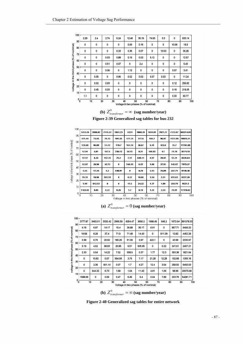
Chapter 2 Estimation of Voltage Sag Performance
- 87 -
(b) 0
transformerZ = ∞ (sag number/year) Figure 2-39 Generalized sag tables for bus 232
(a) 0 0transformerZ = (sag number/year)
(b) 0
transformerZ = ∞ (sag number/year)
Figure 2-40 Generalized sag tables for entire network

Chapter 2 Estimation of Voltage Sag Performance
- 88 -
2.5.4 Pre-fault voltage
In fault calculation by system impedance matrix using sequence network, pre-fault
voltages are usually set to 01 0∠ . This is because load currents are ignored in the
calculation. In a real network when loaded, voltages at network buses will differ
from 01 0∠ even though they are usually very close to 1p.u. and with small phase shift
In order to investigate the influences of pre-fault voltages on estimated sag
performance, a power flow calculation is run in the network to get the steady-state
voltage profile at all buses. The results are listed in Table A-2 in the Appendix.
Simulations are then carried out using these voltages as pre-fault voltages in fault
calculations. Resulting voltage magnitudes at bus 111 due to LLLG faults (bus faults
only) are illustrated in Figure 2-41. Voltage magnitudes at bus 111 due to other types of
faults are given in Figure A-19 – Figure A-27 in the Appendix.
It can be seen from Figure 2-41 that when faults occur at 11kV buses (bus number
was smaller than 233), there is almost no difference in sag performance regardless of
pre-fault voltages. In case of faults at higher voltage level (buses 233-289), the pre-fault
voltages will have more influences on sag performance.
0
0.2
0.4
0.6
0.8
1
1 21 41 61 81 101 121 141 161 181 201 221 241 261 281
Faulted buses
volta
ge m
agni
tude
pre-fault voltage 1 p.u. pre-fault voltage when loaded
Figure 2-41 Voltage at bus 111 for LLLG faults at all buses
2.6 Summary
The chapter demonstrated that it is desirable to perform as comprehensive sag
analysis as possible for the individual site as well as on the whole system in order to
provide valuable information to both utilities and end-users regarding expected severity
and frequency of voltage disturbances. It described in detail the process of sag
performance estimation by fault position method. The major advantage of the method is

Chapter 2 Estimation of Voltage Sag Performance
- 89 -
that it uses standard static fault calculation, which is easy to implement and very fast in
terms of computation time.
A custom made software package developed in MATLAB was used to carry out the
sag analysis in the realistic size test network. Fault calculation method using system
impedance matrix was described in detail. The modelling of system components i.e.,
lines, generator, transformers and loads was highlighted. The fault calculation
procedure from constructing system impedance matrix, formulating fault current for all
types of faults (bus or line faults) to converting between sequence and phase voltage is
described in detail. A comparison of the results obtained from the developed software
and commercial software package SIMPOW verified the efficiency and accuracy of the
coding and models employed.
The sag performance throughout the network was illustrated using conventional 3D
bar charts and ‘generalized sag table’ to demonstrate the efficiency of the latter in
particular for presentation of the results. The chapter further presented the influences of
various uncertainties associated with this method of sag assessment. Those included:
fault resistances, number of fault positions along each line, the transformer neutral
resistance and pre-fault voltage. Simulations showed that fault resistance has significant
influence on resulting sag performance. The influence of number of fault positions
along the line and pre-fault voltage, however, is much smaller if the network sag
performance is of concern. These effects though can be more pronounced if individual
lines and buses are considered.

Chapter 3 Modelling of FACTS Devices for Short-circuit Studies
- 90 -
3 MODELLING OF FACTS DEVICES FOR SHORT-
CIRCUIT STUDIES
3.1 Introduction
In previous chapter, sag performance analysis is proposed to obtain comprehensive
results. Fault calculation method by system impedance matrix is used in this analysis. In
order to evaluate the potential improvements with FACTS based mitigation, the fault
calculation method had to be upgraded to include the influence of FACTS devices.
Therefore in this chapter, the fault calculation with FACTS devices, which could
compensate voltage during fault conditions are explored. In terms of the devices, DVR,
STATCOM and SVC are considered. The prime concern here is to analyse their
influence on sag performance in a steady-state manner. The majority of the chapter
focuses on the mathematical derivation of the models of FACTS devices for the use in
well-known classical fault calculation method. The derivation is illustrated respective to
different fault types. The effectiveness evaluated by the developed of STATCOM and
SVC is compared, so does STATCOM and DVR. Real power injection is modelled in
the case of STATCOM and DVR. The required rating of each device is derived based
on the fault level and load size.
It has to be pointed out that all calculations derived here are based on steady-state
conditions. Since the typical response time of FACTS devices, such as DVR and
STATCOM, is in the range of milliseconds [61], the time response of devices is not
taken into account here, i.e., instantaneous response is assumed. Real power injection is
used only to indicate the rating of these devices and not be representing potential energy
storage availability.

Chapter 3 Modelling of FACTS Devices for Short-circuit Studies
- 91 -
3.2 Compensation devices based on power electronics
FACTS devices were originally introduced in transmission network to increase
power transfer capability, enhance system stability and improve voltage profiles. When
FACTS devices are applied in distribution network with the primary aim of power
quality improvement, they are referred to as Custom Power devices. Silicon-based
thyristor is the major component of the first generation of power electronics including
FACTS devices. Recently, voltage-source converter (VSC) based devices started to
become widely applied due to their fast response and high reliability. A considerable
number of FACTS and Custom Power devices now employs forced-commutated (also
called self-commutated) voltage source converters as their essential parts [103].
An overview of different types of FACTS devices and their principle of operation are
given in Table 3-1.
Table 3-1 Power Electronics based devices Thyristor based VSC based Main function
Series TCSC (Thyristor Controlled
Series Capacitors)
SSSC (Static Synchronous Series Compensator)
Steady-state voltage regulation; Transient rotor angle stability improving
Shunt SVC (Static Var
Compensators)
STATCOM (Static Synchronous
Compensator)
Control voltage profile; Increase power transmission; Enhance system stability;
Unified TCPAR (Thyristor Controlled
Phase Angle Regulator)
UPFC (Unified Power Flow
Controller)
Real and reactive power flow control; Transmission control
Although Custom Power devices originated from ‘conventional’ FACTS devices,
the term is usually specific to devices based on forced-commutated voltage-source
converters with turn-off capability. This is because in a distribution network for power
quality purposes faster response is sometimes critical as well as the higher switching
frequencies, which can be provided by these new technology based converters.
Therefore, the conventional SVC based on thyristor is usually not treated as a Custom
Power device. Nevertheless, it is very common to find SVC connected to the internal
medium-voltage bus in large industries. So SVC is included in the discussion of voltage
sag mitigation in this thesis. The voltage-source converter based equipment discussed
here are: STATCOM and DVR. In this thesis all the devices will be referred to as
FACTS devices.

Chapter 3 Modelling of FACTS Devices for Short-circuit Studies
- 92 -
3.2.1 Thyristor based devices -- SVC
Conventional SVC are the most well known compensators in both transmission and
distribution systems, employing thyristor as switching elements and being shunt
connected to an AC network. These compensators were designed primarily to reduce
voltage fluctuations due to arc furnaces and then developed for voltage control purpose
[50].
Figure 3-1 SVC structure
As shown in Figure 3-1, conventional SVC usually consists of:
- Thyristor Controlled Reactors (TCR);
- Harmonic filter;
- Thyristor Switched Capacitors (TSC).
- Transformer
The SVC can be directly connected to the medium-voltage bus without transformer,
when it is connected to a distribution system. The reactive power output from SVC can
be varied rapidly and continuously between its capacitive and inductive limits by
appropriate coordinated control of its capacitor switching (TSC) and the firing angle of
TCR valves. Thus, SVC can be seen as a controllable shunt connected susceptance in
the network.
Despite the benefits introduced to the power system, such as voltage support,
increase of transient stability and power transmission capacity, the SVC does,
nevertheless, have some disadvantages. For example, it requires the installation of large
reactor and capacitor banks, which means that a large installation area is required.

Chapter 3 Modelling of FACTS Devices for Short-circuit Studies
- 93 -
3.2.2 VSC based devices ---- STATCOM, DVR
The STATCOM is a voltage-source converter based device which maintains the bus
voltage by injecting a variable AC current through a transformer and as such generates
real and reactive power at its ac terminals. It can internally generate both capacitive and
inductive reactive power and can exchange real power with the ac system if it is
coupled to an appropriate energy source. If the real power exchange is not required, it
becomes a self-sufficient reactive power source and the external energy source or
energy storage device can be eliminated [48]. This enables a more robust voltage
support.
(A) (B)
Figure 3-2 Structure of (A) STATCOM and (B) DVR
As displayed in Figure 3-2(A), the STATCOM is composed of:
- Three-phase VSC
- DC capacitor
- Transformer
The VSC component in STATCOM uses forced-commutated power electronic
devices (GTO, or IGBT) to synthesize a voltage from a DC voltage source. Generally,
GTO (gate-turn-off) thyristor is used for higher voltage applications and IGBT
(Integrated Gate Bipolar Transistor) is used for lower voltages. The capacitor on the DC
side acts as a DC voltage source [89].

Chapter 3 Modelling of FACTS Devices for Short-circuit Studies
- 94 -
STATCOM can be installed at the distribution feeder or transmission feeder in the
power system. However, STATCOM for voltage dip mitigation is usually used at
distribution level in the power system, so called D-STATCOM [104].
Compared with SVC, STATCOM is smaller in physical size (about 30 to 40%
reduction in overall size of the SVC [63]). The attainable response time and the
bandwidth of the closed voltage regulation loop of the STATCOM are also significantly
better than those of the SVC. STATCOM can interface suitable energy storage with ac
system for real power exchange. This potential capability provides a new tool for
enhancing dynamic compensation, improving power system efficiency and, potentially,
preventing power outages [103].
DVR, though very similar in design to STATCOM, is a series connected
compensation device as shown in Figure 3-3 (B). It can restore the load-side voltage by
inserting a voltage of required magnitude and frequency. In principle, a DVR is capable
of interchange of both active and reactive power with the power system and it can
compensate voltage in magnitude and phase if a sufficient additional energy source is
available [48].
A DVR will typically have sufficient energy storage capacity to compensate a 50
percent three-phase voltage dip for up to 10 cycles, the period normally required for
fault clearance. Although it may be rated to compensate up to a 90 percent voltage drop,
DVR does not support complete outages. A typical power range to be covered by DVR
is from 3 MVA up to 50 MVA [61].
3.2.3 Voltage Compensation of STATCOM, SVC and DVR
STATCOM, SVC and DVR can be used to compensate voltage at user side. For
voltage control purposes, generally, STATCOM can be modelled as a various current
source, SVC as a various reactance, and DVR as a variable voltage source as shown in
Figure 3-3.

Chapter 3 Modelling of FACTS Devices for Short-circuit Studies
- 95 -
Figure 3-3 Model of FACTS (A-STATCOM B-SVC C-DVR)
From Figure 3-3, it can clearly been seen that DVR is modelled as an additional
voltage source between the system feeder and load site. This indicates one major feature
of DVR: it can provide improved voltage sag only to loads down-stream from it due to
its series connection nature. In other words, DVR would not provide any voltage
regulation benefit to any up-stream loads or adjacent feeders. STATCOM, on the other
hand, is capable of supporting voltage of loads up-stream from the regulated bus. DVR
and STATCOM can also provide other power quality supports to their connected load
and the system, in terms of reducing voltage flicker and harmonics disturbances.
STATCOM and SVC are both shunt connected devices and restore voltage by
injecting current to the system. The current injection by SVC is proportional to terminal
voltages as shown in Figure 3-4. STATCOM however can continue to operate with
rated leading (or lagging) current even down to very low voltage. Thus STATCOM is
able to provide better voltage support when the voltage becomes severely depressed
[48].
The injected power of both STATCOM and SVC is the product of bus voltage and
injected current. As to DVR, the injected power is the product of injected voltage and
load current.

Chapter 3 Modelling of FACTS Devices for Short-circuit Studies
- 96 -
Figure 3-4 V-I characteristic of SVC and STATCOM
3.3 Control Strategy
From the operational point of view, FACTS technology is all about the ability to
control. DVR and STATCOM are converter-based FACTS controllers, which, at least
in theory, can restore voltages completely if they have adequate active power capacity.
The voltage support capability of SVC, however, will deteriorate with decreasing
system voltage. Rating of devices will certainly be the decisive issue in their ability to
control voltage. At the same time, the control strategies employed by these devices will
decide the way of control and will influence the results of control.
The control strategies employed for voltage compensation can generally be
classified into three groups [55]:
- In-phase compensation
- Pre-fault compensation
- Energy saving compensation
The major difference between these methods of control is the way in which the
reference voltage is selected. Pre-fault control strategy restores voltage to the pre-fault
value, i.e. both sag magnitude and phase shift are compensated. The reference voltage is
set as pre-fault voltage magnitude and phase angle. In-phase voltage compensation
restores voltage “in phase with the voltage sag”, in other words, the voltage magnitude
is restored to pre-fault value while the phase angle remains the same as the angle of
sagged voltage. Energy saving compensation tries to minimize the real power injection
while compensating the voltage, so it restores phase angles only partially [105].
In this study, the restoration of voltage magnitude is the main concern. The
mathematical models developed therefore, use pre-fault voltage magnitude as their
compensation criteria and phase angle jump is not considered. To illustrate these three
restoration scenarios in case of compensation by DVR without energy storage (only
reactive power available), Figure 3-5 is given.

Chapter 3 Modelling of FACTS Devices for Short-circuit Studies
- 97 -
Figure 3-5 Restoration of bus voltage with reactive power injection
Because there is no real power injection, Vinjected would always lead the load current
It by 90o. Only shallow voltage sag can be fully restored by injecting Q only, as shown
in (A). For deeper sags, the restoration would be as shown in (B), i.e., full magnitude
restoration is accompanied by a small phase shift. For voltage sags with very small
magnitude (deep sags) voltage can be only partially restored, as shown in (C), due to
the limit on injected voltage (or injected current).

Chapter 3 Modelling of FACTS Devices for Short-circuit Studies
- 98 -
3.4 Mathematical Model of SVC, DVR and STATCOM
System sag performance is also commonly characterized (at least for most practical
studies) using only magnitude and duration of sags. Since the most of the sags in the
system are caused by short-circuit faults in transmission and distribution network, fault
simulations/studies have been historically the most popular tool for voltage sag
estimation [14]. Classical symmetrical component analysis, phase variable approaches
and complete time-domain simulations are among widely used methods for fault
simulation in power system [28].
There are various mathematical models of FACTS devices developed to study
different functions that they can perform in a power system [89]. Quite a few studies in
the past dealt with placement and modelling of FACTS devices for voltage sag
mitigation purposes, e.g., [59, 90]. They were mostly oriented towards the load where
the device is connected and simulations were focusing on the individual buses. This
approach tends to ignore the effect of FACTS devices on neighbouring buses or even
the whole part of the network. In order to properly evaluate the contribution of FACTS
devices to system sag performance two points should be considered: First, the
installation of FACTS device will influence the voltage sag performance of the whole
network (or part of it) even though the primary reason for its installation might have
been to maintain the voltage at one particular bus. So, proper evaluation of the benefits,
from the system point of view, resulting from the installation of the device could reveal
a way to solve a ‘common problem’. Second, due to often prohibitive costs of these
devices the full economic benefits might be derived only if a larger part of the network
is considered (In particular when the power quality problems of the large number of
small users are to be addressed.).
Therefore, it is important to take a brand new look at the benefits that FACTS
devices could bring to the system in terms of voltage sag mitigation. Having in mind a
large number of symmetrical and asymmetrical faults that have to be considered in
large system sag analysis a sequence network fault calculation method is the most
suitable due to its computational efficiency and simple network modelling [106]. In
order to determine the effects of FACTS devices however, the method has to be
upgraded to include appropriate models of FACTS devices. To date, there have been no
published reports that dealt with the fault calculation based on sequence networks in
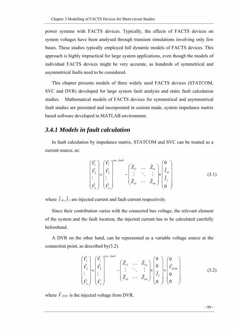
Chapter 3 Modelling of FACTS Devices for Short-circuit Studies
- 99 -
power systems with FACTS devices. Typically, the effects of FACTS devices on
system voltages have been analysed through transient simulations involving only few
buses. These studies typically employed full dynamic models of FACTS devices. This
approach is highly impractical for large system applications, even though the models of
individual FACTS devices might be very accurate, as hundreds of symmetrical and
asymmetrical faults need to be considered.
This chapter presents models of three widely used FACTS devices (STATCOM,
SVC and DVR) developed for large system fault analysis and static fault calculation
studies. Mathematical models of FACTS devices for symmetrical and asymmetrical
fault studies are presented and incorporated in custom made, system impedance matrix
based software developed in MATLAB environment.
3.4.1 Models in fault calculation
In fault calculation by impedance matrix, STATCOM and SVC can be treated as a
current source, as:
1 111 1
2 2
1
0
0
pre fault
nsh
fn nn
n n
V VZ Z
IV VIZ Z
V V
−⎛ ⎞ ⎛ ⎞ ⎛ ⎞
⎛ ⎞⎜ ⎟ ⎜ ⎟ ⎜ ⎟⎜ ⎟⎜ ⎟ ⎜ ⎟ ⎜ ⎟= − ×⎜ ⎟⎜ ⎟ ⎜ ⎟ ⎜ ⎟⎜ ⎟⎜ ⎟ ⎜ ⎟ ⎜ ⎟⎝ ⎠ ⎜ ⎟⎜ ⎟ ⎜ ⎟ ⎝ ⎠⎝ ⎠ ⎝ ⎠
… (3.1)
where shI , fI are injected current and fault current respectively.
Since their contribution varies with the connected bus voltage, the relevant element
of the system and the fault location, the injected current has to be calculated carefully
beforehand.
A DVR on the other hand, can be represented as a variable voltage source at the
connection point, as described by(3.2).
1 111 1
2 2
1
0 00
000
pre fault
nDVR
fn nn
n n
V VZ Z
V V VI
Z ZV V
−⎛ ⎞ ⎛ ⎞ ⎛ ⎞ ⎛ ⎞
⎛ ⎞⎜ ⎟ ⎜ ⎟ ⎜ ⎟ ⎜ ⎟⎜ ⎟⎜ ⎟ ⎜ ⎟ ⎜ ⎟ ⎜ ⎟= − × +⎜ ⎟⎜ ⎟ ⎜ ⎟ ⎜ ⎟ ⎜ ⎟⎜ ⎟⎜ ⎟ ⎜ ⎟ ⎜ ⎟ ⎜ ⎟⎝ ⎠ ⎜ ⎟⎜ ⎟⎜ ⎟ ⎜ ⎟ ⎝ ⎠⎝ ⎠⎝ ⎠ ⎝ ⎠
… (3.2)
where DVRV is the injected voltage from DVR.

Chapter 3 Modelling of FACTS Devices for Short-circuit Studies
- 100 -
3.4.2 Calculation of injected current and voltage
The purpose of this section is to derive the injected current or voltage by FACTSD
depending on fault type, location and system impedance. The rating of devices is also
taken into account in the process of derivation.
The injected current by STATCOM is introduced in full detail with respect to three-
phase to ground (LLLG) fault, single-phase to ground (LG) fault, double-phase to
ground (LLG) fault, and double-phase (LL) fault. The derivation of injected current by
SVC is very similar to that of STATCOM. It is therefore simplified to indicate the
differences only.
Before proceeding to detailed derivation of injected currents and voltages, all
assumptions made have to be specified. Those are listed below:
• All voltages are balanced in steady state (before the fault), pre-fault negative
and zero sequence voltages are therefore zero.
• In the case when real power injection is possible, the injection of real and
reactive power injection is treated separately. Real power is only needed when
voltage magnitude cannot be fully compensated by reactive power alone. The
injected current calculation from available real power starts from the sag
voltage which has already been partially restored by reactive power injection.
• The principal criteria employed in these derivations is that the phase-angle
difference between voltage phasor and line-current phasor, in case of DVR, and
between current phasor and bus voltage phasor, in the case of STATCOM and
SVC, is π/2 with reactive power injection only and zero with real power
injection only.
• Magnitude restoration is the only concern. The FACTS device should restore
the bus voltage to its pre-fault value if possible. In cases of voltage swell
(usually encountered in case of faults in non-solidly grounded systems), the
device is absorbing reactive power to pull the voltage back below i.e.,1.1 p.u.
• In the case of LLL, all phases are compensated equally so the voltage is
balanced after the compensation.
• In the case of asymmetrical LG and LLG faults, voltage compensation is
performed phase by phase since the unbalanced current can flow in zero
sequence.

Chapter 3 Modelling of FACTS Devices for Short-circuit Studies
- 101 -
• In the case of asymmetrical LL faults there is no zero sequence current so the
voltages in two faulted phases are assumed to be equal in magnitude after
compensation.
3.4.2.1 Voltage sag compensation by STATCOM
Detailed derivation of voltage sag compensation by STATOM using Z matrix is
given below. The list of symbols is given below to facilitate better understanding of
derivation:
:::::::
:
t
f
f
tf
sh
tt
ft
fault
V Voltage at bus tV Voltage at faulted bus fI faulted currentZ transfer impedance between bus t and fI Injected currentZ primary impedance of bus tZ transfer impedance between bus f and tZ fault impedance
Restoration by reactive power only:
1) LLL fault
Consider voltages at the compensated bus and faulted bus
-pret t f tf sh ttV V I Z I Z= × + × (3.3)
pref f f ff sh ftV V I Z I Z= − × + × (3.4)
f fault fV Z I= × (3.5) Where Zfault is the fault impedance.
Expressing previous equations in matrix form:
1 11 11
1 10
pret shtt tft
preft ff faultf f
V IZ ZVZ Z ZV I
⎛ ⎞ ⎛ ⎞⎛ ⎞⎛ ⎞ −= − ×⎜ ⎟ ⎜ ⎟⎜ ⎟⎜ ⎟ ⎜ ⎟⎜ ⎟ ⎜ ⎟− +⎝ ⎠ ⎝ ⎠⎝ ⎠ ⎝ ⎠
(3.6)
therefore:
11 1 1 1 11 111 12
1 1 1 121 22
pre presh t t t ttt tf
pre preft ff faultf f f
I V V V VZ Z M MZ Z Z M MI V V
−⎛ ⎞ ⎛ ⎞ ⎛ ⎞− −⎛ ⎞ ⎛ ⎞−= × = ×⎜ ⎟ ⎜ ⎟ ⎜ ⎟⎜ ⎟ ⎜ ⎟⎜ ⎟⎜ ⎟ ⎜ ⎟ ⎜ ⎟− + ⎝ ⎠⎝ ⎠⎝ ⎠ ⎝ ⎠ ⎝ ⎠
(3.7)
then
1 1 111 12 11
pre presh t f tI M V M V M V= × + × − × (3.8)

Chapter 3 Modelling of FACTS Devices for Short-circuit Studies
- 102 -
Let 111 12
pre pres t fV M V M Vγ∠ = × + × , 11M k k β= = ∠ , 1
t tV V α= ∠ ,
Since there is only reactive power considered here, the phase angle of injected
current should be kept perpendicular to the restored terminal voltage tV , so
1 ( / 2 )sh shI I π α= ∠ + (3.9)
sh s tI V kV= − (3.10)
solving (3.10), gives:
2 2sin ( cos )sh t s tI k V V kVβ β= − × × + − (3.11)
2 2( sin ( cos ) ) /t sh s shV I V I kβ β= − + − (3.12)
2 2 21 ( )sin
2t s sh
s sh
kV V IV I
α γ− − −= +
× (3.13)
Therefore, when
cos ( )pre faults t t tV kV and with V Vβ −≥ = (3.14)
voltage magnitude of bus t can be restored to pre-fault value. The injected current and
phase angle are given by equation (3.11) and(3.13).
Otherwise, if
cos ( )pre faults t t tV kV and with V Vβ −< = (3.15)
voltage magnitude can be restored to
coss
tVV
k β= (3.16)
The injected current and phase angle in this case are given by (3.11) and (3.13)
In the case when the current limit is reached,
sh rateI I> (3.17)
The injected current magnitude has to be set to
ratedsh rate pre fault
t
QI IV −= = (3.18)
The restored voltage magnitude that can be restored in such case is given by (3.12)
and the phase angle by (3.13).

Chapter 3 Modelling of FACTS Devices for Short-circuit Studies
- 103 -
2) LG fault
When LG fault occurs, negative and zero sequence networks have to be included in
calculation, so
0 0 0 0 0 0
0 0 0 0 0 0
pret t f tf sh tt
pref f f ff sh ft
V V I Z I Z
V V I Z I Z
⎧ = − × + ×⎪⎨
= − × + ×⎪⎩ (3.19)
1 1 1 1 1 1
1 1 1 1 1 1
pret t f tf sh tt
pref f f ff sh ft
V V I Z I Z
V V I Z I Z
⎧ = − × + ×⎪⎨
= − × + ×⎪⎩ (3.20)
2 2 2 2 2 2
2 2 2 2 2 2
pret t f tf sh tt
pref f f ff sh ft
V V I Z I Z
V V I Z I Z
⎧ = − × + ×⎪⎨
= − × + ×⎪⎩ (3.21)
The following equations have to be satisfied:
0 1 2 / 3f f f fI I I I= = = (3.22)
0 1 2 13f f f f f faultV V V V I Z+ + = = × (3.23)
From (3.19), (3.20), (3.21) and (3.22) yields
1 0 1 2 0 0 1 1 2 2( )pref f f ff ff ff sh tf sh tf sh tfV V I Z Z Z I Z I Z I Z= − + + − − − (3.24)
And further:
00 0 0 0
21 1 1 1
2 2 22 2
0 1 2 012 1
0 0
0 0
0 0
3
pre
sht t tt tf
sht t tf tf
tf tf sht t
ft ft ft ff faultf f f
IV V Z Z
IV V Z Z
Z Z IV V
Z Z Z Z ZV V I
−
−= − ×
−
− +
⎛ ⎞⎛ ⎞ ⎛ ⎞ ⎛ ⎞⎜ ⎟⎜ ⎟ ⎜ ⎟ ⎜ ⎟⎜ ⎟⎜ ⎟ ⎜ ⎟ ⎜ ⎟⎜ ⎟⎜ ⎟ ⎜ ⎟ ⎜ ⎟⎜ ⎟⎜ ⎟ ⎜ ⎟ ⎜ ⎟⎜ ⎟ ⎜ ⎟ ⎜ ⎟⎝ ⎠⎝ ⎠ ⎝ ⎠ ⎝ ⎠
(3.25)
Equation (3.25) then can be changed and written as:
0 0 0 0 010 0
1 1 1 1 11 1
2 22 2 2
0 1 2 0121
0 0
0 0
0 0
3
pre pre
sh t t t ttt tf
pre pre
sh t t t ttf tf
pretf tfsh t t t
preft ft ft ff faultf f
I V V V VZ Z
I V V V VZ Z
Z ZI V V V
Z Z Z Z ZI V
− − −−
− −−= = ×
− −
− +
⎛ ⎞ ⎛ ⎞⎛ ⎞⎜ ⎟ ⎜ ⎟⎜ ⎟⎜ ⎟ ⎜ ⎟⎜ ⎟ ×⎜ ⎟ ⎜ ⎟⎜ ⎟⎜ ⎟ ⎜ ⎟⎜ ⎟⎜ ⎟ ⎜ ⎟⎝ ⎠⎝ ⎠ ⎝ ⎠
M
0
1 1
2 2 2
t
pre
t t
pre
t t
pre pre
f f
V
V V
V V
V V
−
−= ×
− −
⎛ ⎞ ⎛ ⎞⎜ ⎟ ⎜ ⎟⎜ ⎟ ⎜ ⎟⎜ ⎟ ⎜ ⎟⎜ ⎟ ⎜ ⎟⎜ ⎟ ⎜ ⎟⎝ ⎠ ⎝ ⎠
M
(3.26)
From (3.26), follows
1 0 1 222 24 21 22 23
pre presh t f t t tI M V M V M V M V M V= + − − − (3.27)

Chapter 3 Modelling of FACTS Devices for Short-circuit Studies
- 104 -
Let 22 24pre pre
t fV M V M V= × + × , and after combining it with (3.28)
1 21/ 3( )sh a b cI I aI a I= + + (3.28)
0
21
22
1 1 11/ 3 1
1
V
V a aa aV
⎛ ⎞ ⎛ ⎞⎜ ⎟ ⎜ ⎟=⎜ ⎟ ⎜ ⎟⎜ ⎟ ⎜ ⎟⎜ ⎟ ⎝ ⎠⎝ ⎠
(3.29)
where 01 120a = ∠
one can obtain:
2 2 221 22 23 21 22 233 ( ) ( ) ( ) ( )a b c b c b c b c aI V M V V M aV a V M a V aV aI a I M M M V= − + − + − + − − − + + (3.30)
2 2 221 22 23 21 22 231/ (3 ( ) ( ) ( ) ( ) )b a c a c a c a c bI a V M V V M V a V M V aV I a I M aM a M V= − + − + − + − − − + + (3.31)
2 2 221 22 23 21 22 231/ (3 ( ) ( ) ( ) ( ) )c a b a b a b a b cI a V M V V M V aV M V a V I aI M a M aM V= − + − + − + − − − + + (3.32)
Assume that the compensation starts from phase a from now, then Vb, Vc are equal
to uncompensated voltage and Ia, Ib are zero. Let now
2 221 22 233 ( ) ( ) ( )s b c b c b cV V M V V M aV a V M a V aVα∠ = − + − + − + (3.33)
21 22 23k M M Mβ∠ = + + (3.34)
The equation of the same format as (3.10) is obtained. Solving by the previously
described method gives a shI I= , a tV V= , cV equal to the uncompensated voltage, and
0cI = . Then
221 22 231/ (3 ( ) ( ) ( ) )t a c a c a c aV a V M V V M V a V M V aV Iα∠ = − + − + − + − (3.35)
221 22 231/ ( )k a M aM a Mβ∠ = + + (3.36)
Following the same algorithm, gives b shI I= , b tV V=
and further with
2 221 22 231/ (3 ( ) ( ) ( ) )s c a b a b a b a bV I a V M V V M V aV M V a V I aIα∠ = = − + − + − + − − (3.37)
2 221 22 231/ ( )k k a M a M aMβ= ∠ = + + (3.38)
gives, , tcc shI I V V= =
3) LLG fault
For LLG fault, the voltages at faulted bus f and bus t (where STATOCM is placed)
can be described by (3.38). The fault current and voltage can be expressed as:

Chapter 3 Modelling of FACTS Devices for Short-circuit Studies
- 105 -
1 2 0 03f f f fault fV V V Z I= = − (3.39)
02 1
2 0
33
ff faultf f
ff ff fault
Z ZI I
Z Z Z+
= −+ +
(3.40)
20 1
2 0 3ff
f fff ff fault
ZI I
Z Z Z= −
+ + (3.41)
Combining equations (3.39), (3.40) and (3.41) the following is derived.
2 0
0
00
1 1
11
2 0
222
1 0
2 0
0 1 1
0 0
0 0
( )0 0
0( )
0
ff ff
ttpre
k
t sht
tt tf
tt
ff ff fault
tttt
k
f f
ff ff fault
ft ft ff
k
Z ZZ
ZV IV
Z ZVV
Z Z ZZVV
ZV V
Z Z ZZ Z Z
Z
− −
−
= − ×+− −
−+
− +
⎛ ⎞⎜ ⎟⎜ ⎟⎛ ⎞⎛ ⎞⎜ ⎟⎜ ⎟⎜ ⎟⎜ ⎟⎜ ⎟⎜ ⎟⎜ ⎟⎜ ⎟⎜ ⎟⎜ ⎟⎜ ⎟⎜ ⎟ ⎜ ⎟ ⎜ ⎟⎝ ⎠ ⎝ ⎠⎜ ⎟⎜ ⎟⎝ ⎠
0
1
2
1
sh
sh
f
I
I
I
⎛ ⎞⎜ ⎟⎜ ⎟⎜ ⎟⎜ ⎟⎜ ⎟⎝ ⎠
(3.42)
Then
12 0
0
0 0 0
1 1
1 1 1
2 0
22 2
1
2 0
0 1 1
0 0
0 0
( )0 0
( )0
ff ff
tt
prek
sh t t
tt tf pre
sh t t
ff ff fault pre
ttsh t
k
f
ff ff fault
ft ft ff
k
Z ZZ
ZI V V
Z ZI V V
Z Z ZZI V
ZI
Z Z ZZ Z Z
Z
−
− −
−−
−= ×+
− − −
+− +
⎛ ⎞⎜ ⎟⎜ ⎟⎛ ⎞⎜ ⎟⎜ ⎟⎜ ⎟⎜ ⎟⎜ ⎟⎜ ⎟⎜ ⎟⎜ ⎟
⎜ ⎟ ⎜ ⎟⎝ ⎠ ⎜ ⎟⎜ ⎟⎝ ⎠
0 0 0
1 1 1 1
2 2 2 2
pre
t t t
pre pre
t t t t
pre
t t t t
pre pre pre
f f f
V V V
V V V V
V V V V
V V V
− −
− −= × = ×
− −
⎛ ⎞ ⎛ ⎞ ⎛ ⎞⎜ ⎟ ⎜ ⎟ ⎜ ⎟⎜ ⎟ ⎜ ⎟ ⎜ ⎟⎜ ⎟ ⎜ ⎟ ⎜ ⎟⎜ ⎟ ⎜ ⎟ ⎜ ⎟⎜ ⎟ ⎜ ⎟ ⎜ ⎟⎝ ⎠ ⎝ ⎠ ⎝ ⎠
M M
(3.43)
The equation yields the same format as (3.10). Following the same steps as those for
LG fault, the injected currents in each phase can be calculated.
4) LL fault
For LL fault, there is no ground involved, so zero sequence network is not included.
Voltage relations at buses f and t are reduced to:
1 1 1 1 1 1
1 1 1 1 1 1
pret t f tf sh tt
pref f f ff sh ft
V V I Z I Z
V V I Z I Z
⎧ = − × + ×⎪⎨
= − × + ×⎪⎩ (3.44)
2 2 2 2 2 2
2 2 2 2 2 2
pret t f tf sh tt
pref f f ff sh ft
V V I Z I Z
V V I Z I Z
⎧ = − × + ×⎪⎨
= − × + ×⎪⎩ (3.45)

Chapter 3 Modelling of FACTS Devices for Short-circuit Studies
- 106 -
due to
1 2f fI I= − (3.46)
1 2 1f f fault fV V Z I− = × (3.47)
follows
11 1 1 1 1 1 11 1
2 2 2 2 2 2 2
1 2 1 21
00
pre pre presh t t t t t ttt tf
pre presh tt tf t t t t
pre preft ft ff ff faultf f f
I V V V V V VZ ZI Z Z V V V V
Z Z Z Z ZI V V
−⎛ ⎞ ⎛ ⎞ ⎛ ⎞− − −⎛ ⎞−⎜ ⎟ ⎜ ⎟ ⎜ ⎟⎜ ⎟
= − − × − = × − = × −⎜ ⎟ ⎜ ⎟ ⎜ ⎟⎜ ⎟⎜ ⎟ ⎜ ⎟ ⎜ ⎟⎜ ⎟⎜ ⎟ ⎜ ⎟ ⎜ ⎟− + +⎝ ⎠⎝ ⎠ ⎝ ⎠ ⎝ ⎠
M M 2t
pref
V
V
⎛ ⎞⎜ ⎟⎜ ⎟⎜ ⎟⎜ ⎟⎝ ⎠
(3.48)
which yields,
1 1 1 211 12 13( )pre pre
sh t t t fI M V V M V M V= − + + (3.49)
because of 0 00, 0t tV I= =
0a b cV V V+ + = (3.50)
0a b cI I I+ + = (3.51)
Assume that after compensation, phase b and phase c have the same voltage
magnitudes (because phase b and c are the two faulted phases which most likely would
have similar remaining voltage, i.e., sag magnitudes)
b cV V= (3.52)
and that the angle difference between these two phases is expressed as
( ) ( )b cangle V angle V α− = (3.53)
1t α= ∠ (3.54)
then
0a b bV V tV+ + = (3.55)
0a b cI I tI+ + = (3.56)
So
/(1 )b aV V t= − + (3.57)
/(1 )c aV tV t= − + (3.58)
/(1 )b aI I t= − + (3.59)
/(1 )c aI tI t= − + (3.60)

Chapter 3 Modelling of FACTS Devices for Short-circuit Studies
- 107 -
It yields
a s aI V kV= − (3.61)
where
211 133(1 )( )( ) /(1 )pre pre
s t fV t M M V V t a t a= + + + + − − (3.62)
2 211 12 (1 ) /(1 )k M M t at a t a a t= + + − − + − − (3.63)
Following the same algorithm as in case of LLL fault Ia , Va can be derived. After
that, the currents and voltages in the other two phases can be obtained from (3.57) and
(3.59).
All calculated phase injected currents are then converted into sequence components
to get the bus voltages using a sequence components matrix.
Restoration by real power only
When there is real power available only, the mathematical model of STATCOM can
be derived following the same approach as that of STATCOM with reactive power. The
main equation to be solved is in the same form as(3.10), however, the injected current is
now in phase with the restored terminal voltage tV , so in the case of LLL fault,
sh shI I α= ∠ (3.64)
Using (3.64) to solve equation (3.10), yields injected current given by (3.65) and
(3.66)
( )22cos sinsh t s tI kV V kVβ β= − + −
(3.65)
( )22 21cos
2s sh t
s sh
V I kVV I
α θ− + −=
(3.66)
Similar to the solution for reactive power injection, if
sin ( )pre faults t t tV kV and with V Vβ −≥ = (3.67)
Voltage at the compensated bus could be restored to pre-fault value, the injected
current and phase angle are given by (3.65) and (3.66). Otherwise, if
sin ( )pre faults t t tV kV and with V Vβ −< = (3.68)
Voltage magnitude can be restored to

Chapter 3 Modelling of FACTS Devices for Short-circuit Studies
- 108 -
sin
st
VVk β
= (3.69)
The injected current and phase angle are then give by (3.65) and (3.66).
In case when the current limit is reached:
ratedsh rate pre fault
t
PI IV −= = (3.70)
3.4.2.2 Voltage sag compensation by SVC
The derivation of injected current by the SVC is very similar to that of STATCOM.
However, due to the difference of their structure, the current limit in the case of the
STATCOM should be replaced by its limit on susceptance B, which means that the
conditional equation (3.17) has to be replaced by:
limt
sh
V BI
< (3.71)
The rated susceptance of the SVC is given by
2rated
rated pret
QBV
= (3.72)
3.4.2.3 Voltage sag compensation by DVR
A DVR is series connected device and it restores voltage only down stream from the
point of its connection. DVR voltage restoration capacity depends on its reactive and
active power rating. The injected voltage restores the voltage magnitude as much as
possible without considering the phase angle jump. The compensation is carried out
phase by phase. The relationship between the terminal voltage and the voltage injected
by the DVR is given by:
t sag DVRV V V= + (3.73)
If only reactive power is available, then
*DVR tV I jQ× = (3.74)
*t t tV I S× = (3.75)
Where Q is the injected reactive power by the DVR, St is the load at the bus, Vsag is
the voltage sag magnitude and It is the load current. Let t tV V α= ∠ and St = St ∠θ , then:

Chapter 3 Modelling of FACTS Devices for Short-circuit Studies
- 109 -
/ 2 ( )t sag DVRV V Vα γ π θ α∠ = ∠ + ∠ − − (3.76)
By solving (3.76), follows
2 2 2sin cosDVR t sag tV V V Vθ θ= + − (3.77) 2 2 2
1cos2
t sag DVR
DVR t
V V VV V
α γ− + −= + (3.78)
When cossag tV V θ> (Vt is the magnitude of the pre fault voltage), the voltage
magnitude can be restored completely with only reactive power injection. The injected
voltage magnitude and phase angle are given by (3.77) and (3.78).
When the required power to be injected, *DVR tV I× , is greater then the limiting value,
Qrate, the following equations apply and they determine the amount of voltage
restoration (in this case the restored voltage, Vt1, may not be equal to pre-fault voltage).
tt
DVR t
SjQIV V
= = (3.79)
1 /(1 )t sagt
QV V jS
= + (3.80)
Once the reactive power is completely used up the restoration continues with
injection of real power, i.e., *DVR tV I P× = . Injected voltage now is in phase with load
current so
1 ( )t sag DVRV V Vα γ α θ∠ = ∠ + ∠ − (3.81)
Vsag1 in (3.81) is new value of sag magnitude obtained after restoration with reactive
power, i.e., defined by (3.79) as Vt1. From (3.81) follows
2 2 21cos sinDVR t sag tV V V Vθ θ= + − (3.82)
And the phase angle of the restored voltage is given by (3.78).
If the required injected power *DVR tV I× is greater than the limiting value, Prate, the
equations (3.83) apply and they determine the amount of ultimate voltage restoration (in
this case the restored voltage, Vt2, may not be equal to the pre-fault voltage).
tt
DVR t
SPIV V
= = (3.83)
2 1 /(1 )t sagt
PV VS
= + (3.84)

Chapter 3 Modelling of FACTS Devices for Short-circuit Studies
- 110 -
3.4.2.4 Restoration using reactive and real power
Figure 3-6 Real and reactive power injection
As described in previous section, real and reactive power injections are treated
separately in the mathematical derivation for both STATCOM and DVR. The principle
held is that reactive power is injected first, if the voltage can be restored to its pre-fault
value (magnitude), no real power will be used. If the voltage can not be fully restored
by the available reactive power, the real power will be injected depending on its
availability. The voltage restoration approach is illustrated in Figure 3-6.

Chapter 3 Modelling of FACTS Devices for Short-circuit Studies
- 111 -
3.5 Deciding the Rating of FACTS devices
3.5.1 Rating of FACTS devices
In theory, the rating of sag mitigation devices should be selected such that they can
restore all critical voltage sags experienced at the site. However this is not what
happens in practical applications. Implementation of FACTSD is carefully examined in
a much broader context, including financial and environmental considerations in
addition to technical issues. The selected rating of installed device therefore is often a
compromise between various issues.
Irrespective of the final decision regarding the rating of FACTSD a procedure is
needed to determine its rating based on pre-specified technical requirements. The
methodology is developed here to determine the rating of sag mitigation devices
considering only their requirement for sag compensation. Voltage restoration capability
of device should be adequate to restore the voltage at the bus to its pre-fault value for
all sags with magnitudes above given threshold. The rating of devices is calculated
based on short circuit level of the bus connected load and sag characteristics of the bus.
Derivation of the method is demonstrated assuming that the devices is capable of
restoring the voltage to nominal from a 50% voltage drop and phase shift 030≤ .
3.5.2 Mathematical derivation
3.5.2.1 STATCOM
The equivalent network can be viewed from the faulted point of fault as shown in
Figure 3-7.
1 rsag
l
Z VZ
⎛ ⎞+⎜ ⎟
⎝ ⎠lV lZ
rZ
shI
Figure 3-7 Single line diagram of STATCOM connected to a bus
Where lZ : load impedance rZ : Thevenin’s impedance of the system observed from
faulted point. shI : injected current by STATCOM. Voltage at the compensated bus is:
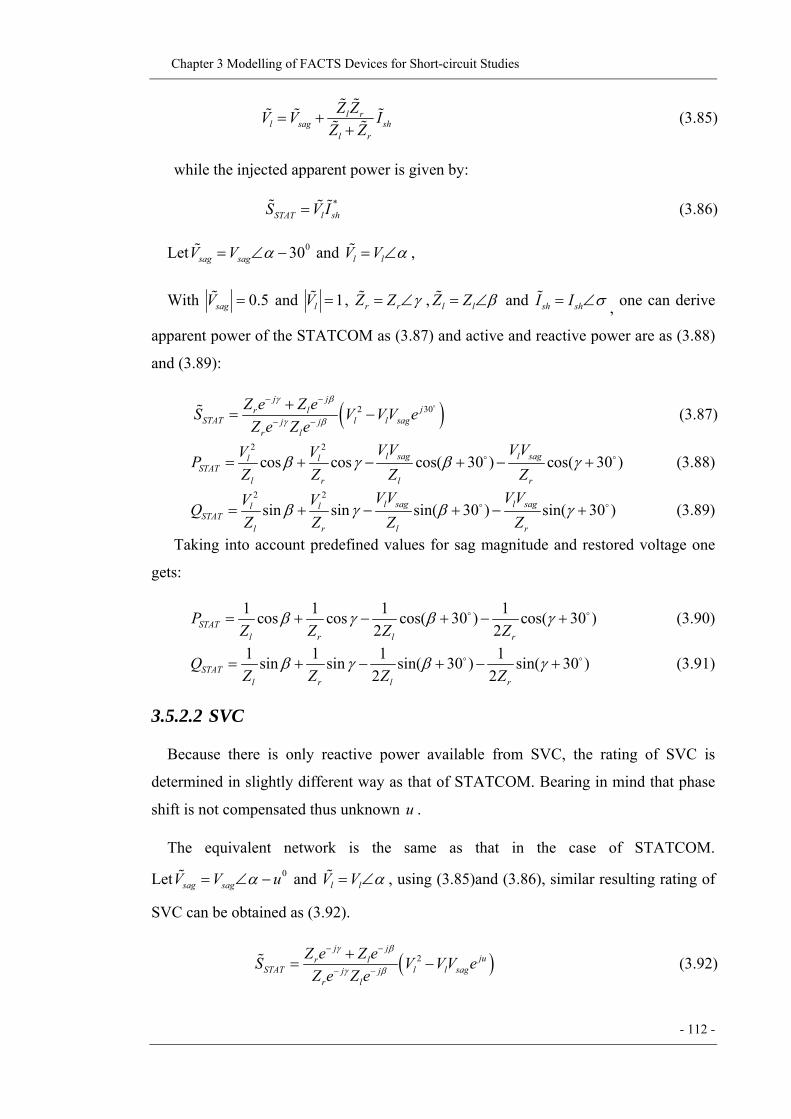
Chapter 3 Modelling of FACTS Devices for Short-circuit Studies
- 112 -
l rl sag sh
l r
Z ZV V IZ Z
= ++
(3.85)
while the injected apparent power is given by:
*STAT l shS V I= (3.86)
Let 030sag sagV V α= ∠ − and l lV V α= ∠ ,
With 0.5sagV = and 1lV = , r rZ Z γ= ∠ , l lZ Z β= ∠ and sh shI I σ= ∠ , one can derive
apparent power of the STATCOM as (3.87) and active and reactive power are as (3.88)
and (3.89):
( )2 30j j
jr lSTAT l l sagj j
r l
Z e Z eS V VV eZ e Z e
γ β
γ β
− −
− −
+= − (3.87)
2 2
cos cos cos( 30 ) cos( 30 )l sag l sagl lSTAT
l r l r
VV VVV VPZ Z Z Z
β γ β γ= + − + − + (3.88)
2 2
sin sin sin( 30 ) sin( 30 )l sag l sagl lSTAT
l r l r
VV VVV VQZ Z Z Z
β γ β γ= + − + − + (3.89)
Taking into account predefined values for sag magnitude and restored voltage one
gets:
1 1 1 1cos cos cos( 30 ) cos( 30 )2 2STAT
l r l r
PZ Z Z Z
β γ β γ= + − + − + (3.90)
1 1 1 1sin sin sin( 30 ) sin( 30 )2 2STAT
l r l r
QZ Z Z Z
β γ β γ= + − + − + (3.91)
3.5.2.2 SVC
Because there is only reactive power available from SVC, the rating of SVC is
determined in slightly different way as that of STATCOM. Bearing in mind that phase
shift is not compensated thus unknown u .
The equivalent network is the same as that in the case of STATCOM.
Let 0sag sagV V uα= ∠ − and l lV V α= ∠ , using (3.85)and (3.86), similar resulting rating of
SVC can be obtained as (3.92).
( )2j j
jur lSTAT l l sagj j
r l
Z e Z eS V VV eZ e Z e
γ β
γ β
− −
− −
+= − (3.92)
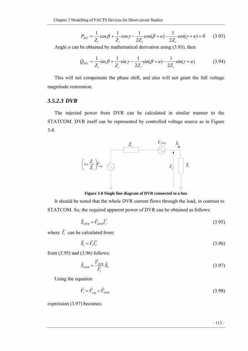
Chapter 3 Modelling of FACTS Devices for Short-circuit Studies
- 113 -
1 1 1 1cos cos cos( ) cos( ) 02 2SVC
l r l r
P u uZ Z Z Z
β γ β γ= + − + − + = (3.93)
Angle u can be obtained by mathematical derivation using (3.93), then
1 1 1 1sin sin sin( ) sin( )2 2SVC
l r l r
Q u uZ Z Z Z
β γ β γ= + − + − + (3.94)
This will not compensate the phase shift, and also will not grant the full voltage
magnitude restoration.
3.5.2.3 DVR
The injected power from DVR can be calculated in similar manner to the
STATCOM. DVR itself can be represented by controlled voltage source as in Figure
3-8.
lV lZ
rZ DVRV lS
1 rsag
l
Z VZ
⎛ ⎞+⎜ ⎟
⎝ ⎠
Figure 3-8 Single line diagram of DVR connected to a bus
It should be noted that the whole DVR current flows through the load, in contrast to
STATCOM. So, the required apparent power of DVR can be obtained as follows:
*DVR DVR lS V I= (3.95)
where *lI can be calculated from:
*l l lS V I= (3.96)
from (3.95) and (3.96) follows:
DVRDVR l
l
VS SV
= (3.97)
Using the equation
l sag DVRV V V= + (3.98)
expression (3.97) becomes:
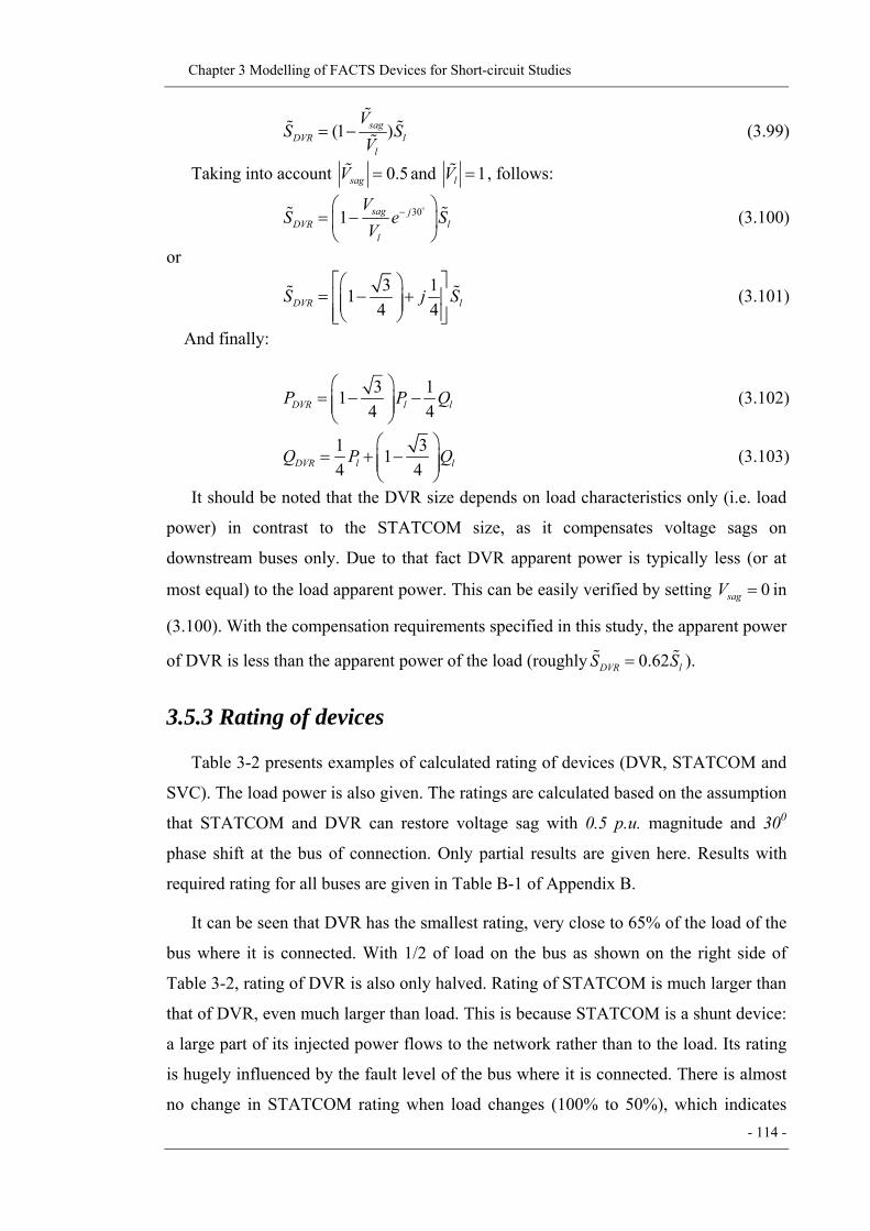
Chapter 3 Modelling of FACTS Devices for Short-circuit Studies
- 114 -
(1 )sagDVR l
l
VS S
V= − (3.99)
Taking into account 0.5sagV = and 1lV = , follows:
301 sag jDVR l
l
VS e S
V−⎛ ⎞
= −⎜ ⎟⎝ ⎠
(3.100)
or 3 11
4 4DVR lS j S⎡ ⎤⎛ ⎞
= − +⎢ ⎥⎜ ⎟⎜ ⎟⎢ ⎥⎝ ⎠⎣ ⎦ (3.101)
And finally:
3 114 4DVR l lP P Q
⎛ ⎞= − −⎜ ⎟⎜ ⎟⎝ ⎠
(3.102)
1 314 4DVR l lQ P Q
⎛ ⎞= + −⎜ ⎟⎜ ⎟
⎝ ⎠ (3.103)
It should be noted that the DVR size depends on load characteristics only (i.e. load
power) in contrast to the STATCOM size, as it compensates voltage sags on
downstream buses only. Due to that fact DVR apparent power is typically less (or at
most equal) to the load apparent power. This can be easily verified by setting 0sagV = in
(3.100). With the compensation requirements specified in this study, the apparent power
of DVR is less than the apparent power of the load (roughly 0.62DVR lS S= ).
3.5.3 Rating of devices
Table 3-2 presents examples of calculated rating of devices (DVR, STATCOM and
SVC). The load power is also given. The ratings are calculated based on the assumption
that STATCOM and DVR can restore voltage sag with 0.5 p.u. magnitude and 300
phase shift at the bus of connection. Only partial results are given here. Results with
required rating for all buses are given in Table B-1 of Appendix B.
It can be seen that DVR has the smallest rating, very close to 65% of the load of the
bus where it is connected. With 1/2 of load on the bus as shown on the right side of
Table 3-2, rating of DVR is also only halved. Rating of STATCOM is much larger than
that of DVR, even much larger than load. This is because STATCOM is a shunt device:
a large part of its injected power flows to the network rather than to the load. Its rating
is hugely influenced by the fault level of the bus where it is connected. There is almost
no change in STATCOM rating when load changes (100% to 50%), which indicates

Chapter 3 Modelling of FACTS Devices for Short-circuit Studies
- 115 -
that loads have little influence on the rating of STATCOM required to restore certain
voltage sag. SVC has a much bigger reactive power rating than STATCOM in some
cases (e.g. bus 13, 158, 193), while some are very close (e.g. bus 258,254 and 225). The
impedance of bus where SVC is connected is the decisive factor in this case.
Table 3-2 Injected power needed from FACTS devices (MW, MVar) load DVR STAT SVC 1/2 load DVR STAT SVC
P Q P Q P Q Q P Q P Q P Q Q 13 0.087 0.013 0.046 0.029 67.1 25.9 81.8 0.044 0.006 0.023 0.015 65.1 27.1 82.4
57 0.165 0.027 0.087 0.057 140.1 113 200.9 0.082 0.014 0.043 0.028 135.8 116.5 187.7
58 0.528 0.137 0.265 0.210 133.3 112 186 0.264 0.069 0.132 0.105 129.4 115.8 176.2
156 0.013 0.002 0.007 0.004 15.6 9.6 24.3 0.006 0.001 0.003 0.002 15.1 9.9 24.4
158 0.035 0.006 0.018 0.012 14.7 8.2 21.7 0.017 0.003 0.009 0.006 14.2 8.5 21.8
184 0.011 0.021 0.001 0.015 9.8 3.4 11.4 0.006 0.010 0.001 0.007 9.6 3.6 11.5
193 0.018 0.003 0.010 0.006 11.6 5 14.9 0.009 0.001 0.005 0.003 11.2 5.2 15
223 0.915 0.180 0.474 0.331 81.4 72.5 111 0.458 0.090 0.237 0.165 78.2 74.4 105.1
225 0.671 0.131 0.347 0.242 20 27.6 28.8 0.335 0.066 0.174 0.121 18.7 27.9 28
254 68.360 12.189 35.712 24.001 935.6 1381 1392 34.180 6.095 17.856 12.000 833.8 1402 1336.1
258 42.904 9.161 22.036 15.920 1001 1582 1545.3 21.452 4.581 11.018 7.960 891.9 1600 1491.3
3.6 Fault Calculation process with FACTS devices
Fault calculation in the network with FACTS devices using sequence networks can
be depicted as follows. (The flow chart of fault calculation with FACTSD is shown in
Figure 6-3).
• Pre-fault bus voltages in the system are obtained from power flow.
• Impedance matrix is formed using step-by-step algorithm described previously.
• Fault calculation is carried out without FACTS devices using impedance matrix
method.
• Depending on fault location and system characteristics at the point of
connection of FACTS devices the injected currents (or voltage) are calculated
taking into account predefined limits for individual FACTS devices.
• Fault calculation is carried out with FACTS devices with faulted current and
injected current and voltage.

Chapter 3 Modelling of FACTS Devices for Short-circuit Studies
- 116 -
3.7 Simulation Results
3.7.1 STATCOM as compensation device (reactive power only)
3.7.1.1 Three phase to ground fault (LLL)
A 20MVAr STATCOM is connected to arbitrarily selected bus 165 of the test
network to assess its contribution to restoration of network voltages during the sag.
Initially, three phase faults are simulated at ten buses in the network without
STATCOM. Voltages at all other buses in the network are calculated. Faulted buses are
selected such that the faults result in voltage sags at bus 165 with magnitudes ranging
from 0.1 p.u. to 0.9 p.u. Sag calculation is then repeated with STATCOM connected at
bus 165. The resulting network sag performances for the two cases are illustrated in
Figure 3-9 and Figure 3-10
(A) Without STATCOM
(B) With STATCOM
Figure 3-9 Sag magnitudes at buses 130-200
(A) Without STATCOM
(B) With STATCOM
Figure 3-10 Sag magnitudes in the whole system

Chapter 3 Modelling of FACTS Devices for Short-circuit Studies
- 117 -
Figure 3-10 illustrates sag performance of the whole network, while Figure 3-9
focuses on close electrical neighbourhood of bus 165 (buses 130 to 200) where the
effects of STATCOM are much more pronounced. It can be clearly seen from these
figures that STATCOM improves voltages for all faults, and not only at bus 165 but
also at other buses, mainly those that are electrically close to bus 165. The overall
improvement of bus voltages in the network ranges from 0% to 40% depending on the
electrical distance of the bus from STATCOM location.
3.7.1.2 Single phase to ground fault (LG)
Single phase faults (phase A is the faulted phase) are simulated at the same buses as
before, and the results are illustrated in Figure 3-11, Figure 3-12 and Figure 3-13.
(A) Without STATCOM
(B) With STATCOM
Figure 3-11 Sag magnitudes at buses 130-200, phase A
(A) Without STATCOM
(B) With STATCOM
Figure 3-12 Sag magnitudes at buses 130-200, phase B

Chapter 3 Modelling of FACTS Devices for Short-circuit Studies
- 118 -
(A) Without STATCOM
(B) With STATCOM
Figure 3-13 Sag magnitudes at buses 130-200, phase C
It can be seen from Figure 3-11, Figure 3-12 and Figure 3-13hat the STATCOM
improves voltage magnitudes in all three phases. The connected STATCOM injects
reactive power when the sag voltage is below pre-fault value and absorbs reactive
power when the swell voltage is above 1.1 p.u., so most of the voltages at electrically
close system buses are smoothened.
3.7.1.3 Double phase to ground fault (LLG)
Double phase to ground faults (phase B and C are the faulted phases) are simulated
at the same ten buses as before and the results are shown in Figure 3-14, Figure 3-15
and Figure 3-16.
(A) Without STATCOM
(B) With STATCOM
Figure 3-14 Sag magnitudes at buses 130-200, phase A
Chapter 3 Modelling of FACTS Devices for Short-circuit Studies
- 119 -
(A) Without STATCOM
(B) With STATCOM
Figure 3-15 Sag magnitudes at buses 130-200, phase B
(A) Without STATCOM
(B) With STATCOM
Figure 3-16 Sag magnitudes at buses 130-200, phase C
The LLG fault is more severe than LG fault. With STATCOM connected at bus 165,
the voltage magnitudes of buses 130-200 are all improved by mitigating the voltage
swell on phase A and compensating the voltage sag on phases B and C.
3.7.1.4 Double phase fault (LL)
LL fault between phases B and C is simulated at same locations as other faults
analysed previously. Since there is no zero sequence current flowing in this case, the
injected current is carefully calculated by the method described in previous sections.
The results are presented in Figure 3-17, Figure 3-18 and Figure 3-19.

Chapter 3 Modelling of FACTS Devices for Short-circuit Studies
- 120 -
(A) Without STATCOM
(B) With STATCOM
Figure 3-17 Sag magnitudes at buses 130-200, phase A
(A) Without STATCOM
(B) With STATCOM
Figure 3-18 Sag magnitudes at buses 130-200, phase B
(A) Without STATCOM
(B) With STATCOM
Figure 3-19 Sag magnitudes at buses 130-200, phase C
3.7.2 SVC as compensation device
The SVC as a compensation device operates in a similar way to STATCOM (as
discussed in previous sections). The STATCOM however, performs much better than
the SVC at very low voltages. To illustrate this behaviour STATCOM and SVC of the
same size (two cases are considered, 100MVAr and 200MVAr rated devices) are

Chapter 3 Modelling of FACTS Devices for Short-circuit Studies
- 121 -
connected at bus 226, and the voltage magnitudes at neighbouring buses (253 to 300)
during the fault calculated. The results are illustrated in Figure 3-20.
Figure 3-20 Voltage magnitudes with STATCOM and SVC at bus 226
It can be observed from Figure 3-20 that for severe voltage sags with very low
magnitudes (between 0.1p.u. and 0.3p.u.), STATCOM tends to perform much better
than the SVC. When the sag magnitude is higher, the restoration highly depends on the
size of the devices. Neither STATCOM nor SVC is able to restore voltage when the sag
magnitude is nearly zero (i.e., short interruption).
3.7.3 STATCOM and SVC with calculated rated power
In this case study, STATCOM and SVC of different ratings are connected at buses
13, 39, 184 and 258. Their respective ratings are calculated using methodology
introduced before. Calculated ratings are given in Table 3-3.
Table 3-3 Rating of STATCOM and SVC at different network buses LOAD STAT SVC P(MW
) Q(MVAR) P(MW) Q(MVAR) Q(MVAR)
13 0.087 0.013 67.1 25.9 81.8 39 0.673 0.215 33.4 7.9 33.4
184 0.011 0.021 9.8 3.4 11.4 258 42.904 9.161 1001 1582 1545.3
The voltage magnitudes and phase angles of buses 13, 39, 184 and 258 following
faults of buses 76, 52, 138 and 258 respectively are listed in Table 3-4. It can be seen
that STATCOM restores voltage in both magnitude and phase to its pre-fault value. The
SVC increases voltage magnitude of the bus but not to its pre-fault value. Furthermore

Chapter 3 Modelling of FACTS Devices for Short-circuit Studies
- 122 -
it does not compensate the phase shift, it makes it worse actually. The result justifies the
advantage of STATCOM over SVC if the cost of devices is not considered.
Table 3-4 Voltage restoration of buses with FACTSDs
pre-fault Voltage sag Mitigation with
STATCOM Mitigation with
SVC Voltage Voltage Voltage Voltage Buses with
STATCOM/SVC Faulted buses V(p.u.) θ(0) V(p.u.) θ(0) V(p.u.) θ(0) V(p.u.) θ(0)
Bus13 76 LLL 0.9896 -8.63 0.5116 -35.4 0.9896 -8.63 0.586 -67.75Bus39 52 LLL 0.9563 -9.21 0.5321 -20.18 0.9563 -9.21 0.6308 -56.26Bus184 138 LLL 0.9741 -7.81 0.5462 -20.97 0.9741 -7.81 0.6627 -52.94Bus258 258 LG 1.0358 23.82 A 0.5288 60.374 1.0358 23.82 0.8903 48.971
B 1.0358 -96.18 1.0358 -96.2 1.0358 -96.18 C 0.5895 104.73 1.0358 143.8 1.0358 101.51
In order to illustrate the influence that STATCOM and SVC have on the whole
system, Figure 3-21 and Figure 3-22 show voltage sag magnitude and phase angle
respectively at all buses in the system for LLLG fault at bus 76. STATCOM and SVC
(with ratings as in Table 3-3) are located at bus 13.
00.20.40.60.8
11.2
1 20 39 58 77 96 115 134 153 172 191 210 229 248 267 286
Bus number
Volta
ge m
agni
tude
pre-fault no compensation STAT on 13 SVC on 13
Figure 3-21 Sag magnitude of all buses when LLL fault on bus 76
-80-60-40-20
020406080
1 16 31 46 61 76 91 106121136151166181196211226241256271286
Bus number
Phas
e sh
ift in
deg
ree
pre-fault no compensation STAT on 13 SVC on 13
Figure 3-22 Sag phase angle of all buses when LLL fault on bus 76
The same trends as before can be observed in the entire system, i.e., STATCOM
restored voltages much more than the SVC (see Figure 3-21) especially at electrically
close buses. Since there is also limited real power injection by STATCOM, the phase
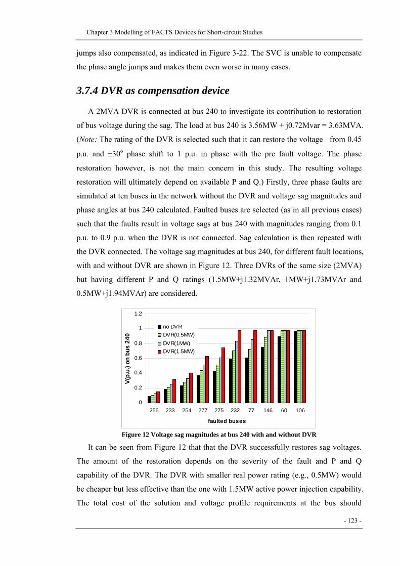
Chapter 3 Modelling of FACTS Devices for Short-circuit Studies
- 123 -
jumps also compensated, as indicated in Figure 3-22. The SVC is unable to compensate
the phase angle jumps and makes them even worse in many cases.
3.7.4 DVR as compensation device
A 2MVA DVR is connected at bus 240 to investigate its contribution to restoration
of bus voltage during the sag. The load at bus 240 is 3.56MW + j0.72Mvar = 3.63MVA.
(Note: The rating of the DVR is selected such that it can restore the voltage from 0.45
p.u. and ±30o phase shift to 1 p.u. in phase with the pre fault voltage. The phase
restoration however, is not the main concern in this study. The resulting voltage
restoration will ultimately depend on available P and Q.) Firstly, three phase faults are
simulated at ten buses in the network without the DVR and voltage sag magnitudes and
phase angles at bus 240 calculated. Faulted buses are selected (as in all previous cases)
such that the faults result in voltage sags at bus 240 with magnitudes ranging from 0.1
p.u. to 0.9 p.u. when the DVR is not connected. Sag calculation is then repeated with
the DVR connected. The voltage sag magnitudes at bus 240, for different fault locations,
with and without DVR are shown in Figure 12. Three DVRs of the same size (2MVA)
but having different P and Q ratings (1.5MW+j1.32MVAr, 1MW+j1.73MVAr and
0.5MW+j1.94MVAr) are considered.
0
0.2
0.4
0.6
0.8
1
1.2
256 233 254 277 275 232 77 146 60 106
faulted buses
V(p.
u.) o
n bu
s 24
0
no DVRDVR(0.5MW)DVR(1MW)DVR(1.5MW)
Figure 12 Voltage sag magnitudes at bus 240 with and without DVR
It can be seen from Figure 12 that that the DVR successfully restores sag voltages.
The amount of the restoration depends on the severity of the fault and P and Q
capability of the DVR. The DVR with smaller real power rating (e.g., 0.5MW) would
be cheaper but less effective than the one with 1.5MW active power injection capability.
The total cost of the solution and voltage profile requirements at the bus should

Chapter 3 Modelling of FACTS Devices for Short-circuit Studies
- 124 -
therefore be taken into account when deciding on DVR’s rating and placement. The
additional energy storage would increase the time the DVR can supply real power and
obviously the cost of the solution. Since the sags considered in this study last only for a
very short time (max 300ms) any of the three applied DVRs could supply available real
power (depending on the reactive power output) without the need for dedicated energy
storage.
3.7.5 Sag performance improvements with FACTS
To illustrate the improvement in sag performance of the network with FACTS
devices, three devices are randomly located in the network and sag performance with
and without them compared. Location, type and size of devices are shown in Table 3-5.
Table 3-5 Solution of sag mitigation Bus number Type Size(MVar)
40 DVR 25 148 SVC 30 154 STATCOM 25
Figure 3-23 (a) and (b) illustrate sag performance of bus 145 with and without
mitigation devices, respectively. Sags are be shifted from low magnitude range to high
magnitude range, e.g. number of sags with magnitude between 0.9 and 1.1 p.u. and sag
duration of 300ms is increased from 854.7 to 1162 by mitigation (red bar in Figure 3-23
(a) and (b)) and sag number with magnitude between 0.7 and 0.9p.u. and duration of
300ms reduced from 254.4 to 170.5 (yellow bar).
(a) Without mitigation (b) With mitigation
Figure 3-23 Bus 145 3-D sag numbers (sag number/year)
It has to be noted that the number of sags in each duration group is not changed
because the calculations of mitigation only considered the influences on sag magnitude,

Chapter 3 Modelling of FACTS Devices for Short-circuit Studies
- 125 -
duration is not considered. Note that no FACTSD is located at bus 145 although the
SVC at bus 148 and STATCOM at bus 154 are nearby. This proved the argument that
the effects of mitigation with FACTSD can spread to nearby buses.
(a) Without mitigation (b) With mitigation
Figure 3-24 Entire network 3-D sag number (sag number/year)
Figure 3-24 (a) and (b), shows sag performance of the whole network with and
without FACTS devices. The same improvement as observed in Figure 3-23 can be
seen here. Sag with low magnitudes are shifted to high magnitude range. Although only
three randomly located FACTSD were connected in the network, the sag performance
of the entire network improved. This proves that the FACTS devices contribute to sag
performance improvement of the whole network.
To illustrate FACTSD contribution to network sag performance in three phases,
Figure 3-25 and Figure 3-26 show the generalized sag tables for bus 145 and entire
network, respectively. It can be seen from Figure 3-25 (a) and (b) that the sags are
pushed from the bottom left corner (low voltage range) to the upper right corner (high
magnitude range), showing the improvement of bus sag performance with FACTS
devices.

Chapter 3 Modelling of FACTS Devices for Short-circuit Studies
- 126 -
(a) Without mitigation (sag number/year)
(b) With mitigation (sag number/year)
Figure 3-25 Generalized sag tables for bus 145
Similarly, Figure 3-26 (a) and (b) shows sag performance of the entire network
with and without mitigation. For example, the number of sags with two phase voltage
magnitude <0.1 and the other phase voltage >0.9 is dramatically reduced from 3764.26
to 1490.96 indicated in red circle.

Chapter 3 Modelling of FACTS Devices for Short-circuit Studies
- 127 -
(a) Without mitigation
(b) With mitigation
Figure 3-26 Generalized sag tables for entire network (sag number/year)
3.8 Summary
The majority of modelling efforts of FACTS devices so far were focused on
development of models in time domain studies. The first Chapter argued that due to the
size of the power network, fault calculation using impedance matrix and sequence
component networks has the advantages of simple methodology and fast computation,

Chapter 3 Modelling of FACTS Devices for Short-circuit Studies
- 128 -
and therefore is a very efficient way for assessment of sag performance. This chapter
justified those arguments and extended the calculation to networks with FACTS devices
by explicitly modelling of their voltage restoration capability.
This chapter first introduced three types of FACTS devices, SVC, STATCOM and
DVR. The voltage compensation control strategies for each of them were then
illustrated in detail. Based on the control strategy of minimizing the input real power,
the mathematical models of these devices were derived for different fault types. The
rating of devices, influenced in this study only by the capability of restoration, was also
derived based on the fault level and load size.
The main aim of mathematical models developed here was to calculate the current
or voltage injections provided by FACTS devices with respect to various types and
locations of faults taking into account the rating of devices. Although this method, same
as other typical sag calculation methods, does not include modelling of system loads
and their effect on voltage sag magnitudes, it does, nevertheless enable more accurate
assessment of voltage sag performance in the networks with FACTS devices. The major
advantage of the method is that it uses standard static fault calculation.
The results of voltage sag mitigation with FACTS devices following symmetrical
and unsymmetrical faults based on a 295-bus generic distribution system were
presented. It is shown that in case of the STATCOM and SVC, the improvement in sag
magnitude is not limited to the bus where the FACTS device is connected only, as is the
case with the DVR. STATCOM performs much better than SVC when deep voltage sag
occurs. The rated power of DVR required to restore certain voltage sag is much smaller
than that of STATCOM and SVC. The results obtained support very well theoretical
reasoning and the models are therefore adequate to study voltage sag performance of
networks with FACTS devices.
The methodology of determining the rating of mitigation devices based on their
location’s fault level and deepness of sag merits further discussion. Although the
determined rating can not be adopted in reality, it does give engineers a good idea of its
capability relating their possible ‘size’.
Chapter 4 Assessment of Financial Consequences of Voltage Sags
- 129 -
4 ASSESSMENT OF FINANCIAL CONSEQUENCES
OF VOLTAGE SAGS
4.1 Introduction
A thorough evaluation of voltage sag performance both, at individual buses and in
the entire network has been done, in the previous chapter. Number of sags of different
characteristics is used as a measure to demonstrate the severity of sag performance. The
reason why sags cause so much concern to end users and network operators are the the
huge financial losses due to voltage sags. FACTS devices on the other hand, are proven
to be effective in reduction of number of critical voltage sags. Their large scale
application is somewhat limited however due to their excessive cost. Essentially two
questions are being asked before adopting any mitigation solutions:
How much will sag events cost end-users?
Does application of FACTSD make financial sense?
This chapter, therefore, is devoted to financial assessment of both, consequences of
voltage sags and corresponding mitigating solutions with FACTSD. The methodology
for sag loss evaluation developed in [39, 40] is introduced first. The process of
estimation of the economic impacts of voltage sags in the network against the costs of
improving the performance by installing rather expensive mitigation devices is
discussed next. The cost of FACTS based devices and the financial analysis methods
are discussed in detail. Net present values analysis and pay back year analysis are used
to assess financial viability of the solution [107].
The discussion is then extended to investigation of the influence of various
‘uncertainties’ involved in the methodology of loss assessment and ‘sensitivity’ of the
results to parameters featuring in NPV analysis on final result.
Finally, newly developed comprehensive method of sag loss estimation is illustrated
in detailed by several examples.
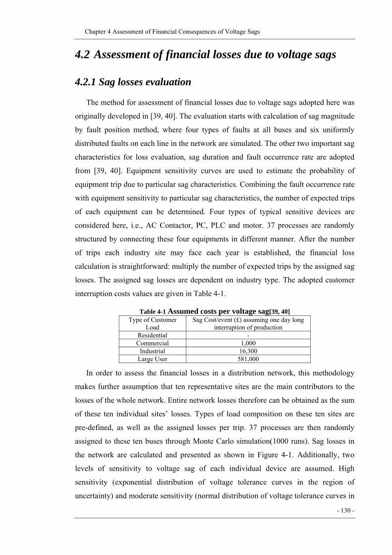
Chapter 4 Assessment of Financial Consequences of Voltage Sags
- 130 -
4.2 Assessment of financial losses due to voltage sags
4.2.1 Sag losses evaluation
The method for assessment of financial losses due to voltage sags adopted here was
originally developed in [39, 40]. The evaluation starts with calculation of sag magnitude
by fault position method, where four types of faults at all buses and six uniformly
distributed faults on each line in the network are simulated. The other two important sag
characteristics for loss evaluation, sag duration and fault occurrence rate are adopted
from [39, 40]. Equipment sensitivity curves are used to estimate the probability of
equipment trip due to particular sag characteristics. Combining the fault occurrence rate
with equipment sensitivity to particular sag characteristics, the number of expected trips
of each equipment can be determined. Four types of typical sensitive devices are
considered here, i.e., AC Contactor, PC, PLC and motor. 37 processes are randomly
structured by connecting these four equipments in different manner. After the number
of trips each industry site may face each year is established, the financial loss
calculation is straightforward: multiply the number of expected trips by the assigned sag
losses. The assigned sag losses are dependent on industry type. The adopted customer
interruption costs values are given in Table 4-1.
Table 4-1 Assumed costs per voltage sag[39, 40] Type of Customer
Load Sag Cost/event (£) assuming one day long
interruption of production Residential - Commercial 1,000
Industrial 16,300 Large User 581,000
In order to assess the financial losses in a distribution network, this methodology
makes further assumption that ten representative sites are the main contributors to the
losses of the whole network. Entire network losses therefore can be obtained as the sum
of these ten individual sites’ losses. Types of load composition on these ten sites are
pre-defined, as well as the assigned losses per trip. 37 processes are then randomly
assigned to these ten buses through Monte Carlo simulation(1000 runs). Sag losses in
the network are calculated and presented as shown in Figure 4-1. Additionally, two
levels of sensitivity to voltage sag of each individual device are assumed. High
sensitivity (exponential distribution of voltage tolerance curves in the region of
uncertainty) and moderate sensitivity (normal distribution of voltage tolerance curves in

Chapter 4 Assessment of Financial Consequences of Voltage Sags
- 131 -
the region of uncertainty). For more details regarding probabilistic modelling of
equipment sensitivity to voltage sag see [39, 40].
0 100 200 300 400 500 600 700 800 900 10006
8
10
12
14
16
18
20
22
Annual variation sag losses
Trial
�M
/ ye
ar
HSMS
average: 13.30
average: 8.63
4.67
Figure 4-1 Sag losses assessment
The results are sorted in an ascending order regardless of the process they are
correspond to since only cumulative value is of interest. It can be seen from Figure 4-1
that the losses in the network with highly sensitive equipment (HS), are much higher
(£4.67M/year) than with moderately sensitive equipments (MS). The difference in
average network losses is about 54% compared to average losses with MS equipment
4.2.2 Probabilistic analysis of sag losses
Accurate prediction of losses due to voltage sag is very important for investment
decision in mitigation devices. For those who has suffered from one severe sag event,
the question would be how significant is the fact that the likelihood of the occurrence of
similar sag is, say, 1 in 10,000? It is unfortunately impossible for any particular utility
or end-user to know the exact number of fault happening each year and it is even more
difficult to evaluate financial losses resulting from voltage sags. It is possible, however,
to calculate the odds of such a loss, based on statistical sampling techniques.
Further analysis was carried out based on the sag losses results presented in Figure
4-1. The losses (with highly sensitive equipment) distribution has a mean of £13.30M
and standard deviation of £2.29M as shown in Figure 4-2 (a). The losses (with
moderately sensitive equipment) distribution has a mean of £8.63M and standard
deviation of £0.77M as shown in Figure 4-2 (b). It can be clearly seen from Figure 4-2
(a) that the highest probability that the network losses is 17% for the losses of £13-14M

Chapter 4 Assessment of Financial Consequences of Voltage Sags
- 132 -
with HS equipment. The highest probability with MS equipment is about 45% for the
losses in the of £8-9M (Figure 4-2 (b)).
8.5 9.5 10.5 11.5 12.5 13.5 14.5 15.5 16.5 17.5 18.5 19.5 20.50
0.02
0.04
0.06
0.08
0.1
0.12
0.14
0.16
0.18
0.2
sag losses in �M / year
prob
abili
ties
cum
ulat
ive
high sensitivitymean:13.2977Std: 2.291
8.5 9.5 10.5 11.5 12.5 13.5 14.5 15.5 16.5 17.5 18.5 19.5 20.50
0.1
0.2
0.3
0.4
0.5
0.6
0.7
0.8
0.9
1
(a) high sensitivity
6.5 7.5 8.5 9.5 10.50
0.05
0.1
0.15
0.2
0.25
0.3
0.35
0.4
0.45
0.5
sag losses in �M / year
prob
abili
ties
cum
ulat
ive
medium sensitivitymean:8.6278Std: 0.7709
6.5 7.5 8.5 9.5 10.50
0.1
0.2
0.3
0.4
0.5
0.6
0.7
0.8
0.9
1
(b) Moderate sensitivity
Figure 4-2 Statistical analysis of sag losses It can be also seen from these figures that there is, for example, 80% probability that
network losses will be less than £14.5M with HS equipment and less than £9M with
MS equipment.
4.3 Saving due to application of FACTS devices
4.3.1 Advantages of application of FACTS devices
FACTS devices (STATCOM, SVC and DVR), have been proved to be capable of
reducing the number of sag or the severity of sags experienced by end-users. It is
therefore certain that the risks of huge financial losses to industry will be reduced by the
application of these devices.

Chapter 4 Assessment of Financial Consequences of Voltage Sags
- 133 -
Additionally there are other benefits of application of FACTSD. For example,
STATCOM can be used to mitigate the harmonics at the site. SVC can improve the
power transfer capacity of the network, etc. When one considers investing in these
devices, all potential benefits should be taken into account. One of the challenges is
identifying and quantifying the respective ‘values’ of these potential benefits in an
effective way. Potential economic impacts are actually very large, but confusion over
who reaps the benefits is a large part of problem [61].
Although FACTS devices are favourable in reducing sag losses, this advantage can
not be achieved inexpensively. Actually as discussed in the Chapter 1 of this thesis,
FACTSD are very expensive. So the bottom line question is:
‘Does investment in FACTSD make financial sense?’
The biggest issue of evaluating accurately the value of investment in FACTSD is
often the limited knowledge about their cost, efficiency and, consequently, the financial
benefits they can generate over the lifetime. Therefore, appropriate valuation tools are
needed that can help in answering these questions.
4.3.2 The cost of FACTSD
The main cost related to investment in FACTSD is the capital and maintenance cost
incurred every year during their life time. It is very difficult to give a general guideline
about the capital and maintenance cost, even for same type, (same brand) of device due
to the complexity involved in their installation and application. Throughout this
research, the cost of FACTSDs are determined by curve fitting of the curves given in
[63] as shown by (4.1) to (4.4). The maintenance costs are assumed to be 10% for SVC,
and 15% for STATCOM and DVR, of their capital cost. It has to be pointed out though,
that the curves given [63] are valid only for the rating of devices between 100MVAR
and 400 MVAR. They are assumed in this research however, to be valid for devices of
all ratings. It is assumed that the cost of DVR is the same as cost of STATCOM and
given by (4.3) and (4.4).
( )2 £553 0.0004 0.262 81.5 [ ]SVC SVC SVCC S SMVAr
= − + (4.1)
( )2 £553 0.0003 0.3051 127.38 [ ]SVC ConCst SVC SVCC S SMVAr+ = − + (4.2)

Chapter 4 Assessment of Financial Consequences of Voltage Sags
- 134 -
( )2 £553 0.0004 0.3225 128.75 [ ]STAT STAT STATC S SMVAr
= − + (4.3)
( )2 £553 0.0008 0.155 120 [ ]STAT ConCst STAT STATC S SMVAr+ = − + + (4.4)
4.4 Investment analysis
4.4.1 Process of analysis
For decision making process regarding investment in these rather expensive
mitigation devices it is essential to evaluate the economic impacts of the power quality
variations in the network against the costs of improving network performance. This
evaluation is ultimately an exercise in economics. The whole process of making
investment decision regarding mitigating devices is diagrammatically shown in Figure
4-3.
Figure 4-3 Process of investment analysis in FACTSD
The main components of an investment decision to be investigated [108] should
include the capital cost of investment, the operating cost reduction due to such
investment and the operating and maintenance expenses during the economic life of the
investment.
4.4.2 Methods of analysis
Conventional financial tools can be used to help the financial analysis process of
investment in FACTSD, such as simply pay back year (PBY), Net Present value (NPV),
Life cycle costs (LCC) or Internal Rate of Return (IRR) [109].
A common and simple way to evaluate the economic merit of an investment is to
calculate its payback period. The payback period is the number of years of operation
with reduced sag losses required to recover the initial cost. To determine the payback

Chapter 4 Assessment of Financial Consequences of Voltage Sags
- 135 -
years, the investor first estimates the total initial cost, annual savings, and annual
operating costs. Dividing total initial cost by the difference between annual savings and
annual operating costs gives the payback period:
Year= capital
sag saving mnt
CC C− −
(4.5)
Where capitalC is the initial capital cost, here, this is the cost of these FACTSDs.
sag savingC − is the saving in sag losses due to the installation of FACTSD, which can be
calculated as no mitigation with mitigationsag loss sag lossC C− −
− −− . mntC is the maintenance cost required each year
during the life time of FACTSD.
Because most of the benefits (as well as some incremental costs) of mitigation
devices occur over time, their future values should be ‘discounted’ to present values.
Within the NPV method, all cash flows during the lifetime of a project are taken into
account. The cash flows involved are: initial investment, maintenance and standby costs
on the negative side and the avoided costs on the positive side. The discount rate on the
capital investment has to be carefully considered. A FACTS device requires a large
initial capital outlay, but over its lifetime it will provide years of voltage support with
only small partial maintenance cost. Some benefits and costs will likely increase over
time, this however is not considered here.
The Net Present Value of these cash flows is given by following formula [110]:
1 (1 )
Nsag saving mnt
capitalnn
C CNPV C
r−
=
−= −
+∑ (4.6)
Where r is the discount rate and N is the number of project life times for the
evaluating investment.
In theory, a company will select all the projects with a positive NPV, regardless of
the capital required. Capital is assumed to be readily available, no matter how much is
needed or what are the constraints on the corporation. This is rarely the case because
access to capital markets is limited according to the overall performance. In case that
required capital is not available and that the money needs to be borrowed for the
investment in solution, the analysis becomes more complex. This option however, was
not considered in the research.

Chapter 4 Assessment of Financial Consequences of Voltage Sags
- 136 -
The NPV index (4.7) calculated by dividing each project’s NPV by its initial cash
outlay is created to ease this disadvantage of NPV. Instead of giving priority to the
project with the highest value, the opportunity is given to project with higher NPV
index.
NPVCapital
NPVIndexC
= (4.7)
4.4.3 Examples
The analysis in Chapter 3 indicates that the benefits of FACTSD for voltage sag
mitigation spreads over the whole network. Thus the many facets of value and
contribution of FACTSD application will not being adequately accounted if only the
connected node is considered. From an application’s standpoint, substantial financial
and technical benefits could be realized if the impacts of FACTSD placement can be
valued at a system level.
To demonstrate the whole process of financial assessment two groups of devices are
randomly allocated in the network, as shown in Table 4-2. It can be seen from Table 4-2
that the costs are reduced with both solutions. With solution 2, the reduction in cost is
more significant than with solution 1 despite the fact that the total capital cost is much
less (£4.13M) for solution 2 than that with solution 1 (£7.43M).
Table 4-2 Solutions of sag mitigation Bus Type Size Price(£M) Maintenance(£M) Saving(£M)76 SVC 105Mvar 40 STATCOM 35MW+10Mvar
Solution 1
243 DVR 15MW+10Mvar
7.43 0.9 1.25
Bus Type Size Price Maintenance saving 111 SVC 30Mvar 137 STATCOM 15MW+10Mvar
Solution 2
247 DVR 20MW+15Mvar
4.13 0.53 1.36
The total sag losses in the network are calculated and results are presented in Figure
4-4, Figure 4-5 and Figure 4-6. With the solution 1 and solution 2, the sag losses are
reduced in both HS equipment and MS equipment cases as shown in Figure 4-4.

Chapter 4 Assessment of Financial Consequences of Voltage Sags
- 137 -
0 100 200 300 400 500 600 700 800 900 10004
6
8
10
12
14
16
18
20
22
Annual variation sag losses
Trial
�M
/ ye
ar
HS baseMS baseHS solution1MS solution1HS solution2MS solution2
Figure 4-4 Annual sag losses with solution 1 and solution 2
The distributions of sag losses with solution 1 and solution 2 are illustrated in Figure
4-5 and Figure 4-6, respectively. They are quite different. With solution 1, Figure 4-5,
higher probability of sag losses is pushed to the left, compared to Figure 4-2 (a), e.g.
loss of £10.5M has the highest probability of about 17.5%, while in Figure 4-2 (a), loss
of £13.5M has the highest probability. Figure 4-6 (with FACTSD) shows that there are
no losses beyond £17.5M while the highest value of sag losses is over £20M without
FACTSD (see Figure 4-2 (a)). This example shows that the locations of FACTSD will
have significant influence on the network sag losses.
7.5 8.5 9.5 10.5 11.5 12.5 13.5 14.5 15.5 16.5 17.5 18.5 19.50
0.02
0.04
0.06
0.08
0.1
0.12
0.14
0.16
0.18
0.2
sag losses in �M / year
prob
abili
ties
cum
ulat
ive
prob
abili
ty
high sensitivity
mean:12.085Std: 2.261
7.5 8.5 9.5 10.5 11.5 12.5 13.5 14.5 15.5 16.5 17.5 18.5 19.50
0.1
0.2
0.3
0.4
0.5
0.6
0.7
0.8
0.9
1
Figure 4-5 Solution1 sag losses

Chapter 4 Assessment of Financial Consequences of Voltage Sags
- 138 -
7.5 8.5 9.5 10.5 11.5 12.5 13.5 14.5 15.5 16.5 17.50
0.02
0.04
0.06
0.08
0.1
0.12
0.14
0.16
0.18
0.2
sag losses in �M / year
prob
abili
ties
cum
ulat
ive
prob
abili
ty
high sensitivity
mean:11.9699Std: 1.914
7.5 8.5 9.5 10.5 11.5 12.5 13.5 14.5 15.5 16.5 17.50
0.1
0.2
0.3
0.4
0.5
0.6
0.7
0.8
0.9
1
Figure 4-6 Solution2 sag losses
The calculated sag losses in solution 1 and solution 2 are compared with losses
obtained in base case without FACTSD and the results of comparison of both, simple
and cumulative probabilities, are shown in Figure 4-7.
7.5 8.5 9.5 10.5 11.5 12.5 13.5 14.5 15.5 16.5 17.5 18.5 19.5 20.50
0.02
0.04
0.06
0.08
0.1
0.12
0.14
0.16
0.18
0.2
sag losses in �M / year
prob
abili
ties
High sensitive
basesolution 1solution 2
(a) Probabilistic
7.5 8.5 9.5 10.5 11.5 12.5 13.5 14.5 15.5 16.5 17.5 18.5 19.5 20.50
0.1
0.2
0.3
0.4
0.5
0.6
0.7
0.8
0.9
1
sag losses in �M / year
cum
ulat
ive
prob
abili
ty
high sensitivity basesolution 1solution 2
(b) Cumulative probabilities
Figure 4-7 Comparing sag losses in solution 1 and solution 2 with base case

Chapter 4 Assessment of Financial Consequences of Voltage Sags
- 139 -
It can be seen from Figure 4-7 (a) that the probabilities of high value of losses are
reduced while the probabilities of low value of losses are increased, e.g., for the losses
of £16.5M/year, the probability is reduced from about 6% (base case) to 2% ( solution 1)
and 1% (solution 2) respectively. Figure 4-7 (b) shows the cumulative probability
curves for all these cases. The improvement of network sag performance (i.e., reduced
losses) is noticeable with both solutions.
By pay-back-year analysis method, these two solutions are compared in Table 4-3.
Solution 2 needs less than 5 years to recover its capital cost. It is much better than
solution 2 which has a pay back of 21.33 years.
Table 4-3 Pay back years analysis Current Solution 1 Solution 2
Equipment None 3 FACTSD 3 FACTSD Mean of sag cost(£M) 13.33 12.08 11.97
devices cost(£M) 0 7.43 4.13 Maintenance(£M) 0 0.9 0.53
Total(£M) 13.33 Savings(£M) 13.33-12.08=1.25 13.33-11.97=1.36
Project Capital Cost(£M) 7.43 4.13 Simple payback(years) 7.43/(1.25-0.9)=21.33 4.13/(1.36-0.53) =4.98
As well known, the benefit will happen over time, so the discounted cash flow has
to be calculated. The assumed life time of devices is 15 years and the discounted rate is
12%. The mean value of sag losses is used for the analysis.
It can be clearly seen from Figure 4-8 and Figure 4-9 that solution 1 is not a feasible
solution since its NPV remains negative for the life time at the project. Solution 2 is
much more attractive because the huge financial benefit is accumulating with years.
Solution 2 will yield benefits from the 8th year onwards after the initial investment.
Using (4.7), the NPV indices of these two solutions are calculated and they are -
0.6689 and 0.3826 respectively. The solution 2 is obviously better as previously
discussed because it has the higher value of the NPV index.

Chapter 4 Assessment of Financial Consequences of Voltage Sags
- 140 -
0 2 4 6 8 10 12 14 16 18-8
-6
-4
-2
0
year
sag
loss
es in
M
year
0123456789101112131415
7.43000000000000000
00.90.90.90.90.90.90.90.90.90.90.90.90.90.90.9
01.251.251.251.251.251.251.251.251.251.251.251.251.251.251.25
-7.430.350.350.350.350.350.350.350.350.350.350.350.350.350.350.35
-7.430.310.280.250.220.2
0.180.160.140.130.110.1
0.090.080.070.06
-7.43-7.12-6.84-6.59-6.37-6.17
-6-5.84-5.7
-5.57-5.46-5.36-5.27-5.19-5.12-5.06
year capital Mnt(M Save(M Cash(M PV(M NPV(M
Figure 4-8 Solution1 NPV analysis
0 2 4 6 8 10 12 14 16 18-5
-4
-3
-2
-1
0
1
2
year
sag
loss
es in
M
year
0123456789101112131415
4.13000000000000000
00.530.530.530.530.530.530.530.530.530.530.530.530.530.530.53
01.361.361.361.361.361.361.361.361.361.361.361.361.361.361.36
-4.130.830.830.830.830.830.830.830.830.830.830.830.830.830.830.83
-4.130.740.660.590.530.470.420.370.330.3
0.270.240.210.190.170.15
-4.13-3.39-2.73-2.14-1.61-1.14-0.72-0.35-0.010.280.550.79
11.191.361.51
year capital Mnt(M Save(M Cash(M PV(M NPV(M
Figure 4-9 Solution2 NPV analysis

Chapter 4 Assessment of Financial Consequences of Voltage Sags
- 141 -
4.5 Uncertainties in sag loss analysis
Selecting the right option would be so much easier if only we could model all the
possible outcomes before deciding. That is however, theoretically perfect but practically
not feasible. Despite the huge computation efforts demanded, the lack of information is
the ‘big unknown’. In cost estimation analysis, one often assumes that the data are
complete and certain based on observations and reasonable judgments, in other words,
one makes assumptions. There are always uncertainties in these assumptions however,
such as fault happening rate, individual user’s sag losses, etc, which will result in over-
or under- estimation of the final result.
The information needed in sag loss evaluation process includes:
− Fault occurenc rate and distribution
− Sag magnitude and duration for each fault in the network
− User’s equipment wiring details (single phase or three phase equipment)
− Equipment sensitivity characteristic (i.e., voltage tolerance curves)
− The losses associated each trip at various load sites
If the uncertainties are substantial, one may not immediately be able to make
definitive recommendation about which decision is ‘the best’. But, one should be able
however to obtain useful insights about the relative importance of various assumptions,
and uncertainties in the inputs. These can indicate whether it is worthwhile to gather
more information, make more careful uncertainty assessment, or refine the model, and
which of these actions would reduce the most uncertainty in conclusions.
4.5.1 Uncertainties due to fault position method
Estimated number of sags is the essential data needed in the process of sag losses
evaluation. All the uncertainties investigated in Chapter2 will impact the result of
estimation of number of sag and therefore the result of financial analysis. Within these
uncertainties (number of fault position on each line, pre-fault voltage and fault
resistance), only fault resistance had noticeable impact on results of calculation of
number of sag as shown in Chapter 2. The focus here therefore, is the influence of fault
resistance on assessment of sag losses.

Chapter 4 Assessment of Financial Consequences of Voltage Sags
- 142 -
For the purpose of understanding the influence of fault resistance on estimation of
sag losses, six cases are simulated. Fault resistances of 0Ω, 1Ω, 2Ω, 5Ω, 10Ω and 15Ω
are considered and the results of analysis are presented in Figure 4-10 and Figure 4-11.
From Figure 4-10, the sag losses with fault resistance of 15Ω are much lower than
those with zero fault resistance. The higher the fault resistances are, the lower are sag
losses. This can be explained by the high sag magnitude resulting from high fault
resistance and such fewer potential trips of equipment. Since the average reduction in
annual sag losses between faults with 0Ω and 15Ω resistance is about £9.133M (69%
reduction compared to losses with 15Ω resistance), the influence of fault resistance on
sag losses estimation is very high. This also indicates that fault calculation based on
solid faults results in over estimation of potential sag losses.
0 100 200 300 400 500 600 700 800 900 10000
5
10
15
20
25
Trials
Sag
loss
es (
M /
year
)
High sensitivity
Zfault=0Zfault=1Zfault=2Zfault=5Zfault=10Zfault=15
9.133
average:13.3
average:11.12
average:9.487
average:6.649
average:5.302average:4.167
Figure 4-10 Sag losses due to various fault impedances
Figure 4-11 shows the cumulative probability of sag losses calculated with various
fault resistances. It is interesting to notice that with high fault resistances (10Ω, 15Ω),
the losses distribution has multi peaks. These two cases are further analyzed in and
illustrated in Figure 4-12 and Figure 4-13. The reason why the losses in these two cases
are different from the others is not clear at this stage of research and will be subject of
further research in the future.

Chapter 4 Assessment of Financial Consequences of Voltage Sags
- 143 -
2.5 4.5 6.5 8.5 10.5 12.5 14.5 16.5 18.5 20.50
0.1
0.2
0.3
0.4
0.5
0.6
0.7
0.8
0.9
1
Sag losses(�M / year)
cum
ulat
ive
prob
abili
ty
High sensitivity
Zfault=0
Zfault=1
Zfault=2
Zfault=5
Zfault=10
Zfault=15
Figure 4-11 Statistical analysis of sag losses due to various fault impedances
1.5 2.5 3.5 4.5 5.5 6.5 7.5 8.5 9.5 10.511.512.513.514.515.516.517.518.519.520.50
0.05
0.1
0.15
0.2
0.25
0.3
0.35
sag losses (�M / year)
prob
abili
ty
High sensitivity
Figure 4-12 Sag losses with 10ohm fault resistance
0 1.5 2.5 3.5 4.5 5.5 6.5 7.5 8.5 9.5 10.511.512.513.514.515.516.517.518.519.520.50
0.05
0.1
0.15
0.2
0.25
0.3
0.35
0.4
0.45
sag losses (�M / year)
prob
abili
ty
High sensitivity
Figure 4-13 Sag losses with 15ohm fault resistance
4.5.2 Various assigned user losses
Another important assumption made in financial estimation is the assigned losses
due to each trip regarding different types of loads. Four types of loads with their

Chapter 4 Assessment of Financial Consequences of Voltage Sags
- 144 -
assumed losses are described in Table 4-1. The assigned loss values try to include all
losses incurred when sites’ devices trip such as loss of product, restarting cost, devices
damage, missed opportunity, etc. However it is very difficult to give a precise value due
to the complexities involved, e.g., some losses such as the damage to the reputation of
company may not be described in a statistical way. Since losses are equal to the number
of trips of equipment multiplied by the assigned losses per trip, the assumed values of
loss per trip would have direct impact on the final calculated loss.
In this study, the assigned losses per site are varied. The variations of assigned
losses are depicted in Figure 4-14. The losses assigned to large user vary the most in
absolute value (from £200000 to £700000). While the losses of residential user vary the
least in absolute value (from 0 to £10000) and the most in relative value, i.e.,
1000000%.
-1 0 1 2 3 4 5 6 7 8
x 105
0 10000 Residential
1000 50000 Commercial
15000 100000 Industry
200000 700000
Large user
base: 00 --> 1000000%
base: 10000 --> 4900%
base:16300-8% --> 513%
base:581000-65.58% --> 20.48%
Figure 4-14 Sag loss variation assigned to different users
Resulted variation of network losses are shown in Figure 4-15. It can be seen that
the variation in assigned losses to industrial users results in the biggest variation in
network sag losses, although variation in losses of industrial users is not the biggest
either in absolute or relative value. Large user has the second-largest resulting variation
despite the fact that its assigned losses vary the most in absolute values. Both,
residential and commercial users have relative small influence on final network losses.
Further statistical analysis of these results is shown in Figure 4-16. The cumulative
probability curve is pushed towards right with higher assigned user losses. This means
that for a given probability of occurrence the network losses increase with the assigned
user losses, as expected.

Chapter 4 Assessment of Financial Consequences of Voltage Sags
- 145 -
200 400
600 800
1000
residentialcommercial
Industrylarge user
0
5
10
15
20
25
30
35
40
trials
loss
es(M�
)
Figure 4-15 Sag losses variation due to various assigned losses’ value
0 3.5 5.5 7.5 9.5 11.5 13.5 15.5 17.5 19.5 21.5 23.5 25.5 27.5 29.5 31.5 33.5 35.50
0.1
0.2
0.3
0.4
0.5
0.6
0.7
0.8
0.9
1
Sag losses (�M / year)
cum
ulat
ive
prob
abili
ty
High sensitivity
base
Res--10K
Com--50K
Ind--15K
Ind--100K
Lar--200K
Lar--700K
Figure 4-16 Statistical analysis of sag losses due to various assigned loss’ values
These results are further analyzed in Figure 4-17. Industry users have the biggest
influence on network losses either in absolute (£12.65M to £25.21M) or relative value
(-1.36% to 96.57%).
5 10 15 20 25 30
12.8248 14.1417 Residential
12.8248 15.0733 Commercial
12.6508 25.2095Industry
6.0195 14.9416 Large user
NPV(M� )
base:12.82480 -->10.27%
base:12.82480 -->17.53%
base:12.8248-1.36% -->96.57%
base:12.8248-53.06% -->16.51%
Figure 4-17 Mean sag losses variations due to various assigned losses’ values

Chapter 4 Assessment of Financial Consequences of Voltage Sags
- 146 -
In analysis shown in Figure 4-15 and Figure 4-17, the biggest variation in absolute
value (25.21-12.65=12.59) comes from industrial user. Assigned loss variation in
residential user was 0 – 1000,000% resulting in variation in sag losses of 0 – 10.27%,
variation in commercial was 0 – 4,900% resulting in (0 – 17.53% variation in sag losses,
variation in industrial user was -8% - 513% resulting in -53.06% - 16.51% variation in
sag losses, variation in large user (-65.58% - 20.48%) result in (-53.06% – 16.51%).
The network losses sensitivity factors (LSF) can be calculated from the above analysis:
5
03
arg
10.27% 0 1.03 101000000% 017.53% 0 3.6 104900% 0
96.57% ( 1.36%) 0.19513% ( 8%)
16.51% ( 53.06%) 0.8120.48% ( 65.58%)
residencial
commercial
industry
l e user
LSF
LSF
LSF
LSF
−
−
−
−= = ×
−−
= = ×−
− −= =
− −− −
= =− −
The residential user has the smallest value of LSF while the large user has the
highest value.
4.6 Uncertainties in NPV analysis
4.6.1 The NPV analysis
NPV is one of the most robust financial evaluation tools to estimate the value of an
investment. The Net Present Value (NPV) of a project or investment is defined as the
sum of the present values of the annual cash flows minus the initial investment. The
initial investment includes all investment made at the beginning of the project such as
hardware cost, software licensing fees, and start-up cost [4].
The calculation of NPV involves three simple steps: 1) To identify the size and
timing of the expected future cash flows generated by the project or investment. 2)To
determine the discount rate or the estimated rate of return for the project. 3)To calculate
the NPV by (4.6).
NPV analysis could indicate the level of risk of a project with consideration of the
time value of money. There are however limitations of this method, such as that it does
not consider the availability of capital investment; it ignores the difficulties of estimate

Chapter 4 Assessment of Financial Consequences of Voltage Sags
- 147 -
the discount rate. And NPV is calculated in a static manner based on information
known at the time of evaluation. Information may change over time; therefore the risk
profile of the project may alter.
4.6.2 Financial analysis with NPV
The NPV analysis is highly flexible and can be combined with other financial
evaluation tools such as decision tree models, scenario and Monte Carlo analysis to
avoid its disadvantages [110].
• Sensitivity analysis: To address the uncertainties involved in NPV analysis, a
sensitivity analysis can be employed. A sensitivity analysis changes each
precedent variable at a time and then notes the changes of the resulting
variable.
• Scenario analysis: A scenario analysis is a special case of a sensitivity analysis
where a pre-determined set of possible outcomes are identified. The pre-
determined case scenarios are usually labelled according to their expected
value from best to worst.
• Decision tree analysis: A decision tree is a graphical representation of all the
possible outcomes and decision points which constructed by identifying the
events and decision nodes of an investment.
4.6.2.1 Sensitivity analysis
The objective of a sensitivity analysis is to identify critical inputs of the financial
model and how their variability impacts the result. A sensitivity analysis can be
represented using a Tornado diagram, which depicts the most sensitive precedent
variable along with the impact on the overall result [107].
Tornado analysis determines the effect on the overall result by changing one
variable at a time. A Monte Carlo simulation determines the effect of changing all the
variables at the same time while introducing probability distributions for each variable.
The Monte Carlo simulation considers all possible combinations and outcomes. The
resulting output will be distribution of the output or resulting variable.
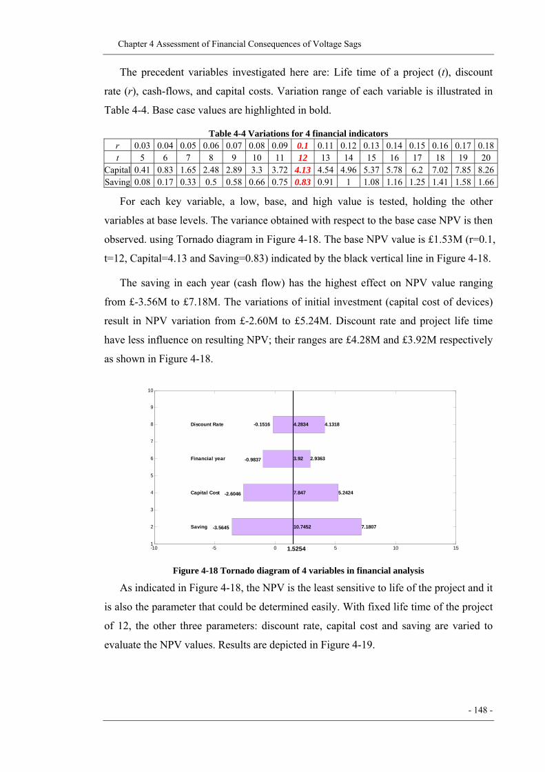
Chapter 4 Assessment of Financial Consequences of Voltage Sags
- 148 -
The precedent variables investigated here are: Life time of a project (t), discount
rate (r), cash-flows, and capital costs. Variation range of each variable is illustrated in
Table 4-4. Base case values are highlighted in bold.
Table 4-4 Variations for 4 financial indicators r 0.03 0.04 0.05 0.06 0.07 0.08 0.09 0.1 0.11 0.12 0.13 0.14 0.15 0.16 0.17 0.18t 5 6 7 8 9 10 11 12 13 14 15 16 17 18 19 20
Capital 0.41 0.83 1.65 2.48 2.89 3.3 3.72 4.13 4.54 4.96 5.37 5.78 6.2 7.02 7.85 8.26Saving 0.08 0.17 0.33 0.5 0.58 0.66 0.75 0.83 0.91 1 1.08 1.16 1.25 1.41 1.58 1.66
For each key variable, a low, base, and high value is tested, holding the other
variables at base levels. The variance obtained with respect to the base case NPV is then
observed. using Tornado diagram in Figure 4-18. The base NPV value is £1.53M (r=0.1,
t=12, Capital=4.13 and Saving=0.83) indicated by the black vertical line in Figure 4-18.
The saving in each year (cash flow) has the highest effect on NPV value ranging
from £-3.56M to £7.18M. The variations of initial investment (capital cost of devices)
result in NPV variation from £-2.60M to £5.24M. Discount rate and project life time
have less influence on resulting NPV; their ranges are £4.28M and £3.92M respectively
as shown in Figure 4-18.
-10 -5 0 5 10 151
2
3
4
5
6
7
8
9
10
4.1318-0.1516 4.2834Discount Rate
2.9363-0.9837 3.92Financial year
5.2424-2.6046 7.847Capital Cost
7.1807-3.5645 10.7452Saving
1.5254
Figure 4-18 Tornado diagram of 4 variables in financial analysis
As indicated in Figure 4-18, the NPV is the least sensitive to life of the project and it
is also the parameter that could be determined easily. With fixed life time of the project
of 12, the other three parameters: discount rate, capital cost and saving are varied to
evaluate the NPV values. Results are depicted in Figure 4-19.
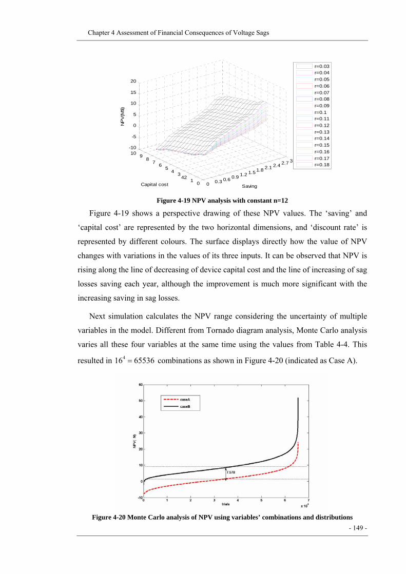
Chapter 4 Assessment of Financial Consequences of Voltage Sags
- 149 -
0 0.3 0.6 0.9 1.2 1.51.8 2.1 2.4 2.7 3
0142
345
678
910-10
-5
0
5
10
15
20
SavingCapital cost
NP
V(M
$)
r=0.03r=0.04r=0.05r=0.06r=0.07r=0.08r=0.09r=0.1r=0.11r=0.12r=0.13r=0.14r=0.15r=0.16r=0.17r=0.18
Figure 4-19 NPV analysis with constant n=12
Figure 4-19 shows a perspective drawing of these NPV values. The ‘saving’ and
‘capital cost’ are represented by the two horizontal dimensions, and ‘discount rate’ is
represented by different colours. The surface displays directly how the value of NPV
changes with variations in the values of its three inputs. It can be observed that NPV is
rising along the line of decreasing of device capital cost and the line of increasing of sag
losses saving each year, although the improvement is much more significant with the
increasing saving in sag losses.
Next simulation calculates the NPV range considering the uncertainty of multiple
variables in the model. Different from Tornado diagram analysis, Monte Carlo analysis
varies all these four variables at the same time using the values from Table 4-4. This
resulted in 416 65536= combinations as shown in Figure 4-20 (indicated as Case A).
Figure 4-20 Monte Carlo analysis of NPV using variables’ combinations and distributions

Chapter 4 Assessment of Financial Consequences of Voltage Sags
- 150 -
The resulting NPV varies from £-7.5M to £24.28M. The statistical analysis of this
result is depicted in Figure 4-21. The most probable (9.5% or so) NPV will be about
£0.5M and 80% of NPV will be below £4.5M.
-8.5 -6.5 -4.5 -2.5 -0.5 1.5 3.5 5.5 7.5 9.5 11.5 13.5 15.5 17.5 19.5 21.5 23.50
0.01
0.02
0.03
0.04
0.05
0.06
0.07
0.08
0.09
0.1
prob
abili
ties
cum
ulat
ive
prob
abili
ty
NPV (�M)
High sensitivity
-8.5 -6.5 -4.5 -2.5 -0.5 1.5 3.5 5.5 7.5 9.5 11.5 13.5 15.5 17.5 19.5 21.5 23.50
0.1
0.2
0.3
0.4
0.5
0.6
0.7
0.8
0.9
1
mean: 1.5988
Figure 4-21 Statistical analysis of NPV
It is acknowledged that all these four uncertain inputs are either empirical quantities
or measurable, at least in principle. So these variations can legitimately be represented
by probability distributions shown in Figure 4-22 to Figure 4-25. Discount rate, life of
the project and capital cost of the investment are assumed to follow normal distribution
in order to model these variables in a more realistic manner. Saving in sag losses here
however is assumed to follow the weibull distribution with the parameters as it is most
likely to increase if additional benefits of FACTSD are considered as described in
Section 4.3.1.
0 0.05 0.1 0.15 0.20
0.02
0.04
0.06
0.08
0.1
0.12
0.14
0.16
Den
sity
Critical Value Figure 4-22 Discount rate Normal distribution withµ=0.1δ=0.025
0 2.5 5 10 15 20 250
0.02
0.04
0.06
0.08
0.1
0.12
0.14
0.16
Den
sity
Critical Value Figure 4-23Project life times Normal
distribution withµ=10δ=2.5

Chapter 4 Assessment of Financial Consequences of Voltage Sags
- 151 -
0 2 4 6 8 100
0.05
0.1
0.15
0.2
0.25
0.3
0.35
0.4
Den
sity
Critical Value Figure 4-24 Capital cost Normal distribution
with µ=4.13δ=1.09
Figure 4-25 Saving Weibull distribution with
A=1, B=1.5
The Monte Carlo simulation here introduces uncertainty as each variable is defined
with a probability distribution. 416 65,536= sets of these four variables (discount rate,
life of the project, capital cost and saving) are generated randomly following the
distributions described in Figure 4-22 to Figure 4-25, respectively. Resulted NPV are
illustrated in Figure 4-20 (indicated as Case B). The resulting NPV varies from £-
1.93M to £51.1M, which is much higher than the values obtained in case A (£7.58M
higher in average value).
-2.5 1.5 5.5 9.5 13.5 17.5 21.5 25.5 29.5 33.5 37.5 41.5 45.5 49.50
0.01
0.02
0.03
0.04
0.05
0.06
0.07
0.08
0.09
0.1
NPV (�M / year)
prob
abili
ties
cum
ulat
ive
prob
abili
tyHigh sensitivity
-2.5 1.5 5.5 9.5 13.5 17.5 21.5 25.5 29.5 33.5 37.5 41.5 45.5 49.50
0.1
0.2
0.3
0.4
0.5
0.6
0.7
0.8
0.9
1
mean: 8.7510
Figure 4-26 Statistical analysis of NPV
Same statistical analysis is performed as before and results are shown in Figure 4-26.
The mean value of NPV (£8.75M) is much higher in Figure 4-26 than in Figure 4-21
(£1.60M), which indicates that resulted NPV is higher in case when normal and weibull
distribution are used for variables (discount rate, life of the project, capital cost and
saving in sag losses). The mean value of NPV (£8.75M) is also higher than NPV

Chapter 4 Assessment of Financial Consequences of Voltage Sags
- 152 -
(£1.53M) obtained in the case of r=0.1, t=12, Capital=4.13 and Saving=0.83. This
shows that the NPV may be under-estimated if variables (discount rate, life of the
project, capital cost and saving in sag losses) are considered constant or uniformly
distributed in the analysis.
As mentioned previously, life of the project is the variable which can be decided
easily and has the least effects on NPV. So here, Monte Carlo simulation is run with
three variables (discount rate, capital cost and saving) having appropriate distributions
and life of the project is assumed to be 5, 10, 15, 20 and 25 years, respectively. Results
in Figure 4-27 indicate that the NPV is much higher with a longer project life
expectancy although the improvement seems to slow down when the project life time
year is longer than 15 years.
0 100 200 300 400 500 600 700 800 900 1000-5
0
5
10
15
20
25
30
35
40
45
trials
NP
V(M
$)
5years
10years
15years
20years
25years
Figure 4-27 Monte Carlo NPV analysis with various project life times
4.6.2.2 Decision tree analysis
A decision tree calculates the expected value under multitude of events and
scenarios, working ‘backwards’ to induce the overall expected value. For example, the
NPV for each outcome is multiplied by the probability of the outcome, then summed
together to produce the final NPV concerned. The calculation can be described by (4.8).
n
i n r c si
NPV NPV P P P P= × × × ×∑ (4.8)
Where, , , ,n r c sP P P P are the probabilities of life of the project, discount rate, Capital
cost and saving, respectively.
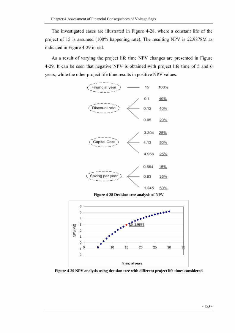
Chapter 4 Assessment of Financial Consequences of Voltage Sags
- 153 -
The investigated cases are illustrated in Figure 4-28, where a constant life of the
project of 15 is assumed (100% happening rate). The resulting NPV is £2.9878M as
indicated in Figure 4-29 in red.
As a result of varying the project life time NPV changes are presented in Figure
4-29. It can be seen that negative NPV is obtained with project life time of 5 and 6
years, while the other project life time results in positive NPV values.
Figure 4-28 Decision tree analysis of NPV
15, 2.9878
-2
-1
0
1
2
3
4
5
6
0 5 10 15 20 25 30 35
financial years
NPV
(M£)
Figure 4-29 NPV analysis using decision tree with different project life times considered

Chapter 4 Assessment of Financial Consequences of Voltage Sags
- 154 -
4.6.3 Uncertainties in NPV
Uncertainty refers to the fact that the analyst cannot be sure today about anything that
is going to happen in the future. Using available information relating to past events the
analyst makes estimates (or assumptions). There always is some uncertainty involved
and the analyst is never certain how close these estimates will be to what actually will
happen. Sensitivity analysis provides a low cost means to identify critical project
parameters in order to design a sound, workable project, and to understand and reduce
the uncertainty surrounding the project outcome. Tornado diagram can help to identify
critical values for a project, thus could lead further possible solutions. Monte Carlo and
cumulative probability analysis offer the possibility to analysis different combinations
at the same time in order to view the outcome of the project in all possible ways. The
following practical systematic approach to analyzing uncertainty is recommended in
[111]:
• Identify likely major sources of uncertainty for the project being analyzed, and
for each source establish some estimate of a reasonable range of values for the
parameters involved.
• Carry out a sensitivity analysis for the project using various combinations of
different assumptions concerning the values of the parameters associated with
the major sources of uncertainty and analyze in more detail the parameters for
which changes in value assumptions are critical in terms of project outcome
• Determine appropriate ways of changing the design of the project or modify it
to eliminate or reduce the major sources of uncertainty which are critical in
terms of project outcome.
4.7 New approach to assessment of sag losses
Financial losses due to voltage sags could show up in many aspect of industrial and
commercial operations, such as loss of revenue, lost opportunities, product damage,
wasted energy and decreased equipment life, field service warranty work,
manufacturing interruption, loss of productivity. So it is very difficult to estimate
exactly the amount of losses incurred by sags. The most uncertain issue is that sags
happen in a stochastic manner. In other words, they may not happen at all. The key

Chapter 4 Assessment of Financial Consequences of Voltage Sags
- 155 -
issue in losses estimation is the immunity of equipment or the whole process. In this
sense, sag losses are highly problematic, and very difficult to estimate. Recently, there
has been large amount of research devoted to sag losses estimation. Various
methodologies have been investigated and tested. Equipment tolerance curves are
mostly used to determine whether the process will trip or not.
A considerable variety of such methods have been developed to assess losses of
voltage sag, with wide differences in conceptual approach, computational effort
required, and the power of their results. However most of these methods only
considered one phase voltage magnitude, and they tend to focus on equipment level.
The connections of equipment were considered but far than adequately because in
reality the wirings of equipment are rather complicated. Therefore, a new methodology
is proposed here to estimate sag losses based on system sensitivity curves with all three
phase voltages considered.
4.7.1 Equipment sensitivity
The reason why voltage sags would cause financial losses is that sensitive
equipment in the plant would trip because of the sag, resulting in trip or mis-operation
of the whole process.
Usually, many types of equipment can ride through voltage sag without causing a
problem. For example, most motor loads can ride through voltage sags without
affecting the process because of the inertia of the motor. The dropping out of motors is
most likely to happen when its protection devices, contactors or relays trip due to sags.
Programmable logic controller (PLC), relays, computers and contactors are considered
to be some of the most sensitive equipments. Voltage tolerance curves for these are
developed to indicate their sensitivity regarding sag magnitude and duration as shown
in Figure 4-30. This figure indicates that voltage sags deeper than minV and longer than
maxT will cause trip of the equipment. The shaded region is the area of uncertainty of
equipment ride through.
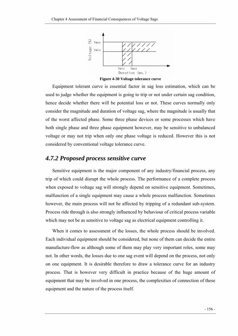
Chapter 4 Assessment of Financial Consequences of Voltage Sags
- 156 -
Figure 4-30 Voltage tolerance curve
Equipment tolerant curve is essential factor in sag loss estimation, which can be
used to judge whether the equipment is going to trip or not under certain sag condition,
hence decide whether there will be potential loss or not. These curves normally only
consider the magnitude and duration of voltage sag, where the magnitude is usually that
of the worst affected phase. Some three phase devices or some processes which have
both single phase and three phase equipment however, may be sensitive to unbalanced
voltage or may not trip when only one phase voltage is reduced. However this is not
considered by conventional voltage tolerance curve.
4.7.2 Proposed process sensitive curve
Sensitive equipment is the major component of any industry/financial process, any
trip of which could disrupt the whole process. The performance of a complete process
when exposed to voltage sag will strongly depend on sensitive equipment. Sometimes,
malfunction of a single equipment may cause a whole process malfunction. Sometimes
however, the main process will not be affected by tripping of a redundant sub-system.
Process ride through is also strongly influenced by behaviour of critical process variable
which may not be as sensitive to voltage sag as electrical equipment controlling it.
When it comes to assessment of the losses, the whole process should be involved.
Each individual equipment should be considered, but none of them can decide the entire
manufacture-flow as although some of them may play very important roles, some may
not. In other words, the losses due to one sag event will depend on the process, not only
on one equipment. It is desirable therefore to draw a tolerance curve for an industry
process. That is however very difficult in practice because of the huge amount of
equipment that may be involved in one process, the complexities of connection of these
equipment and the nature of the process itself.

Chapter 4 Assessment of Financial Consequences of Voltage Sags
- 157 -
It is still possible to estimate to some extent a general tolerance curve of the process
based on individual equipment tolerance curves and reasonable assumptions of process
components and their connections. A cumulative sag tolerance curve of a process is
proposed as in Figure 4-31, where axes present voltage magnitude in % of nominal.
Curves T1, T2, T3 and T4 stand for the sensitivities of process regarding voltage
magnitude and duration. For curve T1, the process will not trip when it exposed to sag
magnitudes to the right of the curve, sag duration is specified by T1. T2, T3 and T4 are
the same sensitivity curves of the process, representing different sag durations,
4 3 2 1T T T T< < < . It is reasonable to assume that with longer sag duration, process
might trip even for shallow voltage sags (with high magnitude). On the other hand, with
shorter sag durations, the process would survive even deeper sags.
Figure 4-31 Process tolerant curve
These voltage tolerance curves take into account all magnitudes in all three phases
and can be problem dependant. They can be used for single equipment or extended to a
whole process line. How to get these curves is essential of course, however, this is not
considered in this study and will be left for future researches. In case when the whole
process is considered simultaneously, T1-T4 may be the process immunity times rather
than sag duration times.
4.7.3 Sag cost factors
Although process trips, when sags are on the left side of T1, T2, T3 and T4, as in
Figure 4-31, the losses may differ because different sag magnitudes may have influence
on final losses due to sags. Especially when unbalanced sags are concerned potential
sag loss is less than that estimated based on three-phase sags from the entire load site.

Chapter 4 Assessment of Financial Consequences of Voltage Sags
- 158 -
Therefore, further assumption is made that the financial losses depend on the
variations of specified magnitudes. Weighting factors are used to characterize this
influence. This is illustrated in example in Figure 4-32.
On the principal diagonal of Figure 4-32, A1, A2…A10 are named the ‘driving cost
factors’, which could be decided by investigators if data is available. To simplify the
illustration assume that:
1 2 3 4 5 100%A A A A A= = = = = , 6 7 70%A A= = , 8 40%A = , 9 10%A = , 10 0A = .
ija are named ‘transfer cost factors’, calculated by (4.9).
Figure 4-32 Assigned losses
2 13 3ij j ia A A= × + × (4.9)
For example, 13 3 1 98 8 92 1 2 1,3 3 3 3
a A A a A A= × + × = × + ×
This assumption is based on the fact that sags with two phase voltage magnitudes in
a given range would certainly cost more than sags with only one phase voltage
magnitude.
Different cost factors are described in Figure 4-33. It indicates that with three phase
voltage magnitudes all below 50% of the nominal, sags would cause 100% losses. In
the case of sags with two phases’ voltage between 80%-90%, one phase’s voltage
between 50% -60%, the loss factor will only be 30%.

Chapter 4 Assessment of Financial Consequences of Voltage Sags
- 159 -
For example, 10,5a (red circled in Figure 4-33) can be calculated as:
10,5 5 102 13 3
a A A= × + × , 5 100%A = and 10 0%A = (black circled in Figure 4-33) should be
pre-defined based on practice information regarding to various user types.
Figure 4-33 Percentage of losses due to various magnitudes of three phases
4.7.4 Evaluation of the losses at user site
4.7.4.1 Tolerance curve and generalized sag table
In order to evaluate the losses of an entire user site, one should combine the
proposed tolerance curve based on the entire site and generalized sag table of that site
together, as shown in Figure 4-34:

Chapter 4 Assessment of Financial Consequences of Voltage Sags
- 160 -
Figure 4-34 Process sensitive curve and generalized sag table
Where:
Curve T1 (black): if the fault duration is <T1, no equipment will trip regardless of
the magnitude of voltage sag.
Curve T2 (green): tolerance curve for sag duration T2.
Curve T3 (yellow): tolerance curve for sag duration T3.
Curve Non-affected (red): if the voltage magnitude is on the right side of this curve,
no equipment will trip regardless the duration of sag.
Cgreen: the losses due to sags on the left side of green line;
Cyellow: the losses due to sags between green and yellow line;
Cread: the losses due to sag between yellow and red line.
All expected sags can be calculated as:
1 2 3( )ij green ij T ij T ij T greenN N N N− − − −= + + (4.10) 2 3( )ij yellow ij T ij T yellowN N N− − −= + (4.11) 3( )ij red ij T redN N− −= (4.12) Taking the cost factors into account, the estimation of sag losses is straightforward:
green ij green ijC N a−= × (4.13) yellow ij yellow ijC N a−= × (4.14) red ij red ijC N a−= × (4.15) ( )total green yellow red cCost C C C C= + + × (4.16)
where Cc is the reference cost of this site.
4.7.4.2 Application example
The methodology is used to evaluate the sag losses at bus 111 in the test network.
First, assume that the cumulative tolerance curve of total load connected at bus 111
is as shown in Figure 4-34, where 3 200T ms= , 2 70T ms= and 1 50T ms= . The cost
factors are the same as in Figure 4-33. The generalized sag tables which are categorized
according to the shape and duration of tolerance
curves 50 , 50 70 ,70 200 , 200ms ms ms ms< − − > are shown in Figure 4-35, Figure
4-36and Figure 4-37. In this case, there is no voltage sag with duration below 50ms.

Chapter 4 Assessment of Financial Consequences of Voltage Sags
- 161 -
0 10 20 30 40 50 60 70 80 90 1000
10
20
30
40
50
60
70
80
90
100
Voltage in two phases (% of nominal)
volta
ge in
the
third
pha
se (%
of n
omin
al)
0.15 0.03 0.07 0.05 0.16 0.62 0.05 0.29 0.71 14.39
0 0 0 0 0.04 0.05 0 0.03 0.08 0.45
0 0 0 0.1 0.04 0.01 0 0.01 0.01 0.41
0 0 0 0.11 0.07 0 0 0 0 0.53
0.01 0 0.11 0.01 0 0.03 0 0 0.04 0.87
0 0 0.03 0 0.05 0 0 0.03 0.05 1.14
0 0.01 0 0.06 0 0 0 0.01 0 0.47
0 0 0.04 0 0 0 0 0.01 0.47 0.35
0.03 0.06 0 0 0 0 0 0.01 0.16 0.17
0.1 0 0 0 0 0 0.03 0 0.01 0.76
Figure 4-35 Number of sags (50- 70ms)
0 10 20 30 40 50 60 70 80 90 1000
10
20
30
40
50
60
70
80
90
100
Voltage in two phases (% of nominal)
volta
ge in
the
third
pha
se (%
of n
omin
al)
0 0 0 0 0.26 5.62 1.67 14.81 18.6 7.3
0 0 0 0 0.31 0.38 0.02 0 0.33 3.66
0 0 0 0.1 0.27 0.09 0 0.07 0.21 5.59
0 0 0.1 0.75 0.34 0 0.02 0 0.31 9.14
0 0 0.48 0.22 0.03 0.42 0 0.31 2.93 6.43
0 0 0.1 0 1.02 0 0.1 2.23 1.68 4.34
0 0 0 0.44 0 0.03 0.05 0.59 0.39 2.16
0 0 0.38 0 0 0 0 0.52 1.34 1.06
0 0.66 0 0 0 0 0 0.52 0 0.07
0.65 0 0 0 0 0 0.94 0.21 0.41 0
Figure 4-36 Number of sags (70-200ms)
0 10 20 30 40 50 60 70 80 90 1000
10
20
30
40
50
60
70
80
90
100
Voltage in two phases (% of nominal)
volta
ge in
the
third
pha
se (%
of n
omin
al)
13.87 7.18 4.44 6.03 19.22 21.43 5.97 0 13.03 1189.45
0.49 0 0 0 1.48 1.23 0 1.48 4.36 22.88
0.25 0 0.83 1.74 0.49 0 0 1.03 0.28 21.17
0.25 0 1.67 0.77 0 0 0 0 0 42.34
0.39 0 2.87 0 0 0.52 0 0 0 46.74
0.28 0.42 0.28 0 3.13 0 0 0 0 37.77
0.28 0.14 0 2.73 0 0 0 0 0 17.11
0.28 0 1.04 0 0 0.25 0 0 7.54 25.94
1.76 1.62 0 0 0 0 0 0 4.17 19.05
7.41 0 0 0 0 0 0 0 0.6 73.24
Figure 4-37 Number of sags (>200ms)
Using (4.10), one can get the sag table of Figure 4-38, where all sags listed in the
table could result in financial losses. Applying (4.13), the influential number of voltage
sags can be calculated as presented in Figure 4-39.

Chapter 4 Assessment of Financial Consequences of Voltage Sags
- 162 -
0 10 20 30 40 50 60 70 80 90 1000
10
20
30
40
50
60
70
80
90
100
Voltage in two phases (% of nominal)
volta
ge in
the
third
pha
se (%
of n
omin
al)
14.02 7.18 4.44 6.03 19.49 21.43 5.97 0 0 0
0.49 0 0 0 1.79 1.23 0 1.48 0 0
0.25 0 0.83 1.85 0.76 0 0 1.03 0.28 21.17
0.25 0 1.77 1.52 0.34 0 0 0 0 42.34
0.4 0 3.34 0.22 0.03 0.52 0 0 0 46.74
0.28 0.42 0.38 0 4.15 0 0.1 2.23 1.68 42.1
0.28 0.15 0 3.17 0 0.03 0.05 0.59 0.39 19.26
0.28 0 1.42 0 0 0.25 0 0.52 8.88 27
1.78 2.34 0 0 0 0 0 0.54 4.33 19.3
8.16 0 0 0 0 0 0.97 0.21 1.01 74
Figure 4-38 Number of sags which will trip the process
0 10 20 30 40 50 60 70 80 90 1000
10
20
30
40
50
60
70
80
90
100
Voltage in two phases (% of nominal)
volta
ge in
the
third
pha
se (%
of n
omin
al)
9.34 4.79 2.96 4.02 12.99 10 2.79 0 0 0
0.35 0 0 0 1.26 0.62 0 0.44 0 0
0.2 0 0.67 1.48 0.61 0 0 0.41 0.06 2.82
0.22 0 1.59 1.37 0.31 0 0 0 0 9.88
0.36 0 3.01 0.2 0.03 0.37 0 0 0 10.91
0.28 0.42 0.38 0 4.15 0 0.08 1.34 0.67 14.03
0.28 0.15 0 3.17 0 0.03 0.04 0.36 0.15 6.42
0.28 0 1.42 0 0 0.2 0 0.31 3.55 9
1.78 2.34 0 0 0 0 0 0.32 1.73 6.43
8.16 0 0 0 0 0 0.78 0.13 0.41 24.67
Figure 4-39 Influential sags which will trip the process
Once the number of influential voltage sags has been calculated, the computation of
voltage sag losses is straight forward: multiply the total number of sags from Figure
4-39 (173.9823) by the reference cost for the site ( cC ).
Assume that all loads fall in one of the categories shown in Table 4-5. (It has to be
pointed out that these losses (£) are based on 100MVA load). After the size of the load
is taken into account, the resulting losses at bus 111 are calculated and listed in Table
4-5. It shows that group I loads result in much more losses than group III loads. (Note:
For a load of 100MW in group I, one trip causes losses of £0.021M while a load of
50MW leads to losses of 0.0105M£.)
Possible losses for bus 111 are listed in Table 4-6. The difference in losses between
different groups is significant. And it depends on how load groups are defined and what
is the value of losses for each type of load. Further information about the load factor

Chapter 4 Assessment of Financial Consequences of Voltage Sags
- 163 -
and correction factor for different types of load and how to include them in the loss
calculation can be found in paper [39, 40].
Table 4-5 User group category(100MVW) [39, 40] Group Type of load Load (%) Cost/sag (£) Correction
factor Load factor Total(£)
Large User 70 581k 0.05 1 I Industrial 30 16.3k 0.2348 0.55
0.0210M
Large User 20 581k 0.05 1 Industrial 70 16.3k 0.2348 0.55
II
Commercial 10 1k 0.3573 0.42
0.0075M
Residential 50 0 - Industrial 20 16.3k 0.2348 0.55
III
Commercial 30 1k 0.3573 0.42
0.0009M
Table 4-6 Bus 111 possible sag losses
group I group II group III sag losses £4.8032K £1.7095 K £0.2074 K
4.7.5 The losses in the network
When it comes to the entire network, the losses are calculated as the sum of all
individual sites in the network. The assumption here is that all loads in the network are
known as well as their sensitivity curves. Then the losses in the network can be
estimated as (4.17).
. .1 1
N T
network i reference i p u i tii t
C C P C N− −= =
= × × ×∑∑ (4.17)
Where i referenceC − is the references cost of load i, . .i p uP− is the power in p.u. unit of
load i (100MVW base), iC is the cost factor regarding load three phases’ voltage
magnitude, tiN is the number of voltage sags with specified magnitude and duration.
In the test network, there are 147 loaded buses. They are categorized into three load
groups as shown in Table 4-5. Voltage tolerance curves and cost factors for each group
are assumed to be the same in order to simplify calculations, as shown in section 4.7.
The reference cost of each group as shown in Table 4-5, depend on the load size (MW).
Table 4-7 The test network loads and assigned cost Group Losses(£) Loaded buses
I 0.0210M Loads > 1MW II 0.0075M 1MW>Loads >0.1MW III 0.0009M Loads<0.1MW
The generalized sag tables showing the influential sags for each group of loads in
the test network are illustrated in Figure 4-40, Figure 4-41 and Figure 4-42. The losses

Chapter 4 Assessment of Financial Consequences of Voltage Sags
- 164 -
arising from each group are: group I: £11.46M, group II: £7.64M and group III: £0.32M,
in total to £19.42M for the entire network.
0 10 20 30 40 50 60 70 80 90 1000
10
20
30
40
50
60
70
80
90
100
Voltage in two phases (% of nominal)
volta
ge in
the
third
pha
se (%
of n
omin
al)
5.14 1.72 6.54 6.97 24.8 9.08 16.23 16.17 0 0
1.24 0.29 1.7 1.14 2.03 2.59 0.93 0.49 0 0
0.92 1.27 2.1 2.3 4.13 0 0 7.74 1.11 20.22
0.77 1.01 3.64 3.24 1.03 0 6.95 2.08 2.08 13.16
0.26 0.24 1.87 0.76 0.06 3.36 0 0.28 0.15 8.45
0.18 0.01 0.85 0 9.98 0.05 0.63 3.88 2.32 25.68
0.14 0.32 0 6.45 0.03 0.75 1.69 1.47 0.44 17.77
1.78 0.14 6.99 0 0.24 1.39 1.97 0.97 3.43 14.8
0 6.63 0 0.1 0.84 2.42 0.5 0.96 0.84 6.4
9.37 0 0.08 0.01 2.6 0.22 0.62 1.81 3.75 16.05
Figure 4-40 Generalized sag table with process tolerance curves for load group I
0 10 20 30 40 50 60 70 80 90 1000
10
20
30
40
50
60
70
80
90
100
Voltage in two phases (% of nominal)
volta
ge in
the
third
pha
se (%
of n
omin
al)
261.36 141.85 110.47 138.35 339.65 189.4 167.29 46.51 0 0
30 3.65 16.63 15.42 14.54 5.67 1.12 7.98 0 0
8.93 8.89 9.12 10.65 16.83 0.63 0 46.03 0.1 230.64
6.88 0.12 14.45 26.08 10.04 0.1 47.42 0.56 3.32 274.39
0.77 0 16.34 8.1 1.37 55.03 0.58 1.07 1.46 214.66
0.73 0.42 7.36 0 85.67 1.85 2.68 37.09 32.36 297.51
0.28 1 0.03 70.44 0.02 0.72 1.82 21.42 15.51 241.87
0.28 1.78 55.55 0 0.07 0.2 0 11.07 21.79 193.51
1.78 58.09 0 0 0 0 3.1 8.79 12.61 218.32
189.95 0 0 0 0 0 17.21 10.04 9.94 718.21
Figure 4-41 Generalized sag table with process tolerance curves for load group II
0 10 20 30 40 50 60 70 80 90 1000
10
20
30
40
50
60
70
80
90
100
Voltage in two phases (% of nominal)
volta
ge in
the
third
pha
se (%
of n
omin
al)
1158.97 860.09 669.22 604.49 1613.25 673.54 412.97 106.18 0 0
29.89 2.91 5.34 3.35 31.15 18.12 1.23 12.2 0 0
65.8 58.39 16.9 34.11 30.07 0 0 34.74 1.95 484.96
7.33 0.25 44.4 74.79 19.72 0 101.08 0 4.83 903.77
7.86 0 84.45 13.56 3.01 125.23 0 0 6.74 717.02
6.19 8.74 21.38 0.03 226.39 0 2.68 42.29 49.95 1095.63
5.14 4.78 0.02 243.16 0 2.26 4.8 21.98 23.81 1203.51
6.52 3.57 256.12 0 0.45 6.32 6.38 10.63 98.78 1237.96
37.46 257.73 0.1 0 0.76 1.96 4.42 10.4 105.4 1328.81
712.62 4.12 1.14 2.24 3.01 5.24 26.51 4.68 39.27 2680.76
Figure 4-42 Generalized sag table with process tolerance curves for load group III
Chapter 4 Assessment of Financial Consequences of Voltage Sags
- 165 -
The process of sag losses evaluation for the entire network can be summarized as
follows:
• Identify typical load types in the network, and group loads with similarity in
assigned loss and their sensitive curves.
• Perform fault analysis to determine all the sag profile for all loads of interest.
• Calculate number of ‘influential sags’ according to sensitivity curves and cost
factors for each load group.
• Multiply assigned loss value with the number of ‘influential sags’ of each
group
• Sum up all these losses to get the total entire network loss.
4.8 Summary
The estimation of the value of the project of investment in FACTSD for voltage sag
mitigation is a process of approximation exercise in economics. Financial analysis tools
such as simple pay back year, net present value are employed here to calculation the
economical merits of the mitigating solutions.
The research suggests that the application of FACTS devices for voltage sag
mitigation is not only technically but also economically justifiable solution. The
financial losses in the entire network due to voltage sags can be significantly reduced by
application of FACTS devices and the network can start reaping financial benefits few
years after the installation of those devices even though the initial capital investment in
the solution can be significant. The overall saving will vary with the type, size and
location of mitigation equipment. Having in mind that the price of these devices is
expected to fall and their effectiveness in voltage sag mitigation increase they could
become even more viable option in the future for voltage sag mitigation. Furthermore,
the benefits resulting from their installation will in practice exceed those identified
through their contributions to voltage sag mitigation alone since FACTS devices
generally contribute to the enhancement of several electrical power network functions.
This chapter also addressed the issue of uncertainty of investment in FACTSDs to
develop a general understanding of the consequences of various alternative choices and
the priorities that should inform decision making. The uncertainties discussed here are

Chapter 4 Assessment of Financial Consequences of Voltage Sags
- 166 -
correlated with analysis involved in sag losses estimation by probabilistic method and
financial analysis by NPV method.
Overall, the results presented in this chapter suggest that there are significant returns
to be expected from investment in mitigation of voltage sags by FACTSD.
In this chapter complete analysis of investment in FACTSDs for the purpose of sag
mitigation is given. The basic framework used for the analysis is the methodology
developed to estimate sag losses of individual buses and then of the entire network. It is
based on newly proposed process tolerance curves and generalized sag tables. The
advantages of developed method are 1) the influence of three phase voltage magnitude
can be taken into account. 2) ‘Cost factors’ are introduced and are very simple to
implement. 3) The rating/size of load (MW) is considered. 4) It can be easily applied to
realistic network.

Chapter 5 Optimization Placement of FACTS Devices
- 167 -
5 OPTIMAL PLACEMENT OF FACTS DEVICES
5.1 Introduction
The idea to comprehensively evaluate the benefits to the whole network, or at least
to more than one customer, arising from the installation of FACTS devices motivates
this research. Optimal placement of FACTS devices for system sag performance
improvement is an area that is much less analysed – not because of its irrelevance, but
because of its difficulty. The research discussed in previous chapters enabled the
optimization be carried out on a much more solid basis.
In this chapter, the research efforts are devoted to optimal placement of FACTS
devices for the purpose of improving sag performance at a system level. The
justification for this is that: 1) the voltage improvement resulting from the application
of mitigation devices such as STATCOM and SVC is not limited to a single bus and it
is distributed over several adjacent buses. 2) various placement of several FACTSD will
result in different sag performance of the entire network.
The aim of this research was not to provide a guide to optimization techniques used
in power system analysis and to discuss their efficiency. Brief introduction about
commonly used optimization technologies though can be found in Chapter 1. The
appeal of GA comes from its simplicity as a robust search algorithm. It is very powerful
optimization tool when dealing with complex nonlinear problems with large search
space and when it is difficult to a priori reduce the search space [91]. GA is employed
as optimization tool for the placement of FACTSD in this research.
This chapter firstly presents the basics of GA with detailed discussion of its five
main operators, i.e., solution representation, evaluation, selection, recombination and
stop criteria. GA parameters such as population size, selection pressure and crossover
and mutate rate are then emphasized. The introduction to niching techniques is then
given and their advantages for application in allocation of FACTSD discussed.
Secondly, objectives of the optimization are formulated in terms of reduction of sag
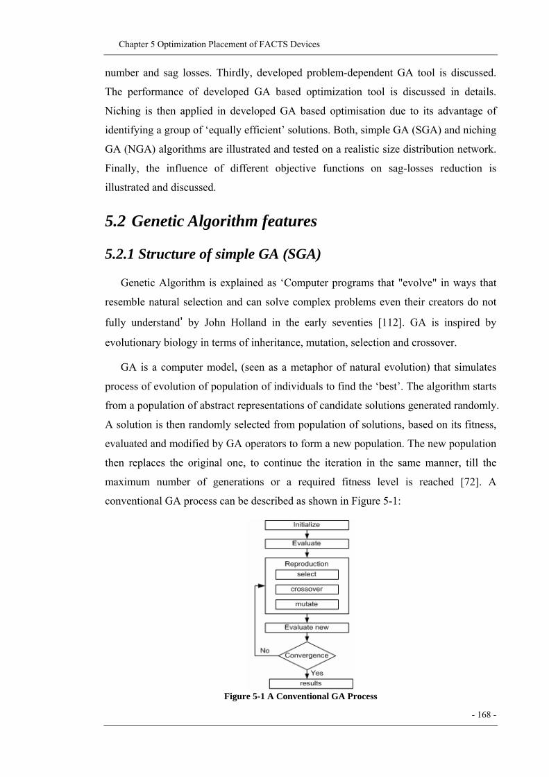
Chapter 5 Optimization Placement of FACTS Devices
- 168 -
number and sag losses. Thirdly, developed problem-dependent GA tool is discussed.
The performance of developed GA based optimization tool is discussed in details.
Niching is then applied in developed GA based optimisation due to its advantage of
identifying a group of ‘equally efficient’ solutions. Both, simple GA (SGA) and niching
GA (NGA) algorithms are illustrated and tested on a realistic size distribution network.
Finally, the influence of different objective functions on sag-losses reduction is
illustrated and discussed.
5.2 Genetic Algorithm features
5.2.1 Structure of simple GA (SGA)
Genetic Algorithm is explained as ‘Computer programs that "evolve" in ways that
resemble natural selection and can solve complex problems even their creators do not
fully understand’ by John Holland in the early seventies [112]. GA is inspired by
evolutionary biology in terms of inheritance, mutation, selection and crossover.
GA is a computer model, (seen as a metaphor of natural evolution) that simulates
process of evolution of population of individuals to find the ‘best’. The algorithm starts
from a population of abstract representations of candidate solutions generated randomly.
A solution is then randomly selected from population of solutions, based on its fitness,
evaluated and modified by GA operators to form a new population. The new population
then replaces the original one, to continue the iteration in the same manner, till the
maximum number of generations or a required fitness level is reached [72]. A
conventional GA process can be described as shown in Figure 5-1:
Figure 5-1 A Conventional GA Process
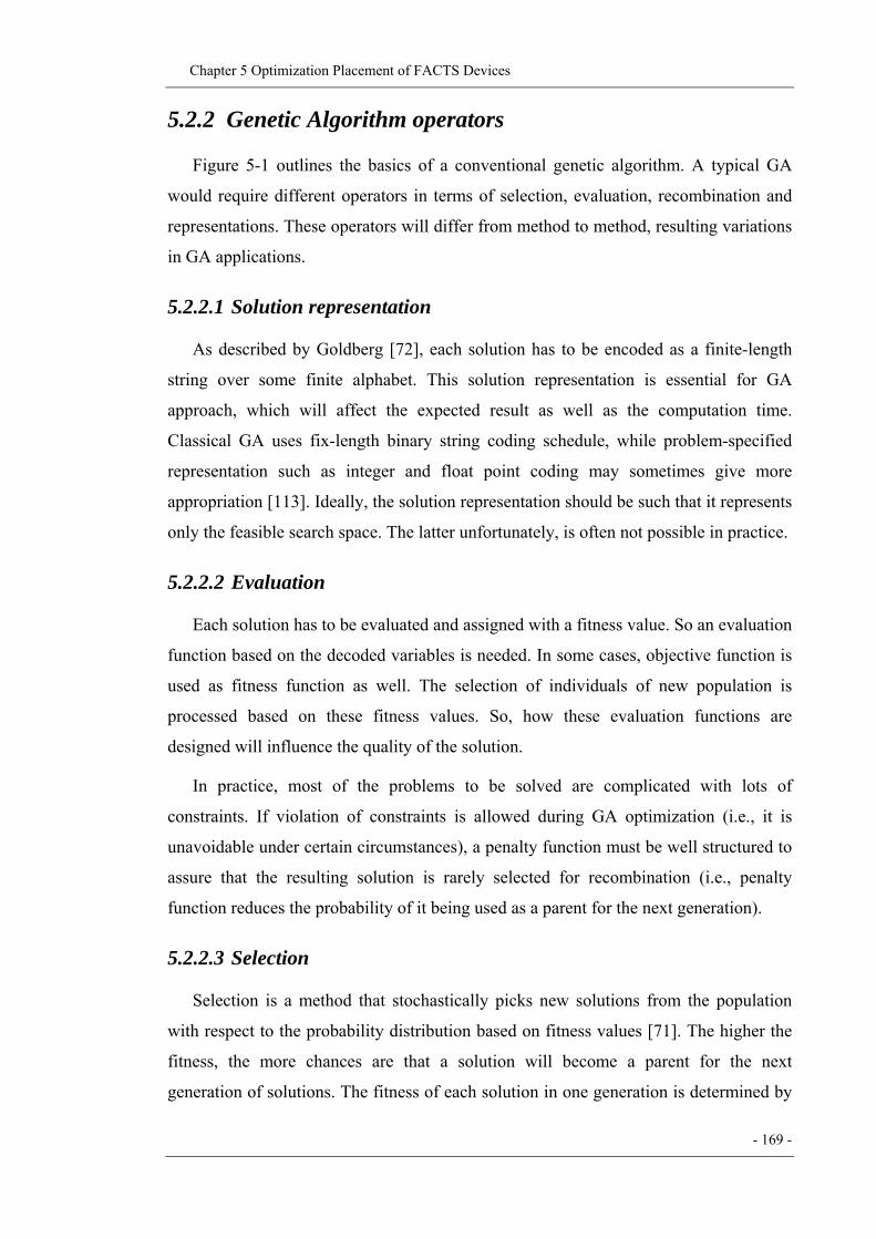
Chapter 5 Optimization Placement of FACTS Devices
- 169 -
5.2.2 Genetic Algorithm operators
Figure 5-1 outlines the basics of a conventional genetic algorithm. A typical GA
would require different operators in terms of selection, evaluation, recombination and
representations. These operators will differ from method to method, resulting variations
in GA applications.
5.2.2.1 Solution representation
As described by Goldberg [72], each solution has to be encoded as a finite-length
string over some finite alphabet. This solution representation is essential for GA
approach, which will affect the expected result as well as the computation time.
Classical GA uses fix-length binary string coding schedule, while problem-specified
representation such as integer and float point coding may sometimes give more
appropriation [113]. Ideally, the solution representation should be such that it represents
only the feasible search space. The latter unfortunately, is often not possible in practice.
5.2.2.2 Evaluation
Each solution has to be evaluated and assigned with a fitness value. So an evaluation
function based on the decoded variables is needed. In some cases, objective function is
used as fitness function as well. The selection of individuals of new population is
processed based on these fitness values. So, how these evaluation functions are
designed will influence the quality of the solution.
In practice, most of the problems to be solved are complicated with lots of
constraints. If violation of constraints is allowed during GA optimization (i.e., it is
unavoidable under certain circumstances), a penalty function must be well structured to
assure that the resulting solution is rarely selected for recombination (i.e., penalty
function reduces the probability of it being used as a parent for the next generation).
5.2.2.3 Selection
Selection is a method that stochastically picks new solutions from the population
with respect to the probability distribution based on fitness values [71]. The higher the
fitness, the more chances are that a solution will become a parent for the next
generation of solutions. The fitness of each solution in one generation is determined by

Chapter 5 Optimization Placement of FACTS Devices
- 170 -
its objective value, which is calculated in the evaluation process. There are three main
types of selection methods: fitness-proportionate, ranking and tournament [71].
5.2.2.4 Recombination
Following the selection, “parent” solutions are recombined to get the “offspring”.
This is usually achieved using crossover and mutation operators. Crossover exploits the
current solutions by exchanging elements of selected parents. One-point or two-point
crossovers are commonly used [72]. Mutation is GA operator which introduces random
changes into solutions after crossover.
5.2.2.5 Stop criteria
Stop criteria defines when to stop the GA process. If the process is stopped too early
the GA will not search enough of solution space to find the global solution. On the
other hand, the computation time will significantly increase if the “search” lasts too
long [71]. Three types of stopping criteria are usually adopted in most GA approaches:
1) Fixed number of generations or iterations reached; 2) Solution has not significantly
changed in the last several iterations; 3) Target value has been reached.
5.2.3 Genetic Algorithm parameters
GA is a rather rough algorithm, which can be tailored to individual problem and
implemented with many different variations to improve its performance. Although the
operating parameters of GA might not affect the final result, they would certainly have
influence on computation time and on the efficiency of GA.
5.2.3.1 Population size
How many solutions should be in iteration? This is the first important choice faced
by any GA users. If the population size is too small, GA may converge too quickly; if it
is too large, GA may waste computational resources: the waiting time for an
improvement might be too long [114]. Goldberg provides a theoretical analysis of the
population size in [72]. In case of simple GA, the size of population remains constant
through the entire process. However, some algorithms such as GAVaPS (Genetic
Algorithm with Varying Population Size) [71] try to optimize the population size at

Chapter 5 Optimization Placement of FACTS Devices
- 171 -
different stages of the search process, which has been proven to have strong influence
on the computational time (i.e., the computational time is reduced).
5.2.3.2 Selection pressure
Selection is a process to pick the “best” solutions from old population according to
their fitness. However, it cannot be based solely on choosing the “best” because they
may not be even close to the optimal solution [114]. The selection pressure defines the
degree to which better individuals are favourites. High selection pressure may lead GA
to converge in a local optimum. In general [113], if the selection pressure is too high
(e.g., 1), then a superior individual strongly dominates the less fit individuals and this
may lead the GA to converge prematurely to a local optimum.
5.2.3.3 Crossover rate and mutation rate
Crossover rate is the percentage of the solutions form the population of offspring
produced in each generation to the population size [66]. Mutation rate is the percentage
of the total number of genes in the population which controls the number of new genes
to be introduced into the population for a trial. If they are too low, a lot of solution
space will never be investigated. If they are high a computation time will be too long.
The method of “elitism” [114] is often used in some GA algorithms, by which at
least one of a generation's best solutions is copied without changes to a new population,
so the best solution can survive to the succeeding generation.
5.2.4 Niching technique
5.2.4.1 Solving PQ problems
It is important to acknowledge that usually there is no single best solution to power
quality problems. For each type of problem, there is a range of possible mitigation
approaches. In the real world, several problems would co-exist, and the solutions
applied should be compatible with each other (i.e., not interfering with each other).
So, in the realm of optimization, quite often there is a need to identify several good
solutions for a problem, as opposed to one optimal solution. This need arises from
several sources. Often, an optimization problem is a simplification of a real world
problem that in part requires human or unquantifiable judgment. In these types of

Chapter 5 Optimization Placement of FACTS Devices
- 172 -
problems, an optimizer needs to suggest various possible alternatives that can later be
judged by a human expert. In other situations, a better understanding of a search space
is desired in terms of the location of its various optima [115].
For the problem of FACTS placement with the objective to improve system sag
performance, it might be more appropriate to identify a group of feasible solutions,
which can be later examined and finely tuned by a human expert. The reasons for this
include:
• The optimization problem has never been simple in a real world. The ‘best’
solution may be unfeasible to be employed when taking into account
environmental, political and other considerations.
• Several problems would co-exist in power system, e.g., the system may suffer
from harmonic as well as voltage sag disturbances. Hence, the solutions
applied should be compatible with each other. Multi-objective function may be
used in this situation. Some non-technical issues however, may not be able to
be statistically described. It is also very difficult to choose the right weighting
parameters.
• Usually there is no single solution to power system problems. For each type of
problem, there is often a range of possible solutions.
• It gives more flexibility to suggest initially several possible solutions, which
can then be ‘post-processed’ using other criteria in order to select the most
suitable one.
5.2.4.2 Application of Niching technique to GA
While a simple GA is capable of finding optimum for various functions, it tends to
converge to local optima when the search domain contains some local or global maxima
(i.e., multimodal problem). Niching method encourages GA to explore more search
space by maintaining genes’ diversity in the population and thereby converges to the
global optima [92]. GA that incorporates niching is capable of locating multiple,
optimal solutions within a single population.
Various methods were devised to solve multimodal problem by niching. The
niching methods generally can be classified along two dimensions of behaviour [116] as
illustrated in Table 5-1.

Chapter 5 Optimization Placement of FACTS Devices
- 173 -
Table 5-1 Niching Methods [116] Single Environments Multiple Environments
Over specification Temporal Sequential Location Ecological GA
Heterozygote Advantage Crowding
Ecological GA
Restricted Competition Spatial
Fitness Sharing Immune Systems
Restricted competition borrows the ecological rule that species that coexist tend to
occupy different environmental niches, so they typically do not compete for resources.
This method, introduced by Goldber, Deb and Korb [116], was recommended for
solving problems of varying sub-function scale, not for locating multiple solutions. Lee
[117] developed a new niching method based on restricted competition selection to
identify and search multiple niches efficiently in a multimodal domain and showed that
restricted competition selection method performs better than two general methods
(Deterministic Crowding and Fitness Sharing).
5.3 Objectives of placement of FACTS devices
5.3.1 Technical objective – to Reduce numbers of sags
As discussed in Chapter 2, system sag performance is typically presented in the
form of sag number (combined with sag magnitude and frequency) and sag duration.
Technically, one can say that the sag performance of the system is improved if the
number of sags in the system is reduced by the installation of FACTSD.
In order to represent sag performance in optimization process, it is necessary to
quantify it by a simple number measure which should carry valuable information.
Hence, a formula that combines number of sags in different magnitude ranges is used
here to quantify the system sag performance. It is given by (5.1):
1 2 3sag LL L MN wV w V w V= + + (5.1)
Where w1, w2 and w3 are weighting coefficients specifying desired shift of sags from
a particular magnitude range such that w1 + w2 + w3 = 1. VLL, VL and VM are number of
expected voltage sags in certain voltage magnitude range defined as:
• VLL: the number of voltage sags with magnitude between 0.7 p.u. and 0.9 p.u.
• VL: the number of voltage sags with magnitude between 0.4 p.u. and 0.7 p.u.
• VM: the number of voltage sags with magnitude below 0.4 p.u.

Chapter 5 Optimization Placement of FACTS Devices
- 174 -
With (5.1), the objective of optimization becomes to minimise the number of
‘influential’ voltage sags in the entire network, i.e.,:
1 2 31
min min ( )SN
sag LLi Li Mii
N wV w V w V=
= + +∑ (5.2)
Where sN is the numbers of buses in the network.
5.3.2 Financial objective— to Reduce sag cost
Placements of FACTS devices could reduce the number of voltage sags that end
users would experience. However the ultimate reason for placement is always financial.
It has been proved in Chapter 4 that significant losses can be saved if a sufficient
investment in mitigating device was made. The cost of device is offsetting the potential
benefits from its application as shown in Figure 5-2.
Figure 5-2 Minimizing power quality improvement costs
Generally, the more is invested in sag mitigation devices, the lower sag losses would
be. The objective of the optimization therefore is to find financially sound solutions.
Building on discussion in Chapter 4 regarding financial analysis methods, the feasible
objective functions are:
1) Minimize the pay back year
-
=+
capitalyear
sag saving mnt
Cmin( n )
C C (5.3)
2) Maximise NPV value
1
max( )(1 )
Nsag saving mnt
capital nn
C CNPV C
r−
=
−= +
+∑ (5.4)

Chapter 5 Optimization Placement of FACTS Devices
- 175 -
5.4 Application of GA for allocation of FACTS devices
5.4.1 Implemented Simple GA
The GA based optimization implemented in this study aimed to find the ”best”
connection point (location) of FACTS devices in the network and the appropriate type
and rating of those devices based on the assessment of network sag performance.
5.4.1.1 Solution representation
Approximations or random variables of several combinations of FACTS devices of
different rating, type and location are formed into an initial population, which can be
represented by a ( )n m s× × matrix as shown in Figure 5-3. Real number representation
is implemented. Where n is the size of each solution in population, s is the population
size (s solutions in one population) and m is the number of variables optimized (location,
size and type). In this study, = 6 = 3 = 20n ,m ,s , which means that there are six
allocated devices, three variables per device and twenty solutions (total size of each
6 3× ) in each population. In the matrix representation shown in Figure 5-3, the first
column represents bus numbers where FACTSD are placed, second column is the type
of device (1: STATCOM 2: SVC 3: DVR), third column is the sizes of FACTSD in p.u.
Figure 5-3 Population representation
5.4.1.2 Evaluation
Equation (5.2), (5.3) and (5.4) are used as objective functions to guide the
optimization process. Each solution in the population is evaluated by the methodology
developed and value of objective function calculated. After that, a linear scaling
function is employed to map these raw objective values into more desirable range. The
fitness values are between 0 and 1..

Chapter 5 Optimization Placement of FACTS Devices
- 176 -
5.4.1.3 Reproduction
Firstly solutions are selected using roulette wheel method. Every parent has a
probability of being selected that is proportional to its fitness. The better the solutions
are, the more chances they have to be selected for the next generation.
Single point crossover is applied afterwards. Mating of pairs of individuals is
performed randomly. A random position in one individual is selected to be the
crossover point. The two individuals then exchange the portions in front of or behind of
the crossover point. There should be no more than one device at each bus. In order to
prevent unfeasible solution in the population, each pair of individuals, which are
randomly paired to do crossover, would adjust their order with respect to the optimized
variables. Figure 5-4 illustrate the one-point crossover proposed, portions to be
exchanged are in shadow blue. As described in Figure 5-4 (a), location of FACTSD
‘63’ appears in both parents (1) and (2). So FACTSD in parent (2) adjusts its order of
FACTSD first, then crossover is applied at point 10 (there are 3 6 18× = points in each
parent). All variables after point 10 switched their place as shown in Figure 5-4 (b).
Figure 5-4 Problem specified crossover
After a crossover is performed, mutation takes place. The mutation is done bit-by-
bit on entire population. A randomly real value is generated to determine where a gene
of population is to be mutated. In order to make sure that there is one device per bus
extra care should be taken so that the randomly generated bus numbers would not be the
same as those already existing in each solution.

Chapter 5 Optimization Placement of FACTS Devices
- 177 -
5.4.1.4 Stop criteria
The GA stop criteria adopted here is that the process stops when the best solution’s
fitness value doesn’t change for 30 iterations because the solutions are considered to be
stable if 30 generations produce the same objective value. Otherwise the process stops
when 100 generations are reached in order to finish the simulation in a reasonable time.
What is the efficient value of maximum generation and how to decide the iteration is
converged are very problem dependent, large number of simulations are required to
approach optimal values. The maximum number of generations (100) and the number
of unchanged iterations (30) are adopted here based on recommended values from
literature.
5.4.2 Niching in GA
5.4.2.1 Distance of each solution
Niching methods need a method to calculate distance between each two individuals.
The performance of a niching method is directly tied to the suitability of its differencing
function [116].
A strategy has to be developed to differentiate similar individuals from dissimilar
ones. This can be seen as ‘distance’ between individuals. The ‘distance’ can be either
real parameter of the search space or the degree of similarity between individuals.
The distance between buses is used for optimal placement of FACTS devices in this
study. It is assumed that the FACTSD located at electrically close buses are solutions
with high similarities. The distance between each two individuals can be calculated by
the closeness between the locations of FACTSD in two solutions: Firstly, a ‘bus map’ is
generated in which each load bus is assigned a series of ‘nearby buses’, as shown in
Table 5-2. Table 5-2 Bus map table
Bus Neighbouring buses 1 55 1 4 56 2 2 55 3 2 178 72 … … … 29 30 27 29 25 89 88 89 286 81 … … …

Chapter 5 Optimization Placement of FACTS Devices
- 178 -
Secondly, two competing solutions are selected (as shown in Figure 5-5). If there
are FACTS devices located at buses that appear in the same row of bus map (Table 5-2),
then the distance is equal to the number of such pairs (pairs of closely located FACTS
devices). For example in Figure 5-5 solution 1 includes buses 29, 50, 11, 63, 89 and 143
and solution 2 buses 147, 21, 95, 25, 81 and 55.
Figure 5-5 Distance between individuals
Bus 25 appears in the neighbourhood of bus 29 in ‘bus map’ of Table 5-2, and bus
81 in the neighbourhood of bus 89, so the distance between the solutions (individuals)
in Figure 5-5 is 2d = .
5.4.2.2 Inclusion of Niching
In this study, a restricted competition selection based niching method is employed,
in which individuals compete to survive within a similar range. The outline of the
method is as follows:
1. Generate initial population with s individuals randomly ( 20s = ).
2. Select M individuals which are the most far away from each other ( 10M = ).
3. Generate new population by crossover and mutation.
4. (Competition selection) For 1:i M= and 1:j N= When 2ijd > , compare
fitness. Set the ‘loser’s’ fitness set to 0. (If the loser is from M individuals,
replace the individual).
5. Select s individuals from (M+s) individuals in the fitness order.
Repeat steps 2-5 until the stop criterion is reached.
5.5 Simulation Results
The GA implemented in this study is coded in MATLAB. And the characteristics of
the implemented GA are given in Table 5-3:

Chapter 5 Optimization Placement of FACTS Devices
- 179 -
Table 5-3 Characteristics of implemented GA Solution representation real number, matrix
Population 20 Stop criteria max generation (200) Mutation rate 0.03
Crossover rate 0.8
Fitness value ranking Selection method roulette wheel
Some key economic indicators employed for objective functions (5.3) and (5.4) are:
• Many utility assets arguably have useful lifetime of 40-50 years. This analysis
has used only 15 (n = 15) years to be somewhat more conservative and
intrinsically attribute less value to far distant cash flows than present ones.
• The assumed maintenance cost of devices is as follows: STATCOM 15% of its
capital cost; DVR 15% of its capital cost; SVC 10% of its capital cost
• The assumed discount rate (r) is assumed 15%.
Three types of devices are placed: STATCOM, DVR and SVC. The rating of SVC
and STATCOM should be 100MVAR≤ of DVR 50MVAR≤ . Only reactive power is
considered here to simplify the simulations
5.5.1 Results with simple GA
5.5.1.1 Reduce number of sags
The sag performance of the entire network is shown in Table 5-4. Total number of
potential sag in the network is 520,510 of which there are 60359 sags with magnitude
below 0.4 p.u.. Most of the faults however will not cause sags at all, as shown in Table
5-4, i.e., for 73.69% sags will have voltage magnitude >0.9 p.u.
It has to be pointed out that through out the research, worst affected phase
assumption results in equivalent three phases sag with sag magnitude in all three phase
equal to magnitude of worst affected phase. The sag performance is worsen by this
assumption. The number of sags in different magnitude ranges is shown in Table 5-4
for both cases, worst affected phase and all sag magnitudes per phase. Throughout this
study, worst affected phase assumption is used in order to simplify the simulation and
to be able to investigate the worst case scenario during the assessment procedure.

Chapter 5 Optimization Placement of FACTS Devices
- 180 -
Table 5-4 Sag performance without FACTS 1. worst phase 2. three phases
VLL(<0.4) 6.04e+04 11.60% 2.59e+04 4.97% VL(0.4-0.7) 4.24e+04 8.16% 1.94e+04 3.74% VM(0.7-0.9) 3.41e+04 6.55% 2.05e+04 3.94%
VH(>0.9) 3.83e+05 73.69% 4.53e+05 87.35% Total 5.20e+05 100.00% 5.20e+05 100.00%
Objective function (5.2) is used to guide the process of optimization. Different
weighing factors ( 1 2 3, ,w w w ) are employed as shown in Table 5-5. The weighing factors
indicate that different “pressure” has been applied to sag of different magnitude. As a
result, three objective functions ( 1, 2, 3f f f ) were actually used at this stage of research.
Table 5-5 Weightings used in different objective functions Weighing
Objective function w1 w2 w3 f1 0.7 0.2 0.1 f2 0.33 0.33 0.33 f3 0.1 0.2 0.7
Three GA based optimisations are performed using OF of f1, f2 and f3 respectively.
The results are given in Table 5-6 and Figure 5-6.
Table 5-6 Optimized system sag performance
As a consequence of placement of FACTS devices in the network, the total number
of expected voltage sags (sum of the sags in different magnitude ranges) is reduced
except in HV range where it is increased (as expected) as shown in Figure 5-6 and Table
5-6. It can be seen that the network sag performance with all three OF improved (f1, f2
and f3 values are reduced, as shown in right hand side of Figure 5-6). It can be also seen
though, that quite different solutions are obtained with different OF. With f1, the focus
is on mitigating voltage sags with magnitudes below 0.4 p.u., while f3 focuses on
mitigation of sags with magnitudes between 0.7 and 0.9p.u. From Table 5-6, the
reduction in objective function f1 (w1 = 0.7) and f3 (w3 = 0.7) are very close, 24.47%
VLL VL VM VH objective value f1 f2 f3
base 60359 42419 34058 383310 54141 45156 38360-25.29% -28.56% -4.14% 7.51% -24.47%
f1 45093 30303 32684 412110 41037 -21.00% -13.73% -18.15% 6.44% -18.04%
f2 47683 36593 27875 408000 37067 28.78% -7.78% -43.11% 0.16% -23.99%
f3 77728 39117 19375 383930 29185

Chapter 5 Optimization Placement of FACTS Devices
- 181 -
and 23.99% respectively. Objective function f2, which has equal weightings for three
voltage magnitude ranges (w1=w2=w3=0.33) leads to smallest reduction in objective
function.
0.00E+00
2.00E+04
4.00E+04
6.00E+04
8.00E+04
f1 f2 f3Objective functions
baseoptimized
0.00E+00
2.00E+04
4.00E+04
6.00E+04
8.00E+04
<0.4 0.4-0.7 0.7-0.9 >0.9sag magnitude range
sag
num
bers
basef1f2f3
0.00E+00
1.50E+05
3.00E+05
4.50E+05
Figure 5-6 Optimization results
11.60%
8.16%
6.55%
73.69%
8.67%5.83%
6.28%
79.22%
9.17%
7.04%
5.36%
78.44%
14.94%
7.52%
3.72%
73.81%
<0.4
0.4-0.7
0.7-0.9
>0.9
(A) basecase (B) f1
(C) f2 (D) f3
Figure 5-7 Number of sags in percentage with different OFs
Figure 5-7 presents numbers of sags in different magnitude ranges (<0.4, 0.4-0.7,
0.7-0.9 and >0.9) as percentage of total number of sags. Since the total number of
simulated faults is constant, the changes in percentage of VLL, VL and VM indicated the
effectiveness of OFs f1, f2 and f3. Using sags with magnitude below 0.4 as measure of
OF effectiveness Figure 5-7 (B) confirms that f1 is the most effective OF.

Chapter 5 Optimization Placement of FACTS Devices
- 182 -
The solutions of FACTSD allocation with f1, f2 and f3 are listed in Table 5-7. They
are quite different as expected due to different OF used.
Table 5-7 Solutions with Simple GA f1 f2 f3
Bus Type Size Bus Type Size Bus Type Size 100 DVR 37.5 51 DVR 47.5 165 SVC 90 232 SVC 50 64 DVR 20 163 SVC 45 150 STAT 90 62 DVR 45 103 SVC 85 89 SVC 50 35 DVR 42.5 62 DVR 47.5 148 STAT 80 232 SVC 40 134 DVR 7.5 142 DVR 20 145 STAT 75 145 SVC 95
The optimisation described takes into account only the worst affected phase i.e.,
equivalent three phase sags. The sag performance of the entire network however was
improved in each phase respectively. The sags in different magnitude ranges after
optimisation obtained when considering all three phases respectively are listed in Table
5-8 and Figure 5-8. The pattern of reductions in sag numbers VLL, VL, VM for different
OFs is the same as before though, actual percentages are different as expected. Same as
before f1 leads to biggest reduction in optical sags. (About 66% reduction in sags with
magnitude 0.7< .)
Table 5-8 Sag number reduction with three phases considered
Vll Vl Vm Vh
base 25862 19428 20513 454333
-31.22% -25.27% -23.40% 3.92% f1 17787 14518 15712 472130
-26.76% -19.44% -14.14% 3.00% f2 18941 15651 17613 467950
22.60% -2.90% -16.66% -0.41% f3 31706 18865 17095 452480
The sag profiles of the entire network (presented using generalized sag table)
without mitigation and with the optimal solutions with f1, f2 and f3 are shown in Figure
5-9 (A), (B), (C) and (D).

Chapter 5 Optimization Placement of FACTS Devices
- 183 -
4.97%3.74%
3.94%
87.35%
3.42%2.79%3.02%
90.77%
3.64%3.01%
3.39%
89.96%
6.01%3.63%
3.29%
86.99%
<0.4
0.4-0.7
0.7-0.9
>0.9
(A)base
(B) f1
(C) f2 (D) f3
Figure 5-8 Number of sags in percentage with different OFs
(A) without mitigation
(B) f1 optimized

Chapter 5 Optimization Placement of FACTS Devices
- 184 -
(C) f2 optimized
(D) f3 optimized
Figure 5-9 Generalized Sag Tables
With each of the three optimal mitigation solutions, sags are effectively shifted from
low magnitude ranges (lower left hand corner of the table) to high magnitude ranges
(upper right hand corner of the table) as shown in Figure 5-9 (B), (C) and (D). The
reductions in different sag magnitude ranges can be obviously tailored by appropriate
selection of weighting coefficients and they vary depending on the objective function
(i.e. weighting coefficients) used. (e.g., Number of sags with all three phase voltages
below 40% is reduced from 540.91 to 451.59 (-16.5%) and 473.51 (-12.5%) by f1, and
f2 respectively, while number of sags with all three phase voltages above 90% is
increased from 3.83e5 (383314.93) to 4.12e5 (411989.01) (+7%), and 4.08e5
(407934.47) (+6.4%) with f1 and f2 respectively. The effect of mitigation with f3 is
most pronounced in case of sags with magnitudes within range between 0.7 and 0.9 p.u.
where initial 1546.59 three phase sags were reduced by 47%, (down to 817.93).

Chapter 5 Optimization Placement of FACTS Devices
- 185 -
From selected set of objective functions used in this analysis (for illustration of the
methodology), the objective function f1 (Figure 5-9 (B)) is the most effective as shown
in Figure 5-9. The number of sags with magnitudes below 40% in two phases is
reduced the most and the sags are "pushed" much further towards high voltage
magnitude range compared to f2 and f3 (Figure 5-9 (C), (D)). The biggest reduction of
objective function value also comes from the optimization with f1. So, the optimization
with f1 (emphasis on sags with magnitudes less than 0.4 p.u., i.e., w1 = 0.7) is the most
effective in terms of reducing number of critical sags.
The OFs’ values used in three optimizations are shown in Figure 5-10, Figure 5-11
and Figure 5-12 against the number of GA generations. It can be seen that the value of
f1 reduced rapidly in the first ten generations (Figure 5-10), then continued to decrease
slowly, and finally stabilized in the last fifteen generations. This shows that the GA
converges well in the application of the placement of FACTSD. The same general
pattern of convergence is also observed in case of f2 and f3.
0 10 20 30 40 50 60 70 80 90 1004
4.2
4.4
4.6
4.8
5
5.2
5.4x 10
4
GA generation
obje
ctiv
e f1
Figure 5-10 Convergence of optimization with f1
0 10 20 30 40 50 60 70 80 90 1003.7
3.8
3.9
4
4.1
4.2
4.3
4.4
4.5x 10
4
GA generation
objective f2
Figure 5-11 Convergence of optimization with f2
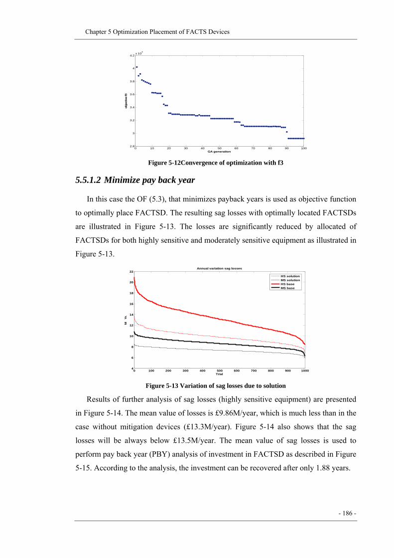
Chapter 5 Optimization Placement of FACTS Devices
- 186 -
0 10 20 30 40 50 60 70 80 90 1002.8
3
3.2
3.4
3.6
3.8
4
4.2x 10
4
GA generation
obje
ctiv
e f3
Figure 5-12Convergence of optimization with f3
5.5.1.2 Minimize pay back year
In this case the OF (5.3), that minimizes payback years is used as objective function
to optimally place FACTSD. The resulting sag losses with optimally located FACTSDs
are illustrated in Figure 5-13. The losses are significantly reduced by allocated of
FACTSDs for both highly sensitive and moderately sensitive equipment as illustrated in
Figure 5-13.
0 100 200 300 400 500 600 700 800 900 10004
6
8
10
12
14
16
18
20
22Annual variation sag losses
Trial
M
Yr.
HS solutionMS solutionHS baseMS base
Figure 5-13 Variation of sag losses due to solution
Results of further analysis of sag losses (highly sensitive equipment) are presented
in Figure 5-14. The mean value of losses is £9.86M/year, which is much less than in the
case without mitigation devices (£13.3M/year). Figure 5-14 also shows that the sag
losses will be always below £13.5M/year. The mean value of sag losses is used to
perform pay back year (PBY) analysis of investment in FACTSD as described in Figure
5-15. According to the analysis, the investment can be recovered after only 1.88 years.

Chapter 5 Optimization Placement of FACTS Devices
- 187 -
6.5 7.5 8.5 9.5 10.5 11.5 12.5 13.50
0.04
0.08
0.12
0.16
0.2
0.24
0.28
0.32
0.36
0.4
sag losses in M year
prob
abili
ties
cum
ulat
ive
high sensitivity
6.5 7.5 8.5 9.5 10.5 11.5 12.5 13.50
0.1
0.2
0.3
0.4
0.5
0.6
0.7
0.8
0.9
1
mean:9.8572M
Figure 5-14 sag losses
Figure 5-15 Pay back year analysis of the solution
The placements of FACTSDs obtained from this optimization are shown in Table
5-9. The convergence characteristic of the GA optimization is shown in Figure 5-16.
Table 5-9 Mitigation solution bus type Size(MVAR)50 SVC 45 14 SVC 15 89 SVC 40 43 SVC 15
111 DVR 5 136 SVC 10

Chapter 5 Optimization Placement of FACTS Devices
- 188 -
0 10 20 30 40 50 60 70 80 90 1000
5
10
15
20
25
GA generation
Obj
ectiv
e pa
y ba
ck y
ear
Figure 5-16 GA approach
5.5.1.3 Maximize NPV
Objective function (5.4) is used to guide the GA optimization process in this case.
With six devices optically allocated in the network, the sag losses per year reduce
significantly both with highly sensitivity and moderately sensitivity equipment as
shown in Figure 5-17. The losses with highly sensitive equipment are further analysed
in Figure 5-18.
0 100 200 300 400 500 600 700 800 900 10004
6
8
10
12
14
16
18
20
22Annual variation sag losses
Trial
M
Yr.
HS baseMS baseHS solutionMS solution
Figure 5-17 Sag losses
The mean value of sag losses in the entire network is £10.95M/year as shown in
Figure 5-18. The most possible annual sag losses are about £9.5 M/year. Same as with
PBY before, Net Present value analysis using the mean value of sag losses is further
detailed in Figure 5-19. Five years after the investment, positive NPV value is obtained
and fifteen years after the investment (assumed life expectation of FACTSD), the NPV
rises to £6.07 M.

Chapter 5 Optimization Placement of FACTS Devices
- 189 -
7.5 8.5 9.5 10.5 11.5 12.5 13.5 14.5 15.5 16.5 17.50
0.05
0.1
0.15
0.2
0.25
sag losses in M year
prob
abili
ties
cum
ulat
ive
high sensitivity
7.5 8.5 9.5 10.5 11.5 12.5 13.5 14.5 15.5 16.5 17.50
0.1
0.2
0.3
0.4
0.5
0.6
0.7
0.8
0.9
1
mean:10.9458M
Figure 5-18 Sag cost with and without the solution
0 1 2 3 4 5 6 7 8 9 10 11 12 13 14 15-10
-5
0
5
10
year
sag
loss
es in
M
year
0123456789101112131415
5.79000000000000000
00.610.610.610.610.610.610.610.610.610.610.610.610.610.610.61
02.352.352.352.352.352.352.352.352.352.352.352.352.352.352.35
-5.791.741.741.741.741.741.741.741.741.741.741.741.741.741.741.74
-5.791.561.391.241.110.990.880.790.7
0.630.560.5
0.450.4
0.360.32
-5.79-4.24-2.85-1.61-0.50.491.372.162.863.494.054.55
55.4
5.756.07
year capital Mnt(M Save(M Cash(M PV(M NPV(M
Figure 5-19 NPV analysis of optimized results
The allocation of FACTSDs obtained in this case is shown in Table 5-10. The
convergence characteristic of the GA optimization is shown in Figure 5-20. The NPV is
increasing with number of generations as expected. The convergence is not so good
however, which indicates that further improvement of the GA is possible.
Table 5-10 Optimized solution bus type Size(MVAR)137 SVC 15 40 SVC 10 34 SVC 30 89 SVC 30
106 STAT 15 146 SVC 30

Chapter 5 Optimization Placement of FACTS Devices
- 190 -
0 10 20 30 40 50 60 70 80 90 1001
2
3
4
5
6
7
GA generation
obje
ctiv
e N
PV
Figure 5-20 GA approach
5.5.2 Results with Niching GA
5.5.2.1 Reduce number of sags
From selected set of objective functions used in the analysis so far, the objective
function f1(Figure 5-9 (B)) is proved to be the most effective as illustrated in previous
sections. The application of NGA is therefore illustrated only with objective function f1.
The selected results with NGA are illustrated in Figure 5-21. The results of the
optimization (the placement of FACTS devices) are shown in Table 5-11. Out of 10
resulting solutions, as defined by the algorithm, only 5 fittest (with smallest objective
function values) are illustrated here.
0.00E+00
2.00E+04
4.00E+04
6.00E+04
<0.4 0.4-0.7 0.7-0.9 >0.9 fResidul voltage in p.u.
Even
t per
yea
r
no mitigation S1S2 S3S4 S5
0.00E+00
1.50E+05
3.00E+05
4.50E+05
>0.9
Figure 5-21 Sag performance with different solutions f1

Chapter 5 Optimization Placement of FACTS Devices
- 191 -
Solutions with f1 are showing reduction of 17% to 25% (Table 5-11) in total
number of sags. More importantly, it can be seen that the locations of FACTS devices
are quite different in different solutions even though the effectiveness of the solutions
are similar. If the only criterion considered in the optimization is the sag number
reduction, the 1st solution should be selected. However, if other/additional evaluation
criteria, e.g., the total size of devices, the price of the devices, etc., are considered the
choice may differ.
The five fittest solutions obtained in the last generation by applying SGA for
objective function f1 are also shown in Table 5-11 for comparative purposes. It can be
seen that all these solutions are very close to each other in terms of FACTS devices
locations although the values of objective function differ (but the difference is smaller
than in case of NGA, 5% compared to about 7.2%). The achieved reduction in objective
function value with SGA (24.47%) is close to the most effective solution (24.99%)
obtained with NGA and shown in Table 5-11.
Table 5-11 Solutions from NGA and GA (five solutions with least objective value)
Bus 197 163 232 22 148 78 100 232 150 89 148 142
Type DVR DVR STAT SVC SVC SVC DVR SVC STAT SVC STAT DVR
Size(Mvar) 37.5 10 60 80 25 25 37.5 50 90 50 80 20 objective 4.06E+04 4.09E+04 Reduction
1
24.99%
1
24.47%
Bus 40 232 148 66 89 154 100 232 150 89 148 142
Type DVR SVC SVC DVR SVC STAT DVR SVC STAT SVC STAT DVR
Size(Mvar) 25 50 30 25 35 25 37.5 50 90 50 80 20
objective 4.09E+04 4.09E+04
Reduction
2
24.43%
2
24.47%
Bus 61 232 220 108 93 142 100 232 150 89 148 142
Type DVR SVC DVR SVC STAT STAT DVR SVC STAT SVC STAT STAT
Size(Mvar) 17.5 35 27.5 35 40 95 37.5 50 90 50 80 70 objective 4.34E+04 4.12E+04 Reduction
3
19.77%
3
23.89%
Bus 152 78 164 190 150 145 100 232 150 89 148 223
Type STAT DVR DVR DVR SVC STAT DVR STAT STAT SVC STAT DVR
Size(Mvar) 75 25 20 45 30 95 37.5 50 90 65 80 20 objective 4.42E+04 4.13E+04 Reduction
4
18.22%
4
23.72%
Bus 152 78 164 190 150 145 100 232 150 89 148 142
Type STAT DVR DVR DVR SVC STAT DVR SVC DVR SVC STAT SVC
Size(Mvar) 75 25 20 45 30 95 37.5 50 90 50 80 40
objective 4.42E+04 4.30E+04
Niching GA
Reduction
5
18.22%
Simple GA
5
20.50%

Chapter 5 Optimization Placement of FACTS Devices
- 192 -
Having in mind that both, SGA and NGA used the same population size and
generation times the NGA performs better than SGA with the same computational
effort as it escapes local optima and gives more options for final selection of the most
appropriate techno-economic solution.
The convergence characteristic of the NGA optimization is shown in Figure 5-22. It
can be seen that the values of OF reduced rapidly in the first thirty generations. Then
the values continue to decrease very slowly, and finally stabilize in the last 10 or so
generations. This shows that the NGA converges well in the application for placement
of FACTSD based on reduction of number of critical sags.
0 10 20 30 40 50 60 70 80 90 1004
4.5
5
5.5x 10
4
NGA generation
obje
ctiv
e N
GA
f1
Figure 5-22 NGA f1 approach
5.5.2.2 Minimize pay back year
Same as before the implemented NGA gave several solutions, as expected. The two
of those with the smallest value of objective function are illustrated in Table 5-12.
Table 5-12 Mitigation solutions P1 and P2 solution P1 solution P2
bus type Size (MVAr) bus type Size (MVAr) 182 STAT 10 50 SVC 45 49 SVC 15 204 SVC 15 89 SVC 35 89 SVC 40 43 SVC 15 24 SVC 40
190 SVC 10 186 SVC 40 136 STAT 10 137 SVC 10
Total 95 Total 190 It can be seen from Table 5-12 that SVC dominates both solutions. Distributions of
associated sag losses are shown in Figure 5-23. The sag losses associated with highly
sensitive equipment are further analysed in Figure 5-24 (A) and (B) for solution P1 and
P2 respectively.

Chapter 5 Optimization Placement of FACTS Devices
- 193 -
0 100 200 300 400 500 600 700 800 900 10004
6
8
10
12
14
16
18
20
22Annual variation sag losses
Trial
M
Yr.
HS baseMS baseHS solution1MS solution1HS solution2MS solution2
Figure 5-23 Sag losses
7.5 8.5 9.5 10.5 11.5 12.5 13.5 14.5 15.5 16.50
0.05
0.1
0.15
0.2
0.25
sag losses in M year
prob
abili
ties
cum
ulat
ive
high sensitivity
mean:11.3033M
7.5 8.5 9.5 10.5 11.5 12.5 13.5 14.5 15.5 16.50
0.1
0.2
0.3
0.4
0.5
0.6
0.7
0.8
0.9
1
(A) Solution P1
7.5 8.5 9.5 10.5 11.5 12.50
0.04
0.08
0.12
0.16
0.2
0.24
0.28
0.32
0.36
0.4
sag losses in M year
prob
abili
ties
cum
ulat
ive
high sensitivity
mean:9.7109M
7.5 8.5 9.5 10.5 11.5 12.50
0.1
0.2
0.3
0.4
0.5
0.6
0.7
0.8
0.9
1
(B) Solution P2
Figure 5-24 Probability of annual sag losses optimized by ‘pay-back year’
The sag costs per year reduce significantly with both solutions. The costs are still
normally distributed, though with lower maximum and mean values than the case
without mitigation. The financial loss of £10.5M/year and £9.5M/year is the most likely
to happen in case of solution P1 and P2 respectively. The means of sag losses of P1 and

Chapter 5 Optimization Placement of FACTS Devices
- 194 -
P2 have reduction of £1.99M/year and £3.59M/year respectively, compared to loss of
£13.3M/year without mitigation.
Together with the costs of required FACTS devices and their associated
maintenance costs, the pay back year analysis of these two solutions P1 and P2 can be
found in Table 5-13. Financial analysis presented in Table 5-13 illustrates that 3.01 and
2.28 years are required to get back the initial investment in mitigation devices with
solution P1 and P2, respectively.
Table 5-13 Financial analysis of solutions P1 and P2 (all costs are in (M£)) Base case Solution P1 Solution P2
Sag costs (mean value) 13.3 11.3 9.71 Devices costs 0 4.52 7.59
Maintenance costs 0 0.49 0.76 Savings per year 1.99 3.59
Projected Capital Cost 4.52 7.59 Simple payback (years) 4.52/(1.99-0.49)=3.01 7.59/(3.59-0.76)=2.68
5.5.2.3 Maximize NPV
In this case, objective function (5.4) is used as objective function to guide the
optimization process. Similarly as before only two solutions with the minimum
objective function values (corresponding to maximum NPV) are analyzed (solutions N1
and N2 shown in Table 5-14).
Table 5-14 Mitigation solutions N1 and N2 solution N1 solution N2
bus type Size (MVAr) bus type Size (MVAr) 106 SVC 15 282 STAT 15 208 SVC 10 19 SVC 10 89 SVC 30 89 SVC 30 142 SVC 15 12 STAT 15 44 DVR 2.5 51 SVC 35 132 SVC 15 132 SVC 15
Total 87.5 Total 120
It can be seen from Table 5-14 that SVC again dominated both solutions since it is
cheaper than DVR and STATCOM. The cumulative probability and mean value of sag
losses as well as capital investment and maintenance cost of FACTS devices for
solutions N1 and N2 are illustrated in Figure 5-25 and Figure 5-26. The mean value of
sag costs reduced from £13.3M/year to £10.56M and £10.60M with solution N1 and N2
respectively. Solution N2, however, requires much higher capital investment than
solution N1 as shown in Figure 5-27.

Chapter 5 Optimization Placement of FACTS Devices
- 195 -
Figure 5-25 Sag losses
7.5 8.5 9.5 10.5 11.5 12.5 13.5 14.50
0.04
0.08
0.12
0.16
0.2
0.24
0.28
0.32
0.36
0.4
sag losses in M year
prob
abili
ties
cum
ulat
ive
high sensitivity
mean:10.5558M
7.5 8.5 9.5 10.5 11.5 12.5 13.5 14.50
0.1
0.2
0.3
0.4
0.5
0.6
0.7
0.8
0.9
1
(A) Solution N1
7.5 8.5 9.5 10.5 11.5 12.5 13.5 14.5 15.50
0.03
0.06
0.09
0.12
0.15
0.18
0.21
0.24
0.27
0.3
sag losses in M year
prob
abili
ties
cum
ulat
ive
high sensitivity
mean:10.5992M
7.5 8.5 9.5 10.5 11.5 12.5 13.5 14.5 15.50
0.1
0.2
0.3
0.4
0.5
0.6
0.7
0.8
0.9
1
(B) Solution N2
Figure 5-26 Probability of annual sag losses optimized by NPV
Taking the time into account, both solutions will be financially beneficial at the end
of FACTS devices economic life (15 years) as illustrated in Figure 5-27 (A) and (B).
The NPV analysis also shows that the investment in solution N1 is much more
attractive than investment in solution N2 since much higher savings accumulate over
the years. The potential savings with solution N2 in each year are slightly higher
Chapter 5 Optimization Placement of FACTS Devices
- 196 -
however; the capital investment in case of this solution is much higher than in case of
solution N1.
0 1 2 3 4 5 6 7 8 9 10 11 12 13 14 15-5
0
5
10
15
year
sag
loss
es in
M
year
0123456789101112131415
3.77000000000000000
00.390.390.390.390.390.390.390.390.390.390.390.390.390.390.39
02.742.742.742.742.742.742.742.742.742.742.742.742.742.742.74
-3.772.362.362.362.362.362.362.362.362.362.362.362.362.362.362.36
-3.772.1
1.881.681.5
1.341.191.070.950.850.760.680.6
0.540.480.43
-3.77-1.670.211.883.384.725.916.987.938.789.5410.2110.8211.3611.8412.27
year capital Mnt(M Save(M Cash(M PV(M NPV(M
(A)
0 1 2 3 4 5 6 7 8 9 10 11 12 13 14 15-10
-5
0
5
10
year
sag
loss
es in
M
year
0123456789101112131415
5.77000000000000000
00.640.640.640.640.640.640.640.640.640.640.640.640.640.640.64
02.72.72.72.72.72.72.72.72.72.72.72.72.72.72.7
-5.772.062.062.062.062.062.062.062.062.062.062.062.062.062.062.06
-5.771.841.641.471.311.171.040.930.830.740.660.590.530.470.420.38
-5.77-3.94-2.29-0.830.481.652.693.624.455.2
5.866.456.987.457.878.25
year capital Mnt(M Save(M Cash(M PV(M NPV(M
(B)
Figure 5-27 NPV values (A) solution N1 (B) solution N2 Detailed NPV analysis of solutions N1 and N2 is shown in Figure 5-27 (A) and (B)..
It can be seen that in the third year after the investment solution N1 results in positive
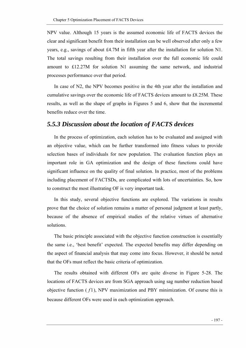
Chapter 5 Optimization Placement of FACTS Devices
- 197 -
NPV value. Although 15 years is the assumed economic life of FACTS devices the
clear and significant benefit from their installation can be well observed after only a few
years, e.g., savings of about £4.7M in fifth year after the installation for solution N1.
The total savings resulting from their installation over the full economic life could
amount to £12.27M for solution N1 assuming the same network, and industrial
processes performance over that period.
In case of N2, the NPV becomes positive in the 4th year after the installation and
cumulative savings over the economic life of FACTS devices amount to £8.25M. These
results, as well as the shape of graphs in Figures 5 and 6, show that the incremental
benefits reduce over the time.
5.5.3 Discussion about the location of FACTS devices
In the process of optimization, each solution has to be evaluated and assigned with
an objective value, which can be further transformed into fitness values to provide
selection bases of individuals for new population. The evaluation function plays an
important role in GA optimization and the design of these functions could have
significant influence on the quality of final solution. In practice, most of the problems
including placement of FACTSDs, are complicated with lots of uncertainties. So, how
to construct the most illustrating OF is very important task.
In this study, several objective functions are explored. The variations in results
prove that the choice of solution remains a matter of personal judgment at least partly,
because of the absence of empirical studies of the relative virtues of alternative
solutions.
The basic principle associated with the objective function construction is essentially
the same i.e., ‘best benefit’ expected. The expected benefits may differ depending on
the aspect of financial analysis that may come into focus. However, it should be noted
that the OFs must reflect the basic criteria of optimization.
The results obtained with different OFs are quite diverse in Figure 5-28. The
locations of FACTS devices are from SGA approach using sag number reduction based
objective function ( 1f ), NPV maximization and PBY minimization. Of course this is
because different OFs were used in each optimization approach.

Chapter 5 Optimization Placement of FACTS Devices
- 198 -
Figure 5-28 Test network with optimal locations of FACTS devices indicated by signs
In addition to this, operating parameters of the employed simple GA may also
influence the final results of optimisation.
• More computational effort is needed. All SGA in this study use maximum
number of generations 100, which may not be enough to get a converged result.
• The mutation rate used is 0.03, which may be too large to make population
converge with a small value of maximum generations of 100.
• In the SGA, the size of device is represented as discrete values. Sizes are
assumed to range from 0 – 100MVar for STATCOM and SVC, 0 – 50MVar for
DVR. However with the size of the step of 5MVar, which may be too big,
some variable solutions such as DVR: 3MVar or 1MVar might be missed.
1%3%11%
13%
5%
10%
14%
29%
10%4%
16
111
34
40
66
76
89
136
242
246
Figure 5-29 Sag losses in 10 load-sites
Although the results are diverse, there are two buses that appeared in all solutions
(with OFs of PBY and NPV) with high probability: bus close to 137, and bus 89 or
buses close to these two buses. This can be explained by the methodology used to

Chapter 5 Optimization Placement of FACTS Devices
- 199 -
estimate sag losses. Only ten buses are assumed to contribute the whole system’s losses
and their contributions are illustrated in Figure 5-29. 29% of the total losses come from
but 137 and 14% from bus 89. Bus 16 contributes only 1% of total losses. It is then
reasonable that these buses with high percentages of loss contributions are favoured by
GA approach.
5.6 Summary
Electronic based mitigation devices provide good solutions to voltage sag problems.
The installation of these devices can improve not only individual user's sag
performance, but also the sag profile of the entire network. Furthermore optimal
placement of FACTS devices for sag mitigation can be considered as a multimodal
optimization problem that has multiple good solutions.
The results illustrated here show that GA is an efficient optimization tool to address
this problem. Even though the global optimum may not be found the GA approach
offers solutions which result in significant reduction in number of critical sags in the
network and in dramatic sag saving each year.
This chapter also introduces a niching genetic algorithm (NGA) to locate multiple
and almost equally feasible solutions. Simulations show that NGA has the advantage
over classical SGA as it increases exploration of the search domain to locate multiple
solutions.
The most significant benefit of the NGA optimization is that it gives a group of
solutions for possible placement of FACTS devices that are almost equally effective in
voltage sag mitigation. In this way it provides important flexibility to decision-making
process in a realistic manner as the final choice could be made by a human expert based
on some additional criteria which are not directly quantifiable.
From the analysis presented in the chapter it is clear that application of FACTS
devices for voltage sag mitigation is not only technically but also economically
justifiable solution. The financial losses in the entire network due to voltage sags can
be significantly reduced by application of FACTS devices and the network can start
reaping financial benefits few years after the installation of those devices even though
the initial capital investment in the solution can be significant. The overall saving will
vary with the type, size and location of mitigation equipment. Having in mind that the

Chapter 5 Optimization Placement of FACTS Devices
- 200 -
price of these devices is expected to fall and their effectiveness in voltage sag
mitigation increase they could become even more valuble option in the future for
voltage sag mitigation. Finally, since FACTS devices generally contribute to the
enhancement of several electrical power network functions the benefits resulting from
their installation will in practice exceed those identified through their contributions to
voltage sag mitigation alone.

Chapter 6 Description of Developed Software
- 201 -
6 DESCRIPTION OF DEVELOPED SOFTWARE
6.1 Introduction
A comprehensive analysis of techno-economic assessment of voltage sag
performance and mitigating solutions has been presented in previous chapters. All
methodologies have been thoroughly discussed and illustrated using numerical
examples and graphical descriptions generated by purposely developed software in
MATLAB environment named vSAS (‘Voltage Sag Assessment Software’).
Software design and development are the main issues discussed in this chapter. In
the software design part, considerations are given to requirement analysis, the system
flow chart construction, the designed software modules and the graphical user interface
(GUI). System files, where both input and calculated data are kept, are also briefly
described. In the software development part, the system development, i.e., MATLAB
and Visual C++ is introduced first followed by the illustration of main user interface.
Several problems occurring during software testing are highlighted for further
development in the final part of this chapter.
6.2 Software design
There are several commercial or free software that can be used in power system
analysis, targeting various research objectives employing either classical or purpose-
developed methodologies. It is difficult however to modify code to include user-
developed models or features, such as the model of FACTS developed in this research.
Therefore in order to perform the studies and analysis effectively and accurately on a
realistic size power system, an automated comprehensive tool is required for the
assessment and visualization of the performance of voltage sags of individual buses and
the entire network. The objective of this chapter is therefore to discuss a stand-alone
software package named as ‘Voltage Sag Assessment Software’ (vSAS), which

Chapter 6 Description of Developed Software
- 202 -
contains all those developed methodologies and simulations and provides user-friendly
interface to explore all the research achievements.
6.2.1 Flow chart
According to the analysis, developed software package should be a stand-alone tool
focused on methodologies and techniques detailed in Chapter 2 – Chapter 5. All tasks
are illustrated in Figure 6-1.
Figure 6-1 Flow chart of whole analysis
6.2.2 System design modules
There are six main parts of the software package as indicated in Figure 6-1. They
include fault calculation, data analysis of monitoring, sag performance analysis,
calculation of sag losses, FACTS investment analysis and optimization analysis. As a
result, the system modules are proposed as shown Figure 6-2.

Chapter 6 Description of Developed Software
- 203 -
Figure 6-2 System design module
○1 Calculation –
○11 Calculation(without FACTSD): produce sag data without FACTSD
○12 Calculation(FACTSD): produce sag data with FACTSD
○13 Rating of FACTSD: calculate the rating of FACTSD of each bus in the network
○2 Sag performance –
○21 Statistic Data: input the data about fault duration, fault occurrence rate
○22 3D-Sag profile: presents sag profile of named bus or buses by three-dimension diagram or generalized sag tables
○23 3D-magnitude: presents sag magnitude of named buses in 3D form.
○24 ProtectionMotortransformer: present sag profile by three-dimension diagram or generalized sag tables with the influences of protection, motor and transformer. If transformer is investigated, figures of the change of phase jump should be displayed as well.
○3 Financial analysis –
○31 Sag losses assessment: calculate sag losses in the network based on the sag data
generated from by ○1 (either with or without the influence of FACTSD).
○32 Sag presentation: graphical representation of sag losses
○33 NPV&PayBackYear: analysis of the investment in FACTSD and graphical presentation of results.
○34 NPV sensitive: perform NPV sensitive analysis and present results in diagrams.
○4 Optimizations –

Chapter 6 Description of Developed Software
- 204 -
○41 Optimization with GA: performs optimization using a simple a GA or a NGA
○5 Monitoring data –
○51 Monitoring data analysis: graphical representation of monitoring sag data (with or without the influences from protection, transformer and motors).
6.2.3 Description of main functions
The software is an interactive tool that supports sag performance and mitigation
analysis and serves the purpose of power quality assessment. Five modules of this
software are designed to fulfil the tasks of involved all the achievements in this PhD
study, which are well illustrated in previous chapters. Here some main functions in
terms of fault calculation with FACTS devices, sag losses evaluation, sag performance
presentation, investment analysis and optimization are introduced in the programming
point of view.
1. Fault calculation with FACTS devices
Figure 6-3 Flow chart of fault calculation with FACTS

Chapter 6 Description of Developed Software
- 205 -
Figure 6-3 shows the flow chart of fault calculation with FACTS devices employed
by fault position method. Fault calculation with and without FACTS is processed
respectively. Faults on buses and faults on lines are also calculated separately.
2. Sag performance presentation
Figure 6-4 Flow chart of sag performance estimation
Figure 6-4 shows the flow chart of how to present the sag performance in the form
of three-dimension diagram or generalized sag table. There are two scenarios here, one
sag performance from monitoring, and the other sag performance from assessment by
calculation. In the case of sag assessment by fault calculation, sag data such as fault
duration and fault rate are input directly from input files. Data related to sag magnitude
and phase jump are obtained by fault position method conducted before the sag
performance presentation step. In the case of presentation of monitoring data, all sag
data are obtained directly from monitoring data. The input files contain sag magnitude
and phase angle of each phase of the bus investigated, as well as sag duration of each
sag. Analysis of the influences of transformer winding connections, protection system

Chapter 6 Description of Developed Software
- 206 -
failure and induction motors is built in both sets of input data afterwards and can be
performed, with either set.
3. Sag losses calculation
Figure 6-5 Flow chat of sag loss calculation
The flow chart of sag losses calculation is depicted in Figure 6-5. The methodology
of sag losses is developed in [39, 40], where the calculation was carried out in Fortran
language. It has been completely re-written in MATLAB so that it can be used in
conjunction with other modules. Trips of four types of equipment (PLC, Contactor, PC
and ASD) due to sag are computed first, and then used to get the trips of a process. 37
processes are generated by calculating individual equipment and then located by
randomly generated number (1-37) to 10 pre-defined buses to produce the entire losses
of the network.
4. FACTS investment analysis
Figure 6-6 illustrates the procedure of FACTS investment analysis. Improvement
(sag losses saving), price of FACTS (capital cost), maintenance, project life time and
discount rate are five factors in the process of analysis.

Chapter 6 Description of Developed Software
- 207 -
Figure 6-6 Flow chart of investment analysis
5. Optimization placement of FACTS
Figure 6-7 Flow chart of Genetic Algorithm

Chapter 6 Description of Developed Software
- 208 -
The optimization approaches both by Simple GA and Niching GA are described in
Figure 6-7. The details of the optimization approaches are introduced in Chapter 5. As
shown in Figure 6-7, the difference of SGA and NGA is in the step of ‘reproduction of
new generation’. NGA employs specific operators to maintain the diversity of the
generation in order to locate as much ‘niching’ as possible in the optimization approach.
6.2.4 Graphical User Interface (GUI)
In order to satisfy the user’s various needs, software products that contain a lot of
functions are developed, however, as the number of function is increased, the GUI
becomes more complicated. Complex user interface makes it difficult for user to
understand and apply the software, so the overall usability of the software is decreased.
Therefore, it is essential that to design a good graphical user interface, which reflects
user’s requirements. Each user view should preferably have the following capabilities:
− Input and edit user data, e.g. network data should be easily assessed.
− Select alternative calculation options, e.g. fault calculations can be done
with fault impedance of zero, or randomly generated value.
− Select right presentation of results, e.g. sag performance can be presented
in the form of three-dimension diagram or generalized sag tables.
− Present the results of calculation in a comprehensive way.
− Store results of calculation in user defined folders.
6.2.5 File dictionary
There is no database system used in this software. All the data are processed in the
form of files. Input data and results are kept individually in user defined folders. All
input data are stored in txt files and all results are kept in the form of MATLAB data
files for the convenience of post processing..
6.2.5.1 Input files
The format of input data is pre-defined, examples are given in sub-folder: input data,
though the names of those files are not compulsory. Input data includes:
1. Network information: lines, buses and transformers.

Chapter 6 Description of Developed Software
- 209 -
The example file is given in Appendix B Figure A-28 – Figure A-32.
2. Information about the fault duration and fault rate
The example file is given in Appendix B Figure A-33.
3. FACTS location, size and type
FACTinf.txt
FACTSinf %bus type P(MW) Q(MVAR) (type: 1-STATCOM; 2-SVC; 3-DVR) 89 2 0 55 144 1 0 55 246 3 0 55 end
4. Information about the loads used for calculation of losses
Loadinf.txt:
load_loss assigned losses correction factor load factor 0.587 0.05 1 0.0163 0.2384 0.55 0.001 0.3573 0.42 0 0 0 End load_structure group ID large user industrial user commercial user residential user 0 0 0 0 1 3 0.015 0.028 0.2 0.5 1 0.7 0.3 0 0 2 0.205 0.095 0.7 0 End rank_buses bus number group ID 16 3 110 3 34 2 40 2 66 2 76 2 89 2 136 2 end
6.2.5.2 Results files
Results are placed in the folder named after the case’s name, which is defined by the
user through the software interface. For example, if there is a case study is with the
named ‘BaseCase1’. A sub-folder under the folder where the software installed (usually
/VSAS/) is then created as: /VSAS/BaseCase1. All the results of simulations based on
this case will be placed in this folder.

Chapter 6 Description of Developed Software
- 210 -
1. Result of sag data: voltage magnitude and phase angle -- sagdata.mat
All fault calculation results are kept in the file named as sagdata.mat, which
contains 20 matrices as follows:
V_lll: Voltages due to LLL faults at all buses
Vline_lll: Voltages due to LLL faults on all lines
V_lga, V_lgb, V_lgc: Voltages due to LG faults at all buses
Vline_lga, Vline_lgb,Vline_lgc: Voltages due to LG faults on all lines
V_llga, V_llgb, V_llgc: Voltages due to LLG faults at all buses
Vline_llga, Vline_llgb, Vline_llgc: Voltages due to LLG faults on all lines
V_lla, V_llb, V_llc: Voltages due to LL faults at all buses
Vline_lla, Vline_llb, Vline_llc: Voltages due to LL faults on all lines
The size of matrices with sag data due to bus faults is bus busN N× , busN is the number
of buses in the network. The size of matrices with sag data due to line faults
is line bus positionN N N× × , lineN is the number of lines in the network, and positionN is the
number of fault positions on each line. Each element of these matrices presents the
voltage magnitude when fault happens somewhere in the network, for example, ijV
represents voltage sag magnitude at bus j for fault at bus i. Vij-2 represents voltage sag
magnitude at bus j for fault at position 2 of line i.
2. Result of sag losses evaluation -- cost.mat:
Results of sag loss evaluation are kept in the file cost.mat, which contains one
1000 2× matrix, indicating that there are 1000 trials random allocation of process. First
column of the matrix are the losses with highly sensitive equipment, the second column
of the matrix are the losses with moderately sensitive equipments.
6.2.5.3 System file
All information about each case study carried out by the software is listed in a file
caseinf.txt.
/VSAT/caseinf.txt CaseID CaseName fN fZ baseMVA pT fT
B Case1 6 0 100 0 0 B Casetest 3 0 100 0 0 B Case3 6 0 100 0 0 CaseID CaseName BasedCaseName BF Casetestfacts Casetest BF case3 Casetest CBF case3 CB Casetest

Chapter 6 Description of Developed Software
- 211 -
Where the first column represents:
fN number of fault position on each line
fZ :fault impedance
pT : 0 – number of fault positions on each line decided by fN
1 – number of fault positions on each line decided by line impedance
fT : 0 – fault impedance decided by fZ
1 – fault impedance is generated following a normal distribution
CaseID:
B: base case simulation, without FACTS devices
BF: simulation, with FACTS devices
CB: base case sag losses simulation, without FACTS devices
CBF: sag losses simulation, with FACTS devices
6.3 Abbreviated user manual
6.3.1 System development environment
The system environment in which the software is developed and operated is
specified in Table 6-1.
Table 6-1 System requirement classification Standard requirement
hardware ,Pentium (R) 4 CPU 1GB software Operating system Windows XP Service Pack 1, Windows XP Service
Language MATLAB 7.0 Financial tool box Interface VC 6.0
The experimental software was written using Microsoft Visual C++ 6.0 and
MATLAB 7.0. Microsoft Visual C++ is part of Microsoft’s software development
environment: Visual Studio, which provides a very powerful and flexible development
platform with an editor, compiler and a debugger. VC 6 has very useful tools for
graphical user interface (GUI) development, which allows the programmer to exploit
the Windows GUI easily.
MATLAB provides various ready-made mathematical and numerical functionalities
as functions. The ability to use these functions from other programming applications
such as C++ is crucial. This would help C++ programmers to avoid implementing
tedious mathematical functionalities.

Chapter 6 Description of Developed Software
- 212 -
6.3.2 Software command windows
Eleven major interfaces designed in this software package are illustrated in Figure
6-8 to Figure 6-18.
Figure 6-8 GUI – calculation (with FACTS)
Through the GUI in Figure 6-8, vSAS will perform fault calculation regarding the
input information and save the results after the key ‘Calculation’ is selected.
○1 The name of the case investigated, which will also be the name of the sub-folder where the results of this case are kept.
○2 The input file which contains all the information of the investigated network, (Example of this file has been given in Appendix B).
○3 Faulted points on lines: choices are given between ‘All uniformly distributed’ and ‘According to line impedance’.
○4 Number of faults on each line (3-9) if in ○3 , ‘All uniformly distributed’ option is chosen.
○5 Fault impedance -- options are given between ‘All the same’ and ‘Random’.
○6 The value of fault impedance in Ω if in○5 ‘All the same’ is chosen.
○7 baseMVA: the MVAbase used in the simulation, is 100.

Chapter 6 Description of Developed Software
- 213 -
Figure 6-9 GUI – Calculation (FACTS)
Through the GUI in Figure 6-9, vSAS performs fault calculation with FACTS
devices regarding to the input information responding to the click of button
‘Calculation’.
○1 The name of the case investigated, also is the name of the sub-folder where the results are kept.
○2 The case name, based on which, case ○1 will build to include the FACTS devices into calculation
○3 FACTS location: the file which contains the information about FACTSD including their location, size and type.
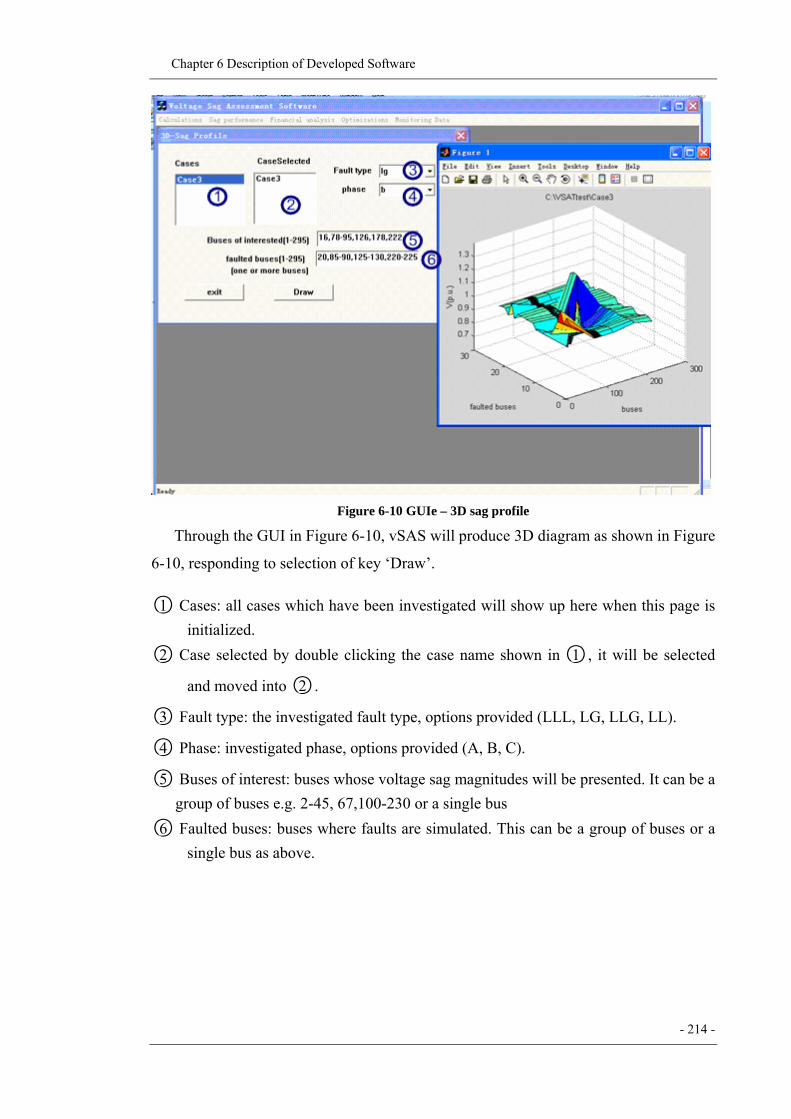
Chapter 6 Description of Developed Software
- 214 -
Figure 6-10 GUIe – 3D sag profile
Through the GUI in Figure 6-10, vSAS will produce 3D diagram as shown in Figure
6-10, responding to selection of key ‘Draw’.
○1 Cases: all cases which have been investigated will show up here when this page is initialized.
○2 Case selected by double clicking the case name shown in ○1 , it will be selected
and moved into ○2 .
○3 Fault type: the investigated fault type, options provided (LLL, LG, LLG, LL).
○4 Phase: investigated phase, options provided (A, B, C).
○5 Buses of interest: buses whose voltage sag magnitudes will be presented. It can be a group of buses e.g. 2-45, 67,100-230 or a single bus
○6 Faulted buses: buses where faults are simulated. This can be a group of buses or a single bus as above.

Chapter 6 Description of Developed Software
- 215 -
Figure 6-11 GUI – 3D sag number
Through the GUI in Figure 6-11, vSAS will 3D diagram as shown in Figure 6-10 ,
responding to selection of key ‘3-D bar’ or produce a generalized sag table responding
to selection of key ‘Generalized Sag Table’.
○1 Cases: all cases which have been investigated will show here when this page is initialized.
○2 Case selected by double clicking on the case name shown in ○1 , it will be selected
and moved into ○2 .
○3 Phase: the investigated phase, options provided (A, B, C).
○4 Buses of interest: buses whose voltage sag magnitudes will be presented. this can be a group of buses e.g. 2-45, 67,100-230 or a single bus.

Chapter 6 Description of Developed Software
- 216 -
Figure 6-12 GUI – Transformer Motor Protection
Through the GUI in Figure 6-12, vSAS will produce a 3D diagram responding to
selection of key ‘3-D bar’ or produce a generalized sag table as shown in Figure 6-12
responding to selection of key ‘Generalized Sag Table’ while taking into account the
influences of protection failure, transformer and induction motor.
○1 Cases: all cases which have been investigated will show when this page is initialized.
○2 Case selected by double clicking the case name shown in ○1 , it will be selected
and moved into ○2 .
○3 Buses of interest: buses whose voltage sag magnitudes will be presented. A single bus number only is allowed here.
○4 If ‘Transformer’ is selected, the type of transformer winding connection should be selected.
○5 If the ‘Motor’ is selected, the file which contains the information about IM should be selected.

Chapter 6 Description of Developed Software
- 217 -
Figure 6-13 GUI – Assessment of Sag Losses
Through the GUI in Figure 6-13, vSAS performs sag losses calculation based on the
case selected by user responding to selection of key ‘Calculation’.
○1 CaseID: The name of the case investigated, also is the name of the sub-folder where the results are kept.
○2 Load structure and losses: the file which contains the information about the loads which contribute of the losses of entire network.

Chapter 6 Description of Developed Software
- 218 -
Figure 6-14 GUI – Presentation of Sag losses
Through the GUI in Figure 6-14, vSAS will produce a diagram as shown in Figure
6-14 responding to selection of key ‘losses’ or produce a diagram showing the
statistical analysis of sag losses responding to selection of key ‘Statistic’.
○1 Cases: all cases which have been investigated will show here when this page is initialized.
○2 Case selected by double clicking the case name shown in ○1 , it will be selected
and moved into ○2 .
○3 The losses associated with highly sensitive equipment will be displayed, if ‘High sensitivity’ is selected, the losses associated with moderately sensitive equipment will be displayed if ‘Medium sensitivity’ is selected. Both of these can be displayed in the same graph if both options were selected.

Chapter 6 Description of Developed Software
- 219 -
Figure 6-15 GUI – NPV&PayBackYear
Through the GUI in Figure 6-15, vSAS will perform NPV or Pay back year analysis of the selected cases and produce corresponding graph responding to selection of ‘PayBackYear’ or ‘NPV’ key
○1 Discount rate: it will be used for the analysis and must be positive.
○2 Financial year: project life time used for NPV analysis
○3 BaseCaseID: the case study for which sag losses had been assessed without FACTSD. All available cases will be provided when this page is initialized.
○4 ImprovedCase: the case study for which sag losses had been assessed with FACTSD. All available cases will be provided when this page initialized.
○5 Maintenance: the cost of maintenance of each type of FACTSD, as percentage of its price (capital cost).
○6 The price of FACTS devices, which can be calculated either using formula defined
in the software or by specifying constant values in ○7 by selecting ‘FIXED’ key.
○7 Cost of FACTSD if ‘FIXED’ key is selected.
○8 The losses associated with highly sensitive devices are used if ‘High sensitivity’ is selected, the losses associated with moderately sensitive is used if ‘Medium sensitivity’ is selected.

Chapter 6 Description of Developed Software
- 220 -
Figure 6-16 GUI – NPV sensitivity analysis
Through the GUI in Figure 6-16, vSAS will perform NPV sensitivity analysis of selected cases and produce corresponding graph by clicking of key ‘Tornado’ or ‘Monte Carlo’.
○1 Discount rate: it will be used for the analysis and must be positive.
○2 The range of discount rate.
○3 The distribution of discount rate, ‘Uniform’ or ‘Normal’ distributions can be used
○4 Financial year: project life time used for NPV analysis, i.e., life expectancy
○5 The range of life expectancy
○6 The distribution of project life time, ‘Uniform’ or ‘Normal’ distributions can be used
○7 The range of savings in percentage of the savings calculated with the sag losses of base case and the improved sag based on mean value.
○8 The distribution of saving, the ‘Uniform’ or ‘Weibull’ distributions can be used
○9 The range of devices total capital cost as percentage of the original value obtained as sum of the prices of FACTSD used in the ImprovedCase loss assessment.
○10 The distribution of price of FACTD, the ‘Uniform’ or ‘Normal’ distributions can be used.

Chapter 6 Description of Developed Software
- 221 -
Figure 6-17 GUI – Optimization
Through the GUI in Figure 6-17, vSAS will perform SGA or NGA optimization using the selected objective function and save results.
○1 CaseID: The name of the case investigated, also the name of the sub-folder where the results are kept.
○2 BaseCase: the case the optimization is going to be performed for.
○3 Objective Function: a selection of objective functions is provided.
○4 Population size: the size of population, suggested value 20.
○5 MaxGeneration: the maximum number of generations the optimization will process (100-500).
○6 Mutate rate: mutate rate, (0.01-0.3)
○7 Crossover rate: crossover rate (0.6-0.9)

Chapter 6 Description of Developed Software
- 222 -
Figure 6-18 GUI – Monitoring Data analysis
Through the GUI in Figure 6-18, vSAS will produce a 3D diagram responding to
selection of key ‘3-D bar’ or produce a generalized sag table as shown in Figure 6-12
responding to selection of key ‘Generalized Sag Table’ while taking into account the
influences from transformer and IM.
○1 The file containing the information of monitoring sag data.
○2 If ‘Transformer’ is selected, the type of transformer winding connection be selected here.
○3 If the ‘Motor’ is selected, the file which contains the information about IM should be selected here.

Chapter 6 Description of Developed Software
- 223 -
6.4 Areas for further software improvement
During the testing of the software package, several issues for further improvement
were identified:
1. Computation time
The time of computation is always very sensitive to optimization method used.
vSAS package can perform SGA and NGA based optimization to place FACTS devices
optimally in the network for the purpose of sag performance improvement. Several
objective functions are provided to guide the optimization. However, they are all rather
time consuming. It takes typically more than 24 hours to complete one optimization
using suggested GA parameters.
The reason is mainly sag performance evaluation methodology, in which thousands
of faults have to be simulated in order to get the comprehensive results. Therefore, there
is little that can be done in programming to speed up the process. The computational
process can only be improved by improving sag performance evaluation and therefore it
was not part of the original project
2. Warning and error messages,
There is no provision for warning or error messages at this moment, which could
inform the users about the mistakes in the input data.
Software development is a complex and often difficult process requiring the
synthesis of many disciplines. Providing helpful warning and error messages sometimes
could be more difficult than the code itself. This is also very time consuming task and
therefore it was not part of the original project brief.
6.5 Environmental set up
These steps describe the process that the user should follow in order to install and
run the vSAS individual personal computer
1. Copy the set-up files into your computer.
2. Install the software by running the VSAS Installer in the set-up files folder. For
example, run setup.exe in C:\VSASsetup.
3. Follow the instructions from the installation interface, finish the setting-up.

Chapter 6 Description of Developed Software
- 224 -
4. Run the vSAS.exe stand-alone application from the installed folder.
6.6 Summary
Voltage sag assessment software (vSAS) developed within this research is described
in this chapter. It contains advanced, coordinated algorithms for fault calculation, sag
losses assessment. FACTSD investment evaluation and optimal placement of FACTSD.
The software is developed in Visual C++ and MATLAB environment. Extensive use of
graphics is made to provide a flexible, highly interactive and easy to use method for
data input, display of results and program operation. This chapter presented full
description of the development of vSAS.
Through the requirement analysis, the major components of the software were
defined, including five designed system modules, i.e., calculation, sag performance,
financial analysis, optimization and monitoring data analysis. The design of GUI
followed principles of flexibility and convenience of implementation.
vSAS is software package that provides full range of voltage sag performance and
mitigation assessment to meet the demand of the power quality analysis. The MATLAB
and Visual C++ were adopted as development platforms because of the powerful
mathematical and numerical computation and graphical presentation functions of
MATLAB and user friendly interface design capability of Visual C++. The
combination of the two resulted in a comprehensive interactive environment for
complex calculation, data visualization and presentation of results.
The software has been thoroughly tested and the results are found to be more than
satisfactory, which proved that vSAS is a powerful tool for voltage sag performance
and mitigation analysis.

Chapter 7 PQ in Market Environment
- 225 -
7 PQ IN MARKET ENVIRONMENT
7.1 Introduction
It is acknowledged that power quality such as voltage sag can be improved
dramatically if necessary investment is made. Even if it can be proved that some
investments are profitable rewarded in a system point of view, the question still remains:
who is going to pay? Since power quality problems, e.g. voltage sags can be initiated at
user-site or transmission site or even the generation site, who should be responsible? To
answer these questions, power quality should be examined from a market point of view
rather than focusing reportedly on its technical or financial values. This chapter,
therefore, aims to provide an overview of power quality in market environment, to spot
main marketing mechanisms which are employed by power market to maintain its
efficiency as well as quality.
First, the use of incentive-based regulatory regime in monopoly networks is
introduced as the efficient rule in the absence of competition, that attempts to mimic
competitive market pressures. Price cap mechanism is discussed in detail as the most
important incentive regulation method in power system. After the description of
services quality incentives for electricity distribution, the chapter illustrates the
possibility of introducing PQ into price cap analysis and presents the difficulties
involved in this approach. This leads to proposal a new method to accommodate the PQ
issue in the incentive regulation.
The PQ contract is then introduced as another method to incentivise PQ
improvement in power system market. The introduction starts from the basics of
contract and contract design in general and then reviews the application of PQ contract
in practice.
The discussion is then extended to PQ market design. The objective and principle of
market design in power system are given first, followed with the introduction of an
example of PQ market design based on ‘emission permit’.

Chapter 7 PQ in Market Environment
- 226 -
Finally, several issues related to incentive schemes for PQ improvement in power
system, e.g., information, legislation and standards are discussed in detail. The
influence of PQ on present power system market is also illustrated.
7.2 PQ in incentive regulation of electricity
7.2.1 Incentive regulation of electricity
The activities of power system include generation, transmission, distribution and
supply (retailing). Generation here refers to production and conversion of electric power.
Transmission and distribution are required to transfer electricity. Transmission usually
transfers electricity at high voltage through long distance. Distribution transfers
electricity at low voltage through local networks. Retailing of electricity deals with
metering, billing and sales of electricity to end user [118].
In power system market, transmission and distribution of electricity are
characterized as natural monopolies, while generation and supply are open to
competition [119]. Incentive-based regulation has been introduced into the natural
monopoly networks in the aims of mimicking competitive market pressures when
competition is missing [120]. Incentive regulation can encourage utilities to improve
their operating and investment efficiency through financial reward or penalty incentive
schemes [118]. Usually an external performance standard that represents average
industry performance will be set as the criteria of judgment [121].
The mainly used incentive regulation methods for electricity utilities are:
price/revenue cap schemes, sliding-scale rate of return, partial cost adjustment, menu of
contracts, and yardstick competition [120]. Among them price cap mechanisms, which
allows utilities the flexibility to change rates, are said to be the most popular form of
incentive regulation used around the world [119]. The framework of price cap uses a
formula to limit rate increases within certain specified criteria: _price cap RPI X= − .
Where the maximum rate of increase of prices is equal to the retail price index (RPI) minus
a X factor which is a productivity growth offset. Therefore, if the regulated utilities can
improve their productivity at a higher rate than the assigned X factor, they can increase
their profits [122].

Chapter 7 PQ in Market Environment
- 227 -
7.2.2 Services quality incentives for electric distribution
company
Incentive regulation can motivate utilities improve their productivities. However, if
the incentive regulation concerns only cost reduction, the quality of services tends to be
decreased. So cost-control incentives usually are combined with quality-related
incentives in order to maintain the quality of services that utilities provided. Incentive
method such as price caps are typically accompanied by other incentive mechanisms to
respond to concerns about service quality [119].
It has been concern of many countries to incentivise investment in various
dimensions of service quality rather than focusing on reducing operating cost only. In
the UK, in order to enhance the service quality, the regulator for UK’s gas and
electricity industries set the price controls schemes that includes interruption (continuity
of service) incentives, guaranteed standards of performance, quality of telephone
service, and (4) a discretionary reward scheme [118]. Figure 7-1 shows the economic
effects of incentive regulation in a few countries.
Figure 7-1 The economic effects of incentive regulation [123]

Chapter 7 PQ in Market Environment
- 228 -
The regulation practice in the UK is to set a performance targets combined with
penalty and reward incentive system. Distribution service quality, at least as measured
by customer interruptions (CI) and customer minutes lost (CML), has improved as
shown in Figure 7-2. This suggests that incentive regulation has led the improvement of
service quality. It has also been advocated that the inclusion of service quality in an
overall efficiency benchmarking of utilities has clear incentive advantages [124, 125].
Figure 7-2 Improvement effects of the incentive/penalty regime in Great Britain [123]
In price cap regulation scheme, the regulator can set differentiated price caps based
on the companies’ efficiency performance estimated from a benchmarking analysis. X-
factors are set equal to the annual target change in productive efficiency for each
individual company [120].
In many countries, e.g. in Norway [126] and in Finland [127], power quality
(interruption) is already part of efficiency benchmarking. One example of network
revenue regulation model with outage costs is presented [126]. In this Norwegian model
outage costs are part of network revenue evaluating process. If outage costs are more
than expected outage costs for certain time period, company are forced to diminish its
revenue by corresponding sum. If company can improve its power quality so that
outage costs are less than expected outage costs, company may increase its profit as
presented in Figure 7-3 [128].
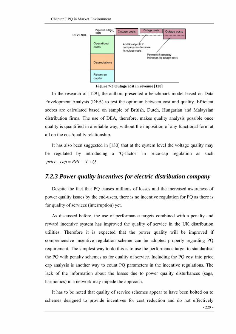
Chapter 7 PQ in Market Environment
- 229 -
Figure 7-3 Outage cost in revenue [128]
In the research of [129], the authors presented a benchmark model based on Data
Envelopment Analysis (DEA) to test the optimum between cost and quality. Efficient
scores are calculated based on sample of British, Dutch, Hungarian and Malaysian
distribution firms. The use of DEA, therefore, makes quality analysis possible once
quality is quantified in a reliable way, without the imposition of any functional form at
all on the cost/quality relationship.
It has also been suggested in [130] that at the system level the voltage quality may
be regulated by introducing a ‘Q-factor’ in price-cap regulation as such
_price cap RPI X Q= − + .
7.2.3 Power quality incentives for electric distribution company
Despite the fact that PQ causes millions of losses and the increased awareness of
power quality issues by the end-users, there is no incentive regulation for PQ as there is
for quality of services (interruption) yet.
As discussed before, the use of performance targets combined with a penalty and
reward incentive system has improved the quality of service in the UK distribution
utilities. Therefore it is expected that the power quality will be improved if
comprehensive incentive regulation scheme can be adopted properly regarding PQ
requirement. The simplest way to do this is to use the performance target to standardise
the PQ with penalty schemes as for quality of service. Including the PQ cost into price
cap analysis is another way to count PQ parameters in the incentive regulations. The
lack of the information about the losses due to power quality disturbances (sags,
harmonics) in a network may impede the approach.
It has to be noted that quality of service schemes appear to have been bolted on to
schemes designed to provide incentives for cost reduction and do not effectively

Chapter 7 PQ in Market Environment
- 230 -
incorporate information on consumer valuations of quality and the costs of varying
quality in different dimensions. In the case of PQ, there is large part of these
disturbances generated from end user site rather than resulting from the operation of
distribution operators. In this sense, distribution operators should not be held
responsible for poor quality, they should not be blamed nor be disadvantaged. At the
same time, end-users are usually considered as consumers and are not regulated.
It can be argued though, that distribution operator can be considered to be
‘responsible’ for the power quality level in their network and be subjected to penalty
and reward by regulators. At the same time, distribution operators can shift these
‘penalty and reward’ to the retailer then to end-user through market mechanism e.g,
pricing or specific contracts. The improvement pressure can then be distributed to those
who should be responsible. Who is going to take the action of improving PQ in the
network will certainly be determined in a more economical way. Whether the
distribution operator should mitigate the PQ disturbances at a system level, or it is more
desirable to mitigate them at the user site, will emerge while working towards a target
of more economical and practical solutions.
Additionally it should be noted that it is more challenging to introduce PQ into
incentive regulation. Whether the extra effort is worth it depends on whether the
performance improvements justify the additional effort.
7.2.4 The emission characteristic of PQ
In the restructured power market of the future, as in many competitive markets,
prices rather than resource needs drive decision. In markets with fairly complete set of
forward prices, it is relatively straightforward to determine the value of many kinds of
investments. Therefore, it is desirable to include the power quality issue into the pricing
of electricity. Here a method to introduce power quality factor into the price after
‘price-cap’ regulation is proposed.
First, a pollution level factor and a security level factor of power quality can be
defined as such:
sPQ : Power quality security level factor, which is the power quality level
supplier promised to deliver.

Chapter 7 PQ in Market Environment
- 231 -
ePQ : Power quality emission level factor, which is the power quality level
consumers are allowed to emit.
The relationship between the changes of these two levels and the price of electricity
can be illustrated as in Figure 7-4. With the increase of demanded PQ security level, the
price will increase, while price will reduce when PQ emission level is decreasing.
Figure 7-4 Pricing of electricity with PQ levels
Of course, the linkage of these two proposed PQ factors and the actual technical
performance presents a challenge. But it can be assumed reasonably that ePQ has more
influence on price than sPQ with the higher level (‘H’ and ‘VH’) while less influence
on price than sPQ with low level (‘L’ and ‘VL’).
Once the actual power quality performances are settled, a designed scheme needs to
be applied to it to transform the performance to power quality factor values. The power
quality source can be: harmonic currents, voltage dips, unbalanced voltage, and flicker.
The adjusted price of electricity can be calculated as (7.1):
0 ( (1.2 ) (1.2 ))s eP P a PQ b PQ= × × − + × − (7.1)
where, 0P is the original price of electricity. ,a b are the sensitivity factors of sPQ and
sPQ .
It is proposed in [131], that PQ disturbances can be classified using ‘ABC’ labels as
shown in Figure 7-5. The same format can be adopted for level of PQ security and
emission as shown in Figure 7-6.

Chapter 7 PQ in Market Environment
- 232 -
Figure 7-5 Classification of power quality characteristics [131]
Figure 7-6 Classification of PQ emission and security level
Then the price of electricity can be adjusted due to different level of PQ emission
and security as illustrated in Table 7-1, where in the upper-left corner of the table (bold
font), 0.4 0.6a b= = , in the lower-right corner of table (bold italic font), 0.6 0.4a b= =
(in order to address the assumption that that ePQ has more influence on price than sPQ
with the higher level (‘H’ and ‘VH’) while less influence on price than sPQ with low
level (‘L’ and ‘VL’)).
Table 7-1 The price according to PQ emission and security level
PQs PQe 1 0.66 0.33 0 -0.33 -0.66 -1
1 20 40.4 48.2 70 66.5 103 120 0.66 33.6 54 73.8 87 83.5 100 137 0.33 46.8 67.2 87 103.5 100 136.5 153.5
0 70 87 103.5 100 116.5 153 170 -0.33 86.5 103.5 120 136.5 133 166.2 159.8 -0.66 103 120 136.5 153 152.8 186 179.6
-1 120 137 153.5 170 173.2 206.4 220

Chapter 7 PQ in Market Environment
- 233 -
The prices as a function of different PQs and PQe can be dawn as in Figure 7-7. It
can be seen that the price is higher with high level of PQ emission and security level. It
also has to be pointed out that the sensitivity factors a, and b will play important role in
forming the price.
Figure 7-7 Price with respect to different PQs and PQe
After the price is changed, the total saving or payment for extra power quality
requirement can be determined straightforward as shown in Figure 7-8. The saving in
electricity cost will drive consumers to improve their power quality emission level. And
the extra cost of extra power quality demand will be justified by the saving due to
power quality improvement. The suppliers will be willing to invest in power quality
improvement due to the extra benefit they can be rewarded afterwards.
Figure 7-8 Yearly saving or payment for PQ in tariff of electricity

Chapter 7 PQ in Market Environment
- 234 -
The use of adjusted price scheme certainly can bring more involvement of the
utilities to achieve common goals. However, the set up of such scheme will need a well
understood actual power quality performance of the existing system in order to set up
the standard point P0 and adequate measurement/monitoring procedures to verify the
on-going power quality factor afterwards.
7.3 Power quality contract
7.3.1 Basics of contract
A contract is an agreement creating and defining the obligations between parties. The
exchanged promises or agreement involved will be enforced by the law [132].
In common law, there are five key requirements for the creation of a contract. These
are offer and acceptance (agreement), consideration, an intention to create legal
relations, capacity and formalities [133]. They are further discussed below:
1. Offer and acceptance
To form a contract, naturally there will be one party who makes an offer for bargain
and another one who is willing to accept. This can be called a 'concurrence of wills' or a
'meeting of the minds' of two or more parties [132].
2. Consideration
Consideration refers the ‘value’ of promises made by parties, which could be a
commodity or certain amount of money. The idea is that all parties involved must bring
something to bargain. Consideration must be sufficient rather than adequate.
3. An intention to create legal relations
Another important aspect to form a contract is that there must be an intention to
create legal bound for all parties. Any agreement between them should be made without
enforcement.
4. Formalities and writing
Usually contract is made in the written form although an informal exchange of
promises can be treated as verbal contracts and can be legally valid. If a contract is in a

Chapter 7 PQ in Market Environment
- 235 -
written form and document are used, all parties must be noticed of all content written
before their entries.
7.3.2 Contract design
In order to design a contract, there are four basic principles can be followed [134]:
• Informativeness Principle
In the absence of a world of perfect information, it is developed in [135] what
became known as the informativeness principle. This indicates that the determination of
any performance (which agreed with all parties) should be included in the contract. Any
measurement should be defined in such a way that it can reduce the aggregate error and
filter out some common noise factors.
• Incentive-Intensity Principle
The incentive intensity principle indicates that how the incentive should change
according to changes in measured performance. It is hard to say that the more
compensation (or reward) schemes vary, the better the incentives will produce. The
optima will depend on the precision of performance measurement, the incremental
increase in profit, the accepted tolerance of risk and the responsiveness to incentives
[134].
• Monitoring intensity principle
The monitoring intensity principle determines how much should be spent increasing
the quality of the performance measures. Usually these kinds of measurements are very
costly. The optimal should balance the cost of more risk against the cost to improving
the measurement. A ‘menu’ of monitoring/incentive intensities would be a good
solution. The monitoring intensity will increase if the level of incentive intensity is high
• Equal Compensation Principle
The principle of equal compensation indicates that all activities of contractors
should be equally valued. The basic thought here is that targeting benefit should not
cause others to suffer. The fairness is also well supported by the law.

Chapter 7 PQ in Market Environment
- 236 -
7.3.3 Existing PQ contracts
Power quality contract aims to improve the electricity quality efficiently to reach
some common goals. Contracts of power quality have already been in applications in
several countries for years as shown. Consumers can negotiate to get certain level of
power quality through specific contracts with the distributors or utilities. The contents
of these contracts of course will vary depending on the demand of consumers. A
through survey presented in [131] shows the different types of premium power quality
contracts already used around the world, which is summarised in Table 7-2.
Table 7-2 PQ contracts [131] country contract main activities
France with standard quality thresholds; with customer-adjusted levels; Plus contract
Compensating;
Italy no contract; no regulation system Monitoring; Building understanding
South Africa
detailed power contracts: national power quality standard; Network-specific option; Premium power option
Measurement; survey of the customer's cost; demonstration of new technology
Detroit Edison Company Special manufacturing contract (SMC) sag score limits;
penalties paid each year
Connecticut continuous measurements; perform benchmarking; inform potential customer
USA
New Jersey measurements; customer surveys; quarterly telephone interviews
Argentinean penalty payment concerning guaranteed levels of harmonics and flicker and the interruptions
Measurement in medium voltage grids
From customers’ point of view, high level of power quality means less risk cost.
Usually it is the distribution company who should identify the additional costs for
improving power quality to the required level and bill the customer for it. The
customers can then evaluate this cost against local alternatives. Some customers who
are not so sensitive to power quality may be willing to accept lower level of PQ in order
to reduce the costs.
From the view point of utilities and distributions, they may be forced to provide
higher level of quality in order to retain existing customers as more and more industrial
customers are become aware of their production losses associated with power quality
disturbances such as voltage sags.

Chapter 7 PQ in Market Environment
- 237 -
Premium service contracts are already being negotiated, implemented and mediated
in many circumstances [131]. The Special manufacturing contract (SMC) between the
Detroit Edison Company and the three automobile manufacturing customers is an
excellent example of a utility providing the additional quality required by sensitive
customers. Such contracts are beneficial for all parties - the utility that retains key
customers, the customer who reduces production losses and the public consumer who
benefits indirectly from the lower production costs [20].
7.3.4 About PQ contract
As it has been introduced in section 7.2.2, it could be a temptation to reduce
investments in quality under price-cap regulation [136]. There are interesting researches
going on to involve the power quality issue in the price-cap evaluation process.
However, it has been noticed that it is rather difficult to do so because of the complexity
involved in quantifying the value of quality. PQ contract can be tailered to meet the
individual requirement of customers and very easy to be implemented. Regulator is
eager to find solutions to bring pressures of improving power quality in the regulated
power markets. Power quality contracts may be the most feasible solution at this
moment.
Regulator is responsible to give the assessment of average level of power quality
and set the basic rules of power contract. Therefore, they should play an important role
in the power quality contract process. Around the world, the existing power quality
contract and the related regulators’ intervention are listed in Figure 7-9. It can be clearly
seen that there is no intervention of regulator in most of the countries. However, some
important issues in power quality contract such as performance measurements, setting
up common targets require more involvement of regulators.
Figure 7-9 Power quality contracts and regulator [123]

Chapter 7 PQ in Market Environment
- 238 -
7.4 PQ market design
7.4.1 Objective of PQ market
The ultimate objective to introduce PQ into power market is to improve the
economic efficiency and to distribute the benefit fairly. PQ competition is expected to:
• Concentrate efforts by utilities to improve the PQ level of electricity supply
• Orient end-user to reduce PQ disturbance emission to the system
• Encourage equipment manufacturers to enforce the ride-through capability of
devices
• Lead to more transparent and effective regulation and other market design, to
better reflect cost and benefit distribution.
Utilities will seek new methods and technologies to ensure that they are able to
provide secure and clean electricity at the lowest possible cost in comparison with their
competitors. End-users will be more aware of not only their PQ requirement but also
their PQ emission level. Business practices in general will become more oriented
towards profitability. Marketing and pricing will increasingly be tailored to user needs
with respect to PQ.
Throughout the world, governments are promoting competitive electricity markets.
There is a trend to reduce the administrative price setting by government institutions
through the introduction of competition. In the recent waves of deregulation in power
industry, the most concern is on generation. However, as experiences with market
reform grow, governments are likely to go further to bring competition among final
electricity suppliers and distributors, i.e., specified power quality requirement. The
pursuit of government policy should not be the obstacle to establish a competitive
market. Social, economic and other policies can be implemented through mechanisms
that allow markets to function. The essential requirement is to translate policy decisions
into constraints and costs that markets can assimilate.
7.4.2 Design of PQ market
As the core conception in economics, efficiency and equity are the fundamental
elements when designing a market. Good market design begins with a thorough
understanding of the market participants including suppliers and consumers. For

Chapter 7 PQ in Market Environment
- 239 -
electricity market, the core aspects determining the market structure can be described as
[137]: Power Producers; Power Marketers; Market/ System/ Transmission Operators;
Distributors; Retail Providers; End-Use Customers; Regulators as shown in Figure
7-10:
Owner of
Transmission
Owner of distribution
Hardware & devices manufacture
regulator
Power retailer
generation
consumer
Figure 7-10 Market structure of PQ
The electricity market can be plotted from different dimensions [138]. In the time
scale, it includes: forward market, spot market and real-time market. According to
traded commodity, it includes: energy market, transmission market and ancillary service
market. In terms of trading mode, electricity power is traded through bilateral
transactions, private exchange and power pool. The linkage between submarkets varies
and depends on the set rules [138].
After the market architecture is established, market-trading rules must be specified.
Trading rules define the function and behaviours of the market. And it must be
structured in such a way that it can avoid gaming and promote efficiency.
7.4.3 PQ market design practice
Power quality market has been generally limited to academic research to date. It is
still arguable whether it is worthy to design an ‘independent’ power quality market
although research efforts, few, have been made on this subject.

Chapter 7 PQ in Market Environment
- 240 -
A market for PQ-related matters, using an emission permits trading system has been
developed in [139]. The designed market assigns, every participator involved, the right
to cause a certain amount of PQ problems. In available electrical distance range, the
permits of emission PQ pollution can then be traded between customers or network
operators, following some pre-defined rules. The sum of these permits must be such
that the worst-case allowed emission is not harmful. Owners of industrial and power
plants must then make the choice, either pay for mitigation equipment or emission
permits. In such a way, the cost of the policy measures is then incorporated in their
commercial decision. The designed PQ market is shown in Figure 7-11.
Figure 7-11 PQ market design [139]
The emission right (permits) gross has further been analysis using an incomplete
static cooperative game theory in [140], which also proposed the Bayes Nash
equilibrium for optimized distribution of initial emission right and high quality electric
energy among market players.
Nevertheless, the actual implementation of a designed power quality market is still a
subject of further research. Sufficient information, accurate incentive and the efficiency
of operation are all very crucial issue to create and operate such a market.
7.5 Issues related to PQ in market environment
7.5.1 Accurate information
Setting continuity standards and incentive/penalty regimes requires reliable data
about the performance of regulated parties. The accuracy of the information is directly
related to the outcomes of regulatory. Establishing the appropriate reporting formats,
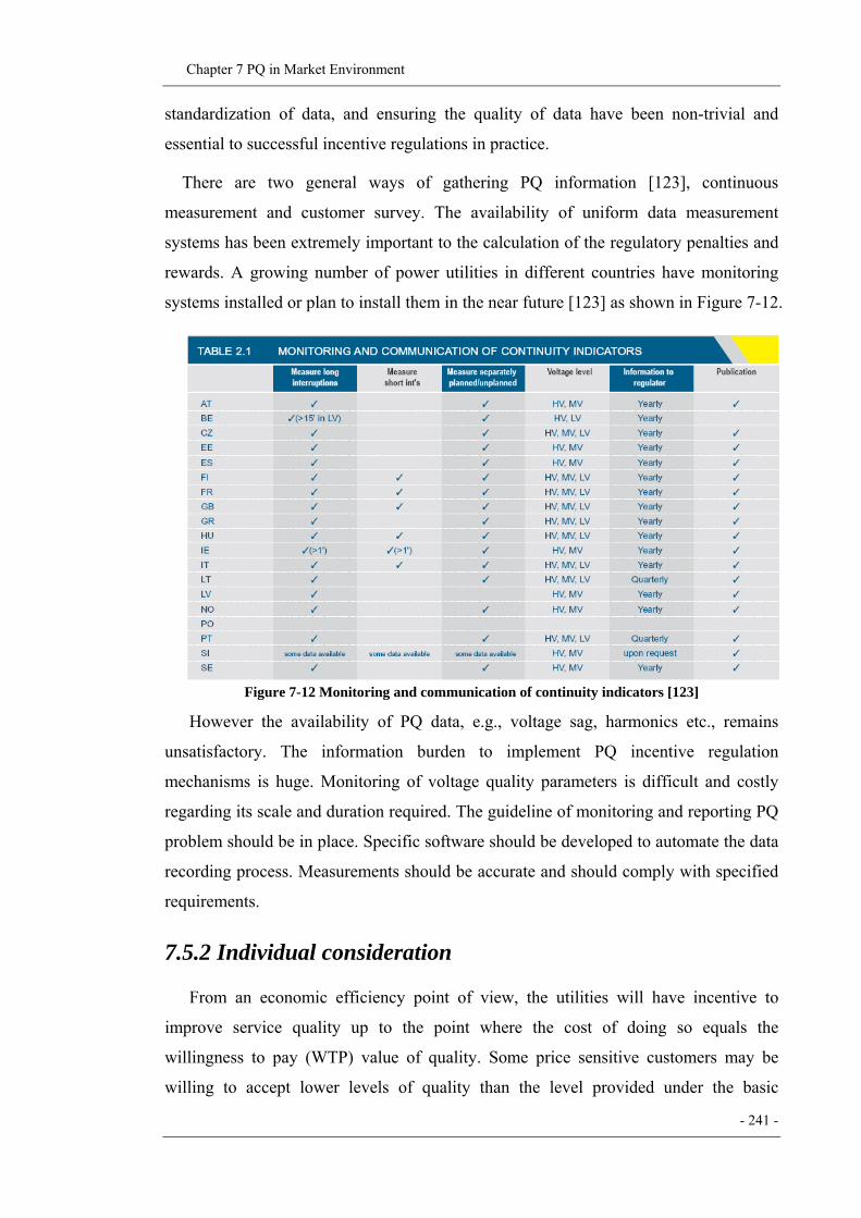
Chapter 7 PQ in Market Environment
- 241 -
standardization of data, and ensuring the quality of data have been non-trivial and
essential to successful incentive regulations in practice.
There are two general ways of gathering PQ information [123], continuous
measurement and customer survey. The availability of uniform data measurement
systems has been extremely important to the calculation of the regulatory penalties and
rewards. A growing number of power utilities in different countries have monitoring
systems installed or plan to install them in the near future [123] as shown in Figure 7-12.
Figure 7-12 Monitoring and communication of continuity indicators [123]
However the availability of PQ data, e.g., voltage sag, harmonics etc., remains
unsatisfactory. The information burden to implement PQ incentive regulation
mechanisms is huge. Monitoring of voltage quality parameters is difficult and costly
regarding its scale and duration required. The guideline of monitoring and reporting PQ
problem should be in place. Specific software should be developed to automate the data
recording process. Measurements should be accurate and should comply with specified
requirements.
7.5.2 Individual consideration
From an economic efficiency point of view, the utilities will have incentive to
improve service quality up to the point where the cost of doing so equals the
willingness to pay (WTP) value of quality. Some price sensitive customers may be
willing to accept lower levels of quality than the level provided under the basic

Chapter 7 PQ in Market Environment
- 242 -
regulated service for a reduced prices. Regulation also has to recognize the differences
in historical and operating conditions of customer. So the improvement targets should
be settled with the consideration of customer density and historical performance.
Furthermore, quality incentive schemes are inherently country-specific: they should be
designed contingent on the actual industry and regulatory framework of the country. A
‘superior’ quality incentive scheme, fitting each possible contingency, probably does
not exist.
Figure 7-13 The evolution pattern of regulation [118]
Nevertheless, the variations encountered in PQ incentive scheme should be
considered and dealt in such a way that both common issues and the differences can be
identified. It may be a good idea to offer a menu of cost-contingent regulatory options
instead of providing only a single profit requirement. The basic idea here is to make it
profitable for a firm with low cost opportunities to choose a relatively high powered
incentive scheme and a firm with high cost opportunities a relatively low powered
scheme [118]. Figure 7-13 indicates the incentive properties of different regulation
models.
7.5.3 Setting the right target
The proper benchmark or standard or settled target of PQ should send proper signals
to the regulator, to the utilities and to end-user about the need for better PQ and thus
encourage them to increase capital investments across the network.

Chapter 7 PQ in Market Environment
- 243 -
The standard EN 50160 determines limits for voltage quality parameters but in most
cases they are only indicative [130] rather than constrainedl. So it is not restrictive
enough and does not constitute a good reference for voltage quality in European
networks [123], where the performance is already better than the values defined in EN
50160. So EN 50160 are actually recommended but compulsory, in some countries
[123]. In this circumstance, some regulators want to set more restrictive standards,
especially looking at voltage supply variations, rapid voltage changes and voltage sags.
Based on careful examination of existing IEEE and IEC [141], the future direction
of power quality are suggested in [141], which indicated that power quality/reliability
characteristics need to be defined in a more statistical manner; the information about
sensitivity of equipment should be the responsibility of manufacturers; further
development is required for monitoring and measurement procedure; system analysis
should accommodate tools or models taking into account power quality issues;
economic analysis of power quality and its solutions should be performed in a
systematic way.
It has also been brought into attention that technical standardisation for monitoring
and measurement are also required with reference to accuracy not only of the measuring
instrument, but of the whole measurement chain.
7.5.4 Government policy and legislation
Power quality improvement can be supported if governments so desire, by
implementable policies, such as taxes, investment support for PQ improvement
equipment, government research and development investment. Even, governments can
require non-competitive parts of the electricity supply to bear the costs of some policies.
Charges on the use of the network can include such a policy-related component.
Regulators need the authority to ask transmission, distribution and industries to
collect performance data, to audit performance data and to analyze these data. Absent
these authorities and resources incentive regulation mechanisms will not achieve their
promises in practice. In this regard, a transparent set of rules, processes, and outcomes
are particularly important. The legislation should be clear regarding the aims of the
regulator’s mandate and areas over which it should have authority.

Chapter 7 PQ in Market Environment
- 244 -
7.5.5 The influence of PQ incentives in the power system
markets
PQ incentive scheme will provide strong incentives to invest in PQ improvement
and will bring new opportunities as well as challenges. Every party involved will face
up to the changes required to provide safe, reliable and profitable electricity in an
increasingly competitive market [139]. In markets where PQ becomes open to
competition, individual investment and operational decisions will no longer incorporate
non-economic requirements unless they are made explicit by government action.
Investment decisions will also reflect commercial reality more closely in projected
investment costs
Utilities will pay more attention to their PQ and consumers will constraint their PQ
disturbances emission because of the fear of punishment and market disadvantages.
This will drive the requirements of industrial equipment with less PQ disturbances and
more mitigation devices. All of these will boost the market of PQ mitigation devices
and the cost of these devices will decrease as new technologies introduced in and with
the increase in demand for such devices.
Ensuring the quality of the electricity supply has become big business: $6.5 billion
in 2003 revenues, according to a new report from ABI Research [142]. According to the
report, revenues in this sector are set to rise to $9.4 billion by 2011 [142].
Equipment ride-through capability is a major component in the PQ discussion, so
manufacturers will be pressured to increase equipment capability of withstands PQ
disturbances. As with other aspects of market competition, this will probably put
pressure on governments to liberalise the manufacture sectors as well.
It is clear that competition leads utilities and consumers to re-orient their research
and enhance its effectiveness. Utilities will tend to increase their focus on
improvements to plant operations and in-plant technologies. "Public good" research
projects with no commercial benefits will be dropped. It is likely that utilities will
participate in collaborative research programmes respect to PQ and solution analysis
more than in the past.
In addition to improvements in performance and operation, competition is likely to
bring improvements to the management and business arrangements of utilities. Among

Chapter 7 PQ in Market Environment
- 245 -
utilities, utility corporate structures may be reorganised to better manage the special
requirements of PQ. Corporate entities may be created to manage special risks or
investment related to PQ activities. Mergers and operating agreements may appear
which will allow companies to share PQ devices and facilities and to spread the fixed of
some PQ activities over a larger total output.
7.6 Summary
This chapter intended to give a comprehensive introduction of PQ incentive
schemes in power system, which can be summarized as follows:
• Including PQ factor into the price cap analysis with proper benchmarking
methodologies.
An appropriate regulatory approach would provide the regulated firm with such
economic incentives as to maximizing the firm’s profit while targeting quality of their
supply. Complying with this “incentive compatibility” is, however, difficult in practice,
because of PQ measurement, variations in consumer’s demand of PQ and the
consideration of ‘trade-off’ between cost and quality improvement.
• Setting targets along with penalty and reward scheme by specific contracts.
Network companies do not have a natural incentive to increase quality unless they
are provided with a financial incentive to make these quality investments. Proper targets
along with penalty and reward scheme gave the right signal that indicates the direction
of PQ improvement. This method is in practice application for quality of services
already. This does not mean however, that it will be easy to apply it for PQ incentive.
The PQ problems are partly geographical dependent and their performance in history
should be carefully considered when setting the targets, this will not therefore be a
simple task. The PQ contracts also need more transparency and guideline on their
content to justify the principle of fairness.
• Designing new PQ market.
Putting PQ into complete competitive market is the most efficient way to incentive
PQ improvement. Designing a new market in power system along with Energy Market,
Transmission Market and Ancillary Service Market is however a challenging task.
Little research has been done in this area. It is feasible based on available literature but
it will place a huge demand for additional efforts on all network participators. Setting

Chapter 7 PQ in Market Environment
- 246 -
proper market rules is very complex considering the nature of PQ disturbances.
Introduction of competition into PQ market will benefit all parties in market. How to
guide the competition and design the rules of competition is the fast task to solve in
order to set an efficient PQ market.
Some important issue related to the development of PQ incentive scheme, e.g., PQ
data collection, setting PQ targets and legislation were also discussed in this chapter.
Based on the introduction of three incentive schemes for PQ improvement, and based
on recent empirical evidence in literature, this chapter concluded with the influences PQ
incentive scheme will have on power system investment, on academic research and on
power system business structure. All in all, introducing PQ into market or market-line
environment will have significant impact on power system operation as well as on
power system regulations.

Chapter 8 Conclusion and Future Work
- 247 -
8 CONCLUSION AND FUTURE WORK
8.1 Conclusion
Voltage sags are short-duration reductions in rms voltage. They may lead to tripping
of sensitive equipment and thus cause huge financial losses. They are widely considered
to be the power quality disturbance causing most concern to industrial customers. A lot
of efforts have been put either to reduce the fault happening rate, and such the number
of potential voltage sags, or to mitigate the influence of voltage sags on end users and
equipment. FACTS based mitigation devices provide effective solution to voltage sag
problems but they are very expensive. This thesis dealt with analysis of voltage sags
and techno-economic assessment of mitigating solutions with FACTS devices.
The voltage sag performance assessment using fault position method was introduced
first. The assessment was based on impedance matrix method and took into account
probabilistic fault happening rate and protection system defined sag duration. The
resulted sag performances were presented in the form of 3D bar charts and generalized
sag tables. The fault calculation was performed using positive, negative and zero
sequence networks. System component modelling, impedance matrix construction and
fault current computation methodology were illustrated in detail. A custom made
software package developed in MATLAB was used to carry out the sag analysis in the
realistic size test network. Simulations based on a generic test system were performed
and numerical results were presented graphically to justify the efficiency and accuracy
of the assessment. The research demonstrated that it is desirable to perform
comprehensive sag analysis at the individual site as well as for the whole network in
order to provide valuable information to both utilities and end-users. The results of this
type of analysis can be used to estimate the expected severity and frequency of voltage
sags in the network.. The estimation process based on fault position method was
introduced in Chapter 2. The major advantage of this method is that it uses standard

Chapter 8 Conclusion and Future Work
- 248 -
static fault calculation. It has been shown that this very computationally efficient
method can provide results of adequate accuracy.
This research then investigated the influences of some uncertainties involved in the
method of fault position such as: fault resistances, number of fault positions along each
line, transformer neutral resistance and pre-fault voltage. Simulations showed that fault
resistance has significant influence on resulting sag performance. The influence of
number of fault positions along the line and pre-fault voltage, however, are much
smaller if the network sag performance is of concern. These effects though, can be more
pronounced if individual lines and buses are considered and therefore should be taken
into account when assessing potential sag exposure of individual customers.
In order to include the influences of mitigation devices (SVC, STATCOM and DVR)
in the classical fault calculation, the mathematical models of these devices were
developed. SVC and STATCOM were modelled as current source and DVR was
modelled as voltage source. Their injected current and voltage were decided by their
location in the network and their rated power. These models enabled an accurate
assessment of voltage sag performance in large networks with FACTS devices by
standard static fault calculation method. The required rating of mitigating devices was
calculated based on the short circuit level at the point of connection and connected load.
Simulation results using the developed models have shown that in case of
STATCOM and SVC, the improvement in sag magnitude is not limited to the bus
where the FACTS device is connected. The improvement in sag performance with DVR
however, is limited to connected (and downstream) bus only. The results also confirmed
that STATCOM performs much better than SVC with deep voltage sags. The rating of
DVR required to restore certain voltage sag is much smaller than that of STATCOM
and SVC. Overall the results of the analysis demonstrated that significant improvement
in network sag performance could be achieved by application of FACTS devices.
Financial losses resulting from voltage sag are the main concern for end-users and
utilities. A comprehensive analysis of sag losses and FACTSD based mitigating
solutions were presented in this research. Statistical loss analysis was performed using
adopted, previously developed sag loss evaluation methodology. The analysis
performed described sag losses in probabilistic manner.
Chapter 8 Conclusion and Future Work
- 249 -
New method for sag loss evaluation was also developed in this research. The
method can be applied to evaluate the financial loss in the whole network or at
individual bus. It is based on proposed process tolerance curves and generalized sag
tables. The advantages of the method include: 1) the influence of three phase voltage
magnitude can be taken into account. 2) ‘Cost factors’ are introduced and very simple
to implement. 3) The size of the load (MW) is taken into account in assessment of sag
losses 4) It can be applied to realistic network.
FACTS devices can compensate sag voltages, thus reducing the sag losses
dramatically. However, they are very expensive. Their financial feasibilities should be
thoroughly examined before the implementation. The estimation of viability of
investment in FACTS devices is an exercise in economic evaluation.. Financial analysis
tools such as simple pay back year and net present value were employed to calculate the
economic merits of mitigating solutions in this research. Uncertainties involved with
methodology of financial loss assessment were also investigated. The dependence of
NPV analysis on its four inputs, namely discount rate, project life time, capital cost and
actual saving per year was investigated through sensitivity analysis and decision tree
analysis. Results helped to develop general understanding of the consequences of
various alternative options and to identify priorities in terms of accurate parameter
settings that should contribute to more informed decision making.
The research proved that mitigating influences of FACTS devices spread across the
whole network. The idea to evaluate the benefits of the installation of FACTS devices
to the whole network, not only to the individual customers, motivated the research in
optimal placements of FACTS devices. New methodology was proposed to optimally
place FACTS devices in the network to improve network sag performance either by
reducing number of sags or by reducing financial losses due to sags. Genetic algorithm
was employed to allocate certain number of FACTS devices (a combination of SVC,
STATCOM and DVR) in the network and to choose optimally location, type, number
and rating of devices. Based on detailed discussion of properties of Genetic Algorithm,
a problem dependent GA was developed to address this issue. Since the optimal
placement of FACTS devices for sag mitigation purpose can be considered as a
multimodal optimization problem that has multiple good solutions, niching technique
was applied in GA. It offers flexibility in approach and suggests a group of equally

Chapter 8 Conclusion and Future Work
- 250 -
good solutions. Various objective functions were employed in Niching and Simple GA
to show their effectiveness.
The results demonstrated that GA is an efficient optimization tool for optimal
placement of FACTSD. Even though the global optimum may not be found the GA
approach offers solutions which result in significant reduction in number of critical sags
in the network and in dramatic savings in sag losses.
The major benefit of NGA optimization on the other hand is that it gives a group of
solutions for possible placement of FACTS devices that are almost equally effective in
voltage sag mitigation (or sag loss reduction). NGA provides flexibility to decision-
making process, as the final choice could be made by a human expert based on
additional criteria which are not directly quantifiable.
Finally, as a part of this research, a comprehensive modular software ‘Voltage Sag
Assessment Software’ was developed. It comprises user friendly interface to explore in
detail all aspects of research results obtained during the work on this thesis.
The last part of the thesis focused on power quality in market environment. It
offered a glimpse into many issues related to potential development of power quality
market in the future. Challenges and possible solutions facing industry in this respect
were clearly identified.
8.2 Future Work
Even though this research managed to provide almost complete picture of techno-
economic assessment of network sag performance, some of the issues addressed require
further research efforts:
• Further development of optimization technique by considering multimodal GA
or hybrid approaches.
• Only three types of mitigation devices are included in this study: SVC, DVR
and STATCOM. More devices, either power electronics based or conventional,
should be investigated and included in the optimization process.
• In the analysis performed DVR and STATCOM were modelled to supply
reactive power only. However, in reality, DVR and STATCOM can be
equipped with some form of energy storage. Devices with energy storage
should therefore be incorporated in the optimization. The question what is the

Chapter 8 Conclusion and Future Work
- 251 -
optimal amount of real power that should be injected for the purpose of sag
mitigation also deserves further investigation.
• As indicated in the thesis, the benefits of FACTSD come from several aspects
of power system rather than only from voltage sag mitigation. It would be
beneficial to include /account for other benefits resulting from their application
in the optimization process.
• The conceptual voltage sag sensitive curve of three phase industrial process is
proposed in the thesis for sag loss evaluation. Further work is required to
develop process sensitivity curves to voltage sags.
• Developed software also requires further refinement, in particular the aspects of
warnings/error detection in input data and handling of monitoring data.
• The concepts of power quality market, contracts and pricing need also further
research efforts, e.g., incentive regulation with consideration of PQ factor and
standardized PQ contracts.

Chapter 9 References
- 252 -
9 REFERENCES
[1] C. J.Melhorn and T. D.Davis, "Voltage sags: their impact on utility and industrial customers," IEEE Transaction on industry applications, vol. 34, 1998.
[2] E. Uzunovic, "EMTP, Transient stability and power flow model and controls of VSC based FACTS controllers," in Electrical and Computer Engineering. vol. Doctor Ontario,Canada: The University of Waterloo, 2001, p. 231.
[3] R. C. Dugan, M. F. McGranaghan, and H. W. Beaty, Electrical power system quality: New York: McGraw-Hill, 1996.
[4] H. D. Keulenaer, "Power quality self-assessment guide," in Power quality application guide -- Copper Development Association. vol. online available: http://www.cda.org.uk/pqp/pqag.htm, 2002.
[5] H. Awad, "Vector control of static series compensator for mitigation of voltage dips," in Department of Electric Power Engineering. vol. Licentiate of Engineering Goteborg, Sweden: Chalmers University of Technology, 2002.
[6] Y. S. Lim, "Probabilistic assessments of voltage-sag occurrence and the evaluation of the dynamic voltage restorer capability," in Department of Electrical Engineering and Electronics. vol. Doctor of Philosophy Manchester: University of Manchester Institute of Science and Technology, 2001, p. 215.
[7] IEEE-Standard-1346, "IEEE recommended practice for evaluating electric power system compatibility with electronic process equipment," IEEE, 1998.
[8] R. C. Leborgne, "Voltage sags characterisation and estimation," in Department of Energy and Environment Division of Electric Power Engineering. vol. Licentiate of Engineering Goteborg, Sweden: Chalmers University of Technology, 2005, p. 81.
[9] PSL, "Tutorials and Standards for the power quality industry," http://www.powerstandards.com/tutor.htm, 2006.
[10] EC&M, "Dealing with voltage sags in your facility" , http://www.ecmweb.com/powerquality/electric_dealing_voltage_sags/, 2006.
[11] S. Z. Djokic, K. Stockman, J. V. Milanovic, J. J. M. Desmet, and R. Belmans, "Sensitivity of AC adjustable speed drives to voltage sags and short interruptions," IEEE Transactions on Power Delivery, vol. 20, pp. 494-505, January 2005.
[12] S. Z. Djokic, J. V. Milanovic, D. J. Chapman, M. F. McGranaghan, and D. S. Kirschen, "A new method for classification and presentation of voltage reduction events," IEEE Transactions on Power Delivery, vol. 20, pp. 2576-2584, 2005.
[13] S. Z. Djokic, J. Desmet, G. Vanalme, J. V. Milanovic, and K. Stockman, "Sensitivity of personal computers to voltage sags and short interruptions," IEEE Transactions on Power Delivery, vol. 20, pp. 375-383, January 2005.
[14] M. H. J. Bollen, Understanding power quality problems: voltage sags and interruptions. New York: Wiley-IEEE press, 1999.

Chapter 9 References
- 253 -
[15] F. C. Pereira, O. C. N. Souto, J. C. De Oliveira, A. L. A. Vilaca, and P. F. Ribeiro, "An analysis of costs related to the loss of power quality," in Harmonics And Quality of Power, 1998. Proceedings. 8th International Conference on, 1998, pp. 777-782 vol.2.
[16] M. Samotyi, "The cost of power disturbances to industrial & digital economy companies," EPRI and the Electricity Innovation Institute June 2001.
[17] D. Chapman, "The cost of poor power quality " in Power quality application guide -- Copper Development Association, 2001.
[18] K. Keller and B. F. C. Franken, "Quality of supply and market regulation; survey within Europe," KEMA Consulting 2006.
[19] "Power quality indices and objectives " Joint working group CIGRE C4.07/CIRED January 2004.
[20] A. Dettloff and D. Sabin, "Power quality performance component of the special manufacturing contracts between power provider and customer," in Harmonics and Quality of Power, 2000. Proceedings. Ninth International Conference on, 2000, pp. 416-424 vol.2.
[21] M. N. Moschakis and N. D. Hatziargyriou, "Analytical calculation and stochastic assessment of voltage sags," IEEE Transactions on Power Delivery, vol. 21, pp. 1727-1734, 2006.
[22] M. H. J. Bollen, G. Yalcinkaya, J. Pellis, and M. R. Qader, "A voltage sag study in a large industrial distribution system," in Industry Applications Conference, 1996. Thirty-First IAS Annual Meeting, IAS '96., 1996, pp. 2372-2377 vol.4.
[23] M. R. Qader, M. H. J. Bollen, and R. N. Allan, "Stochastic prediction of voltage sags in a large transmission system," IEEE Transactions on Industry Applications, vol. 35, pp. 152-162, 1999.
[24] J. A. Martinez and J. Martin-Arnedo, "Voltage sag studies in distribution networks - part II: voltage sag assessment," IEEE Transactions on Power Delivery, vol. 21, pp. 1679-1688, 2006.
[25] E. E. Juarez and A. Hernandez, "An analytical approach for stochastic assessment of balanced and unbalanced voltage sags in large systems," IEEE Transactions on Power Delivery, vol. 21, pp. 1493-1500, 2006.
[26] J. A. Martinez and J. Martin-Arnedo, "Voltage sag studies in distribution networks -- Part I: System modelling," IEEE Transactions on Power Delivery, vol. 21, pp. 1670-1678, July 2006.
[27] J. A. Martinez and J. Martin-Arnedo, "Voltage sag studies in distribution networks -- Part III: Voltage sag Index calculation," IEEE Transactions on Power Delivery, vol. 21, July 2006.
[28] S. M. Halpin and L. L. Grigsby, "A comparison of fault calculation procedures for industrial power distribution systems: the past, the present, and the future," in Industrial Technology, 1994, Proceedings of the IEEE International Conference on Guangzhou, China, 1994.
[29] J. A. Martinez and J. Martin-Arnedo, "Voltage sag analysis using an Electromagnetic Transients Program," in Power Engineering Society Winter Meeting, 2002. IEEE, 2002, pp. 1135-1140 vol.2.
Chapter 9 References
- 254 -
[30] G. Olguin and M. H. J. Bollen, "Stochastic assessment of unbalanced voltage dips in large transmission systems," in Power Tech Conference Proceedings, 2003 IEEE Bologna, 2003, p. 8 pp. Vol.4.
[31] S. M. H. L. Grigsby, C. A. Gross, and R. M. Nelms, "An improved fault analysis algorithm for unbalanced multi-phase power distribution systems," IEEE Transactions on Power Delivery, vol. 9, pp. 1332-1338, July 1994.
[32] J. Wang, S. Chen, and T. T. Lie, "System voltage sag performance estimation," IEEE Transactions on Power Delivery, vol. 20, pp. 1738-1747, April 2005.
[33] D. L. Brooks, R. C. Dugan, M. Waclawiak, and A. Sundaram, "Indices for assessing utility distribution system RMS variation performance," IEEE Transactions on Power Delivery, vol. 13, pp. 254-259, 1998.
[34] M. H. J. Bollen, "Comparing voltage dip survey results," in Power Engineering Society Winter Meeting, 2002. IEEE, 2002, pp. 1130-1134 vol.2.
[35] H. M. S. C. Herath, V. J. Gosbell, and S. Perera, "Benchmarking utilities for the impact of voltage sags on customers," in Harmonics and Quality of Power, 2004. 11th International Conference on, 2004, pp. 425-429.
[36] S. Z. Djokic, J. V. Milanovic, D. J. Chapman, and M. F. McGranaghan, "Shortfalls of existing methods for classification and presentation of voltage reduction events," IEEE Transactions on Power Delivery, vol. 20, pp. 1640-1649, 2005.
[37] P. Heine, P. Pohjanheimo, M. Lehtonen, and E. Lakervi, "A method for estimating the frequency and cost of voltage sags," IEEE Transactions on Power systems, vol. 17, pp. 290-296, May 2002.
[38] S. A. Yin, C. L. Su, and R. F. Chang, "Assessment of power quality cost for high-tech industry," in Power India Conference, 2006 IEEE, 2006.
[39] J. V. Milanovic and C. P. Gupta, "Probabilistic assessment of financial losses due to interruptions and voltage sags - part I: the methodology," IEEE Transactions on Power Delivery, vol. 21, pp. 918-924, April 2006.
[40] J. V. Milanovic and C. P. Gupta, "Probabilistic assessment of financial losses due to interruption and voltage sags - part II: practical implementation," IEEE Transactions on Power Delivery, vol. 21, pp. 925-932, April 2006.
[41] "Business case assessment for power electronics opportunities for the power grid," CEIDS Steering Committee Meeting December 2003.
[42] R. Ghandehari and A. Jalilian, "Economical impacts of power quality in power systems," in Universities power engineering conference, 2004.UPEC 2004.39th International, 2004.
[43] D. Chapman, "Introduction to Power Quality -- Copper Development Association," in Power quality application guide, 2002.
[44] A. M. Sannino, M.G. and M. H. J. Bollen, "Overview of voltage sag mitigation," in IEEE Power Engineering Society Winter Meeting, 2000.
[45] R. Lasseter and C. Hochgraf, "Unbundling power quality services: technical issues," in 30th Annual Hawaii international Conference on System Sciences, 1997.
[46] C. Alvarez, J. Alamar, A. Domijan, Jr., A. Montenegro, and Z. Song, "An investigation toward new technologies and issues in power quality," in Harmonics and Quality of Power, 2000. Proceedings. Ninth International Conference on, 2000, pp. 444-449 vol.2.

Chapter 9 References
- 255 -
[47] S. Chen and G. Joos, "Series and shunt active power conditioners for compensating distribution system faults," in Conference on Electrical and Computer Engineering Canadian, 2000.
[48] Y. H. Song and A. T. Johns, Flexible ac transmission systems (FACTS). London: The Institution of Electrical Engineers, 1999.
[49] M. Bongiorno, "Control of voltage source converters for voltage dip mitigation in shunt and series configurations," in Department of Electric Power Engineering. vol. Licentiate of Engineering Goteborg, Sweden: Chalmers University of Technology, 2004, p. 212.
[50] M. M. d. Oliveira, "Power electronics for mitigation of voltage sags and improved control of AC power systems," in Department of Electric Power Engineering. vol. Doctor Stockholm: Royal Institute of Technology, 2000, p. 249.
[51] N. G. Hingorani, "Introducing custom power," Spectrum, IEEE, vol. 32, pp. 41-48, June 1995.
[52] H. Masdi, N. Mariun, S. Mahmud, A. Mohamed, and S. Yusuf, "Design of a prototype D-STATCOM for voltage sag mitigation," in Power and Energy Conference, 2004. PECon 2004. Proceedings. National, 2004, pp. 61-66.
[53] O. Anaya-Lara and E. Acha, "Modelling and analysis of custom power systems by PSCAD/EMTDC," IEEE Transactions on Power Delivery, vol. 17, pp. 266-272, Jan 2002.
[54] C. Hochgraf and R. H. Lasseter, "Statcom controls for operation with unbalanced voltages," IEEE Transactions on Power Delivery, vol. 13, pp. 538-544, 1998.
[55] S. S. Choi, J. D. Li, and D. M. Vilathgamuwa, "A generalized voltage compensation strategy for mitigating the impacts of voltage sags/swells," IEEE Transactions on Power Delivery, vol. 20, pp. 2289-2297, July 2005.
[56] M. H. Haque, "Voltage sag correction by dynamic voltage restorer with minimum power injection," IEEE Power Engineering Review, vol. 21, pp. 56-58, May 2001.
[57] A. Ghosh and G. Ledwich, "Compensation of distribution system voltage using DVR," IEEE Transactions on Power Delivery, vol. 17, pp. 1030-1036, 2002.
[58] N. Athanasiadis, "Power quality solutions for voltage sags using Dynamic Voltage Restorers," Electric Power Components and systems, vol. 31, pp. 159-70, Feb. 2003.
[59] M. H. Haque, "Compensation of distribution system voltage sag by DVR and D-STATCOM," in Power Tech Proceedings, 2001 IEEE Porto, 2001, p. 5 pp. vol.1.
[60] P. Wang, N. Jenkins, and M. H. J. Bollen, "Experimental investigation of voltage sag mitigation by an advanced static VAr compensator," IEEE Transactions on Power Delivery, vol. 13, pp. 1461-1467, 1998.
[61] R. Grunbaum, R. Sharma, and J.-P. Charpentier, "Improving the efficiency and quality of AC transmission systems " Joint World Bank / ABB Power Systems Paper 24 March 2000.
[62] D. M. Didden, "Voltage Disturbances -- considerations for choosing the appropriate sag mitigation device," in Power quality application guide -- Copper Development Association, 2005.
[63] K. Habur and D. O'Leary, "FACTS - for cost effective and reliable transmission of electrical energy," available: http://www.worldbank.org/html/fpd/em/transmission /facts_siemens.pdf 2004.
[64] M. Noroozian, A. N. Petersson, B. Thorvaldson, B. A. Nilsson, and C. W. Taylor, "Benefits
Chapter 9 References
- 256 -
of SVC and STATCOM for electric utility application," in Transmission and Distribution Conference and Exposition, 2003 IEEE PES, 2003, pp. 1192-1199.
[65] R. M. Freund, "Optimality conditions for constrained optimization problems," Massachusetts Institute of Technology (available at: http://ocw.mit.edu/NR/rdonlyres /Sloan-School-of-Management/15-084JSpring2004/7240EF84-B20D-419F-B1C0-2DAF3277F5C4/0/lec6_constr_opt.pdf) 2004.
[66] J.A.Momoh, Electric Power System Applications of Optimization: Marcel Dekker, Inc, 2001.
[67] D. D. Z. Michalewicz, Evolutionary algorithms in engineering applications: Springer, 1997.
[68] "Optimization technology centre," Department of Energy and Northwestern University, available: www.ece.northwestern.edu/OTC, 2003.
[69] S. Kirkpatrik, C. C. Gelatt, and M. P. Vechi, "Optimization by simulated annealing," Science, vol. 220, pp. 671-680, 1983.
[70] M. A. Abido and Y. L. Abdel-Maqid, "Robust design of multimachine power system stabilizers using tabu search algorithm," IEE Proceedings: Generation, Transmission and Distribution, vol. 147, pp. 387-394, Nov 2000.
[71] M. Zbigniew, Genetic Algorithms + Data Structures = Evolution Programs: Springer, 1992.
[72] D. E. Goldberg, Genetic algorithms in search, optimization, and machine learning: Addison Wesley Longman, Inc, 1953.
[73] K. S. Verma, S. N. Singh, and H. O. Gupta, "FACTS devices location for enhancement of total transfer capability," in Power Engineering Society Winter Meeting, 2001. IEEE, 2001, pp. 522-527 vol.2.
[74] W. Feng and G. B. Shrestha, "Allocation of TCSC devices to optimize total transmission capacity in a competitive power market," in 2001 IEEE Power Engineering Society Winter Meeting Columbus, OH, United States: Institute of Electrical and Electronics Engineers Inc., 2001.
[75] H. Yoshida, K. Kawata, Y. Fukuyama, S. Takayama, and Y. Nakanishi, "A particle swarm optimization for reactive power and voltage control considering voltage security assessment," IEEE Transactions on Power Systems, vol. 15, pp. 1232-1239, Nov 2001.
[76] Y. Malachi and S. Singer, "A genetic algorithm for the corrective control of voltage and reactive power," IEEE Transactions on Power Systems, vol. 21, pp. 295-300, February 2006.
[77] S. Gerbex, R. Cherkaoui, and A. J. Germond, "Optimal location of FACTS devices to enhance power system security," in IEEE Bologna Power Tech Conference Proceedings, 2003.
[78] S. Gerbex, R. Cherkaoui, and A. J. Germond, "Optimal location of multi-type FACTS devices in a power system by means of genetic algorithms," IEEE Transactions on Power Systems, vol. 16, pp. 537-544, August 2001.
[79] E. Zonkoly and Amany, "Optimal meter placement using genetic algorithm to maintain network observability," Expert Systems with Applications, vol. 31, pp. 193-198, July 2006.
[80] T. S. Chung and Y. Z. Li, "Hybrid GA approach for OPF with consideration of FACTS

Chapter 9 References
- 257 -
devices," IEEE Power Engineering Review, vol. 21, pp. 47-50, Feb 2001.
[81] E. E. El-Araby, N. Yorino, and H. Sasaki, "A comprehensive approach for FACTS devices optimal allocation to mitigate voltage collapse," in Transmission and Distribution Conference and Exhibition 2002: Asia Pacific. IEEE/PES, 2002, pp. 62-67 vol.1.
[82] F. Li, J. D. Pilgrim, C. Dabeedin, A. CHebbo, and R. K. Aggarwal, "Genetic algorithms for optimal reactive power compensation on the national grid system," IEEE Transactions on Power Systems, vol. 20, pp. 493-500, Feb 2005.
[83] P. Narayana Prasad, M. A. Abdel-Moamen, and B. J. Praveen Kumar, "Optimal location and initial parameter settings of multiple TCSCs for reactive power planning using genetic algorithms," in Power Engineering Society General Meeting, 2004. IEEE, 2004, pp. 1110-1114 Vol.1.
[84] N. Yorino, E. E. El-Araby, H. Sasaki, and S. Harada, "A new formulation for FACTS allocation for security enhancement against voltage collapse," IEEE Transactions on Power Systems, vol. 18, pp. 3-10, 2003.
[85] S. N. Singh and A. K. David, "A new approach for placement of FACTS devices in open power markets," Power Engineering Review, IEEE, vol. 21, pp. 58-60, 2001.
[86] L. J. Cai, I. Erlich, and G. C. Stamtsis, "Optimal choice and allocation of FACTS devices in deregulated electricity market using genetic algorithms," in 2004 IEEE PES Power Systems Conference and Exposition New York, NY, United States, 2004.
[87] L. Ippolito and P. Siano, "Selection of optimal number and location of thyristor-controlled phase shifters using genetic based algorithms," IEE Proceedings: Generation, Transmission and Distribution, vol. 151, pp. 630-637, September 2004.
[88] F. Busetti, "Genetic algorithms overview," http://www.geocities.com/francorbusetti /gaweb.pdf, 2006.
[89] E. Acha, C. R.Fuerte-Esquivel, H. Ambriz-Perez, and C. Angeles-Camacho, FACTS Modelling and Simulation in Power networks: John Wiler & Sons Ltd, 2004.
[90] E. E. El Araby, N. Yorino, and H. Sasaki, "A comprehensive approach for FACTS devices optimal allocation to mitigate voltage collapse," in Transmission and Distribution Conference and Exhibition 2002: Asia Pacific. IEEE/PES, 2002, pp. 62-67 vol.1.
[91] G.Winter, J.Periaux, and M.Galan, Genetic Algorithms in Engineering and Computer Science: JOHN WILEY & SON Ltd., 1995.
[92] B. Sareni, L. Krahenbuhl, and A. Nicolas, "Niching genetic algorithms for optimization in electromagnetics. I. Fundamentals," Magnetics, IEEE Transactions on, vol. 34, pp. 2984-2987, 1998.
[93] J. J. Grainger, Power system analysis: New York: McGraw-Hill, 1994.
[94] P. M. Anderson, Faulted Power Systems: IEEE PRESS, 1995.
[95] J. A. Martinez, J. Martin-Arnedo, and J. V. Milanovic, "Load modelling for voltage sag studies," in Power Engineering Society General Meeting, 2003, IEEE, 2003, p. 2513 Vol. 4.
[96] K. R. Padiyar, Power system dynamics: stability and control: New York: John Wiley, 1995.
[97] "IEEE recommended practice for Electric Power Distribution for Industrial Plants." vol. IEEE Std 141-1993: IEEE Industry applications Society, 1993.
[98] E. B. Homer, Solution of large networks by matrix methods: New York; London: Wiley-

Chapter 9 References
- 258 -
Interscience, 1975.
[99] G. Olguin, "Voltage dips (sag) estimation in power systems based on stochastic assessment and optimal monitoring," Chalmers Tekniska Hogskolo, Goteborg, S41296, Sweden, 2005, p. 184.
[100] H. L. Willis, Power distribution planning reference book: CRC Press, 2004.
[101] C. P. Gupta and J. V. Milanovic, "Probabilistic Methods For Counting Equipment Trips Due To Voltage Sags," in Probabilistic Methods Applied to Power Systems, 2006. PMAPS 2006. International Conference on, 2006, pp. 1-8.
[102] J. V. Milanovic, M. T. Aung, and C. P. Gupta, "The influence of fault distribution on stochastic prediction of voltage sags," IEEE Transactions on Power Delivery, vol. 20, pp. 278-285, Jan 2005.
[103] N. G.Hingorani and L. Gyugyi, Understanding FACTS The Institute of Electrical and Electronics Engineers, Inc., 2000.
[104] C. Rong, "Analysis of STATCOM for voltage dip mitigation," in Department of Electric Power Engineering. vol. Master Goteborg: Chalmers University of technology, 2004, p. 116.
[105] S. S. Choi, J. D. Li, and D. M. Vilathgamuwa, "Dynamic voltage restoration with minimum energy injection," IEEE Transactions on Power Systems, vol. 15, pp. 51-57, Feb 2000.
[106] G. Olguin, "Stochastic assessment of voltage dips caused by faults in large transmission system," in Department of Electric Power Engineering. vol. Licentiate of engineering Goteborg, Sweden: Chalmers University of Technology, 2003, p. 112.
[107] A. A. Groppelli and E. Nikbakht, Finance: Barrons Educational Series Inc, 2000.
[108] A. Baggini and F. Bua, "Investment analysis for PQ solutions," in Power quality application guide -- Copper Development Association, 2004.
[109] A. Anderton, Economics, 4th edition: Harlow: Causeway, 2000.
[110] T. L. Minnie, E. G. Gaylon, and T. Phillip, Investment analysis for real estate decisions: Dearborn Real Estate Education, 2003.
[111] H. Gregersen and A. Contreras, "Economic assessment of forestry project impacts," World bank united nations environment programme food and agriculture organization of the united nation 1995.
[112] Y.-H. Song, Modern Optimisation Techniques in Power Systems: Kluwer Academic Publishers, The Netherlands, 1999.
[113] U. Department of Automatic Control and Systems Engineering of The University of Sheffield, "Genetic Algorithm Toolbox," Evolutionary computation research group, available: www.shef.ac.uk/acse/research/ecrg/gat.html 1994.
[114] Y. Rahmat-Samii and E. Michielssen, Electromagnetic Optimization by Genetic Algorithms: John Wiley & Sons, Inc, 1999.
[115] G. Harik, "Finding multimodal solutions using restricted tournament selection," in Sixth International Conference on Genetic Algorithms, 1997.
[116] S. W. Mahfoud, "Niching methods for genetic algorithms," Illionois Genetic Algorithms Laboratory, Report No. 95001 May 1995.

Chapter 9 References
- 259 -
[117] L. Cheol-Gyun, C. Dong-Hyeok, and J. Hyun-Kyo, "Niching genetic algorithm with restricted competition selection for multimodal function optimization," IEEE Transactions on Magnetics, vol. 35, pp. 1722-1725, 1999.
[118] T. Jamasb and M. Pollitt, "Incentive regulation of electricity distribution networks: lessons of experience from Britain," University of Cambridge 13 February 2007.
[119] P. L. Joskow, "Incentive regulation in theory and practice: electricity distribution and transmission networks," CWPE 0607 and EPRG 0511 February 2006.
[120] M. Farsi, A. Fetz, and M. Filippini, "benchmarking and regulation in the electricity distribution sector," Department of Management, Technology and Economics, ETH Zurich, Switzerland 2005.
[121] A. Shleifer, "A theory of Yardstick Competition," Rand Journal of Economics, vol. 16, pp. 319-327, 1985.
[122] "Electricity distribution price control review: final proposals," London: Office of Gas and Electricity Markets (OFGEM), available: http://www.ofgem.gov.uk/Markets /RetMkts/Metrng/Metering/Documents1/8944-26504.pdf, 2004.
[123] "Third benchmarking report on quality of electricity supply," Electricity Working Group Quality of Supply Task Force 2005.
[124] D. Giannakis, T. Jamasb, and M. Pollitt, "Benchmarking and Incentive Regulation of Quality of Service: An Application to the UK Electricity Distribution Networks," Energy Policy, vol. 33, pp. 2256-2271, November 2005.
[125] V. Ajodhia, L. I. Schiavo, and R. Malaman, "Quality regulation of electricity distribution in Italy - an evaluation study," Energy Policy, 2005.
[126] T. Langset, F. Trengereid, K. Samdal, and J. Heggset, "Quality dependent revenue caps - a model for quality of supply regulation," in Electricity Distribution, 2001. Part 1: Contributions. CIRED. 16th International Conference and Exhibition on (IEE Conf. Publ No. 482), 2001, pp. 354-354.
[127] J. Lassila, S. Viljainen, and J. Partanen, "Analysis of the benchmarking results of the electricity distribution companies in Finland," in IEEE Postgraduate Conference on Electric Power Systems, Budapest, Hungary, 2002.
[128] J. Lassila, S. Honkapuro, S. Viljainen, K. Tahvanainen, J. Partanen, K. Kivikko, S. Antila, A. Makinen, and P. Jarventausta, "Power Quality Factors in Efficiency Benchmarking," in 18th International Conference on Electricity Distribution, Turin, 2005.
[129] V. Ajodhia, K. Petrov, and G. C. Scarsi, "Integrated cost and quality benchmarking in electricity distribution," Virendra AJODHIA. Delft University of. Technology (the. Netherlands) /KEMA, available: http://www.saee.ch/saee2004/Scarsi_Gian%20 carlo.pdf, 2004.
[130] "First benchmarking report on quality of electricity supply," Electricity Working Group Quality of Supply Task Force September 2001.
[131] W. T. J. Hulshorst, E. L. M. Smeets, and J. A. Wolse, "Premium Power Quality contracts and labelling," European copper institute, Work package 2 of the quality of supply and regulation project 2007.
[132] Wikipedia, "Contract," http://en.wikipedia.org/wiki/Contract, 2008.
[133] E. McKendrick, Contract Law - Text, Cases and materials: Oxford University Press, 2005.

Chapter 9 References
- 260 -
[134] P. Milgrom and J. Roberts, Economics, Organization and Management: Prentice-Hall Englewood Cliffs, NJ, 1992.
[135] B. Holmstrom, "Moral hazard and observability," The Bell Journal of Economics, vol. 10, pp. 74-91, 1979.
[136] Weisman and L. Dennis, "Why less may be more under price cap regulation," Journal of regulatory economics, vol. 6, 1994.
[137] J. Bloom, "Market forecasting and modelling for the power system of the future," EPRI, available: http://www.epri-intelligrid.com/intelligrid/docs/Forecasting_and_Modeling_ Needs-report_1003.pdf, 2003.
[138] Y. P. Zhang, L. W. Jiao, S. S. Chen, and Y. X. Ni, "Information, incentive and efficiency in power market design," in Advances in Power System Control, Operation and Management, 2003. ASDCOM 2003. Sixth International Conference on (Conf. Publ. No. 497), 2003, pp. 587-592.
[139] J. Driesen, T. Green, T. Van Craenenbroeck, and R. Belmans, "The development of power quality markets," in Power Engineering Society Winter Meeting, 2002. IEEE, 2002, pp. 262-267 vol.1.
[140] G. Jin, G. Li, and M. Zhou, "Application of game theory in power quality market," in Power System Technology, 2004. PowerCon 2004. 2004 International Conference on, 2004, pp. 1386-1390 Vol.2.
[141] D. B. Vannoy, M. F. McGranaghan, S. M. Halpin, W. A. Moncrief, and D. D. Sabin, "Roadmap for Power-Quality Standards Development," Industry Applications, IEEE Transactions on, vol. 43, pp. 412-421, 2007.
[142] "ABI research expects power quality market growth," PETech Staff, available: http://powerelectronics.com/news/ABI-Power-Quality/, 2004.

Chapter 9 References
- 261 -
10 APPENDIX
10.1 Appendix A: Results of fault calculations
Table A- 1 Comparison of results from SIMPOW and developed software Bus simpow fc diff Bus simpow fc diff Bus simpow fc diff
1 0.9023 0.9016 -0.0007 100 0.7445 0.7441 -0.0004 198 0.8988 0.8987 -0.0001 2 0.9011 0.9003 -0.0008 101 0.7447 0.7443 -0.0004 199 0.8988 0.8988 0.0000 3 0.8991 0.8981 -0.0010 102 0.7454 0.7450 -0.0004 200 0.8986 0.8986 0.0000 4 0.9010 0.9004 -0.0006 103 0.7452 0.7447 -0.0005 201 0.8984 0.8983 -0.0001 5 0.9002 0.8996 -0.0006 104 0.7452 0.7447 -0.0005 202 0.8982 0.8981 -0.0001 6 0.8997 0.8991 -0.0006 105 0.7449 0.7444 -0.0005 203 0.8981 0.8980 -0.0001 7 0.8995 0.8989 -0.0006 106 0.7448 0.7445 -0.0003 204 0.8979 0.8978 -0.0001 8 0.8995 0.8988 -0.0007 107 0.7446 0.7441 -0.0005 205 0.8978 0.8977 -0.0001 9 0.8995 0.8988 -0.0007 108 0.7442 0.7438 -0.0004 206 0.8977 0.8976 -0.0001
10 0.8994 0.8987 -0.0007 109 0.7440 0.7436 -0.0004 207 0.8976 0.8975 -0.0001 11 0.8994 0.8987 -0.0007 110 0.7439 0.7435 -0.0004 208 0.8976 0.8975 -0.0001 12 0.0027 0.0001 -0.0026 111 0.7436 0.7433 -0.0003 209 0.8975 0.8974 -0.0001 13 0.0034 0.0001 -0.0033 112 0.7439 0.7434 -0.0005 210 0.8991 0.8989 -0.0002 14 0.0025 0.0000 -0.0025 113 0.7437 0.7434 -0.0003 211 0.8985 0.8985 0.0000 15 0.0023 0.0001 -0.0022 114 0.7437 0.7433 -0.0004 212 0.8985 0.8985 0.0000 16 0.0023 0.0001 -0.0022 115 0.7436 0.7433 -0.0003 213 0.8985 0.8984 -0.0001 17 0.0023 0.0001 -0.0022 116 0.7435 0.7430 -0.0005 214 0.8983 0.8982 -0.0001 18 0.0023 0.0001 -0.0022 117 0.7434 0.7429 -0.0005 215 0.8979 0.8978 -0.0001 19 0.0020 0.0001 -0.0019 118 0.7434 0.7429 -0.0005 216 0.8979 0.8978 -0.0001 20 0.0015 0.0000 -0.0015 119 0.7433 0.7429 -0.0004 217 0.8973 0.8972 -0.0001 21 0.0015 0.0002 -0.0013 120 0.7433 0.7429 -0.0004 218 0.8968 0.8967 -0.0001 22 0.0009 0.0000 -0.0009 121 0.7434 0.7429 -0.0005 219 0.8965 0.8964 -0.0001 23 0.0045 0.0001 -0.0044 122 0.7433 0.7429 -0.0004 220 0.8965 0.8963 -0.0002 24 0.0045 0.0001 -0.0044 123 0.7433 0.7429 -0.0004 221 0.0000 0.0001 0.0001 25 0.8969 0.8958 -0.0011 124 0.7433 0.7429 -0.0004 222 0.0059 0.0001 -0.0058 26 0.0052 0.0001 -0.0051 125 0.7432 0.7427 -0.0005 223 0.0000 0.0001 0.0001 27 0.8965 0.8955 -0.0010 126 0.7430 0.7426 -0.0004 224 0.9365 0.9365 0.0000 28 0.0053 0.0000 -0.0053 127 0.7430 0.7425 -0.0005 225 0.9371 0.9370 -0.0001 29 0.8951 0.8941 -0.0010 128 0.7429 0.7425 -0.0004 226 0.9113 0.9111 -0.0002 30 0.8934 0.8923 -0.0011 129 0.9061 0.9060 -0.0001 227 0.9113 0.9111 -0.0002 31 0.8908 0.8897 -0.0011 130 0.9060 0.9060 0.0000 228 0.0000 0.0000 0.0000 32 0.8909 0.8899 -0.0010 131 0.9062 0.9061 -0.0001 229 0.0000 0.0000 0.0000 33 0.8909 0.8899 -0.0010 132 0.9038 0.9038 0.0000 230 0.7577 0.7573 -0.0004 34 0.8907 0.8897 -0.0010 133 0.9017 0.9016 -0.0001 231 0.7577 0.7573 -0.0004 35 0.8907 0.8897 -0.0010 134 0.8985 0.8985 0.0000 232 0.9378 0.9377 -0.0001 36 0.8907 0.8897 -0.0010 135 0.8975 0.8975 0.0000 233 0.9228 0.9226 -0.0002 37 0.0058 0.0001 -0.0057 136 0.8975 0.8975 0.0000 234 0.9228 0.9226 -0.0002 38 0.0058 0.0001 -0.0057 137 0.8936 0.8936 0.0000 235 0.7435 0.7434 -0.0001 39 0.0058 0.0000 -0.0058 138 0.8936 0.8936 0.0000 236 0.7435 0.7434 -0.0001 40 0.0058 0.0001 -0.0057 139 0.9076 0.9075 -0.0001 237 0.8578 0.8578 0.0000 41 0.0058 0.0001 -0.0057 140 0.9076 0.9075 -0.0001 238 0.7435 0.7434 -0.0001 42 0.0059 0.0001 -0.0058 141 0.9106 0.9106 0.0000 239 0.7435 0.7434 -0.0001 43 0.0059 0.0001 -0.0058 142 0.9106 0.9105 -0.0001 240 0.9024 0.9023 -0.0001 44 0.0053 0.0001 -0.0052 143 0.9135 0.9134 -0.0001 241 0.8568 0.8567 -0.0001

Chapter 9 References
- 262 -
45 0.0053 0.0002 -0.0051 144 0.9135 0.9134 -0.0001 242 0.8247 0.8246 -0.0001 46 0.0059 0.0001 -0.0058 145 0.9157 0.9157 0.0000 243 0.8630 0.8629 -0.0001 47 0.0059 0.0001 -0.0058 146 0.9194 0.9193 -0.0001 244 0.8630 0.8629 -0.0001 48 0.0059 0.0001 -0.0058 147 0.9222 0.9222 0.0000 245 0.8382 0.8382 0.0000 49 0.0059 0.0001 -0.0058 148 0.9222 0.9221 -0.0001 246 0.8382 0.8382 0.0000 50 0.0000 0.0001 0.0001 149 0.9280 0.9280 0.0000 247 0.9076 0.9074 -0.0002 51 0.0000 0.0001 0.0001 150 0.9280 0.9279 -0.0001 248 0.9076 0.9074 -0.0002 52 0.0000 0.0000 0.0000 151 0.9331 0.9330 -0.0001 249 0.7636 0.7635 -0.0001 53 0.0000 0.0001 0.0001 152 0.9331 0.9330 -0.0001 250 0.7636 0.7635 -0.0001 54 0.0000 0.0001 0.0001 153 0.9164 0.9163 -0.0001 251 0.8474 0.8474 0.0000 55 0.9024 0.9017 -0.0007 154 0.9164 0.9162 -0.0002 252 0.8448 0.8448 0.0000 56 0.9035 0.9030 -0.0005 155 0.9129 0.9128 -0.0001 253 0.9235 0.9234 -0.0001 57 0.9056 0.9052 -0.0004 156 0.9129 0.9128 -0.0001 254 0.9197 0.9196 -0.0001 58 0.9076 0.9077 0.0001 157 0.9103 0.9102 -0.0001 255 0.9197 0.9196 -0.0001 59 0.9085 0.9082 -0.0003 158 0.9101 0.9100 -0.0001 256 0.9251 0.9250 -0.0001 60 0.9095 0.9093 -0.0002 159 0.9101 0.9099 -0.0002 257 0.9251 0.9250 -0.0001 61 0.9084 0.9081 -0.0003 160 0.9092 0.9091 -0.0001 258 0.9124 0.9124 0.0000 62 0.9063 0.9065 0.0002 161 0.9061 0.9060 -0.0001 259 0.9124 0.9124 0.0000 63 0.9045 0.9048 0.0003 162 0.9058 0.9057 -0.0001 260 0.8461 0.8460 -0.0001 64 0.9036 0.9041 0.0005 163 0.9055 0.9054 -0.0001 261 0.8461 0.8460 -0.0001 65 0.9027 0.9032 0.0005 164 0.9055 0.9054 -0.0001 262 0.9114 0.9113 -0.0001 66 0.8995 0.9008 0.0013 165 0.9035 0.9035 0.0000 263 0.9243 0.9242 -0.0001 67 0.8994 0.8979 -0.0015 166 0.9026 0.9025 -0.0001 264 0.9243 0.9242 -0.0001 68 0.8993 0.8979 -0.0014 167 0.9025 0.9024 -0.0001 265 0.9002 0.9000 -0.0002 69 0.8992 0.8978 -0.0014 168 0.9025 0.9024 -0.0001 266 0.7623 0.7623 0.0000 70 0.8991 0.8979 -0.0012 169 0.9022 0.9021 -0.0001 267 0.7623 0.7623 0.0000 71 0.8989 0.8977 -0.0012 170 0.9020 0.9019 -0.0001 268 0.6842 0.6842 0.0000 72 0.8991 0.8979 -0.0012 171 0.8967 0.8967 0.0000 269 0.6842 0.6842 0.0000 73 0.8991 0.8979 -0.0012 172 0.8966 0.8965 -0.0001 270 0.9054 0.9053 -0.0001 74 0.0000 0.0001 0.0001 173 0.8962 0.8961 -0.0001 271 0.9107 0.9106 -0.0001 75 0.0000 0.0001 0.0001 174 0.8961 0.8960 -0.0001 272 0.9034 0.9034 0.0000 76 0.0000 0.0001 0.0001 175 0.8960 0.8960 0.0000 273 0.9116 0.9114 -0.0002 77 0.9375 0.9373 -0.0002 176 0.8960 0.8959 -0.0001 274 0.9242 0.9241 -0.0001 78 0.7556 0.7551 -0.0005 177 0.8959 0.8958 -0.0001 275 0.9208 0.9206 -0.0002 79 0.7540 0.7535 -0.0005 178 0.8959 0.8958 -0.0001 276 0.9105 0.9104 -0.0001 80 0.7526 0.7521 -0.0005 179 0.8969 0.8958 -0.0011 277 0.9236 0.9236 0.0000 81 0.7478 0.7474 -0.0004 180 0.9019 0.9018 -0.0001 278 0.9237 0.9236 -0.0001 82 0.7477 0.7473 -0.0004 181 0.9017 0.9017 0.0000 279 0.9244 0.9243 -0.0001 83 0.7475 0.7470 -0.0005 182 0.9017 0.9016 -0.0001 280 0.9244 0.9243 -0.0001 84 0.7473 0.7469 -0.0004 183 0.9015 0.9014 -0.0001 285 0.7470 0.7464 -0.0006 85 0.7471 0.7467 -0.0004 184 0.9014 0.9013 -0.0001 286 0.7470 0.7464 -0.0006 86 0.7469 0.7464 -0.0005 185 0.9013 0.9012 -0.0001 287 0.7436 0.7464 0.0028 87 0.7564 0.7559 -0.0005 186 0.9013 0.9012 -0.0001 288 0.7436 0.7464 0.0028 88 0.7472 0.7467 -0.0005 187 0.9011 0.9010 -0.0001 289 0.8461 0.8460 -0.0001 89 0.7465 0.7461 -0.0004 188 0.9016 0.9015 -0.0001 290 0.7468 0.7464 -0.0004 91 0.7466 0.7462 -0.0004 189 0.9016 0.9015 -0.0001 291 0.7468 0.7464 -0.0004 92 0.7461 0.7457 -0.0004 190 0.9016 0.9015 -0.0001 292 0.9494 0.9493 -0.0001 93 0.7461 0.7456 -0.0005 191 0.9015 0.9015 0.0000 293 0.9494 0.9493 -0.0001 94 0.7459 0.7456 -0.0003 192 0.9015 0.9015 0.0000 294 0.9468 0.9467 -0.0001 95 0.7457 0.7453 -0.0004 193 0.9000 0.9000 0.0000 295 0.9519 0.9518 -0.0001 96 0.7452 0.7447 -0.0005 194 0.8994 0.8993 -0.0001 296 0.9514 0.9513 -0.0001 97 0.7452 0.7447 -0.0005 195 0.8994 0.8993 -0.0001 297 0.9514 0.9513 -0.0001 98 0.7449 0.7444 -0.0005 196 0.8994 0.8992 -0.0002 298 0.9512 0.9511 -0.0001 99 0.7447 0.7443 -0.0004 197 0.8992 0.8991 -0.0001 299 0.9512 0.9511 -0.0001 300 0.9531 0.9531 0.0000

Chapter 9 References
- 263 -
Figure A- 1 Four positions on line
Figure A- 2 Generalized sag table of bus
111 with 4 points on each line is used
Figure A- 3 Five positions on line
Figure A- 4 Generalized sag table of bus 111
with 5 points on each line is used
Figure A- 5 Six positions on line
Figure A- 6Generalized sag table of bus 111
with 6 points on each line is used
Figure A- 7 Seven positions on line
Figure A- 8 Generalized sag table of bus 111
with 7 points on each line is used
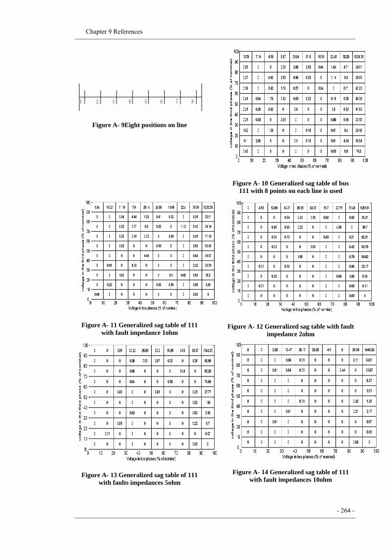
Chapter 9 References
- 264 -
Figure A- 9Eight positions on line
Figure A- 10 Generalized sag table of bus 111 with 8 points on each line is used
Figure A- 11 Generalized sag table of 111 with fault impedance 1ohm
Figure A- 12 Generalized sag table with fault impedance 2ohm
Figure A- 13 Generalized sag table of 111 with faults impedances 5ohm
Figure A- 14 Generalized sag table of 111 with fault impedances 10ohm

Chapter 9 References
- 265 -
Figure A- 15 Generalized sag table of entire network with fault impedance 1ohm
Figure A- 16 Generalized sag table of entire network with fault impedance 2ohm
Figure A- 17 Generalized sag table of entire network with faults impedances 5ohm
Figure A- 18 Generalized sag table of entire network with faults impedances 10OM
Table A- 2 Voltage magnitude, phase angle and voltage level of each bus bus no
voltage magnitud
e
phase angle
(degree)
voltage level
bus no
voltage magnitud
e
phase angle
(degree)
voltage level
bus no
voltage magnitud
e
phase angle
(degree)
voltage level
bus no voltage magnitude
phase angle
(degree)
voltage level
1 0.966 -5.49 11 76 1.015 -8.45 11 152 1.008 -7.03 11 227 0.9761 -5.3 11 2 0.965 -5.52 11 77 1.013 -6.64 11 153 0.99 -7.48 11 228 1.0205 -8.32 11 3 0.962 -5.55 11 78 1.024 -7.6 11 154 0.99 -7.48 11 229 1.0205 -8.32 11 4 0.965 -5.51 11 79 1.022 -7.64 11 155 0.987 -7.55 11 230 1.0273 -7.53 11 5 0.964 -5.52 11 80 1.02 -7.67 11 156 0.987 -7.55 11 231 1.0273 -7.53 11 6 0.963 -5.53 11 81 1.014 -7.61 11 157 0.984 -7.59 11 232 1.0134 -6.62 11 7 0.963 -5.53 11 82 1.014 -7.62 11 158 0.984 -7.59 11 233 0.988 -2.12 132 8 0.963 -5.53 11 83 1.013 -7.63 11 159 0.983 -7.59 11 234 0.988 -2.12 132 9 0.963 -5.53 11 84 1.013 -7.63 11 160 0.983 -7.62 11 235 1.0343 23.78 33 10 0.963 -5.53 11 85 1.013 -7.64 11 161 0.979 -7.7 11 236 1.0343 23.78 33 11 0.963 -5.53 11 86 1.013 -7.65 11 162 0.979 -7.71 11 237 1.0112 24.49 33 12 0.995 -8.58 11 87 1.025 -7.66 11 163 0.979 -7.71 11 238 1.0343 23.78 33 13 0.99 -8.63 11 88 1.013 -7.62 11 164 0.979 -7.71 11 239 1.0343 23.78 33 14 0.998 -8.56 11 89 1.012 -7.63 11 165 0.976 -7.78 11 240 0.9751 25.45 33 15 0.999 -8.55 11 91 1.012 -7.64 11 166 0.975 -7.81 11 241 1.0125 25.17 33 16 0.999 -8.55 11 92 1.012 -7.68 11 167 0.975 -7.81 11 242 1.0323 23.69 33 17 0.999 -8.55 11 93 1.012 -7.68 11 168 0.975 -7.81 11 243 1.0088 24.62 33 18 0.999 -8.55 11 94 1.011 -7.7 11 169 0.975 -7.81 11 244 1.0088 24.62 33 19 1.002 -8.52 11 95 1.011 -7.7 11 170 0.975 -7.81 11 245 1.0144 24.72 33 20 1.006 -8.48 11 96 1.01 -7.71 11 171 0.969 -8.01 11 246 1.0144 24.72 33

Chapter 9 References
- 266 -
21 1.006 -8.49 11 97 1.01 -7.72 11 172 0.969 -8.01 11 247 0.9719 24.23 33 22 1.012 -8.43 11 98 1.01 -7.72 11 173 0.968 -8.02 11 248 0.9719 24.23 33 23 0.98 -8.7 11 99 1.01 -7.72 11 174 0.968 -8.02 11 249 1.0358 23.82 33 24 0.98 -8.7 11 100 1.009 -7.73 11 175 0.968 -8.02 11 250 1.0358 23.82 33 25 0.96 -5.57 11 101 1.01 -7.73 11 176 0.968 -8.02 11 251 1.0157 24.73 33 26 0.976 -8.76 11 102 1.011 -7.74 11 177 0.968 -8.03 11 252 1.0191 24.35 33 27 0.959 -5.58 11 103 1.01 -7.74 11 178 0.968 -8.03 11 253 0.9906 -1.92 132 28 0.975 -8.77 11 104 1.01 -7.75 11 179 0.96 -5.57 11 254 0.9874 -2.3 132 29 0.958 -5.58 11 105 1.01 -7.77 11 180 0.975 -7.81 11 255 0.9874 -2.3 132 30 0.956 -5.58 11 106 1.01 -7.77 11 181 0.975 -7.82 11 256 0.991 -1.86 132 31 0.953 -5.57 11 107 1.01 -7.78 11 182 0.974 -7.82 11 257 0.991 -1.86 132 32 0.953 -5.57 11 108 1.009 -7.8 11 183 0.974 -7.82 11 258 0.986 -2.1 132 33 0.953 -5.57 11 109 1.009 -7.81 11 184 0.974 -7.81 11 259 0.986 -2.1 132 34 0.953 -5.57 11 110 1.009 -7.81 11 185 0.974 -7.82 11 260 1.0173 24.54 33 35 0.953 -5.57 11 111 1.008 -7.81 11 186 0.974 -7.82 11 261 1.0173 24.54 33 36 0.953 -5.57 11 112 1.009 -7.82 11 187 0.974 -7.82 11 262 0.9872 -2.25 132 37 0.954 -9.2 11 113 1.008 -7.82 11 188 0.974 -7.84 11 263 0.9901 -1.89 132 38 0.955 -9.21 11 114 1.008 -7.82 11 189 0.974 -7.84 11 264 0.9901 -1.89 132 39 0.956 -9.21 11 115 1.008 -7.83 11 190 0.974 -7.84 11 265 0.9727 25.2 33 40 0.957 -9.18 11 116 1.008 -7.84 11 191 0.974 -7.84 11 266 1.0341 23.78 33 41 0.959 -9.18 11 117 1.008 -7.84 11 192 0.974 -7.84 11 267 1.0341 23.78 33 42 0.962 -9.19 11 118 1.008 -7.84 11 193 0.973 -7.9 11 268 1.0294 23.68 33 43 0.964 -9.19 11 119 1.008 -7.84 11 194 0.972 -7.91 11 269 1.0294 23.68 33 44 0.972 -8.77 11 120 1.008 -7.84 11 195 0.972 -7.91 11 270 0.9814 -2.16 132 45 0.972 -8.77 11 121 1.008 -7.84 11 196 0.972 -7.91 11 271 0.9865 -2.18 132 46 0.971 -8.82 11 122 1.008 -7.84 11 197 0.972 -7.91 11 272 0.9812 -2.16 132 47 0.971 -8.82 11 123 1.008 -7.84 11 198 0.971 -7.92 11 273 0.985 -2.18 132 48 0.971 -8.82 11 124 1.008 -7.84 11 199 0.971 -7.92 11 274 0.9907 -1.9 132 49 0.971 -8.82 11 125 1.008 -7.84 11 200 0.971 -7.93 11 275 0.9909 -2.03 132 50 1.018 -8.39 11 126 1.007 -7.84 11 201 0.971 -7.93 11 276 0.9864 -2.18 132 51 1.016 -8.42 11 127 1.007 -7.84 11 202 0.971 -7.94 11 277 0.9892 -2.15 132 52 1.017 -8.43 11 128 1.007 -7.85 11 203 0.971 -7.94 11 278 0.9892 -2.15 132 53 1.017 -8.44 11 129 0.979 -7.67 11 204 0.97 -7.94 11 279 0.99 -2.04 132 54 1.018 -8.34 11 130 0.979 -7.67 11 205 0.97 -7.95 11 280 0.99 -2.04 132 55 0.966 -5.49 11 131 0.979 -7.67 11 206 0.97 -7.95 11 285 1.0126 22.37 3.3 56 0.967 -5.47 11 132 0.977 -7.71 11 207 0.97 -7.95 11 286 1.0126 22.37 3.3 57 0.97 -5.42 11 133 0.974 -7.75 11 208 0.97 -7.95 11 287 0.9826 53.78 3.3 58 0.972 -5.38 11 134 0.971 -7.81 11 209 0.97 -7.95 11 288 0.9826 53.78 3.3 59 0.973 -5.48 11 135 0.97 -7.84 11 210 0.972 -7.93 11 289 1.0173 54.54 13.8 60 0.974 -5.33 11 136 0.97 -7.84 11 211 0.971 -7.95 11 290 1.0126 -7.63 11 61 0.973 -5.48 11 137 0.966 -7.96 11 212 0.971 -7.95 11 291 1.0126 -7.63 11 62 0.971 -5.4 11 138 0.966 -7.96 11 213 0.971 -7.95 11 292 0.9987 -0.19 400 63 0.969 -5.43 11 139 0.981 -7.64 11 214 0.971 -7.95 11 293 0.9987 -0.19 400 64 0.969 -5.44 11 140 0.981 -7.64 11 215 0.97 -7.97 11 294 0.9987 -0.5 275 65 0.968 -5.44 11 141 0.984 -7.58 11 216 0.97 -7.97 11 295 0.9996 -0.08 275 66 0.965 -5.43 11 142 0.984 -7.58 11 217 0.97 -7.99 11 296 0.9993 -0.12 275 67 0.962 -5.56 11 143 0.987 -7.53 11 218 0.969 -8 11 297 0.9993 -0.12 275 68 0.962 -5.56 11 144 0.987 -7.53 11 219 0.969 -8.01 11 298 0.9992 -0.13 400 69 0.962 -5.56 11 145 0.99 -7.48 11 220 0.969 -8.01 11 299 0.9992 -0.13 400 70 0.962 -5.56 11 146 0.994 -7.42 11 221 1.017 -8.41 11 300 1 0 400 71 0.962 -5.56 11 147 0.997 -7.35 11 222 0.968 -9.19 11 72 0.962 -5.56 11 148 0.997 -7.35 11 223 1.019 -8.36 11 73 0.962 -5.56 11 149 1.003 -7.21 11 224 1.012 -6.66 11 74 1.015 -8.46 11 150 1.003 -7.21 11 225 1.013 -6.68 11 75 1.014 -8.47 11 151 1.008 -7.03 11 226 0.976 -5.3 11

Chapter 9 References
- 267 -
Figure A- 19 Phase A voltage at bus 111 for LG faults at all buses
Figure A- 20 Phase B voltage at bus 111 for LG faults at all buses
Figure A- 21 Phase C voltage at bus 111 for LG faults at all buses
Figure A- 22 Phase A voltage at bus 111 for LLG faults at all buses
Figure A- 23 Phase B voltage at bus 111 for LLG faults at all buses
Figure A- 24 Phase C voltage at bus 111 for LLG faults at all buses
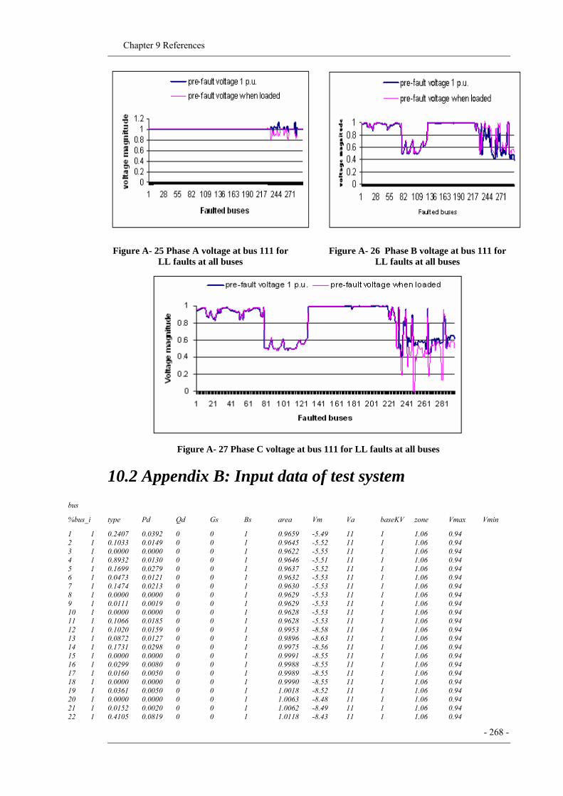
Chapter 9 References
- 268 -
Figure A- 25 Phase A voltage at bus 111 for LL faults at all buses
Figure A- 26 Phase B voltage at bus 111 for LL faults at all buses
Figure A- 27 Phase C voltage at bus 111 for LL faults at all buses
10.2 Appendix B: Input data of test system bus
%bus_i type Pd Qd Gs Bs area Vm Va baseKV zone Vmax Vmin
1 1 0.2407 0.0392 0 0 1 0.9659 -5.49 11 1 1.06 0.94 2 1 0.1033 0.0149 0 0 1 0.9645 -5.52 11 1 1.06 0.94 3 1 0.0000 0.0000 0 0 1 0.9622 -5.55 11 1 1.06 0.94 4 1 0.8932 0.0130 0 0 1 0.9646 -5.51 11 1 1.06 0.94 5 1 0.1699 0.0279 0 0 1 0.9637 -5.52 11 1 1.06 0.94 6 1 0.0473 0.0121 0 0 1 0.9632 -5.53 11 1 1.06 0.94 7 1 0.1474 0.0213 0 0 1 0.9630 -5.53 11 1 1.06 0.94 8 1 0.0000 0.0000 0 0 1 0.9629 -5.53 11 1 1.06 0.94 9 1 0.0111 0.0019 0 0 1 0.9629 -5.53 11 1 1.06 0.94 10 1 0.0000 0.0000 0 0 1 0.9628 -5.53 11 1 1.06 0.94 11 1 0.1066 0.0185 0 0 1 0.9628 -5.53 11 1 1.06 0.94 12 1 0.1020 0.0159 0 0 1 0.9953 -8.58 11 1 1.06 0.94 13 1 0.0872 0.0127 0 0 1 0.9896 -8.63 11 1 1.06 0.94 14 1 0.1731 0.0298 0 0 1 0.9975 -8.56 11 1 1.06 0.94 15 1 0.0000 0.0000 0 0 1 0.9991 -8.55 11 1 1.06 0.94 16 1 0.0299 0.0080 0 0 1 0.9988 -8.55 11 1 1.06 0.94 17 1 0.0160 0.0050 0 0 1 0.9989 -8.55 11 1 1.06 0.94 18 1 0.0000 0.0000 0 0 1 0.9990 -8.55 11 1 1.06 0.94 19 1 0.0361 0.0050 0 0 1 1.0018 -8.52 11 1 1.06 0.94 20 1 0.0000 0.0000 0 0 1 1.0063 -8.48 11 1 1.06 0.94 21 1 0.0152 0.0020 0 0 1 1.0062 -8.49 11 1 1.06 0.94 22 1 0.4105 0.0819 0 0 1 1.0118 -8.43 11 1 1.06 0.94

Chapter 10 References
- 269 -
23 1 0.0000 0.0000 0 0 1 0.9804 -8.70 11 1 1.06 0.94 24 1 0.7024 0.1576 0 0 1 0.9803 -8.70 11 1 1.06 0.94 25 1 0.0000 0.0000 0 0 1 0.9597 -5.57 11 1 1.06 0.94 26 1 0.0000 0.0000 0 0 1 0.9757 -8.76 11 1 1.06 0.94 27 1 0.0000 0.0000 0 0 1 0.9594 -5.58 11 1 1.06 0.94 28 1 0.0000 0.0000 0 0 1 0.9750 -8.77 11 1 1.06 0.94 29 1 0.5936 0.1395 0 0 1 0.9579 -5.58 11 1 1.06 0.94 30 1 0.0786 0.0256 0 0 1 0.9559 -5.58 11 1 1.06 0.94 31 1 0.4062 0.0881 0 0 1 0.9532 -5.57 11 1 1.06 0.94 32 1 0.0000 0.0000 0 0 1 0.9534 -5.57 11 1 1.06 0.94 33 1 0.0000 0.0000 0 0 1 0.9534 -5.57 11 1 1.06 0.94 34 1 0.6605 0.1490 0 0 1 0.9531 -5.57 11 1 1.06 0.94 35 1 0.1326 0.0327 0 0 1 0.9531 -5.57 11 1 1.06 0.94 36 1 0.0391 0.0127 0 0 1 0.9531 -5.57 11 1 1.06 0.94 37 1 0.3897 0.0974 0 0 1 0.9542 -9.20 11 1 1.06 0.94 38 1 0.1095 0.0219 0 0 1 0.9554 -9.21 11 1 1.06 0.94 39 1 0.6730 0.2149 0 0 1 0.9563 -9.21 11 1 1.06 0.94 40 1 0.7774 0.2500 0 0 1 0.9569 -9.18 11 1 1.06 0.94 41 1 0.2059 0.0506 0 0 1 0.9588 -9.18 11 1 1.06 0.94 42 1 0.1184 0.0268 0 0 1 0.9617 -9.19 11 1 1.06 0.94 43 1 0.3977 0.0957 0 0 1 0.9639 -9.19 11 1 1.06 0.94 44 1 0.3127 0.0576 0 0 1 0.9719 -8.77 11 1 1.06 0.94 45 1 0.4198 0.0946 0 0 1 0.9724 -8.77 11 1 1.06 0.94 46 1 0.0000 0.0000 0 0 1 0.9710 -8.82 11 1 1.06 0.94 47 1 0.0000 0.0000 0 0 1 0.9710 -8.82 11 1 1.06 0.94 48 1 0.2733 0.0603 0 0 1 0.9708 -8.82 11 1 1.06 0.94 49 1 0.4437 0.1055 0 0 1 0.9706 -8.82 11 1 1.06 0.94 50 1 0.2681 0.0424 0 0 1 1.0175 -8.39 11 1 1.06 0.94 51 1 0.4793 0.0878 0 0 1 1.0164 -8.42 11 1 1.06 0.94 52 1 0.0000 0.0000 0 0 1 1.0171 -8.43 11 1 1.06 0.94 53 1 0.4992 0.0806 0 0 1 1.0167 -8.44 11 1 1.06 0.94 54 1 0.6236 0.1264 0 0 1 1.0178 -8.34 11 1 1.06 0.94 55 1 0.3901 0.0812 0 0 1 0.9660 -5.49 11 1 1.06 0.94 56 1 0.1188 0.0187 0 0 1 0.9674 -5.47 11 1 1.06 0.94 57 1 0.1646 0.0273 0 0 1 0.9698 -5.42 11 1 1.06 0.94 58 1 0.5276 0.1371 0 0 1 0.9724 -5.38 11 1 1.06 0.94 59 1 0.6552 0.1307 0 0 1 0.9730 -5.48 11 1 1.06 0.94 60 1 0.7942 0.1471 0 0 1 0.9741 -5.33 11 1 1.06 0.94 61 1 0.2830 0.0492 0 0 1 0.9729 -5.48 11 1 1.06 0.94 62 1 0.1565 0.0245 0 0 1 0.9711 -5.40 11 1 1.06 0.94 63 1 0.4096 0.0733 0 0 1 0.9693 -5.43 11 1 1.06 0.94 64 1 0.2411 0.0413 0 0 1 0.9686 -5.44 11 1 1.06 0.94 65 1 0.4400 0.0758 0 0 1 0.9676 -5.44 11 1 1.06 0.94 66 1 0.8287 0.1574 0 0 1 0.9650 -5.43 11 1 1.06 0.94 67 1 0.0000 0.0000 0 0 1 0.9619 -5.56 11 1 1.06 0.94 68 1 0.0000 0.0000 0 0 1 0.9619 -5.56 11 1 1.06 0.94 69 1 0.0167 0.0028 0 0 1 0.9618 -5.56 11 1 1.06 0.94 70 1 0.0000 0.0000 0 0 1 0.9619 -5.56 11 1 1.06 0.94 71 1 0.1628 0.0314 0 0 1 0.9617 -5.56 11 1 1.06 0.94 72 1 0.0000 0.0000 0 0 1 0.9619 -5.56 11 1 1.06 0.94 73 1 0.0231 0.0037 0 0 1 0.9619 -5.56 11 1 1.06 0.94 74 1 0.0000 0.0000 0 0 1 1.0148 -8.46 11 1 1.06 0.94 75 1 0.4166 0.0669 0 0 1 1.0142 -8.47 11 1 1.06 0.94 76 1 0.7046 0.1391 0 0 1 1.0150 -8.45 11 1 1.06 0.94 77 1 0.0000 0.0000 0 0 1 1.0130 -6.64 11 1 1.06 0.94 78 1 0.1007 0.0147 0 0 1 1.0244 -7.60 11 1 1.06 0.94 79 1 0.4065 0.0721 0 0 1 1.0222 -7.64 11 1 1.06 0.94 80 1 0.7890 0.2540 0 0 1 1.0203 -7.67 11 1 1.06 0.94 81 1 0.0000 0.0000 0 0 1 1.0139 -7.61 11 1 1.06 0.94 82 1 0.0000 0.0000 0 0 1 1.0138 -7.62 11 1 1.06 0.94 83 1 0.0370 0.0051 0 0 1 1.0134 -7.63 11 1 1.06 0.94 84 1 0.0308 0.0041 0 0 1 1.0132 -7.63 11 1 1.06 0.94 85 1 0.0000 0.0000 0 0 1 1.0129 -7.64 11 1 1.06 0.94 86 1 0.1251 0.0236 0 0 1 1.0126 -7.65 11 1 1.06 0.94 87 1 0.9032 0.1630 0 0 1 1.0254 -7.66 11 1 1.06 0.94 88 1 0.0000 0.0000 0 0 1 1.0130 -7.62 11 1 1.06 0.94 89 1 1.1915 0.3914 0 0 1 1.0122 -7.63 11 1 1.06 0.94 91 1 0.0000 0.0000 0 0 1 1.0123 -7.64 11 1 1.06 0.94 92 1 0.0000 0.0000 0 0 1 1.0116 -7.68 11 1 1.06 0.94 93 1 0.0440 0.0072 0 0 1 1.0115 -7.68 11 1 1.06 0.94 94 1 0.0000 0.0000 0 0 1 1.0114 -7.70 11 1 1.06 0.94 95 1 0.0082 0.0010 0 0 1 1.0110 -7.70 11 1 1.06 0.94 96 1 0.0000 0.0000 0 0 1 1.0103 -7.71 11 1 1.06 0.94 97 1 0.0367 0.0061 0 0 1 1.0103 -7.72 11 1 1.06 0.94 98 1 0.0000 0.0000 0 0 1 1.0099 -7.72 11 1 1.06 0.94

Chapter 10 References
- 270 -
99 1 0.0163 0.0020 0 0 1 1.0097 -7.72 11 1 1.06 0.94 100 1 0.0825 0.0163 0 0 1 1.0094 -7.73 11 1 1.06 0.94 101 1 0.0734 0.0143 0 0 1 1.0097 -7.73 11 1 1.06 0.94 102 1 0.0000 0.0000 0 0 1 1.0106 -7.74 11 1 1.06 0.94 103 1 0.0663 0.0112 0 0 1 1.0103 -7.74 11 1 1.06 0.94 104 1 0.0092 0.0010 0 0 1 1.0103 -7.75 11 1 1.06 0.94 105 1 0.0000 0.0000 0 0 1 1.0099 -7.77 11 1 1.06 0.94 106 1 0.0235 0.0031 0 0 1 1.0099 -7.77 11 1 1.06 0.94 107 1 0.0387 0.0061 0 0 1 1.0095 -7.78 11 1 1.06 0.94 108 1 0.0183 0.0031 0 0 1 1.0090 -7.80 11 1 1.06 0.94 109 1 0.0000 0.0000 0 0 1 1.0087 -7.81 11 1 1.06 0.94 110 1 0.0000 0.0000 0 0 1 1.0086 -7.81 11 1 1.06 0.94 111 1 0.1291 0.0315 0 0 1 1.0083 -7.81 11 1 1.06 0.94 112 1 0.0203 0.0031 0 0 1 1.0085 -7.82 11 1 1.06 0.94 113 1 0.0000 0.0000 0 0 1 1.0084 -7.82 11 1 1.06 0.94 114 1 0.0061 0.0009 0 0 1 1.0083 -7.82 11 1 1.06 0.94 115 1 0.0102 0.0010 0 0 1 1.0083 -7.83 11 1 1.06 0.94 116 1 0.0000 0.0000 0 0 1 1.0079 -7.84 11 1 1.06 0.94 117 1 0.0061 0.0009 0 0 1 1.0078 -7.84 11 1 1.06 0.94 118 1 0.0000 0.0000 0 0 1 1.0078 -7.84 11 1 1.06 0.94 119 1 0.0051 0.0007 0 0 1 1.0078 -7.84 11 1 1.06 0.94 120 1 0.0081 0.0010 0 0 1 1.0078 -7.84 11 1 1.06 0.94 121 1 0.0000 0.0000 0 0 1 1.0078 -7.84 11 1 1.06 0.94 122 1 0.0000 0.0000 0 0 1 1.0078 -7.84 11 1 1.06 0.94 123 1 0.0000 0.0000 0 0 1 1.0078 -7.84 11 1 1.06 0.94 124 1 0.0000 0.0000 0 0 1 1.0078 -7.84 11 1 1.06 0.94 125 1 0.0091 0.0010 0 0 1 1.0076 -7.84 11 1 1.06 0.94 126 1 0.0233 0.0071 0 0 1 1.0074 -7.84 11 1 1.06 0.94 127 1 0.0071 0.0010 0 0 1 1.0073 -7.84 11 1 1.06 0.94 128 1 0.0203 0.0030 0 0 1 1.0073 -7.85 11 1 1.06 0.94 129 1 0.0000 0.0000 0 0 1 0.9791 -7.67 11 1 1.06 0.94 130 1 0.0431 0.0077 0 0 1 0.9791 -7.67 11 1 1.06 0.94 131 1 0.0000 0.0000 0 0 1 0.9792 -7.67 11 1 1.06 0.94 132 1 0.0353 0.0048 0 0 1 0.9767 -7.71 11 1 1.06 0.94 133 1 0.0180 0.0028 0 0 1 0.9744 -7.75 11 1 1.06 0.94 134 1 0.0170 0.0028 0 0 1 0.9710 -7.81 11 1 1.06 0.94 135 1 0.0000 0.0000 0 0 1 0.9699 -7.84 11 1 1.06 0.94 136 1 0.0094 0.0009 0 0 1 0.9699 -7.84 11 1 1.06 0.94 137 1 0.8682 0.2853 0 0 1 0.9657 -7.96 11 1 1.06 0.94 138 1 0.0000 0.0000 0 0 1 0.9657 -7.96 11 1 1.06 0.94 139 1 0.0000 0.0000 0 0 1 0.9808 -7.64 11 1 1.06 0.94 140 1 0.0096 0.0019 0 0 1 0.9808 -7.64 11 1 1.06 0.94 141 1 0.0000 0.0000 0 0 1 0.9841 -7.58 11 1 1.06 0.94 142 1 0.0213 0.0068 0 0 1 0.9840 -7.58 11 1 1.06 0.94 143 1 0.0000 0.0000 0 0 1 0.9871 -7.53 11 1 1.06 0.94 144 1 0.0029 0.0004 0 0 1 0.9871 -7.53 11 1 1.06 0.94 145 1 0.0029 0.0004 0 0 1 0.9896 -7.48 11 1 1.06 0.94 146 1 0.0000 0.0000 0 0 1 0.9935 -7.42 11 1 1.06 0.94 147 1 0.0000 0.0000 0 0 1 0.9966 -7.35 11 1 1.06 0.94 148 1 0.0189 0.0030 0 0 1 0.9965 -7.35 11 1 1.06 0.94 149 1 0.0000 0.0000 0 0 1 1.0029 -7.21 11 1 1.06 0.94 150 1 0.0201 0.0030 0 0 1 1.0028 -7.21 11 1 1.06 0.94 151 1 0.0000 0.0000 0 0 1 1.0083 -7.03 11 1 1.06 0.94 152 1 0.0091 0.0010 0 0 1 1.0083 -7.03 11 1 1.06 0.94 153 1 0.0000 0.0000 0 0 1 0.9903 -7.48 11 1 1.06 0.94 154 1 0.0206 0.0039 0 0 1 0.9902 -7.48 11 1 1.06 0.94 155 1 0.0000 0.0000 0 0 1 0.9865 -7.55 11 1 1.06 0.94 156 1 0.0127 0.0019 0 0 1 0.9865 -7.55 11 1 1.06 0.94 157 1 0.0000 0.0000 0 0 1 0.9837 -7.59 11 1 1.06 0.94 158 1 0.0348 0.0058 0 0 1 0.9835 -7.59 11 1 1.06 0.94 159 1 0.0203 0.0029 0 0 1 0.9834 -7.59 11 1 1.06 0.94 160 1 0.0183 0.0029 0 0 1 0.9825 -7.62 11 1 1.06 0.94 161 1 0.0000 0.0000 0 0 1 0.9791 -7.70 11 1 1.06 0.94 162 1 0.0345 0.0048 0 0 1 0.9788 -7.71 11 1 1.06 0.94 163 1 0.1312 0.0316 0 0 1 0.9785 -7.71 11 1 1.06 0.94 164 1 0.0048 0.0007 0 0 1 0.9785 -7.71 11 1 1.06 0.94 165 1 0.0076 0.0010 0 0 1 0.9764 -7.78 11 1 1.06 0.94 166 1 0.0000 0.0000 0 0 1 0.9754 -7.81 11 1 1.06 0.94 167 1 0.0000 0.0000 0 0 1 0.9752 -7.81 11 1 1.06 0.94 168 1 0.0200 0.0029 0 0 1 0.9752 -7.81 11 1 1.06 0.94 169 1 0.0390 0.0076 0 0 1 0.9749 -7.81 11 1 1.06 0.94 170 1 0.0000 0.0000 0 0 1 0.9747 -7.81 11 1 1.06 0.94 171 1 0.0000 0.0000 0 0 1 0.9691 -8.01 11 1 1.06 0.94 172 1 0.0000 0.0000 0 0 1 0.9689 -8.01 11 1 1.06 0.94 173 1 0.1116 0.0225 0 0 1 0.9684 -8.02 11 1 1.06 0.94
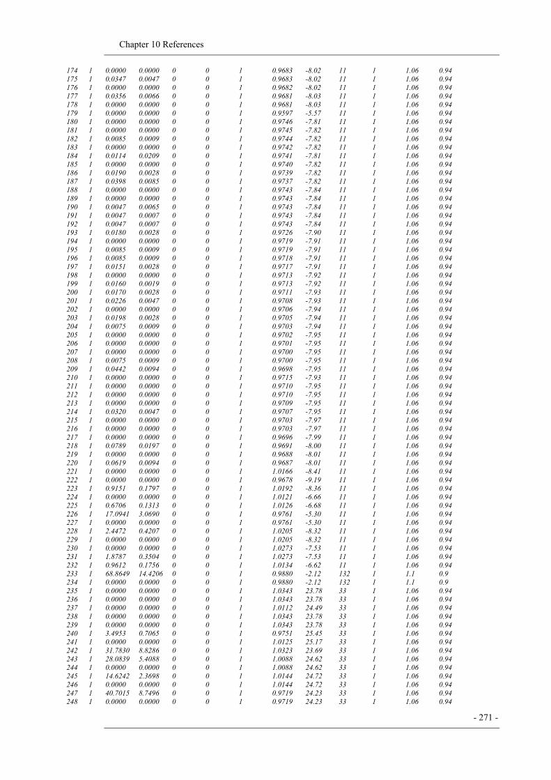
Chapter 10 References
- 271 -
174 1 0.0000 0.0000 0 0 1 0.9683 -8.02 11 1 1.06 0.94 175 1 0.0347 0.0047 0 0 1 0.9683 -8.02 11 1 1.06 0.94 176 1 0.0000 0.0000 0 0 1 0.9682 -8.02 11 1 1.06 0.94 177 1 0.0356 0.0066 0 0 1 0.9681 -8.03 11 1 1.06 0.94 178 1 0.0000 0.0000 0 0 1 0.9681 -8.03 11 1 1.06 0.94 179 1 0.0000 0.0000 0 0 1 0.9597 -5.57 11 1 1.06 0.94 180 1 0.0000 0.0000 0 0 1 0.9746 -7.81 11 1 1.06 0.94 181 1 0.0000 0.0000 0 0 1 0.9745 -7.82 11 1 1.06 0.94 182 1 0.0085 0.0009 0 0 1 0.9744 -7.82 11 1 1.06 0.94 183 1 0.0000 0.0000 0 0 1 0.9742 -7.82 11 1 1.06 0.94 184 1 0.0114 0.0209 0 0 1 0.9741 -7.81 11 1 1.06 0.94 185 1 0.0000 0.0000 0 0 1 0.9740 -7.82 11 1 1.06 0.94 186 1 0.0190 0.0028 0 0 1 0.9739 -7.82 11 1 1.06 0.94 187 1 0.0398 0.0085 0 0 1 0.9737 -7.82 11 1 1.06 0.94 188 1 0.0000 0.0000 0 0 1 0.9743 -7.84 11 1 1.06 0.94 189 1 0.0000 0.0000 0 0 1 0.9743 -7.84 11 1 1.06 0.94 190 1 0.0047 0.0065 0 0 1 0.9743 -7.84 11 1 1.06 0.94 191 1 0.0047 0.0007 0 0 1 0.9743 -7.84 11 1 1.06 0.94 192 1 0.0047 0.0007 0 0 1 0.9743 -7.84 11 1 1.06 0.94 193 1 0.0180 0.0028 0 0 1 0.9726 -7.90 11 1 1.06 0.94 194 1 0.0000 0.0000 0 0 1 0.9719 -7.91 11 1 1.06 0.94 195 1 0.0085 0.0009 0 0 1 0.9719 -7.91 11 1 1.06 0.94 196 1 0.0085 0.0009 0 0 1 0.9718 -7.91 11 1 1.06 0.94 197 1 0.0151 0.0028 0 0 1 0.9717 -7.91 11 1 1.06 0.94 198 1 0.0000 0.0000 0 0 1 0.9713 -7.92 11 1 1.06 0.94 199 1 0.0160 0.0019 0 0 1 0.9713 -7.92 11 1 1.06 0.94 200 1 0.0170 0.0028 0 0 1 0.9711 -7.93 11 1 1.06 0.94 201 1 0.0226 0.0047 0 0 1 0.9708 -7.93 11 1 1.06 0.94 202 1 0.0000 0.0000 0 0 1 0.9706 -7.94 11 1 1.06 0.94 203 1 0.0198 0.0028 0 0 1 0.9705 -7.94 11 1 1.06 0.94 204 1 0.0075 0.0009 0 0 1 0.9703 -7.94 11 1 1.06 0.94 205 1 0.0000 0.0000 0 0 1 0.9702 -7.95 11 1 1.06 0.94 206 1 0.0000 0.0000 0 0 1 0.9701 -7.95 11 1 1.06 0.94 207 1 0.0000 0.0000 0 0 1 0.9700 -7.95 11 1 1.06 0.94 208 1 0.0075 0.0009 0 0 1 0.9700 -7.95 11 1 1.06 0.94 209 1 0.0442 0.0094 0 0 1 0.9698 -7.95 11 1 1.06 0.94 210 1 0.0000 0.0000 0 0 1 0.9715 -7.93 11 1 1.06 0.94 211 1 0.0000 0.0000 0 0 1 0.9710 -7.95 11 1 1.06 0.94 212 1 0.0000 0.0000 0 0 1 0.9710 -7.95 11 1 1.06 0.94 213 1 0.0000 0.0000 0 0 1 0.9709 -7.95 11 1 1.06 0.94 214 1 0.0320 0.0047 0 0 1 0.9707 -7.95 11 1 1.06 0.94 215 1 0.0000 0.0000 0 0 1 0.9703 -7.97 11 1 1.06 0.94 216 1 0.0000 0.0000 0 0 1 0.9703 -7.97 11 1 1.06 0.94 217 1 0.0000 0.0000 0 0 1 0.9696 -7.99 11 1 1.06 0.94 218 1 0.0789 0.0197 0 0 1 0.9691 -8.00 11 1 1.06 0.94 219 1 0.0000 0.0000 0 0 1 0.9688 -8.01 11 1 1.06 0.94 220 1 0.0619 0.0094 0 0 1 0.9687 -8.01 11 1 1.06 0.94 221 1 0.0000 0.0000 0 0 1 1.0166 -8.41 11 1 1.06 0.94 222 1 0.0000 0.0000 0 0 1 0.9678 -9.19 11 1 1.06 0.94 223 1 0.9151 0.1797 0 0 1 1.0192 -8.36 11 1 1.06 0.94 224 1 0.0000 0.0000 0 0 1 1.0121 -6.66 11 1 1.06 0.94 225 1 0.6706 0.1313 0 0 1 1.0126 -6.68 11 1 1.06 0.94 226 1 17.0941 3.0690 0 0 1 0.9761 -5.30 11 1 1.06 0.94 227 1 0.0000 0.0000 0 0 1 0.9761 -5.30 11 1 1.06 0.94 228 1 2.4472 0.4207 0 0 1 1.0205 -8.32 11 1 1.06 0.94 229 1 0.0000 0.0000 0 0 1 1.0205 -8.32 11 1 1.06 0.94 230 1 0.0000 0.0000 0 0 1 1.0273 -7.53 11 1 1.06 0.94 231 1 1.8787 0.3504 0 0 1 1.0273 -7.53 11 1 1.06 0.94 232 1 0.9612 0.1756 0 0 1 1.0134 -6.62 11 1 1.06 0.94 233 1 68.8649 14.4206 0 0 1 0.9880 -2.12 132 1 1.1 0.9 234 1 0.0000 0.0000 0 0 1 0.9880 -2.12 132 1 1.1 0.9 235 1 0.0000 0.0000 0 0 1 1.0343 23.78 33 1 1.06 0.94 236 1 0.0000 0.0000 0 0 1 1.0343 23.78 33 1 1.06 0.94 237 1 0.0000 0.0000 0 0 1 1.0112 24.49 33 1 1.06 0.94 238 1 0.0000 0.0000 0 0 1 1.0343 23.78 33 1 1.06 0.94 239 1 0.0000 0.0000 0 0 1 1.0343 23.78 33 1 1.06 0.94 240 1 3.4953 0.7065 0 0 1 0.9751 25.45 33 1 1.06 0.94 241 1 0.0000 0.0000 0 0 1 1.0125 25.17 33 1 1.06 0.94 242 1 31.7830 8.8286 0 0 1 1.0323 23.69 33 1 1.06 0.94 243 1 28.0839 5.4088 0 0 1 1.0088 24.62 33 1 1.06 0.94 244 1 0.0000 0.0000 0 0 1 1.0088 24.62 33 1 1.06 0.94 245 1 14.6242 2.3698 0 0 1 1.0144 24.72 33 1 1.06 0.94 246 1 0.0000 0.0000 0 0 1 1.0144 24.72 33 1 1.06 0.94 247 1 40.7015 8.7496 0 0 1 0.9719 24.23 33 1 1.06 0.94 248 1 0.0000 0.0000 0 0 1 0.9719 24.23 33 1 1.06 0.94

Chapter 10 References
- 272 -
249 1 26.1959 5.3742 0 0 1 1.0358 23.82 33 1 1.06 0.94 250 1 0.0000 0.0000 0 0 1 1.0358 23.82 33 1 1.06 0.94 251 1 0.0000 0.0000 0 0 1 1.0157 24.73 33 1 1.06 0.94 252 1 0.0000 0.0000 0 0 1 1.0191 24.35 33 1 1.06 0.94 253 1 0.0000 0.0000 0 0 1 0.9906 -1.92 132 1 1.1 0.9 254 1 68.3597 12.1889 0 0 1 0.9874 -2.30 132 1 1.1 0.9 255 1 0.0000 0.0000 0 0 1 0.9874 -2.30 132 1 1.1 0.9 256 1 0.0000 0.0000 0 0 1 0.9910 -1.86 132 1 1.1 0.9 257 1 0.0000 0.0000 0 0 1 0.9910 -1.86 132 1 1.1 0.9 258 1 42.9038 9.1610 0 0 1 0.9860 -2.10 132 1 1.1 0.9 259 1 0.0000 0.0000 0 0 1 0.9860 -2.10 132 1 1.1 0.9 260 1 0.0000 0.0000 0 0 1 1.0173 24.54 33 1 1.06 0.94 261 1 0.0000 0.0000 0 0 1 1.0173 24.54 33 1 1.06 0.94 262 1 0.0000 0.0000 0 0 1 0.9872 -2.25 132 1 1.1 0.9 263 1 0.0000 0.0000 0 0 1 0.9901 -1.89 132 1 1.1 0.9 264 1 0.0000 0.0000 0 0 1 0.9901 -1.89 132 1 1.1 0.9 265 1 0.0000 0.0000 0 0 1 0.9727 25.20 33 1 1.06 0.94 266 1 0.0000 0.0000 0 0 1 1.0341 23.78 33 1 1.06 0.94 267 1 0.0000 0.0000 0 0 1 1.0341 23.78 33 1 1.06 0.94 268 1 0.0000 0.0000 0 0 1 1.0294 23.68 33 1 1.06 0.94 269 1 0.0000 0.0000 0 0 1 1.0294 23.68 33 1 1.06 0.94 270 1 0.0000 0.0000 0 0 1 0.9814 -2.16 132 1 1.1 0.9 271 1 0.0000 0.0000 0 0 1 0.9865 -2.18 132 1 1.1 0.9 272 1 0.0000 0.0000 0 0 1 0.9812 -2.16 132 1 1.1 0.9 273 1 0.0000 0.0000 0 0 1 0.9850 -2.18 132 1 1.1 0.9 274 1 0.0000 0.0000 0 0 1 0.9907 -1.90 132 1 1.1 0.9 275 1 0.0000 0.0000 0 0 1 0.9909 -2.03 132 1 1.1 0.9 276 1 0.0000 0.0000 0 0 1 0.9864 -2.18 132 1 1.1 0.9 277 1 0.0000 0.0000 0 0 1 0.9892 -2.15 132 1 1.1 0.9 278 1 0.0000 0.0000 0 0 1 0.9892 -2.15 132 1 1.1 0.9 279 1 0.0000 0.0000 0 0 1 0.9900 -2.04 132 1 1.1 0.9 280 1 0.0000 0.0000 0 0 1 0.9900 -2.04 132 1 1.1 0.9 285 1 0.000001 0.000001 0 0 1 1.0126 22.37 3.3 1 1.06 0.94 286 1 0.000001 0.000001 0 0 1 1.0126 22.37 3.3 1 1.06 0.94 287 1 0.000001 0.000001 0 0 1 0.9826 53.78 3.3 1 1.06 0.94 288 1 0.000001 0.000001 0 0 1 0.9826 53.78 3.3 1 1.06 0.94 289 1 0.000001 0.000001 0 0 1 1.0173 54.54 13.8 1 1.06 0.94 290 1 0.0000 0.0000 0 0 1 1.0126 -7.63 11 1 1.06 0.94 291 1 0.0000 0.0000 0 0 1 1.0126 -7.63 11 1 1.06 0.94 292 1 0.0000 0.0000 0 0 1 0.9987 -0.19 400 1 1.1 0.9 293 1 0.0000 0.0000 0 0 1 0.9987 -0.19 400 1 1.1 0.9 294 1 0.0000 0.0000 0 0 1 0.9987 -0.50 275 1 1.1 0.9 295 1 0.0000 0.0000 0 0 1 0.9996 -0.08 275 1 1.1 0.9 296 1 0.0000 0.0000 0 0 1 0.9993 -0.12 275 1 1.1 0.9 297 1 0.0000 0.0000 0 0 1 0.9993 -0.12 275 1 1.1 0.9 298 1 0.0000 0.0000 0 0 1 0.9992 -0.13 400 1 1.1 0.9 299 1 0.0000 0.0000 0 0 1 0.9992 -0.13 400 1 1.1 0.9 300 3 0.0000 0.0000 0 0 1 1.0000 0.00 400 1 1.1 0.9 end
Figure A- 28 bus data
% generator data
%bus Pg Qg Qmax Qmin Vg mRate status Pmax Pmin R1 X1 R0 X0
gen
300 0 0 99999 -99999 1 1200 1 99999 0 0 0.020833 0.000625 0.00625;
end
Figure A- 29 Generator data
%% line data %fbus tbus r x b r0 x0 b0 rateA rateB rateC length type(1:o,2:c)
status linedata 233 234 0.00001 0.00001 0 0.00006 0.00003 0 99 0 0 1 1 1 233 279 0.0084 0.00598 0.00136 0.0504 0.01794 0.000453333 99 0 0 1 2 1 279 257 0.00103 0.00736 0.00167 0.00167 0.02208 0.000556667 99 0 0 1 2 1 234 280 0.0084 0.00598 0.00136 0.0504 0.01794 0.000453333 99 0 0 1 2 1 280 256 0.00103 0.00736 0.00167 0.00617 0.00221 0.000556667 99 0 0 1 2 1 257 256 0.00001 0.00001 0 0.00006 0.00001 0 99 0 0 1 1 1 280 277 0.00139 0.00989 0.00225 0.00834 0.02967 0.00075 99 0 0 1 2 1 279 278 0.00139 0.00989 0.00225 0.00834 0.02967 0.00075 99 0 0 1 2 1

Chapter 10 References
- 273 -
248 247 0.00001 0.00001 0 0.00006 0.00003 0 99 0 0 1 1 1 254 255 0.00001 0.00001 0 0.00006 0.00003 0 99 0 0 1 1 1 234 254 0.00388 0.0276 0.00627 0.02328 0.0828 0.00209 99 0 0 1 2 1 233 255 0.00388 0.0276 0.00627 0.02328 0.0828 0.00209 99 0 0 1 2 1 257 264 0.00588 0.00441 0.03391 0.03528 0.01323 0.011303333 99 0 0 1 2 1 256 263 0.00588 0.00441 0.03391 0.03528 0.01323 0.011303333 99 0 0 1 2 1 227 226 0.00001 0.00001 0 0.00006 0.00003 0 99 0 0 1 1 1 227 58 0.12491 0.074 0.00025 0.74946 0.222 8.33E-05 99 0 0 1 2 1 58 62 0.0564 0.02157 0.00005 0.3384 0.06471 1.67E-05 99 0 0 1 2 1 62 63 0.08474 0.04121 0.00012 0.50844 0.12363 0.00004 99 0 0 1 2 1 61 59 0.0294 0.01983 0.00007 0.1764 0.05949 2.33E-05 99 0 0 1 2 1 59 60 0.06 0.276 0.00008 0.36 0.828 2.67E-05 99 0 0 1 2 1 60 227 0.105 0.04831 0.00014 0.63 0.14493 4.67E-05 99 0 0 1 2 1 63 64 0.04237 0.0206 0.00006 0.25422 0.0618 0.00002 99 0 0 1 2 1 226 57 0.12712 0.06181 0.00019 0.76272 0.18543 6.33E-05 99 0 0 1 2 1 57 56 0.04943 0.02404 0.00007 0.29658 0.07212 2.33E-05 99 0 0 1 2 1 56 55 0.02825 0.01374 0.00004 0.1695 0.04122 1.33E-05 99 0 0 1 2 1 64 65 0.21795 0.0321 0.00005 1.3077 0.0963 1.67E-05 99 0 0 1 2 1 64 66 0.40866 0.06019 0.0001 2.45196 0.18057 3.33E-05 99 0 0 1 2 1 67 68 0.09174 0.16264 0 0.55044 0.48792 0.00E+00 99 0 0 1 1 1 68 69 0.07521 0.02876 0.00007 0.45126 0.08628 2.33E-05 99 0 0 1 2 1 68 70 0.07645 0.13554 0 0.4587 0.40662 0.00E+00 99 0 0 1 1 1 70 71 0.11281 0.04314 0.00011 0.67686 0.12942 3.67E-05 99 0 0 1 2 1 70 72 0.03431 0.02314 0.00008 0.20586 0.06942 2.67E-05 99 0 0 1 2 1 72 73 0.08405 0.14909 0 0.5043 0.44727 0.00E+00 99 0 0 1 1 1 72 3 0.12 0.05521 0.00016 0.72 0.16563 5.33E-05 99 0 0 1 2 1 3 2 0.0975 0.04486 0.00013 0.585 0.13458 4.33E-05 99 0 0 1 2 1 2 55 0.06 0.0276 0.00008 0.36 0.0828 2.67E-05 99 0 0 1 2 1 55 1 0.05449 0.00802 0.00001 0.32694 0.02406 3.33E-06 99 0 0 1 2 1 74 75 0.13161 0.05033 0.0013 0.78966 0.15099 0.000433333 99 0 0 1 2 1 74 76 0.0565 0.02747 0.00008 0.339 0.08241 2.67E-05 99 0 0 1 2 1 3 179 0.11281 0.04314 0.00011 0.67686 0.12942 3.67E-05 99 0 0 1 2 1 179 25 0.00001 0.00001 0 0.00006 0.00003 0.00E+00 99 0 0 1 1 1 25 27 0.0147 0.00992 0.00004 0.0882 0.02976 1.33E-05 99 0 0 1 2 1 26 28 0.0147 0.00992 0.00004 0.0882 0.02976 1.33E-05 99 0 0 1 2 1 55 4 0.10248 0.02641 0.00006 0.61488 0.07923 0.00002 99 0 0 1 2 1 4 5 0.17569 0.04527 0.00009 1.05414 0.13581 0.00003 99 0 0 1 2 1 5 6 0.1464 0.03773 0.00008 0.8784 0.11319 2.67E-05 99 0 0 1 2 1 6 7 0.07521 0.02876 0.00007 0.45126 0.08628 2.33E-05 99 0 0 1 2 1 7 8 0.0564 0.02157 0.00005 0.3384 0.06471 1.67E-05 99 0 0 1 2 1 8 9 0.07521 0.02876 0.00007 0.45126 0.08628 2.33E-05 99 0 0 1 2 1 8 10 0.047 0.01798 0.00005 0.282 0.05394 1.67E-05 99 0 0 1 2 1 10 11 0.0188 0.00792 0.00002 0.1128 0.02338 6.67E-06 99 0 0 1 2 1 12 14 0.0376 0.01438 0.00004 0.2256 0.04314 1.33E-05 99 0 0 1 2 1 12 13 0.10341 0.03955 0.001 0.62046 0.11865 0.000333333 99 0 0 1 2 1 13 23 0.16921 0.06471 0.00016 1.01526 0.19413 5.33E-05 99 0 0 1 2 1 24 23 0.0188 0.00719 0.00002 0.1128 0.02157 6.67E-06 99 0 0 1 2 1 23 26 0.09887 0.04807 0.00015 0.59322 0.14421 0.00005 99 0 0 1 2 1 27 29 0.0732 0.01886 0.00004 0.4392 0.05658 1.33E-05 99 0 0 1 2 1 29 30 0.13622 0.02006 0.00003 0.81732 0.06018 0.00001 99 0 0 1 2 1 30 32 0.19071 0.02809 0.00004 1.14426 0.08427 1.33E-05 99 0 0 1 2 1 32 31 0.0282 0.01079 0.00003 0.1692 0.06474 0.00001 99 0 0 1 2 1 32 33 0.00001 0.00001 0 0.00006 0.00003 0 99 0 0 1 1 1 33 34 0.0282 0.01079 0.00003 0.1692 0.03237 0.00001 99 0 0 1 2 1 33 35 0.11712 0.03018 0.00006 0.70272 0.09054 0.00002 99 0 0 1 2 1 35 36 0.10898 0.01605 0.00003 0.65388 0.04815 0.00001 99 0 0 1 2 1 37 38 0.27244 0.04012 0.00006 1.63464 0.12036 0.00002 99 0 0 1 2 1 38 39 0.16346 0.02407 0.00004 0.98076 0.07221 1.33E-05 99 0 0 1 2 1 28 46 0.09887 0.04807 0.00015 0.59322 0.14421 0.00005 99 0 0 1 2 1 46 48 0.08173 0.01204 0.00002 0.49038 0.03612 6.67E-06 99 0 0 1 2 1 47 46 0.00001 0.00001 0 0.00006 0.00003 0 99 0 0 1 1 1 47 49 0.08173 0.01204 0.00002 0.49038 0.03612 6.67E-06 99 0 0 1 2 1 28 45 0.32693 0.04815 0.00008 1.96158 0.14445 2.67E-05 99 0 0 1 2 1 45 44 0.1464 0.03773 0.00008 0.8784 0.11319 2.67E-05 99 0 0 1 2 1 222 47 0.04943 0.2401 0.00007 0.29658 0.07203 2.33E-05 99 0 0 1 2 1 222 43 0.13176 0.03395 0.00007 0.79056 0.10185 2.33E-05 99 0 0 1 2 1 43 42 0.08748 0.02264 0.00005 0.52488 0.06792 1.67E-05 99 0 0 1 2 1 42 41 0.11712 0.03018 0.00006 0.70272 0.09054 0.00002 99 0 0 1 2 1 41 40 0.08784 0.02264 0.00005 0.52704 0.06792 1.67E-05 99 0 0 1 2 1 40 39 0.03814 0.05617 0.00009 0.22884 0.16851 0.00003 99 0 0 1 2 1 228 229 0.00001 0.00001 0 0.00006 0.00003 0.00E+00 99 0 0 1 1 1 76 221 0.14124 0.06868 0.00021 0.72744 0.20604 0.00007 99 0 0 1 2 1 221 50 0.0565 0.02747 0.00008 0.339 0.08241 2.67E-05 99 0 0 1 2 1 50 229 0.15536 0.07555 0.00023 0.93216 0.22665 7.67E-05 99 0 0 1 2 1 221 51 0.04411 0.02975 0.00011 0.26466 0.08925 3.67E-05 99 0 0 1 2 1

Chapter 10 References
- 274 -
52 53 0.07521 0.02876 0.00007 0.45126 0.08628 2.33E-05 99 0 0 1 2 1 52 54 0.09401 0.3595 0.00009 0.56406 1.0785 0.00003 99 0 0 1 2 1 54 229 0.23425 0.06036 0.00013 1.4055 0.18108 4.33E-05 99 0 0 1 2 1 14 15 0.0282 0.01079 0.00003 0.1692 0.03237 0.00001 99 0 0 1 2 1 15 18 0.2787 0.09107 0 1.24722 0.27321 0.00E+00 99 0 0 1 1 1 18 16 0.55431 0.24284 0 0.32586 0.72856 0.00E+00 99 0 0 1 1 1 18 17 0.48502 0.21249 0 2.91012 0.63747 0.00E+00 99 0 0 1 1 1 15 19 0.047 0.01798 0.00005 0.282 0.05394 1.67E-05 99 0 0 1 2 1 19 20 0.07521 0.02876 0.00001 0.45126 0.08628 2.33E-06 99 0 0 1 2 1 20 21 0.13161 0.05033 0.00013 0.78966 0.15099 4.33E-05 99 0 0 1 2 1 20 22 0.09401 0.03595 0.00009 0.56406 0.10785 0.00003 99 0 0 1 2 1 22 228 0.135 0.06211 0.00018 0.81 0.18633 0.00006 99 0 0 1 2 1 256 274 0.00282 0.00298 0.02927 0.01692 0.00894 0.009756667 99 0 0 1 2 1 257 253 0.00282 0.00298 0.02927 0.01692 0.00894 0.009756667 99 0 0 1 2 1 244 243 0.00001 0.00001 0 0.00006 0.00003 0 99 0 0 1 1 1 244 237 0.01274 0.01633 0.00293 0.07644 0.04899 0.000976667 99 0 0 1 2 1 237 252 0.00952 0.05048 0.00006 0.05712 0.15144 0.00002 99 0 0 1 2 1 252 260 0.00504 0.02673 0.00003 0.03024 0.08019 0.00001 99 0 0 1 2 1 251 261 0.00585 0.027 0.00003 0.0351 0.081 0.00001 99 0 0 1 2 1 252 242 0.01776 0.06236 0.00007 0.07056 0.18708 2.33E-05 99 0 0 1 2 1 241 251 0.01176 0.06236 0.00007 0.07056 0.18708 2.33E-05 99 0 0 1 2 1 251 245 0.02414 0.08624 0.00009 0.14484 0.25872 0.00003 99 0 0 1 2 1 245 246 0.00001 0.00001 0 0.00006 0.00003 0 99 0 0 1 1 1 275 253 0.00348 0.01608 0.0035 0.02088 0.04824 0.001166667 99 0 0 1 2 1 259 258 0.00001 0.00001 0 0.00006 0.00003 0 99 0 0 1 1 1 256 258 0.00399 0.02622 0.00596 0.02394 0.07866 0.001986667 99 0 0 1 2 1 257 259 0.00399 0.02622 0.0596 0.02394 0.07866 0.019866667 99 0 0 1 2 1 260 261 0.00001 0.00001 0 0.00006 0.00003 0 99 0 0 1 1 1 276 258 0.00276 0.01272 0.00277 0.01656 0.03816 0.000923333 99 0 0 1 2 1 271 259 0.00197 0.01104 0.00251 0.01182 0.03312 0.000836667 99 0 0 1 2 1 270 258 0.00197 0.01104 0.00251 0.01182 0.03312 0.000836667 99 0 0 1 2 1 258 262 0.00137 0.00897 0.00204 0.00822 0.02691 0.00068 99 0 0 1 2 1 259 272 0.00137 0.00897 0.00204 0.00822 0.02691 0.00068 99 0 0 1 2 1 249 250 0.00001 0.00001 0 0.00006 0.00003 0 99 0 0 1 1 1 249 242 0.02324 0.08624 0.00009 0.13944 0.25872 0.00003 99 0 0 1 2 1 249 235 0.02324 0.01372 0.00153 0.13944 0.04116 0.00051 99 0 0 1 2 1 235 268 0.07471 0.04409 0.00493 0.44826 0.13227 0.001643333 99 0 0 1 2 1 250 236 0.02324 0.01372 0.00153 0.13944 0.04116 0.00051 99 0 0 1 2 1 236 269 0.07471 0.04409 0.00493 0.44826 0.13227 0.001643333 99 0 0 1 2 1 262 254 0.00305 0.02001 0.00455 0.0183 0.06003 0.001516667 99 0 0 1 2 1 249 267 0.05313 0.03135 0.0035 0.31878 0.09405 0.001166667 99 0 0 1 2 1 250 266 0.05313 0.03135 0.0035 0.31878 0.09406 0.001166667 99 0 0 1 2 1 230 231 0.00001 0.00001 0 0.00006 0.00003 0 99 0 0 1 1 1 231 78 0.07841 0.05289 0.0019 0.47046 0.15867 0.000633333 99 0 0 1 2 1 78 79 0.05881 0.03967 0.00014 0.35286 0.11901 4.67E-05 99 0 0 1 2 1 223 228 0.12742 0.08595 0.00031 0.76452 0.25785 0.000103333 99 0 0 1 2 1 79 80 0.0605 0.03388 0.00011 0.363 0.10164 3.67E-05 99 0 0 1 2 1 80 81 0.306 0.0276 0.00008 1.836 0.0828 2.67E-05 99 0 0 1 2 1 81 88 0.045 0.0207 0.00006 0.27 0.0621 0.00002 99 0 0 1 2 1 88 89 0.06 0.02807 0.00008 0.36 0.8421 2.67E-05 99 0 0 1 2 1 88 291 0.06 0.02807 0.00008 0.36 0.08421 2.67E-05 99 0 0 1 2 1 290 291 0.00001 0.00001 0 0.00006 0.00003 0.00E+00 99 0 0 1 1 1 290 91 0.045 0.0207 0.00006 0.27 0.0621 0.00002 99 0 0 1 2 1 91 92 0.07645 0.13554 0 0.4587 0.40662 0.00E+00 99 0 0 1 1 1 92 93 0.1475 0.075 0 0.885 0.225 0.00E+00 99 0 0 1 1 1 92 94 0.03058 0.05421 0 0.18348 0.16263 0.00E+00 99 0 0 1 1 1 94 102 0.1643 0.19791 0 0.9858 0.59373 0.00E+00 99 0 0 1 1 1 102 103 0.3835 0.195 0 2.301 0.585 0.00E+00 99 0 0 1 1 1 102 104 0.05868 0.07068 0 0.35208 0.21204 0.00E+00 99 0 0 1 1 1 104 105 0.10562 0.12723 0 0.63372 0.38169 0.00E+00 99 0 0 1 1 1 105 106 0.1475 0.075 0 0.885 0.225 0.00E+00 99 0 0 1 1 1 105 107 0.105 0.1015 0 0.63 0.3045 0.00E+00 99 0 0 1 1 1 107 108 0.18 0.174 0 1.08 0.522 0.00E+00 99 0 0 1 1 1 108 109 0.09 0.087 0 0.54 0.261 0.00E+00 99 0 0 1 1 1 109 110 0.118 0.06 0 0.708 0.063 0.00E+00 99 0 0 1 1 1 110 111 0.21211 0.02603 0.00003 1.27266 0.07809 0.00001 99 0 0 1 2 1 109 112 0.15085 0.1309 0 0.9051 0.3927 0.00E+00 99 0 0 1 1 1 112 113 0.1724 0.11782 0 1.0344 0.35346 0.00E+00 99 0 0 1 1 1 113 114 0.1475 0.0812 0 0.885 0.2436 0.00E+00 99 0 0 1 1 1 113 115 0.0862 0.05891 0 0.5172 0.17673 0.00E+00 99 0 0 1 1 1 115 116 0.38789 0.26509 0 2.32734 0.79527 0.00E+00 99 0 0 1 1 1 116 117 0.472 0.24 0 2.832 0.72 0.00E+00 99 0 0 1 1 1 117 118 0.236 0.12 0 1.416 0.36 0.00E+00 99 0 0 1 1 1 118 119 0.236 0.12 0 1.416 0.36 0.00E+00 99 0 0 1 1 1 118 120 0.177 0.09 0 1.062 0.27 0.00E+00 99 0 0 1 1 1

Chapter 10 References
- 275 -
116 121 0.1724 0.11782 0 1.0344 0.35346 0.00E+00 99 0 0 1 1 1 121 122 0.05449 0.00802 0.00001 0.32694 0.02406 3.33E-06 99 0 0 1 2 1 122 123 0.05449 0.00802 0.00001 0.32694 0.02406 3.33E-06 99 0 0 1 2 1 122 124 0.05449 0.00802 0.00001 0.32694 0.02406 3.33E-06 99 0 0 1 2 1 124 125 0.2065 0.105 0 1.239 0.315 0.00E+00 99 0 0 1 1 1 125 126 0.413 0.21 0 2.478 0.63 0.00E+00 99 0 0 1 1 1 126 127 0.177 0.09 0 1.062 0.27 0.00E+00 99 0 0 1 1 1 127 128 0.2068 0.105 0 1.239 0.315 0.00E+00 99 0 0 1 1 1 81 82 0.0376 0.01438 0.00004 0.2256 0.04314 1.33E-05 99 0 0 1 2 1 82 83 0.2155 0.14727 0 1.293 0.44181 0.00E+00 99 0 0 1 1 1 83 84 0.1293 0.08836 0 0.7758 0.26508 0.00E+00 99 0 0 1 1 1 84 85 0.2155 0.14727 0 1.293 0.44181 0.00E+00 99 0 0 1 1 1 85 86 0.1724 0.11782 0 1.0344 0.35346 0.00E+00 99 0 0 1 1 1 87 230 0.16818 0.29818 0 1.00908 0.89454 0.00E+00 99 0 0 1 1 1 94 95 0.1475 0.075 0 0.885 0.225 0.00E+00 99 0 0 1 1 1 95 96 0.295 0.15 0 1.77 0.45 0.00E+00 99 0 0 1 1 1 96 97 0.118 0.06 0 0.708 0.18 0.00E+00 99 0 0 1 1 1 96 98 0.236 0.12 0 1.416 0.36 0.00E+00 99 0 0 1 1 1 98 101 0.2655 0.135 0 1.593 0.405 0.00E+00 99 0 0 1 1 1 98 99 0.177 0.09 0 1.062 0.27 0.00E+00 99 0 0 1 1 1 99 100 0.295 0.15 0 1.77 0.45 0.00E+00 99 0 0 1 1 1 259 273 0.00879 0.02175 0.00455 0.05274 0.06525 0.001516667 99 0 0 1 2 1 240 265 0.0418 0.1178 0.0012 0.2508 0.3534 0.0004 99 0 0 1 2 1 232 224 0.04879 0.05058 0.00024 0.29274 0.15174 0.00008 99 0 0 1 2 1 224 151 0.09755 0.33284 0 0.5853 0.99852 0 99 0 0 1 1 1 151 152 0.17322 0.07589 0 1.03932 0.22767 0 99 0 0 1 1 1 151 149 0.21 0.203 0 1.26 0.609 0 99 0 0 1 1 1 149 150 0.2451 0.10624 0 1.4706 0.31872 0 99 0 0 1 1 1 149 147 0.2586 0.17673 0 1.5516 0.53019 0 99 0 0 1 1 1 147 148 0.34645 0.15178 0 2.0787 0.45534 0 99 0 0 1 1 1 147 146 0.1293 0.08836 0 0.7758 0.26508 0 99 0 0 1 1 1 146 153 0.295 0.15 0 1.77 0.45 0 99 0 0 1 1 1 146 145 0.30169 0.20618 0 1.8014 0.61854 0 99 0 0 1 1 1 145 143 0.19395 0.13255 0 1.1637 0.39765 0 99 0 0 1 1 1 143 144 0.17322 0.07589 0 1.03932 0.22767 0 99 0 0 1 1 1 143 141 0.23705 0.162 0 1.4223 0.486 0 99 0 0 1 1 1 141 142 0.20787 0.09107 0 1.24722 0.27321 0 99 0 0 1 1 1 141 139 0.2586 0.17673 0 1.5516 0.53019 0 99 0 0 1 1 1 139 140 0.13858 0.06071 0 0.83148 0.18213 0 99 0 0 1 1 1 139 131 0.1293 0.08836 0 0.7758 0.26508 0 99 0 0 1 1 1 131 132 0.2155 0.14727 0 1.293 0.44181 0 99 0 0 1 1 1 131 129 0.1724 0.11782 0 1.0344 0.35346 0 99 0 0 1 1 1 129 130 0.10775 0.07364 0 0.6465 0.22092 0 99 0 0 1 1 1 232 77 0.05489 0.0569 0.0027 0.32934 0.1707 0.0009 99 0 0 1 2 1 77 225 0.03881 0.104 0 0.23286 0.312 0 99 0 0 1 1 1 215 216 0.1293 0.08836 0 0.7758 0.26508 0 99 0 0 1 1 1 216 217 0.19395 0.13255 0 1.1637 0.39765 0 99 0 0 1 1 1 217 171 0.2586 0.17673 0 1.5516 0.53019 0 99 0 0 1 1 1 171 172 0.06465 0.04418 0 0.3879 0.13254 0 99 0 0 1 1 1 172 173 0.27244 0.04012 0.00006 1.63464 0.12036 0.00002 99 0 0 1 2 1 173 174 0.16346 0.02407 0 0.98076 0.07221 0 99 0 0 1 1 1 174 175 0.0862 0.05891 0 0.5172 0.17673 0 99 0 0 1 1 1 175 176 0.15085 0.10309 0 0.9051 0.30927 0 99 0 0 1 1 1 176 177 0.27244 0.04012 0.00006 1.63464 0.12036 0.00002 99 0 0 1 2 1 217 218 0.27716 0.12142 0 1.66296 0.36429 0 99 0 0 1 1 1 218 219 0.48502 0.21249 0 2.91012 1.27494 0 99 0 0 1 1 1 219 220 0.22621 0.04686 0.00009 1.35726 0.14058 0.00003 99 0 0 1 2 1 153 154 0.20787 0.09107 0 1.24722 0.27321 0 99 0 0 1 1 1 153 155 0.354 0.18 0 2.124 0.54 0 99 0 0 1 1 1 155 156 0.24251 0.10624 0 1.45506 0.31872 0 99 0 0 1 1 1 155 157 0.27716 0.12142 0 1.66296 0.36426 0 99 0 0 1 1 1 157 158 0.2586 0.17673 0 1.5516 0.53019 0 99 0 0 1 1 1 158 159 0.3118 0.1366 0 1.8708 0.4098 0 99 0 0 1 1 1 157 160 0.11149 0.07376 0 0.66894 0.22128 0 99 0 0 1 1 1 160 161 0.34612 0.20653 0 2.07672 0.61959 0 99 0 0 1 1 1 161 162 0.15608 0.10326 0 0.93648 0.30978 0 99 0 0 1 1 1 162 163 0.22298 0.14752 0 1.33788 0.44256 0 99 0 0 1 1 1 163 164 0.2135 0.09126 0 1.281 0.27378 0 99 0 0 1 1 1 161 165 0.34479 0.23564 0 2.06874 0.70692 0 99 0 0 1 1 1 165 166 0.1293 0.08836 0 0.7758 0.26508 0 99 0 0 1 1 1 166 167 0.118 0.06 0 0.708 0.18 0 99 0 0 1 1 1 167 168 0.20787 0.09107 0 1.24722 0.27321 0 99 0 0 1 1 1 167 169 0.236 0.12 0 1.416 0.36 0 99 0 0 1 1 1 169 170 0.177 0.09 0 1.062 0.27 0 99 0 0 1 1 1 170 180 0.09401 0.03595 0.00009 0.56406 0.10785 0.00003 99 0 0 1 2 1

Chapter 10 References
- 276 -
180 181 0.177 0.09 0 1.062 0.27 0 99 0 0 1 1 1 181 182 0.236 0.12 0 1.416 0.36 0 99 0 0 1 1 1 181 183 0.354 0.18 0 2.124 0.54 0 99 0 0 1 1 1 183 184 0.354 0.18 0 2.124 0.54 0 99 0 0 1 1 1 183 185 0.27716 0.12142 0 1.66296 0.36426 0 99 0 0 1 1 1 185 186 0.2135 0.09126 0 1.281 0.27378 0 99 0 0 1 1 1 185 187 0.53374 0.22816 0 3.20244 0.68448 0 99 0 0 1 1 1 132 133 0.19395 0.13255 0 1.1637 0.39765 0 99 0 0 1 1 1 133 134 0.30169 0.20618 0 1.81014 0.61854 0 99 0 0 1 1 1 134 135 0.09 0.087 0 0.54 0.261 0 99 0 0 1 1 1 135 136 0.13161 0.05033 0 0.78966 0.15099 0 99 0 0 1 1 1 135 137 0.36 0.348 0 2.16 1.044 0 99 0 0 1 1 1 137 138 0.12 0.116 0 0.72 0.348 0 99 0 0 1 1 1 166 188 0.1724 0.11782 0 0.0344 0.35346 0 99 0 0 1 1 1 188 189 0.20787 0.09107 0 1.24722 0.27321 0 99 0 0 1 1 1 189 190 0.27716 0.12142 0 1.66296 0.36426 0 99 0 0 1 1 1 189 191 0.41574 0.18213 0 2.4944 0.54639 0 99 0 0 1 1 1 191 192 0.27716 0.12142 0 1.66296 0.36426 0 99 0 0 1 1 1 188 193 0.30169 0.20618 0 1.81014 0.61854 0 99 0 0 1 1 1 193 210 0.2586 0.17673 0 1.5516 0.53019 0 99 0 0 1 1 1 210 211 0.1293 0.08836 0 0.7758 0.26508 0 99 0 0 1 1 1 211 216 0.2155 0.14727 0 1.293 0.44181 0 99 0 0 1 1 1 211 212 0.18258 0.07622 0 1.09548 0.22866 0 99 0 0 1 1 1 212 213 0.29213 0.12195 0 1.75278 0.36585 0 99 0 0 1 1 1 213 214 0.4382 0.17673 0 2.6292 0.53019 0 99 0 0 1 1 1 193 194 0.36517 0.15244 0 2.19102 0.45732 0 99 0 0 1 1 1 194 197 0.14607 0.06098 0 0.87642 0.18294 0 99 0 0 1 1 1 194 195 0.17322 0.07589 0 1.03932 0.22767 0 99 0 0 1 1 1 195 196 0.3118 0.1366 0 1.8708 0.4098 0 99 0 0 1 1 1 197 198 0.25562 0.10671 0 1.53372 0.32013 0 99 0 0 1 1 1 198 199 0.20787 0.09107 0 1.24722 0.27321 0 99 0 0 1 1 1 198 200 0.18258 0.07622 0 1.09548 0.22866 0 99 0 0 1 1 1 202 203 0.09401 0.03595 0.00009 0.56406 0.10785 0.00003 99 0 0 1 2 1 202 204 0.4382 0.18293 0 2.6292 0.54879 0 99 0 0 1 1 1 204 205 0.2191 0.09146 0 1.3146 0.27447 0 99 0 0 1 1 1 205 206 0.07521 0.02876 0.00007 0.45126 0.08628 2.33E-05 99 0 0 1 2 1 206 207 0.14607 0.06098 0 0.87642 0.18294 0 99 0 0 1 1 1 207 208 0.29213 0.12195 0 1.75278 0.36585 0 99 0 0 1 1 1 207 209 0.40168 0.16768 0 2.41008 0.50304 0 99 0 0 1 1 1 246 250 0.04356 0.201 0.00022 0.26136 0.603 7.33E-05 99 0 0 1 2 1 200 201 0.29213 0.12195 0 1.75278 0.36585 0 99 0 0 1 1 1 201 202 0.25562 0.10671 0 1.53372 0.32013 0 99 0 0 1 1 1 235 238 0.036 0.3851 0.00004 0.216 1.1553 1.33E-05 99 0 0 1 2 1 236 239 0.363 0.03851 0.00004 0.2178 0.11553 1.33E-05 99 0 0 1 2 1 177 178 0.49039 0.07222 0.00012 2.94234 0.21666 0.00004 99 0 0 1 2 1 end
Figure A- 30 Line data
% transformer data % from to r x b f_w t_w tap shift ratingA ratingB ratingC
status transformer 299 300 0.0001 0.01 0 1 1 1 0 99 0 0 1 233 299 0.0033 0.1466 0 1 1 1 0 99 0 0 1 298 300 0.0001 0.01 0 1 1 1 0 99 0 0 1 234 298 0.00333 0.14667 0 1 1 1 0 99 0 0 1 247 277 0.00833 0.3 0 0 1 1 30 99 0 0 1 248 278 0.00833 0.3 0 0 1 1 30 99 0 0 1 254 297 0.00417 0.18333 0 1 1 1 0 99 0 0 1 297 300 0.0001 0.01 0 1 1 1 0 99 0 0 1 255 296 0.00417 0.18333 0 1 1 1 0 99 0 0 1 296 300 0.0001 0.01 0 1 1 1 0 99 0 0 1 256 295 0.00556 0.22222 0 1 1 1 0 99 0 0 1 295 300 0.0001 0.01 0 1 1 1 0 99 0 0 1 257 294 0.00278 0.0138 0 1 1 1 0 99 0 0 1 294 300 0.00005 0.005 0 1 1 1 0 99 0 0 1 227 264 0.01587 0.4444 0 1 1 1 0 99 0 0 1 226 263 0.01587 0.4444 0 1 1 1 0 99 0 0 1 244 253 0.0125 0.4 0 0 1 1 30 99 0 0 1 243 274 0.0125 0.4 0 0 1 1 30 99 0 0 1 242 270 0.0125 0.4 0 0 1 1.25 30 99 0 0 1 241 271 0.0125 0.4 0 0 1 1 30 99 0 0 1 245 275 0.025 0.55 0 0 1 1 30 99 0 0 1 246 276 0.025 0.55 0 0 1 1 30 99 0 0 1 293 300 0.0001 0.01 0 1 1 1 0 99 0 0 1
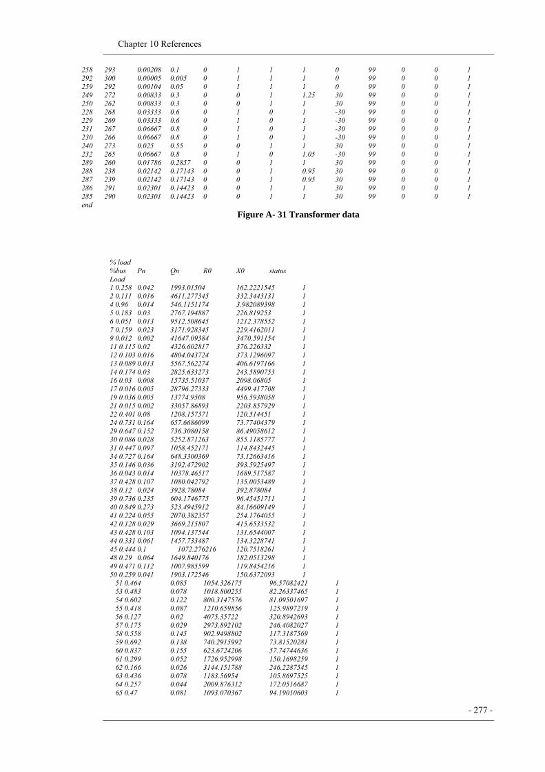
Chapter 10 References
- 277 -
258 293 0.00208 0.1 0 1 1 1 0 99 0 0 1 292 300 0.00005 0.005 0 1 1 1 0 99 0 0 1 259 292 0.00104 0.05 0 1 1 1 0 99 0 0 1 249 272 0.00833 0.3 0 0 1 1.25 30 99 0 0 1 250 262 0.00833 0.3 0 0 1 1 30 99 0 0 1 228 268 0.03333 0.6 0 1 0 1 -30 99 0 0 1 229 269 0.03333 0.6 0 1 0 1 -30 99 0 0 1 231 267 0.06667 0.8 0 1 0 1 -30 99 0 0 1 230 266 0.06667 0.8 0 1 0 1 -30 99 0 0 1 240 273 0.025 0.55 0 0 1 1 30 99 0 0 1 232 265 0.06667 0.8 0 1 0 1.05 -30 99 0 0 1 289 260 0.01786 0.2857 0 0 1 1 30 99 0 0 1 288 238 0.02142 0.17143 0 0 1 0.95 30 99 0 0 1 287 239 0.02142 0.17143 0 0 1 0.95 30 99 0 0 1 286 291 0.02301 0.14423 0 0 1 1 30 99 0 0 1 285 290 0.02301 0.14423 0 0 1 1 30 99 0 0 1 end
Figure A- 31 Transformer data
% load %bus Pn Qn R0 X0 status Load 1 0.258 0.042 1993.01504 162.2221545 1 2 0.111 0.016 4611.277345 332.3443131 1 4 0.96 0.014 546.1151174 3.982089398 1 5 0.183 0.03 2767.194887 226.819253 1 6 0.051 0.013 9512.508645 1212.378552 1 7 0.159 0.023 3171.928345 229.4162011 1 9 0.012 0.002 41647.09384 3470.591154 1 11 0.115 0.02 4326.602817 376.226332 1 12 0.103 0.016 4804.043724 373.1296097 1 13 0.089 0.013 5567.562274 406.6197166 1 14 0.174 0.03 2825.633273 243.5890753 1 16 0.03 0.008 15735.51037 2098.06805 1 17 0.016 0.005 28796.27333 4499.417708 1 19 0.036 0.005 13774.9508 956.5938058 1 21 0.015 0.002 33057.86893 2203.857929 1 22 0.401 0.08 1208.157371 120.514451 1 24 0.731 0.164 657.6686099 73.77404379 1 29 0.647 0.152 736.3080158 86.49058612 1 30 0.086 0.028 5252.871263 855.1185777 1 31 0.447 0.097 1058.452171 114.8432445 1 34 0.727 0.164 648.3300369 73.12663416 1 35 0.146 0.036 3192.472902 393.5925497 1 36 0.043 0.014 10378.46517 1689.517587 1 37 0.428 0.107 1080.042792 135.0053489 1 38 0.12 0.024 3928.78084 392.878084 1 39 0.736 0.235 604.1746775 96.45451711 1 40 0.849 0.273 523.4945912 84.16609149 1 41 0.224 0.055 2070.382357 254.1764055 1 42 0.128 0.029 3669.215807 415.6533532 1 43 0.428 0.103 1094.137544 131.6544007 1 44 0.331 0.061 1457.733487 134.3228741 1 45 0.444 0.1 1072.276216 120.7518261 1 48 0.29 0.064 1649.840176 182.0513298 1 49 0.471 0.112 1007.985599 119.8454216 1 50 0.259 0.041 1903.172546 150.6372093 1
51 0.464 0.085 1054.326175 96.57082421 1 53 0.483 0.078 1018.800255 82.26337465 1 54 0.602 0.122 800.3147576 81.09501697 1 55 0.418 0.087 1210.659856 125.9897219 1 56 0.127 0.02 4075.35722 320.8942693 1 57 0.175 0.029 2973.892102 246.4082027 1 58 0.558 0.145 902.9498802 117.3187569 1 59 0.692 0.138 740.2915992 73.81520281 1 60 0.837 0.155 623.6724206 57.74744636 1 61 0.299 0.052 1726.952998 150.1698259 1 62 0.166 0.026 3144.151788 246.2287545 1 63 0.436 0.078 1183.56954 105.8697525 1 64 0.257 0.044 2009.876312 172.0516687 1 65 0.47 0.081 1093.070367 94.19010603 1
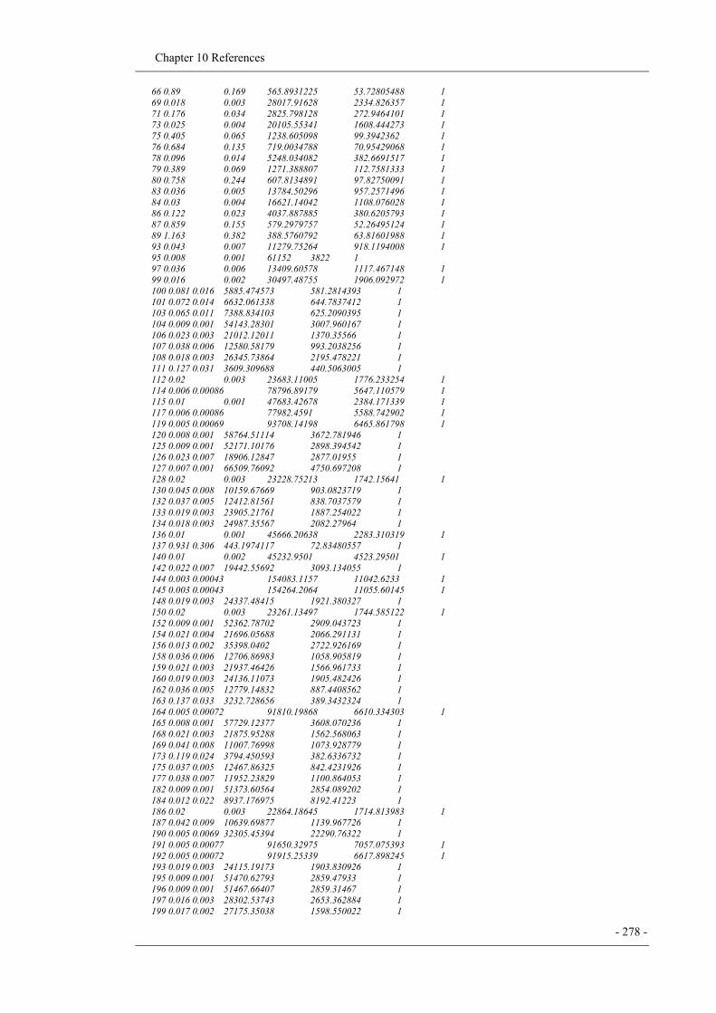
Chapter 10 References
- 278 -
66 0.89 0.169 565.8931225 53.72805488 1 69 0.018 0.003 28017.91628 2334.826357 1 71 0.176 0.034 2825.798128 272.9464101 1 73 0.025 0.004 20105.55341 1608.444273 1 75 0.405 0.065 1238.605098 99.3942362 1 76 0.684 0.135 719.0034788 70.95429068 1 78 0.096 0.014 5248.034082 382.6691517 1 79 0.389 0.069 1271.388807 112.7581333 1 80 0.758 0.244 607.8134891 97.82750091 1 83 0.036 0.005 13784.50296 957.2571496 1 84 0.03 0.004 16621.14042 1108.076028 1 86 0.122 0.023 4037.887885 380.6205793 1 87 0.859 0.155 579.2979757 52.26495124 1 89 1.163 0.382 388.5760792 63.81601988 1 93 0.043 0.007 11279.75264 918.1194008 1 95 0.008 0.001 61152 3822 1 97 0.036 0.006 13409.60578 1117.467148 1 99 0.016 0.002 30497.48755 1906.092972 1 100 0.081 0.016 5885.474573 581.2814393 1 101 0.072 0.014 6632.061338 644.7837412 1 103 0.065 0.011 7388.834103 625.2090395 1 104 0.009 0.001 54143.28301 3007.960167 1 106 0.023 0.003 21012.12011 1370.35566 1 107 0.038 0.006 12580.58179 993.2038256 1 108 0.018 0.003 26345.73864 2195.478221 1 111 0.127 0.031 3609.309688 440.5063005 1 112 0.02 0.003 23683.11005 1776.233254 1 114 0.006 0.00086 78796.89179 5647.110579 1 115 0.01 0.001 47683.42678 2384.171339 1 117 0.006 0.00086 77982.4591 5588.742902 1 119 0.005 0.00069 93708.14198 6465.861798 1 120 0.008 0.001 58764.51114 3672.781946 1 125 0.009 0.001 52171.10176 2898.394542 1 126 0.023 0.007 18906.12847 2877.01955 1 127 0.007 0.001 66509.76092 4750.697208 1 128 0.02 0.003 23228.75213 1742.15641 1 130 0.045 0.008 10159.67669 903.0823719 1 132 0.037 0.005 12412.81561 838.7037579 1 133 0.019 0.003 23905.21761 1887.254022 1 134 0.018 0.003 24987.35567 2082.27964 1 136 0.01 0.001 45666.20638 2283.310319 1 137 0.931 0.306 443.1974117 72.83480557 1 140 0.01 0.002 45232.9501 4523.29501 1 142 0.022 0.007 19442.55692 3093.134055 1 144 0.003 0.00043 154083.1157 11042.6233 1 145 0.003 0.00043 154264.2064 11055.60145 1 148 0.019 0.003 24337.48415 1921.380327 1 150 0.02 0.003 23261.13497 1744.585122 1 152 0.009 0.001 52362.78702 2909.043723 1 154 0.021 0.004 21696.05688 2066.291131 1 156 0.013 0.002 35398.0402 2722.926169 1 158 0.036 0.006 12706.86983 1058.905819 1 159 0.021 0.003 21937.46426 1566.961733 1 160 0.019 0.003 24136.11073 1905.482426 1 162 0.036 0.005 12779.14832 887.4408562 1 163 0.137 0.033 3232.728656 389.3432324 1 164 0.005 0.00072 91810.19868 6610.334303 1 165 0.008 0.001 57729.12377 3608.070236 1 168 0.021 0.003 21875.95288 1562.568063 1 169 0.041 0.008 11007.76998 1073.928779 1 173 0.119 0.024 3794.450593 382.6336732 1 175 0.037 0.005 12467.86325 842.4231926 1 177 0.038 0.007 11952.23829 1100.864053 1 182 0.009 0.001 51373.60564 2854.089202 1 184 0.012 0.022 8937.176975 8192.41223 1 186 0.02 0.003 22864.18645 1714.813983 1 187 0.042 0.009 10639.69877 1139.967726 1 190 0.005 0.0069 32305.45394 22290.76322 1 191 0.005 0.00077 91650.32975 7057.075393 1 192 0.005 0.00072 91915.25339 6617.898245 1 193 0.019 0.003 24115.19173 1903.830926 1 195 0.009 0.001 51470.62793 2859.47933 1 196 0.009 0.001 51467.66407 2859.31467 1 197 0.016 0.003 28302.53743 2653.362884 1 199 0.017 0.002 27175.35038 1598.550022 1
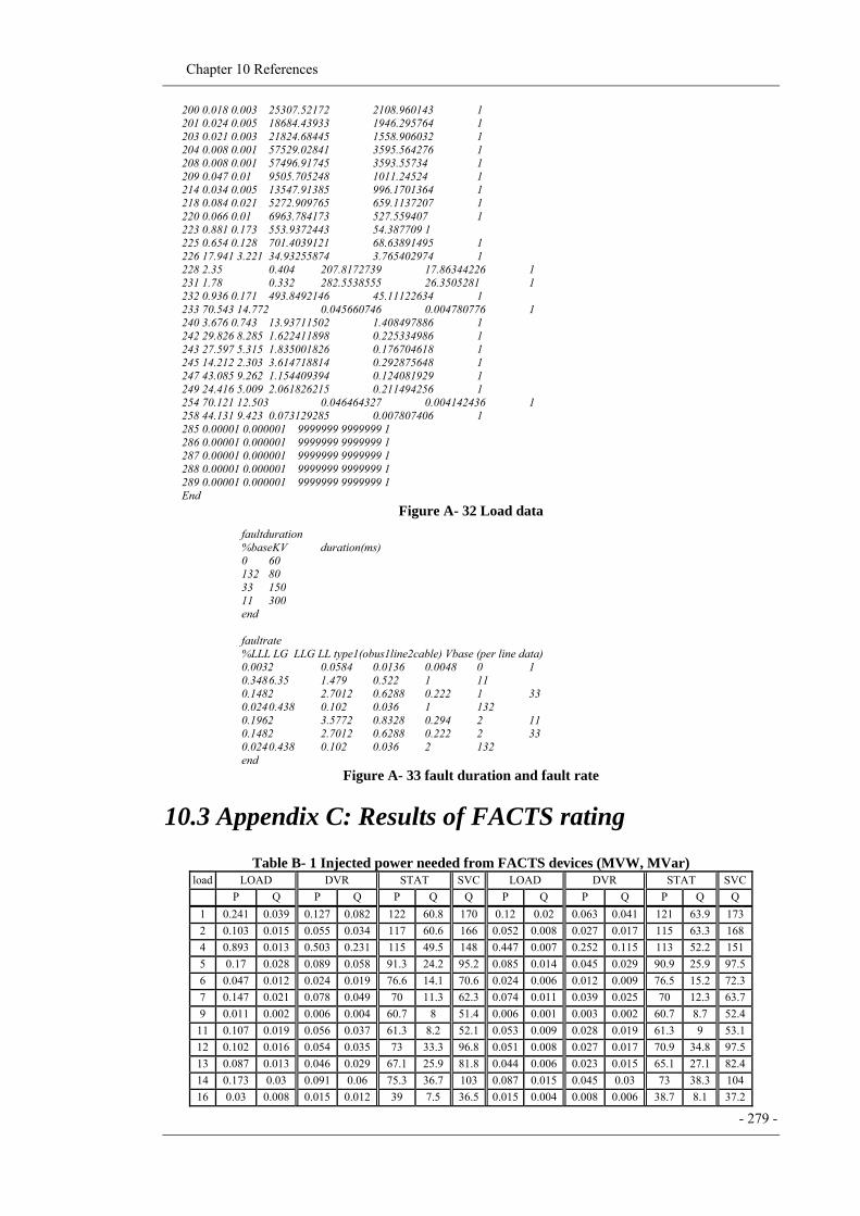
Chapter 10 References
- 279 -
200 0.018 0.003 25307.52172 2108.960143 1 201 0.024 0.005 18684.43933 1946.295764 1 203 0.021 0.003 21824.68445 1558.906032 1 204 0.008 0.001 57529.02841 3595.564276 1 208 0.008 0.001 57496.91745 3593.55734 1 209 0.047 0.01 9505.705248 1011.24524 1 214 0.034 0.005 13547.91385 996.1701364 1 218 0.084 0.021 5272.909765 659.1137207 1 220 0.066 0.01 6963.784173 527.559407 1 223 0.881 0.173 553.9372443 54.387709 1 225 0.654 0.128 701.4039121 68.63891495 1 226 17.941 3.221 34.93255874 3.765402974 1 228 2.35 0.404 207.8172739 17.86344226 1 231 1.78 0.332 282.5538555 26.3505281 1 232 0.936 0.171 493.8492146 45.11122634 1 233 70.543 14.772 0.045660746 0.004780776 1 240 3.676 0.743 13.93711502 1.408497886 1 242 29.826 8.285 1.622411898 0.225334986 1 243 27.597 5.315 1.835001826 0.176704618 1 245 14.212 2.303 3.614718814 0.292875648 1 247 43.085 9.262 1.154409394 0.124081929 1 249 24.416 5.009 2.061826215 0.211494256 1 254 70.121 12.503 0.046464327 0.004142436 1 258 44.131 9.423 0.073129285 0.007807406 1 285 0.00001 0.000001 9999999 9999999 1 286 0.00001 0.000001 9999999 9999999 1 287 0.00001 0.000001 9999999 9999999 1 288 0.00001 0.000001 9999999 9999999 1 289 0.00001 0.000001 9999999 9999999 1 End
Figure A- 32 Load data faultduration %baseKV duration(ms) 0 60 132 80 33 150 11 300 end faultrate %LLL LG LLG LL type1(obus1line2cable) Vbase (per line data) 0.0032 0.0584 0.0136 0.0048 0 1 0.348 6.35 1.479 0.522 1 11 0.1482 2.7012 0.6288 0.222 1 33 0.024 0.438 0.102 0.036 1 132 0.1962 3.5772 0.8328 0.294 2 11 0.1482 2.7012 0.6288 0.222 2 33 0.024 0.438 0.102 0.036 2 132 end
Figure A- 33 fault duration and fault rate
10.3 Appendix C: Results of FACTS rating
Table B- 1 Injected power needed from FACTS devices (MVW, MVar) load LOAD DVR STAT SVC LOAD DVR STAT SVC
P Q P Q P Q Q P Q P Q P Q Q 1 0.241 0.039 0.127 0.082 122 60.8 170 0.12 0.02 0.063 0.041 121 63.9 173 2 0.103 0.015 0.055 0.034 117 60.6 166 0.052 0.008 0.027 0.017 115 63.3 168 4 0.893 0.013 0.503 0.231 115 49.5 148 0.447 0.007 0.252 0.115 113 52.2 151 5 0.17 0.028 0.089 0.058 91.3 24.2 95.2 0.085 0.014 0.045 0.029 90.9 25.9 97.5 6 0.047 0.012 0.024 0.019 76.6 14.1 70.6 0.024 0.006 0.012 0.009 76.5 15.2 72.3 7 0.147 0.021 0.078 0.049 70 11.3 62.3 0.074 0.011 0.039 0.025 70 12.3 63.7 9 0.011 0.002 0.006 0.004 60.7 8 51.4 0.006 0.001 0.003 0.002 60.7 8.7 52.4
11 0.107 0.019 0.056 0.037 61.3 8.2 52.1 0.053 0.009 0.028 0.019 61.3 9 53.1 12 0.102 0.016 0.054 0.035 73 33.3 96.8 0.051 0.008 0.027 0.017 70.9 34.8 97.5 13 0.087 0.013 0.046 0.029 67.1 25.9 81.8 0.044 0.006 0.023 0.015 65.1 27.1 82.4 14 0.173 0.03 0.091 0.06 75.3 36.7 103 0.087 0.015 0.045 0.03 73 38.3 104 16 0.03 0.008 0.015 0.012 39 7.5 36.5 0.015 0.004 0.008 0.006 38.7 8.1 37.2

Chapter 10 References
- 280 -
17 0.016 0.005 0.008 0.007 40.8 8.3 38.9 0.008 0.003 0.004 0.003 40.6 8.9 39.6 19 0.036 0.005 0.019 0.012 79.7 45 118 0.018 0.003 0.01 0.006 77.2 46.7 119 21 0.015 0.002 0.008 0.005 75.2 38.3 106 0.008 0.001 0.004 0.003 73.5 40.1 107 22 0.411 0.082 0.212 0.149 87.4 73 122 0.205 0.041 0.106 0.075 83.6 74.9 114 24 0.702 0.158 0.359 0.265 58 16.9 62.8 0.351 0.079 0.179 0.133 56.1 18 63.1 29 0.594 0.14 0.302 0.228 79.3 21.5 83.3 0.297 0.07 0.151 0.114 78.5 22.7 84.6 30 0.079 0.026 0.038 0.034 69.6 13.1 64.7 0.039 0.013 0.019 0.017 69.1 14.1 65.8 31 0.406 0.088 0.208 0.152 57.6 5.8 46 0.203 0.044 0.104 0.076 57.1 6.5 46.7 34 0.661 0.149 0.337 0.25 57.7 5.7 46.1 0.33 0.075 0.169 0.125 57.2 6.4 46.7 35 0.133 0.033 0.067 0.052 53.2 4.1 40.8 0.066 0.016 0.034 0.026 52.9 4.7 41.4 36 0.039 0.013 0.019 0.017 48.9 2.4 35.3 0.02 0.006 0.01 0.009 48.6 2.9 35.9 37 0.39 0.097 0.197 0.153 27.9 3.9 23.9 0.195 0.049 0.098 0.076 27.1 4.3 24 38 0.11 0.022 0.057 0.04 30.9 6.1 29.1 0.055 0.011 0.028 0.02 29.9 6.5 29.1 39 0.673 0.215 0.328 0.29 33.4 7.9 33.4 0.337 0.108 0.164 0.145 32 8.3 33.1 40 0.777 0.25 0.378 0.336 34.7 7.8 34.1 0.389 0.125 0.189 0.168 33.3 8.3 33.8 41 0.206 0.051 0.104 0.08 35.7 8.9 36.3 0.103 0.025 0.052 0.04 34.4 9.4 36.2 42 0.118 0.027 0.06 0.045 37.5 10.6 40.1 0.059 0.013 0.03 0.022 36.2 11.1 39.9 43 0.398 0.096 0.202 0.154 39.3 12.1 43.4 0.199 0.048 0.101 0.077 37.8 12.6 43.2 44 0.313 0.058 0.163 0.111 39.7 4.6 32.6 0.156 0.029 0.081 0.055 38.8 5.3 33.1 45 0.42 0.095 0.214 0.159 43.6 6.3 37.8 0.21 0.047 0.107 0.079 42.5 7.1 38.2 48 0.273 0.06 0.14 0.103 46.9 10 45.4 0.137 0.03 0.07 0.051 45.5 10.8 45.6 49 0.444 0.106 0.225 0.171 47.1 10 45.4 0.222 0.053 0.113 0.085 45.6 10.8 45.6 50 0.268 0.042 0.141 0.091 84.6 68 121 0.134 0.021 0.071 0.046 81.6 70.1 113 51 0.479 0.088 0.25 0.17 77.5 50.9 126 0.24 0.044 0.125 0.085 75.5 52.8 127 53 0.499 0.081 0.263 0.171 49.6 35.8 85.1 0.25 0.04 0.131 0.085 48.6 36.6 74.9 54 0.624 0.126 0.322 0.228 88.5 54.1 138 0.312 0.063 0.161 0.114 86.3 56.6 140 55 0.39 0.081 0.201 0.144 128 78.2 199 0.195 0.041 0.1 0.072 125 81.4 202 56 0.119 0.019 0.063 0.04 132 88.9 218 0.059 0.009 0.031 0.02 129 92.4 221 57 0.165 0.027 0.087 0.057 140 113 201 0.082 0.014 0.043 0.028 136 117 188 58 0.528 0.137 0.265 0.21 133 112 186 0.264 0.069 0.132 0.105 129 116 176 59 0.655 0.131 0.339 0.238 70.5 75 94.6 0.328 0.065 0.169 0.119 68.6 76.1 92.5 60 0.794 0.147 0.414 0.282 143 126 196 0.397 0.074 0.207 0.141 139 130 187 61 0.283 0.049 0.148 0.099 69.4 69.4 93 0.142 0.025 0.074 0.049 67.9 70.5 91 62 0.157 0.025 0.083 0.053 128 86.8 211 0.078 0.012 0.041 0.027 125 90.1 215 63 0.41 0.073 0.214 0.144 114 60.7 164 0.205 0.037 0.107 0.072 112 63.3 166 64 0.241 0.041 0.126 0.084 106 51.6 146 0.121 0.021 0.063 0.042 105 53.9 148 65 0.44 0.076 0.231 0.153 85.7 21.3 87.2 0.22 0.038 0.115 0.077 85.5 22.7 89.1 66 0.829 0.157 0.431 0.296 70.9 9.5 60.2 0.414 0.079 0.215 0.148 70.6 10.4 61.4 69 0.017 0.003 0.009 0.006 61.3 21.4 71.6 0.008 0.001 0.004 0.003 60.9 22.2 72.5 71 0.163 0.031 0.085 0.059 70.9 19.1 74.3 0.081 0.016 0.042 0.029 70.5 20.1 75.6 73 0.023 0.004 0.012 0.008 67.2 27.2 84 0.012 0.002 0.006 0.004 66.6 28.1 84.9 75 0.417 0.067 0.22 0.142 61.4 25.2 77.2 0.208 0.034 0.11 0.071 60.6 26.5 78.6 76 0.705 0.139 0.365 0.255 72.3 39.4 105 0.352 0.07 0.182 0.128 70.7 41.1 107 78 0.101 0.015 0.053 0.034 67.2 77.9 91.4 0.05 0.007 0.027 0.017 64.5 78.8 89 79 0.407 0.072 0.213 0.143 66.6 67 89.3 0.203 0.036 0.106 0.071 64.3 68 86.3 80 0.789 0.254 0.384 0.341 65.8 58.1 90 0.395 0.127 0.192 0.171 63.7 59.1 85.9 83 0.037 0.005 0.02 0.012 49.1 18.3 59.1 0.019 0.003 0.01 0.006 48.6 19 59.7 84 0.031 0.004 0.016 0.01 43.8 15.3 51.2 0.015 0.002 0.008 0.005 43.4 15.9 51.7 86 0.125 0.024 0.065 0.045 33 10.1 36.3 0.063 0.012 0.033 0.022 32.7 10.4 36.6 87 0.903 0.163 0.471 0.318 48.3 53.3 65.2 0.452 0.082 0.236 0.159 46.8 54 63.6 89 1.192 0.391 0.578 0.52 58.6 23 72.1 0.596 0.196 0.289 0.26 57.4 23.9 72.7 93 0.044 0.007 0.023 0.015 43.1 16 51.7 0.022 0.004 0.012 0.008 42.7 16.5 52.2 95 0.008 0.001 0.004 0.003 41.1 15.8 50.2 0.004 0.001 0.002 0.001 40.7 16.3 50.6 97 0.037 0.006 0.019 0.013 32.1 9.6 35.1 0.018 0.003 0.01 0.006 31.9 9.9 35.4 99 0.016 0.002 0.009 0.005 27.6 7.2 28.6 0.008 0.001 0.004 0.003 27.5 7.4 28.8 100 0.083 0.016 0.043 0.03 24.2 5.6 24.1 0.041 0.008 0.021 0.015 24.1 5.8 24.2 101 0.073 0.014 0.038 0.027 26.5 6.6 27.1 0.037 0.007 0.019 0.013 26.4 6.9 27.3 103 0.066 0.011 0.035 0.023 30.6 10.7 35.7 0.033 0.006 0.017 0.012 30.3 11 36 104 0.009 0.001 0.005 0.003 35.5 15.8 46.4 0.005 0.001 0.003 0.001 35 16.1 46.6 106 0.024 0.003 0.013 0.008 29.9 12.3 37.7 0.012 0.002 0.006 0.004 29.6 12.6 37.9

Chapter 10 References
- 281 -
107 0.039 0.006 0.02 0.013 29.8 13.2 38.8 0.019 0.003 0.01 0.007 29.4 13.4 39 108 0.018 0.003 0.01 0.006 26.4 11.4 34.1 0.009 0.002 0.005 0.003 26.2 11.6 34.2 111 0.129 0.032 0.065 0.05 22.9 7.9 26.6 0.065 0.016 0.033 0.025 22.7 8.1 26.7 112 0.02 0.003 0.011 0.007 23.1 9.7 29.3 0.01 0.002 0.005 0.003 22.9 9.8 29.4 114 0.006 0.001 0.003 0.002 20.4 7.7 24.7 0.003 0 0.002 0.001 20.3 7.9 24.8 115 0.01 0.001 0.006 0.003 20.8 8.1 25.5 0.005 0.001 0.003 0.002 20.6 8.2 25.6 117 0.006 0.001 0.003 0.002 15.8 5 17.6 0.003 0 0.002 0.001 15.7 5 17.7 119 0.005 0.001 0.003 0.002 14 3.9 14.9 0.003 0 0.001 0.001 13.9 4 15 120 0.008 0.001 0.004 0.003 14.2 4 15.2 0.004 0.001 0.002 0.001 14.1 4.1 15.3 125 0.009 0.001 0.005 0.003 15.7 4.9 17.5 0.005 0.001 0.003 0.001 15.7 5 17.5 126 0.023 0.007 0.011 0.01 14.2 4 15.1 0.012 0.004 0.006 0.005 14.1 4.1 15.2 127 0.007 0.001 0.004 0.002 13.6 3.7 14.3 0.004 0.001 0.002 0.001 13.5 3.7 14.3 128 0.02 0.003 0.011 0.007 13 3.4 13.4 0.01 0.002 0.005 0.003 12.9 3.4 13.5 130 0.043 0.008 0.023 0.015 13.3 7.5 19.8 0.022 0.004 0.011 0.008 12.9 7.8 19.8 132 0.035 0.005 0.019 0.012 13.6 7.8 20.3 0.018 0.002 0.009 0.006 13.1 8 20.3 133 0.018 0.003 0.01 0.006 13.1 7.1 19 0.009 0.001 0.005 0.003 12.6 7.3 19 134 0.017 0.003 0.009 0.006 12.3 6.3 17.3 0.009 0.001 0.005 0.003 11.9 6.5 17.3 136 0.009 0.001 0.005 0.003 11.8 5.8 16.2 0.005 0 0.003 0.001 11.4 5.9 16.2 137 0.868 0.285 0.421 0.379 11.6 5.3 15.4 0.434 0.143 0.211 0.189 10.9 5.5 15.2 140 0.01 0.002 0.005 0.004 14.3 8.5 21.9 0.005 0.001 0.003 0.002 13.8 8.8 21.9 142 0.021 0.007 0.01 0.009 14.9 9.4 23.5 0.011 0.003 0.005 0.005 14.4 9.6 23.6 144 0.003 0 0.002 0.001 15.7 10.8 26.2 0.001 0 0.001 0.001 15.1 11.1 25.3 145 0.003 0 0.002 0.001 16.7 13.3 24.1 0.001 0 0.001 0.001 16 13.6 22.1 148 0.019 0.003 0.01 0.006 17.4 14.1 24.7 0.01 0.002 0.005 0.003 16.7 14.5 23 150 0.02 0.003 0.011 0.007 18 17.8 24.2 0.01 0.002 0.005 0.003 17.2 18.1 23.1 152 0.009 0.001 0.005 0.003 18.6 21.9 25.4 0.005 0.001 0.003 0.001 17.6 22.3 24.6 154 0.021 0.004 0.011 0.007 16.6 11.9 28.4 0.01 0.002 0.005 0.004 16 12.2 24.2 156 0.013 0.002 0.007 0.004 15.6 9.6 24.3 0.006 0.001 0.003 0.002 15.1 9.9 24.4 158 0.035 0.006 0.018 0.012 14.7 8.2 21.7 0.017 0.003 0.009 0.006 14.2 8.5 21.8 159 0.02 0.003 0.011 0.007 13.9 7 19.4 0.01 0.001 0.005 0.003 13.5 7.3 19.6 160 0.018 0.003 0.01 0.006 15.3 8.9 23 0.009 0.001 0.005 0.003 14.7 9.2 23.1 162 0.035 0.005 0.018 0.011 13.7 6.9 19.2 0.017 0.002 0.009 0.006 13.3 7.2 19.3 163 0.131 0.032 0.067 0.051 13.1 6.3 17.8 0.066 0.016 0.033 0.025 12.7 6.5 17.9 164 0.005 0.001 0.003 0.002 12.5 5.7 16.6 0.002 0 0.001 0.001 12.2 5.9 16.7 165 0.008 0.001 0.004 0.003 13.1 6.4 18 0.004 0.001 0.002 0.001 12.7 6.6 18.1 168 0.02 0.003 0.011 0.007 12.1 5.2 15.6 0.01 0.001 0.005 0.003 11.7 5.5 15.7 169 0.039 0.008 0.02 0.014 12 5.2 15.5 0.02 0.004 0.01 0.007 11.6 5.4 15.6 173 0.112 0.023 0.058 0.041 9.2 3.1 10.6 0.056 0.011 0.029 0.02 8.9 3.3 10.7 175 0.035 0.005 0.019 0.011 8.9 2.9 10 0.017 0.002 0.009 0.006 8.7 3 10.1 177 0.036 0.007 0.019 0.013 8.4 2.5 9.2 0.018 0.003 0.009 0.006 8.2 2.6 9.3 182 0.009 0.001 0.005 0.003 10.6 4 12.8 0.004 0 0.002 0.001 10.4 4.2 12.9 184 0.011 0.021 0.001 0.015 9.8 3.4 11.4 0.006 0.01 0.001 0.007 9.6 3.6 11.5 186 0.019 0.003 0.01 0.006 9.7 3.2 11 0.01 0.001 0.005 0.003 9.5 3.4 11.2 187 0.04 0.009 0.02 0.015 9.2 2.9 10.3 0.02 0.004 0.01 0.007 9.1 3 10.4 190 0.005 0.007 0.001 0.005 11.4 4.6 14.2 0.002 0.003 0.001 0.002 11.1 4.8 14.3 191 0.005 0.001 0.003 0.002 11.1 4.4 13.6 0.002 0 0.001 0.001 10.8 4.6 13.8 192 0.005 0.001 0.003 0.002 10.6 3.9 12.7 0.002 0 0.001 0.001 10.4 4.1 12.8 193 0.018 0.003 0.01 0.006 11.6 5 14.9 0.009 0.001 0.005 0.003 11.2 5.2 15 195 0.009 0.001 0.005 0.003 10.6 4.1 12.9 0.004 0 0.002 0.001 10.4 4.2 13 196 0.009 0.001 0.005 0.003 10.1 3.6 11.9 0.004 0 0.002 0.001 9.9 3.8 12 197 0.015 0.003 0.008 0.005 10.7 4.1 13 0.008 0.001 0.004 0.003 10.4 4.3 13.1 199 0.016 0.002 0.009 0.005 10 3.4 11.6 0.008 0.001 0.004 0.003 9.7 3.6 11.7 200 0.017 0.003 0.009 0.006 10 3.5 11.7 0.009 0.001 0.005 0.003 9.8 3.7 11.8 201 0.023 0.005 0.012 0.008 9.6 3.1 10.9 0.011 0.002 0.006 0.004 9.4 3.3 11 203 0.02 0.003 0.011 0.007 9.1 2.8 10.1 0.01 0.001 0.005 0.003 8.9 2.9 10.2 204 0.008 0.001 0.004 0.002 8.7 2.5 9.4 0.004 0 0.002 0.001 8.5 2.6 9.5 208 0.008 0.001 0.004 0.002 7.9 2 8.1 0.004 0 0.002 0.001 7.8 2.1 8.2 209 0.044 0.009 0.023 0.016 7.8 1.9 8 0.022 0.005 0.011 0.008 7.7 2.1 8.1 214 0.032 0.005 0.017 0.011 9.4 3.1 10.8 0.016 0.002 0.009 0.005 9.2 3.3 10.9 218 0.079 0.02 0.04 0.031 9.6 3.5 11.4 0.039 0.01 0.02 0.015 9.3 3.6 11.4

Chapter 10 References
- 282 -
220 0.062 0.009 0.033 0.021 8.7 2.7 9.7 0.031 0.005 0.016 0.01 8.5 2.9 9.8 223 0.915 0.18 0.474 0.331 81.4 72.5 111 0.458 0.09 0.237 0.165 78.2 74.4 105 225 0.671 0.131 0.347 0.242 20 27.6 28.8 0.335 0.066 0.174 0.121 18.7 27.9 28 226 17.09 3.069 8.925 6.014 139 209 209 8.547 1.535 4.462 3.007 123 213 201 228 2.447 0.421 1.282 0.85 85.8 109 120 1.224 0.21 0.641 0.425 79.7 111 115 231 1.879 0.35 0.978 0.668 66.1 95.4 97.2 0.939 0.175 0.489 0.334 62.4 96.2 94.9 232 0.961 0.176 0.501 0.34 21.1 31.2 31.4 0.481 0.088 0.251 0.17 19.5 31.5 30.5 233 68.87 14.42 35.44 25.39 1085 1521 1574 34.43 7.21 17.72 12.7 969 1548 1505240 3.495 0.707 1.805 1.274 54 89.1 85.5 1.748 0.353 0.903 0.637 50.2 89.8 83.8 242 31.78 8.829 15.81 12.95 303 393 426 15.89 4.414 7.907 6.476 268 401 401 243 28.08 5.409 14.57 10.09 284 391 409 14.04 2.704 7.286 5.044 255 398 391 245 14.62 2.37 7.699 5 272 393 400 7.312 1.185 3.85 2.5 249 398 387 247 40.7 8.75 20.89 15.14 202 285 294 20.35 4.375 10.45 7.568 173 290 277 249 26.2 5.374 13.51 9.596 304 418 437 13.1 2.687 6.755 4.798 268 425 415 254 68.36 12.19 35.71 24 936 1381 1392 34.18 6.095 17.86 12 834 1402 1336258 42.9 9.161 22.04 15.92 1001 1582 1545 21.45 4.581 11.02 7.96 892 1600 1491
10.4 Appendix D: Author’s thesis based publications
International journal papers:
1. S.Bahadoorsingh, J.V.Milanovic, Y. Zhang, C. P. Gupta, and J. Dragović, “Minimization of Voltage Sag Costs by Optimal Reconfiguration of Distribution Network Using Genetic Algorithms”, IEEE Transactions on Power Delivery, Volume 22, No. 4, 2007, pp. 2271 - 2278
2. J. V. Milanović and Y.Zhang, “Modelling of FACTS Devices for Voltage Sag Mitigation Studies in Large Power Systems”, accepted for publication in the IEEE Transactions on Power Delivery, TPWRD-00768-2006 (26/04/08)
Submitted international journal papers:
3. Y.Zhang, and J. V. Milanović, “Global voltage sag mitigation with FACT based devices”, submitted to the IEEE Transactions on Power Delivery, TPWRD-00504-2007 (02/08/07)
4. J. V. Milanović and Y.Zhang, “Gobal minimisation of financial losses due to voltage sags with FACTS based devices”, submitted to the IEEE Transactions on Power Delivery, TPWRD-00518-2007 (10/08/07)
5. International conference papers:
5. Y.Zhang and J. V. Milanović, “Optimal Placement of FACTS Devices for Voltage Sag Mitigation Based on Genetic Algorithms”, CD ROM of the 12th IEEE International Conference on Harmonics and Quality of Power, ICHQP 2006, Cascais, Portugal, October 1-5, 2006.
6. J. V. Milanović and Y.Zhang, “Modelling of STATCOM and DVR for Voltage Sag Mitigation Studies”, CD ROM of the 12th IEEE International Conference on Harmonics and Quality of Power, ICHQP 2006, Cascais, Portugal, October 1-5, 2006.
Chapter 10 References
- 283 -
7. Y.Zhang and J. V. Milanović, “Application of Niching Genetic Algorithms in system-wide voltage sag mitigation studies ”, CD Rom of the Lausanne PowerTech 2007, 1- 5 July 2007, Lausanne, Switzerland (paper 89)
8. Y.Zhang and J. V. Milanović, “Techno-economic improvement of voltage sag performance with facts devices ”, CD Rom of the 9th International conference on electrical Power Quality and utilization,EPQU’07, Barcelona, Spain, October 9-11, 2006. (27)
9. J. V. Milanović and Y.Zhang, “Voltage sag reduction with optimally placed FACTS devices ”, CD Rom of the 9th International conference on electrical Power Quality and utilization,EPQU’07, Barcelona, Spain, October 9-11, 2006. (26)
10. M.Vekic, Y.Zhang,"Statcom Modeling for Voltage Sag Propagation Studies", Mako Cigre 2007, Ohrid, Macedonia,October 7th-9th, 2007, paper B4-02R,
11. Marko Vekić, Y. Zhang, Jovica Milanović, Vladimir Katić:"Modeling of FACTS Devices for Voltage Sag Propagation Studies", 7th International Power System Conference, November 22-23, Timisoara, Romania, Scientific Bulletin, Tom 52, ISSN 1582-7194
12. Y. Zhang and J. V. Milanovic, "Voltage Sag Cost Assessment Based On Fault Position Method And Generalised Sag Table," accepted for presentation of MedPower ΄08 – 6th Mediterranean Conference and Exhibition on Power Generation, Transmission and Distribution, Thessaloniki, Greece,November 2 - 5 2008.
13. J. Mutale, J. V. Milanovic, and Y. Zhang, "Methodology for robust assessment of the financial viability of wind energy projects," accepted for presentation of MedPower ΄08 – 6th Mediterranean Conference and Exhibition on Power Generation, Transmission and Distribution, Thessaloniki, Greece,November 2 - 5 2008. Technical reports:
1. J.V.Milanovic, C.P.Gupta, Y.Zhang, J.Dragovic, M.T.Aung, and S.C.Vegunta, " Assessment and minimisation of financial losses due to voltage sags and short interruptions in networks with distributed generation by coordinated application of power electronics based devices " , Special report as a part of Deliverable D15 of the EU project ENK5-CT-2002-00658, School of Electrical and Electronic Engineering, The University of Manchester, Manchester, UK, December 2005.
2. J.V.Milanovic, M.Kayikci, S.C.Vegunta, and Y.Zhang, " Modelling and operation of DFIG based wind plants and improvement of quality of electricity supply in isolated networks" Special report as a part of Deliverable D2.3.3 of the EU project INCO-CT-2004-509161, School of Electrical and Electronic Engineering, The University of Manchester, Manchester, UK, December 2006.
3. J.V.Milanovic, M.Kayikci, S.C.Vegunta, and Y.Zhang, " Transient responses of distribution network cell with renewable energy sources" Special report as a part of Deliverable D2.3.3 of the EU project INCO-CT-2004-509161, School of Electrical and Electronic Engineering, The University of Manchester, Manchester, UK, May 2007.