Journal of Neuroscience Methods, 20 (1987) 151 - 166 151 Elsevier

NSM00684

Techniques for obtaining analytical solutions for Rall's model neuron

George W. Bluman and H en ry C. Tuckwel l

Department of Mathematics, University of British Columbia, Vancow,er, B.C. V6T 1 Y4 (Canada) and Department of Applied Mathematics, Unieersi O, of Washington, Seattle, WA 98195 ( U. S. A. )

(Received 26 March 1986) (Revised 23 December 1986)

(Accepted 29 December 1986)

K~v words: Neuronal model; Analytical solution: Cable model

The Green's function (G) is obtained for a cable equation with a lumped soma boundary condition at x = 0 and a sealed end at x = L < ~ . The coefficients in the eigenfunction expansion of G are obtained using the calculus of residues. This expansion converges rapidly for large t. From an estimate of the higher eigenvalues, an approximate bound is obtained for the remainder after so many terms. The leading terms are also obtained in an expansion for G which converges rapidly for small t. Similarly, series expansions for the voltage are obtained which converge rapidly at small or large t when a constant current is injected at the soma and when a (synaptic input) current bte ~,t occurs at a point along the cable.

1. Introduction

Rall's model of a nerve cell is based primarily on anatomical and neurophysio- logical information gathered for spinal motoneurons. Its basic features are as follows.

The voltage across dendritic membranes is assumed to satisfy a cable equation. Assume that appropriate symmetry and other requirements are met, including the so-called 3 halves power law for diameters at dendritic branch points. Then the voltage at points which are at equal electrotonic distances from the soma may be mapped onto a one-dimensional cable. This is known as Rall's equivalent cylinder. Some of the symmetry requirements for the mapping to an equivalent cylinder can be relaxed and the potential on the dendritic trees still mapped onto a one-dimen- sional cable (Walsh and Tuckwell, 1985).

To represent the soma of the cell, one employs an R-C circuit which is affixed to one end of the one-dimensional cable. This is called a lumped soma termination.

Correspondence, H.C. Tuckwell, Monash University, Clayton, Vic. 3168, Australia.

0165-0270/87/$03.50 ~"~ 1987 Elsevier Science Publishers B.V. (Biomedical Division)

152

Full details of the construction of the model may be found in Rail (1977) and in Tuckwell (1987).

A mathematical description of the resulting model is as follows. Let V(x, t) be the depolarization in volts at space point x and time point t, where x, t are measured in units of the membrane's space and time constants respectively, so x and t are dimensionless. Let the distance from the soma to the dendritic terminals be L. Then V satisfies the (cable) partial differential equation

Vt= V, , - V+kl 0 < x < L (1.1) t > 0

where subscripts x and t signify partial derivatives with respect to these variables. In Eqn. 1.1, I = I(x, t) is an applied current density (in coulombs per unit dimensionless time per unit dimensionless distance) and the constant k is a constant of the nerve cell under consideration. In terms of electrical and other constants,

2 ( Pi ) 1/2 k ¢i'Cmd 3/2 ~Pm (1.2)

where Cm = capacitance in F of one square cm of membrane, d = diameter of equivalent cylinder in cm, 3 = membrane thickness in cm and Pi, Pm are the intracellular and membranous resistivities, respectively, in ~9 cm.

The lumped soma assumption results in the following boundary condition at x = 0 :

V(0, t ) + V,(0, t ) - 7V,(0, t)=R~I,(t) (1.3)

where R~ = soma resistance, I s = injected current at soma and 7 = R~/?~ is the ratio of the soma resistance to the resistance of a characteristic length of the equivalent cylinder.

In addition, for the purposes of being specific, we will make the following two assumptions throughout this paper:

(1) The cell is initially uniformly at rest so that the depolarization is zero at t = 0.

V(x, 0) = 0 0,< x,< L (1.4)

(2) The dendritic terminals are sealed so that there is no axial current through them:

V,(L, t ) = 0 t>~0 (1.5)

The techniques we will employ can of course be used for other boundary conditions at x = L. We will obtain various expansions for the Green's function for Eqns. 1.1-1.5. These expansions will be analyzed to ascertain their accuracy when a certain number of terms are employed. For some preliminary analysis of this problem, see Tuckwell (1987, ch. 6).

The purpose of these calculations is that the results may be used to obtain the response to arbitrary space-time distributions of input current. An example is given in Section 4 where the details of the response to a synaptic input of the form of an alpha function are worked out. However, any current waveform could be chosen, e.g, a sinusoid, and the response readily found.

153

Other works containing some of our results or similar ones are Rall (1969), Iansek and Redman (1973), Redman (1973), Jack, Noble and Tsien (1975), Rail (1977), and more recently Durand (1984), Kawato (1984), Turner (1984) and Ashida (1985). The first paper to offer different forms for the solution which converge rapidly for small or large time was that of Rinzel and Rall (1974).

2. Green's function by the Laplace transform method

The Green's function G(x , y; t), is the solution of Eqns. 1.1 1.5 obtained with

k l = 8 ( t ) 8 ( x - y ) 0 < y < L l , ( t ) = 0 (2.1)

That is, it represents the response to a unit impulse at a point y somewhere along the cable. It is useful to have G(x , y; t) since the response to arbitrary input current densities and arbitrary initial distributions of potential can be found from it.

We put

= e ' a (2.2)

to simplify the calculations. It is not hard to show that the Laplace transform of G-. defined as

fO '~ - - - - CJL(x, y; s ) = e " G ( x , y; t) dt (2.3)

is given by

GA(x , y; s) = cosh( (L - y ) ~ - ) [ y cosh(x~-) + Vrs sinh(x~/s)] V~[T sinh(L~/~-) + ~/s cosh(L~s)] x < v (2.4)

This result was derived in Jack and Redman (1971) who inverted the transform as a series of parabolic cylinder functions. We seek alternative expansions which are easier to evaluate.

By separation of variables, it is also not difficult to show that the following eigenfunction expansion may be written for G:

~(x, >,; t)= ~ A,,(y)eo,,(x) e ~-~"' t > 0 (2 .5) t t = 0

where the spatial eigenfunctions are given by

{~,,(x) = cos[X,,(L + x)] cos(X,,L ). (2.6)

and the eigenvalues X,,, n = O, 1, 2 . . . . . are the roots of

y tan(~,L) + X = 0 (2.7)

Tables of values of ?,,, for various ~ are given in Tuckwell (1987).

1 5 4

The coefficients A, , ( y ) cannot be found in the standard way because the ~,,'s are not orthogonal. However, the Laplace transform of Eqn. 2.5 is

~-, (x . y: s ) = A,,( y )q~,( x )

, - 0 s + X], (2.8)

and this must be equal to the RHS of Eqn. 2.4. It is clear from Eqn. 2.8 that GI_ has simple poles at s = -~.~,,, n = 0, 1.2 . . . . and

thus 2.4 has simple poles at the same points, as may be verified directly. We also note that when x = 0, from Eqns. 2.4 and 2.8, we get

Gt.(0, y: s ) = y c o s h ( ( L - y ) ¢ s ) (2.9A) ¢s [ 7 sinh( LC-s ) + ¢s cosh( LOs )]

and

eL(0 , >': s ) = A, , (y)

,,=0 s + X~, (2.9B)

From Eqn. 2.9B we see that A , ( y ) is the coefficient of l / [ s - ( - ~ } , , ) ] , this coefficient being called the residue of (7/(0, )'; s) at the point s-- _X2,,. Using a standard result in complex variable theory (see for example Rudin. 1974), we have

A , ( y ) = lira (s+X-],)Gl_(0, .)'; s) (2.10)

Evaluating these limits with the aid of L'Hospital's rule where necessary gives

A , ) ( y ) "Y (2.11) 1 +TL

A,,(y) = 2y c o s ( X , , ( L - y ) ) n = 1 .2 . . . . . cos()~,,L){1 + TL } - ?,,L s in(X,L)

(2.12)

These quantities were given m, but not derived by Rail (1977).

2.1. Calculation of G for large t Collecting the above results, we have the eigenfunction expansion for G:

G ( x . >.; t) = ~ A,,(y)ep,,(x) e (~:"+')' t > 0 (2.13)

It is desirable to use this series for calculating G at large times because it will converge rapidly.

We can estimate the remainder when a certain number of terms is retained. This enables the accuracy of a numerical calculation of G to be ascertained when a certain number of terms is employed. Put

G ( x , y; t ) = S N + R x (2.14)

where the sum of the first N + 1 terms in Eqn. 2.13 is denoted by: N

S.,.= ~ T,, (2.15) n = 0

155

and the remainder or tail is

R , = y] T,, (2.16) ~1 - - N + l

where T,, is the nth term in Eqn. 2.13. It is shown in Appendix I that the following is an approximate bound for the remainder:

1 exp( ( L-27 }]. { ( 2 N - 1 ) ' a ' ~ t / _ / } x 2 L j (2.17) IR.x[ ~ < ~ - t 1+ , erfc

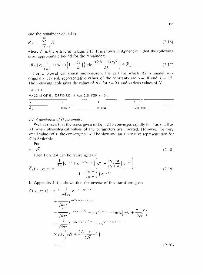
For a typical cat spinal motoneuron, the cell for which Rall's model was originally devised, representative values of the constants are 7 = 10 and L = 1.5. The following table gives the values of/~ ~ for t = 0.1 and various values of N.

F A B L E 1

V A L U E S O F / ~ D E F I N E D IN Eqn. 2.26 F O R t 0.1

~," 3 4 5

/} ~ 0.0082 0.0004 < 0.0001

2.2. Cak'ulation of G for small t We have seen that the series given in Eqn. 2.13 converges rapidly for t as small as

0.1 when physiological values of the parameters are inserted. However, for very small values of t, the convergence will be slow and an alternative representation for G is desirable.

Put

~ , = d (2.18) Then Eqn. 2.4 can be rearranged to

[ ] l [ e .... + e , . 2 : , , ] e . , + C,,.(x, y; s')= 2o~ ' (2.19)

' o~- -y

In Appendix 2 it is shown that the inverse of this transform gives

G ( x , y; t ) = e ' [ ~ e (,,-,,)2,'4t [ ~/4¢rt

1 (21.-.x 1 )2/4t + 4 7- t e

1 _( x +v)2//4/ " + y { x + l } ( e + y e v-' erfc, y~/7

1 {2L+x i}2//4t eVe:+v(2l_+ ~ ~.) _ _ e + y

x er fc(y~-+ 2 L + x - v ) 2~Ut

+ . . - ]

.V+ l' /

+57-/!

(2.20)

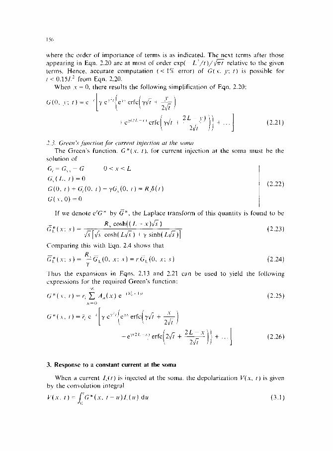
156

where the order of importance of terms is as indicated. The next terms after those appearing in Eqn. 2.20 are at most of order e x p ( - L 2 / t ) / ~ relative to the given terms. Hence, accurate computation (< 1% error) of G(x, y: t) is possible for t < 0.15L e from Eqn. 2.20.

When x = 0, there results the following simplification of Eqn. 2.20:

G(0, y: t ) = e '['~eV~'.(e'<'erfc('~/7+~-~)

+e '<2'- ' )e r fc y~- + T--/ + ... (2.21)

2.3. Green's function for current injection at the soma The Green's function, G*(x, t), for current injection at the soma must be the

solution of

G , = G , , - G 0 < x < L

(;,(L, ~)=0 G(O, t)+ G,(O, t ) - ' /G, (0 , t ) = R ,a ( t ) (2.22)

c,(x, 0)=0

If we denote e 'G* by (7", the Laplace transform of this quantity is found to be

(7~(x: s ) = R, c o s h ( ( L - x ) C s ) ~s[~S 7 cosh(Lv/s) + y sinh( L~/s)] (2.23)

Comparing this with Eqn. 2.4 shows that

( / "~( .¥ ; S) = R" G I . ( 0 , .~.-; J?) = r i {~k(0 , X; 3") ( 2 . 2 4 ) Y

Thus the expansions in Eqns. 2.13 and 2.21 can be used to yield the following expressions for the required Green's function:

(;*(.¥, ,)=~, ~ A,,(x)e (<+i,, n = 0

( ; * ( x , t ) = ~ , e ' 7 e Y~' e v 'er fc " ~ +

+e v~2A '). erfc(2~/t + - -

(2.25)

2Lx) ] 2~/7 + " " (2.26)

3. R e s p o n s e to a c o n s t a n t current at the s o m a

When a current l~(t) is injected at the soma, the depolarization V(x, t) is given by the convolution integral

l / (x . t ) = f ' G * ( x , t - u ) l ~ ( u ) d u (3.1) "O

157

We wish to determine V(x, t) when a constant current of magnitude 1 o is injected at the soma. We can obtain expressions for V which are useful for large and small values of t, respectively, as we did for the Green's function.

3.1. Cah'ulation of V(x, t) jbr large t Substitution of Eqn. 2.42 and l~(u)= 1 o in Eqn. 3.1 gives

v(x, ,)= I,#.~f' Y'. A,,(x)e (x:,,~l,(, , ,)du (3.2) uO n = O

Since the series of terms in the integrand is uniformly convergent with respect to ue[O, t], the order of integration and summation may be reversed. Carrying out the term-by-term integration yields

V(x, ) 'or, ~ A , , ( x ) [ 1 - e 'x~"+')'] t = - ( 3 . 3 ) ,,- 0 he,, + 1

This solution may be separated into steady state and transient components thus:

V(x, t )= IP(x ) - Vs(x, t) (3.4)

where

A,,(x) ~ ( x ) = ~,)~, ~ , ( 3 . 5 )

,,7__(= } X;, + 1

and

A,,(x) (,~z,, + 1 )t e

= (3.6) n - 0 ~2,, + l

A closed-form expression for IP may be obtained by solving the equations satisfied by V when the time derivatives are zero and neglecting the initial condition. This gives

lP(x) = 1(,~, c o s h ( L - x) (3.7)

(1 + t a n h L) c o s h L - y

Clearly, the convergence of Eqn. 3.6 will be even more rapid than Eqn. 2.13 because of the extra factors (X], + 1) ~. Thus a very efficient calculation of V(x, t) for large t( > 0.1) can be performed using Eqns. 3.7 and 3.6.

3.2. Calculation of V(x, t) for small t The Laplace transform of the convolution integral of two functions is the product

of the individual transforms. Putting V(x, t) = e'V(x, t), we find the transform Vt, of ~7 is, from Eqns. 2.9A, 2.24 and the fact that the transform of 10 is lo/s

loR , cosh(( L - x)~/s) F , ( x : s) = (3.8)

( s - 1)~- [~/s - cosh(Lv~-)+ ~, sinh(Lv/s)]

158

In Appendix 3 it is shown that the leading terms of V(x, t) are

v(x, t)

+ , e v~ erfc y ~ + +eVe-t- ' )erfc 7 ~ - + - - 2(r

+Q(x, t )+ . . . The quantity Q(x, t) is given in the Appendix.

f x loR'e-'7 2 v ~ { e " : /4 '+e ( : " - " / / 4 ' } - l < l e r f c ( _ ~ t ) , _

( 2L-x '~ x + < e t a - 1 - I

2 L - x 2(i

3.3. The special case x = 0 When x = 0, the leading term in the expansion for E L for large

VL(O" s)= I°R~ [1 + . . . ] ( , - 1 ) ~ ( v + ~ )

Utilizing the exact result (see Abramowitz and Stegun, 1965) y-,{ b2-a2 } we obtain, as t ---, 0

l°R~l [ ' e r f ( ~ t - ) - I +e('-~ l" erfc(7~-)] [1 +0(e 41£/r)] v(o, t ) - Q

] = Iok,t 1 3 ~ + ~(~2_ 1)t + o(?/~-1

When 7 = 1, a study of the limiting form of Eqn. 3.12 gives, as t ~ 0,

V(O, t ) = l o R , [ t + ( ½ - t ) e r f ( ~ / t ) - ~ e ' ] [I +0(e-4"- ' / t)]

One can also show that Eqn. 3.13 can be expressed as

0,,,,:>) V(O, t )=loR ,t 1 - ~ + [I +

as t - ) 0 .

>>] (3.9)

s] is given by

(3.10)

(3.11)

(3.12)

(3.13)

(3.14)

4. An example - response to a synaptic input modeled with an alpha function

When a synaptic input occurs at a small region on the soma-dendr i t i c surface of a neuron, one may use a modif ied cable equation with reversal potentials and a local

159

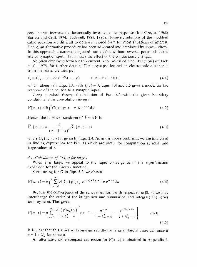
conductance increase to theoretically investigate the response (MacGregor. 1968: Barrett and Crill, 1974; Tuckwell. 1985, 1986). However, solutions of the modified cable equation are difficult to obtain in closed form for most situations of interest. Hence. an alternative procedure has been advocated and employed by some authors. In this approach a current is injected into a cable without reversal potentials at the site of synaptic input. This mimics the effect of the conductance changes.

An often employed form for this current is the so-called alpha-function (see Jack et al.. 1975. for further details). For a synapse located an electrotonic distance v from the soma, we then put

V , = V , , - V + b t e " ' 6 ( x - y ) O < x < L , t > O (4.1)

which, along with Eqn. 1.3, with Ix(t ) = 0 , Eqns. 1.4 and 1.5 gives a model for the response of the neuron to a synaptic input.

Using standard theory, the solution of Eqn. 4.1 with the given boundary conditions is the convolution integral

V(x, t ) = b f o t G ( x , y" t - u ) u e .... du (4.2)

Hence, the Laplace transform of V = e 'V is

b P ~ ( x : s ) - ~ ~ ( x , r: s) ( 4 . 3 )

( s - l + a ) ~

where (7~ (x, y: s) is given by Eqn. 2.4. As in the above problems, we are interested in finding expressions for V(x, t) which are useful for computation at small and large values of t.

4.1. Calculation of V(x, t)for large t When t is large, we appeal to the rapid convergence of the eigenfunction

expansion for the Green's function. Substituting for G in Eqn. 4.2, we obtain

£' V(x, t) = b Y~ A, , (y )~ , , (x ) e I~:i,+,,~, "~u e - " " du (4.4) n = (•

Because the convergence of the series is uniform with respect to uc[0, t], we may interchange the order of the integration and summation and integrate the series

e_.t e-(X~,,+ lit ] t e "' 1 +X, , - a~ + l + ~ , - - - a ] t > 0

(4.5)

It is clear that this series will converge rapidly for large t. Special cases will arise if a = 1 + ?,], for some n.

An alternative more compact expression for V(x, t) is obtained in Appendix 4.

A,,( y )ep,( x ) V(x , t ) = b Z

,,-o 1 + ?t2,,- a

term by term. This gives

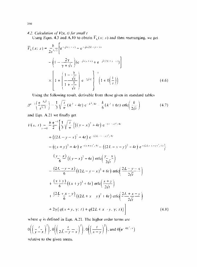
160

4. 2. Calculation of V(x, t) for small t Using Eqns. 4.3 and A.10 to obtain VL(x; s) and then rearranging, we get

Vj.(x: s ) = b [e ~D(>-')+e-dV(2L-v ') 2s5/2 L

- ( 1 .¢+¢[(2T )(e ¢,(,+,,)+e v~c2L + .... ))]

,

1 - ~ e - 2 7 ~ 1 + 0 x 1+ ~,

Using the following result, derivable from those given in standard tables

( e kd~ } l~/~_(k2+4t)e-~-/a, k + 6 / ) e r f c ( ~ - t ) l, = _ ( k 2 k

s-~/: 3V 7r

and Eqn. A.21 we finally get

V(x, t),~o 2 ( y - x ) 2 + 4 t ) e-("-')- '/4'

+ ( ( 2 L - y - x ) 2 + 4 t ) e ,2L ,.-,):,4,

- ( (x+y f+4r ) e-"+'>-'/4'-((2L+x-,'> 2+4t)e -(2L+' ,.,:/4,}

(4.6)

(4.7)

( (y_ , . )_+ v-~,

( 2 L - y - x) ( (2L_v_ x)Z + 6t) erfc( 2 L - y - x ) 6 " 2¢t

x+)'] (x +y ) ((x +y)2 + 6t) e r f c ( 2 ~ t J +- - - - -6 - - - -

, ) + (2L +_6x - y ) ((2L + x - .V) 2 + 6t) erfc( 2L 2¢~t + x - y

+ 2 y { q ( x + y , v" t)+q(2L+x->,, y: t)}l where q is defined in Eqn. A.21. The higher order terms are

O[ t 2 t 2 and

(4.8)

relative to the given terms.

161

Similar calculations to those in this Section may be performed for arbitrary input currents, at arbitrary distances from the soma, by replacing bte "' by the given input current in Eqns. 4.1 and 4.2.

Appendix 1

To estimate the remainder in Eqn. 2.13 as given by Eqn. 2.17 we need two preliminary results (i) and (ii), below.

(i) Approximate L;alues of the eigenvalues X,, for large n From the defining Eqn. 2.7, it is easily seen graphically that for large n the

eigenvalues X,, are close to (2n - 1)Tr/2L. To obtain a better estimate, we put

(2n - 1)Tr X, , - 2L + e (A.1)

where 0 < e << 1. On substituting Eqn. A.1 in Eqn. 2.7, there results

y c o s ( e L ) - ( ( 2 2 - - L 1 ) ~ r + e ) s i n ( e L ) = 0 (A.2)

Using the MacLaurin series for cos(eL) and sin(eL) in Eqn. A.2 and retaining only terms to order e 2, the following quadratic equation is obtained:

(2n - 1)Tr 27 e2+ e - 0 (A.3)

L(2 + 7L) L(2 + 7L)

There is only one positive root of Eqn. A.3. Using the approximate value of this root, we get

(2n - 1)w 27 X, , - 2L + (2n - 1)~r n large. (A.4)

(ii) Approximate values of the coefficients in Eqn. 2.13 for large n Using the approximate expression A.4 it is not difficult to show that for large n

we have

2 A,,(,,)O,,(x) -- zcos(X,,(L -),1) cos(X,,(C + x)) (A.5)

With Eqns. A.4 and A.5 at our disposal, we may now obtain the following.

(iii) Estimate of the tail of the Series 2.13 Let us define

T,, =A,,(y)eo,,(x ) e ~x:"+'" (A.6)

1 6 2

We have. on using a refinement of Eqn. A.5 and then A.4

I R , , I < ~ IT,,l ,l = N + 1

2 e ~ e~e,,t v - T - 2_,

n - N + l

- - 2 e - t ( l + 2 v / L ) / L e x p { (2p/ - 1)2rr2t (A.7) , ' I = N + ] , 4L2

The sum of these exponential terms, which are positive and monotonically decreas- ing as n increases, may be bounded above by an integral as follows:

~.~ exp{ (2n-1)2'rr2t} /~exp( (2x-1,2'rr2t} ,, =.,v + 1 4 L ~ - ~< ~u ~ 4 £ -~2 d x ( A . 8 )

Changing variables in the integral, we can express it in terms of the complementary error function:

2 j~ e x p ( _ z 2 ) d z (A.9) erfc(x) = ~ -

Thus we finally obtain the approximate bound given in Eqn. 2.17.

A p p e n d i x 2

To derive the leading terms in the Green's function for small t as given in Eqn. 2.20 we first rearrange Eqn. 2.19 to get

(~,(x, y; s ) = ~ - I [ -'~(~ '~' e-"~2c "-') (Y-c~ + + ~--~/]

"][1+ e 2°'1 (A.IO)

The following expansion converges for large s:

1 + a - Y e - 2 " c = 1 - ~-~-~T] ... (A.11) a + y

When the expansion A.11 is used in Eqn. A.10 the first 4 terms are

~,(x, v: ~) e - " " - " e - ' ' 2 ' ~ - ' "

" , ~ 2a + 2a

l l _ / 7 - a ] _ e_,, ,+,. , 1 7 - O e ) e ,,2c+, , ,

+ . . . (A.12)

Now we utilize the fact that the terms which dominate the Laplace transform (7c for large Is I are those which dominate G, as a function of t, for small t. This is called the generalized initial value theorem (Spiegel, 1965).

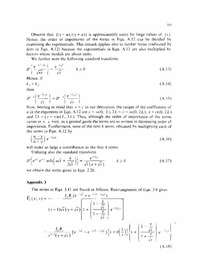
163

Observe that 1 ( ' ¢ - a ) / ( ' ¢ + (~)1 is approximately unity for large values of I s L- Hence, the order or importance of the terms in Eqn. A.12 can be decided by examining the exponentials. This remark applies also to further terms (indicated by dots in Eqn. A.12) because the exponentials in Eqn. A.11 are also multiplied by factors whose moduli are about unity.

We further note the following standard transform.

~ T ' ~s k > O (A.13)

Hence, if

k 1 <" k~ (A.14)

then

't ¢7 > ~ l ~7 J (A.15)

Now, bearing in mind that x < y in our derivation, the ranges of the coefficients of a in the exponents in Eqn. A.12 are y - x{(0, L), 2 L - v - x((0, 2L), x +y{(0, 2L) and 2 L - ( y - x ) e ( L , 2L). Thus, although the order of importance of the terms varies as x, y vary, as a general guide the terms are as written in decreasing order of importance. Furthermore, none of the next 4 terms, obtained by multiplying each of the terms in Eqn. A.12 by

'o~-- T '

will make as large a contribution as the first 4 terms. Utilizing also the standard transform

[ ,ae,,:,erfc(a¢7+ k )} e j'Vv k > 0 (A.17) "W'/,e 7-~-t ¢7(a + ¢~7)

we obtain the terms given in Eqn. 2.20.

Appendix 3

The terms in Eqn. 3.11 are found as follows. Rearrangement of Eqn. 3.8 gives

10R~(e - ' ¢ v + e (2t.-,~¢~)

3'

+ Y

e 2 l.v~ ]

l°R~ {e-'¢X+e (2c ,)v,:v}{ 1 + ,v2(y+¢;) + y

1 + 7 ,

e 2 l v X '1,

(AA8)

1

164

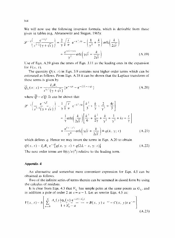
We will now use the following inversion formula, which is derivable from those given in tables (e.g. Abramowitz and Stegun, 1965):

~'-'~ s3"'2(7+~/s)/ = T e- - --7 2 + T erfc ~ - t

+ y2 erfc y~- + (A.19)

Use of Eqn. A.19 gives the terms of Eqn. 3.11 as the leading ones in the expansion for V(x, t).

The quantity Q(x, t) in Eqn. 3.9 contains next higher order terms which can be estimated as follows. From Eqn. A.18 it can be shown that the Laplace transform of these terms is given by

QL(x; s ) - l°R~ {e ' ~ + e {2, ,,vv} (A.20) )

where Q = e'Q. It can be shown that

c f ,{ e-a~'v } 1 ~ _ t e a:/4,[_k~_ k 2 . ~ ]

+ = r + -v + 7r_ +

211erfcl k k 2 k 1 +

e av+v~ [ k ~) + e r f c [ 7 ~ + ~ t - t - q ( k , v ; ,} (A.21)

which defines q. Hence we may invert the terms in Eqn. A.20 to obtain

Q( x, t) = loR~ e - ' [ q ( x , Y; t) + q ( 2 L - x, y; t)] (A.22)

The next order terms are O((t/x) 4) relative to the leading term.

Appendix 4

An alternative and somewhat more convenient expression for Eqn. 4,5 can be obtained as follows.

Two of the infinite series of terms therein can be summed in closed form by using the calculus of residues.

It is clear from Eqn. 4.3 that VL has simple poles at the same points as G L, and in addition a pole of order 2 at s = a - 1. Let us rewrite Eqn. 4.5 as:

= + B ( x , y ) e " ' - C ( x , v ) t e - " ' , , = o 1 + X 2 , , - a

(A.23)

1 6 5

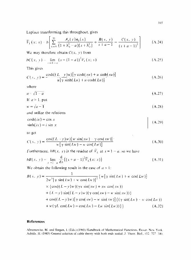
Laplace transforming this throughout, gives

- [ ,@ A, , (y)~ , , (x) + V, (x; s ) = b , , ( I + X - ; , - a ) ( s + X - ; , )

We may therefore obtain C(x, r) from

hC(. \ ' , y ) = lim ( s - ( 1 - a ) ) - V t ( x ; s)

This gives

q

e ( x . y ) + . . . . . ] C(x, v) s + a - 1 ( s + a - l ) - J

C ( x , y ) =

where

u = ~/1 - a

If a > 1, put

w = ~/a- 1

and utilize the relations

cosh(ix) = cos x

sinh(ix) = i sin x

to get

cosh(( L - y ) u )[ Y cosh(xu ) + u sinh( xu )]

u [y s inh(Lu) + u cosh(Lu)]

A.24)

A.25)

A.26)

(A.27)

(A.28)

(A.29)

cos(( L - y ) . , ) [ w sin(.¥. ,) - v cos(x, , , ) ] C ( x , y) = (A.30)

w[y sin(Lw) + w cos(Lw)]

Furthermore. b B ( x , y ) is the residue of VL at s = 1 - a. so we have

b B ( x . y ) = lim d ( ( s + a - 1)2VL(x: s)) (A.31) s ~ 1 a

We obtain the fol lowing result in the case of a > 1:

1 B ( x . y ) = ( w [ ' y s i n ( L w ) + w c o s ( L w ) ]

2,,,3[7 s i n ( L w ) + w cos(Lw)] 2

× { c o s ( ( L - y ) w ) ( y x s i n ( x w ) + xw cos(xw))

+ ( L - y ) s i n ( ( L - y ) w ) ( y cos(x , , ) - w sin(xw))}

+ c o s ( ( L - y ) w ) [ y c o s ( x w ) - w s in (xw) ]{ (y s i n ( L w ) + w cos(Lw))

+ w(yL cos(Lw) + cos(Lw) - L w sin(Lw))} } (A.32)

R e f e r e n c e s

Abramowitz, M. and Stegun, I. (Eds.) (1965) Handbook of Mathematical Functions, Dover. New York. Ash ida, H. (1985) General solution of cable theory with both ends sealed. J. Theor. Biol., 112:727 740.

166

Barrett, J.N. and Crill, W.E. (1974) Influence of dendritic location and membrane properties on the effectiveness of synapses on cat motoneurones, J. Physiol. (London), 293:325 345,

Durand, D. (1984) The somatic shunt cable model for neurons, Biophys. J., 46: 645-653. lansek, R. and Redman, S.J. (1973) An analysis of the cable properties of spinal motoneurons using a

brief intracellular current pulse, J. Physiol. (London), 234: 613-636. ,lack, J.J.B.. Noble, D. and Tsien, R.W. (1975) Electric Current Flow in Excitable Cells. Clarendon Press,

Oxford. ,lack, J.J.B. and Redman, S.J. (1971) An electrical description of the motoneurone, and its application to

the analysis of synaptic potentials, J. Physiol. (London) 215: 321-352. Kawato. M. (1984) Cable properties of a neuron model with non-uniform membrane resistivity, J. Theor.

Biol.. 111: 149-169. MacGregor, R.J. (1968) A model for responses to activation by axodendritic synapses, Biophys. J.. 8:

305-318. Rail, W. (1969) Time constants and electrotonic length of membrane cylinders and neurons, Biophys. J.,

9: 1483-1508. P, all, W. (1977) Core conductor theory and cable properties of neurons. In E.R. Kandel (Ed.), Handbook

of Physiology, Section 1, The Nervous System, Volume 1, Amer. Physiol. Sot., Bethesda. Redman, S.J. (1973) The attenuation of passively propagating dendritic potentials in a motoneurone

cable model, J. Physiol., (London), 234: 637-664. Rinzel, J. and Rail W. (1974) Transient response in a dendritic neuron model for current injected at one

branch, Biophys. J., 14: 759-790. Rudin, W. (1974) Real and Complex Analysis, 2rid edn. McGraw-Hill. New York. Spiegel, M.R. (1965) Laplace Transforms, McGraw-Hill. New York. Tuckwell. H.C. (1985) Some aspects of cable theory with reversal potentials, J. Theoret. Neurobiol., 4:

113 127. l"uckwell, H.C, (1987) Introduction to Mathematical Neurobiology, Vol. 1, Linear Cable Theory and

Dendritic Structure, Cambridge University Press, Cambridge, in press. Tuckwell. H.('. (1986) On shunting inhibition, Biol. Cybernet., 55: 83-90. Turner, D.A. (1984) Segmental cable evaluation of somatic transients in hippocampal neurons (CA1,

CA3 and dentate), Biophys. J., 46: 73-84. Walsh, J.B. and Tuckwell, H.C. (1985) Determination of the electrical potential over dendritic trees by

mapping onto a nerve cylinder, J. Theoret. Neurobiol., 4 : 27 46.