table of contents - royal society of chemistry · 260 240 300 280 0 50 100 150 200 250 300 350 400...

Comprehensive, quantitative bioprocess productivity monitoring using fluorescence EEM spectroscopy and chemometrics. B. Li, M. Shanahan, A. Calvet, K.J. Leister, and A.G. Ryder.

of 14

Supplemental Information:

TABLE OF CONTENTS S1. Additional Experimental Details ............................................................................. 1

S2. Spectral Analysis of EEM Data: Identification of Fluorophores ............................. 1

S3. Dilution Effects ....................................................................................................... 3

S4. MCR-ALS Components ............................................................................................ 4

S5. Fluorescence Lifetime Measurements ................................................................... 5

S6. Model Complexity .................................................................................................. 6

S7. Quantitative Study of DS12 Sample Set ............................................................... 11

S8. PLS Modeling of DS7 Sample Set ......................................................................... 13

S9. References ........................................................................................................... 14

S1. ADDITIONAL EXPERIMENTAL DETAILS Standard Fluorophore Solutions: Tryptophan (90 μM), tyrosine (480 μM), pyridoxine (4.5 μM), phenylalanine (450 μM) solutions were individually made in pH=7 phosphate buffer, and folic acid dehydrate (19.9 μM) in 1.13 g/L NaHCO3. Dilution Effect Test: One typical DS9 sample was tested with respect to the dilution effect in terms of inner filter, energy transfer, and quenching, etc. matrix effects due to the relatively high chromophore concentrations and compositional complexity of the sample solution. By diluting 2, 5, 10, 20, 40, 50, 60, 80, and 100 µL of the original solution with ultrapure water (18MΩ resistance) to 1 mL, a range of dilute solutions of this sample were prepared under aseptic conditions. Then, these solutions were pipetted into cuvettes for EEM measurement. S2. SPECTRAL ANALYSIS OF EEM DATA: IDENTIFICATION OF FLUOROPHORES The fluorophores of tryptophan (Trp), tyrosine (Tyr), pyridoxine (Pyr), phenylalanine (Phe), and folic acid (FA) give elaborate EEM spectra (Figure S-1). Two significant Tyr bands appear at the λex/λem= 230/305 nm and 275/305 nm. Trp emission presents in the range of 300–460 nm, which is comprised of a broad band at 275/355 nm and a shoulder at 230/355 nm in the EEM spectrum. Phe brings forth a single peak at 255/285 nm. The EEM of Pyr solution looks like a saddle due to the bands at 230/395, 250/395 and 325/395 nm. The folic

Electronic Supplementary Material (ESI) for AnalystThis journal is © The Royal Society of Chemistry 2014


of 14

acid fluorescence bands are visible but weak. MCR was implemented on the EEM spectra of these fluorophores to resolve the individual excitation and emission profiles, which are clearly shown in Figure S-1. One can observe that these excitation/emission profiles are overlapping.

300 350 400 450

2402602803000

50

100

150

200

250

300

350

400 Tyr

Emission wavelength / nmExcitation wavelength / nm

Inte

nsity

/ A

rbitr

. Uni

ts

300 350 400 450

2402602803000

50

100

150

200

250 Trp


Inte

nsity

/ A

rbitr

. Uni

ts

300 350 400 450

2402602803000

50

100

150

200 Phe


Inte

nsity

/ A

rbitr

. Uni

ts

300 350 400 450

2402602803000

20

40

60

80

100

120

140

160 Pyr


Inte

nsity

/ A

rbitr

. Uni

ts

300 350 400 450

240260280300

5

10

15

20

25

30FA


Inte

nsity

/ A

rbitr

. Uni

ts

230 240 250 260 270 280 290 300 310

0.0

0.1

0.2

0.3

0.4

0.5

0.6

Excitation wavelength / nm

Inte

nsity

/ A

rbitr

. Uni

ts

PyrFATrpTyrPhe



of 14

Figure S-1: EEM landscapes of the standard fluorophore solutions, and their excitation and emission spectra resolved from the EEM data by MCR-ALS: ○─ tryptophan, □─ tyrosine, ─ pyridoxine, ─ phenylalanine, and ∆─ folic acid. Rayleigh scattering was removed by replacing the data with a curve fit, connecting points either side of the peak using imputation.

280 300 320 340 360 380 400 420 440 460

0.0

0.1

0.2

0.3

0.4

0.5

Emission wavelength / nm

Inte

nsity

/ A

rbitr

. Uni

ts

S3. DILUTION EFFECTS Seen from the EEM spectral profiles of the dilute solutions (Figure S-2), it is pronounced that the EEM band shapes and intensity changed with different dilution factors. The intensities at the significant band of λex/λem=275/355 nm (which is likely to result from Trp) increased as the concentration increased from 2 µL to 100 µL of the original solution. In fact, the intensity of the 275/355 nm band reached maximal value at the concentration of 100µL-in-1mL then decreased with increasing concentration (data not shown). However, the Tyr band at λex/λem=275/305 nm shows somewhat gentle change. From the dilution factor of 2µL-in-1mL to the 50µL-in-1mL, the resultant EEM spectra show less matrix effects (which means that the EEM signals changed with concentration in a more linear way), and then became complicated with increasing concentration. In addition, the dilute solutions, in particular, the two solutions with factors of 50µL-in-1mL and 100µL-in-1mL have pretty stronger intensities than the original solution as such ~620 units for 50µL-in-1mL solution and ~830 units for 100µL-in-1mL solution, respectively. Therefore, the 50µL-in-1mL dilution factor was finally designed for the experimental in this study.

300 350 400 450

2402602803000

100

200

300

400

500

600

700

800 100uL-in-1mL


Inte

nsity

/ A

rbitr

. Uni

ts



of 14

Figure S-2: EEM profiles of two dilute solutions of a DS9 sample showing the influence of dilution on the EEM profile. S4. MCR-ALS COMPONENTS The Noise Perturbation in Functional Principal Component Analysis (NPFPCA) method1 was used for determining the number of significant MCR-ALS components of the spectral data. This eigenvector-based method outperforms the typical eigenvalue-based methods such as the indictor function (IND), eigenvalue ratio (ER), ratio of eigenvalues calculated by smoothed PCA and those calculated by ordinary PCA (RESO), etc. The underlying principle behind NPFPCA is that the addition of random perturbation noise to the original spectroscopic data should not influence the model of significant information but only change the structure of the original noise in the data. Thus if we take the original data and data with added noise, and compute the correlation coefficients (denoted with c) between the eigenvectors generated by ordinary PCA of the original and those obtained by functional PCA of the data after noise addition. This synthetic noise addition process is repeated many times in a Monte Carlo fashion, and the standard deviations (denoted d) of all the obtained correlation coefficients are subsequently calculated for each eigenvector. If the values of resulting correlation coefficients (c) are close to 1 and the standard deviation (d) approach zero, this then indicates that the relevant eigenvector represents a significant component and is not noise. The following example shows the selection of the number of significant MCR-ALS components of the data matrix presented in the manuscript. One can observe that five components were appropriate for MCR-ALS model in the two cases. In fact, the addition of perturbation noise at 1% level of the maximum intensity of the EEM data was repeated 500 times in both the cases. The trial of low level (0.5%) and high level (2%) noise addition led to very similar results, but the data not shown here.

Figure S-3: Selection of the number of significant MCR-ALS components for the dilute solution dataset, which is presented in Figure 3 & Table 2 in the submission manuscript: (left) correlation coefficients and (right) standard deviation of the correlation coefficients.



of 14

Figure S-4: Selection of the number of significant MCR-ALS components for the dataset of samples pulled from a single production lot at 12 stages, which is presented in Table 3 & Figure 4 in the submission manuscript: (left) correlation coefficients and (right) standard deviation of the correlation coefficients. S5. FLUORESCENCE LIFETIME MEASUREMENTS Magic-angle fluorescence decays were recorded using a Time Correlated Single Photon Counting (TCSPC) Fluotime 200 system with a pulsed light emitting diode (295 nm) excitation source (Picoquant GmbH). Fluorescence lifetimes were calculated by deconvolution of the decay data using the Fluofit program (versions 3.3 and 4.1, PicoQuant, Berlin). The fluorescence decay of the solution of pure glycoprotein was measured at 400, 390, 380, 370 and 360 nm. The decays were then fitted globally across the range of emission wavelengths in order to decipher eventual observation of Trp lifetime which would explain a larger fraction of the fluorescence intensity at wavelength closer to 360 nm. A three exponential decay was found to fit best the data with recovered lifetimes of 0.69, 1.49, and 4.25 ns.



of 14

Figure S-5: Distribution of the fluorescence intensity fraction explained by the 3 lifetimes.

Table S-1: χ2 values for the fitting of the fluorescence decays collected at the 5 different wavelengths.*

Wavelength (nm) 360 370 380 390 400 χ2 1.181 1.257 1.220 1.344 1.562

* Note: for all fitted the residuals were randomly distributed around the 0 value.

Figure S-5 suggests that τ1 and τ2 are associated with Trp emission and τ3 originated from dityrosine emission. Trp lifetime can vary extensively with the fluorophore environment within proteins, for example in human lysozyme, Trp lifetimes of 1.2 and 0.4 ns were reported which is close to the 1.5 and 0.7 ns lifetime observed here.2 The fluorescence decay of dityrosine at pH 7.0 in aqueous solution has been reported as consisting of a biexponential decay with τ1 = 4.326 ns (a1 = 0.89) and τ2 = 0.216 ns (a2 = 0.11). In peptides different lifetimes were recorded but the lifetime explaining > 85% of the decay was found to be ~ 4.2 ns.3 It is then reasonable to propose that the species in the glycoprotein product emitting at 400 nm (295 nm excitation) is dityrosine. S6. MODEL COMPLEXITY To properly determine the PLS model complexity and avoid over-fitting the randomization method was implemented on each sample set.4 In contrast to leave-one-out (LOO), r-fold cross validation (CV)5 or Monte Carlo (MC) cross validation6 methods, this pragmatic data-driven approach assesses the statistical significance of each individual component that enters the PLS model, with no requirement to exclude any data, and thus avoid over-fitting problem related to data exclusion. This method is thus preferred for systems with limited sample



of 14

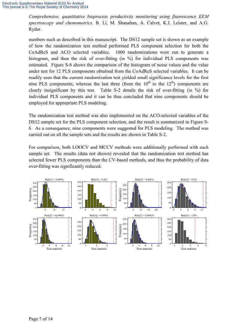
numbers such as described in this manuscript. The DS12 sample set is shown as an example of how the randomization test method performed PLS component selection for both the CoAdReS and ACO selected variables. 1000 randomizations were run to generate a histogram, and then the risk of over-fitting (in %) for individual PLS components was estimated. Figure S-6 shows the comparison of the histogram of noise values and the value under test for 12 PLS components obtained from the CoAdReS selected variables. It can be readily seen that the current randomization test yielded small significance levels for the first nine PLS components, whereas the last three (from the 10th to the 12th) components are clearly insignificant by this test. Table S-2 details the risk of over-fitting (in %) for individual PLS components and it can be thus concluded that nine components should be employed for appropriate PLS modeling. The randomization test method was also implemented on the ACO-selected variables of the DS12 sample set for the PLS component selection, and the result is summarized in Figure S-6. As a consequence, nine components were suggested for PLS modeling. The method was carried out on all the sample sets and the results are shown in Table S-2. For comparison, both LOOCV and MCCV methods were additionally performed with each sample set. The results (data not shown) revealed that the randomization test method has selected fewer PLS components than the CV-based methods, and thus the probability of data over-fitting was significantly reduced.

5 10 150

50

100

150

200

250

300

Freq

uenc

y

Risk[1] = 0.003%

2 4 6 8 100

50

100

150

200

250

300Risk[2] = 0.2%

2 4 6 8 100

50

100

150

200

250

300

Test statistic

Freq

uenc

y

Risk[3] = 8e-006%

1 2 30

50

100

150

200

250

Test statistic

Risk[4] = 0.009%

5 10 15 200

50

100

150

200

250

Freq

uenc

y

Risk[1] = 0.001%

2 4 6 8 100

50

100

150

200

250Risk[2] = 0.2%

2 4 6 8 100

50

100

150

200

250

Test statistic

Freq

uenc

y

Risk[3] = 0.0003%

1 2 3 4 50

50

100

150

200

250

300

Test statistic

Risk[4] = 1.8%



of 14

0.5 1 1.5 2 2.50

50

100

150

200

250

300

Freq

uenc

y

Risk[5] = 0.4%

0.5 1 1.5 20

50

100

150

200

250

Risk[6] = 7e-006%

0.4 0.6 0.8 10

50

100

150

200

250

300

Test statistic

Freq

uenc

y

Risk[7] = 0.01%

0.4 0.6 0.80

50

100

150

200

250

Test statistic

Risk[8] = 4e-005%

1 2 3 4 50

100

200

300

Freq

uenc

y

Risk[5] = 1e-006%

0.5 1 1.5 2 2.50

50

100

150

200

250

300Risk[6] = 2e-009%

0.4 0.6 0.8 10

50

100

150

200

250

Test statistic

Freq

uenc

y

Risk[7] = 1.1%

0.4 0.6 0.80

100

200

300

Test statistic

Risk[8] = 0.2%

0.2 0.3 0.4 0.50

50

100

150

200

250

300

Freq

uenc

y

Risk[9] = 1.2%

0.2 0.25 0.3 0.350

50

100

150

200

Risk[10] = 10.1%

0.15 0.2 0.25 0.30

50

100

150

200

250

300

Test statistic

Freq

uenc

y

Risk[11] = 68%

0.15 0.2 0.250

50

100

150

200

250

Test statistic

Risk[12] = 89.5%

0.3 0.4 0.5 0.60

50

100

150

200

250

300Fr

eque

ncy

Risk[9] = 1.4%

0.2 0.3 0.4 0.50

50

100

150

200

250

300

Risk[10] = 10.3%

0.15 0.2 0.25 0.3 0.350

100

200

300

Test statistic

Freq

uenc

y

Risk[11] = 65.5%

0.15 0.2 0.250

50

100

150

200

250

Test statistic

Risk[12] = 27.9%

Figure S-6: DS12 sample set with (left) CoAdReS- and (right) ACO-selected variables: comparison of the histogram of noise values and the value under test (···) for 12 PLS components.



of 14

Table S-2: Risk of over-fitting (in %) for individual components of PLS models, estimated from 1000 randomizations for each sample set. By the 11th component the risk of over-fitting was > 50% for every data set, except for the 12th component of DS12 ACO model.

DS4 PLS component 1 2 3 4 5 6 7 8 9 10

CoAdReS 26.8 0.3 7×10-6 2×10-6 3×10-3 0.2 2.1 8.49 75.6 99.7 ACO 6.69 3×10-2 4×10-4 5 1×10-5 0.2 0.5 2×10-3 77 81.3

DS5 PLS component 1 2 3 4 5 6 7 8 9 10

CoAdReS 4.8 3×10-5 2×10-7 6.89 7×10-3 0.599 2×10-5 61.7 43.9 99.7 ACO 0.3 0.4 2×10-2 2×10-2 0.2 3.8 6.59 33.2 95.7 100

DS6 PLS component 1 2 3 4 5 6 7 8 9 10

CoAdReS 3.6 4×10-3 1×10-10 1×10-4 2×10-5 4.6 25.1 19.6 78.4 37.8 ACO 4.6 0.3 7×10-8 7×10-3 0.999 3.1 2×10-5 52 40.6 96.5

DS7 PLS component 1 2 3 4 5 6 7 8 9 10

CoAdReS 0.4 3×10-6 3×10-8 4×10-10 1×10-8 1×10-2 0.2 28.7 96.7 82.9 ACO 2×10-2 1.7 4×10-7 3×10-7 3×10-4 3×10-4 0.5 2.7 70.1 94.8

DS8 PLS component 1 2 3 4 5 6 7 8 9 10

CoAdReS 1.7 3×10-4 9×10-8 2×10-5 0.899 0.2 18.1 1.8 68.8 45.7 ACO 3×10-2 4×10-2 2×10-2 2×10-3 1.9 9.09 0.4 3×10-3 90.8 99.9

DS9 PLS component 1 2 3 4 5 6 7 8 9 10

CoAdReS 8.09 2×10-8 0.4 3×10-7 8×10-3 0.3 38.1 0.2 44.1 15.1 ACO 0.699 5×10-2 2×10-2 7×10-3 1.1 25.6 6×10-7 1.7 16.4 85.9

DS10 PLS component 1 2 3 4 5 6 7 8 9 10

CoAdReS 6×10-2 8.59 1×10-12 5×10-8 0.2 0.599 8.59 87.4 76.4 46.3 ACO 5×10-3 5.49 1×10-5 0.599 2.2 7×10-4 2×10-4 5.49 90.2 40.1

DS11 PLS component 1 2 3 4 5 6 7 8 9 10

CoAdReS 0.3 7×10-2 1×10-2 3×10-6 2×10-2 2.3 2.2 7.89 8.29 96 ACO 2×10-2 1.7 8×10-5 3×10-2 0.3 0.3 6×10-2 7.29 86 9.69

DS12 PLS component 1 2 3 4 5 6 7 8 9 10

CoAdReS 3×10-3 0.2 8×10-6 9×10-3 0.4 7×10-6 0.01 4×10-5 1.2 10.1 ACO 1×10-3 0.2 3×10-4 1.8 1×10-6 2×10-9 1.1 0.2 1.4 10.3 The complexity of the PLS model depends on a combination of the sample set complexity, the appropriate data pretreatment, and the proper estimate of the optimal number of PLS components. Bearing in mind the fact that:



of 14

• The samples analyzed in this study were from an industrial bioprocess, therefore very complex and composed of a large number of constituents.

• The EEM spectra are also very complex, with overlapping bands of many fluorophores.

• The limited number of samples (<37) available for this study mean that the calibration models generated here will not be fully representative of all variance in the data. Thus these small sample set models are likely to use more LV’s that are required to model the actual components linked to the glycoprotein product yield. This is illustrated in Figure S-7.

To demonstrate the limitations due to sample set size (and corresponding influence of PLS components) we used the following procedure. However, not all samples had associated glycoprotein product yield data. Only the samples having an associated glycoprotein concentration were used for investigating the interdependence of the prediction errors with the varying numbers of samples and PLS components. Since the samples used in this study were from an industrial bioprocess, each sample was assigned with a unique manufacture date and a specific lot number. Thus, taking the DS12 sample set as an example, samples were selected, according to sample manufacture date and lot number, to construct the data subsets containing 15 to 28 samples. Then, a series of PLS models were built and both the RMSEC and RMSECV values calculated by using varying numbers (1 to 15) of PLS components. LOOCV was used for both the full spectra and CoAdReS-selected variable set. These different PLS models did not cover the exact same glycoprotein concentration ranges (0.67–0.92 g/L) however, the variation is relatively small. The result was then visualized in a 3D plot (Figure S-7) to show the interdependence between the sample set size, model complexity, and prediction errors with regard to the resultant RMSEC/RMSECV values.

510

1516 18 20 22 24 26 280

0.01

0.02

0.03

0.04

0.05

0.06

Number of PLS componentsNumber of Samples

Pred

ictio

n er

rors

Figure S-7: Prediction errors showing the interdependence with the varying numbers of samples and PLS components: (left) CoAdReS-selected variable set, and (right) full Ex/Em range spectra. Blue represents the RMSECV values and red denotes the RMSEC values.



of 14

One can observe that the prediction errors (particularly the RMSECV values) were dramatically improved with the use of the reduced variable set (CoAdReS in this instance) compared to the full spectral range data set. It also clearly shows that for the CoAdReS sample set the RMSECV value tends to a minimum (~0.015 g/L) value with ~12–15 PLS components with ~24 and 28 samples. The overall downward trend with increasing sample number is to be expected and does indicate that the correlation with yield is indeed real. RMSEC values tend to converge at the 9th PLS component once the sample number was ≥22, and the value stays nearly constant with increasing component and/or sample number. This would tend to suggest that 9 components and an RMSEC of ~0.006 g/L will be the best theoretical result obtainable (using this type of EEM data). If we were in a position to double or treble the sample number (which unfortunately we are not) then we would fully expect this trend to continue and the RMSEC/RMSECV values to converge. S7. QUANTITATIVE STUDY OF DS12 SAMPLE SET Both the CoAdReS and ACO methods were implemented on the DS12 sample set: 90 variables were selected by CoAdReS with a histogram threshold value of 0.15, while 129 variables selected by ACO with a histogram threshold of 0.28 (Figure S-8). There were 61 common variables.

300 350 400 450

240260280300

0

50

100

150

200

250

300a


Inte

nsity

/ a.

u.

50 100 150 200 250 300

0.015

0.025

0.035

0.045

0.055

Number of Selected Variables

RM

SEC

V

b

(90 , 0.016)



of 14

300 350 400 450

240260280300

0

50

100

150

200

250

300c


Inte

nsity

/ a.

u.

50 100 150 200 250 300

0.015

0.020

0.025

0.030

0.035

0.040


RM

SEC

V

d

(129 , 0.018)

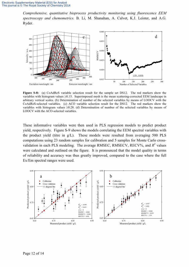
Figure S-8: (a) CoAdReS variable selection result for the sample set DS12. The red markers show the variables with histogram values ≥0.15. Superimposed mesh is the mean scattering-corrected EEM landscape in arbitrary vertical scales. (b) Determination of number of the selected variables by means of LOOCV with the CoAdReS-selected variables. (c) ACO variable selection result for the DS12. The red markers show the variables with histogram values ≥0.28. (d) Determination of number of the selected variables by means of LOOCV with the ACO-selected variables. These informative variables were then used in PLS regression models to predict product yield, respectively. Figure S-9 shows the models correlating the EEM spectral variables with the product yield (titre in g/L). These models were resulted from averaging 500 PLS computations using 23 random samples for calibration and 5 samples for Monte Carlo cross-validation in each PLS modeling. The average RMSEC, RMSECV, RECV%, and R2 values were calculated and outlined on the figure. It is pronounced that the model quality in terms of reliability and accuracy was thus greatly improved, compared to the case where the full Ex/Em spectral ranges were used.

0.65 0.75 0.85 0.950.65

0.75

0.85

0.95

Rcal2 = 0.999

Rcv2 = 0.653

LVs = 9RMSEC = 0.004RMSECV = 0.049RECV% = 6.04

a

Measured product yield / g/L

Pred

icte

d pr

oduc

t yie

ld /

g/L

CalibrationCross validation1:1 diagonal line

0.65 0.75 0.85 0.95

0.65

0.75

0.85

0.95

Rcal2 = 0.997

Rcv2 = 0.982


b


Pred

icte

d pr

oduc

t yie

ld /

g/L




of 14

0.65 0.75 0.85 0.950.65

0.75

0.85

0.95

Rcal2 = 0.997

Rcv2 = 0.977


c


Pred

icte

d pr

oduc

t yie

ld /

g/L


Figure S-9: PLS models for the correlation between the EEM spectral variables of DS12 and product yield (titre in g/L), which were obtained from averaging 500 PLS computations using 23 random samples for calibration and 5 samples for Monte Carlo cross-validation in each PLS modeling by means of: (a) full Ex/Em spectral ranges, (b) CoAdReS selected variables, and (c) ACO selected variables.

S8. PLS MODELING OF DS7 SAMPLE SET

300 350 400 450

240260280300

0

50

100

150

200

250

300

350

400

450

500


a

Inte

nsity

/ a.

u.

50 100 150 200 250 300

0.015

0.025

0.035

0.045

0.055


RM

SEC

V

b

(80 , 0.016)

300 350 400 450

240260280300

0

50

100

150

200

250

300

350

400

450

500


c

Inte

nsity

/ a.

u.

50 100 150 200 250 300

0.02

0.03

0.04

0.05


RM

SEC

V

d

(148 , 0.022)

Figure S-10: (a) CoAdReS variable selection result for the sample set DS7. The red markers show the variables with histogram values ≥0.15. Superimposed mesh is the mean scattering-corrected EEM landscape in arbitrary vertical scales. (b) Determination of number of the selected variables by means of LOOCV with CoAdReS-selected variables. (c) ACO variable selection result for the DS7. The red markers show the



of 14

variables with histogram values ≥0.27. (d) Determination of number of the selected variables by means of LOOCV with ACO-selected variables.

0.65 0.75 0.85 0.950.65

0.75

0.85

0.95

Rcal2 = 0.993

Rcv2 = 0.392


a


Pred

icte

d pr

oduc

t yie

ld /

g/L


0.65 0.75 0.85 0.95

0.65

0.75

0.85

0.95

Rcal2 = 0.995

Rcv2 = 0.981


b


Pred

icte

d pr

oduc

t yie

ld /

g/L


0.65 0.75 0.85 0.950.65

0.75

0.85

0.95

Rcal2 = 0.995

Rcv2 = 0.977


c


Pred

icte

d pr

oduc

t yie

ld /

g/L


Figure S-11: PLS models for the correlation between the EEM spectral variables of DS7 and product yield (titre in g/L), which were obtained from averaging 500 PLS computations using 24 random samples for calibration and 5 samples for Monte Carlo cross-validation in each PLS modeling by means of: (a) full Ex/Em spectral ranges, (b) CoAdReS selected variables, and (c) ACO selected variables.

The quantitative models of all the other available sample sets are available if required. They have not been included here because of page length concern. S9. REFERENCES 1. Y. Hu, B. Y. Li, H. Sato, I. Noda and Y. Ozaki, J. Phys. Chem. A, 2006, 110, 11279-

11290. 2. J. M. Beechem and L. Brand, Annu. Rev. Biochem, 1985, 54, 43-71. 3. G. S. Harms, S. W. Pauls, J. F. Hedstrom and C. K. Johnson, J Fluoresc, 1997, 7,

283-292. 4. S. Wiklund, D. Nilsson, L. Eriksson, M. Sjostrom, S. Wold and K. Faber, J.

Chemometr., 2007, 21, 427-439. 5. H. Martens and T. Naes, Multivariate Calibration, New York, 1989. 6. Q. S. Xu and Y. Z. Liang, Chemometr. Intell. Lab. Syst., 2001, 56, 1-11.


table of contents - royal society of chemistry · 260 240 300 280 0 50 100 150 200 250 300 350 400...

Documents