TA202A: Introduction to Manufacturing Processes (2017-18, 2nd semester)

Instructor-in-Charge Dr. J. Ramkumar

Department of Mechanical Engineering IIT Kanpur

Email:jrkumar@iitk.ac.in

Lectures 2-5 Conventional Machining Processes

Material Removal Processes

A family of shaping operations, the common feature of which is removal of material from a starting work part so the remaining part has the desired geometry Machining : Material removal by a sharp cutting tool, e.g., Turning,

Milling, Drilling Abrasive processes: Material removal by hard, abrasive particles, e.g.,

Grinding Nontraditional processes : Various energy forms other than sharp cutting

tool to remove material

Machining

Excess material removed from the starting piece so what remains is the desired geometry

Examples: (a) Turning, (b) Drilling, and (c) Milling

Material Removal Processes

Any machine tool has 3 different components

Machine Fixture for

holding work piece

Tool

Cutting tool

Block

Concept of tool inserts Inserts are removable cutting tips, which means they are

not brazed or welded to the tool body. They are usually index able. This saves time in manufacturing by allowing fresh

cutting edges.

Geometry of single point cutting tool

Geometry of right hand single point cutting tool

Turning tool with tool insert

Schematic illustration of a right-hand cutting tool

Tool Nomenclature/Angles

Figure: (a) Seven elements of single-point tool geometry; and (b) the tool signature convention that defines the seven elements

Examples of cutting processes

Two-dimensional cutting process, also called orthogonal cutting. Note that the tool shape and its angles, depth of cut, and the cutting speed, V, are all independent variables.

Traditional material removal process :Machining

Cutting action involves shear deformation of work material to form a chip, and as chip is removed, new surface is exposed:

(a) Positive and (b) Negative rake tools

Cutting Conditions in Machining The three dimensions of a machining process: Cutting speed (v) :Primary motion Feed (f) :Secondary motion Depth of cut (d) :Penetration of tool below original work surface For certain operations, material removal rate can be found as:

MRR = v× f × d

Where, v = Cutting speed; f = Feed; d = Depth of cut

Types of cutting Orthogonal Cutting (2-D Cutting): In Orthogonal Cutting, Cutting edge is (1) Straight, (2) Parallel to the original plane surface on the work-piece and (3) Perpendicular to the direction of cutting. For example: Operations: Lathe cut-off operation, Straight milling, etc.

Oblique Cutting Oblique Cutting (3-D Cutting): Cutting edge of the tool is inclined to the line normal to the cutting direction. In actual

machining, Turning, Milling etc. Cutting operations are oblique cutting(3-D)

Mechanics of chip formation The tool will cut or shear off the metal, provided by: The tool is harder than the work metal The tool is properly shaped so that its edge can be effective in cutting the metal. There is movement of tool relative to the material or vice-versa, so as to make cutting action

possible. Mechanics: Plastic deformation along shear plane (Merchant) As can be seen from the first figure below, the work piece remains stationary and the tool advances

in to the work piece towards left. Thus the metal gets compressed very severely, causing shear stress.

This stress is maximum along the plane is called shear plane. If the material of the work-piece is ductile, the material flows plastically along the shear plane,

forming chip, which flows upwards along the face of the tool.

Types of Chips Types of Chips 1. Continues Chips 2. Discontinuous Chips 3. Continuous Chips with BUE

Schematic of different types of chip

Types of Chips

Conditions for (a) Continuous chips:

Sharp cutting edges Low feed rate (f) Large rake angle (α) Ductile work material High cutting speed (v) Low friction at Chip-Tool

interface

Conditions for (b) Discontinuous chips:

Brittle Material Low cutting speed Small rake angle

Conditions for (c) Continuous chips with BUE:

High friction between Tool &

chip Ductile material Particles of chip adhere to the

rake face of the tool near cutting edge

Roughing vs. Finishing Cuts

Higher the rake angle, better is the cutting and less is the cutting force. Several roughing cuts are usually taken on a part, followed by one or two finishing cuts

Roughing - removes large amounts of material from starting work-part Some material remains for finish cutting High feeds and depths, low speeds Finishing - completes part geometry Final dimensions, tolerances, and finish Low feeds and depths, high cutting speeds

Cutting Tool Classification 1. Single-Point Tools One dominant cutting edge Point is usually rounded to form a nose radius Turning uses single point tools 2. Multiple Cutting Edge Tools More than one cutting edge Motion relative to work achieved by rotating Drilling and milling use rotating multiple cutting edge tools

Single-Point Tool Multiple Cutting Edge Tool

Cutting Tool Materials Tool failure modes identify the important properties that a tool material should possess: Toughness - To avoid fracture failure Hot Hardness - Ability to retain hardness at high temperatures Wear Resistance - Hardness is the most important property to resist abrasive wear

Typical hot hardness relationships for selected tool materials. Plain carbon steel shows a rapid loss of hardness as temperature increases.

High speed steel is substantially better, while

cemented carbides and ceramics are significantly harder at elevated temperatures.

Hardness vs. Toughness for different tool Materials

There are two approaches of analyzing forces and shear strain in cutting operations: 1.Thin Plane Model:- Merchant, PiisPanen, Kobayashi & Thomson 2. Thick Deformation Region:- Palmer, (At very low speeds) Oxley, kushina , Hitoni

Thin Zone Model: Merchant’s Model

Assumptions:- Tool tip is sharp, No Rubbing, No Ploughing 2-D deformation. Stress on shear plane is uniformly distributed. Resultant force R on chip applied at shear plane is equal, opposite and collinear to force R’

applied to the chip at tool-chip interface.

Mechanics of Cutting (Shear plane angle)

1/r=k : Chip reduction coefficient

(r)

Why chip thickness(t2) is more than unreformed chip thickness(t1)?

The chip thickness (t2) usually becomes larger than the uncut chip thickness (t1). The reason can be attributed to: Compression of the chip ahead of the tool Frictional resistance to chip flow Plastic deformation

Forces in Orthogonal Cutting:

Friction force, F Force normal to Friction force, N Cutting Force, Fc

Thrust force, Ft

Shear Force, Fs

Force Normal to shear force, Fn

Resultant force, R

F, N, Fs, and Fn cannot be directly measured Forces acting on the tool that can be measured: Cutting force Fc and Thrust force Ft using tool Dynamometer

Force circle diagram (Merchant Circle Diagram)

Merchant Circle Analysis

From the Circle

Expending Fs,Fn,F and N

Merchant’s First Solution

Force analysis Let τ be the strength of the work piece material, b is the width of cut and tu uncut chip thickness Then Fc and Ft in terms of material properties (Strength)

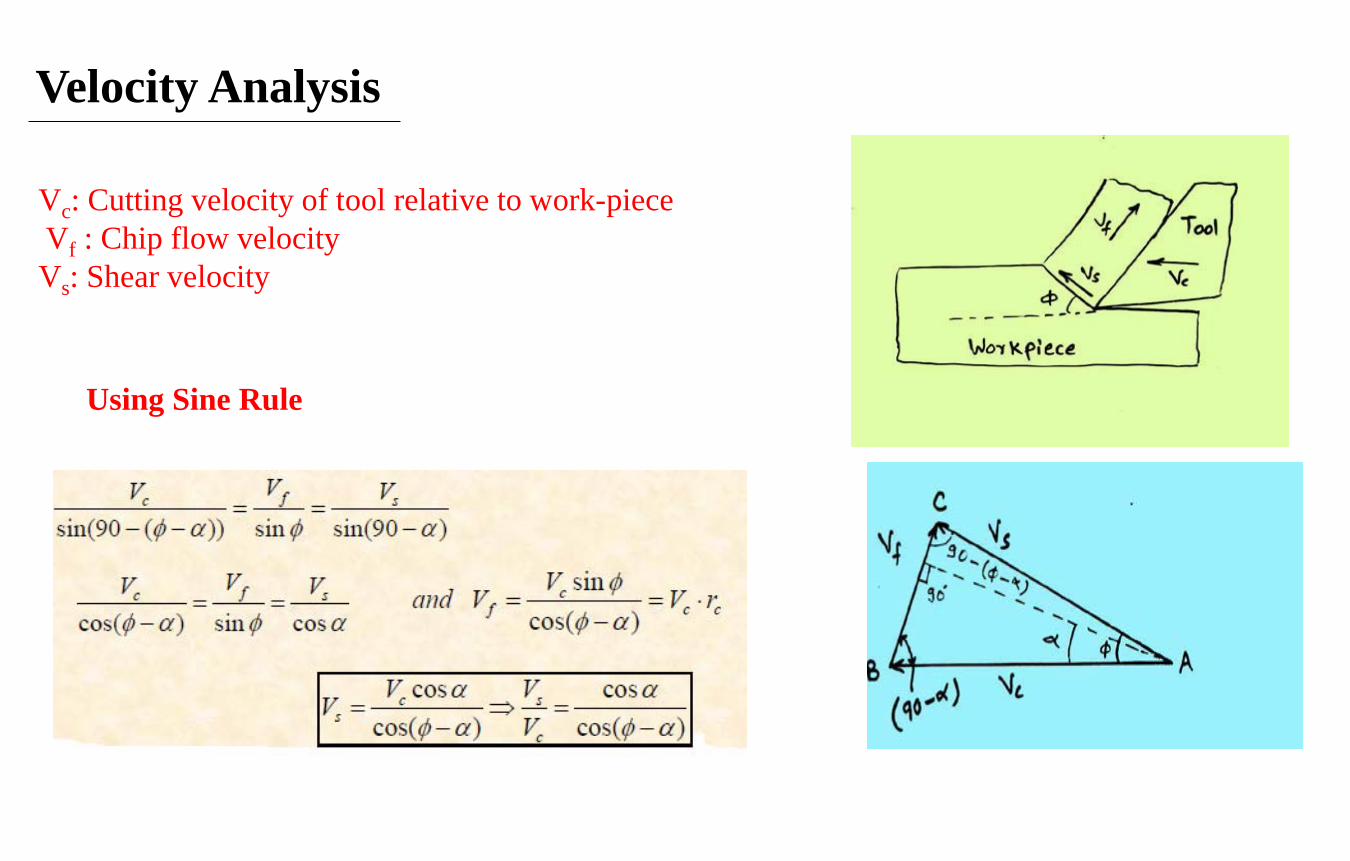
Velocity Analysis

Using Sine Rule

Vc: Cutting velocity of tool relative to work-piece Vf : Chip flow velocity Vs: Shear velocity

Shear Strain and Strain Rate Characteristic of the metal cutting process is that the work-piece material is being

deformed at extremely intense conditions in a small volume. The extreme deformation conditions make metal cutting a remarkable process if compared to other production processes.

Strain rates in machining are in the order of 103–106 s−1. In conventional material tests the strain rates are in the order of 10−3–10−1 s−1, i.e. up to a million times smaller than in machining.

Plastic strain rate can be divided in three zones: the low strain rate region (<1 s−1), the medium rate region (comprehended between the low and high strain rate region values) and the high strain rate region (above 103 or 104 s−1).

Expression for Shear Strain

The deformation can be idealized as a process of block slip (or preferred slip planes)

Shear Strain= deformation/Length

Expending tan and cot angles in terms of sin and cosine angles, we get

Expression for Shear Strain rate

In terms of shear strain, the Shear Strain can be written as:

Where, Δy :Mean thickness of PSDZ

Shear Strain Rate:

From velocity analysis Vs in terms of Vc, Vs =

Power and Energy Relationships

A machining operation requires power as a input source. The power to perform machining can be computed from:

P = Fc× v where P = cutting power; Fc = cutting force; and v = cutting speed Specific Energy in Machining: Power required to remove unit volume of material. Given in

W/mm3

P = Uc × MRR Uc = P/MRR

Uc = specific power, MRR = Volumetric material removal rate

Common Late Operations

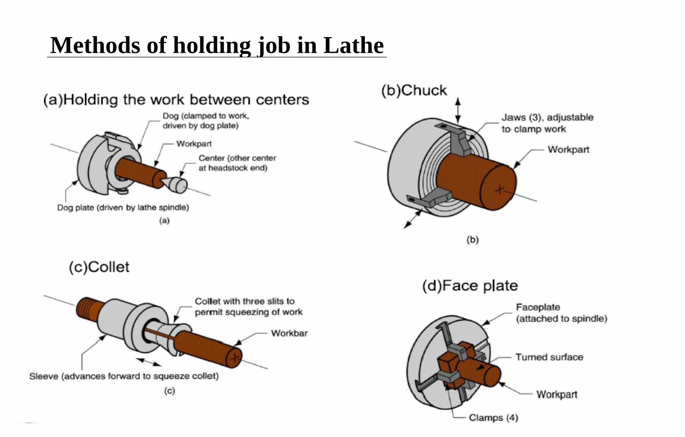
Methods of holding job in Lathe

Lathe Chucks

3-Jaw chuck 4-Jaw chuck

Turning Calculation

Average cutting speed: Vavg = π × Davg × N

Davg is the average diameter of work piece and N is the spindle speed in rpm

Material removal rate (MRR )= Vavg×d × f d is the depth of cut, f is the feed (units: mm/rev or in/rev)

Cutting Power, Pc = Uc × MRR=Fc × V Uc=Specific energy consumption (W/mm3) Fc=Cutting force, V = Cutting speed

Machining time, tm = L/(f × N) = L/f f is the feed rate (units: mm/min or in/min), L= Length of the job

Drilling

Drill geometry

Variation of upper and lower rake angles due to the feed

From the inclination of helix the nominal upper rake angle, which decreases if they are considered smaller diameters.

The upper rake angle determined by the helix suffers a slight variation due to the feed of the drill.

In fact the cutting edge moves along a trajectory inclined at an angle Δα, which is equal to Δγ, compared to the reference surface.

Drilling through and Blind holes

Operation related to Drilling

Drilling Calculations Drill Speed, RPM:

N = kV

Dπ

k is a Units Constant D is Drill Diameter

V is cutting speed V = πND/k

Cutting Time (min): CT = (L + A)

f * N

A is allowance; usually

f is drill feedrate

L is length of Hole

r

D2

r

MRR = Vol.Removed

CT = D Lf N

4 L = D f N

4

2r

2rπ π

2

Milling

Examples of different Milled parts

Part machined using micro-milling operation

Different Milling Operation

Profile Milling, Pocket Milling and Surface Contouring operations

Milling Operations

(a) Slab Milling, (b) Slotting, (c) End Milling

Milling Types

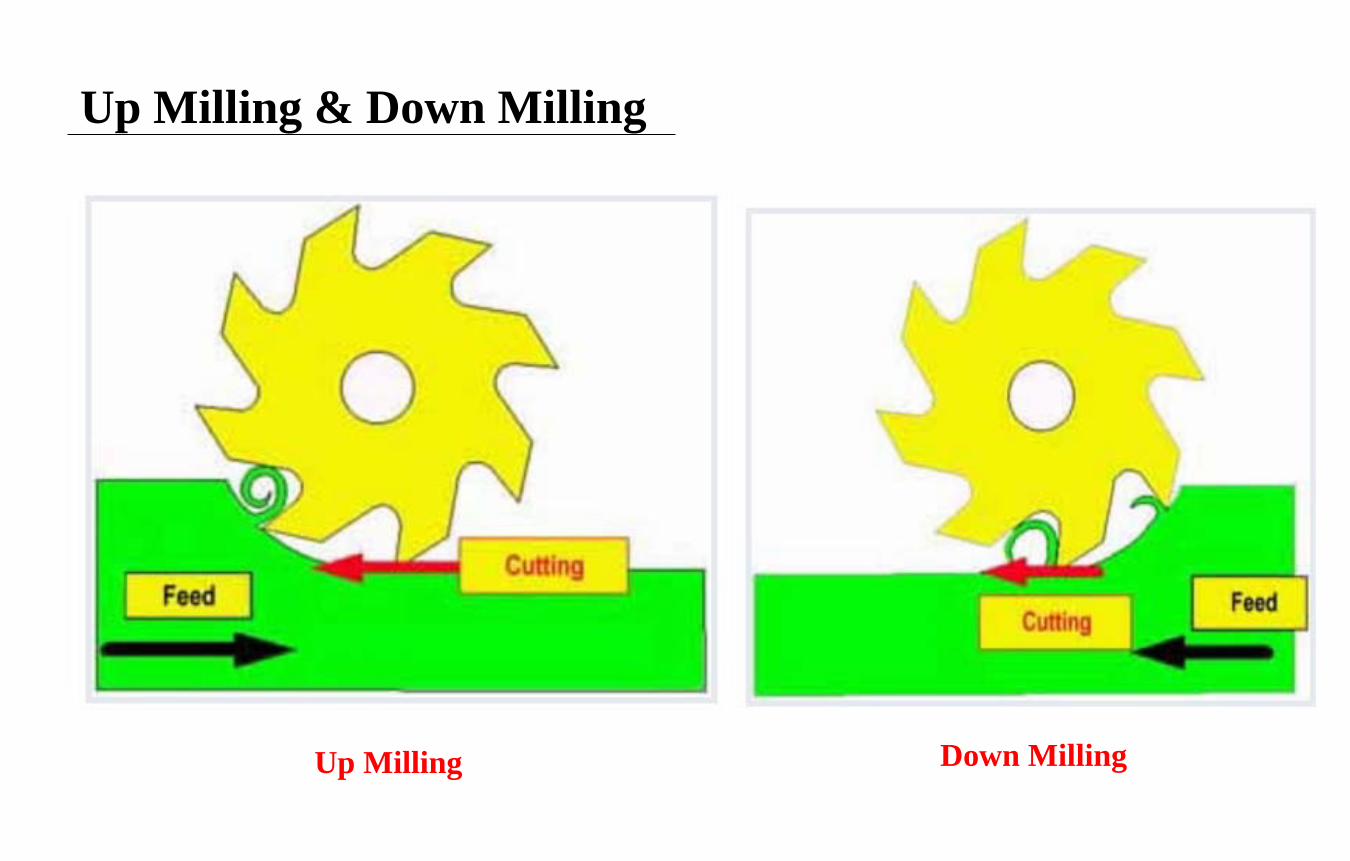
Up Milling & Down Milling

Up Milling Down Milling

Comparison between Up Milling and Down Milling

Milling Machines

Milling cutter nomenclature

Milling Calculation

I. Slab Milling: Cutting speed, V = π × D × N D is the cutter diameter Material removal rate is given as: MRR = f × N × da × dr = F × da × dr da is the axial depth of cut dr is the radial depth of cut f is the feed per revolution F is the feed rate (in/min or mm/min) Cutting power, Pc = Uc × MRR Machining time, tm = (l +2 lc)/F lc is the length of the cutter’s first contact with the work-piece

lc =

Case-2:The second case is when the cutter is offset to one side of the work, as in Figure (b). In this case, the approach distance is given by

Case-1:The first case is when the cutter is centered over a rectangular workpiece as in Figure (a). The cutter feeds from right to left across the workpiece. In order for the cutter to reach the full width of the work, it must travel an approach distance given by the following:

(a) (b)

II. Face Milling

Machining Time for both cases=

A= lc = Approach length F= fr= Feed rate (mm/min)

Tm = L+2A/fr

Plain vs. Face Milling

In peripheral milling, also called plain milling, the axis of the tool is parallel to the surface being machined, and the operation is performed by cutting edges on the outside periphery of the cutter.

Face Milling In face milling, the axis of the cutter is perpendicular to the surface being milled, and machining is performed by cutting edges on both the end and outside periphery of the cutter.

Face Milling Plain milling

Expression for surface finish in Milling operation For a milling operation the following formula will give the value for surface finish. Ra is the surface finish in micro inches. r is the radius of the tool nose in inches f is the feed rate in Inches per revolution for one tooth. For example: A milling cutter with a 1/16" tool nose radius running at .010 inches per revolution will produce, in theory, a surface finish value Ra of 100.

Grinding Operation Grinding is the most common form of abrasive machining. It is a material cutting process which engages an abrasive tool whose cutting

elements are grains of abrasive material known as grit. These grits are characterized by sharp cutting points, high hot hardness, chemical

stability and wear resistance. The grits are held together by a suitable bonding material to give shape of an

abrasive tool.

Grinding wheel and work-piece interaction

Surface Grinding Machine

Grinding operations

Cylindrical Grinding

(a) External cylindrical Grinding(b) Internal cylindrical Grinding

Centreless Grinding

Interaction of the grit with the work-piece

Variation in rake angle with grits of different shape

Grits engage shearing, ploughing and rubbing

Grit with favourable geometry can produce chip in shear mode.

Grits having large negative rake angle or rounded cutting edge do not form chips but

may rub or make a groove by ploughing leading to lateral flow of the workpiece

material as shown in the figure above.

Various stages of grinding with grit depth of cut

Various stages of grinding with grit depth of cut

At a small grit penetration only sliding of the grit occurs against the work piece. In this zone rise of force with increase penetration is quite high. With further increase of grit penetration, grit starts ploughing causing plastic flow of the material associated with high grinding force. It can be seen that with further increase of penetration, the grits start cutting and the rate of rise of force with increase of grit depth of cut is much less than what can be seen in the sliding or ploughing zone

Compositional specifications of Grinding Wheel

Specification of a grinding wheel ordinarily means compositional specification. Conventional Abrasive grinding wheels are specified encompassing the following parameters. (1) The type of grit material (2) The grit size (3) The bond strength of the wheel, commonly known as wheel hardness (4) The structure of the wheel denoting the porosity i.e. the amount of inter grit spacing (5) The type of bond material (6) Other than these parameters, the wheel manufacturer may add their own identification code prefixing or suffixing (or both) the standard code.

Specifications of Grinding Wheel

Heat generation in Metal cutting

Approximately 98% of the energy in machining is converted into heat .This can cause temperatures to be very high at the tool-chip .The remaining energy (about 2%) is retained as elastic energy in the chip

Heat distribution

Primary shear zone where the major part of the energy is converted into heat Secondary deformation zone at the chip – tool interface where further heat is generated

due to rubbing and / or shear At the worn out flanks due to rubbing between the tool and the finished surfaces. The heat generated is shared by the chip, cutting tool and the blank. About 80% of total heat is carried away by the chip. From 10 to 20% of the total heat goes into the tool and some heat is absorbed in the

blank. With the increase in cutting velocity, the chip shares heat increasingly.

80%

10-20%

Cutting Speed and Temperature

Relationship between temperature and Cutting speed

Process of cutting tool failure Tool that no longer performs the desired function can be declared as “failed”

Cutting tools generally fail by :

(i) Mechanical breakage: Due to excessive forces and shocks. Such kind of tool failure is random and catastrophic in nature and hence are extremely detrimental.

(ii) Rapid dulling :By plastic deformation due to intensive stresses and temperature. This type of failure also occurs rapidly and are quite detrimental and unwanted.

(iii) Gradual wear of the cutting tool at its flanks and rake surface.

Edge chipping/breakage Thermal cracks

Gradual Wear of Cutting Tool

Create wear & flank wear Crater wear Flank wear

Tool Wear Mechanisms:

Abrasion wear:

Adhesion wear:

Diffusion wear: This type of wear occurs due to the diffusion process, where atoms in a crystal lattice move from a region of high concentration to low concentration (Ficks law).

Adhesion wear occurred when chip material plucked out the microscopic fragment from the tool. At high temperature and pressure at cutting edge, the tool-chip interface forms a metallic bond in the form of spot welds.

The hard inclusion having sharp edges comes in contact with a cutting tool and removes material from the tool surface by abrasion action. This wears are more predictable and give a stable tool life.

Flank wear and Crater wear are two common wear of cutting tool.

Flank wear and time relationship Three stages of flank wear: 1. Rapid growth region (Break in region) 2. Steady state region (Temperature Insensitive region) 3. Catastrophe failure (Temperature sensitive region)

Flank wear formation depends on * Cutting Conditions (f, d, V, tool angles) * Properties of work material and tool material

Flank wear characterized by wear land (or Height) hf of wear band

Tool Wear Index, Feed Marks and Surface finish Type of wear depends MAINLY on cutting speed If cutting speed increases, predominant wear may be “CRATER” wear else “FLANK”

wear. Failure by crater takes place when index hk reaches 0.4 value, before flank wear limit of

hf=1mm for carbide tools is attained.

Effect of tool wear on machined surface

Dimensional accuracy Process stability Surface finish

Effect of tool wear on machined component dimensions (Exaggerated view)

Tool life & Machinability Tool no longer performs desired function: failed Re-sharpen and use it again. Tool life: Useful life of a tool expressed in terms of time from start of a cut to termination point

(defined by failure criterion). Sometimes also expressed in terms of number of the parts machined.

Mainly concerned with work piece material properties not the tool properties. It depends on work piece material properties and good Machinability means: 1. Ease of machining 2. Low tool wear 3. Good surface finish produced 4. Low cutting forces

Machinability

Taylor’s tool life equation

Cutting velocity vs tool life on a log-log scale

Cutting velocity- tool life relationship

Tool life

Variables affecting tool life Cutting Conditions (V, d, f) Tool Geometry (all six angles, and nose radius) Work piece Material Cutting fluid Machine tool and Work piece region Tool Material

Cutting fluids and Lubrication

The basic purposes of cutting fluid application are : Cooling of the job and the tool to reduce the detrimental effects of cutting temperature

on the job and the tool. Lubrication at the chip–tool interface and the tool flanks to reduce cutting forces and

friction and thus the amount of heat generation. Cleaning the machining zone by washing away the chip – particles and debris which,

if present, spoils the finished surface and accelerates damage of the cutting edges Protection of the nascent finished surface – a thin layer of the cutting fluid sticks to

the machined surface and thus prevents its harmful contamination by the gases like SO2, O2, H2S, NxOy present in the atmosphere.

Essential Properties of Cutting Fluids For cooling : High specific heat, thermal conductivity and film coefficient for heat transfer Spreading and wetting ability For lubrication : High lubricity without gumming and foaming Wetting and spreading High film boiling point Friction reduction at extreme pressure (EP) and temperature Other properties: Chemical stability, non-corrosive to the materials Less volatile and high flash point High resistance to bacterial growth Odourless and also preferably colourless Non toxic in both liquid and gaseous stage Easily available and low cost

Recap

Material Removal processes and their Classifications Conventional Machining processes Single point and multipoint cutting tools Chips formation Mechanics of Cutting Cutting tool materials Heat Generation in cutting Tool life & Tool Wear Calculations of Turning, Drilling and Milling operations Grinding operation Classification of Grinding operations Grinding Wheel Specifications