t7.0 introduction - iowa state universityhome.engineering.iastate.edu/~jdm/ee553/powerflow.pdf · a...

The Power Flow Problem

1


James D. McCalley, Iowa State University

T7.0 Introduction

The power flow problem is a very well known problem in the field of power systems engineering, where

voltage magnitudes and angles for one set of buses are desired, given that voltage magnitudes and power

levels for another set of buses are known and that a model of the network configuration (unit commitment

and circuit topology) is available. A power flow solution procedure is a numerical method that is employed

to solve the power flow problem. A power flow program is a computer code that implements a power flow

solution procedure. The power flow solution contains the voltages and angles at all buses, and from this

information, we may compute the real and reactive generation and load levels at all buses and the real and

reactive flows across all circuits. The above terminology is often used with the word “load” substituted for

“power,” i.e., load flow problem, load flow solution procedure, load flow program, and load flow solution.

However, the former terminology is preferred as one normally does not think of “load” as something that

“flows.”

The power flow problem was originally motivated within planning environments where engineers

considered different network configurations necessary to serve an expected future load. Later, it became an

operational problem as operators and operating engineers were required to monitor the real-time status of

the network in terms of voltage magnitudes and circuit flows. Today, the power flow problem is widely

recognized as a fundamental problem for power system analysis, and there are many advanced, commercial

power flow programs to address it. Most of these programs are capable of solving the power flow program

for tens of thousands of interconnected buses. Engineers that understand the power flow problem, its

formulation, and corresponding solution procedures are in high demand, particularly if they also have

experience with commercial grade power flow programs.

The power flow problem is fundamentally a network analysis problem, and as such, the study of it provides

insight into solutions for similar problems that occur in other areas of electrical engineering. For example,

integrated circuit designers also encounter network analysis problems, although of significantly smaller

physical size, are quite similar otherwise to the power flow problem. For example, references [1,2] are

well-known network analysis texts in VLSI design that also provide good insight into the numerical

analysis needed by the power flow program designer. Similarly, there are numerous classical power system

engineering texts, [3-11] are a representative sample, that provide advanced network analysis methods

applicable to VLSI design and analysis problems.

Section T7.1 identifies a feature of power generators important to the power flow problem – real and

reactive power limits. Section T7.2 defines some additional terminology necessary to understand the power

flow problem and its solution procedure. Section T7.3 introduces the so-called network “Y-bus,” otherwise

known more generally as the network admittance matrix. Section T7.4 develops the power flow equations,

building from module T1 where equations for real and reactive power flow across a transmission line were

introduced. Section T7.5 provides an analytical statement of the power flow problem. Section T7.6 uses a

simple example to introduce the Newton-Raphson algorithm for solving systems of non-linear algebraic

equations. Section T7.7 illustrates application of the Newton-Raphson algorithm to the power flow

problem. Section T7.8 provides an overview of several interesting and advanced attributes of the problem.

Section T7.9 summarizes basic power flow input and output quantities and provides an example associated

with a commercial power flow program.

T7.1 Generator Reactive Limits

It is well known that generators have maximum and minimum real power capabilities. In addition, they also

have maximum and minimum reactive power capabilities. The maximum reactive power capability


2

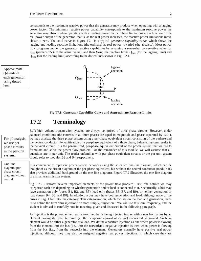
corresponds to the maximum reactive power that the generator may produce when operating with a lagging

power factor. The minimum reactive power capability corresponds to the maximum reactive power the

generator may absorb when operating with a leading power factor. These limitations are a function of the

real power output of the generator, that is, as the real power increases, the reactive power limitations move

closer to zero. The solid curve in Figure T7.1 is a typical generator capability curve, which shows the

lagging and leading reactive limitations (the ordinate) as real power is varied (the abscissa). Most power

flow programs model the generator reactive capabilities by assuming a somewhat conservative value for

Pmax (perhaps 95% of the actual value), and then fixing the reactive limits Qmax (for the lagging limit) and

Qming (for the leading limit) according to the dotted lines shown in Fig. T2.1.

Pmax

Qmax

Qmin

P

Q

leading

operation

lagging

operation

Fig T7.1: Generator Capability Curve and Approximate Reactive Limits

T7.2 Terminology

Bulk high voltage transmission systems are always comprised of three phase circuits. However, under

balanced conditions (the currents in all three phases are equal in magnitude and phase separated by 120),

we may analyze the three phase system using a per-phase equivalent circuit consisting of the a-phase and

the neutral conductor. Per-unitization of a per-phase equivalent of a three phase, balanced system results in

the per-unit circuit. It is the per-unitized, per-phase equivalent circuit of the power system that we use to

formulate and solve the power flow problem. For the remainder of this module, we will assume that all

quantities are in per-unit. The reader unfamiliar with per-phase equivalent circuits or the per-unit system

should refer to modules B3 and B4, respectively.

It is convenient to represent power system networks using the so-called one-line diagram, which can be

thought of as the circuit diagram of the per-phase equivalent, but without the neutral conductor (module B3

also provides additional background on the one-line diagram). Figure T7.2 illustrates the one-line diagram

of a small transmission system.

Fig. T7.2 illustrates several important elements of the power flow problem. First, one notices we may

categorize each bus depending on whether generation and/or load is connected to it. Specifically, a bus may

have generation only (buses B1, B2, and B3), load only (buses B5, B7, and B9), or neither generation or

load (buses B4, B6, and B8). In addition, a bus may have both generation and load, although none of the

buses in Fig. 1 fall into this category. This categorization, which focuses on the load and generation, leads

us to define the term “bus injection” or more simply, “injection.” We will use this term frequently, and the

student is advised to carefully note its meaning, given and discussed in the following paragraph.

An injection is the power, either real or reactive, that is being injected into or withdrawn from a bus by an

element having its other terminal (in the per-phase equivalent circuit) connected to ground. Such an

element would be either a generator or a load. We define a positive injection as one where power is flowing

from the element into the bus (i.e., into the network); a negative injection is then when power is flowing

from the bus (i.e., from the network) into the element. Generators normally have positive real power

injections, although they may also be assigned negative real power injections, in which case they are

Approximate

Q-limits of

each generator

using dotted

box.

For pf analysis,

we use per-

phase circuits

in the per-unit

system.

One-line

diagram: per-

phase circuit

diagram without

neutral.


3

operating as a motor. Generators may have either positive or negative reactive power injections: positive if

the generator is operating lagging and delivering reactive power to the bus, negative if the generator is

operating leading and absorbing reactive power from the bus, and zero if the generator is operating at unity

power factor. Loads normally have negative real and reactive power injections, although they may also be

assigned positive real power injections in the case of very special modeling needs. Figure T7.3 (a) and (b)

illustrate the two most common possibilities. Figure T.7.3 (c) illustrates that we must compute a net

injection as the algebraic sum when a bus has both load and generation; in this case, the net injection for

both real and reactive power is positive (into the bus). Thus, the net real power injection is Pk=Pgk-Pdk, and

the net reactive power injection is Qk=Qgk-Qdk. We may also refer to the net complex power injection as

Sk=Sgk-Sdk, where Sk=Pk+jQk.

Figure T7.2: Single Line Diagram for Simple Power System

Pk=100 Qk=30

(a)

Pk= - 40 Qk= -20

(b)

Pk=100+(-40)=60 Qk=30+(-20)=10

(c)

Fig T7.3: Illustration of (a) positive injection, (b) negative injection, and (c) net injection

Three bus types:

1. PV

2. PQ

3. Swing (Pθ)

Losses are a function of flows.

We do not know flows a priori.

So one gen-bus has injection as

a function of the solution.

P1=PLosses(solution)-Σk=2,N Pk

Q1=QLosses(solution)-Σk=2,N Pk

Real, reactive

power injection:

into bus: gen

out of bus: load

into bus is

defined positive.

There are four

variables for

every bus:

P

Q

V

θ


4

Although it is physically appealing to categorize buses based on the generation/load mix connected to it, we

need to be more precise in order to analytically formulate the power flow problem. For proper analytical

formulation, it is appropriate to categorize the buses according to what information is known about them

before we solve the power flow problem. For each bus, there are four possible variables that characterize

the buses electrical condition. Let us consider an arbitrary bus numbered k. The four variables are real and

reactive power injection, Pk and Qk, respectively, and voltage magnitude and angle, |Vk | and k,

respectively. From this perspective, there are three basic types of buses. We refer to the first two types

using terminology that remind us of the known variables.

PV Buses: For type PV buses, we know Pk and |Vk | but not Qk or k. These buses fall under the

category of voltage-controlled buses because of the ability to specify (and therefore to know) the

voltage magnitude of this bus. Most generator buses fall into this category, independent of whether it

also has load; exceptions are buses that have reactive power injection at either the generator’s upper

limit (Qmax) or its lower limit (Qmin), and (2) the system swing bus (we describe the swing bus below).

There are also special cases where a non-generator bus (i.e., either a bus with load or a bus with neither

generation or load) may be classified as type PV, and some examples of these special cases are buses

having switched shunt capacitors or static var systems (SVCs). We will not address these special cases

in this module. In Fig. T7.2, buses B2 and B3 are type PV. The real power injections of the type PV

buses are chosen according to the system dispatch corresponding to the modeled loading conditions.

The voltage magnitudes of the type PV buses are chosen according to the expected terminal voltage

settings, sometimes called the generator “set points,” of the units.

PQ Buses: For type PQ buses, we know Pk and Qk but not |Vk | or k. All load buses fall into this

category, including buses that have not either load or generation. In Fig. T7.2, buses B4-B9 are all type

PQ. The real power injections of the type PQ buses are chosen according to the loading conditions

being modeled. The reactive power injections of the type PQ buses are chosen according to the

expected power factor of the load.

The third type of bus is referred to as the swing bus. Two other common terms for this bus are slack bus

and reference bus. There is only one swing bus, and it can be designated by the engineer to be any

generator bus in the system. For the swing bus, we know |V| and . The fact that we know is the reason

why it is sometimes called the reference bus. Physically, there is nothing special about the swing bus; in

fact, it is a mathematical artifact of the solution procedure. At this point in our treatment of the power flow

problem, it is most appropriate to understand this last statement in the following way. The generation must

supply both the load and the losses on the circuits. Before solving the power flow problem, we will know

all injections at PQ buses, but we will not know what the losses will be as losses are a function of the flows

on the circuits which are yet to be computed. So we may set the real power injections for, at most, all but

one of the generators. The one generator for which we do not set the real power injection is the one

modeled at the swing bus. Thus, this generator “swings” to compensate for the network losses, or, one may

say that it “takes up the slack.” Therefore, rather than call this generator a |V| bus (as the above naming

convention would have it), we choose the terminology “swing” or “slack” as it helps us to better remember

its function. The voltage magnitude of the swing bus is chosen to correspond to the typical voltage setting

of this generator. The voltage angle may be designated to be any angle, but normally it is designated as 0o.

A word of caution about the swing bus is in order. Because the real power injection of the swing bus is not

set by the engineer but rather is an output of the power flow solution, it can take on mathematically

tractable but physically impossible values. Therefore, the engineer must always check the swing bus

generation level following a solution to ensure that it is within the physical limitations of the generator.

T7.3 The Admittance Matrix Current injections at a bus are analogous to power injections. The student may have already been

introduced to them in the form of current sources at a node. Current injections may be either positive (into

the bus) or negative (out of the bus). Unlike current flowing through a branch (and thus is a branch

quantity), a current injection is a nodal quantity. The admittance matrix, a fundamental network analysis

tool that we shall use heavily, relates current injections at a bus to the bus voltages. Thus, the admittance

matrix relates nodal quantities. We motivate these ideas by introducing a simple example.

Check the

swing bus after

a solution to

ensure it is

within physical

limits.


5

Figure T7.4 shows a network represented in a hybrid fashion using one-line diagram representation for the

nodes (buses 1-4) and circuit representation for the branches connecting the nodes and the branches to

ground. The branches connecting the nodes represent lines. The branches to ground represent any shunt

elements at the buses, including the charging capacitance at either end of the line. All branches are denoted

with their admittance values yij for a branch connecting bus i to bus j and yi for a shunt element at bus i.

The current injections at each bus i are denoted by Ii.

y4 y3

y1

y2

I4

I3 I2

I1

4 3

2

1

y34

y23

y13

y12

Fig. T7.4: Network for Motivating Admittance Matrix

Kirchoff’s Current Law (KCL) requires that each of the current injections be equal to the sum of the

currents flowing out of the bus and into the lines connecting the bus to other buses, or to the ground.

Therefore, recalling Ohm’s Law, I=V/Z=VY, the current injected into bus 1 may be written as:

I1=(V1-V2)y12 + (V1-V3)y13 + V1y1 (T7.1)

To be complete, we may also consider that bus 1 is “connected” to bus 4 through an infinite impedance,

which implies that the corresponding admittance y14 is zero. The advantage to doing this is that it allows us

to consider that bus 1 could be connected to any bus in the network. Then, we have:

I1=(V1-V2)y12 + (V1-V3)y13 + (V1-V4)y14 + V1y1 (T7.2)

Note that the current contribution of the term containing y14 is zero since y14 is zero. Rearranging eq. T7.2,

we have:

I1= V1( y1 + y12 + y13 + y14) + V2(-y12)+ V3(-y13) + V4(-y14) (T7.3)

Similarly, we may develop the current injections at buses 2, 3, and 4 as:

I2= V1(-y21) + V2( y2 + y21 + y23 + y24) + V3(-y23) + V4(-y24) (T7.4)

I3= V1(-y31)+ V2(-y32) + V3( y3 + y31 + y32 + y34) + V4(-y34)

I4= V1(-y41)+ V2(-y42) + V3(-y34)+ V4( y4 + y41 + y42 + y43)

where we recognize that the admittance of the circuit from bus k to bus i is the same as the admittance from

bus i to bus k, i.e., yki=yik From eqs. (T7.3) and (T7.4), we see that the current injections are linear

functions of the nodal voltages. Therefore, we may write these equations in a more compact form using

matrices according to:

4

3

2

1

4342414434241

3434323133231

2423242321221

1413121413121

4

3

2

1

V

V

V

V

yyyyyyy

yyyyyyy

yyyyyyy

yyyyyyy

I

I

I

I

(T7.5)

Express current

injections Ik using

KCL. To be

general, assume a

fully connected

network.


6

The matrix containing the network admittances in eq. (T7.5) is the admittance matrix, also known as the Y-

bus, and denoted as:

4342414434241

3434323133231

2423242321221

1413121413121

yyyyyyy

yyyyyyy

yyyyyyy

yyyyyyy

Y (T7.6)

Denoting the element in row i, column j, as Yij, we rewrite eq. (T7.6) as:

44434241

34333231

24232221

14131211

YYYY

YYYY

YYYY

YYYY

Y (T7.7)

where the terms Yij are not admittances but rather elements of the admittance matrix. Therefore, eq. (T7.6)

becomes:

4

3

2

1

44434241

34333231

24232221

14131211

4

3

2

1

V

V

V

V

YYYY

YYYY

YYYY

YYYY

I

I

I

I

(T7.8)

By using eq. (T7.7) and (T7.8), and defining the vectors V and I, we may write eq. (T7.8) in compact form

according to:

4

3

2

1

4

3

2

1

,

I

I

I

I

I

V

V

V

V

V VYI (T7.9)

We make several observations about the admittance matrix given in eqs. (T7.6) and (T7.7). These

observations hold true for any linear network of any size.

1. The matrix is symmetric, i.e., Yij=Yji.

2. A diagonal element Yii is obtained as the sum of admittances for all branches connected to bus i,

including the shunt branch, i.e.,

N

ikk

ikiii yyY,1

, where we emphasize once again that yik is non-

zero only when there exists a physical connection between buses i and k.

3. The off-diagonal elements are the negative of the admittances connecting buses i and j, i.e., Yij=-yji.

These observations enable us to formulate the admittance matrix very quickly from the network based on

visual inspection. The following example will clarify.

Example T7.1

Consider the network given in Fig. T7.5, where the numbers indicate admittances.

Observe the

symmetry of

the Y-bus.

Y-bus

formulation

rules.


7

j0.4 j0.3

j0.1

j0.2

I4

I3 I2

I1

4 3

2

1

2-j3

2-j5

1-j4

2-j4

Fig. T7.5: Circuit for Example T7.1

The admittance matrix is given by inspection as:

6.223200

327.1155241

0528.8442

041429.72

44434241

34333231

24232221

14131211

jj

jjjj

jjj

jjj

YYYY

YYYY

YYYY

YYYY

Y

T7.4 The power flow equations

We have defined the net complex power injection into a bus, in Section T7.2, as Sk=Sgk-Sdk. In this section,

we desire to derive an expression for this quantity in terms of network voltages and admittances. We begin

by reminding the reader that all quantities are assumed to be in per unit, so we may utilize single-phase

power relations. Drawing on the familiar relation for complex power, we may express Sk as:

Sk=VkIk* (T.7.10)

From eq. (T7.8), we see that the current injection into any bus k may be expressed as

j

N

j

kjk VYI

1

(T7.11)

where, again, we emphasize that the Ykj terms are admittance matrix elements and not admittances.

Substitution of eq. (T7.11) into eq. (T7.10) yields:

*

1

*

*

1

j

N

j

kjkj

N

j

kjkk VYVVYVS

(T7.12)

Recall that Vk is a phasor, having magnitude and angle, so that Vk=|Vk|k. Also, Ykj, being a function of

admittances, is therefore generally complex, and we define Gkj and Bkj as the real and imaginary parts of

the admittance matrix element Ykj, respectively, so that Ykj=Gkj+jBkj. Then we may rewrite eq. (T7.12) as

N

j

kjkjjkjk

N

j

kjkjjjkk

jj

N

j

kjkjkkjj

N

j

kjkjkkj

N

j

kjkk

jBGVVjBGVV

VjBGVVjBGVVYVS

11

1

*

1

**

1

*

)()()(

)()(

(T7.13)

The elements of Y-bus are

designated as Ykj= Gkj+jBkj.

Observe Bkj<0 for diagonal

elements; Bkj>0 otherwise.

The shunt elements all have

positive susceptance, and

must therefore be capacitive.

The most important step in

deriving pf eqts: substitute

Y-bus relation into S=VI*.


8

Recall, from the Euler relation, that a phasor may be expressed as complex function of sinusoids, i.e.,

V=|V|=|V|{cos+jsin}, we may rewrite eq. (T7.13) as

N

j

kjkjjkjkjk

N

j

kjkjjkjkk

jBGjVV

jBGVVS

1

1

)()sin()cos(

)()(

(T7.14)

If we now perform the algebraic multiplication of the two terms inside the parentheses of eq. (T7.14), and

then collect real and imaginary parts, and recall that Sk=Pk+jQk, we can express eq. (T7.14) as two

equations, one for the real part, Pk, and one for the imaginary part, Qk, according to:

N

j

jkkjjkkjjkk

N

j

jkkjjkkjjkk

BGVVQ

BGVVP

1

1

)cos()sin(

)sin()cos(

(T7.15)

The two equations of (T7.15) are called the power flow equations, and they form the fundamental building

block from which we attack the power flow problem.

It is interesting to consider the case of eqs. (T7.15) if bus k, relabeled as bus p, is only connected to one

other bus, let’s say bus q. Then the bus p injection is the same as the flow into the line pq. The situation is

illustrated in Fig. T7.6.

Bus q Bus p Series

admittance G-jB

Bus injection Pp and Qp Line flow

Ppq and Qpq

Fig. T7.6: Bus p Connected to Only Bus q

For the situation illustrated in Fig. T7.6, eqs. (T7.15) become:

)cos()sin(

)sin()cos(

2

2

qppqqpqppqqppppp

qppqqpqppqqppppp

BVVGVVBVQ

BVVGVVGVP

(T7.16)

If the line pq admittance is y=G-jB1, as shown in Fig. T7.6, then Gpq=-G and Bpq=B (see eq. T7.6). If there

is no bus p shunt reactance or line charging, then Gpp=G and Bpp=B. Under these conditions, eqs. (T7.16)

become:

)cos()sin(

)sin()cos(

2

2

qpqpqpqppp

qpqpqpqppp

BVVGVVBVQ

BVVGVVGVP

(T7.17)

1 We have defined the line pq admittance to be y=G-jB, instead of y=G+jB. The reason for defining in this way is because, since the

line admittance y always represents inductive susceptance, the imaginary part of y must be negative; therefore the definition used here requires that B to be a positive number.

The pf equations! We will be

very wise to ensure that the

left-hand-side is always

known.


9

If we simply rearrange the order of the terms in the reactive equation, then we have:

)sin()cos(

)sin()cos(

2

2

qpqpqpqppp

qpqpqpqppp

GVVBVVBVQ

BVVGVVGVP

(T7.18)

T7.5 Analytic statement of the power flow problem

Consider a power system network having N buses, NG of which are voltage-regulating generators. One of

these must be the swing bus. Thus there are NG-1 type PV buses, and N-NG type PQ buses. We assume that

the swing bus is numbered bus 1, the type PV buses are numbered 2,…, NG, and the type PQ buses are

numbered NG+1,…,N (this assumption on numbering is not necessary, but it makes the following

development notationally convenient). It is typical that we know, in advance, the following information

about the network (implying that it is input data to the problem):

1. The admittances of all series and shunt elements (implying that we can obtain the Y-bus),

2. The voltage magnitudes Vk, k=1,…,NG, at all NG generator buses,

3. The real power injection of all buses except the swing bus, Pk, k=2,…,N

4. The reactive power injection of all type PQ buses, Qk, k=NG+1, …, N

Statements 3 and 4 indicate power flow equations for which we know the injections, i.e., the values of the

left-hand side of eqs. (T7.15). These equations are very valuable because they have one less unknown than

equations for which we do not know the left-hand-side. The number of these equations for which we know

the left-hand-side can be determined by adding the number of buses for which we know the real power

injection (statement 3 above) to the number of buses for which we know the reactive power injection

(statement 4 above). This is (N-1)+(N-NG)=2N-NG-1. We repeat the power flow equations here, but this

time, we denote the appropriate number to the right.

NNkBGVVQ

NkBGVVP

G

N

j

jkkjjkkjjkk

N

j

jkkjjkkjjkk

,...,1 , )cos()sin(

,...,2 , )sin()cos(

1

1

(T7.19)

We are trying to find the following information about the network:

a. The angles for the voltage phasors at all buses except the swing bus (it is 0 at the swing bus), i.e.,

k, k=2,…,N

b. The magnitudes for the voltage phasors at all type PQ buses, i.e., |Vk|, k=NG+1, …, N

Statements a and b imply that we have N-1 angle unknowns and N-NG voltage magnitude unknowns, for a

total number of unknowns of (N-1)+(N-NG)=2N-NG-1. Referring to the power flow equations, eq. (T7.19),

we see that there are no other unknowns on the right-hand side besides voltage magnitudes and angles (the

real and imaginary parts of the admittance values, Gkj and Bkj, are known, based on statement 1 above).

Thus we see that the number of equations having known left-hand side (injections) is the same as the

number of unknown voltage magnitudes and angles. Therefore it is possible to solve the system of 2N-NG-1

equations for the 2N-NG-1 unknowns. However, we note from eq. (T7.19) that these equations are not

linear, i.e., they are nonlinear equations. This nonlinearity comes from the fact that we have terms

containing products of some of the unknowns and also terms containing trigonometric functions of some of

the unknowns. Because of these nonlinearities, we are not able to put them directly into the familiar matrix

form of “Ax=b” (where A is a matrix, x is the vector of unknowns, and b is a vector of constants) to obtain

their solution. We must therefore resort to some other methods that are applicable for solving nonlinear

equations. We describe such a method in Section T7.6. Before doing that, however, it may be helpful to

more crisply formulate the exact problem that we want to solve.

#3 is LHS of

N-1 real pf

equations.

#4 is LHS of

N-NG reactive

pf equations.

Since these

LHS quantities

are known,

inclusion of

the

corresponding

pf equation

does not add

an unknown.

Number of

equations=

number of

unknowns!


10

Let’s first define the vector of unknown variables. This we do in two steps. First, define the vector of

unknown angles (an underline beneath the variable means it is a vector or a matrix) and the vector of

unknown voltage magnitudes |V|.

||V

||V

||V

|V |

N

N

N

N

G

G

2

1

3

2

,

(T7.20)

Second, define the vector x as the composite vector of unknown angles and voltage magnitudes.

12

1

1

2

1

2

1

3

2

x

G

G

G

NN

N

N

N

N

N

N

N

x

x

x

x

x

x

||V

||V

||V

θ

θ

θ

|V|

θ

(T7.21)

With this notation, we see that the right-hand sides of eqs. (T7.19) depend on the elements of the unknown

vector x. Expressing this dependence more explicitly, we rewrite eqs. (T7.19) as

,...,NNkxQQ

,...,NkxPP

Gkk

kk

1 , )(

2 , )(

(T7.22)

In eqs. (T7.22), Pk and Qk are the specified injections (known constants) while the right-hand sides are

functions of the elements in the unknown vector x. Bringing the left-hand side over to the right-hand side,

we have that

,...,NNkQxQ

,...,NkPxP

Gkk

kk

1 , 0)(

2 , 0)(

(T7.23)

We now define a vector-valued function f(x) as:

0

0

0

0

0

)(

)(

)(

)(

)(

)(

)(

)(

)(

1

2

11

22

12

1

1

N

N

N

NN

NN

NN

NN

N

N

Q

Q

P

P

QxQ

QxQ

PxP

PxP

xf

xf

xf

xf

xf

GGG

G

(T7.24)

Equation (T7.24) is in the form of f(x)=0, where f(x) is a vector-valued function and 0 is a vector of zeros;

both f(x) and 0 are of dimension (2N-NG-1)1, which is also the dimension of the vector of unknowns, x.

Solution

vector.

Compact

notation for PF

eqts. LHS is a

number; RHS is

a function.

Put in form

f(x)=0.

Write out all

equations.

The mismatch

vector.


11

We have also introduced nomenclature representing the mismatch vector in eq. (T7.24), as the vector of

Pk’s and Qk’s. This vector is used during the solution algorithm, which is iterative, to identify how good

the solution is corresponding to any particular iteration. In the next section, we introduce this solution

algorithm, which can be used to solve this kind of system of equations. The method is called the Newton-

Raphson method.

T7.6 The Newton-Raphson Solution Procedure

There are two basic methods for solving the power flow problem: Gauss-Siedel (GS) and Newton-Raphson

(NR). Both of these methods are iterative root finding schemes.

The GS and NR methods are often classified as root finding schemes because they are geared towards

solving equations like f(x)=0 (or f(x)=0). The solution to such an equation, call it x* (or x*), is clearly a

root of the function f(x) (or f(x)).

The methods are called iterative because they require a series of successive approximations to the solutions.

The procedure is generally as follows. First, guess a solution. Unless we are very fortunate, the guess will

be, of course, wrong. So we determine an update to the “old” solution that moves to a “new” solution with

the intention that the “new” solution is closer to the correct solution than was the “old” solution. A key

aspect to this type of procedure is the way we obtain the update. If we can guarantee that the update is

always improving the solution, such that the “new” solution is in fact always closer to the correct solution

than the “old” solution, then such a procedure can be guaranteed to work if only we are willing to compute

enough updates, i.e., if only we are willing to iterate enough times.

Commercial grade power flow programs may make several different solutions procedures available, but

almost all such programs will have available, minimally, the NR method. It is fair to say that the NR

method has become the de-facto industry standard. The main reason for this is that the convergence

properties of the NR scheme are very desirable when the initial, guessed solution is quite good, i.e., when it

is chosen close to the correct solution. In the power flow problem, it is usually possible to make a good

initial guess regarding the solution. One reason for this is that often, we may actually know the solution of a

particular set of conditions because we have already gone through the solution procedure, and we want to

resolve for a set of conditions that are almost the same as the previous ones, e.g., maybe remove one circuit

or change the load level a little. In this case, we may utilize the previous solution as the initial guessed

solution for the new conditions. This is sometimes referred to as a “hot” start. But even if we do not have a

previous solution, we still may do very well with our guess. The reason for this is that the power flow

problem is always solved with all quantities in per-unit. Because of the way we choose per-unit voltage

bases, the per-unit voltages for all buses, under any reasonably normal condition, will be close to 1.0 per-

unit. Of course, this tells us nothing about the angles, but it is something, and often it is enough to simply

guess that all voltages are 1.0 per-unit and all angles are 0 degrees. This is sometimes called a “flat” start.

But what are “convergence properties” of a root finding method? There are basically two of them. One is

whether the method will converge. The second one is how fast the method will converge. For NR, whether

the method will converge depends on two things: how close the guessed solution is to the correct solution

and the nature of the function close to the correct solution. If the guessed solution is close, and if the

function is reasonably “smooth” close to the correct solution, then the NR will converge. Not only that, but

it will converge quadratically. Quadratic convergence means that each iteration increases the accuracy of

the solution by two decimal places. For example, if the correct solution for a particular problem is

0.123456789, and we guess 0.100000000, then the first iteration will yield 0.123xxxxxx, the second

iteration will yield 0.12345xxxx, the third iteration will yield 0.1234567xx, and the correct solution will be

obtained exactly on the fourth iteration.

In this module, we will not discuss the GS method, but the interested reader may find information about it

in many texts on power systems analysis or in books on numerical methods. We will introduce the NR

method with a simple illustration, obtained from [3].

Iterative

methods

required to

solve this

nonlinear

algebraic

system of

equations.

Method is

guess,

check,

update,

check,

update,

check, …

Initial guess

is very

important.

If you guess

poorly, you

may get

wrong

solution or

no solution.

Divergence

indicates

bad initial

guess or no

solution.

No solution

may be due

to stressed

condition or

bad data.


12

Example T7.2

Consider the scalar function f(x)=x2-5x+4. This function may be easily factored to find the roots as x*=4,1.

Let us now illustrate how the NR method finds one of these roots. We first need the derivative: f”(x)=2x-5.

Assume we are bad guessers, and try an initial guess of x(0)

=6. The following provides the first two

iterations:

1. f(x(0)

)=f(6)=62-5(6)+4=10

2. f”(x(0)

)=f’(6)=2(6)-5=7

3. x(0)

= -f(x(0)

)/f’(x(0)

)= -10/7=-1.429

4. x(1)

=x(0)

+x(0)

=6+(-1.429)=4.571

1. f(x(1)

)=f(4.571)=2.03904

2. f”(x(1)

)=f’(4.571)=4.142

3. x(1)

= -f(x(1)

)/f’(x(1)

)= -2.03904/4.142=-0.492284

4. x(2)

=x(1)

+x(1)

=4.571+(-0.492284)=4.0787

One more iteration yields x(3)

=4.002. Note that by the third iteration, as it is getting very close to the correct

solution, the algorithm has almost obtained quadratic convergence. Fig. T7.7 illustrates how the first

solution x(1)

is found from the initial guessed solution x(0)

during the first iteration of this algorithm.

The NR algorithm is not smart enough to know which root you want, rather, it generally finds the closest

root. This is another reason for making a good initial guess in regards to the solution. Fortunately, in the

case of the power flow problem, alternative solutions are typically “far away” from initial guesses that have

near-unity bus voltage magnitudes. On the other hand, it is possible for the solution to diverge, i.e., not to

converge at all. This may occur if there is simply no solution, which is a case that engineers encounter

frequently when studying highly stressed loading conditions served by weak transmission systems. It also

might occur if the initial guessed solution is too far away from the correct solution. For this reason, “flat”

starts encounter solution divergence more frequently than “hot” starts.

x(1) x(0)

Fig. T7.7: Illustration of the first iteration of the Newton-Raphson algorithm

Next, we develop the NR update formula. We begin with the scalar case, where the update formula may be

easily inferred from Example T7.2.

Numerical

illustration

of N-R

procedure

for a single

variable

root finding

problem.

Graphical

illustration

of NR

iteration 1

for a single

variable

root finding

problem.

If your initial guess is 2.5,

the derivative is 0, and the

algorithm fails (corresponds

to matrix singularity in the

multi-dimensional case). If

your initial guess is >2.5,

you get the solution 4. If

your initial guess is <2.5,

you get the solution 1.


13

Newton Raphson for the Scalar Case:

Assume that we have guessed a solution x(0)

to the problem f(x)=0. Then f(x(0)

)0 because x(0)

is just a

guess. But there must be some x(0)

which will make f(x(0)

+ x(0)

)=0. One way to study this problem is to

expand the function f(x) in a Taylor series, as follows:

0...))((''2

1)(')()( 2)0()0()0()0()0()0()0( xxfxxfxfxxf (T7.25)

If the guess is a good one, then x(0)

will be small, and if this is true, then (x(0)

)2 will be very small, and

any higher order terms (h.o.t.) in eq. (T7.25), which will contain x(0)

raised to even higher powers, will be

infinitesimal. As a result, it is reasonable to approximate eq. (T7.25) as

0)(')()( )0()0()0()0()0( xxfxfxxf (T7.26)

Taking f(x(0)

) to the right hand side, we have

)()(' )0()0()0( xfxxf (T7.27)

We may easily solve eq. (T7.27) for x(0)

according to:

)()(' )0(1)0()0( xfxfx

(T7.28)

Because f ’(x(0)

) in eq. (T7.28) is scalar, it’s inverse is very easily evaluated using simple division so that:

)('

)()0(

)0()0(

xf

xfx

(T.29)

Equation (T7.28) provides the basis for the update formula to be used in the first iteration of the scalar NR

method. This update formula is:

)('

)()0(

)0()0()0()0()1(

xf

xfxxxx

(T7.30)

and from eq. (T7.28), we may infer the update formula for any particular iteration as:

)('

)()(

)()()()()1(

j

jjjjj

xf

xfxxxx

(T7.31)

Next we develop the update formula for the case where we have n equations and n unknowns. We call this

the multidimensional case.

Newton Raphson for the Multidimensional Case:

Assume we have n nonlinear algebraic equations and n unknowns characterized by f(x)=0, and that we

have guessed a solution x(0)

. Then f(x(0)

)0 because x(0)

is just a guess. But there must be some x(0)

which

will make f(x(0)

+ x(0)

)=0. Again, we expand the function f(x) in a Taylor series, as follows:

TSE for

scalar case.

Approximation

depends on a

good guess.

Correction formula.

Update formula.


14

0...))((''2

1)(')()( 2)0()0(

1

)0()0(

1

)0(

1

)0()0(

1 xxfxxfxfxxf

0...))((''2

1)(')()( 2)0()0(

2

)0()0(

2

)0(

2

)0()0(

2 xxfxxfxfxxf (T7.32)

0...))((''2

1)(')()( 2)0()0()0()0()0()0()0(

xxfxxfxfxxf nnnn

Equations (T7.32) may be written more compactly as

0...))((''2

1)(')()( 2)0()0()0()0()0()0()0(

xxfxxfxfxxf (T7.33)

Assuming the guess is a good one such that x(0)

is small, then the higher order terms are also small and we

can write

0)(')()()0()0()0()0()0( xxfxfxxf (T7.34)

One reasonable question to ask at this point is: “Just what is f’(x(0)

) ?” That is, what is the derivative of a

vector-valued function of a vector? Since we have n functions and n variables, we could compute a

derivative for each individual function with respect to each individual unknown, like fk(x)/xj, which

gives the derivative of the kth

function with respect to the jth unknown. Thus, there will be a number of such

derivatives equal to the product of the number of functions by the number of unknowns, in this case, nn.

Thus, it is convenient to store all of these derivatives in a matrix. This matrix has become quite well-known

as the Jacobian matrix, and it is often denoted using the letter J. But how should the nn derivatives be

stored in this matrix J?

The rows of J should be ordered in the same order as the functions, that is, the kth

row should contain the

derivatives of the kth

functions. In eq. (T7.34), since the product f’(x(0)

) x(0)

must provide a correction to

the function f(x(0)

+x(0)

), i.e., since f(x(0)

) = f’(x(0)

) x(0)

, it must be the case that any row of the matrix J

must be ordered so that the term in the jth

column contains a derivative with respect to the jth

unknown of

the vector x.

The reasoning in the last paragraph suggests that we write the Jacobian matrix as:

n

nnn

n

n

x

xf

x

xf

x

xf

x

xf

x

xf

x

xf

x

xf

x

xf

x

xf

J

)()()(

)()()(

)()()(

)0(

2

)0(

1

)0(

)0(

2

2

)0(

2

1

)0(

2

)0(

1

2

)0(

1

1

)0(

1

(T7.35)

In eq. (T7.34), taking f(x(0)

) to the right hand side, we have

)()(')0()0()0(

xfxxf (T7.36)

or, in terms of the Jacobian matrix J, we have:

What is f’(x)?

The Jacobian matrix…


15

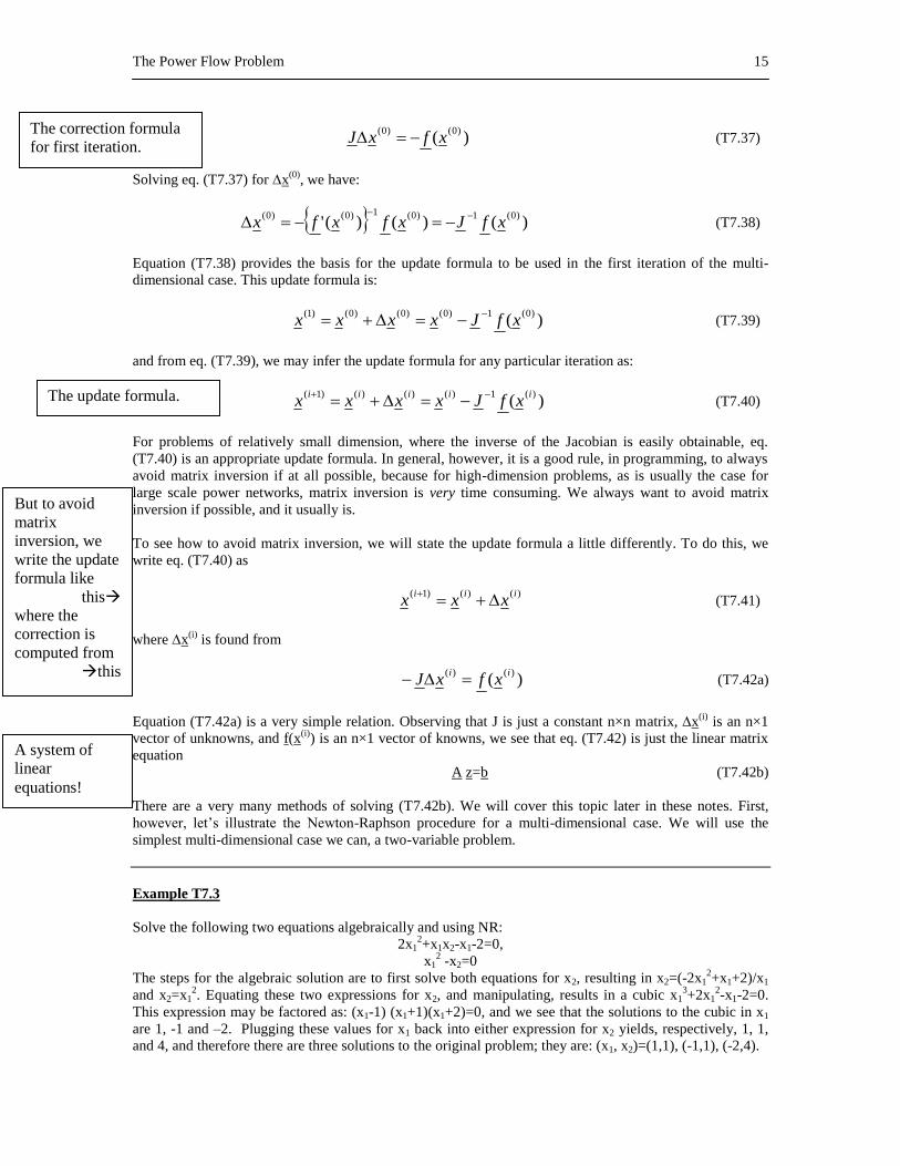
)()0()0(

xfxJ (T7.37)

Solving eq. (T7.37) for x(0)

, we have:

)()()(')0(1)0(1)0()0(

xfJxfxfx

(T7.38)

Equation (T7.38) provides the basis for the update formula to be used in the first iteration of the multi-

dimensional case. This update formula is:

)()0(1)0()0()0()1(

xfJxxxx

(T7.39)

and from eq. (T7.39), we may infer the update formula for any particular iteration as:

)()(1)()()()1( iiiii

xfJxxxx

(T7.40)

For problems of relatively small dimension, where the inverse of the Jacobian is easily obtainable, eq.

(T7.40) is an appropriate update formula. In general, however, it is a good rule, in programming, to always

avoid matrix inversion if at all possible, because for high-dimension problems, as is usually the case for

large scale power networks, matrix inversion is very time consuming. We always want to avoid matrix

inversion if possible, and it usually is.

To see how to avoid matrix inversion, we will state the update formula a little differently. To do this, we

write eq. (T7.40) as

)()()1( iii

xxx

(T7.41)

where x(i)

is found from

)()()( ii

xfxJ (T7.42a)

Equation (T7.42a) is a very simple relation. Observing that J is just a constant n×n matrix, x(i)

is an n×1

vector of unknowns, and f(x(i)

) is an n×1 vector of knowns, we see that eq. (T7.42) is just the linear matrix

equation

A z=b (T7.42b)

There are a very many methods of solving (T7.42b). We will cover this topic later in these notes. First,

however, let’s illustrate the Newton-Raphson procedure for a multi-dimensional case. We will use the

simplest multi-dimensional case we can, a two-variable problem.

Example T7.3

Solve the following two equations algebraically and using NR:

2x12+x1x2-x1-2=0,

x12 -x2=0

The steps for the algebraic solution are to first solve both equations for x2, resulting in x2=(-2x12+x1+2)/x1

and x2=x12. Equating these two expressions for x2, and manipulating, results in a cubic x1

3+2x1

2-x1-2=0.

This expression may be factored as: (x1-1) (x1+1)(x1+2)=0, and we see that the solutions to the cubic in x1

are 1, -1 and –2. Plugging these values for x1 back into either expression for x2 yields, respectively, 1, 1,

and 4, and therefore there are three solutions to the original problem; they are: (x1, x2)=(1,1), (-1,1), (-2,4).

The correction formula

for first iteration.

The update formula.

But to avoid

matrix

inversion, we

write the update

formula like

this

where the

correction is

computed from

this

A system of

linear

equations!


16

Now let’s solve this same problem using NR?

Define the functions f1(x1,x2)= 2x12+x1x2-x1-2 and f2(x1,x2)= x1

2 -x2. Then the Jacobian matrix is:

12

12

),(),(

),(),(

1

121

2

212

1

212

2

211

1

211

x

xxx

x

xxf

x

xxf

x

xxf

x

xxf

J

Let’s act like we do not know the solution and guess at (x1(0)

, x2(0)

)=(0.9,1.1). Then the Jacobian J,

evaluated at this guessed solution, is

18.1

9.09.1

12

12),(

)0(1

121)0(

2

)0(

1

xx

xxxxxJ

Inverting the Jacobian results in:

53977.051136.0

25568.028409.0

9.18.1

9.01

52.3

1

18.1

9.09.11

1J

We also need to evaluate:

29.0

11.022

)(

)()(

)1.1,9.0(2

2

1

1211

)0(

2

)0(

1)0(

)0(x

xx

xxxx

xf

xfxf

We can now update the solution using eq. (T7.40), as

9997160

0053971

1002840

1053970

11

90

290

110

539770511360

255680284090

11

90

)(

)1(

2

)1(

1

)0(1)0()0()0()1(

.

.

.

.

.

.

.

.

..

..

.

.

x

x

xfJxxxx

We see that the first update results in a solution that is very close to the actual solution of (1,1). This good

performance is due to the fact that we made a good initial guess. The student should repeat the above

procedure, but try starting from other points, e.g., (-0.9,1.1), (-1.9,4.1), and (0,1.1), using two iterations

each time. Writing a simple program will greatly reduce the effort.

In general, of course, we usually need to iterate several times in order to obtain a satisfactory solution. How

many times is enough? The NR algorithm must employ a stopping criterion in order to determine when the

solution is satisfactory. There are two ways to do this.

Type 1 stopping criterion: Test the maximum change in the solution elements from one iteration to the

next, and if this maximum change is smaller than a certain predefined tolerance, then stop. This means

to compare the maximum absolute value of elements in x against a small number, call it 1. In

example (T7.3), x = [-0.105397, 0.100284]T, so the maximum absolute value of elements in x is

0.105397. If we had 1=0.15, we could stop. But if we had 1=0.05, we would need to continue to the

next iteration.

Type 2 stopping criterion: Test the maximum value in the function elements of the most current

iteration f(x), and if this maximum value of elements in f(x) is smaller than a certain predefined

tolerance, then stop. This means to compare the maximum absolute value of elements in f(x) against a

small number, call it 1. In example (T7.3), f(x)=[-0.11, -0.29]T, so the maximum absolute value of

elements in f(x) is 0.29. If we had 1=0.3, we could stop. But if we had 1=0.2, we would need to

continue to the next iteration. This is the most common stopping criterion for power flow solutions,

and the value of each element in the function is referred to as the “power mismatch” for the bus

One of these

two stopping

criterion may be

applied.

Type 1: x

Type 2: f(x)

Type 2 is “power

mismatch” and

gives indication

of where

convergence

problems may lie.


17

corresponding to the function. For type PQ buses, we test both real and reactive power mismatches.

For type PV buses, we test only real power mismatches.

T7.7 Application of NR to Power Flow Solution

Let’s revisit the power flow problem outlined in Section T7.5, in light of the NR solution procedure

described in Section T7.6. We desire to solve eq. (T7.24), with the vector of unknowns are given by eq.

(T7.21) and the functions are in the form of eq. (T7.19). These equations are repeated here for convenience:

0

0

0

0

0

)(

)(

)(

)(

)(

)(

)(

)(

)(

1

2

11

22

12

1

1

Q

P

Q

Q

P

P

QxQ

QxQ

PxP

PxP

xf

xf

xf

xf

xf

N

N

N

NN

NN

NN

NN

N

N

GGG

G

(T7.24)

12

1

1

2

1

2

1

3

2

x

G

G

G

NN

N

N

N

N

N

N

N

x

x

x

x

x

x

||V

||V

||V

θ

θ

θ

|V|

θ

(T7.21)

NNkBGVVQ

NkBGVVP

G

N

j

jkkjjkkjjkk

N

j

jkkjjkkjjkk

,...,1 , )cos()sin(

,...,2 , )sin()cos(

1

1

(T7.19)

The solution update formula is given by eq. (T7.40), repeated here for convenience:

)()(1)()()()1( iiiii

xfJxxxx

(T7.40)

Clearly, an essential step in applying NR to the power flow problem is to enable calculation of the Jacobian

elements, given for the general case by eq. (T7.35) as

Mismatch

vector.

Solution vector.

PF equations to

solve.


18

n

nnn

n

n

x

xf

x

xf

x

xf

x

xf

x

xf

x

xf

x

xf

x

xf

x

xf

J

)()()(

)()()(

)()()(

)0(

2

)0(

1

)0(

)0(

2

2

)0(

2

1

)0(

2

)0(

1

2

)0(

1

1

)0(

1

(T7.35)

Evaluation of these elements is facilitated by the recognition, from eq. (T7.24), that there are only two

kinds of equations (real power equations and reactive power equations), and from eq. (T7.21), that there are

only two kinds of unknowns (voltage angle unknowns and voltage magnitude unknowns). Therefore, there

are only four basic types of derivatives in the Jacobian. We denote four sub-matrices

corresponding to these four basic types of derivatives as JP

, JQ

, JPV

, JQV

, where the first

superscript indicates the type of equation we differentiate, and the second superscript indicates

the unknown with respect to which we differentiate. Therefore,

)()()1()(

)()1()1()1(

)12()12(

GGG

G

GG

NNNN

QV

NNN

Q

NNN

PV

NN

PNNNN

JJ

JJJ

(T7.43)

The numbers above each sub-matrix in eq. (T7.43) indicate its dimensions, which can be inferred by

identifying the number of equations of that type (the number of rows of the sub-matrix) and the number of

unknowns of that type (the number of columns of the sub-matrix). We may then identify an individual

element of each sub-matrix as:

k

jQV

jk

k

jPV

jk

k

jQ

jk

k

jP

jkV

QJ

V

PJ

QJ

PJ

(T7.44)

Notationally, observe that the element JjkP

is not the element in row j, column k of the submatrix JP

, rather

it is the derivative of the real power injection equation for bus j with respect to the angle of bus k. Since the

swing bus is numbered 1, the Jacobian matrix will have J22P

as the element in row 1, column 1. The

situation is similar for the other submatrices.

The update equation (T7.42a) is repeated here for convenience:

)()()( ii

xfxJ (T7.42a)

Multiplying both sides by -1, we obtain

)()()( ii

xfxJ (T7.42c)

Using (T7.21), (T7.24), and (T7.43) we can write (T7.42c) as

Q

P

|V|

θ

JJ

JJQVQ

PVP

(T7.42d)

From (T7.42d) we observe that

Jacobian.

n×n differentiations?

Observation:

Only 2 kinds of

equations (P, Q)

Only 2 kinds of

unknowns (|V|, θ)

Compact expression of

Jacobian using above

observation.

Still n×n differentiations,

but are differentiations of

same form?

Study dimensionality

of each sub-matrix.

Subscripts

refer to bus

numbers, not

matrix

location.

Software needs

to track

relation

between bus

numbers &

matrix location

Subscripts j, k

are not row &

column

number due to

(a) removing pf

eq & θ for bus

1; (b) stacking

Q eqs & V-

variables on

top of P eqs &

θ variables.


19

QV|JθJ

PV|JθJ

QVQ

PVP

|

|

(T7.42e)

To get the needed derivatives, it is helpful to more explicitly write out the functions of eq. (T7.24). They

are:

NjNjNjNjNj

N

j

N

NjNjNjNjNj

N

j

N

NjNNjjNNjj

N

j

N

jjjjj

N

j

NN

NN

NN

PBGVV

PBGVV

PBGVV

PBGVV

QxQ

QxQ

PxP

PxP

xf

GGGGGG

GG

sinsin

sinsin

sincos

sincos

)(

)(

)(

)(

)(

,,

1

11,11,1

1

1

1

22222

1

2

11

22

(T7.45)

So each of the four sub-matrices of eq. (T7.43) has elements given by the expressions of eq. (T7.44),

respectively. These expressions are evaluated by taking the appropriate derivatives of the functions in eq.

(T7.45). One might think that this represents a formidable problem, since, based on eq. (T7.43), we have

(2N-1-NG)(2N-1-NG) elements in the Jacobian and therefore the same number of derivatives to evaluate.

A typical power flow model for a US control area might have 5000 nodes (N=5000) and 1000 generators

(NG=1000), resulting in a 98989898 Jacobian matrix containing 97,970,404 elements, with each element

requiring a differentiation of a function like those represented in eq. (T7.45). For a power flow model

having 50000 nodes and 5000 generators, the dimension is 9499894998, giving 9,024,600,000 elements.

Fortunately, all of the derivatives can be expressed by one of just a few differentiations. At first glance,

one might think that there would be four differentiations, one for each sub-matrix. However, for each sub-

matrix, the off-diagonal terms, with jk, are expressed differently than the diagonal terms, with j=k.

Therefore, there are eight differentiations to perform. The student should attempt to obtain a few of these

expressions. In doing so, the following tips are helpful.

Before differentiating, it is helpful to pull out from the summation the term that corresponds to the bus

injection being computed.

When differentiating a sum of terms with respect to a particular unknown, the resulting derivative will

be non-zero only for those terms in which the unknown appears.

When differentiating with respect to the angles, the chain rule must be properly applied to account for

the derivatives of the trigonometric functions and the arguments of those trigonometric functions.

Each of the functions appear in the form of f(x)=g(x)-A. Because A is a constant (represented by

P2,…, PN and QNg+1,…, QN in eq. (T7.45)), it has no effect on the resulting derivatives.

The resulting expressions are given below.

)cos()sin()(

kjjkkjjkkj

k

jP

jk BGVVxP

J

(T7.47)

2

)()(

jjjj

j

jP

jj VBxQxP

J

(T7.48)

)sin()cos()(

kjjkkjjkkj

k

jQ

jk BGVVxQ

J

(T7.49)

98 million

differentiations

for a 5000 bus

model.

9 billion

differentiations

for a 50000 bus

model.

8 basic

derivative

expressions: for

each of 4

submatrices, we

need diagonal

& off-diagonal

expressions.

Observe T7.47 &

T7.53 are similar.

These are off-diagonal

elements in JPθ

& JQV

,

bolded below.

Q

P

|V|

θ

QV

Pθ

J

JQθ

PV

J

J

How many elements is

this? Can we do

something smart here?

Mismatch

vector.


20

2

)()(

jjjj

k

jQ

jj VGxPxQ

J

(T7.50)

)sin()cos()(

kjjkkjjkj

k

jPV

jk BGVV

xPJ

(T7.51)

jjj

j

j

j

jPV

jj VGV

xP

V

xPJ

)()( (T7.52)

)cos()sin()(

kjjkkjjkj

k

jQV

jk BGVV

xQJ

(T7.53)

jjj

j

j

j

jQV

jj VBV

xQ

V

xQJ

)()( (T7.54)

We are now in a position to provide the algorithm for using NR to solve the power flow problem. Before

doing so, it is helpful to more explicitly define the mismatch vector, from eq. (T7.24) or (T7.45) as:

0

)(

)(

)(

)(

)(

)(

)(

)(

)(

1

2

11

22

12

1

1

Q

P

Q

Q

P

P

QxQ

QxQ

PxP

PxP

xf

xf

xf

xf

xf

N

N

N

NN

NN

NN

NN

N

N

GGG

G

(T7.53)

The NR algorithm, for application to the power flow problem, is:

1. Specify:

All admittance data

Pd and Qd for all buses

Pg and |V| for all PV buses

|V| for swing bus, with =0

2. Let the iteration counter j=1. Use one of the following to guess the initial solution.

Flat Start: Vk=1.0 0 for all buses.

Hot Start: Use the solution to a previously solved case for this network.

3. Compute the mismatch vector for x(j)

, denoted as f(x) in eq. (T7.24) and eq. (T7.45). In what follows,

we denote elements of the mismatch vector as Pk and Qk corresponding to the real and reactive

power mismatch, respectively, for the kth

bus (which would not be the kth

element of the mismatch

vector for two reasons: one reason pertains to the swing bus and the other reason to the fact that for

type PQ buses, there are two equations per bus and not one – see boxed comments next to eq. T7.44).

This computation will also result in all necessary calculated real and reactive power injections.

4. Perform the following stopping criterion tests:

If |Pk|< P for all type PQ and PV buses and

If ||Qk|< Q for all type PQ buses,

Then go to step 6

Otherwise, go to step 5.

5. Find an improved solution as follows:

Evaluate the Jacobian J at x(j)

. Denote this Jacobian as J(j)

Solve for x(j)

from:

Observe T7.49 &

T7.51 are similar.

These are off-diagonal

elements in JQθ

& JPV

,

bolded below.

Q

P

|V|

θ

QV

Pθ

J

JQθ

J

PV J

How many elements is

this? Can we do

something smart here?

Flat start/hot

start: common

industry terms

Compute

mismatch

vector.

Check

stopping

criterion


21

Q

P

Jx

Q

P

xJjjj

or 1-(j))()()(

where we must use factorization with the left equation if the system is large, but if the system is

not large, we may use the right hand equation.

Compute the updated solution vector as x(j+1)

= x(j)

+ x(j)

.

Return to step 3 with j=j+1.

6. Stop.

The above algorithm is applicable as long as all PV buses remain within their reactive limits. To account

for generator reactive limits, we must modify the algorithm so that, at each iteration, we check to ensure

PV bus reactive generation is within its limits (see Section T7.1 regarding modeling of reactive limits). In

this case, steps 1-4 remain exactly as given above, but we need a new step 5 and 6, as follows:

5. Check reactive limits for all generator buses as follows:

a. For all type PV buses, perform the following test:

If Qgk>Qgk,max, then

Qgk=Qgk,max and CHANGE bus k to a type PQ bus (see step 6a)

If Qgk< Qgk,min, then

Qgk=Qgk,min and CHANGE bus k to a type PQ bus (see step 6b)

b. For all type PQ generator buses, perform the following test:

If Qgk=Qgk,max and |Vk|>|Vk,set| or if Qgk=Qgk,min and |Vk|<|Vk,set|, then

CHANGE this bus back to a type PV bus (see step 6b)

6. If there were no CHANGES in Step 5, then stop. If there were one or more CHANGES in step 5, then

modify the solution vector and the mismatch vector as follows:

a. For each CHANGE made in step 5-a (changing a PV bus to a PQ bus):

NG=NG-1

Include the variable Vk to the vector x and the variable Vk to the vector x.

Include the reactive equation corresponding to bus k to the vector f(x).

Modify the Jacobian by including a column to JPV

and including a row to JQ

and JQV

.

b. For each CHANGE made in Step 5-b (changing a PQ gen bus back to a PV bus):

NG=NG+1

Remove the variable Vk to the vector x and the variable Vk from the vector x.

Remove the reactive equation corresponding to bus k from the vector f(x).

Modify the Jacobian by removing a column to JPV

and removing a row from JQ

and JQV

.

After modifications have been made for all CHANGES, go back to Step 4.

When the algorithm stops, then all line flows may be computed using ***

][ jkkjjjkjjk yVVVIVS

Example T7.4 [5] (used with permission of V. Vittal)

Find 2, V3, 3, SG1, and QG2 for the system shown in Fig. T7.8. In the transmission system all the shunt

elements are capacitors with an admittance yc = j0.01, while all the series elements are inductors with an

impedance of zL = j0.1.

Factorization: method to

solve linear simultaneous

equations. We will look a

little more at this issue.

Is there a PV bus

that should be PQ?

Is there a PQ gen-bus, which was

a PV bus, that should be now be

PV again?

Another way is to let algorithm

converge, check limits, make

changes, & repeat. But checking

every iteration provides increased

convergence robustness.

Does this equation account for

shunt elements or line charging?

Should it?


22

|V2|=1.05

SG1 PG2=0.6661

V1=10

V3

SD3=2.8653+j1.2244

Fig. T7.8: Three Bus System for Example T7.4

Solution: The admittance matrix for the system shown in Fig. E10.6 is given by

98.191010

1098.1910

101098.19

Y

jjj

jjj

jjj

Bus 1 is the swing bus. Bus 2 is a PV bus. Bus 3 is a PQ bus. We use the NR method in the solution. The

unknown variables are 2, 3, and |V3|. Thus, we will need three equations, and the Jacobian is a 3 x 3

matrix.

We first write eq. (T7.45) for the case at hand, putting in the known values of |V1|, |V2|, 1, and the Bij’s.

Note that since we have neglected line resistance in the problem statement, all Gij’s are zero.

P2 (x) V2 V1 B21sin(2 1 ) V2 V3 B23sin(2 3 )

= 10.5sin2 10.5V3 sin(2 3) (T7.54a)

P3(x) V3 V1 B31sin(3 1) V3 V2 B32sin(3 2 )

= 10.0V3 sin3 10.5V3 sin(3 2 ) (T7.54b)

The equation for Q2(x) will not help since we do not know the reactive injection for bus 2, and its inclusion

would bring in the reactive injection on the left-hand side as an additional unknown. But this loss of an

equation is compensated by the fact that we know |V2| (and this will always be the case for a type PV bus).

So we do not need to write the equation for Q2(x). Yet, because bus 3 is a type PQ bus, we do know its

reactive injection, and so we will know the left hand side of the reactive power flow equation. This is

fortunate, since we do not know |V3| (and this will always be the situation for a type PQ bus).

Observe: (1) no real

parts due to neglect of

resistance; (2) diagonals

are negative (inductive

admittance), (3) off-

diagonals are positive

(negated inductive

admittance)

What are equations to use?

What are unknowns?

What is Jacobian dimension?

What would Jacobian

dimension be if bus 2

changed to PQ?


23

Q3(x) V3 V1 B31cos(3 1 ) V3 V2 B32 cos(3 2 ) V3

2B33

= - 10V3 cos3 10.5V3 cos(3 2 ) 19.98V3

2 (T7.54c)

The update vector and Jacobian matrix is:

3

3

2

x

V

3

3

3

3

2

3

3

3

3

3

2

3

3

2

3

2

2

2

V

QQQ

V

PPP

V

PPP

J

We obtain the various partial derivatives for the Jacobian from eqs. (T7.54a,b,c):

3232322332122112

2

2 cos5.1010.5cos=coscos

VBVVBVV

P

323322332

3

2 cos-10.5=cos

VBVV

P

3232232

3

2 10.5sin=sin

BV

V

P

233

2

3 cos5.10

V

P

23333

3

3 cos5.10cos0.10

VV

P

233

3

3 sin5.10sin10

V

P

2332323

2

3 sin5.10sin10

VVV

Q

23333232333

3

3 sin5.10sin10=sin10sin10

VVVVV

Q


24

3233

3333333232231311

3

3

96.39cos5.10cos10=

coscos

V

BVBVBVBVV

Q

We are ready to start iterating using (T7.40). We note that the injections, to be used on the left hand side of

eqs. (T7.54a,b,c) are P2 = PG2 = 0.6661, P3 = -PD3 = -2.8653, and Q3 = -QD3 = -1.2244; these quantities

remain constant through the entire iterative process. We use a flat start; therefore our initial guess is

2=3=0 and |V3|=1.0.Using eqs. (T7.53) and (T7.54a,b,c) we get:

7044.0

8653.2

6661.0

2244.1

8653.2

6661.0

52.0

0

0

x

x

x

)(

3

3

2

)0(

3

)0(

3

)0(

2

)0(

3

3

2

)0(

Q

P

P

Q

P

P

Q

P

P

xf

As expected for a flat start, the mismatch is large. Next we calculate the Jacobian matrix:

46.1900

05.205.10

05.1021

J (T7.55)

Note that the Jacobian sub-matrices JPV

and JQ

are both filled with zeros. This is because when resistance

is neglected, these derivatives depend on sin terms, and because this is the first iteration of a flat start, all

angles are zero and therefore the sin terms are all zero.

As mentioned, commercial power flow programs normally use LU factorization to obtain the update. In this

case, however, because of the low dimensionality, we may invert the Jacobian. Taking advantage of the

block diagonal structure, we have:

0514.000

00656.00328.0

00328.00640.0

46.1900

0

0

5.205.10

5.1021

1

1

1J

Now we compute:

0362.0

1660.0

0513.0

7044.0

8653.2

6661.0

0514.000

00656.00328.0

00328.00640.0

|| 3

3

2

1-

3

3

2

)(

Q

P

P

J

V

xj

The elements of the update vector corresponding to angles are in radians. We can easily convert them to

degrees:

PU mismatch vector.

Observe mismatch is

very large.

JPV

and JQ

are both

filled with zeros,

because with zero

resistance, they have

only sin terms.

Injections come from

one-line diagram.

Here we inverted J but for larger systems,

you should always use factorization. Angular measures

are in radians.


25

0.0362-

9.5139-

9396.2

0.0362-

rad 0.1660-

rad 0513.0o

o

3

3

2

V

We now find x(1)

as follows:

0.9638

9.5139-

9396.2

0.0362-

9.5139-

9396.2

1

0

0

xxx o

o

o

o

)0()0()1(

We note that the exact solution is

9499.0

01.10

00.3o

o

, so this is pretty good progress for one iteration!

We proceed to the next iteration using the new values 2(1)

=-2.9396, 3(1)

=-9.5139, and |V3|(1)

=0.9638.

Substituting in eq. (T7.54a), we get P2(x(1)

) = 0.6202, and thus P2(1)

= 0.6202-0.6661=-0.0459. Similarly,

using eqs. (T7.54b) and (T7.54c), we get the updated mismatch vector:

2251.0

1145.0

0463.0

3

2

1

Q

P

P

Note that, in just one iteration, the mismatch vector has been reduced by a factor of about 10. Calculating J

using the updated values of the variables, we find that

2199.187508.21582.1

8541.25589.190534.10

2017.10534.105396.20

J

The matrix should be compared with J from the previous iteration. It has not changed much. The elements

in the off-diagonal matrices JPV

and JQ

are no longer zero, but their elements are small compared to the

elements in the diagonal matrices JP

and JQV

. The diagonal matrices themselves have not changed much. It

is also important to note that the upper left-hand Jacobian submatrix (JPθ

) is symmetric. This fact allows for

a significant savings in storage when dealing with large systems.

The updated inverse is

0561.00084.00009.0

0087.00696.00336.0

0010.00336.00651.01

J

Comparing this inverted Jacobian with that of the last iteration, we do not see much change. Using the

same procedure as before to calculate the update vector, we obtain

Now the JPV

and JQ

terms are non-zero since angles

are no longer all zero. But it is interesting that this

Jacobian differs very little from initial one, below.

46.1900

05.205.10

05.1021

J


26

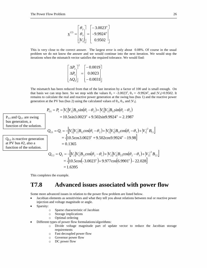
0.9502

9.9924-

0023.3

x o

o

3

3

2

)2(

V

This is very close to the correct answer. The largest error is only about 0.08%. Of course in the usual

problem we do not know the answer and we would continue into the next iteration. We would stop the

iterations when the mismatch vector satisfies the required tolerance. We would find:

0031.0

0023.0

0019.02

3

3

2

Q

P

P

The mismatch has been reduced from that of the last iteration by a factor of 100 and is small enough. On

that basis we can stop here. So we stop with the values 2 = -3.0023o, 3 = -9.9924

o, and |V3|=0.9502. It

remains to calculate the real and reactive power generation at the swing bus (bus 1) and the reactive power

generation at the PV bus (bus 2) using the calculated values of 2, 3, and |V3|.

1987.2sin9.9924502.902310.5sin3.0=

sinsin

oo

31133121122111

BVVBVVPPG

0.1365=

98.1999249.502cos9.+02310.5cos3.0-=

coscos

oo

11

2

131133121122111

BVBVVBVVQQG

1.6395=

028.226.9901cos977.93.0023-10.5cos-=

coscos

oo

22

2

232233212211222

BVBVVBVVQQG

This completes the example.

T7.8 Advanced issues associated with power flow

Some more advanced issues in relation to the power flow problem are listed below.

Jacobian elements as sensitivities and what they tell you about relations between real or reactive power

injection and voltage magnitude or angle.

Sparsity:

o Sparse characteristic of Jacobian

o Storage implications

o Optimal ordering

Different types of power flow formulations/algorithms:

o Divide voltage magnitude part of update vector to reduce the Jacobian storage

requirements

o Fast decoupled power flow

o Governor power flow

o DC power flow

PG1 and QG1 are swing

bus generation, a

function of the solution.

QG2 is reactive generation

at PV bus #2, also a

function of the solution.


27

o Gauss-Seidel

Some advanced modeling issues:

o Transformers: regulating transformers

o Area interchange

o Switched shunt capacitors

T7.9 Input/Output and Commercial Programs

There are a number of very high quality commercial power flow programs on the market today, some of

which include those developed by the Electric Power Research Institute (EPRI), Power Technologies

Incorporated (PTI), Operation Technology, Inc., and EDSA. Most of today’s commercial software

packages are menu-driven from a Windows environment. A predecessor of one of these was interactive

from the command line, and we use it here because its scroll-down recording serves well to illustrate some

basic features of most commercial programs. The following lists of just a few of these features. The item

number in this list is denoted in the illustration that follows, using large 20 font numbers, to help identify

the corresponding parts in the session.

1. Solving the power flow

2. Limit checks – overloads

3. Limit checks – undervoltages

4. Reporting the solution – flows (denoted below as “bus flows”)

5. Reporting the solution – generator operation information (denoted below as plant data)

A one-line diagram for the system on which this session was run is shown in Figure (T7.9). This system is

a test system developed by a subcommittee of the IEEE Power Engineering Society (PES) [12]. It is

referred to as the IEEE RTS’96, and it consists of 24 buses, 11 of which are voltage controlled buses; thus,

13 are type PQ at the beginning of a solution procedure.

Figure T7.9 – The IEEE Reliability Test System [12]


28

1. MAIN MENU

=========

1 LOAD THE PSF 8 DATA VERIFICATIO

2 IMPORTING UTILITIES 9 LIMIT CHECKS

3 INPUT DATA PROCESSING 10 SENSITIVITY FACTORS

4 STUDY PREPARATION UTILITIES 11 EXPORTING UTILITIES

5 POWER FLOW SOLUTION 12 CLOSE THE PSF

6 NETWORK REDUCTION 13 QUIT

7 POWER FLOW SOLUTION REPORTING

ENTER MENU CHOICE: 5

*** POWER FLOW SOLUTION ***

=============================

1 AUTOMATIC SOLUTION

2 FAST DECOUPLED (XB)

3 NEWTON RAPHSON

4 FAST DECOUPLED (BX)

5 LOCALIZED SOLUTION (FD XB)

6 DC POWER FLOW SOLUTION

7 POWER FLOW SOLUTION OPTIONS

ITEM #, EXIT 3

*** START OF NEWTON RAPHSON ITERATIONS ***

ITERATION : 1 NEWTON RAPHSON UNSOLVED ABSOLUTE ERROR

-------------- BUS WITH LARGEST ERROR ------------ BUSES SUMMATION

P(P.U. MW) 0.000375 ( 30 BUS 3138. ) 0 0.0017

V(RADIANS) 0.000179 ( 70 BUS 7138. ) 8 0.0016

Q(P.U. MVAR) 0.001873 ( 120 BUS 12230. ) 0 0.0078

V(P.U. KV) 0.000210 ( 30 BUS 3138. ) 3 0.0009

ITERATION : 2 NEWTON RAPHSON UNSOLVED ABSOLUTE ERROR

-------------- BUS WITH LARGEST ERROR ------------ BUSES SUMMATION

P(P.U. MW) 0.000006 ( 160 BUS 16230. ) 0 0.0000

Q(P.U. MVAR) -0.000008 ( 170 BUS 17230. ) 0 0.0000

*** POWER FLOW SOLUTION IS REACHED IN 2 ITERATIONS ***

2. MAIN MENU

=========

1 LOAD THE PSF 8 DATA VERIFICATION








** LOAD FLOW SOLUTION LIMIT CHECK **

====================================

1 OVERLOADED LINES OR TRANSFORMERS

2 CONTROL PARAMETERS VIOLATION

3 BUS VOLTAGE OUTSIDE SPECIFIED BAND

4 LINES ACROSS WHICH THE ANGLE EXCEEDS THE SPECIFIED VALUE

5 CHECK FOR ALL LIMITS AND VIOLATIONS

6 SORT OPTIONS

ITEM #, SPECIFY SUBSYSTEM, EXIT 1

ALL LINES TRANSFORMERS: A

*** LOAD FLOW SOLUTION LIMIT CHECK ***

1 OVERLOADED BRANCHES RATING GROUP = 1 % LOADING = 100.0

<----- FROM BUS -----> <------ TO BUS ------> MVA MVA PERCENT

NUMBER NAME NUMBER NAME CKT LOADING RATING LOADING

====== ================ ====== ================ ======== ======= ====== =======

60 BUS 6138. 100 BUS 10138. 1 175.4 175.0 100.22

3. ** LOAD FLOW SOLUTION LIMIT CHECK **

====================================

1 OVERLOADED LINES OR TRANSFORMERS

2 CONTROL PARAMETERS VIOLATION

3 BUS VOLTAGE OUTSIDE SPECIFIED BAND

4 LINES ACROSS WHICH THE ANGLE EXCEEDS THE SPECIFIED VALUE

5 CHECK FOR ALL LIMITS AND VIOLATIONS

6 SORT OPTIONS



29

HI VOLTAGE LIMIT LO VOLTAGE LIMIT: L

ENTER VALUE IN PU: .99

*** LOAD FLOW SOLUTION LIMIT CHECK ***

4 BUSES WITH V < 0.990

<-------- BUS --------> <-- VOLTAGE -->

NUMBER NAME TYPE BASE KV MAG ANGLE AREA ZONE OWNER ID

====== ================ ==== ======= ======= ======= ==== ==== ================

30 BUS 3138. 1 138.00 0.9868 -26.02 10 1 BLANK

40 BUS 4138. 1 138.00 0.9888 -20.27 10 1 BLANK

90 BUS 9138. 1 138.00 0.9824 -15.83 10 1 BLANK

120 BUS 12230. 1 230.00 0.9876 -4.73 10 1 BLANK

UP DOWN SCREEN DUMP LIST TO FILE CHANGE RATING EXIT : e

4. MAIN MENU

=========

1 LOAD THE PSF 8 DATA VERIFICATION








** LOAD FLOW SOLUTION REPORTING **

==================================

1 MISMATCH SUMMARY 11 ULTC/PS SUMMARY

2 SUBSYSTEM SUMMARY 12 SERIES COMPENSATORS

3 BUS SHUNT DATA 13 POWER FLOW SUMMARY

4 PLANT DATA 14 SECTIONALIZED BRANCHES

5 MACHINE DATA 15 STATIC TAP CHANGERS / PHASE SHIFTERS

6 AREA INTERCHANGE DATA 16 THREE WINDING TRANSFORMERS

7 TIE LINE FLOWS 17 INTERFACE FLOWS

8 BUS FLOWS 18 VOLTAGE PROFILE

9 DC CONVERTERS 19 SORT OPTIONS

10 DC FLOWS


SUBSYSTEM BUSES PICK BUSES EXIT: p

ENTER BUS LIST FILE NAME OR BUSES TO INCLUDE OR EXCLUDE

> 60

*** SOLUTION REPORTING - BUS FLOWS ***

BUS: 60 BUS 6138.

VOLTAGE : 1.0017 PU ( 138.2 kV) -20.67

BUS NUM NAME AREA CKT MW MVAR MVA TAP

======== ================ ==== ======== ======== ======== = ======== ========

LOAD 136.00 28.00 138.85

SW SHUNT 0.00 100.33 100.33

TO 100 BUS 10138. 10 1 -128.63 -107.64 167.73

TO 20 BUS 2138. 10 1 -7.37 -20.69 21.96

UP DOWN NEXT BUS PREVIOUS BUS SCREEN DUMP LIST TO FILE EXIT : e

SUBSYSTEM BUSES PICK BUSES EXIT: p

ENTER BUS LIST FILE NAME OR BUSES TO INCLUDE OR EXCLUDE

> 100

*** SOLUTION REPORTING - BUS FLOWS ***

BUS: 100 BUS 10138.

VOLTAGE : 1.0132 PU ( 139.8 kV) -16.15

BUS NUM NAME AREA CKT MW MVAR MVA TAP

======== ================ ==== ======== ======== ======== = ======== ========

LOAD 195.00 40.00 199.06

TO 120 BUS 12230. 10 1 -234.48 60.92 242.27 1.0000LK

TO 110 BUS 11230. 10 1 -235.99 52.21 241.70 1.0000LK

TO 80 BUS 8138. 10 1 69.77 -3.74 69.87

TO 60 BUS 6138. 10 1 130.95 -131.80 185.80

TO 50 BUS 5138. 10 1 74.76 -17.59 76.80

UP DOWN NEXT BUS PREVIOUS BUS SCREEN DUMP LIST TO FILE EXIT : e

5. ** LOAD FLOW SOLUTION REPORTING **

==================================

1 MISMATCH SUMMARY 11 ULTC/PS SUMMARY

2 SUBSYSTEM SUMMARY 12 SERIES COMPENSATORS

3 BUS SHUNT DATA 13 POWER FLOW SUMMARY


30

4 PLANT DATA 14 SECTIONALIZED BRANCHES

5 MACHINE DATA 15 STATIC TAP CHANGERS / PHASE SHIFTERS

6 AREA INTERCHANGE DATA 16 THREE WINDING TRANSFORMERS

7 TIE LINE FLOWS 17 INTERFACE FLOWS

8 BUS FLOWS 18 VOLTAGE PROFILE

9 DC CONVERTERS 19 SORT OPTIONS

10 DC FLOWS


*** SOLUTION REPORTING - PLANT DATA ***

=======================================

1 ALL PLANTS

2 ON LINE PLANTS

3 PLANTS AT VAR LIMIT WITH UNEQUAL VAR LIMITS

4 PLANTS WITH UNSCHEDULED REACTIVE POWER

5 PLANTS CONTROLLING A REMOTE BUS

6 PLANTS WITH RESERVE REACTIVE POWER

ITEM #, EXIT 1

*** SOLUTION REPORTING ***

10 PLANTS

PLANT BUS MACHINES

NUM NAME TYPE I/S O/S MW MVAR QMAX QMIN

======== ================ ==== ======== ======== ======== ======== ========

R 10 BUS 1138. 2 4 0 134.70 41.53 280.00 -50.00

R 20 BUS 2138. 2 4 0 187.00 30.50 140.00 -100.00

R 70 BUS 7138. 2 3 0 165.00 91.63 280.00 0.00

R 130 BUS 13230. 3 3 0 337.53 170.64 540.00 -300.00

R 150 BUS 15230. 2 6 0 185.00 40.36 310.00 -55.00

R 160 BUS 16230. 2 1 0 155.00 106.41 280.00 -55.00

R 180 BUS 18230. 2 1 0 400.00 100.73 200.00 -90.00

R 210 BUS 21230. 2 1 0 400.00 25.25 200.00 -90.00

R 220 BUS 22230. 2 6 0 300.00 -80.55 696.00 -560.00

R 230 BUS 23230. 2 3 0 660.00 33.34 310.00 -125.00

UP DOWN OTHER SCREEN SCREEN DUMP LIST TO FILE EXIT : e

References

[1] J. Vlach and K. Singhal, “Computer Methods for Circuit Analysis and Design,” Kluwer Academic

Publications, 1993.

[2] L. Chua and P. Lin, “Computer Aided Analysis of Electronic Circuits: Algorithms and

Computational Techniques,” Prentice Hall, 1975.

[3] O. Elgerd, “Electric Energy Systems Theory,” McGraw-Hill, New York, 1982.

[4] J. Grainger and W. Stevenson, “Power System Analysis,” McGraw-Hill, New York, 1994.

[5] A. Bergen and V. Vittal, “Power Systems Analysis,” second edition, Prentice Hall, Upper Saddle

River, New Jersey, 2000.

[6] C. Gross, “Power System Analysis,” John Wiley & Sons, New York, 1979.

[7] B. Weedy, “Electric Power Systems,” third edition, John Wiley & Sons, London, 1979.

[8] H. Saadat, “Power System Analysis,” McGraw-Hill, New York, 1999.

[9] G. Stagg and A. El-Abiad, “Computer Methods in Power System Analysis,” McGraw-Hill, New

York, 1968.

[10] G. Heydt, “Computer Analysis Methods for Power Systems,” Macmillan Publishing, New York,

1986.

[11] V. Del Toro, “Electric Power Systems,” Printice-Hall, Englewood Cliffs, New Jersey, 1992.

[12] The reliability test system task force of the application of probability methods subcommittee,

“The IEEE reliability test system – 1996”, IEEE Trans. Power Systems, Vol. 14, No. 3, pp. 1010-

1020, 1999.

t7.0 introduction - iowa state universityhome.engineering.iastate.edu/~jdm/ee553/powerflow.pdf · a...

Documents