production costing (chapter 8 of w&w) 1.0...
TRANSCRIPT

1
Production Costing (Chapter 8 of W&W)
1.0 Introduction
Production costs refer to the operational costs
associated with producing electric energy. The most
significant component of production costs are the fuel
costs necessary to run the thermal plants.
A production cost program, also referred to as a
production cost model, is widely used throughout the
electric power industry for many purposes:
Long-range system planning: Here, it is used to
simulate a single future year following the planned
expansion. For example, the Midwest ISO used a
production cost program to understand the effect
on energy prices of building HVDC from the
Midwest US to the East coast.
Fuel budgeting: Many companies run production
cost programs to determine the amount of natural
gas and coal they will need to purchase in the
coming weeks or months.
Maintenance: Production cost programs are run to
determine maintenance schedules for generation.
Energy interchange: Production cost programs are
run to facilitate negotiations for energy interchange
between companies.

2
There are two essential inputs for any production cost
program:
1. Data characterizing future load
2. Data characterizing generation costs, in terms of:
a. Heat rate curves and
b. Fuel costs
All production cost programs require at least the
above data. Specific programs will require additional
data depending on their particular design.
The information provided by production costing
includes the annual costs of operating the generation
facilities, a cost that is dominated by the fuel costs
but also affected by the maintenance costs.
Production costing may also provide more time-
granular estimates of fuel and maintenance costs,
such as monthly, weekly, or hourly, from which it is
then possible to obtain annual production costs.
A simplified way to consider a production cost
program is as an hour-by-hour simulation of the
power system over a duration of T hours, where at
each hour,
The load is specified;
A unit commitment decision is made;
A dispatch decision is made to obtain the
production costs for that hour

3
The total production costs is then the sum of hourly
production costs over all hours 1,…,T.
Some production programs do in fact simulate hour-
by-hour operation in this manner. An important
characterizing feature is how the program makes the
unit commitment (UC) and dispatch decisions.
The simplest approach makes the UC decision based
on priority ordering such that units with lowest
average cost are committed first. Startup costs are
added when a unit is started, but those costs do not
figure into the optimization.
The simplest approach for making the dispatch
decision is referred to as the block loading principle,
where each unit committed is fully loaded before the
next unit is committed. The last unit is dispatched at
that level necessary to satisfy the load.
Greater levels of sophistication may be embedded in
production cost programs, as described below:
Unit commitment and dispatch: A full unit
commitment program may be run for certain blocks
of intervals at a time, e.g., a week.
Hydro: Hydro-thermal coordination may be
implemented.

4
Network representation: The network may be
represented using DC flow and branch limits.
Locational marginal prices: LMPs may be
computed.
Maintenance schedules: Maintenance schedules
may be taken into account.
Uncertainty: Load uncertainty and generator
unavailability may be represented using
probabilistic methods. This allows for computation
of reliability indices such as loss of load
probability (LOLP) and expected unserved energy
(EUE).
Security constraints may be imposed using LODFs.
Below are some slides that Midwest ISO uses to
introduce production cost models.
4
What is a Production Cost Model?
Captures all the costs of operating a fleet of generators
• Originally developed to manage fuel inventories and budget in the mid 1970’s
Developed into an hourly chronological security constrained unit commitment and economic dispatch simulation
• Minimize costs while simultaneously adhering to a wide variety of operating constraints.
• Calculate hourly production costs and location-specific market clearing prices.

5
5
What Are the Advantages of Production Cost Models?
Allows simulation of all the hours in a year, not just peak hour as in power flow models.
Allows us to look at the net energy price effects through
• LMP’s and its components.
• Production cost.
Enables the simulation of the market on a forecast basis
Allows us to look at all control areas simultaneously and evaluate the economic impacts of decisions.
6
Disadvantages of Production Cost Models
Require significant amounts of data
Long processing times
New concept for many Stakeholders
Require significant benchmarking
Time consuming model building process
• Linked to power flow models
Do not model reliability to the same extent as power flow

6
7
Production Cost Model vs. Power Flow
Production Cost Model Power Flow
SCUC&ED: very detailed
Hand dispatch (merit Order)
All hours One hour at a time
DC Transmission AC and DC
Selected security constraints
Large numbers of security constraints
Market analysis/ Transmission analysis/planning
Basis for transmission reliability & operational planning
2.0 Commercial grade production costing tools
We will describe in more detail the construction of
production costing programs later. Here we simply
mention some of the commercially available
production costing tools.
The Ventyx product Promod incorporates details in
generating unit operating characteristics, transmission
grid topology and constraints, unit commitment/
operating conditions, and market system operations.
Promod can operate on nodal or zonal modes
depending on the scope, timeframe, and simulation
resolution of the problem. Promod is not a
forecasting model and does not consider the price and
availability of other fuels.

7
The ADICA product GTMAX, developed by
Argonne National Labs, can be employed to perform
regional power grade or national power development
analysis. GTMax will evaluate system operation,
determine optimal location of power sources, and
assess the benefits of new transmission lines. GTMax
can simulate complex electric market and operating
issues, for both regulated and deregulated market.
The PowerCost, Inc. product GenTrader employs
economic unit dispatch logic to analyze economics,
uncertainty, and risk associated with individual
generation resources and portfolios. GenTrader does
not represent the network.
PROSYM is a multi-area electric energy production
simulation model developed by Henwood energy Inc.
It is an hourly simulation engine for least-cost
optimal production dispatch based on the resources’
marginal costs, with full representation of generating
unit characteristics, network area topology and
electrical loads. PROSYM also considers and
respects operational and chronological constraints;
such as minimum up and down times, random forced
outages and transmission capacity. It is designed to
determine the station generation, emissions and

8
economic transactions between interconnected areas
for each hour in the simulation period.
ABB produced the software called “GridView,”
illustrated below [1].
PLEXOS, from Plexos Solutions, is a versatile
software system that performs production cost
simulation and other functions.
It is interesting to note that Global Energy Solutions
(GES) in 2002 purchased Henwood Associates
(owner of Prosym), then Ventyx (owners of Promod)
purchased GES in 2008, then ABB (owners of
Gridview) purchased Ventyx. At some point, Mark
Henwood went to work for Plexos Solutions (see
[2]). Energy Exemplar now owns Plexos.

9
3.0 Probability models
Key to use of production cost models is the ability to
represent uncertainty in load and in generation
availability.
3.1 Load duration curves
A critical issue for planning is to identify the total
load level for which to plan. One extremely useful
tool for doing this is the so-called load duration
curve, which is formed as follows. Consider that we
have obtained, either through historical data or
through forecasting, a plot of the load vs. time for a
period T, as shown in Fig. 3 below.
Lo
ad
(MW
)
Time T
Fig. 3: Load curve (load vs. time)
Of course, the data characterizing Fig. 3 will be
discrete, as illustrated in Fig. 4.

10
L
oad
(M
W)
Time T
Fig. 4: Discretized Load Curve
We now divide the load range into intervals, as
shown in Fig. 5.
T
10
9
8
7
6
5
4
3
2
1
0
Lo
ad
(MW
)
Time
Fig. 5: Load range divided into intervals
This provides the ability to form a histogram by
counting the number of time intervals contained in
each load range. In this example, we assume that
loads in Fig. 5 at the lower end of the range are “in”
the range. The histogram for Fig. 5 is shown in Fig.
6.
11
0 1 2 3 4 5 6 7 8 9 10 11
9
8
7
6
5
4
3
2
1
0
Co
un
t
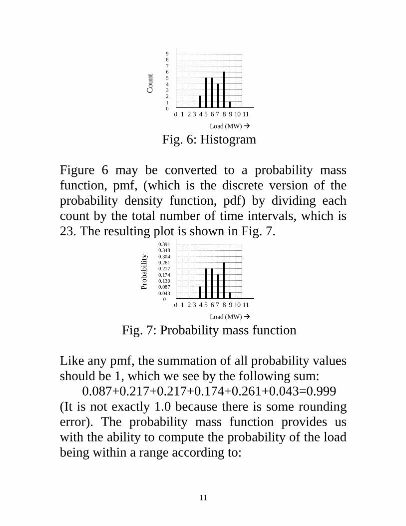
Load (MW) Fig. 6: Histogram
Figure 6 may be converted to a probability mass
function, pmf, (which is the discrete version of the
probability density function, pdf) by dividing each
count by the total number of time intervals, which is
23. The resulting plot is shown in Fig. 7.
0 1 2 3 4 5 6 7 8 9 10 11
0.391
0.348
0.304
0.261
0.217
0.174
0.130
0.087
0.043
0
Pro
bab
ilit
y
Load (MW) Fig. 7: Probability mass function
Like any pmf, the summation of all probability values
should be 1, which we see by the following sum:
0.087+0.217+0.217+0.174+0.261+0.043=0.999
(It is not exactly 1.0 because there is some rounding
error). The probability mass function provides us
with the ability to compute the probability of the load
being within a range according to:

12
Range in L
LLoadRange) within(Load )Pr(Pr (2)
We may use the probability mass function to obtain
the cumulative distribution function (CDF) as:
Value L
LLoadValue) (Load )Pr(Pr (3)
From Fig. 7, we obtain:
0.1)Pr(Pr 1 L
LLoad1) (Load
0.1)Pr(Pr 2 L
LLoad2) (Load
0.1)Pr(Pr 3 L
LLoad3) (Load
0.1)Pr(4) (LoadPr4
L
LLoad
0.9120.0430.2610.1740.2170.217
LLoad5) (Load5 L
)Pr(Pr
0.6950.0430.2610.1740.217
LLoad6) (Load6 L
)Pr(Pr
0.4780.0430.2610.174LLoad7) (Load6 L
)Pr(Pr
0.3040.0430.261LLoad8) (Load8 L
)Pr(Pr
0.043LLoad9) (Load9 L
)Pr(Pr
0LLoad10) (Load10 L
)Pr(Pr

13
Plotting these values vs. the load results in the CDF
of Fig. 8.
1
0.95
0.90
0.85
0.80
0.75
0.70
0.65
0.60
0.55
0.50
0.45
0.40
0.35
0.30
0.25
0.20
0.15
0.10
0.05
0
0 1 2 3 4 5 6 7 8 9 10 11
Pro
bab
ilit
y(L
oad
> L
)
L (MW) Fig. 8: Cumulative distribution function
The plot of Fig. 8 is often shown with the load on the
vertical axis, as given in Fig. 9.
11
10
9
8
7
6
5
4
3
2
1
0 0 0.1 0.2 0.3 0.4 0.5 0.6 0.7 0.8 0.9 1.0
Probability(Load > L)
L
(M
W)
Fig. 9: CDF with axes switched
If the horizontal axis of Fig. 9 is scaled by the time
duration of the interval over which the original load

14
data was taken, T, we obtain the load duration curve.
This curve provides the number of time intervals that
the load equals, or exceeds, a given load level. For
example, if the original load data had been taken over
a year, then the load duration curve would show the
number of hours out of that year for which the load
could be expected to equal or exceed a given load
level, as shown in Fig. 10a.
11
10
9
8
7
6
5
4
3
2
1
0 876 1752 2628 3504 4380 5256 6132 7008 7884 8760
Number of hours that Load > L
L
(M
W)
Fig. 10a: Load duration curve
Load duration curves are useful in a number of ways.
• They provide guidance for judging different
alternative plans. One plan may be satisfactory
for loading levels of 90% of peak and less. One
sees from Fig. 10a that such a plan would be
unsatisfactory for 438 hours per year (5% of the
time).
• They identify the base load. This is the value that
the load always exceeds. In Fig. 10a, this value is
5 MW. In Fig. 10b, which shows the LDC for
the 2003 MISO region, the value is 40GW.

15
40
50
60
70
80
90
100
0 500 1000 1500 2000 2500 3000 3500 4000 4500 5000 5500 6000 6500 7000 7500 8000 8500
Number of Hours
Lo
ad
(GW
)
95% Load Level
Peak load 25% higher than 95% load level
Fig. 10b: MISO LDC for 2003
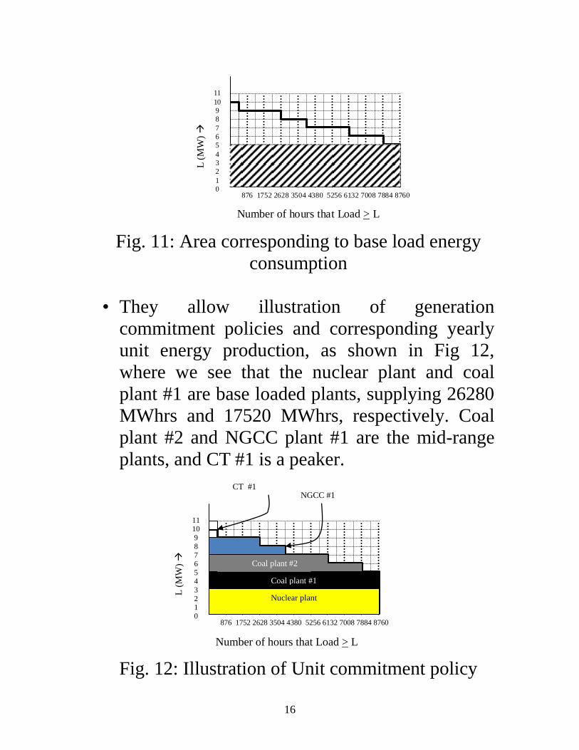
• They provide convenient calculation of energy,
since energy is just the area under the load
duration curve. For example, Fig. 11 shows the
area corresponding to the base load energy
consumption, which is 5MWx8760hr=43800
MW-hrs.
16
11
10
9
8
7
6
5
4
3
2
1
0 876 1752 2628 3504 4380 5256 6132 7008 7884 8760
Number of hours that Load > L
L
(M
W)
Fig. 11: Area corresponding to base load energy
consumption
• They allow illustration of generation
commitment policies and corresponding yearly
unit energy production, as shown in Fig 12,
where we see that the nuclear plant and coal
plant #1 are base loaded plants, supplying 26280
MWhrs and 17520 MWhrs, respectively. Coal
plant #2 and NGCC plant #1 are the mid-range
plants, and CT #1 is a peaker.
11 10
9
8 7
6
5 4
3
2 1
0 876 1752 2628 3504 4380 5256 6132 7008 7884 8760
Number of hours that Load > L
L
(M
W)
Nuclear plant
Coal plant #1
Coal plant #2
NGCC #1 CT #1
Fig. 12: Illustration of Unit commitment policy

17
Load duration curves are also used in reliability and
production costing programs in computing different
reliability indices, as we will see in Sections 4 and 5.
3.2 Generation probability models
We consider that generators obey a two-state model,
i.e., they are either up or down, and we assume that
the process by which each generator moves between
states is Markov, i.e., the probability distribution of
future states depends only on the current state and not
on past states, i.e., the process is memoryless.
In this case, it is possible to show that unavailability
(or forced outage rate, FOR) is the “steady-state” (or
long-run) probability of a component not being
available and is given by
qU (4)
and the availability is the long-run probability of a
component being available and is given by
pA (5)
where λ is the “failure rate” and μ is the “repair rate.”
See www.ee.iastate.edu/~jdm/ee653/U16-inclass.doc
for complete derivation of these expressions.

18
Substituting λ=1/MTTF and μ=1/MTTR, where
MTTF is the mean time to failure, and MTTR is the
mean time to repair, we get that
MTTRMTTF
MTTRqU
(6)
MTTRMTTF
MTTFpA
(7)
The probability mass function representing the
outaged capacity (8a) or available capacity (8b)
corresponding to unit j is then given as fDj(dj),
expressed as )()()( jjjjjjDj Cdqdpdf (8a)
)()()( jjjjjjDj Cdpdqdf (8b)
and illustrated by Fig. 13 (we will use them both).
Aj=pj
fDj(dj)
Outaged capacity, dj Cj 0
Uj=qj Uj=qj
fDj(dj)
Available capacity, dj Cj 0
Aj=pj
Fig. 13: Two state generator outage model
Unavailability U expresses the fraction of time (not
including maintenance time) the generator has been
forced out of service. Availability A is the fraction of
time (not including maintenance time) the generator
is available for service. U+A=1.

19
4.0 Preliminary definitions
Let’s characterize the load shape curve with t=g(d),
as illustrated in Fig. 14. It is important to note that the
load shape curve characterizes the (forecasted) future
time period and is therefore a probabilistic
characterization of the demand.
t
t=g(d)
T
dmax
Demand, d (MW)
Fig. 14: Load shape t=g(d)
Here:
d is the system load
t is the number of time units in the interval T for
which the load equals or exceeds d and is most
typically given in hours or days
t=g(d) expresses functional dependence of t on d

20
T represents, most typically, a year but can be any
interval of time (week, month, season, years).
The cumulative distribution function (cdf) is given by
T
dg
T
tdDPdFD
)()()( (9)
One may also compute the total energy ET consumed
in the period T as the area under the curve, i.e.,
(10)
The average demand in the period T is obtained from
maxmax
00
)()(11 d
D
d
TavgdFdg
TE
Td (11)
Now assume the planned system generation capacity,
i.e, the installed capacity, is CT, and CT<dmax. This is
an undesirable situation, since we will not be able to
serve some demands, even when there is no capacity
outage! Nonetheless, it serves well to understand the
relation of the load duration curve to several useful
indices. The situation is illustrated in Fig. 15.
max
0
) (
d
T dλ g E

21
t
tC
CT
t=g(d)
T
dmax
Demand, d (MW)
Fig. 15: Illustration of Unserved Demand
Then, under the assumption that the given capacity
CT is perfectly reliable, we may express three useful
reliability indices:
Loss of load expectation, LOLE: the expected
number of time units that load will exceed capacity
)(TC
CgtLOLET
(12)
Loss of load probability, LOLP: the probability that
the demand will equal or exceed capacity during T:
)()( TDT CFCDPLOLP (13)
We note that the condition D=CT is assumed here
to represent a loss of load situation, which would
be a conservative assumption.

22
One may think that, if dmax>CT, then LOLP=1.
However, if FD(d) is a true probability distribution,
then it describes the event D>CT with uncertainty
associated with what the load is going to be, i.e.,
only with a probability. One can take an alternative
view, that the load duration curve is certain, which
would be the case if we were considering a
previous year. In this case, LOLP should be
thought of not as a probability but rather as the
percentage of time during the interval T for which
the load equals or exceeds capacity.
It is of interest to reconsider (9), repeated here for
convenience:
T
dg
T
tdDPdFD
)()()( (9)
Substituting d=CT, we get:
T
Cg
T
tCDPCF T
TTD
)()()( (*)
By (12), g(CT)=LOLE; by (13), P(D>CT)=LOLP,
and so (*) becomes:
TLOLPLOLET
LOLELOLP
which expresses that LOLE is the expectation of
the number of time units within T that demand will
exceed capacity.

23
Expected demand not served, EDNS: If the average
(or expected) demand is given by (11), then it
follows that expected demand not served is:
max
)(d
CD
T
dFEDNS (14)
which would be the same area as in Fig. 15 when
the ordinate is normalized to provide FD(d) instead
of t. Reference [3] provides a rigorous derivation
for (14).
Expected energy not served, EENS: This is the
total amount of time multiplied by the expected
demand not served, i.e.,
maxmax
)()(d
C
d
CD
TT
dgdFTEENS (15)
which is the area shown in Fig. 15.
4.1 Effective load approach
The notion of effective load is used to account for the
unreliability of the generation, and it is essential for
understanding the view taken in [3].
The basic idea is that the total system capacity is
always CT, and the effect of capacity outages are
accounted for by changing the load model in an
appropriate fashion, and then the different indices are
computed as given in (12), (13), (14), and (15).

24
A capacity outage of Ci is therefore modeled as an
increase in the demand, not as a decrease in capacity!
We have already defined D as the random variable
characterizing the demand. Now we define two more
random variables:
Dj is the random increase in load for outage of unit i.
De is the random load accounting for outage of all
units and represents the effective load.
Thus, the random variables D, De, and Dj are related:
N
jje
DDD1
(16)
It is important to realize that, whereas Cj represents
the capacity of unit j and is a deterministic value, Dj
represents the increase in load corresponding to
outage of unit j and is a random variable. The
probability mass function (pmf) for Dj is assumed to
be as given in Fig. 16 below, i.e., a two-state model.
We denote the pmf for Dj as fDj(dj). It expresses the
probability that the unit experiences an outage of 0
MW as Aj, and the probability the unit experiences an
outage of Cj MW as Uj.

25
Aj
fDj(dj)
Outage capacity, dj Cj 0
Uj
Fig. 16: Two state generator outage model
Recall from probability theory that the pdf of the sum
of two independent random variables is the
convolution of their individual pdfs, that is, for
random variables X and Y, with Z=X+Y, then
dfzfzf YXZ )()()( (17)
Similarly, we obtain the cdf of two random variables
by convolving the cdf of one of them with the pdf (or
pmf) of the other, that is, for random variables X and
Y, with Z=X+Y, then
dfzFzF YXZ )()()( (18)
Let’s consider the case for only 1 unit, i.e., from (16),
jeDDD (19)
Then, by (18), we have that:

26
dfdFdFjee
DeDeD)()()( )0()1( (20)
where the notation )()( j
DF indicates the cdf after the
jth unit is convolved in. Under this notation, then, (19)
becomes
j
j
e
j
eDDD )1()( (21)
and the general case for (20) is:
dfdFdFjee
De
j
De
j
D)()()( )1()( (22)
which expresses the equivalent load after the jth unit
is convolved in.
Since fDj(dj) is discrete (a pmf), we rewrite (22) as
j
jee
d
jDje
j
De
j
D dfddFdF )()()( )1()(
(23)
From an intuitive perspective, (23) is providing the
convolution of the cdf )()1( j
DF with the set of
impulse functions comprising fDj(dj). When using a 2-
state model for each generator, fDj(dj) is comprised of
only 2 impulse functions, one at 0 and one at Cj.
Recalling that the convolution of a function with an
impulse function simply shifts and scales that
function, (23) can be expressed for the 2-state
generator model as:
)()()( )1()1()(
je
j
Dje
j
Dje
j
DCdFUdFAdF
eee
(24)

27
So the cdf for effective load, following convolution
with capacity outage pmf of the jth unit, is the sum of
the original cdf, scaled by Aj and
the original cdf, scaled by Uj, right-shifted by Cj.
Example 1: Fig. 17 illustrates the convolution process
for a single unit C1=4 MW supplying a system having
peak demand dmax=4 MW, with demand cdf given as
in plot (a) based on a total time interval of T=1 year.
)()0(
eDdF
r
)()1(
eDdF
r
1
1 2 3 4 5 6 7 8 de
0.8
0.6
0.4
0.2
* 1
1 2 3 4 5 6 7 8
C1=4
0.8
0.6
0.4
0.2
1.
1 2 3 4 5 6 7 8 de
0.8
0.6
0.4
0.2
+
1.
1 2 3 4 5 6 7 8 de
0.8
0.6
0.4
0.2
1.0
1 2 3 4 5 6 7 8 de
0.8
0.6
0.4
0.2
=
(c) (d)
(e)
(a) (b) fDj(dj)
Fig. 17: Convolving in the first unit
28
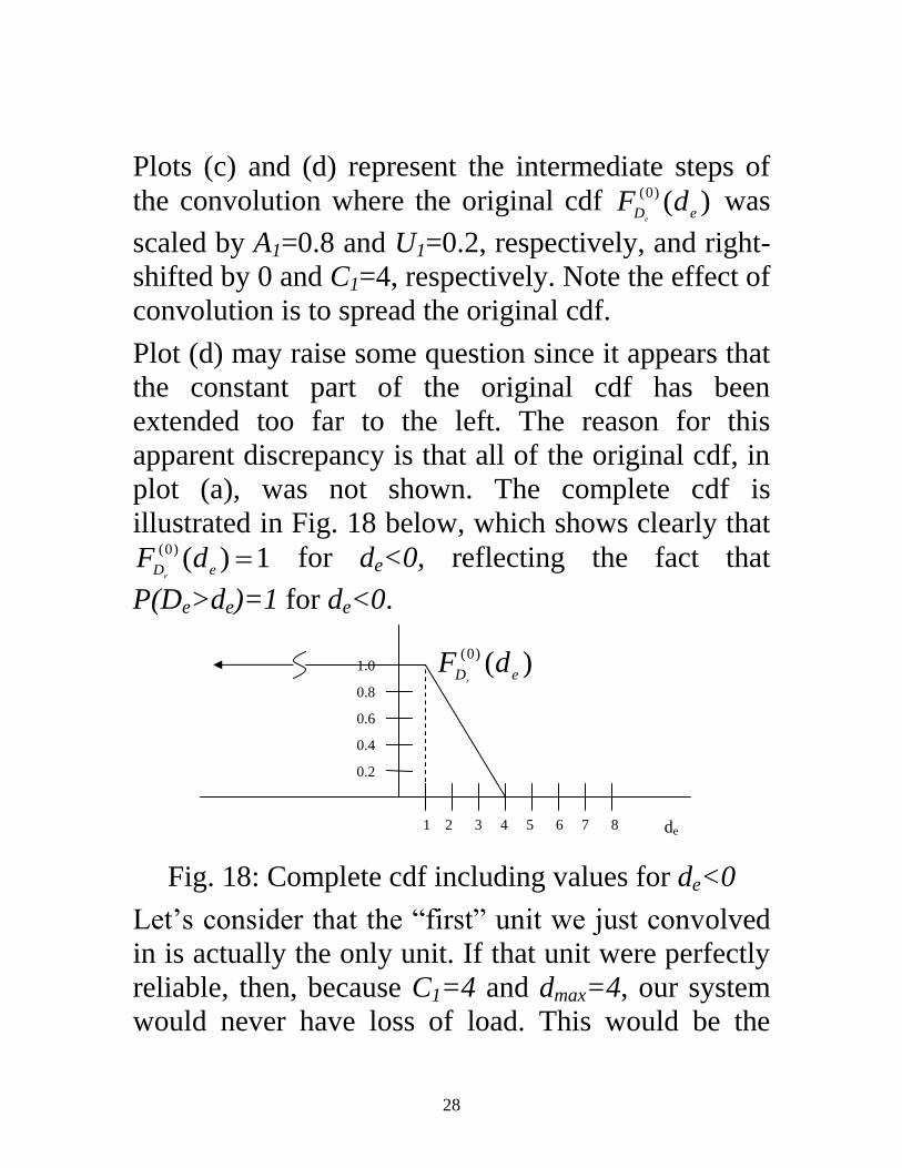
Plots (c) and (d) represent the intermediate steps of
the convolution where the original cdf )()0(
eDdF
e
was
scaled by A1=0.8 and U1=0.2, respectively, and right-
shifted by 0 and C1=4, respectively. Note the effect of
convolution is to spread the original cdf.
Plot (d) may raise some question since it appears that
the constant part of the original cdf has been
extended too far to the left. The reason for this
apparent discrepancy is that all of the original cdf, in
plot (a), was not shown. The complete cdf is
illustrated in Fig. 18 below, which shows clearly that
1)()0( eD
dFe
for de<0, reflecting the fact that
P(De>de)=1 for de<0.
)()0(
eDdF
r
1.0
1 2 3 4 5 6 7 8 de
0.8
0.6
0.4
0.2
Fig. 18: Complete cdf including values for de<0
Let’s consider that the “first” unit we just convolved
in is actually the only unit. If that unit were perfectly
reliable, then, because C1=4 and dmax=4, our system
would never have loss of load. This would be the
29
situation if we applied the ideas of Fig. 15 to Fig. 17,
plot (a).
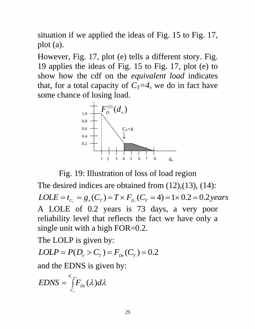
However, Fig. 17, plot (e) tells a different story. Fig.
19 applies the ideas of Fig. 15 to Fig. 17, plot (e) to
show how the cdf on the equivalent load indicates
that, for a total capacity of CT=4, we do in fact have
some chance of losing load.
CT=4
)()1(
eDdF
r
1.0
1 2 3 4 5 6 7 8 de
0.8
0.6
0.4
0.2
Fig. 19: Illustration of loss of load region
The desired indices are obtained from (12),(13), (14):
yearsCFTCgtLOLETDTeC
rT
2.02.01)4()(
A LOLE of 0.2 years is 73 days, a very poor
reliability level that reflects the fact we have only a
single unit with a high FOR=0.2.
The LOLP is given by:
2.0)()( TDeTe
CFCDPLOLP
and the EDNS is given by:
max,
)(e
T
d
CDe
dFEDNS

30
which is just the shaded area in Fig. 19, most easily
computed using the basic geometry of the figure,
according to:
MW5.0)2.0)(3(2
1)1(2.0
The EENS is given by
max,max,
)()(e
T
e
T
d
Ce
d
CDe
dgdFTEENS
or TEDNS=1(0.5)=0.5MW-years,
or 8760(0.5)=4380MWhrs.
Example 2: This example is from [4].
A set of generation data is provided in Table 5.
Table 5
The 4th column provides the forced outage rate,
which we have denoted by U. The two-state

31
generator outage model for each unit is obtained from
this value, together with the rated capacity, as
illustrated in Fig. 20, for unit 1. Notice that the units
are ordered from least cost to highest cost.
Aj=0.8
fDj(dj)
Outage load, dj Cj=200 0
Uj=0.2
Fig. 20: Two-state outage model for Unit 1
Load duration data is provided in Table 6 and plotted
in Fig. 21.
Table 6

32
Fig. 21
We now deploy (24), repeated here for convenience,
)()()( )1()1()(
je
j
Dje
j
Dje
j
DCdFUdFAdF
eee
(24)
to convolve in the unit outage models with the load
duration curve of Fig. 21. The procedure is carried
out in an Excel spread sheet, and the result is
provided in Fig. 22. In Fig. 22, we have shown
Original load duration curve, F0;
Load duration curve with unit 1 convolved in, F1.
Load duration curve with all units convolved in, F9
We could, of course, show the load duration curves
for any number of units convolved in, but this would
be a cluttered plot.

33
Fig. 22
We also show, in Table 7, the results of the
calculations performed to obtain the series of load
duration curves (LDC) F0-F9. Notice the following:
Each LDC is a column FO-F9
The first column, in MW, is the load.
o It begins at -200 to facilitate the convolution for
the largest unit, which is a 200 MW unit.
o Although it extends to 2300 MW, the largest
actual load is 1000 MW; the extension is to
obtain the equivalent load corresponding to a
1000 MW load with 1300 MW of failable
generation.
The entries in the table show the % time the load
exceeds the given value.
LOLP is, for a particular column, the % time load
exceeds the total capacity corresponding to that
column, and is underlined.

34
For example, one observes that LOLP=1 if we only
have units 1 (F1, CT=200) or only units 1 and 2 (F2,
CT=400). This is because the capacity would never
be enough to satisfy the load, at any time. And
LOLP=0.6544 if we have only units 1, 2, and 3 (F3,
CT=600). This is because we would be able to supply
the load for some of the time with this capacity. And
LOLP=0.012299 if we have all units (F9, CT=1300),
which is non-0 (in spite of the fact that CT>1000)
because units can fail.
Table 7

35
5.0 Production cost modeling using effective load
The most basic production cost model obtains
production costs of thermal units over a period of
time, say 1 year, by building upon the equivalent load
duration curve described in Section 5.
To perform this, we will assume that generator
variable cost, in $/MWhr, for unit j operating at Pj
over a time interval t, is expressed by
Cj(Ej)=bjEj
where Ej=Pjt is the energy produced by the unit
during the hour and bj is the unit’s average variable
costs of producing the energy (we omit fixed costs
because we are only trying to quantify production
costs here).
The production cost model begins by assuming the
existence of a loading (or merit) order, which is how
the units are expected to be called upon to meet the
demand facing the system. We assume for simplicity
that each unit consists of a single “block” of capacity
equal to the maximum capacity. It is possible, and
more accurate, to divide each unit into multiple
capacity blocks, but there is no conceptual difference
to the approach when doing so.

36
Table 5, listed previously in Example 2, provides the
variable cost for each unit in the appropriate loading
order. This table is repeated here for convenience.
Table 5
The criterion for determining loading order is clearly
economic. Sometimes it is necessary to alter the
economic loading order to account for must-run units
or spinning reserve requirements. We will not
consider these issues in the discussion that follows.
To motivate the approach, we introduce the concept
of a unit’s observed load as the load “seen” by a unit
just before it is committed in the loading order. Thus,
it will be the case that all higher-priority units will
have been committed.
If all higher-priority units would have been perfectly
reliable (Aj=1), then the observed load seen by the

37
next unit would have been just the total load less the
sum of the capacities of the committed units.
However, all higher-priority units are not perfectly
reliable, i.e., they may fail according to the forced
outage rate Uj. This means we must account for their
stochastic behavior over time. This can be done in a
straight-forward fashion by using the equivalent load
duration curve developed for the last unit committed.
In the notation of (24) unit j sees a load characterized
by )()1(
e
j
D dFe
. Thus, the energy provided by unit j is
proportional to the area under )()1(
e
j
D dFe
from xj-1 to
xj, where
xj-1 is the summed capacity over all previously
committed units and
xj is the summed capacity over all previously
committed units and unit j. But unit j is only going to be available Aj% of the
time. Also, since )()1(
e
j
D dFe
is a probability function,
we must multiply it by T, resulting in the following
expression for energy provided by unit j [5]:
dFTAE
j
j
e
x
x
j
Djj
1
)()1(
(25)
where

38
j
i
ij Cx1
,
1
1
1
j
i
ij Cx (26)
Referring back to Example 2, we describe the
computations for the first three entries. This
description is adapted from [4].
For unit 1, the original load duration curve F0 is
used, as forced outages of any units in the system do
not affect unit l's observed load. The energy
requested by the system from unit 1, excluding unit
l's forced outage time, is the area under )()0(
eD dFe
over
the range of 0 to 200 MW (unit 1 's position in the
loading order) times the number of hours in the
period (8760) times A1. The area under )()0(
eD dFe
from
0 to 200, illustrated in Fig. 23 below, is 200.
Fig. 23

39
Therefore, MWhrs 1,401,6002008.087601 E
For unit 2, the load duration curve F1 is used, as
forced outage of unit 1 will affect unit 2's observed
load. The energy requested by the system from unit 2,
excluding unit 2's forced outage time, is the area
under )()1(
eD dFe
over the range of 200 to 400 MW (unit
2 's position in the loading order) times the number of
hours in the period (8760) times A2. The area under
)()1(
eD dFe
from 200 to 400, illustrated in Fig. 24 below,
is 200.
Fig. 24
Therefore, MWhrs 1,401,6002008.087602 E

40
For unit 3, the load duration curve F2 is used, as
forced outage of units 1 and 2 will affect unit 3's
observed load. The energy requested by the system
from unit 3, excluding unit 3's forced outage time, is
the area under )()2(
eD dFe
over the range of 400 to 600
MW (unit 3 's position in the loading order) times the
number of hours in the period (8760) times A3. The
area under )()2(
eD dFe
from 400 to 600, illustrated in Fig.
25, is calculated below Fig 25. The coordinates on
Fig. 25 are obtained from Table 7, repeated on the
next page for convenience.
Fig. 25
The area, indicated in Fig. 25, is obtained as two
applications of a trapezoidal area (1/2)(h)(a+b), as
(500,0.872)
(600,0.616)

41
1684.746.93
)616.872)(.100(2
1)872.1)(100(
2
1
onRightPortinLeftPortio
Therefore, MWhrs 1,324,5121689.087603 E
Table 7
Continuing in this way, we obtain the energy
produced by all units. This information, together with
the average variable costs from Table 5, and the
resulting energy cost, is provided in Table 8 below.

42
Table 8 Unit MW-hrs Avg. Variable
Costs, $/MWhr
Energy Costs,
$
1 1,401,600 6.5 9,110,400
2 1,401,600 6.5 9,110,400
3 1,324,500 27.0 35,761,500
4 734,200 27.0 19,823,400
5 196,100 58.1 11,393,410
6 117,400 58.1 6,820,940
7 64,100 58.1 3,724,210
8 33,400 58.1 1,940,540
9 16,400 113.2 1,856,480
Total ET=
5,289,300
99,541,280
It is interesting to note that the total energy supplied,
ET=5,289,300 MWhrs, is less than what one obtained
when the original load duration curve is integrated.
This integration can be done by applying our
trapezoidal approach to curve F0 in Table 7. Doing
so results in E0=5,299,800 MWhrs. The difference is
E0-ET=5,299,800-5,289,300=10,500 MWhrs.
What is this difference of 10,500 MWhrs?
To answer this question, consider: The total area under the original curve F0, integrated
from 0 to 1000 (the peak load), is 5,299,800 MWhrs, as
shown in Fig. 26. This is the amount of energy provided
to the actual load if it were supplied by perfectly reliable
generation having capacity of 1000 MW. As indicated
above, we will denote this as E0.

43
Fig. 26
The total area under the final curve, F9, integrated
from 0 to 1300 MW (the generation capacity) is
E1300=6,734,696 MWhrs, as shown in Fig. 27. This
is the amount of energy provided to the effective
load if it were supplied by perfectly reliable
generation having capacity of 1300 MW.
Fig. 27
E0=8760*this area
=5,299,800 MWhrs
E1300= 8760*this area
=6,734,696 MWhrs

44
The energy represented by the area of Fig. 27,
which is the energy provided to the effective load if
it were supplied by perfectly reliable generation
having capacity of 1300 MW, is greater than the
energy provided by the actual 1300 MW, that is
E1300>ET
because E1300 includes load required to be served
when the generators are outaged, and this portion
was explicitly removed from the calculation of
Table 8 (ET). One can observe this readily by
considering a system with only a single unit.
Recalling the general formula (25) for obtaining
actual energy supplied by a unit per the method of
Table 8:
dFTAE
j
j
e
x
x
jDjj
1
)()1(
(25)
and applying this to the one-unit system, we get:
dFTAEE
C
DTe
1
0
)0(11 )(
(27)
In contrast, the energy Ee obtained when we
integrate the effective load duration curve
(accounting for only the one unit) is

45
dFTE
C
Dee
1
0
)1()(
(28)
Recalling the convolution formula (24),
)()()( )1()1()(
je
j
Dje
j
Dje
j
DCdFUdFAdF
eee
(24)
and for the one-unit case, we get
)()()( 1)0(
1)0(
1)1(
CdFUdFAdF eDeDeD eee
(29)
Substituting (29) into (28) results in
dCFUFATE
C
DDeee
1
0
1)0(
1)0(
1 )()( (30)
Breaking up the integral gives
11
11
0
1)0(
1
0
)0(1
0
1)0(
1
0
)0(1
)()(
)()(
C
D
C
D
C
D
C
De
dCFTUdFTA
dCFUTdFATE
ee
ee
(31)
Comparing (31) with (27), repeated here for
convenience:
dFTAEE
C
DTe
1
0
)0(11 )( (27)
we observe the expressions are the same except for
the presence of the second integration in (31). This
proves that Ee>ET, i.e., effective energy demanded > energy served by generation

46
Now consider computing the energy consumed by
the total effective load as represented by Fig. 28
(note that in this figure, the curve should go to zero
at Load=2300 but does not due to limitations of the
drawing facility used).
Fig. 28
Using the trapezoidal method to compute this area
results in E2300=6745200 MWhrs, which is the
energy provided to the effective load if it were
supplied by perfectly reliable generation having
capacity of 2300 MW. This would leave zero
energy unserved.
The difference between o E2300, the energy provided to the effective load if it were
supplied by 2300 MW of perfectly reliable generation and
o E1300, the energy provided to the effective load if it were
supplied by 1300 MW of perfectly reliable generation
is given by:
E2300-E1300=6,745,200-6,734,696=10,504 MWhrs
E2300= 8760*this area
=6,745,200 MWhrs

47
This is the expected energy not served (EENS),
sometimes called the expected unserved energy
(EUE).
We observe, then, that we can obtain EENS in two
different approaches. 1. E0-ET=5,299,800-5,289,300=10,500 MWhrs
2. E2300-E1300=6,745,200-6,734,696=10,504 MWhrs
Approach 1 may be computationally more
convenient for production costing because ET is
easily obtained as the summation of all the energy
values.
Approach 2 may be more convenient conceptually
as it is simply the area under the effective load
curve from total capacity (I call it CT) to infinity.
6.0 Comments on W&W approach
W&W, in section 8.3.2, refers to the “unserved load
method.” It is somewhat different from the “effective
load method” described above.
The main difference can be observed by comparing
equation (8.2) in your text with equation (24) used
above.

48
)()()( )1()1()(
je
j
Dje
j
Dje
j
DCdFUdFAdF
eee
(24)
)()()( CxpPxqPxP nnn (8.2)
Both left-hand expressions are the “new” cdf after
“convolving in” a unit.
Specifically, the nomenclature relates as follows:
de=x (value of equivalent load)
Cj=C (capacity of unit j)
Aj=p (availability of unit j)
Uj=q (unavailability of unit j)
One observes that the two equations are almost the
same, with two exceptions:
1. Shift: Whereas the “shift” on the second term of
(24) is a “right-shift” by an amount C, the “shift”
on the second term of (8.2) is a left-shift by an
amount C.
2. Aj and Uj: Whereas the “unshifted” (first) term of
(24) is multiplied by Aj=p, the “unshifted” (first)
term of (8.2) is multiplied by Uj=q.
The difference should be understood.

49
Whereas
the “effective load” method
o extends or increases the load to
probabilistically account for generator
unavailability,
o and uses total capacity under assumption of
perfect reliability to assess metrics
the “unserved load” method
o reduces or decreases the load to
probabilistically account for generator
availability,
o and uses zero capacity to assess metrics.
6.0 W&W (unserved load) method
We will maintain the notation used in describing the
effective load method. The differences in notation
relative to W&W are described in the previous
section.
Define D as the random variable characterizing the
demand. Now we define two more random variables:
Dj is the random decrease in load for (probabilistic)
availability of unit j.
De is the random load accounting for the
(probabilistic) availability of all units and represents
the unserved load.

50
Thus, the random variables D, De, and Dj are related:
N
j
je DDD1
(25)
Whereas Cj represents the capacity of unit j and is a
deterministic value, Dj represents an effective
decrease in load corresponding to (probabilistic)
availability of unit j and is a random variable.
The probability mass function (pmf) for Dj is
assumed to be as given in Fig. 29, i.e., a two-state
model. We denote the pmf for Dj as fDj(dj). It
expresses the probability that the unit experiences an
outage of 0 MW as Aj, and the probability the unit
experiences an outage of Cj MW as Uj.
Aj
fDj(dj)
Available capacity, dj Cj 0
Uj
Fig. 29: Two state generator availability model
We saw in the above notes that the pdf of the sum of
2 independent random variables is the convolution of
their individual pdfs, that is, for random variables X
and Y, with Z=X+Y, then

51
dfzfzf YXZ )()()( (17)
which can also be written as:
dzffzf YXZ )()()(
Likewise, the pdf of the difference of 2 independent
random variables is also a convolution, that is, for
random variables X and Y, with Z=X-Y, then
dzfzfzf YXZ )()()( (26)
In addition, it is true that the cdf of the difference
between 2 random variables can be found by
convolving the cdf of one of them with the pdf (or
pmf) of the other, that is, for random variables X and
Y, with Z=X-Y, then
dzfzFzF YXZ )()()( (27)
Let’s consider the case for only 1 unit, i.e., from (25),
je DDD (28)
Then, by (27), we have that:

52
ddfFdF eDDeD jee)()()( )0()1(
(20)
where the notation )()( j
DF indicates the cdf after the
jth unit is convolved in. With this notation, (28) is
j
j
e
j
e DDD )1()(
(29)
and the general case for (29) is:
ddfFdF eD
j
De
j
D jee)()()( )1()(
(30)
which expresses the equivalent load after the jth unit
is convolved in, considering the (probabilistic)
availability of unit j and all lower numbered units.
Since fDj(dj) is discrete (a pmf), we rewrite (30) as
j
jee
d
jeDj
j
De
j
D ddfdFdF )()()( )1()(
(31)
From an intuitive perspective, (31) is providing the
convolution of the cdf )()1( j
DF with the set of
impulse functions comprising fDj(dj). When using a 2-
state availability model for each generator, fDj(dj) is
comprised of only 2 impulse functions, one at 0 and
one at Cj. Recalling that the convolution of a function
with an impulse function simply shifts and scales that
function, (31) can be expressed for the 2-state
generator model shown in Fig. 23 as:

53
)()()( )1()1()(
je
j
Dje
j
Dje
j
D CdFAdFUdFeee
(32)
So the cdf for the effective load, following
convolution with capacity outage pmf of the jth unit,
is the sum of
the original cdf, scaled by Uj and
the original cdf, scaled by Aj, left-shifted by Cj.
W&W say this (p. 287):
The first term is the probability that new capacity
Cj is unavailable times the probability of needing
an amount of power de or more;
The second term is the probability Cj is available
times the probability de+Cj or more is needed.
Example 3: Fig. 30 illustrates the convolution process
for a single unit C1=4 MW supplying a system having
peak demand dmax=4 MW, with demand cdf given as
in plot (a) based on a total time interval of T=1 year.

54
)()0(
eDdF
r
)()1(
eDdF
r
1
1 2 3 4 5 6 7 8 de
0.8
0.6
0.4
0.2
* 1
-6 -5 -4 -3 -2 -1 0
U1=0.2
0.8
0.6
0.4
0.2
de
+
1.
1 2 3 4 5 6 7 8 de
0.8
0.6
0.4
0.2
1.0
-4 -3 -2 -1 0 1 2 3 4 de
0.8
0.6
0.4
0.2
=
(c) (d)
(e)
(a) (b) fDj(dj)
A1=0.8
1
0.8
0.6
0.4
0.2
-6 -5 -4 -3 -2 -1 0
Unserved
load
Served
load
Fig. 30: Convolving in the first unit (not perfectly
reliable)
Plots (d) and (c) represent the intermediate steps of
the convolution where the original cdf )()0(
eDdF
e
was
scaled by U1=0.2 and A1=0.8, respectively, and left-
shifted by 0 and C1=4, respectively. Note the effect of
convolution is to shift the original cdf to the left.

55
Plot (c) may raise some question since it appears that
the constant part of the original cdf has been
extended too far to the left. The reason for this is that
all of the original cdf, in plot (a), was not shown. The
complete cdf is illustrated in Fig. 31 below, which
shows clearly that 1)()0( eD
dFe
for de<0, reflecting the
fact that P(De>de)=1 for de<0.
)()0(
eDdF
r
1.0
1 2 3 4 5 6 7 8 de
0.8
0.6
0.4
0.2
Fig. 31: Complete cdf including values for de<0
Let’s consider that the “first” unit we just convolved
in is actually the only unit. If that unit were perfectly
reliable, then, because C1=4 and dmax=4, our system
would never have loss of load. In this case, with
A1=1 and U1=0, the convolution process above would
have resulted in Fig. 32 below. The fact that the final
load duration curve FD(1)(de) shows Pr(de>0)=0 means
that there is no chance we will encounter a load
interruption for this system!

56
)()0(
eDdF
r
)()1(
eDdF
r
1
1 2 3 4 5 6 7 8 de
0.8
0.6
0.4
0.2
* 1
-6 -5 -4 -3 -2 -1 0
U1=0
0.8
0.6
0.4
0.2
de
+
1.
1 2 3 4 5 6 7 8 de
0.8
0.6
0.4
0.2
1.0
-4 -3 -2 -1 0 1 2 3 4 de
0.8
0.6
0.4
0.2
=
(c) (d)
(e)
(a) (b) fDj(dj)
A1=1.0
1
0.8
0.6
0.4
0.2
-6 -5 -4 -3 -2 -1 0
Unserved
load
Served
load
Fig. 32: Convolving in the first unit (perfectly
reliable)
However, Fig. 30, plot (e) tells a different story. The
fact that there is some part of the load duration curve
to the right of de=0 is an indication that there is a
possibility of load interruption.

57
Observe that positive de may be thought of as
unserved load; negative de may be thought of as
served load. In other words, Fig. 32 tells us
Pr(unserved load > 0 MW) = 0
Pr(unserved load > -4 MW)=1.0
Pr(served load < 4 MW)=1.0
Fig. 30 applies the ideas of Fig. 15 to Fig. 30, plot (e)
to show how the cdf on the equivalent load indicates
that, for a total capacity of CT=0, we do in fact have
some chance of losing load.
)()1(
eDdF
r
1.0
-4 -3 -2 -1 0 1 2 3 4 de
0.8
0.6
0.4
0.2
Fig. 33: Illustration of loss of load region
The desired indices are obtained from (12),(13), (14):
yearsCFTCgtLOLE TDTeC rT2.02.01)0()(
A LOLE of 0.2 years is 73 days, a very poor
reliability level that reflects the fact we have only a
single unit with a high FOR=0.2.
The LOLP is given by:

58
2.0)()( TDeTe CFCDPLOLP
and the EDNS is given by:
max,
)(e
T
d
CDe
dFEDNS
which is just the shaded area in Fig. 33, most easily
computed using the basic geometry of the figure,
according to:
MW5.0)2.0)(3(2
1)1(2.0
The EENS is given by
max,max,
)()(e
T
e
T
d
Ce
d
CDe
dgdFTEENS
or TEDNS=1(0.5)=0.5MW-years,
or 8760(0.5)=4380MWhrs.
Example 4: This example is from [6].
A set of generation data is provided in Table 8.
Table 8

59
Observe the units are ordered from least to highest
cost. The 4th column provides the forced outage rate
(FOR), which we have denoted by U. The two-state
generator outage model for each unit (obtained from
the FOR), together with the rated capacity, is
illustrated in Fig. 34, for unit 1.
Aj=0.8
fDj(dj)
Available capacity, dj Cj 0
Uj=0.2
Fig. 34: Two-state outage model for Unit 1
Load duration data is provided in Table 9 and plotted
in Fig. 35.
Table 9

60
Fig. 35
We now deploy (32), repeated here for convenience,
)()()( )1()1()(
je
j
Dje
j
Dje
j
D CdFAdFUdFeee
(32)
to convolve in the unit outage models with the load
duration curve of Fig. 35. The procedure is carried
out in an Excel spread sheet, and the result is
provided in Fig. 36. In Fig. 36, we have shown
Original load duration curve, F0;
Load duration curves with unit j convolved in, Fj,
j=1,…,9.

61
Fig. 36
We also show, in Table 10, the results of the
calculations performed to obtain the series of load
duration curves (LDC) F0-F9. Notice the following:
Each LDC is a column FO-F9
The first column, in MW, is the load.
o It begins at -1400, an arbitrarily chosen large
negative number to ensure each LDC begins
from the left with an ordinate of 1.0 (we really
only need to extend to -900).
o The largest actual load is 1000 MW; the
extension is to obtain the equivalent load
corresponding to a 1000 MW load with 1300
MW of failable generation.
The entries in the table show the % time the
unserved load exceeds the given value.
LOLP is, for a particular column, the % time load
exceeds the total capacity corresponding to that
column, and is underlined.

62
For example, one observes that LOLP=1 if we only
have units 1 (F1, CT=200) or only units 1 and 2 (F2,
CT=400). This is because the capacity would never
be enough to satisfy the load, at any time. And
LOLP=0.6544 if we have only units 1, 2, and 3 (F3,
CT=600). This is because we would be able to supply
the load for some of the time with this capacity. And
LOLP=0.012299 if we have all units (F9, CT=1300),
which is non-0 (in spite of the fact that CT>1000)
because units can fail.
Table 10 F0 F1 F2 F3 F4 F5 F6 F7 F8 F9
0.2 0.2 0.1 0.1 0.1 0.1 0.1 0.1 0.05
0.8 0.8 0.9 0.9 0.9 0.9 0.9 0.9 0.95
200 200 200 200 100 100 100 100 100
Load (MW) Fraction of time load exceeds given load
-1400 1 1 1 1 1 1 1 1 1 1
-1300 1 1 1 1 1 1 1 1 1 1
-1200 1 1 1 1 1 1 1 1 1 1
-1000 1 1 1 1 1 1 1 1 1 1
-900 1 1 1 1 1 1 1 1 1 1
-800 1 1 1 1 1 1 1 1 1 0.935377
-700 1 1 1 1 1 1 1 1 0.931976 0.774008
-600 1 1 1 1 1 1 1 0.924417 0.765694 0.592168
-500 1 1 1 1 1 1 0.916019 0.748058 0.583035 0.397986
-400 1 1 1 1 1 0.906688 0.729395 0.5647 0.388247 0.248591
-300 1 1 1 1 0.89632 0.709696 0.5464 0.368641 0.241241 0.134512
-200 1 1 1 1 0.68896 0.528256 0.34889 0.227085 0.128894 0.069428
-100 1 1 1 0.8848 0.5104 0.32896 0.213551 0.117984 0.066298 0.02979
0 1 1 1 0.6544 0.3088 0.200728 0.107366 0.060556 0.027869 0.012299
100 1 1 0.872 0.4688 0.18872 0.096992 0.055354 0.024237 0.01148 0.004146
200 1 1 0.616 0.2704 0.0868 0.050728 0.02078 0.010062 0.00376 0.001281
300 1 0.84 0.424 0.1576 0.04672 0.017452 0.008871 0.003059 0.00115 0.00033
400 1 0.52 0.232 0.0664 0.0142 0.007918 0.002414 0.000938 0.000287 7.04E-05
500 0.8 0.32 0.128 0.0344 0.00722 0.001802 0.000774 0.000215 5.9E-05 1.25E-05
600 0.4 0.16 0.048 0.0084 0.0012 0.00066 0.000152 4.17E-05 1.01E-05 1.62E-06
700 0.2 0.08 0.024 0.0042 0.0006 0.000096 2.94E-05 6.54E-06 1.18E-06 1.31E-07
800 0.1 0.02 0.004 0.0004 0.00004 0.000022 0.000004 5.8E-07 7.6E-08 5.7E-09
900 0.05 0.01 0.002 0.0002 0.00002 0.000002 2E-07 2E-08 2E-09 1E-10
1000 0 0 0 0 0 0 0 0 0 0

63
7.0 Production cost modeling using unserved load
The most basic production cost model obtains
production costs of thermal units over a period of
time, say 1 year, by building upon the procedures
described in Section 7.
The production cost model begins by assuming the
existence of a loading (or merit) order, which is how
the units are expected to be called upon to meet the
demand facing the system. We assume for simplicity
that each unit consists of a single “block” of capacity
equal to the maximum capacity. It is possible, and
more accurate, to divide each unit into multiple
capacity blocks, but there is no conceptual difference
to the approach when doing so.
Table 5, listed previously in Examples 2 and 4,
provides the variable cost for each unit in the
appropriate loading order. This table is repeated here
for convenience.

64
Table 5
The criterion for determining loading order is clearly
economic. Sometimes it is necessary to alter the
economic loading order to account for must-run units
or spinning reserve requirements. We will not
consider these issues in the discussion that follows.
To motivate the approach, we introduce the concept
of a unit’s observed load as the load “seen” by a unit
just before it is committed in the loading order. Thus,
it will be the case that all higher-priority units will
have been committed.
If all higher-priority units would have been perfectly
reliable (Aj=1), then the observed load seen by the
next unit would have been just the total load less the
sum of the capacities of the committed units.

65
However, all higher-priority units are not perfectly
reliable, i.e., they may fail according to the forced
outage rate Uj. This means we must account for their
stochastic behavior over time. This can be done in a
straight-forward fashion by using the equivalent load
duration curve developed for the last unit committed.
In the notation of (32) unit j sees the unserved load
characterized by )()1(
e
j
D dFe
. Thus, the energy provided
by unit j is proportional to the area under )()1(
e
j
D dFe
from 0 to Cj, where Cj is the capacity of unit j.
In our example 4 above, Unit 1 sees the entire load,
characterized by )()0(
eD dFe
, illustrated as the white area
in Fig. 37.
Fig. 37

66
Unit 2, however, will see the load after unit 1 has
been convolved in (resulting in F1), which will have
the effect of reducing the unserved load, illustrated in
the white area in Fig. 38 (which is less area than the
white area in Fig. 37).
Fig. 38
We want to compute the cost of running each of the
various units j.
We assume that generator cost rate, in $/hr, for unit j
operating at Pj, is linearized, expressed by
Jj=Jj0+Jj1Pj (33)
where
Jj0 is the unit’s no-load cost rate, $/hr and
Jj1 is the unit’s cost of energy production, $/MWhr.
We also assume that unit j has capacity Cj.

67
We obtain the cost associated with scheduling unit j
according to (33). Consideration of the no-load costs
is easy, because we will incur them for every hour the
unit is scheduled. Let’s assume that the unit will be
scheduled for the entire time period, T hours, where T
is the number of hours characterized by the CDF
)()1(
e
j
D dFe
. Therefore the no-load costs is (in $):
NoloadCosts=Jj0T (34)
The variable (fuel) costs could be computed (in $) as:
VariableCosts=Jj1PjT
However, this would require that the unit runs at Pj
for all T hours. That may not happen. A better way to
compute variable costs results from recognizing that
Jj1, with units of $/MWhr, is the cost per unit of
energy. Therefore, if we can get the energy supplied
by unit j, Ej, then this will allow us to compute the
cost of supplying it from
VariableCosts=Jj1Ej (35)
The energy supplied by unit j can be computed from
the CDF )()1(
e
j
D dFe
according to the following:
j
e
C
j
Dj dFTE0
)1( )( (36)
In our example, for unit 1 (a 200 MW unit), this
would correspond to the area denoted by the hatched
region in Fig. 39.

68
Fig. 39
In this particular case, the integration of (36) provides
the same answer as PjT, but this is because this unit is
base-loaded and does in fact run all time at capacity.
And so the total cost of scheduling unit j can be
evaluated as the sum of the no-load and variable
costs, which is:
TotalCosts=NoloadCosts+VariableCosts=Jj0T+ Jj1Ej
(37)
where Ej is given by (36).
There is just one problem with (37)…

69
Once we commit a unit, we do intend that it will be
scheduled for all T hours, However, because the unit
has an availability of Aj, we can only expect that the
unit will be available for a number of hours equal to
AjT, i.e., unit j is only going to be available Aj% of
the time. Therefore, we need to modify (37) to be
TotalCosts=AjJj0T+ AjJj1Ej (38)
where, as before, Ej is given by (36).
Referring back to Example 4, we describe the
computations for the first three entries. This
description is adapted from [4].
For unit 1, the original load duration curve F0 is
used, as forced outages of any units in the system do
not affect unit l's observed load. The energy
requested by the system from unit 1 is the area under
)()0(
eD dFe
over the range of 0 to 200 MW (unit 1’s
capacity) times the number of hours in the period
(8760) times A1=0.8. The area under )()0(
eD dFe
from 0
to 200, has already been illustrated in Fig. 37 above,
and is 200.
Therefore, MWhrs 1,401,6002008.087601 E
and the total cost of unit 1 is

70
For unit 2, the load duration curve F1 is used, as
forced outage of unit 1 will affect unit 2's observed
load. The energy requested by the system from unit 2
is the area under )()1(
eD dFe
over the range of 0 to 200
MW (unit 2’s capacity) times the number of hours in
the period (8760) times A2=0.8. The area under
)()1(
eD dFe
from 0 to 200, illustrated in Fig. 40 below, is
200.
Fig. 40
Therefore, MWhrs 1,401,6002008.087602 E

71
For unit 3, the load duration curve F2 is used, as
forced outage of units 1 and 2 will affect unit 3's
observed load. The energy requested by the system
from unit 3 is the area under )()2(
eD dFe
over the range
of 0 to 200 MW (unit 3’s capacity) times the number
of hours in the period (8760) times A3=0.9. The area
under )()2(
eD dFe
from 0 to 200, illustrated in Fig. 41, is
calculated below. The coordinates on Fig. 41 are
obtained from Table 10, repeated on the next page for
convenience.
Fig. 41
The area, indicated in Fig. 41, is obtained as two
applications of a trapezoidal area (1/2)(h)(a+b), as
1684.746.93
)616.872)(.100(2
1)872.1)(100(
2
1
onRightPortinLeftPortio
(100,0.872)
(20,0.616)

72
Therefore, MWhrs 1,324,5121689.087603 E
Table 10 F0 F1 F2 F3 F4 F5 F6 F7 F8 F9
0.2 0.2 0.1 0.1 0.1 0.1 0.1 0.1 0.05
0.8 0.8 0.9 0.9 0.9 0.9 0.9 0.9 0.95
200 200 200 200 100 100 100 100 100
Load (MW) Fraction of time load exceeds given load
-1400 1 1 1 1 1 1 1 1 1 1
-1300 1 1 1 1 1 1 1 1 1 1
-1200 1 1 1 1 1 1 1 1 1 1
-1000 1 1 1 1 1 1 1 1 1 1
-900 1 1 1 1 1 1 1 1 1 1
-800 1 1 1 1 1 1 1 1 1 0.935377
-700 1 1 1 1 1 1 1 1 0.931976 0.774008
-600 1 1 1 1 1 1 1 0.924417 0.765694 0.592168
-500 1 1 1 1 1 1 0.916019 0.748058 0.583035 0.397986
-400 1 1 1 1 1 0.906688 0.729395 0.5647 0.388247 0.248591
-300 1 1 1 1 0.89632 0.709696 0.5464 0.368641 0.241241 0.134512
-200 1 1 1 1 0.68896 0.528256 0.34889 0.227085 0.128894 0.069428
-100 1 1 1 0.8848 0.5104 0.32896 0.213551 0.117984 0.066298 0.02979
0 1 1 1 0.6544 0.3088 0.200728 0.107366 0.060556 0.027869 0.012299
100 1 1 0.872 0.4688 0.18872 0.096992 0.055354 0.024237 0.01148 0.004146
200 1 1 0.616 0.2704 0.0868 0.050728 0.02078 0.010062 0.00376 0.001281
300 1 0.84 0.424 0.1576 0.04672 0.017452 0.008871 0.003059 0.00115 0.00033
400 1 0.52 0.232 0.0664 0.0142 0.007918 0.002414 0.000938 0.000287 7.04E-05
500 0.8 0.32 0.128 0.0344 0.00722 0.001802 0.000774 0.000215 5.9E-05 1.25E-05
600 0.4 0.16 0.048 0.0084 0.0012 0.00066 0.000152 4.17E-05 1.01E-05 1.62E-06
700 0.2 0.08 0.024 0.0042 0.0006 0.000096 2.94E-05 6.54E-06 1.18E-06 1.31E-07
800 0.1 0.02 0.004 0.0004 0.00004 0.000022 0.000004 5.8E-07 7.6E-08 5.7E-09
900 0.05 0.01 0.002 0.0002 0.00002 0.000002 2E-07 2E-08 2E-09 1E-10
1000 0 0 0 0 0 0 0 0 0 0
Continuing in this way, we obtain the energy
produced by all units. This information, together with
the average variable cost for each unit from Table 5,
and the resulting variable cost for each unit, is
provided in Table 11 below. Observe that in Table
11, the no-load costs are all zero, and so the total
costs are the same as the variable costs.

73
Table 11 Unit
i
No-load
cost
coefficient
J0i
($/hr)
No-load
costs
J0i*T
($)
Energy Ei
(MW-hr)
Variable
cost
coefficient
J1i
($/MWhr)
Variable
Cost
J1iEi
($)
Total costs,
J0i*T+ J1iEi
($)
1 0 0 1,401,600 6.5 9,110,400 9,110,400
2 0 0 1,401,600 6.5 9,110,400 9,110,400
3 0 0 1,324,500 27.0 35,761,500 35,761,500
4 0 0 734,200 27.0 19,823,400 19,823,400
5 0 0 196,100 58.1 11,393,410 11,393,410
6 0 0 117,400 58.1 6,820,940 6,820,940
7 0 0 64,100 58.1 3,724,210 3,724,210
8 0 0 33,400 58.1 1,940,540 1,940,540
9 0 0 16,400 113.2 1,856,480 1,856,480
Total 0 0 ET=
5,289,300
99,541,280 99,541,280
It is interesting to note that the total energy supplied,
ET=5,289,300 MWhrs, is less than what one obtains
when the original load duration curve is integrated.
This integration can be done by applying our
trapezoidal approach to curve F0 in Fig. 37, repeated
here for convenience, to obtain the white area shown
in the figure.

74
Fig. 37
Doing so results in E0=5,299,800 MWhrs. The
difference is
E0-ET=5,299,800-5,289,300=10,500 MWhrs.
What is this difference of 10,500 MWhrs?
To answer this question, consider the load duration
curve after the last unit has been convolved in, curve
F9, as shown in Fig. 42.
The total area under the original curve F0,
integrated from 0 to 1000 (the peak load), is
5,299,800 MWhrs, as shown in Fig. 37. This is the
amount of energy provided to the actual load if it
were supplied by perfectly reliable generation
having capacity of 1000 MW. As indicated above,
we will denote this as E0.
E0=8760*this area
=5,299,800 MWhrs

75
The total area under the final curve, F9, integrated
from -1300 (the total served load) to 0 (the
generation capacity) is Ees=6,734,696 MWhrs, as
shown in Fig. 42. This is the amount of energy
provided to the effective load if it were supplied by
perfectly reliable generation having capacity of
1300 MW. It is the served load.
Fig. 42
The energy represented by the area of Fig. 42,
which is the energy provided to the effective load if
it were supplied by perfectly reliable generation
having capacity of 1300 MW, is greater than the
energy provided by the actual 1300 MW, that is
|Ees| >|ET|
because Ees includes load required to be served
when the generators are outaged, and this portion
was explicitly removed from the calculation of
Table 11 (ET). One can observe this readily by
Ees= 8760*this area
=6,734,696 MWhrs

76
considering a system with only a single unit.
Combining the relations (36) and (38), we can
obtain the actual energy supplied by a unit (same as
method of Table 11):
dFTAE
j
e
C
j
Djj
0
)1( )( (39)
and applying this to the one-unit system, we get:
dFTAEE
C
DTe
1
0
)0(11 )(
(40)
In contrast, the energy served Ees obtained when
we integrate the effective load duration curve
(accounting for the one unit) is
dFTEC
Des e
0
)1(
1
)( (41)
Recalling the convolution formula (32),
)()()( )1()1()(
je
j
Dje
j
Dje
j
D CdFAdFUdFeee
(42)
and for the one-unit case, we get
)()()( 1
)0(
1
)0(
1
)1( CdFAdFUdF eDeDeD eee (43)
Substituting (43) into (41) results in
dCFAFUTEC
DDes ee
0
1
)0(
1
)0(
1
1
)()( (44)
Breaking up the integral gives

77
0
1
)0(
1
0
)0(
1
0
1
)0(
1
0
)0(
1
11
11
)()(
)()(
C
D
C
D
C
D
C
Des
dCFTAdFTU
dCFATdFUTE
ee
ee
(45)
Reversing the order of integration and multiplying
by -1 provides:
11
0
1
)0(
1
0
)0(
1 )()(
C
D
C
Des dCFTAdFTUEee
(46)
Comparing (46) with (40), repeated here for
convenience:
dFTAEE
C
DTe
1
0
)0(11 )(
(40)
we observe the expressions are the same except for
the presence of the second integration in (45). This
proves that |Ees| >|ET|
Now consider computing the energy consumed by
the total effective load, which includes the
unserved load, as represented by Fig. 43.

78
Fig. 43
Using the trapezoidal method to compute this area
results in EeT=6745200 MWhrs, which is the energy
provided to the effective load if it were supplied by
perfectly reliable generation having capacity of 2300
MW. This would leave zero energy unserved.
The difference between o Total effective load, EeT: the energy provided to the
effective load if it were supplied by 2300 MW of perfectly
reliable generation and
o Effective load served, Ees: the energy provided to the
effective load if it were supplied by 1300 MW of perfectly
reliable generation
is given by:
EeT-Ees=6,745,200-6,734,696=10,504 MWhrs
This is the expected energy not served (EENS),
sometimes called the expected unserved energy
(EUE).
EeT = 8760*this area
=6,745,200 MWhrs

79
We observe, then, that we can obtain EENS in two
different approaches. 1. E0-ET=5,299,800-5,289,300=10,500 MWhrs where
E0 is the total energy demanded by the actual load as
computed from the original load duration curve;
ET is the energy served to the actual load by the 1300
MW of generation accounting for each unit’s
potential to fail.
2. EeT-Ees=6,745,200-6,734,696=10,504 MWhrs where
EeT is the total energy demanded by the effective
load as computed from the complete effective load
duration curve;
Ees is the energy served to the effective load by the
1300 MW of generation, assuming the 1300 MW is
perfectly reliable.
Approach 1 may be computationally more
convenient for production costing because ET is
easily obtained as the summation of all the energy
values.
Approach 2 may be more convenient conceptually
as it is simply the area under the effective load
curve from 0 to total capacity (we can call it CT).

80
8.0 Additional W&W comments of interest A few other comments about the W&W text:
Pg. 283: In reality, EENS is energy that would not
be “not served” but rather provided via expensive
interconnection or emergency backup (providing
energy via interconnection was the original
motivation behind interconnecting control areas).
Pg. 286: An alternative method of handling EENS is
to place “emergency sources” of very large capacity
and high cost at the end of the priority list, so that
they only get used if no other capacity is available.
Pg. 284: Mentions NERC’s database. It is called
“GADS” (Generating Availability Data System).
There is also a “TADS” (Transmission Availability
Data System) and a “DADS” (Demand Response
Availability Data System).
Pg. 284: For very large systems, the convolution
method described above can be computationally
intensive. An alternative method is called the
“method of cumulants.”
Pg. 318: All of what we have described also applies
when generators are modeled as multi-state devices.
This can account for the possibility of de-rating a
unit which sometimes occurs when the unit requires
a forced reduction in output due to some particular
part of the plant becoming dysfunctional (e.g., one
out of 6 boiler feedpumps goes down).

81
9.0 Industry-grade commercial production cost
models In the previous notes, we reviewed a relatively simple
production cost model (PCM). This PCM required
two basic kinds of input data:
Annual load duration curve
Unit data:
o Capacity
o Forced outage rate
o Variable costs
It then computes load duration curves for effective
load (which accounts for the unreliability of the
generators supplying that load) through a convolution
process and provides the following information:
Reliability indices: LOLP, LOLE, EDNS, EENS
(EUE)
Annual energy produced by each unit
Annual production costs for each unit
Total system production costs
Another approach to PCMs is to simulate each hour
of the year. This allows much more rigorous models
and more refined results, which comes with a
significant computational cost. Promod is one such
model which you will hear about. I will describe the
conceptual approach to such PCMs.

82
9.1 A refined production cost model
This PCM consists of the following loops:
1. Annual loop: Most PCMs have only one annual
loop, i.e., the annual simulation is deterministic.
But it is conceivable to make multiple runs
through a particular year, each time selecting
various variables based on probability distributions
for those variables. Such an approach is referred to
as a Monte Carlo approach, and it requires many
loops in order to “converge” with respect to the
average annual production costs.
2. UC loop: The program must have a way for
deciding, in each hour, which units are committed.
A UC program could be implemented within the
PCM on a weekly basis, a 48 hour basis, or a day-
ahead basis. The latter seems to be the preferred
approach today because it is consistent with the
fact that most electricity market structures today
depend on the day-ahead using the security-
constrained unit commitment.
3. Hourly loop: A security constrained optimal power
flow (SCOPF) is implemented to dispatch
available units. In addition, it is within the hourly
loop that reliability indices are computed. There
are two ways of doing this. Both ways depend on
the fact that the load is deterministic during the
hour and so is represented by a single number. The
only randomness is in regards to the status of

83
committed generators and whether they are in
service or out of service due to a forced outage.
Monte Carlo: Status of each committed generator
is identified via random draw of a number
between 01. If a number between 0 and the
probability of the unit being down (e.g.,
00.03) is chosen, the unit is outaged. If a
number between probability of unit being down
& 1 is chosen (e.g., 0.031), the unit is in up.
Analytic: A convolution method similar to our
effective load duration approach is employed to
compute reliability indices for the hour. The
method is simpler because the load is
deterministic. The method is referred to as a
capacity outage table approach; I can provide
you with notes on this method if you want them.
Network flows: This approach can also handle
probabilistic treatment of transmission.
Comment: It is important to use outage replacement
rate (ORR) as the probability of the unit being down,
rather than the forced outage rate (FOR). The ORR is
the probability that the unit will go down in the next
hour given it is up at the beginning of the hour.
9.2 A reported model
A model is reported in [7] which captures some of
the above attributes. I have lifted out two of the flow
charts from this reference to illustrate.

84

85
10.0 MISO’s use of Production Costing
Below are a few more slides that characterize how
MISO utilizes production costing.
30
Background
PROMOD is a Production Cost Model developed by Ventyx (Formerly known as NewEnergy Associates, A Siemens Company).
Detailed generator portfolio modeling, with both region zonal price and nodal LMP forecasting and transmission analysis including marginal losses
31
Report Agent
Visualization & Reporting
COH - Firm Requirements and Supply
0
20,000
40,000
60,000
80,000
100,000
120,000
140,000
Feb-0
3
Mar-
03
Win
ter
02-0
3
Apr-
03
May-0
3
Jul-03
Aug-0
3
Sep-0
3
Oct-
03
Sum
mer
2003
Annual 02-0
3
Nov-0
3
MD
TH
Enduser Balancing
Exchange Payback
Injections
Firm Demand
Enduser Supply/Balancing
Exchange Supply
Withdrawals
Purchases
Access, Excel, Pivot Cube…
PSS/E™
Common
Data Source
Common API
- Easy-to-use interface
- Powerful scenario management
- Complete NERC data with solved
powerflow cases
- Detailed unit commitment and
dispatch
- Detailed transmission simulation
- Asset Valuation with
MarketWise
- FTR Valuation with TAM
How PROMOD Works - PROMOD Structure

86
32
How PROMOD Works –Input and Output of PROMOD
Generation Data: heat rate, different costs, etc.
Demand & Energy
Fuel Forecasts: Gas, Coal, Oil
Environmental Costs: Sox, Nox, Mercury
Power Flow Case
Monitored Flowgates
Other Information: reserve requirement, market territory, etc.
PROMOD
Hourly LMP of buses and hubs, include energy, loss and congestion components.
Hourly unit generation and production cost
Hourly binding constraints and shadow prices
Hourly line flows
Hourly company purchase/sale
Environmental emissions.
Fuel consumptions.
etc.
33
Magnitude of the Challenge
Real System Dimensions –
MTEP 08 PROMOD Cases
Footprint: East interconnection excluding FRCC
Generators: ~ 4,700
Buses: ~ 47,500
Branches: ~ 60,000
Monitored Lines: ~ 1,500
Contingencies: ~ 500
Run Time: 60-90 Hrs (for one year 8760 hours)

87
35
Data in PowerBase
Generation
Demand & Energy
Transmission Network Data
Fuel Forecasts
• Coal, Uranium, Gas, Coal, Oil
Environmental Effluent and Costs
• CO2, Sox, Nox, Mercury
37
PROMOD input files
PFF file
• Main input file, includes units, fuels, environmental and transmission data, pool configuration, reserve requirement, run option switches, etc.
Load data file
• Hourly load profiles for each company for a selected study period.
• Based on the 8760 hour load shape and each year’s peak load and annual energy for each company defined in PowerBase.
Gen Outage Library and automatic maintenance schedule
• Same outage library and maintenance schedule used by all cases

88
38
PROMOD input files
Event files
• Define the monitored line/contingency pairs which are the transmission constraints
• Combine MISO and NERC Book of Flowgates
• Modify existing events or add new events according to member’s comments.
• Create new events which have the potential of overflow using PAT tool
39
PROMOD Assumptions
Study Footprint
• East interconnection excluding Florida
• Hourly fixed transactions modeled to include the influence of external areas to the study footprint
SETRANS sale to Florida

89
40
PROMOD Assumptions (Cont’)
Pool Definition
a group of companies in which all its generators are dispatched together to meet its loads.
Hurdle rates are defined between pools to allow the energy exchange between pools.
Hurdle rates are based on the filed transmission through-and-out rates, plus a market inefficiency adder.
In current MISO cases, 11 pools are defined: MISO, PJM, TVA, MRO, East Canada, SPP, IMO, MHEB, ISONE,NYISO,SERC
41
PROMOD Assumptions (Cont’)
Loss Calculation
• Option1: Load is equal to actual load plus loss. Loss and
LMP loss component are not calculated.
• Option 2: Load is equal to actual load plus loss. Loss is
not calculated while LMP loss component is calculated using an approximation method – Single Pass Loss Calculation.
• Option 3: Load is equal to actual load. Loss and LMP
loss component are calculated – Multi Pass Loss Calculation. Run time is 4 times of Option 2.
Option 2 is used in MISO PROMOD cases.

90
42
PROMOD Assumptions (Cont’)
Wind Units – fixed load modifier transactions
Set at a same capacity factor for every hour (~ 33%);
Set different capacity factors for different months (15% for summer months, and 20% for winter months);
Set hourly profile for each unit to capture geographical diversity.
Smelter Loads modeled as transactions
44
PROMOD Output
LMPs (include the energy, loss and congestion components):
Hourly LMP of selected buses, defined hubs.
Hourly Load Weighted and Gen Weighted LMP of defined zones.
Constraints:
Hourly shadow price;
Number of hours at Pmax, total shadow price at Pmax;
Number of hours at Pmin, total shadow price at Pmin;
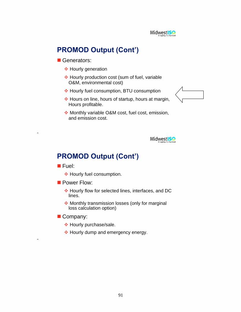
91
45
PROMOD Output (Cont’)
Generators:
Hourly generation
Hourly production cost (sum of fuel, variable O&M, environmental cost)
Hourly fuel consumption, BTU consumption
Hours on line, hours of startup, hours at margin, Hours profitable.
Monthly variable O&M cost, fuel cost, emission, and emission cost.
46
PROMOD Output (Cont’)
Fuel:
Hourly fuel consumption.
Power Flow:
Hourly flow for selected lines, interfaces, and DC lines.
Monthly transmission losses (only for marginal loss calculation option)
Company:
Hourly purchase/sale.
Hourly dump and emergency energy.

92
48
Economic Benefit
To capture the economic benefit of transmission upgrade: run two PROMOD cases, one with transmission upgrade, one without. For each case, calculate (for each region):
• Load Cost = Load LMP * Load
• Adjusted Production Cost = Production Cost + Import * Load Weighted LMP (or) - Export *Gen Weighted LMP
Economic Benefit:
• Load Cost Saving: Load Cost difference between two cases;
• Adjusted Production Cost Saving: Adjusted Production Cost difference between two cases
• RECB II Benefit = sum over all regions (30%* Load Cost Saving + 70%*Adjusted Production Cost Saving)
49
Example: 5 Bus Power Network
d
2
200 MW
Load
4
300 MW
Load
3
100 MW
Load
1
5
600 MW unit
@$30
400 MW unit
@$15
Region 1
Region 2
RECB:
Regional
expansion
criteria and
benefits

93
50
Region 1:Import: 150 MWH
Load Weighted LMP =
(-3,000+4,500)/(100+200)
=5$/MWH
Load Cost = -3,000 + 4,500
= 1,500$
Adjusted Production Cost =
2,250$+150MWH*5$/MWH
=3,000$
5 Bus Power Network (Original) – PROMOD result
50 MW
2
Load: 200 MW
LMP: -15$/MWH
Load Cost: -3,000$
43
1
5
Gen: 150 MW
LMP: 15$/MWH
Prod. Cost: 2,250$
Gen: 450 MW
LMP: 30$/MWH
Prod. Cost: 13,500$ Load: 100 MW
LMP: 45$/MWH
Load Cost: 4,500$
Load: 300 MW
LMP: 75$/MWH
Load Cost: 22,500$
Line is binding
Region 2:Export: 150 MWH
Gen Weighted LMP
=30$/MWH
Load Cost = 22,500$
Adjusted Production
Cost = 13,500$
- 150MWH*30$/MWH
=9,000$
51
Region 1:Export: 100 MWH
Gen Weighted LMP =
=30$/MWH
Load Cost = 6,000 + 3,000
= 9,000$
Adjusted Production Cost =
6,000$-100MWH*30$/MWH
=3,000$
5 Bus Power Network (After upgrade) – PROMOD result
47 MW
2
Load: 200 MW
LMP: 30$/MWH
Load Cost: 6,000$
43
1
5
Gen: 400 MW
LMP: 30$/MWH
Prod. Cost: 6,000$
Gen: 200 MW
LMP: 30$/MWH
Prod. Cost: 6,000$ Load: 100 MW
LMP: 30$/MWH
Load Cost: 3,000$
Load: 300 MW
LMP: 30$/MWH
Load Cost: 9,000$
Region 2:Import: 100 MWH
Load Weighted LMP
=30$/MWH
Load Cost = 9,000$
Adjusted Production
Cost = 6,000$+
100MWH*30$/MWH
=9,000$
New Line

94
52
5 Bus Power Network – New Transmission RECB II Benefit
Original Case Case with New Line
Load Cost
Adjusted
Production
Cost
$1,500
$3,000$3,000
$9,000
Saving
$-7,500
$0
RECB II Benefit = 70% * 0 +30% * (-7,500+13,500) = $1,800
Load Cost
Adjusted
Production
Cost
$22,500
$9,000$9,000
$9,000 $13,500
$0
Re
gio
n 1
Re
gio
n 2
Joint Coordinated System Plan Overlay

95
20% Wind Energy Scenario
Without and With the JCSP
Overlay
Annual Generator Location Marginal Prices

96
2
Value-based Planning Process at Midwest ISO
•Step 1 – Multi-Future Regional
Resource Forecasting
•Step 4 – Test Conceptual
Transmission for Robustness
•Step 7 - Cost Allocation
Analysis
•Step 3 – Design Conceptual
Trans. Overlays by Future
•Step 2 – Site Generation and
Place in Powerflow Model
•Step 5/6 – Core Conceptual
Transmission Development
•Step 5/6 – Perform Reliability
Assessment on Overlays

97
Appendix
[1]http://www05.abb.com/global/scot/scot221.nsf/veritydisplay/581366a0c2
12c93ac1256fda00488562/$file/Gridview%20Brochure.pdf
[2] http://seekingalpha.com/author/mark-henwood
[3] R. Sullivan, “Power System Planning,” McGraw Hill, 1977.
[4] International Atomic Energy Agency, “Expansion planning for electrical
generation systems,” Technical Reports Series No 241, 1984, available at
http://www.energycommunity.org/documents/IAEATRS241.pdf.
[5] X. Wang and J. McDonald, “Modern Power System Planning,”
McGraw-Hill, 1994.
[6] International Atomic Energy Agency, “Expansion planning for electrical
generation systems,” Technical Reports Series No 241, 1984. [7] S. Wang and M. Baran, “Reliability assessment of power systems with wind power
generation,” Proceedings of the IEEE Power and Energy Society General Meeting, 2010.