t2-eta presentation
TRANSCRIPT
The T2-ETA Congestion Pricing ModelFrom:
Dial, Robert B. “Network-Optimized Road Pricing: Part I: AParable and a Model.” Operations Research 47, no. 1 (1999):
54-64.
July 11, 2011
Model Overview
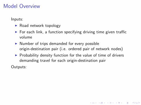
Inputs:
I Road network topology
I For each link, a function specifying driving time given trafficvolume
I Number of trips demanded for every possibleorigin-destination pair (i.e. ordered pair of network nodes)
I Probability density function for the value of time of driversdemanding travel for each origin-destination pair
Outputs:
I A user equilibrium traffic assignment which is at least locallysystem optimal.
I A set of tolls for each link that implements that trafficassignment.
Model Overview
Inputs:
I Road network topology
I For each link, a function specifying driving time given trafficvolume
I Number of trips demanded for every possibleorigin-destination pair (i.e. ordered pair of network nodes)
I Probability density function for the value of time of driversdemanding travel for each origin-destination pair
Outputs:
I A user equilibrium traffic assignment which is at least locallysystem optimal.
I A set of tolls for each link that implements that trafficassignment.
Model Objects
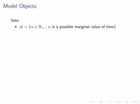
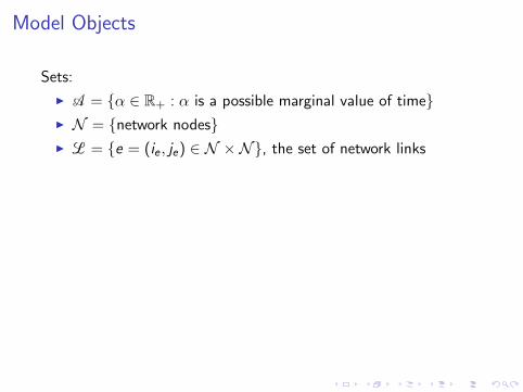
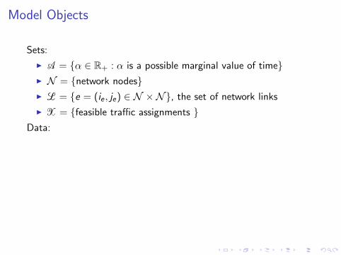
Sets:
I A = {α ∈ R+ : α is a possible marginal value of time}I N = {network nodes}I L = {e = (ie , je) ∈ N ×N}, the set of network links
I X = {feasible traffic assignments }Data:
I G = {N ,L}, the network
I te : R+ → R+, the volume-time function for link e ∈ L
I fod : A → R+, the value of time PDF of trips going fromo ∈ N to d ∈ N
I vod ∈ R+, the (fixed) total demand for trips from o ∈ N tod ∈ N
Model Objects
Sets:
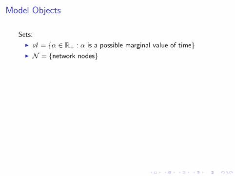
I A = {α ∈ R+ : α is a possible marginal value of time}
I N = {network nodes}I L = {e = (ie , je) ∈ N ×N}, the set of network links
I X = {feasible traffic assignments }Data:
I G = {N ,L}, the network
I te : R+ → R+, the volume-time function for link e ∈ L
I fod : A → R+, the value of time PDF of trips going fromo ∈ N to d ∈ N
I vod ∈ R+, the (fixed) total demand for trips from o ∈ N tod ∈ N
Model Objects
Sets:
I A = {α ∈ R+ : α is a possible marginal value of time}I N = {network nodes}
I L = {e = (ie , je) ∈ N ×N}, the set of network links
I X = {feasible traffic assignments }Data:
I G = {N ,L}, the network
I te : R+ → R+, the volume-time function for link e ∈ L
I fod : A → R+, the value of time PDF of trips going fromo ∈ N to d ∈ N
I vod ∈ R+, the (fixed) total demand for trips from o ∈ N tod ∈ N
Model Objects
Sets:
I A = {α ∈ R+ : α is a possible marginal value of time}I N = {network nodes}I L = {e = (ie , je) ∈ N ×N}, the set of network links
I X = {feasible traffic assignments }Data:
I G = {N ,L}, the network
I te : R+ → R+, the volume-time function for link e ∈ L
I fod : A → R+, the value of time PDF of trips going fromo ∈ N to d ∈ N
I vod ∈ R+, the (fixed) total demand for trips from o ∈ N tod ∈ N

Model Objects
Sets:
I A = {α ∈ R+ : α is a possible marginal value of time}I N = {network nodes}I L = {e = (ie , je) ∈ N ×N}, the set of network links
I X = {feasible traffic assignments }
Data:
I G = {N ,L}, the network
I te : R+ → R+, the volume-time function for link e ∈ L
I fod : A → R+, the value of time PDF of trips going fromo ∈ N to d ∈ N
I vod ∈ R+, the (fixed) total demand for trips from o ∈ N tod ∈ N
Model Objects
Sets:
I A = {α ∈ R+ : α is a possible marginal value of time}I N = {network nodes}I L = {e = (ie , je) ∈ N ×N}, the set of network links
I X = {feasible traffic assignments }Data:
I G = {N ,L}, the network
I te : R+ → R+, the volume-time function for link e ∈ L
I fod : A → R+, the value of time PDF of trips going fromo ∈ N to d ∈ N
I vod ∈ R+, the (fixed) total demand for trips from o ∈ N tod ∈ N

Model Objects
Sets:
I A = {α ∈ R+ : α is a possible marginal value of time}I N = {network nodes}I L = {e = (ie , je) ∈ N ×N}, the set of network links
I X = {feasible traffic assignments }Data:
I G = {N ,L}, the network
I te : R+ → R+, the volume-time function for link e ∈ L
I fod : A → R+, the value of time PDF of trips going fromo ∈ N to d ∈ N
I vod ∈ R+, the (fixed) total demand for trips from o ∈ N tod ∈ N

Model ObjectsDecision Variable:
I Let xoe(α) : A → R+ give the number of trips using link eoriginating at node o and having value of time α.
I Then the decision variable can be written asx = (xoe(α)) ∈ R|N |×|L|×|A|+ .
State Variables:
I xe(α) =∑
o∈N xoe(α), the number of trips with value of timeα ∈ A using link e ∈ L
I xe =∫
A xe(α)dα, the total number of trips using link e ∈ LI ue =
∫A αxe(α)dα, the first moment of α ∈ A on link e ∈ L,
or the combined value of time of all drivers using link e, notto be confused with the value of the total time spent by allthe drivers on link e
I αe = E [α|e] = ue/xe , the mean value of time for all tripsusing link e ∈ L
I ce = αexet′e(xe), the marginal social cost in congestion of
using link e, and the system-optimal toll in user equilibrium

Model ObjectsDecision Variable:
I Let xoe(α) : A → R+ give the number of trips using link eoriginating at node o and having value of time α.
I Then the decision variable can be written asx = (xoe(α)) ∈ R|N |×|L|×|A|+ .
State Variables:
I xe(α) =∑
o∈N xoe(α), the number of trips with value of timeα ∈ A using link e ∈ L
I xe =∫
A xe(α)dα, the total number of trips using link e ∈ L
I ue =∫
A αxe(α)dα, the first moment of α ∈ A on link e ∈ L,or the combined value of time of all drivers using link e, notto be confused with the value of the total time spent by allthe drivers on link e
I αe = E [α|e] = ue/xe , the mean value of time for all tripsusing link e ∈ L
I ce = αexet′e(xe), the marginal social cost in congestion of
using link e, and the system-optimal toll in user equilibrium

Model ObjectsDecision Variable:
I Let xoe(α) : A → R+ give the number of trips using link eoriginating at node o and having value of time α.
I Then the decision variable can be written asx = (xoe(α)) ∈ R|N |×|L|×|A|+ .
State Variables:
I xe(α) =∑
o∈N xoe(α), the number of trips with value of timeα ∈ A using link e ∈ L
I xe =∫
A xe(α)dα, the total number of trips using link e ∈ LI ue =
∫A αxe(α)dα, the first moment of α ∈ A on link e ∈ L,
or the combined value of time of all drivers using link e, notto be confused with the value of the total time spent by allthe drivers on link e
I αe = E [α|e] = ue/xe , the mean value of time for all tripsusing link e ∈ L
I ce = αexet′e(xe), the marginal social cost in congestion of
using link e, and the system-optimal toll in user equilibrium

Model ObjectsDecision Variable:
I Let xoe(α) : A → R+ give the number of trips using link eoriginating at node o and having value of time α.
I Then the decision variable can be written asx = (xoe(α)) ∈ R|N |×|L|×|A|+ .
State Variables:
I xe(α) =∑
o∈N xoe(α), the number of trips with value of timeα ∈ A using link e ∈ L
I xe =∫
A xe(α)dα, the total number of trips using link e ∈ LI ue =
∫A αxe(α)dα, the first moment of α ∈ A on link e ∈ L,
or the combined value of time of all drivers using link e, notto be confused with the value of the total time spent by allthe drivers on link e
I αe = E [α|e] = ue/xe , the mean value of time for all tripsusing link e ∈ L
I ce = αexet′e(xe), the marginal social cost in congestion of
using link e, and the system-optimal toll in user equilibrium

Constraints
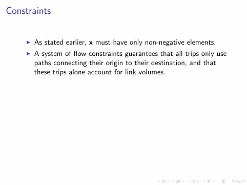
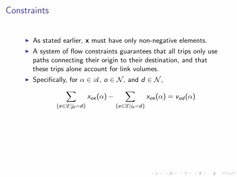
I As stated earlier, x must have only non-negative elements.
I A system of flow constraints guarantees that all trips only usepaths connecting their origin to their destination, and thatthese trips alone account for link volumes.
I Specifically, for α ∈ A, o ∈ N , and d ∈ N ,∑{e∈L|je=d}
xoe(α)−∑
{e∈L|ie=d}
xoe(α) = vod(α)
I Call any value of x satisfying the above two conditions a“feasible traffic assignment” and let X be the set of all suchassignments.
Constraints
I As stated earlier, x must have only non-negative elements.
I A system of flow constraints guarantees that all trips only usepaths connecting their origin to their destination, and thatthese trips alone account for link volumes.
I Specifically, for α ∈ A, o ∈ N , and d ∈ N ,∑{e∈L|je=d}
xoe(α)−∑
{e∈L|ie=d}
xoe(α) = vod(α)
I Call any value of x satisfying the above two conditions a“feasible traffic assignment” and let X be the set of all suchassignments.
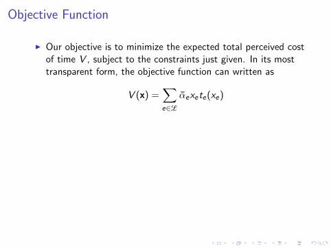
Objective Function
I Our objective is to minimize the expected total perceived costof time V , subject to the constraints just given. In its mosttransparent form, the objective function can written as
V (x) =∑e∈L
αexete(xe)
I Using the state variables already defined, we can rewrite theobjective function to eliminate αe , which is not really definedwhen xe = 0, so that the solution becomes
xopt ∈ argminx∈X
V (x) =∑e∈L
uete(xe)
copte = uopte t ′e(xopte )

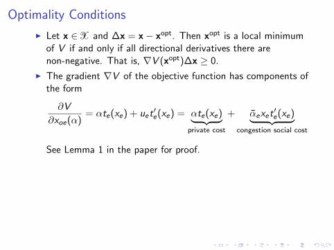
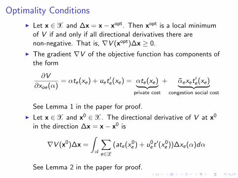
Optimality Conditions
I Let x ∈X and ∆x = x− xopt. Then xopt is a local minimumof V if and only if all directional derivatives there arenon-negative. That is, ∇V (xopt)∆x ≥ 0.
I The gradient ∇V of the objective function has components ofthe form
∂V
∂xoe(α)= αte(xe) + uet
′e(xe) = αte(xe)︸ ︷︷ ︸
private cost
+ αexet′e(xe)︸ ︷︷ ︸
congestion social cost
See Lemma 1 in the paper for proof.
I Let x ∈X and x0 ∈X. The directional derivative of V at x0
in the direction ∆x = x− x0 is
∇V (x0)∆x =
∫A
∑e∈L
(ate(x0e ) + u0e t′(x0e ))∆xe(α)dα
See Lemma 2 in the paper for proof.

Optimal Toll Problem
Let ∆x = x− xopt. V has a local minimum at xopt if and only if∫A
∑e∈L
(ate(xopte ) + uopte t ′(xopte ))∆xe(α)dα ≥ 0.

User-Optimal Equilibrium Traffic Assignment
I A traffic assignment is a user-optimal equilibrium (hereabbreviated T2-ETA) if each trip uses the path with thelowest generalized cost, while the generalized costs for all tripsis determined by and consistent with the aggregate pathchoices of all users. In the context of this model, thegeneralized cost of a driver using a particular path is the sumof all its tolls, and the value of the total time spent driving.
I Some notation: xe signifies the projection of x with respect tothe link e.
I The flow xopt = (xopte ) ∈X is a user-optimal equilibriumtraffic assignment if and only if the following variationalinequality holds for x ∈X:∫
A
∑e∈L
(αte(xopte ) + ce(xopte ))(xe(α)− xopte (α))dα
See Theorem 2 in the paper for proof.
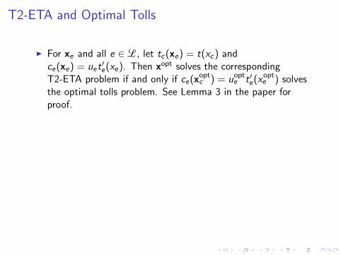
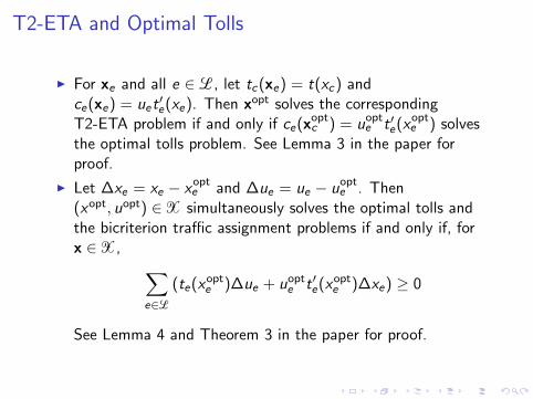
T2-ETA and Optimal Tolls
I For xe and all e ∈ L, let tc(xe) = t(xc) andce(xe) = uet
′e(xe). Then xopt solves the corresponding
T2-ETA problem if and only if ce(xoptc ) = uopte t ′e(xopte ) solvesthe optimal tolls problem. See Lemma 3 in the paper forproof.
I Let ∆xe = xe − xopte and ∆ue = ue − uopte . Then(xopt, uopt) ∈X simultaneously solves the optimal tolls andthe bicriterion traffic assignment problems if and only if, forx ∈X, ∑
e∈L
(te(xopte )∆ue + uopte t ′e(xopte )∆xe) ≥ 0
See Lemma 4 and Theorem 3 in the paper for proof.

Convexity
I There is no proof of the convexity of the objective function V(that I have found). Therefore the “optimal” trafficassignment may technically be only a local minimum V .
I However, computational results from a solution algorithm forthis model (about which I will talk next time) suggest thateither V is in fact convex, or if it is not, the practical impactis probably negligible.
I In many tests conducted by Dial, the algorithm alwaysconverged to the minimum smoothly, and traffic alwaysimproved greatly. No matter how much the initial feasiblesolution used by the algorithm was varied, the equilibriumsolutions calculated were identical.
Improvements to the Model Dynamic Assignment
I As described, the model is static. However, practicalapplications would price links differently at different times ofday. Where traffic follows a regular pattern and is stable for adecent period of time, say for rush hour and the middle of thenight, the static model could probably be applied reasonablywell by considering the two times separately. This will notwork with a large time resolution, however. A dynamic modelis necessary to account for the delaying of departure or arrivaltimes to avoid tolls.
I Dial offers suggestions for making the model dynamic, withthe only major drawback that the solution algorithm becomesmore computationally intensive. However, Dial still believes itwould be feasible, and he tested his original algorithm on a100MHz CPU. On modern hardware, a dynamic version of themodel should be easy to handle.

Improvements to the Model: Elastic Demand
I The model described assumes that demand for trips isconstant, which is unrealistic except in the short run. In thelonger run, people are likely to change their driving habits toreduce travel costs.
I Once again, Dial provides suggestions for implementationelastic demand in a straightforward manner, and he alsosuggests it would be the topic of a future paper. I have notyet found this promised paper, but if it does not exist, Dial’ssuggestions and references should be enough to expand themodel with elastic demand.