systems analysis of small-scale systems for food supply and organic waste management

Systems Analysis of Small-Scale Systems forFood Supply and Organic Waste Management

Olof Thomsson

Department of Agricultural Engineering

SLU, Uppsala

Doctoral thesisSwedish University of Agricultural Sciences

Uppsala 1999

2

Acta Universitatis Agriculturae Sueciae

Agraria 185

ISSN 1401-6249ISBN 91-576-5730-0 1999 Olof Thomsson, UppsalaTryck: SLU Service/Repro, Uppsala 1999

3

Abstract

Thomsson, O. 1999. Systems Analysis of Small-Scale Systems for Food Supply andOrganic Waste Management. Doctor's dissertation.ISSN 1401-6249, ISBN 91-576-5730-0

In this thesis, systems for recycling of household organic waste (easily degradable foodwaste and sewage water) and small-scale systems for food supply were evaluated to seeif they could be environment and energy-conserving options. They were evaluated usingsimulation of static substance-flow models (SFA) combined with life cycle assessmentmethodology (LCA) for aggregation and interpretation of the results. Three systemswere modelled and simulated: i) organic waste management (including transport,spreading on arable land and cropping of grain), ii) bread processing and distributionand finally iii) liquid milk processing and distribution.

The results were found to be very dependent on factors such as choice of systemboundaries, transport distances and type of technology. Thus, it was not possible to drawgeneral conclusions regarding the organic waste management system and the scale offood supply system which were most beneficial. However, for the organic wastemanagement system, it was concluded that toilet water-separating sewage systems are ameans to increase the rate of nutrient recycling. Furthermore, it was found that urine-separating toilet systems increase nitrogen-recycling rate and decrease energyconsumption. The results indicated that anaerobic digestion of organic wastes fromsociety and animal manure could be a system for farmers (or communities) to becomemore energy self-supporting.

With regard to the food supply system (the transport and processing chain of foodstuffs),it was concluded that energy optimised small-scale food processing and distributionsystems could have lower environmental impacts and energy consumption than large-scale systems. However for this to be successful, the advantages of small-scale must beutilised in the entire system, i.e. they should be combined with a nearby local market inorder to minimise all transport. The results obtained indicate that the processing step andthe private-car transport of food from shop to consumer’s home are the most essentialparts of the food supply system with respect to environmental impacts and energyconsumption.

Key words: environment, sustainability, energy, systems analysis, modelling, life cycleassessment, LCA, substance flow analysis, SFA, organic waste management, foodsupply, processing, transport

Author’s address: Olof Thomsson, Department of Agricultural Engineering, SLU,Box 7033, SE-750 07 UPPSALA, Sweden

5

Contents

Preface ..................................................................................................... 9

Introduction .......................................................................................... 11An interdisciplinary project...................................................................... 11General background ................................................................................ 12

Sustainable development; a human-centred concept....................................... 13Physical sustainability, basis for our existence............................................... 16

Life-supporting systems.........................................................................................16Depletion of fossil energy resources.......................................................................18Depletion of natural resources through linear material flows..................................19

Resources and food-production...................................................................... 20Systems thinking and systems analysis ..................................................... 21

Systems analysis methods............................................................................... 23Scope of the work................................................................................... 24Aims and objectives................................................................................. 26

Specific aims and objectives of the organic waste management and grainproduction systems......................................................................................... 26Specific aim and objectives of the bread processing and distribution system .. 27Specific aim and objectives of the milk processing and distribution system..... 27

Methodology.......................................................................................... 29Assessment of resources consumption and environmental impact............. 31

Impact categories included ............................................................................ 32Primary energy resources.......................................................................................32Heavy metal contamination of arable land .............................................................33Eutrophication.......................................................................................................34Global warming .....................................................................................................34Acidification..........................................................................................................35Photo-oxidant formation........................................................................................35

Impact categories excluded............................................................................ 36Validation ............................................................................................... 36Nomenclature.......................................................................................... 37

Organic waste management system...................................................... 39System boundaries................................................................................... 39Assumptions............................................................................................ 43Scenarios ................................................................................................ 43Models.................................................................................................... 45

Sources.......................................................................................................... 46Clean water production................................................................................. 48Treatments..................................................................................................... 49Transport....................................................................................................... 55Spreading on arable land............................................................................... 56

6

Acreage requirement...................................................................................... 57Agriculture .................................................................................................... 58

Results and discussion of the organic waste management study ............... 61Plant nutrients, dry matter, and water in waste fractions............................... 61Plant nutrients recycled to arable land.......................................................... 62

Urine separation; nutrient recycling .......................................................................63Additional yield of grain................................................................................ 64Heavy metal recycling rate and contamination of arable land........................ 67

Recycling of heavy metals from household residues...............................................67Heavy metal contamination of arable land .............................................................70

Energy turnover ............................................................................................. 71Biogas from anaerobic digestion............................................................................73Urine separation; energy consumption and transport..............................................75Energy efficiency...................................................................................................76

Primary energy resources consumption.......................................................... 77Eutrophication............................................................................................... 78Global warming............................................................................................. 79Acidification .................................................................................................. 81Photo-oxidant formation................................................................................ 82Summary of results, organic waste management............................................ 84

Sensitivity analyses; organic waste management ...................................... 88Electricity produced in oil-fired power plant.................................................. 88

Global warming .....................................................................................................88Acidification ..........................................................................................................89Photo-oxidant formation........................................................................................90Primary energy resources and eutrophication.........................................................92Summary of results; oil-fired electricity production...............................................92

Local transport distance set to 10 km............................................................. 94Energy turnover.....................................................................................................94Environmental impacts ..........................................................................................95

Bread production system...................................................................... 97System boundaries .................................................................................. 97Assumptions ........................................................................................... 98Scenarios ................................................................................................ 99Models.................................................................................................. 101

Clean water production............................................................................... 102Grain processing ......................................................................................... 102

Grain drier ...........................................................................................................102Flour-mill.............................................................................................................103

Bakery ......................................................................................................... 104Packaging.................................................................................................... 105

Packaging material waste handling ......................................................................107

7

Transport..................................................................................................... 109Transport of grain from field to drier................................................................... 109Long-distance grain transport............................................................................... 109Inter-regional bread transport............................................................................... 109Local bread distribution ....................................................................................... 109Private car transport............................................................................................. 110

Results and discussion of the bread production system........................... 111Energy consumption..................................................................................... 111

Energy consumption hotspots............................................................................... 112Primary energy resources ............................................................................ 114Global warming........................................................................................... 115Eutrophication............................................................................................. 116Acidification ................................................................................................ 116Photo-oxidant formation.............................................................................. 118Summary of results, bread production system............................................... 120

Sensitivity analyses; bread production system ........................................ 122Fill-up heat from fossil oil ........................................................................... 122Electricity produced in oil-fired power plant................................................ 122

Global warming ................................................................................................... 122Acidification........................................................................................................ 123Photo-oxidant formation...................................................................................... 124Eutrophication..................................................................................................... 124Summary, sensitivity analysis of oil-fired power production................................ 125

Rational scenarios gas-fired instead of electrically heated........................... 126Imported grain............................................................................................. 127

Liquid milk production system........................................................... 129System boundaries................................................................................. 129Scenarios .............................................................................................. 130Models.................................................................................................. 131Results and discussion of the liquid milk production system................... 132Sensitivity analyses; milk production system.......................................... 135

Electricity produced in oil-fired power plant................................................ 135Processed milk not transported inter-regionally........................................... 135

Cyclic small-scale food systems – an example .................................... 137

General discussion............................................................................... 141Organic waste management ................................................................... 141Food production and processing............................................................ 144Cyclic food systems............................................................................... 145Computerised mathematical models as a tool......................................... 148

Conclusions ......................................................................................... 149

References............................................................................................ 151

8

Acknowledgements ............................................................................. 163

Appendices .......................................................................................... 165Appendix 1. Sludge separator and infiltration model data ...................... 165Appendix 2. Liquid compost and peat filter model data. ........................ 167Appendix 3. Tractor and spreading model data...................................... 169Appendix 4. Transport model data; bread production study. .................. 171Appendix 5. Grain drier and mill model data.......................................... 174Appendix 6. Bakery and packaging model data...................................... 177Appendix 7. Packaging waste handling model data ................................ 183Appendix 8. Dairy model data. .............................................................. 185Appendix 9. Soil heavy metal balance – an example............................... 188

9

PrefaceThis thesis was written for the purposes of a Doctoral Degree in AgriculturalEngineering. Hopefully you will also find it useful and instructive in your searchfor more knowledge about technical and natural resources aspects of plant-nutrient (re-)cycling and food supply systems. To non-scientist readers I want tosay – Don’t think that what you read in this book is the Truth. It is merely anattempt to learn more about the complex things that we call society and reality.

This thesis and the research behind it are my way of trying to contribute to asustainable development of our society. This is because I am deeply concerned bywhat our lifestyle and "modern" society bring about in the form of environmentaldisruptions, depletion of natural resources, too great a dependence on importedresources and weird social structures fostering people who not understand theirrole in a larger context. My belief is that, if we continue "the race" full-speedstraight-ahead as we have done so far, it will end up in a crash, with enormoussuffering for the humans in existence at that time. I do not wish that for mychildren Tor and Björn, or their children, or grandchildren….

Ultuna, August 1999

Olof Thomsson

,Q WKHRU\� WKHUH LV QR GLIIHUHQFHEHWZHHQ WKHRU\ DQG SUDFWLFH� EXWLQ SUDFWLFH WKHUH LV�

9LQW &HUI �

10

'H MlU VNLOOQHG SD WL WUR X YLWl�6n PLNl WURU MD L DOOD IDOO DWW MD YDLW�

)|UUH MXOJUDQVI|UVlOMDUHQ $ / 6NRJ �

,W·V GLIIHUHQFH EHWZHHQ EHOLHYLQJ DQG NQRZLQJ�

7KDW PXFK� DW OHDVW� , EHOLHYH , NQRZ�

�7KH IRUPHU &KULVWPDV�WUHH VDOHVPDQ $OQXV )RUUHVW� �

11

Introduction

This thesis deals with natural resources issues and small-scale food systems. Inorder to show why and in what context the work has developed, I first present theproject organisation and a quite extensive outline of the general background. Thegeneral background – including many "soft" humanistic issues – is also importantfor the understanding of the issues which are of concern, and the potentialusefulness of this essay.

An interdisciplinary projectThis is the first doctoral thesis produced within the interdisciplinary project "ToIntegrate Farms and Existing Housing Areas". This project is a joint effortbetween the Departments of Agricultural Engineering, Ecology and CropProduction Science and Landscape Planning Ultuna at the Swedish University ofAgricultural Sciences (SLU). Subjects of major concern in the project areresource management, agroecology, and landscape planning. One licentiate thesiswas published in October 1998 (Eksvärd, 1998).

The main hypothesis in this interdisciplinary project was that a closer integrationbetween housing areas and agricultural farms is positive. From an environmentaland natural resources perspective, it could for example lead to plant nutrients andorganic matter being returned to the soil and environmental impacts beingreduced. Furthermore, food transport distances might be drastically shortened andthe need for packaging minimised. From a social and pedagogical viewpoint,integration between farms and existing housing areas could play an important rolebecause such integration demands "face-to-face" meetings, both between peopleand functions in the system. This would, for example, probably lead to betterunderstanding of where food comes from and waste goes to, and to what use thewaste could be put – i.e. a better understanding of the real life-supportingsystems.

The basic idea of the joint project was to study close integration ofgeographically-defined housing areas with one or a few specific agriculturalfarms at up to 3 km distance (walking distance), i.e. local food-supply systems.The general aim was to describe and analyse the effects of, and possibilities for, acloser integration between housing areas and agricultural farms, and to developtools that could be useful when implementing such integration in reality. Thework in the project was carried out through systems analysis using bothformalised and descriptive models.

Funding was provided by The Swedish Environmental Protection Agency; TheSwedish Council for Planning and Co-ordination of Research; The Faculty ofAgriculture, Landscape Planning, and Horticulture at SLU; and The SwedishCouncil for Building Research.

12

General backgroundThe driving force for my research arises from a "common-sense" awareness of thefact that the present development of industrialised society is not sustainable.Human society causes ever-increasing environmental disruptions and depletion ofnatural resources. Furthermore, it is very dependent on non-renewable (fossil)resources. These problems are probably not a threat to life itself – but they pose asignificant risk to human welfare and to the existence of our culture.

One important scientific theory, lying behind the fear of catastrophe if we do notchange our use of natural resources, is the "pulsing paradigm" presented by H.T.Odum (in e.g. 1994 and 1996). The paradigm in itself does not say anythingabout catastrophes or environmental problems, but results obtained using thistheory may well do so. The paradigm suggests that all developing systems arepulsing – not approaching a steady state as previously suggested by manytheories. The theory has been validated against the real performance of manyecological and economical systems. It is also confirmed by the fact that a steady-state type of sustainability may not be possible because short-term advantagefavours consumers that use up accumulated reserves. The pulsing paradigm iscoupled to the "maximum power principle" discussed later. Figure 1 shows anexample of a mathematically simulated pulsing system.

Figure 1. Growth, climax, and descent as part of a longer-range sustainable oscillation.(after Odum, 1996)

13

Long periods with net production of primary products ("capital" or resources) andsome growth of consumers are followed by shorter periods of frenziedconsumption. After the climax, when the phase of descent starts, bothconsumption and number of consumers decrease drastically. If we assume thatFigure 1 reflects the situation for our society, we are probably in the climaxphase. During the 20th Century, much natural capital has been used up to developgrowth of economic assets, but in the next stage there may be a rebuilding ofenvironmental resources with a decline in developed assets (Odum, 1996). Whatwill happen to humanity when we approach the phase of descent? Manyarguments can surely be raised against this "scenario of disaster", but the risk thatit can be at least partly true makes it worthwhile to consider a change in ourutilisation of and dependence on resources. What one can hope is that we findnew resources and technologies that flatten out the consumption curve and thatthe phase of descent not will be as brutal as forecast in Figure 1.

However, there is not just one problem we face, but several. In the following, Iwill try to give a more structured picture of different aspects of the sustainabledevelopment, environmental problems and depletion of resources we need to takeinto consideration if we want to sustain our society and food production.

Sustainable development; a human-centred conceptSustainability and sustainable development have been the subject of much debate,maybe because what we define to be sustainable is highly dependent on thecontext. It should be noted that the subject is development – not growth. Growthis a quantitative increase on a physical scale, while development is qualitativeimprovement or unfolding of potentialities (Daly, 1990). An example, the authorstates that "Since the human economy is a subsystem of a finite global ecosystemwhich does not grow, even though it does develop, it is clear that growth of theeconomy cannot be sustainable over long periods of time". Furthermore,sustainability is not something which is achieved and then retained. Rather, it is aprocess with a moving target towards which we ought to strive (Flora, 1994), i.e.sustainable development.

There are many opinions as to whether sustainable development really is possibleand, if so, of what it consists. One early definition was given by the BrundtlandReport (World Commission on Environment and Development, 1987); "… meetthe needs of the present without compromising the ability of future generations tomeet their needs". This has been further developed to "a development that securesthe material preconditions for the satisfying of today’s needs without endangeringthe material preconditions for future generations to fulfil their needs" (Helmfrid,1992). These definitions, like many others, are anthropocentric, i.e. it is the livingconditions for human beings that have to be sustained and secured. Both thesedefinitions have long time-perspectives. However, it is important to rememberthat we also have to be sustainable in the short run – we need to survive the dayto be able to think about the future. In fact, there are six types of resources that

14

need to be managed properly to maintain sustainability and resilience in anycommunity: natural, individual, social, historical, organisational, and economic(Berg & Nycander, 1997). Thus, short-term economics are important, but shouldnot be the only measure that decides our actions, as is the case to a large extenttoday.

A broad definition of sustainable developing systems that still comprises manymeasurable details with the potential for use as indicators for assessment ispresented in Eksvärd (1998). The definition consists of three different equallyimportant parts. These concern prerequisites for biological and living systems,prerequisites for human social activities and resource management from aphysical point of view ("The Four System Conditions"). The first two parts arepresented below and the third part is presented under the heading “Physicalsustainability, basis for our existence”.

The systems prerequisites valid for any biological organism or a living system,e.g. societies, have been described by Berg & Nycander (1997). It is argued thatevery sustainable developing system must be able to: a) support itself, b) adapt tochanging situations, c) reproduce both new generations as well as knowledge andculture, d) maintain its boundary functions; i.e. both preserve identity and allowinteractions, and e) control the system; e.g. make laws and plans, maintain amarket and stimulate social self-organisation.

Since most of what we think of concerning sustainable development isanthropocentric, the sustainability of the resource base makes little sense if it isseparated from the human agents who manage the environment (Redclift, 1993).Thus, it should be appropriate to include the prerequisites for human socialactivities, i.e. the human needs, in the definition. Max-Neef (1989) has identifiednine basic unexchangeable human needs: a) material support, b) security, c)appreciation, d) participation, e) creativeness, f) identity, g) freedom, h)relaxation, and i) meaning. All these should be fulfilled if a society claims to besustainable. Of course these "demands" have to be interpreted with commonsense, and differently in different situations and cultures, but in general they arerelevant.

Results from a pilot study presented in Eksvärd (1998) may give an indication ofhow important it is to have ordinary people engaged in the process of sustainabledevelopment. An assessment was conducted of the factors affecting and steeringall physical flows in a rural settlement. It was concluded that personal choices ofcitizens decide, or at least affect all of them (Paper 1 in Eksvärd, 1998). Weathermight be an exception but the burning of fossil fuels affects even that. Choices oftechnology and consumption habits turned out to be the most frequently-occurring factors which decide the physical flows, i.e. the physical sustainabilityof the society. This shows the importance of focusing on human acceptance andparticipation in a process of change that affects each and everyone’s daily life.Furthermore, to achieve sustainability, changes in attitudes and behaviour will berequired at all levels of society (Jacobson et al., 1996). The importance of getting

15

people involved in the sustainable development process is also stressed in theAgenda 21 document agreed on at the UN conference on environment anddevelopment in Rio de Janeiro, 1992 (Agenda 21, 1992).

The involvement of citizens in the development process inevitably also meansthat they have to co-operate in order to organise the development strategy. Oneimportant characteristic for well-functioning organisations on all levels isembedded in the word trust (Gibb, 1978). The so-called Gibb triangles (Figure 2)have developed out of the ideas in this book entitled Trust – A New View ofPersonal and Organizational Development.

Trust and Acceptance

Communication (interactions)

Goals

Control

regulationslaws

policies

ControlGoals

Communication(interactions)

Trust andAcceptance

a) b)

Figure 2. Different strategies of organization: a) Emphasis on Trust and Acceptance; amore self-stabilising system and b) Emphasis on Control; a system that needs laws,regulations and policies to be stable. (idea from Gibb, 1978)

The triangles are an attempt to illustrate the balance between activities needed tomake organisations function well. Organisations are human activity systems,which are fundamental in any discussion about sustainable development. The a)triangle describes the ideal situation: An organisation that relies on trust andacceptance and has well-developed communication and interactions. Goals areneeded and also a degree of control, but not too much. This is a stable systemstanding steady on the ground. The b) triangle shows how organisations and oursocieties often are organised. The emphasis is put on control and common goals.Some efforts are made on communications and interactions but too little. Trustand acceptance have a very small place. This system is more unstable and needsextensive quantities of laws, regulations and policies to be kept running.However, in reality, there is always a need for policies, laws and regulations andthus the optimal system is probably somewhere between the two triangles.

16

Physical sustainability, basis for our existenceTo create a sustainable society, we need to co-operate and have everyone takingpart in the process but ultimately physical conditions are the basis for our life. Itis the earth with its resources and ecosystems we need to nurture and take goodcare of. Thus, knowledge about physical systems is vital to be able to accomplishsustainable development. I will try to explain some different aspects of physicalsustainability below.

Life-supporting systemsThe ecosystems covering the world play an important role in primary production,air and water cleaning, noise reduction, waste assimilation and so on. It is theselife-support systems that make it possible for humans to breathe, drink and eat.The problem is that we tend to take all this work for granted because we don’tpay any money for most of it (Odum E P, 1987). Thus, knowledge about how ouractivities affect these systems is essential to prevent humanity degrading theecosystems vital for our wellbeing.

Nowadays, it is non-point pollution (originating from scattered or diffuse sourcessuch as car exhausts and runoff from agricultural fields) that places the greateststresses on the global life-supporting environment. We have managed to achievea significant reduction in point-source pollution (entering the environmentthrough e.g. chimneys, pipes, and ditches), though much still remains to be done.This is probably because such pollution can be managed at the output side (at theend of the pipe). The non-point pollution is harder to manage, since it can only becontrolled by managing the inputs to production. E P Odum (1987) calls thisInput Management.

This has been further developed in four basic principles for physical sustainabilitycalled "The Four System Conditions" by Holmberg (1995) in collaboration withthe Swedish Foundation "The Natural Step" and a large group of scientists,organisations, companies etc. (Natural Step, 1999). Those principles are thefollowing:

1) Substances from the earth's crust must not systematically increase in nature.

In a sustainable society, human activities such as the burning of fossil fuels andthe mining of metals and minerals would not occur at a rate that causes them tosystematically increase in the ecosphere. In practical terms, the first conditionrequires society to implement comprehensive metal and mineral recyclingprogrammes and to decrease economic dependence on fossil fuels.

2) Substances produced by society must not systematically increase in nature.

In a sustainable society, humans would avoid generating systematic increases inpersistent substances such as DDT, PCBs, and freon. Society needs to find waysto reduce economic dependence on persistent human-made substances.

17

3) The physical basis for the productivity and diversity of nature must notsystematically be diminished.

In a sustainable society, humans would avoid taking more from the biospherethan can be replenished by natural systems. In addition, people would avoidsystematically encroaching upon nature by destroying the habitat of other species.Society's health and prosperity depends on the enduring capacity of nature torenew itself and rebuild waste into resources.

4) We must be fair and efficient in meeting basic human needs.

Meeting the fourth system condition is a way to avoid violating the first threesystem conditions for sustainability. Considering human enterprise as a whole,we need to be efficient with regard to resource use and waste generation in orderto be sustainable. Achieving greater fairness is essential for social stability andthe co-operation needed for making large-scale changes within the frameworklaid out by the first three conditions.

As can be concluded from the four system conditions, it is not the emissions orconsumption of resources per se that are a threat to the life-support system, it istheir magnitude. During recent years, it has been proposed that the Westernindustrialised countries must decrease their consumption of resources by a"Factor 10", i.e. by 90 percent. This does not mean that the use of all materialsshould be decreased to such a large extent, but the most harmful (to humans andenvironment) might have to be completely abandoned, while others can be usedat a less drastically decreased level (Gardner & Sampat, 1999).

It is often claimed that the production of items such as e.g. cars, packaging andtelephones are more efficient concerning the use of resources per unit producedthan ever before, which is thought to lower the total consumption of resources.However – consumption is still growing due to a "growing demand" for evermore products (Gardner & Sampat, 1999). This growing demand can partly beexplained by the worldwide emergence of a "consumer-class", i.e. people withhigh enough income to afford a consumption pattern which demands a high levelof throughput of materials and energy. They own cars, TVs, dishwashers, mobilephones, etcetera, etcetera. This class is also identified by the fact thatconsumption itself has become a social measure (status) of success (Carlsson-Kanyama, 1997). This might also explain why all efficiency improvements in e.g.car engines so far have mainly been utilised in the provision of more power toachieve higher speeds, not decreased consumption of resources. Changing thispattern of living is probably vital, but it is regrettably not within the scope of thiswork.

18

Depletion of fossil energy resourcesThe development of the industrialised society is largely founded on the discoveryof fossil energy sources such as coal, oil and gas. Today we are more dependentthan ever on these energy carriers. In Sweden, about two thirds of the total energysupply comes from fossil energy sources (oil, gas, coal, uranium) (calculationfrom SwNEA, 1998). However, it should be noted that Sweden produces almosthalf of its electricity by hydropower (counted as renewable). Many othercountries are even more heavily dependent on fossil energy. For transportation,which is the fastest growing energy use sector globally (Mårtensson, 1997), fossilfuel is totally dominant.

With regard to these fossil energy resources, one can conclude that even if theexisting amounts of oil, natural gas and coal were excessive they should not beutilised, due to the high risk of climate change and other ecosystem disturbancesdiscussed above. Furthermore, and in the short-terms equally important, is thateven if the sources of fossil energy are vast, these fuels will probably becomemuch more expensive within a decade or two (Agfors, 1996; Hatfield, 1997a;Nilsson, 1997). One important reason is an increasing dominance on the marketof the OPEC-countries. Another reason is that global oil production capacity is at,or is very close to, its historical maximum. Discovery and exploration of "new"oilfields are not keeping pace with production. However, the Energy InformationAdministration of the US Department of Energy (DOE/EIA) writes: "Oil pricesare expected to remain relatively low, and resources are not expected to constrainsubstantial increases in oil demand through 2020." But this prediction assumesthat: "On the other hand, the reference case projection anticipates that as much asthree-fourths of the increase in demand over the next two decades will be met byincreases in production by members of OPEC rather than by non-OPECsuppliers. …. Some analysts suggest that OPEC might prefer and pursuesignificant price escalation through conservative capacity expansion decisionsrather than undertaking such an ambitious production expansion effort. The viewpresented in this outlook discounts such an expectation." (DOE/EIA, 1998).Furthermore, nothing is mentioned about the 40- to 50-year perspective in theDOE/EIA outlook. Other fossil resources such as tar sands, heavy oils and oilshale could possibly be refined to vehicle fuel. The problem is that thedevelopment of refinery processes will probably not be online by the time (2010-2015) they are needed (Hatfield, 1997b).

An important factor concerning the use of natural resources, especially fossilenergy reserves, is the environmental movement and public opinion. This willsurely try to force politicians to put high surcharges on the use of coal inparticular but also on fossil oil and gas and other non-renewable energyresources. In Sweden at least, awareness of environmental issues among a largepart of the population and politicians has grown quite strong during recent years.Much of this is due to broad programmes and discussions spurred on by theAgenda 21 document agreed on in Rio de Janeiro 1992 (Agenda 21, 1992).

19

Altogether, this might lead to society not having access to cheap fossil energy –or not being allowed to use it. Thus, it is of the utmost importance to plan for agenuine shortage of fossil oil now, rather than waiting for it to happen before wereact, as we did in the 1960s and 1970s. To be able to manage the situation, weprobably have to both lower energy consumption and to develop technology forthe utilisation of renewable and environmentally less disturbing energy sources orenergy carriers, e.g. solar cells, hydrogen and fuel cells and biofuels such asbiogas and ethanol.

Depletion of natural resources through linear material flowsOther non-renewable natural resources such as metal and mineral ores are alsoconsumed at a much higher rate than they are re-created. Most scientists seem toagree that the use of these fossil resources will eventually have to be very limitedbut opinions on how fast the change must be accomplished vary greatly.However, in contrast to fossil energy sources, natural resources used as materialscan be reused and recycled. It is also often possible to substitute other metals andmaterials for them.

Not surprisingly, it was concluded in a pilot study comparing two sites ofdifferent size and location (one large on the outskirts of a city and one small ruralvillage), that most physical flows go through the systems, starting in the farsurroundings and ending somewhere else in the far surroundings (Paper 1 inEksvärd, 1998). This might be called linear flow management, in contrast tocyclic flow management where the flows are reconnected. No substantialdifferences in this aspect were found, although the small settlement had some re-connected flows, i.e. the people living in the countryside are also part of thelinear-flow-society. However, one has to remember that when studying materialflows it is very important to carefully consider the choice of system boundaries toobtain a proper scale of the system studied, because in one scale or time-horizonall flows in the system appear linear and in another scale or time-horizon many ofthem appear cyclic. Natural processes such as geohydrological processes andplant-respiration often disperse matter over a wide area; i.e. the feedback processtakes place in a large part of the biosphere. These flows appear linear whenstudied on a local scale but are in fact reconnected. However, the time-span forthese processes is often long.

It should also be remembered that our immense resource consumption is not at allstrange, because when resources are abundant it is competitive to use as much aspossible. However, when resources become scarce and limiting for theperformance of the system, it is efficient to re-cycle and re-use them (Jordan,1996). This linear resource management is probably a heritage from the timewhen man believed in unlimited sources of e.g. oil and metals. Now when it isrecognised that that is not the case anymore, we have to reorganise our systems tobe cyclic in order to use sparse resources efficiently.

The need of feedback as reinforcement in systems is supported by the "maximumpower principle" presented by H T Odum (in e.g. Odum, 1987 and 1996). This

20

author has developed a concept presented by Lotka in the 1920s (Lotka, 1922a;1922b). It suggests that all self-organising systems tend to maximise the use ofpower, because systems which process more useful energy will succeed othersystems since they have more energy to handle unforeseen events and betteradaptation to changing surrounding conditions. Systems that are designed with"autocatalytic" feedback (the production in the system is the product of inputsources and feedback from storages produced in the system) maximise power.This can be explained by the fact that all energy transformations have less energyin the output (according to the Second Law of Thermodynamics), and to prevail,this lesser energy produced or stored must be able to feed back and reinforce theinput production. This is only possible if the feedback multiplies or otherwiseamplifies the process. Thus, energy transformations that do not develop thereinforcing design will not be reinforced nor long continued (Odum, 1996), i.e.they will not be sustainable.

Resources and food-productionResources essential for agricultural production are water, soil suitable forcropping, plant nutrients (as e.g. nitrogen, phosphorus, and potassium), andenergy (for cultivation, weed control, and harvesting). In industrial conventionalagriculture, the energy and nutrients used are often of fossil origin.

Estimations of the remaining available amounts of these differ greatly and thusthe estimated time left for consumption varies a lot. For oil, predictions say atleast between 40 and 200 years (Hatfield, 1997a; DOE/EIA, 1998) and forphosphorus between 200 years (reserves) and 1200 years (estimated geologicalreserves) (Louis, 1993). The resources of potassium are rarely mentioned(probably since it is not recognised as a water pollutant) but potash reservesmineable with current technology and current infrastructure are estimated to lastapproximately 250 years at current consumption levels (Louis, 1993). Potentialreserves (identified resources which demand investments in infrastructure andpossibly technological research) would suffice for 1000 years of presentconsumption level. Anyhow, this dependence on imported resources (long lastingor not) causes a structural vulnerability in agriculture. It is argued that existingSwedish and European agriculture is very vulnerable due to e.g. specialisation,long transport distances and heavy dependence on cheap, ever-flowing fossil fuelsand nutrients for crops and animals (Günther, 1995). Thus, from both anenvironmental and economic point of view there is clear motivation to startplanning for a future society that is less dependent and very efficient in the use offossil resources.

Use of organic wastes as fertilisers in agriculture might be a method to decreasethe dependence on imported resources and to use existing resources moreefficiently. It could also be a means to strengthen the feedback functions in thesystem. For quite a long time, recycling of easily degradable organic waste hasbeen discussed and carried out to some degree but, up to now, the recycling ofphosphorus in particular has been a matter for concern. This might seem a bit

21

odd, since cheap energy, and following that, nitrogen, are likely to be the firstresources to become expensive. The explanation is that phosphorus is recognisedas a major water pollutant at the same time as it is quite easily trapped bychemical precipitation. Nitrogen is also a water pollutant but is harder to catchand recycle.

Another strong argument for organic waste recycling is soil organic matter. Inmany regions of intense cropping (without animal production and grasslandfarming), which rely on chemical fertilisers, there are problems with decreasedhumus content in soils. Organic fertilisers could be a means to prevent increasedsoil erosion. In regions with fertile clay soils, like the plains in southern Sweden,soil erosion is not a matter for concern, but decreased content of organic matter inthe soil results in deterioration in soil structure and physical properties. Clay soilswith mainly annual crops are estimated to be able to produce 10-20 % largeryields of grain if their structure and physical properties are restored to the levelthey had 40-50 years ago – or today's yields could be obtained with use of lessinputs. Better soil structure would also decrease the need of tractive power, andthus energy consumption, by maybe 15-20 % (Johansson et al., 1993). However,organic fertilisers could also carry a risk for increased environmental hazards.Larger content of organic matter in soils may lead to amplified eutrophication ifproper cropping practices are not used.

In addition, human organic wastes could be an important plant nutrient source fororganic farmers, to compensate for nutrients exported in products sold. This isnot possible today due to regulations in, for example, the EU, but if methods forsuch resource utilisation are proven to be proper and hygienically safe, the ruleswill surely be changed. Besides the agricultural need, this also could be a meansto solve some of the waste disposal problems in society, or rather to change itfrom a waste problem to a question of resource utility. These arguments should,logically, have the effect of making recycling (reuse) of plant nutrients andorganic matter a more important issue on the agenda again.

Systems thinking and systems analysisAs discussed in “General background”, it is clear that both natural scienceknowledge about resources consumption and material flows, as well asknowledge in human sciences, together with people's comprehension andenthusiasm are needed to accomplish sustainable developing food supplysystems. For, as Allen et al. (1993) so clearly expressed it: "A sustainable foodand agriculture system is one which is environmentally sound, economicallyviable, socially responsible, nonexploitative, and which serves as the foundationfor future generations".

What seems to be lacking is knowledge about how to accomplish a turnaround inthe development and, maybe even more, the conviction that our changes willhave the desired effect. The latter is, I think, a healthy attitude to ensure that themeasures carried out become improvements and not just changes. Following the

22

"maximum power principle" (discussed above) it is obvious that organisms,species, cultures, etc. that want to keep a place in the system (be sustainable)have to feed back reinforcing energy (in a broad sense) to the system. Thatimplies recycling of e.g. organic material but – and it is an important but – it alsoimplies that the recycling has to promote the entire system. Recycling in itself isof no obvious value and, if it does not have a reinforcing function for the system,it will not be competitive in the long run either.

In other words, it is knowledge about the entire system that is needed. Suchknowledge can only be obtained by use of different systems analysis methods incombination with co-operation between different sciences and competencies.However, there are at least two different types of systems research method.Checkland (1989) describes the two as hard and soft systems methods. The termsystems analysis often refers to hard systems analysis, developed by engineers toanswer questions that have clear and rational causes and/or clear answers. Thequestions are of the type, how do we act to make a process work efficiently orhow do we construct a rocket that can manage to land on the moon? Soft systemsmethodology handles problem situations where human activities are involved andwhere neither questions nor answers are clear – situations of uncertainties. Thequestions are more of the type, what is making a group of people not work welltogether? The soft systems approach identifies both problems or questions thatare best handled by hard systems analysis methods and problems that should bedealt with in a soft systems approach. Starting with a hard systems method oftenhas the result that the soft questions are forgotten. This is one of the reasons forinclusion of this quite extensive chapter about the general background.

For a research method or development strategy to be able to make sustainabledevelopment operative, it has to manage evolutionary perspective at same time asit gives space for systems thinking (Helmfrid, 1992). This might be called holism(Figure 3). Conventional research, which influences the thinking in the entiresociety, is often found in the "other corner" of the diagram of thinking andperspectives.

23

staticperspective

evolutionary(dynamic)perspective

thinking inatoms

thinking insystems

reductionism

holism

Figure 3. Dimensions of thinking and perspectives. (after Helmfrid, 1992)

The term evolutionary refers to a perspective permeated by the consciousness thatevery change in the system will create other changes – everything is part of alarger context that evolves. The work presented in this thesis is definitely foundto the left in the diagram but probably more against the upper (static) sector,although an evolutionary perspective is included.

Systems analysis methodsSince "the environmental problem" has many dimensions, multi-dimensionaltools have to be used. There are several methods under development to assess theenvironmental performance of products, processes, systems, organisations,societies and so on. The different methodologies have somewhat differentpurposes, which I will not comment on any further here. What most of them havein common is the cradle-to-grave perspective, i.e. all impacts from the extractionof raw materials to the management of waste are included. The perhaps mostdeveloped method is Life Cycle Assessment (LCA). Examples of others areEcological Footprints Analysis, Environmental Space Concept, EnvironmentalImpact Assessment (EIA), Substance Flow Analysis (SFA), Material FlowAnalysis (MFA), Environmental Accounting, Foodshed Analysis, and EMERGY

analysis.

It is, however, not only the question of multi-dimensional problems we have todeal with. Since a systems perspective is needed, it also implies that we have tohandle very complex systems. To be able to analyse such (complex) systems,computerised mathematical modelling is a powerful tool. Much knowledge is

24

gained simply by the fact that, to be able to construct sufficiently detailedmodels, one has to collect good data about the system’s structure andperformance. This kind of model also makes it possible to test e.g. differentcombinations of sub-systems, without expensive construction of the real systems.

The mathematical computer models of different systems used in the workpresented in this thesis are a type of hard system analysis combining SFA andLCA methodologies. Thus, they handle both the complexity and the multi-dimensionality. The models are used for simulation of systems with more or lesswell defined properties and behaviour.

Scope of the workThis thesis deals with natural science (hard systems) aspects of cyclic small-scalefood systems. A graphical representation of a cyclic food system as I see it in thiswork is presented in Figure 4. Dotted lines indicate the system boundaries for thestudy.

The work is presented as three separate studies of different parts of the foodsystem. First comes a study of organic waste management. This is an importantpart in the system, concerning both environmental aspects and how to get thesystem more self-dependent for plant nutrients and possibly energy. Included inthis part are also: grain production resulting from the recycling of organic wastes,nitrogen emissions from soil, energy consumption and emissions from grain-production field operations, and manure from fifteen dairy cows including youngstock, i.e. the parts of the agricultural system with direct connections to theorganic waste management system.

The second (bread production system) and third (liquid milk production system)studies concern food processing and distribution, which are also vital parts,especially concerning energy demand and environmental impacts emanating fromthe burning of fuels and production of electricity.

Other parts of concern that have not been included are the major parts of theprimary production (agriculture) and the consumption of the food (consumerphase). These are of importance for environmental impacts and consumption ofresources when the whole food system is discussed, but do not change betweenscenarios of the systems studied here.

25

Figure 4. Schematic representation of the parts in a cyclic food system.

26

Aims and objectivesThe general aim of my work has been to learn more about natural science(physical sustainability) aspects of cyclic and small-scale (locally based) foodsystems and especially the systems that connect agriculture and consumers inboth directions (Figure 5).

Figure 5. Schematic picture of a cyclic and local food supply system.

The general objective was to:

• investigate if development towards cyclic and small-scale food systems couldbe a means to decrease environmental impacts and resource consumption

• develop systems analysis tools that can be used in further case studies and inplanning of real-world sustainable development projects.

Specific aims and objectives of the organic waste management and grainproduction systems The primary issues of concern in this part of the work are recycling of plantnutrients to arable land, expected additional yield of grain resulting from therecycling, energy turnover, and environmental impacts.

The objectives of the organic waste management part of the work were:

• to establish knowledge about the flows of plant nutrients and heavy metals insmall-scale handling system for household wastewater and organic wastes

• to evaluate the importance of flows of household residues compared to theflows of organic residues in agriculture

• to evaluate to what extent these flows can be of importance for agriculture

• to compare different organic waste treatment systems concerningenvironmental impact and consumption of natural resources

• to find efficient (in terms of resource utilisation) recycling systems, whichthus contribute to producing much food and at the same time are energy self-supporting or, even better, net energy-producing

27

Specific aim and objectives of the bread processing and distribution system The aim of the bread production part was to compare large-scale and small-scalefood processing systems and the transport connected to them from an energy andenvironmental point of view.

The objective of the study of bread production systems was:

• to identify important parts in the systems, and to assess their importance forthe whole system

• to establish if long-distance transport is as important as many want to believe

• to evaluate if internal energy efficiency in large-scale facilities is as importantas others claim

Bread was chosen because it is a staple food that is produced all year round andcan easily be produced on different scales. Furthermore, local as well as importedraw products can be used.

Specific aim and objectives of the milk processing and distribution systemAn introductory study of milk processing and distribution was performed in orderto give knowledge comparable to that obtained in the bread production study. Theobjective was to create a broader picture of the system for food processing and toassess the generality of the results obtained in the bread production study. Thus,the same system boundaries as in the bread production study were used in thisstudy.

Milk was chosen to represent a different type of staple food. It is not easilystored, it contains a lot of water (i.e. more energy demanding to transport) and thelarge-scale advantages in its processing are presumed to be larger.

29

Methodology

Cyclic food-supply systems are large and complex. They have many interactionsboth between parts within the system and with other systems. Thus, a systemsanalysis approach is necessary to analyse such a system. Figure 6 shows aconceptual representation of the properties of the system under study.

Transports

Food

Energyturnover

Emissionsto air and

water

Treatment(s)

Sources (as e.g. organic waste):containing plant nutrients, organicmatter, heavy metals, water, etc.

Transports

Energy

Crop production incl.field operations

Transports

Processing

Transports

Figure 6. Conceptual representation of a cyclic food system from a energy andenvironmental emissions point of view.

30

When the issues of concern are quantifiable, mathematical computerised modelsare powerful tools. The model approach makes it possible to perform experimentson whole systems without (or before) constructing them in reality. It also gives anopportunity to compare the performance and importance of different parts in thecontext of the entire system. Furthermore, it is possible to make sensitivityanalyses and thus investigate if and how changes in parts of the system will affectthe total. Since one of the objectives with the study was to determine the flows ofplant nutrients and organic matter etc., a substance flow analysis (SFA) modelwas needed. For the environmental impact assessment, other methods such as e.g.life cycle assessment (LCA) were needed. A SFA model for assessment ofmunicipal organic waste and wastewater management, which may be combinedwith several elements of an life cycle assessment, has been developed in Sweden(Dalemo et al., 1997). The concept of this model, called ORWARE (ORganicWAste REsearch) was found to suit the purpose of the present study well.

Thus, the work presented in this thesis has been carried out through mathematicalmodelling and simulation following the ORWARE modelling concept. Themodels are modular, i.e. each part of the real system is described in sub-modelsthat may be combined to models of different systems. The researcher choosessources, treatments or processes, transport and spreading or distributiontechnology. The models are linear and mainly static. No optimisation is carriedout in the models. Each sub-model calculates the degradation of its incomingmaterial, formation of new substances, division of the material flow(s) intoseveral outputs (e.g. sludge, gases and outlet water), and energy turnover. Modeloutputs are yearly averages of sub-processes and the entire system respectively.The models are programmed in the software Matlab/Simulink (TheMATHWORKS Inc., 1997).

The models used in this study are thoroughly described in the chapters "Organicwaste management system", "Bread production system", and "Milk productionsystem".

Like the original ORWARE sub-models, those developed here had a vector of 43positions, i.e. 43 different substances (or in some cases, groups of substances)were included in the calculations. However, due to lack of data in severalprocesses, only some of these positions were used in this study. For example, itwas not possible to include polyaromatic hydrocarbons (PAH) and adsorbableorganic halogens (AOX). The positions used in the outputs are described in Table1.

31

Table 1. The output variables.

Abbreviation Remarks

N-tot Total nitrogen

N-NH3/NH4+ Nitrogen in ammonia and/or ammonium

N-NO3- Nitrogen in nitrate

P Phosphorus

K Potassium

CO2-f Carbon dioxide of fossil origin

CO Carbon monoxide

CH4 Methane

VOC Volatile Organic Compounds, e.g. un-combustedhydrocarbons from engines

N-NOx Nitrogen in nitrogen oxides

N-N2O Nitrogen in dinitrogen oxide (laughing gas)

S-SOx Sulphur in sulphur oxides

Cl Chlorine

Pb Lead

Cd Cadmium

Hg Mercury

Cu Copper

Cr Chromium

Ni Nickel

Zn Zinc

C-total Total carbon

COD Chemical Oxygen Demand

BOD7 Biological Oxygen Demand during 7 days

VS Volatile Solids (=DM minus ash)

DM Dry Matter

H2O Water

Assessment of resources consumption and environmental impactThe environmental impact was assessed using LCA methodology. First, all inputsand outputs were classified, i.e. grouped in environmental impact categories.Each substance may fall into one or several impact categories. Step 2 was thecharacterisation, where the relative contribution of each substance within theimpact category was assessed and all contributions in the category wereaggregated. Lindfors et al. (1995) propose 15 impact categories (Table 2) thatshould be reported, or at least commented on. These can be further divided intosub-categories.

32

Table 2. List of impact categories (Lindfors et al, 1995)

Impact categories

1. Resources – Energy and materials

2. Resources – Water

3. Resources – Land (including wetlands)

4. Human health – Toxicological impacts (excluding work environment)

5. Human health – Non-toxicological impacts (excluding work environment)

6. Human health impacts in work environment

7. Global warming

8. Depletion of stratospheric ozone

9. Acidification

10. Eutrophication

11. Photo-oxidant formation

12. Ecotoxicological impacts

13. Habitat alterations and impacts on biological diversity

14.# Inflows which are not traced back to the system boundary between the technical systemand nature

15.# Outflows which are not followed to the system boundary between the technical systemand nature

# Not impact categories but should be included

Impact categories includedI chose to include six of the impact categories (or parts of them). These were:consumption of primary energy and water resources, heavy metal contaminationof arable land (ecotoxicological impact), eutrophication, global warming,acidification and photo-oxidant formation. The first three were chosen since theymay differ between the different scenarios studied. The latter three are largely aneffect of energy consumption, chosen since that is the major difference betweenscenarios in primarily the food production (bread and milk) study.

Primary energy resourcesTo be able to make a comparison between scenarios which use much electricitywith those mainly using fuels, energy consumption was traced back to theconsumption of primary energy resources. This measure was an attempt toconsider the resources consumption in the lifecycle of the energy carriers. It didnot evaluate the differences in energy quality. There are other measures, e.g.exergy, embodied energy, and EMERGY, which do, but it was not possible toinclude these in this study.

The primary energy consumption in production of average Swedish electricitydemand is shown in Table 3. Transmission losses in the distribution net (7 %),

33

pre-combustion energy consumption for fuels and efficiency in e.g. hydropowerand nuclear power are included, making 2.35 MJ primary energy per MJelectricity used. The equivalent value for electricity produced in oil-fired powerplants is 2.69 (Habersatter et al., 1998). For reasons of simplicity, I used anaverage for different fuels; 1.2 MJ primary energy per MJ fuel (calc. from Tables16.4 and 16.9 in Habersatter et al., 1998). Fuel oil, fossil gas, petrol, and biofuelsall have values ranging between 1.09 and 1.35 MJ.

Table 3. Energy resources used for average Swedish electricity use (Lundgren, 1992)

Energy resource MJ energy resource per MJ electricity

Fossil oil 0.064

Fossil gas 0.0093

Coal 0.040

Peat 0.0045

Biofuels 0.045

Uranium1 1.60

Hydropower2 0.588

Sum 2.351 Calculated as MJ in uranium. 35 % efficiency is used in the conversion of MJ nuclear electricity to MJ in

uranium, i.e. 35 % of the theoretical heat obtained in the fission process can be utilised as electricity.

2 Calculated as MJ potential energy. 80 % efficiency is used in the conversion of MJ electricity to MJ potentialenergy.

Heavy metal contamination of arable landThe seven most commonly measured heavy metals were included in theassessment (Table 4). These metals are those included in the Swedish regulationsfor heavy metal content in sewage sludge spread on arable land (SFS, 1993;SNFS, 1994). No validation of their respective possible toxicity was performed.

Table 4. Heavy metals included in the environmental assessment.

Pb Lead

Cd Cadmium

Hg Mercury

Cu Copper

Cr Chromium

Ni Nickel

Zn Zinc

34

EutrophicationEutrophication may have an influence on both terrestrial and aquatic systems. Inaquatic systems, the eutrophication may lead to an increased production ofbiomass. The decomposition of biomass requires oxygen, which may lead tooxygen deficiency. Since the impact is site-specific, different scenarios arepresented by Lindfors et al. (1995). In this study the eutrophication impact wascalculated following a conservative approach by using the Maximum scenarioshown in Table 5. When making case studies, the choice has to be adjusted toconditions valid for each case.

Table 5. Eutrophication weighting factors. (kg O2-equivalent per kg compound emitted)

N to air P-limited N-limited N-limited + N to air Maximum

NOx to air 6 0 0 6 6

NH3 to air 16 0 0 16 16

NH4 to water 0 0 15 15 15

NO3 to water 0 0 4.4 4.4 4.4

P to water 0 140 0 0 140

COD to water(chemicaloxygen demand)

0 1 1 1 1

Global warmingSeveral gases contribute to the greenhouse effect. The gases that have a directglobal warming impact are CO2 of fossil origin, CH4, and N2O and these areincluded in the impact assessment. There are also gases that indirectly contributeto the greenhouse effect; e.g. non-methane hydrocarbons (NMHC), carbonmonoxide (CO), and nitrogen oxides (NOx) but no reliable data concerning theirimpact were at hand. Other substances like CFCs (freons) were not used in thesystem under study. The different gases were compared by using GlobalWarming Potentials (GWPs) weighting factors (Lindfors et al., 1995), see Table6. The GWPs were expressed as CO2 equivalents. I have chosen to use a timeframe of 100 years, since that covers a period somewhat longer than theperspective of the study, but not too long to be possible to comprehend.

The CO2 in bio-fuels was not included in the calculations as it is non-fossil, andthus does not contribute to any extra warming impact. This is at least what mostscientists claim. In this study, biofuels were a small part of the total energyconsumption, so the assumption did not have any large impact on the results.

35

Table 6. Potential global warming weighting factors. (g CO2-equivalent per g compoundemitted)

Compound 20 years 100 years 500 years

CO2-fossil 1 1 1

CH4 62 24.5 7.5

N2O 290 320 180

AcidificationThe acidification impact was calculated using the approach suggested byFinnveden et al. (1992), where the effect is defined as the amount of protonsreleased in terrestrial systems. Two scenarios are given. One that takes emissionof nitrogen compounds into account (maximum scenario), and one that does not(minimum scenario). The reason is that the nitrogen has to be leached out fromthe system to have an acidifying impact. In typical situations in Europe, some 10– 30 % are leached. Thus, in practice, acidification should be somewhere inbetween the two scenarios given. In this study, it was primarily the maximumscenario which was used.

Table 7. Acidification weighting factors. (mol H+ per g compound emitted)

Substance Minimum scenario Maximum scenario

SO2 0.031 0.031

HCl 0.027 0.027

NOx 0 0.022

NH3 0 0.059

Photo-oxidant formationWhen reporting photo-oxidant formation, only ozone production is usuallyconsidered. There are however other oxidants of environmental interest, but theyhave been less studied, according to Nordic Guidelines on Life-Cycle Assessment(Lindfors et al., 1995). Following the recommendation in that publication, twodifferent sub-categories were reported here – VOCs (Volatile OrganicCompounds) aggregated according the POCP (Photochemical Ozone CreationPotentials) concept, and nitrous oxides aggregated as NOx (NO2). The POCPswere expressed as ethene-equivalents (Table 8). The scenario suggested byHeijungs et al., which uses average peak ozone data from three trajectories, wasused. It was complemented with the POCP-factor for carbon monoxide (CO)given by Finnveden et al. (1992) (ordinary Swedish background during 0-4 days).

36

Table 8. Photochemical ozone creation potentials (POCP). (g ethene-equivalents per gemitted compound)

Compound POCP

CH4 1 0.007

VOC (Volatile organic compounds) 1 0.337

NMHC, Non methane hydrocarbons (VOC-CH4) 1 0.416

CO, ordinary Swedish background during 0-4 days 2 0.040

Ethanol 1 0.268

1 Heijungs et al., 1992

2 Finnveden et al., 1992

Impact categories excludedThe impact categories excluded might be important as well, but some of them arenot affected much by the different system choices (e.g. depletion of stratosphericozone), and some categories are not yet scientifically well documented andagreed upon (e.g. ecotoxicological impacts).

ValidationValidation of the whole-systems results is almost impossible without constructionof the real systems. Since the purpose in using modelling and simulation is to testdifferent systems without (or before) building them in practice, this was not anoption. Instead the performance of each sub-model was validated for differentconditions and validity ranges. If all sub-models are validated and run underconditions within the validity range, then the entire system put together can besaid to be validated.

37

Nomenclatureenergy consumptionthough energy cannot be consumed (or produced) in a

thermodynamical sense – just transformed to anotherquality – I will use this term as it is commonly used and inan easy way describes the delivery of energy to and fromthe systems

energy production see energy consumption

scenario (here) a model of a complete system, consisting of severalsub-models of sources, transport, treatments, processes etc.

blackwater part of the household wastewater coming from toilets

greywater part of the household wastewater coming from baths andshowers, dish- and laundry-washing

household waste here defined as easily degradable wastes originating fromfoodstuffs handled in households

organic waste here defined as easily degradable waste originating fromhousehold wastes, sewage water, and sometimes manure

manure here always used in the meaning animal manure

cyclic system reconnected systems, that feed back e.g. organic waste

food-system here the entire system producing food, i.e. includingorganic waste management and other fertiliser production

39

Organic waste management system

This chapter presents the study of organic waste management and agriculturalgrain production. It starts with methodological issues and model descriptions andthen continues with results and discussion.

Society produces several different kinds of easily-degradable organic wastes (herecalled organic wastes). Examples are park and garden waste, leftovers and refusefrom groceries and restaurants, grease separated from sewage in restaurants andfood industries, wastewater from households and food industries and wasteproducts from food industries. The latter are, however, largely utilised as animalfodder (Brolin et al., 1996). The largest proportion of all organic wastes ismanure from animals (if harvest residues left on fields are not taken intoaccount).

The treatment of organic waste can consist of biological degradation methodssuch as composting and anaerobic digestion, of incineration (which is oftenenergy-demanding due to large water content), of pyrolysis, or of landfilling.Wastewater is often treated using combinations of biological and chemicalmethods, followed by (or combined with) sludge separation. The sludge can thenbe treated by the methods mentioned above, the effluent water is often let out tosurface watercourses. Biologically treated wastewater might also be stored andused for irrigation of agricultural crops. Alternative treatments of wastewater aresource separation (i.e. no mixing of different fractions) or initial sludgeseparation, followed by sludge treatment as above and simpler treatment orpolishing of the water fraction. A broad spectrum of polishing methods is athand. Examples are infiltration in soil or constructed filter beds, vegetative filters,and wetlands.

System boundariesSince the focus in this study was the interaction between housing areas andagriculture, only household (easily degradable organic) wastes, household sewagewater and animal manure were included. However, other kinds of organic wastecould easily be included in later studies. Treatments chosen to be studied herewere current standard methods in Sweden and methods aiming at resource (plantnutrients, organic matter, and/or water) utilisation. Landfilling of organic wastewill soon be prohibited and has been shown to be a practice which is notrecommendable from an environmental point of view (Sonesson et al., 1997) andwas thus not included. Incineration was not included since the burning of organicwaste, to be practically possible, must be performed in mixed-waste incineration.The energy is utilised, although doubts about the energy value of watery wastecan be raised, but the organic matter is lost. The plant nutrients are also lost sinceit is not likely to be possible to spread ashes on arable land due to their content of

40

environmentally harmful substances. Furthermore, since the focus was on small-scale settlements, no conventional sewage plant was included but can alsopossibly be included in later studies. The parts included and the system boundaryare shown in Figure 7.

SOIL

transport(s)

spreading onarable land

field operations ingrain cropping

N fertiliserproduction

grain yield

foodindustryoffals

restaurantsand trade

P and K fertiliserproduction

grain drying,storage andmilling etc.

clean waterproduction

transportfrom field

organichousehold

waste

blackwater(urine,faeces)

greywater

animalmanure

sewageplant

P traps

incineration

wetlands

landfill

infiltration

on-sitesludge

separator

urinetank

compost liquidcompost

anaerobicdigestion

bioponds

storagereservoirs

sludgetreatmentin sewage

plant

transport(s)

heavymetals

Norganic

K P

Nmineral

pathogens

toxicorganic

substances

fuel andelectricityproduction

organicfertiliser

Figure 7. Parts included and system boundary in the organic waste management study.

41

The housing area which served as the pattern for the study was a rural settlementwith 32 households (100 inhabitants) in single-family houses and one agriculturalfarm where all residues and manure were spread. No industries or food processingplants were taken into account, since the focus in this part of the work was on theconnection between households and agriculture. The transport distances wereshort. All residue transport distances were set to two kilometres, i.e. alltreatments were situated in or nearby the village. The same was valid for thetransport from treatment to the field for spreading. The only exception was thedistance for transportation of on-site separated sludge to sewage plant and thetreated residues returned, which was 30 km. Many of the in-data were averagefigures valid for “normal” households and treatment plants in Sweden, and somewere site-specific data from the "pattern" settlement. Thus, the study should bevalid for similar locations in the southern and central parts of Sweden.

The agricultural parts included comprised the fate of nitrogen in soil, cereal fieldgrain production, energy consumption and air emissions for grain productionfield operations, energy consumption and air and water emissions from possibleadditional N-fertiliser production, and manure from 15 dairy cows includingyoung-stock. The number of animals was chosen to roughly represent the numberof animal equivalents1 per person in Sweden (Naturvårdsverket, 1989; StatisticsSweden, 1997). Since the simulated system had 100 individuals that made 0.15animal equivalent per person. All other parts of the agricultural system wereexcluded since they were assumed not to change between scenarios. In drawingconclusions about the entire food system, this is of course a weakness of thestudy, since the agricultural parts not included are likely to have largeenvironmental impacts.

In order to get the scenarios to produce equal amounts of grain, extra mineralnitrogen fertiliser was added when needed. The need was calculated as thedifference between the scenario producing the largest amount of grain (Scenario 0in Figure 8) and the actual scenario. This was accounted for as “fill-up N-fertiliserproduction” (Scenario 1 in Figure 8). In some cases, where results for householdresidues only were presented, the acreage could not produce enough grain,although mineral fertiliser was added (Scenario 2 in Figure 8). The reason wasthe large difference in acreage utilised for the spreading of organic fertiliserswhen household residues alone were considered. To compensate for thisdeficiency, additional acreage had to be included. This acreage wasconventionally cropped using mineral fertilisers. When this addition wasnecessary, the extra nitrogen fertiliser and the extra acreage were accounted for as“fill-up grain production”.

1 Animal equivalents as given by the Swedish EPA concerning “Environmental protection in animal husbandry”(Naturvårdsverket, 1989). One animal equivalent represents one full-grown cattle, three sows, ten growing-fattening pigs, etc.

42

Organic waste products

Calculated acreagerequirement (ha)

Yield of grainresulting fromorganic waste

recycling




recycling

Yield of grain resultingfrom additional

chemical fertilising




recycling

Max yield of grainresulting from

additional chemicalfertilising

Additional acreage,conventionally croppedusing optimal amount

chemical fertiliser

Yield of grain

Scenario 2

100 = 100

e.g. 80 20 = 100

e.g. 50 e.g. 20 30

Scenario 0

Scenario 1

= 100

Figure 8. Different scenarios of acreage and chemical fertiliser requirements to obtainequal production of grain in the different organic waste management scenarios. Scenario0 = the most grain-producing org. waste scenario; Scenario 1 = the org. waste scenarioswhere additional chemical nitrogen fertilising (on the acreage used for org. wastespreading) is able to rise the yield of grain to the level of Scenario 0; Scenario 2 = theorg. waste scenarios where both optimal additional chemical nitrogen fertilising (on theacreage used for org. waste spreading) and additional conventionally cropped acreage isneeded to produce as large yield of grain as Scenario 0 does.

43

Production and construction of equipment, vehicles, infrastructure, etc. were nottaken into account, i.e. only resources and energy consumed within the systemwere accounted for. The same applied to air and water emissions. This may havebeen a serious simplification of the problem, thus making the results lessrepresentative for the real system performances. However, air emissionsoccurring in the production of chemical nitrogen fertilisers, fuels and electricitywere included.

AssumptionsElectricity was assumed to be produced as Swedish average electricity use, i.e.about equal parts of hydropower and nuclear power. Minor contributions comefrom biofuels, wind, oil, and coal. Implications of the use of electricity producedin oil-fired power plant are described in the chapter "Sensitivity analyses; organicwaste management".

All local transport (all transport except that to and from the sewage plant) was 2km one-way. The scenarios were also run with these transport distances set to 10km in a sensitivity analysis presented in the chapter "Sensitivity analyses; organicwaste management".

Data for energy consumption and emissions in nitrogen fertiliser production(including transport) are average figures valid for Germany, published by Patyk(1996).

ScenariosTwelve different organic waste treatment scenarios were simulated in this study.Six different main treatments were each combined with both non-separatingtoilets as well as with urine-separating toilets.

All scenarios (except scenarios 5 and 6) had sludge separators followed byinfiltration for treatment of either all of the wastewater (scenarios 1-4) or of thegreywater (scenarios 7-12). The sludge was spread on arable land or included inthe treatments in all scenarios. The scenarios 7-12 had blackwater separatingsewage systems where grey- and blackwater were kept apart.

The twelve scenarios were:

1) SludgeToSewPlant, digestion of sludge from single household sludgeseparators in sewage plant, household waste was home-composted andrecycled to arable land. Manure was stored, transported and spreadindependently.

44

2) SludgeToSewPlantUrineSep, as 1) but human urine was separated in thetoilets and stored, transported and spread independently.

3) SludgeToAgr, spreading of sludge from single household sludge separatorson arable land without any treatment, household waste was home-compostedand recycled to arable land. Manure was stored, transported and spreadindependently.

4) SludgeToAgrUrineSep, as 3) but human urine was separated in the toilets andstored, transported and spread independently.

5) Bioponds, mechanical and biological treatments of sewage water (includinghousehold wastes) in open-air bioponds followed by storage reservoirs.Manure was stored, transported and spread independently.

6) BiopondUrineSep, as 5) but human urine was separated in the toilets andstored, transported and spread independently.

7) CompostToilet, composting of faeces, urine and household wastes. Toiletswith dry handling of the excrements. Manure was stored, transported andspread independently.

8) CompostUrineSep, human urine was separated in the toilet and stored,transported and spread independently. Faeces were separated from flush-water and composted together with household wastes. Manure was stored,transported and spread independently.

9) LiquidCompost, liquid composting of blackwater, household wastes andmanure.

10) LiquidCompostUrineSep, as 9) but human urine was separated in the toiletsand stored, transported and spread independently.

11) AnaerobDigestion, anaerobic digestion of blackwater, household wastes andmanure.

12) AnaerobDigestionUrineSep, as 11) but human urine was separated in thetoilets and stored, transported and spread independently.

The anaerobic digestion scenarios were simulated in two different modes – withor without hygienisation (heating to 70º C) of incoming material, makingfourteen scenarios in all for the energy calculations.

The scenarios 5, 6 and 9-12 included kitchen disposers to macerate and blend thehousehold waste with the sewage water.

45

ModelsThe general structure of the organic waste management model, exemplified bythe anaerobic digestion with urine separation scenario (AnaerobDigUSep), isshown in Figure 9. At the top, waste sources are initiated. Then follows the sub-models for calculation of energy turnover and emissions in treatments, transportand spreading of the wastes. Finally the soil nitrogen turnover, grain production,and field-operation energy consumption are calculated in the agriculture sub-model. This block also contains the initialisation of manure. The sub-models aredescribed in more detail below.

Figure 9. General structure of the organic waste management model. The anaerobicdigestion with urine separation scenario.

Figure 9 shows the most complicated system simulated in this study. An exampleof a simpler system, the scenario where sludge from on-site sludge separatedwastewater was transported straight to agricultural land, is shown in Figure 10.

46

Figure 10. The "SludgeToAgr" scenario.

SourcesThe sources, or input vectors, were wastewater and household wastes from 32households and manure from 15 dairy cows and their young stock.

The wastewater was defined as urine, faeces, flush water including paper, andgreywater (Figure 11). These were identical in all scenarios except for the amountof flush water which varied depending on whether or not there was urineseparation (see “Urine separation” below). The household sources have beenthoroughly described in Nybrant et al. (1996). Some minor modifications weremade following the Swedish Environmental Protection Agency “template”figures for content of nutrients and heavy metals in Swedish householdwastewater (1995). It was assumed that 75 percent of the total blackwater wasproduced at home and 25 percent at work. The latter part was not taken intoaccount. Concerning the household data, these were yearly average amountsand/or average content data assumed to be valid for “normal” households inSweden. In reality, the variation could be large due to differences in e.g. age,

47

gender and diets, but that was not possible to take into consideration in this study.In addition, no sufficiently detailed data were available.

Figure 11. The household wastewater (with urine separation) initialisation block.

In practical urine separation, the urine is sorted away “at source” (i.e. nevermixed with the faeces) in two-bowled toilets. The separation efficiency isassumed to be 80 percent, meaning that 20 percent of the urine is misplaced andthus added to the faeces fraction (Jönsson, 1997). The urine is then transported ina pipe to a storage tank where it is stored for several months. It is collected,transported and spread on arable land with a tractor-drawn liquid manurespreader. In the models, the separation is carried out by not mixing the inputflows. The only difference in incoming values is the amount of water. Forordinary toilets, it was assumed that each toilet flushing consists of 6 litres andthat each person flushed 5 times per day, making 30 litres per person and day.When urine separation was used, we assumed two big flushings of 6 litres and 5small flushings for the urine-bowl of 0.2 litres, i.e. 13 litres per person and day.

The manure sub-model is an input vector that defines the amount and content ofmanure from fifteen milking cows including young stock. The content data usedin this study came from a few measurements on liquid manure delivered to ananaerobic digestion plant (Johansson, 1997b). Thus losses of nutrients in theanimal house, storage and transport were included but the emissions due to themwere not accounted for. The content probably varies a lot depending on feedingand production strategies. This should be further examined when real case studiesare performed. The amount of manure was calculated from Claesson & Steineck(1991). The manure was handled as a slurry in all scenarios.

48

Clean water productionWater of drinking quality is used in households for different purposes. In theproduction of this water, chemicals are added to achieve hygienic and functionaldemands. The energy consumption for production and transport of thesechemicals is calculated in the model (Figure 12). In addition, energy consumed inpumping and in transport in connection with service work is also calculated. Airemissions from chemical production and all transport, as well as water emissionsfrom the chemical production, are calculated. This model was developed byKärrman (1999). Data were taken from Tillman et al. (1996) and The SwedishWater & Wastewater Association (1994). Vinnerås (pers. comm) contributed theservice transport part (unpublished data from an investigation of the fresh-waterproduction in Stockholm made in 1998).

Figure 12. Clean-water production sub-model.

49

TreatmentsVery few data seem to be available on the sludge separator process. Those thatare on hand are disparate, probably due to large variations in the functioning ofdifferent types of separators and large variations in incoming sewage watercontent. The sludge separator sub-model is shown in Figure 13.

Figure 13. The sludge separation sub-model. Upper level at left, lower level at right.

I have chosen to use the approximate cleaning efficiencies for organic material(BOD7/COD, 10 percent reduction) and suspended solids (70 percent reduction)given by the Swedish Environmental Protection Agency (1987). The proportionsof nutrients and heavy metals sedimented are calculated from measured contentsin on-site sludge separators (Andersson, 1992; Landers, 1995) and contents inincoming household sewage water (Sundberg, 1995) simply by multiplication ofthe dry matter content in the wastewater by the chosen content per kg dry matterof nutrients and wastewater, i.e. output from the model is sludge with a fixedcontent of plant nutrients and heavy metals. The model is constructed so that thetotal amount of a substance in this predetermined sludge could never be largerthan the amount in incoming wastewater. If the in-data produce such a result, themodel set the output equal to the amount in the wastewater, i.e. all of thesubstance ends up in the sludge. This is of course not the case in reality, but withthe data used in the study this will occur for Cu, which will be further discussedwhen the results are presented. For more details see Appendix 1.

Neither the structure of the model nor the data used is very good, but for the

50

purposes of this study, I judge the model to be sufficiently appropriate. However,if these models are to be used in case studies where the aim is to evaluate theperformance of sludge separators in detail, the model should be furtherelaborated. At the very least, the input data have to be adjusted to localconditions.

The model was not modified when used for urine-sorted wastewater or forgreywater. One analysis made on sludge from an on-site sludge separator fed byurine-sorted household wastewater indicates that the performance is not changed(Johansson, 1997a).

The outlet water was infiltrated in an infiltration bed. As for the sludge separator,I have chosen to use the cleaning efficiencies given by the SwedishEnvironmental Protection Agency (1987). They are quite crude but appropriatesince the focus in this study was not on water emissions and since differentinfiltration structures have a wide range of performance. This sub-model is shownin Figure 14.

Figure 14. The infiltration sub-model.

When the sludge is transported to a municipal sewage plant, it is put in at thedewatering stage prior to the digestion chamber. It is digested together with theraw sludge from the sewage plant treatment of municipal wastewater. The sludgefrom “our” single houses was a very small part of the total sludge digested. Themodel outputs were the differences between two parallel sewage plant sub-models, one with municipal wastewater only, and the other with the samemunicipal wastewater plus the sludge from the single household sludgeseparators. The reason for this model construction was that the model is validated

51

for large-scale treatment of mixed sewage water only. The sewage plant sub-model is described in detail in Dalemo (1996).

At present, about 50 % of the digested sludge from many sewage plants inSweden has a too large a content of heavy metals or organic pollutants to bespread on arable land. In practice, this fraction is put on landfill or incinerated. Ihave chosen to put it on landfill, since that is the most common method oftreatment. The landfill process is divided into two lifetime periods, a shortsurveyable time and an infinite remaining time. The surveyable time for organicwastes is defined as the time it takes for the process to slow down to a pseudo-steady-state. About 100 years is required to reach this stage. Only the emissionsin this period are accounted for in the results. The model is described in detail inMingarini (1996) and Björklund (1998).

When the sludge is transported straight to arable land for immediate spreading,this is done without any further treatment. In practice, there might be ahygienisation treatment before spreading, such as e.g. liming or extended storage,but I have not found any data concerning degradation of the material produced bysuch treatments. The major effect is probably that some, or even much, of thenitrogen is lost. It was assumed that the sludge separators were emptied once ayear, thus did not produce any large amounts of e.g. methane. If the separators areemptied more often, there are data indicating that more nitrogen could be left inthe sludge (Carlsson, 1995).

The bioponds are one or two constructed open-air ponds where the biologicalactivity is high. Most of the organic material is decomposed and some particlesare sedimented (Gotlands kommun, 1996). The World Health Organization(WHO) recognises such "waste stabilising ponds" as a good method forhygienisation of wastewater (Bengtsson et al., 1997). It is further mentioned thatit is a cheap, robust and simple method of wastewater treatment. The onlydisadvantage is the relatively large area of land required. The retention time canbe between 10 to 30 days (Larsson, 1995) or even up to 50 days depending on thedesign and effluent quality required (Mara & Cairncross, 1989). The sewage wateris transported in a pipe system to the ponds without any preceding sludgeseparation.

From the bioponds, the effluent water might be discharged into surfacewatercourses, directly used for irrigation, or pumped to maturation and storagereservoirs for use as irrigation water during the next irrigation season. In thisstudy, it was assumed that the water was stored in such reservoirs and used forirrigation. For hygienisation purposes, the minimum storage time was set to halfa year (valid in Sweden). The reservoirs should hold one year of wastewaterproduction so that all water can be used for irrigation and nothing let out torecipient waters. During the irrigation season there might be a need for severalparallel storage reservoirs in order not to re-infect the cleansed water. Mara &Pearson (1999) describe a hybrid system comprising a series of biopondsfollowed by a single storage reservoir. The idea is that during the non-irrigationseason, the biopond effluent is discharged into the storage reservoir, while during

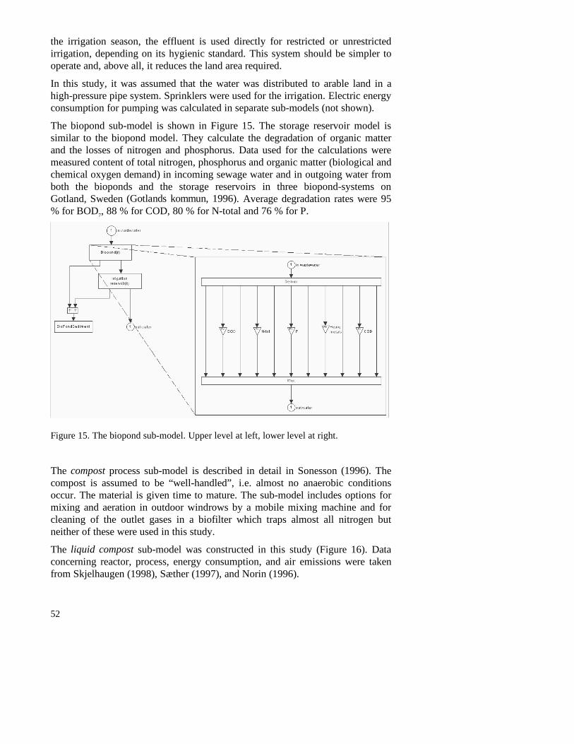
52

the irrigation season, the effluent is used directly for restricted or unrestrictedirrigation, depending on its hygienic standard. This system should be simpler tooperate and, above all, it reduces the land area required.

In this study, it was assumed that the water was distributed to arable land in ahigh-pressure pipe system. Sprinklers were used for the irrigation. Electric energyconsumption for pumping was calculated in separate sub-models (not shown).

The biopond sub-model is shown in Figure 15. The storage reservoir model issimilar to the biopond model. They calculate the degradation of organic matterand the losses of nitrogen and phosphorus. Data used for the calculations weremeasured content of total nitrogen, phosphorus and organic matter (biological andchemical oxygen demand) in incoming sewage water and in outgoing water fromboth the bioponds and the storage reservoirs in three biopond-systems onGotland, Sweden (Gotlands kommun, 1996). Average degradation rates were 95% for BOD7, 88 % for COD, 80 % for N-total and 76 % for P.

Figure 15. The biopond sub-model. Upper level at left, lower level at right.

The compost process sub-model is described in detail in Sonesson (1996). Thecompost is assumed to be “well-handled”, i.e. almost no anaerobic conditionsoccur. The material is given time to mature. The sub-model includes options formixing and aeration in outdoor windrows by a mobile mixing machine and forcleaning of the outlet gases in a biofilter which traps almost all nitrogen butneither of these were used in this study.

The liquid compost sub-model was constructed in this study (Figure 16). Dataconcerning reactor, process, energy consumption, and air emissions were takenfrom Skjelhaugen (1998), Sæther (1997), and Norin (1996).

53

Air is pumped in at the bottom of the reactor to assure that aerobic conditions aremaintained. The air bubbling up also creates a slow blending of the slurry.Process temperature is 55-60 º C. Electricity is used for air pumping, for pumpingof the liquid, and for foam cutting. The total energy consumption is calculated inthe model. The outlet gases are used for heat-exchanging the inflow of air. In thiscooling of the outlet gases, some moisture is condensed and fed back to thereactor. The outlet gases are then supposed to be cleaned in a biofilter (here peat).Also here, excessive water is fed back to the reactor. The filter material wasassumed to be recycled to arable land together with the slurry, thus very littlenutrients were lost. In the model, the post treatment storage period is assumed tobe six months (26 weeks). Skjelhaugen and Donantoni (1998) give reductions ofVS, DM, COD, N-total and N-NH4 after 45 weeks (10 month) of post treatmentstorage. I assumed that the losses were linear over time and thus multiplied theirnumbers by 26/45. This gave 12 % losses of ammonia and 9 % of total nitrogen.The microbial turnover in the slurry is probably not linear over time as assumedhere, so this approximation might be a source of erratic results. For more detailssee Appendix 2.

Figure 16. The liquid compost sub-model.

The anaerobic digestion sub-model describes a continuous, single-stage, mixed-tank digestion chamber operating under mesophilic conditions (37°C). The

54

incoming material can, if chosen, be hygienised (heated to 70O C) or sterilised(heated to 130O C). In this study, the process was simulated both with andwithout hygienisation. Sterilisation was not used here. The loss of ammoniaduring six months post treatment storage was assumed to be 1 percent. The modelis thoroughly described in Dalemo (1996).

In the scenarios with urine-separating toilets, the urine collection is described intwo sub-models – urine pipe and urine collection tank (Jönsson et al., 1999).These are identical except for the optional possibility of including in-leakage tothe pipe (Figure 17). Both calculate the transmission of urea to ammonia and theemission of kg N in ammonia to air. The ammonia emission is assumed smalland thus not affect the amount of nitrogen in the solution. The in-data are pH andtemperature of the urine, the ratio between volume of the exchanged gas and theliquid, the ratio in the gas between actual ammonia pressure and saturationpressure, the liquid volume and finally the amount of nitrogen in ammonia pervolume. The calculations are based on Svensson (1993).

Figure 17. The urine-pipe sub-model.

The kitchen macerator (disposer) makes it possible to mix and transport thehousehold wastes together with the sewage water in the sewage system. The sub-

55

model calculates the energy consumption, 3.7 MJ/person and year, and additionalwater consumption, 3.4 l/person and day (Nilsson et al., 1990). It was used in thebiopond, liquid compost and anaerobic digestion scenarios. The model wasdeveloped within this study (Figure 18).

Figure 18. The kitchen macerator sub-model.

TransportTwo different types of transportation by vehicle were used in the organic wastemanagement study – truck and tractor with manure spreader. The truck was usedfor the longer distance transportation of the on-site separated sludge to the sewageplant and for taking the digested sludge from the sewage plant to the landfill andto arable land. A tractor with manure spreader was used for all short-distancetransportation and spreading of blackwater, urine, sludge, manure, and treatmentresidues. The vehicle models calculate energy consumption and emissions to airdue to the combustion of fuel. All vehicles in the organic waste managementstudy were diesel-fuelled. Emission data are taken from Egebäck & Grägg(1988), Grägg (1990, 1992) and Egebäck & Hedbom (1991) and are the same forall transport.

The truck sub-model (Figure 19) is presented in detail in Sonesson (1996). Thefuel consumption used here was 4.0 litres/10 km (14.2 MJ/km) for transportationof digested sludge to arable land and landfill. For the collection andtransportation of on-site separated sludge, I assumed 4.5 litres/10 km (16.0MJ/km) since the pumping of sludge is energy demanding.

56

Figure 19. The truck sub-model.

Spreading on arable landThe spreading of liquid and solid residues on arable land sub-model (Figure 20)was developed by Håkan Jönsson and later modified by Ulf Sonesson and myself,all at the Department of Agricultural Engineering at SLU in Uppsala, Sweden.The model exists in two versions, which are identical except for the loading-energy demand calculation. The liquid spreader is pump-loaded and the solidmaterials spreader is loaded by wheel-loader. These models calculate the energyconsumption for loading, transport to field and spreading on field; the emissionsto air due to the combustion of fuel; hectares needed for spreading; and traveldistance on fields. The time for all operations is calculated for use in an economicevaluation modelled in the original version. However, neither economy nor timeuse were included in this study.

57

Figure 20. The liquid manure spreader sub-model.

The energy demand is calculated as the mechanical work required to move acertain weight a certain distance with correction for rolling resistance coefficientsand efficiencies in engines, pumps and gearboxes. Formulae are taken fromElinder & Falk (1983) and Jonsson (1993). Input variables for the liquid spreadersub-model are: pump capacity; lift height (for pumping the liquid from storageinto the spreader); amount residue (wet weight); travel distance from storage tofield; spreader tank volume; tractor and spreader combination empty weight;transport velocity; and additional time per load (entering and leaving the tractoretc.). For the solid material spreader, the input variables concerning loading areenergy and time consumption for a wheel-loader (VOLVO BM, 1995), all theothers are the same as for the liquid spreader model. The energy consumptionobtained in the model was judged to be appropriate. Concerning the airemissions, these are calculated using emission data valid for truck engines, whichcould be a source of error since the emissions vary a lot between differentworking conditions for tractor engines according to a preliminary study byHansson et al. (1998). However, no sufficiently detailed data are available as yet.

For road transport with tractor-and-manure-spreader, stripped versions of theliquid and solid material spreader sub-models were used. In this study, drivingspeed for road transport was set to 20 km/h, and one-way transport distance wasset to 2 km. For more details see Appendix 3.

Acreage requirementThe acreage requirement in hectares (ha) is calculated from permissible ordesirable amounts of 15 substances (N, P, K, S, heavy metals and organicpollutants), spread per ha and year as described in Sonesson (1998). The result isboth an output and used internally for the field operation calculations. Theindividual organic wastes were spread on separate acreage, implying that thenumber of hectares and grain production per ha is different between scenarios.

58

AgricultureThe agriculture sub-model (Figure 21) comprised two separate sub-sub-models –nitrogen soil turnover (Soil) and grain production (Crop). To be able to evaluatethe contribution from different organic wastes, four parallel Soil-Crop-combinations were included. Furthermore, the field-operations energyconsumption is calculated, and the amount and content of manure is initiated.

Figure 21. The agriculture sub-model.

The soil sub-model (Figure 22) calculate the fate of nitrogen in organic fertilisersspread on agricultural land. The nitrogen is divided into nitrate (NO3

-),ammonium (NH4

+), and organically bound nitrogen. Plant availability andemissions to air and water are determined. It is assumed that ammonium andnitrate are available to crops to the same degree as mineral fertilisers, except thatsome ammonium is volatilised as ammonia within the first hours after spreading.Organic nitrogen is only plant available after it has been mineralised toammonium or nitrate. In the model, this mineralisation is divided into two timeframes – the year of spreading and the remaining time. Thus, both immediate andlong-term effects of the organic fertiliser can be evaluated. The model uses abudget concept, assuming that all nitrogen added is eventually degraded andbecome either plant nutrient or emission (Clarholm, 1997). It is assumed that 30% of the organically bound nitrogen is mineralised in the first year, i.e. counted

59

as plant available nutrient. Thirty percent of the organic nitrogen not mineralisedin the first year is also counted as fertiliser; the rest is emissions in the form ofN2, N2O or NO3

-. This model is described in detail in Dalemo et al. (1998).

Figure 22. The soil nitrogen turnover sub-model.

The grain production sub-model calculates the expected yield of grain as afunction of the amount of nitrogen applied, using a formula presented byMattsson (1988). The formula is derived as an average nitrogen yield responsefrom many field trials in Sweden. It was assumed that all other nutrients weresupplied in adequate amounts. The sub-model, developed by Jönsson (1999), isshown in Figure 23.

60

Figure 23. The grain production sub-model.

In-data are the ammonia and nitrate calculated as plant available in the precedingsoil-model. From the maximum expected yield, the losses due to soil compactionand timeliness effect can be subtracted. In this study, only the soil-compactionlosses were included. The soil compaction is calculated for the topsoil, thesubsoil between 25 and 40 cm depth, and the subsoil below 40 cm depthrespectively (Arvidsson & Håkansson, 1991, 1992). Variables are number ofpasses made by the implement, working width of the implement, water content ofthe soil, weight on the different axles and tire pressures of the different axles. Forthe topsoil, the clay content is also used as a variable. The compaction in subsoilis only increased by axle loads larger than 4 000 kg in the 25-40 cm layer and byaxle loads larger than 6 000 kg below 40 cm. The losses due to timeliness effectwere neglected in this study due to the large differences in material spread and inspreading time of year. Outputs from the sub-model are total yield of grain peryear, and total yield per hectare and year. Other important aspects for potentialyield of grain, such as phosphorus and organic matter, are not considered in thismodel.

Data for field-operations energy consumption are derived from Sonesson (1993).Some modifications were made about number of operations and powerrequirement. The modifications resulted in a somewhat lower energyconsumption, 4700 MJ per ha, compared to the originally given 6240 MJ per ha.

61

Results and discussion of the organic waste management studyIn the organic waste management study, I occasionally present results both fortreatments of the household residues only (wastewater and household wastes from32 households), as well as for all residues (household residues plus manure from15 dairy cows and their young stock). In practice, it is probably not possible totreat only household residues in a digestion chamber or in a liquid compostreactor, due to the low dry matter content of these residues. However, to get abetter understanding of the results and to show the household residues part in theentire system studied, the results are presented as if these treatments werepossible.

Plant nutrients, dry matter, and water in waste fractionsThe wastewater and household wastes from the 32 household together held about17 % of the total input amount of nitrogen, while manure from the 15 dairy cowsand their young stock contained the rest (Table 9). For phosphorus, the householdshare was about 13 % and for potassium, it was about 6 %. For practical andhygienic reasons, it was assumed that only the blackwater and household wasteswere treated in the reactor treatments (together with the manure). Greywatercontained more than 80 % of all water in the system and it was relativelyunaffected by pathogens, so it could best be treated in an on-site sludgeseparation and infiltration construction or maybe used as irrigation water. Thismeant that about 15 % of the nitrogen and one third of the phosphorus in thehousehold wastewater were “lost” with the greywater. However, the amount ofphosphorus in greywater is highly dependent on which detergents are used forlaundry and washing-up. In Sweden, most of the detergents used are of a low-phosphorus type. When the manure was included in the calculations thegreywater held only a few percent of the total input of nitrogen and phosphorus.

Table 9. Plant nutrients, dry matter and water from different sources included in thestudy. (percent of total input) 1

greywater blackwater urine (incl. inblackwater)

household wastes manure

N-tot 3 12 9 2 83

N-NH4 0 17 13 0 82

P 4 7 4 2 87

K 1 4 2 1 94

Dry matter 5 6 3 6 84

Water 88 5 1 0 7

1 The sum is not always 100 percent due to rounding-off

62

Plant nutrients recycled to arable landThe different scenarios gave, as expected, large differences in performanceconcerning recycling of plant nutrients to arable land, when residues fromhouseholds only were considered (Figure 24). Due to the relatively smallcontribution of household residues to the total, the difference in performance wasless obvious when the manure was included in the simulations (not shown).

0

100

200

300

400

SludgeTo

SewPla

nt

SludgeTo

SewPla

nt Urin

eSep

SludgeTo

Agr

SludgeTo

Agr Urin

eSep

BioPonds

BioPonds U

rineSe

p

CompostT

oilet

Compost

UrineSe

p

Liquid

Compost

Liquid

Compost

UrineSe

p

AnaerobDig

estion

AnaerobDig

estion U

rineSe

p

kg p

er y

ear

N-totPK

Figure 24. Plant nutrients recycled to arable land. Treated wastewater and householdwaste from 32 households. (kg per year)

The reactor treatments recycled much of the nutrients while the on-site sludgeseparating treatments gave large losses primarily of nitrogen but also ofphosphorus and potassium (Figure 25). The biopond scenario gave large losses ofnitrogen and phosphorus but the recycling of potassium was the largest of allscenarios. This owed partly to the fact that the greywater was included withoutsludge separation in the treatment, and partly to a probable under-estimation ofpotassium losses in the model calculations (no reduction was calculated). In thedry compost, it was mostly nitrogen which was lost. Condensation of outlet gaseswould recover most of the ammonia and thus give better results for thistreatment. The difference between the liquid compost and anaerobic digestion inamount total nitrogen recycled was a result of post-treatment storage losses.During both treatments, almost no nitrogen was lost.

63

0%

25%

50%

75%

100%

Sludge

ToSew

Plant

Sludge

ToSew

Plant U

rineS

ep

Sludge

ToAgr

Sludge

ToAgr

Urin

eSep

BioPon

ds

BioPon

ds U

rineS

ep

Compo

stToil

et

Compo

st Urin

eSep

Liquid

Compo

st

Liquid

Compo

st Urin

eSep

Anaer

obDige

stion

Anaer

obDige

stion

Urin

eSep

part

of h

ouse

hold

res

idue

s in

put

N-totPK

Figure 25. Plant nutrients recycled to agriculture, proportion of original content inhousehold wastewater and waste. (percent of original content in household residues)

Urine separation; nutrient recyclingAn introduction of urine-separating toilets gave a substantial increase in nutrientrecycling in the on-site sludge separating and biopond scenarios. In the drycompost scenarios, urine separation resulted in increased nitrogen recycling rate,while the recycling of phosphorus was not affected. The amount of nitrogendelivered to arable land was increased in the two reactor treatment scenarios aswell but to a minor degree since these treatments already retain the larger part ofthe nitrogen.

64

Additional yield of grainThe purpose of organic waste recycling is to utilise the nutrient and organicmatter resources of the waste, i.e. the recycled residue is used as organic fertiliserin order to give larger yields of crops and possibly to upgrade the soil fertility.Thus, for the farmer, the total amount of recycled plant nutrients is not thatrelevant, since different fractions of nitrogen in particular have very differentfertilising properties. Instead, the expected increased yield is important.Furthermore, different waste treatment methods produce residues of variedcontents (Figure 26).

0

100

200

300

400

N-tot N-org N-NH4 N-NO3

kg p

er y

ear

CompostToilet

Compost UrineSep

LiquidCompost

LiquidCompostUrineSep

AnaerobDigestion

AnaerobDigestionUrineSep

Figure 26. N-fractions recycled to arable land in scenarios with blackwater separatingsystems. Treated wastewater and household waste from 32 households.(kg per year)

To be able to assess the fertilising quality of the organic wastes, a model thatcalculated nitrogen plant availability and nitrogen losses in soil was included. Inaddition, to make the results more comprehensible a model that calculated theexpected additional yield of grain due to the recycled plant-available nitrogen wasalso included. The model used for the additional yield calculations was quitecrude since it did not include phosphorus, potassium, organic matter, or water. Itrather assumed that P and K were supplied in sufficient amounts. Despite themodel's imperfections, the results were reasonably appropriate for short-termyield estimation since the rate of recycling of both P and K point in the samedirection as for N, i.e. the growing demand for P and K when more N wassupplied, was probably met. For most soils, phosphorus, potassium and organicmatter are more a matter of long-term soil fertility and are not easily connected tothe next year's yield. However, for long-term yield estimation (which is the reallyinteresting knowledge) these should be included.

The calculations of soil losses, plant availability and additional yield of graingave some changes in results compared to the amount of plant nutrients recycled(Figure 27).

65

0

1 000

2 000

3 000

4 000

5 000

Sludge

ToSew

Plant

Sludge

ToSew

Plant U

rineS

ep

Sludge

ToAgr

Sludge

ToAgr

Urin

eSep

BioPon

ds

BioPon

ds U

rineS

ep

Compo

stToil

et

Compo

st Urin

eSep

Liquid

Compo

st

Liquid

Compo

st Urin

eSep

Anaer

obDige

stion

Anaer

obDige

stion

Urin

eSep

kg g

rain

per

yea

r

Figure 27. Expected additional yield of grain as a result of recycling residues from 32households to arable land. (kg per year)

Dry compost residues, for example, have a high content of organic nitrogen,which was assumed to have about 30 % fertilising efficiency (30 % mineralisedfirst year, plus 30 % in the long-term of the small fraction that remains afteremissions in organic N).

It is noteworthy that an introduction of urine-separating toilets in the on-sitesludge separation, biopond and compost scenarios gave a significant rise in theexpected yield of grain, up to the level of the liquid compost scenario.

Concerning yield of grain in the biopond scenarios, the figures could be anoverestimation, since the losses of nitrogen when spreading the water in this casewere not accounted for (and nitrogen was the only substance included in thecalculation). On the other hand, the rise in yield due to the large amount of waterirrigated was not accounted for either. In practice, the water is spread on growingcrops, often at night when the evaporation rate is low. Altogether, it is likely thatthe model underestimated the expected yield of grain, but this has to be furtherinvestigated.

The differences in expected yield of grain between scenarios were large whenlooking at the household part only but the results were much more levelled outwhen the manure was taken into account (Figure 28).

66

0

10 000

20 000

30 000

40 000

Sludge

ToSew

Plant

Sludge

ToSew

Plant U

rineS

ep

Sludge

ToAgr

Sludge

ToAgr

Urin

eSep

BioPon

ds

BioPon

ds U

rineS

ep

Compo

stToil

et

Compo

st Urin

eSep

Liquid

Compo

st

Liquid

Compo

st Urin

eSep

Anaer

obDige

stion

Anaer

obDige

stion

Urin

eSep

kg g

rain

per

yea

r

householdsmanure

Figure 28. Expected additional yield of grain due to the recycling of organic waste toarable land. Treated wastewater and household waste from 32 households, and manurefrom 15 dairy cows and their young stock. (kg per year)

The difference in expected grain yield between liquid compost and anaerobicdigestion residues is somewhat surprising. It is partly an effect of calculateddifferences of losses during post treatment storage. The liquid compost residuelost 12 % of the ammonia, while the anaerobic digestion residue lost only 1 %.Of more importance is probably the fact that the aerobic compost process built upmore organic material in micro-organisms than the anaerobic process and thushad more nitrogen bound up in the organic matter. However, all organicallybound nitrogen was treated equally in the model (30 % mineralisation in the firstyear). This was probably a good estimation for the dry compost residues that arewell degraded, but for the liquid compost residue, the yield might have be under-estimated, since this organic nitrogen should be more easily degradable than thatin dry compost residues. The difference between digestion and liquid compostingcould also be an effect of the longer retention time in the digestion, resulting inmore breakdown of organic material, which gave a higher content of ammonia.More knowledge about the performance of liquid compost reactors and theutilisation of liquid compost slurry is needed for the improvement of the model.

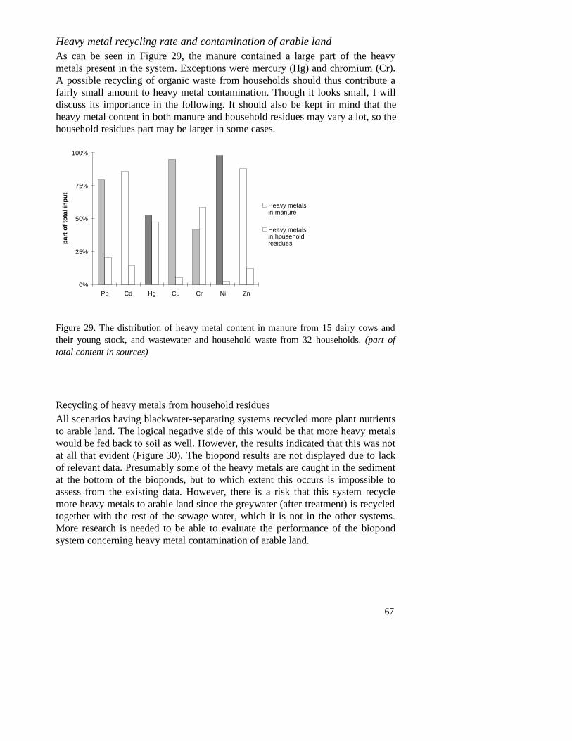
67

Heavy metal recycling rate and contamination of arable landAs can be seen in Figure 29, the manure contained a large part of the heavymetals present in the system. Exceptions were mercury (Hg) and chromium (Cr).A possible recycling of organic waste from households should thus contribute afairly small amount to heavy metal contamination. Though it looks small, I willdiscuss its importance in the following. It should also be kept in mind that theheavy metal content in both manure and household residues may vary a lot, so thehousehold residues part may be larger in some cases.

0%

25%

50%

75%

100%

Pb Cd Hg Cu Cr Ni Zn

part

of t

otal

inpu

t

Heavy metalsin manure

Heavy metalsin householdresidues

Figure 29. The distribution of heavy metal content in manure from 15 dairy cows andtheir young stock, and wastewater and household waste from 32 households. (part oftotal content in sources)

Recycling of heavy metals from household residuesAll scenarios having blackwater-separating systems recycled more plant nutrientsto arable land. The logical negative side of this would be that more heavy metalswould be fed back to soil as well. However, the results indicated that this was notat all that evident (Figure 30). The biopond results are not displayed due to lackof relevant data. Presumably some of the heavy metals are caught in the sedimentat the bottom of the bioponds, but to which extent this occurs is impossible toassess from the existing data. However, there is a risk that this system recyclemore heavy metals to arable land since the greywater (after treatment) is recycledtogether with the rest of the sewage water, which it is not in the other systems.More research is needed to be able to evaluate the performance of the biopondsystem concerning heavy metal contamination of arable land.

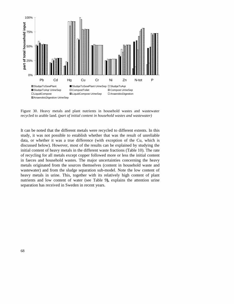
68

0%

25%

50%

75%

100%

Pb Cd Hg Cu Cr Ni Zn N-tot P

part

of t

otal

hou

seho

ld in

put

SludgeToSewPlant SludgeToSewPlant UrineSep SludgeToAgrSludgeToAgr UrineSep CompostToilet Compost UrineSepLiquidCompost LiquidCompost UrineSep AnaerobicDigestionAnaerobicDigestion UrineSep

Figure 30. Heavy metals and plant nutrients in household wastes and wastewaterrecycled to arable land. (part of initial content in household wastes and wastewater)

It can be noted that the different metals were recycled to different extents. In thisstudy, it was not possible to establish whether that was the result of unreliabledata, or whether it was a true difference (with exception of the Cu, which isdiscussed below). However, most of the results can be explained by studying theinitial content of heavy metals in the different waste fractions (Table 10). The rateof recycling for all metals except copper followed more or less the initial contentin faeces and household wastes. The major uncertainties concerning the heavymetals originated from the sources themselves (content in household waste andwastewater) and from the sludge separation sub-model. Note the low content ofheavy metals in urine. This, together with its relatively high content of plantnutrients and low content of water (see Table 9), explains the attention urineseparation has received in Sweden in recent years.

69

Table 10. Heavy metal content in different fractions of household wastewater and waste.(percent of total) 1

greywater urine faeces household waste

Lead (Pb) 53 0.1 1 46

Cadmium (Cd) 76 0.5 8 16

Mercury (Hg) 14 2.9 75 8

Copper (Cu) 63 0.8 11 26

Chromium (Cr) 50 0.2 1 49

Nickel (Ni) 75 0.2 2 23

Zinc (Zn) 57 0.1 18 25

1 The sum is not always 100 percent due to rounding-off

Concerning the (too) large figures for the copper (Cu) recycling ratio inSludgeToAgr-scenarios, they were probably the result of the data used emanatingfrom different sources. Wastewater data were Swedish averages, while data usedin the sludge separation sub-model were measured contents in sludge from placeswith limy soils that give hard water (measured in °dH). This kind of water oftengives a high content of Cu in sludge, as the carbonate ions that accompany thecalcium release copper from hot-water pipes used in houses. Thus the modelprobably over-estimated the content of copper in the sludge. Some regions inSweden with hard water have problems with high copper contents in sewagesludge. Several solutions may be at hand. Central installations for decalcificationof the water have been discussed and investigated in e.g. Uppsala. The problemhere is to remove the calcium and the carbonate without also removingmagnesium (Mg) and other microelements good for human health. Calcium isgood for health but it is judged that it is of greater importance to get rid of it dueto the copper problem. Furthermore, it increases the consumption of soap anddetergents for washing etc. and it may cause calcium-coating problems in waterpipes and different equipment. Ordinary decalcification-installations that use saltto substitute the calcium ion for a sodium ion do not solve the problem of copperrelease to water, since the carbonate-ion not is removed. This type of equipmentalso removes the magnesium.

Another option is to use other materials in water pipes. This is too expensive tobe done in the short term and no guarantee can be given that the new materialswill not give rise to new problems. A third possibility is to use blackwater-separating systems. This is also expensive, but would probably solve the problemwith Cu and other contaminants, since the copper released from hot-water pipeswould not affect the matter destined for use as an organic fertiliser. Additionally,different detergents and chemicals ending up in wastewater largely originate fromgreywater. The greywater would then have to be treated in separate systems.

In this study, it was assumed that sludge from greywater was recycled in the

70

blackwater separating scenarios. The data were unreliable but results (not shown)indicated that it was a question of small amounts. The exception here was alsocopper, probably for the same reason as mentioned above. An assumption that Cuin greywater-sludge was at levels equivalent to the other metals meant that therate of Cu recycling followed the content in household wastes and faeces.

Similar errors, such as those discussed for copper above, may be valid for theother metals. For example,. it might be behind the result for mercury (Hg), whichis found in faeces and probably originates from dental amalgam. According toFigure 30, much Hg was released with the outlet water from sludge separators (asmall amount was caught in the sludge). This could be the case, but it depends onthe form in which the mercury is present (metallic or organic). In organic form, itis hard to get into solution. In metallic form, it might be more loosely bound oradhered to particles and/or organic matter (Wikberg, 1999). Results presented inKärrman et al. (1999) indicate that some 60 % of Hg is caught in the sludge froma sewage plant using chemical precipitation. Since no chemicals are used in thesludge separators, less mercury could be trapped in this case. However,knowledge in this area seems to be sparse.

Heavy metal contamination of arable landA very important question is to what extent the recycling of residues involves aheavy metal contamination of the arable land. This is very hard to assess withoutknowledge about type of soil, type of crop, and other site-specific variables. Anexample of such a balance calculation is shown in Appendix 9. It shows theamounts of heavy metals both recycled to arable land and the possible exportwith the grain produced on that land. The grain included is the total grainproduction, i.e. the potential additional grain-production from the organic wasterecycling plus the base production produced with no fertilising. The differencebetween import and export is reported as net soil contamination. However, itshould be remembered that the contribution from precipitation and other possiblesources was not taken into account. For example, in cadmium contamination ofsoils in Sweden, precipitation is a large contributor (Hedlund et al., 1997).

71

Energy turnoverAn important aspect in the choice of treatment system is the energy turnover. Ihoped to find systems that not only had a low energy demand, but were alsoenergy self-sufficient or even net energy producers. None of the scenarios studiedmanaged to fulfil this goal (Figure 31) when the energy consumption for grainproduction field operations was included. The anaerobic digestion treatment witha urine-separating toilet system and no hygienisation of incoming material wasclosest to reaching the energy self-supporting goal, but needed to decrease itsenergy consumption by a third. It must be remembered when studying thediagrams that energy is presented as if all energy had the same quality, which isnot the case. For example, the liquid compost produced heat ("low-quality"energy) and consumed electricity and fossil oil ("high-quality" energy).Furthermore, the waste-transport distance chosen in this study was fairly short (2km). A sensitivity analysis where the distance was set to 10 km was alsoperformed. It is presented last in this chapter.

The (fossil) oil consumption arose in transportation and spreading of the material,and in the grain-production field operations. The heat and electricity net turnoversoriginated from energy consumption and production in the different treatments. Inaddition, the production of drinking water (used in households for washing,flushing of toilets etc.) consumed both oil for transport and electricity forpumping and production of chemicals. In the biopond scenarios, electricity wasalso consumed by the pump-and-pipe transport of both incoming wastewater andtreated water delivered to irrigation of arable land.

The anaerobic digestion was run in two modes (with or without hygienisation ofincoming material) to show the potential energy production. Both choices arepossible in practice. It is a question of the hygienic standard of incoming materialand of where the residues are going to be spread. Another hygienisation optionmight be extended storage of the treated residues. In Sweden, 6 months storage isgenerally accepted as a hygienisation method.

Also included in the energy consumption diagrams was the energy needed for theproduction of extra (fill-up) nitrogen fertiliser to get the scenarios to produceequal amounts of grain. Where the energy turnover for handling of householdresidues only was presented (Figure 32), energy consumption for an extra area ofgrain production also had to be included in all but two scenarios. This extra areawas necessary since addition of nitrogen up to the desired maximum yield on theacreage fertilised with treated organic wastes was not enough to producesufficient yields of grain. The extra area was conventionally managed, i.e.mineral fertilisers were used.

72

-400 000

-300 000

-200 000

-100 000

0

100 000

200 000

300 000

Sludge

ToSew

Plant

Sludge

ToSew

Plant U

rineS

ep

Sludge

ToAgr

Sludge

ToAgr

Urin

eSep

BioPon

ds

BioPon

ds U

rineS

ep

Compo

stToil

et

Compo

st Urin

eSep

Liquid

Compo

st

Liquid

Compo

st Urin

eSep

Anaer

obDige

stion

Anaer

obDige

stion

Urin

eSep

AnaDigN

oHyg

ienisa

tion

AnaDigU

SepNoH

ygien

isatio

n

MJ

per

year

Energy consumption, fill-up N fertiliser prod.

Fuel consumption,field operations

Fuel consumption,waste handling

Heat net

El net, waste handling

El consumption, water production

Figure 31. Energy turnover for treatment of wastewater and household waste from 32households and manure from 15 dairy cows and their young stock, including water-production and grain-production field operations. (MJ per year)

The compost treatments produced heat that was not easily utilised. It demandedinsulated reactors and heat-exchange systems. In the dry compost, I assumed theheat to be ventilated away, but in a reactor-compost, it could be captured bycondensation of the outlet gases. Concerning the liquid compost, it is probablynot possible to take any heat out from the reactor since the heat produced isneeded to heat incoming slurry. The main part of the heat can instead be drawndirectly after the slurry is taken out of the reactor. There are no readily availablesolutions for doing this (Skjelhaugen, 1997) but I still assumed that the heatproduced could be utilised. Thus, since the data and the assumptions made weresomewhat uncertain, the possible utilisation potential of the heat might beoverestimated in these scenarios.

Concerning the energy turnover results, both liquid compost scenarios gave smallnet energy surpluses (Figure 31) if agriculture was not taken into account. Whenonly the household residues were taken into account (Figure 32), only the liquidcompost scenarios showed results close to break-even energy turnover. All otherscenarios showed clearly negative energy turnovers.

Effects of urine separation are discussed below in sub-chapter “Urine separation;energy consumption and transport”.

73

-300 000

-200 000

-100 000

0

100 000

200 000

Sludge

ToSew

Plant

Sludge

ToSew

Plant U

rineS

ep

Sludge

ToAgr

Sludge

ToAgr

Urin

eSep

BioPon

ds

BioPon

ds U

rineS

ep

Compo

stToil

et

Compo

st Urin

eSep

Liquid

Compo

st

Liquid

Compo

st Urin

eSep

Anaer

obDige

stion

Anaer

obDige

stion

Urin

eSep

AnaDigN

oHyg

ienisa

tion

AnaDigU

SepNoH

ygien

isatio

n

MJ

per

year

Energy cons., fill-up grain prod.



Heat net

El net, wastehandling


Figure 32. Energy turnover for treatment of wastewater and household waste from 32households, including water-production and grain-production field operations.(MJ per year)

Biogas from anaerobic digestionThe biogas produced by anaerobic digestion can be utilised in at least threedifferent ways. Figure 31 and Figure 32 present the case where the gas was usedas fuel in a stationary combustion engine that produced electricity and heat. Thebiogas can also be cleaned and compressed for use as vehicle fuel and it can beburnt for heating of e.g. buildings.

Figure 33 shows the energy value of the methane produced and the actual energyconsumption when manure is included in the system. If the gas is purified andcompressed for use as vehicle fuel, the loss is about 7 % of the initial energycontent (Dalemo, 1998). The remaining gas would in that case hold about 295000 MJ annually, corresponding to some 8.3 m3 diesel.

74

-600 000

-400 000

-200 000

0

200 000

400 000

Anaer

obDige

stion

Anaer

obDige

stion

Urin

eSep

AnaDigN

oHyg

ienisa

tion

AnaDigU

SepNoH

ygien

isatio

n

MJ

per

year

Energy content CH4(total)

Energy consumption,fill-up N-fertiliser prod.



Heat consumption,digestion reactor

El consumption, wastehandling


Figure 33. Energy turnover for anaerobic digestion treatments of wastewater andhousehold waste from 32 households, and manure from 15 dairy cows and their youngstock. Energy value of methane produced compared to actual energy consumption. (MJper year)

All anaerobic digestion scenarios had energy deficiencies, but the scenario withurine-separating toilets and no hygienisation of input material showed a resultthat at least came close to break-even. The energy self-supporting point would bereached if the energy consumption in grain-production field operations weredecreased by approximately 10 %, which is possible if for example theagricultural soils were lighter (sandy). Another possible option is to decrease bothfuel consumption in waste management and clean-water production energyconsumption, by respectively a sixth and two thirds.

A theoretical option is to use some of the gas in a stationary engine, producingelectricity and heat needed for internal use, and to purify and compress the restfor use as vehicle fuel. About 75 % of the gas would have to be used in thestationary engine to produce enough heat. That would give an electricity netproduction of about 40 000 MJ/year (some 11 000 kWh). The gas left for vehiclefuel would supply about 60 % of the field operation's energy requirement orabout 45 % of the total energy requirement for transport and field operations inthe system.

The economics of a small-scale digestion system with equipment for gaspurification and compression were not studied here. The high investment costwould probably make this alternative possible only for larger settlements, or theinvestment may have to wait until the fuel price has risen substantially.

75

Urine separation; energy consumption and transportIt has often been said that the introduction of urine-separating toilets would resultin more transportation work. According to this study, this is not the case, whichis shown in Figure 31, Figure 32, Figure 33 and Figure 34. Most treatmentsshowed about equal energy consumption for systems both with and without urineseparation. In anaerobic digestion scenarios, urine separation resulted in lowerenergy consumption for heating the digestion reactor as well as for transportation.The same was valid for the liquid compost treatment. The largest energy savingeffect was obtained in these treatments internally. The smaller amount of watertreated resulted in lower electricity consumption (approx. 30 %) in the liquidcompost reactor and lower heat consumption (approx. 25 %) in the anaerobicdigestion chamber. Concerning the household residues only, the fuelconsumption for transportation and spreading was decreased by almost the halfdue to the water saving achieved in the urine-separating toilets in liquid compostand anaerobic digestion treatment scenarios (data not shown).

0

40 000

80 000

120 000

160 000

200 000

Sludge

ToSew

Plant

Sludge

ToSew

Plant U

rineS

ep

Sludge

ToAgr

Sludge

ToAgr

Urin

eSep

BioPon

ds

BioPon

ds U

rineS

ep

Compo

stToil

et

Compo

st Urin

eSep

Liquid

Compo

st

Liquid

Compo

st Urin

eSep

Anaer

obDige

stion

Anaer

obDige

stion

Urin

eSep

MJ

per

year

El consumption, trpsewage to treatment

El consumption, trpand spreading water

Fuel consumption, trpto treatment

Fuel consumption, trpand spreading org.fertiliserEnergy consumption,fill-up N-fertiliser prod.

Fuel consumption, fieldoperations

Figure 34. Energy consumption due to transportation and spreading of wastewater andhousehold waste from 32 households and manure from 15 dairy cows and their youngstock; and grain-production field operations plus additional production of nitrogenfertiliser. (MJ per year)

Figure 34 shows that the energy consumption for transporting the organic wastesto arable land and spreading it was somewhat larger when urine separation wasused in systems that did not have vehicle transportation of sewage water. Thatwas, however, compensated for by lower energy consumption in other parts ofthe systems.

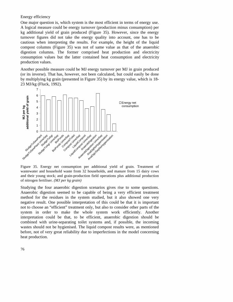
76

Energy efficiencyOne major question is, which system is the most efficient in terms of energy use.A logical measure could be energy turnover (production minus consumption) perkg additional yield of grain produced (Figure 35). However, since the energyturnover figures did not take the energy quality into account, one has to becautious when interpreting the results. For example, the height of the liquidcompost columns (Figure 35) was not of same value as that of the anaerobicdigestion columns. The former comprised heat production and electricityconsumption values but the latter contained heat consumption and electricityproduction values.

Another possible measure could be MJ energy turnover per MJ in grain produced(or its inverse). That has, however, not been calculated, but could easily be doneby multiplying kg grain (presented in Figure 35) by its energy value, which is 18-23 MJ/kg (Fluck, 1992).

0

1

2

3

4

5

6

7

Sludge

ToSew

Plant

Sludge

ToSew

Plant U

rineS

ep

Sludge

ToAgr

Sludge

ToAgr

Urin

eSep

BioPon

ds

BioPon

ds U

rineS

ep

Compo

stToil

et

Compo

st Urin

eSep

Liquid

Compo

st

Liquid

Compo

st Urin

eSep

Anaer

obDige

stion

Anaer

obDige

stion

Urin

eSep

AnaDigN

oHyg

ienisa

tion

AnaDigU

SepNoH

ygien

isatio

n

MJ

per

kg

addi

tiona

l yie

ld o

f gra

in

Energy netconsumption

Figure 35. Energy net consumption per additional yield of grain. Treatment ofwastewater and household waste from 32 households, and manure from 15 dairy cowsand their young stock; and grain-production field operations plus additional productionof nitrogen fertiliser. (MJ per kg grain)

Studying the four anaerobic digestion scenarios gives rise to some questions.Anaerobic digestion seemed to be capable of being a very efficient treatmentmethod for the residues in the system studied, but it also showed one verynegative result. One possible interpretation of this could be that it is importantnot to choose an “efficient” treatment only, but also to consider other parts of thesystem in order to make the whole system work efficiently. Anotherinterpretation could be that, to be efficient, anaerobic digestion should becombined with urine-separating toilet systems and, if possible, the incomingwastes should not be hygienised. The liquid compost results were, as mentionedbefore, not of very great reliability due to imperfections in the model concerningheat production.

77

Primary energy resources consumptionWhen resources were the focus, the consumption of primary energy resources(Figure 36) was a better measure than energy consumption since it tried to assessthe amount of resources consumed under the whole lifecycle of the energycarriers. Here, the result is presented as MJ primary energy resources per kgadditional yield of grain.

-2

0

2

4

6

8

10

12

Sludge

ToSew

Plant

Sludge

ToSew

Plant U

rineS

ep

Sludge

ToAgr

Sludge

ToAgr

Urin

eSep

BioPon

ds

BioPon

ds U

rineS

ep

Compo

stToil

et

Compo

st Urin

eSep

Liquid

Compo

st

Liquid

Compo

st Urin

eSep

Anaer

obDige

stion

Anaer

obDige

stion

Urin

eSep

AnaDigN

oHyg

ienisa

tion

AnaDigU

SepNoH

ygien

isatio

n

MJ

per

kg

addi

tiona

l yie

ld o

f gra

in

Primary energyresourcesconsumption

Figure 36. Primary energy resources consumption per additional yield of grain.Treatment of wastewater and household waste from 32 households, and manure from 15dairy cows and their young stock; and grain-production field operations plus additionalproduction of nitrogen fertiliser. (MJ per kg grain)

When calculating consumption of primary energy sources, biopond and liquidcompost scenarios that used much electricity stood out a bit more since electricityuses more primary energy resources than fuels do. For the same reason, theanaerobic digestion scenarios showed better results here. The negative column forthe last scenario ( Figure 36) denotes that this scenario actually produced aprimary energy surplus. This was possible (although the energy turnover wasnegative) since the gas produced was used for production of electricity (and heat),of which the treatment consumed some but the large part was delivered to theelectricity grid. The electricity assumed to be replaced was Swedish averageelectricity, which consumes 2.35 MJ primary energy resources per MJ electricitydelivered.

78

EutrophicationSix substances were included in the assessment of eutrophication. These werefour water-emissions (ammonium (NH4

+), nitrate (NO3

-), phosphorus (P), andorganic matter measured as chemical oxygen demand (COD)) and two air-emissions (ammonia (NH3) and nitrous oxides (NOx)). A maximum contributionscenario was used, i.e. both phosphorus and nitrogen contributed to theeutrophicating impact. However, in most aquatic systems one or other of them islimiting.

The eutrophicating impacts are shown in Figure 37. Emission of nitrate from soilwas the largest contributor to eutrophication in all scenarios. Slightly more than80 % was leached during the first winter after spreading, the rest was a long-termimpact. It is interesting that the results for liquid compost versus anaerobicdigestion were reversed when the soil emissions were taken into account. Thismight have been a true difference but it could also have been an effect ofimperfections in the model. Nitrate that is lost by leaching emanates fromorganically bound nitrogen. Since the model treated organically bound nitrogenin all different substrates equally, it might have over-estimated the nitrateemissions from liquid compost residues.

0

5000

10000

15000

20000

25000

Sludge

ToSew

Plant

Sludge

ToSew

Plant U

rineS

ep

Sludge

ToAgr

Sludge

ToAgr

Urin

eSep

BioPon

ds

BioPon

ds U

rineS

ep

Compo

stToil

et

Compo

st Urin

eSep

Liquid

Compo

st

Liquid

Compo

st Urin

eSep

Anaer

obDige

stion

Anaer

obDige

stion

Urin

eSep

kg O

2-eq

uiva

lent

s pe

r ye

ar

Soil

Treatments

Field operations

Transports andspreading

System parts concidered that have no or very small impact ( ≤1%):Electricity netWater productionFill-up N-fertiliser production

Figure 37. Eutrophication, maximum scenario. Treatment of wastewater and householdwaste from 32 households, and manure from 15 dairy cows and their young stock; andgrain-production field operations plus additional production of nitrogen fertiliser. (kg O2-equivalents per year)

Concerning the impact from transport and spreading, ammonia emissions inconnection to spreading of the residues were the dominating contributor. Sinceanaerobic digestion residues contained more ammonium than e.g. liquid compostresidues, more was also lost as ammonia.

79

For treatments, phosphorus (P) and nitrate (NO3) emissions together weredominant in the four scenarios having on-site sludge separation of sewage water.An introduction of urine-separating toilets here reduced P-emissions by about 35% and NO3 emissions by 70 %. In the scenarios which had blackwater-separatingsewage systems, where only greywater was released to recipient waters via sludgeseparation and infiltration, the situation was somewhat different. Here,phosphorus dominated the emissions from treatments. Nitrate had about one thirdof the impact that phosphorus had. The higher bars for the dry compostingscenarios concerning treatment (Figure 37) were the result of ammonia emissionfrom the compost. In the dry compost scenario without urine separation, NH3

actually had a three times larger eutrophicating impact than P – when urine-separating toilets were installed, these impacts were about equal. The biopondtreatment resulted in zero emissions to water (from the treatment) since all waterwas treated and used for irrigation. In practice, there may be leakage from pipesand storing reservoirs but that was not considered in the model.

Global warmingThree greenhouse-gases were included in the global warming impact assessment.These were carbon dioxide (CO2), methane (CH4), and dinitrogen oxide (N2O).

The fossil CO2 was emitted in the combustion of fossil fuel used fortransportation work and for production of electricity. The CO2 emissions causedby transportation of household residues were, as for the energy demand shownabove, small in comparison to the emissions occurring due to spreading of themanure except in the liquid compost and anaerobic digestion treatment scenarios.For a system with longer transportation distances the emissions would of coursebe larger. But, following the discussion above about the energy self-sufficientbiogas scenarios, digestion with no hygienisation of incoming material wouldemit almost no fossil CO2 since all fuel needed would be produced internallyfrom the biological wastes.

The CH4 was produced in some of the different treatments and during storage.Data were lacking in some parts but the supposedly most important contributorswere included in the models or will be discussed later.

The sludge separator sub-model did not produce any CH4 emission, which the realconstruction surely does. Such production is, however, probably small if thesludge separator is emptied at least once a year. The liquid compost sub-modeldid not calculate any emissions either. In that case it was not the treatment initself that produced the methane, but the post treatment storage. During storage,anaerobic conditions will occur, but it should take some time for the anaerobic(methane-producing) microorganisms to reproduce since the slurry is completelydominated by the aerobic microorganisms that have developed during the aerobictreatment. The amount of CH4 produced should at least not exceed that producedin digestion residue storage (where the gas is collected and added to the gasproduced in the reactor). The bioponds normally have aerobic conditions, and

80

thus no production of CH4. However, during hard winters, when the ponds andreservoirs get ice-covered, anaerobic conditions may occur. No data wereavailable and it was very hard to even make an assumption of how much methanecould be emitted under such circumstances. There are surely also anaerobicconditions in the bottom sediment during most periods of the year, but there havebeen no observations of gas bubbling up. When measured, no detectableconcentrations of CH4 were found in the air just above the water surface(Duveborg, 1997).

N2O is mainly produced in soil processes, and to some extent in dry compostingand production of nitrogen fertilisers.

The potential global warming impact is shown in Figure 38. The dominant part inthe system was the grain production process, especially the field operations. CO2

emanating from the combustion of fuels was a main contributor to globalwarming. Emissions N2O from soil had a global warming impact but the modelwas quite crude in this respect, so the results have to be interpreted with caution.More research is needed. The impact from treatments was small except in the drycompost scenarios. In these, emissions of mainly N2O and to some extent CH4

from the compost caused the greenhouse effect. Electricity consumption made aminor contribution to global warming when the electricity was produced asSwedish average electricity. The small negative columns for the anaerobicdigestion scenarios (Figure 38) reflect the emissions avoided due to the netproduction of electricity. The net result is thus the positive column subtracted bythe absolute value of the negative column.

-5 000

0

5 000

10 000

15 000

20 000

Sludge

ToSew

Plant

Sludge

ToSew

Plant U

rineS

ep

Sludge

ToAgr

Sludge

ToAgr

Urin

eSep

BioPon

ds

BioPon

ds U

rineS

ep

Compo

stToil

et

Compo

st Urin

eSep

Liquid

Compo

st

Liquid

Compo

st Urin

eSep

Anaer

obDige

stion

Anaer

obDige

stion

Urin

eSep

kg C

O2

equi

vale

nts

per

year

Electricity, net

Fill-up N-fertiliserproduction

Soil emissions(N2O)

Treatments

Field operations


Figure 38. Potential global warming, 100 years scenario. Treatment of wastewater andhousehold waste from 32 households, and manure from 15 dairy cows and their youngstock; and grain- production field operations plus additional production of nitrogenfertiliser. (kg CO2-equivalents per year)

81

AcidificationFour substances were included in the acidification assessment. These wereammonia (NH3), nitrous oxides (NOx), sulphuric oxides (SOx), and hydrochloricacid (HCl). Figure 39 shows the maximum acidification impact. Dominatingcontributors were NH3 emissions in connection with spreading of treated organicwaste and manure, and NOx emission from fuel consumption in field operations.

0

10

20

30

Sludge

ToSew

Plant

Sludge

ToSew

Plant U

rineS

ep

Sludge

ToAgr

Sludge

ToAgr

Urin

eSep

BioPon

ds

BioPon

ds U

rineS

ep

Compo

stToil

et

Compo

st Urin

eSep

Liquid

Compo

st

Liquid

Compo

st Urin

eSep

Anaer

obDige

stion

Anaer

obDige

stion

Urin

eSep

kmol

H+ -e

quiv

alen

ts p

er y

ear

Treatments

Field operations



Figure 39. Acidification, maximum scenario. Treatment of wastewater and householdwaste from 32 households, and manure from 15 dairy cows and their young stock; andgrain-production field operations plus additional production of nitrogen fertiliser. (kmolH+-equivalents per year)

However, in many ecosystems in Scandinavia and Northern Europe, nitrogencompounds are usually neutralised to a large extent. Therefore, the minimumacidification impact, where nitrogen compounds had no effect, is presented inFigure 40. Please note the difference in scale compared with Figure 39. Inpractice, the acidification impact is probably somewhere in between these results.As can be seen, the impact from treatments in anaerobic digestion scenarios wasstill relatively large since it was mainly an effect of emission of SO2. Thedigestion plant in itself did not emit sulphuric oxides, but when gas wascombusted, SOx was emitted. The large acidifying impact from compostingtreatments stemmed from emission of NH3, which had no impact in Figure 40.

Urine-separating systems gave larger ammonia losses in connection withspreading, which resulted in a slightly increased acidifying impact. Likewise,anaerobic digestion scenarios had more emissions of ammonia when digestionresidues were spread, since some organic nitrogen in the manure when digested

82

was mineralised to ammonium, which is more easily vaporised as ammonia.

0

1

2

3

4

5

Sludge

ToSew

Plant

Sludge

ToSew

Plant U

rineS

ep

Sludge

ToAgr

Sludge

ToAgr

Urin

eSep

BioPon

ds

BioPon

ds U

rineS

ep

Compo

stToil

et

Compo

st Urin

eSep

Liquid

Compo

st

Liquid

Compo

st Urin

eSep

Anaer

obDige

stion

Anaer

obDige

stion

Urin

eSep

kmol

H+ -e

quiv

alen

ts p

er y

ear

Fill-up N prod.

Treatments

Field operations


System parts concidered that have no or very small impact ( ≤3%):Electricity netWater production

Figure 40. Acidification, minimum scenario. Treatment of wastewater and householdwaste from 32 households, and manure from 15 dairy cows and their young stock; andgrain-production field operations plus additional production of nitrogen fertiliser. (kmolH+-equivalents per year)

Photo-oxidant formationIn the assessment of photo-oxidant formation, four gases were included. Three ofthese were categorised in photochemical ozone creation potentials (POCPs).These were methane (CH4), non-methane hydrocarbons (NMHC), and carbonmonoxide (CO). However, ozone creation can be limited by organic substanceslike those mentioned and/or by nitrous oxides (NOx) (Lindfors et al., 1995). Forlarge parts of Europe, it is actually expected that emissions of NOx are the mostimportant factor for ozone production (Axelsson et al., 1995). There is nocategorisation factor developed for NOx so this substance is presented in aseparate diagram (Figure 42). The results for POCP are presented in Figure 41.

For POCPs, it was NMHC emissions from the combustion of fuel in grain-production field operations which dominated. However, the data used were validfor the combustion of diesel in lorries and the emission from tractor enginesworking under different conditions may vary a lot. According to Hansson et al.'s(1998) preliminary study, the emission of hydrocarbons (HC) varies between0.041 g/MJ (for harrowing) and 0.238 g/MJ (for loading), but most of the valuesare below or just above 0.100 g/MJ. The model used 0.066 g/MJ, which should

83

be reasonably appropriate, or it may be a slight under-estimation of the NMHC-emissions.

The larger impact from transport and spreading in the liquid compost andanaerobic digestion scenarios was due to the increased amounts of material (muchwater) that had to be transported and spread. The extra emissions of NMHC fromcombustion of fuels mainly caused the increase.

0

1

2

3

4

5

Sludge

ToSew

Plant

Sludge

ToSew

Plant U

rineS

ep

Sludge

ToAgr

Sludge

ToAgr

Urin

eSep

BioPon

ds

BioPon

ds U

rineS

ep

Compo

stToil

et

Compo

st Urin

eSep

Liquid

Compo

st

Liquid

Compo

st Urin

eSep

Anaer

obDige

stion

Anaer

obDige

stion

Urin

eSep

kg e

then

e-eq

uiva

lent

s pe

r ye

ar

Treatments

Field operations



Figure 41. Photo-oxidant formation, using the concept of photochemical ozone creationpotentials (POCPs). Treatment of wastewater and household waste from 32 households,and manure from 15 dairy cows and their young stock; and grain-production fieldoperations plus additional production of nitrogen fertiliser. (kg ethene-equivalents peryear)

Concerning the emissions of NOx (Figure 42), these were dominated by theemissions from field operations. However, the larger impact for the liquidcompost and anaerobic digestion scenarios was due to the increased need fortransportation and (in the case of anaerobic digestion) the emission of NOx whenbiogas was combusted in a stationary engine for electricity production. Thetransportation in these systems could possibly be decreased by proper localisationof treatment plants, so that pumping of the slurry could be used instead of vehicletransportation. The emission of NOx from combustion of the biogas was probablymore difficult to avoid. Thus, in regions where nitrogen compounds have a largephoto-oxidant formation impact, anaerobic digestion might not be the best systemto choose.

84

0

100

200

300

400

Sludge

ToSew

Plant

Sludge

ToSew

Plant U

rineS

ep

Sludge

ToAgr

Sludge

ToAgr

Urin

eSep

BioPon

ds

BioPon

ds U

rineS

ep

Compo

stToil

et

Compo

st Urin

eSep

Liquid

Compo

st

Liquid

Compo

st Urin

eSep

Anaer

obDige

stion

Anaer

obDige

stion

Urin

eSep

kg N

Ox

per

year Fill-up N fertiliser

production

Treatments

Field operations



Figure 42. Emissions of nitrous oxides (NOx, calculated as NO2). Treatment ofwastewater and household waste from 32 households, and manure from 15 dairy cowsand their young stock; and grain-production field operations plus additional productionof nitrogen fertiliser. (kg NOx per year)

Summary of results, organic waste managementEnvironmental impacts, energy consumption, primary energy consumption,amount N and P recycled, and additional yield of grain are summarised in Table11. The figures given are total results per year. The environmental impacts andprimary energy consumption are also shown in Figure 43 as relative valuescompared to the SludgeToSewPlant scenario. Heavy metal contamination ofarable land is not included due to the complexity of those results.

To be remembered when studying the results is that the scenarios did not produceequal amount of utilities. They produced equal amounts of grain (with the help offill-up N fertiliser), but while anaerobic digestion was a net producer ofelectricity, all others consumed this facility. Anaerobic digestion and liquidcomposting also produced heat. Furthermore, the blackwater-separating scenariosrecycled more phosphorus, potassium, organic matter, and micro-plant-nutrients.This is probably important for long-term soil fertility but was not taken intoaccount when grain production was calculated in the model, nor was thepossibility of reusing water for irrigation in biopond systems accounted for. Thisshould be included in future versions of the model to make fair comparisons.

85

Table 11. Summary of results of the organic waste management study. Treatment ofwastewater and household waste from 32 households, and manure from 15 dairy cowsand their young stock; and grain-production field operations plus additional productionof nitrogen fertiliser. (impact per year) 1

Eutro-phic-ation

kg O2-equiv.

Globalwarm-ing

kgCO2-equiv.

Acid-ifica-tion

kmolH+

Photo-oxid.POCP

kgethene-equiv.

Photo-oxid.NOx

kgNOx

Energyconsumption

MJ

Primaryenergycons.

MJ

Re-usedN-eff.

kg

Re-usedP-tot.

kg

Addit-ionalyield ofgrainkg

SludgeToSewPlant

22000 17000 15 4.0 250 180000 230000 1300 470 30000

SludgeToSewPlantUrineSep.

18000 17000 16 4.1 260 170000 220000 1400 490 32000

SludgeToAgriculture

21000 17000 15 3.8 240 170000 220000 1300 480 30000

SludgeToAgricultureUrineSep.

18000 17000 16 4.0 250 170000 220000 1500 500 32000

BioPonds 14000 16000 14 3.8 240 190000 260000 1300 480 30000

BioPondsUrineSep.

14000 16000 15 3.9 250 180000 250000 1500 490 33000

CompostToilet

20000 19000 26 3.9 240 170000 220000 1300 510 30000

CompostUrineSep.

18000 17000 19 4.0 250 170000 220000 1500 510 33000

LiquidCompost

16000 19000 18 4.7 290 120000 350000 1400 510 31000

LiquidCompostUrineSep.

16000 18000 18 4.5 290 130000 300000 1400 510 32000

AnaerobicDigestion

13000 15000 28 4.5 370 230000 200000 1800 510 37000

AnaerobicDigestionUrineSep.

13000 14000 27 4.3 360 140000 90000 1800 510 38000

AnaerobicDig. NoHygien-isation

13000 15000 28 4.5 370 100000 50000 1800 510 37000

Anaer.Dig.UrineSep.No Hygien-isation

13000 14000 27 4.3 360 50000 -20000 1800 510 38000

1 All values given to two valid figures

86

-0.5

0.0

0.5

1.0

1.5

2.0

Slu

dgeT

oSew

Pla

nt

Slu

dgeT

oSew

Pla

ntU

Sep

Slu

dgeT

oAgr

Slu

dgeT

oAgr

Urin

eSep

Bio

Pon

ds

Bio

Pon

dsU

rineS

ep

Com

post

Toi

let

Com

post

Urin

eSep

Liqu

idC

ompo

st

Liqu

idC

ompo

stU

rineS

ep

Ana

erob

Dig

estio

n

Ana

erob

Dig

estio

nUS

ep

Ana

Dig

NoH

ygie

nisa

tion

Ana

Dig

US

epN

oHyg

ieni

satio

n

rela

tive

valu

e

Eutrophication (max. scenario)Global warming (GWPs)Acidification (max. scenario)Photo-oxidant formation (POCPs)Primary energy resources consumption

Figure 43. Environmental impacts, relative to the sludge–to-sewage-plant scenario.Treatment of wastewater and household waste from 32 households, and manure from 15dairy cows and their young stock; and grain-production field operations plus additionalproduction of nitrogen fertiliser. (relative values, 1=SludgeToSewPlant)

87

Studying Figure 43 (or Table 11), it can be concluded that no scenario proved tobe the optimal choice when all impact categories were taken into account. Thus,it is very important to find out which impact categories are most vital for thesystem or region of concern. For example, in many places the POCPs(photochemical ozone creation potentials) have a very small impact on theenvironment. In other places, acidification might not be considered as a problem.

Concerning the six scenarios (at the left of Figure 43) that had mixed-sewage-water systems, there were no big differences, except that the biopond scenarioshad a lower eutrophication impact. On the other hand, the primary energyconsumption was somewhat larger for the bioponds. Neither of the dry compostscenarios showed significantly different results, with the exception of aremarkably increased acidification impact due to ammonia emissions from thecompost. By reduction of this emission, which is certainly possible, thesescenarios would be on a level with the others to the left (Figure 43).

The results for the reactor-treatment scenarios, which had blackwater-sortingsewage systems, stood out some more. The liquid compost scenarios had asmaller eutrophicating impact, but larger impacts on all categories affected byfuel consumption. Pipe-transport of blackwater to treatments would probablyreduce these impacts. Due to their relatively large electricity consumption, theliquid compost scenarios consumed more primary energy resources than all otherscenarios. Anaerobic digestion scenarios produced the best results foreutrophication, global warming and primary energy consumption. However, forPOCPs they had a somewhat larger impact and for acidification the largest impactof all systems. Concerning acidification, anaerobic digestion had double theimpact compared to all other scenarios (except the dry compost scenarios). Thiswas due to larger ammonia emission in connection with spreading and tosulphuric oxide emission when the biogas (methane) was combusted in astationary engine.

Urine-separating toilet systems gave smaller environmental impacts in mostcases. The largest effect was seen for primary energy consumption, where urineseparation gave substantially lower consumption in the reactor-treatmentscenarios. This was due to the decreased amount of water used in this kind ofsystem. In the case of liquid composts, the smaller amount of water savedelectricity used in the composting reactor. When it came to anaerobic digestion,the water saving decreased the heat consumption in the digestion reactor.

88

Sensitivity analyses; organic waste management

Electricity produced in oil-fired power plantSwedish average electricity by no means represents a European average, since itis largely produced by equal parts of hydropower and nuclear power. Therefore, asensitivity analysis where the scenarios were run with electricity produced in oil-fired power plants was also performed.

Global warmingThe potential global warming impact was largely affected by the type ofelectricity production chosen in the scenarios using or producing much electricity(compare Figure 44 and Figure 38). Please note the differences in scale betweenthe two diagrams. When electricity was produced from fossil oil, the CO2-emission from this production was an important contributor to the greenhouseeffect in the scenarios that used much electricity. The negative columns for theanaerobic digestion scenarios (Figure 44) reflect the emissions avoided due to thenet production of electricity. The net result is thus the positive column subtractedby the absolute value of the negative column. The anaerobic digestion scenarioshad almost no impact on global warming if the electricity produced substitutedfor oil-fired power plants. This assumption might be more adequate (thanSwedish average electricity), if one considers this kind of electricity productionas a marginal production, which it is likely to be, if it exists at all. The marginalproduction of electricity in Sweden has been from oil-fired power plants and tosome extent imported electricity from Denmark and Germany, which have largeproportions of coal-fired power plants.

-40 000

-20 000

0

20 000

40 000

60 000

80 000

Sludge

ToSew

Plant

Sludge

ToSew

Plant U

rineS

ep

Sludge

ToAgr

Sludge

ToAgr

Urin

eSep

BioPon

ds

BioPon

ds U

rineS

ep

Compo

stToil

et

Compo

st Urin

eSep

Liquid

Compo

st

Liquid

Compo

st Urin

eSep

Anaer

obDige

stion

Anaer

obDige

stion

Urin

eSep

kg C

O2

equi

vale

nts

per

year

Electricity, net


Soil emissions(N2O)

Treatments

Field operations


Figure 44. Potential global warming, 100 years scenario. Treatment of wastewater andhousehold waste from 32 households, and manure from 15 dairy cows and their youngstock; and grain- production field operations plus additional production of nitrogenfertiliser. Electricity produced in oil-fired power plants. (kg CO2-equivalents per year)

89

AcidificationWhen electricity was produced in oil-fired power plants (Figure 45), the emissionof SOx was also a major acidifying substance. For the two reactor-treatmentsystems (liquid compost and anaerobic digestion) the choice of primary energysource for electricity production was vital. Liquid composting scenarios, havingabout half the acidifying impact compared to digestion scenarios when electricitywas produced as the Swedish average (Figure 39), doubled their impact whenelectricity was produced in oil-fired power plants. This made the net impact fromdigestion scenarios smaller than in the liquid compost scenarios.

-10

0

10

20

30

Sludge

ToSew

Plant

Sludge

ToSew

Plant U

rineS

ep

Sludge

ToAgr

Sludge

ToAgr

Urin

eSep

BioPon

ds

BioPon

ds U

rineS

ep

Compo

stToil

et

Compo

st Urin

eSep

Liquid

Compo

st

Liquid

Compo

st Urin

eSep

Anaer

obDige

stion

Anaer

obDige

stion

Urin

eSep

kmol

H+ -e

quiv

alen

ts p

er y

ear

El net

Treatments

Field operations


System parts concidered that have no or very small impact ( ≤2%):Water productionFill-up N-fertiliser production

Figure 45. Acidification, maximum scenario. Treatment of wastewater and householdwaste from 32 households, and manure from 15 dairy cows and their young stock; andgrain-production field operations plus additional production of nitrogen fertiliser.Electricity produced in oil-fired power plants. (kmol H+-equivalents per year)

As discussed earlier, the minimum acidification scenario could often be a moreappropriate estimation of the acidifying impact in Sweden. The choice of oil-firedelectricity changed the acidifying impact considerably (Figure 46 compared toFigure 40, please note the difference in scale). The large impact for the liquidcompost scenarios emanated from emission of SOx in the oil-fired electricityproduction.

90

-10

-5

0

5

10

15

20

Sludge

ToSew

Plant

Sludge

ToSew

Plant U

rineS

ep

Sludge

ToAgr

Sludge

ToAgr

Urin

eSep

BioPon

ds

BioPon

ds U

rineS

ep

Compo

stToil

et

Compo

st Urin

eSep

Liquid

Compo

st

Liquid

Compo

st Urin

eSep

Anaer

obDige

stion

Anaer

obDige

stion

Urin

eSep

kmol

H+ -e

quiv

alen

ts p

er y

ear

El net

Treatments

Field operations



Figure 46. Acidification, minimum scenario. Treatment of wastewater and householdwaste from 32 households, and manure from 15 dairy cows and their young stock; andgrain-production field operations plus additional production of nitrogen fertiliser.Electricity produced in oil-fired power plants. (kmol H+-equivalents per year)

Photo-oxidant formationThe choice of primary energy source for electricity production had vastconsequences for POCPs (Figure 47 compared to Figure 41, please note thedifference in scale), but not that large an implication where NOx was concerned(Figure 48 compared to Figure 42). The exception was the liquid compostscenarios, which used much electricity. The very large POCP impact forelectricity production when electricity was produced in oil-fired power plants wasdue to emission of NMHC, which had a very large photo-oxidant formationimpact. Compared to this kind of electricity, electricity production from biogasseemed to be a very favourable alternative as regards the photo-oxidant formationimpact.

91

-20

-10

0

10

20

30

40

50

Sludge

ToSew

Plant

Sludge

ToSew

Plant U

rineS

ep

Sludge

ToAgr

Sludge

ToAgr

Urin

eSep

BioPon

ds

BioPon

ds U

rineS

ep

Compo

stToil

et

Compo

st Urin

eSep

Liquid

Compo

st

Liquid

Compo

st Urin

eSep

Anaer

obDige

stion

Anaer

obDige

stion

Urin

eSep

kg e

then

e-eq

uiva

lent

s pe

r ye

arEl net, POCPs

Treatments

Field operations



Figure 47. Photo-oxidant formation, using the concept of photochemical ozone creationpotentials (POCPs). Treatment of wastewater and household waste from 32 households,and manure from 15 dairy cows and their young stock; and grain-production fieldoperations plus additional production of nitrogen fertiliser. Electricity produced in oil-fired power plant. (kg ethene-equivalents per year)

-100

0

100

200

300

400

Sludge

ToSew

Plant

Sludge

ToSew

Plant U

rineS

ep

Sludge

ToAgr

Sludge

ToAgr

Urin

eSep

BioPon

ds

BioPon

ds U

rineS

ep

Compo

stToil

et

Compo

st Urin

eSep

Liquid

Compo

st

Liquid

Compo

st Urin

eSep

Anaer

obDige

stion

Anaer

obDige

stion

Urin

eSep

kg N

Ox

per

year

El net, NOx

Fill-up N fertiliserproductionTreatments

Field operations


System parts concidered that have no or very small impact ( ≤1%):Water production

Figure 48. Emissions of nitrous oxides (NOx, calculated as NO2). Treatment ofwastewater and household waste from 32 households, and manure from 15 dairy cowsand their young stock; and grain-production field operations plus additional productionof nitrogen fertiliser. Electricity produced in oil-fired power plant. (kg NOx per year)

92

Primary energy resources and eutrophicationThe choice of primary energy source for electricity production did not have anygreat impact on primary energy consumption or on eutrophication (not shown).

Summary of results; oil-fired electricity productionThe environmental impacts and primary energy consumption were shown earlierin Figure 43 (electricity produced as Swedish average) and below in Figure 49(electricity produced in oil-fired power plants).

When the electricity consumed or produced in the reactor-treatment-systems wasproduced in oil-fired power plants, the results became clearly negative for liquidcomposting (although eutrophication was not affected). For anaerobic digestion,the outcome was the reverse. All impact categories, with exception ofacidification, showed better figures since emissions from biogas electricityproduction were cleaner than the substituted (more polluting) oil-fired electricityproduction.

93

-2

-1

0

1

2

3

4

5

6

7

Slu

dgeT

oSew

Pla

nt

Slu

dgeT

oSew

Pla

ntU

Sep

Slu

dgeT

oAgr

Slu

dgeT

oAgr

Urin

eSep

Bio

Pon

ds

Bio

Pon

ds U

rineS

ep

Com

post

Toi

let

Com

post

Urin

eSep

Liqu

idC

ompo

st

Liqu

idC

ompo

stU

rineS

ep

Ana

erob

Dig

estio

n

Ana

erob

Dig

estio

nUS

ep

Ana

Dig

NoH

ygie

nisa

tion

Ana

Dig

US

epN

oHyg

ieni

satio

n

rela

tive

valu

e

Eutrophication (max. scenario)Global warming (GWPs)Acidification (max. scenario)Photo-oxidant formation (POCPs)Primary energy resources consumption

Figure 49. Environmental impacts, relative to sludge to sewage plant scenario.

Treatment of wastewater and household waste from 32 households, and manure from 15

dairy cows and their young stock; and grain-production field operations plus additional

production of nitrogen fertiliser. Electricity produced in oil-fired power plant. (relative

values, 1=SludgeToSewPlant)

94

Local transport distance set to 10 kmThe choice of 2 km for all transport distances presumably affected the overallresults. A set-up with the distance set to 10 km is therefore presented here. As canbe seen in the following, it was mainly the liquid compost and anaerobicdigestion scenarios which were affected. This was due to the higher transportrequirements in these scenarios.

Energy turnoverThe energy turnover when the transport distance was set to 10 km is shown inFigure 50. The equivalent for 2 km is shown in Figure 31 (please note thedifference in scale). The longer transport distances resulted in increased energyconsumption by about 30 % in the liquid compost scenarios, and by between 35and 55 % in the anaerobic digestion scenarios (energy production not affected).For the other scenarios, the change was in the order of 10 %.

-500 000

-400 000

-300 000

-200 000

-100 000

0

100 000

200 000

300 000

Sludge

ToSew

Plant

Sludge

ToSew

Plant U

rineS

ep

Sludge

ToAgr

Sludge

ToAgr

Urin

eSep

BioPon

ds

BioPon

ds U

rineS

ep

Compo

stToil

et

Compo

st Urin

eSep

Liquid

Compo

st

Liquid

Compo

st Urin

eSep

Anaer

obDige

stion

Anaer

obDige

stion

Urin

eSep

AnaDigN

oHyg

ienisa

tion

AnaDigU

SepNoH

ygien

isatio

n

MJ

per

year

Energy consumption, fill-up N fertiliser prod.



Heat net

El net, waste handling


Figure 50. Energy turnover for treatment of wastewater and household waste from 32households and manure from 15 dairy cows and their young stock, including water-production and grain-production field operations. Transport distance 10 km. (MJ peryear)

95

Environmental impactsThe increase of transport distances from 2 km to 10 km gave the largest effect onphoto-oxidant formation. The results for these environmental impacts are shownin Figure 51 and Figure 52. They can be compared to Figure 41 and Figure 42(please note the difference in scales).

0

2

4

6

8

Sludge

ToSew

Plant

Sludge

ToSew

Plant U

rineS

ep

Sludge

ToAgr

Sludge

ToAgr

Urin

eSep

BioPon

ds

BioPon

ds U

rineS

ep

Compo

stToil

et

Compo

st Urin

eSep

Liquid

Compo

st

Liquid

Compo

st Urin

eSep

Anaer

obDige

stion

Anaer

obDige

stion

Urin

eSep

kg e

then

e-eq

uiva

lent

s pe

r ye

ar

Treatments

Field operations



Figure 51. Photo-oxidant formation, using the concept of photochemical ozone creationpotentials (POCPs). Treatment of wastewater and household waste from 32 households,and manure from 15 dairy cows and their young stock; and grain-production fieldoperations plus additional production of nitrogen fertiliser. Transport distance 10 km.(kg ethene-equivalents per year)

0

100

200

300

400

500

600

Sludge

ToSew

Plant

Sludge

ToSew

Plant U

rineS

ep

Sludge

ToAgr

Sludge

ToAgr

Urin

eSep

BioPon

ds

BioPon

ds U

rineS

ep

Compo

stToil

et

Compo

st Urin

eSep

Liquid

Compo

st

Liquid

Compo

st Urin

eSep

Anaer

obDige

stion

Anaer

obDige

stion

Urin

eSep

kg N

Ox

per

year

Fill-up N fertiliserproductionTreatments

Field operations



Figure 52. Emissions of nitrous oxides (NOx, calculated as NO2). Treatment ofwastewater and household waste from 32 households, and manure from 15 dairy cowsand their young stock; and grain-production field operations plus additional productionof nitrogen fertiliser. Transport distance 10 km. (kg NOx per year)

96

Global warming was also largely affected (Figure 53). That diagram should becompared to Figure 38 (please note the difference in scale). Acidification wasaffected to a much lesser extent and eutrophication was almost unchanged.

-5 000

0

5 000

10 000

15 000

20 000

25 000

30 000

Sludge

ToSew

Plant

Sludge

ToSew

Plant U

rineS

ep

Sludge

ToAgr

Sludge

ToAgr

Urin

eSep

BioPon

ds

BioPon

ds U

rineS

ep

Compo

stToil

et

Compo

st Urin

eSep

Liqu

idCom

post

Liqu

idCom

post

Urin

eSep

Anaer

obDige

stion

Anaer

obDige

stion

Urin

eSep

kg C

O2

equi

vale

nts

per

year

Electricity, net


Soil emissions(N2O)

Treatments

Field operations


Figure 53. Potential global warming, 100 years scenario. Treatment of wastewater andhousehold waste from 32 households, and manure from 15 dairy cows and their youngstock; and grain production field operations plus additional production of nitrogenfertiliser. Transport distance 10 km. (kg CO2-equivalents per year)

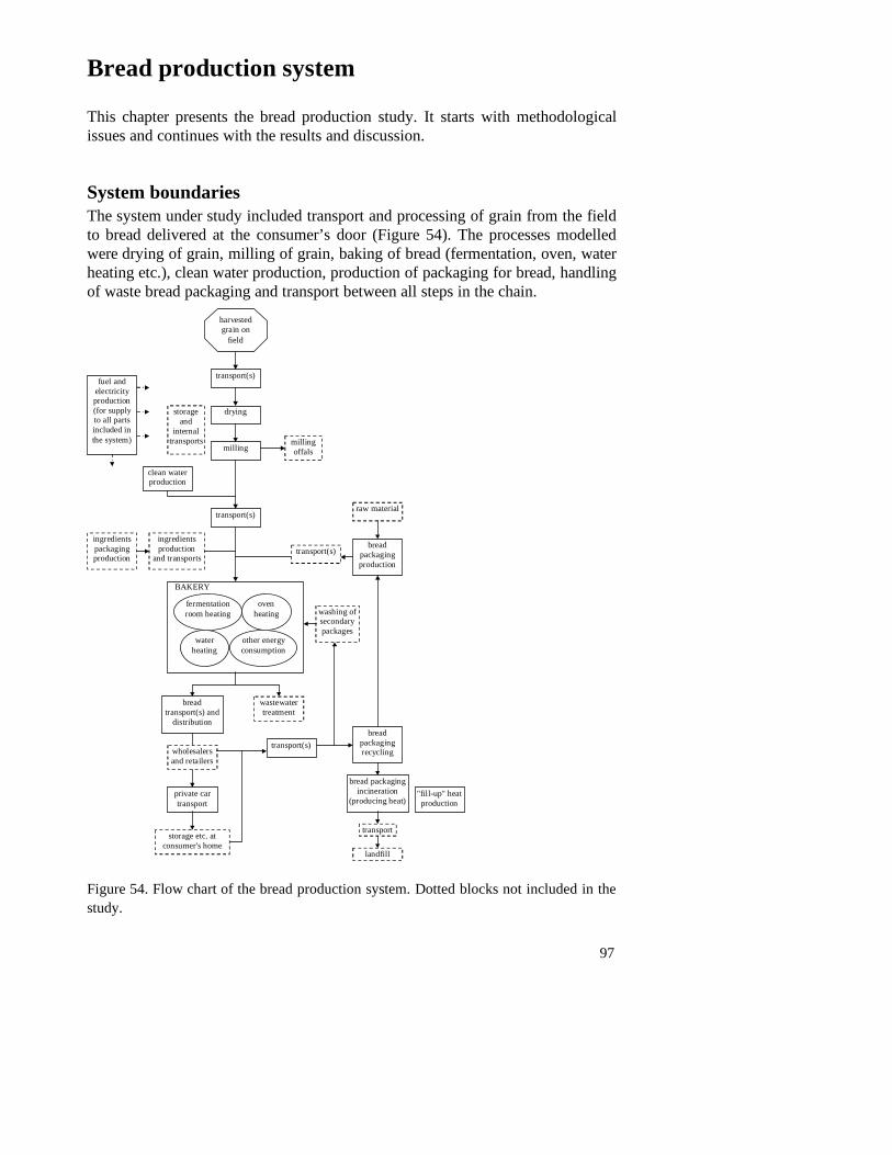
97

Bread production system

This chapter presents the bread production study. It starts with methodologicalissues and continues with the results and discussion.

System boundariesThe system under study included transport and processing of grain from the fieldto bread delivered at the consumer’s door (Figure 54). The processes modelledwere drying of grain, milling of grain, baking of bread (fermentation, oven, waterheating etc.), clean water production, production of packaging for bread, handlingof waste bread packaging and transport between all steps in the chain.

transport(s)

millingoffals


harvestedgrain on

field

fuel andelectricityproduction(for supplyto all partsincluded inthe system)

storageand

internaltransports

drying

milling

transport(s)

breadpackagingproduction

ingredientspackagingproduction

ingredientsproduction

and transportstransport(s)

breadpackagingrecycling

bread packagingincineration

(producing heat)

breadtransport(s) and

distribution

wholesalersand retailers

private cartransport

storage etc. atconsumer's home

transport

transport(s)

wastewatertreatment

ovenheating

fermentationroom heating

other energyconsumption

waterheating

BAKERY

landfill

raw material

washing ofsecondarypackages

"fill-up" heatproduction

Figure 54. Flow chart of the bread production system. Dotted blocks not included in thestudy.

98

Agriculture and cropping of grain were not included in this analysis, neither werethe consumer phase nor its storage. These are of importance but were assumednot to change between the different scenarios and were thus not needed for thecomparison. In addition, the agricultural parts were dealt with in the organicwaste management study, and thus included in the example of a cyclic small-scale food system. The retailer level was also omitted since for bread it wasassumed to have little impact on energy and resources consumption and since itwould anyhow be about equal for all scenarios. Other parts of the system wereomitted from this study because they were assumed to be negligible concerningenergy consumption and environmental impact in comparison to those included.These were storage of grain and flour, the fate of milling offals, production ofadditives (sugar, yeast, spices, etc.), packaging for additives, wholesalers,cleaning of plastic boxes and wastewater treatment. With regard to the packagingwhich was included, the transportation of such packaging from manufacturer tobakery was not included.

The model outputs are yearly amounts of emissions and energy consumption, butall results were recalculated to emissions and energy consumption per kg breadproduced. This was chosen to get more easy-to-understand results. To obtain theresults for a 100-person settlement (the size used in the organic wastemanagement study) the per-kg-bread results have to be multiplied by 3500; 35 kgbread per person and year in Sweden (Becker, 1992) times 100 persons.Furthermore, in order to get the scenarios to produce equal amounts of heat (inthe incineration of packaging wastes) "fill-up" heat production was included inthe system.

AssumptionsAll grain used was assumed to be produced in Sweden, and thus no difference incropping environmental effects was accounted for. Imported grain is sometimesused to get a higher protein (gluten) content in the flour, but there seemed to beno difference between scales in this aspect.

No losses of grain or bread were included. This might be a source of errors sincethere probably are losses, especially of bread in later stages of the chain. Thedifferences between scales are, however, probably not that large.

Electricity used was assumed to be produced as Swedish average electricity, i.e.about equal parts of hydropower and nuclear power with minor parts producedfrom biofuels, wind, oil, and coal.

When plastic boxes were used for secondary packaging, it was assumed that theywere transported back to the bakery by returning lorries, and thus did not createany extra transport. The emissions and energy use for cleaning of them isnegligible (Andersson, 1998a) and was thus not included.

99

The energy consumption was calculated as electrical and thermal energy. Thermalenergy consumption was the sum of fossil fuels (mainly oil and gas), bio-fuelsand internal heat in packaging materials minus the heat recovered by incinerationof packaging materials.

ScenariosFour main scenarios were presented. Two were large-scale systems that producedbread distributed over large distances with long-distance transport plus localdistribution, and two were small-scale systems producing bread for alocal/regional market. Both large-scale and small-scale systems were representedby one "irrational" and one "rational" scenario. Irrational refers to both thelogistical planning of production and to the use of old, non-energy-optimisedtechnology. The logistical planning in the bakery is important because if e.g. pre-heating time and shifts between different sorts of bread in the oven are notminimised, the time for oven heating gets longer and, thus, energy consumptiongets larger. Rational refers to systems where both logistical planning and processcontrol were optimised in order to minimise energy consumption andenvironmental impacts. Additionally, a fifth scenario was included. It was thesmall-scale rational scenario complemented with the private-car transport used inthe other scenarios.

The large-scale scenarios represent realistic "extremes" considering energy usethat seem to exist in Sweden (and probably elsewhere). Assumptions aboutdifferent transport types were intended to represent common situations inSweden. All transport was carried out by diesel-fuelled vehicles unless otherwisestated. Plastic bags were used as primary packaging for the bread in all scenarios.

1. Irrational large-scale, used oil as fuel in an indirect heated oven and steamboiler. In many ways, it resembled a real bakery system described as Industry 1 inAndersson (1998a). Drying of grain was done in an oil-fired indirect heated drier.The secondary packaging for bread distribution was cardboard boxes that wereused only once. Grain was transported 30 km by tractor and wagon (same in allscenarios) to drying and milling plants and then 210 km by truck and trailer to thebakery. Bread was first transported 260 km by truck (inter-regional), then locallydistributed to shops by truck (4 tonnes full load, 350 km round-trip), and finallytransported 5 km by private petrol-driven car to the consumer's home.

2. Rational large-scale, was in many ways similar to Industry 2 in Andersson(1998a). It used electricity for heating of oven, steam boiler, and fermentationroom. The grain was dried in a gas-fuelled direct-heated drier. The secondarypackaging for bread distribution was plastic boxes that were used 500 times.Transport assumptions were equal to those in the irrational large-scale scenario.

For the small-scale scenarios, the intention was to present one environmentally

100

optimised system and one system that developed following other criteria. Bothhad short transport distances in all parts of the chain. The secondary packagingused was plastic boxes.

3. Irrational small-scale, had a bakery that used an oil-fired indirect heated ovenand an oil-fired steam-boiler. The grain was transported 30 km by tractor andwagon to an oil-fired indirect heated drying plant, which was co-located with themilling plant and the bakery. The bread was distributed locally to the shops by adiesel-fuelled pick-up or van (600 kg full load, 100 km round-trip) and then, as inthe large-scale scenarios, transported to the consumer's home by private (petrol-driven) car.

4. Rational small-scale, used electricity for all heating in the energy optimisedbakery. The other big difference between these two scenarios was the home-transport of bread. Here it was done by foot, by bicycle, or by home-distributioncarried out by the bakery. In the latter case, the retailer level was not needed andit was assumed that the home-distribution could be carried out in an energyefficient manner, thus substituting for the local distribution from bakery toretailers. All other transport assumptions were equal to those in the irrationalsmall-scale scenario. Other differences between the irrational and rational small-scale scenarios were the grain-drier, which here was indirectly heated by biofuels,and the mill, which used an energy-saving mechanical internal transport system.

5. Rational small-scale + car transport, was equal to the fourth scenario butcomplemented with vehicle-transport to the consumer's home by private (petrol-driven) car as used in the first three scenarios.

To choose electricity as major energy carrier in the rational scenarios might notbe self-evident. As the Swedish average electricity is largely produced byhydropower and nuclear power, which is quite "clean" in comparison toelectricity produced from fossil coal and oil, the choice was logical. However,land use, storage of nuclear waste, etc. were not taken into account when thischoice was made. In order to evaluate the choice, sensitivity analyses whereelectricity was produced in oil-fired power plants and rational scenarios havinggas-fuelled ovens are presented at the end of this chapter.

101

ModelsThe general structure of the model is shown in Figure 55. Each block in thediagram represents a sub-model that work independently of the others. The grainis defined at the top as a certain amount of dry matter and water. Then thetransformation of incoming material (where appropriate), energy consumption, airemissions from fuel consumption, and possible water emissions are calculated ineach sub-model. Emissions for electricity production are calculated later in ageneral spreadsheet programme (MS Excel).

Figure 55. General structure of the bread production system model.

102

Clean water productionWater of drinking quality is used in the bakery as an ingredient in bread and forcleaning. Some water is also used for steaming but most of the condensed steamis re-circulated so a very small amount is needed for this purpose. The model isdescribed in the chapter "Organic waste management system".

Grain processing

Grain drierIn Sweden, grain usually needs to be dried before storage, but the initial moisturecontent varies a lot between years and between regions. Thus, the model had tobe flexible in this aspect. The grain drier model (Figure 56) calculates the amountof water vaporised from chosen values of moisture content wet base (m.c.) forincoming and dried grain. In this study, grain with 20 % m.c. was dried to 14 %m.c. The amount of water in dried grain is calculated from the amount of drymatter (which was assumed to remain unchanged) and the desired m.c. Theenergy consumption is calculated by multiplication of factors for heating energyconsumption and for electricity consumption for fan propelling, with a calculatedamount of vaporised water. Finally, air emissions due to fuel consumption arecalculated. The Demux-block split the 43-position vector into smaller vectorsand/or scalars. The Mux-block aggregates them to a 43-position vector again.

Figure 56. Grain drier sub-model.

In practise, the heat consumption is dependent on initial m.c. The higher theinitial m.c., the lower the energy consumption per kg water vaporised. I used 5.4MJheat/kg water, which is an approximate average for drying of grain withmoderate m.c. in indirect heated driers (Regnér, 1998).

Direct heated driers using e.g. fossil gas as fuel have 15-30 % lower energyconsumption (Regnér, 1987). When used in this study, they were assumed tohave a 20 % lower energy demand, i.e. 4.3 MJheat/kg water. The electricity

103

demand in all cases was assumed to be 0.3 MJel/kg water (StatensMaskinprovningar, 1987). The model finally calculates the air emissions per MJfuel used. For more details and references, see Appendix 5.

Flour-millEnergy consumption for milling of grain varies a lot depending on e.g. varietyand moisture content of the grain, types of flour produced (rate of extraction), andtype of internal transportation (mechanical or pneumatic) in the mill (Jakubczyket al., 1987). The internal transportation is nowadays often done in pneumaticsystems, which are cleaner but more energy-demanding than mechanical systems.Different sources give energy consumption between 0.1 and 0.45 MJel/kg flourdepending on transport system and flour extraction rate (Jakubczyk et al., 1987;Andersson, 1998a). The lowest figures are valid for systems with mechanicaltransportation systems and high extraction rates. The structure of the mill modelis shown in Figure 57.

Figure 57. Grain mill sub-model.

The electricity consumption was set to 0.36 MJel/kg flour (wet weight) in bothlarge-scale scenarios and in the irrational small-scale scenario. For the rationalsmall-scale scenario I assumed the energy consumption to be considerablysmaller, about 0.15 MJel/kg flour. This level is among the lower range of thosepresented by Jakubczyk et al. (1987), and is also indicated to be valid for thesmall-scale bakery system (including mill) studied in Andersson (1998). Thedifference in the latter case is probably a result of above all a mechanicaltransportation system in combination with higher extraction rate and maybe alarger proportion of rye (which is easier to grind than wheat).

For practical reasons, a medium-range (80 %) flour extraction value was chosenfor all scenarios. This did not have any large implications since the milling offalswere not included in further calculations, though they might be used both as foodfor humans and feed for animals. This simplification should be of minorimportance since the flour is the main product and milling is a minor energy-

104

consuming part in the whole system. Of same reason, I chose to allocate allmilling energy consumption to the flour.

BakeryThe bakery model calculates the energy consumption in different parts of thebakery process (Figure 58). Different literature sources have aggregated (or havemeasured) data in different ways but most of them give at least oven heating andtotal energy consumption per kg bread produced. Therefore all calculations areperformed per kg bread produced and thus the amount of bread produced per kgflour first has to be calculated. This varies a lot between different bakeries (andprobably between different kinds of bread). In this study, it is chosen to use thevalue 1.4 kg bread per kg flour in all scenarios. Furthermore, it was assumed thatall the added weight was water, i.e. additives were neglected. Kent & Evers(1994) stated that one can get 145 kg bread out of 100 kg flour and that only 4 kgadditives need to be added, i.e. about 3 % of the bread weight. In theenvironmental analysis of a medium-sized Swedish bakery (Nilsson, 1996) it isreported that the additives stand for about 13 % of the total bread weight. Toleave the additives out might thus be a source of error in the calculations but Iestimated it to be small.

Figure 58. Bakery sub-model.

105

The model makes calculations for oven heating, fermentation room heating,steam production, water heating, and a remaining part separately. For these, it ispossible to use electricity and/or fuel as energy source. For air emissioncalculation, it is possible to choose different fuels for heating of differentprocesses. It is possible to calculate the water emissions in the model but sincethey are of very small proportions (Andersson, 1998b; Nilsson, 1998) they werenot included in this study. However, the amount water consumed was calculatedfor use in the water-heating energy consumption sub-model. Energy consumptionfor water added to the dough is assumed to be included in the other parts. Formore details see Appendix 6.

PackagingAndersson (1998b) found that the packaging used for the bread is one of themajor energy-consuming parts of the system. The data concerning packagingused in Anderson's Life Cycle Analysis are published by Arnkvist (1997), whohas closely investigated the use of packaging in bread production.

Included in the model calculations were primary packaging (paper or plastic bags)for bread and secondary packaging (corrugated cardboard or plastic boxes) usedfor distribution of bread. The dominating bread primary packaging in Sweden isplastic bags made of low-density polyethylene (LDPE). Paper bags are usuallyonly used by small bakeries for bread sold directly to customers (withoutdistribution to retailer). Bakeries that distribute their bread over large areas (longdistances) use non-returnable corrugated cardboard secondary packaging, whilemany bakeries with local or regional distribution areas use plastic boxes made ofhigh-density polyethylene (HDPE). They are brought back to the bakery, wherethey are cleaned, and used again about 500 times (Arnkvist, 1997). Thepackaging for ingredients is in most cases a small part of the total (Arnkvist,1997) and was thus omitted. This assumption might lead to an under-estimationof the environmental impact from packaging, especially for the small-scalescenarios, but it should be of no vital importance.

The general structure of the packaging sub-model is shown in Figure 59. At thetop, the amount of bread is introduced. The choice of primary packaging type isdone by definition of the constants baPlasticBagChoice and baPaperBagChoice toeither zero or one, or parts of one, i.e. either plastic or paper bags, or acombination of the two. The choice of secondary packaging is performed in aparallel manner. When plastic bags are chosen, plastic clips (polystyrene) are alsoincluded.

106

Figure 59. The sub-model for choices of primary and secondary packaging.

The air and water emissions and energy consumption due to production of thedifferent materials are calculated in the separate parts of the model. Figure 60shows the plastic bag production sub-sub-model. The structure of the others is thesame.

Figure 60. Plastic bag production sub-model.

Lifecycle data are used, i.e. all emissions from raw-oil extraction or timber fellingto the packaging entering the bakery door are included. Data for the production ofplastics are published by Boustead (1993, 1997). Data for paper and cardboardcome from Habersatter et al. (1998). For more details see Appendix 6. The datafor packaging are valid for Central European manufacturing. Compared toSwedish conditions, these data probably give more environmental emissions from

107

energy consumption, since coal and other fossil fuels are more frequently used asenergy carriers. However, this should not be of great importance.

Packaging material waste handlingAfter use, it is assumed that both primary and secondary packaging are eitherincinerated or recycled. However, in this study, all scenarios had recycling ofpackaging materials. Incineration was still needed since the materials could notbe recycled more than a certain amount of times. In practice, this is reflected as aloss of material in each recycling step. Some of this material is in reality put onlandfill, but that was not modelled since landfilling of incinerable wastes is notpreferable from an energy utilisation point of view (Sonesson et al., 1997).Furthermore, landfilling of incinerable wastes will be banned in the EuropeanUnion in a few years time. The incineration plants are often connected to districtheating systems, thus replacing heat produced from other energy carriers. Whenthe material is recycled, it replaces virgin fibres in the production of paper orcardboard and fossil oil in the production of plastics. Concerning plastics, therecycled material is not used for same type of products as in its first lifecycle, butit still replaces virgin oil. Figure 61 shows the structure of the recycling model.First, the choice of recycling or incineration and type of packaging is defined.

Figure 61. General structure of the packaging waste handling sub-model.

When incineration is chosen, energy consumption and production, and air andwater emissions due to transportation and incineration of all material are

108

calculated. The incineration sub-model is described in detail in Mingarini (1996).When recycling is chosen the energy consumption and air emissions due totransportation and processes created by the recycling are calculated. Theallocation factors for plastics and paper make it possible to decide how manytimes the material can be assumed to be recycled before it goes to incineration.Here, it was assumed that plastics were recycled once, while paper products wererecycled four times. This choice had no large impact on the results.

The paper recycling process sub-model is shown in Figure 62. The sub-model forplastics is equivalent. Data for recycling of packaging materials were as given byTillman (1991). To get the share of energy consumption and emissionsoriginating from the recycling, I simply took the differences between recyclingand landfilling scenarios for paper and plastics respectively as they are given inthat reference, i.e. the transport was included with assumptions about distancesetc. made in that study. For all plastics, figures for LDPE were used, thusassuming that LDPE, HDPE and PS were equivalent. For paper and cardboard,data for cardboard were used, thus assuming that the two were equivalent. Boththese assumptions made the results less accurate but any possible errors thatcould arise should be small compared to the energy consumption andenvironmental impacts for the whole system. To obtain total energy consumptionand air emissions, the data are multiplied by the actual weight of material. Formore details see Appendix 7.

Figure 62. Paper recycling sub-model.

109

TransportIn the model, the grain, and later the bread, are transported by vehicle betweenfive different points in the chain from field to consumer in the large-scale system.In reality there might be more transport steps but since I did not include loadingand unloading in the analysis some simplifications have been possible. In thesmall-scale system, this could be reduced to two or three steps.

Four different types of vehicles were used; agricultural tractors with trailers,lorries, pick-ups or vans and private cars. The models were the same as thoseused in the organic waste study presented under "Transport" in the chapter"Organic waste management system". All vehicles except private cars werediesel-fuelled. For more details see Appendix 4.

Transport of grain from field to drierTractor with wagon was used for transport from field to grain drier. The one-waydistance was assumed to be 30 km, and to be the same in all scenarios. In practicethis transport may be divided in two, first a short transport from the field to anon-farm located drier and thereafter transport to a central storage site.

Long-distance grain transportTruck and trailer transports the grain to the mill (in the large-scale scenarios). Theone-way distance was assumed to be 210 km (as given by Andersson 1998a). Thevehicle was assumed to carry a full load (30 tonnes) out and to return empty. Fuelconsumption was 5 litres/10km with a full load and 3 litres/10km empty. Inpractice this transport might also consist of two parts, grain from storage (on-farm or central) to the mill and then transport of the flour to the bakery. However,this is of no importance in the systems perspective of the study.

Inter-regional bread transportIn the first step of the large-scale systems, the bread was assumed to betransported by truck 260 km one-way. This is the average distance for a largeSwedish industrial bakery reported by Andersson (1998a). Fuel consumption wasassumed to be 4 litres/10 km with a full load (13.3 tonnes) and 2 litres/10kmwhen empty. The assumed load-factor was 70 %.

Local bread distributionThe local distribution of bread can be performed in different ways and is highlydependent on local and regional conditions. In the large-scale scenarios Iassumed that the round-trip distance was 350 km, which is equivalent to thedistance given by Andersson (1998a). The fuel consumption was set to 5litres/10km and the max-load to 4 tonnes. For the small-scale bakery, thedistribution step was done using a smaller pick-up with 600 kg bread loadedwhen it leaves the bakery. Its fuel consumption was assumed to be 1.1litres/10km and the round-trip was 100 km. These load and distance data were

110

chosen from existing tours which were assumed to be relevant (Nilsson, 1996).The fuel consumption data were as yet unpublished data from GirmaGebresenbet, Dept. of Agr. Engineering, SLU (pers. comm.).

Private car transportThe transportation from the shop to the consumer's home was assumed to be doneby petrol-driven private car in scenarios 1, 2, 3, and 5. To get the environmentalimpact and energy consumption of this transport, some assumptions had to bemade. The one-way distance driven was 5 km and the trip was made exclusivelyfor shopping. Two kg of bread were bought each time, which is the approximateweekly consumption for a three-person family (Becker, 1992). Bread is about 6% of our average food consumption expenditure (SCB, 1999). Thus, 6 % of thetransport was allocated to the bread. Fuel consumption (1.23 litres/10km) andemission factors are data from Eriksson et al. (1995).

111

Results and discussion of the bread production systemThe results for the bread production study are presented and discussed first inimpact category by category. At the end of the chapter, there follows a summarywhich compares the impacts relative to the large-scale irrational scenario.

Energy consumption

Processes and transport are large parts of the energy consumption, as can be seenin Figure 63. Choice of energy source for heating of bakery oven andfermentation room affect the relationship between electrical and thermal energyuse but not the total energy consumption to any large extent. The difference inprocess energy consumption between rational and irrational scenarios was chosento represent different levels of energy optimised systems. Anyhow, in practice,electrical heating of the bakery oven and fermentation room might reduce theenergy consumption somewhat because direct heating can be used.

0

2

4

6

8

10

Large-scaleirrational (oil)

Large-scalerational (el)

Small-scaleirrational (oil)

Small-scalerational (el)

Small-scalerational

(el+car trp)

MJ

per

kg b

read

"Fill-up" heat

Packages,thermal

Packages,electricity

Processes,fuel

Processes,electricity

Transports,fuel

Figure 63. Electrical and thermal energy consumption due to transport, processes, andpackages. Transport was that performed within the system; i.e. transport in connectionwith e.g. package waste handling were not included here. Processes included graindrying, grain milling, bakery, and water production. Packaging included production,transport, recycling, internal energy value, and heat recovery. (MJ per kg bread)

Note that the small-scale scenarios had somewhat larger energy consumption inprocesses than their large-scale counterparts. That represents the large-scaleeffects on energy efficiency that seem to exist (Trägårdh et al., 1979; Nilsson,1996; Andersson, 1998a).

112

Packaging can be important as well. The larger energy use for packaging in thelarge-scale irrational scenario was due to the choice of single-use cardboard boxesfor bread distribution, instead of plastic multi--use boxes. The irrational large-scale scenario would have had about equal energy consumption to the irrationalsmall-scale if plastic boxes had been used instead.

The difference between the large-scale scenarios and the small-scale irrational oneconcerning the transport energy consumption was an effect of scale anddistribution area. The large-scale scenarios included a 210-km truck and trailertransport of grain and a 260-km truck transport of bread, which the small-scaledid not. The difference between the irrational and rational small-scale systemsconcerning transport was solely a result of the assumptions made about localbread distribution. In the irrational scenario, it was assumed that the bread wastransported 5 km by private car, while in the rational this transport was omitted(done by foot, bicycle or efficient home-distribution system). Like the results ofother studies, e.g. Andersson (1998), one can conclude that the assumptions madeabout the home-transport of food affected the results very much. In this study,that type of transport was more than half of the transport energy consumption insmall-scale scenarios and more than a third in the large-scale scenarios. Addingthis private car transport to the rational small-scale scenario increased its totalenergy consumption by almost 30 %, i.e. almost up to the level of the large-scalerational scenario. Thus, it can be concluded that the small-scale system, to havelower energy consumption, must be small-scale also concerning all transport –especially with respect to the last transport from the shop to homes. Anotherinterpretation of the results could be that the scale of the bakery is of lessimportance concerning energy consumption. It is the efficiency in processes andtransport, along with the consumer’s shopping behaviour, that have the largestimpact on energy consumption.

Milling of grain typically stands for 2 - 5 % of the total energy consumption.Drying of grain is somewhat more energy consuming, between 4 and 8 % of thetotal.

Energy consumption hotspotsEnergy consumption in all modelled parts is shown in Table 12. All figures aregiven to two decimal places although that might be to over-estimate the accuracyof the results. In the table, all separate energy consumption figures larger than 10% of the total are marked as hotspots. Heating of bakery oven and fermentationroom, primary packaging and the local distribution and home-transport of breadstood out in most scenarios. Note that if one counts the total contribution ofpackaging (production, recycling and incineration) it was small in all scenariosexcept the irrational large-scale one. In that particular case, the choice ofcardboard boxes as secondary packaging made the difference.

113

Table 12. Energy consumption in all parts of the system. Hotspots (>10 % of total)darkened. Zero-values indicate lower consumption than 0.00. Empty places indicate zeroconsumption, i.e. not used in the scenario. (MJ per kg bread).


Large-scalerational (el.)


Small-scalerational (el.)

el. thermal el. thermal el. thermal el. thermal

Grain Drier 0.02 0.36 0.02 0.29 0.02 0.36 0.02 0.36

Grain Mill 0.26 0.26 0.26 0.11

Water Production 0.00 0.00 0.00 0.00 0.00 0.00 0.00 0.00

Bakery Oven 2.00 1.00 2.30 1.40Bakery Steam + Ferment. 1.00 0.30 1.50 0.40

Bakery Rest 0.80 0.30 0.80 0.20

Bakery Water Heating 0.21 0.10 0.23 0.23

Prod. Plastic Bag 0.141.19 0.14 1.19 0.14 1.19 0.14 1.19Prod. Plastic Clips 0.00 0.09 0.00 0.09 0.00 0.09 0.00 0.09

Prod. Plastic Box 0.00 0.06 0.00 0.06 0.00 0.06

Prod. Cardboard Box 0.644.22Recycle Plastics1 -0.05 -0.61 -0.05 -0.65 -0.05 -0.65 -0.05 -0.65Recycle Paper1 -0.06 -2.60Incinerator2 0.01 -0.51 0.00 -0.27 0.00 -0.27 0.00 -0.27

"Fill-up" heat3 0.23 0.23 0.23

Tractor Transport Grain 0.13 0.13 0.13 0.13

Truck Transport Grain 0.19 0.19

Regional Distrib. Bread 0.34 0.34

Local Distrib. Bread 0.94 0.94 0.89 0.89Priv. Car TransportBread

1.23 1.23 1.23

Total 4 1.98 7.96 2.08 3.76 1.42 7.05 2.47 2.02

Total, el + thermal 9.94 5.84 8.47 4.49

10 % of the total 0.99 0.58 0.85 0.45

15 % of the total 1.49 0.88 1.27 0.67

20 % of the total 1.99 1.17 1.69 0.90

25 % of the total 2.48 1.46 2.12 1.121 Negative values imply that energy was saved compared to if incineration had been chosen. Including transport.2 Negative values imply that heat was produced. Including transport.3 Additional heat production to get the scenarios to produce equal amounts of heat.4 Total not exactly the sum of the parts due to rounding-off

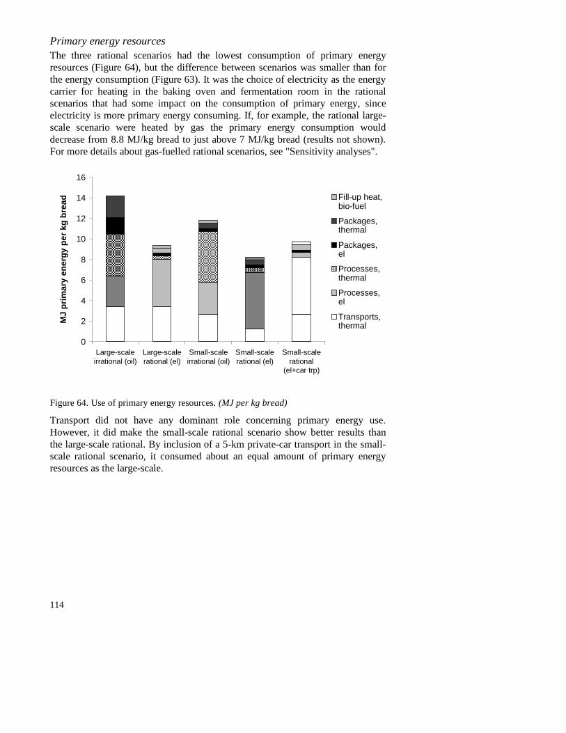
114

Primary energy resourcesThe three rational scenarios had the lowest consumption of primary energyresources (Figure 64), but the difference between scenarios was smaller than forthe energy consumption (Figure 63). It was the choice of electricity as the energycarrier for heating in the baking oven and fermentation room in the rationalscenarios that had some impact on the consumption of primary energy, sinceelectricity is more primary energy consuming. If, for example, the rational large-scale scenario were heated by gas the primary energy consumption woulddecrease from 8.8 MJ/kg bread to just above 7 MJ/kg bread (results not shown).For more details about gas-fuelled rational scenarios, see "Sensitivity analyses".

0

2

4

6

8

10

12

14

16





Small-scalerational

(el+car trp)

MJ

prim

ary

ener

gy p

er k

g br

ead Fill-up heat,

bio-fuel

Packages,thermal

Packages,el

Processes,thermal

Processes,el

Transports,thermal

Figure 64. Use of primary energy resources. (MJ per kg bread)

Transport did not have any dominant role concerning primary energy use.However, it did make the small-scale rational scenario show better results thanthe large-scale rational. By inclusion of a 5-km private-car transport in the small-scale rational scenario, it consumed about an equal amount of primary energyresources as the large-scale.

115

Global warming

The potential global warming impact was largely affected by the choice ofenergy-carrier for heating of ovens and fermentation-rooms and by use of energyconserving technology. The considerably smaller global warming impact fromprocesses in rational scenarios compared to irrational scenarios (Figure 65) wasboth due to the use of electricity for the heating of oven and steam boiler, and torational production and technology. The electricity used was Swedish average,which is mainly hydropower and nuclear power. Choosing e.g. oil-condensedpower would reduce the effect of energy carrier choice (see "Sensitivityanalyses"). However, energy conserving technology also plays an important role.If the bakery in the rational large-scale scenario had been gas-heated, the process-part would still have shown only a third of the global warming potentialcompared to the irrational large-scale scenario.

0.0

0.2

0.4

0.6

0.8

Large-scaleirrational

(oil)


Small-scaleirrational

(oil)


Small-scalerational

(el+car trp)

kg C

O2-

equi

vale

nts

per

kg b

read

Packages

Processes

Transports

System parts concidered that have no or very small impact ( ≤1%):Fill-up heat production

Figure 65. Potential global warming impact (100-years scenario). (kg CO2-equivalentsper kg bread)

The small difference between the contribution from processes in both rationalscenarios was due to the fact that biofuel was chosen as the energy carrier in thegrain-drier in the small-scale system. Furthermore, transport was importantconcerning the greenhouse effect. In fact, for both rational scenarios transport wasthe dominating factor. The difference between scenarios concerning globalwarming was equivalent to those discussed for energy consumption.

116

Eutrophication

The eutrophication impact was largely owing to emissions of nitrous oxides(from burning of fuels) in this study, i.e. in situations where nitrogen did not havea eutrophication impact, the eutrophication was very small in these systems.Since transport was the dominating NOx-emitting part, it is not surprising that thesmall-scale scenarios showed better results for this impact category (Figure 66).For other food-processing systems, e.g. drinking-milk production, which havelarge direct eutrophying emissions in the water, the result could be different tothose obtained here (see “Results and discussion of the liquid milk productionsystem”).

0

5

10

15

20

25

30

35





Small-scalerational

(el+car trp)

g O

2-eq

uiva

lent

s pe

r kg

bre

ad

Packages

Processes

Transports


Figure 66. Eutrophication (maximum scenario). (g O2-equivalents per kg bread)

AcidificationIn all scenarios, acidification was mainly an effect of emission of nitrous oxides(NOx) from vehicle engines (Figure 67). In the two scenarios with oil-fired bakeryovens, sulphuric oxides (SOx) also had considerable impact, i.e. in a situationwhere nitrous oxides did not have any acidifying impact, the differences betweenscenarios were larger and the numbers were smaller (Figure 68, please note thedifference in scale). The production of cardboard boxes (used for distribution ofbread) in the irrational large-scale system contributed to about 10 % of theacidifying effect by emissions of SO2. However, the cardboard data were fromCentral-European producers, who use more sulphur-containing fossil fuels intheir production than do the Swedish producers. Using Swedish data would

117

decrease the acidifying impact for the irrational large-scale scenario, but it wouldnot change the order of the scenarios.

0.00

0.02

0.04

0.06

0.08

0.10

0.12

0.14





Small-scalerational

(el+car trp)

mm

ol H

+ per

kg

brea

d

Packages

Processes

Transports


Figure 67. Acidification (maximum scenario). (mmol H+ per kg bread)

0.00

0.01

0.02

0.03

0.04





Small-scalerational

(el+car trp)

mm

ol H

+ p

er k

g br

ead

Packages

Processes

Transports


Figure 68. Acidification (minimum scenario). (mmol H+ per kg bread)

118

Photo-oxidant formationConcerning photo-oxidant formation too, as can be seen in Figure 69, the rationalsmall-scale scenario had the smallest environmental impact, while there were nolarge differences between the other three.

0

1

2

3

4

5


(oil)



(oil)


Small-scalerational

(el+car trp)

g et

hene

-equ

ival

ents

per

kg

brea

dan

d g

NO

x pe

r kg

bre

ad

Fill-up heat

Packages

Processes

Transports

POCP

POCP

POCP

POCP

NOx

NOx

NOx

NOx

NOx

POCP

Figure 69. Photo-oxidant formation. (photochemical ozone creation potentials (POCP)as g ethene-equivalents per kg bread; and g NOx per kg bread)

The difference concerning POCP was due to the fact that private cars were notused for home-transport of the bread, i.e. petrol-driven vehicles were theabsolutely dominant contributor for POCP looking at the transport alone. It wastheir approximately ten times larger emission of CO than diesel-fuelled transportwhich produced that result. The car transport data are valid for city traffic(Eriksson et al., 1995). However, these data are quite old so their accuracy issomewhat questionable. Exhaust catalysts, which are supposed to decrease theemissions of hydrocarbons, are nowadays standard equipment on cars in Sweden.Eriksson et al. (1995) argue that they are aware of that, but that studies from theUSA show that the introduction of catalysts does not have as large an effect incity traffic as was expected. The reason is that the exhaust catalysts do not workoptimally for the first minutes after the engine is started (5 km shopping trips donot take more than a few minutes), or when the engine has to work hard in e.g.rapid accelerations. They also argue that Swedish conditions, with cold winters,further decrease the performance. In any case, the results concerning the impactof transport on photo-oxidant formation have to be interpreted with the somewhatquestionable quality of the data borne in mind.

Release of ethanol in the fermentation process was the dominating contribution

119

from the processes part concerning POCP. In fact, it represented almost 100 % ofthe processes impact in the rational scenarios, and about 70 % in the irrational.The release of ethanol was set to 3.3 g per kg bread in all scenarios. This is thevalue used by Andersson (1998) for local bakery and home baking, which iscalculated from data given by Pyler (1999). It is of the same order of magnitudeas the value given by Kent & Evers (1994), and thus was chosen since better datawere not available. The ethanol release was equal in all scenarios. Therefore, thedifference between the two large-scale systems could be concluded to depend onthe choice of fuel (oil and electricity respectively) for oven heating and steamingin the bakery. Since the small-scale irrational scenario had larger energyconsumption in bakery processes, and as its shorter diesel-fuelled transport didnot result in a smaller impact, it had an equal POCP impact to the irrational large-scale scenario. The NOx-emissions, as discussed under “Acidification”, largelyoriginated from the combustion of fuel in vehicle engines, so transport was totallydominant for these emissions.

120

Summary of results, bread production systemAll impact categories reported are listed for all scenarios in Table 13. As can beseen, the small-scale rational scenario showed the best results for all impacts,except for water consumption. It might be possible to decrease this consumption,but I chose to keep it high in both small-scale scenarios. Anyway, theenvironmental effect of this would be small.

Table 13. Overall results for different bread production scenarios. (impact per kg bread)


Large-scalerational


Small-scalerational

Small-scalerational +car transport

Global warming, GWPs(kg CO2-equivalents)

0.71 0.36 0.66 0.15 0.29

Acidification, max(mmol H+)

0.138 0.102 0.104 0.053 0.080

Acidification, min(mmol H+)

0.034 0.012 0.025 0.009 0.010

Photo-oxidants, POCPs(g ethene-equivalents)

2.0 1.7 2.0 1.0 1.7

Photo-oxidants, NOx(g NOx)

4.9 4.3 3.7 2.1 3.3

Eutrophication(g O2-equivalents)

32 26 23 13 20

Energy consumption(MJ electricity)

2.0 2.1 1.4 2.5 2.5

Energy consumption(MJ thermal)

8.0 3.8 7.1 2.0 3.3

Primary energy cons.(MJ primary energyresources )

14 9 12 8 10

Water consumption(litre water )

1.4 0.8 1.5 1.5 1.5

The results are also shown relative to the large-scale irrational scenario in Figure70. A large part of the difference between the large-scale and small-scale rationalscenarios can be explained by the choice of transport from retailer to home.However, the small-scale rational scenario still showed better results for globalwarming, acidification, NOx-emission and eutrophication compared to the large-scale rational scenario even if the home-transport was carried out by car. Thus, itcan be concluded that the rational small-scale system had a smaller environmentalimpact but about equal energy consumption compared to the rational large-scalesystem. This indicates that emissions from transport are large.

121

However, the emission data are a few years old and could be a source of error.This is an area that should be followed up more closely.

It can also be seen that the irrational small-scale scenario had a largerenvironmental impact for all categories compared to the rational large-scalescenario. Thus, it can be concluded that a “bad” small-scale system is worseconcerning these environmental impacts than a “good” large-scale system.

0.0

0.2

0.4

0.6

0.8

1.0

1.2

Large-scale

irrational(oil)

Large-scale

rational(el)

Small-scale

irrational(oil)

Small-scale

rational(el)

Small-scale

rational(el+car

trp)

rela

tive

valu

e

Global warming(GWPs, 100 years)

Acidification(maximum scenario)

Photo-oxidantformation (POCPs)

Photo-oxidantformation (NOx)

Eutrophication(maximum scenario)

Energy consumption

Primary energyresources cons.

Figure 70. All impact categories relative to the impact of the large-scale irrationalscenario. (relative values, 1=Large-scale irrational scenario)

122

Sensitivity analyses; bread production system

Fill-up heat from fossil oilThe environmental impacts included in this study were not affected on a systemlevel when the fill-up heat was produced from oil instead of from biofuels (resultsnot shown).

Electricity produced in oil-fired power plant

Since Swedish average electricity is not comparable to electricity produced inmost countries in the world, it might be of interest to run the scenarios withelectricity produced in oil-fired power plants. This is a type of electricityproduction used in Sweden for marginal supply. It is also a "dirtier" type ofproduction, concerning the environmental impacts included here.

Global warmingChoosing oil-condensed power reduced the effect of the different energy carriersused for oven heating concerning global warming impact (Figure 71 compared toFigure 65, please note the difference in scale). The order of the four mainscenarios was not changed, but the fifth scenario (rational small-scale + cartransport) went from a somewhat smaller impact to about equal impact comparedto the rational large-scale scenario. The total global warming impact wassignificantly increased in all scenarios.

0.0

0.2

0.4

0.6

0.8

1.0

1.2

1.4


(oil)



(oil)


Small-scalerational

(el+car trp)

kg C

O2-

equi

vale

nts

per

kg b

read

Packages

Processes

Transports


Figure 71. Potential global warming impact (100-years scenario). Electricity produced inoil-fired power plant. (kg CO2-equivalents per kg bread)

123

AcidificationFor acidification, the choice of oil-fired electricity production had largeimplications (Figure 72 and Figure 73, compared to Figure 67 and Figure 68,please note the differences in scales).

0.00

0.05

0.10

0.15

0.20

0.25

0.30

0.35





Small-scalerational

(el+car trp)

mm

ol H

+ p

er k

g br

ead

Packages

Processes

Transports


Figure 72. Acidification (maximum scenario). Electricity produced in oil-fired powerplant. (mmol H+ per kg bread)

0.00

0.05

0.10

0.15

0.20

0.25





Small-scalerational

(el+car trp)

mm

ol H

+ per

kg

brea

d

Packages

Processes

Transports


Figure 73. Acidification (minimum scenario). Electricity produced in oil-fired powerplant. (mmol H+ per kg bread)

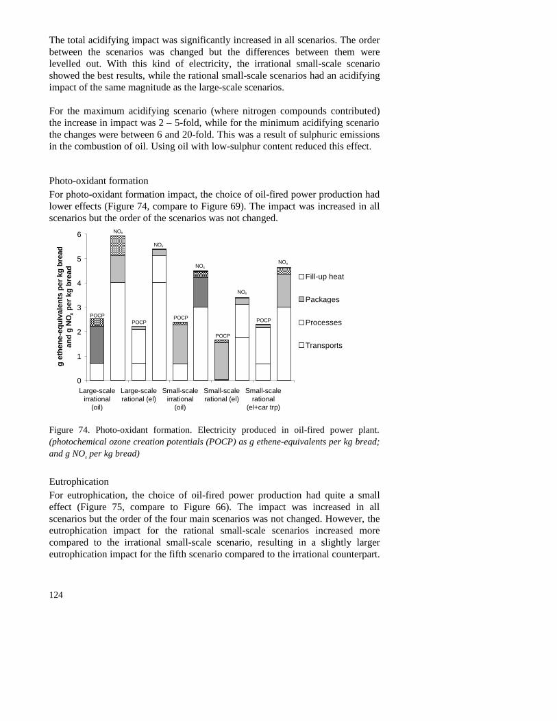
124

The total acidifying impact was significantly increased in all scenarios. The orderbetween the scenarios was changed but the differences between them werelevelled out. With this kind of electricity, the irrational small-scale scenarioshowed the best results, while the rational small-scale scenarios had an acidifyingimpact of the same magnitude as the large-scale scenarios.

For the maximum acidifying scenario (where nitrogen compounds contributed)the increase in impact was 2 – 5-fold, while for the minimum acidifying scenariothe changes were between 6 and 20-fold. This was a result of sulphuric emissionsin the combustion of oil. Using oil with low-sulphur content reduced this effect.

Photo-oxidant formationFor photo-oxidant formation impact, the choice of oil-fired power production hadlower effects (Figure 74, compare to Figure 69). The impact was increased in allscenarios but the order of the scenarios was not changed.

0

1

2

3

4

5

6


(oil)



(oil)


Small-scalerational

(el+car trp)

g et

hene

-equ

ival

ents

per

kg

brea

dan

d g

NO

x pe

r kg

bre

ad Fill-up heat

Packages

Processes

Transports

POCPPOCP

POCP

POCP

NOx

NOx

NOx

NOx

NOx

POCP

Figure 74. Photo-oxidant formation. Electricity produced in oil-fired power plant.(photochemical ozone creation potentials (POCP) as g ethene-equivalents per kg bread;and g NOx per kg bread)

EutrophicationFor eutrophication, the choice of oil-fired power production had quite a smalleffect (Figure 75, compare to Figure 66). The impact was increased in allscenarios but the order of the four main scenarios was not changed. However, theeutrophication impact for the rational small-scale scenarios increased morecompared to the irrational small-scale scenario, resulting in a slightly largereutrophication impact for the fifth scenario compared to the irrational counterpart.

125

0

10

20

30

40





Small-scalerational

(el+car trp)

g O

2-eq

uiva

lent

s pe

r kg

bre

ad

Packages

Processes

Transports


Figure 75. Eutrophication (maximum scenario). Electricity produced in oil-fired powerplant. (g O2-equivalents per kg bread)

Summary, sensitivity analysis of oil-fired power productionFigure 76 shows that the differences in environmental impacts were smaller whenelectricity was produced in oil-fired power plants compared to being produced asSwedish average (Figure 70). The trend was still, however, that the rationalsmall-scale scenario showed the smallest impacts. However, adding the privatecar transport made the rational small-scale scenario level with the rational large-scale scenario.

0.0

0.2

0.4

0.6

0.8

1.0

1.2

Large-scale

irrational(oil)

Large-scale

rational(el)

Small-scale

irrational(oil)

Small-scale

rational(el)

Small-scale

rational(el+car

trp)

rela

tive

valu

e






Energy consumption


Figure 76. All impact categories relative to the impact of the large-scale irrationalscenario. Electricity produced in oil-fired power plant. (relative values, 1=Large-scaleirrational scenario)

126

Rational scenarios gas-fired instead of electrically heatedIn Sweden, where electricity is mainly produced from hydropower and nuclearpower, it seems rational to use electricity for many purposes. However, for manyother places this is not that self-evident. The rational bread production scenariosin this study were, therefore, run in a set-up where the heating of ovens andfermentation rooms was done by burning of fossil gas. In the small-scale rationalscenarios, the grain drying process was also modified from an indirect biofuel-heated to a direct gas-heated drier. The irrational scenarios were not changed. Bycomparing Figure 77 and Figure 70, one can conclude that the shift fromelectricity to fossil gas did not produce any dramatic changes in environmentalimpacts. Only the global warming was affected, in the large-scale scenario byabout 25 %. For the small-scale scenario, the increase was almost 100 %, partlydue to the changes in the grain-drying set-up. In the small-scale scenario whereprivate cars were used for home-transport, the increase in global warming impactwas about 50 %.

The other effect that could be observed was on the consumption of primaryenergy resources. Here, the fossil gas set-up was better. The consumptiondecreased by almost 20 % in the large-scale scenario, by 25 % in the (first) small-scale scenario, and by about 20 % in the small-scale scenario where private carswere used for home-transport. This is an indication that use of electricity forheating purposes is not an efficient use of resources. However, depending on howthe electricity was produced and on which resources were scarce and which wereabundant, electricity nevertheless fell out as the best alternative.

0.0

0.2

0.4

0.6

0.8

1.0

1.2

Large-scale

irrational(oil)

Large-scale

rational(gas)

Small-scale

irrational(oil)

Small-scale

rational(gas)

Small-scale

rational(gas+car

trp)

rela

tive

valu

e






Energy consumption


Figure 77. All impact categories relative to the impact of the large-scale irrationalscenario. Rational scenarios gas-fired. (relative values, 1=Large-scale irrationalscenario)

127

Imported grainImported grain is sometimes used to get a larger protein (gluten) content in theflour, but there seems to be no difference between scales. Possibly it is more anindicator of how well the bakery process is designed, since a gently-handleddough requires flour with lower protein content to make a fluffy bread than doesa roughly-handled dough. To say that it is correlated to scale or energy efficiencyis probably not relevant. Therefore, no sensitivity analysis with use of importedgrain was performed.

129

Liquid milk production system

This chapter presents an introductory study of the liquid milk production system.The aim was, as mentioned before, to study a common type of food that could beexpected to have different properties concerning energy consumption andenvironmental impacts compared to bread production. The presentation startswith methodological issues and continues with the results and discussion.

System boundariesThis study followed the structure of the bread production study. It includedtransport of milk from farm to dairy, processing of milk (dairy total energyconsumption), clean water production, production of packaging for milk,handling of waste milk packaging, sewage plant treatment of dairy wastewater,and transport of liquid milk from the shop to the consumer’s door. The system, asstudied here, is shown in Figure 78.


milk fromfarmfuel and

electricityproduction(for supplyto all partsincluded inthe system)

transport

milkpackagingproduction

ingredientspackagingproduction

ingredientsproduction

and transportstransport(s)

milkpackagingrecycling

milkpackaging

incineration

milktransport(s) and

distribution

wholesalersand retailers

private cartransport

storage etc. atconsumer's home

transport

transport(s)

wastewatertreatment

total energyconsumption

DAIRY

landfill

raw material

washing ofsecondarypackages

cleaningagents

packagingproduction

cleaningagents

productionand transports

Figure 78. Flow chart of the milk production system. Dotted blocks not included in thestudy.

130

In order to give results comparable to the results from the bread production study,the system boundaries were as equal to those in the bread production study aspossible. Thus, the primary production of milk was not included in the analysis,neither were the retailer level nor the consumer phase, although they are probablyof more importance in the milk system than in the bread system. Other parts ofthe system left out were on-farm storage of milk and the fate of dairy by-products. Concerning packaging, the transportation of packaging frommanufacturer to dairy was not included. Since same package type was chosen inall scenarios, no "fill-up" heat production was needed.

The model outputs were yearly amounts of emissions and energy consumption,but all results were recalculated to emissions and energy consumption per kg milkproduced. To obtain the results for a 100-person unit, the per-kg-milk results haveto be multiplied by 15 000; 150 kg milk per person and year in Sweden (Becker,1992) times 100 persons.

ScenariosAs in the bread production study, four main scenarios were presented. Two werelarge-scale systems and two small-scale systems. Additionally, a fifth scenariowas included, namely the small-scale rational scenario complemented with theprivate-car transport used in the other scenarios. The processed milk wasdistributed in cardboard single-use packages in all scenarios. The cardboard wasassumed to be recycled, eventually ending up in an incineration plant. Dairywastewater was treated in a sewage plant in all scenarios.

1. Irrational large-scale, was not energy-optimised and the dairy used oil for heatproduction. Milk was transported 100 km by truck to the dairy. The processedmilk was first transported 100 km by truck (inter-regional), then locallydistributed to shops by truck (100 km round-trip), and finally transported 5 km byprivate petrol-driven car to the consumer's home.

2. Rational large-scale, had an energy-optimised dairy. It used electricity for allheating. Transport was equal to that in the irrational large-scale scenario.

3. Irrational small-scale, had a non-energy-optimised dairy that used oil for heatproduction. The milk was transported 50 km by truck to the dairy. The processedmilk was distributed locally to the shops by truck (100 km round-trip) and then,as in the large-scale scenarios, transported to the consumer's home by private car.

4. Rational small-scale, used electricity for all heating in the dairy, which wasenergy optimised. The transport to the dairy and the distribution to shops wereequal to those in the irrational small-scale scenario. The transport from the shopto the consumer's home was done on foot, by bicycle, or by home-distributioncarried out by the dairy. In the latter case this was assumed to be included in theenergy consumption calculated for the local distribution, and thus assumed to becarried out in an energy efficient manner.

131

5. Rational small-scale + car transport, was equal to the fourth scenario but wascomplemented with the vehicle-transport to the consumer's home by private(petrol-driven) car as used in the first three scenarios.

ModelsThe general structure of the model was equivalent to that in the bread productionstudy. Where appropriate, the same sub-models were used. The dairy model isstructured like the bakery model, but no partition of energy consumption betweendifferent processes was performed, i.e. total energy consumption (includingheating of premises etc.) for dairies was used. The model makes it possible tochoose electricity and/or fuel as the energy source. For air emission calculation, itis possible to choose different fuels for the heat production. The water emissionsare calculated in the model. Concerning the transport from the shop to theconsumer's home by private car, the same assumptions were made as in the breadproduction study. Liquid milk, like bread, stands for about 6 % of the cost of ourfood consumption (SCB, 1999), and thus 6 % of the transport was allocated tothe liquid milk. Data for energy consumption, transport distances, waterconsumption and water emissions are collected from several sources (Elsy, 1981;Cox & Miller, 1985; Lucas, 1985; Verma, 1988; Larsson, 1997; Høgaas Eide,1998; Hedegård, 1999; Bengtsson, 1999; Pyler, 1999; Jürss, 1999). For moredetails see Appendix 8.

132

Results and discussion of the liquid milk production systemFor liquid milk production systems, the small-scale scenarios had no advantagesconcerning energy consumption (Figure 79). The lower energy consumption fortransportation did not compensate for energy consumption in processes, as wasthe case in the bread production system (Figure 63). However, with regard to theenvironmental impacts, the situation was different. As an example, the globalwarming impact is shown in Figure 80. Transport was a more dominant part forenvironmental impacts than for energy consumption. The same was true foracidification, eutrophication and emissions of NOx. Whether this was due to realdifferences or weaknesses in data reliability might be a question for furtherresearch.

0

1

2

3


Large-scalerational


Small-scalerational

Small-scalerational+CarTrp

MJ

per

kg m

ilk

Packages,thermal

Packages,electricity

Processes,fuel

Processes,electricity

Transports,fuel

Figure 79. Energy consumption in different system parts. (MJ per kg milk)

0.00

0.02

0.04

0.06

0.08

0.10

0.12

0.14

0.16


Large-scalerational


Small-scalerational

Small-scalerational+CarTrp

kg C

O2-

equi

vale

nts

per

kg m

ilk

Packages

Processes

Transports

Figure 80. Potential global warming impact (100-years scenario) due to emissions fromdifferent parts in the system. (kg CO2-equivalents per kg milk)

133

The environmental impact categories assessed are listed for the five scenarios inTable 14. The results are also shown relative to the large-scale irrational scenarioin Figure 81. It could be concluded that the tendency was similar to that in thebread production study. Small-scale systems can be better concerning the impactcategories included, but to make significant improvements the small-scale has tobe combined with a local market, i.e. the consumers must be able to walk or biketo the shop, or have the food (energy-efficiently) delivered at the doorstep.

Table 14. Overall results for the different liquid milk proLduction scenarios. (impact perkg milk)


Large-scalerational


Small-scalerational

Small-scalerational +car transport


0.14 0.09 0.15 0.04 0.08

Acidification, max(mmol H+)

0.033 0.030 0.026 0.014 0.021

Acidification, min(mmol H+)

0.005 0.004 0.006 0.003 0.003


1.1 1.1 1.1 0.9 1.1


1.3 1.3 1.0 0.6 0.9

Eutrophication(g O2-equivalents)

9.6 8.7 8.5 4.1 5.9

Energy consumption(MJ electricity)

0.5 0.7 0.8 1.0 1.0

Energy consumption(MJ thermal)

1.7 1.3 1.7 0.8 1.1


3.3 3.2 3.9 3.3 3.7

Water consumption(litre water )

2.0 1.0 4.0 3.0 3.0

134

0.0

0.2

0.4

0.6

0.8

1.0

1.2

1.4

Large-scale

irrational

Large-scale

rational

Small-scale

irrational

Small-scale

rational

Small-scale

rational+CarTrp

rela

tive

valu

eGlobal warming(GWPs, 100 years)





Energy consumption


Figure 81. All impact categories relative to the impact of the large-scale irrationalscenario. (relative values, 1=Large-scale irrational scenario)

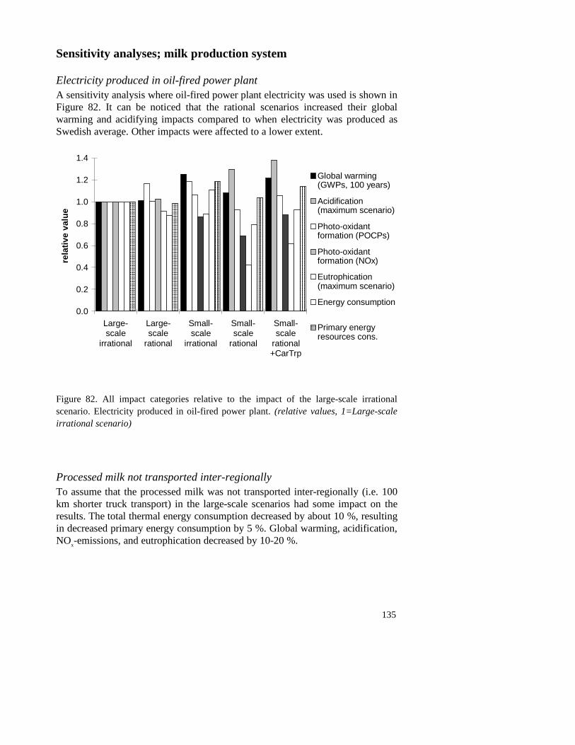
135

Sensitivity analyses; milk production system

Electricity produced in oil-fired power plantA sensitivity analysis where oil-fired power plant electricity was used is shown inFigure 82. It can be noticed that the rational scenarios increased their globalwarming and acidifying impacts compared to when electricity was produced asSwedish average. Other impacts were affected to a lower extent.

0.0

0.2

0.4

0.6

0.8

1.0

1.2

1.4

Large-scale

irrational

Large-scale

rational

Small-scale

irrational

Small-scale

rational

Small-scale

rational+CarTrp

rela

tive

valu

e






Energy consumption


Figure 82. All impact categories relative to the impact of the large-scale irrationalscenario. Electricity produced in oil-fired power plant. (relative values, 1=Large-scaleirrational scenario)

Processed milk not transported inter-regionallyTo assume that the processed milk was not transported inter-regionally (i.e. 100km shorter truck transport) in the large-scale scenarios had some impact on theresults. The total thermal energy consumption decreased by about 10 %, resultingin decreased primary energy consumption by 5 %. Global warming, acidification,NOx-emissions, and eutrophication decreased by 10-20 %.

137

Cyclic small-scale food systems – an example

Though far from complete, I will present an example of a cyclic small-scale foodsystem and compare it to a current system. The aim is to show the maximumeffect that could be obtained if a chain in a food-system were changed to a cyclicsmall-scale system. The parts considered in the system were organic wastemanagement, N emissions from soil, grain-production field operations, chemicalfertiliser production, grain and bread processing, clean water production,production of packaging and transport between all parts in the system, i.e. allparts considered in the previously presented chapters “Organic wastemanagement system” and “Bread production system”. The example reflects onechain of the flow of organic matter that goes from-consumer-via-agriculture-to-consumer.

The perspective when putting together the example, called the Cyclic-Small-Scale-scenario, was to choose a system that was thought to be resourceconserving and energy efficient. It was compared to the Situation-of-Today-scenario, which was thought to represent the large-scale and nonenergy-optimisedsystem that exists today, though many systems are evolving to become large-scale and efficient.

The results for the two scenarios were obtained by summation of results fromscenarios in the studies of organic waste management and bread productionpresented earlier in this thesis. The Situation-of-Today-scenario was the sum ofthe “SludgeToSewPlant” organic waste management scenario and the “Large-scale irrational” bread production scenario. The Cyclic-Small-Scale-scenario wasthe sum of the “AnaerobicDigestionUrineSeparationNoHygienisation” organicwaste management scenario and the “Small-scale rational” bread productionscenario.

A small-scale scenario containing anaerobic digestion could be argued to be veryhypothetical but small-scale digestion is getting increased attention in e.g.Austria, Germany, Denmark, and Sweden (Lindberg & Edström, 1998). Theresults for the Cyclic-Small-Scale example are presented in Figure 83 as relativevalues compared to the Situation-of-Today scenario. For actual contribution toimpact categories see Table 15.

138

-0.5

0

0.5

1

1.5

2re

lativ

e va

lue

Cyclic-Small-Scale, bread production

Cyclic-Small-Scale, org. waste management

Situation-of-Today, bread production

Situation-of-Today, org. waste management

E

utro

phic

atio

n(m

ax. s

cena

rio)

Glo

bal w

arm

ing

(GW

Ps)

Aci

diph

icat

ion

(max

. sce

nario

)

Pho

to-o

xida

nt fo

rmat

ion

(PO

CP

s)

NO

x-em

issi

ons

Ene

rgy

cons

umpt

ion

Prim

ary

ener

gy r

esou

rces

cons

umpt

ion

Wat

er c

onsu

mpt

ion

Figure 83. Environmental impacts and resources consumption. Cyclic-Small-Scalescenario compared to Situation-of-Today scenario. (relative value, 1=Situation-of-Today)

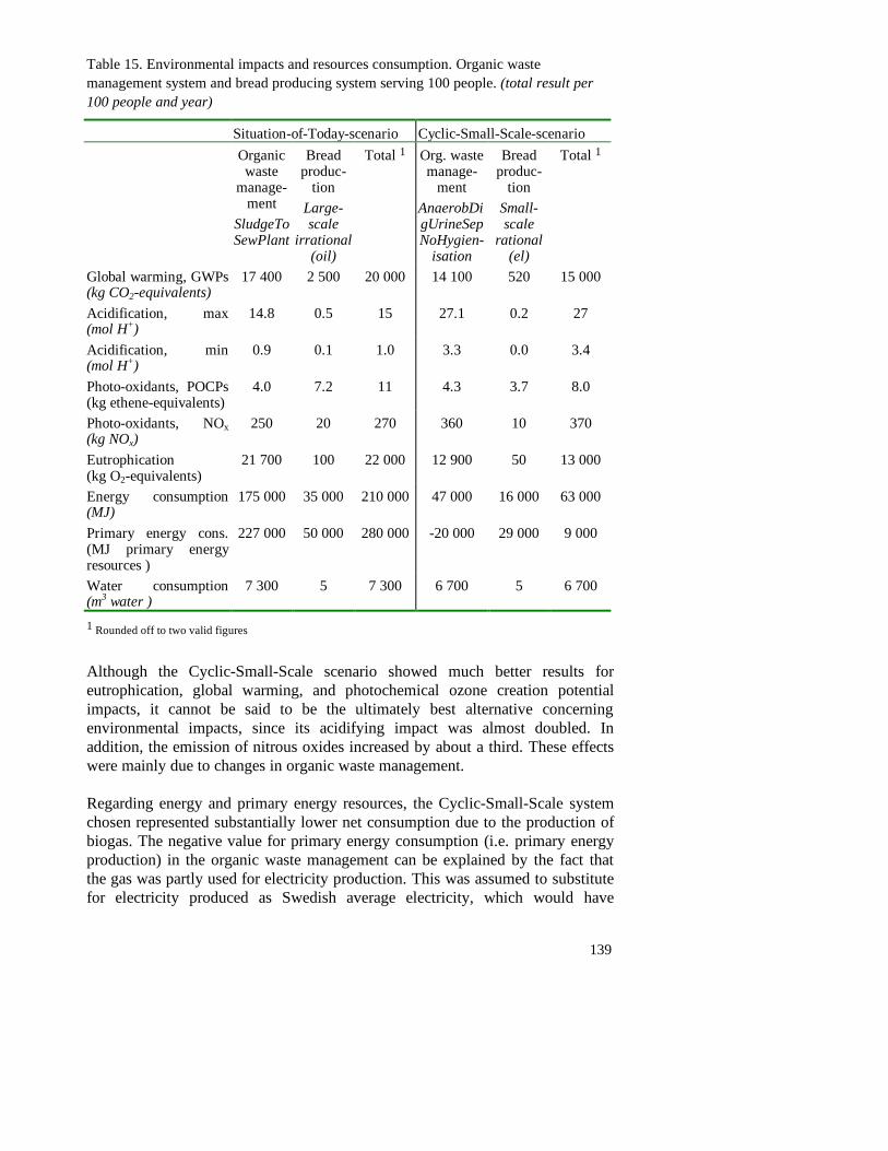
139

Table 15. Environmental impacts and resources consumption. Organic wastemanagement system and bread producing system serving 100 people. (total result per100 people and year)

Situation-of-Today-scenario Cyclic-Small-Scale-scenario

Organicwaste

manage-ment

SludgeToSewPlant

Breadproduc-

tion

Large-scale

irrational(oil)

Total 1 Org. wastemanage-

ment

AnaerobDigUrineSepNoHygien-

isation

Breadproduc-

tion

Small-scale

rational(el)

Total 1


17 400 2 500 20 000 14 100 520 15 000

Acidification, max(mol H+)

14.8 0.5 15 27.1 0.2 27

Acidification, min(mol H+)

0.9 0.1 1.0 3.3 0.0 3.4

Photo-oxidants, POCPs(kg ethene-equivalents)

4.0 7.2 11 4.3 3.7 8.0

Photo-oxidants, NOx(kg NOx)

250 20 270 360 10 370

Eutrophication(kg O2-equivalents)

21 700 100 22 000 12 900 50 13 000

Energy consumption(MJ)

175 000 35 000 210 000 47 000 16 000 63 000


227 000 50 000 280 000 -20 000 29 000 9 000

Water consumption(m3 water )

7 300 5 7 300 6 700 5 6 700

1 Rounded off to two valid figures

Although the Cyclic-Small-Scale scenario showed much better results foreutrophication, global warming, and photochemical ozone creation potentialimpacts, it cannot be said to be the ultimately best alternative concerningenvironmental impacts, since its acidifying impact was almost doubled. Inaddition, the emission of nitrous oxides increased by about a third. These effectswere mainly due to changes in organic waste management.

Regarding energy and primary energy resources, the Cyclic-Small-Scale systemchosen represented substantially lower net consumption due to the production ofbiogas. The negative value for primary energy consumption (i.e. primary energyproduction) in the organic waste management can be explained by the fact thatthe gas was partly used for electricity production. This was assumed to substitutefor electricity produced as Swedish average electricity, which would have

140

consumed 2.35 MJ primary energy resources for each MJ produced. Theequivalent value for electricity produced in an oil-fired power plant is 2.69MJ/MJ.

Concerning acidification, it is important to remember that in many ecosystems inScandinavia and Northern Europe, nitrogen compounds are usually neutralised toa large extent. Therefore, figures for an acidification minimum-impact scenarioare also presented in Table 15. These indicate that the acidification could besubstantially smaller than the maximum acidification scenario. In practice, thesituation should be somewhere in between the two. In the minimum-acidificationcase, the Cyclic-Small-Scale system would have an approximately three timeslarger acidifying impact compared to the Situation-of-Today system. This is dueto the fact that the acidification was largely an effect of nitrogen compounds (notcounted in the minimum acidification scenario) in the Situation-of-Today system,while in the Cyclic-Small-Scale system it was sulphuric oxides from thecombustion of biogas which caused the effect. As mentioned above, this can bedealt with by process adjustments that decrease the creation of hydrogen sulphideor by cleaning of the biogas before combustion.

The emissions of NOx largely emanated from transport.

141

General discussion

This thesis is an attempt to evaluate some environmental impacts andconsumption of some natural resources in small-scale cyclic food-systems.Although the entire food-system has not been included, some general conclusionscan be drawn. The most self-evident conclusion is, as expected, that no singlesystem or scenario is “best” concerning all impact categories. There is always adrawback, which has to be taken into consideration in the process of a real-worldchoice of system. For example, the Cyclic-Small-Scale scenario presented inprevious chapter showed substantially better results for energy turnover and formost of the environmental impacts studied, but had double the contribution toacidification compared to the Situation-of-Today scenario and also somewhatgreater NOx-emissions. Thus if acidification is an environmental problem in thearea/region of concern, maybe this system should not be chosen or, at least,actions to avoid the problem will have to be taken into account. The on-siteimpacts of NOx have also to be examined. Furthermore, it might be proper tomake a normalisation against total emissions from other sources in thearea/region to assess the relative contribution of the system under investigation inits context.

When making a study for later implementation, it is essential to choose scenariosfor impact assessment, types of fuels and electricity production types that arerelevant for the area and situation of concern, as these choices may actuallydetermine the results. Moreover, it is important to be clear about the purpose andgoal of the study and about the timeframe one has in mind for possible systemmodifications.

Organic waste managementConcerning organic waste handling, the scenarios studied represented systemspresent or possible in small towns, villages and rural areas, i.e. no scenario withsewage plant treatment of wastewater was included. I would still claim that manyof the results are general in their character. Firstly, one can conclude that, ingeneral, the household residue part is small compared to the internal flows inagriculture. However, it might be important to recycle these residues in regionswith small numbers of animals, or with large numbers of people. Furthermore,the recycling of municipal organic waste can serve as a means to get bettertreatment for the on-farm organic residues (e.g. manure) as it may change theattitude to organic fertilisers and give opportunities for co-treatment ofagricultural and municipal organic wastes. It could also be an economic sidelinefor farmers to take care of and treat municipal organic wastes.

When comparing different sewage systems, three main criteria are of concern –sanitary performance, conservation of environmental and natural resources assetsand technical and socio-economic aspects (Finnson et al., 1995). Included intechnical and socio-economical aspects are e.g. user friendliness, impact on social

142

planning, questions of responsibility, and economics. Although environmentalimpacts are focused upon here, the other aspects have to be remembered whenreal-life case studies are performed.

As expected, plant nutrient recycling is improved when reactor treatments ofblackwater and organic wastes are used, compared to on-site sludge separationand biopond treatment of unsorted household wastewater in combination withhome composting of organic wastes. However, the study shows that it isimportant to make an analysis of the plant-availability properties of the materialbrought back to arable land, and not only of its amounts, when studying plantnutrient recycling. This may be especially valid for the different fractions ofnitrogen, but phosphorus also seems to have different qualities (see e.g. Hagströmet al., 1997; Linderholm, 1997; Ugland et al., 1998). By calculating expectedyield of grain resulting from the amounts of different fractions of nitrogenrecycled, which have different fertilising efficiencies, I have shown largedifferences in performance between treatments that give comparable results whenlooking at amounts recycled. Thus, when analysing plant nutrient recycling it isimportant to remember that the social residues are going to be utilised inagriculture. Instead of calculating the expected yield of grain, one mightrecalculate the recycled nutrients to chemical fertiliser equivalents but then it iseasy to lose one's perspective on conservation and self-sufficiency with respect tolocally-available resources. However, knowledge about the long-term effects oforganic waste recycling for the soil is limited. More research is needed to be ableto assess the quality of organic fertilisers originating from social wastes.Furthermore, the plant nutrients that are not utilised after recycling might turn outto be pollutants in surrounding ecosystems.

Somewhat surprisingly, the liquid composting treatment resulted in significantlysmaller yields of grain than the anaerobic digestion treatment. This was probablya result of imperfections in the model, but more research is needed to evaluate thereason.

Urine-separating toilet systems increased both the recycling of nutrients to arableland and the expected yield of grain. The effect was most obvious in the on-sitesludge separation scenarios where it gave dramatic improvements (seven to eighttimes larger yield of grain). For the biopond and compost treatments, urineseparation gave about three times larger additional yield of grain while in theliquid compost and anaerobic digestion scenarios it had a minor effect. Theintroduction of urine-separating toilets into the systems studied resulted in equalor smaller energy consumption. The water saving achieved in urine-separatingtoilets resulted in decreased fuel consumption for transportation and spreading ofthe household residues by about a quarter in liquid compost and anaerobicdigestion scenarios. However, the largest energy saving effect in real terms wasobtained internally in those treatments. Other water-saving technologies wouldprobably give a similar result.

The liquid compost and anaerobic digestion scenarios had large energyconsumption for transportation compared to the others, due to the large volume

143

(mostly water) handled. In spite of this, these scenarios showed better resultswhen it came to net energy turnover for the entire system, due to the energyproduction obtained in the treatments. In places where pipe-transport is possible,the energy consumption may be further decreased. Dry composts produce heatthat should also be possible to utilise, for example by condensation of outletgases. This option was, however, not included in this study. By proper treatmentof the condensation water, it should be possible to use it as nitrogen fertiliser.

The anaerobic digestion scenario with urine-separating toilet system and nohygienisation of incoming material showed figures which indicated that a netenergy break-even was possible to reach. Note that this is valid with the 2-kmtransporting distances chosen in this study. Still, some energy saving in thesystem assumed here would have to be performed to reach zero-energy-consumption. Choosing 10 km average transporting distances increased energyconsumption by about 30 % in the liquid compost scenarios, and by between 35and 55 % in the anaerobic digestion scenarios (energy production not affected).For the other scenarios, the change was in the order of 10 %. It might not beeconomically viable to use small-scale anaerobic digestion treatment todaybecause of the high investment cost, but low-tech small-scale digestion is gettingincreased attention in several countries (Lindberg & Edström, 1998). By co-treatment of social and agricultural wastes, digestion seems likely to become analternative for farmers to be less dependent on fossil fuels.

It is at the same time worth noticing that the anaerobic digestion scenariocombined with an ordinary sewage system and hygienisation of incomingmaterial had the most negative energy turnover of all scenarios. On the positiveside for biogas production is the fact that the digestion reactor requires heat (andsome electricity for pumping) but produces gas, which has "higher energyquality". This gas can for example be used for electricity (and heat) production orcleaned and compressed for use as vehicle fuel. The equivalent drawback forliquid composting is that it demands electricity but produces heat. Besides, it isnot easy to utilise the heat produced. However, for hygienisation purposes, theliquid composting system is probably preferable, since the temperature is higherduring a longer period of time. Which of these two systems to choose is a matterof the conditions at the relevant site. Factors influencing this are: the need ofhygienisation before spreading the residues on farmland, access to renewableenergy sources such as wind-power electricity and biofuels, and the potential toutilise the energy produced (heat or gas). In addition, the type of energy sourcessubstituted by utilisation of the energy produced is of vital importance whenchoosing a system. It is of course best to choose a system that decreases theconsumption of the fossil energy sources used today.

The heavy metal contamination of arable land due to recycling of organicresidues was mainly an effect of spreading the manure from the 15 dairy cowsand their young stock included in the calculations. The contribution fromhousehold residues was small, but might still be of importance. Concerning thehousehold residues, the results obtained in this study indicated that, in general, no

144

more heavy metals were recycled when more plant nutrients were recycled sincemany of the metals came with household organic wastes, which were recycled inall scenarios. The exception was mercury (Hg), which was found in faeces(probably originating from dental amalgam, which should disappear over time asother dental materials are used nowadays). However, the results concerning heavymetals have to be carefully interpreted since the quality of the data can bequestioned. In practice, the metal content in different fractions of organic wastemay vary a lot, especially in the case of copper. Regions with hard watergenerally have high levels of copper in sewage sludge. This copper originatesfrom hot-water pipes used in houses. One possible long-term solution discussedpreviously is blackwater separation. It is an expensive, but in the long run maybenecessary, investment to obtain sufficiently clean organic fertilisers. Thegreywater would then have to be dealt with separately.

Food production and processingFor the other half of the cyclic system, the food production and processing part,bread production was closely studied and liquid milk production was the subjectof a preliminary study. These are only two parts of the complex food-productionsystem but they represent two rather different kinds of staple foods. The study ofthese two systems gave results that pointed in the same direction, so I think it ispossible to draw some general conclusions.

The first is that small-scale food-production systems can have advantages froman environmental impact and energy consumption point of view, but that small-scale does not of its own mean "environmentally friendly". The simulationsperformed showed that an energy-optimised large-scale system was better, inthese aspects, than a non-optimised small-scale system. Furthermore, althoughthe energy-optimised small-scale processing plant was assumed to be somewhatmore energy consuming compared to energy-optimised large-scale processingplants, the entire small-scale system showed better results concerning most of theimpacts categories included. This was especially valid for environmental impacts,while for energy consumption the difference was smaller. The two most essentialparts of the systems were the processing and the transport of food from the shopto the consumer’s home by private car. Emissions generated in the long-distancetransport also contributed to environmental impacts but seemed to be relativelysmaller than the private car transport. This is of course very dependent on thechoices of transport distances chosen in the study.

In any case, the second conclusion that can be drawn for food-production systemsis that: if small-scale systems are to have smaller environmental impacts, theyhave to take advantage of the small-scale throughout the entire system, meaningthat not only the processing, but also the distribution system should be small-scale. Thus the local market should be close enough to make it possible forconsumers to walk or to use a bicycle etc. when shopping, all in order tominimise private car transport.

145

Efficient home-distribution systems, similar to the milk-bottle system common ine.g. England, might be another option to lower environmental impacts. Inprincipal, this type of distribution can be used by food-processing companies ofall scales. Small-scale processors may manage such a system themselves, whileon the large-scale this system would probably be administered by retailers,possibly by Internet shopping-systems. This area, which it was not possible toinclude in this study, is of utmost importance when discussing food systems andenvironmental impacts. More research effort needs to be put in here.

Another aspect that may be positive for small-scale processing is the everdecreasing cost of process-regulation technology. As it becomes cheaper, itshould be more available for small-scale implementations, thus making themmore economically competitive. A shift in taxation from taxes on labour to taxeson natural resources would probably also favour the small-scale, since transportwould then become more expensive. On the other hand, energy consumed inprocesses would also become more expensive, which could be negative for small-scale processing since generally more energy is consumed in this part of thesystem compared to large-scale facilities. However, the stationary type of energyconsumption is easier to control than the spread-out consumption in vehicles, sothere might be differences in levels of taxation (in favour of the stationary type).

What might be the largest problem for small-scale processing to deal with wouldbe to keep the energy efficiency high in every part of the system; pre-heating-time and full-temperature-time of heating furnaces, use of warm water,ventilation, etc. This might be hard to combine with production of many types ofproducts, since the internal flow of products gets very complicated and thus hardto manage logistically. A diversified production is probably necessary if one wantto have a local market with short transport distances and a good assortment ofproducts.

Cyclic food systemsWhen studying the examples of the whole food-system presented in this thesis,one can conclude that the small-scale cyclic system needed only a third of theenergy compared to the large-scale conventional system. Dominating here wasthe organic waste management system (including agriculture), while the breadproduction system stood for a minor part. Aggregating processing for manydifferent foods would of course change this relationship. It should also beremembered that this analysis only included a few parts of the agricultural sector.For example animal farming, which is most probably a major contributor toenvironmental impacts and resource consumption, was not included here. It wasassumed that the parts omitted did not change between the scenarios studied. Thatseems reasonable, but – it makes it impossible to decide the importance ofdifferences between scenarios concerning environmental impact in the wholefood system from results obtained here. For this, studies of the agricultural

146

processes involved have to be performed. A recently published LCA study ofprimary milk production (Cederberg, 1998) indicates that global warming,acidification and eutrophication impacts could be much larger in the agriculturalproduction of milk than in processing and distribution (Table 16 compared toTable 14), while photo-oxidant formation and energy consumption could be inthe same order of magnitude in both systems.

Table 16. Environmental impacts and energy consumption for milk primary production.(Cederberg, 1998)

Impact per kg milk

Global warming, GWPs 100 years(kg CO2-equivalents)

0.94 - 0.98

Acidification, max scenario(mmol H+)

0.50 - 0.56


0.28 - 0.36


1.8 - 2.1

Eutrophication, max scenario(g O2-equivalents)

260 - 290


2.4 - 2.8

To be able to compare the environmental impacts for the primary production ofmilk with the impacts for processing and transport of milk studied here, somerecalculations had to be performed. The figures in Table 16 were multiplied by 15000 (150 kg milk per person and year, calculation from Becker, 1992) giving theenvironmental impacts for primary milk production required for 100 people andyear (Table 17). Please note the differences in units. Comparing these figures tothe ones presented in Table 15 gave a somewhat different picture. Almost allimpact categories were in the same order of magnitude (at least for the Cyclic-Small-Scale-scenario), indicating that both the animal production and the parts ofthe food system studied in this thesis should be of importance for environmentalimpacts and energy consumption. Comparing with the Situation-of-Today-scenario, indicates that the processing and distribution are larger contributors toNOx-emission, eutrophication and energy consumption than the primaryproduction of milk.

147

Table 17. Environmental impacts and energy consumption for milk primary production.(calculated from Cederberg, 1998 and Becker, 1992)

Impact per 100 people and year


14 100 - 14 700

Acidification, max(mol H+)

7.5 - 8.4

Photo-oxidants, POCPs(kg ethene-equivalents)

4.2 - 5.2

Photo-oxidants, NOx(kg NOx)

27 - 32

Eutrophication(kg O2-equivalents)

3 900 - 4 350


36 000 - 42 000

An aspect not included in this study is product quality. It is a vast subject thatincludes many different issues like taste, smell, look, freshness, price, hygienicproperties, storage properties, nutritional value, non-toxicity, trust (in a brand orpersonal relationship to producer/processor etc.), packaging, knowledge about theproducer, knowledge about harvest or production date/time, knowledge about"animal-friendly" production, etc. etc. I believe that many, but not all, are in thefavour of local small-scale systems.

Another aspect that may be of importance is the consumption of materials andenvironmental impacts for the construction of infrastructure, vehicles, technicalequipment, buildings etc. Concerning equipment and buildings, it is easy tobelieve that large-scale plants are better. For infrastructure, the small-scalesystems should definitely be more favourable. However, to assume that we wouldmanage with smaller or fewer roads if we chose to have small-scale systemswould probably be to go too far, but this discussion and scientific field should befurther developed (by others). At least, it can be concluded that transport was asignificant contributor to the environmental impacts included in the analysis,although it was not of any large importance concerning energy consumption. Thisindicates that systems using less transportation are to prefer. Furthermore,transports contribute largely to environmental impact categories not included inthis study, like noise, risk for accidents, toxicological impacts on humans, landuse, habitat alterations and influence on biological diversity.

148

Computerised mathematical models as a toolThe models developed in this project should be possible to use as a tool inplanning of new settlements, or in assessment and development of existingstructures. They are, however, not easy to use by whoever is interested. Firstly,they are not constructed to simply put some figures in and get some results out,though in principal it is possible to develop them to such a level. Secondly, theirstructure and many underlying assumptions make them too complex to be usedwithout educated "consultants". Of course, these models can be run by manypeople with some experience in computers, but then they would not producereliable results.

149

Conclusions

• No system is "the best" concerning all environmental impact categories

• Different systems may be appropriate at different places or in differentsituations, as the environmental effects may vary greatly between localities

• Different systems may be appropriate at different places and in differentsituations, due to the energy sources which are available and the energysources which are substituted

• Different systems may be appropriate at different places or in differentsituations, as the purpose the system has to fulfil may vary a lot

• Amounts and environmental impacts of organic wastes from households aregenerally small compared to internal flows of manure etc. in agriculture

• If organic wastes are to be used as fertilisers it is important to remember andkeep track of their properties as fertilisers

• Blackwater sorting systems are a means to increase plant nutrient recyclingrate and thus grain yields

• Urine separation increases nitrogen recycling rate and thus grain yields

• Urine separation lowers the energy consumption

• One scenario, with anaerobic digestion treatment (with no hygienisation ofincoming material) and a urine-separating toilet system, showed resultswhich indicated that the organic waste management system and agriculturecould be energy self-supporting

• Small-scale food-production systems can (but does not necessarily) haveadvantages from an environmental impact and energy point of view

• To really utilise the advantages small-scale systems may have, they shouldbe combined with a nearby local market in order to minimise all transport

• An energy-optimised large-scale system is better, concerning environmentalimpact and energy consumption, than a non-optimised small-scale system

• The two most essential parts in the food-processing systems studied herewere the processing itself and the private-car transport of food from shop toconsumer’s home

• Electricity produced as Swedish average (mainly hydropower and nuclearpower) is clean concerning the environmental impact categories included inthis study, but consumes much primary energy resources – thus, it is bestused for purposes other than heating (where it can more easily be substitutedfor resource conserving and less environmentally disturbing alternatives)

• Transport has a large environmental impact but is not that importantconcerning energy consumption in the systems perspective

151

References

Agenda 21. 1992. Summary of The Earth Summit. United Nations Conference onEnvironment and Development (UNCED), Rio de Janeiro, 3-14 June 1992. Availableat http://www.un.org/geninfo/bp/enviro.html. United Nations Department of PublicInformation.

Agfors G. 1996. Olja och naturgas - nytt bränsle i energidiskussionen (Oil and naturalgas – new fire to the energy discussion: In Swedish). Kemisk Tidskrift 5 p 29-32.

Allen P, van Dusen D, Lundy J & Gliessman S. 1993. Expanding the Definition ofSustainable Agriculture. Sustainability in the Balance. Agroecology Program.University of California. Santa Cruz.

Andersson K. 1998. Life Cycle Assessment (LCA) of bread produced on different scales- Case study. AFR-report 214. Swedish Environmental Protection Agency

Andersson Karin. 1998. Personal communication. Project Manager. E-mail:[email protected]. CIT, Chalmers Univ. of Technology. Göteborg,Sweden.

Andersson R. 1992. Slam från enskilda avlopp - hot eller resurs i ekologiskt lantbruk?(Sludge from single houses sewage - threat or resource in organic farming?: InSwedish). Meddelande 69. Dept of Crop Production Sci, SLU. Uppsala.

Arnkvist J. 1997. LCA of Bread - Comparison of the Packaging Systems in DifferentProduction Scales. Master of Science Thesis, 118. Dept of Food Science, ChalmersUniv of Technology. Göteborg.

Arvidsson J & Håkansson I. 1991. A model for estimating the crop yield losses causedby soil compaction. Soil and Tillage Research 20 p 319-332.

Arvidsson J & Håkansson I. 1992. En modell för att beräkna jordpackningens effekter pågrödors avkastning (An empirical model for estimating the crop yield losses caused bymachinery induced soli compaction: In Swedish). Rapporter frånjordbearbetningsavdelningen 82. Dept of Soil Sciences, SLU. Uppsala.

Axelsson E, Billing P, Guldstrand J, Havi J & Isaksson L. 1995. YTH Ost.Kemicentrum, Livsmedelsindustriutbildningen, YTH. Lund.

Becker W. 1992. Befolkningens kostvanor och näringsintag. (The population’s dietaryhabits and intake of nutrients: In Swedish). Vår Föda 8 p 349-362.

Bengtsson Lennart. 1999. Personal communication. Executive Manager.Phone: +46 35 125506 http://www.wapno.se/ . Wapnö Gods. Halland, Sweden.

Bengtsson M, Lundin M & Molander S. 1997. Life Cycle Assessment of WastewaterSystems - Case Studies of Conventional Treatment, Urine Sorting and LiquidComposting in Three Swedish Municipalities. Report 9. Technical EnvironmentalPlanning, Chalmers. Göteborg.

152

Berg P G & Nycander G. 1997. Sustainable neighbourhoods - a qualitative model forresource management in communities. Landscape and Urban Planning 39:2-3 p 117-135.

Björklund A. 1998. Environmental systems analysis of waste management - withemphasis on substance flows and environmental impact. AFR-report 211. SwedishEnvironmental Protection Agency. Stockholm.

Boustead I. 1993. Eco-profiles of the European plastics industry REPORT 3:POLYETHYLENE and POLYPROPYLENE. Report 3, PWMI. European Centre forPlastics in the Environment. pp 20

Boustead I. 1997. Eco-profiles of the European plastics industry REPORT 4:POLYSTYRENE (second edition). Report 4, PWMI. European Centre for Plastics inthe Environment. pp 33

Brolin L, Lindberg A, Linders H & Cederberg C. 1996. Flöden av organiskt avfall(Flows of organic waste: In Swedish). Report 4611. Naturvårdsverket (SwedishEnvironmental Protection Agency). Stockholm. pp 67

Carlsson A L. 1995. Näring, kadmium och bakterier i hushållsavlopp - en fältstudie avett urinsorterande avloppssystem med Lecabädd i Östhammar (Nutrients, kadmiumand bacterias in houshold sewage: In Swedish). Meddelanden frånjordbearbetningsavdelningen 19. Dept of Soil Sci, SLU. Uppsala. pp 51

Carlsson-Kanyama A. 1997. Food and the Environment - Implications of SwedishConsumption Patterns. AFR-report 161. Swedish Environmental Protection Agency.Stockholm.

Cederberg C. 1998. Life Cycle Assessment of Milk Production - A Comparison ofConventional and Organic Farming. SIK-Report 643. The Swedish Institute for Foodand Biotechnology. Göteborg.

Checkland P. 1989. Soft systems methodology. In: Rational analysis for a problematicworld (Rosenhead J, ed). John Wiley & Sons. pp 71 -100.

Claesson S & Steineck S. 1991. Växtnäring. Hushållning - miljö (Plant nutrients.Economizing - environment: In Swedish). Speciella skrifter 41. SLU. Uppsala.

Clarholm M. 1997. The Nitrogen Problem. In: Ecotoxicology: Responses, Biomarkersand Risk Assessment. An OECD workshop (Zelikoff JT, ed). 27. SOS Publications.Fair Haven, NJ. USA. pp 387 -402.

Cox G C & Miller E J. 1985. Comparative energy efficiencies of the dairymanufacturing and processing industry: Australia and New Zealand. AustralianJournal of Dairy Technology December p 138-142.

Dalemo M. 1996. The ORWARE Simulation Model - Anaerobic Digestion and SewagePlant Sub-models. Report 216. Dept. of Agric. Engineering, SLU. Uppsala.

153

Dalemo Magnus. 1998. Personal communication. AgrD. Senior researcher. Phone: +4618 303338 E-mail: [email protected]. Swedish Institute of AgriculturalEngineering. Uppsala.

Dalemo M, Sonesson U, Björklund A, Mingarini K, Frostell B, Jönsson H, Nybrant T,Sundqvist J-O & Thyselius L. 1997. ORWARE - A simulation model for organicwaste handling systems. Part 1: Model description. Resources, Conservation andRecycling 21 p 17-37.

Dalemo M, Sonesson U, Jönsson H & Björklund A. 1998. Effects of including nitrogenemissions from soil in environmental systems analysis of waste managementstrategies. Resources, Conservation and Recycling 24 p 363-381.

Daly H E. 1990. Toward some operational principles of sustainable development.Ecological Economics 2 p 1-6.

DOE/EIA. 1998. The World Oil Market. Report 0484.http://www.eia.doe.gov/oiaf/ieo98/oil.html#tcwos . Department Of Energy /Environmental Information Administration, USA.

Duveborg Leif. 1997. Personal communication. Phone: +46 498 269221. TechnicalOffice, The Community of Gotland.

Egebäck K-E & Grägg K. 1988. Undersökning av partikelfilter av Wall-Flow-typ(Investigation of Wal Flow-type particle filters: In Swedish). Report 3461. SwedishEnvironmental Protection Agency. Stockholm.

Egebäck K-E & Hedbom A. 1991. Emmissionsdatabank för dieselmotorer (Data bankfor emissions from diesel engines: In Swedish). Rapport Motortestcenter. MTC. ABSvensk Bilprovning. Haninge, Sweden.

Elinder M & Falk C. 1983. Arbets- och maskindata inom jordbruket (Work andmachinery data for agriculture: In Swedish). Maskindata 6. Inst f arbetsmetodik ochteknik, SLU. Uppsala.

Elsy B. 1981. Survey of Energy and Water Usage in Liquid Milk Processing. MilkIndustry 10 p 18-20 22-23.

Eriksson E, Svensson G, Lövgren G, Blinge M, Svingby M & Ölund G. 1995.Transporters miljöpåverkan i ett livscykelperspektiv (The environmental impact oftransportation in a life cycle perspective: In Swedish). FoU 126. StiftelsenREFORSK. Malmö. pp 129

Finnson A, Peters A, Sundberg K, Lind A & Åslander O. 1995. Miljöanpassade vatten-och avloppssystem - Förslag till bedömningsgrunder (Environmentally adapted waterand sewage systems - Proposal of basis for forming an assessment: In Swedish).Report 4429. Swedish Environmental Protection Agency. Stockholm.

Finnveden G, Andersson-Sköld Y, Samuelsson M-O, Zetterberg L & Lindfors L-G.1992. Classification (Impact Analysis) in Connection with Life-Cycle Assessments - APreliminary Study. Product Life Cycle Assessment. 172, pp 231

154

Flora C B. 1994. Science and sustainability: An overview. American Journal ofAlternative Agriculture 9:1-2 p 72-75.

Fluck R C. 1992. Energy of Agricultural Products. In: Energy in Farm Production, vol.6 of Energy in World Agriculture (Fluck R C, ed.; Stout B A, editor-in-chief). ElsevierScience Publishers B.V. Amsterdam.

Gardner G & Sampat P. 1999. Forging a Sustainable Materials Economy. In: State of theWorld '99, Chapter 3. Worldwatch Institute. Washington DC. pp 57 -77.

Gebresenbet Girma. 1998. Personal communication. AgrD. Senior researcher. E-mail:[email protected]. Dept. of Agricultural Engineering, SLU. Uppsala,Sweden.

Gibb J R. 1978. TRUST - A New View of Personal and Organizational Development.The Guild of Tutors Press. LA California.

Gotlands kommun. 1996. Bevattning med avloppsvatten enligt gotlandsmodellen -Utvärdering (Irrigation with sewage water following the Gotland-concept - Anevaluation: In Swedish). Gatukontoret, Gotlands kommun. Visby. pp 39

Grägg K. 1990. Lågemitterande tätorts (LETT)-fordon (Low emission urban vehicles: InSwedish). Rapport Motortestcenter, MTC. AB Svensk Bilprovning. Haninge, Sweden.

Grägg K. 1992. Undersökning av tre dieselbränslen främst med avseende påslutkokpunktens betydelse för avgasutsläppet (Investigation of three diesel fuels,mainly focused on the impact of final vaporising point on exhaust emission: InSwedish). Rapport Motortestcenter MTC. AB Svensk Bilprovning. Haninge, Sweden.

Günther F. 1995. Structural vulnerability in agriculture: Its Alleviation by Means ofIntegration of Agriculture and Settlements. Agriculture, Ecosystems and Environmentp 47.

Habersatter K, Fecker I, Dall'Acqua S, Fawer M, Fallscheer F, Förster R, Maillefer C,Ménard M, Reusser L, Som C, Stahel U & Zimmermann P. 1998a. Life CycleInventories for Packagings. Environmental Series Waste 250/1. SAEFL. Berne. pp 1-320

Habersatter K, Fecker I, Dall'Acqua S, Fawer M, Fallscheer F, Förster R, Maillefer C,Ménard M, Reusser L, Som C, Stahel U & Zimmermann P. 1998b. Life CycleInventories for Packagings. Environmental Series Waste 250/2. SAEFL. Berne. pp321-552

Hagström L, Jönsson L-E, Magnusson P, Bouvman R, Cassidy S, Hansen B, Karlsson I& Pettersson L. 1997. Fosfor och energi ur avloppsslam (Phosphorus and energy fromsludge: In Swedish). Report 4822. Swedish Environmental Protection Agency.Stockholm.

155

Hansson P-A, Burström A, Norén O & Bohm M. 1998. Bestämning av motoremissionerfrån arbetsmaskiner inom jord- och skogsbruk (Engine emissions from agriculturaltractors and forestry machines: In Swedish). Report 232. Dept. of Agric. Engineering,SLU. Uppsala. pp 38

Hatfield C B. 1997a. Oil back on the global agenda. Nature 387 p 121.

Hatfield C B. 1997b. A permanent decline in oil production? (a correspondence). Nature388 p 618.

Hedegård Poul. 1999. Personal communication. Director. AB Kågeröds Mjölkprodukter.Stenhuggaregatan 32, 260 23 KÅGERÖD, Sweden. Phone: +46 418 80370.

Hedlund B, Eriksson J, Petersson-Grawé K & Öborn I. 1997. Kadmium - tillstånd ochtrender (Cadmiuim - state of the art and trends: In Swedish). Report 4759. SwedishEnvironmental Protection Agency. Stockholm. pp 69

Heijungs R, Guinée J B, Huppes G, Lankreijer R M, Udo de Haes H A, WegenerSleeswijk A, Ansems A M M, Eggels P G, van Duin R & de Goede H P. 1992.Environmental Lifecycle Assessment of Products. Guide and Backgrounds. CML,Leiden University. Leiden, The Netherlands.

Helmfrid H. 1992. Vad menas med uthållig utveckling? Begreppsanalys och ansats tilloperationalisering (What is meant by sustainable development? Analysis of conceptsand an operationalisation attempt: In Swedish with English summary). Report 49.Dept. of Economics, Swedish Univ. of Agr. Sci. Uppsala.

Holmberg J. 1995. Socio-ecological principles and indicators for sustainability.Dissertation. Institute of Physical Resource Theory, Chalmers Univ. of Technology.Göteborg.

Høgaas Eide M. 1998. Livsløpsanalyse for transport og produksjon av søt konsummelk.(Life cycle anssessment of transport and processing of drinking milk: In Norwegian)Report 639. Swedish Institute for Food and Biotechnology. Göteborg.

Jacobson C-O, Kessler E & Reuterswärd L. 1996. The Sustainable City. Ambio 25:2 p144-147.

Jakubczyk T, Wojdalski J & Bartnik M. 1987. Energy aspects in storage and processingin cereal raw materials. Acta Alimentaria Polonica 13:3 p 225-233.

Johansson Börje. 1997a. Personal communication. Farmer, Hulta Norrgård. Linköping,Sweden. Phone: +46 13 52150.

Johansson Christer. 1997b. Personal communication. Managing Director. KRAB,Kristianstads Renhållnings AB. Phone: +46 44 100755.

Johansson W, Mattsson L, Thyselius L & Wallgren B. 1993. Energigrödor för biogas -Effekter på odlingssystem (Crops for energy production - Effects on cropping systems:In Swedish). JTI-Rapport 161. Swedish Institute of Agricultural Engineering. Uppsala.pp 53

156

Jonsson B. 1993. Beräkningsmodell för avverkning, arbetsbehov och körsträckor vidstallgödselspridning (Model for calculation of capacity, work requirement and drivingdistances at spreading of animal manure: In Swedish). JTI-Rapport 170. SwedishInstitute of Agricultural Engineering. Uppsala.

Jordan C F. 1996. Management of Natural Resources. Chapter 6 in: Conservation -Replacing Quantity with Quality as a Goal for Global Management. John Wiley &Sons, Inc. New York. pp 166-224

Jönsson Håkan. 1997. Personal communication. AgrD. Senior researcher. Dept. ofAgricultural Engineering, SLU. Uppsala, Sweden. Phone: +46 18 671886 E-mail:[email protected].

Jönsson H, Vinnerås B, Höglund C & Stenström T-A. 1999. Källsorterad humanurin ikretslopp (Recycling of source separated human urine: In Swedish). VA-FORSKReport in print. The Swedish Water and Waste Water Works Association (VAV).

Jürss Kerstin. 1999. Personal communication. Dairy manager. Rösta farm-dairy. TorstaNaturbruksgymnasium. Torsta, Jämtland. Phone: +46 63 147382.

Kent N L & Evers A D. 1994. Technology of cereals - an introduction for students offood science and agriculture, Fourth edition. Pergamon.

Koivostinen P. 1980. Mineral element composition of finnish foods: N, K, Ca, Mg, P, S,Fe, Cu, Mn, Zn, Mo, Co, Ni, Cr, F, Se, Si, Rb, Al, B, Br, Hg, As, Cd, Pb and ash.Acta Agriculturæ Scandinavica supplementum 22

Kärrman Erik. 1999. Personal communication. TeknLic. Dept. of Sanitary Engineering.Chalmers University of Technology. Phone: +46 31 7722167 E-mail:[email protected]. Göteborg, Sweden.

Kärrman E, Jönsson H, Gruvberger C, Dalemo M & Sonesson U. 1999.Hanteringssystem för hushållens avlopp och organiska avfall - en miljösystemanalysav FoU-programmet "Organiskt avfall som växtnäringsresurs" (Handling systems forsewage and organic waste from households: In Swedish). VA-FORSK Report in print.The Swedish Association of Water and Sewage Works Association (VAV).

Landers J. 1995. Avlopp i kretslopp (Sewage in cyclic system: In Swedish).Landsbygdsgruppen / Jordbruksgruppen Linköpings kommun. Linköping. pp 40

Larsson I. 1997. Miljörapport Arla Färskvaror Stockholm År 1997 (EnvironmentalReport Arla Perishables Stockholm year 1997: In Swedish). Arla Färskvaror.Stockholm.

Larsson M. 1995. Bevattning med avloppsvatten - Roma nu och sedan (Irrigation withsewage water: In Swedish). Examensarbete M21. Högskolan Kalmar.

Lindberg A & Edström M. 1998. Småskalig biogas i norra Europa – ennulägesbeskrivning. (Small-scale biogas production in northern Europe – the currentsituation: In Swedish). Rapport Miljöteknikdelegationen 3. pp 26.

157

Linderholm K. 1997. Fosforns växttillgänglighet i olika typer av slam, handelsgödselsamt aska (Plant availability of phosphorus in different kinds of sewage sludge,commercal fertilizer, and ash: In Swedish). VA-FORSK Rapport 6. The SwedishWater and Waste Water Works Association. Stockholm.

Lindfors L-G, Christiansen K, Hoffman L, Virtanen Y, Juntilla V, Hanssen O-J, RønningA, Ekvall T & Finnveden G. 1995. Nordic Guidelines on Life-Cycle Assessment.NORD 20. Nordic Council of Ministers. Copenhagen.

Lotka A J. 1922a. Contribution to the energetics of evolution. Proceedings of theNational Academy of Sciences of the United States of America 8 p 147-151.

Lotka A J. 1922b. Natural selection as a physical principle. Proceedings of the NationalAcademy of Sciences of the United States of America 8 p 151-154.

Louis P L. 1993. Availability of fertiliser raw materials. Proceedings 336. The FertiliserSociety. Peterborough, England. pp 28

Lucas I R. 1985. Study of energy utilisation in the food industry. Process & ControlEngineering 38:7 p 36, 38, 40, 48.

Lundgren L. 1992. Hur mycket påverkas miljön av en kilowattimme el i Sverige? (Howmuch is the environment affected by a kilowatthour used in Sweden?: In Swedish). Ifound the figures in Person&Zackrisson, Livscykelanalys med arbetsmiljö, IVF-skrift95833 (1995). Vattenfall Research

Mara D & Cairncross S. 1989. Guidelines for the safe use of wastewater and excreta inagriculture and aquaculture. World Health Organization and UN EnvironmentProgramme. Geneva. pp 187

Mara D D & Pearson H W. 1999. A hybrid waste stabilization pond and wastewaterstorage and treatment reservoir system for wastewater reuse for both restricted andunrestricted crop irrigation. Water Research 33:2 p 591-594.

The MATHWORKS Inc. 1997. Using SIMULINK Version 2. SIMULINK - DynamicSystem Simulation for MATLAB. The MATHWORKS Inc. Natick, MA, USA.

Mattsson L. 1988. Mindre kvävegivor - inverkan på skörd, ekonomi och kvävebalans(Lower nitrogen doses - influence on yield, economy and nitrogen balance: InSwedish). Fakta Mark/Växter 4. Swedish Univ. of Agric. Sci. Uppsala. pp 4

Max-Neef M, Elizalde A & Hopenhayn M. 1989. Development and Human Needs.Development Dialogue 1 p 17-46.

Mingarini K. 1996. Systems Analysis of Organic Waste - with Emphasis on Modellingof the Incineration and the Landfill Processes. TRITA~IMA 3. Royal Institute ofTechnology. Stockholm.

158

Mårtensson A. 1997. Energy use - For what? In: ENERGY - From fossil fuels tosustainable energy resources. Session 2. A Sustainable Baltic Region (Salay J, ed). 1.The Baltic University. Uppsala. pp 5 -10.

Natural Step. 1999. The Four System Conditions. Homepage of The Natural Step-US.http://www.naturalstep.org/what/index_what.html

Naturvårdsverket. 1987. Små avloppsanläggningar - hushållsspillvatten från högst 5hushåll (Small sewage water treatment facilities: In Swedish). Allmänna råd 6.Naturvårdsverket. Swedish Environmental Protection Agency.

Naturvårdsverket. 1989. Miljöskydd vid djurhållning (Environment protection in animalkeeping: In Swedish). Allmänna råd 6. Naturvårdsverket. Swedish EnvironmentalProtection Agency.

Nilsson J. 1996. Miljöanalys av Eskelunds Hembageri AB. (Environmental analysis ofEskelund's Home-Bakery: In Swedish). Visby. pp 49

Nilsson Jonas. 1998. Personal communication. Environmental protection consultant. E-mail: [email protected]. Åström & Nilsson Miljöinformation AB.Etelhem, Sweden.

Nilsson L J. 1997. The global context. In: ENERGY - From fossil fuels to sustainableenergy resources. Session 2. A Sustainable Baltic Region (Salay J, ed). 2. The BalticUniversity. Uppsala. pp 11 -16.

Nilsson P, Hallin P-O, Johansson J, Karlén L, Lilja G, Petersson B & Pettersson J. 1990.Källsortering med avfallskvarnar - en fallstudie i Staffanstorps kommun (Sourceseparation with disposers - A pilot study in Staffanstorp municipality: In Swedish).FoU 54. Stiftelsen REFORSK.

Norin E. 1996. Våtkompostering som stabiliserings- och hygieniseringsmetod förorganiskt avfall (Liquid composting as stabilising and hygienising method for organicwaste: In Swedish). JTI-rapport, kretslopp & avfall 3. Swedish Institute of Agric.Engineering. Uppsala. pp 103

Nybrant T, Jönsson H, Sonesson U, Frostell B, Mingarini K, Thyselius L, Dalemo M &Sundqvist J-O. 1996. Systems Analysis of Organic Waste - The ORWARE Model,Case study Part One Annual Report. AFR-Report 109. Swedish EnvironmentalProtection Agency. Stockholm. pp 81

Odum E P. 1987. Global stress in life-support ecosystems mandates input managementof production systems. Crafoord Lectures. The Royal Swedish Academy of Sciences.Stockholm. pp 5-18

Odum H T. 1987. Living with complexity. Crafoord Lectures. The Royal SwedishAcademy of Sciences. Stockholm. pp 19-87

Odum H T. 1994. The EMERGY of Natural Capital. In: Investing in Natural Capital.The Ecological Economics Approach to Sustainability (Jansson A, Hammer M, FolkeC, Costanza R, eds). 12. Island Press. Washington. pp 200 -214.

159

Odum H T. 1996. Environmental Accounting - EMERGY and Environmental DecisionMaking. John Wiley & Sons, Inc. New York. pp 370

Patyk A. 1996. Balance of Energy Consumption and Emissions of Fertilizer Productionand Supply. In: International Conference on Application of Life-Cycle Assessment inAgriculture, Food and Non-Food Agro-Industry and Forestry: Achievements andProspects (Ceuterick D, ed). E&M.RA9602. Energy Division VITO. Brussel. pp 47-67

Pyler E J. 1999. Baking Science and Technology, Vol 2. Sosland Publishing Company.Merriam, Kansas, USA.

Redclift M. 1993. Sustainable Development: Concepts, Contradictions, and Conflicts.In: Food for the future. Conditions and contradictions of sustainability (Allen P, ed).John Wiley & Sons Ltd. pp 169 -192.

Regnér S. 1987. Direktuppvärmning av torkluft - Nya regler föreslås efter utredning(Direct heating of drying-air - New regulations proposed after commission: InSwedish). Teknik för Jord & Skog 8 p 12-13.

Regnér Sigurd. 1998. Personal communication. AgrD. Senior researcher. E-mail:[email protected]. Dept. of Agricultural Engineering, SLU. Uppsala, Sweden.

SCB. 1999. Tabell 1. Hushållstyp - utgifter i kronor per hushåll under 1996 (Yearlyexpenditures per household in 1996: In Swedish).http://www.scb.se/scbswe/konsumtion/Tabell1.htm. Statistics Sweden. Stockholm.

SFS. 1993. Förordning om ändring i förordningen (1985:840) om vissa hälso- ochmiljöfarliga produkter m.m. (Ordinance about certain products dangerous for healthand environment: In Swedish). Svensk författningssamling (Swedish statute-book)1271.

Skjelhaugen Odd Jarle. 1997. Personal communication. Dept. of AgriculturalEngineering, Agric. Univ. of Norway. P.O. Box 5065, N-1432 Ås, Norway. E-mail:[email protected]

Skjelhaugen O J & Donantoni L. 1998. Combined Aerobic and Electrolytic Treatment ofCattle Slurry for Control of Odour during Storage. Journal of AgriculturalEngineering Research 70:2 p 209-219.

Skjelhaugen O J & Sæther T. 1994. Ecological wastewater solution - that recyclesnutrients. Dept. of Agric. Engineering, Agric. Univ. of Norway. Ås.

SNFS. 1994. Kungörelse med föreskrifter om skydd för miljön, särskilt marken, näravloppsslam används i jordbruket (Notice with directions for protection ofenvironment, especially soil, when sewage sludge is used in agriculture: In Swedish).Statens naturvårdsverks författningssamling (Statute-book of the SwedishEnvironmental Protection Agency) 2. Naturvårdsverket. Swedish EnvironmentalProtection Agency. pp 12

160

Sonesson U. 1993. Energianalyser av biobränslen från höstvete, raps och salix (EnergyAnalysis of Biofuels from Winter wheat, Rape seed and Salix: In Swedish). Report174. Dept. of Agr. Engineering SLU. Uppsala. pp 54

Sonesson U. 1996. The ORWARE Simulation Model - Compost and Transport Sub-models. Report 215. Dept. of Agric. Engineering, SLU. Uppsala.

Sonesson U. 1998. Calculating transport labour for organic waste from urban to ruralareas. Resources, Conservation and Recycling 24 p 335-348.

Sonesson U, Dalemo M, Mingarini K & Jönsson H. 1997. ORWARE - A simulationmodel for organic waste handling systems. Part 2: Case study and simulation results.Resources, Conservation and Recycling 21 p 39-54.

Statens Maskinprovningar. 1987. Spannmålstork Akron dubbel tork, typ 2A-166 medtorkskiftesautomatik, typ TA 100 (Test results of grain drier: In Swedish). Meddelande3080. Maskinprovningarna. Uppsala.

Statistics Sweden. 1997. Yearbook of Agricultural Statistics. Official Statistics ofSweden. Statistics Sweden. Stockholm.

Sundberg K. 1995. Vad innehåller avlopp från hushåll? (What contains sewage fromhouseholds? In Swedish). Report 4425. Naturvårdsverket. Swedish EnvironmentalProtection Agency. pp 33

Svensson L. 1993. Ammonia Volatilization from Land-Spread Livestock Manure -Effects of Factors Relating to Meteorology, Soil/Manure and Application Technique.Dissertation. Swedish Institute of Agricultural Engineering. Uppsala.

Svensson Sven-Erik. 1997. Personal communication. National extension officer. E-mail:[email protected]. Division of Horticultural engineering, Dept. ofAgricultural Engineering, SLU. Alnarp, Sweden.

SwEPA. 1991. Dairies and dried milk factories. INFORMS, Industry Fact Sheet.Swedish Environmental Protection Agency. Stockholm. pp 16

SwNEA. 1998. Läget 1997 Prognos 1998-2000 (Situation 1997, Prognosis 1998-2000: InSwedish). Energiförsörjningen i Sverige (Energy supply in Sweden). Swedish NationalEnergy Administration. Eskilstuna.

Sæther T. 1997. Liquid Compost Reactor with Ammonia Emission Control. ITF-TRYKK 6. Dept. of Agric. Engineering, Agric. Univ. of Norway. Ås. pp 8

Tillman A-M, Baumann H, Eriksson E & Rydberg T. 1991. Miljön och förpackningarna.Livscykelanalyser för förpackningsmaterial - beräkning av miljöbelastning. (Theenvironment and the packages. Life-cycle assessment of packaging materials -calculation of environmental impact: In Swedish). Statens offentliga utredningar, SOU(The official reports of Sweden) 77. Allmänna Förlaget. Stockholm.

161

Tillman A-M, Lundström H & Svingby M. 1996. Livscykelanalys av alternativaavloppssystem i Bergsjön och Hamburgsund. Del rapport från ECOGUIDE-projektet.(LCA of alternative sewage systems: In Swedish). Rapport 1. Avd f tekniskmiljöplanering, CTH. Göteborg. pp 151

Trägårdh C, Solmar A & Malmström T. 1979. Energy relations in some Swedish foodindustries. Food process engineering 23 p 199-206.

Ugland T N, Ekeberg E & Krogstad T. 1998. Bruk av avløpsslam i jordbruket. (The useof sewage sludge in agriculture: In Norwegian) Grønn forskning 4. pp 13.

VAV. 1994. DRIVA. Not published data from the DRIVA database. The Swedish Water& Waste Water Association, VAV.

Verma R D. 1988. Energy conservationi in dairy processing. Indian dairyman 40:12 p679-689.

Vinnerås Björn. 1998. Personal communication. Graduate student. Dept. of AgriculturalEngineering, SLU. Uppsala, Sweden. E-mail: [email protected].

VOLVO BM. 1995. Produktions- och kostnadsberäkningar. Lastarhandbok Volvo BMHjullastare (Hand book for calculations of capacity and costs for wheel-loaders: InSwedish). Volvo Construction Equipment.

Wikberg A. 1999. Personal communication. TeknLic. Researcher. Swedish Institute ofAgricultural Engineering. Uppsala, Sweden. Phone: +46 18 303380 E-mail:[email protected].

World Commission on Environment and Development. 1987. Our Common Future. The“Brundtland-Report” UNEP/GC.14/13: A. United Nations Environment Programme.Nairobi. pp 349

163

Acknowledgements

First, I want to express my gratitude for the support I have got from mysupervisor Prof. Thomas Nybrant – not too much or very often but appropriateand with perfect timing. Then I am very grateful for the help, inspiration, critiqueand friendship I have got along the project from my room-neighbour UlfSonesson. In bright memory are also all refreshing early-morning discussionswith Sven Smårs. Thank you, Per-Anders Hansson for the sharp-eyed and well-formulated critique upon the thesis manuscript and Håkan Jönsson for greatsupport in the task of modelling the complex organic waste management systemsand for providing me with many research reports. Of course, I want to thank allcolleagues at the Department of Agricultural Engineering for a good workingenvironment, especially those frequently visiting the coffee-room. Not to forgetMagnus Dalemo and others at the Institute of Agricultural Engineering forgenerously answering all my questions about organic waste management.

To my project colleagues Karin Eksvärd, Carina Lindkvist and SusanneJohansson I want to send a special thought for very good co-operation and manyinstructive and inspiring discussions. Many thanks to all supervisors in theproject for their patience and valuable assistance in planning the project work, forattending our many meetings and for scrutinising our manuscripts. Furthermore, Ihave to express my appreciation to Gabriella Lönngren, Kristina Bäärnhielm andKarin Eksvärd for their visionary ideas and successful application for funding ofthe project.

Thank you Börje and Helen Johansson, Hulta Norrgård, for the hospitality andgenerosity when sharing your ideas and experiences of sustainable developmentin practice. I am also grateful to many others who have contributed with personalcommunications, no one mentioned and no one forgotten.

Lars Ohlander and the members of the Faculty Research Theme "ResourceEfficient Agricultural and Horticultural Systems" have been a source ofinspiration in letting me take part in their seminars and study visits, and forforwarding many tips of interesting literature.

I also want to thank my brother Lars for reminding me of, and inviting me to, thereality outside the world of science.

Last but not least, I am grateful for the mental support and the time to finish thework my wife Susanne has given me.

165

Appendices

Appendix 1. Sludge separator and infiltration model data% This procedure initiates the MATLAB vectors used by the Sludge separator and

Infiltration sub-models.

% The %-symbol indicate that what follows are comments used only for explanation

% References to "Hulta" are unpublished data from measurements of single housessludge separators in Hulta, a small village outside Linköping in the south ofSweden.

% DM = dry matter

ssOrgRed=0.10; %A proper designed sludge separation construction reducesBOD/COD with 10-20%. Små avloppsanläggningar. SwEPA 1987.Page 12.

ssDMRed=0.10; %Calc. from amount DM in sludge per person in Hulta and amountDM in sewage water (Sundberg 1995). (4.8 kg DM sludge/pers, year)/ (63,9 kg DM sewagewater/pers, year * 0,75 share "toilet-visits athome")

ssSSRed=0.70; %A proper designed sludge separation construction can reducedeposite and suspended material with circa 70%. "Småavloppsanläggningar. SwEPA 1987. Page 12.

ssH2ORed=0.01; %99% of the water passes through. Calculated from Hulta (800 lsludge/p,år)/(200 l water/p,day*365 days)

ssNutrientsInSludge=[ ; % COLUMNS NUTRIENT CONTENT IN SLUDGEkg/kg DM

50e-3; %N-tot in sludge, kg per kg DM (Landers 1995; Andersson 1992; Hulta 1997)

9.5e-3; %N-NH3 in sludge, kg per kg DM (Andersson R, 1992; Hulta 1997).

8e-3; %P in sludge, kg per kg DM (Andersson 1992; Landers 1995; Hulta 1997)

5e-3; %K in sludge, kg per kg DM (Andersson 1992).

17e-3; %Ca in sludge, kg per kg DM (Andersson 1992).

ssMetalsInSludge=[ ; % COLUMNS HEAVY METAL CONTENT IN SLUDGE kg/kg DM

14e-6; %Pb (Andersson 1992; Hulta 1997).

0.8e-6; %Cd (Landers 1995; Hulta 1997).

0.67e-6; %Hg (Landers 1995; Hulta 1997).

500e-6; %Cu (Landers 1995; Hulta 1997).

8.3e-6; %Cr (Landers 1995; Hulta 1997).

8.9e-6; %Ni (Landers 1995; Hulta 1997).

600e-6; %Zn (Andersson 1992; Hulta 1997).

166

ssInfiltration=[ ; % COLUMNS REDUCTION OF THE SINGLE FRACTIONS INTHE INFILTRATION, PART LEFT IN SOIL

0.75 ;% C-tot, SwEPA 1987.

0.9 ;% BOD7, reduction can be as high as 90 to 95 %. SwEPA 1987.

0.2 ;% N-tot, SwEPA 1987.

0.2 ;% N-/NH4 (ammonium largely converted to nitrate) SwEPA 1987.

0.2 ;% N-NO3

0.6 ;% P, SwEPA 1987.

0.9 ;% Particles/Susp. mtrl, SwEPA 1987.

0.8 ;% COD, SwEPA 1987.

167

Appendix 2. Liquid compost and peat filter model data.%This procedure initiates the vectors and constants used by the liquid compost model.

%The %-symbol indicate that what follows are comments used only for explanation

lcElConsPerM3=100 ;%el cons. MJ/m3, (94 MJ/m3, Sæther 1997)

lcHeatProdPerM3=150 ;%heat production MJ/m3, (180-200 MJ/m3 Norin 1996)

%(Skjelhaugen & Sæther, 1994 gives ca 70-90 MJ/m3)

lcDegrade=[ ; % Columns the PART of the input slurry that is left after thedegradation.% Data available for VS, DM, N-tot, N-NH3 and COD only

0 ;% C-tot, all C parts are diminished but no data available

0.83 ;% VS, calculated from Skjelhaugen&Donantoni 1997 (0,60 Norin -96)

0.85 ;% DM, calculated from Sæther 1997 (0,65 Norin -96)

1 ;% H2O

0.999 ;% N-tot, 0,13 % of N-tot goes of as ammonia, Sæther 1997.

%Norin 1996 gives 4%. The difference reflects differences in air flows.

1.07 ;% N-NH3/NH4, calculated from Sæther 1997

%(increase due to degradation of org. mtrl)

1 ;% S-tot

1 ;% P Norin -96

1 ;% Cl

1 ;% K Norin -96

1 ;% Ca

1 ;% Pb

1 ;% Cd

1 ;% Hg

1 ;% Cu

1 ;% Cr

1 ;% Ni

1 ;% Zn

0.73 ;% COD, calc. from Skjelhaugen&Donantoni 1997 (0,45 Norin -96)

%Biofilter %%%%%%%%%%%%%%%%%%%%%%%%%%

lcPeatDMPerM3=0.03 ;%kg DM spagnum peat per m3 slurry, calculated from Sæther1997. (75,2 kg peat / 638,75 m3 * 0,235 kg dm per kg peat =0,028 kg dm per m3)

lcFilter=[ ; % Columns the part of gases NOT caught in the biofilter

0 ;% N-tot, N-tot = NH3

0 ;% N-NH3/NH4 0% of NH3 goes through the filter, Sæther 1997. (2%, Norin 1996)

lcPeat=[ ; % Columns the peat used in biofilter, kg / kg DM

%All figures from Svensson, 1997

168

0.025 ;% VS

11400e-6 ;% N-tot

371e-6 ;% P

200e-6 ;% K

2590e-6 ;% Ca

11.3e-6 ;% Pb

0.2e-6 ;% Cd

0.1e-6 ;% Hg

20.8e-6 ;% Cu

2.1e-6 ;% Cr

1.4e-6 ;% Ni

24.4e-6 ;% Zn

%Residue tank%%%%%%%%%%%%%%%%%%%%%%%

NEmissionStorage = 0.01 ;% Part of incoming NH4 emitted as NH3 during 6 months

%storage in a covered lagoon, 10 % if not covered.

CH4EmissionStorage = 0.05;% Part of incoming VS emitted as CH4.

lcResidueTank=[ ; %Columns the part of the residue that is left after storage in45 weeks. All figures from Skjelhaugen & Donantoni 1997.Data available for VS, DM, N-tot, N-NH3 and COD only

Losses multiplied with 26/45 to get six months storage.

0.98 ;% VS S&D give 2.8%losses for 45 weeks

0.99 ;% DM S&D give 1.6%losses for 45 weeks

1 ;% H2O

0.91 ;% N-tot S&D give 16%losses for 45 weeks

0.88 ;% N-NH3/NH4 S&D give 20%losses for 45 weeks

1 ;% S-tot

1 ;% P

1 ;% Cl

1 ;% K

1 ;% Ca

1 ;% Pb

1 ;% Cd

1 ;% Hg

1 ;% Cu

1 ;% Cr

1 ;% Ni

1 ;% Zn

0.87 ;% CODS&D give 12.5%losses for 23 weeks

169

Appendix 3. Tractor and spreading model data.%This file initiates the spreading submodel


%-------------Cultivation and Field Data ------------------------------------------

sgDistStore2FieldKm=2 ;%distance store to field in km

sgHoSpreFieldAreaHa=2.0 ;%ha. Field area, ha.

sgHoSpreFieMaxWidm= 100 ;%m. Maximum field width in m.

sgHoSpFieClayPerc=30 ;%Percent clay content. ASSUMED.

sgHoTopSoilH2OCont=3.8 ;%ASSUMED Water content when spreading

sgHoSubSoilH2OCont=4.0 ;%ASSUMED Water content when spreading

sgFieldFormRatio=sgHoSpreFieMaxWidm/(sgHoSpreFieldAreaHa*100);

%-------------Hose Spreader ------------------------------------------

sgDryHiLim=0.9 ;% Products with water content above this is spread with hosespreader, otherwise with dry spreader

sgHoSpreEmptWeigKg=4000 ;%kg

sgHoSpreTankVLitre=10000 ;%

sgHoSprePumpLpH=210000 ;%Pump capacity influences loading time (=3500 l/min)

sgHoSpreTrVelKmpH=15 ;%Velocity to and from the field with hose spreader

sgHoSpreTrAddTime=0.05 ;%Additional time in hours per load for transport to andfrom the field. 0.033 (2 min/load) for 8 and 10 ton, 0.023 for 5 ton spreaderscalc. from Elinder&Falk. A hose ramp might take one more minute

sgHoSpreadPTO=0 ;% Power from PTO, for direct use

sgHoSprePumpHgtmFi=5 ;%Total pressure height in m when loading spreader.

sgHoSpreDistrkW=8.5 ;% Effect for distribution of the slurry, (hydraulic effect)

sgHoSprePumpHgtmSp=5 ;%Total pressure height in m when spreading.

sgHoSpreNH3P2SatPre=1 ;%Ratio between actual pressure and saturation pressure

sgHoSpreNH3EmiPerc=8 ;%Ammonia emission after spreading in percent of NH4+.Choose one figure from below:5-7% :Spring operation, worked into soil after 1 h. (1st value urine,2nd liquid manure)10-20% :Spring operation, worked into soil after 12 h3-10% : Autumn operations, worked into soil after 1 h15-25% :Autumn operations, worked into soil after 12 h

sgHoSpreFieVelKmpH=5 ;% km/h. Work velocity in the field.NOTE, pump capacity limits!! Manually calculated. Tabulated datain Elinder&Falk for liquid manure spreading are 8 and 10 km/h

sgHoSpreWorkWidthm=12 ;%m. Work width of the spreader

sgHoSpreFieAddTPerc=75 ;%In percent of effective work time. Additional timefor field spreading. According to Elinder & Falk 60% should beused for working widths below 6m and 75% for working widthsabove 6m for liquid manure spreaders.

170

sgHoSpreTurnTiHpHa=0.02 ;%hours/ha. Time for turningsIn Elinder & Falk 0.03 hours is used for liquid manure spreaderswith work width up to 4m and 0.02 above 6m work widths.

sgHoSprePassesNo=1 ;%Number of operations by the spreader per year

sgHoSpAxTirePkPaVec=[80, 80, 100, 100] %Column vector with the pressure in thedifferent axles

sgHoSpAxWeiKgVec=[2900, 4000, 4000, 4000] %Column vector with the axle loads ofthe different axles. Valmet 8450 with OMAS MBB100 spreader +800 kg for the hose-ramp

sgHoSpreAWeiFactVec=[1 1 1 1] ;%How the different axles should be weighed in thesubsoil. Axels with linearly changing weight be given as full andempty, each with weigh 0.5

urHoSpreVentAir2Liq=1 ;%Volume of the ventilated air to the liquid

%------------dry spreader------------------------------------------------------------------

sgDrySpreEmptWeigKg=4000 ;%kg. Hilt HS11-2000

sgDrySpreLoadKg=8000 ;%kg. Hilt HS11-2000

sgDrySpreLoadTime=0.1 ;%(guess)(h/load) 12 min=0.2 tim, 5 min = 0.083,%DATABOKEN gives 12 ton/h (40 min) for tractor with frontloader. 25 ton/h for wheel-loader

sgDrySpreFieVelKmpH=6 ;% km/h for spreading dry products

sgDrySpreNH3EmiPerc=15 ;%Ammonia emission after spreading in percent ofNH4+. Choose one figure from below:50% :Spring operation, worked into soil after 12 h20% : Autumn operations, worked into soil after 1 h50% :Autumn operations, worked into soil after 12 h

sgDrySpreHydrkW=7 ;% Hydraulic power (kW) for the bottom conveyor

sgDrySpreadPTO=10 ;% kW Power needed for the rollers

sgDrySpreTrAddTime=0.033 ;%Additional time in hours per load for transport toand from the field. 0.033 (2 min/load) for 8 and 10ton, calculated from Elinder&Falk

sgDrySpreTrVelKm=15 ;%Velocity to and from the field with dry spreader

sgDrySpreWorkWidthm=12 ;%m. Work width of the spreader

sgDrySpreFieAddTPerc=60 ;% As above, for dry spreaders above 3 tons load,add time is 60%

sgDrySpreTurnTiHpHa=0.02 ;% Not mentioned in Elinder & Falk, same value asfor hose spreaders is used

%---------------Tractor ------------------------------------------------------------------------------

sgDrySpreTracWeigKg=5900 ; %Valmet 8450

sgHoSpreTracWeigKg=5900 ;%Valmet 8450

sgFrontLoaderMJPerKg=0.002 ;%ca 0.05 litre/ton, Calc. from Volvo Wheel LoaderAB. 35.8 MJ/l diesel.

%-----------Emissions --------------------------------------

%trEmissionsAB from transport initialisation file (Appendix 4).

171

Appendix 4. Transport model data; bread production study.%This file initiates the transports with truck and trailer, ordinary truck, private car, and

tractor with wagon

%This version used in large-scale bread production scenarios


%-------------TRUCK AND TRAILER (TT) ------------------------------------------

%Trucks and trailers in Bread Production System scenarios

%TT1=Grain transport to mill (in large scale scenarios)

%--------------Distances ------------------------------------------------------

trkmOneWayTT1=210 % Andersson 1998 give 210 km for the two industrial bakeries.

%--------------Loads ----------------------------------------------------------

trMaxLoadOnTT1=30; %Tonnes

trReturnTransTT1=0.5; % If the truck goes empty back insert 0.5, if the truck is full onthe return insert 1. I assumed empty return trip, the lorry uses aspecial body of trailer

%-------------- Fuel consumption -------------------------------------------

trMJPerkmFullTT1=17.8; % 5.0 litre/10 km

trMJPerkmEmptyTT1=10.7; % 3.0 litre/10 km

%--------------------- ORDINARY TRUCK (OT) ------------------------------------

%Trucks in Bread Production System scenarios

%OT1=Plastics and paper to incineration

%OT2=Bread distribution, regional

%OT3=Bread distribution, long-distance

%------------------ Distances -------------------------------------------------

trkmOneWayOT1=18 %Tillman et al. 1991 give 18

trkmOneWayOT2=350 %Andersson 1998 give 347 km for Industry 1 (calc. from) andmax 200 km for Industry 2

%Eskelunds average 202, aver. town only 113

trkmOneWayOT3=260 %Andersson 1998 give 260 km for the Industry 1

%------------------ Loads -----------------------------------------------------

%Tillman 1994 give total truck weights (truck+load): city distrib. 14 tonnes, regional 24t

trMaxLoadOnOT1=8 ; %Tonnes.

trMaxLoadOnOT2=4 %Tonnes. Eskelunds average 0.58, aver. town only 0.64 (van,lower energy cons.!)

trMaxLoadOnOT3=13.3; %Tonnes. Maxload long-distance trp 19 tonnes,loadfactor 70% (Andersson 1998)

trReturnTransOT1=0.5; %If the truck goes empty back, insert 0.5, if the truck is full onthe return, insert 1

trReturnTransOT2=1; %Use 1 for the modified bread distribution model (transportdistances are full-trip-figures)

172

trReturnTransOT3=0.7; %Loadfactor 70% (Andersson 1998).

%-------------- Fuel consumption ----------------------------------------

%Emissions from this set up gives about half of the CO2 and SO2 emissions Tillman1996 give and about 1/4 for NOx. One possible/probable explanation is the rate ofload (48%) Tillman uses and further, for NOx Tillman gives maximum allowedemissions, which is probably higher than in practise.

%trMJPerkmFullOTx=17.8; % 5.0 litres/10 km ord. lorry, city traffic/shorttransports. "Back-calc." of Tillmans figures

%trMJPerkmFullOTx=16.0; % 4.5 litres/10 km sludge suction tank lorry

%trMJPerkmFullOTx=14.2; % 4.0 litres/10 km "ordinary" lorry (ORWARE andpers. comm. Girma Gebresenbet)

%trMJPerkmFullOTx=12.5; % 3.5 litres/10 km straw transport (straw has lessweight)

%trMJPerkmEmptyOTx=10.7; % 3.0 litres/10 km bread distribution load 4-5 tonnesbread (pers. comm. Girma Gebresenbet)

%trMJPerkmEmptyOTx=7.1; % 2.0 litres/10 km empty lorry

%trMJPerkmFullOTx=5.34; % 1.1 litres/10 km Pick-up or van (pers.comm. Girma Gebresenbet)

trMJPerkmFullOT1=17.8; %Collection with many stops and city traffic

trMJPerkmEmptyOT1=7.1;

trMJPerkmFullOT2=10.7

%trMJPerkmEmptyOT2=7.1; not in use, bread distribution average load data

trMJPerkmFullOT3=14.2;

trMJPerkmEmptyOT3=7.1;

%--------------- TRACTOR AND WAGON TRANSPORTS ---------------------------------

trTractorDistOnRoadKm=30 %km

trWagonEmptyWeightKg=3000; %kg.

trLoadKg=8000; %kg.

trLoadTime=0.25; %(hour/load) Loading and/or unloading time when tractor engineruns on low idle rpm. Zero when tractor turned off. 15 min=0.25 h, 12min=0.2 h

trTrpAddTime=0.033; % Additional time in hours per load for trp from the field0.033 (2 min/load) for 8 and 10 ton, calc. from Elinder&Falk (for manurespreading)

trTrpVelocityKmh=20; %Driving velocity. Assume 15 for short trp to/from field, 20for longer road transports.

trTractorWeightKg=5900 ;%Valmet 8450

%------------- CAR (PETROL ENGINE) ------------------------------------------------------

trKmOneWayCar=5

trReturnTransCar=0.5; %If the trip is made exclusively for the shopping (or whateverpurpose is modelled) insert 0.5, if the trip fulfils other purposesas well insert 1. For 25% "shopping-allocation" insert 2.

trKgBoughtEachTime=2 %100 kg bread per 3 persons and year (91.5 g/pers&day ;ages4-74), calc. from Becker 1992. Choose 1 for shopping twice aweek and 2 for once a week, with assumptions above.

173

trMJPerKmCar=4.1; %MJ/km, incl. precombustion (3.85 excl. precomb.)

%(Eriksson et al. 1995; city distribution by car)

trAllocFactorCar=0.06; %Part bread of total bought. Bread is about 6% of total foodconsumed (Calc. from Becker 1992)

%--------------- EMISSIONS FOR ALL A TO B TRANSPORTS ------------------------------

%---------------------------------------------------------------------------------------------------------

%Hansson et al. 1998 indicate different emissions for tractor transports but due to lack ofdata for many substances the data for lorry trps are used for all diesel fuelled trps.

trEmissionsAB=[;% kg/MJ used diesel fuel (Egebäck&Hedbom 1991, and Grägg 1992)(*, complemented with precombustion emissions from Tillman 1994)

21.3e-3 ;% C-tot (12/44 of CO2)

78e-3 ;% CO2 fossil (*) 74+4

1e-6 ;% CH4

0.074e-3 ;% VOC (*) 0.066+0.008 (Tillman give HC = 0.09+0.008)

2.50e-9 ;% PAH

0.29e-3 ;% CO Tillman give 0.34e-3

0.537e-3 ;% N-tot

0.534e-3 ;% NOx-N (*) 0.53+0.004 ORWARE ; Tillman 1994 give 0.9 which ismax. allowed in Sweden

2.6e-6 ;% N2O-N

0.054e-3 ;% S-tot (*)

0.054e-3 ;% SOx-S (*) ORWARE 0.093e-3 (Tillman 0.094+0.014)

13e-6 ;% Particles/Susp. solids (Tillman give 1e-4 !)

trEmissionsCar=[;% kg/MJ used petrol fuel, incl. precombustion (Eriksson et al. 1995)

23.2e-3 ;% C-tot (12/44 of CO2)

85.1e-3 ;% CO2 fossil

24.4e-6 ;% CH4

0.649e-3 ;% VOC

6.39e-3 ;% CO

0.307e-3 ;% N-tot

0.305e-3 ;% NOx-N

1.88e-6 ;% N2O-N

15.1e-6 ;% S-tot

15.1e-6 ;% SOx-S (30.2e-6 kg SOx)

5.56e-6 ;% Particles/Susp. solids

174

Appendix 5. Grain drier and mill model data.%This file initiates the variables and vectors used in grain drying and mill sub-model

and the air emission vectors for heating (used also in the bakery)


%GRAIN DRIER¤¤¤¤¤¤¤¤¤¤¤¤¤¤¤¤¤¤¤¤¤¤¤¤¤¤¤¤¤¤¤¤¤¤¤¤¤¤¤¤¤¤¤¤¤¤¤¤¤

% Amount water evaporised is calculated as follows:

% WC(water content, part of 1) = kgH2O / (kgH2O+kgDM) which givekgH2O=kgDM*WC/(1-WC)

% kgH2Oevaporised = kgH2Oin - kgH2Oout = kgH2Oin -kgDM*grMoistContentOut/(1-grMoistContentOut)

grGrainH2OCont=0.20 ;% (kg/kg grain) Water content in newly harvested grain

grMoistContentOut=0.14 ;%Moisture content in dried grain

grFuelConsDrier=5.4 ;%MJ, fuel consumption per kg water vaporised (incl. heatlosses). Theoretical minimum 2.26 (Jacubczyk et al. 1987)Sigurd Regnér uses 0.125 kg fuel / kg water vaporised, which give5.4 MJ / kg water (pers. comm.)

%Estimation from references below indicate:6 for m. c. below 20%, 5 for higher m.c. and possibly 4-4.5 for m.c.s around 30%6.6 for drying 18% to 15% moisture content (Sonesson 1993, from SMP 3080)GAS FUEL makes it possible with DIRECT HEATING which lowers fuelconsumption by 15-30 % (Regnér,1987) 20% saving of 5.4 give 4.3 MJ/kg water

grElConsDrier=0.3 ;%MJ electricity per kg water vaporised

0.3 for m.c. around or below 20%, for m.c.s around 30% 0.2 or 0.25SMP 3099 & 3193 (1987 & 1989) official testing laboratory reportMEPU-drier 5,3 - 6,2 MJ/kg water (33% and 21% incoming water content)5,1-6,1 MJ fuel/kg water; 0,25-0,32 MJ el/kg waterSMP 3080 (Maskinprovningarna 1987) official testing laboratory reportAkron-drier 3,96 - 6,56 MJ/kg water (32,4 and 16,7 % incoming water content)4,01-6,68 MJ fuel/kg water; 0,16-0,36 MJ el/kg water (valid for wheat)Incoming water contents at 16-18% for wheat give ca 6,5 MJfuel/kg and 0,34MJel/kg

%GRAIN MILL¤¤¤¤¤¤¤¤¤¤¤¤¤¤¤¤¤¤¤¤¤¤¤¤¤¤¤¤¤¤¤¤¤¤¤¤¤¤¤¤¤¤¤¤¤¤¤¤¤

grFlourExtrRate=0.80 %Flour extraction rate (utmalningsgrad)

grEnergyConsMill=0.36 %MJ el/kg flour LARGE DIFFERENCE BETWEENBREEDS AND DIFFERENT WATER CONTENTS0.11-0.37 for wheat, different flour extraction rates (95 and 72 %);0.29 78% extr.rate (Jakubczyk et al. 1987)0.44 calculated from Kent&EversLewicki 1987 give figures ten times higher (probably wrong cited)Andersson 1998 give 0.32 Industry1; 0.42 Industry2; and about 0.1Local bakery; 0.45

175

%EMISSIONS FOR HEATING¤¤¤¤¤¤¤¤¤¤¤¤¤¤¤¤¤¤¤¤¤¤¤¤¤¤¤¤¤¤¤¤¤¤¤

grEmissOilBurning=[ ;% COLUMNS AIR EMISSIONS DUE TO BURNING OFFOSSIL OIL FUEL (kg emission per MJ fuel)

% Habersatter et al. 1998 Table 16.9 page 375 (Heating oil EL)

% ALSO USED FOR OIL-HEATED BAKERY OVEN

0.023 ;% C-tot (12/44 * CO2-f)

0.0829 ;% CO2-f

0.98e-4 ;% CH4

3.1e-4 ;% VOC

6.0e-9 ;% CHx

1.6e-6 ;% PAH

2.7e-5 ;% CO

3.65e-5 ;% N-tot

2.0e-9 ;% N-NH3/NH4 (2.4e-9 kg NH3/kg)

3.6e-5 ;% N-NOx (0.118e-3 kg NO2/kg)

5.4e-7 ;% N-N2O (8.4e-7 kg N2O/kg)

0.06e-3 ;% S-tot

0.06e-3 ;% S-SOx (0.12e-3 kg SO2/kg)

0.24e-6 ;% Cl (0.25e-6 kg HCl)

6e-3 ;% Particles/Susp. mtrl

grEmissGasBurning=[ ;% COLUMNS AIR EMISSIONS DUE TO BURNING OF GASFUEL(kg/MJ used fuel)

% Habersatter et al. 1998 Table 16.9 page 375 (Natural gas)

0.017 ;% C-tot

0.063 ;% CO2-f

0.18e-3 ;% CH4

0.19e-3 ;% VOC (Tillman give 1.5e-8 for HC)

4.2e-11 ;% CHx

55e-6 ;% PAH

26e-6 ;% CO

19.4e-6 ;% N-tot

5.1e-9 ;% N-NH3/NH4 (6.2e-9 kg NH3/kg)

19e-6 ;% N-NOx (64e-6 kg NO2/kg)

0.43e-6 ;% N-N2O (0.67e-6 kg N2O/kg)

17e-6 ;% S-SOx (35e-6 kg SO2/kg)

0.38e-6 ;% Cl (0.39e-6 kg HCl)

3.4e-6 ;% Particles/Susp. mtrl

176

grEmissBioFuelBurning=[ ; % COLUMNS AIR EMISSIONS DUE TO BURNING OFBIO FUEL (kg/MJ used fuel, incl. precombustion)

% Habersatter et al. 1998 Table 16.9 page 375 (Wood)

0.38e-3 ;% C-tot (12/44 of CO2-f plus 12/28 of CO)

0.20e-3 ;% CO2-f

0 ;% CO2-b (should be a value here but it's omitted since notaccounted for later on in the calculations)

4.8e-6 ;% CH4

1.1e-5 ;% VOC (Tillman give 1e-4 for HC)

1.5e-11 ;% CHx

1.9e-6 ;% PAH

0.75e-3 ;% CO

48e-6 ;% N-tot

9e-6 ;% N-NH3/NH4 (11e-6 kg NH3/kg)

39e-6 ;% N-NOx (1.27e-4 kg NO2/kg)

0.5e-6 ;% N-N2O (0.74e-6 kg N2O/kg)

13e-6 ;% S-SOx (26e-6 kg SO2/kg)

1.3e-6 ;% Cl (1.33e-6 kg HCl)


177

Appendix 6. Bakery and packaging model data.%This file initiates the variables and vectors used in bakery and packing sub-models.


%References: Andersson (1998) refer to Andersson Karin, 1998aEskelunds (1996) refer to Nilsson Jonas, 1996

%Scenario specific choices

%primary package

baPlasticBagChoice=1 % 1 if chosen, 0 if paper bags are chosen(also possible to choose parts, e.g. 0.5)

baPaperBagChoice=1-baPlasticBagChoice;

%secondary package

baPlasticBoxChoice=0 % 1 if chosen, 0 if cardboard boxes are chosen

baCardboardBoxChoice=1-baPlasticBoxChoice;

%water consumption

baWaterConsPerKgBread=1.4 %liter per kg bread, water for cleaning and ingredientAndersson (1998): 0.8 Industry2, 1.4 Industry1, 3.0Local bakery (probably 1.5 in bakery). Eskelunds (1996)1.45

%fuels

baEmissHeatingOven=grEmissOilBurning; %Air emissions due to heating of bakeryoven %Choose one of grEmissOilBurning, grEmissGasBurning orgrEmissBioFuelBurning

baEmissFuelSteamCons=grEmissOilBurning ;%Air emissions due to heating ofsteam %Choose one of grEmissOilBurning, grEmissGasBurning orgrEmissBioFuelBurning

%---------------------------------------------------------------------------------------------------------

% BAKERY

baAdditives=1.4 %Value of "fluffyness", higher value fluffier bread(have assumed all additive is water in the model)

100 kg of flour makes 145 kg of bread (Kent&Evers); 4 kg additives, the rest is waterKnut Maroni (enøk 1995) give 1.35Andersson 1998 give Industry1 1.32, Industry2 1.45, Local bakery 1.62Eskelunds 1.49 kg bread / kg flour (all different sorts of bread); 13.5% additives

%OVEN, choose ONE of the energy sources and its appropriate energy consumption, setthe other to zero.

baOvenElConsPerKg=0 %MJ electricity per kg bread (incl. preheating and possiblesteaming in oven)

1.4 electrical heated tunnel oven, large bakery; 2.0 electrical heatedtunnel oven, small bakery "ineffective prod." (Trägårdh et al. 1979)3.11 average for small bakery as above (Trägårdh et al. 1979)1.0 Industry 2 (Andersson 1998)1.19 Eskelunds Hembageri AB, Visby (1996)

178

baOvenFuelConsPerKg=1.7 %MJ fuel per kg bread, incl. pre heating of oven

0.8-0.9 gas heated, probably not incl. preheating (Lucas et al.)1.25 average, incl. steaming(?) and pan, no energy source typegiven (Kent&Evers)1.7 Industry1 (gas), 2.3 Local bakery (oil, probably not only oven)(Andersson 1998)2.73 oil small bakery "ineffective prod." (Trägårdh et al. 1979)

%STEAMING and FERMENTATION

baFermElConsPerKg=0 %MJ electricity per kg bread (heating of fermentationroom)0.36 (lokal bakery, Andersson pers. comm. 1998)1.09 chill-freeze-ferment-chamber (Eskelunds)1.94 small bakery (Trägårdh et al. 1979)

baSteamFuelConsPerKg=1 %MJ fuel per kg bread (steam for oven and/or fermentation)0.80 (might be too high) Industry1, 0.13 Industry2 (Andersson 1998)1.54 (0.41 fermentation + 1.13 steaming) large bakery big losses insteaming (Trägårdh et al. 1979)

%REMAINING ENERGY CONSUMPTION ("THE REST")

baRestElConsPerKg=0.9 %MJ electricity per kg bread (total remaining el. cons. incl.water heating), water heating energy cons. is subtracted in the modelIndustry1 0.27, Industry2 0.4, Local Bakery 0.21 (incl. mill!) (Andersson1998); 0.39 (Eskelunds 1996); 0.85-0.91 (Trägårdh et al. 1979)

baDivFuelConsPerKg=0; %MJ fuel per kg bread (not used so far)

%WATER HEATING

baWaterTempIn=15 ;% o Celcius, Temperature of incoming water

baWaterTempHotWater=60;% o Celcius, Temperature of hot water used for cleaning

baWaterHeatElCons=4.18e-3*1*(baWaterTempHotWater-baWaterTempIn);%MJ electricity per litre WATER used FOR CLEANINGQ=c*m*(t2-t1) WHERE Q=energy in kJ; c=heatcapacitivity inkJ/kg,K; m=mass in kg; t=temperature in degree CelciusHeating of 1 kg water from 15 to 60 degrees is: Q=4.18*1*(60-15)=188.1 kJ i.e. 0.1881 MJ/kg H2O0.031 heating of water in recipe, local bakery (Andersson 1998)

baWaterHeatFuelCons=0; %MJ fuel per kg water (not used in this study)

%¤¤¤¤¤¤¤¤¤¤¤¤¤¤¤¤¤¤¤¤¤¤¤¤¤¤¤¤¤¤¤¤¤¤¤¤¤¤¤¤¤¤¤¤¤¤¤¤¤¤¤¤¤¤¤¤¤¤¤¤¤¤¤¤¤¤¤¤¤¤

%PACKAGING

%##########

%PLASTIC BAGS made of low density polyethylene (LDPE)

baPlasticBagKgPerKgBread=0.015;%kg per kg bread;Arnkvist 1997 (11.5 g industry 2 and 17 g industry 1)

baPlasticBagElCons=9.6 %MJ el. energy per kg PE; Boustead 1993

baPlasticBagThermalCons=79.0 ;%MJ thermal energy per kg PE; Boustead 1993

baHeatValuePlasticBag=43 ;%Heat value, MJ per kg PE;

179

baAirEmPlasticBag=[ ; % COLUMNS AIR EMISSIONS FROM MANUFACTURINGOF PLASTIC BAG PRIMARY PACKAGESkg emission per kg plastic bag (Boustead 1993)

0.34 ;% C-tot (12/44*(CO2-f))

1.25 ;% CO2-f

0.021 ;% VOC

0.9e-3 ;% CO

3.6e-3 ;% N-tot

3.6e-3 ;% N-NOx (12e-3 kg NOx)

4.5e-3 ;% S-tot

4.5e-3 ;% S-SOx (9e-3 kg SO2)

68e-6 ;% Cl (70e-6 kg HCl)

0.003 ;% Particles/Susp. mtrl

baWaterEmPlasticBag=[ ; % COLUMNS WATER EMISSIONS FROMMANUFACTURING OF PLASTIC BAG PRIMARY PACKAGESkg emission per kg plastic bag (Boustead 1993)

3.9e-6 ;% N-NH3/NH4 (5e-6 kg NH4)

1.1e-6 ;% N-NO3 (5e-6 kg NO3)

1.6e-6 ;% P (5e-6 kg PO4)

1.5e-3 ;% COD

%###############

%PAPER BAGS made of craft paper

baPaperBagKgPerKgBread=0.021; %kg per kg bread; Arnkvist 1997

baPaperBagElCons=15 ;%MJ per kg paper; Habersatter et al. 1998

baPaperBagThermalCons=55 ;%MJ per kg paper; Habersatter et al. 1998

baHeatValuePaperBag=17 ;%Heat value, MJ per kg paper;

baAirEmPaperBag=[ ;% COLUMNS AIR EMISSIONS FROM MANUFACTURINGOF PAPER BAG PRIMARY PACKAGESkg emission per kg paper bag (Habersatter 1998; Table 12.32)

0.29 ;% C-tot (12/44 of CO2-f plus 12/28 of CO)

1.08 ;% CO2-f

2.43e-3 ;% CH4

3.65e-3 ;% VOC

22.7e-9 ;% CHX

8.95e-6 ;% PAH

0.98e-3 ;% CO

5.13e-3 ;% N-tot

24.3e-6 ;% N-NH3/NH4

5.13e-3 ;% N-NOx (5.13e-3 kg NO2 per kg paper)

16.6e-6 ;% N-N2O

1.31e-3 ;% S-tot

180

1.31e-3 ;% S-SOx (2.62e-3 kg SO2 per kg paper)

23e-6 ;% Cl (23.6e-6 kg HCl)


baWaterEmPaperBag=[ ; % COLUMNS WATER EMISSIONS FROMMANUFACTURING OF PAPER BAG PRIMARY PACKAGESkg emission per kg paper bag (Habersatter 1998; Table 12.32)

7.7e-6 ;% N-NH3/NH4 (9.95e-6 kg NH4)

55.1e-6 ;% N-NO3 (244e-6 kg NO3)

1.2e-6 ;% P (3.65e-6 kg PO4)

11.1e-3 ;% COD

%##############

%PLASTIC CLIPS made of polystyrene (HIPS)

baPlasticClipsKgPerKgBread=0.001 ;%kg per kg bread;Arnkvist 1997 (0.0005 Industry1 and 0.00143 Industry2)

baPlasticClipsElCons=4.8 ;%MJ per kg PS; (Boustead 1997)

baPlasticClipsThermalCons=85.9 ;%MJ per kg PS; (Boustead 1997)

baHeatValuePlasticClips=40 ;%Heat value, MJ per kg PS;

baAirEmPlasticClips=[ ;% COLUMNS AIR EMISSIONS FROM MANUFACTURINGOF PLASTIC CLIPS PRIMARY PACKAGESkg emission per kg plastic clips (Boustead 1997)

0.8 ;% C-tot (12/44 of CO2-f)

2.8 ;% CO2-f

0.011 ;% CH4

0.0038 ;% VOC

0.0002 ;% PAH

0.0012 ;% CO

10e-6 ;% H

0.0036 ;% N-tot

0.0036 ;% N-NOx, 12e-3 kg NOx (antar NOx = NO2)

0.006 ;% S-tot

0.006 ;% S-SOx, 12e-3 kg SO2

34e-6 ;% Cl (35e-6 kg HCl)


baWaterEmPlasticClips=[ ; % COLUMNS WATER EMISSIONS FROMMANUFACTURING OF PLASTIC CLIPS PRIMARYPACKAGES kg emission per kg plastic clips (Boustead 1997)

6.2e-6 ;% N-NH3/NH4 (8e-6 kg NH4)

0.5e-6 ;% N-NO3 (2e-6 kg NO3)

0.36e-3 ;% COD

181

%#############

%PLASTIC BOXES for distribution of bread made of high-density polyethylene (HDPE)

baPlasticBoxKgPerKgBread=0.414; %kg per kg bread;Arnkvist 1997 (when used one time)

baPlasticBoxElCons=5.79 ;%MJ per kg plastic; Boustead 1993

baPlasticBoxThermalCons=75.2 ;%MJ per kg plastic; Boustead 1993

baHeatValuePlasticBox=43 ;%Heat value, MJ per kg plastic;

baPlasticBoxTimesUsed=500 ;%How many times the box is used in its lifetime

baAirEmPlasticBox=[ ; % COLUMNS AIR EMISSIONS FROM MANUFACTURINGOF PLASTIC BOX SECONDARY PACKAGES (Boustead 1993,Table 20) kg emission per kg plastic box

0.26 ;% C-tot (12/44 of CO2-f)

0.94 ;% CO2-f

0.021 ;% VOC

0.6e-3 ;% CO

1e-6 ;% H

0.003 ;% N-tot

0.003 ;% N-NOx (0.010 kg NOx)

0.003 ;% S-tot

0.003 ;% S-SOx (0.006 kg SO2)

49e-6 ;% Cl (50e-6 kg HCl)


baWaterEmPlasticBox=[ ; % COLUMNS WATER EMISSIONS FROMMANUFACTURING OF PLASTIC BOX SECONDARYPACKAGES (Boustead 1993, Table 19) kg emission per kg plasticbox

7.8e-6 ;% N-NH3/NH4 (10e-6 kg NH4)

2.3e-6 ;% N-NO3 (10e-6 kg NO3)

0.3e-6 ;% P (1e-6 kg PO4)

0.2e-3 ;% COD

182

%CARDBOARD BOXES for distribution of bread (corrugated cardboard)

baCardboardBoxKgPerKgBread=0.117 ;%kg per kg bread; Arnkvist 1997

baCardboardBoxElCons=5.47 ;%MJ per kg cardboard;Habersatter et al. 1998 (table 12.109)

baCardboardBoxThermalCons=36.08 ;%MJ per kg cardboard;Habersatter et al. 1998 (table 12.109)

baHeatValueCardboardBox=17 ;%Heat value, MJ per kg cardboard;

baAirEmCardboardBox=[ ; % COLUMNS AIR EMISSIONS FROMMANUFACTURING OF CORRUGATED CARDBOARD BOXSECONDARY PACKAGES; kg emission per kg cardboard boxHabersatter et al. 1998 (table 12.93)

0.18 ;% C-tot (12/44 of CO2-f)

0.644 ;% CO2-f

1.09e-3 ;% CH4

2.21e-3 ;% VOC

26e-9 ;% CHX

5.75e-6 ;% PAH

0.755e-3 ;% CO

6e-9 ;% Phenols

1.065e-3 ;% N-tot

128e-6 ;% N-NH3/NH4 (156e-6 kg NH3 per kg cardboard)

920e-6 ;% N-NOx (3.01e-3 kg NOx cardboard)

17e-6 ;% N-N2O (0.0265e-3 kg N2O per kg cardboard)

1.4e-3 ;% S-tot

1.4e-3 ;% S-SOx (2.81e-3 kg SO2 cardboard) (Tillman 0.29)

23e-6 ;% Cl (23.3e-6 kg HCl)


baWaterEmCardboardBox=[ ; % COLUMNS WATER EMISSIONS FROMMANUFACTURING OF CORRUGATED CARDBOARD BOXSECONDARY PACKAGES; kg emission per kg cardboard boxHabersatter et al. 1998 (table 12.93)

8.1e-6 ;% N-NH3/NH4 (10,4e-6 kg NH4)

0.3e-3 ;% N-NO3 (1.52e-3 kg NO3)

0.9e-6 ;% P (2.8e-6 kg PO4)

11.1e-3 ;% COD

183

Appendix 7. Packaging waste handling model data%This file initiates the vectors and variables used in the packaging waste management

sub-system (incineration and recycling)


waIncinerationChoice =0 ;% 1 if incineration is chosen, 0 if recycling is chosen(also possible to choose parts)

waRecyclingChoice=1-waIncinerationChoice

waRecPlastAllocFactor=0.5 ;%Part of emissions and energy prod./cons. allocated tothe recycled plastics. When mtrl recycled once 0.5, whenrecycled 4 times 0.2, etc. (1/(x+1))

waRecPaperAllocFactor=0.2 ;%Part of emissions and energy prod./cons. allocated tothe recycled paper

hhDryPaperTsPart=0.88 ;% DM content in paper

hhCardboardTsPart=0.79 ;% DM content in cardboard

hhMixPlasticTsPart=0.95 ;% DM content in plastics

%¤¤¤¤¤¤¤¤¤¤¤¤¤¤¤¤¤¤¤¤¤¤¤¤¤¤¤¤¤¤¤¤¤¤¤¤¤¤¤¤¤¤¤¤¤¤¤¤¤¤¤¤¤¤¤¤¤¤¤¤¤¤¤¤¤¤¤¤¤¤

%RECYCLING

%NOTE! Internal energy value of the material included in thermal energy consumption!

%PLASTICS (assumed that LDPE, HDPE and PS are equivalent; figures for LDPE)

%Figures are calculated as the difference between recycling and landfilling scenarios inTillman et al 1991. I.e. transports are included!

%Negative values imply that recycling lowers the energy consumption or the emissioncompared to the use of virgin material

waPlasticsRecycleElCons=-2.9 ;% MJ el. per kg recycled material

waPlasticsRecycleThermalCons=-38.4 ;% MJ thermal energy per kg recycledmaterial

waPlasticsRecycleEmissions=[ ;% kg emission per kg recycled material

-0.17 ;% C-tot (12/44 * CO2-f)

-0.61 ;% CO2-f

-7.1e-3 ;% VOC

-0.24e-6 ;% Phenols

-0.21e-3 ;% N-tot

-0.21e-3 ;% N-NOx

-0.27e-3 ;% S-tot

-0.27e-3 ;% S-SOx (-0.5439e-3 kg SO2/kg)

-0.05e-3 ;% Particles/Susp. mtrl

184

%PAPER PRODUCTS (assumed that recycling of all paper (craft paper and cardboard)is equivalent to corrugated board

%Figures are calculated as the difference between recycling and landfilling scenarios inTillman et al 1991. I.e. transports are included!

%Negative values imply that recycling lowers the energy consumption or the emissioncompared to the use of virgin material

waPaperRecycleElCons=-0.5 ;% MJ per kg recycled material

waPaperRecycleThermalCons=-22.2 ;% MJ per kg recycled material

waPaperRecycleEmissions=[ ;% kg emission per kg recycled material

-0.025 ;% C-tot (12/44 * CO2-f)

-0.093 ;% CO2-f

-0.089e-3 ;% VOC

-0.12e-3 ;% CO

-3e-9 ;% Phenols

-0.29e-3 ;% N-tot

-0.29e-3 ;% N-NOx (-0.94e-3 kg NOx/kg paper)

-0.08e-3 ;% S-tot

-0.08e-3 ;% S-SOx (-0.17e-3 kg SO2/kg paper)

-0.49e-3 ;% Particles/Susp. mtrl

185

Appendix 8. Dairy model data.%This file initiates the variables and vectors used in dairy and packing sub-models.

%The %-symbol indicate that what follows are comments used only for explanation.

%References to dairies used here refer to following personal references given in thereferences list.

%Arla, Kallhäll (very large dairy in Stockholm)= Larsson Inger, 1997 (environmental report)

%Kågeröd (small dairy in Skåne, Sweden)= Hedegård Poul, 1999 (KM-manual ISO 9002 and ISO 14001, and pers.comm.)

%Torsta/Rösta (mini-dairy in Jämtland, Sweden producing mainly cheese)= Jürss Kerstin, 1999 (pers. comm.)

%Wapnö (on-farm dairy in Halland, Sweden)= Bengtsson Lennart, 1999 (pers. comm.)

%Scenario specific choices

daMilk=15000; %kg milk per year(15000 is approx. cons. per 100 persons, calc. from Becker 1992)

%package type

daCardboardChoice=1; % 1 if chosen, 0 if cardboard packages are chosen (alsopossible to choose parts, e.g. 0.5)

daGlassChoice=1-daCardboardChoice;

%water consumption

daWaterConsPerKgMilk=3 %liter water for cleaning, per kg milk

Arla, Kallhäll (1997) 0.95Kågeröd (1997) 3.5Høgaas Eide (1998) about 1 for all three dairiesSwEPA (1991) 1-2Elsy (1980) small 3.65, middle 2.22, large 2.93, AVERAGE 2.52Torsta/Rösta (allocated) 4.21 litre give water emissions in level with Eide's presented results forlarge-scale dairy.2 litre for middle-size and 3 litres for small-size.

%SCENARIOS: LargeBad 2; LargeGood 1; SmallBad 4; SmallGood 3;

%fuels

daEmissFuelCons=fuEmissOilBurning ;%Air emissions due to heating in dairy%Choose one of fuEmissOilBurning, fuEmissGasBurning orfuEmissBioFuelBurning

%SCENARIOS: LargeBad oil; LargeGood not used; SmallBad oil;SmallGood not used

186

%DAIRY

daElConsPerKg=0.7 %MJ electricity per kg milk%DAIRIES USING FUELS FOR HEATINGKågeröd (1997) 0.33 (+ 0.52 in fuels)Arla,Kallhäll (1997) 0.196 (0.396 incl. heat from electricity)Cox & Miller (1985) newer dairies – average el Australia 0.14 - 0,20 MJ/kg (cartons) el NZ 0.13 - 0,20 MJ/kg (glass bottles)Elsy (1980) small 0.13, middle 0.08, large 0.10, AVERAGE 0.09

%DAIRIES USING ONLY ELECTRICITYWapnö (1999) 0.79Torsta/Rösta (1997) 2.6 (total, allocated, hard to assess actually)Høgaas Eide (1998) small 3.2, middle 1.3, large 0.55 (total,allocated)Cajander (1996) 0.4 (total, calculated from prognosis)Verma (1988) 0.92 modern plant glass bottles, 0.50 modern plantone-way containersLucas (1985) 0.795 (total), target 0.48 (total)

%SCENARIOS: LargeBad 0.2; LargeGood 0.4; SmallBad 0.4; SmallGood 0.7

daFuelConsPerKg=0 %MJ fuel per kg milkArla,Kallhäll 0.199 (produced from el)Kågeröd (1997) 0.52 (0.50 gas + 0.02 oil)Cox & Miller (1985) newer dairies – average fuel Australia 0.22 - 0.46 MJ/kg (cartons) fuel NZ 0.41 - 0.88 MJ/kg (glass bottles)Elsy (1980) small 1.24, middle 0.65, large 0.78, AVERAGE 0.85

%SCENARIOS: LargeBad 0.5; LargeGood 0; SmallBad 0.8; SmallGood 0;

%WASTE WATER

%Høgaaas Eide (1998) present results indicating that content of pollutants in wastewaterdiffer between scales. In that study, water consumption did not varymuch. However, in order to make the water emissions "proper" it isconvenient to adjust the water consumption at top of this file.

%1 litre give water emissions in level with presented results for large-scale. 2 litres formiddle-size. 3 for small.

%Data given for Høgaaas Eide (1998) are the once allocated from specific waterconsumption.

daWaterEmDairy=[ ; %COLUMNS WATER EMISSIONS FROM DAIRY;kg per kg water

0.8e-3 ;% BOD7Kågeröd (1997) 1.282e-3Høgaas Eide (1998) 0.9e-3 large-size dairy, 1.5e-3 middle-size, 2.4e-3 small

50e-6 ;% N-tot ;Høgaas Eide (1998) 50e-6 large-size dairy, 50e-6 middle-size, 140e-6 small

10e-6 ;% P;Arla Kallhäll (1997) 12.1e-6; Kågeröd (1997) 66.29e-6;Høgaas Eide (1998) 7e-6 large-size dairy, 15e-6 middle-size, 27e-6 small

1.5e-3 ;% CODArla 2.1e-3;Høgaas Eide (1998) 1.5e-3 large-size dairy, 2.5e-3 middle-size, 4.0e-3 small

187

%PACKAGING

%##########

%CARDBOARD PACKAGES, "tetras" for milk (liquid packaging board, LPB)

daCardboardKgPerKgMilk=0.028 ;%kg per kg milk(Høgaas-Eide 1998 gives 36 (1-litre?) packages per 1 kg cardboard)

daCardboardElCons=10.97; %MJ per kg cardboard; Habersatter et al. 1998 (table12.76)

daCardboardThermalCons=42.21; %MJ per kg cardboard; Habersatter et al. 1998

daHeatValueCardboard=16.81 ;%Heat value, MJ per kg cardboard;

daAirEmCardboard=[ ; % COLUMNS AIR EMISSIONS FROMMANUFACTURING OF CARDBOARD LIQUID PACKAGES;kg emission per kg cardboard, Habersatter et al. 1998 (table 12.70)

0.09 ;% C-tot (12/44 of CO2-f)

0.331 ;% CO2-f

0.444e-3 ;% CH4

1.432e-3 ;% VOC

19e-9 ;% CHX

4.6e-9 ;% PAH

0.380e-3 ;% CO

915.028e-6 ;% N-tot

0.228e-6 ;% N-NH3/NH4 (0.277e-6 kg NH3)

910e-6 ;% N-NOx (2.99e-3 kg NOx)

4.80e-6 ;% N-N2O (7.54e-6 kg N2O)

0.88e-3 ;% S-tot

0.88e-3 ;% S-SOx (1.76e-3 kg SO2) (Tillman gives 0.29)

9.60e-6 ;% Cl (9.87e-6 kg HCl)

0.0504e-6 ;% Pb

0.0075e-6 ;% Cd

0.00184e-6 ;% Hg

0.461e-6 ;% Ni

0.0965e-6 ;% Zn


daWaterEmCardboard=[ ; % COLUMNS WATER EMISSIONS FROMMANUFACTURING OF CARDBOARD LIQUID PACKAGES;kg emission per kg cardboard, Habersatter et al. 1998 (table 12.70)

6.25e-6 ;% N-NH3/NH4 (8.03e-6 kg NH4)

0.93e-6 ;% N-NO3 (4.12e-6 kg NO3)

0.52e-6 ;% P (1.59e-6 kg PO4)

23.1e-3 ;% COD

%##########%GLASS BOTTLES, not in use yet

188

Appendix 9. Soil heavy metal balance – an example.

This calculation shows the amounts of heavy metals both recycled to arable landand the possible export with the grain produced on that land. The grain includedwas the potential additional grain-production from the organic waste recyclingand the base production produced also with no fertilising. The difference betweenimport and export was reported as net soil contamination. However, it should beremembered that the contribution from precipitation and possible other sourceswas not taken into account. In for example. cadmium contamination of soils inSweden, precipitation is a major contributor.

The balance calculation in Table 18 shows that Pb, Cu, Cr and Ni were recycledto soil to a higher extent than they were exported from soil. Cd and Hg wereabout break-even and Zn was exported to a higher extent than it was recycled.However, these results have to be very carefully interpreted since data and modelqualities were questionable. The heavy metal content in grain in particular canvary a lot depending on species and cultivar of grain, and the soil where it isgrown. Data used here were somewhat old and originated from studies in Finland.Concerning the data for Hg, Cd, and Pb in manure, they were given as "lowerthan detection limit", which implies that the recycled amounts of these metalswere over-estimated. Moreover, it is doubtful if the heavy metal content in grainwould be constant when produced on different soils and in different fertilisingregimes. I chose to present the results, remembering their weaknesses, as anexample of a possible environmental impact. Another relevant comparison thatcould be made is that against the heavy metal contamination when mineralfertilisers are used. Concerning heavy metals and nitrogen, organic fertilisers willinevitably lose the competition since mineral nitrogen fertilisers contain veryclose to zero heavy metals. For phosphorus, the comparison is of more interest,but this is not included in the discussion here. Furthermore, of more interest thancomparing chemical and organic fertilisers is evaluating whether the organicfertilisers will give net contamination of any importance. This is definitely anarea where more research is needed.

189

Table 18. Heavy metals recycled to and removed from soil due to recycling and grainproduction emanating from household wastes and wastewater, and manure from 15 dairycows and their young stock. (kg per year)1

Sludge tosewageplant

Sludgeto sew.plantUrinesep.

Sludgeto agri-culture

Sludgeto agri-cultureUrinesep.

Comp-ost

toilet

Comp-ost

reactorUrinesep.

Liquidcomp-

ost

Liquidcomp-

ostUrinesep.

Anae-robicdiges-tion

Anae-robic

digest.Urinesep.

recycled with residues (numbers in brackets are amount in manure, same for all scenarios)

Pb 0.22(0.19)2

0.22 0.22 0.22 0.22 0.22 0.22 0.22 0.22 0.22

Cd 0.020(0.019)2

0.020 0.020 0.020 0.020 0.020 0.020 0.020 0.020 0.020

Hg 0.003(0.002)2

0.003 0.003 0.003 0.004 0.004 0.004 0.004 0.004 0.004

Cu 5.1(5.0)

5.1 5.2 5.2 5.2 5.2 5.2 5.2 5.2 5.2

Cr 0.14(0.08)

0.14 0.14 0.14 0.14 0.14 0.14 0.14 0.14 0.14

Ni 4.59(4.56)

4.59 4.59 4.59 4.59 4.59 4.59 4.59 4.59 4.59

Zn 11.1(10.6)

11.1 11.2 11.2 11.4 11.3 11.4 11.4 11.4 11.4

removed with grain (Koivostinen, 1980)

Pb 0.03 0.04 0.03 0.04 0.03 0.04 0.03 0.03 0.03 0.04

Cd 0.020 0.021 0.020 0.021 0.020 0.021 0.020 0.021 0.021 0.022

Hg 0.003 0.003 0.003 0.003 0.003 0.003 0.003 0.003 0.003 0.003

Cu 4.1 4.4 4.1 4.4 4.1 4.4 4.1 4.3 4.3 4.6

Cr 0.03 0.03 0.03 0.03 0.03 0.03 0.03 0.03 0.03 0.03

Ni 1.3 1.4 1.3 1.4 1.3 1.4 1.3 1.4 1.4 1.4

Zn 15.8 17.0 15.8 17.0 16.1 17.1 16.1 16.9 16.9 17.8

net soil contaminationPb 0.19 0.18 0.19 0.19 0.19 0.18 0.19 0.18 0.18 0.18

Cd 0.000 -0.001 0.000 -0.001 0.000 -0.001 0.000 -0.001 -0.001 -0.002

Hg 0.000 -0.001 0.000 0.000 0.001 0.001 0.001 0.001 0.001 0.001

Cu 1.1 0.8 1.2 0.9 1.0 0.8 1.1 0.8 0.8 0.6

Cr 0.11 0.11 0.11 0.11 0.11 0.11 0.11 0.11 0.11 0.11

Ni 3.3 3.2 3.3 3.2 3.3 3.2 3.3 3.2 3.2 3.1

Zn -4.7 -6.0 -4.6 -5.9 -4.8 -5.8 -4.7 -5.5 -5.6 -6.5

1 Net soil contamination sometimes not the exact difference due to rounding-off errors

2 Analysis results given as "lower than detection limit"

190

As the manure stands for the major part of the heavy metals recycled it can be ofinterest to show the corresponding figures for the household residues part only(Table 19). For Cd, Cu, Ni and Zn many scenarios actually showed negativefigures, i.e. more was removed with the grain than imported with the residues.However, the question of data and model reliability stands.

Table 19. Heavy metals recycled to and removed from soil due to recycling and grainproduction emanating from household wastes and wastewater. (kg per year)1

Sludgeto

sewageplant

Sludgeto sew.plantUrinesep.

Sludgeto agri-culture

Sludgeto agri-cultureUrinesep.

Comp-ost

toilet

Comp-ost

Urinesep.

Liquidcomp-

ost

Liquidcomp-

ostUrinesep.

Anae-robicdiges-tion

Anae-robic

digest.Urinesep.

recycled with residuesPb 0.03 0.03 0.03 0.03 0.03 0.03 0.03 0.03 0.03 0.03

Cd 0.001 0.001 0.001 0.001 0.001 0.001 0.001 0.001 0.001 0.001

Hg 0.000 0.000 0.000 0.000 0.000 0.000 0.000 0.000 0.000 0.000

Cu 0.16 0.16 0.26 0.25 0.21 0.20 0.21 0.21 0.21 0.21

Cr 0.06 0.06 0.06 0.06 0.06 0.06 0.06 0.06 0.06 0.06

Ni 0.02 0.02 0.02 0.02 0.02 0.02 0.02 0.02 0.02 0.02

Zn 0.51 0.48 0.66 0.59 0.77 0.74 0.77 0.77 0.77 0.77

removed with grain (Koivostinen, 1980)

Pb 0.0003 0.0028 0.0003 0.0028 0.0009 0.0029 0.0030 0.0035 0.0038 0.0040

Cd 0.0002 0.0017 0.0002 0.0017 0.0006 0.0018 0.0018 0.0021 0.0023 0.0024

Hg 0.0000 0.0003 0.0000 0.0003 0.0001 0.0003 0.0003 0.0003 0.0003 0.0004

Cu 0.04 0.34 0.04 0.34 0.12 0.36 0.37 0.44 0.47 0.49

Cr 0.0002 0.0023 0.0003 0.0023 0.0008 0.0024 0.0024 0.0029 0.0031 0.0033

Ni 0.011 0.11 0.01 0.11 0.04 0.12 0.12 0.14 0.15 0.16

Zn 0.14 1.34 0.16 1.34 0.46 1.42 1.44 1.71 1.85 1.93

net soil contaminationPb 0.026 0.023 0.030 0.025 0.026 0.024 0.024 0.023 0.023 0.023

Cd 0.001 -0.001 0.001 -0.001 0.000 -0.001 -0.001 -0.001 -0.001 -0.001

Hg 0.000 0.000 0.000 0.000 0.002 0.002 0.002 0.002 0.002 0.002

Cu 0.13 -0.18 0.22 -0.09 0.09 -0.16 -0.16 -0.23 -0.27 -0.29

Cr 0.055 0.053 0.057 0.055 0.056 0.054 0.054 0.053 0.053 0.053

Ni 0.01 -0.09 0.01 -0.09 -0.01 -0.09 -0.09 -0.11 -0.13 -0.13

Zn 0.37 -0.86 0.50 -0.76 0.31 -0.68 -0.67 -0.94 -1.08 -1.16

1 Net soil contamination sometimes not the exact difference due to rounding-off errors

systems analysis of small-scale systems for food supply and organic waste management

Documents