sw388r7 data analysis & computers ii slide 1 strategy for complete discriminant analysis...

SW388R7Data Analysis

& Computers II

Slide 1

Strategy for Complete Discriminant Analysis

Assumption of normality, linearity, and homogeneity

Outliers

Multicollinearity

Validation

Sample problem

Steps in solving problems


& Computers II

Slide 2

Assumptions of normality, linearity, and homogeneity of variance

The ability of discriminant analysis to extract discriminant functions that are capable of producing accurate classifications is enhanced when the assumptions of normality, linearity, and homogeneity of variance are satisfied.

We will use the script for testing for normality and test substituting the log, square root, or inverse transformation when they induce normality in a variable that fails to satisfy the criteria for normality.

We can compare the accuracy rates in a model using transformed variables to one that does not to evaluate whether or not the improvement gained by transformed variables is sufficient to justify the interpretational burden of explaining transformations.


& Computers II

Slide 3

Assumption of linearity in discriminant analysis

Since the dependent variable is non-metric in discriminant analysis, there is not a linear relationship between the dependent variable and an independent variable.

In discriminant analysis, the assumption of linearity applies to the relationships between pairs of independent variable. To identify violations of linearity, each metric independent variable would have to be tested against all others.

Since non-linearity only reduces the power to detect relationships, the general advice is to attend to it only when we know that a variable in our analysis consistently demonstrated non-linear relationships with other independent variables.

We will not test for linearity in our problems.


& Computers II

Slide 4

Assumption of homogeneity of variance - 1

The assumption of homogeneity of variance is particular important in the classification stage of discriminant analysis.

If one of the groups defined by the dependent variable has greater dispersion than others, cases will tend to be over classified in it.

Homogeneity of variance is tested with Box's M test, which tests the null hypotheses that the group variance-covariance matrices are equal. If we fail to reject this null hypothesis and conclude that the variances are equal, we use the SPSS default of using a pooled covariance matrix in classification.

If we reject the null hypothesis and conclude that the variances are heterogeneous, we substitute separate covariance matrices in the classification, and evaluate whether or not our classification accuracy is improved.


& Computers II

Slide 5

Assumption of homogeneity of variance - 2

SPSS does not calculate a cross-validated accuracy rate when it uses separate covariance matrices in classification.

When we use separate covariance matrices in classification, the decision to use the baseline or the revised model is based on the accuracy rates that SPSS identifies as the % of original grouped cases correctly classified.


& Computers II

Slide 6

Detecting outliers in discriminant analysis - 1

In the classification phase of discriminant analysis, each case will be predicted to be a member of one of the groups defined by the dependent variable.

The assignment is based on proximity, i.e. the case will be assigned to the group it is closest to in multidimensional space.

Just as we use z-scores to measure the location of a case in a distribution with a given mean and standard deviation, we can use Mahalanobis distance as a measure of the location of a case relative to the centroid and covariance matrix for the cases in the distribution for a group of cases. The centroid and covariance matrix are the multivariate equivalents of a mean and standard deviation.


& Computers II

Slide 7


According to the SPSS Base 10.0 Applications Guide, page 259, "cases with large values of Mahalanobis distance from their group mean can be identified as outliers."

In the Casewise Statistics output, SPSS provides us with the Squared Mahalanobis Distance to the Centroid for each of the groups defined by the dependent variable.

If a case has a large Squared Mahalanobis Distance to the Centroid is most likely to belong to, it is an outlier.


& Computers II

Slide 8


If we calculate the critical value that identifies a "large" value for Mahalanobis D² distance, we can scan the Casewise Statistics table to identify outliers.

When we identified multivariate outliers, we used the SPSS function CDF.CHISQ to calculate the probability of obtaining a D² of a certain size, given the number of independent variables in the analysis.

SPSS has a parallel function, IDF.CHISQ, that computes the size of D² needed to reach a specific probability, given the number of independent variables in the analysis.


& Computers II

Slide 9


Since we are dealing with the classification phase of discriminant analysis, we use the number of independent variables included in computing the discriminant scores for cases.

For simultaneous discriminant analysis in which all independent variables are entered at the same time, we use the total number of independent variables in the calculations for the critical value for D².

For stepwise discriminant analysis, in which variables are entered by statistical criteria, we use the number of variables satisfying the statistical criteria in the calculations for the critical value for D².


& Computers II

Slide 10


We will identify outliers as cases whose probability of being in the group that they are most likely to belong it is 0.01 or less. Since the IDF.CHISQ function is based on cumulative probabilities from the left tail of the distribution through the critical value, we will use 1.00 – 0.01 = 0.99 as the probability in the IDF.CHIDQ function.

For simultaneous discriminant analysis with 4 independent variables, the compute command for the critical value of D² is: COMPUTE critval = IDF.CHISQ(0.99, 4).

For stepwise discriminant analysis, in which 2 of for independent variables, the compute command for the critical value of D² is: COMPUTE critval = IDF.CHISQ(0.99, 2).


& Computers II

Slide 11

Multicollinearity

Multicollinearity has the same effect in discriminant analysis that it does in multiple regression, i.e. the importance of an independent variable will be undervalued because it has a very strong relationship to another independent variable or combination of independent variables.

Like multiple regression, multicollinearity in discriminant analysis is identified by examining tolerance values.

While tolerance is routinely included in the output for the stepwise method for including variables, it is not included for simultaneous entry of variables. If a tolerance problem occurs in a simultaneous entry problem, SPSS will include a table titled "Variables Failing Tolerance Test."

We should not attempt to interpret an analysis with a multicollinearity problem until we have resolved the problem by removing or combining the problematic variable.


& Computers II

Slide 12

Validation

The primary criteria for a successful discriminant analysis are: the existence of sufficient statistically significant

discriminant functions to distinguish among the groups defined by the dependent variable, and

an accuracy rate that substantially improves the accuracy rate obtainable by chance alone.

SPSS calculates a cross-validated accuracy rate for the analysis, using a jackknife or leave-one-out at a time strategy. It computes the discriminant analysis once for each case in the sample, leaving the case out of the calculations for the discriminant model. The discriminant model is then used to classify the case that was left out or held out. Thus the bias toward an optimistically high accuracy rate is avoided.

We will use this cross-validation in our problems rather than doing a separate 75-25% cross-validation.


& Computers II

Slide 13

Overall strategy for solving problems

1. Run a baseline discriminant analysis using the method for including variables implied by the problem statement to find the baseline cross-validated accuracy rate for the model.

2. Test for useful transformations to improve normality.3. Substitute transformed variables and check for outliers.4. If cross-validated accuracy rate from discriminant analysis using

transformed variables and omitting outliers is at least 2% better than baseline cross-validated accuracy rate, select it for interpretation; otherwise select baseline model.

5. If the Box’s M statistic is statistically significant, we violate the assumption of homogeneity of variance and re-run the analysis using separate covariance matrices for classification. If the accuracy rate increases by more than 2%, we interpret this model, otherwise return to model using pooled covariance.

6. If the cross-validated accuracy rate is 25% or more higher than proportional by chance accuracy rate, interpret the selected discriminant model: Number of functions and importance of predictors Role of individual variables on functions distinguishing among

groups


& Computers II

Slide 14

Discriminant analysis – stepwise variable entry

The first question requires us to examine the level of measurement requirements for discriminant analysis.

Standard discriminant analysis requires that the dependent variable be nonmetric and the independent variables be metric or dichotomous.


& Computers II

Slide 15

Level of measurement - answer

True with caution is the correct answer.

Standard discriminant analysis requires that the dependent variable be nonmetric and the independent variables be metric or dichotomous.


& Computers II

Slide 16

Sample size requirements

The second question asks about the sample size requirements for discriminant analysis.

To answer this question, we will run the discriminant analysis to obtain some basic data about the problem and solution. The phrase “best subset of predictors” is our clue that we should use the stepwise method for including variables in the model.


& Computers II

Slide 17

The stepwise discriminant analysis – baseline model

To answer the question, we do a stepwise discriminant analysis with natfare as the dependent variable and hrs1, wkrslf, educ, and rincom98, and as the independent variables.

Select the Classify | Discriminant… command from the Analyze menu.


& Computers II

Slide 18

Selecting the dependent variable

Second, click on the right arrow button to move the dependent variable to the Grouping Variable text box.

First, highlight the dependent variable natfare in the list of variables.


& Computers II

Slide 19

Defining the group values

When SPSS moves the dependent variable to the Grouping Variable textbox, it puts two question marks in parentheses after the variable name. This is a reminder that we have to enter the number that represent the groups we want to include in the analysis.

First, to specify the group numbers, click on the Define Range… button.


& Computers II

Slide 20

Completing the range of group values

The value labels for natfare show three categories:

1 = TOO LITTLE2 = ABOUT RIGHT3 = TOO MUCH

The range of values that we need to enter goes from 1 as the minimum and 3 as the maximum.

Third, click on the Continue button to close the dialog box.

First, type in 1 in the Minimum text box.

Second, type in 3 in the Maximum text box.

Note: if we enter the wrong range of group numbers, e.g., 1 to 2 instead of 1 to 3, SPSS will only include groups 1 and 2 in the analysis.


& Computers II

Slide 21

Specifying the method for including variables

SPSS provides us with two methods for including variables: to enter all of the independent variables at one time, and a stepwise method for selecting variables using a statistical test to determine the order in which variables are included.

Since the problem calls for identifying the best predictors, we click on the option button to Use stepwise method.


& Computers II

Slide 22

Requesting statistics for the output

Click on the Statistics… button to select statistics we will need for the analysis.


& Computers II

Slide 23

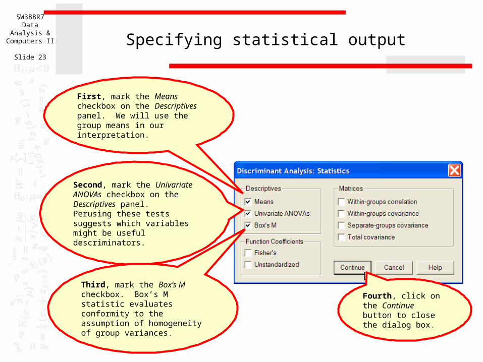
Specifying statistical output

Fourth, click on the Continue button to close the dialog box.

First, mark the Means checkbox on the Descriptives panel. We will use the group means in our interpretation.

Second, mark the Univariate ANOVAs checkbox on the Descriptives panel. Perusing these tests suggests which variables might be useful descriminators.

Third, mark the Box’s M checkbox. Box’s M statistic evaluates conformity to the assumption of homogeneity of group variances.


& Computers II

Slide 24

Specifying details for the stepwise method

Click on the Method… button to specify the specific statistical criteria to use for including variables.


& Computers II

Slide 25

Details for the stepwise method

Third, click on the option button Use probability of F so that we can incorporate the level of significance specified in the problem.

First, mark the Mahalanobis distance option button on the Method panel.

Third, click on the Continue button to close the dialog box.

Second, mark the Summary of steps checkbox to produce a summary table when a new variable is added.

Fourth, type the level of significance in the Entry text box. The Removal value is twice as large as the entry value.


& Computers II

Slide 26

Specifying details for classification

Click on the Classify… button to specify details for the classification phase of the analysis.


& Computers II

Slide 27

Details for classification - 1

Third, mark the Summary table checkbox to include summary tables comparing actual and predicted classification.

First, mark the option button to Compute from group sizes on the Prior Probabilities panel. This incorporates the size of the groups defined by the dependent variable into the classification of cases using the discriminant functions.

Second, mark the Casewise results checkbox on the Display panel to include classification details for each case in the output.


& Computers II

Slide 28


Fourth, mark the Leave-one-out classification checkbox to request SPSS to include a cross-validated classification in the output. This option produces a less biased estimate of classification accuracy by sequentially holding each case out of the calculations for the discriminant functions, and using the derived functions to classify the case held out.


& Computers II

Slide 29


Sixth, mark the Combined-groups checkbox on the Plots panel to obtain a visual plot of the relationship between functions and groups defined by the dependent variable.

Fifth, accept the default of Within-groups option button on the Use Covariance Matrix panel. The Covariance matrices are the measure of the dispersion in the groups defined by the dependent variable. If we fail the homogeneity of group variances test (Box’s M), our option is use Separate groups covariance in classification.

Seventh, click on the Continue button to close the dialog box.


& Computers II

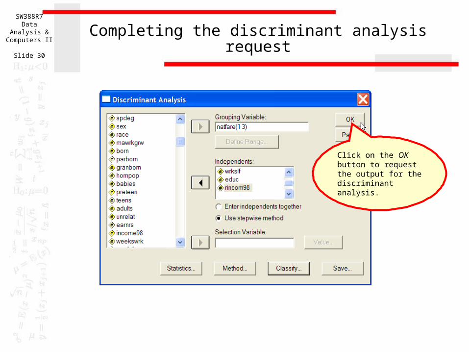
Slide 30

Completing the discriminant analysis request

Click on the OK button to request the output for the discriminant analysis.


& Computers II

Slide 31

Analysis Case Processing Summary

138 51.1

7 2.6

115 42.6

10 3.7

132 48.9

270 100.0

Unweighted CasesValid

Missing or out-of-rangegroup codes

At least one missingdiscriminating variable

Both missing orout-of-range group codesand at least one missingdiscriminating variable

Total

Excluded

Total

N Percent

Sample size – ratio of cases to variablesevidence and answer

The minimum ratio of valid cases to independent variables for discriminant analysis is 5 to 1, with a preferred ratio of 20 to 1. In this analysis, there are 138 valid cases and 4 independent variables.

The ratio of cases to independent variables is 34.5 to 1, which satisfies the minimum requirement. In addition, the ratio of 34.5 to 1 satisfies the preferred ratio of 20 to 1.


& Computers II

Slide 32

Sample size – minimum group sizeevidence and answer

In addition to the requirement for the ratio of cases to independent variables, discriminant analysis requires that there be a minimum number of cases in the smallest group defined by the dependent variable. The number of cases in the smallest group must be larger than the number of independent variables, and preferably contain 20 or more cases.

The number of cases in the smallest group in this problem is 32, which is larger than the number of independent variables (4), satisfying the minimum requirement. In addition, the number of cases in the smallest group satisfies the preferred minimum of 20 cases.

In this problem we satisfy both the minimum and preferred requirements for ratio of cases to independent variables and minimum group size.

For this problem, true is the correct answer.


& Computers II

Slide 33

Classification Resultsb,c

43 15 6 64

26 30 6 62

17 10 9 36

3 3 2 8

67.2 23.4 9.4 100.0

41.9 48.4 9.7 100.0

47.2 27.8 25.0 100.0

37.5 37.5 25.0 100.0

43 15 6 64

26 30 6 62

17 11 8 36

67.2 23.4 9.4 100.0

41.9 48.4 9.7 100.0

47.2 30.6 22.2 100.0

WELFARE1

2

3

Ungrouped cases

1

2

3

Ungrouped cases

1

2

3

1

2

3

Count

%

Count

%

Original

Cross-validateda

1 2 3

Predicted Group Membership

Total

Cross validation is done only for those cases in the analysis. In cross validation, each caseis classified by the functions derived from all cases other than that case.

a.

50.6% of original grouped cases correctly classified.b.

50.0% of cross-validated grouped cases correctly classified.c.

Classification accuracy before transformations or removing outliers

Prior to any transformations of variables to satisfy the assumptions of discriminant analysis or removal of outliers, the cross-validated accuracy rate was 50.0%.

This accuracy rate is the benchmark that we will use to evaluate the utility of transformations and the elimination of outliers.


& Computers II

Slide 34

Assumption of normality of independent variable - question

Having satisfied the level of measurement and sample size requirements, we turn our attention to conformity with the assumption of normality, the detection of outliers, and the assumption of homogeneity of the covariance matrices used in classification.

First, we will evaluate the assumption of normality for the first independent variable.


& Computers II

Slide 35

Test Assumption of Normality with Script

Fourth, mark the dependent variable as nonmetric.

First, move the variables to the list boxes based on the role that the variable plays in the analysis and its level of measurement.

Third, mark the checkboxes for the transformations that we want to test in evaluating the assumption.

Second, click on the Assumption of Normality option button to request that SPSS produce the output needed to evaluate the assumption of normality.

Fifth, click on the OK button to produce the output.


& Computers II

Slide 36

Descriptives

40.99 .958

39.10

42.88

41.21

40.00

161.491

12.708

4

80

76

10.00

-.324 .183

.935 .364

Mean

Lower Bound

Upper Bound

95% ConfidenceInterval for Mean

5% Trimmed Mean

Median

Variance

Std. Deviation

Minimum

Maximum

Range

Interquartile Range

Skewness

Kurtosis

NUMBER OF HOURSWORKED LAST WEEK

Statistic Std. Error

Assumption of normality of independent variable – evidence and answer

The variable "number of hours worked in the past week" [hrs1] satisfies the criteria for a normal distribution. The skewness (-0.324) and kurtosis (0.935) were both between -1.0 and +1.0.

The answer to the question is true.


& Computers II

Slide 37


Next, we will evaluate the assumption of normality for the second independent variable.


& Computers II

Slide 38

Descriptives

13.12 .179

12.77

13.47

13.14

13.00

8.583

2.930

2

20

18

3.00

-.137 .149

1.246 .296

Mean

Lower Bound

Upper Bound


5% Trimmed Mean

Median

Variance

Std. Deviation

Minimum

Maximum

Range

Interquartile Range

Skewness

Kurtosis

HIGHEST YEAR OFSCHOOL COMPLETED

Statistic Std. Error


The independent variable "highest year of school completed" [educ] does not satisfy the criteria for a normal distribution.

The skewness (-0.137) fell between -1.0 and +1.0, but the kurtosis (1.246) fell outside the range from -1.0 to +1.0.


& Computers II

Slide 39


Neither the logarithmic, the square root, nor the inverse transformation normalizes the variable.

The answer to the question is false. A caution should be added to findings involving this variable because of the violation of the assumption of normality.


& Computers II

Slide 40


Finally, we will evaluate the assumption of normality for the third independent variable.


& Computers II

Slide 41

Descriptives

13.35 .419

12.52

14.18

13.54

15.00

29.535

5.435

1

23

22

8.00

-.686 .187

-.253 .373

Mean

Lower Bound

Upper Bound


5% Trimmed Mean

Median

Variance

Std. Deviation

Minimum

Maximum

Range

Interquartile Range

Skewness

Kurtosis

RESPONDENTS INCOMEStatistic Std. Error


The variable "income" [rincom98] satisfies the criteria for a normal distribution. The skewness (-0.686) and kurtosis (-0.253) were both between -1.0 and +1.0.

The answer to this question is true.


& Computers II

Slide 42

Detection of outliers - question

In discriminant analysis, a case can be considered an outlier if it has an unusual combination of scores on the independent variables.

If we had identified any useful transformation, we would run the discriminant analysis again, substituting the transformed variables. Since we did not use any transformations, we can use the casewise statistics from the last analysis to detect outliers.


& Computers II

Slide 43

Detecting outliers

Distance from the centroid of a group is measured by Mahalanobis Distance.

To identify outliers, we scan the column looking for cases with Mahalanobis D² distance greater than a critical value.

The classification output for individual cases can be used to detect outliers. In this context, an outlier is a case that is distant from the centroid of the group to which it has the highest probability of belonging.


& Computers II

Slide 44

Using SPSS to calculate the critical value for Mahalanobis D²

The critical value for Mahalanobis D² is that value that would achieve a specified level of statistical significance given the number of variables that were included in its calculation.

Specifically, we will use an SPSS function to give us the critical value for a probability of 0.01 with the degrees of freedom equal to the number of variables used to compute D².


& Computers II

Slide 45

Variables Ente r ed/Rem oveda,b,c,d

NUMBEROFHOURSWORKEDLASTWEEK

.023 1 and 3 .475 1 135.000 .492

RSELF-EMP ORWORKSFORSOMEBODY

.251 1 and 2 3.289 2 134.000 .040

HIGHESTYEAR OFSCHOOLCOMPLETED

.364 1 and 3 2.433 3 133.000 .068

Step1

2

3

Entered Statis ticBetw eenGroups Statis tic df1 df2 Sig.

Exact F

Min. D Squared

At each step, the variable that maximizes the Mahalanobis distance betw een the tw o c losestgroups is entered.

Max imum number of s teps is 8.a.

Max imum s ignif icance of F to enter is .05.b.

Minimum s ignif icance of F to remove is .10.c .

F level, tolerance, or V IN insuf f ic ient for fur ther computation.d.

The number of variables used to compute Mahalanobis D²

In a direct entry discriminant analysis that includes all variables simultaneously, the number of variables used to compute the values of D² is equal to the number of independent variables included in the analysis.

In stepwise discriminant analysis, the number of variables used to compute the values of D² is equal to the number of independent variables selected for inclusion by the statistical procedure.

In this problem, 3 out of the 4 independent variables were used in the discriminant functions.


& Computers II

Slide 46

Computing the critical value for Mahalanobis D²

First, we open the window to compute a new variable by selecting the Compute… command from the Transform menu.


& Computers II

Slide 47

Selecting the SPSS function

Third, we click on the up arrow button to move the function to the Numeric Expression textbox.

First, we enter the acronym for the variable we want to create in the Target Variable textbox: critval, for critical value.

Second, we scroll down the list of SPSS function to highlight the one we need:

IDF.CHISQ(p, df)


& Computers II

Slide 48

Completing the function arguments

Third, click on the OK… button to compute the variable.

First, the first argument to the IDF.CDF function, p, is replaced by the cumulative probability associated with the critical value, 0.99.

Second, the number of independent variables in the discriminant functions, 3, is used as the df, or degrees of freedom.


& Computers II

Slide 49

The critical value for Mahalanobis D²

The critical value is calculated as a new variable in the SPSS data editor. Even though we only need it calculated a single time, the compute crease a value for every case.

Now that we have the critical value, we can compare it to the values in the table of Casewise Statistics.


& Computers II

Slide 50

Skipping ungrouped cases

Case 50 has a D² 0f 16.603 which is its distance from the centroid of its predicted group 3. However, the actual group for the case was "ungrouped" meaning it was missing data for the dependent variable. This case is not counted as an outlier because it is already omitted from the calculations for the discriminant functions.


& Computers II

Slide 51

Identifying outliers

Case Number 176 has a D² 0f 11.553 which is its distance from the centroid of its predicted group 2, and which is larger than the critical value for D² of 11.345. This case is an outlier and should be omitted in our test for the impact of outliers on the analysis.

Since there is an outlier, the answer to the question is false.


& Computers II

Slide 52

Selecting the model to interpret

Since we found an outlier, we should omit it to test for the impact on the analysis of outliers and substitution of transformations if any were used .

To omit it from the analysis, we will have to find its case id number and eliminate that. We cannot use case numbers to eliminate outliers, because omitting one case changes the case number for all of the other cases after it, and we are likely to exclude the wrong case.


& Computers II

Slide 53

The caseid of the outlier

To omit the outlier, we scroll down the data editor to case 176 and note its caseid value, "20001785."

In this data set, caseids are string or text data, and we represent their values in quotation marks.


& Computers II

Slide 54

Omitting the outliers

To omit outliers, we select into the analysis, the cases that are not outliers.

First, select the Select Cases… command from the Transform menu.


& Computers II

Slide 55

Specifying the condition to omit outliers

First, mark the If condition is satisfied option button to indicate that we will enter a specific condition for including cases.

Second, click on the If… button to specify the criteria for inclusion in the analysis.


& Computers II

Slide 56

The formula for omitting outliers

To eliminate the outliers, we request the cases that are not outliers be included in the analysis. Using this formula, we are selecting cases that do not have a caseid of "20001785".

In the formula, the symbols ~= stands for "not equal to".

If we had more than one outlier, the formula would be expanded to:

caseid~="20001785" and caseid~="20005967" and caseid~="20006102" …

After typing in the formula, click on the Continue button to close the dialog box,


& Computers II

Slide 57

Completing the request for the selection

To complete the request, we click on the OK button.


& Computers II

Slide 58

The omitted outlier

SPSS identifies the excluded cases by drawing a slash mark through the case number.


& Computers II

Slide 59


43 15 6 64

26 29 6 61

17 10 9 36

3 3 2 8

67.2 23.4 9.4 100.0

42.6 47.5 9.8 100.0

47.2 27.8 25.0 100.0

37.5 37.5 25.0 100.0

43 15 6 64

26 29 6 61

17 11 8 36

67.2 23.4 9.4 100.0

42.6 47.5 9.8 100.0

47.2 30.6 22.2 100.0

WELFARE1

2

3

Ungrouped cases

1

2

3

Ungrouped cases

1

2

3

1

2

3

Count

%

Count

%

Original

Cross-validateda

1 2 3


Total

Cross validation is done only for those cases in the analysis. In cross validation, each caseis classified by the functions derived from all cases other than that case.

a.



Selecting the model to interpret – evidence and answer

Prior to any transformations of variables to satisfy the assumptions of normality and the removal of outliers, the cross-validated classification accuracy rate was 50.0%.

After substituting transformed variables and removing outliers, the cross-validated classification accuracy rate was 49.7%. Since the discriminant analysis using transformations and omitting outliers was less accurate in classifying cases than the discriminant analysis with all cases and no transformations, the discriminant analysis with all cases and no transformations was interpreted.

False is the correct answer.


& Computers II

Slide 60

Assumption of Equal Dispersion for Dependent Variable Groups - Question

The assumption of equal dispersion for groups defined by the dependent variable only affects the classification phase of discriminant analysis, and so is not evaluated until we are determining the final accuracy rate of the model.

Box's M test evaluated the homogeneity of dispersion matrices across the subgroups of the dependent variable. The null hypothesis is that the dispersion matrices are homogenous. If the analysis fails this test, we request the use of separate group dispersion matrices in the classification phase of the discriminant analysis to see if this improves our accuracy rate.


& Computers II

Slide 61

Assumption of Equal Dispersion for Dependent Variable Groups – Evidence and Answer

In this analysis, Box's M statistic had a value of 19.386 with a probability of p=0.096. Since the probability for Box's M is greater than the level of significance for testing assumptions (0.01), the null hypothesis is not rejected and the assumption of equal dispersion is satisfied.

The answer to the question is true. We use the pooled or within-groups covariance matrix for classification.


& Computers II

Slide 62

Assumption of Equal Dispersion for Dependent Variable Groups – What if Test Failed

Had we rejected the null hypothesis and concluded that dispersion was not equal across groups, we would have run the analysis again, specifying separate-groups covariance matrices for classification.

If classification using separate covariance matrices were more accurate by 2% or more, we would report classification accuracy based on this model rather than the one that use within-groups covariance.


& Computers II

Slide 63

Multicollinearity - question

Multicollinearity occurs when one independent variable is so strongly correlated with one or more other variables that its relationship to the dependent variable is likely to be misinterpreted. Its potential unique contribution to explaining the dependent variable is minimized by its strong relationship to other independent variables. Multicollinearity is indicated when the tolerance value for an independent variable is less than 0.10.


& Computers II

Slide 64

Multicollinearity – evidence and answer

The tolerance values for all of the independent variables are larger than 0.10. Multicollinearity is not a problem in this discriminant analysis.



& Computers II

Slide 65

Overall relationship - question

The overall relationship in discriminant analysis is based on the existence of sufficient statistically significant discriminant functions to separate all of the groups define by the dependent variable.

In this analysis there were 3 groups defined by opinion about spending on welfare and 4 independent variables, so the maximum possible number of discriminant functions was 2.


& Computers II

Slide 66

Overall relationship – evidence and answer

In the table of Wilks' Lambda which tested functions for statistical significance, the stepwise analysis identified 2 discriminant functions that were statistically significant. The Wilks' lambda statistic for the test of function 1 through 2 functions (Wilks' lambda=.850) had a probability of p=0.001 which was less than or equal to the level of significance of 0.05.

After removing function 1, the Wilks' lambda statistic for the test of function 2 (Wilks' lambda=.949) had a probability of p=0.029 which was less than or equal to the level of significance of 0.05.

True with caution is the correct answer. Caution in interpreting the relationship should be exercised because of the ordinal level variable "income" [rincom98] was treated as metric.


& Computers II

Slide 67

Relationship of functions to groups - question

In order to specify the role that each independent variable plays in predicting group membership on the dependent variable, we must link together the relationship between the discriminant functions and the groups defined by the dependent variable, the role of the significant independent variables in the discriminant functions, and the differences in group means for each of the variables.


& Computers II

Slide 68

Relationship of functions to groups – evidence and answer

The values at group centroids for the first discriminant function were positive for the group who thought we spend about the right amount of money on welfare (.446) and negative for group who thought we spend too little money on welfare (-.220) and group who thought we spend too much money on welfare (-.311). This pattern distinguishes survey respondents who thought we spend about the right amount of money on welfare from survey respondents who thought we spend too little or too much money on welfare.

The values at group centroids for the second discriminant function were positive for the group who thought we spend too little money on welfare (.235) and negative for group who thought we spend too much money on welfare (-.362). This pattern distinguishes survey respondents who thought we spend too little money on welfare from survey respondents who thought we spend too much money on welfare.



& Computers II

Slide 69

Best subset of predictors - question

We use the stepwise method for including variables to identify the best, most parsimonious model.


& Computers II

Slide 70

Best subset of predictors – evidence and answerwhich predictors to interpret

When we use the stepwise method of variable inclusion, we limit our interpretation of independent variable predictors to those entered in the table of Variables Entered/Removed.

We will interpret the impact on membership in groups defined by the dependent variable by the independent variables:

•number of hours worked in the past week•self-employment. •highest year of school completed

Had we use simultaneous entry of all variables, we would not have imposed this limitation.


& Computers II

Slide 71

Best subset of predictors – evidence and answertest of statistical significance

The table of Wilks’ Lambda for the variables (not the one for functions) shows us the results of the statistical test used at each step of the analysis.

Since all three variables entered into the analysis in the order stated in the problem, the correct answer to the question is true.


& Computers II

Slide 72

Relationship of first independent variable - question

We are interested in the role of the independent variable in predicting group membership, i.e. are higher or lower scores on the independent variable associated with membership in one group rather than the other.

This relationship can be stated as a comparison of the means of the groups defined by the dependent variable.


& Computers II

Slide 73

Relationship of first independent variable – evidence and answer: order of entry

In the table of variables entered and removed, "number of hours worked in the past week" [hrs1] was added to the discriminant analysis in step 1.

Number of hours worked in the past week can be characterized as the best predictor.


& Computers II

Slide 74

Relationship of first independent variable – evidence and answer: loadings on functions

In the structure matrix, the largest loading for the variable "number of hours worked in the past week" [hrs1] was -.582 on discriminant function 1 which differentiates survey respondents who thought we spend about the right amount of money on welfare from who thought we spend too little or too much money on welfare.


& Computers II

Slide 75

Relationship of first independent variable – evidence and answer: comparison of means

The average "number of hours worked in the past week" for survey respondents who thought we spend about the right amount of money on welfare (mean=37.90) was lower than the average "number of hours worked in the past week" for survey respondents who thought we spend too little money on welfare (mean=43.96) and survey respondents who thought we spend too much money on welfare (mean=42.03).

This supports the relationship that “survey respondents who thought we spend about the right amount of money on welfare worked fewer hours in the past week than survey respondents who thought we spend too little or too much money on welfare.“

True is the correct answer.


& Computers II

Slide 76

Relationship of second independent variable - question




& Computers II

Slide 77

Relationship of second independent variable – evidence and answer: order of entry

In the table of variables entered and removed, "self-employment" [wrkslf] was added to the discriminant analysis in step 2.

Self-employment can be characterized as the second best predictor.


& Computers II

Slide 78

Relationship of second independent variable – evidence and answer: loadings on functions

In the structure matrix, the largest loading for the variable "self-employment" [wrkslf] was .889 on discriminant function 2 which differentiates survey respondents who thought we spend too little money on welfare from who thought we spend too much money on welfare


& Computers II

Slide 79

Relationship of second independent variable – evidence and answer: comparison of means

Since "self-employment" is a dichotomous variable, the mean is not directly interpretable. Its interpretation must take into account the coding by which 1 corresponds to self-employed and 2 corresponds to working for someone else. The higher means for survey respondents who thought we spend too little money on welfare (mean=1.93), when compared to the means for survey respondents who thought we spend too much money on welfare (mean=1.75), implies that the groups contained fewer survey respondents who were self-employed and more survey respondents who were working for someone else.



& Computers II

Slide 80

Relationship of third independent variable - question




& Computers II

Slide 81

Relationship of third independent variable – evidence and answer: order of entry

In the table of variables entered and removed, "highest year of school completed" [educ] was added to the discriminant analysis in step 3.

Highest year of school completed can be characterized as the third best predictor.


& Computers II

Slide 82

Relationship of third independent variable – evidence and answer: loadings on functions

In the structure matrix, the largest loading for the variable "highest year of school completed" [educ] was .687 on discriminant function 1 which differentiates survey respondents who thought we spend about the right amount of money on welfare from who thought we spend too little or too much money on welfare.


& Computers II

Slide 83

Relationship of third independent variable – evidence and answer: comparison of means

The average "highest year of school completed" for survey respondents who thought we spend about the right amount of money on welfare (mean=14.78) was higher than the average "highest year of school completed" for survey respondents who thought we spend too little money on welfare (mean=13.73) and survey respondents who thought we spend too much money on welfare (mean=13.38).



& Computers II

Slide 84

Relationship of fourth independent variable - question




& Computers II

Slide 85

Relationship of fourth independent variable – evidence and answer: order of entry

The independent variable "income" [rincom98] was not included in the discriminant analysis.

False is the correct answer. We do not interpret this variable.


& Computers II

Slide 86

Classification accuracy - question

The independent variables could be characterized as useful predictors of membership in the groups defined by the dependent variable if the cross-validated classification accuracy rate was significantly higher than the accuracy attainable by chance alone.

Operationally, the cross-validated classification accuracy rate should be 25% or more higher than the proportional by chance accuracy rate.


& Computers II

Slide 87

Prior Probabilities for Groups

.406 56 56.000

.362 50 50.000

.232 32 32.000

1.000 138 138.000

WELFARE1 TOO LITTLE

2 ABOUT RIGHT

3 TOO MUCH

Total

Prior Unweighted Weighted

Cases Used in Analysis

Classification accuracy – evidence and answer:by chance accuracy rate

The proportional by chance accuracy rate was computed by squaring and summing the proportion of cases in each group from the table of prior probabilities for groups (0.406² + 0.362² + 0.232² = 0.350, or 35.0%).

The proportional by chance accuracy criteria was 43.7% (1.25 x 35.0% = 43.7%).


& Computers II

Slide 88


43 15 6 64

26 30 6 62

17 10 9 36

3 3 2 8

67.2 23.4 9.4 100.0

41.9 48.4 9.7 100.0

47.2 27.8 25.0 100.0

37.5 37.5 25.0 100.0

43 15 6 64

26 30 6 62

17 11 8 36

67.2 23.4 9.4 100.0

41.9 48.4 9.7 100.0

47.2 30.6 22.2 100.0

WELFARE1 TOO LITTLE

2 ABOUT RIGHT

3 TOO MUCH

Ungrouped cases

1 TOO LITTLE

2 ABOUT RIGHT

3 TOO MUCH

Ungrouped cases

1 TOO LITTLE

2 ABOUT RIGHT

3 TOO MUCH

1 TOO LITTLE

2 ABOUT RIGHT

3 TOO MUCH

Count

%

Count

%

Original

Cross-validateda

1 TOOLITTLE

2 ABOUTRIGHT 3 TOO MUCH


Total

Cross validation is done only for those cases in the analysis. In cross validation, each case isclassified by the functions derived from all cases other than that case.

a.



Classification accuracy – evidence and answer:classification accuracy

The cross-validated accuracy rate computed by SPSS was 50.0% which was greater than or equal to the proportional by chance accuracy criteria of 43.7% (1.25 x 35.0% = 43.7%). The criteria for classification accuracy is satisfied.



& Computers II

Slide 89

Validation of discriminant model - question


& Computers II

Slide 90


43 15 6 64

26 30 6 62

17 10 9 36

3 3 2 8

67.2 23.4 9.4 100.0

41.9 48.4 9.7 100.0

47.2 27.8 25.0 100.0

37.5 37.5 25.0 100.0

43 15 6 64

26 30 6 62

17 11 8 36

67.2 23.4 9.4 100.0

41.9 48.4 9.7 100.0

47.2 30.6 22.2 100.0

WELFARE1 TOO LITTLE

2 ABOUT RIGHT

3 TOO MUCH

Ungrouped cases

1 TOO LITTLE

2 ABOUT RIGHT

3 TOO MUCH

Ungrouped cases

1 TOO LITTLE

2 ABOUT RIGHT

3 TOO MUCH

1 TOO LITTLE

2 ABOUT RIGHT

3 TOO MUCH

Count

%

Count

%

Original

Cross-validateda

1 TOOLITTLE

2 ABOUTRIGHT 3 TOO MUCH


Total

Cross validation is done only for those cases in the analysis. In cross validation, each case isclassified by the functions derived from all cases other than that case.

a.



Validation of discriminant model – evidence and answer

The cross-validated accuracy rate is a measure of the generalizabillity of the discriminant analysis for correctly classifying populations not included in the original model. Since the cross-validated classification accuracy rate (50.0%) met or exceeded the proportional by chance accuracy criteria (43.7%), this requirement for generalizability was satisfied.



& Computers II

Slide 91

Analysis summary - question

The final question is a summary of the findings of the analysis: overall relationship, individual relationships, and usefulness of the model.

Cautions are added, if needed, for sample size and level of measurement issues.


& Computers II

Slide 92

Analysis summary – evidence and answer

The model was characterized as useful because it equaled the by chance accuracy criterion.

Hours worked, self-employment, and education were the three independent variables we identified as strong contributors to distinguishing between the groups defined by the dependent variable.

The summary correctly states the specific relationships between the dependent variable groups and the independent variables we interpreted.


& Computers II

Slide 93

Analysis summary – evidence and answer


No cautions were added because the preferred sample size requirements were satisfied and the variables included in the summary satisfied the level of measurement requirements for independent variables.


& Computers II

Slide 94

Complete discriminant analysis: level of measurement

Inappropriate application of a statistic

Yes

NoDependent non-metric?Independent variables metric or dichotomous?

Question: Variables included in the analysis satisfy the level of measurement requirements?

Ordinal independent variable included in analysis?

No

Yes

True

True with caution


& Computers II

Slide 95

Complete discriminant analysis: sample size requirements - 1

Yes

Ratio of cases to independent variables at least 5 to 1?

Yes

No Inappropriate application of a statistic

Yes

Number of cases in smallest group greater than number of independent variables?

Yes

No Inappropriate application of a statistic

Question: Number of variables and cases satisfy sample size requirements?

Run discriminant analysis, using method for including variables identified in the research question.


& Computers II

Slide 96

Complete discriminant analysis: sample size requirements - 2

Question: Number of variables and cases satisfy sample size requirements? (continued)

Yes

Satisfies preferred ratio of cases to IV's of 20 to 1

Yes

No

Yes

Satisfies preferred DV group minimum size of 20 cases?

Yes

NoTrue with caution

True with caution

True


& Computers II

Slide 97

Question: Do all of the metric independent variables satisfy the assumption of normality?

Complete discriminant analysis: assumption of normality

The variable satisfies criteria for a normal distribution?

Yes

Use transformation in revised model, no caution needed

Log, square root, or inverse transformation satisfies normality?

If more than one transformation satisfies normality, use one with smallest skew

True

False

Yes

No

No

Use untransformed variable in analysis, add caution to interpretation for violation of normality


& Computers II

Slide 98

Complete discriminant analysis:detection of outliers

No

Is the Mahalanobis D² for closest group > computed critical value?

Question: After incorporating any transformations, no outliers

were detected in the discriminant analysis.

If any variables were transformed for normality or linearity, substitute transformed variables in the regression for the detection of outliers.

Yes False

True

Run revised discriminant using transformed variables and omitting outliers.


& Computers II

Slide 99

Complete discriminant analysis:Model selected for interpretation

Cross-validated accuracy for revised discriminant analysis > accuracy of baseline by 2% or more?

Pick baseline discriminant analysis for interpretation

Pick discriminant analysis with transformations and omitting outliers for interpretation

Yes No

Question: Interpret discriminant model with transformations and excluding outliers, or baseline model?

FalseTrue


& Computers II

Slide 100

Complete discriminant analysis:Assumption of equal dispersion

Probability of Box's M test less than or equal to level of significance for assumptions?

Yes

Re-run discriminant analysis, using separate-groups covariance matricesfor classification

If accuracy rate 2%+ higher using separate-groups covariance matrices for classification

Question: Assumption of equal dispersion of the covariance matrices is satisfied?

No

False

True


& Computers II

Slide 101

Complete discriminant analysis:multicollinearity

Tolerance for all IV’s greater than 0.10, indicating no multicollinearity?

No

Yes

False

Question: Multicollinearity is not a problem in this discriminant analysis?

True


& Computers II

Slide 102

Complete discriminant analysis: 8

Yes

Sufficient statistically significant functions to distinguish DV groups?

NoFalse

Question: Sufficient statistically significant functions to differentiate among groups?

Caution for ordinal variable or sample size not meeting preferred requirements?

No

Yes

True with caution

True


& Computers II

Slide 103

Complete discriminant analysis:groups differentiated by functions

Yes

Pattern of functions evaluated at centroids correctly interpreted?

NoFalse

Question: Groups defined by dependent variable differentiated by discriminant functions?

True


& Computers II

Slide 104

Complete discriminant analysis:individual relationships - 1

Stepwise method of entry used to include independent variables?

Yes

No

Best subset of predictors correctly identified?

YesFalse

Relationships between individual IVs and DV groups interpreted correctly?

No

Yes

False

No

Question: Interpretation of relationship between independent variable and dependent variable groups?


& Computers II

Slide 105

Complete discriminant analysis:individual relationships - 2

Question: Interpretation of relationship between independent variable and dependent variable groups? (cont’d)

Yes


No

YesTrue with caution

True


& Computers II

Slide 106

Complete discriminant analysis:classification accuracy

Yes

Cross-validated accuracy is 25% higher than proportional by chance accuracy rate?

Yes

NoFalse

Question: Classification accuracy sufficient to be characterized as a useful model?

True


& Computers II

Slide 107

Complete discriminant analysis:validation

Yes

Cross-validated accuracy is 25% higher than proportional by chance accuracy rate?

Yes

NoFalse

Question: Classification accuracy sufficient to be characterized as a useful model?

True


& Computers II

Slide 108

Complete discriminant analysis:summary of findings - 1

Question: Summary of findings correctly stated, including cautions?

Overall relationship correctly stated (significant function)?

Yes

NoFalse

Individual relationship with IV and DV correctly stated?

Yes

NoFalse

Classification accuracy supports useful model?

Yes

NoFalse


& Computers II

Slide 109

Complete discriminant analysis:summary of findings - 2

Question: Summary of findings correctly stated, including cautions? (continued)


No

YesTrue with caution

True

sw388r7 data analysis & computers ii slide 1 strategy for complete discriminant analysis...

Documents