coping with multicollinearity: an example on application ... · pdf filecoping with...
TRANSCRIPT
United StatesDepartment ofAgriculture
Forest Service
NortheasternResearch Station
Research Paper NE-721
B. Desta FekedulegnJ.J. ColbertR.R. Hicks, Jr.Michael E. Schuckers
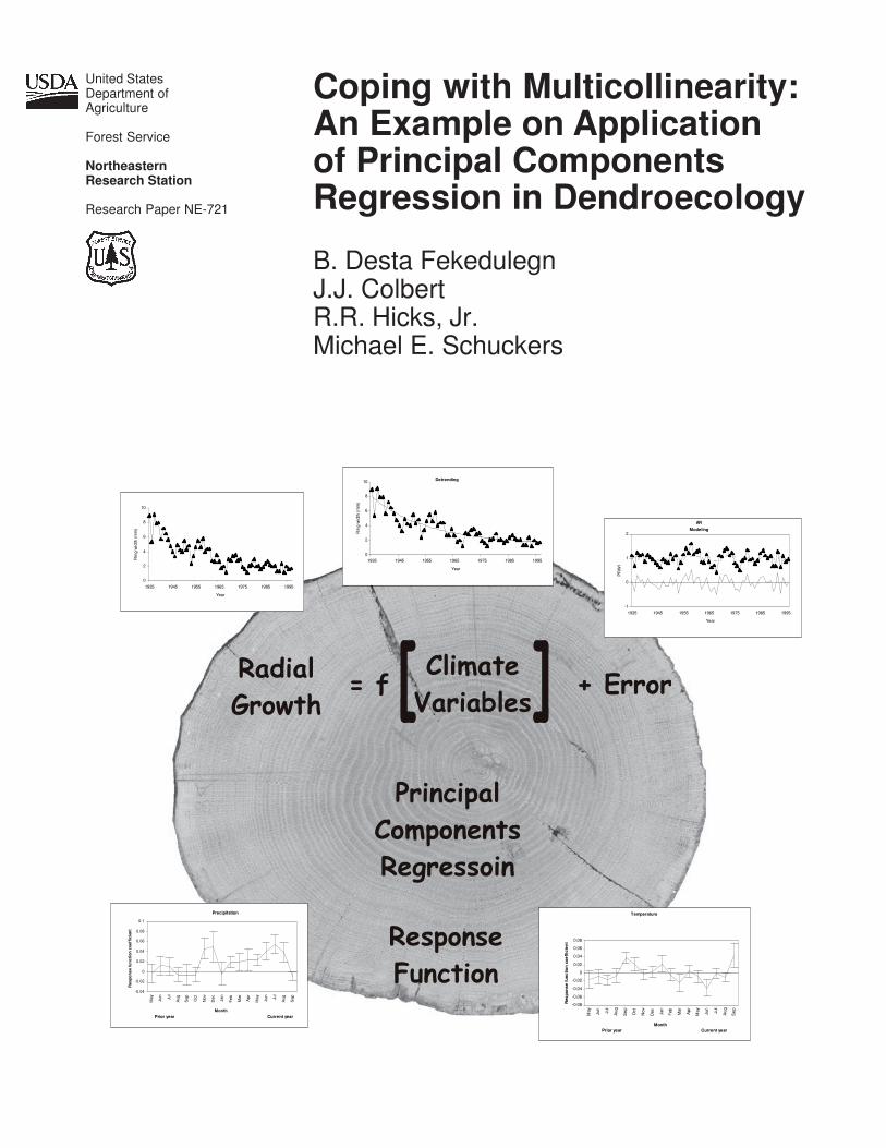
Coping with Multicollinearity:An Example on Applicationof Principal ComponentsRegression in Dendroecology
0
2
4
6
8
10
1935 1945 1955 1965 1975 1985 1995
Year
Rin
g w
idth
(m
m)
0
2
4
6
8
10
1935 1945 1955 1965 1975 1985 1995
Year
Rin
g w
idth
(m
m)
Detrending
-1
0
1
2
1935 1945 1955 1965 1975 1985 1995
YearP
RW
I
AR
Modeling
Temperature
-0.08
-0.06
-0.04
-0.02
0
0.02
0.04
0.06
0.08
May
Jun
Jul
Au
g
Se
p
Oct
Nov
Dec Ja
n
Feb Mar
Ap
r
May
Jun
Jul
Au
g
Se
p
Month
Res
po
nse
fu
nc
tio
n c
oe
ffic
ien
t
Prior year Current year
-0.04
-0.02
0
0.02
0.04
0.06
0.08
0.1
May
Jun
Jul
Aug
Sep Oct
Nov
Dec Ja
n
Feb Mar
Apr
May
Jun
Jul
Aug
Sep
Month
Res
pons
e fu
nct
ion
coe
ffic
ien
t
Precipitation
Prior year Current year
����������
� ���������������� � �����
����������������������������
���������������

Published by: For additional copies:
USDA FOREST SERVICE USDA Forest Service11 CAMPUS BLVD SUITE 200 Publications DistributionNEWTOWN SQUARE PA 19073-3294 359 Main Road
Delaware, OH 43015-8640September 2002 Fax: (740)368-0152
Visit our homepage at: http://www.fs.fed.us/ne
The Authors
B. DESTA FEKEDULEGN is a research associate at Department of Statistics, WestVirginia University. He received a M.S. in forest biometrics at University College Dublinand a M.S. in statistics at West Virginia University. His Ph.D. was in forest resourcescience (dendrochronology) from West Virginia University. His research interestsinclude analytic methods in dendrochronology and forestry, nonlinear modeling, biasedestimation, and working on applied statistics.
J.J. COLBERT is a research mathematician with the Northeastern Research Station,USDA Forest Service. He received an M.S. in mathematics from Idaho State Universityand a Ph.D. in mathematics from Washington State University. His primary researchinterests include the modeling of forest ecosystem processes and integration of effectsof exogenous inputs on forest stand dynamics.
R.R. HICKS, JR. is professor of forestry at West Virginia University. He received hisBSF and MS degrees from the University of Georgia and Ph.D from the StateUniversity of New York at Syracuse. He was assistant and associate professor offorestry at Stephen F. Austin State University in Texas from 1970 to 1978. Since thattime he has been associate professor and professor of forestry at West VirginiaUniversity. He currently coordinates the Forest Resources Management program atWVU.
MICHAEL E. SCHUCKERS is currently an assistant professor at the Department ofStatistics, West Virginia University. He received an A.M. in statistics from the Universityof Michigan and a Ph.D. in statistics from Iowa State University. His primary researchinterests include Bayesian methodology and statistical methods for biometric devices.
Abstract
The theory and application of principal components regression, a method for copingwith multicollinearity among independent variables in analyzing ecological data, isexhibited in detail. A concrete example of the complex procedures that must be carriedout in developing a diagnostic growth-climate model is provided. We use tree radialincrement data taken from breast height as the dependent variable and climatic datafrom the area as the independent data. Thirty-four monthly temperature andprecipitation measurements are used as potential predictors of annual growth.Included are monthly average temperatures and total monthly precipitation for thecurrent and past growing season. The underlying theory and detail illustration of thecomputational procedures provide the reader with the ability to apply this methodologyto other situations where multicollinearity exists. Comparison of the principalcomponent selection rules is shown to significantly influence the regression results. Acomplete derivation of the method used to estimate standard errors of the principalcomponent estimators is provided. The appropriate test statistic, which does notdepend on the selection rule, is discussed. The means to recognize and adjust forautocorrelation in the dependent data is also considered in detail. Appendices anddirections to internet-based example data and codes provide the user with the abilityto examine the code and example output and produce similar results.
Manuscript received for publication 5 May 2002
Contents
Introduction .............................................................................................................................. 1Statistical Method that Accounts for Multicollinearity .......................................................... 1Interpreting Response Function .......................................................................................... 1Developing an Appropriate Measure of Tree Growth .......................................................... 2
Objectives ................................................................................................................................ 2Review of Methodologies......................................................................................................... 2
The Multiple Regression Model ........................................................................................... 2Centering and Scaling ................................................................................................... 3Standardizing................................................................................................................. 4
Principal Components Regression (PCR) ........................................................................... 4The Underlying Concept ................................................................................................ 4Computational Technique .............................................................................................. 4Elimination of Principal Components ............................................................................ 6Transformation Back to the Original Climatic Variables ................................................ 7
Tree-ring and Climatic Data ..................................................................................................... 8Detrending and Autoregressive Modeling ........................................................................... 8
Violation of the Two Assumptions on the Response Model .......................................... 8Transformations Applied to the Ring Width Measurements ........................................ 11
Results and Discussion ......................................................................................................... 18Procedure for Estimating Response Function ................................................................... 18
Response Function Based on Centered and Scaled Climatic Variables .................... 19Response Function Based on Standardized Climatic Variables ................................. 21
Standard Errors of the Principal Component Estimators .................................................. 22Inference Techniques ........................................................................................................ 24Comparison with the Fritts Approach ................................................................................ 26Computational Comparison of Approaches ....................................................................... 27
Response Function and Comparison of the Inferential Procedures ........................... 29Sensitivity of the Response Function to Principal Components Selection Rules ....... 31
Summary and Conclusions .................................................................................................... 34Acknowledgment ................................................................................................................... 34Literature Cited ...................................................................................................................... 35Appendix36
A-SAS Program to Fit the Modified Negative Exponential Model ..................................... 36B-SAS Program to Fit an Autoregressive Model ............................................................... 38C-SAS program to Perform Principal Components Regression........................................ 40
1
Introduction
Many ecological studies include the collection and use of data to investigate the relationship betweena response variable and a set of explanatory factors (predictor variables). If the predictor variables arerelated to one another, then a situation commonly referred to as multicollinearity results. Then resultsfrom many analytic procedures (such as linear regression) become less reliable. In this paper weattempt to provide sufficient detail on a method used to alleviate problems associated withdependence or collinearity among predictor variables in ecological studies. These procedures are alsoapplicable to any analysis where there may be reason to have concern for dependencies amongcontinuous independent variables used in a study. In this study, response function analysis wascarried out using monthly mean temperatures and monthly precipitation totals as independentvariables affecting growth. A response function is a regression model used to diagnose the influenceof climatic variables on the annual radial growth of trees. It is rarely used to predict tree growth.
When the independent variables show mild collinearity, coefficients of a response function may beestimated using the classical method of least squares. Because climatic variables are often highlyintercorrelated (Guiot et al. 1982), use of ordinary least squares (OLS) to estimate the parameters ofthe response function results in instability and variability of the regression coefficients (Cook andJacoby 1977). When the climatic variables exhibit multicollinearity, estimation of the coefficientsusing OLS may result in regression coefficients much larger than the physical or practical situationwould deem reasonable (Draper and Smith 1981); coefficients that wildly fluctuate in sign andmagnitude due to a small change in the dependent or independent variables; and coefficients withinflated standard errors that are consequently nonsignificant. More importantly, OLS inflates thepercentage of variation in annual radial growth accounted for by climate (R2
climate). Therefore, usingordinary regression procedures under high levels of correlation among the climatic variables affectsthe four characteristics of the model that are of major interest to dendroecologists: magnitude, sign,and standard error of the coefficients as well as R2
climate.
Statistical Method that Accounts for Multicollinearity
Principal components regression is a technique to handle the problem of multicollinearity andproduce stable and meaningful estimates for regression coefficients. Fritts et al. (1971) was the first tointroduce the method of principal components regression (PCR) for estimating response functions indendroecology. The estimators of the parameters in the response function, obtained after performingPCR, are referred to as principal component estimators (Gunst and Mason 1980). Fritts (1976) refersto the values of these estimators as elements of the response function.
The methodology of developing a radial growth response model using PCR as presented by Fritts etal. (1971), Fritts (1976), and Guiot et al. (1982) requires further clarifications and improvements.First, we introduce the distribution of the test statistic used for assessing the significance of theclimatic variables. We present the inferential procedure that uses the test statistic given by Gunst andMason (1980); but the original work was done by Mansfield et al. (1977). This test statistic tests thehypothesis that the parameters are zero using the principal component estimator of the coefficients.Second, we present a complete derivation and provide a formula for estimating standard error of theelements of response function. Third, the various principal component selection rules and theireffects on characteristics of the response function are explored.
Interpreting Response Function
Information about the influence of climatic variables on tree radial growth is extracted from the sign,magnitude, and statistical significance of the elements of the response function. The sign indicatesthe direction of the relationship, the magnitude indicates the degree of influence, and the significanceindicates whether the influence was due to chance or not. Detailed review on interpreting responsefunction in dendroecology is given by Fritts (1976).
2
1
2
1
.
.
.
×
=
nny
y
y
y
)1(21
22212
12111
...1
....
....
....
...1
...1
+×
=
knknnn
k
k
xxx
xxx
xxx
X
1)1(
2
1
0
.
.
.
×+
=
kkβ
βββ
and
1
2
1
.
.
.
×
=
nnε
εε
Developing an Appropriate Measure of Tree Growth
In addition to the problem of multicollinearity among the independent variables, the dependentvariable, raw ring width, contains nonclimatic information related to tree size or age. Ring-widthdata also violate the two assumptions required to fit the proposed response function model:assumptions of independence and homogeneity of variance. For completeness, this study also brieflyreviews the methods used to transform ring-width series so that the data satisfies these twoassumptions.
Objectives
The objectives of this study are: to present a step-by-step procedure for estimating a responsefunction using principal components regression; to provide a formula for estimating the standarderrors of the principal component estimators of the coefficients of the independent variables; tointroduce the appropriate test statistic for assessing the significance of the regression coefficientsobtained using principal component regression; to explore the effects of the various methods ofselecting principal components on characteristics of the response function; and to demonstrate themethods (detrending and autoregressive modeling) used to transform ring-width series to produce agrowth measure that reflects the variation in climate.
Review of the Methodologies
The Multiple Regression Model
Consider dendroecological research in which the data consists of a tree-ring chronology (i.e., theresponse variable y ) that spans n years and k climatic variables x
1, x
2, …, x
k. Assume that in the
region of the x’s defined by the data, y is related approximately linearly to the climatic variables. Theaim of response function analysis in dendroecology is to diagnose the influence of variation amonginput variables on the annual radial growth of trees using a model of the form
(1)
where the response variable y is the standard or prewhitened tree-ring chronology, the independentvariables x
1, x
2, …, x
k are monthly total precipitation and monthly mean temperature,
, , , …, are the regression coefficients to be estimated, n is the number of years, and iε isthe ith year model error, assumed uncorrelated from observation to observation, with mean zero andconstant variance. Here y
i is a measure of tree growth at the ith year, x
ji is the ith year reading on the jth
climatic variable. In addition, for the purpose of testing hypotheses and calculating confidenceintervals, it is assumed that iε is normally distributed, ~iε N(0, ). Using matrix notation, themodel in Eq. 1 can be written:
Xy += (2)
where
and
0β 1β 2β kβ
0 1 1 2 2 ... ( 1, 2, ..., )= + + + + + =i i i k ki iy x x x i nβ β β β ε
2σ

3
The least squares estimator of the regression coefficients of the
climatic variables is (assuming X is of full column rank) ( ) yXXXb '' 1ˆ −== and the variance-covariance matrix of the estimated regression coefficients in vector b is(Draper and Smith 1981, Myers 1986). Each column of X represents measurements for a particularclimatic variable.
The multiple linear regression model in Equations 1 and 2 can be written in alternative forms byeither centering and scaling or standardizing the independent variables. Such transformation of theclimatic variables has special merit in dendroecology in that it allows results from different studies tobe comparable. These methods are briefly discussed below.
Centering and Scaling. Suppose that the independent variables (each column of X) are centered andscaled, i.e., x
ji, the ith year measurement on the jth climatic variable (xj) in the natural units, is
transformed into *jix as follows:
j
jjiji s
xxx
−=*
(3)
where ( )∑=
−=n
ijjij xxs
1
2. The process of centering and scaling allows for an alternative
formulation of Eq.1 as follows:
ik
kkik
iii s
xx
s
xx
s
xxy εββββ +
−++
−+
−+= *
2
22*2
1
11*1
*0 ... (4)
Consider the model formulation in Eq. 4. Separating the first column of ones (1) from the X matrixresults in the model form
X1y ++= ***0β (5)
where, in this form, ( )′= **2
*1
* ... kβββ is the vector of coefficients, apart from theintercept, and X* is then n × k matrix of centered and scaled independent variables. The notation 1 isused to denote an n-vector of ones. Centering and scaling makes X*´X* the k × k correlation matrix of
the independent variables. Let the vector ( )′= **2
*1
* ... kbbbb be the least squares estimatorof * .
If a data set is used to fit the centered and scaled model of Eq. 4, one can obtain the estimatedcoefficients in the original model of Eq. 1 using the following transformation:
kjs
bb
j
jj ...,,2,1
*
== (6)
The estimate of the intercept is obtained by computing
k
kk
s
xb
s
xb
s
xbbb
*
2
2*2
1
1*1*
00 ... −−−−= (7)
where *jb are estimates from the centered and scaled model of Eq. 4 and yb =*
0 .
( )0 1 2 . . .′=b kb b b b
( ) ( )Var12 −
= σ 'b X X
4
Standardizing. Consider the model in Eq. 1. Suppose the independent variables x1, x
2, …, x
k are
standardized as follows: xji is transformed into xsji using
jx
jjisji S
xxx
−= (8)
where Sxj is the standard deviation of the independent variable xj and the superscript s indicates thatthe independent variables are standardized. The process of standardizing the independent variablesallows for an alternative formulation of Eq. 1 as follows:
ix
kkisk
x
is
x
issi
kS
xx
S
xx
S
xxy εββββ +
−++
−+
−+= ...21
222
1110 (9)
The model in Eq. 9 can be written in matrix form as:
X1y ++= sss0β (10)
where, in this form, ( )′= sk
sss βββ ...21 is the vector of regression coefficients, apart
from the intercept, and Xs is the n × k matrix of standardized independent variables.
Let ( )′= sk
sss bbb ...21b be the least squares estimator of s . If a dataset is used to fit thestandardized model in Eq. 9, then the estimate of the coefficients of the model of Eq. 1 can beobtained from the estimates of the coefficients for the standardized climatic variables using thefollowing transformations:
jx
sj
j S
bb = , j =1, 2, …, k (11)
and
kx
ksk
x
s
x
ss
S
xb
S
xb
S
xbbb −−−−= ...
21
221100 (12)
Note that jXj SnS ×−= 1 , i.e., centering and scaling only differs from standardizing by the
constant factor, 1−n . The above review indicates that it is always possible to move from onemodel formulation to another regardless of which model was used for the analysis.
Principal Components Regression (PCR)
The Underlying Concept. Principal components regression (PCR) is a method for combatingmulticollinearity and results in estimation and prediction better than ordinary least squares whenused successfully (Draper and Smith 1981, Myers 1986). With this method, the original k climaticvariables are transformed into a new set of orthogonal or uncorrelated variables called principalcomponents of the correlation matrix. This transformation ranks the new orthogonal variables inorder of their importance and the procedure then involves eliminating some of the principalcomponents to effect a reduction in variance. After elimination of the least important principalcomponents, a multiple regression analysis of the response variable against the reduced set ofprincipal components is performed using ordinary least squares estimation (OLS). Because theprincipal components are orthogonal, they are pair-wise independent and hence OLS is appropriate.Once the regression coefficients for the reduced set of orthogonal variables have been calculated, theyare mathematically transformed into a new set of coefficients that correspond to the original or initialcorrelated set of variables. These new coefficients are principal component estimators (Gunst andMason 1980). In dendroecological literature, the values of these estimators are known as elements ofthe response function (Fritts 1976).
5
Computational Technique. Let X* be the centered and scaled n × k data matrix as given in Eq. 5.The k × k correlation matrix of the climatic variables is then **'XXC = . Let 1λ , 2λ , …, kλ be theeigenvalues of the correlation matrix, and [ ]kvvvV ...21= be the k × k matrixconsisting of the normalized eigenvectors associated with each eigenvalue. Note that the eigenvaluesare the solutions of the determinant equation 0**' =− IXX λ (Draper and Smith 1981), andassociated with each eigenvalue, jλ , is a vector, vj, that satisfies the set of homogeneousequations ( ) 0vIXX =− jjλ**' .
The vectors, ( )′= kjjjj vvv ...21v , are the normalized solutions such that 1=′ jjvv and0=′ ijvv for ji ≠ . That is, the eigenvectors have unit length and are orthogonal to one another.
Hence the eigenvector matrix V is orthonormal, i.e., IVV =′ .
Now consider the model formulation given in Eq. 5. That is, X1y ++= ***0β . Since IVV =′
one can write the original regression model (Eq. 5) in the form
VVX1y +′+= ***0β (13)
or
Z1y ++= *0β (14)
where Z = X*V and *V′= . Z is an n × k matrix of principal components and
( )′= kααα ...21 is a k × 1 vector of new coefficients. The model formulation in Eq. 14
can be expanded as εαααβ +++++= kk zzzy ...2211*0 , where z
1, z
2, …, z
k are the k new
variables called principal components of the correlation matrix. Hence, the model formulation in Eq.14 is nothing more than the regression of the response variable on the principal components, and thetransformed data matrix Z consists of the k principal components.
For the model in Eq. 14 the principal components are computed using:
Z = X*V (15)
where X* is the n × k matrix of centered and scaled climatic variables without the column of ones, andV is the k × k orthonormal matrix of eigenvectors. The principal components are orthogonal to eachother, that is:
( ) ( ) ( )kλλλ ...,,,diag 21**** =′=′=′=′ ′ CVVVXXVVXVXZZ (16)
Equation 16 shows that jjjjj λ=′=′ Cvvzz and 0=′ ijzz , ji ≠ . From Eq. 15, one can see thatthe principal components are simply linear functions of the centered and scaled climatic variables andthe coefficients of this linear combination are the eigenvectors. For example, the elements of the jth
principal component, zj, are computed as follows:
**22
*11 ... kkjjjj xvxvxvz +++= (17)
where kjjj vvv ,...,, 21 are elements of the eigenvector associated with λj, and *jx ’s are the centered
and scaled climatic variables obtained using Eq. 3. Note that 01
=∑=
n
ijiz and the sum of squares of
the elements of jz (∑=
n
ijiz
1
2 ) is λj. Since k
k
jj =∑
=1
λ then the total sum of squares, ∑ ∑= =
k
j
n
ijiz
1 1
2 ,
is k . zj accounts for λj of the total variance.
6
If the response variable (y) is regressed against the k principal components using the model in Eq. 14,then the least squares estimator for the regression coefficients in vector is the vector
( ) yZZZ ′′= −1ˆ and the variance-covariance matrix of the estimated coefficients in vector ˆ isgiven by
( ) ( ) ( )112
11
212 ...,,,diagˆˆˆ −−−− =′= kVar λλλσσ ZZ (18)
If all of the k principal components are retained in the regression model of Eq. 14, then all that hasbeen accomplished by the transformation is a rotation of the k original climatic variables.
Elimination of Principal Components. Even though the new variables are orthogonal, the samemagnitude of variance is retained. But if multicollinearity is severe, there will be at least one smalleigenvalue. An elimination of one or more principal components associated with the smallesteigenvalues will reduce the total variance in the model and thus produce an appreciably improveddiagnostic or prediction model (Draper and Smith 1981, Myers 1986).
The principal component matrix Z contains exactly the same information as the original centeredand scaled climatic dataset (X*), except that the data are arranged into a set of new variables which arecompletely uncorrelated with one another and which can be ordered or ranked with respect to themagnitude of their eigenvalues (Draper and Smith 1981, Myers 1986). Note that zj corresponding to
the largest λj accounts for the largest portion of the variation in the original data. Further zj’s explain
smaller and smaller proportions, until all the variation is explained; that is, kk
jj =∑
=1
λ . Thus, the zj
are indexed so that 0...21 >>>> kλλλ .
In regression model of Eq. 14 one does not use all the z’s, but follows some selection rule. Theproperty that makes PCR unique and more complex is that there is no universally agreed uponprocedure in selecting the zj’s to be included in the reduced model of Eq. 14 (Draper and Smith1981). Methods used to determine which and how many principal components should be removedto gain a substantial reduction in variance include:
a. The strategy of elimination of principal components should be to begin by discarding thecomponent associated with the smallest eigenvalue. The rationale is that the principalcomponent with smallest eigenvalue is the least informative. Using this procedure, principalcomponents are eliminated until the remaining components explain some pre-selectedpercentage of the total variance (for example, 85 percent or more). That is, one selects the set oflargest r contributors (principal components), which first achieve
85.01 >∑
=
k
r
jjλ
.
b. Some researchers use the rule that only principal components associated with eigenvaluesgreater than 1.00 are of interest (Draper and Smith 1981). This method is often referred to asthe “Kaiser-Gutman Rule” (Loehlin 1998).
c. Others use the selection rule that keeps the first principal components whose combinedeigenvalue product is greater than 1.00 (Guiot et al. 1982).
d. A more objective statistical strategy is to treat the principal component reduction as if it were astandard variable screening problem. Since the principal components are orthogonal regressorvariables, a reasonable criterion to control the order of reduction are the t-statistics given by
SSt
jjj
j
λαα
α
ˆˆ
ˆ
== (19)
7
where j
Sα̂ is the standard error ( ) of jα̂ (Myers 1986). Recall that from Eq. 18
( ) 12ˆ −= jj SVar λα , where 22 σ̂=S and hence, . In this procedure,
t-values should be rank ordered and components should be considered for elimination
beginning with the smallest t-value.
Suppose that some such selection rule results in elimination of r principal components, that is, themodel in Eq. 14 will now use only k – r components. Let us denote the reduced Z matrix of Eq. 14by Zk – r (n × (k – r) matrix). Let the reduced vector of coefficients ( ) be
( )′= −− rkrk ααα ...21. The reduced model, after elimination of r principal
components, can be written as
Z1y ++= −− rkrk*0β (20)
The symbol on εεεεε is used simply to differentiate it from εεεεε in Eq. 14, since they are not the same.But the predicted values and residuals of the model in Eq. 13 or 14 are the same as those in Eq. 1 or2, 4 or 5, and 9 or 10. Note that:
rkrk −− = VXZ * (21)
where [ ]rkrk −− = vvvV ...21 is a k × (k – r) matrix of eigenvectors associated with theretained eigenvalues or principal components.
The least squares procedure is then used to obtain a diagnostic or prediction equation for theresponse y as a function of the selected z’s; that is, fitting the model in Eq. 20 using ordinary leastsquares. Once the fitted equation is obtained in terms of the selected z’s, it can be transformed backinto a function of the original x’s as described in the following sub-section.
Transformation Back to the Original Climatic Variables. Suppose with k variables and hence kprincipal components, r < k components are eliminated. From Eq. 14, with the retention of allcomponents, *V′= , and the coefficients for the centered and scaled climatic variables areobtained as:
V=* (22)
If one eliminates r components and fits the model given in Eq. 20, the principal componentestimators of the regression coefficients, in terms of the centered and scaled climatic variables for all kparameters of the model in Eq. 5, are given by (Gunst and Mason 1980, Myers 1986)
[ ]
=
=
−
−
−−
rk
rk
pck
pc
pc
rkrkpc
b
b
b
α
αα
ˆ
.
.
.
ˆ
ˆ
...
.
.
.
ˆ
2
1
21
*,
*,2
*,1
*
vvv
Vb
(23)
where Vk–r is defined as in Eq. 21, rk−ˆ is the vector of estimated coefficients (apart from theintercept) in the model of Eq. 20, and *
pcb is a vector of estimated coefficients (apart from theintercept) of the parameters in vector * of Eq. 5. Note that the elements of *
pcb are principalcomponent estimators of the coefficients of the centered and scaled climatic variables, and subscript
s.e.
( ) ( ) 1ˆ
−=s.e. Sj jα λ
8
pc is simply used to denote that the estimators are principal component estimators rather thanordinary least squares estimators. Since the x’s are centered and scaled, the estimate of the constantterm ( *
0β ) in the model of Eq. 5 and 20 is y , that is, y=*0β̂ .
Transformation to the coefficients of the natural climatic variables is done as follows: the principalcomponent estimator, ( )′= pckpcpcpc bbb ,,1,0 ...b , of is
kjs
bb
j
pcjpcj ,...,2,1,
*,
, == (24)
and
k
kpckpcpcpcpc s
xb
s
xb
s
xbbb
*,
2
2*,2
1
1*,1*
,0,0 ... −−−−= (25)
Tree-ring and Climatic Data
Tree-ring data from 38 dominant and codominant yellow-poplar (Liriodendron tulipefera L.) treessampled at Coppers Rock Forest, 13 km east of Morgantown, WV (39o39’43" N, 79o45’28" W),were used. Sampled trees were on average 65 years old and the mean diameter at breast height was 38cm. The climatic variables used to develop the response function were mean monthly temperatureand total monthly precipitation for a 17-month period from May of the year preceding to Septemberof the current year, for a total of 34 monthly climatic variables. The monthly climate data forCoopers Rock weather station were obtained from the National Climatic Data Center. When missingdata were encountered, extrapolations were made using data from near by weather stations(Fekedulegn 2001).
An examination of the correlation matrix of the 34 variables revealed that there were 48 pairs ofsignificant correlations among the climatic variables (21 of them were just betweentemperature variables, four between precipitation variables, and 23 were between temperature andprecipitation variables). The smallest eigenvalue of the correlation matrix was 0.001. Smalleigenvalues suggest problems of multicollinearity among the predictors. Having the tree-ring andclimatic data, the main steps toward developing the response function are developing an appropriatemeasure of tree growth (from tree-ring data) followed by application of PCR.
Detrending and Autoregressive Modeling
Violation of the Two Assumptions on the Response Model. Using the raw ring-widthmeasurements as the response variable (measure of tree growth) in the multiple regression model ofEq. 1 violates the two assumptions of the model: ring-width measurements are independent(uncorrelated), and have a constant (homogeneous) variance independent of time or age of the tree.Ring widths are time-series data that are recorded annually. Radial growth at year t-1 has a positiveeffect on radial growth for year t; this characteristic violates the assumption of independence. Inaddition, the variability of ring width is a function of age and decreases with increasing age, acharacteristic that violates the assumption of homogeneity of variance.
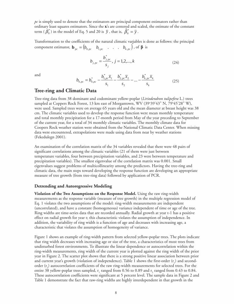
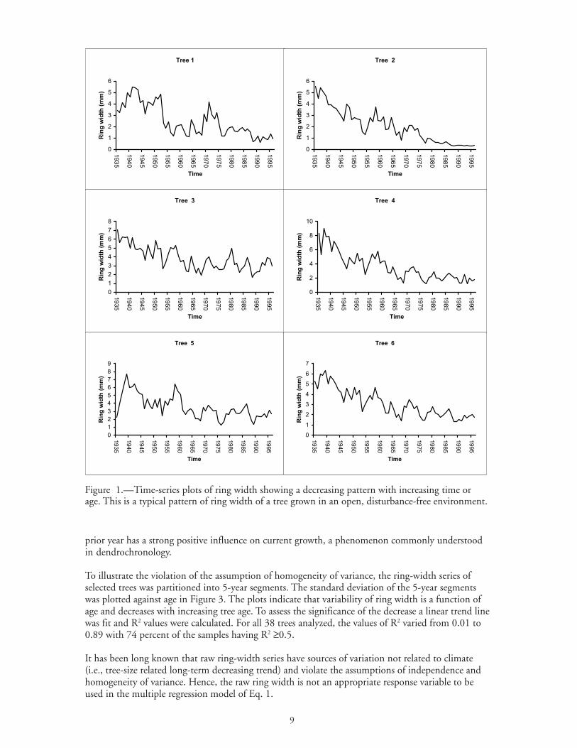
Figure 1 shows an example of ring-width pattern from selected yellow-poplar trees. The plots indicatethat ring width decreases with increasing age or size of the tree, a characteristics of most trees fromundisturbed forest environments. To illustrate the linear dependence or autocorrelation within thering-width measurements, ring width of the current year is plotted against the ring width of the prioryear in Figure 2. The scatter plot shows that there is a strong positive linear association between priorand current year’s growth (violation of independence). Table 1 shows the first-order (r
1) and second-
order (r2) autocorrelation coefficients of the raw ring-width measurements for selected trees. For the
entire 38 yellow-poplar trees sampled, r1 ranged from 0.56 to 0.89 and r
2 ranged from 0.43 to 0.84.
These autocorrelation coefficients were significant at 5 percent level. The sample data in Figure 2 andTable 1 demonstrate the fact that raw-ring widths are highly interdependent in that growth in the
9
prior year has a strong positive influence on current growth, a phenomenon commonly understoodin dendrochronology.
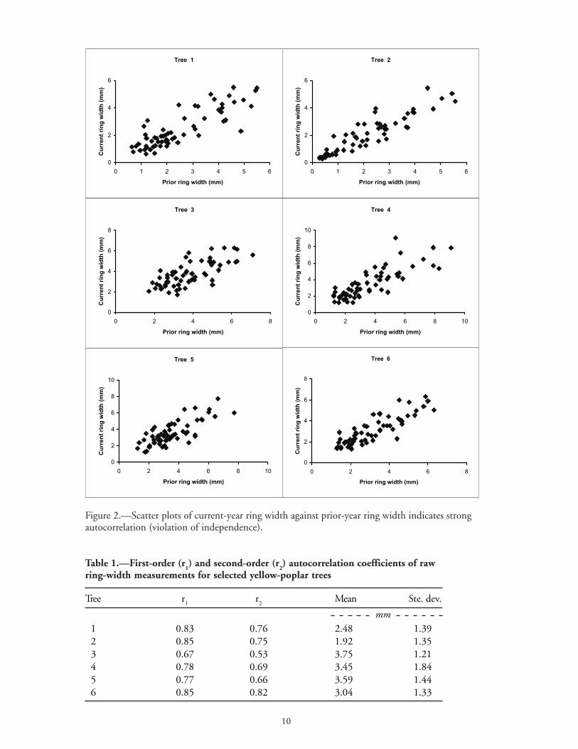
To illustrate the violation of the assumption of homogeneity of variance, the ring-width series ofselected trees was partitioned into 5-year segments. The standard deviation of the 5-year segmentswas plotted against age in Figure 3. The plots indicate that variability of ring width is a function ofage and decreases with increasing tree age. To assess the significance of the decrease a linear trend linewas fit and R2 values were calculated. For all 38 trees analyzed, the values of R2 varied from 0.01 to0.89 with 74 percent of the samples having R2 ≥0.5.
It has been long known that raw ring-width series have sources of variation not related to climate(i.e., tree-size related long-term decreasing trend) and violate the assumptions of independence andhomogeneity of variance. Hence, the raw ring width is not an appropriate response variable to beused in the multiple regression model of Eq. 1.
Figure 1.—Time-series plots of ring width showing a decreasing pattern with increasing time orage. This is a typical pattern of ring width of a tree grown in an open, disturbance-free environment.
Tree 1
0
1
2
3
4
5
6
1935
1940
1945
1950
1955
1960
1965
1970
1975
1980
1985
1990
1995
Time
Rin
g w
idth
(m
m)
Tree 2
0
1
2
3
4
5
6
1935
1940
1945
1950
1955
1960
1965
1970
1975
1980
1985
1990
1995
Time
Rin
g w
idth
(m
m)
Tree 3
0
1
2
3
4
5
6
7
8
1935
1940
1945
1950
1955
1960
1965
1970
1975
1980
1985
1990
1995
Time
Rin
g w
idth
(m
m)
Tree 4
0
2
4
6
8
10
1935
1940
1945
1950
1955
1960
1965
1970
1975
1980
1985
1990
1995
Time
Rin
g w
idth
(m
m)
Tree 5
0
1
2
3
4
5
6
7
8
9
1935
1940
1945
1950
1955
1960
1965
1970
1975
1980
1985
1990
1995
Time
Rin
g w
idth
(m
m)
Tree 6
0
1
2
3
4
5
6
7
1935
1940
1945
1950
1955
1960
1965
1970
1975
1980
1985
1990
1995
Time
Rin
g w
idth
(m
m)
10
Figure 2.—Scatter plots of current-year ring width against prior-year ring width indicates strongautocorrelation (violation of independence).
Tree 1
0
2
4
6
0 1 2 3 4 5 6
Prior ring width (mm)
Cu
rren
t ri
ng
wid
th (
mm
)
Tree 2
0
2
4
6
0 1 2 3 4 5 6
Prior ring width (mm)
Cu
rren
t ri
ng
wid
th (
mm
)
Tree 3
0
2
4
6
8
0 2 4 6 8
Prior ring width (mm)
Cu
rren
t ri
ng
wid
th (
mm
)
Tree 4
0
2
4
6
8
10
0 2 4 6 8 10
Prior ring width (mm)
Cu
rren
t ri
ng
wid
th (
mm
)
Tree 5
0
2
4
6
8
10
0 2 4 6 8 10
Prior ring width (mm)
Cu
rren
t ri
ng
wid
th (
mm
)
Tree 6
0
2
4
6
8
0 2 4 6 8
Prior ring width (mm)
Cu
rren
t ri
ng
wid
th (
mm
)
Table 1.—First-order (r1) and second-order (r
2) autocorrelation coefficients of raw
ring-width measurements for selected yellow-poplar trees
Tree r1
r2
Mean Ste. dev.
mm1 0.83 0.76 2.48 1.392 0.85 0.75 1.92 1.353 0.67 0.53 3.75 1.214 0.78 0.69 3.45 1.845 0.77 0.66 3.59 1.446 0.85 0.82 3.04 1.33
11
Transformation Applied to the Raw Ring-Width Measurements
Removing the trend associated with tree-size (detrending). There are several methods for removingthe long-term trend from the raw ring-width series (Fritts 1976, Cook 1985, Monserud 1986). Butthe choice of one detrending model over another depends on study objectives and the actual patternof the tree-ring series. The choice of a detrending model affects the characteristic of the ring-widthindex (RWI) and results of growth-climate relations (Fekedulegn 2001).
A model for removing this age-related trend in ring-width series is the modified negative exponentialmodel (Fritts 1976) that has the form
( ) kbtaGt +−= exp (26)
Tree 1 Ste. dev. = -0.0448(age) + 0.8961
R2
= 0.2647
0
0.2
0.4
0.6
0.8
1
1.2
1.4
1.6
5 10 15 20 25 30 35 40 45 50 55 60
age (years)
Sta
nd
ard
devia
tio
n (
mm
)
Tree 2 Ste. dev. = -0.0555(age) + 0.7407
R2 = 0.7246
0
0.1
0.2
0.3
0.4
0.5
0.6
0.7
0.8
5 10 15 20 25 30 35 40 45 50 55
age (years)
Sta
nd
ard
devia
tio
n (
mm
)
Tree 3 Ste. dev.= -0.0122(age) + 0.83
R2 = 0.055
0
0.2
0.4
0.6
0.8
1
1.2
5 10 15 20 25 30 35 40 45 50 55 60
age (years)
Sta
nd
ard
devia
tio
n (
mm
)
Tree 4 Ste. dev. = -0.0845(age) + 1.3348
R2 = 0.8108
0
0.2
0.4
0.6
0.8
1
1.2
1.4
1.6
5 10 15 20 25 30 35 40 45 50 55 60
age (years)S
tan
dard
devia
tio
n (
mm
)
Tree 5 Ste. dev.= -0.056(age) + 1.1223
R2 = 0.2046
0
0.5
1
1.5
2
2.5
5 10 15 20 25 30 35 40 45 50 55 60
age (years)
Sta
nd
ard
devia
tio
n (
mm
)
Tree 6
Ste. dev. = -0.0356(age) + 0.7812
R2 = 0.4626
0
0.1
0.2
0.3
0.4
0.5
0.6
0.7
0.8
0.9
5 10 15 20 25 30 35 40 45 50 55 60
age (years)
Sta
nd
ard
devia
tio
n (
mm
)
Figure 3.—Patterns of standard deviation of 5-year segments of the ring width series for selectedtrees. The variability of ring width decreases with increasing time or age (violation of homogeneityof variance).
12
where a, b, and k are coefficients to be estimated by least squares, t is age in years and tG is the valueof the fitted curve at time t. Detrending is accomplished by fitting the model in Eq. 26 to the rawring-width series for a tree and calculating the detrended series (RWI) as ratios of actual (R
t) to fitted
values (Gt ). That is, the RWI ( tI ) at time t is
t
tt G
RI = (27)
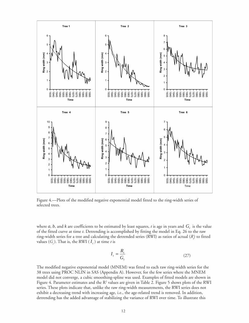
The modified negative exponential model (MNEM) was fitted to each raw ring-width series for the38 trees using PROC NLIN in SAS (Appendix A). However, for the few series where the MNEMmodel did not converge, a cubic smoothing-spline was used. Examples of fitted models are shown inFigure 4. Parameter estimates and the R2 values are given in Table 2. Figure 5 shows plots of the RWIseries. These plots indicate that, unlike the raw ring-width measurements, the RWI series does notexhibit a decreasing trend with increasing age, i.e., the age-related trend is removed. In addition,detrending has the added advantage of stabilizing the variance of RWI over time. To illustrate this
Figure 4.—Plots of the modified negative exponential model fitted to the ring-width series ofselected trees.
Tree 1
0
1
2
3
4
5
6
1935
1940
1945
1950
1955
1960
1965
1970
1975
1980
1985
1990
1995
Time
Rin
g w
idth
(m
m)
Tree 2
0
1
2
3
4
5
6
1935
1940
1945
1950
1955
1960
1965
1970
1975
1980
1985
1990
1995
TimeR
ing
wid
th (
mm
)
Tree 3
0
1
2
3
4
5
6
7
8
1935
1940
1945
1950
1955
1960
1965
1970
1975
1980
1985
1990
1995
Time
Rin
g w
idth
(m
m)
Tree 4
0
1
2
3
4
5
6
7
8
9
10
1935
1940
1945
1950
1955
1960
1965
1970
1975
1980
1985
1990
1995
Time
Rin
g w
idth
(m
m)
Tree 5
0
1
2
3
4
5
6
7
8
9
1935
1940
1945
1950
1955
1960
1965
1970
1975
1980
1985
1990
1995
Time
Rin
g w
idth
(m
m)
Tree 6
0
1
2
3
4
5
6
7
1935
1940
1945
1950
1955
1960
1965
1970
1975
1980
1985
1990
1995
Time
Rin
g w
idth
(m
m)
13
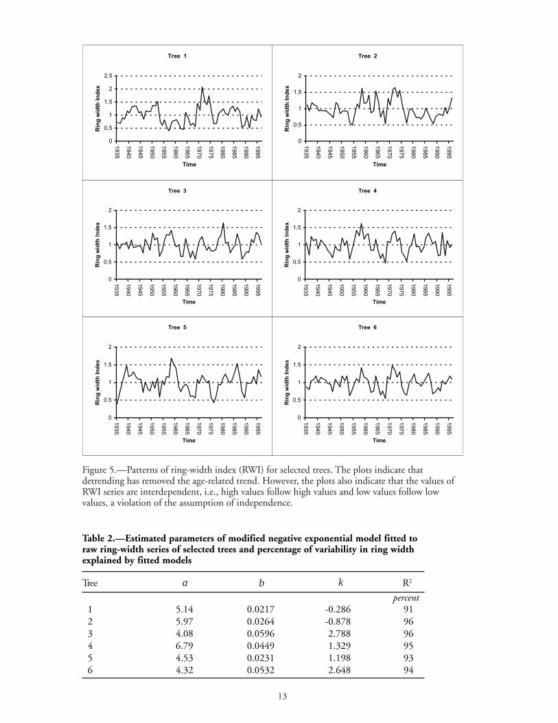
Figure 5.—Patterns of ring-width index (RWI) for selected trees. The plots indicate thatdetrending has removed the age-related trend. However, the plots also indicate that the values ofRWI series are interdependent, i.e., high values follow high values and low values follow lowvalues, a violation of the assumption of independence.
Tree 1
0
0.5
1
1.5
2
2.5
1935
1940
1945
1950
1955
1960
1965
1970
1975
1980
1985
1990
1995
Time
Rin
g w
idth
In
dex
Tree 2
0
0.5
1
1.5
2
1935
1940
1945
1950
1955
1960
1965
1970
1975
1980
1985
1990
1995
Time
Rin
g w
idth
In
dex
Tree 3
0
0.5
1
1.5
2
1935
1940
1945
1950
1955
1960
1965
1970
1975
1980
1985
1990
1995
Time
Rin
g w
idth
In
dex
Tree 4
0
0.5
1
1.5
2
1935
1940
1945
1950
1955
1960
1965
1970
1975
1980
1985
1990
1995
Time
Rin
g w
idth
In
dex
Tree 5
0
0.5
1
1.5
2
1935
1940
1945
1950
1955
1960
1965
1970
1975
1980
1985
1990
1995
Time
Rin
g w
idth
In
dex
Tree 6
0
0.5
1
1.5
2
1935
1940
1945
1950
1955
1960
1965
1970
1975
1980
1985
1990
1995
Time
Rin
g w
idth
In
dex
Table 2.—Estimated parameters of modified negative exponential model fitted toraw ring-width series of selected trees and percentage of variability in ring widthexplained by fitted models
Tree a b k R2
percent1 5.14 0.0217 -0.286 912 5.97 0.0264 -0.878 963 4.08 0.0596 2.788 964 6.79 0.0449 1.329 955 4.53 0.0231 1.198 936 4.32 0.0532 2.648 94
14
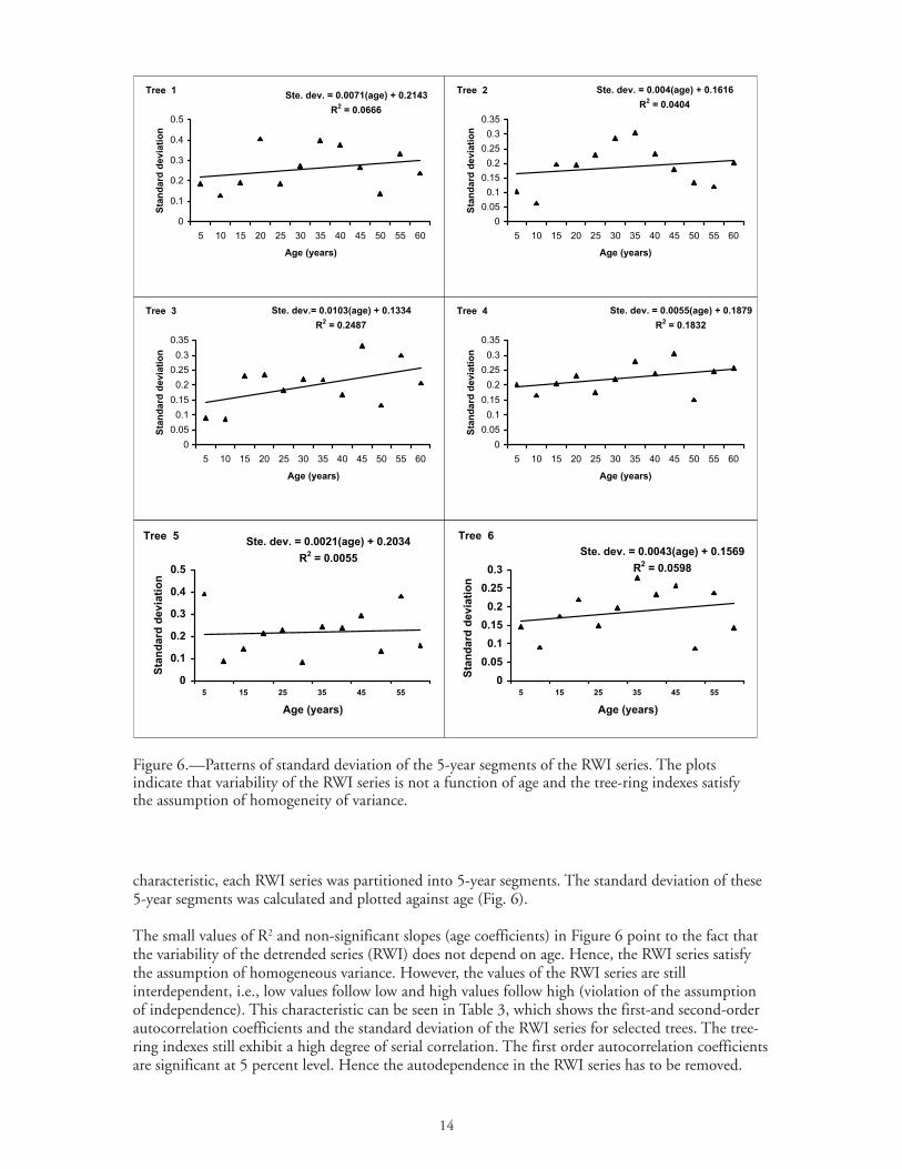
characteristic, each RWI series was partitioned into 5-year segments. The standard deviation of these5-year segments was calculated and plotted against age (Fig. 6).
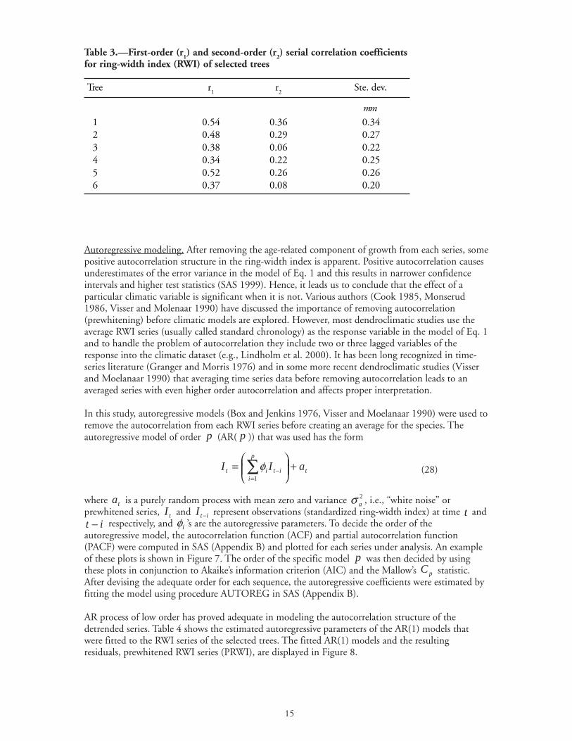
The small values of R2 and non-significant slopes (age coefficients) in Figure 6 point to the fact thatthe variability of the detrended series (RWI) does not depend on age. Hence, the RWI series satisfythe assumption of homogeneous variance. However, the values of the RWI series are stillinterdependent, i.e., low values follow low and high values follow high (violation of the assumptionof independence). This characteristic can be seen in Table 3, which shows the first-and second-orderautocorrelation coefficients and the standard deviation of the RWI series for selected trees. The tree-ring indexes still exhibit a high degree of serial correlation. The first order autocorrelation coefficientsare significant at 5 percent level. Hence the autodependence in the RWI series has to be removed.
Figure 6.—Patterns of standard deviation of the 5-year segments of the RWI series. The plotsindicate that variability of the RWI series is not a function of age and the tree-ring indexes satisfythe assumption of homogeneity of variance.
Tree 1Ste. dev. = 0.0071(age) + 0.2143
R2 = 0.0666
0
0.1
0.2
0.3
0.4
0.5
5 10 15 20 25 30 35 40 45 50 55 60
Age (years)
Sta
nd
ard
devia
tio
n
Tree 2 Ste. dev. = 0.004(age) + 0.1616
R2 = 0.0404
0
0.05
0.1
0.15
0.2
0.25
0.3
0.35
5 10 15 20 25 30 35 40 45 50 55 60
Age (years)
Sta
nd
ard
devia
tio
n
Tree 3 Ste. dev.= 0.0103(age) + 0.1334
R2 = 0.2487
0
0.05
0.1
0.15
0.2
0.25
0.3
0.35
5 10 15 20 25 30 35 40 45 50 55 60
Age (years)
Sta
nd
ard
devia
tio
n
Tree 4 Ste. dev. = 0.0055(age) + 0.1879
R2 = 0.1832
0
0.05
0.1
0.15
0.2
0.25
0.3
0.35
5 10 15 20 25 30 35 40 45 50 55 60
Age (years)S
tan
dard
devia
tio
n
Tree 5Ste. dev. = 0.0021(age) + 0.2034
R2 = 0.0055
0
0.1
0.2
0.3
0.4
0.5
5 15 25 35 45 55
Age (years)
Sta
nd
ard
devia
tio
n
Tree 6
Ste. dev. = 0.0043(age) + 0.1569
R2 = 0.0598
0
0.05
0.1
0.15
0.2
0.25
0.3
5 15 25 35 45 55
Age (years)
Sta
nd
ard
devia
tio
n
15
Autoregressive modeling. After removing the age-related component of growth from each series, somepositive autocorrelation structure in the ring-width index is apparent. Positive autocorrelation causesunderestimates of the error variance in the model of Eq. 1 and this results in narrower confidenceintervals and higher test statistics (SAS 1999). Hence, it leads us to conclude that the effect of aparticular climatic variable is significant when it is not. Various authors (Cook 1985, Monserud1986, Visser and Molenaar 1990) have discussed the importance of removing autocorrelation(prewhitening) before climatic models are explored. However, most dendroclimatic studies use theaverage RWI series (usually called standard chronology) as the response variable in the model of Eq. 1and to handle the problem of autocorrelation they include two or three lagged variables of theresponse into the climatic dataset (e.g., Lindholm et al. 2000). It has been long recognized in time-series literature (Granger and Morris 1976) and in some more recent dendroclimatic studies (Visserand Moelanaar 1990) that averaging time series data before removing autocorrelation leads to anaveraged series with even higher order autocorrelation and affects proper interpretation.
In this study, autoregressive models (Box and Jenkins 1976, Visser and Moelanaar 1990) were used toremove the autocorrelation from each RWI series before creating an average for the species. Theautoregressive model of order p (AR( p )) that was used has the form
t
p
iitit aII +
= ∑=
−1
φ (28)
where ta is a purely random process with mean zero and variance 2aσ , i.e., “white noise” or
prewhitened series, tI and itI − represent observations (standardized ring-width index) at time t andit − respectively, and iφ ’s are the autoregressive parameters. To decide the order of the
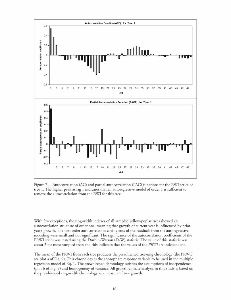
autoregressive model, the autocorrelation function (ACF) and partial autocorrelation function(PACF) were computed in SAS (Appendix B) and plotted for each series under analysis. An exampleof these plots is shown in Figure 7. The order of the specific model p was then decided by usingthese plots in conjunction to Akaike’s information criterion (AIC) and the Mallow’s pC statistic.After devising the adequate order for each sequence, the autoregressive coefficients were estimated byfitting the model using procedure AUTOREG in SAS (Appendix B).
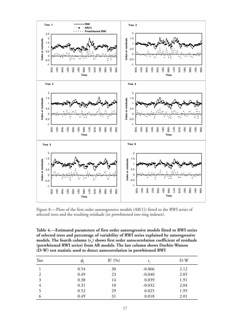
AR process of low order has proved adequate in modeling the autocorrelation structure of thedetrended series. Table 4 shows the estimated autoregressive parameters of the AR(1) models thatwere fitted to the RWI series of the selected trees. The fitted AR(1) models and the resultingresiduals, prewhitened RWI series (PRWI), are displayed in Figure 8.
Table 3.—First-order (r1) and second-order (r2) serial correlation coefficientsfor ring-width index (RWI) of selected trees
Tree r1
r2
Ste. dev.
mm 1 0.54 0.36 0.342 0.48 0.29 0.273 0.38 0.06 0.224 0.34 0.22 0.255 0.52 0.26 0.266 0.37 0.08 0.20
16
With few exceptions, the ring-width indexes of all sampled yellow-poplar trees showed anautocorrelation structure of order one, meaning that growth of current year is influenced by prioryear’s growth. The first order autocorrelation coefficients of the residuals from the autoregressivemodeling were small and not significant. The significance of the autocorrelation coefficients of thePRWI series was tested using the Durbin-Watson (D-W) statistic. The value of this statistic wasabout 2 for most sampled trees and this indicates that the values of the PRWI are independent.
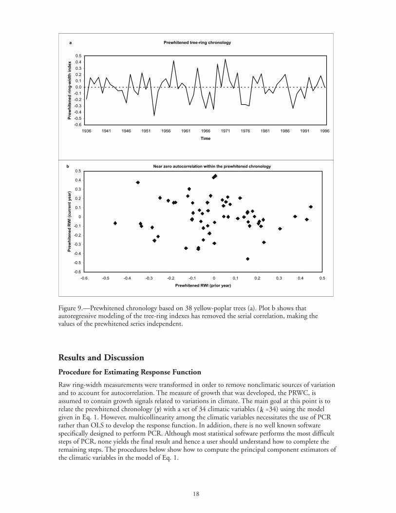
The mean of the PRWI from each tree produces the prewhitened tree-ring chronology (the PRWC,see plot a of Fig. 9). This chronology is the appropriate response variable to be used in the multipleregression model of Eq. 1. The prewhitened chronology satisfies the assumptions of independence(plot b of Fig. 9) and homogeneity of variance. All growth-climate analysis in this study is based onthe prewhitened ring-width chronology as a measure of tree growth.
Figure 7.—Autocorrelation (AC) and partial autocorrelation (PAC) functions for the RWI series oftree 1. The higher peak at lag 1 indicates that an autoregressive model of order 1 is sufficient toremove the autocorrelation from the RWI for this tree.
-0.6
-0.4
-0.2
0
0.2
0.4
0.6
1 3 5 7 9 11 13 15 17 19 21 23 25 27 29 31 33 35 37 39 41 43 45 47 49
Lag
Au
toco
rrela
tio
n c
oeff
icie
nt
Autocorrelation Function (ACF) for Tree 1
-0.3
-0.2
-0.1
0
0.1
0.2
0.3
0.4
0.5
0.6
1 3 5 7 9 11 13 15 17 19 21 23 25 27 29 31 33 35 37 39 41 43 45 47 49
Lag
Part
ial au
toco
rrela
tio
n c
oeff
icie
nt
Partial Autocorrelation Function (PACF) for Tree 1
17
Table 4.—Estimated parameters of first order autoregressive models fitted to RWI seriesof selected trees and percentage of variability of RWI series explained by autoregressivemodels. The fourth column (r1) shows first order autocorrelation coefficient of residuals(prewhitened RWI series) from AR models. The last column shows Durbin-Watson(D-W) test statistic used to detect autocorrelation in prewhitened RWI
Tree 1φ R2 (%) r1
D-W
1 0.54 30 -0.066 2.122 0.49 23 -0.040 2.053 0.38 14 0.039 1.914 0.31 10 -0.032 2.045 0.52 29 0.025 1.956 0.49 31 0.018 2.01
Figure 8.—Plots of the first order autoregressive models (AR(1)) fitted to the RWI series ofselected trees and the resulting residuals (or prewhitened tree-ring indexes).
-1
-0.5
0
0.5
1
1.5
2
2.5
1936
1941
1946
1951
1956
1961
1966
1971
1976
1981
1986
1991
1996
Time
Ind
ex o
r re
sid
uals
RWI
AR(1)
Prewhitened RWI
Tree 1
-1
-0.5
0
0.5
1
1.5
2
1936
1941
1946
1951
1956
1961
1966
1971
1976
1981
1986
1991
1996
Time
Ind
ex o
r re
sid
uals
Tree 2
-1
-0.5
0
0.5
1
1.5
2
1936
1941
1946
1951
1956
1961
1966
1971
1976
1981
1986
1991
1996
Time
Ind
ex o
r re
sid
uals
Tree 3
-1
-0.5
0
0.5
1
1.5
2
1936
1941
1946
1951
1956
1961
1966
1971
1976
1981
1986
1991
1996
Time
Ind
ex o
r re
sid
uals
Tree 4
-1
-0.5
0
0.5
1
1.5
2
1936
1941
1946
1951
1956
1961
1966
1971
1976
1981
1986
1991
1996
Time
Ind
ex o
r re
sid
uals
Tree 5
-1
-0.5
0
0.5
1
1.5
2
1936
1941
1946
1951
1956
1961
1966
1971
1976
1981
1986
1991
1996
Time
Ind
ex o
r re
sid
uals
Tree 6
18
Results and Discussion
Procedure for Estimating Response Function
Raw ring-width measurements were transformed in order to remove nonclimatic sources of variationand to account for autocorrelation. The measure of growth that was developed, the PRWC, isassumed to contain growth signals related to variations in climate. The main goal at this point is torelate the prewhitened chronology (y) with a set of 34 climatic variables ( k =34) using the modelgiven in Eq. 1. However, multicollinearity among the climatic variables necessitates the use of PCRrather than OLS to develop the response function. In addition, there is no well known softwarespecifically designed to perform PCR. Although most statistical software performs the most difficultsteps of PCR, none yields the final result and hence a user should understand how to complete theremaining steps. The procedures below show how to compute the principal component estimators ofthe climatic variables in the model of Eq. 1.
Figure 9.—Prewhitened chronology based on 38 yellow-poplar trees (a). Plot b shows thatautoregressive modeling of the tree-ring indexes has removed the serial correlation, making thevalues of the prewhitened series independent.
Prewhitened tree-ring chronology
-0.6
-0.5
-0.4
-0.3
-0.2
-0.1
0.0
0.1
0.2
0.3
0.4
0.5
1936 1941 1946 1951 1956 1961 1966 1971 1976 1981 1986 1991 1996
Time
Pre
wh
iten
ed
rin
g-w
idth
in
dex
a
-0.6
-0.5
-0.4
-0.3
-0.2
-0.1
0
0.1
0.2
0.3
0.4
0.5
-0.6 -0.5 -0.4 -0.3 -0.2 -0.1 0 0.1 0.2 0.3 0.4 0.5
Prewhitened RWI (prior year)
Pre
wh
iten
ed
RW
I (c
urr
en
t year)
b Near zero autocorrelation within the prewhitened chronology
19
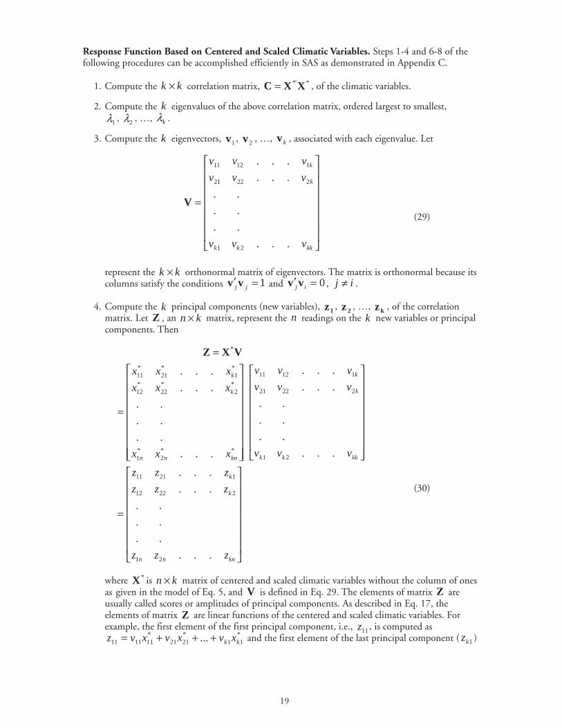
Response Function Based on Centered and Scaled Climatic Variables. Steps 1-4 and 6-8 of thefollowing procedures can be accomplished efficiently in SAS as demonstrated in Appendix C.
1. Compute the kk × correlation matrix, **'XXC = , of the climatic variables.
2. Compute the k eigenvalues of the above correlation matrix, ordered largest to smallest,
1λ , 2λ , …, kλ .
3. Compute the k eigenvectors, 1v , 2v , …, kv , associated with each eigenvalue. Let
=
kkkk
k
k
vvv
vvv
vvv
...
..
..
..
...
...
21
22221
11211
V(29)
represent the kk × orthonormal matrix of eigenvectors. The matrix is orthonormal because itscolumns satisfy the conditions 1=′ jjvv and 0=′ ijvv , ij ≠ .
4. Compute the k principal components (new variables), 1z , 2z , …, kz , of the correlationmatrix. Let Z , an kn × matrix, represent the n readings on the k new variables or principalcomponents. Then
=
=
=
knnn
k
k
kkkk
k
k
knnn
k
k
zzz
zzz
zzz
vvv
vvv
vvv
xxx
xxx
xxx
...
..
..
..
...
...
...
..
..
..
...
...
...
..
..
..
...
...
21
22212
12111
21
22221
11211
**2
*1
*2
*22
*12
*1
*21
*11
*VXZ
(30)
where *X is kn × matrix of centered and scaled climatic variables without the column of onesas given in the model of Eq. 5, and V is defined in Eq. 29. The elements of matrix Z areusually called scores or amplitudes of principal components. As described in Eq. 17, theelements of matrix Z are linear functions of the centered and scaled climatic variables. Forexample, the first element of the first principal component, i.e., 11z , is computed as
*11
*2121
*111111 ... kk xvxvxvz +++= and the first element of the last principal component ( 1kz )
20
is computed as *1
*212
*1111 ... kkkkkk xvxvxvz +++= . Some of the properties of these new
variables or principal components are as follows:
a. mean of the column vectors, jz , is zero, 0=jz ,
b. the sum of squares of elements of jz is jλ , ( ) j
n
iji
n
ijjijj zzz λ==−=′ ∑∑
== 1
22
1
zz ,
c. the variance of jz is hence 1−njλ , and
d. since 0=′ ijzz , i≠j, the principal components are independent (orthogonal) of each other,and ( )kλλλ ,...,,diag 21=′ZZ .
5. Using one of the principal components selection rules discussed earlier, eliminate some of theprincipal components. Suppose kr < components are eliminated. These selection methodsstill leave some principal components that have nonsignificant weight on the dependentvariable and hence nonsignificant components can be rejected using the strategy (rule)described in (d, page 6). However, to this date, dendroecological studies (e.g., Fritts 1976,Guiot et al. 1982, Lindholm et al. 2000) use a stepwise regression procedure to eliminate thenonsignificant principal components. This is described below.
6. Regress the prewhitened tree-ring chronology y against the remaining rk − principalcomponents using linear regression (OLS). That is, estimate the parameters of the model in Eq.20. Here we use the same decision criteria that is used by default in SAS and other statisticalanalysis packages. Fifteen percent is the commonly used probability level for entry of acomponent into a model (Fritts 1976, SAS 1999). Because of changes in the mean squarederror from a full model with nonsignificant terms to a reduced model, we recommend initiallyconsidering terms with p-values slightly larger than 0.15. These should then be reinvestigatedfor the reduced model once all clearly nonsignificant terms have been removed.
If one decides to use the stepwise analysis, what is being accomplished can be done using the teststatistic in Eq. 19 and it is important to understand that the order of entry of the principalcomponents is irrelevant since they are orthogonal to one another. Once a principal component isadded to the model of Eq. 20, its effect is not altered by the components already in the model or bythe addition of other components because each principal component has an independentcontribution in explaining the variation in the response variable.
To summarize the point, in most dendroecological studies the selection of principal components isaccomplished in two stages: eliminate kr < principal components using the cumulative eigenvalueproduct rule (rule c, page 6), and then further screen the remaining rk − components using asignificance level of 15 percent.
Suppose that such a principal components selection rule results in retention of l of the rk −components. The response function will then be computed based on these l principal components( *
lZ ).
7. Regress the prewhitened tree-ring chronology y against these l principal components. That is,fit the model
Z1y ++= ll**
0β (31)
where ll VXZ ** = is an ln × matrix, lV is a lk × matrix of eigenvectors corresponding tothese l components, and l is 1×l vector of coefficients associated with the l components.For example, with 34=k climatic variables and hence 34 principal components, suppose thatat step 5 the last eight principal components with small eigenvalues are eliminated, that is,
8=r , and 26=− rk . Further assume that the regression at step 6 eliminates 10 of the 26principal components, that is, 16=l . These 16 components that remained in the model of Eq.
21
31 are not necessarily the first 16 principal components. The matrix lV contains theeigenvectors corresponding to these components.
8. Compute the mean square error (MSE), and standard error of the estimated coefficients invector lˆ of the model in Eq. 31. Recall that from Eq. 18 ( 22 σ̂=S ).Let the estimated standard errors of the estimated coefficients in lˆ be represented by an 1×lvector
(32)
These standard errors will be used later for testing the statistical significance of the elements of theresponse function, i.e., to construct confidence intervals.
9. Obtain the principal component estimators of the coefficients in terms of the centered andscaled climatic variables using Eq. 23. That is, yb pc =*
,0 and the remaining estimators areobtained as follows:
[ ]
=
l
l
pck
pc
pc
b
b
b
α
αα
ˆ
.
.
.
ˆ
ˆ
...
.
.
.2
1
21
*,
*,2
*,1
vvv
(33)
10. Now transform the coefficients back to the natural climatic variables using Eq. 24 and Eq. 25.
The coefficients obtained at step 10 are the principal component estimators of the regressioncoefficients of the climatic variables in the model of Eq. 1. The coefficients obtained at step 9 are theprincipal component estimators of the regression coefficients of the climatic variables in the model ofEq. 5. The principal component estimators at steps 9 and 10 have the same sign and test statistic butdifferent magnitudes and standard errors.
If one decides to report the values of the principal component estimators at step 10 then twodifficulties arise: if response functions are calculated by different researchers who use different scalesof measurement on the same variables (for example, inches and centimeters for precipitation, degree-Fahrenheit and degree-Centigrade for temperature), the resulting coefficients are not directlycomparable; and when comparing the relative importance of several climatic variables in the responsefunction, the climatic variable with the largest magnitude might not be the most influential variable.Its magnitude could be due mainly to the scale in which it was measured. Therefore, to avoid theaforementioned problems, researchers should report the principal component estimates of thecentered and scaled climatic variables obtained at step 9.
Response Function Based on Standardized Climatic Variables. Statistical packages such as SAS(1999) compute amplitudes or scores of the principal components as a function of the standardizedclimatic variables as follows:
VXZ ss = (34)
where sX is kn × matrix of standardized climatic variables without the column of ones as given inEq. 10, V is defined in Eq. 26, and sZ is kn × matrix of principal components, s
1z , s2z , …, s
kz .The superscript s is used to indicate that the components are computed using the standardizedregressors.
( ) ( ) 1
j jˆ
−=α λSs.e.
( )1 2 lˆ ˆ ˆ. . .
′= s.e. s.e. s.e.α α α
22
Properties of the principal components computed using Eq. 34 are:
• mean of sjz is zero, 0=s
jz ,
• the variance of sjz is jλ , and
• the components are orthogonal (independent). That is, ssZZ′ is a diagonal matrix where thediagonal elements are the sums of squares of the principal components.
If one is interested in computing a response function based on the standardized climatic variables,Eq. 34, the steps outlined above should be followed with the following adjustments (note that steps 1to 3 are standard computations needed in either approach):
a. at step 4 the principal components should be computed using Eq. 34 rather than Eq. 30.That is, replace *
lZ by sZ and *X by sX ,
b. at step 7 replace *lZ by s
lZ , l by sl , and lV by s
lV ,
c. at step 8 replace by s ,
d. at step 9 in Eq. 33 replace *, pcjb by s
pcjb , . The results obtained at step 9 will be coefficientsfor the standardized climatic variables (rather than centered and scaled variables). Note that
ybspc =,0 , and
e. the appropriate transformation of the coefficients back to the natural (original) variables atstep 10 is accomplished by using Eq. 11 and 12. That is,
kjS
bb
jx
spcj
pcj ,..,2,1,,, == (35)
and
kx
ks
pck
x
spc
x
spcs
pcpc S
xb
S
xb
S
xbbb ,2,21,1
,0,0 ...21
−−−−= (36)
where jxS is the standard deviation of the thj original climatic variable jx and s
pcb ,0 , spcb ,1 , s
pcb ,2 ,…, s
pckb , are coefficients of the standardized climatic variables obtained at step 9.
Standard Errors of the Principal Component Estimators
Let ( )′= ll ααα ˆ...ˆˆˆ 21 be the vector of the estimated coefficients in Eq. 31, and
is the vector of the estimated standard errors of the coefficients in
vector lˆ . Note that both lˆ and are 1×l column vectors. Let lV be the lk × matrix of
eigenvectors.
Now, the prewhitened tree-ring chronology can be statistically predicted from the climatic data usingthe fitted model of Eq. 31:
( ) ( ) ***0
**0
**0
*0
ˆˆˆˆˆˆˆˆ pclllll bX1VX1VX1Z1y +=+=+=+= ββββ (37)
Recall that the principal component estimators of the coefficients of the centered and scaled climaticvariables, *
pcb , was given by llpc Vb ˆ* = . From the expression llpc Vb ˆ* = , one can easily recognizethat the coefficients in vector *
pcb are linear combinations of the coefficients of vector lˆ . That is
( )1 2 lˆ ˆ ˆ. . .= s.e. s.e. s.e.α α α
′
23
=
lklkk
l
l
pck
pc
pc
vvv
vvv
vvv
b
b
b
α
αα
ˆ
.
.
.
ˆ
ˆ
...
..
..
..
...
...
.
.
.2
1
21
22221
11211
*,
*,2
*,1
(38)
For example, the first coefficient *,1 pcb is computed as llpc vvvb ααα ˆ...ˆˆ 1212111
*,1 +++= . Hence,
*,1 pcb is a linear function of 1α̂ , 2α̂ , …, and lα̂ where the coefficients of the linear combination are
the eigenvectors. Note that the estimators 1α̂ , 2α̂ , …, and lα̂ are independent since they arecoefficients of l orthogonal variables (principal components). Mutual independence of 1α̂ , 2α̂ , …,and lα̂ facilitates easy computation of the variance (or standard error) of any linear combination ofthese estimators.
Therefore, the variance and standard error of the coefficients in vector *pcb can be computed easily
given the variance and standard error of the estimated coefficients in vector lˆ . For example, thevariance of *
,1 pcb is computed as:
( ) ( ) ( ) ( ) ( )( ) ( ) ( ) ( )llpc
llllpc
vvvb
vvvvvvb
ααα
αααααα
ˆvar...ˆvarˆvarvar
ˆvar...ˆvarˆvarˆ...ˆˆvarvar212
2121
211
*,1
12121111212111*,1
+++=
+++=+++=(39)
To generalize the above formulation using a matrix notation let us label the equations used tocalculate the variance of each element of the vector *
pcb from 1 to k as follows:
( ) ( ) ( ) ( )( ) ( ) ( ) ( )
( ) ( ) ( ) ( ) ]k[ˆvar...ˆvarˆvarvar
.
.
.
]2[ˆvar...ˆvarˆvarvar
]1[ˆvar...ˆvarˆvarvar
22
221
21
*,
222
2221
221
*,2
212
2121
211
*,1
lklkkpck
llpc
llpc
vvvb
vvvb
vvvb
ααα
ααα
ααα
+++=
+++=
+++=
In matrix notation the expressions from [1] to [k] can be rewritten as follows:
( )
=
)ˆvar(
.
.
.
)ˆvar(
)ˆvar(
...
..
..
..
...
...
2
1
222
21
22
222
221
21
212
211
*
lklkk
l
l
pc
vvv
vvv
vvv
Var
α
αα
b(40)
The vector ( )*pcVar b , therefore, gives the variance of the principal component estimators of the
coefficients for the centered and scaled climatic variables. The standard deviation of the sampling
24
distribution of the elements of *pcb (also called standard error) is simply the square root of the
variance of the coefficients. That is
(41)
where here the square root is done elementwise for each element of this column vector.
The principal component estimators of the regression coefficients in the model of Eq. 1 are obtained
using the relationship j
pcjpcj s
bb
*,
, = where js is a scale constant defined in Eq. 3. Hence standard
error of the principal component estimators of the coefficients of the natural climatic variables are
obtained as follows (for the thj principal component estimator):
(42)
where is the standard error of the principal component estimator of the coefficientassociated with the thj centered and scaled climatic variable, or it is the thj element of the vectorgiven in Eq. 41.
If the response function is developed using the standardized climatic variables, then the variance ofthe principal component estimators of coefficients for the standardized climatic variables is given by
( ) ssl
spcVar b = (43)
where sl contains the squares of the elements of s
lV , and s contains the squares of the elementsof sκ . Paralleling Eq. 41, the corresponding standard errors are given by
(44)
Recall that the principal component estimator of the coefficients of the original climatic variables areobtained using Eq. 35. Hence the standard error of the principal component estimator associatedwith the thj original variable is
(45)
Inference Techniques
To test a hypothesis about the significance of the influence of a climatic variable ( 0: *0 =jH β vs.
0: * ≠jaH β ) using the principal component estimators, Mansfield et al. (1977) and Gunst andMason (1980) have shown that the appropriate statistic to use is
2
1
1
21
*,
=
∑=
−l
mjmm
pcj
vMSE
bt
λ (46)
( ) ( )1
* * 2pc pc
= b bs.e. Var
( ) ( ) ( ) ( )1var var var
= = = =
**j, pcj, pc *
j, pc j, pc j, pcj
s.e. bbs.e. b b
j j
bs s s2
( )*j, pcs.e. b
( ) ( )1
2 = b bs.e. s spc pcVar
( ) ( )=
sj, pc
j, pc
s.e. bs.e. b
jxS
25
where *, pcjb is the principal component estimator of *
jβ , MSE is the mean square error of the l-variable model in Eq. 31, jmv is the thj element of the eigenvector mv ( lm ,...,2,1= ), mλ is thecorresponding eigenvalue, and the summation in Eq. 46 is taken over only those componentsretained at the end of the stepwise analysis. The statistic in Eq. 46 follows the Student’s tdistribution with ( 1−− kn ) degrees of freedom under 0H provided that the true coefficients of thecomponents eliminated at step 5 and 6 on page 20 are zero. Therefore, to test 0: *
0 =jH β vs.0: * ≠jaH β with significance level of α , reject 0H if the absolute value of the test statistic in Eq.
46 is greater than or equal to the critical value ( ( )1,2 −−knt α ).
The denominator in Eq. 46 is the standard error of *, pcjb , the thj element of the vector given in Eq.
41. From Eq. 40 one can see that (note: ( ) jjj MSEVar λλσα == 2ˆˆ )
( )
=
+++=
+++=
∑=
l
m m
jm
ljljj
ljljjpcj
vMSE
MSEv
MSEv
MSEv
vvvbVar
1
2
2
2
22
1
21
22
221
21
*,
...
)ˆvar(...)ˆvar()ˆvar(
λ
λλλ
ααα
(47)
Hence, the test statistic in Eq. 46 simplifies to . However, if the hypothesis to betested is 0:0 =s
jH β vs. 0: ≠sjaH β , then the test statistic becomes
2
1
1
21
,
1
−
=
∑=
−l
mjmm
spcj
vn
MSE
bt
λ (48)
The denominator of the test statistic in Eq. 48 is the standard error of spcjb , , the thj element of the
vector given in Eq. 44. Note that if principal component scores are computed using Eq. 34 then ( ))1(...,),1(),1( 21 −−−=′ nnndiag k
ss λλλZZ and the matrix
( ) ( )
−−−
×=′= −
)1(1
...,,)1(
1,
)1(1
ˆ21
1
nnndiagMSEMSEVar
k
sss
λλλZZ is the variance-
covariance matrix of the estimated coefficients associated with the principal components. Hence, ( ) )1(ˆ −= nMSEVar j
sj λα . From Eq. 43 the variance of s
pcjb , is then
( )
−
=
−++
−+
−=
+++=
∑=
l
m m
jm
ljljj
sljl
sj
sj
spcj
v
n
MSE
n
MSEv
n
MSEv
n
MSEv
vvvbVar
1
2
2
2
22
1
21
22
221
21,
1
)1(...
)1()1(
)ˆvar(...)ˆvar()ˆvar(
λ
λλλ
ααα
(49)
Fritts et al. (1971) and Fritts (1976) suggest that the hypothesis 0: *0 =jH β vs. 0: * ≠jaH β can
be tested by constructing a 95 percent confidence interval of the form ,
where 1v is the number of nonzero elements of lˆ and 12 2 vnv −−= . However, Fritts et al.(1971) and Fritts (1976) do not indicate the original source of the above F statistic nor do they give
( )=t * *j, pc j, pcb s.e. b
1 20.05, , ( )± ×v vF* *j, pc j, pcb s.e. b
26
a theoretical derivation. In dendroecological studies where the chronology length and the number ofclimatic variables are large, the two inferential procedures can lead to different and possiblycontradicting results. Hence we suggest that users should adopt the test statistic developed byMansfield et al. (1971) for testing significance of the regression coefficients in the model of Eq. 1,Eq. 5 or Eq. 10 when collinearity is present.
Comparison with the Fritts Approach
Here, we contrast the approach presented in this study and that of Fritts et al. (1971). These contrastsrelate to the type of response variable used and the relationships between the formulas for estimatingstandard errors of the elements of the response function.
Fritts et al. (1971) and Fritts (1976) illustrate the concept, method of computation, andinterpretation of the response function in dendroecological analysis. The approach in these and otherliterature uses a standard chronology (average of tree-ring indexes from a set of trees) as a responsevariable. The regressors are the climatic variables, and additional three-predictor variables thatrepresent ring-width indexes for the 3 most recent years. The purpose of the three additionalpredictor variables was to account for possible interdependence in ring-width indexes measured bythe first-, second-, and third-order autocorrelation.
The approach presented here assumes that the user prewhiten tree-ring indexes from each tree beforecomputing the chronology. Therefore, the use of additional predictor variables that represent ring-width indexes of prior years is not necessary. Averaging tree-ring indexes from a set of trees, whereeach series exhibit a certain degree of autocorrelation, generally will yield a standard chronology witha higher order of autocorrelation (Granger and Morris 1976, Cook 1985) masking the trueautodependence of tree growth. Hence, prewhitening has statistical advantage.
Fritts et al. (1971) and Fritts (1976) compute amplitudes of the principal components of thecorrelation matrix as a function of the standardized climatic variables. The discussion on thecomputation of the response function, though not clearly presented in terms of statistical and linearalgebra details, is essentially the same as the procedure presented in this study.
Fritts (1976) defines the elements of the response function as the estimated regression coefficientsassociated with the original (or natural) climatic variables. In this study, these are coefficientsobtained at step 10 of the step-by-step procedure, given that the principal components are computedusing Eq.34. Fritts et al. (1971) and Fritts (1976) compute standard errors of the elements of theresponse function, , from the standard errors of the coefficients in the vector s
lˆ . Using thenotation in this study, the required transformation given in Fritts (1976) is
'sl
sl UUVVS = (50)
where slV is lk × matrix of eigenvectors, U is ll × diagonal matrix whose diagonal elements are
standard errors of the coefficients in slˆ , i.e., the diagonal elements of U are elements of the vector
sκ and S is kk × symmetric matrix whose diagonal elements are the square of the standard errorsof the elements of the response function. However, the diagonal elements of S are not the square ofthe standard errors of the elements of the response function, rather they are the variances (square ofthe standard errors) of the coefficients for the standardized climatic variables. That is, the thjdiagonal element of S is not the same as ( )pcjb ,var but it is the same as ( )s
pcjb ,var .
The diagonal elements of the matrix S from Fritts (1976) are equivalent to elements of the vector
( )spcVar b given in Eq. 43. A user that employs Fritts (1976) equation, i.e., Eq. 50, ends up getting
variances of the coefficients for the standardized climatic variables and hence, a straightforwardfollow-up computation is needed to obtain variance (or standard errors) of the elements of the
( )j, pcs.e. b
27
response function. The standard error of the thj element of the response function should becomputed as
(51)
Computational Comparison of Approaches
In this section a demonstration of the step-by-step procedure for computation of a response functionis presented. The eigenvalues, eigenvectors, and the orthogonal principal components of thecorrelation matrix of the 34 climatic variables were computed in SAS1 (steps 1-4). Then thecumulative eigenvalue product rule was used to eliminate the last 9 components and the first 25 werekept (step 5). The prewhitened tree-ring chronology was regressed against the 25 orthogonal variablesand further screening of these components was carried out by keeping components that weresignificant at probability level of 20 percent (step 6). This has resulted in retention of fourcomponents ( 4=l ) all of which have probability below 15 percent.
For the model relating the response with the four selected components, the estimated regressioncoefficients (apart from the intercept), s
lˆ , and the matrix of eigenvectors associated with the 4=lretained principal components, s
lV are given below: (step 7)
−
−=
=×
055.0
030.0
055.0
028.0
ˆ
ˆ
ˆ
ˆ
ˆ
4
3
2
1
14
s
s
s
s
s
αααα
−
−−
−
=×
20.005.020.014.0
....
....
....
05.001.004.031.0
06.028.014.006.0
23.011.021.031.0
434sV
The estimated standard errors of the coefficients in vector s14ˆ × (step 8) are given by
[ ]′= 02855.001873.001751.001632.0s
The principal component estimators of the coefficients of the standardized climatic variables wereobtained using Eq. 33. That is, sss
pcj 14434, ˆ ××= Vb (Note: the intercept 00.0,0 == ybspc ): (step 9)
=
spc
spc
spc
b
b
b
,34
,2
,1
.
.
.
−
−−
−
20.005.020.014.0
....
....
....
05.001.004.031.0
06.028.014.006.0
23.011.021.031.0
−
−
055.0
030.0
055.0
028.0
=
−−
004998.0
.
.
.
008144.0
00085.0
02928.0
1Except for steps 9 and 10, all computations indicated in the step-by-step procedure can be accomplished in SAS.
( ) ( )1
12 diagonal element of matrix −= =
Sj, pcs.e. b
j
j
jj xx
thjs S
S
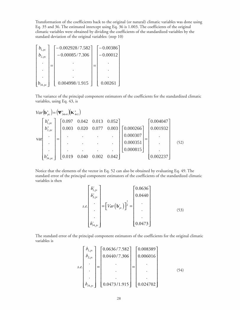
28
Transformation of the coefficients back to the original (or natural) climatic variables was done usingEq. 35 and 36. The estimated intercept using Eq. 36 is 1.003. The coefficients of the originalclimatic variables were obtained by dividing the coefficients of the standardized variables by thestandard deviation of the original variables: (step 10)
−−
=
−
−
=
00261.0
.
.
.
00012.0
00386.0
915.1/004998.0
.
.
.
306.7/00085.0
582.7/002928.0
.
.
.
,34
,2
,1
pc
pc
pc
b
b
b
The variance of the principal component estimators of the coefficients for the standardized climaticvariables, using Eq. 43, is
( ) ( )( )
=
=
= ××
002237.0
.
.
.
001932.0
004047.0
000815.0
000351.0
000307.0
000266.0
042.0002.0040.0019.0
....
....
....
003.0077.0020.0003.0
052.0013.0042.0097.0
.
.
.var
,34
,2
,1
14434
spc
spc
spc
ssspc
b
b
b
Var b
(52)
Notice that the elements of the vector in Eq. 52 can also be obtained by evaluating Eq. 49. Thestandard error of the principal component estimators of the coefficients of the standardized climaticvariables is then
(53)
The standard error of the principal component estimators of the coefficients for the original climaticvariables is
(54)
( )1
2
0.0636
0.0440
. .
. .
. .
0.0473
= =
b spc
b
b
Var
b
spc
spc
spc
s.e.
1,
2,
34,
0.0636/ 7.582 0.008389
0.0440/7.306 0.006016
. .
. .
. .
0.0473/1.915 0.024702
= =
pc
pc
pc
b
b
.s.e.
.
.
b
1,
2,
34,
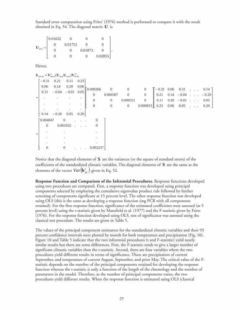
29
Standard error computation using Fritts’ (1976) method is performed to compare it with the resultobtained in Eq. 54. The diagonal matrix U is
=×
02855.0000
001873.000
0001751.00
00001632.0
44U.
Hence,
=
−−−
−
−
−−
−
=
= ×××××
002237.0...00
...
...
...
0...001932.00
0...0004047.0
20.0...05.006.023.0
05.0...01.028.011.0
20.0...04.014.021.0
14.0...31.006.031.0
000815.0000
0000351.000
00000307.00
000000266.0
20.005.020.014.0
....
....
....
05.001.004.031.0
06.028.014.006.0
23.011.021.031.0
)( /34444444343434
Ss VUUVS
Notice that the diagonal elements of S are the variances (or the square of standard errors) of thecoefficients of the standardized climatic variables. The diagonal elements of S are the same as theelements of the vector ( )s
pcVar b given in Eq. 52.
Response Function and Comparison of the Inferential Procedures. Response functions developedusing two procedures are compared. First, a response function was developed using principalcomponents selected by employing the cumulative eigenvalue product rule followed by furtherscreening of components significant at 15 percent level. The other response function was developedusing OLS (this is the same as developing a response function sing PCR with all componentsretained). For the first response function, significance of the estimated coefficients were assessed (at 5percent level) using the t-statistic given by Mansfield et al. (1977) and the F-statistic given by Fritts(1976). For the response function developed using OLS, test of significance was assessed using theclassical test procedure. The results are given in Table 5.
The values of the principal component estimators for the standardized climatic variables and their 95percent confidence intervals were plotted by month for both temperature and precipitation (Fig. 10).Figure 10 and Table 5 indicate that the two inferential procedures (t and F-statistic) yield nearlysimilar results but there are some differences. First, the F-statistic tends to give a larger number ofsignificant climatic variables than the t-statistic. Second, there are four variables where the twoprocedures yield different results in terms of significance. These are precipitation of currentSeptember, and temperature of current August, September, and prior May. The critical value of the F-statistic depends on the number of the principal components retained for developing the responsefunction whereas the t-statistic is only a function of the length of the chronology and the number ofparameters in the model. Therefore, as the number of principal components varies, the twoprocedures yield different results. When the response function is estimated using OLS (classical
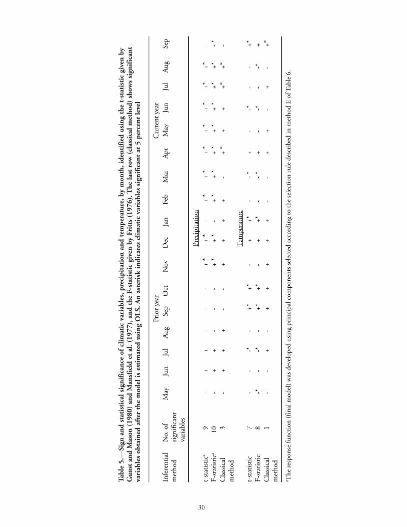
30
Tabl
e 5.
—Si
gn a
nd s
tati
stic
al s
igni
fica
nce
of c
limat
ic v
aria
bles
, pre
cipi
tati
on a
nd t
empe
ratu
re, b
y m
onth
, ide
ntif
ied
usin
g th
e t-
stat
isti
c gi
ven
byG
unst
and
Mas
on (
1980
) an
d M
ansf
ield
et
al. (
1977
), a
nd t
he F
-sta
tist
ic g
iven
by
Frit
ts (
1976
). T
he la
st r
ow (
clas
sica
l met
hod)
sho
ws
sign
ific
ant
vari
able
s ob
tain
ed a
fter
the
mod
el is
est
imat
ed u
sing
OL
S. A
n as
teri
sk in
dica
tes
clim
atic
var
iabl
es s
igni
fica
nt a
t 5
perc
ent
leve
l
Prio
r ye
arC
urre
nt y
ear
Infe
rent
ial
No.
of
May
Jun
Jul
Aug
Sep
Oct
Nov
Dec
Jan
Feb
Mar
Apr
May
Jun
Jul
Aug
Sep
met
hod
sign
ifica
ntva
riab
les
Prec
ipit
atio
nt-
stat
isti
ca9
-+
+-
--
+ *
+ *
-+
*+
*+
*+
*+
*+*
+*-
F-st
atis
tica
10-
++
--
-+
*+
*-
+ *
+ *
+ *
+ *
+ *
+*+*
- *
Cla
ssic
al3
-+
++
--
++
++
-+
*+
++*
+*-
met
hod
Tem
pera
ture
t-st
atis
tic
7-
--*
-+*
+*-
++*
--
*+
--*
--
+*F-
stat
isti
c8
-*-
-*-
+*+*
-+
+*-
- *
+-
-*-
-*+
Cla
ssic
al1
--
+-
++
++
+-
-+
+-
+-
+*m
etho
d
a The
resp
onse
func
tion
(fin
al m
odel
) was
dev
elop
ed u
sing
pri
ncip
al c
ompo
nent
s sel
ecte
d ac
cord
ing
to th
e se
lect
ion
rule
des
crib
ed in
met
hod
E o
f Tab
le 6
.

31
method) there are only four significant variables (Table 5). This was the consequence ofmulticollinearity that inflated the standard error of the estimated coefficients. Besides picking fewernumbers of significant variables, the classical method also suggests some unrealistic results, such aslarger radial growth when the temperature of current July is higher than average. There are sevenvariables where the sign of the predicted coefficient is opposite from that provided by the other twomethods. This is one of the main reasons for using PCR than OLS to study radial growth of trees inrelation to climate.
Sensitivity of the Response Function to Principal Components Selection Rules. The effect of thevarious methods of selecting principal components on R2 of the final model is compared in Table 6.The methods select principal components to be included into the model of Eq. 20 based on fivedifferent criteria and are described as follows:
A. selects the first components which explain 85 percent of the total variance in the original data;
Figure 10.—Response function of yellow-poplar. The statistical significance of the parameters wastested according to the F-statistic (plots a and c) given by Fritts (1976) and the t-statistic (plots b andd) given by Mansfield et al. (1977) and Gunst and Mason (1980). Vertical bars represent the 95percent confidence interval for each of the response function elements. Significant elements are thosefor which the confidence interval does not cross the zero line.
Precipitation (F-statistic)
-0.04
-0.02
0
0.02
0.04
0.06
0.08
0.1
May
Jun
Jul
Aug
Sep
Oct
Nov
Dec
Jan
Feb
Mar
Apr
May
Jun
Jul
Aug
Sep
Month
Resp
on
se f
un
cti
on
co
eff
icie
nt
Prior year Current year
a
-0.04
-0.02
0
0.02
0.04
0.06
0.08
0.1
May
Jun
Jul
Aug
Sep
Oct
Nov
Dec
Jan
Feb
Mar
Apr
May
Jun
Jul
Aug
Sep
Month
Resp
on
se f
un
cti
on
co
eff
icie
nt
Precipitation (t-statistic)
Prior year Current year
b
Temperature (F-statistic)
-0.08
-0.06
-0.04
-0.02
0
0.02
0.04
0.06
0.08
0.1
May
Jun
Jul
Aug
Sep
Oct
Nov
Dec
Jan
Feb
Mar
Apr
May
Jun
Jul
Aug
Sep
Month
Resp
on
se f
un
cti
on
co
eff
icie
nt
Prior year Current year
cTemperature (t-statistic)
-0.08
-0.06
-0.04
-0.02
0
0.02
0.04
0.06
0.08
May
Jun
Jul
Aug
Sep
Oct
Nov
Dec
Jan
Feb
Mar
Apr
May
Jun
Jul
Aug
Sep
Month
Resp
on
se f
un
cti
on
co
eff
icie
nt
Prior year Current year
d
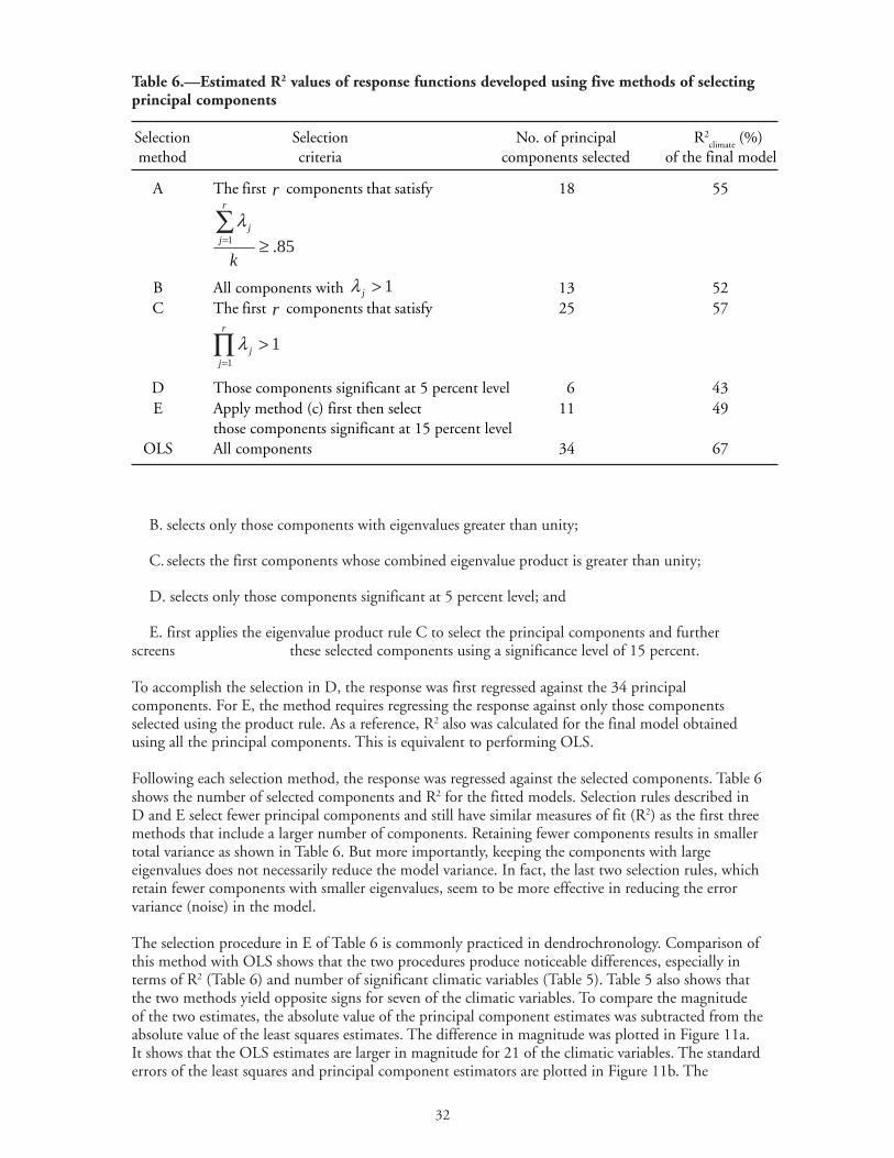
32
B. selects only those components with eigenvalues greater than unity;
C. selects the first components whose combined eigenvalue product is greater than unity;
D. selects only those components significant at 5 percent level; and
E. first applies the eigenvalue product rule C to select the principal components and furtherscreens these selected components using a significance level of 15 percent.
To accomplish the selection in D, the response was first regressed against the 34 principalcomponents. For E, the method requires regressing the response against only those componentsselected using the product rule. As a reference, R2 also was calculated for the final model obtainedusing all the principal components. This is equivalent to performing OLS.
Following each selection method, the response was regressed against the selected components. Table 6shows the number of selected components and R2 for the fitted models. Selection rules described inD and E select fewer principal components and still have similar measures of fit (R2) as the first threemethods that include a larger number of components. Retaining fewer components results in smallertotal variance as shown in Table 6. But more importantly, keeping the components with largeeigenvalues does not necessarily reduce the model variance. In fact, the last two selection rules, whichretain fewer components with smaller eigenvalues, seem to be more effective in reducing the errorvariance (noise) in the model.
The selection procedure in E of Table 6 is commonly practiced in dendrochronology. Comparison ofthis method with OLS shows that the two procedures produce noticeable differences, especially interms of R2 (Table 6) and number of significant climatic variables (Table 5). Table 5 also shows thatthe two methods yield opposite signs for seven of the climatic variables. To compare the magnitudeof the two estimates, the absolute value of the principal component estimates was subtracted from theabsolute value of the least squares estimates. The difference in magnitude was plotted in Figure 11a.It shows that the OLS estimates are larger in magnitude for 21 of the climatic variables. The standarderrors of the least squares and principal component estimators are plotted in Figure 11b. The
Table 6.—Estimated R2 values of response functions developed using five methods of selectingprincipal components
Selection Selection No. of principal R2climate
(%)method criteria components selected of the final model
A The first r components that satisfy 18 55
B All components with 1>jλ 13 52C The first r components that satisfy 25 57
D Those components significant at 5 percent level 6 43E Apply method (c) first then select 11 49
those components significant at 15 percent levelOLS All components 34 67
11
>∏=
r
jjλ
85.1 ≥∑
=
k
r
jjλ
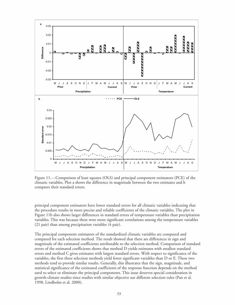
33
principal component estimators have lower standard errors for all climatic variables indicating thatthe procedure results in more precise and reliable coefficients of the climatic variables. The plot inFigure 11b also shows larger differences in standard errors of temperature variables than precipitationvariables. This was because there were more significant correlations among the temperature variables(21 pair) than among precipitation variables (4 pair).
The principal component estimators of the standardized climatic variables are computed andcompared for each selection method. The result showed that there are differences in sign andmagnitude of the estimated coefficients attributable to the selection method. Comparison of standarderrors of the estimated coefficients shows that method D yields estimates with smallest standarderrors and method C gives estimates with largest standard errors. With respect to significance of thevariables, the first three selection methods yield fewer significant variables than D or E. These twomethods tend to provide similar results. Generally, this illustrates that the sign, magnitude, andstatistical significance of the estimated coefficients of the response function depends on the methodused to select or eliminate the principal components. This issue deserves special consideration ingrowth-climate studies since studies with similar objective use different selection rules (Pan et al.1998, Lindholm et al. 2000).
Figure 11.—Comparison of least squares (OLS) and principal component estimators (PCE) of theclimatic variables. Plot a shows the difference in magnitude between the two estimates and bcompares their standard errors.
-0.03
-0.02
-0.01
0
0.01
0.02
0.03
M J J A S O N D J F M A M J J A S M J J A S O N D J F M A M J J A S
Dif
fere
nce
Precipitation Temperature
Prior Current Prior Current
a
0
0.005
0.01
0.015
0.02
0.025
0.03
M J J A S O N D J F M A M J J A S M J J A S O N D J F M A M J J A S
Sta
nd
ard
err
or
PCE OLS
Precipitation Temperature
b
34
Summary and Conclusions
The theoretical basis, the procedure, and the application of PCR in dendroecology have beenillustrated. Selection of principal components is the most important step and makes the procedureunique. Depending on the selection rule, the percentage of variation in annual growth explained byclimate varied from 43 to 67 percent. However, dendroecological studies are not consistent withrespect to principal components selection rules. For example, Fritts (1976) and Lindholm et al.(2000) use the cumulative eigenvalue product rule followed by screening of components significantat 15 percent level (method E) while Pan et al. (1998) simply choose the first r components thatexplained certain preselected percentage of the variation in the original climatic data (method A). Themethod of selecting principal components is shown to affect all the important attributes of theresulting model used for interpreting the effects of climatic variables on radial growth.
While diverse methods for studying annual growth of trees in relation to climate exists, the methodof principal components regression has been recognized as good tool for developing responsefunctions. However, differences in the procedure (especially selection of principal components) leadto differences in interpretations regarding tree growth and climatic variables. The accuracy andreliability of the selection procedures has not been fully explored in dendrochronologial literature.Based on the analysis made in this study, we draw the following conclusions:
• The difficulty of PCR is to decide how many principal components to introduce and whatcriterion to use for the selection. The comparison of the various selection procedures showed thatimportant final model characteristics (sign, magnitude, and significance) of the coefficients of theclimatic variables and R2
climate vary significantly depending on the selection rule. This demonstrates
that consistency in the choice of selection rule is necessary for results of dendroecological studies tobe comparable. There is no universally accepted rule for selecting principal components and mostcurrent selection rules eliminate principal components that account for the largest variance in theoriginal climatic data. This property is thought to be undesirable. Therefore, this issue deservesfurther investigation.
• This study has shown a complete derivation of the method used to estimate the standard errors ofthe principal component estimators for both the natural and transformed climatic variables.
• An appropriate inference procedure (t-statistic) to test the statistical significance of the regressioncoefficients obtained using PCR is introduced.
• Finally, provided that one has a regression dataset where the predictors exhibit the problem ofmulticollinearity, the results in this study can be used in any discipline to develop a more stablemodel, estimate standard errors of the principal component estimators, and test the statisticalsignificance of the individual regressors.
Acknowledgment
The authors thank the following for reviewing an earlier draft of this manuscript: Sara Duke,Northeastern Research Station; William F. Christensen, Department of Statistical Science, SouthernMethodist University; Robert A. Monserud, Pacific Northwest Research Station; Edward Cook,Lamont-Doherty Earth Observatory; Harry T. Valentine, Northeastern Research Station, and MairtinMac Siurtain, Faculty of Agriculture, University College, Dublin, Ireland.
35
Literature Cited
Box, G.E.P.; Jenkins, G.M. 1976. Time series analysis: forecasting and control. Rev. ed. SanFrancisco: Holden Day. 553 p.
Cook, E.R. 1985. A time series analysis approach to tree-ring standardization. Tucson:University of Arizona. 171 p. Ph.D. dissertation.
Cook, E.R.; Jacoby, G.C. Jr. 1977. Tree-ring-drought relationships in the Hudson Valley, NewYork. Science. 198: 399-401.
Draper, N.R.; Smith, H. 1981. Applied regression analysis. 2nd edition. New York: John Wileyand Sons. 709 p.
Fekedulegn, Desta. 2001. Spatial and temporal analysis of radial growth in an Appalachianwatershed. Morgantown, WV: West Virginia University. 270 p. Ph.D. dissertation.
Fritts, H.C. 1976. Tree rings and climate. New York: Academic Press. 567 p.
Fritts, H.C.; Blasing, T.J.; Hayden, B.P.; Kutzbach, J.E. 1971. Multivariate techniques forspecifying tree-growth and climate relationships and for reconstructing anomalies inpaleoclimate. Journal of Applied Meteorology. 10: 845-864.
Granger, C.W.J.; Morris, M.J. 1976. Time series modeling and interpretation. Journal of theRoyal Statistical Society. 139: 246-257.
Guiot, J.; Berger, A.L.; Munaut, A.V. 1982. Response functions. In: Hughes, M.K.; Kelly, P.M.;Pilcher, J.R.; LaMarche, V.C., eds. Climate from tree rings. Cambridge, UK: CambridgeUniversity Press: 38-45.
Gunst, R.F.; Mason, R.L. 1980. Regression analysis and its application: a data-orientedapproach. New York: Marcel Dekker. 402 p.
Lindholm, M.; Lethonen, H.; Kolstrom, T.; Merilainen, J.; Eronen, M.; Timonen, M. 2000.Climatic signals extracted from ring-width chronologies of Scots pines from the northern,middle and southern parts of the boreal forest belt in Finland. Silva Fennica. 34: 317-330.
Loehlin, J.C. 1992. Latent variable models: an introduction to factor, path, and structuralanalysis. Hillsdale, NJ: Lawrence Erlbaum Associates. 292 p.
Mansfield, E.R.; Webster, J.T.; Gunst, R.F. 1977. An analytic variable selection technique forprincipal components regression. Applied Statistics. 6: 34-40.
Monserud, R.A. 1986. Time series analysis of tree-ring chronologies. Forest Science. 32: 349-372.
Myers, R.H. 1986. Classical and modern regression with applications. Boston: Duxbury Press.359 p.
Pan, C.; Tajchman, S.J.; Kochenderfer, J.N. 1997. Dendroclimatological analysis of majorforest species of the central Appalachians. Forest Ecology and Management. 98: 77-87.
SAS Institute, Inc. 1999. SAS/STAT user’s guide, version 6. 4th ed. Vol. 2. Cary, NC: SASInstitute. 883 p.
Visser, H.; Molenaar, J. 1990. Estimating trends in tree-ring data. Forest Science. 36: 87-100.
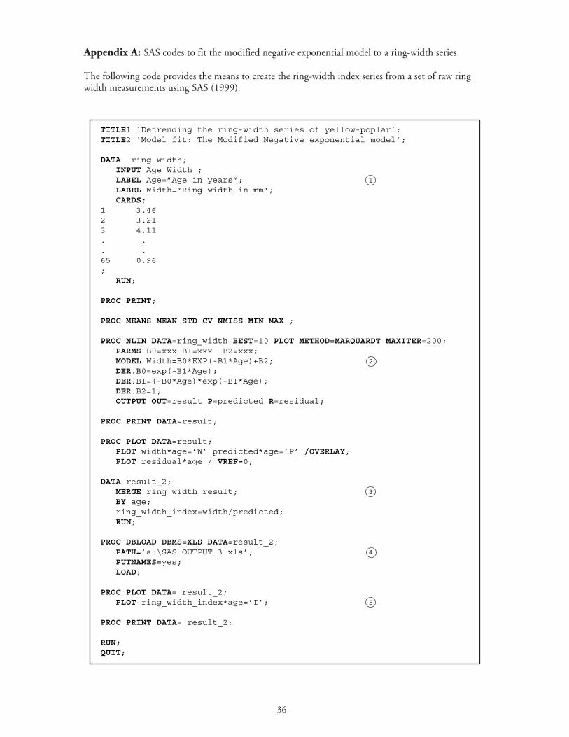
36
Appendix A: SAS codes to fit the modified negative exponential model to a ring-width series.
The following code provides the means to create the ring-width index series from a set of raw ringwidth measurements using SAS (1999).
TITLE1 ‘Detrending the ring-width series of yellow-poplar’;TITLE2 ‘Model fit: The Modified Negative exponential model’;
DATA ring_width; INPUT Age Width ; LABEL Age=”Age in years”; 1
LABEL Width=”Ring width in mm”; CARDS;1 3.462 3.213 4.11. .. .65 0.96; RUN;
PROC PRINT;
PROC MEANS MEAN STD CV NMISS MIN MAX ;
PROC NLIN DATA=ring_width BEST=10 PLOT METHOD=MARQUARDT MAXITER=200; PARMS B0=xxx B1=xxx B2=xxx; MODEL Width=B0*EXP(-B1*Age)+B2; 2
DER.B0=exp(-B1*Age); DER.B1=(-B0*Age)*exp(-B1*Age); DER.B2=1; OUTPUT OUT=result P=predicted R=residual;
PROC PRINT DATA=result;
PROC PLOT DATA=result; PLOT width*age=’W’ predicted*age=’P’ /OVERLAY; PLOT residual*age / VREF=0;
DATA result_2; MERGE ring_width result; 3
BY age; ring_width_index=width/predicted; RUN;
PROC DBLOAD DBMS=XLS DATA=result_2; PATH=’a:\SAS_OUTPUT_3.xls’; 4
PUTNAMES=yes; LOAD;
PROC PLOT DATA= result_2; PLOT ring_width_index*age=’I’; 5
PROC PRINT DATA= result_2;
RUN;QUIT;
37
Explanation of the Code
1. This data step reads a ring-width data and creates a temporary SAS dataset called“ring_width”. This dataset contains two variables, age in years and annual ring widths to thenearest 0.01 mm. Here data are read directly within the data step from card images. It also lists andprints summary statistics for the two variables.
2. This step carries out nonlinear regression and fits the modified negative exponential model to thering-width series. In this program the user should specify starting values for each of the threeparameters prior to executing the program. On the PARMS line, BO=xxx indicates that the user mustspecify a starting value for BO (for example BO =5.5). Reasonable starting values here are BO =7.0,B1=0.05, and B2=1.0 for most data. BO is the value of the detrending line at age 0, B1 is the slopeparameter (natural logarithm 1n[B0/B2]/MaxAge, where MaxAge is the length of series), and B2is the lower limit or asymptote of the detrending line. You also can use the largest ring width for BOand the smallest for B2 starting values. After fitting the model, the outputs from the program (thepredicted values, residuals, etc.) are saved in a SAS dataset called “result”. The contents of the“result” dataset are printed and the program also plots ring width and predicted ring widthagainst age in the same graph.
3. This step creates a SAS dataset called “result_2”. This dataset contain all the variables in datasets “ring_width” and “result”. Then the code calculates ring-width index as a ratio of actualring width to predicted ring width.
4. This procedure saves the dataset “result_2” in an Excel spreadsheet producing five variables:age, actual ring width (measurements), predicted ring width from the fitted model, the residuals, andthe ring-width index (RWI). This provides the user with the ability to review and compare dataamong individual trees, produce graphs, and perform other operations on these data external to SAS.
5. This step creates a plot of ring-width index against age and also prints the contents of the SASdataset “result_2”.
The SAS code for this and each of the other appendices, along with the example datacan be found at: http://www.fs.fed.us/ne/morgantown/4557/dendrochron
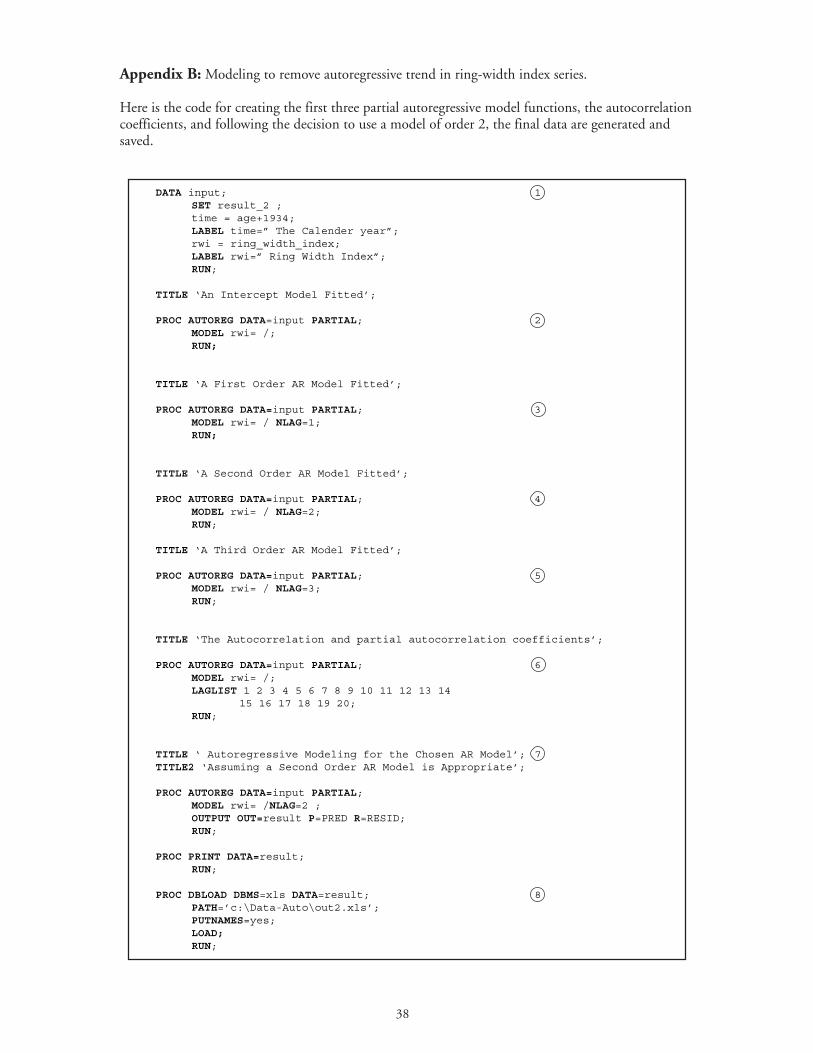
38
Appendix B: Modeling to remove autoregressive trend in ring-width index series.
Here is the code for creating the first three partial autoregressive model functions, the autocorrelationcoefficients, and following the decision to use a model of order 2, the final data are generated andsaved.
DATA input; 1SET result_2 ;time = age+1934;LABEL time=” The Calender year”;rwi = ring_width_index;LABEL rwi=” Ring Width Index”;RUN;
TITLE ‘An Intercept Model Fitted’;
PROC AUTOREG DATA=input PARTIAL; 2MODEL rwi= /;RUN;
TITLE ‘A First Order AR Model Fitted’;
PROC AUTOREG DATA=input PARTIAL; 3MODEL rwi= / NLAG=1;RUN;
TITLE ‘A Second Order AR Model Fitted’;
PROC AUTOREG DATA=input PARTIAL; 4MODEL rwi= / NLAG=2;RUN;
TITLE ‘A Third Order AR Model Fitted’;
PROC AUTOREG DATA=input PARTIAL; 5MODEL rwi= / NLAG=3;RUN;
TITLE ‘The Autocorrelation and partial autocorrelation coefficients’;
PROC AUTOREG DATA=input PARTIAL; 6MODEL rwi= /;LAGLIST 1 2 3 4 5 6 7 8 9 10 11 12 13 14
15 16 17 18 19 20;RUN;
TITLE ‘ Autoregressive Modeling for the Chosen AR Model’; 7TITLE2 ‘Assuming a Second Order AR Model is Appropriate’;
PROC AUTOREG DATA=input PARTIAL;MODEL rwi= /NLAG=2 ;OUTPUT OUT=result P=PRED R=RESID;RUN;
PROC PRINT DATA=result;RUN;
PROC DBLOAD DBMS=xls DATA=result; 8PATH=’c:\Data-Auto\out2.xls’;PUTNAMES=yes;LOAD;RUN;
39
Explanation of Code
1. The data step reads the data and creates a SAS dataset called “input”. Dataset “input” contains twonew variables: the calendar year and the corresponding ring-width index (RWI) for that year, bothderived from the output generated in Appendix A.
2. This code fits an intercept model. That is no autoregressive terms are used. The model fitted hasthe form tRWI = b
0 + error
where tRWI is RWI at time t.
3. This code fits a first order autoregressive model
tRWI = b0 + b
1 ( 1−tRWI ) + error
The output gives the estimated coefficient (b1) and its significance, the first order autocorrelation
coefficient and other summary statistics such as R2, the AIC (Akakiean Information Criterion) etc.Note that the sign of the autoregressive parameters from PROC AUTOREG are reversed. Forexample if the output gives b
1 = -0.386, then the first order autoregressive parameters is 0.386. User
should record summary statistics of the fitted model (R2, AIC, etc) from the output with heading“Yule-Walker Estimates”.
4. This code fits a second order autoregressive model
tRWI = b0 + b
1 ( 1−tRWI )+ b
2 ( 2−tRWI )+ error
2−tRWI is the ring-width index from two years prior. The output gives the estimated coefficients (b1,
b2) and their significance, the first and second order autocorrelation and partial autocorrelation
coefficients and other summary statistics of the fitted model such as R2, AIC, etc. Note that the signof the autoregressive parameters from PROC AUTOREG are reversed. User should record summarystatistics of the fitted model from the output with heading “Yule-Walker Estimates”.
5. This code fits a third order autoregressive model
tRWI = b0 + b
1 ( 1−tRWI )+ b
2 ( 2−tRWI )+ b
3 ( 3−tRWI )+error
The output gives the estimated coefficients (b1, b
2, b
3) and their significance, the first, second, and
third order autocorrelation and partial autocorrelation coefficients, and other summary statistics ofthe fitted model such as R2 and AIC. User again should record summary statistics of the fitted modelfrom the output with heading “Yule-Walker Estimates”.
6. This code calculates autocorrelations and partial autocorrelations for lags 1 to 20. Thesecoefficients should be plotted against lag to help determine the correct AR model for the particularring-width series. These plots in conjunction with comparison of the three models (from 3 to 5)based on significance of the coefficients, R2, AIC should be used to decide the correct autoregressivemodel for each ring-width index series.
7. Suppose a second order AR model is found to be reasonable for a particular ring-width series. Thiscode fits a second order AR model and saves the predicted ring-width index and the residuals (theprewhitened ring-width index = PRWI) in a SAS dataset named “result” and also prints thecontents of this dataset.
8. This code saves the contents of the SAS dataset “result” in an Excel spreadsheet file named“Out2.xls”. The spreadsheet contains the following variables: time, RWI, predicted RWI, and theresiduals (PRWI). This is useful for plotting the fitted model and the residuals.

40
Appendix C: SAS Program To Develop Response Function
The following steps generate the principal components from the raw data:
a. utilize the eigenvalues to decide how many principal components to retain, i.e., derive thereduced set of eigenvectors and principal components associated with the product selectionrule;
b. screen these to arrive at the final set of vectors;
c. develop the final model and compute the significance of the original variables as predictors ofclimate effects on radial growth. First is the annotated SAS code, followed by the notes andrelated outputs. The numbers inside circles within the code listing refer to the numbered notesthat follow the listing.
OPTIONS PS=56 linesize=150 nodate nonumber ; /* SYMBOLGEN; Add to get values of macro variables placed in log. This will cause the log to be longer and less easily read.*/
/* Library definition describes where we want to retrieve or to archive datasets.*/LIBNAME L ‘C:\PCR\8-Appendix’;DATA Response_Function; 1
SET L.climate_data; RUN;
TITLE ‘Create the principal components from the initial climate data for the 62 years.’;2
PROC PRINCOMP DATA=Response_Function OUT=L.Result_1 N=34 PREFIX=Z OUTSTAT = L.Result_2; VAR May_PP Jun_PP Jul_PP Aug_PP Sep_PP Oct_PP Nov_PP Dec_PP Jan_CP Feb_CP Mar_CP Apr_CP May_CP Jun_CP Jul_CP Aug_CP Sep_CP May_PT Jun_PT Jul_PT Aug_PT Sep_PT Oct_PT Nov_PT Dec_PT Jan_CT Feb_CT Mar_CT Apr_CT May_CT Jun_CT Jul_CT Aug_CT Sep_CT ; RUN;
/*Here we find the number of eigenvectors to keep. Using the product rule, the GLOBAL variable, num, will contain the count of eigenvectors*/
%GLOBAL num ;
DATA temp; 3 SET L.Result_2; IF _TYPE_ = “EIGENVAL” THEN DO; ARRAY eigen{34} May_PP Jun_PP Jul_PP Aug_PP Sep_PP Oct_PP Nov_PP Dec_PP Jan_CP Feb_CP Mar_CP Apr_CP May_CP Jun_CP Jul_CP Aug_CP Sep_CP May_PT Jun_PT Jul_PT Aug_PT Sep_PT Oct_PT Nov_PT Dec_PT Jan_CT Feb_CT Mar_CT Apr_CT May_CT Jun_CT Jul_CT Aug_CT Sep_CT ; prod = 1.0; i = 1; DO WHILE(prod GE 1.0); prod = prod*eigen{i}; i = i + 1; END; CALL SYMPUT(‘num’,i - 2); /*num is two less than the exit value of i. */ END; RUN;
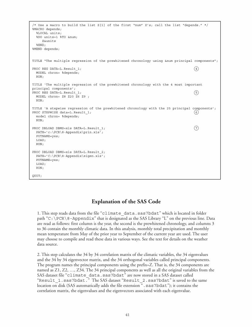
41
Explanation of the SAS Code
1. This step reads data from the file “climate_data.sas7bdat” which is located in folderpath “C:\PCR\8-Appendix” that is designated as the SAS Library “L” on the previous line. Dataare read as follows: first column is the year, the second is the prewhitened chronology, and columns 3to 36 contain the monthly climatic data. In this analysis, monthly total precipitation and monthlymean temperature from May of the prior year to September of the current year are used. The usermay choose to compile and read these data in various ways. See the text for details on the weatherdata source.
2. This step calculates the 34 by 34 correlation matrix of the climatic variables, the 34 eigenvaluesand the 34 by 34 eigenvector matrix, and the 34 orthogonal variables called principal components.The program names the principal components using the prefix=Z. That is, the 34 components arenamed as Z1, Z2, …, Z34. The 34 principal components as well as all the original variables from theSAS dataset file “climate_data.sas7bdat” are now stored in a SAS dataset called“Result_1.sas7bdat.” The SAS dataset “Result_2.sas7bdat” is saved to the samelocation on disk (SAS automatically adds the file extension “.sas7bdat”); it contains thecorrelation matrix, the eigenvalues and the eigenvectors associated with each eigenvalue.
/* Use a macro to build the list Z[i] of the first “num” Z’s; call the list “depends.” */%MACRO depends; %LOCAL units; %DO units=1 %TO # Z&units %END;%MEND depends;
TITLE “The multiple regression of the prewhitened chronology using &num principal components”;
PROC REG DATA=L.Result_1; 4 MODEL chron= %depends; RUN;
TITLE ‘The multiple regression of the prewhitened chronology with the 4 most importantprincipal components’;PROC REG DATA=L.Result_1; 5 MODEL chron= Z8 Z20 Z6 Z9 ; RUN;
TITLE ‘A stepwise regression of the prewhitened chronology with the 25 principal components’;PROC STEPWISE data=L.Result_1; 6 model chron= %depends; RUN;
PROC DBLOAD DBMS=xls DATA=L.Result_1; 7 PATH=’c:\PCR\8-Appendix\prin.xls’; PUTNAME=yes; LOAD; RUN;
PROC DBLOAD DBMS=xls DATA=L.Result_2; PATH=’C:\PCR\8-Appendix\eigen.xls’; PUTNAME=yes; LOAD; RUN;
QUIT;
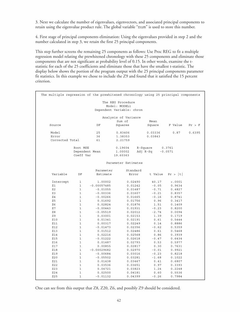
42
3. Next we calculate the number of eigenvalues, eigenvectors, and associated principal components toretain using the eigenvalue product rule. The global variable “num” is used to store this number.
4. First stage of principal components elimination: Using the eigenvalues provided in step 2 and thenumber calculated in step 3, we retain the first 25 principal components.
This step further screens the remaining 25 components as follows: Use Proc REG to fit a multipleregression model relating the prewhitened chronology with these 25 components and eliminate thosecomponents that are not significant at probability level of 0.15. In other words, examine the t-statistic for each of the 25 coefficients and eliminate those that have the smallest t-statistic. Thedisplay below shows the portion of the program output with the 25 principal components parameterfit statistics. In this example we chose to include the Z9 and found that it satisfied the 15 percentcriterion.
The multiple regression of the prewhitened chronology using 25 principal components
The REG Procedure Model: MODEL1 Dependent Variable: chron
Analysis of VarianceSum of Mean
Source DF Squares Square F Value Pr > F
Model 25 0.83406 0.03336 0.87 0.6395 Error 36 1.38353 0.03843 Corrected Total 61 2.21759
Root MSE 0.19604 R-Square 0.3761 Dependent Mean 1.00002 Adj R-Sq -0.0571 Coeff Var 19.60363
Parameter Estimates
Parameter StandardVariable DF Estimate Error t Value Pr > |t|
Intercept 1 1.00002 0.02490 40.17 <.0001Z1 1 -0.00057485 0.01242 -0.05 0.9634Z2 1 -0.01055 0.01487 -0.71 0.4827Z3 1 -0.00336 0.01607 -0.21 0.8357Z4 1 -0.00266 0.01665 -0.16 0.8741Z5 1 0.01692 0.01756 0.96 0.3417Z6 1 0.02824 0.01876 1.51 0.1409Z7 1 -0.00443 0.01931 -0.23 0.8200Z8 1 -0.05519 0.02012 -2.74 0.0094Z9 1 0.03001 0.02153 1.39 0.1719Z10 1 0.01341 0.02191 0.61 0.5444Z11 1 0.00317 0.02249 0.14 0.8886Z12 1 -0.01473 0.02356 -0.62 0.5359Z13 1 0.01512 0.02486 0.61 0.5468Z14 1 0.02216 0.02568 0.86 0.3939Z15 1 -0.01222 0.02618 -0.47 0.6434Z16 1 0.01487 0.02793 0.53 0.5977Z17 1 0.00855 0.02817 0.30 0.7631Z18 1 -0.00029682 0.02970 -0.01 0.9921Z19 1 -0.00684 0.03016 -0.23 0.8218Z20 1 -0.05502 0.03281 -1.68 0.1022Z21 1 0.01438 0.03467 0.41 0.6807Z22 1 0.03536 0.03651 0.97 0.3393Z23 1 0.04721 0.03823 1.24 0.2248Z24 1 0.02500 0.04181 0.60 0.5536Z25 1 -0.01132 0.04399 -0.26 0.7984
One can see from this output that Z8, Z20, Z6, and possibly Z9 should be considered.

43
5. Second stage of principal components elimination: Further screening of the 25 components (in thestep above) resulted in retention of only four components. These four components will be used todevelop the response function. The linear regression program (PROC REG) fits a multiple regressionmodel relating the prewhitened chronology with four components. The estimated coefficients of thefour components, their standard errors and the mean square error for the fitted model are veryimportant for further analysis. Note that the four components are not necessarily the first fourcomponents with largest eigenvalue. These components are strongly related to the response (theprewhitened chronology). The output from this step should be recorded for further analyses. Theoutput includes the estimated coefficients of the four components, which are denoted by lˆ (see step8 of the step-by-step procedure in the text), and the estimated standard errors of the four coefficients,which are denoted by . Recall that in step 9 of the step-by-step procedure (see the text), lVrepresents a 34 by l matrix containing eigenvectors corresponding these four retained componentsderived from the original 34 climate variables. To obtain the elements of this matrix, examine thecomplete eigenvector matrix in “Result_2.sas7bdat” and select those vectors correspondingthe four retained components. The user may choose to carry out the computation in steps 9 and 10using SAS, a spreadsheet, or hand calculator.
6. (Optional) Historical Comparison: Traditionally, the last screening of principal components inmost dendroecological studies was performed by relating the growth response with the principalcomponents using stepwise regression. This step is provided to demonstrate that the same result isobtained in either case. This step is redundant since the principal components are orthogonal andhence the significance of a particular component is not affected by exclusion or inclusion of anothercomponent.
7. Finally, the data generated from the study are saved to an Excel spreadsheet format to permitfurther computations, as described in the text.

Printed on Recycled Paper
Fekedulegn, B. Desta; Colbert, J.J.; Hicks, R.R., Jr.; Schuckers, Michael E. 2002. Copingwith Multicollinearity: An Example on Application of Principal ComponentsRegression in Dendroecology. Res. Pap. NE-721. Newton Square, PA: U.S.Department of Agriculture, Forest Service, Northeastern Research Station. 43p.
The theory and application of principal components regression, a method for coping withmulticollinearity among independent variables in analyzing ecological data, is exhibited indetail. A concrete example of the complex procedures that must be carried out indeveloping a diagnostic growth-climate model is provided. We use tree radial incrementdata taken from breast height as the dependent variable and climatic data from the area asthe independent data. Thirty-four monthly temperature and precipitation measurements areused as potential predictors of annual growth. Included are monthly average temperaturesand total monthly precipitation for the current and past growing season. The underlyingtheory and detail illustration of the computational procedures provide the reader with theability to apply this methodology to other situations where multicollinearity exists.Comparison of the principal component selection rules is shown to significantly influencethe regression results. A complete derivation of the method used to estimate standarderrors of the principal component estimators is provided. The appropriate test statistic,which does not depend on the selection rule, is discussed. The means to recognize andadjust for autocorrelation in the dependent data is also considered in detail. Appendicesand directions to internet-based example data and codes provide the user with the abilityto examine the code and example output and produce similar results.
Keywords: Multicollinearity, PCR, PC selection methods, radial growth, climate
Headquarters of the Northeastern Research Station is in Newtown Square,Pennsylvania. Field laboratories are maintained at:
Amherst, Massachusetts, in cooperation with the University of Massachusetts
Burlington, Vermont, in cooperation with the University of Vermont
Delaware, Ohio
Durham, New Hampshire, in cooperation with the University of New Hampshire
Hamden, Connecticut, in cooperation with Yale University
Morgantown, West Virginia, in cooperation with West Virginia University
Parsons, West Virginia
Princeton, West Virginia
Syracuse, New York, in cooperation with the State University of New York,College of Environmental Sciences and Forestry at Syracuse University
Warren, Pennsylvania
The U. S. Department of Agriculture (USDA) prohibits discrimination in all its programs andactivities on the basis of race, color, national origin, gender, religion, age, disability, politicalbeliefs, sexual orientation, and marital or family status. (Not all prohibited bases apply to allprograms.) Persons with disabilities who require alternative means for communication ofprogram information (Braille, large print, audiotape, etc.) should contact the USDA's TARGETCenter at (202)720-2600 (voice and TDD).
To file a complaint of discrimination, write USDA, Director, Office of Civil Rights, Room 326-W,Whitten Building, 14th and Independence Avenue SW, Washington, DC 20250-9410, or call(202)720-5964 (voice and TDD). USDA is an equal opportunity provider and employer.
“Ca“Ca“Ca“Ca“Carrrrring for the Land and Seing for the Land and Seing for the Land and Seing for the Land and Seing for the Land and Serrrrrving People Thrving People Thrving People Thrving People Thrving People Through Reseaough Reseaough Reseaough Reseaough Researrrrrch”ch”ch”ch”ch”