testing for multicollinearity using microsoft …...testing for multicollinearity using microsoft...

TESTING FOR MULTICOLLINEARITY USING MICROSOFT EXCEL: USING THE VARIANCE INFLATION FACTOR?

ADESETE AHMED ADEFEMI

COMPUTING AND INTERPRETING THE VARIANCE INFLATION FACTOR

MARCH, 2019

RESEARCH SOLUTION GROUP

PUBLISHED ARTICLES BY THE AUTHOR

ADESETE AHMED ADEFEMI 2

TESTING FOR MULTICOLLINEARITY USING MICROSOFT EXCEL

MULTICOLLINEARITY:

Multicollinearity is one of the factor often overlooked by researchers when using the ordinary least

square(OLS) technique. Multicollinearity can simply be described as a condition in which there is an

inter-association amongst independent/explanatory variables in a multiple regression model.

However, multicollinearity does not decrease the reliability/predictive power of the model but it may

affect calculations regarding the individual predictors.

If the correlation between two explanatory variables is 1, then we can conclude there is perfect

multicollinearity between the variables. That is, there is an exact linear relationship between the two

explanatory variables. On the other hand, if the correlation between the two explanatory variables is

zero(0), we can conclude that, there is no evidence of multicollinearity between the two variables. In

practice, there is rarely a case of perfect multicollinearity or no evidence of multicollinearity because

there is usually an iota of inter-association between variables except in rare cases of some raw data.

CAUSES/REASONS FOR MULTICOLLINEARITY

(1) There is tendency that most economic variables moves together overtime. In periods of economic

boom, economic variables such as employment, economic growth, investment increases together

during this period. However there is tendency for multicollinearity between these variables.

(2) The use of lagged values of dependent variables as explanatory variables is another common

reason for the little presence of multicollinearity in a multiple regression model. Investment in the

immediate past one period and investment in immediate past two periods may affect investment in the

current period.

CONSEQUENCES OF MULTICOLLINEARITY

(1) It may affect calculations regarding the individual predictors.

(2) The standard errors of the individual predictors are large.



(3) In the case of a perfect multicollinearity, the estimates of the individual predictors are

indeterminate.

INDICATORS FOR DETECTING MULTICOLLINEARITY

(1) Large changes in the estimated regression coefficients when an explanatory variable is added or

deleted.

(2) The affected variables are statistically insignificant but the F-test indicates the model is

statistically significant.

(3) An explanatory variable is insignificant in a multiple regression but significant in a simple

regression.

TEST FOR DETECTING MULTICOLLINEARITY

(1) Correlation test that is by constructing a correlation matrix of the data. The major set-back of this

technique is, correlation indicates bivariate relationship but multicollinearity is a multivariate

phenomenon. Problem arises when a multiple regression model is involved.

(2) Variance Inflation Factor(VIF): VIF is majorly used to measure the severity of multicollinearity

in a multiple regression model. It is usually measured as the variance of a model with multiple terms

divided by the variance of a model with one term alone.

Decision criterion:

VIF value Multicollinearity severity Less than 5 Low

Between 5 and 10 Medium

Greater than 10 High



VIF Formula =

R2 ------- Coefficient of determination for the estimated regression function

(3) Farrar-Glauber test: According to this test, explanatory variables in a multiple regression are

orthogonal if there is no multicollinearity between them. However, if the variables are not orthogonal,

there is little evidence of multicollinearity between them.

SOLUTION TO MULTICOLLINEARITY: If multicollinearity does not affect the predictor

coefficients much, the variable can be retained. If there is high degree of multicollinearity as a result

of lagged values of explanatory variables or the dependent variables, then a distributed lagged model

technique can be adopted. However, if the high degree of multicollinearity is as a result of other

factors;

(1) More data can be obtained by increasing the sample size of the data.

(2) Drop the variables causing multicollinearity but one has to be careful of mis-specification bias

when adopting this method.

(3) Partial least squares method can also be adopted.

In this article, our emphasis would be on using the Variance Inflation Factor to detect

multicollinearity in a multiple regression with the aid of Microsoft excel package.



COMPUTING AND INTERPRETING THE VARIANCE INFLATION FACTOR IN

MICROSOFT EXCEL.

STEP ONE: Open the Microsoft excel file where the data is stored.

Note: MGDP is the dependent variable while INFR, UNEMP, EXR and FDI are the explanatory

variables.


STEP TWO: If you do not have data analysis tab in your Microsoft excel, Navigate to the highlighted

excel icon and Click



excel icon and Click



excel icon and Click excel options



excel options











6




STEP THREE: Click on add-ins, and navigate to Analysis toolpak and click on GO ;



STEP FOUR: Click/Tick Analysis ToolPak, Analysis ToolPak-VBA and Solver Add-in then Click

OK



You would observe you have a new tab Data in the Microsoft excel windows display

Click on the Data tab, this would appear

STEP FIVE: Arrange the data in order in which they would be regressed in the microsoft excel file

with each arrangement in separate excel sheets.

INFR, UNEMP, EXR and FDI are the explanatory variables in this study.

INFR = f(UNEMP, EXR, FDI) ................(1)

UNEMP = f(EXR, FDI, INFR) ................(2)

FDI = f(INFR, UNEMP, EXR) ................(3)

EXR = f(INFR, UNEMP, FDI) ................(4)

NOTE: The explanatory variable to be used as dependent variable should come first when

arranging the variables in Microsoft excel while the other explanatory variables follows.



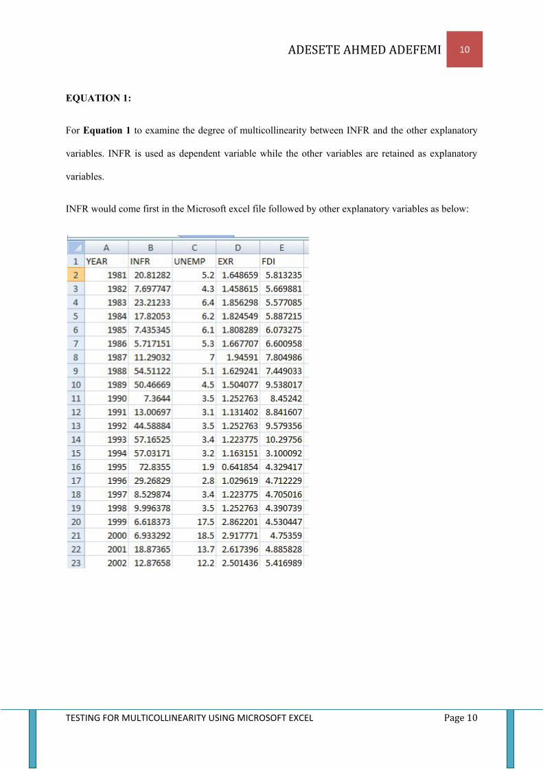
EQUATION 1:

For Equation 1 to examine the degree of multicollinearity between INFR and the other explanatory

variables. INFR is used as dependent variable while the other variables are retained as explanatory

variables.

INFR would come first in the Microsoft excel file followed by other explanatory variables as below:



EQUATION 2:

For Equation 2 to examine the degree of multicollinearity between UNEMP and the other

explanatory variables. UNEMP is used as dependent variable while the other variables are retained as

explanatory variables.

UNEMP would come first in the Microsoft excel file followed by other explanatory variables as

below:

EQUATION 3:

For Equation 3 to examine the degree of multicollinearity between FDI and the other explanatory

variables. FDI is used as dependent variable while the other variables are retained as explanatory

variables.

FDI would come first in the Microsoft excel file followed by other explanatory variables as below:



EQUATION 4:

For Equation 4 to examine the degree of multicollinearity between EXR and the other explanatory

variables. EXR is used as dependent variable while the other variables are retained as explanatory

variables.

EXR would come first in the Microsoft excel file followed by other explanatory variables as below:



STEP SIX: Regress each explanatory variable on other explanatory variables. That is one explanatory

variable would be used as dependent variable while the other explanatory variable would be retained

as explanatory variable.

INFR, UNEMP, EXR and FDI are the explanatory variables in this study.

INFR = f(UNEMP, EXR, FDI) ................(1)

UNEMP = f(EXR, FDI, INFR) ................(2)

FDI = f(INFR, UNEMP, EXR) ................(3)

EXR = f(INFR, UNEMP, FDI) ................(4)

Navigate: Data >> Data analysis >> Regression

Click OK, this window displays



STEP SEVEN:

EQUATION 1:

INFR = f(UNEMP, EXR, FDI)

Put the mouse cursor in the Input Y range and Highlight the Y variable which is INFR column

and do the same for the X variables which are UNEMP, EXR and FDI.

FOR Y



FOR X

Click OK and the regression result shows:

The same procedure would be followed for other variables.



EQUATION 2

EQUATION 3



EQUATION 4

STEP EIGHT: Collect the R2 of each equation/variable and put it in a table

EQUATION VARIABLE R2

1 INFR 0.363227848

2 UNEMP 0.930691032

3 FDI 0.208836755

4 EXR 0.937053465

STEP NINE: Compute 1 - R2

EQUATION VARIABLE R2 1 - R2

1 INFR 0.363227848 0.636772

2 UNEMP 0.930691032 0.069309

3 FDI 0.208836755 0.791163

4 EXR 0.937053465 0.062947



STEP TEN: Compute Variance Inflation factor for each variable and interpret.

VIF Formula =

EQUATION VARIABLE R2 1 - R2 VIF

1 INFR 0.363227848 0.636772 1.57042

2 UNEMP 0.930691032 0.069309 14.42815

3 FDI 0.208836755 0.791163 1.263962

4 EXR 0.937053465 0.062947 15.8865

Decision:

EQUATION VARIABLE R2 1 - R2 VIF Decision

1 INFR 0.363227848 0.636772 1.57042

VIF < 5, There is little or no evidence of

multicollinearity of INFR with other explanatory

variables.

2 UNEMP 0.930691032 0.069309 14.42815

VIF > 10, There is evidence of high

multicollinearity of UNEMP with other

explanatory variables.

3 FDI 0.208836755 0.791163 1.263962

VIF < 5, There is little or no evidence of

multicollinearity of FDI with other explanatory

variables.

4 EXR 0.937053465 0.062947 15.8865

VIF > 10, There is evidence of high

multicollinearity of EXR with other explanatory

variables.



STEP ELEVEN: Investigate the source of the multicollinearity by computing a correlation

matrix.

Navigate: Data >> Data analysis >> Correlation

Then highlight all explanatory variables:

Click OK

From the result of the correlation matrix, there is high correlation of above 0.5 between

inflation rate and exchange rate, between unemployment rate and exchange rate which shows

the source of the multicollinearity of exchange rate and unemployment rate with other

explanatory variables. This result shows that all other explanatory variable shares little



evidence of multicollinearity with exchange rate and unemployment rate except inflation rate

and exchange rate which shows there is multicollinearity only between inflation rate and

exchange rate, and only multicollinearity between unemployment rate and exchange rate.

STEP TWELVE: Either the sample size of the data is increased or the multicollinear variables are

added and removed from the final regression and the R2 , significance, sign and size of the variables

being observed to choose the best model. Or the multicollinear variables are removed, but in the case

of this study, both multicollinear variables are economic indicators so it would be better to increase

their sample size or try adding and removing the variables to check the most important variable of the

two.

MGDP = f(UNEMP, INFR, EXR, FDI)

Removing both variables

Removing both variables gives an adjusted R2 of 0.409 and a significance F of 0.000142105 and also,

unemployment is the only significant factor with a coefficient estimate of 0.119243 and the sign of

UNEMP and FDI is positive and negative respectively.



Adding INFR

Adding INFR gives an adjusted R2 of 0.432 and a significance F of 0.000209395 and also,

unemployment is the only significant factor with a coefficient estimate of 0.139497 and the sign of

UNEMP and FDI is positive and negative respectively as with the regression result of removing both

variables.

Adding EXR



Adding EXR and removing INFR gives an adjusted R2 of 0.446549 and a significance F of

0.000144929 and also, unemployment is a significant factor at both 5% and 10% significance level

while EXR is a significant factor at 10% with a coefficient estimate of 0.260698 and -1.301745

respectively. The sign of UNEMP and FDI is positive and negative respectively as with the previous

regression results above.

Adding both EXR and INFR

Adding both EXR and INFR gives an adjusted R2 of 0.441376 and a significance F of 0.000363 and

also, unemployment is a significant factor at 5% significance level and a coefficient estimate of -

1.301745. The sign of UNEMP, EXR, INFR and FDI are the same as with the previous regression

results above.

However, this study concludes that regression result in which only EXR is added and INFR is

removed is the most appropriate result because adding INFR decreases the adjusted R2 , increases the

significance F and also decreased the number of significant variables from two to one. However INFR

would be removed from the final equation to correct for the effect of high multicollinearity.



However, for further rigorous analysis, the mis-specification bias test is necessary to determine if

there is specification bias after removing or adding a variable.

FINAL EQUATION

Any further research questions or questions regarding this article should be forwarded to

[email protected].

Use of information on this publication/website is at your own risk. No part of this publication

may be reproduced, downloaded or transmitted in any form or by any means published

somewhere without the author permission. All publications are copyrighted by the author and

publications are used for research and understanding purposes.



DATA USED

YEAR MGDP INFR UNEMP EXR FDI 1981 3.455099 20.81282 5.2 1.648659 5.813235 1982 3.603718 7.697747 4.3 1.458615 5.669881 1983 3.745081 23.21233 6.4 1.856298 5.577085 1984 3.647969 17.82053 6.2 1.824549 5.887215 1985 3.853885 7.435345 6.1 1.808289 6.073275 1986 3.466818 5.717151 5.3 1.667707 6.600958 1987 3.837841 11.29032 7 1.94591 7.804986 1988 4.113863 54.51122 5.1 1.629241 7.449033 1989 4.346632 50.46669 4.5 1.504077 9.538017 1990 3.709202 7.3644 3.5 1.252763 8.45242 1991 4.591557 13.00697 3.1 1.131402 8.841607 1992 4.972358 44.58884 3.5 1.252763 9.579356 1993 5.111336 57.16525 3.4 1.223775 10.29756 1994 5.392955 57.03171 3.2 1.163151 3.100092 1995 5.689688 72.8355 1.9 0.641854 4.329417 1996 5.859654 29.26829 2.8 1.029619 4.712229 1997 5.947055 8.529874 3.4 1.223775 4.705016 1998 5.980828 9.996378 3.5 1.252763 4.390739 1999 6.054937 6.618373 17.5 2.862201 4.530447 2000 6.148523 6.933292 18.5 2.917771 4.75359 2001 6.283754 18.87365 13.7 2.617396 4.885828 2002 6.23016 12.87658 12.2 2.501436 5.416989 2003 6.143781 14.03178 14.8 2.694627 5.554509 2004 5.855978 14.99803 11.8 2.4681 5.514235 2005 6.012168 17.86349 11.9 2.476538 7.560705 2006 6.170707 8.239527 12.3 2.509599 10.62424 2007 6.255526 5.382224 12.3 2.509599 11.60058 2008 6.372591 11.57798 12.7 2.541602 11.73322 2009 6.417237 11.53767 14.7 2.687847 12.33312 2010 6.466254 13.7202 14.7 2.687847 11.82795 2011 6.543644 10.84079 21.1 3.049273 11.7414 2012 6.635247 12.21701 23.9 3.173878 12.39253 2013 6.714001 8.475827 23 3.135494 12.17091

testing for multicollinearity using microsoft …...testing for multicollinearity using microsoft...

Documents