Summary session 5

Structure & outcomes

• Before coffee break – Surface subsurface climate variability

• After coffee break– Oxygen & nutrient – Fisheries

• Outcomes– Updated synthesis of climate processes in the N-Pac– Interpret IPCC5 projections in the context of N-Pac

Cliamte dynamics

Mat Collins

• Anomalies 1986-2005 average. • Transient climate response is likely in the

range 1-2.5C and extremely unlikely greater than 3c. (box 12.2)

• My interest: Tropical atmospheric circulation is weakened, subtropics creeps poleward.

• Five consistent models show faster reduction of sea-ice.

Mat Collins 2

• SAT change 2081-2100 minus 1986-2005– Global mean, land-sea contrast, polar amplification

(themodynamic processes) are removed. Then PICES region is fastest warming

– Dynamical SAT changes seem much smaller – although of crucial in the tropics (Xie et al. 2010)

• Vertical winds (omega) = precipitation (P) / humidity (q) – This relation is good for global, but not in Asian – Chadwick et al. (2013)

Mat Collins 3

• Global mean changes are sub-Clausius-Clapeyron,

• Confidence in storminess is low.

Mat Collins 4

• Chapter 14: climate phenomne and their relevance for future regional climate change

• Any specific projected change in ENSO variability in the 21st century remains low. Associated precipitation changes will be intensified.

• Extreme El Ninos (Cai et al, Nature Climate Change 2014) will be doubled.

Mat Collins

• Changing El Nino teleconnections associated with Walker Circulation Change – Chung et al. Cdyn 2014– Power et al. Nature 2013

Mat Collins

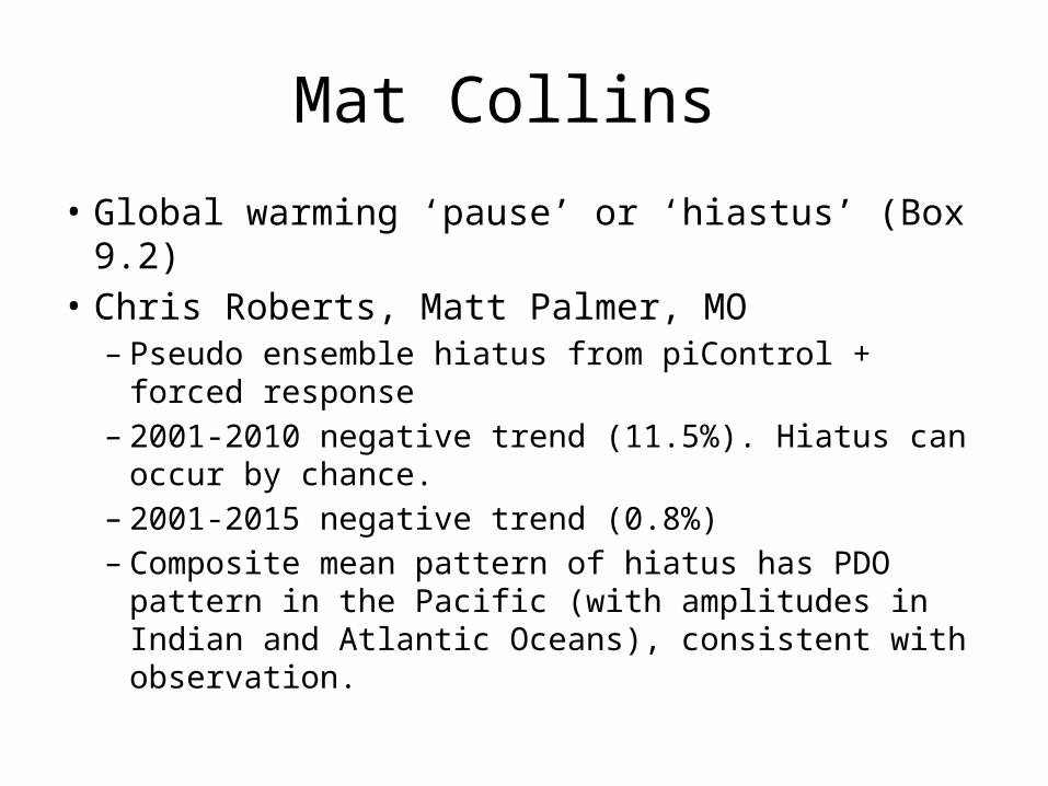
• Global warming ‘pause’ or ‘hiastus’ (Box 9.2)• Chris Roberts, Matt Palmer, MO– Pseudo ensemble hiatus from piControl + forced

response – 2001-2010 negative trend (11.5%). Hiatus can occur

by chance. – 2001-2015 negative trend (0.8%) – Composite mean pattern of hiatus has PDO pattern

in the Pacific (with amplitudes in Indian and Atlantic Oceans), consistent with observation.

Mat Collins

• Trade wind strengthening: England et al. Nature Climate Change 2014– See also Kosaka and Xie 2013

Mat Summary

• Large-scale thermodynamic response of temp relatively well understood; global + land/sea + polar amplification. Could build a quantitative theory. – Interestingly, after removal of them SAT change is

largest PICES region. Can be associated with polar amplification (just masking)

• Precip: weakened circulation and increase humidity • Challenge is to combine information from

imperfect models with our (sometimes quite good) understanding of physical processes.

Nate Mantua

• 1998-2013 minus 1977-1997• Max corr. Is 0.53 Beween negative pole in C-N-

Pac and pole in E-N-Pac. • ER-SST (1900-2012) USHCNv2 GHCNv3 (1900-

2012), flux SODA (1900-)• EOF east of dateline (max corr 0.82): horse

shoe-oval still (ship track is good in this region)• SLP PC1 max at 150W, 35N (shifted east than

NPI)

Nate Mantua 2

• SST = 0.81 SST(t-1) + 0.27 SLP(t) + eps(t) (monthly)– Good reconstuction =0.79 (monthly)

• SST tendency due to latent heat flux, horizontal Ekman transport, vertical T-advection

• Coastal air-temperature は annual meanでよく一致．• SLP forcing accounts for all of the SST trend & most of

SAT trend (from northern California to Washington) • Circulation changes looks to be free (not forced) from

4 CMIP5 models (31 members), consistent with Deser et al. (2012, 2014), Oshima et al. (2012)

Mat Newman 1

• PDO is reddened ENSO + lagged KOE due to Rossby waves – PDO (yr) = 0.6 PDO (yr-1) + 0.6 ENSO(yr) + eps

• Multivariate red noise (Ornstein-Uhlenbeck)– dx/dt = B x + fs – If B is nonnormal (not symmetric), transient anomaly

growth is possible even through exponential growth is not.

– Detemine B with LIM from lagged covariance (space and time) statistics of X

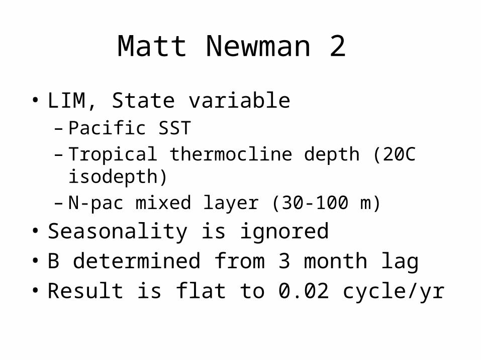
Matt Newman 2

• LIM, State variable – Pacific SST – Tropical thermocline depth (20C isodepth) – N-pac mixed layer (30-100 m)

• Seasonality is ignored • B determined from 3 month lag• Result is flat to 0.02 cycle/yr

Mat Newman 3

• After removal tropical forcing, Oyashio SST anomalies stand out

• Trend + KOE-related + decadal ENSO (aka CP ENSO)

• PDO may generally provide only weak forcing of the atmosphere (Kumar et al. 2012)

• Smirnov et al. (2014) HR model KOE -> G Alaska

Bo Qiu 1

• Unstable states lagged by 4-yrs to PDO, 3-yr to NPGO. Due to Rossby waves. – Stable -> strong gradient?

• KE index: sum of four indices, extended using OFES to 1956 (just SSH anomaly in KE region).

• two way prediction model has a better skill 4-5 years

• Northward-shifted and stable KE will last further several years. (Qiu 2014 JC)

Nikas 1

• Taguchi & Schneider JC 2014 submitted• 0-300 m HC propagate eastward • Higher vertical mode• Density-spiciness split– δT = d[T]/dρ δρ + δ T’ (vertical movement +

spiciness) – Spiciness is dominant – Meridional displacement produces spiciness

Niklas 2 summary

• Westward propagating SSHa• Eastward propagating OHCa– Generation meridional migration – Mean advection – Damping produces higher vertical modes

Krovnin 1

• Azores high & icelandic low longitudes and Z500 – 1950-1977: – 1978-2005:

• Atlantic influence -> Eurasia -> North Pacific• Ocean tracers as integrators– Long memory -> red noise (Ito & Deutsch 2010;

2013)– Double integration (Di Lorenzo & Ohman 2013)

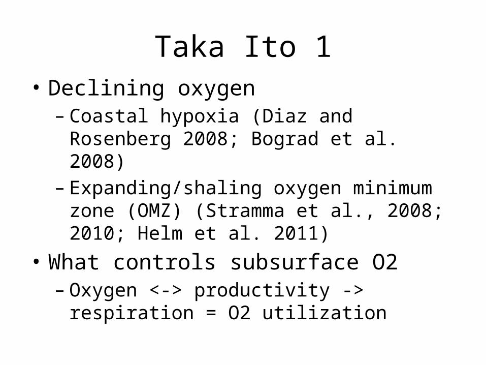
Taka Ito 1• Declining oxygen – Coastal hypoxia (Diaz and Rosenberg 2008; Bograd

et al. 2008)– Expanding/shaling oxygen minimum zone (OMZ)

(Stramma et al., 2008; 2010; Helm et al. 2011)• What controls subsurface O2– Oxygen <-> productivity -> respiration = O2

utilization

Taka Ito 2

• Helm et al. (2011) WOCE vs historic data 1992-1970 in 100-1000 m

• 1990-2008 minus 1960-74 diff (Stramma et al. 2010) O2 decline <- AOU increase in the topical oceans

• Warming • Weakening ocean vertical exchange – Weaker physical O2 -> weaker nutrient upwelling ->

weaker productivity • Tropics incease oxygen (Cocco et al. 2013)

Taka Ito 3

• Tropical O2 paradox – There are a number of suggestions including

decadal variability of Deutsch et al. (2011) – This study : anthropogenic nutrient flux – Mineral Fe : acidification aerosol makes solble

iron. – Anthropogenic Fe decomposition promoves ocean

productivity (Krishnamurty 2009?)

Taka Ito 4

• Global 1x1, L23 (MITgcm –Ecco) • 2 biogeochemistry models • Soluble Fe flux 100 years-> macro nutrient

down -> productivity up -> O2 down – This effect is not in CMIP5 models.

• This can explain the reduction of topical oxygen reduction.

Sung Yong Kim (KAIST)

• CalCOFI region • 6 harmonics T, T/2, T/3 … T/6 • Fitted with seasonal cycle, ENSO, PDO, NPGO,

trend

Di Lorenzo

• Good coastal hypoxia map (Diaz and Rosenberg Science 2008)

• Isopycnal 26.5 • d O’shelf /dt = -(1+r) w’ [Osub] + [w] Osub’ –

eps O’shelf• Northward poleward undercurrent bring low

O2 (high NO3) from the south• Gyre brings high O2 (low NO3)

Di Lorenzo 2

• Salinity anomalies in ECMWF ORA3 on isopycnal 26.5 is used as a proxy of Oxygen– Good in ColCOFI and Statin P – CalCOFI papers: Bograd et al 2008; Koslow et al

2011; Peterson et al. 2013• Subtropical gyre in the central Pacific N-Pac

oxygen (index) can predict CalCOFI oxygen with lag of 8-10 years

Art Miller 1

• CCE-LTER founded in 2004• Rykaczewki and Checkley (2008): off-shore

Ekman pumping is important as coastal upwelling

• Warm water coming from depth

Shin-ichi Ito

• Pacific saury: subarctic feeding, subtopics spawning, Surf riding theory

• Examine using NEMURO.FISH• Previous 3box -> Euler model – Velocity (Ambe 08) 1/3 deg, temperature (MODIS/Terra 1/12

deg), Chl-a SeaSiFS (1/12 deg)• Feeding migration: highest grwoth, spawning migration, • Order is good, but interannual variation 2002-2009 is

not good enough– Adjust westward migration speed. ->

Shin-ichi Ito 2

• Westward migration is low in 2004 high in 2008– SST west is warmer (cooler in east) -> faster

westward migration – Saury may see light (cloudiness)

Sukgeun Jung

• Pacific cod (cold water spices) in Korea waters increase from 1999 to 2011.

• Common squid (warm water) dominant • Increase Sardine (warm) and Cod (cold) since

the late 1990s. • Corresponding analysis -> dim1 & dim2 – Dim1 is correlated to temp 100-500 m

Sukgeun Jung, Summary

• Upper layer (50-100)– Temp increase 1988-89– Warm water species (Sardin -> Squid)

• Deep layer 100-500 m – Cold water species (Filefish -> Cod & Herring)

• Time lag between the shifts in the upper and dep layer was 5-6 years.