Structural multiscale topology optimizationwith stress constraint for additive

manufacturing ∗

Ferdinando Auricchio†, Elena Bonetti‡, Massimo Carraturo§,Dietmar Hömberg ¶, Alessandro Reali‖and Elisabetta Rocca∗∗

July 16, 2019

Abstract. In this paper a phase-field approach for structural topology optimizationfor a 3D-printing process which includes stress constraint and potentially multiple ma-terials or multiscales is analyzed. First order necessary optimality conditions are rigor-ously derived and a numerical algorithm which implements the method is presented. Asensitivity study with respect to some parameters is conducted for a two-dimensionalcantilever beam problem. Finally, a possible workflow to obtain a 3D-printed objectfrom the numerical solutions is described and the final structure is printed using afused deposition modeling (FDM) 3D printer.

∗This work was partially supported by Regione Lombardia through the project "TPro.SL - TechProfiles for Smart Living" (No. 379384) within the Smart Living program, and through the project"MADE4LO - Metal ADditivE for LOmbardy" (No. 240963) within the POR FESR 2014-2020program. MC and AR have been partially supported by Fondazione Cariplo - Regione Lombardiathrough the project “Verso nuovi strumenti di simulazione super veloci ed accurati basati sull’analisiisogeometrica”, within the program RST - rafforzamento. The financial support of the project Fon-dazione Cariplo-Regione Lombardia MEGAsTAR “Matematica d’Eccellenza in biologia ed ingegneriacome acceleratore di una nuova strateGia per l’ATtRattività dell’ateneo pavese” is gratefully acknowl-edged. The paper also benefits from the support of the GNAMPA (Gruppo Nazionale per l’AnalisiMatematica, la Probabilità e le loro Applicazioni) of INdAM (Istituto Nazionale di Alta Matemat-ica) for EB and ER. This research was supported by the Italian Ministry of Education, Universityand Research (MIUR): Dipartimenti di Eccellenza Program (2018–2022) - Dept. of Mathematics “F.Casorati”, University of Pavia. A grateful acknowledgment goes to Dr. Ing. Gianluca Alaimo for hissupport and precious suggestions on additive manufacturing technology.†Dipartimento di Ingegneria Civile e Architettura (DICAR), Università di Pavia, and IMATI-

C.N.R., Via Ferrata 5, I-27100 Pavia, Italy (ferdinando.auricchio@unipv.it).‡Dipartimento di Matematica “F. Enriques’, ’ Università di Milano, and IMATI-C.N.R., Via Saldini

50, I-20133 Milano, Italy (elena.bonetti@unimi.it).§Dipartimento di Ingegneria Civile e Architettura (DICAR), Università di Pavia, Via Ferrata 5,

I-27100 Pavia, Italy and Chair of Computational in Engineering, Technical University of Munich,Munich, Germany (massimo.carraturo01@universitadipavia.it).¶Weierstrass Institute for Applied Analysis and Stochastics, Mohrenstrasse 39, D-10117 Berlin,

Germany (hoemberg@wias-berlin.de)‖Dipartimento di Ingegneria Civile e Architettura (DICAR), Università di Pavia, and IMATI-

C.N.R., Via Ferrata 5, I-27100 Pavia, Italy (alessandro.reali@unipv.it)∗∗Dipartimento di Matematica “F. Casorati”, Università di Pavia, and IMATI-C.N.R., Via Ferrata

5, I-27100 Pavia, Italy (elisabetta.rocca@unipv.it).

1

arX

iv:1

907.

0635

5v1

[m

ath.

OC

] 1

5 Ju

l 201

9

Key words: Additive manufacturing, first-order necessary optimality conditions,phase-field method, structural topology optimization, functionally graded material

AMS (MOS) subject classification: 74P05, 49M05, 74B99.

1 Introduction

Additive manufacturing (often denoted by AM), e.g. 3D printing, is nowadays recog-nized as a very challenging subject of research, also due to the strategic position of AMtechnology with respect to many applications. This innovative technology is, at thesame time, disruptive, as well as widespread and transversal. Indeed, the applicationscover several fields, like architecture, medicine, surgery, dentistry, arts. AM is deeplychanging paradigms in design and industrial production in comparison with more tra-ditional technologies, like casting, stamping, and milling. This kind of technology isbased on the fact that components or complete structures are constructed throughsequences of material layers deposition and/or curing. The layer by layer fashion isobtained through deposition of fused material (in the Fused Deposition Material -FDM technology) or by melting/sintering of powders (Selecting Laser Sintering - SLSand Selective Laser Melting - SLM technologies). Hence, hardening and solidificationof the material, prior to the application of the next layer, occur mainly by thermalactions and form the bulk part.In recent years, in the fields of engineering and materials science, large efforts havebeen devoted to model AM processes with particular regard to single layer behaviour,concerning interaction between the temperature and the stress field, heat transfer, andmechanical aspects (see e.g. [17,18,31]). Also mesoscopic models have been developedfor the layer by layer fashion, for instance applying a lattice Boltzmann method forthe treatment of free surface flows [2, 3]. In a different framework, some interestingresults, that have been recently achieved for modeling epitaxial growth, could be putinto some relation with AM modeling (see, e.g., [15]).However, it is still necessary to introduce tools able to produce simultaneously op-timization of printing materials and adjustment of prototyping processes. Thus, inthe present paper we focus on a first typical problem occurring in additive manu-facturing/3D printing processes: the problem of structural optimization consisting intrying to find the best way to distribute a material in order to minimize an objectivefunctional [4, 5, 25, 26]. The shape of the domain is a-priori unknown, while knownquantities are the applied loads as well as regions where we want to have holes ormaterial. Our main interest is to find regions which should be filled by material inorder to optimize some properties of the sample, which is mathematically translatedin the optimization of a suitable objective functional (denoted by J in the rest of thepaper). Since we are clearly in presence of a free-boundary problem, we decide hereto handle it by means of the well-known phase-field method.With respect to previous papers in the literature, the main novelties here are twofold.First, we include in the functional a constraint on the stress σ , which should range

2

in the physically elastic domain. In previous papers either such a constraint was notincluded or it was imposed pointwise (cf. [10]), but, in that case only partial resultscould be obtained on the minimization problem and no optimality conditions could berigorously determined.The second and most important novelty is the derivation of a multiscale phase-fieldconcept by introducing a second order parameter representing the micro-scale. Thisconcept allows to obtain functionally graded material (FGM) structures.The classical approach to shape and topology optimization is using boundary varia-tions in order to compute shape derivatives and to decrease the functional by deformingthe boundary in a shape descendant way (cf., e.g., [27,28]). Another possibility, espe-cially in order to deal with the multiscale case, is to adopt the homogenization methods(cf., e.g., [1, 16]) or the level set method which has been exploited by several authors(cf., e.g., [9] and references therein). The phase-field approach has been already usedin structural optimization by several authors (cf., e.g., [10, 29, 30, 32]), but still fewanalytical results are present in the literature (cf. [6, 7, 24]).A topology optimization based on homogenization and including a two-scale (micro-macro) relationship has been introduced in [19] for non linear elastic problems. Theirapproach decouples the analysis of the micro structure (performed using a phase fieldmethod) from the macro structural optimization routine which uses a classical SIMPapproach instead. In [14], it is experimentally observed that topologycally optimizedinfill structures (e.g., lattice structures) present an improved buckling load comparedto weight with respect to bulk material structures. Regarding topology optimizationfor FGM, a possible approach consists in using an unpenalized SIMP method (SIM) toobtain gray scale regions which can be mapped to different lattice volumes (cf. [8, 12,23]). Nevertheless, all these approaches do not allow to clearly define the boundariesof the structure which have to be reconstructed in a second step and might lead tonon-optimal results.In fact, the present work aims at obtaining a 3D-printed model by means of a multi-scale phase-field topology optimization scheme, providing at the same time a completederivation of the first order optimality conditions. This choice turns out to be math-ematically tractable. The related analysis is indeed not very different from the onecontained in [6] and we utilize differentiability results already obtained therein. How-ever, the convex set to which the two order parameters belong is different from thesimplex used in [6], where a vectorial phase field variable is introduced in order to treatthe case of multi-materials. Our approach incorporates the creation of graded materialstructures, which could again be generalized to allow for multi-material graded struc-tures. Moreover, our objective functional contains a constraint on the stress σ whichwas not present in [6] and which will prove to be important for the application to theAM technology, especially in the case of lightweight structures with small materialvolume.The work is organized as follows. In Section 2 the optimization problem is described.Section 3 presents the main analytical results. In Section 4 we first introduce a numer-ical algorithm implementing the method, then we discuss the results of a sensitivitystudy with respect to a problem parameter, and finally we describe a simple workflowto obtain a 3D printed structure using an FDM 3D printer. Finally, in Section 5 we

3

draw the main conclusions of the problem and possible further outlooks of the pre-sented work. Notice that other sensitivity analyses and more comparisons with thesingle-material cases for a simplified cost functional have been performed in the recentpaper [11] by the same authors.

2 The problem

Let us consider a component located in an open bounded and connected set Ω ⊂ R3 ,with a smooth boundary ∂Ω , and let n denote the outward unit normal to ∂Ω . Weassume that ∂Ω is decomposed into ΓD∪Γg , ΓD with positive measure. Indeed, we willprescribe Dirichlet boundary conditions on ΓD and non-homogeneous Neumann typeprescription (corresponding to a traction applied) on the part Γg . We also introducethe following notation: we denote by H1

D(Ω;Rd) := v ∈ H1(Ω;Rd) : v = 0 on ΓDand by H(div,Ω) := v ∈ L2(Ω;Rd×d) : div v ∈ L2(Ω;Rd) .As it is known, one of the main characteristic of AM technology is the possibility toconstruct objects with prescribed macroscopic and microscopic structure. We aim tointroduce a model to get a combined optimization of the two scales of this structure:a macroscopic scale corresponding either to the presence of material or to the presenceof no material (i.e. voids), and a microscopic scale corresponding to the microscopicdensity of the material. To this purpose we introduce a new double phase-fields model(cf. also [33] for similar approaches). We let Ω0, Ω1 be two sets of positive measurecontained in Ω such that Ω0∩Ω1 = ∅ . We aim to introduce a model to get a simultane-ous optimization of the two scales of this structure: a macroscopic scale correspondingto the presence of material (or voids), and a microscopic scale corresponding to themicroscopic density of the material, when it is present. To this purpose we intro-duce a new two-scale phase-field model, where the two phase parameters describe thepresence of the material and its density. In particular, the parameter standing forthe microscopic density of the material depends on the macroscopic phase parameterthrough an internal constraint. Hence, we first introduce the phase variable ϕ todenote a macro-scale parameter, meaning that in the regions of Ω where ϕ = 1 wehave the presence of the material, while when ϕ = 0 we have voids (no material). Inorder to describe the micro-scale effects (corresponding to possible different densitiesof the material) we include in the model a second phase parameter which we denoteby χ related to different microscopic configurations of the object. More precisely, χ isforced to belong to the interval [0, ϕ] , so that in particular χ is forced to be 0 wherewe have voids, i.e. where ϕ = 0 . Note that, within the phase-field approach, for ϕ weassume that the interface between the two phases (material and voids) is not sharpbut diffuse with small thickness γ (see (2.1)). The same diffuse interface is assumedfor the microscopic density denoted by χ .Now, let us introduce the optimization problem and make precise the cost functionaldepending on the parameters (ϕ, χ) . As far as the cost functional corresponding toϕ , we first approximate the standard perimeter term by a multiple of the so-called

4

Ginzburg-Landau type functional

(2.1)∫

Ω

(W(ϕ)

γ+ γ|∇ϕ|2

2

)dx

where W is a potential function attaining global minima at ϕ = 1 (material) andϕ = 0 (void). A typical example of W is the standard double well potential W(ϕ) =(ϕ−ϕ2)2 . Let us notice that the potential W could include a linear term of the type∫

Ωϕdx . This would correspond to a minimization of the volume of the material we

use to create the sample and so it would be compatible both with the experiments andalso with the analytical assumptions we need to prescribe on W (cf. (H1)). Further-more, to impose a constraint on the admissible values for the two phase variables, weintroduce in the cost functional (2.5) the following term∫

Ω

IC(ϕ, χ) dx

where IC(ϕ, χ) denotes the characteristic function of the convex set

(2.2) C := (ϕ, χ) : ϕ ∈ [0, 1], χ ∈ [0, ϕ],

that is

IC(ϕ, χ) =

0 if (ϕ, χ) ∈ C+∞ otherwise.

Assuming to deal with a linear elasticity regime problem under the assumption ofsmall displacements, we denote by u : Ω → Rd the displacement vector and byε(u) := (∇u)sym the linearized symmetric strain tensor.Then, let us introduce the set of admissible designs

Uad := (u,σ, ϕ, χ) ∈ H1D(Ω;Rd)× L2(Ω;Rd×d)× (H1(Ω;R))2 : (ϕ, χ) ∈ Cad,(2.3)

based on the set of admissible controls

Cad :=

(ϕ, χ) ∈ (H1(Ω;R))2 ∩ C : ϕ = 0 a.e. on Ω0, ϕ = 1 a.e. on Ω1,

∫Ω

ϕdx = m|Ω|(2.4)

and the convex set C being defined in (2.2). Note that we have included a volumeconstraint demanding that only the fraction m ∈ (0, 1) of the available volume is filledby the material.The goal of structural topology optimization then is to find an optimal distributionof this material fraction characterized by the macro and micro phase field parameters(ϕ, χ) acting as control parameters such that the resulting structure has a maximalstiffness. Since the inverse of stiffness is flexibility or compliance, we can rephrase thisin terms of the following minimization problem:

(CP) Minimize the cost functional

J (u,σ, ϕ, χ) =κ1

∫Ω

(W(ϕ)

γ+ γ|∇ϕ|2

2

)dx+ κ2

∫Ω

(IC(ϕ, χ) +

|∇χ|2

2

)dx(2.5)

+ κ3

∫Ω

ϕ (f · u) dx+ κ4

∫Γg

g · u dx+ κ5

∫Ω

F (σ) dx

5

over (u,σ, ϕ, χ) ∈ Uad , and subject to the stress-strain state relation

− divσ = ϕ f in Ω(2.6)σ · n = g on Γg(2.7)σ = K(ϕ, χ)ε(u) in Ω(2.8)

where the f ∈ L2(Ω;Rd) is a vector volume force, g ∈ L2(Γg;Rd) denotes a boundarytraction acting on the structure, and K stands for the symmetric, positive definiteelasticity tensor. A possible example of K(ϕ, χ) is the following interpolation matrix

(2.9) K(ϕ, χ) = KM(χ)ϕ3 + KV (χ)(1− ϕ)3,

where, in order to be compatible with a possible sharp interface limit (as γ → 0),we can choose KV = γ2KV , where KV denotes a fixed elasticity tensor (cf. [6]) and,e.g., KM(χ) = KV (χ) = KAχ+ 1

βKA(1−χ) , with β ∈ (0, 1) . Even if FGM are intrin-

secally heterogeneous, the assumption of asymptotic homogenization can be assumedwithin the structure (cf. [13]). Since an experimental validations of the numerical re-sults goes beyond the scope of this work, we assume a simple linear interpolation forthe material properties, but more complex material models can be directly employedwithin this general framework. In this way the object’s topology is defined by theparameter ϕ , while the stiffness of the material continuously varies according to thedistribution of the parameter χ . Note that the equations (2.6)-(2.8) correspond tothe quasi-static momentum balance equation combined with Dirichlet and Neumannboundary conditions.

Remark 2.1. Let us note that we could encompass the case of a multi-material gradedstructure by assuming the field variable ϕ to be replaced by a vector ϕ . In this case,we have to rewrite the relation between χ and the new ϕ (depending on the physicalproblem we are considering) and consequently introduce in the free energy a newconvex set in place of C in (2.2). Actually, for the sake of simplicity, but without lossof generality, we restrict ourselves to the case of a scalar variable χ .

Remark 2.2. Let us point out that in the cost functional (2.5), we include the lastterm in order to possibly account for the stress constraint, which naturally appears inapplications for example in structural engineering problems where we want the stressnot to exceed some material dependent threshold. In the ideal case, we would liketo impose a maximum stress ratio based on a given stress criterion (e.g., von Mises,Tresca, Hill, ...), such that

(2.10) σmax = max(σeσy

),

where σe is the equivalent stress depending on the chosen criterion and σy the materialdependent yield stress. Since this function is not differentiable, a very popular solutionin the literature of topology optimization with stress constraints (cf., e.g. [20, 21, 34])is to employ the p-norm function defined as

σPN =

(∫Ω

(σeσy

)p)1/p

,

6

where the parameter p controls the level of smoothness of the function, with p→∞leading to the max function of Eq. (2.10). Finally, the function F can be taken as

F (σ) =| σPN − 1 |2 .

In the next Section 3 we state our main analytical results concerning the proof of firstorder optimality conditions for (CP) .

3 Main results

Let us first introduce some notation in order to rewrite the state system in a weakform. Given a matrix K , we introduce the product of matrices A , B

〈A,B〉K :=

∫Ω

A : KB,

where we have used the notation A : B :=∑d

i,j=1AijBij . Then, the elastic boundaryvalue problem (2.6–2.8) can be rewritten in a weak formulation as

(3.1) 〈ε(u), ε(v)〉K(ϕ,χ) = G(v, ϕ) ∀v ∈ H1D(Ω;Rd)

where G(v, ϕ) :=∫

Ωϕ f · v dx+

∫Γg

g · v and K(ϕ, χ) is the elasticity tensor definedas in (2.9).Now, let us consider the following assumptions on the data introduced in Section 1.

Hypothesis 3.1. Assume that there exist positive constants cw , θ , Θ , Λ such that

(H1) W ∈ C1(R) , W ≥ −cw

(H2) Ki,j,k,l ∈ C1,1(R2,R) , i, j, k, l ∈ 1, . . . , d , Kijkl = Kjikl = Kijlk = Kklij , and

θ|A|2 ≤ K(ϕ, χ)A : A ≤ Θ|A|2, |∂ϕK(ϕ, χ)A : B|+|∂χK(ϕ, χ)A : B| ≤ Λ|A||B| ,

for all symmetric matrices A , B ∈ Rd×d \ 0 and for all ϕ ∈ R

(H3) (f ,g) ∈ L2(Ω;Rd)× L2(Γg;Rd)

(H4) F ∈ C1(Rd×d;R+) is a convex function.

The argument we are introducing exploits the results stated in [6]. Actually, in ourcase we have to deal with two state variables (ϕ, χ) and with two control parameters(u,σ) , so that the proofs have to be adapted to the vectorial case. For the sake ofcoherence we also use notations introduce in the same paper.First, we recall a known result on the state system (3.1) (cf. [6, Thm. 3.1, 3.2]).

Theorem 3.2. For any given (ϕ, χ) ∈ L∞(Ω)×L∞(Ω) , there exists a unique (u,σ) ∈H1(Ω;Rd) × H(div,Ω) which fulfills (3.1) and (2.8). Moreover, there exist positiveconstants C1 and C2 such that

(3.2) ‖(u,σ)‖H1(Ω;Rd)×H(div,Ω) ≤ C1(‖ϕ‖L∞(Ω) + ‖χ‖L∞(Ω) + 1)

7

and

(3.3) ‖u1−u2‖H1D(Ω;Rd)+‖σ1−σ2‖L2(Ω,Rd×d) ≤ C2

(‖ϕ1 − ϕ2‖L∞(Ω) + ‖χ1 − χ2‖L∞(Ω)

)where C2 depends on the problem data and on ‖ϕi‖L∞(Ω) , ‖χi‖L∞(Ω) , i = 1, 2 and(ui,σi) = S(ϕi, χi) , being S : (L∞(Ω))2 → H1

D(Ω;Rd) × L2(Ω,Rd×d) defined as thesolution control-to-state operator which assigns to a given control (ϕ, χ) a uniquestate variable (u,σ) ∈ H1

D(Ω;Rd)× L2(Ω,Rd×d) .

Then, we can state our main result related to the existence of solution to Problem(CP) and the derivation of first order necessary optimality conditions.

Theorem 3.3. The problem (CP) has a minimizer.

Proof. Let us denote by Gad := (u,σ, ϕ, χ) ∈ Uad : (u,σ, ϕ, χ) fulfills (3.1) . Byvirtue of (3.1) and the Hypothesis 3.1, and taking v = u in (3.1), we can deduce thatJ is bounded from below on Gad , which is not empty. Thus, the infimum of J onGad exists and we can find a minimizing sequence (uk,σk, ϕk, χk) ⊂ Gad . Moreover,using (3.2), we obtain that

J (uk,σk, ϕk, χk) ≥ δ

(γ

2‖∇ϕk‖2

L2(Ω) +1

2‖∇χk‖2

L2(Ω)

)− Cδ

for some δ > 0 and Cδ > 0 . This inequality follows by convexity and the boundednessof (ϕ, χ) (see, e.g., (2.2)). Hence, by using the fact that ϕk belong to [0, 1] (cf. (2.2))for all k ∈ N and by means of Poincaré inequality we obtain that the sequence ϕkis bounded in H1(Ω) ∩ L∞(Ω) . The same can be deduced for χk , which is uniformlybounded, too. Hence, by Theorem 3.2, we have that also the sequences of (uk,σk)of corresponding states are bounded in H1

D(Ω;Rd)×H(div,Ω) and that there exists,by compactness, some (u, σ, ϕ, χ) ∈ H1

D(Ω;Rd)×H(div,Ω))× (H1(Ω;R))2 such that(as k →∞) at least for subsequences

uk → u weakly in H1D(Ω;Rd) and strongly in L2(Ω;Rd)(3.4)

σk → σ weakly in L2(Ω;Rd×d)(3.5)ϕk → ϕ weakly in H1(Ω) and strongly in L2(Ω)(3.6)χk → χ weakly in H1(Ω) and strongly in L2(Ω) .(3.7)

Moreover, since the set Uad is convex and closed (and so also weakly closed), we alsoget (u, σ, ϕ, χ) ∈ Uad . Using (H1) and the weak lower semicontinuity of IC , of normsand of F (cf. (H4)), we get

J (u, σ, ϕ, χ) ≤ limk→∞J (uk,σk, ϕk, χk).

Finally, due to the fact that (uk,σk, ϕk) fulfills (3.1) we can deduce in additionthat (u, σ, ϕ) fulfills it because K(ϕk, χk)ε(v) converges strongly to K(ϕ, χ)ε(v) inL2(Ω;Rd×d) and so, using (3.4), we get∫

Ω

K(ϕk, χk)ε(uk) : ε(v) dx→∫

Ω

K(ϕ, χ)ε(u) : ε(v) dx .

8

Therefore (u, σ, ϕ, χ) ∈ Uad turns out to be a minimizer for (CP) .In order to deduce first order necessary optimality conditions, we first introduce thelinearized system with respect to the variable φ and a direction h in a neighborhoodof (φ, χ) . We use the notation

(ξh,ηh) = ∂φS(φ, χ)h,

where (ξh,ηh) satisfies:

− div ηh = fh(3.8)ηh · n = 0(3.9)

ηh = Kφ(φ, χ)hε(u) + K(φ, χ)ε(ξh).(3.10)

Here u stand for the first component of S(φ, χ) . Analogously, we introduce thelinearized system with respect to χ in a general direction h . Letting

(ζh,νh) = ∂χS(φ, χ)h,

where (ζh,νh) satisfies:

− div νh = 0 in Ω(3.11)νh · n = 0 on Γg(3.12)

νh = Kχ(φ, χ)hε(u) + K(φ, χ)ε(ζh) in Ω.(3.13)

We can now reformulate the optimal control problem (CP) by means of the so-calledreduced functional

j(ϕ, χ) := J (S(ϕ, χ), ϕ, χ)

which is Fréchet differentiable in (H1(Ω) ∩ L∞(Ω))2 . This fact is a consequence ofthe Fréchet differentiability of J (cf. [6, Lemma 4.2]), the differentiability of thecontrol-to-state operator (cf. [6, Thm. 3.3]) and a standard chain rule formula (cf. [30,Thm. 2.20]). In particular, we have

∂ϕj(ϕ, χ)h = Ju(u,σ, ϕ, χ)ξh + Jσ(u,σ, ϕ, χ)ηh + Jϕ(u,σ, ϕ, χ)

and∂χj(ϕ, χ)h = Ju(u,σ, ϕ, χ)ζh + Jσ(u,σ, ϕ, χ)νh + Jχ(u,σ, ϕ, χ).

We can now restate the Problem (CP) in terms of minimizers of the cost functional,i.e., (CP)R :

min(ϕ,χ)∈Uad

j(ϕ, χ).(3.14)

Then, in order to find the first order necessary optimality conditions, we introduce theso-called Lagrangian:

L(u,σ, ϕ, χ,U,Σ) =J (u,σ, ϕ, χ)−∫

Ω

σ : ε(U) dx+

∫Ω

f · (ϕU) dx(3.15)

+

∫Γg

g ·U dx+

∫Ω

(σ −K(ϕ, χ)ε(u))Σ dx.

9

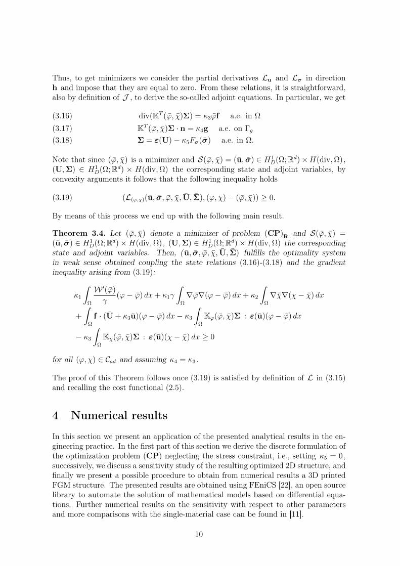
Thus, to get minimizers we consider the partial derivatives Lu and Lσ in directionh and impose that they are equal to zero. From these relations, it is straightforward,also by definition of J , to derive the so-called adjoint equations. In particular, we get

div(KT (ϕ, χ)Σ) = κ3ϕf a.e. in Ω(3.16)KT (ϕ, χ)Σ · n = κ4g a.e. on Γg(3.17)Σ = ε(U)− κ5Fσ(σ) a.e. in Ω.(3.18)

Note that since (ϕ, χ) is a minimizer and S(ϕ, χ) = (u, σ) ∈ H1D(Ω;Rd)×H(div,Ω) ,

(U,Σ) ∈ H1D(Ω;Rd) × H(div,Ω) the corresponding state and adjoint variables, by

convexity arguments it follows that the following inequality holds

(L(ϕ,χ)(u, σ, ϕ, χ, U, Σ), (ϕ, χ)− (ϕ, χ)) ≥ 0.(3.19)

By means of this process we end up with the following main result.

Theorem 3.4. Let (ϕ, χ) denote a minimizer of problem (CP)R and S(ϕ, χ) =(u, σ) ∈ H1

D(Ω;Rd)×H(div,Ω) , (U,Σ) ∈ H1D(Ω;Rd)×H(div,Ω) the corresponding

state and adjoint variables. Then, ( u, σ, ϕ, χ, U, Σ) fulfills the optimality systemin weak sense obtained coupling the state relations (3.16)-(3.18) and the gradientinequality arising from (3.19):

κ1

∫Ω

W ′(ϕ)

γ(ϕ− ϕ) dx+ κ1γ

∫Ω

∇ϕ∇(ϕ− ϕ) dx+ κ2

∫Ω

∇χ∇(χ− χ) dx

+

∫Ω

f · (U + κ3u)(ϕ− ϕ) dx− κ3

∫Ω

Kϕ(ϕ, χ)Σ : ε(u)(ϕ− ϕ) dx

− κ3

∫Ω

Kχ(ϕ, χ)Σ : ε(u)(χ− χ) dx ≥ 0

for all (ϕ, χ) ∈ Cad and assuming κ4 = κ3 .

The proof of this Theorem follows once (3.19) is satisfied by definition of L in (3.15)and recalling the cost functional (2.5).

4 Numerical results

In this section we present an application of the presented analytical results in the en-gineering practice. In the first part of this section we derive the discrete formulation ofthe optimization problem (CP) neglecting the stress constraint, i.e., setting κ5 = 0 ,successively, we discuss a sensitivity study of the resulting optimized 2D structure, andfinally we present a possible procedure to obtain from numerical results a 3D printedFGM structure. The presented results are obtained using FEniCS [22], an open sourcelibrary to automate the solution of mathematical models based on differential equa-tions. Further numerical results on the sensitivity with respect to other parametersand more comparisons with the single-material case can be found in [11].

10

4.1 Discrete problem formulation

Allen-Cahn gradient flow

To obtain a discrete version of the problem (CP) we employ Allen-Cahn gradient flowapproach, a steepest descendant pseudo-time stepping method. Given a fixed time-step increment τ the Allen-Cahn gradient flow leads to the following set of equations:

(4.1)γϕτ

∫Ω

(ϕn+1 − ϕn)(ϕ− ϕn+1) dx+ κ1γ

∫Ω

∇ϕn+1∇(ϕ− ϕn+1) dx−

κ3

∫Ω

Kϕ(ϕn, χn)Σ : ε(un)(ϕ−ϕn+1) dx+κ1

γ

∫Ω

W ′(ϕn)(ϕ−ϕn+1) dx ≥ 0, ∀ (ϕ, χ) ∈ Cad,

(4.2)γχτ

∫Ω

(χn+1 − χn)(χ− χn+1)d dx+ κ2

∫Ω

∇χn+1 · ∇(χ− χn+1) dx−

κ3

∫Ω

Kχ(ϕn, χn)Σ : ε(un)(χ− χn+1) dx ≥ 0, ∀ (ϕ, χ) ∈ Cad

to be solved under the volume constraint:

(4.3)∫

Ω

(ϕn+1 −m) dx = 0.

Finite element discretization

We then discretize the physical domain Ω employing four triangular meshes Qu , Qϕ ,Qχ and QU , one for each variable of the problem. At the nodes of each triangularelement we interpolate, by means of piecewise linear basis functions, the correspondingvariables u , ϕ , χ , and U together with their variations v , vϕ , vχ and vU , obtainingthe following finite element expansions:

u ≈ Nuu, v ≈ Nuv,

ϕ ≈ Nϕϕ, vϕ ≈ Nϕvϕ,

χ ≈ Nχχ, vχ ≈ Nχvχ,

U ≈ NUU, vU ≈ NUvU,

where Nu,Nϕ,Nχ,NU are the piecewise linear shape function vectors or matriceswhich interpolate the nodal degrees of freedoms u, ϕ, χ, U and their variations v, vϕ, vχ, vU .Finally, the Lagrange multiplier λ used to constrain the volume is applied using a con-stant scalar value on the domain Ω .We can now write the discretized version of the optimal control problem (CP), as

11

follows:(4.4)

1

τ

0 0 0 0 00 0 0 0 00 0 Mϕϕ 0 Mϕλ

0 0 0 Mχχ 00 0 Mλϕ 0 0

u

Uϕχ

λ

+

Kuu 0 0 0

0 KUU 0 0 00 0 Kϕϕ 0 00 0 0 Kχχ 00 0 0 0 0

u

Uϕχ

λ

=

f

F + qσ

qϕ + qs + qψ

qχ + qs′

qλ

with the matrix and vector terms defined as:

Kuu =

∫Ω

∇NuTK∇Nu dΩ,

KUU =

∫Ω

∇NUTK∇NU dΩ,

Mϕϕ = γϕ

∫Ω

NTϕNϕ dΩ,

Kϕϕ = κ1γϕ

∫Ω

∇NTϕ∇Nϕ dΩ,

Kχχ = κ2γχ

∫Ω

∇NTχ∇Nχ dΩ,

Mχχ = γχ

∫Ω

NTχNχ dΩ,

Mλϕ = τ

∫Ω

NTλNϕdΩ =

(Mϕλ

)T,

f =

∫ΓN

NuTg dΓ,

F =

∫ΓN

NTUg dΓ,

qσ = κ5

∫Ω

NTUFσ(σn+1), dΩ,

qϕ =γϕτ

∫Ω

(NTϕNϕ

)ϕn dΩ = Mϕϕϕn,

qλ =

∫Ω

mdΩ,

qs =

∫Ω

NTϕKϕ(ϕn, χn)Σn+1 : ε(un+1) dΩ,

qψ =κ3

γϕ

∫Ω

NTϕW ′(ϕn) dΩ.

qχ =γχτ

∫Ω

(NTχNχ)χn dΩ = Mχχχn,

qs′ =

∫Ω

NTϕKχ(ϕn, χn)Σn+1 : ε(un+1) dΩ.

12

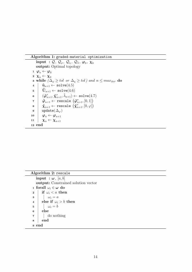
A graded material algorithm

To obtain a topologically optimized structure with continuously varying material prop-erties, we solve the problem in (4.4) employing a staggered iterative approach as de-scribed in Algorithm 1. In fact, the linear system in (4.4) can be split into three linearsystems which we solve separately: the state equation system

(4.5) Kuuu = f ,

the adjoint problem system

(4.6) KUUU = F + qσ,

and the phase-field system

(4.7)1

τ

Mϕϕ 0 Mϕλ

0 Mχχ 0Mλϕ 0 0

ϕχλ

+

Kϕϕ 0 00 Kχχ 00 0 0

ϕχλ

=

qϕ + qs + qψ

qχ + qs′

qλ

.The graded-material optimization routine defined in Algorithm 1 presents an iter-ative procedure where we first solve the state equation system (4.5) to get the solutionvector un+1 , secondly we need to solve the adjoint system (4.6), and finally we evaluatethe phase-field system (4.7) to obtain the two phase-field solution vectors ϕ∗

n+1 , χ∗n+1

together with the Lagrange multiplier λn+1 . Every iteration ends calling the functionrescale , as defined in Algorithm 2 to impose the constraints on the phase-field vari-ables ϕ and χ directly at the nodal values. The graded-material optimizationroutine is then repeated until either the maximum number of iteration (maxiter ) isreached or the L2−norm of both phase-field variable increment ∆ϕ =‖ ϕn+1−ϕn ‖L2

and microscopic density variable increment ∆χ =‖ χn+1 − χn ‖L2 are below a giventolerance (tol ).

4.2 Optimization of a cantilever beam

We now apply the implemented numerical method to solve a two-dimensional op-timization problem. We choose to solve the cantilever beam problem depicted inFigure 1, where a = 200mm , b = 100mm , g = (0,−600) [N/mm] , f = 0 and withan upper bound for the volume filling rate m equal to 0.8. We choose a materialhaving Young modulus E = 12.5GPa, Poisson coefficient ν = 0.25 , and yield stressσy = 45MPa (ABS plastic). We set the parameter β = 1/6 , γϕ = 0.01 , κ1 = 400 ,κ3 = κ4 = κ5 = 1 , and τ = 1E − 6 . For our sensitivity study we decided to vary thepenalty parameter κ2 of the gradient term

∫Ω∇χn+1 · ∇(χ − χn+1) dx among three

different values: 40, 4000, and 400000.Figure 2 shows the result for the reference optimized structure obtained using a single-material, i.e., setting β = 1 , while in Figure 3 we can observe the FGM structures forthe three different values of κ2 . From this figure it is evident the strong influence ofκ2 on the final distribution of the variable χ . In particular, we can observe how a toohigh value of the penalty parameter κ2 delivers a structure where the variable χ is

13

Algorithm 1: graded-material optimizationinput : Q , Qϕ , Qχ , Qλ , ϕ0 , χ0

output: Optimal topology1 ϕn ← ϕ0

2 χn ← χ0

3 while (∆ϕ ≥ tol or ∆χ ≥ tol) and n ≤ maxiter do4 un+1 ← solve(4.5)5 Un+1 ← solve(4.6)6 (ϕ∗n+1, χ

∗n+1, λn+1)← solve(4.7)

7 ϕn+1 ← rescale(ϕ∗n+1, [0, 1]

)8 χn+1 ← rescale

(χ∗n+1, [0, ϕ]

)9 update(∆ϕ )

10 ϕn ← ϕn+1

11 χn ← χn+1

12 end

Algorithm 2: rescaleinput : ω , [a, b]output: Constrained solution vector

1 forall ωi ∈ ω do2 if ωi < a then3 ωi = a4 else if ωi > b then5 ωi = b6 else7 do nothing8 end9 end

14

not able to properly distribute (see Figure 3c), while on the other hand small valuesof κ2 allows too strong oscillations and the algorithm do not converge anymore (seeFigure 3a). A reasonable choice for the parameter κ2 seems to be the one reportedin Figure 3b, where the variable χ gradually vary from the baseline bulk materialto regions where a lower stiffness is required. In Figure 4 we can observe that themaximum value of the von Mises stress is kept always below σy , fulfilling the prescribedstress constraint. The overall stress distribution is very similar in all three cases. Themajor difference lies in the higher maximum stress values concentrated at the leftcorners of the structures.

x

y

ΓD Ω

a

bΓN

g

Figure 1: Cantilever beam: Problem definition.

Figure 2: Cantilever beam: Reference structure obtained using a single material.

In order to estimate the total amount of material in the structure, we define a materialfraction index mχ as:

mχ =1

| Ω |

∫Ω

χdΩ,

which can be considered as a measure of the global amount of material used to printthe structure. Table 1 reports the values of both the compliance and the materialfraction index mχ for both the single-material case and for the graded-material results.

15

(a) κχ = 40 (b) κχ = 4000 (c) κχ = 400000

Figure 3: Cantilever beam: Sensitivity study of the graded-material structure withrespect to the parameter κ2 . χ value distribution.

(a) κχ = 40 (b) κχ = 4000 (c) κχ = 400000

Figure 4: Cantilever beam: Sensitivity study of the graded-material structure withrespect to the parameter κ2 . Von Mises stress value distribution.

The lowest value of the compliance is achieved when a single stiffer material is used.Nevertheless, it can be observed that employing a graded-material method we are ableto obtain FGM structures with a relatively low compliance using considerably lessmaterial. We want to remark here that in general the stiffness for graded-materialstructure do not scale linearly with the density, but it is strongly influenced by themicro-structure of the partially filled regions. This effect is not yet included with thepresent implementation of the method and is left to future investigations.

Table 1: Cantilever beam: Sensitivity study of compliance and material fraction indexmχ for the parameter κ2 .

κ2 compliance[mmN

]mχ convergence

40 7325 0.241 NO4000 4166 0.527 YES400000 3762 0.673 YESfull dense material 3130 0.8 YES

16

4.3 A 3D printing workflow for topologically optimized FGMstructures

The topologically optimized cantilever beam of Figure 3b is printed using the Fused De-position Modeling (FDM) 3D printer located at the ProtoLab http://www-4.unipv.it/3d/our-services/protolab of the University of Pavia (see Figure 5a). This ma-chine prints a filament of thermoplastic polymer which is first heated and then extrudedthrough a printing nozzle. The extruded filament is deployed layer by layer until thedesired object is obtained (Figure 5b). Figure 6 presents a very simple workflow to ob-tain from the numerical solution a 3D printed object. To generate a printable structurewe decided to set a threshold in the χ distribution, separating the resulting structurein two regions which we print using two different plastic materials. We then extractthe .STL files of the these two regions which can be now extruded and directly printedusing the FDM machine. This extremely intuitive approach to generate printable AMstructure is well suited for plastic components but it is yet not optimal. In fact, it doesnot allow to locally vary the material density as we observe instead in the numericalresults. We are currently working on a more complex approach based on local densitymapping but we leave it to forthcoming contributions.

(a) (b)

Figure 5: FDM machine at ProtoLab and 3D printed cantilever beam

5 Conclusions

The present work analyses a phase-field approach for graded materials suitable toobtain topologically optimized structures for 3D printing processes, including stressconstraints. Together with a rigorous analysis of the problem a numerical algorithmhas been implemented to obtain FGM structures. A sensitivity study with respect toa problem parameter has been conducted comparing the resulting structures with asingle-material reference result. Moreover, we have introduced a simple but effectiveworkflow which from the numerical solutions leads to a 3D printed structure. Such aworkflow allows us to print an optimized FGM structure using an FDM 3D printer.

17

Extraction of STL files

Extrusion

Printing

(a)

(d) (c)

(b)

Figure 6: Description of possible workflow to obtain from a continuous χ distributiona 3D printed object: In the first step the continuous χ distribution (a) is splitted intwo parts and the corresponding .STL files are generate (b), in a second step the 2Dgeometries are extruded to obtain a printable file (c) which can be directly sent to theFDM machine to obtain the printed structure (d).

As further outlooks for the present contribution we plan to investigate the influenceof the microstructure on the material model and to extend the numerical algorithm to3D problems.

References

[1] Allaire G., Shape optimization by the homogenization method. Applied Mathe-matical Sciences, 146. Springer-Verlag, New York, 2002.

[2] Attar E., Korner K., Lattice Boltzmann method for dynamic wetting problems,Journal of Colloid and Interfaces Science, vol. 335 (2009), 84-93.

[3] Attar E., Korner K., Lattice Boltzmann model for thermal free surface flows withliquid-solid phase transition, International Journal of Heat and Fluid Flow, vol.32 (2011), 156-163.

[4] Bendsøe, M.P., On obtaining a solution to optimization problems for solid, elasticplates by restriction of the design space, J. Struct. Mech., vol. 11 (1983), 501–521.

[5] Bendsøe, M.P. and Sigmund O., Topology Optimization - Theory, Methods, andApplications, ed. Springer Verlag (2003).

[6] Blank L., Garcke H., Farshbaf-Shaker M.H., Styles V., Relating phase field andsharp interface approaches to structural topology optimization. ESAIM ControlOptim. Calc. Var. 20 (2014), 1025–1058.

18

[7] Bourdin B., Chambolle A., Design-dependent loads in topology optimization.ESAIM Control Optim. Calc. Var. 9 (2003), 19–48.

[8] Brackett D., Ashcroft I., Hague R., Topology Optimization for Additive Manu-facturing, Solid Freeform Fabrication Symposium (SFF), Austin (2014).

[9] Burger M., A framework for the construction of level set methods for shape opti-mization and reconstruction. Interfaces Free Bound. 5 (2003), 301–329.

[10] Burger M., Stainko R., Phase-field relaxation of topology optimization with localstress constraints. SIAM J. Control Optim. 45 (2006), 1447–1466.

[11] Carraturo M., Rocca E., Bonetti E., Hömberg D., Reali A., Auricchio A., Graded-material Design based on Phase-field and Topology Optimization, ComputationalMechanics (2019), DOI: 10.1007/s00466-019-01736-w.

[12] Cheng L., Zhang P., Biyikli E., Pilz S., To A.C., Integration of Topology Op-timization with Efficient Design of Additive Manufactured Cellular Structures,Solid Freeform Fabrication Symposium (SFF), Austin (2015).

[13] Cheng L., Bai J., To A.C., Functionally graded lattice structure topology opti-mization for the design of additive manufactured components with stress con-straints, Computer Methods in Applied Mechanics and Engineering, 344 (2019)334–359.

[14] Clausen A., Aage N., Sigmund O., Exploiting Additive Manufacturing Infill inTopology Optimization for Improved Buckling Load, Engineering 2 (2016), 250–257.

[15] Dal Maso G., Fonseca I., Leoni G., Analytical Validation of a Continuum Modelfor Epitaxial Growth with Elasticity on Vicinal Surfaces, Archive for RationalMechanics and Analysis, vol. 212 (2014), 1037–1064.

[16] Eck C., Homogenization of a phase field model for binary mixtures. MultiscaleModel. Simul. 3 (2004/05), 1–27.

[17] Hodge N.E., Ferencz R.M., Solberg J.M., Implementation of a thermomechanicalmodel for the simulation of selective laser melting, Comput. Mech., vol. 54 (2014),33–51.

[18] Hussein A., Hao L., Yan C., Everson R., Finite element simulation of the temper-ature and stress fields in single layers without-support in selective laser melting,Materials and Design, vol. 52 (2013), 638–647.

[19] Kato J., Yachi D., Terada K., Kyoya T., Topology optimization of micro-structurefor composites applying a decoupling multi-scale analysis, Struct Multidisc Op-tim, vol. 49 (2014), 595–608.

[20] Le C., Norato J., Bruns T., Ha C., Tortorelli D., Stress-based topology optimiza-tion for continua, Struct Multidisc. Optim 41 (2010) 605–620.

19

[21] Lee E., James K.A., Martins J.R.R.A., Stress-Constrained Topology Optimizationwith Design-Dependent Loading, Struct Multidisc. Optim 46 (2012) 647–661.

[22] Logg A., Mardal K.-A., Wells G, N., Automated Solution of Differential Equationsby the Finite Element Method, Springer (2012).

[23] Panesar A., Abdi M., Hickman D., Ashcroft I., Strategies for functionally gradedlattice structures derived using topology optimisation for Additive Manufacturing,Additive Manufacturing 19 (2018) 81–94.

[24] Penzler P., Rumpf M., Wirth B., A phase-field model for compliance shape op-timization in nonlinear elasticity. ESAIM Control Optim. Calc. Var. 18 (2012),229–258.

[25] Sigmund O. and Petersson J., Numerical instabilities in topology optimization:A survey on procedures dealing with cheackboards, mesh-dependencies and localminima, Structural Optimization, vol 16 (1998), 68–75.

[26] Sigmund O. and Maute K., Topology Optimization Approaches: A ComparativeReview, Structural and Multidisciplinary Optimization, vol. 48 (2013), 1031–1055.

[27] Simon J., Differentiation with respect to the domain in boundary value problems.Numer. Funct. Anal. Optim. 2 (1980), 649–687.

[28] Sokołowski J., Zolésio J.-P., Introduction to shape optimization. Shape sensitiv-ity analysis. Springer Series in Computational Mathematics, 16. Springer-Verlag,Berlin, 1992.

[29] Takezawa A., Nishiwaki S., Kitamura M., Shape and topology optimization basedon the phase field method and sensitivity analysis. J. Comput. Phys. 229 (2010),2697–2718.

[30] Tröltzsch F., Optimal control of partial differential equations. Theory, methodsand applications. Graduate Studies in Mathematics, 112. American MathematicalSociety, Providence, RI, 2010.

[31] Turner B.N., Strong R., Gold S.A., A review of melt extrusion additive manu-facturing processes: I. Process design and modeling, Rapid Prototyping Journal,vol. 20 (2014), 192 - 204.

[32] Wang M.Y., Zhou S., Phase field: a variational method for structural topologyoptimization. CMES Comput. Model. Eng. Sci. 6 (2004), 547–566.

[33] Xia L., Breitkopf, Recent advances on topology optimization of multiscale non-linear structures. Arch. Comput. Methods Eng. 24 (2017), 227–249.

[34] Zhou M., Sigmund O., On fully stressed design and p-norm measures in structuraloptimization, Struct Multidisc. Optim 56 (2017) 731–736.

20